the effets of line fishing on the great barrier reef and
TRANSCRIPT

THE EFFECTS OF LINE FISHING ON THE GREAT BARRIER REEF AND EVALUATIONS OF ALTERNATIVE POTENTIAL
MANAGEMENT STRATEGIES
Principal Investigator
B D Mapstone
Authors
BD Mapstone CR Davies LR Little AE Punt ADM Smith F Pantus DC Lou AJ Williams A Jones
AM Ayling GR Russ AD McDonald
Project No 97124$
13 CRC Reef Research Centre Ltd Fisheries Research and Development Corporation and Great Barrier Reef Marine Park Authority
The Effects of Line Fishing on the Great Barrier Reef and Evaluations of Alternative Potential Management Strategies
National Library of Australia Cataloguing-in-Publication entry
Bibliography
Includes index
ISBN 1 876054 89 1
1 Fishing - Queensland - Great Barrier Reef 2 Fishery management - Queensland -Great Barrier Reef I Mapstone Bruce D (Bruce David) II CRC Reef Research Centre (Series CRC Reef Research Centre technical report no 54)
338209943
This publication should be cited as Mapstone BD Davies CR Little LR Punt AE Smith ADM Pantus F Lou DC Williams AJ Jones A Ayling AM Russ GR McDonald AD 2004 The Effects of Line Fishing on the Great Barrier Reef and Evaluations of Alternative Potential Management Strategies CRC Reef Research Centre Technical Report No 52 CRC Reef Research Centre Townsville Australia
This work is copyright The Copyright Act 1968 permits fair dealing for study research news reporting criticism or review Although the use of the PDF format causes the whole work to be downloaded any subsequent use is restricted to the reproduction of selected passages constituting less than 10 of the whole work or individual tables or diagrams for the fair dealing purposes In each use the source must be properly acknowledged Major extracts or the entire document may not be reproduced by any process whatsoever without written permission of the Chief Executive Officer CRC Reef Research Centre
While every effort has been made to ensure the accuracy and completeness of information in this report CRC Reef Research Centre Ltd accepts no responsibility for losses damage costs and other consequences resulting directly or indirectly from its use
In some cases the material may incorporate or summarise views standards or recommendations of a third party Such material is assembled in good faith but does not necessarily reflect the considered views of CRC Reef Research Centre Ltd or indicate a commitment to a particular course of action
The Fisheries Research and Development Corporation plans invests in and manages fisheries research and development throughout Australia It is a federal statutory authority jointly funded by the Australian Government and the fishing industry
Published by the CRC Reef Research Centre Ltd PO Box 772 Townsville Qld 4810 Australia
Non-Technical Summary
Non-Technical Summary
97124 The Effects of Line Fishing on the Great Barrier Reef and Evaluations of Alternative Potential Management Strategies
Principal Investigator Dr BD Mapstone
Address$ CRC Reef Research Centre James Cook University Townsville Qld 4811 Telephone 07 4781 5113 Fax 07 4781 4099
Authors BD Mapstone1 CR Davies2 LR Little3 AE Punt34 ADM Smith3 F Pantus5 DC Lou6 AJ Williams7 A Jones7 AM Ayling GR Russ6 AD McDonald3
Objectives I To understand the level of fishing that existing fish stocks and reef communities can
sustain via bull Investigations of demographic characteristics of targeted species bull Experimental manipulations of fishing effort and management strategies bull Monitoring responses of non-target species to changes in fishing pressure
including responses of selected benthos and prey of target species and bull Relating responses of target and non-target species on experimental reefs to
longer-term broader scale information on abundances and (where appropriate) catch rates
II To evaluate the efficacy of current management practices specifically zoning strategies with respect to the ecologically sustainable management of tropical reef line fishing
III To document the limits of fishing induced changes in fish catch and other aspects of reef use that would be acceptable economically and socially to reef users
IV To evaluate quantitatively potential management strategies for the future regulation of fishing such that fish stocks ecosystem function and yields to fisheries will be conserved
1 ACE CRC Private Bag 80 Hobart 7005 Australia 2 Australian Antarctic Division Channel Highway Kingston TAS 7050 Australia 3 CSIRO Marine Research GPO Box 1538 Hobart TAS 7001 Australia 4 School of Aquatic and Fishery Sciences University of Washington BOX 305520 Seattle WA98195 USA 5 CSIRO Marine Research GPO Box 120 Cleveland QLD 4163 Australia 6 CRC Reef Research Centre and School of Marine Biology and Aquaculture James Cook University
Townsville QLD 4811 Australia 7 CRC Reef Research Centre James Cook University Townsville QLD 4811 Australia
i
ELF Experiment and Management Strategy Evaluations
Executive Summary$
The effects of reef line fishing on the productivity of targeted species and its impacts on other reef species on the Great Barrier Reef (GBR) have been poorly understood Understanding the distribution intensity and effects of reef line fishing is essential for successful management of both fishing and other recreational and commercial activities in the GBR region as well as for conservation of the GBR ecosystem
The GBR Reef Line Fishery (RLF) comprises socially and economically important commercial charter and recreational fishing sectors The fishery has been undergoing some change over the last decade particularly manifest as considerable increases in effort and catch in the commercial fishery since 1995 These changes probably arise from several events including changing management arrangements in other fisheries the introduction of Dugong Protection Areas in in-shore areas the process of reviewing management arrangements for the Reef Line Fishery and the development of lucrative export markets for live reef fish for consumption Collectively these influences have resulted in nearly 50 increase in commercial effort and 40 increase in catch since 1996 There also is potential for increased recreational fishing pressure along the GBR coast simply because of population growth and increased tourism Management arrangements for the Coral Reef Fin Fish Fishery are now under review with new management arrangements likely to regulate commercial effort in the fishery explicitly
Conservation management of the GBR Marine Park also is undergoing significant change The current zoning system is being substantially upgraded with the development of a comprehensive adequate and representative system of no-take areas for biodiversity conservation of the GBR ecosystem ndash the Representative Areas Program This revision is likely to increase the area of the GBR closed to reef line fishing Realising the minimum regime of 20 of all GBR bioregions being lsquono-takersquo will inevitably result in significant increases in the amount of coral reef habitat closed to the Reef Line Fishery in some areas These factors combined with limited historical information about the fishery or its main target species present significant problems for planning appropriate management strategies of the fishery and the GBR World Heritage Area
These factors combined with limited historical information about the fishery or its main target species present significant problems for the development of appropriate management strategies for the fishery and the GBR World Heritage Area In this research we have quantified some of the primary impacts of the RLF on targeted stocks and assessed secondary impacts on other components of the GBR ecosystem We have assessed experimentally the degree to which area closure strategies are likely to have ameliorated those impacts Finally we evaluated the prospects for alternative mixes of strategies for conservation and fishery management in the region to realise the objectives of diverse stakeholders
Surveys of areas that had been open and closed to fishing for over a decade showed that the two main target species of the RLF the common coral trout and the red throat emperor were significantly more abundant larger and older in areas zoned Marine National Park lsquoBrsquo (and so closed to fishing) than in adjacent General Use areas that have always been open to fishing The magnitude of these differences varied regionally from near-zero around Lizard Island to several-fold for some population characteristics in the southern regions of the GBR The pattern in apparent lsquoeffectivenessrsquo of past closures matched closely patterns in the amount of fishing effort and catch and underlying patterns in the abundances of several harvest and non-harvest species We present circumstantial arguments that this regional variation in the apparent lsquoeffectivenessrsquo of Marine Protected Areas is likely to reflect long-standing regional variations in the amounts of fishing and its impacts outside closed areas rather than wholesale subversion of zoning strategies by high levels of poaching That is the lack of contrast between open and closed areas in the Lizard Region probably arises because the open areas are lightly fished whereas the strong contrasts in the other regions arises because of relatively heavy fishing in the open areas in those regions
ii
Non-Technical Summary
Experimental manipulations of reef zoning status and fishing effort verified that fishing on reefs that had been closed historically reduced the abundances of target species on those reefs to levels similar to surrounding open reefs In the absence of prior data with which to compare open and closed reefs before zoning was implemented these manipulations provide the most convincing evidence that the Marine Park zoning strategies have been effective in protecting sub-populations of the fishery resource from the impacts of harvest The protection of such refuges with sufficient compliance thus has the potential to sustain high biomass of reproductively mature populations of harvested species in spite of an active fishery on the GBR
Indirect effects of line fishing on non-harvest fish were less conspicuous Whilst differences existed between open and closed reefs in abundances of the prey of targeted species the nature of the patterns varied regionally through time and with species or species group In some situations the patterns in abundance suggested that removal of a key predator (coral trout) by fishing might have allowed populations of some prey to grow on fished reefs but the evidence was neither uniform nor convincing
We have evaluated prospectively the relative merits for managers and stakeholders of alternative strategies for effort management and area closure on the GBR We based these evaluations on a set of simulation models (lsquoELFSimrsquo) for the population dynamics and harvest of common coral trout on the GBR The population dynamics model is spatially structured depicting nearly 4000 reef-associated populations of coral trout inter-connected via larval dispersal The reef-associated post-settlement populations are age size and sex structured and we allow for variation in most of the key demographic parameters such as natural mortality growth recruitment etc The harvest model predicts the allocation of fishing effort over the GBR by three fishing fleets parameterised with historical catch and effort data to represent the commercial charter and recreational sectors of the RLF
Objectives for the future status of coral trout populations and for the RLF were developed by a diverse set of stakeholders in the fishery and the GBR World Heritage Area in association with the Reef Line Fishery Management Advisory Committee (ReefMAC) Contributing stakeholders included state and federal managers commercial charter and recreational fishers conservation organisations and researchers Stakeholder objectives included preserving near-virgin biomass of coral trout on reefs closed to fishing ensuring satisfactory levels of populations available for harvest maintaining economically viable commercial catch rates and recreationally rewarding recreational catches of coral trout and minimising variation in harvests from year to year Quantitative articulations of these and other objectives were derived and agreed with stakeholders together with associated performance indicators
The same set of stakeholders advised on the mix of potential strategies to be considered for achieving their respective objectives We were asked to compare the efficacy of three levels of fishing effort ranging from half of 1996 levels to 1frac12 times 1996 levels and three levels of area closure ranging from current closures to nearly three times current closures The outputs from these Management Strategy Evaluations provide comparative assessments of the likelihood that each of the stakeholder objectives will be met by each combination of effort control and area closure strategy The results are not intended to prescribe which strategy mix should be adopted but to provide a basis for stakeholders to negotiate such an outcome based on the degree to which different combinations of strategies meet their needs
Harvest-related objectives (eg maintaining CPUE increased chance of catching a large fish preserving biomass available for harvest) were most likely to be achieved when effort was lowest under any area closure strategy but were less likely to be achieved as increasing amounts of area were closed to fishing The principle stock-conservation objective represented by preserving the spawning biomass of the whole population was most likely to be achieved by increasing the amount of area closure and was only relatively slightly impacted by increasing fishing effort within each area closure strategy
iii
ELF Experiment and Management Strategy Evaluations
Importantly the observed increase in fishing effort in recent years is most likely to impact most negatively on the performance indicators for areas open to fishing especially those reflecting what fishers would consider satisfactory performance of the fishery (eg catch rates and sizes of fish) The increase in area closures under the Representative Areas Program is likely to exacerbate the depreciation of fishery performance but our results suggest that growth in fishing effort will be considerably more influential than changes in areas available to the fishery Our results suggest that the currently elevated levels of effort (~15 time 1996 levels) will reduce significantly the prospects of fishers in all sectors realising their objectives in future years irrespective of the inevitable increases in protected areas under the Representative Areas Program
Reducing effort conversely is the strategy of those considered in our evaluations most likely to realise direct fisheries-related objectives The conundrum in these results however is that the improved prospects from effort reduction would apply only to those fishers remaining in the fishery We are unable to assess the magnitude of financial costs likely to be incurred by those fishers excluded through the effort reductions that would now be necessary to achieve the two lower effort scenarios we considered
Changing effort had relatively little impact on most performance indicators for closed areas especially conservation of spawning biomass of coral trout within Marine Protected Areas even allowing for low levels of infringement of closed areas The most effective mechanism by which to increase total spawning stock biomass over the GBR domain therefore was increasing the area closed to fishing presuming that compliance with those closures was relatively high
It is important to note that the status of coral trout populations in areas open to fishing remained relatively robust under all strategies we considered For example even under the most lsquoadversersquo scenario of maximum effort constrained to the smallest fishable area spawning biomass (in the open areas) remained above 50 of virgin spawning biomass and biomass available for harvest (ie above the minimum legal size limit) remained above 30 of virgin available biomass These statistics generally would be considered acceptable for a harvested stock In large part this is likely to be the consequence of the biologically precautionary minimum legal size limit on harvest of common coral trout which ensures that most fish can spawn in at least one year before reaching harvestable size
Sensitivity analyses for the simulations showed that the qualitative relationships among scenarios were robust to changes in model parameters Accordingly the conclusions about the relative merits of increasing or decreasing fishing effort or area closures are robust to most changes in model assumptions It should be noted however that our evaluations relate only to the populations and harvest of common coral trout (P leopardus) Though several other species harvested in the Reef Line Fishery are taxonomically close to P leopardus they are generally considered to be less abundant and longer lived than P leopardus and their populations dynamics are perhaps less resilient to harvest than that of P leopardus Accordingly conservative regulations for the harvest of these other species would be prudent at this stage
This research has laid bare some of the inevitable trade-offs among different scenarios for managing the harvest of common coral trout by the RLF in the GBR World Heritage Area Most importantly the trade-offs have been assessed in relation to objectives and performance indicators specified by diverse stakeholders in the fishery and the World Heritage Area We present the tradeoffs in ways that allow direct comparisons among disparate objectives essentially providing a common currency for comparing performance across fundamentally different types of objectives In so doing we hope that the costs and benefits of different management options are more transparent to all stakeholders than might otherwise have been the case We hope that such transparency aids in the negotiation of acceptable and effective future management arrangements for the Great Barrier Reef World Heritage Area and the Reef Line Fishery
iv
Contents
Contents$
Non-Technical Summary i$Objectives i Executive Summary ii
Contentsv$Acknowledgements viii
Need ix Objectives x$Achievement of Objectivesx$General Introduction 1$
The Demersal Reef Line Fishery 2The Commercial Sector of the Reef Line Fishery 2+The Charter and Recreational Sectors of the Reef Line Fishery 3+Distribution of Reef Line Fishing 4+
Management Arrangements Affecting the Reef Line Fishery 4The Effects of Line Fishing Experiment 7$Introduction 7$
Box 2 Background to the Effects of Line Fishing Project 7Materials and Methods10$
Experimental Design10 Field Sampling 12
Line Fishing Catch Surveys 13+Underwater Visual Surveys 15+
Laboratory Methods 16 Otolith Processing 16+
Estimates of Catch and Effort from Experimental Reefs17Compulsory Fishing Logbooks 17+Aerial and Vessel Surveillance 17+On-site Observations 17+
Data Management 18Analytical Methods18
Preliminary Processing of Data 18+Research Data 18+Logbook Catch and Effort Data 19+
Tests for Effects of Fishing Region and Zone 20+Preliminary Applications of Depletion Estimators to ELF Experimental Data 22+
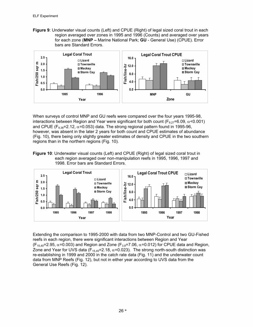
Results 23$Catch and Effort on Experimental Reefs23Tests for Region Zone and Effects of Fishing25
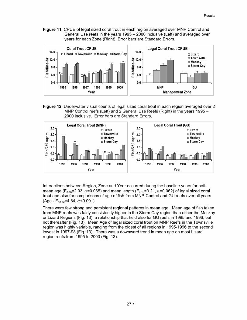
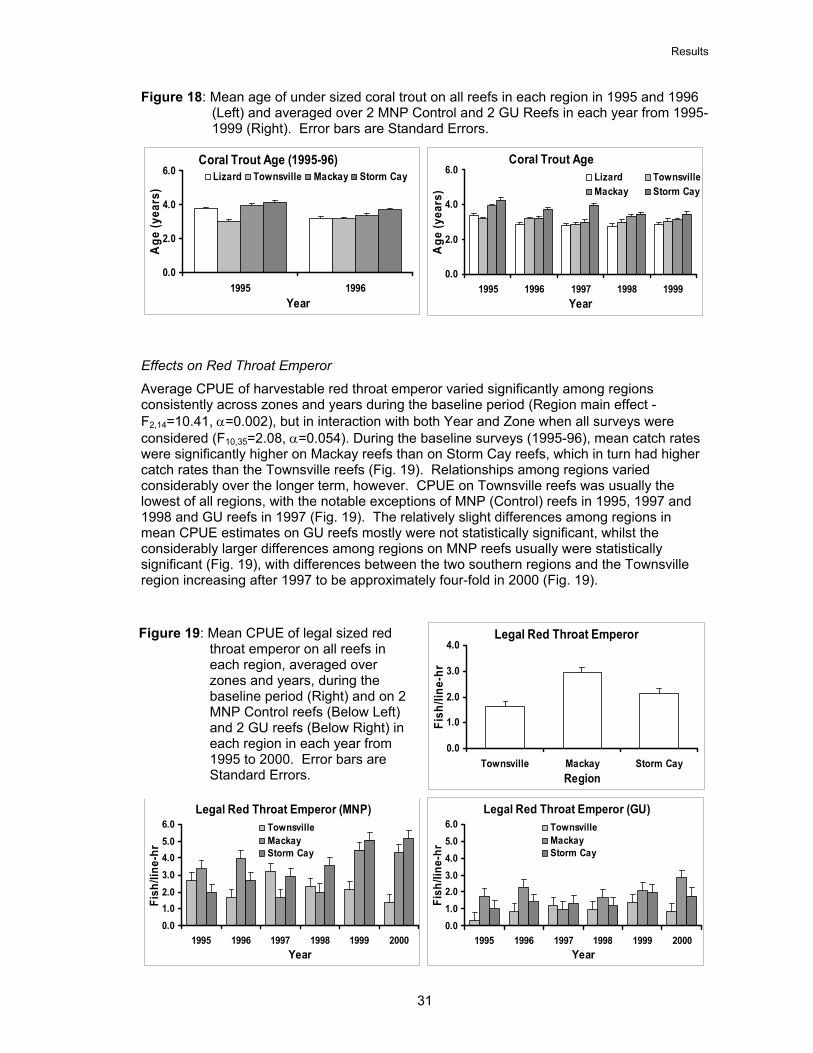
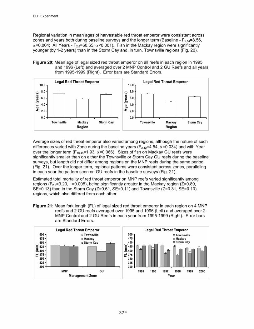
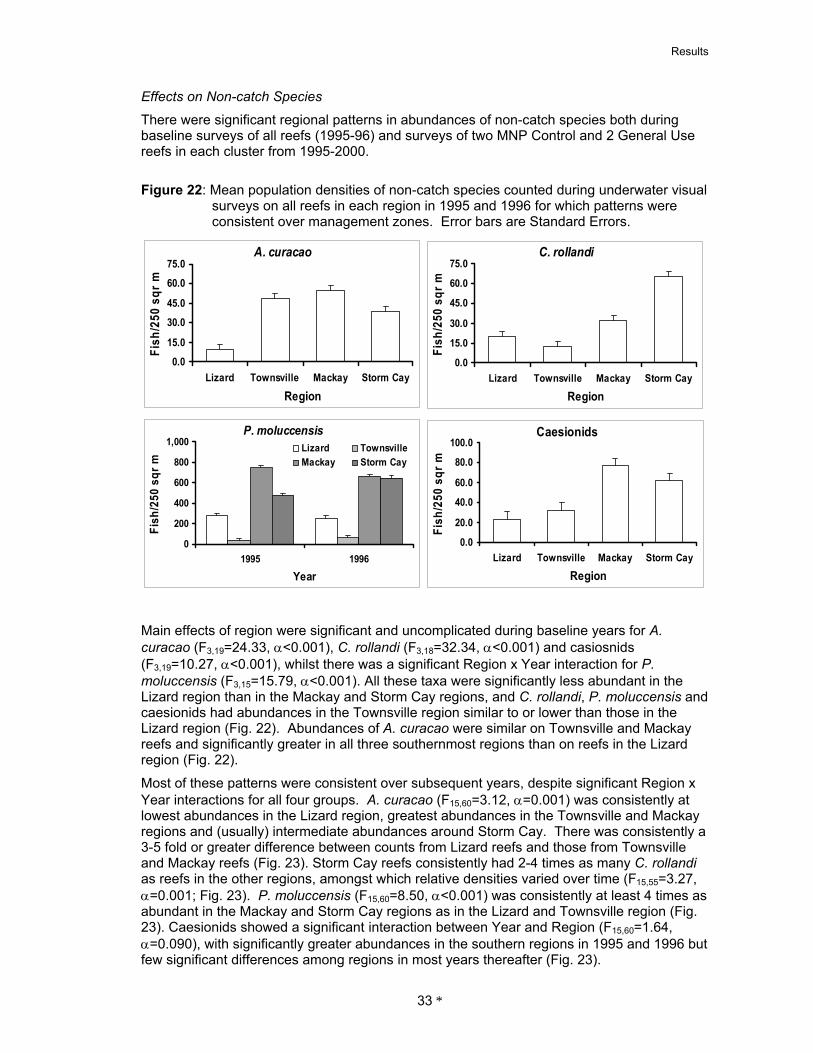
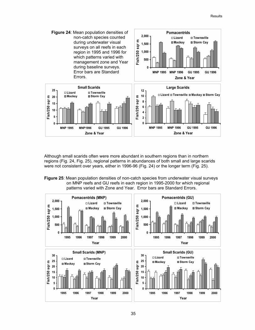
Patterns Among Regions 25+Effects on Legal Sized Coral Trout 25+Effects on Under Sized Coral Trout 28+Effects on Red Throat Emperor 31+Effects on Non-catch Species33+
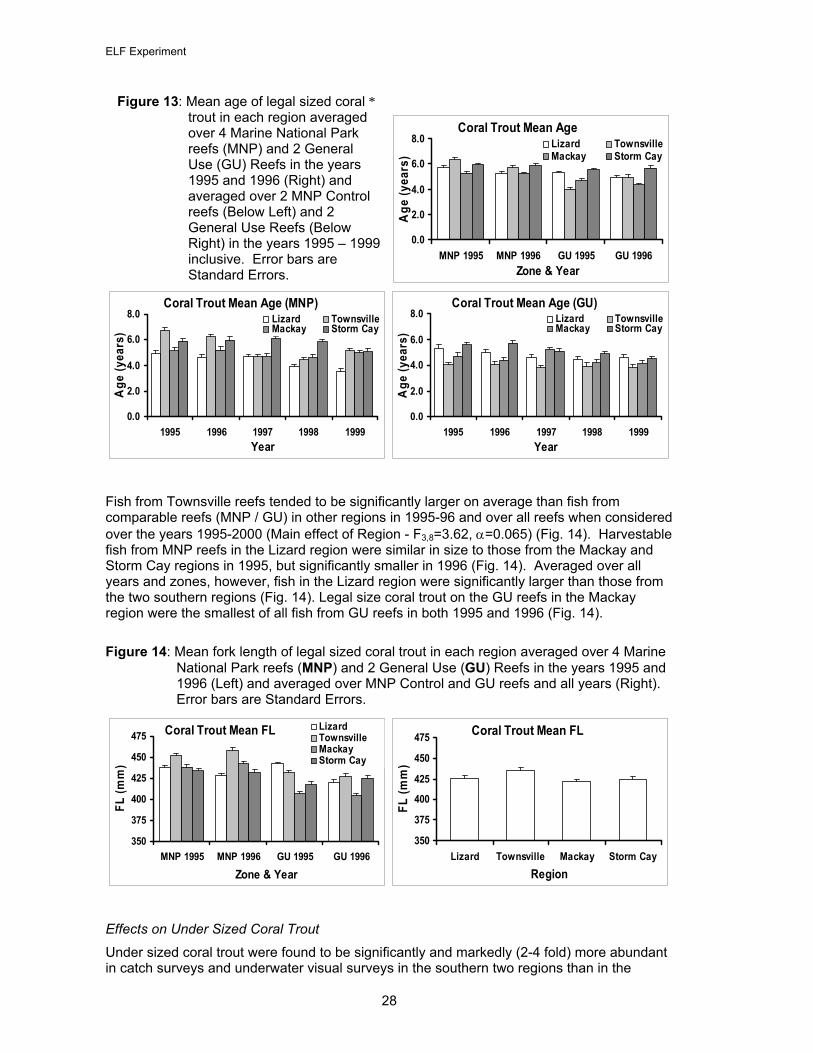
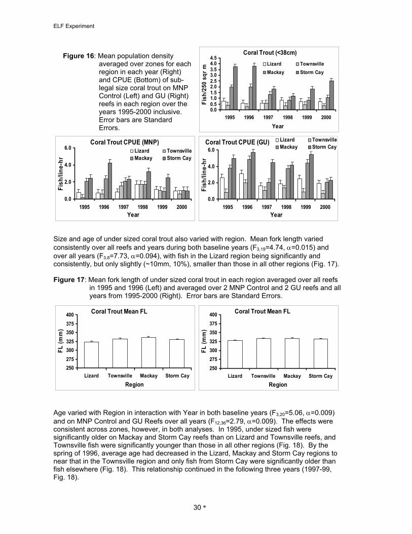
Effects of Management Zone 36+Effects on Legal Sized Coral Trout 36+Effects on Under Sized Coral Trout 41+Effects on Red Throat Emperor 42+Effects on Non-catch Species45+
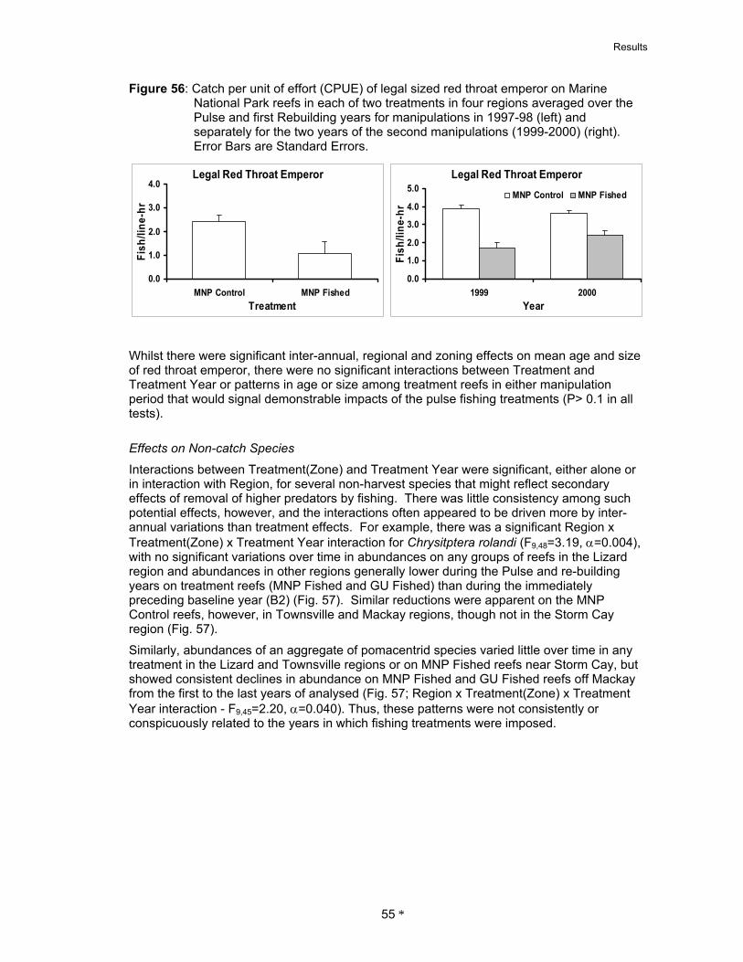
Effects of Fishing Manipulations 49+Effects on Legal Sized Coral Trout 49+Effects on Under Sized Coral Trout 52+Effects on Red Throat Emperor 54+Effects on Non-catch Species55+
v
ELF Experiment and Management Strategy Evaluations
Discussion 58$Implementing the Experiment 58+Biomass Estimates and Future Monitoring Procedures 58+Effects of Marine Park Zoning 59+Regional Variation 60+Indirect Effects of Fishing 61+
Management Strategy Evaluations 63$Introduction 63$Methods 65$
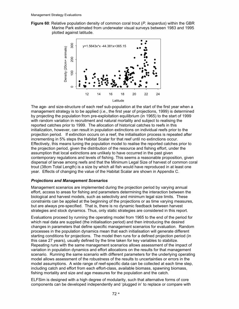
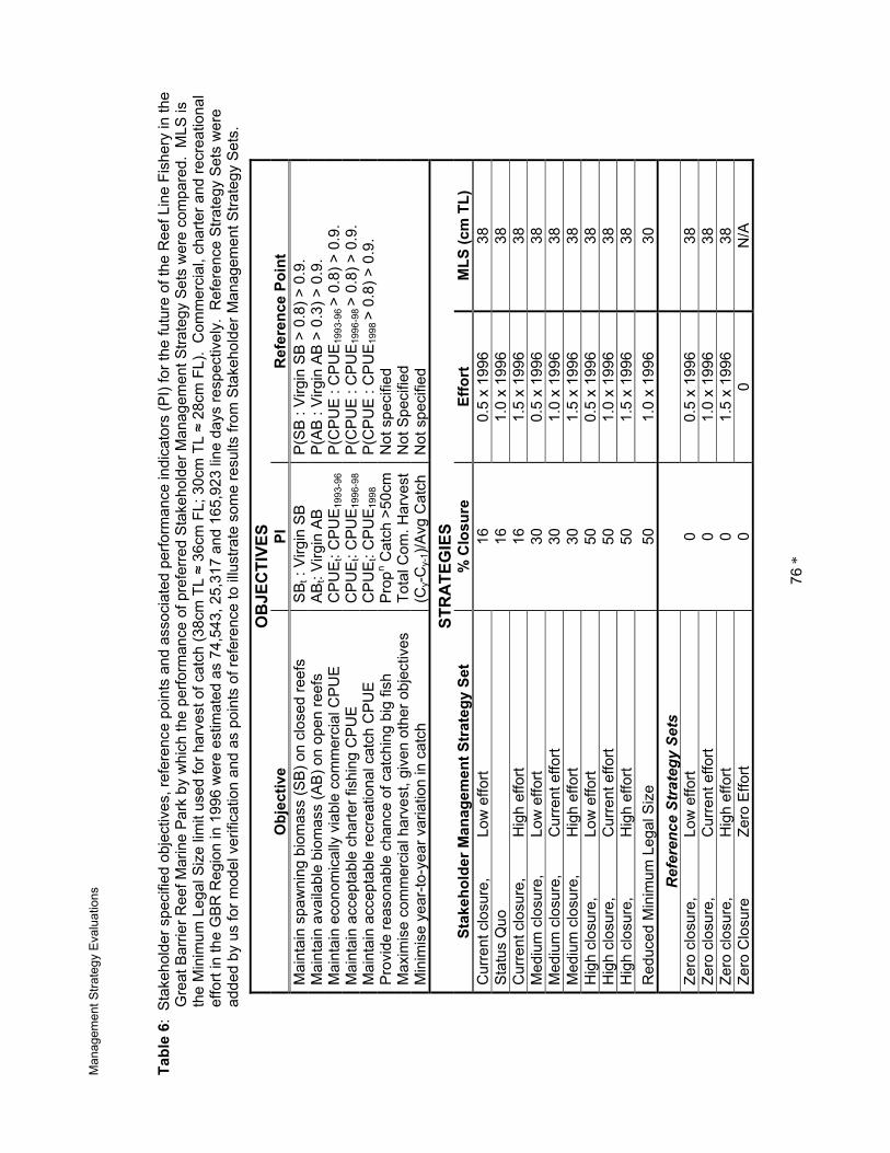
The Biological Component of the Operating Model 65+The Harvest Component of the Operating Model 68+Catches 70 Initialisation 71 Projections and Management Scenarios 72+Setting Objectives Performance Indicators and Management Strategies 73+Objectives 75+
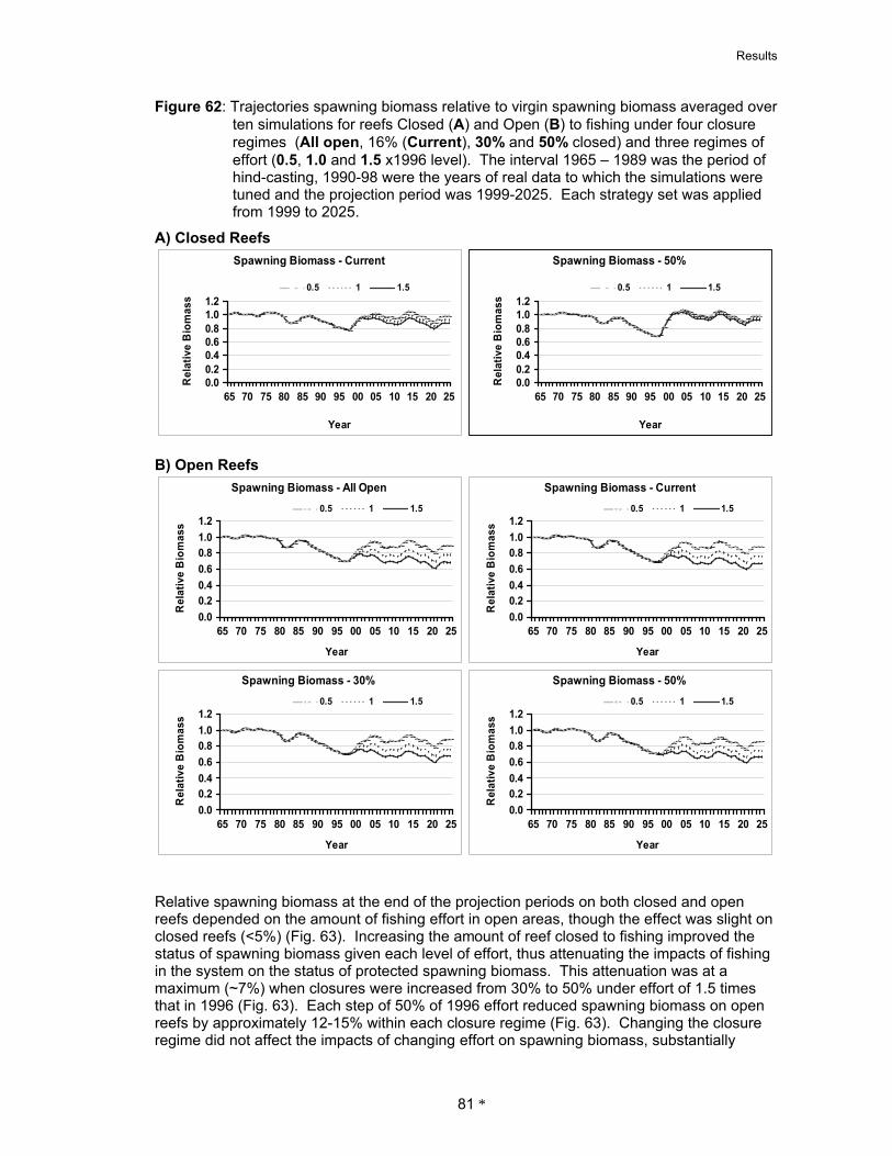
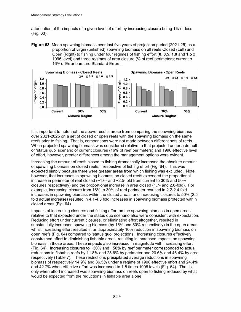
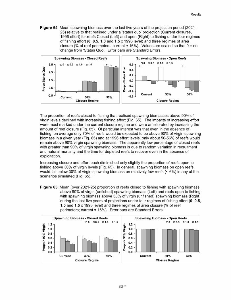
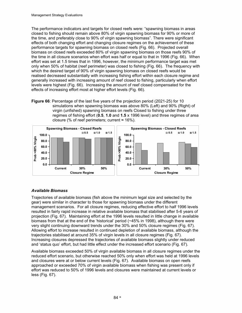
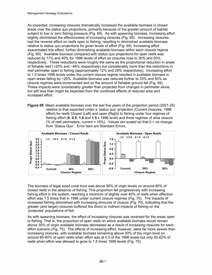
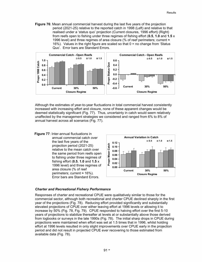
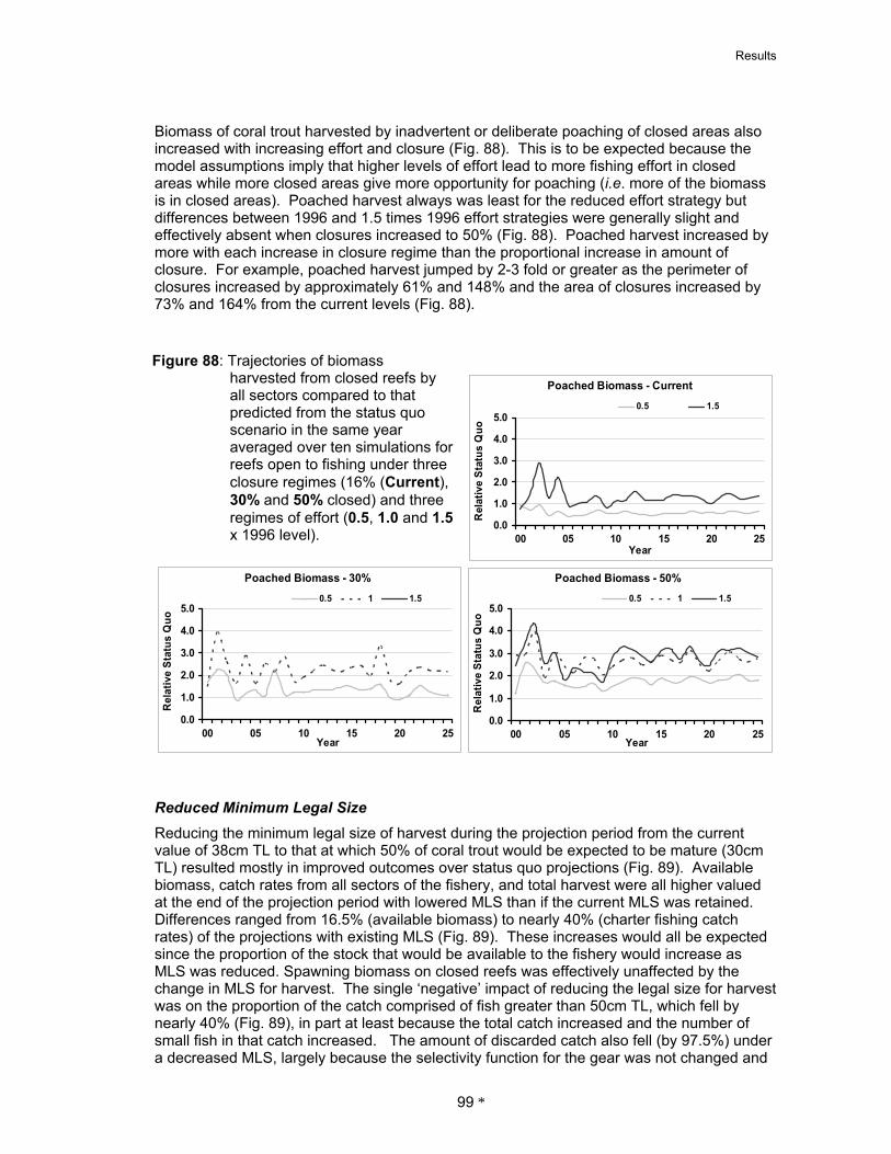
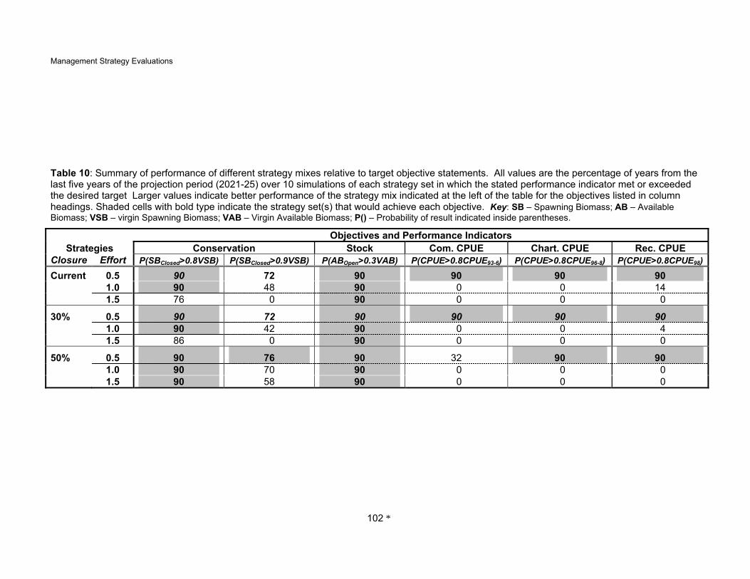
MSE Results 80$Results Summary 80 Simulation Results 80
Spawning Biomass 80+Available Biomass 84+Commercial Fishery Performance 88+Charter and Recreational Fishery Performance 91+Poached and Discarded Catch 97+Reduced Minimum Legal Size 99+
Performance Summary 100Discussion 103$Benefits 107$Further Development 107$Conclusion 108$References 109$Appendix A Applying a Population Dynamics Model ELF Experiment Data 117
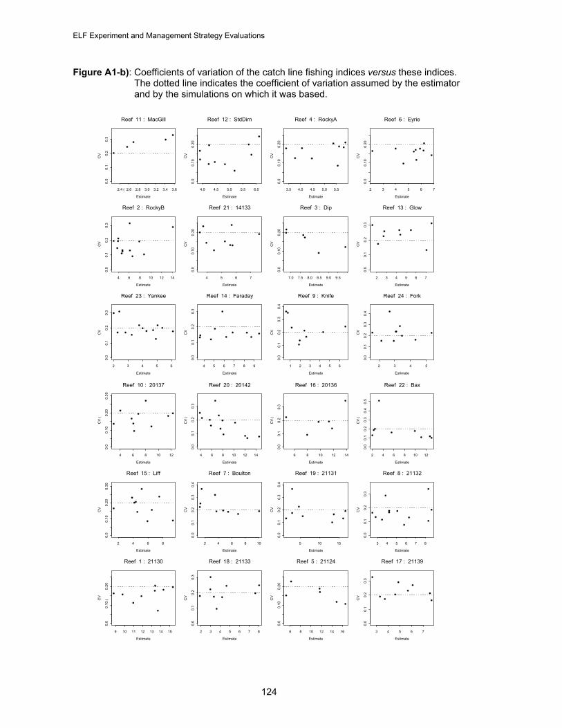
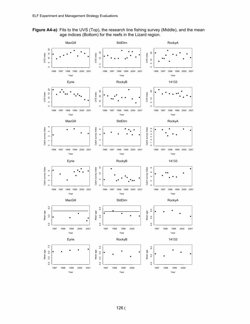
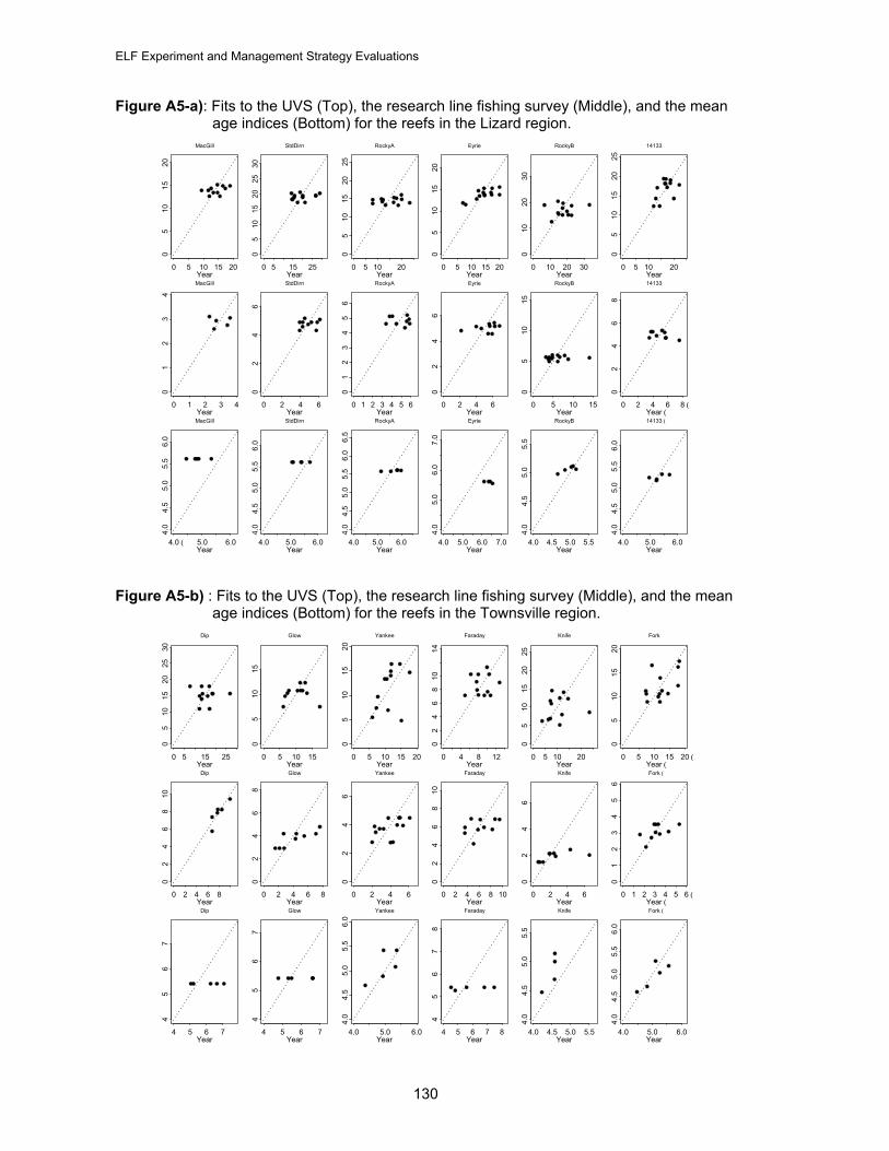
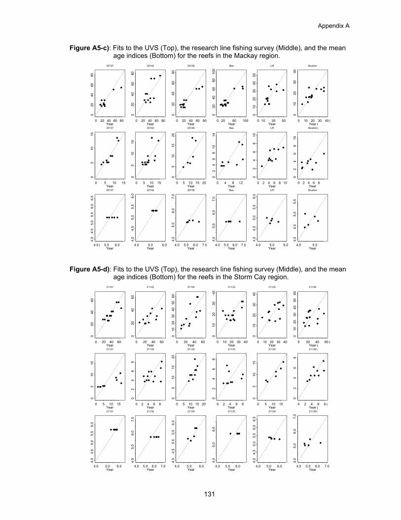
Introduction 117The Data and Derived Inferences 117Fitting the Model to the Data 125
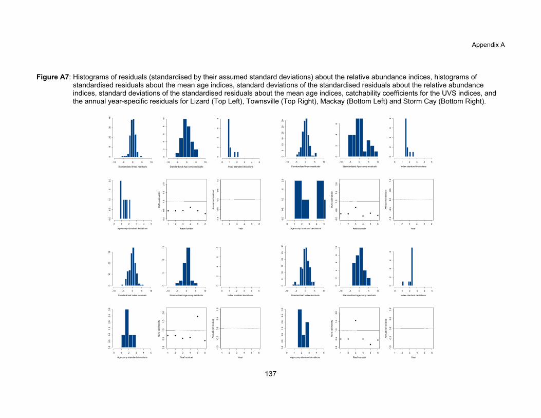
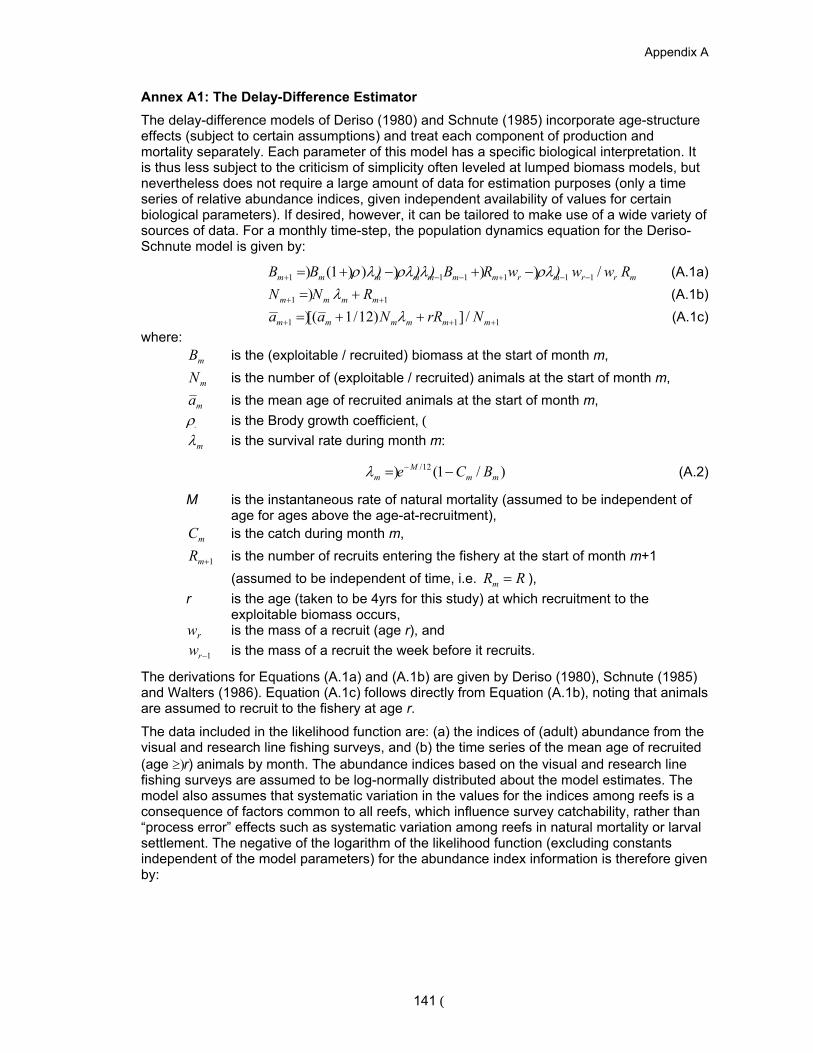
Base-case analysis 125+Sensitivity tests 140Recommendations for additional analyses 140Annex A1 The Delay-Difference Estimator 141
Appendix B The ELFSim Operating Model 144The Biological Components of the Operating Model 144
Basic Population Dynamics 144+0-Year-Olds 145+Recruitment to Reefs 147+Natural mortality 148+Growth 150
The Harvest Components of the Operating Model 150Effort Allocation 150+Catches 153+
Establishing Initial Conditions for Simulations 154Historical catch and effort data 155+
Further work 156Annex B1 The Derivation of Equation (B8) 157Annex B2 The Relationship between Steepness and Parameters of Equation (B 9a) 157Annex B3 Estimating the Parameters of the Growth Curves 158
vi
Contents
Appendix C Summary Diagnostics and Sensitivity Analyses for ELFSim162Required Numbers of Simulations 162Distribution of Catch and Effort 163Effects of Habitat Scalar and Uneven Catch-Effort Distribution164Relative Depletion of Reefs 166
Effects of Different Values for the Steepness Parameter 167+Appendix D Report from the ELF MSE 1st Stakeholder Workshop169
Contents170Introduction 171The ELF Project 172 Issues for Management of the Reef Line Fishery 172What is Management Strategy Evaluation173The First MSE Stakeholders Workshop174Workshop Goals 174 Meeting Summary175
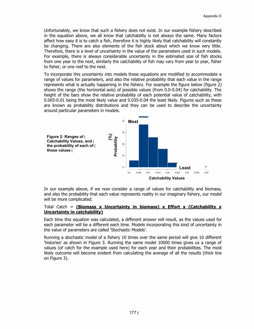
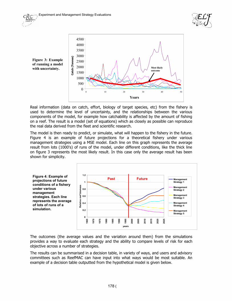
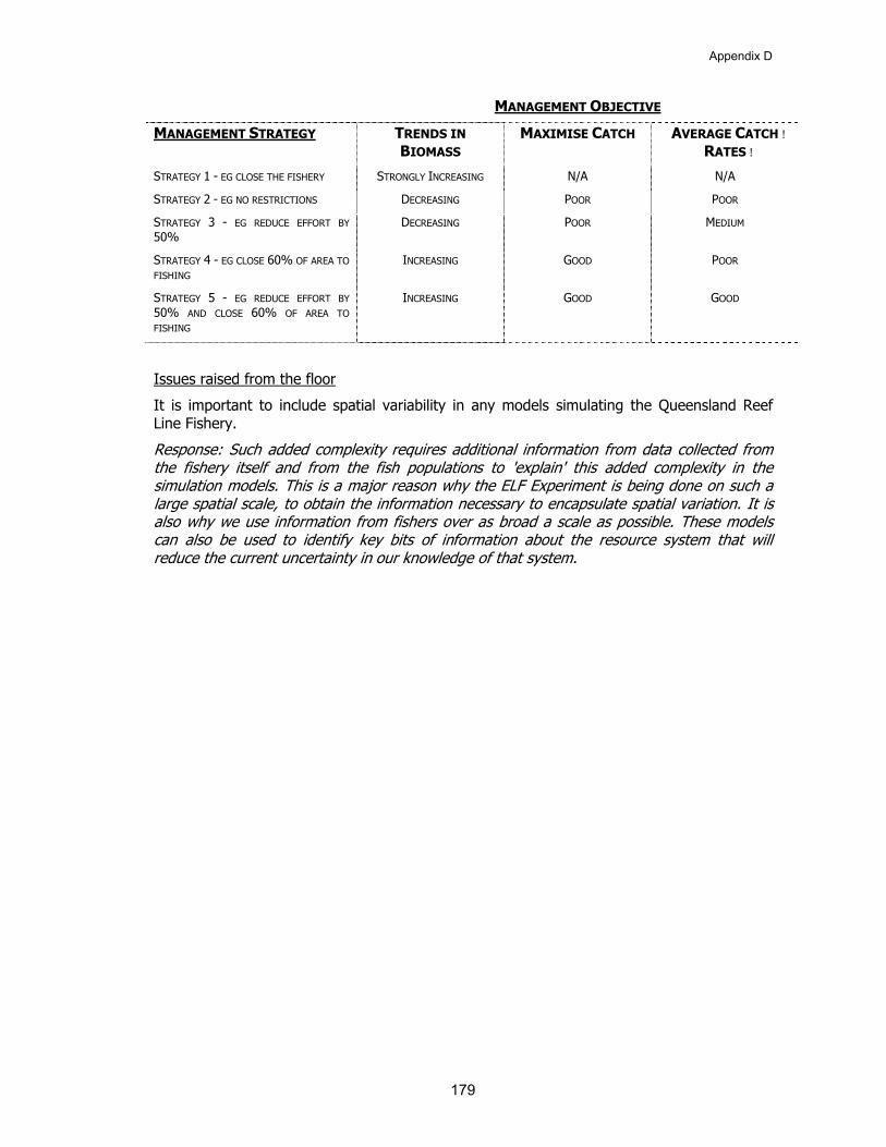
Opening Comments 175+General Background to Quantitative Fisheries Management 175+MSE Concepts Explained Using a Hypothetical Example 176+The ELF Project and MSE for the Reef Line Fishery 180+User Expectations and Issues in the Medium Term 181+
MSE for Coral Trout The ELF Models (ELFSIM) 183Closing Comments and Where to From Here184Participants 185
Appendix E Report from the ELF MSE 2ND Stakeholder Workshop 186Contents187Introduction 1882nd Workshop Objectives 188The ELF Project 189 Issues for Management of the Reef Line Fishery 189The 1st MSE Stakeholders Workshop 190
Objectives 190+Strategies 190+
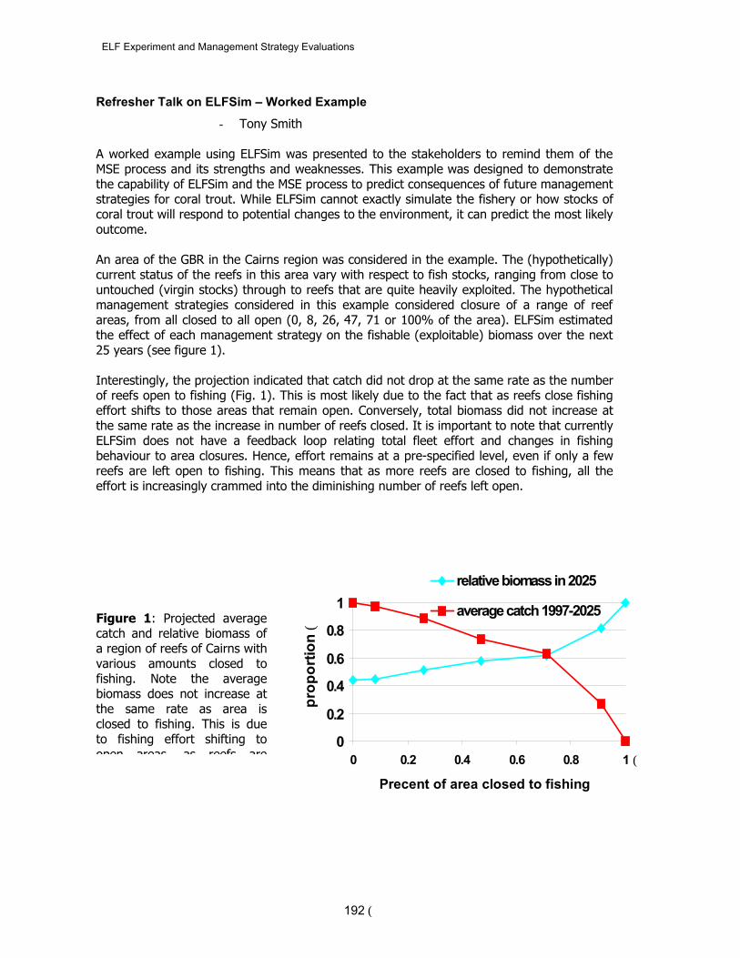
Meeting Summary191Opening Comments 191+Refresher Talk on ELFSim ndash Worked Example 192+Objectives and Performance Indicators from Stakeholders 193+ELFSim lsquoon the flyrsquo ndash What it can do 198+Management Strategies favoured by Stakeholders 199+
Discussion200Examining the unknowns and testing key assumptions 201+Where to now 202+Closing Comments 202+
Participants 203Apologies 203Glossary204
Appendix F Intellectual Property 205$Appendix G Staff 205$
vii
ELF Experiment and Management Strategy Evaluations
Acknowledgements Many people have contributed greatly to this project both directly and indirectly These people include Samantha Adams Kyi Bean Tony Ayling Mikaela Bergenius Belinda Boyce Rob Campbell Gary Carlos Adam Davidson Beth Fulton Siriol Giffney Barry Goldman Bridget Green John McKinlay Amos Mapleston Ross Marriott Cameron Murchie Renae Partridge John Robertson Melita Samoilys Stephanie Slade Angus Thompson Andrew Tobin Sally Troy Dave Welch and a raft of other people including commercial and recreational fishers and charter vessel operators who have helped tremendously over the last few years We especially thank Robyn Stewart and Mary Peterson for their invaluable support and hard work during the catch surveys
We thank also Mick Bishop Martin Breen Wendy Craik Chris Crossland Eddie Heggerl Ted Loveday Helene Marsh Russell Reichelt Duncan Souter John Tanzer Di Tarte Allan Turnbull Simon Woodley and the members of ReefMAC for their support in the development and implementation of the Effects of Line Fishing Experiment
Many of the data behind this report were generously and freely provided by the Great Barrier Reef Marine Park Authority the Queensland Fisheries Management Authority the Queensland Fisheries Service commercial fishers and charter vessel operators in the GBR region
Bruce Mapstone is particularly grateful to Gina Mercer and Lucy Mercer Mapstone for their patience tolerance and support over the many years that this work has dominated our lives and especially during the preparation of this report
Finally we acknowledge the CRC Reef Research Centre for its long-term support and major funding of the ELF Project and the various fishing sectors on the Great Barrier Reef for all the in-kind support we have received The Fisheries Research and Development Corporation the Great Barrier Reef Marine Park Authority the Queensland Fisheries Management Authority and James Cook University provided top-up funding over various periods of the ELF Project
viii
Need
Need The potential for reef line fishing to significantly affect targeted species or indirectly impact other reef species is poorly understood Understanding the distribution intensity and effects of reef line fishing is essential for successful management of both fishing and other recreational and commercial activities in the Great Barrier Reef (GBR) region as well as for conservation of the GBR ecosystem
The GBR Reef Line Fishery (RLF) has undergone substantial change since 1993 particularly manifest as increases in effort and catch in the commercial fishery since 1995 These changes probably resulted from several events including restrictions introduced for other fisheries (spanner crab in-shore net and trawl) by the Queensland Fisheries Management Authority (QFMA) and Queensland Fisheries Service (QFS) on behalf of the Queensland Government the introduction of Dugong Protection Areas in in-shore areas gazetted by the Great Barrier Reef Marine Park Authority (GBRMPA) on behalf of the Commonwealth Government the announcement of a major review of management arrangements for the RLF and the development of lucrative export markets for live reef fish for consumption Indirect indicators of the attractiveness of the RLF to commercial fishers include the 2-3 fold increase in the market value of reef line fishing licences since 1994 the acquisition of multiple vessels by some operators purchases of large purpose built or re-fitted vessels for the live fish sector of the fishery and increased participation in the commercial fishery by licence holders who previously had not harvested reef fish There is also considerable potential for increased recreational fishing pressure simply because of population growth and increased tourism These factors combined with the dearth of historical information about the fishery or its main target species present significant problems for formulating appropriate management strategies for the fishery and the GBR World Heritage Area
Conservation management of the GBR Marine Park also is undergoing significant change with the development of a comprehensive adequate and representative system of no-take areas likely to increase the area of the GBR closed to reef line fishing Management arrangements for the Coral Reef Fin Fish Fishery are under review with new management arrangements likely to regulate commercial effort in the fishery explicitly There is an immediate need for quantitative assessments of the impacts of line fishing on targeted stocks and other fishes and for prospective evaluation of the value of proposed management strategies in relation to economic social biological and conservation objectives for the GBR and its use In ldquoResearch Needs and Prioritiesrdquo (1996) key topics for research related to the Reef Line Fishery flagged by the QFMA included Appraise management measures for the sustainable use of reef fish Determine an effective mix of measures for reef fish management planning including fishery dependent and independent monitoring Determination of the size of stocks of common coral trout Determination of the proportion of blue-spot trout in the reef line catch and assess regional catch rates of red-throat sweetlip
The CRC Reef Effects of Line Fishing (ELF) Project was designed to produce results of direct relevance to these and other needs and in so doing contribute management-relevant information for the GBR RLF Two components of the ELF Project the ELF Experiment and Management Strategy Evaluations (MSE) for the RLF were specifically designed to meet several of the above priority needs This report documents key results to date from these two components of the ELF Project
ix
ELF Experiment and Management Strategy Evaluations
Objectives
Below are the objectives for the CRC Reef Effects of Line Fishing Project Specific subsidiary objectives of particular sub-tasks are listed in Box 1
I To document the distribution and intensity of reef-based fishing catch and effort and patterns in relative abundance of fish stocks
II To understand the level of fishing that existing fish stocks and reef communities can sustain via
a Investigations of demographic characteristics of targeted species b Experimental manipulations of fishing effort and management strategies c Monitoring responses of non-target species to changes in fishing pressure
including responses of selected benthos and prey of target species and d Relating responses of target and non-target species on experimental reefs to
longer-term broader scale information on abundances and (where appropriate) catch rates
III To evaluate the efficacy of current management practices specifically zoning strategies with respect to the ecologically sustainable management of tropical reef line fishing
IV To document the limits of fishing induced changes in fish catch and other aspects of reef use that would be acceptable economically and socially to reef users
V To evaluate quantitatively potential management strategies for the future regulation of fishing such that fish stocks ecosystem function and yields to fisheries will be conserved
This report addresses objectives II ndash V or substantive components of them
Achievement of Objectives The distribution and intensity of fishing has been described from analyses of compulsory logbook data from the commercial and charter sectors of the fishery provided by the Queensland Fisheries Management Authority and Queensland Fisheries Service (QFS) Interpretation of the analyses has been supplement from interviews voluntary research logbook programs and observer programs as part of the ELF Project Characteristics of the small-boat recreational fishery have been provided to the project by QFS
Objectives II and III have been achieved via successful implementation of the ELF Experiment involving changes in reef zoning status (opened or closed to fishing) Responses to the manipulations have been assessed by Underwater Visual Surveys and line fishing Catch Surveys the latter also facilitating collection of biological data for harvest species Several post-graduate research projects have aided in achieving these objectives
Objective IV has been achieved via a series of formal and informal workshops with diverse stakeholders in the GBR and the RLF Contributing stakeholders included Marine Park and Fishery managers commercial recreational and charter fishers fish marketers conservation lobbyists and researchers Achieving this objective was central to completion of objective V
Objective V has been achieved in part through the achievement of the other objectives but substantially via the development of sophisticated computer simulations of the population dynamics and harvest of coral trout over the extent of the GBR The Effects of Line Fishing Simulator (ELFSim) captures the spatial and biological complexity of the GBR and the diversity of harvest behaviours employed by commercial recreational and charter fishers of the resource ELFSim has been used to assess the prospects of achieving diverse stakeholder-specified objectives through an array of combinations of proposed fishery and conservation management strategies
x
Objectives
Box 1 Sub-task Specific Objectives 1 Catch Surveys
a) To establish structured catch surveys in which the fishing characteristics personnel vessel and data collection are standardised across all reefs and times from which to estimated a) differences among reefs historically closed or open to fishing b) regional patterns in catch rates c) effects of simulated increases in fishing pressure and protection from fishing in the ELF Experiment
b) To compare the relationship between CPUE data from line and spear fishing and underwater visual survey (UVS) and the capacity of each method to detect a known decrease in fish abundance
c) To collect size otolith gonad and gut samples from fish caught during the ELF Experiment for studies of population dynamics of major target species
2 Visual Surveys a) To provide fishery independent underwater visual estimates of population densities of target fish
species prey species and other reef organisms on the reefs involved in the ELF Experiment b) To monitor recruitment of the main target species for the RLF to the experimental reefs
3 Demographic Studies a) To derive age-structure data as a primary indicator of the effects of fishing on reef fish stocks b) To use age and length structure data to estimate growth and mortality rates and provide measures of
recruitment rates to reef fish stocks c) To provide catch-at-age data from which to model population dynamics of target species
4 Fleet Dynamics and Fishery Information a) To establish and maintain cooperative links with the recreational commercial and charter boat line
fishing community to a) increase fishing effort on the manipulation reefs in the ELF Experiment and b) obtain detailed fleet catch and effort information from the reefs involved in the ELF Experiment
b) To identify and compare factors which affect the fleet dynamics and on site fishing practices in the RLF within and among regions of the GBR
5 Assessment of Bias in Line-caught Samples a) To compare age and size structures of populations of common coral trout (Plectropomus leopardus)
sampled by spear fishing among reefs open and closed to fishing and among regions of the Great Barrier Reef (GBR)
b) To examine the size and age selectivity of line fishing by comparing age and size structures of samples of common coral trout taken from reefs open and closed to fishing by spear and line fishing
c) To examine the relative biases of line and spear fishing as techniques for sampling reef fish 6 Modelling and Management Strategy Evaluation
a) To develop and parameterise population dynamics models of the primary target (fished) species (P leopardus) that are appropriate for the spatially structured GBR and that are amenable to application to secondary target species
b) To develop models of effort allocation and where possible fleet dynamics of different components of the fishery including consideration of the commercial recreational and charter fishing sectors that are appropriate for the dynamics of the reef line fishery in the spatially complex GBR
c) To provide an integrated framework based on the population and effort dynamic models for evaluating alternative management scenarios to quantify the likely trade-offs between conflicting objectives and their consequences for the coral trout fishery and the fish stocks
d) To develop with stakeholders in the GBR line fishery operational objectives and potential future management strategies relevant and amenable to evaluation from biological and fishery information
e) To apply the management strategy evaluation framework to evaluate risks and benefits of alternative strategies for managing the RLF on the GBR against stakeholder objectives for the fishery
7 Coordination and liaison a) To coordinate the implementation of all components of the ELF Project in a coherent manner across
multiple institutions and with stakeholder groups b) To manage peer review of the ELF Experiment c) To coordinate liaison with researchers and stakeholders across a range of levels from senior policy
fora to the general public d) To manage the coherent collation and archival of data and biological material from the ELF Project
xi
General Introduction
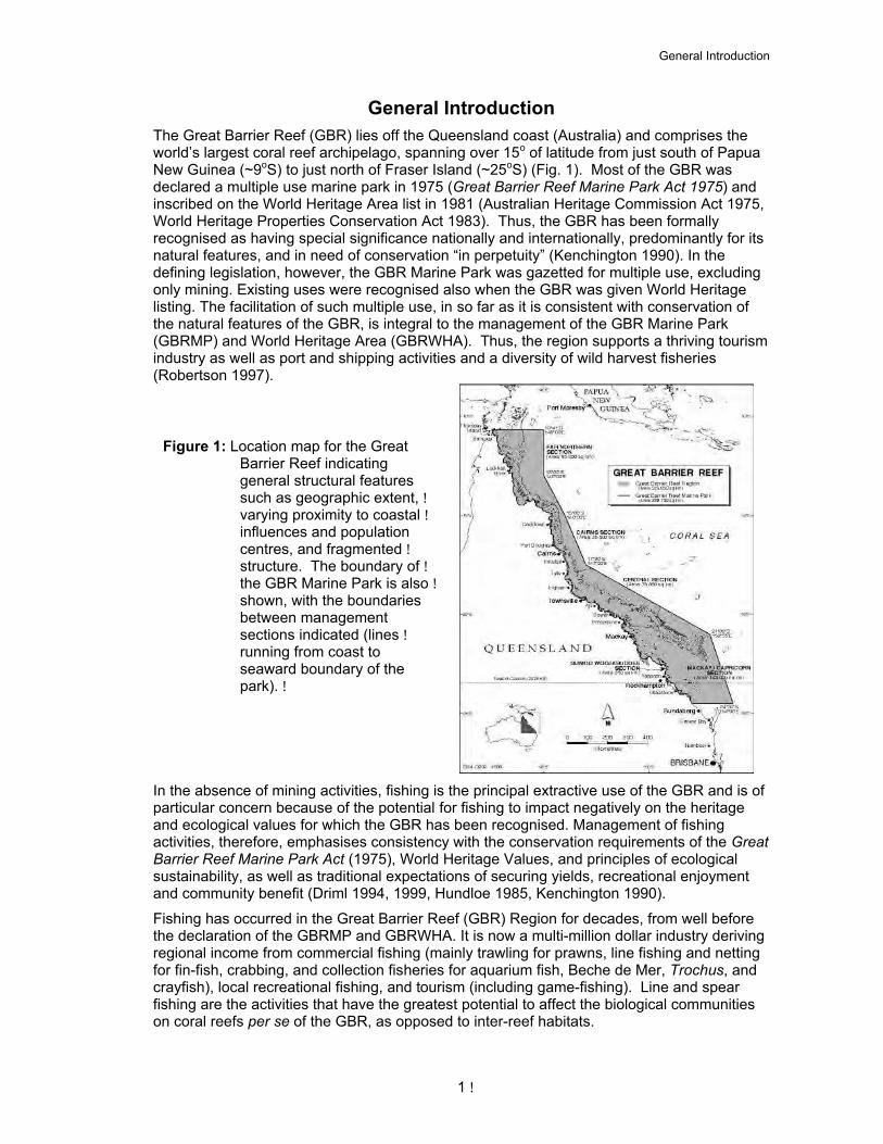
General Introduction The Great Barrier Reef (GBR) lies off the Queensland coast (Australia) and comprises the worldrsquos largest coral reef archipelago spanning over 15o of latitude from just south of Papua New Guinea (~9oS) to just north of Fraser Island (~25oS) (Fig 1) Most of the GBR was declared a multiple use marine park in 1975 (Great Barrier Reef Marine Park Act 1975) and inscribed on the World Heritage Area list in 1981 (Australian Heritage Commission Act 1975 World Heritage Properties Conservation Act 1983) Thus the GBR has been formally recognised as having special significance nationally and internationally predominantly for its natural features and in need of conservation ldquoin perpetuityrdquo (Kenchington 1990) In the defining legislation however the GBR Marine Park was gazetted for multiple use excluding only mining Existing uses were recognised also when the GBR was given World Heritage listing The facilitation of such multiple use in so far as it is consistent with conservation of the natural features of the GBR is integral to the management of the GBR Marine Park (GBRMP) and World Heritage Area (GBRWHA) Thus the region supports a thriving tourism industry as well as port and shipping activities and a diversity of wild harvest fisheries (Robertson 1997)
Figure 1 Location map for the Great Barrier Reef indicating general structural features such as geographic extentvarying proximity to coastalinfluences and population centres and fragmentedstructure The boundary ofthe GBR Marine Park is alsoshown with the boundaries between management sections indicated (linesrunning from coast to seaward boundary of the park)
In the absence of mining activities fishing is the principal extractive use of the GBR and is of particular concern because of the potential for fishing to impact negatively on the heritage and ecological values for which the GBR has been recognised Management of fishing activities therefore emphasises consistency with the conservation requirements of the Great Barrier Reef Marine Park Act (1975) World Heritage Values and principles of ecological sustainability as well as traditional expectations of securing yields recreational enjoyment and community benefit (Driml 1994 1999 Hundloe 1985 Kenchington 1990)
Fishing has occurred in the Great Barrier Reef (GBR) Region for decades from well before the declaration of the GBRMP and GBRWHA It is now a multi-million dollar industry deriving regional income from commercial fishing (mainly trawling for prawns line fishing and netting for fin-fish crabbing and collection fisheries for aquarium fish Beche de Mer Trochus and crayfish) local recreational fishing and tourism (including game-fishing) Line and spear fishing are the activities that have the greatest potential to affect the biological communities on coral reefs per se of the GBR as opposed to inter-reef habitats
1
ELF Experiment and Management Strategy Evaluations
The Demersal Reef Line Fishery The RLF is comprised of three main sectors a commercial sector a charter fishing sector and a private recreational sector Fishers in all sectors use basically similar gears typically consisting of single baited hooks on heavy line on rod and reel or hand reel The RLF is multi-species in all sectors with over 125 species or species groups being reported by the commercial sector (Mapstone et al 1996abc) and at least 108 species or species groups reported in the catch from the charter and recreational sectors (Green et al in prep Higgs 1999 Morgan 1999) The primary targeted species in the fishery are the common coral trout (Plectropomus leopardus) and the red throat emperor (Lethrinus miniatus) (Mapstone et al 1996abc Queensland Fisheries Management Authority (QFMA) 1996 Queensland Fisheries Service (QFS) 2002) The generic group lsquocoral troutrsquo comprising three main harvested species and four lesser species are estimated to comprise approximately 35-55 of the catch by commercial fishers approximately 20-25 of the charter catch and 15-20 of the recreational catch of demersal reef fish from the GBR region L miniatus comprises about 20 of the commercial catch up to 40 of the charter fishing catch and about 30-35 of the recreational demersal catch annually Other emperors especially spangled emperor (L nebulosus) and snappers (mostly red emperor Lutjanus sebae and large and small mouth nannygai L malabaricus L erythropterus) and serranids other than coral trout are the next most targeted demersal species with their relative importance varying among sectors and among regions within sectors (Green et al in prep Higgs 1999 Mapstone et al 1996a 1997 QFS 2002)
The Commercial Sector of the Reef Line Fishery The bulk of the commercial fishery occurs from 4-7m dories based on 8-19m primary vessels though fishing also occurs from the primary vessels The most active commercial reef-line operations have 2-5 dories per primary vessel whilst the majority of operations have no dories and report relatively little catch and effort (Mapstone et al 1996a)
The commercial Reef Line Fishery has been undergoing some change since 1993 particularly manifest as considerable increase in effort since 1995 These changes probably resulted from several events including restrictions on other fisheries (spanner crab in-shore net and trawl) the introduction of Dugong Protection Areas in in-shore areas the announcement of a major review of management arrangements for the RLF and the development of lucrative export markets for live reef fish for consumption Each of these events has the potential to have prompted activation of latent effort or the transfer of effort from other fisheries to the RLF and corresponding increases in commercial fishing effort
The value added to the commercial catch as a result of high market values for live fish (beach prices up to $45kg in 1996 and $58kg in 2000) in particular provides increased financial incentives to participate in the RLF Indirect indicators of the attractiveness of the RLF to commercial fishers include the 2-3 fold increase in the market value of reef line commercial fishing licences since 1994 the acquisition of multiple vessels by some operators and purchases of large purpose built or re-fitted vessels for the live fish fishery
Compulsory logbooks of catch and effort were introduced for commercial fishers only in 1988 Between 1988 and 1994 there were between 361 and 416 commercial line fishing operations reporting catch of demersal coral reef species from the GBR The 20 most active operations accounted for over 60 of the catch in most years and the majority of operations reported less than 1 tonne of catch annually (Gwynne 1990 Mapstone et al 1996abc Trainor 1991) Total annual harvest of all species (including pelagic species) by the commercial RLF over that period was between 2873 and 3725 tonnes arising from 16000 ndash 18500 fishing days (Mapstone et al 1996ab) Since 1994 however reported effort and catch have increased substantially (QFS 2002 Williams 2002 Fig 2) reaching their highest levels of nearly 40000 fishing days by over 700 operations taking 4400 tonnes of demersal reef fish from all Queensland waters in 2001 (QFS 2002)
2
General Introduction
Figure 2 Annual commercial catches of coral trout (all species of Plectropomus spp and Variola spp) red throat emperor (Lethrinus miniatus RTE) and other demersal reef fish (others) from the GBR Marine Park between 1989 and 2000 and the number of reported fishing days from which the catch came
Commercial Catch amp Effort
0 500
1000 1500 2000 2500 3000 3500 4000
1989 1990 1991 1992 1993 1994 1995 1996 1997 1998 1999 2000 Year
Cat
ch (t
)
0 5000 10000 15000 20000 25000 30000 35000
Effo
rt (f
ishi
ng-d
ays)
Coral Trout Others RTE Effort
The Charter and Recreational Sectors of the Reef Line Fishery Recreational fishing occurs from both privately owned boats mostly outboard powered or from charter vessels that take single or multi-day trips to the GBR Prior to 1996 information about the private recreational fishing fleet came only from boat registrations and mostly recall data obtained from fishers during various creel telephone or postal surveys (Blamey and Hundloe 1993 Craik and Fallows 1980 Higgs 1996) The longest history of data derives from line and spear fishing club competition records (Higgs 1996 Nakaya 1998) but recent population surveys indicated that those data represent at most 6 of the recreational fishing population (Morgan 1999)
Blamey and Hundloe (1993) estimated that the total recreational catch in the GBR region in 1989-90 was between 3500 and 4300 tonnes from approximately 210000-270000 lsquofishing trips to searsquo by 160000 recreational fishers in private vessels Only 54-135 of these trips (depending on region) however went lsquooff-shorersquo and smaller proportions visited the lsquoGBR properrsquo More recent research and surveys sponsored by the Queensland Fisheries Management Authority (QFMA) and Queensland Fisheries Service (QFS) indicated similar distributions of recreational fishing between near shore and off-shore waters (Fig 3) and indicate that recreational anglers took approximately 2000t of demersal reef fish per year in the late 1990s (Higgs 1996 1999 Mapstone et al 1997 QFS 2002 Williams 2002) There is considerable potential for increased recreational fishing pressure along the GBR coast because of population growth and increased tourism Financial constraints such as the cost of fuel for long trips to the off-shore reefs however probably dampen effects of population growth on off-shore reefs
Fishing on charter trips occurs mostly from the main charter vessel but dories are also used on some extended charters There were 415 operators of charter vessels in the GBR region holding permits to take clients reef fishing in 1995 though most of these probably did lsquofishing tripsrsquo infrequently Green et al (in prep) estimated that only about 120 charter fishing operations regularly took clients to sea predominantly for fishing in 1999-2000 Fishers on charter trips to the GBR fished for an estimated 11030-22880 line-days between 1996 and 1998 and kept 50-51 tonnes of coral trout and related species of demersal reef fish (QFS unpublished data) Compulsory logbooks for charter vessel operators were introduced only in 1996-97
3
ELF Experiment and Management Strategy Evaluations
Figure 3 Percentages of recreational boating trips from the Ingham area in May-July 1995 that went to near shore islands (black) off-shore reefs of the GBR (white) or in-shore areas (grey) The pie on the left was derived from interviews at boat ramps that on the right from voluntary angler logbooks (Mapstone et al 1997)
1 1 5 5
98
90
Distribution of Reef Line Fishing Line fishing occurs over the entirety of the GBR though by far the majority of catch and effort is in the southern half of the GBR south of Cairns (Blamey and Hundloe 1993 Gwynne 1990 Higgs 1996 Mapstone et al 1996ac Trainor 1991) The greatest small-boat recreational effort on the off-shore GBR occurs between north of Townsville and just north of Cairns (Blamey and Hundloe 1993 Higgs 1996 1999) the majority of charter vessel effort is centred on Gladstone Mackay Airlie Beach and Cairns (Green et al in prep) and the bulk of the commercial effort occurs south of Cairns and north of Rockhampton (Mapstone et al 1996a) (Fig 4)
Management Arrangements Affecting the Reef Line Fishery The management reacutegime for the GBR region is complex with responsibility for conservation management and fisheries management being divided constitutionally legislatively and operationally between the Australian Commonwealth and Queensland Governments Management responsibilities for the GBR Marine Park and World Heritage Area are vested by the Commonwealth with the Great Barrier Reef Marine Park Authority (GBRMPA) a Commonwealth Statutory Authority (GBR Marine Park Act 1975) The GBRMPA has responsibility for management for lsquoprotection and wise use in perpetuityrsquo but explicitly does not have authority for fisheries management Consistent with the Off-shore Constitutional Settlement (1981) responsibility for managing fisheries is delegated to the Queensland Government which administers that mandate through the Queensland Fisheries Service8
(QFS) (Queensland Fisheries Act 1994 1999)
The GBRMPA has to date employed a strategy of zoning for conservation management of the GBR Under zoning plans developed by the Authority and enacted by the Federal Parliament different areas of the marine park are designated for different types of permissible use ranging from most extractive activities (General Use zones) to lsquolook but donrsquot touchrsquo (Marine National Park-B zones) and lsquono-gorsquo areas (Preservation zones) Although not specifically designed as fisheries management strategies these zoning strategies effectively regulate fishing through the implementation of area closures that protect various species from harvest and impose broad restrictions on fishersrsquo access to stocks Although the 2000km length of the GBR Marine Park has been divided into four major sections for zoning (Fig 1) to date the zoning plans applied to each have been very similar and have not resulted in region-specific management
8 Management of fisheries in Queensland was through the Queensland Fisheries Management Authority (QFMA) a statutory Authority between 1993 and 2000 but from July 1 2000 the QFMA was dissolved and responsibility for managing fishing in Queensland was transferred to the Queensland Fisheries Service within the portfolio responsibilities of the Department of Primary Industries
4
General Introduction
Figure 4 Annual total effort and total catch of all line-caught species as reported in the compulsory commercial logbooks in each region in 1990 1992 and 1994 Region boundaries are shown in the figure at bottom right with the key to region abbreviations in the table below the map (Adapted from Mapstone et al 1996a)
5
GC WTS ETS FN
CNS TVL
WTS ETS
FN Weipa bull
Cape Melville bullCape Flattery bull
Cooktown bull CNSGC Port Douglas bull
Cairns bull OCS
Cardwell bull TVL
Townsville bull Bowen bull
MKY
SWN Mackay bull
C-BRockhampton bull
Bundaberg bull
STROP Brisbane bull
140 145 150 155
Longitude Key to Regions Indicated on Map
Gulf of Carpentaria MKY Mackay Western Torres Straits SWN Swains Eastern Torres Straits C-B Capricorn Bunkers Far Northern OCS Off-shore Coral
Sea Cairns STROP Sub-tropical Townsville
Latit
ude
-30
-25
-20
-15
-10
ELF Experiment and Management Strategy Evaluations
The RLF also is managed uniformly over the length of entire GBR (QFMA 1999 QFS 2002) although since April 1999 reefs in the Torres Strait north of 10o20rsquo S fall under a different jurisdiction from the remainder of the GBR (AFMA 2001) The prospect arises therefore that management arrangements might become non-uniform if changes are legislated in either jurisdiction without reflection in the other The QFS and formerly the QFMA impose a number of explicit fisheries management strategies in Marine Park zones of the GBR where line fishing is allowed (QFMA 1999 QFS 2002) Minimum legal size limits for several of the main target species apply to all sectors of the fishery as do gear restrictions
Commercial fishing is managed via a two-tiered limited entry licensing scheme combined with vessel length constraints common to both The two tiers were defined in 1993 in relation to the evidence of prior participation in the RLF and are implemented as limits on the numbers of dories that can be used in conjunction with each primary vessel Licences with an lsquoL2rsquo endorsement are allowed up to seven dories per primary vessel with the number specific to each licence and fixed as of 1993 L2 endorsed primary vessels support an average of 3-4 dories lsquoL3rsquo endorsed licences allow fishing from at most one dory in addition to the primary vessel There are no restrictions on the numbers of lines or fishers per operation except those imposed by survey conditions of the primary vessel In addition to the lsquoL2rsquo or lsquoL3rsquo endorsements most commercial licence packages carry multiple other endorsements including one or more of the available line net and crab spanner crab and trawl endorsements Movement among fisheries is at the discretion of the master fishermen providing they hold the appropriate endorsements
Recreational fishers are regulated by per-person lsquoin possessionrsquo total bag limits of 30 fish per angler for reef fish which includes smaller bag limits for several species or species groups Fishers on day trips are allowed 1 bag per person per day but fishers on extended trips to sea (gt 48 hours at sea) on charter vessels are allowed 2 bags each for the trip Charter fishing operators are regulated by permits issued by the GBRMPA (for operation in the GBRMP) and QFS (for operation in Queensland waters) but otherwise there is no license or permitting system in place for recreational fishers Management arrangements for all sectors of the RLF under Queensland jurisdiction (which excludes the Torres Strait) are currently under review
The relative shortage of historical information about the fishery its main target species or its environmental impacts (see Mapstone et al1997 for review) combined with changes in the fishery since the mid-1990s present major issues for planning appropriate management strategies for the fishery and the GBR WHA (QFS 2002)
6
Introduction
The Effects of Line Fishing Experiment Introduction The Effects of Line Fishing (ELF) Experiment has its genesis in a research proposal to the Great Barrier Reef Marine Park Authority (GBRMPA) in 1988 (Mapstone et al 1988) and a workshop convened jointly by the GBRMPA and the Queensland Department of Primary Industries (QDPI) in the February 1989 under the advice of the Advisory Committee on Research into the Effects of Fishing on the Great Barrier Reef (Craik et al 1989) Trawl and line fisheries were considered to be those in greatest need of information for management in the GBR Marine Park and a major recommendation from the workshop was the development of a large scale manipulative experiment to examine the ecosystem effects of these fisheries and derive important parameters for their management In 1990 the GBRMPA commissioned a study to examine the feasibility of such an approach and recommend experimental designs and necessary preliminary research (Walters and Sainsbury 1990) Although Walters and Sainsbury (1990) recommended a study to examine the joint and interactive effects of trawling and line fishing subsequent research bifurcated into separate studies of the two fisheries Whilst research into the effects of prawn trawling was championed by the CSIRO (then) Division of Fisheries research into the effects of line fishing lacked an institutional focus until 1993 The establishment of the Cooperative Research Centre for the Ecologically Sustainable Development of the Great Barrier Reef1
(CRC Reef) in 1993 provided a vehicle for the development of a comprehensive program of research into line fishing on the GBR including but not restricted to the experimental approach discussed since 1989 (The Effects of Line Fishing (ELF) Project Box 2)
Box 2 Background to the Effects of Line Fishing Project
The ELF Project commenced in 1993 as a core task of the CRC Reef to fill some of the gaps in information about the RLF and its impacts on the GBR The ELF Project involves collaborations among CRC Reef funded researchers and researchers from the Australian Institute of Marine Science CSIRO James Cook University Queensland Department of Primary Industries Sea Research and the University of Queensland managers from the GBRMPA and QFS and fishers from the commercial charter and recreational sectors of the RLF Cash funding for the ELF Project is predominantly from the CRC Reef but significant funds are provided also by the Fisheries Research and Development Corporation (1997-2004) the GBRMPA (1997-2000) QFMA and James Cook University Substantial in-kind funding derives from the participating research institutions management agencies and sectors of the RLF
The project involves six main research areas i) Documenting the fishery history from catch and effort data oral history and structured interviews ii) Monitoring the fishery from contemporary research and management logbooks research surveys student projects and collaboration with other agencies iii) Documenting biological characteristics of the targeted stocks and other fish impacted by the fishery either as by-product or by-catch iv) Testing responses of target stocks their prey and fishing fleets to changes in fishing pressure through a large-scale controlled experiment v) Evaluating the strengths and weaknesses of alternative potential management strategies for the GBR Marine Park and the RLF through dynamic computer models and vi) Liaison and extension of research results to stakeholders and into policy fora Extension activities include representation on Management Advisory Committees presentations to peak bodies and management agencies face-to-face discussions with stakeholders at ports public meetings and trade fairs publication of articles in the popular and technical press and the distribution of a quarterly newsletter to ~2000 recipients The ELF Project currently has support until June 2006
Several studies were done prior to 1994 as pilot studies in anticipation of the eventual implementation of a large scale experiment to examine the effects of line fishing on the GBR These projects included methodological studies (Cappo and Brown 1996 Mapstone and
1 The tenure of this CRC was 1993-2000 It has subsequently been revised and re-funded as the CRC for the Great Barrier Reef World Heritage Area with tenure extended to 2006
7
ELF Experiment
Ayling 1998) exploration of key assumptions underlying Waltersrsquo and Sainsburyrsquos recommendations (Davies 1995 ab) and biological studies of the key target species of the Reef Line Fishery (Ayling and Ayling 1992ab Brown et al 1994 Ferreira and Russ 1994 1995 Russ et al 1995 1996 Samoilys and Squire 1994 Samoilys 1997 Williams and Russ 1994) and surveys of the effects of changed zoning of reefs (Ayling and Ayling 1992b 1994 1995 Bienssen 1989 Brown et al 1993 1996 Mapstone et al 1996d) In 1994 a second design evaluation was done in the light of the more recent information provided by these and other studies and the logistic and financial resources available under the CRC programme (Mapstone et al 1996e Campbell et al 2001) The feasibility and desirability of a large-scale experiment to examine the effects of line fishing on the GBR were confirmed and a revised experimental design recommended (Mapstone et al 1996e Campbell et al 2001)
During 1995 and 1996 the recommended experimental design was canvassed widely among interested stakeholders to assess its legal political and logistic feasibility The consultation process involved a combination of public and stakeholder-specific meetings explanatory articles in the popular press discussions with a range of multi-sectoral regional management advisory committees a formal nationally advertised public review process and consideration of the proposed experiment by the Federal Parliament the Australian Heritage Commission and the Commonwealth Environment Protection Group Inevitably some aspects of the suggested implementation of the experiment were changed because of logistic and political constraints highlighted during the consultation phase2 but the basic recommendations for the ELF Experiment received wide support
The ELF Experiment was opposed by some conservation groups on the grounds that it involved opening to fishing some reefs that had been closed to fishing previously (Marine National Park B zones lsquogreenrsquo reefs) and opposed by some fishers because it involved the additional closures of reefs available to the fishery (General Use (GU) lsquobluersquo reefs) The experiment was supported however by the relevant management agencies (GBRMPA and the QFMA) representative bodies of both recreational and commercial fishing sectors (respectively SUNFISH and the Queensland Commercial Fishermenrsquos Organisation QCFO) the Queensland Conservation Council the Australian Marine Conservation Society the Australian Marine Science Association researchers Regional Marine Resource Advisory Committees the Reef Line Fishery Management Advisory Committee (ReefMAC) and recreational and commercial fishers and charter vessel operators along the GBR Coast
Implementing the ELF Experiment involved changes to the GBRMPA zoning provisions for some of the reefs involved and those changes were outside the scope of the GBRMPArsquos mandate allowed by the existing Zoning Plans approved by the Federal Parliament Accordingly the experiment could proceed only if the Federal Parliament amended the relevant Zoning Plans to allow the unusual changes in current management provisions The necessary amendments to the GBR Zoning Plans were passed by the Federal Parliament in November 1996 and the decision by the GBRMPA to implement the amendments was gazetted on January 8 1997
The primary objective of the ELF Experiment is to provide through deliberate manipulations of fishing pressure and reef closures to fishing field data from which to derive key underlying parameters for the evaluation of biological and fishery responses to alternative management scenarios In particular the contrast in population properties induced by the experiment should provide the empirical basis for estimating
1 Reef-specific population size and estimates of sustainable harvest 2 The coefficient of catchability for key target species and 3 Fishing mortality and natural mortality of target species
These parameters will be estimated from
2 In particular a) the timing of the manipulations was condensed such that manipulations of fishing pressure and reef closure were to be applied over 2 years instead of 4 and b) suggestions of sponsored fishing by clubs andor spear fishers and subsidised commercial fishing to force down populations on previously fished reefs were abandoned
8
Introduction
4Empirical estimates of demographic responses of the main target species to changes in fishing mortality
5Comparisons of the behaviours of catch per unit of effort and underwater visual counts as indices of relative stock density specifically in relation to changes in stock size under changed harvest reacutegimes
In addition the experiment will provide direct evidence about 6Regional patterns in the effects of prior closure of reefs to fishing on catch rates
population densities age size and sex structures of target species of the RLF 7The dynamics of recovery of reef fish populations after protection from fishing and 8Changes in prey species abundances following reductions in predator density by
fishing
Because of the controversy about the experiment and its conduct in a World Heritage Area the merits of continuing with the work after 1998 were reviewed by an international panel This review followed the first set of experimental manipulations of zoning and fishing on selected reefs and preceded the proposed second set of such manipulations The review panel recommended that the experiment should proceed to completion (Mapstone et al 1998a Davies et al1998)
The ELF Experiment is not yet complete however being scheduled to finish the full experimental cycle in June 2006 Accordingly this report serves as a progress report for the experiment from 1995 to 2000 The report is focussed on documenting the impacts of the experimental manipulations on some basic demographic parameters of the two primary target species common coral trout (Plectropomus leopardus) and red throat emperor (Lethrinus miniatus) and the abundances of some of the prey species of coral trout We present also an analysis of the experimental data with respect to estimating reef-specific biomass experimental depletions and natural mortality of coral trout Several other aspects of results from the ELF Experiment have been reported elsewhere (Adams 1996 2002 Adams et al 2001 Bean et al in press Williams et al in press Welch 2001) or are the subject of PhD theses and other reports in progress (A Williams James Cook University (JCU) M Bergenius JCU R Marriott JCU J Mosse JCU R Pears JCU C Davies Fisheries Research and Development Corporation (FRDC) Project 98-131) and will not be repeated here
9
ELF Experiment
Materials and Methods
Experimental Design The experiment involves 24 reefs spanning 7o of latitude or approximately half of the length of the GBR The 24 reefs are grouped into four ldquoclustersrdquo each with six adjacent reefs located in four regions of the GBR around Lizard Island (~145o S) off Townsville (~185o S) off Mackay (~205o S) and around Storm Cay (~215o S) (Fig 5) in the north-western Swains reefs Four reefs in each cluster had been zoned as Marine National Park B (MNP-B lsquogreenrsquo) meaning no fishing was allowed for 10-12 years prior to the start of the experiment in 1995 and two reefs had been open to fishing historically (General Use zoning GU lsquobluersquo reefs) The reefs included in the experiment (Table 1) were selected on the basis of the juxtaposition of the required set of MNP-B and GU reefs and extensive consultation with commercial and recreational fishers scientists and the GBRMPA3
Figure 5 Map indicating the locations and arrangements of reefs used for the Effects of Line Fishing Experiment Named reefs (except for Lizard Island) are those used in the ELF Experiment and their treatments are given in Table 1
3 Consultation was via a folded A3 pamphlet comprising maps of all potential reefs and a questionnaire Over 4000 pamphlets were distributed to individuals community groups and organisations on the Queensland Coast
10
Materials and Methods
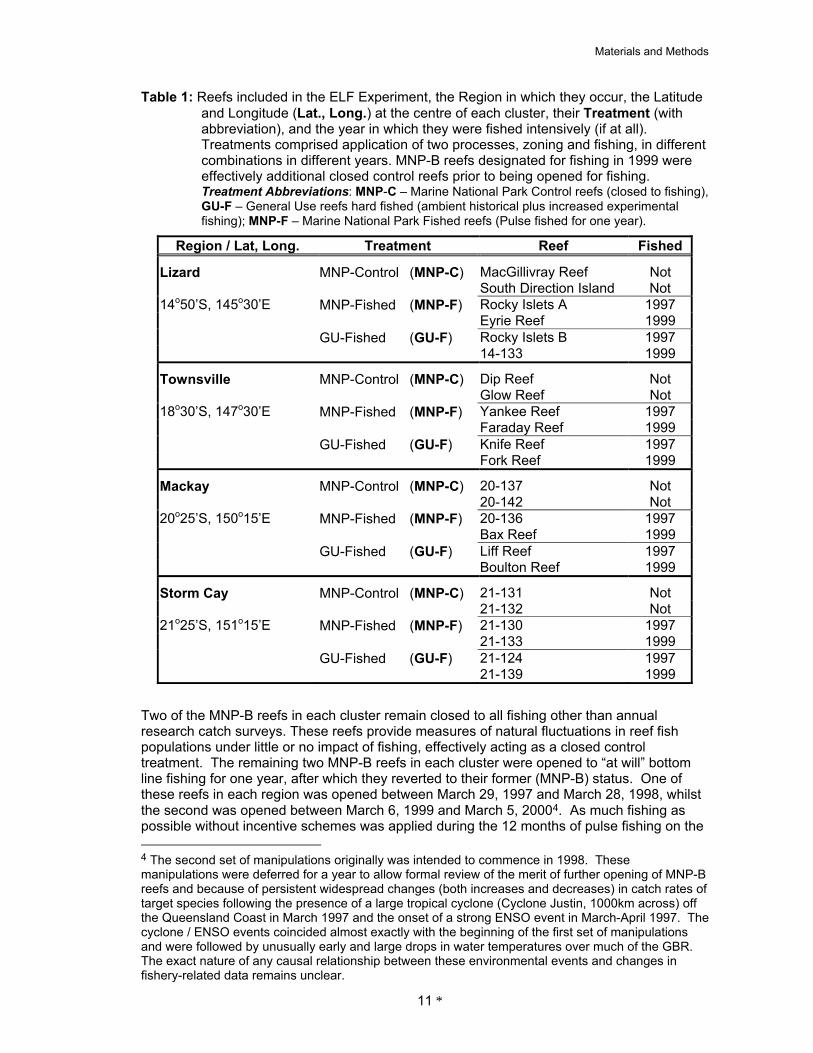
Table 1 Reefs included in the ELF Experiment the Region in which they occur the Latitude and Longitude (Lat Long) at the centre of each cluster their Treatment (with abbreviation) and the year in which they were fished intensively (if at all) Treatments comprised application of two processes zoning and fishing in different combinations in different years MNP-B reefs designated for fishing in 1999 were effectively additional closed control reefs prior to being opened for fishing Treatment Abbreviations MNP-C ndash Marine National Park Control reefs (closed to fishing) GU-F ndash General Use reefs hard fished (ambient historical plus increased experimental fishing) MNP-F ndash Marine National Park Fished reefs (Pulse fished for one year)
Region Lat Long Treatment Reef Fished
Lizard
14o50rsquoS 145o30rsquoE
MNP-Control
MNP-Fished
GU-Fished
(MNP-C)
(MNP-F)
(GU-F)
MacGillivray Reef South Direction Island Rocky Islets A Eyrie Reef Rocky Islets B 14-133
Not Not
1997 1999 1997 1999
Townsville
18o30rsquoS 147o30rsquoE
MNP-Control
MNP-Fished
GU-Fished
(MNP-C)
(MNP-F)
(GU-F)
Dip Reef Glow Reef Yankee Reef Faraday Reef Knife Reef Fork Reef
Not Not
1997 1999 1997 1999
Mackay
20o25rsquoS 150o15rsquoE
MNP-Control
MNP-Fished
GU-Fished
(MNP-C)
(MNP-F)
(GU-F)
20-137 20-142 20-136 Bax Reef Liff Reef Boulton Reef
Not Not
1997 1999 1997 1999
Storm Cay
21o25rsquoS 151o15rsquoE
MNP-Control
MNP-Fished
GU-Fished
(MNP-C)
(MNP-F)
(GU-F)
21-131 21-132 21-130 21-133 21-124 21-139
Not Not
1997 1999 1997 1999
Two of the MNP-B reefs in each cluster remain closed to all fishing other than annual research catch surveys These reefs provide measures of natural fluctuations in reef fish populations under little or no impact of fishing effectively acting as a closed control treatment The remaining two MNP-B reefs in each cluster were opened to ldquoat willrdquo bottom line fishing for one year after which they reverted to their former (MNP-B) status One of these reefs in each region was opened between March 29 1997 and March 28 1998 whilst the second was opened between March 6 1999 and March 5 20004 As much fishing as possible without incentive schemes was applied during the 12 months of pulse fishing on the
4 The second set of manipulations originally was intended to commence in 1998 These manipulations were deferred for a year to allow formal review of the merit of further opening of MNP-B reefs and because of persistent widespread changes (both increases and decreases) in catch rates of target species following the presence of a large tropical cyclone (Cyclone Justin 1000km across) off the Queensland Coast in March 1997 and the onset of a strong ENSO event in March-April 1997 The cyclone ENSO events coincided almost exactly with the beginning of the first set of manipulations and were followed by unusually early and large drops in water temperatures over much of the GBR The exact nature of any causal relationship between these environmental events and changes in fishery-related data remains unclear
11
ELF Experiment
experimental reefs by commercial charter and recreational fishers On completion of each year of pulse fishing each reef reverted to its lsquoclosedrsquo status indefinitely Increased pulses of fishing also were encouraged on one of the two GU reefs in each cluster during each of these two years after which the reefs were closed to further fishing for a period of five years These GU reefs will revert to their lsquoopenrsquo status on March 29 2003 (for those closed 1998) and March 6 2005 (for those closed in 2000) The experimental design is schematised in Table 2
Table 2 Summary of the experimental design and schedule of experimental treatments for one cluster of six reefs involved in the ELF Experiment The experimental schedule is the same for each of the four clusters involved in the experiment Key C - closed to fishing O - open to fishing P ndash pulsed fishing subscripts indicate the reefs treated first and second in each cluster
Year Reef 1995 1996 1997 1998 1999 2000 2001 2002 2003 2004 2005 MNP-Control1 C C C C C C C C C C C MNP-Control 2 C C C C C C C C C C C MNP-Fished 1 C C P C C C C C C C C MNP-Fished 2 C C C C P C C C C C C GU-Fished 1 O O P C C C C C O O O GU-Fished 2 O O O O P C C C C C O
The geographic scope of the experiment and replication of treatment reefs within each region provides data from which to estimate regional variation in the biological characteristics of several main and secondary target species and regional variations in the responses of populations of those species to changed fishing pressure Such regional considerations were considered essential for the application of Management Strategy Evaluations (MSE) to the entire GBR especially given the expected high level of among-reef and regional variation in population dynamics of target species and the known regional variation in bio-physical structure of the environment (Doherty 1987 Maxwell 1968 Oliver et al 1995 Williams 1991 Wolanski 1994) and properties of the Reef Line Fishery (Blamey and Hundloe 1993 Green et al in press Mapstone et al 1996a Trainor 1991)
Applying treatments in different years allowed the inclusion in results of inter-annual variation in treatment effects (over all regions) Explicit inclusion of inter-annual variation available only with replication of treatments over years was considered important because of the considerable inter-annual variation in recruitment of reef fishes (Doherty 1987 1991 Doherty and Williams 1988) and the potential for events in any one year to influence substantially the outcomes of the experiment (Mapstone et al 1996e 1998a Walters et al 1988 Walters and Sainsbury 1990) Because only one reef of each zoning history (MNP-B GU) in each region was subject to the pulse fishing treatment in each year however the interaction between treatment year and region is not separable from reef-reef variation within years and regions This design compromise was adopted for two reasons i) Including within-year replication of treatment reefs in each region would have increased the number of experimental reefs to at least 40 and would have proved logistically environmentally politically and economically difficult or unfeasible and ii) this level of detail (Year x Region x Treatment interactions) is of little interest given that management strategies for the GBR are unlikely to be tailored to specific inter-annual or regional changes in conditions but will be applied over several years at a time
Field Sampling All 24 experimental reefs (including controls) are sampled by structured underwater visual surveys (UVS) and line fishing catch surveys in the Austral Spring of each year Surveys have been done from and including 1995 Sampling currently is funded until the Austral
12
Materials and Methods
Spring in 2005 Surveys during 1995 and 1996 provided lsquobaselinersquo (with respect to the proposed manipulations) data for the reefs prior to commencing manipulative treatments Surveys during 1997-98 and 1999-2000 provided estimates of the effects of the increases in fishing pressure and surveys following reef closures provide data on the rebuilding of stocks following depletion by fishing
Additional UVS and catch surveys of each of the two manipulated reefs (one MNP-Fished and one GU-Fished reef) and one un-changed (control) MNP-B5 reef in each region were done to monitor changes during the years of manipulations This meant that additional visual surveys were planned for March 1997 and March 1999 immediately prior to beginning manipulations and August 1997 and August 1999 between the Autumn and Spring surveys Additional catch surveys of the same three reefs in each cluster were planned for March May and August in both 1997 and 1999 and April of 1998 and 2000 immediately after closure of the manipulated reefs Thus the two manipulated reefs and one control reef in each cluster were to be sampled 5 times during the manipulations including surveys immediately prior to and following increased fishing pressure In practice the surveys immediately prior to the reef openings in 1997 were impossible because of bad weather throughout March 1997 caused by Cyclone Justin Data from these surveys of only 12 of the 24 reefs (three per region) are used primarily for the derivation of depletion estimators of reef-specific biomass and are not otherwise considered in this report
Line Fishing Catch Surveys Line fishing catch surveys are done in the Austral Spring of each year to coincide with the spawning period of common coral trout (Plectropomus leopardus) The spring surveys are designed to sample fish during their spawning period when gonads are active and provide most information about the reproductive status of local populations The surveys are timed around the full moons however to avoid the times of peak spawning activity (centred on Spring new moons Samoilys 1997) and avoid potential biases incurred from sampling fish when they are aggregated for spawning6
Catch surveys are done via the charter of an active commercial fishing operation with master fisherman and four dory-fishermen accompanied for the surveys by four research staff Whenever possible at least some of the dorymen were constant among surveys The high turnover of crew among vessels in the reef line fishing fleet however meant that considerable changes in dorymen occurred among surveys The same master fisherman was used for all surveys between 1995 and 2000 but different master fishermen had to be employed thereafter
Fishing gear is standardised among fishers and over time to be comparable with standard contemporary gear used in the commercial RLF on the GBR We use 80lb monofilament fishing line with a ldquorunning sinkerrdquo rig consisting of a bean sinker rigged on the main line above a single 80 hook (Mustard pattern 4279) Western Australian pilchards are used as the standard bait as is the case in the commercial RLF The use of ldquohard baitrdquo(strips of freshly caught fish fillet) is not permitted again to standardise methods among fishers and over time Each fisher uses only one line at any time
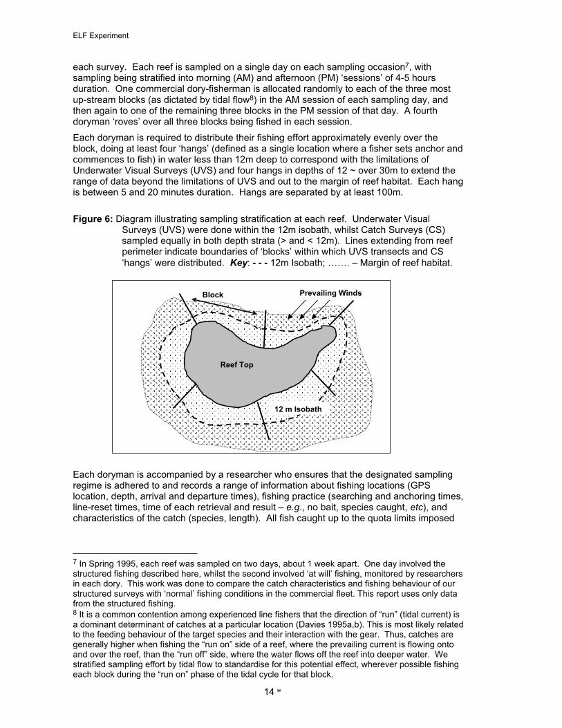
Sampling at each reef involves the same general design as follows Each reef is divided into six approximately equal sized contiguous lsquoblocksrsquo three on the windward aspect of the reef and three on the leeward aspect (Fig 6) Block boundaries are located by GPS during
5 During the first set of manipulations (1997) the MN-P B reefs that were destined to be opened to fishing in 1999 were used as these controls This strategy was adopted to avoid impacts of additional sampling during 1997-98 on the overall control reefs effectively limiting impacts of frequent sampling to those MNP-B reefs that would eventually be opened to fishing anyway 6 Studies of the spawning behaviour of P leopardus indicates that for 3-4 days either side of the Spring new moons they aggregate daily to spawn (at dusk) but disperse between new moons and sometimes disperse each day after spawning within the spawning period (Samoilys and Squire 1994 Samoilys 1997 Zeller 1998)
13
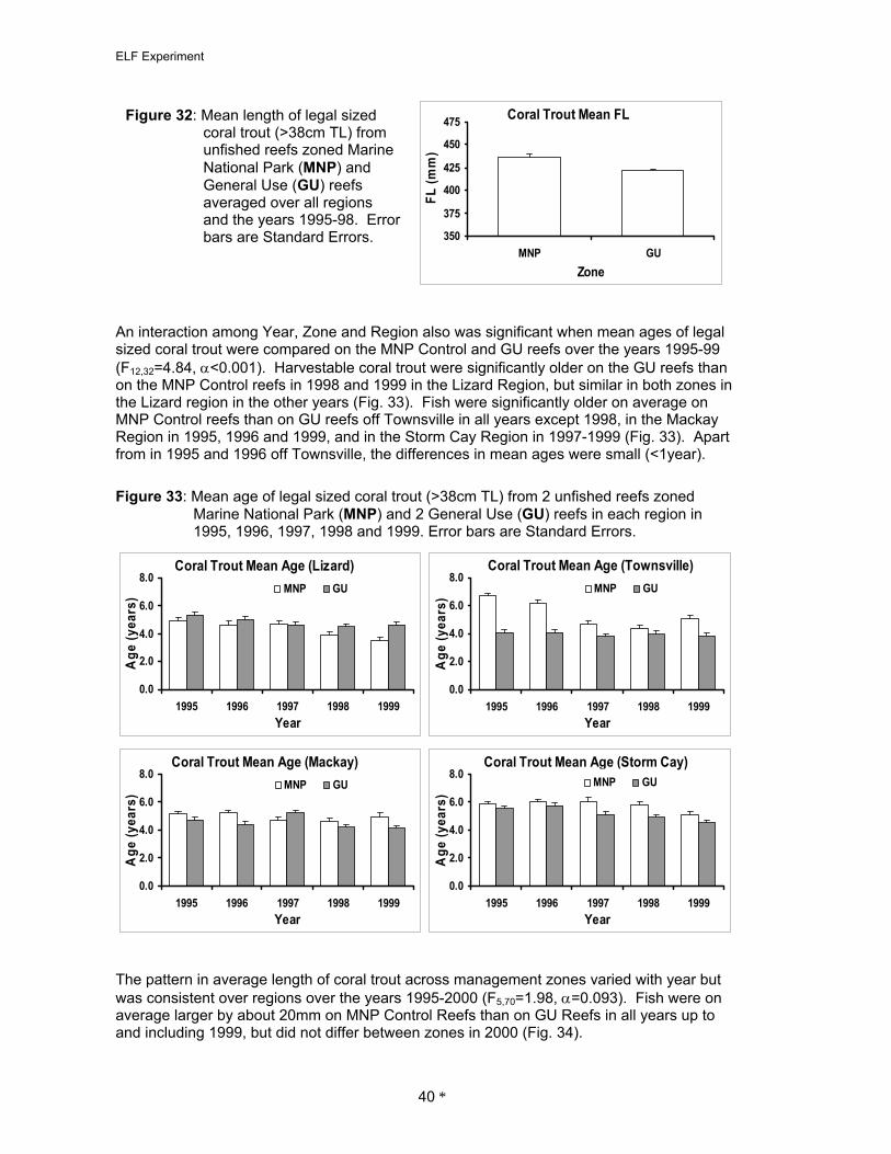
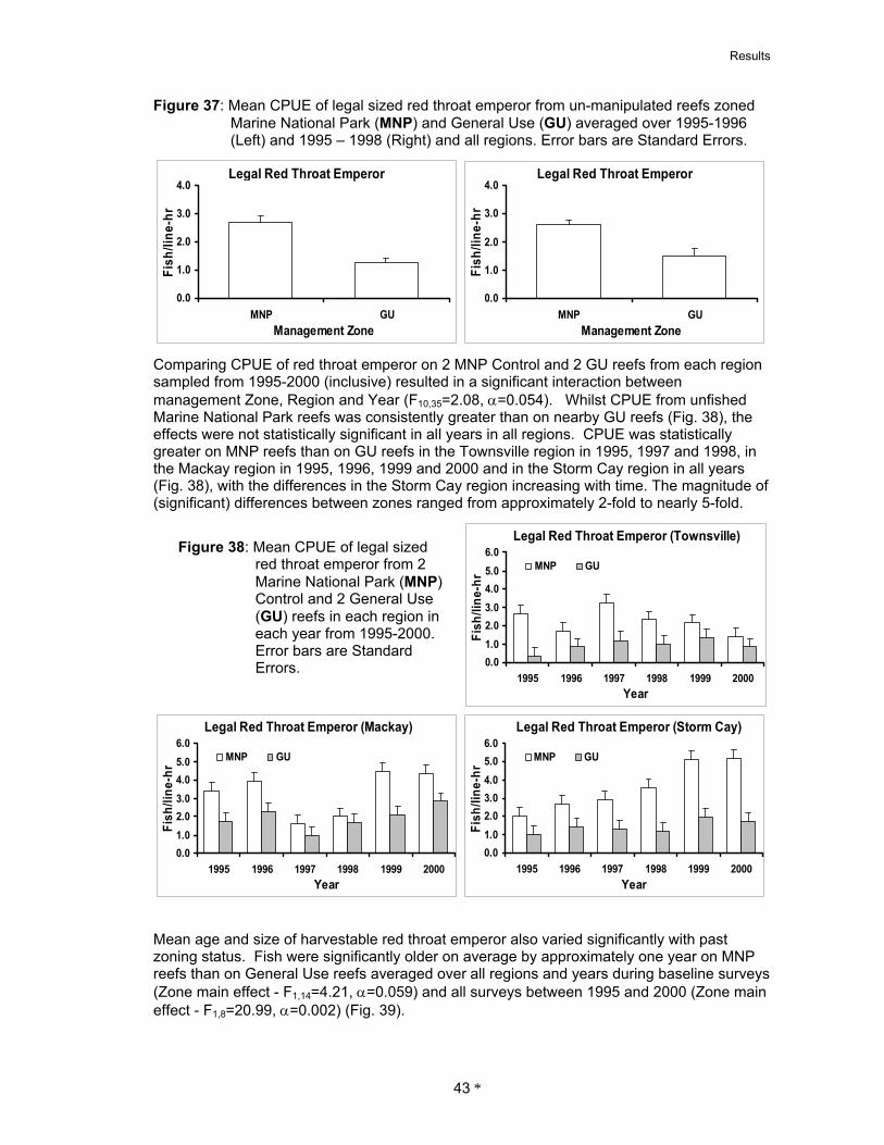
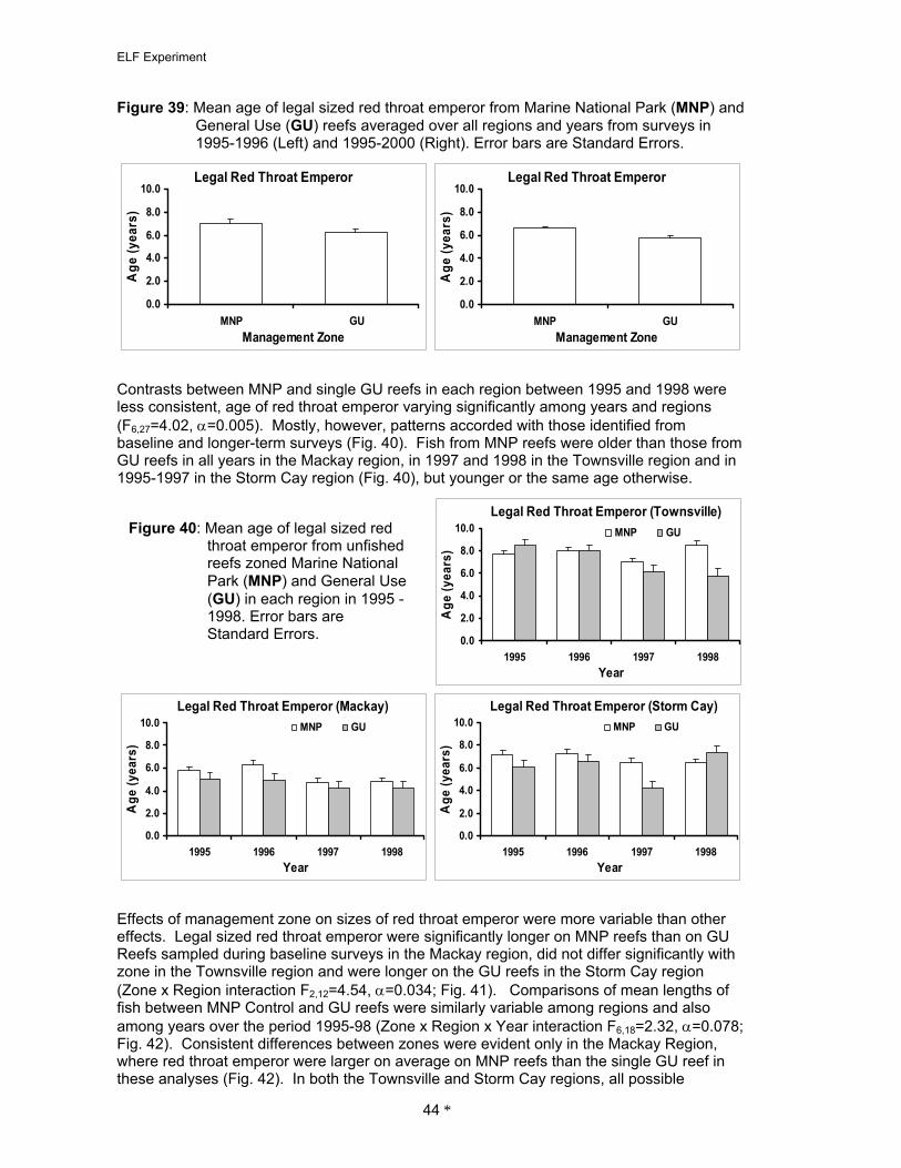
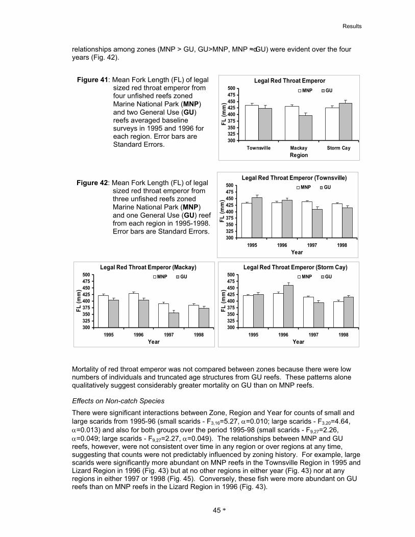
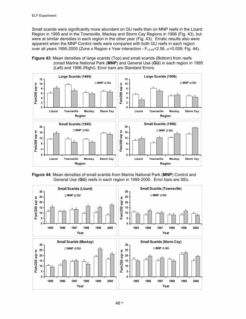
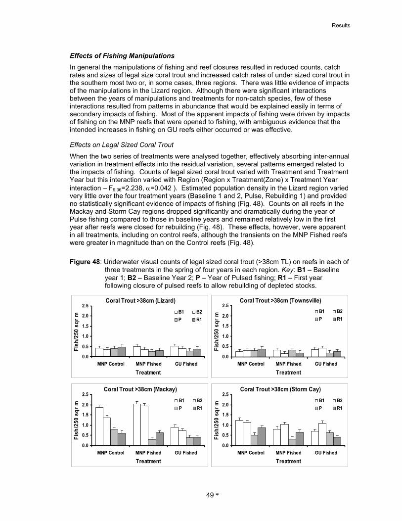
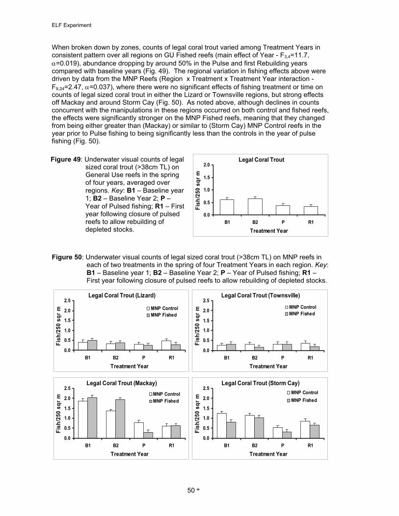
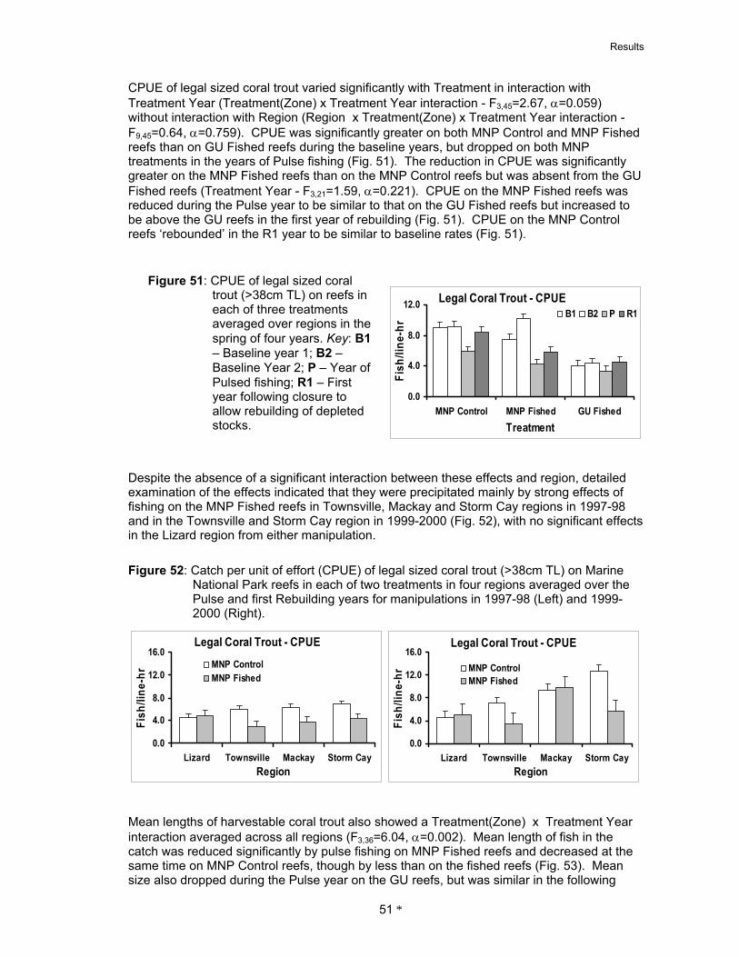
ELF Experiment
each survey Each reef is sampled on a single day on each sampling occasion7 with sampling being stratified into morning (AM) and afternoon (PM) lsquosessionsrsquo of 4-5 hours duration One commercial dory-fisherman is allocated randomly to each of the three most up-stream blocks (as dictated by tidal flow8) in the AM session of each sampling day and then again to one of the remaining three blocks in the PM session of that day A fourth doryman lsquorovesrsquo over all three blocks being fished in each session
Each doryman is required to distribute their fishing effort approximately evenly over the block doing at least four lsquohangsrsquo (defined as a single location where a fisher sets anchor and commences to fish) in water less than 12m deep to correspond with the limitations of Underwater Visual Surveys (UVS) and four hangs in depths of 12 ~ over 30m to extend the range of data beyond the limitations of UVS and out to the margin of reef habitat Each hang is between 5 and 20 minutes duration Hangs are separated by at least 100m
Figure 6 Diagram illustrating sampling stratification at each reef Underwater Visual Surveys (UVS) were done within the 12m isobath whilst Catch Surveys (CS) sampled equally in both depth strata (gt and lt 12m) Lines extending from reef perimeter indicate boundaries of lsquoblocksrsquo within which UVS transects and CS lsquohangsrsquo were distributed Key - - - 12m Isobath helliphellip ndash Margin of reef habitat
Block
Reef Top
12 m Isobath
Prevailing Winds
Each doryman is accompanied by a researcher who ensures that the designated sampling regime is adhered to and records a range of information about fishing locations (GPS location depth arrival and departure times) fishing practice (searching and anchoring times line-reset times time of each retrieval and result ndash eg no bait species caught etc) and characteristics of the catch (species length) All fish caught up to the quota limits imposed
7 In Spring 1995 each reef was sampled on two days about 1 week apart One day involved the structured fishing described here whilst the second involved lsquoat willrsquo fishing monitored by researchers in each dory This work was done to compare the catch characteristics and fishing behaviour of our structured surveys with lsquonormalrsquo fishing conditions in the commercial fleet This report uses only data from the structured fishing 8 It is a common contention among experienced line fishers that the direction of ldquorunrdquo (tidal current) is a dominant determinant of catches at a particular location (Davies 1995ab) This is most likely related to the feeding behaviour of the target species and their interaction with the gear Thus catches are generally higher when fishing the ldquorun onrdquo side of a reef where the prevailing current is flowing onto and over the reef than the ldquorun offrdquo side where the water flows off the reef into deeper water We stratified sampling effort by tidal flow to standardise for this potential effect wherever possible fishing each block during the ldquorun onrdquo phase of the tidal cycle for that block
14
Materials and Methods
by GBRMPA and QFMA QFS permit conditions9 are tagged and kept for processing that evening Fishing continues for the full day on each reef irrespective of whether the quotas have been reached with any fish caught over-quota being measured and held in live fish tanks in the dories and then released at the end of each hang
In the evening of each day the catch is processed for sale10 and the collection of biological samples Each fish is identified (independently of its identification in the dory) weighed has gonads and otoliths removed labelled and stored and is then filleted or gilled and gutted before being snap-frozen for sale Most fish are processed completely at sea but where this cannot be done lsquoframesrsquo (head viscera and skeleton) are frozen and processed on return to the laboratory
Underwater Visual Surveys Underwater Visual Surveys (UVS) were done twice annually once in Autumn (April-May) and once in Spring (September-NovemberDecember) until 2000 and once annually in Spring thereafter The Autumn surveys were timed such that young-of-the-year coral trout could be distinguished by size from older fish hence providing an index of recruitment to the reef following larval dispersal These Autumn surveys were discontinued because a) counts of very small P leopardus were insufficient to be informative b) there was no clear differentiation of a mode in the distribution of estimated sizes (Ayling 1983) that could be interpreted to represent the young of the year cohort and c) the additional data did not alter substantially the inferences drawn from only Spring surveys and so were considered an extra cost offering only marginal additional benefit
Catch and underwater surveys are timed closely within each sampling period such that UV surveys precede catch surveys of each reef by a few days Sampling within each reef is stratified similarly by blocks for both underwater and catch surveys Underwater visual surveys involve a team of 3 divers and a boat person and are based from a chartered support vessel The same observer counts all fishes in all surveys11 whilst various assistant divers count various benthic organisms Diving safety considerations mean that these counts are restricted to the shallow depth stratum between 2m and 12m depth Each reef (6 blocks 5 transects per block) takes one day to sample on each occasion
Transects are laid and counts done following the methods recommended by Mapstone and Ayling (1998) and used by Mapstone et al (1998bc 1999) and Ayling and Ayling (1992b 1994 1995) One diver runs out a 50 m fiberglass tape along the reef slope at a depth of about 2-8 m The principal observer swims beside the tape layer counting each species of coral trout lethrinids lutjanids and (where feasible) chaetodontids and scarids and caesionids as multi-species groups within an estimated 5 m of the seaward side of the tape Scarids are counted in two size classes (summed across species) 8-25cm total length (TL) and gt 25cm TL corresponding to whether they were likely to be within or above the size preyed upon by coral trout (St John 1995) Caesionids are summed (over all species) separately for each 10m segment of the 5m wide transect (ie five subdivisions) and then summed for the transect Bait fish schools (hardy heads and clupeids) are recorded as present (1) or absent (0) within 10m of each side of each 10m segment of transect giving a bait fish index of 0-5 for each transect Acanthaster planci are also counted within the 5m wide transects
9 Total allowable catch was 300 P leopardus per reef per survey with up to 90 undersized Pleopardus (lt38cm TL) and up to 350 individuals of all other species combined also with variousspecies-specific limits on the numbers of sub-legal sized fish that could be retained10 Following extraction of biological samples all catch was processed on the main vessel as in thecommercial fishery and product from legal-sized fish sold with the proceeds of the sale returned to theELF Project to partially off-set the costs of chartering the fishing operation for the catch surveys11 Duplicate counts are done concurrently by a back-up observer once per year with indexing of theobserversrsquo counts against each other to cater for any future absence of the primary observer
15
ELF Experiment
When the principal observer completes the large transect he returns along the tape counting pomacentrid fishes 05 m each side of the tape (50 x 1m) The pomacentrids are counted in four categories corresponding to their relative importance in the diet of coral trout Amblyglyphidodon curacao Chrysiptera rollandi Pomacentrus moluccensis and the remainder of pomacentrids (grouped) The tape layer follows winding in the tape and summing hard coral intercepts for the first 20 m of the return soft coral intercepts for the next 20 m of the tape and sponge intercepts for the last 10 m (back from the start point) These techniques maximise consistency and minimise potential for errors as the principal observer is responsible for recording all the most important groups
At the start of each transect the tape is run out at right angles to the proposed transect line to show the principal observer the 5m width of the transect At the end of the first pass along the transect the principal observer indicates his estimate of the width of the transect and this is measured with another tape by the tape layer and recorded
The minimum total length of fish recorded in the counts is 6 cm for Plectropomus spp 10 cm for lethrinids and lutjanids 4 cm for chaetodontids and 2 cm for pomacentrids Total lengths are estimated for all Plectropomus spp and selected lethrinid and lutjanid species harvested by the RLF Length estimation re-training using wooden coral trout models is undertaken by the principal observer at the beginning of each survey All data are recorded on ruled waterproof paper sheets in a standard format that has been well trialled in previous work and makes for easy computer entry
Laboratory Methods All sagittal otoliths and gonads are catalogued and stored for later processing as soon as possible following their return from field surveys Ages of fish are estimated from counts of annuli on otoliths and reproductive stages of fish are assessed from histology of the gonads Samples are processed roughly in order of speciesrsquo abundances and economic importance to the fishery Accordingly the main focus of work to date has been on the common coral trout (Plectropomus leopardus) and the red throat emperor (Lethrinus miniatus) Only these harvested species are discussed in detail in this report Results of reproductive analyses are the subject of other reports arising from the ELF Experiment including Adams (1996 2002) Adams et al (2001) Bean et al (in press) and several PhD theses and a companion FRDC project report (FRC Project 98-131) and are not discussed here
Otolith Processing The right sagittal otolith is used to estimate the age of all fish unless it is missing or damaged in which case the left otolith is used The right otolith is used for age determination simply for consistency there being no difference between left and right otoliths in either weight (Hatcher 1996) or counts of annuli (Ferreira and Russ 1994)
Methods of estimating age from otoliths differed among species depending on the characteristics of the otoliths Otoliths of red throat emperor and a number of other lethrinids are remarkably translucent and initial trials showed that reading these fishesrsquo otoliths whole provided the same age estimates as the sectioned otoliths Accordingly all such otoliths were read whole Otoliths from all other species were read in sectioned form as described below The reading procedures and rules for assigning age were the same for all species irrespective of how the otoliths were prepared for reading
Each sagittal otolith is weighed to the nearest 01 mg using a Sartorius electronic balance before being embedded in epoxy resin and then sectioned transversely through the core with a Multi-Drive low-speed saw with diamond edged blade Sections are mounted on glass slides with Crystal Bond 509 adhesive ground on 600- and 1200-grade carborundum paper and polished with 03 m alumina micropolish before reading
Annuli are counted in sectioned otoliths under a dissecting microscope at 40X magnification with reflected light and a black background following the methodology described by Ferreira
16
Materials and Methods
and Russ (1994) Annuli are counted from the nucleus to the proximal surface of the sagitta along the ventral margin of the sulcus acousticus The outermost annulus (opaque band) is counted providing that the otolith has a hyaline outer margin
Otoliths from each survey are read in strictly random order with no prior knowledge of location of capture or size of the fish from which each otolith came Each otolith is read by at least two independent experienced readers If the counts from the two readers are the same it is accepted as the age of the fish If the counts differ a third count is made by a third independent experienced reader If the third count matched either the first or second count that age is accepted If there is no agreement between any two of the three readers a final count is made by all three readers together If no agreement can be reached on this final count the otolith is discarded
Estimates of Catch and Effort from Experimental Reefs Data from which to estimate the effectiveness of the experimental manipulations in changing effort and catch on the experimental reefs were collected from three independent regimes First daily catch and effort were estimated from compulsory commercial fishery logbook data Second aerial and vessel surveillance data provided intermittent estimates of (potential) fishing activities on experimental reefs Third researchers were placed on site at MNP-Fished reefs when they were first opened to fishing
Compulsory Fishing Logbooks All Queensland commercial fishermen have been required by QFMA and QFS since 1988 to report their fishing location and catch (by species or species groups) for each day Data must be reported at the scale of 30rsquo x 30rsquo grids and since 1993 optionally at the scale of 6rsquo x 6rsquo sites within these grids Fishers also are expected to report the numbers of crew lines and dories used each day though these data are optional Complete data from the commercial RLF from 1988 onwards were made available for this project by the QFMA and QFS Charter vessel operators also have been required to keep logbooks of their fishing activities since 1996 though reporting coverage was not complete until 1997-9812
Aerial and Vessel Surveillance The GBRMPA requested on behalf of the ELF Project that existing aerial surveillance flights by the Queensland Department of Environment (QDoE) and Coastwatch over the GBR be diverted andor increased where possible to survey experimental reefs immediately prior to them opening and subsequently This would have resulted in planned over-flights on average approximately twice per week In practice however this frequency was reduced because of funding constraints (QDoE) and bad weather (preventing flying) or higher priority demands on aerial surveillance (eg customs activities) Over-flight frequencies during 1997 ranged from approximately 15 per week for the Lizard Island Cluster to slightly more than one flight per fortnight over the Mackay and Storm Cay Clusters and have become considerably less frequent since On each flight the position of each vessel sighted its type and apparent activity and where possible registration details were recorded In practice the frequency and accuracy of records of ldquoline fishingrdquo vessels proved to be insufficient for estimation of total effort and are not considered further
On-site Observations Researchers on-site at the four MNP Fished reefs being opened in each year made continuous observations of fishing activity (effort and catch) during the initial weeks that the reefs were opened to fishing Each researcher worked from a 6m Yamaha Southwind utility boat that allowed them to circumnavigate the treatment reefs and visit all fishing operations present Researchers lsquocampedrsquo on islands (in the Lizard region) on fishing vessels or
12 Note that because the charter vessel logbook programme is new there is likely to be less certainty about the data arising from it than from other sources
17
ELF Experiment
Queensland Boating and Fishing Patrol vessels each night and remained on-site until there were no vessels present on which to stay Where intermittent fishing activity persisted above lsquonormalrsquo levels on-site observations were prolonged by chartering vessels to accommodate observers or accompanying fishing operations that were working in the vicinity of experimental reefs On-site observations ranged from 7 to 23 days after opening reefs
Data Management All data from the ELF Experiment (and other aspects of the ELF Project) are stored on centralised relational databases on Windows NT Servers The databases are being developed for long term integrated management of the data Links with other relevant databases (eg long-term monitoring data from AIMS QFS logbook data) have been anticipated in the structure of the database
All data collected by the ELF team are entered twice into separate dedicated Microsoft Access databases via data-entry forms with filters to trap suspect (eg out of reasonable range) data The two data entry processes are independent with all data entered by different operators on each occasion These lsquodouble punchedrsquo data are then compared with purpose built software disparate values compared with original datasheets and errors corrected in either (or both) databases Finally a wide range or error checking (eg random data audits range checks verification of sampling sizes and times etc) is done prior to analyses to trap inconsistencies or suspect data that survive the prior error checks
Analytical Methods
Preliminary Processing of Data Research Data A range of variables were derived from field and laboratory data prior to analysis Underwater Visual Survey count data were transformed to densities of fish per 250m2 whilst the summed index data for each transect were analysed for estimates of baitfish abundance Catch rates from catch surveys were calculated as numbers of fish caught per line hour (Catch per Unit of Effort CPUE) per block per survey These indices were calculated by summing the numbers of fish caught (the catch) and actual fishing times (ie time between the first bait being set and the last bait being retrieved the effort) across all hangs within each block and dividing the catch by the effort Mean fork lengths (FL) and ages of fish were calculated across all fish caught and processed within each block and survey Total rates of mortality were estimated from the catches each of several cohorts over consecutive years Estimates were computed for data from GU reefs in all years (total mortality) and MNP reefs in years before they were opened to fishing (Natural mortality) These analyses included only fish at and older than ages expected to be fully recruited to the fishery and available to the gear (four years and older for P leopardus six years and older for L miniatus) and from cohorts that were represented in catches from at least three successive years These cohort-specific estimates of mortality were then averaged within reefs to give average estimates of mortality on MNP Closed reefs and GU Fished reefs in each Region Mortality was compared among Zones and Regions by 2-factor ANOVAs with the fixed factors Region and Zone and reef-specific estimates of mean total mortality as replicates
If fishing times were missing because either the lsquostart fishingrsquo or lsquoend fishingrsquo variables were absent fishing time was derived from substituting the nearest (in time) available datum for the missing value The substitutions for missing lsquostart fishing timesrsquo were sought from (in order) lsquoset timersquo lsquoend search timersquo lsquostart search timersquo time of first fish caughtrsquo for the same hang and lsquoend fishing timersquo from the previous hang Substitutions for missing lsquoend fishing timesrsquo were sought from (in order) lsquotime of last fish caughtrsquo in the same hang and lsquobegin search timersquo lsquoend search timersquo lsquoset timersquo and lsquostart fishing timersquo for the following hang If none of these substitutions were not available (eg because of failure to record times in dories) then the fishing time for the hang was derived from the fishing times for other hangs in the same block by taking a random normal variate with mean and variance of the recorded
18
Materials and Methods
fishing times for other hangs in the same block or (if few other times were available) other blocks at the same reef on the same survey
Finally there was one case where data were missing from an entire reef in the Lizard region because bad weather prevented sampling that reef during the spring survey in 1996 In this case the block-level data were estimated as a random normal variate with weighted mean and variance of the corresponding variables recorded from the same block in the one previous and three following years
Logbook Catch and Effort Data
Catch and effort for the experimental reefs could only be resolved from 6rsquo x 6rsquo site-level compulsory logbook data Use of only site-level data however would mean ignoring much of the logbook data since some fishers report only at grid-scale (30rsquo x 30rsquo) To allow use of the data reported only at grid-scale we used the available site-level data to determine the relative distribution of fishing effort and catch among sites within each grid within each year or averaged over all years when necessary and used these distributions to allocate grid-scale data among sites within grids This has the advantage that all reported catch and effort is used but the disadvantage that some catch may be attributed to sites from which it was not taken An underlying assumption in this process is that when reporting only at grid level fishers do not allocate their effort significantly differently than when reporting at site level Effort was calculated as both fishing operation-days (an operation comprising a main boat and its dories and crew) and as estimated line-days Catch was calculated as whole weights of fish
Because catch and effort data are not reported by reef we could only estimate reef-specific catches by attributing catch or effort within a six minute site among reefs that existed in that site We did this pro-rata according to the perimeter of reefs within each site The zoning status of the reefs was used to weight the distribution of catch and effort as follows Where only MNP (closed) or only GU (open) reefs were present in a site all catch and effort from the site was attributed to reefs strictly pro-rata by their perimeters Where both MNP and GU reefs were present the allocation of catch and effort was weighted such that reefs closed to fishing were attributed 20 of that catch and effort that would have been appropriate based on their perimeters and the remaining catch and effort was attributed to the open reefs In these ways we allowed for inadvertent or deliberate infringements of closures but assumed that such infringements would not equate with normal levels of fishing on open reefs
Catch and effort data for the species or groups lsquocoral troutrsquo13 red throat emperor (L miniatus) and lsquoother mixed demersal reef speciesrsquo were summed for each 6rsquox6rsquo site over 12 month intervals defined by the start and end dates of manipulations That is for reefs that were pulse fished between March 29 1997 and March 28 1998 data were aggregated from March 29 in one year to March 28 in the following year For reefs that were pulse fished between March 6 1999 and March 5 2000 data were aggregated from March 6 in one year to March 5 in the following year Data from MNP Control reefs were aggregated from March 6 to March 5 because it was expected that the major pulse in effort and catch would occur in the first months of manipulations and would be relatively trivial at the end of the manipulation periods Thus the March 6-March 5 period would capture such pulses (on fished reefs) for both manipulative periods and provide for best comparison with all manipulation reefs
Catch and effort were summed within reefs and divided by the reef perimeter to estimate effective catch (or effort) density and facilitate meaningful averaging of catch and effort statistics across reefs with similar zoning and treatment status in each year but with considerably different sizes Catch density on reefs subject to pulse fishing in 1997 was compared with catch density on non-pulsed but otherwise similar reefs in the same year
13 The generic term lsquocoral troutrsquo is used here because there is no discrimination in logbook data among species of coral trout P leopardus P laevis P maculatus P aereolatus and Variola spp all occur in the catch but are reported collectively with P leopardus as lsquocoral troutrsquo and rarely reported separately)
19
ELF Experiment
and all similarly zoned reefs in previous years as the basis for assessing the effectiveness of intended fishing or closure treatments
Tests for Effects of Fishing Region and Zone Only selected research variables were analysed for this report Variables were selected according to their data density across all reefs and to illustrate different characteristics (abundance age size) of patterns in the demographics of harvested species or their prey Accordingly the following variables were analysed independently for this report Population density (from UVS) and CPUE mean age and mean fork length (FL) (from Catch Surveys) of legal sized and under sized (or sub-legal) P leopardus (hereafter coral trout) and legal sized L miniatus (hereafter red throat emperor) and population densities of A curacao C rolandi P moluccensis lsquootherrsquo pomacentrids caesionids small ( 25cm) and large (gt 25cm) scarids Each of these variables was analysed in the same way as described below Red throat emperor are caught rarely north of Cairns and analyses for this species included data only from the southern three regions Townsville Mackay and Storm Cay
Prior to analysis reef means were derived as weighted means of block means where the weights for each block were the numbers of samples (eg hangs fish) from that block Reef means were used in analyses because reefs were the units of experimental manipulation and so constituted the true replicates for comparisons of treatment zoning or regional effects This process also had the advantage that the data subject to analysis being means of many other data were normally distributed (by the Central Limit Theorem) and also were generally homoscedastic Accordingly data were not transformed before analyses Data within reefs were thus sub-samples of the experimental units collected in stratified ways to adequately represent the overall status of each reef and were not of interest per-se for this report Reef means were compared among Regions Zones and Treatments over survey Years by a series of repeated measures analyses of variance run using SAS software
The repeated measures analyses involved the between-subject (subjects = reefs) factors Region (Lizard Townsville Mackay Storm Cay) Zone (GU MNP-B) and Treatment (MNP-Control MNP-Fished GU-Fished) nested within Zone Within-subject (repeated measures) factors were either calendar Year (1995-2000) or Treatment Year (Baseline years 1 and 2 year of Pulse fishing or the first year of post-treatment stock Rebuilding) dependent on the model involved (below) All factors were considered fixed effects
The levels of the factor Treatment Year were constructed from considering time in relation to the pulse fishing events for each reef as follows The lsquoBaseline 1rsquo and lsquoBaseline 2rsquo treatment years were comprised of data from 1995 and 1996 respectively for all treatments (MNP-Control MNP-Fished and GU-Fished) in all regions The lsquoPulsersquo year comprised data from the MNP-Fished and GU-Fished reefs in each region from the year in which each reef was subject to pulse fishing That is one MNP-Fished and one GU-Fished reef in each region would be represented by 1997 data whilst the other reef in each of these treatments would be represented by data from 1999 Similarly the lsquoRebuild 1rsquo year comprised data from 1998 or 2000 for reefs that were fished in 1997 or 1999 respectively Finally the MNP-Control reefs were represented in the lsquoPulsersquo Treatment Year by the average of data from 1997 and 1999 (the years in which fishing treatments were applied to other reefs) and represented in the lsquoRebuild 1rsquo Treatment Year by the average of data from 1998 and 2000 being the years following closure of fished reefs
Two primary sets of analyses were used to explore different questions First the effects of Zone and Region were examined by three applications of the following model
yijkl = + Ri+Zj+RZij+13k(ij) +Yl+RYil+ZYjl+RZYijl+k(ij)l (1) where
yijkl is the observation from reef k in Zone j and Region i in Year l is the true population mean for variable y
Rihellip is the effect of being in Region i (Lizard Townsville Mackay Storm Cay) Zj is the effect of Zone j (Marine National Park-B General Use)
20
Materials and Methods
13k(ij) is the residual variation attributable to being on reef k in Region i and Zone j Yhellipl is the effect of Year l (1995-2000) k(ij)l is the interaction between reefs and Years and The remaining terms are the interactions among the main effects R Z and Y
The between-reefs residual Mean Square 13k(ij) was the error variance for tests of the main effects of Region and Zone and their interactions whilst the effects of Year its interactions with Region and Zone were tested against the within-reef residual Mean Square k(ij)l
The three applications of this model involved three different subsets of reefs and years a) all reefs during the baseline years 1995 and 1996 only b) three MNP reefs and one GU reef unaffected by pulse fishing in 1997 considered over the four years 1995-98 and c) two MNP Control reefs and the two General Use reefs compared over all years 1995-200014 Effects of Zone were inferred from all three analyses whilst the Regional patterns were inferred only from analyses a) and c)
Second the impacts of the experimental treatments were explored via tests for selected terms in the following model
yijklm = +Rihellip+Zj+RZijhellip+T(Z)k(j)+RT(Z)ik(j)+13l(ijk) +T-Ym+ RT-Yihellipm
+ZT-Yjm+RZT-Yijm+T(Z)T-Yk(j)m +RT(Z)T-Yik(j)m+l(ijk)m (2) where
yijklm is the observation from reef l within Treatment k in Zone j and Region i in Treatment Year m is the true population mean for variable y
Rihellip is the effect of being in Region i (Lizard Is Townsville Mackay Storm Cay) Zj is the effect of Zone j (Marine National Park-B General Use) T(Z)k(j)is the effect of Treatment k (MNP Control MNP Fished GU Fished) in Zone j 13l(ijk) is the residual variation attributable to reef l T-Ym is the effect of Treatment Year m (Baseline 1 Baseline 2 Pulse Rebuild 1) l(ijk)m is the interaction between reefs and Treatment Years and The remaining terms are the interactions among the main effects R Z T(Z) and T-Y
The between-reefs residual Mean Square 13l(ijk) was the error variance for tests of the main effects of Region Zone and Treatment(Zone) and their interactions whilst the effects of Treatment Year and its interactions with Region Zone and Treatment(Zone) were tested against the within-reef residual Mean Square l(ijk)m
In this second suite of analyses we were interested only in the interaction between Treatment within Zone (Treatment(Zone)) and Treatment Year either alone or in interaction with Region andor Zone These interactions would indicate differences among Treatments in the response of variables over years potentially in response to Pulse fishing and would be a necessary pre-requisite to the inference of an effect of the fishing treatment as opposed to effects of Zone Region or time unrelated to the fishing treatment If one or more of these key interactions was statistically significant the model was broken down into sub-models to explore the sources of these interactions The sub models involved a) tests of Treatment Year and Region effects for GU Fished Reefs alone b) application of the above model to only MNP Control and MNP Fished Reefs and c) tests of Treatment (MNP Control vs MNP Fished) and Region effects for MNP reefs only in the separate treatment events 1997-98 and 1999-2000 In the latter analyses the model involved the orthogonal factors Region Treatment (between subjects effects) and calendar Year (within subjects)
Both multivariate and univariate tests of repeated measures were run in the above analyses [(1) and (2)] and the multivariate result accepted if the results were qualitatively different (eg one significant the other not) The Huyne-Feldt correction for non-sphericity of variance-covariance error matrices was applied to univariate tests (Winer et al 1992)
14 Complete age data for coral trout were available at the time of analyses only for the years 1995-99 Thus only the Treatment Years Baseline 1 and 2 and Pulse and calendar years 1995-99 were analysed
21
ELF Experiment
Terms were considered statistically significant and worth further exploration if P(data|H0) lt 01 Sums of Squares (SS) and degrees of freedom (df) of interaction terms were pooled with the relevant residual SS and df when Pgt025 Tests and pooling progressed from the highest order interaction down to the two-way interactions with each interaction remaining in the model being tested after any term was lsquopooledrsquo to maximise the statistical power of tests at each step Main effects were not considered in these pooling procedures For brevity test statistics and associated probabilities are reported only for significant effects
Preliminary Applications of Depletion Estimators to ELF Experimental Data Punt et al (2001) explored the application of population dynamic models to ELF field data in order to estimate reef-specific biomass natural mortality reef-specific biomass depletions from fishing catchability and the relative merits of Underwater Visual Surveys and Catch Surveys for providing abundance indices for coral trout This work has been extended but is still under development The ability to estimate biomass precisely depends (inter alia) on the amount of contrast in the data which will be maximised after the re-building phase of the ELF Experiment is completed The methods to be used to estimate biomass and fishing mortality depend on the nature of the data and the properties of those are being refined as part of the experiment Accordingly we do not present definitive results from this work at this stage We include in Appendix A however an updated description of the methods being pursued and results of a range of sensitivity analyses done with the data available so far We do not report on this work other than in this appendix
22
Results
Results Catch and Effort on Experimental Reefs On-site observations during the opening of the experimental reefs revealed that the bulk of the fishing effort and catch during the periods following opening of MNP Reefs to fishing was by commercial fishing operations (Table 3) The average annual catch and effort by commercial fishers in the degree of latitude around each set of experimental reefs estimated from compulsory logbooks varied regionally (Fig 7) as would be expected from previous analyses of regional variation in commercial catch and effort (Mapstone et al 1996a)
Table 3 Summary harvest and effort recorded by on-site observers during the initial 2 weeks after MNP reefs were opened to fishing in each region in 1997 and 1999
No Boats Harvest (kg) 1997
Region Comm Charter Rec Coral Trout Others Lizard 1 1 1 12 0 Townsville 9 2 4 1217 1514 Mackay 8 1 2 1724 1338 Storm Cay 14+ 0 0 2587 1912
1999 Region Comm Charter Rec Coral Trout Others
Lizard 3 1 2 467 333 Townsville 5 2 1 279 145 Mackay 10+ 10 10 2925 2040 Storm Cay 3 0 0 492 318
Figure 7 Average annual catch of demersal species and commercial fishing effort between 1989 and 1997 in the 1o of latitude around each cluster of experimental reefs
Catch amp Effort
0 100 200 300 400 500 600 700 800
Lizard Townsville Mackay Storm Cay
Region
Dem
ersa
l Fis
h (t)
0
2000
4000
6000
8000
10000
12000
14000
Effo
rt (L
ine-
days
) CATCH EFFORT
The effectiveness of experimental treatments varied among regions and zones as did the historical amounts of fishing around reefs open and closed to fishing (Fig 8) Catches attributed to MNP reefs in the Lizard region were broadly similar to those attributed to GU reefs and were not greatly elevated on treatment reefs during the pulse fishing years Indeed catch density around closed MNP reefs in 1997-98 and GU closed reefs in 1999-2000 were among the highest since 1990 (Fig 8) The degree to which these elevated catch densities represent infringements of the closures or fishing around the margins of closures cannot be verified
23
ELF Experiment
Figure 8 Mean annual catch density (kg fish per km reef perimeter) of all demersal species from ELF Experimental reefs zoned General Use B (GU Left) or Marine National Park B15 (MNP Right) in each region and year since 1990 Data were averaged over reefs within zones having the same status (Closed or Open) or subject to the same experimental treatment (Pulsed) in each year The effectiveness of attempts to increase fishing are inferred from comparing reefs lsquoPulsedrsquo in 1997 or 1999 with similar but un-manipulated reefs in the same or previous years
Catch Density (Lizard - GU) Catch Density (Lizard - MNP)
200 400 600 800
1000
kg
km
GU Open GU Pulse GU Closed
200 400 600 800
1000
kg
km
MNP CLosed MNP Pulse
0 90 91 92 93 94 95 96 97 98 99 00
0 90 91 92 93 94 95 96 97 98 99 00
Year Year
Catch Density (Townsville - GU) Catch Density (Townsville - MNP)
1200 GU Open 1200 MNP CLosed 1000 GU Pulse 1000 MNP Pulse
400 600 800
kg
km GU Closed
400 600 800
kg
km
200 200 0 0
90 91 92 93 94 95 96 97 98 99 00 90 91 92 93 94 95 96 97 98 99 00 Year Year
Catch Density (Mackay - GU) Catch Density (Mackay - MNP) 500 GU Open 500 MNP CLosed 400 GU Pulse 400 MNP Pulse
200 300
kg
km GU Closed
200 300
kg
km
100 100 0 0
90 91 92 93 94 95 96 97 98 99 00 90 91 92 93 94 95 96 97 98 99 00 Year Year
Catch Density (Storm Cay - GU) Catch Density (Storm Cay - MNP)
1000 GU Open 1000 MNP CLosed
400 600 800
kg
km
GU Pulse GU Closed
400 600 800
kg
km MNP Pulse
200 200 0 0
90 91 92 93 94 95 96 97 98 99 00 90 91 92 93 94 95 96 97 98 99 00 Year Year
15 Because catch and effort data are reported by at best 6rsquox6rsquo site legitimate catch and effort records exist for sites containing one or more closed reefs but also containing area open to fishing In the above figures we have assigned such catch to the closed reef as described in the methods
24
Results
Opening MNP-Fished reefs to fishing resulted in dramatic increases in catch density around those reefs in the remaining three regions though the effect was absent from the Storm Cay region in 1999 (Fig 8) Evidence was ambiguous as to whether attempts to increase fishing on selected GU reefs in 1997 and 1999 were effective in any region Although sharp increases in catch density were evident on open reefs off Townsville in 1997 and 1998 these increases were on the GU reef not intended for increased fishing Catch density from the GU treatment reef off Townsville in 1999 was significantly greater than in years prior to commencing manipulations though not as great as on the same reef in the previous two years (Fig 8) Catch densities on GU treatment reefs in the Mackay and Storm Cay regions during 1997 were slightly greater than on the non-treatment GU reefs but in 1999 catch densities on GU treatment reefs were among the lowest recorded since 1990 (Fig 8)
Tests for Region Zone and Effects of Fishing Patterns Among Regions Regional patterns were common in the analyses across both target and non-target species Though regional patterns in abundances were variable among years in most cases abundances of coral trout red throat emperor most pomacentrids and caesionids were considerably greater in the southern regions of Mackay and Storm Cay than in the more northern Lizard and Townsville regions Abundances of small and large scarids were more variable over time than other taxa but tended to decline in abundances with increasing latitudes There also were significant regional patterns in the size and age of coral trout and red throat emperor Both legal sized and under sized coral trout tended to be older and slightly smaller on average on southern reefs (where they were most abundant) than on northern reefs though these patterns were attenuated on General Use reefs compared with those on MNP reefs Red throat emperor were significantly smaller and younger in the Mackay region where they were also most abundant than in either the Townsville or Storm Cay regions
Effects on Legal Sized Coral Trout
Strong regional patterns in abundance indices for legal sized coral trout were evident from both underwater visual surveys and catch surveys during baseline years Counts of legal size coral trout were significantly and dramatically greater on reefs in the Mackay and Storm Cay regions than the Townsville and Lizard Regions in both 1995 and 1996 although the relationship between Storm Cay reefs and Mackay reefs varied between the two years (RegionxYear interaction - F316=407 0=0025 Fig 9) CPUE data showed a strong interaction between Region and Zone (F313=488 0=0017) with a north-south distinction similar to the UVS data on the MNP Reefs averaged over 1995 and 1996 but no significant differences among regions on GU reefs (Fig 9)
25
ELF Experiment
Figure 9 Underwater visual counts (Left) and CPUE (Right) of legal sized coral trout in each region averaged over zones in 1995 and 1996 (Counts) and averaged over years for each zone (MNP ndash Marine National Park GU - General Use) (CPUE) Error bars are Standard Errors
00
05
10
15
20
25
Fish
250
sqr
m
Legal Coral Trout
1995 1996
Year
Lizard Townsville Mackay Storm Cay
00
40
80
120
160
Fish
line
-hr
Legal Coral Trout CPUE
MNP GU Zone
Lizard Townsville Mackay Storm Cay
When surveys of control MNP and GU reefs were compared over the four years 1995-98 interactions between Region and Year were significant for both count (F927=609 0lt0001) and CPUE (F936=212 0=0053) data The strong regional pattern found in 1995-96 however was absent in the later 2 years for both count and CPUE estimates of abundance (Fig 10) there being only slightly greater estimates of density and CPUE in the two southern regions than in the northern regions (Fig 10)
Figure 10 Underwater visual counts (Left) and CPUE (Right) of legal sized coral trout in each region averaged over non-manipulation reefs in 1995 1996 1997 and 1998 Error bars are Standard Errors
00
05
10
15
20
25
Fish
250
sqr
m
Legal Coral Trout Lizard Townsville Mackay Storm Cay
00
40
80
120
160
Fish
line
-hr
Legal Coral Trout CPUE Lizard Townsville Mackay Storm Cay
1995 1996 1997 1998 1995 1996 1997 1998 Year Year
Extending the comparison to 1995-2000 with data from two MNP-Control and two GU-Fished reefs in each region there were significant interactions between Region and Year (F1540=295 0=0003) and Region and Zone (F38=706 0=0012) for CPUE data and Region Zone and Year for UVS data (F1545=218 0=0023) The strong north-south distinction was re-establishing in 1999 and 2000 in the catch rate data (Fig 11) and the underwater count data from MNP Reefs (Fig 12) but not in either year according to UVS data from the General Use Reefs (Fig 12)
26
Results
Figure 11 CPUE of legal sized coral trout in each region averaged over MNP Control and General Use reefs in the years 1995 ndash 2000 inclusive (Left) and averaged over years for each Zone (Right) Error bars are Standard Errors
00
40
80
120
160 Fi
shli
ne-h
r Coral Trout CPUE
1995 1996 1997 1998 1999 2000 Year
Lizard Townsville Mackay Storm Cay
00
40
80
120
160
Fish
line
-hr
Legal Coral Trout CPUE
MNP GU Management Zone
Lizard Townsville Mackay Storm Cay
Figure 12 Underwater visual counts of legal sized coral trout in each region averaged over 2 MNP Control reefs (Left) and 2 General Use Reefs (Right) in the years 1995 ndash 2000 inclusive Error bars are Standard Errors
00
05
10
15
20
25
Fish
250
sqr
m
Legal Coral Trout (MNP)
1995 1996 1997 1998 1999 2000
Year
Lizard Townsville Mackay Storm Cay
00
05
10
15
20
25 Fi
sh2
50 s
qr m
1995
Legal Coral Trout (GU)
1996 1997 1998 1999 2000
Year
Lizard Townsville Mackay Storm Cay
Interactions between Region Zone and Year occurred during the baseline years for both mean age (F316=293 0=0065) and mean length (F312=321 0=0062) of legal sized coral trout and also for comparisons of age of fish from MNP-Control and GU reefs over all years (Age - F1232=484 0lt0001)
There were few strong and persistent regional patterns in mean age Mean age of fish taken from MNP reefs was fairly consistently higher in the Storm Cay region than either the Mackay or Lizard Regions (Fig 13) a relationship that held also for GU reefs in 1995 and 1996 but not thereafter (Fig 13) Mean Age of legal sized coral trout on MNP Reefs in the Townsville region was highly variable ranging from the oldest of all regions in 1995-1996 to the second lowest in 1997-98 (Fig 13) There was a downward trend in mean age on most Lizard region reefs from 1995 to 2000 (Fig 13)
27
ELF Experiment
Figure 13 Mean age of legal sized coral trout in each region averaged over 4 Marine National Park reefs (MNP) and 2 General Use (GU) Reefs in the years 1995 and 1996 (Right) and averaged over 2 MNP Control reefs (Below Left) and 2 General Use Reefs (Below Right) in the years 1995 ndash 1999 inclusive Error bars are Standard Errors
00
20
40
60
80
A ge
(yea
rs)
Coral Trout Mean Age
MNP 1995 MNP 1996 GU 1995 GU 1996 Zone amp Year
Lizard Townsville Mackay Storm Cay
00
20
40
60
80
Age
(yea
rs)
Coral Trout Mean Age (MNP)
1995 1996 1997 1998 1999 Year
Lizard Townsville Mackay Storm Cay
00
20
40
60
80
Age
(yea
rs)
Coral Trout Mean Age (GU)
1995 1996 1997 1998 1999 Year
Lizard Townsville Mackay Storm Cay
Fish from Townsville reefs tended to be significantly larger on average than fish from comparable reefs (MNP GU) in other regions in 1995-96 and over all reefs when considered over the years 1995-2000 (Main effect of Region - F38=362 0=0065) (Fig 14) Harvestable fish from MNP reefs in the Lizard region were similar in size to those from the Mackay and Storm Cay regions in 1995 but significantly smaller in 1996 (Fig 14) Averaged over all years and zones however fish in the Lizard region were significantly larger than those from the two southern regions (Fig 14) Legal size coral trout on the GU reefs in the Mackay region were the smallest of all fish from GU reefs in both 1995 and 1996 (Fig 14)
Figure 14 Mean fork length of legal sized coral trout in each region averaged over 4 Marine National Park reefs (MNP) and 2 General Use (GU) Reefs in the years 1995 and 1996 (Left) and averaged over MNP Control and GU reefs and all years (Right) Error bars are Standard Errors
350
375
400
425
450
475
FL (m
m)
Coral Trout Mean FL
MNP 1995 MNP 1996 GU 1995 GU 1996
Zone amp Year
Lizard Townsville MackayStorm Cay
350
375
400
425
450
475
FL (m
m)
Coral Trout Mean FL
Lizard Townsville Mackay Storm Cay Region
Effects on Under Sized Coral Trout
Under sized coral trout were found to be significantly and markedly (2-4 fold) more abundant in catch surveys and underwater visual surveys in the southern two regions than in the
28
Results
northern regions during both baseline years (Fig 15) This pattern was not complicated by interactions with other factors and was thus manifest as significant main effects in analyses of both CPUE (F318=1296 0lt0001) and population density (F319=834 0=0009)
Figure 15 Mean population density (Left) and CPUE (Right) of sub-legal size coral trout during baseline surveys averaged over all reefs and 1995 and 1996 in each region Error bars are Standard Errors
00 05 10 15 20 25 30 35 40
Fish
250
sqr
m
Coral Trout (lt38cm)
Lizard Townsville Mackay Storm Cay
Region
00
20
40
60
Fish
line
-hr
Coral Trout CPUE (lt38cm)
Lizard Townsville Mackay Storm Cay Region
Considered over the period 1995-2000 on MNP Control and GU reefs however this regional contrast was not so consistent Averaged over zones in each region and year abundances of under sized coral trout estimated from underwater visual surveys declined sharply in the Mackay and Storm Cay Regions in 1997 and 1998 to reach levels in 1998 similar to those in the Lizard Island Region though still greater than off Townsville (RegionxYear interaction -F1560=548 0lt0001 Fig 16) Abundances on Storm Cay reefs increased markedly again during 1999 and 2000 but those on Mackay reefs remained at the relatively low levels reached in 1998 and similar to levels in the Lizard region ( Fig 16) Reefs in the Townsville region consistently had the lowest population densities of sub-legal coral trout
CPUE of under sized coral trout from catch surveys over all years also showed inter-annual variation in regional patterns but these interactions also varied with zoning status of reefs (F1540=168 0=0096) The large difference in CPUE between the Storm Cay and Mackay MNP reefs on the one hand and the Lizard and Townsville MNP reefs on the other in 1995-96 diminished in 1997 because of substantial drops in CPUE in the southern two regions and a slight increase in the Townsville region (Fig 16) During 1998 and 1999 MNP reefs around Storm Cay had significantly higher CPUE of sub-legal coral trout than on MNP reefs in the other three regions which did not differ from each other but in 2000 CPUE near Storm Cay also dropped again to the levels evident in other regions (Fig 16) CPUE on Lizard and Townsville reefs in 2000 were similar to what they had been in 1995-96 after having been elevated considerably during the intervening years (Fig 16)
CPUE on General Use reefs in the Storm Cay region remained dramatically greater than in the northern regions from 1995 to 1999 and was similarly high on GU reefs in the Mackay Region in 1995-96 and 1998-99 (Fig 16) CPUE in both regions plummeted in 2000 to levels similar to those on Lizard reefs which had remained relatively stable over years (Fig 16) CPUE of sub-legal coral trout from GU reefs off Townsville were the lowest of all regions in all years though not significantly lower than on Lizard reefs in 1997 or 1998
29
ELF Experiment
Figure 16 Mean population density averaged over zones for each region in each year (Right) and CPUE (Bottom) of sub-legal size coral trout on MNP Control (Left) and GU (Right) reefs in each region over the years 1995-2000 inclusive Error bars are Standard Errors
Coral Trout (lt38cm)
00 05 10 15 20 25 30 35 40 45
1995 1996 1997 1998 1999 2000
Year
Fish
250
sqr
m
Lizard Townsville Mackay Storm Cay
Coral Trout CPUE (MNP)
00
20
40
60
1995 1996 1997 1998 1999 2000 Year
Fish
line
-hr
Lizard Townsville Mackay Storm Cay
Coral Trout CPUE (GU)
00
20
40
60
1995 1996 1997 1998 1999 2000 Year
Fish
line
-hr
Lizard Townsville Mackay Storm Cay
Size and age of under sized coral trout also varied with region Mean fork length varied consistently over all reefs and years during both baseline years (F319=474 0=0015) and over all years (F38=773 0=0094) with fish in the Lizard region being significantly and consistently but only slightly (~10mm 10) smaller than those in all other regions (Fig 17)
Figure 17 Mean fork length of under sized coral trout in each region averaged over all reefs in 1995 and 1996 (Left) and averaged over 2 MNP Control and 2 GU reefs and all years from 1995-2000 (Right) Error bars are Standard Errors
400 Coral Trout Mean FL 400 Coral Trout Mean FL
375 375
325 350
(mm
)
325 350
(mm
)
300 FL
300 FL
275 275 250 250
Lizard Townsville Mackay Storm Cay Lizard Townsville Mackay Storm Cay Region Region
Age varied with Region in interaction with Year in both baseline years (F320=506 0=0009) and on MNP Control and GU Reefs over all years (F1236=279 0=0009) The effects were consistent across zones however in both analyses In 1995 under sized fish were significantly older on Mackay and Storm Cay reefs than on Lizard and Townsville reefs and Townsville fish were significantly younger than those in all other regions (Fig 18) By the spring of 1996 average age had decreased in the Lizard Mackay and Storm Cay regions to near that in the Townsville region and only fish from Storm Cay were significantly older than fish elsewhere (Fig 18) This relationship continued in the following three years (1997-99 Fig 18)
30
Results
Figure 18 Mean age of under sized coral trout on all reefs in each region in 1995 and 1996 (Left) and averaged over 2 MNP Control and 2 GU Reefs in each year from 1995-1999 (Right) Error bars are Standard Errors
20
40
60 A
ge (y
ears
) Coral Trout Age (1995-96)
Lizard Townsville Mackay Storm Cay
20
40
60
Age
(yea
rs)
Coral Trout Age Lizard Townsville Mackay Storm Cay
00 00 1995 1996 1995 1996 1997 1998 1999
Year Year
Effects on Red Throat Emperor
Average CPUE of harvestable red throat emperor varied significantly among regions consistently across zones and years during the baseline period (Region main effect -F214=1041 0=0002) but in interaction with both Year and Zone when all surveys were considered (F1035=208 0=0054) During the baseline surveys (1995-96) mean catch rates were significantly higher on Mackay reefs than on Storm Cay reefs which in turn had higher catch rates than the Townsville reefs (Fig 19) Relationships among regions varied considerably over the longer term however CPUE on Townsville reefs was usually the lowest of all regions with the notable exceptions of MNP (Control) reefs in 1995 1997 and 1998 and GU reefs in 1997 (Fig 19) The relatively slight differences among regions in mean CPUE estimates on GU reefs mostly were not statistically significant whilst the considerably larger differences among regions on MNP reefs usually were statistically significant (Fig 19) with differences between the two southern regions and the Townsville region increasing after 1997 to be approximately four-fold in 2000 (Fig 19)
31
Figure 19 Mean CPUE of legal sized red throat emperor on all reefs in each region averaged over zones and years during the baseline period (Right) and on 2 MNP Control reefs (Below Left) and 2 GU reefs (Below Right) in each region in each year from 1995 to 2000 Error bars are Standard Errors
Legal Red Throat Emperor (MNP) 60 50 40
Townsville Mackay Storm Cay
1995 1996 1997 1998 1999 2000 Year
Legal Red Throat Emperor
00
10
20
30
40
Townsville Mackay Storm Cay Region
Fish
line
-hr
Legal Red Throat Emperor (GU)
00 10 20 30 40 50 60
1995 1996 1997 1998 1999 2000 Year
Fish
line
-hr
Townsville Mackay Storm Cay
Fish
line
-hr
30 20 10 00
ELF Experiment
Regional variation in mean ages of harvestable red throat emperor were consistent across zones and years both during baseline surveys and the longer term (Baseline - F214=856 0=0004 All Years - F28=6065 0lt0001) Fish in the Mackay region were significantly younger (by 1-2 years) than in the Storm Cay and in turn Townsville regions (Fig 20)
Figure 20 Mean age of legal sized red throat emperor on all reefs in each region in 1995 and 1996 (Left) and averaged over 2 MNP Control and 2 GU Reefs and all years from 1995-1999 (Right) Error bars are Standard Errors
00
20
40
60
80
100
Age
(yea
rs)
Legal Red Throat Emperor
Townsville Mackay Storm Cay Region
00
20
40
60
80
100
Age
(yea
rs)
Legal Red Throat Emperor
Townsville Mackay Storm Cay Region
Average sizes of red throat emperor also varied among regions although the nature of such differences varied with Zone during the baseline years (F212=454 0=0034) and with Year over the longer term (F1045=193 0=0066) Sizes of fish on Mackay GU reefs were significantly smaller than on either the Townsville or Storm Cay GU reefs during the baseline surveys but length did not differ among regions on the MNP reefs during the same period (Fig 21) Over the longer term regional patterns were consistent across zones paralleling in each year the pattern seen on GU reefs in the baseline surveys (Fig 21)
Estimated total mortality of red throat emperor on MNP reefs varied significantly among regions (F28=920 =0008) being significantly greater in the Mackay region (Z=089 SE=013) than in the Storm Cay (Z=061 SE=011) and Townsville (Z=031 SE=010) regions which also differed from each other
Figure 21 Mean fork length (FL) of legal sized red throat emperor in each region on 4 MNP reefs and 2 GU reefs averaged over 1995 and 1996 (Left) and averaged over 2 MNP Control and 2 GU Reefs in each year from 1995-1999 (Right) Error bars are Standard Errors
Legal Red Throat Emperor
300 325 350 375 400 425 450 475 500
MNP GU Management Zone
FL (m
m)
Townsville Mackay Storm Cay
Legal Red Throat Emperor
300 325 350 375 400 425 450 475 500
1995 1996 1997 1998 1999 2000 Year
FL (m
m)
Townsville MackayStorm Cay
32
Results
Effects on Non-catch Species
There were significant regional patterns in abundances of non-catch species both during baseline surveys of all reefs (1995-96) and surveys of two MNP Control and 2 General Use reefs in each cluster from 1995-2000
Figure 22 Mean population densities of non-catch species counted during underwater visual surveys on all reefs in each region in 1995 and 1996 for which patterns were consistent over management zones Error bars are Standard Errors
00
150
300
450
600
750
Fish
250
sqr
m
A curacao
Lizard Townsville Mackay Storm Cay
Region
00
150
300
450
600
750
Fish
250
sqr
m
C rollandi
Lizard Townsville Mackay Storm Cay
Region
0
200
400
600
800
1000
Fish
250
sqr
m
P moluccensis
1995 1996
Year
Lizard Townsville Mackay Storm Cay
00
200
400
600
800
1000 Fi
sh2
50 s
qr m
Caesionids
Lizard Townsville Mackay Storm Cay
Region
Main effects of region were significant and uncomplicated during baseline years for A curacao (F319=2433 0lt0001) C rollandi (F318=3234 0lt0001) and casiosnids (F319=1027 0lt0001) whilst there was a significant Region x Year interaction for P moluccensis (F315=1579 0lt0001) All these taxa were significantly less abundant in the Lizard region than in the Mackay and Storm Cay regions and C rollandi P moluccensis and caesionids had abundances in the Townsville region similar to or lower than those in the Lizard region (Fig 22) Abundances of A curacao were similar on Townsville and Mackay reefs and significantly greater in all three southernmost regions than on reefs in the Lizard region (Fig 22)
Most of these patterns were consistent over subsequent years despite significant Region x Year interactions for all four groups A curacao (F1560=312 0=0001) was consistently at lowest abundances in the Lizard region greatest abundances in the Townsville and Mackay regions and (usually) intermediate abundances around Storm Cay There was consistently a 3-5 fold or greater difference between counts from Lizard reefs and those from Townsville and Mackay reefs (Fig 23) Storm Cay reefs consistently had 2-4 times as many C rollandi as reefs in the other regions amongst which relative densities varied over time (F1555=327 0=0001 Fig 23) P moluccensis (F1560=850 0lt0001) was consistently at least 4 times as abundant in the Mackay and Storm Cay regions as in the Lizard and Townsville region (Fig 23) Caesionids showed a significant interaction between Year and Region (F1560=164 0=0090) with significantly greater abundances in the southern regions in 1995 and 1996 but few significant differences among regions in most years thereafter (Fig 23)
33
Large Scarids
0
2 4
6
8 10
12
1995 1996 1997 1998 1999 2000
Year
Fish
250
sqr
m Lizard Townsville
Mackay Storm Cay
A curacao
00
150
300
450
600
750
1995 1996 1997 1998 1999 2000
Year
Fish
250
sqr
m
Lizard Townsville Mackay Storm Cay
C rollandi
00
150
300
450
600
750
1995 1996 1997 1998 1999 2000
Year Fi
sh2
50 s
qr m
Lizard Townsville Mackay Storm Cay
Caesionids
00
200
400
600
800
1000
1995 1996 1997 1998 1999 2000
Year
Fish
250
sqr
m
Lizard Townsville Mackay Storm Cay
P moluccensis
0
200
400
600
800
1000
1995 1996 1997 1998 1999 2000
Year
Fish
250
sqr
m Lizard Townsville
Mackay Storm Cay
Figure 23 Mean population densities of non-catch species counted during underwater visual surveys on MNP Control and GU r eefs in each region in 1995-2000 for which regional patterns varied with year but were consistent over management zones Error bars are Standard Errors
ELF Experiment
Large Scarids also varied significantly with Region and Year (F1555=232 0=0012) and although generally more regionally uniform in abundance than the above taxa tended to be least abundant around Storm Cay and most abundant in Lizard and or Townsville regions in most years (Fig 23)
Interactions among Region Zone and Year significantly affected abundances of large scarids during baseline surveys (F320=464 0=0013) and abundances of mixed pomacentrids and small scarids during the baseline period (Pomacentrids - F316=3077 0=0058 small scarids - F316=527 0=0010) and in the longer term (Pomacentrids - F1545=171 0=0083 small scarids - F1540=258 0=0009) Despite these interactions the pomacentrids were consistently more abundant in the southern two regions than in the northern two regions (Fig 24 Fig 25) The differences were larger on MNP reefs than GU reefs but were significant in all cases except for the contrast between Mackay region reefs and Townsville reefs in 1999 and Lizard reefs in 1998 (Fig 24 Fig 25) The relationships between Lizard and Townsville reefs varied with time in both zones as did the relationship between Mackay and Storm Cay reefs (Fig 25)
34
Results
35
Figure 24 Mean population densities of non-catch species counted during underwater visual surveys on all reefs in each region in 1995 and 1996 for which patterns varied with management zone and Year during baseline surveys Error bars are Standard Errors
Pomacentrids
0
500
1000
1500
2000
MNP 1995 MNP 1996 GU 1995 GU 1996
Zone amp Year
Fish
250
sqr
m Lizard Townsville
Mackay Storm Cay
Small Scarids
0
5
10
15
20
25
MNP 1995 MNP1996 GU 1995 GU 1996
Zone amp Year
Fish
250
sqr
m Lizard Townsville
Mackay Storm Cay
Large Scarids
0 2
4 6 8
10 12
MNP 1995 MNP 1996 GU 1995 GU 1996
Zone amp Year Fi
sh2
50 s
qr m
Lizard Townsville Mackay Storm Cay
Although small scarids often were more abundant in southern regions than in northern regions (Fig 24 Fig 25) regional patterns in abundances of both small and large scarids were not consistent over years either in 1996-96 (Fig 24) or the longer term (Fig 25)
Figure 25 Mean population densities of non-catch species from underwater visual surveys on MNP reefs and GU reefs in each region in 1995-2000 for which regional patterns varied with Zone and Year Error bars are Standard Errors
Pomacentrids (MNP)
0
500
1000
1500
2000
1995 1996 1997 1998 1999 2000
Year
Fish
250
sqr
m Lizard Townsville
Mackay Storm Cay
Pomacentrids (GU)
0
500
1000
1500
2000
1995 1996 1997 1998 1999 2000
Year
Fish
250
sqr
m Lizard Townsville
Mackay Storm Cay
Small Scarids (MNP)
0
5
10
15
20
25
30
1995 1996 1997 1998 1999 2000
Year
Fish
250
sqr
m Lizard Townsville
Mackay Storm Cay
Small Scarids (GU)
0
5
10
15
20
25
30
1995 1996 1997 1998 1999 2000
Year
Fish
250
sqr
m Lizard Townsville
Mackay Storm Cay
ELF Experiment
Effects of Management Zone Effects of prior zoning status (open or closed to fishing) were evident for abundances size and age of both coral trout and red throat emperor but the effects varied regionally and in some cases over time Legal sized coral trout were fairly consistently more abundant larger and slightly older on MNP (closed) reefs than on GU (open) reefs in the Townsville Mackay and Storm Cay regions but usually similar in most respects on open and closed reefs around Lizard Island In general the magnitude of the differences between zones increased with latitude Similarly legal sized red throat emperor were more abundant on the closed reefs though the effects of zoning on age and size of red throat emperor were variable Conversely under sized coral trout were most often significantly more abundant on the GU reefs than the MNP reefs Relationships between zoning history and abundances of non-catch species were not consistent over years or regions
Effects on Legal Sized Coral Trout
Underwater counts of legal sized coral trout during baseline surveys (1995-96) differed between reefs zoned Marine National Park and reefs zoned General Use but the differences were region specific (Region x Zone interaction - F313=1037 0=0001) Average densities of legal size coral trout on the four MNP reefs were significantly greater (by more than 100) than on the two General Use Reefs in the Mackay Region but did not differ significantly with zoning history in the other regions (Fig 26) Results were slightly more complex when the two MNP Control reefs were compared to the two GU reefs in each region over the six years 1995-2000 (Region x Year x Zone interaction - F1545=218 0=0023) Counts were significantly greater on MNP reefs than on GU reefs in the Lizard Region only in 1999 not at all in the Townsville region in the Mackay region in all years except 1999 and in the Storm Cay Region in 1995 and 2000 (Fig 27)
Figure 26 Underwater visual counts of legal sized coral trout (gt38cm TL) averaged over 1995 and 1996 from reefs zoned Marine National Park (MNP) and General Use (GU) in each region Error bars are Standard Errors
Coral Trout (gt38cm)
00
05
10
15
20
25
Lizard Townsville Mackay Storm Cay
Region
Fish
250
sqr
m MNP GU
36
Results
Figure 27 Underwater visual counts of legal sized coral trout (gt38cm TL) in 1995-2000 from 2 reefs zoned Marine National Park (MNP) and 2 reefs zoned General Use (GU) in each region Error bars are Standard Errors
Coral Trout (Lizard) Coral Trout (Townsville) 25 25
20 r m MNP GU 20 r m MNP GU
15
Fish
250
sq 15
Fish
250
sq
00
05
10
00
05
10
1995 1996 1997 1998 1999 2000 1995 1996 1997 1998 1999 2000
Year Year
00
05
10
15
20
25
Fish
250
sqr
m
Coral Trout (Mackay)
MNP GU
00
05
10
15
20
25
Fish
250
sqr
m
Coral Trout (Storm Cay)
MNP GU
1995 1996 1997 1998 1999 2000 1995 1996 1997 1998 1999 2000
Year Year
Catch rates of legal sized coral trout also varied significantly between Marine National Park and General Use reefs during baseline surveys though the differences varied with region (Zone x Region interaction - F313=488 0=0017) During 1995-96 CPUE of legal coral trout was almost identical on MNP and GU reefs in the Lizard Region was greater though not significantly so on MNP reefs than on GU reefs off Townsville and significantly and dramatically higher (by about 3-fold) on MNP reefs than on GU reefs in the Mackay and Storm Cay regions (Fig 28) When three MNP reefs were compared with a single GU reef in each region over the years 1995-98 the difference between the MNP and GU reefs was consistent among regions and over years (Main effect of Zone - F111=592 0=0033) with the overall average CPUE being around twice as high on the closed reefs (Fig 28)
Figure 28 Mean CPUE of legal sized coral trout (gt38cm TL) from reefs zoned Marine National Park (MNP) and General Use (GU) in each region averaged over 1995 and 1996 (Left) and averaged over 1995 ndash 1998 and all regions (Right) Error bars are Standard Errors
00
40
80
120
160
Fish
line
-hr
Coral Trout CPUE
Lizard Townsville Mackay Region
MNP GU
Storm Cay 00
40
80
120
160
Fish
line
-hr
Legal Coral Trout CPUE
MNP GU Zone
37
ELF Experiment
Considered over all years 1995-2000 catch rates of legal sized coral trout varied in interactions between Zone and Region (F38=706 0=0012) and Zone and Year (F540=275 0=0032) Averaged over all years CPUE on the two MNP Control reefs was approximately 2-25 times as great as on the two GU reefs in the Townsville Mackay and Storm Cay Regions but did not differ between zones in the Lizard region (Fig 29) Averaged over all regions catch rates were significantly greater on MNP reefs than on GU reefs in all years with the differences being at least two-fold in 1995-97 and then diminishing to less than 25 in 2000 (Fig 29)
Figure 29 Mean CPUE for legal sized coral trout from 2 unfished Marine National Park (MNP) and 2 General Use (GU) reefs in each region sampled between 1995 and 2000 Left - Means for the Zone x Region interaction Right ndash Means for the Zone x Year interaction Error bars are Standard Errors
Legal Coral Trout CPUE
00
40
80
120
160
Lizard Townsville Mackay Storm Cay Region
Fish
line
-hr MNP GU
Coral Trout CPUE
00
40
80
120
160
1995 1996 1997 1998 1999 2000 Year
Fish
line
-hr
MNP GU
Average age and size of harvestable coral trout also varied with zoning status Fish on GU reefs were never significantly older or larger than those on MNP reefs but both the magnitude and significance of differences between zones varied with regions and years
Figure 30 Mean age (Top) and length (Bottom) of legal sized coral trout (gt38cm TL) from reefs zoned Marine National Park (MNP) and General Use (GU) in each region in 1995 (left) and 1996 (right) Error bars are Standard Errors
Coral Trout Mean Age (1995) Coral Trout Mean Age (1996) 80 MNP GU 80 MNP GU
20
40
60
A ge
(yea
rs)
20
40
60
Age
(yea
rs)
00 00 Lizard Townsville Mackay Storm Cay Lizard Townsville Mackay Storm Cay
Region Region
475 Coral Trout Mean FL (1995) 475 Coral Trout Mean FL (1996) MNP GU MNP GU
450 450
400
425
FL (m
m)
400
425
FL (m
m)
375 375
350 350 Lizard Townsville Mackay Storm Cay Lizard Townsville Mackay Storm Cay
Region Region
38
During the baseline years of the experiment significant interactions between Year Region and Zone were evident for both mean age (F316=293 0=0065) and mean FL (F312=321 0=0062) Legal sized coral trout were on average significantly older and larger on MNP reefs than on GU reefs in both the Townsville and Mackay Regions in both 1995 and 1996 (Fig 30) and larger but not older on MNP reefs in the Storm Cay region in both years (Fig 30) Coral trout were significantly older but not significantly larger on MNP reefs in the Lizard Region in 1995 and larger but not older in 1996 (Fig 30) The magnitudes of differences in age ranged from nearly two years (50) in the Townsville region to almost nothing in the Storm Cay region whilst differences in length ranged from about 40mm (10) in the Mackay Region to just a few millimetres in the Lizard Region (Fig 30)
A significant interaction between Year Zone and Region resulted when ages of legal sized coral trout from un-fished MNP and GU reefs were compared over the four years 1995-98 (F927=451 0=0001) Again mean ages on GU reefs never significantly exceeded those on MNP reefs but ages on MNP reefs significantly exceeded those on GU reefs only in the Townsville and Mackay Region in 1995 and 1996 and in the Storm Cay Region in 1997 and 1998 (Fig 31)
Figure 31 Mean age of legal sized coral trout (gt38cm TL) from u nfished reefs zoned Marine National Park (MNP) and General Use (GU) reefs in each region in 1995 1996 1997 and 1998 Error bars are Standard Errors
Coral Trout Mean Age (1995)
00
20
40
60
80
Lizard Townsville Mackay Storm Cay Region
A ge
(yea
rs) MNP GU
Coral Trout Mean Age (1996)
00
20
40
60
80
Lizard Townsville Mackay Storm Cay Region
Age
(yea
rs) MNP GU
Coral Trout Mean Age (1997)
00
20
40
60
80
Lizard Townsville Mackay Storm Cay Region
A ge
(yea
rs) MNP GU
Coral Trout Mean Age (1998)
00
20
40
60
80
Lizard Townsville Mackay Storm Cay Region
A ge
(yea
rs) MNP GU
Results
Fork lengths of legal sized coral trout from the same reefs and years differed with zone consistently over years and regions (main effect of Zone - F18=1101 0=0011) with fish being approximately 20mm (5) longer on the closed reefs than on the reefs open to fishing (Fig 32)
39
Figure 32 Mean length of legal sized coral trout (gt38cm TL) from unfished reefs zoned Marine National Park (MNP) and General Use (GU) reefs averaged over all regions and the years 1995-98 Error bars are Standard Errors
Coral Trout Mean FL
350
375
400
425
450
475
MNP GU Zone
FL (m
m)
An interaction among Year Zone and Region also was significant when mean ages of legal sized coral trout were compared on the MNP Control and GU reefs over the years 1995-99 (F1232=484 0lt0001) Harvestable coral trout were significantly older on the GU reefs than on the MNP Control reefs in 1998 and 1999 in the Lizard Region but similar in both zones in the Lizard region in the other years (Fig 33) Fish were significantly older on average on MNP Control reefs than on GU r eefs off Townsville in all years except 1998 in the Mackay Region in 1995 1996 and 1999 and in the Storm Cay Region in 1997-1999 (Fig 33) Apart from in 1995 and 1996 off Townsville the differences in mean ages were small (lt1year)
Figure 33 Mean age of legal sized coral trout (gt38cm TL) from 2 unfished reefs zoned Marine National Park (MNP) and 2 General Use (GU) reefs in each region in 1995 1996 1997 1998 and 1999 Error bars are Standard Errors
Coral Trout Mean Age (Storm Cay)
Coral Trout Mean Age (Lizard)
00
20
40
60
80
1995 1996 1997 1998 1999 Year
A ge
(yea
rs) MNP GU
Coral Trout Mean Age (Townsville)
00
20
40
60
80
1995 1996 1997 1998 1999 Year
A ge
(yea
rs)
MNP GU
Coral Trout Mean Age (Mackay)
00
20
40
60
80
1995 1996 1997 1998 1999 Year
Age
(yea
rs)
MNP GU
00
20
40
60
80
1995 1996 1997 1998 1999 Year
Age
(yea
rs)
MNP GU
ELF Experiment
The pattern in average length of coral trout across management zones varied with year but was consistent over regions over the years 1995-2000 (F570=198 0=0093) Fish were on average larger by about 20mm on MNP Control Reefs than on GU Reefs in all years up to and including 1999 but did not differ between zones in 2000 (Fig 34)
40
Results
Figure 34 Mean length of legal sized coral trout (gt38cm TL) from unfished reefs zoned Marine National Park (MNP) and General Use (GU) reefs averaged over all regions in the years 1995-99 Error bars are Standard Errors
Coral Trout Mean FL
350
375
400
425
450
475
1995 1996 1997 1998 1999 2000 Year
FL (m
m)
MNP GU
Estimates of total mortality of coral trout considered fully recruited to the gear (those aged 4 years and older) were lower on MNP reefs than GU reefs in each region and were generally greatest in the Storm Cay region and least in the Townsville region in both zones (Table 4) None of these apparent differences were statistically significant however (Pgt01 in all tests)
Table 4 Estimated total mortality (Z) of fully recruited coral trout on un-manipulated MNP reefs and GU reefs in each region over the years 1995-99
Zone MNP GU
Region Mortality (SE) Mortality (SE) Lizard 061 (014) 063 (014) Townsville 045 (011) 058 (023) Mackay 061 (011) 075 (015) Storm Cay 084 (011) 093 (018)
Effects on Under Sized Coral Trout
Both underwater visual counts and catch surveys indicated significantly lower abundances of undersize coral trout on MNP reefs than on GU reefs during 1995 and 1996 Moreover both results were consistent over both regions and years leaving clear main effects of zones (Visual Surveys -F119=834 0=0009 Catch Surveys - F118=1451 0=0001) (Fig 35) The same main-effect result was evident in the underwater visual survey data for MNP Control and GU reefs over the years 1995-2000 (F111=697 0=0023 GU reefs ndash 132 fish250m2 MNP reefs ndash 115 fish250m2)
Figure 35 Mean density estimated from underwater visual surveys (Left) and CPUE from structured catch surveys (Right) of sub-legal coral trout (lt38cm TL) from reefs zoned Marine National Park (MNP) and General Use (GU) averaged over all regions and 1995-1996 Error bars are Standard Errors
20 25 30 35 40
qr m
Coral Trout (lt38cm)
40
60
line-
hr
Coral Trout CPUE (lt38cm)
10 15
sh2
50 s
20
Fish
05 Fi
00 00 MNP GU MNP GU
Management Zone Management Zone
41
ELF Experiment
CPUE of sub-legal coral trout from MNP Control and GU reefs over the years 1995-2000 varied with Region Zone and Year (F1540=168 0=0096) For the most part the same pattern was evident as during the baseline years with CPUE of under sized coral trout never being significantly greater on MNP Control reefs than on GU Reefs Catch rates were significantly greater on GU reefs than on unfished MNP reefs in Lizard Mackay and Storm Cay Region in all years except 1997 and 1998 (Lizard Region) 1997 (Mackay) and 1998 (Storm Cay) (Fig 36) In the Townsville Region catch rates were significantly greater on the GU reefs in 1995 and 1996 but no other years (Fig 36)
Figure 36 Mean CPUE of sub-legal coral trout (lt38cm TL) from Marine National Park (MNP) Control and General Use (GU) reefs in each region in each year from 1995-2000 Error bars are Standard Errors
00
20
40
60
Fish
line
-hr
Coral Trout CPUE (Lizard)
1995 1996 1997 1998 1999 2000 Year
MNP GU
00
20
40
60
Fish
line
-hr
Coral Trout CPUE (Townsville)
1995 1996 1997 1998 1999 2000 Year
MNP GU
00
20
40
60
Fish
line
-hr
Coral Trout CPUE (Mackay)
1995 1996 1997 1998 1999 2000 Year
MNP GU
00
20
40
60
Fish
line
-hr
Coral Trout CPUE (Storm Cay)
1995 1996 1997 1998 1999 2000 Year
MNP GU
There were no significant effects of zoning on mean age or fork length of sub-legal coral trout (Pgt01 in all tests)
Effects on Red Throat Emperor
There were conspicuous and relatively uncomplicated differences in CPUE of red throat emperor between reefs zoned Marine National Park (MNP) and those zoned General Use (GU) in all regions During baseline surveys effects of management zone were consistent over years and regions (Zone main effect - F114=3371 0lt0001) overall average CPUE being nearly three times as high on 16 MNP reefs as on the 8 GU reefs (Fig 37) A parallel result arose from comparing 3 MNP control and 2 GU reefs from each region over the years 1995-98 (F18=1118 0=0010 Fig 37)
42
Figure 37 Mean CPUE of legal sized red throat emperor from un-manipulated reefs zoned Marine National Park (MNP) and General Use (GU) averaged over 1995-1996 (Left) and 1995 ndash 1998 (Right) and all regions Error bars are Standard Errors
Legal Red Throat Emperor
00
10
20
30
40
MNP GU Management Zone
Fish
line
-hr
Legal Red Throat Emperor
00
10
20
30
40
MNP GU Management Zone
Fish
line
-hr
Comparing CPUE of red throat emperor on 2 MNP Control and 2 GU reefs from each region sampled from 1995-2000 (inclusive) resulted in a significant interaction between management Zone Region and Year (F1035=208 0=0054) Whilst CPUE from unfished Marine National Park reefs was consistently greater than on nearby GU reefs (Fig 38) the effects were not statistically significant in all years in all regions CPUE was statistically greater on MNP reefs than on GU reefs in the Townsville region in 1995 1997 and 1998 in the Mackay region in 1995 1996 1999 and 2000 and in the Storm Cay region in all years (Fig 38) with the differences in the Storm Cay region increasing with time The magnitude of (significant) differences between zones ranged from approximately 2-fold to nearly 5-fold
Figure 38 Mean CPUE of legal sized red throat emperor from 2 Marine National Park (MNP) Control and 2 General Use (GU) reefs in each region in each year from 1995-2000 Error bars are Standard Errors
Legal Red Throat Emperor (Townsville)
00 10 20 30 40 50 60
1995 1996 1997 1998 1999 2000 Year
Fish
line
-hr
MNP GU
Legal Red Throat Emperor (Mackay)
00 10 20 30 40 50 60
1995 1996 1997 1998 1999 2000 Year
Fish
line
-hr
MNP GU
Legal Red Throat Emperor (Storm Cay)
00 10 20 30 40 50 60
1995 1996 1997 1998 1999 2000 Year
Fish
line
-hr
MNP GU
Results
Mean age and size of harvestable red throat emperor also varied significantly with past zoning status Fish were significantly older on average by approximately one year on MNP reefs than on General Use reefs averaged over all regions and years during baseline surveys (Zone main effect - F114=421 0=0059) and all surveys between 1995 and 2000 (Zone main effect - F18=2099 0=0002) (Fig 39)
43
Figure 39 Mean age of legal sized red throat emperor from Marine National Park (MNP) and General Use (GU) reefs averaged over all regions and years from surveys in 1995-1996 (Left) and 1995-2000 (Right) Error bars are Standard Errors
Legal Red Throat Emperor
00
20
40
60
80
100
MNP GU Management Zone
Age
(yea
rs)
Legal Red Throat Emperor
00
20
40
60
80
100
MNP GU Management Zone
Age
(yea
rs)
Contrasts between MNP and single GU reefs in each region between 1995 and 1998 were less consistent age of red throat emperor varying significantly among years and regions (F627=402 0=0005) Mostly however patterns accorded with those identified from baseline and longer-term surveys (Fig 40) Fish from MNP reefs were older than those from GU reefs in all years in the Mackay region in 1997 and 1998 in the Townsville region and in 1995-1997 in the Storm Cay region (Fig 40) but younger or the same age otherwise
Figure 40 Mean age of legal sized red throat emperor from unfished reefs zoned Marine National Park (MNP) and General Use (GU) in each region in 1995 -1998 Error bars are Standard Errors
Legal Red Throat Emperor (Townsville)
00
20
40
60
80
100
1995 1996 1997 1998 Year
Age
(yea
rs)
MNP GU
Legal Red Throat Emperor (Mackay)
00
20
40
60
80
100
1995 1996 1997 1998 Year
Age
(yea
rs)
MNP GU
Legal Red Throat Emperor (Storm Cay)
00
20
40
60
80
100
1995 1996 1997 1998 Year
Age
(yea
rs)
MNP GU
ELF Experiment
Effects of management zone on sizes of red throat emperor were more variable than other effects Legal sized red throat emperor were significantly longer on MNP reefs than on GU Reefs sampled during baseline surveys in the Mackay region did not differ significantly with zone in the Townsville region and were longer on the GU reefs in the Storm Cay region (Zone x Region interaction F212=454 0=0034 Fig 41) Comparisons of mean lengths of fish between MNP Control and GU reefs were similarly variable among regions and also among years over the period 1995-98 (Zone x Region x Year interaction F618=232 0=0078 Fig 42) Consistent differences between zones were evident only in the Mackay Region where red throat emperor were larger on average on MNP reefs than the single GU reef in these analyses (Fig 42) In both the Townsville and Storm Cay regions all possible
44
Results
relationships among zones (MNP gt GU GUgtMNP MNP 13 GU) were evident over the four years (Fig 42)
Figure 41 Mean Fork Length (FL) of legal sized red throat emperor from four unfished reefs zoned Marine National Park (MNP) and two General Use (GU) reefs averaged baseline surveys in 1995 and 1996 for each region Error bars are Standard Errors
Legal Red Throat Emperor
300 325 350 375 400 425 450 475 500
Townsville Mackay Storm Cay Region
FL (m
m)
MNP GU
Figure 42 Mean Fork Length (FL) of legal sized red throat emperor from three unfished reefs zoned Marine National Park (MNP) and one General Use (GU) reeffrom each region in 1995-1998 Error bars are Standard Errors
Legal Red Throat Emperor (Townsville)
300 325 350 375 400 425 450 475 500
1995 1996 1997 1998 Year
FL (m
m)
MNP GU
Legal Red Throat Emperor (Mackay)
300 325 350 375 400 425 450 475 500
1995 1996 1997 1998 Year
FL (m
m)
MNP GU
Legal Red Throat Emperor (Storm Cay)
300 325 350 375 400 425 450 475 500
1995 1996 1997 1998 Year
FL (m
m)
MNP GU
Mortality of red throat emperor was not compared between zones because there were low numbers of individuals and truncated age structures from GU reefs These patterns alone qualitatively suggest considerably greater mortality on GU than on MNP reefs
Effects on Non-catch Species
There were significant interactions between Zone Region and Year for counts of small and large scarids from 1995-96 (small scarids - F316=527 0=0010 large scarids - F320=464 0=0013) and also for both groups over the period 1995-98 (small scarids - F927=226 0=0049 large scarids - F927=227 0=0049) The relationships between MNP and GU reefs however were not consistent over time in any region or over regions at any time suggesting that counts were not predictably influenced by zoning history For example large scarids were significantly more abundant on MNP reefs in the Townsville Region in 1995 and Lizard Region in 1996 (Fig 43) but at no other regions in either year (Fig 43) nor at any regions in either 1997 or 1998 (Fig 45) Conversely these fish were more abundant on GU reefs than on MNP reefs in the Lizard Region in 1996 (Fig 43)
45
ELF Experiment
Small scarids were significantly more abundant on GU reefs than on MNP reefs in the Lizard Region in 1995 and in the Townsville Mackay and Storm Cay Regions in 1996 (Fig 43) but were at similar densities in each region in the other year (Fig 43) Erratic results also were apparent when the MNP Control reefs were compared with both GU reefs in each region over all years 1995-2000 (Zone x Region x Year interaction - F1540=258 0=0009 Fig 44)
Figure 43 Mean densities of large scarids (Top) and small scarids (Bottom) from reefs zoned Marine National Park (MNP) and General Use (GU) in each region in 1995 (Left) and 1996 (Right) Error bars are Standard Errors
Large Scarids (1995)
0 2 4 6
8 10 12
Lizard Townsville Mackay Storm Cay
Region
Fish
250
sqr
m
MNP GU
Large Scarids (1996)
0 2
4 6 8
10 12
Lizard Townsville Mackay Storm Cay
Region Fi
sh2
50 s
qr m
MNP GU
Small Scarids (1995)
0
4
8
12
16
20
Lizard Townsville Mackay Storm Cay
Region
Fish
250
sqr
m
MNP GU
Small Scarids (1996)
0
4
8
12
16
20
Lizard Townsville Mackay Storm Cay
Region
Fish
250
sqr
m
MNP GU
Figure 44 Mean densities of small scarids from Marine National Park (MNP) Control and General Use (GU) reefs in each region in 1995-2000 Error bars are SEs
Small Scarids (Lizard)
0
5
10
15
20
25
30
1995 1996 1997 1998 1999 2000
Year
Fish
250
sqr
m
MNP GU
Small Scarids (Townsville)
0
5
10
15
20
25
30
1995 1996 1997 1998 1999 2000
Year
Fish
250
sqr
m MNP GU
Small Scarids (Mackay)
0
5
10
15
20
25
30
1995 1996 1997 1998 1999 2000
Year
Fish
250
sqr
m MNP GU
Small Scarids (Storm Cay)
0
5
10
15
20
25
30
1995 1996 1997 1998 1999 2000
Year
Fish
250
sqr
m MNP GU
46
Results
Similarly in 1997 small scarids were more abundant on the General Use reef than on the three MNP reefs around Storm Cay but nowhere else and in 1998 they were significantly more abundant on the GU reef in the Lizard Region but nowhere else (Fig 45) It is noteworthy however that small scarids were never at significantly greater densities on MNP reefs than on GU reefs
Figure 45 Mean densities of large scarids (A) and small scarids (B) averaged over Marine National Park (MNP) Control reefs and General Use (GU) reefs in each region in 1995 1996 1997 and 1998 Error bars are Standard Errors
A) Large Scarids
Large Scarids (1995)
0 2
4 6 8
10 12
Lizard Townsville Mackay Storm Cay
Region
Fish
250
sqr
m
MNP GU
Large Scarids (1996)
0 2
4 6
8 10
12
Lizard Townsville Mackay Storm Cay
Region
Fish
250
sqr
m
MNP GU
Large Scarids (1997)
0 2
4 6
8 10
12
Lizard Townsville Mackay Storm Cay
Region
Fish
250
sqr
m
MNP GU
Large Scarids (1998)
0 2
4 6
8 10
12
Lizard Townsville Mackay Storm Cay
Region
Fish
250
sqr
m
MNP GU
B) Small Scarids$
Small Scarids (1995)
0
5
10
15
20
25
Lizard Townsville Mackay Storm Cay
Region
Fish
250
sqr
m
MNP GU
Small Scarids (1996)
0
5
10
15
20
25
Lizard Townsville Mackay Storm Cay
Region
Fish
250
sqr
m MNP GU
Small Scarids (1997)
0
5
10
15
20
25
Lizard Townsville Mackay Storm Cay
Region
Fish
250
sqr
m
MNP GU
Small Scarids (1998)
0
5
10
15
20
25
Lizard Townsville Mackay Storm Cay
Region
Fish
250
sqr
m
MNP GU
47
ELF Experiment
Effects of zoning on other non-harvested fish were evident for caesionids (Zone x Year interaction 1995-98 - F333=226 0=0100 Fig 46) and grouped pomacentrids (Zone x Region x Year interactions 1995-96 - F316=3077 0=0058 1995-2000 - F1545=171 0=0083 Fig 47) As with the scarids there was no consistent Zone effect although abundances of pomacentrids were generally significantly higher on closed than open reefs off Mackay and greater on open than closed reefs off Townsville (Fig 47)
Figure 46 Mean densities of caesionids on reefs zoned Marine National Park (MNP) and General Use (GU) averaged over regions in 1995 1996 1997 and 1998 Error bars are Standard Errors
Caesionids
00
200
400
600
800
1000
1995 1996 1997 1998
Year
Fish
250
sqr
m MNP GU
Figure 47 Mean densities of pomacentrids from Marine National Park (MNP) and General Use (GU) reefs in each region in 1995 (Top Left) and 1996 (Top Right) and in 1995-2000 for each region (Middle and Bottom) Error bars are Standard Errors
Pomacentrids (1995) Pomacentrids (1996) 2000 2000
500
1000
1500
Fish
250
sqr
m MNP GU
500
1000
1500
Fish
250
sqr
m MNP GU
0 0 Lizard Townsville Mackay Storm Cay Lizard Townsville Mackay Storm Cay
Region Region
Pomacentrids (Lizard) Pomacentrids (Townsville) 2000 2000
500
1000
1500
Fish
250
sqr
m MNP GU
500
1000
1500
Fish
250
sqr
m MNP GU
0 0 1995 1996 1997 1998 1999 2000 1995 1996 1997 1998 1999 2000
Year Year
Pomacentrids (Mackay) Pomacentrids (Storm Cay) 2000 2000
500
1000
1500
Fish
250
sqr
m MNP GU
500
1000
1500
Fish
250
sqr
m MNP GU
0 0 1995 1996 1997 1998 1999 2000 1995 1996 1997 1998 1999 2000
Year Year
48
Results
Effects of Fishing Manipulations In general the manipulations of fishing and reef closures resulted in reduced counts catch rates and sizes of legal size coral trout and increased catch rates of under sized coral trout in the southern most two or in some cases three regions There was little evidence of impacts of the manipulations in the Lizard region Although there were significant interactions between the years of manipulations and treatments for non-catch species few of these interactions resulted from patterns in abundance that would be explained easily in terms of secondary impacts of fishing Most of the apparent impacts of fishing were driven by impacts of fishing on the MNP reefs that were opened to fishing with ambiguous evidence that the intended increases in fishing on GU reefs either occurred or was effective
Effects on Legal Sized Coral Trout
When the two series of treatments were analysed together effectively absorbing inter-annual variation in treatment effects into the residual variation several patterns emerged related to the impacts of fishing Counts of legal sized coral trout varied with Treatment and Treatment Year but this interaction varied with Region (Region x Treatment(Zone) x Treatment Year interaction ndash F936=2238 0=0042 ) Estimated population density in the Lizard region varied very little over the four treatment years (Baseline 1 and 2 Pulse Rebuilding 1) and provided no statistically significant evidence of impacts of fishing (Fig 48) Counts on all reefs in the Mackay and Storm Cay regions dropped significantly and dramatically during the year of Pulse fishing compared to those in baseline years and remained relatively low in the first year after reefs were closed for rebuilding (Fig 48) These effects however were apparent in all treatments including on control reefs although the transients on the MNP Fished reefs were greater in magnitude than on the Control reefs (Fig 48)
Figure 48 Underwater visual counts of legal sized coral trout (gt38cm TL) on reefs in each of three treatments in the spring of four years in each region Key B1 ndash Baseline year 1 B2 ndash Baseline Year 2 P ndash Year of Pulsed fishing R1 ndash First year following closure of pulsed reefs to allow rebuilding of depleted stocks
00
05
10
15
20
25
Fish
250
sqr
m
Coral Trout gt38cm (Lizard)
MNP Control MNP Fished GU Fished
Treatment
B1 B2 P R1
00
05
10
15
20
25
Fish
250
sqr
m
Coral Trout gt38cm (Townsville)
MNP Control MNP Fished GU Fished
Treatment
B1 B2 P R1
00
05
10
15
20
25
Fish
250
sqr
m
Coral Trout gt38cm (Mackay)
MNP Control MNP Fished GU Fished
Treatment
B1 B2 P R1
00
05
10
15
20
25
Fish
250
sqr
m
Coral Trout gt38cm (Storm Cay)
MNP Control MNP Fished GU Fished
Treatment
B1 B2 P R1
49
ELF Experiment
When broken down by zones counts of legal coral trout varied among Treatment Years in consistent pattern over all regions on GU Fished reefs (main effect of Year - F34=117 0=0019) abundance dropping by around 50 in the Pulse and first Rebuilding years compared with baseline years (Fig 49) The regional variation in fishing effects above were driven by data from the MNP Reefs (Region x Treatment x Treatment Year interaction - F924=247 0=0037) where there were no significant effects of fishing treatment or time on counts of legal sized coral trout in either the Lizard or Townsville regions but strong effects off Mackay and around Storm Cay (Fig 50) As noted above although declines in counts concurrent with the manipulations in these regions occurred on both control and fished reefs the effects were significantly stronger on the MNP Fished reefs meaning that they changed from being either greater than (Mackay) or similar to (Storm Cay) MNP Control reefs in the year prior to Pulse fishing to being significantly less than the controls in the year of pulse fishing (Fig 50)
Figure 49 Underwater visual counts of legal sized coral trout (gt38cm TL) on General Use reefs in the spring of four years averaged over regions Key B1 ndash Baseline year 1 B2 ndash Baseline Year 2 P ndash Year of Pulsed fishing R1 ndash First year following closure of pulsed reefs to allow rebuilding of depleted stocks
Legal Coral Trout
00
05
10
15
20
B1 B2 P R1
Treatment Year
Fish
250
sqr
m
Figure 50 Underwater visual counts of legal sized coral trout (gt38cm TL) on MNP reefs in each of two treatments in the spring of four Treatment Years in each region Key B1 ndash Baseline year 1 B2 ndash Baseline Year 2 P ndash Year of Pulsed fishing R1 ndash First year following closure of pulsed reefs to allow rebuilding of depleted stocks
Legal Coral Trout (Lizard)
00
05
10
15
20
25
B1 B2 P R1
Treatment Year
Fish
250
sqr
m MNP Control MNP Fished
Legal Coral Trout (Townsville)
00
05
10
15
20
25
B1 B2 P R1
Treatment Year
Fish
250
sqr
m
MNP Control MNP Fished
Legal Coral Trout (Mackay)
00
05
10
15
20
25
B1 B2 P R1
Treatment Year
Fish
250
sqr
m
MNP Control MNP Fished
Legal Coral Trout (Storm Cay)
00
05
10
15
20
25
B1 B2 P R1
Treatment Year
Fish
250
sqr
m MNP Control
MNP Fished
50
CPUE of legal sized coral trout varied significantly with Treatment in interaction with Treatment Year (Treatment(Zone) x Treatment Year interaction - F345=267 0=0059) without interaction with Region (Region x Treatment(Zone) x Treatment Year interaction - F945=064 0=0759) CPUE was significantly greater on both MNP Control and MNP Fished reefs than on GU Fished reefs during the baseline years but dropped on both MNP treatments in the years of Pulse fishing (Fig 51) The reduction in CPUE was significantly greater on the MNP Fished reefs than on the MNP Control reefs but was absent from the GU Fished reefs (Treatment Year - F321=159 0=0221) CPUE on the MNP Fished reefs was reduced during the Pulse year to be similar to that on the GU Fished reefs but increased to be above the GU reefs in the first year of rebuilding (Fig 51) CPUE on the MNP Control reefs lsquoreboundedrsquo in the R1 year to be similar to baseline rates (Fig 51)
Figure 51 CPUE of legal sized coral trout (gt38cm TL) on reefs in each of three treatments averaged over regions in the spring of four years Key B1 ndash Baseline year 1 B2 ndash Baseline Year 2 P ndash Year of Pulsed fishing R1 ndash First year following closure to allow rebuilding of depleted stocks
Legal Coral Trout - CPUE
00
40
80
120
MNP Control MNP Fished GU Fished Treatment
Fish
line
-hr B1 B2 P R1
Despite the absence of a significant interaction between these effects and region detailed examination of the effects indicated that they were precipitated mainly by strong effects of fishing on the MNP Fished reefs in Townsville Mackay and Storm Cay regions in 1997-98 and in the Townsville and Storm Cay region in 1999-2000 (Fig 52) with no significant effects in the Lizard region from either manipulation
Figure 52 Catch per unit of effort (CPUE) of legal sized coral trout (gt38cm TL) on Marine National Park reefs in each of two treatments in four regions averaged over the Pulse and first Rebuilding years for manipulations in 1997-98 (Left) and 1999-2000 (Right)
Legal Coral Trout - CPUE
00
40
80
120
160
Lizard Townsville Mackay Storm Cay Region
Fish
line
-hr MNP Control
MNP Fished
Legal Coral Trout - CPUE
00
40
80
120
160
Lizard Townsville Mackay Storm Cay Region
Fish
line
-hr MNP Control
MNP Fished
Results
Mean lengths of harvestable coral trout also showed a Treatment(Zone) x Treatment Year interaction averaged across all regions (F336=604 0=0002) Mean length of fish in the catch was reduced significantly by pulse fishing on MNP Fished reefs and decreased at the same time on MNP Control reefs though by less than on the fished reefs (Fig 53) Mean size also dropped during the Pulse year on the GU reefs but was similar in the following
51
ELF Experiment
(Rebuilding) year to mean sizes during the baseline years (Fig 53) The mean size on GU reefs was consistently less than that on MNP Reefs when the latter were not exposed to fishing (Fig 53) Mean age of harvestable coral trout were not affected significantly by any treatment-related effects (Pgt03 in all tests)
Figure 53 Average fork length (FL) oflegal sized coral trout (gt38cm TL) on reefs in each of three treatments in the spring of fouryears in each region Key B1 ndash Baseline year 1 B2 ndash BaselineYear 2 P ndash Year of Pulsed fishing R1 ndash First yearfollowing closure of pulsed reefs to allow rebuilding of depleted stocks
Mean FL of Legal Coral Trout
350
375
400
425
450
475
MNP Control MNP Fished GU Fished Treatment
FL (m
m)
B1 B2 P R1
Effects on Under Sized Coral Trout
There were no significant interactions between Treatment and Treatment Year either alone or in conjunction with other factors for average length age or underwater counts of sub-legal sized coral trout (Pgt01 in all tests) CPUE of under sized coral trout however did vary with Treatment(Zone) and Treatment Year in interaction with Regions(F948=245 0=0022) The effects were variable regionally and not consistently related to pulse fishing (Fig 54-A) For example catch rates of under sized coral trout were less on GU Fished reefs in all regions and on MNP Fished reefs in the Lizard region during and after the Pulse year than during one or both baseline years but increased in the years of pulse fishing on MNP Fished reefs in the Townsville Mackay and Storm Cay regions (Fig 54-A) Similarly CPUE of under sized coral trout on MNP Control reefs showed regionally variable changes in the manipulation years ranging from being significantly less than in baseline years around Storm Cay to no significant change from baseline years around Lizard Island and off Mackay to a significant increase over baseline years off Townsville (Fig 54-A)
Some interesting relatively consistent (over years) contrasts in CPUE existed among reefs in different treatments (Fig 54-B) Catch rates of under sized coral trout on General Use reefs were significantly greater than on MNP Control Reefs in all years in the Lizard Mackay and Storm Cay regions and in one year off Townsville In the Lizard region CPUE also was significantly greater in all years on MNP Fished Reefs than on MNP Control reefs and did not differ in any years between MNP Fished and GU reefs (Fig 54-B) In the Mackay and Storm Cay regions where impacts of pulse fishing on MNP Fished reefs were greatest on legal sized coral trout (above) catch rates of under sized coral trout on the MNP Fished reefs jumped from being similar to those on MNP Control reefs during the baseline years to being more similar to those on the GU reefs in the Pulse and subsequent years (Fig 54-B)
52
Results
Figure 54 Catch per unit of effort of under sized coral trout (lt38cm TL) on reefs in each of three treatments in the spring of four treatment years in each region Key B1 ndash Baseline year 1 B2 ndash Baseline Year 2 P ndash Year of Pulsed fishing R1 ndash First year following closure of pulsed reefs to allow rebuilding of depleted stocks In A) the data are arranged to illustrate effects of pulse fishing whilst in B) data are arranged to illustrate static relationships among reefs
A)
00
20
40
60
Fish
line
-hr
Coral Trout CPUE (Lizard)
MNP Control MNP Fished GU Fished Treatment
B1 B2 P R1
00
20
40
60
Fish
line
-hr
Coral Trout CPUE (Townsville)
MNP Control MNP Fished GU Fished Treatment
B1 B2 P R1
00
20
40
60
Fish
line
-hr
Coral Trout CPUE (Mackay)
MNP Control MNP Fished GU Fished Treatment
B1 B2 P R1
00
20
40
60
Fish
line
-hr
Coral Trout CPUE (Storm Cay)
MNP Control MNP Fished GU Fished Treatment
B1 B2 P R1
B)$
00
20
40
60
Fish
line
-hr
Coral Trout CPUE (Lizard)
B1 B2 P Treatment Year
MNP Control MNP Fished
R1
GU Fished
00
20
40
60
Fish
line
-hr
Coral Trout CPUE (Townsville)
B1 B2 P R1 Treatment Year
MNP Control MNP Fished GU Fished
00
20
40
60
Fish
line
-hr
Coral Trout CPUE (Mackay)
B1 B2 P Treatment Year
MNP Control MNP Fished
R1
GU Fished
00
20
40
60
Fish
line
-hr
Coral Trout CPUE (Storm Cay)
B1 B2 P R1 Treatment Year
MNP Control MNP Fished GU Fished
53
Effects on Red Throat Emperor
There was a significant interaction between fishing Treatment(Zone) Treatment Years and Region for red throat emperor (F633=299 0=0019) The apparent impacts of the fishing treatments were restricted to MNP reefs however there being no significant effects for General Use Reefs (F315=107 0=0392) When averaged over the two years of manipulations CPUE of legal sized red throat emperor on MNP Fished reefs was generally lower than on MNP Control reefs during and after the pulse fishing years despite having being similar to or greater than those on control reefs in baseline years (Fig 55) Further increases in CPUE in Pulse and Rebuilding years on MNP Control reefs were damped or absent on the MNP Fished reefs (Fig 55)
Figure 55 Catch per unit of effort of legal sized red throat emperor on reefs in each of three treatments in the spring of four treatment years in the Townsville Mackay and Storm Cay regions Key B1 B2 ndash Baseline Year 1 and 2 P ndash Year of Pulsed fishing R1 ndash First year following closure
ELF Experiment
Legal Red Throat Emperor (Townsville)
00 10 20 30 40 50 60
MNP Control MNP Fished GU Fished Treatment
Fish
line
-hr B1 B2 P R1
Legal Red Throat Emperor (Mackay)
00 10 20 30 40 50 60
MNP Control MNP Fished GU Fished Treatment
Fish
line
-hr
B1 B2 P R1
Legal Red Throat Emperor (Storm Cay)
00 10 20 30 40 50 60
MNP Control MNP Fished GU Fished Treatment
Fish
line
-hr
B1 B2 P R1
When contrasts between MNP Control and MNP Fished reefs were compared separately for each treatment event (1997-98 1999-2000) significant differences consistent with expected impacts of fishing were evident in both pulses in all regions (Main effects of Treatment 1997-98 - F18=559 0=0046 Treatment x Year interaction 1999-2000 - F13=834 0=0063 Fig 56) In the 1997-98 period effects were consistent over years (Pulse and Rebuild 1) and all regions whilst in the second manipulation period CPUE on MNP Fished reefs had increased slightly in the Rebuild year compared to the year of Pulse fishing although in both years CPUE from MNP Fished reefs was significantly lower than on MNP Control reefs in all regions (Fig 56)
54
Results
Figure 56 Catch per unit of effort (CPUE) of legal sized red throat emperor on Marine National Park reefs in each of two treatments in four regions averaged over the Pulse and first Rebuilding years for manipulations in 1997-98 (left) and separately for the two years of the second manipulations (1999-2000) (right) Error Bars are Standard Errors
Legal Red Throat Emperor
00
10
20
30
40
MNP Control MNP Fished Treatment
Fish
line
-hr
Legal Red Throat Emperor
00
10
20
30
40
50
1999 2000 Year
Fish
line
-hr
MNP Control MNP Fished
Whilst there were significant inter-annual regional and zoning effects on mean age and size of red throat emperor there were no significant interactions between Treatment and Treatment Year or patterns in age or size among treatment reefs in either manipulation period that would signal demonstrable impacts of the pulse fishing treatments (Pgt 01 in all tests)
Effects on Non-catch Species
Interactions between Treatment(Zone) and Treatment Year were significant either alone or in interaction with Region for several non-harvest species that might reflect secondary effects of removal of higher predators by fishing There was little consistency among such potential effects however and the interactions often appeared to be driven more by inter-annual variations than treatment effects For example there was a significant Region x Treatment(Zone) x Treatment Year interaction for Chrysitptera rolandi (F948=319 0=0004) with no significant variations over time in abundances on any groups of reefs in the Lizard region and abundances in other regions generally lower during the Pulse and re-building years on treatment reefs (MNP Fished and GU Fished) than during the immediately preceding baseline year (B2) (Fig 57) Similar reductions were apparent on the MNP Control reefs however in Townsville and Mackay regions though not in the Storm Cay region (Fig 57)
Similarly abundances of an aggregate of pomacentrid species varied little over time in any treatment in the Lizard and Townsville regions or on MNP Fished reefs near Storm Cay but showed consistent declines in abundance on MNP Fished and GU Fished reefs off Mackay from the first to the last years of analysed (Fig 57 Region x Treatment(Zone) x Treatment Year interaction - F945=220 0=0040) Thus these patterns were not consistently or conspicuously related to the years in which fishing treatments were imposed
55
ELF Experiment
Figure 57 Underwater visual counts of Chrysiptera rollandi (A) and other pomacentrids (apart from P moluccensis and A curacao) (B) on reefs in each of three treatments in the spring of four years in each region Key B1 ndash Baseline year 1 B2 ndash Baseline Year 2 P ndash Year of Pulsed fishing R1 ndash First year following closure of pulsed reefs to allow rebuilding of depleted stocks
A) Chrysiptera rollandi
C rollandi (Lizard)
00
200
400
600
800
1000
MNP Control MNP Fished GU Fished
Treatment
Fish
250
sqr
m
B1 B2 P R1
C rollandi (Townsville)
00
200
400
600
800
1000
MNP Control MNP Fished GU Fished
Treatment
Fish
250
sqr
m
B1 B2 P R1
C rollandi (Mackay)
00
200
400
600
800
1000
MNP Control MNP Fished GU Fished
Treatment
Fish
250
sqr
m
B1 B2 P R1
C rollandi (Storm Cay)
00
200
400
600
800
1000
MNP Control MNP Fished GU Fished
Treatment
Fish
250
sqr
mB1 B2 P R1
B) Other Pomacentrids$
0
500
1000
1500
2000
Fish
250
sqr
m
Pomacentrids (Lizard)
MNP Control MNP Fished GU Fished
Treatment
B1 B2 P R1
Pomacentrids (Townsville)
0
500
1000
1500
2000
MNP Control MNP Fished GU Fished
Treatment
Fish
250
sqr
m B1 B2 P R1
0
500
1000
1500
2000
Fish
250
sqr
m
Pomacentrids (Mackay)
MNP Control MNP Fished GU Fished
Treatment
B1 B2 P R1
Pomacentrids (Storm Cay)
0
500
1000
1500
2000
MNP Control MNP Fished GU Fished
Treatment
Fish
250
sqr
m B1 B2 P R1
Small scarids also varied with Treatment Year in interaction with Treatment(Zone) and Region (F939=201 0=0064) but again the patterns of variation were not obviously related to
56
Results
those expected if they had been generated by the fishing treatments (Fig 58) Pomacentrus moluccensis varied with Treatment(Zone) and Treatment Year consistently over regions (F354=261 0=0061) but that interaction arose because a) densities on MNP Control reefs in the Pulse year were less than on MNP Fished reefs in the same year whilst in the following year densities were lower on average on General Use reefs than on MNP Control or MNP Fished reefs (Fig 59) Densities during the baseline years were similar across all reefs irrespective of treatment and dropped in all treatments by similar amounts (~20) in the Pulse and following years (Fig 59)
Figure 58 Underwater visual counts of small scarids (lt30cm TL) on reefs in each of three treatments in the spring of four years in each region Key B1 ndash Baseline year 1 B2 ndash Baseline Year 2 P ndash Year of Pulsed fishing R1 ndash First year following closure of pulsed reefs to allow rebuilding of depleted stocks
Small Scarids (Lizard)
0
5
10
15
20
25
MNP Control MNP Fished GU Fished
Treatment
Fish
250
sqr
m
B1 B2 P R1
Small Scarids (Townsville)
0
5
10
15
20
25
MNP Control MNP Fished GU Fished
Treatment
Fish
250
sqr
m
B1 B2 P R1
Small Scarids (Mackay)
0
5
10
15
20
25
MNP Control MNP Fished GU Fished
Treatment
Fish
250
sqr
m
B1 B2 P R1
Small Scarids (Storm Cay)
0
5
10
15
20
25
MNP Control MNP Fished GU Fished
Treatment
Fish
250
sqr
m B1 B2 P R1
Figure 59 Underwater visual counts of Pomacentrus moluccensis on reefs in each of three treatments averaged over all regions in the spring of four years Key B1 B2ndash Baseline years 1 and 2 P ndash Year of Pulsed fishing R1 ndash First year following closures
P moluccensis
0
200
400
600
800
1000
B1 B2 P R1
Treatment Year
Fish
250
sqr
m MNP Control MNP Fished GU Fished
57
Results
Discussion We have demonstrated through the Effects of Line Fishing (ELF) Experiment the capacity for line fishing on the Great Barrier Reef (GBR) to impact significantly the status and characteristics of target reef fish stocks Such impacts though expected (Johannes and Riepen 1995 Polunin and Roberts 1996 Russ et al 1995 1996 Sadovy and Vincent 2002) can be manifest over a relatively short time (one year in this case) to the extent that the characteristics of populations previously protected to some extent from fishing can be rendered indistinguishable from populations that have been harvested for decades (Alcala and Russ 1990 Russ and Alcala 1989 Russ 2002) We cannot demonstrate however how closely the depletion through pulse fishing reflects the impacts of fishing an unharvested (virgin) resource since we cannot be certain how effective the notional closures to fishing have been and how close to virgin were the populations on the MNP reefs No data exist from which to assess whether recruitment and survivorship of coral trout and red throat emperor since the MNP reefs were closed to fishing (lat 1980s) have been sufficient to rebuild populations to their virgin status
Implementing the Experiment The magnitudes of responses of the Reef Line Fishery (RLF) to small amounts of new fishing ground (the opening of MNP-Fished reefs) varied regionally largely in proportion to the existing regional distribution of effort Fishers in general seemed unwilling to travel significantly beyond their historical fishing range even with the prospect of harvesting resources that were believed to be more abundant (by virtue of being closed to fishing) in spite of widespread belief that some poaching of those resources had already occurred Thus our capacity to precipitate changes in fishing pressure and consequent changes in the resource was limited by the availability of effective effort in each of the regions This meant that there was negligible if any impact of the manipulations in the Lizard Region in either round of reef openings largely due to the low numbers of vessels operating in that region
Further we realised only limited success in increasing fishing effort on reefs already open to fishing Whilst this might not be surprising it signifies a practical problem with the implementation of experiments such as the ELF Experiment Invariably the success of such large-scale experiments with a resource management focus will require the support and participation of industry sectors That participation typically will depend on two things clear benefits to users of participating in the experiment (in this case to increase fishing on selected reefs) and the credibility of the proposed manipulative procedures especially the degree to which induced changes in harvest reacutegimes can be considered believable and relevant to existing or prospective industry practices It is clear from the poor response to entreaties to lsquofish harderrsquo on existing open reefs that the prospect of improved information for management of the fishery constituted insufficient incentive for participation Additional probably economic incentives would have been required to produce more substantial treatment effects on the General Use reefs The purchase of dedicated fishing effort on target reefs was not supported initially by users because it was considered to represent uncharacteristic fishing behaviours that might precipitate results of dubious relevance to management of the real fishery Moreover the financial subsidy of fishing sufficient to concentrate effort on reefs with diminishing resources and impose desired treatment effects would have been prohibitive especially in the context of the rapid and sustained increases in beach prices for live reef fish over recent years Such obstacles will likely exist for any fishery-scale manipulative experimental approaches to management research and will be a major challenge in the implementation of any future research of the type we have done
Biomass Estimates and Future Monitoring Procedures Despite the lack of success in pulse fishing open reefs the ELF experiment did manage to achieve significant effects of fishing on the opened MNP reefs This successful treatment has provided both additional inferential strength to our assessments of the utility of area closures on the GBR and the only current estimates of reef-specific biomass and the utility of underwater visual surveys and line fishing catch surveys for future monitoring of coral trout
58
Discussion
populations Whilst further refinement of the depletion estimators is clearly warranted (see Appendix A) work so far indicates that the completion of the ELF Experiment will yield our first reasonable estimates of biomass on at least a subset of the reefs of the GBR Extrapolating such estimates to the entire GBR however will hinge on improving our knowledge of the extent of reef habitat (see following section of Management Strategy Evaluations) and better establishing the relationship between existing maps of reefs and the biomass on them These are important directions for future research
Results from the experimental data so far indicate that CPUE data from catch surveys are likely to be considerably more responsive to changes in abundance than underwater visual surveys Catch surveys have the potential to sample over the entirety of the fished habitat whereas UVS for the most part is restricted to habitat less than 12m deep Further catch surveys provide additional and more precise data on the sizes and ages of harvested fish that are not available from UVS Alternatively the UVS can provide a broader range of ecological data that will not be provided from catch surveys Further work is required before definitive conclusions can be drawn about the advantages and disadvantages of the two monitoring methods for tracking populations of harvested species but it is clear that non-destructive sampling (counting) cannot provide the full suite of data necessary for resource assessments Where area closures are used for resource management this means that some destructive sampling of populations within closed areas will be required to adequately measure the performance of the area closure strategies
Effects of Marine Park Zoning Despite uncertainty about the degree of compliance with area closures to fishing we have demonstrated that P leopardus and L miniatus on at least some of the reefs closed to fishing for over a decade were significantly more abundant larger and older on average than on nearby reefs that have always been open to fishing Such contrasts have been reported widely on coral reefs elsewhere especially where fishing intensity is high (Alcala and Russ 1990 Bohnsack 1994 Polunin and Roberts 1993 Russ and Alcala 1989 see Russ 2002 for a thorough review) but similar results have not been so frequent on the Great Barrier Reef (Mapstone et al 1999 Russ et al1995 1996) Patterns such as these often are taken prima facie as evidence of the effectiveness of Marine Protected Area strategies in protecting marine resources from harvest (Russ 2002) In a recent review however Russ (2002) pointed out that this inference is logically flawed because areas that can be or are considered desirable to be closed to exploitation may be different a priori to those areas that are not closed to exploitation Two main circumstances might result in such bias in the choice of areas for closure to harvest First where there is great social or economic dependence on fishing it is likely that only areas that are little used (and so lightly exploited) will be available socially or politically for closure Second in choosing areas for protection from harvest and perhaps other impacts of use it is likely that sites that are considered to be lsquospecialrsquo in one or more respects will be favoured over lsquoaveragersquo sites Thus areas with greater diversity more or larger fish where animals aggregate at times etc may be more likely to be included in MPA networks than other sites Moreover it is more often the case than not that data about the status of closed areas relative to surrounding areas is not available from prior to closure or even for several years after closure This is generally the case for various zones in the GBR Marine Park (Mapstone et al 1999) including the reefs in the ELF Experiment As Russ (2002) points out for all these reasons simple post-hoc retrospective comparisons of areas open and closed to fishing may provide misleading information about the effectiveness of MPAs as either conservation or harvest-protection management strategies
Our manipulations of the closure status of reefs however has provided a considerably sounder basis from which to infer the effectiveness of the lsquono-takersquo zoning strategies used for conservation management on the GBR even though we do not have data prior to declaration of these zoning strategies for most of the reefs in the ELF Experiment Our observations of rapid changes in population characteristics of the primary target species of the Reef Line Fishery when closed areas were opened to fishing adds weight to the inference that those reefs would have been similar to surrounding open reefs had they not been closed to fishing
59
ELF Experiment
Thus irrespective of at least some level of infringement zoning reefs as lsquono takersquo apparently has protected harvest species to a considerable extent from the impacts of line fishing
In addition to the conspicuous impacts of open-access fishing on protected populations there are early indications of increasing abundance and sizes of P leopardus and L miniatus on reefs protected from fishing either after pulse fishing or following decades of exposure to fishing Verification of such growth of populations and individuals through the remaining period of the ELF Experiment would significantly strengthen the inference that area closures on the southern GBR have been effective in protecting stocks from impacts of fishing
Regional Variation Regional replication of experimental treatments at whole-reef scales is an essential component of the ELF Experiment This regional structure in the design has proved particularly important because it has enabled us to illustrate significant regional variation in both the responses of fishing fleets and fish stocks to past zoning strategies and opening and closing reefs to fishing The above arguments about the effectiveness of zoning strategies apply convincingly only to the southern two (Mackay and Storm Cay) regions in which the ELF Experiment was done Arguably similar though weaker inferences can be made also in the Townsville region There was considerably less if any substantive evidence for either the impacts of fishing or effects of historic reef closure in the Lizard Region however Three hypotheses can be posited to explain this regional variation and we have only circumstantial evidence and argument to discriminate among them
First it might be argued that rates or extent of infringement of closed areas have been considerably greater in the northern GBR than in the southern GBR thereby eliminating the lsquorefugersquo effects of (notionally) closing reefs to fishing This seems unlikely for a number of reasons The distribution of fishing effort and catch from all sectors of the RLF is substantially biased toward regions south of Cairns (Mapstone et al 1996 Green et al in prep Higgs 2002) with fishing effort regularly being approximately 2-8 times greater in the southern regions than near the experimental reefs around Lizard Island Thus the rate of infringement (proportion of fishing days spent lsquopoachingrsquo) would have to be several times higher in the Lizard Region than in the southern regions to generate even similar impacts of infringement in closed areas This seems unlikely in part because of the proximity of the ELF experimental reefs in the Lizard region to Lizard Island where there is a permanent presence at the Lizard Island Research Station and Lizard Island Resort Combined with the daily flights to and from Lizard Island that traverse the experimental reefs this would be a significant deterrent to infringement on the closed experimental reefs Further aerial surveillance to the north of Cairns is the most frequent along the GBR for reasons primarily unrelated to fishing The reef matrix is at its narrowest in the northern GBR (Fig 1) meaning that surveillance intensity over any given reef is likely to be considerably greater than on reefs south of 18oS where the reef matrix is significantly wider more extensive and farther off-shore and aerial surveillance relatively less frequent (GBRMPA unpub data) Taken together these circumstances would be expected to make infringements of area closures in the Lizard region less likely than on the experimental reefs in other regions
Second it might be argued that the population dynamics of coral trout in the Lizard Region (red throat emperor do not usually occur there) make the detection of differences between open and closed reefs more difficult than in the southern regions Certainly historical and current evidence is that population densities and annual recruitment of coral trout in the northern GBR are considerably less than in southern regions These features alone would render the statistical power to detect differences among management zones less than where fish were more abundant given the same sampling intensity (Mapstone et al 1998c) Lower rates of recruitment would diminish the potential for protected reefs to accumulate large populations of otherwise harvested fish and would also diminish the capacity for harvested populations to re-build so perpetuating the effects of annual harvest Conversely where recruitment was on average greater the rate and amount of accumulation of fish on protected reefs would be accelerated as would be the rate of recovery from depletion on fished reefs It is not categorically clear what would be the balance between these apposite consequences of
60
Discussion
low (or high) recruitment or whether the net effect would diminish or enhance contrast between fished and protected reefs It is likely however that the distribution of commercial fishing effort is in part a response to the capacity of reefs to sustain harvest year after year substantially driven by recruitment For example it is a widely touted anecdote in the commercial fishery that the northern reefs are lsquofar less productiversquo and lsquotake longer to bounce back after being fishedrsquo than reefs in the southern GBR If this is the case then the effects of high or low recruitment might favour the exaggeration or diminution respectively of the effects of protection from harvest
Third it might be hypothesised that the absence of conspicuous differences between closed and open reefs and only weak or negligible effects of fishing manipulations in the Lizard Region simply might be the product of relatively low levels of fishing and correspondingly slight impacts of fishing where it occurs Certainly the correlation between the magnitude of impacts of fishing and differences between historically open and closed reefs we have documented would be consistent with this hypothesis
In reality it seems likely that all three hypotheses contribute to the regional differences in the apparent lsquoeffectivenessrsquo of reef closures Importantly however this variation and the multiplicity of potential explanations for it highlight some key issues in assessing the effectiveness of area closure strategies and the deficiencies of seeking to demonstrate lsquoeffectivenessrsquo only in retrospect Four things will be crucial to avoiding such ambiguities in the future assessments of zoning strategies on the GBR such as those being introduced in the Representative Areas Program First it is critical that the objectives for which Marine Protected Areas (MPAs) are being established are clearly articulated Second it is important to identify those (usually human) impacts from which the closed areas are being protected and which will be most likely to precipitate contrast between MPAs and surrounding areas through their continued impacts on unprotected areas Third it is necessary to assess the status of the closed and surrounding areas prior to the introduction of exclusions to document their relative status and to evaluate the likely existing and potential future impacts of designated activities Finally it will be necessary to establish regular monitoring of key variables that will inform assessments of both changes or stasis in status of the protected and unprotected areas and the dynamics of the impacting activities the removal of which is expected to precipitate changes in state in the protected areas Without each of these components correctly interpreting future assessments of the utility of MPA strategies will be compromised and potentially result in erroneous conclusions that such strategies are ineffective (a Type II error) Had we considered only the reefs in the Lizard Region for example we might have come to just such a conclusion (Mapstone et al 1998b)
Indirect Effects of Fishing Contrasts between reefs historically open and closed to fishing were evident on the catch rates of both legal and under sized coral trout Differences in catch rates and fishery-independent estimates of density of legal sized fish would be expected if fishing was sufficient to generate impacts on abundance and area closures were substantially respected Differences in abundance indices of sub-legal fish however might indicate indirect effects of fishing due to post-release mortality The differences that we observed however involved greater abundances of sub-legal fish in areas open to fishing contrary to expectation if the indirect impacts of fishing were via post release mortality Ayling et al (1991) and Mapstone et al (1997) suggested that there was fairly consistent evidence of small increases in abundance of sub-legal P leopardus on fished compared with unfished reefs over many years of underwater visual surveys They hypothesised that these patterns might reflect net reduction in mortality of juvenile coral trout because of reduced cannibalism on fished reefs St John (1996) demonstrated that P leopardus are indeed cannibalistic but the rates of cannibalism suggested by her extensive sampling of coral trout diets seemed relatively slight and probably inconsequential
Whilst we found some evidence of relatively strong contrast between historically fished and protected reefs that would be consistent with a predation-release hypothesis our data also suggest that perceived abundances of juvenile and under sized coral trout might be influenced
61
ELF Experiment
by another process We found significant increases in catch rates of under sized coral trout on those reefs where pulse fishing substantially reduced catch rates and counts of legal sized coral trout These relatively large increases occurred within a year of reefs being opened to fishing making it unlikely that they could have arisen from increased survivorship alone Direct observation of coral trout behaviour around baited hooks suggests that there is a size-based hierarchy in feeding behaviour especially when many fish are present at a bait Large P leopardus have been observed actively chasing smaller coral trout away from baits even if the larger fish does not take the bait immediately Further preliminary analyses of catch sequence data indicate that the larger fish taken on a hang are taken earlier in the hang than smaller coral trout Thus the dynamics in catch rates of smaller coral trout may be in part a product of interactions with larger coral trout mediated by the density of the larger fish Similarly it may be that juvenile coral trout behave more cryptically and so have less visibility to divers when large fish are abundant thus contributing to the perception of a compensatory response in juvenile survival to harvest of larger fish
Whilst it has been shown that coral trout do not move significantly among reefs after settlement it is generally believed that red throat emperor probably do migrate among reefs post-settlement (Brown et al 1994 Williams et al in press W Sumpton and I Brown unpub data A Williams unpublished data) Movement among reefs subject to different zoning would be expected to diminish the effectiveness of area closures as harvest refuges with the diluting of the effect increasing with greater migration among reefs (Walters and Sainsbury 1990 Russ 2002 Mapstone et al 1998b 1999) We found that catch rates and mean age of red throat emperor on MNP reefs often were significantly greater than on GU reefs and that opening MNP reefs to fishing did significantly reduce abundances to values similar to those on reefs that had always been open to fishing The existence of differences between reefs in different zones suggests that whatever inter-reef migration of red throat emperor might occur it is insufficient to counter the effects of closing reefs to fishing or to compensate for the effects of harvest on open reefs Williams et al (unpublished data) suggest that red throat emperor on the GBR might undergo extended inter-regional migration over several years effectively diffusing outwards from centres of high recruitment Such large-scale movement would involve reef to reef migration but our data suggest that the residence times on each reef are likely to be relatively long (years rather than months) thus facilitating the accumulation of biomass on reefs where fishing mortality is low or absent
We saw little evidence of immediate responses to the ELF Experiment in abundances of prey species of the common coral trout This is an expected short-term result since the effects of the experimental manipulations would be expected to be mediated through changes in predation on such species and thus unlikely to be manifest immediately Taxa such as pomacentrids and scarids that are known to be relatively long-lived (Choat and Axe 1996 Choat et al 1996 Choat and Robertson 2002 Doherty and Fowler 1994 Fowler and Doherty 1992 Mapstone 1988) might take some years to exhibit any responses to diminished or increased predation if at all
We also found little evidence for consistent differences in abundances of prey taxa between management zones even where fishing pressure has been highest and impacts of fishing on target species apparent (Townsville Mackay and Storm Cay regions) Though differences occurred in some case consistently they generally varied with region and were both consistent with a predation-release response and contrary to such an indirect effect The ambiguity of these patterns may have arisen in part from strong and persistent regional patterns in abundances of prey species (Mapstone et al 1999 Oliver et al 1985 Sale et al 1984) and because of considerable inter-annual variation in abundances Both of these effects were likely to be substantially driven by recruitment processes (Doherty 1987 1991 Doherty et al 1984) and are likely to both complicate and make more difficult to detect secondary effects of the Reef Line Fishery
62
Introduction
Management Strategy Evaluations
Introduction Management of the harvest of natural resources typically is reactive rather than proactive (Hilborn and Walters 1992) and conservative rather than adaptive (Walters 1986) Management planning and regulatory actions for fisheries usually follow the initial exploitation of targeted resources and adjustments to regulatory measures are made most often in response to analyses of past data usually derived from historical trajectories of catch and effort or biological samples taken from past catches (Haddon 2001 Hilborn and Walters 1992 Walters 1996) Thus planning for the future is based on perspectives of the past often with a qualitative rather than a quantitative evaluation of the relationship between the two Consequences of such retrospective assessments and speculative planning typically include overcapitalisation of fishing fleets relative to sustainable harvests recognition of the need for regulatory adjustments only after over-harvest has occurred and decision making constrained by the financial and social hardships either being experienced or likely to be experienced as a result of management actions required to rebuild over-exploited resources Difficulties then arise in reconciling the social economic stock conservation individual and institutional objectives of different stakeholders in a fishery
Several authors have argued that we should be seeking alternatives to existing singular management strategies that attempt to maximise the prospects of meeting management objectives and instead designing management actions to maximise the information that can be derived from the responses of the system to those actions (Walters and Holling 1990 Walters 1986 Hilborn and Walters 1992) Ideally such an approach (active adaptive management) would involve selecting alternative management strategies in the same way that different treatments are selected in designed experiments to highlight the contrasts between alternative hypotheses about the system In reality such an approach is difficult to implement unlikely to be supported politically and often unfeasible given the logistics of most fisheries and their history (McAllister and Peterman 1992)
Use of simulations of the fishery system however obviate most of these issues and facilitate quantitative prospective exploration of management strategies (De la Mare 1996 Francis 1992 Francis and Shotton 1997 Smith 1994 Smith et al 1993) Termed Management Strategy Evaluation (MSE Smith 1993 1994) the approach varies from more conventional approaches to fisheries stock assessments in several ways First MSE is focused on evaluating the medium to long term performance of management strategies rather than on short term assessments of regulatory practice Second MSE is comparative rather than prescriptive seeking to compare likely outcomes of a range of management scenarios rather than to prescribe actions that should be taken under an existing regulatory framework Third MSE seeks to compare the future status of a range of performance indicators with their desired values (objectives) under a range of management strategies rather than identify the objective (usually the level of fishing mortality that should be allowed) that should be pursued by an existing strategy Fourth MSE seeks to compare the performance of a range of candidate management strategies in terms of multiple performance indicators that reflect a diversity of stakeholder objectives including social economic and biological instead of considering only a single performance indicator (usually the size of the harvested resource) that would reflect on only a single objective Finally MSE seeks to provide a system for comparing the performance of alternative management strategies against different stakeholdersrsquo objectives based on a common currency across all or most objectives
Management Strategy Evaluations require a number of key elements for successful application First it is necessary to have the capacity to simulate the dynamics of the harvested stock or stocks (ie a fully parameterised a population dynamics model) the dynamics of harvest of the stock (a harvest model) and the interactions between the population and harvest models (collectively an operating model) The operating model must be a credible representation of the actual biological and fishery system necessitating considerable amounts of biological information and other data Second MSE requires the
63
Management Strategy Evaluations
identification of quantitative objectives performance indicators and (preferably) target values for those performance indicators (Smith 1994) The management objectives must adequately reflect the desires of the stakeholders in the fishery if the results of MSE are to be accepted and influential (Stephenson and Lane 1995) Finally specification of a range of alternative management strategies or scenarios by which the objectives might be achieved is required together with the capacity to implement representations of those strategies in the simulation framework These management strategies compared must be both feasible and likely to be supported Thus MSE requires not only a credible research base but also the active engagement of a diversity of stakeholders in the formulation of management objectives and strategies
The GBR has many features that would provide for active adaptive management in practice but the fact that it is a World Heritage Area and hence cloaked in political and environmental sensitivities means that management approaches are likely to be conservative and incremental rather than exploratory and adaptive There are however different management strategies in place that directly or indirectly regulate the reef line fishery although their relative or absolute performance has not been evaluated The existence of several agendas for managing use of the GBR means that evaluation of these different strategies is complicated and often undertaken from the perspective of apparently competing objectives Management Strategy Evaluation has considerable potential benefit in such an environment
We sought to develop a Management Strategy Evaluation system for application to the Reef Line Fishery operating in the GBR Marine Park and World Heritage Area We have developed a detailed Effects of Line Fishery Simulator (ELFSim) based on prior more rudimentary models of coral trout populations on the GBR (Campbell et al 2001 Mapstone et al 1996e Walters and Sainsbury 1990) In developing credible population dynamics and harvest models we sought also to engage the major stakeholders in the fishery and the World Heritage Area in the research to lsquoanchorrsquo the Management Strategy Evaluations to the objectives expectations and management directions of people involved in the system What follows is a summary these efforts and the results from them
64
Methods
Methods We developed an operating model for the harvest of common coral trout (P leopardus) over the highly fragmented coral reef habitats of the Great Barrier Reef The model has biological and harvest components representing the population dynamics and harvest of the resource by commercial charter and recreational The geographic scope of the model was restricted to the boundaries of the GBR Marine Park (Fig 1) A general description of the operating model is presented below whilst the details of the model are described in Appendix B
The Biological Component of the Operating Model The biological component of the operating model simulates the population dynamics of a species subject to harvest in this case P leopardus The population dynamics model in ELFSim was developed initially for common coral trout because a) it is the primary target species in the RLF especially for the commercial sector that accounts for the majority of catch and b) it was the only target species for which there was sufficient biological information available to parameterise an operating model when the work commenced This component of the operating model is an extension of the model first developed by Walters and Sainsbury (1990) and subsequently modified as described by Mapstone et al (1996e) and Campbell et al (2001) In refining the model for this work we sought to provide a model that could be extended to other species with generally similar demographics and life-history strategies as sufficient data became available The model currently is being developed further for application red throat emperor Lethrinus miniatus
The coral trout resource on the GBR is represented as a meta-population of post-settlement individuals in which the sub-populations interact only via larval dispersal The model allows for movement of larvae among the sub-populations but movement of animals aged 1 year and older is precluded because there is little evidence for movement of such animals (Davies 1995ab) Each post-settlement sub-population is associated with a single reef
There are currently 3822 sub-populations depicted in the model This number is 1182 greater than the gazetted and mapped number of reefs in the GBRMP because we have included lsquovirtual reefsrsquo in the operating model Virtual reefs were included because there were 1182 sites1 in the catch and effort data for the commercial or charter fishery from which catches of coral trout were reported but where there was no mapped coral reef Two parsimonious options were considered for handling these records a) assume that they were erroneous and disregard them or b) assume that they were legitimate and reflected fishing on reef substratum that was not mapped and include them in the simulations We chose the latter because we were aware of numerous such uncharted usually submerged reefs and shoals in the GBR and commentary from fishers was that such reefs are targeted from time to time Because post-settlement populations are associated with reef habitat we had to assign measures of habitat (reef perimeter2) to these sites in order to sustain populations that could be harvested at them Catch and effort from these sites generally were amongst the lowest of all records for sites where reef was mapped accounting for only 3 of all reported effort during 1989-1996 We allocated virtual reefs to each lsquoreef-freersquo site with a reef perimeter equivalent to the reef with the most similar catch from the surrounding nearest 10 reefs thus preserving the spatial patterns in attributes of reef perimeter catch and effort
The population dynamics model is age- sex- and size-structured and assumes that the number of 0-year-olds is related to the size of the reproductive component of the population according to a Beverton-Holt stock-recruitment relationship with steepness of 053 (Francis 1992) Several sources of process error (sensu Francis and Shotton 1997) such as variation
1 Catch and effort data are reported against a set of geographic grids (30rsquox30rsquo) and optionally sites$(6rsquox6rsquo) within grids and not by reef In this report lsquositersquo refers to the 6rsquox6rsquo cells in this reporting systemHow we relate catch and effort data to reefs is described in Appendix B Note also that there were atotal of 2098 lsquoreef-freersquo sites from which catch was reported 1182 within the domain for this report2 Perimeters of gazetted reefs were provided by the GBRMPA3 Sensitivity of the results to different values of steepness was explored when developing the modelThe impact of changing steepness on modelled population dynamics is illustrated in Appendix C
65
Management Strategy Evaluations
in natural mortality larval survival and recruitment (to the post-settlement sub-populations) are included in the biological component of the operating model
Growth in the length of an individual is described by the von Bertalanffy growth equation Variation in growth among individuals is modelled by dividing each cohort into ten growth groups and assigning different von Bertalanffy parameters to each group All animals within a growth group are assumed to grow according to the same growth curve The values for the parameters determining growth in each group and the proportion of 0-year-olds in each growth group were determined by fitting a model to length-at-age data after accounting for gear selectivity (Annex B3 Appendix B) Mass of individuals is derived from the standard allometric equation relating weight to length parameterised from field data (Table 5)
Natural mortality fecundity sex-change and growth are reef dependent in the model thereby allowing for systematic as well as stochastic variation in these parameters at any scale of reefs or greater Data to estimate such parameters however were available for only a small subset of reefs and so variation in these parameters was set to be spatially uniform over all reefs in the simulations reported here Temporal variation enters the model in both the average and variance of age-specific natural mortality facilitating the simulation of catastrophic events and time-trends in natural mortality as well as stochastic processes It is assumed that catastrophic events have the same impact across all of the reefs included in a given run of the model thus providing a framework within which to explore some of the possible impacts of large-scale or global environmental events on the dynamics of and the fishery for coral trout Natural mortality is age-specific and assumed to be greater for younger animals (ages 0 and 1 Mapstone et al 1996e Campbell et al 2001) than for older animals with fish aged 2 and older having a constant rate of natural mortality (M) of 03 yr-1 (Table 5) The values implemented for natural mortality-at-age were derived by reference to previously published estimates and based on the assumption that natural mortality will decline with size (and age) and with reference to the observed age-structure of coral trout on closed reefs (Mapstone et al 1996e Campbell et al 2001)
Recruitment to each reef-associated sub-population occurs at the start of each year (Ferriera and Russ 1994 Russ et al 1996) and all fish are assumed to recruit as females (Adams et al 2001 Adams 2002) The number of 0-year-olds on each reef at the start of each year comprises contributions from spawning on that and other reefs (Mapstone et al 1996) The relative contributions of larvae to each reef from itself (lsquoself seedingrsquo) and from other reefs is specified by a larval dispersal matrix that defines the fraction of larvae that move from each reef to each other reef Three alternative approaches for deriving the larval dispersal matrix are included in the model i) a uniform distribution of larvae where the probability of larval exchange between reefs is distance-independent ii) a distance-based distribution of larvae in which the rate of larval seeding between reefs declines exponentially with increasing distance between them and iii) a pre-specified larval dispersal matrix derived by modelling likely dispersal scenarios from hydrodynamic models of the GBR (James et al 2002)
A uniform distribution of larvae (alternative i) seems unrealistic for scenarios including large numbers of reefs over large distances and the larval mixing matrices derived from hydrodynamics (alternative iii) currently are available only for the Cairns section of the GBR Marine Park Accordingly the simulations reported here are based on the inverse-distance model of larval dispersal4 Use of larval dispersal rates determined from models of larval advection and larval behaviour are clearly more desirable and the models to provide such inputs currently are being extended to cover the entire GBR
4 Comparisons of results from using the distance-based and hydrodynamic model-based larval mixing matrices for the Cairns Section of the GBRMP showed that the methods produced similar results when aggregated over all reefs but increasingly different results as smaller scales were compared
66
Met
hods
Tabl
e 5
Def
ault
valu
es o
f the
key
par
amet
ers
of th
e op
erat
ing
mod
el u
sed
whe
n as
sess
ing
the
perfo
rman
ce o
f alte
rnat
ive
man
agem
ent s
trate
gies
Para
met
er
Bas
e-ca
se v
alue
So
urce
M
axim
um a
ge
Mo r
talit
y
Age
0
Mor
talit
y
Age
1
Mor
talit
y
Age
2+
Tem
pora
l var
iatio
n in
nat
ural
mor
talit
y Te
mpo
ral a
uto-
corr
elat
ion
in n
atur
al m
orta
lity
Var
iatio
n in
0-y
ear-
old
surv
ival
S
patia
l cor
rela
tion
in 0
-yea
r-ol
d su
rviv
al
Larv
al s
elf s
eedi
ng
Larv
al re
tent
ion
prob
abili
ty
Larv
al d
ispe
rsal
mat
rix
Tim
e of
larv
al s
ettle
men
t
18 y
r 0
4 yr
-1
035
yr-1
03
yr-1
005
0 0
6 0
5 0
1 0
05
Inve
rse
dist
ance
Ja
nuar
y
Map
ston
e et
al
1996
Fer
reira
and
Rus
s 19
94
Map
ston
e et
al
1996
Cam
pbel
l et a
l 20
01
B M
apst
one
et a
l 19
96 C
ampb
ell e
t al
2001
B
Map
ston
e et
al
1996
Cam
pbel
l et a
l 20
01
Map
ston
e et
al
1996
A
ssum
ed
Map
ston
e et
al
1996
Cam
pbel
l et a
l 20
01
Ass
umed
Jo
nes
et a
l 19
99 J
ames
et a
l 20
02
Map
ston
e et
al
1996
P
re-s
peci
fied
P J
Doh
erty
per
s c
om
Ste
epne
ss h
Le
ngth
-mas
s pa
ram
eter
s n(
)b 1
b
2
Leng
th-a
t-50
-sel
ectiv
ity (F
L)
Leng
th-a
t-95
-sel
ectiv
ity (F
L)
Leng
th-a
t-50
-mat
urity
(FL)
Le
ngth
-at-9
5-m
atur
ity (F
L)
Leng
th-a
t-50
-sex
cha
nge
Leng
th-a
t-95
-sex
cha
nge
05
-11
03
297
32
2 m
m T
L 37
5 m
m T
L 28
0 m
m F
L 36
0 m
m F
L 45
0 m
m F
L 50
0 m
m F
L
Pre
-spe
cifie
d
GR
Rus
s pe
rs c
om M
apst
one
unpu
b d
ata
Fu
lton
1996
Ful
ton
et a
l 19
99
Fulto
n 19
96 F
ulto
n et
al
1999
A
dam
s 19
96 2
002
Ada
ms
et a
l 20
01
Ada
ms
1996
200
2 A
dam
s et
al
2001
A
dam
s 19
96 2
002
Ada
ms
et a
l 20
01
Ada
ms
1996
200
2 A
dam
s et
al
2001
E
xten
t of d
ensi
ty-d
epen
denc
e in
cat
chab
ility
V
aria
bilit
y in
effo
rt-fis
hing
mor
talit
y re
latio
nshi
p C
losu
re in
fring
emen
t par
amet
er M
H
abita
t sca
lar
hs
Effo
rt co
ncen
tratio
n pa
ram
eter
Ti
me
step
0 03
099
9 0
25
0 1 m
onth
Ass
umed
A
ssum
ed
Pre
-spe
cifie
d P
re-s
peci
fied
Pre
-spe
cifie
d P
re-s
peci
fied
Alte
rnat
ive
valu
es fo
r the
se p
aram
eter
s w
ere
expl
ored
to a
sses
s th
e se
nsiti
vity
of t
he m
odel
resu
lts to
cha
nges
in th
eir v
alue
R
esul
ts o
f the
se s
ensi
tivity
an
alys
es a
re s
umm
aris
ed in
App
endi
x C
67
Management Strategy Evaluations
Sex change is implemented by modelling the fraction of the animals that are mature and those that are male by separate logistic functions of length thereby allowing for the known variation in both the onset of maturity and size of sex change (Adams 2002)
The number of 1-year-olds in each growth group on each reef in each year is determined from the number of zero-year-olds on the reef in that growth group in the previous year modified by the density-dependent mortality between ages 0 and 1 plus the impact of random environmental variability and lsquorecruitment pulsesrsquo This means that lsquorecruitment pulsesrsquo can lead to higher or lower numbers of individuals surviving from age 0 to age 1 Recruitment pulses can be tuned to be effective over different scales so that groups of reefs can receive recruitment pulses at the same time The centres for the lsquorecruitmentrsquo pulses in the current simulations were distributed randomly over the Great Barrier Reef
The Harvest Component of the Operating Model The harvest component of the operating model (or lsquoeffort allocation modelrsquo) is required to simulate the harvest of the population(s) represented by the biological population dynamics model (described above) A harvest model should represent the distribution of fishing effort over the fishing ground and simulate shifts in fishing effort (in space and time) in response to imposed management strategies The harvest model also must impose fishing mortality on the resource and optionally keep track of resulting catch
The harvest component of the operating model in ELFSim allows for multiple effort-classes representing different fishing fleets Each effort-class can be divided into sub-groups that operate within a pre-specified spatial domain (or lsquoregionrsquo) Regions are currently implemented as those defined by Mapstone et al (1996a) based on the operational characteristics of the commercial fleet during the early 1990s Regions need not be mutually-exclusive and we have implemented an additional lsquoregionrsquo defined as the entire GBR Marine Park to cater for vessels that roam widely and do not restrict their operations to particular regions within the GBR The work reported here is based on three effort classes parameterised to represent the commercial charter and recreational sectors of the reef line fishery each operating over the entire GBR Marine Park
The effort allocation model is not intended to mimic the decision making behaviours of individual skippers but simply to capture the net effect of all such individual decisions when aggregated up to fleet level Whilst models of individual-based (Mapstone et al 1999) or group-based (Little et al 2001) vessel dynamics are being developed they were not available for the current sets of simulations The effort allocation algorithm used however provided adequate representation of the historical patterns in fishing over the GBR given the constraints of data available to parameterise the models and the run-time necessary to complete simulations
From 1965 to 1998 the effort and catch allocated to each site and thence to reefs within sites is the actual (reported) catch of coral trout and the associated effort or values interpolated backwards from those reported data Actual catch and effort data exist from 1989 onwards for the commercial sector from 1996 onwards for the charter sector and bi-annually from 1998 for the recreational sector Therefore for the years prior to these dates catches are interpolated linearly for each calendar month backwards to a value of zero in 1965 The starting points for these interpolations are the years immediately prior to the earliest year of actual data for each sector when the catch for each month is assigned the average of reported values in that month from 1989-92 for the commercial sector 1996-1998 for the charter sector and in 1998 for the recreational sector This strategy preserves in the historical dynamics the seasonality observed in the fishery since 1989
The spatial distributions of catch and effort data for the commercial and charter fleets were as reported in the respective logbooks since in both cases skippers have to report their fishing location daily Few analogous data exist for independent recreational fishers however so we inferred the distribution of recreational fishing based on boat ramp survey data (Blamey and Hundloe 1993 Higgs 1996 Mapstone et al 1997 Higgs Mapstone unpub data) and recreational fishing diary data (Higgs Mapstone QFS unpub data)
68
Methods
Recreational fishing effort (and catch) is modelled to be distributed in proportion to the inverse of the distance of the centroid of each site from major known access points along the coast (typically boat ramps) with a limit of 60nm beyond which we considered recreational fishers would not normally travel The total amount of catch of coral trout and fishing effort available for distribution from each access point was based on data collected for each coastal statistical division in 1998 by the QFS during bi-annual surveys of recreational fishing in Queensland This procedure captured the major regional patterns in recreational fishing activity and meant that most recreational fishing was deemed to occur in near-shore sites with negligible amounts of effort being assigned to reefs well off-shore This is consistent with previous research results (Blamey and Hundloe 1993 Mapstone et al 1997 Higgs 1996)
The effort allocation algorithm allocates effort dynamically over the spatial domain at each time step (in this case 1 month) during the projection period (1999-2025) The basic information required about fishing effort for the projection period is the annual level of effort (by effort-class and region) for the first year of the projection period (1999) and either the rate at which annual effort increases or the specified proportion of the initial (1999) effort to be extant after some period of transition For example effort may be set to increase annually until it reaches 150 of the initial effort after five years This last option is used to avoid severe discontinuities in effort between the historical and projection periods by allowing a gradual change in total effort over time Such changes in effort are assumed to be linear
The total annual effort is divided among the time-steps within the year according to intra-annual patterns known from recorded data to preserve seasonality in the distribution of effort during the projection period This is accomplished by selecting a year at random from the period for which there are real data (1989ndash98 commercial 1996ndash1998 charter and 1998 recreational) calculating the fraction of that yearrsquos effort that occurred in each time step during the year and using these fractions to distribute the total effort allocated for the future year among the time steps within that future year
Once the effort available for allocation in each time-step and each effort-class is determined four steps are involved in the spatial allocation process (in this case to 6rsquox6rsquo sites5) These steps make use of the catch rates and effort levels for each effort-class in each site in the past (during both initialisation and projection periods) and the management status of each site or reef (open or closed to fishing ndash see below) The four steps are
a)Sites that were fished in the previous time step are ranked according to their weighted CPUE up to that time The weighted historical CPUE is calculated as the ratio of summed previous catches to summed previous effort where the summed previous catches and effort is multiplied at each time step by a discount factor that effectively down-weights the influence of older data Changing the discount factor changes the period over which catch and effort from a given step influences future decisions Historical summations of catch and effort can be set to sum over all preceding months in the same calendar year or sum over the current calendar month (eg January) in all previous years The latter strategy has been used in the simulations presented here because of the known seasonality in the dynamics of the fleets in the RLF
b)Effort is first allocated to the highest ranked (most desirable) site and then consecutively to the next ranked sites in turn until there is no effort left or all of the sites that were fished in the previous time step have been assigned effort The effort allocated to each site is the weighted average historical effort for that site in a given month multiplied by a lsquoconcentration factorrsquo that determines the degree to which effort is likely to aggregate at more lsquodesirablersquo (in terms of CPUE) sites at the expense of lower ranked sites The effort concentration parameter was set to
5 The operating model has since been refined to allocate effort directly among reefs based on an a priori disaggregation of the reported effort and catch data from the grid-site reporting frame to reefs as described above The model then has only the reef specific data available thus obviating the need to translate between grid-site and reef frames of reference at each iteration of the effort allocation ndash harvest process
69
Management Strategy Evaluations
0 for simulations reported here effectively meaning that future distributions of effort were dictated principally by past distributions without any additional favouring of sites with higher CPUE
c) If effort remains to be allocated after step b) it is allocated to the sites that were not fished in the previous time step but had been fished at some earlier time As in steps a)-b) these previously fished sites are ranked according to CPUE and effort is allocated to them in order until either there is no effort left or all of these sites have been assigned some effort
d) If unallocated effort still remains it is allocated randomly to sites in small (5) portions until all remaining effort is allocated This step allows for exploration of new fishing grounds and is the only way that effort can be allocated to sites that have not been fished historically
The proportion of annual effort allocated to ldquovirtualrdquo reefs is constrained to fall within the proportions reported in the logbook data from 1989 to 1998 because of the uncertainty about how much habitat really exists in such sites and hence uncertainty about the standing of CPUE from those sites relative to others
All sites in the domain for which a simulation is run have a lsquomanagement statusrsquo of open or closed to fishing Management status is set as a variable (M) however valued between 0 (open) and 1 (completely closed) Allowing for values of M between 0 and 1 facilitates setting some level of infringement of putative closures The effective effort assigned to a site is calculated as that effort that would have been allocated to the site if it was open to fishing multiplied by 1-M The value of M can vary with time allowing for seasonal (intra-annual) or rotational (inter-annual) closures to be implemented
Closures were implemented by site (6rsquo x 6rsquo map reference) and the closure status of each reef within a site was determined by proportion of its perimeter that lay within that site If 50 or more of a reefrsquos perimeter was within a closed site (or sites) that reef was deemed closed to fishing otherwise it was considered open for the purposes of effort allocation Where a reef straddled a boundary between a closed site and an adjacent open site the potential existed for that reef to be allocated some effort from the open site and thus be subject to fishing mortality This meant that there was some lsquoleakagersquo of fishing mortality onto closed reefs effectively mimicking some unspecified level of infringement The consequence of this phenomenon as with infringement in reality would be to reduce the effectiveness of closures and diminish contrasts between management scenarios involving different levels of closure Because of this issue we set a very low level (ltlt1) of lsquodeliberatersquo infringement (as described above) in the current simulations This uncontrolled infringement has been removed since obviating the use of grid-site geo-referencing in ELFSim (the Effects of Line Fishing Simulator) by prior allocation of recorded effort to reefs The implications of various known rates of infringement under alternative closure regimes is being explored elsewhere (Little et al in prep)
Provision also exists for both spatial (edge effects) and temporal patterns in infringement of closed areas The edge effect specifies that effort inside a closed area diminishes exponentially with distance from the closure border The parameters of the decay curve can be varied to change the effective lsquohardnessrsquo of closed area boundaries We used a value that meant that infringement effort would be at 50 of its boundary value 1 site (~6 nm) into a closed area Temporal patterns in infringement are modelled in similar fashion with exponential changes in infringement from a given time (such as the time of closure) allowing for decreasing or increasing infringement over time
Catches The catch (in mass) of fish from each reef in each time-step (month) is calculated separately for each effort-class represented in the operating model The catch is a function of the biomass available to the fishery on each reef at the start of the month the amount of effort from each sector of the fishery applied to the reef in that month and sector-specific selectivity and catchability functions Selectivity for the commercial fishery was estimated by Fulton (1996 Fulton et al 2000) and currently is applied to all effort-classes in the model
70
Methods
because there is no empirical basis for estimating selectivity for the charter and recreational sectors The harvest model distinguishes between retained and discarded catch according to the Minimum Legal Size Limit (MLS) set for the fishery Harvest (retained catch) is all that catch which is greater than the MLS (Appendix B) Illegal retention of under sized catch and post-release mortality is allowed for by designating a proportion of the under sized catch that dies as a result of capture We assumed that 15 of under sized catch died in the simulations reported here
Catchability coefficients for each effort-class are estimated by reef from reported catch and effort data (Appendix B) Since this approach cannot be applied to reefs for which there are no catch and effort data catchability coefficients for such reefs must be assigned rather than estimated The commercial catchability coefficient for a reef without catch and effort data is taken to be that from the nearest reef for which catch and effort data exist Catchability coefficients for such reefs for the charter and recreational sectors however were set to zero because applying a similar approach to that used for the commercial sector resulted in an unrealistically uniform spread of charter and recreational effort over the entire GBR This problem arose largely because of the relatively small number of reefs from which catch and effort data either existed or could be inferred for the charter and recreational sectors This approach however prevented recreational effort occurring in the future on reefs that had not been visited by recreational fishers in the past
Initialisation For the purposes of the simulations we assumed that each reef-associated sub-population was at pre-exploitation equilibrium with the corresponding age- and sex-structure at the start of 1965 This starting date was arbitrary and not related to any assessment of the actual history of the fishery It should be noted however that the choice of date would not impact on performance of the operating model or projections from it given that the only fishery data used in tuning the model were from 1989 to 1998
The pre-exploitation sub-population size for each reef is calculated as a function of reef perimeter and population density data for common coral trout from reefs closed to fishing A lsquoHabitat Scalarrsquo parameter is used to convert the product of (predicted) population density and reef perimeter to the numbers of animals in the unfished sub-populations The Habitat Scalar provides a means of setting virgin population sizes such that after running the operating model from 1965 to 1989 the actual catches observed during the 1990s are realised in the simulation data The value of the lsquoHabitat Scalarrsquo is largely arbitrary however because we have a poor understanding of the amount of reef in the GBR habitable to coral trout or its relationship with mapped reef perimeters Thus observed catches could be realised with relatively low fishing mortality and a large value for the lsquoHabitat Scalarrsquo or higher fishing mortality and lower values for the Habitat Scalar We chose a value for the Habitat Scalar that minimised the frequency of reef-level extinctions of coral trout in the simulations (see below) and led to levels of depletions of reef-specific sub-populations that approximated what would be expected given the available size and age data from heavily fished reefs We also ran simulations with different values of the Habitat Scalar to assess the sensitivity of the outcomes to changes in its value
Regional variation in pre-exploitation equilibria (lsquocarrying capacityrsquo) of reefs is derived from past underwater visual surveys that established a relationship between the population density of fish larger tha 20cm (TL) and latitude (Ayling and Ayling 1986 1992a) (Fig 60) This regional variation is captured by scaling each reef to the value corresponding to its latitude in the curve in Figure 60 and dividing by the value at the minimum of the curve (1650S - ie the scalar is 1 for reefs at 1650S) This scalar can be modified to realise different distributions of the resource at the start of projections if desired
71
Management Strategy Evaluations
Figure 60 Relative population density of common coral trout (P leopardus) within the GBR Marine Park estimated from underwater visual surveys between 1983 and 1995 plotted against latitude
Latitude
Den
sity
(20c
m+
anim
als)
12 14 16 18 20 22 24
0 10
0 20
0 30
0
y=15643xx -44381x+36515
The age- and size-structure of each reef sub-population at the start of the first year when a management strategy is to be applied (ie the first year of projections 1999) is determined by projecting the population from pre-exploitation equilibrium (in 1965) to the start of 1999 with random variation in recruitment and natural mortality and subject to realising the reported catches prior to 1999 The allocation of historical catches to reefs in this initialization however can result in population extinctions on individual reefs prior to the projection period If extinction occurs on a reef the initialisation process is repeated after incrementing in 5 steps the Habitat Scalar for that reef until no extinctions occur Effectively this means tuning the population model to realise the reported catches prior to the projection period given the distribution of the resource and fishing effort under the assumption that local extinctions are unlikely to have occurred in the past given contemporary regulations and levels of fishing This seems a reasonable proposition given dispersal of larvae among reefs and that the Minimum Legal Size of harvest of common coral trout (38cm Total Length) is a size by which all fish would have reproduced in at least one year Effects of changing the value of the Habitat Scalar are shown in Appendix C
Projections and Management Scenarios Management scenarios are implemented during the projection period by varying annual effort access to areas for fishing and parameters determining the interaction between the biological and harvest models such as selectivity and minimum legal size limits These constraints can be applied at the beginning of the projections or as time varying measures but are always pre-specified That is there is no dynamic feedback between harvest strategies and stock dynamics Thus only static strategies are considered in this report
Evaluations proceed by running the operating model from 1965 to the end of the period for which real data are supplied (the initialisation period) and then introducing the desired changes in parameters that define specific management scenarios for evaluation Random processes in the population dynamics mean that each initialisation will generate different starting conditions for projections The model then runs for a defined projection period (in this case 27 years) usually defined by the time taken for key variables to stabilize Repeating runs with the same management scenarios allows assessment of the impact of variation in population dynamics and effort allocations on the results for that management scenario Running the same scenario with different parameters for the underlying operating model allows assessment of the robustness of the results to uncertainties or errors in the model assumptions A wide range of reef-specific data can be collected at each time step including catch and effort from each effort-class available biomass spawning biomass fishing mortality and size and age measures for the population and the catch
ELFSim is designed with a high degree of modularity such that alternative forms of core components can be developed independently and lsquoplugged inrsquo to replace or compare with
72
Methods
existing components Thus alternative procedures for modelling effort allocation via explicit representation of vessel behaviours will be incorporated with minimal need to modify the population dynamics in the operating model Much of the input data with which the model is parameterised is provided via free-standing MS Access databases or GIS shape files allowing straightforward re-parameterisation of the model for new species fleets or spatial domains Similarly output is written to MS Access databases for analyses with other software ELFSim also contains a graphical user interface (GUI) from which many of the run-time choices of parameters can be set and summary results can be viewed as reef-specific statistics and plots The GUI aids with running the software and is particularly useful for discussing the software and the results it generates with stakeholders
Setting Objectives Performance Indicators and Management Strategies ELFSim has the potential to run a great diversity of scenarios to investigate the impacts of changes in very many parameters governing both the population dynamics of the harvested species their harvest and the strategies by which they are managed The primary purpose of the tool however is to explore the performance of key performance-indicating variables under a range of selected conditions and to allow systematic comparison of the merits of alternative strategies for regulating harvest The choice of the management strategies to be compared the desired outcomes (objectives) against which their success will be measured and the performance indicators by which they are evaluated is central to the MSE process
We sought input from a wide range of stakeholders in the RLF to identify key objectives for the fishery and the feasible management strategies by which those objectives might be pursued We did so via formal and informal workshops and meetings over a period of two years Our objective in this process was not to seek consensus among the different interest groups but rather to identify the range of specific quantifiable objectives and strategies that were considered desirable or feasible by one or more groups These objectives were subject only to the constraint of what was amenable to evaluation using ELFSim It is important to note that during this process several other objectives and management strategies were identified that were important but could not be evaluated with ELFSim
Formal workshops with a diversity of stakeholders were convened in December 1999 and November 2000 The workshops were convened in conjunction with meetings of the Reef Line Fishery Management Advisory Committee (ReefMAC) to align the MSE process with policy development and management process for the fishery In the first workshop we presented the concept of MSE and the modelling framework being developed demonstrated ELFSim and initiated discussion about what was required in objectives and strategies and what sorts of performance indicators might be appropriate
Following that workshop we met informally and separately with a range of people from different stakeholder interests to clarify their interests and assist in the formulation of the specific objectives most important to them During these meetings we followed the hierarchical process suggested by Chesson et al (1996) for resolving objectives and their associated performance indicators The groups we worked with included management agencies (QFS GBRMPA) enforcement staff (QBFP) commercial charter and recreational fishers and their peak representative bodies fish buyers and members of conservation non-government organizations (CNGOs) including the North Queensland Conservation Council WWF the Queensland Conservation Council Australian Marine Conservation Society and the Marine and Coastal Community Network
The second formal workshop was focused on selecting a set of management scenarios for application in ELFSim and determining specific quantitative objectives and performance indicators by which to compare their performance Summary reports from the first and second formal workshops are provided in Appendices D and E respectively
Two main management approaches were recommended by stakeholders for evaluation with ELFSim effort regulations and area closures These approaches respectively represented the main instruments being used at the time by the QFS and GBRMPA to manage the RLF and conserve biodiversity on the GBR We were asked to consider four levels of future
73
Management Strategy Evaluations
fishing effort and three area closure regimes in combination providing a total of 12 strategy sets The effort strategies comprised projections with effective fishing effort for each of the recreational charter and commercial sectors set at the then-current (1999) levels those reported in 1996 half that level and 15 times that level Each of these effort levels was to be assessed under the current GBRMP area closure regime (~16 by number and reef perimeter 23 by reef area) and two higher levels of closure (~30 and ~50 by reef perimeter) On examination we found the then current effort levels to be similar to those in 1996 and hence redundant thus reducing the number of strategy sets from 12 to 9
The rationale for the chosen effort levels was that they bracketed the range of effort regulation options considered possible and feasible at the time The then draft management plan for the coral reef fin fish fishery had pinned a major review event to effort levels exceeding those present in 1996 for the commercial sector or increases of more than 5 per year in the recreational and charter sectors Accordingly the approximate level of effort in the RLF in 1996 was considered a lsquostatus quorsquo reference point against which to assess the effects of either allowing effort to grow or reducing effort in future It was considered by stakeholders at the workshop that effort was unlikely to grow beyond 150 of the 1996 reference level and that effort reductions beyond 50 of the 1996 level were unlikely to be either necessary or feasible unless there were dramatic changes in perceptions of current stock status Thus expectations of future levels of effort were between these extremes
In considering these effort levels we infer that our projections have the effective level of effort equated to multiples of that in 1996 We did not attempt to model lsquoeffort creeprsquo there being no data from which to parameterise changes in effectiveness of a unit of effort Thus our projections are appropriate either for the designated level of future effort with static effectiveness (ie with no lsquoeffort creeprsquo) or for some discounted level of effort with increased effectiveness such that the net effectiveness of the effort is equivalent that modelled
The three regimes of area closures were chosen following extensive discussion of the expected increase in the amount of coral reef habitat closed to fishing under the GBRMPArsquos Representative Areas Program then in the early stages of development Whilst the principles under which the Representative Areas Program was being developed were well known the results of the program in terms of amounts of area gazetted as lsquono takersquo were not known It was agreed however that there would not be less reef habitat closed under the program than closed currently Accordingly two scenarios of increased closure were chosen that represented significant increases over current (lsquostatus-quorsquo) closures up to what was considered to be the most extreme level of closure likely (50 by reef perimeter)
A single additional management instrument also was suggested for evaluation This involved reducing the minimum legal size limit (MLS) for harvest of coral trout from the current 38cm Total Length (TL) to 30cm This would represent changing the MLS from a length by which most fish would have reproduced in at least one year to the size at which only 50 of individuals would have matured (Adams 1996 2002 Adams et al 2001) This strategy was to be applied under the otherwise lsquostatus quorsquo conditions of current closures and current (=1996) effort6
In addition to the above strategies we ran strategy sets of zero closures for each level of effort (ie entire fishing ground available) and a zero effort regime (fishery completely closed) to provide lsquobase casersquo reference sets for each of the above strategies The latter strategies were not proposed as either feasible or desirable by stakeholders but used by us principally in the process of verifying the behaviour of the models The strategy sets evaluated for this report are summarised in table 6
Objectives The primary qualitative objectives of importance to various stakeholders related to
a) the protection of some parts of the GBR from all impacts of line fishing
6 An error in setting up the runs in ELFSim meant that the reduced MLS limit strategy was actually run under the scenario of 50 closure and current (1996) effort meaning that the appropriate control set against which this option was compared involved 50 closures 1996 effort and current MLS
74
Methods
b) conservation of coral trout stocks specifically their reproductive capacity genetic diversity and age and the size structures of unfished populations
c) maintenance of satisfactory levels of stock available for harvest (above the MLS) d) provision for economic viability of the commercial and charter sectors and e) provision of satisfying fishing experiences for recreational fishers
Some of these qualitative objectives such as maintaining genetic diversity could not be addressed directly or even indirectly by ELFSim Other objectives such as maintaining economic viability and fishing satisfaction could not be addressed directly but could be translated into specific objectives which were considered necessary or sufficient conditions for meeting the more general qualitative objectives Accordingly the following specific objectives for the RLF were agreed during the second formal workshop
Conservation Spawning biomass in areas closed to fishing should remain above 80 of virgin spawning biomass for 90 or more of the time and preferably close to 90 of virgin spawning biomass This was an accepted surrogate for the objectives of protecting portions of the coral trout stock from fishing and conserving populations in closed areas since it was expected that the conservation objective would only be met if the (protected) populations were in most respects (size and age structure sex ratio) close to their unfished state We report also on the status of lsquoavailablersquo biomass in the closed areas and the status of spawning biomass in areas open to fishing as additional indicators of the conservation status of coral trout stocks
Status of Harvestable Stock Available biomass (fish above the MLS and available to the gear) in areas open to fishing should remain above 30 of virgin levels 90 of the time The limit reference value of 30 was arbitrary but considered to be the minimum level to which available biomass should be allowed to fall assuming reasonable protection of populations in closed areas We report also on the likelihood that available biomass would exceed higher reference points specifically 50 and 70 of virgin available biomass
Economic Viability Commercial catch rate was accepted as an indicator of economic viability for the commercial fishery This assessment was made in the absence of explicit economic models of the RLF and under the assumption that the price of product would change roughly in proportion to costs of harvest or more advantageously and so net value of revenue to operators would be dependent mainly on the rate at which fish could be harvested Fishers cited the early to mid 1990rsquos as a relatively profitable and stable period in the fishery and suggested that catch rates close to those from 1993-96 would ensure economic viability of most commercial line fishing operations Accordingly the objective became that annual average CPUE for the commercial sector of the RLF should remain above 80 of the 1993-96 average 90 of the time For consistency we also report performance against analogous objectives for the charter and recreational sectors with reference values of the average of 1996-98 and 1998 data respectively7
7 The specific target CPUErsquos for the charter sector from the workshop were absolute quantities of 1 and 4 coral trout per angler per day for day-trip and extended operators respectively Since these were estimated as the catch rates from survey data and for comparison with objectives for the commercial sector we translated these reference points to be relative to the data from which they were estimated
75
Obj
ectiv
e PI
R
efer
ence
Poi
nt
Mai
ntai
n sp
awni
ng b
iom
ass
(SB
) on
clos
ed re
efs
SB t
V
irgin
SB
P
(SB
V
irgin
SB
gt 0
8) gt
09
M
aint
ain
avai
labl
e bi
omas
s (A
B) o
n op
en re
efs
AB
t V
irgin
AB
P
(AB
V
irgin
AB
gt 0
3) gt
09
M
aint
ain
econ
omic
ally
via
ble
com
mer
cial
CP
UE
P
(CP
UE
C
PU
E 199
3-96
gt 0
8) gt
09
C
PU
E t C
PU
E19
93-9
6 M
aint
ain
acce
ptab
le c
harte
r fis
hing
CPU
E
P(C
PU
E
CP
UE 1
996-
98 gt
08
) gt 0
9
CP
UE
t C
PU
E19
96-9
8 M
aint
ain
acce
ptab
le re
crea
tiona
l cat
ch C
PU
E
CP
UE
t C
PU
E19
98
P(C
PU
E
CP
UE 1
998 gt
08)
gt 0
9
Pro
vide
reas
onab
le c
hanc
e of
cat
chin
g bi
g fis
h P
ropn
Cat
ch gt
50cm
N
ot s
peci
fied
Max
imis
e co
mm
erci
al h
arve
st g
iven
oth
er o
bjec
tives
To
tal C
om H
arve
st
Not
Spe
cifie
d M
inim
ise
year
-to-y
ear v
aria
tion
in c
atch
(C
y-Cy-
1)A
vg C
atch
N
ot s
peci
fied
STR
ATE
GIE
S St
akeh
olde
r Man
agem
ent S
trat
egy
Set
C
losu
re
Effo
rt
MLS
(cm
TL)
C
urre
nt c
losu
re
Low
effo
rt 16
0
5 x
1996
38
S
tatu
s Q
uo
16
10
x 19
96
38
Cur
rent
clo
sure
H
igh
effo
rt 16
1
5 x
1996
38
M
ediu
m c
losu
re
Low
effo
rt 30
0
5 x
1996
38
M
ediu
m c
losu
re
Cur
rent
effo
rt 30
1
0 x
1996
38
M
ediu
m c
losu
re
Hig
h ef
fort
30
15
x 19
96
38
Hig
h cl
osur
e
Low
effo
rt 50
0
5 x
1996
38
H
igh
clos
ure
C
urre
nt e
ffort
50
10
x 19
96
38
Hig
h cl
osur
e
Hig
h ef
fort
50
15
x 19
96
38
Red
uced
Min
imum
Leg
al S
ize
50
10
x 19
96
30
Ref
eren
ce S
trat
egy
Sets
Ze
ro c
losu
re
Low
effo
rt 0
05
x 19
96
38
Zero
clo
sure
C
urre
nt e
ffort
0 1
0 x
1996
38
Ze
ro c
losu
re
Hig
h ef
fort
0 1
5 x
1996
38
Ze
ro C
losu
re
Zero
Effo
rt 0
0 N
A
Man
agem
ent S
trate
gy E
valu
atio
ns
Tabl
e 6
Sta
keho
lder
spe
cifie
d ob
ject
ives
ref
eren
ce p
oint
s an
d as
soci
ated
per
form
ance
indi
cato
rs (P
I) fo
r the
futu
re o
f the
Ree
f Lin
e Fi
sher
y in
the
Gre
at B
arrie
r Ree
f Mar
ine
Par
k by
whi
ch th
e pe
rform
ance
of p
refe
rred
Sta
keho
lder
Man
agem
ent S
trate
gy S
ets
wer
e co
mpa
red
MLS
is
the
Min
imum
Leg
al S
ize
limit
used
for h
arve
st o
f cat
ch (3
8cm
TLd
36cm
FL
30c
m T
L d
28cm
FL)
C
omm
erci
al c
harte
r and
recr
eatio
nal
effo
rt in
the
GB
R R
egio
n in
199
6 w
ere
estim
ated
as
745
43 2
531
7 an
d 16
592
3 lin
e da
ys re
spec
tivel
y R
efer
ence
Stra
tegy
Set
s w
ere
adde
d by
us
for m
odel
ver
ifica
tion
and
as p
oint
s of
refe
renc
e to
illu
stra
te s
ome
resu
lts fr
om S
take
hold
er M
anag
emen
t Stra
tegy
Set
s
OB
JEC
TIVE
S
76
Methods
Fishing Satisfaction Fishing amenity or lsquosatisfactionrsquo rather than the quantity of catch was a key concern for recreational and charter fishers especially since both sectors were subject to possession limits and the charter sectorrsquos economic viability rested on being able to provide valued recreational experiences to clients Whilst satisfaction entailed many features that were not amenable to consideration using ELFSim having a good chance of catching a lsquogood sizersquo (trophy) fish was considered an important component of satisfaction for recreational anglers Whilst a definition of a lsquogood sizedrsquo coral trout (50cm TL) was agreed at the workshop a specific objective for the frequency with which such fish should be caught could not be formulated and so we simply report the proportion of the catch that would exceed 50cm as an indicator for the qualitative objective of lsquohaving a reasonable prospect of catching a trophy fishrsquo
In addition to the above objectives stakeholders stated two additional qualitative objectives without specific targets that commercial harvest should be maximised and variation in catch should be minimised subject to achieving the above objectives Since no reference points were stated for these objectives we simply report on the status of catch and inter-annual variation in catch under each strategy set We also report two other variables of relevance to the proposed management strategies lsquoPoachedrsquo biomass is reported because it provides a direct indication of infringements under changing closure regimes given a constant formulation of the infringement process Discarded biomass is reported because a major management instrument in the RLF is a minimum legal size limit (MLS) for harvest (38cm TL 36cm FL) Given that fish are selected by the gear below the MLS (Table 5) the relative level of discards provides feedback about potential unintended impacts of fishing because of changes in discard frequency under different management strategies The objectives considered in this report and the relevant performance indicators are listed in Table 6
Summary statistics for the numbers and perimeters of all reefs (gazetted and virtual) and areas of gazetted reefs closed and open to fishing under each closure regime are shown in Table 7 The numbers and perimeters of virtual reefs in each scenario are given n Table 8 The intended increases in closure regimes were not realised exactly reaching only 26 and 401 of total reef perimeter closed for notional closures of 30 and 50 respectively This under-representation of reef perimeters in closure regimes arose because the increases in closures were judged by the perimeter of the entire area closed not the perimeters of the reefs within those areas We do not consider this discrepancy between intended and actual increases in perimeters of closures particularly important since the figures of 30 and 50 were arbitrary and the realised actual increases in perimeters closed to fishing do represent significant increases over current closures (by ~16 and ~25 fold Table 7)
Table 7 Aggregate numbers (No) and Perimeters of all reefs (Gazetted + Virtual) and Areas of gazetted reefs Open and Closed to fishing under different Closure Regimes respective percentages () of each variable in each category and percentage change from the current closures (Cc) to alternative closure regimes Note that virtual reefs were not assigned an area
Closure No Reefs Reef Area Reef Perimeter Status Regime No Cc Km2 Cc Km Cc
Open 0 3822 100 20372 100 36033 100 Current 3240 848 15877 779 30211 838
30 2919 764 -99 12609 619 -206 26649 74 -118 50 2398 627 -260 8504 417 -464 21566 599 -286
Closed 0 0 0 0 Current 582 152 4495 221 5822 162
30 903 236 1553 7762 381 1727 9384 26 1612 50 1424 373 2447 11868 583 2640 14467 401 2485
77
Management Strategy Evaluations
Table 8 Numbers (No) and Perimeters of virtual reefs Open and Closed to fishing under different Closure Regimes respective percentages () of each variable in each category percentage of all reefs that virtual reefs represented ( All) and percentage change in virtual reef characteristics from the current closures (Cc) to alternative closure regimes Virtual reefs were not allocated areas
Closure No Reefs Reef Perimeter Status Regime No All Cc km All Cc
Open 0 1182 100 310 10522 100 292 Current 1180 998 364 10485 996 347
30 1158 980 397 -19 10305 979 387 -17 50 1120 948 467 -51 9974 948 462 -49
Closed 0 0 0 0 0 Current 2 02 03 37 04 06
30 50
24 62
20 52
26 44
1200 3100
217 548
21 52
23 38
5865 1481
The distributions by latitude of reefs reef area and reef perimeter closed under each closure regime are shown in Figure 61 Placing the additional closures under 30 and 50 regimes away from the large closure in the far north did result in greater balance between the far north and southern regions but did not alter significantly the particularly low frequency of closures in the central latitudes (16oS and 19oS) This continued imbalance arose as a side effect of building additional closures around current closures which are relatively few in these central latitudes (Fig 61)
Figure 61 Relative distribution of closures to fishing plotted against latitude in terms of numbers of closed reefs (Right) closed area (Below Left) and closed perimeter (Below Right) for each closure scenario (Current d 16 ~30 and ~50 by perimeter)
Distribution of Closed Reefs
000
005
010
015
020
025
030
11 12 13 14 15 16 17 18 19 20 21 22 23 24 Latitude
Rel
ativ
e Fr
eque
ncy Current 30 50
Distribution of Closed Area
000
010
020
030
040
050
11 12 13 14 15 16 17 18 19 20 21 22 23 24 Latitude
Prop
n of
Are
a
Current 30 50
Distribution of Closed Perimeter
000 005 010 015 020 025 030 035
11 12 13 14 15 16 17 18 19 20 21 22 23 24 Latitude
Prop
n of
Per
imet
er Current 30 50
We present all performance indicators relative to one of two reference points an historic status such as prior to the (presumed) start of the fishery (eg virgin biomass) or at a nominated time for which real data exist (eg target CPUE) or the status of the indicator under the default or status quo projection with current closures and 1996 levels of effort
78
Methods
We present results of simulations in terms of these relative performance indicators in several ways First we present plots of the trajectories of selected performance indicators Where it is informative we present the trajectories for both initialisation and projection periods (eg relative spawning biomass relative available biomass) Where historical trajectories are either not of interest irrelevant or meaningless we present trajectories only for the periods for which real data exist or the projection period (eg CPUE discarded biomass poached biomass) or both These trajectories display the dynamics of the performance indicator especially during the transition from conditions constrained by the historical data to stable periods of future projections
Second we summarise the relative status of the performance indicators over the last five years of the projection period and plot the value for each management scenario These plots provide a perspective on the likely lsquostable statersquo performance of the strategy set under consideration
Third where quantitative objectives were articulated by stakeholders and target values were stipulated for relevant performance indicators we show the frequency with which those targets were likely to be met during the final five years of projections (summed over replicate projections for each scenario) These statistics indicate the likely degree to which different strategy sets will meet management objectives They cannot be interpreted as the probability of realising the target in any year because of the correlations in the performance indicators among successive years within a replicate projection but they are perhaps lsquorealisticrsquo estimates of the likely performance of a management scenario given that such temporal correlations in the behaviour of harvest and harvested populations are likely to be features of reality
79
Management Strategy Evaluations
MSE Results
Results Summary Most performance indictors were affected more by changes in effort levels than changes in amounts of area closed to fishing Harvest-related objectives (eg maintaining CPUE increased chance of catching a large fish preserving available biomass) were most likely to be achieved when effort was lowest under any area closure strategy but were less likely to be achieved as increasing amounts of area were closed to fishing The principal stock-conservation objective represented by preserving spawning biomass was most likely to be achieved by increasing the amount of area closed to fishing and was only relatively slightly impacted by increasing fishing effort (relative to the lsquostatus quorsquo)
Most performance indicators varied substantially and conspicuously among projections under different sets of management strategies Variation in the values of performance indicators among replicate runs of the same scenario stabilised after relatively few runs (8-10) and was consistently very small relative to the average value of performance indicators (CV ~1-3) This result meant that there was little advantage to running more than 10 replicate projections of each scenario (Appendix C) The low variation among sets arose because the performance indicators were derived from data summed over hundreds or thousands of reefs Whilst variation in most variables among reefs and through time (for individual reefs) was relatively large it was not correlated over the entire spatial domain Thus the summed results tended to be relatively invariant8
Simulation Results
Spawning Biomass Spawning biomass responded rapidly to reef closures under all effort and closure scenarios with relative spawning biomass rapidly reaching levels close to virgin levels and remaining so for most of the projection period (Fig 62) Relative spawning biomass was slightly greater and impacts of fishing outside of closures slightly reduced at higher levels of closure (Fig 62-A) but the effects of changing closure regime generally were slight
Reducing effort to half of that in 1996 reversed the downward trend in spawning biomass for open reefs under all closure regimes and resulted in improved stabilised levels relatively quickly (Fig 62-B) Maintaining 1996 effort or allowing effort to grow resulted in sustained declines in spawning biomass on open reefs (Fig 62-B) Changing closure regimes had only minor effects on the variation in trajectories of spawning biomass on open reefs caused by changing effort regimes (Fig 62-B) Note however that the projections for each closure regime in Figure 62-B are for different sets of reefs and comparisons among the panels in the figure indicate only the extent to which changing closure regimes are likely to precipitate changes in the status of reefs left open to fishing compared to their prior status rather than changes in the total spawning biomass per se
8 Because of the very low variation among replicate runs for the same management scenarios error bars are not plotted on trajectories of variables presented below
80
Results
Figure 62 Trajectories spawning biomass relative to virgin spawning biomass averaged over ten simulations for reefs Closed (A) and Open (B) to fishing under four closure regimes (All open 16 (Current) 30 and 50 closed) and three regimes of effort (05 10 and 15 x1996 level) The interval 1965 ndash 1989 was the period of hind-casting 1990-98 were the years of real data to which the simulations were tuned and the projection period was 1999-2025 Each strategy set was applied from 1999 to 2025
A) Closed Reefs Spawning Biomass - Current Spawning Biomass - 50
05 1 15 05 1 15
Rel
ativ
e B
iom
ass 12
10 08 06 04 02 00
Rel
ativ
e B
iom
ass
Rel
ativ
e B
iom
ass
Rel
ativ
e B
iom
ass 12
10 08 06 04 02 00
65 70 75 80 85 90 95 00 05 10 15 20 25 65 70 75 80 85 90 95 00 05 10 15 20 25
Year Year
B) Open Reefs Spawning Biomass - All Open Spawning Biomass - Current
05 1 15 05 1 15
Rel
ativ
e B
iom
ass
Rel
ativ
e B
iom
ass 12 12
10 08 06 04 02 00
10 08 06 04 02 00
12
65 70 75 80 85 90 95 00 05 10 15 20 25 65 70 75 80 85 90 95 00 05 10 15 20 25
Year Year
Spawning Biomass - 30 Spawning Biomass - 50 05 1 15 05 1 15
12 10 08 06 04 02
10 08 06 04 02 00 00
65 70 75 80 85 90 95 00 05 10 15 20 25 65 70 75 80 85 90 95 00 05 10 15 20 25
Year Year
Relative spawning biomass at the end of the projection periods on both closed and open reefs depended on the amount of fishing effort in open areas though the effect was slight on closed reefs (lt5) (Fig 63) Increasing the amount of reef closed to fishing improved the status of spawning biomass given each level of effort thus attenuating the impacts of fishing in the system on the status of protected spawning biomass This attenuation was at a maximum (~7) when closures were increased from 30 to 50 under effort of 15 times that in 1996 (Fig 63) Each step of 50 of 1996 effort reduced spawning biomass on open reefs by approximately 12-15 within each closure regime (Fig 63) Changing the closure regime did not affect the impacts of changing effort on spawning biomass substantially
81
Management Strategy Evaluations
attenuation of the impacts of a given level of effort by increasing closure being 1 or less (Fig 63)
Figure 63 Mean spawning biomass over last five years of projection period (2021-25) as a proportion of virgin (unfished) spawning biomass on all reefs Closed (Left) and Open (Right) to fishing under four regimes of fishing effort (0 05 10 and 15 x 1996 level) and three regimes of area closure ( of reef perimeters current d 16) Error bars are Standard Errors
Spawning Biomass - Closed Reefs
00 02 04 06 08 10 12
Current 30 50 Closure Regime
Prop
n of
Virg
in
0 05 10 15 Spawning Biomass - Open Reefs
00 02 04 06 08 10 12
Current 30 50 Closure Regime
Prop
n of
Virg
in 0 05 10 15
It is important to note that the above results arose from comparing the spawning biomass over 2021-2025 on a set of closed or open reefs with the spawning biomass on the same reefs prior to fishing That is comparisons were not made between different sets of reefs When projected spawning biomass was considered relative to that projected under a default or lsquostatus quorsquo scenario of current closures (16 of reef perimeters) and 1996 effective level of effort however greater differences among the management options were evident
Increasing the amount of reefs closed to fishing dramatically increased the absolute amount of spawning biomass on closed reefs irrespective of fishing effort (Fig 64) This was expected simply because there were greater areas from which fishing was excluded Note however that increases in spawning biomass on closed reefs exceeded the proportional increase in perimeter of reef closed (~16- and ~25-fold from current to 30 and 50 closures respectively) and the proportional increase in area closed (17- and 26-fold) For example increasing closure from 16 to 30 of reef perimeter resulted in 22-24 fold increases in spawning biomass within the closed areas and increasing closures to 50 (25-fold actual increase) resulted in 41-43 fold increases in spawning biomass protected within closed areas (Fig 64)
Impacts of increasing closures and fishing effort on the spawning biomass in open areas relative to that expected under the status quo scenario also were consistent with expectation Reducing effort under current closures or eliminating effort altogether resulted in substantially increased spawning biomass (by 15 and 50 respectively) in the open areas whilst increasing effort resulted in an approximately 10 reduction in spawning biomass on open reefs (Fig 64) compared to lsquostatus quorsquo projections Increasing closures effectively constrained effort to diminishing fishable areas resulting in increased impacts on spawning biomass in those areas These impacts also increased in magnitude with increasing effort (Fig 64) Increasing closures to ~30 and ~50 by reef perimeter corresponded to actual reductions in fishable reefs by 118 and 286 by perimeter and 206 and 464 by area respectively (Table 7) These restrictions precipitated average reductions in spawning biomass of respectively 149 and 365 under a regime of 1996 effective effort and 244 and 427 when effective effort was increased to 15 times 1996 levels (Fig 64) That is only when effort increased was spawning biomass on reefs open to fishing reduced by what would be expected from the reductions in fishable area alone
82
Results
Figure 64 Mean spawning biomass over the last five years of the projection period (2021-25) relative to that realised under a lsquostatus quorsquo projection (Current closures 1996 effort) for reefs Closed (Left) and open (Right) to fishing under four regimes of fishing effort (0 05 10 and 15 x 1996 level) and three regimes of area closure ( of reef perimeters current d 16) Values are scaled so that 0 = no change from lsquoStatus Quorsquo Error bars are Standard Errors
Spawning Biomass - Closed Reefs
-05
05
15
25
35
Current 30 50 Closure Regime
Prop
n St
atus
Quo
0 05 10 15
Spawning Biomass - Open Reefs
-06
-04
-02
00
02
04
06
Current 30 50
Closure Regime
Prop
n St
atus
Quo
0 05 10 15
The proportion of reefs closed to fishing that realised spawning biomasses above 90 of virgin levels declined with increasing fishing effort (Fig 65) The impacts of increasing effort were most marked under the current closure regime and were ameliorated by increasing the amount of reef closure (Fig 65) Of particular interest was that even in the absence of fishing on average only 70 of reefs would be expected to be above 90 of virgin spawning biomass in a given year (Fig 65) and at 1996 effort levels only about 50-56 of reefs would remain above 90 virgin spawning biomass The apparently low percentage of closed reefs with greater than 90 of virgin spawning biomass is due to random variation in recruitment and natural mortality and the time for depleted reefs to recover even in the absence of exploitation
Increasing closure and effort each diminished only slightly the proportion of reefs open to fishing above 30 of virgin levels (Fig 65) In general spawning biomass on open reefs would fall below 30 of virgin spawning biomass on relatively few reefs (lt 6) in any of the scenarios simulated (Fig 65)
Figure 65 Mean (over 2021-25) proportion of reefs closed to fishing with spawning biomass above 90 of virgin (unfished) spawning biomass (Left) and reefs open to fishing with spawning biomass above 30 of virgin (unfished) spawning biomass (Right) during the last five years of projections under four regimes of fishing effort (0 05 10 and 15 x 1996 level) and three regimes of area closure ( of reef perimeters current d 16) Error bars are Standard Errors
Spawning Biomass - Closed Reefs
00 02 04 06 08 10 12
Current 30 50 Closure Regime
Prop
n gt
90
Virg
in 0 05 10 15
Spawning Biomass - Open Reefs
00 02 04 06 08 10 12
Current 30 50 Closure Regime
Prop
n gt
30
Virg
in 0 05 10 15
83
Management Strategy Evaluations
The performance indicators and targets for closed reefs were ldquospawning biomass in areas closed to fishing should remain above 80 of virgin spawning biomass for 90 or more of the time and preferably close to 90 of virgin spawning biomassrdquo There were significant effects of both changing effort and changing closure regimes on the achievement of these performance targets for spawning biomass on closed reefs (Fig 66) Projected overall biomass on closed reefs exceeded 80 of virgin spawning biomass on those reefs 90 of the time in all closure scenarios when effort was half or equal to that in 1996 (Fig 66) When effort was set at 15 times that in 1996 however the minimum performance target was met only when 50 of habitat (reef perimeter) was closed to fishing (Fig 66) The frequency with which the desired target of 90 of virgin spawning biomass on closed reefs would be realised decreased substantially with increasing fishing effort within each closure regime and generally increased with increasing amount of reef closed to fishing particularly when effort levels were highest (Fig 66) Increasing the amount of reef closed compensated for the effects of increasing effort most at higher effort levels (Fig 66)
Figure 66 Percentage of the last five years of the projection period (2021-25) for 10 simulations when spawning biomass was above 80 (Left) and 90 (Right) of virgin (unfished) spawning biomass on reefs Closed to fishing under three regimes of fishing effort (05 10 and 15 x 1996 level) and three regimes of area closure ( of reef perimeters current d 16)
Spawning Biomass - Closed Reefs
00
200
400
600
800
1000
Current 30 50 Closure Regime
Prob
gt80
V
irgin
05 10 15 Spawning Biomass - Closed Reefs
00
200
400
600
800
1000
Current 30 50 Closure Regime
Prob
gt90
V
irgin
05 10 15
Available Biomass Trajectories of available biomass (fish above the minimum legal size and selected by the gear) were similar in character to those for spawning biomass under the different management scenarios For all closure regimes reducing effective effort to half 1996 levels resulted in fairly rapid increase in relative available biomass that stabilised after 5-6 years of projection (Fig 67) Maintaining effort at the 1996 levels resulted in little change in available biomass from that at the end of the lsquohistoricalrsquo period (~45 in 1998) although there were very slight continuing downward trends under the 30 and 50 closure regimes (Fig 67) Allowing effort to increase resulted in continued depletion of available biomass although the trajectories stabilised at around 35 of virgin levels in all closure regimes (Fig 67) Increasing closures depressed the trajectories of available biomass slightly under reduced and lsquostatus quorsquo effort but had little effect under the increased effort scenario (Fig 67)
Available biomass exceeded 50 of virgin available biomass in all closure regimes under the reduced effort scenario but otherwise reached 50 only when effort was held at 1996 levels and closures were at or below current levels (Fig 67) Available biomass on open reefs approached or exceeded 70 of virgin available biomass when fishing was present only if effort was reduced to 50 of 1996 levels and closures were maintained at current levels or less (Fig 67)
84
Results
Figure 67 Trajectories of mean available biomass (legal sized fish gt 38cm TL) relative to virgin available biomass for reefs Open to fishing under four closure regimes (All open 16 (Current) 30 and 50 closed) and three effort regimes (05 10 and 15 x 1996 level) The interval 1965ndash89 was the period of hind-casting 1990-98 were the years of real data to which the simulations were tuned and the projection period was 1999-2025 Each strategy set was applied from 1999
Available Biomass - All Open 05 1 15
Available Biomass - Current 05 1 15
09
11
mas
s
09
11
mas
s
05 07 B
ioiv
e 05 07 B
ioiv
e
03
Rel
at 03
Rel
at
01 01 65 70 75 80 85 90 95 00 05 10 15 20 25 65 70 75 80 85 90 95 00 05 10 15 20 25
Year Year
Available Biomass - 30
05 1 15
Available Biomass - 50
05 1 15
09 11
mas
s
09 11
mas
s
05
07 Bio
05
07 Bio
03
Rel
ativ
e
03
Rel
ativ
e
01 01 65 70 75 80 85 90 95 00 05 10 15 20 25 65 70 75 80 85 90 95 00 05 10 15 20 25
Year Year
Available biomass at the end of the projection period on closed reefs remained high relative to un-fished levels in all closure and effort scenarios Only slight improvements were gained through increasing amounts of closure (Fig 68) Increasing effort significantly reduced available biomass on the open reefs under each of the closure strategies and again increasing closure had only marginal effects on the impacts of changing effort (Fig 68)
Figure 68 Mean available biomass over the last five years of the projection period (2021-25) as a proportion of virgin (unfished) available biomass on all reefs Closed (Left) and Open (Right) to fishing under four regimes of fishing effort (0 05 10 and 15 x 1996 level) and three regimes of area closure ( of reef perimeters current d 16) Error bars are Standard Errors
Available Biomass - Closed Reefs
00 02 04 06 08 10 12
Current 30 50 Closure Regime
Prop
n of
Virg
in
0 05 10 15 Available Biomass - Open Reefs
00 02 04 06 08 10 12
Current 30 50 Closure Regime
Prop
n of
Virg
in 0 05 10 15
85
Management Strategy Evaluations
As expected increasing closures dramatically increased the available biomass in closed areas over the status quo projections primarily because of the greater amount of habitat subject to low or zero fishing pressure (Fig 69) As with spawning biomass increasing effort slightly diminished the effectiveness of increasing closures (Fig 69) Increasing closures had the reverse effect on reefs open to fishing resulting in diminished available biomass relative to status quo projections for given levels of effort (Fig 69) Increasing effort exacerbated this effect further diminishing available biomass within each closure regime (Fig 69) Available biomass compared with status quo projections for open reefs was reduced by 17 and 40 for 1996 levels of effort as closures rose to 30 and 50 respectively These reductions were roughly the same as the proportional reduction in areas of fishable reef (~20 and ~46 respectively) but considerably more than the reductions in reef perimeter open to fishing (approximately 12 and 29 respectively) Increasing effort to 15 times 1996 levels under the current closure regime resulted in available biomass in open areas falling by ~20 Available biomass was reduced further to 33 and 50 as closure regimes were incremented and so the amount of fishable ground fell (Fig 69) These impacts were considerably greater than projected from changes in perimeter alone but still less than might be expected from the combined effects of reduced area and increased effort
Figure 69 Mean available biomass over the last five years of the projection period (2021-25) relative to that expected under a lsquostatus quorsquo projection (Current closures 1996 effort) for reefs Closed (Left) and open (Right) to fishing under four regimes of fishing effort (0 05 10 and 15 x 1996 level) and three regimes of area closure ( of reef perimeters current d 16) Values are scaled so that 0 = no change from lsquoStatus Quorsquo Error bars are Standard Errors
Available Biomass - Closed Reefs
-04 00 04 08 12 16 20 24 28 32 36
Current 30 50 Closure Regime
Prop
n St
atus
Quo
0 05 10 15
Available Biomass - Open Reefs
-08
-04
00
04
08
12
16
Current 30 50 Closure Regime
Prop
n St
atus
Quo
0 05 10 15
The biomass of legal sized coral trout was above 90 of virgin levels on around 80 of closed reefs in the absence of fishing This proportion fell progressively with increasing fishing effort in the system reaching a minimum of slightly over 40 of reefs when effective effort was 15 times that in 1996 under current closure regimes (Fig 70) The impacts of increased fishing diminished with increasing amounts of closure (Fig 70) indicating that the greater (and larger) closures buffered the direct or indirect impacts of fishing on the lsquoprotectedrsquo populations of fish
As with spawning biomass the effect of increasing closures was reversed for the areas open to fishing That is the proportion of open reefs on which available biomass would remain above 30 of virgin available biomass decreased as a result of increasing closures for each effort scenario (Fig 70) The effects of increasing effort however were far more severe than increasing closures with available biomass remaining above 30 of the virgin level on around 85-90 of open reefs when effort was at 05 of the 1996 levels but only 55-62 of reefs when effort was allowed to grow to 15 times 1996 levels (Fig 70)
86
Results
Figure 70 Mean proportion of closed reefs with available biomass above 90 of virgin (unfished) available biomass (Left) and open reefs with over 30 virgin available biomass (Right) during the last five years (2021-25) of the projection period under four effort regimes (0 05 10 and 15 x 1996 level) and three closure regimes ( of reef perimeters current d 16) Error bars are Standard Errors
Available Biomass - Closed Reefs
00 02 04 06 08 10 12
Current 30 50 Closure Regime
Prop
n gt
90
Virg
in 0 05 10 15
Available Biomass - Open Reefs
00 02 04 06 08 10 12
Current 30 50 Closure Regime
Prop
n gt
30
Virg
in 0 05 10 15
The performance objective for available biomass on open reefs (available biomass in areas open to fishing being above 30 of virgin available biomass 90 of the time) would be likely to be met under all of the management scenarios examined with available overall biomass expected to remain above 30 of virgin level in 9 out of 10 years under each strategy set (Fig 71) Aggregate available biomass on closed reefs would be expected to remain above 80 of virgin levels under all strategy sets except those involving increased effort and current or 30 closure regimes (Fig 71) Available biomass on the closed reefs would be highly likely to remain above 90 of virgin however only with fishing effort at half of the 1996 level (Fig 71)
87
Available Biomass Closed Reefs
Figure 71 Percentage of the last five years of the projection period (2021-25) for 10 simulations when available biomass was above 30 of virgin available biomass on reefs open to fishing (Right) and above 80 or 90 of virgin levels on reefs Closed to fishing (Bottom) under three regimes of effort (05 10 and 15x1996 level) and three area closure regimes (current d 16) -
05 10 15
Available Biomass - Open Reefs
00
200
400
600
800
1000
Current 30 50 Closure Regime
Prob
gt30
V
irgin
05 10 15
Available Biomass - Closed Reefs
00
200
400
600
800
1000
Current 30 50 Closure Regime
Prob
gt90
V
irgin
05 10 15
Prob
gt80
V
irgin
1000
800
600
400
200
00 Current 30 50(
Closure Regime(
Management Strategy Evaluations
Commercial Fishery Performance Trajectories of commercial catch per unit of fishing effort (CPUE) indicated that maintaining effective effort at 1996 levels would result in CPUE remaining relatively static over the projection period at around 80 of what it had been between 1993 and 1996 (Fig 72) Note that CPUE had already dropped to slightly (~10) below the 1993-96 average by the time the projections began in 1999 Increasing or decreasing effort resulted in a period of adjustment in CPUE lasting approximately 5-10 years followed by relatively constant trajectories at levels respectively approximately 40 below or 20 above the reference value (Fig 72) These changes in CPUE represented respectively a slight reduction (by ~ 15) and considerable enhancement (by ~70) from the status of commercial CPUE at the beginning of the projection period (Fig 72) Changing the amount of area closed to fishing had negligible effects on CPUE trajectories (Fig 72)
Figure 72 Trajectories of mean catch per unit of effort (CPUE) by commercial fishers relative to average CPUE between 1993 and 1996 over ten simulations for reefs open to fishing under four closure regimes (All open 16 (Current) 30 and 50 closed) and three regimes of effort (05 10 and 15 x 1996 level) The interval 1995 ndash 1998 are years of real data with trajectories thereafter being projections under each strategy set
Commercial CPUE - All Open
00 02 04 06 08 10 12 14
95 00 05 10 15 20 25 Year
Prop
n 19
93-9
6
05 1 15
Commercial CPUE - Current
00 02 04 06 08 10 12 14
95 00 05 10 15 20 25 Year
Prop
n 19
93-9
6
05 1 15
Commercial CPUE - 30
00 02 04 06 08 10 12 14
95 00 05 10 15 20 25 Year
Prop
n 19
93-9
6
05 1 15
Commercial CPUE - 50
00 02 04 06 08 10 12 14
95 00 05 10 15 20 25 Year
Prop
n 19
93-9
6
05 1 15
As expected from the above trajectories commercial CPUE at the end of projections relative to average CPUE historically (1993-96) varied greatly with effort within each closure regime but was affected only slightly by changing the amount of closed reef under a given level of effort (Fig 73) Halving effort under current closures resulted in CPUE exceeding that historically and being more than 50 better than projected from current effort and closure regimes (Fig 73) Even with effort static at 1996 the level projected CPUE would be predicted to be only around 75 of the 1993-96 average under current closures and slightly less if closures were increased (Fig 73) Increasing effort by 50 led to greater diminution of relative CPUE with projections being 25-30 less at the end of the projection period than for the 1996 levels of effort and around 40 of the 1993-96 average catch rates (Fig 73)
88
Results
The interaction between closure regime and amount of effort became clearer when projected CPUE was compared to that expected under projected status quo conditions Increases in CPUE that would accrue through reducing effort would be eroded as closures were increased and fishable area decreased For example the gains from halving effort fell from around 55 under current closures to less than 20 with ~50 of reef perimeters closed to fishing (Fig 73) Conversely the penalties to CPUE arising from increased effort were exacerbated by increasing closures For example CPUE fell by approximately 30 when effort was increased by 50 under current closures but fell by over 50 when closures were increased to 50 of reef perimeters (Fig 73)
Figure 73 Mean CPUE of commercial fishers during the last five years of the projection period (2021-25) relative to the average commercial CPUE in the period 1993-96 (Left) and relative to that realised under a lsquostatus quorsquo projection (Current closures 1996 effort) (Right) from reefs open to fishing under three regimes of fishing effort (05 10 and 15 x 1996 level) and three regimes of area closure ( of reef perimeters current d 16) Values in the right figure are scaled so that 0 = no change from lsquoStatus Quorsquo Error bars are Standard Errors
Commercial CPUE - Open Reefs
00 02 04 06 08 10 12
Current 30 50 Closure Regime
Prop
n 19
93-6
Mea
n
05 10 15 Commercial CPUE - Open Reefs
-06 -04
-02 00
02 04
06
Current 30 50
Closure Regime
Prop
n St
atus
Quo
05 10 15
The objective target for commercial CPUE was that CPUE remain above 80 of the mean CPUE derived from compulsory logbook records between 1993 and 1996 This target was likely to be met consistently only if effort was reduced from the 1996 level and would be unlikely to be met even then if areas closed to fishing were increased to 50 (Fig 74) In contrast increasing closure from current levels (~16) to 30 of reef perimeters had negligible impact on the likelihood that the objective target would be realised (Fig 64)
Figure 74 Percentage of the last fiveyears of the projection period(2021-25) for 10 simulationswhen annual averagecommercial CPUE was above 80 of the 1993-96 average on reefs open to fishing under three regimes of effort (05 10(and 15 x 1996 level) and threeclosure regimes ( of reefperimeters current d 16)
Commercial CPUE - Open Reefs
00
200
400
600
800
1000
Current 30 50 Closure Regime
Prob
gt19
93-9
6
05 10 15
Projected commercial harvest from open reefs changed with changing levels of effort but the relationship was not linear Under current or zero closure regimes total harvest from open reefs relative to that in 1996 decreased substantially (by ~25) with reduced effort but increased only slightly (~5) with increased effort (Fig 75) Relative harvest decreased as
89
Management Strategy Evaluations
closure regimes increased and the effects of changing effort were substantially diminished as the amount of closure was increased (Fig 75) Notably commercial harvest was almost always less than that in 1996 even under status quo projections largely because the harvest of coral trout in 1996 was one of the highest recorded (QFS 2002)
Figure 75 Trajectories of commercial harvest from open reefs relative to reported harvest in 1996 from reefs open to fishing then averaged over ten simulations for reefs open to fishing under four closure regimes (All open 16 (Current) 30 and 50 closed) and three regimes of effort (05 10 and 15 x 1996 level) The interval 1990 ndash 1998 are years of real data with trajectories thereafter being projections under each strategy set
Commercial Harvest - All Open Commercial Harvest - Current
05 1 15 05 1 15 12 12
02
04
06
08
10
Prop
n 19
96 H
arve
st
02
04
06
08
10
Prop
n 19
96 H
arve
st
00 00 90 95 00 05 10 15 20 25 90 95 00 05 10 15 20 25
Year Year
Commercial Harvest - 30 Commercial Harvest - 50
05 1 15 05 1 15 12 12
02 04
06
08 10
Prop
n 19
96 H
arve
st
02
04 06
08
10
Prop
n 19
96 H
arve
st
00 00 90 95 00 05 10 15 20 25 90 95 00 05 10 15 20 25
Year Year
Figure 76 shows average annual harvest over the last five years of projections (2021-25) relative to a common index ndash total reported harvest in 1998 at the end of the initialisation period Total harvest fell when effort was halved and fell with increasing closures (Fig 76) Neither of these reductions however was in proportion to the reduction of either effort or fishing ground Reductions in harvest attributable to a 50 effort reduction ranged from approximately 22 under current closures to only 14 in the 50 closure regime (Fig 76) Total commercial catch of coral trout also increased with increasing effort but only very slightly (5) under current closures and not at all when closures were increased to 50 of reef perimeters (Fig 76) With effort constant at 1996 levels projected total commercial harvest in 2021-25 declined from a high of 91 (of 1998 catch) under current closures to a low of 64 of the 1998 catch when 50 of reef perimeters were closed to fishing
Projected catch for each management set was never substantially greater than that projected under status quo conditions and was usually was substantially less because of either decreased effort or decreased fishing ground (and so available biomass) or both (Fig 76) Reductions in total catch resulting from increasing closures exceeded any increase in catch resulting from increased effort and significantly reduced the total harvest taken under any level of effort (Fig 76) Thus total commercial harvest would be maximised by allowing increased fishing effort under the current closure regime although even under these conditions the total harvest was not predicted to exceed that taken in 1998 (Fig 76)
90
Results
Figure 76 Mean annual commercial harvest during the last five years of the projection period (2021-25) relative to the reported catch in 1998 (Left) and relative to that realised under a lsquostatus quorsquo projection (Current closures 1996 effort) (Right) from reefs open to fishing under three regimes of fishing effort (05 10 and 15 x 1996 level) and three regimes of area closure ( of reef perimeters current d 16) Values in the right figure are scaled so that 0 = no change from lsquoStatus Quorsquo Error bars are Standard Errors
Commercial Catch - Open Reefs
00
02
04
06
08
10
Current 30 50 Closure Regime
Prop
n 19
98 C
atch
05 10 15 Commercial Catch - Open Reefs
-06
-04 -02
00
02 04
06
Current 30 50
Closure Regime
Prop
n St
atus
Quo
05 10 15
Although the estimates of year-to-year fluctuations in total commercial harvest consistently increased with increasing effort and closure none of these apparent changes would be deemed statistically significant (Fig 77) Thus uncertainty in catch would seem relatively unaffected by the management strategies we considered and ranged from 6 to 8 of annual harvest across all scenarios (Fig 77)
Figure 77 Inter-annual fluctuations in annual commercial catch over the last five years of the projection period (2021-25) relative to the mean catch over the same period from reefs open to fishing under three regimes of fishing effort (05 10 and 15 x 1996 level) and three regimes of area closure ( of reef perimeters current d 16) Error bars are Standard Errors
Charter and Recreational Fishery Performance Responses of charter and recreational CPUE were qualitatively similar to those for the commercial sector although both recreational and charter CPUE declined sharply in the first year of the projections (Fig 78) Reducing effort provided significantly and substantially elevated projections of CPUE over either leaving effort at 1996 levels or allowing it to increase by 50 (Fig 78 Fig 79) CPUE responded to halving effort over the first 5-10 years of projections to stabilize thereafter at levels at or substantially above those derived from logbooks or surveys in the late 1990s (Fig 78) The initial sharp drops in CPUE during projections were maintained when effort was set at 15 times that in 1996 whilst holding effort at 1996 levels resulted in only slight improvements over CPUE early in the projection period and did not result in projected CPUE ever recovering to those estimated from available data (Fig 78)
Annual Variation in Catch
000 002 004 006 008 010 012
Current 30 50 Closure Regime
Prop
n M
ean
Cat
ch 05 10 15
91
Management Strategy Evaluations
Figure 78 Trajectories of catch per unit of effort (CPUE) by charter fishers (A) relative to average CPUE between 1996 and 1998 and recreational fishers (B) relative to reported CPUE in 1998 averaged over ten simulations for reefs open to fishing under four closure regimes (All open 16 (Current) 30 and 50 closed) and three regimes of effort (05 10 and 15 x 1996 level)
A) Charter Fishing Relative CPUE Charter CPUE - All Open Charter CPUE - Current
05 1 15 05 1 15 18 18
04 06 08 10 12 14 16
Prop
n 19
96-9
8
04 06 08 10 12 14 16
Prop
n 19
96-9
8
02 02 00 00
95 00 05 10 15 20 95 00 05 10 15 20 25 Year Year
Charter CPUE -30 Charter CPUE - 50 05 1 15 05 1 15
18 18
04 06 08 10 12 14 16
Prop
n 19
96-9
8
04 06 08 10 12 14 16
Prop
n 19
96-9
8
02 02 00 00
95 00 05 10 15 20 25 95 00 05 10 15 20 25 Year Year
B) Recreational Relative CPUE(
Recreational CPUE - All Open Recreational CPUE - Current 05 1 15 05 1 15
14 14 12 12
04 06 08 10
Prop
n 19
98
04 06 08 10
Prop
n 19
98
02 02 00 00
95 00 05 10 15 20 25 95 00 05 10 15 20 25 Year Year
Recreational CPUE - 30 Recreational CPUE - 50 05 1 15 05 1 15
14 14 12 12
04 06 08 10
Prop
n 19
98
04 06 08 10
Prop
n 19
98
02 02 00 00
95 00 05 10 15 20 25 95 00 05 10 15 20 25 Year Year
It was clear that reducing effort provided substantially better outcomes at the end of the projections than either of the other effort control strategies (Fig 79) CPUE exceeded the
92
Results
historical reference levels only if effort was reduced Under projections of 1996 or greater levels of effort recreational and charter CPUE was less than 65 of historical levels (Fig 79) As with commercial CPUE the benefits of reducing effort were decreased and the impacts of increasing effort were exacerbated by increasing the amount of area closed to fishing (Fig 79) The impacts of increasing effort (of all sectors) and increasing closures on historically indexed CPUE were more dramatic for charter fishers than for either recreational fishers (Fig 79) or commercial fishers (Fig 73)
Similarly differences between status quo and other projections were more extreme for charter fishersrsquo CPUE than for either recreational or commercial CPUE although the character of the results was consistent across all sectors (Fig 79 Fig 73) Notably the impacts of changing closure regimes on endpoints of projections relative to those from the status quo scenario were relatively minor for recreational fishers (Fig 79)
Figure 79 Mean CPUE of charter fishers (Top) and recreational fishers (Bottom) during the last five years of the projection period (2021-25) relative to the average CPUE in the period 1996-98 (Charter) or 1998 (Recreational) (Left) and relative to that realised under a lsquostatus quorsquo projection (Current closures 1996 effort) (Right) from reefs open to fishing under three regimes of fishing effort (05 10 and 15 x 1996 level) and three regimes of area closure ( of reef perimeters current d 16) Values in the right figure are scaled so that 0 = no change from lsquoStatus Quorsquo Error bars are Standard Errors
Charter CPUE - Open Reefs
00
03
06
09
12
15
Current 30 50 Closure Regime
Prop
n 19
96-8
Mea
n
05 10 15 Charter CPUE - Open Reefs
-06 -03
00 03
06 09 12
Current 30 50 Closure Regime
Prop
n St
atus
Quo
05 10 15
Recreational CPUE - Open Reefs
00
03
06
09
12
15
Current 30 50 Closure Regime
Prop
n 19
98 M
ean
05 10 15 Recreational CPUE - Open Reefs
-06 -04
-02 00
02
04 06
Current 30 50
Closure Regime
Prop
n St
atus
Quo
05 10 15
Figure 80 shows the results of applying a similar objective target to charter and recreational fishing catch rates as that applied to commercial fishing As with commercial fishing the objective was likely to be met only under conditions of reduced fishing effort irrespective of closure regime (Fig 80)
93
Management Strategy Evaluations
Figure 80 Percentage of the last five years of the projection period (2021-25) for 10 simulations when annual average charter CPUE (left) and recreational CPUE (right) was above 80 of the 1996-98 (charter) or 1998 (recreational) average on reefs open to fishing under three regimes of effort (05 10 and 15 x 1996 level) and three closure regimes ( of reef perimeters current d 16)
Charter CPUE - Open Reefs
00
200
400
600
800
1000
Current 30 50 Closure Regime
Prob
gt19
96-9
8
05 10 15 Recreational CPUE - Open Reefs
00
200
400
600
800
1000
Current 30 50 Closure Regime
Prob
gt19
98
05 10 15
Relative total catches by both the recreational and charter sectors varied with effort and closure regime but in patterns qualitatively and quantitatively different from those for the commercial sector and from each other
Recreational catches plummeted rapidly in the early years of the projections but recovered rapidly over the following 5-10 years under status quo and increased effort scenarios (Fig 81) Reduced effort resulted in continued decline in catches which stabilised well below those estimated in 1996 and those resulting from the initial fall in the early years of projections (Fig 81) Changing closure regimes had relatively slight impacts on either the amount of catch taken relative to 1996 (~5 depreciation with each step in effort) or on the effects of changing fishing effort (Fig 81)
Averaged over the last five years of the projection period recreational catches decreased with decreased effort and increased marginally with increased effort though by considerably less than the magnitude of effort increase (Fig 82) similar to catches from commercial fishers (Fig 76) Changing closure regimes however had negligible effect on either relative recreational catches or on the magnitudes of effects of different levels of effort (Fig 82) This differed markedly from the effects of changing closure regime on catches by the commercial fishery (Fig 76) Thus projected catches relative to those under status quo conditions varied (or remained static) in accordance with variations in effort decreasing effort resulting in diminished total harvest and increased effort resulting in increased harvest relative to status quo conditions (Fig 82)
94
Results
Figure 81 Trajectories of recreational harvest from open reefs relative to estimated harvest from open reefs in 1996 averaged over ten simulations under four closure regimes (All open 16 (Current) 30 and 50 closed) and three regimes of effort (05 10 and 15 x 1996 level) 1998 was the single year of real data and trajectories thereafter are projections under each strategy set
Recreational Harvest - All Open Recreational Harvest - Current
05 1 15 05 1 15 12 12
02 04
06
08 10
Prop
n 19
96 H
arve
st
02 04
06
08 10
Prop
n 19
96 H
arve
st
00 00 90 95 00 05 10 15 20 25 90 95 00 05 10 15 20 25
Year Year
Recreational Harvest - 30 Recreational Harvest - 50
05 1 15 05 1 15 12 12
02
04 06
08
10
Prop
n 19
96 H
arve
st
02
04
06
08
10
Prop
n 19
96 H
arve
st
00 00 90 95 00 05 10 15 20 25 90 95 00 05 10 15 20 25
Year Year
Figure 82 Mean annual recreational catch during the last five years of the projection period (2021-25) relative to the catch in 1998 (Left) and relative to that realised under a lsquostatus quorsquo projection (Current closures 1996 effort) (Right) with four effort regimes (0 05 10 and 15 x 1996 level) and three closure regimes (current d 16) Values in the right figure are scaled so that 0 = no change from lsquoStatus Quorsquo Error bars are Standard Errors
Recreational Catch - Open Reefs
00 02 04 06 08 10 12
Current 30 50 Closure Regime
Prop
n 19
98 C
atch
05 10 15 Recreational Catch - Open Reefs
-06
-04
-02
00 02
04
06
Current 30 50
Closure Regime
Prop
n St
atus
Quo
05 10 15
Contrary to results from both commercial and recreational sectors relative total catch from the charter sector was unresponsive to changes in either effort or closure regime beyond the first 5-10 years of projections (Fig 83 Fig 84) By the end of the projection period (2021-2025) harvest by the charter sector actually decreased marginally with increased effort and increased marginally with reduced effort (Fig 84) The effects of increased closure were more conspicuous for charter catches than for recreational catches however (Fig 83 cf Fig 81) With each increase in reef closure projected harvest by the charter sector dropped by approximately 10-15 of the 1996 harvest irrespective of effort level (Fig 83)
95
Management Strategy Evaluations
Figure 83 Trajectories of charter harvest from open reefs relative to estimated harvest in 1996 from reefs open to fishing then averaged over ten simulations for reefs open to fishing under four closure regimes (All open 16 (Current) 30 and 50 closed) and three regimes of effort (05 10 and 15 x 1996 level) The interval 1996ndash1998 are years of real data with trajectories thereafter being projections under each strategy set
Charter Harvest - All Open Charter Harvest - Current
05 1 15 05 1 15 12 12
02
04
06
08 10
Prop
n 19
96 H
arve
st
02
04
06
08 10
Prop
n 19
96 H
arve
st
00 00 90 95 00 05 10 15 20 25 90 95 00 05 10 15 20 25
Year Year
Charter Harvest - 30 Charter Harvest - 50
05 1 15 05 1 15 12 12
02
04 06
08
10
Prop
n 19
96 H
arve
st
02
04
06
08
10
Prop
n 19
96 H
arve
st
00 00 90 95 00 05 10 15 20 25 90 95 00 05 10 15 20 25
Year Year
Comparison of summaries from the final five years of projections under different management scenarios produced similarly uniform results with the maximum change from the status quo scenario (1996 effort current closures) being a 126 greater catch under 30 closure and half of the 1996 effort (Fig 84)
Figure 84 Mean annual charter sector catch during the last five years of the projection period (2021-25) relative to the catch in 1998 (Left) and relative to that from a lsquostatus quorsquo projection (Current closures 1996 effort) (Right) from reefs open to fishing under four regimes of fishing effort (0 05 10 and 15 x 1996 level) and three regimes of area closure (Current d 16) Values in the right figure are scaled so that 0 = no change from lsquoStatus Quorsquo Error bars are Standard Errors
Charter Catch - Open Reefs
00
02
04
06
08
10
Current 30 50 Closure Regime
Prop
n 19
98 C
atch
05 10 15 Charter Catch - Open Reefs
-06 -04
-02 00
02
04
06
Current 30 50
Closure Regime
Prop
n St
atus
Quo
05 10 15
Proportions of catches comprised of large lsquotrophyrsquo fish (coral trout gt 50cm) varied in direct proportion with effort for each closure regime and were reduced slightly with diminishing fishable areas (increasing closures) (Fig 85) Proportions of catches represented by large
96
Results
fish ranged from approximately 6frac12 -14 (Fig 85) Compared with status quo projections recreational fishers would be most satisfied from effort reductions under current closures with nearly 40 greater likelihood of catching large fish whilst any increase in overall effort or area closed to fishing would reduce the potential to take large fish compared with current closures under 1996 levels of effort (Fig 85)
Figure 85 Mean proportion of fish longer than 50cm in catches during the last five years of the projection period (2021-25) (Left) and relative to that realised under a lsquostatus quorsquo projection (Current closures 1996 effort) (Right) from reefs open to fishing under four regimes of fishing effort (0 05 10 and 15 x 1996 level) and three regimes of area closure ( of reef perimeters current d 16) Values in the right figure are scaled so that 0 = no change from lsquoStatus Quorsquo Error bars are Standard Errors
Catch of Fish gt 50cm
000
004
008
012
016
020
Current 30 50 Closure Regime
Prop
n of
Cat
ch
05 10 15 Catch of Fish gt 50cm
-060 -040 -020
000 020 040
060
Current 30 50
Closure Regime
Prop
n St
atus
Quo
05 10 15
Poached and Discarded Catch Catch that was under sized and discarded was compared in each year of the projection period with the amount of discard projected under the status quo scenario in the same year (Fig 86) After an initial period of instability discards under increased effort scenarios were consistently greater than in all other scenarios and increased slightly throughout time to reach around 14 times the reference level over the later years of the projection (Fig 86) Discards from fishing at 1996 levels under all area closure strategies approximated those under current closures whilst reducing effort to half of 1996 levels reduced discards by about 50 Because the projections in Figure 86 are all indexed to a common reference straightforward comparisons among the plots from different closure regimes are legitimate Such comparisons indicated that closures reduced discards significantly only when closures were at their greatest (Fig 86) This result is consistent with the reductions in total harvest under that scenario predominantly driven by reduced commercial harvest (Fig 76)
The proportion of the total catch that was under sized in each year decreased with increasing constraints on effort but increased with increasing closure (Fig 87) The effect of increasing closure was particularly noticeable when closures were increased to 50 resulting in an increase in percentage of the catch discarded by approximately 20-30 for each effort regime This effect was less under lower effort regimes than when effort was high (Fig 87) Thus the proportion of catch discarded was at a maximum when both effort and closures were at their maxima
97
Management Strategy Evaluations
Figure 86 Trajectories of caught and discarded biomass from all sectors compared to that predicted from status the quo scenario (1996 effort current closures) in the same year averaged over ten simulations for reefs open to fishing under four closure regimes (All open 16 (Current) 30 and 50 closed) and three regimes of effort (05 10 and 15 x 1996 level)
00 02 04 06 08 10 12 14 16 18
00
Rel
ativ
e St
atus
Quo
Discarded Biomass - All Open
05 10 15 Year
05 1
20 25
15
00 02 04 06 08 10 12 14 16 18
00
Rel
ativ
e St
atus
Quo
Discarded Biomass - Current
05 10 15 20 Year
05 15
25
00 02 04 06 08 10 12 14 16 18
00
Rel
ativ
e St
atus
Quo
Discarded Biomass - 30
05 10 15 Year
05 1
20 25
15
00 02 04 06 08 10 12 14 16 18
00
Rel
ativ
e St
atus
Quo
Discarded Biomass - 50
05 10 15 20 Year
05 1
25
15
Figure 87 Trajectories of caught and discarded biomass as a percentage of the total catch from all sectors in each year averaged over ten simulations for reefs open to fishing under four closure regimes (All open 16 (Current) 30 and 50 closed) and three regimes of effort (05 10 and 15 x 1996 level)
Discarded Biomass - All Open Discarded Biomass - Current 05 1 15 05 1 15
24 24 21 21
06 09 12 15 18
o
f Cat
ch
06 09 12 15 18
o
f Cat
ch
03 03 00 00
00 05 10 15 20 25 00 05 10 15 20 25 Year Year
Discarded Biomass - 30 Discarded Biomass - 50
21 24
05 1 15
21 24
05 1 15
06 09 12 15 18
o
f Cat
ch
06 09 12 15 18
o
f Cat
ch
03 03 00 00
00 05 10 15 20 25 00 05 10 15 20 25 Year Year
98
Biomass of coral trout harvested by inadvertent or deliberate poaching of closed areas also increased with increasing effort and closure (Fig 88) This is to be expected because the model assumptions imply that higher levels of effort lead to more fishing effort in closed areas while more closed areas give more opportunity for poaching (ie more of the biomass is in closed areas) Poached harvest always was least for the reduced effort strategy but differences between 1996 and 15 times 1996 effort strategies were generally slight and effectively absent when closures increased to 50 (Fig 88) Poached harvest increased by more with each increase in closure regime than the proportional increase in amount of closure For example poached harvest jumped by 2-3 fold or greater as the perimeter of closures increased by approximately 61 and 148 and the area of closures increased by 73 and 164 from the current levels (Fig 88)
Figure 88 Trajectories of biomass harvested from closed reefs by all sectors compared to that predicted from the status quo scenario in the same year averaged over ten simulations for reefs open to fishing under three closure regimes (16 (Current) 30 and 50 closed) and three regimes of effort (05 10 and 15 x 1996 level)
Poached Biomass - Current
00
10
20
30
40
50
00 05 10 15 20 25 Year
Rel
ativ
e St
atus
Quo
05 15
Poached Biomass - 30
00
10
20
30
40
50
00 05 10 15 20 25 Year
Rel
ativ
e St
atus
Quo
05 1 15
Poached Biomass - 50
00
10
20
30
40
50
00 05 10 15 20 25 Year
Rel
ativ
e St
atus
Quo
05 1 15
Results
Reduced Minimum Legal Size Reducing the minimum legal size of harvest during the projection period from the current value of 38cm TL to that at which 50 of coral trout would be expected to be mature (30cm TL) resulted mostly in improved outcomes over status quo projections (Fig 89) Available biomass catch rates from all sectors of the fishery and total harvest were all higher valued at the end of the projection period with lowered MLS than if the current MLS was retained Differences ranged from 165 (available biomass) to nearly 40 (charter fishing catch rates) of the projections with existing MLS (Fig 89) These increases would all be expected since the proportion of the stock that would be available to the fishery would increase as MLS was reduced Spawning biomass on closed reefs was effectively unaffected by the change in MLS for harvest The single lsquonegativersquo impact of reducing the legal size for harvest was on the proportion of the catch comprised of fish greater than 50cm TL which fell by nearly 40 (Fig 89) in part at least because the total catch increased and the number of small fish in that catch increased The amount of discarded catch also fell (by 975) under a decreased MLS largely because the selectivity function for the gear was not changed and
99
Management Strategy Evaluations
selection of fish smaller than 30cm was low In reality a smaller MLS would probably precipitate a shift to smaller hooks with a commensurate increase in the selectivity of small fish and increased discard rate compared to that we expected with a reduced MLS and no change in selectivity
Figure 89 Mean spawning biomass on closed reefs (SpBio) and available biomass (AvBio) catch rates by commercial (CR-P) charter (CR-C) and recreational (CR-R) fishers total annual harvest (Harvest) and proportion of landed coral trout gt50m TL (Big Fish) from reefs open to fishing during the last five years of the projection period (2021-25) when the minimum legal size for harvest (MLS) was reduced to that at which 50 of fish would be mature under 50 closures and 1996 level of effort relative to the analogous values realised with the current MLS under the same closure and effort regime Values are scaled so that 0 = no change from lsquo50 closed 1996 Effort Current MLSrsquo Error bars are Standard Errors
Reduced MLS - Open Reefs
-10
-08
-05
-03
00
03
05
SpBio
AvBio
CR-P
CR-CCR-R
Harvest
Big Fish Variable
Prop
n S
tatu
s Q
uo
Performance Summary Compiling performance indicators for seven objectives over the nine sets of stakeholder specified management strategies indicated that five of the seven performance indicators would be maximised when effort was reduced under the current closure regime (Table 9) The two exceptions were the conservation performance indicator (status of spawning biomass on closed reefs) and the harvest performance indicator (maximising commercial harvest) the former being satisfied best by increasing the amount of reef closed to fishing and decreasing effort and the latter maximised by allowing effort to increase or remain at 1996 levels under the current closure regime (Table 9) It is noteworthy also that the second-ranked strategy sets for conservation of spawning biomass were current and 30 closures combined with effort reduction The lsquosecond bestrsquo strategy for six of the seven performance indicators was effort reduction combined with 30 closures (Table 9) This strategy mix would be the second worst however in terms of maximising total commercial harvest
The values for the performance indicators should be considered relative to the agreed targets rather than just in absolute value When compared to those targets several of the performance indicators were relatively high valued under several management strategy sets meaning that the targets for some objective statements also were met by several combinations of area closure and effort control (Table 10) In particular available biomass was likely to remain above the 30 minimum most of the time under all scenarios and spawning biomass on closed reefs was likely to meet the objective target (above 80 virgin spawning biomass 90 of the time) in all scenarios except those with the greatest effort and current or 30 closure (Table 10) Spawning biomass on closed reefs was likely to be maintained above the desired average (90 virgin level) however only under the maximum closure and minimum effort scenario The objectives for individual fishers maintaining catch rates above 80 of reference levels were likely to be met frequently only with reduced effort irrespective of closure regime (Table 10)
100
Results
Table 9 Summar y Performance Indicators from the las t five years of the projection period (2021-25) for different objectives under nine management strategies comprising three regimes of fishing effort (05 10 and 15 x 1996 level) each combined with three regimes of area closure ( of reef perimeters current d 16 30 and 50) Larger values indicate better performance of the strategy mix indicate d at the left of the table for the objectives listed in column headings Shaded cells indicate the best strategy set to achieve each objective whilst bold-italicised values indicate the second best alternative strateg y set for each objective Key SB ndash Spawning Biomass AB ndash Available Biomass VSB ndash virgi n Spawnin g Biomass VAB ndash Virgin Available Biomass
101
Management Objectives and Performance Indicators Strategies Conservation Fishable Total Economic Satisfaction
Stock Harvest Commercial Charter Recreational Chart and Rec Closure Effort SBClosed VSB ABOpen VAB Catch Catch1998 CPUE CPUE93-6 CPUE CPUE96-8 CPUE CPUE98 Fish gt 50cm
Current 05 059 096 071 110 134 120 014 10 047 082 091 072 071 081 010 15 035 063 095 050 043 060 008
30 05 058 095 066 102 121 116 013 10 047 078 082 064 058 078 009 15 041 059 084 045 036 058 007
50 05 063 091 055 086 097 108 011 10 056 070 064 050 046 072 008 15 052 055 064 034 030 053 006
Management Strategy Evaluations
Table 10 Summary of performance of different strategy mixes relative to target objective statements All values are the percentage of years from the last five years of the projection period (2021-25) over 10 simulations of each strategy set in which the stated performance indicator met or exceeded the desired target Larger values indicate better performance of the strategy mix indicated at the left of the table for the objectives listed in column headings Shaded cells with bold type indicate the strategy set(s) that would achieve each objective Key SB ndash Spawning Biomass AB ndash Available Biomass VSB ndash virgin Spawning Biomass VAB ndash Virgin Available Biomass P() ndash Probability of result indicated inside parentheses
Objectives and Performance Indicators Strategies Conservation Stock Com CPUE Chart CPUE Rec CPUE
Closure Effort P(SBClosedgt08VSB) P(SBClosedgt09VSB) P(ABOpengt03VAB) P(CPUEgt08CPUE93-6) P(CPUEgt08CPUE96-8) P(CPUEgt08CPUE98) Current 05 90 72 90 90 90 90
10 90 48 90 0 0 14 15 76 0 90 0 0 0
30 05 90 72 90 90 90 90 10 90 42 90 0 0 4 15 86 0 90 0 0 0
50 05 90 76 90 32 90 90 10 90 70 90 0 0 0 15 90 58 90 0 0 0
102
Discussion
Discussion The comparisons of alternative management strategies we have presented clearly indicate the trade-offs likely to be associated with policy decisions on future management of the Reef Line Fishery on the Great Barrier Reef The relevance of this work has been highlighted in recent years by the substantial growth in commercial fishing effort (QFS 2002) and the resolution of target amounts of no-take closures for all bioregions on the GBR under the GBRMPArsquos Representative Areas Program
The most recent estimates place current commercial fishing effort at or above 15 times that in 1996 that we modelled as an upper limit to likely effort growth Just two years ago such levels of effort were considered unlikely for the RLF but it has been suggested by some that effort creep may mean that the effective effort is now even greater than the raw number of reported fishing days would suggest The proposed closure regime for the entire GBR of 25 by area over all bioregions will mean considerable increases in the amounts of lsquono-fishingrsquo areas especially in the southern frac12 - 13 of the Marine Park where fishing effort is traditionally greatest The 25 target for the RAP perhaps most likely approximates the 30 closure regime we modelled given the overall increases in closure that will arise as a result of balancing closures of reef-habitats over all bioregions The results we present above therefore provide some clear indications of the consequences of these changes in real circumstances for the objectives most important to various stakeholders
Our results suggest that the currently elevated level of effort will reduce significantly the prospects of fishers in all sectors realising their objectives in future years irrespective of the ultimate amount of habitat closed to fishing under the Representative Areas Program Reducing effort conversely is the strategy considered in our Management Strategy Evaluations most likely to realise direct fisheries-related objectives in the areas open to fishing
Changing effort had relatively little impact however on most performance indicators for closed areas especially conservation of spawning biomass of coral trout The most effective mechanism by which to increase net spawning stock biomass clearly was to increase the area closed to fishing presuming that compliance with those closures was relatively high
Although we did not model explicitly the impacts of varying infringements of closures our results arise in spite of some infringements because of effort lsquoleakagersquo into closed reefs (see methods) The rates of infringement of closed areas that arose in our simulations were approximately 2-4 by total catch per unit of area That is catch taken from closed areas was approximately 2-4 of that taken from comparable amounts of open areas at the end of projection periods We cannot estimate how close these rates are to actual rates of infringement whether deliberate or accidental The rates of infringement in our results however will have varied in direct proportion to the amount of effort in the vicinity of closed reefs and so would have been considerably higher than the overall GBR average around the high catch reefs and the southern GBR generally This is likely to be a reasonable representation of reality and the results we have presented are robust to such effects It is likely however that the relative benefits gained from area closures (such as the maintenance of a refuge of near-virgin spawning biomass) will be increasingly compromised by increasing infringement
It is important to note that the status of coral trout populations in areas open to fishing remained relatively robust under all strategies we considered For example even under the most lsquoadversersquo scenario we considered (maximum effort constrained to the smallest fishable area) spawning biomass (in the open areas) remained above 50 of virgin spawning biomass and available biomass remained above 30 of virgin available biomass These statistics generally would be considered acceptable for a harvested stock managed under conventional input (effort gear regulation) or output (catch quota) strategies (Hilborn and Walters 1992 Haddon 2001) In large part this is likely to be the consequence of the relatively precautionary minimum legal size limit on harvest of common coral trout and the probable supply of recruits from areas closed to fishing
103
Management Strategy Evaluations
If the above is the case post release mortality or harvesting sub-legal sized fish pose potential threats to our conclusion of relatively robust coral trout stocks Despite the absence of good estimates of post-release mortality of coral trout we consider our results likely to be relatively robust to infringements of the MLS limit for several reasons The level of mortality of sub-legal fish either through illegal harvest or post-release fatalities we incorporated (15) was significantly greater than those estimates that do exist for post-release mortality of reef fish taken in relatively shallow water (5-10) Further the growth in trade of live reef fish is likely to reduce rather than exacerbate such mortalities in the future for three reasons First fish have to survive capture for one to several weeks to reach the market place Thus fish are taken from depths that minimize the risk of embolism increasingly by gear that reduces injury (eg barbless hooks) and handled in ways that maximize survival All of these things are likely to reduce post-release mortality though to what level we still do not know Second the retention of fish alive rather than as fillet makes enforcement of minimum legal size limits more straightforward (but see Mapstone et al in review) Third the increasing reticence of fishing crew to process fish for sale as frozen product and the value differential between doing so and selling fish alive means that the risk of under sized coral trout being sold as fillets of lower valued fish is diminished Thus we consider that the rate of incidental mortality of sub-legal catch used in the model is conservative
The scenarios we considered treated all fishing sectors in the same way That is we simulated simultaneous increases or decreases in effort in all sectors Whilst there is conspicuous evidence of recent increases in effort in the commercial sector no similar evidence exists for either the recreational or charter sector Nevertheless our results were qualitatively similar across all sectors This is particularly interesting because to a large degree there was only relatively minor overlap in the distributions of fishing effort and catch among the sectors even though they are allowed to access most of the same areas The substantial segregation of the sectors was evident in the historical data for charter and commercial fishing and arose from our distribution of recreational fishing Although we allowed for lsquoexploratoryrsquo fishing by the commercial effort class our restriction of the charter and recreational effort to those sites where they had fished historically could have perpetuated the separation of effort during the projections Thus the projected behaviours in sector-specific performance indicators (eg CPUE) were likely to be most influenced by changes in scenarios for that sector The dispersal of larvae among reefs would provide a mechanism for the indirect effects of depletion by one sector on recruitment to reefs fished by another sector but we could not estimate such indirect (dispersal mediated) interactions among fleets from the simulations run for this report9 Accordingly our conclusions about the relative merits of alternative management strategy sets should have generality across fishing sectors although the specific regulatory responses necessary to realise different strategies might vary among sectors For example to realise 1996 levels of effort would require significant effort reduction in the commercial sector but based on current information might require little immediate action for the charter and recreational sectors
The consequences of changing closure regimes were negligible for recreational harvests Given that the closure regimes we considered were focused on corral reefs and not on other habitats in the GBR lagoon or near-shore the difference between the commercial and recreational sectors almost certainly arose because most of the recreational effort was close to the coast and not in the areas most affected by changing closure regimes In reality the effects of closures of near-shore areas are likely to be more influential on the outcomes for recreational fishers
9 It is likely that such indirect effects will be asymmetrical in nature because of the different amounts of catch taken by the different sectors For example the consequences of the commercial harvest on overall spawning biomass and hence recruitment potential to reefs fished predominantly by the recreational or charter fleets are likely to be greater than the consequences of either recreational or charter harvests on reefs fished by commercial operators simply because the commercial catch is so much greater than catches by either of the other sectors
104
Discussion
The other main difference among the fishing sectors was that effort levels did not affect the trajectories of total harvest from the charter sector but did affect those from the commercial and recreational sectors Basically reducing charter fishing effort resulted in such dramatically enhanced CPUE that the consequences for total catch of having fewer people fishing were countered by the fact that each fisher was taking dramatically more fish per unit of effort than in other scenarios In reality this effect would be expected to be tempered somewhat by bag limits The fact that we didnrsquot see similar results for the other sectors is likely to be a product of effectively lsquorestrictingrsquo charter fishing effort to the (relatively) small number of reefs from which catch was reported in the available data combined with the relatively slight overlap in the distribution of effort by commercial and charter sectors
It is noteworthy that the trajectories of relative CPUE for all sectors dropped substantially over the initial years of projections Reasons for these declines almost certainly varied among sectors CPUE in the commercial sector had been declining prior to the projection period and the decline in the first few years of projections was consistent with the extension of this trend in the real data Changes in the charter sector however were at odds with the pattern in the real data where CPUE was relatively constant over the four years prior to projections This was caused by an initial transience in the effort allocation model in shifting from the historical period in which catches are dictated by the data to the projection period in which catches depend on where effort is allocated Effort allocation in the projection period is based on the principle of maximising CPUE conditioned on past experiences Since CPUE is an indicator of abundance it is apparent in the first year of projection that charter experiences constrained the effort to reefs with low available biomass Consequently it is certainly possible that the objective of maximising CPUE does not apply to the charter fishers and that perhaps they allocate effort according to a different criterion With only a single year of reference data it is not clear what prior trends were present in the recreational fishery but initial transience in the recreational CPUE was also the likely cause for the initial decline of CPUE in the projection period Because of the lack of data recreational effort was allocated considerably different from the other fleets by implementing a static rather than a dynamic effort allocation algorithm (Appendix B)
Another likely origin of these apparently anomalous drops in CPUE for the charter and recreational sectors lies in the resolution of the data from which we estimated prior CPUE In particular the resolution of catch and effort data available to us was generally poor and it is likely that the catches of common coral trout which was what we modelled were significantly over-estimated by the lsquorealrsquo catch data we used This was likely to have occurred for two reasons First it was unclear whether reported catch was kept or discarded and so we treated all reported catch as harvest Second we erred on the side of inclusion rather than exclusion of catch that was possibly (rather than definitely) coral trout and we counted all catches of lsquocoral troutrsquo as P leopardus when in many instances (particularly for near-shore catches) the catch was likely to be P maculatus Third the recreational catch data we received were numbers of fish and our conversion to biomass may have over-estimated the biomass of recreational (and charter) catch especially if we had included as harvest lsquocatchrsquo that was under sized (and released) These uncertainties however would have affected the values of relative CPUE within each scenario but would not have affected the qualitative relationships among management strategy scenarios which are the primary focus of Management Strategy Evaluations
It might be argued that several of the assumptions (eg the values we used for Habitat Scalar and steepness of the stock-recruitment relationship) and level of aggregation of results (the entire GBR) might have influenced substantially the nature of the results we present Sensitivity analyses of the simulations support such contentions however only in respect of the magnitude of effects of alternative scenarios and the magnitude of contrasts among them Importantly the qualitative relationships among scenarios were robust to changes in model parameters Accordingly the conclusions about the relative merits of increasing or decreasing fishing effort or area closures are robust to most changes in model assumptions
105
Management Strategy Evaluations
Importantly the increases in fishing effort in recent years are most likely to impact most negatively on the performance indicators for areas open to fishing The likely increase in area closures under the Representative Areas Program is likely to exacerbate the decline in fishery performance but our results suggest that the growth in fishing effort is likely to be considerably more influential than changes in areas available to the fishery Given the growth in commercial effort since the inception of this work there would appear to be substantial economic incentive to the commercial sector and the broader economy to develop specific strategies to reduce total real effort in the commercial sector from current levels The conundrum in these results however is that the improved prospects we suggest from effort reduction would apply only to those fishers remaining with economically viable amounts of effort in the fishery We are unable to assess the magnitude of costs likely to be incurred by those fishers excluded or severely constrained through the effort reductions that would now be necessary to achieve the two lower effort scenarios we considered
It should be noted that our evaluations related only to objectives for and about the RLF and the status of the primary target species common coral trout We did not consider and make no comment here on the several other objectives such as conservation of biodiversity and ecosystem function that are typically associated with the use of Marine Protected Areas as a management strategy The relative merits of area closures and effort control strategies might look very different if judged against such other sets of objectives The development of MSE methods to evaluate the performance of alternative fisheries and conservation management strategies against mutli-species ecosystem and broader social and economic objectives remains an important area for further work and one that is on urgent need of attention
Nevertheless this research has laid bare some of the inevitable trade-offs among different scenarios for managing the Reef Line Fishery in the Great Barrier Reef World Heritage Area Most importantly the trade-offs have been assessed in relation to objectives and performance indicators specified by diverse stakeholders in the fishery and the World Heritage Area We present the tradeoffs in ways that allow direct comparisons among disparate objectives essentially providing a common currency for comparing performance across fundamentally different types of objectives In so doing we hope that the costs and benefits of different management options are more transparent to all stakeholders than might otherwise have been the case We hope that such transparency aids in the negotiation of acceptable future management arrangements for the Great Barrier Reef World Heritage Area and the Reef Line Fishery
106
Benefits and Further Development
Benefits
All stakeholders in the Reef Line Fishery and the Great Barrier Reef Marine Park and World Heritage Area will benefit from empirical insights into the direct and indirect effects of line fishing on the Great Barrier Reef The results of this work demonstrated a considerable measure of effectiveness in existing management strategies for both the fishery and conservation of the resource The provision of quantitative assessments of the prospects for alternative management strategies to achieve management and stakeholder objectives provides clear indications of the trade-offs between the costs of various regulatory measures and benefits to the resource and the fishery of those measures The development of clearly articulated and quantified objectives for the diverse stakeholders in the fishery provides a clearer foundation for negotiation among stakeholders about the strategies that will best meet their respective needs The provision in a common currency for assessments of the likelihood that objectives would be achieved by one or other management strategies provides a transparent basis for comparing costs and benefits to different stakeholders whose needs are expressed in qualitatively different terms This information will benefit both the Queensland Fisheries Service (in managing the fishery) the Great Barrier Reef Marine Park Authority (in managing the Great Barrier Reef Marine Park where most of the reef line fishing occurs) the fishers who seek to retain acceptable access to and benefit from the fishery policy makers who are required to set future directions for ecologically sustainable use of the GBR World Heritage Area and conservation lobbyists who seek reassurance that management of the fishery is consistent with biodiversity conservation
Further Development
There are several areas for further development from the work presented here In particular we recommend the following in addition to work that is underway already
13 Verification of the extent of habitat and the best way to relate biomass to habitat
13 Verification of catchability uncertainties especially whether catchability declines for large fish
13 Better resolution of infringement rates
13 Exploration of potential indirect (larval subsidy) benefits of closure
13 Development of models with which to explore indirect effects of fishing especially those potential effects that might relate to ecosystem objectives of stakeholders
13 Exploration of interactions among different sector-specific effort dynamics
13 Verification of the relationship between Underwater Visual Survey and Catch Survey indices of abundance
13 Exploration of the extent to which persistent regional patterns in abundance might be the product of larval mixing relationships over large distances on the GBR
13 Exploration of interactions between small and large fish around baits
13 Exploration of the degree to which the ELFSim models might be simplified and made more efficient without significant loss of predictive power
13 Development of explicit feed-back links between the effort allocation andmanagement components of the ELFSim package
107
ELF Experiment and Management Strategy Evaluations
Conclusion We have shown that reef line fishing has significant impacts on the primary target stocks in some regions of the Great Barrier Reef Fish in areas available to the fishery were less abundant smaller and younger than in areas historically protected from fishing Manipulations of fishing effort and protection status showed that these differences most likely reflected the impacts of fishing in harvested areas and the protection from impacts of fishing in the closed areas rather than pre-existing differences between areas selected for closure or left open to the fishery The magnitude of these impacts varied approximately in proportion to the amount of fishing effort Deliberate or inadvertent infringement of closures and any migration of fish across closure boundaries have been insufficient so far to counter completely the effects of protecting local populations from harvest Thus areas closed to fishing by the Great Barrier Reef Marine Park Authority via zoning have been effective in ameliorating the impacts of fishing and protecting significant portions of the coral trout and red throat emperor populations on the GBR where fishing effort has been greatest
There was little convincing evidence of consistent secondary effects of fishing on for example the prey of the primary harvest species common coral trout The absence of such effects might arise because of confounding influences of significant regional variations in abundances of both predators and prey and the amount of fishing mortality on the predators as well as apparently large inter-annual changes in prey abundances which were probably driven by recruitment variation
Evaluations of alternative management strategies posited by a diversity of stakeholders showed significant differences in the outcomes to be expected from the alternatives Most stakeholder objectives were likely to be met most effectively by control of fishing effort Area closures were effective in preserving the mature component of populations of coral trout in spite of minor levels of infringement The utility of the area closures was most compromised when fishing effort was greatest and the effects of increased fishing effort were most severe when area closures were greatest
Despite the clear evidence of trade-offs between closure and effort regulation strategies and clear impacts of fishing the simulations indicated that under all strategy sets populations of common coral trout were likely to remain biologically robust to harvest This projection was most likely the product of the currently generous minimum legal size of harvest even in the absence of area closures The inference was robust to moderate levels of mortality of sub-legal sized fish
Importantly the increases in fishing effort in recent years are most likely to impact most negatively on the performance indicators for areas open to fishing The likely increase in area closures under the Representative Areas Program is likely to exacerbate the decline in fishery performance but our results suggest that the growth in fishing effort is likely to be considerably more influential than changes in areas available to the fishery
Finally it should be noted that our results to date directly address only the impacts of harvest on the common coral trout P leopardus and cannot be taken to indicate how other species exploited by the Reef Line Fishery might respond to sustained harvest Limited information about the diversity among species in abundance life-history distribution and population dynamics are likely to mean that many species are likely to be less robust to harvest than the common coral trout Accordingly conservative regulations for the harvest of those species would seem prudent at this stage
108
References
References
Adams S 1996 A study of the sex structure of the common coral trout on reefs open to fishing and closed to fishing in two regions of the GBR Hons Thesis James Cook University Townsville
Adams S 2002 Effects of fishing on the reproductive dynamics of the common coral trout Plectropomus leopardus and comparisons with the congeners P laevis and P maculatus on the Great Barrier Reef PhD Thesis James Cook University
Adams S Mapstone B D Russ G R and Davies C R (2001) Geographic variation in the sex specific size and age structure of Plectropomus leopardus (Serranidae) between reefs open and closed to fishing on the Great Barrier Reef Canadian Journal of Fisheries and Aquatic Science 57 1448-1458
Alcala AC and GR Russ 1990 A direct test of the effects of protective management on abundance and yield of tropical marine resources J Cons Int Explor Mer 46 40-47
AFMA 2001 Protected Zone Joint Authority Annual Report 1999-2000 Australian Fisheries Management Authority Canberra 81pp
Ayling AM 1983a Coral trout survey methods with special reference to estimating juvenile numbers Unpublished Report to GBRMPA 7pp
Ayling AM and AL Ayling 1986 Coral Trout Survey Data Unpublished Report to GBRMPA 212pp
Ayling AM and Ayling AL 1992a Abundance distribution and length frequencies of a group of large piscivorous fishes Plectropomus spp (Pisces Serranidae) on the Great Barrier Reef Unpublished Report to GBRMPA
Ayling AM and Ayling AL 1992b Effects of fishing pilot study visual surveys on Cairns cluster reefs and closed reefs that will be opened under the new zoning plan Unpublished Report to GBRMPA
Ayling AM and Ayling AL 1994 Effects of fishing resumption on a group of previously protected reefs in the Cairns Section Unpublished report to GBRMPA
Ayling AM and Ayling AL 1995 Bramble reef replenishment area - 1994 and 1995 surveys Unpublished Report to GBRMPA
Ayling AM Ayling AL and Mapstone BD 1991 Possible effects of protection from fishing pressure on recruitment rates of the coral trout Plectropomus leopardus Serranidae Proceedings of Workshop of Recruitment Processes Australian Soc for Fish Biol Hobart
Beinssen K 1989 Results of the Boult Reef replenishment area study Unpublished Report to the Department of Conservation Parks and Wildlife
Blamey RK and Hundloe TJ 1993 Charactersitics of recreational boat fishing in the Great Barrier Reef Region Unpublished Report to GBRMPA
Bean K CR Davies BD Mapstone CD Murchie and AJ Williams (in press) Gonad development and evidence of protogyny in the red-throat emperor (Lethrinus miniatus Bloch and Schneider) on the Great Barrier Reef J Fish Biol
Bohnsack JA 1994 How marine fishery reserves can improve reef fisheries pp 217-241 in Proc 43rd Gulf and Caribbean Fisheries Institute
109
ELF Experiment and Management Strategy Evaluations
Brown IW Doherty PJ Ferreira B Keenan C McPherson G Russ G Samoilys M and Sumpton W 1994 Growth reproduction and recruitment of Great Barrier Reef food fish stocks Unpublished Final Report to Fisheries Research and Development Corporation FRDC Project 9018 Queensland Dept of Primary Industries Southern Fisheries Centre 154pp
Brown IW Squire L Baltus C and Sellin M 1996 Effects of zoning changes on the fish populations of unexploited reefs - Stage 2 Post-opening assessment Unpublished Report to GBRMPA
Brown IW Squire L and Mikula L 1993 Effects of zoning changes on the fish populations of unexploited reefs - Stage 1 Pre-opening assessment Unpublished Report to GBRMPA
Campbell RA Mapstone BD and Smith ADM 2001 Evaluating large-scale experimental designs for management of Coral Trout on the Great Barrier Reef Ecol App 11 1763-1777
Cappo M and Brown IW 1996 Evaluation of sampling methods for reef fish populations of commercial and recreational interest CRC Reef Research Centre Technical Report No 6 Townsville CRC Reef Research Centre 72pp
Choat J H Axe LM 1996 Growth and longevity in acanthurid fishes An analysis of otolith increments Mar Ecol Prog Ser 134 15-26
Choat JH L Axe and DC Lou 1996 Growth and longevity in fishes of the family Scaridae Mar Ecol Prog Ser 14533-41
Choat JH and DR Robertson 2002 Age based studies Chapter 3 pp57-80 in Sale PF (ed) 2002 Coral Reef Fishes Dynamics and diversity in a complex ecosystem Academic Press New York 549pp
Craik GJS Glaister J and Poiner I 1989 Effects of fishing in the Great Barrier Reef region Proceedings of a workshop held under the auspices of the Advisory Committee on Research in Fishing in the Great Barrier Reef region Feb 19-24 1989 GBRMPA
Craik WJ Fallows J 1980 A survey of boat ramps from Tully to Port Douglas Unpublished GBRMPA report
Davies CR 1995a Patterns of movement of three species of coral reef fish on the Great Barrier Reef PhD Thesis James Cook University Townsville 212 pp
Davies CR 1995b Inter-reef movement of the common coral trout Plectropomus leopardus Unpublished Report to GBRMPA
Davies CR Mapstone BD Ayling A Lou DC Punt AE Russ GR Samoilys MA Smith ADM Welch DJ and DMcB Williams 1998 Effects of Line Fishing Experiment 1995-1997 Project structure and operations A supplementary document to Progress Report Report to the CRC Reef Effects of Line Fishing Steering Committee 29 pp
Deriso RB 1980 Harvesting strategies and parameter estimation for an age-structured model Can J Fish Aquat Sci 37 268-282
Doherty PJ 1987 The replenishment of populations of coral reef fishes recruitment surveys and the problems of variability manifest on multiple scales Bull Mar Sci 41411-422
Doherty PJ 1991 Spatial and temporal patterns in the recruitment of a coral reef fish pp 261-293 in PF Sale (ed) The Ecology of Fishes on Coral Reefs Academic Press San Diego
110
References
Doherty PJ and AJ Fowler 1994 Demographic consequences of variable recruitment to coral reef fish populations A congeneric comparison of two damselfishes Bull Mar Sci 54 297-313
Doherty PJ AJ Fowler M Samoilys and DA Harris 1994 Monitoring the replenishment of coral trout (Pisces Serranidae) populations Bull Mar Sci 54343-355
Doherty PJ and D McB Williams 1988 The replenishment of coral reef fish populations Oceanogr Mar Biol Ann Rev 26 487-551
Driml S 1994 Protection for Profit GBRMPA Research Publication No 35 GBRMPA Townsville
Driml S 1999 Dollar Values and trends of major uses of the Great Barrier Reef Marine Park GBRMPA Research Publication No 56 GBRMPA Townsville
Dow NG 1992 Growth parameter estimation from tagging and ageing data pp 185-192 In DA Hancock (ed) Bureau of Rural Resources Proceedings No 12 The Measurement of Age and Growth in Fish and Shellfish Australian Society for Fish Biology Workshop Lorne 22-23 August 1990 Bureau of Rural Resources Canberra
Ferreira BP and Russ GR 1994 Age validation and estimation of the growth rate of the coral trout Plectropomus leopardus (Lacepede 1802) from Lizard Island Northern Great Barrier Reef Fish Bull US 92 46-57
Ferreira BP and Russ GR 1995 Population structure of the coral trout Plectropomus leopardus (Lacepede 1802) on fished and unfished reefs off Townsville Central Great Barrier Reef Australia Fish Bull 93
Fournier D and CP Archibald 1982 A general theory for analyzing catch at age data Can J Fish Aquat Sci 391195-1207
Fowler AJ and PJ Doherty 1992 Validation of annual growth increments in the otoliths of two species of damselfish from the southern Great Barrier Reef Aust J Mar Freshwater Res 43 1057-1068
Francis RICC 1992 Use of risk analysis to assess fishery management strategies a case study using orange roughy (Hoplostethus atlanticus) on the Chatham Rise New Zealand Can J Fish Aquat Sci 49 922ndash930
Francis RICC and Shotton R 1997 ldquoRiskrdquo in fisheries management A review Can J Fish Aquat Sci 54 1699-1715
Fulton E 1996 An investigation of the determinants of the commercial catch rate of Plectropomus leopardus (Serranidae) with regard to the targeting of spawning aggregations using computer simulation Honours Thesis James Cook University 72pp
Fulton EA Kault D Mapstone BD and Shaeves M 1999 Spawning season influences on commercial catch rates computer simulation and Plectropomus leopardus a case in point Can J Fish Aquat Sci 56 1096-1108
Goeden GB 1982 Intensive fishing and a keystone predator species ingredients for community instability Biological Conservation 22 273-281
Green B S Troy and BD Mapstone In prep A description of the Great Barrier Reef charter fishery CRC Technical Report
Gwynne L (1990) A review of the reef line fishery and proposed management measures A discussion paper Queensland Fish Management Authority Brisbane 16pp
Haddon M 2001 Modelling and quantitative methods in fisheries Chapman and Hall London 406pp
111
ELF Experiment and Management Strategy Evaluations
Hatcher C 1996 The use of otolith weight and other parameters to predict age in coral trout Plectropomus leopardus Minor Project Report for the postgraduate diploma in Tropical Marine Ecology and Fisheries Biology Department of Marine Biology James Cook University of North Queensland
Higgs JB 1996 A review of published fisheries dependent and independent surveys of the recreational Great Barrier Reef line fisheries and demersal reef fish stocks Report to the Queensland Fisheries Management Authority
Higgs J 1999 Experimental recreational catch estimates for Queensland Residents RFISH Technical Report 2 ndash Results from the 1997 diary round Report to the Queensland Fisheries Management Authority Brisbane 55pp
Hilborn R and Walters C J 1992 Quantitative Fisheries Stock Assessment choice dynamics and uncertainty Chapman and Hall International Thomson Publishing 570pp
Hundloe T 1985 Fisheries of the Great Barrier Reef GBRMPA Special Publication Series 2 GBRMPA Townsville 158pp
James M K PR Armsworth LB Mason and L Bode 2002 The structure of reef fish metapopulations modelling larval dispersal and retention patterns Proc R Soc Lond 269 2079-2086
Johannes R E and Riepen M (1995) Environmental economic and social implications of the live fish trade in Asia and the western Pacific South Pacific Forum Fisheries Agency 81pp
Jones GP MI Milicich MJ Emslie and C Lunow 1999 Self-recruitment in a coral reef fish population Nature (London) 402 802-804
Kenchington RA 1990 Managing Marine Environments Taylor and Francis New York 248pp
Linhart H and Zucchini W 1986 Model Selection Wiley New York 301pp
Little LR S Kuikka A Punt F Pantus A Smith AD McDonald CR Davies and BD Mapstone 2001 A Fleet Dynamics Model with Information Sharing among Vessels Modelled Using a Bayesian Network Proceedings of ModSim 2001 International Congress on Modelling and Simulation Canberra Australia December 2001
Little LR ADM Smith F Pantus AE Punt BD Mapstone CR Davies and AD McDonald (in prep) Size and configuration matter impacts of boundary infringements in marine protected areas
McAllister MK and RM Peterman 1992 Experimental design in management of fisheries a review North American J Fisheries Management 12 1-18
Mapstone BD 1988 The determination of patterns in the abundance of Pomacentrus moluccensis Bleeker on the southern Great Barrier Reef PhD Thesis University of Sydney 240pp
Mapstone BD and Ayling AM 1998 An investigation of optimum methods and unit sizes for the visual estimation of abundances of some coral reef organisms Great Barrier Reef Marine Park Authority Research Publication No 47
Mapstone BD AM Ayling and JH Choat 1998b Habitat cross shelf and regional patterns in the distributions and abundances of some coral reef organisms on the northern Great Barrier Reef with comment on the implications for future monitoring Research Publication No 48 Great Barrier Reef Marine Park Authority Townsville 71pp
112
References
Mapstone BD AM Ayling and JH Choat 1998c Scales and magnitudes of variation in population densities of some coral reef organisms Implications for the design of sampling and monitoring procedures Great Barrier Reef Marine Park Authority Research Publication Series No 49 77pp
Mapstone BD AM Ayling and JH Choat 1999 A Visual Survey of Demersal Biota In the Cairns Section of the Great Barrier Reef Marine Park Great Barrier Reef Marine Park Authority Research Publication Series No 60 47pp
Mapstone BD Campbell RA and Smith ADM 1996e Design of experimental investigations of the effects of line and spear fishing on the Great Barrier Reef CRC Reef Research Centre Technical Report No 7 Townsville CRC Reef Mapstone BD G Carlos C Lunow and AE Reid (in review) Uncertainty in Length Measurements of Live Coral Trout Implications for Compliance to and Enforcement of Minimum Legal Size Limits CRC Technical Report 18pp
Mapstone BD Davies CR Higgs JB and Welch DJ 1996d The effect of re-opening Bramble Reef to bottom fishing on fishing behaviour and catch rates of commercial and recreational line fishers Proceedings of 2nd World Fisheries Congress Vol 1 24
Mapstone BM Davies CR Lou DC Punt AE Russ GR Ryan DAJ Smith ADM and DB McWillaims 1998 Effects of Line Fishing Experiment 1995-97 Progress Report CRC Reef Research Centre Townsville Australia 86 pp
Mapstone B Davies C and Robertson J 1997 The effects of fishing on the Great Barrier Reef available evidence and future directions Proceedings of the Great Barrier Reef science use and management conference Vol1 pp178-192
Mapstone BD McKinlay JP and Davies CR 1996a A description of the commercial reef line fishery logbook data held by the Queensland Fisheries Management Authority Report to the Queensland Fisheries Management Authority 480pp
Mapstone BD JP McKinlay and CR Davies 1996b Summary Report on A description of the commercial reef line logbook data held by the Queensland Fisheries Management Authority Report to the QFMA 36pp
Mapstone BD JP McKinlay and CR Davies 1996c A description of the commercial reef line logbook data held by the Queensland Fisheries Management Authority Description of the Fishery pp54-61 in Queensland Fisheries Management Authority 1996 The Queensland tropical coral reef fin fish fishery - Discussion Paper No 2 Queensland Fisheries Management Authority Brisbane 68pp
Mapstone BD ADM Smith AE Punt LR Little and CR Davies 1999 Modelling multi-species targeting of fishing effort in the Queensland coral reef fin fish fishery Fisheries Research and Development Corporation Project 2000-020 (Unpublished Proposal)
Mapstone B D G R Russ and A M Ayling 1988 A large scale experimental investigation of the effects of reef protection by legislative zoning on the recovery of exploited populations of coral reef fish Proposal to the Great Barrier Reef Marine Park Authority 10pp
Maxwell WGH 1968 Atlas of the Great Barrier Reef Elsevier Publishing Company London 166figs 258pp
Methot RD 1989 Synthetic estimates of historical abundance and mortality for northern anchovy American Fisheries Society Symposium American Fisheries Society Bethesda MD 6 66-82
Morgan R 1999 Recreational Fishing in Queensland ndash a survey of Queensland residents Report to the Queensland Fisheries Management Authority Brisbane 51pp
113
ELF Experiment and Management Strategy Evaluations
Nakaya S 1998 Understanding behaviour motivations and attitudes of spearfishers on the Great Barrier Reef through the multidimensional specialisation concept PhD Thesis James Cook University 219pp
Oliver JO DeAth G Done T Williams D Furnas M and Moran P (eds) 1995 Long-term monitoring of the Grat Barrier Reef Status Report No 1 Australian Institute of Marine Science Townsville
Paul LJ Maolagain CO Francis MP Dunn A and RICC Francis 2000 Age growth and yield per recruit of butterfish (Odax pullus) in Cook Strait New Zealand New Zealand Assessment Research Document 20006 30pp
Polunin NVC and CM Roberts 1993 Greater biomass and value of target coral reef fishes in two small Caribbean marine reserves Mar Ecol Prog Ser 100 167-176
Polunin NVC and CM Roberts 1996 Reef Fisheries Chapman and Hall London
Punt AE Smith ADM Davidson AJ Mapstone BD and CR Davies (2001) Evaluating the scientific benefits of spatially explicit experimental manipulations of common coral trout Plectropomus leopardus populations on the Great Barrier Reef Australia p 67-103 In GH Kruse N Bez A Booth MW Dorn S Hills RN Lipcius D Pelletier C Roy SJ Smith and D Withrell [Ed] University of Alaska Sea Grant AK-SG-01-02 Fairbanks
Punt AE 1992 Selecting management methodologies for marine resources with an illustration for southern African hake S Afr J Mar Sci 12 943-958
Punt AE 1997b The performance of VPA-based management Fish Res 29 217-243
Queensland Fisheries Management Authority 1996 The Queensland tropical coral reef fin fish fishery - Discussion Paper No 2 Queensland Fisheries Management Authority Brisbane 68pp
Queensland Fisheries Management Authority 1999 Draft management plan and regulatory impact statement Queensland Coral Reef Fin Fish Fishery Brisbane Queensland Queensland Fisheries Management Authority
Queensland Fisheries Service 2002 Coral reef fin fish fishery consultation paper and draft management plan Queensland Department of Primary Industries Brisbane 132pp
Robertson JWA 1997 The management of fisheries in the Great Barrier Reef Marine Park In D Wachenfeld DR JK Oliver and K Davis (eds) 1997 Proceedings of the State of the Great Barrier Reef World Heritage Area Workshop A technical workshop in Townsville Australia 25-29 November 1995 GBRMPA 472pp
Russ GR 2002 Yet another review of marine reserves as reef fishery management tools Chapter 19 pp 421-443 in Sale PF (ed) 2002 Coral Reef Fishes Dynamics and diversity in a complex ecosystem Academic Press New York 549pp
Russ GR and AC Alcala 1989 Effects of intense fishing pressure on an assemblage of coral reef fishes Mar Ecol Prog Ser 56 13-27
Russ GR Ferreira BP and Lou DC 1996 Population structure of the coral trout Plectropomus leopardus on fished and unfished reefs off Townsville central Great Barrier Reef Australia Can J Fish Aquat Sci
Russ GR Lou DC and Ferreira BP 1995 A long-term study on population structure of the coral trout Plectropomus leopardus on reefs open and closed to fishing in the central Great Barrier Reef Australia CRC Reef Research Centre Technical Report No 3 Townsville CRC Reef Research Centre 30pp
Sadovy YJ and ACJ Vincent 2002 Ecological Issues and the Trades in live reef fishes Chapter 18 pp391-420 in Sale PF (ed) 2002 Coral Reef Fishes Dynamics and diversity in a complex ecosystem Academic Press New York 549pp
114
References
Samoilys MA 1996 Spawning periodicity of coral trout Plectropomus leopardus (Pisces Serranidae) on the northern Great Barrier Reef Abstractsof the Great Barrier Reef Science Use and Management James Cook University Townsville
Samoilys MA 1997 Periodicity of spawning aggregations of coral trout Plectropomus leopardus (Pisces Serranidae) on the northern Great Barrier Reef Mar Ecol Prog Ser 160 149-159
Samoilys MA and Squire LC 1994 Preliminary observations on the spawning behaviour of coral trout Plectropomus leopardus Pisces Serranidae on the Great Barrier Reef Bull Mar Sci 541 332-342
Schnute JT 1985 A general theory for analysis of catch and effort data Can J Fish Aquat Sci 42 414-429
Sale PF PJ Doherty GJ Eckert WA Douglas and DJ Ferrell 1984 Large scale spatial and temporal variation in recruitment to fish populations on coral reefs Oecologia (Berlin) 64191-198
Smith ADM 1993 Risk assessment or management strategy evaluation what do managers need and want ICES CM D 18 ICES Copenhagen
Smith ADM 1994 Management Strategy Evaluation ndash the light on the hill Pp 249-253 in Populations Dynamics for Fisheries Management Australian Society for Fish Biology Proceedings of Annual Meeting 1994
Smith SJ JJ Hunt and D Rivard (eds) 1993 Risk evaluation and biological reference points for fisheries management Can J Fish Aquat Scie Special Publication No
120
Stephenson RL and DE Lane 1995 Fisheries management science a plea for conceptual change Can J Fish Aquat Sci 522051-2056
St John J 1996 Feeding ecology of the coral trout Plectropomus leopardus (Serranidae) on the Great barrier Reef Australia PhD Thesis James Cook University 227pp
Trainor N 1991 Logbook Feature Commercial Line Fishing The Queensland Fisherman March
Walters CJ 1986 Adaptive Management of Renewable Resources MacMillan New York 374pp
Walters CJ JS Collie and T Webb 1988 Experimental designs for estimating transient responses to management disturbances Can J Fish Aquat Sci 45 530-538
Walters CJ and CS Holling 1990 Large-scale management experiments and learning by doing Ecology 71 2060-2068
Walters CJ and Sainsbury KJ 1990 Design of a large scale experiment for measuring the effects of fishing on the Great Barrier Reef Unpublished report to GBRMPA
Welch D 2001 Bias in size and age samples of Plectropomus leopardus taken by line fishing among regions and management zones of the Great Barrier Reef MSc Thesis James Cook University 73pp
Williams AJ CR Davies BD Mapstone and GR Russ (in press) Scales of spatial variation in demographic parameters of a large coral reef fish An exception to the typical model Fish Bull
Williams DMcB 1991 Patterns and processes in the distribution of coral reef fishes In The ecology of fishes on coral reefs Edited by PF Sale Academic Press Inc Orlando Fla pp 437-474
Williams DMcB and Russ GR 1994 Review of data on fishes of commercial and recreational fishing interest in the Great Barrier Reef Volume 1 Great Barrier Reef Marine Park Authority Research Publication No 33
115
ELF Experiment and Management Strategy Evaluations
Williams LE 2002 Queenlandrsquos fisheries resources ndash Current condition and recent trends 1988-2000 Queensland Department of Primary Industries Brisbane 182pp
Winer BJ DR Brown and KM Michels 1992 Statistical Principles in Experimental Design 3rd Ed McGraw-Hill Kogakusha Tokyo 1057pp
Wolanski E 1994 Physical Oceanographic Processes of the Great Barrier Reef CRC Press London
Zeller DC 1998 Spawning aggregations patterns of movement of the coral trout Plectropomus leopardus (Serranidae) as determined by ultrasonic telemetry Mar Ecol Prog Ser 162 253-263
116
Appendix A
Appendix A Applying a Population Dynamics Model to ELF Experiment Data
Introduction One of the objectives of the ELF experiment is to obtain data from which to estimate some of the quantities to parameterise operating models for common coral trout (P leopardus) on the Great Barrier Reef These operating models form the basis for the evaluation of alternative management strategies in terms of their ability to satisfy the agreed management objectives for the Great Barrier Reef and the Reef Line Fishery (Mapstone et al 1998 Davies et al 1998)
Punt et al (2001) used Monte Carlo simulation techniques to evaluate the ability of a variety of potential methods for estimating quantities that could be used to parameterise operating models Methods (estimators) were evaluated in terms of their ability to estimate fishable biomass (relative and absolute levels) exploitation rates the instantaneous rate of natural mortality (M) and the relationship between commercial catch rates and abundance None of the estimators examined by Punt et al (2001) were capable of establishing the relationship between commercial catch rates and abundance reliably However an estimator based on the Deriso (1980) delay-difference model that used the Underwater Visual Survey (UVS) the research line fishing survey and the mean age data estimated the remaining quantities reasonably successfully by the end of ELF experiment if the pulsing of reefs was achieved and the data were collected with the sample sizes and frequency assumed during the simulations The ability to estimate biomass and fishing mortality was severely compromised when only the data up to 2000 were used
Annex A1 provides the technical details of a slightly modified version of the estimator selected by Punt et al (2001) The modifications involve including a correction factor derived by Schnute (1985) to the basic dynamics equation to account for the fact that the mass of an animal one year before recruitment is non-zero (as is assumed by the Deriso delay-difference model) and assuming that the mean age data are absolute rather than relative indices of the actual mean age of the catch (ie the value of the parameter q in Equation A5 is assumed to be 1 rather than being estimated from the data) The first modification was made because the original formulation led to unrealistic estimates for the mean weight of animals aged 5 and older (20kg+) while the second modification was made because the estimate of the bias between the actual and the observed mean age of the catch was almost 50 - a value considered unrealistic and completely inconsistent with the levels for this bias underlying the simulations on which the estimator was based The impact of using the original rather than the modified estimator is considered in one of the tests of sensitivity
This appendix applies variants of the estimator in Annex A1 to the ELF experimental data available up to 20001 The purpose of this application is to assess how sensitive key outputs are to different formulations of the estimator and whether the assumptions underlying the simulations upon which the estimator was based remain valid given the data so far collected
The Data and Derived Inferences A summary of the ELF experimental data upon which the analyses of this appendix are based is provided in Table A1 Overall the data have been collected at the expected frequency and with age-structure sample sizes not too different from those assumed by Punt et al (2001) The major differences between the data available for estimation purposes and the assumptions implicit in the simulations considered by Punt et al (2001) relate to the sample sizes for 1995 (the actual sample sizes are smaller) and the availability of the age-composition data for 2000 and for the Autumn and Winter surveys during 1997 and 1999
1 Some information is available for 2001 but was ignored for the analyses in this appendix
117(
ELF Experiment and Management Strategy Evaluations
Table A1 Overview of the data available for inclusion in the analyses a) - Key to reef names and treatments represented by abbreviations in b)-d) b) - Underwater Visual Survey data c) - Research line fishing surveys d) - Age-composition sample sizes (all ages) In b) and c) entries of lsquo1rsquo indicate data available lsquo0rsquo indicate data not available
Table A1-a) Key to reef abbreviations
Lizard Region Townsville Region Abbrev Reef Name Treatment Abbrev Reef Name Treatment
L1 MacGillivray MNP-Control T1 Dip MNP-Control L2 South Direction MNP-Control T2 Glow MNP-Control L3 Rocky-A MNP-Fished (1) T3 Yankee MNP-Fished (1) L4 Eyrie MNP-Fished (2) T4 Faraday MNP-Fished (2) L5 Rocky-B GU-Fished (1) T5 Knife GU-Fished (1) L6 14-133 GU-Fished (1) T6 Fork GU-Fished (1)
Mackay Region Storm Cay Region Abbrev Reef Name Treatment Abbrev Reef Name Treatment
M1 20-137 MNP-Control S1 21-131 MNP-Control M2 20-142 MNP-Control S2 21-132 MNP-Control M3 20-136 MNP-Fished (1) S3 21-130 MNP-Fished (1) M4 Bax MNP-Fished (2) S4 21-133 MNP-Fished (2) M5 Liff GU-Fished (1) S5 21-134 GU-Fished (1) M6 Boulton GU-Fished (1) S6 21-139 GU-Fished (1)
118(
Reg
ion
and
Ree
f Li
zard
Reg
ion
Tow
nsvi
lle R
egio
n M
acka
y R
egio
n St
orm
Cay
Reg
ion
Year
Se
ason
L1
L2
L3
L4
L5
L6
T1
T2
T3
T4
T5
T6
M
1 M
2 M
3 M
4 M
5 M
6 S1
S2
S3
S4
S5
S6
1995
Su
mm
er
0 0
0 0
0 0
0 0
0 0
0 0
0 0
0 0
0 0
0 0
0 0
0 0
Aut
umn
0 0
0 0
0 0
0 0
0 0
0 0
0 0
0 0
0 0
0 0
0 0
0 0
Win
ter
0 0
0 0
0 0
0 0
0 0
0 0
0 0
0 0
0 0
0 0
0 0
0 0
Sprin
g 1
1 1
1 1
1 1
1 1
1 1
1 1
1 1
1 1
1 1
1 1
1 1
1
1996
Su
m
0 0
0 0
0 0
0 0
0 0
0 0
0 0
0 0
0 0
0 0
0 0
0 0
Aut
umn
1 1
1 1
1 1
1 1
1 1
1 1
1 1
1 1
1 1
1 1
1 1
1 1
Win
ter
0 0
0 0
0 0
0 0
0 0
0 0
0 0
0 0
0 0
0 0
0 0
0 0
Sprin
g 1
1 1
1 1
1 1
1 1
0 1
1 1
1 1
1 1
1 1
1 1
1 1
1
1997
Su
mm
er
0 0
1 1
1 0
0 0
0 0
0 0
0 0
0 0
0 0
0 0
0 0
0 0
Aut
umn
1 1
1 1
1 1
1 1
1 1
1 1
1 1
1 1
1 1
1 1
1 1
1 1
Win
ter
0 0
1 1
1 0
0 0
1 1
1 0
0 0
1 1
1 0
0 0
1 1
1 0
Sprin
g 1
1 1
1 1
1 1
1 1
1 1
1 1
1 1
1 1
1 1
1 1
1 1
1
1998
Su
mm
er
0 0
0 0
0 0
0 0
0 0
0 0
0 0
0 0
0 0
0 0
0 0
0 0
Aut
umn
1 1
1 1
1 1
1 1
1 1
1 1
1 1
1 1
1 1
1 1
1 1
1 1
Win
ter
0 0
0 0
0 0
0 0
0 0
0 0
0 0
0 0
0 0
0 0
0 0
0 0
Sprin
g 1
1 1
1 1
1 1
1 1
1 1
1 1
1 1
1 1
1 1
1 1
1 1
1
1999
Su
mm
er
0 1
0 1
0 1
0 0
0 0
0 1
1 0
0 1
0 1
1 0
0 1
0 1
Aut
umn
1 1
1 1
1 1
1 1
1 1
1 1
1 1
1 1
1 1
1 1
1 1
1 1
Win
ter
0 1
0 1
0 1
1 0
0 1
0 1
1 0
0 1
0 1
1 0
0 1
0 1
Sprin
g 1
1 1
1 1
1 1
1 1
1 1
1 1
1 1
1 1
1 1
1 1
1 1
1
2000
Su
mm
er
0 0
0 0
0 0
0 0
0 0
0 0
0 0
0 0
0 0
0 0
0 0
0 0
Aut
umn
1 1
1 1
1 1
1 1
1 1
1 1
1 1
1 1
1 1
1 1
1 1
1 1
Win
ter
0 0
0 0
0 0
0 0
0 0
0 0
0 0
0 0
0 0
0 0
0 0
0 0
Sprin
g 1
1 1
1 1
1 1
1 1
1 1
1 1
1 1
1 1
1 1
1 1
1 1
1
119
(
Appe
ndix
A
Tabl
e A
1-b)
Ava
ilabi
lity
of U
nder
wat
er V
isua
l Sur
vey
Dat
a (1
=Yes
0=N
o)(
ELF
Expe
rimen
t and
Man
agem
ent S
trate
gy E
valu
atio
ns
Tabl
e A
1-c)
Ava
ilabi
lity
of R
esea
rch
Line
Fis
hing
Cat
ch S
urve
y D
ata
(1=Y
es 0
=No)
(
Reg
ion
and
Ree
f Li
zard
Reg
ion
Tow
nsvi
lle R
egio
n M
acka
y R
egio
n St
orm
Cay
Reg
ion
Year
Se
ason
L1
L2
L3
L4
L5
L6
T1
T2
T3
T4
T5
T6
M
1 M
2 M
3 M
4 M
5 M
6 S1
S2
S3
S4
S5
S6
1995
Su
mm
er
0 0
0 0
0 0
0 0
0 0
0 0
0 0
0 0
0 0
0 0
0 0
0 0
Aut
umn
0 0
0 0
0 0
0 0
0 0
0 0
0 0
0 0
0 0
0 0
0 0
0 0
Win
ter
0 0
0 0
0 0
0 0
0 0
0 0
0 0
0 0
0 0
0 0
0 0
0 0
Sprin
g 1
1 1
1 1
1 1
1 1
1 1
1 1
1 1
1 1
1 1
1 1
1 1
1
1996
Su
mm
er
0 0
0 0
0 0
0 0
0 0
0 0
0 0
0 0
0 0
0 0
0 0
0 0
Aut
umn
0 0
0 0
0 0
0 0
0 0
0 0
0 0
0 0
0 0
0 0
0 0
0 0
Win
ter
0 0
0 0
0 0
0 0
0 0
0 0
0 0
0 0
0 0
0 0
0 0
0 0
Sprin
g 0
1 1
1 1
1 1
1 1
1 1
1 1
1 1
1 1
1 1
1 1
1 1
1
1997
Su
mm
er
0 0
0 0
0 0
0 0
0 0
0 0
0 0
0 0
0 0
0 0
0 0
0 0
Aut
umn
0 0
1 0
1 1
0 1
1 0
1 0
0 1
0 1
0 1
1 1
0 1
0 0
Win
ter
0 0
1 0
1 1
0 1
1 0
1 0
0 1
0 1
0 1
1 1
0 1
0 0
Sprin
g 1
1 1
1 1
1 1
1 1
1 1
1 1
1 1
1 1
1 1
1 1
1 1
1
1998
Su
mm
er
0 0
0 0
0 0
0 0
0 0
0 0
0 0
0 0
0 0
0 0
0 0
0 0
Aut
umn
0 0
1 0
1 1
0 1
1 0
1 0
0 1
0 1
0 1
1 1
0 1
0 0
Win
ter
0 0
0 0
0 0
0 0
0 0
0 0
0 0
0 0
0 0
0 0
0 0
0 0
Sprin
g 1
1 1
1 1
1 1
1 1
1 1
1 1
1 1
1 1
1 1
1 1
1 1
1
1999
Su
mm
er
0 1
0 1
1 0
0 0
1 1
0 1
1 1
0 0
1 0
0 0
0 0
0 0
Aut
umn
0 1
0 1
1 0
0 0
1 1
0 1
1 1
0 0
1 0
0 1
1 0
0 1
Win
ter
0 1
0 1
1 0
0 0
1 1
0 1
1 1
0 0
1 0
0 1
1 0
0 1
Sprin
g 1
1 1
1 1
1 1
1 1
1 1
1 1
1 1
1 1
1 1
1 1
1 1
1
2000
Su
mm
er
0 1
0 1
1 0
0 0
1 1
0 1
1 1
0 0
1 0
0 1
1 0
0 1
Aut
umn
0 0
0 0
0 0
0 0
0 0
0 0
0 0
0 0
0 0
0 0
0 0
0 0
Win
ter
0 0
0 0
0 0
0 0
0 0
0 0
0 0
0 0
0 0
0 0
0 0
0 0
Sprin
g 1
1 1
1 1
1 1
1 1
1 1
1 1
1 1
1 1
1 1
1 1
1 1
1
120
(
Appe
ndix
A
Tabl
e A
1-d)
Sam
ple
Siz
es o
f Age
Com
posi
tion
Dat
a (N
umbe
r of o
tolit
hs re
liabl
y ag
ed)
Reg
ion
and
Ree
f Li
zard
Reg
ion
Tow
nsvi
lle R
egio
n M
acka
y R
egio
n St
orm
Cay
Reg
ion
Year
Se
ason
L1
L2
L3
L4
L5
L6
T1
T2
T3
T4
T5
T6
M
1 M
2 M
3 M
4 M
5 M
6 S1
S2
S3
S4
S5
S6
1995
Su
mm
er
0 0
0 0
0 0
0 0
0 0
0 0
0 0
0 0
0 0
0 0
0 0
0 0
Aut
umn
0 0
0 0
0 0
0 0
0 0
0 0
0 0
0 0
0 0
0 0
0 0
0 0
Win
ter
0 0
0 0
0 0
0 0
0 0
0 0
0 0
0 0
0 0
0 0
0 0
0 0
Sprin
g 43
13
0 16
0 88
14
7 12
8 88
18
0 11
0 48
46
59
29
8 23
3 30
8 19
0 10
1 20
1 27
8 29
7 29
6 17
0 16
6 15
8
1996
Su
m
0 0
0 0
0 0
0 0
0 0
0 0
0 0
0 0
0 0
0 0
0 0
0 0
Aut
umn
0 0
0 0
0 0
0 0
0 0
0 0
0 0
0 0
0 0
0 0
0 0
0 0
Win
ter
0 0
0 0
0 0
0 0
0 0
0 0
0 0
0 0
0 0
0 0
0 0
0 0
Sprin
g 0
46
67
145
69
72
42
144
106
32
58
56
161
242
258
217
103
89
228
263
265
142
101
146
1997
Su
mm
er
0 0
0 0
0 0
0 0
0 0
0 0
0 0
0 0
0 0
0 0
0 0
0 0
Aut
umn
0 0
1 0
0 0
0 0
0 0
0 0
0 0
0 0
0 0
0 0
0 0
0 0
Win
ter
0 0
0 1
0 0
0 0
0 0
0 0
0 0
0 0
0 0
0 0
0 0
0 0
Sprin
g 72
56
17
1 12
3 10
5 10
6 12
1 15
4 15
12
0 24
66
73
12
8 11
1 10
4 74
33
20
2 13
4 10
1 89
13
9 64
1998
Su
mm
er
0 0
0 0
0 0
0 0
0 0
0 0
0 0
0 0
0 0
0 0
0 0
0 0
Aut
umn
0 0
1 0
1 0
0 0
0 0
0 0
0 0
2 1
1 0
0 0
0 1
3 0
Win
ter
0 0
0 0
0 0
0 0
0 0
0 0
0 0
0 0
0 0
0 0
0 0
0 0
Sprin
g 70
11
6 10
2 14
2 76
99
16
0 16
9 83
11
0 51
87
15
1 19
3 18
1 23
8 89
12
9 27
0 13
4 15
1 10
7 14
9 89
1999
Su
mm
er
0 0
0 0
0 0
0 0
0 0
0 0
0 0
0 0
0 0
0 0
0 0
0 0
Aut
umn
0 0
0 0
0 0
1 0
0 0
0 0
0 0
0 0
0 0
0 0
0 0
0 0
Win
ter
0 0
0 0
0 0
0 0
0 1
0 0
0 0
0 0
0 0
0 0
0 0
0 0
Sprin
g 49
12
6 16
7 99
14
0 99
10
3 21
8 15
1 92
96
65
12
9 21
2 23
7 17
4 18
7 13
4 27
3 26
3 25
6 13
7 21
1 17
2
2000
Su
mm
er
0 0
0 0
0 0
0 0
0 0
0 0
0 0
0 0
0 0
0 0
0 0
0 0
Aut
umn
0 0
0 0
0 0
0 0
0 0
0 0
0 0
0 0
0 0
0 0
0 0
0 0
Win
ter
0 0
0 0
0 0
0 0
0 0
0 0
0 0
0 0
0 0
0 0
0 0
0 0
Sprin
g 0
0 0
0 0
0 0
0 0
0 0
0 0
0 0
0 0
0 0
0 0
0 0
0
Ave
rage
47
95
96
10
0 90
10
1 86
17
3 93
67
55
67
16
2 20
2 18
3 15
4 79
11
7 31
3 27
3 21
4 12
9 11
0 15
7
121
ELF Experiment and Management Strategy Evaluations
Figure A1 plots the coefficient of variation CV of the UVS and research line fishing indices against these indices for each of the 24 experimental reefs The assumption underlying the estimator and the simulations of Punt et al (2001) is that the CVs would be independent of the indices and equal to 02 (the dotted line in Figure A1) The results in Figure A1 suggest that this assumption is not violated to a substantial extent
Catch data are available from the QFS at the level of 6rsquox6rsquo site2 The base-case rule used to allocate catches (by site) to reefs for these analyses is as follows If a reef is closed the catch from that reef is assumed to be zero and the reef is then ignored for the purposes of catch allocation If more than one fished reef occurs within a site the catches are allocated to reefs in proportion to reef perimeter Catch data are not available for 2000 but this should not be important because all experimental reefs were closed to fishing during most of 2000
The simulations of Punt et al (2001) assumed that the catches from closed reefs would not be available for use by the estimator even if infringement of closures occurred In contrast information on catches from reefs nominally closed are available for the entire 1995-99 period (see for example Figure A2 which plots the catches for the closed and pulsed reefs in the northernmost Lizard region) The bulk of the analyses ignore catches from closed reefs essentially assuming that such catches are reporting errors or are from open reefs in the same reporting site as the closed reefs concerned In reality however the possibility of fairly substantial poaching cannot be ruled out as a plausible hypothesis Punt et al (2001) show that poaching from closed reefs will lead to possibly severe reductions in the accuracy and precision of the results from any analyses of the data from the ELF experiment
2 Although some data are provided only by 30rsquo x 30rsquo grids all data are disaggregated to 6rsquo x 6rsquo sites prior to analyses See methods sections of the report for details of how the disaggregation is done
122(
Appendix A
Reef 11 MacGill Reef 12 StdDirn Reef 4 RockyA Reef 6 Eyrie
CV
CV
CV
C
VC
VC
V
00
01
02
03
04
00
01
02
03
04
05
00
01
02
03
04
00
01
02
03
04
05
00
01
02
03
00
01
02
03
04
CV
CV
CV
C
VC
VC
V
00
010
0
20
030
0
0 0
1 0
2 0
3 0
4 0
0 0
1 0
2 0
3 0
4 0
0 0
1 0
2 0
3 0
4 0
0 0
10
020
0
30
00
01
02
03
CV
CV
CV
C
VC
VC
V
00
01
02
03
04
05
00
01
02
03
00
01
02
03
00
010
0
20
00
01
02
03
04
05
00
01
02
03
CV
CV
CV
C
VC
VC
V
00
010
0
20
00
01
02
03
00
01
02
03
04
00
01
02
03
00
01
02
03
04
00
010
0
20
10 12 14 16 18 14 16 18 20 22 24 26 28 10 15 20 8 10 12 14 16 18 20
Estimate Estimate Estimate Estimate
Reef 2 RockyB Reef 21 14133 Reef 3 Dip Reef 13 Glow
10 15 20 25 30 12 14 16 18 20 22 10 15 20 25 6 8 10 12 14 16
Estimate Estimate Estimate Estimate
Reef 23 Yankee Reef 14 Faraday Reef 9 Knife Reef 24 Fork
6 8 10 12 14 16 18 6 8 10 12 5 10 15 20 8 10 12 14 16 18
Estimate Estimate Estimate Estimate
Reef 10 20137 Reef 20 20142 Reef 16 20136 Reef 22 Bax
20 30 40 50 60 70 80 30 40 50 60 70 10 20 30 40 50 60 70 20 40 60 80
Estimate Estimate Estimate Estimate
Reef 15 Liff Reef 7 Boulton Reef 19 21131 Reef 8 21132
20 30 40 50 5 10 15 20 25 30 35 20 30 40 50 60 10 20 30 40 50 60
Estimate Estimate Estimate Estimate
Reef 1 21130 Reef 18 21133 Reef 5 21124 Reef 17 21139
10 20 30 40 50 10 15 20 25 30 35 5 10 15 20 25 30 35 10 20 30 40 50
Estimate Estimate Estimate Estimate
Figure A1-a) Coefficients of variation of the UVS indices versus these indices The dotted line indicates the coefficient of variation assumed by the estimator and by the simulations on which it was based
123
ELF Experiment and Management Strategy Evaluations
Figure A1-b) Coefficients of variation of the catch line fishing indices versus these indices The dotted line indicates the coefficient of variation assumed by the estimator and by the simulations on which it was based
124
Reef 11 MacGill Reef 12 StdDirn Reef 4 RockyA Reef 6 Eyrie
CV
CV
CV
(C
VC
VC
V
00
010
(0
20
00
010
0
20
030
0
0 0
10
020
0
30
00
01
02
03
00
01
02
03
00
01
02
03
CV
CV
CV
(C
VC
VC
V
00
01
02
03
00
01
02
03
04
00
01
02
03
00
01
02
03
00
010
0
20
00
010
0
20
CV
CV
CV
(C
VC
VC
V
00
010
0
20
00
01
02
03
04
00
01
02
03
00
01
02
03
04
00
010
0
20
00
010
0
20
CV
CV
CV
(C
VC
VC
V
00
01
02
03
00
01
02
03
00
01
02
03
04
05
00
01
02
03
04
00
01
02
03
00
010
0
20
24( 26 28 30 32 34 36 40 45 50 55 60 35 40 45 50 55 2 3 4 5 6 7
Estimate Estimate Estimate Estimate
Reef 2 RockyB Reef 21 14133 Reef 3 Dip Reef 13 Glow
4 6 8 10 12 14 4 5 6 7 70 75 80 85 90 95 2 3 4 5 6 7
Estimate Estimate Estimate Estimate
Reef 23 Yankee Reef 14 Faraday Reef 9 Knife Reef 24 Fork
2 3 4 5 6 4 5 6 7 8 9 1 2 3 4 5 6 2 3 4 5
Estimate Estimate Estimate Estimate
Reef 10 20137 Reef 20 20142 Reef 16 20136 Reef 22 Bax
4 6 8 10 12 4 6 8 10 12 14 6 8 10 12 14 2 4 6 8 10 12
Estimate Estimate Estimate Estimate
Reef 15 Liff Reef 7 Boulton Reef 19 21131 Reef 8 21132
2 4 6 8 2 4 6 8 10 5 10 15 3 4 5 6 7 8
Estimate Estimate Estimate Estimate
Reef 1 21130 Reef 18 21133 Reef 5 21124 Reef 17 21139
9 10 11 12 13 14 15 2 3 4 5 6 7 8 6 8 10 12 14 16 3 4 5 6 7
Estimate Estimate Estimate Estimate
125
Appendix A
Figure A2 Catches recorded for the MNP-Control and MNP-Fished reefs in the Lizard region The catches from April 1997 ndash March 1998 (Rocky A) and March 1999 ndash February 2000 (Eyrie) can be attributed to the attempt to pulse the ldquoMNP-Fishedrdquo reefs
MacGill - GC Std Dirn - GC
Cat
ch (k
g)
0 20
0 40
0 60
0 80
0 10
00
1200
Rocky A - GF-1Eyrie - GF-2
1995 1996 1997( 1998 1999 2000 2001
Year
Fitting the Model to the Data
Base-case analysis Figure A3 shows the time-trajectories of exploitable (4+) biomass in tonnes during 1995-2001 for each of the 24 experimental reefs for the base-case analysis (Table A2 lists specifications for this analysis and seven sensitivity tests) Figure A4 shows the fits to the UVS research line fishing and mean age indices over the same period Figure A5 examines the fits to the three data sources further by plotting observed and model-predicted indices
Figure A3 Estimated exploitable biomass trajectories for 24 reefs in the ELF Experiment Lizard cluster( Townsville cluster
Expl
oita
ble
biom
ass
(t)(
Expl
oita
ble
biom
ass
(t)
0 5
10
15
200
(5
10
15
20 MacGill StdDirn
Expl
oita
ble
biom
ass
(t)
Expl
oita
ble
biom
ass
(t)(
0 5
10
15
200
5 10
15
20
DipGlow(Yankee FaradayKnife Fork
RockyAEyrieRockyB14133
1995 1996 1997 1998 1999 2000 2001 1995 1996 1997 1998 1999 2000 2001
Year Year
Mackay cluster( Storm Cay cluster
20137 21131 20142 21132 20136 Bax Liff Boulton
21130 21133 21124 21139
1995 1996 1997 1998 1999 2000 2001 1995 1996 1997 1998 1999 2000 2001
Year Year
ELF Experiment and Management Strategy Evaluations
Figure A4-a) Fits to the UVS (Top) the research line fishing survey (Middle) and the mean age indices (Bottom) for the reefs in the Lizard region
126(
MacGill StdDirn RockyA M
ean
age
Cat
ch s
urve
y in
dex
Cat
ch s
urve
y in
dex
UVS
inde
x U
VS in
dex
40
50
60
70
0 2
4 6
0 1
2 3
4 0
510
15
20
0
510
15
20
Mea
n ag
e C
atch
sur
vey
inde
x C
atch
sur
vey
inde
x U
VS in
dex
UVS
inde
x
40
45
50
55
0 5
10
15
0 2
4 6
010
20
30
0
5 15
25
Mea
n ag
e C
atch
sur
vey
inde
x C
atch
sur
vey
inde
xU
VS in
dex
UVS
inde
x
40
50
60
0 2
4 6
8 0
12
34
56
05
10
20
05
10
20
1996 1997 1998 1999 2000 2001 1996 1997 1998 1999 2000 2001 1996 1997 1998 1999 2000 2001
Year Year Year
Eyrie RockyB 14133
1996 1997 1998 1999 2000 2001 1996 1997 1998 1999 2000 2001 1996 1997 1998 1999 2000 2001
Year Year Year
MacGill StdDirn RockyA
1996 1997 1998 1999 2000 2001 1996 1997 1998 1999 2000 2001 1996 1997 1998 1999 2000 2001
Year Year Year
Eyrie RockyB 14133
1996 1997 1998 1999 2000 2001 1996 1997 1998 1999 2000 2001 1996 1997 1998 1999 2000 2001
Year Year Year
MacGill StdDirn RockyA
Mea
n ag
e
40
50
60
Mea
n ag
e
40
50
60
Mea
n ag
e
40
50
60
1997 1998 1999 2000 2001 1997 1998 1999 2000 1997 1998 1999 2000 2001
Year Year Year
Eyrie RockyB 14133
1997 1998 1999 2000 2001 1997 1998 1999 2000 1997 1998 1999 2000
Year Year Year
Appendix A
Figure A4-b) Fits to the UVS (Top) the research line fishing survey (Middle) and the mean age indices (Bottom) for the reefs in the Townsville region
Dip Glow Yankee
Mea
n ag
e M
ean
age
Cat
ch s
urve
y in
dex
Cat
ch s
urve
y in
dex
UVS
inde
x U
VS in
dex
40
50
60
40
50
60
01
23
45
6 0
2 4
6 0
5 10
15
20
0
5 10
15
20
Mea
n ag
e M
ean
age
Cat
ch s
urve
y in
dex
Cat
ch s
urve
y in
dex
UVS
inde
x U
VS in
dex
4 5
67
8 4
5 6
7 0
24
68
10
02
46
810
0
4 8
12
05
15
25
Mea
n ag
e M
ean
age
Cat
ch s
urve
y in
dex
Cat
ch s
urve
y in
dex
UVS
inde
x U
VS in
dex
40
45
50
55
4 5
6 7
0 2
4 6
02
46
8 0
510
20
0
510
15
1996 1997 1998 1999 2000 2001 1996 1997 1998 1999 2000 2001 1996 1997 1998 1999 2000 2001
Year Year Year
Faraday Knife Fork
1996 1997 1998 1999 2000 2001 1996 1997 1998 1999 2000 2001 1996 1997 1998 1999 2000 2001
Year Year Year
Dip Glow Yankee
1996 1997 1998 1999 2000 2001 1996 1997 1998 1999 2000 2001 1996 1997 1998 1999 2000 2001
Year Year Year
Faraday Knife Fork
1996 1997 1998 1999 2000 2001 1996 1997 1998 1999 2000 2001 1996 1997 1998 1999 2000 2001
Year Year Year
Dip Glow Yankee
1997 1998 1999 2000 2001 1997 1998 1999 2000 2001 1997 1998 1999 2000 2001
Year Year Year
Faraday Knife Fork
1997 1998 1999 2000 2001 1997 1998 1999 2000 1997 1998 1999 2000
Year Year Year
127(
ELF Experiment and Management Strategy Evaluations
Figure A4-c) Fits to the UVS (Top) the research line fishing survey (Middle) and the mean age indices (Bottom) for the reefs in the Mackay region
20137 20142 20136 M
ean
age
Mea
n ag
e C
atch
sur
vey
inde
x C
atch
sur
vey
inde
x U
VS in
dex
UVS
inde
x
40
50
60
70
40
50
60
0 4
8 12
0
5 10
15
0
20
60
100
020
40
60
80
Mea
n ag
e M
ean
age
Cat
ch s
urve
y in
dex
Cat
ch s
urve
y in
dex
UVS
inde
x U
VS in
dex
40
50
60
40
50
60
02
46
810
0
5 10
15
0
10
30
50
020
40
60
80
Mea
n ag
e M
ean
age
Cat
ch s
urve
y in
dex
Cat
ch s
urve
y in
dex
UVS
inde
x U
VS in
dex
40
45
50
55
40
50
60
70
02
46
810
0
5 10
15
20
0
10
20
30
40
0 20
40
60
80
1996 1997 1998 1999 2000 2001 1996 1997 1998 1999 2000 2001 1996 1997 1998 1999 2000 2001
Year Year Year
Bax Liff Boulton
1996 1997 1998 1999 2000 2001 1996 1997 1998 1999 2000 2001 1996 1997 1998 1999 2000 2001
Year Year Year
20137 20142 20136
1996 1997 1998 1999 2000 2001 1996 1997 1998 1999 2000 2001 1996 1997 1998 1999 2000 2001
Year Year Year
Bax Liff Boulton
1996 1997 1998 1999 2000 2001 1996 1997 1998 1999 2000 2001 1996 1997 1998 1999 2000 2001
Year Year Year
20137 20142 20136
1997 1998 1999 2000 2001 1997 1998 1999 2000 2001 1997 1998 1999 2000 2001
Year Year Year
Bax Liff Boulton
1997 1998 1999 2000 2001 1997 1998 1999 2000 2001 1997 1998 1999 2000 2001
Year Year Year
128(
Appendix A
Figure A4-d) Fits to the UVS (Top) the research line fishing survey (Middle) and the mean age indices (Bottom) for the reefs in the Storm Cay region
21131 21132 21130
Mea
n ag
e M
ean
age
Cat
ch s
urve
y in
dex
Cat
ch s
urve
y in
dex
UVS
inde
x U
VS in
dex
40
50
60
40
50
60
70
0 5
10
15
02
46
8 0
10
20
30
40
0 20
40
60
Mea
n ag
e M
ean
age
Cat
ch s
urve
y in
dex
Cat
ch s
urve
y in
dex
UVS
inde
x U
VS in
dex
40
50
60
70
40
50
60
02
46
8 0
510
15
20
0
20
40
60
0 20
40
60
Mea
n ag
e M
ean
age
Cat
ch s
urve
y in
dex
Cat
ch s
urve
y in
dex
UVS
inde
x U
VS in
dex
40
50
60
40
50
60
02
46
8 0
5 10
15
0
10
20
30
40
0 20
40
60
1996 1997 1998 1999 2000 2001 1996 1997 1998 1999 2000 2001 1996 1997 1998 1999 2000 2001
Year Year Year
21133 21124 21139
1996 1997 1998 1999 2000 2001 1996 1997 1998 1999 2000 2001 1996 1997 1998 1999 2000 2001
Year Year Year
21131 21132 21130
1996 1997 1998 1999 2000 2001 1996 1997 1998 1999 2000 2001 1996 1997 1998 1999 2000 2001
Year Year Year
21133 21124 21139
1996 1997 1998 1999 2000 2001 1996 1997 1998 1999 2000 2001 1996 1997 1998 1999 2000 2001
Year Year Year
21131 21132 21130
1997 1998 1999 2000 2001 1997 1998 1999 2000 2001 1997 1998 1999 2000 2001
Year Year Year
21133 21124 21139
1997 1998 1999 2000 2001 1997 1998 1999 2000 2001 1997 1998 1999 2000 2001
Year Year Year
129(
ELF Experiment and Management Strategy Evaluations
Figure A5-a) Fits to the UVS (Top) the research line fishing survey (Middle) and the mean age indices (Bottom) for the reefs in the Lizard region
MacGill StdDirn RockyA Eyrie RockyB 14133
40( 50 60 40 50 60 40 50 60 40 50 60 70 40 45 50 55 40 50 60 Year Year Year Year Year Year
40
45
50
55
60
0 1
2 3
4 0
5 10
15
20
0 1 2 3 4 0 2 4 6 0 1 2 3 4 5 6 0 2 4 6 0 5 10 15 0 2 4 6 8(Year Year Year Year Year Year(MacGill StdDirn RockyA Eyrie RockyB 14133(
0 5 10 15 20 0 5 15 25 0 5 10 20 0 5 10 15 20 0 10 20 30 0 5 10 20 Year Year Year Year Year Year MacGill StdDirn RockyA Eyrie RockyB 14133
40
45
50
55
60
0 2
4 6
0 5
10
15
20
25
30
40
45
50
55
60
65
0 1
2 3
4 5
6 0
5 10
15
20
25
40
50
60
70
0 2
4 6
05
10
15
20
40
45
50
55
0 5
10
15
0 10
20
30
40
45
50
55
60
0 2
4 6
8 0
5 10
15
20
25
Figure A5-b) Fits to the UVS (Top) the research line fishing survey (Middle) and the mean age indices (Bottom) for the reefs in the Townsville region
Dip Glow Yankee Faraday Knife Fork
4 5
6 7
0 2
4 6
810
0
510
15
20
25
30
0 2 4 6 8 0 2 4 6 8 0 2 4 6 0 2 4 6 8 10 0 2 4 6 0 1 2 3 4 5 6(Year Year Year Year Year Year(
Dip Glow Yankee Faraday Knife Fork(
0 5 15 25 0 5 10 15 0 5 10 15 20 0 4 8 12 0 5 10 20 0 5 10 15 20(Year Year Year Year Year Year(
Dip Glow Yankee Faraday Knife Fork(
4 5
6 7
02
46
8 0
510
15
40
45
50
55
60
0 2
4 6
0 5
10
15
20
4 5
6 7
8 0
24
68
10
02
46
810
14
40
45
50
55
0 2
4 6
0 5
10
15
20
25
40
45
50
55
60
01
23
45
6 0
5 10
15
20
4 5 6 7 4 5 6 7 40 50 60 4 5 6 7 8 40 45 50 55 40 50 60 Year Year Year Year Year Year
130
Appendix A
Figure A5-c) Fits to the UVS (Top) the research line fishing survey (Middle) and the mean age indices (Bottom) for the reefs in the Mackay region
20137 20142 20136 Bax Liff Boulton
40( 50 60 40 50 60 40 50 60 70 40 50 60 70 40 50 60 40 50 Year Year Year Year Year Year
40
45
50
55
60
65
0 5
10
15
0 20
40
60
80
0 5 10 15 0 5 10 15 0 5 10 15 20 0 4 8 12 0 2 4 6 8 10 0 2 4 6 8 Year Year Year Year Year Year 20137 20142 20136 Bax Liff Boulton
0 20 40 60 80 0 20 40 60 80 0 20 40 60 80 0 20 60 100 0 10 30 50 0 10 20 30 40(Year Year Year Year Year Year(20137 20142 20136 Bax Liff Boulton(
40
45
50
55
60
0 5
10
15
0 20
40
60
80
40
50
60
70
0 5
10
15
20
0 20
40
60
80
40
50
60
70
02
46
810
14
0
20
40
60
80
100
40
45
50
55
60
0 2
4 6
8 10
0
10
20
30
40
50
40
45
50
55
02
46
810
0
10
20
30
40
Figure A5-d) Fits to the UVS (Top) the research line fishing survey (Middle) and the mean age indices (Bottom) for the reefs in the Storm Cay region
21131 21132 21130 21133 21124 21139
40
45
50
55
60
0 5
10
15
0 20
40
60
0 5 10 15 0 2 4 6 8 0 5 10 15 20 0 2 4 6 8 0 5 10 15 0 2 4 6 8(Year Year Year Year Year Year(21131 21132 21130 21133 21124 21139(
0 20 40 60 0 20 40 60 0 20 40 60 0 10 20 30 40 0 10 20 30 40 0 20 40 60(Year Year Year Year Year Year(21131 21132 21130 21133 21124 21139(
40
50
60
70
02
46
8 0
20
40
60
40
45
50
55
60
0 5
10
15
20
0 10
20
30
40
50
60
40
50
60
02
46
8 0
10
20
30
40
40
45
50
55
60
65
0 5
10
15
0 10
20
30
40
40
50
60
70
0 2
4 6
8 0
10
20
30
40
50
60
40 50 60 40 50 60 70 40 50 60 40 50 60 40 50 60 40 50 60 70 Year Year Year Year Year Year
131
ELF Experiment and Management Strategy Evaluations
Table A3 summarizes the results from all eight analyses The table lists for the Marine National Park reefs opened to fishing (lsquoMNP-Fishedrsquo reefs) in each region the estimates and asymptotic coefficients of variation of the exploitable biomass at the start of 1996 (B96) the exploitable biomass at the start of 2000 (B00) the ratio of B00 to B96 expressed as a percentage and the exploitation rate in April 1997 The ratio B00B96 represents slightly different things for the reefs pulsed in 1997 and 1999 For the 1997-pulsed reefs the ratio represents the degree to which the biomass has rebuilt toward pre-harvest biomass (B96) in the 2 years since closure following fishing For the 1999-pulsed reefs the ratio represents the degree to fishing in 1999-2000 has depleted the biomass relative to pre-harvest biomass (B96) Table A3 also lists M the objective function (see Equations A3-A5) the contribution to the value of the objective function by the UVS and research line fishing index data combined and the contribution by the mean age data
Exploitable biomass for the MNP-Control reefs is independent of time which is also the case for the MNP-Fished reefs before they are lsquopulse fishedrsquo in 1997 and 1999 This is because the estimator ignores stochastic fluctuations in population size (due for example to variation in recruitment and natural mortality) and the catches from closed reefs are assumed to be zero for the base-case analysis The impact of ldquopulsingrdquo of (opened) MNP reefs is most evident for Yankee reef and reef 21-130 (Fig A3)
The fits to the data series are generally rather poor This is primarily due to the lack of clear signals in the data This is most evident for the Lizard region (Fig A4a A5a) although the lack of data contrast for this region was anticipated soon after the attempt to pulse the MNP-Fished reef in this region in 1997-98 (Mapstone et al 1998) The impact of pulsing of MNP-Fished reefs in 1997-98 is evident in the UVS and research line fishing survey data for Yankee reef (Townsville region) reef 20-136 (Mackay region) and reef 21-130 (Storm Cay region) (Figures A4b ndash A4d A5b ndash A5d) The model tends to mimic the trends in abundance indices for these reefs reasonably well There is no evidence for the impact of pulse fishing on any of the GU-Fished reefs and the MNP reefs pulsed during 1999-2000 The fits to the data for reefs 20-137 21-131 and 21-139 and Bax and Boulton reefs appear reasonable although of course care needs to be taken when examining noisy fits visually
The estimates of natural mortality for the base-case analysis range from 057yr-1 to 073yr-1
(Table A3a) These estimates are substantially larger than the 02yr-1 for age 4+ animals on which the simulations conducted by Punt et al (2001) were based and the 03yr-1 used for ELFSIM The estimates of M are determined primarily from the age-composition data for the unfished (ldquoMNP-Controlrdquo) reefs However the age-composition data for these reefs (Figure A6) drop off rapidly with age above the assumed age-at-recruitment of 4 years Reasons other than high natural mortality for the age-profiles in Figure A6 include poaching on green reefs declining selectivity with age and the impact of delayed recovery of previously fished reefs (most of the MNP reefs were closed for many years prior to the ELF surveys commencing but one was closed only about 2 years prior) If the estimates of M based on the unfished reefs in Table A3 are considered implausible it may be necessary to pre-specify the value for M based on auxiliary information when applying estimators to the ELF experimental data and perhaps even ignoring the age-composition data altogether It should be noted that Deriso-Schnute delay-difference models are all based on the assumption of flat selectivity above the age-at-recruitment If estimators that allow selectivity to drop off with age are to be considered this will necessitate the development of a completely new estimator
The coefficients of variation for the estimates of biomass depletion and exploitation rate (Table A3b) exhibit some general patterns The coefficients of variation for the reefs that were fished in 1999 are higher than those for the reefs that were fished in 1997 This is not unexpected because the recovery period for the reefs fished in 1997 is already underway increasing the contrast in the data The coefficients of variation for the reefs in the Lizard region are higher than those for the reefs in the other three regions This is due to the particularly uninformative nature of the data for the Lizard region (Figures A4a and A5a) The coefficients of variation for the lsquoMNP-fished 1997rsquo reefs in the Townsville and Storm Cay
132(
regions are very small and should be viewed with circumspection ndash clearly these CVs under-estimate the true extent of uncertainty This is evident for example by comparing the point estimates of biomass depletion and exploitation rate for these reefs across the sensitivity tests in Table A3b
Figure A6 Age-frequency distributions (pooled over time and reefs) for the ldquoMNP-Controlrdquo reefs in each region
0 50
10
0 15
0 20
0
Lizard cluster N = 708
0 10
0 20
0 30
0
Townsville cluster N = 1380
0 1 2 3 4 5 6 7 8 9 10 11 12 13 14 0 1 2 3 4 5 6 7 8 9 10 11 12 13 14
Mackay cluster N = 1820 Storm Cay cluster N = 2341
0 10
0 20
0 30
0 40
0 50
0
0 10
0 20
0 30
0 40
0 50
0
0 1 2 3 4 5 6 7 8 9 10 11 12 13 14 0 1 2 3 4 5 6 7 8 9 10 11 12 13 14
Appendix A
133(
ELF Experiment and Management Strategy Evaluations
Table A2 Specifications of scenarios for the eight analyses of Experimental data A Base case and 7 sensitivity analyses (2-8)
Alternative Run Specification Base 2 3 4 5 6 7 8
Ignored Ignored Included Ignored Ignored Included Ignored Ignored Catches on closed reefs Yes No Yes Yes Yes Yes Yes Yes Schnute modification Yes No Yes Yes Yes Yes Yes Yes Mean age = absolute index
GU only GU only GU only All None All MNP=08 MNP=06 Reefs assumed fished
Table A3 Results of the application of the estimator to the ELF experimental data given the specifications of the analyses provided in Table A2
Table A3-a) Quantities common across regions ldquoIndexrdquo ldquoAgerdquo and ldquoTotalrdquo list respectively the contributions of the abundance index and age data to the objective function and the value of the objective function itself
Run Lizard Region Townsville Region Mackay Region Storm Cay Region
M Index Age Total M Index Age Total M Index Age Total M Index Age Total Base
2 3 4 5 6 7 8
060 016 058 050 065 046 056 050
-918 -954 -957 -925 -938
-1023 -918 -912
824 228 781 500 970 407 860 932
-222 -866 -277 -522
-97 -684 -169
-68
069 047 063 066 070 059 064
06
39 -245
14 57 70 36 72
119
2014 1744 1728 1965 2043 1619 2238 2535
2006 1442 1771 1973 2126 1692 2264 2610
073 022 073 068 081 068 067 060
-75 -134
-58 -96 45
-76 -95
-115
564 512 567 517
1056 512 577 645
511 380 526 444
1090 456 507 559
057 025 053 051 058 048 052 045
366 293 318 391 369 275 422 497
835 523 739 688 878 666 900
1033
1230 803
1048 1100 1259
924 1351 1556
Table A3-b) Reef-specific biomass and exploitation rate estimates (and CVs) Key B96 ndash Biomass in 1996 before pulse fishing B00 ndash Biomass in 2000 B00B96 ndash Status of the stock after fishing as of B96 F97 ndash Fishing mortality on open reefs in 1997
MNP-Fished 1997 MNP-Fished 1999 Run Region B96 (kg) B00 (kg) B00B96 () F97 B96 (kg) B00 (kg) B00B96 () Base Lizard 6119 057 5986 057 978 058 0006 001 6722 066 5663 078 843 012
Townsville 5522 006 4051 006 734 008 0305 003 6046 023 3833 036 634 013 Mackay 7423 031 6955 031 937 033 0188 002 31924 043 29372 047 920 004
Storm Cay 8280 010 6053 008 731 011 0144 003 10189 048 10189 048 1000 000
134(
Appendix A
Table A3-b) (Continued) MNP-Fished 1997 MNP-Fished 1999
Run Region B96 (kg) B00 (kg) B00B96 () F97 B96 (kg) B00 (kg) B00B96 () 2 Lizard 17639 061 17292 061 980 063 0002 001 20421 056 19149 060 938 004
Townsville 10057 023 6544 023 651 032 0166 011 8137 030 5519 044 678 014 Mackay 13221 067 11511 067 871 075 0106 009 91376 069 88436 071 968 002
Storm Cay 29628 041 24276 039 819 045 0033 007 27108 052 27108 052 1000 000 3 Lizard 13245 047 14200 049 1072 045 0003 003 29855 041 27589 044 924 003
Townsville 6011 005 3820 004 635 008 0321 004 4994 012 2231 028 447 016 Mackay 8439 030 7572 030 897 033 0169 003 33008 045 30665 049 929 003
Storm Cay 12499 013 7921 008 634 013 012 005 10933 046 10933 046 1000 000 4 Lizard 2969 067 3258 067 1097 070 0011 008 4440 054 3334 072 751 018
Townsville 4958 006 4328 007 873 009 0309 008 6000 023 3767 036 628 013 Mackay 6631 029 6101 029 920 031 0211 003 30824 042 28798 045 934 007
Storm Cay 7110 010 6252 008 879 011 0152 006 9682 048 9682 048 1000 000 5 Lizard 6338 053 6217 053 981 054 0006 001 6686 063 5646 075 845 012
Townsville 5617 006 4192 006 746 009 03 003 6018 021 3817 033 634 012 Mackay 5981 027 5590 027 935 029 0234 002 15353 055 12845 066 837 011
Storm Cay 8308 011 6124 008 737 011 0143 003 9096 048 9096 048 1000 000 6 Lizard 3395 032 4267 033 1257 032 001 008 17393 037 14686 044 844 007
Townsville 5153 005 4273 006 829 008 0327 008 4906 011 2066 028 421 016 Mackay 7541 028 6588 027 874 031 019 004 29142 045 26877 049 922 008
Storm Cay 11399 014 9345 008 820 014 0117 008 10300 047 10772 046 1046 007 7 Lizard 4267 058 4647 058 1089 060 0008 002 4376 062 3825 080 874 018
Townsville 5076 005 4048 005 797 008 0313 003 5229 022 3601 036 689 014 Mackay 6104 028 6265 028 1026 030 0216 003 27760 042 28425 046 1024 004
Storm Cay 7432 009 5823 007 784 010 0154 003 8509 048 9572 048 1125 000 8 Lizard 2611 058 3223 058 1234 061 0012 003 2684 044 2365 065 881 021
Townsville 4600 005 4069 005 885 008 032 003 4383 021 3343 035 763 014 Mackay 4847 025 5562 024 1148 027 0252 003 23618 041 27738 045 1174 004
Storm Cay 6627 008 5651 006 853 009 0164 003 6955 048 9056 048 1302 001
135(
ELF Experiment and Management Strategy Evaluations
Figure A7 summarizes the residuals about the UVS research line fishing indices and the mean age data by means of the histograms of residuals (standardised by their assumed standard deviations) and shows the histograms of the standard deviations of the standardised residuals If the standard deviations assumed by the estimator (and by the protocol for testing estimators) were correct the histograms of residuals should resemble a
2N (01 ) distribution and the histograms of the standard deviations of the standardised residuals should be centred around 1 In contrast the residuals are far more variable than
2expected from a N (01 ) distribution and the standard deviations of the standardised residuals are typically 2 rather than 1 These results indicate that the assumed measurement error standard deviations are too small Punt et al (2001) show that a reduction in estimation ability is to be expected if the indices are less precise than expected (measurement error CVs of 02)
Figure A7 also shows the catchability coefficients for the UVS indices when these indices are fitted to the number of ldquolegalrdquo animals on each reef divided by reef perimeter The values for the UVS catchability coefficients are generally lower than 1 which suggests that the assumption that reef perimeter provides a relatively good way to standardize abundances among reefs is perhaps not an ideal assumption
The exploitation rates in April 1997 for the MNP-Fished reefs in the Townsville and Mackay regions (Yankee reef and reef 20-136) exceed 025 (Table A3b) These exploitation rates are not inconsistent with those that underlie the simulations conducted by Punt et al (2001)
Figure A8 plots the UVS and research line fishing indices along with least squares fits (to aid the eye) The ideal relationship between the indices would be a straight line through the origin The plots are complicated by error in the UVS indices and high observation error This precludes definitive conclusions from these data In contrast the results of this figure further emphasize the importance of considering the form of the relationship between the indices and abundance explicitly One consequence of the noisy relationships in Figure A8 and (in some cases) the lack of even a monotonic relationship between the UVS and research line fishing indices is that the estimates of 0 (see Equation A4) vary substantially among regions (-006 -003 15 004 for the Lizard Townsville MacKay and Storm Cay regions respectively) The 0 values for the Lizard Townsville and Storm Cay regions imply that the model estimates that the research line fishing indices are essentially independent of abundances estimated by Underwater Visual Surveys (within the range of the data)
Figure A9 explores the relationship between the UVS and research line fishing indices further by fitting power relationships by means of standard linear regression and functional regression (assuming equal error variances on a log-scale) The relationships based on standard linear and functional regression differ substantially for some reefs highlighting the importance of accounting for observation error in the UVS and research line fishing indices when attempting to identify the relationship between these indices In general the functional regression results suggest that research line survey indices change faster with abundance than the UVS indices
FRDC Project 97124 - 136 -
Appendix A
Figure A7 Histograms of residuals (standardised by their assumed standard deviations) about the relative abundance indices histograms of standardised residuals about the mean age indices standard deviations of the standardised residuals about the relative abundance indices standard deviations of the standardised residuals about the mean age indices catchability coefficients for the UVS indices andthe annual year-specific residuals for Lizard (Top Left) Townsville (Top Right) Mackay (Bottom Left) and Storm Cay (Bottom Right)
0 1 2 3 4 5 1 2 3 4 5 6 1 2 3 4 5 6 0 1 2 3 4 5 1 2 3 4 5 6 1 2 3 4 5 6
Age-comp standard deviations Reef number Year Age-comp standard deviations Reef number Year
00
05
10
15
20
25
30
0 10
20
30
0
0 0
5 1
0 1
5 2
0 0
10
20
30
40
-10 -5 0 5 10 -10 -5 0 5 10 0 1 2 3 4 5 -10 -5 0 5 10 -10 -5 0 5 10 0 1 2 3 4 5
Standardized Index residuals Standardized Age-comp residuals Index standard deviations Standardized Index residuals Standardized Age-comp residuals Index standard deviations
A nn
ua l n
et re
s idu
al
-1 0
-0
5
00
05
10
0 2
4 6
8
0 1 2 3 4 5 1 2 3 4 5 6 1 2 3 4 5 6 0 1 2 3 4 5 1 2 3 4 5 6 1 2 3 4 5 6
Age-comp standard deviations Reef number Year Age-comp standard deviations Reef number Year
An n
u al n
e t re
sidu
al
-10
-0
5
00
05
10
-10 -5 0 5 10 -10 -5 0 5 10 0 1 2 3 4 5 -10 -5 0 5 10 -10 -5 0 5 10 0 1 2 3 4 5
Standardized Index residuals Standardized Age-comp residuals Index standard deviations Standardized Index residuals Standardized Age-comp residuals Index standard deviations
UV
S c
atch
abilit
y U
VS
cat
chab
ility
00
05
10
15
20
0 5
10
15
00
05
10
15
20
0 2
4 6
810
0 2
4 6
8
00
05
10
15
20
25
30
0 5
10
15
20
25
30
00
05
10
15
20
0 5
10
15
20
25
30
02
46
02
46
8
UV
S c
atch
abilit
y U
VS
cat
chab
ility
00
05
10
15
20
0 2
4 6
810
0
0 0
5 1
0 1
5 2
0
A nn
ua l n
et re
s idu
al
-1 0
-0
5
00
05
10
0 2
4 6
8
An n
u al n
et re
sidu
al
-1 0
-0
5
00
05
10
137
ELF Experiment and Management Strategy Evaluations
Figure A8 Correlations between the UVS (x-axis) and research line fishing catch survey (y-axis) indices of abundance over all surveys for each reef The solid lines are least squares fits to the data
Reef 11 MacGill Reef 12 StdDirn Reef 4 RockyA Reef 6 Eyrie
Cat
ch S
urve
y C
atch
Sur
vey
Cat
ch S
urve
y C
atch
Sur
vey
Cat
ch S
urve
y C
atch
Sur
vey
0 5
10
15
02
46
810
0
24
68
10
12
14
01
23
45
6 0
5 10
15
0
1 2
3 4
Cat
ch S
urve
y C
atch
Sur
vey
Cat
ch S
urve
y C
atch
Sur
vey
Cat
ch S
urve
y C
atch
Sur
vey
0 5
10
15
0 5
10
15
0 5
10
15
0 2
4 6
02
46
810
0
12
34
56
Cat
ch S
urve
y C
atch
Sur
vey
Cat
ch S
urve
y C
atch
Sur
vey
Cat
ch S
urve
y C
atch
Sur
vey
02
46
8 0
24
68
10
0 5
10
15
02
46
810
0
24
68
0 2
4 6
Cat
ch S
urve
y C
atch
Sur
vey
Cat
ch S
urve
y C
atch
Sur
vey
Cat
ch S
urve
y C
atch
Sur
vey
02
46
8 0
24
68
02
46
810
12
14
0
12
34
56
02
46
8 0
2 4
6
0 5( 10 15 20 0 5 10 15 20 25 30 0 5 10 15 20 25 0 5 10 15 20
UVS UVS UVS UVS
Reef 2 RockyB Reef 21 14133 Reef 3 Dip Reef 13 Glow
0 10 20 30 0 5 10 15 20 0 5 10 15 20 0 5 10 15
UVS UVS UVS UVS
Reef 23 Yankee Reef 14 Faraday Reef 9 Knife Reef 24 Fork
0 5 10 15 20 0 2 4 6 8 10 12 14 0 5 10 15 20 25 0 5 10 15 20
UVS UVS UVS UVS
Reef 10 20137 Reef 20 20142 Reef 16 20136 Reef 22 Bax
0 20 40 60 80 0 20 40 60 80 0 20 40 60 80 0 20 40 60 80 100
UVS UVS UVS UVS
Reef 15 Liff Reef 7 Boulton Reef 19 21131 Reef 8 21132
0 10 20 30 40 0 10 20 30 40 0 20 40 60 0 10 20 30 40 50
UVS UVS UVS UVS
Reef 1 21130 Reef 18 21133 Reef 5 21124 Reef 17 21139
0 10 20 30 40 50 60 0 10 20 30 0 10 20 30 0 10 20 30 40 50 60
UVS UVS UVS UVS
138
Appendix A
Figure A9 UVS and research line fishing catch survey indices for each reef The solid and dotted lines are functional and standard linear regression fits to the data
Reef 11 MacGill Reef 12 StdDirn Reef 4 RockyA Reef 6 Eyrie
Cat
ch S
urve
y C
atch
Sur
vey
Cat
ch S
urve
y C
atch
Sur
vey
Cat
ch S
urve
y C
atch
Sur
vey
0 5
10
15
20
02
46
810
12
0
24
68
10
12
14
01
23
45
6 0
24
68
10
12
14
16
0 1
2 3
4
Cat
ch S
urve
y C
atch
Sur
vey
Cat
ch S
urve
y C
atch
Sur
vey
Cat
ch S
urve
y C
atch
Sur
vey
(
0 2
4 6
8 10
0
24
68
10
12
0 5
10
15
20
02
46
810
12
0
2 4
6 8
10
01
23
45
67
(
Cat
ch S
urve
y C
atch
Sur
vey
Cat
ch S
urve
y C
atch
Sur
vey
Cat
ch S
urve
y C
atch
Sur
vey
(
0 5
10
15
20
0 5
10
15
20
02
46
810
12
14
16
0
2 4
6 8
02
46
810
12
0
12
34
56
7(
Cat
ch S
urve
y C
atch
Sur
vey
Cat
ch S
urve
y C
atch
Sur
vey
Cat
ch S
urve
y C
atch
Sur
vey
02
46
810
0
24
68
10
02
46
810
12
14
16
0
12
34
56
02
46
810
0
2 4
6 8
0 5 10 15 20 25 0 5 10 15 20 25 30 0 5 10 15 20 25 30 0 5 10 15 20 25
UVS UVS UVS UVS
Reef 2 RockyB Reef 21 14133 Reef 3 Dip Reef 13 Glow
0 10 20 30 40 0 5 10 15 20 25 0 5 10 15 20 25 0 5 10 15 20
UVS UVS UVS UVS
Reef 23 Yankee Reef 14 Faraday Reef 9 Knife Reef 24 Fork
0 5 10 15 20 0 2 4 6 8 10 12 14 16 0 5 10 15 20 25 30 0 5 10 15 20
UVS UVS UVS UVS
Reef 10 20137 Reef 20 20142 Reef 16 20136 Reef 22 Bax
0 20 40 60 80 100 0 20 40 60 80 0 20 40 60 80 100 0 20 40 60 80 100
UVS UVS UVS UVS
Reef 15 Liff Reef 7 Boulton Reef 19 21131 Reef 8 21132
0 10 20 30 40 0 10 20 30 40 0 20 40 60 80 0 10 20 30 40 50 60
UVS UVS UVS UVS
Reef 1 21130 Reef 18 21133 Reef 5 21124 Reef 17 21139
0 10 20 30 40 50 60 0 10 20 30 40 0 5 10 15 20 25 30 35 40 0 10 20 30 40 50 60 70
UVS UVS UVS UVS
139(
ELF Experiment and Management Strategy Evaluations
Sensitivity tests Table A3 lists results for seven sensitivity tests in addition to those for the base-case analysis The estimator selected by Punt et al (2001) (run 2 in Table A3) leads to better fits to the data (indicated in Table A3a by lower values for the total objective function3) However this is at the expense of larger mean catch weights (5-15kg per fish) Including the catches for the MNP Control reefs for all years in the analysis (run 3 in Table A3a) leads to slightly improved fits for the Lizard Townsville and Storm Cay regions
The sensitivity to which reefs are assumed to be unfished at the start of 1995 (and hence for which reefs an initial biomass needs to be estimated) is examined in runs 4 5 7 and 8 As expected the lowest objective functions occur for run 4 which estimates a total of 6 initial biomasses for each region ndash the base-case analysis estimates only two initial biomasses for each region The impact of this is most marked for the Lizard and Storm Cay regions and virtually non-existent for the Townsville region Estimating a larger number of initial biomasses leads to lower values for M but except for the Lizard region the effect is relatively small compared to the difference between 0203yr-1 and the estimates of M for the base-case analyses This result suggests that the impact of fishing prior to the start of the experiment is not likely to be the reason for the lower average ages in the research survey catches Fixing the initial (1995) biomasses for the MNP-Control and MNP-Fished reefs to 80 (run 7) and 60 (run 8) of the virgin level leads to larger values for the objective function This is because given the assumption of zero catches except when reefs are pulsed recovery should be expected over the period 1995-2001 (compare the estimates of B B for runs 7 and 8 with those for the base-case analysis in Table A3b) Recovery of 00 96
biomass is however not consistent with the data available for these reefs
The combination of sensitivity tests 3 and 4 is shown in run 6 The values for the objective function for this run are generally the lowest of those in Table A3a (ignoring the results for run 2) suggesting that there is probably value in including the reported catches for the MNP-Control and MNP-Fished reefs when computing biomasses even though these catches may not all have been taken from closed reefs
Recommendations for additional analyses 1( Information on selectivity from experimental fishing should be examined for the
possibility that selectivity drops off with increasing age size resulting in over-estimates of M
2( The performance of estimators that pre-specify rather than estimate M should be examined
3( Simulations in which the amount of measurement error is defined so that the application of the current estimator leads to residuals with the amount of variation evident in for example Figure A7 should be conducted
4( The simulations were parameterised using data on biological parameters (eg growth selectivity) available in 1997 It may be appropriate to update the simulations based on the new biological information
5( Future simulations (based on a revised simulation protocol) will allow the utility of estimators based on different data types (eg ignoring the mean age information) to be re-evaluated given the revised understanding of the uncertainties associated with the data
3 No attempt will be made here to comment on the statistical differences among the runs because it is clear from Figures A4 and A7 that none of the models provide an adequate fit to the data given their assumed residual standard deviations Use of standard model selection criteria (eg AIC) in this case would inappropriately lead to rejection of simpler models at the expense of more complex models
140(
Appendix A
Annex A1 The Delay-Difference Estimator The delay-difference models of Deriso (1980) and Schnute (1985) incorporate age-structure effects (subject to certain assumptions) and treat each component of production and mortality separately Each parameter of this model has a specific biological interpretation It is thus less subject to the criticism of simplicity often leveled at lumped biomass models but nevertheless does not require a large amount of data for estimation purposes (only a time series of relative abundance indices given independent availability of values for certain biological parameters) If desired however it can be tailored to make use of a wide variety of sources of data For a monthly time-step the population dynamics equation for the Deriso-Schnute model is given by
m
B $ B (1 5 )3 53 3 B R w 53 w w R m1 m m m m1 m1 m1 r m1 r1 r m (A1a)
m1 m m m1N $ N 3 R (A1b)
m1 m m m m1 m1a $ [(a 112)N 3 rR ] N (A1c) where
B is the (exploitable recruited) biomass at the start of month m Nm is the number of (exploitable recruited) animals at the start of month m am is the mean age of recruited animals at the start of month m 5 is the Brody growth coefficient(3m is the survival rate during month m
M 12 (13 $ e C B ) (A2) m m m
M is the instantaneous rate of natural mortality (assumed to be independent of age for ages above the age-at-recruitment)
Cm is the catch during month m Rm1 is the number of recruits entering the fishery at the start of month m+1
(assumed to be independent of time ie Rm $ R ) r is the age (taken to be 4yrs for this study) at which recruitment to the
exploitable biomass occurs wr is the mass of a recruit (age r) and
is the mass of a recruit the week before it recruits wr1
The derivations for Equations (A1a) and (A1b) are given by Deriso (1980) Schnute (1985) and Walters (1986) Equation (A1c) follows directly from Equation (A1b) noting that animals are assumed to recruit to the fishery at age r
The data included in the likelihood function are (a) the indices of (adult) abundance from the visual and research line fishing surveys and (b) the time series of the mean age of recruited (age = r) animals by month The abundance indices based on the visual and research line fishing surveys are assumed to be log-normally distributed about the model estimates The model also assumes that systematic variation in the values for the indices among reefs is a consequence of factors common to all reefs which influence survey catchability rather than ldquoprocess errorrdquo effects such as systematic variation among reefs in natural mortality or larval settlement The negative of the logarithm of the likelihood function (excluding constants independent of the model parameters) for the abundance index information is therefore given by
141(
JG 1 v R
L $ 3n6 i ˆ 2 J1 H
i v
Jq 133nI 32 m nIm y S (A3)
i v m I 26 q TJ
where I i v m is the observed index for index-type v (visual or research line fishing
surveys) and reef i during month m I i v m is the model-estimate of the index for index-type v and reef i during month
m I i vm $ q i v[(B B ) 2]0
v)m m1I (A4)
qi v is the survey catchability coefficient for reef i and index-type v y accounts for sources of observation error which vary systematically among
reefs (assumed to depend on year rather than on month) 0 v is a factor to account for non-linearity in the relationship between research
survey catch rate and abundance (0 is assumed equal to 1 for the index based on the visual surveys) and
6q is the standard deviation of the logarithms of the random fluctuations in survey catchability
The information on the mean age of the catch is assumed to be a relative index of the model-estimate of mean age of the catch (see Equation A1c) The negative of the logarithm of the likelihood function (excluding constants independent of the model parameters) for the mean age data is therefore given by
RL2
G 2i (a i obs i i ~
q a ) $ H3n6obs
m m m iobs 2 S) (A5)
i m I 2(6m ) T where a i Iobsm is the observed mean age of recruited (age = r years) animals on reef i
during month m 6i Iobs m is the standard deviation of a i obsm defined using the equation
6ampamp 2i Iobs
m $ 1Ii i na
i m 13a i obs
n nm ( m 1)am
a r=
ni m is the number of animals sampled from reef i during month m and aged to be age r or greater
ni a m is the number of animals sampled from reef i during month m and aged to
be age a ( ni $ ni m a m ) and a r=
~q i is the constant of proportionality between the observed and model-predicted mean ages
Term L2 assumes that the mean age information is a relative index of the mean age of the ~population (ie q i 1) Equation (A5) is based on the assumption that mean age of the
catch is normally distributed This assumption differs from the conventional assumption made when conducting statistical catch-at-age analysis that the proportion of the catch in a given age-class is multinomially distributed (eg Fournier and Archibald 1982) because the delay difference model does not keep explicit track of the number of animals in each age-class
ELF Experiment and Management Strategy Evaluations
142(
Appendix A
The negative of the logarithm of the likelihood function also includes a constraint on the year-specific deviations in catchability and a constraint on the values for the catchability coefficients for the visual surveys
L $ 93n6 2
2 r
y3 r 26
(A6) y
JG ~ (3nq obs i 3n(z q i1 )) 2 JRL4 $ H3n6 q ~ 2 S (A7) i 6 IJ 2 q T J
where z is the mean of the catchability coefficients for the visual surveys
6 r is the standard deviation of the y rsquos
qobs i is a relative measure of the catchability coefficient for the visual survey index for reef i (the perimeter of the reef) and
6~Iq is the standard error of the logarithm of qobsi
5 6 ~ It is assumed that the value of is known and equal to 099999 and those of q and 6 q are known and equal to 02 and 04 respectively The value of M is treated as an estimable parameter For the reefs that are lsquoclosedrsquo at the start of the experiment the population is assumed to be in equilibrium while for the reefs that are lsquoopenrsquo at the start of the experiment the equilibrium biomass is multiplied by a reef-specific factor B1 The model is fitted to the data for each of the regions separately The free parameters of the model are listed in Table A1-1
)
Table A1-1 The free parameters of the model The number of parameters refers to a (base-case) fit to the information for a region of six reefs
SYMBOL Description No parameters R B1
r6 0 q z y q ~
Recruitment Ratio of initial to virgin biomass Extent of systematic variation in catchability Non-linearity factor Survey catchability coefficients Mean survey catchability (visual surveys)
Observation error deviations Constant of proportionality ndash age data
6 2 1 1
12 1
each year 6
The estimates for these parameters can be obtained analytically as a function of those for the remaining parameters
143(
ELF Experiment and Management Strategy Evaluations
Appendix B The ELFSim Operating Model The Biological Components of the Operating Model The biological component of the operating model incorporates many of the features of the models of coral trout population dynamics developed by Walters and Sainsbury (1990) and Mapstone et al (1996e) The coral trout resource on the Great Barrier Reef is assumed to consist of several post-larval post settlement sub-populations Each sub-population is associated with a single reef The population dynamics model is age- sex- and size-structured assumes that the number of 0-year-olds is related to the size of the reproductive component of the population according to a form of the Beverton-Holt stock-recruitment relationship and allows for larval movement among post-settlement sub-populations Several sources of process error (Francis and Shotton 1997) such as variation in natural mortality and larval survival are included in the operating model The operating model allows for multiple effort-classes The current implementation includes three effort-classes (commercial effort effort-class 0 charter effort effort-class 1 and recreational effort effort-class 2)
The size-structure of the population is modelled by dividing each cohort into ten growth groups All animals within a growth group are assumed to grow according to the same growth curve but growth curves differ among growth groups The model allows for movement of larvae but ignores the possibility of movement of animals aged 1 and older there being little evidence for movement of such animals (Davies 1995ab) In addition ignoring such movement is conservative because movement of 1+ animals among reefs would decrease recovery times for depleted populations
The equations below assume that the parameters determining natural mortality fecundity sex-change and growth are independent of reef The software that implements the model has the functionality to allow these parameters to depend on reef but reef-dependence has been ignored in this Appendix for ease of presentation
Basic Population Dynamics The resource dynamics are modelled using the equations
GN r k
J y1a a $ 0 1
JN $ N eZ r kr k
r k y 12a1
y1a H y 12a1 a $ 2 x 1 (B1) J N eZ r k
N eZ r k
J r k y 12x1 r k
I y 12x a $ x
y 12x1 y12x
e N r k is the number of fish of age a in growth group k on reef r at the start of year y
wher
y a
N r k is the number of fish of age a in growth group k on reef r at the start of monthy ma
r k r km of year y (by definition Ny 1a $ Ny a ) i j ki j k i j k Z y m aN y m1a $ Ny ma e (B2)
Z r k is the total mortality on fish of age a in growth group k on reef r during month yma
m of year y r k r kZ yma $ M y a 12 Fy mav (B3)
v
My a is the instantaneous rate of natural mortality on fish of age a during year y
F r k is the fishing mortality on fish of age a in growth group k on reef r duringy mav
month m of year y by vessel-class v and x is the maximum age considered (taken to be a ldquoplus grouprdquo)
144(
Appendix B
The maximum age x (18 yr ndash Table B1) has little impact on the results because the rate of natural mortality assumed for animals aged 2 and older (03 yr-1) implies that very few coral trout reach age 18
0-Year-Olds All fish are born as females The number of 0-year-olds on reef r at the start of year y4 is determined from a contribution from spawning on reef r and from a contribution from all other reefs (Mapstone et al 1996)
r k k r r r rNy 0 $ K (ss f S y c BL y )I (B4) where
Syr is size of the reproductive component of the population on reef r at the start of
year y (taken to be the biomass of mature females ndash also referred to as the spawner biomass)
x r r k Sy $ fL wL N (1 P
)I (B5)
k a k a y a Lk a a$1 k
fr is the maximum rate of larval survival to settlement in the absence of density-dependent mortality of larvae multiplied by the average number of eggs per kg body weight for reef r
Lk a is the length of a fish of age a in growth group k
ss is the proportion of larvae that settle on the same reef as they were spawned Kk is the fraction of larvae that fall into growth group k wL is the mass of a fish of length L f L is the fraction of animals of length L that are mature(PL is the probability that a fish of length L is male BLry is the background supply of larvae to reef r from all reefs during year y
r r I r r BL ry $ f S y ( (B6) r
cr is the scaling factor for reef r to account for variation in background larval supply among reefs and
(r r is the fraction of larvae that move from reef r to reef r
The values in the larval dispersal matrix ( are proportional to the fraction of larvae that move from reef r to reef r because the value for cr provides an overall scaling factor The values in the larval dispersal matrix are determined using one of three approaches
(r r a)( ldquoUniformrdquo distribution of larvae ie $1 (r rb)( Pre-specified ie The values for the are determined directly from models of
larval movement (James et al 2002) r r () exp( 34 391) where thec)( Distance-based distribution of larvae ie $ dist r r ( )
function dist determines the distance between the centroids of reefs r and r This relationship is based on fitting a linear model to the logarithm of fraction of the larvae which move from one reef to another from the model of larval movement
The bulk of the analyses are based on the distance-based approach (approach c) because a uniform distribution of larvae (b) is unrealistic particularly when the model is applied to a large geographic area Use of larval dispersal rates determined from models of larval advection and larval behaviour are clearly desirable but at present such a model exists for only a small fraction of the Great Barrier Reef (321 reefs in the Cairns Section) and does not
4 Births are assumed to occur at the start of the year following Ferriera and Russ (1994) and Russ et al (1996)
145(
ELF Experiment and Management Strategy Evaluations
include all the reefs in the ELFSim model (eg no virtual reefs are included in the dispersal models of James et al 2002) The dedicated fine-scale hydrodynamic and larval advection models are being extended to encompass the entire GBR and will facilitate future use of approach b) in ELFSim
The value for fr is determined from the parameters ss st and the age-structure of the population on reef r at (deterministic) pre-exploitation equilibrium
st N r r 00 f $ r (B7)
ss S0
where S0 r is the size of the reproductive component of the population on reef r at pre-
exploitation equilibrium st is the fraction of the larvae that settle on reef r that originated from reef r N r is the number of 0-year-olds on reef r at pre-exploitation equilibrium 00
The values for the reef scaling parameters cr are then determined using the equation r r
r ss (1 st f N ) 01 c $ (B8) r r r r st f N01 ( r
where N r is the number of 1-year-olds on reef r at pre-exploitation equilibrium 01
The value of cr (see Annex B1 for derivation) depends on the larval dispersal matrix The value of cr is recalculated annually for scenarios in which the larval dispersal matrix is based on the model of larval advection and behaviour and hence varies among years
Figure B1 Fraction of animals that are mature (solid line) and male (dotted line) by length
Length (mm)
Frac
tion
0 20 40 60 80
00
02
04
06
08
10
The fraction of the animals that are mature fL and the fraction of animals that are male PLare determined from logistic functions of length (Fig B1 Table B2)
146(
Appendix B
Recruitment to Reefs The number of 1-year-olds in growth group k on reef r at the start of year y+1 is the number of zero-year-olds in growth group k on reef r the previous year modified by the density-dependent mortality between ages 0 and 1 plus the impact of random environmental variability and lsquorecruitment pulsesrsquo5
x 8
N r k $ N r k eM r (Ur Ur 1) e r 6 2 y i exp( p dist (r ci )) y 0 y1 0 y r 2 i y11 y 0 e (B9a)
J
U r r k My 0 y1 $ (Ny 0 e N r k
y1 a ) (B9b) k a$2
r y $7 r zy 17 2 zr r y (B9c) where r is the density-dependence parameter for reef r
U r 0 is the value of U r
y at pre-exploitation equilibrium J is the maximum age of a lsquojuvenilersquo z y z
ry are iid random deviates from N ( 0 6 2r )
6 2 r is the overall inter-annual variation in larval abundance
7 r is the correlation in larval abundance among reefs x y i is the magnitude of the irsquoth lsquorecruitment pulsersquo during year y generated from
the normal distribution N (01 2 ) 8 p is the parameter that determines the spatial extent of a lsquorecruitment pulsersquo
and ci is the center of the irsquoth lsquorecruitment pulsersquo
Given the formalism adopted lsquorecruitment pulsesrsquo can lead to higher or lower than expected survival rates from age 0 to age 1 The centres for the lsquorecruitmentrsquo pulses are distributed randomly over the Great Barrier Reef Note that if the model is run for a subset of the GBR it is possible that the centres for some of the lsquorecruitment pulsesrsquo may fall outside the area considered in the model
The value for the parameter r is determined by solving a system of equations for a pre-specified value for the steepness of the stock-recruitment recruitment h (Annex B2) Steepness is defined after Francis (1992) to be the fraction of the (average) pre-exploitation number of 1-year-olds to be expected when the spawner biomass is reduced to 20 of its (average) pre-exploitation level Four levels for steepness (035 05 065 and 08) were considered (Appendix C) with a value of 05 being used in most simulations
5 The noise terms also can be considered to impact larval mortality rather than that between ages 0 and 1
147(
ELF Experiment and Management Strategy Evaluations
Natural mortality The model used to determine natural mortality by age and year allows for differences in the mean value of natural mortality among ages variability in natural mortality over time the impact of catastrophic events and time-trends in natural mortality
M $ (M )M M 2 7 M
(M e
y a (6 ) 2 ) 1( 7M ) 2 My a y 1a y a y a ~ N (0 ( 6 M )2 ) (B10a)
GM a M c 1y if y yJ fst
J M ( y y )y a $ HM M fst
a fin a ( y y 1
Jfin fst )
Mc y if y fst y ylst (B10b)
I JM a M fin a M c1 y otherwisewhere Ma is the expected rate of natural mortality on animals of age a
6 M is the parameter that determines the extent of temporal variation in natural mortality
7 M determines the extent of temporal correlation in natural mortality y fst is the year in which the natural mortality rate begins to change
ylst is the year after which the natural mortality rate ceases to change and remains constant
M fin a is the amount by which natural mortality changes for an animal of age a
Mc is the amount by which natural mortality increases during a catastrophic event 1y is a random variable that is 1 with probability pc and 0 otherwise and
pc is the probability of a catastrophic event
Equation (B10) allows for catastrophic events (such as the impact of a cyclone) to increase natural mortality on all fish by Mc yr-1 The probability of a catastrophic event is assumed to be pc (base-case value zero) The value of 1y is independent of reef so that it is assumed that a catastrophic event has the same impact across all of the reefs included in the model Time-trends in natural mortality cause natural mortality for age a to increase from Ma to Ma M over the years to ylst This formulation provides a framework within whichfin a y fstsome of the possible impacts of global climate change on the dynamics of and fishery for coral trout can be investigated if credible parameterisations were available The base-case trial ignores the possibility of climate change The base-case values for the remaining parameters that determine natural mortality ( Ma 6
M and 7 M ) are listed in Table B1 The values for natural mortality-at-age are guestimates based roughly on the assumption that natural mortality should decline with age and the observed age-size-structure of coral trout on closed reefs
148(
App
endi
x B
Tabl
e B
1 T
he b
ase-
valu
es fo
r the
fixe
d pa
ram
eter
s of
the
oper
atin
g m
odel
The
val
ues
for t
he p
aram
eter
s re
late
d to
cha
nges
ove
r tim
e in
nat
ural
m
orta
lity
and
to c
atas
troph
ic e
vent
s ar
e no
t lis
ted
as th
ese
fact
ors
are
not p
art o
f the
bas
e-ca
se a
naly
ses
Para
met
er
Bas
e-ca
se v
alue
So
urce
M
axim
um a
gendash
x M
orta
lity
A
ge 0
M
orta
lity
A
ge 1
M
orta
lity
A
ge 2
+ Te
mpo
ral v
aria
tion
in n
atur
al m
orta
lity
-6M
Tem
pora
l aut
o-co
rrel
atio
n in
nat
ural
mor
talit
y -7M
Var
iatio
n in
0-y
ear-
old
surv
ival
-r
6 S
patia
l cor
rela
tion
in 0
-yea
r-ol
d su
rviv
al -
7 r
Larv
al s
elf s
eedi
ng ndash
st
Larv
al re
tent
ion
prob
abili
ty -ss
M
axim
um a
ge o
f a lsquoj
uven
ilersquo ndash
J
18 y
r 0
4 yr
-1
035
yr-1
03
yr-1
005
0 0
6 0
5 0
1 0
05
18
Map
ston
e et
al
1996
Fer
reira
and
Rus
s 19
94
Map
ston
e et
al
1996
Cam
pbel
l et a
l 20
01
B M
apst
one
et a
l 19
96 C
ampb
ell e
t al
2001
B
Map
ston
e et
al
1996
Cam
pbel
l et a
l 20
01
Map
ston
e et
al
1996
A
ssum
ed
Map
ston
e et
al
1996
Cam
pbel
l et a
l 20
01
Ass
umed
Jo
nes
et a
l 19
99 J
ames
et a
l 20
02
Map
ston
e et
al
1996
M
apst
one
et a
l 19
96
Ste
epne
ss h
Le
ngth
-mas
s pa
ram
eter
s
n(
)b 1
3 b
2
Ext
ent o
f den
sity
-dep
ende
nce
in c
atch
abili
ty -
V
aria
bilit
y in
effo
rt-fis
hing
mor
talit
y re
latio
nshi
p -
6
05
-11
03
297
0 0
3
Pre
-spe
cifie
d
GR
Rus
s pe
rs c
om M
apst
one
unpu
b d
ata
A
ssum
ed
Ass
umed
Res
ults
of t
hese
sen
sitiv
ity a
naly
ses
for a
ltern
ativ
e va
lues
of t
hese
par
amet
ers
are
sum
mar
ised
in A
ppen
dix
C
Tabl
e B
2 P
aram
eter
s re
late
d to
sel
ectiv
ity m
atur
ity a
nd th
e pr
opor
tion
mal
e s
ex-c
hang
e
Para
met
er
Bas
e-ca
se v
alue
So
urce
Le
ngth
-at-5
0-s
elec
tivity
(FL)
Le
ngth
-at-9
5-s
elec
tivity
(FL)
Le
ngth
-at-5
0-m
atur
ity (F
L)
Leng
th-a
t-95
-mat
urity
(FL)
Le
ngth
-at-5
0-s
ex c
hang
e Le
ngth
-at-9
5-s
ex c
hang
e
322
mm
TL
375
mm
TL
280
mm
FL
360
mm
FL
450
mm
FL
500
mm
FL
Fulto
n 19
96 F
ulto
n et
al
1999
Fu
lton
1996
Ful
ton
et a
l 19
99
Ada
ms
1996
200
2 A
dam
s et
al
2001
A
dam
s 19
96 2
002
Ada
ms
et a
l 20
01
Ada
ms
1996
200
2 A
dam
s et
al
2001
A
dam
s 19
96 2
002
Ada
ms
et a
l 20
01
149
(
ELF Experiment and Management Strategy Evaluations
Growth The growth of an individual is assumed to be governed by the von Bertalanffy growth equation
k k k )2 (a t0L $ l lt (1 e ) (B11) k a
Variation in growth among individuals is modelled by assuming that the parameters 2 l lt
and t0 differ among growth groups but that all animals within a growth group grow according to the same growth curve The values for the parameters that determine growth (ie the values for 2 l lt and t0 ) and those that determine the proportion of 0-year-olds in each growth group (ie the values for the Kk ) are determined by fitting a model to data collected on length-at-age after accounting for gear selectivity (Annex B3)
Mass as a function of length is determined using the allometric equation
wL $ b1(L)b2 (B12)
where b1b2 are the parameters of the relationship between length and mass (Table B1)
The Harvest Components of the Operating Model The harvest components of the ELFSim operating model comprise two main processes allocating effort over the simulation doman and lsquoharvestingrsquo catch from the reef-specific post-settlement populations
Effort Allocation The effort allocation algorithm in ELFSim determines the spatial distribution of fishing effort at each time step given a specification for the total fishing effort by time step This algorithm is not intended to mimic the individual decisions of skippers but instead represents the net effect of these actions at the fleet (effort-class) level By applying the effort allocation algorithm to the entire effort-class or to sub-groups of effort-classes in particular regions both data requirements and computer search time are reduced without necessarily sacrificing the ability of the model to mimic historical and predict future distributions of effort
Briefly the algorithm works for a given region and effort-class by ranking the sites (6rsquo x 6rsquo map references by which catch and effort is reported in commercial and charter fishing logbooks) in that region according to their historical catch rates and then distributing the total effort for the region starting with the highest-ranked site This algorithm therefore depends on the assumption that fishers seek to maximise their catch rates Limits are placed on the amount of effort that can be allocated to each site
The effort allocation algorithm can be applied to different effort-classes (commercial charter and recreational) and to different regions The regions need not be separate For example to model the behaviour of vessels that fish the entire GBR (the lsquotransientrdquo vessels) the region is taken to be the entire GBR
The information supplied to ELFSim is the level of effort (by effort-class and region) for the first year of the projection period (1999) and either the rate at which annual effort increases or the specified proportion of the initial (currently 1999) effort to be allocated after some time period For example effort may be set to 150 of the initial effort after five years This last option is used to avoid discontinuities in effort between the historical and projection periods by allowing a gradual change in total effort over time Effort is assumed to change linearly with time
The proportion of total effort allocated to ldquovirtualrdquo reefs is constrained to the historical proportion from 1989 to 1998 because of a lack of empirical information on the amount of habitat on such reefs
150(
Appendix B
The total annual effort for each year of the projection period is divided among to the time-steps within the year to capture seasonal patterns Seasonality in fleet effort is based on the distribution of effort by time step for the years for which real data are available The allocation process for a future year (t) involves selecting a year at random from the appropriate period for each effort class (1989ndash98 commercial 1996ndash1998 charter and 1998 recreational) calculating the fraction of effort by time step for that year and using these fractions to distribute total effort for projection year t to each time step
ELFSim allocates effort to sites based on a four-step procedure a) The sites that were fished in the previous time step are ranked according to past
CPUE b)( Beginning with the top-ranked site effort (based on the weighted average
historical effort ndash see below for the details of how historical effort is weighted) is allocated until either there is no effort left or all of these sites have been assigned some effort
c)( If effort remains to be allocated after step b) it is allocated to the sites that were not fished in the previous time step but have been fished at some prior time prior As in step b) these remaining sites are ranked according to historical CPUE and effort is allocated based on the weighted average historical effort in the site until either there is no effort left or all of these sites have been assigned some effort
d)( If effort remains to be allocated after steps b) and c) it is allocated randomly to sites in small (5) proportions This step allows for exploration of new fishing grounds and is the only way that effort can be allocated to sites that have not been fished historically
This algorithm depends on the historical CPUE for a site The historical CPUE for a site in time step t used to allocate effort is calculated initially from the data for all previous years The CPUE is then updated at the end of each time-step This updating process down-weights older data using the formula
CPU t $ t tE C E (B13) where
CPUEt is the historical CPUE after time step t6 t $ - Ct t Ct (B13a) C amp
Ct t amp is the discounted total catch one year before time step t Ct is the catch during time step t
Et $ - Et t Et (B13b) amp
Et t amp is the discounted effort one year before time step t(Et is the effort during time step t and - is a discount factor
The amount of effort assigned to a site depends on its average historical effort and its ldquomanagement statusrdquo The weighted average historical effort for a given site and month is the product of the average historical effort Et
H and concentration factor J EtH is based on the
sitersquos cumulative effort ET $ E and the number years that the site has been fished in t t t t
each month NtF The value for Et
H depends on the whether the site was fished in the ldquoprevious monthrdquo (Equation B14a) or not (Equation B14b)
6 The dependence of these variables on site has been suppressed here for ease of presentation
151(
ELF Experiment and Management Strategy Evaluations
G T OD Et EtJ05 EEt F P (A14a) EtH $ H
J F Nt 1 Q J Et
T
(A14b)J FNI t
ELFSim can be run defining the ldquoprevious monthrdquo for month t as one month before month t or the same month as month t the previous year For the second of these options the cumulative effort is computed for the same months as month t The latter option was used for the simulations in this report
ELFSim has the ability to concentrate effort in the sites with the highest CPUE The concentration factor for site g is given by
A 1 L+
Jg $ BC M (B15) B MrC g N where
rg is the rank of site g + is the effort concentration parameter and(C is a constant such that(
A 1 L+
BC M $ G (B15b) B Mrg C g N where G is the number of sites
A value of +=1 implies that for C=05 the top-ranked site is given 150 of its average effort whereas the 10th ranked site is given only 60 of its average effort The base-case simulations ignore concentration of effort (ie +=0)
Site management status (eg open or closed to fishing) is a variable in ELFSim specified by a ldquomanagement status numberrdquo M between 0 (open) and 1 (closed) Values between 0 and 1 represent closed sites (or reefs) with some level of infringement The effort assigned to a site is calculated as the average historical effort multiplied by 1-M
ELFSim allows for both spatial (edge effects) and temporal components to infringement of closed areas The edge effort for a closed site g is calculated as
1 1 rdi 1I g $
4 I g i $ 4 )1 99e (B16)
i i
where di is the distance from site g to the edge of the closed area in direction i (north
south east and west) and r is the parameter that specifies the rate with which infringements change with
distance (base-case value 23) The base-case value implies a 50 reduction of infringement 3 sites (18 miles) from the edge of a closed area
The temporal component to infringement of a closed site g is calculated as st 1Hg $ 1 )1 99e (B17)
where t is the time (years) that site g has been closed and s is the parameter that specifies the rate at which infringement changes with time
(base-case value 23) The base-case value implies a 50 reduction of infringement 3 years since the area was closed
152(
Appendix B
An open site g with average effort x would therefore be allocated Jg x days of effort a closed site with full enforcement would be allocated 0 days and a closed site with a management status of 05 would be allocated J I H x days of effort By varying M withg g g
time rotational or seasonal closures of sites can be implemented on an annual basis as well as monthly
Catches
The catch (in mass) of fish from reef r during month m of year y by effort-class v computed using the equation
where VLDLF r y mv
r By m
Br 0
Er y mv
Eb y mv
r b By m
Pr b r y mv
qvr
r kx w D Fy m a v r kLk a L ( 0 r k Zy m a r ( 0 m 5) 12 k a m 5) 12 C $ Z r k N (1 e )y m v y m a
a$0 k y m a r k rF $V F y m a v L ( 0 m 5) 12 y m v k a
is the selectivity of the gear on fish of length L
Cr is y mv
(B18a)
(B18b)
is the fraction of animals of length L that are retained following capture is the ldquofully-selectedrdquo fishing mortality applied to reef r by effort-class v during month m of year y
r r r r r 6 2y m v F $ q B r 2
( ) B E e (B19) y m v v 0 y m y m v
is the biomass on reef r at the start of month m of year y available to the fishery (the exploitable biomass)
x r r k B w D V Ny m y m a $ L ( 05) 12 Lk a m 5) 12 L k a m ( 0 ( 0 m 5) 12k a
a$0 k
is the value of Br at the pre-exploitation equilibrium levely m
is a parameter that permits catchability to be density-dependent is the effort applied by effort-class v on reef r during month m of year y
br b B Er y m y m v y m v $ E r b
b B y m r
(B20)
(B21)
is the effort applied by effort-class v in block b during month m of year y (determined by the effort dynamics model) is the biomass in block b during month m of year y available to the fishery that originates from reef r
r b r b rB $ P By mv y mv
is the proportion of reef r that is in block b is a factor to account for random variation in catchability ( r y mv
and is the catchability coefficient for effort-class v and reef r
(B22)
~ N (06 2 ) )
In an ideal world all under sized animals should be released alive following capture so that VL should be a knife-edged function at the minimum size (36cm Fork Length 38cm Total Length) Some under sized animals will die following release however while some under sized coral trout will be marketed illegally Selectivity is assumed to be a logistic function of length whilst post release mortality and illegal harvest of under sized individuals is
153(
ELF Experiment and Management Strategy Evaluations
implemented as constant additional mortality applied to under sized fish in the catch (Fig B2 Table B2)
Figure B2 Selectivity (solid line) and the proportion retained (dotted line) as a function of length
Length (mm)
Frac
tion
0 20 40 60 80
00
02
04
06
08
10
If catch and effort data are available for reef r the catchability coefficients for each effort-class are computed using the formula
r r r r r q exp( l n n B (B23) v $ Fy m v l Ey m v (By m 0 ) ) y m y m
where the summations over year are restricted to the years for which effort data are available (see Historical Catch and Effort Data below) This approach cannot be applied to reefs for which there are no catch and effort data Thus the commercial catchability coefficient for a reef for which there are no catch and effort data is taken to be the catchability coefficient for the closest reef This approach is not used for the charter and recreational effort-classes because it would lead to an unrealistic spread of charter and recreational effort over the Great Barrier Reef in the future Instead the catchability coefficients for the charter and recreational effort-classes for reefs without catch and effort information is set equal to zero which given the effort allocation algorithm prevents recreational effort occurring on those reefs in the future and renders only a small amount of lsquoexploratoryrsquo fishing by the charter fleet
Establishing Initial Conditions for Simulations The model assumes that the population was at pre-exploitation equilibrium with the corresponding age- and sex-structure at the start of 1965 The population sizes on each reef at the start of the first year of the projection period (1999) and the corresponding age- and sex-structures are computed using the following algorithm
a)( The number of 20cm+ animals on reef r nr is generated from a lognormal r r 2 rdistribution LN I ( 1 rp 05 ) where rp is the perimeter of reef r in kilometers
b) The number of 1-year-olds of reef r is then determined using the formula(r r kN $ n
x
N (B24) 01 a a$1 k
where N ~ ak is the age-structure of the population in a virgin state expressed as a
fraction of the number of 1-year-olds and the summation over age and growth group is restricted to Lk a 20cm
c)( The age- and size-structure of the population on each reef at the start of the first year in which a harvest strategy is to be applied is determined by projecting the population from pre-exploitation equilibrium to the start of 1999 with random variation in recruitment and natural mortality and catches equal to the actual estimatedassumed
154(
Appendix B
catches by 6rsquox6rsquo block In order to conduct this projection it is necessary to allocate the historical catches by block and month to reef This is achieved using the formula7
b C Br b r b y m v y m Cy m v $ B (B25) r b y m
r
d)( The biomass corresponding to the generated value for nr can be such that the population would be extinct at the start of the projection period If this occurs the value for I1
r is increased by 5 and steps a) to d) are repeated
The values for the reef perimeters for the reefs that have been documented are based on GBRMPA data Historical catch and effort data are available however for 6rsquo x 6rsquo blocks in which no documented reefs are found Of the 3263 6rsquo x 6rsquo blocks that contain some effort 2098 do not contain any documented reefs8 Therefore the model contains an option to assume that these blocks each contain a lsquovirtualrsquo reef (at their centers) and to set its reef perimeter to that for the reef for which the total effort over period 1989ndash98 is closest to that for the lsquovirtualrsquo reef Only the 10 closest reefs to the lsquovirtualrsquo reef are considered in this process to retain any spatial attributes of reef perimeter
The base-case values assumed the I1 r are derived from a relationship between reef density
and latitude (Fig B3) The value for I1 r is determined by dividing the value from the curve in
rFigure B3 by the value for a latitude of 1650S (ie I1 =1 for reefs at 1650S) This divisor can be modified to achieve different scenarios regarding the status of the resource at the start of 1999
Figure B3 Density (20cm+ animals per unit area) from visual surveys and a fitted quadratic curve
Latitude
Den
sity
(20c
m+
anim
als)
12 14 16 18 20 22 24
0 10
0 20
0 30
0
y=15643xx -44381x+36515
Historical catch and effort data The information required to initialize the operating model and to compute the catchability coefficients by reef are the catches and efforts by month block and effort-class from 1965 to 1998 (ie the Cb and the Ey m v
b ) Information on commercial catch and effort is available y m v
for 1989ndash98 (commercial effort-class) 1996-98 (charter effort-class) and 1998 (recreational effort-class)
7 Equation (A25) is an approximate solution to the system of equations defined by Equations (A18a)((A18b) and (A22) This approximation has been chosen because it avoids the need to solve a large(system of non-linear equations in each year(8 These 2098 blocks contain however only about 3 of the total effort recorded during 1989ndash96
155(
ELF Experiment and Management Strategy Evaluations
It is necessary to extrapolate this information to compute catches by month and block for 1965ndash88 (commercial effort-class) 1965ndash95 (charter effort-class) and 1965ndash97 (recreational effort-class) This is achieved using the following algorithm (the years listed relate to the application for the commercial effort-class)
a) The mean catch by month and block is computed from the data for 1989ndash92 b) The catch by month for the years 1965ndash91 is then computed by assuming that the
catch increased linearly from 0 in 1965 to the mean computed at step a) in 1991 c) The results obtained at step b) are assumed to apply to the years 1965ndash89
This approach has been adopted because it captures the seasonality of the fishery (as reflected in the data for the years 1989ndash92) and because a linear increase in catch is the most parsimonious representation of the change in catch over time A similar procedure to that described is used to generate historical catches by the charter and recreational effort-classes except that algorithm is based on the data for 1996ndash98 and 1998 respectively
Further work
gt) Include alternative definitions for the definition of the reproductive component of the population (mature females or males) and for the relationship between egg production and subsequent recruitment (Beverton-Holt Ricker)
gt Allow for spatial differences in the biological parameters (natural mortality growth fecundity and sex-change)
gt Provide model-based larval mixing matrices for the entire GBR including all the reefs included in the model
gt) The scheme used to determine the initial conditions while conceptually what is needed has several deficiencies Prime among these is that the distribution for n is largely arbitrary At attempt should (must) be made to examine the data for lsquogreenrsquo reefs to determine the dependence of x on longitude latitude location within the reef complex etc
gt) Modify the approach used to model larval dispersal to avoid overemphasizing self-seeding
156(
Appendix B
Annex B1 The Derivation of Equation (B8)(Consider a population at pre-exploitation equilibrium and denote the pre-exploitation value of a quantity by a subscript lsquo0rsquo (for example S0
r is the (female) spawner biomass on reef r at pre-exploitation equilibrium) The number of zero-year-olds at pre-exploitation equilibrium on reef r is defined by the summation over growth group of Equation (B4)
r k r r r r r r r rN00 $ K (ss f S0 c BL0 ) $ ss f S0 c BL0 (B11) k
r r r r ss r rFrom the definitions of st and ss it follows that st N00 $ ss f S0 or N00 $ f S0 st
ss r rr r r r r rSubstituting f S0 for N00 and f S0 ( for 0 BL (see Equation (B6)) in Equation
st r
(B11) yields ss r r r r r r r rr f S0 $ ss f S0 c f S0 ( (B12)st r
Solving Equation (B12) for cr then yields ) r r
r ss (1 st f S0c $ (B13)r r r rst f S0 ( r
Equation (B8) follows from Equation (B13) after noting that S0 r is proportional to N0
r 1 if all
the biological parameters are independent of reef
Annex B2 The Relationship between Steepness and Parameters of Equation (B 9a) Steepness is defined as the ratio of the expected number of one-year-olds when the spawner biomass is reduced to 20 of the pre-exploitation level to the number of one-year-olds at pre-exploitation equilibrium Assume (without loss of generality) that the number of one-year-olds at pre-exploitation equilibrium is 1 and that there is only a single reef (or equivalently that the level of fixing mortality is the same across all reefs and the biological parameters are also the same across all reefs) The number of one-year-olds as a function of the fully-selected fishing mortality ( )R F is given by
( ) ( ) ( )S F U F U 0( ) $ + eR F (B21)S(0)
where ( ) is the spawner biomass when the fully-selected fishing mortality is FS F
x
( ) $ ( ) f w N F ( P
)S F R F L L ak ( ) 1 L (B22)
k a k a k a a$1 k
( ) is the number of lsquojuvenilesrsquo as a function of FU F
( ) JkU F
S F a ( ) (B23)( ) $ R F( ) N FS(0) a$2 k
ak ( )N F is the number of a-year-old animals in growth group k when fishing mortality is
F given that the number of one-year-olds in growth group k is K k GKk
if a $ 0 M S Fk k a1 Lk a 0 5$
JJH F e i N F( ) N ( ) f 0 a x (B24)a a1 J M S F M S FN k ( ) x1 Lk x 0 5 (1 e x Lk x 0 5 ) if a x$F eJ x1I)
+ are the parameters of the stock-recruitment relationship
157(
ELF Experiment and Management Strategy Evaluations
The use of a Ricker-like relationship for the mortality between ages 0 and 1 is based on the assumption that this mortality is due to competition between settling animals and the 1+ population already on the reef
Now evaluating Equation (B21) at the pre-exploitation level yields e 1$+ or + $ e (B25)
Substituting Equation (B25) into Equation (B21) then yields ( ) ( ( )U F U (0) 1S F )( ) e (B26) R F $ S(0)
Denoting S F R F ( ) ( ) as S F and U F R F ( ) ( ) as U F( ) ( ) it is possible to solve Equation (B26) for ( )R F
R F S0) ( ) ( ) $ l n S F e [ ( ) ( ] [ U F U (0)] (B27)
The algorithm used to find the value for (and hence through Equation (B25) the value of + ) is
a) Guess a value for and calculate the value for 13 from Equation (B25) b) Find the value for F such that the ratio ( ) ( ) ( $ 2 - a bisection method is R F S F S 0) 0
used for this purpose c) Compare ( ) R F with the pre-specified value for steepness(d) Repeat steps a) ndash c) until ( ) R F equals the pre-specified steepness
Equation (B9a) is then obtained from Equation (B26) after replacing the ratio ( ) (0 by S F S )the product of the spawner biomass and the survival from age 0 to age 1 at pre-exploitation equilibrium
Annex B3 Estimating the Parameters of the Growth Curves The data on length-at-age collected during the ELF experiment (Mapstone et al 1998 Davies et al 1998) form the basis for the estimation of the parameters of the growth function and those that determine the fraction of 0-year-olds in each growth group It is commonly assumed when fitting growth curves that the data on length-at-age is a random sample from the population or at least that the sample for a given age is a random sample from the fish of that age However this assumption is invalid for the length-at-age data for coral trout because due to the selectivity of gear employed in the fishery animals of different lengths are not equally vulnerable to capture (see Fig B2) Ignoring gear selectivity when fitting a von Bertalanffy curve leads to negatively biased estimate of 2 Dow (1992) developed a method that given the relationship between length and the probability of capture corrects for this bias9
Dow (1992) noted that the probability of capturing an animal of length 3 is the product of the probability that it has length 3 P( )3 and the probability that it has been captured given that it has length 3 V ( )l The functional form of V and the values for its parameters are assumed to be known exactly (see Fig B2) Therefore it is only the functional form of P and the values for its parameters that have to be determined from the data The likelihood function for a single datum is of the form
( ) ( | ) V x P x L x( | ) $ (B31)
( ) ( | )dyV y P y K
9 Essentially the same method was developed independently by Paul et al (2000)
158(
Appendix B
Notice that the denominator is a scaling constant such that K L( x |)dx $ 1 The total likelihood to be maximised to estimate the parameters of the growth model is the product of Equation (B31) over all data points There are several ways of modelling data on length-at-age However for the purposes of this study it is assumed that length-at-age is normally distributed about its expected value
K( l L 2
k k a )
P(l | a ) $ e 26 2
(B32) k 246
where Lk a is the model-estimate of the length of an animal of age a in growth group k
(determined from a von Bertalanffy growth equation where the values of l lt 2 and t0 are assumed to differ among growth groups)
L $ l kk (a t k0 )
k a lt (1 e 2 ) (B33)
Kk is the proportion of the population in growth group k
Parameteric forms are assumed for l lt 2 t0 and K to reduce the number of estimable parameters
2 k $ 2 2 s (k (n 1) 2) (B34a)
l k lt $ l lt l s (k (n 1) 2) (B34b)
0 k $ t0 s ( (n 1) 2) (B34c) t t k k 2 2K $ exp( ( k (n 1) 2) 6 K ) (B34d)
where n is the number of growth groups (10) l lt 2 t0 are the means of the distributions for l lt 2 and t0 l 2 t are the parameters that determine the distribution of l 2 and t0 among s s s lt
growth groups and 6 K determines the proportion of the population in each growth group
The data analysed consisted of 5041 age-length data pairs Only ages obtained after sectioning the otoliths were included in the data set and any animals for which both age and length were not available were excluded No account was taken of the time of year when the otoliths were sampled The model was fitted by first fixing the values for l lt 2 and t0 to the values obtained from an analysis based on a single growth group and then finding the values for the parameters l s 2 s ts and 6 K that maximise the likelihood function (Table B31) The value for the parameter 6 in Equation B32 was fixed at 15cm because the operating model does not consider errors in measuring length only that different animals grow according to different growth curves
Figure B31 shows the fits to the data Figure B32(a) shows the ten growth curves and Figure B32(b) the weight assigned to each of these growth curves (growth curve 1 is the top growth curve in Figure B32(a) growth curve 2 the second growth curve from the tophellip) The ten growth curves cover a wide range However the four central curves are assigned by far the greatest weight (Figure B32b Table B32)
159(
ELF Experiment and Management Strategy Evaluations
Table B31 Estimates (with asymptotic standard errors in parenthesis) of the parameters of the von Bertalanffy growth equation
Parameter Value (SE)
ltl 5630 (98) 2 0206 (00073) t0 -0881 (0204) sl 4031 (236) s2 00219 (00241) st -224 (0411) K6 2158 (00039)
Figure B31 The fits to the ageing data The solid dots indicate the actual data the dotted bars the population length-at-age distributions the solid line the selectivity pattern and the solid bars the catch length-at-age distributions
Freq
uenc
y
0 20
40
60
80
10
0
Age 2 Fr
eque
ncy
0 20
40
60
80
10
0 Age 4
0 200 400 600 0 200 400 600
Length (mm) Length (mm)
Freq
uenc
y
0 20
40
60
80
10
0
Age 6
Freq
uenc
y
0 20
40
60
80
10
0
Age 8
0 200 400 600 0 200 400 600
Length (mm) Length (mm)
160(
Appendix B
Figure B32 Growth curves by growth group (left panel) and the relative weight assigned to each growth group (right panel)
Leng
th (m
m)
0 20
0 40
0 60
0 80
0
00
02
04
06
08
Rel
ativ
e w
eigh
t
5 10 15 20 1 2 3 4 5 6 7 8 9 10
Age (yr) Growth curve number
Table B32 The growth parameters for each growth group and the relative proportion of births in each growth group
Growth Group
Parameter Values
ltl (mm) 2 t0 (yr) K 1 2 3 4 5 6 7 8 9
10
7444 7041 6638 6234 5831 5428 5025 4622 4219 3816
0216 0214 0211 0209 0207 0205 0203 0200 0198 0196
-1889 -1665 -1441 -1217 -0993 -0769 -0545 -0320 -0096 0128
0003 0019 0068 0161 0248 0248 0161 0068 0019 0003
161(
ELF Experiment and Management Strategy Evaluations
Appendix C Summary Diagnostics and Sensitivity Analyses for(ELFSim
In this appendix we present summaries of some of the diagnostics and sensitivity analyses done during the development and application of ELFSim The material presented is not exhaustive but is intended to illustrate the consequences of key assumptions and uncertainties about which we had to make decisions prior to running the MSEs presented in the body of the report In particular our emphasis is on whether the results of comparisons of alterative strategy sets would be qualitatively different under alternative assumptions or default model settings We use outputs for available biomass to illustrate all points but results for other variable were qualitatively similar to those for available biomass
Required Numbers of Simulations
Figure C1 Mean available biomass from different numbers of simulations under the status quo scenario as a proportion of the grand mean of all simulations (Left) and mean standard deviation (SD) as a proportion of grand mean standard deviation from the same runs (Right) plotted against number of simulations Plots are for estimated virgin available biomass (1965 Top) available biomass in the first year of real catch and effort data after hind-casting (1989 Middle) and in the penultimate year before projections (1997 Bottom)
Relative Mean Available Biomass 1965 Relative SD Available Biomass 1965 1010 175
0990
0995
1000
1005
Rel
ativ
e M
ean
AB
025 050 075 100 125 150
Rel
ativ
e SD
AB
2 3 4 5 6 7 8 9 10 11 12 13 14 15 2 3 4 5 6 7 8 9 10 11 12 13 14 15 Number of Simulations Number of Simulations
Relative Mean Available Biomass 1989 Relative SD Available Biomass 1989 1025 150
0950
0975
1000
Rel
ativ
e M
ean
AB
000 025 050 075 100 125
Rel
ativ
e SD
AB
2 3 4 5 6 7 8 9 10 11 12 13 14 15 2 3 4 5 6 7 8 9 10 11 12 13 14 15 Number of Simulations Number of Simulations
Relative Mean Available Biomass 1997 Relative SD Available Biomass 1997 1025 150
0950
0975
1000
Rel
ativ
e M
ean
AB
025
050
075
100
125
Rel
ativ
e SD
AB
2 3 4 5 6 7 8 9 10 11 12 13 14 15 2 3 4 5 6 7 8 9 10 11 12 13 14 15 Number of Simulations Number of Simulations
162(
Appendix C
Estimates of mean values of performance indicators stabilised rapidly with increasing numbers of simulations for a given scenario as did variation among replicate runs of the same scenario (Fig C1) After only 8-10 runs standard deviations of the estimates were consistently very small relative to the average values of performance indicators (CV ~1-3) and showed very slow further improvement with additional runs (Fig C2) Thus there was little advantage to running more than 10 replicate projections of each strategy set The low variation among sets arose because performance indicators were derived from data summed over hundreds or thousands of reefs Whilst variation in most variables among reefs and for individual reefs through time was relatively large that reef-specific variation was not correlated over the entire domain meaning that the summed results tended to be relatively invariant
Figure C2 Coefficient of Variation (CV = SEMean) from different numbers of simulations under the status quo scenario plotted against number of simulations for estimated virgin available biomass (1965 Left) and available biomass in the penultimate year before projections (1997 Right)
CV Available Biomass 1965
0000
0005
0010
0015
0020
2 3 4 5 6 7 8 9 10 11 12 13 14 15 Number of Simulations
CV
CV Available Biomass 1997
0000
0005
0010
0015
0020
0025
2 3 4 5 6 7 8 9 10 11 12 13 14 15 Number of Simulations
CV
Distribution of Catch and Effort Catch and effort by all sectors was non-uniform over the GBR as described previously by Mapstone et al (1996a) and QFS (2002) Green et al (in prep) and Higgs (1996 1999) Approximately 75 of all reported commercial catch between 1989 and 1998 was taken from just 658 or 172 of the possible 3822 reefs (including virtual reefs) in the simulation domain (the GBR Marine Park) These 658 lsquohigh catchrsquo reefs were non-uniformly distributed and also distributed differently along the GBR than the remaining 3164 reefs with high catch reefs accounting for disproportionately more of the reefs between 17oS and 21oS than the low catch reefs The high catch reefs also accounted for disproportionately fewer of the virtual reefs and reefs in the far north of the GBR Marine Park (Fig C3) This distribution reflects the previously documented distribution of fishing effort in the GBR with catch and effort being greatest between Cairns (17oS) and the Swains Reefs (22oS)
Figure C3 Relative frequencies of lsquohigh catch reefsrsquo and the remaining lsquolow catch reefsrsquo by latitude along the GBR Also shown is the proportion of each group that were virtual reefs (VR)
Distribution of High Catch Reefs
000 005 010 015 020 025 030 035 040
10 11 12 13 14 15 16 17 18 19 20 21 22 23 24 VR
Latitude
Rel
ativ
e Fr
eque
ncy
High Catch Reefs
Low Catch Reefs
163(
ELF Experiment and Management Strategy Evaluations
The high catch reefs accounted for ~67 of mapped reef area and ~35 of reef perimeters indicating that they tended to be larger than other reefs High catch reefs also are under-represented compared to other reefs in the current closure scenario (Table C1) This inequity is largely attributable to the disproportionate number of closed reefs in the northern GBR under existing zoning strategies and was corrected somewhat under the increased closure regimes considered for this report (Table C1) as increasing closures were applied in the southern GBR Despite this lsquobalancing uprsquo the proportions of previous catch and effort from reefs that were open or closed in future scenarios represented by that from high catch reefs was relatively constant across all scenarios (Table C2) This indicates that the impacts of alternative closure scenarios on the re-distribution of effort and consequent catch was not disproportionately biased in relation to reefs that previously had experienced high or low catch and effort (Table C2) The high catch reefs were defined in terms of the commercial catch from them and they accounted for relatively smaller proportions of recreational catch and effort historically This is a consequences of the biased distribution of recreational effort toward near shore sites and commercial and charter effort toward off-shore reefs
Effects of Habitat Scalar and Uneven Catch-Effort Distribution The relative concentration of effort and catch on the high catch reefs meant that those reefs showed slightly exaggerated responses to management scenarios (such as closures) compared with the responses summed over all reefs (Fig C4) Similarly reducing the value of the Habitat Scalar increased the contrast among alternative management scenarios for all performance indicators though the relationships among different strategy sets were qualitatively the same irrespective of chosen value for Habitat Scalar The difference between high catch reefs and other reefs tended to be more accentuated as Habitat Scalar was increased (Fig C4)
Figure C4 Mean available biomass over the last five years of the projection period (2021-25) as a proportion of virgin available biomass on all closed reefs (Left) and on historically high catch reefs (HC Reefs) that were closed to fishing (Right) under four regimes of fishing effort (0 05 10 and 15 x 1996 level) and three regimes of area closure ( of reef perimeters current = 16) when the Habitat Scalar (HS) was set at 025 (Top) and 05 (Bottom) Error bars are Standard Errors
Available Biomass - Closed Reefs (HS=025)
00 02 04 06 08 10 12
Current 30 50 Closure Regime
Prop
n of
Virg
in 0 05 10 15
Available Biomass - Closed HC Reefs (HS=025)
00 02 04 06 08 10 12
Current 30 50 Closure Regime
Prop
n of
Virg
in 0 05 10 15
Available Biomass - Closed Reefs (HS=05)
00 02 04 06 08 10 12
Current 30 50 Closure Regime
Prop
n of
Virg
in 0 05 10 15
Available Biomass - Closed HC Reefs (HS=05)
00 02 04 06 08 10 12
Current 30 50 Closure Regime
Prop
n of
Virg
in 0 05 10 15
164(
Appendix C
Table C1 Representation of lsquohigh catchrsquo reefs by frequency (No) area (km2) and perimeter (km) Open or Closed to fishing under each Closure Regime Also shown are the respective percentages of all reef habitats in each closure regime represented by high catch reefs ( Hab) the percentage of the high catch reefs in each open or closed scenario ( HC) and the percentage change from the current closure regime (Cc) incurred as other closure regimes affected high catch reefs
Closure No Reefs Reef Area Reef Perimeter Status Regime No Hab HC Cc km2 Hab HC Cc km Hab HC Cc
Open 0 658 172 100 13673 671 100 12524 348 100 Current 603 186 916 12279 773 898 11263 373 899
30 505 173 767 -163 9934 788 727 -191 9177 344 737 -1852 50 372 155 565 -383 6391 751 467 -480 6319 293 505 -439
Closed 0 0 0 0 0 0 0 Current 55 95 84 1393 31 102 1261 217 101
30 153 169 233 1782 3738 481 273 1683 3347 357 267 16543 50 286 20 435 4200 7282 613 533 4228 6208 429 495 3923
Table C2 Mean reported Catch (t) and Effort (line-days) by Commercial (1989-98) Charter (1996-98) and Recreational (1998) fishing fleets from the lsquohigh catchrsquo reefs destined to be Open or Closed in each of the Closure Regimes Also shown are the respective percentages of all reported catch (Cat) and effort (Eff) by each fleet that had occurred on high catch reefs subsequently included in each closure regime
Closure Commercial Fleet Charter Fleet Recreational Fleet Status Regime Catch Effort Cat Eff Catch Effort Cat Eff Catch Effort Cat Eff
Open 0 10814 47275 774 769 340 18113 673 685 617 31519 179 179 Current 10178 44367 784 778 307 16459
2 698 715 568 29010
2 177 177
30 8017 35169 761 752 199 11849 8
648 674 521 26646 1
169 169 50 5544 24411 741 727 172 10476
3 677 686 405 20688
4 149 149
Closed 0 00 0 00 00 00 00 00 00 00 00 00 00 Current 636 2907 646 654 32 16545 502 484 49 25093 200 200
30 2797 12106 815 821 141 62638 713 707 95 48735 256 256 50 5270 22864 812 819 168 76373 670 685 212 10831
1 287 287
165(
ELF Experiment and Management Strategy Evaluations
Similar results were obtained for open reefs with contrasts among strategy sets being greater for high catch reefs than for all reefs and contrasts being diminished with higher values for the Habitat Scalar (Fig C5) Importantly however neither the variations in Habitat Scalar we considered nor considering the uneven distribution of fishing catch and effort changed qualitatively comparisons of alternative strategy sets
Figure C5 Mean available biomass over the last five years of the projection period (2021-25) as a proportion of virgin available biomass on all reefs open to fishing (Left) and historically high catch reefs (HC Reefs) open to fishing (Right) under four regimes of fishing effort (0 05 10 and 15 x 1996 level) and three regimes of area closure ( of reef perimeters current = 16) when the Habitat Scalar (HS) was set at 025 (Top) and 05 (Bottom) Error bars are Standard Errors
Available Biomass - Open Reefs (HS=025)
00 02 04 06 08 10 12
Current 30 50 Closure Regime
Prop
n of
Virg
in 0 05 10 15
Available Biomass - Open HC Reefs (HS=025)
00 02 04 06 08 10 12
Current 30 50 Closure Regime
Prop
n of
Virg
in 0 05 10 15
Available Biomass - Open Reefs (HS=05)
00 02 04 06 08 10 12
Current 30 50 Closure Regime
Prop
n of
Virg
in 0 05 10 15
Available Biomass - Open HC Reefs (HS=05)
00 02 04 06 08 10 12
Current 30 50 Closure Regime
Prop
n of
Virg
in 0 05 10 15
Relative Depletion of Reefs The value of the Habitat Scalar also influenced the relative depletion of reef-specific biomass during the intialisation period (Fig C6) This result is to be expected since the Habitat Scalar basically scaled the size of the resource available for harvest with the amount of harvest during the historical period coming from data and thus remaining constant for all simulations As the value of the Habitat Scalar increased the distribution of reefs according to their depletion by historical fishing shifted to the right with more reefs remaining closer to virgin status than under lower values of the Habitat Scalar (Fig C6) This effect was less evident for high catch reefs and virtual reefs than when all reefs or all gazetted reefs were considered (Fig C6)
High catch reefs tended to be more severely depleted by historical fishing irrespective of the value of the Habitat Scalar as might be expected by virtue of the concentration of fishing on them Virtual reefs however generally were less depleted than other reefs This effect arose because catches from virtual reefs tended to be small compared to those from other reefs and because the process for allocating perimeter to them meant that the amount of habitat represented by them was not different from other reefs Thus the resources on virtual reefs remained relatively lightly exploited Since effort allocation to these reefs during
166(
Appendix C
future projections was constrained to remain within the bounds of historical effort this situation would have been perpetuated in projections This would likely have attenuated the aggregate effects of fishing on open reefs
Figure C6 Distribution of reef-specific available biomass at the end of the initialisation period (1998) as a proportion of virgin (unfished) available biomass for all reefs compared with high catch reefs (Left) and gazetted and virtual reefs (Right) when the Habitat Scalar (HS) was set at 025 (Top) and 05 (Bottom) Error bars are Standard Errors
Reef Depletion Frequencies (HS=025)
000
005
010
015
020
0 01 02 03 04 05 06 07 08 09 1
Biomass 1998 Virgin Biomass
Rel
ativ
e Fr
eque
ncy All Reefs HC Reefs
Reef Depletion Frequencies (HS=025)
000
005
010
015
020
025
0 01 02 03 04 05 06 07 08 09 1
Biomass 1998 Virgin Biomass
Rel
ativ
e Fr
eque
ncy
Real Reefs Virtual Reefs
Reef Depletion Frequencies (HS=05)
000
005
010
015
020
0 01 02 03 04 05 06 07 08 09 1
Biomass 1998 Virgin Biomass
Rel
ativ
e Fr
eque
ncy All Reefs HC Reefs
Reef Depletion Frequencies (HS=05)
000
005
010
015
020
025
0 01 02 03 04 05 06 07 08 09 1
Biomass 1998 Virgin Biomass
Rel
ativ
e Fr
eque
ncy
Real Reefs Virtual Reefs
Effects of Different Values for the Steepness Parameter The steepness parameter (Francis 1992) is a measure of the expected recruitment at some defined stage (in our case at aged 1) when the biomass of spawners is reduced to 20 of its virgin level Thus higher values for steepness will equate with higher likelihood of large recruitment when biomass is depleted than when steepness is lower This effectively means that populations modelled with higher steepness values are more buffered against recruitment-mediated impacts of harvest than those with lower steepness (Fig C7) In the absence of an empirical stock-recruitment relationship for coral trout we considered 4 values of steepness in terms of their impacts on the ability of stocks to rebuild when released from fishing pressure at the beginning of the projection period (Fig C7) In all cases populations had stabilised after 5-10 years of projections with the lowest value for steepness precipitating a significantly greater depletion status after initialization and a substantially greater lag in recovery than the three larger values of steepness
167(
Figure C7 Trajectories of total available biomass as a proportion of virgin available biomass (1965) under four different values of steepness (Francis 1992) Responses during the projection period are those expected when fishing stopped at the end of the initialisation period (1998)
Available Biomass Relative to 1965
12
10
08
06
h=065(h=080(
h=035 h=050
04
02
00 1970 1980 1990 2000 2010 2020
Year
ELF Experiment and Management Strategy Evaluations
Changing the steepness parameter affected the frequency distribution of reef-specific depletion with higher steepness values reducing the degree of depletion of reefs by historical fishing (Fig C8) The most dramatic shift in depletions occurred with steepness being decreased from 05 to 035 (Fig C8) We used a steepness value of 05 in our simulations because it produced results fairly similar to the higher values but intermediate between the extremes (Fig C7 Fig C8)
Figure C8 Relative frequencies of reef-specific available biomass at the end of initialisations relative to virgin available biomass (1965) for four values of steepness
168(
00 02 04 06 08 10
Relative Frequency of Reef Available Biomass
000
002
004
006
008
010 h=035 h=05 h=065 h=08
Available Biomass in 1998 Relative to 1965(
Appendix D
Appendix D Report from the ELF MSE 1st Stakeholder Workshop
REPORT FROM
EFFECTS OF LINE FISHING
PROJECT MANAGEMENT
STRATEGY EVALUATION
1ST STAKEHOLDERS WORKSHOP
Cairns Cruising Yacht Squadron42-48 Tingira Street
PortsmithCairns
1st December 1999
Report Compiled by Annabel Jones
Bruce Mapstone Campbell Davies
169(
ELF
Experiment and Management Strategy Evaluations
Contents
INTRODUCTION ( 3(
THE ELF PROJECT 172(
ISSUES FOR MANAGEMENT OF THE REEF LINE FISHERY 172(
WHAT IS MANAGEMENT STRATEGY EVALUATION 173(
THE FIRST MSE STAKEHOLDER WORKSHOP 174(
WORKSHOP GOALS 174(
MEETING SUMMARY 175(Opening Comments 175(General Background to Quantitative Fisheries Management 175(MSE Concepts Explained Using a Hypothetical Example 176(The ELF Project and MSE for the Reef Line Fishery 180(User Expectations and Issues in the Medium Term 181(MSE for Coral Trout The ELF Models (ELFSIM) 183(
CLOSING COMMENTS AND WHERE TO FROM HERE 184(
ATTACHMENTS - PRESENTATION SLIDES 18(GENERAL BACKGROUND TO QUANTITATIVE FISHERIES MANAGEMENT 18 MSE CONCEPTS DEMONSTRATED USING A HYPOTHETICAL MODEL 21 THE ELF PROJECT AND MSE FOR THE REEF LINE FISHERY 23 MSE FOR CORAL TROUT THE ELF MODELS (ELFSIM) 26
170(
Appendix D
Introduction
December 1st 1999 was a landmark day for the Effects of Line Fishing Project heralding a major milestone for the project The event was the first of a series of meetings with stakeholders to initiate discussions of one of the vehicles for transferring the outcomes from the ELF Project into management policy for the Reef Line Fishery This is being developed specifically for the Queensland Reef Line Fishery by the ELF Research Team and will provide essential tools for managers of the fishery and those groups that advise them These tools are referred to as Management Strategy Evaluation or MSE Specifically MSE involves using computer models to evaluate the relative performance of different management strategies in meeting management objectives for the Reef Line Fishery
This document summarises the information that was provided to the stakeholder representatives at this meeting and the discussions that occurred It provides a background to the MSE approach what MSE is and what it can and cant do how MSE fits into the ELF Project and how the ELF Experiment is providing data for the development of the MSE models The slides presented at the workshop accompany this document as an attachment
The ELF team welcomes any comments regarding this document the first ELF MSE Stakeholders Workshop the MSE approach or any other aspect of the ELF Project Questions or comments can be directed to
Annabel Jones
Liaison Officer Ph 07 47816365 Fishing and Fisheries Project Mob 0417 612737 CRC Reef Research Centre Fax 07 47814099 James Cook University Email annabeljonesjcueduau Townsville 4811
171(
ELF
Experiment and Management Strategy Evaluations
The ELF Project
The ELF Project is based at the CRC for the Great Barrier Reef World Heritage Area (CRC Reef) The research team comprises a collaborative team of researchers from James Cook University (JCU) the Australian Institute of Marine Science (AIMS) the Queensland Department of Primary Industries (QDPI) and the CSIRO Marine Division In addition the project has developed strong links with representative industry bodies such as the Queensland Commercial Fishermans Organisation (QCFO) Sunfish and fishers from all sectors of the fishery and the main management agencies (QFMA and GBRMPA)
The ELF Project consists of four core areas of research 1) Fisheries information and fleet characteristics 2) Biology of target and non-target species 3) Modeling and Management Strategy Evaluation 4) Liaison and Information Transfer
Issues for Management of the Reef Line Fishery
The GBR region supports multiple use and is a World Heritage listed area of ecological significance Management of the region therefore must facilitate continued multiple use of the GBR (including fishing) whilst ensuring that such use does not threaten the ecological aesthetic and cultural values for which it was listed
The fishery in the GBR Region is accessed by a variety of user groups including recreational fishers charter boat operators commercial fishers and non-fishers These users have access to the same areas but with some differences in management reacutegimes applied depending on activity The different sectors have very different motivations and behavior and consequently different distributions of effort
The Queensland Reef Line Fishery is a complex one in that it is a multi-species fishery where a large number of fish species are targeted by fishers in most areas However coral trout and red throat emperor are the major target species and comprise the majority of the catch The biology of many tropical reef species including the main target species can also complicate management of the fishery Many have complex life history strategies (for example many change sex during their life) and their abundance varies from one region of the GBR to another
Effective management of fishing requires knowledge of the characteristics of the fisheries (catch effort fishing practices economics etc) and of the consequences of fishing for the harvested stocks and the ecosystem Management of line fishing to date has been hampered however by a shortage of information about fishers activities their effect on the resource and our knowledge of the biology and dynamics of fish species
The ELF Project was established to provide the necessary technical base for quantitative evaluations of potential management strategies for line fishing in the GBR environment
172(
Appendix D
What is Management Strategy Evaluation
Management Strategy Evaluation (MSE) involves assessing the strengths and weaknesses of different management strategies by showing the likely consequences of each if implemented Following evaluation the results are presented in a way which lays bare the trade-offs in performance of each strategy across a range of management objectives rather than trying to identify a single best option
A major advantage of the MSE approach over other methods is that uncertainty in what is known about the status of the fishery and its response to fishing is taken into account incorporated as a measure of risk of a strategy not meeting particular objectives Thus the risk involved with each strategy is clear to the stakeholders
The MSE approach provides a transparent way for stakeholders to be involved in the refinement of measurable objectives and alternative strategies and the evaluation process This approach can significantly enhance the level of understanding of key areas of uncertainty in the assessment and management of the fishery This approach will also give a sense of ownership in fisheries management among stakeholders hopefully resulting in greater levels of agreement on final management decisions
The MSE approach requires a number of key ingredients These are
gt A clearly defined set of quantitative management objectives (termed operational objectives)
gt A set of criteria to measure the performance of each strategy in meeting the objectives gt A means of calculating these performance criteria for each management strategy gt A set of management strategies to be considered
An example of a general management objective could be to maintain a stable level of catch However a more measurable version of this example would be to maintain catches such that there is a very low risk of more than 25 change in catch from one year to another
Performance measures are an indication of how well a particular objective is met by different strategies A performance measure for the example given above would be the average change in catch between years over the period of the evaluation (eg 20-30 years)
A number of strategies could be implemented to meet the objective given as an example above One such strategy could be a reduction in the number of operating boats (effort controls) Another strategy could be the implementation of a catch quota (harvest control) and yet another strategy may be implementation of area closures to fishing
A range of each or all of the strategies can be evaluated For example for effort controls the evaluations may include cutting effort by 10 20 or 30 Which one would provide the greatest chance of meeting the above management objective as indicated by the performance measure This is the job of the MSE in that it provides an objective way to compare alternatives and include major sources of uncertainty
173(
ELF
Experiment and Management Strategy Evaluations
The First MSE Stakeholders Workshop
On the surface this may have appeared as simply a meeting bringing together various representatives and their relevant expertise from a range of stakeholder groups with a collective interest in future management of the Queensland Line Fishing Resource However the relevance of this meeting went much deeper
The aims of this meeting were two fold Firstly to inform stakeholders about how MSEs work and how they will be of benefit to them Secondly and most importantly the meeting aimed at fulfilling one of the most important requirements in the development of MSEs -refining a set of quantitative management objectives performance measures and alternative strategies that stakeholders may ask to be evaluated once the MSE models are operational This is a crucial step in MSE development to correctly set the boundaries for the MSE models However this step is often a major hurdle in the development of these tools
Workshop Goals
To let you know where we are up to and where we are going with ELF tools for Management Strategy Evaluation (MSE) and to get your help to focus the ELF tools on things that matter to you in the reef line fishery
1 To familiarise stakeholders with current work in MSE arising from the ELF Project to aid management of the GBR Reef Line Fishery -11 What the ELF Project cancannot provide
2 To initiate formal discussions with stakeholders on 21 Specific operational objectives for future management of the fishery 22 HarvestConservation management strategies and performance indicators for each
strategy 23 Performance measures for use in MSE for the Reef Line Fishery
3 To discuss with stakeholders their expectations of the MSE approach
4 To clarify data requirements for further development of ELF MSE
174(
Appendix D
Meeting Summary
Opening Comments
- John Kerin and Bruce Mapstone
It is now clear that it is only through research education and science that natural resource management will work efficiently and be successful This is reflected in the fact that ReefMac has been working for four years to get agreement on the Coral Reef Fin Fish Management Plan The debate on this plan continues and it is clear that the tools being developed by the ELF Team would be helpful in this matter However this workshop was not aimed at debating current policy or management plans but to discuss the ELF Management Strategy Evaluation tools their use and implementation
General Background to Quantitative Fisheries Management
- Tony Smith A fishery is a complex resource where the system is constantly in a state of flux In a dynamic system such as this management will always be a challenge - What is a sustainable level of fishing in the long term - What is the best strategy for managing the fish stocks to meet the needs of multiple users often with conflicting needs This is the challenge for fisheries management in Queensland
This workshop is an important part of a longer term goal aimed to provide tools (the ELF MSE model) and information to stakeholders and in particular the ReefMAC to assist them in making management decisions for the Queensland Reef Line Fishery This process will aid identification of longer-term strategies for managing the fishery
In the first instance the focus of the ELF Project MSE will be on management of common coral trout (Plectropomus leopardus) as the main target species in this fishery However the longer term plan will be to produce models that are applicable to a multi-species fishery such as the GBR Line Fishery
A key step in the process is to refine specific measurable management objectives from the more general ones that stakeholders have for management of the fishery Management strategies are put in place to deliver the management objectives This is where the ELF management strategy evaluation models become important These tools will help decision makers such as ReefMac by predicting the probability that particular strategies will achieve various management objectives clearly identifying trade-offs between strategies The decision-makers can then make an informed decision on which strategy is most likely to meet a particular set of objectives given current knowledge of the system
The benefits of using a MSE approach such as being developed by the ELF team is that it allows pre-testing of management strategies before putting them into legislation
gt Issues raised from the floor
It is important to include flexibility in the models to take into account any uncertainty in the fishery The Fishery can not be molded to fit the model
Response This is an important point and it is in this area that the MSE approach has some advantage By identifying areas of uncertainty in the resource - for example the variation in recruitment levels of young fish to the fishery each year (something we know little about) -this uncertainty can be incorporated into MSE models and taken into account when examining the strengths and weaknesses of various potential management strategies A major feature of the MSE approach is including as much of the known uncertainty as possible
175(
ELF
Experiment and Management Strategy Evaluations
MSE Concepts Explained Using a Hypothetical Example
- Francis Pantus
The MSE principle relies on calculation of performance measures for each objective to determine how each will be met under certain conditions (eg different management strategies) Performance measures provide the means to measure the performance of particular management strategies but how are they calculated In order to make these calculations computer simulations (termed models) are used
A model is a simplified computer representation of reality It consists of equations made up of various parameters (in bold in the equation below) representing particular features of the fish stock and the fishery and the relationship between them For example
Total Catch = Biomass (average weight x number of fish) x Effort (how many lines time spent fishing) x Catchability (how readily each fish is caught)
Models can be used to simulate and predict whole fishery systems (fishers the fish management) over time and are used to calculate performance measures Common examples of performance measure include the total catch over a certain period of time the average catch rate over a period of time or the extent of depletion of the stock from its unfished state over time
If variability and uncertainty in the fishery being examined are considered to be zero - that is we know everything about the fishery with absolute confidence - every time the calculation is completed the answer will be the same It would not matter how many times you did the calculations the result would always be exactly the same
For the example model given above if Biomass = 4000t Effort = 20 days of fishing and catchability = 001 of the biomass per day of fishing the predicted total catch would always be
Total Catch = Biomass x Effort x Catchability
800 t = 4000 t x 20 x 01
If this was calculated for many years the resulting graph would look like that in figure 1 In 50 years the catch would be around 450 tonnes
0
200
400
600
800
1000
1200
0 10 20 30 40 50 60
Cat
ch (
Ton
nes
)
Figure 1 Example of running a model with no uncertainty
Years
176(
Unfortunately we know that such a fishery does not exist In our example fishery described in the equation above we all know that catchability is not always the same Many factors affect how easy it is to catch a fish therefore it is highly likely that catchability will constantly be changing There are also elements of the fish stock about which we know very little Therefore there is a level of uncertainty in the value of the parameters used in such models For example there is always considerable uncertainty in the estimated size of fish stocks from one year to the next similarly the catchability of fish may vary from year to year fisher to fisher or one reef to the next
To incorporate this uncertainty into models these equations are modified to accommodate a range of values for parameters and also the relative probability that each value in the range represents what is actually happening in the fishery For example the figure below (figure 2) shows the range (the horizontal axis) of possible values (from 00-004) for catchability The height of the bars show the relative probability of each potential value of catchability with 0005-001 being the most likely value and 0035-004 the least likely Figures such as these are known as probability distributions and they can be used to describe the uncertainty around particular parameters in models
0005 0015 0025 0035
Catchability Values
()
Prob
abili
ty
0 10
20
30
40
Most
Least 00 001 002 003 004
Appendix D
Figure 2 Ranges of(Catchability Values and(the probability of each of(those values(
In our example above if we now consider a range of values for catchability and biomass and also the probability that each value represents reality in our imaginary fishery our model will be more complicated
Total Catch = (Biomass x Uncertainty in biomass) x Effort x (Catchability x Uncertainty in catchability)
Each time this equation was calculated a different answer will result as the values used for each parameter will be a different each time Models incorporating this kind of uncertainty in the value of parameters are called Stochastic Models
Running a stochastic model of a fishery 10 times over the same period will give 10 different histories as shown in Figure 3 Running the same model 10000 times gives us a range of values (of catch for the example used here) for each year and their probabilities The most likely outcome will become evident from calculating the average of all the results (thick line on Figure 3)
177(
ELF
Experiment and Management Strategy Evaluations
0 500
1000 1500 2000 2500 3000 3500 4000 4500
0 10 20 30 40 50
Years
Most likely outcome
Figure 3 Example of running a model with uncertainty
Cat
ch (
Ton
nes
)
Real information (data on catch effort biology of target species etc) from the fishery is used to determine the level of uncertainty and the relationships between the various components of the model for example how catchability is affected by the amount of fishing on a reef The result is a model (set of equations) which as closely as possible can reproduce the real data derived from the fleet and scientific research
The model is then ready to predict or simulate what will happen to the fishery in the future Figure 4 is an example of future projections for a theoretical fishery under various management strategies using a MSE model Each line on this graph represents the average result from lots (1000s) of runs of the model under different conditions like the thick line on figure 3 represents the most likely result In this case only the average result has been shown for simplicity
Figure 4 Example of projections of future conditions of a fisheryunder various management strategies Each line represents the average of lots of runs of a simulation
0
02
04
06
08
1
12
1965
1970
1975
1980
1985
1990
1995
2000
2005
2010
2015
2020
2025
years
Rel
ativ
e re
ef b
iom
ass
Management Strategy 1
Management Strategy 2
Management Strategy 3
Management Strategy 4
Management Strategy 5
Past Future
The outcomes (the average values and the variation around them) from the simulations provides a way to evaluate each strategy and the ability to compare levels of risk for each objective across a number of strategies
The results can be summarised in a decision table in variety of ways and users and advisory committees such as ReefMAC can have input into what ways would be most suitable An example of a decision table outputted from the hypothetical model is given below
178(
MANAGEMENT OBJECTIVE
TRENDS IN BIOMASS
STRONGLY INCREASING
DECREASING
DECREASING
INCREASING
INCREASING
MANAGEMENT STRATEGY MAXIMISE CATCH
STRATEGY 1 - EG CLOSE THE FISHERY NA
STRATEGY 2 - EG NO RESTRICTIONS POOR
STRATEGY 3 - EG REDUCE EFFORT BY POOR50
STRATEGY 4 - EG CLOSE 60 OF AREA TO GOODFISHING
STRATEGY 5 - EG REDUCE EFFORT BY GOOD
50 AND CLOSE 60 OF AREA TO FISHING
AVERAGE CATCH
RATES
NA
POOR
MEDIUM
POOR
GOOD
Appendix D
Issues raised from the floor
It is important to include spatial variability in any models simulating the Queensland Reef Line Fishery
Response Such added complexity requires additional information from data collected from the fishery itself and from the fish populations to explain this added complexity in the simulation models This is a major reason why the ELF Experiment is being done on such a large spatial scale to obtain the information necessary to encapsulate spatial variation It is also why we use information from fishers over as broad a scale as possible These models can also be used to identify key bits of information about the resource system that will reduce the current uncertainty in our knowledge of that system
179
ELF
Experiment and Management Strategy Evaluations
The ELF Project and MSE for the Reef Line Fishery
- Campbell Davies
The ELF Project aims to gather basic information on biology of a number of target and non-target reef fish species Information of interest include longevity growth age at 1st reproduction age at recruitment Such information will aid in refinement of existing and proposed fisheries regulations and as input for the MSE models
The ELF Project is also collating a large amount of information on the behavior of fishing fleets their responses to changing conditions and what motivates fishers in their day-to-day decision making This includes gaining information on fine-scale movements of vessels economic responses of fishers to changed markets (eg live fishing regional variation in operations) and likely responses to management strategies This also includes analysis of catch and effort information from the local to regional scales
The ELF Experiment has a central role in the ELF Project This experiment will provide important information on the responses of stocks to changes in fishing effort and the recovery of fish stocks following protection The ELF Experiment will also provide some important inputs to the MSE models including measures of
- catchability of target species - reef specific biomass - relationships between fishing effort and fishing mortality
Fishing has been an important activity in Queensland for many years with the commercial fishery being active in the GBR since the 1940s However there are very few years of comprehensive catch and effort data from the commercial fleet and only very limited data from the recreational fleet
What the ELF Project needs from workshop participants is
1 Specific operational objectives for management of fish stocks and the Fishery
2 Identification of measurable performance indicators with which to evaluate these objectives
3 Suggestions of alternative management strategies for the fishery
4 Identification of major sources of uncertainty within the fishery that we have overlooked
gt) Issues raised from the Floor
It was suggested that the information base on recreational fishing effort might be increased from registration data from the Queensland Transport Department data from Jim Higgs research on recreational fishing and QFMAs Rfish program
Response The ELF team has regular contact with QFMA on estimates of recreational fishing effort The main issue is getting estimates of spatial distribution of recreational fishing effort on the level of individual reefs rather than from which port or town Use of Queensland Department of Transport data is a useful suggestion though such data need to be interpreted with caution because data such as boat registrations do not necessarily correspond well with levels of recreational fishing in off-shore waters where the coral reef fin fishery is mostly focused
180(
Appendix D
User Expectations and Issues in the Medium Term
- Group Discussion
The group sessions were intended to encourage discussion on how general management objectives for the Queensland Reef Line Fishery could be refined into specific operational objectives against which it would be possible to measure performance of different stratagies The participants were then encouraged to suggest strategies that could be used to meet these objectives The outcomes from these group discussions were then discussed at the workshop level
A hypothetical example of the desired outcome of this discussion session is given below for the general objective of managing the fishery in an ecologically sustainable way
Broad Objective Manage reef fish in an ecologically sustainable way
Operational Maintain Common Coral Trout spawning stock biomass (ssb) above a Objective specified threshold level (eg 40 of unfished level)
Strategy (1) Limit effort in fishery to X line-days so that relative biomass does not fall below threshold level
Strategy (2) Close Y of the known habitat to fishing Strategy (3) Set minimum legal size so that the estimated SSB protected by the size
limit is equal to threshold level for spawning stock biomass
Performance (1) Relative abundance of common coral trout SSB (from catch rates or measures Underwater Visual Survey counts) (For all Strategies)
(2) Amount of effort (line-days) in fishery (for Strategy 1) (3) Change in size at 1st reproduction and fecundity by size relationship
over time (for Strategy 3)
The objectives and strategies that were discussed in this session are summarised below Please note that these are objectives suggested by workshop participants for future consideration only and in no way represent formal endorsement by any particular individual or group participating at the workshop or by the ELF Project Team
Objectives
gt Maintain healthy and stable catch rates over time and space For example catch rates do not decline over three years (by more than 10 per year) in any region
gt Maintain ecosystem diversity
gt Have a profitable commercial fishery
gt Have satisfied recreational and traditional fishers
gt Maintain maximum community benefits from the resource
gt No increases in movement or changes in fishing practices by fishers
gt Decrease by-catch and or release mortality
181(
ELF
Experiment and Management Strategy Evaluations
gt Manage fishery to promote an increase in fish size It was pointed out that this would be directly at odds with objectives from the commercial fishing sector and was therefore was not a universally agreed objective
gt Increase fish biomass
gt Maintain fish abundance For example fish numbers diversity and size (both for adults and juveniles) increase to levels seen 10-20 years ago depending on region
gt Minimise risk of stock falling below a secure reference level - a preserved component of the stock is maintained
Management Strategies
Effort Controls
gt Spawning closures
gt Limits on the number of active commercial and charter vessels
gt Limits on level of recreational fishing effort by use of permits
gt Effort reduction of around 50
Area Closures
gt 30 - 50 of reef habitat closed
gt Rotational closures of reef habitat focused on 30 of reefs over three years
gt Selective rotational closures of 15 of the reef habitat coupled with permanent closures of 25 of the reef habitat and effort reduction strategies for those open areas
gt) Seasonal strip closures to protect 50 of spawning stock biomass or equivalent area closures with clear open areas and transit lanes for vessels
gt) Zoning system to restrict shifts in fishing effort Would also promote conservation of local area by resident fishers
gt) Zoning system with closures within zones
Limits on catch
gt) Bag limits on the recreational fishers
gt) Catch quota for commercial fishers
gt) Additional size limit restrictions
gt) Output controls within zones
Other issues raised
gt) Enhanced enforcement to overcome black marketing of Queensland reef fish
gt) Improved equity in regulations
gt) Management regulations would benefit by being simpler as it would enhance compliance
gt) Why use multiple strategies to meet one objective
gt) The use of technology to enhance stocks and get them back to desired levels includes restocking and aquaculture techniques
A selection of the objectives and strategies raised in this workshop will now be refined and revised to be used as examples for demonstrations of the MSE in future workshops
182(
Appendix D
MSE for Coral Trout The ELF Models (ELFSIM)
- Andreacute Punt Campbell Davies Tony Smith Francis Pantus
ELFSIM is a computer model designed by the ELF team and developed by team members based at CSIRO Hobart The model is designed specifically for the Queensland Reef Line Fishery with much of the data used in the model derived from the ELF Experiment previous research and the fishery The current software is designed to explore management strategies for coral trout but will be extended to other species in the future The ELFSIM model is still in the developmental stage Currently the model works on a spatial resolution of individual reefs and 6rsquox6rsquo grid squares (approx 11 km x 11 km) in one month time steps
There are sub-models within the main model to account for fish biology dynamics of the fishery and fisheries management
The biological component of the model takes into account the dynamics of coral trout populations including growth mortality (natural and fishing) larval production and movement recruitment and sex reversal The ELF Experiment is contributing greatly to the information base for this component of ELFSIM Each reef is treated as a separate biological population of fish Adults are assumed to not move between individual reefs however movement of larval stages between reefs is included in the model allowing the impact of sink and source reefs to be considered
Including a fisheries dynamics component in a MSE model is a fairly novel approach In the past models have focused on the fish (biology) rather than the fishers themselves The lack of consideration of the fleet activities has been cited as a common reason for some inaccurate assessments of fish stocks throughout the world This component of the ELFSIM model will be the most difficult to develop as there are few previous examples from which to work The basic approach will be to use information from QFMA compulsory commercial logbooks to mimic historic patterns of effort over the regions of the GBR This will provide information on how effort has been distributed (over time) across the GBR In the future we will add to this information about fishers motivations and their possible response to changing conditions such as shifts in markets (live fish trade) changing stock sizes or catch rates weather (eg seasonal variation in trade winds) and new management regulations
The fisheries management component will include information on management constraints that might be placed on fishers For instance limits on catch or effort by introduction of any quota system the extension of closed areas or introduction of closed seasons This will allow predictions to be made about how fishers will react to new conditions such as new management strategies and consequently how these strategies might affect fish stocks
gt Issues raised from the Floor
The issue of the influence of weather on catchability of some fish species was raised with respect to the ability of the model to include this type of variability
Response This generally depends on the scale of the weather factor eg a south-easterly blow compared with an El Nino event The consideration of adverse weather halting fishing has already implicitly been including in the model For example if certain months have historically been bad for weather this will be indicated by a decrease in fishing effort and will be reflected in simulations through the fisheries component of the ELFSIM Model
183(
ELF
GBRMPAELF Experiment ELF MSE Effects of Fishing Program
Baseline 1995 Surveys CRC Reef Effects of1997 First Round Line Fishing Manipulations P j t
Second Round March 1999(Manipulations( First MSE Stakeholders
WorkshopDecember WE ARE HEREMay 2000
Second MSE Stakeholders August 2000 Workshop Release of ELF MSE December Recovery Phase
Refine MSE Models
2006
CRC REEF
184(
Experiment and Management Strategy Evaluations
Closing Comments and Where to From Here
- Bruce Mapstone
The workshop has been a resounding success for the ELF Team We have gained a tremendous amount from the participation of those who attended and for this we are very grateful The suggestions and comments expressed on the day will be of great benefit to the further development and refinement of the MSE models We will now be able to go away and have a much clearer idea of the types of questions stakeholders will be asking of the models
The ELF Team will now consider the outcomes of this workshop We will seek to implement new features which were raised at this workshop in the models for example recruitment pulses additional areas of uncertainty in the fishery and alternate management strategies that stakeholders may wish to evaluate using the ELFSIM model
The outcomes of this meeting will be evident in the next workshop planned for around August 2000 with the presentation of a more highly developed working model of ELFSIM The aim of this workshop will be to test the working ELFSIM model and make suggestions for further refinements of objectives performance measures and management strategies prior to the final launch of ELFSIM in December 2000 We will be contacting participants for further discussions on management objectives before the August workshop
The ELF Team would like to thank you for your participation in the First MSE Stakeholders Workshop Your comments and suggestions have contributed greatly to the development of the MSE tools and will be of great benefit to management decision-makers in the future All participants are welcome to contact the ELF Team if they have any further questions or comments We look forward to your continued association with this MSE process in the future
Appendix D
Participants
Independent Chair ReefMAC Charter Fishing
Commercial Fishing
of QFMA and John Kerin Bill Edwards Bruce Stobo Peter Todd Cliff Greenhalgh Bill Weekes
Conservation Interests Day-to-Day Management
GBRMPA
Robin Stewart Carol Booth Bob Grimley Peter Finglas Mick Bishop John Tanzer
QFMA
Recreational Fishing
Research
Phil Cadwalleder Rosemary Lea Mark Elmer Graeme Vallance John Robinson Vern Veitch David Williams Andrew Tobin
APPOLOGIES
Seafood Processor Graham Caracciolo Conservation Interests QFMA Charter
Eddie Hegerl Danny Brooks John Evetts
PRESENTERS
Bruce Mapstone Tony Smith Campbell Davies Andreacute Punt Francis Pantus Sally Troy
Workshop Coordinator - ELF Project Leader CSIRO Hobart - ELF MSE Task Leader ELF Team Project Officer CSIRO Hobart- ELF Team Project Officer CSIRO Cleveland- ELF Team Project Officer ELF Team Project Officer
185(
ELF Experiment and Management Strategy Evaluations
Appendix E Report from the ELF MSE 2nd Stakeholder Workshop
SUMMARY REPORT FROM
EFFECTS OF LINE FISHING PROJECT
MANAGEMENT STRATEGY EVALUATION
2ND STAKEHOLDERS WORKSHOP
Southbank Convention Centre
Townsville
14th and 15th November 2000
Report Compiled by
Annabel Jones Belinda Boyce
Bruce Mapstone Campbell Davies
186(
Appendix E
Contents
CONTENTS 187
INTRODUCTION 188
2ND WORKSHOP OBJECTIVES188
THE ELF PROJECT 189
ISSUES FOR MANAGEMENT OF THE REEF LINE FISHERY 189
THE 1ST MSE STAKEHOLDERS WORKSHOP 190
MEETING SUMMARY 191 Opening Comments191 Refresher Talk on ELFSim ndash Worked Example 192 Objectives and Performance Indicators from Stakeholders193 ELFSim lsquoon the flyrsquo ndash What it can do198 Management Strategies favoured by Stakeholders199 Examining the unknowns and testing key assumptions 201 Where to now202 Closing Comments 202
PARTICIPANTS 203
APOLOGIES 203
GLOSSARY 204
187(
ELF Experiment and Management Strategy Evaluations
Introduction
The 2nd Stakeholder Workshop on the ELF Management Strategy Evaluations (MSE) held on the 14th and 15th November 2000 sought to build on the progress made at the 1st workshop and subsequent discussions with participants
A major aim of this 2nd workshop was to refine and formalise operational objectives and management strategies Clear objectives and relevant management strategies are essential for the final development of the MSE model ELFSim The 2nd workshop also involved discussion of appropriate performance indicators for identified objectives and strategies
It was also intended that participants would leave the workshop with a clear idea of where the MSE research would go from this workshop to its ultimate release in 2001 New directions for further refinement of ELFSim identified at this second workshop will be explored as will potential extension activities for reporting the MSE tools to the wider community
This summary document is intended to provide participants with a record of the workshops proceedings The ELF team welcomes any comments regarding this document the 2nd ELF MSE Stakeholders Workshop the MSE approach or any other aspect of the ELF Project Questions or comments can be directed to
Annabel Jones
Liaison Officer Ph 07 4781 6365 Fishing and Fisheries Project Mob 0417 612737 CRC Reef Research Centre Fax 07 4781 4099 James Cook University Email annabeljonesjcueduau Townsville 4811
2nd Workshop Objectives
To let you know where we are up to and where we are going with ELF tools for Management Strategy Evaluation (MSE) and to get
your help to focus the ELF tools on things that matter to you in the reef line fishery
1 To resolve specific objectives that reflect the needsdesires of stakeholders for management of reef line fishing in the GBRWHA in the medium-long term and which are relevant to the ELF Management Strategy Evaluation tools (ELFSim)
2 To identify potential management strategies expected to realise those objectives in the medium-long term and which are appropriate for evaluation using ELFSim
3 To specify desirable performance indicators for the above operational objectives and strategies
4 To further familiarise stakeholders with the MSE approach and features of ELFSim
5 To clarify follow-up and extension strategies for delivering final results of ELFSim and for future use of ELFSim
188(
Appendix E
The ELF Project
The ELF Project is based at the CRC for the Great Barrier Reef World Heritage Area (CRC Reef) The research team comprises a collaborative team of researchers from James Cook University (JCU) the Australian Institute of Marine Science (AIMS) the Queensland Department of Primary Industries (QDPI) and the CSIRO Marine Research In addition the project has developed strong links with representative industry bodies such as the Queensland Seafood Industries Association (QSIA) Sunfish and fishers from all sectors of the fishery and the main management agencies (QFS and GBRMPA)
The ELF Project consists of four core areas of research 5) Fisheries information and fleet characteristics 6) Biology of target and non-target species 7) Modeling and Management Strategy Evaluation 8) Liaison and Information Transfer
Issues for Management of the Reef Line Fishery
The GBR region supports multiple use and is a World Heritage listed area of ecological significance Management of the region therefore must facilitate continued multiple use of the GBR (including fishing) whilst ensuring that such use does not threaten the ecological aesthetic and cultural values for which it was listed
The fishery in the GBR Region is accessed by a variety of user groups including recreational fishers charter boat operators commercial fishers and non-fishers These users have access to the same areas but with some differences in management reacutegimes applied depending on activity The different sectors have very different motivations and behavior and consequently different distributions of effort
The Queensland Reef Line Fishery is a complex one in that it is a multi-species fishery where a large number of fish species are targeted by fishers in most areas Coral trout and red throat emperor are the major target species however and comprise the majority of the catch in most regions The biology of many tropical reef species including the main target species can also complicate management of the fishery Many species have complex life history strategies (for example many change sex during their life) and their abundance varies from one region of the GBR to another
Effective management of fishing requires knowledge of the characteristics of the fisheries (catch effort fishing practices economics etc) and of the consequences of fishing for the harvested stocks and the ecosystem Management of line fishing to date has been hampered however by a shortage of information about fishers activities their effect on the resource and our knowledge of the biology and dynamics of fish species
The ELF Project was established to provide the necessary technical base for quantitative evaluations of potential management strategies for line fishing in the GBR environment
189(
ELF Experiment and Management Strategy Evaluations
The 1st MSE Stakeholders Workshop
The 1st MSE Stakeholder Workshop initiated essential dialogue among the representative stakeholder groups and developed a firm foundation for refinement of the MSE model (ELFSim) being developed for the Queensland Reef Line Fishery
This workshop was successful in identifying a number of broad management objectives important to stakeholders and suggested strategies to meet these objectives In summary these included
Objectives
gt Maintenance of healthy and stable catch rates both temporally and spatially
gt Ensure a profitable commercial fishery
gt Maintenance of fish abundance
gt Maintenance of a component of fish stocks
gt Satisfied recreational and traditional fishers
gt Maximisation of community benefit from the resource
gt Maintenance of fleet movements and changes in fishing practices
Strategies
gt Introduction of spawning closures
gt Limit the number of active commercial and charter vessels
gt Limit recreational fishing effort by introduction of a permit system
gt Reduction of fishing effort by 50
gt Introduction of commercial catch quotas
gt Introduction of catch quotas in each zone
gt Increase size limit restrictions
gt Introduce additional bag limits for recreational fishers
Following this workshop the ELF team endeavoured to meet with all of the participants to further refine these objectives and strategies in preparation for the 2nd workshop just held
190(
Appendix E
Meeting Summary
Opening Comments
- Bruce Mapstone
The 1st Stakeholder workshop and subsequent discussions provided much toward to refining ELFSim setting clear operational objectives and potential management strategies that could meet these objectives This workshop was therefore an important step in the development of ELF MSE tools which will have a major role in forward thinking management of the GBR fishery in the future The 2nd Stakeholder workshop now seeks to build on this promising start
We hope participants will gain from this workshop an awareness of the importance of clear operational management objectives in evaluating management options In this workshop we also intend to explore the implications of assumptions inherent in the management objectives and in the choice of performance indicators and clarify what uncertainties exist about fish stocks and the exploitation of these stocks
Clarification of a clear set of operational objectives and management strategies from this workshop will ensure that the outcomes of ELFSim will have maximum relevance and benefit to the Queensland Reef Line Fishery With these objectives ELFSim can provide comparative information about stock and catch performance under alternative management strategies ELFSim will also be able to provide evaluation of how likely strategies are to meet specific objectives Thus the objectives of this workshop are as follows
gt To resolve specific objectives
gt To identify potential management strategies
gt To specify desirable performance indicators
gt To further explore MSE and ELFSim
gt To clarify follow up and extension strategies
It was not intended that this workshop would see participating stakeholders reaching consensus on all issues discussed It is not necessary to have all groups agreeing on strategies or objectives and this workshop was not the relevant forum to seek such agreement We do hope however that it will provide a vehicle for free constructive deliberation of a wide range of options for management of the reef line fishery Also this workshop was not the arena to discuss the Queensland Fisheries Services Draft Management Plan for the Coral Reef Fin Fishery although ELFSim will be a valuable tool for consideration of reviews of such plans in the future
Finally this workshop is a starting point rather than the final word as far as ELFSim or management objectives for Reef Line Fishery are concerned ELFSim and the ELF team can provide assistance in this process by developing and applying the MSE approach but the process will be an ongoing one that depends substantially on the participation of stakeholders
191(
ELF Experiment and Management Strategy Evaluations
Refresher Talk on ELFSim ndash Worked Example
- Tony Smith
A worked example using ELFSim was presented to the stakeholders to remind them of the MSE process and its strengths and weaknesses This example was designed to demonstrate the capability of ELFSim and the MSE process to predict consequences of future management strategies for coral trout While ELFSim cannot exactly simulate the fishery or how stocks of coral trout will respond to potential changes to the environment it can predict the most likely outcome
An area of the GBR in the Cairns region was considered in the example The (hypothetically) current status of the reefs in this area vary with respect to fish stocks ranging from close to untouched (virgin stocks) through to reefs that are quite heavily exploited The hypothetical management strategies considered in this example considered closure of a range of reef areas from all closed to all open (0 8 26 47 71 or 100 of the area) ELFSim estimated the effect of each management strategy on the fishable (exploitable) biomass over the next 25 years (see figure 1)
Interestingly the projection indicated that catch did not drop at the same rate as the number of reefs open to fishing (Fig 1) This is most likely due to the fact that as reefs close fishing effort shifts to those areas that remain open Conversely total biomass did not increase at the same rate as the increase in number of reefs closed It is important to note that currently ELFSim does not have a feedback loop relating total fleet effort and changes in fishing behaviour to area closures Hence effort remains at a pre-specified level even if only a few reefs are left open to fishing This means that as more reefs are closed to fishing all the effort is increasingly crammed into the diminishing number of reefs left open
Figure 1 Projected average catch and relative biomass of a region of reefs of Cairns with various amounts closed to fishing Note the average biomass does not increase at the same rate as area is closed to fishing This is due to fishing effort shifting to open areas as reefs are
192(
relativebiomassin2025 1
08
06
04
02
0
Precent of area closed to fishing
prop
ortio
n(
averagecatch 1997-2025
0 02 04 06 08 1(
Appendix E
In the absence of any management objectives against which to measure each option it was unclear as to which option (amount of area closed) was most appropriate in the example presented This clearly demonstrated the need for operational objectives with clearly specified performance measures against which the potential success or failure of each strategy can be evaluated In the absence of operational objectives ELFSim will only be able to provide stakeholders with an assortment of summary statistics such as catch catch rates etc This abundance of additional data alone will not necessarily make the process of evaluating different and possibly conflicting options easier
If reference levels or desirable targets can be agreed for performance indicators however ELFSim can estimate the probability of exceeding those reference levels under different management strategies This will allow direct comparisons of the relative performance of different strategies against a range of competing objectives If the desired probability of exceeding the reference levels can also be pre-specified the results can be expressed simply in terms of whether the objective was satisfied or not by each strategy [This step is probably beyond our collective capability at this stage for the reef line fishery]
The results from each hypothetical evaluation were presented as a decision table This table lays bare the trade-offs among different strategies in the same lsquocurrencyrsquo allowing comparison of the performance of each management strategy relative to each other strategy The key advantage of a decision table is that it provides a clear synthesis of a great deal of information providing a framework for useful consideration of the different management options
In conclusion when setting objectives important considerations are
gt Which variables are to be used (eg spawning biomass versus fishable biomass)
gt The period of time to consider for evaluations (eg the situation at the end of the period or the average over time)
gt Choice of target level (eg 50 of virgin stock for an indicator based on spawning biomass)
gt The probability that the performance indicator exceeds the target level
Objectives and Performance Indicators from Stakeholders
- Campbell Davies
In discussing operational objectives with participating stakeholder groups prior to this workshop participants generally erred on the side of conservatism and had some difficulty ldquoputting numbersrdquo on objectives However participantrsquos felt that operational objectives should be regional as well as GBR wide and should reflect the general desire to maintain stocks in a relatively ldquonaturalrdquo state The objectives identified by stakeholders prior to the workshop mostly fitted into three common categories
1 Objectives for Coral Trout Stocks
gt Some reasonable proportion of stock remains protected from the fishery
gt Maintain sex ratios
gt Ensure some proportion of the stock was allowed to reach maturity and spawn each year
193(
ELF Experiment and Management Strategy Evaluations
gt Ensure adequate representation of all agessizes in population
gt Minimise disruption to spawning
2 Catches of Coral Trout (All catch objectives were contingent on stock objectives outlined in 1 above)
gt Allow maximum catch to be taken
gt Ensure no significant reduction in 11 ratio of legalundersize coral trout caught over any three year period
gt Ensure sizes of fish in catch satisfy stakeholdersrsquo needs (a possible surrogate for social objectives which can not be assessed by ELFSim directly)
gt 100 probability of catching a coral troutgt 2kg in allany years
3 Stability of Catches of Coral Trout
gt Minimise risk of decline in potential yield in long term (Decades)
gt Minimise disruption to the harvest
gt Range of inter-annual variation should not exceed 10 of long term average
It was noted that fish stocks (biomass) will not return to virgin condition in the short term even if an area is closed Therefore recovery-related performance measures should be considered over the medium to long term However for catch it is necessary to consider short-term as well as medium and long-term effects
Several of these objectives were discussed in further detail to determine their importance accuracy in reflecting stakeholders requirements and to aid refinement where required
Objectives for Coral Trout Stocks
OBJECTIVE 1
Biomass of coral trout in closed area Broad objective Maintain some proportion of coral trout stocks in closed areas at an unfished state in all regions of GBR
Operational Objective Ensure that the mature biomass in closed areas does not fall below lsquoXrsquo of the unfished mature biomass in any region of GBR
This needs to be refined further before evaluation by ELFSim ie a value for lsquoXrsquo is required Campbell suggested lsquoXrsquo = 70 or 80 to initiate discussion
Also two secondary objectives came to light during discussions
Secondary objective 1 Ensure closed areas are effective in protecting coral trout stocks from fishing ie the catch from the closed areas should be zero (this is a performance measure (Pi) for secondary objective)
Secondary objective 2 Maintain sex ratio of stocks in closed areas to within limits of unfished stocks (regionally)
It was generally agreed that if stock biomass was maintained at adequate levels sex ratio would be maintained also
194(
Appendix E
A suggestion for lsquoXrsquo of 80 to 90 was made by participants Given fishing is allowed in open areas of the GBR and some level of infringement at the margins of openclosed areas will occur the biomass would not be expected to always recover to 100 of unfished levels in closed area
A value of lsquoXrsquo = 80 was suggested as a bottom-line (threshold level) which if transgressed would precipitate immediate action Participants felt that the biomass in closed areas should be above this level at least 90 of the time A further suggestion set a target level rather than a threshold level of lsquoXrsquo = 90 around which biomass could fluctuate
Action The ELF team will evaluate the operational objective and report on the average mature biomass relative to the unfished level as well as the probability that the mature biomass in the closed areas exceeds 80 of the unfished level over the last 5-10 years of simulation
OBJECTIVE 2
Biomass of coral trout in open areas
Broad Objective Maintain sustainable stocks of coral trout in open areas in all regions of GBR
Operational Objective Ensure that the mature biomass of coral trout in open areas does not fall below lsquoYrsquo of the unfished mature biomass in any region
Again this operational objective requires refinement in selecting a value for lsquoYrsquo Campbell suggested values of lsquoYrsquo = 20 40 or 60 There was some discussion around these values resulting in the conclusion that none of us had sufficient knowledge at this stage to stipulate what would constitute a single most sensible value Thus it was agreed that ELFSim would be used to provide feedback on performance of different strategies against a range of potential reference levels (as indicated below)
Action It was agreed that the probability of the mature biomass being above 30 40 50 and 70 of the unfished level would be reported for simulations together with the actual values of biomass
Secondary objective Ensure lsquoadequatersquo representation of all ages and sizes of fish in the open areas compared to those present in the unfished stock Performance Indicator -average sizeage of fish relative to unfished stock or the sex ratio of mature population relative to unfished stock
The ELF team indicated that sex ratios are naturally highly variable and may not be a sensitive indicator of performance against objectives It was also pointed out that sex ratios were likely to be highly susceptible to fishers selectively targeting a particular size of coral trout (and therefore more of one sex than the other) For instance the live fish trade prefers plate size coral trout Such size-specific targeting would almost certainly lead to misinterpretation of sex ratio as a Performance Indicator ELFSim can incorporate targeting of particular size of fish as well as gear selectivity to evaluate such effects although current information on gear selection is limited to the gear most used in the commercial fishery ELFSim will need more information on other gear type (eg hook sizes) to incorporate gear selectivity over a whole range of gears
It was suggested therefore that the average age of catch would be a more sensitive measure of change in population structure that the mean length of the catch or the sex ratio
195(
ELF Experiment and Management Strategy Evaluations
It was noted however that measuring the mean age of the catch in the field would be difficult but that the PI could still be used usefully as part of ELFSim evaluations
A range for lsquoYrsquo (= ratio of average or size in catch to average age or size in unfished population) from 35 to 70 was suggested by participants
OBJECTIVE 3
Catch of coral trout from open areas
Broad Objective 1 Maximise catch of coral trout (given stock objectives above)
PI = average catch of legal size of coral troutyear in open areas
Broad Objective 2 Minimise variability in catches of coral trout from open areas
PI = Average of (catch this year ndash catch last year)Average annual catch
These objectives were not refined to any finer detail
Catch rates of coral trout from open areas
Broad Objective Maintain minimum average catch rates in open areas above economicsatisfaction threshold of (initial values for discussion)
For commercial fishers 15 coral troutdoryday
For charter fishers 2-4 coral troutclientday
For Recreational fishes 2-4 coral troutfisherday
These target levels are a suggestion only and there was much discussion of how appropriate they were In selecting values it is necessary to distinguish between thresholdsbottom lines (levels below which a commercial fisher would no longer consider the fishery viable or a recreational fisher would no longer go fishing) and targets The PI for this objective was suggested to be average catch rate
This PI could be considered a surrogate for the economic viabilitysatisfaction aspects of the fishery that can not be evaluated directly by ELFSim
Discussion
The reference level set for the commercial fishers will probably most appropriately be a bottom line as commercial success has a clear bottom line beyond which fishers cease to make a profit For charter and recreational fishers however a reference level will probably be more appropriately set as a target level that would indicate satisfactory catch rates
It was suggested that a target level for commercial catch rates that would be acceptable would be around 20ndash30kgs coral troutdoryday (around 20-30 fish) A further suggestion was that target reference levels for the commercial fishery could be set from historic catch records during periods that were generally considered to be profitable For instance catch rates (lsquoYrsquo) for evaluation of this objective could be set at 80 of average commercial catch rates over the last three years of fishing
It was pointed out that there is a need to consider this figure over all commercial operations ie large and small operations and those supplying the markets for live and dead fish The ELF Team was questioned by stakeholders on whether ELFSim could report on different components of the commercial fleet to capture the impacts of management strategies on both dedicated and occasional line fishing operations (eg trawlers net fishers etc who only
196(
Appendix E
line fish opportunistically) This would be possible in the model but requires some modification to the ELFSim software Given that management strategies do not consider managing these components of the commercial fishery differently it was noted that this additional information might not provide much to the management debate at present Nevertheless the ELF team will investigate this modification
Regional issues were important for both the charter and recreational fishers An example was presented to the meeting of charter fishers from the Cairns and Swains region In Cairns catches of 1-2 coral troutclientday were considered acceptable However in the Swains region catches of 4-6 coral troutclientday would be acceptable To capture this range of values for acceptable catch rates from various regions of the GBR it was suggested that the ELF team report on performance of management strategies against reference levels (lsquoYrsquo) of 1 and 5 coral troutfisherday for charter and recreational catch rates
Action For commercial catch rates target reference levels (lsquoYrsquo) will be set at 80 of average catch from 1993-96 For charter and recreational sectors target reference levels (lsquoYrsquo) will be set at 1 and 5 coral troutfisherday The ELF team will also report back on the possibility of ELFSim being able to incorporate different components of commercial operations
Action Other performance indicators the ELF team will report back on include
gt) Catch for all fishing sectors in open areas
gt) Average age of the catch compared to average age of the catch in an unfished state
gt) Sex ratio relative to the unfished sex ratio This may not be very informative as there appears to be quite a bit of variability in sex structures throughout the GBR and even within regions We need more information on sex structures of coral trout before this measure may be more informative
gt) Average year to year variation in catch
gt) Relative proportion of big fish (gt45cm FL) in the catch
There were also some objectives proposed by stakeholders that ELFSim will not be able to evaluate These were
gt) Biological features eg maintenance of genetic diversity
gt) Social Factors eg ensure equitable access to fish stocks and enhance economic benefits of recreational fishing and tourism
gt) Regulation such as introduction of capped charter vessel licences
It was emphasised by several stakeholders that although the MSE process canrsquot consider them such objectives are important points to be considered by advisory groups such as ReefMAC in consultative processes Highlighting these objectives can emphasise areas of the fishery that may require further research
General Discussion of Objectives
In discussion of the above objectives it was clear that stakeholders need to prioritise the objectives which they feel are important to the fishery This could provide a hierarchical framework which could streamline the process of selecting objectives for the MSE process
Participants should consider if they wish PIrsquos to be set as threshold or target levels A threshold level should be considered the bottom line beyond which the fishery or stocks would be considered in an unacceptable state It generally would be considered extremely undesirable that a PI would fall below this level and hence the risk of falling below a threshold level should be very low However if target levels are chosen as PIrsquos there should
197(
ELF Experiment and Management Strategy Evaluations
be a greater tolerance of falling below the reference level that is there should be acceptance of a greater risk of falling below this level
The values listed above are only suggestions and hence a starting point for further analysis and discussion There was concern that any target levels agreed in this forum would become the lsquobenchmarkrsquo for management This workshop is not intended to be a management forum and ELF scientists reiterated that details discussed here are a starting point only Following evaluation by ELFSim and reporting back to stakeholders the objectives and performance indicators will be refined The MSE process aims to assist managers and advisory groups to set appropriate targets by providing information not the answer How stakeholders respond to results from the MSE process is a management planning issue that should not impinge on the use of the research to inform future decisions
ELFSim lsquoon the flyrsquo ndash What it can do
- Andre PuntRich Little
ELFSIM is a computer model designed by the ELF team It is designed specifically for the Queensland Reef Line Fishery with the data used in the model derived from the ELF Experiment previous research and the fishery The current version of ELFSim is designed to explore management strategies for coral trout but will be extended to other species in the future ELFSim is still in the developmental stage Currently the model works on a spatial resolution of individual reefs and 6rsquox6rsquo grid squares (approx 11 km x 11 km) in one-month time steps
There are sub-models within the main model to account for fish biology dynamics of the fishery and fisheries management
The front end of ELFSim was run through with participants to provide a tangible demonstration of what can be included in ELFSim and how simulations are set up The parameters that determine the properties of each simulation can be set via a series of input screens covering the following subjects
Runtime Parameters
These parameters specify the time period to consider in the model The model includes a method for introducing external features that can effect natural mortality of coral trout (positive and negative) including climatic effects eg global warming and other factors such as recruitment pulses
Population Parameters
These parameters allow the user to specify the extent of variation in natural mortality of coral trout between reefs and at different times They also allow tuning of the initial state of the resource and the level of depletion at some period after historic fishing (eg in 1996)
Spatial Structure
ELFSim models the coral trout resource on the GBR to the level of individual reef Areas of the GBR can be selected and within these areas reefs can be selected to be closed or open to fishing Once an area is selected ELFSim can output historical catch for that area It should be noted actual catch data is available from 1986 through to present and that it is necessary therefore to project catches back to 1965 in a linear fashion 1965 is the year in which the line fishery was assumed to have started (for ELFSim purposes) This starting date could be changed but there would be little advantage to making it earlier and such a change would increase the time taken to run the simulations
198(
Appendix E
Effort Allocation and Fleet Effort
This screen is where the effort model of ELFSim is represented in the user interface Future levels of effort (for the whole GBR andor by region) for the commercial charter and recreational fleets can be specified here as can the relative catchability coefficients for the three sectors of the fishery
Output
Any reef can be selected and ELFSim will output a number of graphs reporting various PIrsquos over all years of history (to1965) and future projection (to whatever year is set as the end point of future scenarios) Alternatively a particular year of the projection can be selected and the spatial variation in a PI graphed One suggestion from the previous stakeholder workshop was that a measure of the proportion of big coral trout (gt45cm fork length) in the catch was important This measure is now implemented in ELFSim and can be reported for the charter and commercial fleet
In summary there are many options available in ELFSim allowing a very large number of scenarios to be considered The negative aspect of this flexibility however is that without clear operational objectives and prioritising strategies to evaluate the evaluations will be either unfeasible (due to the required computing time) or uninterpretable (due to the complexity of the final decision tables) This again highlights the need to clearly set operational objectives and strategies that stakeholders wish to evaluate with ELFSim
Management Strategies favoured by Stakeholders
- Bruce Mapstone
The range of strategies that had been tabled at the first MSE stakeholder workshop was reviewed and together with subsequent discussions with stakeholders were grouped into four main categories
gt Area Closures
gt Effort Controls
gt Size Limits (minimum and maximum)
gt Catch Limits
Strategies which can not be evaluated by ELFSim at the moment
Some of the desired strategies were not amenable to evaluate by ELFSim at this stage
gt Bag limits and regional or area specific bag limits
gt Commercial catch quotarsquos (except for olympic type quotas) Catch quotas were not considered a priority strategy as they are not currently being considered for the Queensland Reef Line Fishery
gt Minimum gear restrictions (eg hook size)
gt Individual day quotas for the commercial fleet
199(
ELF Experiment and Management Strategy Evaluations
Discussion
Gear restrictions could be incorporated in ELFSim However we do not have data at present on the selectivity of possible alternative gear types
A surrogate was suggested to test bag limits Calculation of the distribution of catch of recreational fishers could be used to determine the effect of a lower bag limit by removing only the effort of those fishers which catch over a new bag limit To model bag limits directly you really need information on individual behaviour of fishers and an individual based model Neither is currently available Similarly individual day quotas for the commercial fleet cannot be evaluated as it requires information on individual operations that is not available in ELFSim currently
Things that we can evaluate by ELFSim
The following broad classes of strategies can be assessed by ELFSim now
gt) Area closures (Likely to be a primary strategy of GBRMPA for some time to come with GBRMP and RAP) Suggested at 30 -50 of GBR reefs closed to fishing as a starting point for discussion of potential strategies
gt) Rotational area closures (eg 30 of GBR closed to fishing at any one time on a three year rotation 15 at a time on year rotation + 25 reef closed permanently)
gt) Seasonal (Spawning) closure ( eg Large strips closed over spawning season Complete closure for partall of spawning season)
gt) Size limits (minimum and maximum)
gt) Effort limits for commercial and charter sectors both over whole GBR and also regionally
ELFSim currently assumes that effort not used during spawning (or other seasonal) closures will be re-allocated at other times of year and therefore total effort is unchanged by these strategies If stakeholders also want to reduce effort this must be made explicit in strategies
Final suggestions for strategies to be evaluated by ELFSim
A range of 9 alternative strategies (or combinations of strategies) that captured a range of stakeholder suggestions was tabled to stimulate discussion After some discussion the following set of strategies was agreed to form the basis of the MSEs that would be done to complete this stage of the ELF Project
1 Status Quo ndash Current levels of effort area closures and current size limits
Area Closures
2 No area closures with current levels of effort and current size limits
3 Area closures increased to 50region with current levels of effort and current size limits This strategy represents the RAP strategy
Effort Limits
4 Increase effort to 15 x 1996 level of effort with current area closures and size limits
200(
Appendix E
5 Reduce effort to 1996 level of effort with current area closures and size limits
6 Reduce effort to 50 of 1996 level of effort with current area closures and size limits
Seasonal Closures
7 Spawning season closures with effort at 1996 level and current area closures and size limits This strategy evaluates strategy proposed in QFS Draft Management Plan
Size Limits
8 Size limits changed to 50 size of maturity with current levels of effort and area closures
9 Size limits changed to 50 size of maturity with 1996 effort
Examining the unknowns and testing key assumptions
- Tony Smith
There are at least two types of uncertainty
gt Random events such as variability in recruitment and natural mortality The implications of these can be assessed but this type of uncertainty cannot be reduced by research
gt Uncertainty in key model assumptions such as relative depletion of the resource after a historic period of fishing (eg to 1996) These can be reduced with more research information
Sensitivity tests provide information on the effect of the values we chose for sources of uncertainty and model assumptions Some will make a difference to the performance measures some will not
Based on previous experience the key biological uncertainties which the ELF team will investigate further include
gt Current levels of relative biomass
gt Resilience of populations (ability to recover from depletion quickly)
For each of the strategies evaluated by ELFSim four scenarios (two alternative values for each of the key biological uncertainties) will be run to examine the effects of the above uncertainties on the conclusions we draw from ELFSim
The question was raised as to whether ELFSim could also look at sensitivity to lsquomanagement uncertaintyrsquo For example what effect infringements could have on the ability of a particular management strategy to meet a set objective Hence it would be useful to evaluate the sensitivity of various strategies to varying levels of infringement Participants suggested that levels of infringement that may be meaningful would be 5 and 10 that is in a closed area fishing effort would be set at 5 or 10 of the fishing effort recorded in an adjacent area that is open to fishing
201(
ELF Experiment and Management Strategy Evaluations
Where to now
- Bruce Mapstone
This Stakeholder Workshop was been highly successful in identifying clear operational objectives and management strategies to meet these objectives The ELF team will now undertake to evaluate these scenarios with ELFSim Input from participants was sought as to how to report the results of these evaluations back to stakeholders
Suggestions included
gt 3rd Stakeholder Workshop planned for early 2001
gt Formal Reports to funding bodies including CRC FRDC and GBRMPA
gt Summary report from this workshop
gt Articles in the popular press and ELF Newsletter
gt Oral presentations to stakeholder groups on request
gt Scientific publications
gt Information brochure
It was emphasised by stakeholders that careful consideration must be given to how information resulting from the MSE work is to be distributed In particular some of the scenarios that were discussed at this workshop are to be explored to capture a wide range of responses to potential management scenarios and it must be emphasised that these particular scenarios were not being recommended as the favoured strategies for managing the fishery Despite the concerns however it was generally agreed that it was more important to distribute the information in an appropriate way rather than to withhold the information It was suggested that the ELF Steering Committee may be a useful vehicle for ensuring distributed information is appropriate and for managing potential misunderstandings of the MSE results
There was discussion about future requests for evaluation of management strategies by ELFSim ELFSim is a complex computer model and although it will be refined in future to be more streamlined its use will continue to require expertise and have high computational capacity Hence it was agreed that a formal process for evaluating requests is critical to streamline the process ReefMAC andor the ELF Steering Committee were suggested as appropriate organisations through which to channel requests for future evaluations The ELF Team will devise a formal process and report back to stakeholders at the next workshop
Closing Comments
- John Kerin closed the workshop
202(
Appendix E
Participants
Independent Chair of QFMA and ReefMAC John Kerin Commercial Fishing Cliff Greenhalgh
Bill Weekes Conservation Interests Carol Booth
Jeremy Tager Anne Ferguson
CRC Reef Research CentreFRDC Russell Reichelt FRDC Alex Wells GBRMPA Mick Bishop QFMA Rosemary Lea
Mark Elmer Danny Brooks
QSIA Duncan Souter Recreational Fishing Vern Veitch
John Robinson Research Bruce Mapstone
Campbell Davies Annabel Jones Tony Smith Andre Punt Francis Pantus David McDonald Rich Little David Williams
Bridget Green Mikaela Bergenius
Administrative Support Belinda Boyce
Apologies
Charter Fishing Bill Edwards Bruce Stobo John Evetts Peter Todd
Commercial Fishing Robin Stewart Conservation Interests Eddie Hegerl Day-to-Day Management Bob Grimley
Phil Cadwalleder GBRMPA
John Tanzer Recreational Fishing Graeme Vallance Seafood Processor Graham Caracciolo
203(
ELF Experiment and Management Strategy Evaluations
Glossary
Biomass Measure of weight of fish in a stock
Mature Biomass Biomass of those fish which are reproductively mature
Fishable Biomass Biomass of fish vulnerable to fishing gear eg hooks
Spawning Stock Biomass Measure of total weight of all reproductive fish in a stock
Biomass of stock in a particular year relative to biomass Relative Biomass before fishing started (BBo)
Operational Objective
Management Scenario
Management Strategy
A status target summarizes how well a specific management Performance Measure objective has been achieved
Shows how well a range of strategies achieve management Decision Table objectives
Risk Chance (probability) of an event
Robust management strategies How well strategy works under uncertainty
204(
Appendix F and G
Appendix F Intellectual Property
No patentable or marketable products or processes have arisen from this research All results will be published in scientific and non-technical literature The raw data from compulsory fishing logbooks and voluntary fishing diaries remains the intellectual property of the Queensland Fisheries Service Raw catch data provided by individual fishers to project staff remains the intellectual property of the fishers Intellectual property accruing from the analysis and interpretation of raw data computer models and simulation results vests jointly with the Fisheries Research and Development Corporation The CRC Reef CSIRO James Cook University the Great Barrier Reef Marine Park Authority and the Principal and Co-Investigators
Appendix G Staff
Principal Investigator( Bruce Mapstone
Co-Investigators( Campbell Davies Annabel Jones Rich Little Dong Chung Lou David MacDonald Anthony DM Smith Francis Pantus Andre Punt Garry Russ Ashley Williams
Liaison Officer( Annabel Jones
Senior Project Officers( Stephanie Slade Gary Carlos
Project Staff( Samantha Adams James Aumend Kyi Bean Janine Kuhl Mikaela Bergenius Adam Davidson Bridget Green Kevin Kane Ross Marriott Cameron Murchie Declan OrsquoToole Renae Partridge Andrew Tobin Angus Thompson Sally Troy David Welch Annelise Wiebkin
Consultant( Tony Ayling
205(

13 CRC Reef Research Centre Ltd Fisheries Research and Development Corporation and Great Barrier Reef Marine Park Authority
The Effects of Line Fishing on the Great Barrier Reef and Evaluations of Alternative Potential Management Strategies
National Library of Australia Cataloguing-in-Publication entry
Bibliography
Includes index
ISBN 1 876054 89 1
1 Fishing - Queensland - Great Barrier Reef 2 Fishery management - Queensland -Great Barrier Reef I Mapstone Bruce D (Bruce David) II CRC Reef Research Centre (Series CRC Reef Research Centre technical report no 54)
338209943
This publication should be cited as Mapstone BD Davies CR Little LR Punt AE Smith ADM Pantus F Lou DC Williams AJ Jones A Ayling AM Russ GR McDonald AD 2004 The Effects of Line Fishing on the Great Barrier Reef and Evaluations of Alternative Potential Management Strategies CRC Reef Research Centre Technical Report No 52 CRC Reef Research Centre Townsville Australia
This work is copyright The Copyright Act 1968 permits fair dealing for study research news reporting criticism or review Although the use of the PDF format causes the whole work to be downloaded any subsequent use is restricted to the reproduction of selected passages constituting less than 10 of the whole work or individual tables or diagrams for the fair dealing purposes In each use the source must be properly acknowledged Major extracts or the entire document may not be reproduced by any process whatsoever without written permission of the Chief Executive Officer CRC Reef Research Centre
While every effort has been made to ensure the accuracy and completeness of information in this report CRC Reef Research Centre Ltd accepts no responsibility for losses damage costs and other consequences resulting directly or indirectly from its use
In some cases the material may incorporate or summarise views standards or recommendations of a third party Such material is assembled in good faith but does not necessarily reflect the considered views of CRC Reef Research Centre Ltd or indicate a commitment to a particular course of action
The Fisheries Research and Development Corporation plans invests in and manages fisheries research and development throughout Australia It is a federal statutory authority jointly funded by the Australian Government and the fishing industry
Published by the CRC Reef Research Centre Ltd PO Box 772 Townsville Qld 4810 Australia
Non-Technical Summary
Non-Technical Summary
97124 The Effects of Line Fishing on the Great Barrier Reef and Evaluations of Alternative Potential Management Strategies
Principal Investigator Dr BD Mapstone
Address$ CRC Reef Research Centre James Cook University Townsville Qld 4811 Telephone 07 4781 5113 Fax 07 4781 4099
Authors BD Mapstone1 CR Davies2 LR Little3 AE Punt34 ADM Smith3 F Pantus5 DC Lou6 AJ Williams7 A Jones7 AM Ayling GR Russ6 AD McDonald3
Objectives I To understand the level of fishing that existing fish stocks and reef communities can
sustain via bull Investigations of demographic characteristics of targeted species bull Experimental manipulations of fishing effort and management strategies bull Monitoring responses of non-target species to changes in fishing pressure
including responses of selected benthos and prey of target species and bull Relating responses of target and non-target species on experimental reefs to
longer-term broader scale information on abundances and (where appropriate) catch rates
II To evaluate the efficacy of current management practices specifically zoning strategies with respect to the ecologically sustainable management of tropical reef line fishing
III To document the limits of fishing induced changes in fish catch and other aspects of reef use that would be acceptable economically and socially to reef users
IV To evaluate quantitatively potential management strategies for the future regulation of fishing such that fish stocks ecosystem function and yields to fisheries will be conserved
1 ACE CRC Private Bag 80 Hobart 7005 Australia 2 Australian Antarctic Division Channel Highway Kingston TAS 7050 Australia 3 CSIRO Marine Research GPO Box 1538 Hobart TAS 7001 Australia 4 School of Aquatic and Fishery Sciences University of Washington BOX 305520 Seattle WA98195 USA 5 CSIRO Marine Research GPO Box 120 Cleveland QLD 4163 Australia 6 CRC Reef Research Centre and School of Marine Biology and Aquaculture James Cook University
Townsville QLD 4811 Australia 7 CRC Reef Research Centre James Cook University Townsville QLD 4811 Australia
i
ELF Experiment and Management Strategy Evaluations
Executive Summary$
The effects of reef line fishing on the productivity of targeted species and its impacts on other reef species on the Great Barrier Reef (GBR) have been poorly understood Understanding the distribution intensity and effects of reef line fishing is essential for successful management of both fishing and other recreational and commercial activities in the GBR region as well as for conservation of the GBR ecosystem
The GBR Reef Line Fishery (RLF) comprises socially and economically important commercial charter and recreational fishing sectors The fishery has been undergoing some change over the last decade particularly manifest as considerable increases in effort and catch in the commercial fishery since 1995 These changes probably arise from several events including changing management arrangements in other fisheries the introduction of Dugong Protection Areas in in-shore areas the process of reviewing management arrangements for the Reef Line Fishery and the development of lucrative export markets for live reef fish for consumption Collectively these influences have resulted in nearly 50 increase in commercial effort and 40 increase in catch since 1996 There also is potential for increased recreational fishing pressure along the GBR coast simply because of population growth and increased tourism Management arrangements for the Coral Reef Fin Fish Fishery are now under review with new management arrangements likely to regulate commercial effort in the fishery explicitly
Conservation management of the GBR Marine Park also is undergoing significant change The current zoning system is being substantially upgraded with the development of a comprehensive adequate and representative system of no-take areas for biodiversity conservation of the GBR ecosystem ndash the Representative Areas Program This revision is likely to increase the area of the GBR closed to reef line fishing Realising the minimum regime of 20 of all GBR bioregions being lsquono-takersquo will inevitably result in significant increases in the amount of coral reef habitat closed to the Reef Line Fishery in some areas These factors combined with limited historical information about the fishery or its main target species present significant problems for planning appropriate management strategies of the fishery and the GBR World Heritage Area
These factors combined with limited historical information about the fishery or its main target species present significant problems for the development of appropriate management strategies for the fishery and the GBR World Heritage Area In this research we have quantified some of the primary impacts of the RLF on targeted stocks and assessed secondary impacts on other components of the GBR ecosystem We have assessed experimentally the degree to which area closure strategies are likely to have ameliorated those impacts Finally we evaluated the prospects for alternative mixes of strategies for conservation and fishery management in the region to realise the objectives of diverse stakeholders
Surveys of areas that had been open and closed to fishing for over a decade showed that the two main target species of the RLF the common coral trout and the red throat emperor were significantly more abundant larger and older in areas zoned Marine National Park lsquoBrsquo (and so closed to fishing) than in adjacent General Use areas that have always been open to fishing The magnitude of these differences varied regionally from near-zero around Lizard Island to several-fold for some population characteristics in the southern regions of the GBR The pattern in apparent lsquoeffectivenessrsquo of past closures matched closely patterns in the amount of fishing effort and catch and underlying patterns in the abundances of several harvest and non-harvest species We present circumstantial arguments that this regional variation in the apparent lsquoeffectivenessrsquo of Marine Protected Areas is likely to reflect long-standing regional variations in the amounts of fishing and its impacts outside closed areas rather than wholesale subversion of zoning strategies by high levels of poaching That is the lack of contrast between open and closed areas in the Lizard Region probably arises because the open areas are lightly fished whereas the strong contrasts in the other regions arises because of relatively heavy fishing in the open areas in those regions
ii
Non-Technical Summary
Experimental manipulations of reef zoning status and fishing effort verified that fishing on reefs that had been closed historically reduced the abundances of target species on those reefs to levels similar to surrounding open reefs In the absence of prior data with which to compare open and closed reefs before zoning was implemented these manipulations provide the most convincing evidence that the Marine Park zoning strategies have been effective in protecting sub-populations of the fishery resource from the impacts of harvest The protection of such refuges with sufficient compliance thus has the potential to sustain high biomass of reproductively mature populations of harvested species in spite of an active fishery on the GBR
Indirect effects of line fishing on non-harvest fish were less conspicuous Whilst differences existed between open and closed reefs in abundances of the prey of targeted species the nature of the patterns varied regionally through time and with species or species group In some situations the patterns in abundance suggested that removal of a key predator (coral trout) by fishing might have allowed populations of some prey to grow on fished reefs but the evidence was neither uniform nor convincing
We have evaluated prospectively the relative merits for managers and stakeholders of alternative strategies for effort management and area closure on the GBR We based these evaluations on a set of simulation models (lsquoELFSimrsquo) for the population dynamics and harvest of common coral trout on the GBR The population dynamics model is spatially structured depicting nearly 4000 reef-associated populations of coral trout inter-connected via larval dispersal The reef-associated post-settlement populations are age size and sex structured and we allow for variation in most of the key demographic parameters such as natural mortality growth recruitment etc The harvest model predicts the allocation of fishing effort over the GBR by three fishing fleets parameterised with historical catch and effort data to represent the commercial charter and recreational sectors of the RLF
Objectives for the future status of coral trout populations and for the RLF were developed by a diverse set of stakeholders in the fishery and the GBR World Heritage Area in association with the Reef Line Fishery Management Advisory Committee (ReefMAC) Contributing stakeholders included state and federal managers commercial charter and recreational fishers conservation organisations and researchers Stakeholder objectives included preserving near-virgin biomass of coral trout on reefs closed to fishing ensuring satisfactory levels of populations available for harvest maintaining economically viable commercial catch rates and recreationally rewarding recreational catches of coral trout and minimising variation in harvests from year to year Quantitative articulations of these and other objectives were derived and agreed with stakeholders together with associated performance indicators
The same set of stakeholders advised on the mix of potential strategies to be considered for achieving their respective objectives We were asked to compare the efficacy of three levels of fishing effort ranging from half of 1996 levels to 1frac12 times 1996 levels and three levels of area closure ranging from current closures to nearly three times current closures The outputs from these Management Strategy Evaluations provide comparative assessments of the likelihood that each of the stakeholder objectives will be met by each combination of effort control and area closure strategy The results are not intended to prescribe which strategy mix should be adopted but to provide a basis for stakeholders to negotiate such an outcome based on the degree to which different combinations of strategies meet their needs
Harvest-related objectives (eg maintaining CPUE increased chance of catching a large fish preserving biomass available for harvest) were most likely to be achieved when effort was lowest under any area closure strategy but were less likely to be achieved as increasing amounts of area were closed to fishing The principle stock-conservation objective represented by preserving the spawning biomass of the whole population was most likely to be achieved by increasing the amount of area closure and was only relatively slightly impacted by increasing fishing effort within each area closure strategy
iii
ELF Experiment and Management Strategy Evaluations
Importantly the observed increase in fishing effort in recent years is most likely to impact most negatively on the performance indicators for areas open to fishing especially those reflecting what fishers would consider satisfactory performance of the fishery (eg catch rates and sizes of fish) The increase in area closures under the Representative Areas Program is likely to exacerbate the depreciation of fishery performance but our results suggest that growth in fishing effort will be considerably more influential than changes in areas available to the fishery Our results suggest that the currently elevated levels of effort (~15 time 1996 levels) will reduce significantly the prospects of fishers in all sectors realising their objectives in future years irrespective of the inevitable increases in protected areas under the Representative Areas Program
Reducing effort conversely is the strategy of those considered in our evaluations most likely to realise direct fisheries-related objectives The conundrum in these results however is that the improved prospects from effort reduction would apply only to those fishers remaining in the fishery We are unable to assess the magnitude of financial costs likely to be incurred by those fishers excluded through the effort reductions that would now be necessary to achieve the two lower effort scenarios we considered
Changing effort had relatively little impact on most performance indicators for closed areas especially conservation of spawning biomass of coral trout within Marine Protected Areas even allowing for low levels of infringement of closed areas The most effective mechanism by which to increase total spawning stock biomass over the GBR domain therefore was increasing the area closed to fishing presuming that compliance with those closures was relatively high
It is important to note that the status of coral trout populations in areas open to fishing remained relatively robust under all strategies we considered For example even under the most lsquoadversersquo scenario of maximum effort constrained to the smallest fishable area spawning biomass (in the open areas) remained above 50 of virgin spawning biomass and biomass available for harvest (ie above the minimum legal size limit) remained above 30 of virgin available biomass These statistics generally would be considered acceptable for a harvested stock In large part this is likely to be the consequence of the biologically precautionary minimum legal size limit on harvest of common coral trout which ensures that most fish can spawn in at least one year before reaching harvestable size
Sensitivity analyses for the simulations showed that the qualitative relationships among scenarios were robust to changes in model parameters Accordingly the conclusions about the relative merits of increasing or decreasing fishing effort or area closures are robust to most changes in model assumptions It should be noted however that our evaluations relate only to the populations and harvest of common coral trout (P leopardus) Though several other species harvested in the Reef Line Fishery are taxonomically close to P leopardus they are generally considered to be less abundant and longer lived than P leopardus and their populations dynamics are perhaps less resilient to harvest than that of P leopardus Accordingly conservative regulations for the harvest of these other species would be prudent at this stage
This research has laid bare some of the inevitable trade-offs among different scenarios for managing the harvest of common coral trout by the RLF in the GBR World Heritage Area Most importantly the trade-offs have been assessed in relation to objectives and performance indicators specified by diverse stakeholders in the fishery and the World Heritage Area We present the tradeoffs in ways that allow direct comparisons among disparate objectives essentially providing a common currency for comparing performance across fundamentally different types of objectives In so doing we hope that the costs and benefits of different management options are more transparent to all stakeholders than might otherwise have been the case We hope that such transparency aids in the negotiation of acceptable and effective future management arrangements for the Great Barrier Reef World Heritage Area and the Reef Line Fishery
iv
Contents
Contents$
Non-Technical Summary i$Objectives i Executive Summary ii
Contentsv$Acknowledgements viii
Need ix Objectives x$Achievement of Objectivesx$General Introduction 1$
The Demersal Reef Line Fishery 2The Commercial Sector of the Reef Line Fishery 2+The Charter and Recreational Sectors of the Reef Line Fishery 3+Distribution of Reef Line Fishing 4+
Management Arrangements Affecting the Reef Line Fishery 4The Effects of Line Fishing Experiment 7$Introduction 7$
Box 2 Background to the Effects of Line Fishing Project 7Materials and Methods10$
Experimental Design10 Field Sampling 12
Line Fishing Catch Surveys 13+Underwater Visual Surveys 15+
Laboratory Methods 16 Otolith Processing 16+
Estimates of Catch and Effort from Experimental Reefs17Compulsory Fishing Logbooks 17+Aerial and Vessel Surveillance 17+On-site Observations 17+
Data Management 18Analytical Methods18
Preliminary Processing of Data 18+Research Data 18+Logbook Catch and Effort Data 19+
Tests for Effects of Fishing Region and Zone 20+Preliminary Applications of Depletion Estimators to ELF Experimental Data 22+
Results 23$Catch and Effort on Experimental Reefs23Tests for Region Zone and Effects of Fishing25
Patterns Among Regions 25+Effects on Legal Sized Coral Trout 25+Effects on Under Sized Coral Trout 28+Effects on Red Throat Emperor 31+Effects on Non-catch Species33+
Effects of Management Zone 36+Effects on Legal Sized Coral Trout 36+Effects on Under Sized Coral Trout 41+Effects on Red Throat Emperor 42+Effects on Non-catch Species45+
Effects of Fishing Manipulations 49+Effects on Legal Sized Coral Trout 49+Effects on Under Sized Coral Trout 52+Effects on Red Throat Emperor 54+Effects on Non-catch Species55+
v
ELF Experiment and Management Strategy Evaluations
Discussion 58$Implementing the Experiment 58+Biomass Estimates and Future Monitoring Procedures 58+Effects of Marine Park Zoning 59+Regional Variation 60+Indirect Effects of Fishing 61+
Management Strategy Evaluations 63$Introduction 63$Methods 65$
The Biological Component of the Operating Model 65+The Harvest Component of the Operating Model 68+Catches 70 Initialisation 71 Projections and Management Scenarios 72+Setting Objectives Performance Indicators and Management Strategies 73+Objectives 75+
MSE Results 80$Results Summary 80 Simulation Results 80
Spawning Biomass 80+Available Biomass 84+Commercial Fishery Performance 88+Charter and Recreational Fishery Performance 91+Poached and Discarded Catch 97+Reduced Minimum Legal Size 99+
Performance Summary 100Discussion 103$Benefits 107$Further Development 107$Conclusion 108$References 109$Appendix A Applying a Population Dynamics Model ELF Experiment Data 117
Introduction 117The Data and Derived Inferences 117Fitting the Model to the Data 125
Base-case analysis 125+Sensitivity tests 140Recommendations for additional analyses 140Annex A1 The Delay-Difference Estimator 141
Appendix B The ELFSim Operating Model 144The Biological Components of the Operating Model 144
Basic Population Dynamics 144+0-Year-Olds 145+Recruitment to Reefs 147+Natural mortality 148+Growth 150
The Harvest Components of the Operating Model 150Effort Allocation 150+Catches 153+
Establishing Initial Conditions for Simulations 154Historical catch and effort data 155+
Further work 156Annex B1 The Derivation of Equation (B8) 157Annex B2 The Relationship between Steepness and Parameters of Equation (B 9a) 157Annex B3 Estimating the Parameters of the Growth Curves 158
vi
Contents
Appendix C Summary Diagnostics and Sensitivity Analyses for ELFSim162Required Numbers of Simulations 162Distribution of Catch and Effort 163Effects of Habitat Scalar and Uneven Catch-Effort Distribution164Relative Depletion of Reefs 166
Effects of Different Values for the Steepness Parameter 167+Appendix D Report from the ELF MSE 1st Stakeholder Workshop169
Contents170Introduction 171The ELF Project 172 Issues for Management of the Reef Line Fishery 172What is Management Strategy Evaluation173The First MSE Stakeholders Workshop174Workshop Goals 174 Meeting Summary175
Opening Comments 175+General Background to Quantitative Fisheries Management 175+MSE Concepts Explained Using a Hypothetical Example 176+The ELF Project and MSE for the Reef Line Fishery 180+User Expectations and Issues in the Medium Term 181+
MSE for Coral Trout The ELF Models (ELFSIM) 183Closing Comments and Where to From Here184Participants 185
Appendix E Report from the ELF MSE 2ND Stakeholder Workshop 186Contents187Introduction 1882nd Workshop Objectives 188The ELF Project 189 Issues for Management of the Reef Line Fishery 189The 1st MSE Stakeholders Workshop 190
Objectives 190+Strategies 190+
Meeting Summary191Opening Comments 191+Refresher Talk on ELFSim ndash Worked Example 192+Objectives and Performance Indicators from Stakeholders 193+ELFSim lsquoon the flyrsquo ndash What it can do 198+Management Strategies favoured by Stakeholders 199+
Discussion200Examining the unknowns and testing key assumptions 201+Where to now 202+Closing Comments 202+
Participants 203Apologies 203Glossary204
Appendix F Intellectual Property 205$Appendix G Staff 205$
vii
ELF Experiment and Management Strategy Evaluations
Acknowledgements Many people have contributed greatly to this project both directly and indirectly These people include Samantha Adams Kyi Bean Tony Ayling Mikaela Bergenius Belinda Boyce Rob Campbell Gary Carlos Adam Davidson Beth Fulton Siriol Giffney Barry Goldman Bridget Green John McKinlay Amos Mapleston Ross Marriott Cameron Murchie Renae Partridge John Robertson Melita Samoilys Stephanie Slade Angus Thompson Andrew Tobin Sally Troy Dave Welch and a raft of other people including commercial and recreational fishers and charter vessel operators who have helped tremendously over the last few years We especially thank Robyn Stewart and Mary Peterson for their invaluable support and hard work during the catch surveys
We thank also Mick Bishop Martin Breen Wendy Craik Chris Crossland Eddie Heggerl Ted Loveday Helene Marsh Russell Reichelt Duncan Souter John Tanzer Di Tarte Allan Turnbull Simon Woodley and the members of ReefMAC for their support in the development and implementation of the Effects of Line Fishing Experiment
Many of the data behind this report were generously and freely provided by the Great Barrier Reef Marine Park Authority the Queensland Fisheries Management Authority the Queensland Fisheries Service commercial fishers and charter vessel operators in the GBR region
Bruce Mapstone is particularly grateful to Gina Mercer and Lucy Mercer Mapstone for their patience tolerance and support over the many years that this work has dominated our lives and especially during the preparation of this report
Finally we acknowledge the CRC Reef Research Centre for its long-term support and major funding of the ELF Project and the various fishing sectors on the Great Barrier Reef for all the in-kind support we have received The Fisheries Research and Development Corporation the Great Barrier Reef Marine Park Authority the Queensland Fisheries Management Authority and James Cook University provided top-up funding over various periods of the ELF Project
viii
Need
Need The potential for reef line fishing to significantly affect targeted species or indirectly impact other reef species is poorly understood Understanding the distribution intensity and effects of reef line fishing is essential for successful management of both fishing and other recreational and commercial activities in the Great Barrier Reef (GBR) region as well as for conservation of the GBR ecosystem
The GBR Reef Line Fishery (RLF) has undergone substantial change since 1993 particularly manifest as increases in effort and catch in the commercial fishery since 1995 These changes probably resulted from several events including restrictions introduced for other fisheries (spanner crab in-shore net and trawl) by the Queensland Fisheries Management Authority (QFMA) and Queensland Fisheries Service (QFS) on behalf of the Queensland Government the introduction of Dugong Protection Areas in in-shore areas gazetted by the Great Barrier Reef Marine Park Authority (GBRMPA) on behalf of the Commonwealth Government the announcement of a major review of management arrangements for the RLF and the development of lucrative export markets for live reef fish for consumption Indirect indicators of the attractiveness of the RLF to commercial fishers include the 2-3 fold increase in the market value of reef line fishing licences since 1994 the acquisition of multiple vessels by some operators purchases of large purpose built or re-fitted vessels for the live fish sector of the fishery and increased participation in the commercial fishery by licence holders who previously had not harvested reef fish There is also considerable potential for increased recreational fishing pressure simply because of population growth and increased tourism These factors combined with the dearth of historical information about the fishery or its main target species present significant problems for formulating appropriate management strategies for the fishery and the GBR World Heritage Area
Conservation management of the GBR Marine Park also is undergoing significant change with the development of a comprehensive adequate and representative system of no-take areas likely to increase the area of the GBR closed to reef line fishing Management arrangements for the Coral Reef Fin Fish Fishery are under review with new management arrangements likely to regulate commercial effort in the fishery explicitly There is an immediate need for quantitative assessments of the impacts of line fishing on targeted stocks and other fishes and for prospective evaluation of the value of proposed management strategies in relation to economic social biological and conservation objectives for the GBR and its use In ldquoResearch Needs and Prioritiesrdquo (1996) key topics for research related to the Reef Line Fishery flagged by the QFMA included Appraise management measures for the sustainable use of reef fish Determine an effective mix of measures for reef fish management planning including fishery dependent and independent monitoring Determination of the size of stocks of common coral trout Determination of the proportion of blue-spot trout in the reef line catch and assess regional catch rates of red-throat sweetlip
The CRC Reef Effects of Line Fishing (ELF) Project was designed to produce results of direct relevance to these and other needs and in so doing contribute management-relevant information for the GBR RLF Two components of the ELF Project the ELF Experiment and Management Strategy Evaluations (MSE) for the RLF were specifically designed to meet several of the above priority needs This report documents key results to date from these two components of the ELF Project
ix
ELF Experiment and Management Strategy Evaluations
Objectives
Below are the objectives for the CRC Reef Effects of Line Fishing Project Specific subsidiary objectives of particular sub-tasks are listed in Box 1
I To document the distribution and intensity of reef-based fishing catch and effort and patterns in relative abundance of fish stocks
II To understand the level of fishing that existing fish stocks and reef communities can sustain via
a Investigations of demographic characteristics of targeted species b Experimental manipulations of fishing effort and management strategies c Monitoring responses of non-target species to changes in fishing pressure
including responses of selected benthos and prey of target species and d Relating responses of target and non-target species on experimental reefs to
longer-term broader scale information on abundances and (where appropriate) catch rates
III To evaluate the efficacy of current management practices specifically zoning strategies with respect to the ecologically sustainable management of tropical reef line fishing
IV To document the limits of fishing induced changes in fish catch and other aspects of reef use that would be acceptable economically and socially to reef users
V To evaluate quantitatively potential management strategies for the future regulation of fishing such that fish stocks ecosystem function and yields to fisheries will be conserved
This report addresses objectives II ndash V or substantive components of them
Achievement of Objectives The distribution and intensity of fishing has been described from analyses of compulsory logbook data from the commercial and charter sectors of the fishery provided by the Queensland Fisheries Management Authority and Queensland Fisheries Service (QFS) Interpretation of the analyses has been supplement from interviews voluntary research logbook programs and observer programs as part of the ELF Project Characteristics of the small-boat recreational fishery have been provided to the project by QFS
Objectives II and III have been achieved via successful implementation of the ELF Experiment involving changes in reef zoning status (opened or closed to fishing) Responses to the manipulations have been assessed by Underwater Visual Surveys and line fishing Catch Surveys the latter also facilitating collection of biological data for harvest species Several post-graduate research projects have aided in achieving these objectives
Objective IV has been achieved via a series of formal and informal workshops with diverse stakeholders in the GBR and the RLF Contributing stakeholders included Marine Park and Fishery managers commercial recreational and charter fishers fish marketers conservation lobbyists and researchers Achieving this objective was central to completion of objective V
Objective V has been achieved in part through the achievement of the other objectives but substantially via the development of sophisticated computer simulations of the population dynamics and harvest of coral trout over the extent of the GBR The Effects of Line Fishing Simulator (ELFSim) captures the spatial and biological complexity of the GBR and the diversity of harvest behaviours employed by commercial recreational and charter fishers of the resource ELFSim has been used to assess the prospects of achieving diverse stakeholder-specified objectives through an array of combinations of proposed fishery and conservation management strategies
x
Objectives
Box 1 Sub-task Specific Objectives 1 Catch Surveys
a) To establish structured catch surveys in which the fishing characteristics personnel vessel and data collection are standardised across all reefs and times from which to estimated a) differences among reefs historically closed or open to fishing b) regional patterns in catch rates c) effects of simulated increases in fishing pressure and protection from fishing in the ELF Experiment
b) To compare the relationship between CPUE data from line and spear fishing and underwater visual survey (UVS) and the capacity of each method to detect a known decrease in fish abundance
c) To collect size otolith gonad and gut samples from fish caught during the ELF Experiment for studies of population dynamics of major target species
2 Visual Surveys a) To provide fishery independent underwater visual estimates of population densities of target fish
species prey species and other reef organisms on the reefs involved in the ELF Experiment b) To monitor recruitment of the main target species for the RLF to the experimental reefs
3 Demographic Studies a) To derive age-structure data as a primary indicator of the effects of fishing on reef fish stocks b) To use age and length structure data to estimate growth and mortality rates and provide measures of
recruitment rates to reef fish stocks c) To provide catch-at-age data from which to model population dynamics of target species
4 Fleet Dynamics and Fishery Information a) To establish and maintain cooperative links with the recreational commercial and charter boat line
fishing community to a) increase fishing effort on the manipulation reefs in the ELF Experiment and b) obtain detailed fleet catch and effort information from the reefs involved in the ELF Experiment
b) To identify and compare factors which affect the fleet dynamics and on site fishing practices in the RLF within and among regions of the GBR
5 Assessment of Bias in Line-caught Samples a) To compare age and size structures of populations of common coral trout (Plectropomus leopardus)
sampled by spear fishing among reefs open and closed to fishing and among regions of the Great Barrier Reef (GBR)
b) To examine the size and age selectivity of line fishing by comparing age and size structures of samples of common coral trout taken from reefs open and closed to fishing by spear and line fishing
c) To examine the relative biases of line and spear fishing as techniques for sampling reef fish 6 Modelling and Management Strategy Evaluation
a) To develop and parameterise population dynamics models of the primary target (fished) species (P leopardus) that are appropriate for the spatially structured GBR and that are amenable to application to secondary target species
b) To develop models of effort allocation and where possible fleet dynamics of different components of the fishery including consideration of the commercial recreational and charter fishing sectors that are appropriate for the dynamics of the reef line fishery in the spatially complex GBR
c) To provide an integrated framework based on the population and effort dynamic models for evaluating alternative management scenarios to quantify the likely trade-offs between conflicting objectives and their consequences for the coral trout fishery and the fish stocks
d) To develop with stakeholders in the GBR line fishery operational objectives and potential future management strategies relevant and amenable to evaluation from biological and fishery information
e) To apply the management strategy evaluation framework to evaluate risks and benefits of alternative strategies for managing the RLF on the GBR against stakeholder objectives for the fishery
7 Coordination and liaison a) To coordinate the implementation of all components of the ELF Project in a coherent manner across
multiple institutions and with stakeholder groups b) To manage peer review of the ELF Experiment c) To coordinate liaison with researchers and stakeholders across a range of levels from senior policy
fora to the general public d) To manage the coherent collation and archival of data and biological material from the ELF Project
xi
General Introduction
General Introduction The Great Barrier Reef (GBR) lies off the Queensland coast (Australia) and comprises the worldrsquos largest coral reef archipelago spanning over 15o of latitude from just south of Papua New Guinea (~9oS) to just north of Fraser Island (~25oS) (Fig 1) Most of the GBR was declared a multiple use marine park in 1975 (Great Barrier Reef Marine Park Act 1975) and inscribed on the World Heritage Area list in 1981 (Australian Heritage Commission Act 1975 World Heritage Properties Conservation Act 1983) Thus the GBR has been formally recognised as having special significance nationally and internationally predominantly for its natural features and in need of conservation ldquoin perpetuityrdquo (Kenchington 1990) In the defining legislation however the GBR Marine Park was gazetted for multiple use excluding only mining Existing uses were recognised also when the GBR was given World Heritage listing The facilitation of such multiple use in so far as it is consistent with conservation of the natural features of the GBR is integral to the management of the GBR Marine Park (GBRMP) and World Heritage Area (GBRWHA) Thus the region supports a thriving tourism industry as well as port and shipping activities and a diversity of wild harvest fisheries (Robertson 1997)
Figure 1 Location map for the Great Barrier Reef indicating general structural features such as geographic extentvarying proximity to coastalinfluences and population centres and fragmentedstructure The boundary ofthe GBR Marine Park is alsoshown with the boundaries between management sections indicated (linesrunning from coast to seaward boundary of the park)
In the absence of mining activities fishing is the principal extractive use of the GBR and is of particular concern because of the potential for fishing to impact negatively on the heritage and ecological values for which the GBR has been recognised Management of fishing activities therefore emphasises consistency with the conservation requirements of the Great Barrier Reef Marine Park Act (1975) World Heritage Values and principles of ecological sustainability as well as traditional expectations of securing yields recreational enjoyment and community benefit (Driml 1994 1999 Hundloe 1985 Kenchington 1990)
Fishing has occurred in the Great Barrier Reef (GBR) Region for decades from well before the declaration of the GBRMP and GBRWHA It is now a multi-million dollar industry deriving regional income from commercial fishing (mainly trawling for prawns line fishing and netting for fin-fish crabbing and collection fisheries for aquarium fish Beche de Mer Trochus and crayfish) local recreational fishing and tourism (including game-fishing) Line and spear fishing are the activities that have the greatest potential to affect the biological communities on coral reefs per se of the GBR as opposed to inter-reef habitats
1
ELF Experiment and Management Strategy Evaluations
The Demersal Reef Line Fishery The RLF is comprised of three main sectors a commercial sector a charter fishing sector and a private recreational sector Fishers in all sectors use basically similar gears typically consisting of single baited hooks on heavy line on rod and reel or hand reel The RLF is multi-species in all sectors with over 125 species or species groups being reported by the commercial sector (Mapstone et al 1996abc) and at least 108 species or species groups reported in the catch from the charter and recreational sectors (Green et al in prep Higgs 1999 Morgan 1999) The primary targeted species in the fishery are the common coral trout (Plectropomus leopardus) and the red throat emperor (Lethrinus miniatus) (Mapstone et al 1996abc Queensland Fisheries Management Authority (QFMA) 1996 Queensland Fisheries Service (QFS) 2002) The generic group lsquocoral troutrsquo comprising three main harvested species and four lesser species are estimated to comprise approximately 35-55 of the catch by commercial fishers approximately 20-25 of the charter catch and 15-20 of the recreational catch of demersal reef fish from the GBR region L miniatus comprises about 20 of the commercial catch up to 40 of the charter fishing catch and about 30-35 of the recreational demersal catch annually Other emperors especially spangled emperor (L nebulosus) and snappers (mostly red emperor Lutjanus sebae and large and small mouth nannygai L malabaricus L erythropterus) and serranids other than coral trout are the next most targeted demersal species with their relative importance varying among sectors and among regions within sectors (Green et al in prep Higgs 1999 Mapstone et al 1996a 1997 QFS 2002)
The Commercial Sector of the Reef Line Fishery The bulk of the commercial fishery occurs from 4-7m dories based on 8-19m primary vessels though fishing also occurs from the primary vessels The most active commercial reef-line operations have 2-5 dories per primary vessel whilst the majority of operations have no dories and report relatively little catch and effort (Mapstone et al 1996a)
The commercial Reef Line Fishery has been undergoing some change since 1993 particularly manifest as considerable increase in effort since 1995 These changes probably resulted from several events including restrictions on other fisheries (spanner crab in-shore net and trawl) the introduction of Dugong Protection Areas in in-shore areas the announcement of a major review of management arrangements for the RLF and the development of lucrative export markets for live reef fish for consumption Each of these events has the potential to have prompted activation of latent effort or the transfer of effort from other fisheries to the RLF and corresponding increases in commercial fishing effort
The value added to the commercial catch as a result of high market values for live fish (beach prices up to $45kg in 1996 and $58kg in 2000) in particular provides increased financial incentives to participate in the RLF Indirect indicators of the attractiveness of the RLF to commercial fishers include the 2-3 fold increase in the market value of reef line commercial fishing licences since 1994 the acquisition of multiple vessels by some operators and purchases of large purpose built or re-fitted vessels for the live fish fishery
Compulsory logbooks of catch and effort were introduced for commercial fishers only in 1988 Between 1988 and 1994 there were between 361 and 416 commercial line fishing operations reporting catch of demersal coral reef species from the GBR The 20 most active operations accounted for over 60 of the catch in most years and the majority of operations reported less than 1 tonne of catch annually (Gwynne 1990 Mapstone et al 1996abc Trainor 1991) Total annual harvest of all species (including pelagic species) by the commercial RLF over that period was between 2873 and 3725 tonnes arising from 16000 ndash 18500 fishing days (Mapstone et al 1996ab) Since 1994 however reported effort and catch have increased substantially (QFS 2002 Williams 2002 Fig 2) reaching their highest levels of nearly 40000 fishing days by over 700 operations taking 4400 tonnes of demersal reef fish from all Queensland waters in 2001 (QFS 2002)
2
General Introduction
Figure 2 Annual commercial catches of coral trout (all species of Plectropomus spp and Variola spp) red throat emperor (Lethrinus miniatus RTE) and other demersal reef fish (others) from the GBR Marine Park between 1989 and 2000 and the number of reported fishing days from which the catch came
Commercial Catch amp Effort
0 500
1000 1500 2000 2500 3000 3500 4000
1989 1990 1991 1992 1993 1994 1995 1996 1997 1998 1999 2000 Year
Cat
ch (t
)
0 5000 10000 15000 20000 25000 30000 35000
Effo
rt (f
ishi
ng-d
ays)
Coral Trout Others RTE Effort
The Charter and Recreational Sectors of the Reef Line Fishery Recreational fishing occurs from both privately owned boats mostly outboard powered or from charter vessels that take single or multi-day trips to the GBR Prior to 1996 information about the private recreational fishing fleet came only from boat registrations and mostly recall data obtained from fishers during various creel telephone or postal surveys (Blamey and Hundloe 1993 Craik and Fallows 1980 Higgs 1996) The longest history of data derives from line and spear fishing club competition records (Higgs 1996 Nakaya 1998) but recent population surveys indicated that those data represent at most 6 of the recreational fishing population (Morgan 1999)
Blamey and Hundloe (1993) estimated that the total recreational catch in the GBR region in 1989-90 was between 3500 and 4300 tonnes from approximately 210000-270000 lsquofishing trips to searsquo by 160000 recreational fishers in private vessels Only 54-135 of these trips (depending on region) however went lsquooff-shorersquo and smaller proportions visited the lsquoGBR properrsquo More recent research and surveys sponsored by the Queensland Fisheries Management Authority (QFMA) and Queensland Fisheries Service (QFS) indicated similar distributions of recreational fishing between near shore and off-shore waters (Fig 3) and indicate that recreational anglers took approximately 2000t of demersal reef fish per year in the late 1990s (Higgs 1996 1999 Mapstone et al 1997 QFS 2002 Williams 2002) There is considerable potential for increased recreational fishing pressure along the GBR coast because of population growth and increased tourism Financial constraints such as the cost of fuel for long trips to the off-shore reefs however probably dampen effects of population growth on off-shore reefs
Fishing on charter trips occurs mostly from the main charter vessel but dories are also used on some extended charters There were 415 operators of charter vessels in the GBR region holding permits to take clients reef fishing in 1995 though most of these probably did lsquofishing tripsrsquo infrequently Green et al (in prep) estimated that only about 120 charter fishing operations regularly took clients to sea predominantly for fishing in 1999-2000 Fishers on charter trips to the GBR fished for an estimated 11030-22880 line-days between 1996 and 1998 and kept 50-51 tonnes of coral trout and related species of demersal reef fish (QFS unpublished data) Compulsory logbooks for charter vessel operators were introduced only in 1996-97
3
ELF Experiment and Management Strategy Evaluations
Figure 3 Percentages of recreational boating trips from the Ingham area in May-July 1995 that went to near shore islands (black) off-shore reefs of the GBR (white) or in-shore areas (grey) The pie on the left was derived from interviews at boat ramps that on the right from voluntary angler logbooks (Mapstone et al 1997)
1 1 5 5
98
90
Distribution of Reef Line Fishing Line fishing occurs over the entirety of the GBR though by far the majority of catch and effort is in the southern half of the GBR south of Cairns (Blamey and Hundloe 1993 Gwynne 1990 Higgs 1996 Mapstone et al 1996ac Trainor 1991) The greatest small-boat recreational effort on the off-shore GBR occurs between north of Townsville and just north of Cairns (Blamey and Hundloe 1993 Higgs 1996 1999) the majority of charter vessel effort is centred on Gladstone Mackay Airlie Beach and Cairns (Green et al in prep) and the bulk of the commercial effort occurs south of Cairns and north of Rockhampton (Mapstone et al 1996a) (Fig 4)
Management Arrangements Affecting the Reef Line Fishery The management reacutegime for the GBR region is complex with responsibility for conservation management and fisheries management being divided constitutionally legislatively and operationally between the Australian Commonwealth and Queensland Governments Management responsibilities for the GBR Marine Park and World Heritage Area are vested by the Commonwealth with the Great Barrier Reef Marine Park Authority (GBRMPA) a Commonwealth Statutory Authority (GBR Marine Park Act 1975) The GBRMPA has responsibility for management for lsquoprotection and wise use in perpetuityrsquo but explicitly does not have authority for fisheries management Consistent with the Off-shore Constitutional Settlement (1981) responsibility for managing fisheries is delegated to the Queensland Government which administers that mandate through the Queensland Fisheries Service8
(QFS) (Queensland Fisheries Act 1994 1999)
The GBRMPA has to date employed a strategy of zoning for conservation management of the GBR Under zoning plans developed by the Authority and enacted by the Federal Parliament different areas of the marine park are designated for different types of permissible use ranging from most extractive activities (General Use zones) to lsquolook but donrsquot touchrsquo (Marine National Park-B zones) and lsquono-gorsquo areas (Preservation zones) Although not specifically designed as fisheries management strategies these zoning strategies effectively regulate fishing through the implementation of area closures that protect various species from harvest and impose broad restrictions on fishersrsquo access to stocks Although the 2000km length of the GBR Marine Park has been divided into four major sections for zoning (Fig 1) to date the zoning plans applied to each have been very similar and have not resulted in region-specific management
8 Management of fisheries in Queensland was through the Queensland Fisheries Management Authority (QFMA) a statutory Authority between 1993 and 2000 but from July 1 2000 the QFMA was dissolved and responsibility for managing fishing in Queensland was transferred to the Queensland Fisheries Service within the portfolio responsibilities of the Department of Primary Industries
4
General Introduction
Figure 4 Annual total effort and total catch of all line-caught species as reported in the compulsory commercial logbooks in each region in 1990 1992 and 1994 Region boundaries are shown in the figure at bottom right with the key to region abbreviations in the table below the map (Adapted from Mapstone et al 1996a)
5
GC WTS ETS FN
CNS TVL
WTS ETS
FN Weipa bull
Cape Melville bullCape Flattery bull
Cooktown bull CNSGC Port Douglas bull
Cairns bull OCS
Cardwell bull TVL
Townsville bull Bowen bull
MKY
SWN Mackay bull
C-BRockhampton bull
Bundaberg bull
STROP Brisbane bull
140 145 150 155
Longitude Key to Regions Indicated on Map
Gulf of Carpentaria MKY Mackay Western Torres Straits SWN Swains Eastern Torres Straits C-B Capricorn Bunkers Far Northern OCS Off-shore Coral
Sea Cairns STROP Sub-tropical Townsville
Latit
ude
-30
-25
-20
-15
-10
ELF Experiment and Management Strategy Evaluations
The RLF also is managed uniformly over the length of entire GBR (QFMA 1999 QFS 2002) although since April 1999 reefs in the Torres Strait north of 10o20rsquo S fall under a different jurisdiction from the remainder of the GBR (AFMA 2001) The prospect arises therefore that management arrangements might become non-uniform if changes are legislated in either jurisdiction without reflection in the other The QFS and formerly the QFMA impose a number of explicit fisheries management strategies in Marine Park zones of the GBR where line fishing is allowed (QFMA 1999 QFS 2002) Minimum legal size limits for several of the main target species apply to all sectors of the fishery as do gear restrictions
Commercial fishing is managed via a two-tiered limited entry licensing scheme combined with vessel length constraints common to both The two tiers were defined in 1993 in relation to the evidence of prior participation in the RLF and are implemented as limits on the numbers of dories that can be used in conjunction with each primary vessel Licences with an lsquoL2rsquo endorsement are allowed up to seven dories per primary vessel with the number specific to each licence and fixed as of 1993 L2 endorsed primary vessels support an average of 3-4 dories lsquoL3rsquo endorsed licences allow fishing from at most one dory in addition to the primary vessel There are no restrictions on the numbers of lines or fishers per operation except those imposed by survey conditions of the primary vessel In addition to the lsquoL2rsquo or lsquoL3rsquo endorsements most commercial licence packages carry multiple other endorsements including one or more of the available line net and crab spanner crab and trawl endorsements Movement among fisheries is at the discretion of the master fishermen providing they hold the appropriate endorsements
Recreational fishers are regulated by per-person lsquoin possessionrsquo total bag limits of 30 fish per angler for reef fish which includes smaller bag limits for several species or species groups Fishers on day trips are allowed 1 bag per person per day but fishers on extended trips to sea (gt 48 hours at sea) on charter vessels are allowed 2 bags each for the trip Charter fishing operators are regulated by permits issued by the GBRMPA (for operation in the GBRMP) and QFS (for operation in Queensland waters) but otherwise there is no license or permitting system in place for recreational fishers Management arrangements for all sectors of the RLF under Queensland jurisdiction (which excludes the Torres Strait) are currently under review
The relative shortage of historical information about the fishery its main target species or its environmental impacts (see Mapstone et al1997 for review) combined with changes in the fishery since the mid-1990s present major issues for planning appropriate management strategies for the fishery and the GBR WHA (QFS 2002)
6
Introduction
The Effects of Line Fishing Experiment Introduction The Effects of Line Fishing (ELF) Experiment has its genesis in a research proposal to the Great Barrier Reef Marine Park Authority (GBRMPA) in 1988 (Mapstone et al 1988) and a workshop convened jointly by the GBRMPA and the Queensland Department of Primary Industries (QDPI) in the February 1989 under the advice of the Advisory Committee on Research into the Effects of Fishing on the Great Barrier Reef (Craik et al 1989) Trawl and line fisheries were considered to be those in greatest need of information for management in the GBR Marine Park and a major recommendation from the workshop was the development of a large scale manipulative experiment to examine the ecosystem effects of these fisheries and derive important parameters for their management In 1990 the GBRMPA commissioned a study to examine the feasibility of such an approach and recommend experimental designs and necessary preliminary research (Walters and Sainsbury 1990) Although Walters and Sainsbury (1990) recommended a study to examine the joint and interactive effects of trawling and line fishing subsequent research bifurcated into separate studies of the two fisheries Whilst research into the effects of prawn trawling was championed by the CSIRO (then) Division of Fisheries research into the effects of line fishing lacked an institutional focus until 1993 The establishment of the Cooperative Research Centre for the Ecologically Sustainable Development of the Great Barrier Reef1
(CRC Reef) in 1993 provided a vehicle for the development of a comprehensive program of research into line fishing on the GBR including but not restricted to the experimental approach discussed since 1989 (The Effects of Line Fishing (ELF) Project Box 2)
Box 2 Background to the Effects of Line Fishing Project
The ELF Project commenced in 1993 as a core task of the CRC Reef to fill some of the gaps in information about the RLF and its impacts on the GBR The ELF Project involves collaborations among CRC Reef funded researchers and researchers from the Australian Institute of Marine Science CSIRO James Cook University Queensland Department of Primary Industries Sea Research and the University of Queensland managers from the GBRMPA and QFS and fishers from the commercial charter and recreational sectors of the RLF Cash funding for the ELF Project is predominantly from the CRC Reef but significant funds are provided also by the Fisheries Research and Development Corporation (1997-2004) the GBRMPA (1997-2000) QFMA and James Cook University Substantial in-kind funding derives from the participating research institutions management agencies and sectors of the RLF
The project involves six main research areas i) Documenting the fishery history from catch and effort data oral history and structured interviews ii) Monitoring the fishery from contemporary research and management logbooks research surveys student projects and collaboration with other agencies iii) Documenting biological characteristics of the targeted stocks and other fish impacted by the fishery either as by-product or by-catch iv) Testing responses of target stocks their prey and fishing fleets to changes in fishing pressure through a large-scale controlled experiment v) Evaluating the strengths and weaknesses of alternative potential management strategies for the GBR Marine Park and the RLF through dynamic computer models and vi) Liaison and extension of research results to stakeholders and into policy fora Extension activities include representation on Management Advisory Committees presentations to peak bodies and management agencies face-to-face discussions with stakeholders at ports public meetings and trade fairs publication of articles in the popular and technical press and the distribution of a quarterly newsletter to ~2000 recipients The ELF Project currently has support until June 2006
Several studies were done prior to 1994 as pilot studies in anticipation of the eventual implementation of a large scale experiment to examine the effects of line fishing on the GBR These projects included methodological studies (Cappo and Brown 1996 Mapstone and
1 The tenure of this CRC was 1993-2000 It has subsequently been revised and re-funded as the CRC for the Great Barrier Reef World Heritage Area with tenure extended to 2006
7
ELF Experiment
Ayling 1998) exploration of key assumptions underlying Waltersrsquo and Sainsburyrsquos recommendations (Davies 1995 ab) and biological studies of the key target species of the Reef Line Fishery (Ayling and Ayling 1992ab Brown et al 1994 Ferreira and Russ 1994 1995 Russ et al 1995 1996 Samoilys and Squire 1994 Samoilys 1997 Williams and Russ 1994) and surveys of the effects of changed zoning of reefs (Ayling and Ayling 1992b 1994 1995 Bienssen 1989 Brown et al 1993 1996 Mapstone et al 1996d) In 1994 a second design evaluation was done in the light of the more recent information provided by these and other studies and the logistic and financial resources available under the CRC programme (Mapstone et al 1996e Campbell et al 2001) The feasibility and desirability of a large-scale experiment to examine the effects of line fishing on the GBR were confirmed and a revised experimental design recommended (Mapstone et al 1996e Campbell et al 2001)
During 1995 and 1996 the recommended experimental design was canvassed widely among interested stakeholders to assess its legal political and logistic feasibility The consultation process involved a combination of public and stakeholder-specific meetings explanatory articles in the popular press discussions with a range of multi-sectoral regional management advisory committees a formal nationally advertised public review process and consideration of the proposed experiment by the Federal Parliament the Australian Heritage Commission and the Commonwealth Environment Protection Group Inevitably some aspects of the suggested implementation of the experiment were changed because of logistic and political constraints highlighted during the consultation phase2 but the basic recommendations for the ELF Experiment received wide support
The ELF Experiment was opposed by some conservation groups on the grounds that it involved opening to fishing some reefs that had been closed to fishing previously (Marine National Park B zones lsquogreenrsquo reefs) and opposed by some fishers because it involved the additional closures of reefs available to the fishery (General Use (GU) lsquobluersquo reefs) The experiment was supported however by the relevant management agencies (GBRMPA and the QFMA) representative bodies of both recreational and commercial fishing sectors (respectively SUNFISH and the Queensland Commercial Fishermenrsquos Organisation QCFO) the Queensland Conservation Council the Australian Marine Conservation Society the Australian Marine Science Association researchers Regional Marine Resource Advisory Committees the Reef Line Fishery Management Advisory Committee (ReefMAC) and recreational and commercial fishers and charter vessel operators along the GBR Coast
Implementing the ELF Experiment involved changes to the GBRMPA zoning provisions for some of the reefs involved and those changes were outside the scope of the GBRMPArsquos mandate allowed by the existing Zoning Plans approved by the Federal Parliament Accordingly the experiment could proceed only if the Federal Parliament amended the relevant Zoning Plans to allow the unusual changes in current management provisions The necessary amendments to the GBR Zoning Plans were passed by the Federal Parliament in November 1996 and the decision by the GBRMPA to implement the amendments was gazetted on January 8 1997
The primary objective of the ELF Experiment is to provide through deliberate manipulations of fishing pressure and reef closures to fishing field data from which to derive key underlying parameters for the evaluation of biological and fishery responses to alternative management scenarios In particular the contrast in population properties induced by the experiment should provide the empirical basis for estimating
1 Reef-specific population size and estimates of sustainable harvest 2 The coefficient of catchability for key target species and 3 Fishing mortality and natural mortality of target species
These parameters will be estimated from
2 In particular a) the timing of the manipulations was condensed such that manipulations of fishing pressure and reef closure were to be applied over 2 years instead of 4 and b) suggestions of sponsored fishing by clubs andor spear fishers and subsidised commercial fishing to force down populations on previously fished reefs were abandoned
8
Introduction
4Empirical estimates of demographic responses of the main target species to changes in fishing mortality
5Comparisons of the behaviours of catch per unit of effort and underwater visual counts as indices of relative stock density specifically in relation to changes in stock size under changed harvest reacutegimes
In addition the experiment will provide direct evidence about 6Regional patterns in the effects of prior closure of reefs to fishing on catch rates
population densities age size and sex structures of target species of the RLF 7The dynamics of recovery of reef fish populations after protection from fishing and 8Changes in prey species abundances following reductions in predator density by
fishing
Because of the controversy about the experiment and its conduct in a World Heritage Area the merits of continuing with the work after 1998 were reviewed by an international panel This review followed the first set of experimental manipulations of zoning and fishing on selected reefs and preceded the proposed second set of such manipulations The review panel recommended that the experiment should proceed to completion (Mapstone et al 1998a Davies et al1998)
The ELF Experiment is not yet complete however being scheduled to finish the full experimental cycle in June 2006 Accordingly this report serves as a progress report for the experiment from 1995 to 2000 The report is focussed on documenting the impacts of the experimental manipulations on some basic demographic parameters of the two primary target species common coral trout (Plectropomus leopardus) and red throat emperor (Lethrinus miniatus) and the abundances of some of the prey species of coral trout We present also an analysis of the experimental data with respect to estimating reef-specific biomass experimental depletions and natural mortality of coral trout Several other aspects of results from the ELF Experiment have been reported elsewhere (Adams 1996 2002 Adams et al 2001 Bean et al in press Williams et al in press Welch 2001) or are the subject of PhD theses and other reports in progress (A Williams James Cook University (JCU) M Bergenius JCU R Marriott JCU J Mosse JCU R Pears JCU C Davies Fisheries Research and Development Corporation (FRDC) Project 98-131) and will not be repeated here
9
ELF Experiment
Materials and Methods
Experimental Design The experiment involves 24 reefs spanning 7o of latitude or approximately half of the length of the GBR The 24 reefs are grouped into four ldquoclustersrdquo each with six adjacent reefs located in four regions of the GBR around Lizard Island (~145o S) off Townsville (~185o S) off Mackay (~205o S) and around Storm Cay (~215o S) (Fig 5) in the north-western Swains reefs Four reefs in each cluster had been zoned as Marine National Park B (MNP-B lsquogreenrsquo) meaning no fishing was allowed for 10-12 years prior to the start of the experiment in 1995 and two reefs had been open to fishing historically (General Use zoning GU lsquobluersquo reefs) The reefs included in the experiment (Table 1) were selected on the basis of the juxtaposition of the required set of MNP-B and GU reefs and extensive consultation with commercial and recreational fishers scientists and the GBRMPA3
Figure 5 Map indicating the locations and arrangements of reefs used for the Effects of Line Fishing Experiment Named reefs (except for Lizard Island) are those used in the ELF Experiment and their treatments are given in Table 1
3 Consultation was via a folded A3 pamphlet comprising maps of all potential reefs and a questionnaire Over 4000 pamphlets were distributed to individuals community groups and organisations on the Queensland Coast
10
Materials and Methods
Table 1 Reefs included in the ELF Experiment the Region in which they occur the Latitude and Longitude (Lat Long) at the centre of each cluster their Treatment (with abbreviation) and the year in which they were fished intensively (if at all) Treatments comprised application of two processes zoning and fishing in different combinations in different years MNP-B reefs designated for fishing in 1999 were effectively additional closed control reefs prior to being opened for fishing Treatment Abbreviations MNP-C ndash Marine National Park Control reefs (closed to fishing) GU-F ndash General Use reefs hard fished (ambient historical plus increased experimental fishing) MNP-F ndash Marine National Park Fished reefs (Pulse fished for one year)
Region Lat Long Treatment Reef Fished
Lizard
14o50rsquoS 145o30rsquoE
MNP-Control
MNP-Fished
GU-Fished
(MNP-C)
(MNP-F)
(GU-F)
MacGillivray Reef South Direction Island Rocky Islets A Eyrie Reef Rocky Islets B 14-133
Not Not
1997 1999 1997 1999
Townsville
18o30rsquoS 147o30rsquoE
MNP-Control
MNP-Fished
GU-Fished
(MNP-C)
(MNP-F)
(GU-F)
Dip Reef Glow Reef Yankee Reef Faraday Reef Knife Reef Fork Reef
Not Not
1997 1999 1997 1999
Mackay
20o25rsquoS 150o15rsquoE
MNP-Control
MNP-Fished
GU-Fished
(MNP-C)
(MNP-F)
(GU-F)
20-137 20-142 20-136 Bax Reef Liff Reef Boulton Reef
Not Not
1997 1999 1997 1999
Storm Cay
21o25rsquoS 151o15rsquoE
MNP-Control
MNP-Fished
GU-Fished
(MNP-C)
(MNP-F)
(GU-F)
21-131 21-132 21-130 21-133 21-124 21-139
Not Not
1997 1999 1997 1999
Two of the MNP-B reefs in each cluster remain closed to all fishing other than annual research catch surveys These reefs provide measures of natural fluctuations in reef fish populations under little or no impact of fishing effectively acting as a closed control treatment The remaining two MNP-B reefs in each cluster were opened to ldquoat willrdquo bottom line fishing for one year after which they reverted to their former (MNP-B) status One of these reefs in each region was opened between March 29 1997 and March 28 1998 whilst the second was opened between March 6 1999 and March 5 20004 As much fishing as possible without incentive schemes was applied during the 12 months of pulse fishing on the
4 The second set of manipulations originally was intended to commence in 1998 These manipulations were deferred for a year to allow formal review of the merit of further opening of MNP-B reefs and because of persistent widespread changes (both increases and decreases) in catch rates of target species following the presence of a large tropical cyclone (Cyclone Justin 1000km across) off the Queensland Coast in March 1997 and the onset of a strong ENSO event in March-April 1997 The cyclone ENSO events coincided almost exactly with the beginning of the first set of manipulations and were followed by unusually early and large drops in water temperatures over much of the GBR The exact nature of any causal relationship between these environmental events and changes in fishery-related data remains unclear
11
ELF Experiment
experimental reefs by commercial charter and recreational fishers On completion of each year of pulse fishing each reef reverted to its lsquoclosedrsquo status indefinitely Increased pulses of fishing also were encouraged on one of the two GU reefs in each cluster during each of these two years after which the reefs were closed to further fishing for a period of five years These GU reefs will revert to their lsquoopenrsquo status on March 29 2003 (for those closed 1998) and March 6 2005 (for those closed in 2000) The experimental design is schematised in Table 2
Table 2 Summary of the experimental design and schedule of experimental treatments for one cluster of six reefs involved in the ELF Experiment The experimental schedule is the same for each of the four clusters involved in the experiment Key C - closed to fishing O - open to fishing P ndash pulsed fishing subscripts indicate the reefs treated first and second in each cluster
Year Reef 1995 1996 1997 1998 1999 2000 2001 2002 2003 2004 2005 MNP-Control1 C C C C C C C C C C C MNP-Control 2 C C C C C C C C C C C MNP-Fished 1 C C P C C C C C C C C MNP-Fished 2 C C C C P C C C C C C GU-Fished 1 O O P C C C C C O O O GU-Fished 2 O O O O P C C C C C O
The geographic scope of the experiment and replication of treatment reefs within each region provides data from which to estimate regional variation in the biological characteristics of several main and secondary target species and regional variations in the responses of populations of those species to changed fishing pressure Such regional considerations were considered essential for the application of Management Strategy Evaluations (MSE) to the entire GBR especially given the expected high level of among-reef and regional variation in population dynamics of target species and the known regional variation in bio-physical structure of the environment (Doherty 1987 Maxwell 1968 Oliver et al 1995 Williams 1991 Wolanski 1994) and properties of the Reef Line Fishery (Blamey and Hundloe 1993 Green et al in press Mapstone et al 1996a Trainor 1991)
Applying treatments in different years allowed the inclusion in results of inter-annual variation in treatment effects (over all regions) Explicit inclusion of inter-annual variation available only with replication of treatments over years was considered important because of the considerable inter-annual variation in recruitment of reef fishes (Doherty 1987 1991 Doherty and Williams 1988) and the potential for events in any one year to influence substantially the outcomes of the experiment (Mapstone et al 1996e 1998a Walters et al 1988 Walters and Sainsbury 1990) Because only one reef of each zoning history (MNP-B GU) in each region was subject to the pulse fishing treatment in each year however the interaction between treatment year and region is not separable from reef-reef variation within years and regions This design compromise was adopted for two reasons i) Including within-year replication of treatment reefs in each region would have increased the number of experimental reefs to at least 40 and would have proved logistically environmentally politically and economically difficult or unfeasible and ii) this level of detail (Year x Region x Treatment interactions) is of little interest given that management strategies for the GBR are unlikely to be tailored to specific inter-annual or regional changes in conditions but will be applied over several years at a time
Field Sampling All 24 experimental reefs (including controls) are sampled by structured underwater visual surveys (UVS) and line fishing catch surveys in the Austral Spring of each year Surveys have been done from and including 1995 Sampling currently is funded until the Austral
12
Materials and Methods
Spring in 2005 Surveys during 1995 and 1996 provided lsquobaselinersquo (with respect to the proposed manipulations) data for the reefs prior to commencing manipulative treatments Surveys during 1997-98 and 1999-2000 provided estimates of the effects of the increases in fishing pressure and surveys following reef closures provide data on the rebuilding of stocks following depletion by fishing
Additional UVS and catch surveys of each of the two manipulated reefs (one MNP-Fished and one GU-Fished reef) and one un-changed (control) MNP-B5 reef in each region were done to monitor changes during the years of manipulations This meant that additional visual surveys were planned for March 1997 and March 1999 immediately prior to beginning manipulations and August 1997 and August 1999 between the Autumn and Spring surveys Additional catch surveys of the same three reefs in each cluster were planned for March May and August in both 1997 and 1999 and April of 1998 and 2000 immediately after closure of the manipulated reefs Thus the two manipulated reefs and one control reef in each cluster were to be sampled 5 times during the manipulations including surveys immediately prior to and following increased fishing pressure In practice the surveys immediately prior to the reef openings in 1997 were impossible because of bad weather throughout March 1997 caused by Cyclone Justin Data from these surveys of only 12 of the 24 reefs (three per region) are used primarily for the derivation of depletion estimators of reef-specific biomass and are not otherwise considered in this report
Line Fishing Catch Surveys Line fishing catch surveys are done in the Austral Spring of each year to coincide with the spawning period of common coral trout (Plectropomus leopardus) The spring surveys are designed to sample fish during their spawning period when gonads are active and provide most information about the reproductive status of local populations The surveys are timed around the full moons however to avoid the times of peak spawning activity (centred on Spring new moons Samoilys 1997) and avoid potential biases incurred from sampling fish when they are aggregated for spawning6
Catch surveys are done via the charter of an active commercial fishing operation with master fisherman and four dory-fishermen accompanied for the surveys by four research staff Whenever possible at least some of the dorymen were constant among surveys The high turnover of crew among vessels in the reef line fishing fleet however meant that considerable changes in dorymen occurred among surveys The same master fisherman was used for all surveys between 1995 and 2000 but different master fishermen had to be employed thereafter
Fishing gear is standardised among fishers and over time to be comparable with standard contemporary gear used in the commercial RLF on the GBR We use 80lb monofilament fishing line with a ldquorunning sinkerrdquo rig consisting of a bean sinker rigged on the main line above a single 80 hook (Mustard pattern 4279) Western Australian pilchards are used as the standard bait as is the case in the commercial RLF The use of ldquohard baitrdquo(strips of freshly caught fish fillet) is not permitted again to standardise methods among fishers and over time Each fisher uses only one line at any time
Sampling at each reef involves the same general design as follows Each reef is divided into six approximately equal sized contiguous lsquoblocksrsquo three on the windward aspect of the reef and three on the leeward aspect (Fig 6) Block boundaries are located by GPS during
5 During the first set of manipulations (1997) the MN-P B reefs that were destined to be opened to fishing in 1999 were used as these controls This strategy was adopted to avoid impacts of additional sampling during 1997-98 on the overall control reefs effectively limiting impacts of frequent sampling to those MNP-B reefs that would eventually be opened to fishing anyway 6 Studies of the spawning behaviour of P leopardus indicates that for 3-4 days either side of the Spring new moons they aggregate daily to spawn (at dusk) but disperse between new moons and sometimes disperse each day after spawning within the spawning period (Samoilys and Squire 1994 Samoilys 1997 Zeller 1998)
13
ELF Experiment
each survey Each reef is sampled on a single day on each sampling occasion7 with sampling being stratified into morning (AM) and afternoon (PM) lsquosessionsrsquo of 4-5 hours duration One commercial dory-fisherman is allocated randomly to each of the three most up-stream blocks (as dictated by tidal flow8) in the AM session of each sampling day and then again to one of the remaining three blocks in the PM session of that day A fourth doryman lsquorovesrsquo over all three blocks being fished in each session
Each doryman is required to distribute their fishing effort approximately evenly over the block doing at least four lsquohangsrsquo (defined as a single location where a fisher sets anchor and commences to fish) in water less than 12m deep to correspond with the limitations of Underwater Visual Surveys (UVS) and four hangs in depths of 12 ~ over 30m to extend the range of data beyond the limitations of UVS and out to the margin of reef habitat Each hang is between 5 and 20 minutes duration Hangs are separated by at least 100m
Figure 6 Diagram illustrating sampling stratification at each reef Underwater Visual Surveys (UVS) were done within the 12m isobath whilst Catch Surveys (CS) sampled equally in both depth strata (gt and lt 12m) Lines extending from reef perimeter indicate boundaries of lsquoblocksrsquo within which UVS transects and CS lsquohangsrsquo were distributed Key - - - 12m Isobath helliphellip ndash Margin of reef habitat
Block
Reef Top
12 m Isobath
Prevailing Winds
Each doryman is accompanied by a researcher who ensures that the designated sampling regime is adhered to and records a range of information about fishing locations (GPS location depth arrival and departure times) fishing practice (searching and anchoring times line-reset times time of each retrieval and result ndash eg no bait species caught etc) and characteristics of the catch (species length) All fish caught up to the quota limits imposed
7 In Spring 1995 each reef was sampled on two days about 1 week apart One day involved the structured fishing described here whilst the second involved lsquoat willrsquo fishing monitored by researchers in each dory This work was done to compare the catch characteristics and fishing behaviour of our structured surveys with lsquonormalrsquo fishing conditions in the commercial fleet This report uses only data from the structured fishing 8 It is a common contention among experienced line fishers that the direction of ldquorunrdquo (tidal current) is a dominant determinant of catches at a particular location (Davies 1995ab) This is most likely related to the feeding behaviour of the target species and their interaction with the gear Thus catches are generally higher when fishing the ldquorun onrdquo side of a reef where the prevailing current is flowing onto and over the reef than the ldquorun offrdquo side where the water flows off the reef into deeper water We stratified sampling effort by tidal flow to standardise for this potential effect wherever possible fishing each block during the ldquorun onrdquo phase of the tidal cycle for that block
14
Materials and Methods
by GBRMPA and QFMA QFS permit conditions9 are tagged and kept for processing that evening Fishing continues for the full day on each reef irrespective of whether the quotas have been reached with any fish caught over-quota being measured and held in live fish tanks in the dories and then released at the end of each hang
In the evening of each day the catch is processed for sale10 and the collection of biological samples Each fish is identified (independently of its identification in the dory) weighed has gonads and otoliths removed labelled and stored and is then filleted or gilled and gutted before being snap-frozen for sale Most fish are processed completely at sea but where this cannot be done lsquoframesrsquo (head viscera and skeleton) are frozen and processed on return to the laboratory
Underwater Visual Surveys Underwater Visual Surveys (UVS) were done twice annually once in Autumn (April-May) and once in Spring (September-NovemberDecember) until 2000 and once annually in Spring thereafter The Autumn surveys were timed such that young-of-the-year coral trout could be distinguished by size from older fish hence providing an index of recruitment to the reef following larval dispersal These Autumn surveys were discontinued because a) counts of very small P leopardus were insufficient to be informative b) there was no clear differentiation of a mode in the distribution of estimated sizes (Ayling 1983) that could be interpreted to represent the young of the year cohort and c) the additional data did not alter substantially the inferences drawn from only Spring surveys and so were considered an extra cost offering only marginal additional benefit
Catch and underwater surveys are timed closely within each sampling period such that UV surveys precede catch surveys of each reef by a few days Sampling within each reef is stratified similarly by blocks for both underwater and catch surveys Underwater visual surveys involve a team of 3 divers and a boat person and are based from a chartered support vessel The same observer counts all fishes in all surveys11 whilst various assistant divers count various benthic organisms Diving safety considerations mean that these counts are restricted to the shallow depth stratum between 2m and 12m depth Each reef (6 blocks 5 transects per block) takes one day to sample on each occasion
Transects are laid and counts done following the methods recommended by Mapstone and Ayling (1998) and used by Mapstone et al (1998bc 1999) and Ayling and Ayling (1992b 1994 1995) One diver runs out a 50 m fiberglass tape along the reef slope at a depth of about 2-8 m The principal observer swims beside the tape layer counting each species of coral trout lethrinids lutjanids and (where feasible) chaetodontids and scarids and caesionids as multi-species groups within an estimated 5 m of the seaward side of the tape Scarids are counted in two size classes (summed across species) 8-25cm total length (TL) and gt 25cm TL corresponding to whether they were likely to be within or above the size preyed upon by coral trout (St John 1995) Caesionids are summed (over all species) separately for each 10m segment of the 5m wide transect (ie five subdivisions) and then summed for the transect Bait fish schools (hardy heads and clupeids) are recorded as present (1) or absent (0) within 10m of each side of each 10m segment of transect giving a bait fish index of 0-5 for each transect Acanthaster planci are also counted within the 5m wide transects
9 Total allowable catch was 300 P leopardus per reef per survey with up to 90 undersized Pleopardus (lt38cm TL) and up to 350 individuals of all other species combined also with variousspecies-specific limits on the numbers of sub-legal sized fish that could be retained10 Following extraction of biological samples all catch was processed on the main vessel as in thecommercial fishery and product from legal-sized fish sold with the proceeds of the sale returned to theELF Project to partially off-set the costs of chartering the fishing operation for the catch surveys11 Duplicate counts are done concurrently by a back-up observer once per year with indexing of theobserversrsquo counts against each other to cater for any future absence of the primary observer
15
ELF Experiment
When the principal observer completes the large transect he returns along the tape counting pomacentrid fishes 05 m each side of the tape (50 x 1m) The pomacentrids are counted in four categories corresponding to their relative importance in the diet of coral trout Amblyglyphidodon curacao Chrysiptera rollandi Pomacentrus moluccensis and the remainder of pomacentrids (grouped) The tape layer follows winding in the tape and summing hard coral intercepts for the first 20 m of the return soft coral intercepts for the next 20 m of the tape and sponge intercepts for the last 10 m (back from the start point) These techniques maximise consistency and minimise potential for errors as the principal observer is responsible for recording all the most important groups
At the start of each transect the tape is run out at right angles to the proposed transect line to show the principal observer the 5m width of the transect At the end of the first pass along the transect the principal observer indicates his estimate of the width of the transect and this is measured with another tape by the tape layer and recorded
The minimum total length of fish recorded in the counts is 6 cm for Plectropomus spp 10 cm for lethrinids and lutjanids 4 cm for chaetodontids and 2 cm for pomacentrids Total lengths are estimated for all Plectropomus spp and selected lethrinid and lutjanid species harvested by the RLF Length estimation re-training using wooden coral trout models is undertaken by the principal observer at the beginning of each survey All data are recorded on ruled waterproof paper sheets in a standard format that has been well trialled in previous work and makes for easy computer entry
Laboratory Methods All sagittal otoliths and gonads are catalogued and stored for later processing as soon as possible following their return from field surveys Ages of fish are estimated from counts of annuli on otoliths and reproductive stages of fish are assessed from histology of the gonads Samples are processed roughly in order of speciesrsquo abundances and economic importance to the fishery Accordingly the main focus of work to date has been on the common coral trout (Plectropomus leopardus) and the red throat emperor (Lethrinus miniatus) Only these harvested species are discussed in detail in this report Results of reproductive analyses are the subject of other reports arising from the ELF Experiment including Adams (1996 2002) Adams et al (2001) Bean et al (in press) and several PhD theses and a companion FRDC project report (FRC Project 98-131) and are not discussed here
Otolith Processing The right sagittal otolith is used to estimate the age of all fish unless it is missing or damaged in which case the left otolith is used The right otolith is used for age determination simply for consistency there being no difference between left and right otoliths in either weight (Hatcher 1996) or counts of annuli (Ferreira and Russ 1994)
Methods of estimating age from otoliths differed among species depending on the characteristics of the otoliths Otoliths of red throat emperor and a number of other lethrinids are remarkably translucent and initial trials showed that reading these fishesrsquo otoliths whole provided the same age estimates as the sectioned otoliths Accordingly all such otoliths were read whole Otoliths from all other species were read in sectioned form as described below The reading procedures and rules for assigning age were the same for all species irrespective of how the otoliths were prepared for reading
Each sagittal otolith is weighed to the nearest 01 mg using a Sartorius electronic balance before being embedded in epoxy resin and then sectioned transversely through the core with a Multi-Drive low-speed saw with diamond edged blade Sections are mounted on glass slides with Crystal Bond 509 adhesive ground on 600- and 1200-grade carborundum paper and polished with 03 m alumina micropolish before reading
Annuli are counted in sectioned otoliths under a dissecting microscope at 40X magnification with reflected light and a black background following the methodology described by Ferreira
16
Materials and Methods
and Russ (1994) Annuli are counted from the nucleus to the proximal surface of the sagitta along the ventral margin of the sulcus acousticus The outermost annulus (opaque band) is counted providing that the otolith has a hyaline outer margin
Otoliths from each survey are read in strictly random order with no prior knowledge of location of capture or size of the fish from which each otolith came Each otolith is read by at least two independent experienced readers If the counts from the two readers are the same it is accepted as the age of the fish If the counts differ a third count is made by a third independent experienced reader If the third count matched either the first or second count that age is accepted If there is no agreement between any two of the three readers a final count is made by all three readers together If no agreement can be reached on this final count the otolith is discarded
Estimates of Catch and Effort from Experimental Reefs Data from which to estimate the effectiveness of the experimental manipulations in changing effort and catch on the experimental reefs were collected from three independent regimes First daily catch and effort were estimated from compulsory commercial fishery logbook data Second aerial and vessel surveillance data provided intermittent estimates of (potential) fishing activities on experimental reefs Third researchers were placed on site at MNP-Fished reefs when they were first opened to fishing
Compulsory Fishing Logbooks All Queensland commercial fishermen have been required by QFMA and QFS since 1988 to report their fishing location and catch (by species or species groups) for each day Data must be reported at the scale of 30rsquo x 30rsquo grids and since 1993 optionally at the scale of 6rsquo x 6rsquo sites within these grids Fishers also are expected to report the numbers of crew lines and dories used each day though these data are optional Complete data from the commercial RLF from 1988 onwards were made available for this project by the QFMA and QFS Charter vessel operators also have been required to keep logbooks of their fishing activities since 1996 though reporting coverage was not complete until 1997-9812
Aerial and Vessel Surveillance The GBRMPA requested on behalf of the ELF Project that existing aerial surveillance flights by the Queensland Department of Environment (QDoE) and Coastwatch over the GBR be diverted andor increased where possible to survey experimental reefs immediately prior to them opening and subsequently This would have resulted in planned over-flights on average approximately twice per week In practice however this frequency was reduced because of funding constraints (QDoE) and bad weather (preventing flying) or higher priority demands on aerial surveillance (eg customs activities) Over-flight frequencies during 1997 ranged from approximately 15 per week for the Lizard Island Cluster to slightly more than one flight per fortnight over the Mackay and Storm Cay Clusters and have become considerably less frequent since On each flight the position of each vessel sighted its type and apparent activity and where possible registration details were recorded In practice the frequency and accuracy of records of ldquoline fishingrdquo vessels proved to be insufficient for estimation of total effort and are not considered further
On-site Observations Researchers on-site at the four MNP Fished reefs being opened in each year made continuous observations of fishing activity (effort and catch) during the initial weeks that the reefs were opened to fishing Each researcher worked from a 6m Yamaha Southwind utility boat that allowed them to circumnavigate the treatment reefs and visit all fishing operations present Researchers lsquocampedrsquo on islands (in the Lizard region) on fishing vessels or
12 Note that because the charter vessel logbook programme is new there is likely to be less certainty about the data arising from it than from other sources
17
ELF Experiment
Queensland Boating and Fishing Patrol vessels each night and remained on-site until there were no vessels present on which to stay Where intermittent fishing activity persisted above lsquonormalrsquo levels on-site observations were prolonged by chartering vessels to accommodate observers or accompanying fishing operations that were working in the vicinity of experimental reefs On-site observations ranged from 7 to 23 days after opening reefs
Data Management All data from the ELF Experiment (and other aspects of the ELF Project) are stored on centralised relational databases on Windows NT Servers The databases are being developed for long term integrated management of the data Links with other relevant databases (eg long-term monitoring data from AIMS QFS logbook data) have been anticipated in the structure of the database
All data collected by the ELF team are entered twice into separate dedicated Microsoft Access databases via data-entry forms with filters to trap suspect (eg out of reasonable range) data The two data entry processes are independent with all data entered by different operators on each occasion These lsquodouble punchedrsquo data are then compared with purpose built software disparate values compared with original datasheets and errors corrected in either (or both) databases Finally a wide range or error checking (eg random data audits range checks verification of sampling sizes and times etc) is done prior to analyses to trap inconsistencies or suspect data that survive the prior error checks
Analytical Methods
Preliminary Processing of Data Research Data A range of variables were derived from field and laboratory data prior to analysis Underwater Visual Survey count data were transformed to densities of fish per 250m2 whilst the summed index data for each transect were analysed for estimates of baitfish abundance Catch rates from catch surveys were calculated as numbers of fish caught per line hour (Catch per Unit of Effort CPUE) per block per survey These indices were calculated by summing the numbers of fish caught (the catch) and actual fishing times (ie time between the first bait being set and the last bait being retrieved the effort) across all hangs within each block and dividing the catch by the effort Mean fork lengths (FL) and ages of fish were calculated across all fish caught and processed within each block and survey Total rates of mortality were estimated from the catches each of several cohorts over consecutive years Estimates were computed for data from GU reefs in all years (total mortality) and MNP reefs in years before they were opened to fishing (Natural mortality) These analyses included only fish at and older than ages expected to be fully recruited to the fishery and available to the gear (four years and older for P leopardus six years and older for L miniatus) and from cohorts that were represented in catches from at least three successive years These cohort-specific estimates of mortality were then averaged within reefs to give average estimates of mortality on MNP Closed reefs and GU Fished reefs in each Region Mortality was compared among Zones and Regions by 2-factor ANOVAs with the fixed factors Region and Zone and reef-specific estimates of mean total mortality as replicates
If fishing times were missing because either the lsquostart fishingrsquo or lsquoend fishingrsquo variables were absent fishing time was derived from substituting the nearest (in time) available datum for the missing value The substitutions for missing lsquostart fishing timesrsquo were sought from (in order) lsquoset timersquo lsquoend search timersquo lsquostart search timersquo time of first fish caughtrsquo for the same hang and lsquoend fishing timersquo from the previous hang Substitutions for missing lsquoend fishing timesrsquo were sought from (in order) lsquotime of last fish caughtrsquo in the same hang and lsquobegin search timersquo lsquoend search timersquo lsquoset timersquo and lsquostart fishing timersquo for the following hang If none of these substitutions were not available (eg because of failure to record times in dories) then the fishing time for the hang was derived from the fishing times for other hangs in the same block by taking a random normal variate with mean and variance of the recorded
18
Materials and Methods
fishing times for other hangs in the same block or (if few other times were available) other blocks at the same reef on the same survey
Finally there was one case where data were missing from an entire reef in the Lizard region because bad weather prevented sampling that reef during the spring survey in 1996 In this case the block-level data were estimated as a random normal variate with weighted mean and variance of the corresponding variables recorded from the same block in the one previous and three following years
Logbook Catch and Effort Data
Catch and effort for the experimental reefs could only be resolved from 6rsquo x 6rsquo site-level compulsory logbook data Use of only site-level data however would mean ignoring much of the logbook data since some fishers report only at grid-scale (30rsquo x 30rsquo) To allow use of the data reported only at grid-scale we used the available site-level data to determine the relative distribution of fishing effort and catch among sites within each grid within each year or averaged over all years when necessary and used these distributions to allocate grid-scale data among sites within grids This has the advantage that all reported catch and effort is used but the disadvantage that some catch may be attributed to sites from which it was not taken An underlying assumption in this process is that when reporting only at grid level fishers do not allocate their effort significantly differently than when reporting at site level Effort was calculated as both fishing operation-days (an operation comprising a main boat and its dories and crew) and as estimated line-days Catch was calculated as whole weights of fish
Because catch and effort data are not reported by reef we could only estimate reef-specific catches by attributing catch or effort within a six minute site among reefs that existed in that site We did this pro-rata according to the perimeter of reefs within each site The zoning status of the reefs was used to weight the distribution of catch and effort as follows Where only MNP (closed) or only GU (open) reefs were present in a site all catch and effort from the site was attributed to reefs strictly pro-rata by their perimeters Where both MNP and GU reefs were present the allocation of catch and effort was weighted such that reefs closed to fishing were attributed 20 of that catch and effort that would have been appropriate based on their perimeters and the remaining catch and effort was attributed to the open reefs In these ways we allowed for inadvertent or deliberate infringements of closures but assumed that such infringements would not equate with normal levels of fishing on open reefs
Catch and effort data for the species or groups lsquocoral troutrsquo13 red throat emperor (L miniatus) and lsquoother mixed demersal reef speciesrsquo were summed for each 6rsquox6rsquo site over 12 month intervals defined by the start and end dates of manipulations That is for reefs that were pulse fished between March 29 1997 and March 28 1998 data were aggregated from March 29 in one year to March 28 in the following year For reefs that were pulse fished between March 6 1999 and March 5 2000 data were aggregated from March 6 in one year to March 5 in the following year Data from MNP Control reefs were aggregated from March 6 to March 5 because it was expected that the major pulse in effort and catch would occur in the first months of manipulations and would be relatively trivial at the end of the manipulation periods Thus the March 6-March 5 period would capture such pulses (on fished reefs) for both manipulative periods and provide for best comparison with all manipulation reefs
Catch and effort were summed within reefs and divided by the reef perimeter to estimate effective catch (or effort) density and facilitate meaningful averaging of catch and effort statistics across reefs with similar zoning and treatment status in each year but with considerably different sizes Catch density on reefs subject to pulse fishing in 1997 was compared with catch density on non-pulsed but otherwise similar reefs in the same year
13 The generic term lsquocoral troutrsquo is used here because there is no discrimination in logbook data among species of coral trout P leopardus P laevis P maculatus P aereolatus and Variola spp all occur in the catch but are reported collectively with P leopardus as lsquocoral troutrsquo and rarely reported separately)
19
ELF Experiment
and all similarly zoned reefs in previous years as the basis for assessing the effectiveness of intended fishing or closure treatments
Tests for Effects of Fishing Region and Zone Only selected research variables were analysed for this report Variables were selected according to their data density across all reefs and to illustrate different characteristics (abundance age size) of patterns in the demographics of harvested species or their prey Accordingly the following variables were analysed independently for this report Population density (from UVS) and CPUE mean age and mean fork length (FL) (from Catch Surveys) of legal sized and under sized (or sub-legal) P leopardus (hereafter coral trout) and legal sized L miniatus (hereafter red throat emperor) and population densities of A curacao C rolandi P moluccensis lsquootherrsquo pomacentrids caesionids small ( 25cm) and large (gt 25cm) scarids Each of these variables was analysed in the same way as described below Red throat emperor are caught rarely north of Cairns and analyses for this species included data only from the southern three regions Townsville Mackay and Storm Cay
Prior to analysis reef means were derived as weighted means of block means where the weights for each block were the numbers of samples (eg hangs fish) from that block Reef means were used in analyses because reefs were the units of experimental manipulation and so constituted the true replicates for comparisons of treatment zoning or regional effects This process also had the advantage that the data subject to analysis being means of many other data were normally distributed (by the Central Limit Theorem) and also were generally homoscedastic Accordingly data were not transformed before analyses Data within reefs were thus sub-samples of the experimental units collected in stratified ways to adequately represent the overall status of each reef and were not of interest per-se for this report Reef means were compared among Regions Zones and Treatments over survey Years by a series of repeated measures analyses of variance run using SAS software
The repeated measures analyses involved the between-subject (subjects = reefs) factors Region (Lizard Townsville Mackay Storm Cay) Zone (GU MNP-B) and Treatment (MNP-Control MNP-Fished GU-Fished) nested within Zone Within-subject (repeated measures) factors were either calendar Year (1995-2000) or Treatment Year (Baseline years 1 and 2 year of Pulse fishing or the first year of post-treatment stock Rebuilding) dependent on the model involved (below) All factors were considered fixed effects
The levels of the factor Treatment Year were constructed from considering time in relation to the pulse fishing events for each reef as follows The lsquoBaseline 1rsquo and lsquoBaseline 2rsquo treatment years were comprised of data from 1995 and 1996 respectively for all treatments (MNP-Control MNP-Fished and GU-Fished) in all regions The lsquoPulsersquo year comprised data from the MNP-Fished and GU-Fished reefs in each region from the year in which each reef was subject to pulse fishing That is one MNP-Fished and one GU-Fished reef in each region would be represented by 1997 data whilst the other reef in each of these treatments would be represented by data from 1999 Similarly the lsquoRebuild 1rsquo year comprised data from 1998 or 2000 for reefs that were fished in 1997 or 1999 respectively Finally the MNP-Control reefs were represented in the lsquoPulsersquo Treatment Year by the average of data from 1997 and 1999 (the years in which fishing treatments were applied to other reefs) and represented in the lsquoRebuild 1rsquo Treatment Year by the average of data from 1998 and 2000 being the years following closure of fished reefs
Two primary sets of analyses were used to explore different questions First the effects of Zone and Region were examined by three applications of the following model
yijkl = + Ri+Zj+RZij+13k(ij) +Yl+RYil+ZYjl+RZYijl+k(ij)l (1) where
yijkl is the observation from reef k in Zone j and Region i in Year l is the true population mean for variable y
Rihellip is the effect of being in Region i (Lizard Townsville Mackay Storm Cay) Zj is the effect of Zone j (Marine National Park-B General Use)
20
Materials and Methods
13k(ij) is the residual variation attributable to being on reef k in Region i and Zone j Yhellipl is the effect of Year l (1995-2000) k(ij)l is the interaction between reefs and Years and The remaining terms are the interactions among the main effects R Z and Y
The between-reefs residual Mean Square 13k(ij) was the error variance for tests of the main effects of Region and Zone and their interactions whilst the effects of Year its interactions with Region and Zone were tested against the within-reef residual Mean Square k(ij)l
The three applications of this model involved three different subsets of reefs and years a) all reefs during the baseline years 1995 and 1996 only b) three MNP reefs and one GU reef unaffected by pulse fishing in 1997 considered over the four years 1995-98 and c) two MNP Control reefs and the two General Use reefs compared over all years 1995-200014 Effects of Zone were inferred from all three analyses whilst the Regional patterns were inferred only from analyses a) and c)
Second the impacts of the experimental treatments were explored via tests for selected terms in the following model
yijklm = +Rihellip+Zj+RZijhellip+T(Z)k(j)+RT(Z)ik(j)+13l(ijk) +T-Ym+ RT-Yihellipm
+ZT-Yjm+RZT-Yijm+T(Z)T-Yk(j)m +RT(Z)T-Yik(j)m+l(ijk)m (2) where
yijklm is the observation from reef l within Treatment k in Zone j and Region i in Treatment Year m is the true population mean for variable y
Rihellip is the effect of being in Region i (Lizard Is Townsville Mackay Storm Cay) Zj is the effect of Zone j (Marine National Park-B General Use) T(Z)k(j)is the effect of Treatment k (MNP Control MNP Fished GU Fished) in Zone j 13l(ijk) is the residual variation attributable to reef l T-Ym is the effect of Treatment Year m (Baseline 1 Baseline 2 Pulse Rebuild 1) l(ijk)m is the interaction between reefs and Treatment Years and The remaining terms are the interactions among the main effects R Z T(Z) and T-Y
The between-reefs residual Mean Square 13l(ijk) was the error variance for tests of the main effects of Region Zone and Treatment(Zone) and their interactions whilst the effects of Treatment Year and its interactions with Region Zone and Treatment(Zone) were tested against the within-reef residual Mean Square l(ijk)m
In this second suite of analyses we were interested only in the interaction between Treatment within Zone (Treatment(Zone)) and Treatment Year either alone or in interaction with Region andor Zone These interactions would indicate differences among Treatments in the response of variables over years potentially in response to Pulse fishing and would be a necessary pre-requisite to the inference of an effect of the fishing treatment as opposed to effects of Zone Region or time unrelated to the fishing treatment If one or more of these key interactions was statistically significant the model was broken down into sub-models to explore the sources of these interactions The sub models involved a) tests of Treatment Year and Region effects for GU Fished Reefs alone b) application of the above model to only MNP Control and MNP Fished Reefs and c) tests of Treatment (MNP Control vs MNP Fished) and Region effects for MNP reefs only in the separate treatment events 1997-98 and 1999-2000 In the latter analyses the model involved the orthogonal factors Region Treatment (between subjects effects) and calendar Year (within subjects)
Both multivariate and univariate tests of repeated measures were run in the above analyses [(1) and (2)] and the multivariate result accepted if the results were qualitatively different (eg one significant the other not) The Huyne-Feldt correction for non-sphericity of variance-covariance error matrices was applied to univariate tests (Winer et al 1992)
14 Complete age data for coral trout were available at the time of analyses only for the years 1995-99 Thus only the Treatment Years Baseline 1 and 2 and Pulse and calendar years 1995-99 were analysed
21
ELF Experiment
Terms were considered statistically significant and worth further exploration if P(data|H0) lt 01 Sums of Squares (SS) and degrees of freedom (df) of interaction terms were pooled with the relevant residual SS and df when Pgt025 Tests and pooling progressed from the highest order interaction down to the two-way interactions with each interaction remaining in the model being tested after any term was lsquopooledrsquo to maximise the statistical power of tests at each step Main effects were not considered in these pooling procedures For brevity test statistics and associated probabilities are reported only for significant effects
Preliminary Applications of Depletion Estimators to ELF Experimental Data Punt et al (2001) explored the application of population dynamic models to ELF field data in order to estimate reef-specific biomass natural mortality reef-specific biomass depletions from fishing catchability and the relative merits of Underwater Visual Surveys and Catch Surveys for providing abundance indices for coral trout This work has been extended but is still under development The ability to estimate biomass precisely depends (inter alia) on the amount of contrast in the data which will be maximised after the re-building phase of the ELF Experiment is completed The methods to be used to estimate biomass and fishing mortality depend on the nature of the data and the properties of those are being refined as part of the experiment Accordingly we do not present definitive results from this work at this stage We include in Appendix A however an updated description of the methods being pursued and results of a range of sensitivity analyses done with the data available so far We do not report on this work other than in this appendix
22
Results
Results Catch and Effort on Experimental Reefs On-site observations during the opening of the experimental reefs revealed that the bulk of the fishing effort and catch during the periods following opening of MNP Reefs to fishing was by commercial fishing operations (Table 3) The average annual catch and effort by commercial fishers in the degree of latitude around each set of experimental reefs estimated from compulsory logbooks varied regionally (Fig 7) as would be expected from previous analyses of regional variation in commercial catch and effort (Mapstone et al 1996a)
Table 3 Summary harvest and effort recorded by on-site observers during the initial 2 weeks after MNP reefs were opened to fishing in each region in 1997 and 1999
No Boats Harvest (kg) 1997
Region Comm Charter Rec Coral Trout Others Lizard 1 1 1 12 0 Townsville 9 2 4 1217 1514 Mackay 8 1 2 1724 1338 Storm Cay 14+ 0 0 2587 1912
1999 Region Comm Charter Rec Coral Trout Others
Lizard 3 1 2 467 333 Townsville 5 2 1 279 145 Mackay 10+ 10 10 2925 2040 Storm Cay 3 0 0 492 318
Figure 7 Average annual catch of demersal species and commercial fishing effort between 1989 and 1997 in the 1o of latitude around each cluster of experimental reefs
Catch amp Effort
0 100 200 300 400 500 600 700 800
Lizard Townsville Mackay Storm Cay
Region
Dem
ersa
l Fis
h (t)
0
2000
4000
6000
8000
10000
12000
14000
Effo
rt (L
ine-
days
) CATCH EFFORT
The effectiveness of experimental treatments varied among regions and zones as did the historical amounts of fishing around reefs open and closed to fishing (Fig 8) Catches attributed to MNP reefs in the Lizard region were broadly similar to those attributed to GU reefs and were not greatly elevated on treatment reefs during the pulse fishing years Indeed catch density around closed MNP reefs in 1997-98 and GU closed reefs in 1999-2000 were among the highest since 1990 (Fig 8) The degree to which these elevated catch densities represent infringements of the closures or fishing around the margins of closures cannot be verified
23
ELF Experiment
Figure 8 Mean annual catch density (kg fish per km reef perimeter) of all demersal species from ELF Experimental reefs zoned General Use B (GU Left) or Marine National Park B15 (MNP Right) in each region and year since 1990 Data were averaged over reefs within zones having the same status (Closed or Open) or subject to the same experimental treatment (Pulsed) in each year The effectiveness of attempts to increase fishing are inferred from comparing reefs lsquoPulsedrsquo in 1997 or 1999 with similar but un-manipulated reefs in the same or previous years
Catch Density (Lizard - GU) Catch Density (Lizard - MNP)
200 400 600 800
1000
kg
km
GU Open GU Pulse GU Closed
200 400 600 800
1000
kg
km
MNP CLosed MNP Pulse
0 90 91 92 93 94 95 96 97 98 99 00
0 90 91 92 93 94 95 96 97 98 99 00
Year Year
Catch Density (Townsville - GU) Catch Density (Townsville - MNP)
1200 GU Open 1200 MNP CLosed 1000 GU Pulse 1000 MNP Pulse
400 600 800
kg
km GU Closed
400 600 800
kg
km
200 200 0 0
90 91 92 93 94 95 96 97 98 99 00 90 91 92 93 94 95 96 97 98 99 00 Year Year
Catch Density (Mackay - GU) Catch Density (Mackay - MNP) 500 GU Open 500 MNP CLosed 400 GU Pulse 400 MNP Pulse
200 300
kg
km GU Closed
200 300
kg
km
100 100 0 0
90 91 92 93 94 95 96 97 98 99 00 90 91 92 93 94 95 96 97 98 99 00 Year Year
Catch Density (Storm Cay - GU) Catch Density (Storm Cay - MNP)
1000 GU Open 1000 MNP CLosed
400 600 800
kg
km
GU Pulse GU Closed
400 600 800
kg
km MNP Pulse
200 200 0 0
90 91 92 93 94 95 96 97 98 99 00 90 91 92 93 94 95 96 97 98 99 00 Year Year
15 Because catch and effort data are reported by at best 6rsquox6rsquo site legitimate catch and effort records exist for sites containing one or more closed reefs but also containing area open to fishing In the above figures we have assigned such catch to the closed reef as described in the methods
24
Results
Opening MNP-Fished reefs to fishing resulted in dramatic increases in catch density around those reefs in the remaining three regions though the effect was absent from the Storm Cay region in 1999 (Fig 8) Evidence was ambiguous as to whether attempts to increase fishing on selected GU reefs in 1997 and 1999 were effective in any region Although sharp increases in catch density were evident on open reefs off Townsville in 1997 and 1998 these increases were on the GU reef not intended for increased fishing Catch density from the GU treatment reef off Townsville in 1999 was significantly greater than in years prior to commencing manipulations though not as great as on the same reef in the previous two years (Fig 8) Catch densities on GU treatment reefs in the Mackay and Storm Cay regions during 1997 were slightly greater than on the non-treatment GU reefs but in 1999 catch densities on GU treatment reefs were among the lowest recorded since 1990 (Fig 8)
Tests for Region Zone and Effects of Fishing Patterns Among Regions Regional patterns were common in the analyses across both target and non-target species Though regional patterns in abundances were variable among years in most cases abundances of coral trout red throat emperor most pomacentrids and caesionids were considerably greater in the southern regions of Mackay and Storm Cay than in the more northern Lizard and Townsville regions Abundances of small and large scarids were more variable over time than other taxa but tended to decline in abundances with increasing latitudes There also were significant regional patterns in the size and age of coral trout and red throat emperor Both legal sized and under sized coral trout tended to be older and slightly smaller on average on southern reefs (where they were most abundant) than on northern reefs though these patterns were attenuated on General Use reefs compared with those on MNP reefs Red throat emperor were significantly smaller and younger in the Mackay region where they were also most abundant than in either the Townsville or Storm Cay regions
Effects on Legal Sized Coral Trout
Strong regional patterns in abundance indices for legal sized coral trout were evident from both underwater visual surveys and catch surveys during baseline years Counts of legal size coral trout were significantly and dramatically greater on reefs in the Mackay and Storm Cay regions than the Townsville and Lizard Regions in both 1995 and 1996 although the relationship between Storm Cay reefs and Mackay reefs varied between the two years (RegionxYear interaction - F316=407 0=0025 Fig 9) CPUE data showed a strong interaction between Region and Zone (F313=488 0=0017) with a north-south distinction similar to the UVS data on the MNP Reefs averaged over 1995 and 1996 but no significant differences among regions on GU reefs (Fig 9)
25
ELF Experiment
Figure 9 Underwater visual counts (Left) and CPUE (Right) of legal sized coral trout in each region averaged over zones in 1995 and 1996 (Counts) and averaged over years for each zone (MNP ndash Marine National Park GU - General Use) (CPUE) Error bars are Standard Errors
00
05
10
15
20
25
Fish
250
sqr
m
Legal Coral Trout
1995 1996
Year
Lizard Townsville Mackay Storm Cay
00
40
80
120
160
Fish
line
-hr
Legal Coral Trout CPUE
MNP GU Zone
Lizard Townsville Mackay Storm Cay
When surveys of control MNP and GU reefs were compared over the four years 1995-98 interactions between Region and Year were significant for both count (F927=609 0lt0001) and CPUE (F936=212 0=0053) data The strong regional pattern found in 1995-96 however was absent in the later 2 years for both count and CPUE estimates of abundance (Fig 10) there being only slightly greater estimates of density and CPUE in the two southern regions than in the northern regions (Fig 10)
Figure 10 Underwater visual counts (Left) and CPUE (Right) of legal sized coral trout in each region averaged over non-manipulation reefs in 1995 1996 1997 and 1998 Error bars are Standard Errors
00
05
10
15
20
25
Fish
250
sqr
m
Legal Coral Trout Lizard Townsville Mackay Storm Cay
00
40
80
120
160
Fish
line
-hr
Legal Coral Trout CPUE Lizard Townsville Mackay Storm Cay
1995 1996 1997 1998 1995 1996 1997 1998 Year Year
Extending the comparison to 1995-2000 with data from two MNP-Control and two GU-Fished reefs in each region there were significant interactions between Region and Year (F1540=295 0=0003) and Region and Zone (F38=706 0=0012) for CPUE data and Region Zone and Year for UVS data (F1545=218 0=0023) The strong north-south distinction was re-establishing in 1999 and 2000 in the catch rate data (Fig 11) and the underwater count data from MNP Reefs (Fig 12) but not in either year according to UVS data from the General Use Reefs (Fig 12)
26
Results
Figure 11 CPUE of legal sized coral trout in each region averaged over MNP Control and General Use reefs in the years 1995 ndash 2000 inclusive (Left) and averaged over years for each Zone (Right) Error bars are Standard Errors
00
40
80
120
160 Fi
shli
ne-h
r Coral Trout CPUE
1995 1996 1997 1998 1999 2000 Year
Lizard Townsville Mackay Storm Cay
00
40
80
120
160
Fish
line
-hr
Legal Coral Trout CPUE
MNP GU Management Zone
Lizard Townsville Mackay Storm Cay
Figure 12 Underwater visual counts of legal sized coral trout in each region averaged over 2 MNP Control reefs (Left) and 2 General Use Reefs (Right) in the years 1995 ndash 2000 inclusive Error bars are Standard Errors
00
05
10
15
20
25
Fish
250
sqr
m
Legal Coral Trout (MNP)
1995 1996 1997 1998 1999 2000
Year
Lizard Townsville Mackay Storm Cay
00
05
10
15
20
25 Fi
sh2
50 s
qr m
1995
Legal Coral Trout (GU)
1996 1997 1998 1999 2000
Year
Lizard Townsville Mackay Storm Cay
Interactions between Region Zone and Year occurred during the baseline years for both mean age (F316=293 0=0065) and mean length (F312=321 0=0062) of legal sized coral trout and also for comparisons of age of fish from MNP-Control and GU reefs over all years (Age - F1232=484 0lt0001)
There were few strong and persistent regional patterns in mean age Mean age of fish taken from MNP reefs was fairly consistently higher in the Storm Cay region than either the Mackay or Lizard Regions (Fig 13) a relationship that held also for GU reefs in 1995 and 1996 but not thereafter (Fig 13) Mean Age of legal sized coral trout on MNP Reefs in the Townsville region was highly variable ranging from the oldest of all regions in 1995-1996 to the second lowest in 1997-98 (Fig 13) There was a downward trend in mean age on most Lizard region reefs from 1995 to 2000 (Fig 13)
27
ELF Experiment
Figure 13 Mean age of legal sized coral trout in each region averaged over 4 Marine National Park reefs (MNP) and 2 General Use (GU) Reefs in the years 1995 and 1996 (Right) and averaged over 2 MNP Control reefs (Below Left) and 2 General Use Reefs (Below Right) in the years 1995 ndash 1999 inclusive Error bars are Standard Errors
00
20
40
60
80
A ge
(yea
rs)
Coral Trout Mean Age
MNP 1995 MNP 1996 GU 1995 GU 1996 Zone amp Year
Lizard Townsville Mackay Storm Cay
00
20
40
60
80
Age
(yea
rs)
Coral Trout Mean Age (MNP)
1995 1996 1997 1998 1999 Year
Lizard Townsville Mackay Storm Cay
00
20
40
60
80
Age
(yea
rs)
Coral Trout Mean Age (GU)
1995 1996 1997 1998 1999 Year
Lizard Townsville Mackay Storm Cay
Fish from Townsville reefs tended to be significantly larger on average than fish from comparable reefs (MNP GU) in other regions in 1995-96 and over all reefs when considered over the years 1995-2000 (Main effect of Region - F38=362 0=0065) (Fig 14) Harvestable fish from MNP reefs in the Lizard region were similar in size to those from the Mackay and Storm Cay regions in 1995 but significantly smaller in 1996 (Fig 14) Averaged over all years and zones however fish in the Lizard region were significantly larger than those from the two southern regions (Fig 14) Legal size coral trout on the GU reefs in the Mackay region were the smallest of all fish from GU reefs in both 1995 and 1996 (Fig 14)
Figure 14 Mean fork length of legal sized coral trout in each region averaged over 4 Marine National Park reefs (MNP) and 2 General Use (GU) Reefs in the years 1995 and 1996 (Left) and averaged over MNP Control and GU reefs and all years (Right) Error bars are Standard Errors
350
375
400
425
450
475
FL (m
m)
Coral Trout Mean FL
MNP 1995 MNP 1996 GU 1995 GU 1996
Zone amp Year
Lizard Townsville MackayStorm Cay
350
375
400
425
450
475
FL (m
m)
Coral Trout Mean FL
Lizard Townsville Mackay Storm Cay Region
Effects on Under Sized Coral Trout
Under sized coral trout were found to be significantly and markedly (2-4 fold) more abundant in catch surveys and underwater visual surveys in the southern two regions than in the
28
Results
northern regions during both baseline years (Fig 15) This pattern was not complicated by interactions with other factors and was thus manifest as significant main effects in analyses of both CPUE (F318=1296 0lt0001) and population density (F319=834 0=0009)
Figure 15 Mean population density (Left) and CPUE (Right) of sub-legal size coral trout during baseline surveys averaged over all reefs and 1995 and 1996 in each region Error bars are Standard Errors
00 05 10 15 20 25 30 35 40
Fish
250
sqr
m
Coral Trout (lt38cm)
Lizard Townsville Mackay Storm Cay
Region
00
20
40
60
Fish
line
-hr
Coral Trout CPUE (lt38cm)
Lizard Townsville Mackay Storm Cay Region
Considered over the period 1995-2000 on MNP Control and GU reefs however this regional contrast was not so consistent Averaged over zones in each region and year abundances of under sized coral trout estimated from underwater visual surveys declined sharply in the Mackay and Storm Cay Regions in 1997 and 1998 to reach levels in 1998 similar to those in the Lizard Island Region though still greater than off Townsville (RegionxYear interaction -F1560=548 0lt0001 Fig 16) Abundances on Storm Cay reefs increased markedly again during 1999 and 2000 but those on Mackay reefs remained at the relatively low levels reached in 1998 and similar to levels in the Lizard region ( Fig 16) Reefs in the Townsville region consistently had the lowest population densities of sub-legal coral trout
CPUE of under sized coral trout from catch surveys over all years also showed inter-annual variation in regional patterns but these interactions also varied with zoning status of reefs (F1540=168 0=0096) The large difference in CPUE between the Storm Cay and Mackay MNP reefs on the one hand and the Lizard and Townsville MNP reefs on the other in 1995-96 diminished in 1997 because of substantial drops in CPUE in the southern two regions and a slight increase in the Townsville region (Fig 16) During 1998 and 1999 MNP reefs around Storm Cay had significantly higher CPUE of sub-legal coral trout than on MNP reefs in the other three regions which did not differ from each other but in 2000 CPUE near Storm Cay also dropped again to the levels evident in other regions (Fig 16) CPUE on Lizard and Townsville reefs in 2000 were similar to what they had been in 1995-96 after having been elevated considerably during the intervening years (Fig 16)
CPUE on General Use reefs in the Storm Cay region remained dramatically greater than in the northern regions from 1995 to 1999 and was similarly high on GU reefs in the Mackay Region in 1995-96 and 1998-99 (Fig 16) CPUE in both regions plummeted in 2000 to levels similar to those on Lizard reefs which had remained relatively stable over years (Fig 16) CPUE of sub-legal coral trout from GU reefs off Townsville were the lowest of all regions in all years though not significantly lower than on Lizard reefs in 1997 or 1998
29
ELF Experiment
Figure 16 Mean population density averaged over zones for each region in each year (Right) and CPUE (Bottom) of sub-legal size coral trout on MNP Control (Left) and GU (Right) reefs in each region over the years 1995-2000 inclusive Error bars are Standard Errors
Coral Trout (lt38cm)
00 05 10 15 20 25 30 35 40 45
1995 1996 1997 1998 1999 2000
Year
Fish
250
sqr
m
Lizard Townsville Mackay Storm Cay
Coral Trout CPUE (MNP)
00
20
40
60
1995 1996 1997 1998 1999 2000 Year
Fish
line
-hr
Lizard Townsville Mackay Storm Cay
Coral Trout CPUE (GU)
00
20
40
60
1995 1996 1997 1998 1999 2000 Year
Fish
line
-hr
Lizard Townsville Mackay Storm Cay
Size and age of under sized coral trout also varied with region Mean fork length varied consistently over all reefs and years during both baseline years (F319=474 0=0015) and over all years (F38=773 0=0094) with fish in the Lizard region being significantly and consistently but only slightly (~10mm 10) smaller than those in all other regions (Fig 17)
Figure 17 Mean fork length of under sized coral trout in each region averaged over all reefs in 1995 and 1996 (Left) and averaged over 2 MNP Control and 2 GU reefs and all years from 1995-2000 (Right) Error bars are Standard Errors
400 Coral Trout Mean FL 400 Coral Trout Mean FL
375 375
325 350
(mm
)
325 350
(mm
)
300 FL
300 FL
275 275 250 250
Lizard Townsville Mackay Storm Cay Lizard Townsville Mackay Storm Cay Region Region
Age varied with Region in interaction with Year in both baseline years (F320=506 0=0009) and on MNP Control and GU Reefs over all years (F1236=279 0=0009) The effects were consistent across zones however in both analyses In 1995 under sized fish were significantly older on Mackay and Storm Cay reefs than on Lizard and Townsville reefs and Townsville fish were significantly younger than those in all other regions (Fig 18) By the spring of 1996 average age had decreased in the Lizard Mackay and Storm Cay regions to near that in the Townsville region and only fish from Storm Cay were significantly older than fish elsewhere (Fig 18) This relationship continued in the following three years (1997-99 Fig 18)
30
Results
Figure 18 Mean age of under sized coral trout on all reefs in each region in 1995 and 1996 (Left) and averaged over 2 MNP Control and 2 GU Reefs in each year from 1995-1999 (Right) Error bars are Standard Errors
20
40
60 A
ge (y
ears
) Coral Trout Age (1995-96)
Lizard Townsville Mackay Storm Cay
20
40
60
Age
(yea
rs)
Coral Trout Age Lizard Townsville Mackay Storm Cay
00 00 1995 1996 1995 1996 1997 1998 1999
Year Year
Effects on Red Throat Emperor
Average CPUE of harvestable red throat emperor varied significantly among regions consistently across zones and years during the baseline period (Region main effect -F214=1041 0=0002) but in interaction with both Year and Zone when all surveys were considered (F1035=208 0=0054) During the baseline surveys (1995-96) mean catch rates were significantly higher on Mackay reefs than on Storm Cay reefs which in turn had higher catch rates than the Townsville reefs (Fig 19) Relationships among regions varied considerably over the longer term however CPUE on Townsville reefs was usually the lowest of all regions with the notable exceptions of MNP (Control) reefs in 1995 1997 and 1998 and GU reefs in 1997 (Fig 19) The relatively slight differences among regions in mean CPUE estimates on GU reefs mostly were not statistically significant whilst the considerably larger differences among regions on MNP reefs usually were statistically significant (Fig 19) with differences between the two southern regions and the Townsville region increasing after 1997 to be approximately four-fold in 2000 (Fig 19)
31
Figure 19 Mean CPUE of legal sized red throat emperor on all reefs in each region averaged over zones and years during the baseline period (Right) and on 2 MNP Control reefs (Below Left) and 2 GU reefs (Below Right) in each region in each year from 1995 to 2000 Error bars are Standard Errors
Legal Red Throat Emperor (MNP) 60 50 40
Townsville Mackay Storm Cay
1995 1996 1997 1998 1999 2000 Year
Legal Red Throat Emperor
00
10
20
30
40
Townsville Mackay Storm Cay Region
Fish
line
-hr
Legal Red Throat Emperor (GU)
00 10 20 30 40 50 60
1995 1996 1997 1998 1999 2000 Year
Fish
line
-hr
Townsville Mackay Storm Cay
Fish
line
-hr
30 20 10 00
ELF Experiment
Regional variation in mean ages of harvestable red throat emperor were consistent across zones and years both during baseline surveys and the longer term (Baseline - F214=856 0=0004 All Years - F28=6065 0lt0001) Fish in the Mackay region were significantly younger (by 1-2 years) than in the Storm Cay and in turn Townsville regions (Fig 20)
Figure 20 Mean age of legal sized red throat emperor on all reefs in each region in 1995 and 1996 (Left) and averaged over 2 MNP Control and 2 GU Reefs and all years from 1995-1999 (Right) Error bars are Standard Errors
00
20
40
60
80
100
Age
(yea
rs)
Legal Red Throat Emperor
Townsville Mackay Storm Cay Region
00
20
40
60
80
100
Age
(yea
rs)
Legal Red Throat Emperor
Townsville Mackay Storm Cay Region
Average sizes of red throat emperor also varied among regions although the nature of such differences varied with Zone during the baseline years (F212=454 0=0034) and with Year over the longer term (F1045=193 0=0066) Sizes of fish on Mackay GU reefs were significantly smaller than on either the Townsville or Storm Cay GU reefs during the baseline surveys but length did not differ among regions on the MNP reefs during the same period (Fig 21) Over the longer term regional patterns were consistent across zones paralleling in each year the pattern seen on GU reefs in the baseline surveys (Fig 21)
Estimated total mortality of red throat emperor on MNP reefs varied significantly among regions (F28=920 =0008) being significantly greater in the Mackay region (Z=089 SE=013) than in the Storm Cay (Z=061 SE=011) and Townsville (Z=031 SE=010) regions which also differed from each other
Figure 21 Mean fork length (FL) of legal sized red throat emperor in each region on 4 MNP reefs and 2 GU reefs averaged over 1995 and 1996 (Left) and averaged over 2 MNP Control and 2 GU Reefs in each year from 1995-1999 (Right) Error bars are Standard Errors
Legal Red Throat Emperor
300 325 350 375 400 425 450 475 500
MNP GU Management Zone
FL (m
m)
Townsville Mackay Storm Cay
Legal Red Throat Emperor
300 325 350 375 400 425 450 475 500
1995 1996 1997 1998 1999 2000 Year
FL (m
m)
Townsville MackayStorm Cay
32
Results
Effects on Non-catch Species
There were significant regional patterns in abundances of non-catch species both during baseline surveys of all reefs (1995-96) and surveys of two MNP Control and 2 General Use reefs in each cluster from 1995-2000
Figure 22 Mean population densities of non-catch species counted during underwater visual surveys on all reefs in each region in 1995 and 1996 for which patterns were consistent over management zones Error bars are Standard Errors
00
150
300
450
600
750
Fish
250
sqr
m
A curacao
Lizard Townsville Mackay Storm Cay
Region
00
150
300
450
600
750
Fish
250
sqr
m
C rollandi
Lizard Townsville Mackay Storm Cay
Region
0
200
400
600
800
1000
Fish
250
sqr
m
P moluccensis
1995 1996
Year
Lizard Townsville Mackay Storm Cay
00
200
400
600
800
1000 Fi
sh2
50 s
qr m
Caesionids
Lizard Townsville Mackay Storm Cay
Region
Main effects of region were significant and uncomplicated during baseline years for A curacao (F319=2433 0lt0001) C rollandi (F318=3234 0lt0001) and casiosnids (F319=1027 0lt0001) whilst there was a significant Region x Year interaction for P moluccensis (F315=1579 0lt0001) All these taxa were significantly less abundant in the Lizard region than in the Mackay and Storm Cay regions and C rollandi P moluccensis and caesionids had abundances in the Townsville region similar to or lower than those in the Lizard region (Fig 22) Abundances of A curacao were similar on Townsville and Mackay reefs and significantly greater in all three southernmost regions than on reefs in the Lizard region (Fig 22)
Most of these patterns were consistent over subsequent years despite significant Region x Year interactions for all four groups A curacao (F1560=312 0=0001) was consistently at lowest abundances in the Lizard region greatest abundances in the Townsville and Mackay regions and (usually) intermediate abundances around Storm Cay There was consistently a 3-5 fold or greater difference between counts from Lizard reefs and those from Townsville and Mackay reefs (Fig 23) Storm Cay reefs consistently had 2-4 times as many C rollandi as reefs in the other regions amongst which relative densities varied over time (F1555=327 0=0001 Fig 23) P moluccensis (F1560=850 0lt0001) was consistently at least 4 times as abundant in the Mackay and Storm Cay regions as in the Lizard and Townsville region (Fig 23) Caesionids showed a significant interaction between Year and Region (F1560=164 0=0090) with significantly greater abundances in the southern regions in 1995 and 1996 but few significant differences among regions in most years thereafter (Fig 23)
33
Large Scarids
0
2 4
6
8 10
12
1995 1996 1997 1998 1999 2000
Year
Fish
250
sqr
m Lizard Townsville
Mackay Storm Cay
A curacao
00
150
300
450
600
750
1995 1996 1997 1998 1999 2000
Year
Fish
250
sqr
m
Lizard Townsville Mackay Storm Cay
C rollandi
00
150
300
450
600
750
1995 1996 1997 1998 1999 2000
Year Fi
sh2
50 s
qr m
Lizard Townsville Mackay Storm Cay
Caesionids
00
200
400
600
800
1000
1995 1996 1997 1998 1999 2000
Year
Fish
250
sqr
m
Lizard Townsville Mackay Storm Cay
P moluccensis
0
200
400
600
800
1000
1995 1996 1997 1998 1999 2000
Year
Fish
250
sqr
m Lizard Townsville
Mackay Storm Cay
Figure 23 Mean population densities of non-catch species counted during underwater visual surveys on MNP Control and GU r eefs in each region in 1995-2000 for which regional patterns varied with year but were consistent over management zones Error bars are Standard Errors
ELF Experiment
Large Scarids also varied significantly with Region and Year (F1555=232 0=0012) and although generally more regionally uniform in abundance than the above taxa tended to be least abundant around Storm Cay and most abundant in Lizard and or Townsville regions in most years (Fig 23)
Interactions among Region Zone and Year significantly affected abundances of large scarids during baseline surveys (F320=464 0=0013) and abundances of mixed pomacentrids and small scarids during the baseline period (Pomacentrids - F316=3077 0=0058 small scarids - F316=527 0=0010) and in the longer term (Pomacentrids - F1545=171 0=0083 small scarids - F1540=258 0=0009) Despite these interactions the pomacentrids were consistently more abundant in the southern two regions than in the northern two regions (Fig 24 Fig 25) The differences were larger on MNP reefs than GU reefs but were significant in all cases except for the contrast between Mackay region reefs and Townsville reefs in 1999 and Lizard reefs in 1998 (Fig 24 Fig 25) The relationships between Lizard and Townsville reefs varied with time in both zones as did the relationship between Mackay and Storm Cay reefs (Fig 25)
34
Results
35
Figure 24 Mean population densities of non-catch species counted during underwater visual surveys on all reefs in each region in 1995 and 1996 for which patterns varied with management zone and Year during baseline surveys Error bars are Standard Errors
Pomacentrids
0
500
1000
1500
2000
MNP 1995 MNP 1996 GU 1995 GU 1996
Zone amp Year
Fish
250
sqr
m Lizard Townsville
Mackay Storm Cay
Small Scarids
0
5
10
15
20
25
MNP 1995 MNP1996 GU 1995 GU 1996
Zone amp Year
Fish
250
sqr
m Lizard Townsville
Mackay Storm Cay
Large Scarids
0 2
4 6 8
10 12
MNP 1995 MNP 1996 GU 1995 GU 1996
Zone amp Year Fi
sh2
50 s
qr m
Lizard Townsville Mackay Storm Cay
Although small scarids often were more abundant in southern regions than in northern regions (Fig 24 Fig 25) regional patterns in abundances of both small and large scarids were not consistent over years either in 1996-96 (Fig 24) or the longer term (Fig 25)
Figure 25 Mean population densities of non-catch species from underwater visual surveys on MNP reefs and GU reefs in each region in 1995-2000 for which regional patterns varied with Zone and Year Error bars are Standard Errors
Pomacentrids (MNP)
0
500
1000
1500
2000
1995 1996 1997 1998 1999 2000
Year
Fish
250
sqr
m Lizard Townsville
Mackay Storm Cay
Pomacentrids (GU)
0
500
1000
1500
2000
1995 1996 1997 1998 1999 2000
Year
Fish
250
sqr
m Lizard Townsville
Mackay Storm Cay
Small Scarids (MNP)
0
5
10
15
20
25
30
1995 1996 1997 1998 1999 2000
Year
Fish
250
sqr
m Lizard Townsville
Mackay Storm Cay
Small Scarids (GU)
0
5
10
15
20
25
30
1995 1996 1997 1998 1999 2000
Year
Fish
250
sqr
m Lizard Townsville
Mackay Storm Cay
ELF Experiment
Effects of Management Zone Effects of prior zoning status (open or closed to fishing) were evident for abundances size and age of both coral trout and red throat emperor but the effects varied regionally and in some cases over time Legal sized coral trout were fairly consistently more abundant larger and slightly older on MNP (closed) reefs than on GU (open) reefs in the Townsville Mackay and Storm Cay regions but usually similar in most respects on open and closed reefs around Lizard Island In general the magnitude of the differences between zones increased with latitude Similarly legal sized red throat emperor were more abundant on the closed reefs though the effects of zoning on age and size of red throat emperor were variable Conversely under sized coral trout were most often significantly more abundant on the GU reefs than the MNP reefs Relationships between zoning history and abundances of non-catch species were not consistent over years or regions
Effects on Legal Sized Coral Trout
Underwater counts of legal sized coral trout during baseline surveys (1995-96) differed between reefs zoned Marine National Park and reefs zoned General Use but the differences were region specific (Region x Zone interaction - F313=1037 0=0001) Average densities of legal size coral trout on the four MNP reefs were significantly greater (by more than 100) than on the two General Use Reefs in the Mackay Region but did not differ significantly with zoning history in the other regions (Fig 26) Results were slightly more complex when the two MNP Control reefs were compared to the two GU reefs in each region over the six years 1995-2000 (Region x Year x Zone interaction - F1545=218 0=0023) Counts were significantly greater on MNP reefs than on GU reefs in the Lizard Region only in 1999 not at all in the Townsville region in the Mackay region in all years except 1999 and in the Storm Cay Region in 1995 and 2000 (Fig 27)
Figure 26 Underwater visual counts of legal sized coral trout (gt38cm TL) averaged over 1995 and 1996 from reefs zoned Marine National Park (MNP) and General Use (GU) in each region Error bars are Standard Errors
Coral Trout (gt38cm)
00
05
10
15
20
25
Lizard Townsville Mackay Storm Cay
Region
Fish
250
sqr
m MNP GU
36
Results
Figure 27 Underwater visual counts of legal sized coral trout (gt38cm TL) in 1995-2000 from 2 reefs zoned Marine National Park (MNP) and 2 reefs zoned General Use (GU) in each region Error bars are Standard Errors
Coral Trout (Lizard) Coral Trout (Townsville) 25 25
20 r m MNP GU 20 r m MNP GU
15
Fish
250
sq 15
Fish
250
sq
00
05
10
00
05
10
1995 1996 1997 1998 1999 2000 1995 1996 1997 1998 1999 2000
Year Year
00
05
10
15
20
25
Fish
250
sqr
m
Coral Trout (Mackay)
MNP GU
00
05
10
15
20
25
Fish
250
sqr
m
Coral Trout (Storm Cay)
MNP GU
1995 1996 1997 1998 1999 2000 1995 1996 1997 1998 1999 2000
Year Year
Catch rates of legal sized coral trout also varied significantly between Marine National Park and General Use reefs during baseline surveys though the differences varied with region (Zone x Region interaction - F313=488 0=0017) During 1995-96 CPUE of legal coral trout was almost identical on MNP and GU reefs in the Lizard Region was greater though not significantly so on MNP reefs than on GU reefs off Townsville and significantly and dramatically higher (by about 3-fold) on MNP reefs than on GU reefs in the Mackay and Storm Cay regions (Fig 28) When three MNP reefs were compared with a single GU reef in each region over the years 1995-98 the difference between the MNP and GU reefs was consistent among regions and over years (Main effect of Zone - F111=592 0=0033) with the overall average CPUE being around twice as high on the closed reefs (Fig 28)
Figure 28 Mean CPUE of legal sized coral trout (gt38cm TL) from reefs zoned Marine National Park (MNP) and General Use (GU) in each region averaged over 1995 and 1996 (Left) and averaged over 1995 ndash 1998 and all regions (Right) Error bars are Standard Errors
00
40
80
120
160
Fish
line
-hr
Coral Trout CPUE
Lizard Townsville Mackay Region
MNP GU
Storm Cay 00
40
80
120
160
Fish
line
-hr
Legal Coral Trout CPUE
MNP GU Zone
37
ELF Experiment
Considered over all years 1995-2000 catch rates of legal sized coral trout varied in interactions between Zone and Region (F38=706 0=0012) and Zone and Year (F540=275 0=0032) Averaged over all years CPUE on the two MNP Control reefs was approximately 2-25 times as great as on the two GU reefs in the Townsville Mackay and Storm Cay Regions but did not differ between zones in the Lizard region (Fig 29) Averaged over all regions catch rates were significantly greater on MNP reefs than on GU reefs in all years with the differences being at least two-fold in 1995-97 and then diminishing to less than 25 in 2000 (Fig 29)
Figure 29 Mean CPUE for legal sized coral trout from 2 unfished Marine National Park (MNP) and 2 General Use (GU) reefs in each region sampled between 1995 and 2000 Left - Means for the Zone x Region interaction Right ndash Means for the Zone x Year interaction Error bars are Standard Errors
Legal Coral Trout CPUE
00
40
80
120
160
Lizard Townsville Mackay Storm Cay Region
Fish
line
-hr MNP GU
Coral Trout CPUE
00
40
80
120
160
1995 1996 1997 1998 1999 2000 Year
Fish
line
-hr
MNP GU
Average age and size of harvestable coral trout also varied with zoning status Fish on GU reefs were never significantly older or larger than those on MNP reefs but both the magnitude and significance of differences between zones varied with regions and years
Figure 30 Mean age (Top) and length (Bottom) of legal sized coral trout (gt38cm TL) from reefs zoned Marine National Park (MNP) and General Use (GU) in each region in 1995 (left) and 1996 (right) Error bars are Standard Errors
Coral Trout Mean Age (1995) Coral Trout Mean Age (1996) 80 MNP GU 80 MNP GU
20
40
60
A ge
(yea
rs)
20
40
60
Age
(yea
rs)
00 00 Lizard Townsville Mackay Storm Cay Lizard Townsville Mackay Storm Cay
Region Region
475 Coral Trout Mean FL (1995) 475 Coral Trout Mean FL (1996) MNP GU MNP GU
450 450
400
425
FL (m
m)
400
425
FL (m
m)
375 375
350 350 Lizard Townsville Mackay Storm Cay Lizard Townsville Mackay Storm Cay
Region Region
38
During the baseline years of the experiment significant interactions between Year Region and Zone were evident for both mean age (F316=293 0=0065) and mean FL (F312=321 0=0062) Legal sized coral trout were on average significantly older and larger on MNP reefs than on GU reefs in both the Townsville and Mackay Regions in both 1995 and 1996 (Fig 30) and larger but not older on MNP reefs in the Storm Cay region in both years (Fig 30) Coral trout were significantly older but not significantly larger on MNP reefs in the Lizard Region in 1995 and larger but not older in 1996 (Fig 30) The magnitudes of differences in age ranged from nearly two years (50) in the Townsville region to almost nothing in the Storm Cay region whilst differences in length ranged from about 40mm (10) in the Mackay Region to just a few millimetres in the Lizard Region (Fig 30)
A significant interaction between Year Zone and Region resulted when ages of legal sized coral trout from un-fished MNP and GU reefs were compared over the four years 1995-98 (F927=451 0=0001) Again mean ages on GU reefs never significantly exceeded those on MNP reefs but ages on MNP reefs significantly exceeded those on GU reefs only in the Townsville and Mackay Region in 1995 and 1996 and in the Storm Cay Region in 1997 and 1998 (Fig 31)
Figure 31 Mean age of legal sized coral trout (gt38cm TL) from u nfished reefs zoned Marine National Park (MNP) and General Use (GU) reefs in each region in 1995 1996 1997 and 1998 Error bars are Standard Errors
Coral Trout Mean Age (1995)
00
20
40
60
80
Lizard Townsville Mackay Storm Cay Region
A ge
(yea
rs) MNP GU
Coral Trout Mean Age (1996)
00
20
40
60
80
Lizard Townsville Mackay Storm Cay Region
Age
(yea
rs) MNP GU
Coral Trout Mean Age (1997)
00
20
40
60
80
Lizard Townsville Mackay Storm Cay Region
A ge
(yea
rs) MNP GU
Coral Trout Mean Age (1998)
00
20
40
60
80
Lizard Townsville Mackay Storm Cay Region
A ge
(yea
rs) MNP GU
Results
Fork lengths of legal sized coral trout from the same reefs and years differed with zone consistently over years and regions (main effect of Zone - F18=1101 0=0011) with fish being approximately 20mm (5) longer on the closed reefs than on the reefs open to fishing (Fig 32)
39
Figure 32 Mean length of legal sized coral trout (gt38cm TL) from unfished reefs zoned Marine National Park (MNP) and General Use (GU) reefs averaged over all regions and the years 1995-98 Error bars are Standard Errors
Coral Trout Mean FL
350
375
400
425
450
475
MNP GU Zone
FL (m
m)
An interaction among Year Zone and Region also was significant when mean ages of legal sized coral trout were compared on the MNP Control and GU reefs over the years 1995-99 (F1232=484 0lt0001) Harvestable coral trout were significantly older on the GU reefs than on the MNP Control reefs in 1998 and 1999 in the Lizard Region but similar in both zones in the Lizard region in the other years (Fig 33) Fish were significantly older on average on MNP Control reefs than on GU r eefs off Townsville in all years except 1998 in the Mackay Region in 1995 1996 and 1999 and in the Storm Cay Region in 1997-1999 (Fig 33) Apart from in 1995 and 1996 off Townsville the differences in mean ages were small (lt1year)
Figure 33 Mean age of legal sized coral trout (gt38cm TL) from 2 unfished reefs zoned Marine National Park (MNP) and 2 General Use (GU) reefs in each region in 1995 1996 1997 1998 and 1999 Error bars are Standard Errors
Coral Trout Mean Age (Storm Cay)
Coral Trout Mean Age (Lizard)
00
20
40
60
80
1995 1996 1997 1998 1999 Year
A ge
(yea
rs) MNP GU
Coral Trout Mean Age (Townsville)
00
20
40
60
80
1995 1996 1997 1998 1999 Year
A ge
(yea
rs)
MNP GU
Coral Trout Mean Age (Mackay)
00
20
40
60
80
1995 1996 1997 1998 1999 Year
Age
(yea
rs)
MNP GU
00
20
40
60
80
1995 1996 1997 1998 1999 Year
Age
(yea
rs)
MNP GU
ELF Experiment
The pattern in average length of coral trout across management zones varied with year but was consistent over regions over the years 1995-2000 (F570=198 0=0093) Fish were on average larger by about 20mm on MNP Control Reefs than on GU Reefs in all years up to and including 1999 but did not differ between zones in 2000 (Fig 34)
40
Results
Figure 34 Mean length of legal sized coral trout (gt38cm TL) from unfished reefs zoned Marine National Park (MNP) and General Use (GU) reefs averaged over all regions in the years 1995-99 Error bars are Standard Errors
Coral Trout Mean FL
350
375
400
425
450
475
1995 1996 1997 1998 1999 2000 Year
FL (m
m)
MNP GU
Estimates of total mortality of coral trout considered fully recruited to the gear (those aged 4 years and older) were lower on MNP reefs than GU reefs in each region and were generally greatest in the Storm Cay region and least in the Townsville region in both zones (Table 4) None of these apparent differences were statistically significant however (Pgt01 in all tests)
Table 4 Estimated total mortality (Z) of fully recruited coral trout on un-manipulated MNP reefs and GU reefs in each region over the years 1995-99
Zone MNP GU
Region Mortality (SE) Mortality (SE) Lizard 061 (014) 063 (014) Townsville 045 (011) 058 (023) Mackay 061 (011) 075 (015) Storm Cay 084 (011) 093 (018)
Effects on Under Sized Coral Trout
Both underwater visual counts and catch surveys indicated significantly lower abundances of undersize coral trout on MNP reefs than on GU reefs during 1995 and 1996 Moreover both results were consistent over both regions and years leaving clear main effects of zones (Visual Surveys -F119=834 0=0009 Catch Surveys - F118=1451 0=0001) (Fig 35) The same main-effect result was evident in the underwater visual survey data for MNP Control and GU reefs over the years 1995-2000 (F111=697 0=0023 GU reefs ndash 132 fish250m2 MNP reefs ndash 115 fish250m2)
Figure 35 Mean density estimated from underwater visual surveys (Left) and CPUE from structured catch surveys (Right) of sub-legal coral trout (lt38cm TL) from reefs zoned Marine National Park (MNP) and General Use (GU) averaged over all regions and 1995-1996 Error bars are Standard Errors
20 25 30 35 40
qr m
Coral Trout (lt38cm)
40
60
line-
hr
Coral Trout CPUE (lt38cm)
10 15
sh2
50 s
20
Fish
05 Fi
00 00 MNP GU MNP GU
Management Zone Management Zone
41
ELF Experiment
CPUE of sub-legal coral trout from MNP Control and GU reefs over the years 1995-2000 varied with Region Zone and Year (F1540=168 0=0096) For the most part the same pattern was evident as during the baseline years with CPUE of under sized coral trout never being significantly greater on MNP Control reefs than on GU Reefs Catch rates were significantly greater on GU reefs than on unfished MNP reefs in Lizard Mackay and Storm Cay Region in all years except 1997 and 1998 (Lizard Region) 1997 (Mackay) and 1998 (Storm Cay) (Fig 36) In the Townsville Region catch rates were significantly greater on the GU reefs in 1995 and 1996 but no other years (Fig 36)
Figure 36 Mean CPUE of sub-legal coral trout (lt38cm TL) from Marine National Park (MNP) Control and General Use (GU) reefs in each region in each year from 1995-2000 Error bars are Standard Errors
00
20
40
60
Fish
line
-hr
Coral Trout CPUE (Lizard)
1995 1996 1997 1998 1999 2000 Year
MNP GU
00
20
40
60
Fish
line
-hr
Coral Trout CPUE (Townsville)
1995 1996 1997 1998 1999 2000 Year
MNP GU
00
20
40
60
Fish
line
-hr
Coral Trout CPUE (Mackay)
1995 1996 1997 1998 1999 2000 Year
MNP GU
00
20
40
60
Fish
line
-hr
Coral Trout CPUE (Storm Cay)
1995 1996 1997 1998 1999 2000 Year
MNP GU
There were no significant effects of zoning on mean age or fork length of sub-legal coral trout (Pgt01 in all tests)
Effects on Red Throat Emperor
There were conspicuous and relatively uncomplicated differences in CPUE of red throat emperor between reefs zoned Marine National Park (MNP) and those zoned General Use (GU) in all regions During baseline surveys effects of management zone were consistent over years and regions (Zone main effect - F114=3371 0lt0001) overall average CPUE being nearly three times as high on 16 MNP reefs as on the 8 GU reefs (Fig 37) A parallel result arose from comparing 3 MNP control and 2 GU reefs from each region over the years 1995-98 (F18=1118 0=0010 Fig 37)
42
Figure 37 Mean CPUE of legal sized red throat emperor from un-manipulated reefs zoned Marine National Park (MNP) and General Use (GU) averaged over 1995-1996 (Left) and 1995 ndash 1998 (Right) and all regions Error bars are Standard Errors
Legal Red Throat Emperor
00
10
20
30
40
MNP GU Management Zone
Fish
line
-hr
Legal Red Throat Emperor
00
10
20
30
40
MNP GU Management Zone
Fish
line
-hr
Comparing CPUE of red throat emperor on 2 MNP Control and 2 GU reefs from each region sampled from 1995-2000 (inclusive) resulted in a significant interaction between management Zone Region and Year (F1035=208 0=0054) Whilst CPUE from unfished Marine National Park reefs was consistently greater than on nearby GU reefs (Fig 38) the effects were not statistically significant in all years in all regions CPUE was statistically greater on MNP reefs than on GU reefs in the Townsville region in 1995 1997 and 1998 in the Mackay region in 1995 1996 1999 and 2000 and in the Storm Cay region in all years (Fig 38) with the differences in the Storm Cay region increasing with time The magnitude of (significant) differences between zones ranged from approximately 2-fold to nearly 5-fold
Figure 38 Mean CPUE of legal sized red throat emperor from 2 Marine National Park (MNP) Control and 2 General Use (GU) reefs in each region in each year from 1995-2000 Error bars are Standard Errors
Legal Red Throat Emperor (Townsville)
00 10 20 30 40 50 60
1995 1996 1997 1998 1999 2000 Year
Fish
line
-hr
MNP GU
Legal Red Throat Emperor (Mackay)
00 10 20 30 40 50 60
1995 1996 1997 1998 1999 2000 Year
Fish
line
-hr
MNP GU
Legal Red Throat Emperor (Storm Cay)
00 10 20 30 40 50 60
1995 1996 1997 1998 1999 2000 Year
Fish
line
-hr
MNP GU
Results
Mean age and size of harvestable red throat emperor also varied significantly with past zoning status Fish were significantly older on average by approximately one year on MNP reefs than on General Use reefs averaged over all regions and years during baseline surveys (Zone main effect - F114=421 0=0059) and all surveys between 1995 and 2000 (Zone main effect - F18=2099 0=0002) (Fig 39)
43
Figure 39 Mean age of legal sized red throat emperor from Marine National Park (MNP) and General Use (GU) reefs averaged over all regions and years from surveys in 1995-1996 (Left) and 1995-2000 (Right) Error bars are Standard Errors
Legal Red Throat Emperor
00
20
40
60
80
100
MNP GU Management Zone
Age
(yea
rs)
Legal Red Throat Emperor
00
20
40
60
80
100
MNP GU Management Zone
Age
(yea
rs)
Contrasts between MNP and single GU reefs in each region between 1995 and 1998 were less consistent age of red throat emperor varying significantly among years and regions (F627=402 0=0005) Mostly however patterns accorded with those identified from baseline and longer-term surveys (Fig 40) Fish from MNP reefs were older than those from GU reefs in all years in the Mackay region in 1997 and 1998 in the Townsville region and in 1995-1997 in the Storm Cay region (Fig 40) but younger or the same age otherwise
Figure 40 Mean age of legal sized red throat emperor from unfished reefs zoned Marine National Park (MNP) and General Use (GU) in each region in 1995 -1998 Error bars are Standard Errors
Legal Red Throat Emperor (Townsville)
00
20
40
60
80
100
1995 1996 1997 1998 Year
Age
(yea
rs)
MNP GU
Legal Red Throat Emperor (Mackay)
00
20
40
60
80
100
1995 1996 1997 1998 Year
Age
(yea
rs)
MNP GU
Legal Red Throat Emperor (Storm Cay)
00
20
40
60
80
100
1995 1996 1997 1998 Year
Age
(yea
rs)
MNP GU
ELF Experiment
Effects of management zone on sizes of red throat emperor were more variable than other effects Legal sized red throat emperor were significantly longer on MNP reefs than on GU Reefs sampled during baseline surveys in the Mackay region did not differ significantly with zone in the Townsville region and were longer on the GU reefs in the Storm Cay region (Zone x Region interaction F212=454 0=0034 Fig 41) Comparisons of mean lengths of fish between MNP Control and GU reefs were similarly variable among regions and also among years over the period 1995-98 (Zone x Region x Year interaction F618=232 0=0078 Fig 42) Consistent differences between zones were evident only in the Mackay Region where red throat emperor were larger on average on MNP reefs than the single GU reef in these analyses (Fig 42) In both the Townsville and Storm Cay regions all possible
44
Results
relationships among zones (MNP gt GU GUgtMNP MNP 13 GU) were evident over the four years (Fig 42)
Figure 41 Mean Fork Length (FL) of legal sized red throat emperor from four unfished reefs zoned Marine National Park (MNP) and two General Use (GU) reefs averaged baseline surveys in 1995 and 1996 for each region Error bars are Standard Errors
Legal Red Throat Emperor
300 325 350 375 400 425 450 475 500
Townsville Mackay Storm Cay Region
FL (m
m)
MNP GU
Figure 42 Mean Fork Length (FL) of legal sized red throat emperor from three unfished reefs zoned Marine National Park (MNP) and one General Use (GU) reeffrom each region in 1995-1998 Error bars are Standard Errors
Legal Red Throat Emperor (Townsville)
300 325 350 375 400 425 450 475 500
1995 1996 1997 1998 Year
FL (m
m)
MNP GU
Legal Red Throat Emperor (Mackay)
300 325 350 375 400 425 450 475 500
1995 1996 1997 1998 Year
FL (m
m)
MNP GU
Legal Red Throat Emperor (Storm Cay)
300 325 350 375 400 425 450 475 500
1995 1996 1997 1998 Year
FL (m
m)
MNP GU
Mortality of red throat emperor was not compared between zones because there were low numbers of individuals and truncated age structures from GU reefs These patterns alone qualitatively suggest considerably greater mortality on GU than on MNP reefs
Effects on Non-catch Species
There were significant interactions between Zone Region and Year for counts of small and large scarids from 1995-96 (small scarids - F316=527 0=0010 large scarids - F320=464 0=0013) and also for both groups over the period 1995-98 (small scarids - F927=226 0=0049 large scarids - F927=227 0=0049) The relationships between MNP and GU reefs however were not consistent over time in any region or over regions at any time suggesting that counts were not predictably influenced by zoning history For example large scarids were significantly more abundant on MNP reefs in the Townsville Region in 1995 and Lizard Region in 1996 (Fig 43) but at no other regions in either year (Fig 43) nor at any regions in either 1997 or 1998 (Fig 45) Conversely these fish were more abundant on GU reefs than on MNP reefs in the Lizard Region in 1996 (Fig 43)
45
ELF Experiment
Small scarids were significantly more abundant on GU reefs than on MNP reefs in the Lizard Region in 1995 and in the Townsville Mackay and Storm Cay Regions in 1996 (Fig 43) but were at similar densities in each region in the other year (Fig 43) Erratic results also were apparent when the MNP Control reefs were compared with both GU reefs in each region over all years 1995-2000 (Zone x Region x Year interaction - F1540=258 0=0009 Fig 44)
Figure 43 Mean densities of large scarids (Top) and small scarids (Bottom) from reefs zoned Marine National Park (MNP) and General Use (GU) in each region in 1995 (Left) and 1996 (Right) Error bars are Standard Errors
Large Scarids (1995)
0 2 4 6
8 10 12
Lizard Townsville Mackay Storm Cay
Region
Fish
250
sqr
m
MNP GU
Large Scarids (1996)
0 2
4 6 8
10 12
Lizard Townsville Mackay Storm Cay
Region Fi
sh2
50 s
qr m
MNP GU
Small Scarids (1995)
0
4
8
12
16
20
Lizard Townsville Mackay Storm Cay
Region
Fish
250
sqr
m
MNP GU
Small Scarids (1996)
0
4
8
12
16
20
Lizard Townsville Mackay Storm Cay
Region
Fish
250
sqr
m
MNP GU
Figure 44 Mean densities of small scarids from Marine National Park (MNP) Control and General Use (GU) reefs in each region in 1995-2000 Error bars are SEs
Small Scarids (Lizard)
0
5
10
15
20
25
30
1995 1996 1997 1998 1999 2000
Year
Fish
250
sqr
m
MNP GU
Small Scarids (Townsville)
0
5
10
15
20
25
30
1995 1996 1997 1998 1999 2000
Year
Fish
250
sqr
m MNP GU
Small Scarids (Mackay)
0
5
10
15
20
25
30
1995 1996 1997 1998 1999 2000
Year
Fish
250
sqr
m MNP GU
Small Scarids (Storm Cay)
0
5
10
15
20
25
30
1995 1996 1997 1998 1999 2000
Year
Fish
250
sqr
m MNP GU
46
Results
Similarly in 1997 small scarids were more abundant on the General Use reef than on the three MNP reefs around Storm Cay but nowhere else and in 1998 they were significantly more abundant on the GU reef in the Lizard Region but nowhere else (Fig 45) It is noteworthy however that small scarids were never at significantly greater densities on MNP reefs than on GU reefs
Figure 45 Mean densities of large scarids (A) and small scarids (B) averaged over Marine National Park (MNP) Control reefs and General Use (GU) reefs in each region in 1995 1996 1997 and 1998 Error bars are Standard Errors
A) Large Scarids
Large Scarids (1995)
0 2
4 6 8
10 12
Lizard Townsville Mackay Storm Cay
Region
Fish
250
sqr
m
MNP GU
Large Scarids (1996)
0 2
4 6
8 10
12
Lizard Townsville Mackay Storm Cay
Region
Fish
250
sqr
m
MNP GU
Large Scarids (1997)
0 2
4 6
8 10
12
Lizard Townsville Mackay Storm Cay
Region
Fish
250
sqr
m
MNP GU
Large Scarids (1998)
0 2
4 6
8 10
12
Lizard Townsville Mackay Storm Cay
Region
Fish
250
sqr
m
MNP GU
B) Small Scarids$
Small Scarids (1995)
0
5
10
15
20
25
Lizard Townsville Mackay Storm Cay
Region
Fish
250
sqr
m
MNP GU
Small Scarids (1996)
0
5
10
15
20
25
Lizard Townsville Mackay Storm Cay
Region
Fish
250
sqr
m MNP GU
Small Scarids (1997)
0
5
10
15
20
25
Lizard Townsville Mackay Storm Cay
Region
Fish
250
sqr
m
MNP GU
Small Scarids (1998)
0
5
10
15
20
25
Lizard Townsville Mackay Storm Cay
Region
Fish
250
sqr
m
MNP GU
47
ELF Experiment
Effects of zoning on other non-harvested fish were evident for caesionids (Zone x Year interaction 1995-98 - F333=226 0=0100 Fig 46) and grouped pomacentrids (Zone x Region x Year interactions 1995-96 - F316=3077 0=0058 1995-2000 - F1545=171 0=0083 Fig 47) As with the scarids there was no consistent Zone effect although abundances of pomacentrids were generally significantly higher on closed than open reefs off Mackay and greater on open than closed reefs off Townsville (Fig 47)
Figure 46 Mean densities of caesionids on reefs zoned Marine National Park (MNP) and General Use (GU) averaged over regions in 1995 1996 1997 and 1998 Error bars are Standard Errors
Caesionids
00
200
400
600
800
1000
1995 1996 1997 1998
Year
Fish
250
sqr
m MNP GU
Figure 47 Mean densities of pomacentrids from Marine National Park (MNP) and General Use (GU) reefs in each region in 1995 (Top Left) and 1996 (Top Right) and in 1995-2000 for each region (Middle and Bottom) Error bars are Standard Errors
Pomacentrids (1995) Pomacentrids (1996) 2000 2000
500
1000
1500
Fish
250
sqr
m MNP GU
500
1000
1500
Fish
250
sqr
m MNP GU
0 0 Lizard Townsville Mackay Storm Cay Lizard Townsville Mackay Storm Cay
Region Region
Pomacentrids (Lizard) Pomacentrids (Townsville) 2000 2000
500
1000
1500
Fish
250
sqr
m MNP GU
500
1000
1500
Fish
250
sqr
m MNP GU
0 0 1995 1996 1997 1998 1999 2000 1995 1996 1997 1998 1999 2000
Year Year
Pomacentrids (Mackay) Pomacentrids (Storm Cay) 2000 2000
500
1000
1500
Fish
250
sqr
m MNP GU
500
1000
1500
Fish
250
sqr
m MNP GU
0 0 1995 1996 1997 1998 1999 2000 1995 1996 1997 1998 1999 2000
Year Year
48
Results
Effects of Fishing Manipulations In general the manipulations of fishing and reef closures resulted in reduced counts catch rates and sizes of legal size coral trout and increased catch rates of under sized coral trout in the southern most two or in some cases three regions There was little evidence of impacts of the manipulations in the Lizard region Although there were significant interactions between the years of manipulations and treatments for non-catch species few of these interactions resulted from patterns in abundance that would be explained easily in terms of secondary impacts of fishing Most of the apparent impacts of fishing were driven by impacts of fishing on the MNP reefs that were opened to fishing with ambiguous evidence that the intended increases in fishing on GU reefs either occurred or was effective
Effects on Legal Sized Coral Trout
When the two series of treatments were analysed together effectively absorbing inter-annual variation in treatment effects into the residual variation several patterns emerged related to the impacts of fishing Counts of legal sized coral trout varied with Treatment and Treatment Year but this interaction varied with Region (Region x Treatment(Zone) x Treatment Year interaction ndash F936=2238 0=0042 ) Estimated population density in the Lizard region varied very little over the four treatment years (Baseline 1 and 2 Pulse Rebuilding 1) and provided no statistically significant evidence of impacts of fishing (Fig 48) Counts on all reefs in the Mackay and Storm Cay regions dropped significantly and dramatically during the year of Pulse fishing compared to those in baseline years and remained relatively low in the first year after reefs were closed for rebuilding (Fig 48) These effects however were apparent in all treatments including on control reefs although the transients on the MNP Fished reefs were greater in magnitude than on the Control reefs (Fig 48)
Figure 48 Underwater visual counts of legal sized coral trout (gt38cm TL) on reefs in each of three treatments in the spring of four years in each region Key B1 ndash Baseline year 1 B2 ndash Baseline Year 2 P ndash Year of Pulsed fishing R1 ndash First year following closure of pulsed reefs to allow rebuilding of depleted stocks
00
05
10
15
20
25
Fish
250
sqr
m
Coral Trout gt38cm (Lizard)
MNP Control MNP Fished GU Fished
Treatment
B1 B2 P R1
00
05
10
15
20
25
Fish
250
sqr
m
Coral Trout gt38cm (Townsville)
MNP Control MNP Fished GU Fished
Treatment
B1 B2 P R1
00
05
10
15
20
25
Fish
250
sqr
m
Coral Trout gt38cm (Mackay)
MNP Control MNP Fished GU Fished
Treatment
B1 B2 P R1
00
05
10
15
20
25
Fish
250
sqr
m
Coral Trout gt38cm (Storm Cay)
MNP Control MNP Fished GU Fished
Treatment
B1 B2 P R1
49
ELF Experiment
When broken down by zones counts of legal coral trout varied among Treatment Years in consistent pattern over all regions on GU Fished reefs (main effect of Year - F34=117 0=0019) abundance dropping by around 50 in the Pulse and first Rebuilding years compared with baseline years (Fig 49) The regional variation in fishing effects above were driven by data from the MNP Reefs (Region x Treatment x Treatment Year interaction - F924=247 0=0037) where there were no significant effects of fishing treatment or time on counts of legal sized coral trout in either the Lizard or Townsville regions but strong effects off Mackay and around Storm Cay (Fig 50) As noted above although declines in counts concurrent with the manipulations in these regions occurred on both control and fished reefs the effects were significantly stronger on the MNP Fished reefs meaning that they changed from being either greater than (Mackay) or similar to (Storm Cay) MNP Control reefs in the year prior to Pulse fishing to being significantly less than the controls in the year of pulse fishing (Fig 50)
Figure 49 Underwater visual counts of legal sized coral trout (gt38cm TL) on General Use reefs in the spring of four years averaged over regions Key B1 ndash Baseline year 1 B2 ndash Baseline Year 2 P ndash Year of Pulsed fishing R1 ndash First year following closure of pulsed reefs to allow rebuilding of depleted stocks
Legal Coral Trout
00
05
10
15
20
B1 B2 P R1
Treatment Year
Fish
250
sqr
m
Figure 50 Underwater visual counts of legal sized coral trout (gt38cm TL) on MNP reefs in each of two treatments in the spring of four Treatment Years in each region Key B1 ndash Baseline year 1 B2 ndash Baseline Year 2 P ndash Year of Pulsed fishing R1 ndash First year following closure of pulsed reefs to allow rebuilding of depleted stocks
Legal Coral Trout (Lizard)
00
05
10
15
20
25
B1 B2 P R1
Treatment Year
Fish
250
sqr
m MNP Control MNP Fished
Legal Coral Trout (Townsville)
00
05
10
15
20
25
B1 B2 P R1
Treatment Year
Fish
250
sqr
m
MNP Control MNP Fished
Legal Coral Trout (Mackay)
00
05
10
15
20
25
B1 B2 P R1
Treatment Year
Fish
250
sqr
m
MNP Control MNP Fished
Legal Coral Trout (Storm Cay)
00
05
10
15
20
25
B1 B2 P R1
Treatment Year
Fish
250
sqr
m MNP Control
MNP Fished
50
CPUE of legal sized coral trout varied significantly with Treatment in interaction with Treatment Year (Treatment(Zone) x Treatment Year interaction - F345=267 0=0059) without interaction with Region (Region x Treatment(Zone) x Treatment Year interaction - F945=064 0=0759) CPUE was significantly greater on both MNP Control and MNP Fished reefs than on GU Fished reefs during the baseline years but dropped on both MNP treatments in the years of Pulse fishing (Fig 51) The reduction in CPUE was significantly greater on the MNP Fished reefs than on the MNP Control reefs but was absent from the GU Fished reefs (Treatment Year - F321=159 0=0221) CPUE on the MNP Fished reefs was reduced during the Pulse year to be similar to that on the GU Fished reefs but increased to be above the GU reefs in the first year of rebuilding (Fig 51) CPUE on the MNP Control reefs lsquoreboundedrsquo in the R1 year to be similar to baseline rates (Fig 51)
Figure 51 CPUE of legal sized coral trout (gt38cm TL) on reefs in each of three treatments averaged over regions in the spring of four years Key B1 ndash Baseline year 1 B2 ndash Baseline Year 2 P ndash Year of Pulsed fishing R1 ndash First year following closure to allow rebuilding of depleted stocks
Legal Coral Trout - CPUE
00
40
80
120
MNP Control MNP Fished GU Fished Treatment
Fish
line
-hr B1 B2 P R1
Despite the absence of a significant interaction between these effects and region detailed examination of the effects indicated that they were precipitated mainly by strong effects of fishing on the MNP Fished reefs in Townsville Mackay and Storm Cay regions in 1997-98 and in the Townsville and Storm Cay region in 1999-2000 (Fig 52) with no significant effects in the Lizard region from either manipulation
Figure 52 Catch per unit of effort (CPUE) of legal sized coral trout (gt38cm TL) on Marine National Park reefs in each of two treatments in four regions averaged over the Pulse and first Rebuilding years for manipulations in 1997-98 (Left) and 1999-2000 (Right)
Legal Coral Trout - CPUE
00
40
80
120
160
Lizard Townsville Mackay Storm Cay Region
Fish
line
-hr MNP Control
MNP Fished
Legal Coral Trout - CPUE
00
40
80
120
160
Lizard Townsville Mackay Storm Cay Region
Fish
line
-hr MNP Control
MNP Fished
Results
Mean lengths of harvestable coral trout also showed a Treatment(Zone) x Treatment Year interaction averaged across all regions (F336=604 0=0002) Mean length of fish in the catch was reduced significantly by pulse fishing on MNP Fished reefs and decreased at the same time on MNP Control reefs though by less than on the fished reefs (Fig 53) Mean size also dropped during the Pulse year on the GU reefs but was similar in the following
51
ELF Experiment
(Rebuilding) year to mean sizes during the baseline years (Fig 53) The mean size on GU reefs was consistently less than that on MNP Reefs when the latter were not exposed to fishing (Fig 53) Mean age of harvestable coral trout were not affected significantly by any treatment-related effects (Pgt03 in all tests)
Figure 53 Average fork length (FL) oflegal sized coral trout (gt38cm TL) on reefs in each of three treatments in the spring of fouryears in each region Key B1 ndash Baseline year 1 B2 ndash BaselineYear 2 P ndash Year of Pulsed fishing R1 ndash First yearfollowing closure of pulsed reefs to allow rebuilding of depleted stocks
Mean FL of Legal Coral Trout
350
375
400
425
450
475
MNP Control MNP Fished GU Fished Treatment
FL (m
m)
B1 B2 P R1
Effects on Under Sized Coral Trout
There were no significant interactions between Treatment and Treatment Year either alone or in conjunction with other factors for average length age or underwater counts of sub-legal sized coral trout (Pgt01 in all tests) CPUE of under sized coral trout however did vary with Treatment(Zone) and Treatment Year in interaction with Regions(F948=245 0=0022) The effects were variable regionally and not consistently related to pulse fishing (Fig 54-A) For example catch rates of under sized coral trout were less on GU Fished reefs in all regions and on MNP Fished reefs in the Lizard region during and after the Pulse year than during one or both baseline years but increased in the years of pulse fishing on MNP Fished reefs in the Townsville Mackay and Storm Cay regions (Fig 54-A) Similarly CPUE of under sized coral trout on MNP Control reefs showed regionally variable changes in the manipulation years ranging from being significantly less than in baseline years around Storm Cay to no significant change from baseline years around Lizard Island and off Mackay to a significant increase over baseline years off Townsville (Fig 54-A)
Some interesting relatively consistent (over years) contrasts in CPUE existed among reefs in different treatments (Fig 54-B) Catch rates of under sized coral trout on General Use reefs were significantly greater than on MNP Control Reefs in all years in the Lizard Mackay and Storm Cay regions and in one year off Townsville In the Lizard region CPUE also was significantly greater in all years on MNP Fished Reefs than on MNP Control reefs and did not differ in any years between MNP Fished and GU reefs (Fig 54-B) In the Mackay and Storm Cay regions where impacts of pulse fishing on MNP Fished reefs were greatest on legal sized coral trout (above) catch rates of under sized coral trout on the MNP Fished reefs jumped from being similar to those on MNP Control reefs during the baseline years to being more similar to those on the GU reefs in the Pulse and subsequent years (Fig 54-B)
52
Results
Figure 54 Catch per unit of effort of under sized coral trout (lt38cm TL) on reefs in each of three treatments in the spring of four treatment years in each region Key B1 ndash Baseline year 1 B2 ndash Baseline Year 2 P ndash Year of Pulsed fishing R1 ndash First year following closure of pulsed reefs to allow rebuilding of depleted stocks In A) the data are arranged to illustrate effects of pulse fishing whilst in B) data are arranged to illustrate static relationships among reefs
A)
00
20
40
60
Fish
line
-hr
Coral Trout CPUE (Lizard)
MNP Control MNP Fished GU Fished Treatment
B1 B2 P R1
00
20
40
60
Fish
line
-hr
Coral Trout CPUE (Townsville)
MNP Control MNP Fished GU Fished Treatment
B1 B2 P R1
00
20
40
60
Fish
line
-hr
Coral Trout CPUE (Mackay)
MNP Control MNP Fished GU Fished Treatment
B1 B2 P R1
00
20
40
60
Fish
line
-hr
Coral Trout CPUE (Storm Cay)
MNP Control MNP Fished GU Fished Treatment
B1 B2 P R1
B)$
00
20
40
60
Fish
line
-hr
Coral Trout CPUE (Lizard)
B1 B2 P Treatment Year
MNP Control MNP Fished
R1
GU Fished
00
20
40
60
Fish
line
-hr
Coral Trout CPUE (Townsville)
B1 B2 P R1 Treatment Year
MNP Control MNP Fished GU Fished
00
20
40
60
Fish
line
-hr
Coral Trout CPUE (Mackay)
B1 B2 P Treatment Year
MNP Control MNP Fished
R1
GU Fished
00
20
40
60
Fish
line
-hr
Coral Trout CPUE (Storm Cay)
B1 B2 P R1 Treatment Year
MNP Control MNP Fished GU Fished
53
Effects on Red Throat Emperor
There was a significant interaction between fishing Treatment(Zone) Treatment Years and Region for red throat emperor (F633=299 0=0019) The apparent impacts of the fishing treatments were restricted to MNP reefs however there being no significant effects for General Use Reefs (F315=107 0=0392) When averaged over the two years of manipulations CPUE of legal sized red throat emperor on MNP Fished reefs was generally lower than on MNP Control reefs during and after the pulse fishing years despite having being similar to or greater than those on control reefs in baseline years (Fig 55) Further increases in CPUE in Pulse and Rebuilding years on MNP Control reefs were damped or absent on the MNP Fished reefs (Fig 55)
Figure 55 Catch per unit of effort of legal sized red throat emperor on reefs in each of three treatments in the spring of four treatment years in the Townsville Mackay and Storm Cay regions Key B1 B2 ndash Baseline Year 1 and 2 P ndash Year of Pulsed fishing R1 ndash First year following closure
ELF Experiment
Legal Red Throat Emperor (Townsville)
00 10 20 30 40 50 60
MNP Control MNP Fished GU Fished Treatment
Fish
line
-hr B1 B2 P R1
Legal Red Throat Emperor (Mackay)
00 10 20 30 40 50 60
MNP Control MNP Fished GU Fished Treatment
Fish
line
-hr
B1 B2 P R1
Legal Red Throat Emperor (Storm Cay)
00 10 20 30 40 50 60
MNP Control MNP Fished GU Fished Treatment
Fish
line
-hr
B1 B2 P R1
When contrasts between MNP Control and MNP Fished reefs were compared separately for each treatment event (1997-98 1999-2000) significant differences consistent with expected impacts of fishing were evident in both pulses in all regions (Main effects of Treatment 1997-98 - F18=559 0=0046 Treatment x Year interaction 1999-2000 - F13=834 0=0063 Fig 56) In the 1997-98 period effects were consistent over years (Pulse and Rebuild 1) and all regions whilst in the second manipulation period CPUE on MNP Fished reefs had increased slightly in the Rebuild year compared to the year of Pulse fishing although in both years CPUE from MNP Fished reefs was significantly lower than on MNP Control reefs in all regions (Fig 56)
54
Results
Figure 56 Catch per unit of effort (CPUE) of legal sized red throat emperor on Marine National Park reefs in each of two treatments in four regions averaged over the Pulse and first Rebuilding years for manipulations in 1997-98 (left) and separately for the two years of the second manipulations (1999-2000) (right) Error Bars are Standard Errors
Legal Red Throat Emperor
00
10
20
30
40
MNP Control MNP Fished Treatment
Fish
line
-hr
Legal Red Throat Emperor
00
10
20
30
40
50
1999 2000 Year
Fish
line
-hr
MNP Control MNP Fished
Whilst there were significant inter-annual regional and zoning effects on mean age and size of red throat emperor there were no significant interactions between Treatment and Treatment Year or patterns in age or size among treatment reefs in either manipulation period that would signal demonstrable impacts of the pulse fishing treatments (Pgt 01 in all tests)
Effects on Non-catch Species
Interactions between Treatment(Zone) and Treatment Year were significant either alone or in interaction with Region for several non-harvest species that might reflect secondary effects of removal of higher predators by fishing There was little consistency among such potential effects however and the interactions often appeared to be driven more by inter-annual variations than treatment effects For example there was a significant Region x Treatment(Zone) x Treatment Year interaction for Chrysitptera rolandi (F948=319 0=0004) with no significant variations over time in abundances on any groups of reefs in the Lizard region and abundances in other regions generally lower during the Pulse and re-building years on treatment reefs (MNP Fished and GU Fished) than during the immediately preceding baseline year (B2) (Fig 57) Similar reductions were apparent on the MNP Control reefs however in Townsville and Mackay regions though not in the Storm Cay region (Fig 57)
Similarly abundances of an aggregate of pomacentrid species varied little over time in any treatment in the Lizard and Townsville regions or on MNP Fished reefs near Storm Cay but showed consistent declines in abundance on MNP Fished and GU Fished reefs off Mackay from the first to the last years of analysed (Fig 57 Region x Treatment(Zone) x Treatment Year interaction - F945=220 0=0040) Thus these patterns were not consistently or conspicuously related to the years in which fishing treatments were imposed
55
ELF Experiment
Figure 57 Underwater visual counts of Chrysiptera rollandi (A) and other pomacentrids (apart from P moluccensis and A curacao) (B) on reefs in each of three treatments in the spring of four years in each region Key B1 ndash Baseline year 1 B2 ndash Baseline Year 2 P ndash Year of Pulsed fishing R1 ndash First year following closure of pulsed reefs to allow rebuilding of depleted stocks
A) Chrysiptera rollandi
C rollandi (Lizard)
00
200
400
600
800
1000
MNP Control MNP Fished GU Fished
Treatment
Fish
250
sqr
m
B1 B2 P R1
C rollandi (Townsville)
00
200
400
600
800
1000
MNP Control MNP Fished GU Fished
Treatment
Fish
250
sqr
m
B1 B2 P R1
C rollandi (Mackay)
00
200
400
600
800
1000
MNP Control MNP Fished GU Fished
Treatment
Fish
250
sqr
m
B1 B2 P R1
C rollandi (Storm Cay)
00
200
400
600
800
1000
MNP Control MNP Fished GU Fished
Treatment
Fish
250
sqr
mB1 B2 P R1
B) Other Pomacentrids$
0
500
1000
1500
2000
Fish
250
sqr
m
Pomacentrids (Lizard)
MNP Control MNP Fished GU Fished
Treatment
B1 B2 P R1
Pomacentrids (Townsville)
0
500
1000
1500
2000
MNP Control MNP Fished GU Fished
Treatment
Fish
250
sqr
m B1 B2 P R1
0
500
1000
1500
2000
Fish
250
sqr
m
Pomacentrids (Mackay)
MNP Control MNP Fished GU Fished
Treatment
B1 B2 P R1
Pomacentrids (Storm Cay)
0
500
1000
1500
2000
MNP Control MNP Fished GU Fished
Treatment
Fish
250
sqr
m B1 B2 P R1
Small scarids also varied with Treatment Year in interaction with Treatment(Zone) and Region (F939=201 0=0064) but again the patterns of variation were not obviously related to
56
Results
those expected if they had been generated by the fishing treatments (Fig 58) Pomacentrus moluccensis varied with Treatment(Zone) and Treatment Year consistently over regions (F354=261 0=0061) but that interaction arose because a) densities on MNP Control reefs in the Pulse year were less than on MNP Fished reefs in the same year whilst in the following year densities were lower on average on General Use reefs than on MNP Control or MNP Fished reefs (Fig 59) Densities during the baseline years were similar across all reefs irrespective of treatment and dropped in all treatments by similar amounts (~20) in the Pulse and following years (Fig 59)
Figure 58 Underwater visual counts of small scarids (lt30cm TL) on reefs in each of three treatments in the spring of four years in each region Key B1 ndash Baseline year 1 B2 ndash Baseline Year 2 P ndash Year of Pulsed fishing R1 ndash First year following closure of pulsed reefs to allow rebuilding of depleted stocks
Small Scarids (Lizard)
0
5
10
15
20
25
MNP Control MNP Fished GU Fished
Treatment
Fish
250
sqr
m
B1 B2 P R1
Small Scarids (Townsville)
0
5
10
15
20
25
MNP Control MNP Fished GU Fished
Treatment
Fish
250
sqr
m
B1 B2 P R1
Small Scarids (Mackay)
0
5
10
15
20
25
MNP Control MNP Fished GU Fished
Treatment
Fish
250
sqr
m
B1 B2 P R1
Small Scarids (Storm Cay)
0
5
10
15
20
25
MNP Control MNP Fished GU Fished
Treatment
Fish
250
sqr
m B1 B2 P R1
Figure 59 Underwater visual counts of Pomacentrus moluccensis on reefs in each of three treatments averaged over all regions in the spring of four years Key B1 B2ndash Baseline years 1 and 2 P ndash Year of Pulsed fishing R1 ndash First year following closures
P moluccensis
0
200
400
600
800
1000
B1 B2 P R1
Treatment Year
Fish
250
sqr
m MNP Control MNP Fished GU Fished
57
Results
Discussion We have demonstrated through the Effects of Line Fishing (ELF) Experiment the capacity for line fishing on the Great Barrier Reef (GBR) to impact significantly the status and characteristics of target reef fish stocks Such impacts though expected (Johannes and Riepen 1995 Polunin and Roberts 1996 Russ et al 1995 1996 Sadovy and Vincent 2002) can be manifest over a relatively short time (one year in this case) to the extent that the characteristics of populations previously protected to some extent from fishing can be rendered indistinguishable from populations that have been harvested for decades (Alcala and Russ 1990 Russ and Alcala 1989 Russ 2002) We cannot demonstrate however how closely the depletion through pulse fishing reflects the impacts of fishing an unharvested (virgin) resource since we cannot be certain how effective the notional closures to fishing have been and how close to virgin were the populations on the MNP reefs No data exist from which to assess whether recruitment and survivorship of coral trout and red throat emperor since the MNP reefs were closed to fishing (lat 1980s) have been sufficient to rebuild populations to their virgin status
Implementing the Experiment The magnitudes of responses of the Reef Line Fishery (RLF) to small amounts of new fishing ground (the opening of MNP-Fished reefs) varied regionally largely in proportion to the existing regional distribution of effort Fishers in general seemed unwilling to travel significantly beyond their historical fishing range even with the prospect of harvesting resources that were believed to be more abundant (by virtue of being closed to fishing) in spite of widespread belief that some poaching of those resources had already occurred Thus our capacity to precipitate changes in fishing pressure and consequent changes in the resource was limited by the availability of effective effort in each of the regions This meant that there was negligible if any impact of the manipulations in the Lizard Region in either round of reef openings largely due to the low numbers of vessels operating in that region
Further we realised only limited success in increasing fishing effort on reefs already open to fishing Whilst this might not be surprising it signifies a practical problem with the implementation of experiments such as the ELF Experiment Invariably the success of such large-scale experiments with a resource management focus will require the support and participation of industry sectors That participation typically will depend on two things clear benefits to users of participating in the experiment (in this case to increase fishing on selected reefs) and the credibility of the proposed manipulative procedures especially the degree to which induced changes in harvest reacutegimes can be considered believable and relevant to existing or prospective industry practices It is clear from the poor response to entreaties to lsquofish harderrsquo on existing open reefs that the prospect of improved information for management of the fishery constituted insufficient incentive for participation Additional probably economic incentives would have been required to produce more substantial treatment effects on the General Use reefs The purchase of dedicated fishing effort on target reefs was not supported initially by users because it was considered to represent uncharacteristic fishing behaviours that might precipitate results of dubious relevance to management of the real fishery Moreover the financial subsidy of fishing sufficient to concentrate effort on reefs with diminishing resources and impose desired treatment effects would have been prohibitive especially in the context of the rapid and sustained increases in beach prices for live reef fish over recent years Such obstacles will likely exist for any fishery-scale manipulative experimental approaches to management research and will be a major challenge in the implementation of any future research of the type we have done
Biomass Estimates and Future Monitoring Procedures Despite the lack of success in pulse fishing open reefs the ELF experiment did manage to achieve significant effects of fishing on the opened MNP reefs This successful treatment has provided both additional inferential strength to our assessments of the utility of area closures on the GBR and the only current estimates of reef-specific biomass and the utility of underwater visual surveys and line fishing catch surveys for future monitoring of coral trout
58
Discussion
populations Whilst further refinement of the depletion estimators is clearly warranted (see Appendix A) work so far indicates that the completion of the ELF Experiment will yield our first reasonable estimates of biomass on at least a subset of the reefs of the GBR Extrapolating such estimates to the entire GBR however will hinge on improving our knowledge of the extent of reef habitat (see following section of Management Strategy Evaluations) and better establishing the relationship between existing maps of reefs and the biomass on them These are important directions for future research
Results from the experimental data so far indicate that CPUE data from catch surveys are likely to be considerably more responsive to changes in abundance than underwater visual surveys Catch surveys have the potential to sample over the entirety of the fished habitat whereas UVS for the most part is restricted to habitat less than 12m deep Further catch surveys provide additional and more precise data on the sizes and ages of harvested fish that are not available from UVS Alternatively the UVS can provide a broader range of ecological data that will not be provided from catch surveys Further work is required before definitive conclusions can be drawn about the advantages and disadvantages of the two monitoring methods for tracking populations of harvested species but it is clear that non-destructive sampling (counting) cannot provide the full suite of data necessary for resource assessments Where area closures are used for resource management this means that some destructive sampling of populations within closed areas will be required to adequately measure the performance of the area closure strategies
Effects of Marine Park Zoning Despite uncertainty about the degree of compliance with area closures to fishing we have demonstrated that P leopardus and L miniatus on at least some of the reefs closed to fishing for over a decade were significantly more abundant larger and older on average than on nearby reefs that have always been open to fishing Such contrasts have been reported widely on coral reefs elsewhere especially where fishing intensity is high (Alcala and Russ 1990 Bohnsack 1994 Polunin and Roberts 1993 Russ and Alcala 1989 see Russ 2002 for a thorough review) but similar results have not been so frequent on the Great Barrier Reef (Mapstone et al 1999 Russ et al1995 1996) Patterns such as these often are taken prima facie as evidence of the effectiveness of Marine Protected Area strategies in protecting marine resources from harvest (Russ 2002) In a recent review however Russ (2002) pointed out that this inference is logically flawed because areas that can be or are considered desirable to be closed to exploitation may be different a priori to those areas that are not closed to exploitation Two main circumstances might result in such bias in the choice of areas for closure to harvest First where there is great social or economic dependence on fishing it is likely that only areas that are little used (and so lightly exploited) will be available socially or politically for closure Second in choosing areas for protection from harvest and perhaps other impacts of use it is likely that sites that are considered to be lsquospecialrsquo in one or more respects will be favoured over lsquoaveragersquo sites Thus areas with greater diversity more or larger fish where animals aggregate at times etc may be more likely to be included in MPA networks than other sites Moreover it is more often the case than not that data about the status of closed areas relative to surrounding areas is not available from prior to closure or even for several years after closure This is generally the case for various zones in the GBR Marine Park (Mapstone et al 1999) including the reefs in the ELF Experiment As Russ (2002) points out for all these reasons simple post-hoc retrospective comparisons of areas open and closed to fishing may provide misleading information about the effectiveness of MPAs as either conservation or harvest-protection management strategies
Our manipulations of the closure status of reefs however has provided a considerably sounder basis from which to infer the effectiveness of the lsquono-takersquo zoning strategies used for conservation management on the GBR even though we do not have data prior to declaration of these zoning strategies for most of the reefs in the ELF Experiment Our observations of rapid changes in population characteristics of the primary target species of the Reef Line Fishery when closed areas were opened to fishing adds weight to the inference that those reefs would have been similar to surrounding open reefs had they not been closed to fishing
59
ELF Experiment
Thus irrespective of at least some level of infringement zoning reefs as lsquono takersquo apparently has protected harvest species to a considerable extent from the impacts of line fishing
In addition to the conspicuous impacts of open-access fishing on protected populations there are early indications of increasing abundance and sizes of P leopardus and L miniatus on reefs protected from fishing either after pulse fishing or following decades of exposure to fishing Verification of such growth of populations and individuals through the remaining period of the ELF Experiment would significantly strengthen the inference that area closures on the southern GBR have been effective in protecting stocks from impacts of fishing
Regional Variation Regional replication of experimental treatments at whole-reef scales is an essential component of the ELF Experiment This regional structure in the design has proved particularly important because it has enabled us to illustrate significant regional variation in both the responses of fishing fleets and fish stocks to past zoning strategies and opening and closing reefs to fishing The above arguments about the effectiveness of zoning strategies apply convincingly only to the southern two (Mackay and Storm Cay) regions in which the ELF Experiment was done Arguably similar though weaker inferences can be made also in the Townsville region There was considerably less if any substantive evidence for either the impacts of fishing or effects of historic reef closure in the Lizard Region however Three hypotheses can be posited to explain this regional variation and we have only circumstantial evidence and argument to discriminate among them
First it might be argued that rates or extent of infringement of closed areas have been considerably greater in the northern GBR than in the southern GBR thereby eliminating the lsquorefugersquo effects of (notionally) closing reefs to fishing This seems unlikely for a number of reasons The distribution of fishing effort and catch from all sectors of the RLF is substantially biased toward regions south of Cairns (Mapstone et al 1996 Green et al in prep Higgs 2002) with fishing effort regularly being approximately 2-8 times greater in the southern regions than near the experimental reefs around Lizard Island Thus the rate of infringement (proportion of fishing days spent lsquopoachingrsquo) would have to be several times higher in the Lizard Region than in the southern regions to generate even similar impacts of infringement in closed areas This seems unlikely in part because of the proximity of the ELF experimental reefs in the Lizard region to Lizard Island where there is a permanent presence at the Lizard Island Research Station and Lizard Island Resort Combined with the daily flights to and from Lizard Island that traverse the experimental reefs this would be a significant deterrent to infringement on the closed experimental reefs Further aerial surveillance to the north of Cairns is the most frequent along the GBR for reasons primarily unrelated to fishing The reef matrix is at its narrowest in the northern GBR (Fig 1) meaning that surveillance intensity over any given reef is likely to be considerably greater than on reefs south of 18oS where the reef matrix is significantly wider more extensive and farther off-shore and aerial surveillance relatively less frequent (GBRMPA unpub data) Taken together these circumstances would be expected to make infringements of area closures in the Lizard region less likely than on the experimental reefs in other regions
Second it might be argued that the population dynamics of coral trout in the Lizard Region (red throat emperor do not usually occur there) make the detection of differences between open and closed reefs more difficult than in the southern regions Certainly historical and current evidence is that population densities and annual recruitment of coral trout in the northern GBR are considerably less than in southern regions These features alone would render the statistical power to detect differences among management zones less than where fish were more abundant given the same sampling intensity (Mapstone et al 1998c) Lower rates of recruitment would diminish the potential for protected reefs to accumulate large populations of otherwise harvested fish and would also diminish the capacity for harvested populations to re-build so perpetuating the effects of annual harvest Conversely where recruitment was on average greater the rate and amount of accumulation of fish on protected reefs would be accelerated as would be the rate of recovery from depletion on fished reefs It is not categorically clear what would be the balance between these apposite consequences of
60
Discussion
low (or high) recruitment or whether the net effect would diminish or enhance contrast between fished and protected reefs It is likely however that the distribution of commercial fishing effort is in part a response to the capacity of reefs to sustain harvest year after year substantially driven by recruitment For example it is a widely touted anecdote in the commercial fishery that the northern reefs are lsquofar less productiversquo and lsquotake longer to bounce back after being fishedrsquo than reefs in the southern GBR If this is the case then the effects of high or low recruitment might favour the exaggeration or diminution respectively of the effects of protection from harvest
Third it might be hypothesised that the absence of conspicuous differences between closed and open reefs and only weak or negligible effects of fishing manipulations in the Lizard Region simply might be the product of relatively low levels of fishing and correspondingly slight impacts of fishing where it occurs Certainly the correlation between the magnitude of impacts of fishing and differences between historically open and closed reefs we have documented would be consistent with this hypothesis
In reality it seems likely that all three hypotheses contribute to the regional differences in the apparent lsquoeffectivenessrsquo of reef closures Importantly however this variation and the multiplicity of potential explanations for it highlight some key issues in assessing the effectiveness of area closure strategies and the deficiencies of seeking to demonstrate lsquoeffectivenessrsquo only in retrospect Four things will be crucial to avoiding such ambiguities in the future assessments of zoning strategies on the GBR such as those being introduced in the Representative Areas Program First it is critical that the objectives for which Marine Protected Areas (MPAs) are being established are clearly articulated Second it is important to identify those (usually human) impacts from which the closed areas are being protected and which will be most likely to precipitate contrast between MPAs and surrounding areas through their continued impacts on unprotected areas Third it is necessary to assess the status of the closed and surrounding areas prior to the introduction of exclusions to document their relative status and to evaluate the likely existing and potential future impacts of designated activities Finally it will be necessary to establish regular monitoring of key variables that will inform assessments of both changes or stasis in status of the protected and unprotected areas and the dynamics of the impacting activities the removal of which is expected to precipitate changes in state in the protected areas Without each of these components correctly interpreting future assessments of the utility of MPA strategies will be compromised and potentially result in erroneous conclusions that such strategies are ineffective (a Type II error) Had we considered only the reefs in the Lizard Region for example we might have come to just such a conclusion (Mapstone et al 1998b)
Indirect Effects of Fishing Contrasts between reefs historically open and closed to fishing were evident on the catch rates of both legal and under sized coral trout Differences in catch rates and fishery-independent estimates of density of legal sized fish would be expected if fishing was sufficient to generate impacts on abundance and area closures were substantially respected Differences in abundance indices of sub-legal fish however might indicate indirect effects of fishing due to post-release mortality The differences that we observed however involved greater abundances of sub-legal fish in areas open to fishing contrary to expectation if the indirect impacts of fishing were via post release mortality Ayling et al (1991) and Mapstone et al (1997) suggested that there was fairly consistent evidence of small increases in abundance of sub-legal P leopardus on fished compared with unfished reefs over many years of underwater visual surveys They hypothesised that these patterns might reflect net reduction in mortality of juvenile coral trout because of reduced cannibalism on fished reefs St John (1996) demonstrated that P leopardus are indeed cannibalistic but the rates of cannibalism suggested by her extensive sampling of coral trout diets seemed relatively slight and probably inconsequential
Whilst we found some evidence of relatively strong contrast between historically fished and protected reefs that would be consistent with a predation-release hypothesis our data also suggest that perceived abundances of juvenile and under sized coral trout might be influenced
61
ELF Experiment
by another process We found significant increases in catch rates of under sized coral trout on those reefs where pulse fishing substantially reduced catch rates and counts of legal sized coral trout These relatively large increases occurred within a year of reefs being opened to fishing making it unlikely that they could have arisen from increased survivorship alone Direct observation of coral trout behaviour around baited hooks suggests that there is a size-based hierarchy in feeding behaviour especially when many fish are present at a bait Large P leopardus have been observed actively chasing smaller coral trout away from baits even if the larger fish does not take the bait immediately Further preliminary analyses of catch sequence data indicate that the larger fish taken on a hang are taken earlier in the hang than smaller coral trout Thus the dynamics in catch rates of smaller coral trout may be in part a product of interactions with larger coral trout mediated by the density of the larger fish Similarly it may be that juvenile coral trout behave more cryptically and so have less visibility to divers when large fish are abundant thus contributing to the perception of a compensatory response in juvenile survival to harvest of larger fish
Whilst it has been shown that coral trout do not move significantly among reefs after settlement it is generally believed that red throat emperor probably do migrate among reefs post-settlement (Brown et al 1994 Williams et al in press W Sumpton and I Brown unpub data A Williams unpublished data) Movement among reefs subject to different zoning would be expected to diminish the effectiveness of area closures as harvest refuges with the diluting of the effect increasing with greater migration among reefs (Walters and Sainsbury 1990 Russ 2002 Mapstone et al 1998b 1999) We found that catch rates and mean age of red throat emperor on MNP reefs often were significantly greater than on GU reefs and that opening MNP reefs to fishing did significantly reduce abundances to values similar to those on reefs that had always been open to fishing The existence of differences between reefs in different zones suggests that whatever inter-reef migration of red throat emperor might occur it is insufficient to counter the effects of closing reefs to fishing or to compensate for the effects of harvest on open reefs Williams et al (unpublished data) suggest that red throat emperor on the GBR might undergo extended inter-regional migration over several years effectively diffusing outwards from centres of high recruitment Such large-scale movement would involve reef to reef migration but our data suggest that the residence times on each reef are likely to be relatively long (years rather than months) thus facilitating the accumulation of biomass on reefs where fishing mortality is low or absent
We saw little evidence of immediate responses to the ELF Experiment in abundances of prey species of the common coral trout This is an expected short-term result since the effects of the experimental manipulations would be expected to be mediated through changes in predation on such species and thus unlikely to be manifest immediately Taxa such as pomacentrids and scarids that are known to be relatively long-lived (Choat and Axe 1996 Choat et al 1996 Choat and Robertson 2002 Doherty and Fowler 1994 Fowler and Doherty 1992 Mapstone 1988) might take some years to exhibit any responses to diminished or increased predation if at all
We also found little evidence for consistent differences in abundances of prey taxa between management zones even where fishing pressure has been highest and impacts of fishing on target species apparent (Townsville Mackay and Storm Cay regions) Though differences occurred in some case consistently they generally varied with region and were both consistent with a predation-release response and contrary to such an indirect effect The ambiguity of these patterns may have arisen in part from strong and persistent regional patterns in abundances of prey species (Mapstone et al 1999 Oliver et al 1985 Sale et al 1984) and because of considerable inter-annual variation in abundances Both of these effects were likely to be substantially driven by recruitment processes (Doherty 1987 1991 Doherty et al 1984) and are likely to both complicate and make more difficult to detect secondary effects of the Reef Line Fishery
62
Introduction
Management Strategy Evaluations
Introduction Management of the harvest of natural resources typically is reactive rather than proactive (Hilborn and Walters 1992) and conservative rather than adaptive (Walters 1986) Management planning and regulatory actions for fisheries usually follow the initial exploitation of targeted resources and adjustments to regulatory measures are made most often in response to analyses of past data usually derived from historical trajectories of catch and effort or biological samples taken from past catches (Haddon 2001 Hilborn and Walters 1992 Walters 1996) Thus planning for the future is based on perspectives of the past often with a qualitative rather than a quantitative evaluation of the relationship between the two Consequences of such retrospective assessments and speculative planning typically include overcapitalisation of fishing fleets relative to sustainable harvests recognition of the need for regulatory adjustments only after over-harvest has occurred and decision making constrained by the financial and social hardships either being experienced or likely to be experienced as a result of management actions required to rebuild over-exploited resources Difficulties then arise in reconciling the social economic stock conservation individual and institutional objectives of different stakeholders in a fishery
Several authors have argued that we should be seeking alternatives to existing singular management strategies that attempt to maximise the prospects of meeting management objectives and instead designing management actions to maximise the information that can be derived from the responses of the system to those actions (Walters and Holling 1990 Walters 1986 Hilborn and Walters 1992) Ideally such an approach (active adaptive management) would involve selecting alternative management strategies in the same way that different treatments are selected in designed experiments to highlight the contrasts between alternative hypotheses about the system In reality such an approach is difficult to implement unlikely to be supported politically and often unfeasible given the logistics of most fisheries and their history (McAllister and Peterman 1992)
Use of simulations of the fishery system however obviate most of these issues and facilitate quantitative prospective exploration of management strategies (De la Mare 1996 Francis 1992 Francis and Shotton 1997 Smith 1994 Smith et al 1993) Termed Management Strategy Evaluation (MSE Smith 1993 1994) the approach varies from more conventional approaches to fisheries stock assessments in several ways First MSE is focused on evaluating the medium to long term performance of management strategies rather than on short term assessments of regulatory practice Second MSE is comparative rather than prescriptive seeking to compare likely outcomes of a range of management scenarios rather than to prescribe actions that should be taken under an existing regulatory framework Third MSE seeks to compare the future status of a range of performance indicators with their desired values (objectives) under a range of management strategies rather than identify the objective (usually the level of fishing mortality that should be allowed) that should be pursued by an existing strategy Fourth MSE seeks to compare the performance of a range of candidate management strategies in terms of multiple performance indicators that reflect a diversity of stakeholder objectives including social economic and biological instead of considering only a single performance indicator (usually the size of the harvested resource) that would reflect on only a single objective Finally MSE seeks to provide a system for comparing the performance of alternative management strategies against different stakeholdersrsquo objectives based on a common currency across all or most objectives
Management Strategy Evaluations require a number of key elements for successful application First it is necessary to have the capacity to simulate the dynamics of the harvested stock or stocks (ie a fully parameterised a population dynamics model) the dynamics of harvest of the stock (a harvest model) and the interactions between the population and harvest models (collectively an operating model) The operating model must be a credible representation of the actual biological and fishery system necessitating considerable amounts of biological information and other data Second MSE requires the
63
Management Strategy Evaluations
identification of quantitative objectives performance indicators and (preferably) target values for those performance indicators (Smith 1994) The management objectives must adequately reflect the desires of the stakeholders in the fishery if the results of MSE are to be accepted and influential (Stephenson and Lane 1995) Finally specification of a range of alternative management strategies or scenarios by which the objectives might be achieved is required together with the capacity to implement representations of those strategies in the simulation framework These management strategies compared must be both feasible and likely to be supported Thus MSE requires not only a credible research base but also the active engagement of a diversity of stakeholders in the formulation of management objectives and strategies
The GBR has many features that would provide for active adaptive management in practice but the fact that it is a World Heritage Area and hence cloaked in political and environmental sensitivities means that management approaches are likely to be conservative and incremental rather than exploratory and adaptive There are however different management strategies in place that directly or indirectly regulate the reef line fishery although their relative or absolute performance has not been evaluated The existence of several agendas for managing use of the GBR means that evaluation of these different strategies is complicated and often undertaken from the perspective of apparently competing objectives Management Strategy Evaluation has considerable potential benefit in such an environment
We sought to develop a Management Strategy Evaluation system for application to the Reef Line Fishery operating in the GBR Marine Park and World Heritage Area We have developed a detailed Effects of Line Fishery Simulator (ELFSim) based on prior more rudimentary models of coral trout populations on the GBR (Campbell et al 2001 Mapstone et al 1996e Walters and Sainsbury 1990) In developing credible population dynamics and harvest models we sought also to engage the major stakeholders in the fishery and the World Heritage Area in the research to lsquoanchorrsquo the Management Strategy Evaluations to the objectives expectations and management directions of people involved in the system What follows is a summary these efforts and the results from them
64
Methods
Methods We developed an operating model for the harvest of common coral trout (P leopardus) over the highly fragmented coral reef habitats of the Great Barrier Reef The model has biological and harvest components representing the population dynamics and harvest of the resource by commercial charter and recreational The geographic scope of the model was restricted to the boundaries of the GBR Marine Park (Fig 1) A general description of the operating model is presented below whilst the details of the model are described in Appendix B
The Biological Component of the Operating Model The biological component of the operating model simulates the population dynamics of a species subject to harvest in this case P leopardus The population dynamics model in ELFSim was developed initially for common coral trout because a) it is the primary target species in the RLF especially for the commercial sector that accounts for the majority of catch and b) it was the only target species for which there was sufficient biological information available to parameterise an operating model when the work commenced This component of the operating model is an extension of the model first developed by Walters and Sainsbury (1990) and subsequently modified as described by Mapstone et al (1996e) and Campbell et al (2001) In refining the model for this work we sought to provide a model that could be extended to other species with generally similar demographics and life-history strategies as sufficient data became available The model currently is being developed further for application red throat emperor Lethrinus miniatus
The coral trout resource on the GBR is represented as a meta-population of post-settlement individuals in which the sub-populations interact only via larval dispersal The model allows for movement of larvae among the sub-populations but movement of animals aged 1 year and older is precluded because there is little evidence for movement of such animals (Davies 1995ab) Each post-settlement sub-population is associated with a single reef
There are currently 3822 sub-populations depicted in the model This number is 1182 greater than the gazetted and mapped number of reefs in the GBRMP because we have included lsquovirtual reefsrsquo in the operating model Virtual reefs were included because there were 1182 sites1 in the catch and effort data for the commercial or charter fishery from which catches of coral trout were reported but where there was no mapped coral reef Two parsimonious options were considered for handling these records a) assume that they were erroneous and disregard them or b) assume that they were legitimate and reflected fishing on reef substratum that was not mapped and include them in the simulations We chose the latter because we were aware of numerous such uncharted usually submerged reefs and shoals in the GBR and commentary from fishers was that such reefs are targeted from time to time Because post-settlement populations are associated with reef habitat we had to assign measures of habitat (reef perimeter2) to these sites in order to sustain populations that could be harvested at them Catch and effort from these sites generally were amongst the lowest of all records for sites where reef was mapped accounting for only 3 of all reported effort during 1989-1996 We allocated virtual reefs to each lsquoreef-freersquo site with a reef perimeter equivalent to the reef with the most similar catch from the surrounding nearest 10 reefs thus preserving the spatial patterns in attributes of reef perimeter catch and effort
The population dynamics model is age- sex- and size-structured and assumes that the number of 0-year-olds is related to the size of the reproductive component of the population according to a Beverton-Holt stock-recruitment relationship with steepness of 053 (Francis 1992) Several sources of process error (sensu Francis and Shotton 1997) such as variation
1 Catch and effort data are reported against a set of geographic grids (30rsquox30rsquo) and optionally sites$(6rsquox6rsquo) within grids and not by reef In this report lsquositersquo refers to the 6rsquox6rsquo cells in this reporting systemHow we relate catch and effort data to reefs is described in Appendix B Note also that there were atotal of 2098 lsquoreef-freersquo sites from which catch was reported 1182 within the domain for this report2 Perimeters of gazetted reefs were provided by the GBRMPA3 Sensitivity of the results to different values of steepness was explored when developing the modelThe impact of changing steepness on modelled population dynamics is illustrated in Appendix C
65
Management Strategy Evaluations
in natural mortality larval survival and recruitment (to the post-settlement sub-populations) are included in the biological component of the operating model
Growth in the length of an individual is described by the von Bertalanffy growth equation Variation in growth among individuals is modelled by dividing each cohort into ten growth groups and assigning different von Bertalanffy parameters to each group All animals within a growth group are assumed to grow according to the same growth curve The values for the parameters determining growth in each group and the proportion of 0-year-olds in each growth group were determined by fitting a model to length-at-age data after accounting for gear selectivity (Annex B3 Appendix B) Mass of individuals is derived from the standard allometric equation relating weight to length parameterised from field data (Table 5)
Natural mortality fecundity sex-change and growth are reef dependent in the model thereby allowing for systematic as well as stochastic variation in these parameters at any scale of reefs or greater Data to estimate such parameters however were available for only a small subset of reefs and so variation in these parameters was set to be spatially uniform over all reefs in the simulations reported here Temporal variation enters the model in both the average and variance of age-specific natural mortality facilitating the simulation of catastrophic events and time-trends in natural mortality as well as stochastic processes It is assumed that catastrophic events have the same impact across all of the reefs included in a given run of the model thus providing a framework within which to explore some of the possible impacts of large-scale or global environmental events on the dynamics of and the fishery for coral trout Natural mortality is age-specific and assumed to be greater for younger animals (ages 0 and 1 Mapstone et al 1996e Campbell et al 2001) than for older animals with fish aged 2 and older having a constant rate of natural mortality (M) of 03 yr-1 (Table 5) The values implemented for natural mortality-at-age were derived by reference to previously published estimates and based on the assumption that natural mortality will decline with size (and age) and with reference to the observed age-structure of coral trout on closed reefs (Mapstone et al 1996e Campbell et al 2001)
Recruitment to each reef-associated sub-population occurs at the start of each year (Ferriera and Russ 1994 Russ et al 1996) and all fish are assumed to recruit as females (Adams et al 2001 Adams 2002) The number of 0-year-olds on each reef at the start of each year comprises contributions from spawning on that and other reefs (Mapstone et al 1996) The relative contributions of larvae to each reef from itself (lsquoself seedingrsquo) and from other reefs is specified by a larval dispersal matrix that defines the fraction of larvae that move from each reef to each other reef Three alternative approaches for deriving the larval dispersal matrix are included in the model i) a uniform distribution of larvae where the probability of larval exchange between reefs is distance-independent ii) a distance-based distribution of larvae in which the rate of larval seeding between reefs declines exponentially with increasing distance between them and iii) a pre-specified larval dispersal matrix derived by modelling likely dispersal scenarios from hydrodynamic models of the GBR (James et al 2002)
A uniform distribution of larvae (alternative i) seems unrealistic for scenarios including large numbers of reefs over large distances and the larval mixing matrices derived from hydrodynamics (alternative iii) currently are available only for the Cairns section of the GBR Marine Park Accordingly the simulations reported here are based on the inverse-distance model of larval dispersal4 Use of larval dispersal rates determined from models of larval advection and larval behaviour are clearly more desirable and the models to provide such inputs currently are being extended to cover the entire GBR
4 Comparisons of results from using the distance-based and hydrodynamic model-based larval mixing matrices for the Cairns Section of the GBRMP showed that the methods produced similar results when aggregated over all reefs but increasingly different results as smaller scales were compared
66
Met
hods
Tabl
e 5
Def
ault
valu
es o
f the
key
par
amet
ers
of th
e op
erat
ing
mod
el u
sed
whe
n as
sess
ing
the
perfo
rman
ce o
f alte
rnat
ive
man
agem
ent s
trate
gies
Para
met
er
Bas
e-ca
se v
alue
So
urce
M
axim
um a
ge
Mo r
talit
y
Age
0
Mor
talit
y
Age
1
Mor
talit
y
Age
2+
Tem
pora
l var
iatio
n in
nat
ural
mor
talit
y Te
mpo
ral a
uto-
corr
elat
ion
in n
atur
al m
orta
lity
Var
iatio
n in
0-y
ear-
old
surv
ival
S
patia
l cor
rela
tion
in 0
-yea
r-ol
d su
rviv
al
Larv
al s
elf s
eedi
ng
Larv
al re
tent
ion
prob
abili
ty
Larv
al d
ispe
rsal
mat
rix
Tim
e of
larv
al s
ettle
men
t
18 y
r 0
4 yr
-1
035
yr-1
03
yr-1
005
0 0
6 0
5 0
1 0
05
Inve
rse
dist
ance
Ja
nuar
y
Map
ston
e et
al
1996
Fer
reira
and
Rus
s 19
94
Map
ston
e et
al
1996
Cam
pbel
l et a
l 20
01
B M
apst
one
et a
l 19
96 C
ampb
ell e
t al
2001
B
Map
ston
e et
al
1996
Cam
pbel
l et a
l 20
01
Map
ston
e et
al
1996
A
ssum
ed
Map
ston
e et
al
1996
Cam
pbel
l et a
l 20
01
Ass
umed
Jo
nes
et a
l 19
99 J
ames
et a
l 20
02
Map
ston
e et
al
1996
P
re-s
peci
fied
P J
Doh
erty
per
s c
om
Ste
epne
ss h
Le
ngth
-mas
s pa
ram
eter
s n(
)b 1
b
2
Leng
th-a
t-50
-sel
ectiv
ity (F
L)
Leng
th-a
t-95
-sel
ectiv
ity (F
L)
Leng
th-a
t-50
-mat
urity
(FL)
Le
ngth
-at-9
5-m
atur
ity (F
L)
Leng
th-a
t-50
-sex
cha
nge
Leng
th-a
t-95
-sex
cha
nge
05
-11
03
297
32
2 m
m T
L 37
5 m
m T
L 28
0 m
m F
L 36
0 m
m F
L 45
0 m
m F
L 50
0 m
m F
L
Pre
-spe
cifie
d
GR
Rus
s pe
rs c
om M
apst
one
unpu
b d
ata
Fu
lton
1996
Ful
ton
et a
l 19
99
Fulto
n 19
96 F
ulto
n et
al
1999
A
dam
s 19
96 2
002
Ada
ms
et a
l 20
01
Ada
ms
1996
200
2 A
dam
s et
al
2001
A
dam
s 19
96 2
002
Ada
ms
et a
l 20
01
Ada
ms
1996
200
2 A
dam
s et
al
2001
E
xten
t of d
ensi
ty-d
epen
denc
e in
cat
chab
ility
V
aria
bilit
y in
effo
rt-fis
hing
mor
talit
y re
latio
nshi
p C
losu
re in
fring
emen
t par
amet
er M
H
abita
t sca
lar
hs
Effo
rt co
ncen
tratio
n pa
ram
eter
Ti
me
step
0 03
099
9 0
25
0 1 m
onth
Ass
umed
A
ssum
ed
Pre
-spe
cifie
d P
re-s
peci
fied
Pre
-spe
cifie
d P
re-s
peci
fied
Alte
rnat
ive
valu
es fo
r the
se p
aram
eter
s w
ere
expl
ored
to a
sses
s th
e se
nsiti
vity
of t
he m
odel
resu
lts to
cha
nges
in th
eir v
alue
R
esul
ts o
f the
se s
ensi
tivity
an
alys
es a
re s
umm
aris
ed in
App
endi
x C
67
Management Strategy Evaluations
Sex change is implemented by modelling the fraction of the animals that are mature and those that are male by separate logistic functions of length thereby allowing for the known variation in both the onset of maturity and size of sex change (Adams 2002)
The number of 1-year-olds in each growth group on each reef in each year is determined from the number of zero-year-olds on the reef in that growth group in the previous year modified by the density-dependent mortality between ages 0 and 1 plus the impact of random environmental variability and lsquorecruitment pulsesrsquo This means that lsquorecruitment pulsesrsquo can lead to higher or lower numbers of individuals surviving from age 0 to age 1 Recruitment pulses can be tuned to be effective over different scales so that groups of reefs can receive recruitment pulses at the same time The centres for the lsquorecruitmentrsquo pulses in the current simulations were distributed randomly over the Great Barrier Reef
The Harvest Component of the Operating Model The harvest component of the operating model (or lsquoeffort allocation modelrsquo) is required to simulate the harvest of the population(s) represented by the biological population dynamics model (described above) A harvest model should represent the distribution of fishing effort over the fishing ground and simulate shifts in fishing effort (in space and time) in response to imposed management strategies The harvest model also must impose fishing mortality on the resource and optionally keep track of resulting catch
The harvest component of the operating model in ELFSim allows for multiple effort-classes representing different fishing fleets Each effort-class can be divided into sub-groups that operate within a pre-specified spatial domain (or lsquoregionrsquo) Regions are currently implemented as those defined by Mapstone et al (1996a) based on the operational characteristics of the commercial fleet during the early 1990s Regions need not be mutually-exclusive and we have implemented an additional lsquoregionrsquo defined as the entire GBR Marine Park to cater for vessels that roam widely and do not restrict their operations to particular regions within the GBR The work reported here is based on three effort classes parameterised to represent the commercial charter and recreational sectors of the reef line fishery each operating over the entire GBR Marine Park
The effort allocation model is not intended to mimic the decision making behaviours of individual skippers but simply to capture the net effect of all such individual decisions when aggregated up to fleet level Whilst models of individual-based (Mapstone et al 1999) or group-based (Little et al 2001) vessel dynamics are being developed they were not available for the current sets of simulations The effort allocation algorithm used however provided adequate representation of the historical patterns in fishing over the GBR given the constraints of data available to parameterise the models and the run-time necessary to complete simulations
From 1965 to 1998 the effort and catch allocated to each site and thence to reefs within sites is the actual (reported) catch of coral trout and the associated effort or values interpolated backwards from those reported data Actual catch and effort data exist from 1989 onwards for the commercial sector from 1996 onwards for the charter sector and bi-annually from 1998 for the recreational sector Therefore for the years prior to these dates catches are interpolated linearly for each calendar month backwards to a value of zero in 1965 The starting points for these interpolations are the years immediately prior to the earliest year of actual data for each sector when the catch for each month is assigned the average of reported values in that month from 1989-92 for the commercial sector 1996-1998 for the charter sector and in 1998 for the recreational sector This strategy preserves in the historical dynamics the seasonality observed in the fishery since 1989
The spatial distributions of catch and effort data for the commercial and charter fleets were as reported in the respective logbooks since in both cases skippers have to report their fishing location daily Few analogous data exist for independent recreational fishers however so we inferred the distribution of recreational fishing based on boat ramp survey data (Blamey and Hundloe 1993 Higgs 1996 Mapstone et al 1997 Higgs Mapstone unpub data) and recreational fishing diary data (Higgs Mapstone QFS unpub data)
68
Methods
Recreational fishing effort (and catch) is modelled to be distributed in proportion to the inverse of the distance of the centroid of each site from major known access points along the coast (typically boat ramps) with a limit of 60nm beyond which we considered recreational fishers would not normally travel The total amount of catch of coral trout and fishing effort available for distribution from each access point was based on data collected for each coastal statistical division in 1998 by the QFS during bi-annual surveys of recreational fishing in Queensland This procedure captured the major regional patterns in recreational fishing activity and meant that most recreational fishing was deemed to occur in near-shore sites with negligible amounts of effort being assigned to reefs well off-shore This is consistent with previous research results (Blamey and Hundloe 1993 Mapstone et al 1997 Higgs 1996)
The effort allocation algorithm allocates effort dynamically over the spatial domain at each time step (in this case 1 month) during the projection period (1999-2025) The basic information required about fishing effort for the projection period is the annual level of effort (by effort-class and region) for the first year of the projection period (1999) and either the rate at which annual effort increases or the specified proportion of the initial (1999) effort to be extant after some period of transition For example effort may be set to increase annually until it reaches 150 of the initial effort after five years This last option is used to avoid severe discontinuities in effort between the historical and projection periods by allowing a gradual change in total effort over time Such changes in effort are assumed to be linear
The total annual effort is divided among the time-steps within the year according to intra-annual patterns known from recorded data to preserve seasonality in the distribution of effort during the projection period This is accomplished by selecting a year at random from the period for which there are real data (1989ndash98 commercial 1996ndash1998 charter and 1998 recreational) calculating the fraction of that yearrsquos effort that occurred in each time step during the year and using these fractions to distribute the total effort allocated for the future year among the time steps within that future year
Once the effort available for allocation in each time-step and each effort-class is determined four steps are involved in the spatial allocation process (in this case to 6rsquox6rsquo sites5) These steps make use of the catch rates and effort levels for each effort-class in each site in the past (during both initialisation and projection periods) and the management status of each site or reef (open or closed to fishing ndash see below) The four steps are
a)Sites that were fished in the previous time step are ranked according to their weighted CPUE up to that time The weighted historical CPUE is calculated as the ratio of summed previous catches to summed previous effort where the summed previous catches and effort is multiplied at each time step by a discount factor that effectively down-weights the influence of older data Changing the discount factor changes the period over which catch and effort from a given step influences future decisions Historical summations of catch and effort can be set to sum over all preceding months in the same calendar year or sum over the current calendar month (eg January) in all previous years The latter strategy has been used in the simulations presented here because of the known seasonality in the dynamics of the fleets in the RLF
b)Effort is first allocated to the highest ranked (most desirable) site and then consecutively to the next ranked sites in turn until there is no effort left or all of the sites that were fished in the previous time step have been assigned effort The effort allocated to each site is the weighted average historical effort for that site in a given month multiplied by a lsquoconcentration factorrsquo that determines the degree to which effort is likely to aggregate at more lsquodesirablersquo (in terms of CPUE) sites at the expense of lower ranked sites The effort concentration parameter was set to
5 The operating model has since been refined to allocate effort directly among reefs based on an a priori disaggregation of the reported effort and catch data from the grid-site reporting frame to reefs as described above The model then has only the reef specific data available thus obviating the need to translate between grid-site and reef frames of reference at each iteration of the effort allocation ndash harvest process
69
Management Strategy Evaluations
0 for simulations reported here effectively meaning that future distributions of effort were dictated principally by past distributions without any additional favouring of sites with higher CPUE
c) If effort remains to be allocated after step b) it is allocated to the sites that were not fished in the previous time step but had been fished at some earlier time As in steps a)-b) these previously fished sites are ranked according to CPUE and effort is allocated to them in order until either there is no effort left or all of these sites have been assigned some effort
d) If unallocated effort still remains it is allocated randomly to sites in small (5) portions until all remaining effort is allocated This step allows for exploration of new fishing grounds and is the only way that effort can be allocated to sites that have not been fished historically
The proportion of annual effort allocated to ldquovirtualrdquo reefs is constrained to fall within the proportions reported in the logbook data from 1989 to 1998 because of the uncertainty about how much habitat really exists in such sites and hence uncertainty about the standing of CPUE from those sites relative to others
All sites in the domain for which a simulation is run have a lsquomanagement statusrsquo of open or closed to fishing Management status is set as a variable (M) however valued between 0 (open) and 1 (completely closed) Allowing for values of M between 0 and 1 facilitates setting some level of infringement of putative closures The effective effort assigned to a site is calculated as that effort that would have been allocated to the site if it was open to fishing multiplied by 1-M The value of M can vary with time allowing for seasonal (intra-annual) or rotational (inter-annual) closures to be implemented
Closures were implemented by site (6rsquo x 6rsquo map reference) and the closure status of each reef within a site was determined by proportion of its perimeter that lay within that site If 50 or more of a reefrsquos perimeter was within a closed site (or sites) that reef was deemed closed to fishing otherwise it was considered open for the purposes of effort allocation Where a reef straddled a boundary between a closed site and an adjacent open site the potential existed for that reef to be allocated some effort from the open site and thus be subject to fishing mortality This meant that there was some lsquoleakagersquo of fishing mortality onto closed reefs effectively mimicking some unspecified level of infringement The consequence of this phenomenon as with infringement in reality would be to reduce the effectiveness of closures and diminish contrasts between management scenarios involving different levels of closure Because of this issue we set a very low level (ltlt1) of lsquodeliberatersquo infringement (as described above) in the current simulations This uncontrolled infringement has been removed since obviating the use of grid-site geo-referencing in ELFSim (the Effects of Line Fishing Simulator) by prior allocation of recorded effort to reefs The implications of various known rates of infringement under alternative closure regimes is being explored elsewhere (Little et al in prep)
Provision also exists for both spatial (edge effects) and temporal patterns in infringement of closed areas The edge effect specifies that effort inside a closed area diminishes exponentially with distance from the closure border The parameters of the decay curve can be varied to change the effective lsquohardnessrsquo of closed area boundaries We used a value that meant that infringement effort would be at 50 of its boundary value 1 site (~6 nm) into a closed area Temporal patterns in infringement are modelled in similar fashion with exponential changes in infringement from a given time (such as the time of closure) allowing for decreasing or increasing infringement over time
Catches The catch (in mass) of fish from each reef in each time-step (month) is calculated separately for each effort-class represented in the operating model The catch is a function of the biomass available to the fishery on each reef at the start of the month the amount of effort from each sector of the fishery applied to the reef in that month and sector-specific selectivity and catchability functions Selectivity for the commercial fishery was estimated by Fulton (1996 Fulton et al 2000) and currently is applied to all effort-classes in the model
70
Methods
because there is no empirical basis for estimating selectivity for the charter and recreational sectors The harvest model distinguishes between retained and discarded catch according to the Minimum Legal Size Limit (MLS) set for the fishery Harvest (retained catch) is all that catch which is greater than the MLS (Appendix B) Illegal retention of under sized catch and post-release mortality is allowed for by designating a proportion of the under sized catch that dies as a result of capture We assumed that 15 of under sized catch died in the simulations reported here
Catchability coefficients for each effort-class are estimated by reef from reported catch and effort data (Appendix B) Since this approach cannot be applied to reefs for which there are no catch and effort data catchability coefficients for such reefs must be assigned rather than estimated The commercial catchability coefficient for a reef without catch and effort data is taken to be that from the nearest reef for which catch and effort data exist Catchability coefficients for such reefs for the charter and recreational sectors however were set to zero because applying a similar approach to that used for the commercial sector resulted in an unrealistically uniform spread of charter and recreational effort over the entire GBR This problem arose largely because of the relatively small number of reefs from which catch and effort data either existed or could be inferred for the charter and recreational sectors This approach however prevented recreational effort occurring in the future on reefs that had not been visited by recreational fishers in the past
Initialisation For the purposes of the simulations we assumed that each reef-associated sub-population was at pre-exploitation equilibrium with the corresponding age- and sex-structure at the start of 1965 This starting date was arbitrary and not related to any assessment of the actual history of the fishery It should be noted however that the choice of date would not impact on performance of the operating model or projections from it given that the only fishery data used in tuning the model were from 1989 to 1998
The pre-exploitation sub-population size for each reef is calculated as a function of reef perimeter and population density data for common coral trout from reefs closed to fishing A lsquoHabitat Scalarrsquo parameter is used to convert the product of (predicted) population density and reef perimeter to the numbers of animals in the unfished sub-populations The Habitat Scalar provides a means of setting virgin population sizes such that after running the operating model from 1965 to 1989 the actual catches observed during the 1990s are realised in the simulation data The value of the lsquoHabitat Scalarrsquo is largely arbitrary however because we have a poor understanding of the amount of reef in the GBR habitable to coral trout or its relationship with mapped reef perimeters Thus observed catches could be realised with relatively low fishing mortality and a large value for the lsquoHabitat Scalarrsquo or higher fishing mortality and lower values for the Habitat Scalar We chose a value for the Habitat Scalar that minimised the frequency of reef-level extinctions of coral trout in the simulations (see below) and led to levels of depletions of reef-specific sub-populations that approximated what would be expected given the available size and age data from heavily fished reefs We also ran simulations with different values of the Habitat Scalar to assess the sensitivity of the outcomes to changes in its value
Regional variation in pre-exploitation equilibria (lsquocarrying capacityrsquo) of reefs is derived from past underwater visual surveys that established a relationship between the population density of fish larger tha 20cm (TL) and latitude (Ayling and Ayling 1986 1992a) (Fig 60) This regional variation is captured by scaling each reef to the value corresponding to its latitude in the curve in Figure 60 and dividing by the value at the minimum of the curve (1650S - ie the scalar is 1 for reefs at 1650S) This scalar can be modified to realise different distributions of the resource at the start of projections if desired
71
Management Strategy Evaluations
Figure 60 Relative population density of common coral trout (P leopardus) within the GBR Marine Park estimated from underwater visual surveys between 1983 and 1995 plotted against latitude
Latitude
Den
sity
(20c
m+
anim
als)
12 14 16 18 20 22 24
0 10
0 20
0 30
0
y=15643xx -44381x+36515
The age- and size-structure of each reef sub-population at the start of the first year when a management strategy is to be applied (ie the first year of projections 1999) is determined by projecting the population from pre-exploitation equilibrium (in 1965) to the start of 1999 with random variation in recruitment and natural mortality and subject to realising the reported catches prior to 1999 The allocation of historical catches to reefs in this initialization however can result in population extinctions on individual reefs prior to the projection period If extinction occurs on a reef the initialisation process is repeated after incrementing in 5 steps the Habitat Scalar for that reef until no extinctions occur Effectively this means tuning the population model to realise the reported catches prior to the projection period given the distribution of the resource and fishing effort under the assumption that local extinctions are unlikely to have occurred in the past given contemporary regulations and levels of fishing This seems a reasonable proposition given dispersal of larvae among reefs and that the Minimum Legal Size of harvest of common coral trout (38cm Total Length) is a size by which all fish would have reproduced in at least one year Effects of changing the value of the Habitat Scalar are shown in Appendix C
Projections and Management Scenarios Management scenarios are implemented during the projection period by varying annual effort access to areas for fishing and parameters determining the interaction between the biological and harvest models such as selectivity and minimum legal size limits These constraints can be applied at the beginning of the projections or as time varying measures but are always pre-specified That is there is no dynamic feedback between harvest strategies and stock dynamics Thus only static strategies are considered in this report
Evaluations proceed by running the operating model from 1965 to the end of the period for which real data are supplied (the initialisation period) and then introducing the desired changes in parameters that define specific management scenarios for evaluation Random processes in the population dynamics mean that each initialisation will generate different starting conditions for projections The model then runs for a defined projection period (in this case 27 years) usually defined by the time taken for key variables to stabilize Repeating runs with the same management scenarios allows assessment of the impact of variation in population dynamics and effort allocations on the results for that management scenario Running the same scenario with different parameters for the underlying operating model allows assessment of the robustness of the results to uncertainties or errors in the model assumptions A wide range of reef-specific data can be collected at each time step including catch and effort from each effort-class available biomass spawning biomass fishing mortality and size and age measures for the population and the catch
ELFSim is designed with a high degree of modularity such that alternative forms of core components can be developed independently and lsquoplugged inrsquo to replace or compare with
72
Methods
existing components Thus alternative procedures for modelling effort allocation via explicit representation of vessel behaviours will be incorporated with minimal need to modify the population dynamics in the operating model Much of the input data with which the model is parameterised is provided via free-standing MS Access databases or GIS shape files allowing straightforward re-parameterisation of the model for new species fleets or spatial domains Similarly output is written to MS Access databases for analyses with other software ELFSim also contains a graphical user interface (GUI) from which many of the run-time choices of parameters can be set and summary results can be viewed as reef-specific statistics and plots The GUI aids with running the software and is particularly useful for discussing the software and the results it generates with stakeholders
Setting Objectives Performance Indicators and Management Strategies ELFSim has the potential to run a great diversity of scenarios to investigate the impacts of changes in very many parameters governing both the population dynamics of the harvested species their harvest and the strategies by which they are managed The primary purpose of the tool however is to explore the performance of key performance-indicating variables under a range of selected conditions and to allow systematic comparison of the merits of alternative strategies for regulating harvest The choice of the management strategies to be compared the desired outcomes (objectives) against which their success will be measured and the performance indicators by which they are evaluated is central to the MSE process
We sought input from a wide range of stakeholders in the RLF to identify key objectives for the fishery and the feasible management strategies by which those objectives might be pursued We did so via formal and informal workshops and meetings over a period of two years Our objective in this process was not to seek consensus among the different interest groups but rather to identify the range of specific quantifiable objectives and strategies that were considered desirable or feasible by one or more groups These objectives were subject only to the constraint of what was amenable to evaluation using ELFSim It is important to note that during this process several other objectives and management strategies were identified that were important but could not be evaluated with ELFSim
Formal workshops with a diversity of stakeholders were convened in December 1999 and November 2000 The workshops were convened in conjunction with meetings of the Reef Line Fishery Management Advisory Committee (ReefMAC) to align the MSE process with policy development and management process for the fishery In the first workshop we presented the concept of MSE and the modelling framework being developed demonstrated ELFSim and initiated discussion about what was required in objectives and strategies and what sorts of performance indicators might be appropriate
Following that workshop we met informally and separately with a range of people from different stakeholder interests to clarify their interests and assist in the formulation of the specific objectives most important to them During these meetings we followed the hierarchical process suggested by Chesson et al (1996) for resolving objectives and their associated performance indicators The groups we worked with included management agencies (QFS GBRMPA) enforcement staff (QBFP) commercial charter and recreational fishers and their peak representative bodies fish buyers and members of conservation non-government organizations (CNGOs) including the North Queensland Conservation Council WWF the Queensland Conservation Council Australian Marine Conservation Society and the Marine and Coastal Community Network
The second formal workshop was focused on selecting a set of management scenarios for application in ELFSim and determining specific quantitative objectives and performance indicators by which to compare their performance Summary reports from the first and second formal workshops are provided in Appendices D and E respectively
Two main management approaches were recommended by stakeholders for evaluation with ELFSim effort regulations and area closures These approaches respectively represented the main instruments being used at the time by the QFS and GBRMPA to manage the RLF and conserve biodiversity on the GBR We were asked to consider four levels of future
73
Management Strategy Evaluations
fishing effort and three area closure regimes in combination providing a total of 12 strategy sets The effort strategies comprised projections with effective fishing effort for each of the recreational charter and commercial sectors set at the then-current (1999) levels those reported in 1996 half that level and 15 times that level Each of these effort levels was to be assessed under the current GBRMP area closure regime (~16 by number and reef perimeter 23 by reef area) and two higher levels of closure (~30 and ~50 by reef perimeter) On examination we found the then current effort levels to be similar to those in 1996 and hence redundant thus reducing the number of strategy sets from 12 to 9
The rationale for the chosen effort levels was that they bracketed the range of effort regulation options considered possible and feasible at the time The then draft management plan for the coral reef fin fish fishery had pinned a major review event to effort levels exceeding those present in 1996 for the commercial sector or increases of more than 5 per year in the recreational and charter sectors Accordingly the approximate level of effort in the RLF in 1996 was considered a lsquostatus quorsquo reference point against which to assess the effects of either allowing effort to grow or reducing effort in future It was considered by stakeholders at the workshop that effort was unlikely to grow beyond 150 of the 1996 reference level and that effort reductions beyond 50 of the 1996 level were unlikely to be either necessary or feasible unless there were dramatic changes in perceptions of current stock status Thus expectations of future levels of effort were between these extremes
In considering these effort levels we infer that our projections have the effective level of effort equated to multiples of that in 1996 We did not attempt to model lsquoeffort creeprsquo there being no data from which to parameterise changes in effectiveness of a unit of effort Thus our projections are appropriate either for the designated level of future effort with static effectiveness (ie with no lsquoeffort creeprsquo) or for some discounted level of effort with increased effectiveness such that the net effectiveness of the effort is equivalent that modelled
The three regimes of area closures were chosen following extensive discussion of the expected increase in the amount of coral reef habitat closed to fishing under the GBRMPArsquos Representative Areas Program then in the early stages of development Whilst the principles under which the Representative Areas Program was being developed were well known the results of the program in terms of amounts of area gazetted as lsquono takersquo were not known It was agreed however that there would not be less reef habitat closed under the program than closed currently Accordingly two scenarios of increased closure were chosen that represented significant increases over current (lsquostatus-quorsquo) closures up to what was considered to be the most extreme level of closure likely (50 by reef perimeter)
A single additional management instrument also was suggested for evaluation This involved reducing the minimum legal size limit (MLS) for harvest of coral trout from the current 38cm Total Length (TL) to 30cm This would represent changing the MLS from a length by which most fish would have reproduced in at least one year to the size at which only 50 of individuals would have matured (Adams 1996 2002 Adams et al 2001) This strategy was to be applied under the otherwise lsquostatus quorsquo conditions of current closures and current (=1996) effort6
In addition to the above strategies we ran strategy sets of zero closures for each level of effort (ie entire fishing ground available) and a zero effort regime (fishery completely closed) to provide lsquobase casersquo reference sets for each of the above strategies The latter strategies were not proposed as either feasible or desirable by stakeholders but used by us principally in the process of verifying the behaviour of the models The strategy sets evaluated for this report are summarised in table 6
Objectives The primary qualitative objectives of importance to various stakeholders related to
a) the protection of some parts of the GBR from all impacts of line fishing
6 An error in setting up the runs in ELFSim meant that the reduced MLS limit strategy was actually run under the scenario of 50 closure and current (1996) effort meaning that the appropriate control set against which this option was compared involved 50 closures 1996 effort and current MLS
74
Methods
b) conservation of coral trout stocks specifically their reproductive capacity genetic diversity and age and the size structures of unfished populations
c) maintenance of satisfactory levels of stock available for harvest (above the MLS) d) provision for economic viability of the commercial and charter sectors and e) provision of satisfying fishing experiences for recreational fishers
Some of these qualitative objectives such as maintaining genetic diversity could not be addressed directly or even indirectly by ELFSim Other objectives such as maintaining economic viability and fishing satisfaction could not be addressed directly but could be translated into specific objectives which were considered necessary or sufficient conditions for meeting the more general qualitative objectives Accordingly the following specific objectives for the RLF were agreed during the second formal workshop
Conservation Spawning biomass in areas closed to fishing should remain above 80 of virgin spawning biomass for 90 or more of the time and preferably close to 90 of virgin spawning biomass This was an accepted surrogate for the objectives of protecting portions of the coral trout stock from fishing and conserving populations in closed areas since it was expected that the conservation objective would only be met if the (protected) populations were in most respects (size and age structure sex ratio) close to their unfished state We report also on the status of lsquoavailablersquo biomass in the closed areas and the status of spawning biomass in areas open to fishing as additional indicators of the conservation status of coral trout stocks
Status of Harvestable Stock Available biomass (fish above the MLS and available to the gear) in areas open to fishing should remain above 30 of virgin levels 90 of the time The limit reference value of 30 was arbitrary but considered to be the minimum level to which available biomass should be allowed to fall assuming reasonable protection of populations in closed areas We report also on the likelihood that available biomass would exceed higher reference points specifically 50 and 70 of virgin available biomass
Economic Viability Commercial catch rate was accepted as an indicator of economic viability for the commercial fishery This assessment was made in the absence of explicit economic models of the RLF and under the assumption that the price of product would change roughly in proportion to costs of harvest or more advantageously and so net value of revenue to operators would be dependent mainly on the rate at which fish could be harvested Fishers cited the early to mid 1990rsquos as a relatively profitable and stable period in the fishery and suggested that catch rates close to those from 1993-96 would ensure economic viability of most commercial line fishing operations Accordingly the objective became that annual average CPUE for the commercial sector of the RLF should remain above 80 of the 1993-96 average 90 of the time For consistency we also report performance against analogous objectives for the charter and recreational sectors with reference values of the average of 1996-98 and 1998 data respectively7
7 The specific target CPUErsquos for the charter sector from the workshop were absolute quantities of 1 and 4 coral trout per angler per day for day-trip and extended operators respectively Since these were estimated as the catch rates from survey data and for comparison with objectives for the commercial sector we translated these reference points to be relative to the data from which they were estimated
75
Obj
ectiv
e PI
R
efer
ence
Poi
nt
Mai
ntai
n sp
awni
ng b
iom
ass
(SB
) on
clos
ed re
efs
SB t
V
irgin
SB
P
(SB
V
irgin
SB
gt 0
8) gt
09
M
aint
ain
avai
labl
e bi
omas
s (A
B) o
n op
en re
efs
AB
t V
irgin
AB
P
(AB
V
irgin
AB
gt 0
3) gt
09
M
aint
ain
econ
omic
ally
via
ble
com
mer
cial
CP
UE
P
(CP
UE
C
PU
E 199
3-96
gt 0
8) gt
09
C
PU
E t C
PU
E19
93-9
6 M
aint
ain
acce
ptab
le c
harte
r fis
hing
CPU
E
P(C
PU
E
CP
UE 1
996-
98 gt
08
) gt 0
9
CP
UE
t C
PU
E19
96-9
8 M
aint
ain
acce
ptab
le re
crea
tiona
l cat
ch C
PU
E
CP
UE
t C
PU
E19
98
P(C
PU
E
CP
UE 1
998 gt
08)
gt 0
9
Pro
vide
reas
onab
le c
hanc
e of
cat
chin
g bi
g fis
h P
ropn
Cat
ch gt
50cm
N
ot s
peci
fied
Max
imis
e co
mm
erci
al h
arve
st g
iven
oth
er o
bjec
tives
To
tal C
om H
arve
st
Not
Spe
cifie
d M
inim
ise
year
-to-y
ear v
aria
tion
in c
atch
(C
y-Cy-
1)A
vg C
atch
N
ot s
peci
fied
STR
ATE
GIE
S St
akeh
olde
r Man
agem
ent S
trat
egy
Set
C
losu
re
Effo
rt
MLS
(cm
TL)
C
urre
nt c
losu
re
Low
effo
rt 16
0
5 x
1996
38
S
tatu
s Q
uo
16
10
x 19
96
38
Cur
rent
clo
sure
H
igh
effo
rt 16
1
5 x
1996
38
M
ediu
m c
losu
re
Low
effo
rt 30
0
5 x
1996
38
M
ediu
m c
losu
re
Cur
rent
effo
rt 30
1
0 x
1996
38
M
ediu
m c
losu
re
Hig
h ef
fort
30
15
x 19
96
38
Hig
h cl
osur
e
Low
effo
rt 50
0
5 x
1996
38
H
igh
clos
ure
C
urre
nt e
ffort
50
10
x 19
96
38
Hig
h cl
osur
e
Hig
h ef
fort
50
15
x 19
96
38
Red
uced
Min
imum
Leg
al S
ize
50
10
x 19
96
30
Ref
eren
ce S
trat
egy
Sets
Ze
ro c
losu
re
Low
effo
rt 0
05
x 19
96
38
Zero
clo
sure
C
urre
nt e
ffort
0 1
0 x
1996
38
Ze
ro c
losu
re
Hig
h ef
fort
0 1
5 x
1996
38
Ze
ro C
losu
re
Zero
Effo
rt 0
0 N
A
Man
agem
ent S
trate
gy E
valu
atio
ns
Tabl
e 6
Sta
keho
lder
spe
cifie
d ob
ject
ives
ref
eren
ce p
oint
s an
d as
soci
ated
per
form
ance
indi
cato
rs (P
I) fo
r the
futu
re o
f the
Ree
f Lin
e Fi
sher
y in
the
Gre
at B
arrie
r Ree
f Mar
ine
Par
k by
whi
ch th
e pe
rform
ance
of p
refe
rred
Sta
keho
lder
Man
agem
ent S
trate
gy S
ets
wer
e co
mpa
red
MLS
is
the
Min
imum
Leg
al S
ize
limit
used
for h
arve
st o
f cat
ch (3
8cm
TLd
36cm
FL
30c
m T
L d
28cm
FL)
C
omm
erci
al c
harte
r and
recr
eatio
nal
effo
rt in
the
GB
R R
egio
n in
199
6 w
ere
estim
ated
as
745
43 2
531
7 an
d 16
592
3 lin
e da
ys re
spec
tivel
y R
efer
ence
Stra
tegy
Set
s w
ere
adde
d by
us
for m
odel
ver
ifica
tion
and
as p
oint
s of
refe
renc
e to
illu
stra
te s
ome
resu
lts fr
om S
take
hold
er M
anag
emen
t Stra
tegy
Set
s
OB
JEC
TIVE
S
76
Methods
Fishing Satisfaction Fishing amenity or lsquosatisfactionrsquo rather than the quantity of catch was a key concern for recreational and charter fishers especially since both sectors were subject to possession limits and the charter sectorrsquos economic viability rested on being able to provide valued recreational experiences to clients Whilst satisfaction entailed many features that were not amenable to consideration using ELFSim having a good chance of catching a lsquogood sizersquo (trophy) fish was considered an important component of satisfaction for recreational anglers Whilst a definition of a lsquogood sizedrsquo coral trout (50cm TL) was agreed at the workshop a specific objective for the frequency with which such fish should be caught could not be formulated and so we simply report the proportion of the catch that would exceed 50cm as an indicator for the qualitative objective of lsquohaving a reasonable prospect of catching a trophy fishrsquo
In addition to the above objectives stakeholders stated two additional qualitative objectives without specific targets that commercial harvest should be maximised and variation in catch should be minimised subject to achieving the above objectives Since no reference points were stated for these objectives we simply report on the status of catch and inter-annual variation in catch under each strategy set We also report two other variables of relevance to the proposed management strategies lsquoPoachedrsquo biomass is reported because it provides a direct indication of infringements under changing closure regimes given a constant formulation of the infringement process Discarded biomass is reported because a major management instrument in the RLF is a minimum legal size limit (MLS) for harvest (38cm TL 36cm FL) Given that fish are selected by the gear below the MLS (Table 5) the relative level of discards provides feedback about potential unintended impacts of fishing because of changes in discard frequency under different management strategies The objectives considered in this report and the relevant performance indicators are listed in Table 6
Summary statistics for the numbers and perimeters of all reefs (gazetted and virtual) and areas of gazetted reefs closed and open to fishing under each closure regime are shown in Table 7 The numbers and perimeters of virtual reefs in each scenario are given n Table 8 The intended increases in closure regimes were not realised exactly reaching only 26 and 401 of total reef perimeter closed for notional closures of 30 and 50 respectively This under-representation of reef perimeters in closure regimes arose because the increases in closures were judged by the perimeter of the entire area closed not the perimeters of the reefs within those areas We do not consider this discrepancy between intended and actual increases in perimeters of closures particularly important since the figures of 30 and 50 were arbitrary and the realised actual increases in perimeters closed to fishing do represent significant increases over current closures (by ~16 and ~25 fold Table 7)
Table 7 Aggregate numbers (No) and Perimeters of all reefs (Gazetted + Virtual) and Areas of gazetted reefs Open and Closed to fishing under different Closure Regimes respective percentages () of each variable in each category and percentage change from the current closures (Cc) to alternative closure regimes Note that virtual reefs were not assigned an area
Closure No Reefs Reef Area Reef Perimeter Status Regime No Cc Km2 Cc Km Cc
Open 0 3822 100 20372 100 36033 100 Current 3240 848 15877 779 30211 838
30 2919 764 -99 12609 619 -206 26649 74 -118 50 2398 627 -260 8504 417 -464 21566 599 -286
Closed 0 0 0 0 Current 582 152 4495 221 5822 162
30 903 236 1553 7762 381 1727 9384 26 1612 50 1424 373 2447 11868 583 2640 14467 401 2485
77
Management Strategy Evaluations
Table 8 Numbers (No) and Perimeters of virtual reefs Open and Closed to fishing under different Closure Regimes respective percentages () of each variable in each category percentage of all reefs that virtual reefs represented ( All) and percentage change in virtual reef characteristics from the current closures (Cc) to alternative closure regimes Virtual reefs were not allocated areas
Closure No Reefs Reef Perimeter Status Regime No All Cc km All Cc
Open 0 1182 100 310 10522 100 292 Current 1180 998 364 10485 996 347
30 1158 980 397 -19 10305 979 387 -17 50 1120 948 467 -51 9974 948 462 -49
Closed 0 0 0 0 0 Current 2 02 03 37 04 06
30 50
24 62
20 52
26 44
1200 3100
217 548
21 52
23 38
5865 1481
The distributions by latitude of reefs reef area and reef perimeter closed under each closure regime are shown in Figure 61 Placing the additional closures under 30 and 50 regimes away from the large closure in the far north did result in greater balance between the far north and southern regions but did not alter significantly the particularly low frequency of closures in the central latitudes (16oS and 19oS) This continued imbalance arose as a side effect of building additional closures around current closures which are relatively few in these central latitudes (Fig 61)
Figure 61 Relative distribution of closures to fishing plotted against latitude in terms of numbers of closed reefs (Right) closed area (Below Left) and closed perimeter (Below Right) for each closure scenario (Current d 16 ~30 and ~50 by perimeter)
Distribution of Closed Reefs
000
005
010
015
020
025
030
11 12 13 14 15 16 17 18 19 20 21 22 23 24 Latitude
Rel
ativ
e Fr
eque
ncy Current 30 50
Distribution of Closed Area
000
010
020
030
040
050
11 12 13 14 15 16 17 18 19 20 21 22 23 24 Latitude
Prop
n of
Are
a
Current 30 50
Distribution of Closed Perimeter
000 005 010 015 020 025 030 035
11 12 13 14 15 16 17 18 19 20 21 22 23 24 Latitude
Prop
n of
Per
imet
er Current 30 50
We present all performance indicators relative to one of two reference points an historic status such as prior to the (presumed) start of the fishery (eg virgin biomass) or at a nominated time for which real data exist (eg target CPUE) or the status of the indicator under the default or status quo projection with current closures and 1996 levels of effort
78
Methods
We present results of simulations in terms of these relative performance indicators in several ways First we present plots of the trajectories of selected performance indicators Where it is informative we present the trajectories for both initialisation and projection periods (eg relative spawning biomass relative available biomass) Where historical trajectories are either not of interest irrelevant or meaningless we present trajectories only for the periods for which real data exist or the projection period (eg CPUE discarded biomass poached biomass) or both These trajectories display the dynamics of the performance indicator especially during the transition from conditions constrained by the historical data to stable periods of future projections
Second we summarise the relative status of the performance indicators over the last five years of the projection period and plot the value for each management scenario These plots provide a perspective on the likely lsquostable statersquo performance of the strategy set under consideration
Third where quantitative objectives were articulated by stakeholders and target values were stipulated for relevant performance indicators we show the frequency with which those targets were likely to be met during the final five years of projections (summed over replicate projections for each scenario) These statistics indicate the likely degree to which different strategy sets will meet management objectives They cannot be interpreted as the probability of realising the target in any year because of the correlations in the performance indicators among successive years within a replicate projection but they are perhaps lsquorealisticrsquo estimates of the likely performance of a management scenario given that such temporal correlations in the behaviour of harvest and harvested populations are likely to be features of reality
79
Management Strategy Evaluations
MSE Results
Results Summary Most performance indictors were affected more by changes in effort levels than changes in amounts of area closed to fishing Harvest-related objectives (eg maintaining CPUE increased chance of catching a large fish preserving available biomass) were most likely to be achieved when effort was lowest under any area closure strategy but were less likely to be achieved as increasing amounts of area were closed to fishing The principal stock-conservation objective represented by preserving spawning biomass was most likely to be achieved by increasing the amount of area closed to fishing and was only relatively slightly impacted by increasing fishing effort (relative to the lsquostatus quorsquo)
Most performance indicators varied substantially and conspicuously among projections under different sets of management strategies Variation in the values of performance indicators among replicate runs of the same scenario stabilised after relatively few runs (8-10) and was consistently very small relative to the average value of performance indicators (CV ~1-3) This result meant that there was little advantage to running more than 10 replicate projections of each scenario (Appendix C) The low variation among sets arose because the performance indicators were derived from data summed over hundreds or thousands of reefs Whilst variation in most variables among reefs and through time (for individual reefs) was relatively large it was not correlated over the entire spatial domain Thus the summed results tended to be relatively invariant8
Simulation Results
Spawning Biomass Spawning biomass responded rapidly to reef closures under all effort and closure scenarios with relative spawning biomass rapidly reaching levels close to virgin levels and remaining so for most of the projection period (Fig 62) Relative spawning biomass was slightly greater and impacts of fishing outside of closures slightly reduced at higher levels of closure (Fig 62-A) but the effects of changing closure regime generally were slight
Reducing effort to half of that in 1996 reversed the downward trend in spawning biomass for open reefs under all closure regimes and resulted in improved stabilised levels relatively quickly (Fig 62-B) Maintaining 1996 effort or allowing effort to grow resulted in sustained declines in spawning biomass on open reefs (Fig 62-B) Changing closure regimes had only minor effects on the variation in trajectories of spawning biomass on open reefs caused by changing effort regimes (Fig 62-B) Note however that the projections for each closure regime in Figure 62-B are for different sets of reefs and comparisons among the panels in the figure indicate only the extent to which changing closure regimes are likely to precipitate changes in the status of reefs left open to fishing compared to their prior status rather than changes in the total spawning biomass per se
8 Because of the very low variation among replicate runs for the same management scenarios error bars are not plotted on trajectories of variables presented below
80
Results
Figure 62 Trajectories spawning biomass relative to virgin spawning biomass averaged over ten simulations for reefs Closed (A) and Open (B) to fishing under four closure regimes (All open 16 (Current) 30 and 50 closed) and three regimes of effort (05 10 and 15 x1996 level) The interval 1965 ndash 1989 was the period of hind-casting 1990-98 were the years of real data to which the simulations were tuned and the projection period was 1999-2025 Each strategy set was applied from 1999 to 2025
A) Closed Reefs Spawning Biomass - Current Spawning Biomass - 50
05 1 15 05 1 15
Rel
ativ
e B
iom
ass 12
10 08 06 04 02 00
Rel
ativ
e B
iom
ass
Rel
ativ
e B
iom
ass
Rel
ativ
e B
iom
ass 12
10 08 06 04 02 00
65 70 75 80 85 90 95 00 05 10 15 20 25 65 70 75 80 85 90 95 00 05 10 15 20 25
Year Year
B) Open Reefs Spawning Biomass - All Open Spawning Biomass - Current
05 1 15 05 1 15
Rel
ativ
e B
iom
ass
Rel
ativ
e B
iom
ass 12 12
10 08 06 04 02 00
10 08 06 04 02 00
12
65 70 75 80 85 90 95 00 05 10 15 20 25 65 70 75 80 85 90 95 00 05 10 15 20 25
Year Year
Spawning Biomass - 30 Spawning Biomass - 50 05 1 15 05 1 15
12 10 08 06 04 02
10 08 06 04 02 00 00
65 70 75 80 85 90 95 00 05 10 15 20 25 65 70 75 80 85 90 95 00 05 10 15 20 25
Year Year
Relative spawning biomass at the end of the projection periods on both closed and open reefs depended on the amount of fishing effort in open areas though the effect was slight on closed reefs (lt5) (Fig 63) Increasing the amount of reef closed to fishing improved the status of spawning biomass given each level of effort thus attenuating the impacts of fishing in the system on the status of protected spawning biomass This attenuation was at a maximum (~7) when closures were increased from 30 to 50 under effort of 15 times that in 1996 (Fig 63) Each step of 50 of 1996 effort reduced spawning biomass on open reefs by approximately 12-15 within each closure regime (Fig 63) Changing the closure regime did not affect the impacts of changing effort on spawning biomass substantially
81
Management Strategy Evaluations
attenuation of the impacts of a given level of effort by increasing closure being 1 or less (Fig 63)
Figure 63 Mean spawning biomass over last five years of projection period (2021-25) as a proportion of virgin (unfished) spawning biomass on all reefs Closed (Left) and Open (Right) to fishing under four regimes of fishing effort (0 05 10 and 15 x 1996 level) and three regimes of area closure ( of reef perimeters current d 16) Error bars are Standard Errors
Spawning Biomass - Closed Reefs
00 02 04 06 08 10 12
Current 30 50 Closure Regime
Prop
n of
Virg
in
0 05 10 15 Spawning Biomass - Open Reefs
00 02 04 06 08 10 12
Current 30 50 Closure Regime
Prop
n of
Virg
in 0 05 10 15
It is important to note that the above results arose from comparing the spawning biomass over 2021-2025 on a set of closed or open reefs with the spawning biomass on the same reefs prior to fishing That is comparisons were not made between different sets of reefs When projected spawning biomass was considered relative to that projected under a default or lsquostatus quorsquo scenario of current closures (16 of reef perimeters) and 1996 effective level of effort however greater differences among the management options were evident
Increasing the amount of reefs closed to fishing dramatically increased the absolute amount of spawning biomass on closed reefs irrespective of fishing effort (Fig 64) This was expected simply because there were greater areas from which fishing was excluded Note however that increases in spawning biomass on closed reefs exceeded the proportional increase in perimeter of reef closed (~16- and ~25-fold from current to 30 and 50 closures respectively) and the proportional increase in area closed (17- and 26-fold) For example increasing closure from 16 to 30 of reef perimeter resulted in 22-24 fold increases in spawning biomass within the closed areas and increasing closures to 50 (25-fold actual increase) resulted in 41-43 fold increases in spawning biomass protected within closed areas (Fig 64)
Impacts of increasing closures and fishing effort on the spawning biomass in open areas relative to that expected under the status quo scenario also were consistent with expectation Reducing effort under current closures or eliminating effort altogether resulted in substantially increased spawning biomass (by 15 and 50 respectively) in the open areas whilst increasing effort resulted in an approximately 10 reduction in spawning biomass on open reefs (Fig 64) compared to lsquostatus quorsquo projections Increasing closures effectively constrained effort to diminishing fishable areas resulting in increased impacts on spawning biomass in those areas These impacts also increased in magnitude with increasing effort (Fig 64) Increasing closures to ~30 and ~50 by reef perimeter corresponded to actual reductions in fishable reefs by 118 and 286 by perimeter and 206 and 464 by area respectively (Table 7) These restrictions precipitated average reductions in spawning biomass of respectively 149 and 365 under a regime of 1996 effective effort and 244 and 427 when effective effort was increased to 15 times 1996 levels (Fig 64) That is only when effort increased was spawning biomass on reefs open to fishing reduced by what would be expected from the reductions in fishable area alone
82
Results
Figure 64 Mean spawning biomass over the last five years of the projection period (2021-25) relative to that realised under a lsquostatus quorsquo projection (Current closures 1996 effort) for reefs Closed (Left) and open (Right) to fishing under four regimes of fishing effort (0 05 10 and 15 x 1996 level) and three regimes of area closure ( of reef perimeters current d 16) Values are scaled so that 0 = no change from lsquoStatus Quorsquo Error bars are Standard Errors
Spawning Biomass - Closed Reefs
-05
05
15
25
35
Current 30 50 Closure Regime
Prop
n St
atus
Quo
0 05 10 15
Spawning Biomass - Open Reefs
-06
-04
-02
00
02
04
06
Current 30 50
Closure Regime
Prop
n St
atus
Quo
0 05 10 15
The proportion of reefs closed to fishing that realised spawning biomasses above 90 of virgin levels declined with increasing fishing effort (Fig 65) The impacts of increasing effort were most marked under the current closure regime and were ameliorated by increasing the amount of reef closure (Fig 65) Of particular interest was that even in the absence of fishing on average only 70 of reefs would be expected to be above 90 of virgin spawning biomass in a given year (Fig 65) and at 1996 effort levels only about 50-56 of reefs would remain above 90 virgin spawning biomass The apparently low percentage of closed reefs with greater than 90 of virgin spawning biomass is due to random variation in recruitment and natural mortality and the time for depleted reefs to recover even in the absence of exploitation
Increasing closure and effort each diminished only slightly the proportion of reefs open to fishing above 30 of virgin levels (Fig 65) In general spawning biomass on open reefs would fall below 30 of virgin spawning biomass on relatively few reefs (lt 6) in any of the scenarios simulated (Fig 65)
Figure 65 Mean (over 2021-25) proportion of reefs closed to fishing with spawning biomass above 90 of virgin (unfished) spawning biomass (Left) and reefs open to fishing with spawning biomass above 30 of virgin (unfished) spawning biomass (Right) during the last five years of projections under four regimes of fishing effort (0 05 10 and 15 x 1996 level) and three regimes of area closure ( of reef perimeters current d 16) Error bars are Standard Errors
Spawning Biomass - Closed Reefs
00 02 04 06 08 10 12
Current 30 50 Closure Regime
Prop
n gt
90
Virg
in 0 05 10 15
Spawning Biomass - Open Reefs
00 02 04 06 08 10 12
Current 30 50 Closure Regime
Prop
n gt
30
Virg
in 0 05 10 15
83
Management Strategy Evaluations
The performance indicators and targets for closed reefs were ldquospawning biomass in areas closed to fishing should remain above 80 of virgin spawning biomass for 90 or more of the time and preferably close to 90 of virgin spawning biomassrdquo There were significant effects of both changing effort and changing closure regimes on the achievement of these performance targets for spawning biomass on closed reefs (Fig 66) Projected overall biomass on closed reefs exceeded 80 of virgin spawning biomass on those reefs 90 of the time in all closure scenarios when effort was half or equal to that in 1996 (Fig 66) When effort was set at 15 times that in 1996 however the minimum performance target was met only when 50 of habitat (reef perimeter) was closed to fishing (Fig 66) The frequency with which the desired target of 90 of virgin spawning biomass on closed reefs would be realised decreased substantially with increasing fishing effort within each closure regime and generally increased with increasing amount of reef closed to fishing particularly when effort levels were highest (Fig 66) Increasing the amount of reef closed compensated for the effects of increasing effort most at higher effort levels (Fig 66)
Figure 66 Percentage of the last five years of the projection period (2021-25) for 10 simulations when spawning biomass was above 80 (Left) and 90 (Right) of virgin (unfished) spawning biomass on reefs Closed to fishing under three regimes of fishing effort (05 10 and 15 x 1996 level) and three regimes of area closure ( of reef perimeters current d 16)
Spawning Biomass - Closed Reefs
00
200
400
600
800
1000
Current 30 50 Closure Regime
Prob
gt80
V
irgin
05 10 15 Spawning Biomass - Closed Reefs
00
200
400
600
800
1000
Current 30 50 Closure Regime
Prob
gt90
V
irgin
05 10 15
Available Biomass Trajectories of available biomass (fish above the minimum legal size and selected by the gear) were similar in character to those for spawning biomass under the different management scenarios For all closure regimes reducing effective effort to half 1996 levels resulted in fairly rapid increase in relative available biomass that stabilised after 5-6 years of projection (Fig 67) Maintaining effort at the 1996 levels resulted in little change in available biomass from that at the end of the lsquohistoricalrsquo period (~45 in 1998) although there were very slight continuing downward trends under the 30 and 50 closure regimes (Fig 67) Allowing effort to increase resulted in continued depletion of available biomass although the trajectories stabilised at around 35 of virgin levels in all closure regimes (Fig 67) Increasing closures depressed the trajectories of available biomass slightly under reduced and lsquostatus quorsquo effort but had little effect under the increased effort scenario (Fig 67)
Available biomass exceeded 50 of virgin available biomass in all closure regimes under the reduced effort scenario but otherwise reached 50 only when effort was held at 1996 levels and closures were at or below current levels (Fig 67) Available biomass on open reefs approached or exceeded 70 of virgin available biomass when fishing was present only if effort was reduced to 50 of 1996 levels and closures were maintained at current levels or less (Fig 67)
84
Results
Figure 67 Trajectories of mean available biomass (legal sized fish gt 38cm TL) relative to virgin available biomass for reefs Open to fishing under four closure regimes (All open 16 (Current) 30 and 50 closed) and three effort regimes (05 10 and 15 x 1996 level) The interval 1965ndash89 was the period of hind-casting 1990-98 were the years of real data to which the simulations were tuned and the projection period was 1999-2025 Each strategy set was applied from 1999
Available Biomass - All Open 05 1 15
Available Biomass - Current 05 1 15
09
11
mas
s
09
11
mas
s
05 07 B
ioiv
e 05 07 B
ioiv
e
03
Rel
at 03
Rel
at
01 01 65 70 75 80 85 90 95 00 05 10 15 20 25 65 70 75 80 85 90 95 00 05 10 15 20 25
Year Year
Available Biomass - 30
05 1 15
Available Biomass - 50
05 1 15
09 11
mas
s
09 11
mas
s
05
07 Bio
05
07 Bio
03
Rel
ativ
e
03
Rel
ativ
e
01 01 65 70 75 80 85 90 95 00 05 10 15 20 25 65 70 75 80 85 90 95 00 05 10 15 20 25
Year Year
Available biomass at the end of the projection period on closed reefs remained high relative to un-fished levels in all closure and effort scenarios Only slight improvements were gained through increasing amounts of closure (Fig 68) Increasing effort significantly reduced available biomass on the open reefs under each of the closure strategies and again increasing closure had only marginal effects on the impacts of changing effort (Fig 68)
Figure 68 Mean available biomass over the last five years of the projection period (2021-25) as a proportion of virgin (unfished) available biomass on all reefs Closed (Left) and Open (Right) to fishing under four regimes of fishing effort (0 05 10 and 15 x 1996 level) and three regimes of area closure ( of reef perimeters current d 16) Error bars are Standard Errors
Available Biomass - Closed Reefs
00 02 04 06 08 10 12
Current 30 50 Closure Regime
Prop
n of
Virg
in
0 05 10 15 Available Biomass - Open Reefs
00 02 04 06 08 10 12
Current 30 50 Closure Regime
Prop
n of
Virg
in 0 05 10 15
85
Management Strategy Evaluations
As expected increasing closures dramatically increased the available biomass in closed areas over the status quo projections primarily because of the greater amount of habitat subject to low or zero fishing pressure (Fig 69) As with spawning biomass increasing effort slightly diminished the effectiveness of increasing closures (Fig 69) Increasing closures had the reverse effect on reefs open to fishing resulting in diminished available biomass relative to status quo projections for given levels of effort (Fig 69) Increasing effort exacerbated this effect further diminishing available biomass within each closure regime (Fig 69) Available biomass compared with status quo projections for open reefs was reduced by 17 and 40 for 1996 levels of effort as closures rose to 30 and 50 respectively These reductions were roughly the same as the proportional reduction in areas of fishable reef (~20 and ~46 respectively) but considerably more than the reductions in reef perimeter open to fishing (approximately 12 and 29 respectively) Increasing effort to 15 times 1996 levels under the current closure regime resulted in available biomass in open areas falling by ~20 Available biomass was reduced further to 33 and 50 as closure regimes were incremented and so the amount of fishable ground fell (Fig 69) These impacts were considerably greater than projected from changes in perimeter alone but still less than might be expected from the combined effects of reduced area and increased effort
Figure 69 Mean available biomass over the last five years of the projection period (2021-25) relative to that expected under a lsquostatus quorsquo projection (Current closures 1996 effort) for reefs Closed (Left) and open (Right) to fishing under four regimes of fishing effort (0 05 10 and 15 x 1996 level) and three regimes of area closure ( of reef perimeters current d 16) Values are scaled so that 0 = no change from lsquoStatus Quorsquo Error bars are Standard Errors
Available Biomass - Closed Reefs
-04 00 04 08 12 16 20 24 28 32 36
Current 30 50 Closure Regime
Prop
n St
atus
Quo
0 05 10 15
Available Biomass - Open Reefs
-08
-04
00
04
08
12
16
Current 30 50 Closure Regime
Prop
n St
atus
Quo
0 05 10 15
The biomass of legal sized coral trout was above 90 of virgin levels on around 80 of closed reefs in the absence of fishing This proportion fell progressively with increasing fishing effort in the system reaching a minimum of slightly over 40 of reefs when effective effort was 15 times that in 1996 under current closure regimes (Fig 70) The impacts of increased fishing diminished with increasing amounts of closure (Fig 70) indicating that the greater (and larger) closures buffered the direct or indirect impacts of fishing on the lsquoprotectedrsquo populations of fish
As with spawning biomass the effect of increasing closures was reversed for the areas open to fishing That is the proportion of open reefs on which available biomass would remain above 30 of virgin available biomass decreased as a result of increasing closures for each effort scenario (Fig 70) The effects of increasing effort however were far more severe than increasing closures with available biomass remaining above 30 of the virgin level on around 85-90 of open reefs when effort was at 05 of the 1996 levels but only 55-62 of reefs when effort was allowed to grow to 15 times 1996 levels (Fig 70)
86
Results
Figure 70 Mean proportion of closed reefs with available biomass above 90 of virgin (unfished) available biomass (Left) and open reefs with over 30 virgin available biomass (Right) during the last five years (2021-25) of the projection period under four effort regimes (0 05 10 and 15 x 1996 level) and three closure regimes ( of reef perimeters current d 16) Error bars are Standard Errors
Available Biomass - Closed Reefs
00 02 04 06 08 10 12
Current 30 50 Closure Regime
Prop
n gt
90
Virg
in 0 05 10 15
Available Biomass - Open Reefs
00 02 04 06 08 10 12
Current 30 50 Closure Regime
Prop
n gt
30
Virg
in 0 05 10 15
The performance objective for available biomass on open reefs (available biomass in areas open to fishing being above 30 of virgin available biomass 90 of the time) would be likely to be met under all of the management scenarios examined with available overall biomass expected to remain above 30 of virgin level in 9 out of 10 years under each strategy set (Fig 71) Aggregate available biomass on closed reefs would be expected to remain above 80 of virgin levels under all strategy sets except those involving increased effort and current or 30 closure regimes (Fig 71) Available biomass on the closed reefs would be highly likely to remain above 90 of virgin however only with fishing effort at half of the 1996 level (Fig 71)
87
Available Biomass Closed Reefs
Figure 71 Percentage of the last five years of the projection period (2021-25) for 10 simulations when available biomass was above 30 of virgin available biomass on reefs open to fishing (Right) and above 80 or 90 of virgin levels on reefs Closed to fishing (Bottom) under three regimes of effort (05 10 and 15x1996 level) and three area closure regimes (current d 16) -
05 10 15
Available Biomass - Open Reefs
00
200
400
600
800
1000
Current 30 50 Closure Regime
Prob
gt30
V
irgin
05 10 15
Available Biomass - Closed Reefs
00
200
400
600
800
1000
Current 30 50 Closure Regime
Prob
gt90
V
irgin
05 10 15
Prob
gt80
V
irgin
1000
800
600
400
200
00 Current 30 50(
Closure Regime(
Management Strategy Evaluations
Commercial Fishery Performance Trajectories of commercial catch per unit of fishing effort (CPUE) indicated that maintaining effective effort at 1996 levels would result in CPUE remaining relatively static over the projection period at around 80 of what it had been between 1993 and 1996 (Fig 72) Note that CPUE had already dropped to slightly (~10) below the 1993-96 average by the time the projections began in 1999 Increasing or decreasing effort resulted in a period of adjustment in CPUE lasting approximately 5-10 years followed by relatively constant trajectories at levels respectively approximately 40 below or 20 above the reference value (Fig 72) These changes in CPUE represented respectively a slight reduction (by ~ 15) and considerable enhancement (by ~70) from the status of commercial CPUE at the beginning of the projection period (Fig 72) Changing the amount of area closed to fishing had negligible effects on CPUE trajectories (Fig 72)
Figure 72 Trajectories of mean catch per unit of effort (CPUE) by commercial fishers relative to average CPUE between 1993 and 1996 over ten simulations for reefs open to fishing under four closure regimes (All open 16 (Current) 30 and 50 closed) and three regimes of effort (05 10 and 15 x 1996 level) The interval 1995 ndash 1998 are years of real data with trajectories thereafter being projections under each strategy set
Commercial CPUE - All Open
00 02 04 06 08 10 12 14
95 00 05 10 15 20 25 Year
Prop
n 19
93-9
6
05 1 15
Commercial CPUE - Current
00 02 04 06 08 10 12 14
95 00 05 10 15 20 25 Year
Prop
n 19
93-9
6
05 1 15
Commercial CPUE - 30
00 02 04 06 08 10 12 14
95 00 05 10 15 20 25 Year
Prop
n 19
93-9
6
05 1 15
Commercial CPUE - 50
00 02 04 06 08 10 12 14
95 00 05 10 15 20 25 Year
Prop
n 19
93-9
6
05 1 15
As expected from the above trajectories commercial CPUE at the end of projections relative to average CPUE historically (1993-96) varied greatly with effort within each closure regime but was affected only slightly by changing the amount of closed reef under a given level of effort (Fig 73) Halving effort under current closures resulted in CPUE exceeding that historically and being more than 50 better than projected from current effort and closure regimes (Fig 73) Even with effort static at 1996 the level projected CPUE would be predicted to be only around 75 of the 1993-96 average under current closures and slightly less if closures were increased (Fig 73) Increasing effort by 50 led to greater diminution of relative CPUE with projections being 25-30 less at the end of the projection period than for the 1996 levels of effort and around 40 of the 1993-96 average catch rates (Fig 73)
88
Results
The interaction between closure regime and amount of effort became clearer when projected CPUE was compared to that expected under projected status quo conditions Increases in CPUE that would accrue through reducing effort would be eroded as closures were increased and fishable area decreased For example the gains from halving effort fell from around 55 under current closures to less than 20 with ~50 of reef perimeters closed to fishing (Fig 73) Conversely the penalties to CPUE arising from increased effort were exacerbated by increasing closures For example CPUE fell by approximately 30 when effort was increased by 50 under current closures but fell by over 50 when closures were increased to 50 of reef perimeters (Fig 73)
Figure 73 Mean CPUE of commercial fishers during the last five years of the projection period (2021-25) relative to the average commercial CPUE in the period 1993-96 (Left) and relative to that realised under a lsquostatus quorsquo projection (Current closures 1996 effort) (Right) from reefs open to fishing under three regimes of fishing effort (05 10 and 15 x 1996 level) and three regimes of area closure ( of reef perimeters current d 16) Values in the right figure are scaled so that 0 = no change from lsquoStatus Quorsquo Error bars are Standard Errors
Commercial CPUE - Open Reefs
00 02 04 06 08 10 12
Current 30 50 Closure Regime
Prop
n 19
93-6
Mea
n
05 10 15 Commercial CPUE - Open Reefs
-06 -04
-02 00
02 04
06
Current 30 50
Closure Regime
Prop
n St
atus
Quo
05 10 15
The objective target for commercial CPUE was that CPUE remain above 80 of the mean CPUE derived from compulsory logbook records between 1993 and 1996 This target was likely to be met consistently only if effort was reduced from the 1996 level and would be unlikely to be met even then if areas closed to fishing were increased to 50 (Fig 74) In contrast increasing closure from current levels (~16) to 30 of reef perimeters had negligible impact on the likelihood that the objective target would be realised (Fig 64)
Figure 74 Percentage of the last fiveyears of the projection period(2021-25) for 10 simulationswhen annual averagecommercial CPUE was above 80 of the 1993-96 average on reefs open to fishing under three regimes of effort (05 10(and 15 x 1996 level) and threeclosure regimes ( of reefperimeters current d 16)
Commercial CPUE - Open Reefs
00
200
400
600
800
1000
Current 30 50 Closure Regime
Prob
gt19
93-9
6
05 10 15
Projected commercial harvest from open reefs changed with changing levels of effort but the relationship was not linear Under current or zero closure regimes total harvest from open reefs relative to that in 1996 decreased substantially (by ~25) with reduced effort but increased only slightly (~5) with increased effort (Fig 75) Relative harvest decreased as
89
Management Strategy Evaluations
closure regimes increased and the effects of changing effort were substantially diminished as the amount of closure was increased (Fig 75) Notably commercial harvest was almost always less than that in 1996 even under status quo projections largely because the harvest of coral trout in 1996 was one of the highest recorded (QFS 2002)
Figure 75 Trajectories of commercial harvest from open reefs relative to reported harvest in 1996 from reefs open to fishing then averaged over ten simulations for reefs open to fishing under four closure regimes (All open 16 (Current) 30 and 50 closed) and three regimes of effort (05 10 and 15 x 1996 level) The interval 1990 ndash 1998 are years of real data with trajectories thereafter being projections under each strategy set
Commercial Harvest - All Open Commercial Harvest - Current
05 1 15 05 1 15 12 12
02
04
06
08
10
Prop
n 19
96 H
arve
st
02
04
06
08
10
Prop
n 19
96 H
arve
st
00 00 90 95 00 05 10 15 20 25 90 95 00 05 10 15 20 25
Year Year
Commercial Harvest - 30 Commercial Harvest - 50
05 1 15 05 1 15 12 12
02 04
06
08 10
Prop
n 19
96 H
arve
st
02
04 06
08
10
Prop
n 19
96 H
arve
st
00 00 90 95 00 05 10 15 20 25 90 95 00 05 10 15 20 25
Year Year
Figure 76 shows average annual harvest over the last five years of projections (2021-25) relative to a common index ndash total reported harvest in 1998 at the end of the initialisation period Total harvest fell when effort was halved and fell with increasing closures (Fig 76) Neither of these reductions however was in proportion to the reduction of either effort or fishing ground Reductions in harvest attributable to a 50 effort reduction ranged from approximately 22 under current closures to only 14 in the 50 closure regime (Fig 76) Total commercial catch of coral trout also increased with increasing effort but only very slightly (5) under current closures and not at all when closures were increased to 50 of reef perimeters (Fig 76) With effort constant at 1996 levels projected total commercial harvest in 2021-25 declined from a high of 91 (of 1998 catch) under current closures to a low of 64 of the 1998 catch when 50 of reef perimeters were closed to fishing
Projected catch for each management set was never substantially greater than that projected under status quo conditions and was usually was substantially less because of either decreased effort or decreased fishing ground (and so available biomass) or both (Fig 76) Reductions in total catch resulting from increasing closures exceeded any increase in catch resulting from increased effort and significantly reduced the total harvest taken under any level of effort (Fig 76) Thus total commercial harvest would be maximised by allowing increased fishing effort under the current closure regime although even under these conditions the total harvest was not predicted to exceed that taken in 1998 (Fig 76)
90
Results
Figure 76 Mean annual commercial harvest during the last five years of the projection period (2021-25) relative to the reported catch in 1998 (Left) and relative to that realised under a lsquostatus quorsquo projection (Current closures 1996 effort) (Right) from reefs open to fishing under three regimes of fishing effort (05 10 and 15 x 1996 level) and three regimes of area closure ( of reef perimeters current d 16) Values in the right figure are scaled so that 0 = no change from lsquoStatus Quorsquo Error bars are Standard Errors
Commercial Catch - Open Reefs
00
02
04
06
08
10
Current 30 50 Closure Regime
Prop
n 19
98 C
atch
05 10 15 Commercial Catch - Open Reefs
-06
-04 -02
00
02 04
06
Current 30 50
Closure Regime
Prop
n St
atus
Quo
05 10 15
Although the estimates of year-to-year fluctuations in total commercial harvest consistently increased with increasing effort and closure none of these apparent changes would be deemed statistically significant (Fig 77) Thus uncertainty in catch would seem relatively unaffected by the management strategies we considered and ranged from 6 to 8 of annual harvest across all scenarios (Fig 77)
Figure 77 Inter-annual fluctuations in annual commercial catch over the last five years of the projection period (2021-25) relative to the mean catch over the same period from reefs open to fishing under three regimes of fishing effort (05 10 and 15 x 1996 level) and three regimes of area closure ( of reef perimeters current d 16) Error bars are Standard Errors
Charter and Recreational Fishery Performance Responses of charter and recreational CPUE were qualitatively similar to those for the commercial sector although both recreational and charter CPUE declined sharply in the first year of the projections (Fig 78) Reducing effort provided significantly and substantially elevated projections of CPUE over either leaving effort at 1996 levels or allowing it to increase by 50 (Fig 78 Fig 79) CPUE responded to halving effort over the first 5-10 years of projections to stabilize thereafter at levels at or substantially above those derived from logbooks or surveys in the late 1990s (Fig 78) The initial sharp drops in CPUE during projections were maintained when effort was set at 15 times that in 1996 whilst holding effort at 1996 levels resulted in only slight improvements over CPUE early in the projection period and did not result in projected CPUE ever recovering to those estimated from available data (Fig 78)
Annual Variation in Catch
000 002 004 006 008 010 012
Current 30 50 Closure Regime
Prop
n M
ean
Cat
ch 05 10 15
91
Management Strategy Evaluations
Figure 78 Trajectories of catch per unit of effort (CPUE) by charter fishers (A) relative to average CPUE between 1996 and 1998 and recreational fishers (B) relative to reported CPUE in 1998 averaged over ten simulations for reefs open to fishing under four closure regimes (All open 16 (Current) 30 and 50 closed) and three regimes of effort (05 10 and 15 x 1996 level)
A) Charter Fishing Relative CPUE Charter CPUE - All Open Charter CPUE - Current
05 1 15 05 1 15 18 18
04 06 08 10 12 14 16
Prop
n 19
96-9
8
04 06 08 10 12 14 16
Prop
n 19
96-9
8
02 02 00 00
95 00 05 10 15 20 95 00 05 10 15 20 25 Year Year
Charter CPUE -30 Charter CPUE - 50 05 1 15 05 1 15
18 18
04 06 08 10 12 14 16
Prop
n 19
96-9
8
04 06 08 10 12 14 16
Prop
n 19
96-9
8
02 02 00 00
95 00 05 10 15 20 25 95 00 05 10 15 20 25 Year Year
B) Recreational Relative CPUE(
Recreational CPUE - All Open Recreational CPUE - Current 05 1 15 05 1 15
14 14 12 12
04 06 08 10
Prop
n 19
98
04 06 08 10
Prop
n 19
98
02 02 00 00
95 00 05 10 15 20 25 95 00 05 10 15 20 25 Year Year
Recreational CPUE - 30 Recreational CPUE - 50 05 1 15 05 1 15
14 14 12 12
04 06 08 10
Prop
n 19
98
04 06 08 10
Prop
n 19
98
02 02 00 00
95 00 05 10 15 20 25 95 00 05 10 15 20 25 Year Year
It was clear that reducing effort provided substantially better outcomes at the end of the projections than either of the other effort control strategies (Fig 79) CPUE exceeded the
92
Results
historical reference levels only if effort was reduced Under projections of 1996 or greater levels of effort recreational and charter CPUE was less than 65 of historical levels (Fig 79) As with commercial CPUE the benefits of reducing effort were decreased and the impacts of increasing effort were exacerbated by increasing the amount of area closed to fishing (Fig 79) The impacts of increasing effort (of all sectors) and increasing closures on historically indexed CPUE were more dramatic for charter fishers than for either recreational fishers (Fig 79) or commercial fishers (Fig 73)
Similarly differences between status quo and other projections were more extreme for charter fishersrsquo CPUE than for either recreational or commercial CPUE although the character of the results was consistent across all sectors (Fig 79 Fig 73) Notably the impacts of changing closure regimes on endpoints of projections relative to those from the status quo scenario were relatively minor for recreational fishers (Fig 79)
Figure 79 Mean CPUE of charter fishers (Top) and recreational fishers (Bottom) during the last five years of the projection period (2021-25) relative to the average CPUE in the period 1996-98 (Charter) or 1998 (Recreational) (Left) and relative to that realised under a lsquostatus quorsquo projection (Current closures 1996 effort) (Right) from reefs open to fishing under three regimes of fishing effort (05 10 and 15 x 1996 level) and three regimes of area closure ( of reef perimeters current d 16) Values in the right figure are scaled so that 0 = no change from lsquoStatus Quorsquo Error bars are Standard Errors
Charter CPUE - Open Reefs
00
03
06
09
12
15
Current 30 50 Closure Regime
Prop
n 19
96-8
Mea
n
05 10 15 Charter CPUE - Open Reefs
-06 -03
00 03
06 09 12
Current 30 50 Closure Regime
Prop
n St
atus
Quo
05 10 15
Recreational CPUE - Open Reefs
00
03
06
09
12
15
Current 30 50 Closure Regime
Prop
n 19
98 M
ean
05 10 15 Recreational CPUE - Open Reefs
-06 -04
-02 00
02
04 06
Current 30 50
Closure Regime
Prop
n St
atus
Quo
05 10 15
Figure 80 shows the results of applying a similar objective target to charter and recreational fishing catch rates as that applied to commercial fishing As with commercial fishing the objective was likely to be met only under conditions of reduced fishing effort irrespective of closure regime (Fig 80)
93
Management Strategy Evaluations
Figure 80 Percentage of the last five years of the projection period (2021-25) for 10 simulations when annual average charter CPUE (left) and recreational CPUE (right) was above 80 of the 1996-98 (charter) or 1998 (recreational) average on reefs open to fishing under three regimes of effort (05 10 and 15 x 1996 level) and three closure regimes ( of reef perimeters current d 16)
Charter CPUE - Open Reefs
00
200
400
600
800
1000
Current 30 50 Closure Regime
Prob
gt19
96-9
8
05 10 15 Recreational CPUE - Open Reefs
00
200
400
600
800
1000
Current 30 50 Closure Regime
Prob
gt19
98
05 10 15
Relative total catches by both the recreational and charter sectors varied with effort and closure regime but in patterns qualitatively and quantitatively different from those for the commercial sector and from each other
Recreational catches plummeted rapidly in the early years of the projections but recovered rapidly over the following 5-10 years under status quo and increased effort scenarios (Fig 81) Reduced effort resulted in continued decline in catches which stabilised well below those estimated in 1996 and those resulting from the initial fall in the early years of projections (Fig 81) Changing closure regimes had relatively slight impacts on either the amount of catch taken relative to 1996 (~5 depreciation with each step in effort) or on the effects of changing fishing effort (Fig 81)
Averaged over the last five years of the projection period recreational catches decreased with decreased effort and increased marginally with increased effort though by considerably less than the magnitude of effort increase (Fig 82) similar to catches from commercial fishers (Fig 76) Changing closure regimes however had negligible effect on either relative recreational catches or on the magnitudes of effects of different levels of effort (Fig 82) This differed markedly from the effects of changing closure regime on catches by the commercial fishery (Fig 76) Thus projected catches relative to those under status quo conditions varied (or remained static) in accordance with variations in effort decreasing effort resulting in diminished total harvest and increased effort resulting in increased harvest relative to status quo conditions (Fig 82)
94
Results
Figure 81 Trajectories of recreational harvest from open reefs relative to estimated harvest from open reefs in 1996 averaged over ten simulations under four closure regimes (All open 16 (Current) 30 and 50 closed) and three regimes of effort (05 10 and 15 x 1996 level) 1998 was the single year of real data and trajectories thereafter are projections under each strategy set
Recreational Harvest - All Open Recreational Harvest - Current
05 1 15 05 1 15 12 12
02 04
06
08 10
Prop
n 19
96 H
arve
st
02 04
06
08 10
Prop
n 19
96 H
arve
st
00 00 90 95 00 05 10 15 20 25 90 95 00 05 10 15 20 25
Year Year
Recreational Harvest - 30 Recreational Harvest - 50
05 1 15 05 1 15 12 12
02
04 06
08
10
Prop
n 19
96 H
arve
st
02
04
06
08
10
Prop
n 19
96 H
arve
st
00 00 90 95 00 05 10 15 20 25 90 95 00 05 10 15 20 25
Year Year
Figure 82 Mean annual recreational catch during the last five years of the projection period (2021-25) relative to the catch in 1998 (Left) and relative to that realised under a lsquostatus quorsquo projection (Current closures 1996 effort) (Right) with four effort regimes (0 05 10 and 15 x 1996 level) and three closure regimes (current d 16) Values in the right figure are scaled so that 0 = no change from lsquoStatus Quorsquo Error bars are Standard Errors
Recreational Catch - Open Reefs
00 02 04 06 08 10 12
Current 30 50 Closure Regime
Prop
n 19
98 C
atch
05 10 15 Recreational Catch - Open Reefs
-06
-04
-02
00 02
04
06
Current 30 50
Closure Regime
Prop
n St
atus
Quo
05 10 15
Contrary to results from both commercial and recreational sectors relative total catch from the charter sector was unresponsive to changes in either effort or closure regime beyond the first 5-10 years of projections (Fig 83 Fig 84) By the end of the projection period (2021-2025) harvest by the charter sector actually decreased marginally with increased effort and increased marginally with reduced effort (Fig 84) The effects of increased closure were more conspicuous for charter catches than for recreational catches however (Fig 83 cf Fig 81) With each increase in reef closure projected harvest by the charter sector dropped by approximately 10-15 of the 1996 harvest irrespective of effort level (Fig 83)
95
Management Strategy Evaluations
Figure 83 Trajectories of charter harvest from open reefs relative to estimated harvest in 1996 from reefs open to fishing then averaged over ten simulations for reefs open to fishing under four closure regimes (All open 16 (Current) 30 and 50 closed) and three regimes of effort (05 10 and 15 x 1996 level) The interval 1996ndash1998 are years of real data with trajectories thereafter being projections under each strategy set
Charter Harvest - All Open Charter Harvest - Current
05 1 15 05 1 15 12 12
02
04
06
08 10
Prop
n 19
96 H
arve
st
02
04
06
08 10
Prop
n 19
96 H
arve
st
00 00 90 95 00 05 10 15 20 25 90 95 00 05 10 15 20 25
Year Year
Charter Harvest - 30 Charter Harvest - 50
05 1 15 05 1 15 12 12
02
04 06
08
10
Prop
n 19
96 H
arve
st
02
04
06
08
10
Prop
n 19
96 H
arve
st
00 00 90 95 00 05 10 15 20 25 90 95 00 05 10 15 20 25
Year Year
Comparison of summaries from the final five years of projections under different management scenarios produced similarly uniform results with the maximum change from the status quo scenario (1996 effort current closures) being a 126 greater catch under 30 closure and half of the 1996 effort (Fig 84)
Figure 84 Mean annual charter sector catch during the last five years of the projection period (2021-25) relative to the catch in 1998 (Left) and relative to that from a lsquostatus quorsquo projection (Current closures 1996 effort) (Right) from reefs open to fishing under four regimes of fishing effort (0 05 10 and 15 x 1996 level) and three regimes of area closure (Current d 16) Values in the right figure are scaled so that 0 = no change from lsquoStatus Quorsquo Error bars are Standard Errors
Charter Catch - Open Reefs
00
02
04
06
08
10
Current 30 50 Closure Regime
Prop
n 19
98 C
atch
05 10 15 Charter Catch - Open Reefs
-06 -04
-02 00
02
04
06
Current 30 50
Closure Regime
Prop
n St
atus
Quo
05 10 15
Proportions of catches comprised of large lsquotrophyrsquo fish (coral trout gt 50cm) varied in direct proportion with effort for each closure regime and were reduced slightly with diminishing fishable areas (increasing closures) (Fig 85) Proportions of catches represented by large
96
Results
fish ranged from approximately 6frac12 -14 (Fig 85) Compared with status quo projections recreational fishers would be most satisfied from effort reductions under current closures with nearly 40 greater likelihood of catching large fish whilst any increase in overall effort or area closed to fishing would reduce the potential to take large fish compared with current closures under 1996 levels of effort (Fig 85)
Figure 85 Mean proportion of fish longer than 50cm in catches during the last five years of the projection period (2021-25) (Left) and relative to that realised under a lsquostatus quorsquo projection (Current closures 1996 effort) (Right) from reefs open to fishing under four regimes of fishing effort (0 05 10 and 15 x 1996 level) and three regimes of area closure ( of reef perimeters current d 16) Values in the right figure are scaled so that 0 = no change from lsquoStatus Quorsquo Error bars are Standard Errors
Catch of Fish gt 50cm
000
004
008
012
016
020
Current 30 50 Closure Regime
Prop
n of
Cat
ch
05 10 15 Catch of Fish gt 50cm
-060 -040 -020
000 020 040
060
Current 30 50
Closure Regime
Prop
n St
atus
Quo
05 10 15
Poached and Discarded Catch Catch that was under sized and discarded was compared in each year of the projection period with the amount of discard projected under the status quo scenario in the same year (Fig 86) After an initial period of instability discards under increased effort scenarios were consistently greater than in all other scenarios and increased slightly throughout time to reach around 14 times the reference level over the later years of the projection (Fig 86) Discards from fishing at 1996 levels under all area closure strategies approximated those under current closures whilst reducing effort to half of 1996 levels reduced discards by about 50 Because the projections in Figure 86 are all indexed to a common reference straightforward comparisons among the plots from different closure regimes are legitimate Such comparisons indicated that closures reduced discards significantly only when closures were at their greatest (Fig 86) This result is consistent with the reductions in total harvest under that scenario predominantly driven by reduced commercial harvest (Fig 76)
The proportion of the total catch that was under sized in each year decreased with increasing constraints on effort but increased with increasing closure (Fig 87) The effect of increasing closure was particularly noticeable when closures were increased to 50 resulting in an increase in percentage of the catch discarded by approximately 20-30 for each effort regime This effect was less under lower effort regimes than when effort was high (Fig 87) Thus the proportion of catch discarded was at a maximum when both effort and closures were at their maxima
97
Management Strategy Evaluations
Figure 86 Trajectories of caught and discarded biomass from all sectors compared to that predicted from status the quo scenario (1996 effort current closures) in the same year averaged over ten simulations for reefs open to fishing under four closure regimes (All open 16 (Current) 30 and 50 closed) and three regimes of effort (05 10 and 15 x 1996 level)
00 02 04 06 08 10 12 14 16 18
00
Rel
ativ
e St
atus
Quo
Discarded Biomass - All Open
05 10 15 Year
05 1
20 25
15
00 02 04 06 08 10 12 14 16 18
00
Rel
ativ
e St
atus
Quo
Discarded Biomass - Current
05 10 15 20 Year
05 15
25
00 02 04 06 08 10 12 14 16 18
00
Rel
ativ
e St
atus
Quo
Discarded Biomass - 30
05 10 15 Year
05 1
20 25
15
00 02 04 06 08 10 12 14 16 18
00
Rel
ativ
e St
atus
Quo
Discarded Biomass - 50
05 10 15 20 Year
05 1
25
15
Figure 87 Trajectories of caught and discarded biomass as a percentage of the total catch from all sectors in each year averaged over ten simulations for reefs open to fishing under four closure regimes (All open 16 (Current) 30 and 50 closed) and three regimes of effort (05 10 and 15 x 1996 level)
Discarded Biomass - All Open Discarded Biomass - Current 05 1 15 05 1 15
24 24 21 21
06 09 12 15 18
o
f Cat
ch
06 09 12 15 18
o
f Cat
ch
03 03 00 00
00 05 10 15 20 25 00 05 10 15 20 25 Year Year
Discarded Biomass - 30 Discarded Biomass - 50
21 24
05 1 15
21 24
05 1 15
06 09 12 15 18
o
f Cat
ch
06 09 12 15 18
o
f Cat
ch
03 03 00 00
00 05 10 15 20 25 00 05 10 15 20 25 Year Year
98
Biomass of coral trout harvested by inadvertent or deliberate poaching of closed areas also increased with increasing effort and closure (Fig 88) This is to be expected because the model assumptions imply that higher levels of effort lead to more fishing effort in closed areas while more closed areas give more opportunity for poaching (ie more of the biomass is in closed areas) Poached harvest always was least for the reduced effort strategy but differences between 1996 and 15 times 1996 effort strategies were generally slight and effectively absent when closures increased to 50 (Fig 88) Poached harvest increased by more with each increase in closure regime than the proportional increase in amount of closure For example poached harvest jumped by 2-3 fold or greater as the perimeter of closures increased by approximately 61 and 148 and the area of closures increased by 73 and 164 from the current levels (Fig 88)
Figure 88 Trajectories of biomass harvested from closed reefs by all sectors compared to that predicted from the status quo scenario in the same year averaged over ten simulations for reefs open to fishing under three closure regimes (16 (Current) 30 and 50 closed) and three regimes of effort (05 10 and 15 x 1996 level)
Poached Biomass - Current
00
10
20
30
40
50
00 05 10 15 20 25 Year
Rel
ativ
e St
atus
Quo
05 15
Poached Biomass - 30
00
10
20
30
40
50
00 05 10 15 20 25 Year
Rel
ativ
e St
atus
Quo
05 1 15
Poached Biomass - 50
00
10
20
30
40
50
00 05 10 15 20 25 Year
Rel
ativ
e St
atus
Quo
05 1 15
Results
Reduced Minimum Legal Size Reducing the minimum legal size of harvest during the projection period from the current value of 38cm TL to that at which 50 of coral trout would be expected to be mature (30cm TL) resulted mostly in improved outcomes over status quo projections (Fig 89) Available biomass catch rates from all sectors of the fishery and total harvest were all higher valued at the end of the projection period with lowered MLS than if the current MLS was retained Differences ranged from 165 (available biomass) to nearly 40 (charter fishing catch rates) of the projections with existing MLS (Fig 89) These increases would all be expected since the proportion of the stock that would be available to the fishery would increase as MLS was reduced Spawning biomass on closed reefs was effectively unaffected by the change in MLS for harvest The single lsquonegativersquo impact of reducing the legal size for harvest was on the proportion of the catch comprised of fish greater than 50cm TL which fell by nearly 40 (Fig 89) in part at least because the total catch increased and the number of small fish in that catch increased The amount of discarded catch also fell (by 975) under a decreased MLS largely because the selectivity function for the gear was not changed and
99
Management Strategy Evaluations
selection of fish smaller than 30cm was low In reality a smaller MLS would probably precipitate a shift to smaller hooks with a commensurate increase in the selectivity of small fish and increased discard rate compared to that we expected with a reduced MLS and no change in selectivity
Figure 89 Mean spawning biomass on closed reefs (SpBio) and available biomass (AvBio) catch rates by commercial (CR-P) charter (CR-C) and recreational (CR-R) fishers total annual harvest (Harvest) and proportion of landed coral trout gt50m TL (Big Fish) from reefs open to fishing during the last five years of the projection period (2021-25) when the minimum legal size for harvest (MLS) was reduced to that at which 50 of fish would be mature under 50 closures and 1996 level of effort relative to the analogous values realised with the current MLS under the same closure and effort regime Values are scaled so that 0 = no change from lsquo50 closed 1996 Effort Current MLSrsquo Error bars are Standard Errors
Reduced MLS - Open Reefs
-10
-08
-05
-03
00
03
05
SpBio
AvBio
CR-P
CR-CCR-R
Harvest
Big Fish Variable
Prop
n S
tatu
s Q
uo
Performance Summary Compiling performance indicators for seven objectives over the nine sets of stakeholder specified management strategies indicated that five of the seven performance indicators would be maximised when effort was reduced under the current closure regime (Table 9) The two exceptions were the conservation performance indicator (status of spawning biomass on closed reefs) and the harvest performance indicator (maximising commercial harvest) the former being satisfied best by increasing the amount of reef closed to fishing and decreasing effort and the latter maximised by allowing effort to increase or remain at 1996 levels under the current closure regime (Table 9) It is noteworthy also that the second-ranked strategy sets for conservation of spawning biomass were current and 30 closures combined with effort reduction The lsquosecond bestrsquo strategy for six of the seven performance indicators was effort reduction combined with 30 closures (Table 9) This strategy mix would be the second worst however in terms of maximising total commercial harvest
The values for the performance indicators should be considered relative to the agreed targets rather than just in absolute value When compared to those targets several of the performance indicators were relatively high valued under several management strategy sets meaning that the targets for some objective statements also were met by several combinations of area closure and effort control (Table 10) In particular available biomass was likely to remain above the 30 minimum most of the time under all scenarios and spawning biomass on closed reefs was likely to meet the objective target (above 80 virgin spawning biomass 90 of the time) in all scenarios except those with the greatest effort and current or 30 closure (Table 10) Spawning biomass on closed reefs was likely to be maintained above the desired average (90 virgin level) however only under the maximum closure and minimum effort scenario The objectives for individual fishers maintaining catch rates above 80 of reference levels were likely to be met frequently only with reduced effort irrespective of closure regime (Table 10)
100
Results
Table 9 Summar y Performance Indicators from the las t five years of the projection period (2021-25) for different objectives under nine management strategies comprising three regimes of fishing effort (05 10 and 15 x 1996 level) each combined with three regimes of area closure ( of reef perimeters current d 16 30 and 50) Larger values indicate better performance of the strategy mix indicate d at the left of the table for the objectives listed in column headings Shaded cells indicate the best strategy set to achieve each objective whilst bold-italicised values indicate the second best alternative strateg y set for each objective Key SB ndash Spawning Biomass AB ndash Available Biomass VSB ndash virgi n Spawnin g Biomass VAB ndash Virgin Available Biomass
101
Management Objectives and Performance Indicators Strategies Conservation Fishable Total Economic Satisfaction
Stock Harvest Commercial Charter Recreational Chart and Rec Closure Effort SBClosed VSB ABOpen VAB Catch Catch1998 CPUE CPUE93-6 CPUE CPUE96-8 CPUE CPUE98 Fish gt 50cm
Current 05 059 096 071 110 134 120 014 10 047 082 091 072 071 081 010 15 035 063 095 050 043 060 008
30 05 058 095 066 102 121 116 013 10 047 078 082 064 058 078 009 15 041 059 084 045 036 058 007
50 05 063 091 055 086 097 108 011 10 056 070 064 050 046 072 008 15 052 055 064 034 030 053 006
Management Strategy Evaluations
Table 10 Summary of performance of different strategy mixes relative to target objective statements All values are the percentage of years from the last five years of the projection period (2021-25) over 10 simulations of each strategy set in which the stated performance indicator met or exceeded the desired target Larger values indicate better performance of the strategy mix indicated at the left of the table for the objectives listed in column headings Shaded cells with bold type indicate the strategy set(s) that would achieve each objective Key SB ndash Spawning Biomass AB ndash Available Biomass VSB ndash virgin Spawning Biomass VAB ndash Virgin Available Biomass P() ndash Probability of result indicated inside parentheses
Objectives and Performance Indicators Strategies Conservation Stock Com CPUE Chart CPUE Rec CPUE
Closure Effort P(SBClosedgt08VSB) P(SBClosedgt09VSB) P(ABOpengt03VAB) P(CPUEgt08CPUE93-6) P(CPUEgt08CPUE96-8) P(CPUEgt08CPUE98) Current 05 90 72 90 90 90 90
10 90 48 90 0 0 14 15 76 0 90 0 0 0
30 05 90 72 90 90 90 90 10 90 42 90 0 0 4 15 86 0 90 0 0 0
50 05 90 76 90 32 90 90 10 90 70 90 0 0 0 15 90 58 90 0 0 0
102
Discussion
Discussion The comparisons of alternative management strategies we have presented clearly indicate the trade-offs likely to be associated with policy decisions on future management of the Reef Line Fishery on the Great Barrier Reef The relevance of this work has been highlighted in recent years by the substantial growth in commercial fishing effort (QFS 2002) and the resolution of target amounts of no-take closures for all bioregions on the GBR under the GBRMPArsquos Representative Areas Program
The most recent estimates place current commercial fishing effort at or above 15 times that in 1996 that we modelled as an upper limit to likely effort growth Just two years ago such levels of effort were considered unlikely for the RLF but it has been suggested by some that effort creep may mean that the effective effort is now even greater than the raw number of reported fishing days would suggest The proposed closure regime for the entire GBR of 25 by area over all bioregions will mean considerable increases in the amounts of lsquono-fishingrsquo areas especially in the southern frac12 - 13 of the Marine Park where fishing effort is traditionally greatest The 25 target for the RAP perhaps most likely approximates the 30 closure regime we modelled given the overall increases in closure that will arise as a result of balancing closures of reef-habitats over all bioregions The results we present above therefore provide some clear indications of the consequences of these changes in real circumstances for the objectives most important to various stakeholders
Our results suggest that the currently elevated level of effort will reduce significantly the prospects of fishers in all sectors realising their objectives in future years irrespective of the ultimate amount of habitat closed to fishing under the Representative Areas Program Reducing effort conversely is the strategy considered in our Management Strategy Evaluations most likely to realise direct fisheries-related objectives in the areas open to fishing
Changing effort had relatively little impact however on most performance indicators for closed areas especially conservation of spawning biomass of coral trout The most effective mechanism by which to increase net spawning stock biomass clearly was to increase the area closed to fishing presuming that compliance with those closures was relatively high
Although we did not model explicitly the impacts of varying infringements of closures our results arise in spite of some infringements because of effort lsquoleakagersquo into closed reefs (see methods) The rates of infringement of closed areas that arose in our simulations were approximately 2-4 by total catch per unit of area That is catch taken from closed areas was approximately 2-4 of that taken from comparable amounts of open areas at the end of projection periods We cannot estimate how close these rates are to actual rates of infringement whether deliberate or accidental The rates of infringement in our results however will have varied in direct proportion to the amount of effort in the vicinity of closed reefs and so would have been considerably higher than the overall GBR average around the high catch reefs and the southern GBR generally This is likely to be a reasonable representation of reality and the results we have presented are robust to such effects It is likely however that the relative benefits gained from area closures (such as the maintenance of a refuge of near-virgin spawning biomass) will be increasingly compromised by increasing infringement
It is important to note that the status of coral trout populations in areas open to fishing remained relatively robust under all strategies we considered For example even under the most lsquoadversersquo scenario we considered (maximum effort constrained to the smallest fishable area) spawning biomass (in the open areas) remained above 50 of virgin spawning biomass and available biomass remained above 30 of virgin available biomass These statistics generally would be considered acceptable for a harvested stock managed under conventional input (effort gear regulation) or output (catch quota) strategies (Hilborn and Walters 1992 Haddon 2001) In large part this is likely to be the consequence of the relatively precautionary minimum legal size limit on harvest of common coral trout and the probable supply of recruits from areas closed to fishing
103
Management Strategy Evaluations
If the above is the case post release mortality or harvesting sub-legal sized fish pose potential threats to our conclusion of relatively robust coral trout stocks Despite the absence of good estimates of post-release mortality of coral trout we consider our results likely to be relatively robust to infringements of the MLS limit for several reasons The level of mortality of sub-legal fish either through illegal harvest or post-release fatalities we incorporated (15) was significantly greater than those estimates that do exist for post-release mortality of reef fish taken in relatively shallow water (5-10) Further the growth in trade of live reef fish is likely to reduce rather than exacerbate such mortalities in the future for three reasons First fish have to survive capture for one to several weeks to reach the market place Thus fish are taken from depths that minimize the risk of embolism increasingly by gear that reduces injury (eg barbless hooks) and handled in ways that maximize survival All of these things are likely to reduce post-release mortality though to what level we still do not know Second the retention of fish alive rather than as fillet makes enforcement of minimum legal size limits more straightforward (but see Mapstone et al in review) Third the increasing reticence of fishing crew to process fish for sale as frozen product and the value differential between doing so and selling fish alive means that the risk of under sized coral trout being sold as fillets of lower valued fish is diminished Thus we consider that the rate of incidental mortality of sub-legal catch used in the model is conservative
The scenarios we considered treated all fishing sectors in the same way That is we simulated simultaneous increases or decreases in effort in all sectors Whilst there is conspicuous evidence of recent increases in effort in the commercial sector no similar evidence exists for either the recreational or charter sector Nevertheless our results were qualitatively similar across all sectors This is particularly interesting because to a large degree there was only relatively minor overlap in the distributions of fishing effort and catch among the sectors even though they are allowed to access most of the same areas The substantial segregation of the sectors was evident in the historical data for charter and commercial fishing and arose from our distribution of recreational fishing Although we allowed for lsquoexploratoryrsquo fishing by the commercial effort class our restriction of the charter and recreational effort to those sites where they had fished historically could have perpetuated the separation of effort during the projections Thus the projected behaviours in sector-specific performance indicators (eg CPUE) were likely to be most influenced by changes in scenarios for that sector The dispersal of larvae among reefs would provide a mechanism for the indirect effects of depletion by one sector on recruitment to reefs fished by another sector but we could not estimate such indirect (dispersal mediated) interactions among fleets from the simulations run for this report9 Accordingly our conclusions about the relative merits of alternative management strategy sets should have generality across fishing sectors although the specific regulatory responses necessary to realise different strategies might vary among sectors For example to realise 1996 levels of effort would require significant effort reduction in the commercial sector but based on current information might require little immediate action for the charter and recreational sectors
The consequences of changing closure regimes were negligible for recreational harvests Given that the closure regimes we considered were focused on corral reefs and not on other habitats in the GBR lagoon or near-shore the difference between the commercial and recreational sectors almost certainly arose because most of the recreational effort was close to the coast and not in the areas most affected by changing closure regimes In reality the effects of closures of near-shore areas are likely to be more influential on the outcomes for recreational fishers
9 It is likely that such indirect effects will be asymmetrical in nature because of the different amounts of catch taken by the different sectors For example the consequences of the commercial harvest on overall spawning biomass and hence recruitment potential to reefs fished predominantly by the recreational or charter fleets are likely to be greater than the consequences of either recreational or charter harvests on reefs fished by commercial operators simply because the commercial catch is so much greater than catches by either of the other sectors
104
Discussion
The other main difference among the fishing sectors was that effort levels did not affect the trajectories of total harvest from the charter sector but did affect those from the commercial and recreational sectors Basically reducing charter fishing effort resulted in such dramatically enhanced CPUE that the consequences for total catch of having fewer people fishing were countered by the fact that each fisher was taking dramatically more fish per unit of effort than in other scenarios In reality this effect would be expected to be tempered somewhat by bag limits The fact that we didnrsquot see similar results for the other sectors is likely to be a product of effectively lsquorestrictingrsquo charter fishing effort to the (relatively) small number of reefs from which catch was reported in the available data combined with the relatively slight overlap in the distribution of effort by commercial and charter sectors
It is noteworthy that the trajectories of relative CPUE for all sectors dropped substantially over the initial years of projections Reasons for these declines almost certainly varied among sectors CPUE in the commercial sector had been declining prior to the projection period and the decline in the first few years of projections was consistent with the extension of this trend in the real data Changes in the charter sector however were at odds with the pattern in the real data where CPUE was relatively constant over the four years prior to projections This was caused by an initial transience in the effort allocation model in shifting from the historical period in which catches are dictated by the data to the projection period in which catches depend on where effort is allocated Effort allocation in the projection period is based on the principle of maximising CPUE conditioned on past experiences Since CPUE is an indicator of abundance it is apparent in the first year of projection that charter experiences constrained the effort to reefs with low available biomass Consequently it is certainly possible that the objective of maximising CPUE does not apply to the charter fishers and that perhaps they allocate effort according to a different criterion With only a single year of reference data it is not clear what prior trends were present in the recreational fishery but initial transience in the recreational CPUE was also the likely cause for the initial decline of CPUE in the projection period Because of the lack of data recreational effort was allocated considerably different from the other fleets by implementing a static rather than a dynamic effort allocation algorithm (Appendix B)
Another likely origin of these apparently anomalous drops in CPUE for the charter and recreational sectors lies in the resolution of the data from which we estimated prior CPUE In particular the resolution of catch and effort data available to us was generally poor and it is likely that the catches of common coral trout which was what we modelled were significantly over-estimated by the lsquorealrsquo catch data we used This was likely to have occurred for two reasons First it was unclear whether reported catch was kept or discarded and so we treated all reported catch as harvest Second we erred on the side of inclusion rather than exclusion of catch that was possibly (rather than definitely) coral trout and we counted all catches of lsquocoral troutrsquo as P leopardus when in many instances (particularly for near-shore catches) the catch was likely to be P maculatus Third the recreational catch data we received were numbers of fish and our conversion to biomass may have over-estimated the biomass of recreational (and charter) catch especially if we had included as harvest lsquocatchrsquo that was under sized (and released) These uncertainties however would have affected the values of relative CPUE within each scenario but would not have affected the qualitative relationships among management strategy scenarios which are the primary focus of Management Strategy Evaluations
It might be argued that several of the assumptions (eg the values we used for Habitat Scalar and steepness of the stock-recruitment relationship) and level of aggregation of results (the entire GBR) might have influenced substantially the nature of the results we present Sensitivity analyses of the simulations support such contentions however only in respect of the magnitude of effects of alternative scenarios and the magnitude of contrasts among them Importantly the qualitative relationships among scenarios were robust to changes in model parameters Accordingly the conclusions about the relative merits of increasing or decreasing fishing effort or area closures are robust to most changes in model assumptions
105
Management Strategy Evaluations
Importantly the increases in fishing effort in recent years are most likely to impact most negatively on the performance indicators for areas open to fishing The likely increase in area closures under the Representative Areas Program is likely to exacerbate the decline in fishery performance but our results suggest that the growth in fishing effort is likely to be considerably more influential than changes in areas available to the fishery Given the growth in commercial effort since the inception of this work there would appear to be substantial economic incentive to the commercial sector and the broader economy to develop specific strategies to reduce total real effort in the commercial sector from current levels The conundrum in these results however is that the improved prospects we suggest from effort reduction would apply only to those fishers remaining with economically viable amounts of effort in the fishery We are unable to assess the magnitude of costs likely to be incurred by those fishers excluded or severely constrained through the effort reductions that would now be necessary to achieve the two lower effort scenarios we considered
It should be noted that our evaluations related only to objectives for and about the RLF and the status of the primary target species common coral trout We did not consider and make no comment here on the several other objectives such as conservation of biodiversity and ecosystem function that are typically associated with the use of Marine Protected Areas as a management strategy The relative merits of area closures and effort control strategies might look very different if judged against such other sets of objectives The development of MSE methods to evaluate the performance of alternative fisheries and conservation management strategies against mutli-species ecosystem and broader social and economic objectives remains an important area for further work and one that is on urgent need of attention
Nevertheless this research has laid bare some of the inevitable trade-offs among different scenarios for managing the Reef Line Fishery in the Great Barrier Reef World Heritage Area Most importantly the trade-offs have been assessed in relation to objectives and performance indicators specified by diverse stakeholders in the fishery and the World Heritage Area We present the tradeoffs in ways that allow direct comparisons among disparate objectives essentially providing a common currency for comparing performance across fundamentally different types of objectives In so doing we hope that the costs and benefits of different management options are more transparent to all stakeholders than might otherwise have been the case We hope that such transparency aids in the negotiation of acceptable future management arrangements for the Great Barrier Reef World Heritage Area and the Reef Line Fishery
106
Benefits and Further Development
Benefits
All stakeholders in the Reef Line Fishery and the Great Barrier Reef Marine Park and World Heritage Area will benefit from empirical insights into the direct and indirect effects of line fishing on the Great Barrier Reef The results of this work demonstrated a considerable measure of effectiveness in existing management strategies for both the fishery and conservation of the resource The provision of quantitative assessments of the prospects for alternative management strategies to achieve management and stakeholder objectives provides clear indications of the trade-offs between the costs of various regulatory measures and benefits to the resource and the fishery of those measures The development of clearly articulated and quantified objectives for the diverse stakeholders in the fishery provides a clearer foundation for negotiation among stakeholders about the strategies that will best meet their respective needs The provision in a common currency for assessments of the likelihood that objectives would be achieved by one or other management strategies provides a transparent basis for comparing costs and benefits to different stakeholders whose needs are expressed in qualitatively different terms This information will benefit both the Queensland Fisheries Service (in managing the fishery) the Great Barrier Reef Marine Park Authority (in managing the Great Barrier Reef Marine Park where most of the reef line fishing occurs) the fishers who seek to retain acceptable access to and benefit from the fishery policy makers who are required to set future directions for ecologically sustainable use of the GBR World Heritage Area and conservation lobbyists who seek reassurance that management of the fishery is consistent with biodiversity conservation
Further Development
There are several areas for further development from the work presented here In particular we recommend the following in addition to work that is underway already
13 Verification of the extent of habitat and the best way to relate biomass to habitat
13 Verification of catchability uncertainties especially whether catchability declines for large fish
13 Better resolution of infringement rates
13 Exploration of potential indirect (larval subsidy) benefits of closure
13 Development of models with which to explore indirect effects of fishing especially those potential effects that might relate to ecosystem objectives of stakeholders
13 Exploration of interactions among different sector-specific effort dynamics
13 Verification of the relationship between Underwater Visual Survey and Catch Survey indices of abundance
13 Exploration of the extent to which persistent regional patterns in abundance might be the product of larval mixing relationships over large distances on the GBR
13 Exploration of interactions between small and large fish around baits
13 Exploration of the degree to which the ELFSim models might be simplified and made more efficient without significant loss of predictive power
13 Development of explicit feed-back links between the effort allocation andmanagement components of the ELFSim package
107
ELF Experiment and Management Strategy Evaluations
Conclusion We have shown that reef line fishing has significant impacts on the primary target stocks in some regions of the Great Barrier Reef Fish in areas available to the fishery were less abundant smaller and younger than in areas historically protected from fishing Manipulations of fishing effort and protection status showed that these differences most likely reflected the impacts of fishing in harvested areas and the protection from impacts of fishing in the closed areas rather than pre-existing differences between areas selected for closure or left open to the fishery The magnitude of these impacts varied approximately in proportion to the amount of fishing effort Deliberate or inadvertent infringement of closures and any migration of fish across closure boundaries have been insufficient so far to counter completely the effects of protecting local populations from harvest Thus areas closed to fishing by the Great Barrier Reef Marine Park Authority via zoning have been effective in ameliorating the impacts of fishing and protecting significant portions of the coral trout and red throat emperor populations on the GBR where fishing effort has been greatest
There was little convincing evidence of consistent secondary effects of fishing on for example the prey of the primary harvest species common coral trout The absence of such effects might arise because of confounding influences of significant regional variations in abundances of both predators and prey and the amount of fishing mortality on the predators as well as apparently large inter-annual changes in prey abundances which were probably driven by recruitment variation
Evaluations of alternative management strategies posited by a diversity of stakeholders showed significant differences in the outcomes to be expected from the alternatives Most stakeholder objectives were likely to be met most effectively by control of fishing effort Area closures were effective in preserving the mature component of populations of coral trout in spite of minor levels of infringement The utility of the area closures was most compromised when fishing effort was greatest and the effects of increased fishing effort were most severe when area closures were greatest
Despite the clear evidence of trade-offs between closure and effort regulation strategies and clear impacts of fishing the simulations indicated that under all strategy sets populations of common coral trout were likely to remain biologically robust to harvest This projection was most likely the product of the currently generous minimum legal size of harvest even in the absence of area closures The inference was robust to moderate levels of mortality of sub-legal sized fish
Importantly the increases in fishing effort in recent years are most likely to impact most negatively on the performance indicators for areas open to fishing The likely increase in area closures under the Representative Areas Program is likely to exacerbate the decline in fishery performance but our results suggest that the growth in fishing effort is likely to be considerably more influential than changes in areas available to the fishery
Finally it should be noted that our results to date directly address only the impacts of harvest on the common coral trout P leopardus and cannot be taken to indicate how other species exploited by the Reef Line Fishery might respond to sustained harvest Limited information about the diversity among species in abundance life-history distribution and population dynamics are likely to mean that many species are likely to be less robust to harvest than the common coral trout Accordingly conservative regulations for the harvest of those species would seem prudent at this stage
108
References
References
Adams S 1996 A study of the sex structure of the common coral trout on reefs open to fishing and closed to fishing in two regions of the GBR Hons Thesis James Cook University Townsville
Adams S 2002 Effects of fishing on the reproductive dynamics of the common coral trout Plectropomus leopardus and comparisons with the congeners P laevis and P maculatus on the Great Barrier Reef PhD Thesis James Cook University
Adams S Mapstone B D Russ G R and Davies C R (2001) Geographic variation in the sex specific size and age structure of Plectropomus leopardus (Serranidae) between reefs open and closed to fishing on the Great Barrier Reef Canadian Journal of Fisheries and Aquatic Science 57 1448-1458
Alcala AC and GR Russ 1990 A direct test of the effects of protective management on abundance and yield of tropical marine resources J Cons Int Explor Mer 46 40-47
AFMA 2001 Protected Zone Joint Authority Annual Report 1999-2000 Australian Fisheries Management Authority Canberra 81pp
Ayling AM 1983a Coral trout survey methods with special reference to estimating juvenile numbers Unpublished Report to GBRMPA 7pp
Ayling AM and AL Ayling 1986 Coral Trout Survey Data Unpublished Report to GBRMPA 212pp
Ayling AM and Ayling AL 1992a Abundance distribution and length frequencies of a group of large piscivorous fishes Plectropomus spp (Pisces Serranidae) on the Great Barrier Reef Unpublished Report to GBRMPA
Ayling AM and Ayling AL 1992b Effects of fishing pilot study visual surveys on Cairns cluster reefs and closed reefs that will be opened under the new zoning plan Unpublished Report to GBRMPA
Ayling AM and Ayling AL 1994 Effects of fishing resumption on a group of previously protected reefs in the Cairns Section Unpublished report to GBRMPA
Ayling AM and Ayling AL 1995 Bramble reef replenishment area - 1994 and 1995 surveys Unpublished Report to GBRMPA
Ayling AM Ayling AL and Mapstone BD 1991 Possible effects of protection from fishing pressure on recruitment rates of the coral trout Plectropomus leopardus Serranidae Proceedings of Workshop of Recruitment Processes Australian Soc for Fish Biol Hobart
Beinssen K 1989 Results of the Boult Reef replenishment area study Unpublished Report to the Department of Conservation Parks and Wildlife
Blamey RK and Hundloe TJ 1993 Charactersitics of recreational boat fishing in the Great Barrier Reef Region Unpublished Report to GBRMPA
Bean K CR Davies BD Mapstone CD Murchie and AJ Williams (in press) Gonad development and evidence of protogyny in the red-throat emperor (Lethrinus miniatus Bloch and Schneider) on the Great Barrier Reef J Fish Biol
Bohnsack JA 1994 How marine fishery reserves can improve reef fisheries pp 217-241 in Proc 43rd Gulf and Caribbean Fisheries Institute
109
ELF Experiment and Management Strategy Evaluations
Brown IW Doherty PJ Ferreira B Keenan C McPherson G Russ G Samoilys M and Sumpton W 1994 Growth reproduction and recruitment of Great Barrier Reef food fish stocks Unpublished Final Report to Fisheries Research and Development Corporation FRDC Project 9018 Queensland Dept of Primary Industries Southern Fisheries Centre 154pp
Brown IW Squire L Baltus C and Sellin M 1996 Effects of zoning changes on the fish populations of unexploited reefs - Stage 2 Post-opening assessment Unpublished Report to GBRMPA
Brown IW Squire L and Mikula L 1993 Effects of zoning changes on the fish populations of unexploited reefs - Stage 1 Pre-opening assessment Unpublished Report to GBRMPA
Campbell RA Mapstone BD and Smith ADM 2001 Evaluating large-scale experimental designs for management of Coral Trout on the Great Barrier Reef Ecol App 11 1763-1777
Cappo M and Brown IW 1996 Evaluation of sampling methods for reef fish populations of commercial and recreational interest CRC Reef Research Centre Technical Report No 6 Townsville CRC Reef Research Centre 72pp
Choat J H Axe LM 1996 Growth and longevity in acanthurid fishes An analysis of otolith increments Mar Ecol Prog Ser 134 15-26
Choat JH L Axe and DC Lou 1996 Growth and longevity in fishes of the family Scaridae Mar Ecol Prog Ser 14533-41
Choat JH and DR Robertson 2002 Age based studies Chapter 3 pp57-80 in Sale PF (ed) 2002 Coral Reef Fishes Dynamics and diversity in a complex ecosystem Academic Press New York 549pp
Craik GJS Glaister J and Poiner I 1989 Effects of fishing in the Great Barrier Reef region Proceedings of a workshop held under the auspices of the Advisory Committee on Research in Fishing in the Great Barrier Reef region Feb 19-24 1989 GBRMPA
Craik WJ Fallows J 1980 A survey of boat ramps from Tully to Port Douglas Unpublished GBRMPA report
Davies CR 1995a Patterns of movement of three species of coral reef fish on the Great Barrier Reef PhD Thesis James Cook University Townsville 212 pp
Davies CR 1995b Inter-reef movement of the common coral trout Plectropomus leopardus Unpublished Report to GBRMPA
Davies CR Mapstone BD Ayling A Lou DC Punt AE Russ GR Samoilys MA Smith ADM Welch DJ and DMcB Williams 1998 Effects of Line Fishing Experiment 1995-1997 Project structure and operations A supplementary document to Progress Report Report to the CRC Reef Effects of Line Fishing Steering Committee 29 pp
Deriso RB 1980 Harvesting strategies and parameter estimation for an age-structured model Can J Fish Aquat Sci 37 268-282
Doherty PJ 1987 The replenishment of populations of coral reef fishes recruitment surveys and the problems of variability manifest on multiple scales Bull Mar Sci 41411-422
Doherty PJ 1991 Spatial and temporal patterns in the recruitment of a coral reef fish pp 261-293 in PF Sale (ed) The Ecology of Fishes on Coral Reefs Academic Press San Diego
110
References
Doherty PJ and AJ Fowler 1994 Demographic consequences of variable recruitment to coral reef fish populations A congeneric comparison of two damselfishes Bull Mar Sci 54 297-313
Doherty PJ AJ Fowler M Samoilys and DA Harris 1994 Monitoring the replenishment of coral trout (Pisces Serranidae) populations Bull Mar Sci 54343-355
Doherty PJ and D McB Williams 1988 The replenishment of coral reef fish populations Oceanogr Mar Biol Ann Rev 26 487-551
Driml S 1994 Protection for Profit GBRMPA Research Publication No 35 GBRMPA Townsville
Driml S 1999 Dollar Values and trends of major uses of the Great Barrier Reef Marine Park GBRMPA Research Publication No 56 GBRMPA Townsville
Dow NG 1992 Growth parameter estimation from tagging and ageing data pp 185-192 In DA Hancock (ed) Bureau of Rural Resources Proceedings No 12 The Measurement of Age and Growth in Fish and Shellfish Australian Society for Fish Biology Workshop Lorne 22-23 August 1990 Bureau of Rural Resources Canberra
Ferreira BP and Russ GR 1994 Age validation and estimation of the growth rate of the coral trout Plectropomus leopardus (Lacepede 1802) from Lizard Island Northern Great Barrier Reef Fish Bull US 92 46-57
Ferreira BP and Russ GR 1995 Population structure of the coral trout Plectropomus leopardus (Lacepede 1802) on fished and unfished reefs off Townsville Central Great Barrier Reef Australia Fish Bull 93
Fournier D and CP Archibald 1982 A general theory for analyzing catch at age data Can J Fish Aquat Sci 391195-1207
Fowler AJ and PJ Doherty 1992 Validation of annual growth increments in the otoliths of two species of damselfish from the southern Great Barrier Reef Aust J Mar Freshwater Res 43 1057-1068
Francis RICC 1992 Use of risk analysis to assess fishery management strategies a case study using orange roughy (Hoplostethus atlanticus) on the Chatham Rise New Zealand Can J Fish Aquat Sci 49 922ndash930
Francis RICC and Shotton R 1997 ldquoRiskrdquo in fisheries management A review Can J Fish Aquat Sci 54 1699-1715
Fulton E 1996 An investigation of the determinants of the commercial catch rate of Plectropomus leopardus (Serranidae) with regard to the targeting of spawning aggregations using computer simulation Honours Thesis James Cook University 72pp
Fulton EA Kault D Mapstone BD and Shaeves M 1999 Spawning season influences on commercial catch rates computer simulation and Plectropomus leopardus a case in point Can J Fish Aquat Sci 56 1096-1108
Goeden GB 1982 Intensive fishing and a keystone predator species ingredients for community instability Biological Conservation 22 273-281
Green B S Troy and BD Mapstone In prep A description of the Great Barrier Reef charter fishery CRC Technical Report
Gwynne L (1990) A review of the reef line fishery and proposed management measures A discussion paper Queensland Fish Management Authority Brisbane 16pp
Haddon M 2001 Modelling and quantitative methods in fisheries Chapman and Hall London 406pp
111
ELF Experiment and Management Strategy Evaluations
Hatcher C 1996 The use of otolith weight and other parameters to predict age in coral trout Plectropomus leopardus Minor Project Report for the postgraduate diploma in Tropical Marine Ecology and Fisheries Biology Department of Marine Biology James Cook University of North Queensland
Higgs JB 1996 A review of published fisheries dependent and independent surveys of the recreational Great Barrier Reef line fisheries and demersal reef fish stocks Report to the Queensland Fisheries Management Authority
Higgs J 1999 Experimental recreational catch estimates for Queensland Residents RFISH Technical Report 2 ndash Results from the 1997 diary round Report to the Queensland Fisheries Management Authority Brisbane 55pp
Hilborn R and Walters C J 1992 Quantitative Fisheries Stock Assessment choice dynamics and uncertainty Chapman and Hall International Thomson Publishing 570pp
Hundloe T 1985 Fisheries of the Great Barrier Reef GBRMPA Special Publication Series 2 GBRMPA Townsville 158pp
James M K PR Armsworth LB Mason and L Bode 2002 The structure of reef fish metapopulations modelling larval dispersal and retention patterns Proc R Soc Lond 269 2079-2086
Johannes R E and Riepen M (1995) Environmental economic and social implications of the live fish trade in Asia and the western Pacific South Pacific Forum Fisheries Agency 81pp
Jones GP MI Milicich MJ Emslie and C Lunow 1999 Self-recruitment in a coral reef fish population Nature (London) 402 802-804
Kenchington RA 1990 Managing Marine Environments Taylor and Francis New York 248pp
Linhart H and Zucchini W 1986 Model Selection Wiley New York 301pp
Little LR S Kuikka A Punt F Pantus A Smith AD McDonald CR Davies and BD Mapstone 2001 A Fleet Dynamics Model with Information Sharing among Vessels Modelled Using a Bayesian Network Proceedings of ModSim 2001 International Congress on Modelling and Simulation Canberra Australia December 2001
Little LR ADM Smith F Pantus AE Punt BD Mapstone CR Davies and AD McDonald (in prep) Size and configuration matter impacts of boundary infringements in marine protected areas
McAllister MK and RM Peterman 1992 Experimental design in management of fisheries a review North American J Fisheries Management 12 1-18
Mapstone BD 1988 The determination of patterns in the abundance of Pomacentrus moluccensis Bleeker on the southern Great Barrier Reef PhD Thesis University of Sydney 240pp
Mapstone BD and Ayling AM 1998 An investigation of optimum methods and unit sizes for the visual estimation of abundances of some coral reef organisms Great Barrier Reef Marine Park Authority Research Publication No 47
Mapstone BD AM Ayling and JH Choat 1998b Habitat cross shelf and regional patterns in the distributions and abundances of some coral reef organisms on the northern Great Barrier Reef with comment on the implications for future monitoring Research Publication No 48 Great Barrier Reef Marine Park Authority Townsville 71pp
112
References
Mapstone BD AM Ayling and JH Choat 1998c Scales and magnitudes of variation in population densities of some coral reef organisms Implications for the design of sampling and monitoring procedures Great Barrier Reef Marine Park Authority Research Publication Series No 49 77pp
Mapstone BD AM Ayling and JH Choat 1999 A Visual Survey of Demersal Biota In the Cairns Section of the Great Barrier Reef Marine Park Great Barrier Reef Marine Park Authority Research Publication Series No 60 47pp
Mapstone BD Campbell RA and Smith ADM 1996e Design of experimental investigations of the effects of line and spear fishing on the Great Barrier Reef CRC Reef Research Centre Technical Report No 7 Townsville CRC Reef Mapstone BD G Carlos C Lunow and AE Reid (in review) Uncertainty in Length Measurements of Live Coral Trout Implications for Compliance to and Enforcement of Minimum Legal Size Limits CRC Technical Report 18pp
Mapstone BD Davies CR Higgs JB and Welch DJ 1996d The effect of re-opening Bramble Reef to bottom fishing on fishing behaviour and catch rates of commercial and recreational line fishers Proceedings of 2nd World Fisheries Congress Vol 1 24
Mapstone BM Davies CR Lou DC Punt AE Russ GR Ryan DAJ Smith ADM and DB McWillaims 1998 Effects of Line Fishing Experiment 1995-97 Progress Report CRC Reef Research Centre Townsville Australia 86 pp
Mapstone B Davies C and Robertson J 1997 The effects of fishing on the Great Barrier Reef available evidence and future directions Proceedings of the Great Barrier Reef science use and management conference Vol1 pp178-192
Mapstone BD McKinlay JP and Davies CR 1996a A description of the commercial reef line fishery logbook data held by the Queensland Fisheries Management Authority Report to the Queensland Fisheries Management Authority 480pp
Mapstone BD JP McKinlay and CR Davies 1996b Summary Report on A description of the commercial reef line logbook data held by the Queensland Fisheries Management Authority Report to the QFMA 36pp
Mapstone BD JP McKinlay and CR Davies 1996c A description of the commercial reef line logbook data held by the Queensland Fisheries Management Authority Description of the Fishery pp54-61 in Queensland Fisheries Management Authority 1996 The Queensland tropical coral reef fin fish fishery - Discussion Paper No 2 Queensland Fisheries Management Authority Brisbane 68pp
Mapstone BD ADM Smith AE Punt LR Little and CR Davies 1999 Modelling multi-species targeting of fishing effort in the Queensland coral reef fin fish fishery Fisheries Research and Development Corporation Project 2000-020 (Unpublished Proposal)
Mapstone B D G R Russ and A M Ayling 1988 A large scale experimental investigation of the effects of reef protection by legislative zoning on the recovery of exploited populations of coral reef fish Proposal to the Great Barrier Reef Marine Park Authority 10pp
Maxwell WGH 1968 Atlas of the Great Barrier Reef Elsevier Publishing Company London 166figs 258pp
Methot RD 1989 Synthetic estimates of historical abundance and mortality for northern anchovy American Fisheries Society Symposium American Fisheries Society Bethesda MD 6 66-82
Morgan R 1999 Recreational Fishing in Queensland ndash a survey of Queensland residents Report to the Queensland Fisheries Management Authority Brisbane 51pp
113
ELF Experiment and Management Strategy Evaluations
Nakaya S 1998 Understanding behaviour motivations and attitudes of spearfishers on the Great Barrier Reef through the multidimensional specialisation concept PhD Thesis James Cook University 219pp
Oliver JO DeAth G Done T Williams D Furnas M and Moran P (eds) 1995 Long-term monitoring of the Grat Barrier Reef Status Report No 1 Australian Institute of Marine Science Townsville
Paul LJ Maolagain CO Francis MP Dunn A and RICC Francis 2000 Age growth and yield per recruit of butterfish (Odax pullus) in Cook Strait New Zealand New Zealand Assessment Research Document 20006 30pp
Polunin NVC and CM Roberts 1993 Greater biomass and value of target coral reef fishes in two small Caribbean marine reserves Mar Ecol Prog Ser 100 167-176
Polunin NVC and CM Roberts 1996 Reef Fisheries Chapman and Hall London
Punt AE Smith ADM Davidson AJ Mapstone BD and CR Davies (2001) Evaluating the scientific benefits of spatially explicit experimental manipulations of common coral trout Plectropomus leopardus populations on the Great Barrier Reef Australia p 67-103 In GH Kruse N Bez A Booth MW Dorn S Hills RN Lipcius D Pelletier C Roy SJ Smith and D Withrell [Ed] University of Alaska Sea Grant AK-SG-01-02 Fairbanks
Punt AE 1992 Selecting management methodologies for marine resources with an illustration for southern African hake S Afr J Mar Sci 12 943-958
Punt AE 1997b The performance of VPA-based management Fish Res 29 217-243
Queensland Fisheries Management Authority 1996 The Queensland tropical coral reef fin fish fishery - Discussion Paper No 2 Queensland Fisheries Management Authority Brisbane 68pp
Queensland Fisheries Management Authority 1999 Draft management plan and regulatory impact statement Queensland Coral Reef Fin Fish Fishery Brisbane Queensland Queensland Fisheries Management Authority
Queensland Fisheries Service 2002 Coral reef fin fish fishery consultation paper and draft management plan Queensland Department of Primary Industries Brisbane 132pp
Robertson JWA 1997 The management of fisheries in the Great Barrier Reef Marine Park In D Wachenfeld DR JK Oliver and K Davis (eds) 1997 Proceedings of the State of the Great Barrier Reef World Heritage Area Workshop A technical workshop in Townsville Australia 25-29 November 1995 GBRMPA 472pp
Russ GR 2002 Yet another review of marine reserves as reef fishery management tools Chapter 19 pp 421-443 in Sale PF (ed) 2002 Coral Reef Fishes Dynamics and diversity in a complex ecosystem Academic Press New York 549pp
Russ GR and AC Alcala 1989 Effects of intense fishing pressure on an assemblage of coral reef fishes Mar Ecol Prog Ser 56 13-27
Russ GR Ferreira BP and Lou DC 1996 Population structure of the coral trout Plectropomus leopardus on fished and unfished reefs off Townsville central Great Barrier Reef Australia Can J Fish Aquat Sci
Russ GR Lou DC and Ferreira BP 1995 A long-term study on population structure of the coral trout Plectropomus leopardus on reefs open and closed to fishing in the central Great Barrier Reef Australia CRC Reef Research Centre Technical Report No 3 Townsville CRC Reef Research Centre 30pp
Sadovy YJ and ACJ Vincent 2002 Ecological Issues and the Trades in live reef fishes Chapter 18 pp391-420 in Sale PF (ed) 2002 Coral Reef Fishes Dynamics and diversity in a complex ecosystem Academic Press New York 549pp
114
References
Samoilys MA 1996 Spawning periodicity of coral trout Plectropomus leopardus (Pisces Serranidae) on the northern Great Barrier Reef Abstractsof the Great Barrier Reef Science Use and Management James Cook University Townsville
Samoilys MA 1997 Periodicity of spawning aggregations of coral trout Plectropomus leopardus (Pisces Serranidae) on the northern Great Barrier Reef Mar Ecol Prog Ser 160 149-159
Samoilys MA and Squire LC 1994 Preliminary observations on the spawning behaviour of coral trout Plectropomus leopardus Pisces Serranidae on the Great Barrier Reef Bull Mar Sci 541 332-342
Schnute JT 1985 A general theory for analysis of catch and effort data Can J Fish Aquat Sci 42 414-429
Sale PF PJ Doherty GJ Eckert WA Douglas and DJ Ferrell 1984 Large scale spatial and temporal variation in recruitment to fish populations on coral reefs Oecologia (Berlin) 64191-198
Smith ADM 1993 Risk assessment or management strategy evaluation what do managers need and want ICES CM D 18 ICES Copenhagen
Smith ADM 1994 Management Strategy Evaluation ndash the light on the hill Pp 249-253 in Populations Dynamics for Fisheries Management Australian Society for Fish Biology Proceedings of Annual Meeting 1994
Smith SJ JJ Hunt and D Rivard (eds) 1993 Risk evaluation and biological reference points for fisheries management Can J Fish Aquat Scie Special Publication No
120
Stephenson RL and DE Lane 1995 Fisheries management science a plea for conceptual change Can J Fish Aquat Sci 522051-2056
St John J 1996 Feeding ecology of the coral trout Plectropomus leopardus (Serranidae) on the Great barrier Reef Australia PhD Thesis James Cook University 227pp
Trainor N 1991 Logbook Feature Commercial Line Fishing The Queensland Fisherman March
Walters CJ 1986 Adaptive Management of Renewable Resources MacMillan New York 374pp
Walters CJ JS Collie and T Webb 1988 Experimental designs for estimating transient responses to management disturbances Can J Fish Aquat Sci 45 530-538
Walters CJ and CS Holling 1990 Large-scale management experiments and learning by doing Ecology 71 2060-2068
Walters CJ and Sainsbury KJ 1990 Design of a large scale experiment for measuring the effects of fishing on the Great Barrier Reef Unpublished report to GBRMPA
Welch D 2001 Bias in size and age samples of Plectropomus leopardus taken by line fishing among regions and management zones of the Great Barrier Reef MSc Thesis James Cook University 73pp
Williams AJ CR Davies BD Mapstone and GR Russ (in press) Scales of spatial variation in demographic parameters of a large coral reef fish An exception to the typical model Fish Bull
Williams DMcB 1991 Patterns and processes in the distribution of coral reef fishes In The ecology of fishes on coral reefs Edited by PF Sale Academic Press Inc Orlando Fla pp 437-474
Williams DMcB and Russ GR 1994 Review of data on fishes of commercial and recreational fishing interest in the Great Barrier Reef Volume 1 Great Barrier Reef Marine Park Authority Research Publication No 33
115
ELF Experiment and Management Strategy Evaluations
Williams LE 2002 Queenlandrsquos fisheries resources ndash Current condition and recent trends 1988-2000 Queensland Department of Primary Industries Brisbane 182pp
Winer BJ DR Brown and KM Michels 1992 Statistical Principles in Experimental Design 3rd Ed McGraw-Hill Kogakusha Tokyo 1057pp
Wolanski E 1994 Physical Oceanographic Processes of the Great Barrier Reef CRC Press London
Zeller DC 1998 Spawning aggregations patterns of movement of the coral trout Plectropomus leopardus (Serranidae) as determined by ultrasonic telemetry Mar Ecol Prog Ser 162 253-263
116
Appendix A
Appendix A Applying a Population Dynamics Model to ELF Experiment Data
Introduction One of the objectives of the ELF experiment is to obtain data from which to estimate some of the quantities to parameterise operating models for common coral trout (P leopardus) on the Great Barrier Reef These operating models form the basis for the evaluation of alternative management strategies in terms of their ability to satisfy the agreed management objectives for the Great Barrier Reef and the Reef Line Fishery (Mapstone et al 1998 Davies et al 1998)
Punt et al (2001) used Monte Carlo simulation techniques to evaluate the ability of a variety of potential methods for estimating quantities that could be used to parameterise operating models Methods (estimators) were evaluated in terms of their ability to estimate fishable biomass (relative and absolute levels) exploitation rates the instantaneous rate of natural mortality (M) and the relationship between commercial catch rates and abundance None of the estimators examined by Punt et al (2001) were capable of establishing the relationship between commercial catch rates and abundance reliably However an estimator based on the Deriso (1980) delay-difference model that used the Underwater Visual Survey (UVS) the research line fishing survey and the mean age data estimated the remaining quantities reasonably successfully by the end of ELF experiment if the pulsing of reefs was achieved and the data were collected with the sample sizes and frequency assumed during the simulations The ability to estimate biomass and fishing mortality was severely compromised when only the data up to 2000 were used
Annex A1 provides the technical details of a slightly modified version of the estimator selected by Punt et al (2001) The modifications involve including a correction factor derived by Schnute (1985) to the basic dynamics equation to account for the fact that the mass of an animal one year before recruitment is non-zero (as is assumed by the Deriso delay-difference model) and assuming that the mean age data are absolute rather than relative indices of the actual mean age of the catch (ie the value of the parameter q in Equation A5 is assumed to be 1 rather than being estimated from the data) The first modification was made because the original formulation led to unrealistic estimates for the mean weight of animals aged 5 and older (20kg+) while the second modification was made because the estimate of the bias between the actual and the observed mean age of the catch was almost 50 - a value considered unrealistic and completely inconsistent with the levels for this bias underlying the simulations on which the estimator was based The impact of using the original rather than the modified estimator is considered in one of the tests of sensitivity
This appendix applies variants of the estimator in Annex A1 to the ELF experimental data available up to 20001 The purpose of this application is to assess how sensitive key outputs are to different formulations of the estimator and whether the assumptions underlying the simulations upon which the estimator was based remain valid given the data so far collected
The Data and Derived Inferences A summary of the ELF experimental data upon which the analyses of this appendix are based is provided in Table A1 Overall the data have been collected at the expected frequency and with age-structure sample sizes not too different from those assumed by Punt et al (2001) The major differences between the data available for estimation purposes and the assumptions implicit in the simulations considered by Punt et al (2001) relate to the sample sizes for 1995 (the actual sample sizes are smaller) and the availability of the age-composition data for 2000 and for the Autumn and Winter surveys during 1997 and 1999
1 Some information is available for 2001 but was ignored for the analyses in this appendix
117(
ELF Experiment and Management Strategy Evaluations
Table A1 Overview of the data available for inclusion in the analyses a) - Key to reef names and treatments represented by abbreviations in b)-d) b) - Underwater Visual Survey data c) - Research line fishing surveys d) - Age-composition sample sizes (all ages) In b) and c) entries of lsquo1rsquo indicate data available lsquo0rsquo indicate data not available
Table A1-a) Key to reef abbreviations
Lizard Region Townsville Region Abbrev Reef Name Treatment Abbrev Reef Name Treatment
L1 MacGillivray MNP-Control T1 Dip MNP-Control L2 South Direction MNP-Control T2 Glow MNP-Control L3 Rocky-A MNP-Fished (1) T3 Yankee MNP-Fished (1) L4 Eyrie MNP-Fished (2) T4 Faraday MNP-Fished (2) L5 Rocky-B GU-Fished (1) T5 Knife GU-Fished (1) L6 14-133 GU-Fished (1) T6 Fork GU-Fished (1)
Mackay Region Storm Cay Region Abbrev Reef Name Treatment Abbrev Reef Name Treatment
M1 20-137 MNP-Control S1 21-131 MNP-Control M2 20-142 MNP-Control S2 21-132 MNP-Control M3 20-136 MNP-Fished (1) S3 21-130 MNP-Fished (1) M4 Bax MNP-Fished (2) S4 21-133 MNP-Fished (2) M5 Liff GU-Fished (1) S5 21-134 GU-Fished (1) M6 Boulton GU-Fished (1) S6 21-139 GU-Fished (1)
118(
Reg
ion
and
Ree
f Li
zard
Reg
ion
Tow
nsvi
lle R
egio
n M
acka
y R
egio
n St
orm
Cay
Reg
ion
Year
Se
ason
L1
L2
L3
L4
L5
L6
T1
T2
T3
T4
T5
T6
M
1 M
2 M
3 M
4 M
5 M
6 S1
S2
S3
S4
S5
S6
1995
Su
mm
er
0 0
0 0
0 0
0 0
0 0
0 0
0 0
0 0
0 0
0 0
0 0
0 0
Aut
umn
0 0
0 0
0 0
0 0
0 0
0 0
0 0
0 0
0 0
0 0
0 0
0 0
Win
ter
0 0
0 0
0 0
0 0
0 0
0 0
0 0
0 0
0 0
0 0
0 0
0 0
Sprin
g 1
1 1
1 1
1 1
1 1
1 1
1 1
1 1
1 1
1 1
1 1
1 1
1
1996
Su
m
0 0
0 0
0 0
0 0
0 0
0 0
0 0
0 0
0 0
0 0
0 0
0 0
Aut
umn
1 1
1 1
1 1
1 1
1 1
1 1
1 1
1 1
1 1
1 1
1 1
1 1
Win
ter
0 0
0 0
0 0
0 0
0 0
0 0
0 0
0 0
0 0
0 0
0 0
0 0
Sprin
g 1
1 1
1 1
1 1
1 1
0 1
1 1
1 1
1 1
1 1
1 1
1 1
1
1997
Su
mm
er
0 0
1 1
1 0
0 0
0 0
0 0
0 0
0 0
0 0
0 0
0 0
0 0
Aut
umn
1 1
1 1
1 1
1 1
1 1
1 1
1 1
1 1
1 1
1 1
1 1
1 1
Win
ter
0 0
1 1
1 0
0 0
1 1
1 0
0 0
1 1
1 0
0 0
1 1
1 0
Sprin
g 1
1 1
1 1
1 1
1 1
1 1
1 1
1 1
1 1
1 1
1 1
1 1
1
1998
Su
mm
er
0 0
0 0
0 0
0 0
0 0
0 0
0 0
0 0
0 0
0 0
0 0
0 0
Aut
umn
1 1
1 1
1 1
1 1
1 1
1 1
1 1
1 1
1 1
1 1
1 1
1 1
Win
ter
0 0
0 0
0 0
0 0
0 0
0 0
0 0
0 0
0 0
0 0
0 0
0 0
Sprin
g 1
1 1
1 1
1 1
1 1
1 1
1 1
1 1
1 1
1 1
1 1
1 1
1
1999
Su
mm
er
0 1
0 1
0 1
0 0
0 0
0 1
1 0
0 1
0 1
1 0
0 1
0 1
Aut
umn
1 1
1 1
1 1
1 1
1 1
1 1
1 1
1 1
1 1
1 1
1 1
1 1
Win
ter
0 1
0 1
0 1
1 0
0 1
0 1
1 0
0 1
0 1
1 0
0 1
0 1
Sprin
g 1
1 1
1 1
1 1
1 1
1 1
1 1
1 1
1 1
1 1
1 1
1 1
1
2000
Su
mm
er
0 0
0 0
0 0
0 0
0 0
0 0
0 0
0 0
0 0
0 0
0 0
0 0
Aut
umn
1 1
1 1
1 1
1 1
1 1
1 1
1 1
1 1
1 1
1 1
1 1
1 1
Win
ter
0 0
0 0
0 0
0 0
0 0
0 0
0 0
0 0
0 0
0 0
0 0
0 0
Sprin
g 1
1 1
1 1
1 1
1 1
1 1
1 1
1 1
1 1
1 1
1 1
1 1
1
119
(
Appe
ndix
A
Tabl
e A
1-b)
Ava
ilabi
lity
of U
nder
wat
er V
isua
l Sur
vey
Dat
a (1
=Yes
0=N
o)(
ELF
Expe
rimen
t and
Man
agem
ent S
trate
gy E
valu
atio
ns
Tabl
e A
1-c)
Ava
ilabi
lity
of R
esea
rch
Line
Fis
hing
Cat
ch S
urve
y D
ata
(1=Y
es 0
=No)
(
Reg
ion
and
Ree
f Li
zard
Reg
ion
Tow
nsvi
lle R
egio
n M
acka
y R
egio
n St
orm
Cay
Reg
ion
Year
Se
ason
L1
L2
L3
L4
L5
L6
T1
T2
T3
T4
T5
T6
M
1 M
2 M
3 M
4 M
5 M
6 S1
S2
S3
S4
S5
S6
1995
Su
mm
er
0 0
0 0
0 0
0 0
0 0
0 0
0 0
0 0
0 0
0 0
0 0
0 0
Aut
umn
0 0
0 0
0 0
0 0
0 0
0 0
0 0
0 0
0 0
0 0
0 0
0 0
Win
ter
0 0
0 0
0 0
0 0
0 0
0 0
0 0
0 0
0 0
0 0
0 0
0 0
Sprin
g 1
1 1
1 1
1 1
1 1
1 1
1 1
1 1
1 1
1 1
1 1
1 1
1
1996
Su
mm
er
0 0
0 0
0 0
0 0
0 0
0 0
0 0
0 0
0 0
0 0
0 0
0 0
Aut
umn
0 0
0 0
0 0
0 0
0 0
0 0
0 0
0 0
0 0
0 0
0 0
0 0
Win
ter
0 0
0 0
0 0
0 0
0 0
0 0
0 0
0 0
0 0
0 0
0 0
0 0
Sprin
g 0
1 1
1 1
1 1
1 1
1 1
1 1
1 1
1 1
1 1
1 1
1 1
1
1997
Su
mm
er
0 0
0 0
0 0
0 0
0 0
0 0
0 0
0 0
0 0
0 0
0 0
0 0
Aut
umn
0 0
1 0
1 1
0 1
1 0
1 0
0 1
0 1
0 1
1 1
0 1
0 0
Win
ter
0 0
1 0
1 1
0 1
1 0
1 0
0 1
0 1
0 1
1 1
0 1
0 0
Sprin
g 1
1 1
1 1
1 1
1 1
1 1
1 1
1 1
1 1
1 1
1 1
1 1
1
1998
Su
mm
er
0 0
0 0
0 0
0 0
0 0
0 0
0 0
0 0
0 0
0 0
0 0
0 0
Aut
umn
0 0
1 0
1 1
0 1
1 0
1 0
0 1
0 1
0 1
1 1
0 1
0 0
Win
ter
0 0
0 0
0 0
0 0
0 0
0 0
0 0
0 0
0 0
0 0
0 0
0 0
Sprin
g 1
1 1
1 1
1 1
1 1
1 1
1 1
1 1
1 1
1 1
1 1
1 1
1
1999
Su
mm
er
0 1
0 1
1 0
0 0
1 1
0 1
1 1
0 0
1 0
0 0
0 0
0 0
Aut
umn
0 1
0 1
1 0
0 0
1 1
0 1
1 1
0 0
1 0
0 1
1 0
0 1
Win
ter
0 1
0 1
1 0
0 0
1 1
0 1
1 1
0 0
1 0
0 1
1 0
0 1
Sprin
g 1
1 1
1 1
1 1
1 1
1 1
1 1
1 1
1 1
1 1
1 1
1 1
1
2000
Su
mm
er
0 1
0 1
1 0
0 0
1 1
0 1
1 1
0 0
1 0
0 1
1 0
0 1
Aut
umn
0 0
0 0
0 0
0 0
0 0
0 0
0 0
0 0
0 0
0 0
0 0
0 0
Win
ter
0 0
0 0
0 0
0 0
0 0
0 0
0 0
0 0
0 0
0 0
0 0
0 0
Sprin
g 1
1 1
1 1
1 1
1 1
1 1
1 1
1 1
1 1
1 1
1 1
1 1
1
120
(
Appe
ndix
A
Tabl
e A
1-d)
Sam
ple
Siz
es o
f Age
Com
posi
tion
Dat
a (N
umbe
r of o
tolit
hs re
liabl
y ag
ed)
Reg
ion
and
Ree
f Li
zard
Reg
ion
Tow
nsvi
lle R
egio
n M
acka
y R
egio
n St
orm
Cay
Reg
ion
Year
Se
ason
L1
L2
L3
L4
L5
L6
T1
T2
T3
T4
T5
T6
M
1 M
2 M
3 M
4 M
5 M
6 S1
S2
S3
S4
S5
S6
1995
Su
mm
er
0 0
0 0
0 0
0 0
0 0
0 0
0 0
0 0
0 0
0 0
0 0
0 0
Aut
umn
0 0
0 0
0 0
0 0
0 0
0 0
0 0
0 0
0 0
0 0
0 0
0 0
Win
ter
0 0
0 0
0 0
0 0
0 0
0 0
0 0
0 0
0 0
0 0
0 0
0 0
Sprin
g 43
13
0 16
0 88
14
7 12
8 88
18
0 11
0 48
46
59
29
8 23
3 30
8 19
0 10
1 20
1 27
8 29
7 29
6 17
0 16
6 15
8
1996
Su
m
0 0
0 0
0 0
0 0
0 0
0 0
0 0
0 0
0 0
0 0
0 0
0 0
Aut
umn
0 0
0 0
0 0
0 0
0 0
0 0
0 0
0 0
0 0
0 0
0 0
0 0
Win
ter
0 0
0 0
0 0
0 0
0 0
0 0
0 0
0 0
0 0
0 0
0 0
0 0
Sprin
g 0
46
67
145
69
72
42
144
106
32
58
56
161
242
258
217
103
89
228
263
265
142
101
146
1997
Su
mm
er
0 0
0 0
0 0
0 0
0 0
0 0
0 0
0 0
0 0
0 0
0 0
0 0
Aut
umn
0 0
1 0
0 0
0 0
0 0
0 0
0 0
0 0
0 0
0 0
0 0
0 0
Win
ter
0 0
0 1
0 0
0 0
0 0
0 0
0 0
0 0
0 0
0 0
0 0
0 0
Sprin
g 72
56
17
1 12
3 10
5 10
6 12
1 15
4 15
12
0 24
66
73
12
8 11
1 10
4 74
33
20
2 13
4 10
1 89
13
9 64
1998
Su
mm
er
0 0
0 0
0 0
0 0
0 0
0 0
0 0
0 0
0 0
0 0
0 0
0 0
Aut
umn
0 0
1 0
1 0
0 0
0 0
0 0
0 0
2 1
1 0
0 0
0 1
3 0
Win
ter
0 0
0 0
0 0
0 0
0 0
0 0
0 0
0 0
0 0
0 0
0 0
0 0
Sprin
g 70
11
6 10
2 14
2 76
99
16
0 16
9 83
11
0 51
87
15
1 19
3 18
1 23
8 89
12
9 27
0 13
4 15
1 10
7 14
9 89
1999
Su
mm
er
0 0
0 0
0 0
0 0
0 0
0 0
0 0
0 0
0 0
0 0
0 0
0 0
Aut
umn
0 0
0 0
0 0
1 0
0 0
0 0
0 0
0 0
0 0
0 0
0 0
0 0
Win
ter
0 0
0 0
0 0
0 0
0 1
0 0
0 0
0 0
0 0
0 0
0 0
0 0
Sprin
g 49
12
6 16
7 99
14
0 99
10
3 21
8 15
1 92
96
65
12
9 21
2 23
7 17
4 18
7 13
4 27
3 26
3 25
6 13
7 21
1 17
2
2000
Su
mm
er
0 0
0 0
0 0
0 0
0 0
0 0
0 0
0 0
0 0
0 0
0 0
0 0
Aut
umn
0 0
0 0
0 0
0 0
0 0
0 0
0 0
0 0
0 0
0 0
0 0
0 0
Win
ter
0 0
0 0
0 0
0 0
0 0
0 0
0 0
0 0
0 0
0 0
0 0
0 0
Sprin
g 0
0 0
0 0
0 0
0 0
0 0
0 0
0 0
0 0
0 0
0 0
0 0
0
Ave
rage
47
95
96
10
0 90
10
1 86
17
3 93
67
55
67
16
2 20
2 18
3 15
4 79
11
7 31
3 27
3 21
4 12
9 11
0 15
7
121
ELF Experiment and Management Strategy Evaluations
Figure A1 plots the coefficient of variation CV of the UVS and research line fishing indices against these indices for each of the 24 experimental reefs The assumption underlying the estimator and the simulations of Punt et al (2001) is that the CVs would be independent of the indices and equal to 02 (the dotted line in Figure A1) The results in Figure A1 suggest that this assumption is not violated to a substantial extent
Catch data are available from the QFS at the level of 6rsquox6rsquo site2 The base-case rule used to allocate catches (by site) to reefs for these analyses is as follows If a reef is closed the catch from that reef is assumed to be zero and the reef is then ignored for the purposes of catch allocation If more than one fished reef occurs within a site the catches are allocated to reefs in proportion to reef perimeter Catch data are not available for 2000 but this should not be important because all experimental reefs were closed to fishing during most of 2000
The simulations of Punt et al (2001) assumed that the catches from closed reefs would not be available for use by the estimator even if infringement of closures occurred In contrast information on catches from reefs nominally closed are available for the entire 1995-99 period (see for example Figure A2 which plots the catches for the closed and pulsed reefs in the northernmost Lizard region) The bulk of the analyses ignore catches from closed reefs essentially assuming that such catches are reporting errors or are from open reefs in the same reporting site as the closed reefs concerned In reality however the possibility of fairly substantial poaching cannot be ruled out as a plausible hypothesis Punt et al (2001) show that poaching from closed reefs will lead to possibly severe reductions in the accuracy and precision of the results from any analyses of the data from the ELF experiment
2 Although some data are provided only by 30rsquo x 30rsquo grids all data are disaggregated to 6rsquo x 6rsquo sites prior to analyses See methods sections of the report for details of how the disaggregation is done
122(
Appendix A
Reef 11 MacGill Reef 12 StdDirn Reef 4 RockyA Reef 6 Eyrie
CV
CV
CV
C
VC
VC
V
00
01
02
03
04
00
01
02
03
04
05
00
01
02
03
04
00
01
02
03
04
05
00
01
02
03
00
01
02
03
04
CV
CV
CV
C
VC
VC
V
00
010
0
20
030
0
0 0
1 0
2 0
3 0
4 0
0 0
1 0
2 0
3 0
4 0
0 0
1 0
2 0
3 0
4 0
0 0
10
020
0
30
00
01
02
03
CV
CV
CV
C
VC
VC
V
00
01
02
03
04
05
00
01
02
03
00
01
02
03
00
010
0
20
00
01
02
03
04
05
00
01
02
03
CV
CV
CV
C
VC
VC
V
00
010
0
20
00
01
02
03
00
01
02
03
04
00
01
02
03
00
01
02
03
04
00
010
0
20
10 12 14 16 18 14 16 18 20 22 24 26 28 10 15 20 8 10 12 14 16 18 20
Estimate Estimate Estimate Estimate
Reef 2 RockyB Reef 21 14133 Reef 3 Dip Reef 13 Glow
10 15 20 25 30 12 14 16 18 20 22 10 15 20 25 6 8 10 12 14 16
Estimate Estimate Estimate Estimate
Reef 23 Yankee Reef 14 Faraday Reef 9 Knife Reef 24 Fork
6 8 10 12 14 16 18 6 8 10 12 5 10 15 20 8 10 12 14 16 18
Estimate Estimate Estimate Estimate
Reef 10 20137 Reef 20 20142 Reef 16 20136 Reef 22 Bax
20 30 40 50 60 70 80 30 40 50 60 70 10 20 30 40 50 60 70 20 40 60 80
Estimate Estimate Estimate Estimate
Reef 15 Liff Reef 7 Boulton Reef 19 21131 Reef 8 21132
20 30 40 50 5 10 15 20 25 30 35 20 30 40 50 60 10 20 30 40 50 60
Estimate Estimate Estimate Estimate
Reef 1 21130 Reef 18 21133 Reef 5 21124 Reef 17 21139
10 20 30 40 50 10 15 20 25 30 35 5 10 15 20 25 30 35 10 20 30 40 50
Estimate Estimate Estimate Estimate
Figure A1-a) Coefficients of variation of the UVS indices versus these indices The dotted line indicates the coefficient of variation assumed by the estimator and by the simulations on which it was based
123
ELF Experiment and Management Strategy Evaluations
Figure A1-b) Coefficients of variation of the catch line fishing indices versus these indices The dotted line indicates the coefficient of variation assumed by the estimator and by the simulations on which it was based
124
Reef 11 MacGill Reef 12 StdDirn Reef 4 RockyA Reef 6 Eyrie
CV
CV
CV
(C
VC
VC
V
00
010
(0
20
00
010
0
20
030
0
0 0
10
020
0
30
00
01
02
03
00
01
02
03
00
01
02
03
CV
CV
CV
(C
VC
VC
V
00
01
02
03
00
01
02
03
04
00
01
02
03
00
01
02
03
00
010
0
20
00
010
0
20
CV
CV
CV
(C
VC
VC
V
00
010
0
20
00
01
02
03
04
00
01
02
03
00
01
02
03
04
00
010
0
20
00
010
0
20
CV
CV
CV
(C
VC
VC
V
00
01
02
03
00
01
02
03
00
01
02
03
04
05
00
01
02
03
04
00
01
02
03
00
010
0
20
24( 26 28 30 32 34 36 40 45 50 55 60 35 40 45 50 55 2 3 4 5 6 7
Estimate Estimate Estimate Estimate
Reef 2 RockyB Reef 21 14133 Reef 3 Dip Reef 13 Glow
4 6 8 10 12 14 4 5 6 7 70 75 80 85 90 95 2 3 4 5 6 7
Estimate Estimate Estimate Estimate
Reef 23 Yankee Reef 14 Faraday Reef 9 Knife Reef 24 Fork
2 3 4 5 6 4 5 6 7 8 9 1 2 3 4 5 6 2 3 4 5
Estimate Estimate Estimate Estimate
Reef 10 20137 Reef 20 20142 Reef 16 20136 Reef 22 Bax
4 6 8 10 12 4 6 8 10 12 14 6 8 10 12 14 2 4 6 8 10 12
Estimate Estimate Estimate Estimate
Reef 15 Liff Reef 7 Boulton Reef 19 21131 Reef 8 21132
2 4 6 8 2 4 6 8 10 5 10 15 3 4 5 6 7 8
Estimate Estimate Estimate Estimate
Reef 1 21130 Reef 18 21133 Reef 5 21124 Reef 17 21139
9 10 11 12 13 14 15 2 3 4 5 6 7 8 6 8 10 12 14 16 3 4 5 6 7
Estimate Estimate Estimate Estimate
125
Appendix A
Figure A2 Catches recorded for the MNP-Control and MNP-Fished reefs in the Lizard region The catches from April 1997 ndash March 1998 (Rocky A) and March 1999 ndash February 2000 (Eyrie) can be attributed to the attempt to pulse the ldquoMNP-Fishedrdquo reefs
MacGill - GC Std Dirn - GC
Cat
ch (k
g)
0 20
0 40
0 60
0 80
0 10
00
1200
Rocky A - GF-1Eyrie - GF-2
1995 1996 1997( 1998 1999 2000 2001
Year
Fitting the Model to the Data
Base-case analysis Figure A3 shows the time-trajectories of exploitable (4+) biomass in tonnes during 1995-2001 for each of the 24 experimental reefs for the base-case analysis (Table A2 lists specifications for this analysis and seven sensitivity tests) Figure A4 shows the fits to the UVS research line fishing and mean age indices over the same period Figure A5 examines the fits to the three data sources further by plotting observed and model-predicted indices
Figure A3 Estimated exploitable biomass trajectories for 24 reefs in the ELF Experiment Lizard cluster( Townsville cluster
Expl
oita
ble
biom
ass
(t)(
Expl
oita
ble
biom
ass
(t)
0 5
10
15
200
(5
10
15
20 MacGill StdDirn
Expl
oita
ble
biom
ass
(t)
Expl
oita
ble
biom
ass
(t)(
0 5
10
15
200
5 10
15
20
DipGlow(Yankee FaradayKnife Fork
RockyAEyrieRockyB14133
1995 1996 1997 1998 1999 2000 2001 1995 1996 1997 1998 1999 2000 2001
Year Year
Mackay cluster( Storm Cay cluster
20137 21131 20142 21132 20136 Bax Liff Boulton
21130 21133 21124 21139
1995 1996 1997 1998 1999 2000 2001 1995 1996 1997 1998 1999 2000 2001
Year Year
ELF Experiment and Management Strategy Evaluations
Figure A4-a) Fits to the UVS (Top) the research line fishing survey (Middle) and the mean age indices (Bottom) for the reefs in the Lizard region
126(
MacGill StdDirn RockyA M
ean
age
Cat
ch s
urve
y in
dex
Cat
ch s
urve
y in
dex
UVS
inde
x U
VS in
dex
40
50
60
70
0 2
4 6
0 1
2 3
4 0
510
15
20
0
510
15
20
Mea
n ag
e C
atch
sur
vey
inde
x C
atch
sur
vey
inde
x U
VS in
dex
UVS
inde
x
40
45
50
55
0 5
10
15
0 2
4 6
010
20
30
0
5 15
25
Mea
n ag
e C
atch
sur
vey
inde
x C
atch
sur
vey
inde
xU
VS in
dex
UVS
inde
x
40
50
60
0 2
4 6
8 0
12
34
56
05
10
20
05
10
20
1996 1997 1998 1999 2000 2001 1996 1997 1998 1999 2000 2001 1996 1997 1998 1999 2000 2001
Year Year Year
Eyrie RockyB 14133
1996 1997 1998 1999 2000 2001 1996 1997 1998 1999 2000 2001 1996 1997 1998 1999 2000 2001
Year Year Year
MacGill StdDirn RockyA
1996 1997 1998 1999 2000 2001 1996 1997 1998 1999 2000 2001 1996 1997 1998 1999 2000 2001
Year Year Year
Eyrie RockyB 14133
1996 1997 1998 1999 2000 2001 1996 1997 1998 1999 2000 2001 1996 1997 1998 1999 2000 2001
Year Year Year
MacGill StdDirn RockyA
Mea
n ag
e
40
50
60
Mea
n ag
e
40
50
60
Mea
n ag
e
40
50
60
1997 1998 1999 2000 2001 1997 1998 1999 2000 1997 1998 1999 2000 2001
Year Year Year
Eyrie RockyB 14133
1997 1998 1999 2000 2001 1997 1998 1999 2000 1997 1998 1999 2000
Year Year Year
Appendix A
Figure A4-b) Fits to the UVS (Top) the research line fishing survey (Middle) and the mean age indices (Bottom) for the reefs in the Townsville region
Dip Glow Yankee
Mea
n ag
e M
ean
age
Cat
ch s
urve
y in
dex
Cat
ch s
urve
y in
dex
UVS
inde
x U
VS in
dex
40
50
60
40
50
60
01
23
45
6 0
2 4
6 0
5 10
15
20
0
5 10
15
20
Mea
n ag
e M
ean
age
Cat
ch s
urve
y in
dex
Cat
ch s
urve
y in
dex
UVS
inde
x U
VS in
dex
4 5
67
8 4
5 6
7 0
24
68
10
02
46
810
0
4 8
12
05
15
25
Mea
n ag
e M
ean
age
Cat
ch s
urve
y in
dex
Cat
ch s
urve
y in
dex
UVS
inde
x U
VS in
dex
40
45
50
55
4 5
6 7
0 2
4 6
02
46
8 0
510
20
0
510
15
1996 1997 1998 1999 2000 2001 1996 1997 1998 1999 2000 2001 1996 1997 1998 1999 2000 2001
Year Year Year
Faraday Knife Fork
1996 1997 1998 1999 2000 2001 1996 1997 1998 1999 2000 2001 1996 1997 1998 1999 2000 2001
Year Year Year
Dip Glow Yankee
1996 1997 1998 1999 2000 2001 1996 1997 1998 1999 2000 2001 1996 1997 1998 1999 2000 2001
Year Year Year
Faraday Knife Fork
1996 1997 1998 1999 2000 2001 1996 1997 1998 1999 2000 2001 1996 1997 1998 1999 2000 2001
Year Year Year
Dip Glow Yankee
1997 1998 1999 2000 2001 1997 1998 1999 2000 2001 1997 1998 1999 2000 2001
Year Year Year
Faraday Knife Fork
1997 1998 1999 2000 2001 1997 1998 1999 2000 1997 1998 1999 2000
Year Year Year
127(
ELF Experiment and Management Strategy Evaluations
Figure A4-c) Fits to the UVS (Top) the research line fishing survey (Middle) and the mean age indices (Bottom) for the reefs in the Mackay region
20137 20142 20136 M
ean
age
Mea
n ag
e C
atch
sur
vey
inde
x C
atch
sur
vey
inde
x U
VS in
dex
UVS
inde
x
40
50
60
70
40
50
60
0 4
8 12
0
5 10
15
0
20
60
100
020
40
60
80
Mea
n ag
e M
ean
age
Cat
ch s
urve
y in
dex
Cat
ch s
urve
y in
dex
UVS
inde
x U
VS in
dex
40
50
60
40
50
60
02
46
810
0
5 10
15
0
10
30
50
020
40
60
80
Mea
n ag
e M
ean
age
Cat
ch s
urve
y in
dex
Cat
ch s
urve
y in
dex
UVS
inde
x U
VS in
dex
40
45
50
55
40
50
60
70
02
46
810
0
5 10
15
20
0
10
20
30
40
0 20
40
60
80
1996 1997 1998 1999 2000 2001 1996 1997 1998 1999 2000 2001 1996 1997 1998 1999 2000 2001
Year Year Year
Bax Liff Boulton
1996 1997 1998 1999 2000 2001 1996 1997 1998 1999 2000 2001 1996 1997 1998 1999 2000 2001
Year Year Year
20137 20142 20136
1996 1997 1998 1999 2000 2001 1996 1997 1998 1999 2000 2001 1996 1997 1998 1999 2000 2001
Year Year Year
Bax Liff Boulton
1996 1997 1998 1999 2000 2001 1996 1997 1998 1999 2000 2001 1996 1997 1998 1999 2000 2001
Year Year Year
20137 20142 20136
1997 1998 1999 2000 2001 1997 1998 1999 2000 2001 1997 1998 1999 2000 2001
Year Year Year
Bax Liff Boulton
1997 1998 1999 2000 2001 1997 1998 1999 2000 2001 1997 1998 1999 2000 2001
Year Year Year
128(
Appendix A
Figure A4-d) Fits to the UVS (Top) the research line fishing survey (Middle) and the mean age indices (Bottom) for the reefs in the Storm Cay region
21131 21132 21130
Mea
n ag
e M
ean
age
Cat
ch s
urve
y in
dex
Cat
ch s
urve
y in
dex
UVS
inde
x U
VS in
dex
40
50
60
40
50
60
70
0 5
10
15
02
46
8 0
10
20
30
40
0 20
40
60
Mea
n ag
e M
ean
age
Cat
ch s
urve
y in
dex
Cat
ch s
urve
y in
dex
UVS
inde
x U
VS in
dex
40
50
60
70
40
50
60
02
46
8 0
510
15
20
0
20
40
60
0 20
40
60
Mea
n ag
e M
ean
age
Cat
ch s
urve
y in
dex
Cat
ch s
urve
y in
dex
UVS
inde
x U
VS in
dex
40
50
60
40
50
60
02
46
8 0
5 10
15
0
10
20
30
40
0 20
40
60
1996 1997 1998 1999 2000 2001 1996 1997 1998 1999 2000 2001 1996 1997 1998 1999 2000 2001
Year Year Year
21133 21124 21139
1996 1997 1998 1999 2000 2001 1996 1997 1998 1999 2000 2001 1996 1997 1998 1999 2000 2001
Year Year Year
21131 21132 21130
1996 1997 1998 1999 2000 2001 1996 1997 1998 1999 2000 2001 1996 1997 1998 1999 2000 2001
Year Year Year
21133 21124 21139
1996 1997 1998 1999 2000 2001 1996 1997 1998 1999 2000 2001 1996 1997 1998 1999 2000 2001
Year Year Year
21131 21132 21130
1997 1998 1999 2000 2001 1997 1998 1999 2000 2001 1997 1998 1999 2000 2001
Year Year Year
21133 21124 21139
1997 1998 1999 2000 2001 1997 1998 1999 2000 2001 1997 1998 1999 2000 2001
Year Year Year
129(
ELF Experiment and Management Strategy Evaluations
Figure A5-a) Fits to the UVS (Top) the research line fishing survey (Middle) and the mean age indices (Bottom) for the reefs in the Lizard region
MacGill StdDirn RockyA Eyrie RockyB 14133
40( 50 60 40 50 60 40 50 60 40 50 60 70 40 45 50 55 40 50 60 Year Year Year Year Year Year
40
45
50
55
60
0 1
2 3
4 0
5 10
15
20
0 1 2 3 4 0 2 4 6 0 1 2 3 4 5 6 0 2 4 6 0 5 10 15 0 2 4 6 8(Year Year Year Year Year Year(MacGill StdDirn RockyA Eyrie RockyB 14133(
0 5 10 15 20 0 5 15 25 0 5 10 20 0 5 10 15 20 0 10 20 30 0 5 10 20 Year Year Year Year Year Year MacGill StdDirn RockyA Eyrie RockyB 14133
40
45
50
55
60
0 2
4 6
0 5
10
15
20
25
30
40
45
50
55
60
65
0 1
2 3
4 5
6 0
5 10
15
20
25
40
50
60
70
0 2
4 6
05
10
15
20
40
45
50
55
0 5
10
15
0 10
20
30
40
45
50
55
60
0 2
4 6
8 0
5 10
15
20
25
Figure A5-b) Fits to the UVS (Top) the research line fishing survey (Middle) and the mean age indices (Bottom) for the reefs in the Townsville region
Dip Glow Yankee Faraday Knife Fork
4 5
6 7
0 2
4 6
810
0
510
15
20
25
30
0 2 4 6 8 0 2 4 6 8 0 2 4 6 0 2 4 6 8 10 0 2 4 6 0 1 2 3 4 5 6(Year Year Year Year Year Year(
Dip Glow Yankee Faraday Knife Fork(
0 5 15 25 0 5 10 15 0 5 10 15 20 0 4 8 12 0 5 10 20 0 5 10 15 20(Year Year Year Year Year Year(
Dip Glow Yankee Faraday Knife Fork(
4 5
6 7
02
46
8 0
510
15
40
45
50
55
60
0 2
4 6
0 5
10
15
20
4 5
6 7
8 0
24
68
10
02
46
810
14
40
45
50
55
0 2
4 6
0 5
10
15
20
25
40
45
50
55
60
01
23
45
6 0
5 10
15
20
4 5 6 7 4 5 6 7 40 50 60 4 5 6 7 8 40 45 50 55 40 50 60 Year Year Year Year Year Year
130
Appendix A
Figure A5-c) Fits to the UVS (Top) the research line fishing survey (Middle) and the mean age indices (Bottom) for the reefs in the Mackay region
20137 20142 20136 Bax Liff Boulton
40( 50 60 40 50 60 40 50 60 70 40 50 60 70 40 50 60 40 50 Year Year Year Year Year Year
40
45
50
55
60
65
0 5
10
15
0 20
40
60
80
0 5 10 15 0 5 10 15 0 5 10 15 20 0 4 8 12 0 2 4 6 8 10 0 2 4 6 8 Year Year Year Year Year Year 20137 20142 20136 Bax Liff Boulton
0 20 40 60 80 0 20 40 60 80 0 20 40 60 80 0 20 60 100 0 10 30 50 0 10 20 30 40(Year Year Year Year Year Year(20137 20142 20136 Bax Liff Boulton(
40
45
50
55
60
0 5
10
15
0 20
40
60
80
40
50
60
70
0 5
10
15
20
0 20
40
60
80
40
50
60
70
02
46
810
14
0
20
40
60
80
100
40
45
50
55
60
0 2
4 6
8 10
0
10
20
30
40
50
40
45
50
55
02
46
810
0
10
20
30
40
Figure A5-d) Fits to the UVS (Top) the research line fishing survey (Middle) and the mean age indices (Bottom) for the reefs in the Storm Cay region
21131 21132 21130 21133 21124 21139
40
45
50
55
60
0 5
10
15
0 20
40
60
0 5 10 15 0 2 4 6 8 0 5 10 15 20 0 2 4 6 8 0 5 10 15 0 2 4 6 8(Year Year Year Year Year Year(21131 21132 21130 21133 21124 21139(
0 20 40 60 0 20 40 60 0 20 40 60 0 10 20 30 40 0 10 20 30 40 0 20 40 60(Year Year Year Year Year Year(21131 21132 21130 21133 21124 21139(
40
50
60
70
02
46
8 0
20
40
60
40
45
50
55
60
0 5
10
15
20
0 10
20
30
40
50
60
40
50
60
02
46
8 0
10
20
30
40
40
45
50
55
60
65
0 5
10
15
0 10
20
30
40
40
50
60
70
0 2
4 6
8 0
10
20
30
40
50
60
40 50 60 40 50 60 70 40 50 60 40 50 60 40 50 60 40 50 60 70 Year Year Year Year Year Year
131
ELF Experiment and Management Strategy Evaluations
Table A3 summarizes the results from all eight analyses The table lists for the Marine National Park reefs opened to fishing (lsquoMNP-Fishedrsquo reefs) in each region the estimates and asymptotic coefficients of variation of the exploitable biomass at the start of 1996 (B96) the exploitable biomass at the start of 2000 (B00) the ratio of B00 to B96 expressed as a percentage and the exploitation rate in April 1997 The ratio B00B96 represents slightly different things for the reefs pulsed in 1997 and 1999 For the 1997-pulsed reefs the ratio represents the degree to which the biomass has rebuilt toward pre-harvest biomass (B96) in the 2 years since closure following fishing For the 1999-pulsed reefs the ratio represents the degree to fishing in 1999-2000 has depleted the biomass relative to pre-harvest biomass (B96) Table A3 also lists M the objective function (see Equations A3-A5) the contribution to the value of the objective function by the UVS and research line fishing index data combined and the contribution by the mean age data
Exploitable biomass for the MNP-Control reefs is independent of time which is also the case for the MNP-Fished reefs before they are lsquopulse fishedrsquo in 1997 and 1999 This is because the estimator ignores stochastic fluctuations in population size (due for example to variation in recruitment and natural mortality) and the catches from closed reefs are assumed to be zero for the base-case analysis The impact of ldquopulsingrdquo of (opened) MNP reefs is most evident for Yankee reef and reef 21-130 (Fig A3)
The fits to the data series are generally rather poor This is primarily due to the lack of clear signals in the data This is most evident for the Lizard region (Fig A4a A5a) although the lack of data contrast for this region was anticipated soon after the attempt to pulse the MNP-Fished reef in this region in 1997-98 (Mapstone et al 1998) The impact of pulsing of MNP-Fished reefs in 1997-98 is evident in the UVS and research line fishing survey data for Yankee reef (Townsville region) reef 20-136 (Mackay region) and reef 21-130 (Storm Cay region) (Figures A4b ndash A4d A5b ndash A5d) The model tends to mimic the trends in abundance indices for these reefs reasonably well There is no evidence for the impact of pulse fishing on any of the GU-Fished reefs and the MNP reefs pulsed during 1999-2000 The fits to the data for reefs 20-137 21-131 and 21-139 and Bax and Boulton reefs appear reasonable although of course care needs to be taken when examining noisy fits visually
The estimates of natural mortality for the base-case analysis range from 057yr-1 to 073yr-1
(Table A3a) These estimates are substantially larger than the 02yr-1 for age 4+ animals on which the simulations conducted by Punt et al (2001) were based and the 03yr-1 used for ELFSIM The estimates of M are determined primarily from the age-composition data for the unfished (ldquoMNP-Controlrdquo) reefs However the age-composition data for these reefs (Figure A6) drop off rapidly with age above the assumed age-at-recruitment of 4 years Reasons other than high natural mortality for the age-profiles in Figure A6 include poaching on green reefs declining selectivity with age and the impact of delayed recovery of previously fished reefs (most of the MNP reefs were closed for many years prior to the ELF surveys commencing but one was closed only about 2 years prior) If the estimates of M based on the unfished reefs in Table A3 are considered implausible it may be necessary to pre-specify the value for M based on auxiliary information when applying estimators to the ELF experimental data and perhaps even ignoring the age-composition data altogether It should be noted that Deriso-Schnute delay-difference models are all based on the assumption of flat selectivity above the age-at-recruitment If estimators that allow selectivity to drop off with age are to be considered this will necessitate the development of a completely new estimator
The coefficients of variation for the estimates of biomass depletion and exploitation rate (Table A3b) exhibit some general patterns The coefficients of variation for the reefs that were fished in 1999 are higher than those for the reefs that were fished in 1997 This is not unexpected because the recovery period for the reefs fished in 1997 is already underway increasing the contrast in the data The coefficients of variation for the reefs in the Lizard region are higher than those for the reefs in the other three regions This is due to the particularly uninformative nature of the data for the Lizard region (Figures A4a and A5a) The coefficients of variation for the lsquoMNP-fished 1997rsquo reefs in the Townsville and Storm Cay
132(
regions are very small and should be viewed with circumspection ndash clearly these CVs under-estimate the true extent of uncertainty This is evident for example by comparing the point estimates of biomass depletion and exploitation rate for these reefs across the sensitivity tests in Table A3b
Figure A6 Age-frequency distributions (pooled over time and reefs) for the ldquoMNP-Controlrdquo reefs in each region
0 50
10
0 15
0 20
0
Lizard cluster N = 708
0 10
0 20
0 30
0
Townsville cluster N = 1380
0 1 2 3 4 5 6 7 8 9 10 11 12 13 14 0 1 2 3 4 5 6 7 8 9 10 11 12 13 14
Mackay cluster N = 1820 Storm Cay cluster N = 2341
0 10
0 20
0 30
0 40
0 50
0
0 10
0 20
0 30
0 40
0 50
0
0 1 2 3 4 5 6 7 8 9 10 11 12 13 14 0 1 2 3 4 5 6 7 8 9 10 11 12 13 14
Appendix A
133(
ELF Experiment and Management Strategy Evaluations
Table A2 Specifications of scenarios for the eight analyses of Experimental data A Base case and 7 sensitivity analyses (2-8)
Alternative Run Specification Base 2 3 4 5 6 7 8
Ignored Ignored Included Ignored Ignored Included Ignored Ignored Catches on closed reefs Yes No Yes Yes Yes Yes Yes Yes Schnute modification Yes No Yes Yes Yes Yes Yes Yes Mean age = absolute index
GU only GU only GU only All None All MNP=08 MNP=06 Reefs assumed fished
Table A3 Results of the application of the estimator to the ELF experimental data given the specifications of the analyses provided in Table A2
Table A3-a) Quantities common across regions ldquoIndexrdquo ldquoAgerdquo and ldquoTotalrdquo list respectively the contributions of the abundance index and age data to the objective function and the value of the objective function itself
Run Lizard Region Townsville Region Mackay Region Storm Cay Region
M Index Age Total M Index Age Total M Index Age Total M Index Age Total Base
2 3 4 5 6 7 8
060 016 058 050 065 046 056 050
-918 -954 -957 -925 -938
-1023 -918 -912
824 228 781 500 970 407 860 932
-222 -866 -277 -522
-97 -684 -169
-68
069 047 063 066 070 059 064
06
39 -245
14 57 70 36 72
119
2014 1744 1728 1965 2043 1619 2238 2535
2006 1442 1771 1973 2126 1692 2264 2610
073 022 073 068 081 068 067 060
-75 -134
-58 -96 45
-76 -95
-115
564 512 567 517
1056 512 577 645
511 380 526 444
1090 456 507 559
057 025 053 051 058 048 052 045
366 293 318 391 369 275 422 497
835 523 739 688 878 666 900
1033
1230 803
1048 1100 1259
924 1351 1556
Table A3-b) Reef-specific biomass and exploitation rate estimates (and CVs) Key B96 ndash Biomass in 1996 before pulse fishing B00 ndash Biomass in 2000 B00B96 ndash Status of the stock after fishing as of B96 F97 ndash Fishing mortality on open reefs in 1997
MNP-Fished 1997 MNP-Fished 1999 Run Region B96 (kg) B00 (kg) B00B96 () F97 B96 (kg) B00 (kg) B00B96 () Base Lizard 6119 057 5986 057 978 058 0006 001 6722 066 5663 078 843 012
Townsville 5522 006 4051 006 734 008 0305 003 6046 023 3833 036 634 013 Mackay 7423 031 6955 031 937 033 0188 002 31924 043 29372 047 920 004
Storm Cay 8280 010 6053 008 731 011 0144 003 10189 048 10189 048 1000 000
134(
Appendix A
Table A3-b) (Continued) MNP-Fished 1997 MNP-Fished 1999
Run Region B96 (kg) B00 (kg) B00B96 () F97 B96 (kg) B00 (kg) B00B96 () 2 Lizard 17639 061 17292 061 980 063 0002 001 20421 056 19149 060 938 004
Townsville 10057 023 6544 023 651 032 0166 011 8137 030 5519 044 678 014 Mackay 13221 067 11511 067 871 075 0106 009 91376 069 88436 071 968 002
Storm Cay 29628 041 24276 039 819 045 0033 007 27108 052 27108 052 1000 000 3 Lizard 13245 047 14200 049 1072 045 0003 003 29855 041 27589 044 924 003
Townsville 6011 005 3820 004 635 008 0321 004 4994 012 2231 028 447 016 Mackay 8439 030 7572 030 897 033 0169 003 33008 045 30665 049 929 003
Storm Cay 12499 013 7921 008 634 013 012 005 10933 046 10933 046 1000 000 4 Lizard 2969 067 3258 067 1097 070 0011 008 4440 054 3334 072 751 018
Townsville 4958 006 4328 007 873 009 0309 008 6000 023 3767 036 628 013 Mackay 6631 029 6101 029 920 031 0211 003 30824 042 28798 045 934 007
Storm Cay 7110 010 6252 008 879 011 0152 006 9682 048 9682 048 1000 000 5 Lizard 6338 053 6217 053 981 054 0006 001 6686 063 5646 075 845 012
Townsville 5617 006 4192 006 746 009 03 003 6018 021 3817 033 634 012 Mackay 5981 027 5590 027 935 029 0234 002 15353 055 12845 066 837 011
Storm Cay 8308 011 6124 008 737 011 0143 003 9096 048 9096 048 1000 000 6 Lizard 3395 032 4267 033 1257 032 001 008 17393 037 14686 044 844 007
Townsville 5153 005 4273 006 829 008 0327 008 4906 011 2066 028 421 016 Mackay 7541 028 6588 027 874 031 019 004 29142 045 26877 049 922 008
Storm Cay 11399 014 9345 008 820 014 0117 008 10300 047 10772 046 1046 007 7 Lizard 4267 058 4647 058 1089 060 0008 002 4376 062 3825 080 874 018
Townsville 5076 005 4048 005 797 008 0313 003 5229 022 3601 036 689 014 Mackay 6104 028 6265 028 1026 030 0216 003 27760 042 28425 046 1024 004
Storm Cay 7432 009 5823 007 784 010 0154 003 8509 048 9572 048 1125 000 8 Lizard 2611 058 3223 058 1234 061 0012 003 2684 044 2365 065 881 021
Townsville 4600 005 4069 005 885 008 032 003 4383 021 3343 035 763 014 Mackay 4847 025 5562 024 1148 027 0252 003 23618 041 27738 045 1174 004
Storm Cay 6627 008 5651 006 853 009 0164 003 6955 048 9056 048 1302 001
135(
ELF Experiment and Management Strategy Evaluations
Figure A7 summarizes the residuals about the UVS research line fishing indices and the mean age data by means of the histograms of residuals (standardised by their assumed standard deviations) and shows the histograms of the standard deviations of the standardised residuals If the standard deviations assumed by the estimator (and by the protocol for testing estimators) were correct the histograms of residuals should resemble a
2N (01 ) distribution and the histograms of the standard deviations of the standardised residuals should be centred around 1 In contrast the residuals are far more variable than
2expected from a N (01 ) distribution and the standard deviations of the standardised residuals are typically 2 rather than 1 These results indicate that the assumed measurement error standard deviations are too small Punt et al (2001) show that a reduction in estimation ability is to be expected if the indices are less precise than expected (measurement error CVs of 02)
Figure A7 also shows the catchability coefficients for the UVS indices when these indices are fitted to the number of ldquolegalrdquo animals on each reef divided by reef perimeter The values for the UVS catchability coefficients are generally lower than 1 which suggests that the assumption that reef perimeter provides a relatively good way to standardize abundances among reefs is perhaps not an ideal assumption
The exploitation rates in April 1997 for the MNP-Fished reefs in the Townsville and Mackay regions (Yankee reef and reef 20-136) exceed 025 (Table A3b) These exploitation rates are not inconsistent with those that underlie the simulations conducted by Punt et al (2001)
Figure A8 plots the UVS and research line fishing indices along with least squares fits (to aid the eye) The ideal relationship between the indices would be a straight line through the origin The plots are complicated by error in the UVS indices and high observation error This precludes definitive conclusions from these data In contrast the results of this figure further emphasize the importance of considering the form of the relationship between the indices and abundance explicitly One consequence of the noisy relationships in Figure A8 and (in some cases) the lack of even a monotonic relationship between the UVS and research line fishing indices is that the estimates of 0 (see Equation A4) vary substantially among regions (-006 -003 15 004 for the Lizard Townsville MacKay and Storm Cay regions respectively) The 0 values for the Lizard Townsville and Storm Cay regions imply that the model estimates that the research line fishing indices are essentially independent of abundances estimated by Underwater Visual Surveys (within the range of the data)
Figure A9 explores the relationship between the UVS and research line fishing indices further by fitting power relationships by means of standard linear regression and functional regression (assuming equal error variances on a log-scale) The relationships based on standard linear and functional regression differ substantially for some reefs highlighting the importance of accounting for observation error in the UVS and research line fishing indices when attempting to identify the relationship between these indices In general the functional regression results suggest that research line survey indices change faster with abundance than the UVS indices
FRDC Project 97124 - 136 -
Appendix A
Figure A7 Histograms of residuals (standardised by their assumed standard deviations) about the relative abundance indices histograms of standardised residuals about the mean age indices standard deviations of the standardised residuals about the relative abundance indices standard deviations of the standardised residuals about the mean age indices catchability coefficients for the UVS indices andthe annual year-specific residuals for Lizard (Top Left) Townsville (Top Right) Mackay (Bottom Left) and Storm Cay (Bottom Right)
0 1 2 3 4 5 1 2 3 4 5 6 1 2 3 4 5 6 0 1 2 3 4 5 1 2 3 4 5 6 1 2 3 4 5 6
Age-comp standard deviations Reef number Year Age-comp standard deviations Reef number Year
00
05
10
15
20
25
30
0 10
20
30
0
0 0
5 1
0 1
5 2
0 0
10
20
30
40
-10 -5 0 5 10 -10 -5 0 5 10 0 1 2 3 4 5 -10 -5 0 5 10 -10 -5 0 5 10 0 1 2 3 4 5
Standardized Index residuals Standardized Age-comp residuals Index standard deviations Standardized Index residuals Standardized Age-comp residuals Index standard deviations
A nn
ua l n
et re
s idu
al
-1 0
-0
5
00
05
10
0 2
4 6
8
0 1 2 3 4 5 1 2 3 4 5 6 1 2 3 4 5 6 0 1 2 3 4 5 1 2 3 4 5 6 1 2 3 4 5 6
Age-comp standard deviations Reef number Year Age-comp standard deviations Reef number Year
An n
u al n
e t re
sidu
al
-10
-0
5
00
05
10
-10 -5 0 5 10 -10 -5 0 5 10 0 1 2 3 4 5 -10 -5 0 5 10 -10 -5 0 5 10 0 1 2 3 4 5
Standardized Index residuals Standardized Age-comp residuals Index standard deviations Standardized Index residuals Standardized Age-comp residuals Index standard deviations
UV
S c
atch
abilit
y U
VS
cat
chab
ility
00
05
10
15
20
0 5
10
15
00
05
10
15
20
0 2
4 6
810
0 2
4 6
8
00
05
10
15
20
25
30
0 5
10
15
20
25
30
00
05
10
15
20
0 5
10
15
20
25
30
02
46
02
46
8
UV
S c
atch
abilit
y U
VS
cat
chab
ility
00
05
10
15
20
0 2
4 6
810
0
0 0
5 1
0 1
5 2
0
A nn
ua l n
et re
s idu
al
-1 0
-0
5
00
05
10
0 2
4 6
8
An n
u al n
et re
sidu
al
-1 0
-0
5
00
05
10
137
ELF Experiment and Management Strategy Evaluations
Figure A8 Correlations between the UVS (x-axis) and research line fishing catch survey (y-axis) indices of abundance over all surveys for each reef The solid lines are least squares fits to the data
Reef 11 MacGill Reef 12 StdDirn Reef 4 RockyA Reef 6 Eyrie
Cat
ch S
urve
y C
atch
Sur
vey
Cat
ch S
urve
y C
atch
Sur
vey
Cat
ch S
urve
y C
atch
Sur
vey
0 5
10
15
02
46
810
0
24
68
10
12
14
01
23
45
6 0
5 10
15
0
1 2
3 4
Cat
ch S
urve
y C
atch
Sur
vey
Cat
ch S
urve
y C
atch
Sur
vey
Cat
ch S
urve
y C
atch
Sur
vey
0 5
10
15
0 5
10
15
0 5
10
15
0 2
4 6
02
46
810
0
12
34
56
Cat
ch S
urve
y C
atch
Sur
vey
Cat
ch S
urve
y C
atch
Sur
vey
Cat
ch S
urve
y C
atch
Sur
vey
02
46
8 0
24
68
10
0 5
10
15
02
46
810
0
24
68
0 2
4 6
Cat
ch S
urve
y C
atch
Sur
vey
Cat
ch S
urve
y C
atch
Sur
vey
Cat
ch S
urve
y C
atch
Sur
vey
02
46
8 0
24
68
02
46
810
12
14
0
12
34
56
02
46
8 0
2 4
6
0 5( 10 15 20 0 5 10 15 20 25 30 0 5 10 15 20 25 0 5 10 15 20
UVS UVS UVS UVS
Reef 2 RockyB Reef 21 14133 Reef 3 Dip Reef 13 Glow
0 10 20 30 0 5 10 15 20 0 5 10 15 20 0 5 10 15
UVS UVS UVS UVS
Reef 23 Yankee Reef 14 Faraday Reef 9 Knife Reef 24 Fork
0 5 10 15 20 0 2 4 6 8 10 12 14 0 5 10 15 20 25 0 5 10 15 20
UVS UVS UVS UVS
Reef 10 20137 Reef 20 20142 Reef 16 20136 Reef 22 Bax
0 20 40 60 80 0 20 40 60 80 0 20 40 60 80 0 20 40 60 80 100
UVS UVS UVS UVS
Reef 15 Liff Reef 7 Boulton Reef 19 21131 Reef 8 21132
0 10 20 30 40 0 10 20 30 40 0 20 40 60 0 10 20 30 40 50
UVS UVS UVS UVS
Reef 1 21130 Reef 18 21133 Reef 5 21124 Reef 17 21139
0 10 20 30 40 50 60 0 10 20 30 0 10 20 30 0 10 20 30 40 50 60
UVS UVS UVS UVS
138
Appendix A
Figure A9 UVS and research line fishing catch survey indices for each reef The solid and dotted lines are functional and standard linear regression fits to the data
Reef 11 MacGill Reef 12 StdDirn Reef 4 RockyA Reef 6 Eyrie
Cat
ch S
urve
y C
atch
Sur
vey
Cat
ch S
urve
y C
atch
Sur
vey
Cat
ch S
urve
y C
atch
Sur
vey
0 5
10
15
20
02
46
810
12
0
24
68
10
12
14
01
23
45
6 0
24
68
10
12
14
16
0 1
2 3
4
Cat
ch S
urve
y C
atch
Sur
vey
Cat
ch S
urve
y C
atch
Sur
vey
Cat
ch S
urve
y C
atch
Sur
vey
(
0 2
4 6
8 10
0
24
68
10
12
0 5
10
15
20
02
46
810
12
0
2 4
6 8
10
01
23
45
67
(
Cat
ch S
urve
y C
atch
Sur
vey
Cat
ch S
urve
y C
atch
Sur
vey
Cat
ch S
urve
y C
atch
Sur
vey
(
0 5
10
15
20
0 5
10
15
20
02
46
810
12
14
16
0
2 4
6 8
02
46
810
12
0
12
34
56
7(
Cat
ch S
urve
y C
atch
Sur
vey
Cat
ch S
urve
y C
atch
Sur
vey
Cat
ch S
urve
y C
atch
Sur
vey
02
46
810
0
24
68
10
02
46
810
12
14
16
0
12
34
56
02
46
810
0
2 4
6 8
0 5 10 15 20 25 0 5 10 15 20 25 30 0 5 10 15 20 25 30 0 5 10 15 20 25
UVS UVS UVS UVS
Reef 2 RockyB Reef 21 14133 Reef 3 Dip Reef 13 Glow
0 10 20 30 40 0 5 10 15 20 25 0 5 10 15 20 25 0 5 10 15 20
UVS UVS UVS UVS
Reef 23 Yankee Reef 14 Faraday Reef 9 Knife Reef 24 Fork
0 5 10 15 20 0 2 4 6 8 10 12 14 16 0 5 10 15 20 25 30 0 5 10 15 20
UVS UVS UVS UVS
Reef 10 20137 Reef 20 20142 Reef 16 20136 Reef 22 Bax
0 20 40 60 80 100 0 20 40 60 80 0 20 40 60 80 100 0 20 40 60 80 100
UVS UVS UVS UVS
Reef 15 Liff Reef 7 Boulton Reef 19 21131 Reef 8 21132
0 10 20 30 40 0 10 20 30 40 0 20 40 60 80 0 10 20 30 40 50 60
UVS UVS UVS UVS
Reef 1 21130 Reef 18 21133 Reef 5 21124 Reef 17 21139
0 10 20 30 40 50 60 0 10 20 30 40 0 5 10 15 20 25 30 35 40 0 10 20 30 40 50 60 70
UVS UVS UVS UVS
139(
ELF Experiment and Management Strategy Evaluations
Sensitivity tests Table A3 lists results for seven sensitivity tests in addition to those for the base-case analysis The estimator selected by Punt et al (2001) (run 2 in Table A3) leads to better fits to the data (indicated in Table A3a by lower values for the total objective function3) However this is at the expense of larger mean catch weights (5-15kg per fish) Including the catches for the MNP Control reefs for all years in the analysis (run 3 in Table A3a) leads to slightly improved fits for the Lizard Townsville and Storm Cay regions
The sensitivity to which reefs are assumed to be unfished at the start of 1995 (and hence for which reefs an initial biomass needs to be estimated) is examined in runs 4 5 7 and 8 As expected the lowest objective functions occur for run 4 which estimates a total of 6 initial biomasses for each region ndash the base-case analysis estimates only two initial biomasses for each region The impact of this is most marked for the Lizard and Storm Cay regions and virtually non-existent for the Townsville region Estimating a larger number of initial biomasses leads to lower values for M but except for the Lizard region the effect is relatively small compared to the difference between 0203yr-1 and the estimates of M for the base-case analyses This result suggests that the impact of fishing prior to the start of the experiment is not likely to be the reason for the lower average ages in the research survey catches Fixing the initial (1995) biomasses for the MNP-Control and MNP-Fished reefs to 80 (run 7) and 60 (run 8) of the virgin level leads to larger values for the objective function This is because given the assumption of zero catches except when reefs are pulsed recovery should be expected over the period 1995-2001 (compare the estimates of B B for runs 7 and 8 with those for the base-case analysis in Table A3b) Recovery of 00 96
biomass is however not consistent with the data available for these reefs
The combination of sensitivity tests 3 and 4 is shown in run 6 The values for the objective function for this run are generally the lowest of those in Table A3a (ignoring the results for run 2) suggesting that there is probably value in including the reported catches for the MNP-Control and MNP-Fished reefs when computing biomasses even though these catches may not all have been taken from closed reefs
Recommendations for additional analyses 1( Information on selectivity from experimental fishing should be examined for the
possibility that selectivity drops off with increasing age size resulting in over-estimates of M
2( The performance of estimators that pre-specify rather than estimate M should be examined
3( Simulations in which the amount of measurement error is defined so that the application of the current estimator leads to residuals with the amount of variation evident in for example Figure A7 should be conducted
4( The simulations were parameterised using data on biological parameters (eg growth selectivity) available in 1997 It may be appropriate to update the simulations based on the new biological information
5( Future simulations (based on a revised simulation protocol) will allow the utility of estimators based on different data types (eg ignoring the mean age information) to be re-evaluated given the revised understanding of the uncertainties associated with the data
3 No attempt will be made here to comment on the statistical differences among the runs because it is clear from Figures A4 and A7 that none of the models provide an adequate fit to the data given their assumed residual standard deviations Use of standard model selection criteria (eg AIC) in this case would inappropriately lead to rejection of simpler models at the expense of more complex models
140(
Appendix A
Annex A1 The Delay-Difference Estimator The delay-difference models of Deriso (1980) and Schnute (1985) incorporate age-structure effects (subject to certain assumptions) and treat each component of production and mortality separately Each parameter of this model has a specific biological interpretation It is thus less subject to the criticism of simplicity often leveled at lumped biomass models but nevertheless does not require a large amount of data for estimation purposes (only a time series of relative abundance indices given independent availability of values for certain biological parameters) If desired however it can be tailored to make use of a wide variety of sources of data For a monthly time-step the population dynamics equation for the Deriso-Schnute model is given by
m
B $ B (1 5 )3 53 3 B R w 53 w w R m1 m m m m1 m1 m1 r m1 r1 r m (A1a)
m1 m m m1N $ N 3 R (A1b)
m1 m m m m1 m1a $ [(a 112)N 3 rR ] N (A1c) where
B is the (exploitable recruited) biomass at the start of month m Nm is the number of (exploitable recruited) animals at the start of month m am is the mean age of recruited animals at the start of month m 5 is the Brody growth coefficient(3m is the survival rate during month m
M 12 (13 $ e C B ) (A2) m m m
M is the instantaneous rate of natural mortality (assumed to be independent of age for ages above the age-at-recruitment)
Cm is the catch during month m Rm1 is the number of recruits entering the fishery at the start of month m+1
(assumed to be independent of time ie Rm $ R ) r is the age (taken to be 4yrs for this study) at which recruitment to the
exploitable biomass occurs wr is the mass of a recruit (age r) and
is the mass of a recruit the week before it recruits wr1
The derivations for Equations (A1a) and (A1b) are given by Deriso (1980) Schnute (1985) and Walters (1986) Equation (A1c) follows directly from Equation (A1b) noting that animals are assumed to recruit to the fishery at age r
The data included in the likelihood function are (a) the indices of (adult) abundance from the visual and research line fishing surveys and (b) the time series of the mean age of recruited (age = r) animals by month The abundance indices based on the visual and research line fishing surveys are assumed to be log-normally distributed about the model estimates The model also assumes that systematic variation in the values for the indices among reefs is a consequence of factors common to all reefs which influence survey catchability rather than ldquoprocess errorrdquo effects such as systematic variation among reefs in natural mortality or larval settlement The negative of the logarithm of the likelihood function (excluding constants independent of the model parameters) for the abundance index information is therefore given by
141(
JG 1 v R
L $ 3n6 i ˆ 2 J1 H
i v
Jq 133nI 32 m nIm y S (A3)
i v m I 26 q TJ
where I i v m is the observed index for index-type v (visual or research line fishing
surveys) and reef i during month m I i v m is the model-estimate of the index for index-type v and reef i during month
m I i vm $ q i v[(B B ) 2]0
v)m m1I (A4)
qi v is the survey catchability coefficient for reef i and index-type v y accounts for sources of observation error which vary systematically among
reefs (assumed to depend on year rather than on month) 0 v is a factor to account for non-linearity in the relationship between research
survey catch rate and abundance (0 is assumed equal to 1 for the index based on the visual surveys) and
6q is the standard deviation of the logarithms of the random fluctuations in survey catchability
The information on the mean age of the catch is assumed to be a relative index of the model-estimate of mean age of the catch (see Equation A1c) The negative of the logarithm of the likelihood function (excluding constants independent of the model parameters) for the mean age data is therefore given by
RL2
G 2i (a i obs i i ~
q a ) $ H3n6obs
m m m iobs 2 S) (A5)
i m I 2(6m ) T where a i Iobsm is the observed mean age of recruited (age = r years) animals on reef i
during month m 6i Iobs m is the standard deviation of a i obsm defined using the equation
6ampamp 2i Iobs
m $ 1Ii i na
i m 13a i obs
n nm ( m 1)am
a r=
ni m is the number of animals sampled from reef i during month m and aged to be age r or greater
ni a m is the number of animals sampled from reef i during month m and aged to
be age a ( ni $ ni m a m ) and a r=
~q i is the constant of proportionality between the observed and model-predicted mean ages
Term L2 assumes that the mean age information is a relative index of the mean age of the ~population (ie q i 1) Equation (A5) is based on the assumption that mean age of the
catch is normally distributed This assumption differs from the conventional assumption made when conducting statistical catch-at-age analysis that the proportion of the catch in a given age-class is multinomially distributed (eg Fournier and Archibald 1982) because the delay difference model does not keep explicit track of the number of animals in each age-class
ELF Experiment and Management Strategy Evaluations
142(
Appendix A
The negative of the logarithm of the likelihood function also includes a constraint on the year-specific deviations in catchability and a constraint on the values for the catchability coefficients for the visual surveys
L $ 93n6 2
2 r
y3 r 26
(A6) y
JG ~ (3nq obs i 3n(z q i1 )) 2 JRL4 $ H3n6 q ~ 2 S (A7) i 6 IJ 2 q T J
where z is the mean of the catchability coefficients for the visual surveys
6 r is the standard deviation of the y rsquos
qobs i is a relative measure of the catchability coefficient for the visual survey index for reef i (the perimeter of the reef) and
6~Iq is the standard error of the logarithm of qobsi
5 6 ~ It is assumed that the value of is known and equal to 099999 and those of q and 6 q are known and equal to 02 and 04 respectively The value of M is treated as an estimable parameter For the reefs that are lsquoclosedrsquo at the start of the experiment the population is assumed to be in equilibrium while for the reefs that are lsquoopenrsquo at the start of the experiment the equilibrium biomass is multiplied by a reef-specific factor B1 The model is fitted to the data for each of the regions separately The free parameters of the model are listed in Table A1-1
)
Table A1-1 The free parameters of the model The number of parameters refers to a (base-case) fit to the information for a region of six reefs
SYMBOL Description No parameters R B1
r6 0 q z y q ~
Recruitment Ratio of initial to virgin biomass Extent of systematic variation in catchability Non-linearity factor Survey catchability coefficients Mean survey catchability (visual surveys)
Observation error deviations Constant of proportionality ndash age data
6 2 1 1
12 1
each year 6
The estimates for these parameters can be obtained analytically as a function of those for the remaining parameters
143(
ELF Experiment and Management Strategy Evaluations
Appendix B The ELFSim Operating Model The Biological Components of the Operating Model The biological component of the operating model incorporates many of the features of the models of coral trout population dynamics developed by Walters and Sainsbury (1990) and Mapstone et al (1996e) The coral trout resource on the Great Barrier Reef is assumed to consist of several post-larval post settlement sub-populations Each sub-population is associated with a single reef The population dynamics model is age- sex- and size-structured assumes that the number of 0-year-olds is related to the size of the reproductive component of the population according to a form of the Beverton-Holt stock-recruitment relationship and allows for larval movement among post-settlement sub-populations Several sources of process error (Francis and Shotton 1997) such as variation in natural mortality and larval survival are included in the operating model The operating model allows for multiple effort-classes The current implementation includes three effort-classes (commercial effort effort-class 0 charter effort effort-class 1 and recreational effort effort-class 2)
The size-structure of the population is modelled by dividing each cohort into ten growth groups All animals within a growth group are assumed to grow according to the same growth curve but growth curves differ among growth groups The model allows for movement of larvae but ignores the possibility of movement of animals aged 1 and older there being little evidence for movement of such animals (Davies 1995ab) In addition ignoring such movement is conservative because movement of 1+ animals among reefs would decrease recovery times for depleted populations
The equations below assume that the parameters determining natural mortality fecundity sex-change and growth are independent of reef The software that implements the model has the functionality to allow these parameters to depend on reef but reef-dependence has been ignored in this Appendix for ease of presentation
Basic Population Dynamics The resource dynamics are modelled using the equations
GN r k
J y1a a $ 0 1
JN $ N eZ r kr k
r k y 12a1
y1a H y 12a1 a $ 2 x 1 (B1) J N eZ r k
N eZ r k
J r k y 12x1 r k
I y 12x a $ x
y 12x1 y12x
e N r k is the number of fish of age a in growth group k on reef r at the start of year y
wher
y a
N r k is the number of fish of age a in growth group k on reef r at the start of monthy ma
r k r km of year y (by definition Ny 1a $ Ny a ) i j ki j k i j k Z y m aN y m1a $ Ny ma e (B2)
Z r k is the total mortality on fish of age a in growth group k on reef r during month yma
m of year y r k r kZ yma $ M y a 12 Fy mav (B3)
v
My a is the instantaneous rate of natural mortality on fish of age a during year y
F r k is the fishing mortality on fish of age a in growth group k on reef r duringy mav
month m of year y by vessel-class v and x is the maximum age considered (taken to be a ldquoplus grouprdquo)
144(
Appendix B
The maximum age x (18 yr ndash Table B1) has little impact on the results because the rate of natural mortality assumed for animals aged 2 and older (03 yr-1) implies that very few coral trout reach age 18
0-Year-Olds All fish are born as females The number of 0-year-olds on reef r at the start of year y4 is determined from a contribution from spawning on reef r and from a contribution from all other reefs (Mapstone et al 1996)
r k k r r r rNy 0 $ K (ss f S y c BL y )I (B4) where
Syr is size of the reproductive component of the population on reef r at the start of
year y (taken to be the biomass of mature females ndash also referred to as the spawner biomass)
x r r k Sy $ fL wL N (1 P
)I (B5)
k a k a y a Lk a a$1 k
fr is the maximum rate of larval survival to settlement in the absence of density-dependent mortality of larvae multiplied by the average number of eggs per kg body weight for reef r
Lk a is the length of a fish of age a in growth group k
ss is the proportion of larvae that settle on the same reef as they were spawned Kk is the fraction of larvae that fall into growth group k wL is the mass of a fish of length L f L is the fraction of animals of length L that are mature(PL is the probability that a fish of length L is male BLry is the background supply of larvae to reef r from all reefs during year y
r r I r r BL ry $ f S y ( (B6) r
cr is the scaling factor for reef r to account for variation in background larval supply among reefs and
(r r is the fraction of larvae that move from reef r to reef r
The values in the larval dispersal matrix ( are proportional to the fraction of larvae that move from reef r to reef r because the value for cr provides an overall scaling factor The values in the larval dispersal matrix are determined using one of three approaches
(r r a)( ldquoUniformrdquo distribution of larvae ie $1 (r rb)( Pre-specified ie The values for the are determined directly from models of
larval movement (James et al 2002) r r () exp( 34 391) where thec)( Distance-based distribution of larvae ie $ dist r r ( )
function dist determines the distance between the centroids of reefs r and r This relationship is based on fitting a linear model to the logarithm of fraction of the larvae which move from one reef to another from the model of larval movement
The bulk of the analyses are based on the distance-based approach (approach c) because a uniform distribution of larvae (b) is unrealistic particularly when the model is applied to a large geographic area Use of larval dispersal rates determined from models of larval advection and larval behaviour are clearly desirable but at present such a model exists for only a small fraction of the Great Barrier Reef (321 reefs in the Cairns Section) and does not
4 Births are assumed to occur at the start of the year following Ferriera and Russ (1994) and Russ et al (1996)
145(
ELF Experiment and Management Strategy Evaluations
include all the reefs in the ELFSim model (eg no virtual reefs are included in the dispersal models of James et al 2002) The dedicated fine-scale hydrodynamic and larval advection models are being extended to encompass the entire GBR and will facilitate future use of approach b) in ELFSim
The value for fr is determined from the parameters ss st and the age-structure of the population on reef r at (deterministic) pre-exploitation equilibrium
st N r r 00 f $ r (B7)
ss S0
where S0 r is the size of the reproductive component of the population on reef r at pre-
exploitation equilibrium st is the fraction of the larvae that settle on reef r that originated from reef r N r is the number of 0-year-olds on reef r at pre-exploitation equilibrium 00
The values for the reef scaling parameters cr are then determined using the equation r r
r ss (1 st f N ) 01 c $ (B8) r r r r st f N01 ( r
where N r is the number of 1-year-olds on reef r at pre-exploitation equilibrium 01
The value of cr (see Annex B1 for derivation) depends on the larval dispersal matrix The value of cr is recalculated annually for scenarios in which the larval dispersal matrix is based on the model of larval advection and behaviour and hence varies among years
Figure B1 Fraction of animals that are mature (solid line) and male (dotted line) by length
Length (mm)
Frac
tion
0 20 40 60 80
00
02
04
06
08
10
The fraction of the animals that are mature fL and the fraction of animals that are male PLare determined from logistic functions of length (Fig B1 Table B2)
146(
Appendix B
Recruitment to Reefs The number of 1-year-olds in growth group k on reef r at the start of year y+1 is the number of zero-year-olds in growth group k on reef r the previous year modified by the density-dependent mortality between ages 0 and 1 plus the impact of random environmental variability and lsquorecruitment pulsesrsquo5
x 8
N r k $ N r k eM r (Ur Ur 1) e r 6 2 y i exp( p dist (r ci )) y 0 y1 0 y r 2 i y11 y 0 e (B9a)
J
U r r k My 0 y1 $ (Ny 0 e N r k
y1 a ) (B9b) k a$2
r y $7 r zy 17 2 zr r y (B9c) where r is the density-dependence parameter for reef r
U r 0 is the value of U r
y at pre-exploitation equilibrium J is the maximum age of a lsquojuvenilersquo z y z
ry are iid random deviates from N ( 0 6 2r )
6 2 r is the overall inter-annual variation in larval abundance
7 r is the correlation in larval abundance among reefs x y i is the magnitude of the irsquoth lsquorecruitment pulsersquo during year y generated from
the normal distribution N (01 2 ) 8 p is the parameter that determines the spatial extent of a lsquorecruitment pulsersquo
and ci is the center of the irsquoth lsquorecruitment pulsersquo
Given the formalism adopted lsquorecruitment pulsesrsquo can lead to higher or lower than expected survival rates from age 0 to age 1 The centres for the lsquorecruitmentrsquo pulses are distributed randomly over the Great Barrier Reef Note that if the model is run for a subset of the GBR it is possible that the centres for some of the lsquorecruitment pulsesrsquo may fall outside the area considered in the model
The value for the parameter r is determined by solving a system of equations for a pre-specified value for the steepness of the stock-recruitment recruitment h (Annex B2) Steepness is defined after Francis (1992) to be the fraction of the (average) pre-exploitation number of 1-year-olds to be expected when the spawner biomass is reduced to 20 of its (average) pre-exploitation level Four levels for steepness (035 05 065 and 08) were considered (Appendix C) with a value of 05 being used in most simulations
5 The noise terms also can be considered to impact larval mortality rather than that between ages 0 and 1
147(
ELF Experiment and Management Strategy Evaluations
Natural mortality The model used to determine natural mortality by age and year allows for differences in the mean value of natural mortality among ages variability in natural mortality over time the impact of catastrophic events and time-trends in natural mortality
M $ (M )M M 2 7 M
(M e
y a (6 ) 2 ) 1( 7M ) 2 My a y 1a y a y a ~ N (0 ( 6 M )2 ) (B10a)
GM a M c 1y if y yJ fst
J M ( y y )y a $ HM M fst
a fin a ( y y 1
Jfin fst )
Mc y if y fst y ylst (B10b)
I JM a M fin a M c1 y otherwisewhere Ma is the expected rate of natural mortality on animals of age a
6 M is the parameter that determines the extent of temporal variation in natural mortality
7 M determines the extent of temporal correlation in natural mortality y fst is the year in which the natural mortality rate begins to change
ylst is the year after which the natural mortality rate ceases to change and remains constant
M fin a is the amount by which natural mortality changes for an animal of age a
Mc is the amount by which natural mortality increases during a catastrophic event 1y is a random variable that is 1 with probability pc and 0 otherwise and
pc is the probability of a catastrophic event
Equation (B10) allows for catastrophic events (such as the impact of a cyclone) to increase natural mortality on all fish by Mc yr-1 The probability of a catastrophic event is assumed to be pc (base-case value zero) The value of 1y is independent of reef so that it is assumed that a catastrophic event has the same impact across all of the reefs included in the model Time-trends in natural mortality cause natural mortality for age a to increase from Ma to Ma M over the years to ylst This formulation provides a framework within whichfin a y fstsome of the possible impacts of global climate change on the dynamics of and fishery for coral trout can be investigated if credible parameterisations were available The base-case trial ignores the possibility of climate change The base-case values for the remaining parameters that determine natural mortality ( Ma 6
M and 7 M ) are listed in Table B1 The values for natural mortality-at-age are guestimates based roughly on the assumption that natural mortality should decline with age and the observed age-size-structure of coral trout on closed reefs
148(
App
endi
x B
Tabl
e B
1 T
he b
ase-
valu
es fo
r the
fixe
d pa
ram
eter
s of
the
oper
atin
g m
odel
The
val
ues
for t
he p
aram
eter
s re
late
d to
cha
nges
ove
r tim
e in
nat
ural
m
orta
lity
and
to c
atas
troph
ic e
vent
s ar
e no
t lis
ted
as th
ese
fact
ors
are
not p
art o
f the
bas
e-ca
se a
naly
ses
Para
met
er
Bas
e-ca
se v
alue
So
urce
M
axim
um a
gendash
x M
orta
lity
A
ge 0
M
orta
lity
A
ge 1
M
orta
lity
A
ge 2
+ Te
mpo
ral v
aria
tion
in n
atur
al m
orta
lity
-6M
Tem
pora
l aut
o-co
rrel
atio
n in
nat
ural
mor
talit
y -7M
Var
iatio
n in
0-y
ear-
old
surv
ival
-r
6 S
patia
l cor
rela
tion
in 0
-yea
r-ol
d su
rviv
al -
7 r
Larv
al s
elf s
eedi
ng ndash
st
Larv
al re
tent
ion
prob
abili
ty -ss
M
axim
um a
ge o
f a lsquoj
uven
ilersquo ndash
J
18 y
r 0
4 yr
-1
035
yr-1
03
yr-1
005
0 0
6 0
5 0
1 0
05
18
Map
ston
e et
al
1996
Fer
reira
and
Rus
s 19
94
Map
ston
e et
al
1996
Cam
pbel
l et a
l 20
01
B M
apst
one
et a
l 19
96 C
ampb
ell e
t al
2001
B
Map
ston
e et
al
1996
Cam
pbel
l et a
l 20
01
Map
ston
e et
al
1996
A
ssum
ed
Map
ston
e et
al
1996
Cam
pbel
l et a
l 20
01
Ass
umed
Jo
nes
et a
l 19
99 J
ames
et a
l 20
02
Map
ston
e et
al
1996
M
apst
one
et a
l 19
96
Ste
epne
ss h
Le
ngth
-mas
s pa
ram
eter
s
n(
)b 1
3 b
2
Ext
ent o
f den
sity
-dep
ende
nce
in c
atch
abili
ty -
V
aria
bilit
y in
effo
rt-fis
hing
mor
talit
y re
latio
nshi
p -
6
05
-11
03
297
0 0
3
Pre
-spe
cifie
d
GR
Rus
s pe
rs c
om M
apst
one
unpu
b d
ata
A
ssum
ed
Ass
umed
Res
ults
of t
hese
sen
sitiv
ity a
naly
ses
for a
ltern
ativ
e va
lues
of t
hese
par
amet
ers
are
sum
mar
ised
in A
ppen
dix
C
Tabl
e B
2 P
aram
eter
s re
late
d to
sel
ectiv
ity m
atur
ity a
nd th
e pr
opor
tion
mal
e s
ex-c
hang
e
Para
met
er
Bas
e-ca
se v
alue
So
urce
Le
ngth
-at-5
0-s
elec
tivity
(FL)
Le
ngth
-at-9
5-s
elec
tivity
(FL)
Le
ngth
-at-5
0-m
atur
ity (F
L)
Leng
th-a
t-95
-mat
urity
(FL)
Le
ngth
-at-5
0-s
ex c
hang
e Le
ngth
-at-9
5-s
ex c
hang
e
322
mm
TL
375
mm
TL
280
mm
FL
360
mm
FL
450
mm
FL
500
mm
FL
Fulto
n 19
96 F
ulto
n et
al
1999
Fu
lton
1996
Ful
ton
et a
l 19
99
Ada
ms
1996
200
2 A
dam
s et
al
2001
A
dam
s 19
96 2
002
Ada
ms
et a
l 20
01
Ada
ms
1996
200
2 A
dam
s et
al
2001
A
dam
s 19
96 2
002
Ada
ms
et a
l 20
01
149
(
ELF Experiment and Management Strategy Evaluations
Growth The growth of an individual is assumed to be governed by the von Bertalanffy growth equation
k k k )2 (a t0L $ l lt (1 e ) (B11) k a
Variation in growth among individuals is modelled by assuming that the parameters 2 l lt
and t0 differ among growth groups but that all animals within a growth group grow according to the same growth curve The values for the parameters that determine growth (ie the values for 2 l lt and t0 ) and those that determine the proportion of 0-year-olds in each growth group (ie the values for the Kk ) are determined by fitting a model to data collected on length-at-age after accounting for gear selectivity (Annex B3)
Mass as a function of length is determined using the allometric equation
wL $ b1(L)b2 (B12)
where b1b2 are the parameters of the relationship between length and mass (Table B1)
The Harvest Components of the Operating Model The harvest components of the ELFSim operating model comprise two main processes allocating effort over the simulation doman and lsquoharvestingrsquo catch from the reef-specific post-settlement populations
Effort Allocation The effort allocation algorithm in ELFSim determines the spatial distribution of fishing effort at each time step given a specification for the total fishing effort by time step This algorithm is not intended to mimic the individual decisions of skippers but instead represents the net effect of these actions at the fleet (effort-class) level By applying the effort allocation algorithm to the entire effort-class or to sub-groups of effort-classes in particular regions both data requirements and computer search time are reduced without necessarily sacrificing the ability of the model to mimic historical and predict future distributions of effort
Briefly the algorithm works for a given region and effort-class by ranking the sites (6rsquo x 6rsquo map references by which catch and effort is reported in commercial and charter fishing logbooks) in that region according to their historical catch rates and then distributing the total effort for the region starting with the highest-ranked site This algorithm therefore depends on the assumption that fishers seek to maximise their catch rates Limits are placed on the amount of effort that can be allocated to each site
The effort allocation algorithm can be applied to different effort-classes (commercial charter and recreational) and to different regions The regions need not be separate For example to model the behaviour of vessels that fish the entire GBR (the lsquotransientrdquo vessels) the region is taken to be the entire GBR
The information supplied to ELFSim is the level of effort (by effort-class and region) for the first year of the projection period (1999) and either the rate at which annual effort increases or the specified proportion of the initial (currently 1999) effort to be allocated after some time period For example effort may be set to 150 of the initial effort after five years This last option is used to avoid discontinuities in effort between the historical and projection periods by allowing a gradual change in total effort over time Effort is assumed to change linearly with time
The proportion of total effort allocated to ldquovirtualrdquo reefs is constrained to the historical proportion from 1989 to 1998 because of a lack of empirical information on the amount of habitat on such reefs
150(
Appendix B
The total annual effort for each year of the projection period is divided among to the time-steps within the year to capture seasonal patterns Seasonality in fleet effort is based on the distribution of effort by time step for the years for which real data are available The allocation process for a future year (t) involves selecting a year at random from the appropriate period for each effort class (1989ndash98 commercial 1996ndash1998 charter and 1998 recreational) calculating the fraction of effort by time step for that year and using these fractions to distribute total effort for projection year t to each time step
ELFSim allocates effort to sites based on a four-step procedure a) The sites that were fished in the previous time step are ranked according to past
CPUE b)( Beginning with the top-ranked site effort (based on the weighted average
historical effort ndash see below for the details of how historical effort is weighted) is allocated until either there is no effort left or all of these sites have been assigned some effort
c)( If effort remains to be allocated after step b) it is allocated to the sites that were not fished in the previous time step but have been fished at some prior time prior As in step b) these remaining sites are ranked according to historical CPUE and effort is allocated based on the weighted average historical effort in the site until either there is no effort left or all of these sites have been assigned some effort
d)( If effort remains to be allocated after steps b) and c) it is allocated randomly to sites in small (5) proportions This step allows for exploration of new fishing grounds and is the only way that effort can be allocated to sites that have not been fished historically
This algorithm depends on the historical CPUE for a site The historical CPUE for a site in time step t used to allocate effort is calculated initially from the data for all previous years The CPUE is then updated at the end of each time-step This updating process down-weights older data using the formula
CPU t $ t tE C E (B13) where
CPUEt is the historical CPUE after time step t6 t $ - Ct t Ct (B13a) C amp
Ct t amp is the discounted total catch one year before time step t Ct is the catch during time step t
Et $ - Et t Et (B13b) amp
Et t amp is the discounted effort one year before time step t(Et is the effort during time step t and - is a discount factor
The amount of effort assigned to a site depends on its average historical effort and its ldquomanagement statusrdquo The weighted average historical effort for a given site and month is the product of the average historical effort Et
H and concentration factor J EtH is based on the
sitersquos cumulative effort ET $ E and the number years that the site has been fished in t t t t
each month NtF The value for Et
H depends on the whether the site was fished in the ldquoprevious monthrdquo (Equation B14a) or not (Equation B14b)
6 The dependence of these variables on site has been suppressed here for ease of presentation
151(
ELF Experiment and Management Strategy Evaluations
G T OD Et EtJ05 EEt F P (A14a) EtH $ H
J F Nt 1 Q J Et
T
(A14b)J FNI t
ELFSim can be run defining the ldquoprevious monthrdquo for month t as one month before month t or the same month as month t the previous year For the second of these options the cumulative effort is computed for the same months as month t The latter option was used for the simulations in this report
ELFSim has the ability to concentrate effort in the sites with the highest CPUE The concentration factor for site g is given by
A 1 L+
Jg $ BC M (B15) B MrC g N where
rg is the rank of site g + is the effort concentration parameter and(C is a constant such that(
A 1 L+
BC M $ G (B15b) B Mrg C g N where G is the number of sites
A value of +=1 implies that for C=05 the top-ranked site is given 150 of its average effort whereas the 10th ranked site is given only 60 of its average effort The base-case simulations ignore concentration of effort (ie +=0)
Site management status (eg open or closed to fishing) is a variable in ELFSim specified by a ldquomanagement status numberrdquo M between 0 (open) and 1 (closed) Values between 0 and 1 represent closed sites (or reefs) with some level of infringement The effort assigned to a site is calculated as the average historical effort multiplied by 1-M
ELFSim allows for both spatial (edge effects) and temporal components to infringement of closed areas The edge effort for a closed site g is calculated as
1 1 rdi 1I g $
4 I g i $ 4 )1 99e (B16)
i i
where di is the distance from site g to the edge of the closed area in direction i (north
south east and west) and r is the parameter that specifies the rate with which infringements change with
distance (base-case value 23) The base-case value implies a 50 reduction of infringement 3 sites (18 miles) from the edge of a closed area
The temporal component to infringement of a closed site g is calculated as st 1Hg $ 1 )1 99e (B17)
where t is the time (years) that site g has been closed and s is the parameter that specifies the rate at which infringement changes with time
(base-case value 23) The base-case value implies a 50 reduction of infringement 3 years since the area was closed
152(
Appendix B
An open site g with average effort x would therefore be allocated Jg x days of effort a closed site with full enforcement would be allocated 0 days and a closed site with a management status of 05 would be allocated J I H x days of effort By varying M withg g g
time rotational or seasonal closures of sites can be implemented on an annual basis as well as monthly
Catches
The catch (in mass) of fish from reef r during month m of year y by effort-class v computed using the equation
where VLDLF r y mv
r By m
Br 0
Er y mv
Eb y mv
r b By m
Pr b r y mv
qvr
r kx w D Fy m a v r kLk a L ( 0 r k Zy m a r ( 0 m 5) 12 k a m 5) 12 C $ Z r k N (1 e )y m v y m a
a$0 k y m a r k rF $V F y m a v L ( 0 m 5) 12 y m v k a
is the selectivity of the gear on fish of length L
Cr is y mv
(B18a)
(B18b)
is the fraction of animals of length L that are retained following capture is the ldquofully-selectedrdquo fishing mortality applied to reef r by effort-class v during month m of year y
r r r r r 6 2y m v F $ q B r 2
( ) B E e (B19) y m v v 0 y m y m v
is the biomass on reef r at the start of month m of year y available to the fishery (the exploitable biomass)
x r r k B w D V Ny m y m a $ L ( 05) 12 Lk a m 5) 12 L k a m ( 0 ( 0 m 5) 12k a
a$0 k
is the value of Br at the pre-exploitation equilibrium levely m
is a parameter that permits catchability to be density-dependent is the effort applied by effort-class v on reef r during month m of year y
br b B Er y m y m v y m v $ E r b
b B y m r
(B20)
(B21)
is the effort applied by effort-class v in block b during month m of year y (determined by the effort dynamics model) is the biomass in block b during month m of year y available to the fishery that originates from reef r
r b r b rB $ P By mv y mv
is the proportion of reef r that is in block b is a factor to account for random variation in catchability ( r y mv
and is the catchability coefficient for effort-class v and reef r
(B22)
~ N (06 2 ) )
In an ideal world all under sized animals should be released alive following capture so that VL should be a knife-edged function at the minimum size (36cm Fork Length 38cm Total Length) Some under sized animals will die following release however while some under sized coral trout will be marketed illegally Selectivity is assumed to be a logistic function of length whilst post release mortality and illegal harvest of under sized individuals is
153(
ELF Experiment and Management Strategy Evaluations
implemented as constant additional mortality applied to under sized fish in the catch (Fig B2 Table B2)
Figure B2 Selectivity (solid line) and the proportion retained (dotted line) as a function of length
Length (mm)
Frac
tion
0 20 40 60 80
00
02
04
06
08
10
If catch and effort data are available for reef r the catchability coefficients for each effort-class are computed using the formula
r r r r r q exp( l n n B (B23) v $ Fy m v l Ey m v (By m 0 ) ) y m y m
where the summations over year are restricted to the years for which effort data are available (see Historical Catch and Effort Data below) This approach cannot be applied to reefs for which there are no catch and effort data Thus the commercial catchability coefficient for a reef for which there are no catch and effort data is taken to be the catchability coefficient for the closest reef This approach is not used for the charter and recreational effort-classes because it would lead to an unrealistic spread of charter and recreational effort over the Great Barrier Reef in the future Instead the catchability coefficients for the charter and recreational effort-classes for reefs without catch and effort information is set equal to zero which given the effort allocation algorithm prevents recreational effort occurring on those reefs in the future and renders only a small amount of lsquoexploratoryrsquo fishing by the charter fleet
Establishing Initial Conditions for Simulations The model assumes that the population was at pre-exploitation equilibrium with the corresponding age- and sex-structure at the start of 1965 The population sizes on each reef at the start of the first year of the projection period (1999) and the corresponding age- and sex-structures are computed using the following algorithm
a)( The number of 20cm+ animals on reef r nr is generated from a lognormal r r 2 rdistribution LN I ( 1 rp 05 ) where rp is the perimeter of reef r in kilometers
b) The number of 1-year-olds of reef r is then determined using the formula(r r kN $ n
x
N (B24) 01 a a$1 k
where N ~ ak is the age-structure of the population in a virgin state expressed as a
fraction of the number of 1-year-olds and the summation over age and growth group is restricted to Lk a 20cm
c)( The age- and size-structure of the population on each reef at the start of the first year in which a harvest strategy is to be applied is determined by projecting the population from pre-exploitation equilibrium to the start of 1999 with random variation in recruitment and natural mortality and catches equal to the actual estimatedassumed
154(
Appendix B
catches by 6rsquox6rsquo block In order to conduct this projection it is necessary to allocate the historical catches by block and month to reef This is achieved using the formula7
b C Br b r b y m v y m Cy m v $ B (B25) r b y m
r
d)( The biomass corresponding to the generated value for nr can be such that the population would be extinct at the start of the projection period If this occurs the value for I1
r is increased by 5 and steps a) to d) are repeated
The values for the reef perimeters for the reefs that have been documented are based on GBRMPA data Historical catch and effort data are available however for 6rsquo x 6rsquo blocks in which no documented reefs are found Of the 3263 6rsquo x 6rsquo blocks that contain some effort 2098 do not contain any documented reefs8 Therefore the model contains an option to assume that these blocks each contain a lsquovirtualrsquo reef (at their centers) and to set its reef perimeter to that for the reef for which the total effort over period 1989ndash98 is closest to that for the lsquovirtualrsquo reef Only the 10 closest reefs to the lsquovirtualrsquo reef are considered in this process to retain any spatial attributes of reef perimeter
The base-case values assumed the I1 r are derived from a relationship between reef density
and latitude (Fig B3) The value for I1 r is determined by dividing the value from the curve in
rFigure B3 by the value for a latitude of 1650S (ie I1 =1 for reefs at 1650S) This divisor can be modified to achieve different scenarios regarding the status of the resource at the start of 1999
Figure B3 Density (20cm+ animals per unit area) from visual surveys and a fitted quadratic curve
Latitude
Den
sity
(20c
m+
anim
als)
12 14 16 18 20 22 24
0 10
0 20
0 30
0
y=15643xx -44381x+36515
Historical catch and effort data The information required to initialize the operating model and to compute the catchability coefficients by reef are the catches and efforts by month block and effort-class from 1965 to 1998 (ie the Cb and the Ey m v
b ) Information on commercial catch and effort is available y m v
for 1989ndash98 (commercial effort-class) 1996-98 (charter effort-class) and 1998 (recreational effort-class)
7 Equation (A25) is an approximate solution to the system of equations defined by Equations (A18a)((A18b) and (A22) This approximation has been chosen because it avoids the need to solve a large(system of non-linear equations in each year(8 These 2098 blocks contain however only about 3 of the total effort recorded during 1989ndash96
155(
ELF Experiment and Management Strategy Evaluations
It is necessary to extrapolate this information to compute catches by month and block for 1965ndash88 (commercial effort-class) 1965ndash95 (charter effort-class) and 1965ndash97 (recreational effort-class) This is achieved using the following algorithm (the years listed relate to the application for the commercial effort-class)
a) The mean catch by month and block is computed from the data for 1989ndash92 b) The catch by month for the years 1965ndash91 is then computed by assuming that the
catch increased linearly from 0 in 1965 to the mean computed at step a) in 1991 c) The results obtained at step b) are assumed to apply to the years 1965ndash89
This approach has been adopted because it captures the seasonality of the fishery (as reflected in the data for the years 1989ndash92) and because a linear increase in catch is the most parsimonious representation of the change in catch over time A similar procedure to that described is used to generate historical catches by the charter and recreational effort-classes except that algorithm is based on the data for 1996ndash98 and 1998 respectively
Further work
gt) Include alternative definitions for the definition of the reproductive component of the population (mature females or males) and for the relationship between egg production and subsequent recruitment (Beverton-Holt Ricker)
gt Allow for spatial differences in the biological parameters (natural mortality growth fecundity and sex-change)
gt Provide model-based larval mixing matrices for the entire GBR including all the reefs included in the model
gt) The scheme used to determine the initial conditions while conceptually what is needed has several deficiencies Prime among these is that the distribution for n is largely arbitrary At attempt should (must) be made to examine the data for lsquogreenrsquo reefs to determine the dependence of x on longitude latitude location within the reef complex etc
gt) Modify the approach used to model larval dispersal to avoid overemphasizing self-seeding
156(
Appendix B
Annex B1 The Derivation of Equation (B8)(Consider a population at pre-exploitation equilibrium and denote the pre-exploitation value of a quantity by a subscript lsquo0rsquo (for example S0
r is the (female) spawner biomass on reef r at pre-exploitation equilibrium) The number of zero-year-olds at pre-exploitation equilibrium on reef r is defined by the summation over growth group of Equation (B4)
r k r r r r r r r rN00 $ K (ss f S0 c BL0 ) $ ss f S0 c BL0 (B11) k
r r r r ss r rFrom the definitions of st and ss it follows that st N00 $ ss f S0 or N00 $ f S0 st
ss r rr r r r r rSubstituting f S0 for N00 and f S0 ( for 0 BL (see Equation (B6)) in Equation
st r
(B11) yields ss r r r r r r r rr f S0 $ ss f S0 c f S0 ( (B12)st r
Solving Equation (B12) for cr then yields ) r r
r ss (1 st f S0c $ (B13)r r r rst f S0 ( r
Equation (B8) follows from Equation (B13) after noting that S0 r is proportional to N0
r 1 if all
the biological parameters are independent of reef
Annex B2 The Relationship between Steepness and Parameters of Equation (B 9a) Steepness is defined as the ratio of the expected number of one-year-olds when the spawner biomass is reduced to 20 of the pre-exploitation level to the number of one-year-olds at pre-exploitation equilibrium Assume (without loss of generality) that the number of one-year-olds at pre-exploitation equilibrium is 1 and that there is only a single reef (or equivalently that the level of fixing mortality is the same across all reefs and the biological parameters are also the same across all reefs) The number of one-year-olds as a function of the fully-selected fishing mortality ( )R F is given by
( ) ( ) ( )S F U F U 0( ) $ + eR F (B21)S(0)
where ( ) is the spawner biomass when the fully-selected fishing mortality is FS F
x
( ) $ ( ) f w N F ( P
)S F R F L L ak ( ) 1 L (B22)
k a k a k a a$1 k
( ) is the number of lsquojuvenilesrsquo as a function of FU F
( ) JkU F
S F a ( ) (B23)( ) $ R F( ) N FS(0) a$2 k
ak ( )N F is the number of a-year-old animals in growth group k when fishing mortality is
F given that the number of one-year-olds in growth group k is K k GKk
if a $ 0 M S Fk k a1 Lk a 0 5$
JJH F e i N F( ) N ( ) f 0 a x (B24)a a1 J M S F M S FN k ( ) x1 Lk x 0 5 (1 e x Lk x 0 5 ) if a x$F eJ x1I)
+ are the parameters of the stock-recruitment relationship
157(
ELF Experiment and Management Strategy Evaluations
The use of a Ricker-like relationship for the mortality between ages 0 and 1 is based on the assumption that this mortality is due to competition between settling animals and the 1+ population already on the reef
Now evaluating Equation (B21) at the pre-exploitation level yields e 1$+ or + $ e (B25)
Substituting Equation (B25) into Equation (B21) then yields ( ) ( ( )U F U (0) 1S F )( ) e (B26) R F $ S(0)
Denoting S F R F ( ) ( ) as S F and U F R F ( ) ( ) as U F( ) ( ) it is possible to solve Equation (B26) for ( )R F
R F S0) ( ) ( ) $ l n S F e [ ( ) ( ] [ U F U (0)] (B27)
The algorithm used to find the value for (and hence through Equation (B25) the value of + ) is
a) Guess a value for and calculate the value for 13 from Equation (B25) b) Find the value for F such that the ratio ( ) ( ) ( $ 2 - a bisection method is R F S F S 0) 0
used for this purpose c) Compare ( ) R F with the pre-specified value for steepness(d) Repeat steps a) ndash c) until ( ) R F equals the pre-specified steepness
Equation (B9a) is then obtained from Equation (B26) after replacing the ratio ( ) (0 by S F S )the product of the spawner biomass and the survival from age 0 to age 1 at pre-exploitation equilibrium
Annex B3 Estimating the Parameters of the Growth Curves The data on length-at-age collected during the ELF experiment (Mapstone et al 1998 Davies et al 1998) form the basis for the estimation of the parameters of the growth function and those that determine the fraction of 0-year-olds in each growth group It is commonly assumed when fitting growth curves that the data on length-at-age is a random sample from the population or at least that the sample for a given age is a random sample from the fish of that age However this assumption is invalid for the length-at-age data for coral trout because due to the selectivity of gear employed in the fishery animals of different lengths are not equally vulnerable to capture (see Fig B2) Ignoring gear selectivity when fitting a von Bertalanffy curve leads to negatively biased estimate of 2 Dow (1992) developed a method that given the relationship between length and the probability of capture corrects for this bias9
Dow (1992) noted that the probability of capturing an animal of length 3 is the product of the probability that it has length 3 P( )3 and the probability that it has been captured given that it has length 3 V ( )l The functional form of V and the values for its parameters are assumed to be known exactly (see Fig B2) Therefore it is only the functional form of P and the values for its parameters that have to be determined from the data The likelihood function for a single datum is of the form
( ) ( | ) V x P x L x( | ) $ (B31)
( ) ( | )dyV y P y K
9 Essentially the same method was developed independently by Paul et al (2000)
158(
Appendix B
Notice that the denominator is a scaling constant such that K L( x |)dx $ 1 The total likelihood to be maximised to estimate the parameters of the growth model is the product of Equation (B31) over all data points There are several ways of modelling data on length-at-age However for the purposes of this study it is assumed that length-at-age is normally distributed about its expected value
K( l L 2
k k a )
P(l | a ) $ e 26 2
(B32) k 246
where Lk a is the model-estimate of the length of an animal of age a in growth group k
(determined from a von Bertalanffy growth equation where the values of l lt 2 and t0 are assumed to differ among growth groups)
L $ l kk (a t k0 )
k a lt (1 e 2 ) (B33)
Kk is the proportion of the population in growth group k
Parameteric forms are assumed for l lt 2 t0 and K to reduce the number of estimable parameters
2 k $ 2 2 s (k (n 1) 2) (B34a)
l k lt $ l lt l s (k (n 1) 2) (B34b)
0 k $ t0 s ( (n 1) 2) (B34c) t t k k 2 2K $ exp( ( k (n 1) 2) 6 K ) (B34d)
where n is the number of growth groups (10) l lt 2 t0 are the means of the distributions for l lt 2 and t0 l 2 t are the parameters that determine the distribution of l 2 and t0 among s s s lt
growth groups and 6 K determines the proportion of the population in each growth group
The data analysed consisted of 5041 age-length data pairs Only ages obtained after sectioning the otoliths were included in the data set and any animals for which both age and length were not available were excluded No account was taken of the time of year when the otoliths were sampled The model was fitted by first fixing the values for l lt 2 and t0 to the values obtained from an analysis based on a single growth group and then finding the values for the parameters l s 2 s ts and 6 K that maximise the likelihood function (Table B31) The value for the parameter 6 in Equation B32 was fixed at 15cm because the operating model does not consider errors in measuring length only that different animals grow according to different growth curves
Figure B31 shows the fits to the data Figure B32(a) shows the ten growth curves and Figure B32(b) the weight assigned to each of these growth curves (growth curve 1 is the top growth curve in Figure B32(a) growth curve 2 the second growth curve from the tophellip) The ten growth curves cover a wide range However the four central curves are assigned by far the greatest weight (Figure B32b Table B32)
159(
ELF Experiment and Management Strategy Evaluations
Table B31 Estimates (with asymptotic standard errors in parenthesis) of the parameters of the von Bertalanffy growth equation
Parameter Value (SE)
ltl 5630 (98) 2 0206 (00073) t0 -0881 (0204) sl 4031 (236) s2 00219 (00241) st -224 (0411) K6 2158 (00039)
Figure B31 The fits to the ageing data The solid dots indicate the actual data the dotted bars the population length-at-age distributions the solid line the selectivity pattern and the solid bars the catch length-at-age distributions
Freq
uenc
y
0 20
40
60
80
10
0
Age 2 Fr
eque
ncy
0 20
40
60
80
10
0 Age 4
0 200 400 600 0 200 400 600
Length (mm) Length (mm)
Freq
uenc
y
0 20
40
60
80
10
0
Age 6
Freq
uenc
y
0 20
40
60
80
10
0
Age 8
0 200 400 600 0 200 400 600
Length (mm) Length (mm)
160(
Appendix B
Figure B32 Growth curves by growth group (left panel) and the relative weight assigned to each growth group (right panel)
Leng
th (m
m)
0 20
0 40
0 60
0 80
0
00
02
04
06
08
Rel
ativ
e w
eigh
t
5 10 15 20 1 2 3 4 5 6 7 8 9 10
Age (yr) Growth curve number
Table B32 The growth parameters for each growth group and the relative proportion of births in each growth group
Growth Group
Parameter Values
ltl (mm) 2 t0 (yr) K 1 2 3 4 5 6 7 8 9
10
7444 7041 6638 6234 5831 5428 5025 4622 4219 3816
0216 0214 0211 0209 0207 0205 0203 0200 0198 0196
-1889 -1665 -1441 -1217 -0993 -0769 -0545 -0320 -0096 0128
0003 0019 0068 0161 0248 0248 0161 0068 0019 0003
161(
ELF Experiment and Management Strategy Evaluations
Appendix C Summary Diagnostics and Sensitivity Analyses for(ELFSim
In this appendix we present summaries of some of the diagnostics and sensitivity analyses done during the development and application of ELFSim The material presented is not exhaustive but is intended to illustrate the consequences of key assumptions and uncertainties about which we had to make decisions prior to running the MSEs presented in the body of the report In particular our emphasis is on whether the results of comparisons of alterative strategy sets would be qualitatively different under alternative assumptions or default model settings We use outputs for available biomass to illustrate all points but results for other variable were qualitatively similar to those for available biomass
Required Numbers of Simulations
Figure C1 Mean available biomass from different numbers of simulations under the status quo scenario as a proportion of the grand mean of all simulations (Left) and mean standard deviation (SD) as a proportion of grand mean standard deviation from the same runs (Right) plotted against number of simulations Plots are for estimated virgin available biomass (1965 Top) available biomass in the first year of real catch and effort data after hind-casting (1989 Middle) and in the penultimate year before projections (1997 Bottom)
Relative Mean Available Biomass 1965 Relative SD Available Biomass 1965 1010 175
0990
0995
1000
1005
Rel
ativ
e M
ean
AB
025 050 075 100 125 150
Rel
ativ
e SD
AB
2 3 4 5 6 7 8 9 10 11 12 13 14 15 2 3 4 5 6 7 8 9 10 11 12 13 14 15 Number of Simulations Number of Simulations
Relative Mean Available Biomass 1989 Relative SD Available Biomass 1989 1025 150
0950
0975
1000
Rel
ativ
e M
ean
AB
000 025 050 075 100 125
Rel
ativ
e SD
AB
2 3 4 5 6 7 8 9 10 11 12 13 14 15 2 3 4 5 6 7 8 9 10 11 12 13 14 15 Number of Simulations Number of Simulations
Relative Mean Available Biomass 1997 Relative SD Available Biomass 1997 1025 150
0950
0975
1000
Rel
ativ
e M
ean
AB
025
050
075
100
125
Rel
ativ
e SD
AB
2 3 4 5 6 7 8 9 10 11 12 13 14 15 2 3 4 5 6 7 8 9 10 11 12 13 14 15 Number of Simulations Number of Simulations
162(
Appendix C
Estimates of mean values of performance indicators stabilised rapidly with increasing numbers of simulations for a given scenario as did variation among replicate runs of the same scenario (Fig C1) After only 8-10 runs standard deviations of the estimates were consistently very small relative to the average values of performance indicators (CV ~1-3) and showed very slow further improvement with additional runs (Fig C2) Thus there was little advantage to running more than 10 replicate projections of each strategy set The low variation among sets arose because performance indicators were derived from data summed over hundreds or thousands of reefs Whilst variation in most variables among reefs and for individual reefs through time was relatively large that reef-specific variation was not correlated over the entire domain meaning that the summed results tended to be relatively invariant
Figure C2 Coefficient of Variation (CV = SEMean) from different numbers of simulations under the status quo scenario plotted against number of simulations for estimated virgin available biomass (1965 Left) and available biomass in the penultimate year before projections (1997 Right)
CV Available Biomass 1965
0000
0005
0010
0015
0020
2 3 4 5 6 7 8 9 10 11 12 13 14 15 Number of Simulations
CV
CV Available Biomass 1997
0000
0005
0010
0015
0020
0025
2 3 4 5 6 7 8 9 10 11 12 13 14 15 Number of Simulations
CV
Distribution of Catch and Effort Catch and effort by all sectors was non-uniform over the GBR as described previously by Mapstone et al (1996a) and QFS (2002) Green et al (in prep) and Higgs (1996 1999) Approximately 75 of all reported commercial catch between 1989 and 1998 was taken from just 658 or 172 of the possible 3822 reefs (including virtual reefs) in the simulation domain (the GBR Marine Park) These 658 lsquohigh catchrsquo reefs were non-uniformly distributed and also distributed differently along the GBR than the remaining 3164 reefs with high catch reefs accounting for disproportionately more of the reefs between 17oS and 21oS than the low catch reefs The high catch reefs also accounted for disproportionately fewer of the virtual reefs and reefs in the far north of the GBR Marine Park (Fig C3) This distribution reflects the previously documented distribution of fishing effort in the GBR with catch and effort being greatest between Cairns (17oS) and the Swains Reefs (22oS)
Figure C3 Relative frequencies of lsquohigh catch reefsrsquo and the remaining lsquolow catch reefsrsquo by latitude along the GBR Also shown is the proportion of each group that were virtual reefs (VR)
Distribution of High Catch Reefs
000 005 010 015 020 025 030 035 040
10 11 12 13 14 15 16 17 18 19 20 21 22 23 24 VR
Latitude
Rel
ativ
e Fr
eque
ncy
High Catch Reefs
Low Catch Reefs
163(
ELF Experiment and Management Strategy Evaluations
The high catch reefs accounted for ~67 of mapped reef area and ~35 of reef perimeters indicating that they tended to be larger than other reefs High catch reefs also are under-represented compared to other reefs in the current closure scenario (Table C1) This inequity is largely attributable to the disproportionate number of closed reefs in the northern GBR under existing zoning strategies and was corrected somewhat under the increased closure regimes considered for this report (Table C1) as increasing closures were applied in the southern GBR Despite this lsquobalancing uprsquo the proportions of previous catch and effort from reefs that were open or closed in future scenarios represented by that from high catch reefs was relatively constant across all scenarios (Table C2) This indicates that the impacts of alternative closure scenarios on the re-distribution of effort and consequent catch was not disproportionately biased in relation to reefs that previously had experienced high or low catch and effort (Table C2) The high catch reefs were defined in terms of the commercial catch from them and they accounted for relatively smaller proportions of recreational catch and effort historically This is a consequences of the biased distribution of recreational effort toward near shore sites and commercial and charter effort toward off-shore reefs
Effects of Habitat Scalar and Uneven Catch-Effort Distribution The relative concentration of effort and catch on the high catch reefs meant that those reefs showed slightly exaggerated responses to management scenarios (such as closures) compared with the responses summed over all reefs (Fig C4) Similarly reducing the value of the Habitat Scalar increased the contrast among alternative management scenarios for all performance indicators though the relationships among different strategy sets were qualitatively the same irrespective of chosen value for Habitat Scalar The difference between high catch reefs and other reefs tended to be more accentuated as Habitat Scalar was increased (Fig C4)
Figure C4 Mean available biomass over the last five years of the projection period (2021-25) as a proportion of virgin available biomass on all closed reefs (Left) and on historically high catch reefs (HC Reefs) that were closed to fishing (Right) under four regimes of fishing effort (0 05 10 and 15 x 1996 level) and three regimes of area closure ( of reef perimeters current = 16) when the Habitat Scalar (HS) was set at 025 (Top) and 05 (Bottom) Error bars are Standard Errors
Available Biomass - Closed Reefs (HS=025)
00 02 04 06 08 10 12
Current 30 50 Closure Regime
Prop
n of
Virg
in 0 05 10 15
Available Biomass - Closed HC Reefs (HS=025)
00 02 04 06 08 10 12
Current 30 50 Closure Regime
Prop
n of
Virg
in 0 05 10 15
Available Biomass - Closed Reefs (HS=05)
00 02 04 06 08 10 12
Current 30 50 Closure Regime
Prop
n of
Virg
in 0 05 10 15
Available Biomass - Closed HC Reefs (HS=05)
00 02 04 06 08 10 12
Current 30 50 Closure Regime
Prop
n of
Virg
in 0 05 10 15
164(
Appendix C
Table C1 Representation of lsquohigh catchrsquo reefs by frequency (No) area (km2) and perimeter (km) Open or Closed to fishing under each Closure Regime Also shown are the respective percentages of all reef habitats in each closure regime represented by high catch reefs ( Hab) the percentage of the high catch reefs in each open or closed scenario ( HC) and the percentage change from the current closure regime (Cc) incurred as other closure regimes affected high catch reefs
Closure No Reefs Reef Area Reef Perimeter Status Regime No Hab HC Cc km2 Hab HC Cc km Hab HC Cc
Open 0 658 172 100 13673 671 100 12524 348 100 Current 603 186 916 12279 773 898 11263 373 899
30 505 173 767 -163 9934 788 727 -191 9177 344 737 -1852 50 372 155 565 -383 6391 751 467 -480 6319 293 505 -439
Closed 0 0 0 0 0 0 0 Current 55 95 84 1393 31 102 1261 217 101
30 153 169 233 1782 3738 481 273 1683 3347 357 267 16543 50 286 20 435 4200 7282 613 533 4228 6208 429 495 3923
Table C2 Mean reported Catch (t) and Effort (line-days) by Commercial (1989-98) Charter (1996-98) and Recreational (1998) fishing fleets from the lsquohigh catchrsquo reefs destined to be Open or Closed in each of the Closure Regimes Also shown are the respective percentages of all reported catch (Cat) and effort (Eff) by each fleet that had occurred on high catch reefs subsequently included in each closure regime
Closure Commercial Fleet Charter Fleet Recreational Fleet Status Regime Catch Effort Cat Eff Catch Effort Cat Eff Catch Effort Cat Eff
Open 0 10814 47275 774 769 340 18113 673 685 617 31519 179 179 Current 10178 44367 784 778 307 16459
2 698 715 568 29010
2 177 177
30 8017 35169 761 752 199 11849 8
648 674 521 26646 1
169 169 50 5544 24411 741 727 172 10476
3 677 686 405 20688
4 149 149
Closed 0 00 0 00 00 00 00 00 00 00 00 00 00 Current 636 2907 646 654 32 16545 502 484 49 25093 200 200
30 2797 12106 815 821 141 62638 713 707 95 48735 256 256 50 5270 22864 812 819 168 76373 670 685 212 10831
1 287 287
165(
ELF Experiment and Management Strategy Evaluations
Similar results were obtained for open reefs with contrasts among strategy sets being greater for high catch reefs than for all reefs and contrasts being diminished with higher values for the Habitat Scalar (Fig C5) Importantly however neither the variations in Habitat Scalar we considered nor considering the uneven distribution of fishing catch and effort changed qualitatively comparisons of alternative strategy sets
Figure C5 Mean available biomass over the last five years of the projection period (2021-25) as a proportion of virgin available biomass on all reefs open to fishing (Left) and historically high catch reefs (HC Reefs) open to fishing (Right) under four regimes of fishing effort (0 05 10 and 15 x 1996 level) and three regimes of area closure ( of reef perimeters current = 16) when the Habitat Scalar (HS) was set at 025 (Top) and 05 (Bottom) Error bars are Standard Errors
Available Biomass - Open Reefs (HS=025)
00 02 04 06 08 10 12
Current 30 50 Closure Regime
Prop
n of
Virg
in 0 05 10 15
Available Biomass - Open HC Reefs (HS=025)
00 02 04 06 08 10 12
Current 30 50 Closure Regime
Prop
n of
Virg
in 0 05 10 15
Available Biomass - Open Reefs (HS=05)
00 02 04 06 08 10 12
Current 30 50 Closure Regime
Prop
n of
Virg
in 0 05 10 15
Available Biomass - Open HC Reefs (HS=05)
00 02 04 06 08 10 12
Current 30 50 Closure Regime
Prop
n of
Virg
in 0 05 10 15
Relative Depletion of Reefs The value of the Habitat Scalar also influenced the relative depletion of reef-specific biomass during the intialisation period (Fig C6) This result is to be expected since the Habitat Scalar basically scaled the size of the resource available for harvest with the amount of harvest during the historical period coming from data and thus remaining constant for all simulations As the value of the Habitat Scalar increased the distribution of reefs according to their depletion by historical fishing shifted to the right with more reefs remaining closer to virgin status than under lower values of the Habitat Scalar (Fig C6) This effect was less evident for high catch reefs and virtual reefs than when all reefs or all gazetted reefs were considered (Fig C6)
High catch reefs tended to be more severely depleted by historical fishing irrespective of the value of the Habitat Scalar as might be expected by virtue of the concentration of fishing on them Virtual reefs however generally were less depleted than other reefs This effect arose because catches from virtual reefs tended to be small compared to those from other reefs and because the process for allocating perimeter to them meant that the amount of habitat represented by them was not different from other reefs Thus the resources on virtual reefs remained relatively lightly exploited Since effort allocation to these reefs during
166(
Appendix C
future projections was constrained to remain within the bounds of historical effort this situation would have been perpetuated in projections This would likely have attenuated the aggregate effects of fishing on open reefs
Figure C6 Distribution of reef-specific available biomass at the end of the initialisation period (1998) as a proportion of virgin (unfished) available biomass for all reefs compared with high catch reefs (Left) and gazetted and virtual reefs (Right) when the Habitat Scalar (HS) was set at 025 (Top) and 05 (Bottom) Error bars are Standard Errors
Reef Depletion Frequencies (HS=025)
000
005
010
015
020
0 01 02 03 04 05 06 07 08 09 1
Biomass 1998 Virgin Biomass
Rel
ativ
e Fr
eque
ncy All Reefs HC Reefs
Reef Depletion Frequencies (HS=025)
000
005
010
015
020
025
0 01 02 03 04 05 06 07 08 09 1
Biomass 1998 Virgin Biomass
Rel
ativ
e Fr
eque
ncy
Real Reefs Virtual Reefs
Reef Depletion Frequencies (HS=05)
000
005
010
015
020
0 01 02 03 04 05 06 07 08 09 1
Biomass 1998 Virgin Biomass
Rel
ativ
e Fr
eque
ncy All Reefs HC Reefs
Reef Depletion Frequencies (HS=05)
000
005
010
015
020
025
0 01 02 03 04 05 06 07 08 09 1
Biomass 1998 Virgin Biomass
Rel
ativ
e Fr
eque
ncy
Real Reefs Virtual Reefs
Effects of Different Values for the Steepness Parameter The steepness parameter (Francis 1992) is a measure of the expected recruitment at some defined stage (in our case at aged 1) when the biomass of spawners is reduced to 20 of its virgin level Thus higher values for steepness will equate with higher likelihood of large recruitment when biomass is depleted than when steepness is lower This effectively means that populations modelled with higher steepness values are more buffered against recruitment-mediated impacts of harvest than those with lower steepness (Fig C7) In the absence of an empirical stock-recruitment relationship for coral trout we considered 4 values of steepness in terms of their impacts on the ability of stocks to rebuild when released from fishing pressure at the beginning of the projection period (Fig C7) In all cases populations had stabilised after 5-10 years of projections with the lowest value for steepness precipitating a significantly greater depletion status after initialization and a substantially greater lag in recovery than the three larger values of steepness
167(
Figure C7 Trajectories of total available biomass as a proportion of virgin available biomass (1965) under four different values of steepness (Francis 1992) Responses during the projection period are those expected when fishing stopped at the end of the initialisation period (1998)
Available Biomass Relative to 1965
12
10
08
06
h=065(h=080(
h=035 h=050
04
02
00 1970 1980 1990 2000 2010 2020
Year
ELF Experiment and Management Strategy Evaluations
Changing the steepness parameter affected the frequency distribution of reef-specific depletion with higher steepness values reducing the degree of depletion of reefs by historical fishing (Fig C8) The most dramatic shift in depletions occurred with steepness being decreased from 05 to 035 (Fig C8) We used a steepness value of 05 in our simulations because it produced results fairly similar to the higher values but intermediate between the extremes (Fig C7 Fig C8)
Figure C8 Relative frequencies of reef-specific available biomass at the end of initialisations relative to virgin available biomass (1965) for four values of steepness
168(
00 02 04 06 08 10
Relative Frequency of Reef Available Biomass
000
002
004
006
008
010 h=035 h=05 h=065 h=08
Available Biomass in 1998 Relative to 1965(
Appendix D
Appendix D Report from the ELF MSE 1st Stakeholder Workshop
REPORT FROM
EFFECTS OF LINE FISHING
PROJECT MANAGEMENT
STRATEGY EVALUATION
1ST STAKEHOLDERS WORKSHOP
Cairns Cruising Yacht Squadron42-48 Tingira Street
PortsmithCairns
1st December 1999
Report Compiled by Annabel Jones
Bruce Mapstone Campbell Davies
169(
ELF
Experiment and Management Strategy Evaluations
Contents
INTRODUCTION ( 3(
THE ELF PROJECT 172(
ISSUES FOR MANAGEMENT OF THE REEF LINE FISHERY 172(
WHAT IS MANAGEMENT STRATEGY EVALUATION 173(
THE FIRST MSE STAKEHOLDER WORKSHOP 174(
WORKSHOP GOALS 174(
MEETING SUMMARY 175(Opening Comments 175(General Background to Quantitative Fisheries Management 175(MSE Concepts Explained Using a Hypothetical Example 176(The ELF Project and MSE for the Reef Line Fishery 180(User Expectations and Issues in the Medium Term 181(MSE for Coral Trout The ELF Models (ELFSIM) 183(
CLOSING COMMENTS AND WHERE TO FROM HERE 184(
ATTACHMENTS - PRESENTATION SLIDES 18(GENERAL BACKGROUND TO QUANTITATIVE FISHERIES MANAGEMENT 18 MSE CONCEPTS DEMONSTRATED USING A HYPOTHETICAL MODEL 21 THE ELF PROJECT AND MSE FOR THE REEF LINE FISHERY 23 MSE FOR CORAL TROUT THE ELF MODELS (ELFSIM) 26
170(
Appendix D
Introduction
December 1st 1999 was a landmark day for the Effects of Line Fishing Project heralding a major milestone for the project The event was the first of a series of meetings with stakeholders to initiate discussions of one of the vehicles for transferring the outcomes from the ELF Project into management policy for the Reef Line Fishery This is being developed specifically for the Queensland Reef Line Fishery by the ELF Research Team and will provide essential tools for managers of the fishery and those groups that advise them These tools are referred to as Management Strategy Evaluation or MSE Specifically MSE involves using computer models to evaluate the relative performance of different management strategies in meeting management objectives for the Reef Line Fishery
This document summarises the information that was provided to the stakeholder representatives at this meeting and the discussions that occurred It provides a background to the MSE approach what MSE is and what it can and cant do how MSE fits into the ELF Project and how the ELF Experiment is providing data for the development of the MSE models The slides presented at the workshop accompany this document as an attachment
The ELF team welcomes any comments regarding this document the first ELF MSE Stakeholders Workshop the MSE approach or any other aspect of the ELF Project Questions or comments can be directed to
Annabel Jones
Liaison Officer Ph 07 47816365 Fishing and Fisheries Project Mob 0417 612737 CRC Reef Research Centre Fax 07 47814099 James Cook University Email annabeljonesjcueduau Townsville 4811
171(
ELF
Experiment and Management Strategy Evaluations
The ELF Project
The ELF Project is based at the CRC for the Great Barrier Reef World Heritage Area (CRC Reef) The research team comprises a collaborative team of researchers from James Cook University (JCU) the Australian Institute of Marine Science (AIMS) the Queensland Department of Primary Industries (QDPI) and the CSIRO Marine Division In addition the project has developed strong links with representative industry bodies such as the Queensland Commercial Fishermans Organisation (QCFO) Sunfish and fishers from all sectors of the fishery and the main management agencies (QFMA and GBRMPA)
The ELF Project consists of four core areas of research 1) Fisheries information and fleet characteristics 2) Biology of target and non-target species 3) Modeling and Management Strategy Evaluation 4) Liaison and Information Transfer
Issues for Management of the Reef Line Fishery
The GBR region supports multiple use and is a World Heritage listed area of ecological significance Management of the region therefore must facilitate continued multiple use of the GBR (including fishing) whilst ensuring that such use does not threaten the ecological aesthetic and cultural values for which it was listed
The fishery in the GBR Region is accessed by a variety of user groups including recreational fishers charter boat operators commercial fishers and non-fishers These users have access to the same areas but with some differences in management reacutegimes applied depending on activity The different sectors have very different motivations and behavior and consequently different distributions of effort
The Queensland Reef Line Fishery is a complex one in that it is a multi-species fishery where a large number of fish species are targeted by fishers in most areas However coral trout and red throat emperor are the major target species and comprise the majority of the catch The biology of many tropical reef species including the main target species can also complicate management of the fishery Many have complex life history strategies (for example many change sex during their life) and their abundance varies from one region of the GBR to another
Effective management of fishing requires knowledge of the characteristics of the fisheries (catch effort fishing practices economics etc) and of the consequences of fishing for the harvested stocks and the ecosystem Management of line fishing to date has been hampered however by a shortage of information about fishers activities their effect on the resource and our knowledge of the biology and dynamics of fish species
The ELF Project was established to provide the necessary technical base for quantitative evaluations of potential management strategies for line fishing in the GBR environment
172(
Appendix D
What is Management Strategy Evaluation
Management Strategy Evaluation (MSE) involves assessing the strengths and weaknesses of different management strategies by showing the likely consequences of each if implemented Following evaluation the results are presented in a way which lays bare the trade-offs in performance of each strategy across a range of management objectives rather than trying to identify a single best option
A major advantage of the MSE approach over other methods is that uncertainty in what is known about the status of the fishery and its response to fishing is taken into account incorporated as a measure of risk of a strategy not meeting particular objectives Thus the risk involved with each strategy is clear to the stakeholders
The MSE approach provides a transparent way for stakeholders to be involved in the refinement of measurable objectives and alternative strategies and the evaluation process This approach can significantly enhance the level of understanding of key areas of uncertainty in the assessment and management of the fishery This approach will also give a sense of ownership in fisheries management among stakeholders hopefully resulting in greater levels of agreement on final management decisions
The MSE approach requires a number of key ingredients These are
gt A clearly defined set of quantitative management objectives (termed operational objectives)
gt A set of criteria to measure the performance of each strategy in meeting the objectives gt A means of calculating these performance criteria for each management strategy gt A set of management strategies to be considered
An example of a general management objective could be to maintain a stable level of catch However a more measurable version of this example would be to maintain catches such that there is a very low risk of more than 25 change in catch from one year to another
Performance measures are an indication of how well a particular objective is met by different strategies A performance measure for the example given above would be the average change in catch between years over the period of the evaluation (eg 20-30 years)
A number of strategies could be implemented to meet the objective given as an example above One such strategy could be a reduction in the number of operating boats (effort controls) Another strategy could be the implementation of a catch quota (harvest control) and yet another strategy may be implementation of area closures to fishing
A range of each or all of the strategies can be evaluated For example for effort controls the evaluations may include cutting effort by 10 20 or 30 Which one would provide the greatest chance of meeting the above management objective as indicated by the performance measure This is the job of the MSE in that it provides an objective way to compare alternatives and include major sources of uncertainty
173(
ELF
Experiment and Management Strategy Evaluations
The First MSE Stakeholders Workshop
On the surface this may have appeared as simply a meeting bringing together various representatives and their relevant expertise from a range of stakeholder groups with a collective interest in future management of the Queensland Line Fishing Resource However the relevance of this meeting went much deeper
The aims of this meeting were two fold Firstly to inform stakeholders about how MSEs work and how they will be of benefit to them Secondly and most importantly the meeting aimed at fulfilling one of the most important requirements in the development of MSEs -refining a set of quantitative management objectives performance measures and alternative strategies that stakeholders may ask to be evaluated once the MSE models are operational This is a crucial step in MSE development to correctly set the boundaries for the MSE models However this step is often a major hurdle in the development of these tools
Workshop Goals
To let you know where we are up to and where we are going with ELF tools for Management Strategy Evaluation (MSE) and to get your help to focus the ELF tools on things that matter to you in the reef line fishery
1 To familiarise stakeholders with current work in MSE arising from the ELF Project to aid management of the GBR Reef Line Fishery -11 What the ELF Project cancannot provide
2 To initiate formal discussions with stakeholders on 21 Specific operational objectives for future management of the fishery 22 HarvestConservation management strategies and performance indicators for each
strategy 23 Performance measures for use in MSE for the Reef Line Fishery
3 To discuss with stakeholders their expectations of the MSE approach
4 To clarify data requirements for further development of ELF MSE
174(
Appendix D
Meeting Summary
Opening Comments
- John Kerin and Bruce Mapstone
It is now clear that it is only through research education and science that natural resource management will work efficiently and be successful This is reflected in the fact that ReefMac has been working for four years to get agreement on the Coral Reef Fin Fish Management Plan The debate on this plan continues and it is clear that the tools being developed by the ELF Team would be helpful in this matter However this workshop was not aimed at debating current policy or management plans but to discuss the ELF Management Strategy Evaluation tools their use and implementation
General Background to Quantitative Fisheries Management
- Tony Smith A fishery is a complex resource where the system is constantly in a state of flux In a dynamic system such as this management will always be a challenge - What is a sustainable level of fishing in the long term - What is the best strategy for managing the fish stocks to meet the needs of multiple users often with conflicting needs This is the challenge for fisheries management in Queensland
This workshop is an important part of a longer term goal aimed to provide tools (the ELF MSE model) and information to stakeholders and in particular the ReefMAC to assist them in making management decisions for the Queensland Reef Line Fishery This process will aid identification of longer-term strategies for managing the fishery
In the first instance the focus of the ELF Project MSE will be on management of common coral trout (Plectropomus leopardus) as the main target species in this fishery However the longer term plan will be to produce models that are applicable to a multi-species fishery such as the GBR Line Fishery
A key step in the process is to refine specific measurable management objectives from the more general ones that stakeholders have for management of the fishery Management strategies are put in place to deliver the management objectives This is where the ELF management strategy evaluation models become important These tools will help decision makers such as ReefMac by predicting the probability that particular strategies will achieve various management objectives clearly identifying trade-offs between strategies The decision-makers can then make an informed decision on which strategy is most likely to meet a particular set of objectives given current knowledge of the system
The benefits of using a MSE approach such as being developed by the ELF team is that it allows pre-testing of management strategies before putting them into legislation
gt Issues raised from the floor
It is important to include flexibility in the models to take into account any uncertainty in the fishery The Fishery can not be molded to fit the model
Response This is an important point and it is in this area that the MSE approach has some advantage By identifying areas of uncertainty in the resource - for example the variation in recruitment levels of young fish to the fishery each year (something we know little about) -this uncertainty can be incorporated into MSE models and taken into account when examining the strengths and weaknesses of various potential management strategies A major feature of the MSE approach is including as much of the known uncertainty as possible
175(
ELF
Experiment and Management Strategy Evaluations
MSE Concepts Explained Using a Hypothetical Example
- Francis Pantus
The MSE principle relies on calculation of performance measures for each objective to determine how each will be met under certain conditions (eg different management strategies) Performance measures provide the means to measure the performance of particular management strategies but how are they calculated In order to make these calculations computer simulations (termed models) are used
A model is a simplified computer representation of reality It consists of equations made up of various parameters (in bold in the equation below) representing particular features of the fish stock and the fishery and the relationship between them For example
Total Catch = Biomass (average weight x number of fish) x Effort (how many lines time spent fishing) x Catchability (how readily each fish is caught)
Models can be used to simulate and predict whole fishery systems (fishers the fish management) over time and are used to calculate performance measures Common examples of performance measure include the total catch over a certain period of time the average catch rate over a period of time or the extent of depletion of the stock from its unfished state over time
If variability and uncertainty in the fishery being examined are considered to be zero - that is we know everything about the fishery with absolute confidence - every time the calculation is completed the answer will be the same It would not matter how many times you did the calculations the result would always be exactly the same
For the example model given above if Biomass = 4000t Effort = 20 days of fishing and catchability = 001 of the biomass per day of fishing the predicted total catch would always be
Total Catch = Biomass x Effort x Catchability
800 t = 4000 t x 20 x 01
If this was calculated for many years the resulting graph would look like that in figure 1 In 50 years the catch would be around 450 tonnes
0
200
400
600
800
1000
1200
0 10 20 30 40 50 60
Cat
ch (
Ton
nes
)
Figure 1 Example of running a model with no uncertainty
Years
176(
Unfortunately we know that such a fishery does not exist In our example fishery described in the equation above we all know that catchability is not always the same Many factors affect how easy it is to catch a fish therefore it is highly likely that catchability will constantly be changing There are also elements of the fish stock about which we know very little Therefore there is a level of uncertainty in the value of the parameters used in such models For example there is always considerable uncertainty in the estimated size of fish stocks from one year to the next similarly the catchability of fish may vary from year to year fisher to fisher or one reef to the next
To incorporate this uncertainty into models these equations are modified to accommodate a range of values for parameters and also the relative probability that each value in the range represents what is actually happening in the fishery For example the figure below (figure 2) shows the range (the horizontal axis) of possible values (from 00-004) for catchability The height of the bars show the relative probability of each potential value of catchability with 0005-001 being the most likely value and 0035-004 the least likely Figures such as these are known as probability distributions and they can be used to describe the uncertainty around particular parameters in models
0005 0015 0025 0035
Catchability Values
()
Prob
abili
ty
0 10
20
30
40
Most
Least 00 001 002 003 004
Appendix D
Figure 2 Ranges of(Catchability Values and(the probability of each of(those values(
In our example above if we now consider a range of values for catchability and biomass and also the probability that each value represents reality in our imaginary fishery our model will be more complicated
Total Catch = (Biomass x Uncertainty in biomass) x Effort x (Catchability x Uncertainty in catchability)
Each time this equation was calculated a different answer will result as the values used for each parameter will be a different each time Models incorporating this kind of uncertainty in the value of parameters are called Stochastic Models
Running a stochastic model of a fishery 10 times over the same period will give 10 different histories as shown in Figure 3 Running the same model 10000 times gives us a range of values (of catch for the example used here) for each year and their probabilities The most likely outcome will become evident from calculating the average of all the results (thick line on Figure 3)
177(
ELF
Experiment and Management Strategy Evaluations
0 500
1000 1500 2000 2500 3000 3500 4000 4500
0 10 20 30 40 50
Years
Most likely outcome
Figure 3 Example of running a model with uncertainty
Cat
ch (
Ton
nes
)
Real information (data on catch effort biology of target species etc) from the fishery is used to determine the level of uncertainty and the relationships between the various components of the model for example how catchability is affected by the amount of fishing on a reef The result is a model (set of equations) which as closely as possible can reproduce the real data derived from the fleet and scientific research
The model is then ready to predict or simulate what will happen to the fishery in the future Figure 4 is an example of future projections for a theoretical fishery under various management strategies using a MSE model Each line on this graph represents the average result from lots (1000s) of runs of the model under different conditions like the thick line on figure 3 represents the most likely result In this case only the average result has been shown for simplicity
Figure 4 Example of projections of future conditions of a fisheryunder various management strategies Each line represents the average of lots of runs of a simulation
0
02
04
06
08
1
12
1965
1970
1975
1980
1985
1990
1995
2000
2005
2010
2015
2020
2025
years
Rel
ativ
e re
ef b
iom
ass
Management Strategy 1
Management Strategy 2
Management Strategy 3
Management Strategy 4
Management Strategy 5
Past Future
The outcomes (the average values and the variation around them) from the simulations provides a way to evaluate each strategy and the ability to compare levels of risk for each objective across a number of strategies
The results can be summarised in a decision table in variety of ways and users and advisory committees such as ReefMAC can have input into what ways would be most suitable An example of a decision table outputted from the hypothetical model is given below
178(
MANAGEMENT OBJECTIVE
TRENDS IN BIOMASS
STRONGLY INCREASING
DECREASING
DECREASING
INCREASING
INCREASING
MANAGEMENT STRATEGY MAXIMISE CATCH
STRATEGY 1 - EG CLOSE THE FISHERY NA
STRATEGY 2 - EG NO RESTRICTIONS POOR
STRATEGY 3 - EG REDUCE EFFORT BY POOR50
STRATEGY 4 - EG CLOSE 60 OF AREA TO GOODFISHING
STRATEGY 5 - EG REDUCE EFFORT BY GOOD
50 AND CLOSE 60 OF AREA TO FISHING
AVERAGE CATCH
RATES
NA
POOR
MEDIUM
POOR
GOOD
Appendix D
Issues raised from the floor
It is important to include spatial variability in any models simulating the Queensland Reef Line Fishery
Response Such added complexity requires additional information from data collected from the fishery itself and from the fish populations to explain this added complexity in the simulation models This is a major reason why the ELF Experiment is being done on such a large spatial scale to obtain the information necessary to encapsulate spatial variation It is also why we use information from fishers over as broad a scale as possible These models can also be used to identify key bits of information about the resource system that will reduce the current uncertainty in our knowledge of that system
179
ELF
Experiment and Management Strategy Evaluations
The ELF Project and MSE for the Reef Line Fishery
- Campbell Davies
The ELF Project aims to gather basic information on biology of a number of target and non-target reef fish species Information of interest include longevity growth age at 1st reproduction age at recruitment Such information will aid in refinement of existing and proposed fisheries regulations and as input for the MSE models
The ELF Project is also collating a large amount of information on the behavior of fishing fleets their responses to changing conditions and what motivates fishers in their day-to-day decision making This includes gaining information on fine-scale movements of vessels economic responses of fishers to changed markets (eg live fishing regional variation in operations) and likely responses to management strategies This also includes analysis of catch and effort information from the local to regional scales
The ELF Experiment has a central role in the ELF Project This experiment will provide important information on the responses of stocks to changes in fishing effort and the recovery of fish stocks following protection The ELF Experiment will also provide some important inputs to the MSE models including measures of
- catchability of target species - reef specific biomass - relationships between fishing effort and fishing mortality
Fishing has been an important activity in Queensland for many years with the commercial fishery being active in the GBR since the 1940s However there are very few years of comprehensive catch and effort data from the commercial fleet and only very limited data from the recreational fleet
What the ELF Project needs from workshop participants is
1 Specific operational objectives for management of fish stocks and the Fishery
2 Identification of measurable performance indicators with which to evaluate these objectives
3 Suggestions of alternative management strategies for the fishery
4 Identification of major sources of uncertainty within the fishery that we have overlooked
gt) Issues raised from the Floor
It was suggested that the information base on recreational fishing effort might be increased from registration data from the Queensland Transport Department data from Jim Higgs research on recreational fishing and QFMAs Rfish program
Response The ELF team has regular contact with QFMA on estimates of recreational fishing effort The main issue is getting estimates of spatial distribution of recreational fishing effort on the level of individual reefs rather than from which port or town Use of Queensland Department of Transport data is a useful suggestion though such data need to be interpreted with caution because data such as boat registrations do not necessarily correspond well with levels of recreational fishing in off-shore waters where the coral reef fin fishery is mostly focused
180(
Appendix D
User Expectations and Issues in the Medium Term
- Group Discussion
The group sessions were intended to encourage discussion on how general management objectives for the Queensland Reef Line Fishery could be refined into specific operational objectives against which it would be possible to measure performance of different stratagies The participants were then encouraged to suggest strategies that could be used to meet these objectives The outcomes from these group discussions were then discussed at the workshop level
A hypothetical example of the desired outcome of this discussion session is given below for the general objective of managing the fishery in an ecologically sustainable way
Broad Objective Manage reef fish in an ecologically sustainable way
Operational Maintain Common Coral Trout spawning stock biomass (ssb) above a Objective specified threshold level (eg 40 of unfished level)
Strategy (1) Limit effort in fishery to X line-days so that relative biomass does not fall below threshold level
Strategy (2) Close Y of the known habitat to fishing Strategy (3) Set minimum legal size so that the estimated SSB protected by the size
limit is equal to threshold level for spawning stock biomass
Performance (1) Relative abundance of common coral trout SSB (from catch rates or measures Underwater Visual Survey counts) (For all Strategies)
(2) Amount of effort (line-days) in fishery (for Strategy 1) (3) Change in size at 1st reproduction and fecundity by size relationship
over time (for Strategy 3)
The objectives and strategies that were discussed in this session are summarised below Please note that these are objectives suggested by workshop participants for future consideration only and in no way represent formal endorsement by any particular individual or group participating at the workshop or by the ELF Project Team
Objectives
gt Maintain healthy and stable catch rates over time and space For example catch rates do not decline over three years (by more than 10 per year) in any region
gt Maintain ecosystem diversity
gt Have a profitable commercial fishery
gt Have satisfied recreational and traditional fishers
gt Maintain maximum community benefits from the resource
gt No increases in movement or changes in fishing practices by fishers
gt Decrease by-catch and or release mortality
181(
ELF
Experiment and Management Strategy Evaluations
gt Manage fishery to promote an increase in fish size It was pointed out that this would be directly at odds with objectives from the commercial fishing sector and was therefore was not a universally agreed objective
gt Increase fish biomass
gt Maintain fish abundance For example fish numbers diversity and size (both for adults and juveniles) increase to levels seen 10-20 years ago depending on region
gt Minimise risk of stock falling below a secure reference level - a preserved component of the stock is maintained
Management Strategies
Effort Controls
gt Spawning closures
gt Limits on the number of active commercial and charter vessels
gt Limits on level of recreational fishing effort by use of permits
gt Effort reduction of around 50
Area Closures
gt 30 - 50 of reef habitat closed
gt Rotational closures of reef habitat focused on 30 of reefs over three years
gt Selective rotational closures of 15 of the reef habitat coupled with permanent closures of 25 of the reef habitat and effort reduction strategies for those open areas
gt) Seasonal strip closures to protect 50 of spawning stock biomass or equivalent area closures with clear open areas and transit lanes for vessels
gt) Zoning system to restrict shifts in fishing effort Would also promote conservation of local area by resident fishers
gt) Zoning system with closures within zones
Limits on catch
gt) Bag limits on the recreational fishers
gt) Catch quota for commercial fishers
gt) Additional size limit restrictions
gt) Output controls within zones
Other issues raised
gt) Enhanced enforcement to overcome black marketing of Queensland reef fish
gt) Improved equity in regulations
gt) Management regulations would benefit by being simpler as it would enhance compliance
gt) Why use multiple strategies to meet one objective
gt) The use of technology to enhance stocks and get them back to desired levels includes restocking and aquaculture techniques
A selection of the objectives and strategies raised in this workshop will now be refined and revised to be used as examples for demonstrations of the MSE in future workshops
182(
Appendix D
MSE for Coral Trout The ELF Models (ELFSIM)
- Andreacute Punt Campbell Davies Tony Smith Francis Pantus
ELFSIM is a computer model designed by the ELF team and developed by team members based at CSIRO Hobart The model is designed specifically for the Queensland Reef Line Fishery with much of the data used in the model derived from the ELF Experiment previous research and the fishery The current software is designed to explore management strategies for coral trout but will be extended to other species in the future The ELFSIM model is still in the developmental stage Currently the model works on a spatial resolution of individual reefs and 6rsquox6rsquo grid squares (approx 11 km x 11 km) in one month time steps
There are sub-models within the main model to account for fish biology dynamics of the fishery and fisheries management
The biological component of the model takes into account the dynamics of coral trout populations including growth mortality (natural and fishing) larval production and movement recruitment and sex reversal The ELF Experiment is contributing greatly to the information base for this component of ELFSIM Each reef is treated as a separate biological population of fish Adults are assumed to not move between individual reefs however movement of larval stages between reefs is included in the model allowing the impact of sink and source reefs to be considered
Including a fisheries dynamics component in a MSE model is a fairly novel approach In the past models have focused on the fish (biology) rather than the fishers themselves The lack of consideration of the fleet activities has been cited as a common reason for some inaccurate assessments of fish stocks throughout the world This component of the ELFSIM model will be the most difficult to develop as there are few previous examples from which to work The basic approach will be to use information from QFMA compulsory commercial logbooks to mimic historic patterns of effort over the regions of the GBR This will provide information on how effort has been distributed (over time) across the GBR In the future we will add to this information about fishers motivations and their possible response to changing conditions such as shifts in markets (live fish trade) changing stock sizes or catch rates weather (eg seasonal variation in trade winds) and new management regulations
The fisheries management component will include information on management constraints that might be placed on fishers For instance limits on catch or effort by introduction of any quota system the extension of closed areas or introduction of closed seasons This will allow predictions to be made about how fishers will react to new conditions such as new management strategies and consequently how these strategies might affect fish stocks
gt Issues raised from the Floor
The issue of the influence of weather on catchability of some fish species was raised with respect to the ability of the model to include this type of variability
Response This generally depends on the scale of the weather factor eg a south-easterly blow compared with an El Nino event The consideration of adverse weather halting fishing has already implicitly been including in the model For example if certain months have historically been bad for weather this will be indicated by a decrease in fishing effort and will be reflected in simulations through the fisheries component of the ELFSIM Model
183(
ELF
GBRMPAELF Experiment ELF MSE Effects of Fishing Program
Baseline 1995 Surveys CRC Reef Effects of1997 First Round Line Fishing Manipulations P j t
Second Round March 1999(Manipulations( First MSE Stakeholders
WorkshopDecember WE ARE HEREMay 2000
Second MSE Stakeholders August 2000 Workshop Release of ELF MSE December Recovery Phase
Refine MSE Models
2006
CRC REEF
184(
Experiment and Management Strategy Evaluations
Closing Comments and Where to From Here
- Bruce Mapstone
The workshop has been a resounding success for the ELF Team We have gained a tremendous amount from the participation of those who attended and for this we are very grateful The suggestions and comments expressed on the day will be of great benefit to the further development and refinement of the MSE models We will now be able to go away and have a much clearer idea of the types of questions stakeholders will be asking of the models
The ELF Team will now consider the outcomes of this workshop We will seek to implement new features which were raised at this workshop in the models for example recruitment pulses additional areas of uncertainty in the fishery and alternate management strategies that stakeholders may wish to evaluate using the ELFSIM model
The outcomes of this meeting will be evident in the next workshop planned for around August 2000 with the presentation of a more highly developed working model of ELFSIM The aim of this workshop will be to test the working ELFSIM model and make suggestions for further refinements of objectives performance measures and management strategies prior to the final launch of ELFSIM in December 2000 We will be contacting participants for further discussions on management objectives before the August workshop
The ELF Team would like to thank you for your participation in the First MSE Stakeholders Workshop Your comments and suggestions have contributed greatly to the development of the MSE tools and will be of great benefit to management decision-makers in the future All participants are welcome to contact the ELF Team if they have any further questions or comments We look forward to your continued association with this MSE process in the future
Appendix D
Participants
Independent Chair ReefMAC Charter Fishing
Commercial Fishing
of QFMA and John Kerin Bill Edwards Bruce Stobo Peter Todd Cliff Greenhalgh Bill Weekes
Conservation Interests Day-to-Day Management
GBRMPA
Robin Stewart Carol Booth Bob Grimley Peter Finglas Mick Bishop John Tanzer
QFMA
Recreational Fishing
Research
Phil Cadwalleder Rosemary Lea Mark Elmer Graeme Vallance John Robinson Vern Veitch David Williams Andrew Tobin
APPOLOGIES
Seafood Processor Graham Caracciolo Conservation Interests QFMA Charter
Eddie Hegerl Danny Brooks John Evetts
PRESENTERS
Bruce Mapstone Tony Smith Campbell Davies Andreacute Punt Francis Pantus Sally Troy
Workshop Coordinator - ELF Project Leader CSIRO Hobart - ELF MSE Task Leader ELF Team Project Officer CSIRO Hobart- ELF Team Project Officer CSIRO Cleveland- ELF Team Project Officer ELF Team Project Officer
185(
ELF Experiment and Management Strategy Evaluations
Appendix E Report from the ELF MSE 2nd Stakeholder Workshop
SUMMARY REPORT FROM
EFFECTS OF LINE FISHING PROJECT
MANAGEMENT STRATEGY EVALUATION
2ND STAKEHOLDERS WORKSHOP
Southbank Convention Centre
Townsville
14th and 15th November 2000
Report Compiled by
Annabel Jones Belinda Boyce
Bruce Mapstone Campbell Davies
186(
Appendix E
Contents
CONTENTS 187
INTRODUCTION 188
2ND WORKSHOP OBJECTIVES188
THE ELF PROJECT 189
ISSUES FOR MANAGEMENT OF THE REEF LINE FISHERY 189
THE 1ST MSE STAKEHOLDERS WORKSHOP 190
MEETING SUMMARY 191 Opening Comments191 Refresher Talk on ELFSim ndash Worked Example 192 Objectives and Performance Indicators from Stakeholders193 ELFSim lsquoon the flyrsquo ndash What it can do198 Management Strategies favoured by Stakeholders199 Examining the unknowns and testing key assumptions 201 Where to now202 Closing Comments 202
PARTICIPANTS 203
APOLOGIES 203
GLOSSARY 204
187(
ELF Experiment and Management Strategy Evaluations
Introduction
The 2nd Stakeholder Workshop on the ELF Management Strategy Evaluations (MSE) held on the 14th and 15th November 2000 sought to build on the progress made at the 1st workshop and subsequent discussions with participants
A major aim of this 2nd workshop was to refine and formalise operational objectives and management strategies Clear objectives and relevant management strategies are essential for the final development of the MSE model ELFSim The 2nd workshop also involved discussion of appropriate performance indicators for identified objectives and strategies
It was also intended that participants would leave the workshop with a clear idea of where the MSE research would go from this workshop to its ultimate release in 2001 New directions for further refinement of ELFSim identified at this second workshop will be explored as will potential extension activities for reporting the MSE tools to the wider community
This summary document is intended to provide participants with a record of the workshops proceedings The ELF team welcomes any comments regarding this document the 2nd ELF MSE Stakeholders Workshop the MSE approach or any other aspect of the ELF Project Questions or comments can be directed to
Annabel Jones
Liaison Officer Ph 07 4781 6365 Fishing and Fisheries Project Mob 0417 612737 CRC Reef Research Centre Fax 07 4781 4099 James Cook University Email annabeljonesjcueduau Townsville 4811
2nd Workshop Objectives
To let you know where we are up to and where we are going with ELF tools for Management Strategy Evaluation (MSE) and to get
your help to focus the ELF tools on things that matter to you in the reef line fishery
1 To resolve specific objectives that reflect the needsdesires of stakeholders for management of reef line fishing in the GBRWHA in the medium-long term and which are relevant to the ELF Management Strategy Evaluation tools (ELFSim)
2 To identify potential management strategies expected to realise those objectives in the medium-long term and which are appropriate for evaluation using ELFSim
3 To specify desirable performance indicators for the above operational objectives and strategies
4 To further familiarise stakeholders with the MSE approach and features of ELFSim
5 To clarify follow-up and extension strategies for delivering final results of ELFSim and for future use of ELFSim
188(
Appendix E
The ELF Project
The ELF Project is based at the CRC for the Great Barrier Reef World Heritage Area (CRC Reef) The research team comprises a collaborative team of researchers from James Cook University (JCU) the Australian Institute of Marine Science (AIMS) the Queensland Department of Primary Industries (QDPI) and the CSIRO Marine Research In addition the project has developed strong links with representative industry bodies such as the Queensland Seafood Industries Association (QSIA) Sunfish and fishers from all sectors of the fishery and the main management agencies (QFS and GBRMPA)
The ELF Project consists of four core areas of research 5) Fisheries information and fleet characteristics 6) Biology of target and non-target species 7) Modeling and Management Strategy Evaluation 8) Liaison and Information Transfer
Issues for Management of the Reef Line Fishery
The GBR region supports multiple use and is a World Heritage listed area of ecological significance Management of the region therefore must facilitate continued multiple use of the GBR (including fishing) whilst ensuring that such use does not threaten the ecological aesthetic and cultural values for which it was listed
The fishery in the GBR Region is accessed by a variety of user groups including recreational fishers charter boat operators commercial fishers and non-fishers These users have access to the same areas but with some differences in management reacutegimes applied depending on activity The different sectors have very different motivations and behavior and consequently different distributions of effort
The Queensland Reef Line Fishery is a complex one in that it is a multi-species fishery where a large number of fish species are targeted by fishers in most areas Coral trout and red throat emperor are the major target species however and comprise the majority of the catch in most regions The biology of many tropical reef species including the main target species can also complicate management of the fishery Many species have complex life history strategies (for example many change sex during their life) and their abundance varies from one region of the GBR to another
Effective management of fishing requires knowledge of the characteristics of the fisheries (catch effort fishing practices economics etc) and of the consequences of fishing for the harvested stocks and the ecosystem Management of line fishing to date has been hampered however by a shortage of information about fishers activities their effect on the resource and our knowledge of the biology and dynamics of fish species
The ELF Project was established to provide the necessary technical base for quantitative evaluations of potential management strategies for line fishing in the GBR environment
189(
ELF Experiment and Management Strategy Evaluations
The 1st MSE Stakeholders Workshop
The 1st MSE Stakeholder Workshop initiated essential dialogue among the representative stakeholder groups and developed a firm foundation for refinement of the MSE model (ELFSim) being developed for the Queensland Reef Line Fishery
This workshop was successful in identifying a number of broad management objectives important to stakeholders and suggested strategies to meet these objectives In summary these included
Objectives
gt Maintenance of healthy and stable catch rates both temporally and spatially
gt Ensure a profitable commercial fishery
gt Maintenance of fish abundance
gt Maintenance of a component of fish stocks
gt Satisfied recreational and traditional fishers
gt Maximisation of community benefit from the resource
gt Maintenance of fleet movements and changes in fishing practices
Strategies
gt Introduction of spawning closures
gt Limit the number of active commercial and charter vessels
gt Limit recreational fishing effort by introduction of a permit system
gt Reduction of fishing effort by 50
gt Introduction of commercial catch quotas
gt Introduction of catch quotas in each zone
gt Increase size limit restrictions
gt Introduce additional bag limits for recreational fishers
Following this workshop the ELF team endeavoured to meet with all of the participants to further refine these objectives and strategies in preparation for the 2nd workshop just held
190(
Appendix E
Meeting Summary
Opening Comments
- Bruce Mapstone
The 1st Stakeholder workshop and subsequent discussions provided much toward to refining ELFSim setting clear operational objectives and potential management strategies that could meet these objectives This workshop was therefore an important step in the development of ELF MSE tools which will have a major role in forward thinking management of the GBR fishery in the future The 2nd Stakeholder workshop now seeks to build on this promising start
We hope participants will gain from this workshop an awareness of the importance of clear operational management objectives in evaluating management options In this workshop we also intend to explore the implications of assumptions inherent in the management objectives and in the choice of performance indicators and clarify what uncertainties exist about fish stocks and the exploitation of these stocks
Clarification of a clear set of operational objectives and management strategies from this workshop will ensure that the outcomes of ELFSim will have maximum relevance and benefit to the Queensland Reef Line Fishery With these objectives ELFSim can provide comparative information about stock and catch performance under alternative management strategies ELFSim will also be able to provide evaluation of how likely strategies are to meet specific objectives Thus the objectives of this workshop are as follows
gt To resolve specific objectives
gt To identify potential management strategies
gt To specify desirable performance indicators
gt To further explore MSE and ELFSim
gt To clarify follow up and extension strategies
It was not intended that this workshop would see participating stakeholders reaching consensus on all issues discussed It is not necessary to have all groups agreeing on strategies or objectives and this workshop was not the relevant forum to seek such agreement We do hope however that it will provide a vehicle for free constructive deliberation of a wide range of options for management of the reef line fishery Also this workshop was not the arena to discuss the Queensland Fisheries Services Draft Management Plan for the Coral Reef Fin Fishery although ELFSim will be a valuable tool for consideration of reviews of such plans in the future
Finally this workshop is a starting point rather than the final word as far as ELFSim or management objectives for Reef Line Fishery are concerned ELFSim and the ELF team can provide assistance in this process by developing and applying the MSE approach but the process will be an ongoing one that depends substantially on the participation of stakeholders
191(
ELF Experiment and Management Strategy Evaluations
Refresher Talk on ELFSim ndash Worked Example
- Tony Smith
A worked example using ELFSim was presented to the stakeholders to remind them of the MSE process and its strengths and weaknesses This example was designed to demonstrate the capability of ELFSim and the MSE process to predict consequences of future management strategies for coral trout While ELFSim cannot exactly simulate the fishery or how stocks of coral trout will respond to potential changes to the environment it can predict the most likely outcome
An area of the GBR in the Cairns region was considered in the example The (hypothetically) current status of the reefs in this area vary with respect to fish stocks ranging from close to untouched (virgin stocks) through to reefs that are quite heavily exploited The hypothetical management strategies considered in this example considered closure of a range of reef areas from all closed to all open (0 8 26 47 71 or 100 of the area) ELFSim estimated the effect of each management strategy on the fishable (exploitable) biomass over the next 25 years (see figure 1)
Interestingly the projection indicated that catch did not drop at the same rate as the number of reefs open to fishing (Fig 1) This is most likely due to the fact that as reefs close fishing effort shifts to those areas that remain open Conversely total biomass did not increase at the same rate as the increase in number of reefs closed It is important to note that currently ELFSim does not have a feedback loop relating total fleet effort and changes in fishing behaviour to area closures Hence effort remains at a pre-specified level even if only a few reefs are left open to fishing This means that as more reefs are closed to fishing all the effort is increasingly crammed into the diminishing number of reefs left open
Figure 1 Projected average catch and relative biomass of a region of reefs of Cairns with various amounts closed to fishing Note the average biomass does not increase at the same rate as area is closed to fishing This is due to fishing effort shifting to open areas as reefs are
192(
relativebiomassin2025 1
08
06
04
02
0
Precent of area closed to fishing
prop
ortio
n(
averagecatch 1997-2025
0 02 04 06 08 1(
Appendix E
In the absence of any management objectives against which to measure each option it was unclear as to which option (amount of area closed) was most appropriate in the example presented This clearly demonstrated the need for operational objectives with clearly specified performance measures against which the potential success or failure of each strategy can be evaluated In the absence of operational objectives ELFSim will only be able to provide stakeholders with an assortment of summary statistics such as catch catch rates etc This abundance of additional data alone will not necessarily make the process of evaluating different and possibly conflicting options easier
If reference levels or desirable targets can be agreed for performance indicators however ELFSim can estimate the probability of exceeding those reference levels under different management strategies This will allow direct comparisons of the relative performance of different strategies against a range of competing objectives If the desired probability of exceeding the reference levels can also be pre-specified the results can be expressed simply in terms of whether the objective was satisfied or not by each strategy [This step is probably beyond our collective capability at this stage for the reef line fishery]
The results from each hypothetical evaluation were presented as a decision table This table lays bare the trade-offs among different strategies in the same lsquocurrencyrsquo allowing comparison of the performance of each management strategy relative to each other strategy The key advantage of a decision table is that it provides a clear synthesis of a great deal of information providing a framework for useful consideration of the different management options
In conclusion when setting objectives important considerations are
gt Which variables are to be used (eg spawning biomass versus fishable biomass)
gt The period of time to consider for evaluations (eg the situation at the end of the period or the average over time)
gt Choice of target level (eg 50 of virgin stock for an indicator based on spawning biomass)
gt The probability that the performance indicator exceeds the target level
Objectives and Performance Indicators from Stakeholders
- Campbell Davies
In discussing operational objectives with participating stakeholder groups prior to this workshop participants generally erred on the side of conservatism and had some difficulty ldquoputting numbersrdquo on objectives However participantrsquos felt that operational objectives should be regional as well as GBR wide and should reflect the general desire to maintain stocks in a relatively ldquonaturalrdquo state The objectives identified by stakeholders prior to the workshop mostly fitted into three common categories
1 Objectives for Coral Trout Stocks
gt Some reasonable proportion of stock remains protected from the fishery
gt Maintain sex ratios
gt Ensure some proportion of the stock was allowed to reach maturity and spawn each year
193(
ELF Experiment and Management Strategy Evaluations
gt Ensure adequate representation of all agessizes in population
gt Minimise disruption to spawning
2 Catches of Coral Trout (All catch objectives were contingent on stock objectives outlined in 1 above)
gt Allow maximum catch to be taken
gt Ensure no significant reduction in 11 ratio of legalundersize coral trout caught over any three year period
gt Ensure sizes of fish in catch satisfy stakeholdersrsquo needs (a possible surrogate for social objectives which can not be assessed by ELFSim directly)
gt 100 probability of catching a coral troutgt 2kg in allany years
3 Stability of Catches of Coral Trout
gt Minimise risk of decline in potential yield in long term (Decades)
gt Minimise disruption to the harvest
gt Range of inter-annual variation should not exceed 10 of long term average
It was noted that fish stocks (biomass) will not return to virgin condition in the short term even if an area is closed Therefore recovery-related performance measures should be considered over the medium to long term However for catch it is necessary to consider short-term as well as medium and long-term effects
Several of these objectives were discussed in further detail to determine their importance accuracy in reflecting stakeholders requirements and to aid refinement where required
Objectives for Coral Trout Stocks
OBJECTIVE 1
Biomass of coral trout in closed area Broad objective Maintain some proportion of coral trout stocks in closed areas at an unfished state in all regions of GBR
Operational Objective Ensure that the mature biomass in closed areas does not fall below lsquoXrsquo of the unfished mature biomass in any region of GBR
This needs to be refined further before evaluation by ELFSim ie a value for lsquoXrsquo is required Campbell suggested lsquoXrsquo = 70 or 80 to initiate discussion
Also two secondary objectives came to light during discussions
Secondary objective 1 Ensure closed areas are effective in protecting coral trout stocks from fishing ie the catch from the closed areas should be zero (this is a performance measure (Pi) for secondary objective)
Secondary objective 2 Maintain sex ratio of stocks in closed areas to within limits of unfished stocks (regionally)
It was generally agreed that if stock biomass was maintained at adequate levels sex ratio would be maintained also
194(
Appendix E
A suggestion for lsquoXrsquo of 80 to 90 was made by participants Given fishing is allowed in open areas of the GBR and some level of infringement at the margins of openclosed areas will occur the biomass would not be expected to always recover to 100 of unfished levels in closed area
A value of lsquoXrsquo = 80 was suggested as a bottom-line (threshold level) which if transgressed would precipitate immediate action Participants felt that the biomass in closed areas should be above this level at least 90 of the time A further suggestion set a target level rather than a threshold level of lsquoXrsquo = 90 around which biomass could fluctuate
Action The ELF team will evaluate the operational objective and report on the average mature biomass relative to the unfished level as well as the probability that the mature biomass in the closed areas exceeds 80 of the unfished level over the last 5-10 years of simulation
OBJECTIVE 2
Biomass of coral trout in open areas
Broad Objective Maintain sustainable stocks of coral trout in open areas in all regions of GBR
Operational Objective Ensure that the mature biomass of coral trout in open areas does not fall below lsquoYrsquo of the unfished mature biomass in any region
Again this operational objective requires refinement in selecting a value for lsquoYrsquo Campbell suggested values of lsquoYrsquo = 20 40 or 60 There was some discussion around these values resulting in the conclusion that none of us had sufficient knowledge at this stage to stipulate what would constitute a single most sensible value Thus it was agreed that ELFSim would be used to provide feedback on performance of different strategies against a range of potential reference levels (as indicated below)
Action It was agreed that the probability of the mature biomass being above 30 40 50 and 70 of the unfished level would be reported for simulations together with the actual values of biomass
Secondary objective Ensure lsquoadequatersquo representation of all ages and sizes of fish in the open areas compared to those present in the unfished stock Performance Indicator -average sizeage of fish relative to unfished stock or the sex ratio of mature population relative to unfished stock
The ELF team indicated that sex ratios are naturally highly variable and may not be a sensitive indicator of performance against objectives It was also pointed out that sex ratios were likely to be highly susceptible to fishers selectively targeting a particular size of coral trout (and therefore more of one sex than the other) For instance the live fish trade prefers plate size coral trout Such size-specific targeting would almost certainly lead to misinterpretation of sex ratio as a Performance Indicator ELFSim can incorporate targeting of particular size of fish as well as gear selectivity to evaluate such effects although current information on gear selection is limited to the gear most used in the commercial fishery ELFSim will need more information on other gear type (eg hook sizes) to incorporate gear selectivity over a whole range of gears
It was suggested therefore that the average age of catch would be a more sensitive measure of change in population structure that the mean length of the catch or the sex ratio
195(
ELF Experiment and Management Strategy Evaluations
It was noted however that measuring the mean age of the catch in the field would be difficult but that the PI could still be used usefully as part of ELFSim evaluations
A range for lsquoYrsquo (= ratio of average or size in catch to average age or size in unfished population) from 35 to 70 was suggested by participants
OBJECTIVE 3
Catch of coral trout from open areas
Broad Objective 1 Maximise catch of coral trout (given stock objectives above)
PI = average catch of legal size of coral troutyear in open areas
Broad Objective 2 Minimise variability in catches of coral trout from open areas
PI = Average of (catch this year ndash catch last year)Average annual catch
These objectives were not refined to any finer detail
Catch rates of coral trout from open areas
Broad Objective Maintain minimum average catch rates in open areas above economicsatisfaction threshold of (initial values for discussion)
For commercial fishers 15 coral troutdoryday
For charter fishers 2-4 coral troutclientday
For Recreational fishes 2-4 coral troutfisherday
These target levels are a suggestion only and there was much discussion of how appropriate they were In selecting values it is necessary to distinguish between thresholdsbottom lines (levels below which a commercial fisher would no longer consider the fishery viable or a recreational fisher would no longer go fishing) and targets The PI for this objective was suggested to be average catch rate
This PI could be considered a surrogate for the economic viabilitysatisfaction aspects of the fishery that can not be evaluated directly by ELFSim
Discussion
The reference level set for the commercial fishers will probably most appropriately be a bottom line as commercial success has a clear bottom line beyond which fishers cease to make a profit For charter and recreational fishers however a reference level will probably be more appropriately set as a target level that would indicate satisfactory catch rates
It was suggested that a target level for commercial catch rates that would be acceptable would be around 20ndash30kgs coral troutdoryday (around 20-30 fish) A further suggestion was that target reference levels for the commercial fishery could be set from historic catch records during periods that were generally considered to be profitable For instance catch rates (lsquoYrsquo) for evaluation of this objective could be set at 80 of average commercial catch rates over the last three years of fishing
It was pointed out that there is a need to consider this figure over all commercial operations ie large and small operations and those supplying the markets for live and dead fish The ELF Team was questioned by stakeholders on whether ELFSim could report on different components of the commercial fleet to capture the impacts of management strategies on both dedicated and occasional line fishing operations (eg trawlers net fishers etc who only
196(
Appendix E
line fish opportunistically) This would be possible in the model but requires some modification to the ELFSim software Given that management strategies do not consider managing these components of the commercial fishery differently it was noted that this additional information might not provide much to the management debate at present Nevertheless the ELF team will investigate this modification
Regional issues were important for both the charter and recreational fishers An example was presented to the meeting of charter fishers from the Cairns and Swains region In Cairns catches of 1-2 coral troutclientday were considered acceptable However in the Swains region catches of 4-6 coral troutclientday would be acceptable To capture this range of values for acceptable catch rates from various regions of the GBR it was suggested that the ELF team report on performance of management strategies against reference levels (lsquoYrsquo) of 1 and 5 coral troutfisherday for charter and recreational catch rates
Action For commercial catch rates target reference levels (lsquoYrsquo) will be set at 80 of average catch from 1993-96 For charter and recreational sectors target reference levels (lsquoYrsquo) will be set at 1 and 5 coral troutfisherday The ELF team will also report back on the possibility of ELFSim being able to incorporate different components of commercial operations
Action Other performance indicators the ELF team will report back on include
gt) Catch for all fishing sectors in open areas
gt) Average age of the catch compared to average age of the catch in an unfished state
gt) Sex ratio relative to the unfished sex ratio This may not be very informative as there appears to be quite a bit of variability in sex structures throughout the GBR and even within regions We need more information on sex structures of coral trout before this measure may be more informative
gt) Average year to year variation in catch
gt) Relative proportion of big fish (gt45cm FL) in the catch
There were also some objectives proposed by stakeholders that ELFSim will not be able to evaluate These were
gt) Biological features eg maintenance of genetic diversity
gt) Social Factors eg ensure equitable access to fish stocks and enhance economic benefits of recreational fishing and tourism
gt) Regulation such as introduction of capped charter vessel licences
It was emphasised by several stakeholders that although the MSE process canrsquot consider them such objectives are important points to be considered by advisory groups such as ReefMAC in consultative processes Highlighting these objectives can emphasise areas of the fishery that may require further research
General Discussion of Objectives
In discussion of the above objectives it was clear that stakeholders need to prioritise the objectives which they feel are important to the fishery This could provide a hierarchical framework which could streamline the process of selecting objectives for the MSE process
Participants should consider if they wish PIrsquos to be set as threshold or target levels A threshold level should be considered the bottom line beyond which the fishery or stocks would be considered in an unacceptable state It generally would be considered extremely undesirable that a PI would fall below this level and hence the risk of falling below a threshold level should be very low However if target levels are chosen as PIrsquos there should
197(
ELF Experiment and Management Strategy Evaluations
be a greater tolerance of falling below the reference level that is there should be acceptance of a greater risk of falling below this level
The values listed above are only suggestions and hence a starting point for further analysis and discussion There was concern that any target levels agreed in this forum would become the lsquobenchmarkrsquo for management This workshop is not intended to be a management forum and ELF scientists reiterated that details discussed here are a starting point only Following evaluation by ELFSim and reporting back to stakeholders the objectives and performance indicators will be refined The MSE process aims to assist managers and advisory groups to set appropriate targets by providing information not the answer How stakeholders respond to results from the MSE process is a management planning issue that should not impinge on the use of the research to inform future decisions
ELFSim lsquoon the flyrsquo ndash What it can do
- Andre PuntRich Little
ELFSIM is a computer model designed by the ELF team It is designed specifically for the Queensland Reef Line Fishery with the data used in the model derived from the ELF Experiment previous research and the fishery The current version of ELFSim is designed to explore management strategies for coral trout but will be extended to other species in the future ELFSim is still in the developmental stage Currently the model works on a spatial resolution of individual reefs and 6rsquox6rsquo grid squares (approx 11 km x 11 km) in one-month time steps
There are sub-models within the main model to account for fish biology dynamics of the fishery and fisheries management
The front end of ELFSim was run through with participants to provide a tangible demonstration of what can be included in ELFSim and how simulations are set up The parameters that determine the properties of each simulation can be set via a series of input screens covering the following subjects
Runtime Parameters
These parameters specify the time period to consider in the model The model includes a method for introducing external features that can effect natural mortality of coral trout (positive and negative) including climatic effects eg global warming and other factors such as recruitment pulses
Population Parameters
These parameters allow the user to specify the extent of variation in natural mortality of coral trout between reefs and at different times They also allow tuning of the initial state of the resource and the level of depletion at some period after historic fishing (eg in 1996)
Spatial Structure
ELFSim models the coral trout resource on the GBR to the level of individual reef Areas of the GBR can be selected and within these areas reefs can be selected to be closed or open to fishing Once an area is selected ELFSim can output historical catch for that area It should be noted actual catch data is available from 1986 through to present and that it is necessary therefore to project catches back to 1965 in a linear fashion 1965 is the year in which the line fishery was assumed to have started (for ELFSim purposes) This starting date could be changed but there would be little advantage to making it earlier and such a change would increase the time taken to run the simulations
198(
Appendix E
Effort Allocation and Fleet Effort
This screen is where the effort model of ELFSim is represented in the user interface Future levels of effort (for the whole GBR andor by region) for the commercial charter and recreational fleets can be specified here as can the relative catchability coefficients for the three sectors of the fishery
Output
Any reef can be selected and ELFSim will output a number of graphs reporting various PIrsquos over all years of history (to1965) and future projection (to whatever year is set as the end point of future scenarios) Alternatively a particular year of the projection can be selected and the spatial variation in a PI graphed One suggestion from the previous stakeholder workshop was that a measure of the proportion of big coral trout (gt45cm fork length) in the catch was important This measure is now implemented in ELFSim and can be reported for the charter and commercial fleet
In summary there are many options available in ELFSim allowing a very large number of scenarios to be considered The negative aspect of this flexibility however is that without clear operational objectives and prioritising strategies to evaluate the evaluations will be either unfeasible (due to the required computing time) or uninterpretable (due to the complexity of the final decision tables) This again highlights the need to clearly set operational objectives and strategies that stakeholders wish to evaluate with ELFSim
Management Strategies favoured by Stakeholders
- Bruce Mapstone
The range of strategies that had been tabled at the first MSE stakeholder workshop was reviewed and together with subsequent discussions with stakeholders were grouped into four main categories
gt Area Closures
gt Effort Controls
gt Size Limits (minimum and maximum)
gt Catch Limits
Strategies which can not be evaluated by ELFSim at the moment
Some of the desired strategies were not amenable to evaluate by ELFSim at this stage
gt Bag limits and regional or area specific bag limits
gt Commercial catch quotarsquos (except for olympic type quotas) Catch quotas were not considered a priority strategy as they are not currently being considered for the Queensland Reef Line Fishery
gt Minimum gear restrictions (eg hook size)
gt Individual day quotas for the commercial fleet
199(
ELF Experiment and Management Strategy Evaluations
Discussion
Gear restrictions could be incorporated in ELFSim However we do not have data at present on the selectivity of possible alternative gear types
A surrogate was suggested to test bag limits Calculation of the distribution of catch of recreational fishers could be used to determine the effect of a lower bag limit by removing only the effort of those fishers which catch over a new bag limit To model bag limits directly you really need information on individual behaviour of fishers and an individual based model Neither is currently available Similarly individual day quotas for the commercial fleet cannot be evaluated as it requires information on individual operations that is not available in ELFSim currently
Things that we can evaluate by ELFSim
The following broad classes of strategies can be assessed by ELFSim now
gt) Area closures (Likely to be a primary strategy of GBRMPA for some time to come with GBRMP and RAP) Suggested at 30 -50 of GBR reefs closed to fishing as a starting point for discussion of potential strategies
gt) Rotational area closures (eg 30 of GBR closed to fishing at any one time on a three year rotation 15 at a time on year rotation + 25 reef closed permanently)
gt) Seasonal (Spawning) closure ( eg Large strips closed over spawning season Complete closure for partall of spawning season)
gt) Size limits (minimum and maximum)
gt) Effort limits for commercial and charter sectors both over whole GBR and also regionally
ELFSim currently assumes that effort not used during spawning (or other seasonal) closures will be re-allocated at other times of year and therefore total effort is unchanged by these strategies If stakeholders also want to reduce effort this must be made explicit in strategies
Final suggestions for strategies to be evaluated by ELFSim
A range of 9 alternative strategies (or combinations of strategies) that captured a range of stakeholder suggestions was tabled to stimulate discussion After some discussion the following set of strategies was agreed to form the basis of the MSEs that would be done to complete this stage of the ELF Project
1 Status Quo ndash Current levels of effort area closures and current size limits
Area Closures
2 No area closures with current levels of effort and current size limits
3 Area closures increased to 50region with current levels of effort and current size limits This strategy represents the RAP strategy
Effort Limits
4 Increase effort to 15 x 1996 level of effort with current area closures and size limits
200(
Appendix E
5 Reduce effort to 1996 level of effort with current area closures and size limits
6 Reduce effort to 50 of 1996 level of effort with current area closures and size limits
Seasonal Closures
7 Spawning season closures with effort at 1996 level and current area closures and size limits This strategy evaluates strategy proposed in QFS Draft Management Plan
Size Limits
8 Size limits changed to 50 size of maturity with current levels of effort and area closures
9 Size limits changed to 50 size of maturity with 1996 effort
Examining the unknowns and testing key assumptions
- Tony Smith
There are at least two types of uncertainty
gt Random events such as variability in recruitment and natural mortality The implications of these can be assessed but this type of uncertainty cannot be reduced by research
gt Uncertainty in key model assumptions such as relative depletion of the resource after a historic period of fishing (eg to 1996) These can be reduced with more research information
Sensitivity tests provide information on the effect of the values we chose for sources of uncertainty and model assumptions Some will make a difference to the performance measures some will not
Based on previous experience the key biological uncertainties which the ELF team will investigate further include
gt Current levels of relative biomass
gt Resilience of populations (ability to recover from depletion quickly)
For each of the strategies evaluated by ELFSim four scenarios (two alternative values for each of the key biological uncertainties) will be run to examine the effects of the above uncertainties on the conclusions we draw from ELFSim
The question was raised as to whether ELFSim could also look at sensitivity to lsquomanagement uncertaintyrsquo For example what effect infringements could have on the ability of a particular management strategy to meet a set objective Hence it would be useful to evaluate the sensitivity of various strategies to varying levels of infringement Participants suggested that levels of infringement that may be meaningful would be 5 and 10 that is in a closed area fishing effort would be set at 5 or 10 of the fishing effort recorded in an adjacent area that is open to fishing
201(
ELF Experiment and Management Strategy Evaluations
Where to now
- Bruce Mapstone
This Stakeholder Workshop was been highly successful in identifying clear operational objectives and management strategies to meet these objectives The ELF team will now undertake to evaluate these scenarios with ELFSim Input from participants was sought as to how to report the results of these evaluations back to stakeholders
Suggestions included
gt 3rd Stakeholder Workshop planned for early 2001
gt Formal Reports to funding bodies including CRC FRDC and GBRMPA
gt Summary report from this workshop
gt Articles in the popular press and ELF Newsletter
gt Oral presentations to stakeholder groups on request
gt Scientific publications
gt Information brochure
It was emphasised by stakeholders that careful consideration must be given to how information resulting from the MSE work is to be distributed In particular some of the scenarios that were discussed at this workshop are to be explored to capture a wide range of responses to potential management scenarios and it must be emphasised that these particular scenarios were not being recommended as the favoured strategies for managing the fishery Despite the concerns however it was generally agreed that it was more important to distribute the information in an appropriate way rather than to withhold the information It was suggested that the ELF Steering Committee may be a useful vehicle for ensuring distributed information is appropriate and for managing potential misunderstandings of the MSE results
There was discussion about future requests for evaluation of management strategies by ELFSim ELFSim is a complex computer model and although it will be refined in future to be more streamlined its use will continue to require expertise and have high computational capacity Hence it was agreed that a formal process for evaluating requests is critical to streamline the process ReefMAC andor the ELF Steering Committee were suggested as appropriate organisations through which to channel requests for future evaluations The ELF Team will devise a formal process and report back to stakeholders at the next workshop
Closing Comments
- John Kerin closed the workshop
202(
Appendix E
Participants
Independent Chair of QFMA and ReefMAC John Kerin Commercial Fishing Cliff Greenhalgh
Bill Weekes Conservation Interests Carol Booth
Jeremy Tager Anne Ferguson
CRC Reef Research CentreFRDC Russell Reichelt FRDC Alex Wells GBRMPA Mick Bishop QFMA Rosemary Lea
Mark Elmer Danny Brooks
QSIA Duncan Souter Recreational Fishing Vern Veitch
John Robinson Research Bruce Mapstone
Campbell Davies Annabel Jones Tony Smith Andre Punt Francis Pantus David McDonald Rich Little David Williams
Bridget Green Mikaela Bergenius
Administrative Support Belinda Boyce
Apologies
Charter Fishing Bill Edwards Bruce Stobo John Evetts Peter Todd
Commercial Fishing Robin Stewart Conservation Interests Eddie Hegerl Day-to-Day Management Bob Grimley
Phil Cadwalleder GBRMPA
John Tanzer Recreational Fishing Graeme Vallance Seafood Processor Graham Caracciolo
203(
ELF Experiment and Management Strategy Evaluations
Glossary
Biomass Measure of weight of fish in a stock
Mature Biomass Biomass of those fish which are reproductively mature
Fishable Biomass Biomass of fish vulnerable to fishing gear eg hooks
Spawning Stock Biomass Measure of total weight of all reproductive fish in a stock
Biomass of stock in a particular year relative to biomass Relative Biomass before fishing started (BBo)
Operational Objective
Management Scenario
Management Strategy
A status target summarizes how well a specific management Performance Measure objective has been achieved
Shows how well a range of strategies achieve management Decision Table objectives
Risk Chance (probability) of an event
Robust management strategies How well strategy works under uncertainty
204(
Appendix F and G
Appendix F Intellectual Property
No patentable or marketable products or processes have arisen from this research All results will be published in scientific and non-technical literature The raw data from compulsory fishing logbooks and voluntary fishing diaries remains the intellectual property of the Queensland Fisheries Service Raw catch data provided by individual fishers to project staff remains the intellectual property of the fishers Intellectual property accruing from the analysis and interpretation of raw data computer models and simulation results vests jointly with the Fisheries Research and Development Corporation The CRC Reef CSIRO James Cook University the Great Barrier Reef Marine Park Authority and the Principal and Co-Investigators
Appendix G Staff
Principal Investigator( Bruce Mapstone
Co-Investigators( Campbell Davies Annabel Jones Rich Little Dong Chung Lou David MacDonald Anthony DM Smith Francis Pantus Andre Punt Garry Russ Ashley Williams
Liaison Officer( Annabel Jones
Senior Project Officers( Stephanie Slade Gary Carlos
Project Staff( Samantha Adams James Aumend Kyi Bean Janine Kuhl Mikaela Bergenius Adam Davidson Bridget Green Kevin Kane Ross Marriott Cameron Murchie Declan OrsquoToole Renae Partridge Andrew Tobin Angus Thompson Sally Troy David Welch Annelise Wiebkin
Consultant( Tony Ayling
205(
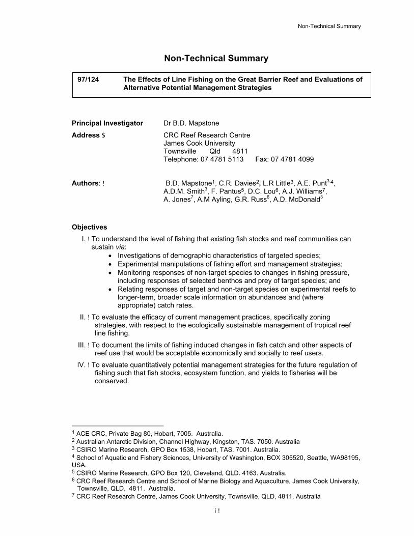
Non-Technical Summary
Non-Technical Summary
97124 The Effects of Line Fishing on the Great Barrier Reef and Evaluations of Alternative Potential Management Strategies
Principal Investigator Dr BD Mapstone
Address$ CRC Reef Research Centre James Cook University Townsville Qld 4811 Telephone 07 4781 5113 Fax 07 4781 4099
Authors BD Mapstone1 CR Davies2 LR Little3 AE Punt34 ADM Smith3 F Pantus5 DC Lou6 AJ Williams7 A Jones7 AM Ayling GR Russ6 AD McDonald3
Objectives I To understand the level of fishing that existing fish stocks and reef communities can
sustain via bull Investigations of demographic characteristics of targeted species bull Experimental manipulations of fishing effort and management strategies bull Monitoring responses of non-target species to changes in fishing pressure
including responses of selected benthos and prey of target species and bull Relating responses of target and non-target species on experimental reefs to
longer-term broader scale information on abundances and (where appropriate) catch rates
II To evaluate the efficacy of current management practices specifically zoning strategies with respect to the ecologically sustainable management of tropical reef line fishing
III To document the limits of fishing induced changes in fish catch and other aspects of reef use that would be acceptable economically and socially to reef users
IV To evaluate quantitatively potential management strategies for the future regulation of fishing such that fish stocks ecosystem function and yields to fisheries will be conserved
1 ACE CRC Private Bag 80 Hobart 7005 Australia 2 Australian Antarctic Division Channel Highway Kingston TAS 7050 Australia 3 CSIRO Marine Research GPO Box 1538 Hobart TAS 7001 Australia 4 School of Aquatic and Fishery Sciences University of Washington BOX 305520 Seattle WA98195 USA 5 CSIRO Marine Research GPO Box 120 Cleveland QLD 4163 Australia 6 CRC Reef Research Centre and School of Marine Biology and Aquaculture James Cook University
Townsville QLD 4811 Australia 7 CRC Reef Research Centre James Cook University Townsville QLD 4811 Australia
i
ELF Experiment and Management Strategy Evaluations
Executive Summary$
The effects of reef line fishing on the productivity of targeted species and its impacts on other reef species on the Great Barrier Reef (GBR) have been poorly understood Understanding the distribution intensity and effects of reef line fishing is essential for successful management of both fishing and other recreational and commercial activities in the GBR region as well as for conservation of the GBR ecosystem
The GBR Reef Line Fishery (RLF) comprises socially and economically important commercial charter and recreational fishing sectors The fishery has been undergoing some change over the last decade particularly manifest as considerable increases in effort and catch in the commercial fishery since 1995 These changes probably arise from several events including changing management arrangements in other fisheries the introduction of Dugong Protection Areas in in-shore areas the process of reviewing management arrangements for the Reef Line Fishery and the development of lucrative export markets for live reef fish for consumption Collectively these influences have resulted in nearly 50 increase in commercial effort and 40 increase in catch since 1996 There also is potential for increased recreational fishing pressure along the GBR coast simply because of population growth and increased tourism Management arrangements for the Coral Reef Fin Fish Fishery are now under review with new management arrangements likely to regulate commercial effort in the fishery explicitly
Conservation management of the GBR Marine Park also is undergoing significant change The current zoning system is being substantially upgraded with the development of a comprehensive adequate and representative system of no-take areas for biodiversity conservation of the GBR ecosystem ndash the Representative Areas Program This revision is likely to increase the area of the GBR closed to reef line fishing Realising the minimum regime of 20 of all GBR bioregions being lsquono-takersquo will inevitably result in significant increases in the amount of coral reef habitat closed to the Reef Line Fishery in some areas These factors combined with limited historical information about the fishery or its main target species present significant problems for planning appropriate management strategies of the fishery and the GBR World Heritage Area
These factors combined with limited historical information about the fishery or its main target species present significant problems for the development of appropriate management strategies for the fishery and the GBR World Heritage Area In this research we have quantified some of the primary impacts of the RLF on targeted stocks and assessed secondary impacts on other components of the GBR ecosystem We have assessed experimentally the degree to which area closure strategies are likely to have ameliorated those impacts Finally we evaluated the prospects for alternative mixes of strategies for conservation and fishery management in the region to realise the objectives of diverse stakeholders
Surveys of areas that had been open and closed to fishing for over a decade showed that the two main target species of the RLF the common coral trout and the red throat emperor were significantly more abundant larger and older in areas zoned Marine National Park lsquoBrsquo (and so closed to fishing) than in adjacent General Use areas that have always been open to fishing The magnitude of these differences varied regionally from near-zero around Lizard Island to several-fold for some population characteristics in the southern regions of the GBR The pattern in apparent lsquoeffectivenessrsquo of past closures matched closely patterns in the amount of fishing effort and catch and underlying patterns in the abundances of several harvest and non-harvest species We present circumstantial arguments that this regional variation in the apparent lsquoeffectivenessrsquo of Marine Protected Areas is likely to reflect long-standing regional variations in the amounts of fishing and its impacts outside closed areas rather than wholesale subversion of zoning strategies by high levels of poaching That is the lack of contrast between open and closed areas in the Lizard Region probably arises because the open areas are lightly fished whereas the strong contrasts in the other regions arises because of relatively heavy fishing in the open areas in those regions
ii
Non-Technical Summary
Experimental manipulations of reef zoning status and fishing effort verified that fishing on reefs that had been closed historically reduced the abundances of target species on those reefs to levels similar to surrounding open reefs In the absence of prior data with which to compare open and closed reefs before zoning was implemented these manipulations provide the most convincing evidence that the Marine Park zoning strategies have been effective in protecting sub-populations of the fishery resource from the impacts of harvest The protection of such refuges with sufficient compliance thus has the potential to sustain high biomass of reproductively mature populations of harvested species in spite of an active fishery on the GBR
Indirect effects of line fishing on non-harvest fish were less conspicuous Whilst differences existed between open and closed reefs in abundances of the prey of targeted species the nature of the patterns varied regionally through time and with species or species group In some situations the patterns in abundance suggested that removal of a key predator (coral trout) by fishing might have allowed populations of some prey to grow on fished reefs but the evidence was neither uniform nor convincing
We have evaluated prospectively the relative merits for managers and stakeholders of alternative strategies for effort management and area closure on the GBR We based these evaluations on a set of simulation models (lsquoELFSimrsquo) for the population dynamics and harvest of common coral trout on the GBR The population dynamics model is spatially structured depicting nearly 4000 reef-associated populations of coral trout inter-connected via larval dispersal The reef-associated post-settlement populations are age size and sex structured and we allow for variation in most of the key demographic parameters such as natural mortality growth recruitment etc The harvest model predicts the allocation of fishing effort over the GBR by three fishing fleets parameterised with historical catch and effort data to represent the commercial charter and recreational sectors of the RLF
Objectives for the future status of coral trout populations and for the RLF were developed by a diverse set of stakeholders in the fishery and the GBR World Heritage Area in association with the Reef Line Fishery Management Advisory Committee (ReefMAC) Contributing stakeholders included state and federal managers commercial charter and recreational fishers conservation organisations and researchers Stakeholder objectives included preserving near-virgin biomass of coral trout on reefs closed to fishing ensuring satisfactory levels of populations available for harvest maintaining economically viable commercial catch rates and recreationally rewarding recreational catches of coral trout and minimising variation in harvests from year to year Quantitative articulations of these and other objectives were derived and agreed with stakeholders together with associated performance indicators
The same set of stakeholders advised on the mix of potential strategies to be considered for achieving their respective objectives We were asked to compare the efficacy of three levels of fishing effort ranging from half of 1996 levels to 1frac12 times 1996 levels and three levels of area closure ranging from current closures to nearly three times current closures The outputs from these Management Strategy Evaluations provide comparative assessments of the likelihood that each of the stakeholder objectives will be met by each combination of effort control and area closure strategy The results are not intended to prescribe which strategy mix should be adopted but to provide a basis for stakeholders to negotiate such an outcome based on the degree to which different combinations of strategies meet their needs
Harvest-related objectives (eg maintaining CPUE increased chance of catching a large fish preserving biomass available for harvest) were most likely to be achieved when effort was lowest under any area closure strategy but were less likely to be achieved as increasing amounts of area were closed to fishing The principle stock-conservation objective represented by preserving the spawning biomass of the whole population was most likely to be achieved by increasing the amount of area closure and was only relatively slightly impacted by increasing fishing effort within each area closure strategy
iii
ELF Experiment and Management Strategy Evaluations
Importantly the observed increase in fishing effort in recent years is most likely to impact most negatively on the performance indicators for areas open to fishing especially those reflecting what fishers would consider satisfactory performance of the fishery (eg catch rates and sizes of fish) The increase in area closures under the Representative Areas Program is likely to exacerbate the depreciation of fishery performance but our results suggest that growth in fishing effort will be considerably more influential than changes in areas available to the fishery Our results suggest that the currently elevated levels of effort (~15 time 1996 levels) will reduce significantly the prospects of fishers in all sectors realising their objectives in future years irrespective of the inevitable increases in protected areas under the Representative Areas Program
Reducing effort conversely is the strategy of those considered in our evaluations most likely to realise direct fisheries-related objectives The conundrum in these results however is that the improved prospects from effort reduction would apply only to those fishers remaining in the fishery We are unable to assess the magnitude of financial costs likely to be incurred by those fishers excluded through the effort reductions that would now be necessary to achieve the two lower effort scenarios we considered
Changing effort had relatively little impact on most performance indicators for closed areas especially conservation of spawning biomass of coral trout within Marine Protected Areas even allowing for low levels of infringement of closed areas The most effective mechanism by which to increase total spawning stock biomass over the GBR domain therefore was increasing the area closed to fishing presuming that compliance with those closures was relatively high
It is important to note that the status of coral trout populations in areas open to fishing remained relatively robust under all strategies we considered For example even under the most lsquoadversersquo scenario of maximum effort constrained to the smallest fishable area spawning biomass (in the open areas) remained above 50 of virgin spawning biomass and biomass available for harvest (ie above the minimum legal size limit) remained above 30 of virgin available biomass These statistics generally would be considered acceptable for a harvested stock In large part this is likely to be the consequence of the biologically precautionary minimum legal size limit on harvest of common coral trout which ensures that most fish can spawn in at least one year before reaching harvestable size
Sensitivity analyses for the simulations showed that the qualitative relationships among scenarios were robust to changes in model parameters Accordingly the conclusions about the relative merits of increasing or decreasing fishing effort or area closures are robust to most changes in model assumptions It should be noted however that our evaluations relate only to the populations and harvest of common coral trout (P leopardus) Though several other species harvested in the Reef Line Fishery are taxonomically close to P leopardus they are generally considered to be less abundant and longer lived than P leopardus and their populations dynamics are perhaps less resilient to harvest than that of P leopardus Accordingly conservative regulations for the harvest of these other species would be prudent at this stage
This research has laid bare some of the inevitable trade-offs among different scenarios for managing the harvest of common coral trout by the RLF in the GBR World Heritage Area Most importantly the trade-offs have been assessed in relation to objectives and performance indicators specified by diverse stakeholders in the fishery and the World Heritage Area We present the tradeoffs in ways that allow direct comparisons among disparate objectives essentially providing a common currency for comparing performance across fundamentally different types of objectives In so doing we hope that the costs and benefits of different management options are more transparent to all stakeholders than might otherwise have been the case We hope that such transparency aids in the negotiation of acceptable and effective future management arrangements for the Great Barrier Reef World Heritage Area and the Reef Line Fishery
iv
Contents
Contents$
Non-Technical Summary i$Objectives i Executive Summary ii
Contentsv$Acknowledgements viii
Need ix Objectives x$Achievement of Objectivesx$General Introduction 1$
The Demersal Reef Line Fishery 2The Commercial Sector of the Reef Line Fishery 2+The Charter and Recreational Sectors of the Reef Line Fishery 3+Distribution of Reef Line Fishing 4+
Management Arrangements Affecting the Reef Line Fishery 4The Effects of Line Fishing Experiment 7$Introduction 7$
Box 2 Background to the Effects of Line Fishing Project 7Materials and Methods10$
Experimental Design10 Field Sampling 12
Line Fishing Catch Surveys 13+Underwater Visual Surveys 15+
Laboratory Methods 16 Otolith Processing 16+
Estimates of Catch and Effort from Experimental Reefs17Compulsory Fishing Logbooks 17+Aerial and Vessel Surveillance 17+On-site Observations 17+
Data Management 18Analytical Methods18
Preliminary Processing of Data 18+Research Data 18+Logbook Catch and Effort Data 19+
Tests for Effects of Fishing Region and Zone 20+Preliminary Applications of Depletion Estimators to ELF Experimental Data 22+
Results 23$Catch and Effort on Experimental Reefs23Tests for Region Zone and Effects of Fishing25
Patterns Among Regions 25+Effects on Legal Sized Coral Trout 25+Effects on Under Sized Coral Trout 28+Effects on Red Throat Emperor 31+Effects on Non-catch Species33+
Effects of Management Zone 36+Effects on Legal Sized Coral Trout 36+Effects on Under Sized Coral Trout 41+Effects on Red Throat Emperor 42+Effects on Non-catch Species45+
Effects of Fishing Manipulations 49+Effects on Legal Sized Coral Trout 49+Effects on Under Sized Coral Trout 52+Effects on Red Throat Emperor 54+Effects on Non-catch Species55+
v
ELF Experiment and Management Strategy Evaluations
Discussion 58$Implementing the Experiment 58+Biomass Estimates and Future Monitoring Procedures 58+Effects of Marine Park Zoning 59+Regional Variation 60+Indirect Effects of Fishing 61+
Management Strategy Evaluations 63$Introduction 63$Methods 65$
The Biological Component of the Operating Model 65+The Harvest Component of the Operating Model 68+Catches 70 Initialisation 71 Projections and Management Scenarios 72+Setting Objectives Performance Indicators and Management Strategies 73+Objectives 75+
MSE Results 80$Results Summary 80 Simulation Results 80
Spawning Biomass 80+Available Biomass 84+Commercial Fishery Performance 88+Charter and Recreational Fishery Performance 91+Poached and Discarded Catch 97+Reduced Minimum Legal Size 99+
Performance Summary 100Discussion 103$Benefits 107$Further Development 107$Conclusion 108$References 109$Appendix A Applying a Population Dynamics Model ELF Experiment Data 117
Introduction 117The Data and Derived Inferences 117Fitting the Model to the Data 125
Base-case analysis 125+Sensitivity tests 140Recommendations for additional analyses 140Annex A1 The Delay-Difference Estimator 141
Appendix B The ELFSim Operating Model 144The Biological Components of the Operating Model 144
Basic Population Dynamics 144+0-Year-Olds 145+Recruitment to Reefs 147+Natural mortality 148+Growth 150
The Harvest Components of the Operating Model 150Effort Allocation 150+Catches 153+
Establishing Initial Conditions for Simulations 154Historical catch and effort data 155+
Further work 156Annex B1 The Derivation of Equation (B8) 157Annex B2 The Relationship between Steepness and Parameters of Equation (B 9a) 157Annex B3 Estimating the Parameters of the Growth Curves 158
vi
Contents
Appendix C Summary Diagnostics and Sensitivity Analyses for ELFSim162Required Numbers of Simulations 162Distribution of Catch and Effort 163Effects of Habitat Scalar and Uneven Catch-Effort Distribution164Relative Depletion of Reefs 166
Effects of Different Values for the Steepness Parameter 167+Appendix D Report from the ELF MSE 1st Stakeholder Workshop169
Contents170Introduction 171The ELF Project 172 Issues for Management of the Reef Line Fishery 172What is Management Strategy Evaluation173The First MSE Stakeholders Workshop174Workshop Goals 174 Meeting Summary175
Opening Comments 175+General Background to Quantitative Fisheries Management 175+MSE Concepts Explained Using a Hypothetical Example 176+The ELF Project and MSE for the Reef Line Fishery 180+User Expectations and Issues in the Medium Term 181+
MSE for Coral Trout The ELF Models (ELFSIM) 183Closing Comments and Where to From Here184Participants 185
Appendix E Report from the ELF MSE 2ND Stakeholder Workshop 186Contents187Introduction 1882nd Workshop Objectives 188The ELF Project 189 Issues for Management of the Reef Line Fishery 189The 1st MSE Stakeholders Workshop 190
Objectives 190+Strategies 190+
Meeting Summary191Opening Comments 191+Refresher Talk on ELFSim ndash Worked Example 192+Objectives and Performance Indicators from Stakeholders 193+ELFSim lsquoon the flyrsquo ndash What it can do 198+Management Strategies favoured by Stakeholders 199+
Discussion200Examining the unknowns and testing key assumptions 201+Where to now 202+Closing Comments 202+
Participants 203Apologies 203Glossary204
Appendix F Intellectual Property 205$Appendix G Staff 205$
vii
ELF Experiment and Management Strategy Evaluations
Acknowledgements Many people have contributed greatly to this project both directly and indirectly These people include Samantha Adams Kyi Bean Tony Ayling Mikaela Bergenius Belinda Boyce Rob Campbell Gary Carlos Adam Davidson Beth Fulton Siriol Giffney Barry Goldman Bridget Green John McKinlay Amos Mapleston Ross Marriott Cameron Murchie Renae Partridge John Robertson Melita Samoilys Stephanie Slade Angus Thompson Andrew Tobin Sally Troy Dave Welch and a raft of other people including commercial and recreational fishers and charter vessel operators who have helped tremendously over the last few years We especially thank Robyn Stewart and Mary Peterson for their invaluable support and hard work during the catch surveys
We thank also Mick Bishop Martin Breen Wendy Craik Chris Crossland Eddie Heggerl Ted Loveday Helene Marsh Russell Reichelt Duncan Souter John Tanzer Di Tarte Allan Turnbull Simon Woodley and the members of ReefMAC for their support in the development and implementation of the Effects of Line Fishing Experiment
Many of the data behind this report were generously and freely provided by the Great Barrier Reef Marine Park Authority the Queensland Fisheries Management Authority the Queensland Fisheries Service commercial fishers and charter vessel operators in the GBR region
Bruce Mapstone is particularly grateful to Gina Mercer and Lucy Mercer Mapstone for their patience tolerance and support over the many years that this work has dominated our lives and especially during the preparation of this report
Finally we acknowledge the CRC Reef Research Centre for its long-term support and major funding of the ELF Project and the various fishing sectors on the Great Barrier Reef for all the in-kind support we have received The Fisheries Research and Development Corporation the Great Barrier Reef Marine Park Authority the Queensland Fisheries Management Authority and James Cook University provided top-up funding over various periods of the ELF Project
viii
Need
Need The potential for reef line fishing to significantly affect targeted species or indirectly impact other reef species is poorly understood Understanding the distribution intensity and effects of reef line fishing is essential for successful management of both fishing and other recreational and commercial activities in the Great Barrier Reef (GBR) region as well as for conservation of the GBR ecosystem
The GBR Reef Line Fishery (RLF) has undergone substantial change since 1993 particularly manifest as increases in effort and catch in the commercial fishery since 1995 These changes probably resulted from several events including restrictions introduced for other fisheries (spanner crab in-shore net and trawl) by the Queensland Fisheries Management Authority (QFMA) and Queensland Fisheries Service (QFS) on behalf of the Queensland Government the introduction of Dugong Protection Areas in in-shore areas gazetted by the Great Barrier Reef Marine Park Authority (GBRMPA) on behalf of the Commonwealth Government the announcement of a major review of management arrangements for the RLF and the development of lucrative export markets for live reef fish for consumption Indirect indicators of the attractiveness of the RLF to commercial fishers include the 2-3 fold increase in the market value of reef line fishing licences since 1994 the acquisition of multiple vessels by some operators purchases of large purpose built or re-fitted vessels for the live fish sector of the fishery and increased participation in the commercial fishery by licence holders who previously had not harvested reef fish There is also considerable potential for increased recreational fishing pressure simply because of population growth and increased tourism These factors combined with the dearth of historical information about the fishery or its main target species present significant problems for formulating appropriate management strategies for the fishery and the GBR World Heritage Area
Conservation management of the GBR Marine Park also is undergoing significant change with the development of a comprehensive adequate and representative system of no-take areas likely to increase the area of the GBR closed to reef line fishing Management arrangements for the Coral Reef Fin Fish Fishery are under review with new management arrangements likely to regulate commercial effort in the fishery explicitly There is an immediate need for quantitative assessments of the impacts of line fishing on targeted stocks and other fishes and for prospective evaluation of the value of proposed management strategies in relation to economic social biological and conservation objectives for the GBR and its use In ldquoResearch Needs and Prioritiesrdquo (1996) key topics for research related to the Reef Line Fishery flagged by the QFMA included Appraise management measures for the sustainable use of reef fish Determine an effective mix of measures for reef fish management planning including fishery dependent and independent monitoring Determination of the size of stocks of common coral trout Determination of the proportion of blue-spot trout in the reef line catch and assess regional catch rates of red-throat sweetlip
The CRC Reef Effects of Line Fishing (ELF) Project was designed to produce results of direct relevance to these and other needs and in so doing contribute management-relevant information for the GBR RLF Two components of the ELF Project the ELF Experiment and Management Strategy Evaluations (MSE) for the RLF were specifically designed to meet several of the above priority needs This report documents key results to date from these two components of the ELF Project
ix
ELF Experiment and Management Strategy Evaluations
Objectives
Below are the objectives for the CRC Reef Effects of Line Fishing Project Specific subsidiary objectives of particular sub-tasks are listed in Box 1
I To document the distribution and intensity of reef-based fishing catch and effort and patterns in relative abundance of fish stocks
II To understand the level of fishing that existing fish stocks and reef communities can sustain via
a Investigations of demographic characteristics of targeted species b Experimental manipulations of fishing effort and management strategies c Monitoring responses of non-target species to changes in fishing pressure
including responses of selected benthos and prey of target species and d Relating responses of target and non-target species on experimental reefs to
longer-term broader scale information on abundances and (where appropriate) catch rates
III To evaluate the efficacy of current management practices specifically zoning strategies with respect to the ecologically sustainable management of tropical reef line fishing
IV To document the limits of fishing induced changes in fish catch and other aspects of reef use that would be acceptable economically and socially to reef users
V To evaluate quantitatively potential management strategies for the future regulation of fishing such that fish stocks ecosystem function and yields to fisheries will be conserved
This report addresses objectives II ndash V or substantive components of them
Achievement of Objectives The distribution and intensity of fishing has been described from analyses of compulsory logbook data from the commercial and charter sectors of the fishery provided by the Queensland Fisheries Management Authority and Queensland Fisheries Service (QFS) Interpretation of the analyses has been supplement from interviews voluntary research logbook programs and observer programs as part of the ELF Project Characteristics of the small-boat recreational fishery have been provided to the project by QFS
Objectives II and III have been achieved via successful implementation of the ELF Experiment involving changes in reef zoning status (opened or closed to fishing) Responses to the manipulations have been assessed by Underwater Visual Surveys and line fishing Catch Surveys the latter also facilitating collection of biological data for harvest species Several post-graduate research projects have aided in achieving these objectives
Objective IV has been achieved via a series of formal and informal workshops with diverse stakeholders in the GBR and the RLF Contributing stakeholders included Marine Park and Fishery managers commercial recreational and charter fishers fish marketers conservation lobbyists and researchers Achieving this objective was central to completion of objective V
Objective V has been achieved in part through the achievement of the other objectives but substantially via the development of sophisticated computer simulations of the population dynamics and harvest of coral trout over the extent of the GBR The Effects of Line Fishing Simulator (ELFSim) captures the spatial and biological complexity of the GBR and the diversity of harvest behaviours employed by commercial recreational and charter fishers of the resource ELFSim has been used to assess the prospects of achieving diverse stakeholder-specified objectives through an array of combinations of proposed fishery and conservation management strategies
x
Objectives
Box 1 Sub-task Specific Objectives 1 Catch Surveys
a) To establish structured catch surveys in which the fishing characteristics personnel vessel and data collection are standardised across all reefs and times from which to estimated a) differences among reefs historically closed or open to fishing b) regional patterns in catch rates c) effects of simulated increases in fishing pressure and protection from fishing in the ELF Experiment
b) To compare the relationship between CPUE data from line and spear fishing and underwater visual survey (UVS) and the capacity of each method to detect a known decrease in fish abundance
c) To collect size otolith gonad and gut samples from fish caught during the ELF Experiment for studies of population dynamics of major target species
2 Visual Surveys a) To provide fishery independent underwater visual estimates of population densities of target fish
species prey species and other reef organisms on the reefs involved in the ELF Experiment b) To monitor recruitment of the main target species for the RLF to the experimental reefs
3 Demographic Studies a) To derive age-structure data as a primary indicator of the effects of fishing on reef fish stocks b) To use age and length structure data to estimate growth and mortality rates and provide measures of
recruitment rates to reef fish stocks c) To provide catch-at-age data from which to model population dynamics of target species
4 Fleet Dynamics and Fishery Information a) To establish and maintain cooperative links with the recreational commercial and charter boat line
fishing community to a) increase fishing effort on the manipulation reefs in the ELF Experiment and b) obtain detailed fleet catch and effort information from the reefs involved in the ELF Experiment
b) To identify and compare factors which affect the fleet dynamics and on site fishing practices in the RLF within and among regions of the GBR
5 Assessment of Bias in Line-caught Samples a) To compare age and size structures of populations of common coral trout (Plectropomus leopardus)
sampled by spear fishing among reefs open and closed to fishing and among regions of the Great Barrier Reef (GBR)
b) To examine the size and age selectivity of line fishing by comparing age and size structures of samples of common coral trout taken from reefs open and closed to fishing by spear and line fishing
c) To examine the relative biases of line and spear fishing as techniques for sampling reef fish 6 Modelling and Management Strategy Evaluation
a) To develop and parameterise population dynamics models of the primary target (fished) species (P leopardus) that are appropriate for the spatially structured GBR and that are amenable to application to secondary target species
b) To develop models of effort allocation and where possible fleet dynamics of different components of the fishery including consideration of the commercial recreational and charter fishing sectors that are appropriate for the dynamics of the reef line fishery in the spatially complex GBR
c) To provide an integrated framework based on the population and effort dynamic models for evaluating alternative management scenarios to quantify the likely trade-offs between conflicting objectives and their consequences for the coral trout fishery and the fish stocks
d) To develop with stakeholders in the GBR line fishery operational objectives and potential future management strategies relevant and amenable to evaluation from biological and fishery information
e) To apply the management strategy evaluation framework to evaluate risks and benefits of alternative strategies for managing the RLF on the GBR against stakeholder objectives for the fishery
7 Coordination and liaison a) To coordinate the implementation of all components of the ELF Project in a coherent manner across
multiple institutions and with stakeholder groups b) To manage peer review of the ELF Experiment c) To coordinate liaison with researchers and stakeholders across a range of levels from senior policy
fora to the general public d) To manage the coherent collation and archival of data and biological material from the ELF Project
xi
General Introduction
General Introduction The Great Barrier Reef (GBR) lies off the Queensland coast (Australia) and comprises the worldrsquos largest coral reef archipelago spanning over 15o of latitude from just south of Papua New Guinea (~9oS) to just north of Fraser Island (~25oS) (Fig 1) Most of the GBR was declared a multiple use marine park in 1975 (Great Barrier Reef Marine Park Act 1975) and inscribed on the World Heritage Area list in 1981 (Australian Heritage Commission Act 1975 World Heritage Properties Conservation Act 1983) Thus the GBR has been formally recognised as having special significance nationally and internationally predominantly for its natural features and in need of conservation ldquoin perpetuityrdquo (Kenchington 1990) In the defining legislation however the GBR Marine Park was gazetted for multiple use excluding only mining Existing uses were recognised also when the GBR was given World Heritage listing The facilitation of such multiple use in so far as it is consistent with conservation of the natural features of the GBR is integral to the management of the GBR Marine Park (GBRMP) and World Heritage Area (GBRWHA) Thus the region supports a thriving tourism industry as well as port and shipping activities and a diversity of wild harvest fisheries (Robertson 1997)
Figure 1 Location map for the Great Barrier Reef indicating general structural features such as geographic extentvarying proximity to coastalinfluences and population centres and fragmentedstructure The boundary ofthe GBR Marine Park is alsoshown with the boundaries between management sections indicated (linesrunning from coast to seaward boundary of the park)
In the absence of mining activities fishing is the principal extractive use of the GBR and is of particular concern because of the potential for fishing to impact negatively on the heritage and ecological values for which the GBR has been recognised Management of fishing activities therefore emphasises consistency with the conservation requirements of the Great Barrier Reef Marine Park Act (1975) World Heritage Values and principles of ecological sustainability as well as traditional expectations of securing yields recreational enjoyment and community benefit (Driml 1994 1999 Hundloe 1985 Kenchington 1990)
Fishing has occurred in the Great Barrier Reef (GBR) Region for decades from well before the declaration of the GBRMP and GBRWHA It is now a multi-million dollar industry deriving regional income from commercial fishing (mainly trawling for prawns line fishing and netting for fin-fish crabbing and collection fisheries for aquarium fish Beche de Mer Trochus and crayfish) local recreational fishing and tourism (including game-fishing) Line and spear fishing are the activities that have the greatest potential to affect the biological communities on coral reefs per se of the GBR as opposed to inter-reef habitats
1
ELF Experiment and Management Strategy Evaluations
The Demersal Reef Line Fishery The RLF is comprised of three main sectors a commercial sector a charter fishing sector and a private recreational sector Fishers in all sectors use basically similar gears typically consisting of single baited hooks on heavy line on rod and reel or hand reel The RLF is multi-species in all sectors with over 125 species or species groups being reported by the commercial sector (Mapstone et al 1996abc) and at least 108 species or species groups reported in the catch from the charter and recreational sectors (Green et al in prep Higgs 1999 Morgan 1999) The primary targeted species in the fishery are the common coral trout (Plectropomus leopardus) and the red throat emperor (Lethrinus miniatus) (Mapstone et al 1996abc Queensland Fisheries Management Authority (QFMA) 1996 Queensland Fisheries Service (QFS) 2002) The generic group lsquocoral troutrsquo comprising three main harvested species and four lesser species are estimated to comprise approximately 35-55 of the catch by commercial fishers approximately 20-25 of the charter catch and 15-20 of the recreational catch of demersal reef fish from the GBR region L miniatus comprises about 20 of the commercial catch up to 40 of the charter fishing catch and about 30-35 of the recreational demersal catch annually Other emperors especially spangled emperor (L nebulosus) and snappers (mostly red emperor Lutjanus sebae and large and small mouth nannygai L malabaricus L erythropterus) and serranids other than coral trout are the next most targeted demersal species with their relative importance varying among sectors and among regions within sectors (Green et al in prep Higgs 1999 Mapstone et al 1996a 1997 QFS 2002)
The Commercial Sector of the Reef Line Fishery The bulk of the commercial fishery occurs from 4-7m dories based on 8-19m primary vessels though fishing also occurs from the primary vessels The most active commercial reef-line operations have 2-5 dories per primary vessel whilst the majority of operations have no dories and report relatively little catch and effort (Mapstone et al 1996a)
The commercial Reef Line Fishery has been undergoing some change since 1993 particularly manifest as considerable increase in effort since 1995 These changes probably resulted from several events including restrictions on other fisheries (spanner crab in-shore net and trawl) the introduction of Dugong Protection Areas in in-shore areas the announcement of a major review of management arrangements for the RLF and the development of lucrative export markets for live reef fish for consumption Each of these events has the potential to have prompted activation of latent effort or the transfer of effort from other fisheries to the RLF and corresponding increases in commercial fishing effort
The value added to the commercial catch as a result of high market values for live fish (beach prices up to $45kg in 1996 and $58kg in 2000) in particular provides increased financial incentives to participate in the RLF Indirect indicators of the attractiveness of the RLF to commercial fishers include the 2-3 fold increase in the market value of reef line commercial fishing licences since 1994 the acquisition of multiple vessels by some operators and purchases of large purpose built or re-fitted vessels for the live fish fishery
Compulsory logbooks of catch and effort were introduced for commercial fishers only in 1988 Between 1988 and 1994 there were between 361 and 416 commercial line fishing operations reporting catch of demersal coral reef species from the GBR The 20 most active operations accounted for over 60 of the catch in most years and the majority of operations reported less than 1 tonne of catch annually (Gwynne 1990 Mapstone et al 1996abc Trainor 1991) Total annual harvest of all species (including pelagic species) by the commercial RLF over that period was between 2873 and 3725 tonnes arising from 16000 ndash 18500 fishing days (Mapstone et al 1996ab) Since 1994 however reported effort and catch have increased substantially (QFS 2002 Williams 2002 Fig 2) reaching their highest levels of nearly 40000 fishing days by over 700 operations taking 4400 tonnes of demersal reef fish from all Queensland waters in 2001 (QFS 2002)
2
General Introduction
Figure 2 Annual commercial catches of coral trout (all species of Plectropomus spp and Variola spp) red throat emperor (Lethrinus miniatus RTE) and other demersal reef fish (others) from the GBR Marine Park between 1989 and 2000 and the number of reported fishing days from which the catch came
Commercial Catch amp Effort
0 500
1000 1500 2000 2500 3000 3500 4000
1989 1990 1991 1992 1993 1994 1995 1996 1997 1998 1999 2000 Year
Cat
ch (t
)
0 5000 10000 15000 20000 25000 30000 35000
Effo
rt (f
ishi
ng-d
ays)
Coral Trout Others RTE Effort
The Charter and Recreational Sectors of the Reef Line Fishery Recreational fishing occurs from both privately owned boats mostly outboard powered or from charter vessels that take single or multi-day trips to the GBR Prior to 1996 information about the private recreational fishing fleet came only from boat registrations and mostly recall data obtained from fishers during various creel telephone or postal surveys (Blamey and Hundloe 1993 Craik and Fallows 1980 Higgs 1996) The longest history of data derives from line and spear fishing club competition records (Higgs 1996 Nakaya 1998) but recent population surveys indicated that those data represent at most 6 of the recreational fishing population (Morgan 1999)
Blamey and Hundloe (1993) estimated that the total recreational catch in the GBR region in 1989-90 was between 3500 and 4300 tonnes from approximately 210000-270000 lsquofishing trips to searsquo by 160000 recreational fishers in private vessels Only 54-135 of these trips (depending on region) however went lsquooff-shorersquo and smaller proportions visited the lsquoGBR properrsquo More recent research and surveys sponsored by the Queensland Fisheries Management Authority (QFMA) and Queensland Fisheries Service (QFS) indicated similar distributions of recreational fishing between near shore and off-shore waters (Fig 3) and indicate that recreational anglers took approximately 2000t of demersal reef fish per year in the late 1990s (Higgs 1996 1999 Mapstone et al 1997 QFS 2002 Williams 2002) There is considerable potential for increased recreational fishing pressure along the GBR coast because of population growth and increased tourism Financial constraints such as the cost of fuel for long trips to the off-shore reefs however probably dampen effects of population growth on off-shore reefs
Fishing on charter trips occurs mostly from the main charter vessel but dories are also used on some extended charters There were 415 operators of charter vessels in the GBR region holding permits to take clients reef fishing in 1995 though most of these probably did lsquofishing tripsrsquo infrequently Green et al (in prep) estimated that only about 120 charter fishing operations regularly took clients to sea predominantly for fishing in 1999-2000 Fishers on charter trips to the GBR fished for an estimated 11030-22880 line-days between 1996 and 1998 and kept 50-51 tonnes of coral trout and related species of demersal reef fish (QFS unpublished data) Compulsory logbooks for charter vessel operators were introduced only in 1996-97
3
ELF Experiment and Management Strategy Evaluations
Figure 3 Percentages of recreational boating trips from the Ingham area in May-July 1995 that went to near shore islands (black) off-shore reefs of the GBR (white) or in-shore areas (grey) The pie on the left was derived from interviews at boat ramps that on the right from voluntary angler logbooks (Mapstone et al 1997)
1 1 5 5
98
90
Distribution of Reef Line Fishing Line fishing occurs over the entirety of the GBR though by far the majority of catch and effort is in the southern half of the GBR south of Cairns (Blamey and Hundloe 1993 Gwynne 1990 Higgs 1996 Mapstone et al 1996ac Trainor 1991) The greatest small-boat recreational effort on the off-shore GBR occurs between north of Townsville and just north of Cairns (Blamey and Hundloe 1993 Higgs 1996 1999) the majority of charter vessel effort is centred on Gladstone Mackay Airlie Beach and Cairns (Green et al in prep) and the bulk of the commercial effort occurs south of Cairns and north of Rockhampton (Mapstone et al 1996a) (Fig 4)
Management Arrangements Affecting the Reef Line Fishery The management reacutegime for the GBR region is complex with responsibility for conservation management and fisheries management being divided constitutionally legislatively and operationally between the Australian Commonwealth and Queensland Governments Management responsibilities for the GBR Marine Park and World Heritage Area are vested by the Commonwealth with the Great Barrier Reef Marine Park Authority (GBRMPA) a Commonwealth Statutory Authority (GBR Marine Park Act 1975) The GBRMPA has responsibility for management for lsquoprotection and wise use in perpetuityrsquo but explicitly does not have authority for fisheries management Consistent with the Off-shore Constitutional Settlement (1981) responsibility for managing fisheries is delegated to the Queensland Government which administers that mandate through the Queensland Fisheries Service8
(QFS) (Queensland Fisheries Act 1994 1999)
The GBRMPA has to date employed a strategy of zoning for conservation management of the GBR Under zoning plans developed by the Authority and enacted by the Federal Parliament different areas of the marine park are designated for different types of permissible use ranging from most extractive activities (General Use zones) to lsquolook but donrsquot touchrsquo (Marine National Park-B zones) and lsquono-gorsquo areas (Preservation zones) Although not specifically designed as fisheries management strategies these zoning strategies effectively regulate fishing through the implementation of area closures that protect various species from harvest and impose broad restrictions on fishersrsquo access to stocks Although the 2000km length of the GBR Marine Park has been divided into four major sections for zoning (Fig 1) to date the zoning plans applied to each have been very similar and have not resulted in region-specific management
8 Management of fisheries in Queensland was through the Queensland Fisheries Management Authority (QFMA) a statutory Authority between 1993 and 2000 but from July 1 2000 the QFMA was dissolved and responsibility for managing fishing in Queensland was transferred to the Queensland Fisheries Service within the portfolio responsibilities of the Department of Primary Industries
4
General Introduction
Figure 4 Annual total effort and total catch of all line-caught species as reported in the compulsory commercial logbooks in each region in 1990 1992 and 1994 Region boundaries are shown in the figure at bottom right with the key to region abbreviations in the table below the map (Adapted from Mapstone et al 1996a)
5
GC WTS ETS FN
CNS TVL
WTS ETS
FN Weipa bull
Cape Melville bullCape Flattery bull
Cooktown bull CNSGC Port Douglas bull
Cairns bull OCS
Cardwell bull TVL
Townsville bull Bowen bull
MKY
SWN Mackay bull
C-BRockhampton bull
Bundaberg bull
STROP Brisbane bull
140 145 150 155
Longitude Key to Regions Indicated on Map
Gulf of Carpentaria MKY Mackay Western Torres Straits SWN Swains Eastern Torres Straits C-B Capricorn Bunkers Far Northern OCS Off-shore Coral
Sea Cairns STROP Sub-tropical Townsville
Latit
ude
-30
-25
-20
-15
-10
ELF Experiment and Management Strategy Evaluations
The RLF also is managed uniformly over the length of entire GBR (QFMA 1999 QFS 2002) although since April 1999 reefs in the Torres Strait north of 10o20rsquo S fall under a different jurisdiction from the remainder of the GBR (AFMA 2001) The prospect arises therefore that management arrangements might become non-uniform if changes are legislated in either jurisdiction without reflection in the other The QFS and formerly the QFMA impose a number of explicit fisheries management strategies in Marine Park zones of the GBR where line fishing is allowed (QFMA 1999 QFS 2002) Minimum legal size limits for several of the main target species apply to all sectors of the fishery as do gear restrictions
Commercial fishing is managed via a two-tiered limited entry licensing scheme combined with vessel length constraints common to both The two tiers were defined in 1993 in relation to the evidence of prior participation in the RLF and are implemented as limits on the numbers of dories that can be used in conjunction with each primary vessel Licences with an lsquoL2rsquo endorsement are allowed up to seven dories per primary vessel with the number specific to each licence and fixed as of 1993 L2 endorsed primary vessels support an average of 3-4 dories lsquoL3rsquo endorsed licences allow fishing from at most one dory in addition to the primary vessel There are no restrictions on the numbers of lines or fishers per operation except those imposed by survey conditions of the primary vessel In addition to the lsquoL2rsquo or lsquoL3rsquo endorsements most commercial licence packages carry multiple other endorsements including one or more of the available line net and crab spanner crab and trawl endorsements Movement among fisheries is at the discretion of the master fishermen providing they hold the appropriate endorsements
Recreational fishers are regulated by per-person lsquoin possessionrsquo total bag limits of 30 fish per angler for reef fish which includes smaller bag limits for several species or species groups Fishers on day trips are allowed 1 bag per person per day but fishers on extended trips to sea (gt 48 hours at sea) on charter vessels are allowed 2 bags each for the trip Charter fishing operators are regulated by permits issued by the GBRMPA (for operation in the GBRMP) and QFS (for operation in Queensland waters) but otherwise there is no license or permitting system in place for recreational fishers Management arrangements for all sectors of the RLF under Queensland jurisdiction (which excludes the Torres Strait) are currently under review
The relative shortage of historical information about the fishery its main target species or its environmental impacts (see Mapstone et al1997 for review) combined with changes in the fishery since the mid-1990s present major issues for planning appropriate management strategies for the fishery and the GBR WHA (QFS 2002)
6
Introduction
The Effects of Line Fishing Experiment Introduction The Effects of Line Fishing (ELF) Experiment has its genesis in a research proposal to the Great Barrier Reef Marine Park Authority (GBRMPA) in 1988 (Mapstone et al 1988) and a workshop convened jointly by the GBRMPA and the Queensland Department of Primary Industries (QDPI) in the February 1989 under the advice of the Advisory Committee on Research into the Effects of Fishing on the Great Barrier Reef (Craik et al 1989) Trawl and line fisheries were considered to be those in greatest need of information for management in the GBR Marine Park and a major recommendation from the workshop was the development of a large scale manipulative experiment to examine the ecosystem effects of these fisheries and derive important parameters for their management In 1990 the GBRMPA commissioned a study to examine the feasibility of such an approach and recommend experimental designs and necessary preliminary research (Walters and Sainsbury 1990) Although Walters and Sainsbury (1990) recommended a study to examine the joint and interactive effects of trawling and line fishing subsequent research bifurcated into separate studies of the two fisheries Whilst research into the effects of prawn trawling was championed by the CSIRO (then) Division of Fisheries research into the effects of line fishing lacked an institutional focus until 1993 The establishment of the Cooperative Research Centre for the Ecologically Sustainable Development of the Great Barrier Reef1
(CRC Reef) in 1993 provided a vehicle for the development of a comprehensive program of research into line fishing on the GBR including but not restricted to the experimental approach discussed since 1989 (The Effects of Line Fishing (ELF) Project Box 2)
Box 2 Background to the Effects of Line Fishing Project
The ELF Project commenced in 1993 as a core task of the CRC Reef to fill some of the gaps in information about the RLF and its impacts on the GBR The ELF Project involves collaborations among CRC Reef funded researchers and researchers from the Australian Institute of Marine Science CSIRO James Cook University Queensland Department of Primary Industries Sea Research and the University of Queensland managers from the GBRMPA and QFS and fishers from the commercial charter and recreational sectors of the RLF Cash funding for the ELF Project is predominantly from the CRC Reef but significant funds are provided also by the Fisheries Research and Development Corporation (1997-2004) the GBRMPA (1997-2000) QFMA and James Cook University Substantial in-kind funding derives from the participating research institutions management agencies and sectors of the RLF
The project involves six main research areas i) Documenting the fishery history from catch and effort data oral history and structured interviews ii) Monitoring the fishery from contemporary research and management logbooks research surveys student projects and collaboration with other agencies iii) Documenting biological characteristics of the targeted stocks and other fish impacted by the fishery either as by-product or by-catch iv) Testing responses of target stocks their prey and fishing fleets to changes in fishing pressure through a large-scale controlled experiment v) Evaluating the strengths and weaknesses of alternative potential management strategies for the GBR Marine Park and the RLF through dynamic computer models and vi) Liaison and extension of research results to stakeholders and into policy fora Extension activities include representation on Management Advisory Committees presentations to peak bodies and management agencies face-to-face discussions with stakeholders at ports public meetings and trade fairs publication of articles in the popular and technical press and the distribution of a quarterly newsletter to ~2000 recipients The ELF Project currently has support until June 2006
Several studies were done prior to 1994 as pilot studies in anticipation of the eventual implementation of a large scale experiment to examine the effects of line fishing on the GBR These projects included methodological studies (Cappo and Brown 1996 Mapstone and
1 The tenure of this CRC was 1993-2000 It has subsequently been revised and re-funded as the CRC for the Great Barrier Reef World Heritage Area with tenure extended to 2006
7
ELF Experiment
Ayling 1998) exploration of key assumptions underlying Waltersrsquo and Sainsburyrsquos recommendations (Davies 1995 ab) and biological studies of the key target species of the Reef Line Fishery (Ayling and Ayling 1992ab Brown et al 1994 Ferreira and Russ 1994 1995 Russ et al 1995 1996 Samoilys and Squire 1994 Samoilys 1997 Williams and Russ 1994) and surveys of the effects of changed zoning of reefs (Ayling and Ayling 1992b 1994 1995 Bienssen 1989 Brown et al 1993 1996 Mapstone et al 1996d) In 1994 a second design evaluation was done in the light of the more recent information provided by these and other studies and the logistic and financial resources available under the CRC programme (Mapstone et al 1996e Campbell et al 2001) The feasibility and desirability of a large-scale experiment to examine the effects of line fishing on the GBR were confirmed and a revised experimental design recommended (Mapstone et al 1996e Campbell et al 2001)
During 1995 and 1996 the recommended experimental design was canvassed widely among interested stakeholders to assess its legal political and logistic feasibility The consultation process involved a combination of public and stakeholder-specific meetings explanatory articles in the popular press discussions with a range of multi-sectoral regional management advisory committees a formal nationally advertised public review process and consideration of the proposed experiment by the Federal Parliament the Australian Heritage Commission and the Commonwealth Environment Protection Group Inevitably some aspects of the suggested implementation of the experiment were changed because of logistic and political constraints highlighted during the consultation phase2 but the basic recommendations for the ELF Experiment received wide support
The ELF Experiment was opposed by some conservation groups on the grounds that it involved opening to fishing some reefs that had been closed to fishing previously (Marine National Park B zones lsquogreenrsquo reefs) and opposed by some fishers because it involved the additional closures of reefs available to the fishery (General Use (GU) lsquobluersquo reefs) The experiment was supported however by the relevant management agencies (GBRMPA and the QFMA) representative bodies of both recreational and commercial fishing sectors (respectively SUNFISH and the Queensland Commercial Fishermenrsquos Organisation QCFO) the Queensland Conservation Council the Australian Marine Conservation Society the Australian Marine Science Association researchers Regional Marine Resource Advisory Committees the Reef Line Fishery Management Advisory Committee (ReefMAC) and recreational and commercial fishers and charter vessel operators along the GBR Coast
Implementing the ELF Experiment involved changes to the GBRMPA zoning provisions for some of the reefs involved and those changes were outside the scope of the GBRMPArsquos mandate allowed by the existing Zoning Plans approved by the Federal Parliament Accordingly the experiment could proceed only if the Federal Parliament amended the relevant Zoning Plans to allow the unusual changes in current management provisions The necessary amendments to the GBR Zoning Plans were passed by the Federal Parliament in November 1996 and the decision by the GBRMPA to implement the amendments was gazetted on January 8 1997
The primary objective of the ELF Experiment is to provide through deliberate manipulations of fishing pressure and reef closures to fishing field data from which to derive key underlying parameters for the evaluation of biological and fishery responses to alternative management scenarios In particular the contrast in population properties induced by the experiment should provide the empirical basis for estimating
1 Reef-specific population size and estimates of sustainable harvest 2 The coefficient of catchability for key target species and 3 Fishing mortality and natural mortality of target species
These parameters will be estimated from
2 In particular a) the timing of the manipulations was condensed such that manipulations of fishing pressure and reef closure were to be applied over 2 years instead of 4 and b) suggestions of sponsored fishing by clubs andor spear fishers and subsidised commercial fishing to force down populations on previously fished reefs were abandoned
8
Introduction
4Empirical estimates of demographic responses of the main target species to changes in fishing mortality
5Comparisons of the behaviours of catch per unit of effort and underwater visual counts as indices of relative stock density specifically in relation to changes in stock size under changed harvest reacutegimes
In addition the experiment will provide direct evidence about 6Regional patterns in the effects of prior closure of reefs to fishing on catch rates
population densities age size and sex structures of target species of the RLF 7The dynamics of recovery of reef fish populations after protection from fishing and 8Changes in prey species abundances following reductions in predator density by
fishing
Because of the controversy about the experiment and its conduct in a World Heritage Area the merits of continuing with the work after 1998 were reviewed by an international panel This review followed the first set of experimental manipulations of zoning and fishing on selected reefs and preceded the proposed second set of such manipulations The review panel recommended that the experiment should proceed to completion (Mapstone et al 1998a Davies et al1998)
The ELF Experiment is not yet complete however being scheduled to finish the full experimental cycle in June 2006 Accordingly this report serves as a progress report for the experiment from 1995 to 2000 The report is focussed on documenting the impacts of the experimental manipulations on some basic demographic parameters of the two primary target species common coral trout (Plectropomus leopardus) and red throat emperor (Lethrinus miniatus) and the abundances of some of the prey species of coral trout We present also an analysis of the experimental data with respect to estimating reef-specific biomass experimental depletions and natural mortality of coral trout Several other aspects of results from the ELF Experiment have been reported elsewhere (Adams 1996 2002 Adams et al 2001 Bean et al in press Williams et al in press Welch 2001) or are the subject of PhD theses and other reports in progress (A Williams James Cook University (JCU) M Bergenius JCU R Marriott JCU J Mosse JCU R Pears JCU C Davies Fisheries Research and Development Corporation (FRDC) Project 98-131) and will not be repeated here
9
ELF Experiment
Materials and Methods
Experimental Design The experiment involves 24 reefs spanning 7o of latitude or approximately half of the length of the GBR The 24 reefs are grouped into four ldquoclustersrdquo each with six adjacent reefs located in four regions of the GBR around Lizard Island (~145o S) off Townsville (~185o S) off Mackay (~205o S) and around Storm Cay (~215o S) (Fig 5) in the north-western Swains reefs Four reefs in each cluster had been zoned as Marine National Park B (MNP-B lsquogreenrsquo) meaning no fishing was allowed for 10-12 years prior to the start of the experiment in 1995 and two reefs had been open to fishing historically (General Use zoning GU lsquobluersquo reefs) The reefs included in the experiment (Table 1) were selected on the basis of the juxtaposition of the required set of MNP-B and GU reefs and extensive consultation with commercial and recreational fishers scientists and the GBRMPA3
Figure 5 Map indicating the locations and arrangements of reefs used for the Effects of Line Fishing Experiment Named reefs (except for Lizard Island) are those used in the ELF Experiment and their treatments are given in Table 1
3 Consultation was via a folded A3 pamphlet comprising maps of all potential reefs and a questionnaire Over 4000 pamphlets were distributed to individuals community groups and organisations on the Queensland Coast
10
Materials and Methods
Table 1 Reefs included in the ELF Experiment the Region in which they occur the Latitude and Longitude (Lat Long) at the centre of each cluster their Treatment (with abbreviation) and the year in which they were fished intensively (if at all) Treatments comprised application of two processes zoning and fishing in different combinations in different years MNP-B reefs designated for fishing in 1999 were effectively additional closed control reefs prior to being opened for fishing Treatment Abbreviations MNP-C ndash Marine National Park Control reefs (closed to fishing) GU-F ndash General Use reefs hard fished (ambient historical plus increased experimental fishing) MNP-F ndash Marine National Park Fished reefs (Pulse fished for one year)
Region Lat Long Treatment Reef Fished
Lizard
14o50rsquoS 145o30rsquoE
MNP-Control
MNP-Fished
GU-Fished
(MNP-C)
(MNP-F)
(GU-F)
MacGillivray Reef South Direction Island Rocky Islets A Eyrie Reef Rocky Islets B 14-133
Not Not
1997 1999 1997 1999
Townsville
18o30rsquoS 147o30rsquoE
MNP-Control
MNP-Fished
GU-Fished
(MNP-C)
(MNP-F)
(GU-F)
Dip Reef Glow Reef Yankee Reef Faraday Reef Knife Reef Fork Reef
Not Not
1997 1999 1997 1999
Mackay
20o25rsquoS 150o15rsquoE
MNP-Control
MNP-Fished
GU-Fished
(MNP-C)
(MNP-F)
(GU-F)
20-137 20-142 20-136 Bax Reef Liff Reef Boulton Reef
Not Not
1997 1999 1997 1999
Storm Cay
21o25rsquoS 151o15rsquoE
MNP-Control
MNP-Fished
GU-Fished
(MNP-C)
(MNP-F)
(GU-F)
21-131 21-132 21-130 21-133 21-124 21-139
Not Not
1997 1999 1997 1999
Two of the MNP-B reefs in each cluster remain closed to all fishing other than annual research catch surveys These reefs provide measures of natural fluctuations in reef fish populations under little or no impact of fishing effectively acting as a closed control treatment The remaining two MNP-B reefs in each cluster were opened to ldquoat willrdquo bottom line fishing for one year after which they reverted to their former (MNP-B) status One of these reefs in each region was opened between March 29 1997 and March 28 1998 whilst the second was opened between March 6 1999 and March 5 20004 As much fishing as possible without incentive schemes was applied during the 12 months of pulse fishing on the
4 The second set of manipulations originally was intended to commence in 1998 These manipulations were deferred for a year to allow formal review of the merit of further opening of MNP-B reefs and because of persistent widespread changes (both increases and decreases) in catch rates of target species following the presence of a large tropical cyclone (Cyclone Justin 1000km across) off the Queensland Coast in March 1997 and the onset of a strong ENSO event in March-April 1997 The cyclone ENSO events coincided almost exactly with the beginning of the first set of manipulations and were followed by unusually early and large drops in water temperatures over much of the GBR The exact nature of any causal relationship between these environmental events and changes in fishery-related data remains unclear
11
ELF Experiment
experimental reefs by commercial charter and recreational fishers On completion of each year of pulse fishing each reef reverted to its lsquoclosedrsquo status indefinitely Increased pulses of fishing also were encouraged on one of the two GU reefs in each cluster during each of these two years after which the reefs were closed to further fishing for a period of five years These GU reefs will revert to their lsquoopenrsquo status on March 29 2003 (for those closed 1998) and March 6 2005 (for those closed in 2000) The experimental design is schematised in Table 2
Table 2 Summary of the experimental design and schedule of experimental treatments for one cluster of six reefs involved in the ELF Experiment The experimental schedule is the same for each of the four clusters involved in the experiment Key C - closed to fishing O - open to fishing P ndash pulsed fishing subscripts indicate the reefs treated first and second in each cluster
Year Reef 1995 1996 1997 1998 1999 2000 2001 2002 2003 2004 2005 MNP-Control1 C C C C C C C C C C C MNP-Control 2 C C C C C C C C C C C MNP-Fished 1 C C P C C C C C C C C MNP-Fished 2 C C C C P C C C C C C GU-Fished 1 O O P C C C C C O O O GU-Fished 2 O O O O P C C C C C O
The geographic scope of the experiment and replication of treatment reefs within each region provides data from which to estimate regional variation in the biological characteristics of several main and secondary target species and regional variations in the responses of populations of those species to changed fishing pressure Such regional considerations were considered essential for the application of Management Strategy Evaluations (MSE) to the entire GBR especially given the expected high level of among-reef and regional variation in population dynamics of target species and the known regional variation in bio-physical structure of the environment (Doherty 1987 Maxwell 1968 Oliver et al 1995 Williams 1991 Wolanski 1994) and properties of the Reef Line Fishery (Blamey and Hundloe 1993 Green et al in press Mapstone et al 1996a Trainor 1991)
Applying treatments in different years allowed the inclusion in results of inter-annual variation in treatment effects (over all regions) Explicit inclusion of inter-annual variation available only with replication of treatments over years was considered important because of the considerable inter-annual variation in recruitment of reef fishes (Doherty 1987 1991 Doherty and Williams 1988) and the potential for events in any one year to influence substantially the outcomes of the experiment (Mapstone et al 1996e 1998a Walters et al 1988 Walters and Sainsbury 1990) Because only one reef of each zoning history (MNP-B GU) in each region was subject to the pulse fishing treatment in each year however the interaction between treatment year and region is not separable from reef-reef variation within years and regions This design compromise was adopted for two reasons i) Including within-year replication of treatment reefs in each region would have increased the number of experimental reefs to at least 40 and would have proved logistically environmentally politically and economically difficult or unfeasible and ii) this level of detail (Year x Region x Treatment interactions) is of little interest given that management strategies for the GBR are unlikely to be tailored to specific inter-annual or regional changes in conditions but will be applied over several years at a time
Field Sampling All 24 experimental reefs (including controls) are sampled by structured underwater visual surveys (UVS) and line fishing catch surveys in the Austral Spring of each year Surveys have been done from and including 1995 Sampling currently is funded until the Austral
12
Materials and Methods
Spring in 2005 Surveys during 1995 and 1996 provided lsquobaselinersquo (with respect to the proposed manipulations) data for the reefs prior to commencing manipulative treatments Surveys during 1997-98 and 1999-2000 provided estimates of the effects of the increases in fishing pressure and surveys following reef closures provide data on the rebuilding of stocks following depletion by fishing
Additional UVS and catch surveys of each of the two manipulated reefs (one MNP-Fished and one GU-Fished reef) and one un-changed (control) MNP-B5 reef in each region were done to monitor changes during the years of manipulations This meant that additional visual surveys were planned for March 1997 and March 1999 immediately prior to beginning manipulations and August 1997 and August 1999 between the Autumn and Spring surveys Additional catch surveys of the same three reefs in each cluster were planned for March May and August in both 1997 and 1999 and April of 1998 and 2000 immediately after closure of the manipulated reefs Thus the two manipulated reefs and one control reef in each cluster were to be sampled 5 times during the manipulations including surveys immediately prior to and following increased fishing pressure In practice the surveys immediately prior to the reef openings in 1997 were impossible because of bad weather throughout March 1997 caused by Cyclone Justin Data from these surveys of only 12 of the 24 reefs (three per region) are used primarily for the derivation of depletion estimators of reef-specific biomass and are not otherwise considered in this report
Line Fishing Catch Surveys Line fishing catch surveys are done in the Austral Spring of each year to coincide with the spawning period of common coral trout (Plectropomus leopardus) The spring surveys are designed to sample fish during their spawning period when gonads are active and provide most information about the reproductive status of local populations The surveys are timed around the full moons however to avoid the times of peak spawning activity (centred on Spring new moons Samoilys 1997) and avoid potential biases incurred from sampling fish when they are aggregated for spawning6
Catch surveys are done via the charter of an active commercial fishing operation with master fisherman and four dory-fishermen accompanied for the surveys by four research staff Whenever possible at least some of the dorymen were constant among surveys The high turnover of crew among vessels in the reef line fishing fleet however meant that considerable changes in dorymen occurred among surveys The same master fisherman was used for all surveys between 1995 and 2000 but different master fishermen had to be employed thereafter
Fishing gear is standardised among fishers and over time to be comparable with standard contemporary gear used in the commercial RLF on the GBR We use 80lb monofilament fishing line with a ldquorunning sinkerrdquo rig consisting of a bean sinker rigged on the main line above a single 80 hook (Mustard pattern 4279) Western Australian pilchards are used as the standard bait as is the case in the commercial RLF The use of ldquohard baitrdquo(strips of freshly caught fish fillet) is not permitted again to standardise methods among fishers and over time Each fisher uses only one line at any time
Sampling at each reef involves the same general design as follows Each reef is divided into six approximately equal sized contiguous lsquoblocksrsquo three on the windward aspect of the reef and three on the leeward aspect (Fig 6) Block boundaries are located by GPS during
5 During the first set of manipulations (1997) the MN-P B reefs that were destined to be opened to fishing in 1999 were used as these controls This strategy was adopted to avoid impacts of additional sampling during 1997-98 on the overall control reefs effectively limiting impacts of frequent sampling to those MNP-B reefs that would eventually be opened to fishing anyway 6 Studies of the spawning behaviour of P leopardus indicates that for 3-4 days either side of the Spring new moons they aggregate daily to spawn (at dusk) but disperse between new moons and sometimes disperse each day after spawning within the spawning period (Samoilys and Squire 1994 Samoilys 1997 Zeller 1998)
13
ELF Experiment
each survey Each reef is sampled on a single day on each sampling occasion7 with sampling being stratified into morning (AM) and afternoon (PM) lsquosessionsrsquo of 4-5 hours duration One commercial dory-fisherman is allocated randomly to each of the three most up-stream blocks (as dictated by tidal flow8) in the AM session of each sampling day and then again to one of the remaining three blocks in the PM session of that day A fourth doryman lsquorovesrsquo over all three blocks being fished in each session
Each doryman is required to distribute their fishing effort approximately evenly over the block doing at least four lsquohangsrsquo (defined as a single location where a fisher sets anchor and commences to fish) in water less than 12m deep to correspond with the limitations of Underwater Visual Surveys (UVS) and four hangs in depths of 12 ~ over 30m to extend the range of data beyond the limitations of UVS and out to the margin of reef habitat Each hang is between 5 and 20 minutes duration Hangs are separated by at least 100m
Figure 6 Diagram illustrating sampling stratification at each reef Underwater Visual Surveys (UVS) were done within the 12m isobath whilst Catch Surveys (CS) sampled equally in both depth strata (gt and lt 12m) Lines extending from reef perimeter indicate boundaries of lsquoblocksrsquo within which UVS transects and CS lsquohangsrsquo were distributed Key - - - 12m Isobath helliphellip ndash Margin of reef habitat
Block
Reef Top
12 m Isobath
Prevailing Winds
Each doryman is accompanied by a researcher who ensures that the designated sampling regime is adhered to and records a range of information about fishing locations (GPS location depth arrival and departure times) fishing practice (searching and anchoring times line-reset times time of each retrieval and result ndash eg no bait species caught etc) and characteristics of the catch (species length) All fish caught up to the quota limits imposed
7 In Spring 1995 each reef was sampled on two days about 1 week apart One day involved the structured fishing described here whilst the second involved lsquoat willrsquo fishing monitored by researchers in each dory This work was done to compare the catch characteristics and fishing behaviour of our structured surveys with lsquonormalrsquo fishing conditions in the commercial fleet This report uses only data from the structured fishing 8 It is a common contention among experienced line fishers that the direction of ldquorunrdquo (tidal current) is a dominant determinant of catches at a particular location (Davies 1995ab) This is most likely related to the feeding behaviour of the target species and their interaction with the gear Thus catches are generally higher when fishing the ldquorun onrdquo side of a reef where the prevailing current is flowing onto and over the reef than the ldquorun offrdquo side where the water flows off the reef into deeper water We stratified sampling effort by tidal flow to standardise for this potential effect wherever possible fishing each block during the ldquorun onrdquo phase of the tidal cycle for that block
14
Materials and Methods
by GBRMPA and QFMA QFS permit conditions9 are tagged and kept for processing that evening Fishing continues for the full day on each reef irrespective of whether the quotas have been reached with any fish caught over-quota being measured and held in live fish tanks in the dories and then released at the end of each hang
In the evening of each day the catch is processed for sale10 and the collection of biological samples Each fish is identified (independently of its identification in the dory) weighed has gonads and otoliths removed labelled and stored and is then filleted or gilled and gutted before being snap-frozen for sale Most fish are processed completely at sea but where this cannot be done lsquoframesrsquo (head viscera and skeleton) are frozen and processed on return to the laboratory
Underwater Visual Surveys Underwater Visual Surveys (UVS) were done twice annually once in Autumn (April-May) and once in Spring (September-NovemberDecember) until 2000 and once annually in Spring thereafter The Autumn surveys were timed such that young-of-the-year coral trout could be distinguished by size from older fish hence providing an index of recruitment to the reef following larval dispersal These Autumn surveys were discontinued because a) counts of very small P leopardus were insufficient to be informative b) there was no clear differentiation of a mode in the distribution of estimated sizes (Ayling 1983) that could be interpreted to represent the young of the year cohort and c) the additional data did not alter substantially the inferences drawn from only Spring surveys and so were considered an extra cost offering only marginal additional benefit
Catch and underwater surveys are timed closely within each sampling period such that UV surveys precede catch surveys of each reef by a few days Sampling within each reef is stratified similarly by blocks for both underwater and catch surveys Underwater visual surveys involve a team of 3 divers and a boat person and are based from a chartered support vessel The same observer counts all fishes in all surveys11 whilst various assistant divers count various benthic organisms Diving safety considerations mean that these counts are restricted to the shallow depth stratum between 2m and 12m depth Each reef (6 blocks 5 transects per block) takes one day to sample on each occasion
Transects are laid and counts done following the methods recommended by Mapstone and Ayling (1998) and used by Mapstone et al (1998bc 1999) and Ayling and Ayling (1992b 1994 1995) One diver runs out a 50 m fiberglass tape along the reef slope at a depth of about 2-8 m The principal observer swims beside the tape layer counting each species of coral trout lethrinids lutjanids and (where feasible) chaetodontids and scarids and caesionids as multi-species groups within an estimated 5 m of the seaward side of the tape Scarids are counted in two size classes (summed across species) 8-25cm total length (TL) and gt 25cm TL corresponding to whether they were likely to be within or above the size preyed upon by coral trout (St John 1995) Caesionids are summed (over all species) separately for each 10m segment of the 5m wide transect (ie five subdivisions) and then summed for the transect Bait fish schools (hardy heads and clupeids) are recorded as present (1) or absent (0) within 10m of each side of each 10m segment of transect giving a bait fish index of 0-5 for each transect Acanthaster planci are also counted within the 5m wide transects
9 Total allowable catch was 300 P leopardus per reef per survey with up to 90 undersized Pleopardus (lt38cm TL) and up to 350 individuals of all other species combined also with variousspecies-specific limits on the numbers of sub-legal sized fish that could be retained10 Following extraction of biological samples all catch was processed on the main vessel as in thecommercial fishery and product from legal-sized fish sold with the proceeds of the sale returned to theELF Project to partially off-set the costs of chartering the fishing operation for the catch surveys11 Duplicate counts are done concurrently by a back-up observer once per year with indexing of theobserversrsquo counts against each other to cater for any future absence of the primary observer
15
ELF Experiment
When the principal observer completes the large transect he returns along the tape counting pomacentrid fishes 05 m each side of the tape (50 x 1m) The pomacentrids are counted in four categories corresponding to their relative importance in the diet of coral trout Amblyglyphidodon curacao Chrysiptera rollandi Pomacentrus moluccensis and the remainder of pomacentrids (grouped) The tape layer follows winding in the tape and summing hard coral intercepts for the first 20 m of the return soft coral intercepts for the next 20 m of the tape and sponge intercepts for the last 10 m (back from the start point) These techniques maximise consistency and minimise potential for errors as the principal observer is responsible for recording all the most important groups
At the start of each transect the tape is run out at right angles to the proposed transect line to show the principal observer the 5m width of the transect At the end of the first pass along the transect the principal observer indicates his estimate of the width of the transect and this is measured with another tape by the tape layer and recorded
The minimum total length of fish recorded in the counts is 6 cm for Plectropomus spp 10 cm for lethrinids and lutjanids 4 cm for chaetodontids and 2 cm for pomacentrids Total lengths are estimated for all Plectropomus spp and selected lethrinid and lutjanid species harvested by the RLF Length estimation re-training using wooden coral trout models is undertaken by the principal observer at the beginning of each survey All data are recorded on ruled waterproof paper sheets in a standard format that has been well trialled in previous work and makes for easy computer entry
Laboratory Methods All sagittal otoliths and gonads are catalogued and stored for later processing as soon as possible following their return from field surveys Ages of fish are estimated from counts of annuli on otoliths and reproductive stages of fish are assessed from histology of the gonads Samples are processed roughly in order of speciesrsquo abundances and economic importance to the fishery Accordingly the main focus of work to date has been on the common coral trout (Plectropomus leopardus) and the red throat emperor (Lethrinus miniatus) Only these harvested species are discussed in detail in this report Results of reproductive analyses are the subject of other reports arising from the ELF Experiment including Adams (1996 2002) Adams et al (2001) Bean et al (in press) and several PhD theses and a companion FRDC project report (FRC Project 98-131) and are not discussed here
Otolith Processing The right sagittal otolith is used to estimate the age of all fish unless it is missing or damaged in which case the left otolith is used The right otolith is used for age determination simply for consistency there being no difference between left and right otoliths in either weight (Hatcher 1996) or counts of annuli (Ferreira and Russ 1994)
Methods of estimating age from otoliths differed among species depending on the characteristics of the otoliths Otoliths of red throat emperor and a number of other lethrinids are remarkably translucent and initial trials showed that reading these fishesrsquo otoliths whole provided the same age estimates as the sectioned otoliths Accordingly all such otoliths were read whole Otoliths from all other species were read in sectioned form as described below The reading procedures and rules for assigning age were the same for all species irrespective of how the otoliths were prepared for reading
Each sagittal otolith is weighed to the nearest 01 mg using a Sartorius electronic balance before being embedded in epoxy resin and then sectioned transversely through the core with a Multi-Drive low-speed saw with diamond edged blade Sections are mounted on glass slides with Crystal Bond 509 adhesive ground on 600- and 1200-grade carborundum paper and polished with 03 m alumina micropolish before reading
Annuli are counted in sectioned otoliths under a dissecting microscope at 40X magnification with reflected light and a black background following the methodology described by Ferreira
16
Materials and Methods
and Russ (1994) Annuli are counted from the nucleus to the proximal surface of the sagitta along the ventral margin of the sulcus acousticus The outermost annulus (opaque band) is counted providing that the otolith has a hyaline outer margin
Otoliths from each survey are read in strictly random order with no prior knowledge of location of capture or size of the fish from which each otolith came Each otolith is read by at least two independent experienced readers If the counts from the two readers are the same it is accepted as the age of the fish If the counts differ a third count is made by a third independent experienced reader If the third count matched either the first or second count that age is accepted If there is no agreement between any two of the three readers a final count is made by all three readers together If no agreement can be reached on this final count the otolith is discarded
Estimates of Catch and Effort from Experimental Reefs Data from which to estimate the effectiveness of the experimental manipulations in changing effort and catch on the experimental reefs were collected from three independent regimes First daily catch and effort were estimated from compulsory commercial fishery logbook data Second aerial and vessel surveillance data provided intermittent estimates of (potential) fishing activities on experimental reefs Third researchers were placed on site at MNP-Fished reefs when they were first opened to fishing
Compulsory Fishing Logbooks All Queensland commercial fishermen have been required by QFMA and QFS since 1988 to report their fishing location and catch (by species or species groups) for each day Data must be reported at the scale of 30rsquo x 30rsquo grids and since 1993 optionally at the scale of 6rsquo x 6rsquo sites within these grids Fishers also are expected to report the numbers of crew lines and dories used each day though these data are optional Complete data from the commercial RLF from 1988 onwards were made available for this project by the QFMA and QFS Charter vessel operators also have been required to keep logbooks of their fishing activities since 1996 though reporting coverage was not complete until 1997-9812
Aerial and Vessel Surveillance The GBRMPA requested on behalf of the ELF Project that existing aerial surveillance flights by the Queensland Department of Environment (QDoE) and Coastwatch over the GBR be diverted andor increased where possible to survey experimental reefs immediately prior to them opening and subsequently This would have resulted in planned over-flights on average approximately twice per week In practice however this frequency was reduced because of funding constraints (QDoE) and bad weather (preventing flying) or higher priority demands on aerial surveillance (eg customs activities) Over-flight frequencies during 1997 ranged from approximately 15 per week for the Lizard Island Cluster to slightly more than one flight per fortnight over the Mackay and Storm Cay Clusters and have become considerably less frequent since On each flight the position of each vessel sighted its type and apparent activity and where possible registration details were recorded In practice the frequency and accuracy of records of ldquoline fishingrdquo vessels proved to be insufficient for estimation of total effort and are not considered further
On-site Observations Researchers on-site at the four MNP Fished reefs being opened in each year made continuous observations of fishing activity (effort and catch) during the initial weeks that the reefs were opened to fishing Each researcher worked from a 6m Yamaha Southwind utility boat that allowed them to circumnavigate the treatment reefs and visit all fishing operations present Researchers lsquocampedrsquo on islands (in the Lizard region) on fishing vessels or
12 Note that because the charter vessel logbook programme is new there is likely to be less certainty about the data arising from it than from other sources
17
ELF Experiment
Queensland Boating and Fishing Patrol vessels each night and remained on-site until there were no vessels present on which to stay Where intermittent fishing activity persisted above lsquonormalrsquo levels on-site observations were prolonged by chartering vessels to accommodate observers or accompanying fishing operations that were working in the vicinity of experimental reefs On-site observations ranged from 7 to 23 days after opening reefs
Data Management All data from the ELF Experiment (and other aspects of the ELF Project) are stored on centralised relational databases on Windows NT Servers The databases are being developed for long term integrated management of the data Links with other relevant databases (eg long-term monitoring data from AIMS QFS logbook data) have been anticipated in the structure of the database
All data collected by the ELF team are entered twice into separate dedicated Microsoft Access databases via data-entry forms with filters to trap suspect (eg out of reasonable range) data The two data entry processes are independent with all data entered by different operators on each occasion These lsquodouble punchedrsquo data are then compared with purpose built software disparate values compared with original datasheets and errors corrected in either (or both) databases Finally a wide range or error checking (eg random data audits range checks verification of sampling sizes and times etc) is done prior to analyses to trap inconsistencies or suspect data that survive the prior error checks
Analytical Methods
Preliminary Processing of Data Research Data A range of variables were derived from field and laboratory data prior to analysis Underwater Visual Survey count data were transformed to densities of fish per 250m2 whilst the summed index data for each transect were analysed for estimates of baitfish abundance Catch rates from catch surveys were calculated as numbers of fish caught per line hour (Catch per Unit of Effort CPUE) per block per survey These indices were calculated by summing the numbers of fish caught (the catch) and actual fishing times (ie time between the first bait being set and the last bait being retrieved the effort) across all hangs within each block and dividing the catch by the effort Mean fork lengths (FL) and ages of fish were calculated across all fish caught and processed within each block and survey Total rates of mortality were estimated from the catches each of several cohorts over consecutive years Estimates were computed for data from GU reefs in all years (total mortality) and MNP reefs in years before they were opened to fishing (Natural mortality) These analyses included only fish at and older than ages expected to be fully recruited to the fishery and available to the gear (four years and older for P leopardus six years and older for L miniatus) and from cohorts that were represented in catches from at least three successive years These cohort-specific estimates of mortality were then averaged within reefs to give average estimates of mortality on MNP Closed reefs and GU Fished reefs in each Region Mortality was compared among Zones and Regions by 2-factor ANOVAs with the fixed factors Region and Zone and reef-specific estimates of mean total mortality as replicates
If fishing times were missing because either the lsquostart fishingrsquo or lsquoend fishingrsquo variables were absent fishing time was derived from substituting the nearest (in time) available datum for the missing value The substitutions for missing lsquostart fishing timesrsquo were sought from (in order) lsquoset timersquo lsquoend search timersquo lsquostart search timersquo time of first fish caughtrsquo for the same hang and lsquoend fishing timersquo from the previous hang Substitutions for missing lsquoend fishing timesrsquo were sought from (in order) lsquotime of last fish caughtrsquo in the same hang and lsquobegin search timersquo lsquoend search timersquo lsquoset timersquo and lsquostart fishing timersquo for the following hang If none of these substitutions were not available (eg because of failure to record times in dories) then the fishing time for the hang was derived from the fishing times for other hangs in the same block by taking a random normal variate with mean and variance of the recorded
18
Materials and Methods
fishing times for other hangs in the same block or (if few other times were available) other blocks at the same reef on the same survey
Finally there was one case where data were missing from an entire reef in the Lizard region because bad weather prevented sampling that reef during the spring survey in 1996 In this case the block-level data were estimated as a random normal variate with weighted mean and variance of the corresponding variables recorded from the same block in the one previous and three following years
Logbook Catch and Effort Data
Catch and effort for the experimental reefs could only be resolved from 6rsquo x 6rsquo site-level compulsory logbook data Use of only site-level data however would mean ignoring much of the logbook data since some fishers report only at grid-scale (30rsquo x 30rsquo) To allow use of the data reported only at grid-scale we used the available site-level data to determine the relative distribution of fishing effort and catch among sites within each grid within each year or averaged over all years when necessary and used these distributions to allocate grid-scale data among sites within grids This has the advantage that all reported catch and effort is used but the disadvantage that some catch may be attributed to sites from which it was not taken An underlying assumption in this process is that when reporting only at grid level fishers do not allocate their effort significantly differently than when reporting at site level Effort was calculated as both fishing operation-days (an operation comprising a main boat and its dories and crew) and as estimated line-days Catch was calculated as whole weights of fish
Because catch and effort data are not reported by reef we could only estimate reef-specific catches by attributing catch or effort within a six minute site among reefs that existed in that site We did this pro-rata according to the perimeter of reefs within each site The zoning status of the reefs was used to weight the distribution of catch and effort as follows Where only MNP (closed) or only GU (open) reefs were present in a site all catch and effort from the site was attributed to reefs strictly pro-rata by their perimeters Where both MNP and GU reefs were present the allocation of catch and effort was weighted such that reefs closed to fishing were attributed 20 of that catch and effort that would have been appropriate based on their perimeters and the remaining catch and effort was attributed to the open reefs In these ways we allowed for inadvertent or deliberate infringements of closures but assumed that such infringements would not equate with normal levels of fishing on open reefs
Catch and effort data for the species or groups lsquocoral troutrsquo13 red throat emperor (L miniatus) and lsquoother mixed demersal reef speciesrsquo were summed for each 6rsquox6rsquo site over 12 month intervals defined by the start and end dates of manipulations That is for reefs that were pulse fished between March 29 1997 and March 28 1998 data were aggregated from March 29 in one year to March 28 in the following year For reefs that were pulse fished between March 6 1999 and March 5 2000 data were aggregated from March 6 in one year to March 5 in the following year Data from MNP Control reefs were aggregated from March 6 to March 5 because it was expected that the major pulse in effort and catch would occur in the first months of manipulations and would be relatively trivial at the end of the manipulation periods Thus the March 6-March 5 period would capture such pulses (on fished reefs) for both manipulative periods and provide for best comparison with all manipulation reefs
Catch and effort were summed within reefs and divided by the reef perimeter to estimate effective catch (or effort) density and facilitate meaningful averaging of catch and effort statistics across reefs with similar zoning and treatment status in each year but with considerably different sizes Catch density on reefs subject to pulse fishing in 1997 was compared with catch density on non-pulsed but otherwise similar reefs in the same year
13 The generic term lsquocoral troutrsquo is used here because there is no discrimination in logbook data among species of coral trout P leopardus P laevis P maculatus P aereolatus and Variola spp all occur in the catch but are reported collectively with P leopardus as lsquocoral troutrsquo and rarely reported separately)
19
ELF Experiment
and all similarly zoned reefs in previous years as the basis for assessing the effectiveness of intended fishing or closure treatments
Tests for Effects of Fishing Region and Zone Only selected research variables were analysed for this report Variables were selected according to their data density across all reefs and to illustrate different characteristics (abundance age size) of patterns in the demographics of harvested species or their prey Accordingly the following variables were analysed independently for this report Population density (from UVS) and CPUE mean age and mean fork length (FL) (from Catch Surveys) of legal sized and under sized (or sub-legal) P leopardus (hereafter coral trout) and legal sized L miniatus (hereafter red throat emperor) and population densities of A curacao C rolandi P moluccensis lsquootherrsquo pomacentrids caesionids small ( 25cm) and large (gt 25cm) scarids Each of these variables was analysed in the same way as described below Red throat emperor are caught rarely north of Cairns and analyses for this species included data only from the southern three regions Townsville Mackay and Storm Cay
Prior to analysis reef means were derived as weighted means of block means where the weights for each block were the numbers of samples (eg hangs fish) from that block Reef means were used in analyses because reefs were the units of experimental manipulation and so constituted the true replicates for comparisons of treatment zoning or regional effects This process also had the advantage that the data subject to analysis being means of many other data were normally distributed (by the Central Limit Theorem) and also were generally homoscedastic Accordingly data were not transformed before analyses Data within reefs were thus sub-samples of the experimental units collected in stratified ways to adequately represent the overall status of each reef and were not of interest per-se for this report Reef means were compared among Regions Zones and Treatments over survey Years by a series of repeated measures analyses of variance run using SAS software
The repeated measures analyses involved the between-subject (subjects = reefs) factors Region (Lizard Townsville Mackay Storm Cay) Zone (GU MNP-B) and Treatment (MNP-Control MNP-Fished GU-Fished) nested within Zone Within-subject (repeated measures) factors were either calendar Year (1995-2000) or Treatment Year (Baseline years 1 and 2 year of Pulse fishing or the first year of post-treatment stock Rebuilding) dependent on the model involved (below) All factors were considered fixed effects
The levels of the factor Treatment Year were constructed from considering time in relation to the pulse fishing events for each reef as follows The lsquoBaseline 1rsquo and lsquoBaseline 2rsquo treatment years were comprised of data from 1995 and 1996 respectively for all treatments (MNP-Control MNP-Fished and GU-Fished) in all regions The lsquoPulsersquo year comprised data from the MNP-Fished and GU-Fished reefs in each region from the year in which each reef was subject to pulse fishing That is one MNP-Fished and one GU-Fished reef in each region would be represented by 1997 data whilst the other reef in each of these treatments would be represented by data from 1999 Similarly the lsquoRebuild 1rsquo year comprised data from 1998 or 2000 for reefs that were fished in 1997 or 1999 respectively Finally the MNP-Control reefs were represented in the lsquoPulsersquo Treatment Year by the average of data from 1997 and 1999 (the years in which fishing treatments were applied to other reefs) and represented in the lsquoRebuild 1rsquo Treatment Year by the average of data from 1998 and 2000 being the years following closure of fished reefs
Two primary sets of analyses were used to explore different questions First the effects of Zone and Region were examined by three applications of the following model
yijkl = + Ri+Zj+RZij+13k(ij) +Yl+RYil+ZYjl+RZYijl+k(ij)l (1) where
yijkl is the observation from reef k in Zone j and Region i in Year l is the true population mean for variable y
Rihellip is the effect of being in Region i (Lizard Townsville Mackay Storm Cay) Zj is the effect of Zone j (Marine National Park-B General Use)
20
Materials and Methods
13k(ij) is the residual variation attributable to being on reef k in Region i and Zone j Yhellipl is the effect of Year l (1995-2000) k(ij)l is the interaction between reefs and Years and The remaining terms are the interactions among the main effects R Z and Y
The between-reefs residual Mean Square 13k(ij) was the error variance for tests of the main effects of Region and Zone and their interactions whilst the effects of Year its interactions with Region and Zone were tested against the within-reef residual Mean Square k(ij)l
The three applications of this model involved three different subsets of reefs and years a) all reefs during the baseline years 1995 and 1996 only b) three MNP reefs and one GU reef unaffected by pulse fishing in 1997 considered over the four years 1995-98 and c) two MNP Control reefs and the two General Use reefs compared over all years 1995-200014 Effects of Zone were inferred from all three analyses whilst the Regional patterns were inferred only from analyses a) and c)
Second the impacts of the experimental treatments were explored via tests for selected terms in the following model
yijklm = +Rihellip+Zj+RZijhellip+T(Z)k(j)+RT(Z)ik(j)+13l(ijk) +T-Ym+ RT-Yihellipm
+ZT-Yjm+RZT-Yijm+T(Z)T-Yk(j)m +RT(Z)T-Yik(j)m+l(ijk)m (2) where
yijklm is the observation from reef l within Treatment k in Zone j and Region i in Treatment Year m is the true population mean for variable y
Rihellip is the effect of being in Region i (Lizard Is Townsville Mackay Storm Cay) Zj is the effect of Zone j (Marine National Park-B General Use) T(Z)k(j)is the effect of Treatment k (MNP Control MNP Fished GU Fished) in Zone j 13l(ijk) is the residual variation attributable to reef l T-Ym is the effect of Treatment Year m (Baseline 1 Baseline 2 Pulse Rebuild 1) l(ijk)m is the interaction between reefs and Treatment Years and The remaining terms are the interactions among the main effects R Z T(Z) and T-Y
The between-reefs residual Mean Square 13l(ijk) was the error variance for tests of the main effects of Region Zone and Treatment(Zone) and their interactions whilst the effects of Treatment Year and its interactions with Region Zone and Treatment(Zone) were tested against the within-reef residual Mean Square l(ijk)m
In this second suite of analyses we were interested only in the interaction between Treatment within Zone (Treatment(Zone)) and Treatment Year either alone or in interaction with Region andor Zone These interactions would indicate differences among Treatments in the response of variables over years potentially in response to Pulse fishing and would be a necessary pre-requisite to the inference of an effect of the fishing treatment as opposed to effects of Zone Region or time unrelated to the fishing treatment If one or more of these key interactions was statistically significant the model was broken down into sub-models to explore the sources of these interactions The sub models involved a) tests of Treatment Year and Region effects for GU Fished Reefs alone b) application of the above model to only MNP Control and MNP Fished Reefs and c) tests of Treatment (MNP Control vs MNP Fished) and Region effects for MNP reefs only in the separate treatment events 1997-98 and 1999-2000 In the latter analyses the model involved the orthogonal factors Region Treatment (between subjects effects) and calendar Year (within subjects)
Both multivariate and univariate tests of repeated measures were run in the above analyses [(1) and (2)] and the multivariate result accepted if the results were qualitatively different (eg one significant the other not) The Huyne-Feldt correction for non-sphericity of variance-covariance error matrices was applied to univariate tests (Winer et al 1992)
14 Complete age data for coral trout were available at the time of analyses only for the years 1995-99 Thus only the Treatment Years Baseline 1 and 2 and Pulse and calendar years 1995-99 were analysed
21
ELF Experiment
Terms were considered statistically significant and worth further exploration if P(data|H0) lt 01 Sums of Squares (SS) and degrees of freedom (df) of interaction terms were pooled with the relevant residual SS and df when Pgt025 Tests and pooling progressed from the highest order interaction down to the two-way interactions with each interaction remaining in the model being tested after any term was lsquopooledrsquo to maximise the statistical power of tests at each step Main effects were not considered in these pooling procedures For brevity test statistics and associated probabilities are reported only for significant effects
Preliminary Applications of Depletion Estimators to ELF Experimental Data Punt et al (2001) explored the application of population dynamic models to ELF field data in order to estimate reef-specific biomass natural mortality reef-specific biomass depletions from fishing catchability and the relative merits of Underwater Visual Surveys and Catch Surveys for providing abundance indices for coral trout This work has been extended but is still under development The ability to estimate biomass precisely depends (inter alia) on the amount of contrast in the data which will be maximised after the re-building phase of the ELF Experiment is completed The methods to be used to estimate biomass and fishing mortality depend on the nature of the data and the properties of those are being refined as part of the experiment Accordingly we do not present definitive results from this work at this stage We include in Appendix A however an updated description of the methods being pursued and results of a range of sensitivity analyses done with the data available so far We do not report on this work other than in this appendix
22
Results
Results Catch and Effort on Experimental Reefs On-site observations during the opening of the experimental reefs revealed that the bulk of the fishing effort and catch during the periods following opening of MNP Reefs to fishing was by commercial fishing operations (Table 3) The average annual catch and effort by commercial fishers in the degree of latitude around each set of experimental reefs estimated from compulsory logbooks varied regionally (Fig 7) as would be expected from previous analyses of regional variation in commercial catch and effort (Mapstone et al 1996a)
Table 3 Summary harvest and effort recorded by on-site observers during the initial 2 weeks after MNP reefs were opened to fishing in each region in 1997 and 1999
No Boats Harvest (kg) 1997
Region Comm Charter Rec Coral Trout Others Lizard 1 1 1 12 0 Townsville 9 2 4 1217 1514 Mackay 8 1 2 1724 1338 Storm Cay 14+ 0 0 2587 1912
1999 Region Comm Charter Rec Coral Trout Others
Lizard 3 1 2 467 333 Townsville 5 2 1 279 145 Mackay 10+ 10 10 2925 2040 Storm Cay 3 0 0 492 318
Figure 7 Average annual catch of demersal species and commercial fishing effort between 1989 and 1997 in the 1o of latitude around each cluster of experimental reefs
Catch amp Effort
0 100 200 300 400 500 600 700 800
Lizard Townsville Mackay Storm Cay
Region
Dem
ersa
l Fis
h (t)
0
2000
4000
6000
8000
10000
12000
14000
Effo
rt (L
ine-
days
) CATCH EFFORT
The effectiveness of experimental treatments varied among regions and zones as did the historical amounts of fishing around reefs open and closed to fishing (Fig 8) Catches attributed to MNP reefs in the Lizard region were broadly similar to those attributed to GU reefs and were not greatly elevated on treatment reefs during the pulse fishing years Indeed catch density around closed MNP reefs in 1997-98 and GU closed reefs in 1999-2000 were among the highest since 1990 (Fig 8) The degree to which these elevated catch densities represent infringements of the closures or fishing around the margins of closures cannot be verified
23
ELF Experiment
Figure 8 Mean annual catch density (kg fish per km reef perimeter) of all demersal species from ELF Experimental reefs zoned General Use B (GU Left) or Marine National Park B15 (MNP Right) in each region and year since 1990 Data were averaged over reefs within zones having the same status (Closed or Open) or subject to the same experimental treatment (Pulsed) in each year The effectiveness of attempts to increase fishing are inferred from comparing reefs lsquoPulsedrsquo in 1997 or 1999 with similar but un-manipulated reefs in the same or previous years
Catch Density (Lizard - GU) Catch Density (Lizard - MNP)
200 400 600 800
1000
kg
km
GU Open GU Pulse GU Closed
200 400 600 800
1000
kg
km
MNP CLosed MNP Pulse
0 90 91 92 93 94 95 96 97 98 99 00
0 90 91 92 93 94 95 96 97 98 99 00
Year Year
Catch Density (Townsville - GU) Catch Density (Townsville - MNP)
1200 GU Open 1200 MNP CLosed 1000 GU Pulse 1000 MNP Pulse
400 600 800
kg
km GU Closed
400 600 800
kg
km
200 200 0 0
90 91 92 93 94 95 96 97 98 99 00 90 91 92 93 94 95 96 97 98 99 00 Year Year
Catch Density (Mackay - GU) Catch Density (Mackay - MNP) 500 GU Open 500 MNP CLosed 400 GU Pulse 400 MNP Pulse
200 300
kg
km GU Closed
200 300
kg
km
100 100 0 0
90 91 92 93 94 95 96 97 98 99 00 90 91 92 93 94 95 96 97 98 99 00 Year Year
Catch Density (Storm Cay - GU) Catch Density (Storm Cay - MNP)
1000 GU Open 1000 MNP CLosed
400 600 800
kg
km
GU Pulse GU Closed
400 600 800
kg
km MNP Pulse
200 200 0 0
90 91 92 93 94 95 96 97 98 99 00 90 91 92 93 94 95 96 97 98 99 00 Year Year
15 Because catch and effort data are reported by at best 6rsquox6rsquo site legitimate catch and effort records exist for sites containing one or more closed reefs but also containing area open to fishing In the above figures we have assigned such catch to the closed reef as described in the methods
24
Results
Opening MNP-Fished reefs to fishing resulted in dramatic increases in catch density around those reefs in the remaining three regions though the effect was absent from the Storm Cay region in 1999 (Fig 8) Evidence was ambiguous as to whether attempts to increase fishing on selected GU reefs in 1997 and 1999 were effective in any region Although sharp increases in catch density were evident on open reefs off Townsville in 1997 and 1998 these increases were on the GU reef not intended for increased fishing Catch density from the GU treatment reef off Townsville in 1999 was significantly greater than in years prior to commencing manipulations though not as great as on the same reef in the previous two years (Fig 8) Catch densities on GU treatment reefs in the Mackay and Storm Cay regions during 1997 were slightly greater than on the non-treatment GU reefs but in 1999 catch densities on GU treatment reefs were among the lowest recorded since 1990 (Fig 8)
Tests for Region Zone and Effects of Fishing Patterns Among Regions Regional patterns were common in the analyses across both target and non-target species Though regional patterns in abundances were variable among years in most cases abundances of coral trout red throat emperor most pomacentrids and caesionids were considerably greater in the southern regions of Mackay and Storm Cay than in the more northern Lizard and Townsville regions Abundances of small and large scarids were more variable over time than other taxa but tended to decline in abundances with increasing latitudes There also were significant regional patterns in the size and age of coral trout and red throat emperor Both legal sized and under sized coral trout tended to be older and slightly smaller on average on southern reefs (where they were most abundant) than on northern reefs though these patterns were attenuated on General Use reefs compared with those on MNP reefs Red throat emperor were significantly smaller and younger in the Mackay region where they were also most abundant than in either the Townsville or Storm Cay regions
Effects on Legal Sized Coral Trout
Strong regional patterns in abundance indices for legal sized coral trout were evident from both underwater visual surveys and catch surveys during baseline years Counts of legal size coral trout were significantly and dramatically greater on reefs in the Mackay and Storm Cay regions than the Townsville and Lizard Regions in both 1995 and 1996 although the relationship between Storm Cay reefs and Mackay reefs varied between the two years (RegionxYear interaction - F316=407 0=0025 Fig 9) CPUE data showed a strong interaction between Region and Zone (F313=488 0=0017) with a north-south distinction similar to the UVS data on the MNP Reefs averaged over 1995 and 1996 but no significant differences among regions on GU reefs (Fig 9)
25
ELF Experiment
Figure 9 Underwater visual counts (Left) and CPUE (Right) of legal sized coral trout in each region averaged over zones in 1995 and 1996 (Counts) and averaged over years for each zone (MNP ndash Marine National Park GU - General Use) (CPUE) Error bars are Standard Errors
00
05
10
15
20
25
Fish
250
sqr
m
Legal Coral Trout
1995 1996
Year
Lizard Townsville Mackay Storm Cay
00
40
80
120
160
Fish
line
-hr
Legal Coral Trout CPUE
MNP GU Zone
Lizard Townsville Mackay Storm Cay
When surveys of control MNP and GU reefs were compared over the four years 1995-98 interactions between Region and Year were significant for both count (F927=609 0lt0001) and CPUE (F936=212 0=0053) data The strong regional pattern found in 1995-96 however was absent in the later 2 years for both count and CPUE estimates of abundance (Fig 10) there being only slightly greater estimates of density and CPUE in the two southern regions than in the northern regions (Fig 10)
Figure 10 Underwater visual counts (Left) and CPUE (Right) of legal sized coral trout in each region averaged over non-manipulation reefs in 1995 1996 1997 and 1998 Error bars are Standard Errors
00
05
10
15
20
25
Fish
250
sqr
m
Legal Coral Trout Lizard Townsville Mackay Storm Cay
00
40
80
120
160
Fish
line
-hr
Legal Coral Trout CPUE Lizard Townsville Mackay Storm Cay
1995 1996 1997 1998 1995 1996 1997 1998 Year Year
Extending the comparison to 1995-2000 with data from two MNP-Control and two GU-Fished reefs in each region there were significant interactions between Region and Year (F1540=295 0=0003) and Region and Zone (F38=706 0=0012) for CPUE data and Region Zone and Year for UVS data (F1545=218 0=0023) The strong north-south distinction was re-establishing in 1999 and 2000 in the catch rate data (Fig 11) and the underwater count data from MNP Reefs (Fig 12) but not in either year according to UVS data from the General Use Reefs (Fig 12)
26
Results
Figure 11 CPUE of legal sized coral trout in each region averaged over MNP Control and General Use reefs in the years 1995 ndash 2000 inclusive (Left) and averaged over years for each Zone (Right) Error bars are Standard Errors
00
40
80
120
160 Fi
shli
ne-h
r Coral Trout CPUE
1995 1996 1997 1998 1999 2000 Year
Lizard Townsville Mackay Storm Cay
00
40
80
120
160
Fish
line
-hr
Legal Coral Trout CPUE
MNP GU Management Zone
Lizard Townsville Mackay Storm Cay
Figure 12 Underwater visual counts of legal sized coral trout in each region averaged over 2 MNP Control reefs (Left) and 2 General Use Reefs (Right) in the years 1995 ndash 2000 inclusive Error bars are Standard Errors
00
05
10
15
20
25
Fish
250
sqr
m
Legal Coral Trout (MNP)
1995 1996 1997 1998 1999 2000
Year
Lizard Townsville Mackay Storm Cay
00
05
10
15
20
25 Fi
sh2
50 s
qr m
1995
Legal Coral Trout (GU)
1996 1997 1998 1999 2000
Year
Lizard Townsville Mackay Storm Cay
Interactions between Region Zone and Year occurred during the baseline years for both mean age (F316=293 0=0065) and mean length (F312=321 0=0062) of legal sized coral trout and also for comparisons of age of fish from MNP-Control and GU reefs over all years (Age - F1232=484 0lt0001)
There were few strong and persistent regional patterns in mean age Mean age of fish taken from MNP reefs was fairly consistently higher in the Storm Cay region than either the Mackay or Lizard Regions (Fig 13) a relationship that held also for GU reefs in 1995 and 1996 but not thereafter (Fig 13) Mean Age of legal sized coral trout on MNP Reefs in the Townsville region was highly variable ranging from the oldest of all regions in 1995-1996 to the second lowest in 1997-98 (Fig 13) There was a downward trend in mean age on most Lizard region reefs from 1995 to 2000 (Fig 13)
27
ELF Experiment
Figure 13 Mean age of legal sized coral trout in each region averaged over 4 Marine National Park reefs (MNP) and 2 General Use (GU) Reefs in the years 1995 and 1996 (Right) and averaged over 2 MNP Control reefs (Below Left) and 2 General Use Reefs (Below Right) in the years 1995 ndash 1999 inclusive Error bars are Standard Errors
00
20
40
60
80
A ge
(yea
rs)
Coral Trout Mean Age
MNP 1995 MNP 1996 GU 1995 GU 1996 Zone amp Year
Lizard Townsville Mackay Storm Cay
00
20
40
60
80
Age
(yea
rs)
Coral Trout Mean Age (MNP)
1995 1996 1997 1998 1999 Year
Lizard Townsville Mackay Storm Cay
00
20
40
60
80
Age
(yea
rs)
Coral Trout Mean Age (GU)
1995 1996 1997 1998 1999 Year
Lizard Townsville Mackay Storm Cay
Fish from Townsville reefs tended to be significantly larger on average than fish from comparable reefs (MNP GU) in other regions in 1995-96 and over all reefs when considered over the years 1995-2000 (Main effect of Region - F38=362 0=0065) (Fig 14) Harvestable fish from MNP reefs in the Lizard region were similar in size to those from the Mackay and Storm Cay regions in 1995 but significantly smaller in 1996 (Fig 14) Averaged over all years and zones however fish in the Lizard region were significantly larger than those from the two southern regions (Fig 14) Legal size coral trout on the GU reefs in the Mackay region were the smallest of all fish from GU reefs in both 1995 and 1996 (Fig 14)
Figure 14 Mean fork length of legal sized coral trout in each region averaged over 4 Marine National Park reefs (MNP) and 2 General Use (GU) Reefs in the years 1995 and 1996 (Left) and averaged over MNP Control and GU reefs and all years (Right) Error bars are Standard Errors
350
375
400
425
450
475
FL (m
m)
Coral Trout Mean FL
MNP 1995 MNP 1996 GU 1995 GU 1996
Zone amp Year
Lizard Townsville MackayStorm Cay
350
375
400
425
450
475
FL (m
m)
Coral Trout Mean FL
Lizard Townsville Mackay Storm Cay Region
Effects on Under Sized Coral Trout
Under sized coral trout were found to be significantly and markedly (2-4 fold) more abundant in catch surveys and underwater visual surveys in the southern two regions than in the
28
Results
northern regions during both baseline years (Fig 15) This pattern was not complicated by interactions with other factors and was thus manifest as significant main effects in analyses of both CPUE (F318=1296 0lt0001) and population density (F319=834 0=0009)
Figure 15 Mean population density (Left) and CPUE (Right) of sub-legal size coral trout during baseline surveys averaged over all reefs and 1995 and 1996 in each region Error bars are Standard Errors
00 05 10 15 20 25 30 35 40
Fish
250
sqr
m
Coral Trout (lt38cm)
Lizard Townsville Mackay Storm Cay
Region
00
20
40
60
Fish
line
-hr
Coral Trout CPUE (lt38cm)
Lizard Townsville Mackay Storm Cay Region
Considered over the period 1995-2000 on MNP Control and GU reefs however this regional contrast was not so consistent Averaged over zones in each region and year abundances of under sized coral trout estimated from underwater visual surveys declined sharply in the Mackay and Storm Cay Regions in 1997 and 1998 to reach levels in 1998 similar to those in the Lizard Island Region though still greater than off Townsville (RegionxYear interaction -F1560=548 0lt0001 Fig 16) Abundances on Storm Cay reefs increased markedly again during 1999 and 2000 but those on Mackay reefs remained at the relatively low levels reached in 1998 and similar to levels in the Lizard region ( Fig 16) Reefs in the Townsville region consistently had the lowest population densities of sub-legal coral trout
CPUE of under sized coral trout from catch surveys over all years also showed inter-annual variation in regional patterns but these interactions also varied with zoning status of reefs (F1540=168 0=0096) The large difference in CPUE between the Storm Cay and Mackay MNP reefs on the one hand and the Lizard and Townsville MNP reefs on the other in 1995-96 diminished in 1997 because of substantial drops in CPUE in the southern two regions and a slight increase in the Townsville region (Fig 16) During 1998 and 1999 MNP reefs around Storm Cay had significantly higher CPUE of sub-legal coral trout than on MNP reefs in the other three regions which did not differ from each other but in 2000 CPUE near Storm Cay also dropped again to the levels evident in other regions (Fig 16) CPUE on Lizard and Townsville reefs in 2000 were similar to what they had been in 1995-96 after having been elevated considerably during the intervening years (Fig 16)
CPUE on General Use reefs in the Storm Cay region remained dramatically greater than in the northern regions from 1995 to 1999 and was similarly high on GU reefs in the Mackay Region in 1995-96 and 1998-99 (Fig 16) CPUE in both regions plummeted in 2000 to levels similar to those on Lizard reefs which had remained relatively stable over years (Fig 16) CPUE of sub-legal coral trout from GU reefs off Townsville were the lowest of all regions in all years though not significantly lower than on Lizard reefs in 1997 or 1998
29
ELF Experiment
Figure 16 Mean population density averaged over zones for each region in each year (Right) and CPUE (Bottom) of sub-legal size coral trout on MNP Control (Left) and GU (Right) reefs in each region over the years 1995-2000 inclusive Error bars are Standard Errors
Coral Trout (lt38cm)
00 05 10 15 20 25 30 35 40 45
1995 1996 1997 1998 1999 2000
Year
Fish
250
sqr
m
Lizard Townsville Mackay Storm Cay
Coral Trout CPUE (MNP)
00
20
40
60
1995 1996 1997 1998 1999 2000 Year
Fish
line
-hr
Lizard Townsville Mackay Storm Cay
Coral Trout CPUE (GU)
00
20
40
60
1995 1996 1997 1998 1999 2000 Year
Fish
line
-hr
Lizard Townsville Mackay Storm Cay
Size and age of under sized coral trout also varied with region Mean fork length varied consistently over all reefs and years during both baseline years (F319=474 0=0015) and over all years (F38=773 0=0094) with fish in the Lizard region being significantly and consistently but only slightly (~10mm 10) smaller than those in all other regions (Fig 17)
Figure 17 Mean fork length of under sized coral trout in each region averaged over all reefs in 1995 and 1996 (Left) and averaged over 2 MNP Control and 2 GU reefs and all years from 1995-2000 (Right) Error bars are Standard Errors
400 Coral Trout Mean FL 400 Coral Trout Mean FL
375 375
325 350
(mm
)
325 350
(mm
)
300 FL
300 FL
275 275 250 250
Lizard Townsville Mackay Storm Cay Lizard Townsville Mackay Storm Cay Region Region
Age varied with Region in interaction with Year in both baseline years (F320=506 0=0009) and on MNP Control and GU Reefs over all years (F1236=279 0=0009) The effects were consistent across zones however in both analyses In 1995 under sized fish were significantly older on Mackay and Storm Cay reefs than on Lizard and Townsville reefs and Townsville fish were significantly younger than those in all other regions (Fig 18) By the spring of 1996 average age had decreased in the Lizard Mackay and Storm Cay regions to near that in the Townsville region and only fish from Storm Cay were significantly older than fish elsewhere (Fig 18) This relationship continued in the following three years (1997-99 Fig 18)
30
Results
Figure 18 Mean age of under sized coral trout on all reefs in each region in 1995 and 1996 (Left) and averaged over 2 MNP Control and 2 GU Reefs in each year from 1995-1999 (Right) Error bars are Standard Errors
20
40
60 A
ge (y
ears
) Coral Trout Age (1995-96)
Lizard Townsville Mackay Storm Cay
20
40
60
Age
(yea
rs)
Coral Trout Age Lizard Townsville Mackay Storm Cay
00 00 1995 1996 1995 1996 1997 1998 1999
Year Year
Effects on Red Throat Emperor
Average CPUE of harvestable red throat emperor varied significantly among regions consistently across zones and years during the baseline period (Region main effect -F214=1041 0=0002) but in interaction with both Year and Zone when all surveys were considered (F1035=208 0=0054) During the baseline surveys (1995-96) mean catch rates were significantly higher on Mackay reefs than on Storm Cay reefs which in turn had higher catch rates than the Townsville reefs (Fig 19) Relationships among regions varied considerably over the longer term however CPUE on Townsville reefs was usually the lowest of all regions with the notable exceptions of MNP (Control) reefs in 1995 1997 and 1998 and GU reefs in 1997 (Fig 19) The relatively slight differences among regions in mean CPUE estimates on GU reefs mostly were not statistically significant whilst the considerably larger differences among regions on MNP reefs usually were statistically significant (Fig 19) with differences between the two southern regions and the Townsville region increasing after 1997 to be approximately four-fold in 2000 (Fig 19)
31
Figure 19 Mean CPUE of legal sized red throat emperor on all reefs in each region averaged over zones and years during the baseline period (Right) and on 2 MNP Control reefs (Below Left) and 2 GU reefs (Below Right) in each region in each year from 1995 to 2000 Error bars are Standard Errors
Legal Red Throat Emperor (MNP) 60 50 40
Townsville Mackay Storm Cay
1995 1996 1997 1998 1999 2000 Year
Legal Red Throat Emperor
00
10
20
30
40
Townsville Mackay Storm Cay Region
Fish
line
-hr
Legal Red Throat Emperor (GU)
00 10 20 30 40 50 60
1995 1996 1997 1998 1999 2000 Year
Fish
line
-hr
Townsville Mackay Storm Cay
Fish
line
-hr
30 20 10 00
ELF Experiment
Regional variation in mean ages of harvestable red throat emperor were consistent across zones and years both during baseline surveys and the longer term (Baseline - F214=856 0=0004 All Years - F28=6065 0lt0001) Fish in the Mackay region were significantly younger (by 1-2 years) than in the Storm Cay and in turn Townsville regions (Fig 20)
Figure 20 Mean age of legal sized red throat emperor on all reefs in each region in 1995 and 1996 (Left) and averaged over 2 MNP Control and 2 GU Reefs and all years from 1995-1999 (Right) Error bars are Standard Errors
00
20
40
60
80
100
Age
(yea
rs)
Legal Red Throat Emperor
Townsville Mackay Storm Cay Region
00
20
40
60
80
100
Age
(yea
rs)
Legal Red Throat Emperor
Townsville Mackay Storm Cay Region
Average sizes of red throat emperor also varied among regions although the nature of such differences varied with Zone during the baseline years (F212=454 0=0034) and with Year over the longer term (F1045=193 0=0066) Sizes of fish on Mackay GU reefs were significantly smaller than on either the Townsville or Storm Cay GU reefs during the baseline surveys but length did not differ among regions on the MNP reefs during the same period (Fig 21) Over the longer term regional patterns were consistent across zones paralleling in each year the pattern seen on GU reefs in the baseline surveys (Fig 21)
Estimated total mortality of red throat emperor on MNP reefs varied significantly among regions (F28=920 =0008) being significantly greater in the Mackay region (Z=089 SE=013) than in the Storm Cay (Z=061 SE=011) and Townsville (Z=031 SE=010) regions which also differed from each other
Figure 21 Mean fork length (FL) of legal sized red throat emperor in each region on 4 MNP reefs and 2 GU reefs averaged over 1995 and 1996 (Left) and averaged over 2 MNP Control and 2 GU Reefs in each year from 1995-1999 (Right) Error bars are Standard Errors
Legal Red Throat Emperor
300 325 350 375 400 425 450 475 500
MNP GU Management Zone
FL (m
m)
Townsville Mackay Storm Cay
Legal Red Throat Emperor
300 325 350 375 400 425 450 475 500
1995 1996 1997 1998 1999 2000 Year
FL (m
m)
Townsville MackayStorm Cay
32
Results
Effects on Non-catch Species
There were significant regional patterns in abundances of non-catch species both during baseline surveys of all reefs (1995-96) and surveys of two MNP Control and 2 General Use reefs in each cluster from 1995-2000
Figure 22 Mean population densities of non-catch species counted during underwater visual surveys on all reefs in each region in 1995 and 1996 for which patterns were consistent over management zones Error bars are Standard Errors
00
150
300
450
600
750
Fish
250
sqr
m
A curacao
Lizard Townsville Mackay Storm Cay
Region
00
150
300
450
600
750
Fish
250
sqr
m
C rollandi
Lizard Townsville Mackay Storm Cay
Region
0
200
400
600
800
1000
Fish
250
sqr
m
P moluccensis
1995 1996
Year
Lizard Townsville Mackay Storm Cay
00
200
400
600
800
1000 Fi
sh2
50 s
qr m
Caesionids
Lizard Townsville Mackay Storm Cay
Region
Main effects of region were significant and uncomplicated during baseline years for A curacao (F319=2433 0lt0001) C rollandi (F318=3234 0lt0001) and casiosnids (F319=1027 0lt0001) whilst there was a significant Region x Year interaction for P moluccensis (F315=1579 0lt0001) All these taxa were significantly less abundant in the Lizard region than in the Mackay and Storm Cay regions and C rollandi P moluccensis and caesionids had abundances in the Townsville region similar to or lower than those in the Lizard region (Fig 22) Abundances of A curacao were similar on Townsville and Mackay reefs and significantly greater in all three southernmost regions than on reefs in the Lizard region (Fig 22)
Most of these patterns were consistent over subsequent years despite significant Region x Year interactions for all four groups A curacao (F1560=312 0=0001) was consistently at lowest abundances in the Lizard region greatest abundances in the Townsville and Mackay regions and (usually) intermediate abundances around Storm Cay There was consistently a 3-5 fold or greater difference between counts from Lizard reefs and those from Townsville and Mackay reefs (Fig 23) Storm Cay reefs consistently had 2-4 times as many C rollandi as reefs in the other regions amongst which relative densities varied over time (F1555=327 0=0001 Fig 23) P moluccensis (F1560=850 0lt0001) was consistently at least 4 times as abundant in the Mackay and Storm Cay regions as in the Lizard and Townsville region (Fig 23) Caesionids showed a significant interaction between Year and Region (F1560=164 0=0090) with significantly greater abundances in the southern regions in 1995 and 1996 but few significant differences among regions in most years thereafter (Fig 23)
33
Large Scarids
0
2 4
6
8 10
12
1995 1996 1997 1998 1999 2000
Year
Fish
250
sqr
m Lizard Townsville
Mackay Storm Cay
A curacao
00
150
300
450
600
750
1995 1996 1997 1998 1999 2000
Year
Fish
250
sqr
m
Lizard Townsville Mackay Storm Cay
C rollandi
00
150
300
450
600
750
1995 1996 1997 1998 1999 2000
Year Fi
sh2
50 s
qr m
Lizard Townsville Mackay Storm Cay
Caesionids
00
200
400
600
800
1000
1995 1996 1997 1998 1999 2000
Year
Fish
250
sqr
m
Lizard Townsville Mackay Storm Cay
P moluccensis
0
200
400
600
800
1000
1995 1996 1997 1998 1999 2000
Year
Fish
250
sqr
m Lizard Townsville
Mackay Storm Cay
Figure 23 Mean population densities of non-catch species counted during underwater visual surveys on MNP Control and GU r eefs in each region in 1995-2000 for which regional patterns varied with year but were consistent over management zones Error bars are Standard Errors
ELF Experiment
Large Scarids also varied significantly with Region and Year (F1555=232 0=0012) and although generally more regionally uniform in abundance than the above taxa tended to be least abundant around Storm Cay and most abundant in Lizard and or Townsville regions in most years (Fig 23)
Interactions among Region Zone and Year significantly affected abundances of large scarids during baseline surveys (F320=464 0=0013) and abundances of mixed pomacentrids and small scarids during the baseline period (Pomacentrids - F316=3077 0=0058 small scarids - F316=527 0=0010) and in the longer term (Pomacentrids - F1545=171 0=0083 small scarids - F1540=258 0=0009) Despite these interactions the pomacentrids were consistently more abundant in the southern two regions than in the northern two regions (Fig 24 Fig 25) The differences were larger on MNP reefs than GU reefs but were significant in all cases except for the contrast between Mackay region reefs and Townsville reefs in 1999 and Lizard reefs in 1998 (Fig 24 Fig 25) The relationships between Lizard and Townsville reefs varied with time in both zones as did the relationship between Mackay and Storm Cay reefs (Fig 25)
34
Results
35
Figure 24 Mean population densities of non-catch species counted during underwater visual surveys on all reefs in each region in 1995 and 1996 for which patterns varied with management zone and Year during baseline surveys Error bars are Standard Errors
Pomacentrids
0
500
1000
1500
2000
MNP 1995 MNP 1996 GU 1995 GU 1996
Zone amp Year
Fish
250
sqr
m Lizard Townsville
Mackay Storm Cay
Small Scarids
0
5
10
15
20
25
MNP 1995 MNP1996 GU 1995 GU 1996
Zone amp Year
Fish
250
sqr
m Lizard Townsville
Mackay Storm Cay
Large Scarids
0 2
4 6 8
10 12
MNP 1995 MNP 1996 GU 1995 GU 1996
Zone amp Year Fi
sh2
50 s
qr m
Lizard Townsville Mackay Storm Cay
Although small scarids often were more abundant in southern regions than in northern regions (Fig 24 Fig 25) regional patterns in abundances of both small and large scarids were not consistent over years either in 1996-96 (Fig 24) or the longer term (Fig 25)
Figure 25 Mean population densities of non-catch species from underwater visual surveys on MNP reefs and GU reefs in each region in 1995-2000 for which regional patterns varied with Zone and Year Error bars are Standard Errors
Pomacentrids (MNP)
0
500
1000
1500
2000
1995 1996 1997 1998 1999 2000
Year
Fish
250
sqr
m Lizard Townsville
Mackay Storm Cay
Pomacentrids (GU)
0
500
1000
1500
2000
1995 1996 1997 1998 1999 2000
Year
Fish
250
sqr
m Lizard Townsville
Mackay Storm Cay
Small Scarids (MNP)
0
5
10
15
20
25
30
1995 1996 1997 1998 1999 2000
Year
Fish
250
sqr
m Lizard Townsville
Mackay Storm Cay
Small Scarids (GU)
0
5
10
15
20
25
30
1995 1996 1997 1998 1999 2000
Year
Fish
250
sqr
m Lizard Townsville
Mackay Storm Cay
ELF Experiment
Effects of Management Zone Effects of prior zoning status (open or closed to fishing) were evident for abundances size and age of both coral trout and red throat emperor but the effects varied regionally and in some cases over time Legal sized coral trout were fairly consistently more abundant larger and slightly older on MNP (closed) reefs than on GU (open) reefs in the Townsville Mackay and Storm Cay regions but usually similar in most respects on open and closed reefs around Lizard Island In general the magnitude of the differences between zones increased with latitude Similarly legal sized red throat emperor were more abundant on the closed reefs though the effects of zoning on age and size of red throat emperor were variable Conversely under sized coral trout were most often significantly more abundant on the GU reefs than the MNP reefs Relationships between zoning history and abundances of non-catch species were not consistent over years or regions
Effects on Legal Sized Coral Trout
Underwater counts of legal sized coral trout during baseline surveys (1995-96) differed between reefs zoned Marine National Park and reefs zoned General Use but the differences were region specific (Region x Zone interaction - F313=1037 0=0001) Average densities of legal size coral trout on the four MNP reefs were significantly greater (by more than 100) than on the two General Use Reefs in the Mackay Region but did not differ significantly with zoning history in the other regions (Fig 26) Results were slightly more complex when the two MNP Control reefs were compared to the two GU reefs in each region over the six years 1995-2000 (Region x Year x Zone interaction - F1545=218 0=0023) Counts were significantly greater on MNP reefs than on GU reefs in the Lizard Region only in 1999 not at all in the Townsville region in the Mackay region in all years except 1999 and in the Storm Cay Region in 1995 and 2000 (Fig 27)
Figure 26 Underwater visual counts of legal sized coral trout (gt38cm TL) averaged over 1995 and 1996 from reefs zoned Marine National Park (MNP) and General Use (GU) in each region Error bars are Standard Errors
Coral Trout (gt38cm)
00
05
10
15
20
25
Lizard Townsville Mackay Storm Cay
Region
Fish
250
sqr
m MNP GU
36
Results
Figure 27 Underwater visual counts of legal sized coral trout (gt38cm TL) in 1995-2000 from 2 reefs zoned Marine National Park (MNP) and 2 reefs zoned General Use (GU) in each region Error bars are Standard Errors
Coral Trout (Lizard) Coral Trout (Townsville) 25 25
20 r m MNP GU 20 r m MNP GU
15
Fish
250
sq 15
Fish
250
sq
00
05
10
00
05
10
1995 1996 1997 1998 1999 2000 1995 1996 1997 1998 1999 2000
Year Year
00
05
10
15
20
25
Fish
250
sqr
m
Coral Trout (Mackay)
MNP GU
00
05
10
15
20
25
Fish
250
sqr
m
Coral Trout (Storm Cay)
MNP GU
1995 1996 1997 1998 1999 2000 1995 1996 1997 1998 1999 2000
Year Year
Catch rates of legal sized coral trout also varied significantly between Marine National Park and General Use reefs during baseline surveys though the differences varied with region (Zone x Region interaction - F313=488 0=0017) During 1995-96 CPUE of legal coral trout was almost identical on MNP and GU reefs in the Lizard Region was greater though not significantly so on MNP reefs than on GU reefs off Townsville and significantly and dramatically higher (by about 3-fold) on MNP reefs than on GU reefs in the Mackay and Storm Cay regions (Fig 28) When three MNP reefs were compared with a single GU reef in each region over the years 1995-98 the difference between the MNP and GU reefs was consistent among regions and over years (Main effect of Zone - F111=592 0=0033) with the overall average CPUE being around twice as high on the closed reefs (Fig 28)
Figure 28 Mean CPUE of legal sized coral trout (gt38cm TL) from reefs zoned Marine National Park (MNP) and General Use (GU) in each region averaged over 1995 and 1996 (Left) and averaged over 1995 ndash 1998 and all regions (Right) Error bars are Standard Errors
00
40
80
120
160
Fish
line
-hr
Coral Trout CPUE
Lizard Townsville Mackay Region
MNP GU
Storm Cay 00
40
80
120
160
Fish
line
-hr
Legal Coral Trout CPUE
MNP GU Zone
37
ELF Experiment
Considered over all years 1995-2000 catch rates of legal sized coral trout varied in interactions between Zone and Region (F38=706 0=0012) and Zone and Year (F540=275 0=0032) Averaged over all years CPUE on the two MNP Control reefs was approximately 2-25 times as great as on the two GU reefs in the Townsville Mackay and Storm Cay Regions but did not differ between zones in the Lizard region (Fig 29) Averaged over all regions catch rates were significantly greater on MNP reefs than on GU reefs in all years with the differences being at least two-fold in 1995-97 and then diminishing to less than 25 in 2000 (Fig 29)
Figure 29 Mean CPUE for legal sized coral trout from 2 unfished Marine National Park (MNP) and 2 General Use (GU) reefs in each region sampled between 1995 and 2000 Left - Means for the Zone x Region interaction Right ndash Means for the Zone x Year interaction Error bars are Standard Errors
Legal Coral Trout CPUE
00
40
80
120
160
Lizard Townsville Mackay Storm Cay Region
Fish
line
-hr MNP GU
Coral Trout CPUE
00
40
80
120
160
1995 1996 1997 1998 1999 2000 Year
Fish
line
-hr
MNP GU
Average age and size of harvestable coral trout also varied with zoning status Fish on GU reefs were never significantly older or larger than those on MNP reefs but both the magnitude and significance of differences between zones varied with regions and years
Figure 30 Mean age (Top) and length (Bottom) of legal sized coral trout (gt38cm TL) from reefs zoned Marine National Park (MNP) and General Use (GU) in each region in 1995 (left) and 1996 (right) Error bars are Standard Errors
Coral Trout Mean Age (1995) Coral Trout Mean Age (1996) 80 MNP GU 80 MNP GU
20
40
60
A ge
(yea
rs)
20
40
60
Age
(yea
rs)
00 00 Lizard Townsville Mackay Storm Cay Lizard Townsville Mackay Storm Cay
Region Region
475 Coral Trout Mean FL (1995) 475 Coral Trout Mean FL (1996) MNP GU MNP GU
450 450
400
425
FL (m
m)
400
425
FL (m
m)
375 375
350 350 Lizard Townsville Mackay Storm Cay Lizard Townsville Mackay Storm Cay
Region Region
38
During the baseline years of the experiment significant interactions between Year Region and Zone were evident for both mean age (F316=293 0=0065) and mean FL (F312=321 0=0062) Legal sized coral trout were on average significantly older and larger on MNP reefs than on GU reefs in both the Townsville and Mackay Regions in both 1995 and 1996 (Fig 30) and larger but not older on MNP reefs in the Storm Cay region in both years (Fig 30) Coral trout were significantly older but not significantly larger on MNP reefs in the Lizard Region in 1995 and larger but not older in 1996 (Fig 30) The magnitudes of differences in age ranged from nearly two years (50) in the Townsville region to almost nothing in the Storm Cay region whilst differences in length ranged from about 40mm (10) in the Mackay Region to just a few millimetres in the Lizard Region (Fig 30)
A significant interaction between Year Zone and Region resulted when ages of legal sized coral trout from un-fished MNP and GU reefs were compared over the four years 1995-98 (F927=451 0=0001) Again mean ages on GU reefs never significantly exceeded those on MNP reefs but ages on MNP reefs significantly exceeded those on GU reefs only in the Townsville and Mackay Region in 1995 and 1996 and in the Storm Cay Region in 1997 and 1998 (Fig 31)
Figure 31 Mean age of legal sized coral trout (gt38cm TL) from u nfished reefs zoned Marine National Park (MNP) and General Use (GU) reefs in each region in 1995 1996 1997 and 1998 Error bars are Standard Errors
Coral Trout Mean Age (1995)
00
20
40
60
80
Lizard Townsville Mackay Storm Cay Region
A ge
(yea
rs) MNP GU
Coral Trout Mean Age (1996)
00
20
40
60
80
Lizard Townsville Mackay Storm Cay Region
Age
(yea
rs) MNP GU
Coral Trout Mean Age (1997)
00
20
40
60
80
Lizard Townsville Mackay Storm Cay Region
A ge
(yea
rs) MNP GU
Coral Trout Mean Age (1998)
00
20
40
60
80
Lizard Townsville Mackay Storm Cay Region
A ge
(yea
rs) MNP GU
Results
Fork lengths of legal sized coral trout from the same reefs and years differed with zone consistently over years and regions (main effect of Zone - F18=1101 0=0011) with fish being approximately 20mm (5) longer on the closed reefs than on the reefs open to fishing (Fig 32)
39
Figure 32 Mean length of legal sized coral trout (gt38cm TL) from unfished reefs zoned Marine National Park (MNP) and General Use (GU) reefs averaged over all regions and the years 1995-98 Error bars are Standard Errors
Coral Trout Mean FL
350
375
400
425
450
475
MNP GU Zone
FL (m
m)
An interaction among Year Zone and Region also was significant when mean ages of legal sized coral trout were compared on the MNP Control and GU reefs over the years 1995-99 (F1232=484 0lt0001) Harvestable coral trout were significantly older on the GU reefs than on the MNP Control reefs in 1998 and 1999 in the Lizard Region but similar in both zones in the Lizard region in the other years (Fig 33) Fish were significantly older on average on MNP Control reefs than on GU r eefs off Townsville in all years except 1998 in the Mackay Region in 1995 1996 and 1999 and in the Storm Cay Region in 1997-1999 (Fig 33) Apart from in 1995 and 1996 off Townsville the differences in mean ages were small (lt1year)
Figure 33 Mean age of legal sized coral trout (gt38cm TL) from 2 unfished reefs zoned Marine National Park (MNP) and 2 General Use (GU) reefs in each region in 1995 1996 1997 1998 and 1999 Error bars are Standard Errors
Coral Trout Mean Age (Storm Cay)
Coral Trout Mean Age (Lizard)
00
20
40
60
80
1995 1996 1997 1998 1999 Year
A ge
(yea
rs) MNP GU
Coral Trout Mean Age (Townsville)
00
20
40
60
80
1995 1996 1997 1998 1999 Year
A ge
(yea
rs)
MNP GU
Coral Trout Mean Age (Mackay)
00
20
40
60
80
1995 1996 1997 1998 1999 Year
Age
(yea
rs)
MNP GU
00
20
40
60
80
1995 1996 1997 1998 1999 Year
Age
(yea
rs)
MNP GU
ELF Experiment
The pattern in average length of coral trout across management zones varied with year but was consistent over regions over the years 1995-2000 (F570=198 0=0093) Fish were on average larger by about 20mm on MNP Control Reefs than on GU Reefs in all years up to and including 1999 but did not differ between zones in 2000 (Fig 34)
40
Results
Figure 34 Mean length of legal sized coral trout (gt38cm TL) from unfished reefs zoned Marine National Park (MNP) and General Use (GU) reefs averaged over all regions in the years 1995-99 Error bars are Standard Errors
Coral Trout Mean FL
350
375
400
425
450
475
1995 1996 1997 1998 1999 2000 Year
FL (m
m)
MNP GU
Estimates of total mortality of coral trout considered fully recruited to the gear (those aged 4 years and older) were lower on MNP reefs than GU reefs in each region and were generally greatest in the Storm Cay region and least in the Townsville region in both zones (Table 4) None of these apparent differences were statistically significant however (Pgt01 in all tests)
Table 4 Estimated total mortality (Z) of fully recruited coral trout on un-manipulated MNP reefs and GU reefs in each region over the years 1995-99
Zone MNP GU
Region Mortality (SE) Mortality (SE) Lizard 061 (014) 063 (014) Townsville 045 (011) 058 (023) Mackay 061 (011) 075 (015) Storm Cay 084 (011) 093 (018)
Effects on Under Sized Coral Trout
Both underwater visual counts and catch surveys indicated significantly lower abundances of undersize coral trout on MNP reefs than on GU reefs during 1995 and 1996 Moreover both results were consistent over both regions and years leaving clear main effects of zones (Visual Surveys -F119=834 0=0009 Catch Surveys - F118=1451 0=0001) (Fig 35) The same main-effect result was evident in the underwater visual survey data for MNP Control and GU reefs over the years 1995-2000 (F111=697 0=0023 GU reefs ndash 132 fish250m2 MNP reefs ndash 115 fish250m2)
Figure 35 Mean density estimated from underwater visual surveys (Left) and CPUE from structured catch surveys (Right) of sub-legal coral trout (lt38cm TL) from reefs zoned Marine National Park (MNP) and General Use (GU) averaged over all regions and 1995-1996 Error bars are Standard Errors
20 25 30 35 40
qr m
Coral Trout (lt38cm)
40
60
line-
hr
Coral Trout CPUE (lt38cm)
10 15
sh2
50 s
20
Fish
05 Fi
00 00 MNP GU MNP GU
Management Zone Management Zone
41
ELF Experiment
CPUE of sub-legal coral trout from MNP Control and GU reefs over the years 1995-2000 varied with Region Zone and Year (F1540=168 0=0096) For the most part the same pattern was evident as during the baseline years with CPUE of under sized coral trout never being significantly greater on MNP Control reefs than on GU Reefs Catch rates were significantly greater on GU reefs than on unfished MNP reefs in Lizard Mackay and Storm Cay Region in all years except 1997 and 1998 (Lizard Region) 1997 (Mackay) and 1998 (Storm Cay) (Fig 36) In the Townsville Region catch rates were significantly greater on the GU reefs in 1995 and 1996 but no other years (Fig 36)
Figure 36 Mean CPUE of sub-legal coral trout (lt38cm TL) from Marine National Park (MNP) Control and General Use (GU) reefs in each region in each year from 1995-2000 Error bars are Standard Errors
00
20
40
60
Fish
line
-hr
Coral Trout CPUE (Lizard)
1995 1996 1997 1998 1999 2000 Year
MNP GU
00
20
40
60
Fish
line
-hr
Coral Trout CPUE (Townsville)
1995 1996 1997 1998 1999 2000 Year
MNP GU
00
20
40
60
Fish
line
-hr
Coral Trout CPUE (Mackay)
1995 1996 1997 1998 1999 2000 Year
MNP GU
00
20
40
60
Fish
line
-hr
Coral Trout CPUE (Storm Cay)
1995 1996 1997 1998 1999 2000 Year
MNP GU
There were no significant effects of zoning on mean age or fork length of sub-legal coral trout (Pgt01 in all tests)
Effects on Red Throat Emperor
There were conspicuous and relatively uncomplicated differences in CPUE of red throat emperor between reefs zoned Marine National Park (MNP) and those zoned General Use (GU) in all regions During baseline surveys effects of management zone were consistent over years and regions (Zone main effect - F114=3371 0lt0001) overall average CPUE being nearly three times as high on 16 MNP reefs as on the 8 GU reefs (Fig 37) A parallel result arose from comparing 3 MNP control and 2 GU reefs from each region over the years 1995-98 (F18=1118 0=0010 Fig 37)
42
Figure 37 Mean CPUE of legal sized red throat emperor from un-manipulated reefs zoned Marine National Park (MNP) and General Use (GU) averaged over 1995-1996 (Left) and 1995 ndash 1998 (Right) and all regions Error bars are Standard Errors
Legal Red Throat Emperor
00
10
20
30
40
MNP GU Management Zone
Fish
line
-hr
Legal Red Throat Emperor
00
10
20
30
40
MNP GU Management Zone
Fish
line
-hr
Comparing CPUE of red throat emperor on 2 MNP Control and 2 GU reefs from each region sampled from 1995-2000 (inclusive) resulted in a significant interaction between management Zone Region and Year (F1035=208 0=0054) Whilst CPUE from unfished Marine National Park reefs was consistently greater than on nearby GU reefs (Fig 38) the effects were not statistically significant in all years in all regions CPUE was statistically greater on MNP reefs than on GU reefs in the Townsville region in 1995 1997 and 1998 in the Mackay region in 1995 1996 1999 and 2000 and in the Storm Cay region in all years (Fig 38) with the differences in the Storm Cay region increasing with time The magnitude of (significant) differences between zones ranged from approximately 2-fold to nearly 5-fold
Figure 38 Mean CPUE of legal sized red throat emperor from 2 Marine National Park (MNP) Control and 2 General Use (GU) reefs in each region in each year from 1995-2000 Error bars are Standard Errors
Legal Red Throat Emperor (Townsville)
00 10 20 30 40 50 60
1995 1996 1997 1998 1999 2000 Year
Fish
line
-hr
MNP GU
Legal Red Throat Emperor (Mackay)
00 10 20 30 40 50 60
1995 1996 1997 1998 1999 2000 Year
Fish
line
-hr
MNP GU
Legal Red Throat Emperor (Storm Cay)
00 10 20 30 40 50 60
1995 1996 1997 1998 1999 2000 Year
Fish
line
-hr
MNP GU
Results
Mean age and size of harvestable red throat emperor also varied significantly with past zoning status Fish were significantly older on average by approximately one year on MNP reefs than on General Use reefs averaged over all regions and years during baseline surveys (Zone main effect - F114=421 0=0059) and all surveys between 1995 and 2000 (Zone main effect - F18=2099 0=0002) (Fig 39)
43
Figure 39 Mean age of legal sized red throat emperor from Marine National Park (MNP) and General Use (GU) reefs averaged over all regions and years from surveys in 1995-1996 (Left) and 1995-2000 (Right) Error bars are Standard Errors
Legal Red Throat Emperor
00
20
40
60
80
100
MNP GU Management Zone
Age
(yea
rs)
Legal Red Throat Emperor
00
20
40
60
80
100
MNP GU Management Zone
Age
(yea
rs)
Contrasts between MNP and single GU reefs in each region between 1995 and 1998 were less consistent age of red throat emperor varying significantly among years and regions (F627=402 0=0005) Mostly however patterns accorded with those identified from baseline and longer-term surveys (Fig 40) Fish from MNP reefs were older than those from GU reefs in all years in the Mackay region in 1997 and 1998 in the Townsville region and in 1995-1997 in the Storm Cay region (Fig 40) but younger or the same age otherwise
Figure 40 Mean age of legal sized red throat emperor from unfished reefs zoned Marine National Park (MNP) and General Use (GU) in each region in 1995 -1998 Error bars are Standard Errors
Legal Red Throat Emperor (Townsville)
00
20
40
60
80
100
1995 1996 1997 1998 Year
Age
(yea
rs)
MNP GU
Legal Red Throat Emperor (Mackay)
00
20
40
60
80
100
1995 1996 1997 1998 Year
Age
(yea
rs)
MNP GU
Legal Red Throat Emperor (Storm Cay)
00
20
40
60
80
100
1995 1996 1997 1998 Year
Age
(yea
rs)
MNP GU
ELF Experiment
Effects of management zone on sizes of red throat emperor were more variable than other effects Legal sized red throat emperor were significantly longer on MNP reefs than on GU Reefs sampled during baseline surveys in the Mackay region did not differ significantly with zone in the Townsville region and were longer on the GU reefs in the Storm Cay region (Zone x Region interaction F212=454 0=0034 Fig 41) Comparisons of mean lengths of fish between MNP Control and GU reefs were similarly variable among regions and also among years over the period 1995-98 (Zone x Region x Year interaction F618=232 0=0078 Fig 42) Consistent differences between zones were evident only in the Mackay Region where red throat emperor were larger on average on MNP reefs than the single GU reef in these analyses (Fig 42) In both the Townsville and Storm Cay regions all possible
44
Results
relationships among zones (MNP gt GU GUgtMNP MNP 13 GU) were evident over the four years (Fig 42)
Figure 41 Mean Fork Length (FL) of legal sized red throat emperor from four unfished reefs zoned Marine National Park (MNP) and two General Use (GU) reefs averaged baseline surveys in 1995 and 1996 for each region Error bars are Standard Errors
Legal Red Throat Emperor
300 325 350 375 400 425 450 475 500
Townsville Mackay Storm Cay Region
FL (m
m)
MNP GU
Figure 42 Mean Fork Length (FL) of legal sized red throat emperor from three unfished reefs zoned Marine National Park (MNP) and one General Use (GU) reeffrom each region in 1995-1998 Error bars are Standard Errors
Legal Red Throat Emperor (Townsville)
300 325 350 375 400 425 450 475 500
1995 1996 1997 1998 Year
FL (m
m)
MNP GU
Legal Red Throat Emperor (Mackay)
300 325 350 375 400 425 450 475 500
1995 1996 1997 1998 Year
FL (m
m)
MNP GU
Legal Red Throat Emperor (Storm Cay)
300 325 350 375 400 425 450 475 500
1995 1996 1997 1998 Year
FL (m
m)
MNP GU
Mortality of red throat emperor was not compared between zones because there were low numbers of individuals and truncated age structures from GU reefs These patterns alone qualitatively suggest considerably greater mortality on GU than on MNP reefs
Effects on Non-catch Species
There were significant interactions between Zone Region and Year for counts of small and large scarids from 1995-96 (small scarids - F316=527 0=0010 large scarids - F320=464 0=0013) and also for both groups over the period 1995-98 (small scarids - F927=226 0=0049 large scarids - F927=227 0=0049) The relationships between MNP and GU reefs however were not consistent over time in any region or over regions at any time suggesting that counts were not predictably influenced by zoning history For example large scarids were significantly more abundant on MNP reefs in the Townsville Region in 1995 and Lizard Region in 1996 (Fig 43) but at no other regions in either year (Fig 43) nor at any regions in either 1997 or 1998 (Fig 45) Conversely these fish were more abundant on GU reefs than on MNP reefs in the Lizard Region in 1996 (Fig 43)
45
ELF Experiment
Small scarids were significantly more abundant on GU reefs than on MNP reefs in the Lizard Region in 1995 and in the Townsville Mackay and Storm Cay Regions in 1996 (Fig 43) but were at similar densities in each region in the other year (Fig 43) Erratic results also were apparent when the MNP Control reefs were compared with both GU reefs in each region over all years 1995-2000 (Zone x Region x Year interaction - F1540=258 0=0009 Fig 44)
Figure 43 Mean densities of large scarids (Top) and small scarids (Bottom) from reefs zoned Marine National Park (MNP) and General Use (GU) in each region in 1995 (Left) and 1996 (Right) Error bars are Standard Errors
Large Scarids (1995)
0 2 4 6
8 10 12
Lizard Townsville Mackay Storm Cay
Region
Fish
250
sqr
m
MNP GU
Large Scarids (1996)
0 2
4 6 8
10 12
Lizard Townsville Mackay Storm Cay
Region Fi
sh2
50 s
qr m
MNP GU
Small Scarids (1995)
0
4
8
12
16
20
Lizard Townsville Mackay Storm Cay
Region
Fish
250
sqr
m
MNP GU
Small Scarids (1996)
0
4
8
12
16
20
Lizard Townsville Mackay Storm Cay
Region
Fish
250
sqr
m
MNP GU
Figure 44 Mean densities of small scarids from Marine National Park (MNP) Control and General Use (GU) reefs in each region in 1995-2000 Error bars are SEs
Small Scarids (Lizard)
0
5
10
15
20
25
30
1995 1996 1997 1998 1999 2000
Year
Fish
250
sqr
m
MNP GU
Small Scarids (Townsville)
0
5
10
15
20
25
30
1995 1996 1997 1998 1999 2000
Year
Fish
250
sqr
m MNP GU
Small Scarids (Mackay)
0
5
10
15
20
25
30
1995 1996 1997 1998 1999 2000
Year
Fish
250
sqr
m MNP GU
Small Scarids (Storm Cay)
0
5
10
15
20
25
30
1995 1996 1997 1998 1999 2000
Year
Fish
250
sqr
m MNP GU
46
Results
Similarly in 1997 small scarids were more abundant on the General Use reef than on the three MNP reefs around Storm Cay but nowhere else and in 1998 they were significantly more abundant on the GU reef in the Lizard Region but nowhere else (Fig 45) It is noteworthy however that small scarids were never at significantly greater densities on MNP reefs than on GU reefs
Figure 45 Mean densities of large scarids (A) and small scarids (B) averaged over Marine National Park (MNP) Control reefs and General Use (GU) reefs in each region in 1995 1996 1997 and 1998 Error bars are Standard Errors
A) Large Scarids
Large Scarids (1995)
0 2
4 6 8
10 12
Lizard Townsville Mackay Storm Cay
Region
Fish
250
sqr
m
MNP GU
Large Scarids (1996)
0 2
4 6
8 10
12
Lizard Townsville Mackay Storm Cay
Region
Fish
250
sqr
m
MNP GU
Large Scarids (1997)
0 2
4 6
8 10
12
Lizard Townsville Mackay Storm Cay
Region
Fish
250
sqr
m
MNP GU
Large Scarids (1998)
0 2
4 6
8 10
12
Lizard Townsville Mackay Storm Cay
Region
Fish
250
sqr
m
MNP GU
B) Small Scarids$
Small Scarids (1995)
0
5
10
15
20
25
Lizard Townsville Mackay Storm Cay
Region
Fish
250
sqr
m
MNP GU
Small Scarids (1996)
0
5
10
15
20
25
Lizard Townsville Mackay Storm Cay
Region
Fish
250
sqr
m MNP GU
Small Scarids (1997)
0
5
10
15
20
25
Lizard Townsville Mackay Storm Cay
Region
Fish
250
sqr
m
MNP GU
Small Scarids (1998)
0
5
10
15
20
25
Lizard Townsville Mackay Storm Cay
Region
Fish
250
sqr
m
MNP GU
47
ELF Experiment
Effects of zoning on other non-harvested fish were evident for caesionids (Zone x Year interaction 1995-98 - F333=226 0=0100 Fig 46) and grouped pomacentrids (Zone x Region x Year interactions 1995-96 - F316=3077 0=0058 1995-2000 - F1545=171 0=0083 Fig 47) As with the scarids there was no consistent Zone effect although abundances of pomacentrids were generally significantly higher on closed than open reefs off Mackay and greater on open than closed reefs off Townsville (Fig 47)
Figure 46 Mean densities of caesionids on reefs zoned Marine National Park (MNP) and General Use (GU) averaged over regions in 1995 1996 1997 and 1998 Error bars are Standard Errors
Caesionids
00
200
400
600
800
1000
1995 1996 1997 1998
Year
Fish
250
sqr
m MNP GU
Figure 47 Mean densities of pomacentrids from Marine National Park (MNP) and General Use (GU) reefs in each region in 1995 (Top Left) and 1996 (Top Right) and in 1995-2000 for each region (Middle and Bottom) Error bars are Standard Errors
Pomacentrids (1995) Pomacentrids (1996) 2000 2000
500
1000
1500
Fish
250
sqr
m MNP GU
500
1000
1500
Fish
250
sqr
m MNP GU
0 0 Lizard Townsville Mackay Storm Cay Lizard Townsville Mackay Storm Cay
Region Region
Pomacentrids (Lizard) Pomacentrids (Townsville) 2000 2000
500
1000
1500
Fish
250
sqr
m MNP GU
500
1000
1500
Fish
250
sqr
m MNP GU
0 0 1995 1996 1997 1998 1999 2000 1995 1996 1997 1998 1999 2000
Year Year
Pomacentrids (Mackay) Pomacentrids (Storm Cay) 2000 2000
500
1000
1500
Fish
250
sqr
m MNP GU
500
1000
1500
Fish
250
sqr
m MNP GU
0 0 1995 1996 1997 1998 1999 2000 1995 1996 1997 1998 1999 2000
Year Year
48
Results
Effects of Fishing Manipulations In general the manipulations of fishing and reef closures resulted in reduced counts catch rates and sizes of legal size coral trout and increased catch rates of under sized coral trout in the southern most two or in some cases three regions There was little evidence of impacts of the manipulations in the Lizard region Although there were significant interactions between the years of manipulations and treatments for non-catch species few of these interactions resulted from patterns in abundance that would be explained easily in terms of secondary impacts of fishing Most of the apparent impacts of fishing were driven by impacts of fishing on the MNP reefs that were opened to fishing with ambiguous evidence that the intended increases in fishing on GU reefs either occurred or was effective
Effects on Legal Sized Coral Trout
When the two series of treatments were analysed together effectively absorbing inter-annual variation in treatment effects into the residual variation several patterns emerged related to the impacts of fishing Counts of legal sized coral trout varied with Treatment and Treatment Year but this interaction varied with Region (Region x Treatment(Zone) x Treatment Year interaction ndash F936=2238 0=0042 ) Estimated population density in the Lizard region varied very little over the four treatment years (Baseline 1 and 2 Pulse Rebuilding 1) and provided no statistically significant evidence of impacts of fishing (Fig 48) Counts on all reefs in the Mackay and Storm Cay regions dropped significantly and dramatically during the year of Pulse fishing compared to those in baseline years and remained relatively low in the first year after reefs were closed for rebuilding (Fig 48) These effects however were apparent in all treatments including on control reefs although the transients on the MNP Fished reefs were greater in magnitude than on the Control reefs (Fig 48)
Figure 48 Underwater visual counts of legal sized coral trout (gt38cm TL) on reefs in each of three treatments in the spring of four years in each region Key B1 ndash Baseline year 1 B2 ndash Baseline Year 2 P ndash Year of Pulsed fishing R1 ndash First year following closure of pulsed reefs to allow rebuilding of depleted stocks
00
05
10
15
20
25
Fish
250
sqr
m
Coral Trout gt38cm (Lizard)
MNP Control MNP Fished GU Fished
Treatment
B1 B2 P R1
00
05
10
15
20
25
Fish
250
sqr
m
Coral Trout gt38cm (Townsville)
MNP Control MNP Fished GU Fished
Treatment
B1 B2 P R1
00
05
10
15
20
25
Fish
250
sqr
m
Coral Trout gt38cm (Mackay)
MNP Control MNP Fished GU Fished
Treatment
B1 B2 P R1
00
05
10
15
20
25
Fish
250
sqr
m
Coral Trout gt38cm (Storm Cay)
MNP Control MNP Fished GU Fished
Treatment
B1 B2 P R1
49
ELF Experiment
When broken down by zones counts of legal coral trout varied among Treatment Years in consistent pattern over all regions on GU Fished reefs (main effect of Year - F34=117 0=0019) abundance dropping by around 50 in the Pulse and first Rebuilding years compared with baseline years (Fig 49) The regional variation in fishing effects above were driven by data from the MNP Reefs (Region x Treatment x Treatment Year interaction - F924=247 0=0037) where there were no significant effects of fishing treatment or time on counts of legal sized coral trout in either the Lizard or Townsville regions but strong effects off Mackay and around Storm Cay (Fig 50) As noted above although declines in counts concurrent with the manipulations in these regions occurred on both control and fished reefs the effects were significantly stronger on the MNP Fished reefs meaning that they changed from being either greater than (Mackay) or similar to (Storm Cay) MNP Control reefs in the year prior to Pulse fishing to being significantly less than the controls in the year of pulse fishing (Fig 50)
Figure 49 Underwater visual counts of legal sized coral trout (gt38cm TL) on General Use reefs in the spring of four years averaged over regions Key B1 ndash Baseline year 1 B2 ndash Baseline Year 2 P ndash Year of Pulsed fishing R1 ndash First year following closure of pulsed reefs to allow rebuilding of depleted stocks
Legal Coral Trout
00
05
10
15
20
B1 B2 P R1
Treatment Year
Fish
250
sqr
m
Figure 50 Underwater visual counts of legal sized coral trout (gt38cm TL) on MNP reefs in each of two treatments in the spring of four Treatment Years in each region Key B1 ndash Baseline year 1 B2 ndash Baseline Year 2 P ndash Year of Pulsed fishing R1 ndash First year following closure of pulsed reefs to allow rebuilding of depleted stocks
Legal Coral Trout (Lizard)
00
05
10
15
20
25
B1 B2 P R1
Treatment Year
Fish
250
sqr
m MNP Control MNP Fished
Legal Coral Trout (Townsville)
00
05
10
15
20
25
B1 B2 P R1
Treatment Year
Fish
250
sqr
m
MNP Control MNP Fished
Legal Coral Trout (Mackay)
00
05
10
15
20
25
B1 B2 P R1
Treatment Year
Fish
250
sqr
m
MNP Control MNP Fished
Legal Coral Trout (Storm Cay)
00
05
10
15
20
25
B1 B2 P R1
Treatment Year
Fish
250
sqr
m MNP Control
MNP Fished
50
CPUE of legal sized coral trout varied significantly with Treatment in interaction with Treatment Year (Treatment(Zone) x Treatment Year interaction - F345=267 0=0059) without interaction with Region (Region x Treatment(Zone) x Treatment Year interaction - F945=064 0=0759) CPUE was significantly greater on both MNP Control and MNP Fished reefs than on GU Fished reefs during the baseline years but dropped on both MNP treatments in the years of Pulse fishing (Fig 51) The reduction in CPUE was significantly greater on the MNP Fished reefs than on the MNP Control reefs but was absent from the GU Fished reefs (Treatment Year - F321=159 0=0221) CPUE on the MNP Fished reefs was reduced during the Pulse year to be similar to that on the GU Fished reefs but increased to be above the GU reefs in the first year of rebuilding (Fig 51) CPUE on the MNP Control reefs lsquoreboundedrsquo in the R1 year to be similar to baseline rates (Fig 51)
Figure 51 CPUE of legal sized coral trout (gt38cm TL) on reefs in each of three treatments averaged over regions in the spring of four years Key B1 ndash Baseline year 1 B2 ndash Baseline Year 2 P ndash Year of Pulsed fishing R1 ndash First year following closure to allow rebuilding of depleted stocks
Legal Coral Trout - CPUE
00
40
80
120
MNP Control MNP Fished GU Fished Treatment
Fish
line
-hr B1 B2 P R1
Despite the absence of a significant interaction between these effects and region detailed examination of the effects indicated that they were precipitated mainly by strong effects of fishing on the MNP Fished reefs in Townsville Mackay and Storm Cay regions in 1997-98 and in the Townsville and Storm Cay region in 1999-2000 (Fig 52) with no significant effects in the Lizard region from either manipulation
Figure 52 Catch per unit of effort (CPUE) of legal sized coral trout (gt38cm TL) on Marine National Park reefs in each of two treatments in four regions averaged over the Pulse and first Rebuilding years for manipulations in 1997-98 (Left) and 1999-2000 (Right)
Legal Coral Trout - CPUE
00
40
80
120
160
Lizard Townsville Mackay Storm Cay Region
Fish
line
-hr MNP Control
MNP Fished
Legal Coral Trout - CPUE
00
40
80
120
160
Lizard Townsville Mackay Storm Cay Region
Fish
line
-hr MNP Control
MNP Fished
Results
Mean lengths of harvestable coral trout also showed a Treatment(Zone) x Treatment Year interaction averaged across all regions (F336=604 0=0002) Mean length of fish in the catch was reduced significantly by pulse fishing on MNP Fished reefs and decreased at the same time on MNP Control reefs though by less than on the fished reefs (Fig 53) Mean size also dropped during the Pulse year on the GU reefs but was similar in the following
51
ELF Experiment
(Rebuilding) year to mean sizes during the baseline years (Fig 53) The mean size on GU reefs was consistently less than that on MNP Reefs when the latter were not exposed to fishing (Fig 53) Mean age of harvestable coral trout were not affected significantly by any treatment-related effects (Pgt03 in all tests)
Figure 53 Average fork length (FL) oflegal sized coral trout (gt38cm TL) on reefs in each of three treatments in the spring of fouryears in each region Key B1 ndash Baseline year 1 B2 ndash BaselineYear 2 P ndash Year of Pulsed fishing R1 ndash First yearfollowing closure of pulsed reefs to allow rebuilding of depleted stocks
Mean FL of Legal Coral Trout
350
375
400
425
450
475
MNP Control MNP Fished GU Fished Treatment
FL (m
m)
B1 B2 P R1
Effects on Under Sized Coral Trout
There were no significant interactions between Treatment and Treatment Year either alone or in conjunction with other factors for average length age or underwater counts of sub-legal sized coral trout (Pgt01 in all tests) CPUE of under sized coral trout however did vary with Treatment(Zone) and Treatment Year in interaction with Regions(F948=245 0=0022) The effects were variable regionally and not consistently related to pulse fishing (Fig 54-A) For example catch rates of under sized coral trout were less on GU Fished reefs in all regions and on MNP Fished reefs in the Lizard region during and after the Pulse year than during one or both baseline years but increased in the years of pulse fishing on MNP Fished reefs in the Townsville Mackay and Storm Cay regions (Fig 54-A) Similarly CPUE of under sized coral trout on MNP Control reefs showed regionally variable changes in the manipulation years ranging from being significantly less than in baseline years around Storm Cay to no significant change from baseline years around Lizard Island and off Mackay to a significant increase over baseline years off Townsville (Fig 54-A)
Some interesting relatively consistent (over years) contrasts in CPUE existed among reefs in different treatments (Fig 54-B) Catch rates of under sized coral trout on General Use reefs were significantly greater than on MNP Control Reefs in all years in the Lizard Mackay and Storm Cay regions and in one year off Townsville In the Lizard region CPUE also was significantly greater in all years on MNP Fished Reefs than on MNP Control reefs and did not differ in any years between MNP Fished and GU reefs (Fig 54-B) In the Mackay and Storm Cay regions where impacts of pulse fishing on MNP Fished reefs were greatest on legal sized coral trout (above) catch rates of under sized coral trout on the MNP Fished reefs jumped from being similar to those on MNP Control reefs during the baseline years to being more similar to those on the GU reefs in the Pulse and subsequent years (Fig 54-B)
52
Results
Figure 54 Catch per unit of effort of under sized coral trout (lt38cm TL) on reefs in each of three treatments in the spring of four treatment years in each region Key B1 ndash Baseline year 1 B2 ndash Baseline Year 2 P ndash Year of Pulsed fishing R1 ndash First year following closure of pulsed reefs to allow rebuilding of depleted stocks In A) the data are arranged to illustrate effects of pulse fishing whilst in B) data are arranged to illustrate static relationships among reefs
A)
00
20
40
60
Fish
line
-hr
Coral Trout CPUE (Lizard)
MNP Control MNP Fished GU Fished Treatment
B1 B2 P R1
00
20
40
60
Fish
line
-hr
Coral Trout CPUE (Townsville)
MNP Control MNP Fished GU Fished Treatment
B1 B2 P R1
00
20
40
60
Fish
line
-hr
Coral Trout CPUE (Mackay)
MNP Control MNP Fished GU Fished Treatment
B1 B2 P R1
00
20
40
60
Fish
line
-hr
Coral Trout CPUE (Storm Cay)
MNP Control MNP Fished GU Fished Treatment
B1 B2 P R1
B)$
00
20
40
60
Fish
line
-hr
Coral Trout CPUE (Lizard)
B1 B2 P Treatment Year
MNP Control MNP Fished
R1
GU Fished
00
20
40
60
Fish
line
-hr
Coral Trout CPUE (Townsville)
B1 B2 P R1 Treatment Year
MNP Control MNP Fished GU Fished
00
20
40
60
Fish
line
-hr
Coral Trout CPUE (Mackay)
B1 B2 P Treatment Year
MNP Control MNP Fished
R1
GU Fished
00
20
40
60
Fish
line
-hr
Coral Trout CPUE (Storm Cay)
B1 B2 P R1 Treatment Year
MNP Control MNP Fished GU Fished
53
Effects on Red Throat Emperor
There was a significant interaction between fishing Treatment(Zone) Treatment Years and Region for red throat emperor (F633=299 0=0019) The apparent impacts of the fishing treatments were restricted to MNP reefs however there being no significant effects for General Use Reefs (F315=107 0=0392) When averaged over the two years of manipulations CPUE of legal sized red throat emperor on MNP Fished reefs was generally lower than on MNP Control reefs during and after the pulse fishing years despite having being similar to or greater than those on control reefs in baseline years (Fig 55) Further increases in CPUE in Pulse and Rebuilding years on MNP Control reefs were damped or absent on the MNP Fished reefs (Fig 55)
Figure 55 Catch per unit of effort of legal sized red throat emperor on reefs in each of three treatments in the spring of four treatment years in the Townsville Mackay and Storm Cay regions Key B1 B2 ndash Baseline Year 1 and 2 P ndash Year of Pulsed fishing R1 ndash First year following closure
ELF Experiment
Legal Red Throat Emperor (Townsville)
00 10 20 30 40 50 60
MNP Control MNP Fished GU Fished Treatment
Fish
line
-hr B1 B2 P R1
Legal Red Throat Emperor (Mackay)
00 10 20 30 40 50 60
MNP Control MNP Fished GU Fished Treatment
Fish
line
-hr
B1 B2 P R1
Legal Red Throat Emperor (Storm Cay)
00 10 20 30 40 50 60
MNP Control MNP Fished GU Fished Treatment
Fish
line
-hr
B1 B2 P R1
When contrasts between MNP Control and MNP Fished reefs were compared separately for each treatment event (1997-98 1999-2000) significant differences consistent with expected impacts of fishing were evident in both pulses in all regions (Main effects of Treatment 1997-98 - F18=559 0=0046 Treatment x Year interaction 1999-2000 - F13=834 0=0063 Fig 56) In the 1997-98 period effects were consistent over years (Pulse and Rebuild 1) and all regions whilst in the second manipulation period CPUE on MNP Fished reefs had increased slightly in the Rebuild year compared to the year of Pulse fishing although in both years CPUE from MNP Fished reefs was significantly lower than on MNP Control reefs in all regions (Fig 56)
54
Results
Figure 56 Catch per unit of effort (CPUE) of legal sized red throat emperor on Marine National Park reefs in each of two treatments in four regions averaged over the Pulse and first Rebuilding years for manipulations in 1997-98 (left) and separately for the two years of the second manipulations (1999-2000) (right) Error Bars are Standard Errors
Legal Red Throat Emperor
00
10
20
30
40
MNP Control MNP Fished Treatment
Fish
line
-hr
Legal Red Throat Emperor
00
10
20
30
40
50
1999 2000 Year
Fish
line
-hr
MNP Control MNP Fished
Whilst there were significant inter-annual regional and zoning effects on mean age and size of red throat emperor there were no significant interactions between Treatment and Treatment Year or patterns in age or size among treatment reefs in either manipulation period that would signal demonstrable impacts of the pulse fishing treatments (Pgt 01 in all tests)
Effects on Non-catch Species
Interactions between Treatment(Zone) and Treatment Year were significant either alone or in interaction with Region for several non-harvest species that might reflect secondary effects of removal of higher predators by fishing There was little consistency among such potential effects however and the interactions often appeared to be driven more by inter-annual variations than treatment effects For example there was a significant Region x Treatment(Zone) x Treatment Year interaction for Chrysitptera rolandi (F948=319 0=0004) with no significant variations over time in abundances on any groups of reefs in the Lizard region and abundances in other regions generally lower during the Pulse and re-building years on treatment reefs (MNP Fished and GU Fished) than during the immediately preceding baseline year (B2) (Fig 57) Similar reductions were apparent on the MNP Control reefs however in Townsville and Mackay regions though not in the Storm Cay region (Fig 57)
Similarly abundances of an aggregate of pomacentrid species varied little over time in any treatment in the Lizard and Townsville regions or on MNP Fished reefs near Storm Cay but showed consistent declines in abundance on MNP Fished and GU Fished reefs off Mackay from the first to the last years of analysed (Fig 57 Region x Treatment(Zone) x Treatment Year interaction - F945=220 0=0040) Thus these patterns were not consistently or conspicuously related to the years in which fishing treatments were imposed
55
ELF Experiment
Figure 57 Underwater visual counts of Chrysiptera rollandi (A) and other pomacentrids (apart from P moluccensis and A curacao) (B) on reefs in each of three treatments in the spring of four years in each region Key B1 ndash Baseline year 1 B2 ndash Baseline Year 2 P ndash Year of Pulsed fishing R1 ndash First year following closure of pulsed reefs to allow rebuilding of depleted stocks
A) Chrysiptera rollandi
C rollandi (Lizard)
00
200
400
600
800
1000
MNP Control MNP Fished GU Fished
Treatment
Fish
250
sqr
m
B1 B2 P R1
C rollandi (Townsville)
00
200
400
600
800
1000
MNP Control MNP Fished GU Fished
Treatment
Fish
250
sqr
m
B1 B2 P R1
C rollandi (Mackay)
00
200
400
600
800
1000
MNP Control MNP Fished GU Fished
Treatment
Fish
250
sqr
m
B1 B2 P R1
C rollandi (Storm Cay)
00
200
400
600
800
1000
MNP Control MNP Fished GU Fished
Treatment
Fish
250
sqr
mB1 B2 P R1
B) Other Pomacentrids$
0
500
1000
1500
2000
Fish
250
sqr
m
Pomacentrids (Lizard)
MNP Control MNP Fished GU Fished
Treatment
B1 B2 P R1
Pomacentrids (Townsville)
0
500
1000
1500
2000
MNP Control MNP Fished GU Fished
Treatment
Fish
250
sqr
m B1 B2 P R1
0
500
1000
1500
2000
Fish
250
sqr
m
Pomacentrids (Mackay)
MNP Control MNP Fished GU Fished
Treatment
B1 B2 P R1
Pomacentrids (Storm Cay)
0
500
1000
1500
2000
MNP Control MNP Fished GU Fished
Treatment
Fish
250
sqr
m B1 B2 P R1
Small scarids also varied with Treatment Year in interaction with Treatment(Zone) and Region (F939=201 0=0064) but again the patterns of variation were not obviously related to
56
Results
those expected if they had been generated by the fishing treatments (Fig 58) Pomacentrus moluccensis varied with Treatment(Zone) and Treatment Year consistently over regions (F354=261 0=0061) but that interaction arose because a) densities on MNP Control reefs in the Pulse year were less than on MNP Fished reefs in the same year whilst in the following year densities were lower on average on General Use reefs than on MNP Control or MNP Fished reefs (Fig 59) Densities during the baseline years were similar across all reefs irrespective of treatment and dropped in all treatments by similar amounts (~20) in the Pulse and following years (Fig 59)
Figure 58 Underwater visual counts of small scarids (lt30cm TL) on reefs in each of three treatments in the spring of four years in each region Key B1 ndash Baseline year 1 B2 ndash Baseline Year 2 P ndash Year of Pulsed fishing R1 ndash First year following closure of pulsed reefs to allow rebuilding of depleted stocks
Small Scarids (Lizard)
0
5
10
15
20
25
MNP Control MNP Fished GU Fished
Treatment
Fish
250
sqr
m
B1 B2 P R1
Small Scarids (Townsville)
0
5
10
15
20
25
MNP Control MNP Fished GU Fished
Treatment
Fish
250
sqr
m
B1 B2 P R1
Small Scarids (Mackay)
0
5
10
15
20
25
MNP Control MNP Fished GU Fished
Treatment
Fish
250
sqr
m
B1 B2 P R1
Small Scarids (Storm Cay)
0
5
10
15
20
25
MNP Control MNP Fished GU Fished
Treatment
Fish
250
sqr
m B1 B2 P R1
Figure 59 Underwater visual counts of Pomacentrus moluccensis on reefs in each of three treatments averaged over all regions in the spring of four years Key B1 B2ndash Baseline years 1 and 2 P ndash Year of Pulsed fishing R1 ndash First year following closures
P moluccensis
0
200
400
600
800
1000
B1 B2 P R1
Treatment Year
Fish
250
sqr
m MNP Control MNP Fished GU Fished
57
Results
Discussion We have demonstrated through the Effects of Line Fishing (ELF) Experiment the capacity for line fishing on the Great Barrier Reef (GBR) to impact significantly the status and characteristics of target reef fish stocks Such impacts though expected (Johannes and Riepen 1995 Polunin and Roberts 1996 Russ et al 1995 1996 Sadovy and Vincent 2002) can be manifest over a relatively short time (one year in this case) to the extent that the characteristics of populations previously protected to some extent from fishing can be rendered indistinguishable from populations that have been harvested for decades (Alcala and Russ 1990 Russ and Alcala 1989 Russ 2002) We cannot demonstrate however how closely the depletion through pulse fishing reflects the impacts of fishing an unharvested (virgin) resource since we cannot be certain how effective the notional closures to fishing have been and how close to virgin were the populations on the MNP reefs No data exist from which to assess whether recruitment and survivorship of coral trout and red throat emperor since the MNP reefs were closed to fishing (lat 1980s) have been sufficient to rebuild populations to their virgin status
Implementing the Experiment The magnitudes of responses of the Reef Line Fishery (RLF) to small amounts of new fishing ground (the opening of MNP-Fished reefs) varied regionally largely in proportion to the existing regional distribution of effort Fishers in general seemed unwilling to travel significantly beyond their historical fishing range even with the prospect of harvesting resources that were believed to be more abundant (by virtue of being closed to fishing) in spite of widespread belief that some poaching of those resources had already occurred Thus our capacity to precipitate changes in fishing pressure and consequent changes in the resource was limited by the availability of effective effort in each of the regions This meant that there was negligible if any impact of the manipulations in the Lizard Region in either round of reef openings largely due to the low numbers of vessels operating in that region
Further we realised only limited success in increasing fishing effort on reefs already open to fishing Whilst this might not be surprising it signifies a practical problem with the implementation of experiments such as the ELF Experiment Invariably the success of such large-scale experiments with a resource management focus will require the support and participation of industry sectors That participation typically will depend on two things clear benefits to users of participating in the experiment (in this case to increase fishing on selected reefs) and the credibility of the proposed manipulative procedures especially the degree to which induced changes in harvest reacutegimes can be considered believable and relevant to existing or prospective industry practices It is clear from the poor response to entreaties to lsquofish harderrsquo on existing open reefs that the prospect of improved information for management of the fishery constituted insufficient incentive for participation Additional probably economic incentives would have been required to produce more substantial treatment effects on the General Use reefs The purchase of dedicated fishing effort on target reefs was not supported initially by users because it was considered to represent uncharacteristic fishing behaviours that might precipitate results of dubious relevance to management of the real fishery Moreover the financial subsidy of fishing sufficient to concentrate effort on reefs with diminishing resources and impose desired treatment effects would have been prohibitive especially in the context of the rapid and sustained increases in beach prices for live reef fish over recent years Such obstacles will likely exist for any fishery-scale manipulative experimental approaches to management research and will be a major challenge in the implementation of any future research of the type we have done
Biomass Estimates and Future Monitoring Procedures Despite the lack of success in pulse fishing open reefs the ELF experiment did manage to achieve significant effects of fishing on the opened MNP reefs This successful treatment has provided both additional inferential strength to our assessments of the utility of area closures on the GBR and the only current estimates of reef-specific biomass and the utility of underwater visual surveys and line fishing catch surveys for future monitoring of coral trout
58
Discussion
populations Whilst further refinement of the depletion estimators is clearly warranted (see Appendix A) work so far indicates that the completion of the ELF Experiment will yield our first reasonable estimates of biomass on at least a subset of the reefs of the GBR Extrapolating such estimates to the entire GBR however will hinge on improving our knowledge of the extent of reef habitat (see following section of Management Strategy Evaluations) and better establishing the relationship between existing maps of reefs and the biomass on them These are important directions for future research
Results from the experimental data so far indicate that CPUE data from catch surveys are likely to be considerably more responsive to changes in abundance than underwater visual surveys Catch surveys have the potential to sample over the entirety of the fished habitat whereas UVS for the most part is restricted to habitat less than 12m deep Further catch surveys provide additional and more precise data on the sizes and ages of harvested fish that are not available from UVS Alternatively the UVS can provide a broader range of ecological data that will not be provided from catch surveys Further work is required before definitive conclusions can be drawn about the advantages and disadvantages of the two monitoring methods for tracking populations of harvested species but it is clear that non-destructive sampling (counting) cannot provide the full suite of data necessary for resource assessments Where area closures are used for resource management this means that some destructive sampling of populations within closed areas will be required to adequately measure the performance of the area closure strategies
Effects of Marine Park Zoning Despite uncertainty about the degree of compliance with area closures to fishing we have demonstrated that P leopardus and L miniatus on at least some of the reefs closed to fishing for over a decade were significantly more abundant larger and older on average than on nearby reefs that have always been open to fishing Such contrasts have been reported widely on coral reefs elsewhere especially where fishing intensity is high (Alcala and Russ 1990 Bohnsack 1994 Polunin and Roberts 1993 Russ and Alcala 1989 see Russ 2002 for a thorough review) but similar results have not been so frequent on the Great Barrier Reef (Mapstone et al 1999 Russ et al1995 1996) Patterns such as these often are taken prima facie as evidence of the effectiveness of Marine Protected Area strategies in protecting marine resources from harvest (Russ 2002) In a recent review however Russ (2002) pointed out that this inference is logically flawed because areas that can be or are considered desirable to be closed to exploitation may be different a priori to those areas that are not closed to exploitation Two main circumstances might result in such bias in the choice of areas for closure to harvest First where there is great social or economic dependence on fishing it is likely that only areas that are little used (and so lightly exploited) will be available socially or politically for closure Second in choosing areas for protection from harvest and perhaps other impacts of use it is likely that sites that are considered to be lsquospecialrsquo in one or more respects will be favoured over lsquoaveragersquo sites Thus areas with greater diversity more or larger fish where animals aggregate at times etc may be more likely to be included in MPA networks than other sites Moreover it is more often the case than not that data about the status of closed areas relative to surrounding areas is not available from prior to closure or even for several years after closure This is generally the case for various zones in the GBR Marine Park (Mapstone et al 1999) including the reefs in the ELF Experiment As Russ (2002) points out for all these reasons simple post-hoc retrospective comparisons of areas open and closed to fishing may provide misleading information about the effectiveness of MPAs as either conservation or harvest-protection management strategies
Our manipulations of the closure status of reefs however has provided a considerably sounder basis from which to infer the effectiveness of the lsquono-takersquo zoning strategies used for conservation management on the GBR even though we do not have data prior to declaration of these zoning strategies for most of the reefs in the ELF Experiment Our observations of rapid changes in population characteristics of the primary target species of the Reef Line Fishery when closed areas were opened to fishing adds weight to the inference that those reefs would have been similar to surrounding open reefs had they not been closed to fishing
59
ELF Experiment
Thus irrespective of at least some level of infringement zoning reefs as lsquono takersquo apparently has protected harvest species to a considerable extent from the impacts of line fishing
In addition to the conspicuous impacts of open-access fishing on protected populations there are early indications of increasing abundance and sizes of P leopardus and L miniatus on reefs protected from fishing either after pulse fishing or following decades of exposure to fishing Verification of such growth of populations and individuals through the remaining period of the ELF Experiment would significantly strengthen the inference that area closures on the southern GBR have been effective in protecting stocks from impacts of fishing
Regional Variation Regional replication of experimental treatments at whole-reef scales is an essential component of the ELF Experiment This regional structure in the design has proved particularly important because it has enabled us to illustrate significant regional variation in both the responses of fishing fleets and fish stocks to past zoning strategies and opening and closing reefs to fishing The above arguments about the effectiveness of zoning strategies apply convincingly only to the southern two (Mackay and Storm Cay) regions in which the ELF Experiment was done Arguably similar though weaker inferences can be made also in the Townsville region There was considerably less if any substantive evidence for either the impacts of fishing or effects of historic reef closure in the Lizard Region however Three hypotheses can be posited to explain this regional variation and we have only circumstantial evidence and argument to discriminate among them
First it might be argued that rates or extent of infringement of closed areas have been considerably greater in the northern GBR than in the southern GBR thereby eliminating the lsquorefugersquo effects of (notionally) closing reefs to fishing This seems unlikely for a number of reasons The distribution of fishing effort and catch from all sectors of the RLF is substantially biased toward regions south of Cairns (Mapstone et al 1996 Green et al in prep Higgs 2002) with fishing effort regularly being approximately 2-8 times greater in the southern regions than near the experimental reefs around Lizard Island Thus the rate of infringement (proportion of fishing days spent lsquopoachingrsquo) would have to be several times higher in the Lizard Region than in the southern regions to generate even similar impacts of infringement in closed areas This seems unlikely in part because of the proximity of the ELF experimental reefs in the Lizard region to Lizard Island where there is a permanent presence at the Lizard Island Research Station and Lizard Island Resort Combined with the daily flights to and from Lizard Island that traverse the experimental reefs this would be a significant deterrent to infringement on the closed experimental reefs Further aerial surveillance to the north of Cairns is the most frequent along the GBR for reasons primarily unrelated to fishing The reef matrix is at its narrowest in the northern GBR (Fig 1) meaning that surveillance intensity over any given reef is likely to be considerably greater than on reefs south of 18oS where the reef matrix is significantly wider more extensive and farther off-shore and aerial surveillance relatively less frequent (GBRMPA unpub data) Taken together these circumstances would be expected to make infringements of area closures in the Lizard region less likely than on the experimental reefs in other regions
Second it might be argued that the population dynamics of coral trout in the Lizard Region (red throat emperor do not usually occur there) make the detection of differences between open and closed reefs more difficult than in the southern regions Certainly historical and current evidence is that population densities and annual recruitment of coral trout in the northern GBR are considerably less than in southern regions These features alone would render the statistical power to detect differences among management zones less than where fish were more abundant given the same sampling intensity (Mapstone et al 1998c) Lower rates of recruitment would diminish the potential for protected reefs to accumulate large populations of otherwise harvested fish and would also diminish the capacity for harvested populations to re-build so perpetuating the effects of annual harvest Conversely where recruitment was on average greater the rate and amount of accumulation of fish on protected reefs would be accelerated as would be the rate of recovery from depletion on fished reefs It is not categorically clear what would be the balance between these apposite consequences of
60
Discussion
low (or high) recruitment or whether the net effect would diminish or enhance contrast between fished and protected reefs It is likely however that the distribution of commercial fishing effort is in part a response to the capacity of reefs to sustain harvest year after year substantially driven by recruitment For example it is a widely touted anecdote in the commercial fishery that the northern reefs are lsquofar less productiversquo and lsquotake longer to bounce back after being fishedrsquo than reefs in the southern GBR If this is the case then the effects of high or low recruitment might favour the exaggeration or diminution respectively of the effects of protection from harvest
Third it might be hypothesised that the absence of conspicuous differences between closed and open reefs and only weak or negligible effects of fishing manipulations in the Lizard Region simply might be the product of relatively low levels of fishing and correspondingly slight impacts of fishing where it occurs Certainly the correlation between the magnitude of impacts of fishing and differences between historically open and closed reefs we have documented would be consistent with this hypothesis
In reality it seems likely that all three hypotheses contribute to the regional differences in the apparent lsquoeffectivenessrsquo of reef closures Importantly however this variation and the multiplicity of potential explanations for it highlight some key issues in assessing the effectiveness of area closure strategies and the deficiencies of seeking to demonstrate lsquoeffectivenessrsquo only in retrospect Four things will be crucial to avoiding such ambiguities in the future assessments of zoning strategies on the GBR such as those being introduced in the Representative Areas Program First it is critical that the objectives for which Marine Protected Areas (MPAs) are being established are clearly articulated Second it is important to identify those (usually human) impacts from which the closed areas are being protected and which will be most likely to precipitate contrast between MPAs and surrounding areas through their continued impacts on unprotected areas Third it is necessary to assess the status of the closed and surrounding areas prior to the introduction of exclusions to document their relative status and to evaluate the likely existing and potential future impacts of designated activities Finally it will be necessary to establish regular monitoring of key variables that will inform assessments of both changes or stasis in status of the protected and unprotected areas and the dynamics of the impacting activities the removal of which is expected to precipitate changes in state in the protected areas Without each of these components correctly interpreting future assessments of the utility of MPA strategies will be compromised and potentially result in erroneous conclusions that such strategies are ineffective (a Type II error) Had we considered only the reefs in the Lizard Region for example we might have come to just such a conclusion (Mapstone et al 1998b)
Indirect Effects of Fishing Contrasts between reefs historically open and closed to fishing were evident on the catch rates of both legal and under sized coral trout Differences in catch rates and fishery-independent estimates of density of legal sized fish would be expected if fishing was sufficient to generate impacts on abundance and area closures were substantially respected Differences in abundance indices of sub-legal fish however might indicate indirect effects of fishing due to post-release mortality The differences that we observed however involved greater abundances of sub-legal fish in areas open to fishing contrary to expectation if the indirect impacts of fishing were via post release mortality Ayling et al (1991) and Mapstone et al (1997) suggested that there was fairly consistent evidence of small increases in abundance of sub-legal P leopardus on fished compared with unfished reefs over many years of underwater visual surveys They hypothesised that these patterns might reflect net reduction in mortality of juvenile coral trout because of reduced cannibalism on fished reefs St John (1996) demonstrated that P leopardus are indeed cannibalistic but the rates of cannibalism suggested by her extensive sampling of coral trout diets seemed relatively slight and probably inconsequential
Whilst we found some evidence of relatively strong contrast between historically fished and protected reefs that would be consistent with a predation-release hypothesis our data also suggest that perceived abundances of juvenile and under sized coral trout might be influenced
61
ELF Experiment
by another process We found significant increases in catch rates of under sized coral trout on those reefs where pulse fishing substantially reduced catch rates and counts of legal sized coral trout These relatively large increases occurred within a year of reefs being opened to fishing making it unlikely that they could have arisen from increased survivorship alone Direct observation of coral trout behaviour around baited hooks suggests that there is a size-based hierarchy in feeding behaviour especially when many fish are present at a bait Large P leopardus have been observed actively chasing smaller coral trout away from baits even if the larger fish does not take the bait immediately Further preliminary analyses of catch sequence data indicate that the larger fish taken on a hang are taken earlier in the hang than smaller coral trout Thus the dynamics in catch rates of smaller coral trout may be in part a product of interactions with larger coral trout mediated by the density of the larger fish Similarly it may be that juvenile coral trout behave more cryptically and so have less visibility to divers when large fish are abundant thus contributing to the perception of a compensatory response in juvenile survival to harvest of larger fish
Whilst it has been shown that coral trout do not move significantly among reefs after settlement it is generally believed that red throat emperor probably do migrate among reefs post-settlement (Brown et al 1994 Williams et al in press W Sumpton and I Brown unpub data A Williams unpublished data) Movement among reefs subject to different zoning would be expected to diminish the effectiveness of area closures as harvest refuges with the diluting of the effect increasing with greater migration among reefs (Walters and Sainsbury 1990 Russ 2002 Mapstone et al 1998b 1999) We found that catch rates and mean age of red throat emperor on MNP reefs often were significantly greater than on GU reefs and that opening MNP reefs to fishing did significantly reduce abundances to values similar to those on reefs that had always been open to fishing The existence of differences between reefs in different zones suggests that whatever inter-reef migration of red throat emperor might occur it is insufficient to counter the effects of closing reefs to fishing or to compensate for the effects of harvest on open reefs Williams et al (unpublished data) suggest that red throat emperor on the GBR might undergo extended inter-regional migration over several years effectively diffusing outwards from centres of high recruitment Such large-scale movement would involve reef to reef migration but our data suggest that the residence times on each reef are likely to be relatively long (years rather than months) thus facilitating the accumulation of biomass on reefs where fishing mortality is low or absent
We saw little evidence of immediate responses to the ELF Experiment in abundances of prey species of the common coral trout This is an expected short-term result since the effects of the experimental manipulations would be expected to be mediated through changes in predation on such species and thus unlikely to be manifest immediately Taxa such as pomacentrids and scarids that are known to be relatively long-lived (Choat and Axe 1996 Choat et al 1996 Choat and Robertson 2002 Doherty and Fowler 1994 Fowler and Doherty 1992 Mapstone 1988) might take some years to exhibit any responses to diminished or increased predation if at all
We also found little evidence for consistent differences in abundances of prey taxa between management zones even where fishing pressure has been highest and impacts of fishing on target species apparent (Townsville Mackay and Storm Cay regions) Though differences occurred in some case consistently they generally varied with region and were both consistent with a predation-release response and contrary to such an indirect effect The ambiguity of these patterns may have arisen in part from strong and persistent regional patterns in abundances of prey species (Mapstone et al 1999 Oliver et al 1985 Sale et al 1984) and because of considerable inter-annual variation in abundances Both of these effects were likely to be substantially driven by recruitment processes (Doherty 1987 1991 Doherty et al 1984) and are likely to both complicate and make more difficult to detect secondary effects of the Reef Line Fishery
62
Introduction
Management Strategy Evaluations
Introduction Management of the harvest of natural resources typically is reactive rather than proactive (Hilborn and Walters 1992) and conservative rather than adaptive (Walters 1986) Management planning and regulatory actions for fisheries usually follow the initial exploitation of targeted resources and adjustments to regulatory measures are made most often in response to analyses of past data usually derived from historical trajectories of catch and effort or biological samples taken from past catches (Haddon 2001 Hilborn and Walters 1992 Walters 1996) Thus planning for the future is based on perspectives of the past often with a qualitative rather than a quantitative evaluation of the relationship between the two Consequences of such retrospective assessments and speculative planning typically include overcapitalisation of fishing fleets relative to sustainable harvests recognition of the need for regulatory adjustments only after over-harvest has occurred and decision making constrained by the financial and social hardships either being experienced or likely to be experienced as a result of management actions required to rebuild over-exploited resources Difficulties then arise in reconciling the social economic stock conservation individual and institutional objectives of different stakeholders in a fishery
Several authors have argued that we should be seeking alternatives to existing singular management strategies that attempt to maximise the prospects of meeting management objectives and instead designing management actions to maximise the information that can be derived from the responses of the system to those actions (Walters and Holling 1990 Walters 1986 Hilborn and Walters 1992) Ideally such an approach (active adaptive management) would involve selecting alternative management strategies in the same way that different treatments are selected in designed experiments to highlight the contrasts between alternative hypotheses about the system In reality such an approach is difficult to implement unlikely to be supported politically and often unfeasible given the logistics of most fisheries and their history (McAllister and Peterman 1992)
Use of simulations of the fishery system however obviate most of these issues and facilitate quantitative prospective exploration of management strategies (De la Mare 1996 Francis 1992 Francis and Shotton 1997 Smith 1994 Smith et al 1993) Termed Management Strategy Evaluation (MSE Smith 1993 1994) the approach varies from more conventional approaches to fisheries stock assessments in several ways First MSE is focused on evaluating the medium to long term performance of management strategies rather than on short term assessments of regulatory practice Second MSE is comparative rather than prescriptive seeking to compare likely outcomes of a range of management scenarios rather than to prescribe actions that should be taken under an existing regulatory framework Third MSE seeks to compare the future status of a range of performance indicators with their desired values (objectives) under a range of management strategies rather than identify the objective (usually the level of fishing mortality that should be allowed) that should be pursued by an existing strategy Fourth MSE seeks to compare the performance of a range of candidate management strategies in terms of multiple performance indicators that reflect a diversity of stakeholder objectives including social economic and biological instead of considering only a single performance indicator (usually the size of the harvested resource) that would reflect on only a single objective Finally MSE seeks to provide a system for comparing the performance of alternative management strategies against different stakeholdersrsquo objectives based on a common currency across all or most objectives
Management Strategy Evaluations require a number of key elements for successful application First it is necessary to have the capacity to simulate the dynamics of the harvested stock or stocks (ie a fully parameterised a population dynamics model) the dynamics of harvest of the stock (a harvest model) and the interactions between the population and harvest models (collectively an operating model) The operating model must be a credible representation of the actual biological and fishery system necessitating considerable amounts of biological information and other data Second MSE requires the
63
Management Strategy Evaluations
identification of quantitative objectives performance indicators and (preferably) target values for those performance indicators (Smith 1994) The management objectives must adequately reflect the desires of the stakeholders in the fishery if the results of MSE are to be accepted and influential (Stephenson and Lane 1995) Finally specification of a range of alternative management strategies or scenarios by which the objectives might be achieved is required together with the capacity to implement representations of those strategies in the simulation framework These management strategies compared must be both feasible and likely to be supported Thus MSE requires not only a credible research base but also the active engagement of a diversity of stakeholders in the formulation of management objectives and strategies
The GBR has many features that would provide for active adaptive management in practice but the fact that it is a World Heritage Area and hence cloaked in political and environmental sensitivities means that management approaches are likely to be conservative and incremental rather than exploratory and adaptive There are however different management strategies in place that directly or indirectly regulate the reef line fishery although their relative or absolute performance has not been evaluated The existence of several agendas for managing use of the GBR means that evaluation of these different strategies is complicated and often undertaken from the perspective of apparently competing objectives Management Strategy Evaluation has considerable potential benefit in such an environment
We sought to develop a Management Strategy Evaluation system for application to the Reef Line Fishery operating in the GBR Marine Park and World Heritage Area We have developed a detailed Effects of Line Fishery Simulator (ELFSim) based on prior more rudimentary models of coral trout populations on the GBR (Campbell et al 2001 Mapstone et al 1996e Walters and Sainsbury 1990) In developing credible population dynamics and harvest models we sought also to engage the major stakeholders in the fishery and the World Heritage Area in the research to lsquoanchorrsquo the Management Strategy Evaluations to the objectives expectations and management directions of people involved in the system What follows is a summary these efforts and the results from them
64
Methods
Methods We developed an operating model for the harvest of common coral trout (P leopardus) over the highly fragmented coral reef habitats of the Great Barrier Reef The model has biological and harvest components representing the population dynamics and harvest of the resource by commercial charter and recreational The geographic scope of the model was restricted to the boundaries of the GBR Marine Park (Fig 1) A general description of the operating model is presented below whilst the details of the model are described in Appendix B
The Biological Component of the Operating Model The biological component of the operating model simulates the population dynamics of a species subject to harvest in this case P leopardus The population dynamics model in ELFSim was developed initially for common coral trout because a) it is the primary target species in the RLF especially for the commercial sector that accounts for the majority of catch and b) it was the only target species for which there was sufficient biological information available to parameterise an operating model when the work commenced This component of the operating model is an extension of the model first developed by Walters and Sainsbury (1990) and subsequently modified as described by Mapstone et al (1996e) and Campbell et al (2001) In refining the model for this work we sought to provide a model that could be extended to other species with generally similar demographics and life-history strategies as sufficient data became available The model currently is being developed further for application red throat emperor Lethrinus miniatus
The coral trout resource on the GBR is represented as a meta-population of post-settlement individuals in which the sub-populations interact only via larval dispersal The model allows for movement of larvae among the sub-populations but movement of animals aged 1 year and older is precluded because there is little evidence for movement of such animals (Davies 1995ab) Each post-settlement sub-population is associated with a single reef
There are currently 3822 sub-populations depicted in the model This number is 1182 greater than the gazetted and mapped number of reefs in the GBRMP because we have included lsquovirtual reefsrsquo in the operating model Virtual reefs were included because there were 1182 sites1 in the catch and effort data for the commercial or charter fishery from which catches of coral trout were reported but where there was no mapped coral reef Two parsimonious options were considered for handling these records a) assume that they were erroneous and disregard them or b) assume that they were legitimate and reflected fishing on reef substratum that was not mapped and include them in the simulations We chose the latter because we were aware of numerous such uncharted usually submerged reefs and shoals in the GBR and commentary from fishers was that such reefs are targeted from time to time Because post-settlement populations are associated with reef habitat we had to assign measures of habitat (reef perimeter2) to these sites in order to sustain populations that could be harvested at them Catch and effort from these sites generally were amongst the lowest of all records for sites where reef was mapped accounting for only 3 of all reported effort during 1989-1996 We allocated virtual reefs to each lsquoreef-freersquo site with a reef perimeter equivalent to the reef with the most similar catch from the surrounding nearest 10 reefs thus preserving the spatial patterns in attributes of reef perimeter catch and effort
The population dynamics model is age- sex- and size-structured and assumes that the number of 0-year-olds is related to the size of the reproductive component of the population according to a Beverton-Holt stock-recruitment relationship with steepness of 053 (Francis 1992) Several sources of process error (sensu Francis and Shotton 1997) such as variation
1 Catch and effort data are reported against a set of geographic grids (30rsquox30rsquo) and optionally sites$(6rsquox6rsquo) within grids and not by reef In this report lsquositersquo refers to the 6rsquox6rsquo cells in this reporting systemHow we relate catch and effort data to reefs is described in Appendix B Note also that there were atotal of 2098 lsquoreef-freersquo sites from which catch was reported 1182 within the domain for this report2 Perimeters of gazetted reefs were provided by the GBRMPA3 Sensitivity of the results to different values of steepness was explored when developing the modelThe impact of changing steepness on modelled population dynamics is illustrated in Appendix C
65
Management Strategy Evaluations
in natural mortality larval survival and recruitment (to the post-settlement sub-populations) are included in the biological component of the operating model
Growth in the length of an individual is described by the von Bertalanffy growth equation Variation in growth among individuals is modelled by dividing each cohort into ten growth groups and assigning different von Bertalanffy parameters to each group All animals within a growth group are assumed to grow according to the same growth curve The values for the parameters determining growth in each group and the proportion of 0-year-olds in each growth group were determined by fitting a model to length-at-age data after accounting for gear selectivity (Annex B3 Appendix B) Mass of individuals is derived from the standard allometric equation relating weight to length parameterised from field data (Table 5)
Natural mortality fecundity sex-change and growth are reef dependent in the model thereby allowing for systematic as well as stochastic variation in these parameters at any scale of reefs or greater Data to estimate such parameters however were available for only a small subset of reefs and so variation in these parameters was set to be spatially uniform over all reefs in the simulations reported here Temporal variation enters the model in both the average and variance of age-specific natural mortality facilitating the simulation of catastrophic events and time-trends in natural mortality as well as stochastic processes It is assumed that catastrophic events have the same impact across all of the reefs included in a given run of the model thus providing a framework within which to explore some of the possible impacts of large-scale or global environmental events on the dynamics of and the fishery for coral trout Natural mortality is age-specific and assumed to be greater for younger animals (ages 0 and 1 Mapstone et al 1996e Campbell et al 2001) than for older animals with fish aged 2 and older having a constant rate of natural mortality (M) of 03 yr-1 (Table 5) The values implemented for natural mortality-at-age were derived by reference to previously published estimates and based on the assumption that natural mortality will decline with size (and age) and with reference to the observed age-structure of coral trout on closed reefs (Mapstone et al 1996e Campbell et al 2001)
Recruitment to each reef-associated sub-population occurs at the start of each year (Ferriera and Russ 1994 Russ et al 1996) and all fish are assumed to recruit as females (Adams et al 2001 Adams 2002) The number of 0-year-olds on each reef at the start of each year comprises contributions from spawning on that and other reefs (Mapstone et al 1996) The relative contributions of larvae to each reef from itself (lsquoself seedingrsquo) and from other reefs is specified by a larval dispersal matrix that defines the fraction of larvae that move from each reef to each other reef Three alternative approaches for deriving the larval dispersal matrix are included in the model i) a uniform distribution of larvae where the probability of larval exchange between reefs is distance-independent ii) a distance-based distribution of larvae in which the rate of larval seeding between reefs declines exponentially with increasing distance between them and iii) a pre-specified larval dispersal matrix derived by modelling likely dispersal scenarios from hydrodynamic models of the GBR (James et al 2002)
A uniform distribution of larvae (alternative i) seems unrealistic for scenarios including large numbers of reefs over large distances and the larval mixing matrices derived from hydrodynamics (alternative iii) currently are available only for the Cairns section of the GBR Marine Park Accordingly the simulations reported here are based on the inverse-distance model of larval dispersal4 Use of larval dispersal rates determined from models of larval advection and larval behaviour are clearly more desirable and the models to provide such inputs currently are being extended to cover the entire GBR
4 Comparisons of results from using the distance-based and hydrodynamic model-based larval mixing matrices for the Cairns Section of the GBRMP showed that the methods produced similar results when aggregated over all reefs but increasingly different results as smaller scales were compared
66
Met
hods
Tabl
e 5
Def
ault
valu
es o
f the
key
par
amet
ers
of th
e op
erat
ing
mod
el u
sed
whe
n as
sess
ing
the
perfo
rman
ce o
f alte
rnat
ive
man
agem
ent s
trate
gies
Para
met
er
Bas
e-ca
se v
alue
So
urce
M
axim
um a
ge
Mo r
talit
y
Age
0
Mor
talit
y
Age
1
Mor
talit
y
Age
2+
Tem
pora
l var
iatio
n in
nat
ural
mor
talit
y Te
mpo
ral a
uto-
corr
elat
ion
in n
atur
al m
orta
lity
Var
iatio
n in
0-y
ear-
old
surv
ival
S
patia
l cor
rela
tion
in 0
-yea
r-ol
d su
rviv
al
Larv
al s
elf s
eedi
ng
Larv
al re
tent
ion
prob
abili
ty
Larv
al d
ispe
rsal
mat
rix
Tim
e of
larv
al s
ettle
men
t
18 y
r 0
4 yr
-1
035
yr-1
03
yr-1
005
0 0
6 0
5 0
1 0
05
Inve
rse
dist
ance
Ja
nuar
y
Map
ston
e et
al
1996
Fer
reira
and
Rus
s 19
94
Map
ston
e et
al
1996
Cam
pbel
l et a
l 20
01
B M
apst
one
et a
l 19
96 C
ampb
ell e
t al
2001
B
Map
ston
e et
al
1996
Cam
pbel
l et a
l 20
01
Map
ston
e et
al
1996
A
ssum
ed
Map
ston
e et
al
1996
Cam
pbel
l et a
l 20
01
Ass
umed
Jo
nes
et a
l 19
99 J
ames
et a
l 20
02
Map
ston
e et
al
1996
P
re-s
peci
fied
P J
Doh
erty
per
s c
om
Ste
epne
ss h
Le
ngth
-mas
s pa
ram
eter
s n(
)b 1
b
2
Leng
th-a
t-50
-sel
ectiv
ity (F
L)
Leng
th-a
t-95
-sel
ectiv
ity (F
L)
Leng
th-a
t-50
-mat
urity
(FL)
Le
ngth
-at-9
5-m
atur
ity (F
L)
Leng
th-a
t-50
-sex
cha
nge
Leng
th-a
t-95
-sex
cha
nge
05
-11
03
297
32
2 m
m T
L 37
5 m
m T
L 28
0 m
m F
L 36
0 m
m F
L 45
0 m
m F
L 50
0 m
m F
L
Pre
-spe
cifie
d
GR
Rus
s pe
rs c
om M
apst
one
unpu
b d
ata
Fu
lton
1996
Ful
ton
et a
l 19
99
Fulto
n 19
96 F
ulto
n et
al
1999
A
dam
s 19
96 2
002
Ada
ms
et a
l 20
01
Ada
ms
1996
200
2 A
dam
s et
al
2001
A
dam
s 19
96 2
002
Ada
ms
et a
l 20
01
Ada
ms
1996
200
2 A
dam
s et
al
2001
E
xten
t of d
ensi
ty-d
epen
denc
e in
cat
chab
ility
V
aria
bilit
y in
effo
rt-fis
hing
mor
talit
y re
latio
nshi
p C
losu
re in
fring
emen
t par
amet
er M
H
abita
t sca
lar
hs
Effo
rt co
ncen
tratio
n pa
ram
eter
Ti
me
step
0 03
099
9 0
25
0 1 m
onth
Ass
umed
A
ssum
ed
Pre
-spe
cifie
d P
re-s
peci
fied
Pre
-spe
cifie
d P
re-s
peci
fied
Alte
rnat
ive
valu
es fo
r the
se p
aram
eter
s w
ere
expl
ored
to a
sses
s th
e se
nsiti
vity
of t
he m
odel
resu
lts to
cha
nges
in th
eir v
alue
R
esul
ts o
f the
se s
ensi
tivity
an
alys
es a
re s
umm
aris
ed in
App
endi
x C
67
Management Strategy Evaluations
Sex change is implemented by modelling the fraction of the animals that are mature and those that are male by separate logistic functions of length thereby allowing for the known variation in both the onset of maturity and size of sex change (Adams 2002)
The number of 1-year-olds in each growth group on each reef in each year is determined from the number of zero-year-olds on the reef in that growth group in the previous year modified by the density-dependent mortality between ages 0 and 1 plus the impact of random environmental variability and lsquorecruitment pulsesrsquo This means that lsquorecruitment pulsesrsquo can lead to higher or lower numbers of individuals surviving from age 0 to age 1 Recruitment pulses can be tuned to be effective over different scales so that groups of reefs can receive recruitment pulses at the same time The centres for the lsquorecruitmentrsquo pulses in the current simulations were distributed randomly over the Great Barrier Reef
The Harvest Component of the Operating Model The harvest component of the operating model (or lsquoeffort allocation modelrsquo) is required to simulate the harvest of the population(s) represented by the biological population dynamics model (described above) A harvest model should represent the distribution of fishing effort over the fishing ground and simulate shifts in fishing effort (in space and time) in response to imposed management strategies The harvest model also must impose fishing mortality on the resource and optionally keep track of resulting catch
The harvest component of the operating model in ELFSim allows for multiple effort-classes representing different fishing fleets Each effort-class can be divided into sub-groups that operate within a pre-specified spatial domain (or lsquoregionrsquo) Regions are currently implemented as those defined by Mapstone et al (1996a) based on the operational characteristics of the commercial fleet during the early 1990s Regions need not be mutually-exclusive and we have implemented an additional lsquoregionrsquo defined as the entire GBR Marine Park to cater for vessels that roam widely and do not restrict their operations to particular regions within the GBR The work reported here is based on three effort classes parameterised to represent the commercial charter and recreational sectors of the reef line fishery each operating over the entire GBR Marine Park
The effort allocation model is not intended to mimic the decision making behaviours of individual skippers but simply to capture the net effect of all such individual decisions when aggregated up to fleet level Whilst models of individual-based (Mapstone et al 1999) or group-based (Little et al 2001) vessel dynamics are being developed they were not available for the current sets of simulations The effort allocation algorithm used however provided adequate representation of the historical patterns in fishing over the GBR given the constraints of data available to parameterise the models and the run-time necessary to complete simulations
From 1965 to 1998 the effort and catch allocated to each site and thence to reefs within sites is the actual (reported) catch of coral trout and the associated effort or values interpolated backwards from those reported data Actual catch and effort data exist from 1989 onwards for the commercial sector from 1996 onwards for the charter sector and bi-annually from 1998 for the recreational sector Therefore for the years prior to these dates catches are interpolated linearly for each calendar month backwards to a value of zero in 1965 The starting points for these interpolations are the years immediately prior to the earliest year of actual data for each sector when the catch for each month is assigned the average of reported values in that month from 1989-92 for the commercial sector 1996-1998 for the charter sector and in 1998 for the recreational sector This strategy preserves in the historical dynamics the seasonality observed in the fishery since 1989
The spatial distributions of catch and effort data for the commercial and charter fleets were as reported in the respective logbooks since in both cases skippers have to report their fishing location daily Few analogous data exist for independent recreational fishers however so we inferred the distribution of recreational fishing based on boat ramp survey data (Blamey and Hundloe 1993 Higgs 1996 Mapstone et al 1997 Higgs Mapstone unpub data) and recreational fishing diary data (Higgs Mapstone QFS unpub data)
68
Methods
Recreational fishing effort (and catch) is modelled to be distributed in proportion to the inverse of the distance of the centroid of each site from major known access points along the coast (typically boat ramps) with a limit of 60nm beyond which we considered recreational fishers would not normally travel The total amount of catch of coral trout and fishing effort available for distribution from each access point was based on data collected for each coastal statistical division in 1998 by the QFS during bi-annual surveys of recreational fishing in Queensland This procedure captured the major regional patterns in recreational fishing activity and meant that most recreational fishing was deemed to occur in near-shore sites with negligible amounts of effort being assigned to reefs well off-shore This is consistent with previous research results (Blamey and Hundloe 1993 Mapstone et al 1997 Higgs 1996)
The effort allocation algorithm allocates effort dynamically over the spatial domain at each time step (in this case 1 month) during the projection period (1999-2025) The basic information required about fishing effort for the projection period is the annual level of effort (by effort-class and region) for the first year of the projection period (1999) and either the rate at which annual effort increases or the specified proportion of the initial (1999) effort to be extant after some period of transition For example effort may be set to increase annually until it reaches 150 of the initial effort after five years This last option is used to avoid severe discontinuities in effort between the historical and projection periods by allowing a gradual change in total effort over time Such changes in effort are assumed to be linear
The total annual effort is divided among the time-steps within the year according to intra-annual patterns known from recorded data to preserve seasonality in the distribution of effort during the projection period This is accomplished by selecting a year at random from the period for which there are real data (1989ndash98 commercial 1996ndash1998 charter and 1998 recreational) calculating the fraction of that yearrsquos effort that occurred in each time step during the year and using these fractions to distribute the total effort allocated for the future year among the time steps within that future year
Once the effort available for allocation in each time-step and each effort-class is determined four steps are involved in the spatial allocation process (in this case to 6rsquox6rsquo sites5) These steps make use of the catch rates and effort levels for each effort-class in each site in the past (during both initialisation and projection periods) and the management status of each site or reef (open or closed to fishing ndash see below) The four steps are
a)Sites that were fished in the previous time step are ranked according to their weighted CPUE up to that time The weighted historical CPUE is calculated as the ratio of summed previous catches to summed previous effort where the summed previous catches and effort is multiplied at each time step by a discount factor that effectively down-weights the influence of older data Changing the discount factor changes the period over which catch and effort from a given step influences future decisions Historical summations of catch and effort can be set to sum over all preceding months in the same calendar year or sum over the current calendar month (eg January) in all previous years The latter strategy has been used in the simulations presented here because of the known seasonality in the dynamics of the fleets in the RLF
b)Effort is first allocated to the highest ranked (most desirable) site and then consecutively to the next ranked sites in turn until there is no effort left or all of the sites that were fished in the previous time step have been assigned effort The effort allocated to each site is the weighted average historical effort for that site in a given month multiplied by a lsquoconcentration factorrsquo that determines the degree to which effort is likely to aggregate at more lsquodesirablersquo (in terms of CPUE) sites at the expense of lower ranked sites The effort concentration parameter was set to
5 The operating model has since been refined to allocate effort directly among reefs based on an a priori disaggregation of the reported effort and catch data from the grid-site reporting frame to reefs as described above The model then has only the reef specific data available thus obviating the need to translate between grid-site and reef frames of reference at each iteration of the effort allocation ndash harvest process
69
Management Strategy Evaluations
0 for simulations reported here effectively meaning that future distributions of effort were dictated principally by past distributions without any additional favouring of sites with higher CPUE
c) If effort remains to be allocated after step b) it is allocated to the sites that were not fished in the previous time step but had been fished at some earlier time As in steps a)-b) these previously fished sites are ranked according to CPUE and effort is allocated to them in order until either there is no effort left or all of these sites have been assigned some effort
d) If unallocated effort still remains it is allocated randomly to sites in small (5) portions until all remaining effort is allocated This step allows for exploration of new fishing grounds and is the only way that effort can be allocated to sites that have not been fished historically
The proportion of annual effort allocated to ldquovirtualrdquo reefs is constrained to fall within the proportions reported in the logbook data from 1989 to 1998 because of the uncertainty about how much habitat really exists in such sites and hence uncertainty about the standing of CPUE from those sites relative to others
All sites in the domain for which a simulation is run have a lsquomanagement statusrsquo of open or closed to fishing Management status is set as a variable (M) however valued between 0 (open) and 1 (completely closed) Allowing for values of M between 0 and 1 facilitates setting some level of infringement of putative closures The effective effort assigned to a site is calculated as that effort that would have been allocated to the site if it was open to fishing multiplied by 1-M The value of M can vary with time allowing for seasonal (intra-annual) or rotational (inter-annual) closures to be implemented
Closures were implemented by site (6rsquo x 6rsquo map reference) and the closure status of each reef within a site was determined by proportion of its perimeter that lay within that site If 50 or more of a reefrsquos perimeter was within a closed site (or sites) that reef was deemed closed to fishing otherwise it was considered open for the purposes of effort allocation Where a reef straddled a boundary between a closed site and an adjacent open site the potential existed for that reef to be allocated some effort from the open site and thus be subject to fishing mortality This meant that there was some lsquoleakagersquo of fishing mortality onto closed reefs effectively mimicking some unspecified level of infringement The consequence of this phenomenon as with infringement in reality would be to reduce the effectiveness of closures and diminish contrasts between management scenarios involving different levels of closure Because of this issue we set a very low level (ltlt1) of lsquodeliberatersquo infringement (as described above) in the current simulations This uncontrolled infringement has been removed since obviating the use of grid-site geo-referencing in ELFSim (the Effects of Line Fishing Simulator) by prior allocation of recorded effort to reefs The implications of various known rates of infringement under alternative closure regimes is being explored elsewhere (Little et al in prep)
Provision also exists for both spatial (edge effects) and temporal patterns in infringement of closed areas The edge effect specifies that effort inside a closed area diminishes exponentially with distance from the closure border The parameters of the decay curve can be varied to change the effective lsquohardnessrsquo of closed area boundaries We used a value that meant that infringement effort would be at 50 of its boundary value 1 site (~6 nm) into a closed area Temporal patterns in infringement are modelled in similar fashion with exponential changes in infringement from a given time (such as the time of closure) allowing for decreasing or increasing infringement over time
Catches The catch (in mass) of fish from each reef in each time-step (month) is calculated separately for each effort-class represented in the operating model The catch is a function of the biomass available to the fishery on each reef at the start of the month the amount of effort from each sector of the fishery applied to the reef in that month and sector-specific selectivity and catchability functions Selectivity for the commercial fishery was estimated by Fulton (1996 Fulton et al 2000) and currently is applied to all effort-classes in the model
70
Methods
because there is no empirical basis for estimating selectivity for the charter and recreational sectors The harvest model distinguishes between retained and discarded catch according to the Minimum Legal Size Limit (MLS) set for the fishery Harvest (retained catch) is all that catch which is greater than the MLS (Appendix B) Illegal retention of under sized catch and post-release mortality is allowed for by designating a proportion of the under sized catch that dies as a result of capture We assumed that 15 of under sized catch died in the simulations reported here
Catchability coefficients for each effort-class are estimated by reef from reported catch and effort data (Appendix B) Since this approach cannot be applied to reefs for which there are no catch and effort data catchability coefficients for such reefs must be assigned rather than estimated The commercial catchability coefficient for a reef without catch and effort data is taken to be that from the nearest reef for which catch and effort data exist Catchability coefficients for such reefs for the charter and recreational sectors however were set to zero because applying a similar approach to that used for the commercial sector resulted in an unrealistically uniform spread of charter and recreational effort over the entire GBR This problem arose largely because of the relatively small number of reefs from which catch and effort data either existed or could be inferred for the charter and recreational sectors This approach however prevented recreational effort occurring in the future on reefs that had not been visited by recreational fishers in the past
Initialisation For the purposes of the simulations we assumed that each reef-associated sub-population was at pre-exploitation equilibrium with the corresponding age- and sex-structure at the start of 1965 This starting date was arbitrary and not related to any assessment of the actual history of the fishery It should be noted however that the choice of date would not impact on performance of the operating model or projections from it given that the only fishery data used in tuning the model were from 1989 to 1998
The pre-exploitation sub-population size for each reef is calculated as a function of reef perimeter and population density data for common coral trout from reefs closed to fishing A lsquoHabitat Scalarrsquo parameter is used to convert the product of (predicted) population density and reef perimeter to the numbers of animals in the unfished sub-populations The Habitat Scalar provides a means of setting virgin population sizes such that after running the operating model from 1965 to 1989 the actual catches observed during the 1990s are realised in the simulation data The value of the lsquoHabitat Scalarrsquo is largely arbitrary however because we have a poor understanding of the amount of reef in the GBR habitable to coral trout or its relationship with mapped reef perimeters Thus observed catches could be realised with relatively low fishing mortality and a large value for the lsquoHabitat Scalarrsquo or higher fishing mortality and lower values for the Habitat Scalar We chose a value for the Habitat Scalar that minimised the frequency of reef-level extinctions of coral trout in the simulations (see below) and led to levels of depletions of reef-specific sub-populations that approximated what would be expected given the available size and age data from heavily fished reefs We also ran simulations with different values of the Habitat Scalar to assess the sensitivity of the outcomes to changes in its value
Regional variation in pre-exploitation equilibria (lsquocarrying capacityrsquo) of reefs is derived from past underwater visual surveys that established a relationship between the population density of fish larger tha 20cm (TL) and latitude (Ayling and Ayling 1986 1992a) (Fig 60) This regional variation is captured by scaling each reef to the value corresponding to its latitude in the curve in Figure 60 and dividing by the value at the minimum of the curve (1650S - ie the scalar is 1 for reefs at 1650S) This scalar can be modified to realise different distributions of the resource at the start of projections if desired
71
Management Strategy Evaluations
Figure 60 Relative population density of common coral trout (P leopardus) within the GBR Marine Park estimated from underwater visual surveys between 1983 and 1995 plotted against latitude
Latitude
Den
sity
(20c
m+
anim
als)
12 14 16 18 20 22 24
0 10
0 20
0 30
0
y=15643xx -44381x+36515
The age- and size-structure of each reef sub-population at the start of the first year when a management strategy is to be applied (ie the first year of projections 1999) is determined by projecting the population from pre-exploitation equilibrium (in 1965) to the start of 1999 with random variation in recruitment and natural mortality and subject to realising the reported catches prior to 1999 The allocation of historical catches to reefs in this initialization however can result in population extinctions on individual reefs prior to the projection period If extinction occurs on a reef the initialisation process is repeated after incrementing in 5 steps the Habitat Scalar for that reef until no extinctions occur Effectively this means tuning the population model to realise the reported catches prior to the projection period given the distribution of the resource and fishing effort under the assumption that local extinctions are unlikely to have occurred in the past given contemporary regulations and levels of fishing This seems a reasonable proposition given dispersal of larvae among reefs and that the Minimum Legal Size of harvest of common coral trout (38cm Total Length) is a size by which all fish would have reproduced in at least one year Effects of changing the value of the Habitat Scalar are shown in Appendix C
Projections and Management Scenarios Management scenarios are implemented during the projection period by varying annual effort access to areas for fishing and parameters determining the interaction between the biological and harvest models such as selectivity and minimum legal size limits These constraints can be applied at the beginning of the projections or as time varying measures but are always pre-specified That is there is no dynamic feedback between harvest strategies and stock dynamics Thus only static strategies are considered in this report
Evaluations proceed by running the operating model from 1965 to the end of the period for which real data are supplied (the initialisation period) and then introducing the desired changes in parameters that define specific management scenarios for evaluation Random processes in the population dynamics mean that each initialisation will generate different starting conditions for projections The model then runs for a defined projection period (in this case 27 years) usually defined by the time taken for key variables to stabilize Repeating runs with the same management scenarios allows assessment of the impact of variation in population dynamics and effort allocations on the results for that management scenario Running the same scenario with different parameters for the underlying operating model allows assessment of the robustness of the results to uncertainties or errors in the model assumptions A wide range of reef-specific data can be collected at each time step including catch and effort from each effort-class available biomass spawning biomass fishing mortality and size and age measures for the population and the catch
ELFSim is designed with a high degree of modularity such that alternative forms of core components can be developed independently and lsquoplugged inrsquo to replace or compare with
72
Methods
existing components Thus alternative procedures for modelling effort allocation via explicit representation of vessel behaviours will be incorporated with minimal need to modify the population dynamics in the operating model Much of the input data with which the model is parameterised is provided via free-standing MS Access databases or GIS shape files allowing straightforward re-parameterisation of the model for new species fleets or spatial domains Similarly output is written to MS Access databases for analyses with other software ELFSim also contains a graphical user interface (GUI) from which many of the run-time choices of parameters can be set and summary results can be viewed as reef-specific statistics and plots The GUI aids with running the software and is particularly useful for discussing the software and the results it generates with stakeholders
Setting Objectives Performance Indicators and Management Strategies ELFSim has the potential to run a great diversity of scenarios to investigate the impacts of changes in very many parameters governing both the population dynamics of the harvested species their harvest and the strategies by which they are managed The primary purpose of the tool however is to explore the performance of key performance-indicating variables under a range of selected conditions and to allow systematic comparison of the merits of alternative strategies for regulating harvest The choice of the management strategies to be compared the desired outcomes (objectives) against which their success will be measured and the performance indicators by which they are evaluated is central to the MSE process
We sought input from a wide range of stakeholders in the RLF to identify key objectives for the fishery and the feasible management strategies by which those objectives might be pursued We did so via formal and informal workshops and meetings over a period of two years Our objective in this process was not to seek consensus among the different interest groups but rather to identify the range of specific quantifiable objectives and strategies that were considered desirable or feasible by one or more groups These objectives were subject only to the constraint of what was amenable to evaluation using ELFSim It is important to note that during this process several other objectives and management strategies were identified that were important but could not be evaluated with ELFSim
Formal workshops with a diversity of stakeholders were convened in December 1999 and November 2000 The workshops were convened in conjunction with meetings of the Reef Line Fishery Management Advisory Committee (ReefMAC) to align the MSE process with policy development and management process for the fishery In the first workshop we presented the concept of MSE and the modelling framework being developed demonstrated ELFSim and initiated discussion about what was required in objectives and strategies and what sorts of performance indicators might be appropriate
Following that workshop we met informally and separately with a range of people from different stakeholder interests to clarify their interests and assist in the formulation of the specific objectives most important to them During these meetings we followed the hierarchical process suggested by Chesson et al (1996) for resolving objectives and their associated performance indicators The groups we worked with included management agencies (QFS GBRMPA) enforcement staff (QBFP) commercial charter and recreational fishers and their peak representative bodies fish buyers and members of conservation non-government organizations (CNGOs) including the North Queensland Conservation Council WWF the Queensland Conservation Council Australian Marine Conservation Society and the Marine and Coastal Community Network
The second formal workshop was focused on selecting a set of management scenarios for application in ELFSim and determining specific quantitative objectives and performance indicators by which to compare their performance Summary reports from the first and second formal workshops are provided in Appendices D and E respectively
Two main management approaches were recommended by stakeholders for evaluation with ELFSim effort regulations and area closures These approaches respectively represented the main instruments being used at the time by the QFS and GBRMPA to manage the RLF and conserve biodiversity on the GBR We were asked to consider four levels of future
73
Management Strategy Evaluations
fishing effort and three area closure regimes in combination providing a total of 12 strategy sets The effort strategies comprised projections with effective fishing effort for each of the recreational charter and commercial sectors set at the then-current (1999) levels those reported in 1996 half that level and 15 times that level Each of these effort levels was to be assessed under the current GBRMP area closure regime (~16 by number and reef perimeter 23 by reef area) and two higher levels of closure (~30 and ~50 by reef perimeter) On examination we found the then current effort levels to be similar to those in 1996 and hence redundant thus reducing the number of strategy sets from 12 to 9
The rationale for the chosen effort levels was that they bracketed the range of effort regulation options considered possible and feasible at the time The then draft management plan for the coral reef fin fish fishery had pinned a major review event to effort levels exceeding those present in 1996 for the commercial sector or increases of more than 5 per year in the recreational and charter sectors Accordingly the approximate level of effort in the RLF in 1996 was considered a lsquostatus quorsquo reference point against which to assess the effects of either allowing effort to grow or reducing effort in future It was considered by stakeholders at the workshop that effort was unlikely to grow beyond 150 of the 1996 reference level and that effort reductions beyond 50 of the 1996 level were unlikely to be either necessary or feasible unless there were dramatic changes in perceptions of current stock status Thus expectations of future levels of effort were between these extremes
In considering these effort levels we infer that our projections have the effective level of effort equated to multiples of that in 1996 We did not attempt to model lsquoeffort creeprsquo there being no data from which to parameterise changes in effectiveness of a unit of effort Thus our projections are appropriate either for the designated level of future effort with static effectiveness (ie with no lsquoeffort creeprsquo) or for some discounted level of effort with increased effectiveness such that the net effectiveness of the effort is equivalent that modelled
The three regimes of area closures were chosen following extensive discussion of the expected increase in the amount of coral reef habitat closed to fishing under the GBRMPArsquos Representative Areas Program then in the early stages of development Whilst the principles under which the Representative Areas Program was being developed were well known the results of the program in terms of amounts of area gazetted as lsquono takersquo were not known It was agreed however that there would not be less reef habitat closed under the program than closed currently Accordingly two scenarios of increased closure were chosen that represented significant increases over current (lsquostatus-quorsquo) closures up to what was considered to be the most extreme level of closure likely (50 by reef perimeter)
A single additional management instrument also was suggested for evaluation This involved reducing the minimum legal size limit (MLS) for harvest of coral trout from the current 38cm Total Length (TL) to 30cm This would represent changing the MLS from a length by which most fish would have reproduced in at least one year to the size at which only 50 of individuals would have matured (Adams 1996 2002 Adams et al 2001) This strategy was to be applied under the otherwise lsquostatus quorsquo conditions of current closures and current (=1996) effort6
In addition to the above strategies we ran strategy sets of zero closures for each level of effort (ie entire fishing ground available) and a zero effort regime (fishery completely closed) to provide lsquobase casersquo reference sets for each of the above strategies The latter strategies were not proposed as either feasible or desirable by stakeholders but used by us principally in the process of verifying the behaviour of the models The strategy sets evaluated for this report are summarised in table 6
Objectives The primary qualitative objectives of importance to various stakeholders related to
a) the protection of some parts of the GBR from all impacts of line fishing
6 An error in setting up the runs in ELFSim meant that the reduced MLS limit strategy was actually run under the scenario of 50 closure and current (1996) effort meaning that the appropriate control set against which this option was compared involved 50 closures 1996 effort and current MLS
74
Methods
b) conservation of coral trout stocks specifically their reproductive capacity genetic diversity and age and the size structures of unfished populations
c) maintenance of satisfactory levels of stock available for harvest (above the MLS) d) provision for economic viability of the commercial and charter sectors and e) provision of satisfying fishing experiences for recreational fishers
Some of these qualitative objectives such as maintaining genetic diversity could not be addressed directly or even indirectly by ELFSim Other objectives such as maintaining economic viability and fishing satisfaction could not be addressed directly but could be translated into specific objectives which were considered necessary or sufficient conditions for meeting the more general qualitative objectives Accordingly the following specific objectives for the RLF were agreed during the second formal workshop
Conservation Spawning biomass in areas closed to fishing should remain above 80 of virgin spawning biomass for 90 or more of the time and preferably close to 90 of virgin spawning biomass This was an accepted surrogate for the objectives of protecting portions of the coral trout stock from fishing and conserving populations in closed areas since it was expected that the conservation objective would only be met if the (protected) populations were in most respects (size and age structure sex ratio) close to their unfished state We report also on the status of lsquoavailablersquo biomass in the closed areas and the status of spawning biomass in areas open to fishing as additional indicators of the conservation status of coral trout stocks
Status of Harvestable Stock Available biomass (fish above the MLS and available to the gear) in areas open to fishing should remain above 30 of virgin levels 90 of the time The limit reference value of 30 was arbitrary but considered to be the minimum level to which available biomass should be allowed to fall assuming reasonable protection of populations in closed areas We report also on the likelihood that available biomass would exceed higher reference points specifically 50 and 70 of virgin available biomass
Economic Viability Commercial catch rate was accepted as an indicator of economic viability for the commercial fishery This assessment was made in the absence of explicit economic models of the RLF and under the assumption that the price of product would change roughly in proportion to costs of harvest or more advantageously and so net value of revenue to operators would be dependent mainly on the rate at which fish could be harvested Fishers cited the early to mid 1990rsquos as a relatively profitable and stable period in the fishery and suggested that catch rates close to those from 1993-96 would ensure economic viability of most commercial line fishing operations Accordingly the objective became that annual average CPUE for the commercial sector of the RLF should remain above 80 of the 1993-96 average 90 of the time For consistency we also report performance against analogous objectives for the charter and recreational sectors with reference values of the average of 1996-98 and 1998 data respectively7
7 The specific target CPUErsquos for the charter sector from the workshop were absolute quantities of 1 and 4 coral trout per angler per day for day-trip and extended operators respectively Since these were estimated as the catch rates from survey data and for comparison with objectives for the commercial sector we translated these reference points to be relative to the data from which they were estimated
75
Obj
ectiv
e PI
R
efer
ence
Poi
nt
Mai
ntai
n sp
awni
ng b
iom
ass
(SB
) on
clos
ed re
efs
SB t
V
irgin
SB
P
(SB
V
irgin
SB
gt 0
8) gt
09
M
aint
ain
avai
labl
e bi
omas
s (A
B) o
n op
en re
efs
AB
t V
irgin
AB
P
(AB
V
irgin
AB
gt 0
3) gt
09
M
aint
ain
econ
omic
ally
via
ble
com
mer
cial
CP
UE
P
(CP
UE
C
PU
E 199
3-96
gt 0
8) gt
09
C
PU
E t C
PU
E19
93-9
6 M
aint
ain
acce
ptab
le c
harte
r fis
hing
CPU
E
P(C
PU
E
CP
UE 1
996-
98 gt
08
) gt 0
9
CP
UE
t C
PU
E19
96-9
8 M
aint
ain
acce
ptab
le re
crea
tiona
l cat
ch C
PU
E
CP
UE
t C
PU
E19
98
P(C
PU
E
CP
UE 1
998 gt
08)
gt 0
9
Pro
vide
reas
onab
le c
hanc
e of
cat
chin
g bi
g fis
h P
ropn
Cat
ch gt
50cm
N
ot s
peci
fied
Max
imis
e co
mm
erci
al h
arve
st g
iven
oth
er o
bjec
tives
To
tal C
om H
arve
st
Not
Spe
cifie
d M
inim
ise
year
-to-y
ear v
aria
tion
in c
atch
(C
y-Cy-
1)A
vg C
atch
N
ot s
peci
fied
STR
ATE
GIE
S St
akeh
olde
r Man
agem
ent S
trat
egy
Set
C
losu
re
Effo
rt
MLS
(cm
TL)
C
urre
nt c
losu
re
Low
effo
rt 16
0
5 x
1996
38
S
tatu
s Q
uo
16
10
x 19
96
38
Cur
rent
clo
sure
H
igh
effo
rt 16
1
5 x
1996
38
M
ediu
m c
losu
re
Low
effo
rt 30
0
5 x
1996
38
M
ediu
m c
losu
re
Cur
rent
effo
rt 30
1
0 x
1996
38
M
ediu
m c
losu
re
Hig
h ef
fort
30
15
x 19
96
38
Hig
h cl
osur
e
Low
effo
rt 50
0
5 x
1996
38
H
igh
clos
ure
C
urre
nt e
ffort
50
10
x 19
96
38
Hig
h cl
osur
e
Hig
h ef
fort
50
15
x 19
96
38
Red
uced
Min
imum
Leg
al S
ize
50
10
x 19
96
30
Ref
eren
ce S
trat
egy
Sets
Ze
ro c
losu
re
Low
effo
rt 0
05
x 19
96
38
Zero
clo
sure
C
urre
nt e
ffort
0 1
0 x
1996
38
Ze
ro c
losu
re
Hig
h ef
fort
0 1
5 x
1996
38
Ze
ro C
losu
re
Zero
Effo
rt 0
0 N
A
Man
agem
ent S
trate
gy E
valu
atio
ns
Tabl
e 6
Sta
keho
lder
spe
cifie
d ob
ject
ives
ref
eren
ce p
oint
s an
d as
soci
ated
per
form
ance
indi
cato
rs (P
I) fo
r the
futu
re o
f the
Ree
f Lin
e Fi
sher
y in
the
Gre
at B
arrie
r Ree
f Mar
ine
Par
k by
whi
ch th
e pe
rform
ance
of p
refe
rred
Sta
keho
lder
Man
agem
ent S
trate
gy S
ets
wer
e co
mpa
red
MLS
is
the
Min
imum
Leg
al S
ize
limit
used
for h
arve
st o
f cat
ch (3
8cm
TLd
36cm
FL
30c
m T
L d
28cm
FL)
C
omm
erci
al c
harte
r and
recr
eatio
nal
effo
rt in
the
GB
R R
egio
n in
199
6 w
ere
estim
ated
as
745
43 2
531
7 an
d 16
592
3 lin
e da
ys re
spec
tivel
y R
efer
ence
Stra
tegy
Set
s w
ere
adde
d by
us
for m
odel
ver
ifica
tion
and
as p
oint
s of
refe
renc
e to
illu
stra
te s
ome
resu
lts fr
om S
take
hold
er M
anag
emen
t Stra
tegy
Set
s
OB
JEC
TIVE
S
76
Methods
Fishing Satisfaction Fishing amenity or lsquosatisfactionrsquo rather than the quantity of catch was a key concern for recreational and charter fishers especially since both sectors were subject to possession limits and the charter sectorrsquos economic viability rested on being able to provide valued recreational experiences to clients Whilst satisfaction entailed many features that were not amenable to consideration using ELFSim having a good chance of catching a lsquogood sizersquo (trophy) fish was considered an important component of satisfaction for recreational anglers Whilst a definition of a lsquogood sizedrsquo coral trout (50cm TL) was agreed at the workshop a specific objective for the frequency with which such fish should be caught could not be formulated and so we simply report the proportion of the catch that would exceed 50cm as an indicator for the qualitative objective of lsquohaving a reasonable prospect of catching a trophy fishrsquo
In addition to the above objectives stakeholders stated two additional qualitative objectives without specific targets that commercial harvest should be maximised and variation in catch should be minimised subject to achieving the above objectives Since no reference points were stated for these objectives we simply report on the status of catch and inter-annual variation in catch under each strategy set We also report two other variables of relevance to the proposed management strategies lsquoPoachedrsquo biomass is reported because it provides a direct indication of infringements under changing closure regimes given a constant formulation of the infringement process Discarded biomass is reported because a major management instrument in the RLF is a minimum legal size limit (MLS) for harvest (38cm TL 36cm FL) Given that fish are selected by the gear below the MLS (Table 5) the relative level of discards provides feedback about potential unintended impacts of fishing because of changes in discard frequency under different management strategies The objectives considered in this report and the relevant performance indicators are listed in Table 6
Summary statistics for the numbers and perimeters of all reefs (gazetted and virtual) and areas of gazetted reefs closed and open to fishing under each closure regime are shown in Table 7 The numbers and perimeters of virtual reefs in each scenario are given n Table 8 The intended increases in closure regimes were not realised exactly reaching only 26 and 401 of total reef perimeter closed for notional closures of 30 and 50 respectively This under-representation of reef perimeters in closure regimes arose because the increases in closures were judged by the perimeter of the entire area closed not the perimeters of the reefs within those areas We do not consider this discrepancy between intended and actual increases in perimeters of closures particularly important since the figures of 30 and 50 were arbitrary and the realised actual increases in perimeters closed to fishing do represent significant increases over current closures (by ~16 and ~25 fold Table 7)
Table 7 Aggregate numbers (No) and Perimeters of all reefs (Gazetted + Virtual) and Areas of gazetted reefs Open and Closed to fishing under different Closure Regimes respective percentages () of each variable in each category and percentage change from the current closures (Cc) to alternative closure regimes Note that virtual reefs were not assigned an area
Closure No Reefs Reef Area Reef Perimeter Status Regime No Cc Km2 Cc Km Cc
Open 0 3822 100 20372 100 36033 100 Current 3240 848 15877 779 30211 838
30 2919 764 -99 12609 619 -206 26649 74 -118 50 2398 627 -260 8504 417 -464 21566 599 -286
Closed 0 0 0 0 Current 582 152 4495 221 5822 162
30 903 236 1553 7762 381 1727 9384 26 1612 50 1424 373 2447 11868 583 2640 14467 401 2485
77
Management Strategy Evaluations
Table 8 Numbers (No) and Perimeters of virtual reefs Open and Closed to fishing under different Closure Regimes respective percentages () of each variable in each category percentage of all reefs that virtual reefs represented ( All) and percentage change in virtual reef characteristics from the current closures (Cc) to alternative closure regimes Virtual reefs were not allocated areas
Closure No Reefs Reef Perimeter Status Regime No All Cc km All Cc
Open 0 1182 100 310 10522 100 292 Current 1180 998 364 10485 996 347
30 1158 980 397 -19 10305 979 387 -17 50 1120 948 467 -51 9974 948 462 -49
Closed 0 0 0 0 0 Current 2 02 03 37 04 06
30 50
24 62
20 52
26 44
1200 3100
217 548
21 52
23 38
5865 1481
The distributions by latitude of reefs reef area and reef perimeter closed under each closure regime are shown in Figure 61 Placing the additional closures under 30 and 50 regimes away from the large closure in the far north did result in greater balance between the far north and southern regions but did not alter significantly the particularly low frequency of closures in the central latitudes (16oS and 19oS) This continued imbalance arose as a side effect of building additional closures around current closures which are relatively few in these central latitudes (Fig 61)
Figure 61 Relative distribution of closures to fishing plotted against latitude in terms of numbers of closed reefs (Right) closed area (Below Left) and closed perimeter (Below Right) for each closure scenario (Current d 16 ~30 and ~50 by perimeter)
Distribution of Closed Reefs
000
005
010
015
020
025
030
11 12 13 14 15 16 17 18 19 20 21 22 23 24 Latitude
Rel
ativ
e Fr
eque
ncy Current 30 50
Distribution of Closed Area
000
010
020
030
040
050
11 12 13 14 15 16 17 18 19 20 21 22 23 24 Latitude
Prop
n of
Are
a
Current 30 50
Distribution of Closed Perimeter
000 005 010 015 020 025 030 035
11 12 13 14 15 16 17 18 19 20 21 22 23 24 Latitude
Prop
n of
Per
imet
er Current 30 50
We present all performance indicators relative to one of two reference points an historic status such as prior to the (presumed) start of the fishery (eg virgin biomass) or at a nominated time for which real data exist (eg target CPUE) or the status of the indicator under the default or status quo projection with current closures and 1996 levels of effort
78
Methods
We present results of simulations in terms of these relative performance indicators in several ways First we present plots of the trajectories of selected performance indicators Where it is informative we present the trajectories for both initialisation and projection periods (eg relative spawning biomass relative available biomass) Where historical trajectories are either not of interest irrelevant or meaningless we present trajectories only for the periods for which real data exist or the projection period (eg CPUE discarded biomass poached biomass) or both These trajectories display the dynamics of the performance indicator especially during the transition from conditions constrained by the historical data to stable periods of future projections
Second we summarise the relative status of the performance indicators over the last five years of the projection period and plot the value for each management scenario These plots provide a perspective on the likely lsquostable statersquo performance of the strategy set under consideration
Third where quantitative objectives were articulated by stakeholders and target values were stipulated for relevant performance indicators we show the frequency with which those targets were likely to be met during the final five years of projections (summed over replicate projections for each scenario) These statistics indicate the likely degree to which different strategy sets will meet management objectives They cannot be interpreted as the probability of realising the target in any year because of the correlations in the performance indicators among successive years within a replicate projection but they are perhaps lsquorealisticrsquo estimates of the likely performance of a management scenario given that such temporal correlations in the behaviour of harvest and harvested populations are likely to be features of reality
79
Management Strategy Evaluations
MSE Results
Results Summary Most performance indictors were affected more by changes in effort levels than changes in amounts of area closed to fishing Harvest-related objectives (eg maintaining CPUE increased chance of catching a large fish preserving available biomass) were most likely to be achieved when effort was lowest under any area closure strategy but were less likely to be achieved as increasing amounts of area were closed to fishing The principal stock-conservation objective represented by preserving spawning biomass was most likely to be achieved by increasing the amount of area closed to fishing and was only relatively slightly impacted by increasing fishing effort (relative to the lsquostatus quorsquo)
Most performance indicators varied substantially and conspicuously among projections under different sets of management strategies Variation in the values of performance indicators among replicate runs of the same scenario stabilised after relatively few runs (8-10) and was consistently very small relative to the average value of performance indicators (CV ~1-3) This result meant that there was little advantage to running more than 10 replicate projections of each scenario (Appendix C) The low variation among sets arose because the performance indicators were derived from data summed over hundreds or thousands of reefs Whilst variation in most variables among reefs and through time (for individual reefs) was relatively large it was not correlated over the entire spatial domain Thus the summed results tended to be relatively invariant8
Simulation Results
Spawning Biomass Spawning biomass responded rapidly to reef closures under all effort and closure scenarios with relative spawning biomass rapidly reaching levels close to virgin levels and remaining so for most of the projection period (Fig 62) Relative spawning biomass was slightly greater and impacts of fishing outside of closures slightly reduced at higher levels of closure (Fig 62-A) but the effects of changing closure regime generally were slight
Reducing effort to half of that in 1996 reversed the downward trend in spawning biomass for open reefs under all closure regimes and resulted in improved stabilised levels relatively quickly (Fig 62-B) Maintaining 1996 effort or allowing effort to grow resulted in sustained declines in spawning biomass on open reefs (Fig 62-B) Changing closure regimes had only minor effects on the variation in trajectories of spawning biomass on open reefs caused by changing effort regimes (Fig 62-B) Note however that the projections for each closure regime in Figure 62-B are for different sets of reefs and comparisons among the panels in the figure indicate only the extent to which changing closure regimes are likely to precipitate changes in the status of reefs left open to fishing compared to their prior status rather than changes in the total spawning biomass per se
8 Because of the very low variation among replicate runs for the same management scenarios error bars are not plotted on trajectories of variables presented below
80
Results
Figure 62 Trajectories spawning biomass relative to virgin spawning biomass averaged over ten simulations for reefs Closed (A) and Open (B) to fishing under four closure regimes (All open 16 (Current) 30 and 50 closed) and three regimes of effort (05 10 and 15 x1996 level) The interval 1965 ndash 1989 was the period of hind-casting 1990-98 were the years of real data to which the simulations were tuned and the projection period was 1999-2025 Each strategy set was applied from 1999 to 2025
A) Closed Reefs Spawning Biomass - Current Spawning Biomass - 50
05 1 15 05 1 15
Rel
ativ
e B
iom
ass 12
10 08 06 04 02 00
Rel
ativ
e B
iom
ass
Rel
ativ
e B
iom
ass
Rel
ativ
e B
iom
ass 12
10 08 06 04 02 00
65 70 75 80 85 90 95 00 05 10 15 20 25 65 70 75 80 85 90 95 00 05 10 15 20 25
Year Year
B) Open Reefs Spawning Biomass - All Open Spawning Biomass - Current
05 1 15 05 1 15
Rel
ativ
e B
iom
ass
Rel
ativ
e B
iom
ass 12 12
10 08 06 04 02 00
10 08 06 04 02 00
12
65 70 75 80 85 90 95 00 05 10 15 20 25 65 70 75 80 85 90 95 00 05 10 15 20 25
Year Year
Spawning Biomass - 30 Spawning Biomass - 50 05 1 15 05 1 15
12 10 08 06 04 02
10 08 06 04 02 00 00
65 70 75 80 85 90 95 00 05 10 15 20 25 65 70 75 80 85 90 95 00 05 10 15 20 25
Year Year
Relative spawning biomass at the end of the projection periods on both closed and open reefs depended on the amount of fishing effort in open areas though the effect was slight on closed reefs (lt5) (Fig 63) Increasing the amount of reef closed to fishing improved the status of spawning biomass given each level of effort thus attenuating the impacts of fishing in the system on the status of protected spawning biomass This attenuation was at a maximum (~7) when closures were increased from 30 to 50 under effort of 15 times that in 1996 (Fig 63) Each step of 50 of 1996 effort reduced spawning biomass on open reefs by approximately 12-15 within each closure regime (Fig 63) Changing the closure regime did not affect the impacts of changing effort on spawning biomass substantially
81
Management Strategy Evaluations
attenuation of the impacts of a given level of effort by increasing closure being 1 or less (Fig 63)
Figure 63 Mean spawning biomass over last five years of projection period (2021-25) as a proportion of virgin (unfished) spawning biomass on all reefs Closed (Left) and Open (Right) to fishing under four regimes of fishing effort (0 05 10 and 15 x 1996 level) and three regimes of area closure ( of reef perimeters current d 16) Error bars are Standard Errors
Spawning Biomass - Closed Reefs
00 02 04 06 08 10 12
Current 30 50 Closure Regime
Prop
n of
Virg
in
0 05 10 15 Spawning Biomass - Open Reefs
00 02 04 06 08 10 12
Current 30 50 Closure Regime
Prop
n of
Virg
in 0 05 10 15
It is important to note that the above results arose from comparing the spawning biomass over 2021-2025 on a set of closed or open reefs with the spawning biomass on the same reefs prior to fishing That is comparisons were not made between different sets of reefs When projected spawning biomass was considered relative to that projected under a default or lsquostatus quorsquo scenario of current closures (16 of reef perimeters) and 1996 effective level of effort however greater differences among the management options were evident
Increasing the amount of reefs closed to fishing dramatically increased the absolute amount of spawning biomass on closed reefs irrespective of fishing effort (Fig 64) This was expected simply because there were greater areas from which fishing was excluded Note however that increases in spawning biomass on closed reefs exceeded the proportional increase in perimeter of reef closed (~16- and ~25-fold from current to 30 and 50 closures respectively) and the proportional increase in area closed (17- and 26-fold) For example increasing closure from 16 to 30 of reef perimeter resulted in 22-24 fold increases in spawning biomass within the closed areas and increasing closures to 50 (25-fold actual increase) resulted in 41-43 fold increases in spawning biomass protected within closed areas (Fig 64)
Impacts of increasing closures and fishing effort on the spawning biomass in open areas relative to that expected under the status quo scenario also were consistent with expectation Reducing effort under current closures or eliminating effort altogether resulted in substantially increased spawning biomass (by 15 and 50 respectively) in the open areas whilst increasing effort resulted in an approximately 10 reduction in spawning biomass on open reefs (Fig 64) compared to lsquostatus quorsquo projections Increasing closures effectively constrained effort to diminishing fishable areas resulting in increased impacts on spawning biomass in those areas These impacts also increased in magnitude with increasing effort (Fig 64) Increasing closures to ~30 and ~50 by reef perimeter corresponded to actual reductions in fishable reefs by 118 and 286 by perimeter and 206 and 464 by area respectively (Table 7) These restrictions precipitated average reductions in spawning biomass of respectively 149 and 365 under a regime of 1996 effective effort and 244 and 427 when effective effort was increased to 15 times 1996 levels (Fig 64) That is only when effort increased was spawning biomass on reefs open to fishing reduced by what would be expected from the reductions in fishable area alone
82
Results
Figure 64 Mean spawning biomass over the last five years of the projection period (2021-25) relative to that realised under a lsquostatus quorsquo projection (Current closures 1996 effort) for reefs Closed (Left) and open (Right) to fishing under four regimes of fishing effort (0 05 10 and 15 x 1996 level) and three regimes of area closure ( of reef perimeters current d 16) Values are scaled so that 0 = no change from lsquoStatus Quorsquo Error bars are Standard Errors
Spawning Biomass - Closed Reefs
-05
05
15
25
35
Current 30 50 Closure Regime
Prop
n St
atus
Quo
0 05 10 15
Spawning Biomass - Open Reefs
-06
-04
-02
00
02
04
06
Current 30 50
Closure Regime
Prop
n St
atus
Quo
0 05 10 15
The proportion of reefs closed to fishing that realised spawning biomasses above 90 of virgin levels declined with increasing fishing effort (Fig 65) The impacts of increasing effort were most marked under the current closure regime and were ameliorated by increasing the amount of reef closure (Fig 65) Of particular interest was that even in the absence of fishing on average only 70 of reefs would be expected to be above 90 of virgin spawning biomass in a given year (Fig 65) and at 1996 effort levels only about 50-56 of reefs would remain above 90 virgin spawning biomass The apparently low percentage of closed reefs with greater than 90 of virgin spawning biomass is due to random variation in recruitment and natural mortality and the time for depleted reefs to recover even in the absence of exploitation
Increasing closure and effort each diminished only slightly the proportion of reefs open to fishing above 30 of virgin levels (Fig 65) In general spawning biomass on open reefs would fall below 30 of virgin spawning biomass on relatively few reefs (lt 6) in any of the scenarios simulated (Fig 65)
Figure 65 Mean (over 2021-25) proportion of reefs closed to fishing with spawning biomass above 90 of virgin (unfished) spawning biomass (Left) and reefs open to fishing with spawning biomass above 30 of virgin (unfished) spawning biomass (Right) during the last five years of projections under four regimes of fishing effort (0 05 10 and 15 x 1996 level) and three regimes of area closure ( of reef perimeters current d 16) Error bars are Standard Errors
Spawning Biomass - Closed Reefs
00 02 04 06 08 10 12
Current 30 50 Closure Regime
Prop
n gt
90
Virg
in 0 05 10 15
Spawning Biomass - Open Reefs
00 02 04 06 08 10 12
Current 30 50 Closure Regime
Prop
n gt
30
Virg
in 0 05 10 15
83
Management Strategy Evaluations
The performance indicators and targets for closed reefs were ldquospawning biomass in areas closed to fishing should remain above 80 of virgin spawning biomass for 90 or more of the time and preferably close to 90 of virgin spawning biomassrdquo There were significant effects of both changing effort and changing closure regimes on the achievement of these performance targets for spawning biomass on closed reefs (Fig 66) Projected overall biomass on closed reefs exceeded 80 of virgin spawning biomass on those reefs 90 of the time in all closure scenarios when effort was half or equal to that in 1996 (Fig 66) When effort was set at 15 times that in 1996 however the minimum performance target was met only when 50 of habitat (reef perimeter) was closed to fishing (Fig 66) The frequency with which the desired target of 90 of virgin spawning biomass on closed reefs would be realised decreased substantially with increasing fishing effort within each closure regime and generally increased with increasing amount of reef closed to fishing particularly when effort levels were highest (Fig 66) Increasing the amount of reef closed compensated for the effects of increasing effort most at higher effort levels (Fig 66)
Figure 66 Percentage of the last five years of the projection period (2021-25) for 10 simulations when spawning biomass was above 80 (Left) and 90 (Right) of virgin (unfished) spawning biomass on reefs Closed to fishing under three regimes of fishing effort (05 10 and 15 x 1996 level) and three regimes of area closure ( of reef perimeters current d 16)
Spawning Biomass - Closed Reefs
00
200
400
600
800
1000
Current 30 50 Closure Regime
Prob
gt80
V
irgin
05 10 15 Spawning Biomass - Closed Reefs
00
200
400
600
800
1000
Current 30 50 Closure Regime
Prob
gt90
V
irgin
05 10 15
Available Biomass Trajectories of available biomass (fish above the minimum legal size and selected by the gear) were similar in character to those for spawning biomass under the different management scenarios For all closure regimes reducing effective effort to half 1996 levels resulted in fairly rapid increase in relative available biomass that stabilised after 5-6 years of projection (Fig 67) Maintaining effort at the 1996 levels resulted in little change in available biomass from that at the end of the lsquohistoricalrsquo period (~45 in 1998) although there were very slight continuing downward trends under the 30 and 50 closure regimes (Fig 67) Allowing effort to increase resulted in continued depletion of available biomass although the trajectories stabilised at around 35 of virgin levels in all closure regimes (Fig 67) Increasing closures depressed the trajectories of available biomass slightly under reduced and lsquostatus quorsquo effort but had little effect under the increased effort scenario (Fig 67)
Available biomass exceeded 50 of virgin available biomass in all closure regimes under the reduced effort scenario but otherwise reached 50 only when effort was held at 1996 levels and closures were at or below current levels (Fig 67) Available biomass on open reefs approached or exceeded 70 of virgin available biomass when fishing was present only if effort was reduced to 50 of 1996 levels and closures were maintained at current levels or less (Fig 67)
84
Results
Figure 67 Trajectories of mean available biomass (legal sized fish gt 38cm TL) relative to virgin available biomass for reefs Open to fishing under four closure regimes (All open 16 (Current) 30 and 50 closed) and three effort regimes (05 10 and 15 x 1996 level) The interval 1965ndash89 was the period of hind-casting 1990-98 were the years of real data to which the simulations were tuned and the projection period was 1999-2025 Each strategy set was applied from 1999
Available Biomass - All Open 05 1 15
Available Biomass - Current 05 1 15
09
11
mas
s
09
11
mas
s
05 07 B
ioiv
e 05 07 B
ioiv
e
03
Rel
at 03
Rel
at
01 01 65 70 75 80 85 90 95 00 05 10 15 20 25 65 70 75 80 85 90 95 00 05 10 15 20 25
Year Year
Available Biomass - 30
05 1 15
Available Biomass - 50
05 1 15
09 11
mas
s
09 11
mas
s
05
07 Bio
05
07 Bio
03
Rel
ativ
e
03
Rel
ativ
e
01 01 65 70 75 80 85 90 95 00 05 10 15 20 25 65 70 75 80 85 90 95 00 05 10 15 20 25
Year Year
Available biomass at the end of the projection period on closed reefs remained high relative to un-fished levels in all closure and effort scenarios Only slight improvements were gained through increasing amounts of closure (Fig 68) Increasing effort significantly reduced available biomass on the open reefs under each of the closure strategies and again increasing closure had only marginal effects on the impacts of changing effort (Fig 68)
Figure 68 Mean available biomass over the last five years of the projection period (2021-25) as a proportion of virgin (unfished) available biomass on all reefs Closed (Left) and Open (Right) to fishing under four regimes of fishing effort (0 05 10 and 15 x 1996 level) and three regimes of area closure ( of reef perimeters current d 16) Error bars are Standard Errors
Available Biomass - Closed Reefs
00 02 04 06 08 10 12
Current 30 50 Closure Regime
Prop
n of
Virg
in
0 05 10 15 Available Biomass - Open Reefs
00 02 04 06 08 10 12
Current 30 50 Closure Regime
Prop
n of
Virg
in 0 05 10 15
85
Management Strategy Evaluations
As expected increasing closures dramatically increased the available biomass in closed areas over the status quo projections primarily because of the greater amount of habitat subject to low or zero fishing pressure (Fig 69) As with spawning biomass increasing effort slightly diminished the effectiveness of increasing closures (Fig 69) Increasing closures had the reverse effect on reefs open to fishing resulting in diminished available biomass relative to status quo projections for given levels of effort (Fig 69) Increasing effort exacerbated this effect further diminishing available biomass within each closure regime (Fig 69) Available biomass compared with status quo projections for open reefs was reduced by 17 and 40 for 1996 levels of effort as closures rose to 30 and 50 respectively These reductions were roughly the same as the proportional reduction in areas of fishable reef (~20 and ~46 respectively) but considerably more than the reductions in reef perimeter open to fishing (approximately 12 and 29 respectively) Increasing effort to 15 times 1996 levels under the current closure regime resulted in available biomass in open areas falling by ~20 Available biomass was reduced further to 33 and 50 as closure regimes were incremented and so the amount of fishable ground fell (Fig 69) These impacts were considerably greater than projected from changes in perimeter alone but still less than might be expected from the combined effects of reduced area and increased effort
Figure 69 Mean available biomass over the last five years of the projection period (2021-25) relative to that expected under a lsquostatus quorsquo projection (Current closures 1996 effort) for reefs Closed (Left) and open (Right) to fishing under four regimes of fishing effort (0 05 10 and 15 x 1996 level) and three regimes of area closure ( of reef perimeters current d 16) Values are scaled so that 0 = no change from lsquoStatus Quorsquo Error bars are Standard Errors
Available Biomass - Closed Reefs
-04 00 04 08 12 16 20 24 28 32 36
Current 30 50 Closure Regime
Prop
n St
atus
Quo
0 05 10 15
Available Biomass - Open Reefs
-08
-04
00
04
08
12
16
Current 30 50 Closure Regime
Prop
n St
atus
Quo
0 05 10 15
The biomass of legal sized coral trout was above 90 of virgin levels on around 80 of closed reefs in the absence of fishing This proportion fell progressively with increasing fishing effort in the system reaching a minimum of slightly over 40 of reefs when effective effort was 15 times that in 1996 under current closure regimes (Fig 70) The impacts of increased fishing diminished with increasing amounts of closure (Fig 70) indicating that the greater (and larger) closures buffered the direct or indirect impacts of fishing on the lsquoprotectedrsquo populations of fish
As with spawning biomass the effect of increasing closures was reversed for the areas open to fishing That is the proportion of open reefs on which available biomass would remain above 30 of virgin available biomass decreased as a result of increasing closures for each effort scenario (Fig 70) The effects of increasing effort however were far more severe than increasing closures with available biomass remaining above 30 of the virgin level on around 85-90 of open reefs when effort was at 05 of the 1996 levels but only 55-62 of reefs when effort was allowed to grow to 15 times 1996 levels (Fig 70)
86
Results
Figure 70 Mean proportion of closed reefs with available biomass above 90 of virgin (unfished) available biomass (Left) and open reefs with over 30 virgin available biomass (Right) during the last five years (2021-25) of the projection period under four effort regimes (0 05 10 and 15 x 1996 level) and three closure regimes ( of reef perimeters current d 16) Error bars are Standard Errors
Available Biomass - Closed Reefs
00 02 04 06 08 10 12
Current 30 50 Closure Regime
Prop
n gt
90
Virg
in 0 05 10 15
Available Biomass - Open Reefs
00 02 04 06 08 10 12
Current 30 50 Closure Regime
Prop
n gt
30
Virg
in 0 05 10 15
The performance objective for available biomass on open reefs (available biomass in areas open to fishing being above 30 of virgin available biomass 90 of the time) would be likely to be met under all of the management scenarios examined with available overall biomass expected to remain above 30 of virgin level in 9 out of 10 years under each strategy set (Fig 71) Aggregate available biomass on closed reefs would be expected to remain above 80 of virgin levels under all strategy sets except those involving increased effort and current or 30 closure regimes (Fig 71) Available biomass on the closed reefs would be highly likely to remain above 90 of virgin however only with fishing effort at half of the 1996 level (Fig 71)
87
Available Biomass Closed Reefs
Figure 71 Percentage of the last five years of the projection period (2021-25) for 10 simulations when available biomass was above 30 of virgin available biomass on reefs open to fishing (Right) and above 80 or 90 of virgin levels on reefs Closed to fishing (Bottom) under three regimes of effort (05 10 and 15x1996 level) and three area closure regimes (current d 16) -
05 10 15
Available Biomass - Open Reefs
00
200
400
600
800
1000
Current 30 50 Closure Regime
Prob
gt30
V
irgin
05 10 15
Available Biomass - Closed Reefs
00
200
400
600
800
1000
Current 30 50 Closure Regime
Prob
gt90
V
irgin
05 10 15
Prob
gt80
V
irgin
1000
800
600
400
200
00 Current 30 50(
Closure Regime(
Management Strategy Evaluations
Commercial Fishery Performance Trajectories of commercial catch per unit of fishing effort (CPUE) indicated that maintaining effective effort at 1996 levels would result in CPUE remaining relatively static over the projection period at around 80 of what it had been between 1993 and 1996 (Fig 72) Note that CPUE had already dropped to slightly (~10) below the 1993-96 average by the time the projections began in 1999 Increasing or decreasing effort resulted in a period of adjustment in CPUE lasting approximately 5-10 years followed by relatively constant trajectories at levels respectively approximately 40 below or 20 above the reference value (Fig 72) These changes in CPUE represented respectively a slight reduction (by ~ 15) and considerable enhancement (by ~70) from the status of commercial CPUE at the beginning of the projection period (Fig 72) Changing the amount of area closed to fishing had negligible effects on CPUE trajectories (Fig 72)
Figure 72 Trajectories of mean catch per unit of effort (CPUE) by commercial fishers relative to average CPUE between 1993 and 1996 over ten simulations for reefs open to fishing under four closure regimes (All open 16 (Current) 30 and 50 closed) and three regimes of effort (05 10 and 15 x 1996 level) The interval 1995 ndash 1998 are years of real data with trajectories thereafter being projections under each strategy set
Commercial CPUE - All Open
00 02 04 06 08 10 12 14
95 00 05 10 15 20 25 Year
Prop
n 19
93-9
6
05 1 15
Commercial CPUE - Current
00 02 04 06 08 10 12 14
95 00 05 10 15 20 25 Year
Prop
n 19
93-9
6
05 1 15
Commercial CPUE - 30
00 02 04 06 08 10 12 14
95 00 05 10 15 20 25 Year
Prop
n 19
93-9
6
05 1 15
Commercial CPUE - 50
00 02 04 06 08 10 12 14
95 00 05 10 15 20 25 Year
Prop
n 19
93-9
6
05 1 15
As expected from the above trajectories commercial CPUE at the end of projections relative to average CPUE historically (1993-96) varied greatly with effort within each closure regime but was affected only slightly by changing the amount of closed reef under a given level of effort (Fig 73) Halving effort under current closures resulted in CPUE exceeding that historically and being more than 50 better than projected from current effort and closure regimes (Fig 73) Even with effort static at 1996 the level projected CPUE would be predicted to be only around 75 of the 1993-96 average under current closures and slightly less if closures were increased (Fig 73) Increasing effort by 50 led to greater diminution of relative CPUE with projections being 25-30 less at the end of the projection period than for the 1996 levels of effort and around 40 of the 1993-96 average catch rates (Fig 73)
88
Results
The interaction between closure regime and amount of effort became clearer when projected CPUE was compared to that expected under projected status quo conditions Increases in CPUE that would accrue through reducing effort would be eroded as closures were increased and fishable area decreased For example the gains from halving effort fell from around 55 under current closures to less than 20 with ~50 of reef perimeters closed to fishing (Fig 73) Conversely the penalties to CPUE arising from increased effort were exacerbated by increasing closures For example CPUE fell by approximately 30 when effort was increased by 50 under current closures but fell by over 50 when closures were increased to 50 of reef perimeters (Fig 73)
Figure 73 Mean CPUE of commercial fishers during the last five years of the projection period (2021-25) relative to the average commercial CPUE in the period 1993-96 (Left) and relative to that realised under a lsquostatus quorsquo projection (Current closures 1996 effort) (Right) from reefs open to fishing under three regimes of fishing effort (05 10 and 15 x 1996 level) and three regimes of area closure ( of reef perimeters current d 16) Values in the right figure are scaled so that 0 = no change from lsquoStatus Quorsquo Error bars are Standard Errors
Commercial CPUE - Open Reefs
00 02 04 06 08 10 12
Current 30 50 Closure Regime
Prop
n 19
93-6
Mea
n
05 10 15 Commercial CPUE - Open Reefs
-06 -04
-02 00
02 04
06
Current 30 50
Closure Regime
Prop
n St
atus
Quo
05 10 15
The objective target for commercial CPUE was that CPUE remain above 80 of the mean CPUE derived from compulsory logbook records between 1993 and 1996 This target was likely to be met consistently only if effort was reduced from the 1996 level and would be unlikely to be met even then if areas closed to fishing were increased to 50 (Fig 74) In contrast increasing closure from current levels (~16) to 30 of reef perimeters had negligible impact on the likelihood that the objective target would be realised (Fig 64)
Figure 74 Percentage of the last fiveyears of the projection period(2021-25) for 10 simulationswhen annual averagecommercial CPUE was above 80 of the 1993-96 average on reefs open to fishing under three regimes of effort (05 10(and 15 x 1996 level) and threeclosure regimes ( of reefperimeters current d 16)
Commercial CPUE - Open Reefs
00
200
400
600
800
1000
Current 30 50 Closure Regime
Prob
gt19
93-9
6
05 10 15
Projected commercial harvest from open reefs changed with changing levels of effort but the relationship was not linear Under current or zero closure regimes total harvest from open reefs relative to that in 1996 decreased substantially (by ~25) with reduced effort but increased only slightly (~5) with increased effort (Fig 75) Relative harvest decreased as
89
Management Strategy Evaluations
closure regimes increased and the effects of changing effort were substantially diminished as the amount of closure was increased (Fig 75) Notably commercial harvest was almost always less than that in 1996 even under status quo projections largely because the harvest of coral trout in 1996 was one of the highest recorded (QFS 2002)
Figure 75 Trajectories of commercial harvest from open reefs relative to reported harvest in 1996 from reefs open to fishing then averaged over ten simulations for reefs open to fishing under four closure regimes (All open 16 (Current) 30 and 50 closed) and three regimes of effort (05 10 and 15 x 1996 level) The interval 1990 ndash 1998 are years of real data with trajectories thereafter being projections under each strategy set
Commercial Harvest - All Open Commercial Harvest - Current
05 1 15 05 1 15 12 12
02
04
06
08
10
Prop
n 19
96 H
arve
st
02
04
06
08
10
Prop
n 19
96 H
arve
st
00 00 90 95 00 05 10 15 20 25 90 95 00 05 10 15 20 25
Year Year
Commercial Harvest - 30 Commercial Harvest - 50
05 1 15 05 1 15 12 12
02 04
06
08 10
Prop
n 19
96 H
arve
st
02
04 06
08
10
Prop
n 19
96 H
arve
st
00 00 90 95 00 05 10 15 20 25 90 95 00 05 10 15 20 25
Year Year
Figure 76 shows average annual harvest over the last five years of projections (2021-25) relative to a common index ndash total reported harvest in 1998 at the end of the initialisation period Total harvest fell when effort was halved and fell with increasing closures (Fig 76) Neither of these reductions however was in proportion to the reduction of either effort or fishing ground Reductions in harvest attributable to a 50 effort reduction ranged from approximately 22 under current closures to only 14 in the 50 closure regime (Fig 76) Total commercial catch of coral trout also increased with increasing effort but only very slightly (5) under current closures and not at all when closures were increased to 50 of reef perimeters (Fig 76) With effort constant at 1996 levels projected total commercial harvest in 2021-25 declined from a high of 91 (of 1998 catch) under current closures to a low of 64 of the 1998 catch when 50 of reef perimeters were closed to fishing
Projected catch for each management set was never substantially greater than that projected under status quo conditions and was usually was substantially less because of either decreased effort or decreased fishing ground (and so available biomass) or both (Fig 76) Reductions in total catch resulting from increasing closures exceeded any increase in catch resulting from increased effort and significantly reduced the total harvest taken under any level of effort (Fig 76) Thus total commercial harvest would be maximised by allowing increased fishing effort under the current closure regime although even under these conditions the total harvest was not predicted to exceed that taken in 1998 (Fig 76)
90
Results
Figure 76 Mean annual commercial harvest during the last five years of the projection period (2021-25) relative to the reported catch in 1998 (Left) and relative to that realised under a lsquostatus quorsquo projection (Current closures 1996 effort) (Right) from reefs open to fishing under three regimes of fishing effort (05 10 and 15 x 1996 level) and three regimes of area closure ( of reef perimeters current d 16) Values in the right figure are scaled so that 0 = no change from lsquoStatus Quorsquo Error bars are Standard Errors
Commercial Catch - Open Reefs
00
02
04
06
08
10
Current 30 50 Closure Regime
Prop
n 19
98 C
atch
05 10 15 Commercial Catch - Open Reefs
-06
-04 -02
00
02 04
06
Current 30 50
Closure Regime
Prop
n St
atus
Quo
05 10 15
Although the estimates of year-to-year fluctuations in total commercial harvest consistently increased with increasing effort and closure none of these apparent changes would be deemed statistically significant (Fig 77) Thus uncertainty in catch would seem relatively unaffected by the management strategies we considered and ranged from 6 to 8 of annual harvest across all scenarios (Fig 77)
Figure 77 Inter-annual fluctuations in annual commercial catch over the last five years of the projection period (2021-25) relative to the mean catch over the same period from reefs open to fishing under three regimes of fishing effort (05 10 and 15 x 1996 level) and three regimes of area closure ( of reef perimeters current d 16) Error bars are Standard Errors
Charter and Recreational Fishery Performance Responses of charter and recreational CPUE were qualitatively similar to those for the commercial sector although both recreational and charter CPUE declined sharply in the first year of the projections (Fig 78) Reducing effort provided significantly and substantially elevated projections of CPUE over either leaving effort at 1996 levels or allowing it to increase by 50 (Fig 78 Fig 79) CPUE responded to halving effort over the first 5-10 years of projections to stabilize thereafter at levels at or substantially above those derived from logbooks or surveys in the late 1990s (Fig 78) The initial sharp drops in CPUE during projections were maintained when effort was set at 15 times that in 1996 whilst holding effort at 1996 levels resulted in only slight improvements over CPUE early in the projection period and did not result in projected CPUE ever recovering to those estimated from available data (Fig 78)
Annual Variation in Catch
000 002 004 006 008 010 012
Current 30 50 Closure Regime
Prop
n M
ean
Cat
ch 05 10 15
91
Management Strategy Evaluations
Figure 78 Trajectories of catch per unit of effort (CPUE) by charter fishers (A) relative to average CPUE between 1996 and 1998 and recreational fishers (B) relative to reported CPUE in 1998 averaged over ten simulations for reefs open to fishing under four closure regimes (All open 16 (Current) 30 and 50 closed) and three regimes of effort (05 10 and 15 x 1996 level)
A) Charter Fishing Relative CPUE Charter CPUE - All Open Charter CPUE - Current
05 1 15 05 1 15 18 18
04 06 08 10 12 14 16
Prop
n 19
96-9
8
04 06 08 10 12 14 16
Prop
n 19
96-9
8
02 02 00 00
95 00 05 10 15 20 95 00 05 10 15 20 25 Year Year
Charter CPUE -30 Charter CPUE - 50 05 1 15 05 1 15
18 18
04 06 08 10 12 14 16
Prop
n 19
96-9
8
04 06 08 10 12 14 16
Prop
n 19
96-9
8
02 02 00 00
95 00 05 10 15 20 25 95 00 05 10 15 20 25 Year Year
B) Recreational Relative CPUE(
Recreational CPUE - All Open Recreational CPUE - Current 05 1 15 05 1 15
14 14 12 12
04 06 08 10
Prop
n 19
98
04 06 08 10
Prop
n 19
98
02 02 00 00
95 00 05 10 15 20 25 95 00 05 10 15 20 25 Year Year
Recreational CPUE - 30 Recreational CPUE - 50 05 1 15 05 1 15
14 14 12 12
04 06 08 10
Prop
n 19
98
04 06 08 10
Prop
n 19
98
02 02 00 00
95 00 05 10 15 20 25 95 00 05 10 15 20 25 Year Year
It was clear that reducing effort provided substantially better outcomes at the end of the projections than either of the other effort control strategies (Fig 79) CPUE exceeded the
92
Results
historical reference levels only if effort was reduced Under projections of 1996 or greater levels of effort recreational and charter CPUE was less than 65 of historical levels (Fig 79) As with commercial CPUE the benefits of reducing effort were decreased and the impacts of increasing effort were exacerbated by increasing the amount of area closed to fishing (Fig 79) The impacts of increasing effort (of all sectors) and increasing closures on historically indexed CPUE were more dramatic for charter fishers than for either recreational fishers (Fig 79) or commercial fishers (Fig 73)
Similarly differences between status quo and other projections were more extreme for charter fishersrsquo CPUE than for either recreational or commercial CPUE although the character of the results was consistent across all sectors (Fig 79 Fig 73) Notably the impacts of changing closure regimes on endpoints of projections relative to those from the status quo scenario were relatively minor for recreational fishers (Fig 79)
Figure 79 Mean CPUE of charter fishers (Top) and recreational fishers (Bottom) during the last five years of the projection period (2021-25) relative to the average CPUE in the period 1996-98 (Charter) or 1998 (Recreational) (Left) and relative to that realised under a lsquostatus quorsquo projection (Current closures 1996 effort) (Right) from reefs open to fishing under three regimes of fishing effort (05 10 and 15 x 1996 level) and three regimes of area closure ( of reef perimeters current d 16) Values in the right figure are scaled so that 0 = no change from lsquoStatus Quorsquo Error bars are Standard Errors
Charter CPUE - Open Reefs
00
03
06
09
12
15
Current 30 50 Closure Regime
Prop
n 19
96-8
Mea
n
05 10 15 Charter CPUE - Open Reefs
-06 -03
00 03
06 09 12
Current 30 50 Closure Regime
Prop
n St
atus
Quo
05 10 15
Recreational CPUE - Open Reefs
00
03
06
09
12
15
Current 30 50 Closure Regime
Prop
n 19
98 M
ean
05 10 15 Recreational CPUE - Open Reefs
-06 -04
-02 00
02
04 06
Current 30 50
Closure Regime
Prop
n St
atus
Quo
05 10 15
Figure 80 shows the results of applying a similar objective target to charter and recreational fishing catch rates as that applied to commercial fishing As with commercial fishing the objective was likely to be met only under conditions of reduced fishing effort irrespective of closure regime (Fig 80)
93
Management Strategy Evaluations
Figure 80 Percentage of the last five years of the projection period (2021-25) for 10 simulations when annual average charter CPUE (left) and recreational CPUE (right) was above 80 of the 1996-98 (charter) or 1998 (recreational) average on reefs open to fishing under three regimes of effort (05 10 and 15 x 1996 level) and three closure regimes ( of reef perimeters current d 16)
Charter CPUE - Open Reefs
00
200
400
600
800
1000
Current 30 50 Closure Regime
Prob
gt19
96-9
8
05 10 15 Recreational CPUE - Open Reefs
00
200
400
600
800
1000
Current 30 50 Closure Regime
Prob
gt19
98
05 10 15
Relative total catches by both the recreational and charter sectors varied with effort and closure regime but in patterns qualitatively and quantitatively different from those for the commercial sector and from each other
Recreational catches plummeted rapidly in the early years of the projections but recovered rapidly over the following 5-10 years under status quo and increased effort scenarios (Fig 81) Reduced effort resulted in continued decline in catches which stabilised well below those estimated in 1996 and those resulting from the initial fall in the early years of projections (Fig 81) Changing closure regimes had relatively slight impacts on either the amount of catch taken relative to 1996 (~5 depreciation with each step in effort) or on the effects of changing fishing effort (Fig 81)
Averaged over the last five years of the projection period recreational catches decreased with decreased effort and increased marginally with increased effort though by considerably less than the magnitude of effort increase (Fig 82) similar to catches from commercial fishers (Fig 76) Changing closure regimes however had negligible effect on either relative recreational catches or on the magnitudes of effects of different levels of effort (Fig 82) This differed markedly from the effects of changing closure regime on catches by the commercial fishery (Fig 76) Thus projected catches relative to those under status quo conditions varied (or remained static) in accordance with variations in effort decreasing effort resulting in diminished total harvest and increased effort resulting in increased harvest relative to status quo conditions (Fig 82)
94
Results
Figure 81 Trajectories of recreational harvest from open reefs relative to estimated harvest from open reefs in 1996 averaged over ten simulations under four closure regimes (All open 16 (Current) 30 and 50 closed) and three regimes of effort (05 10 and 15 x 1996 level) 1998 was the single year of real data and trajectories thereafter are projections under each strategy set
Recreational Harvest - All Open Recreational Harvest - Current
05 1 15 05 1 15 12 12
02 04
06
08 10
Prop
n 19
96 H
arve
st
02 04
06
08 10
Prop
n 19
96 H
arve
st
00 00 90 95 00 05 10 15 20 25 90 95 00 05 10 15 20 25
Year Year
Recreational Harvest - 30 Recreational Harvest - 50
05 1 15 05 1 15 12 12
02
04 06
08
10
Prop
n 19
96 H
arve
st
02
04
06
08
10
Prop
n 19
96 H
arve
st
00 00 90 95 00 05 10 15 20 25 90 95 00 05 10 15 20 25
Year Year
Figure 82 Mean annual recreational catch during the last five years of the projection period (2021-25) relative to the catch in 1998 (Left) and relative to that realised under a lsquostatus quorsquo projection (Current closures 1996 effort) (Right) with four effort regimes (0 05 10 and 15 x 1996 level) and three closure regimes (current d 16) Values in the right figure are scaled so that 0 = no change from lsquoStatus Quorsquo Error bars are Standard Errors
Recreational Catch - Open Reefs
00 02 04 06 08 10 12
Current 30 50 Closure Regime
Prop
n 19
98 C
atch
05 10 15 Recreational Catch - Open Reefs
-06
-04
-02
00 02
04
06
Current 30 50
Closure Regime
Prop
n St
atus
Quo
05 10 15
Contrary to results from both commercial and recreational sectors relative total catch from the charter sector was unresponsive to changes in either effort or closure regime beyond the first 5-10 years of projections (Fig 83 Fig 84) By the end of the projection period (2021-2025) harvest by the charter sector actually decreased marginally with increased effort and increased marginally with reduced effort (Fig 84) The effects of increased closure were more conspicuous for charter catches than for recreational catches however (Fig 83 cf Fig 81) With each increase in reef closure projected harvest by the charter sector dropped by approximately 10-15 of the 1996 harvest irrespective of effort level (Fig 83)
95
Management Strategy Evaluations
Figure 83 Trajectories of charter harvest from open reefs relative to estimated harvest in 1996 from reefs open to fishing then averaged over ten simulations for reefs open to fishing under four closure regimes (All open 16 (Current) 30 and 50 closed) and three regimes of effort (05 10 and 15 x 1996 level) The interval 1996ndash1998 are years of real data with trajectories thereafter being projections under each strategy set
Charter Harvest - All Open Charter Harvest - Current
05 1 15 05 1 15 12 12
02
04
06
08 10
Prop
n 19
96 H
arve
st
02
04
06
08 10
Prop
n 19
96 H
arve
st
00 00 90 95 00 05 10 15 20 25 90 95 00 05 10 15 20 25
Year Year
Charter Harvest - 30 Charter Harvest - 50
05 1 15 05 1 15 12 12
02
04 06
08
10
Prop
n 19
96 H
arve
st
02
04
06
08
10
Prop
n 19
96 H
arve
st
00 00 90 95 00 05 10 15 20 25 90 95 00 05 10 15 20 25
Year Year
Comparison of summaries from the final five years of projections under different management scenarios produced similarly uniform results with the maximum change from the status quo scenario (1996 effort current closures) being a 126 greater catch under 30 closure and half of the 1996 effort (Fig 84)
Figure 84 Mean annual charter sector catch during the last five years of the projection period (2021-25) relative to the catch in 1998 (Left) and relative to that from a lsquostatus quorsquo projection (Current closures 1996 effort) (Right) from reefs open to fishing under four regimes of fishing effort (0 05 10 and 15 x 1996 level) and three regimes of area closure (Current d 16) Values in the right figure are scaled so that 0 = no change from lsquoStatus Quorsquo Error bars are Standard Errors
Charter Catch - Open Reefs
00
02
04
06
08
10
Current 30 50 Closure Regime
Prop
n 19
98 C
atch
05 10 15 Charter Catch - Open Reefs
-06 -04
-02 00
02
04
06
Current 30 50
Closure Regime
Prop
n St
atus
Quo
05 10 15
Proportions of catches comprised of large lsquotrophyrsquo fish (coral trout gt 50cm) varied in direct proportion with effort for each closure regime and were reduced slightly with diminishing fishable areas (increasing closures) (Fig 85) Proportions of catches represented by large
96
Results
fish ranged from approximately 6frac12 -14 (Fig 85) Compared with status quo projections recreational fishers would be most satisfied from effort reductions under current closures with nearly 40 greater likelihood of catching large fish whilst any increase in overall effort or area closed to fishing would reduce the potential to take large fish compared with current closures under 1996 levels of effort (Fig 85)
Figure 85 Mean proportion of fish longer than 50cm in catches during the last five years of the projection period (2021-25) (Left) and relative to that realised under a lsquostatus quorsquo projection (Current closures 1996 effort) (Right) from reefs open to fishing under four regimes of fishing effort (0 05 10 and 15 x 1996 level) and three regimes of area closure ( of reef perimeters current d 16) Values in the right figure are scaled so that 0 = no change from lsquoStatus Quorsquo Error bars are Standard Errors
Catch of Fish gt 50cm
000
004
008
012
016
020
Current 30 50 Closure Regime
Prop
n of
Cat
ch
05 10 15 Catch of Fish gt 50cm
-060 -040 -020
000 020 040
060
Current 30 50
Closure Regime
Prop
n St
atus
Quo
05 10 15
Poached and Discarded Catch Catch that was under sized and discarded was compared in each year of the projection period with the amount of discard projected under the status quo scenario in the same year (Fig 86) After an initial period of instability discards under increased effort scenarios were consistently greater than in all other scenarios and increased slightly throughout time to reach around 14 times the reference level over the later years of the projection (Fig 86) Discards from fishing at 1996 levels under all area closure strategies approximated those under current closures whilst reducing effort to half of 1996 levels reduced discards by about 50 Because the projections in Figure 86 are all indexed to a common reference straightforward comparisons among the plots from different closure regimes are legitimate Such comparisons indicated that closures reduced discards significantly only when closures were at their greatest (Fig 86) This result is consistent with the reductions in total harvest under that scenario predominantly driven by reduced commercial harvest (Fig 76)
The proportion of the total catch that was under sized in each year decreased with increasing constraints on effort but increased with increasing closure (Fig 87) The effect of increasing closure was particularly noticeable when closures were increased to 50 resulting in an increase in percentage of the catch discarded by approximately 20-30 for each effort regime This effect was less under lower effort regimes than when effort was high (Fig 87) Thus the proportion of catch discarded was at a maximum when both effort and closures were at their maxima
97
Management Strategy Evaluations
Figure 86 Trajectories of caught and discarded biomass from all sectors compared to that predicted from status the quo scenario (1996 effort current closures) in the same year averaged over ten simulations for reefs open to fishing under four closure regimes (All open 16 (Current) 30 and 50 closed) and three regimes of effort (05 10 and 15 x 1996 level)
00 02 04 06 08 10 12 14 16 18
00
Rel
ativ
e St
atus
Quo
Discarded Biomass - All Open
05 10 15 Year
05 1
20 25
15
00 02 04 06 08 10 12 14 16 18
00
Rel
ativ
e St
atus
Quo
Discarded Biomass - Current
05 10 15 20 Year
05 15
25
00 02 04 06 08 10 12 14 16 18
00
Rel
ativ
e St
atus
Quo
Discarded Biomass - 30
05 10 15 Year
05 1
20 25
15
00 02 04 06 08 10 12 14 16 18
00
Rel
ativ
e St
atus
Quo
Discarded Biomass - 50
05 10 15 20 Year
05 1
25
15
Figure 87 Trajectories of caught and discarded biomass as a percentage of the total catch from all sectors in each year averaged over ten simulations for reefs open to fishing under four closure regimes (All open 16 (Current) 30 and 50 closed) and three regimes of effort (05 10 and 15 x 1996 level)
Discarded Biomass - All Open Discarded Biomass - Current 05 1 15 05 1 15
24 24 21 21
06 09 12 15 18
o
f Cat
ch
06 09 12 15 18
o
f Cat
ch
03 03 00 00
00 05 10 15 20 25 00 05 10 15 20 25 Year Year
Discarded Biomass - 30 Discarded Biomass - 50
21 24
05 1 15
21 24
05 1 15
06 09 12 15 18
o
f Cat
ch
06 09 12 15 18
o
f Cat
ch
03 03 00 00
00 05 10 15 20 25 00 05 10 15 20 25 Year Year
98
Biomass of coral trout harvested by inadvertent or deliberate poaching of closed areas also increased with increasing effort and closure (Fig 88) This is to be expected because the model assumptions imply that higher levels of effort lead to more fishing effort in closed areas while more closed areas give more opportunity for poaching (ie more of the biomass is in closed areas) Poached harvest always was least for the reduced effort strategy but differences between 1996 and 15 times 1996 effort strategies were generally slight and effectively absent when closures increased to 50 (Fig 88) Poached harvest increased by more with each increase in closure regime than the proportional increase in amount of closure For example poached harvest jumped by 2-3 fold or greater as the perimeter of closures increased by approximately 61 and 148 and the area of closures increased by 73 and 164 from the current levels (Fig 88)
Figure 88 Trajectories of biomass harvested from closed reefs by all sectors compared to that predicted from the status quo scenario in the same year averaged over ten simulations for reefs open to fishing under three closure regimes (16 (Current) 30 and 50 closed) and three regimes of effort (05 10 and 15 x 1996 level)
Poached Biomass - Current
00
10
20
30
40
50
00 05 10 15 20 25 Year
Rel
ativ
e St
atus
Quo
05 15
Poached Biomass - 30
00
10
20
30
40
50
00 05 10 15 20 25 Year
Rel
ativ
e St
atus
Quo
05 1 15
Poached Biomass - 50
00
10
20
30
40
50
00 05 10 15 20 25 Year
Rel
ativ
e St
atus
Quo
05 1 15
Results
Reduced Minimum Legal Size Reducing the minimum legal size of harvest during the projection period from the current value of 38cm TL to that at which 50 of coral trout would be expected to be mature (30cm TL) resulted mostly in improved outcomes over status quo projections (Fig 89) Available biomass catch rates from all sectors of the fishery and total harvest were all higher valued at the end of the projection period with lowered MLS than if the current MLS was retained Differences ranged from 165 (available biomass) to nearly 40 (charter fishing catch rates) of the projections with existing MLS (Fig 89) These increases would all be expected since the proportion of the stock that would be available to the fishery would increase as MLS was reduced Spawning biomass on closed reefs was effectively unaffected by the change in MLS for harvest The single lsquonegativersquo impact of reducing the legal size for harvest was on the proportion of the catch comprised of fish greater than 50cm TL which fell by nearly 40 (Fig 89) in part at least because the total catch increased and the number of small fish in that catch increased The amount of discarded catch also fell (by 975) under a decreased MLS largely because the selectivity function for the gear was not changed and
99
Management Strategy Evaluations
selection of fish smaller than 30cm was low In reality a smaller MLS would probably precipitate a shift to smaller hooks with a commensurate increase in the selectivity of small fish and increased discard rate compared to that we expected with a reduced MLS and no change in selectivity
Figure 89 Mean spawning biomass on closed reefs (SpBio) and available biomass (AvBio) catch rates by commercial (CR-P) charter (CR-C) and recreational (CR-R) fishers total annual harvest (Harvest) and proportion of landed coral trout gt50m TL (Big Fish) from reefs open to fishing during the last five years of the projection period (2021-25) when the minimum legal size for harvest (MLS) was reduced to that at which 50 of fish would be mature under 50 closures and 1996 level of effort relative to the analogous values realised with the current MLS under the same closure and effort regime Values are scaled so that 0 = no change from lsquo50 closed 1996 Effort Current MLSrsquo Error bars are Standard Errors
Reduced MLS - Open Reefs
-10
-08
-05
-03
00
03
05
SpBio
AvBio
CR-P
CR-CCR-R
Harvest
Big Fish Variable
Prop
n S
tatu
s Q
uo
Performance Summary Compiling performance indicators for seven objectives over the nine sets of stakeholder specified management strategies indicated that five of the seven performance indicators would be maximised when effort was reduced under the current closure regime (Table 9) The two exceptions were the conservation performance indicator (status of spawning biomass on closed reefs) and the harvest performance indicator (maximising commercial harvest) the former being satisfied best by increasing the amount of reef closed to fishing and decreasing effort and the latter maximised by allowing effort to increase or remain at 1996 levels under the current closure regime (Table 9) It is noteworthy also that the second-ranked strategy sets for conservation of spawning biomass were current and 30 closures combined with effort reduction The lsquosecond bestrsquo strategy for six of the seven performance indicators was effort reduction combined with 30 closures (Table 9) This strategy mix would be the second worst however in terms of maximising total commercial harvest
The values for the performance indicators should be considered relative to the agreed targets rather than just in absolute value When compared to those targets several of the performance indicators were relatively high valued under several management strategy sets meaning that the targets for some objective statements also were met by several combinations of area closure and effort control (Table 10) In particular available biomass was likely to remain above the 30 minimum most of the time under all scenarios and spawning biomass on closed reefs was likely to meet the objective target (above 80 virgin spawning biomass 90 of the time) in all scenarios except those with the greatest effort and current or 30 closure (Table 10) Spawning biomass on closed reefs was likely to be maintained above the desired average (90 virgin level) however only under the maximum closure and minimum effort scenario The objectives for individual fishers maintaining catch rates above 80 of reference levels were likely to be met frequently only with reduced effort irrespective of closure regime (Table 10)
100
Results
Table 9 Summar y Performance Indicators from the las t five years of the projection period (2021-25) for different objectives under nine management strategies comprising three regimes of fishing effort (05 10 and 15 x 1996 level) each combined with three regimes of area closure ( of reef perimeters current d 16 30 and 50) Larger values indicate better performance of the strategy mix indicate d at the left of the table for the objectives listed in column headings Shaded cells indicate the best strategy set to achieve each objective whilst bold-italicised values indicate the second best alternative strateg y set for each objective Key SB ndash Spawning Biomass AB ndash Available Biomass VSB ndash virgi n Spawnin g Biomass VAB ndash Virgin Available Biomass
101
Management Objectives and Performance Indicators Strategies Conservation Fishable Total Economic Satisfaction
Stock Harvest Commercial Charter Recreational Chart and Rec Closure Effort SBClosed VSB ABOpen VAB Catch Catch1998 CPUE CPUE93-6 CPUE CPUE96-8 CPUE CPUE98 Fish gt 50cm
Current 05 059 096 071 110 134 120 014 10 047 082 091 072 071 081 010 15 035 063 095 050 043 060 008
30 05 058 095 066 102 121 116 013 10 047 078 082 064 058 078 009 15 041 059 084 045 036 058 007
50 05 063 091 055 086 097 108 011 10 056 070 064 050 046 072 008 15 052 055 064 034 030 053 006
Management Strategy Evaluations
Table 10 Summary of performance of different strategy mixes relative to target objective statements All values are the percentage of years from the last five years of the projection period (2021-25) over 10 simulations of each strategy set in which the stated performance indicator met or exceeded the desired target Larger values indicate better performance of the strategy mix indicated at the left of the table for the objectives listed in column headings Shaded cells with bold type indicate the strategy set(s) that would achieve each objective Key SB ndash Spawning Biomass AB ndash Available Biomass VSB ndash virgin Spawning Biomass VAB ndash Virgin Available Biomass P() ndash Probability of result indicated inside parentheses
Objectives and Performance Indicators Strategies Conservation Stock Com CPUE Chart CPUE Rec CPUE
Closure Effort P(SBClosedgt08VSB) P(SBClosedgt09VSB) P(ABOpengt03VAB) P(CPUEgt08CPUE93-6) P(CPUEgt08CPUE96-8) P(CPUEgt08CPUE98) Current 05 90 72 90 90 90 90
10 90 48 90 0 0 14 15 76 0 90 0 0 0
30 05 90 72 90 90 90 90 10 90 42 90 0 0 4 15 86 0 90 0 0 0
50 05 90 76 90 32 90 90 10 90 70 90 0 0 0 15 90 58 90 0 0 0
102
Discussion
Discussion The comparisons of alternative management strategies we have presented clearly indicate the trade-offs likely to be associated with policy decisions on future management of the Reef Line Fishery on the Great Barrier Reef The relevance of this work has been highlighted in recent years by the substantial growth in commercial fishing effort (QFS 2002) and the resolution of target amounts of no-take closures for all bioregions on the GBR under the GBRMPArsquos Representative Areas Program
The most recent estimates place current commercial fishing effort at or above 15 times that in 1996 that we modelled as an upper limit to likely effort growth Just two years ago such levels of effort were considered unlikely for the RLF but it has been suggested by some that effort creep may mean that the effective effort is now even greater than the raw number of reported fishing days would suggest The proposed closure regime for the entire GBR of 25 by area over all bioregions will mean considerable increases in the amounts of lsquono-fishingrsquo areas especially in the southern frac12 - 13 of the Marine Park where fishing effort is traditionally greatest The 25 target for the RAP perhaps most likely approximates the 30 closure regime we modelled given the overall increases in closure that will arise as a result of balancing closures of reef-habitats over all bioregions The results we present above therefore provide some clear indications of the consequences of these changes in real circumstances for the objectives most important to various stakeholders
Our results suggest that the currently elevated level of effort will reduce significantly the prospects of fishers in all sectors realising their objectives in future years irrespective of the ultimate amount of habitat closed to fishing under the Representative Areas Program Reducing effort conversely is the strategy considered in our Management Strategy Evaluations most likely to realise direct fisheries-related objectives in the areas open to fishing
Changing effort had relatively little impact however on most performance indicators for closed areas especially conservation of spawning biomass of coral trout The most effective mechanism by which to increase net spawning stock biomass clearly was to increase the area closed to fishing presuming that compliance with those closures was relatively high
Although we did not model explicitly the impacts of varying infringements of closures our results arise in spite of some infringements because of effort lsquoleakagersquo into closed reefs (see methods) The rates of infringement of closed areas that arose in our simulations were approximately 2-4 by total catch per unit of area That is catch taken from closed areas was approximately 2-4 of that taken from comparable amounts of open areas at the end of projection periods We cannot estimate how close these rates are to actual rates of infringement whether deliberate or accidental The rates of infringement in our results however will have varied in direct proportion to the amount of effort in the vicinity of closed reefs and so would have been considerably higher than the overall GBR average around the high catch reefs and the southern GBR generally This is likely to be a reasonable representation of reality and the results we have presented are robust to such effects It is likely however that the relative benefits gained from area closures (such as the maintenance of a refuge of near-virgin spawning biomass) will be increasingly compromised by increasing infringement
It is important to note that the status of coral trout populations in areas open to fishing remained relatively robust under all strategies we considered For example even under the most lsquoadversersquo scenario we considered (maximum effort constrained to the smallest fishable area) spawning biomass (in the open areas) remained above 50 of virgin spawning biomass and available biomass remained above 30 of virgin available biomass These statistics generally would be considered acceptable for a harvested stock managed under conventional input (effort gear regulation) or output (catch quota) strategies (Hilborn and Walters 1992 Haddon 2001) In large part this is likely to be the consequence of the relatively precautionary minimum legal size limit on harvest of common coral trout and the probable supply of recruits from areas closed to fishing
103
Management Strategy Evaluations
If the above is the case post release mortality or harvesting sub-legal sized fish pose potential threats to our conclusion of relatively robust coral trout stocks Despite the absence of good estimates of post-release mortality of coral trout we consider our results likely to be relatively robust to infringements of the MLS limit for several reasons The level of mortality of sub-legal fish either through illegal harvest or post-release fatalities we incorporated (15) was significantly greater than those estimates that do exist for post-release mortality of reef fish taken in relatively shallow water (5-10) Further the growth in trade of live reef fish is likely to reduce rather than exacerbate such mortalities in the future for three reasons First fish have to survive capture for one to several weeks to reach the market place Thus fish are taken from depths that minimize the risk of embolism increasingly by gear that reduces injury (eg barbless hooks) and handled in ways that maximize survival All of these things are likely to reduce post-release mortality though to what level we still do not know Second the retention of fish alive rather than as fillet makes enforcement of minimum legal size limits more straightforward (but see Mapstone et al in review) Third the increasing reticence of fishing crew to process fish for sale as frozen product and the value differential between doing so and selling fish alive means that the risk of under sized coral trout being sold as fillets of lower valued fish is diminished Thus we consider that the rate of incidental mortality of sub-legal catch used in the model is conservative
The scenarios we considered treated all fishing sectors in the same way That is we simulated simultaneous increases or decreases in effort in all sectors Whilst there is conspicuous evidence of recent increases in effort in the commercial sector no similar evidence exists for either the recreational or charter sector Nevertheless our results were qualitatively similar across all sectors This is particularly interesting because to a large degree there was only relatively minor overlap in the distributions of fishing effort and catch among the sectors even though they are allowed to access most of the same areas The substantial segregation of the sectors was evident in the historical data for charter and commercial fishing and arose from our distribution of recreational fishing Although we allowed for lsquoexploratoryrsquo fishing by the commercial effort class our restriction of the charter and recreational effort to those sites where they had fished historically could have perpetuated the separation of effort during the projections Thus the projected behaviours in sector-specific performance indicators (eg CPUE) were likely to be most influenced by changes in scenarios for that sector The dispersal of larvae among reefs would provide a mechanism for the indirect effects of depletion by one sector on recruitment to reefs fished by another sector but we could not estimate such indirect (dispersal mediated) interactions among fleets from the simulations run for this report9 Accordingly our conclusions about the relative merits of alternative management strategy sets should have generality across fishing sectors although the specific regulatory responses necessary to realise different strategies might vary among sectors For example to realise 1996 levels of effort would require significant effort reduction in the commercial sector but based on current information might require little immediate action for the charter and recreational sectors
The consequences of changing closure regimes were negligible for recreational harvests Given that the closure regimes we considered were focused on corral reefs and not on other habitats in the GBR lagoon or near-shore the difference between the commercial and recreational sectors almost certainly arose because most of the recreational effort was close to the coast and not in the areas most affected by changing closure regimes In reality the effects of closures of near-shore areas are likely to be more influential on the outcomes for recreational fishers
9 It is likely that such indirect effects will be asymmetrical in nature because of the different amounts of catch taken by the different sectors For example the consequences of the commercial harvest on overall spawning biomass and hence recruitment potential to reefs fished predominantly by the recreational or charter fleets are likely to be greater than the consequences of either recreational or charter harvests on reefs fished by commercial operators simply because the commercial catch is so much greater than catches by either of the other sectors
104
Discussion
The other main difference among the fishing sectors was that effort levels did not affect the trajectories of total harvest from the charter sector but did affect those from the commercial and recreational sectors Basically reducing charter fishing effort resulted in such dramatically enhanced CPUE that the consequences for total catch of having fewer people fishing were countered by the fact that each fisher was taking dramatically more fish per unit of effort than in other scenarios In reality this effect would be expected to be tempered somewhat by bag limits The fact that we didnrsquot see similar results for the other sectors is likely to be a product of effectively lsquorestrictingrsquo charter fishing effort to the (relatively) small number of reefs from which catch was reported in the available data combined with the relatively slight overlap in the distribution of effort by commercial and charter sectors
It is noteworthy that the trajectories of relative CPUE for all sectors dropped substantially over the initial years of projections Reasons for these declines almost certainly varied among sectors CPUE in the commercial sector had been declining prior to the projection period and the decline in the first few years of projections was consistent with the extension of this trend in the real data Changes in the charter sector however were at odds with the pattern in the real data where CPUE was relatively constant over the four years prior to projections This was caused by an initial transience in the effort allocation model in shifting from the historical period in which catches are dictated by the data to the projection period in which catches depend on where effort is allocated Effort allocation in the projection period is based on the principle of maximising CPUE conditioned on past experiences Since CPUE is an indicator of abundance it is apparent in the first year of projection that charter experiences constrained the effort to reefs with low available biomass Consequently it is certainly possible that the objective of maximising CPUE does not apply to the charter fishers and that perhaps they allocate effort according to a different criterion With only a single year of reference data it is not clear what prior trends were present in the recreational fishery but initial transience in the recreational CPUE was also the likely cause for the initial decline of CPUE in the projection period Because of the lack of data recreational effort was allocated considerably different from the other fleets by implementing a static rather than a dynamic effort allocation algorithm (Appendix B)
Another likely origin of these apparently anomalous drops in CPUE for the charter and recreational sectors lies in the resolution of the data from which we estimated prior CPUE In particular the resolution of catch and effort data available to us was generally poor and it is likely that the catches of common coral trout which was what we modelled were significantly over-estimated by the lsquorealrsquo catch data we used This was likely to have occurred for two reasons First it was unclear whether reported catch was kept or discarded and so we treated all reported catch as harvest Second we erred on the side of inclusion rather than exclusion of catch that was possibly (rather than definitely) coral trout and we counted all catches of lsquocoral troutrsquo as P leopardus when in many instances (particularly for near-shore catches) the catch was likely to be P maculatus Third the recreational catch data we received were numbers of fish and our conversion to biomass may have over-estimated the biomass of recreational (and charter) catch especially if we had included as harvest lsquocatchrsquo that was under sized (and released) These uncertainties however would have affected the values of relative CPUE within each scenario but would not have affected the qualitative relationships among management strategy scenarios which are the primary focus of Management Strategy Evaluations
It might be argued that several of the assumptions (eg the values we used for Habitat Scalar and steepness of the stock-recruitment relationship) and level of aggregation of results (the entire GBR) might have influenced substantially the nature of the results we present Sensitivity analyses of the simulations support such contentions however only in respect of the magnitude of effects of alternative scenarios and the magnitude of contrasts among them Importantly the qualitative relationships among scenarios were robust to changes in model parameters Accordingly the conclusions about the relative merits of increasing or decreasing fishing effort or area closures are robust to most changes in model assumptions
105
Management Strategy Evaluations
Importantly the increases in fishing effort in recent years are most likely to impact most negatively on the performance indicators for areas open to fishing The likely increase in area closures under the Representative Areas Program is likely to exacerbate the decline in fishery performance but our results suggest that the growth in fishing effort is likely to be considerably more influential than changes in areas available to the fishery Given the growth in commercial effort since the inception of this work there would appear to be substantial economic incentive to the commercial sector and the broader economy to develop specific strategies to reduce total real effort in the commercial sector from current levels The conundrum in these results however is that the improved prospects we suggest from effort reduction would apply only to those fishers remaining with economically viable amounts of effort in the fishery We are unable to assess the magnitude of costs likely to be incurred by those fishers excluded or severely constrained through the effort reductions that would now be necessary to achieve the two lower effort scenarios we considered
It should be noted that our evaluations related only to objectives for and about the RLF and the status of the primary target species common coral trout We did not consider and make no comment here on the several other objectives such as conservation of biodiversity and ecosystem function that are typically associated with the use of Marine Protected Areas as a management strategy The relative merits of area closures and effort control strategies might look very different if judged against such other sets of objectives The development of MSE methods to evaluate the performance of alternative fisheries and conservation management strategies against mutli-species ecosystem and broader social and economic objectives remains an important area for further work and one that is on urgent need of attention
Nevertheless this research has laid bare some of the inevitable trade-offs among different scenarios for managing the Reef Line Fishery in the Great Barrier Reef World Heritage Area Most importantly the trade-offs have been assessed in relation to objectives and performance indicators specified by diverse stakeholders in the fishery and the World Heritage Area We present the tradeoffs in ways that allow direct comparisons among disparate objectives essentially providing a common currency for comparing performance across fundamentally different types of objectives In so doing we hope that the costs and benefits of different management options are more transparent to all stakeholders than might otherwise have been the case We hope that such transparency aids in the negotiation of acceptable future management arrangements for the Great Barrier Reef World Heritage Area and the Reef Line Fishery
106
Benefits and Further Development
Benefits
All stakeholders in the Reef Line Fishery and the Great Barrier Reef Marine Park and World Heritage Area will benefit from empirical insights into the direct and indirect effects of line fishing on the Great Barrier Reef The results of this work demonstrated a considerable measure of effectiveness in existing management strategies for both the fishery and conservation of the resource The provision of quantitative assessments of the prospects for alternative management strategies to achieve management and stakeholder objectives provides clear indications of the trade-offs between the costs of various regulatory measures and benefits to the resource and the fishery of those measures The development of clearly articulated and quantified objectives for the diverse stakeholders in the fishery provides a clearer foundation for negotiation among stakeholders about the strategies that will best meet their respective needs The provision in a common currency for assessments of the likelihood that objectives would be achieved by one or other management strategies provides a transparent basis for comparing costs and benefits to different stakeholders whose needs are expressed in qualitatively different terms This information will benefit both the Queensland Fisheries Service (in managing the fishery) the Great Barrier Reef Marine Park Authority (in managing the Great Barrier Reef Marine Park where most of the reef line fishing occurs) the fishers who seek to retain acceptable access to and benefit from the fishery policy makers who are required to set future directions for ecologically sustainable use of the GBR World Heritage Area and conservation lobbyists who seek reassurance that management of the fishery is consistent with biodiversity conservation
Further Development
There are several areas for further development from the work presented here In particular we recommend the following in addition to work that is underway already
13 Verification of the extent of habitat and the best way to relate biomass to habitat
13 Verification of catchability uncertainties especially whether catchability declines for large fish
13 Better resolution of infringement rates
13 Exploration of potential indirect (larval subsidy) benefits of closure
13 Development of models with which to explore indirect effects of fishing especially those potential effects that might relate to ecosystem objectives of stakeholders
13 Exploration of interactions among different sector-specific effort dynamics
13 Verification of the relationship between Underwater Visual Survey and Catch Survey indices of abundance
13 Exploration of the extent to which persistent regional patterns in abundance might be the product of larval mixing relationships over large distances on the GBR
13 Exploration of interactions between small and large fish around baits
13 Exploration of the degree to which the ELFSim models might be simplified and made more efficient without significant loss of predictive power
13 Development of explicit feed-back links between the effort allocation andmanagement components of the ELFSim package
107
ELF Experiment and Management Strategy Evaluations
Conclusion We have shown that reef line fishing has significant impacts on the primary target stocks in some regions of the Great Barrier Reef Fish in areas available to the fishery were less abundant smaller and younger than in areas historically protected from fishing Manipulations of fishing effort and protection status showed that these differences most likely reflected the impacts of fishing in harvested areas and the protection from impacts of fishing in the closed areas rather than pre-existing differences between areas selected for closure or left open to the fishery The magnitude of these impacts varied approximately in proportion to the amount of fishing effort Deliberate or inadvertent infringement of closures and any migration of fish across closure boundaries have been insufficient so far to counter completely the effects of protecting local populations from harvest Thus areas closed to fishing by the Great Barrier Reef Marine Park Authority via zoning have been effective in ameliorating the impacts of fishing and protecting significant portions of the coral trout and red throat emperor populations on the GBR where fishing effort has been greatest
There was little convincing evidence of consistent secondary effects of fishing on for example the prey of the primary harvest species common coral trout The absence of such effects might arise because of confounding influences of significant regional variations in abundances of both predators and prey and the amount of fishing mortality on the predators as well as apparently large inter-annual changes in prey abundances which were probably driven by recruitment variation
Evaluations of alternative management strategies posited by a diversity of stakeholders showed significant differences in the outcomes to be expected from the alternatives Most stakeholder objectives were likely to be met most effectively by control of fishing effort Area closures were effective in preserving the mature component of populations of coral trout in spite of minor levels of infringement The utility of the area closures was most compromised when fishing effort was greatest and the effects of increased fishing effort were most severe when area closures were greatest
Despite the clear evidence of trade-offs between closure and effort regulation strategies and clear impacts of fishing the simulations indicated that under all strategy sets populations of common coral trout were likely to remain biologically robust to harvest This projection was most likely the product of the currently generous minimum legal size of harvest even in the absence of area closures The inference was robust to moderate levels of mortality of sub-legal sized fish
Importantly the increases in fishing effort in recent years are most likely to impact most negatively on the performance indicators for areas open to fishing The likely increase in area closures under the Representative Areas Program is likely to exacerbate the decline in fishery performance but our results suggest that the growth in fishing effort is likely to be considerably more influential than changes in areas available to the fishery
Finally it should be noted that our results to date directly address only the impacts of harvest on the common coral trout P leopardus and cannot be taken to indicate how other species exploited by the Reef Line Fishery might respond to sustained harvest Limited information about the diversity among species in abundance life-history distribution and population dynamics are likely to mean that many species are likely to be less robust to harvest than the common coral trout Accordingly conservative regulations for the harvest of those species would seem prudent at this stage
108
References
References
Adams S 1996 A study of the sex structure of the common coral trout on reefs open to fishing and closed to fishing in two regions of the GBR Hons Thesis James Cook University Townsville
Adams S 2002 Effects of fishing on the reproductive dynamics of the common coral trout Plectropomus leopardus and comparisons with the congeners P laevis and P maculatus on the Great Barrier Reef PhD Thesis James Cook University
Adams S Mapstone B D Russ G R and Davies C R (2001) Geographic variation in the sex specific size and age structure of Plectropomus leopardus (Serranidae) between reefs open and closed to fishing on the Great Barrier Reef Canadian Journal of Fisheries and Aquatic Science 57 1448-1458
Alcala AC and GR Russ 1990 A direct test of the effects of protective management on abundance and yield of tropical marine resources J Cons Int Explor Mer 46 40-47
AFMA 2001 Protected Zone Joint Authority Annual Report 1999-2000 Australian Fisheries Management Authority Canberra 81pp
Ayling AM 1983a Coral trout survey methods with special reference to estimating juvenile numbers Unpublished Report to GBRMPA 7pp
Ayling AM and AL Ayling 1986 Coral Trout Survey Data Unpublished Report to GBRMPA 212pp
Ayling AM and Ayling AL 1992a Abundance distribution and length frequencies of a group of large piscivorous fishes Plectropomus spp (Pisces Serranidae) on the Great Barrier Reef Unpublished Report to GBRMPA
Ayling AM and Ayling AL 1992b Effects of fishing pilot study visual surveys on Cairns cluster reefs and closed reefs that will be opened under the new zoning plan Unpublished Report to GBRMPA
Ayling AM and Ayling AL 1994 Effects of fishing resumption on a group of previously protected reefs in the Cairns Section Unpublished report to GBRMPA
Ayling AM and Ayling AL 1995 Bramble reef replenishment area - 1994 and 1995 surveys Unpublished Report to GBRMPA
Ayling AM Ayling AL and Mapstone BD 1991 Possible effects of protection from fishing pressure on recruitment rates of the coral trout Plectropomus leopardus Serranidae Proceedings of Workshop of Recruitment Processes Australian Soc for Fish Biol Hobart
Beinssen K 1989 Results of the Boult Reef replenishment area study Unpublished Report to the Department of Conservation Parks and Wildlife
Blamey RK and Hundloe TJ 1993 Charactersitics of recreational boat fishing in the Great Barrier Reef Region Unpublished Report to GBRMPA
Bean K CR Davies BD Mapstone CD Murchie and AJ Williams (in press) Gonad development and evidence of protogyny in the red-throat emperor (Lethrinus miniatus Bloch and Schneider) on the Great Barrier Reef J Fish Biol
Bohnsack JA 1994 How marine fishery reserves can improve reef fisheries pp 217-241 in Proc 43rd Gulf and Caribbean Fisheries Institute
109
ELF Experiment and Management Strategy Evaluations
Brown IW Doherty PJ Ferreira B Keenan C McPherson G Russ G Samoilys M and Sumpton W 1994 Growth reproduction and recruitment of Great Barrier Reef food fish stocks Unpublished Final Report to Fisheries Research and Development Corporation FRDC Project 9018 Queensland Dept of Primary Industries Southern Fisheries Centre 154pp
Brown IW Squire L Baltus C and Sellin M 1996 Effects of zoning changes on the fish populations of unexploited reefs - Stage 2 Post-opening assessment Unpublished Report to GBRMPA
Brown IW Squire L and Mikula L 1993 Effects of zoning changes on the fish populations of unexploited reefs - Stage 1 Pre-opening assessment Unpublished Report to GBRMPA
Campbell RA Mapstone BD and Smith ADM 2001 Evaluating large-scale experimental designs for management of Coral Trout on the Great Barrier Reef Ecol App 11 1763-1777
Cappo M and Brown IW 1996 Evaluation of sampling methods for reef fish populations of commercial and recreational interest CRC Reef Research Centre Technical Report No 6 Townsville CRC Reef Research Centre 72pp
Choat J H Axe LM 1996 Growth and longevity in acanthurid fishes An analysis of otolith increments Mar Ecol Prog Ser 134 15-26
Choat JH L Axe and DC Lou 1996 Growth and longevity in fishes of the family Scaridae Mar Ecol Prog Ser 14533-41
Choat JH and DR Robertson 2002 Age based studies Chapter 3 pp57-80 in Sale PF (ed) 2002 Coral Reef Fishes Dynamics and diversity in a complex ecosystem Academic Press New York 549pp
Craik GJS Glaister J and Poiner I 1989 Effects of fishing in the Great Barrier Reef region Proceedings of a workshop held under the auspices of the Advisory Committee on Research in Fishing in the Great Barrier Reef region Feb 19-24 1989 GBRMPA
Craik WJ Fallows J 1980 A survey of boat ramps from Tully to Port Douglas Unpublished GBRMPA report
Davies CR 1995a Patterns of movement of three species of coral reef fish on the Great Barrier Reef PhD Thesis James Cook University Townsville 212 pp
Davies CR 1995b Inter-reef movement of the common coral trout Plectropomus leopardus Unpublished Report to GBRMPA
Davies CR Mapstone BD Ayling A Lou DC Punt AE Russ GR Samoilys MA Smith ADM Welch DJ and DMcB Williams 1998 Effects of Line Fishing Experiment 1995-1997 Project structure and operations A supplementary document to Progress Report Report to the CRC Reef Effects of Line Fishing Steering Committee 29 pp
Deriso RB 1980 Harvesting strategies and parameter estimation for an age-structured model Can J Fish Aquat Sci 37 268-282
Doherty PJ 1987 The replenishment of populations of coral reef fishes recruitment surveys and the problems of variability manifest on multiple scales Bull Mar Sci 41411-422
Doherty PJ 1991 Spatial and temporal patterns in the recruitment of a coral reef fish pp 261-293 in PF Sale (ed) The Ecology of Fishes on Coral Reefs Academic Press San Diego
110
References
Doherty PJ and AJ Fowler 1994 Demographic consequences of variable recruitment to coral reef fish populations A congeneric comparison of two damselfishes Bull Mar Sci 54 297-313
Doherty PJ AJ Fowler M Samoilys and DA Harris 1994 Monitoring the replenishment of coral trout (Pisces Serranidae) populations Bull Mar Sci 54343-355
Doherty PJ and D McB Williams 1988 The replenishment of coral reef fish populations Oceanogr Mar Biol Ann Rev 26 487-551
Driml S 1994 Protection for Profit GBRMPA Research Publication No 35 GBRMPA Townsville
Driml S 1999 Dollar Values and trends of major uses of the Great Barrier Reef Marine Park GBRMPA Research Publication No 56 GBRMPA Townsville
Dow NG 1992 Growth parameter estimation from tagging and ageing data pp 185-192 In DA Hancock (ed) Bureau of Rural Resources Proceedings No 12 The Measurement of Age and Growth in Fish and Shellfish Australian Society for Fish Biology Workshop Lorne 22-23 August 1990 Bureau of Rural Resources Canberra
Ferreira BP and Russ GR 1994 Age validation and estimation of the growth rate of the coral trout Plectropomus leopardus (Lacepede 1802) from Lizard Island Northern Great Barrier Reef Fish Bull US 92 46-57
Ferreira BP and Russ GR 1995 Population structure of the coral trout Plectropomus leopardus (Lacepede 1802) on fished and unfished reefs off Townsville Central Great Barrier Reef Australia Fish Bull 93
Fournier D and CP Archibald 1982 A general theory for analyzing catch at age data Can J Fish Aquat Sci 391195-1207
Fowler AJ and PJ Doherty 1992 Validation of annual growth increments in the otoliths of two species of damselfish from the southern Great Barrier Reef Aust J Mar Freshwater Res 43 1057-1068
Francis RICC 1992 Use of risk analysis to assess fishery management strategies a case study using orange roughy (Hoplostethus atlanticus) on the Chatham Rise New Zealand Can J Fish Aquat Sci 49 922ndash930
Francis RICC and Shotton R 1997 ldquoRiskrdquo in fisheries management A review Can J Fish Aquat Sci 54 1699-1715
Fulton E 1996 An investigation of the determinants of the commercial catch rate of Plectropomus leopardus (Serranidae) with regard to the targeting of spawning aggregations using computer simulation Honours Thesis James Cook University 72pp
Fulton EA Kault D Mapstone BD and Shaeves M 1999 Spawning season influences on commercial catch rates computer simulation and Plectropomus leopardus a case in point Can J Fish Aquat Sci 56 1096-1108
Goeden GB 1982 Intensive fishing and a keystone predator species ingredients for community instability Biological Conservation 22 273-281
Green B S Troy and BD Mapstone In prep A description of the Great Barrier Reef charter fishery CRC Technical Report
Gwynne L (1990) A review of the reef line fishery and proposed management measures A discussion paper Queensland Fish Management Authority Brisbane 16pp
Haddon M 2001 Modelling and quantitative methods in fisheries Chapman and Hall London 406pp
111
ELF Experiment and Management Strategy Evaluations
Hatcher C 1996 The use of otolith weight and other parameters to predict age in coral trout Plectropomus leopardus Minor Project Report for the postgraduate diploma in Tropical Marine Ecology and Fisheries Biology Department of Marine Biology James Cook University of North Queensland
Higgs JB 1996 A review of published fisheries dependent and independent surveys of the recreational Great Barrier Reef line fisheries and demersal reef fish stocks Report to the Queensland Fisheries Management Authority
Higgs J 1999 Experimental recreational catch estimates for Queensland Residents RFISH Technical Report 2 ndash Results from the 1997 diary round Report to the Queensland Fisheries Management Authority Brisbane 55pp
Hilborn R and Walters C J 1992 Quantitative Fisheries Stock Assessment choice dynamics and uncertainty Chapman and Hall International Thomson Publishing 570pp
Hundloe T 1985 Fisheries of the Great Barrier Reef GBRMPA Special Publication Series 2 GBRMPA Townsville 158pp
James M K PR Armsworth LB Mason and L Bode 2002 The structure of reef fish metapopulations modelling larval dispersal and retention patterns Proc R Soc Lond 269 2079-2086
Johannes R E and Riepen M (1995) Environmental economic and social implications of the live fish trade in Asia and the western Pacific South Pacific Forum Fisheries Agency 81pp
Jones GP MI Milicich MJ Emslie and C Lunow 1999 Self-recruitment in a coral reef fish population Nature (London) 402 802-804
Kenchington RA 1990 Managing Marine Environments Taylor and Francis New York 248pp
Linhart H and Zucchini W 1986 Model Selection Wiley New York 301pp
Little LR S Kuikka A Punt F Pantus A Smith AD McDonald CR Davies and BD Mapstone 2001 A Fleet Dynamics Model with Information Sharing among Vessels Modelled Using a Bayesian Network Proceedings of ModSim 2001 International Congress on Modelling and Simulation Canberra Australia December 2001
Little LR ADM Smith F Pantus AE Punt BD Mapstone CR Davies and AD McDonald (in prep) Size and configuration matter impacts of boundary infringements in marine protected areas
McAllister MK and RM Peterman 1992 Experimental design in management of fisheries a review North American J Fisheries Management 12 1-18
Mapstone BD 1988 The determination of patterns in the abundance of Pomacentrus moluccensis Bleeker on the southern Great Barrier Reef PhD Thesis University of Sydney 240pp
Mapstone BD and Ayling AM 1998 An investigation of optimum methods and unit sizes for the visual estimation of abundances of some coral reef organisms Great Barrier Reef Marine Park Authority Research Publication No 47
Mapstone BD AM Ayling and JH Choat 1998b Habitat cross shelf and regional patterns in the distributions and abundances of some coral reef organisms on the northern Great Barrier Reef with comment on the implications for future monitoring Research Publication No 48 Great Barrier Reef Marine Park Authority Townsville 71pp
112
References
Mapstone BD AM Ayling and JH Choat 1998c Scales and magnitudes of variation in population densities of some coral reef organisms Implications for the design of sampling and monitoring procedures Great Barrier Reef Marine Park Authority Research Publication Series No 49 77pp
Mapstone BD AM Ayling and JH Choat 1999 A Visual Survey of Demersal Biota In the Cairns Section of the Great Barrier Reef Marine Park Great Barrier Reef Marine Park Authority Research Publication Series No 60 47pp
Mapstone BD Campbell RA and Smith ADM 1996e Design of experimental investigations of the effects of line and spear fishing on the Great Barrier Reef CRC Reef Research Centre Technical Report No 7 Townsville CRC Reef Mapstone BD G Carlos C Lunow and AE Reid (in review) Uncertainty in Length Measurements of Live Coral Trout Implications for Compliance to and Enforcement of Minimum Legal Size Limits CRC Technical Report 18pp
Mapstone BD Davies CR Higgs JB and Welch DJ 1996d The effect of re-opening Bramble Reef to bottom fishing on fishing behaviour and catch rates of commercial and recreational line fishers Proceedings of 2nd World Fisheries Congress Vol 1 24
Mapstone BM Davies CR Lou DC Punt AE Russ GR Ryan DAJ Smith ADM and DB McWillaims 1998 Effects of Line Fishing Experiment 1995-97 Progress Report CRC Reef Research Centre Townsville Australia 86 pp
Mapstone B Davies C and Robertson J 1997 The effects of fishing on the Great Barrier Reef available evidence and future directions Proceedings of the Great Barrier Reef science use and management conference Vol1 pp178-192
Mapstone BD McKinlay JP and Davies CR 1996a A description of the commercial reef line fishery logbook data held by the Queensland Fisheries Management Authority Report to the Queensland Fisheries Management Authority 480pp
Mapstone BD JP McKinlay and CR Davies 1996b Summary Report on A description of the commercial reef line logbook data held by the Queensland Fisheries Management Authority Report to the QFMA 36pp
Mapstone BD JP McKinlay and CR Davies 1996c A description of the commercial reef line logbook data held by the Queensland Fisheries Management Authority Description of the Fishery pp54-61 in Queensland Fisheries Management Authority 1996 The Queensland tropical coral reef fin fish fishery - Discussion Paper No 2 Queensland Fisheries Management Authority Brisbane 68pp
Mapstone BD ADM Smith AE Punt LR Little and CR Davies 1999 Modelling multi-species targeting of fishing effort in the Queensland coral reef fin fish fishery Fisheries Research and Development Corporation Project 2000-020 (Unpublished Proposal)
Mapstone B D G R Russ and A M Ayling 1988 A large scale experimental investigation of the effects of reef protection by legislative zoning on the recovery of exploited populations of coral reef fish Proposal to the Great Barrier Reef Marine Park Authority 10pp
Maxwell WGH 1968 Atlas of the Great Barrier Reef Elsevier Publishing Company London 166figs 258pp
Methot RD 1989 Synthetic estimates of historical abundance and mortality for northern anchovy American Fisheries Society Symposium American Fisheries Society Bethesda MD 6 66-82
Morgan R 1999 Recreational Fishing in Queensland ndash a survey of Queensland residents Report to the Queensland Fisheries Management Authority Brisbane 51pp
113
ELF Experiment and Management Strategy Evaluations
Nakaya S 1998 Understanding behaviour motivations and attitudes of spearfishers on the Great Barrier Reef through the multidimensional specialisation concept PhD Thesis James Cook University 219pp
Oliver JO DeAth G Done T Williams D Furnas M and Moran P (eds) 1995 Long-term monitoring of the Grat Barrier Reef Status Report No 1 Australian Institute of Marine Science Townsville
Paul LJ Maolagain CO Francis MP Dunn A and RICC Francis 2000 Age growth and yield per recruit of butterfish (Odax pullus) in Cook Strait New Zealand New Zealand Assessment Research Document 20006 30pp
Polunin NVC and CM Roberts 1993 Greater biomass and value of target coral reef fishes in two small Caribbean marine reserves Mar Ecol Prog Ser 100 167-176
Polunin NVC and CM Roberts 1996 Reef Fisheries Chapman and Hall London
Punt AE Smith ADM Davidson AJ Mapstone BD and CR Davies (2001) Evaluating the scientific benefits of spatially explicit experimental manipulations of common coral trout Plectropomus leopardus populations on the Great Barrier Reef Australia p 67-103 In GH Kruse N Bez A Booth MW Dorn S Hills RN Lipcius D Pelletier C Roy SJ Smith and D Withrell [Ed] University of Alaska Sea Grant AK-SG-01-02 Fairbanks
Punt AE 1992 Selecting management methodologies for marine resources with an illustration for southern African hake S Afr J Mar Sci 12 943-958
Punt AE 1997b The performance of VPA-based management Fish Res 29 217-243
Queensland Fisheries Management Authority 1996 The Queensland tropical coral reef fin fish fishery - Discussion Paper No 2 Queensland Fisheries Management Authority Brisbane 68pp
Queensland Fisheries Management Authority 1999 Draft management plan and regulatory impact statement Queensland Coral Reef Fin Fish Fishery Brisbane Queensland Queensland Fisheries Management Authority
Queensland Fisheries Service 2002 Coral reef fin fish fishery consultation paper and draft management plan Queensland Department of Primary Industries Brisbane 132pp
Robertson JWA 1997 The management of fisheries in the Great Barrier Reef Marine Park In D Wachenfeld DR JK Oliver and K Davis (eds) 1997 Proceedings of the State of the Great Barrier Reef World Heritage Area Workshop A technical workshop in Townsville Australia 25-29 November 1995 GBRMPA 472pp
Russ GR 2002 Yet another review of marine reserves as reef fishery management tools Chapter 19 pp 421-443 in Sale PF (ed) 2002 Coral Reef Fishes Dynamics and diversity in a complex ecosystem Academic Press New York 549pp
Russ GR and AC Alcala 1989 Effects of intense fishing pressure on an assemblage of coral reef fishes Mar Ecol Prog Ser 56 13-27
Russ GR Ferreira BP and Lou DC 1996 Population structure of the coral trout Plectropomus leopardus on fished and unfished reefs off Townsville central Great Barrier Reef Australia Can J Fish Aquat Sci
Russ GR Lou DC and Ferreira BP 1995 A long-term study on population structure of the coral trout Plectropomus leopardus on reefs open and closed to fishing in the central Great Barrier Reef Australia CRC Reef Research Centre Technical Report No 3 Townsville CRC Reef Research Centre 30pp
Sadovy YJ and ACJ Vincent 2002 Ecological Issues and the Trades in live reef fishes Chapter 18 pp391-420 in Sale PF (ed) 2002 Coral Reef Fishes Dynamics and diversity in a complex ecosystem Academic Press New York 549pp
114
References
Samoilys MA 1996 Spawning periodicity of coral trout Plectropomus leopardus (Pisces Serranidae) on the northern Great Barrier Reef Abstractsof the Great Barrier Reef Science Use and Management James Cook University Townsville
Samoilys MA 1997 Periodicity of spawning aggregations of coral trout Plectropomus leopardus (Pisces Serranidae) on the northern Great Barrier Reef Mar Ecol Prog Ser 160 149-159
Samoilys MA and Squire LC 1994 Preliminary observations on the spawning behaviour of coral trout Plectropomus leopardus Pisces Serranidae on the Great Barrier Reef Bull Mar Sci 541 332-342
Schnute JT 1985 A general theory for analysis of catch and effort data Can J Fish Aquat Sci 42 414-429
Sale PF PJ Doherty GJ Eckert WA Douglas and DJ Ferrell 1984 Large scale spatial and temporal variation in recruitment to fish populations on coral reefs Oecologia (Berlin) 64191-198
Smith ADM 1993 Risk assessment or management strategy evaluation what do managers need and want ICES CM D 18 ICES Copenhagen
Smith ADM 1994 Management Strategy Evaluation ndash the light on the hill Pp 249-253 in Populations Dynamics for Fisheries Management Australian Society for Fish Biology Proceedings of Annual Meeting 1994
Smith SJ JJ Hunt and D Rivard (eds) 1993 Risk evaluation and biological reference points for fisheries management Can J Fish Aquat Scie Special Publication No
120
Stephenson RL and DE Lane 1995 Fisheries management science a plea for conceptual change Can J Fish Aquat Sci 522051-2056
St John J 1996 Feeding ecology of the coral trout Plectropomus leopardus (Serranidae) on the Great barrier Reef Australia PhD Thesis James Cook University 227pp
Trainor N 1991 Logbook Feature Commercial Line Fishing The Queensland Fisherman March
Walters CJ 1986 Adaptive Management of Renewable Resources MacMillan New York 374pp
Walters CJ JS Collie and T Webb 1988 Experimental designs for estimating transient responses to management disturbances Can J Fish Aquat Sci 45 530-538
Walters CJ and CS Holling 1990 Large-scale management experiments and learning by doing Ecology 71 2060-2068
Walters CJ and Sainsbury KJ 1990 Design of a large scale experiment for measuring the effects of fishing on the Great Barrier Reef Unpublished report to GBRMPA
Welch D 2001 Bias in size and age samples of Plectropomus leopardus taken by line fishing among regions and management zones of the Great Barrier Reef MSc Thesis James Cook University 73pp
Williams AJ CR Davies BD Mapstone and GR Russ (in press) Scales of spatial variation in demographic parameters of a large coral reef fish An exception to the typical model Fish Bull
Williams DMcB 1991 Patterns and processes in the distribution of coral reef fishes In The ecology of fishes on coral reefs Edited by PF Sale Academic Press Inc Orlando Fla pp 437-474
Williams DMcB and Russ GR 1994 Review of data on fishes of commercial and recreational fishing interest in the Great Barrier Reef Volume 1 Great Barrier Reef Marine Park Authority Research Publication No 33
115
ELF Experiment and Management Strategy Evaluations
Williams LE 2002 Queenlandrsquos fisheries resources ndash Current condition and recent trends 1988-2000 Queensland Department of Primary Industries Brisbane 182pp
Winer BJ DR Brown and KM Michels 1992 Statistical Principles in Experimental Design 3rd Ed McGraw-Hill Kogakusha Tokyo 1057pp
Wolanski E 1994 Physical Oceanographic Processes of the Great Barrier Reef CRC Press London
Zeller DC 1998 Spawning aggregations patterns of movement of the coral trout Plectropomus leopardus (Serranidae) as determined by ultrasonic telemetry Mar Ecol Prog Ser 162 253-263
116
Appendix A
Appendix A Applying a Population Dynamics Model to ELF Experiment Data
Introduction One of the objectives of the ELF experiment is to obtain data from which to estimate some of the quantities to parameterise operating models for common coral trout (P leopardus) on the Great Barrier Reef These operating models form the basis for the evaluation of alternative management strategies in terms of their ability to satisfy the agreed management objectives for the Great Barrier Reef and the Reef Line Fishery (Mapstone et al 1998 Davies et al 1998)
Punt et al (2001) used Monte Carlo simulation techniques to evaluate the ability of a variety of potential methods for estimating quantities that could be used to parameterise operating models Methods (estimators) were evaluated in terms of their ability to estimate fishable biomass (relative and absolute levels) exploitation rates the instantaneous rate of natural mortality (M) and the relationship between commercial catch rates and abundance None of the estimators examined by Punt et al (2001) were capable of establishing the relationship between commercial catch rates and abundance reliably However an estimator based on the Deriso (1980) delay-difference model that used the Underwater Visual Survey (UVS) the research line fishing survey and the mean age data estimated the remaining quantities reasonably successfully by the end of ELF experiment if the pulsing of reefs was achieved and the data were collected with the sample sizes and frequency assumed during the simulations The ability to estimate biomass and fishing mortality was severely compromised when only the data up to 2000 were used
Annex A1 provides the technical details of a slightly modified version of the estimator selected by Punt et al (2001) The modifications involve including a correction factor derived by Schnute (1985) to the basic dynamics equation to account for the fact that the mass of an animal one year before recruitment is non-zero (as is assumed by the Deriso delay-difference model) and assuming that the mean age data are absolute rather than relative indices of the actual mean age of the catch (ie the value of the parameter q in Equation A5 is assumed to be 1 rather than being estimated from the data) The first modification was made because the original formulation led to unrealistic estimates for the mean weight of animals aged 5 and older (20kg+) while the second modification was made because the estimate of the bias between the actual and the observed mean age of the catch was almost 50 - a value considered unrealistic and completely inconsistent with the levels for this bias underlying the simulations on which the estimator was based The impact of using the original rather than the modified estimator is considered in one of the tests of sensitivity
This appendix applies variants of the estimator in Annex A1 to the ELF experimental data available up to 20001 The purpose of this application is to assess how sensitive key outputs are to different formulations of the estimator and whether the assumptions underlying the simulations upon which the estimator was based remain valid given the data so far collected
The Data and Derived Inferences A summary of the ELF experimental data upon which the analyses of this appendix are based is provided in Table A1 Overall the data have been collected at the expected frequency and with age-structure sample sizes not too different from those assumed by Punt et al (2001) The major differences between the data available for estimation purposes and the assumptions implicit in the simulations considered by Punt et al (2001) relate to the sample sizes for 1995 (the actual sample sizes are smaller) and the availability of the age-composition data for 2000 and for the Autumn and Winter surveys during 1997 and 1999
1 Some information is available for 2001 but was ignored for the analyses in this appendix
117(
ELF Experiment and Management Strategy Evaluations
Table A1 Overview of the data available for inclusion in the analyses a) - Key to reef names and treatments represented by abbreviations in b)-d) b) - Underwater Visual Survey data c) - Research line fishing surveys d) - Age-composition sample sizes (all ages) In b) and c) entries of lsquo1rsquo indicate data available lsquo0rsquo indicate data not available
Table A1-a) Key to reef abbreviations
Lizard Region Townsville Region Abbrev Reef Name Treatment Abbrev Reef Name Treatment
L1 MacGillivray MNP-Control T1 Dip MNP-Control L2 South Direction MNP-Control T2 Glow MNP-Control L3 Rocky-A MNP-Fished (1) T3 Yankee MNP-Fished (1) L4 Eyrie MNP-Fished (2) T4 Faraday MNP-Fished (2) L5 Rocky-B GU-Fished (1) T5 Knife GU-Fished (1) L6 14-133 GU-Fished (1) T6 Fork GU-Fished (1)
Mackay Region Storm Cay Region Abbrev Reef Name Treatment Abbrev Reef Name Treatment
M1 20-137 MNP-Control S1 21-131 MNP-Control M2 20-142 MNP-Control S2 21-132 MNP-Control M3 20-136 MNP-Fished (1) S3 21-130 MNP-Fished (1) M4 Bax MNP-Fished (2) S4 21-133 MNP-Fished (2) M5 Liff GU-Fished (1) S5 21-134 GU-Fished (1) M6 Boulton GU-Fished (1) S6 21-139 GU-Fished (1)
118(
Reg
ion
and
Ree
f Li
zard
Reg
ion
Tow
nsvi
lle R
egio
n M
acka
y R
egio
n St
orm
Cay
Reg
ion
Year
Se
ason
L1
L2
L3
L4
L5
L6
T1
T2
T3
T4
T5
T6
M
1 M
2 M
3 M
4 M
5 M
6 S1
S2
S3
S4
S5
S6
1995
Su
mm
er
0 0
0 0
0 0
0 0
0 0
0 0
0 0
0 0
0 0
0 0
0 0
0 0
Aut
umn
0 0
0 0
0 0
0 0
0 0
0 0
0 0
0 0
0 0
0 0
0 0
0 0
Win
ter
0 0
0 0
0 0
0 0
0 0
0 0
0 0
0 0
0 0
0 0
0 0
0 0
Sprin
g 1
1 1
1 1
1 1
1 1
1 1
1 1
1 1
1 1
1 1
1 1
1 1
1
1996
Su
m
0 0
0 0
0 0
0 0
0 0
0 0
0 0
0 0
0 0
0 0
0 0
0 0
Aut
umn
1 1
1 1
1 1
1 1
1 1
1 1
1 1
1 1
1 1
1 1
1 1
1 1
Win
ter
0 0
0 0
0 0
0 0
0 0
0 0
0 0
0 0
0 0
0 0
0 0
0 0
Sprin
g 1
1 1
1 1
1 1
1 1
0 1
1 1
1 1
1 1
1 1
1 1
1 1
1
1997
Su
mm
er
0 0
1 1
1 0
0 0
0 0
0 0
0 0
0 0
0 0
0 0
0 0
0 0
Aut
umn
1 1
1 1
1 1
1 1
1 1
1 1
1 1
1 1
1 1
1 1
1 1
1 1
Win
ter
0 0
1 1
1 0
0 0
1 1
1 0
0 0
1 1
1 0
0 0
1 1
1 0
Sprin
g 1
1 1
1 1
1 1
1 1
1 1
1 1
1 1
1 1
1 1
1 1
1 1
1
1998
Su
mm
er
0 0
0 0
0 0
0 0
0 0
0 0
0 0
0 0
0 0
0 0
0 0
0 0
Aut
umn
1 1
1 1
1 1
1 1
1 1
1 1
1 1
1 1
1 1
1 1
1 1
1 1
Win
ter
0 0
0 0
0 0
0 0
0 0
0 0
0 0
0 0
0 0
0 0
0 0
0 0
Sprin
g 1
1 1
1 1
1 1
1 1
1 1
1 1
1 1
1 1
1 1
1 1
1 1
1
1999
Su
mm
er
0 1
0 1
0 1
0 0
0 0
0 1
1 0
0 1
0 1
1 0
0 1
0 1
Aut
umn
1 1
1 1
1 1
1 1
1 1
1 1
1 1
1 1
1 1
1 1
1 1
1 1
Win
ter
0 1
0 1
0 1
1 0
0 1
0 1
1 0
0 1
0 1
1 0
0 1
0 1
Sprin
g 1
1 1
1 1
1 1
1 1
1 1
1 1
1 1
1 1
1 1
1 1
1 1
1
2000
Su
mm
er
0 0
0 0
0 0
0 0
0 0
0 0
0 0
0 0
0 0
0 0
0 0
0 0
Aut
umn
1 1
1 1
1 1
1 1
1 1
1 1
1 1
1 1
1 1
1 1
1 1
1 1
Win
ter
0 0
0 0
0 0
0 0
0 0
0 0
0 0
0 0
0 0
0 0
0 0
0 0
Sprin
g 1
1 1
1 1
1 1
1 1
1 1
1 1
1 1
1 1
1 1
1 1
1 1
1
119
(
Appe
ndix
A
Tabl
e A
1-b)
Ava
ilabi
lity
of U
nder
wat
er V
isua
l Sur
vey
Dat
a (1
=Yes
0=N
o)(
ELF
Expe
rimen
t and
Man
agem
ent S
trate
gy E
valu
atio
ns
Tabl
e A
1-c)
Ava
ilabi
lity
of R
esea
rch
Line
Fis
hing
Cat
ch S
urve
y D
ata
(1=Y
es 0
=No)
(
Reg
ion
and
Ree
f Li
zard
Reg
ion
Tow
nsvi
lle R
egio
n M
acka
y R
egio
n St
orm
Cay
Reg
ion
Year
Se
ason
L1
L2
L3
L4
L5
L6
T1
T2
T3
T4
T5
T6
M
1 M
2 M
3 M
4 M
5 M
6 S1
S2
S3
S4
S5
S6
1995
Su
mm
er
0 0
0 0
0 0
0 0
0 0
0 0
0 0
0 0
0 0
0 0
0 0
0 0
Aut
umn
0 0
0 0
0 0
0 0
0 0
0 0
0 0
0 0
0 0
0 0
0 0
0 0
Win
ter
0 0
0 0
0 0
0 0
0 0
0 0
0 0
0 0
0 0
0 0
0 0
0 0
Sprin
g 1
1 1
1 1
1 1
1 1
1 1
1 1
1 1
1 1
1 1
1 1
1 1
1
1996
Su
mm
er
0 0
0 0
0 0
0 0
0 0
0 0
0 0
0 0
0 0
0 0
0 0
0 0
Aut
umn
0 0
0 0
0 0
0 0
0 0
0 0
0 0
0 0
0 0
0 0
0 0
0 0
Win
ter
0 0
0 0
0 0
0 0
0 0
0 0
0 0
0 0
0 0
0 0
0 0
0 0
Sprin
g 0
1 1
1 1
1 1
1 1
1 1
1 1
1 1
1 1
1 1
1 1
1 1
1
1997
Su
mm
er
0 0
0 0
0 0
0 0
0 0
0 0
0 0
0 0
0 0
0 0
0 0
0 0
Aut
umn
0 0
1 0
1 1
0 1
1 0
1 0
0 1
0 1
0 1
1 1
0 1
0 0
Win
ter
0 0
1 0
1 1
0 1
1 0
1 0
0 1
0 1
0 1
1 1
0 1
0 0
Sprin
g 1
1 1
1 1
1 1
1 1
1 1
1 1
1 1
1 1
1 1
1 1
1 1
1
1998
Su
mm
er
0 0
0 0
0 0
0 0
0 0
0 0
0 0
0 0
0 0
0 0
0 0
0 0
Aut
umn
0 0
1 0
1 1
0 1
1 0
1 0
0 1
0 1
0 1
1 1
0 1
0 0
Win
ter
0 0
0 0
0 0
0 0
0 0
0 0
0 0
0 0
0 0
0 0
0 0
0 0
Sprin
g 1
1 1
1 1
1 1
1 1
1 1
1 1
1 1
1 1
1 1
1 1
1 1
1
1999
Su
mm
er
0 1
0 1
1 0
0 0
1 1
0 1
1 1
0 0
1 0
0 0
0 0
0 0
Aut
umn
0 1
0 1
1 0
0 0
1 1
0 1
1 1
0 0
1 0
0 1
1 0
0 1
Win
ter
0 1
0 1
1 0
0 0
1 1
0 1
1 1
0 0
1 0
0 1
1 0
0 1
Sprin
g 1
1 1
1 1
1 1
1 1
1 1
1 1
1 1
1 1
1 1
1 1
1 1
1
2000
Su
mm
er
0 1
0 1
1 0
0 0
1 1
0 1
1 1
0 0
1 0
0 1
1 0
0 1
Aut
umn
0 0
0 0
0 0
0 0
0 0
0 0
0 0
0 0
0 0
0 0
0 0
0 0
Win
ter
0 0
0 0
0 0
0 0
0 0
0 0
0 0
0 0
0 0
0 0
0 0
0 0
Sprin
g 1
1 1
1 1
1 1
1 1
1 1
1 1
1 1
1 1
1 1
1 1
1 1
1
120
(
Appe
ndix
A
Tabl
e A
1-d)
Sam
ple
Siz
es o
f Age
Com
posi
tion
Dat
a (N
umbe
r of o
tolit
hs re
liabl
y ag
ed)
Reg
ion
and
Ree
f Li
zard
Reg
ion
Tow
nsvi
lle R
egio
n M
acka
y R
egio
n St
orm
Cay
Reg
ion
Year
Se
ason
L1
L2
L3
L4
L5
L6
T1
T2
T3
T4
T5
T6
M
1 M
2 M
3 M
4 M
5 M
6 S1
S2
S3
S4
S5
S6
1995
Su
mm
er
0 0
0 0
0 0
0 0
0 0
0 0
0 0
0 0
0 0
0 0
0 0
0 0
Aut
umn
0 0
0 0
0 0
0 0
0 0
0 0
0 0
0 0
0 0
0 0
0 0
0 0
Win
ter
0 0
0 0
0 0
0 0
0 0
0 0
0 0
0 0
0 0
0 0
0 0
0 0
Sprin
g 43
13
0 16
0 88
14
7 12
8 88
18
0 11
0 48
46
59
29
8 23
3 30
8 19
0 10
1 20
1 27
8 29
7 29
6 17
0 16
6 15
8
1996
Su
m
0 0
0 0
0 0
0 0
0 0
0 0
0 0
0 0
0 0
0 0
0 0
0 0
Aut
umn
0 0
0 0
0 0
0 0
0 0
0 0
0 0
0 0
0 0
0 0
0 0
0 0
Win
ter
0 0
0 0
0 0
0 0
0 0
0 0
0 0
0 0
0 0
0 0
0 0
0 0
Sprin
g 0
46
67
145
69
72
42
144
106
32
58
56
161
242
258
217
103
89
228
263
265
142
101
146
1997
Su
mm
er
0 0
0 0
0 0
0 0
0 0
0 0
0 0
0 0
0 0
0 0
0 0
0 0
Aut
umn
0 0
1 0
0 0
0 0
0 0
0 0
0 0
0 0
0 0
0 0
0 0
0 0
Win
ter
0 0
0 1
0 0
0 0
0 0
0 0
0 0
0 0
0 0
0 0
0 0
0 0
Sprin
g 72
56
17
1 12
3 10
5 10
6 12
1 15
4 15
12
0 24
66
73
12
8 11
1 10
4 74
33
20
2 13
4 10
1 89
13
9 64
1998
Su
mm
er
0 0
0 0
0 0
0 0
0 0
0 0
0 0
0 0
0 0
0 0
0 0
0 0
Aut
umn
0 0
1 0
1 0
0 0
0 0
0 0
0 0
2 1
1 0
0 0
0 1
3 0
Win
ter
0 0
0 0
0 0
0 0
0 0
0 0
0 0
0 0
0 0
0 0
0 0
0 0
Sprin
g 70
11
6 10
2 14
2 76
99
16
0 16
9 83
11
0 51
87
15
1 19
3 18
1 23
8 89
12
9 27
0 13
4 15
1 10
7 14
9 89
1999
Su
mm
er
0 0
0 0
0 0
0 0
0 0
0 0
0 0
0 0
0 0
0 0
0 0
0 0
Aut
umn
0 0
0 0
0 0
1 0
0 0
0 0
0 0
0 0
0 0
0 0
0 0
0 0
Win
ter
0 0
0 0
0 0
0 0
0 1
0 0
0 0
0 0
0 0
0 0
0 0
0 0
Sprin
g 49
12
6 16
7 99
14
0 99
10
3 21
8 15
1 92
96
65
12
9 21
2 23
7 17
4 18
7 13
4 27
3 26
3 25
6 13
7 21
1 17
2
2000
Su
mm
er
0 0
0 0
0 0
0 0
0 0
0 0
0 0
0 0
0 0
0 0
0 0
0 0
Aut
umn
0 0
0 0
0 0
0 0
0 0
0 0
0 0
0 0
0 0
0 0
0 0
0 0
Win
ter
0 0
0 0
0 0
0 0
0 0
0 0
0 0
0 0
0 0
0 0
0 0
0 0
Sprin
g 0
0 0
0 0
0 0
0 0
0 0
0 0
0 0
0 0
0 0
0 0
0 0
0
Ave
rage
47
95
96
10
0 90
10
1 86
17
3 93
67
55
67
16
2 20
2 18
3 15
4 79
11
7 31
3 27
3 21
4 12
9 11
0 15
7
121
ELF Experiment and Management Strategy Evaluations
Figure A1 plots the coefficient of variation CV of the UVS and research line fishing indices against these indices for each of the 24 experimental reefs The assumption underlying the estimator and the simulations of Punt et al (2001) is that the CVs would be independent of the indices and equal to 02 (the dotted line in Figure A1) The results in Figure A1 suggest that this assumption is not violated to a substantial extent
Catch data are available from the QFS at the level of 6rsquox6rsquo site2 The base-case rule used to allocate catches (by site) to reefs for these analyses is as follows If a reef is closed the catch from that reef is assumed to be zero and the reef is then ignored for the purposes of catch allocation If more than one fished reef occurs within a site the catches are allocated to reefs in proportion to reef perimeter Catch data are not available for 2000 but this should not be important because all experimental reefs were closed to fishing during most of 2000
The simulations of Punt et al (2001) assumed that the catches from closed reefs would not be available for use by the estimator even if infringement of closures occurred In contrast information on catches from reefs nominally closed are available for the entire 1995-99 period (see for example Figure A2 which plots the catches for the closed and pulsed reefs in the northernmost Lizard region) The bulk of the analyses ignore catches from closed reefs essentially assuming that such catches are reporting errors or are from open reefs in the same reporting site as the closed reefs concerned In reality however the possibility of fairly substantial poaching cannot be ruled out as a plausible hypothesis Punt et al (2001) show that poaching from closed reefs will lead to possibly severe reductions in the accuracy and precision of the results from any analyses of the data from the ELF experiment
2 Although some data are provided only by 30rsquo x 30rsquo grids all data are disaggregated to 6rsquo x 6rsquo sites prior to analyses See methods sections of the report for details of how the disaggregation is done
122(
Appendix A
Reef 11 MacGill Reef 12 StdDirn Reef 4 RockyA Reef 6 Eyrie
CV
CV
CV
C
VC
VC
V
00
01
02
03
04
00
01
02
03
04
05
00
01
02
03
04
00
01
02
03
04
05
00
01
02
03
00
01
02
03
04
CV
CV
CV
C
VC
VC
V
00
010
0
20
030
0
0 0
1 0
2 0
3 0
4 0
0 0
1 0
2 0
3 0
4 0
0 0
1 0
2 0
3 0
4 0
0 0
10
020
0
30
00
01
02
03
CV
CV
CV
C
VC
VC
V
00
01
02
03
04
05
00
01
02
03
00
01
02
03
00
010
0
20
00
01
02
03
04
05
00
01
02
03
CV
CV
CV
C
VC
VC
V
00
010
0
20
00
01
02
03
00
01
02
03
04
00
01
02
03
00
01
02
03
04
00
010
0
20
10 12 14 16 18 14 16 18 20 22 24 26 28 10 15 20 8 10 12 14 16 18 20
Estimate Estimate Estimate Estimate
Reef 2 RockyB Reef 21 14133 Reef 3 Dip Reef 13 Glow
10 15 20 25 30 12 14 16 18 20 22 10 15 20 25 6 8 10 12 14 16
Estimate Estimate Estimate Estimate
Reef 23 Yankee Reef 14 Faraday Reef 9 Knife Reef 24 Fork
6 8 10 12 14 16 18 6 8 10 12 5 10 15 20 8 10 12 14 16 18
Estimate Estimate Estimate Estimate
Reef 10 20137 Reef 20 20142 Reef 16 20136 Reef 22 Bax
20 30 40 50 60 70 80 30 40 50 60 70 10 20 30 40 50 60 70 20 40 60 80
Estimate Estimate Estimate Estimate
Reef 15 Liff Reef 7 Boulton Reef 19 21131 Reef 8 21132
20 30 40 50 5 10 15 20 25 30 35 20 30 40 50 60 10 20 30 40 50 60
Estimate Estimate Estimate Estimate
Reef 1 21130 Reef 18 21133 Reef 5 21124 Reef 17 21139
10 20 30 40 50 10 15 20 25 30 35 5 10 15 20 25 30 35 10 20 30 40 50
Estimate Estimate Estimate Estimate
Figure A1-a) Coefficients of variation of the UVS indices versus these indices The dotted line indicates the coefficient of variation assumed by the estimator and by the simulations on which it was based
123
ELF Experiment and Management Strategy Evaluations
Figure A1-b) Coefficients of variation of the catch line fishing indices versus these indices The dotted line indicates the coefficient of variation assumed by the estimator and by the simulations on which it was based
124
Reef 11 MacGill Reef 12 StdDirn Reef 4 RockyA Reef 6 Eyrie
CV
CV
CV
(C
VC
VC
V
00
010
(0
20
00
010
0
20
030
0
0 0
10
020
0
30
00
01
02
03
00
01
02
03
00
01
02
03
CV
CV
CV
(C
VC
VC
V
00
01
02
03
00
01
02
03
04
00
01
02
03
00
01
02
03
00
010
0
20
00
010
0
20
CV
CV
CV
(C
VC
VC
V
00
010
0
20
00
01
02
03
04
00
01
02
03
00
01
02
03
04
00
010
0
20
00
010
0
20
CV
CV
CV
(C
VC
VC
V
00
01
02
03
00
01
02
03
00
01
02
03
04
05
00
01
02
03
04
00
01
02
03
00
010
0
20
24( 26 28 30 32 34 36 40 45 50 55 60 35 40 45 50 55 2 3 4 5 6 7
Estimate Estimate Estimate Estimate
Reef 2 RockyB Reef 21 14133 Reef 3 Dip Reef 13 Glow
4 6 8 10 12 14 4 5 6 7 70 75 80 85 90 95 2 3 4 5 6 7
Estimate Estimate Estimate Estimate
Reef 23 Yankee Reef 14 Faraday Reef 9 Knife Reef 24 Fork
2 3 4 5 6 4 5 6 7 8 9 1 2 3 4 5 6 2 3 4 5
Estimate Estimate Estimate Estimate
Reef 10 20137 Reef 20 20142 Reef 16 20136 Reef 22 Bax
4 6 8 10 12 4 6 8 10 12 14 6 8 10 12 14 2 4 6 8 10 12
Estimate Estimate Estimate Estimate
Reef 15 Liff Reef 7 Boulton Reef 19 21131 Reef 8 21132
2 4 6 8 2 4 6 8 10 5 10 15 3 4 5 6 7 8
Estimate Estimate Estimate Estimate
Reef 1 21130 Reef 18 21133 Reef 5 21124 Reef 17 21139
9 10 11 12 13 14 15 2 3 4 5 6 7 8 6 8 10 12 14 16 3 4 5 6 7
Estimate Estimate Estimate Estimate
125
Appendix A
Figure A2 Catches recorded for the MNP-Control and MNP-Fished reefs in the Lizard region The catches from April 1997 ndash March 1998 (Rocky A) and March 1999 ndash February 2000 (Eyrie) can be attributed to the attempt to pulse the ldquoMNP-Fishedrdquo reefs
MacGill - GC Std Dirn - GC
Cat
ch (k
g)
0 20
0 40
0 60
0 80
0 10
00
1200
Rocky A - GF-1Eyrie - GF-2
1995 1996 1997( 1998 1999 2000 2001
Year
Fitting the Model to the Data
Base-case analysis Figure A3 shows the time-trajectories of exploitable (4+) biomass in tonnes during 1995-2001 for each of the 24 experimental reefs for the base-case analysis (Table A2 lists specifications for this analysis and seven sensitivity tests) Figure A4 shows the fits to the UVS research line fishing and mean age indices over the same period Figure A5 examines the fits to the three data sources further by plotting observed and model-predicted indices
Figure A3 Estimated exploitable biomass trajectories for 24 reefs in the ELF Experiment Lizard cluster( Townsville cluster
Expl
oita
ble
biom
ass
(t)(
Expl
oita
ble
biom
ass
(t)
0 5
10
15
200
(5
10
15
20 MacGill StdDirn
Expl
oita
ble
biom
ass
(t)
Expl
oita
ble
biom
ass
(t)(
0 5
10
15
200
5 10
15
20
DipGlow(Yankee FaradayKnife Fork
RockyAEyrieRockyB14133
1995 1996 1997 1998 1999 2000 2001 1995 1996 1997 1998 1999 2000 2001
Year Year
Mackay cluster( Storm Cay cluster
20137 21131 20142 21132 20136 Bax Liff Boulton
21130 21133 21124 21139
1995 1996 1997 1998 1999 2000 2001 1995 1996 1997 1998 1999 2000 2001
Year Year
ELF Experiment and Management Strategy Evaluations
Figure A4-a) Fits to the UVS (Top) the research line fishing survey (Middle) and the mean age indices (Bottom) for the reefs in the Lizard region
126(
MacGill StdDirn RockyA M
ean
age
Cat
ch s
urve
y in
dex
Cat
ch s
urve
y in
dex
UVS
inde
x U
VS in
dex
40
50
60
70
0 2
4 6
0 1
2 3
4 0
510
15
20
0
510
15
20
Mea
n ag
e C
atch
sur
vey
inde
x C
atch
sur
vey
inde
x U
VS in
dex
UVS
inde
x
40
45
50
55
0 5
10
15
0 2
4 6
010
20
30
0
5 15
25
Mea
n ag
e C
atch
sur
vey
inde
x C
atch
sur
vey
inde
xU
VS in
dex
UVS
inde
x
40
50
60
0 2
4 6
8 0
12
34
56
05
10
20
05
10
20
1996 1997 1998 1999 2000 2001 1996 1997 1998 1999 2000 2001 1996 1997 1998 1999 2000 2001
Year Year Year
Eyrie RockyB 14133
1996 1997 1998 1999 2000 2001 1996 1997 1998 1999 2000 2001 1996 1997 1998 1999 2000 2001
Year Year Year
MacGill StdDirn RockyA
1996 1997 1998 1999 2000 2001 1996 1997 1998 1999 2000 2001 1996 1997 1998 1999 2000 2001
Year Year Year
Eyrie RockyB 14133
1996 1997 1998 1999 2000 2001 1996 1997 1998 1999 2000 2001 1996 1997 1998 1999 2000 2001
Year Year Year
MacGill StdDirn RockyA
Mea
n ag
e
40
50
60
Mea
n ag
e
40
50
60
Mea
n ag
e
40
50
60
1997 1998 1999 2000 2001 1997 1998 1999 2000 1997 1998 1999 2000 2001
Year Year Year
Eyrie RockyB 14133
1997 1998 1999 2000 2001 1997 1998 1999 2000 1997 1998 1999 2000
Year Year Year
Appendix A
Figure A4-b) Fits to the UVS (Top) the research line fishing survey (Middle) and the mean age indices (Bottom) for the reefs in the Townsville region
Dip Glow Yankee
Mea
n ag
e M
ean
age
Cat
ch s
urve
y in
dex
Cat
ch s
urve
y in
dex
UVS
inde
x U
VS in
dex
40
50
60
40
50
60
01
23
45
6 0
2 4
6 0
5 10
15
20
0
5 10
15
20
Mea
n ag
e M
ean
age
Cat
ch s
urve
y in
dex
Cat
ch s
urve
y in
dex
UVS
inde
x U
VS in
dex
4 5
67
8 4
5 6
7 0
24
68
10
02
46
810
0
4 8
12
05
15
25
Mea
n ag
e M
ean
age
Cat
ch s
urve
y in
dex
Cat
ch s
urve
y in
dex
UVS
inde
x U
VS in
dex
40
45
50
55
4 5
6 7
0 2
4 6
02
46
8 0
510
20
0
510
15
1996 1997 1998 1999 2000 2001 1996 1997 1998 1999 2000 2001 1996 1997 1998 1999 2000 2001
Year Year Year
Faraday Knife Fork
1996 1997 1998 1999 2000 2001 1996 1997 1998 1999 2000 2001 1996 1997 1998 1999 2000 2001
Year Year Year
Dip Glow Yankee
1996 1997 1998 1999 2000 2001 1996 1997 1998 1999 2000 2001 1996 1997 1998 1999 2000 2001
Year Year Year
Faraday Knife Fork
1996 1997 1998 1999 2000 2001 1996 1997 1998 1999 2000 2001 1996 1997 1998 1999 2000 2001
Year Year Year
Dip Glow Yankee
1997 1998 1999 2000 2001 1997 1998 1999 2000 2001 1997 1998 1999 2000 2001
Year Year Year
Faraday Knife Fork
1997 1998 1999 2000 2001 1997 1998 1999 2000 1997 1998 1999 2000
Year Year Year
127(
ELF Experiment and Management Strategy Evaluations
Figure A4-c) Fits to the UVS (Top) the research line fishing survey (Middle) and the mean age indices (Bottom) for the reefs in the Mackay region
20137 20142 20136 M
ean
age
Mea
n ag
e C
atch
sur
vey
inde
x C
atch
sur
vey
inde
x U
VS in
dex
UVS
inde
x
40
50
60
70
40
50
60
0 4
8 12
0
5 10
15
0
20
60
100
020
40
60
80
Mea
n ag
e M
ean
age
Cat
ch s
urve
y in
dex
Cat
ch s
urve
y in
dex
UVS
inde
x U
VS in
dex
40
50
60
40
50
60
02
46
810
0
5 10
15
0
10
30
50
020
40
60
80
Mea
n ag
e M
ean
age
Cat
ch s
urve
y in
dex
Cat
ch s
urve
y in
dex
UVS
inde
x U
VS in
dex
40
45
50
55
40
50
60
70
02
46
810
0
5 10
15
20
0
10
20
30
40
0 20
40
60
80
1996 1997 1998 1999 2000 2001 1996 1997 1998 1999 2000 2001 1996 1997 1998 1999 2000 2001
Year Year Year
Bax Liff Boulton
1996 1997 1998 1999 2000 2001 1996 1997 1998 1999 2000 2001 1996 1997 1998 1999 2000 2001
Year Year Year
20137 20142 20136
1996 1997 1998 1999 2000 2001 1996 1997 1998 1999 2000 2001 1996 1997 1998 1999 2000 2001
Year Year Year
Bax Liff Boulton
1996 1997 1998 1999 2000 2001 1996 1997 1998 1999 2000 2001 1996 1997 1998 1999 2000 2001
Year Year Year
20137 20142 20136
1997 1998 1999 2000 2001 1997 1998 1999 2000 2001 1997 1998 1999 2000 2001
Year Year Year
Bax Liff Boulton
1997 1998 1999 2000 2001 1997 1998 1999 2000 2001 1997 1998 1999 2000 2001
Year Year Year
128(
Appendix A
Figure A4-d) Fits to the UVS (Top) the research line fishing survey (Middle) and the mean age indices (Bottom) for the reefs in the Storm Cay region
21131 21132 21130
Mea
n ag
e M
ean
age
Cat
ch s
urve
y in
dex
Cat
ch s
urve
y in
dex
UVS
inde
x U
VS in
dex
40
50
60
40
50
60
70
0 5
10
15
02
46
8 0
10
20
30
40
0 20
40
60
Mea
n ag
e M
ean
age
Cat
ch s
urve
y in
dex
Cat
ch s
urve
y in
dex
UVS
inde
x U
VS in
dex
40
50
60
70
40
50
60
02
46
8 0
510
15
20
0
20
40
60
0 20
40
60
Mea
n ag
e M
ean
age
Cat
ch s
urve
y in
dex
Cat
ch s
urve
y in
dex
UVS
inde
x U
VS in
dex
40
50
60
40
50
60
02
46
8 0
5 10
15
0
10
20
30
40
0 20
40
60
1996 1997 1998 1999 2000 2001 1996 1997 1998 1999 2000 2001 1996 1997 1998 1999 2000 2001
Year Year Year
21133 21124 21139
1996 1997 1998 1999 2000 2001 1996 1997 1998 1999 2000 2001 1996 1997 1998 1999 2000 2001
Year Year Year
21131 21132 21130
1996 1997 1998 1999 2000 2001 1996 1997 1998 1999 2000 2001 1996 1997 1998 1999 2000 2001
Year Year Year
21133 21124 21139
1996 1997 1998 1999 2000 2001 1996 1997 1998 1999 2000 2001 1996 1997 1998 1999 2000 2001
Year Year Year
21131 21132 21130
1997 1998 1999 2000 2001 1997 1998 1999 2000 2001 1997 1998 1999 2000 2001
Year Year Year
21133 21124 21139
1997 1998 1999 2000 2001 1997 1998 1999 2000 2001 1997 1998 1999 2000 2001
Year Year Year
129(
ELF Experiment and Management Strategy Evaluations
Figure A5-a) Fits to the UVS (Top) the research line fishing survey (Middle) and the mean age indices (Bottom) for the reefs in the Lizard region
MacGill StdDirn RockyA Eyrie RockyB 14133
40( 50 60 40 50 60 40 50 60 40 50 60 70 40 45 50 55 40 50 60 Year Year Year Year Year Year
40
45
50
55
60
0 1
2 3
4 0
5 10
15
20
0 1 2 3 4 0 2 4 6 0 1 2 3 4 5 6 0 2 4 6 0 5 10 15 0 2 4 6 8(Year Year Year Year Year Year(MacGill StdDirn RockyA Eyrie RockyB 14133(
0 5 10 15 20 0 5 15 25 0 5 10 20 0 5 10 15 20 0 10 20 30 0 5 10 20 Year Year Year Year Year Year MacGill StdDirn RockyA Eyrie RockyB 14133
40
45
50
55
60
0 2
4 6
0 5
10
15
20
25
30
40
45
50
55
60
65
0 1
2 3
4 5
6 0
5 10
15
20
25
40
50
60
70
0 2
4 6
05
10
15
20
40
45
50
55
0 5
10
15
0 10
20
30
40
45
50
55
60
0 2
4 6
8 0
5 10
15
20
25
Figure A5-b) Fits to the UVS (Top) the research line fishing survey (Middle) and the mean age indices (Bottom) for the reefs in the Townsville region
Dip Glow Yankee Faraday Knife Fork
4 5
6 7
0 2
4 6
810
0
510
15
20
25
30
0 2 4 6 8 0 2 4 6 8 0 2 4 6 0 2 4 6 8 10 0 2 4 6 0 1 2 3 4 5 6(Year Year Year Year Year Year(
Dip Glow Yankee Faraday Knife Fork(
0 5 15 25 0 5 10 15 0 5 10 15 20 0 4 8 12 0 5 10 20 0 5 10 15 20(Year Year Year Year Year Year(
Dip Glow Yankee Faraday Knife Fork(
4 5
6 7
02
46
8 0
510
15
40
45
50
55
60
0 2
4 6
0 5
10
15
20
4 5
6 7
8 0
24
68
10
02
46
810
14
40
45
50
55
0 2
4 6
0 5
10
15
20
25
40
45
50
55
60
01
23
45
6 0
5 10
15
20
4 5 6 7 4 5 6 7 40 50 60 4 5 6 7 8 40 45 50 55 40 50 60 Year Year Year Year Year Year
130
Appendix A
Figure A5-c) Fits to the UVS (Top) the research line fishing survey (Middle) and the mean age indices (Bottom) for the reefs in the Mackay region
20137 20142 20136 Bax Liff Boulton
40( 50 60 40 50 60 40 50 60 70 40 50 60 70 40 50 60 40 50 Year Year Year Year Year Year
40
45
50
55
60
65
0 5
10
15
0 20
40
60
80
0 5 10 15 0 5 10 15 0 5 10 15 20 0 4 8 12 0 2 4 6 8 10 0 2 4 6 8 Year Year Year Year Year Year 20137 20142 20136 Bax Liff Boulton
0 20 40 60 80 0 20 40 60 80 0 20 40 60 80 0 20 60 100 0 10 30 50 0 10 20 30 40(Year Year Year Year Year Year(20137 20142 20136 Bax Liff Boulton(
40
45
50
55
60
0 5
10
15
0 20
40
60
80
40
50
60
70
0 5
10
15
20
0 20
40
60
80
40
50
60
70
02
46
810
14
0
20
40
60
80
100
40
45
50
55
60
0 2
4 6
8 10
0
10
20
30
40
50
40
45
50
55
02
46
810
0
10
20
30
40
Figure A5-d) Fits to the UVS (Top) the research line fishing survey (Middle) and the mean age indices (Bottom) for the reefs in the Storm Cay region
21131 21132 21130 21133 21124 21139
40
45
50
55
60
0 5
10
15
0 20
40
60
0 5 10 15 0 2 4 6 8 0 5 10 15 20 0 2 4 6 8 0 5 10 15 0 2 4 6 8(Year Year Year Year Year Year(21131 21132 21130 21133 21124 21139(
0 20 40 60 0 20 40 60 0 20 40 60 0 10 20 30 40 0 10 20 30 40 0 20 40 60(Year Year Year Year Year Year(21131 21132 21130 21133 21124 21139(
40
50
60
70
02
46
8 0
20
40
60
40
45
50
55
60
0 5
10
15
20
0 10
20
30
40
50
60
40
50
60
02
46
8 0
10
20
30
40
40
45
50
55
60
65
0 5
10
15
0 10
20
30
40
40
50
60
70
0 2
4 6
8 0
10
20
30
40
50
60
40 50 60 40 50 60 70 40 50 60 40 50 60 40 50 60 40 50 60 70 Year Year Year Year Year Year
131
ELF Experiment and Management Strategy Evaluations
Table A3 summarizes the results from all eight analyses The table lists for the Marine National Park reefs opened to fishing (lsquoMNP-Fishedrsquo reefs) in each region the estimates and asymptotic coefficients of variation of the exploitable biomass at the start of 1996 (B96) the exploitable biomass at the start of 2000 (B00) the ratio of B00 to B96 expressed as a percentage and the exploitation rate in April 1997 The ratio B00B96 represents slightly different things for the reefs pulsed in 1997 and 1999 For the 1997-pulsed reefs the ratio represents the degree to which the biomass has rebuilt toward pre-harvest biomass (B96) in the 2 years since closure following fishing For the 1999-pulsed reefs the ratio represents the degree to fishing in 1999-2000 has depleted the biomass relative to pre-harvest biomass (B96) Table A3 also lists M the objective function (see Equations A3-A5) the contribution to the value of the objective function by the UVS and research line fishing index data combined and the contribution by the mean age data
Exploitable biomass for the MNP-Control reefs is independent of time which is also the case for the MNP-Fished reefs before they are lsquopulse fishedrsquo in 1997 and 1999 This is because the estimator ignores stochastic fluctuations in population size (due for example to variation in recruitment and natural mortality) and the catches from closed reefs are assumed to be zero for the base-case analysis The impact of ldquopulsingrdquo of (opened) MNP reefs is most evident for Yankee reef and reef 21-130 (Fig A3)
The fits to the data series are generally rather poor This is primarily due to the lack of clear signals in the data This is most evident for the Lizard region (Fig A4a A5a) although the lack of data contrast for this region was anticipated soon after the attempt to pulse the MNP-Fished reef in this region in 1997-98 (Mapstone et al 1998) The impact of pulsing of MNP-Fished reefs in 1997-98 is evident in the UVS and research line fishing survey data for Yankee reef (Townsville region) reef 20-136 (Mackay region) and reef 21-130 (Storm Cay region) (Figures A4b ndash A4d A5b ndash A5d) The model tends to mimic the trends in abundance indices for these reefs reasonably well There is no evidence for the impact of pulse fishing on any of the GU-Fished reefs and the MNP reefs pulsed during 1999-2000 The fits to the data for reefs 20-137 21-131 and 21-139 and Bax and Boulton reefs appear reasonable although of course care needs to be taken when examining noisy fits visually
The estimates of natural mortality for the base-case analysis range from 057yr-1 to 073yr-1
(Table A3a) These estimates are substantially larger than the 02yr-1 for age 4+ animals on which the simulations conducted by Punt et al (2001) were based and the 03yr-1 used for ELFSIM The estimates of M are determined primarily from the age-composition data for the unfished (ldquoMNP-Controlrdquo) reefs However the age-composition data for these reefs (Figure A6) drop off rapidly with age above the assumed age-at-recruitment of 4 years Reasons other than high natural mortality for the age-profiles in Figure A6 include poaching on green reefs declining selectivity with age and the impact of delayed recovery of previously fished reefs (most of the MNP reefs were closed for many years prior to the ELF surveys commencing but one was closed only about 2 years prior) If the estimates of M based on the unfished reefs in Table A3 are considered implausible it may be necessary to pre-specify the value for M based on auxiliary information when applying estimators to the ELF experimental data and perhaps even ignoring the age-composition data altogether It should be noted that Deriso-Schnute delay-difference models are all based on the assumption of flat selectivity above the age-at-recruitment If estimators that allow selectivity to drop off with age are to be considered this will necessitate the development of a completely new estimator
The coefficients of variation for the estimates of biomass depletion and exploitation rate (Table A3b) exhibit some general patterns The coefficients of variation for the reefs that were fished in 1999 are higher than those for the reefs that were fished in 1997 This is not unexpected because the recovery period for the reefs fished in 1997 is already underway increasing the contrast in the data The coefficients of variation for the reefs in the Lizard region are higher than those for the reefs in the other three regions This is due to the particularly uninformative nature of the data for the Lizard region (Figures A4a and A5a) The coefficients of variation for the lsquoMNP-fished 1997rsquo reefs in the Townsville and Storm Cay
132(
regions are very small and should be viewed with circumspection ndash clearly these CVs under-estimate the true extent of uncertainty This is evident for example by comparing the point estimates of biomass depletion and exploitation rate for these reefs across the sensitivity tests in Table A3b
Figure A6 Age-frequency distributions (pooled over time and reefs) for the ldquoMNP-Controlrdquo reefs in each region
0 50
10
0 15
0 20
0
Lizard cluster N = 708
0 10
0 20
0 30
0
Townsville cluster N = 1380
0 1 2 3 4 5 6 7 8 9 10 11 12 13 14 0 1 2 3 4 5 6 7 8 9 10 11 12 13 14
Mackay cluster N = 1820 Storm Cay cluster N = 2341
0 10
0 20
0 30
0 40
0 50
0
0 10
0 20
0 30
0 40
0 50
0
0 1 2 3 4 5 6 7 8 9 10 11 12 13 14 0 1 2 3 4 5 6 7 8 9 10 11 12 13 14
Appendix A
133(
ELF Experiment and Management Strategy Evaluations
Table A2 Specifications of scenarios for the eight analyses of Experimental data A Base case and 7 sensitivity analyses (2-8)
Alternative Run Specification Base 2 3 4 5 6 7 8
Ignored Ignored Included Ignored Ignored Included Ignored Ignored Catches on closed reefs Yes No Yes Yes Yes Yes Yes Yes Schnute modification Yes No Yes Yes Yes Yes Yes Yes Mean age = absolute index
GU only GU only GU only All None All MNP=08 MNP=06 Reefs assumed fished
Table A3 Results of the application of the estimator to the ELF experimental data given the specifications of the analyses provided in Table A2
Table A3-a) Quantities common across regions ldquoIndexrdquo ldquoAgerdquo and ldquoTotalrdquo list respectively the contributions of the abundance index and age data to the objective function and the value of the objective function itself
Run Lizard Region Townsville Region Mackay Region Storm Cay Region
M Index Age Total M Index Age Total M Index Age Total M Index Age Total Base
2 3 4 5 6 7 8
060 016 058 050 065 046 056 050
-918 -954 -957 -925 -938
-1023 -918 -912
824 228 781 500 970 407 860 932
-222 -866 -277 -522
-97 -684 -169
-68
069 047 063 066 070 059 064
06
39 -245
14 57 70 36 72
119
2014 1744 1728 1965 2043 1619 2238 2535
2006 1442 1771 1973 2126 1692 2264 2610
073 022 073 068 081 068 067 060
-75 -134
-58 -96 45
-76 -95
-115
564 512 567 517
1056 512 577 645
511 380 526 444
1090 456 507 559
057 025 053 051 058 048 052 045
366 293 318 391 369 275 422 497
835 523 739 688 878 666 900
1033
1230 803
1048 1100 1259
924 1351 1556
Table A3-b) Reef-specific biomass and exploitation rate estimates (and CVs) Key B96 ndash Biomass in 1996 before pulse fishing B00 ndash Biomass in 2000 B00B96 ndash Status of the stock after fishing as of B96 F97 ndash Fishing mortality on open reefs in 1997
MNP-Fished 1997 MNP-Fished 1999 Run Region B96 (kg) B00 (kg) B00B96 () F97 B96 (kg) B00 (kg) B00B96 () Base Lizard 6119 057 5986 057 978 058 0006 001 6722 066 5663 078 843 012
Townsville 5522 006 4051 006 734 008 0305 003 6046 023 3833 036 634 013 Mackay 7423 031 6955 031 937 033 0188 002 31924 043 29372 047 920 004
Storm Cay 8280 010 6053 008 731 011 0144 003 10189 048 10189 048 1000 000
134(
Appendix A
Table A3-b) (Continued) MNP-Fished 1997 MNP-Fished 1999
Run Region B96 (kg) B00 (kg) B00B96 () F97 B96 (kg) B00 (kg) B00B96 () 2 Lizard 17639 061 17292 061 980 063 0002 001 20421 056 19149 060 938 004
Townsville 10057 023 6544 023 651 032 0166 011 8137 030 5519 044 678 014 Mackay 13221 067 11511 067 871 075 0106 009 91376 069 88436 071 968 002
Storm Cay 29628 041 24276 039 819 045 0033 007 27108 052 27108 052 1000 000 3 Lizard 13245 047 14200 049 1072 045 0003 003 29855 041 27589 044 924 003
Townsville 6011 005 3820 004 635 008 0321 004 4994 012 2231 028 447 016 Mackay 8439 030 7572 030 897 033 0169 003 33008 045 30665 049 929 003
Storm Cay 12499 013 7921 008 634 013 012 005 10933 046 10933 046 1000 000 4 Lizard 2969 067 3258 067 1097 070 0011 008 4440 054 3334 072 751 018
Townsville 4958 006 4328 007 873 009 0309 008 6000 023 3767 036 628 013 Mackay 6631 029 6101 029 920 031 0211 003 30824 042 28798 045 934 007
Storm Cay 7110 010 6252 008 879 011 0152 006 9682 048 9682 048 1000 000 5 Lizard 6338 053 6217 053 981 054 0006 001 6686 063 5646 075 845 012
Townsville 5617 006 4192 006 746 009 03 003 6018 021 3817 033 634 012 Mackay 5981 027 5590 027 935 029 0234 002 15353 055 12845 066 837 011
Storm Cay 8308 011 6124 008 737 011 0143 003 9096 048 9096 048 1000 000 6 Lizard 3395 032 4267 033 1257 032 001 008 17393 037 14686 044 844 007
Townsville 5153 005 4273 006 829 008 0327 008 4906 011 2066 028 421 016 Mackay 7541 028 6588 027 874 031 019 004 29142 045 26877 049 922 008
Storm Cay 11399 014 9345 008 820 014 0117 008 10300 047 10772 046 1046 007 7 Lizard 4267 058 4647 058 1089 060 0008 002 4376 062 3825 080 874 018
Townsville 5076 005 4048 005 797 008 0313 003 5229 022 3601 036 689 014 Mackay 6104 028 6265 028 1026 030 0216 003 27760 042 28425 046 1024 004
Storm Cay 7432 009 5823 007 784 010 0154 003 8509 048 9572 048 1125 000 8 Lizard 2611 058 3223 058 1234 061 0012 003 2684 044 2365 065 881 021
Townsville 4600 005 4069 005 885 008 032 003 4383 021 3343 035 763 014 Mackay 4847 025 5562 024 1148 027 0252 003 23618 041 27738 045 1174 004
Storm Cay 6627 008 5651 006 853 009 0164 003 6955 048 9056 048 1302 001
135(
ELF Experiment and Management Strategy Evaluations
Figure A7 summarizes the residuals about the UVS research line fishing indices and the mean age data by means of the histograms of residuals (standardised by their assumed standard deviations) and shows the histograms of the standard deviations of the standardised residuals If the standard deviations assumed by the estimator (and by the protocol for testing estimators) were correct the histograms of residuals should resemble a
2N (01 ) distribution and the histograms of the standard deviations of the standardised residuals should be centred around 1 In contrast the residuals are far more variable than
2expected from a N (01 ) distribution and the standard deviations of the standardised residuals are typically 2 rather than 1 These results indicate that the assumed measurement error standard deviations are too small Punt et al (2001) show that a reduction in estimation ability is to be expected if the indices are less precise than expected (measurement error CVs of 02)
Figure A7 also shows the catchability coefficients for the UVS indices when these indices are fitted to the number of ldquolegalrdquo animals on each reef divided by reef perimeter The values for the UVS catchability coefficients are generally lower than 1 which suggests that the assumption that reef perimeter provides a relatively good way to standardize abundances among reefs is perhaps not an ideal assumption
The exploitation rates in April 1997 for the MNP-Fished reefs in the Townsville and Mackay regions (Yankee reef and reef 20-136) exceed 025 (Table A3b) These exploitation rates are not inconsistent with those that underlie the simulations conducted by Punt et al (2001)
Figure A8 plots the UVS and research line fishing indices along with least squares fits (to aid the eye) The ideal relationship between the indices would be a straight line through the origin The plots are complicated by error in the UVS indices and high observation error This precludes definitive conclusions from these data In contrast the results of this figure further emphasize the importance of considering the form of the relationship between the indices and abundance explicitly One consequence of the noisy relationships in Figure A8 and (in some cases) the lack of even a monotonic relationship between the UVS and research line fishing indices is that the estimates of 0 (see Equation A4) vary substantially among regions (-006 -003 15 004 for the Lizard Townsville MacKay and Storm Cay regions respectively) The 0 values for the Lizard Townsville and Storm Cay regions imply that the model estimates that the research line fishing indices are essentially independent of abundances estimated by Underwater Visual Surveys (within the range of the data)
Figure A9 explores the relationship between the UVS and research line fishing indices further by fitting power relationships by means of standard linear regression and functional regression (assuming equal error variances on a log-scale) The relationships based on standard linear and functional regression differ substantially for some reefs highlighting the importance of accounting for observation error in the UVS and research line fishing indices when attempting to identify the relationship between these indices In general the functional regression results suggest that research line survey indices change faster with abundance than the UVS indices
FRDC Project 97124 - 136 -
Appendix A
Figure A7 Histograms of residuals (standardised by their assumed standard deviations) about the relative abundance indices histograms of standardised residuals about the mean age indices standard deviations of the standardised residuals about the relative abundance indices standard deviations of the standardised residuals about the mean age indices catchability coefficients for the UVS indices andthe annual year-specific residuals for Lizard (Top Left) Townsville (Top Right) Mackay (Bottom Left) and Storm Cay (Bottom Right)
0 1 2 3 4 5 1 2 3 4 5 6 1 2 3 4 5 6 0 1 2 3 4 5 1 2 3 4 5 6 1 2 3 4 5 6
Age-comp standard deviations Reef number Year Age-comp standard deviations Reef number Year
00
05
10
15
20
25
30
0 10
20
30
0
0 0
5 1
0 1
5 2
0 0
10
20
30
40
-10 -5 0 5 10 -10 -5 0 5 10 0 1 2 3 4 5 -10 -5 0 5 10 -10 -5 0 5 10 0 1 2 3 4 5
Standardized Index residuals Standardized Age-comp residuals Index standard deviations Standardized Index residuals Standardized Age-comp residuals Index standard deviations
A nn
ua l n
et re
s idu
al
-1 0
-0
5
00
05
10
0 2
4 6
8
0 1 2 3 4 5 1 2 3 4 5 6 1 2 3 4 5 6 0 1 2 3 4 5 1 2 3 4 5 6 1 2 3 4 5 6
Age-comp standard deviations Reef number Year Age-comp standard deviations Reef number Year
An n
u al n
e t re
sidu
al
-10
-0
5
00
05
10
-10 -5 0 5 10 -10 -5 0 5 10 0 1 2 3 4 5 -10 -5 0 5 10 -10 -5 0 5 10 0 1 2 3 4 5
Standardized Index residuals Standardized Age-comp residuals Index standard deviations Standardized Index residuals Standardized Age-comp residuals Index standard deviations
UV
S c
atch
abilit
y U
VS
cat
chab
ility
00
05
10
15
20
0 5
10
15
00
05
10
15
20
0 2
4 6
810
0 2
4 6
8
00
05
10
15
20
25
30
0 5
10
15
20
25
30
00
05
10
15
20
0 5
10
15
20
25
30
02
46
02
46
8
UV
S c
atch
abilit
y U
VS
cat
chab
ility
00
05
10
15
20
0 2
4 6
810
0
0 0
5 1
0 1
5 2
0
A nn
ua l n
et re
s idu
al
-1 0
-0
5
00
05
10
0 2
4 6
8
An n
u al n
et re
sidu
al
-1 0
-0
5
00
05
10
137
ELF Experiment and Management Strategy Evaluations
Figure A8 Correlations between the UVS (x-axis) and research line fishing catch survey (y-axis) indices of abundance over all surveys for each reef The solid lines are least squares fits to the data
Reef 11 MacGill Reef 12 StdDirn Reef 4 RockyA Reef 6 Eyrie
Cat
ch S
urve
y C
atch
Sur
vey
Cat
ch S
urve
y C
atch
Sur
vey
Cat
ch S
urve
y C
atch
Sur
vey
0 5
10
15
02
46
810
0
24
68
10
12
14
01
23
45
6 0
5 10
15
0
1 2
3 4
Cat
ch S
urve
y C
atch
Sur
vey
Cat
ch S
urve
y C
atch
Sur
vey
Cat
ch S
urve
y C
atch
Sur
vey
0 5
10
15
0 5
10
15
0 5
10
15
0 2
4 6
02
46
810
0
12
34
56
Cat
ch S
urve
y C
atch
Sur
vey
Cat
ch S
urve
y C
atch
Sur
vey
Cat
ch S
urve
y C
atch
Sur
vey
02
46
8 0
24
68
10
0 5
10
15
02
46
810
0
24
68
0 2
4 6
Cat
ch S
urve
y C
atch
Sur
vey
Cat
ch S
urve
y C
atch
Sur
vey
Cat
ch S
urve
y C
atch
Sur
vey
02
46
8 0
24
68
02
46
810
12
14
0
12
34
56
02
46
8 0
2 4
6
0 5( 10 15 20 0 5 10 15 20 25 30 0 5 10 15 20 25 0 5 10 15 20
UVS UVS UVS UVS
Reef 2 RockyB Reef 21 14133 Reef 3 Dip Reef 13 Glow
0 10 20 30 0 5 10 15 20 0 5 10 15 20 0 5 10 15
UVS UVS UVS UVS
Reef 23 Yankee Reef 14 Faraday Reef 9 Knife Reef 24 Fork
0 5 10 15 20 0 2 4 6 8 10 12 14 0 5 10 15 20 25 0 5 10 15 20
UVS UVS UVS UVS
Reef 10 20137 Reef 20 20142 Reef 16 20136 Reef 22 Bax
0 20 40 60 80 0 20 40 60 80 0 20 40 60 80 0 20 40 60 80 100
UVS UVS UVS UVS
Reef 15 Liff Reef 7 Boulton Reef 19 21131 Reef 8 21132
0 10 20 30 40 0 10 20 30 40 0 20 40 60 0 10 20 30 40 50
UVS UVS UVS UVS
Reef 1 21130 Reef 18 21133 Reef 5 21124 Reef 17 21139
0 10 20 30 40 50 60 0 10 20 30 0 10 20 30 0 10 20 30 40 50 60
UVS UVS UVS UVS
138
Appendix A
Figure A9 UVS and research line fishing catch survey indices for each reef The solid and dotted lines are functional and standard linear regression fits to the data
Reef 11 MacGill Reef 12 StdDirn Reef 4 RockyA Reef 6 Eyrie
Cat
ch S
urve
y C
atch
Sur
vey
Cat
ch S
urve
y C
atch
Sur
vey
Cat
ch S
urve
y C
atch
Sur
vey
0 5
10
15
20
02
46
810
12
0
24
68
10
12
14
01
23
45
6 0
24
68
10
12
14
16
0 1
2 3
4
Cat
ch S
urve
y C
atch
Sur
vey
Cat
ch S
urve
y C
atch
Sur
vey
Cat
ch S
urve
y C
atch
Sur
vey
(
0 2
4 6
8 10
0
24
68
10
12
0 5
10
15
20
02
46
810
12
0
2 4
6 8
10
01
23
45
67
(
Cat
ch S
urve
y C
atch
Sur
vey
Cat
ch S
urve
y C
atch
Sur
vey
Cat
ch S
urve
y C
atch
Sur
vey
(
0 5
10
15
20
0 5
10
15
20
02
46
810
12
14
16
0
2 4
6 8
02
46
810
12
0
12
34
56
7(
Cat
ch S
urve
y C
atch
Sur
vey
Cat
ch S
urve
y C
atch
Sur
vey
Cat
ch S
urve
y C
atch
Sur
vey
02
46
810
0
24
68
10
02
46
810
12
14
16
0
12
34
56
02
46
810
0
2 4
6 8
0 5 10 15 20 25 0 5 10 15 20 25 30 0 5 10 15 20 25 30 0 5 10 15 20 25
UVS UVS UVS UVS
Reef 2 RockyB Reef 21 14133 Reef 3 Dip Reef 13 Glow
0 10 20 30 40 0 5 10 15 20 25 0 5 10 15 20 25 0 5 10 15 20
UVS UVS UVS UVS
Reef 23 Yankee Reef 14 Faraday Reef 9 Knife Reef 24 Fork
0 5 10 15 20 0 2 4 6 8 10 12 14 16 0 5 10 15 20 25 30 0 5 10 15 20
UVS UVS UVS UVS
Reef 10 20137 Reef 20 20142 Reef 16 20136 Reef 22 Bax
0 20 40 60 80 100 0 20 40 60 80 0 20 40 60 80 100 0 20 40 60 80 100
UVS UVS UVS UVS
Reef 15 Liff Reef 7 Boulton Reef 19 21131 Reef 8 21132
0 10 20 30 40 0 10 20 30 40 0 20 40 60 80 0 10 20 30 40 50 60
UVS UVS UVS UVS
Reef 1 21130 Reef 18 21133 Reef 5 21124 Reef 17 21139
0 10 20 30 40 50 60 0 10 20 30 40 0 5 10 15 20 25 30 35 40 0 10 20 30 40 50 60 70
UVS UVS UVS UVS
139(
ELF Experiment and Management Strategy Evaluations
Sensitivity tests Table A3 lists results for seven sensitivity tests in addition to those for the base-case analysis The estimator selected by Punt et al (2001) (run 2 in Table A3) leads to better fits to the data (indicated in Table A3a by lower values for the total objective function3) However this is at the expense of larger mean catch weights (5-15kg per fish) Including the catches for the MNP Control reefs for all years in the analysis (run 3 in Table A3a) leads to slightly improved fits for the Lizard Townsville and Storm Cay regions
The sensitivity to which reefs are assumed to be unfished at the start of 1995 (and hence for which reefs an initial biomass needs to be estimated) is examined in runs 4 5 7 and 8 As expected the lowest objective functions occur for run 4 which estimates a total of 6 initial biomasses for each region ndash the base-case analysis estimates only two initial biomasses for each region The impact of this is most marked for the Lizard and Storm Cay regions and virtually non-existent for the Townsville region Estimating a larger number of initial biomasses leads to lower values for M but except for the Lizard region the effect is relatively small compared to the difference between 0203yr-1 and the estimates of M for the base-case analyses This result suggests that the impact of fishing prior to the start of the experiment is not likely to be the reason for the lower average ages in the research survey catches Fixing the initial (1995) biomasses for the MNP-Control and MNP-Fished reefs to 80 (run 7) and 60 (run 8) of the virgin level leads to larger values for the objective function This is because given the assumption of zero catches except when reefs are pulsed recovery should be expected over the period 1995-2001 (compare the estimates of B B for runs 7 and 8 with those for the base-case analysis in Table A3b) Recovery of 00 96
biomass is however not consistent with the data available for these reefs
The combination of sensitivity tests 3 and 4 is shown in run 6 The values for the objective function for this run are generally the lowest of those in Table A3a (ignoring the results for run 2) suggesting that there is probably value in including the reported catches for the MNP-Control and MNP-Fished reefs when computing biomasses even though these catches may not all have been taken from closed reefs
Recommendations for additional analyses 1( Information on selectivity from experimental fishing should be examined for the
possibility that selectivity drops off with increasing age size resulting in over-estimates of M
2( The performance of estimators that pre-specify rather than estimate M should be examined
3( Simulations in which the amount of measurement error is defined so that the application of the current estimator leads to residuals with the amount of variation evident in for example Figure A7 should be conducted
4( The simulations were parameterised using data on biological parameters (eg growth selectivity) available in 1997 It may be appropriate to update the simulations based on the new biological information
5( Future simulations (based on a revised simulation protocol) will allow the utility of estimators based on different data types (eg ignoring the mean age information) to be re-evaluated given the revised understanding of the uncertainties associated with the data
3 No attempt will be made here to comment on the statistical differences among the runs because it is clear from Figures A4 and A7 that none of the models provide an adequate fit to the data given their assumed residual standard deviations Use of standard model selection criteria (eg AIC) in this case would inappropriately lead to rejection of simpler models at the expense of more complex models
140(
Appendix A
Annex A1 The Delay-Difference Estimator The delay-difference models of Deriso (1980) and Schnute (1985) incorporate age-structure effects (subject to certain assumptions) and treat each component of production and mortality separately Each parameter of this model has a specific biological interpretation It is thus less subject to the criticism of simplicity often leveled at lumped biomass models but nevertheless does not require a large amount of data for estimation purposes (only a time series of relative abundance indices given independent availability of values for certain biological parameters) If desired however it can be tailored to make use of a wide variety of sources of data For a monthly time-step the population dynamics equation for the Deriso-Schnute model is given by
m
B $ B (1 5 )3 53 3 B R w 53 w w R m1 m m m m1 m1 m1 r m1 r1 r m (A1a)
m1 m m m1N $ N 3 R (A1b)
m1 m m m m1 m1a $ [(a 112)N 3 rR ] N (A1c) where
B is the (exploitable recruited) biomass at the start of month m Nm is the number of (exploitable recruited) animals at the start of month m am is the mean age of recruited animals at the start of month m 5 is the Brody growth coefficient(3m is the survival rate during month m
M 12 (13 $ e C B ) (A2) m m m
M is the instantaneous rate of natural mortality (assumed to be independent of age for ages above the age-at-recruitment)
Cm is the catch during month m Rm1 is the number of recruits entering the fishery at the start of month m+1
(assumed to be independent of time ie Rm $ R ) r is the age (taken to be 4yrs for this study) at which recruitment to the
exploitable biomass occurs wr is the mass of a recruit (age r) and
is the mass of a recruit the week before it recruits wr1
The derivations for Equations (A1a) and (A1b) are given by Deriso (1980) Schnute (1985) and Walters (1986) Equation (A1c) follows directly from Equation (A1b) noting that animals are assumed to recruit to the fishery at age r
The data included in the likelihood function are (a) the indices of (adult) abundance from the visual and research line fishing surveys and (b) the time series of the mean age of recruited (age = r) animals by month The abundance indices based on the visual and research line fishing surveys are assumed to be log-normally distributed about the model estimates The model also assumes that systematic variation in the values for the indices among reefs is a consequence of factors common to all reefs which influence survey catchability rather than ldquoprocess errorrdquo effects such as systematic variation among reefs in natural mortality or larval settlement The negative of the logarithm of the likelihood function (excluding constants independent of the model parameters) for the abundance index information is therefore given by
141(
JG 1 v R
L $ 3n6 i ˆ 2 J1 H
i v
Jq 133nI 32 m nIm y S (A3)
i v m I 26 q TJ
where I i v m is the observed index for index-type v (visual or research line fishing
surveys) and reef i during month m I i v m is the model-estimate of the index for index-type v and reef i during month
m I i vm $ q i v[(B B ) 2]0
v)m m1I (A4)
qi v is the survey catchability coefficient for reef i and index-type v y accounts for sources of observation error which vary systematically among
reefs (assumed to depend on year rather than on month) 0 v is a factor to account for non-linearity in the relationship between research
survey catch rate and abundance (0 is assumed equal to 1 for the index based on the visual surveys) and
6q is the standard deviation of the logarithms of the random fluctuations in survey catchability
The information on the mean age of the catch is assumed to be a relative index of the model-estimate of mean age of the catch (see Equation A1c) The negative of the logarithm of the likelihood function (excluding constants independent of the model parameters) for the mean age data is therefore given by
RL2
G 2i (a i obs i i ~
q a ) $ H3n6obs
m m m iobs 2 S) (A5)
i m I 2(6m ) T where a i Iobsm is the observed mean age of recruited (age = r years) animals on reef i
during month m 6i Iobs m is the standard deviation of a i obsm defined using the equation
6ampamp 2i Iobs
m $ 1Ii i na
i m 13a i obs
n nm ( m 1)am
a r=
ni m is the number of animals sampled from reef i during month m and aged to be age r or greater
ni a m is the number of animals sampled from reef i during month m and aged to
be age a ( ni $ ni m a m ) and a r=
~q i is the constant of proportionality between the observed and model-predicted mean ages
Term L2 assumes that the mean age information is a relative index of the mean age of the ~population (ie q i 1) Equation (A5) is based on the assumption that mean age of the
catch is normally distributed This assumption differs from the conventional assumption made when conducting statistical catch-at-age analysis that the proportion of the catch in a given age-class is multinomially distributed (eg Fournier and Archibald 1982) because the delay difference model does not keep explicit track of the number of animals in each age-class
ELF Experiment and Management Strategy Evaluations
142(
Appendix A
The negative of the logarithm of the likelihood function also includes a constraint on the year-specific deviations in catchability and a constraint on the values for the catchability coefficients for the visual surveys
L $ 93n6 2
2 r
y3 r 26
(A6) y
JG ~ (3nq obs i 3n(z q i1 )) 2 JRL4 $ H3n6 q ~ 2 S (A7) i 6 IJ 2 q T J
where z is the mean of the catchability coefficients for the visual surveys
6 r is the standard deviation of the y rsquos
qobs i is a relative measure of the catchability coefficient for the visual survey index for reef i (the perimeter of the reef) and
6~Iq is the standard error of the logarithm of qobsi
5 6 ~ It is assumed that the value of is known and equal to 099999 and those of q and 6 q are known and equal to 02 and 04 respectively The value of M is treated as an estimable parameter For the reefs that are lsquoclosedrsquo at the start of the experiment the population is assumed to be in equilibrium while for the reefs that are lsquoopenrsquo at the start of the experiment the equilibrium biomass is multiplied by a reef-specific factor B1 The model is fitted to the data for each of the regions separately The free parameters of the model are listed in Table A1-1
)
Table A1-1 The free parameters of the model The number of parameters refers to a (base-case) fit to the information for a region of six reefs
SYMBOL Description No parameters R B1
r6 0 q z y q ~
Recruitment Ratio of initial to virgin biomass Extent of systematic variation in catchability Non-linearity factor Survey catchability coefficients Mean survey catchability (visual surveys)
Observation error deviations Constant of proportionality ndash age data
6 2 1 1
12 1
each year 6
The estimates for these parameters can be obtained analytically as a function of those for the remaining parameters
143(
ELF Experiment and Management Strategy Evaluations
Appendix B The ELFSim Operating Model The Biological Components of the Operating Model The biological component of the operating model incorporates many of the features of the models of coral trout population dynamics developed by Walters and Sainsbury (1990) and Mapstone et al (1996e) The coral trout resource on the Great Barrier Reef is assumed to consist of several post-larval post settlement sub-populations Each sub-population is associated with a single reef The population dynamics model is age- sex- and size-structured assumes that the number of 0-year-olds is related to the size of the reproductive component of the population according to a form of the Beverton-Holt stock-recruitment relationship and allows for larval movement among post-settlement sub-populations Several sources of process error (Francis and Shotton 1997) such as variation in natural mortality and larval survival are included in the operating model The operating model allows for multiple effort-classes The current implementation includes three effort-classes (commercial effort effort-class 0 charter effort effort-class 1 and recreational effort effort-class 2)
The size-structure of the population is modelled by dividing each cohort into ten growth groups All animals within a growth group are assumed to grow according to the same growth curve but growth curves differ among growth groups The model allows for movement of larvae but ignores the possibility of movement of animals aged 1 and older there being little evidence for movement of such animals (Davies 1995ab) In addition ignoring such movement is conservative because movement of 1+ animals among reefs would decrease recovery times for depleted populations
The equations below assume that the parameters determining natural mortality fecundity sex-change and growth are independent of reef The software that implements the model has the functionality to allow these parameters to depend on reef but reef-dependence has been ignored in this Appendix for ease of presentation
Basic Population Dynamics The resource dynamics are modelled using the equations
GN r k
J y1a a $ 0 1
JN $ N eZ r kr k
r k y 12a1
y1a H y 12a1 a $ 2 x 1 (B1) J N eZ r k
N eZ r k
J r k y 12x1 r k
I y 12x a $ x
y 12x1 y12x
e N r k is the number of fish of age a in growth group k on reef r at the start of year y
wher
y a
N r k is the number of fish of age a in growth group k on reef r at the start of monthy ma
r k r km of year y (by definition Ny 1a $ Ny a ) i j ki j k i j k Z y m aN y m1a $ Ny ma e (B2)
Z r k is the total mortality on fish of age a in growth group k on reef r during month yma
m of year y r k r kZ yma $ M y a 12 Fy mav (B3)
v
My a is the instantaneous rate of natural mortality on fish of age a during year y
F r k is the fishing mortality on fish of age a in growth group k on reef r duringy mav
month m of year y by vessel-class v and x is the maximum age considered (taken to be a ldquoplus grouprdquo)
144(
Appendix B
The maximum age x (18 yr ndash Table B1) has little impact on the results because the rate of natural mortality assumed for animals aged 2 and older (03 yr-1) implies that very few coral trout reach age 18
0-Year-Olds All fish are born as females The number of 0-year-olds on reef r at the start of year y4 is determined from a contribution from spawning on reef r and from a contribution from all other reefs (Mapstone et al 1996)
r k k r r r rNy 0 $ K (ss f S y c BL y )I (B4) where
Syr is size of the reproductive component of the population on reef r at the start of
year y (taken to be the biomass of mature females ndash also referred to as the spawner biomass)
x r r k Sy $ fL wL N (1 P
)I (B5)
k a k a y a Lk a a$1 k
fr is the maximum rate of larval survival to settlement in the absence of density-dependent mortality of larvae multiplied by the average number of eggs per kg body weight for reef r
Lk a is the length of a fish of age a in growth group k
ss is the proportion of larvae that settle on the same reef as they were spawned Kk is the fraction of larvae that fall into growth group k wL is the mass of a fish of length L f L is the fraction of animals of length L that are mature(PL is the probability that a fish of length L is male BLry is the background supply of larvae to reef r from all reefs during year y
r r I r r BL ry $ f S y ( (B6) r
cr is the scaling factor for reef r to account for variation in background larval supply among reefs and
(r r is the fraction of larvae that move from reef r to reef r
The values in the larval dispersal matrix ( are proportional to the fraction of larvae that move from reef r to reef r because the value for cr provides an overall scaling factor The values in the larval dispersal matrix are determined using one of three approaches
(r r a)( ldquoUniformrdquo distribution of larvae ie $1 (r rb)( Pre-specified ie The values for the are determined directly from models of
larval movement (James et al 2002) r r () exp( 34 391) where thec)( Distance-based distribution of larvae ie $ dist r r ( )
function dist determines the distance between the centroids of reefs r and r This relationship is based on fitting a linear model to the logarithm of fraction of the larvae which move from one reef to another from the model of larval movement
The bulk of the analyses are based on the distance-based approach (approach c) because a uniform distribution of larvae (b) is unrealistic particularly when the model is applied to a large geographic area Use of larval dispersal rates determined from models of larval advection and larval behaviour are clearly desirable but at present such a model exists for only a small fraction of the Great Barrier Reef (321 reefs in the Cairns Section) and does not
4 Births are assumed to occur at the start of the year following Ferriera and Russ (1994) and Russ et al (1996)
145(
ELF Experiment and Management Strategy Evaluations
include all the reefs in the ELFSim model (eg no virtual reefs are included in the dispersal models of James et al 2002) The dedicated fine-scale hydrodynamic and larval advection models are being extended to encompass the entire GBR and will facilitate future use of approach b) in ELFSim
The value for fr is determined from the parameters ss st and the age-structure of the population on reef r at (deterministic) pre-exploitation equilibrium
st N r r 00 f $ r (B7)
ss S0
where S0 r is the size of the reproductive component of the population on reef r at pre-
exploitation equilibrium st is the fraction of the larvae that settle on reef r that originated from reef r N r is the number of 0-year-olds on reef r at pre-exploitation equilibrium 00
The values for the reef scaling parameters cr are then determined using the equation r r
r ss (1 st f N ) 01 c $ (B8) r r r r st f N01 ( r
where N r is the number of 1-year-olds on reef r at pre-exploitation equilibrium 01
The value of cr (see Annex B1 for derivation) depends on the larval dispersal matrix The value of cr is recalculated annually for scenarios in which the larval dispersal matrix is based on the model of larval advection and behaviour and hence varies among years
Figure B1 Fraction of animals that are mature (solid line) and male (dotted line) by length
Length (mm)
Frac
tion
0 20 40 60 80
00
02
04
06
08
10
The fraction of the animals that are mature fL and the fraction of animals that are male PLare determined from logistic functions of length (Fig B1 Table B2)
146(
Appendix B
Recruitment to Reefs The number of 1-year-olds in growth group k on reef r at the start of year y+1 is the number of zero-year-olds in growth group k on reef r the previous year modified by the density-dependent mortality between ages 0 and 1 plus the impact of random environmental variability and lsquorecruitment pulsesrsquo5
x 8
N r k $ N r k eM r (Ur Ur 1) e r 6 2 y i exp( p dist (r ci )) y 0 y1 0 y r 2 i y11 y 0 e (B9a)
J
U r r k My 0 y1 $ (Ny 0 e N r k
y1 a ) (B9b) k a$2
r y $7 r zy 17 2 zr r y (B9c) where r is the density-dependence parameter for reef r
U r 0 is the value of U r
y at pre-exploitation equilibrium J is the maximum age of a lsquojuvenilersquo z y z
ry are iid random deviates from N ( 0 6 2r )
6 2 r is the overall inter-annual variation in larval abundance
7 r is the correlation in larval abundance among reefs x y i is the magnitude of the irsquoth lsquorecruitment pulsersquo during year y generated from
the normal distribution N (01 2 ) 8 p is the parameter that determines the spatial extent of a lsquorecruitment pulsersquo
and ci is the center of the irsquoth lsquorecruitment pulsersquo
Given the formalism adopted lsquorecruitment pulsesrsquo can lead to higher or lower than expected survival rates from age 0 to age 1 The centres for the lsquorecruitmentrsquo pulses are distributed randomly over the Great Barrier Reef Note that if the model is run for a subset of the GBR it is possible that the centres for some of the lsquorecruitment pulsesrsquo may fall outside the area considered in the model
The value for the parameter r is determined by solving a system of equations for a pre-specified value for the steepness of the stock-recruitment recruitment h (Annex B2) Steepness is defined after Francis (1992) to be the fraction of the (average) pre-exploitation number of 1-year-olds to be expected when the spawner biomass is reduced to 20 of its (average) pre-exploitation level Four levels for steepness (035 05 065 and 08) were considered (Appendix C) with a value of 05 being used in most simulations
5 The noise terms also can be considered to impact larval mortality rather than that between ages 0 and 1
147(
ELF Experiment and Management Strategy Evaluations
Natural mortality The model used to determine natural mortality by age and year allows for differences in the mean value of natural mortality among ages variability in natural mortality over time the impact of catastrophic events and time-trends in natural mortality
M $ (M )M M 2 7 M
(M e
y a (6 ) 2 ) 1( 7M ) 2 My a y 1a y a y a ~ N (0 ( 6 M )2 ) (B10a)
GM a M c 1y if y yJ fst
J M ( y y )y a $ HM M fst
a fin a ( y y 1
Jfin fst )
Mc y if y fst y ylst (B10b)
I JM a M fin a M c1 y otherwisewhere Ma is the expected rate of natural mortality on animals of age a
6 M is the parameter that determines the extent of temporal variation in natural mortality
7 M determines the extent of temporal correlation in natural mortality y fst is the year in which the natural mortality rate begins to change
ylst is the year after which the natural mortality rate ceases to change and remains constant
M fin a is the amount by which natural mortality changes for an animal of age a
Mc is the amount by which natural mortality increases during a catastrophic event 1y is a random variable that is 1 with probability pc and 0 otherwise and
pc is the probability of a catastrophic event
Equation (B10) allows for catastrophic events (such as the impact of a cyclone) to increase natural mortality on all fish by Mc yr-1 The probability of a catastrophic event is assumed to be pc (base-case value zero) The value of 1y is independent of reef so that it is assumed that a catastrophic event has the same impact across all of the reefs included in the model Time-trends in natural mortality cause natural mortality for age a to increase from Ma to Ma M over the years to ylst This formulation provides a framework within whichfin a y fstsome of the possible impacts of global climate change on the dynamics of and fishery for coral trout can be investigated if credible parameterisations were available The base-case trial ignores the possibility of climate change The base-case values for the remaining parameters that determine natural mortality ( Ma 6
M and 7 M ) are listed in Table B1 The values for natural mortality-at-age are guestimates based roughly on the assumption that natural mortality should decline with age and the observed age-size-structure of coral trout on closed reefs
148(
App
endi
x B
Tabl
e B
1 T
he b
ase-
valu
es fo
r the
fixe
d pa
ram
eter
s of
the
oper
atin
g m
odel
The
val
ues
for t
he p
aram
eter
s re
late
d to
cha
nges
ove
r tim
e in
nat
ural
m
orta
lity
and
to c
atas
troph
ic e
vent
s ar
e no
t lis
ted
as th
ese
fact
ors
are
not p
art o
f the
bas
e-ca
se a
naly
ses
Para
met
er
Bas
e-ca
se v
alue
So
urce
M
axim
um a
gendash
x M
orta
lity
A
ge 0
M
orta
lity
A
ge 1
M
orta
lity
A
ge 2
+ Te
mpo
ral v
aria
tion
in n
atur
al m
orta
lity
-6M
Tem
pora
l aut
o-co
rrel
atio
n in
nat
ural
mor
talit
y -7M
Var
iatio
n in
0-y
ear-
old
surv
ival
-r
6 S
patia
l cor
rela
tion
in 0
-yea
r-ol
d su
rviv
al -
7 r
Larv
al s
elf s
eedi
ng ndash
st
Larv
al re
tent
ion
prob
abili
ty -ss
M
axim
um a
ge o
f a lsquoj
uven
ilersquo ndash
J
18 y
r 0
4 yr
-1
035
yr-1
03
yr-1
005
0 0
6 0
5 0
1 0
05
18
Map
ston
e et
al
1996
Fer
reira
and
Rus
s 19
94
Map
ston
e et
al
1996
Cam
pbel
l et a
l 20
01
B M
apst
one
et a
l 19
96 C
ampb
ell e
t al
2001
B
Map
ston
e et
al
1996
Cam
pbel
l et a
l 20
01
Map
ston
e et
al
1996
A
ssum
ed
Map
ston
e et
al
1996
Cam
pbel
l et a
l 20
01
Ass
umed
Jo
nes
et a
l 19
99 J
ames
et a
l 20
02
Map
ston
e et
al
1996
M
apst
one
et a
l 19
96
Ste
epne
ss h
Le
ngth
-mas
s pa
ram
eter
s
n(
)b 1
3 b
2
Ext
ent o
f den
sity
-dep
ende
nce
in c
atch
abili
ty -
V
aria
bilit
y in
effo
rt-fis
hing
mor
talit
y re
latio
nshi
p -
6
05
-11
03
297
0 0
3
Pre
-spe
cifie
d
GR
Rus
s pe
rs c
om M
apst
one
unpu
b d
ata
A
ssum
ed
Ass
umed
Res
ults
of t
hese
sen
sitiv
ity a
naly
ses
for a
ltern
ativ
e va
lues
of t
hese
par
amet
ers
are
sum
mar
ised
in A
ppen
dix
C
Tabl
e B
2 P
aram
eter
s re
late
d to
sel
ectiv
ity m
atur
ity a
nd th
e pr
opor
tion
mal
e s
ex-c
hang
e
Para
met
er
Bas
e-ca
se v
alue
So
urce
Le
ngth
-at-5
0-s
elec
tivity
(FL)
Le
ngth
-at-9
5-s
elec
tivity
(FL)
Le
ngth
-at-5
0-m
atur
ity (F
L)
Leng
th-a
t-95
-mat
urity
(FL)
Le
ngth
-at-5
0-s
ex c
hang
e Le
ngth
-at-9
5-s
ex c
hang
e
322
mm
TL
375
mm
TL
280
mm
FL
360
mm
FL
450
mm
FL
500
mm
FL
Fulto
n 19
96 F
ulto
n et
al
1999
Fu
lton
1996
Ful
ton
et a
l 19
99
Ada
ms
1996
200
2 A
dam
s et
al
2001
A
dam
s 19
96 2
002
Ada
ms
et a
l 20
01
Ada
ms
1996
200
2 A
dam
s et
al
2001
A
dam
s 19
96 2
002
Ada
ms
et a
l 20
01
149
(
ELF Experiment and Management Strategy Evaluations
Growth The growth of an individual is assumed to be governed by the von Bertalanffy growth equation
k k k )2 (a t0L $ l lt (1 e ) (B11) k a
Variation in growth among individuals is modelled by assuming that the parameters 2 l lt
and t0 differ among growth groups but that all animals within a growth group grow according to the same growth curve The values for the parameters that determine growth (ie the values for 2 l lt and t0 ) and those that determine the proportion of 0-year-olds in each growth group (ie the values for the Kk ) are determined by fitting a model to data collected on length-at-age after accounting for gear selectivity (Annex B3)
Mass as a function of length is determined using the allometric equation
wL $ b1(L)b2 (B12)
where b1b2 are the parameters of the relationship between length and mass (Table B1)
The Harvest Components of the Operating Model The harvest components of the ELFSim operating model comprise two main processes allocating effort over the simulation doman and lsquoharvestingrsquo catch from the reef-specific post-settlement populations
Effort Allocation The effort allocation algorithm in ELFSim determines the spatial distribution of fishing effort at each time step given a specification for the total fishing effort by time step This algorithm is not intended to mimic the individual decisions of skippers but instead represents the net effect of these actions at the fleet (effort-class) level By applying the effort allocation algorithm to the entire effort-class or to sub-groups of effort-classes in particular regions both data requirements and computer search time are reduced without necessarily sacrificing the ability of the model to mimic historical and predict future distributions of effort
Briefly the algorithm works for a given region and effort-class by ranking the sites (6rsquo x 6rsquo map references by which catch and effort is reported in commercial and charter fishing logbooks) in that region according to their historical catch rates and then distributing the total effort for the region starting with the highest-ranked site This algorithm therefore depends on the assumption that fishers seek to maximise their catch rates Limits are placed on the amount of effort that can be allocated to each site
The effort allocation algorithm can be applied to different effort-classes (commercial charter and recreational) and to different regions The regions need not be separate For example to model the behaviour of vessels that fish the entire GBR (the lsquotransientrdquo vessels) the region is taken to be the entire GBR
The information supplied to ELFSim is the level of effort (by effort-class and region) for the first year of the projection period (1999) and either the rate at which annual effort increases or the specified proportion of the initial (currently 1999) effort to be allocated after some time period For example effort may be set to 150 of the initial effort after five years This last option is used to avoid discontinuities in effort between the historical and projection periods by allowing a gradual change in total effort over time Effort is assumed to change linearly with time
The proportion of total effort allocated to ldquovirtualrdquo reefs is constrained to the historical proportion from 1989 to 1998 because of a lack of empirical information on the amount of habitat on such reefs
150(
Appendix B
The total annual effort for each year of the projection period is divided among to the time-steps within the year to capture seasonal patterns Seasonality in fleet effort is based on the distribution of effort by time step for the years for which real data are available The allocation process for a future year (t) involves selecting a year at random from the appropriate period for each effort class (1989ndash98 commercial 1996ndash1998 charter and 1998 recreational) calculating the fraction of effort by time step for that year and using these fractions to distribute total effort for projection year t to each time step
ELFSim allocates effort to sites based on a four-step procedure a) The sites that were fished in the previous time step are ranked according to past
CPUE b)( Beginning with the top-ranked site effort (based on the weighted average
historical effort ndash see below for the details of how historical effort is weighted) is allocated until either there is no effort left or all of these sites have been assigned some effort
c)( If effort remains to be allocated after step b) it is allocated to the sites that were not fished in the previous time step but have been fished at some prior time prior As in step b) these remaining sites are ranked according to historical CPUE and effort is allocated based on the weighted average historical effort in the site until either there is no effort left or all of these sites have been assigned some effort
d)( If effort remains to be allocated after steps b) and c) it is allocated randomly to sites in small (5) proportions This step allows for exploration of new fishing grounds and is the only way that effort can be allocated to sites that have not been fished historically
This algorithm depends on the historical CPUE for a site The historical CPUE for a site in time step t used to allocate effort is calculated initially from the data for all previous years The CPUE is then updated at the end of each time-step This updating process down-weights older data using the formula
CPU t $ t tE C E (B13) where
CPUEt is the historical CPUE after time step t6 t $ - Ct t Ct (B13a) C amp
Ct t amp is the discounted total catch one year before time step t Ct is the catch during time step t
Et $ - Et t Et (B13b) amp
Et t amp is the discounted effort one year before time step t(Et is the effort during time step t and - is a discount factor
The amount of effort assigned to a site depends on its average historical effort and its ldquomanagement statusrdquo The weighted average historical effort for a given site and month is the product of the average historical effort Et
H and concentration factor J EtH is based on the
sitersquos cumulative effort ET $ E and the number years that the site has been fished in t t t t
each month NtF The value for Et
H depends on the whether the site was fished in the ldquoprevious monthrdquo (Equation B14a) or not (Equation B14b)
6 The dependence of these variables on site has been suppressed here for ease of presentation
151(
ELF Experiment and Management Strategy Evaluations
G T OD Et EtJ05 EEt F P (A14a) EtH $ H
J F Nt 1 Q J Et
T
(A14b)J FNI t
ELFSim can be run defining the ldquoprevious monthrdquo for month t as one month before month t or the same month as month t the previous year For the second of these options the cumulative effort is computed for the same months as month t The latter option was used for the simulations in this report
ELFSim has the ability to concentrate effort in the sites with the highest CPUE The concentration factor for site g is given by
A 1 L+
Jg $ BC M (B15) B MrC g N where
rg is the rank of site g + is the effort concentration parameter and(C is a constant such that(
A 1 L+
BC M $ G (B15b) B Mrg C g N where G is the number of sites
A value of +=1 implies that for C=05 the top-ranked site is given 150 of its average effort whereas the 10th ranked site is given only 60 of its average effort The base-case simulations ignore concentration of effort (ie +=0)
Site management status (eg open or closed to fishing) is a variable in ELFSim specified by a ldquomanagement status numberrdquo M between 0 (open) and 1 (closed) Values between 0 and 1 represent closed sites (or reefs) with some level of infringement The effort assigned to a site is calculated as the average historical effort multiplied by 1-M
ELFSim allows for both spatial (edge effects) and temporal components to infringement of closed areas The edge effort for a closed site g is calculated as
1 1 rdi 1I g $
4 I g i $ 4 )1 99e (B16)
i i
where di is the distance from site g to the edge of the closed area in direction i (north
south east and west) and r is the parameter that specifies the rate with which infringements change with
distance (base-case value 23) The base-case value implies a 50 reduction of infringement 3 sites (18 miles) from the edge of a closed area
The temporal component to infringement of a closed site g is calculated as st 1Hg $ 1 )1 99e (B17)
where t is the time (years) that site g has been closed and s is the parameter that specifies the rate at which infringement changes with time
(base-case value 23) The base-case value implies a 50 reduction of infringement 3 years since the area was closed
152(
Appendix B
An open site g with average effort x would therefore be allocated Jg x days of effort a closed site with full enforcement would be allocated 0 days and a closed site with a management status of 05 would be allocated J I H x days of effort By varying M withg g g
time rotational or seasonal closures of sites can be implemented on an annual basis as well as monthly
Catches
The catch (in mass) of fish from reef r during month m of year y by effort-class v computed using the equation
where VLDLF r y mv
r By m
Br 0
Er y mv
Eb y mv
r b By m
Pr b r y mv
qvr
r kx w D Fy m a v r kLk a L ( 0 r k Zy m a r ( 0 m 5) 12 k a m 5) 12 C $ Z r k N (1 e )y m v y m a
a$0 k y m a r k rF $V F y m a v L ( 0 m 5) 12 y m v k a
is the selectivity of the gear on fish of length L
Cr is y mv
(B18a)
(B18b)
is the fraction of animals of length L that are retained following capture is the ldquofully-selectedrdquo fishing mortality applied to reef r by effort-class v during month m of year y
r r r r r 6 2y m v F $ q B r 2
( ) B E e (B19) y m v v 0 y m y m v
is the biomass on reef r at the start of month m of year y available to the fishery (the exploitable biomass)
x r r k B w D V Ny m y m a $ L ( 05) 12 Lk a m 5) 12 L k a m ( 0 ( 0 m 5) 12k a
a$0 k
is the value of Br at the pre-exploitation equilibrium levely m
is a parameter that permits catchability to be density-dependent is the effort applied by effort-class v on reef r during month m of year y
br b B Er y m y m v y m v $ E r b
b B y m r
(B20)
(B21)
is the effort applied by effort-class v in block b during month m of year y (determined by the effort dynamics model) is the biomass in block b during month m of year y available to the fishery that originates from reef r
r b r b rB $ P By mv y mv
is the proportion of reef r that is in block b is a factor to account for random variation in catchability ( r y mv
and is the catchability coefficient for effort-class v and reef r
(B22)
~ N (06 2 ) )
In an ideal world all under sized animals should be released alive following capture so that VL should be a knife-edged function at the minimum size (36cm Fork Length 38cm Total Length) Some under sized animals will die following release however while some under sized coral trout will be marketed illegally Selectivity is assumed to be a logistic function of length whilst post release mortality and illegal harvest of under sized individuals is
153(
ELF Experiment and Management Strategy Evaluations
implemented as constant additional mortality applied to under sized fish in the catch (Fig B2 Table B2)
Figure B2 Selectivity (solid line) and the proportion retained (dotted line) as a function of length
Length (mm)
Frac
tion
0 20 40 60 80
00
02
04
06
08
10
If catch and effort data are available for reef r the catchability coefficients for each effort-class are computed using the formula
r r r r r q exp( l n n B (B23) v $ Fy m v l Ey m v (By m 0 ) ) y m y m
where the summations over year are restricted to the years for which effort data are available (see Historical Catch and Effort Data below) This approach cannot be applied to reefs for which there are no catch and effort data Thus the commercial catchability coefficient for a reef for which there are no catch and effort data is taken to be the catchability coefficient for the closest reef This approach is not used for the charter and recreational effort-classes because it would lead to an unrealistic spread of charter and recreational effort over the Great Barrier Reef in the future Instead the catchability coefficients for the charter and recreational effort-classes for reefs without catch and effort information is set equal to zero which given the effort allocation algorithm prevents recreational effort occurring on those reefs in the future and renders only a small amount of lsquoexploratoryrsquo fishing by the charter fleet
Establishing Initial Conditions for Simulations The model assumes that the population was at pre-exploitation equilibrium with the corresponding age- and sex-structure at the start of 1965 The population sizes on each reef at the start of the first year of the projection period (1999) and the corresponding age- and sex-structures are computed using the following algorithm
a)( The number of 20cm+ animals on reef r nr is generated from a lognormal r r 2 rdistribution LN I ( 1 rp 05 ) where rp is the perimeter of reef r in kilometers
b) The number of 1-year-olds of reef r is then determined using the formula(r r kN $ n
x
N (B24) 01 a a$1 k
where N ~ ak is the age-structure of the population in a virgin state expressed as a
fraction of the number of 1-year-olds and the summation over age and growth group is restricted to Lk a 20cm
c)( The age- and size-structure of the population on each reef at the start of the first year in which a harvest strategy is to be applied is determined by projecting the population from pre-exploitation equilibrium to the start of 1999 with random variation in recruitment and natural mortality and catches equal to the actual estimatedassumed
154(
Appendix B
catches by 6rsquox6rsquo block In order to conduct this projection it is necessary to allocate the historical catches by block and month to reef This is achieved using the formula7
b C Br b r b y m v y m Cy m v $ B (B25) r b y m
r
d)( The biomass corresponding to the generated value for nr can be such that the population would be extinct at the start of the projection period If this occurs the value for I1
r is increased by 5 and steps a) to d) are repeated
The values for the reef perimeters for the reefs that have been documented are based on GBRMPA data Historical catch and effort data are available however for 6rsquo x 6rsquo blocks in which no documented reefs are found Of the 3263 6rsquo x 6rsquo blocks that contain some effort 2098 do not contain any documented reefs8 Therefore the model contains an option to assume that these blocks each contain a lsquovirtualrsquo reef (at their centers) and to set its reef perimeter to that for the reef for which the total effort over period 1989ndash98 is closest to that for the lsquovirtualrsquo reef Only the 10 closest reefs to the lsquovirtualrsquo reef are considered in this process to retain any spatial attributes of reef perimeter
The base-case values assumed the I1 r are derived from a relationship between reef density
and latitude (Fig B3) The value for I1 r is determined by dividing the value from the curve in
rFigure B3 by the value for a latitude of 1650S (ie I1 =1 for reefs at 1650S) This divisor can be modified to achieve different scenarios regarding the status of the resource at the start of 1999
Figure B3 Density (20cm+ animals per unit area) from visual surveys and a fitted quadratic curve
Latitude
Den
sity
(20c
m+
anim
als)
12 14 16 18 20 22 24
0 10
0 20
0 30
0
y=15643xx -44381x+36515
Historical catch and effort data The information required to initialize the operating model and to compute the catchability coefficients by reef are the catches and efforts by month block and effort-class from 1965 to 1998 (ie the Cb and the Ey m v
b ) Information on commercial catch and effort is available y m v
for 1989ndash98 (commercial effort-class) 1996-98 (charter effort-class) and 1998 (recreational effort-class)
7 Equation (A25) is an approximate solution to the system of equations defined by Equations (A18a)((A18b) and (A22) This approximation has been chosen because it avoids the need to solve a large(system of non-linear equations in each year(8 These 2098 blocks contain however only about 3 of the total effort recorded during 1989ndash96
155(
ELF Experiment and Management Strategy Evaluations
It is necessary to extrapolate this information to compute catches by month and block for 1965ndash88 (commercial effort-class) 1965ndash95 (charter effort-class) and 1965ndash97 (recreational effort-class) This is achieved using the following algorithm (the years listed relate to the application for the commercial effort-class)
a) The mean catch by month and block is computed from the data for 1989ndash92 b) The catch by month for the years 1965ndash91 is then computed by assuming that the
catch increased linearly from 0 in 1965 to the mean computed at step a) in 1991 c) The results obtained at step b) are assumed to apply to the years 1965ndash89
This approach has been adopted because it captures the seasonality of the fishery (as reflected in the data for the years 1989ndash92) and because a linear increase in catch is the most parsimonious representation of the change in catch over time A similar procedure to that described is used to generate historical catches by the charter and recreational effort-classes except that algorithm is based on the data for 1996ndash98 and 1998 respectively
Further work
gt) Include alternative definitions for the definition of the reproductive component of the population (mature females or males) and for the relationship between egg production and subsequent recruitment (Beverton-Holt Ricker)
gt Allow for spatial differences in the biological parameters (natural mortality growth fecundity and sex-change)
gt Provide model-based larval mixing matrices for the entire GBR including all the reefs included in the model
gt) The scheme used to determine the initial conditions while conceptually what is needed has several deficiencies Prime among these is that the distribution for n is largely arbitrary At attempt should (must) be made to examine the data for lsquogreenrsquo reefs to determine the dependence of x on longitude latitude location within the reef complex etc
gt) Modify the approach used to model larval dispersal to avoid overemphasizing self-seeding
156(
Appendix B
Annex B1 The Derivation of Equation (B8)(Consider a population at pre-exploitation equilibrium and denote the pre-exploitation value of a quantity by a subscript lsquo0rsquo (for example S0
r is the (female) spawner biomass on reef r at pre-exploitation equilibrium) The number of zero-year-olds at pre-exploitation equilibrium on reef r is defined by the summation over growth group of Equation (B4)
r k r r r r r r r rN00 $ K (ss f S0 c BL0 ) $ ss f S0 c BL0 (B11) k
r r r r ss r rFrom the definitions of st and ss it follows that st N00 $ ss f S0 or N00 $ f S0 st
ss r rr r r r r rSubstituting f S0 for N00 and f S0 ( for 0 BL (see Equation (B6)) in Equation
st r
(B11) yields ss r r r r r r r rr f S0 $ ss f S0 c f S0 ( (B12)st r
Solving Equation (B12) for cr then yields ) r r
r ss (1 st f S0c $ (B13)r r r rst f S0 ( r
Equation (B8) follows from Equation (B13) after noting that S0 r is proportional to N0
r 1 if all
the biological parameters are independent of reef
Annex B2 The Relationship between Steepness and Parameters of Equation (B 9a) Steepness is defined as the ratio of the expected number of one-year-olds when the spawner biomass is reduced to 20 of the pre-exploitation level to the number of one-year-olds at pre-exploitation equilibrium Assume (without loss of generality) that the number of one-year-olds at pre-exploitation equilibrium is 1 and that there is only a single reef (or equivalently that the level of fixing mortality is the same across all reefs and the biological parameters are also the same across all reefs) The number of one-year-olds as a function of the fully-selected fishing mortality ( )R F is given by
( ) ( ) ( )S F U F U 0( ) $ + eR F (B21)S(0)
where ( ) is the spawner biomass when the fully-selected fishing mortality is FS F
x
( ) $ ( ) f w N F ( P
)S F R F L L ak ( ) 1 L (B22)
k a k a k a a$1 k
( ) is the number of lsquojuvenilesrsquo as a function of FU F
( ) JkU F
S F a ( ) (B23)( ) $ R F( ) N FS(0) a$2 k
ak ( )N F is the number of a-year-old animals in growth group k when fishing mortality is
F given that the number of one-year-olds in growth group k is K k GKk
if a $ 0 M S Fk k a1 Lk a 0 5$
JJH F e i N F( ) N ( ) f 0 a x (B24)a a1 J M S F M S FN k ( ) x1 Lk x 0 5 (1 e x Lk x 0 5 ) if a x$F eJ x1I)
+ are the parameters of the stock-recruitment relationship
157(
ELF Experiment and Management Strategy Evaluations
The use of a Ricker-like relationship for the mortality between ages 0 and 1 is based on the assumption that this mortality is due to competition between settling animals and the 1+ population already on the reef
Now evaluating Equation (B21) at the pre-exploitation level yields e 1$+ or + $ e (B25)
Substituting Equation (B25) into Equation (B21) then yields ( ) ( ( )U F U (0) 1S F )( ) e (B26) R F $ S(0)
Denoting S F R F ( ) ( ) as S F and U F R F ( ) ( ) as U F( ) ( ) it is possible to solve Equation (B26) for ( )R F
R F S0) ( ) ( ) $ l n S F e [ ( ) ( ] [ U F U (0)] (B27)
The algorithm used to find the value for (and hence through Equation (B25) the value of + ) is
a) Guess a value for and calculate the value for 13 from Equation (B25) b) Find the value for F such that the ratio ( ) ( ) ( $ 2 - a bisection method is R F S F S 0) 0
used for this purpose c) Compare ( ) R F with the pre-specified value for steepness(d) Repeat steps a) ndash c) until ( ) R F equals the pre-specified steepness
Equation (B9a) is then obtained from Equation (B26) after replacing the ratio ( ) (0 by S F S )the product of the spawner biomass and the survival from age 0 to age 1 at pre-exploitation equilibrium
Annex B3 Estimating the Parameters of the Growth Curves The data on length-at-age collected during the ELF experiment (Mapstone et al 1998 Davies et al 1998) form the basis for the estimation of the parameters of the growth function and those that determine the fraction of 0-year-olds in each growth group It is commonly assumed when fitting growth curves that the data on length-at-age is a random sample from the population or at least that the sample for a given age is a random sample from the fish of that age However this assumption is invalid for the length-at-age data for coral trout because due to the selectivity of gear employed in the fishery animals of different lengths are not equally vulnerable to capture (see Fig B2) Ignoring gear selectivity when fitting a von Bertalanffy curve leads to negatively biased estimate of 2 Dow (1992) developed a method that given the relationship between length and the probability of capture corrects for this bias9
Dow (1992) noted that the probability of capturing an animal of length 3 is the product of the probability that it has length 3 P( )3 and the probability that it has been captured given that it has length 3 V ( )l The functional form of V and the values for its parameters are assumed to be known exactly (see Fig B2) Therefore it is only the functional form of P and the values for its parameters that have to be determined from the data The likelihood function for a single datum is of the form
( ) ( | ) V x P x L x( | ) $ (B31)
( ) ( | )dyV y P y K
9 Essentially the same method was developed independently by Paul et al (2000)
158(
Appendix B
Notice that the denominator is a scaling constant such that K L( x |)dx $ 1 The total likelihood to be maximised to estimate the parameters of the growth model is the product of Equation (B31) over all data points There are several ways of modelling data on length-at-age However for the purposes of this study it is assumed that length-at-age is normally distributed about its expected value
K( l L 2
k k a )
P(l | a ) $ e 26 2
(B32) k 246
where Lk a is the model-estimate of the length of an animal of age a in growth group k
(determined from a von Bertalanffy growth equation where the values of l lt 2 and t0 are assumed to differ among growth groups)
L $ l kk (a t k0 )
k a lt (1 e 2 ) (B33)
Kk is the proportion of the population in growth group k
Parameteric forms are assumed for l lt 2 t0 and K to reduce the number of estimable parameters
2 k $ 2 2 s (k (n 1) 2) (B34a)
l k lt $ l lt l s (k (n 1) 2) (B34b)
0 k $ t0 s ( (n 1) 2) (B34c) t t k k 2 2K $ exp( ( k (n 1) 2) 6 K ) (B34d)
where n is the number of growth groups (10) l lt 2 t0 are the means of the distributions for l lt 2 and t0 l 2 t are the parameters that determine the distribution of l 2 and t0 among s s s lt
growth groups and 6 K determines the proportion of the population in each growth group
The data analysed consisted of 5041 age-length data pairs Only ages obtained after sectioning the otoliths were included in the data set and any animals for which both age and length were not available were excluded No account was taken of the time of year when the otoliths were sampled The model was fitted by first fixing the values for l lt 2 and t0 to the values obtained from an analysis based on a single growth group and then finding the values for the parameters l s 2 s ts and 6 K that maximise the likelihood function (Table B31) The value for the parameter 6 in Equation B32 was fixed at 15cm because the operating model does not consider errors in measuring length only that different animals grow according to different growth curves
Figure B31 shows the fits to the data Figure B32(a) shows the ten growth curves and Figure B32(b) the weight assigned to each of these growth curves (growth curve 1 is the top growth curve in Figure B32(a) growth curve 2 the second growth curve from the tophellip) The ten growth curves cover a wide range However the four central curves are assigned by far the greatest weight (Figure B32b Table B32)
159(
ELF Experiment and Management Strategy Evaluations
Table B31 Estimates (with asymptotic standard errors in parenthesis) of the parameters of the von Bertalanffy growth equation
Parameter Value (SE)
ltl 5630 (98) 2 0206 (00073) t0 -0881 (0204) sl 4031 (236) s2 00219 (00241) st -224 (0411) K6 2158 (00039)
Figure B31 The fits to the ageing data The solid dots indicate the actual data the dotted bars the population length-at-age distributions the solid line the selectivity pattern and the solid bars the catch length-at-age distributions
Freq
uenc
y
0 20
40
60
80
10
0
Age 2 Fr
eque
ncy
0 20
40
60
80
10
0 Age 4
0 200 400 600 0 200 400 600
Length (mm) Length (mm)
Freq
uenc
y
0 20
40
60
80
10
0
Age 6
Freq
uenc
y
0 20
40
60
80
10
0
Age 8
0 200 400 600 0 200 400 600
Length (mm) Length (mm)
160(
Appendix B
Figure B32 Growth curves by growth group (left panel) and the relative weight assigned to each growth group (right panel)
Leng
th (m
m)
0 20
0 40
0 60
0 80
0
00
02
04
06
08
Rel
ativ
e w
eigh
t
5 10 15 20 1 2 3 4 5 6 7 8 9 10
Age (yr) Growth curve number
Table B32 The growth parameters for each growth group and the relative proportion of births in each growth group
Growth Group
Parameter Values
ltl (mm) 2 t0 (yr) K 1 2 3 4 5 6 7 8 9
10
7444 7041 6638 6234 5831 5428 5025 4622 4219 3816
0216 0214 0211 0209 0207 0205 0203 0200 0198 0196
-1889 -1665 -1441 -1217 -0993 -0769 -0545 -0320 -0096 0128
0003 0019 0068 0161 0248 0248 0161 0068 0019 0003
161(
ELF Experiment and Management Strategy Evaluations
Appendix C Summary Diagnostics and Sensitivity Analyses for(ELFSim
In this appendix we present summaries of some of the diagnostics and sensitivity analyses done during the development and application of ELFSim The material presented is not exhaustive but is intended to illustrate the consequences of key assumptions and uncertainties about which we had to make decisions prior to running the MSEs presented in the body of the report In particular our emphasis is on whether the results of comparisons of alterative strategy sets would be qualitatively different under alternative assumptions or default model settings We use outputs for available biomass to illustrate all points but results for other variable were qualitatively similar to those for available biomass
Required Numbers of Simulations
Figure C1 Mean available biomass from different numbers of simulations under the status quo scenario as a proportion of the grand mean of all simulations (Left) and mean standard deviation (SD) as a proportion of grand mean standard deviation from the same runs (Right) plotted against number of simulations Plots are for estimated virgin available biomass (1965 Top) available biomass in the first year of real catch and effort data after hind-casting (1989 Middle) and in the penultimate year before projections (1997 Bottom)
Relative Mean Available Biomass 1965 Relative SD Available Biomass 1965 1010 175
0990
0995
1000
1005
Rel
ativ
e M
ean
AB
025 050 075 100 125 150
Rel
ativ
e SD
AB
2 3 4 5 6 7 8 9 10 11 12 13 14 15 2 3 4 5 6 7 8 9 10 11 12 13 14 15 Number of Simulations Number of Simulations
Relative Mean Available Biomass 1989 Relative SD Available Biomass 1989 1025 150
0950
0975
1000
Rel
ativ
e M
ean
AB
000 025 050 075 100 125
Rel
ativ
e SD
AB
2 3 4 5 6 7 8 9 10 11 12 13 14 15 2 3 4 5 6 7 8 9 10 11 12 13 14 15 Number of Simulations Number of Simulations
Relative Mean Available Biomass 1997 Relative SD Available Biomass 1997 1025 150
0950
0975
1000
Rel
ativ
e M
ean
AB
025
050
075
100
125
Rel
ativ
e SD
AB
2 3 4 5 6 7 8 9 10 11 12 13 14 15 2 3 4 5 6 7 8 9 10 11 12 13 14 15 Number of Simulations Number of Simulations
162(
Appendix C
Estimates of mean values of performance indicators stabilised rapidly with increasing numbers of simulations for a given scenario as did variation among replicate runs of the same scenario (Fig C1) After only 8-10 runs standard deviations of the estimates were consistently very small relative to the average values of performance indicators (CV ~1-3) and showed very slow further improvement with additional runs (Fig C2) Thus there was little advantage to running more than 10 replicate projections of each strategy set The low variation among sets arose because performance indicators were derived from data summed over hundreds or thousands of reefs Whilst variation in most variables among reefs and for individual reefs through time was relatively large that reef-specific variation was not correlated over the entire domain meaning that the summed results tended to be relatively invariant
Figure C2 Coefficient of Variation (CV = SEMean) from different numbers of simulations under the status quo scenario plotted against number of simulations for estimated virgin available biomass (1965 Left) and available biomass in the penultimate year before projections (1997 Right)
CV Available Biomass 1965
0000
0005
0010
0015
0020
2 3 4 5 6 7 8 9 10 11 12 13 14 15 Number of Simulations
CV
CV Available Biomass 1997
0000
0005
0010
0015
0020
0025
2 3 4 5 6 7 8 9 10 11 12 13 14 15 Number of Simulations
CV
Distribution of Catch and Effort Catch and effort by all sectors was non-uniform over the GBR as described previously by Mapstone et al (1996a) and QFS (2002) Green et al (in prep) and Higgs (1996 1999) Approximately 75 of all reported commercial catch between 1989 and 1998 was taken from just 658 or 172 of the possible 3822 reefs (including virtual reefs) in the simulation domain (the GBR Marine Park) These 658 lsquohigh catchrsquo reefs were non-uniformly distributed and also distributed differently along the GBR than the remaining 3164 reefs with high catch reefs accounting for disproportionately more of the reefs between 17oS and 21oS than the low catch reefs The high catch reefs also accounted for disproportionately fewer of the virtual reefs and reefs in the far north of the GBR Marine Park (Fig C3) This distribution reflects the previously documented distribution of fishing effort in the GBR with catch and effort being greatest between Cairns (17oS) and the Swains Reefs (22oS)
Figure C3 Relative frequencies of lsquohigh catch reefsrsquo and the remaining lsquolow catch reefsrsquo by latitude along the GBR Also shown is the proportion of each group that were virtual reefs (VR)
Distribution of High Catch Reefs
000 005 010 015 020 025 030 035 040
10 11 12 13 14 15 16 17 18 19 20 21 22 23 24 VR
Latitude
Rel
ativ
e Fr
eque
ncy
High Catch Reefs
Low Catch Reefs
163(
ELF Experiment and Management Strategy Evaluations
The high catch reefs accounted for ~67 of mapped reef area and ~35 of reef perimeters indicating that they tended to be larger than other reefs High catch reefs also are under-represented compared to other reefs in the current closure scenario (Table C1) This inequity is largely attributable to the disproportionate number of closed reefs in the northern GBR under existing zoning strategies and was corrected somewhat under the increased closure regimes considered for this report (Table C1) as increasing closures were applied in the southern GBR Despite this lsquobalancing uprsquo the proportions of previous catch and effort from reefs that were open or closed in future scenarios represented by that from high catch reefs was relatively constant across all scenarios (Table C2) This indicates that the impacts of alternative closure scenarios on the re-distribution of effort and consequent catch was not disproportionately biased in relation to reefs that previously had experienced high or low catch and effort (Table C2) The high catch reefs were defined in terms of the commercial catch from them and they accounted for relatively smaller proportions of recreational catch and effort historically This is a consequences of the biased distribution of recreational effort toward near shore sites and commercial and charter effort toward off-shore reefs
Effects of Habitat Scalar and Uneven Catch-Effort Distribution The relative concentration of effort and catch on the high catch reefs meant that those reefs showed slightly exaggerated responses to management scenarios (such as closures) compared with the responses summed over all reefs (Fig C4) Similarly reducing the value of the Habitat Scalar increased the contrast among alternative management scenarios for all performance indicators though the relationships among different strategy sets were qualitatively the same irrespective of chosen value for Habitat Scalar The difference between high catch reefs and other reefs tended to be more accentuated as Habitat Scalar was increased (Fig C4)
Figure C4 Mean available biomass over the last five years of the projection period (2021-25) as a proportion of virgin available biomass on all closed reefs (Left) and on historically high catch reefs (HC Reefs) that were closed to fishing (Right) under four regimes of fishing effort (0 05 10 and 15 x 1996 level) and three regimes of area closure ( of reef perimeters current = 16) when the Habitat Scalar (HS) was set at 025 (Top) and 05 (Bottom) Error bars are Standard Errors
Available Biomass - Closed Reefs (HS=025)
00 02 04 06 08 10 12
Current 30 50 Closure Regime
Prop
n of
Virg
in 0 05 10 15
Available Biomass - Closed HC Reefs (HS=025)
00 02 04 06 08 10 12
Current 30 50 Closure Regime
Prop
n of
Virg
in 0 05 10 15
Available Biomass - Closed Reefs (HS=05)
00 02 04 06 08 10 12
Current 30 50 Closure Regime
Prop
n of
Virg
in 0 05 10 15
Available Biomass - Closed HC Reefs (HS=05)
00 02 04 06 08 10 12
Current 30 50 Closure Regime
Prop
n of
Virg
in 0 05 10 15
164(
Appendix C
Table C1 Representation of lsquohigh catchrsquo reefs by frequency (No) area (km2) and perimeter (km) Open or Closed to fishing under each Closure Regime Also shown are the respective percentages of all reef habitats in each closure regime represented by high catch reefs ( Hab) the percentage of the high catch reefs in each open or closed scenario ( HC) and the percentage change from the current closure regime (Cc) incurred as other closure regimes affected high catch reefs
Closure No Reefs Reef Area Reef Perimeter Status Regime No Hab HC Cc km2 Hab HC Cc km Hab HC Cc
Open 0 658 172 100 13673 671 100 12524 348 100 Current 603 186 916 12279 773 898 11263 373 899
30 505 173 767 -163 9934 788 727 -191 9177 344 737 -1852 50 372 155 565 -383 6391 751 467 -480 6319 293 505 -439
Closed 0 0 0 0 0 0 0 Current 55 95 84 1393 31 102 1261 217 101
30 153 169 233 1782 3738 481 273 1683 3347 357 267 16543 50 286 20 435 4200 7282 613 533 4228 6208 429 495 3923
Table C2 Mean reported Catch (t) and Effort (line-days) by Commercial (1989-98) Charter (1996-98) and Recreational (1998) fishing fleets from the lsquohigh catchrsquo reefs destined to be Open or Closed in each of the Closure Regimes Also shown are the respective percentages of all reported catch (Cat) and effort (Eff) by each fleet that had occurred on high catch reefs subsequently included in each closure regime
Closure Commercial Fleet Charter Fleet Recreational Fleet Status Regime Catch Effort Cat Eff Catch Effort Cat Eff Catch Effort Cat Eff
Open 0 10814 47275 774 769 340 18113 673 685 617 31519 179 179 Current 10178 44367 784 778 307 16459
2 698 715 568 29010
2 177 177
30 8017 35169 761 752 199 11849 8
648 674 521 26646 1
169 169 50 5544 24411 741 727 172 10476
3 677 686 405 20688
4 149 149
Closed 0 00 0 00 00 00 00 00 00 00 00 00 00 Current 636 2907 646 654 32 16545 502 484 49 25093 200 200
30 2797 12106 815 821 141 62638 713 707 95 48735 256 256 50 5270 22864 812 819 168 76373 670 685 212 10831
1 287 287
165(
ELF Experiment and Management Strategy Evaluations
Similar results were obtained for open reefs with contrasts among strategy sets being greater for high catch reefs than for all reefs and contrasts being diminished with higher values for the Habitat Scalar (Fig C5) Importantly however neither the variations in Habitat Scalar we considered nor considering the uneven distribution of fishing catch and effort changed qualitatively comparisons of alternative strategy sets
Figure C5 Mean available biomass over the last five years of the projection period (2021-25) as a proportion of virgin available biomass on all reefs open to fishing (Left) and historically high catch reefs (HC Reefs) open to fishing (Right) under four regimes of fishing effort (0 05 10 and 15 x 1996 level) and three regimes of area closure ( of reef perimeters current = 16) when the Habitat Scalar (HS) was set at 025 (Top) and 05 (Bottom) Error bars are Standard Errors
Available Biomass - Open Reefs (HS=025)
00 02 04 06 08 10 12
Current 30 50 Closure Regime
Prop
n of
Virg
in 0 05 10 15
Available Biomass - Open HC Reefs (HS=025)
00 02 04 06 08 10 12
Current 30 50 Closure Regime
Prop
n of
Virg
in 0 05 10 15
Available Biomass - Open Reefs (HS=05)
00 02 04 06 08 10 12
Current 30 50 Closure Regime
Prop
n of
Virg
in 0 05 10 15
Available Biomass - Open HC Reefs (HS=05)
00 02 04 06 08 10 12
Current 30 50 Closure Regime
Prop
n of
Virg
in 0 05 10 15
Relative Depletion of Reefs The value of the Habitat Scalar also influenced the relative depletion of reef-specific biomass during the intialisation period (Fig C6) This result is to be expected since the Habitat Scalar basically scaled the size of the resource available for harvest with the amount of harvest during the historical period coming from data and thus remaining constant for all simulations As the value of the Habitat Scalar increased the distribution of reefs according to their depletion by historical fishing shifted to the right with more reefs remaining closer to virgin status than under lower values of the Habitat Scalar (Fig C6) This effect was less evident for high catch reefs and virtual reefs than when all reefs or all gazetted reefs were considered (Fig C6)
High catch reefs tended to be more severely depleted by historical fishing irrespective of the value of the Habitat Scalar as might be expected by virtue of the concentration of fishing on them Virtual reefs however generally were less depleted than other reefs This effect arose because catches from virtual reefs tended to be small compared to those from other reefs and because the process for allocating perimeter to them meant that the amount of habitat represented by them was not different from other reefs Thus the resources on virtual reefs remained relatively lightly exploited Since effort allocation to these reefs during
166(
Appendix C
future projections was constrained to remain within the bounds of historical effort this situation would have been perpetuated in projections This would likely have attenuated the aggregate effects of fishing on open reefs
Figure C6 Distribution of reef-specific available biomass at the end of the initialisation period (1998) as a proportion of virgin (unfished) available biomass for all reefs compared with high catch reefs (Left) and gazetted and virtual reefs (Right) when the Habitat Scalar (HS) was set at 025 (Top) and 05 (Bottom) Error bars are Standard Errors
Reef Depletion Frequencies (HS=025)
000
005
010
015
020
0 01 02 03 04 05 06 07 08 09 1
Biomass 1998 Virgin Biomass
Rel
ativ
e Fr
eque
ncy All Reefs HC Reefs
Reef Depletion Frequencies (HS=025)
000
005
010
015
020
025
0 01 02 03 04 05 06 07 08 09 1
Biomass 1998 Virgin Biomass
Rel
ativ
e Fr
eque
ncy
Real Reefs Virtual Reefs
Reef Depletion Frequencies (HS=05)
000
005
010
015
020
0 01 02 03 04 05 06 07 08 09 1
Biomass 1998 Virgin Biomass
Rel
ativ
e Fr
eque
ncy All Reefs HC Reefs
Reef Depletion Frequencies (HS=05)
000
005
010
015
020
025
0 01 02 03 04 05 06 07 08 09 1
Biomass 1998 Virgin Biomass
Rel
ativ
e Fr
eque
ncy
Real Reefs Virtual Reefs
Effects of Different Values for the Steepness Parameter The steepness parameter (Francis 1992) is a measure of the expected recruitment at some defined stage (in our case at aged 1) when the biomass of spawners is reduced to 20 of its virgin level Thus higher values for steepness will equate with higher likelihood of large recruitment when biomass is depleted than when steepness is lower This effectively means that populations modelled with higher steepness values are more buffered against recruitment-mediated impacts of harvest than those with lower steepness (Fig C7) In the absence of an empirical stock-recruitment relationship for coral trout we considered 4 values of steepness in terms of their impacts on the ability of stocks to rebuild when released from fishing pressure at the beginning of the projection period (Fig C7) In all cases populations had stabilised after 5-10 years of projections with the lowest value for steepness precipitating a significantly greater depletion status after initialization and a substantially greater lag in recovery than the three larger values of steepness
167(
Figure C7 Trajectories of total available biomass as a proportion of virgin available biomass (1965) under four different values of steepness (Francis 1992) Responses during the projection period are those expected when fishing stopped at the end of the initialisation period (1998)
Available Biomass Relative to 1965
12
10
08
06
h=065(h=080(
h=035 h=050
04
02
00 1970 1980 1990 2000 2010 2020
Year
ELF Experiment and Management Strategy Evaluations
Changing the steepness parameter affected the frequency distribution of reef-specific depletion with higher steepness values reducing the degree of depletion of reefs by historical fishing (Fig C8) The most dramatic shift in depletions occurred with steepness being decreased from 05 to 035 (Fig C8) We used a steepness value of 05 in our simulations because it produced results fairly similar to the higher values but intermediate between the extremes (Fig C7 Fig C8)
Figure C8 Relative frequencies of reef-specific available biomass at the end of initialisations relative to virgin available biomass (1965) for four values of steepness
168(
00 02 04 06 08 10
Relative Frequency of Reef Available Biomass
000
002
004
006
008
010 h=035 h=05 h=065 h=08
Available Biomass in 1998 Relative to 1965(
Appendix D
Appendix D Report from the ELF MSE 1st Stakeholder Workshop
REPORT FROM
EFFECTS OF LINE FISHING
PROJECT MANAGEMENT
STRATEGY EVALUATION
1ST STAKEHOLDERS WORKSHOP
Cairns Cruising Yacht Squadron42-48 Tingira Street
PortsmithCairns
1st December 1999
Report Compiled by Annabel Jones
Bruce Mapstone Campbell Davies
169(
ELF
Experiment and Management Strategy Evaluations
Contents
INTRODUCTION ( 3(
THE ELF PROJECT 172(
ISSUES FOR MANAGEMENT OF THE REEF LINE FISHERY 172(
WHAT IS MANAGEMENT STRATEGY EVALUATION 173(
THE FIRST MSE STAKEHOLDER WORKSHOP 174(
WORKSHOP GOALS 174(
MEETING SUMMARY 175(Opening Comments 175(General Background to Quantitative Fisheries Management 175(MSE Concepts Explained Using a Hypothetical Example 176(The ELF Project and MSE for the Reef Line Fishery 180(User Expectations and Issues in the Medium Term 181(MSE for Coral Trout The ELF Models (ELFSIM) 183(
CLOSING COMMENTS AND WHERE TO FROM HERE 184(
ATTACHMENTS - PRESENTATION SLIDES 18(GENERAL BACKGROUND TO QUANTITATIVE FISHERIES MANAGEMENT 18 MSE CONCEPTS DEMONSTRATED USING A HYPOTHETICAL MODEL 21 THE ELF PROJECT AND MSE FOR THE REEF LINE FISHERY 23 MSE FOR CORAL TROUT THE ELF MODELS (ELFSIM) 26
170(
Appendix D
Introduction
December 1st 1999 was a landmark day for the Effects of Line Fishing Project heralding a major milestone for the project The event was the first of a series of meetings with stakeholders to initiate discussions of one of the vehicles for transferring the outcomes from the ELF Project into management policy for the Reef Line Fishery This is being developed specifically for the Queensland Reef Line Fishery by the ELF Research Team and will provide essential tools for managers of the fishery and those groups that advise them These tools are referred to as Management Strategy Evaluation or MSE Specifically MSE involves using computer models to evaluate the relative performance of different management strategies in meeting management objectives for the Reef Line Fishery
This document summarises the information that was provided to the stakeholder representatives at this meeting and the discussions that occurred It provides a background to the MSE approach what MSE is and what it can and cant do how MSE fits into the ELF Project and how the ELF Experiment is providing data for the development of the MSE models The slides presented at the workshop accompany this document as an attachment
The ELF team welcomes any comments regarding this document the first ELF MSE Stakeholders Workshop the MSE approach or any other aspect of the ELF Project Questions or comments can be directed to
Annabel Jones
Liaison Officer Ph 07 47816365 Fishing and Fisheries Project Mob 0417 612737 CRC Reef Research Centre Fax 07 47814099 James Cook University Email annabeljonesjcueduau Townsville 4811
171(
ELF
Experiment and Management Strategy Evaluations
The ELF Project
The ELF Project is based at the CRC for the Great Barrier Reef World Heritage Area (CRC Reef) The research team comprises a collaborative team of researchers from James Cook University (JCU) the Australian Institute of Marine Science (AIMS) the Queensland Department of Primary Industries (QDPI) and the CSIRO Marine Division In addition the project has developed strong links with representative industry bodies such as the Queensland Commercial Fishermans Organisation (QCFO) Sunfish and fishers from all sectors of the fishery and the main management agencies (QFMA and GBRMPA)
The ELF Project consists of four core areas of research 1) Fisheries information and fleet characteristics 2) Biology of target and non-target species 3) Modeling and Management Strategy Evaluation 4) Liaison and Information Transfer
Issues for Management of the Reef Line Fishery
The GBR region supports multiple use and is a World Heritage listed area of ecological significance Management of the region therefore must facilitate continued multiple use of the GBR (including fishing) whilst ensuring that such use does not threaten the ecological aesthetic and cultural values for which it was listed
The fishery in the GBR Region is accessed by a variety of user groups including recreational fishers charter boat operators commercial fishers and non-fishers These users have access to the same areas but with some differences in management reacutegimes applied depending on activity The different sectors have very different motivations and behavior and consequently different distributions of effort
The Queensland Reef Line Fishery is a complex one in that it is a multi-species fishery where a large number of fish species are targeted by fishers in most areas However coral trout and red throat emperor are the major target species and comprise the majority of the catch The biology of many tropical reef species including the main target species can also complicate management of the fishery Many have complex life history strategies (for example many change sex during their life) and their abundance varies from one region of the GBR to another
Effective management of fishing requires knowledge of the characteristics of the fisheries (catch effort fishing practices economics etc) and of the consequences of fishing for the harvested stocks and the ecosystem Management of line fishing to date has been hampered however by a shortage of information about fishers activities their effect on the resource and our knowledge of the biology and dynamics of fish species
The ELF Project was established to provide the necessary technical base for quantitative evaluations of potential management strategies for line fishing in the GBR environment
172(
Appendix D
What is Management Strategy Evaluation
Management Strategy Evaluation (MSE) involves assessing the strengths and weaknesses of different management strategies by showing the likely consequences of each if implemented Following evaluation the results are presented in a way which lays bare the trade-offs in performance of each strategy across a range of management objectives rather than trying to identify a single best option
A major advantage of the MSE approach over other methods is that uncertainty in what is known about the status of the fishery and its response to fishing is taken into account incorporated as a measure of risk of a strategy not meeting particular objectives Thus the risk involved with each strategy is clear to the stakeholders
The MSE approach provides a transparent way for stakeholders to be involved in the refinement of measurable objectives and alternative strategies and the evaluation process This approach can significantly enhance the level of understanding of key areas of uncertainty in the assessment and management of the fishery This approach will also give a sense of ownership in fisheries management among stakeholders hopefully resulting in greater levels of agreement on final management decisions
The MSE approach requires a number of key ingredients These are
gt A clearly defined set of quantitative management objectives (termed operational objectives)
gt A set of criteria to measure the performance of each strategy in meeting the objectives gt A means of calculating these performance criteria for each management strategy gt A set of management strategies to be considered
An example of a general management objective could be to maintain a stable level of catch However a more measurable version of this example would be to maintain catches such that there is a very low risk of more than 25 change in catch from one year to another
Performance measures are an indication of how well a particular objective is met by different strategies A performance measure for the example given above would be the average change in catch between years over the period of the evaluation (eg 20-30 years)
A number of strategies could be implemented to meet the objective given as an example above One such strategy could be a reduction in the number of operating boats (effort controls) Another strategy could be the implementation of a catch quota (harvest control) and yet another strategy may be implementation of area closures to fishing
A range of each or all of the strategies can be evaluated For example for effort controls the evaluations may include cutting effort by 10 20 or 30 Which one would provide the greatest chance of meeting the above management objective as indicated by the performance measure This is the job of the MSE in that it provides an objective way to compare alternatives and include major sources of uncertainty
173(
ELF
Experiment and Management Strategy Evaluations
The First MSE Stakeholders Workshop
On the surface this may have appeared as simply a meeting bringing together various representatives and their relevant expertise from a range of stakeholder groups with a collective interest in future management of the Queensland Line Fishing Resource However the relevance of this meeting went much deeper
The aims of this meeting were two fold Firstly to inform stakeholders about how MSEs work and how they will be of benefit to them Secondly and most importantly the meeting aimed at fulfilling one of the most important requirements in the development of MSEs -refining a set of quantitative management objectives performance measures and alternative strategies that stakeholders may ask to be evaluated once the MSE models are operational This is a crucial step in MSE development to correctly set the boundaries for the MSE models However this step is often a major hurdle in the development of these tools
Workshop Goals
To let you know where we are up to and where we are going with ELF tools for Management Strategy Evaluation (MSE) and to get your help to focus the ELF tools on things that matter to you in the reef line fishery
1 To familiarise stakeholders with current work in MSE arising from the ELF Project to aid management of the GBR Reef Line Fishery -11 What the ELF Project cancannot provide
2 To initiate formal discussions with stakeholders on 21 Specific operational objectives for future management of the fishery 22 HarvestConservation management strategies and performance indicators for each
strategy 23 Performance measures for use in MSE for the Reef Line Fishery
3 To discuss with stakeholders their expectations of the MSE approach
4 To clarify data requirements for further development of ELF MSE
174(
Appendix D
Meeting Summary
Opening Comments
- John Kerin and Bruce Mapstone
It is now clear that it is only through research education and science that natural resource management will work efficiently and be successful This is reflected in the fact that ReefMac has been working for four years to get agreement on the Coral Reef Fin Fish Management Plan The debate on this plan continues and it is clear that the tools being developed by the ELF Team would be helpful in this matter However this workshop was not aimed at debating current policy or management plans but to discuss the ELF Management Strategy Evaluation tools their use and implementation
General Background to Quantitative Fisheries Management
- Tony Smith A fishery is a complex resource where the system is constantly in a state of flux In a dynamic system such as this management will always be a challenge - What is a sustainable level of fishing in the long term - What is the best strategy for managing the fish stocks to meet the needs of multiple users often with conflicting needs This is the challenge for fisheries management in Queensland
This workshop is an important part of a longer term goal aimed to provide tools (the ELF MSE model) and information to stakeholders and in particular the ReefMAC to assist them in making management decisions for the Queensland Reef Line Fishery This process will aid identification of longer-term strategies for managing the fishery
In the first instance the focus of the ELF Project MSE will be on management of common coral trout (Plectropomus leopardus) as the main target species in this fishery However the longer term plan will be to produce models that are applicable to a multi-species fishery such as the GBR Line Fishery
A key step in the process is to refine specific measurable management objectives from the more general ones that stakeholders have for management of the fishery Management strategies are put in place to deliver the management objectives This is where the ELF management strategy evaluation models become important These tools will help decision makers such as ReefMac by predicting the probability that particular strategies will achieve various management objectives clearly identifying trade-offs between strategies The decision-makers can then make an informed decision on which strategy is most likely to meet a particular set of objectives given current knowledge of the system
The benefits of using a MSE approach such as being developed by the ELF team is that it allows pre-testing of management strategies before putting them into legislation
gt Issues raised from the floor
It is important to include flexibility in the models to take into account any uncertainty in the fishery The Fishery can not be molded to fit the model
Response This is an important point and it is in this area that the MSE approach has some advantage By identifying areas of uncertainty in the resource - for example the variation in recruitment levels of young fish to the fishery each year (something we know little about) -this uncertainty can be incorporated into MSE models and taken into account when examining the strengths and weaknesses of various potential management strategies A major feature of the MSE approach is including as much of the known uncertainty as possible
175(
ELF
Experiment and Management Strategy Evaluations
MSE Concepts Explained Using a Hypothetical Example
- Francis Pantus
The MSE principle relies on calculation of performance measures for each objective to determine how each will be met under certain conditions (eg different management strategies) Performance measures provide the means to measure the performance of particular management strategies but how are they calculated In order to make these calculations computer simulations (termed models) are used
A model is a simplified computer representation of reality It consists of equations made up of various parameters (in bold in the equation below) representing particular features of the fish stock and the fishery and the relationship between them For example
Total Catch = Biomass (average weight x number of fish) x Effort (how many lines time spent fishing) x Catchability (how readily each fish is caught)
Models can be used to simulate and predict whole fishery systems (fishers the fish management) over time and are used to calculate performance measures Common examples of performance measure include the total catch over a certain period of time the average catch rate over a period of time or the extent of depletion of the stock from its unfished state over time
If variability and uncertainty in the fishery being examined are considered to be zero - that is we know everything about the fishery with absolute confidence - every time the calculation is completed the answer will be the same It would not matter how many times you did the calculations the result would always be exactly the same
For the example model given above if Biomass = 4000t Effort = 20 days of fishing and catchability = 001 of the biomass per day of fishing the predicted total catch would always be
Total Catch = Biomass x Effort x Catchability
800 t = 4000 t x 20 x 01
If this was calculated for many years the resulting graph would look like that in figure 1 In 50 years the catch would be around 450 tonnes
0
200
400
600
800
1000
1200
0 10 20 30 40 50 60
Cat
ch (
Ton
nes
)
Figure 1 Example of running a model with no uncertainty
Years
176(
Unfortunately we know that such a fishery does not exist In our example fishery described in the equation above we all know that catchability is not always the same Many factors affect how easy it is to catch a fish therefore it is highly likely that catchability will constantly be changing There are also elements of the fish stock about which we know very little Therefore there is a level of uncertainty in the value of the parameters used in such models For example there is always considerable uncertainty in the estimated size of fish stocks from one year to the next similarly the catchability of fish may vary from year to year fisher to fisher or one reef to the next
To incorporate this uncertainty into models these equations are modified to accommodate a range of values for parameters and also the relative probability that each value in the range represents what is actually happening in the fishery For example the figure below (figure 2) shows the range (the horizontal axis) of possible values (from 00-004) for catchability The height of the bars show the relative probability of each potential value of catchability with 0005-001 being the most likely value and 0035-004 the least likely Figures such as these are known as probability distributions and they can be used to describe the uncertainty around particular parameters in models
0005 0015 0025 0035
Catchability Values
()
Prob
abili
ty
0 10
20
30
40
Most
Least 00 001 002 003 004
Appendix D
Figure 2 Ranges of(Catchability Values and(the probability of each of(those values(
In our example above if we now consider a range of values for catchability and biomass and also the probability that each value represents reality in our imaginary fishery our model will be more complicated
Total Catch = (Biomass x Uncertainty in biomass) x Effort x (Catchability x Uncertainty in catchability)
Each time this equation was calculated a different answer will result as the values used for each parameter will be a different each time Models incorporating this kind of uncertainty in the value of parameters are called Stochastic Models
Running a stochastic model of a fishery 10 times over the same period will give 10 different histories as shown in Figure 3 Running the same model 10000 times gives us a range of values (of catch for the example used here) for each year and their probabilities The most likely outcome will become evident from calculating the average of all the results (thick line on Figure 3)
177(
ELF
Experiment and Management Strategy Evaluations
0 500
1000 1500 2000 2500 3000 3500 4000 4500
0 10 20 30 40 50
Years
Most likely outcome
Figure 3 Example of running a model with uncertainty
Cat
ch (
Ton
nes
)
Real information (data on catch effort biology of target species etc) from the fishery is used to determine the level of uncertainty and the relationships between the various components of the model for example how catchability is affected by the amount of fishing on a reef The result is a model (set of equations) which as closely as possible can reproduce the real data derived from the fleet and scientific research
The model is then ready to predict or simulate what will happen to the fishery in the future Figure 4 is an example of future projections for a theoretical fishery under various management strategies using a MSE model Each line on this graph represents the average result from lots (1000s) of runs of the model under different conditions like the thick line on figure 3 represents the most likely result In this case only the average result has been shown for simplicity
Figure 4 Example of projections of future conditions of a fisheryunder various management strategies Each line represents the average of lots of runs of a simulation
0
02
04
06
08
1
12
1965
1970
1975
1980
1985
1990
1995
2000
2005
2010
2015
2020
2025
years
Rel
ativ
e re
ef b
iom
ass
Management Strategy 1
Management Strategy 2
Management Strategy 3
Management Strategy 4
Management Strategy 5
Past Future
The outcomes (the average values and the variation around them) from the simulations provides a way to evaluate each strategy and the ability to compare levels of risk for each objective across a number of strategies
The results can be summarised in a decision table in variety of ways and users and advisory committees such as ReefMAC can have input into what ways would be most suitable An example of a decision table outputted from the hypothetical model is given below
178(
MANAGEMENT OBJECTIVE
TRENDS IN BIOMASS
STRONGLY INCREASING
DECREASING
DECREASING
INCREASING
INCREASING
MANAGEMENT STRATEGY MAXIMISE CATCH
STRATEGY 1 - EG CLOSE THE FISHERY NA
STRATEGY 2 - EG NO RESTRICTIONS POOR
STRATEGY 3 - EG REDUCE EFFORT BY POOR50
STRATEGY 4 - EG CLOSE 60 OF AREA TO GOODFISHING
STRATEGY 5 - EG REDUCE EFFORT BY GOOD
50 AND CLOSE 60 OF AREA TO FISHING
AVERAGE CATCH
RATES
NA
POOR
MEDIUM
POOR
GOOD
Appendix D
Issues raised from the floor
It is important to include spatial variability in any models simulating the Queensland Reef Line Fishery
Response Such added complexity requires additional information from data collected from the fishery itself and from the fish populations to explain this added complexity in the simulation models This is a major reason why the ELF Experiment is being done on such a large spatial scale to obtain the information necessary to encapsulate spatial variation It is also why we use information from fishers over as broad a scale as possible These models can also be used to identify key bits of information about the resource system that will reduce the current uncertainty in our knowledge of that system
179
ELF
Experiment and Management Strategy Evaluations
The ELF Project and MSE for the Reef Line Fishery
- Campbell Davies
The ELF Project aims to gather basic information on biology of a number of target and non-target reef fish species Information of interest include longevity growth age at 1st reproduction age at recruitment Such information will aid in refinement of existing and proposed fisheries regulations and as input for the MSE models
The ELF Project is also collating a large amount of information on the behavior of fishing fleets their responses to changing conditions and what motivates fishers in their day-to-day decision making This includes gaining information on fine-scale movements of vessels economic responses of fishers to changed markets (eg live fishing regional variation in operations) and likely responses to management strategies This also includes analysis of catch and effort information from the local to regional scales
The ELF Experiment has a central role in the ELF Project This experiment will provide important information on the responses of stocks to changes in fishing effort and the recovery of fish stocks following protection The ELF Experiment will also provide some important inputs to the MSE models including measures of
- catchability of target species - reef specific biomass - relationships between fishing effort and fishing mortality
Fishing has been an important activity in Queensland for many years with the commercial fishery being active in the GBR since the 1940s However there are very few years of comprehensive catch and effort data from the commercial fleet and only very limited data from the recreational fleet
What the ELF Project needs from workshop participants is
1 Specific operational objectives for management of fish stocks and the Fishery
2 Identification of measurable performance indicators with which to evaluate these objectives
3 Suggestions of alternative management strategies for the fishery
4 Identification of major sources of uncertainty within the fishery that we have overlooked
gt) Issues raised from the Floor
It was suggested that the information base on recreational fishing effort might be increased from registration data from the Queensland Transport Department data from Jim Higgs research on recreational fishing and QFMAs Rfish program
Response The ELF team has regular contact with QFMA on estimates of recreational fishing effort The main issue is getting estimates of spatial distribution of recreational fishing effort on the level of individual reefs rather than from which port or town Use of Queensland Department of Transport data is a useful suggestion though such data need to be interpreted with caution because data such as boat registrations do not necessarily correspond well with levels of recreational fishing in off-shore waters where the coral reef fin fishery is mostly focused
180(
Appendix D
User Expectations and Issues in the Medium Term
- Group Discussion
The group sessions were intended to encourage discussion on how general management objectives for the Queensland Reef Line Fishery could be refined into specific operational objectives against which it would be possible to measure performance of different stratagies The participants were then encouraged to suggest strategies that could be used to meet these objectives The outcomes from these group discussions were then discussed at the workshop level
A hypothetical example of the desired outcome of this discussion session is given below for the general objective of managing the fishery in an ecologically sustainable way
Broad Objective Manage reef fish in an ecologically sustainable way
Operational Maintain Common Coral Trout spawning stock biomass (ssb) above a Objective specified threshold level (eg 40 of unfished level)
Strategy (1) Limit effort in fishery to X line-days so that relative biomass does not fall below threshold level
Strategy (2) Close Y of the known habitat to fishing Strategy (3) Set minimum legal size so that the estimated SSB protected by the size
limit is equal to threshold level for spawning stock biomass
Performance (1) Relative abundance of common coral trout SSB (from catch rates or measures Underwater Visual Survey counts) (For all Strategies)
(2) Amount of effort (line-days) in fishery (for Strategy 1) (3) Change in size at 1st reproduction and fecundity by size relationship
over time (for Strategy 3)
The objectives and strategies that were discussed in this session are summarised below Please note that these are objectives suggested by workshop participants for future consideration only and in no way represent formal endorsement by any particular individual or group participating at the workshop or by the ELF Project Team
Objectives
gt Maintain healthy and stable catch rates over time and space For example catch rates do not decline over three years (by more than 10 per year) in any region
gt Maintain ecosystem diversity
gt Have a profitable commercial fishery
gt Have satisfied recreational and traditional fishers
gt Maintain maximum community benefits from the resource
gt No increases in movement or changes in fishing practices by fishers
gt Decrease by-catch and or release mortality
181(
ELF
Experiment and Management Strategy Evaluations
gt Manage fishery to promote an increase in fish size It was pointed out that this would be directly at odds with objectives from the commercial fishing sector and was therefore was not a universally agreed objective
gt Increase fish biomass
gt Maintain fish abundance For example fish numbers diversity and size (both for adults and juveniles) increase to levels seen 10-20 years ago depending on region
gt Minimise risk of stock falling below a secure reference level - a preserved component of the stock is maintained
Management Strategies
Effort Controls
gt Spawning closures
gt Limits on the number of active commercial and charter vessels
gt Limits on level of recreational fishing effort by use of permits
gt Effort reduction of around 50
Area Closures
gt 30 - 50 of reef habitat closed
gt Rotational closures of reef habitat focused on 30 of reefs over three years
gt Selective rotational closures of 15 of the reef habitat coupled with permanent closures of 25 of the reef habitat and effort reduction strategies for those open areas
gt) Seasonal strip closures to protect 50 of spawning stock biomass or equivalent area closures with clear open areas and transit lanes for vessels
gt) Zoning system to restrict shifts in fishing effort Would also promote conservation of local area by resident fishers
gt) Zoning system with closures within zones
Limits on catch
gt) Bag limits on the recreational fishers
gt) Catch quota for commercial fishers
gt) Additional size limit restrictions
gt) Output controls within zones
Other issues raised
gt) Enhanced enforcement to overcome black marketing of Queensland reef fish
gt) Improved equity in regulations
gt) Management regulations would benefit by being simpler as it would enhance compliance
gt) Why use multiple strategies to meet one objective
gt) The use of technology to enhance stocks and get them back to desired levels includes restocking and aquaculture techniques
A selection of the objectives and strategies raised in this workshop will now be refined and revised to be used as examples for demonstrations of the MSE in future workshops
182(
Appendix D
MSE for Coral Trout The ELF Models (ELFSIM)
- Andreacute Punt Campbell Davies Tony Smith Francis Pantus
ELFSIM is a computer model designed by the ELF team and developed by team members based at CSIRO Hobart The model is designed specifically for the Queensland Reef Line Fishery with much of the data used in the model derived from the ELF Experiment previous research and the fishery The current software is designed to explore management strategies for coral trout but will be extended to other species in the future The ELFSIM model is still in the developmental stage Currently the model works on a spatial resolution of individual reefs and 6rsquox6rsquo grid squares (approx 11 km x 11 km) in one month time steps
There are sub-models within the main model to account for fish biology dynamics of the fishery and fisheries management
The biological component of the model takes into account the dynamics of coral trout populations including growth mortality (natural and fishing) larval production and movement recruitment and sex reversal The ELF Experiment is contributing greatly to the information base for this component of ELFSIM Each reef is treated as a separate biological population of fish Adults are assumed to not move between individual reefs however movement of larval stages between reefs is included in the model allowing the impact of sink and source reefs to be considered
Including a fisheries dynamics component in a MSE model is a fairly novel approach In the past models have focused on the fish (biology) rather than the fishers themselves The lack of consideration of the fleet activities has been cited as a common reason for some inaccurate assessments of fish stocks throughout the world This component of the ELFSIM model will be the most difficult to develop as there are few previous examples from which to work The basic approach will be to use information from QFMA compulsory commercial logbooks to mimic historic patterns of effort over the regions of the GBR This will provide information on how effort has been distributed (over time) across the GBR In the future we will add to this information about fishers motivations and their possible response to changing conditions such as shifts in markets (live fish trade) changing stock sizes or catch rates weather (eg seasonal variation in trade winds) and new management regulations
The fisheries management component will include information on management constraints that might be placed on fishers For instance limits on catch or effort by introduction of any quota system the extension of closed areas or introduction of closed seasons This will allow predictions to be made about how fishers will react to new conditions such as new management strategies and consequently how these strategies might affect fish stocks
gt Issues raised from the Floor
The issue of the influence of weather on catchability of some fish species was raised with respect to the ability of the model to include this type of variability
Response This generally depends on the scale of the weather factor eg a south-easterly blow compared with an El Nino event The consideration of adverse weather halting fishing has already implicitly been including in the model For example if certain months have historically been bad for weather this will be indicated by a decrease in fishing effort and will be reflected in simulations through the fisheries component of the ELFSIM Model
183(
ELF
GBRMPAELF Experiment ELF MSE Effects of Fishing Program
Baseline 1995 Surveys CRC Reef Effects of1997 First Round Line Fishing Manipulations P j t
Second Round March 1999(Manipulations( First MSE Stakeholders
WorkshopDecember WE ARE HEREMay 2000
Second MSE Stakeholders August 2000 Workshop Release of ELF MSE December Recovery Phase
Refine MSE Models
2006
CRC REEF
184(
Experiment and Management Strategy Evaluations
Closing Comments and Where to From Here
- Bruce Mapstone
The workshop has been a resounding success for the ELF Team We have gained a tremendous amount from the participation of those who attended and for this we are very grateful The suggestions and comments expressed on the day will be of great benefit to the further development and refinement of the MSE models We will now be able to go away and have a much clearer idea of the types of questions stakeholders will be asking of the models
The ELF Team will now consider the outcomes of this workshop We will seek to implement new features which were raised at this workshop in the models for example recruitment pulses additional areas of uncertainty in the fishery and alternate management strategies that stakeholders may wish to evaluate using the ELFSIM model
The outcomes of this meeting will be evident in the next workshop planned for around August 2000 with the presentation of a more highly developed working model of ELFSIM The aim of this workshop will be to test the working ELFSIM model and make suggestions for further refinements of objectives performance measures and management strategies prior to the final launch of ELFSIM in December 2000 We will be contacting participants for further discussions on management objectives before the August workshop
The ELF Team would like to thank you for your participation in the First MSE Stakeholders Workshop Your comments and suggestions have contributed greatly to the development of the MSE tools and will be of great benefit to management decision-makers in the future All participants are welcome to contact the ELF Team if they have any further questions or comments We look forward to your continued association with this MSE process in the future
Appendix D
Participants
Independent Chair ReefMAC Charter Fishing
Commercial Fishing
of QFMA and John Kerin Bill Edwards Bruce Stobo Peter Todd Cliff Greenhalgh Bill Weekes
Conservation Interests Day-to-Day Management
GBRMPA
Robin Stewart Carol Booth Bob Grimley Peter Finglas Mick Bishop John Tanzer
QFMA
Recreational Fishing
Research
Phil Cadwalleder Rosemary Lea Mark Elmer Graeme Vallance John Robinson Vern Veitch David Williams Andrew Tobin
APPOLOGIES
Seafood Processor Graham Caracciolo Conservation Interests QFMA Charter
Eddie Hegerl Danny Brooks John Evetts
PRESENTERS
Bruce Mapstone Tony Smith Campbell Davies Andreacute Punt Francis Pantus Sally Troy
Workshop Coordinator - ELF Project Leader CSIRO Hobart - ELF MSE Task Leader ELF Team Project Officer CSIRO Hobart- ELF Team Project Officer CSIRO Cleveland- ELF Team Project Officer ELF Team Project Officer
185(
ELF Experiment and Management Strategy Evaluations
Appendix E Report from the ELF MSE 2nd Stakeholder Workshop
SUMMARY REPORT FROM
EFFECTS OF LINE FISHING PROJECT
MANAGEMENT STRATEGY EVALUATION
2ND STAKEHOLDERS WORKSHOP
Southbank Convention Centre
Townsville
14th and 15th November 2000
Report Compiled by
Annabel Jones Belinda Boyce
Bruce Mapstone Campbell Davies
186(
Appendix E
Contents
CONTENTS 187
INTRODUCTION 188
2ND WORKSHOP OBJECTIVES188
THE ELF PROJECT 189
ISSUES FOR MANAGEMENT OF THE REEF LINE FISHERY 189
THE 1ST MSE STAKEHOLDERS WORKSHOP 190
MEETING SUMMARY 191 Opening Comments191 Refresher Talk on ELFSim ndash Worked Example 192 Objectives and Performance Indicators from Stakeholders193 ELFSim lsquoon the flyrsquo ndash What it can do198 Management Strategies favoured by Stakeholders199 Examining the unknowns and testing key assumptions 201 Where to now202 Closing Comments 202
PARTICIPANTS 203
APOLOGIES 203
GLOSSARY 204
187(
ELF Experiment and Management Strategy Evaluations
Introduction
The 2nd Stakeholder Workshop on the ELF Management Strategy Evaluations (MSE) held on the 14th and 15th November 2000 sought to build on the progress made at the 1st workshop and subsequent discussions with participants
A major aim of this 2nd workshop was to refine and formalise operational objectives and management strategies Clear objectives and relevant management strategies are essential for the final development of the MSE model ELFSim The 2nd workshop also involved discussion of appropriate performance indicators for identified objectives and strategies
It was also intended that participants would leave the workshop with a clear idea of where the MSE research would go from this workshop to its ultimate release in 2001 New directions for further refinement of ELFSim identified at this second workshop will be explored as will potential extension activities for reporting the MSE tools to the wider community
This summary document is intended to provide participants with a record of the workshops proceedings The ELF team welcomes any comments regarding this document the 2nd ELF MSE Stakeholders Workshop the MSE approach or any other aspect of the ELF Project Questions or comments can be directed to
Annabel Jones
Liaison Officer Ph 07 4781 6365 Fishing and Fisheries Project Mob 0417 612737 CRC Reef Research Centre Fax 07 4781 4099 James Cook University Email annabeljonesjcueduau Townsville 4811
2nd Workshop Objectives
To let you know where we are up to and where we are going with ELF tools for Management Strategy Evaluation (MSE) and to get
your help to focus the ELF tools on things that matter to you in the reef line fishery
1 To resolve specific objectives that reflect the needsdesires of stakeholders for management of reef line fishing in the GBRWHA in the medium-long term and which are relevant to the ELF Management Strategy Evaluation tools (ELFSim)
2 To identify potential management strategies expected to realise those objectives in the medium-long term and which are appropriate for evaluation using ELFSim
3 To specify desirable performance indicators for the above operational objectives and strategies
4 To further familiarise stakeholders with the MSE approach and features of ELFSim
5 To clarify follow-up and extension strategies for delivering final results of ELFSim and for future use of ELFSim
188(
Appendix E
The ELF Project
The ELF Project is based at the CRC for the Great Barrier Reef World Heritage Area (CRC Reef) The research team comprises a collaborative team of researchers from James Cook University (JCU) the Australian Institute of Marine Science (AIMS) the Queensland Department of Primary Industries (QDPI) and the CSIRO Marine Research In addition the project has developed strong links with representative industry bodies such as the Queensland Seafood Industries Association (QSIA) Sunfish and fishers from all sectors of the fishery and the main management agencies (QFS and GBRMPA)
The ELF Project consists of four core areas of research 5) Fisheries information and fleet characteristics 6) Biology of target and non-target species 7) Modeling and Management Strategy Evaluation 8) Liaison and Information Transfer
Issues for Management of the Reef Line Fishery
The GBR region supports multiple use and is a World Heritage listed area of ecological significance Management of the region therefore must facilitate continued multiple use of the GBR (including fishing) whilst ensuring that such use does not threaten the ecological aesthetic and cultural values for which it was listed
The fishery in the GBR Region is accessed by a variety of user groups including recreational fishers charter boat operators commercial fishers and non-fishers These users have access to the same areas but with some differences in management reacutegimes applied depending on activity The different sectors have very different motivations and behavior and consequently different distributions of effort
The Queensland Reef Line Fishery is a complex one in that it is a multi-species fishery where a large number of fish species are targeted by fishers in most areas Coral trout and red throat emperor are the major target species however and comprise the majority of the catch in most regions The biology of many tropical reef species including the main target species can also complicate management of the fishery Many species have complex life history strategies (for example many change sex during their life) and their abundance varies from one region of the GBR to another
Effective management of fishing requires knowledge of the characteristics of the fisheries (catch effort fishing practices economics etc) and of the consequences of fishing for the harvested stocks and the ecosystem Management of line fishing to date has been hampered however by a shortage of information about fishers activities their effect on the resource and our knowledge of the biology and dynamics of fish species
The ELF Project was established to provide the necessary technical base for quantitative evaluations of potential management strategies for line fishing in the GBR environment
189(
ELF Experiment and Management Strategy Evaluations
The 1st MSE Stakeholders Workshop
The 1st MSE Stakeholder Workshop initiated essential dialogue among the representative stakeholder groups and developed a firm foundation for refinement of the MSE model (ELFSim) being developed for the Queensland Reef Line Fishery
This workshop was successful in identifying a number of broad management objectives important to stakeholders and suggested strategies to meet these objectives In summary these included
Objectives
gt Maintenance of healthy and stable catch rates both temporally and spatially
gt Ensure a profitable commercial fishery
gt Maintenance of fish abundance
gt Maintenance of a component of fish stocks
gt Satisfied recreational and traditional fishers
gt Maximisation of community benefit from the resource
gt Maintenance of fleet movements and changes in fishing practices
Strategies
gt Introduction of spawning closures
gt Limit the number of active commercial and charter vessels
gt Limit recreational fishing effort by introduction of a permit system
gt Reduction of fishing effort by 50
gt Introduction of commercial catch quotas
gt Introduction of catch quotas in each zone
gt Increase size limit restrictions
gt Introduce additional bag limits for recreational fishers
Following this workshop the ELF team endeavoured to meet with all of the participants to further refine these objectives and strategies in preparation for the 2nd workshop just held
190(
Appendix E
Meeting Summary
Opening Comments
- Bruce Mapstone
The 1st Stakeholder workshop and subsequent discussions provided much toward to refining ELFSim setting clear operational objectives and potential management strategies that could meet these objectives This workshop was therefore an important step in the development of ELF MSE tools which will have a major role in forward thinking management of the GBR fishery in the future The 2nd Stakeholder workshop now seeks to build on this promising start
We hope participants will gain from this workshop an awareness of the importance of clear operational management objectives in evaluating management options In this workshop we also intend to explore the implications of assumptions inherent in the management objectives and in the choice of performance indicators and clarify what uncertainties exist about fish stocks and the exploitation of these stocks
Clarification of a clear set of operational objectives and management strategies from this workshop will ensure that the outcomes of ELFSim will have maximum relevance and benefit to the Queensland Reef Line Fishery With these objectives ELFSim can provide comparative information about stock and catch performance under alternative management strategies ELFSim will also be able to provide evaluation of how likely strategies are to meet specific objectives Thus the objectives of this workshop are as follows
gt To resolve specific objectives
gt To identify potential management strategies
gt To specify desirable performance indicators
gt To further explore MSE and ELFSim
gt To clarify follow up and extension strategies
It was not intended that this workshop would see participating stakeholders reaching consensus on all issues discussed It is not necessary to have all groups agreeing on strategies or objectives and this workshop was not the relevant forum to seek such agreement We do hope however that it will provide a vehicle for free constructive deliberation of a wide range of options for management of the reef line fishery Also this workshop was not the arena to discuss the Queensland Fisheries Services Draft Management Plan for the Coral Reef Fin Fishery although ELFSim will be a valuable tool for consideration of reviews of such plans in the future
Finally this workshop is a starting point rather than the final word as far as ELFSim or management objectives for Reef Line Fishery are concerned ELFSim and the ELF team can provide assistance in this process by developing and applying the MSE approach but the process will be an ongoing one that depends substantially on the participation of stakeholders
191(
ELF Experiment and Management Strategy Evaluations
Refresher Talk on ELFSim ndash Worked Example
- Tony Smith
A worked example using ELFSim was presented to the stakeholders to remind them of the MSE process and its strengths and weaknesses This example was designed to demonstrate the capability of ELFSim and the MSE process to predict consequences of future management strategies for coral trout While ELFSim cannot exactly simulate the fishery or how stocks of coral trout will respond to potential changes to the environment it can predict the most likely outcome
An area of the GBR in the Cairns region was considered in the example The (hypothetically) current status of the reefs in this area vary with respect to fish stocks ranging from close to untouched (virgin stocks) through to reefs that are quite heavily exploited The hypothetical management strategies considered in this example considered closure of a range of reef areas from all closed to all open (0 8 26 47 71 or 100 of the area) ELFSim estimated the effect of each management strategy on the fishable (exploitable) biomass over the next 25 years (see figure 1)
Interestingly the projection indicated that catch did not drop at the same rate as the number of reefs open to fishing (Fig 1) This is most likely due to the fact that as reefs close fishing effort shifts to those areas that remain open Conversely total biomass did not increase at the same rate as the increase in number of reefs closed It is important to note that currently ELFSim does not have a feedback loop relating total fleet effort and changes in fishing behaviour to area closures Hence effort remains at a pre-specified level even if only a few reefs are left open to fishing This means that as more reefs are closed to fishing all the effort is increasingly crammed into the diminishing number of reefs left open
Figure 1 Projected average catch and relative biomass of a region of reefs of Cairns with various amounts closed to fishing Note the average biomass does not increase at the same rate as area is closed to fishing This is due to fishing effort shifting to open areas as reefs are
192(
relativebiomassin2025 1
08
06
04
02
0
Precent of area closed to fishing
prop
ortio
n(
averagecatch 1997-2025
0 02 04 06 08 1(
Appendix E
In the absence of any management objectives against which to measure each option it was unclear as to which option (amount of area closed) was most appropriate in the example presented This clearly demonstrated the need for operational objectives with clearly specified performance measures against which the potential success or failure of each strategy can be evaluated In the absence of operational objectives ELFSim will only be able to provide stakeholders with an assortment of summary statistics such as catch catch rates etc This abundance of additional data alone will not necessarily make the process of evaluating different and possibly conflicting options easier
If reference levels or desirable targets can be agreed for performance indicators however ELFSim can estimate the probability of exceeding those reference levels under different management strategies This will allow direct comparisons of the relative performance of different strategies against a range of competing objectives If the desired probability of exceeding the reference levels can also be pre-specified the results can be expressed simply in terms of whether the objective was satisfied or not by each strategy [This step is probably beyond our collective capability at this stage for the reef line fishery]
The results from each hypothetical evaluation were presented as a decision table This table lays bare the trade-offs among different strategies in the same lsquocurrencyrsquo allowing comparison of the performance of each management strategy relative to each other strategy The key advantage of a decision table is that it provides a clear synthesis of a great deal of information providing a framework for useful consideration of the different management options
In conclusion when setting objectives important considerations are
gt Which variables are to be used (eg spawning biomass versus fishable biomass)
gt The period of time to consider for evaluations (eg the situation at the end of the period or the average over time)
gt Choice of target level (eg 50 of virgin stock for an indicator based on spawning biomass)
gt The probability that the performance indicator exceeds the target level
Objectives and Performance Indicators from Stakeholders
- Campbell Davies
In discussing operational objectives with participating stakeholder groups prior to this workshop participants generally erred on the side of conservatism and had some difficulty ldquoputting numbersrdquo on objectives However participantrsquos felt that operational objectives should be regional as well as GBR wide and should reflect the general desire to maintain stocks in a relatively ldquonaturalrdquo state The objectives identified by stakeholders prior to the workshop mostly fitted into three common categories
1 Objectives for Coral Trout Stocks
gt Some reasonable proportion of stock remains protected from the fishery
gt Maintain sex ratios
gt Ensure some proportion of the stock was allowed to reach maturity and spawn each year
193(
ELF Experiment and Management Strategy Evaluations
gt Ensure adequate representation of all agessizes in population
gt Minimise disruption to spawning
2 Catches of Coral Trout (All catch objectives were contingent on stock objectives outlined in 1 above)
gt Allow maximum catch to be taken
gt Ensure no significant reduction in 11 ratio of legalundersize coral trout caught over any three year period
gt Ensure sizes of fish in catch satisfy stakeholdersrsquo needs (a possible surrogate for social objectives which can not be assessed by ELFSim directly)
gt 100 probability of catching a coral troutgt 2kg in allany years
3 Stability of Catches of Coral Trout
gt Minimise risk of decline in potential yield in long term (Decades)
gt Minimise disruption to the harvest
gt Range of inter-annual variation should not exceed 10 of long term average
It was noted that fish stocks (biomass) will not return to virgin condition in the short term even if an area is closed Therefore recovery-related performance measures should be considered over the medium to long term However for catch it is necessary to consider short-term as well as medium and long-term effects
Several of these objectives were discussed in further detail to determine their importance accuracy in reflecting stakeholders requirements and to aid refinement where required
Objectives for Coral Trout Stocks
OBJECTIVE 1
Biomass of coral trout in closed area Broad objective Maintain some proportion of coral trout stocks in closed areas at an unfished state in all regions of GBR
Operational Objective Ensure that the mature biomass in closed areas does not fall below lsquoXrsquo of the unfished mature biomass in any region of GBR
This needs to be refined further before evaluation by ELFSim ie a value for lsquoXrsquo is required Campbell suggested lsquoXrsquo = 70 or 80 to initiate discussion
Also two secondary objectives came to light during discussions
Secondary objective 1 Ensure closed areas are effective in protecting coral trout stocks from fishing ie the catch from the closed areas should be zero (this is a performance measure (Pi) for secondary objective)
Secondary objective 2 Maintain sex ratio of stocks in closed areas to within limits of unfished stocks (regionally)
It was generally agreed that if stock biomass was maintained at adequate levels sex ratio would be maintained also
194(
Appendix E
A suggestion for lsquoXrsquo of 80 to 90 was made by participants Given fishing is allowed in open areas of the GBR and some level of infringement at the margins of openclosed areas will occur the biomass would not be expected to always recover to 100 of unfished levels in closed area
A value of lsquoXrsquo = 80 was suggested as a bottom-line (threshold level) which if transgressed would precipitate immediate action Participants felt that the biomass in closed areas should be above this level at least 90 of the time A further suggestion set a target level rather than a threshold level of lsquoXrsquo = 90 around which biomass could fluctuate
Action The ELF team will evaluate the operational objective and report on the average mature biomass relative to the unfished level as well as the probability that the mature biomass in the closed areas exceeds 80 of the unfished level over the last 5-10 years of simulation
OBJECTIVE 2
Biomass of coral trout in open areas
Broad Objective Maintain sustainable stocks of coral trout in open areas in all regions of GBR
Operational Objective Ensure that the mature biomass of coral trout in open areas does not fall below lsquoYrsquo of the unfished mature biomass in any region
Again this operational objective requires refinement in selecting a value for lsquoYrsquo Campbell suggested values of lsquoYrsquo = 20 40 or 60 There was some discussion around these values resulting in the conclusion that none of us had sufficient knowledge at this stage to stipulate what would constitute a single most sensible value Thus it was agreed that ELFSim would be used to provide feedback on performance of different strategies against a range of potential reference levels (as indicated below)
Action It was agreed that the probability of the mature biomass being above 30 40 50 and 70 of the unfished level would be reported for simulations together with the actual values of biomass
Secondary objective Ensure lsquoadequatersquo representation of all ages and sizes of fish in the open areas compared to those present in the unfished stock Performance Indicator -average sizeage of fish relative to unfished stock or the sex ratio of mature population relative to unfished stock
The ELF team indicated that sex ratios are naturally highly variable and may not be a sensitive indicator of performance against objectives It was also pointed out that sex ratios were likely to be highly susceptible to fishers selectively targeting a particular size of coral trout (and therefore more of one sex than the other) For instance the live fish trade prefers plate size coral trout Such size-specific targeting would almost certainly lead to misinterpretation of sex ratio as a Performance Indicator ELFSim can incorporate targeting of particular size of fish as well as gear selectivity to evaluate such effects although current information on gear selection is limited to the gear most used in the commercial fishery ELFSim will need more information on other gear type (eg hook sizes) to incorporate gear selectivity over a whole range of gears
It was suggested therefore that the average age of catch would be a more sensitive measure of change in population structure that the mean length of the catch or the sex ratio
195(
ELF Experiment and Management Strategy Evaluations
It was noted however that measuring the mean age of the catch in the field would be difficult but that the PI could still be used usefully as part of ELFSim evaluations
A range for lsquoYrsquo (= ratio of average or size in catch to average age or size in unfished population) from 35 to 70 was suggested by participants
OBJECTIVE 3
Catch of coral trout from open areas
Broad Objective 1 Maximise catch of coral trout (given stock objectives above)
PI = average catch of legal size of coral troutyear in open areas
Broad Objective 2 Minimise variability in catches of coral trout from open areas
PI = Average of (catch this year ndash catch last year)Average annual catch
These objectives were not refined to any finer detail
Catch rates of coral trout from open areas
Broad Objective Maintain minimum average catch rates in open areas above economicsatisfaction threshold of (initial values for discussion)
For commercial fishers 15 coral troutdoryday
For charter fishers 2-4 coral troutclientday
For Recreational fishes 2-4 coral troutfisherday
These target levels are a suggestion only and there was much discussion of how appropriate they were In selecting values it is necessary to distinguish between thresholdsbottom lines (levels below which a commercial fisher would no longer consider the fishery viable or a recreational fisher would no longer go fishing) and targets The PI for this objective was suggested to be average catch rate
This PI could be considered a surrogate for the economic viabilitysatisfaction aspects of the fishery that can not be evaluated directly by ELFSim
Discussion
The reference level set for the commercial fishers will probably most appropriately be a bottom line as commercial success has a clear bottom line beyond which fishers cease to make a profit For charter and recreational fishers however a reference level will probably be more appropriately set as a target level that would indicate satisfactory catch rates
It was suggested that a target level for commercial catch rates that would be acceptable would be around 20ndash30kgs coral troutdoryday (around 20-30 fish) A further suggestion was that target reference levels for the commercial fishery could be set from historic catch records during periods that were generally considered to be profitable For instance catch rates (lsquoYrsquo) for evaluation of this objective could be set at 80 of average commercial catch rates over the last three years of fishing
It was pointed out that there is a need to consider this figure over all commercial operations ie large and small operations and those supplying the markets for live and dead fish The ELF Team was questioned by stakeholders on whether ELFSim could report on different components of the commercial fleet to capture the impacts of management strategies on both dedicated and occasional line fishing operations (eg trawlers net fishers etc who only
196(
Appendix E
line fish opportunistically) This would be possible in the model but requires some modification to the ELFSim software Given that management strategies do not consider managing these components of the commercial fishery differently it was noted that this additional information might not provide much to the management debate at present Nevertheless the ELF team will investigate this modification
Regional issues were important for both the charter and recreational fishers An example was presented to the meeting of charter fishers from the Cairns and Swains region In Cairns catches of 1-2 coral troutclientday were considered acceptable However in the Swains region catches of 4-6 coral troutclientday would be acceptable To capture this range of values for acceptable catch rates from various regions of the GBR it was suggested that the ELF team report on performance of management strategies against reference levels (lsquoYrsquo) of 1 and 5 coral troutfisherday for charter and recreational catch rates
Action For commercial catch rates target reference levels (lsquoYrsquo) will be set at 80 of average catch from 1993-96 For charter and recreational sectors target reference levels (lsquoYrsquo) will be set at 1 and 5 coral troutfisherday The ELF team will also report back on the possibility of ELFSim being able to incorporate different components of commercial operations
Action Other performance indicators the ELF team will report back on include
gt) Catch for all fishing sectors in open areas
gt) Average age of the catch compared to average age of the catch in an unfished state
gt) Sex ratio relative to the unfished sex ratio This may not be very informative as there appears to be quite a bit of variability in sex structures throughout the GBR and even within regions We need more information on sex structures of coral trout before this measure may be more informative
gt) Average year to year variation in catch
gt) Relative proportion of big fish (gt45cm FL) in the catch
There were also some objectives proposed by stakeholders that ELFSim will not be able to evaluate These were
gt) Biological features eg maintenance of genetic diversity
gt) Social Factors eg ensure equitable access to fish stocks and enhance economic benefits of recreational fishing and tourism
gt) Regulation such as introduction of capped charter vessel licences
It was emphasised by several stakeholders that although the MSE process canrsquot consider them such objectives are important points to be considered by advisory groups such as ReefMAC in consultative processes Highlighting these objectives can emphasise areas of the fishery that may require further research
General Discussion of Objectives
In discussion of the above objectives it was clear that stakeholders need to prioritise the objectives which they feel are important to the fishery This could provide a hierarchical framework which could streamline the process of selecting objectives for the MSE process
Participants should consider if they wish PIrsquos to be set as threshold or target levels A threshold level should be considered the bottom line beyond which the fishery or stocks would be considered in an unacceptable state It generally would be considered extremely undesirable that a PI would fall below this level and hence the risk of falling below a threshold level should be very low However if target levels are chosen as PIrsquos there should
197(
ELF Experiment and Management Strategy Evaluations
be a greater tolerance of falling below the reference level that is there should be acceptance of a greater risk of falling below this level
The values listed above are only suggestions and hence a starting point for further analysis and discussion There was concern that any target levels agreed in this forum would become the lsquobenchmarkrsquo for management This workshop is not intended to be a management forum and ELF scientists reiterated that details discussed here are a starting point only Following evaluation by ELFSim and reporting back to stakeholders the objectives and performance indicators will be refined The MSE process aims to assist managers and advisory groups to set appropriate targets by providing information not the answer How stakeholders respond to results from the MSE process is a management planning issue that should not impinge on the use of the research to inform future decisions
ELFSim lsquoon the flyrsquo ndash What it can do
- Andre PuntRich Little
ELFSIM is a computer model designed by the ELF team It is designed specifically for the Queensland Reef Line Fishery with the data used in the model derived from the ELF Experiment previous research and the fishery The current version of ELFSim is designed to explore management strategies for coral trout but will be extended to other species in the future ELFSim is still in the developmental stage Currently the model works on a spatial resolution of individual reefs and 6rsquox6rsquo grid squares (approx 11 km x 11 km) in one-month time steps
There are sub-models within the main model to account for fish biology dynamics of the fishery and fisheries management
The front end of ELFSim was run through with participants to provide a tangible demonstration of what can be included in ELFSim and how simulations are set up The parameters that determine the properties of each simulation can be set via a series of input screens covering the following subjects
Runtime Parameters
These parameters specify the time period to consider in the model The model includes a method for introducing external features that can effect natural mortality of coral trout (positive and negative) including climatic effects eg global warming and other factors such as recruitment pulses
Population Parameters
These parameters allow the user to specify the extent of variation in natural mortality of coral trout between reefs and at different times They also allow tuning of the initial state of the resource and the level of depletion at some period after historic fishing (eg in 1996)
Spatial Structure
ELFSim models the coral trout resource on the GBR to the level of individual reef Areas of the GBR can be selected and within these areas reefs can be selected to be closed or open to fishing Once an area is selected ELFSim can output historical catch for that area It should be noted actual catch data is available from 1986 through to present and that it is necessary therefore to project catches back to 1965 in a linear fashion 1965 is the year in which the line fishery was assumed to have started (for ELFSim purposes) This starting date could be changed but there would be little advantage to making it earlier and such a change would increase the time taken to run the simulations
198(
Appendix E
Effort Allocation and Fleet Effort
This screen is where the effort model of ELFSim is represented in the user interface Future levels of effort (for the whole GBR andor by region) for the commercial charter and recreational fleets can be specified here as can the relative catchability coefficients for the three sectors of the fishery
Output
Any reef can be selected and ELFSim will output a number of graphs reporting various PIrsquos over all years of history (to1965) and future projection (to whatever year is set as the end point of future scenarios) Alternatively a particular year of the projection can be selected and the spatial variation in a PI graphed One suggestion from the previous stakeholder workshop was that a measure of the proportion of big coral trout (gt45cm fork length) in the catch was important This measure is now implemented in ELFSim and can be reported for the charter and commercial fleet
In summary there are many options available in ELFSim allowing a very large number of scenarios to be considered The negative aspect of this flexibility however is that without clear operational objectives and prioritising strategies to evaluate the evaluations will be either unfeasible (due to the required computing time) or uninterpretable (due to the complexity of the final decision tables) This again highlights the need to clearly set operational objectives and strategies that stakeholders wish to evaluate with ELFSim
Management Strategies favoured by Stakeholders
- Bruce Mapstone
The range of strategies that had been tabled at the first MSE stakeholder workshop was reviewed and together with subsequent discussions with stakeholders were grouped into four main categories
gt Area Closures
gt Effort Controls
gt Size Limits (minimum and maximum)
gt Catch Limits
Strategies which can not be evaluated by ELFSim at the moment
Some of the desired strategies were not amenable to evaluate by ELFSim at this stage
gt Bag limits and regional or area specific bag limits
gt Commercial catch quotarsquos (except for olympic type quotas) Catch quotas were not considered a priority strategy as they are not currently being considered for the Queensland Reef Line Fishery
gt Minimum gear restrictions (eg hook size)
gt Individual day quotas for the commercial fleet
199(
ELF Experiment and Management Strategy Evaluations
Discussion
Gear restrictions could be incorporated in ELFSim However we do not have data at present on the selectivity of possible alternative gear types
A surrogate was suggested to test bag limits Calculation of the distribution of catch of recreational fishers could be used to determine the effect of a lower bag limit by removing only the effort of those fishers which catch over a new bag limit To model bag limits directly you really need information on individual behaviour of fishers and an individual based model Neither is currently available Similarly individual day quotas for the commercial fleet cannot be evaluated as it requires information on individual operations that is not available in ELFSim currently
Things that we can evaluate by ELFSim
The following broad classes of strategies can be assessed by ELFSim now
gt) Area closures (Likely to be a primary strategy of GBRMPA for some time to come with GBRMP and RAP) Suggested at 30 -50 of GBR reefs closed to fishing as a starting point for discussion of potential strategies
gt) Rotational area closures (eg 30 of GBR closed to fishing at any one time on a three year rotation 15 at a time on year rotation + 25 reef closed permanently)
gt) Seasonal (Spawning) closure ( eg Large strips closed over spawning season Complete closure for partall of spawning season)
gt) Size limits (minimum and maximum)
gt) Effort limits for commercial and charter sectors both over whole GBR and also regionally
ELFSim currently assumes that effort not used during spawning (or other seasonal) closures will be re-allocated at other times of year and therefore total effort is unchanged by these strategies If stakeholders also want to reduce effort this must be made explicit in strategies
Final suggestions for strategies to be evaluated by ELFSim
A range of 9 alternative strategies (or combinations of strategies) that captured a range of stakeholder suggestions was tabled to stimulate discussion After some discussion the following set of strategies was agreed to form the basis of the MSEs that would be done to complete this stage of the ELF Project
1 Status Quo ndash Current levels of effort area closures and current size limits
Area Closures
2 No area closures with current levels of effort and current size limits
3 Area closures increased to 50region with current levels of effort and current size limits This strategy represents the RAP strategy
Effort Limits
4 Increase effort to 15 x 1996 level of effort with current area closures and size limits
200(
Appendix E
5 Reduce effort to 1996 level of effort with current area closures and size limits
6 Reduce effort to 50 of 1996 level of effort with current area closures and size limits
Seasonal Closures
7 Spawning season closures with effort at 1996 level and current area closures and size limits This strategy evaluates strategy proposed in QFS Draft Management Plan
Size Limits
8 Size limits changed to 50 size of maturity with current levels of effort and area closures
9 Size limits changed to 50 size of maturity with 1996 effort
Examining the unknowns and testing key assumptions
- Tony Smith
There are at least two types of uncertainty
gt Random events such as variability in recruitment and natural mortality The implications of these can be assessed but this type of uncertainty cannot be reduced by research
gt Uncertainty in key model assumptions such as relative depletion of the resource after a historic period of fishing (eg to 1996) These can be reduced with more research information
Sensitivity tests provide information on the effect of the values we chose for sources of uncertainty and model assumptions Some will make a difference to the performance measures some will not
Based on previous experience the key biological uncertainties which the ELF team will investigate further include
gt Current levels of relative biomass
gt Resilience of populations (ability to recover from depletion quickly)
For each of the strategies evaluated by ELFSim four scenarios (two alternative values for each of the key biological uncertainties) will be run to examine the effects of the above uncertainties on the conclusions we draw from ELFSim
The question was raised as to whether ELFSim could also look at sensitivity to lsquomanagement uncertaintyrsquo For example what effect infringements could have on the ability of a particular management strategy to meet a set objective Hence it would be useful to evaluate the sensitivity of various strategies to varying levels of infringement Participants suggested that levels of infringement that may be meaningful would be 5 and 10 that is in a closed area fishing effort would be set at 5 or 10 of the fishing effort recorded in an adjacent area that is open to fishing
201(
ELF Experiment and Management Strategy Evaluations
Where to now
- Bruce Mapstone
This Stakeholder Workshop was been highly successful in identifying clear operational objectives and management strategies to meet these objectives The ELF team will now undertake to evaluate these scenarios with ELFSim Input from participants was sought as to how to report the results of these evaluations back to stakeholders
Suggestions included
gt 3rd Stakeholder Workshop planned for early 2001
gt Formal Reports to funding bodies including CRC FRDC and GBRMPA
gt Summary report from this workshop
gt Articles in the popular press and ELF Newsletter
gt Oral presentations to stakeholder groups on request
gt Scientific publications
gt Information brochure
It was emphasised by stakeholders that careful consideration must be given to how information resulting from the MSE work is to be distributed In particular some of the scenarios that were discussed at this workshop are to be explored to capture a wide range of responses to potential management scenarios and it must be emphasised that these particular scenarios were not being recommended as the favoured strategies for managing the fishery Despite the concerns however it was generally agreed that it was more important to distribute the information in an appropriate way rather than to withhold the information It was suggested that the ELF Steering Committee may be a useful vehicle for ensuring distributed information is appropriate and for managing potential misunderstandings of the MSE results
There was discussion about future requests for evaluation of management strategies by ELFSim ELFSim is a complex computer model and although it will be refined in future to be more streamlined its use will continue to require expertise and have high computational capacity Hence it was agreed that a formal process for evaluating requests is critical to streamline the process ReefMAC andor the ELF Steering Committee were suggested as appropriate organisations through which to channel requests for future evaluations The ELF Team will devise a formal process and report back to stakeholders at the next workshop
Closing Comments
- John Kerin closed the workshop
202(
Appendix E
Participants
Independent Chair of QFMA and ReefMAC John Kerin Commercial Fishing Cliff Greenhalgh
Bill Weekes Conservation Interests Carol Booth
Jeremy Tager Anne Ferguson
CRC Reef Research CentreFRDC Russell Reichelt FRDC Alex Wells GBRMPA Mick Bishop QFMA Rosemary Lea
Mark Elmer Danny Brooks
QSIA Duncan Souter Recreational Fishing Vern Veitch
John Robinson Research Bruce Mapstone
Campbell Davies Annabel Jones Tony Smith Andre Punt Francis Pantus David McDonald Rich Little David Williams
Bridget Green Mikaela Bergenius
Administrative Support Belinda Boyce
Apologies
Charter Fishing Bill Edwards Bruce Stobo John Evetts Peter Todd
Commercial Fishing Robin Stewart Conservation Interests Eddie Hegerl Day-to-Day Management Bob Grimley
Phil Cadwalleder GBRMPA
John Tanzer Recreational Fishing Graeme Vallance Seafood Processor Graham Caracciolo
203(
ELF Experiment and Management Strategy Evaluations
Glossary
Biomass Measure of weight of fish in a stock
Mature Biomass Biomass of those fish which are reproductively mature
Fishable Biomass Biomass of fish vulnerable to fishing gear eg hooks
Spawning Stock Biomass Measure of total weight of all reproductive fish in a stock
Biomass of stock in a particular year relative to biomass Relative Biomass before fishing started (BBo)
Operational Objective
Management Scenario
Management Strategy
A status target summarizes how well a specific management Performance Measure objective has been achieved
Shows how well a range of strategies achieve management Decision Table objectives
Risk Chance (probability) of an event
Robust management strategies How well strategy works under uncertainty
204(
Appendix F and G
Appendix F Intellectual Property
No patentable or marketable products or processes have arisen from this research All results will be published in scientific and non-technical literature The raw data from compulsory fishing logbooks and voluntary fishing diaries remains the intellectual property of the Queensland Fisheries Service Raw catch data provided by individual fishers to project staff remains the intellectual property of the fishers Intellectual property accruing from the analysis and interpretation of raw data computer models and simulation results vests jointly with the Fisheries Research and Development Corporation The CRC Reef CSIRO James Cook University the Great Barrier Reef Marine Park Authority and the Principal and Co-Investigators
Appendix G Staff
Principal Investigator( Bruce Mapstone
Co-Investigators( Campbell Davies Annabel Jones Rich Little Dong Chung Lou David MacDonald Anthony DM Smith Francis Pantus Andre Punt Garry Russ Ashley Williams
Liaison Officer( Annabel Jones
Senior Project Officers( Stephanie Slade Gary Carlos
Project Staff( Samantha Adams James Aumend Kyi Bean Janine Kuhl Mikaela Bergenius Adam Davidson Bridget Green Kevin Kane Ross Marriott Cameron Murchie Declan OrsquoToole Renae Partridge Andrew Tobin Angus Thompson Sally Troy David Welch Annelise Wiebkin
Consultant( Tony Ayling
205(

ELF Experiment and Management Strategy Evaluations
Executive Summary$
The effects of reef line fishing on the productivity of targeted species and its impacts on other reef species on the Great Barrier Reef (GBR) have been poorly understood Understanding the distribution intensity and effects of reef line fishing is essential for successful management of both fishing and other recreational and commercial activities in the GBR region as well as for conservation of the GBR ecosystem
The GBR Reef Line Fishery (RLF) comprises socially and economically important commercial charter and recreational fishing sectors The fishery has been undergoing some change over the last decade particularly manifest as considerable increases in effort and catch in the commercial fishery since 1995 These changes probably arise from several events including changing management arrangements in other fisheries the introduction of Dugong Protection Areas in in-shore areas the process of reviewing management arrangements for the Reef Line Fishery and the development of lucrative export markets for live reef fish for consumption Collectively these influences have resulted in nearly 50 increase in commercial effort and 40 increase in catch since 1996 There also is potential for increased recreational fishing pressure along the GBR coast simply because of population growth and increased tourism Management arrangements for the Coral Reef Fin Fish Fishery are now under review with new management arrangements likely to regulate commercial effort in the fishery explicitly
Conservation management of the GBR Marine Park also is undergoing significant change The current zoning system is being substantially upgraded with the development of a comprehensive adequate and representative system of no-take areas for biodiversity conservation of the GBR ecosystem ndash the Representative Areas Program This revision is likely to increase the area of the GBR closed to reef line fishing Realising the minimum regime of 20 of all GBR bioregions being lsquono-takersquo will inevitably result in significant increases in the amount of coral reef habitat closed to the Reef Line Fishery in some areas These factors combined with limited historical information about the fishery or its main target species present significant problems for planning appropriate management strategies of the fishery and the GBR World Heritage Area
These factors combined with limited historical information about the fishery or its main target species present significant problems for the development of appropriate management strategies for the fishery and the GBR World Heritage Area In this research we have quantified some of the primary impacts of the RLF on targeted stocks and assessed secondary impacts on other components of the GBR ecosystem We have assessed experimentally the degree to which area closure strategies are likely to have ameliorated those impacts Finally we evaluated the prospects for alternative mixes of strategies for conservation and fishery management in the region to realise the objectives of diverse stakeholders
Surveys of areas that had been open and closed to fishing for over a decade showed that the two main target species of the RLF the common coral trout and the red throat emperor were significantly more abundant larger and older in areas zoned Marine National Park lsquoBrsquo (and so closed to fishing) than in adjacent General Use areas that have always been open to fishing The magnitude of these differences varied regionally from near-zero around Lizard Island to several-fold for some population characteristics in the southern regions of the GBR The pattern in apparent lsquoeffectivenessrsquo of past closures matched closely patterns in the amount of fishing effort and catch and underlying patterns in the abundances of several harvest and non-harvest species We present circumstantial arguments that this regional variation in the apparent lsquoeffectivenessrsquo of Marine Protected Areas is likely to reflect long-standing regional variations in the amounts of fishing and its impacts outside closed areas rather than wholesale subversion of zoning strategies by high levels of poaching That is the lack of contrast between open and closed areas in the Lizard Region probably arises because the open areas are lightly fished whereas the strong contrasts in the other regions arises because of relatively heavy fishing in the open areas in those regions
ii
Non-Technical Summary
Experimental manipulations of reef zoning status and fishing effort verified that fishing on reefs that had been closed historically reduced the abundances of target species on those reefs to levels similar to surrounding open reefs In the absence of prior data with which to compare open and closed reefs before zoning was implemented these manipulations provide the most convincing evidence that the Marine Park zoning strategies have been effective in protecting sub-populations of the fishery resource from the impacts of harvest The protection of such refuges with sufficient compliance thus has the potential to sustain high biomass of reproductively mature populations of harvested species in spite of an active fishery on the GBR
Indirect effects of line fishing on non-harvest fish were less conspicuous Whilst differences existed between open and closed reefs in abundances of the prey of targeted species the nature of the patterns varied regionally through time and with species or species group In some situations the patterns in abundance suggested that removal of a key predator (coral trout) by fishing might have allowed populations of some prey to grow on fished reefs but the evidence was neither uniform nor convincing
We have evaluated prospectively the relative merits for managers and stakeholders of alternative strategies for effort management and area closure on the GBR We based these evaluations on a set of simulation models (lsquoELFSimrsquo) for the population dynamics and harvest of common coral trout on the GBR The population dynamics model is spatially structured depicting nearly 4000 reef-associated populations of coral trout inter-connected via larval dispersal The reef-associated post-settlement populations are age size and sex structured and we allow for variation in most of the key demographic parameters such as natural mortality growth recruitment etc The harvest model predicts the allocation of fishing effort over the GBR by three fishing fleets parameterised with historical catch and effort data to represent the commercial charter and recreational sectors of the RLF
Objectives for the future status of coral trout populations and for the RLF were developed by a diverse set of stakeholders in the fishery and the GBR World Heritage Area in association with the Reef Line Fishery Management Advisory Committee (ReefMAC) Contributing stakeholders included state and federal managers commercial charter and recreational fishers conservation organisations and researchers Stakeholder objectives included preserving near-virgin biomass of coral trout on reefs closed to fishing ensuring satisfactory levels of populations available for harvest maintaining economically viable commercial catch rates and recreationally rewarding recreational catches of coral trout and minimising variation in harvests from year to year Quantitative articulations of these and other objectives were derived and agreed with stakeholders together with associated performance indicators
The same set of stakeholders advised on the mix of potential strategies to be considered for achieving their respective objectives We were asked to compare the efficacy of three levels of fishing effort ranging from half of 1996 levels to 1frac12 times 1996 levels and three levels of area closure ranging from current closures to nearly three times current closures The outputs from these Management Strategy Evaluations provide comparative assessments of the likelihood that each of the stakeholder objectives will be met by each combination of effort control and area closure strategy The results are not intended to prescribe which strategy mix should be adopted but to provide a basis for stakeholders to negotiate such an outcome based on the degree to which different combinations of strategies meet their needs
Harvest-related objectives (eg maintaining CPUE increased chance of catching a large fish preserving biomass available for harvest) were most likely to be achieved when effort was lowest under any area closure strategy but were less likely to be achieved as increasing amounts of area were closed to fishing The principle stock-conservation objective represented by preserving the spawning biomass of the whole population was most likely to be achieved by increasing the amount of area closure and was only relatively slightly impacted by increasing fishing effort within each area closure strategy
iii
ELF Experiment and Management Strategy Evaluations
Importantly the observed increase in fishing effort in recent years is most likely to impact most negatively on the performance indicators for areas open to fishing especially those reflecting what fishers would consider satisfactory performance of the fishery (eg catch rates and sizes of fish) The increase in area closures under the Representative Areas Program is likely to exacerbate the depreciation of fishery performance but our results suggest that growth in fishing effort will be considerably more influential than changes in areas available to the fishery Our results suggest that the currently elevated levels of effort (~15 time 1996 levels) will reduce significantly the prospects of fishers in all sectors realising their objectives in future years irrespective of the inevitable increases in protected areas under the Representative Areas Program
Reducing effort conversely is the strategy of those considered in our evaluations most likely to realise direct fisheries-related objectives The conundrum in these results however is that the improved prospects from effort reduction would apply only to those fishers remaining in the fishery We are unable to assess the magnitude of financial costs likely to be incurred by those fishers excluded through the effort reductions that would now be necessary to achieve the two lower effort scenarios we considered
Changing effort had relatively little impact on most performance indicators for closed areas especially conservation of spawning biomass of coral trout within Marine Protected Areas even allowing for low levels of infringement of closed areas The most effective mechanism by which to increase total spawning stock biomass over the GBR domain therefore was increasing the area closed to fishing presuming that compliance with those closures was relatively high
It is important to note that the status of coral trout populations in areas open to fishing remained relatively robust under all strategies we considered For example even under the most lsquoadversersquo scenario of maximum effort constrained to the smallest fishable area spawning biomass (in the open areas) remained above 50 of virgin spawning biomass and biomass available for harvest (ie above the minimum legal size limit) remained above 30 of virgin available biomass These statistics generally would be considered acceptable for a harvested stock In large part this is likely to be the consequence of the biologically precautionary minimum legal size limit on harvest of common coral trout which ensures that most fish can spawn in at least one year before reaching harvestable size
Sensitivity analyses for the simulations showed that the qualitative relationships among scenarios were robust to changes in model parameters Accordingly the conclusions about the relative merits of increasing or decreasing fishing effort or area closures are robust to most changes in model assumptions It should be noted however that our evaluations relate only to the populations and harvest of common coral trout (P leopardus) Though several other species harvested in the Reef Line Fishery are taxonomically close to P leopardus they are generally considered to be less abundant and longer lived than P leopardus and their populations dynamics are perhaps less resilient to harvest than that of P leopardus Accordingly conservative regulations for the harvest of these other species would be prudent at this stage
This research has laid bare some of the inevitable trade-offs among different scenarios for managing the harvest of common coral trout by the RLF in the GBR World Heritage Area Most importantly the trade-offs have been assessed in relation to objectives and performance indicators specified by diverse stakeholders in the fishery and the World Heritage Area We present the tradeoffs in ways that allow direct comparisons among disparate objectives essentially providing a common currency for comparing performance across fundamentally different types of objectives In so doing we hope that the costs and benefits of different management options are more transparent to all stakeholders than might otherwise have been the case We hope that such transparency aids in the negotiation of acceptable and effective future management arrangements for the Great Barrier Reef World Heritage Area and the Reef Line Fishery
iv
Contents
Contents$
Non-Technical Summary i$Objectives i Executive Summary ii
Contentsv$Acknowledgements viii
Need ix Objectives x$Achievement of Objectivesx$General Introduction 1$
The Demersal Reef Line Fishery 2The Commercial Sector of the Reef Line Fishery 2+The Charter and Recreational Sectors of the Reef Line Fishery 3+Distribution of Reef Line Fishing 4+
Management Arrangements Affecting the Reef Line Fishery 4The Effects of Line Fishing Experiment 7$Introduction 7$
Box 2 Background to the Effects of Line Fishing Project 7Materials and Methods10$
Experimental Design10 Field Sampling 12
Line Fishing Catch Surveys 13+Underwater Visual Surveys 15+
Laboratory Methods 16 Otolith Processing 16+
Estimates of Catch and Effort from Experimental Reefs17Compulsory Fishing Logbooks 17+Aerial and Vessel Surveillance 17+On-site Observations 17+
Data Management 18Analytical Methods18
Preliminary Processing of Data 18+Research Data 18+Logbook Catch and Effort Data 19+
Tests for Effects of Fishing Region and Zone 20+Preliminary Applications of Depletion Estimators to ELF Experimental Data 22+
Results 23$Catch and Effort on Experimental Reefs23Tests for Region Zone and Effects of Fishing25
Patterns Among Regions 25+Effects on Legal Sized Coral Trout 25+Effects on Under Sized Coral Trout 28+Effects on Red Throat Emperor 31+Effects on Non-catch Species33+
Effects of Management Zone 36+Effects on Legal Sized Coral Trout 36+Effects on Under Sized Coral Trout 41+Effects on Red Throat Emperor 42+Effects on Non-catch Species45+
Effects of Fishing Manipulations 49+Effects on Legal Sized Coral Trout 49+Effects on Under Sized Coral Trout 52+Effects on Red Throat Emperor 54+Effects on Non-catch Species55+
v
ELF Experiment and Management Strategy Evaluations
Discussion 58$Implementing the Experiment 58+Biomass Estimates and Future Monitoring Procedures 58+Effects of Marine Park Zoning 59+Regional Variation 60+Indirect Effects of Fishing 61+
Management Strategy Evaluations 63$Introduction 63$Methods 65$
The Biological Component of the Operating Model 65+The Harvest Component of the Operating Model 68+Catches 70 Initialisation 71 Projections and Management Scenarios 72+Setting Objectives Performance Indicators and Management Strategies 73+Objectives 75+
MSE Results 80$Results Summary 80 Simulation Results 80
Spawning Biomass 80+Available Biomass 84+Commercial Fishery Performance 88+Charter and Recreational Fishery Performance 91+Poached and Discarded Catch 97+Reduced Minimum Legal Size 99+
Performance Summary 100Discussion 103$Benefits 107$Further Development 107$Conclusion 108$References 109$Appendix A Applying a Population Dynamics Model ELF Experiment Data 117
Introduction 117The Data and Derived Inferences 117Fitting the Model to the Data 125
Base-case analysis 125+Sensitivity tests 140Recommendations for additional analyses 140Annex A1 The Delay-Difference Estimator 141
Appendix B The ELFSim Operating Model 144The Biological Components of the Operating Model 144
Basic Population Dynamics 144+0-Year-Olds 145+Recruitment to Reefs 147+Natural mortality 148+Growth 150
The Harvest Components of the Operating Model 150Effort Allocation 150+Catches 153+
Establishing Initial Conditions for Simulations 154Historical catch and effort data 155+
Further work 156Annex B1 The Derivation of Equation (B8) 157Annex B2 The Relationship between Steepness and Parameters of Equation (B 9a) 157Annex B3 Estimating the Parameters of the Growth Curves 158
vi
Contents
Appendix C Summary Diagnostics and Sensitivity Analyses for ELFSim162Required Numbers of Simulations 162Distribution of Catch and Effort 163Effects of Habitat Scalar and Uneven Catch-Effort Distribution164Relative Depletion of Reefs 166
Effects of Different Values for the Steepness Parameter 167+Appendix D Report from the ELF MSE 1st Stakeholder Workshop169
Contents170Introduction 171The ELF Project 172 Issues for Management of the Reef Line Fishery 172What is Management Strategy Evaluation173The First MSE Stakeholders Workshop174Workshop Goals 174 Meeting Summary175
Opening Comments 175+General Background to Quantitative Fisheries Management 175+MSE Concepts Explained Using a Hypothetical Example 176+The ELF Project and MSE for the Reef Line Fishery 180+User Expectations and Issues in the Medium Term 181+
MSE for Coral Trout The ELF Models (ELFSIM) 183Closing Comments and Where to From Here184Participants 185
Appendix E Report from the ELF MSE 2ND Stakeholder Workshop 186Contents187Introduction 1882nd Workshop Objectives 188The ELF Project 189 Issues for Management of the Reef Line Fishery 189The 1st MSE Stakeholders Workshop 190
Objectives 190+Strategies 190+
Meeting Summary191Opening Comments 191+Refresher Talk on ELFSim ndash Worked Example 192+Objectives and Performance Indicators from Stakeholders 193+ELFSim lsquoon the flyrsquo ndash What it can do 198+Management Strategies favoured by Stakeholders 199+
Discussion200Examining the unknowns and testing key assumptions 201+Where to now 202+Closing Comments 202+
Participants 203Apologies 203Glossary204
Appendix F Intellectual Property 205$Appendix G Staff 205$
vii
ELF Experiment and Management Strategy Evaluations
Acknowledgements Many people have contributed greatly to this project both directly and indirectly These people include Samantha Adams Kyi Bean Tony Ayling Mikaela Bergenius Belinda Boyce Rob Campbell Gary Carlos Adam Davidson Beth Fulton Siriol Giffney Barry Goldman Bridget Green John McKinlay Amos Mapleston Ross Marriott Cameron Murchie Renae Partridge John Robertson Melita Samoilys Stephanie Slade Angus Thompson Andrew Tobin Sally Troy Dave Welch and a raft of other people including commercial and recreational fishers and charter vessel operators who have helped tremendously over the last few years We especially thank Robyn Stewart and Mary Peterson for their invaluable support and hard work during the catch surveys
We thank also Mick Bishop Martin Breen Wendy Craik Chris Crossland Eddie Heggerl Ted Loveday Helene Marsh Russell Reichelt Duncan Souter John Tanzer Di Tarte Allan Turnbull Simon Woodley and the members of ReefMAC for their support in the development and implementation of the Effects of Line Fishing Experiment
Many of the data behind this report were generously and freely provided by the Great Barrier Reef Marine Park Authority the Queensland Fisheries Management Authority the Queensland Fisheries Service commercial fishers and charter vessel operators in the GBR region
Bruce Mapstone is particularly grateful to Gina Mercer and Lucy Mercer Mapstone for their patience tolerance and support over the many years that this work has dominated our lives and especially during the preparation of this report
Finally we acknowledge the CRC Reef Research Centre for its long-term support and major funding of the ELF Project and the various fishing sectors on the Great Barrier Reef for all the in-kind support we have received The Fisheries Research and Development Corporation the Great Barrier Reef Marine Park Authority the Queensland Fisheries Management Authority and James Cook University provided top-up funding over various periods of the ELF Project
viii
Need
Need The potential for reef line fishing to significantly affect targeted species or indirectly impact other reef species is poorly understood Understanding the distribution intensity and effects of reef line fishing is essential for successful management of both fishing and other recreational and commercial activities in the Great Barrier Reef (GBR) region as well as for conservation of the GBR ecosystem
The GBR Reef Line Fishery (RLF) has undergone substantial change since 1993 particularly manifest as increases in effort and catch in the commercial fishery since 1995 These changes probably resulted from several events including restrictions introduced for other fisheries (spanner crab in-shore net and trawl) by the Queensland Fisheries Management Authority (QFMA) and Queensland Fisheries Service (QFS) on behalf of the Queensland Government the introduction of Dugong Protection Areas in in-shore areas gazetted by the Great Barrier Reef Marine Park Authority (GBRMPA) on behalf of the Commonwealth Government the announcement of a major review of management arrangements for the RLF and the development of lucrative export markets for live reef fish for consumption Indirect indicators of the attractiveness of the RLF to commercial fishers include the 2-3 fold increase in the market value of reef line fishing licences since 1994 the acquisition of multiple vessels by some operators purchases of large purpose built or re-fitted vessels for the live fish sector of the fishery and increased participation in the commercial fishery by licence holders who previously had not harvested reef fish There is also considerable potential for increased recreational fishing pressure simply because of population growth and increased tourism These factors combined with the dearth of historical information about the fishery or its main target species present significant problems for formulating appropriate management strategies for the fishery and the GBR World Heritage Area
Conservation management of the GBR Marine Park also is undergoing significant change with the development of a comprehensive adequate and representative system of no-take areas likely to increase the area of the GBR closed to reef line fishing Management arrangements for the Coral Reef Fin Fish Fishery are under review with new management arrangements likely to regulate commercial effort in the fishery explicitly There is an immediate need for quantitative assessments of the impacts of line fishing on targeted stocks and other fishes and for prospective evaluation of the value of proposed management strategies in relation to economic social biological and conservation objectives for the GBR and its use In ldquoResearch Needs and Prioritiesrdquo (1996) key topics for research related to the Reef Line Fishery flagged by the QFMA included Appraise management measures for the sustainable use of reef fish Determine an effective mix of measures for reef fish management planning including fishery dependent and independent monitoring Determination of the size of stocks of common coral trout Determination of the proportion of blue-spot trout in the reef line catch and assess regional catch rates of red-throat sweetlip
The CRC Reef Effects of Line Fishing (ELF) Project was designed to produce results of direct relevance to these and other needs and in so doing contribute management-relevant information for the GBR RLF Two components of the ELF Project the ELF Experiment and Management Strategy Evaluations (MSE) for the RLF were specifically designed to meet several of the above priority needs This report documents key results to date from these two components of the ELF Project
ix
ELF Experiment and Management Strategy Evaluations
Objectives
Below are the objectives for the CRC Reef Effects of Line Fishing Project Specific subsidiary objectives of particular sub-tasks are listed in Box 1
I To document the distribution and intensity of reef-based fishing catch and effort and patterns in relative abundance of fish stocks
II To understand the level of fishing that existing fish stocks and reef communities can sustain via
a Investigations of demographic characteristics of targeted species b Experimental manipulations of fishing effort and management strategies c Monitoring responses of non-target species to changes in fishing pressure
including responses of selected benthos and prey of target species and d Relating responses of target and non-target species on experimental reefs to
longer-term broader scale information on abundances and (where appropriate) catch rates
III To evaluate the efficacy of current management practices specifically zoning strategies with respect to the ecologically sustainable management of tropical reef line fishing
IV To document the limits of fishing induced changes in fish catch and other aspects of reef use that would be acceptable economically and socially to reef users
V To evaluate quantitatively potential management strategies for the future regulation of fishing such that fish stocks ecosystem function and yields to fisheries will be conserved
This report addresses objectives II ndash V or substantive components of them
Achievement of Objectives The distribution and intensity of fishing has been described from analyses of compulsory logbook data from the commercial and charter sectors of the fishery provided by the Queensland Fisheries Management Authority and Queensland Fisheries Service (QFS) Interpretation of the analyses has been supplement from interviews voluntary research logbook programs and observer programs as part of the ELF Project Characteristics of the small-boat recreational fishery have been provided to the project by QFS
Objectives II and III have been achieved via successful implementation of the ELF Experiment involving changes in reef zoning status (opened or closed to fishing) Responses to the manipulations have been assessed by Underwater Visual Surveys and line fishing Catch Surveys the latter also facilitating collection of biological data for harvest species Several post-graduate research projects have aided in achieving these objectives
Objective IV has been achieved via a series of formal and informal workshops with diverse stakeholders in the GBR and the RLF Contributing stakeholders included Marine Park and Fishery managers commercial recreational and charter fishers fish marketers conservation lobbyists and researchers Achieving this objective was central to completion of objective V
Objective V has been achieved in part through the achievement of the other objectives but substantially via the development of sophisticated computer simulations of the population dynamics and harvest of coral trout over the extent of the GBR The Effects of Line Fishing Simulator (ELFSim) captures the spatial and biological complexity of the GBR and the diversity of harvest behaviours employed by commercial recreational and charter fishers of the resource ELFSim has been used to assess the prospects of achieving diverse stakeholder-specified objectives through an array of combinations of proposed fishery and conservation management strategies
x
Objectives
Box 1 Sub-task Specific Objectives 1 Catch Surveys
a) To establish structured catch surveys in which the fishing characteristics personnel vessel and data collection are standardised across all reefs and times from which to estimated a) differences among reefs historically closed or open to fishing b) regional patterns in catch rates c) effects of simulated increases in fishing pressure and protection from fishing in the ELF Experiment
b) To compare the relationship between CPUE data from line and spear fishing and underwater visual survey (UVS) and the capacity of each method to detect a known decrease in fish abundance
c) To collect size otolith gonad and gut samples from fish caught during the ELF Experiment for studies of population dynamics of major target species
2 Visual Surveys a) To provide fishery independent underwater visual estimates of population densities of target fish
species prey species and other reef organisms on the reefs involved in the ELF Experiment b) To monitor recruitment of the main target species for the RLF to the experimental reefs
3 Demographic Studies a) To derive age-structure data as a primary indicator of the effects of fishing on reef fish stocks b) To use age and length structure data to estimate growth and mortality rates and provide measures of
recruitment rates to reef fish stocks c) To provide catch-at-age data from which to model population dynamics of target species
4 Fleet Dynamics and Fishery Information a) To establish and maintain cooperative links with the recreational commercial and charter boat line
fishing community to a) increase fishing effort on the manipulation reefs in the ELF Experiment and b) obtain detailed fleet catch and effort information from the reefs involved in the ELF Experiment
b) To identify and compare factors which affect the fleet dynamics and on site fishing practices in the RLF within and among regions of the GBR
5 Assessment of Bias in Line-caught Samples a) To compare age and size structures of populations of common coral trout (Plectropomus leopardus)
sampled by spear fishing among reefs open and closed to fishing and among regions of the Great Barrier Reef (GBR)
b) To examine the size and age selectivity of line fishing by comparing age and size structures of samples of common coral trout taken from reefs open and closed to fishing by spear and line fishing
c) To examine the relative biases of line and spear fishing as techniques for sampling reef fish 6 Modelling and Management Strategy Evaluation
a) To develop and parameterise population dynamics models of the primary target (fished) species (P leopardus) that are appropriate for the spatially structured GBR and that are amenable to application to secondary target species
b) To develop models of effort allocation and where possible fleet dynamics of different components of the fishery including consideration of the commercial recreational and charter fishing sectors that are appropriate for the dynamics of the reef line fishery in the spatially complex GBR
c) To provide an integrated framework based on the population and effort dynamic models for evaluating alternative management scenarios to quantify the likely trade-offs between conflicting objectives and their consequences for the coral trout fishery and the fish stocks
d) To develop with stakeholders in the GBR line fishery operational objectives and potential future management strategies relevant and amenable to evaluation from biological and fishery information
e) To apply the management strategy evaluation framework to evaluate risks and benefits of alternative strategies for managing the RLF on the GBR against stakeholder objectives for the fishery
7 Coordination and liaison a) To coordinate the implementation of all components of the ELF Project in a coherent manner across
multiple institutions and with stakeholder groups b) To manage peer review of the ELF Experiment c) To coordinate liaison with researchers and stakeholders across a range of levels from senior policy
fora to the general public d) To manage the coherent collation and archival of data and biological material from the ELF Project
xi
General Introduction
General Introduction The Great Barrier Reef (GBR) lies off the Queensland coast (Australia) and comprises the worldrsquos largest coral reef archipelago spanning over 15o of latitude from just south of Papua New Guinea (~9oS) to just north of Fraser Island (~25oS) (Fig 1) Most of the GBR was declared a multiple use marine park in 1975 (Great Barrier Reef Marine Park Act 1975) and inscribed on the World Heritage Area list in 1981 (Australian Heritage Commission Act 1975 World Heritage Properties Conservation Act 1983) Thus the GBR has been formally recognised as having special significance nationally and internationally predominantly for its natural features and in need of conservation ldquoin perpetuityrdquo (Kenchington 1990) In the defining legislation however the GBR Marine Park was gazetted for multiple use excluding only mining Existing uses were recognised also when the GBR was given World Heritage listing The facilitation of such multiple use in so far as it is consistent with conservation of the natural features of the GBR is integral to the management of the GBR Marine Park (GBRMP) and World Heritage Area (GBRWHA) Thus the region supports a thriving tourism industry as well as port and shipping activities and a diversity of wild harvest fisheries (Robertson 1997)
Figure 1 Location map for the Great Barrier Reef indicating general structural features such as geographic extentvarying proximity to coastalinfluences and population centres and fragmentedstructure The boundary ofthe GBR Marine Park is alsoshown with the boundaries between management sections indicated (linesrunning from coast to seaward boundary of the park)
In the absence of mining activities fishing is the principal extractive use of the GBR and is of particular concern because of the potential for fishing to impact negatively on the heritage and ecological values for which the GBR has been recognised Management of fishing activities therefore emphasises consistency with the conservation requirements of the Great Barrier Reef Marine Park Act (1975) World Heritage Values and principles of ecological sustainability as well as traditional expectations of securing yields recreational enjoyment and community benefit (Driml 1994 1999 Hundloe 1985 Kenchington 1990)
Fishing has occurred in the Great Barrier Reef (GBR) Region for decades from well before the declaration of the GBRMP and GBRWHA It is now a multi-million dollar industry deriving regional income from commercial fishing (mainly trawling for prawns line fishing and netting for fin-fish crabbing and collection fisheries for aquarium fish Beche de Mer Trochus and crayfish) local recreational fishing and tourism (including game-fishing) Line and spear fishing are the activities that have the greatest potential to affect the biological communities on coral reefs per se of the GBR as opposed to inter-reef habitats
1
ELF Experiment and Management Strategy Evaluations
The Demersal Reef Line Fishery The RLF is comprised of three main sectors a commercial sector a charter fishing sector and a private recreational sector Fishers in all sectors use basically similar gears typically consisting of single baited hooks on heavy line on rod and reel or hand reel The RLF is multi-species in all sectors with over 125 species or species groups being reported by the commercial sector (Mapstone et al 1996abc) and at least 108 species or species groups reported in the catch from the charter and recreational sectors (Green et al in prep Higgs 1999 Morgan 1999) The primary targeted species in the fishery are the common coral trout (Plectropomus leopardus) and the red throat emperor (Lethrinus miniatus) (Mapstone et al 1996abc Queensland Fisheries Management Authority (QFMA) 1996 Queensland Fisheries Service (QFS) 2002) The generic group lsquocoral troutrsquo comprising three main harvested species and four lesser species are estimated to comprise approximately 35-55 of the catch by commercial fishers approximately 20-25 of the charter catch and 15-20 of the recreational catch of demersal reef fish from the GBR region L miniatus comprises about 20 of the commercial catch up to 40 of the charter fishing catch and about 30-35 of the recreational demersal catch annually Other emperors especially spangled emperor (L nebulosus) and snappers (mostly red emperor Lutjanus sebae and large and small mouth nannygai L malabaricus L erythropterus) and serranids other than coral trout are the next most targeted demersal species with their relative importance varying among sectors and among regions within sectors (Green et al in prep Higgs 1999 Mapstone et al 1996a 1997 QFS 2002)
The Commercial Sector of the Reef Line Fishery The bulk of the commercial fishery occurs from 4-7m dories based on 8-19m primary vessels though fishing also occurs from the primary vessels The most active commercial reef-line operations have 2-5 dories per primary vessel whilst the majority of operations have no dories and report relatively little catch and effort (Mapstone et al 1996a)
The commercial Reef Line Fishery has been undergoing some change since 1993 particularly manifest as considerable increase in effort since 1995 These changes probably resulted from several events including restrictions on other fisheries (spanner crab in-shore net and trawl) the introduction of Dugong Protection Areas in in-shore areas the announcement of a major review of management arrangements for the RLF and the development of lucrative export markets for live reef fish for consumption Each of these events has the potential to have prompted activation of latent effort or the transfer of effort from other fisheries to the RLF and corresponding increases in commercial fishing effort
The value added to the commercial catch as a result of high market values for live fish (beach prices up to $45kg in 1996 and $58kg in 2000) in particular provides increased financial incentives to participate in the RLF Indirect indicators of the attractiveness of the RLF to commercial fishers include the 2-3 fold increase in the market value of reef line commercial fishing licences since 1994 the acquisition of multiple vessels by some operators and purchases of large purpose built or re-fitted vessels for the live fish fishery
Compulsory logbooks of catch and effort were introduced for commercial fishers only in 1988 Between 1988 and 1994 there were between 361 and 416 commercial line fishing operations reporting catch of demersal coral reef species from the GBR The 20 most active operations accounted for over 60 of the catch in most years and the majority of operations reported less than 1 tonne of catch annually (Gwynne 1990 Mapstone et al 1996abc Trainor 1991) Total annual harvest of all species (including pelagic species) by the commercial RLF over that period was between 2873 and 3725 tonnes arising from 16000 ndash 18500 fishing days (Mapstone et al 1996ab) Since 1994 however reported effort and catch have increased substantially (QFS 2002 Williams 2002 Fig 2) reaching their highest levels of nearly 40000 fishing days by over 700 operations taking 4400 tonnes of demersal reef fish from all Queensland waters in 2001 (QFS 2002)
2
General Introduction
Figure 2 Annual commercial catches of coral trout (all species of Plectropomus spp and Variola spp) red throat emperor (Lethrinus miniatus RTE) and other demersal reef fish (others) from the GBR Marine Park between 1989 and 2000 and the number of reported fishing days from which the catch came
Commercial Catch amp Effort
0 500
1000 1500 2000 2500 3000 3500 4000
1989 1990 1991 1992 1993 1994 1995 1996 1997 1998 1999 2000 Year
Cat
ch (t
)
0 5000 10000 15000 20000 25000 30000 35000
Effo
rt (f
ishi
ng-d
ays)
Coral Trout Others RTE Effort
The Charter and Recreational Sectors of the Reef Line Fishery Recreational fishing occurs from both privately owned boats mostly outboard powered or from charter vessels that take single or multi-day trips to the GBR Prior to 1996 information about the private recreational fishing fleet came only from boat registrations and mostly recall data obtained from fishers during various creel telephone or postal surveys (Blamey and Hundloe 1993 Craik and Fallows 1980 Higgs 1996) The longest history of data derives from line and spear fishing club competition records (Higgs 1996 Nakaya 1998) but recent population surveys indicated that those data represent at most 6 of the recreational fishing population (Morgan 1999)
Blamey and Hundloe (1993) estimated that the total recreational catch in the GBR region in 1989-90 was between 3500 and 4300 tonnes from approximately 210000-270000 lsquofishing trips to searsquo by 160000 recreational fishers in private vessels Only 54-135 of these trips (depending on region) however went lsquooff-shorersquo and smaller proportions visited the lsquoGBR properrsquo More recent research and surveys sponsored by the Queensland Fisheries Management Authority (QFMA) and Queensland Fisheries Service (QFS) indicated similar distributions of recreational fishing between near shore and off-shore waters (Fig 3) and indicate that recreational anglers took approximately 2000t of demersal reef fish per year in the late 1990s (Higgs 1996 1999 Mapstone et al 1997 QFS 2002 Williams 2002) There is considerable potential for increased recreational fishing pressure along the GBR coast because of population growth and increased tourism Financial constraints such as the cost of fuel for long trips to the off-shore reefs however probably dampen effects of population growth on off-shore reefs
Fishing on charter trips occurs mostly from the main charter vessel but dories are also used on some extended charters There were 415 operators of charter vessels in the GBR region holding permits to take clients reef fishing in 1995 though most of these probably did lsquofishing tripsrsquo infrequently Green et al (in prep) estimated that only about 120 charter fishing operations regularly took clients to sea predominantly for fishing in 1999-2000 Fishers on charter trips to the GBR fished for an estimated 11030-22880 line-days between 1996 and 1998 and kept 50-51 tonnes of coral trout and related species of demersal reef fish (QFS unpublished data) Compulsory logbooks for charter vessel operators were introduced only in 1996-97
3
ELF Experiment and Management Strategy Evaluations
Figure 3 Percentages of recreational boating trips from the Ingham area in May-July 1995 that went to near shore islands (black) off-shore reefs of the GBR (white) or in-shore areas (grey) The pie on the left was derived from interviews at boat ramps that on the right from voluntary angler logbooks (Mapstone et al 1997)
1 1 5 5
98
90
Distribution of Reef Line Fishing Line fishing occurs over the entirety of the GBR though by far the majority of catch and effort is in the southern half of the GBR south of Cairns (Blamey and Hundloe 1993 Gwynne 1990 Higgs 1996 Mapstone et al 1996ac Trainor 1991) The greatest small-boat recreational effort on the off-shore GBR occurs between north of Townsville and just north of Cairns (Blamey and Hundloe 1993 Higgs 1996 1999) the majority of charter vessel effort is centred on Gladstone Mackay Airlie Beach and Cairns (Green et al in prep) and the bulk of the commercial effort occurs south of Cairns and north of Rockhampton (Mapstone et al 1996a) (Fig 4)
Management Arrangements Affecting the Reef Line Fishery The management reacutegime for the GBR region is complex with responsibility for conservation management and fisheries management being divided constitutionally legislatively and operationally between the Australian Commonwealth and Queensland Governments Management responsibilities for the GBR Marine Park and World Heritage Area are vested by the Commonwealth with the Great Barrier Reef Marine Park Authority (GBRMPA) a Commonwealth Statutory Authority (GBR Marine Park Act 1975) The GBRMPA has responsibility for management for lsquoprotection and wise use in perpetuityrsquo but explicitly does not have authority for fisheries management Consistent with the Off-shore Constitutional Settlement (1981) responsibility for managing fisheries is delegated to the Queensland Government which administers that mandate through the Queensland Fisheries Service8
(QFS) (Queensland Fisheries Act 1994 1999)
The GBRMPA has to date employed a strategy of zoning for conservation management of the GBR Under zoning plans developed by the Authority and enacted by the Federal Parliament different areas of the marine park are designated for different types of permissible use ranging from most extractive activities (General Use zones) to lsquolook but donrsquot touchrsquo (Marine National Park-B zones) and lsquono-gorsquo areas (Preservation zones) Although not specifically designed as fisheries management strategies these zoning strategies effectively regulate fishing through the implementation of area closures that protect various species from harvest and impose broad restrictions on fishersrsquo access to stocks Although the 2000km length of the GBR Marine Park has been divided into four major sections for zoning (Fig 1) to date the zoning plans applied to each have been very similar and have not resulted in region-specific management
8 Management of fisheries in Queensland was through the Queensland Fisheries Management Authority (QFMA) a statutory Authority between 1993 and 2000 but from July 1 2000 the QFMA was dissolved and responsibility for managing fishing in Queensland was transferred to the Queensland Fisheries Service within the portfolio responsibilities of the Department of Primary Industries
4
General Introduction
Figure 4 Annual total effort and total catch of all line-caught species as reported in the compulsory commercial logbooks in each region in 1990 1992 and 1994 Region boundaries are shown in the figure at bottom right with the key to region abbreviations in the table below the map (Adapted from Mapstone et al 1996a)
5
GC WTS ETS FN
CNS TVL
WTS ETS
FN Weipa bull
Cape Melville bullCape Flattery bull
Cooktown bull CNSGC Port Douglas bull
Cairns bull OCS
Cardwell bull TVL
Townsville bull Bowen bull
MKY
SWN Mackay bull
C-BRockhampton bull
Bundaberg bull
STROP Brisbane bull
140 145 150 155
Longitude Key to Regions Indicated on Map
Gulf of Carpentaria MKY Mackay Western Torres Straits SWN Swains Eastern Torres Straits C-B Capricorn Bunkers Far Northern OCS Off-shore Coral
Sea Cairns STROP Sub-tropical Townsville
Latit
ude
-30
-25
-20
-15
-10
ELF Experiment and Management Strategy Evaluations
The RLF also is managed uniformly over the length of entire GBR (QFMA 1999 QFS 2002) although since April 1999 reefs in the Torres Strait north of 10o20rsquo S fall under a different jurisdiction from the remainder of the GBR (AFMA 2001) The prospect arises therefore that management arrangements might become non-uniform if changes are legislated in either jurisdiction without reflection in the other The QFS and formerly the QFMA impose a number of explicit fisheries management strategies in Marine Park zones of the GBR where line fishing is allowed (QFMA 1999 QFS 2002) Minimum legal size limits for several of the main target species apply to all sectors of the fishery as do gear restrictions
Commercial fishing is managed via a two-tiered limited entry licensing scheme combined with vessel length constraints common to both The two tiers were defined in 1993 in relation to the evidence of prior participation in the RLF and are implemented as limits on the numbers of dories that can be used in conjunction with each primary vessel Licences with an lsquoL2rsquo endorsement are allowed up to seven dories per primary vessel with the number specific to each licence and fixed as of 1993 L2 endorsed primary vessels support an average of 3-4 dories lsquoL3rsquo endorsed licences allow fishing from at most one dory in addition to the primary vessel There are no restrictions on the numbers of lines or fishers per operation except those imposed by survey conditions of the primary vessel In addition to the lsquoL2rsquo or lsquoL3rsquo endorsements most commercial licence packages carry multiple other endorsements including one or more of the available line net and crab spanner crab and trawl endorsements Movement among fisheries is at the discretion of the master fishermen providing they hold the appropriate endorsements
Recreational fishers are regulated by per-person lsquoin possessionrsquo total bag limits of 30 fish per angler for reef fish which includes smaller bag limits for several species or species groups Fishers on day trips are allowed 1 bag per person per day but fishers on extended trips to sea (gt 48 hours at sea) on charter vessels are allowed 2 bags each for the trip Charter fishing operators are regulated by permits issued by the GBRMPA (for operation in the GBRMP) and QFS (for operation in Queensland waters) but otherwise there is no license or permitting system in place for recreational fishers Management arrangements for all sectors of the RLF under Queensland jurisdiction (which excludes the Torres Strait) are currently under review
The relative shortage of historical information about the fishery its main target species or its environmental impacts (see Mapstone et al1997 for review) combined with changes in the fishery since the mid-1990s present major issues for planning appropriate management strategies for the fishery and the GBR WHA (QFS 2002)
6
Introduction
The Effects of Line Fishing Experiment Introduction The Effects of Line Fishing (ELF) Experiment has its genesis in a research proposal to the Great Barrier Reef Marine Park Authority (GBRMPA) in 1988 (Mapstone et al 1988) and a workshop convened jointly by the GBRMPA and the Queensland Department of Primary Industries (QDPI) in the February 1989 under the advice of the Advisory Committee on Research into the Effects of Fishing on the Great Barrier Reef (Craik et al 1989) Trawl and line fisheries were considered to be those in greatest need of information for management in the GBR Marine Park and a major recommendation from the workshop was the development of a large scale manipulative experiment to examine the ecosystem effects of these fisheries and derive important parameters for their management In 1990 the GBRMPA commissioned a study to examine the feasibility of such an approach and recommend experimental designs and necessary preliminary research (Walters and Sainsbury 1990) Although Walters and Sainsbury (1990) recommended a study to examine the joint and interactive effects of trawling and line fishing subsequent research bifurcated into separate studies of the two fisheries Whilst research into the effects of prawn trawling was championed by the CSIRO (then) Division of Fisheries research into the effects of line fishing lacked an institutional focus until 1993 The establishment of the Cooperative Research Centre for the Ecologically Sustainable Development of the Great Barrier Reef1
(CRC Reef) in 1993 provided a vehicle for the development of a comprehensive program of research into line fishing on the GBR including but not restricted to the experimental approach discussed since 1989 (The Effects of Line Fishing (ELF) Project Box 2)
Box 2 Background to the Effects of Line Fishing Project
The ELF Project commenced in 1993 as a core task of the CRC Reef to fill some of the gaps in information about the RLF and its impacts on the GBR The ELF Project involves collaborations among CRC Reef funded researchers and researchers from the Australian Institute of Marine Science CSIRO James Cook University Queensland Department of Primary Industries Sea Research and the University of Queensland managers from the GBRMPA and QFS and fishers from the commercial charter and recreational sectors of the RLF Cash funding for the ELF Project is predominantly from the CRC Reef but significant funds are provided also by the Fisheries Research and Development Corporation (1997-2004) the GBRMPA (1997-2000) QFMA and James Cook University Substantial in-kind funding derives from the participating research institutions management agencies and sectors of the RLF
The project involves six main research areas i) Documenting the fishery history from catch and effort data oral history and structured interviews ii) Monitoring the fishery from contemporary research and management logbooks research surveys student projects and collaboration with other agencies iii) Documenting biological characteristics of the targeted stocks and other fish impacted by the fishery either as by-product or by-catch iv) Testing responses of target stocks their prey and fishing fleets to changes in fishing pressure through a large-scale controlled experiment v) Evaluating the strengths and weaknesses of alternative potential management strategies for the GBR Marine Park and the RLF through dynamic computer models and vi) Liaison and extension of research results to stakeholders and into policy fora Extension activities include representation on Management Advisory Committees presentations to peak bodies and management agencies face-to-face discussions with stakeholders at ports public meetings and trade fairs publication of articles in the popular and technical press and the distribution of a quarterly newsletter to ~2000 recipients The ELF Project currently has support until June 2006
Several studies were done prior to 1994 as pilot studies in anticipation of the eventual implementation of a large scale experiment to examine the effects of line fishing on the GBR These projects included methodological studies (Cappo and Brown 1996 Mapstone and
1 The tenure of this CRC was 1993-2000 It has subsequently been revised and re-funded as the CRC for the Great Barrier Reef World Heritage Area with tenure extended to 2006
7
ELF Experiment
Ayling 1998) exploration of key assumptions underlying Waltersrsquo and Sainsburyrsquos recommendations (Davies 1995 ab) and biological studies of the key target species of the Reef Line Fishery (Ayling and Ayling 1992ab Brown et al 1994 Ferreira and Russ 1994 1995 Russ et al 1995 1996 Samoilys and Squire 1994 Samoilys 1997 Williams and Russ 1994) and surveys of the effects of changed zoning of reefs (Ayling and Ayling 1992b 1994 1995 Bienssen 1989 Brown et al 1993 1996 Mapstone et al 1996d) In 1994 a second design evaluation was done in the light of the more recent information provided by these and other studies and the logistic and financial resources available under the CRC programme (Mapstone et al 1996e Campbell et al 2001) The feasibility and desirability of a large-scale experiment to examine the effects of line fishing on the GBR were confirmed and a revised experimental design recommended (Mapstone et al 1996e Campbell et al 2001)
During 1995 and 1996 the recommended experimental design was canvassed widely among interested stakeholders to assess its legal political and logistic feasibility The consultation process involved a combination of public and stakeholder-specific meetings explanatory articles in the popular press discussions with a range of multi-sectoral regional management advisory committees a formal nationally advertised public review process and consideration of the proposed experiment by the Federal Parliament the Australian Heritage Commission and the Commonwealth Environment Protection Group Inevitably some aspects of the suggested implementation of the experiment were changed because of logistic and political constraints highlighted during the consultation phase2 but the basic recommendations for the ELF Experiment received wide support
The ELF Experiment was opposed by some conservation groups on the grounds that it involved opening to fishing some reefs that had been closed to fishing previously (Marine National Park B zones lsquogreenrsquo reefs) and opposed by some fishers because it involved the additional closures of reefs available to the fishery (General Use (GU) lsquobluersquo reefs) The experiment was supported however by the relevant management agencies (GBRMPA and the QFMA) representative bodies of both recreational and commercial fishing sectors (respectively SUNFISH and the Queensland Commercial Fishermenrsquos Organisation QCFO) the Queensland Conservation Council the Australian Marine Conservation Society the Australian Marine Science Association researchers Regional Marine Resource Advisory Committees the Reef Line Fishery Management Advisory Committee (ReefMAC) and recreational and commercial fishers and charter vessel operators along the GBR Coast
Implementing the ELF Experiment involved changes to the GBRMPA zoning provisions for some of the reefs involved and those changes were outside the scope of the GBRMPArsquos mandate allowed by the existing Zoning Plans approved by the Federal Parliament Accordingly the experiment could proceed only if the Federal Parliament amended the relevant Zoning Plans to allow the unusual changes in current management provisions The necessary amendments to the GBR Zoning Plans were passed by the Federal Parliament in November 1996 and the decision by the GBRMPA to implement the amendments was gazetted on January 8 1997
The primary objective of the ELF Experiment is to provide through deliberate manipulations of fishing pressure and reef closures to fishing field data from which to derive key underlying parameters for the evaluation of biological and fishery responses to alternative management scenarios In particular the contrast in population properties induced by the experiment should provide the empirical basis for estimating
1 Reef-specific population size and estimates of sustainable harvest 2 The coefficient of catchability for key target species and 3 Fishing mortality and natural mortality of target species
These parameters will be estimated from
2 In particular a) the timing of the manipulations was condensed such that manipulations of fishing pressure and reef closure were to be applied over 2 years instead of 4 and b) suggestions of sponsored fishing by clubs andor spear fishers and subsidised commercial fishing to force down populations on previously fished reefs were abandoned
8
Introduction
4Empirical estimates of demographic responses of the main target species to changes in fishing mortality
5Comparisons of the behaviours of catch per unit of effort and underwater visual counts as indices of relative stock density specifically in relation to changes in stock size under changed harvest reacutegimes
In addition the experiment will provide direct evidence about 6Regional patterns in the effects of prior closure of reefs to fishing on catch rates
population densities age size and sex structures of target species of the RLF 7The dynamics of recovery of reef fish populations after protection from fishing and 8Changes in prey species abundances following reductions in predator density by
fishing
Because of the controversy about the experiment and its conduct in a World Heritage Area the merits of continuing with the work after 1998 were reviewed by an international panel This review followed the first set of experimental manipulations of zoning and fishing on selected reefs and preceded the proposed second set of such manipulations The review panel recommended that the experiment should proceed to completion (Mapstone et al 1998a Davies et al1998)
The ELF Experiment is not yet complete however being scheduled to finish the full experimental cycle in June 2006 Accordingly this report serves as a progress report for the experiment from 1995 to 2000 The report is focussed on documenting the impacts of the experimental manipulations on some basic demographic parameters of the two primary target species common coral trout (Plectropomus leopardus) and red throat emperor (Lethrinus miniatus) and the abundances of some of the prey species of coral trout We present also an analysis of the experimental data with respect to estimating reef-specific biomass experimental depletions and natural mortality of coral trout Several other aspects of results from the ELF Experiment have been reported elsewhere (Adams 1996 2002 Adams et al 2001 Bean et al in press Williams et al in press Welch 2001) or are the subject of PhD theses and other reports in progress (A Williams James Cook University (JCU) M Bergenius JCU R Marriott JCU J Mosse JCU R Pears JCU C Davies Fisheries Research and Development Corporation (FRDC) Project 98-131) and will not be repeated here
9
ELF Experiment
Materials and Methods
Experimental Design The experiment involves 24 reefs spanning 7o of latitude or approximately half of the length of the GBR The 24 reefs are grouped into four ldquoclustersrdquo each with six adjacent reefs located in four regions of the GBR around Lizard Island (~145o S) off Townsville (~185o S) off Mackay (~205o S) and around Storm Cay (~215o S) (Fig 5) in the north-western Swains reefs Four reefs in each cluster had been zoned as Marine National Park B (MNP-B lsquogreenrsquo) meaning no fishing was allowed for 10-12 years prior to the start of the experiment in 1995 and two reefs had been open to fishing historically (General Use zoning GU lsquobluersquo reefs) The reefs included in the experiment (Table 1) were selected on the basis of the juxtaposition of the required set of MNP-B and GU reefs and extensive consultation with commercial and recreational fishers scientists and the GBRMPA3
Figure 5 Map indicating the locations and arrangements of reefs used for the Effects of Line Fishing Experiment Named reefs (except for Lizard Island) are those used in the ELF Experiment and their treatments are given in Table 1
3 Consultation was via a folded A3 pamphlet comprising maps of all potential reefs and a questionnaire Over 4000 pamphlets were distributed to individuals community groups and organisations on the Queensland Coast
10
Materials and Methods
Table 1 Reefs included in the ELF Experiment the Region in which they occur the Latitude and Longitude (Lat Long) at the centre of each cluster their Treatment (with abbreviation) and the year in which they were fished intensively (if at all) Treatments comprised application of two processes zoning and fishing in different combinations in different years MNP-B reefs designated for fishing in 1999 were effectively additional closed control reefs prior to being opened for fishing Treatment Abbreviations MNP-C ndash Marine National Park Control reefs (closed to fishing) GU-F ndash General Use reefs hard fished (ambient historical plus increased experimental fishing) MNP-F ndash Marine National Park Fished reefs (Pulse fished for one year)
Region Lat Long Treatment Reef Fished
Lizard
14o50rsquoS 145o30rsquoE
MNP-Control
MNP-Fished
GU-Fished
(MNP-C)
(MNP-F)
(GU-F)
MacGillivray Reef South Direction Island Rocky Islets A Eyrie Reef Rocky Islets B 14-133
Not Not
1997 1999 1997 1999
Townsville
18o30rsquoS 147o30rsquoE
MNP-Control
MNP-Fished
GU-Fished
(MNP-C)
(MNP-F)
(GU-F)
Dip Reef Glow Reef Yankee Reef Faraday Reef Knife Reef Fork Reef
Not Not
1997 1999 1997 1999
Mackay
20o25rsquoS 150o15rsquoE
MNP-Control
MNP-Fished
GU-Fished
(MNP-C)
(MNP-F)
(GU-F)
20-137 20-142 20-136 Bax Reef Liff Reef Boulton Reef
Not Not
1997 1999 1997 1999
Storm Cay
21o25rsquoS 151o15rsquoE
MNP-Control
MNP-Fished
GU-Fished
(MNP-C)
(MNP-F)
(GU-F)
21-131 21-132 21-130 21-133 21-124 21-139
Not Not
1997 1999 1997 1999
Two of the MNP-B reefs in each cluster remain closed to all fishing other than annual research catch surveys These reefs provide measures of natural fluctuations in reef fish populations under little or no impact of fishing effectively acting as a closed control treatment The remaining two MNP-B reefs in each cluster were opened to ldquoat willrdquo bottom line fishing for one year after which they reverted to their former (MNP-B) status One of these reefs in each region was opened between March 29 1997 and March 28 1998 whilst the second was opened between March 6 1999 and March 5 20004 As much fishing as possible without incentive schemes was applied during the 12 months of pulse fishing on the
4 The second set of manipulations originally was intended to commence in 1998 These manipulations were deferred for a year to allow formal review of the merit of further opening of MNP-B reefs and because of persistent widespread changes (both increases and decreases) in catch rates of target species following the presence of a large tropical cyclone (Cyclone Justin 1000km across) off the Queensland Coast in March 1997 and the onset of a strong ENSO event in March-April 1997 The cyclone ENSO events coincided almost exactly with the beginning of the first set of manipulations and were followed by unusually early and large drops in water temperatures over much of the GBR The exact nature of any causal relationship between these environmental events and changes in fishery-related data remains unclear
11
ELF Experiment
experimental reefs by commercial charter and recreational fishers On completion of each year of pulse fishing each reef reverted to its lsquoclosedrsquo status indefinitely Increased pulses of fishing also were encouraged on one of the two GU reefs in each cluster during each of these two years after which the reefs were closed to further fishing for a period of five years These GU reefs will revert to their lsquoopenrsquo status on March 29 2003 (for those closed 1998) and March 6 2005 (for those closed in 2000) The experimental design is schematised in Table 2
Table 2 Summary of the experimental design and schedule of experimental treatments for one cluster of six reefs involved in the ELF Experiment The experimental schedule is the same for each of the four clusters involved in the experiment Key C - closed to fishing O - open to fishing P ndash pulsed fishing subscripts indicate the reefs treated first and second in each cluster
Year Reef 1995 1996 1997 1998 1999 2000 2001 2002 2003 2004 2005 MNP-Control1 C C C C C C C C C C C MNP-Control 2 C C C C C C C C C C C MNP-Fished 1 C C P C C C C C C C C MNP-Fished 2 C C C C P C C C C C C GU-Fished 1 O O P C C C C C O O O GU-Fished 2 O O O O P C C C C C O
The geographic scope of the experiment and replication of treatment reefs within each region provides data from which to estimate regional variation in the biological characteristics of several main and secondary target species and regional variations in the responses of populations of those species to changed fishing pressure Such regional considerations were considered essential for the application of Management Strategy Evaluations (MSE) to the entire GBR especially given the expected high level of among-reef and regional variation in population dynamics of target species and the known regional variation in bio-physical structure of the environment (Doherty 1987 Maxwell 1968 Oliver et al 1995 Williams 1991 Wolanski 1994) and properties of the Reef Line Fishery (Blamey and Hundloe 1993 Green et al in press Mapstone et al 1996a Trainor 1991)
Applying treatments in different years allowed the inclusion in results of inter-annual variation in treatment effects (over all regions) Explicit inclusion of inter-annual variation available only with replication of treatments over years was considered important because of the considerable inter-annual variation in recruitment of reef fishes (Doherty 1987 1991 Doherty and Williams 1988) and the potential for events in any one year to influence substantially the outcomes of the experiment (Mapstone et al 1996e 1998a Walters et al 1988 Walters and Sainsbury 1990) Because only one reef of each zoning history (MNP-B GU) in each region was subject to the pulse fishing treatment in each year however the interaction between treatment year and region is not separable from reef-reef variation within years and regions This design compromise was adopted for two reasons i) Including within-year replication of treatment reefs in each region would have increased the number of experimental reefs to at least 40 and would have proved logistically environmentally politically and economically difficult or unfeasible and ii) this level of detail (Year x Region x Treatment interactions) is of little interest given that management strategies for the GBR are unlikely to be tailored to specific inter-annual or regional changes in conditions but will be applied over several years at a time
Field Sampling All 24 experimental reefs (including controls) are sampled by structured underwater visual surveys (UVS) and line fishing catch surveys in the Austral Spring of each year Surveys have been done from and including 1995 Sampling currently is funded until the Austral
12
Materials and Methods
Spring in 2005 Surveys during 1995 and 1996 provided lsquobaselinersquo (with respect to the proposed manipulations) data for the reefs prior to commencing manipulative treatments Surveys during 1997-98 and 1999-2000 provided estimates of the effects of the increases in fishing pressure and surveys following reef closures provide data on the rebuilding of stocks following depletion by fishing
Additional UVS and catch surveys of each of the two manipulated reefs (one MNP-Fished and one GU-Fished reef) and one un-changed (control) MNP-B5 reef in each region were done to monitor changes during the years of manipulations This meant that additional visual surveys were planned for March 1997 and March 1999 immediately prior to beginning manipulations and August 1997 and August 1999 between the Autumn and Spring surveys Additional catch surveys of the same three reefs in each cluster were planned for March May and August in both 1997 and 1999 and April of 1998 and 2000 immediately after closure of the manipulated reefs Thus the two manipulated reefs and one control reef in each cluster were to be sampled 5 times during the manipulations including surveys immediately prior to and following increased fishing pressure In practice the surveys immediately prior to the reef openings in 1997 were impossible because of bad weather throughout March 1997 caused by Cyclone Justin Data from these surveys of only 12 of the 24 reefs (three per region) are used primarily for the derivation of depletion estimators of reef-specific biomass and are not otherwise considered in this report
Line Fishing Catch Surveys Line fishing catch surveys are done in the Austral Spring of each year to coincide with the spawning period of common coral trout (Plectropomus leopardus) The spring surveys are designed to sample fish during their spawning period when gonads are active and provide most information about the reproductive status of local populations The surveys are timed around the full moons however to avoid the times of peak spawning activity (centred on Spring new moons Samoilys 1997) and avoid potential biases incurred from sampling fish when they are aggregated for spawning6
Catch surveys are done via the charter of an active commercial fishing operation with master fisherman and four dory-fishermen accompanied for the surveys by four research staff Whenever possible at least some of the dorymen were constant among surveys The high turnover of crew among vessels in the reef line fishing fleet however meant that considerable changes in dorymen occurred among surveys The same master fisherman was used for all surveys between 1995 and 2000 but different master fishermen had to be employed thereafter
Fishing gear is standardised among fishers and over time to be comparable with standard contemporary gear used in the commercial RLF on the GBR We use 80lb monofilament fishing line with a ldquorunning sinkerrdquo rig consisting of a bean sinker rigged on the main line above a single 80 hook (Mustard pattern 4279) Western Australian pilchards are used as the standard bait as is the case in the commercial RLF The use of ldquohard baitrdquo(strips of freshly caught fish fillet) is not permitted again to standardise methods among fishers and over time Each fisher uses only one line at any time
Sampling at each reef involves the same general design as follows Each reef is divided into six approximately equal sized contiguous lsquoblocksrsquo three on the windward aspect of the reef and three on the leeward aspect (Fig 6) Block boundaries are located by GPS during
5 During the first set of manipulations (1997) the MN-P B reefs that were destined to be opened to fishing in 1999 were used as these controls This strategy was adopted to avoid impacts of additional sampling during 1997-98 on the overall control reefs effectively limiting impacts of frequent sampling to those MNP-B reefs that would eventually be opened to fishing anyway 6 Studies of the spawning behaviour of P leopardus indicates that for 3-4 days either side of the Spring new moons they aggregate daily to spawn (at dusk) but disperse between new moons and sometimes disperse each day after spawning within the spawning period (Samoilys and Squire 1994 Samoilys 1997 Zeller 1998)
13
ELF Experiment
each survey Each reef is sampled on a single day on each sampling occasion7 with sampling being stratified into morning (AM) and afternoon (PM) lsquosessionsrsquo of 4-5 hours duration One commercial dory-fisherman is allocated randomly to each of the three most up-stream blocks (as dictated by tidal flow8) in the AM session of each sampling day and then again to one of the remaining three blocks in the PM session of that day A fourth doryman lsquorovesrsquo over all three blocks being fished in each session
Each doryman is required to distribute their fishing effort approximately evenly over the block doing at least four lsquohangsrsquo (defined as a single location where a fisher sets anchor and commences to fish) in water less than 12m deep to correspond with the limitations of Underwater Visual Surveys (UVS) and four hangs in depths of 12 ~ over 30m to extend the range of data beyond the limitations of UVS and out to the margin of reef habitat Each hang is between 5 and 20 minutes duration Hangs are separated by at least 100m
Figure 6 Diagram illustrating sampling stratification at each reef Underwater Visual Surveys (UVS) were done within the 12m isobath whilst Catch Surveys (CS) sampled equally in both depth strata (gt and lt 12m) Lines extending from reef perimeter indicate boundaries of lsquoblocksrsquo within which UVS transects and CS lsquohangsrsquo were distributed Key - - - 12m Isobath helliphellip ndash Margin of reef habitat
Block
Reef Top
12 m Isobath
Prevailing Winds
Each doryman is accompanied by a researcher who ensures that the designated sampling regime is adhered to and records a range of information about fishing locations (GPS location depth arrival and departure times) fishing practice (searching and anchoring times line-reset times time of each retrieval and result ndash eg no bait species caught etc) and characteristics of the catch (species length) All fish caught up to the quota limits imposed
7 In Spring 1995 each reef was sampled on two days about 1 week apart One day involved the structured fishing described here whilst the second involved lsquoat willrsquo fishing monitored by researchers in each dory This work was done to compare the catch characteristics and fishing behaviour of our structured surveys with lsquonormalrsquo fishing conditions in the commercial fleet This report uses only data from the structured fishing 8 It is a common contention among experienced line fishers that the direction of ldquorunrdquo (tidal current) is a dominant determinant of catches at a particular location (Davies 1995ab) This is most likely related to the feeding behaviour of the target species and their interaction with the gear Thus catches are generally higher when fishing the ldquorun onrdquo side of a reef where the prevailing current is flowing onto and over the reef than the ldquorun offrdquo side where the water flows off the reef into deeper water We stratified sampling effort by tidal flow to standardise for this potential effect wherever possible fishing each block during the ldquorun onrdquo phase of the tidal cycle for that block
14
Materials and Methods
by GBRMPA and QFMA QFS permit conditions9 are tagged and kept for processing that evening Fishing continues for the full day on each reef irrespective of whether the quotas have been reached with any fish caught over-quota being measured and held in live fish tanks in the dories and then released at the end of each hang
In the evening of each day the catch is processed for sale10 and the collection of biological samples Each fish is identified (independently of its identification in the dory) weighed has gonads and otoliths removed labelled and stored and is then filleted or gilled and gutted before being snap-frozen for sale Most fish are processed completely at sea but where this cannot be done lsquoframesrsquo (head viscera and skeleton) are frozen and processed on return to the laboratory
Underwater Visual Surveys Underwater Visual Surveys (UVS) were done twice annually once in Autumn (April-May) and once in Spring (September-NovemberDecember) until 2000 and once annually in Spring thereafter The Autumn surveys were timed such that young-of-the-year coral trout could be distinguished by size from older fish hence providing an index of recruitment to the reef following larval dispersal These Autumn surveys were discontinued because a) counts of very small P leopardus were insufficient to be informative b) there was no clear differentiation of a mode in the distribution of estimated sizes (Ayling 1983) that could be interpreted to represent the young of the year cohort and c) the additional data did not alter substantially the inferences drawn from only Spring surveys and so were considered an extra cost offering only marginal additional benefit
Catch and underwater surveys are timed closely within each sampling period such that UV surveys precede catch surveys of each reef by a few days Sampling within each reef is stratified similarly by blocks for both underwater and catch surveys Underwater visual surveys involve a team of 3 divers and a boat person and are based from a chartered support vessel The same observer counts all fishes in all surveys11 whilst various assistant divers count various benthic organisms Diving safety considerations mean that these counts are restricted to the shallow depth stratum between 2m and 12m depth Each reef (6 blocks 5 transects per block) takes one day to sample on each occasion
Transects are laid and counts done following the methods recommended by Mapstone and Ayling (1998) and used by Mapstone et al (1998bc 1999) and Ayling and Ayling (1992b 1994 1995) One diver runs out a 50 m fiberglass tape along the reef slope at a depth of about 2-8 m The principal observer swims beside the tape layer counting each species of coral trout lethrinids lutjanids and (where feasible) chaetodontids and scarids and caesionids as multi-species groups within an estimated 5 m of the seaward side of the tape Scarids are counted in two size classes (summed across species) 8-25cm total length (TL) and gt 25cm TL corresponding to whether they were likely to be within or above the size preyed upon by coral trout (St John 1995) Caesionids are summed (over all species) separately for each 10m segment of the 5m wide transect (ie five subdivisions) and then summed for the transect Bait fish schools (hardy heads and clupeids) are recorded as present (1) or absent (0) within 10m of each side of each 10m segment of transect giving a bait fish index of 0-5 for each transect Acanthaster planci are also counted within the 5m wide transects
9 Total allowable catch was 300 P leopardus per reef per survey with up to 90 undersized Pleopardus (lt38cm TL) and up to 350 individuals of all other species combined also with variousspecies-specific limits on the numbers of sub-legal sized fish that could be retained10 Following extraction of biological samples all catch was processed on the main vessel as in thecommercial fishery and product from legal-sized fish sold with the proceeds of the sale returned to theELF Project to partially off-set the costs of chartering the fishing operation for the catch surveys11 Duplicate counts are done concurrently by a back-up observer once per year with indexing of theobserversrsquo counts against each other to cater for any future absence of the primary observer
15
ELF Experiment
When the principal observer completes the large transect he returns along the tape counting pomacentrid fishes 05 m each side of the tape (50 x 1m) The pomacentrids are counted in four categories corresponding to their relative importance in the diet of coral trout Amblyglyphidodon curacao Chrysiptera rollandi Pomacentrus moluccensis and the remainder of pomacentrids (grouped) The tape layer follows winding in the tape and summing hard coral intercepts for the first 20 m of the return soft coral intercepts for the next 20 m of the tape and sponge intercepts for the last 10 m (back from the start point) These techniques maximise consistency and minimise potential for errors as the principal observer is responsible for recording all the most important groups
At the start of each transect the tape is run out at right angles to the proposed transect line to show the principal observer the 5m width of the transect At the end of the first pass along the transect the principal observer indicates his estimate of the width of the transect and this is measured with another tape by the tape layer and recorded
The minimum total length of fish recorded in the counts is 6 cm for Plectropomus spp 10 cm for lethrinids and lutjanids 4 cm for chaetodontids and 2 cm for pomacentrids Total lengths are estimated for all Plectropomus spp and selected lethrinid and lutjanid species harvested by the RLF Length estimation re-training using wooden coral trout models is undertaken by the principal observer at the beginning of each survey All data are recorded on ruled waterproof paper sheets in a standard format that has been well trialled in previous work and makes for easy computer entry
Laboratory Methods All sagittal otoliths and gonads are catalogued and stored for later processing as soon as possible following their return from field surveys Ages of fish are estimated from counts of annuli on otoliths and reproductive stages of fish are assessed from histology of the gonads Samples are processed roughly in order of speciesrsquo abundances and economic importance to the fishery Accordingly the main focus of work to date has been on the common coral trout (Plectropomus leopardus) and the red throat emperor (Lethrinus miniatus) Only these harvested species are discussed in detail in this report Results of reproductive analyses are the subject of other reports arising from the ELF Experiment including Adams (1996 2002) Adams et al (2001) Bean et al (in press) and several PhD theses and a companion FRDC project report (FRC Project 98-131) and are not discussed here
Otolith Processing The right sagittal otolith is used to estimate the age of all fish unless it is missing or damaged in which case the left otolith is used The right otolith is used for age determination simply for consistency there being no difference between left and right otoliths in either weight (Hatcher 1996) or counts of annuli (Ferreira and Russ 1994)
Methods of estimating age from otoliths differed among species depending on the characteristics of the otoliths Otoliths of red throat emperor and a number of other lethrinids are remarkably translucent and initial trials showed that reading these fishesrsquo otoliths whole provided the same age estimates as the sectioned otoliths Accordingly all such otoliths were read whole Otoliths from all other species were read in sectioned form as described below The reading procedures and rules for assigning age were the same for all species irrespective of how the otoliths were prepared for reading
Each sagittal otolith is weighed to the nearest 01 mg using a Sartorius electronic balance before being embedded in epoxy resin and then sectioned transversely through the core with a Multi-Drive low-speed saw with diamond edged blade Sections are mounted on glass slides with Crystal Bond 509 adhesive ground on 600- and 1200-grade carborundum paper and polished with 03 m alumina micropolish before reading
Annuli are counted in sectioned otoliths under a dissecting microscope at 40X magnification with reflected light and a black background following the methodology described by Ferreira
16
Materials and Methods
and Russ (1994) Annuli are counted from the nucleus to the proximal surface of the sagitta along the ventral margin of the sulcus acousticus The outermost annulus (opaque band) is counted providing that the otolith has a hyaline outer margin
Otoliths from each survey are read in strictly random order with no prior knowledge of location of capture or size of the fish from which each otolith came Each otolith is read by at least two independent experienced readers If the counts from the two readers are the same it is accepted as the age of the fish If the counts differ a third count is made by a third independent experienced reader If the third count matched either the first or second count that age is accepted If there is no agreement between any two of the three readers a final count is made by all three readers together If no agreement can be reached on this final count the otolith is discarded
Estimates of Catch and Effort from Experimental Reefs Data from which to estimate the effectiveness of the experimental manipulations in changing effort and catch on the experimental reefs were collected from three independent regimes First daily catch and effort were estimated from compulsory commercial fishery logbook data Second aerial and vessel surveillance data provided intermittent estimates of (potential) fishing activities on experimental reefs Third researchers were placed on site at MNP-Fished reefs when they were first opened to fishing
Compulsory Fishing Logbooks All Queensland commercial fishermen have been required by QFMA and QFS since 1988 to report their fishing location and catch (by species or species groups) for each day Data must be reported at the scale of 30rsquo x 30rsquo grids and since 1993 optionally at the scale of 6rsquo x 6rsquo sites within these grids Fishers also are expected to report the numbers of crew lines and dories used each day though these data are optional Complete data from the commercial RLF from 1988 onwards were made available for this project by the QFMA and QFS Charter vessel operators also have been required to keep logbooks of their fishing activities since 1996 though reporting coverage was not complete until 1997-9812
Aerial and Vessel Surveillance The GBRMPA requested on behalf of the ELF Project that existing aerial surveillance flights by the Queensland Department of Environment (QDoE) and Coastwatch over the GBR be diverted andor increased where possible to survey experimental reefs immediately prior to them opening and subsequently This would have resulted in planned over-flights on average approximately twice per week In practice however this frequency was reduced because of funding constraints (QDoE) and bad weather (preventing flying) or higher priority demands on aerial surveillance (eg customs activities) Over-flight frequencies during 1997 ranged from approximately 15 per week for the Lizard Island Cluster to slightly more than one flight per fortnight over the Mackay and Storm Cay Clusters and have become considerably less frequent since On each flight the position of each vessel sighted its type and apparent activity and where possible registration details were recorded In practice the frequency and accuracy of records of ldquoline fishingrdquo vessels proved to be insufficient for estimation of total effort and are not considered further
On-site Observations Researchers on-site at the four MNP Fished reefs being opened in each year made continuous observations of fishing activity (effort and catch) during the initial weeks that the reefs were opened to fishing Each researcher worked from a 6m Yamaha Southwind utility boat that allowed them to circumnavigate the treatment reefs and visit all fishing operations present Researchers lsquocampedrsquo on islands (in the Lizard region) on fishing vessels or
12 Note that because the charter vessel logbook programme is new there is likely to be less certainty about the data arising from it than from other sources
17
ELF Experiment
Queensland Boating and Fishing Patrol vessels each night and remained on-site until there were no vessels present on which to stay Where intermittent fishing activity persisted above lsquonormalrsquo levels on-site observations were prolonged by chartering vessels to accommodate observers or accompanying fishing operations that were working in the vicinity of experimental reefs On-site observations ranged from 7 to 23 days after opening reefs
Data Management All data from the ELF Experiment (and other aspects of the ELF Project) are stored on centralised relational databases on Windows NT Servers The databases are being developed for long term integrated management of the data Links with other relevant databases (eg long-term monitoring data from AIMS QFS logbook data) have been anticipated in the structure of the database
All data collected by the ELF team are entered twice into separate dedicated Microsoft Access databases via data-entry forms with filters to trap suspect (eg out of reasonable range) data The two data entry processes are independent with all data entered by different operators on each occasion These lsquodouble punchedrsquo data are then compared with purpose built software disparate values compared with original datasheets and errors corrected in either (or both) databases Finally a wide range or error checking (eg random data audits range checks verification of sampling sizes and times etc) is done prior to analyses to trap inconsistencies or suspect data that survive the prior error checks
Analytical Methods
Preliminary Processing of Data Research Data A range of variables were derived from field and laboratory data prior to analysis Underwater Visual Survey count data were transformed to densities of fish per 250m2 whilst the summed index data for each transect were analysed for estimates of baitfish abundance Catch rates from catch surveys were calculated as numbers of fish caught per line hour (Catch per Unit of Effort CPUE) per block per survey These indices were calculated by summing the numbers of fish caught (the catch) and actual fishing times (ie time between the first bait being set and the last bait being retrieved the effort) across all hangs within each block and dividing the catch by the effort Mean fork lengths (FL) and ages of fish were calculated across all fish caught and processed within each block and survey Total rates of mortality were estimated from the catches each of several cohorts over consecutive years Estimates were computed for data from GU reefs in all years (total mortality) and MNP reefs in years before they were opened to fishing (Natural mortality) These analyses included only fish at and older than ages expected to be fully recruited to the fishery and available to the gear (four years and older for P leopardus six years and older for L miniatus) and from cohorts that were represented in catches from at least three successive years These cohort-specific estimates of mortality were then averaged within reefs to give average estimates of mortality on MNP Closed reefs and GU Fished reefs in each Region Mortality was compared among Zones and Regions by 2-factor ANOVAs with the fixed factors Region and Zone and reef-specific estimates of mean total mortality as replicates
If fishing times were missing because either the lsquostart fishingrsquo or lsquoend fishingrsquo variables were absent fishing time was derived from substituting the nearest (in time) available datum for the missing value The substitutions for missing lsquostart fishing timesrsquo were sought from (in order) lsquoset timersquo lsquoend search timersquo lsquostart search timersquo time of first fish caughtrsquo for the same hang and lsquoend fishing timersquo from the previous hang Substitutions for missing lsquoend fishing timesrsquo were sought from (in order) lsquotime of last fish caughtrsquo in the same hang and lsquobegin search timersquo lsquoend search timersquo lsquoset timersquo and lsquostart fishing timersquo for the following hang If none of these substitutions were not available (eg because of failure to record times in dories) then the fishing time for the hang was derived from the fishing times for other hangs in the same block by taking a random normal variate with mean and variance of the recorded
18
Materials and Methods
fishing times for other hangs in the same block or (if few other times were available) other blocks at the same reef on the same survey
Finally there was one case where data were missing from an entire reef in the Lizard region because bad weather prevented sampling that reef during the spring survey in 1996 In this case the block-level data were estimated as a random normal variate with weighted mean and variance of the corresponding variables recorded from the same block in the one previous and three following years
Logbook Catch and Effort Data
Catch and effort for the experimental reefs could only be resolved from 6rsquo x 6rsquo site-level compulsory logbook data Use of only site-level data however would mean ignoring much of the logbook data since some fishers report only at grid-scale (30rsquo x 30rsquo) To allow use of the data reported only at grid-scale we used the available site-level data to determine the relative distribution of fishing effort and catch among sites within each grid within each year or averaged over all years when necessary and used these distributions to allocate grid-scale data among sites within grids This has the advantage that all reported catch and effort is used but the disadvantage that some catch may be attributed to sites from which it was not taken An underlying assumption in this process is that when reporting only at grid level fishers do not allocate their effort significantly differently than when reporting at site level Effort was calculated as both fishing operation-days (an operation comprising a main boat and its dories and crew) and as estimated line-days Catch was calculated as whole weights of fish
Because catch and effort data are not reported by reef we could only estimate reef-specific catches by attributing catch or effort within a six minute site among reefs that existed in that site We did this pro-rata according to the perimeter of reefs within each site The zoning status of the reefs was used to weight the distribution of catch and effort as follows Where only MNP (closed) or only GU (open) reefs were present in a site all catch and effort from the site was attributed to reefs strictly pro-rata by their perimeters Where both MNP and GU reefs were present the allocation of catch and effort was weighted such that reefs closed to fishing were attributed 20 of that catch and effort that would have been appropriate based on their perimeters and the remaining catch and effort was attributed to the open reefs In these ways we allowed for inadvertent or deliberate infringements of closures but assumed that such infringements would not equate with normal levels of fishing on open reefs
Catch and effort data for the species or groups lsquocoral troutrsquo13 red throat emperor (L miniatus) and lsquoother mixed demersal reef speciesrsquo were summed for each 6rsquox6rsquo site over 12 month intervals defined by the start and end dates of manipulations That is for reefs that were pulse fished between March 29 1997 and March 28 1998 data were aggregated from March 29 in one year to March 28 in the following year For reefs that were pulse fished between March 6 1999 and March 5 2000 data were aggregated from March 6 in one year to March 5 in the following year Data from MNP Control reefs were aggregated from March 6 to March 5 because it was expected that the major pulse in effort and catch would occur in the first months of manipulations and would be relatively trivial at the end of the manipulation periods Thus the March 6-March 5 period would capture such pulses (on fished reefs) for both manipulative periods and provide for best comparison with all manipulation reefs
Catch and effort were summed within reefs and divided by the reef perimeter to estimate effective catch (or effort) density and facilitate meaningful averaging of catch and effort statistics across reefs with similar zoning and treatment status in each year but with considerably different sizes Catch density on reefs subject to pulse fishing in 1997 was compared with catch density on non-pulsed but otherwise similar reefs in the same year
13 The generic term lsquocoral troutrsquo is used here because there is no discrimination in logbook data among species of coral trout P leopardus P laevis P maculatus P aereolatus and Variola spp all occur in the catch but are reported collectively with P leopardus as lsquocoral troutrsquo and rarely reported separately)
19
ELF Experiment
and all similarly zoned reefs in previous years as the basis for assessing the effectiveness of intended fishing or closure treatments
Tests for Effects of Fishing Region and Zone Only selected research variables were analysed for this report Variables were selected according to their data density across all reefs and to illustrate different characteristics (abundance age size) of patterns in the demographics of harvested species or their prey Accordingly the following variables were analysed independently for this report Population density (from UVS) and CPUE mean age and mean fork length (FL) (from Catch Surveys) of legal sized and under sized (or sub-legal) P leopardus (hereafter coral trout) and legal sized L miniatus (hereafter red throat emperor) and population densities of A curacao C rolandi P moluccensis lsquootherrsquo pomacentrids caesionids small ( 25cm) and large (gt 25cm) scarids Each of these variables was analysed in the same way as described below Red throat emperor are caught rarely north of Cairns and analyses for this species included data only from the southern three regions Townsville Mackay and Storm Cay
Prior to analysis reef means were derived as weighted means of block means where the weights for each block were the numbers of samples (eg hangs fish) from that block Reef means were used in analyses because reefs were the units of experimental manipulation and so constituted the true replicates for comparisons of treatment zoning or regional effects This process also had the advantage that the data subject to analysis being means of many other data were normally distributed (by the Central Limit Theorem) and also were generally homoscedastic Accordingly data were not transformed before analyses Data within reefs were thus sub-samples of the experimental units collected in stratified ways to adequately represent the overall status of each reef and were not of interest per-se for this report Reef means were compared among Regions Zones and Treatments over survey Years by a series of repeated measures analyses of variance run using SAS software
The repeated measures analyses involved the between-subject (subjects = reefs) factors Region (Lizard Townsville Mackay Storm Cay) Zone (GU MNP-B) and Treatment (MNP-Control MNP-Fished GU-Fished) nested within Zone Within-subject (repeated measures) factors were either calendar Year (1995-2000) or Treatment Year (Baseline years 1 and 2 year of Pulse fishing or the first year of post-treatment stock Rebuilding) dependent on the model involved (below) All factors were considered fixed effects
The levels of the factor Treatment Year were constructed from considering time in relation to the pulse fishing events for each reef as follows The lsquoBaseline 1rsquo and lsquoBaseline 2rsquo treatment years were comprised of data from 1995 and 1996 respectively for all treatments (MNP-Control MNP-Fished and GU-Fished) in all regions The lsquoPulsersquo year comprised data from the MNP-Fished and GU-Fished reefs in each region from the year in which each reef was subject to pulse fishing That is one MNP-Fished and one GU-Fished reef in each region would be represented by 1997 data whilst the other reef in each of these treatments would be represented by data from 1999 Similarly the lsquoRebuild 1rsquo year comprised data from 1998 or 2000 for reefs that were fished in 1997 or 1999 respectively Finally the MNP-Control reefs were represented in the lsquoPulsersquo Treatment Year by the average of data from 1997 and 1999 (the years in which fishing treatments were applied to other reefs) and represented in the lsquoRebuild 1rsquo Treatment Year by the average of data from 1998 and 2000 being the years following closure of fished reefs
Two primary sets of analyses were used to explore different questions First the effects of Zone and Region were examined by three applications of the following model
yijkl = + Ri+Zj+RZij+13k(ij) +Yl+RYil+ZYjl+RZYijl+k(ij)l (1) where
yijkl is the observation from reef k in Zone j and Region i in Year l is the true population mean for variable y
Rihellip is the effect of being in Region i (Lizard Townsville Mackay Storm Cay) Zj is the effect of Zone j (Marine National Park-B General Use)
20
Materials and Methods
13k(ij) is the residual variation attributable to being on reef k in Region i and Zone j Yhellipl is the effect of Year l (1995-2000) k(ij)l is the interaction between reefs and Years and The remaining terms are the interactions among the main effects R Z and Y
The between-reefs residual Mean Square 13k(ij) was the error variance for tests of the main effects of Region and Zone and their interactions whilst the effects of Year its interactions with Region and Zone were tested against the within-reef residual Mean Square k(ij)l
The three applications of this model involved three different subsets of reefs and years a) all reefs during the baseline years 1995 and 1996 only b) three MNP reefs and one GU reef unaffected by pulse fishing in 1997 considered over the four years 1995-98 and c) two MNP Control reefs and the two General Use reefs compared over all years 1995-200014 Effects of Zone were inferred from all three analyses whilst the Regional patterns were inferred only from analyses a) and c)
Second the impacts of the experimental treatments were explored via tests for selected terms in the following model
yijklm = +Rihellip+Zj+RZijhellip+T(Z)k(j)+RT(Z)ik(j)+13l(ijk) +T-Ym+ RT-Yihellipm
+ZT-Yjm+RZT-Yijm+T(Z)T-Yk(j)m +RT(Z)T-Yik(j)m+l(ijk)m (2) where
yijklm is the observation from reef l within Treatment k in Zone j and Region i in Treatment Year m is the true population mean for variable y
Rihellip is the effect of being in Region i (Lizard Is Townsville Mackay Storm Cay) Zj is the effect of Zone j (Marine National Park-B General Use) T(Z)k(j)is the effect of Treatment k (MNP Control MNP Fished GU Fished) in Zone j 13l(ijk) is the residual variation attributable to reef l T-Ym is the effect of Treatment Year m (Baseline 1 Baseline 2 Pulse Rebuild 1) l(ijk)m is the interaction between reefs and Treatment Years and The remaining terms are the interactions among the main effects R Z T(Z) and T-Y
The between-reefs residual Mean Square 13l(ijk) was the error variance for tests of the main effects of Region Zone and Treatment(Zone) and their interactions whilst the effects of Treatment Year and its interactions with Region Zone and Treatment(Zone) were tested against the within-reef residual Mean Square l(ijk)m
In this second suite of analyses we were interested only in the interaction between Treatment within Zone (Treatment(Zone)) and Treatment Year either alone or in interaction with Region andor Zone These interactions would indicate differences among Treatments in the response of variables over years potentially in response to Pulse fishing and would be a necessary pre-requisite to the inference of an effect of the fishing treatment as opposed to effects of Zone Region or time unrelated to the fishing treatment If one or more of these key interactions was statistically significant the model was broken down into sub-models to explore the sources of these interactions The sub models involved a) tests of Treatment Year and Region effects for GU Fished Reefs alone b) application of the above model to only MNP Control and MNP Fished Reefs and c) tests of Treatment (MNP Control vs MNP Fished) and Region effects for MNP reefs only in the separate treatment events 1997-98 and 1999-2000 In the latter analyses the model involved the orthogonal factors Region Treatment (between subjects effects) and calendar Year (within subjects)
Both multivariate and univariate tests of repeated measures were run in the above analyses [(1) and (2)] and the multivariate result accepted if the results were qualitatively different (eg one significant the other not) The Huyne-Feldt correction for non-sphericity of variance-covariance error matrices was applied to univariate tests (Winer et al 1992)
14 Complete age data for coral trout were available at the time of analyses only for the years 1995-99 Thus only the Treatment Years Baseline 1 and 2 and Pulse and calendar years 1995-99 were analysed
21
ELF Experiment
Terms were considered statistically significant and worth further exploration if P(data|H0) lt 01 Sums of Squares (SS) and degrees of freedom (df) of interaction terms were pooled with the relevant residual SS and df when Pgt025 Tests and pooling progressed from the highest order interaction down to the two-way interactions with each interaction remaining in the model being tested after any term was lsquopooledrsquo to maximise the statistical power of tests at each step Main effects were not considered in these pooling procedures For brevity test statistics and associated probabilities are reported only for significant effects
Preliminary Applications of Depletion Estimators to ELF Experimental Data Punt et al (2001) explored the application of population dynamic models to ELF field data in order to estimate reef-specific biomass natural mortality reef-specific biomass depletions from fishing catchability and the relative merits of Underwater Visual Surveys and Catch Surveys for providing abundance indices for coral trout This work has been extended but is still under development The ability to estimate biomass precisely depends (inter alia) on the amount of contrast in the data which will be maximised after the re-building phase of the ELF Experiment is completed The methods to be used to estimate biomass and fishing mortality depend on the nature of the data and the properties of those are being refined as part of the experiment Accordingly we do not present definitive results from this work at this stage We include in Appendix A however an updated description of the methods being pursued and results of a range of sensitivity analyses done with the data available so far We do not report on this work other than in this appendix
22
Results
Results Catch and Effort on Experimental Reefs On-site observations during the opening of the experimental reefs revealed that the bulk of the fishing effort and catch during the periods following opening of MNP Reefs to fishing was by commercial fishing operations (Table 3) The average annual catch and effort by commercial fishers in the degree of latitude around each set of experimental reefs estimated from compulsory logbooks varied regionally (Fig 7) as would be expected from previous analyses of regional variation in commercial catch and effort (Mapstone et al 1996a)
Table 3 Summary harvest and effort recorded by on-site observers during the initial 2 weeks after MNP reefs were opened to fishing in each region in 1997 and 1999
No Boats Harvest (kg) 1997
Region Comm Charter Rec Coral Trout Others Lizard 1 1 1 12 0 Townsville 9 2 4 1217 1514 Mackay 8 1 2 1724 1338 Storm Cay 14+ 0 0 2587 1912
1999 Region Comm Charter Rec Coral Trout Others
Lizard 3 1 2 467 333 Townsville 5 2 1 279 145 Mackay 10+ 10 10 2925 2040 Storm Cay 3 0 0 492 318
Figure 7 Average annual catch of demersal species and commercial fishing effort between 1989 and 1997 in the 1o of latitude around each cluster of experimental reefs
Catch amp Effort
0 100 200 300 400 500 600 700 800
Lizard Townsville Mackay Storm Cay
Region
Dem
ersa
l Fis
h (t)
0
2000
4000
6000
8000
10000
12000
14000
Effo
rt (L
ine-
days
) CATCH EFFORT
The effectiveness of experimental treatments varied among regions and zones as did the historical amounts of fishing around reefs open and closed to fishing (Fig 8) Catches attributed to MNP reefs in the Lizard region were broadly similar to those attributed to GU reefs and were not greatly elevated on treatment reefs during the pulse fishing years Indeed catch density around closed MNP reefs in 1997-98 and GU closed reefs in 1999-2000 were among the highest since 1990 (Fig 8) The degree to which these elevated catch densities represent infringements of the closures or fishing around the margins of closures cannot be verified
23
ELF Experiment
Figure 8 Mean annual catch density (kg fish per km reef perimeter) of all demersal species from ELF Experimental reefs zoned General Use B (GU Left) or Marine National Park B15 (MNP Right) in each region and year since 1990 Data were averaged over reefs within zones having the same status (Closed or Open) or subject to the same experimental treatment (Pulsed) in each year The effectiveness of attempts to increase fishing are inferred from comparing reefs lsquoPulsedrsquo in 1997 or 1999 with similar but un-manipulated reefs in the same or previous years
Catch Density (Lizard - GU) Catch Density (Lizard - MNP)
200 400 600 800
1000
kg
km
GU Open GU Pulse GU Closed
200 400 600 800
1000
kg
km
MNP CLosed MNP Pulse
0 90 91 92 93 94 95 96 97 98 99 00
0 90 91 92 93 94 95 96 97 98 99 00
Year Year
Catch Density (Townsville - GU) Catch Density (Townsville - MNP)
1200 GU Open 1200 MNP CLosed 1000 GU Pulse 1000 MNP Pulse
400 600 800
kg
km GU Closed
400 600 800
kg
km
200 200 0 0
90 91 92 93 94 95 96 97 98 99 00 90 91 92 93 94 95 96 97 98 99 00 Year Year
Catch Density (Mackay - GU) Catch Density (Mackay - MNP) 500 GU Open 500 MNP CLosed 400 GU Pulse 400 MNP Pulse
200 300
kg
km GU Closed
200 300
kg
km
100 100 0 0
90 91 92 93 94 95 96 97 98 99 00 90 91 92 93 94 95 96 97 98 99 00 Year Year
Catch Density (Storm Cay - GU) Catch Density (Storm Cay - MNP)
1000 GU Open 1000 MNP CLosed
400 600 800
kg
km
GU Pulse GU Closed
400 600 800
kg
km MNP Pulse
200 200 0 0
90 91 92 93 94 95 96 97 98 99 00 90 91 92 93 94 95 96 97 98 99 00 Year Year
15 Because catch and effort data are reported by at best 6rsquox6rsquo site legitimate catch and effort records exist for sites containing one or more closed reefs but also containing area open to fishing In the above figures we have assigned such catch to the closed reef as described in the methods
24
Results
Opening MNP-Fished reefs to fishing resulted in dramatic increases in catch density around those reefs in the remaining three regions though the effect was absent from the Storm Cay region in 1999 (Fig 8) Evidence was ambiguous as to whether attempts to increase fishing on selected GU reefs in 1997 and 1999 were effective in any region Although sharp increases in catch density were evident on open reefs off Townsville in 1997 and 1998 these increases were on the GU reef not intended for increased fishing Catch density from the GU treatment reef off Townsville in 1999 was significantly greater than in years prior to commencing manipulations though not as great as on the same reef in the previous two years (Fig 8) Catch densities on GU treatment reefs in the Mackay and Storm Cay regions during 1997 were slightly greater than on the non-treatment GU reefs but in 1999 catch densities on GU treatment reefs were among the lowest recorded since 1990 (Fig 8)
Tests for Region Zone and Effects of Fishing Patterns Among Regions Regional patterns were common in the analyses across both target and non-target species Though regional patterns in abundances were variable among years in most cases abundances of coral trout red throat emperor most pomacentrids and caesionids were considerably greater in the southern regions of Mackay and Storm Cay than in the more northern Lizard and Townsville regions Abundances of small and large scarids were more variable over time than other taxa but tended to decline in abundances with increasing latitudes There also were significant regional patterns in the size and age of coral trout and red throat emperor Both legal sized and under sized coral trout tended to be older and slightly smaller on average on southern reefs (where they were most abundant) than on northern reefs though these patterns were attenuated on General Use reefs compared with those on MNP reefs Red throat emperor were significantly smaller and younger in the Mackay region where they were also most abundant than in either the Townsville or Storm Cay regions
Effects on Legal Sized Coral Trout
Strong regional patterns in abundance indices for legal sized coral trout were evident from both underwater visual surveys and catch surveys during baseline years Counts of legal size coral trout were significantly and dramatically greater on reefs in the Mackay and Storm Cay regions than the Townsville and Lizard Regions in both 1995 and 1996 although the relationship between Storm Cay reefs and Mackay reefs varied between the two years (RegionxYear interaction - F316=407 0=0025 Fig 9) CPUE data showed a strong interaction between Region and Zone (F313=488 0=0017) with a north-south distinction similar to the UVS data on the MNP Reefs averaged over 1995 and 1996 but no significant differences among regions on GU reefs (Fig 9)
25
ELF Experiment
Figure 9 Underwater visual counts (Left) and CPUE (Right) of legal sized coral trout in each region averaged over zones in 1995 and 1996 (Counts) and averaged over years for each zone (MNP ndash Marine National Park GU - General Use) (CPUE) Error bars are Standard Errors
00
05
10
15
20
25
Fish
250
sqr
m
Legal Coral Trout
1995 1996
Year
Lizard Townsville Mackay Storm Cay
00
40
80
120
160
Fish
line
-hr
Legal Coral Trout CPUE
MNP GU Zone
Lizard Townsville Mackay Storm Cay
When surveys of control MNP and GU reefs were compared over the four years 1995-98 interactions between Region and Year were significant for both count (F927=609 0lt0001) and CPUE (F936=212 0=0053) data The strong regional pattern found in 1995-96 however was absent in the later 2 years for both count and CPUE estimates of abundance (Fig 10) there being only slightly greater estimates of density and CPUE in the two southern regions than in the northern regions (Fig 10)
Figure 10 Underwater visual counts (Left) and CPUE (Right) of legal sized coral trout in each region averaged over non-manipulation reefs in 1995 1996 1997 and 1998 Error bars are Standard Errors
00
05
10
15
20
25
Fish
250
sqr
m
Legal Coral Trout Lizard Townsville Mackay Storm Cay
00
40
80
120
160
Fish
line
-hr
Legal Coral Trout CPUE Lizard Townsville Mackay Storm Cay
1995 1996 1997 1998 1995 1996 1997 1998 Year Year
Extending the comparison to 1995-2000 with data from two MNP-Control and two GU-Fished reefs in each region there were significant interactions between Region and Year (F1540=295 0=0003) and Region and Zone (F38=706 0=0012) for CPUE data and Region Zone and Year for UVS data (F1545=218 0=0023) The strong north-south distinction was re-establishing in 1999 and 2000 in the catch rate data (Fig 11) and the underwater count data from MNP Reefs (Fig 12) but not in either year according to UVS data from the General Use Reefs (Fig 12)
26
Results
Figure 11 CPUE of legal sized coral trout in each region averaged over MNP Control and General Use reefs in the years 1995 ndash 2000 inclusive (Left) and averaged over years for each Zone (Right) Error bars are Standard Errors
00
40
80
120
160 Fi
shli
ne-h
r Coral Trout CPUE
1995 1996 1997 1998 1999 2000 Year
Lizard Townsville Mackay Storm Cay
00
40
80
120
160
Fish
line
-hr
Legal Coral Trout CPUE
MNP GU Management Zone
Lizard Townsville Mackay Storm Cay
Figure 12 Underwater visual counts of legal sized coral trout in each region averaged over 2 MNP Control reefs (Left) and 2 General Use Reefs (Right) in the years 1995 ndash 2000 inclusive Error bars are Standard Errors
00
05
10
15
20
25
Fish
250
sqr
m
Legal Coral Trout (MNP)
1995 1996 1997 1998 1999 2000
Year
Lizard Townsville Mackay Storm Cay
00
05
10
15
20
25 Fi
sh2
50 s
qr m
1995
Legal Coral Trout (GU)
1996 1997 1998 1999 2000
Year
Lizard Townsville Mackay Storm Cay
Interactions between Region Zone and Year occurred during the baseline years for both mean age (F316=293 0=0065) and mean length (F312=321 0=0062) of legal sized coral trout and also for comparisons of age of fish from MNP-Control and GU reefs over all years (Age - F1232=484 0lt0001)
There were few strong and persistent regional patterns in mean age Mean age of fish taken from MNP reefs was fairly consistently higher in the Storm Cay region than either the Mackay or Lizard Regions (Fig 13) a relationship that held also for GU reefs in 1995 and 1996 but not thereafter (Fig 13) Mean Age of legal sized coral trout on MNP Reefs in the Townsville region was highly variable ranging from the oldest of all regions in 1995-1996 to the second lowest in 1997-98 (Fig 13) There was a downward trend in mean age on most Lizard region reefs from 1995 to 2000 (Fig 13)
27
ELF Experiment
Figure 13 Mean age of legal sized coral trout in each region averaged over 4 Marine National Park reefs (MNP) and 2 General Use (GU) Reefs in the years 1995 and 1996 (Right) and averaged over 2 MNP Control reefs (Below Left) and 2 General Use Reefs (Below Right) in the years 1995 ndash 1999 inclusive Error bars are Standard Errors
00
20
40
60
80
A ge
(yea
rs)
Coral Trout Mean Age
MNP 1995 MNP 1996 GU 1995 GU 1996 Zone amp Year
Lizard Townsville Mackay Storm Cay
00
20
40
60
80
Age
(yea
rs)
Coral Trout Mean Age (MNP)
1995 1996 1997 1998 1999 Year
Lizard Townsville Mackay Storm Cay
00
20
40
60
80
Age
(yea
rs)
Coral Trout Mean Age (GU)
1995 1996 1997 1998 1999 Year
Lizard Townsville Mackay Storm Cay
Fish from Townsville reefs tended to be significantly larger on average than fish from comparable reefs (MNP GU) in other regions in 1995-96 and over all reefs when considered over the years 1995-2000 (Main effect of Region - F38=362 0=0065) (Fig 14) Harvestable fish from MNP reefs in the Lizard region were similar in size to those from the Mackay and Storm Cay regions in 1995 but significantly smaller in 1996 (Fig 14) Averaged over all years and zones however fish in the Lizard region were significantly larger than those from the two southern regions (Fig 14) Legal size coral trout on the GU reefs in the Mackay region were the smallest of all fish from GU reefs in both 1995 and 1996 (Fig 14)
Figure 14 Mean fork length of legal sized coral trout in each region averaged over 4 Marine National Park reefs (MNP) and 2 General Use (GU) Reefs in the years 1995 and 1996 (Left) and averaged over MNP Control and GU reefs and all years (Right) Error bars are Standard Errors
350
375
400
425
450
475
FL (m
m)
Coral Trout Mean FL
MNP 1995 MNP 1996 GU 1995 GU 1996
Zone amp Year
Lizard Townsville MackayStorm Cay
350
375
400
425
450
475
FL (m
m)
Coral Trout Mean FL
Lizard Townsville Mackay Storm Cay Region
Effects on Under Sized Coral Trout
Under sized coral trout were found to be significantly and markedly (2-4 fold) more abundant in catch surveys and underwater visual surveys in the southern two regions than in the
28
Results
northern regions during both baseline years (Fig 15) This pattern was not complicated by interactions with other factors and was thus manifest as significant main effects in analyses of both CPUE (F318=1296 0lt0001) and population density (F319=834 0=0009)
Figure 15 Mean population density (Left) and CPUE (Right) of sub-legal size coral trout during baseline surveys averaged over all reefs and 1995 and 1996 in each region Error bars are Standard Errors
00 05 10 15 20 25 30 35 40
Fish
250
sqr
m
Coral Trout (lt38cm)
Lizard Townsville Mackay Storm Cay
Region
00
20
40
60
Fish
line
-hr
Coral Trout CPUE (lt38cm)
Lizard Townsville Mackay Storm Cay Region
Considered over the period 1995-2000 on MNP Control and GU reefs however this regional contrast was not so consistent Averaged over zones in each region and year abundances of under sized coral trout estimated from underwater visual surveys declined sharply in the Mackay and Storm Cay Regions in 1997 and 1998 to reach levels in 1998 similar to those in the Lizard Island Region though still greater than off Townsville (RegionxYear interaction -F1560=548 0lt0001 Fig 16) Abundances on Storm Cay reefs increased markedly again during 1999 and 2000 but those on Mackay reefs remained at the relatively low levels reached in 1998 and similar to levels in the Lizard region ( Fig 16) Reefs in the Townsville region consistently had the lowest population densities of sub-legal coral trout
CPUE of under sized coral trout from catch surveys over all years also showed inter-annual variation in regional patterns but these interactions also varied with zoning status of reefs (F1540=168 0=0096) The large difference in CPUE between the Storm Cay and Mackay MNP reefs on the one hand and the Lizard and Townsville MNP reefs on the other in 1995-96 diminished in 1997 because of substantial drops in CPUE in the southern two regions and a slight increase in the Townsville region (Fig 16) During 1998 and 1999 MNP reefs around Storm Cay had significantly higher CPUE of sub-legal coral trout than on MNP reefs in the other three regions which did not differ from each other but in 2000 CPUE near Storm Cay also dropped again to the levels evident in other regions (Fig 16) CPUE on Lizard and Townsville reefs in 2000 were similar to what they had been in 1995-96 after having been elevated considerably during the intervening years (Fig 16)
CPUE on General Use reefs in the Storm Cay region remained dramatically greater than in the northern regions from 1995 to 1999 and was similarly high on GU reefs in the Mackay Region in 1995-96 and 1998-99 (Fig 16) CPUE in both regions plummeted in 2000 to levels similar to those on Lizard reefs which had remained relatively stable over years (Fig 16) CPUE of sub-legal coral trout from GU reefs off Townsville were the lowest of all regions in all years though not significantly lower than on Lizard reefs in 1997 or 1998
29
ELF Experiment
Figure 16 Mean population density averaged over zones for each region in each year (Right) and CPUE (Bottom) of sub-legal size coral trout on MNP Control (Left) and GU (Right) reefs in each region over the years 1995-2000 inclusive Error bars are Standard Errors
Coral Trout (lt38cm)
00 05 10 15 20 25 30 35 40 45
1995 1996 1997 1998 1999 2000
Year
Fish
250
sqr
m
Lizard Townsville Mackay Storm Cay
Coral Trout CPUE (MNP)
00
20
40
60
1995 1996 1997 1998 1999 2000 Year
Fish
line
-hr
Lizard Townsville Mackay Storm Cay
Coral Trout CPUE (GU)
00
20
40
60
1995 1996 1997 1998 1999 2000 Year
Fish
line
-hr
Lizard Townsville Mackay Storm Cay
Size and age of under sized coral trout also varied with region Mean fork length varied consistently over all reefs and years during both baseline years (F319=474 0=0015) and over all years (F38=773 0=0094) with fish in the Lizard region being significantly and consistently but only slightly (~10mm 10) smaller than those in all other regions (Fig 17)
Figure 17 Mean fork length of under sized coral trout in each region averaged over all reefs in 1995 and 1996 (Left) and averaged over 2 MNP Control and 2 GU reefs and all years from 1995-2000 (Right) Error bars are Standard Errors
400 Coral Trout Mean FL 400 Coral Trout Mean FL
375 375
325 350
(mm
)
325 350
(mm
)
300 FL
300 FL
275 275 250 250
Lizard Townsville Mackay Storm Cay Lizard Townsville Mackay Storm Cay Region Region
Age varied with Region in interaction with Year in both baseline years (F320=506 0=0009) and on MNP Control and GU Reefs over all years (F1236=279 0=0009) The effects were consistent across zones however in both analyses In 1995 under sized fish were significantly older on Mackay and Storm Cay reefs than on Lizard and Townsville reefs and Townsville fish were significantly younger than those in all other regions (Fig 18) By the spring of 1996 average age had decreased in the Lizard Mackay and Storm Cay regions to near that in the Townsville region and only fish from Storm Cay were significantly older than fish elsewhere (Fig 18) This relationship continued in the following three years (1997-99 Fig 18)
30
Results
Figure 18 Mean age of under sized coral trout on all reefs in each region in 1995 and 1996 (Left) and averaged over 2 MNP Control and 2 GU Reefs in each year from 1995-1999 (Right) Error bars are Standard Errors
20
40
60 A
ge (y
ears
) Coral Trout Age (1995-96)
Lizard Townsville Mackay Storm Cay
20
40
60
Age
(yea
rs)
Coral Trout Age Lizard Townsville Mackay Storm Cay
00 00 1995 1996 1995 1996 1997 1998 1999
Year Year
Effects on Red Throat Emperor
Average CPUE of harvestable red throat emperor varied significantly among regions consistently across zones and years during the baseline period (Region main effect -F214=1041 0=0002) but in interaction with both Year and Zone when all surveys were considered (F1035=208 0=0054) During the baseline surveys (1995-96) mean catch rates were significantly higher on Mackay reefs than on Storm Cay reefs which in turn had higher catch rates than the Townsville reefs (Fig 19) Relationships among regions varied considerably over the longer term however CPUE on Townsville reefs was usually the lowest of all regions with the notable exceptions of MNP (Control) reefs in 1995 1997 and 1998 and GU reefs in 1997 (Fig 19) The relatively slight differences among regions in mean CPUE estimates on GU reefs mostly were not statistically significant whilst the considerably larger differences among regions on MNP reefs usually were statistically significant (Fig 19) with differences between the two southern regions and the Townsville region increasing after 1997 to be approximately four-fold in 2000 (Fig 19)
31
Figure 19 Mean CPUE of legal sized red throat emperor on all reefs in each region averaged over zones and years during the baseline period (Right) and on 2 MNP Control reefs (Below Left) and 2 GU reefs (Below Right) in each region in each year from 1995 to 2000 Error bars are Standard Errors
Legal Red Throat Emperor (MNP) 60 50 40
Townsville Mackay Storm Cay
1995 1996 1997 1998 1999 2000 Year
Legal Red Throat Emperor
00
10
20
30
40
Townsville Mackay Storm Cay Region
Fish
line
-hr
Legal Red Throat Emperor (GU)
00 10 20 30 40 50 60
1995 1996 1997 1998 1999 2000 Year
Fish
line
-hr
Townsville Mackay Storm Cay
Fish
line
-hr
30 20 10 00
ELF Experiment
Regional variation in mean ages of harvestable red throat emperor were consistent across zones and years both during baseline surveys and the longer term (Baseline - F214=856 0=0004 All Years - F28=6065 0lt0001) Fish in the Mackay region were significantly younger (by 1-2 years) than in the Storm Cay and in turn Townsville regions (Fig 20)
Figure 20 Mean age of legal sized red throat emperor on all reefs in each region in 1995 and 1996 (Left) and averaged over 2 MNP Control and 2 GU Reefs and all years from 1995-1999 (Right) Error bars are Standard Errors
00
20
40
60
80
100
Age
(yea
rs)
Legal Red Throat Emperor
Townsville Mackay Storm Cay Region
00
20
40
60
80
100
Age
(yea
rs)
Legal Red Throat Emperor
Townsville Mackay Storm Cay Region
Average sizes of red throat emperor also varied among regions although the nature of such differences varied with Zone during the baseline years (F212=454 0=0034) and with Year over the longer term (F1045=193 0=0066) Sizes of fish on Mackay GU reefs were significantly smaller than on either the Townsville or Storm Cay GU reefs during the baseline surveys but length did not differ among regions on the MNP reefs during the same period (Fig 21) Over the longer term regional patterns were consistent across zones paralleling in each year the pattern seen on GU reefs in the baseline surveys (Fig 21)
Estimated total mortality of red throat emperor on MNP reefs varied significantly among regions (F28=920 =0008) being significantly greater in the Mackay region (Z=089 SE=013) than in the Storm Cay (Z=061 SE=011) and Townsville (Z=031 SE=010) regions which also differed from each other
Figure 21 Mean fork length (FL) of legal sized red throat emperor in each region on 4 MNP reefs and 2 GU reefs averaged over 1995 and 1996 (Left) and averaged over 2 MNP Control and 2 GU Reefs in each year from 1995-1999 (Right) Error bars are Standard Errors
Legal Red Throat Emperor
300 325 350 375 400 425 450 475 500
MNP GU Management Zone
FL (m
m)
Townsville Mackay Storm Cay
Legal Red Throat Emperor
300 325 350 375 400 425 450 475 500
1995 1996 1997 1998 1999 2000 Year
FL (m
m)
Townsville MackayStorm Cay
32
Results
Effects on Non-catch Species
There were significant regional patterns in abundances of non-catch species both during baseline surveys of all reefs (1995-96) and surveys of two MNP Control and 2 General Use reefs in each cluster from 1995-2000
Figure 22 Mean population densities of non-catch species counted during underwater visual surveys on all reefs in each region in 1995 and 1996 for which patterns were consistent over management zones Error bars are Standard Errors
00
150
300
450
600
750
Fish
250
sqr
m
A curacao
Lizard Townsville Mackay Storm Cay
Region
00
150
300
450
600
750
Fish
250
sqr
m
C rollandi
Lizard Townsville Mackay Storm Cay
Region
0
200
400
600
800
1000
Fish
250
sqr
m
P moluccensis
1995 1996
Year
Lizard Townsville Mackay Storm Cay
00
200
400
600
800
1000 Fi
sh2
50 s
qr m
Caesionids
Lizard Townsville Mackay Storm Cay
Region
Main effects of region were significant and uncomplicated during baseline years for A curacao (F319=2433 0lt0001) C rollandi (F318=3234 0lt0001) and casiosnids (F319=1027 0lt0001) whilst there was a significant Region x Year interaction for P moluccensis (F315=1579 0lt0001) All these taxa were significantly less abundant in the Lizard region than in the Mackay and Storm Cay regions and C rollandi P moluccensis and caesionids had abundances in the Townsville region similar to or lower than those in the Lizard region (Fig 22) Abundances of A curacao were similar on Townsville and Mackay reefs and significantly greater in all three southernmost regions than on reefs in the Lizard region (Fig 22)
Most of these patterns were consistent over subsequent years despite significant Region x Year interactions for all four groups A curacao (F1560=312 0=0001) was consistently at lowest abundances in the Lizard region greatest abundances in the Townsville and Mackay regions and (usually) intermediate abundances around Storm Cay There was consistently a 3-5 fold or greater difference between counts from Lizard reefs and those from Townsville and Mackay reefs (Fig 23) Storm Cay reefs consistently had 2-4 times as many C rollandi as reefs in the other regions amongst which relative densities varied over time (F1555=327 0=0001 Fig 23) P moluccensis (F1560=850 0lt0001) was consistently at least 4 times as abundant in the Mackay and Storm Cay regions as in the Lizard and Townsville region (Fig 23) Caesionids showed a significant interaction between Year and Region (F1560=164 0=0090) with significantly greater abundances in the southern regions in 1995 and 1996 but few significant differences among regions in most years thereafter (Fig 23)
33
Large Scarids
0
2 4
6
8 10
12
1995 1996 1997 1998 1999 2000
Year
Fish
250
sqr
m Lizard Townsville
Mackay Storm Cay
A curacao
00
150
300
450
600
750
1995 1996 1997 1998 1999 2000
Year
Fish
250
sqr
m
Lizard Townsville Mackay Storm Cay
C rollandi
00
150
300
450
600
750
1995 1996 1997 1998 1999 2000
Year Fi
sh2
50 s
qr m
Lizard Townsville Mackay Storm Cay
Caesionids
00
200
400
600
800
1000
1995 1996 1997 1998 1999 2000
Year
Fish
250
sqr
m
Lizard Townsville Mackay Storm Cay
P moluccensis
0
200
400
600
800
1000
1995 1996 1997 1998 1999 2000
Year
Fish
250
sqr
m Lizard Townsville
Mackay Storm Cay
Figure 23 Mean population densities of non-catch species counted during underwater visual surveys on MNP Control and GU r eefs in each region in 1995-2000 for which regional patterns varied with year but were consistent over management zones Error bars are Standard Errors
ELF Experiment
Large Scarids also varied significantly with Region and Year (F1555=232 0=0012) and although generally more regionally uniform in abundance than the above taxa tended to be least abundant around Storm Cay and most abundant in Lizard and or Townsville regions in most years (Fig 23)
Interactions among Region Zone and Year significantly affected abundances of large scarids during baseline surveys (F320=464 0=0013) and abundances of mixed pomacentrids and small scarids during the baseline period (Pomacentrids - F316=3077 0=0058 small scarids - F316=527 0=0010) and in the longer term (Pomacentrids - F1545=171 0=0083 small scarids - F1540=258 0=0009) Despite these interactions the pomacentrids were consistently more abundant in the southern two regions than in the northern two regions (Fig 24 Fig 25) The differences were larger on MNP reefs than GU reefs but were significant in all cases except for the contrast between Mackay region reefs and Townsville reefs in 1999 and Lizard reefs in 1998 (Fig 24 Fig 25) The relationships between Lizard and Townsville reefs varied with time in both zones as did the relationship between Mackay and Storm Cay reefs (Fig 25)
34
Results
35
Figure 24 Mean population densities of non-catch species counted during underwater visual surveys on all reefs in each region in 1995 and 1996 for which patterns varied with management zone and Year during baseline surveys Error bars are Standard Errors
Pomacentrids
0
500
1000
1500
2000
MNP 1995 MNP 1996 GU 1995 GU 1996
Zone amp Year
Fish
250
sqr
m Lizard Townsville
Mackay Storm Cay
Small Scarids
0
5
10
15
20
25
MNP 1995 MNP1996 GU 1995 GU 1996
Zone amp Year
Fish
250
sqr
m Lizard Townsville
Mackay Storm Cay
Large Scarids
0 2
4 6 8
10 12
MNP 1995 MNP 1996 GU 1995 GU 1996
Zone amp Year Fi
sh2
50 s
qr m
Lizard Townsville Mackay Storm Cay
Although small scarids often were more abundant in southern regions than in northern regions (Fig 24 Fig 25) regional patterns in abundances of both small and large scarids were not consistent over years either in 1996-96 (Fig 24) or the longer term (Fig 25)
Figure 25 Mean population densities of non-catch species from underwater visual surveys on MNP reefs and GU reefs in each region in 1995-2000 for which regional patterns varied with Zone and Year Error bars are Standard Errors
Pomacentrids (MNP)
0
500
1000
1500
2000
1995 1996 1997 1998 1999 2000
Year
Fish
250
sqr
m Lizard Townsville
Mackay Storm Cay
Pomacentrids (GU)
0
500
1000
1500
2000
1995 1996 1997 1998 1999 2000
Year
Fish
250
sqr
m Lizard Townsville
Mackay Storm Cay
Small Scarids (MNP)
0
5
10
15
20
25
30
1995 1996 1997 1998 1999 2000
Year
Fish
250
sqr
m Lizard Townsville
Mackay Storm Cay
Small Scarids (GU)
0
5
10
15
20
25
30
1995 1996 1997 1998 1999 2000
Year
Fish
250
sqr
m Lizard Townsville
Mackay Storm Cay
ELF Experiment
Effects of Management Zone Effects of prior zoning status (open or closed to fishing) were evident for abundances size and age of both coral trout and red throat emperor but the effects varied regionally and in some cases over time Legal sized coral trout were fairly consistently more abundant larger and slightly older on MNP (closed) reefs than on GU (open) reefs in the Townsville Mackay and Storm Cay regions but usually similar in most respects on open and closed reefs around Lizard Island In general the magnitude of the differences between zones increased with latitude Similarly legal sized red throat emperor were more abundant on the closed reefs though the effects of zoning on age and size of red throat emperor were variable Conversely under sized coral trout were most often significantly more abundant on the GU reefs than the MNP reefs Relationships between zoning history and abundances of non-catch species were not consistent over years or regions
Effects on Legal Sized Coral Trout
Underwater counts of legal sized coral trout during baseline surveys (1995-96) differed between reefs zoned Marine National Park and reefs zoned General Use but the differences were region specific (Region x Zone interaction - F313=1037 0=0001) Average densities of legal size coral trout on the four MNP reefs were significantly greater (by more than 100) than on the two General Use Reefs in the Mackay Region but did not differ significantly with zoning history in the other regions (Fig 26) Results were slightly more complex when the two MNP Control reefs were compared to the two GU reefs in each region over the six years 1995-2000 (Region x Year x Zone interaction - F1545=218 0=0023) Counts were significantly greater on MNP reefs than on GU reefs in the Lizard Region only in 1999 not at all in the Townsville region in the Mackay region in all years except 1999 and in the Storm Cay Region in 1995 and 2000 (Fig 27)
Figure 26 Underwater visual counts of legal sized coral trout (gt38cm TL) averaged over 1995 and 1996 from reefs zoned Marine National Park (MNP) and General Use (GU) in each region Error bars are Standard Errors
Coral Trout (gt38cm)
00
05
10
15
20
25
Lizard Townsville Mackay Storm Cay
Region
Fish
250
sqr
m MNP GU
36
Results
Figure 27 Underwater visual counts of legal sized coral trout (gt38cm TL) in 1995-2000 from 2 reefs zoned Marine National Park (MNP) and 2 reefs zoned General Use (GU) in each region Error bars are Standard Errors
Coral Trout (Lizard) Coral Trout (Townsville) 25 25
20 r m MNP GU 20 r m MNP GU
15
Fish
250
sq 15
Fish
250
sq
00
05
10
00
05
10
1995 1996 1997 1998 1999 2000 1995 1996 1997 1998 1999 2000
Year Year
00
05
10
15
20
25
Fish
250
sqr
m
Coral Trout (Mackay)
MNP GU
00
05
10
15
20
25
Fish
250
sqr
m
Coral Trout (Storm Cay)
MNP GU
1995 1996 1997 1998 1999 2000 1995 1996 1997 1998 1999 2000
Year Year
Catch rates of legal sized coral trout also varied significantly between Marine National Park and General Use reefs during baseline surveys though the differences varied with region (Zone x Region interaction - F313=488 0=0017) During 1995-96 CPUE of legal coral trout was almost identical on MNP and GU reefs in the Lizard Region was greater though not significantly so on MNP reefs than on GU reefs off Townsville and significantly and dramatically higher (by about 3-fold) on MNP reefs than on GU reefs in the Mackay and Storm Cay regions (Fig 28) When three MNP reefs were compared with a single GU reef in each region over the years 1995-98 the difference between the MNP and GU reefs was consistent among regions and over years (Main effect of Zone - F111=592 0=0033) with the overall average CPUE being around twice as high on the closed reefs (Fig 28)
Figure 28 Mean CPUE of legal sized coral trout (gt38cm TL) from reefs zoned Marine National Park (MNP) and General Use (GU) in each region averaged over 1995 and 1996 (Left) and averaged over 1995 ndash 1998 and all regions (Right) Error bars are Standard Errors
00
40
80
120
160
Fish
line
-hr
Coral Trout CPUE
Lizard Townsville Mackay Region
MNP GU
Storm Cay 00
40
80
120
160
Fish
line
-hr
Legal Coral Trout CPUE
MNP GU Zone
37
ELF Experiment
Considered over all years 1995-2000 catch rates of legal sized coral trout varied in interactions between Zone and Region (F38=706 0=0012) and Zone and Year (F540=275 0=0032) Averaged over all years CPUE on the two MNP Control reefs was approximately 2-25 times as great as on the two GU reefs in the Townsville Mackay and Storm Cay Regions but did not differ between zones in the Lizard region (Fig 29) Averaged over all regions catch rates were significantly greater on MNP reefs than on GU reefs in all years with the differences being at least two-fold in 1995-97 and then diminishing to less than 25 in 2000 (Fig 29)
Figure 29 Mean CPUE for legal sized coral trout from 2 unfished Marine National Park (MNP) and 2 General Use (GU) reefs in each region sampled between 1995 and 2000 Left - Means for the Zone x Region interaction Right ndash Means for the Zone x Year interaction Error bars are Standard Errors
Legal Coral Trout CPUE
00
40
80
120
160
Lizard Townsville Mackay Storm Cay Region
Fish
line
-hr MNP GU
Coral Trout CPUE
00
40
80
120
160
1995 1996 1997 1998 1999 2000 Year
Fish
line
-hr
MNP GU
Average age and size of harvestable coral trout also varied with zoning status Fish on GU reefs were never significantly older or larger than those on MNP reefs but both the magnitude and significance of differences between zones varied with regions and years
Figure 30 Mean age (Top) and length (Bottom) of legal sized coral trout (gt38cm TL) from reefs zoned Marine National Park (MNP) and General Use (GU) in each region in 1995 (left) and 1996 (right) Error bars are Standard Errors
Coral Trout Mean Age (1995) Coral Trout Mean Age (1996) 80 MNP GU 80 MNP GU
20
40
60
A ge
(yea
rs)
20
40
60
Age
(yea
rs)
00 00 Lizard Townsville Mackay Storm Cay Lizard Townsville Mackay Storm Cay
Region Region
475 Coral Trout Mean FL (1995) 475 Coral Trout Mean FL (1996) MNP GU MNP GU
450 450
400
425
FL (m
m)
400
425
FL (m
m)
375 375
350 350 Lizard Townsville Mackay Storm Cay Lizard Townsville Mackay Storm Cay
Region Region
38
During the baseline years of the experiment significant interactions between Year Region and Zone were evident for both mean age (F316=293 0=0065) and mean FL (F312=321 0=0062) Legal sized coral trout were on average significantly older and larger on MNP reefs than on GU reefs in both the Townsville and Mackay Regions in both 1995 and 1996 (Fig 30) and larger but not older on MNP reefs in the Storm Cay region in both years (Fig 30) Coral trout were significantly older but not significantly larger on MNP reefs in the Lizard Region in 1995 and larger but not older in 1996 (Fig 30) The magnitudes of differences in age ranged from nearly two years (50) in the Townsville region to almost nothing in the Storm Cay region whilst differences in length ranged from about 40mm (10) in the Mackay Region to just a few millimetres in the Lizard Region (Fig 30)
A significant interaction between Year Zone and Region resulted when ages of legal sized coral trout from un-fished MNP and GU reefs were compared over the four years 1995-98 (F927=451 0=0001) Again mean ages on GU reefs never significantly exceeded those on MNP reefs but ages on MNP reefs significantly exceeded those on GU reefs only in the Townsville and Mackay Region in 1995 and 1996 and in the Storm Cay Region in 1997 and 1998 (Fig 31)
Figure 31 Mean age of legal sized coral trout (gt38cm TL) from u nfished reefs zoned Marine National Park (MNP) and General Use (GU) reefs in each region in 1995 1996 1997 and 1998 Error bars are Standard Errors
Coral Trout Mean Age (1995)
00
20
40
60
80
Lizard Townsville Mackay Storm Cay Region
A ge
(yea
rs) MNP GU
Coral Trout Mean Age (1996)
00
20
40
60
80
Lizard Townsville Mackay Storm Cay Region
Age
(yea
rs) MNP GU
Coral Trout Mean Age (1997)
00
20
40
60
80
Lizard Townsville Mackay Storm Cay Region
A ge
(yea
rs) MNP GU
Coral Trout Mean Age (1998)
00
20
40
60
80
Lizard Townsville Mackay Storm Cay Region
A ge
(yea
rs) MNP GU
Results
Fork lengths of legal sized coral trout from the same reefs and years differed with zone consistently over years and regions (main effect of Zone - F18=1101 0=0011) with fish being approximately 20mm (5) longer on the closed reefs than on the reefs open to fishing (Fig 32)
39
Figure 32 Mean length of legal sized coral trout (gt38cm TL) from unfished reefs zoned Marine National Park (MNP) and General Use (GU) reefs averaged over all regions and the years 1995-98 Error bars are Standard Errors
Coral Trout Mean FL
350
375
400
425
450
475
MNP GU Zone
FL (m
m)
An interaction among Year Zone and Region also was significant when mean ages of legal sized coral trout were compared on the MNP Control and GU reefs over the years 1995-99 (F1232=484 0lt0001) Harvestable coral trout were significantly older on the GU reefs than on the MNP Control reefs in 1998 and 1999 in the Lizard Region but similar in both zones in the Lizard region in the other years (Fig 33) Fish were significantly older on average on MNP Control reefs than on GU r eefs off Townsville in all years except 1998 in the Mackay Region in 1995 1996 and 1999 and in the Storm Cay Region in 1997-1999 (Fig 33) Apart from in 1995 and 1996 off Townsville the differences in mean ages were small (lt1year)
Figure 33 Mean age of legal sized coral trout (gt38cm TL) from 2 unfished reefs zoned Marine National Park (MNP) and 2 General Use (GU) reefs in each region in 1995 1996 1997 1998 and 1999 Error bars are Standard Errors
Coral Trout Mean Age (Storm Cay)
Coral Trout Mean Age (Lizard)
00
20
40
60
80
1995 1996 1997 1998 1999 Year
A ge
(yea
rs) MNP GU
Coral Trout Mean Age (Townsville)
00
20
40
60
80
1995 1996 1997 1998 1999 Year
A ge
(yea
rs)
MNP GU
Coral Trout Mean Age (Mackay)
00
20
40
60
80
1995 1996 1997 1998 1999 Year
Age
(yea
rs)
MNP GU
00
20
40
60
80
1995 1996 1997 1998 1999 Year
Age
(yea
rs)
MNP GU
ELF Experiment
The pattern in average length of coral trout across management zones varied with year but was consistent over regions over the years 1995-2000 (F570=198 0=0093) Fish were on average larger by about 20mm on MNP Control Reefs than on GU Reefs in all years up to and including 1999 but did not differ between zones in 2000 (Fig 34)
40
Results
Figure 34 Mean length of legal sized coral trout (gt38cm TL) from unfished reefs zoned Marine National Park (MNP) and General Use (GU) reefs averaged over all regions in the years 1995-99 Error bars are Standard Errors
Coral Trout Mean FL
350
375
400
425
450
475
1995 1996 1997 1998 1999 2000 Year
FL (m
m)
MNP GU
Estimates of total mortality of coral trout considered fully recruited to the gear (those aged 4 years and older) were lower on MNP reefs than GU reefs in each region and were generally greatest in the Storm Cay region and least in the Townsville region in both zones (Table 4) None of these apparent differences were statistically significant however (Pgt01 in all tests)
Table 4 Estimated total mortality (Z) of fully recruited coral trout on un-manipulated MNP reefs and GU reefs in each region over the years 1995-99
Zone MNP GU
Region Mortality (SE) Mortality (SE) Lizard 061 (014) 063 (014) Townsville 045 (011) 058 (023) Mackay 061 (011) 075 (015) Storm Cay 084 (011) 093 (018)
Effects on Under Sized Coral Trout
Both underwater visual counts and catch surveys indicated significantly lower abundances of undersize coral trout on MNP reefs than on GU reefs during 1995 and 1996 Moreover both results were consistent over both regions and years leaving clear main effects of zones (Visual Surveys -F119=834 0=0009 Catch Surveys - F118=1451 0=0001) (Fig 35) The same main-effect result was evident in the underwater visual survey data for MNP Control and GU reefs over the years 1995-2000 (F111=697 0=0023 GU reefs ndash 132 fish250m2 MNP reefs ndash 115 fish250m2)
Figure 35 Mean density estimated from underwater visual surveys (Left) and CPUE from structured catch surveys (Right) of sub-legal coral trout (lt38cm TL) from reefs zoned Marine National Park (MNP) and General Use (GU) averaged over all regions and 1995-1996 Error bars are Standard Errors
20 25 30 35 40
qr m
Coral Trout (lt38cm)
40
60
line-
hr
Coral Trout CPUE (lt38cm)
10 15
sh2
50 s
20
Fish
05 Fi
00 00 MNP GU MNP GU
Management Zone Management Zone
41
ELF Experiment
CPUE of sub-legal coral trout from MNP Control and GU reefs over the years 1995-2000 varied with Region Zone and Year (F1540=168 0=0096) For the most part the same pattern was evident as during the baseline years with CPUE of under sized coral trout never being significantly greater on MNP Control reefs than on GU Reefs Catch rates were significantly greater on GU reefs than on unfished MNP reefs in Lizard Mackay and Storm Cay Region in all years except 1997 and 1998 (Lizard Region) 1997 (Mackay) and 1998 (Storm Cay) (Fig 36) In the Townsville Region catch rates were significantly greater on the GU reefs in 1995 and 1996 but no other years (Fig 36)
Figure 36 Mean CPUE of sub-legal coral trout (lt38cm TL) from Marine National Park (MNP) Control and General Use (GU) reefs in each region in each year from 1995-2000 Error bars are Standard Errors
00
20
40
60
Fish
line
-hr
Coral Trout CPUE (Lizard)
1995 1996 1997 1998 1999 2000 Year
MNP GU
00
20
40
60
Fish
line
-hr
Coral Trout CPUE (Townsville)
1995 1996 1997 1998 1999 2000 Year
MNP GU
00
20
40
60
Fish
line
-hr
Coral Trout CPUE (Mackay)
1995 1996 1997 1998 1999 2000 Year
MNP GU
00
20
40
60
Fish
line
-hr
Coral Trout CPUE (Storm Cay)
1995 1996 1997 1998 1999 2000 Year
MNP GU
There were no significant effects of zoning on mean age or fork length of sub-legal coral trout (Pgt01 in all tests)
Effects on Red Throat Emperor
There were conspicuous and relatively uncomplicated differences in CPUE of red throat emperor between reefs zoned Marine National Park (MNP) and those zoned General Use (GU) in all regions During baseline surveys effects of management zone were consistent over years and regions (Zone main effect - F114=3371 0lt0001) overall average CPUE being nearly three times as high on 16 MNP reefs as on the 8 GU reefs (Fig 37) A parallel result arose from comparing 3 MNP control and 2 GU reefs from each region over the years 1995-98 (F18=1118 0=0010 Fig 37)
42
Figure 37 Mean CPUE of legal sized red throat emperor from un-manipulated reefs zoned Marine National Park (MNP) and General Use (GU) averaged over 1995-1996 (Left) and 1995 ndash 1998 (Right) and all regions Error bars are Standard Errors
Legal Red Throat Emperor
00
10
20
30
40
MNP GU Management Zone
Fish
line
-hr
Legal Red Throat Emperor
00
10
20
30
40
MNP GU Management Zone
Fish
line
-hr
Comparing CPUE of red throat emperor on 2 MNP Control and 2 GU reefs from each region sampled from 1995-2000 (inclusive) resulted in a significant interaction between management Zone Region and Year (F1035=208 0=0054) Whilst CPUE from unfished Marine National Park reefs was consistently greater than on nearby GU reefs (Fig 38) the effects were not statistically significant in all years in all regions CPUE was statistically greater on MNP reefs than on GU reefs in the Townsville region in 1995 1997 and 1998 in the Mackay region in 1995 1996 1999 and 2000 and in the Storm Cay region in all years (Fig 38) with the differences in the Storm Cay region increasing with time The magnitude of (significant) differences between zones ranged from approximately 2-fold to nearly 5-fold
Figure 38 Mean CPUE of legal sized red throat emperor from 2 Marine National Park (MNP) Control and 2 General Use (GU) reefs in each region in each year from 1995-2000 Error bars are Standard Errors
Legal Red Throat Emperor (Townsville)
00 10 20 30 40 50 60
1995 1996 1997 1998 1999 2000 Year
Fish
line
-hr
MNP GU
Legal Red Throat Emperor (Mackay)
00 10 20 30 40 50 60
1995 1996 1997 1998 1999 2000 Year
Fish
line
-hr
MNP GU
Legal Red Throat Emperor (Storm Cay)
00 10 20 30 40 50 60
1995 1996 1997 1998 1999 2000 Year
Fish
line
-hr
MNP GU
Results
Mean age and size of harvestable red throat emperor also varied significantly with past zoning status Fish were significantly older on average by approximately one year on MNP reefs than on General Use reefs averaged over all regions and years during baseline surveys (Zone main effect - F114=421 0=0059) and all surveys between 1995 and 2000 (Zone main effect - F18=2099 0=0002) (Fig 39)
43
Figure 39 Mean age of legal sized red throat emperor from Marine National Park (MNP) and General Use (GU) reefs averaged over all regions and years from surveys in 1995-1996 (Left) and 1995-2000 (Right) Error bars are Standard Errors
Legal Red Throat Emperor
00
20
40
60
80
100
MNP GU Management Zone
Age
(yea
rs)
Legal Red Throat Emperor
00
20
40
60
80
100
MNP GU Management Zone
Age
(yea
rs)
Contrasts between MNP and single GU reefs in each region between 1995 and 1998 were less consistent age of red throat emperor varying significantly among years and regions (F627=402 0=0005) Mostly however patterns accorded with those identified from baseline and longer-term surveys (Fig 40) Fish from MNP reefs were older than those from GU reefs in all years in the Mackay region in 1997 and 1998 in the Townsville region and in 1995-1997 in the Storm Cay region (Fig 40) but younger or the same age otherwise
Figure 40 Mean age of legal sized red throat emperor from unfished reefs zoned Marine National Park (MNP) and General Use (GU) in each region in 1995 -1998 Error bars are Standard Errors
Legal Red Throat Emperor (Townsville)
00
20
40
60
80
100
1995 1996 1997 1998 Year
Age
(yea
rs)
MNP GU
Legal Red Throat Emperor (Mackay)
00
20
40
60
80
100
1995 1996 1997 1998 Year
Age
(yea
rs)
MNP GU
Legal Red Throat Emperor (Storm Cay)
00
20
40
60
80
100
1995 1996 1997 1998 Year
Age
(yea
rs)
MNP GU
ELF Experiment
Effects of management zone on sizes of red throat emperor were more variable than other effects Legal sized red throat emperor were significantly longer on MNP reefs than on GU Reefs sampled during baseline surveys in the Mackay region did not differ significantly with zone in the Townsville region and were longer on the GU reefs in the Storm Cay region (Zone x Region interaction F212=454 0=0034 Fig 41) Comparisons of mean lengths of fish between MNP Control and GU reefs were similarly variable among regions and also among years over the period 1995-98 (Zone x Region x Year interaction F618=232 0=0078 Fig 42) Consistent differences between zones were evident only in the Mackay Region where red throat emperor were larger on average on MNP reefs than the single GU reef in these analyses (Fig 42) In both the Townsville and Storm Cay regions all possible
44
Results
relationships among zones (MNP gt GU GUgtMNP MNP 13 GU) were evident over the four years (Fig 42)
Figure 41 Mean Fork Length (FL) of legal sized red throat emperor from four unfished reefs zoned Marine National Park (MNP) and two General Use (GU) reefs averaged baseline surveys in 1995 and 1996 for each region Error bars are Standard Errors
Legal Red Throat Emperor
300 325 350 375 400 425 450 475 500
Townsville Mackay Storm Cay Region
FL (m
m)
MNP GU
Figure 42 Mean Fork Length (FL) of legal sized red throat emperor from three unfished reefs zoned Marine National Park (MNP) and one General Use (GU) reeffrom each region in 1995-1998 Error bars are Standard Errors
Legal Red Throat Emperor (Townsville)
300 325 350 375 400 425 450 475 500
1995 1996 1997 1998 Year
FL (m
m)
MNP GU
Legal Red Throat Emperor (Mackay)
300 325 350 375 400 425 450 475 500
1995 1996 1997 1998 Year
FL (m
m)
MNP GU
Legal Red Throat Emperor (Storm Cay)
300 325 350 375 400 425 450 475 500
1995 1996 1997 1998 Year
FL (m
m)
MNP GU
Mortality of red throat emperor was not compared between zones because there were low numbers of individuals and truncated age structures from GU reefs These patterns alone qualitatively suggest considerably greater mortality on GU than on MNP reefs
Effects on Non-catch Species
There were significant interactions between Zone Region and Year for counts of small and large scarids from 1995-96 (small scarids - F316=527 0=0010 large scarids - F320=464 0=0013) and also for both groups over the period 1995-98 (small scarids - F927=226 0=0049 large scarids - F927=227 0=0049) The relationships between MNP and GU reefs however were not consistent over time in any region or over regions at any time suggesting that counts were not predictably influenced by zoning history For example large scarids were significantly more abundant on MNP reefs in the Townsville Region in 1995 and Lizard Region in 1996 (Fig 43) but at no other regions in either year (Fig 43) nor at any regions in either 1997 or 1998 (Fig 45) Conversely these fish were more abundant on GU reefs than on MNP reefs in the Lizard Region in 1996 (Fig 43)
45
ELF Experiment
Small scarids were significantly more abundant on GU reefs than on MNP reefs in the Lizard Region in 1995 and in the Townsville Mackay and Storm Cay Regions in 1996 (Fig 43) but were at similar densities in each region in the other year (Fig 43) Erratic results also were apparent when the MNP Control reefs were compared with both GU reefs in each region over all years 1995-2000 (Zone x Region x Year interaction - F1540=258 0=0009 Fig 44)
Figure 43 Mean densities of large scarids (Top) and small scarids (Bottom) from reefs zoned Marine National Park (MNP) and General Use (GU) in each region in 1995 (Left) and 1996 (Right) Error bars are Standard Errors
Large Scarids (1995)
0 2 4 6
8 10 12
Lizard Townsville Mackay Storm Cay
Region
Fish
250
sqr
m
MNP GU
Large Scarids (1996)
0 2
4 6 8
10 12
Lizard Townsville Mackay Storm Cay
Region Fi
sh2
50 s
qr m
MNP GU
Small Scarids (1995)
0
4
8
12
16
20
Lizard Townsville Mackay Storm Cay
Region
Fish
250
sqr
m
MNP GU
Small Scarids (1996)
0
4
8
12
16
20
Lizard Townsville Mackay Storm Cay
Region
Fish
250
sqr
m
MNP GU
Figure 44 Mean densities of small scarids from Marine National Park (MNP) Control and General Use (GU) reefs in each region in 1995-2000 Error bars are SEs
Small Scarids (Lizard)
0
5
10
15
20
25
30
1995 1996 1997 1998 1999 2000
Year
Fish
250
sqr
m
MNP GU
Small Scarids (Townsville)
0
5
10
15
20
25
30
1995 1996 1997 1998 1999 2000
Year
Fish
250
sqr
m MNP GU
Small Scarids (Mackay)
0
5
10
15
20
25
30
1995 1996 1997 1998 1999 2000
Year
Fish
250
sqr
m MNP GU
Small Scarids (Storm Cay)
0
5
10
15
20
25
30
1995 1996 1997 1998 1999 2000
Year
Fish
250
sqr
m MNP GU
46
Results
Similarly in 1997 small scarids were more abundant on the General Use reef than on the three MNP reefs around Storm Cay but nowhere else and in 1998 they were significantly more abundant on the GU reef in the Lizard Region but nowhere else (Fig 45) It is noteworthy however that small scarids were never at significantly greater densities on MNP reefs than on GU reefs
Figure 45 Mean densities of large scarids (A) and small scarids (B) averaged over Marine National Park (MNP) Control reefs and General Use (GU) reefs in each region in 1995 1996 1997 and 1998 Error bars are Standard Errors
A) Large Scarids
Large Scarids (1995)
0 2
4 6 8
10 12
Lizard Townsville Mackay Storm Cay
Region
Fish
250
sqr
m
MNP GU
Large Scarids (1996)
0 2
4 6
8 10
12
Lizard Townsville Mackay Storm Cay
Region
Fish
250
sqr
m
MNP GU
Large Scarids (1997)
0 2
4 6
8 10
12
Lizard Townsville Mackay Storm Cay
Region
Fish
250
sqr
m
MNP GU
Large Scarids (1998)
0 2
4 6
8 10
12
Lizard Townsville Mackay Storm Cay
Region
Fish
250
sqr
m
MNP GU
B) Small Scarids$
Small Scarids (1995)
0
5
10
15
20
25
Lizard Townsville Mackay Storm Cay
Region
Fish
250
sqr
m
MNP GU
Small Scarids (1996)
0
5
10
15
20
25
Lizard Townsville Mackay Storm Cay
Region
Fish
250
sqr
m MNP GU
Small Scarids (1997)
0
5
10
15
20
25
Lizard Townsville Mackay Storm Cay
Region
Fish
250
sqr
m
MNP GU
Small Scarids (1998)
0
5
10
15
20
25
Lizard Townsville Mackay Storm Cay
Region
Fish
250
sqr
m
MNP GU
47
ELF Experiment
Effects of zoning on other non-harvested fish were evident for caesionids (Zone x Year interaction 1995-98 - F333=226 0=0100 Fig 46) and grouped pomacentrids (Zone x Region x Year interactions 1995-96 - F316=3077 0=0058 1995-2000 - F1545=171 0=0083 Fig 47) As with the scarids there was no consistent Zone effect although abundances of pomacentrids were generally significantly higher on closed than open reefs off Mackay and greater on open than closed reefs off Townsville (Fig 47)
Figure 46 Mean densities of caesionids on reefs zoned Marine National Park (MNP) and General Use (GU) averaged over regions in 1995 1996 1997 and 1998 Error bars are Standard Errors
Caesionids
00
200
400
600
800
1000
1995 1996 1997 1998
Year
Fish
250
sqr
m MNP GU
Figure 47 Mean densities of pomacentrids from Marine National Park (MNP) and General Use (GU) reefs in each region in 1995 (Top Left) and 1996 (Top Right) and in 1995-2000 for each region (Middle and Bottom) Error bars are Standard Errors
Pomacentrids (1995) Pomacentrids (1996) 2000 2000
500
1000
1500
Fish
250
sqr
m MNP GU
500
1000
1500
Fish
250
sqr
m MNP GU
0 0 Lizard Townsville Mackay Storm Cay Lizard Townsville Mackay Storm Cay
Region Region
Pomacentrids (Lizard) Pomacentrids (Townsville) 2000 2000
500
1000
1500
Fish
250
sqr
m MNP GU
500
1000
1500
Fish
250
sqr
m MNP GU
0 0 1995 1996 1997 1998 1999 2000 1995 1996 1997 1998 1999 2000
Year Year
Pomacentrids (Mackay) Pomacentrids (Storm Cay) 2000 2000
500
1000
1500
Fish
250
sqr
m MNP GU
500
1000
1500
Fish
250
sqr
m MNP GU
0 0 1995 1996 1997 1998 1999 2000 1995 1996 1997 1998 1999 2000
Year Year
48
Results
Effects of Fishing Manipulations In general the manipulations of fishing and reef closures resulted in reduced counts catch rates and sizes of legal size coral trout and increased catch rates of under sized coral trout in the southern most two or in some cases three regions There was little evidence of impacts of the manipulations in the Lizard region Although there were significant interactions between the years of manipulations and treatments for non-catch species few of these interactions resulted from patterns in abundance that would be explained easily in terms of secondary impacts of fishing Most of the apparent impacts of fishing were driven by impacts of fishing on the MNP reefs that were opened to fishing with ambiguous evidence that the intended increases in fishing on GU reefs either occurred or was effective
Effects on Legal Sized Coral Trout
When the two series of treatments were analysed together effectively absorbing inter-annual variation in treatment effects into the residual variation several patterns emerged related to the impacts of fishing Counts of legal sized coral trout varied with Treatment and Treatment Year but this interaction varied with Region (Region x Treatment(Zone) x Treatment Year interaction ndash F936=2238 0=0042 ) Estimated population density in the Lizard region varied very little over the four treatment years (Baseline 1 and 2 Pulse Rebuilding 1) and provided no statistically significant evidence of impacts of fishing (Fig 48) Counts on all reefs in the Mackay and Storm Cay regions dropped significantly and dramatically during the year of Pulse fishing compared to those in baseline years and remained relatively low in the first year after reefs were closed for rebuilding (Fig 48) These effects however were apparent in all treatments including on control reefs although the transients on the MNP Fished reefs were greater in magnitude than on the Control reefs (Fig 48)
Figure 48 Underwater visual counts of legal sized coral trout (gt38cm TL) on reefs in each of three treatments in the spring of four years in each region Key B1 ndash Baseline year 1 B2 ndash Baseline Year 2 P ndash Year of Pulsed fishing R1 ndash First year following closure of pulsed reefs to allow rebuilding of depleted stocks
00
05
10
15
20
25
Fish
250
sqr
m
Coral Trout gt38cm (Lizard)
MNP Control MNP Fished GU Fished
Treatment
B1 B2 P R1
00
05
10
15
20
25
Fish
250
sqr
m
Coral Trout gt38cm (Townsville)
MNP Control MNP Fished GU Fished
Treatment
B1 B2 P R1
00
05
10
15
20
25
Fish
250
sqr
m
Coral Trout gt38cm (Mackay)
MNP Control MNP Fished GU Fished
Treatment
B1 B2 P R1
00
05
10
15
20
25
Fish
250
sqr
m
Coral Trout gt38cm (Storm Cay)
MNP Control MNP Fished GU Fished
Treatment
B1 B2 P R1
49
ELF Experiment
When broken down by zones counts of legal coral trout varied among Treatment Years in consistent pattern over all regions on GU Fished reefs (main effect of Year - F34=117 0=0019) abundance dropping by around 50 in the Pulse and first Rebuilding years compared with baseline years (Fig 49) The regional variation in fishing effects above were driven by data from the MNP Reefs (Region x Treatment x Treatment Year interaction - F924=247 0=0037) where there were no significant effects of fishing treatment or time on counts of legal sized coral trout in either the Lizard or Townsville regions but strong effects off Mackay and around Storm Cay (Fig 50) As noted above although declines in counts concurrent with the manipulations in these regions occurred on both control and fished reefs the effects were significantly stronger on the MNP Fished reefs meaning that they changed from being either greater than (Mackay) or similar to (Storm Cay) MNP Control reefs in the year prior to Pulse fishing to being significantly less than the controls in the year of pulse fishing (Fig 50)
Figure 49 Underwater visual counts of legal sized coral trout (gt38cm TL) on General Use reefs in the spring of four years averaged over regions Key B1 ndash Baseline year 1 B2 ndash Baseline Year 2 P ndash Year of Pulsed fishing R1 ndash First year following closure of pulsed reefs to allow rebuilding of depleted stocks
Legal Coral Trout
00
05
10
15
20
B1 B2 P R1
Treatment Year
Fish
250
sqr
m
Figure 50 Underwater visual counts of legal sized coral trout (gt38cm TL) on MNP reefs in each of two treatments in the spring of four Treatment Years in each region Key B1 ndash Baseline year 1 B2 ndash Baseline Year 2 P ndash Year of Pulsed fishing R1 ndash First year following closure of pulsed reefs to allow rebuilding of depleted stocks
Legal Coral Trout (Lizard)
00
05
10
15
20
25
B1 B2 P R1
Treatment Year
Fish
250
sqr
m MNP Control MNP Fished
Legal Coral Trout (Townsville)
00
05
10
15
20
25
B1 B2 P R1
Treatment Year
Fish
250
sqr
m
MNP Control MNP Fished
Legal Coral Trout (Mackay)
00
05
10
15
20
25
B1 B2 P R1
Treatment Year
Fish
250
sqr
m
MNP Control MNP Fished
Legal Coral Trout (Storm Cay)
00
05
10
15
20
25
B1 B2 P R1
Treatment Year
Fish
250
sqr
m MNP Control
MNP Fished
50
CPUE of legal sized coral trout varied significantly with Treatment in interaction with Treatment Year (Treatment(Zone) x Treatment Year interaction - F345=267 0=0059) without interaction with Region (Region x Treatment(Zone) x Treatment Year interaction - F945=064 0=0759) CPUE was significantly greater on both MNP Control and MNP Fished reefs than on GU Fished reefs during the baseline years but dropped on both MNP treatments in the years of Pulse fishing (Fig 51) The reduction in CPUE was significantly greater on the MNP Fished reefs than on the MNP Control reefs but was absent from the GU Fished reefs (Treatment Year - F321=159 0=0221) CPUE on the MNP Fished reefs was reduced during the Pulse year to be similar to that on the GU Fished reefs but increased to be above the GU reefs in the first year of rebuilding (Fig 51) CPUE on the MNP Control reefs lsquoreboundedrsquo in the R1 year to be similar to baseline rates (Fig 51)
Figure 51 CPUE of legal sized coral trout (gt38cm TL) on reefs in each of three treatments averaged over regions in the spring of four years Key B1 ndash Baseline year 1 B2 ndash Baseline Year 2 P ndash Year of Pulsed fishing R1 ndash First year following closure to allow rebuilding of depleted stocks
Legal Coral Trout - CPUE
00
40
80
120
MNP Control MNP Fished GU Fished Treatment
Fish
line
-hr B1 B2 P R1
Despite the absence of a significant interaction between these effects and region detailed examination of the effects indicated that they were precipitated mainly by strong effects of fishing on the MNP Fished reefs in Townsville Mackay and Storm Cay regions in 1997-98 and in the Townsville and Storm Cay region in 1999-2000 (Fig 52) with no significant effects in the Lizard region from either manipulation
Figure 52 Catch per unit of effort (CPUE) of legal sized coral trout (gt38cm TL) on Marine National Park reefs in each of two treatments in four regions averaged over the Pulse and first Rebuilding years for manipulations in 1997-98 (Left) and 1999-2000 (Right)
Legal Coral Trout - CPUE
00
40
80
120
160
Lizard Townsville Mackay Storm Cay Region
Fish
line
-hr MNP Control
MNP Fished
Legal Coral Trout - CPUE
00
40
80
120
160
Lizard Townsville Mackay Storm Cay Region
Fish
line
-hr MNP Control
MNP Fished
Results
Mean lengths of harvestable coral trout also showed a Treatment(Zone) x Treatment Year interaction averaged across all regions (F336=604 0=0002) Mean length of fish in the catch was reduced significantly by pulse fishing on MNP Fished reefs and decreased at the same time on MNP Control reefs though by less than on the fished reefs (Fig 53) Mean size also dropped during the Pulse year on the GU reefs but was similar in the following
51
ELF Experiment
(Rebuilding) year to mean sizes during the baseline years (Fig 53) The mean size on GU reefs was consistently less than that on MNP Reefs when the latter were not exposed to fishing (Fig 53) Mean age of harvestable coral trout were not affected significantly by any treatment-related effects (Pgt03 in all tests)
Figure 53 Average fork length (FL) oflegal sized coral trout (gt38cm TL) on reefs in each of three treatments in the spring of fouryears in each region Key B1 ndash Baseline year 1 B2 ndash BaselineYear 2 P ndash Year of Pulsed fishing R1 ndash First yearfollowing closure of pulsed reefs to allow rebuilding of depleted stocks
Mean FL of Legal Coral Trout
350
375
400
425
450
475
MNP Control MNP Fished GU Fished Treatment
FL (m
m)
B1 B2 P R1
Effects on Under Sized Coral Trout
There were no significant interactions between Treatment and Treatment Year either alone or in conjunction with other factors for average length age or underwater counts of sub-legal sized coral trout (Pgt01 in all tests) CPUE of under sized coral trout however did vary with Treatment(Zone) and Treatment Year in interaction with Regions(F948=245 0=0022) The effects were variable regionally and not consistently related to pulse fishing (Fig 54-A) For example catch rates of under sized coral trout were less on GU Fished reefs in all regions and on MNP Fished reefs in the Lizard region during and after the Pulse year than during one or both baseline years but increased in the years of pulse fishing on MNP Fished reefs in the Townsville Mackay and Storm Cay regions (Fig 54-A) Similarly CPUE of under sized coral trout on MNP Control reefs showed regionally variable changes in the manipulation years ranging from being significantly less than in baseline years around Storm Cay to no significant change from baseline years around Lizard Island and off Mackay to a significant increase over baseline years off Townsville (Fig 54-A)
Some interesting relatively consistent (over years) contrasts in CPUE existed among reefs in different treatments (Fig 54-B) Catch rates of under sized coral trout on General Use reefs were significantly greater than on MNP Control Reefs in all years in the Lizard Mackay and Storm Cay regions and in one year off Townsville In the Lizard region CPUE also was significantly greater in all years on MNP Fished Reefs than on MNP Control reefs and did not differ in any years between MNP Fished and GU reefs (Fig 54-B) In the Mackay and Storm Cay regions where impacts of pulse fishing on MNP Fished reefs were greatest on legal sized coral trout (above) catch rates of under sized coral trout on the MNP Fished reefs jumped from being similar to those on MNP Control reefs during the baseline years to being more similar to those on the GU reefs in the Pulse and subsequent years (Fig 54-B)
52
Results
Figure 54 Catch per unit of effort of under sized coral trout (lt38cm TL) on reefs in each of three treatments in the spring of four treatment years in each region Key B1 ndash Baseline year 1 B2 ndash Baseline Year 2 P ndash Year of Pulsed fishing R1 ndash First year following closure of pulsed reefs to allow rebuilding of depleted stocks In A) the data are arranged to illustrate effects of pulse fishing whilst in B) data are arranged to illustrate static relationships among reefs
A)
00
20
40
60
Fish
line
-hr
Coral Trout CPUE (Lizard)
MNP Control MNP Fished GU Fished Treatment
B1 B2 P R1
00
20
40
60
Fish
line
-hr
Coral Trout CPUE (Townsville)
MNP Control MNP Fished GU Fished Treatment
B1 B2 P R1
00
20
40
60
Fish
line
-hr
Coral Trout CPUE (Mackay)
MNP Control MNP Fished GU Fished Treatment
B1 B2 P R1
00
20
40
60
Fish
line
-hr
Coral Trout CPUE (Storm Cay)
MNP Control MNP Fished GU Fished Treatment
B1 B2 P R1
B)$
00
20
40
60
Fish
line
-hr
Coral Trout CPUE (Lizard)
B1 B2 P Treatment Year
MNP Control MNP Fished
R1
GU Fished
00
20
40
60
Fish
line
-hr
Coral Trout CPUE (Townsville)
B1 B2 P R1 Treatment Year
MNP Control MNP Fished GU Fished
00
20
40
60
Fish
line
-hr
Coral Trout CPUE (Mackay)
B1 B2 P Treatment Year
MNP Control MNP Fished
R1
GU Fished
00
20
40
60
Fish
line
-hr
Coral Trout CPUE (Storm Cay)
B1 B2 P R1 Treatment Year
MNP Control MNP Fished GU Fished
53
Effects on Red Throat Emperor
There was a significant interaction between fishing Treatment(Zone) Treatment Years and Region for red throat emperor (F633=299 0=0019) The apparent impacts of the fishing treatments were restricted to MNP reefs however there being no significant effects for General Use Reefs (F315=107 0=0392) When averaged over the two years of manipulations CPUE of legal sized red throat emperor on MNP Fished reefs was generally lower than on MNP Control reefs during and after the pulse fishing years despite having being similar to or greater than those on control reefs in baseline years (Fig 55) Further increases in CPUE in Pulse and Rebuilding years on MNP Control reefs were damped or absent on the MNP Fished reefs (Fig 55)
Figure 55 Catch per unit of effort of legal sized red throat emperor on reefs in each of three treatments in the spring of four treatment years in the Townsville Mackay and Storm Cay regions Key B1 B2 ndash Baseline Year 1 and 2 P ndash Year of Pulsed fishing R1 ndash First year following closure
ELF Experiment
Legal Red Throat Emperor (Townsville)
00 10 20 30 40 50 60
MNP Control MNP Fished GU Fished Treatment
Fish
line
-hr B1 B2 P R1
Legal Red Throat Emperor (Mackay)
00 10 20 30 40 50 60
MNP Control MNP Fished GU Fished Treatment
Fish
line
-hr
B1 B2 P R1
Legal Red Throat Emperor (Storm Cay)
00 10 20 30 40 50 60
MNP Control MNP Fished GU Fished Treatment
Fish
line
-hr
B1 B2 P R1
When contrasts between MNP Control and MNP Fished reefs were compared separately for each treatment event (1997-98 1999-2000) significant differences consistent with expected impacts of fishing were evident in both pulses in all regions (Main effects of Treatment 1997-98 - F18=559 0=0046 Treatment x Year interaction 1999-2000 - F13=834 0=0063 Fig 56) In the 1997-98 period effects were consistent over years (Pulse and Rebuild 1) and all regions whilst in the second manipulation period CPUE on MNP Fished reefs had increased slightly in the Rebuild year compared to the year of Pulse fishing although in both years CPUE from MNP Fished reefs was significantly lower than on MNP Control reefs in all regions (Fig 56)
54
Results
Figure 56 Catch per unit of effort (CPUE) of legal sized red throat emperor on Marine National Park reefs in each of two treatments in four regions averaged over the Pulse and first Rebuilding years for manipulations in 1997-98 (left) and separately for the two years of the second manipulations (1999-2000) (right) Error Bars are Standard Errors
Legal Red Throat Emperor
00
10
20
30
40
MNP Control MNP Fished Treatment
Fish
line
-hr
Legal Red Throat Emperor
00
10
20
30
40
50
1999 2000 Year
Fish
line
-hr
MNP Control MNP Fished
Whilst there were significant inter-annual regional and zoning effects on mean age and size of red throat emperor there were no significant interactions between Treatment and Treatment Year or patterns in age or size among treatment reefs in either manipulation period that would signal demonstrable impacts of the pulse fishing treatments (Pgt 01 in all tests)
Effects on Non-catch Species
Interactions between Treatment(Zone) and Treatment Year were significant either alone or in interaction with Region for several non-harvest species that might reflect secondary effects of removal of higher predators by fishing There was little consistency among such potential effects however and the interactions often appeared to be driven more by inter-annual variations than treatment effects For example there was a significant Region x Treatment(Zone) x Treatment Year interaction for Chrysitptera rolandi (F948=319 0=0004) with no significant variations over time in abundances on any groups of reefs in the Lizard region and abundances in other regions generally lower during the Pulse and re-building years on treatment reefs (MNP Fished and GU Fished) than during the immediately preceding baseline year (B2) (Fig 57) Similar reductions were apparent on the MNP Control reefs however in Townsville and Mackay regions though not in the Storm Cay region (Fig 57)
Similarly abundances of an aggregate of pomacentrid species varied little over time in any treatment in the Lizard and Townsville regions or on MNP Fished reefs near Storm Cay but showed consistent declines in abundance on MNP Fished and GU Fished reefs off Mackay from the first to the last years of analysed (Fig 57 Region x Treatment(Zone) x Treatment Year interaction - F945=220 0=0040) Thus these patterns were not consistently or conspicuously related to the years in which fishing treatments were imposed
55
ELF Experiment
Figure 57 Underwater visual counts of Chrysiptera rollandi (A) and other pomacentrids (apart from P moluccensis and A curacao) (B) on reefs in each of three treatments in the spring of four years in each region Key B1 ndash Baseline year 1 B2 ndash Baseline Year 2 P ndash Year of Pulsed fishing R1 ndash First year following closure of pulsed reefs to allow rebuilding of depleted stocks
A) Chrysiptera rollandi
C rollandi (Lizard)
00
200
400
600
800
1000
MNP Control MNP Fished GU Fished
Treatment
Fish
250
sqr
m
B1 B2 P R1
C rollandi (Townsville)
00
200
400
600
800
1000
MNP Control MNP Fished GU Fished
Treatment
Fish
250
sqr
m
B1 B2 P R1
C rollandi (Mackay)
00
200
400
600
800
1000
MNP Control MNP Fished GU Fished
Treatment
Fish
250
sqr
m
B1 B2 P R1
C rollandi (Storm Cay)
00
200
400
600
800
1000
MNP Control MNP Fished GU Fished
Treatment
Fish
250
sqr
mB1 B2 P R1
B) Other Pomacentrids$
0
500
1000
1500
2000
Fish
250
sqr
m
Pomacentrids (Lizard)
MNP Control MNP Fished GU Fished
Treatment
B1 B2 P R1
Pomacentrids (Townsville)
0
500
1000
1500
2000
MNP Control MNP Fished GU Fished
Treatment
Fish
250
sqr
m B1 B2 P R1
0
500
1000
1500
2000
Fish
250
sqr
m
Pomacentrids (Mackay)
MNP Control MNP Fished GU Fished
Treatment
B1 B2 P R1
Pomacentrids (Storm Cay)
0
500
1000
1500
2000
MNP Control MNP Fished GU Fished
Treatment
Fish
250
sqr
m B1 B2 P R1
Small scarids also varied with Treatment Year in interaction with Treatment(Zone) and Region (F939=201 0=0064) but again the patterns of variation were not obviously related to
56
Results
those expected if they had been generated by the fishing treatments (Fig 58) Pomacentrus moluccensis varied with Treatment(Zone) and Treatment Year consistently over regions (F354=261 0=0061) but that interaction arose because a) densities on MNP Control reefs in the Pulse year were less than on MNP Fished reefs in the same year whilst in the following year densities were lower on average on General Use reefs than on MNP Control or MNP Fished reefs (Fig 59) Densities during the baseline years were similar across all reefs irrespective of treatment and dropped in all treatments by similar amounts (~20) in the Pulse and following years (Fig 59)
Figure 58 Underwater visual counts of small scarids (lt30cm TL) on reefs in each of three treatments in the spring of four years in each region Key B1 ndash Baseline year 1 B2 ndash Baseline Year 2 P ndash Year of Pulsed fishing R1 ndash First year following closure of pulsed reefs to allow rebuilding of depleted stocks
Small Scarids (Lizard)
0
5
10
15
20
25
MNP Control MNP Fished GU Fished
Treatment
Fish
250
sqr
m
B1 B2 P R1
Small Scarids (Townsville)
0
5
10
15
20
25
MNP Control MNP Fished GU Fished
Treatment
Fish
250
sqr
m
B1 B2 P R1
Small Scarids (Mackay)
0
5
10
15
20
25
MNP Control MNP Fished GU Fished
Treatment
Fish
250
sqr
m
B1 B2 P R1
Small Scarids (Storm Cay)
0
5
10
15
20
25
MNP Control MNP Fished GU Fished
Treatment
Fish
250
sqr
m B1 B2 P R1
Figure 59 Underwater visual counts of Pomacentrus moluccensis on reefs in each of three treatments averaged over all regions in the spring of four years Key B1 B2ndash Baseline years 1 and 2 P ndash Year of Pulsed fishing R1 ndash First year following closures
P moluccensis
0
200
400
600
800
1000
B1 B2 P R1
Treatment Year
Fish
250
sqr
m MNP Control MNP Fished GU Fished
57
Results
Discussion We have demonstrated through the Effects of Line Fishing (ELF) Experiment the capacity for line fishing on the Great Barrier Reef (GBR) to impact significantly the status and characteristics of target reef fish stocks Such impacts though expected (Johannes and Riepen 1995 Polunin and Roberts 1996 Russ et al 1995 1996 Sadovy and Vincent 2002) can be manifest over a relatively short time (one year in this case) to the extent that the characteristics of populations previously protected to some extent from fishing can be rendered indistinguishable from populations that have been harvested for decades (Alcala and Russ 1990 Russ and Alcala 1989 Russ 2002) We cannot demonstrate however how closely the depletion through pulse fishing reflects the impacts of fishing an unharvested (virgin) resource since we cannot be certain how effective the notional closures to fishing have been and how close to virgin were the populations on the MNP reefs No data exist from which to assess whether recruitment and survivorship of coral trout and red throat emperor since the MNP reefs were closed to fishing (lat 1980s) have been sufficient to rebuild populations to their virgin status
Implementing the Experiment The magnitudes of responses of the Reef Line Fishery (RLF) to small amounts of new fishing ground (the opening of MNP-Fished reefs) varied regionally largely in proportion to the existing regional distribution of effort Fishers in general seemed unwilling to travel significantly beyond their historical fishing range even with the prospect of harvesting resources that were believed to be more abundant (by virtue of being closed to fishing) in spite of widespread belief that some poaching of those resources had already occurred Thus our capacity to precipitate changes in fishing pressure and consequent changes in the resource was limited by the availability of effective effort in each of the regions This meant that there was negligible if any impact of the manipulations in the Lizard Region in either round of reef openings largely due to the low numbers of vessels operating in that region
Further we realised only limited success in increasing fishing effort on reefs already open to fishing Whilst this might not be surprising it signifies a practical problem with the implementation of experiments such as the ELF Experiment Invariably the success of such large-scale experiments with a resource management focus will require the support and participation of industry sectors That participation typically will depend on two things clear benefits to users of participating in the experiment (in this case to increase fishing on selected reefs) and the credibility of the proposed manipulative procedures especially the degree to which induced changes in harvest reacutegimes can be considered believable and relevant to existing or prospective industry practices It is clear from the poor response to entreaties to lsquofish harderrsquo on existing open reefs that the prospect of improved information for management of the fishery constituted insufficient incentive for participation Additional probably economic incentives would have been required to produce more substantial treatment effects on the General Use reefs The purchase of dedicated fishing effort on target reefs was not supported initially by users because it was considered to represent uncharacteristic fishing behaviours that might precipitate results of dubious relevance to management of the real fishery Moreover the financial subsidy of fishing sufficient to concentrate effort on reefs with diminishing resources and impose desired treatment effects would have been prohibitive especially in the context of the rapid and sustained increases in beach prices for live reef fish over recent years Such obstacles will likely exist for any fishery-scale manipulative experimental approaches to management research and will be a major challenge in the implementation of any future research of the type we have done
Biomass Estimates and Future Monitoring Procedures Despite the lack of success in pulse fishing open reefs the ELF experiment did manage to achieve significant effects of fishing on the opened MNP reefs This successful treatment has provided both additional inferential strength to our assessments of the utility of area closures on the GBR and the only current estimates of reef-specific biomass and the utility of underwater visual surveys and line fishing catch surveys for future monitoring of coral trout
58
Discussion
populations Whilst further refinement of the depletion estimators is clearly warranted (see Appendix A) work so far indicates that the completion of the ELF Experiment will yield our first reasonable estimates of biomass on at least a subset of the reefs of the GBR Extrapolating such estimates to the entire GBR however will hinge on improving our knowledge of the extent of reef habitat (see following section of Management Strategy Evaluations) and better establishing the relationship between existing maps of reefs and the biomass on them These are important directions for future research
Results from the experimental data so far indicate that CPUE data from catch surveys are likely to be considerably more responsive to changes in abundance than underwater visual surveys Catch surveys have the potential to sample over the entirety of the fished habitat whereas UVS for the most part is restricted to habitat less than 12m deep Further catch surveys provide additional and more precise data on the sizes and ages of harvested fish that are not available from UVS Alternatively the UVS can provide a broader range of ecological data that will not be provided from catch surveys Further work is required before definitive conclusions can be drawn about the advantages and disadvantages of the two monitoring methods for tracking populations of harvested species but it is clear that non-destructive sampling (counting) cannot provide the full suite of data necessary for resource assessments Where area closures are used for resource management this means that some destructive sampling of populations within closed areas will be required to adequately measure the performance of the area closure strategies
Effects of Marine Park Zoning Despite uncertainty about the degree of compliance with area closures to fishing we have demonstrated that P leopardus and L miniatus on at least some of the reefs closed to fishing for over a decade were significantly more abundant larger and older on average than on nearby reefs that have always been open to fishing Such contrasts have been reported widely on coral reefs elsewhere especially where fishing intensity is high (Alcala and Russ 1990 Bohnsack 1994 Polunin and Roberts 1993 Russ and Alcala 1989 see Russ 2002 for a thorough review) but similar results have not been so frequent on the Great Barrier Reef (Mapstone et al 1999 Russ et al1995 1996) Patterns such as these often are taken prima facie as evidence of the effectiveness of Marine Protected Area strategies in protecting marine resources from harvest (Russ 2002) In a recent review however Russ (2002) pointed out that this inference is logically flawed because areas that can be or are considered desirable to be closed to exploitation may be different a priori to those areas that are not closed to exploitation Two main circumstances might result in such bias in the choice of areas for closure to harvest First where there is great social or economic dependence on fishing it is likely that only areas that are little used (and so lightly exploited) will be available socially or politically for closure Second in choosing areas for protection from harvest and perhaps other impacts of use it is likely that sites that are considered to be lsquospecialrsquo in one or more respects will be favoured over lsquoaveragersquo sites Thus areas with greater diversity more or larger fish where animals aggregate at times etc may be more likely to be included in MPA networks than other sites Moreover it is more often the case than not that data about the status of closed areas relative to surrounding areas is not available from prior to closure or even for several years after closure This is generally the case for various zones in the GBR Marine Park (Mapstone et al 1999) including the reefs in the ELF Experiment As Russ (2002) points out for all these reasons simple post-hoc retrospective comparisons of areas open and closed to fishing may provide misleading information about the effectiveness of MPAs as either conservation or harvest-protection management strategies
Our manipulations of the closure status of reefs however has provided a considerably sounder basis from which to infer the effectiveness of the lsquono-takersquo zoning strategies used for conservation management on the GBR even though we do not have data prior to declaration of these zoning strategies for most of the reefs in the ELF Experiment Our observations of rapid changes in population characteristics of the primary target species of the Reef Line Fishery when closed areas were opened to fishing adds weight to the inference that those reefs would have been similar to surrounding open reefs had they not been closed to fishing
59
ELF Experiment
Thus irrespective of at least some level of infringement zoning reefs as lsquono takersquo apparently has protected harvest species to a considerable extent from the impacts of line fishing
In addition to the conspicuous impacts of open-access fishing on protected populations there are early indications of increasing abundance and sizes of P leopardus and L miniatus on reefs protected from fishing either after pulse fishing or following decades of exposure to fishing Verification of such growth of populations and individuals through the remaining period of the ELF Experiment would significantly strengthen the inference that area closures on the southern GBR have been effective in protecting stocks from impacts of fishing
Regional Variation Regional replication of experimental treatments at whole-reef scales is an essential component of the ELF Experiment This regional structure in the design has proved particularly important because it has enabled us to illustrate significant regional variation in both the responses of fishing fleets and fish stocks to past zoning strategies and opening and closing reefs to fishing The above arguments about the effectiveness of zoning strategies apply convincingly only to the southern two (Mackay and Storm Cay) regions in which the ELF Experiment was done Arguably similar though weaker inferences can be made also in the Townsville region There was considerably less if any substantive evidence for either the impacts of fishing or effects of historic reef closure in the Lizard Region however Three hypotheses can be posited to explain this regional variation and we have only circumstantial evidence and argument to discriminate among them
First it might be argued that rates or extent of infringement of closed areas have been considerably greater in the northern GBR than in the southern GBR thereby eliminating the lsquorefugersquo effects of (notionally) closing reefs to fishing This seems unlikely for a number of reasons The distribution of fishing effort and catch from all sectors of the RLF is substantially biased toward regions south of Cairns (Mapstone et al 1996 Green et al in prep Higgs 2002) with fishing effort regularly being approximately 2-8 times greater in the southern regions than near the experimental reefs around Lizard Island Thus the rate of infringement (proportion of fishing days spent lsquopoachingrsquo) would have to be several times higher in the Lizard Region than in the southern regions to generate even similar impacts of infringement in closed areas This seems unlikely in part because of the proximity of the ELF experimental reefs in the Lizard region to Lizard Island where there is a permanent presence at the Lizard Island Research Station and Lizard Island Resort Combined with the daily flights to and from Lizard Island that traverse the experimental reefs this would be a significant deterrent to infringement on the closed experimental reefs Further aerial surveillance to the north of Cairns is the most frequent along the GBR for reasons primarily unrelated to fishing The reef matrix is at its narrowest in the northern GBR (Fig 1) meaning that surveillance intensity over any given reef is likely to be considerably greater than on reefs south of 18oS where the reef matrix is significantly wider more extensive and farther off-shore and aerial surveillance relatively less frequent (GBRMPA unpub data) Taken together these circumstances would be expected to make infringements of area closures in the Lizard region less likely than on the experimental reefs in other regions
Second it might be argued that the population dynamics of coral trout in the Lizard Region (red throat emperor do not usually occur there) make the detection of differences between open and closed reefs more difficult than in the southern regions Certainly historical and current evidence is that population densities and annual recruitment of coral trout in the northern GBR are considerably less than in southern regions These features alone would render the statistical power to detect differences among management zones less than where fish were more abundant given the same sampling intensity (Mapstone et al 1998c) Lower rates of recruitment would diminish the potential for protected reefs to accumulate large populations of otherwise harvested fish and would also diminish the capacity for harvested populations to re-build so perpetuating the effects of annual harvest Conversely where recruitment was on average greater the rate and amount of accumulation of fish on protected reefs would be accelerated as would be the rate of recovery from depletion on fished reefs It is not categorically clear what would be the balance between these apposite consequences of
60
Discussion
low (or high) recruitment or whether the net effect would diminish or enhance contrast between fished and protected reefs It is likely however that the distribution of commercial fishing effort is in part a response to the capacity of reefs to sustain harvest year after year substantially driven by recruitment For example it is a widely touted anecdote in the commercial fishery that the northern reefs are lsquofar less productiversquo and lsquotake longer to bounce back after being fishedrsquo than reefs in the southern GBR If this is the case then the effects of high or low recruitment might favour the exaggeration or diminution respectively of the effects of protection from harvest
Third it might be hypothesised that the absence of conspicuous differences between closed and open reefs and only weak or negligible effects of fishing manipulations in the Lizard Region simply might be the product of relatively low levels of fishing and correspondingly slight impacts of fishing where it occurs Certainly the correlation between the magnitude of impacts of fishing and differences between historically open and closed reefs we have documented would be consistent with this hypothesis
In reality it seems likely that all three hypotheses contribute to the regional differences in the apparent lsquoeffectivenessrsquo of reef closures Importantly however this variation and the multiplicity of potential explanations for it highlight some key issues in assessing the effectiveness of area closure strategies and the deficiencies of seeking to demonstrate lsquoeffectivenessrsquo only in retrospect Four things will be crucial to avoiding such ambiguities in the future assessments of zoning strategies on the GBR such as those being introduced in the Representative Areas Program First it is critical that the objectives for which Marine Protected Areas (MPAs) are being established are clearly articulated Second it is important to identify those (usually human) impacts from which the closed areas are being protected and which will be most likely to precipitate contrast between MPAs and surrounding areas through their continued impacts on unprotected areas Third it is necessary to assess the status of the closed and surrounding areas prior to the introduction of exclusions to document their relative status and to evaluate the likely existing and potential future impacts of designated activities Finally it will be necessary to establish regular monitoring of key variables that will inform assessments of both changes or stasis in status of the protected and unprotected areas and the dynamics of the impacting activities the removal of which is expected to precipitate changes in state in the protected areas Without each of these components correctly interpreting future assessments of the utility of MPA strategies will be compromised and potentially result in erroneous conclusions that such strategies are ineffective (a Type II error) Had we considered only the reefs in the Lizard Region for example we might have come to just such a conclusion (Mapstone et al 1998b)
Indirect Effects of Fishing Contrasts between reefs historically open and closed to fishing were evident on the catch rates of both legal and under sized coral trout Differences in catch rates and fishery-independent estimates of density of legal sized fish would be expected if fishing was sufficient to generate impacts on abundance and area closures were substantially respected Differences in abundance indices of sub-legal fish however might indicate indirect effects of fishing due to post-release mortality The differences that we observed however involved greater abundances of sub-legal fish in areas open to fishing contrary to expectation if the indirect impacts of fishing were via post release mortality Ayling et al (1991) and Mapstone et al (1997) suggested that there was fairly consistent evidence of small increases in abundance of sub-legal P leopardus on fished compared with unfished reefs over many years of underwater visual surveys They hypothesised that these patterns might reflect net reduction in mortality of juvenile coral trout because of reduced cannibalism on fished reefs St John (1996) demonstrated that P leopardus are indeed cannibalistic but the rates of cannibalism suggested by her extensive sampling of coral trout diets seemed relatively slight and probably inconsequential
Whilst we found some evidence of relatively strong contrast between historically fished and protected reefs that would be consistent with a predation-release hypothesis our data also suggest that perceived abundances of juvenile and under sized coral trout might be influenced
61
ELF Experiment
by another process We found significant increases in catch rates of under sized coral trout on those reefs where pulse fishing substantially reduced catch rates and counts of legal sized coral trout These relatively large increases occurred within a year of reefs being opened to fishing making it unlikely that they could have arisen from increased survivorship alone Direct observation of coral trout behaviour around baited hooks suggests that there is a size-based hierarchy in feeding behaviour especially when many fish are present at a bait Large P leopardus have been observed actively chasing smaller coral trout away from baits even if the larger fish does not take the bait immediately Further preliminary analyses of catch sequence data indicate that the larger fish taken on a hang are taken earlier in the hang than smaller coral trout Thus the dynamics in catch rates of smaller coral trout may be in part a product of interactions with larger coral trout mediated by the density of the larger fish Similarly it may be that juvenile coral trout behave more cryptically and so have less visibility to divers when large fish are abundant thus contributing to the perception of a compensatory response in juvenile survival to harvest of larger fish
Whilst it has been shown that coral trout do not move significantly among reefs after settlement it is generally believed that red throat emperor probably do migrate among reefs post-settlement (Brown et al 1994 Williams et al in press W Sumpton and I Brown unpub data A Williams unpublished data) Movement among reefs subject to different zoning would be expected to diminish the effectiveness of area closures as harvest refuges with the diluting of the effect increasing with greater migration among reefs (Walters and Sainsbury 1990 Russ 2002 Mapstone et al 1998b 1999) We found that catch rates and mean age of red throat emperor on MNP reefs often were significantly greater than on GU reefs and that opening MNP reefs to fishing did significantly reduce abundances to values similar to those on reefs that had always been open to fishing The existence of differences between reefs in different zones suggests that whatever inter-reef migration of red throat emperor might occur it is insufficient to counter the effects of closing reefs to fishing or to compensate for the effects of harvest on open reefs Williams et al (unpublished data) suggest that red throat emperor on the GBR might undergo extended inter-regional migration over several years effectively diffusing outwards from centres of high recruitment Such large-scale movement would involve reef to reef migration but our data suggest that the residence times on each reef are likely to be relatively long (years rather than months) thus facilitating the accumulation of biomass on reefs where fishing mortality is low or absent
We saw little evidence of immediate responses to the ELF Experiment in abundances of prey species of the common coral trout This is an expected short-term result since the effects of the experimental manipulations would be expected to be mediated through changes in predation on such species and thus unlikely to be manifest immediately Taxa such as pomacentrids and scarids that are known to be relatively long-lived (Choat and Axe 1996 Choat et al 1996 Choat and Robertson 2002 Doherty and Fowler 1994 Fowler and Doherty 1992 Mapstone 1988) might take some years to exhibit any responses to diminished or increased predation if at all
We also found little evidence for consistent differences in abundances of prey taxa between management zones even where fishing pressure has been highest and impacts of fishing on target species apparent (Townsville Mackay and Storm Cay regions) Though differences occurred in some case consistently they generally varied with region and were both consistent with a predation-release response and contrary to such an indirect effect The ambiguity of these patterns may have arisen in part from strong and persistent regional patterns in abundances of prey species (Mapstone et al 1999 Oliver et al 1985 Sale et al 1984) and because of considerable inter-annual variation in abundances Both of these effects were likely to be substantially driven by recruitment processes (Doherty 1987 1991 Doherty et al 1984) and are likely to both complicate and make more difficult to detect secondary effects of the Reef Line Fishery
62
Introduction
Management Strategy Evaluations
Introduction Management of the harvest of natural resources typically is reactive rather than proactive (Hilborn and Walters 1992) and conservative rather than adaptive (Walters 1986) Management planning and regulatory actions for fisheries usually follow the initial exploitation of targeted resources and adjustments to regulatory measures are made most often in response to analyses of past data usually derived from historical trajectories of catch and effort or biological samples taken from past catches (Haddon 2001 Hilborn and Walters 1992 Walters 1996) Thus planning for the future is based on perspectives of the past often with a qualitative rather than a quantitative evaluation of the relationship between the two Consequences of such retrospective assessments and speculative planning typically include overcapitalisation of fishing fleets relative to sustainable harvests recognition of the need for regulatory adjustments only after over-harvest has occurred and decision making constrained by the financial and social hardships either being experienced or likely to be experienced as a result of management actions required to rebuild over-exploited resources Difficulties then arise in reconciling the social economic stock conservation individual and institutional objectives of different stakeholders in a fishery
Several authors have argued that we should be seeking alternatives to existing singular management strategies that attempt to maximise the prospects of meeting management objectives and instead designing management actions to maximise the information that can be derived from the responses of the system to those actions (Walters and Holling 1990 Walters 1986 Hilborn and Walters 1992) Ideally such an approach (active adaptive management) would involve selecting alternative management strategies in the same way that different treatments are selected in designed experiments to highlight the contrasts between alternative hypotheses about the system In reality such an approach is difficult to implement unlikely to be supported politically and often unfeasible given the logistics of most fisheries and their history (McAllister and Peterman 1992)
Use of simulations of the fishery system however obviate most of these issues and facilitate quantitative prospective exploration of management strategies (De la Mare 1996 Francis 1992 Francis and Shotton 1997 Smith 1994 Smith et al 1993) Termed Management Strategy Evaluation (MSE Smith 1993 1994) the approach varies from more conventional approaches to fisheries stock assessments in several ways First MSE is focused on evaluating the medium to long term performance of management strategies rather than on short term assessments of regulatory practice Second MSE is comparative rather than prescriptive seeking to compare likely outcomes of a range of management scenarios rather than to prescribe actions that should be taken under an existing regulatory framework Third MSE seeks to compare the future status of a range of performance indicators with their desired values (objectives) under a range of management strategies rather than identify the objective (usually the level of fishing mortality that should be allowed) that should be pursued by an existing strategy Fourth MSE seeks to compare the performance of a range of candidate management strategies in terms of multiple performance indicators that reflect a diversity of stakeholder objectives including social economic and biological instead of considering only a single performance indicator (usually the size of the harvested resource) that would reflect on only a single objective Finally MSE seeks to provide a system for comparing the performance of alternative management strategies against different stakeholdersrsquo objectives based on a common currency across all or most objectives
Management Strategy Evaluations require a number of key elements for successful application First it is necessary to have the capacity to simulate the dynamics of the harvested stock or stocks (ie a fully parameterised a population dynamics model) the dynamics of harvest of the stock (a harvest model) and the interactions between the population and harvest models (collectively an operating model) The operating model must be a credible representation of the actual biological and fishery system necessitating considerable amounts of biological information and other data Second MSE requires the
63
Management Strategy Evaluations
identification of quantitative objectives performance indicators and (preferably) target values for those performance indicators (Smith 1994) The management objectives must adequately reflect the desires of the stakeholders in the fishery if the results of MSE are to be accepted and influential (Stephenson and Lane 1995) Finally specification of a range of alternative management strategies or scenarios by which the objectives might be achieved is required together with the capacity to implement representations of those strategies in the simulation framework These management strategies compared must be both feasible and likely to be supported Thus MSE requires not only a credible research base but also the active engagement of a diversity of stakeholders in the formulation of management objectives and strategies
The GBR has many features that would provide for active adaptive management in practice but the fact that it is a World Heritage Area and hence cloaked in political and environmental sensitivities means that management approaches are likely to be conservative and incremental rather than exploratory and adaptive There are however different management strategies in place that directly or indirectly regulate the reef line fishery although their relative or absolute performance has not been evaluated The existence of several agendas for managing use of the GBR means that evaluation of these different strategies is complicated and often undertaken from the perspective of apparently competing objectives Management Strategy Evaluation has considerable potential benefit in such an environment
We sought to develop a Management Strategy Evaluation system for application to the Reef Line Fishery operating in the GBR Marine Park and World Heritage Area We have developed a detailed Effects of Line Fishery Simulator (ELFSim) based on prior more rudimentary models of coral trout populations on the GBR (Campbell et al 2001 Mapstone et al 1996e Walters and Sainsbury 1990) In developing credible population dynamics and harvest models we sought also to engage the major stakeholders in the fishery and the World Heritage Area in the research to lsquoanchorrsquo the Management Strategy Evaluations to the objectives expectations and management directions of people involved in the system What follows is a summary these efforts and the results from them
64
Methods
Methods We developed an operating model for the harvest of common coral trout (P leopardus) over the highly fragmented coral reef habitats of the Great Barrier Reef The model has biological and harvest components representing the population dynamics and harvest of the resource by commercial charter and recreational The geographic scope of the model was restricted to the boundaries of the GBR Marine Park (Fig 1) A general description of the operating model is presented below whilst the details of the model are described in Appendix B
The Biological Component of the Operating Model The biological component of the operating model simulates the population dynamics of a species subject to harvest in this case P leopardus The population dynamics model in ELFSim was developed initially for common coral trout because a) it is the primary target species in the RLF especially for the commercial sector that accounts for the majority of catch and b) it was the only target species for which there was sufficient biological information available to parameterise an operating model when the work commenced This component of the operating model is an extension of the model first developed by Walters and Sainsbury (1990) and subsequently modified as described by Mapstone et al (1996e) and Campbell et al (2001) In refining the model for this work we sought to provide a model that could be extended to other species with generally similar demographics and life-history strategies as sufficient data became available The model currently is being developed further for application red throat emperor Lethrinus miniatus
The coral trout resource on the GBR is represented as a meta-population of post-settlement individuals in which the sub-populations interact only via larval dispersal The model allows for movement of larvae among the sub-populations but movement of animals aged 1 year and older is precluded because there is little evidence for movement of such animals (Davies 1995ab) Each post-settlement sub-population is associated with a single reef
There are currently 3822 sub-populations depicted in the model This number is 1182 greater than the gazetted and mapped number of reefs in the GBRMP because we have included lsquovirtual reefsrsquo in the operating model Virtual reefs were included because there were 1182 sites1 in the catch and effort data for the commercial or charter fishery from which catches of coral trout were reported but where there was no mapped coral reef Two parsimonious options were considered for handling these records a) assume that they were erroneous and disregard them or b) assume that they were legitimate and reflected fishing on reef substratum that was not mapped and include them in the simulations We chose the latter because we were aware of numerous such uncharted usually submerged reefs and shoals in the GBR and commentary from fishers was that such reefs are targeted from time to time Because post-settlement populations are associated with reef habitat we had to assign measures of habitat (reef perimeter2) to these sites in order to sustain populations that could be harvested at them Catch and effort from these sites generally were amongst the lowest of all records for sites where reef was mapped accounting for only 3 of all reported effort during 1989-1996 We allocated virtual reefs to each lsquoreef-freersquo site with a reef perimeter equivalent to the reef with the most similar catch from the surrounding nearest 10 reefs thus preserving the spatial patterns in attributes of reef perimeter catch and effort
The population dynamics model is age- sex- and size-structured and assumes that the number of 0-year-olds is related to the size of the reproductive component of the population according to a Beverton-Holt stock-recruitment relationship with steepness of 053 (Francis 1992) Several sources of process error (sensu Francis and Shotton 1997) such as variation
1 Catch and effort data are reported against a set of geographic grids (30rsquox30rsquo) and optionally sites$(6rsquox6rsquo) within grids and not by reef In this report lsquositersquo refers to the 6rsquox6rsquo cells in this reporting systemHow we relate catch and effort data to reefs is described in Appendix B Note also that there were atotal of 2098 lsquoreef-freersquo sites from which catch was reported 1182 within the domain for this report2 Perimeters of gazetted reefs were provided by the GBRMPA3 Sensitivity of the results to different values of steepness was explored when developing the modelThe impact of changing steepness on modelled population dynamics is illustrated in Appendix C
65
Management Strategy Evaluations
in natural mortality larval survival and recruitment (to the post-settlement sub-populations) are included in the biological component of the operating model
Growth in the length of an individual is described by the von Bertalanffy growth equation Variation in growth among individuals is modelled by dividing each cohort into ten growth groups and assigning different von Bertalanffy parameters to each group All animals within a growth group are assumed to grow according to the same growth curve The values for the parameters determining growth in each group and the proportion of 0-year-olds in each growth group were determined by fitting a model to length-at-age data after accounting for gear selectivity (Annex B3 Appendix B) Mass of individuals is derived from the standard allometric equation relating weight to length parameterised from field data (Table 5)
Natural mortality fecundity sex-change and growth are reef dependent in the model thereby allowing for systematic as well as stochastic variation in these parameters at any scale of reefs or greater Data to estimate such parameters however were available for only a small subset of reefs and so variation in these parameters was set to be spatially uniform over all reefs in the simulations reported here Temporal variation enters the model in both the average and variance of age-specific natural mortality facilitating the simulation of catastrophic events and time-trends in natural mortality as well as stochastic processes It is assumed that catastrophic events have the same impact across all of the reefs included in a given run of the model thus providing a framework within which to explore some of the possible impacts of large-scale or global environmental events on the dynamics of and the fishery for coral trout Natural mortality is age-specific and assumed to be greater for younger animals (ages 0 and 1 Mapstone et al 1996e Campbell et al 2001) than for older animals with fish aged 2 and older having a constant rate of natural mortality (M) of 03 yr-1 (Table 5) The values implemented for natural mortality-at-age were derived by reference to previously published estimates and based on the assumption that natural mortality will decline with size (and age) and with reference to the observed age-structure of coral trout on closed reefs (Mapstone et al 1996e Campbell et al 2001)
Recruitment to each reef-associated sub-population occurs at the start of each year (Ferriera and Russ 1994 Russ et al 1996) and all fish are assumed to recruit as females (Adams et al 2001 Adams 2002) The number of 0-year-olds on each reef at the start of each year comprises contributions from spawning on that and other reefs (Mapstone et al 1996) The relative contributions of larvae to each reef from itself (lsquoself seedingrsquo) and from other reefs is specified by a larval dispersal matrix that defines the fraction of larvae that move from each reef to each other reef Three alternative approaches for deriving the larval dispersal matrix are included in the model i) a uniform distribution of larvae where the probability of larval exchange between reefs is distance-independent ii) a distance-based distribution of larvae in which the rate of larval seeding between reefs declines exponentially with increasing distance between them and iii) a pre-specified larval dispersal matrix derived by modelling likely dispersal scenarios from hydrodynamic models of the GBR (James et al 2002)
A uniform distribution of larvae (alternative i) seems unrealistic for scenarios including large numbers of reefs over large distances and the larval mixing matrices derived from hydrodynamics (alternative iii) currently are available only for the Cairns section of the GBR Marine Park Accordingly the simulations reported here are based on the inverse-distance model of larval dispersal4 Use of larval dispersal rates determined from models of larval advection and larval behaviour are clearly more desirable and the models to provide such inputs currently are being extended to cover the entire GBR
4 Comparisons of results from using the distance-based and hydrodynamic model-based larval mixing matrices for the Cairns Section of the GBRMP showed that the methods produced similar results when aggregated over all reefs but increasingly different results as smaller scales were compared
66
Met
hods
Tabl
e 5
Def
ault
valu
es o
f the
key
par
amet
ers
of th
e op
erat
ing
mod
el u
sed
whe
n as
sess
ing
the
perfo
rman
ce o
f alte
rnat
ive
man
agem
ent s
trate
gies
Para
met
er
Bas
e-ca
se v
alue
So
urce
M
axim
um a
ge
Mo r
talit
y
Age
0
Mor
talit
y
Age
1
Mor
talit
y
Age
2+
Tem
pora
l var
iatio
n in
nat
ural
mor
talit
y Te
mpo
ral a
uto-
corr
elat
ion
in n
atur
al m
orta
lity
Var
iatio
n in
0-y
ear-
old
surv
ival
S
patia
l cor
rela
tion
in 0
-yea
r-ol
d su
rviv
al
Larv
al s
elf s
eedi
ng
Larv
al re
tent
ion
prob
abili
ty
Larv
al d
ispe
rsal
mat
rix
Tim
e of
larv
al s
ettle
men
t
18 y
r 0
4 yr
-1
035
yr-1
03
yr-1
005
0 0
6 0
5 0
1 0
05
Inve
rse
dist
ance
Ja
nuar
y
Map
ston
e et
al
1996
Fer
reira
and
Rus
s 19
94
Map
ston
e et
al
1996
Cam
pbel
l et a
l 20
01
B M
apst
one
et a
l 19
96 C
ampb
ell e
t al
2001
B
Map
ston
e et
al
1996
Cam
pbel
l et a
l 20
01
Map
ston
e et
al
1996
A
ssum
ed
Map
ston
e et
al
1996
Cam
pbel
l et a
l 20
01
Ass
umed
Jo
nes
et a
l 19
99 J
ames
et a
l 20
02
Map
ston
e et
al
1996
P
re-s
peci
fied
P J
Doh
erty
per
s c
om
Ste
epne
ss h
Le
ngth
-mas
s pa
ram
eter
s n(
)b 1
b
2
Leng
th-a
t-50
-sel
ectiv
ity (F
L)
Leng
th-a
t-95
-sel
ectiv
ity (F
L)
Leng
th-a
t-50
-mat
urity
(FL)
Le
ngth
-at-9
5-m
atur
ity (F
L)
Leng
th-a
t-50
-sex
cha
nge
Leng
th-a
t-95
-sex
cha
nge
05
-11
03
297
32
2 m
m T
L 37
5 m
m T
L 28
0 m
m F
L 36
0 m
m F
L 45
0 m
m F
L 50
0 m
m F
L
Pre
-spe
cifie
d
GR
Rus
s pe
rs c
om M
apst
one
unpu
b d
ata
Fu
lton
1996
Ful
ton
et a
l 19
99
Fulto
n 19
96 F
ulto
n et
al
1999
A
dam
s 19
96 2
002
Ada
ms
et a
l 20
01
Ada
ms
1996
200
2 A
dam
s et
al
2001
A
dam
s 19
96 2
002
Ada
ms
et a
l 20
01
Ada
ms
1996
200
2 A
dam
s et
al
2001
E
xten
t of d
ensi
ty-d
epen
denc
e in
cat
chab
ility
V
aria
bilit
y in
effo
rt-fis
hing
mor
talit
y re
latio
nshi
p C
losu
re in
fring
emen
t par
amet
er M
H
abita
t sca
lar
hs
Effo
rt co
ncen
tratio
n pa
ram
eter
Ti
me
step
0 03
099
9 0
25
0 1 m
onth
Ass
umed
A
ssum
ed
Pre
-spe
cifie
d P
re-s
peci
fied
Pre
-spe
cifie
d P
re-s
peci
fied
Alte
rnat
ive
valu
es fo
r the
se p
aram
eter
s w
ere
expl
ored
to a
sses
s th
e se
nsiti
vity
of t
he m
odel
resu
lts to
cha
nges
in th
eir v
alue
R
esul
ts o
f the
se s
ensi
tivity
an
alys
es a
re s
umm
aris
ed in
App
endi
x C
67
Management Strategy Evaluations
Sex change is implemented by modelling the fraction of the animals that are mature and those that are male by separate logistic functions of length thereby allowing for the known variation in both the onset of maturity and size of sex change (Adams 2002)
The number of 1-year-olds in each growth group on each reef in each year is determined from the number of zero-year-olds on the reef in that growth group in the previous year modified by the density-dependent mortality between ages 0 and 1 plus the impact of random environmental variability and lsquorecruitment pulsesrsquo This means that lsquorecruitment pulsesrsquo can lead to higher or lower numbers of individuals surviving from age 0 to age 1 Recruitment pulses can be tuned to be effective over different scales so that groups of reefs can receive recruitment pulses at the same time The centres for the lsquorecruitmentrsquo pulses in the current simulations were distributed randomly over the Great Barrier Reef
The Harvest Component of the Operating Model The harvest component of the operating model (or lsquoeffort allocation modelrsquo) is required to simulate the harvest of the population(s) represented by the biological population dynamics model (described above) A harvest model should represent the distribution of fishing effort over the fishing ground and simulate shifts in fishing effort (in space and time) in response to imposed management strategies The harvest model also must impose fishing mortality on the resource and optionally keep track of resulting catch
The harvest component of the operating model in ELFSim allows for multiple effort-classes representing different fishing fleets Each effort-class can be divided into sub-groups that operate within a pre-specified spatial domain (or lsquoregionrsquo) Regions are currently implemented as those defined by Mapstone et al (1996a) based on the operational characteristics of the commercial fleet during the early 1990s Regions need not be mutually-exclusive and we have implemented an additional lsquoregionrsquo defined as the entire GBR Marine Park to cater for vessels that roam widely and do not restrict their operations to particular regions within the GBR The work reported here is based on three effort classes parameterised to represent the commercial charter and recreational sectors of the reef line fishery each operating over the entire GBR Marine Park
The effort allocation model is not intended to mimic the decision making behaviours of individual skippers but simply to capture the net effect of all such individual decisions when aggregated up to fleet level Whilst models of individual-based (Mapstone et al 1999) or group-based (Little et al 2001) vessel dynamics are being developed they were not available for the current sets of simulations The effort allocation algorithm used however provided adequate representation of the historical patterns in fishing over the GBR given the constraints of data available to parameterise the models and the run-time necessary to complete simulations
From 1965 to 1998 the effort and catch allocated to each site and thence to reefs within sites is the actual (reported) catch of coral trout and the associated effort or values interpolated backwards from those reported data Actual catch and effort data exist from 1989 onwards for the commercial sector from 1996 onwards for the charter sector and bi-annually from 1998 for the recreational sector Therefore for the years prior to these dates catches are interpolated linearly for each calendar month backwards to a value of zero in 1965 The starting points for these interpolations are the years immediately prior to the earliest year of actual data for each sector when the catch for each month is assigned the average of reported values in that month from 1989-92 for the commercial sector 1996-1998 for the charter sector and in 1998 for the recreational sector This strategy preserves in the historical dynamics the seasonality observed in the fishery since 1989
The spatial distributions of catch and effort data for the commercial and charter fleets were as reported in the respective logbooks since in both cases skippers have to report their fishing location daily Few analogous data exist for independent recreational fishers however so we inferred the distribution of recreational fishing based on boat ramp survey data (Blamey and Hundloe 1993 Higgs 1996 Mapstone et al 1997 Higgs Mapstone unpub data) and recreational fishing diary data (Higgs Mapstone QFS unpub data)
68
Methods
Recreational fishing effort (and catch) is modelled to be distributed in proportion to the inverse of the distance of the centroid of each site from major known access points along the coast (typically boat ramps) with a limit of 60nm beyond which we considered recreational fishers would not normally travel The total amount of catch of coral trout and fishing effort available for distribution from each access point was based on data collected for each coastal statistical division in 1998 by the QFS during bi-annual surveys of recreational fishing in Queensland This procedure captured the major regional patterns in recreational fishing activity and meant that most recreational fishing was deemed to occur in near-shore sites with negligible amounts of effort being assigned to reefs well off-shore This is consistent with previous research results (Blamey and Hundloe 1993 Mapstone et al 1997 Higgs 1996)
The effort allocation algorithm allocates effort dynamically over the spatial domain at each time step (in this case 1 month) during the projection period (1999-2025) The basic information required about fishing effort for the projection period is the annual level of effort (by effort-class and region) for the first year of the projection period (1999) and either the rate at which annual effort increases or the specified proportion of the initial (1999) effort to be extant after some period of transition For example effort may be set to increase annually until it reaches 150 of the initial effort after five years This last option is used to avoid severe discontinuities in effort between the historical and projection periods by allowing a gradual change in total effort over time Such changes in effort are assumed to be linear
The total annual effort is divided among the time-steps within the year according to intra-annual patterns known from recorded data to preserve seasonality in the distribution of effort during the projection period This is accomplished by selecting a year at random from the period for which there are real data (1989ndash98 commercial 1996ndash1998 charter and 1998 recreational) calculating the fraction of that yearrsquos effort that occurred in each time step during the year and using these fractions to distribute the total effort allocated for the future year among the time steps within that future year
Once the effort available for allocation in each time-step and each effort-class is determined four steps are involved in the spatial allocation process (in this case to 6rsquox6rsquo sites5) These steps make use of the catch rates and effort levels for each effort-class in each site in the past (during both initialisation and projection periods) and the management status of each site or reef (open or closed to fishing ndash see below) The four steps are
a)Sites that were fished in the previous time step are ranked according to their weighted CPUE up to that time The weighted historical CPUE is calculated as the ratio of summed previous catches to summed previous effort where the summed previous catches and effort is multiplied at each time step by a discount factor that effectively down-weights the influence of older data Changing the discount factor changes the period over which catch and effort from a given step influences future decisions Historical summations of catch and effort can be set to sum over all preceding months in the same calendar year or sum over the current calendar month (eg January) in all previous years The latter strategy has been used in the simulations presented here because of the known seasonality in the dynamics of the fleets in the RLF
b)Effort is first allocated to the highest ranked (most desirable) site and then consecutively to the next ranked sites in turn until there is no effort left or all of the sites that were fished in the previous time step have been assigned effort The effort allocated to each site is the weighted average historical effort for that site in a given month multiplied by a lsquoconcentration factorrsquo that determines the degree to which effort is likely to aggregate at more lsquodesirablersquo (in terms of CPUE) sites at the expense of lower ranked sites The effort concentration parameter was set to
5 The operating model has since been refined to allocate effort directly among reefs based on an a priori disaggregation of the reported effort and catch data from the grid-site reporting frame to reefs as described above The model then has only the reef specific data available thus obviating the need to translate between grid-site and reef frames of reference at each iteration of the effort allocation ndash harvest process
69
Management Strategy Evaluations
0 for simulations reported here effectively meaning that future distributions of effort were dictated principally by past distributions without any additional favouring of sites with higher CPUE
c) If effort remains to be allocated after step b) it is allocated to the sites that were not fished in the previous time step but had been fished at some earlier time As in steps a)-b) these previously fished sites are ranked according to CPUE and effort is allocated to them in order until either there is no effort left or all of these sites have been assigned some effort
d) If unallocated effort still remains it is allocated randomly to sites in small (5) portions until all remaining effort is allocated This step allows for exploration of new fishing grounds and is the only way that effort can be allocated to sites that have not been fished historically
The proportion of annual effort allocated to ldquovirtualrdquo reefs is constrained to fall within the proportions reported in the logbook data from 1989 to 1998 because of the uncertainty about how much habitat really exists in such sites and hence uncertainty about the standing of CPUE from those sites relative to others
All sites in the domain for which a simulation is run have a lsquomanagement statusrsquo of open or closed to fishing Management status is set as a variable (M) however valued between 0 (open) and 1 (completely closed) Allowing for values of M between 0 and 1 facilitates setting some level of infringement of putative closures The effective effort assigned to a site is calculated as that effort that would have been allocated to the site if it was open to fishing multiplied by 1-M The value of M can vary with time allowing for seasonal (intra-annual) or rotational (inter-annual) closures to be implemented
Closures were implemented by site (6rsquo x 6rsquo map reference) and the closure status of each reef within a site was determined by proportion of its perimeter that lay within that site If 50 or more of a reefrsquos perimeter was within a closed site (or sites) that reef was deemed closed to fishing otherwise it was considered open for the purposes of effort allocation Where a reef straddled a boundary between a closed site and an adjacent open site the potential existed for that reef to be allocated some effort from the open site and thus be subject to fishing mortality This meant that there was some lsquoleakagersquo of fishing mortality onto closed reefs effectively mimicking some unspecified level of infringement The consequence of this phenomenon as with infringement in reality would be to reduce the effectiveness of closures and diminish contrasts between management scenarios involving different levels of closure Because of this issue we set a very low level (ltlt1) of lsquodeliberatersquo infringement (as described above) in the current simulations This uncontrolled infringement has been removed since obviating the use of grid-site geo-referencing in ELFSim (the Effects of Line Fishing Simulator) by prior allocation of recorded effort to reefs The implications of various known rates of infringement under alternative closure regimes is being explored elsewhere (Little et al in prep)
Provision also exists for both spatial (edge effects) and temporal patterns in infringement of closed areas The edge effect specifies that effort inside a closed area diminishes exponentially with distance from the closure border The parameters of the decay curve can be varied to change the effective lsquohardnessrsquo of closed area boundaries We used a value that meant that infringement effort would be at 50 of its boundary value 1 site (~6 nm) into a closed area Temporal patterns in infringement are modelled in similar fashion with exponential changes in infringement from a given time (such as the time of closure) allowing for decreasing or increasing infringement over time
Catches The catch (in mass) of fish from each reef in each time-step (month) is calculated separately for each effort-class represented in the operating model The catch is a function of the biomass available to the fishery on each reef at the start of the month the amount of effort from each sector of the fishery applied to the reef in that month and sector-specific selectivity and catchability functions Selectivity for the commercial fishery was estimated by Fulton (1996 Fulton et al 2000) and currently is applied to all effort-classes in the model
70
Methods
because there is no empirical basis for estimating selectivity for the charter and recreational sectors The harvest model distinguishes between retained and discarded catch according to the Minimum Legal Size Limit (MLS) set for the fishery Harvest (retained catch) is all that catch which is greater than the MLS (Appendix B) Illegal retention of under sized catch and post-release mortality is allowed for by designating a proportion of the under sized catch that dies as a result of capture We assumed that 15 of under sized catch died in the simulations reported here
Catchability coefficients for each effort-class are estimated by reef from reported catch and effort data (Appendix B) Since this approach cannot be applied to reefs for which there are no catch and effort data catchability coefficients for such reefs must be assigned rather than estimated The commercial catchability coefficient for a reef without catch and effort data is taken to be that from the nearest reef for which catch and effort data exist Catchability coefficients for such reefs for the charter and recreational sectors however were set to zero because applying a similar approach to that used for the commercial sector resulted in an unrealistically uniform spread of charter and recreational effort over the entire GBR This problem arose largely because of the relatively small number of reefs from which catch and effort data either existed or could be inferred for the charter and recreational sectors This approach however prevented recreational effort occurring in the future on reefs that had not been visited by recreational fishers in the past
Initialisation For the purposes of the simulations we assumed that each reef-associated sub-population was at pre-exploitation equilibrium with the corresponding age- and sex-structure at the start of 1965 This starting date was arbitrary and not related to any assessment of the actual history of the fishery It should be noted however that the choice of date would not impact on performance of the operating model or projections from it given that the only fishery data used in tuning the model were from 1989 to 1998
The pre-exploitation sub-population size for each reef is calculated as a function of reef perimeter and population density data for common coral trout from reefs closed to fishing A lsquoHabitat Scalarrsquo parameter is used to convert the product of (predicted) population density and reef perimeter to the numbers of animals in the unfished sub-populations The Habitat Scalar provides a means of setting virgin population sizes such that after running the operating model from 1965 to 1989 the actual catches observed during the 1990s are realised in the simulation data The value of the lsquoHabitat Scalarrsquo is largely arbitrary however because we have a poor understanding of the amount of reef in the GBR habitable to coral trout or its relationship with mapped reef perimeters Thus observed catches could be realised with relatively low fishing mortality and a large value for the lsquoHabitat Scalarrsquo or higher fishing mortality and lower values for the Habitat Scalar We chose a value for the Habitat Scalar that minimised the frequency of reef-level extinctions of coral trout in the simulations (see below) and led to levels of depletions of reef-specific sub-populations that approximated what would be expected given the available size and age data from heavily fished reefs We also ran simulations with different values of the Habitat Scalar to assess the sensitivity of the outcomes to changes in its value
Regional variation in pre-exploitation equilibria (lsquocarrying capacityrsquo) of reefs is derived from past underwater visual surveys that established a relationship between the population density of fish larger tha 20cm (TL) and latitude (Ayling and Ayling 1986 1992a) (Fig 60) This regional variation is captured by scaling each reef to the value corresponding to its latitude in the curve in Figure 60 and dividing by the value at the minimum of the curve (1650S - ie the scalar is 1 for reefs at 1650S) This scalar can be modified to realise different distributions of the resource at the start of projections if desired
71
Management Strategy Evaluations
Figure 60 Relative population density of common coral trout (P leopardus) within the GBR Marine Park estimated from underwater visual surveys between 1983 and 1995 plotted against latitude
Latitude
Den
sity
(20c
m+
anim
als)
12 14 16 18 20 22 24
0 10
0 20
0 30
0
y=15643xx -44381x+36515
The age- and size-structure of each reef sub-population at the start of the first year when a management strategy is to be applied (ie the first year of projections 1999) is determined by projecting the population from pre-exploitation equilibrium (in 1965) to the start of 1999 with random variation in recruitment and natural mortality and subject to realising the reported catches prior to 1999 The allocation of historical catches to reefs in this initialization however can result in population extinctions on individual reefs prior to the projection period If extinction occurs on a reef the initialisation process is repeated after incrementing in 5 steps the Habitat Scalar for that reef until no extinctions occur Effectively this means tuning the population model to realise the reported catches prior to the projection period given the distribution of the resource and fishing effort under the assumption that local extinctions are unlikely to have occurred in the past given contemporary regulations and levels of fishing This seems a reasonable proposition given dispersal of larvae among reefs and that the Minimum Legal Size of harvest of common coral trout (38cm Total Length) is a size by which all fish would have reproduced in at least one year Effects of changing the value of the Habitat Scalar are shown in Appendix C
Projections and Management Scenarios Management scenarios are implemented during the projection period by varying annual effort access to areas for fishing and parameters determining the interaction between the biological and harvest models such as selectivity and minimum legal size limits These constraints can be applied at the beginning of the projections or as time varying measures but are always pre-specified That is there is no dynamic feedback between harvest strategies and stock dynamics Thus only static strategies are considered in this report
Evaluations proceed by running the operating model from 1965 to the end of the period for which real data are supplied (the initialisation period) and then introducing the desired changes in parameters that define specific management scenarios for evaluation Random processes in the population dynamics mean that each initialisation will generate different starting conditions for projections The model then runs for a defined projection period (in this case 27 years) usually defined by the time taken for key variables to stabilize Repeating runs with the same management scenarios allows assessment of the impact of variation in population dynamics and effort allocations on the results for that management scenario Running the same scenario with different parameters for the underlying operating model allows assessment of the robustness of the results to uncertainties or errors in the model assumptions A wide range of reef-specific data can be collected at each time step including catch and effort from each effort-class available biomass spawning biomass fishing mortality and size and age measures for the population and the catch
ELFSim is designed with a high degree of modularity such that alternative forms of core components can be developed independently and lsquoplugged inrsquo to replace or compare with
72
Methods
existing components Thus alternative procedures for modelling effort allocation via explicit representation of vessel behaviours will be incorporated with minimal need to modify the population dynamics in the operating model Much of the input data with which the model is parameterised is provided via free-standing MS Access databases or GIS shape files allowing straightforward re-parameterisation of the model for new species fleets or spatial domains Similarly output is written to MS Access databases for analyses with other software ELFSim also contains a graphical user interface (GUI) from which many of the run-time choices of parameters can be set and summary results can be viewed as reef-specific statistics and plots The GUI aids with running the software and is particularly useful for discussing the software and the results it generates with stakeholders
Setting Objectives Performance Indicators and Management Strategies ELFSim has the potential to run a great diversity of scenarios to investigate the impacts of changes in very many parameters governing both the population dynamics of the harvested species their harvest and the strategies by which they are managed The primary purpose of the tool however is to explore the performance of key performance-indicating variables under a range of selected conditions and to allow systematic comparison of the merits of alternative strategies for regulating harvest The choice of the management strategies to be compared the desired outcomes (objectives) against which their success will be measured and the performance indicators by which they are evaluated is central to the MSE process
We sought input from a wide range of stakeholders in the RLF to identify key objectives for the fishery and the feasible management strategies by which those objectives might be pursued We did so via formal and informal workshops and meetings over a period of two years Our objective in this process was not to seek consensus among the different interest groups but rather to identify the range of specific quantifiable objectives and strategies that were considered desirable or feasible by one or more groups These objectives were subject only to the constraint of what was amenable to evaluation using ELFSim It is important to note that during this process several other objectives and management strategies were identified that were important but could not be evaluated with ELFSim
Formal workshops with a diversity of stakeholders were convened in December 1999 and November 2000 The workshops were convened in conjunction with meetings of the Reef Line Fishery Management Advisory Committee (ReefMAC) to align the MSE process with policy development and management process for the fishery In the first workshop we presented the concept of MSE and the modelling framework being developed demonstrated ELFSim and initiated discussion about what was required in objectives and strategies and what sorts of performance indicators might be appropriate
Following that workshop we met informally and separately with a range of people from different stakeholder interests to clarify their interests and assist in the formulation of the specific objectives most important to them During these meetings we followed the hierarchical process suggested by Chesson et al (1996) for resolving objectives and their associated performance indicators The groups we worked with included management agencies (QFS GBRMPA) enforcement staff (QBFP) commercial charter and recreational fishers and their peak representative bodies fish buyers and members of conservation non-government organizations (CNGOs) including the North Queensland Conservation Council WWF the Queensland Conservation Council Australian Marine Conservation Society and the Marine and Coastal Community Network
The second formal workshop was focused on selecting a set of management scenarios for application in ELFSim and determining specific quantitative objectives and performance indicators by which to compare their performance Summary reports from the first and second formal workshops are provided in Appendices D and E respectively
Two main management approaches were recommended by stakeholders for evaluation with ELFSim effort regulations and area closures These approaches respectively represented the main instruments being used at the time by the QFS and GBRMPA to manage the RLF and conserve biodiversity on the GBR We were asked to consider four levels of future
73
Management Strategy Evaluations
fishing effort and three area closure regimes in combination providing a total of 12 strategy sets The effort strategies comprised projections with effective fishing effort for each of the recreational charter and commercial sectors set at the then-current (1999) levels those reported in 1996 half that level and 15 times that level Each of these effort levels was to be assessed under the current GBRMP area closure regime (~16 by number and reef perimeter 23 by reef area) and two higher levels of closure (~30 and ~50 by reef perimeter) On examination we found the then current effort levels to be similar to those in 1996 and hence redundant thus reducing the number of strategy sets from 12 to 9
The rationale for the chosen effort levels was that they bracketed the range of effort regulation options considered possible and feasible at the time The then draft management plan for the coral reef fin fish fishery had pinned a major review event to effort levels exceeding those present in 1996 for the commercial sector or increases of more than 5 per year in the recreational and charter sectors Accordingly the approximate level of effort in the RLF in 1996 was considered a lsquostatus quorsquo reference point against which to assess the effects of either allowing effort to grow or reducing effort in future It was considered by stakeholders at the workshop that effort was unlikely to grow beyond 150 of the 1996 reference level and that effort reductions beyond 50 of the 1996 level were unlikely to be either necessary or feasible unless there were dramatic changes in perceptions of current stock status Thus expectations of future levels of effort were between these extremes
In considering these effort levels we infer that our projections have the effective level of effort equated to multiples of that in 1996 We did not attempt to model lsquoeffort creeprsquo there being no data from which to parameterise changes in effectiveness of a unit of effort Thus our projections are appropriate either for the designated level of future effort with static effectiveness (ie with no lsquoeffort creeprsquo) or for some discounted level of effort with increased effectiveness such that the net effectiveness of the effort is equivalent that modelled
The three regimes of area closures were chosen following extensive discussion of the expected increase in the amount of coral reef habitat closed to fishing under the GBRMPArsquos Representative Areas Program then in the early stages of development Whilst the principles under which the Representative Areas Program was being developed were well known the results of the program in terms of amounts of area gazetted as lsquono takersquo were not known It was agreed however that there would not be less reef habitat closed under the program than closed currently Accordingly two scenarios of increased closure were chosen that represented significant increases over current (lsquostatus-quorsquo) closures up to what was considered to be the most extreme level of closure likely (50 by reef perimeter)
A single additional management instrument also was suggested for evaluation This involved reducing the minimum legal size limit (MLS) for harvest of coral trout from the current 38cm Total Length (TL) to 30cm This would represent changing the MLS from a length by which most fish would have reproduced in at least one year to the size at which only 50 of individuals would have matured (Adams 1996 2002 Adams et al 2001) This strategy was to be applied under the otherwise lsquostatus quorsquo conditions of current closures and current (=1996) effort6
In addition to the above strategies we ran strategy sets of zero closures for each level of effort (ie entire fishing ground available) and a zero effort regime (fishery completely closed) to provide lsquobase casersquo reference sets for each of the above strategies The latter strategies were not proposed as either feasible or desirable by stakeholders but used by us principally in the process of verifying the behaviour of the models The strategy sets evaluated for this report are summarised in table 6
Objectives The primary qualitative objectives of importance to various stakeholders related to
a) the protection of some parts of the GBR from all impacts of line fishing
6 An error in setting up the runs in ELFSim meant that the reduced MLS limit strategy was actually run under the scenario of 50 closure and current (1996) effort meaning that the appropriate control set against which this option was compared involved 50 closures 1996 effort and current MLS
74
Methods
b) conservation of coral trout stocks specifically their reproductive capacity genetic diversity and age and the size structures of unfished populations
c) maintenance of satisfactory levels of stock available for harvest (above the MLS) d) provision for economic viability of the commercial and charter sectors and e) provision of satisfying fishing experiences for recreational fishers
Some of these qualitative objectives such as maintaining genetic diversity could not be addressed directly or even indirectly by ELFSim Other objectives such as maintaining economic viability and fishing satisfaction could not be addressed directly but could be translated into specific objectives which were considered necessary or sufficient conditions for meeting the more general qualitative objectives Accordingly the following specific objectives for the RLF were agreed during the second formal workshop
Conservation Spawning biomass in areas closed to fishing should remain above 80 of virgin spawning biomass for 90 or more of the time and preferably close to 90 of virgin spawning biomass This was an accepted surrogate for the objectives of protecting portions of the coral trout stock from fishing and conserving populations in closed areas since it was expected that the conservation objective would only be met if the (protected) populations were in most respects (size and age structure sex ratio) close to their unfished state We report also on the status of lsquoavailablersquo biomass in the closed areas and the status of spawning biomass in areas open to fishing as additional indicators of the conservation status of coral trout stocks
Status of Harvestable Stock Available biomass (fish above the MLS and available to the gear) in areas open to fishing should remain above 30 of virgin levels 90 of the time The limit reference value of 30 was arbitrary but considered to be the minimum level to which available biomass should be allowed to fall assuming reasonable protection of populations in closed areas We report also on the likelihood that available biomass would exceed higher reference points specifically 50 and 70 of virgin available biomass
Economic Viability Commercial catch rate was accepted as an indicator of economic viability for the commercial fishery This assessment was made in the absence of explicit economic models of the RLF and under the assumption that the price of product would change roughly in proportion to costs of harvest or more advantageously and so net value of revenue to operators would be dependent mainly on the rate at which fish could be harvested Fishers cited the early to mid 1990rsquos as a relatively profitable and stable period in the fishery and suggested that catch rates close to those from 1993-96 would ensure economic viability of most commercial line fishing operations Accordingly the objective became that annual average CPUE for the commercial sector of the RLF should remain above 80 of the 1993-96 average 90 of the time For consistency we also report performance against analogous objectives for the charter and recreational sectors with reference values of the average of 1996-98 and 1998 data respectively7
7 The specific target CPUErsquos for the charter sector from the workshop were absolute quantities of 1 and 4 coral trout per angler per day for day-trip and extended operators respectively Since these were estimated as the catch rates from survey data and for comparison with objectives for the commercial sector we translated these reference points to be relative to the data from which they were estimated
75
Obj
ectiv
e PI
R
efer
ence
Poi
nt
Mai
ntai
n sp
awni
ng b
iom
ass
(SB
) on
clos
ed re
efs
SB t
V
irgin
SB
P
(SB
V
irgin
SB
gt 0
8) gt
09
M
aint
ain
avai
labl
e bi
omas
s (A
B) o
n op
en re
efs
AB
t V
irgin
AB
P
(AB
V
irgin
AB
gt 0
3) gt
09
M
aint
ain
econ
omic
ally
via
ble
com
mer
cial
CP
UE
P
(CP
UE
C
PU
E 199
3-96
gt 0
8) gt
09
C
PU
E t C
PU
E19
93-9
6 M
aint
ain
acce
ptab
le c
harte
r fis
hing
CPU
E
P(C
PU
E
CP
UE 1
996-
98 gt
08
) gt 0
9
CP
UE
t C
PU
E19
96-9
8 M
aint
ain
acce
ptab
le re
crea
tiona
l cat
ch C
PU
E
CP
UE
t C
PU
E19
98
P(C
PU
E
CP
UE 1
998 gt
08)
gt 0
9
Pro
vide
reas
onab
le c
hanc
e of
cat
chin
g bi
g fis
h P
ropn
Cat
ch gt
50cm
N
ot s
peci
fied
Max
imis
e co
mm
erci
al h
arve
st g
iven
oth
er o
bjec
tives
To
tal C
om H
arve
st
Not
Spe
cifie
d M
inim
ise
year
-to-y
ear v
aria
tion
in c
atch
(C
y-Cy-
1)A
vg C
atch
N
ot s
peci
fied
STR
ATE
GIE
S St
akeh
olde
r Man
agem
ent S
trat
egy
Set
C
losu
re
Effo
rt
MLS
(cm
TL)
C
urre
nt c
losu
re
Low
effo
rt 16
0
5 x
1996
38
S
tatu
s Q
uo
16
10
x 19
96
38
Cur
rent
clo
sure
H
igh
effo
rt 16
1
5 x
1996
38
M
ediu
m c
losu
re
Low
effo
rt 30
0
5 x
1996
38
M
ediu
m c
losu
re
Cur
rent
effo
rt 30
1
0 x
1996
38
M
ediu
m c
losu
re
Hig
h ef
fort
30
15
x 19
96
38
Hig
h cl
osur
e
Low
effo
rt 50
0
5 x
1996
38
H
igh
clos
ure
C
urre
nt e
ffort
50
10
x 19
96
38
Hig
h cl
osur
e
Hig
h ef
fort
50
15
x 19
96
38
Red
uced
Min
imum
Leg
al S
ize
50
10
x 19
96
30
Ref
eren
ce S
trat
egy
Sets
Ze
ro c
losu
re
Low
effo
rt 0
05
x 19
96
38
Zero
clo
sure
C
urre
nt e
ffort
0 1
0 x
1996
38
Ze
ro c
losu
re
Hig
h ef
fort
0 1
5 x
1996
38
Ze
ro C
losu
re
Zero
Effo
rt 0
0 N
A
Man
agem
ent S
trate
gy E
valu
atio
ns
Tabl
e 6
Sta
keho
lder
spe
cifie
d ob
ject
ives
ref
eren
ce p
oint
s an
d as
soci
ated
per
form
ance
indi
cato
rs (P
I) fo
r the
futu
re o
f the
Ree
f Lin
e Fi
sher
y in
the
Gre
at B
arrie
r Ree
f Mar
ine
Par
k by
whi
ch th
e pe
rform
ance
of p
refe
rred
Sta
keho
lder
Man
agem
ent S
trate
gy S
ets
wer
e co
mpa
red
MLS
is
the
Min
imum
Leg
al S
ize
limit
used
for h
arve
st o
f cat
ch (3
8cm
TLd
36cm
FL
30c
m T
L d
28cm
FL)
C
omm
erci
al c
harte
r and
recr
eatio
nal
effo
rt in
the
GB
R R
egio
n in
199
6 w
ere
estim
ated
as
745
43 2
531
7 an
d 16
592
3 lin
e da
ys re
spec
tivel
y R
efer
ence
Stra
tegy
Set
s w
ere
adde
d by
us
for m
odel
ver
ifica
tion
and
as p
oint
s of
refe
renc
e to
illu
stra
te s
ome
resu
lts fr
om S
take
hold
er M
anag
emen
t Stra
tegy
Set
s
OB
JEC
TIVE
S
76
Methods
Fishing Satisfaction Fishing amenity or lsquosatisfactionrsquo rather than the quantity of catch was a key concern for recreational and charter fishers especially since both sectors were subject to possession limits and the charter sectorrsquos economic viability rested on being able to provide valued recreational experiences to clients Whilst satisfaction entailed many features that were not amenable to consideration using ELFSim having a good chance of catching a lsquogood sizersquo (trophy) fish was considered an important component of satisfaction for recreational anglers Whilst a definition of a lsquogood sizedrsquo coral trout (50cm TL) was agreed at the workshop a specific objective for the frequency with which such fish should be caught could not be formulated and so we simply report the proportion of the catch that would exceed 50cm as an indicator for the qualitative objective of lsquohaving a reasonable prospect of catching a trophy fishrsquo
In addition to the above objectives stakeholders stated two additional qualitative objectives without specific targets that commercial harvest should be maximised and variation in catch should be minimised subject to achieving the above objectives Since no reference points were stated for these objectives we simply report on the status of catch and inter-annual variation in catch under each strategy set We also report two other variables of relevance to the proposed management strategies lsquoPoachedrsquo biomass is reported because it provides a direct indication of infringements under changing closure regimes given a constant formulation of the infringement process Discarded biomass is reported because a major management instrument in the RLF is a minimum legal size limit (MLS) for harvest (38cm TL 36cm FL) Given that fish are selected by the gear below the MLS (Table 5) the relative level of discards provides feedback about potential unintended impacts of fishing because of changes in discard frequency under different management strategies The objectives considered in this report and the relevant performance indicators are listed in Table 6
Summary statistics for the numbers and perimeters of all reefs (gazetted and virtual) and areas of gazetted reefs closed and open to fishing under each closure regime are shown in Table 7 The numbers and perimeters of virtual reefs in each scenario are given n Table 8 The intended increases in closure regimes were not realised exactly reaching only 26 and 401 of total reef perimeter closed for notional closures of 30 and 50 respectively This under-representation of reef perimeters in closure regimes arose because the increases in closures were judged by the perimeter of the entire area closed not the perimeters of the reefs within those areas We do not consider this discrepancy between intended and actual increases in perimeters of closures particularly important since the figures of 30 and 50 were arbitrary and the realised actual increases in perimeters closed to fishing do represent significant increases over current closures (by ~16 and ~25 fold Table 7)
Table 7 Aggregate numbers (No) and Perimeters of all reefs (Gazetted + Virtual) and Areas of gazetted reefs Open and Closed to fishing under different Closure Regimes respective percentages () of each variable in each category and percentage change from the current closures (Cc) to alternative closure regimes Note that virtual reefs were not assigned an area
Closure No Reefs Reef Area Reef Perimeter Status Regime No Cc Km2 Cc Km Cc
Open 0 3822 100 20372 100 36033 100 Current 3240 848 15877 779 30211 838
30 2919 764 -99 12609 619 -206 26649 74 -118 50 2398 627 -260 8504 417 -464 21566 599 -286
Closed 0 0 0 0 Current 582 152 4495 221 5822 162
30 903 236 1553 7762 381 1727 9384 26 1612 50 1424 373 2447 11868 583 2640 14467 401 2485
77
Management Strategy Evaluations
Table 8 Numbers (No) and Perimeters of virtual reefs Open and Closed to fishing under different Closure Regimes respective percentages () of each variable in each category percentage of all reefs that virtual reefs represented ( All) and percentage change in virtual reef characteristics from the current closures (Cc) to alternative closure regimes Virtual reefs were not allocated areas
Closure No Reefs Reef Perimeter Status Regime No All Cc km All Cc
Open 0 1182 100 310 10522 100 292 Current 1180 998 364 10485 996 347
30 1158 980 397 -19 10305 979 387 -17 50 1120 948 467 -51 9974 948 462 -49
Closed 0 0 0 0 0 Current 2 02 03 37 04 06
30 50
24 62
20 52
26 44
1200 3100
217 548
21 52
23 38
5865 1481
The distributions by latitude of reefs reef area and reef perimeter closed under each closure regime are shown in Figure 61 Placing the additional closures under 30 and 50 regimes away from the large closure in the far north did result in greater balance between the far north and southern regions but did not alter significantly the particularly low frequency of closures in the central latitudes (16oS and 19oS) This continued imbalance arose as a side effect of building additional closures around current closures which are relatively few in these central latitudes (Fig 61)
Figure 61 Relative distribution of closures to fishing plotted against latitude in terms of numbers of closed reefs (Right) closed area (Below Left) and closed perimeter (Below Right) for each closure scenario (Current d 16 ~30 and ~50 by perimeter)
Distribution of Closed Reefs
000
005
010
015
020
025
030
11 12 13 14 15 16 17 18 19 20 21 22 23 24 Latitude
Rel
ativ
e Fr
eque
ncy Current 30 50
Distribution of Closed Area
000
010
020
030
040
050
11 12 13 14 15 16 17 18 19 20 21 22 23 24 Latitude
Prop
n of
Are
a
Current 30 50
Distribution of Closed Perimeter
000 005 010 015 020 025 030 035
11 12 13 14 15 16 17 18 19 20 21 22 23 24 Latitude
Prop
n of
Per
imet
er Current 30 50
We present all performance indicators relative to one of two reference points an historic status such as prior to the (presumed) start of the fishery (eg virgin biomass) or at a nominated time for which real data exist (eg target CPUE) or the status of the indicator under the default or status quo projection with current closures and 1996 levels of effort
78
Methods
We present results of simulations in terms of these relative performance indicators in several ways First we present plots of the trajectories of selected performance indicators Where it is informative we present the trajectories for both initialisation and projection periods (eg relative spawning biomass relative available biomass) Where historical trajectories are either not of interest irrelevant or meaningless we present trajectories only for the periods for which real data exist or the projection period (eg CPUE discarded biomass poached biomass) or both These trajectories display the dynamics of the performance indicator especially during the transition from conditions constrained by the historical data to stable periods of future projections
Second we summarise the relative status of the performance indicators over the last five years of the projection period and plot the value for each management scenario These plots provide a perspective on the likely lsquostable statersquo performance of the strategy set under consideration
Third where quantitative objectives were articulated by stakeholders and target values were stipulated for relevant performance indicators we show the frequency with which those targets were likely to be met during the final five years of projections (summed over replicate projections for each scenario) These statistics indicate the likely degree to which different strategy sets will meet management objectives They cannot be interpreted as the probability of realising the target in any year because of the correlations in the performance indicators among successive years within a replicate projection but they are perhaps lsquorealisticrsquo estimates of the likely performance of a management scenario given that such temporal correlations in the behaviour of harvest and harvested populations are likely to be features of reality
79
Management Strategy Evaluations
MSE Results
Results Summary Most performance indictors were affected more by changes in effort levels than changes in amounts of area closed to fishing Harvest-related objectives (eg maintaining CPUE increased chance of catching a large fish preserving available biomass) were most likely to be achieved when effort was lowest under any area closure strategy but were less likely to be achieved as increasing amounts of area were closed to fishing The principal stock-conservation objective represented by preserving spawning biomass was most likely to be achieved by increasing the amount of area closed to fishing and was only relatively slightly impacted by increasing fishing effort (relative to the lsquostatus quorsquo)
Most performance indicators varied substantially and conspicuously among projections under different sets of management strategies Variation in the values of performance indicators among replicate runs of the same scenario stabilised after relatively few runs (8-10) and was consistently very small relative to the average value of performance indicators (CV ~1-3) This result meant that there was little advantage to running more than 10 replicate projections of each scenario (Appendix C) The low variation among sets arose because the performance indicators were derived from data summed over hundreds or thousands of reefs Whilst variation in most variables among reefs and through time (for individual reefs) was relatively large it was not correlated over the entire spatial domain Thus the summed results tended to be relatively invariant8
Simulation Results
Spawning Biomass Spawning biomass responded rapidly to reef closures under all effort and closure scenarios with relative spawning biomass rapidly reaching levels close to virgin levels and remaining so for most of the projection period (Fig 62) Relative spawning biomass was slightly greater and impacts of fishing outside of closures slightly reduced at higher levels of closure (Fig 62-A) but the effects of changing closure regime generally were slight
Reducing effort to half of that in 1996 reversed the downward trend in spawning biomass for open reefs under all closure regimes and resulted in improved stabilised levels relatively quickly (Fig 62-B) Maintaining 1996 effort or allowing effort to grow resulted in sustained declines in spawning biomass on open reefs (Fig 62-B) Changing closure regimes had only minor effects on the variation in trajectories of spawning biomass on open reefs caused by changing effort regimes (Fig 62-B) Note however that the projections for each closure regime in Figure 62-B are for different sets of reefs and comparisons among the panels in the figure indicate only the extent to which changing closure regimes are likely to precipitate changes in the status of reefs left open to fishing compared to their prior status rather than changes in the total spawning biomass per se
8 Because of the very low variation among replicate runs for the same management scenarios error bars are not plotted on trajectories of variables presented below
80
Results
Figure 62 Trajectories spawning biomass relative to virgin spawning biomass averaged over ten simulations for reefs Closed (A) and Open (B) to fishing under four closure regimes (All open 16 (Current) 30 and 50 closed) and three regimes of effort (05 10 and 15 x1996 level) The interval 1965 ndash 1989 was the period of hind-casting 1990-98 were the years of real data to which the simulations were tuned and the projection period was 1999-2025 Each strategy set was applied from 1999 to 2025
A) Closed Reefs Spawning Biomass - Current Spawning Biomass - 50
05 1 15 05 1 15
Rel
ativ
e B
iom
ass 12
10 08 06 04 02 00
Rel
ativ
e B
iom
ass
Rel
ativ
e B
iom
ass
Rel
ativ
e B
iom
ass 12
10 08 06 04 02 00
65 70 75 80 85 90 95 00 05 10 15 20 25 65 70 75 80 85 90 95 00 05 10 15 20 25
Year Year
B) Open Reefs Spawning Biomass - All Open Spawning Biomass - Current
05 1 15 05 1 15
Rel
ativ
e B
iom
ass
Rel
ativ
e B
iom
ass 12 12
10 08 06 04 02 00
10 08 06 04 02 00
12
65 70 75 80 85 90 95 00 05 10 15 20 25 65 70 75 80 85 90 95 00 05 10 15 20 25
Year Year
Spawning Biomass - 30 Spawning Biomass - 50 05 1 15 05 1 15
12 10 08 06 04 02
10 08 06 04 02 00 00
65 70 75 80 85 90 95 00 05 10 15 20 25 65 70 75 80 85 90 95 00 05 10 15 20 25
Year Year
Relative spawning biomass at the end of the projection periods on both closed and open reefs depended on the amount of fishing effort in open areas though the effect was slight on closed reefs (lt5) (Fig 63) Increasing the amount of reef closed to fishing improved the status of spawning biomass given each level of effort thus attenuating the impacts of fishing in the system on the status of protected spawning biomass This attenuation was at a maximum (~7) when closures were increased from 30 to 50 under effort of 15 times that in 1996 (Fig 63) Each step of 50 of 1996 effort reduced spawning biomass on open reefs by approximately 12-15 within each closure regime (Fig 63) Changing the closure regime did not affect the impacts of changing effort on spawning biomass substantially
81
Management Strategy Evaluations
attenuation of the impacts of a given level of effort by increasing closure being 1 or less (Fig 63)
Figure 63 Mean spawning biomass over last five years of projection period (2021-25) as a proportion of virgin (unfished) spawning biomass on all reefs Closed (Left) and Open (Right) to fishing under four regimes of fishing effort (0 05 10 and 15 x 1996 level) and three regimes of area closure ( of reef perimeters current d 16) Error bars are Standard Errors
Spawning Biomass - Closed Reefs
00 02 04 06 08 10 12
Current 30 50 Closure Regime
Prop
n of
Virg
in
0 05 10 15 Spawning Biomass - Open Reefs
00 02 04 06 08 10 12
Current 30 50 Closure Regime
Prop
n of
Virg
in 0 05 10 15
It is important to note that the above results arose from comparing the spawning biomass over 2021-2025 on a set of closed or open reefs with the spawning biomass on the same reefs prior to fishing That is comparisons were not made between different sets of reefs When projected spawning biomass was considered relative to that projected under a default or lsquostatus quorsquo scenario of current closures (16 of reef perimeters) and 1996 effective level of effort however greater differences among the management options were evident
Increasing the amount of reefs closed to fishing dramatically increased the absolute amount of spawning biomass on closed reefs irrespective of fishing effort (Fig 64) This was expected simply because there were greater areas from which fishing was excluded Note however that increases in spawning biomass on closed reefs exceeded the proportional increase in perimeter of reef closed (~16- and ~25-fold from current to 30 and 50 closures respectively) and the proportional increase in area closed (17- and 26-fold) For example increasing closure from 16 to 30 of reef perimeter resulted in 22-24 fold increases in spawning biomass within the closed areas and increasing closures to 50 (25-fold actual increase) resulted in 41-43 fold increases in spawning biomass protected within closed areas (Fig 64)
Impacts of increasing closures and fishing effort on the spawning biomass in open areas relative to that expected under the status quo scenario also were consistent with expectation Reducing effort under current closures or eliminating effort altogether resulted in substantially increased spawning biomass (by 15 and 50 respectively) in the open areas whilst increasing effort resulted in an approximately 10 reduction in spawning biomass on open reefs (Fig 64) compared to lsquostatus quorsquo projections Increasing closures effectively constrained effort to diminishing fishable areas resulting in increased impacts on spawning biomass in those areas These impacts also increased in magnitude with increasing effort (Fig 64) Increasing closures to ~30 and ~50 by reef perimeter corresponded to actual reductions in fishable reefs by 118 and 286 by perimeter and 206 and 464 by area respectively (Table 7) These restrictions precipitated average reductions in spawning biomass of respectively 149 and 365 under a regime of 1996 effective effort and 244 and 427 when effective effort was increased to 15 times 1996 levels (Fig 64) That is only when effort increased was spawning biomass on reefs open to fishing reduced by what would be expected from the reductions in fishable area alone
82
Results
Figure 64 Mean spawning biomass over the last five years of the projection period (2021-25) relative to that realised under a lsquostatus quorsquo projection (Current closures 1996 effort) for reefs Closed (Left) and open (Right) to fishing under four regimes of fishing effort (0 05 10 and 15 x 1996 level) and three regimes of area closure ( of reef perimeters current d 16) Values are scaled so that 0 = no change from lsquoStatus Quorsquo Error bars are Standard Errors
Spawning Biomass - Closed Reefs
-05
05
15
25
35
Current 30 50 Closure Regime
Prop
n St
atus
Quo
0 05 10 15
Spawning Biomass - Open Reefs
-06
-04
-02
00
02
04
06
Current 30 50
Closure Regime
Prop
n St
atus
Quo
0 05 10 15
The proportion of reefs closed to fishing that realised spawning biomasses above 90 of virgin levels declined with increasing fishing effort (Fig 65) The impacts of increasing effort were most marked under the current closure regime and were ameliorated by increasing the amount of reef closure (Fig 65) Of particular interest was that even in the absence of fishing on average only 70 of reefs would be expected to be above 90 of virgin spawning biomass in a given year (Fig 65) and at 1996 effort levels only about 50-56 of reefs would remain above 90 virgin spawning biomass The apparently low percentage of closed reefs with greater than 90 of virgin spawning biomass is due to random variation in recruitment and natural mortality and the time for depleted reefs to recover even in the absence of exploitation
Increasing closure and effort each diminished only slightly the proportion of reefs open to fishing above 30 of virgin levels (Fig 65) In general spawning biomass on open reefs would fall below 30 of virgin spawning biomass on relatively few reefs (lt 6) in any of the scenarios simulated (Fig 65)
Figure 65 Mean (over 2021-25) proportion of reefs closed to fishing with spawning biomass above 90 of virgin (unfished) spawning biomass (Left) and reefs open to fishing with spawning biomass above 30 of virgin (unfished) spawning biomass (Right) during the last five years of projections under four regimes of fishing effort (0 05 10 and 15 x 1996 level) and three regimes of area closure ( of reef perimeters current d 16) Error bars are Standard Errors
Spawning Biomass - Closed Reefs
00 02 04 06 08 10 12
Current 30 50 Closure Regime
Prop
n gt
90
Virg
in 0 05 10 15
Spawning Biomass - Open Reefs
00 02 04 06 08 10 12
Current 30 50 Closure Regime
Prop
n gt
30
Virg
in 0 05 10 15
83
Management Strategy Evaluations
The performance indicators and targets for closed reefs were ldquospawning biomass in areas closed to fishing should remain above 80 of virgin spawning biomass for 90 or more of the time and preferably close to 90 of virgin spawning biomassrdquo There were significant effects of both changing effort and changing closure regimes on the achievement of these performance targets for spawning biomass on closed reefs (Fig 66) Projected overall biomass on closed reefs exceeded 80 of virgin spawning biomass on those reefs 90 of the time in all closure scenarios when effort was half or equal to that in 1996 (Fig 66) When effort was set at 15 times that in 1996 however the minimum performance target was met only when 50 of habitat (reef perimeter) was closed to fishing (Fig 66) The frequency with which the desired target of 90 of virgin spawning biomass on closed reefs would be realised decreased substantially with increasing fishing effort within each closure regime and generally increased with increasing amount of reef closed to fishing particularly when effort levels were highest (Fig 66) Increasing the amount of reef closed compensated for the effects of increasing effort most at higher effort levels (Fig 66)
Figure 66 Percentage of the last five years of the projection period (2021-25) for 10 simulations when spawning biomass was above 80 (Left) and 90 (Right) of virgin (unfished) spawning biomass on reefs Closed to fishing under three regimes of fishing effort (05 10 and 15 x 1996 level) and three regimes of area closure ( of reef perimeters current d 16)
Spawning Biomass - Closed Reefs
00
200
400
600
800
1000
Current 30 50 Closure Regime
Prob
gt80
V
irgin
05 10 15 Spawning Biomass - Closed Reefs
00
200
400
600
800
1000
Current 30 50 Closure Regime
Prob
gt90
V
irgin
05 10 15
Available Biomass Trajectories of available biomass (fish above the minimum legal size and selected by the gear) were similar in character to those for spawning biomass under the different management scenarios For all closure regimes reducing effective effort to half 1996 levels resulted in fairly rapid increase in relative available biomass that stabilised after 5-6 years of projection (Fig 67) Maintaining effort at the 1996 levels resulted in little change in available biomass from that at the end of the lsquohistoricalrsquo period (~45 in 1998) although there were very slight continuing downward trends under the 30 and 50 closure regimes (Fig 67) Allowing effort to increase resulted in continued depletion of available biomass although the trajectories stabilised at around 35 of virgin levels in all closure regimes (Fig 67) Increasing closures depressed the trajectories of available biomass slightly under reduced and lsquostatus quorsquo effort but had little effect under the increased effort scenario (Fig 67)
Available biomass exceeded 50 of virgin available biomass in all closure regimes under the reduced effort scenario but otherwise reached 50 only when effort was held at 1996 levels and closures were at or below current levels (Fig 67) Available biomass on open reefs approached or exceeded 70 of virgin available biomass when fishing was present only if effort was reduced to 50 of 1996 levels and closures were maintained at current levels or less (Fig 67)
84
Results
Figure 67 Trajectories of mean available biomass (legal sized fish gt 38cm TL) relative to virgin available biomass for reefs Open to fishing under four closure regimes (All open 16 (Current) 30 and 50 closed) and three effort regimes (05 10 and 15 x 1996 level) The interval 1965ndash89 was the period of hind-casting 1990-98 were the years of real data to which the simulations were tuned and the projection period was 1999-2025 Each strategy set was applied from 1999
Available Biomass - All Open 05 1 15
Available Biomass - Current 05 1 15
09
11
mas
s
09
11
mas
s
05 07 B
ioiv
e 05 07 B
ioiv
e
03
Rel
at 03
Rel
at
01 01 65 70 75 80 85 90 95 00 05 10 15 20 25 65 70 75 80 85 90 95 00 05 10 15 20 25
Year Year
Available Biomass - 30
05 1 15
Available Biomass - 50
05 1 15
09 11
mas
s
09 11
mas
s
05
07 Bio
05
07 Bio
03
Rel
ativ
e
03
Rel
ativ
e
01 01 65 70 75 80 85 90 95 00 05 10 15 20 25 65 70 75 80 85 90 95 00 05 10 15 20 25
Year Year
Available biomass at the end of the projection period on closed reefs remained high relative to un-fished levels in all closure and effort scenarios Only slight improvements were gained through increasing amounts of closure (Fig 68) Increasing effort significantly reduced available biomass on the open reefs under each of the closure strategies and again increasing closure had only marginal effects on the impacts of changing effort (Fig 68)
Figure 68 Mean available biomass over the last five years of the projection period (2021-25) as a proportion of virgin (unfished) available biomass on all reefs Closed (Left) and Open (Right) to fishing under four regimes of fishing effort (0 05 10 and 15 x 1996 level) and three regimes of area closure ( of reef perimeters current d 16) Error bars are Standard Errors
Available Biomass - Closed Reefs
00 02 04 06 08 10 12
Current 30 50 Closure Regime
Prop
n of
Virg
in
0 05 10 15 Available Biomass - Open Reefs
00 02 04 06 08 10 12
Current 30 50 Closure Regime
Prop
n of
Virg
in 0 05 10 15
85
Management Strategy Evaluations
As expected increasing closures dramatically increased the available biomass in closed areas over the status quo projections primarily because of the greater amount of habitat subject to low or zero fishing pressure (Fig 69) As with spawning biomass increasing effort slightly diminished the effectiveness of increasing closures (Fig 69) Increasing closures had the reverse effect on reefs open to fishing resulting in diminished available biomass relative to status quo projections for given levels of effort (Fig 69) Increasing effort exacerbated this effect further diminishing available biomass within each closure regime (Fig 69) Available biomass compared with status quo projections for open reefs was reduced by 17 and 40 for 1996 levels of effort as closures rose to 30 and 50 respectively These reductions were roughly the same as the proportional reduction in areas of fishable reef (~20 and ~46 respectively) but considerably more than the reductions in reef perimeter open to fishing (approximately 12 and 29 respectively) Increasing effort to 15 times 1996 levels under the current closure regime resulted in available biomass in open areas falling by ~20 Available biomass was reduced further to 33 and 50 as closure regimes were incremented and so the amount of fishable ground fell (Fig 69) These impacts were considerably greater than projected from changes in perimeter alone but still less than might be expected from the combined effects of reduced area and increased effort
Figure 69 Mean available biomass over the last five years of the projection period (2021-25) relative to that expected under a lsquostatus quorsquo projection (Current closures 1996 effort) for reefs Closed (Left) and open (Right) to fishing under four regimes of fishing effort (0 05 10 and 15 x 1996 level) and three regimes of area closure ( of reef perimeters current d 16) Values are scaled so that 0 = no change from lsquoStatus Quorsquo Error bars are Standard Errors
Available Biomass - Closed Reefs
-04 00 04 08 12 16 20 24 28 32 36
Current 30 50 Closure Regime
Prop
n St
atus
Quo
0 05 10 15
Available Biomass - Open Reefs
-08
-04
00
04
08
12
16
Current 30 50 Closure Regime
Prop
n St
atus
Quo
0 05 10 15
The biomass of legal sized coral trout was above 90 of virgin levels on around 80 of closed reefs in the absence of fishing This proportion fell progressively with increasing fishing effort in the system reaching a minimum of slightly over 40 of reefs when effective effort was 15 times that in 1996 under current closure regimes (Fig 70) The impacts of increased fishing diminished with increasing amounts of closure (Fig 70) indicating that the greater (and larger) closures buffered the direct or indirect impacts of fishing on the lsquoprotectedrsquo populations of fish
As with spawning biomass the effect of increasing closures was reversed for the areas open to fishing That is the proportion of open reefs on which available biomass would remain above 30 of virgin available biomass decreased as a result of increasing closures for each effort scenario (Fig 70) The effects of increasing effort however were far more severe than increasing closures with available biomass remaining above 30 of the virgin level on around 85-90 of open reefs when effort was at 05 of the 1996 levels but only 55-62 of reefs when effort was allowed to grow to 15 times 1996 levels (Fig 70)
86
Results
Figure 70 Mean proportion of closed reefs with available biomass above 90 of virgin (unfished) available biomass (Left) and open reefs with over 30 virgin available biomass (Right) during the last five years (2021-25) of the projection period under four effort regimes (0 05 10 and 15 x 1996 level) and three closure regimes ( of reef perimeters current d 16) Error bars are Standard Errors
Available Biomass - Closed Reefs
00 02 04 06 08 10 12
Current 30 50 Closure Regime
Prop
n gt
90
Virg
in 0 05 10 15
Available Biomass - Open Reefs
00 02 04 06 08 10 12
Current 30 50 Closure Regime
Prop
n gt
30
Virg
in 0 05 10 15
The performance objective for available biomass on open reefs (available biomass in areas open to fishing being above 30 of virgin available biomass 90 of the time) would be likely to be met under all of the management scenarios examined with available overall biomass expected to remain above 30 of virgin level in 9 out of 10 years under each strategy set (Fig 71) Aggregate available biomass on closed reefs would be expected to remain above 80 of virgin levels under all strategy sets except those involving increased effort and current or 30 closure regimes (Fig 71) Available biomass on the closed reefs would be highly likely to remain above 90 of virgin however only with fishing effort at half of the 1996 level (Fig 71)
87
Available Biomass Closed Reefs
Figure 71 Percentage of the last five years of the projection period (2021-25) for 10 simulations when available biomass was above 30 of virgin available biomass on reefs open to fishing (Right) and above 80 or 90 of virgin levels on reefs Closed to fishing (Bottom) under three regimes of effort (05 10 and 15x1996 level) and three area closure regimes (current d 16) -
05 10 15
Available Biomass - Open Reefs
00
200
400
600
800
1000
Current 30 50 Closure Regime
Prob
gt30
V
irgin
05 10 15
Available Biomass - Closed Reefs
00
200
400
600
800
1000
Current 30 50 Closure Regime
Prob
gt90
V
irgin
05 10 15
Prob
gt80
V
irgin
1000
800
600
400
200
00 Current 30 50(
Closure Regime(
Management Strategy Evaluations
Commercial Fishery Performance Trajectories of commercial catch per unit of fishing effort (CPUE) indicated that maintaining effective effort at 1996 levels would result in CPUE remaining relatively static over the projection period at around 80 of what it had been between 1993 and 1996 (Fig 72) Note that CPUE had already dropped to slightly (~10) below the 1993-96 average by the time the projections began in 1999 Increasing or decreasing effort resulted in a period of adjustment in CPUE lasting approximately 5-10 years followed by relatively constant trajectories at levels respectively approximately 40 below or 20 above the reference value (Fig 72) These changes in CPUE represented respectively a slight reduction (by ~ 15) and considerable enhancement (by ~70) from the status of commercial CPUE at the beginning of the projection period (Fig 72) Changing the amount of area closed to fishing had negligible effects on CPUE trajectories (Fig 72)
Figure 72 Trajectories of mean catch per unit of effort (CPUE) by commercial fishers relative to average CPUE between 1993 and 1996 over ten simulations for reefs open to fishing under four closure regimes (All open 16 (Current) 30 and 50 closed) and three regimes of effort (05 10 and 15 x 1996 level) The interval 1995 ndash 1998 are years of real data with trajectories thereafter being projections under each strategy set
Commercial CPUE - All Open
00 02 04 06 08 10 12 14
95 00 05 10 15 20 25 Year
Prop
n 19
93-9
6
05 1 15
Commercial CPUE - Current
00 02 04 06 08 10 12 14
95 00 05 10 15 20 25 Year
Prop
n 19
93-9
6
05 1 15
Commercial CPUE - 30
00 02 04 06 08 10 12 14
95 00 05 10 15 20 25 Year
Prop
n 19
93-9
6
05 1 15
Commercial CPUE - 50
00 02 04 06 08 10 12 14
95 00 05 10 15 20 25 Year
Prop
n 19
93-9
6
05 1 15
As expected from the above trajectories commercial CPUE at the end of projections relative to average CPUE historically (1993-96) varied greatly with effort within each closure regime but was affected only slightly by changing the amount of closed reef under a given level of effort (Fig 73) Halving effort under current closures resulted in CPUE exceeding that historically and being more than 50 better than projected from current effort and closure regimes (Fig 73) Even with effort static at 1996 the level projected CPUE would be predicted to be only around 75 of the 1993-96 average under current closures and slightly less if closures were increased (Fig 73) Increasing effort by 50 led to greater diminution of relative CPUE with projections being 25-30 less at the end of the projection period than for the 1996 levels of effort and around 40 of the 1993-96 average catch rates (Fig 73)
88
Results
The interaction between closure regime and amount of effort became clearer when projected CPUE was compared to that expected under projected status quo conditions Increases in CPUE that would accrue through reducing effort would be eroded as closures were increased and fishable area decreased For example the gains from halving effort fell from around 55 under current closures to less than 20 with ~50 of reef perimeters closed to fishing (Fig 73) Conversely the penalties to CPUE arising from increased effort were exacerbated by increasing closures For example CPUE fell by approximately 30 when effort was increased by 50 under current closures but fell by over 50 when closures were increased to 50 of reef perimeters (Fig 73)
Figure 73 Mean CPUE of commercial fishers during the last five years of the projection period (2021-25) relative to the average commercial CPUE in the period 1993-96 (Left) and relative to that realised under a lsquostatus quorsquo projection (Current closures 1996 effort) (Right) from reefs open to fishing under three regimes of fishing effort (05 10 and 15 x 1996 level) and three regimes of area closure ( of reef perimeters current d 16) Values in the right figure are scaled so that 0 = no change from lsquoStatus Quorsquo Error bars are Standard Errors
Commercial CPUE - Open Reefs
00 02 04 06 08 10 12
Current 30 50 Closure Regime
Prop
n 19
93-6
Mea
n
05 10 15 Commercial CPUE - Open Reefs
-06 -04
-02 00
02 04
06
Current 30 50
Closure Regime
Prop
n St
atus
Quo
05 10 15
The objective target for commercial CPUE was that CPUE remain above 80 of the mean CPUE derived from compulsory logbook records between 1993 and 1996 This target was likely to be met consistently only if effort was reduced from the 1996 level and would be unlikely to be met even then if areas closed to fishing were increased to 50 (Fig 74) In contrast increasing closure from current levels (~16) to 30 of reef perimeters had negligible impact on the likelihood that the objective target would be realised (Fig 64)
Figure 74 Percentage of the last fiveyears of the projection period(2021-25) for 10 simulationswhen annual averagecommercial CPUE was above 80 of the 1993-96 average on reefs open to fishing under three regimes of effort (05 10(and 15 x 1996 level) and threeclosure regimes ( of reefperimeters current d 16)
Commercial CPUE - Open Reefs
00
200
400
600
800
1000
Current 30 50 Closure Regime
Prob
gt19
93-9
6
05 10 15
Projected commercial harvest from open reefs changed with changing levels of effort but the relationship was not linear Under current or zero closure regimes total harvest from open reefs relative to that in 1996 decreased substantially (by ~25) with reduced effort but increased only slightly (~5) with increased effort (Fig 75) Relative harvest decreased as
89
Management Strategy Evaluations
closure regimes increased and the effects of changing effort were substantially diminished as the amount of closure was increased (Fig 75) Notably commercial harvest was almost always less than that in 1996 even under status quo projections largely because the harvest of coral trout in 1996 was one of the highest recorded (QFS 2002)
Figure 75 Trajectories of commercial harvest from open reefs relative to reported harvest in 1996 from reefs open to fishing then averaged over ten simulations for reefs open to fishing under four closure regimes (All open 16 (Current) 30 and 50 closed) and three regimes of effort (05 10 and 15 x 1996 level) The interval 1990 ndash 1998 are years of real data with trajectories thereafter being projections under each strategy set
Commercial Harvest - All Open Commercial Harvest - Current
05 1 15 05 1 15 12 12
02
04
06
08
10
Prop
n 19
96 H
arve
st
02
04
06
08
10
Prop
n 19
96 H
arve
st
00 00 90 95 00 05 10 15 20 25 90 95 00 05 10 15 20 25
Year Year
Commercial Harvest - 30 Commercial Harvest - 50
05 1 15 05 1 15 12 12
02 04
06
08 10
Prop
n 19
96 H
arve
st
02
04 06
08
10
Prop
n 19
96 H
arve
st
00 00 90 95 00 05 10 15 20 25 90 95 00 05 10 15 20 25
Year Year
Figure 76 shows average annual harvest over the last five years of projections (2021-25) relative to a common index ndash total reported harvest in 1998 at the end of the initialisation period Total harvest fell when effort was halved and fell with increasing closures (Fig 76) Neither of these reductions however was in proportion to the reduction of either effort or fishing ground Reductions in harvest attributable to a 50 effort reduction ranged from approximately 22 under current closures to only 14 in the 50 closure regime (Fig 76) Total commercial catch of coral trout also increased with increasing effort but only very slightly (5) under current closures and not at all when closures were increased to 50 of reef perimeters (Fig 76) With effort constant at 1996 levels projected total commercial harvest in 2021-25 declined from a high of 91 (of 1998 catch) under current closures to a low of 64 of the 1998 catch when 50 of reef perimeters were closed to fishing
Projected catch for each management set was never substantially greater than that projected under status quo conditions and was usually was substantially less because of either decreased effort or decreased fishing ground (and so available biomass) or both (Fig 76) Reductions in total catch resulting from increasing closures exceeded any increase in catch resulting from increased effort and significantly reduced the total harvest taken under any level of effort (Fig 76) Thus total commercial harvest would be maximised by allowing increased fishing effort under the current closure regime although even under these conditions the total harvest was not predicted to exceed that taken in 1998 (Fig 76)
90
Results
Figure 76 Mean annual commercial harvest during the last five years of the projection period (2021-25) relative to the reported catch in 1998 (Left) and relative to that realised under a lsquostatus quorsquo projection (Current closures 1996 effort) (Right) from reefs open to fishing under three regimes of fishing effort (05 10 and 15 x 1996 level) and three regimes of area closure ( of reef perimeters current d 16) Values in the right figure are scaled so that 0 = no change from lsquoStatus Quorsquo Error bars are Standard Errors
Commercial Catch - Open Reefs
00
02
04
06
08
10
Current 30 50 Closure Regime
Prop
n 19
98 C
atch
05 10 15 Commercial Catch - Open Reefs
-06
-04 -02
00
02 04
06
Current 30 50
Closure Regime
Prop
n St
atus
Quo
05 10 15
Although the estimates of year-to-year fluctuations in total commercial harvest consistently increased with increasing effort and closure none of these apparent changes would be deemed statistically significant (Fig 77) Thus uncertainty in catch would seem relatively unaffected by the management strategies we considered and ranged from 6 to 8 of annual harvest across all scenarios (Fig 77)
Figure 77 Inter-annual fluctuations in annual commercial catch over the last five years of the projection period (2021-25) relative to the mean catch over the same period from reefs open to fishing under three regimes of fishing effort (05 10 and 15 x 1996 level) and three regimes of area closure ( of reef perimeters current d 16) Error bars are Standard Errors
Charter and Recreational Fishery Performance Responses of charter and recreational CPUE were qualitatively similar to those for the commercial sector although both recreational and charter CPUE declined sharply in the first year of the projections (Fig 78) Reducing effort provided significantly and substantially elevated projections of CPUE over either leaving effort at 1996 levels or allowing it to increase by 50 (Fig 78 Fig 79) CPUE responded to halving effort over the first 5-10 years of projections to stabilize thereafter at levels at or substantially above those derived from logbooks or surveys in the late 1990s (Fig 78) The initial sharp drops in CPUE during projections were maintained when effort was set at 15 times that in 1996 whilst holding effort at 1996 levels resulted in only slight improvements over CPUE early in the projection period and did not result in projected CPUE ever recovering to those estimated from available data (Fig 78)
Annual Variation in Catch
000 002 004 006 008 010 012
Current 30 50 Closure Regime
Prop
n M
ean
Cat
ch 05 10 15
91
Management Strategy Evaluations
Figure 78 Trajectories of catch per unit of effort (CPUE) by charter fishers (A) relative to average CPUE between 1996 and 1998 and recreational fishers (B) relative to reported CPUE in 1998 averaged over ten simulations for reefs open to fishing under four closure regimes (All open 16 (Current) 30 and 50 closed) and three regimes of effort (05 10 and 15 x 1996 level)
A) Charter Fishing Relative CPUE Charter CPUE - All Open Charter CPUE - Current
05 1 15 05 1 15 18 18
04 06 08 10 12 14 16
Prop
n 19
96-9
8
04 06 08 10 12 14 16
Prop
n 19
96-9
8
02 02 00 00
95 00 05 10 15 20 95 00 05 10 15 20 25 Year Year
Charter CPUE -30 Charter CPUE - 50 05 1 15 05 1 15
18 18
04 06 08 10 12 14 16
Prop
n 19
96-9
8
04 06 08 10 12 14 16
Prop
n 19
96-9
8
02 02 00 00
95 00 05 10 15 20 25 95 00 05 10 15 20 25 Year Year
B) Recreational Relative CPUE(
Recreational CPUE - All Open Recreational CPUE - Current 05 1 15 05 1 15
14 14 12 12
04 06 08 10
Prop
n 19
98
04 06 08 10
Prop
n 19
98
02 02 00 00
95 00 05 10 15 20 25 95 00 05 10 15 20 25 Year Year
Recreational CPUE - 30 Recreational CPUE - 50 05 1 15 05 1 15
14 14 12 12
04 06 08 10
Prop
n 19
98
04 06 08 10
Prop
n 19
98
02 02 00 00
95 00 05 10 15 20 25 95 00 05 10 15 20 25 Year Year
It was clear that reducing effort provided substantially better outcomes at the end of the projections than either of the other effort control strategies (Fig 79) CPUE exceeded the
92
Results
historical reference levels only if effort was reduced Under projections of 1996 or greater levels of effort recreational and charter CPUE was less than 65 of historical levels (Fig 79) As with commercial CPUE the benefits of reducing effort were decreased and the impacts of increasing effort were exacerbated by increasing the amount of area closed to fishing (Fig 79) The impacts of increasing effort (of all sectors) and increasing closures on historically indexed CPUE were more dramatic for charter fishers than for either recreational fishers (Fig 79) or commercial fishers (Fig 73)
Similarly differences between status quo and other projections were more extreme for charter fishersrsquo CPUE than for either recreational or commercial CPUE although the character of the results was consistent across all sectors (Fig 79 Fig 73) Notably the impacts of changing closure regimes on endpoints of projections relative to those from the status quo scenario were relatively minor for recreational fishers (Fig 79)
Figure 79 Mean CPUE of charter fishers (Top) and recreational fishers (Bottom) during the last five years of the projection period (2021-25) relative to the average CPUE in the period 1996-98 (Charter) or 1998 (Recreational) (Left) and relative to that realised under a lsquostatus quorsquo projection (Current closures 1996 effort) (Right) from reefs open to fishing under three regimes of fishing effort (05 10 and 15 x 1996 level) and three regimes of area closure ( of reef perimeters current d 16) Values in the right figure are scaled so that 0 = no change from lsquoStatus Quorsquo Error bars are Standard Errors
Charter CPUE - Open Reefs
00
03
06
09
12
15
Current 30 50 Closure Regime
Prop
n 19
96-8
Mea
n
05 10 15 Charter CPUE - Open Reefs
-06 -03
00 03
06 09 12
Current 30 50 Closure Regime
Prop
n St
atus
Quo
05 10 15
Recreational CPUE - Open Reefs
00
03
06
09
12
15
Current 30 50 Closure Regime
Prop
n 19
98 M
ean
05 10 15 Recreational CPUE - Open Reefs
-06 -04
-02 00
02
04 06
Current 30 50
Closure Regime
Prop
n St
atus
Quo
05 10 15
Figure 80 shows the results of applying a similar objective target to charter and recreational fishing catch rates as that applied to commercial fishing As with commercial fishing the objective was likely to be met only under conditions of reduced fishing effort irrespective of closure regime (Fig 80)
93
Management Strategy Evaluations
Figure 80 Percentage of the last five years of the projection period (2021-25) for 10 simulations when annual average charter CPUE (left) and recreational CPUE (right) was above 80 of the 1996-98 (charter) or 1998 (recreational) average on reefs open to fishing under three regimes of effort (05 10 and 15 x 1996 level) and three closure regimes ( of reef perimeters current d 16)
Charter CPUE - Open Reefs
00
200
400
600
800
1000
Current 30 50 Closure Regime
Prob
gt19
96-9
8
05 10 15 Recreational CPUE - Open Reefs
00
200
400
600
800
1000
Current 30 50 Closure Regime
Prob
gt19
98
05 10 15
Relative total catches by both the recreational and charter sectors varied with effort and closure regime but in patterns qualitatively and quantitatively different from those for the commercial sector and from each other
Recreational catches plummeted rapidly in the early years of the projections but recovered rapidly over the following 5-10 years under status quo and increased effort scenarios (Fig 81) Reduced effort resulted in continued decline in catches which stabilised well below those estimated in 1996 and those resulting from the initial fall in the early years of projections (Fig 81) Changing closure regimes had relatively slight impacts on either the amount of catch taken relative to 1996 (~5 depreciation with each step in effort) or on the effects of changing fishing effort (Fig 81)
Averaged over the last five years of the projection period recreational catches decreased with decreased effort and increased marginally with increased effort though by considerably less than the magnitude of effort increase (Fig 82) similar to catches from commercial fishers (Fig 76) Changing closure regimes however had negligible effect on either relative recreational catches or on the magnitudes of effects of different levels of effort (Fig 82) This differed markedly from the effects of changing closure regime on catches by the commercial fishery (Fig 76) Thus projected catches relative to those under status quo conditions varied (or remained static) in accordance with variations in effort decreasing effort resulting in diminished total harvest and increased effort resulting in increased harvest relative to status quo conditions (Fig 82)
94
Results
Figure 81 Trajectories of recreational harvest from open reefs relative to estimated harvest from open reefs in 1996 averaged over ten simulations under four closure regimes (All open 16 (Current) 30 and 50 closed) and three regimes of effort (05 10 and 15 x 1996 level) 1998 was the single year of real data and trajectories thereafter are projections under each strategy set
Recreational Harvest - All Open Recreational Harvest - Current
05 1 15 05 1 15 12 12
02 04
06
08 10
Prop
n 19
96 H
arve
st
02 04
06
08 10
Prop
n 19
96 H
arve
st
00 00 90 95 00 05 10 15 20 25 90 95 00 05 10 15 20 25
Year Year
Recreational Harvest - 30 Recreational Harvest - 50
05 1 15 05 1 15 12 12
02
04 06
08
10
Prop
n 19
96 H
arve
st
02
04
06
08
10
Prop
n 19
96 H
arve
st
00 00 90 95 00 05 10 15 20 25 90 95 00 05 10 15 20 25
Year Year
Figure 82 Mean annual recreational catch during the last five years of the projection period (2021-25) relative to the catch in 1998 (Left) and relative to that realised under a lsquostatus quorsquo projection (Current closures 1996 effort) (Right) with four effort regimes (0 05 10 and 15 x 1996 level) and three closure regimes (current d 16) Values in the right figure are scaled so that 0 = no change from lsquoStatus Quorsquo Error bars are Standard Errors
Recreational Catch - Open Reefs
00 02 04 06 08 10 12
Current 30 50 Closure Regime
Prop
n 19
98 C
atch
05 10 15 Recreational Catch - Open Reefs
-06
-04
-02
00 02
04
06
Current 30 50
Closure Regime
Prop
n St
atus
Quo
05 10 15
Contrary to results from both commercial and recreational sectors relative total catch from the charter sector was unresponsive to changes in either effort or closure regime beyond the first 5-10 years of projections (Fig 83 Fig 84) By the end of the projection period (2021-2025) harvest by the charter sector actually decreased marginally with increased effort and increased marginally with reduced effort (Fig 84) The effects of increased closure were more conspicuous for charter catches than for recreational catches however (Fig 83 cf Fig 81) With each increase in reef closure projected harvest by the charter sector dropped by approximately 10-15 of the 1996 harvest irrespective of effort level (Fig 83)
95
Management Strategy Evaluations
Figure 83 Trajectories of charter harvest from open reefs relative to estimated harvest in 1996 from reefs open to fishing then averaged over ten simulations for reefs open to fishing under four closure regimes (All open 16 (Current) 30 and 50 closed) and three regimes of effort (05 10 and 15 x 1996 level) The interval 1996ndash1998 are years of real data with trajectories thereafter being projections under each strategy set
Charter Harvest - All Open Charter Harvest - Current
05 1 15 05 1 15 12 12
02
04
06
08 10
Prop
n 19
96 H
arve
st
02
04
06
08 10
Prop
n 19
96 H
arve
st
00 00 90 95 00 05 10 15 20 25 90 95 00 05 10 15 20 25
Year Year
Charter Harvest - 30 Charter Harvest - 50
05 1 15 05 1 15 12 12
02
04 06
08
10
Prop
n 19
96 H
arve
st
02
04
06
08
10
Prop
n 19
96 H
arve
st
00 00 90 95 00 05 10 15 20 25 90 95 00 05 10 15 20 25
Year Year
Comparison of summaries from the final five years of projections under different management scenarios produced similarly uniform results with the maximum change from the status quo scenario (1996 effort current closures) being a 126 greater catch under 30 closure and half of the 1996 effort (Fig 84)
Figure 84 Mean annual charter sector catch during the last five years of the projection period (2021-25) relative to the catch in 1998 (Left) and relative to that from a lsquostatus quorsquo projection (Current closures 1996 effort) (Right) from reefs open to fishing under four regimes of fishing effort (0 05 10 and 15 x 1996 level) and three regimes of area closure (Current d 16) Values in the right figure are scaled so that 0 = no change from lsquoStatus Quorsquo Error bars are Standard Errors
Charter Catch - Open Reefs
00
02
04
06
08
10
Current 30 50 Closure Regime
Prop
n 19
98 C
atch
05 10 15 Charter Catch - Open Reefs
-06 -04
-02 00
02
04
06
Current 30 50
Closure Regime
Prop
n St
atus
Quo
05 10 15
Proportions of catches comprised of large lsquotrophyrsquo fish (coral trout gt 50cm) varied in direct proportion with effort for each closure regime and were reduced slightly with diminishing fishable areas (increasing closures) (Fig 85) Proportions of catches represented by large
96
Results
fish ranged from approximately 6frac12 -14 (Fig 85) Compared with status quo projections recreational fishers would be most satisfied from effort reductions under current closures with nearly 40 greater likelihood of catching large fish whilst any increase in overall effort or area closed to fishing would reduce the potential to take large fish compared with current closures under 1996 levels of effort (Fig 85)
Figure 85 Mean proportion of fish longer than 50cm in catches during the last five years of the projection period (2021-25) (Left) and relative to that realised under a lsquostatus quorsquo projection (Current closures 1996 effort) (Right) from reefs open to fishing under four regimes of fishing effort (0 05 10 and 15 x 1996 level) and three regimes of area closure ( of reef perimeters current d 16) Values in the right figure are scaled so that 0 = no change from lsquoStatus Quorsquo Error bars are Standard Errors
Catch of Fish gt 50cm
000
004
008
012
016
020
Current 30 50 Closure Regime
Prop
n of
Cat
ch
05 10 15 Catch of Fish gt 50cm
-060 -040 -020
000 020 040
060
Current 30 50
Closure Regime
Prop
n St
atus
Quo
05 10 15
Poached and Discarded Catch Catch that was under sized and discarded was compared in each year of the projection period with the amount of discard projected under the status quo scenario in the same year (Fig 86) After an initial period of instability discards under increased effort scenarios were consistently greater than in all other scenarios and increased slightly throughout time to reach around 14 times the reference level over the later years of the projection (Fig 86) Discards from fishing at 1996 levels under all area closure strategies approximated those under current closures whilst reducing effort to half of 1996 levels reduced discards by about 50 Because the projections in Figure 86 are all indexed to a common reference straightforward comparisons among the plots from different closure regimes are legitimate Such comparisons indicated that closures reduced discards significantly only when closures were at their greatest (Fig 86) This result is consistent with the reductions in total harvest under that scenario predominantly driven by reduced commercial harvest (Fig 76)
The proportion of the total catch that was under sized in each year decreased with increasing constraints on effort but increased with increasing closure (Fig 87) The effect of increasing closure was particularly noticeable when closures were increased to 50 resulting in an increase in percentage of the catch discarded by approximately 20-30 for each effort regime This effect was less under lower effort regimes than when effort was high (Fig 87) Thus the proportion of catch discarded was at a maximum when both effort and closures were at their maxima
97
Management Strategy Evaluations
Figure 86 Trajectories of caught and discarded biomass from all sectors compared to that predicted from status the quo scenario (1996 effort current closures) in the same year averaged over ten simulations for reefs open to fishing under four closure regimes (All open 16 (Current) 30 and 50 closed) and three regimes of effort (05 10 and 15 x 1996 level)
00 02 04 06 08 10 12 14 16 18
00
Rel
ativ
e St
atus
Quo
Discarded Biomass - All Open
05 10 15 Year
05 1
20 25
15
00 02 04 06 08 10 12 14 16 18
00
Rel
ativ
e St
atus
Quo
Discarded Biomass - Current
05 10 15 20 Year
05 15
25
00 02 04 06 08 10 12 14 16 18
00
Rel
ativ
e St
atus
Quo
Discarded Biomass - 30
05 10 15 Year
05 1
20 25
15
00 02 04 06 08 10 12 14 16 18
00
Rel
ativ
e St
atus
Quo
Discarded Biomass - 50
05 10 15 20 Year
05 1
25
15
Figure 87 Trajectories of caught and discarded biomass as a percentage of the total catch from all sectors in each year averaged over ten simulations for reefs open to fishing under four closure regimes (All open 16 (Current) 30 and 50 closed) and three regimes of effort (05 10 and 15 x 1996 level)
Discarded Biomass - All Open Discarded Biomass - Current 05 1 15 05 1 15
24 24 21 21
06 09 12 15 18
o
f Cat
ch
06 09 12 15 18
o
f Cat
ch
03 03 00 00
00 05 10 15 20 25 00 05 10 15 20 25 Year Year
Discarded Biomass - 30 Discarded Biomass - 50
21 24
05 1 15
21 24
05 1 15
06 09 12 15 18
o
f Cat
ch
06 09 12 15 18
o
f Cat
ch
03 03 00 00
00 05 10 15 20 25 00 05 10 15 20 25 Year Year
98
Biomass of coral trout harvested by inadvertent or deliberate poaching of closed areas also increased with increasing effort and closure (Fig 88) This is to be expected because the model assumptions imply that higher levels of effort lead to more fishing effort in closed areas while more closed areas give more opportunity for poaching (ie more of the biomass is in closed areas) Poached harvest always was least for the reduced effort strategy but differences between 1996 and 15 times 1996 effort strategies were generally slight and effectively absent when closures increased to 50 (Fig 88) Poached harvest increased by more with each increase in closure regime than the proportional increase in amount of closure For example poached harvest jumped by 2-3 fold or greater as the perimeter of closures increased by approximately 61 and 148 and the area of closures increased by 73 and 164 from the current levels (Fig 88)
Figure 88 Trajectories of biomass harvested from closed reefs by all sectors compared to that predicted from the status quo scenario in the same year averaged over ten simulations for reefs open to fishing under three closure regimes (16 (Current) 30 and 50 closed) and three regimes of effort (05 10 and 15 x 1996 level)
Poached Biomass - Current
00
10
20
30
40
50
00 05 10 15 20 25 Year
Rel
ativ
e St
atus
Quo
05 15
Poached Biomass - 30
00
10
20
30
40
50
00 05 10 15 20 25 Year
Rel
ativ
e St
atus
Quo
05 1 15
Poached Biomass - 50
00
10
20
30
40
50
00 05 10 15 20 25 Year
Rel
ativ
e St
atus
Quo
05 1 15
Results
Reduced Minimum Legal Size Reducing the minimum legal size of harvest during the projection period from the current value of 38cm TL to that at which 50 of coral trout would be expected to be mature (30cm TL) resulted mostly in improved outcomes over status quo projections (Fig 89) Available biomass catch rates from all sectors of the fishery and total harvest were all higher valued at the end of the projection period with lowered MLS than if the current MLS was retained Differences ranged from 165 (available biomass) to nearly 40 (charter fishing catch rates) of the projections with existing MLS (Fig 89) These increases would all be expected since the proportion of the stock that would be available to the fishery would increase as MLS was reduced Spawning biomass on closed reefs was effectively unaffected by the change in MLS for harvest The single lsquonegativersquo impact of reducing the legal size for harvest was on the proportion of the catch comprised of fish greater than 50cm TL which fell by nearly 40 (Fig 89) in part at least because the total catch increased and the number of small fish in that catch increased The amount of discarded catch also fell (by 975) under a decreased MLS largely because the selectivity function for the gear was not changed and
99
Management Strategy Evaluations
selection of fish smaller than 30cm was low In reality a smaller MLS would probably precipitate a shift to smaller hooks with a commensurate increase in the selectivity of small fish and increased discard rate compared to that we expected with a reduced MLS and no change in selectivity
Figure 89 Mean spawning biomass on closed reefs (SpBio) and available biomass (AvBio) catch rates by commercial (CR-P) charter (CR-C) and recreational (CR-R) fishers total annual harvest (Harvest) and proportion of landed coral trout gt50m TL (Big Fish) from reefs open to fishing during the last five years of the projection period (2021-25) when the minimum legal size for harvest (MLS) was reduced to that at which 50 of fish would be mature under 50 closures and 1996 level of effort relative to the analogous values realised with the current MLS under the same closure and effort regime Values are scaled so that 0 = no change from lsquo50 closed 1996 Effort Current MLSrsquo Error bars are Standard Errors
Reduced MLS - Open Reefs
-10
-08
-05
-03
00
03
05
SpBio
AvBio
CR-P
CR-CCR-R
Harvest
Big Fish Variable
Prop
n S
tatu
s Q
uo
Performance Summary Compiling performance indicators for seven objectives over the nine sets of stakeholder specified management strategies indicated that five of the seven performance indicators would be maximised when effort was reduced under the current closure regime (Table 9) The two exceptions were the conservation performance indicator (status of spawning biomass on closed reefs) and the harvest performance indicator (maximising commercial harvest) the former being satisfied best by increasing the amount of reef closed to fishing and decreasing effort and the latter maximised by allowing effort to increase or remain at 1996 levels under the current closure regime (Table 9) It is noteworthy also that the second-ranked strategy sets for conservation of spawning biomass were current and 30 closures combined with effort reduction The lsquosecond bestrsquo strategy for six of the seven performance indicators was effort reduction combined with 30 closures (Table 9) This strategy mix would be the second worst however in terms of maximising total commercial harvest
The values for the performance indicators should be considered relative to the agreed targets rather than just in absolute value When compared to those targets several of the performance indicators were relatively high valued under several management strategy sets meaning that the targets for some objective statements also were met by several combinations of area closure and effort control (Table 10) In particular available biomass was likely to remain above the 30 minimum most of the time under all scenarios and spawning biomass on closed reefs was likely to meet the objective target (above 80 virgin spawning biomass 90 of the time) in all scenarios except those with the greatest effort and current or 30 closure (Table 10) Spawning biomass on closed reefs was likely to be maintained above the desired average (90 virgin level) however only under the maximum closure and minimum effort scenario The objectives for individual fishers maintaining catch rates above 80 of reference levels were likely to be met frequently only with reduced effort irrespective of closure regime (Table 10)
100
Results
Table 9 Summar y Performance Indicators from the las t five years of the projection period (2021-25) for different objectives under nine management strategies comprising three regimes of fishing effort (05 10 and 15 x 1996 level) each combined with three regimes of area closure ( of reef perimeters current d 16 30 and 50) Larger values indicate better performance of the strategy mix indicate d at the left of the table for the objectives listed in column headings Shaded cells indicate the best strategy set to achieve each objective whilst bold-italicised values indicate the second best alternative strateg y set for each objective Key SB ndash Spawning Biomass AB ndash Available Biomass VSB ndash virgi n Spawnin g Biomass VAB ndash Virgin Available Biomass
101
Management Objectives and Performance Indicators Strategies Conservation Fishable Total Economic Satisfaction
Stock Harvest Commercial Charter Recreational Chart and Rec Closure Effort SBClosed VSB ABOpen VAB Catch Catch1998 CPUE CPUE93-6 CPUE CPUE96-8 CPUE CPUE98 Fish gt 50cm
Current 05 059 096 071 110 134 120 014 10 047 082 091 072 071 081 010 15 035 063 095 050 043 060 008
30 05 058 095 066 102 121 116 013 10 047 078 082 064 058 078 009 15 041 059 084 045 036 058 007
50 05 063 091 055 086 097 108 011 10 056 070 064 050 046 072 008 15 052 055 064 034 030 053 006
Management Strategy Evaluations
Table 10 Summary of performance of different strategy mixes relative to target objective statements All values are the percentage of years from the last five years of the projection period (2021-25) over 10 simulations of each strategy set in which the stated performance indicator met or exceeded the desired target Larger values indicate better performance of the strategy mix indicated at the left of the table for the objectives listed in column headings Shaded cells with bold type indicate the strategy set(s) that would achieve each objective Key SB ndash Spawning Biomass AB ndash Available Biomass VSB ndash virgin Spawning Biomass VAB ndash Virgin Available Biomass P() ndash Probability of result indicated inside parentheses
Objectives and Performance Indicators Strategies Conservation Stock Com CPUE Chart CPUE Rec CPUE
Closure Effort P(SBClosedgt08VSB) P(SBClosedgt09VSB) P(ABOpengt03VAB) P(CPUEgt08CPUE93-6) P(CPUEgt08CPUE96-8) P(CPUEgt08CPUE98) Current 05 90 72 90 90 90 90
10 90 48 90 0 0 14 15 76 0 90 0 0 0
30 05 90 72 90 90 90 90 10 90 42 90 0 0 4 15 86 0 90 0 0 0
50 05 90 76 90 32 90 90 10 90 70 90 0 0 0 15 90 58 90 0 0 0
102
Discussion
Discussion The comparisons of alternative management strategies we have presented clearly indicate the trade-offs likely to be associated with policy decisions on future management of the Reef Line Fishery on the Great Barrier Reef The relevance of this work has been highlighted in recent years by the substantial growth in commercial fishing effort (QFS 2002) and the resolution of target amounts of no-take closures for all bioregions on the GBR under the GBRMPArsquos Representative Areas Program
The most recent estimates place current commercial fishing effort at or above 15 times that in 1996 that we modelled as an upper limit to likely effort growth Just two years ago such levels of effort were considered unlikely for the RLF but it has been suggested by some that effort creep may mean that the effective effort is now even greater than the raw number of reported fishing days would suggest The proposed closure regime for the entire GBR of 25 by area over all bioregions will mean considerable increases in the amounts of lsquono-fishingrsquo areas especially in the southern frac12 - 13 of the Marine Park where fishing effort is traditionally greatest The 25 target for the RAP perhaps most likely approximates the 30 closure regime we modelled given the overall increases in closure that will arise as a result of balancing closures of reef-habitats over all bioregions The results we present above therefore provide some clear indications of the consequences of these changes in real circumstances for the objectives most important to various stakeholders
Our results suggest that the currently elevated level of effort will reduce significantly the prospects of fishers in all sectors realising their objectives in future years irrespective of the ultimate amount of habitat closed to fishing under the Representative Areas Program Reducing effort conversely is the strategy considered in our Management Strategy Evaluations most likely to realise direct fisheries-related objectives in the areas open to fishing
Changing effort had relatively little impact however on most performance indicators for closed areas especially conservation of spawning biomass of coral trout The most effective mechanism by which to increase net spawning stock biomass clearly was to increase the area closed to fishing presuming that compliance with those closures was relatively high
Although we did not model explicitly the impacts of varying infringements of closures our results arise in spite of some infringements because of effort lsquoleakagersquo into closed reefs (see methods) The rates of infringement of closed areas that arose in our simulations were approximately 2-4 by total catch per unit of area That is catch taken from closed areas was approximately 2-4 of that taken from comparable amounts of open areas at the end of projection periods We cannot estimate how close these rates are to actual rates of infringement whether deliberate or accidental The rates of infringement in our results however will have varied in direct proportion to the amount of effort in the vicinity of closed reefs and so would have been considerably higher than the overall GBR average around the high catch reefs and the southern GBR generally This is likely to be a reasonable representation of reality and the results we have presented are robust to such effects It is likely however that the relative benefits gained from area closures (such as the maintenance of a refuge of near-virgin spawning biomass) will be increasingly compromised by increasing infringement
It is important to note that the status of coral trout populations in areas open to fishing remained relatively robust under all strategies we considered For example even under the most lsquoadversersquo scenario we considered (maximum effort constrained to the smallest fishable area) spawning biomass (in the open areas) remained above 50 of virgin spawning biomass and available biomass remained above 30 of virgin available biomass These statistics generally would be considered acceptable for a harvested stock managed under conventional input (effort gear regulation) or output (catch quota) strategies (Hilborn and Walters 1992 Haddon 2001) In large part this is likely to be the consequence of the relatively precautionary minimum legal size limit on harvest of common coral trout and the probable supply of recruits from areas closed to fishing
103
Management Strategy Evaluations
If the above is the case post release mortality or harvesting sub-legal sized fish pose potential threats to our conclusion of relatively robust coral trout stocks Despite the absence of good estimates of post-release mortality of coral trout we consider our results likely to be relatively robust to infringements of the MLS limit for several reasons The level of mortality of sub-legal fish either through illegal harvest or post-release fatalities we incorporated (15) was significantly greater than those estimates that do exist for post-release mortality of reef fish taken in relatively shallow water (5-10) Further the growth in trade of live reef fish is likely to reduce rather than exacerbate such mortalities in the future for three reasons First fish have to survive capture for one to several weeks to reach the market place Thus fish are taken from depths that minimize the risk of embolism increasingly by gear that reduces injury (eg barbless hooks) and handled in ways that maximize survival All of these things are likely to reduce post-release mortality though to what level we still do not know Second the retention of fish alive rather than as fillet makes enforcement of minimum legal size limits more straightforward (but see Mapstone et al in review) Third the increasing reticence of fishing crew to process fish for sale as frozen product and the value differential between doing so and selling fish alive means that the risk of under sized coral trout being sold as fillets of lower valued fish is diminished Thus we consider that the rate of incidental mortality of sub-legal catch used in the model is conservative
The scenarios we considered treated all fishing sectors in the same way That is we simulated simultaneous increases or decreases in effort in all sectors Whilst there is conspicuous evidence of recent increases in effort in the commercial sector no similar evidence exists for either the recreational or charter sector Nevertheless our results were qualitatively similar across all sectors This is particularly interesting because to a large degree there was only relatively minor overlap in the distributions of fishing effort and catch among the sectors even though they are allowed to access most of the same areas The substantial segregation of the sectors was evident in the historical data for charter and commercial fishing and arose from our distribution of recreational fishing Although we allowed for lsquoexploratoryrsquo fishing by the commercial effort class our restriction of the charter and recreational effort to those sites where they had fished historically could have perpetuated the separation of effort during the projections Thus the projected behaviours in sector-specific performance indicators (eg CPUE) were likely to be most influenced by changes in scenarios for that sector The dispersal of larvae among reefs would provide a mechanism for the indirect effects of depletion by one sector on recruitment to reefs fished by another sector but we could not estimate such indirect (dispersal mediated) interactions among fleets from the simulations run for this report9 Accordingly our conclusions about the relative merits of alternative management strategy sets should have generality across fishing sectors although the specific regulatory responses necessary to realise different strategies might vary among sectors For example to realise 1996 levels of effort would require significant effort reduction in the commercial sector but based on current information might require little immediate action for the charter and recreational sectors
The consequences of changing closure regimes were negligible for recreational harvests Given that the closure regimes we considered were focused on corral reefs and not on other habitats in the GBR lagoon or near-shore the difference between the commercial and recreational sectors almost certainly arose because most of the recreational effort was close to the coast and not in the areas most affected by changing closure regimes In reality the effects of closures of near-shore areas are likely to be more influential on the outcomes for recreational fishers
9 It is likely that such indirect effects will be asymmetrical in nature because of the different amounts of catch taken by the different sectors For example the consequences of the commercial harvest on overall spawning biomass and hence recruitment potential to reefs fished predominantly by the recreational or charter fleets are likely to be greater than the consequences of either recreational or charter harvests on reefs fished by commercial operators simply because the commercial catch is so much greater than catches by either of the other sectors
104
Discussion
The other main difference among the fishing sectors was that effort levels did not affect the trajectories of total harvest from the charter sector but did affect those from the commercial and recreational sectors Basically reducing charter fishing effort resulted in such dramatically enhanced CPUE that the consequences for total catch of having fewer people fishing were countered by the fact that each fisher was taking dramatically more fish per unit of effort than in other scenarios In reality this effect would be expected to be tempered somewhat by bag limits The fact that we didnrsquot see similar results for the other sectors is likely to be a product of effectively lsquorestrictingrsquo charter fishing effort to the (relatively) small number of reefs from which catch was reported in the available data combined with the relatively slight overlap in the distribution of effort by commercial and charter sectors
It is noteworthy that the trajectories of relative CPUE for all sectors dropped substantially over the initial years of projections Reasons for these declines almost certainly varied among sectors CPUE in the commercial sector had been declining prior to the projection period and the decline in the first few years of projections was consistent with the extension of this trend in the real data Changes in the charter sector however were at odds with the pattern in the real data where CPUE was relatively constant over the four years prior to projections This was caused by an initial transience in the effort allocation model in shifting from the historical period in which catches are dictated by the data to the projection period in which catches depend on where effort is allocated Effort allocation in the projection period is based on the principle of maximising CPUE conditioned on past experiences Since CPUE is an indicator of abundance it is apparent in the first year of projection that charter experiences constrained the effort to reefs with low available biomass Consequently it is certainly possible that the objective of maximising CPUE does not apply to the charter fishers and that perhaps they allocate effort according to a different criterion With only a single year of reference data it is not clear what prior trends were present in the recreational fishery but initial transience in the recreational CPUE was also the likely cause for the initial decline of CPUE in the projection period Because of the lack of data recreational effort was allocated considerably different from the other fleets by implementing a static rather than a dynamic effort allocation algorithm (Appendix B)
Another likely origin of these apparently anomalous drops in CPUE for the charter and recreational sectors lies in the resolution of the data from which we estimated prior CPUE In particular the resolution of catch and effort data available to us was generally poor and it is likely that the catches of common coral trout which was what we modelled were significantly over-estimated by the lsquorealrsquo catch data we used This was likely to have occurred for two reasons First it was unclear whether reported catch was kept or discarded and so we treated all reported catch as harvest Second we erred on the side of inclusion rather than exclusion of catch that was possibly (rather than definitely) coral trout and we counted all catches of lsquocoral troutrsquo as P leopardus when in many instances (particularly for near-shore catches) the catch was likely to be P maculatus Third the recreational catch data we received were numbers of fish and our conversion to biomass may have over-estimated the biomass of recreational (and charter) catch especially if we had included as harvest lsquocatchrsquo that was under sized (and released) These uncertainties however would have affected the values of relative CPUE within each scenario but would not have affected the qualitative relationships among management strategy scenarios which are the primary focus of Management Strategy Evaluations
It might be argued that several of the assumptions (eg the values we used for Habitat Scalar and steepness of the stock-recruitment relationship) and level of aggregation of results (the entire GBR) might have influenced substantially the nature of the results we present Sensitivity analyses of the simulations support such contentions however only in respect of the magnitude of effects of alternative scenarios and the magnitude of contrasts among them Importantly the qualitative relationships among scenarios were robust to changes in model parameters Accordingly the conclusions about the relative merits of increasing or decreasing fishing effort or area closures are robust to most changes in model assumptions
105
Management Strategy Evaluations
Importantly the increases in fishing effort in recent years are most likely to impact most negatively on the performance indicators for areas open to fishing The likely increase in area closures under the Representative Areas Program is likely to exacerbate the decline in fishery performance but our results suggest that the growth in fishing effort is likely to be considerably more influential than changes in areas available to the fishery Given the growth in commercial effort since the inception of this work there would appear to be substantial economic incentive to the commercial sector and the broader economy to develop specific strategies to reduce total real effort in the commercial sector from current levels The conundrum in these results however is that the improved prospects we suggest from effort reduction would apply only to those fishers remaining with economically viable amounts of effort in the fishery We are unable to assess the magnitude of costs likely to be incurred by those fishers excluded or severely constrained through the effort reductions that would now be necessary to achieve the two lower effort scenarios we considered
It should be noted that our evaluations related only to objectives for and about the RLF and the status of the primary target species common coral trout We did not consider and make no comment here on the several other objectives such as conservation of biodiversity and ecosystem function that are typically associated with the use of Marine Protected Areas as a management strategy The relative merits of area closures and effort control strategies might look very different if judged against such other sets of objectives The development of MSE methods to evaluate the performance of alternative fisheries and conservation management strategies against mutli-species ecosystem and broader social and economic objectives remains an important area for further work and one that is on urgent need of attention
Nevertheless this research has laid bare some of the inevitable trade-offs among different scenarios for managing the Reef Line Fishery in the Great Barrier Reef World Heritage Area Most importantly the trade-offs have been assessed in relation to objectives and performance indicators specified by diverse stakeholders in the fishery and the World Heritage Area We present the tradeoffs in ways that allow direct comparisons among disparate objectives essentially providing a common currency for comparing performance across fundamentally different types of objectives In so doing we hope that the costs and benefits of different management options are more transparent to all stakeholders than might otherwise have been the case We hope that such transparency aids in the negotiation of acceptable future management arrangements for the Great Barrier Reef World Heritage Area and the Reef Line Fishery
106
Benefits and Further Development
Benefits
All stakeholders in the Reef Line Fishery and the Great Barrier Reef Marine Park and World Heritage Area will benefit from empirical insights into the direct and indirect effects of line fishing on the Great Barrier Reef The results of this work demonstrated a considerable measure of effectiveness in existing management strategies for both the fishery and conservation of the resource The provision of quantitative assessments of the prospects for alternative management strategies to achieve management and stakeholder objectives provides clear indications of the trade-offs between the costs of various regulatory measures and benefits to the resource and the fishery of those measures The development of clearly articulated and quantified objectives for the diverse stakeholders in the fishery provides a clearer foundation for negotiation among stakeholders about the strategies that will best meet their respective needs The provision in a common currency for assessments of the likelihood that objectives would be achieved by one or other management strategies provides a transparent basis for comparing costs and benefits to different stakeholders whose needs are expressed in qualitatively different terms This information will benefit both the Queensland Fisheries Service (in managing the fishery) the Great Barrier Reef Marine Park Authority (in managing the Great Barrier Reef Marine Park where most of the reef line fishing occurs) the fishers who seek to retain acceptable access to and benefit from the fishery policy makers who are required to set future directions for ecologically sustainable use of the GBR World Heritage Area and conservation lobbyists who seek reassurance that management of the fishery is consistent with biodiversity conservation
Further Development
There are several areas for further development from the work presented here In particular we recommend the following in addition to work that is underway already
13 Verification of the extent of habitat and the best way to relate biomass to habitat
13 Verification of catchability uncertainties especially whether catchability declines for large fish
13 Better resolution of infringement rates
13 Exploration of potential indirect (larval subsidy) benefits of closure
13 Development of models with which to explore indirect effects of fishing especially those potential effects that might relate to ecosystem objectives of stakeholders
13 Exploration of interactions among different sector-specific effort dynamics
13 Verification of the relationship between Underwater Visual Survey and Catch Survey indices of abundance
13 Exploration of the extent to which persistent regional patterns in abundance might be the product of larval mixing relationships over large distances on the GBR
13 Exploration of interactions between small and large fish around baits
13 Exploration of the degree to which the ELFSim models might be simplified and made more efficient without significant loss of predictive power
13 Development of explicit feed-back links between the effort allocation andmanagement components of the ELFSim package
107
ELF Experiment and Management Strategy Evaluations
Conclusion We have shown that reef line fishing has significant impacts on the primary target stocks in some regions of the Great Barrier Reef Fish in areas available to the fishery were less abundant smaller and younger than in areas historically protected from fishing Manipulations of fishing effort and protection status showed that these differences most likely reflected the impacts of fishing in harvested areas and the protection from impacts of fishing in the closed areas rather than pre-existing differences between areas selected for closure or left open to the fishery The magnitude of these impacts varied approximately in proportion to the amount of fishing effort Deliberate or inadvertent infringement of closures and any migration of fish across closure boundaries have been insufficient so far to counter completely the effects of protecting local populations from harvest Thus areas closed to fishing by the Great Barrier Reef Marine Park Authority via zoning have been effective in ameliorating the impacts of fishing and protecting significant portions of the coral trout and red throat emperor populations on the GBR where fishing effort has been greatest
There was little convincing evidence of consistent secondary effects of fishing on for example the prey of the primary harvest species common coral trout The absence of such effects might arise because of confounding influences of significant regional variations in abundances of both predators and prey and the amount of fishing mortality on the predators as well as apparently large inter-annual changes in prey abundances which were probably driven by recruitment variation
Evaluations of alternative management strategies posited by a diversity of stakeholders showed significant differences in the outcomes to be expected from the alternatives Most stakeholder objectives were likely to be met most effectively by control of fishing effort Area closures were effective in preserving the mature component of populations of coral trout in spite of minor levels of infringement The utility of the area closures was most compromised when fishing effort was greatest and the effects of increased fishing effort were most severe when area closures were greatest
Despite the clear evidence of trade-offs between closure and effort regulation strategies and clear impacts of fishing the simulations indicated that under all strategy sets populations of common coral trout were likely to remain biologically robust to harvest This projection was most likely the product of the currently generous minimum legal size of harvest even in the absence of area closures The inference was robust to moderate levels of mortality of sub-legal sized fish
Importantly the increases in fishing effort in recent years are most likely to impact most negatively on the performance indicators for areas open to fishing The likely increase in area closures under the Representative Areas Program is likely to exacerbate the decline in fishery performance but our results suggest that the growth in fishing effort is likely to be considerably more influential than changes in areas available to the fishery
Finally it should be noted that our results to date directly address only the impacts of harvest on the common coral trout P leopardus and cannot be taken to indicate how other species exploited by the Reef Line Fishery might respond to sustained harvest Limited information about the diversity among species in abundance life-history distribution and population dynamics are likely to mean that many species are likely to be less robust to harvest than the common coral trout Accordingly conservative regulations for the harvest of those species would seem prudent at this stage
108
References
References
Adams S 1996 A study of the sex structure of the common coral trout on reefs open to fishing and closed to fishing in two regions of the GBR Hons Thesis James Cook University Townsville
Adams S 2002 Effects of fishing on the reproductive dynamics of the common coral trout Plectropomus leopardus and comparisons with the congeners P laevis and P maculatus on the Great Barrier Reef PhD Thesis James Cook University
Adams S Mapstone B D Russ G R and Davies C R (2001) Geographic variation in the sex specific size and age structure of Plectropomus leopardus (Serranidae) between reefs open and closed to fishing on the Great Barrier Reef Canadian Journal of Fisheries and Aquatic Science 57 1448-1458
Alcala AC and GR Russ 1990 A direct test of the effects of protective management on abundance and yield of tropical marine resources J Cons Int Explor Mer 46 40-47
AFMA 2001 Protected Zone Joint Authority Annual Report 1999-2000 Australian Fisheries Management Authority Canberra 81pp
Ayling AM 1983a Coral trout survey methods with special reference to estimating juvenile numbers Unpublished Report to GBRMPA 7pp
Ayling AM and AL Ayling 1986 Coral Trout Survey Data Unpublished Report to GBRMPA 212pp
Ayling AM and Ayling AL 1992a Abundance distribution and length frequencies of a group of large piscivorous fishes Plectropomus spp (Pisces Serranidae) on the Great Barrier Reef Unpublished Report to GBRMPA
Ayling AM and Ayling AL 1992b Effects of fishing pilot study visual surveys on Cairns cluster reefs and closed reefs that will be opened under the new zoning plan Unpublished Report to GBRMPA
Ayling AM and Ayling AL 1994 Effects of fishing resumption on a group of previously protected reefs in the Cairns Section Unpublished report to GBRMPA
Ayling AM and Ayling AL 1995 Bramble reef replenishment area - 1994 and 1995 surveys Unpublished Report to GBRMPA
Ayling AM Ayling AL and Mapstone BD 1991 Possible effects of protection from fishing pressure on recruitment rates of the coral trout Plectropomus leopardus Serranidae Proceedings of Workshop of Recruitment Processes Australian Soc for Fish Biol Hobart
Beinssen K 1989 Results of the Boult Reef replenishment area study Unpublished Report to the Department of Conservation Parks and Wildlife
Blamey RK and Hundloe TJ 1993 Charactersitics of recreational boat fishing in the Great Barrier Reef Region Unpublished Report to GBRMPA
Bean K CR Davies BD Mapstone CD Murchie and AJ Williams (in press) Gonad development and evidence of protogyny in the red-throat emperor (Lethrinus miniatus Bloch and Schneider) on the Great Barrier Reef J Fish Biol
Bohnsack JA 1994 How marine fishery reserves can improve reef fisheries pp 217-241 in Proc 43rd Gulf and Caribbean Fisheries Institute
109
ELF Experiment and Management Strategy Evaluations
Brown IW Doherty PJ Ferreira B Keenan C McPherson G Russ G Samoilys M and Sumpton W 1994 Growth reproduction and recruitment of Great Barrier Reef food fish stocks Unpublished Final Report to Fisheries Research and Development Corporation FRDC Project 9018 Queensland Dept of Primary Industries Southern Fisheries Centre 154pp
Brown IW Squire L Baltus C and Sellin M 1996 Effects of zoning changes on the fish populations of unexploited reefs - Stage 2 Post-opening assessment Unpublished Report to GBRMPA
Brown IW Squire L and Mikula L 1993 Effects of zoning changes on the fish populations of unexploited reefs - Stage 1 Pre-opening assessment Unpublished Report to GBRMPA
Campbell RA Mapstone BD and Smith ADM 2001 Evaluating large-scale experimental designs for management of Coral Trout on the Great Barrier Reef Ecol App 11 1763-1777
Cappo M and Brown IW 1996 Evaluation of sampling methods for reef fish populations of commercial and recreational interest CRC Reef Research Centre Technical Report No 6 Townsville CRC Reef Research Centre 72pp
Choat J H Axe LM 1996 Growth and longevity in acanthurid fishes An analysis of otolith increments Mar Ecol Prog Ser 134 15-26
Choat JH L Axe and DC Lou 1996 Growth and longevity in fishes of the family Scaridae Mar Ecol Prog Ser 14533-41
Choat JH and DR Robertson 2002 Age based studies Chapter 3 pp57-80 in Sale PF (ed) 2002 Coral Reef Fishes Dynamics and diversity in a complex ecosystem Academic Press New York 549pp
Craik GJS Glaister J and Poiner I 1989 Effects of fishing in the Great Barrier Reef region Proceedings of a workshop held under the auspices of the Advisory Committee on Research in Fishing in the Great Barrier Reef region Feb 19-24 1989 GBRMPA
Craik WJ Fallows J 1980 A survey of boat ramps from Tully to Port Douglas Unpublished GBRMPA report
Davies CR 1995a Patterns of movement of three species of coral reef fish on the Great Barrier Reef PhD Thesis James Cook University Townsville 212 pp
Davies CR 1995b Inter-reef movement of the common coral trout Plectropomus leopardus Unpublished Report to GBRMPA
Davies CR Mapstone BD Ayling A Lou DC Punt AE Russ GR Samoilys MA Smith ADM Welch DJ and DMcB Williams 1998 Effects of Line Fishing Experiment 1995-1997 Project structure and operations A supplementary document to Progress Report Report to the CRC Reef Effects of Line Fishing Steering Committee 29 pp
Deriso RB 1980 Harvesting strategies and parameter estimation for an age-structured model Can J Fish Aquat Sci 37 268-282
Doherty PJ 1987 The replenishment of populations of coral reef fishes recruitment surveys and the problems of variability manifest on multiple scales Bull Mar Sci 41411-422
Doherty PJ 1991 Spatial and temporal patterns in the recruitment of a coral reef fish pp 261-293 in PF Sale (ed) The Ecology of Fishes on Coral Reefs Academic Press San Diego
110
References
Doherty PJ and AJ Fowler 1994 Demographic consequences of variable recruitment to coral reef fish populations A congeneric comparison of two damselfishes Bull Mar Sci 54 297-313
Doherty PJ AJ Fowler M Samoilys and DA Harris 1994 Monitoring the replenishment of coral trout (Pisces Serranidae) populations Bull Mar Sci 54343-355
Doherty PJ and D McB Williams 1988 The replenishment of coral reef fish populations Oceanogr Mar Biol Ann Rev 26 487-551
Driml S 1994 Protection for Profit GBRMPA Research Publication No 35 GBRMPA Townsville
Driml S 1999 Dollar Values and trends of major uses of the Great Barrier Reef Marine Park GBRMPA Research Publication No 56 GBRMPA Townsville
Dow NG 1992 Growth parameter estimation from tagging and ageing data pp 185-192 In DA Hancock (ed) Bureau of Rural Resources Proceedings No 12 The Measurement of Age and Growth in Fish and Shellfish Australian Society for Fish Biology Workshop Lorne 22-23 August 1990 Bureau of Rural Resources Canberra
Ferreira BP and Russ GR 1994 Age validation and estimation of the growth rate of the coral trout Plectropomus leopardus (Lacepede 1802) from Lizard Island Northern Great Barrier Reef Fish Bull US 92 46-57
Ferreira BP and Russ GR 1995 Population structure of the coral trout Plectropomus leopardus (Lacepede 1802) on fished and unfished reefs off Townsville Central Great Barrier Reef Australia Fish Bull 93
Fournier D and CP Archibald 1982 A general theory for analyzing catch at age data Can J Fish Aquat Sci 391195-1207
Fowler AJ and PJ Doherty 1992 Validation of annual growth increments in the otoliths of two species of damselfish from the southern Great Barrier Reef Aust J Mar Freshwater Res 43 1057-1068
Francis RICC 1992 Use of risk analysis to assess fishery management strategies a case study using orange roughy (Hoplostethus atlanticus) on the Chatham Rise New Zealand Can J Fish Aquat Sci 49 922ndash930
Francis RICC and Shotton R 1997 ldquoRiskrdquo in fisheries management A review Can J Fish Aquat Sci 54 1699-1715
Fulton E 1996 An investigation of the determinants of the commercial catch rate of Plectropomus leopardus (Serranidae) with regard to the targeting of spawning aggregations using computer simulation Honours Thesis James Cook University 72pp
Fulton EA Kault D Mapstone BD and Shaeves M 1999 Spawning season influences on commercial catch rates computer simulation and Plectropomus leopardus a case in point Can J Fish Aquat Sci 56 1096-1108
Goeden GB 1982 Intensive fishing and a keystone predator species ingredients for community instability Biological Conservation 22 273-281
Green B S Troy and BD Mapstone In prep A description of the Great Barrier Reef charter fishery CRC Technical Report
Gwynne L (1990) A review of the reef line fishery and proposed management measures A discussion paper Queensland Fish Management Authority Brisbane 16pp
Haddon M 2001 Modelling and quantitative methods in fisheries Chapman and Hall London 406pp
111
ELF Experiment and Management Strategy Evaluations
Hatcher C 1996 The use of otolith weight and other parameters to predict age in coral trout Plectropomus leopardus Minor Project Report for the postgraduate diploma in Tropical Marine Ecology and Fisheries Biology Department of Marine Biology James Cook University of North Queensland
Higgs JB 1996 A review of published fisheries dependent and independent surveys of the recreational Great Barrier Reef line fisheries and demersal reef fish stocks Report to the Queensland Fisheries Management Authority
Higgs J 1999 Experimental recreational catch estimates for Queensland Residents RFISH Technical Report 2 ndash Results from the 1997 diary round Report to the Queensland Fisheries Management Authority Brisbane 55pp
Hilborn R and Walters C J 1992 Quantitative Fisheries Stock Assessment choice dynamics and uncertainty Chapman and Hall International Thomson Publishing 570pp
Hundloe T 1985 Fisheries of the Great Barrier Reef GBRMPA Special Publication Series 2 GBRMPA Townsville 158pp
James M K PR Armsworth LB Mason and L Bode 2002 The structure of reef fish metapopulations modelling larval dispersal and retention patterns Proc R Soc Lond 269 2079-2086
Johannes R E and Riepen M (1995) Environmental economic and social implications of the live fish trade in Asia and the western Pacific South Pacific Forum Fisheries Agency 81pp
Jones GP MI Milicich MJ Emslie and C Lunow 1999 Self-recruitment in a coral reef fish population Nature (London) 402 802-804
Kenchington RA 1990 Managing Marine Environments Taylor and Francis New York 248pp
Linhart H and Zucchini W 1986 Model Selection Wiley New York 301pp
Little LR S Kuikka A Punt F Pantus A Smith AD McDonald CR Davies and BD Mapstone 2001 A Fleet Dynamics Model with Information Sharing among Vessels Modelled Using a Bayesian Network Proceedings of ModSim 2001 International Congress on Modelling and Simulation Canberra Australia December 2001
Little LR ADM Smith F Pantus AE Punt BD Mapstone CR Davies and AD McDonald (in prep) Size and configuration matter impacts of boundary infringements in marine protected areas
McAllister MK and RM Peterman 1992 Experimental design in management of fisheries a review North American J Fisheries Management 12 1-18
Mapstone BD 1988 The determination of patterns in the abundance of Pomacentrus moluccensis Bleeker on the southern Great Barrier Reef PhD Thesis University of Sydney 240pp
Mapstone BD and Ayling AM 1998 An investigation of optimum methods and unit sizes for the visual estimation of abundances of some coral reef organisms Great Barrier Reef Marine Park Authority Research Publication No 47
Mapstone BD AM Ayling and JH Choat 1998b Habitat cross shelf and regional patterns in the distributions and abundances of some coral reef organisms on the northern Great Barrier Reef with comment on the implications for future monitoring Research Publication No 48 Great Barrier Reef Marine Park Authority Townsville 71pp
112
References
Mapstone BD AM Ayling and JH Choat 1998c Scales and magnitudes of variation in population densities of some coral reef organisms Implications for the design of sampling and monitoring procedures Great Barrier Reef Marine Park Authority Research Publication Series No 49 77pp
Mapstone BD AM Ayling and JH Choat 1999 A Visual Survey of Demersal Biota In the Cairns Section of the Great Barrier Reef Marine Park Great Barrier Reef Marine Park Authority Research Publication Series No 60 47pp
Mapstone BD Campbell RA and Smith ADM 1996e Design of experimental investigations of the effects of line and spear fishing on the Great Barrier Reef CRC Reef Research Centre Technical Report No 7 Townsville CRC Reef Mapstone BD G Carlos C Lunow and AE Reid (in review) Uncertainty in Length Measurements of Live Coral Trout Implications for Compliance to and Enforcement of Minimum Legal Size Limits CRC Technical Report 18pp
Mapstone BD Davies CR Higgs JB and Welch DJ 1996d The effect of re-opening Bramble Reef to bottom fishing on fishing behaviour and catch rates of commercial and recreational line fishers Proceedings of 2nd World Fisheries Congress Vol 1 24
Mapstone BM Davies CR Lou DC Punt AE Russ GR Ryan DAJ Smith ADM and DB McWillaims 1998 Effects of Line Fishing Experiment 1995-97 Progress Report CRC Reef Research Centre Townsville Australia 86 pp
Mapstone B Davies C and Robertson J 1997 The effects of fishing on the Great Barrier Reef available evidence and future directions Proceedings of the Great Barrier Reef science use and management conference Vol1 pp178-192
Mapstone BD McKinlay JP and Davies CR 1996a A description of the commercial reef line fishery logbook data held by the Queensland Fisheries Management Authority Report to the Queensland Fisheries Management Authority 480pp
Mapstone BD JP McKinlay and CR Davies 1996b Summary Report on A description of the commercial reef line logbook data held by the Queensland Fisheries Management Authority Report to the QFMA 36pp
Mapstone BD JP McKinlay and CR Davies 1996c A description of the commercial reef line logbook data held by the Queensland Fisheries Management Authority Description of the Fishery pp54-61 in Queensland Fisheries Management Authority 1996 The Queensland tropical coral reef fin fish fishery - Discussion Paper No 2 Queensland Fisheries Management Authority Brisbane 68pp
Mapstone BD ADM Smith AE Punt LR Little and CR Davies 1999 Modelling multi-species targeting of fishing effort in the Queensland coral reef fin fish fishery Fisheries Research and Development Corporation Project 2000-020 (Unpublished Proposal)
Mapstone B D G R Russ and A M Ayling 1988 A large scale experimental investigation of the effects of reef protection by legislative zoning on the recovery of exploited populations of coral reef fish Proposal to the Great Barrier Reef Marine Park Authority 10pp
Maxwell WGH 1968 Atlas of the Great Barrier Reef Elsevier Publishing Company London 166figs 258pp
Methot RD 1989 Synthetic estimates of historical abundance and mortality for northern anchovy American Fisheries Society Symposium American Fisheries Society Bethesda MD 6 66-82
Morgan R 1999 Recreational Fishing in Queensland ndash a survey of Queensland residents Report to the Queensland Fisheries Management Authority Brisbane 51pp
113
ELF Experiment and Management Strategy Evaluations
Nakaya S 1998 Understanding behaviour motivations and attitudes of spearfishers on the Great Barrier Reef through the multidimensional specialisation concept PhD Thesis James Cook University 219pp
Oliver JO DeAth G Done T Williams D Furnas M and Moran P (eds) 1995 Long-term monitoring of the Grat Barrier Reef Status Report No 1 Australian Institute of Marine Science Townsville
Paul LJ Maolagain CO Francis MP Dunn A and RICC Francis 2000 Age growth and yield per recruit of butterfish (Odax pullus) in Cook Strait New Zealand New Zealand Assessment Research Document 20006 30pp
Polunin NVC and CM Roberts 1993 Greater biomass and value of target coral reef fishes in two small Caribbean marine reserves Mar Ecol Prog Ser 100 167-176
Polunin NVC and CM Roberts 1996 Reef Fisheries Chapman and Hall London
Punt AE Smith ADM Davidson AJ Mapstone BD and CR Davies (2001) Evaluating the scientific benefits of spatially explicit experimental manipulations of common coral trout Plectropomus leopardus populations on the Great Barrier Reef Australia p 67-103 In GH Kruse N Bez A Booth MW Dorn S Hills RN Lipcius D Pelletier C Roy SJ Smith and D Withrell [Ed] University of Alaska Sea Grant AK-SG-01-02 Fairbanks
Punt AE 1992 Selecting management methodologies for marine resources with an illustration for southern African hake S Afr J Mar Sci 12 943-958
Punt AE 1997b The performance of VPA-based management Fish Res 29 217-243
Queensland Fisheries Management Authority 1996 The Queensland tropical coral reef fin fish fishery - Discussion Paper No 2 Queensland Fisheries Management Authority Brisbane 68pp
Queensland Fisheries Management Authority 1999 Draft management plan and regulatory impact statement Queensland Coral Reef Fin Fish Fishery Brisbane Queensland Queensland Fisheries Management Authority
Queensland Fisheries Service 2002 Coral reef fin fish fishery consultation paper and draft management plan Queensland Department of Primary Industries Brisbane 132pp
Robertson JWA 1997 The management of fisheries in the Great Barrier Reef Marine Park In D Wachenfeld DR JK Oliver and K Davis (eds) 1997 Proceedings of the State of the Great Barrier Reef World Heritage Area Workshop A technical workshop in Townsville Australia 25-29 November 1995 GBRMPA 472pp
Russ GR 2002 Yet another review of marine reserves as reef fishery management tools Chapter 19 pp 421-443 in Sale PF (ed) 2002 Coral Reef Fishes Dynamics and diversity in a complex ecosystem Academic Press New York 549pp
Russ GR and AC Alcala 1989 Effects of intense fishing pressure on an assemblage of coral reef fishes Mar Ecol Prog Ser 56 13-27
Russ GR Ferreira BP and Lou DC 1996 Population structure of the coral trout Plectropomus leopardus on fished and unfished reefs off Townsville central Great Barrier Reef Australia Can J Fish Aquat Sci
Russ GR Lou DC and Ferreira BP 1995 A long-term study on population structure of the coral trout Plectropomus leopardus on reefs open and closed to fishing in the central Great Barrier Reef Australia CRC Reef Research Centre Technical Report No 3 Townsville CRC Reef Research Centre 30pp
Sadovy YJ and ACJ Vincent 2002 Ecological Issues and the Trades in live reef fishes Chapter 18 pp391-420 in Sale PF (ed) 2002 Coral Reef Fishes Dynamics and diversity in a complex ecosystem Academic Press New York 549pp
114
References
Samoilys MA 1996 Spawning periodicity of coral trout Plectropomus leopardus (Pisces Serranidae) on the northern Great Barrier Reef Abstractsof the Great Barrier Reef Science Use and Management James Cook University Townsville
Samoilys MA 1997 Periodicity of spawning aggregations of coral trout Plectropomus leopardus (Pisces Serranidae) on the northern Great Barrier Reef Mar Ecol Prog Ser 160 149-159
Samoilys MA and Squire LC 1994 Preliminary observations on the spawning behaviour of coral trout Plectropomus leopardus Pisces Serranidae on the Great Barrier Reef Bull Mar Sci 541 332-342
Schnute JT 1985 A general theory for analysis of catch and effort data Can J Fish Aquat Sci 42 414-429
Sale PF PJ Doherty GJ Eckert WA Douglas and DJ Ferrell 1984 Large scale spatial and temporal variation in recruitment to fish populations on coral reefs Oecologia (Berlin) 64191-198
Smith ADM 1993 Risk assessment or management strategy evaluation what do managers need and want ICES CM D 18 ICES Copenhagen
Smith ADM 1994 Management Strategy Evaluation ndash the light on the hill Pp 249-253 in Populations Dynamics for Fisheries Management Australian Society for Fish Biology Proceedings of Annual Meeting 1994
Smith SJ JJ Hunt and D Rivard (eds) 1993 Risk evaluation and biological reference points for fisheries management Can J Fish Aquat Scie Special Publication No
120
Stephenson RL and DE Lane 1995 Fisheries management science a plea for conceptual change Can J Fish Aquat Sci 522051-2056
St John J 1996 Feeding ecology of the coral trout Plectropomus leopardus (Serranidae) on the Great barrier Reef Australia PhD Thesis James Cook University 227pp
Trainor N 1991 Logbook Feature Commercial Line Fishing The Queensland Fisherman March
Walters CJ 1986 Adaptive Management of Renewable Resources MacMillan New York 374pp
Walters CJ JS Collie and T Webb 1988 Experimental designs for estimating transient responses to management disturbances Can J Fish Aquat Sci 45 530-538
Walters CJ and CS Holling 1990 Large-scale management experiments and learning by doing Ecology 71 2060-2068
Walters CJ and Sainsbury KJ 1990 Design of a large scale experiment for measuring the effects of fishing on the Great Barrier Reef Unpublished report to GBRMPA
Welch D 2001 Bias in size and age samples of Plectropomus leopardus taken by line fishing among regions and management zones of the Great Barrier Reef MSc Thesis James Cook University 73pp
Williams AJ CR Davies BD Mapstone and GR Russ (in press) Scales of spatial variation in demographic parameters of a large coral reef fish An exception to the typical model Fish Bull
Williams DMcB 1991 Patterns and processes in the distribution of coral reef fishes In The ecology of fishes on coral reefs Edited by PF Sale Academic Press Inc Orlando Fla pp 437-474
Williams DMcB and Russ GR 1994 Review of data on fishes of commercial and recreational fishing interest in the Great Barrier Reef Volume 1 Great Barrier Reef Marine Park Authority Research Publication No 33
115
ELF Experiment and Management Strategy Evaluations
Williams LE 2002 Queenlandrsquos fisheries resources ndash Current condition and recent trends 1988-2000 Queensland Department of Primary Industries Brisbane 182pp
Winer BJ DR Brown and KM Michels 1992 Statistical Principles in Experimental Design 3rd Ed McGraw-Hill Kogakusha Tokyo 1057pp
Wolanski E 1994 Physical Oceanographic Processes of the Great Barrier Reef CRC Press London
Zeller DC 1998 Spawning aggregations patterns of movement of the coral trout Plectropomus leopardus (Serranidae) as determined by ultrasonic telemetry Mar Ecol Prog Ser 162 253-263
116
Appendix A
Appendix A Applying a Population Dynamics Model to ELF Experiment Data
Introduction One of the objectives of the ELF experiment is to obtain data from which to estimate some of the quantities to parameterise operating models for common coral trout (P leopardus) on the Great Barrier Reef These operating models form the basis for the evaluation of alternative management strategies in terms of their ability to satisfy the agreed management objectives for the Great Barrier Reef and the Reef Line Fishery (Mapstone et al 1998 Davies et al 1998)
Punt et al (2001) used Monte Carlo simulation techniques to evaluate the ability of a variety of potential methods for estimating quantities that could be used to parameterise operating models Methods (estimators) were evaluated in terms of their ability to estimate fishable biomass (relative and absolute levels) exploitation rates the instantaneous rate of natural mortality (M) and the relationship between commercial catch rates and abundance None of the estimators examined by Punt et al (2001) were capable of establishing the relationship between commercial catch rates and abundance reliably However an estimator based on the Deriso (1980) delay-difference model that used the Underwater Visual Survey (UVS) the research line fishing survey and the mean age data estimated the remaining quantities reasonably successfully by the end of ELF experiment if the pulsing of reefs was achieved and the data were collected with the sample sizes and frequency assumed during the simulations The ability to estimate biomass and fishing mortality was severely compromised when only the data up to 2000 were used
Annex A1 provides the technical details of a slightly modified version of the estimator selected by Punt et al (2001) The modifications involve including a correction factor derived by Schnute (1985) to the basic dynamics equation to account for the fact that the mass of an animal one year before recruitment is non-zero (as is assumed by the Deriso delay-difference model) and assuming that the mean age data are absolute rather than relative indices of the actual mean age of the catch (ie the value of the parameter q in Equation A5 is assumed to be 1 rather than being estimated from the data) The first modification was made because the original formulation led to unrealistic estimates for the mean weight of animals aged 5 and older (20kg+) while the second modification was made because the estimate of the bias between the actual and the observed mean age of the catch was almost 50 - a value considered unrealistic and completely inconsistent with the levels for this bias underlying the simulations on which the estimator was based The impact of using the original rather than the modified estimator is considered in one of the tests of sensitivity
This appendix applies variants of the estimator in Annex A1 to the ELF experimental data available up to 20001 The purpose of this application is to assess how sensitive key outputs are to different formulations of the estimator and whether the assumptions underlying the simulations upon which the estimator was based remain valid given the data so far collected
The Data and Derived Inferences A summary of the ELF experimental data upon which the analyses of this appendix are based is provided in Table A1 Overall the data have been collected at the expected frequency and with age-structure sample sizes not too different from those assumed by Punt et al (2001) The major differences between the data available for estimation purposes and the assumptions implicit in the simulations considered by Punt et al (2001) relate to the sample sizes for 1995 (the actual sample sizes are smaller) and the availability of the age-composition data for 2000 and for the Autumn and Winter surveys during 1997 and 1999
1 Some information is available for 2001 but was ignored for the analyses in this appendix
117(
ELF Experiment and Management Strategy Evaluations
Table A1 Overview of the data available for inclusion in the analyses a) - Key to reef names and treatments represented by abbreviations in b)-d) b) - Underwater Visual Survey data c) - Research line fishing surveys d) - Age-composition sample sizes (all ages) In b) and c) entries of lsquo1rsquo indicate data available lsquo0rsquo indicate data not available
Table A1-a) Key to reef abbreviations
Lizard Region Townsville Region Abbrev Reef Name Treatment Abbrev Reef Name Treatment
L1 MacGillivray MNP-Control T1 Dip MNP-Control L2 South Direction MNP-Control T2 Glow MNP-Control L3 Rocky-A MNP-Fished (1) T3 Yankee MNP-Fished (1) L4 Eyrie MNP-Fished (2) T4 Faraday MNP-Fished (2) L5 Rocky-B GU-Fished (1) T5 Knife GU-Fished (1) L6 14-133 GU-Fished (1) T6 Fork GU-Fished (1)
Mackay Region Storm Cay Region Abbrev Reef Name Treatment Abbrev Reef Name Treatment
M1 20-137 MNP-Control S1 21-131 MNP-Control M2 20-142 MNP-Control S2 21-132 MNP-Control M3 20-136 MNP-Fished (1) S3 21-130 MNP-Fished (1) M4 Bax MNP-Fished (2) S4 21-133 MNP-Fished (2) M5 Liff GU-Fished (1) S5 21-134 GU-Fished (1) M6 Boulton GU-Fished (1) S6 21-139 GU-Fished (1)
118(
Reg
ion
and
Ree
f Li
zard
Reg
ion
Tow
nsvi
lle R
egio
n M
acka
y R
egio
n St
orm
Cay
Reg
ion
Year
Se
ason
L1
L2
L3
L4
L5
L6
T1
T2
T3
T4
T5
T6
M
1 M
2 M
3 M
4 M
5 M
6 S1
S2
S3
S4
S5
S6
1995
Su
mm
er
0 0
0 0
0 0
0 0
0 0
0 0
0 0
0 0
0 0
0 0
0 0
0 0
Aut
umn
0 0
0 0
0 0
0 0
0 0
0 0
0 0
0 0
0 0
0 0
0 0
0 0
Win
ter
0 0
0 0
0 0
0 0
0 0
0 0
0 0
0 0
0 0
0 0
0 0
0 0
Sprin
g 1
1 1
1 1
1 1
1 1
1 1
1 1
1 1
1 1
1 1
1 1
1 1
1
1996
Su
m
0 0
0 0
0 0
0 0
0 0
0 0
0 0
0 0
0 0
0 0
0 0
0 0
Aut
umn
1 1
1 1
1 1
1 1
1 1
1 1
1 1
1 1
1 1
1 1
1 1
1 1
Win
ter
0 0
0 0
0 0
0 0
0 0
0 0
0 0
0 0
0 0
0 0
0 0
0 0
Sprin
g 1
1 1
1 1
1 1
1 1
0 1
1 1
1 1
1 1
1 1
1 1
1 1
1
1997
Su
mm
er
0 0
1 1
1 0
0 0
0 0
0 0
0 0
0 0
0 0
0 0
0 0
0 0
Aut
umn
1 1
1 1
1 1
1 1
1 1
1 1
1 1
1 1
1 1
1 1
1 1
1 1
Win
ter
0 0
1 1
1 0
0 0
1 1
1 0
0 0
1 1
1 0
0 0
1 1
1 0
Sprin
g 1
1 1
1 1
1 1
1 1
1 1
1 1
1 1
1 1
1 1
1 1
1 1
1
1998
Su
mm
er
0 0
0 0
0 0
0 0
0 0
0 0
0 0
0 0
0 0
0 0
0 0
0 0
Aut
umn
1 1
1 1
1 1
1 1
1 1
1 1
1 1
1 1
1 1
1 1
1 1
1 1
Win
ter
0 0
0 0
0 0
0 0
0 0
0 0
0 0
0 0
0 0
0 0
0 0
0 0
Sprin
g 1
1 1
1 1
1 1
1 1
1 1
1 1
1 1
1 1
1 1
1 1
1 1
1
1999
Su
mm
er
0 1
0 1
0 1
0 0
0 0
0 1
1 0
0 1
0 1
1 0
0 1
0 1
Aut
umn
1 1
1 1
1 1
1 1
1 1
1 1
1 1
1 1
1 1
1 1
1 1
1 1
Win
ter
0 1
0 1
0 1
1 0
0 1
0 1
1 0
0 1
0 1
1 0
0 1
0 1
Sprin
g 1
1 1
1 1
1 1
1 1
1 1
1 1
1 1
1 1
1 1
1 1
1 1
1
2000
Su
mm
er
0 0
0 0
0 0
0 0
0 0
0 0
0 0
0 0
0 0
0 0
0 0
0 0
Aut
umn
1 1
1 1
1 1
1 1
1 1
1 1
1 1
1 1
1 1
1 1
1 1
1 1
Win
ter
0 0
0 0
0 0
0 0
0 0
0 0
0 0
0 0
0 0
0 0
0 0
0 0
Sprin
g 1
1 1
1 1
1 1
1 1
1 1
1 1
1 1
1 1
1 1
1 1
1 1
1
119
(
Appe
ndix
A
Tabl
e A
1-b)
Ava
ilabi
lity
of U
nder
wat
er V
isua
l Sur
vey
Dat
a (1
=Yes
0=N
o)(
ELF
Expe
rimen
t and
Man
agem
ent S
trate
gy E
valu
atio
ns
Tabl
e A
1-c)
Ava
ilabi
lity
of R
esea
rch
Line
Fis
hing
Cat
ch S
urve
y D
ata
(1=Y
es 0
=No)
(
Reg
ion
and
Ree
f Li
zard
Reg
ion
Tow
nsvi
lle R
egio
n M
acka
y R
egio
n St
orm
Cay
Reg
ion
Year
Se
ason
L1
L2
L3
L4
L5
L6
T1
T2
T3
T4
T5
T6
M
1 M
2 M
3 M
4 M
5 M
6 S1
S2
S3
S4
S5
S6
1995
Su
mm
er
0 0
0 0
0 0
0 0
0 0
0 0
0 0
0 0
0 0
0 0
0 0
0 0
Aut
umn
0 0
0 0
0 0
0 0
0 0
0 0
0 0
0 0
0 0
0 0
0 0
0 0
Win
ter
0 0
0 0
0 0
0 0
0 0
0 0
0 0
0 0
0 0
0 0
0 0
0 0
Sprin
g 1
1 1
1 1
1 1
1 1
1 1
1 1
1 1
1 1
1 1
1 1
1 1
1
1996
Su
mm
er
0 0
0 0
0 0
0 0
0 0
0 0
0 0
0 0
0 0
0 0
0 0
0 0
Aut
umn
0 0
0 0
0 0
0 0
0 0
0 0
0 0
0 0
0 0
0 0
0 0
0 0
Win
ter
0 0
0 0
0 0
0 0
0 0
0 0
0 0
0 0
0 0
0 0
0 0
0 0
Sprin
g 0
1 1
1 1
1 1
1 1
1 1
1 1
1 1
1 1
1 1
1 1
1 1
1
1997
Su
mm
er
0 0
0 0
0 0
0 0
0 0
0 0
0 0
0 0
0 0
0 0
0 0
0 0
Aut
umn
0 0
1 0
1 1
0 1
1 0
1 0
0 1
0 1
0 1
1 1
0 1
0 0
Win
ter
0 0
1 0
1 1
0 1
1 0
1 0
0 1
0 1
0 1
1 1
0 1
0 0
Sprin
g 1
1 1
1 1
1 1
1 1
1 1
1 1
1 1
1 1
1 1
1 1
1 1
1
1998
Su
mm
er
0 0
0 0
0 0
0 0
0 0
0 0
0 0
0 0
0 0
0 0
0 0
0 0
Aut
umn
0 0
1 0
1 1
0 1
1 0
1 0
0 1
0 1
0 1
1 1
0 1
0 0
Win
ter
0 0
0 0
0 0
0 0
0 0
0 0
0 0
0 0
0 0
0 0
0 0
0 0
Sprin
g 1
1 1
1 1
1 1
1 1
1 1
1 1
1 1
1 1
1 1
1 1
1 1
1
1999
Su
mm
er
0 1
0 1
1 0
0 0
1 1
0 1
1 1
0 0
1 0
0 0
0 0
0 0
Aut
umn
0 1
0 1
1 0
0 0
1 1
0 1
1 1
0 0
1 0
0 1
1 0
0 1
Win
ter
0 1
0 1
1 0
0 0
1 1
0 1
1 1
0 0
1 0
0 1
1 0
0 1
Sprin
g 1
1 1
1 1
1 1
1 1
1 1
1 1
1 1
1 1
1 1
1 1
1 1
1
2000
Su
mm
er
0 1
0 1
1 0
0 0
1 1
0 1
1 1
0 0
1 0
0 1
1 0
0 1
Aut
umn
0 0
0 0
0 0
0 0
0 0
0 0
0 0
0 0
0 0
0 0
0 0
0 0
Win
ter
0 0
0 0
0 0
0 0
0 0
0 0
0 0
0 0
0 0
0 0
0 0
0 0
Sprin
g 1
1 1
1 1
1 1
1 1
1 1
1 1
1 1
1 1
1 1
1 1
1 1
1
120
(
Appe
ndix
A
Tabl
e A
1-d)
Sam
ple
Siz
es o
f Age
Com
posi
tion
Dat
a (N
umbe
r of o
tolit
hs re
liabl
y ag
ed)
Reg
ion
and
Ree
f Li
zard
Reg
ion
Tow
nsvi
lle R
egio
n M
acka
y R
egio
n St
orm
Cay
Reg
ion
Year
Se
ason
L1
L2
L3
L4
L5
L6
T1
T2
T3
T4
T5
T6
M
1 M
2 M
3 M
4 M
5 M
6 S1
S2
S3
S4
S5
S6
1995
Su
mm
er
0 0
0 0
0 0
0 0
0 0
0 0
0 0
0 0
0 0
0 0
0 0
0 0
Aut
umn
0 0
0 0
0 0
0 0
0 0
0 0
0 0
0 0
0 0
0 0
0 0
0 0
Win
ter
0 0
0 0
0 0
0 0
0 0
0 0
0 0
0 0
0 0
0 0
0 0
0 0
Sprin
g 43
13
0 16
0 88
14
7 12
8 88
18
0 11
0 48
46
59
29
8 23
3 30
8 19
0 10
1 20
1 27
8 29
7 29
6 17
0 16
6 15
8
1996
Su
m
0 0
0 0
0 0
0 0
0 0
0 0
0 0
0 0
0 0
0 0
0 0
0 0
Aut
umn
0 0
0 0
0 0
0 0
0 0
0 0
0 0
0 0
0 0
0 0
0 0
0 0
Win
ter
0 0
0 0
0 0
0 0
0 0
0 0
0 0
0 0
0 0
0 0
0 0
0 0
Sprin
g 0
46
67
145
69
72
42
144
106
32
58
56
161
242
258
217
103
89
228
263
265
142
101
146
1997
Su
mm
er
0 0
0 0
0 0
0 0
0 0
0 0
0 0
0 0
0 0
0 0
0 0
0 0
Aut
umn
0 0
1 0
0 0
0 0
0 0
0 0
0 0
0 0
0 0
0 0
0 0
0 0
Win
ter
0 0
0 1
0 0
0 0
0 0
0 0
0 0
0 0
0 0
0 0
0 0
0 0
Sprin
g 72
56
17
1 12
3 10
5 10
6 12
1 15
4 15
12
0 24
66
73
12
8 11
1 10
4 74
33
20
2 13
4 10
1 89
13
9 64
1998
Su
mm
er
0 0
0 0
0 0
0 0
0 0
0 0
0 0
0 0
0 0
0 0
0 0
0 0
Aut
umn
0 0
1 0
1 0
0 0
0 0
0 0
0 0
2 1
1 0
0 0
0 1
3 0
Win
ter
0 0
0 0
0 0
0 0
0 0
0 0
0 0
0 0
0 0
0 0
0 0
0 0
Sprin
g 70
11
6 10
2 14
2 76
99
16
0 16
9 83
11
0 51
87
15
1 19
3 18
1 23
8 89
12
9 27
0 13
4 15
1 10
7 14
9 89
1999
Su
mm
er
0 0
0 0
0 0
0 0
0 0
0 0
0 0
0 0
0 0
0 0
0 0
0 0
Aut
umn
0 0
0 0
0 0
1 0
0 0
0 0
0 0
0 0
0 0
0 0
0 0
0 0
Win
ter
0 0
0 0
0 0
0 0
0 1
0 0
0 0
0 0
0 0
0 0
0 0
0 0
Sprin
g 49
12
6 16
7 99
14
0 99
10
3 21
8 15
1 92
96
65
12
9 21
2 23
7 17
4 18
7 13
4 27
3 26
3 25
6 13
7 21
1 17
2
2000
Su
mm
er
0 0
0 0
0 0
0 0
0 0
0 0
0 0
0 0
0 0
0 0
0 0
0 0
Aut
umn
0 0
0 0
0 0
0 0
0 0
0 0
0 0
0 0
0 0
0 0
0 0
0 0
Win
ter
0 0
0 0
0 0
0 0
0 0
0 0
0 0
0 0
0 0
0 0
0 0
0 0
Sprin
g 0
0 0
0 0
0 0
0 0
0 0
0 0
0 0
0 0
0 0
0 0
0 0
0
Ave
rage
47
95
96
10
0 90
10
1 86
17
3 93
67
55
67
16
2 20
2 18
3 15
4 79
11
7 31
3 27
3 21
4 12
9 11
0 15
7
121
ELF Experiment and Management Strategy Evaluations
Figure A1 plots the coefficient of variation CV of the UVS and research line fishing indices against these indices for each of the 24 experimental reefs The assumption underlying the estimator and the simulations of Punt et al (2001) is that the CVs would be independent of the indices and equal to 02 (the dotted line in Figure A1) The results in Figure A1 suggest that this assumption is not violated to a substantial extent
Catch data are available from the QFS at the level of 6rsquox6rsquo site2 The base-case rule used to allocate catches (by site) to reefs for these analyses is as follows If a reef is closed the catch from that reef is assumed to be zero and the reef is then ignored for the purposes of catch allocation If more than one fished reef occurs within a site the catches are allocated to reefs in proportion to reef perimeter Catch data are not available for 2000 but this should not be important because all experimental reefs were closed to fishing during most of 2000
The simulations of Punt et al (2001) assumed that the catches from closed reefs would not be available for use by the estimator even if infringement of closures occurred In contrast information on catches from reefs nominally closed are available for the entire 1995-99 period (see for example Figure A2 which plots the catches for the closed and pulsed reefs in the northernmost Lizard region) The bulk of the analyses ignore catches from closed reefs essentially assuming that such catches are reporting errors or are from open reefs in the same reporting site as the closed reefs concerned In reality however the possibility of fairly substantial poaching cannot be ruled out as a plausible hypothesis Punt et al (2001) show that poaching from closed reefs will lead to possibly severe reductions in the accuracy and precision of the results from any analyses of the data from the ELF experiment
2 Although some data are provided only by 30rsquo x 30rsquo grids all data are disaggregated to 6rsquo x 6rsquo sites prior to analyses See methods sections of the report for details of how the disaggregation is done
122(
Appendix A
Reef 11 MacGill Reef 12 StdDirn Reef 4 RockyA Reef 6 Eyrie
CV
CV
CV
C
VC
VC
V
00
01
02
03
04
00
01
02
03
04
05
00
01
02
03
04
00
01
02
03
04
05
00
01
02
03
00
01
02
03
04
CV
CV
CV
C
VC
VC
V
00
010
0
20
030
0
0 0
1 0
2 0
3 0
4 0
0 0
1 0
2 0
3 0
4 0
0 0
1 0
2 0
3 0
4 0
0 0
10
020
0
30
00
01
02
03
CV
CV
CV
C
VC
VC
V
00
01
02
03
04
05
00
01
02
03
00
01
02
03
00
010
0
20
00
01
02
03
04
05
00
01
02
03
CV
CV
CV
C
VC
VC
V
00
010
0
20
00
01
02
03
00
01
02
03
04
00
01
02
03
00
01
02
03
04
00
010
0
20
10 12 14 16 18 14 16 18 20 22 24 26 28 10 15 20 8 10 12 14 16 18 20
Estimate Estimate Estimate Estimate
Reef 2 RockyB Reef 21 14133 Reef 3 Dip Reef 13 Glow
10 15 20 25 30 12 14 16 18 20 22 10 15 20 25 6 8 10 12 14 16
Estimate Estimate Estimate Estimate
Reef 23 Yankee Reef 14 Faraday Reef 9 Knife Reef 24 Fork
6 8 10 12 14 16 18 6 8 10 12 5 10 15 20 8 10 12 14 16 18
Estimate Estimate Estimate Estimate
Reef 10 20137 Reef 20 20142 Reef 16 20136 Reef 22 Bax
20 30 40 50 60 70 80 30 40 50 60 70 10 20 30 40 50 60 70 20 40 60 80
Estimate Estimate Estimate Estimate
Reef 15 Liff Reef 7 Boulton Reef 19 21131 Reef 8 21132
20 30 40 50 5 10 15 20 25 30 35 20 30 40 50 60 10 20 30 40 50 60
Estimate Estimate Estimate Estimate
Reef 1 21130 Reef 18 21133 Reef 5 21124 Reef 17 21139
10 20 30 40 50 10 15 20 25 30 35 5 10 15 20 25 30 35 10 20 30 40 50
Estimate Estimate Estimate Estimate
Figure A1-a) Coefficients of variation of the UVS indices versus these indices The dotted line indicates the coefficient of variation assumed by the estimator and by the simulations on which it was based
123
ELF Experiment and Management Strategy Evaluations
Figure A1-b) Coefficients of variation of the catch line fishing indices versus these indices The dotted line indicates the coefficient of variation assumed by the estimator and by the simulations on which it was based
124
Reef 11 MacGill Reef 12 StdDirn Reef 4 RockyA Reef 6 Eyrie
CV
CV
CV
(C
VC
VC
V
00
010
(0
20
00
010
0
20
030
0
0 0
10
020
0
30
00
01
02
03
00
01
02
03
00
01
02
03
CV
CV
CV
(C
VC
VC
V
00
01
02
03
00
01
02
03
04
00
01
02
03
00
01
02
03
00
010
0
20
00
010
0
20
CV
CV
CV
(C
VC
VC
V
00
010
0
20
00
01
02
03
04
00
01
02
03
00
01
02
03
04
00
010
0
20
00
010
0
20
CV
CV
CV
(C
VC
VC
V
00
01
02
03
00
01
02
03
00
01
02
03
04
05
00
01
02
03
04
00
01
02
03
00
010
0
20
24( 26 28 30 32 34 36 40 45 50 55 60 35 40 45 50 55 2 3 4 5 6 7
Estimate Estimate Estimate Estimate
Reef 2 RockyB Reef 21 14133 Reef 3 Dip Reef 13 Glow
4 6 8 10 12 14 4 5 6 7 70 75 80 85 90 95 2 3 4 5 6 7
Estimate Estimate Estimate Estimate
Reef 23 Yankee Reef 14 Faraday Reef 9 Knife Reef 24 Fork
2 3 4 5 6 4 5 6 7 8 9 1 2 3 4 5 6 2 3 4 5
Estimate Estimate Estimate Estimate
Reef 10 20137 Reef 20 20142 Reef 16 20136 Reef 22 Bax
4 6 8 10 12 4 6 8 10 12 14 6 8 10 12 14 2 4 6 8 10 12
Estimate Estimate Estimate Estimate
Reef 15 Liff Reef 7 Boulton Reef 19 21131 Reef 8 21132
2 4 6 8 2 4 6 8 10 5 10 15 3 4 5 6 7 8
Estimate Estimate Estimate Estimate
Reef 1 21130 Reef 18 21133 Reef 5 21124 Reef 17 21139
9 10 11 12 13 14 15 2 3 4 5 6 7 8 6 8 10 12 14 16 3 4 5 6 7
Estimate Estimate Estimate Estimate
125
Appendix A
Figure A2 Catches recorded for the MNP-Control and MNP-Fished reefs in the Lizard region The catches from April 1997 ndash March 1998 (Rocky A) and March 1999 ndash February 2000 (Eyrie) can be attributed to the attempt to pulse the ldquoMNP-Fishedrdquo reefs
MacGill - GC Std Dirn - GC
Cat
ch (k
g)
0 20
0 40
0 60
0 80
0 10
00
1200
Rocky A - GF-1Eyrie - GF-2
1995 1996 1997( 1998 1999 2000 2001
Year
Fitting the Model to the Data
Base-case analysis Figure A3 shows the time-trajectories of exploitable (4+) biomass in tonnes during 1995-2001 for each of the 24 experimental reefs for the base-case analysis (Table A2 lists specifications for this analysis and seven sensitivity tests) Figure A4 shows the fits to the UVS research line fishing and mean age indices over the same period Figure A5 examines the fits to the three data sources further by plotting observed and model-predicted indices
Figure A3 Estimated exploitable biomass trajectories for 24 reefs in the ELF Experiment Lizard cluster( Townsville cluster
Expl
oita
ble
biom
ass
(t)(
Expl
oita
ble
biom
ass
(t)
0 5
10
15
200
(5
10
15
20 MacGill StdDirn
Expl
oita
ble
biom
ass
(t)
Expl
oita
ble
biom
ass
(t)(
0 5
10
15
200
5 10
15
20
DipGlow(Yankee FaradayKnife Fork
RockyAEyrieRockyB14133
1995 1996 1997 1998 1999 2000 2001 1995 1996 1997 1998 1999 2000 2001
Year Year
Mackay cluster( Storm Cay cluster
20137 21131 20142 21132 20136 Bax Liff Boulton
21130 21133 21124 21139
1995 1996 1997 1998 1999 2000 2001 1995 1996 1997 1998 1999 2000 2001
Year Year
ELF Experiment and Management Strategy Evaluations
Figure A4-a) Fits to the UVS (Top) the research line fishing survey (Middle) and the mean age indices (Bottom) for the reefs in the Lizard region
126(
MacGill StdDirn RockyA M
ean
age
Cat
ch s
urve
y in
dex
Cat
ch s
urve
y in
dex
UVS
inde
x U
VS in
dex
40
50
60
70
0 2
4 6
0 1
2 3
4 0
510
15
20
0
510
15
20
Mea
n ag
e C
atch
sur
vey
inde
x C
atch
sur
vey
inde
x U
VS in
dex
UVS
inde
x
40
45
50
55
0 5
10
15
0 2
4 6
010
20
30
0
5 15
25
Mea
n ag
e C
atch
sur
vey
inde
x C
atch
sur
vey
inde
xU
VS in
dex
UVS
inde
x
40
50
60
0 2
4 6
8 0
12
34
56
05
10
20
05
10
20
1996 1997 1998 1999 2000 2001 1996 1997 1998 1999 2000 2001 1996 1997 1998 1999 2000 2001
Year Year Year
Eyrie RockyB 14133
1996 1997 1998 1999 2000 2001 1996 1997 1998 1999 2000 2001 1996 1997 1998 1999 2000 2001
Year Year Year
MacGill StdDirn RockyA
1996 1997 1998 1999 2000 2001 1996 1997 1998 1999 2000 2001 1996 1997 1998 1999 2000 2001
Year Year Year
Eyrie RockyB 14133
1996 1997 1998 1999 2000 2001 1996 1997 1998 1999 2000 2001 1996 1997 1998 1999 2000 2001
Year Year Year
MacGill StdDirn RockyA
Mea
n ag
e
40
50
60
Mea
n ag
e
40
50
60
Mea
n ag
e
40
50
60
1997 1998 1999 2000 2001 1997 1998 1999 2000 1997 1998 1999 2000 2001
Year Year Year
Eyrie RockyB 14133
1997 1998 1999 2000 2001 1997 1998 1999 2000 1997 1998 1999 2000
Year Year Year
Appendix A
Figure A4-b) Fits to the UVS (Top) the research line fishing survey (Middle) and the mean age indices (Bottom) for the reefs in the Townsville region
Dip Glow Yankee
Mea
n ag
e M
ean
age
Cat
ch s
urve
y in
dex
Cat
ch s
urve
y in
dex
UVS
inde
x U
VS in
dex
40
50
60
40
50
60
01
23
45
6 0
2 4
6 0
5 10
15
20
0
5 10
15
20
Mea
n ag
e M
ean
age
Cat
ch s
urve
y in
dex
Cat
ch s
urve
y in
dex
UVS
inde
x U
VS in
dex
4 5
67
8 4
5 6
7 0
24
68
10
02
46
810
0
4 8
12
05
15
25
Mea
n ag
e M
ean
age
Cat
ch s
urve
y in
dex
Cat
ch s
urve
y in
dex
UVS
inde
x U
VS in
dex
40
45
50
55
4 5
6 7
0 2
4 6
02
46
8 0
510
20
0
510
15
1996 1997 1998 1999 2000 2001 1996 1997 1998 1999 2000 2001 1996 1997 1998 1999 2000 2001
Year Year Year
Faraday Knife Fork
1996 1997 1998 1999 2000 2001 1996 1997 1998 1999 2000 2001 1996 1997 1998 1999 2000 2001
Year Year Year
Dip Glow Yankee
1996 1997 1998 1999 2000 2001 1996 1997 1998 1999 2000 2001 1996 1997 1998 1999 2000 2001
Year Year Year
Faraday Knife Fork
1996 1997 1998 1999 2000 2001 1996 1997 1998 1999 2000 2001 1996 1997 1998 1999 2000 2001
Year Year Year
Dip Glow Yankee
1997 1998 1999 2000 2001 1997 1998 1999 2000 2001 1997 1998 1999 2000 2001
Year Year Year
Faraday Knife Fork
1997 1998 1999 2000 2001 1997 1998 1999 2000 1997 1998 1999 2000
Year Year Year
127(
ELF Experiment and Management Strategy Evaluations
Figure A4-c) Fits to the UVS (Top) the research line fishing survey (Middle) and the mean age indices (Bottom) for the reefs in the Mackay region
20137 20142 20136 M
ean
age
Mea
n ag
e C
atch
sur
vey
inde
x C
atch
sur
vey
inde
x U
VS in
dex
UVS
inde
x
40
50
60
70
40
50
60
0 4
8 12
0
5 10
15
0
20
60
100
020
40
60
80
Mea
n ag
e M
ean
age
Cat
ch s
urve
y in
dex
Cat
ch s
urve
y in
dex
UVS
inde
x U
VS in
dex
40
50
60
40
50
60
02
46
810
0
5 10
15
0
10
30
50
020
40
60
80
Mea
n ag
e M
ean
age
Cat
ch s
urve
y in
dex
Cat
ch s
urve
y in
dex
UVS
inde
x U
VS in
dex
40
45
50
55
40
50
60
70
02
46
810
0
5 10
15
20
0
10
20
30
40
0 20
40
60
80
1996 1997 1998 1999 2000 2001 1996 1997 1998 1999 2000 2001 1996 1997 1998 1999 2000 2001
Year Year Year
Bax Liff Boulton
1996 1997 1998 1999 2000 2001 1996 1997 1998 1999 2000 2001 1996 1997 1998 1999 2000 2001
Year Year Year
20137 20142 20136
1996 1997 1998 1999 2000 2001 1996 1997 1998 1999 2000 2001 1996 1997 1998 1999 2000 2001
Year Year Year
Bax Liff Boulton
1996 1997 1998 1999 2000 2001 1996 1997 1998 1999 2000 2001 1996 1997 1998 1999 2000 2001
Year Year Year
20137 20142 20136
1997 1998 1999 2000 2001 1997 1998 1999 2000 2001 1997 1998 1999 2000 2001
Year Year Year
Bax Liff Boulton
1997 1998 1999 2000 2001 1997 1998 1999 2000 2001 1997 1998 1999 2000 2001
Year Year Year
128(
Appendix A
Figure A4-d) Fits to the UVS (Top) the research line fishing survey (Middle) and the mean age indices (Bottom) for the reefs in the Storm Cay region
21131 21132 21130
Mea
n ag
e M
ean
age
Cat
ch s
urve
y in
dex
Cat
ch s
urve
y in
dex
UVS
inde
x U
VS in
dex
40
50
60
40
50
60
70
0 5
10
15
02
46
8 0
10
20
30
40
0 20
40
60
Mea
n ag
e M
ean
age
Cat
ch s
urve
y in
dex
Cat
ch s
urve
y in
dex
UVS
inde
x U
VS in
dex
40
50
60
70
40
50
60
02
46
8 0
510
15
20
0
20
40
60
0 20
40
60
Mea
n ag
e M
ean
age
Cat
ch s
urve
y in
dex
Cat
ch s
urve
y in
dex
UVS
inde
x U
VS in
dex
40
50
60
40
50
60
02
46
8 0
5 10
15
0
10
20
30
40
0 20
40
60
1996 1997 1998 1999 2000 2001 1996 1997 1998 1999 2000 2001 1996 1997 1998 1999 2000 2001
Year Year Year
21133 21124 21139
1996 1997 1998 1999 2000 2001 1996 1997 1998 1999 2000 2001 1996 1997 1998 1999 2000 2001
Year Year Year
21131 21132 21130
1996 1997 1998 1999 2000 2001 1996 1997 1998 1999 2000 2001 1996 1997 1998 1999 2000 2001
Year Year Year
21133 21124 21139
1996 1997 1998 1999 2000 2001 1996 1997 1998 1999 2000 2001 1996 1997 1998 1999 2000 2001
Year Year Year
21131 21132 21130
1997 1998 1999 2000 2001 1997 1998 1999 2000 2001 1997 1998 1999 2000 2001
Year Year Year
21133 21124 21139
1997 1998 1999 2000 2001 1997 1998 1999 2000 2001 1997 1998 1999 2000 2001
Year Year Year
129(
ELF Experiment and Management Strategy Evaluations
Figure A5-a) Fits to the UVS (Top) the research line fishing survey (Middle) and the mean age indices (Bottom) for the reefs in the Lizard region
MacGill StdDirn RockyA Eyrie RockyB 14133
40( 50 60 40 50 60 40 50 60 40 50 60 70 40 45 50 55 40 50 60 Year Year Year Year Year Year
40
45
50
55
60
0 1
2 3
4 0
5 10
15
20
0 1 2 3 4 0 2 4 6 0 1 2 3 4 5 6 0 2 4 6 0 5 10 15 0 2 4 6 8(Year Year Year Year Year Year(MacGill StdDirn RockyA Eyrie RockyB 14133(
0 5 10 15 20 0 5 15 25 0 5 10 20 0 5 10 15 20 0 10 20 30 0 5 10 20 Year Year Year Year Year Year MacGill StdDirn RockyA Eyrie RockyB 14133
40
45
50
55
60
0 2
4 6
0 5
10
15
20
25
30
40
45
50
55
60
65
0 1
2 3
4 5
6 0
5 10
15
20
25
40
50
60
70
0 2
4 6
05
10
15
20
40
45
50
55
0 5
10
15
0 10
20
30
40
45
50
55
60
0 2
4 6
8 0
5 10
15
20
25
Figure A5-b) Fits to the UVS (Top) the research line fishing survey (Middle) and the mean age indices (Bottom) for the reefs in the Townsville region
Dip Glow Yankee Faraday Knife Fork
4 5
6 7
0 2
4 6
810
0
510
15
20
25
30
0 2 4 6 8 0 2 4 6 8 0 2 4 6 0 2 4 6 8 10 0 2 4 6 0 1 2 3 4 5 6(Year Year Year Year Year Year(
Dip Glow Yankee Faraday Knife Fork(
0 5 15 25 0 5 10 15 0 5 10 15 20 0 4 8 12 0 5 10 20 0 5 10 15 20(Year Year Year Year Year Year(
Dip Glow Yankee Faraday Knife Fork(
4 5
6 7
02
46
8 0
510
15
40
45
50
55
60
0 2
4 6
0 5
10
15
20
4 5
6 7
8 0
24
68
10
02
46
810
14
40
45
50
55
0 2
4 6
0 5
10
15
20
25
40
45
50
55
60
01
23
45
6 0
5 10
15
20
4 5 6 7 4 5 6 7 40 50 60 4 5 6 7 8 40 45 50 55 40 50 60 Year Year Year Year Year Year
130
Appendix A
Figure A5-c) Fits to the UVS (Top) the research line fishing survey (Middle) and the mean age indices (Bottom) for the reefs in the Mackay region
20137 20142 20136 Bax Liff Boulton
40( 50 60 40 50 60 40 50 60 70 40 50 60 70 40 50 60 40 50 Year Year Year Year Year Year
40
45
50
55
60
65
0 5
10
15
0 20
40
60
80
0 5 10 15 0 5 10 15 0 5 10 15 20 0 4 8 12 0 2 4 6 8 10 0 2 4 6 8 Year Year Year Year Year Year 20137 20142 20136 Bax Liff Boulton
0 20 40 60 80 0 20 40 60 80 0 20 40 60 80 0 20 60 100 0 10 30 50 0 10 20 30 40(Year Year Year Year Year Year(20137 20142 20136 Bax Liff Boulton(
40
45
50
55
60
0 5
10
15
0 20
40
60
80
40
50
60
70
0 5
10
15
20
0 20
40
60
80
40
50
60
70
02
46
810
14
0
20
40
60
80
100
40
45
50
55
60
0 2
4 6
8 10
0
10
20
30
40
50
40
45
50
55
02
46
810
0
10
20
30
40
Figure A5-d) Fits to the UVS (Top) the research line fishing survey (Middle) and the mean age indices (Bottom) for the reefs in the Storm Cay region
21131 21132 21130 21133 21124 21139
40
45
50
55
60
0 5
10
15
0 20
40
60
0 5 10 15 0 2 4 6 8 0 5 10 15 20 0 2 4 6 8 0 5 10 15 0 2 4 6 8(Year Year Year Year Year Year(21131 21132 21130 21133 21124 21139(
0 20 40 60 0 20 40 60 0 20 40 60 0 10 20 30 40 0 10 20 30 40 0 20 40 60(Year Year Year Year Year Year(21131 21132 21130 21133 21124 21139(
40
50
60
70
02
46
8 0
20
40
60
40
45
50
55
60
0 5
10
15
20
0 10
20
30
40
50
60
40
50
60
02
46
8 0
10
20
30
40
40
45
50
55
60
65
0 5
10
15
0 10
20
30
40
40
50
60
70
0 2
4 6
8 0
10
20
30
40
50
60
40 50 60 40 50 60 70 40 50 60 40 50 60 40 50 60 40 50 60 70 Year Year Year Year Year Year
131
ELF Experiment and Management Strategy Evaluations
Table A3 summarizes the results from all eight analyses The table lists for the Marine National Park reefs opened to fishing (lsquoMNP-Fishedrsquo reefs) in each region the estimates and asymptotic coefficients of variation of the exploitable biomass at the start of 1996 (B96) the exploitable biomass at the start of 2000 (B00) the ratio of B00 to B96 expressed as a percentage and the exploitation rate in April 1997 The ratio B00B96 represents slightly different things for the reefs pulsed in 1997 and 1999 For the 1997-pulsed reefs the ratio represents the degree to which the biomass has rebuilt toward pre-harvest biomass (B96) in the 2 years since closure following fishing For the 1999-pulsed reefs the ratio represents the degree to fishing in 1999-2000 has depleted the biomass relative to pre-harvest biomass (B96) Table A3 also lists M the objective function (see Equations A3-A5) the contribution to the value of the objective function by the UVS and research line fishing index data combined and the contribution by the mean age data
Exploitable biomass for the MNP-Control reefs is independent of time which is also the case for the MNP-Fished reefs before they are lsquopulse fishedrsquo in 1997 and 1999 This is because the estimator ignores stochastic fluctuations in population size (due for example to variation in recruitment and natural mortality) and the catches from closed reefs are assumed to be zero for the base-case analysis The impact of ldquopulsingrdquo of (opened) MNP reefs is most evident for Yankee reef and reef 21-130 (Fig A3)
The fits to the data series are generally rather poor This is primarily due to the lack of clear signals in the data This is most evident for the Lizard region (Fig A4a A5a) although the lack of data contrast for this region was anticipated soon after the attempt to pulse the MNP-Fished reef in this region in 1997-98 (Mapstone et al 1998) The impact of pulsing of MNP-Fished reefs in 1997-98 is evident in the UVS and research line fishing survey data for Yankee reef (Townsville region) reef 20-136 (Mackay region) and reef 21-130 (Storm Cay region) (Figures A4b ndash A4d A5b ndash A5d) The model tends to mimic the trends in abundance indices for these reefs reasonably well There is no evidence for the impact of pulse fishing on any of the GU-Fished reefs and the MNP reefs pulsed during 1999-2000 The fits to the data for reefs 20-137 21-131 and 21-139 and Bax and Boulton reefs appear reasonable although of course care needs to be taken when examining noisy fits visually
The estimates of natural mortality for the base-case analysis range from 057yr-1 to 073yr-1
(Table A3a) These estimates are substantially larger than the 02yr-1 for age 4+ animals on which the simulations conducted by Punt et al (2001) were based and the 03yr-1 used for ELFSIM The estimates of M are determined primarily from the age-composition data for the unfished (ldquoMNP-Controlrdquo) reefs However the age-composition data for these reefs (Figure A6) drop off rapidly with age above the assumed age-at-recruitment of 4 years Reasons other than high natural mortality for the age-profiles in Figure A6 include poaching on green reefs declining selectivity with age and the impact of delayed recovery of previously fished reefs (most of the MNP reefs were closed for many years prior to the ELF surveys commencing but one was closed only about 2 years prior) If the estimates of M based on the unfished reefs in Table A3 are considered implausible it may be necessary to pre-specify the value for M based on auxiliary information when applying estimators to the ELF experimental data and perhaps even ignoring the age-composition data altogether It should be noted that Deriso-Schnute delay-difference models are all based on the assumption of flat selectivity above the age-at-recruitment If estimators that allow selectivity to drop off with age are to be considered this will necessitate the development of a completely new estimator
The coefficients of variation for the estimates of biomass depletion and exploitation rate (Table A3b) exhibit some general patterns The coefficients of variation for the reefs that were fished in 1999 are higher than those for the reefs that were fished in 1997 This is not unexpected because the recovery period for the reefs fished in 1997 is already underway increasing the contrast in the data The coefficients of variation for the reefs in the Lizard region are higher than those for the reefs in the other three regions This is due to the particularly uninformative nature of the data for the Lizard region (Figures A4a and A5a) The coefficients of variation for the lsquoMNP-fished 1997rsquo reefs in the Townsville and Storm Cay
132(
regions are very small and should be viewed with circumspection ndash clearly these CVs under-estimate the true extent of uncertainty This is evident for example by comparing the point estimates of biomass depletion and exploitation rate for these reefs across the sensitivity tests in Table A3b
Figure A6 Age-frequency distributions (pooled over time and reefs) for the ldquoMNP-Controlrdquo reefs in each region
0 50
10
0 15
0 20
0
Lizard cluster N = 708
0 10
0 20
0 30
0
Townsville cluster N = 1380
0 1 2 3 4 5 6 7 8 9 10 11 12 13 14 0 1 2 3 4 5 6 7 8 9 10 11 12 13 14
Mackay cluster N = 1820 Storm Cay cluster N = 2341
0 10
0 20
0 30
0 40
0 50
0
0 10
0 20
0 30
0 40
0 50
0
0 1 2 3 4 5 6 7 8 9 10 11 12 13 14 0 1 2 3 4 5 6 7 8 9 10 11 12 13 14
Appendix A
133(
ELF Experiment and Management Strategy Evaluations
Table A2 Specifications of scenarios for the eight analyses of Experimental data A Base case and 7 sensitivity analyses (2-8)
Alternative Run Specification Base 2 3 4 5 6 7 8
Ignored Ignored Included Ignored Ignored Included Ignored Ignored Catches on closed reefs Yes No Yes Yes Yes Yes Yes Yes Schnute modification Yes No Yes Yes Yes Yes Yes Yes Mean age = absolute index
GU only GU only GU only All None All MNP=08 MNP=06 Reefs assumed fished
Table A3 Results of the application of the estimator to the ELF experimental data given the specifications of the analyses provided in Table A2
Table A3-a) Quantities common across regions ldquoIndexrdquo ldquoAgerdquo and ldquoTotalrdquo list respectively the contributions of the abundance index and age data to the objective function and the value of the objective function itself
Run Lizard Region Townsville Region Mackay Region Storm Cay Region
M Index Age Total M Index Age Total M Index Age Total M Index Age Total Base
2 3 4 5 6 7 8
060 016 058 050 065 046 056 050
-918 -954 -957 -925 -938
-1023 -918 -912
824 228 781 500 970 407 860 932
-222 -866 -277 -522
-97 -684 -169
-68
069 047 063 066 070 059 064
06
39 -245
14 57 70 36 72
119
2014 1744 1728 1965 2043 1619 2238 2535
2006 1442 1771 1973 2126 1692 2264 2610
073 022 073 068 081 068 067 060
-75 -134
-58 -96 45
-76 -95
-115
564 512 567 517
1056 512 577 645
511 380 526 444
1090 456 507 559
057 025 053 051 058 048 052 045
366 293 318 391 369 275 422 497
835 523 739 688 878 666 900
1033
1230 803
1048 1100 1259
924 1351 1556
Table A3-b) Reef-specific biomass and exploitation rate estimates (and CVs) Key B96 ndash Biomass in 1996 before pulse fishing B00 ndash Biomass in 2000 B00B96 ndash Status of the stock after fishing as of B96 F97 ndash Fishing mortality on open reefs in 1997
MNP-Fished 1997 MNP-Fished 1999 Run Region B96 (kg) B00 (kg) B00B96 () F97 B96 (kg) B00 (kg) B00B96 () Base Lizard 6119 057 5986 057 978 058 0006 001 6722 066 5663 078 843 012
Townsville 5522 006 4051 006 734 008 0305 003 6046 023 3833 036 634 013 Mackay 7423 031 6955 031 937 033 0188 002 31924 043 29372 047 920 004
Storm Cay 8280 010 6053 008 731 011 0144 003 10189 048 10189 048 1000 000
134(
Appendix A
Table A3-b) (Continued) MNP-Fished 1997 MNP-Fished 1999
Run Region B96 (kg) B00 (kg) B00B96 () F97 B96 (kg) B00 (kg) B00B96 () 2 Lizard 17639 061 17292 061 980 063 0002 001 20421 056 19149 060 938 004
Townsville 10057 023 6544 023 651 032 0166 011 8137 030 5519 044 678 014 Mackay 13221 067 11511 067 871 075 0106 009 91376 069 88436 071 968 002
Storm Cay 29628 041 24276 039 819 045 0033 007 27108 052 27108 052 1000 000 3 Lizard 13245 047 14200 049 1072 045 0003 003 29855 041 27589 044 924 003
Townsville 6011 005 3820 004 635 008 0321 004 4994 012 2231 028 447 016 Mackay 8439 030 7572 030 897 033 0169 003 33008 045 30665 049 929 003
Storm Cay 12499 013 7921 008 634 013 012 005 10933 046 10933 046 1000 000 4 Lizard 2969 067 3258 067 1097 070 0011 008 4440 054 3334 072 751 018
Townsville 4958 006 4328 007 873 009 0309 008 6000 023 3767 036 628 013 Mackay 6631 029 6101 029 920 031 0211 003 30824 042 28798 045 934 007
Storm Cay 7110 010 6252 008 879 011 0152 006 9682 048 9682 048 1000 000 5 Lizard 6338 053 6217 053 981 054 0006 001 6686 063 5646 075 845 012
Townsville 5617 006 4192 006 746 009 03 003 6018 021 3817 033 634 012 Mackay 5981 027 5590 027 935 029 0234 002 15353 055 12845 066 837 011
Storm Cay 8308 011 6124 008 737 011 0143 003 9096 048 9096 048 1000 000 6 Lizard 3395 032 4267 033 1257 032 001 008 17393 037 14686 044 844 007
Townsville 5153 005 4273 006 829 008 0327 008 4906 011 2066 028 421 016 Mackay 7541 028 6588 027 874 031 019 004 29142 045 26877 049 922 008
Storm Cay 11399 014 9345 008 820 014 0117 008 10300 047 10772 046 1046 007 7 Lizard 4267 058 4647 058 1089 060 0008 002 4376 062 3825 080 874 018
Townsville 5076 005 4048 005 797 008 0313 003 5229 022 3601 036 689 014 Mackay 6104 028 6265 028 1026 030 0216 003 27760 042 28425 046 1024 004
Storm Cay 7432 009 5823 007 784 010 0154 003 8509 048 9572 048 1125 000 8 Lizard 2611 058 3223 058 1234 061 0012 003 2684 044 2365 065 881 021
Townsville 4600 005 4069 005 885 008 032 003 4383 021 3343 035 763 014 Mackay 4847 025 5562 024 1148 027 0252 003 23618 041 27738 045 1174 004
Storm Cay 6627 008 5651 006 853 009 0164 003 6955 048 9056 048 1302 001
135(
ELF Experiment and Management Strategy Evaluations
Figure A7 summarizes the residuals about the UVS research line fishing indices and the mean age data by means of the histograms of residuals (standardised by their assumed standard deviations) and shows the histograms of the standard deviations of the standardised residuals If the standard deviations assumed by the estimator (and by the protocol for testing estimators) were correct the histograms of residuals should resemble a
2N (01 ) distribution and the histograms of the standard deviations of the standardised residuals should be centred around 1 In contrast the residuals are far more variable than
2expected from a N (01 ) distribution and the standard deviations of the standardised residuals are typically 2 rather than 1 These results indicate that the assumed measurement error standard deviations are too small Punt et al (2001) show that a reduction in estimation ability is to be expected if the indices are less precise than expected (measurement error CVs of 02)
Figure A7 also shows the catchability coefficients for the UVS indices when these indices are fitted to the number of ldquolegalrdquo animals on each reef divided by reef perimeter The values for the UVS catchability coefficients are generally lower than 1 which suggests that the assumption that reef perimeter provides a relatively good way to standardize abundances among reefs is perhaps not an ideal assumption
The exploitation rates in April 1997 for the MNP-Fished reefs in the Townsville and Mackay regions (Yankee reef and reef 20-136) exceed 025 (Table A3b) These exploitation rates are not inconsistent with those that underlie the simulations conducted by Punt et al (2001)
Figure A8 plots the UVS and research line fishing indices along with least squares fits (to aid the eye) The ideal relationship between the indices would be a straight line through the origin The plots are complicated by error in the UVS indices and high observation error This precludes definitive conclusions from these data In contrast the results of this figure further emphasize the importance of considering the form of the relationship between the indices and abundance explicitly One consequence of the noisy relationships in Figure A8 and (in some cases) the lack of even a monotonic relationship between the UVS and research line fishing indices is that the estimates of 0 (see Equation A4) vary substantially among regions (-006 -003 15 004 for the Lizard Townsville MacKay and Storm Cay regions respectively) The 0 values for the Lizard Townsville and Storm Cay regions imply that the model estimates that the research line fishing indices are essentially independent of abundances estimated by Underwater Visual Surveys (within the range of the data)
Figure A9 explores the relationship between the UVS and research line fishing indices further by fitting power relationships by means of standard linear regression and functional regression (assuming equal error variances on a log-scale) The relationships based on standard linear and functional regression differ substantially for some reefs highlighting the importance of accounting for observation error in the UVS and research line fishing indices when attempting to identify the relationship between these indices In general the functional regression results suggest that research line survey indices change faster with abundance than the UVS indices
FRDC Project 97124 - 136 -
Appendix A
Figure A7 Histograms of residuals (standardised by their assumed standard deviations) about the relative abundance indices histograms of standardised residuals about the mean age indices standard deviations of the standardised residuals about the relative abundance indices standard deviations of the standardised residuals about the mean age indices catchability coefficients for the UVS indices andthe annual year-specific residuals for Lizard (Top Left) Townsville (Top Right) Mackay (Bottom Left) and Storm Cay (Bottom Right)
0 1 2 3 4 5 1 2 3 4 5 6 1 2 3 4 5 6 0 1 2 3 4 5 1 2 3 4 5 6 1 2 3 4 5 6
Age-comp standard deviations Reef number Year Age-comp standard deviations Reef number Year
00
05
10
15
20
25
30
0 10
20
30
0
0 0
5 1
0 1
5 2
0 0
10
20
30
40
-10 -5 0 5 10 -10 -5 0 5 10 0 1 2 3 4 5 -10 -5 0 5 10 -10 -5 0 5 10 0 1 2 3 4 5
Standardized Index residuals Standardized Age-comp residuals Index standard deviations Standardized Index residuals Standardized Age-comp residuals Index standard deviations
A nn
ua l n
et re
s idu
al
-1 0
-0
5
00
05
10
0 2
4 6
8
0 1 2 3 4 5 1 2 3 4 5 6 1 2 3 4 5 6 0 1 2 3 4 5 1 2 3 4 5 6 1 2 3 4 5 6
Age-comp standard deviations Reef number Year Age-comp standard deviations Reef number Year
An n
u al n
e t re
sidu
al
-10
-0
5
00
05
10
-10 -5 0 5 10 -10 -5 0 5 10 0 1 2 3 4 5 -10 -5 0 5 10 -10 -5 0 5 10 0 1 2 3 4 5
Standardized Index residuals Standardized Age-comp residuals Index standard deviations Standardized Index residuals Standardized Age-comp residuals Index standard deviations
UV
S c
atch
abilit
y U
VS
cat
chab
ility
00
05
10
15
20
0 5
10
15
00
05
10
15
20
0 2
4 6
810
0 2
4 6
8
00
05
10
15
20
25
30
0 5
10
15
20
25
30
00
05
10
15
20
0 5
10
15
20
25
30
02
46
02
46
8
UV
S c
atch
abilit
y U
VS
cat
chab
ility
00
05
10
15
20
0 2
4 6
810
0
0 0
5 1
0 1
5 2
0
A nn
ua l n
et re
s idu
al
-1 0
-0
5
00
05
10
0 2
4 6
8
An n
u al n
et re
sidu
al
-1 0
-0
5
00
05
10
137
ELF Experiment and Management Strategy Evaluations
Figure A8 Correlations between the UVS (x-axis) and research line fishing catch survey (y-axis) indices of abundance over all surveys for each reef The solid lines are least squares fits to the data
Reef 11 MacGill Reef 12 StdDirn Reef 4 RockyA Reef 6 Eyrie
Cat
ch S
urve
y C
atch
Sur
vey
Cat
ch S
urve
y C
atch
Sur
vey
Cat
ch S
urve
y C
atch
Sur
vey
0 5
10
15
02
46
810
0
24
68
10
12
14
01
23
45
6 0
5 10
15
0
1 2
3 4
Cat
ch S
urve
y C
atch
Sur
vey
Cat
ch S
urve
y C
atch
Sur
vey
Cat
ch S
urve
y C
atch
Sur
vey
0 5
10
15
0 5
10
15
0 5
10
15
0 2
4 6
02
46
810
0
12
34
56
Cat
ch S
urve
y C
atch
Sur
vey
Cat
ch S
urve
y C
atch
Sur
vey
Cat
ch S
urve
y C
atch
Sur
vey
02
46
8 0
24
68
10
0 5
10
15
02
46
810
0
24
68
0 2
4 6
Cat
ch S
urve
y C
atch
Sur
vey
Cat
ch S
urve
y C
atch
Sur
vey
Cat
ch S
urve
y C
atch
Sur
vey
02
46
8 0
24
68
02
46
810
12
14
0
12
34
56
02
46
8 0
2 4
6
0 5( 10 15 20 0 5 10 15 20 25 30 0 5 10 15 20 25 0 5 10 15 20
UVS UVS UVS UVS
Reef 2 RockyB Reef 21 14133 Reef 3 Dip Reef 13 Glow
0 10 20 30 0 5 10 15 20 0 5 10 15 20 0 5 10 15
UVS UVS UVS UVS
Reef 23 Yankee Reef 14 Faraday Reef 9 Knife Reef 24 Fork
0 5 10 15 20 0 2 4 6 8 10 12 14 0 5 10 15 20 25 0 5 10 15 20
UVS UVS UVS UVS
Reef 10 20137 Reef 20 20142 Reef 16 20136 Reef 22 Bax
0 20 40 60 80 0 20 40 60 80 0 20 40 60 80 0 20 40 60 80 100
UVS UVS UVS UVS
Reef 15 Liff Reef 7 Boulton Reef 19 21131 Reef 8 21132
0 10 20 30 40 0 10 20 30 40 0 20 40 60 0 10 20 30 40 50
UVS UVS UVS UVS
Reef 1 21130 Reef 18 21133 Reef 5 21124 Reef 17 21139
0 10 20 30 40 50 60 0 10 20 30 0 10 20 30 0 10 20 30 40 50 60
UVS UVS UVS UVS
138
Appendix A
Figure A9 UVS and research line fishing catch survey indices for each reef The solid and dotted lines are functional and standard linear regression fits to the data
Reef 11 MacGill Reef 12 StdDirn Reef 4 RockyA Reef 6 Eyrie
Cat
ch S
urve
y C
atch
Sur
vey
Cat
ch S
urve
y C
atch
Sur
vey
Cat
ch S
urve
y C
atch
Sur
vey
0 5
10
15
20
02
46
810
12
0
24
68
10
12
14
01
23
45
6 0
24
68
10
12
14
16
0 1
2 3
4
Cat
ch S
urve
y C
atch
Sur
vey
Cat
ch S
urve
y C
atch
Sur
vey
Cat
ch S
urve
y C
atch
Sur
vey
(
0 2
4 6
8 10
0
24
68
10
12
0 5
10
15
20
02
46
810
12
0
2 4
6 8
10
01
23
45
67
(
Cat
ch S
urve
y C
atch
Sur
vey
Cat
ch S
urve
y C
atch
Sur
vey
Cat
ch S
urve
y C
atch
Sur
vey
(
0 5
10
15
20
0 5
10
15
20
02
46
810
12
14
16
0
2 4
6 8
02
46
810
12
0
12
34
56
7(
Cat
ch S
urve
y C
atch
Sur
vey
Cat
ch S
urve
y C
atch
Sur
vey
Cat
ch S
urve
y C
atch
Sur
vey
02
46
810
0
24
68
10
02
46
810
12
14
16
0
12
34
56
02
46
810
0
2 4
6 8
0 5 10 15 20 25 0 5 10 15 20 25 30 0 5 10 15 20 25 30 0 5 10 15 20 25
UVS UVS UVS UVS
Reef 2 RockyB Reef 21 14133 Reef 3 Dip Reef 13 Glow
0 10 20 30 40 0 5 10 15 20 25 0 5 10 15 20 25 0 5 10 15 20
UVS UVS UVS UVS
Reef 23 Yankee Reef 14 Faraday Reef 9 Knife Reef 24 Fork
0 5 10 15 20 0 2 4 6 8 10 12 14 16 0 5 10 15 20 25 30 0 5 10 15 20
UVS UVS UVS UVS
Reef 10 20137 Reef 20 20142 Reef 16 20136 Reef 22 Bax
0 20 40 60 80 100 0 20 40 60 80 0 20 40 60 80 100 0 20 40 60 80 100
UVS UVS UVS UVS
Reef 15 Liff Reef 7 Boulton Reef 19 21131 Reef 8 21132
0 10 20 30 40 0 10 20 30 40 0 20 40 60 80 0 10 20 30 40 50 60
UVS UVS UVS UVS
Reef 1 21130 Reef 18 21133 Reef 5 21124 Reef 17 21139
0 10 20 30 40 50 60 0 10 20 30 40 0 5 10 15 20 25 30 35 40 0 10 20 30 40 50 60 70
UVS UVS UVS UVS
139(
ELF Experiment and Management Strategy Evaluations
Sensitivity tests Table A3 lists results for seven sensitivity tests in addition to those for the base-case analysis The estimator selected by Punt et al (2001) (run 2 in Table A3) leads to better fits to the data (indicated in Table A3a by lower values for the total objective function3) However this is at the expense of larger mean catch weights (5-15kg per fish) Including the catches for the MNP Control reefs for all years in the analysis (run 3 in Table A3a) leads to slightly improved fits for the Lizard Townsville and Storm Cay regions
The sensitivity to which reefs are assumed to be unfished at the start of 1995 (and hence for which reefs an initial biomass needs to be estimated) is examined in runs 4 5 7 and 8 As expected the lowest objective functions occur for run 4 which estimates a total of 6 initial biomasses for each region ndash the base-case analysis estimates only two initial biomasses for each region The impact of this is most marked for the Lizard and Storm Cay regions and virtually non-existent for the Townsville region Estimating a larger number of initial biomasses leads to lower values for M but except for the Lizard region the effect is relatively small compared to the difference between 0203yr-1 and the estimates of M for the base-case analyses This result suggests that the impact of fishing prior to the start of the experiment is not likely to be the reason for the lower average ages in the research survey catches Fixing the initial (1995) biomasses for the MNP-Control and MNP-Fished reefs to 80 (run 7) and 60 (run 8) of the virgin level leads to larger values for the objective function This is because given the assumption of zero catches except when reefs are pulsed recovery should be expected over the period 1995-2001 (compare the estimates of B B for runs 7 and 8 with those for the base-case analysis in Table A3b) Recovery of 00 96
biomass is however not consistent with the data available for these reefs
The combination of sensitivity tests 3 and 4 is shown in run 6 The values for the objective function for this run are generally the lowest of those in Table A3a (ignoring the results for run 2) suggesting that there is probably value in including the reported catches for the MNP-Control and MNP-Fished reefs when computing biomasses even though these catches may not all have been taken from closed reefs
Recommendations for additional analyses 1( Information on selectivity from experimental fishing should be examined for the
possibility that selectivity drops off with increasing age size resulting in over-estimates of M
2( The performance of estimators that pre-specify rather than estimate M should be examined
3( Simulations in which the amount of measurement error is defined so that the application of the current estimator leads to residuals with the amount of variation evident in for example Figure A7 should be conducted
4( The simulations were parameterised using data on biological parameters (eg growth selectivity) available in 1997 It may be appropriate to update the simulations based on the new biological information
5( Future simulations (based on a revised simulation protocol) will allow the utility of estimators based on different data types (eg ignoring the mean age information) to be re-evaluated given the revised understanding of the uncertainties associated with the data
3 No attempt will be made here to comment on the statistical differences among the runs because it is clear from Figures A4 and A7 that none of the models provide an adequate fit to the data given their assumed residual standard deviations Use of standard model selection criteria (eg AIC) in this case would inappropriately lead to rejection of simpler models at the expense of more complex models
140(
Appendix A
Annex A1 The Delay-Difference Estimator The delay-difference models of Deriso (1980) and Schnute (1985) incorporate age-structure effects (subject to certain assumptions) and treat each component of production and mortality separately Each parameter of this model has a specific biological interpretation It is thus less subject to the criticism of simplicity often leveled at lumped biomass models but nevertheless does not require a large amount of data for estimation purposes (only a time series of relative abundance indices given independent availability of values for certain biological parameters) If desired however it can be tailored to make use of a wide variety of sources of data For a monthly time-step the population dynamics equation for the Deriso-Schnute model is given by
m
B $ B (1 5 )3 53 3 B R w 53 w w R m1 m m m m1 m1 m1 r m1 r1 r m (A1a)
m1 m m m1N $ N 3 R (A1b)
m1 m m m m1 m1a $ [(a 112)N 3 rR ] N (A1c) where
B is the (exploitable recruited) biomass at the start of month m Nm is the number of (exploitable recruited) animals at the start of month m am is the mean age of recruited animals at the start of month m 5 is the Brody growth coefficient(3m is the survival rate during month m
M 12 (13 $ e C B ) (A2) m m m
M is the instantaneous rate of natural mortality (assumed to be independent of age for ages above the age-at-recruitment)
Cm is the catch during month m Rm1 is the number of recruits entering the fishery at the start of month m+1
(assumed to be independent of time ie Rm $ R ) r is the age (taken to be 4yrs for this study) at which recruitment to the
exploitable biomass occurs wr is the mass of a recruit (age r) and
is the mass of a recruit the week before it recruits wr1
The derivations for Equations (A1a) and (A1b) are given by Deriso (1980) Schnute (1985) and Walters (1986) Equation (A1c) follows directly from Equation (A1b) noting that animals are assumed to recruit to the fishery at age r
The data included in the likelihood function are (a) the indices of (adult) abundance from the visual and research line fishing surveys and (b) the time series of the mean age of recruited (age = r) animals by month The abundance indices based on the visual and research line fishing surveys are assumed to be log-normally distributed about the model estimates The model also assumes that systematic variation in the values for the indices among reefs is a consequence of factors common to all reefs which influence survey catchability rather than ldquoprocess errorrdquo effects such as systematic variation among reefs in natural mortality or larval settlement The negative of the logarithm of the likelihood function (excluding constants independent of the model parameters) for the abundance index information is therefore given by
141(
JG 1 v R
L $ 3n6 i ˆ 2 J1 H
i v
Jq 133nI 32 m nIm y S (A3)
i v m I 26 q TJ
where I i v m is the observed index for index-type v (visual or research line fishing
surveys) and reef i during month m I i v m is the model-estimate of the index for index-type v and reef i during month
m I i vm $ q i v[(B B ) 2]0
v)m m1I (A4)
qi v is the survey catchability coefficient for reef i and index-type v y accounts for sources of observation error which vary systematically among
reefs (assumed to depend on year rather than on month) 0 v is a factor to account for non-linearity in the relationship between research
survey catch rate and abundance (0 is assumed equal to 1 for the index based on the visual surveys) and
6q is the standard deviation of the logarithms of the random fluctuations in survey catchability
The information on the mean age of the catch is assumed to be a relative index of the model-estimate of mean age of the catch (see Equation A1c) The negative of the logarithm of the likelihood function (excluding constants independent of the model parameters) for the mean age data is therefore given by
RL2
G 2i (a i obs i i ~
q a ) $ H3n6obs
m m m iobs 2 S) (A5)
i m I 2(6m ) T where a i Iobsm is the observed mean age of recruited (age = r years) animals on reef i
during month m 6i Iobs m is the standard deviation of a i obsm defined using the equation
6ampamp 2i Iobs
m $ 1Ii i na
i m 13a i obs
n nm ( m 1)am
a r=
ni m is the number of animals sampled from reef i during month m and aged to be age r or greater
ni a m is the number of animals sampled from reef i during month m and aged to
be age a ( ni $ ni m a m ) and a r=
~q i is the constant of proportionality between the observed and model-predicted mean ages
Term L2 assumes that the mean age information is a relative index of the mean age of the ~population (ie q i 1) Equation (A5) is based on the assumption that mean age of the
catch is normally distributed This assumption differs from the conventional assumption made when conducting statistical catch-at-age analysis that the proportion of the catch in a given age-class is multinomially distributed (eg Fournier and Archibald 1982) because the delay difference model does not keep explicit track of the number of animals in each age-class
ELF Experiment and Management Strategy Evaluations
142(
Appendix A
The negative of the logarithm of the likelihood function also includes a constraint on the year-specific deviations in catchability and a constraint on the values for the catchability coefficients for the visual surveys
L $ 93n6 2
2 r
y3 r 26
(A6) y
JG ~ (3nq obs i 3n(z q i1 )) 2 JRL4 $ H3n6 q ~ 2 S (A7) i 6 IJ 2 q T J
where z is the mean of the catchability coefficients for the visual surveys
6 r is the standard deviation of the y rsquos
qobs i is a relative measure of the catchability coefficient for the visual survey index for reef i (the perimeter of the reef) and
6~Iq is the standard error of the logarithm of qobsi
5 6 ~ It is assumed that the value of is known and equal to 099999 and those of q and 6 q are known and equal to 02 and 04 respectively The value of M is treated as an estimable parameter For the reefs that are lsquoclosedrsquo at the start of the experiment the population is assumed to be in equilibrium while for the reefs that are lsquoopenrsquo at the start of the experiment the equilibrium biomass is multiplied by a reef-specific factor B1 The model is fitted to the data for each of the regions separately The free parameters of the model are listed in Table A1-1
)
Table A1-1 The free parameters of the model The number of parameters refers to a (base-case) fit to the information for a region of six reefs
SYMBOL Description No parameters R B1
r6 0 q z y q ~
Recruitment Ratio of initial to virgin biomass Extent of systematic variation in catchability Non-linearity factor Survey catchability coefficients Mean survey catchability (visual surveys)
Observation error deviations Constant of proportionality ndash age data
6 2 1 1
12 1
each year 6
The estimates for these parameters can be obtained analytically as a function of those for the remaining parameters
143(
ELF Experiment and Management Strategy Evaluations
Appendix B The ELFSim Operating Model The Biological Components of the Operating Model The biological component of the operating model incorporates many of the features of the models of coral trout population dynamics developed by Walters and Sainsbury (1990) and Mapstone et al (1996e) The coral trout resource on the Great Barrier Reef is assumed to consist of several post-larval post settlement sub-populations Each sub-population is associated with a single reef The population dynamics model is age- sex- and size-structured assumes that the number of 0-year-olds is related to the size of the reproductive component of the population according to a form of the Beverton-Holt stock-recruitment relationship and allows for larval movement among post-settlement sub-populations Several sources of process error (Francis and Shotton 1997) such as variation in natural mortality and larval survival are included in the operating model The operating model allows for multiple effort-classes The current implementation includes three effort-classes (commercial effort effort-class 0 charter effort effort-class 1 and recreational effort effort-class 2)
The size-structure of the population is modelled by dividing each cohort into ten growth groups All animals within a growth group are assumed to grow according to the same growth curve but growth curves differ among growth groups The model allows for movement of larvae but ignores the possibility of movement of animals aged 1 and older there being little evidence for movement of such animals (Davies 1995ab) In addition ignoring such movement is conservative because movement of 1+ animals among reefs would decrease recovery times for depleted populations
The equations below assume that the parameters determining natural mortality fecundity sex-change and growth are independent of reef The software that implements the model has the functionality to allow these parameters to depend on reef but reef-dependence has been ignored in this Appendix for ease of presentation
Basic Population Dynamics The resource dynamics are modelled using the equations
GN r k
J y1a a $ 0 1
JN $ N eZ r kr k
r k y 12a1
y1a H y 12a1 a $ 2 x 1 (B1) J N eZ r k
N eZ r k
J r k y 12x1 r k
I y 12x a $ x
y 12x1 y12x
e N r k is the number of fish of age a in growth group k on reef r at the start of year y
wher
y a
N r k is the number of fish of age a in growth group k on reef r at the start of monthy ma
r k r km of year y (by definition Ny 1a $ Ny a ) i j ki j k i j k Z y m aN y m1a $ Ny ma e (B2)
Z r k is the total mortality on fish of age a in growth group k on reef r during month yma
m of year y r k r kZ yma $ M y a 12 Fy mav (B3)
v
My a is the instantaneous rate of natural mortality on fish of age a during year y
F r k is the fishing mortality on fish of age a in growth group k on reef r duringy mav
month m of year y by vessel-class v and x is the maximum age considered (taken to be a ldquoplus grouprdquo)
144(
Appendix B
The maximum age x (18 yr ndash Table B1) has little impact on the results because the rate of natural mortality assumed for animals aged 2 and older (03 yr-1) implies that very few coral trout reach age 18
0-Year-Olds All fish are born as females The number of 0-year-olds on reef r at the start of year y4 is determined from a contribution from spawning on reef r and from a contribution from all other reefs (Mapstone et al 1996)
r k k r r r rNy 0 $ K (ss f S y c BL y )I (B4) where
Syr is size of the reproductive component of the population on reef r at the start of
year y (taken to be the biomass of mature females ndash also referred to as the spawner biomass)
x r r k Sy $ fL wL N (1 P
)I (B5)
k a k a y a Lk a a$1 k
fr is the maximum rate of larval survival to settlement in the absence of density-dependent mortality of larvae multiplied by the average number of eggs per kg body weight for reef r
Lk a is the length of a fish of age a in growth group k
ss is the proportion of larvae that settle on the same reef as they were spawned Kk is the fraction of larvae that fall into growth group k wL is the mass of a fish of length L f L is the fraction of animals of length L that are mature(PL is the probability that a fish of length L is male BLry is the background supply of larvae to reef r from all reefs during year y
r r I r r BL ry $ f S y ( (B6) r
cr is the scaling factor for reef r to account for variation in background larval supply among reefs and
(r r is the fraction of larvae that move from reef r to reef r
The values in the larval dispersal matrix ( are proportional to the fraction of larvae that move from reef r to reef r because the value for cr provides an overall scaling factor The values in the larval dispersal matrix are determined using one of three approaches
(r r a)( ldquoUniformrdquo distribution of larvae ie $1 (r rb)( Pre-specified ie The values for the are determined directly from models of
larval movement (James et al 2002) r r () exp( 34 391) where thec)( Distance-based distribution of larvae ie $ dist r r ( )
function dist determines the distance between the centroids of reefs r and r This relationship is based on fitting a linear model to the logarithm of fraction of the larvae which move from one reef to another from the model of larval movement
The bulk of the analyses are based on the distance-based approach (approach c) because a uniform distribution of larvae (b) is unrealistic particularly when the model is applied to a large geographic area Use of larval dispersal rates determined from models of larval advection and larval behaviour are clearly desirable but at present such a model exists for only a small fraction of the Great Barrier Reef (321 reefs in the Cairns Section) and does not
4 Births are assumed to occur at the start of the year following Ferriera and Russ (1994) and Russ et al (1996)
145(
ELF Experiment and Management Strategy Evaluations
include all the reefs in the ELFSim model (eg no virtual reefs are included in the dispersal models of James et al 2002) The dedicated fine-scale hydrodynamic and larval advection models are being extended to encompass the entire GBR and will facilitate future use of approach b) in ELFSim
The value for fr is determined from the parameters ss st and the age-structure of the population on reef r at (deterministic) pre-exploitation equilibrium
st N r r 00 f $ r (B7)
ss S0
where S0 r is the size of the reproductive component of the population on reef r at pre-
exploitation equilibrium st is the fraction of the larvae that settle on reef r that originated from reef r N r is the number of 0-year-olds on reef r at pre-exploitation equilibrium 00
The values for the reef scaling parameters cr are then determined using the equation r r
r ss (1 st f N ) 01 c $ (B8) r r r r st f N01 ( r
where N r is the number of 1-year-olds on reef r at pre-exploitation equilibrium 01
The value of cr (see Annex B1 for derivation) depends on the larval dispersal matrix The value of cr is recalculated annually for scenarios in which the larval dispersal matrix is based on the model of larval advection and behaviour and hence varies among years
Figure B1 Fraction of animals that are mature (solid line) and male (dotted line) by length
Length (mm)
Frac
tion
0 20 40 60 80
00
02
04
06
08
10
The fraction of the animals that are mature fL and the fraction of animals that are male PLare determined from logistic functions of length (Fig B1 Table B2)
146(
Appendix B
Recruitment to Reefs The number of 1-year-olds in growth group k on reef r at the start of year y+1 is the number of zero-year-olds in growth group k on reef r the previous year modified by the density-dependent mortality between ages 0 and 1 plus the impact of random environmental variability and lsquorecruitment pulsesrsquo5
x 8
N r k $ N r k eM r (Ur Ur 1) e r 6 2 y i exp( p dist (r ci )) y 0 y1 0 y r 2 i y11 y 0 e (B9a)
J
U r r k My 0 y1 $ (Ny 0 e N r k
y1 a ) (B9b) k a$2
r y $7 r zy 17 2 zr r y (B9c) where r is the density-dependence parameter for reef r
U r 0 is the value of U r
y at pre-exploitation equilibrium J is the maximum age of a lsquojuvenilersquo z y z
ry are iid random deviates from N ( 0 6 2r )
6 2 r is the overall inter-annual variation in larval abundance
7 r is the correlation in larval abundance among reefs x y i is the magnitude of the irsquoth lsquorecruitment pulsersquo during year y generated from
the normal distribution N (01 2 ) 8 p is the parameter that determines the spatial extent of a lsquorecruitment pulsersquo
and ci is the center of the irsquoth lsquorecruitment pulsersquo
Given the formalism adopted lsquorecruitment pulsesrsquo can lead to higher or lower than expected survival rates from age 0 to age 1 The centres for the lsquorecruitmentrsquo pulses are distributed randomly over the Great Barrier Reef Note that if the model is run for a subset of the GBR it is possible that the centres for some of the lsquorecruitment pulsesrsquo may fall outside the area considered in the model
The value for the parameter r is determined by solving a system of equations for a pre-specified value for the steepness of the stock-recruitment recruitment h (Annex B2) Steepness is defined after Francis (1992) to be the fraction of the (average) pre-exploitation number of 1-year-olds to be expected when the spawner biomass is reduced to 20 of its (average) pre-exploitation level Four levels for steepness (035 05 065 and 08) were considered (Appendix C) with a value of 05 being used in most simulations
5 The noise terms also can be considered to impact larval mortality rather than that between ages 0 and 1
147(
ELF Experiment and Management Strategy Evaluations
Natural mortality The model used to determine natural mortality by age and year allows for differences in the mean value of natural mortality among ages variability in natural mortality over time the impact of catastrophic events and time-trends in natural mortality
M $ (M )M M 2 7 M
(M e
y a (6 ) 2 ) 1( 7M ) 2 My a y 1a y a y a ~ N (0 ( 6 M )2 ) (B10a)
GM a M c 1y if y yJ fst
J M ( y y )y a $ HM M fst
a fin a ( y y 1
Jfin fst )
Mc y if y fst y ylst (B10b)
I JM a M fin a M c1 y otherwisewhere Ma is the expected rate of natural mortality on animals of age a
6 M is the parameter that determines the extent of temporal variation in natural mortality
7 M determines the extent of temporal correlation in natural mortality y fst is the year in which the natural mortality rate begins to change
ylst is the year after which the natural mortality rate ceases to change and remains constant
M fin a is the amount by which natural mortality changes for an animal of age a
Mc is the amount by which natural mortality increases during a catastrophic event 1y is a random variable that is 1 with probability pc and 0 otherwise and
pc is the probability of a catastrophic event
Equation (B10) allows for catastrophic events (such as the impact of a cyclone) to increase natural mortality on all fish by Mc yr-1 The probability of a catastrophic event is assumed to be pc (base-case value zero) The value of 1y is independent of reef so that it is assumed that a catastrophic event has the same impact across all of the reefs included in the model Time-trends in natural mortality cause natural mortality for age a to increase from Ma to Ma M over the years to ylst This formulation provides a framework within whichfin a y fstsome of the possible impacts of global climate change on the dynamics of and fishery for coral trout can be investigated if credible parameterisations were available The base-case trial ignores the possibility of climate change The base-case values for the remaining parameters that determine natural mortality ( Ma 6
M and 7 M ) are listed in Table B1 The values for natural mortality-at-age are guestimates based roughly on the assumption that natural mortality should decline with age and the observed age-size-structure of coral trout on closed reefs
148(
App
endi
x B
Tabl
e B
1 T
he b
ase-
valu
es fo
r the
fixe
d pa
ram
eter
s of
the
oper
atin
g m
odel
The
val
ues
for t
he p
aram
eter
s re
late
d to
cha
nges
ove
r tim
e in
nat
ural
m
orta
lity
and
to c
atas
troph
ic e
vent
s ar
e no
t lis
ted
as th
ese
fact
ors
are
not p
art o
f the
bas
e-ca
se a
naly
ses
Para
met
er
Bas
e-ca
se v
alue
So
urce
M
axim
um a
gendash
x M
orta
lity
A
ge 0
M
orta
lity
A
ge 1
M
orta
lity
A
ge 2
+ Te
mpo
ral v
aria
tion
in n
atur
al m
orta
lity
-6M
Tem
pora
l aut
o-co
rrel
atio
n in
nat
ural
mor
talit
y -7M
Var
iatio
n in
0-y
ear-
old
surv
ival
-r
6 S
patia
l cor
rela
tion
in 0
-yea
r-ol
d su
rviv
al -
7 r
Larv
al s
elf s
eedi
ng ndash
st
Larv
al re
tent
ion
prob
abili
ty -ss
M
axim
um a
ge o
f a lsquoj
uven
ilersquo ndash
J
18 y
r 0
4 yr
-1
035
yr-1
03
yr-1
005
0 0
6 0
5 0
1 0
05
18
Map
ston
e et
al
1996
Fer
reira
and
Rus
s 19
94
Map
ston
e et
al
1996
Cam
pbel
l et a
l 20
01
B M
apst
one
et a
l 19
96 C
ampb
ell e
t al
2001
B
Map
ston
e et
al
1996
Cam
pbel
l et a
l 20
01
Map
ston
e et
al
1996
A
ssum
ed
Map
ston
e et
al
1996
Cam
pbel
l et a
l 20
01
Ass
umed
Jo
nes
et a
l 19
99 J
ames
et a
l 20
02
Map
ston
e et
al
1996
M
apst
one
et a
l 19
96
Ste
epne
ss h
Le
ngth
-mas
s pa
ram
eter
s
n(
)b 1
3 b
2
Ext
ent o
f den
sity
-dep
ende
nce
in c
atch
abili
ty -
V
aria
bilit
y in
effo
rt-fis
hing
mor
talit
y re
latio
nshi
p -
6
05
-11
03
297
0 0
3
Pre
-spe
cifie
d
GR
Rus
s pe
rs c
om M
apst
one
unpu
b d
ata
A
ssum
ed
Ass
umed
Res
ults
of t
hese
sen
sitiv
ity a
naly
ses
for a
ltern
ativ
e va
lues
of t
hese
par
amet
ers
are
sum
mar
ised
in A
ppen
dix
C
Tabl
e B
2 P
aram
eter
s re
late
d to
sel
ectiv
ity m
atur
ity a
nd th
e pr
opor
tion
mal
e s
ex-c
hang
e
Para
met
er
Bas
e-ca
se v
alue
So
urce
Le
ngth
-at-5
0-s
elec
tivity
(FL)
Le
ngth
-at-9
5-s
elec
tivity
(FL)
Le
ngth
-at-5
0-m
atur
ity (F
L)
Leng
th-a
t-95
-mat
urity
(FL)
Le
ngth
-at-5
0-s
ex c
hang
e Le
ngth
-at-9
5-s
ex c
hang
e
322
mm
TL
375
mm
TL
280
mm
FL
360
mm
FL
450
mm
FL
500
mm
FL
Fulto
n 19
96 F
ulto
n et
al
1999
Fu
lton
1996
Ful
ton
et a
l 19
99
Ada
ms
1996
200
2 A
dam
s et
al
2001
A
dam
s 19
96 2
002
Ada
ms
et a
l 20
01
Ada
ms
1996
200
2 A
dam
s et
al
2001
A
dam
s 19
96 2
002
Ada
ms
et a
l 20
01
149
(
ELF Experiment and Management Strategy Evaluations
Growth The growth of an individual is assumed to be governed by the von Bertalanffy growth equation
k k k )2 (a t0L $ l lt (1 e ) (B11) k a
Variation in growth among individuals is modelled by assuming that the parameters 2 l lt
and t0 differ among growth groups but that all animals within a growth group grow according to the same growth curve The values for the parameters that determine growth (ie the values for 2 l lt and t0 ) and those that determine the proportion of 0-year-olds in each growth group (ie the values for the Kk ) are determined by fitting a model to data collected on length-at-age after accounting for gear selectivity (Annex B3)
Mass as a function of length is determined using the allometric equation
wL $ b1(L)b2 (B12)
where b1b2 are the parameters of the relationship between length and mass (Table B1)
The Harvest Components of the Operating Model The harvest components of the ELFSim operating model comprise two main processes allocating effort over the simulation doman and lsquoharvestingrsquo catch from the reef-specific post-settlement populations
Effort Allocation The effort allocation algorithm in ELFSim determines the spatial distribution of fishing effort at each time step given a specification for the total fishing effort by time step This algorithm is not intended to mimic the individual decisions of skippers but instead represents the net effect of these actions at the fleet (effort-class) level By applying the effort allocation algorithm to the entire effort-class or to sub-groups of effort-classes in particular regions both data requirements and computer search time are reduced without necessarily sacrificing the ability of the model to mimic historical and predict future distributions of effort
Briefly the algorithm works for a given region and effort-class by ranking the sites (6rsquo x 6rsquo map references by which catch and effort is reported in commercial and charter fishing logbooks) in that region according to their historical catch rates and then distributing the total effort for the region starting with the highest-ranked site This algorithm therefore depends on the assumption that fishers seek to maximise their catch rates Limits are placed on the amount of effort that can be allocated to each site
The effort allocation algorithm can be applied to different effort-classes (commercial charter and recreational) and to different regions The regions need not be separate For example to model the behaviour of vessels that fish the entire GBR (the lsquotransientrdquo vessels) the region is taken to be the entire GBR
The information supplied to ELFSim is the level of effort (by effort-class and region) for the first year of the projection period (1999) and either the rate at which annual effort increases or the specified proportion of the initial (currently 1999) effort to be allocated after some time period For example effort may be set to 150 of the initial effort after five years This last option is used to avoid discontinuities in effort between the historical and projection periods by allowing a gradual change in total effort over time Effort is assumed to change linearly with time
The proportion of total effort allocated to ldquovirtualrdquo reefs is constrained to the historical proportion from 1989 to 1998 because of a lack of empirical information on the amount of habitat on such reefs
150(
Appendix B
The total annual effort for each year of the projection period is divided among to the time-steps within the year to capture seasonal patterns Seasonality in fleet effort is based on the distribution of effort by time step for the years for which real data are available The allocation process for a future year (t) involves selecting a year at random from the appropriate period for each effort class (1989ndash98 commercial 1996ndash1998 charter and 1998 recreational) calculating the fraction of effort by time step for that year and using these fractions to distribute total effort for projection year t to each time step
ELFSim allocates effort to sites based on a four-step procedure a) The sites that were fished in the previous time step are ranked according to past
CPUE b)( Beginning with the top-ranked site effort (based on the weighted average
historical effort ndash see below for the details of how historical effort is weighted) is allocated until either there is no effort left or all of these sites have been assigned some effort
c)( If effort remains to be allocated after step b) it is allocated to the sites that were not fished in the previous time step but have been fished at some prior time prior As in step b) these remaining sites are ranked according to historical CPUE and effort is allocated based on the weighted average historical effort in the site until either there is no effort left or all of these sites have been assigned some effort
d)( If effort remains to be allocated after steps b) and c) it is allocated randomly to sites in small (5) proportions This step allows for exploration of new fishing grounds and is the only way that effort can be allocated to sites that have not been fished historically
This algorithm depends on the historical CPUE for a site The historical CPUE for a site in time step t used to allocate effort is calculated initially from the data for all previous years The CPUE is then updated at the end of each time-step This updating process down-weights older data using the formula
CPU t $ t tE C E (B13) where
CPUEt is the historical CPUE after time step t6 t $ - Ct t Ct (B13a) C amp
Ct t amp is the discounted total catch one year before time step t Ct is the catch during time step t
Et $ - Et t Et (B13b) amp
Et t amp is the discounted effort one year before time step t(Et is the effort during time step t and - is a discount factor
The amount of effort assigned to a site depends on its average historical effort and its ldquomanagement statusrdquo The weighted average historical effort for a given site and month is the product of the average historical effort Et
H and concentration factor J EtH is based on the
sitersquos cumulative effort ET $ E and the number years that the site has been fished in t t t t
each month NtF The value for Et
H depends on the whether the site was fished in the ldquoprevious monthrdquo (Equation B14a) or not (Equation B14b)
6 The dependence of these variables on site has been suppressed here for ease of presentation
151(
ELF Experiment and Management Strategy Evaluations
G T OD Et EtJ05 EEt F P (A14a) EtH $ H
J F Nt 1 Q J Et
T
(A14b)J FNI t
ELFSim can be run defining the ldquoprevious monthrdquo for month t as one month before month t or the same month as month t the previous year For the second of these options the cumulative effort is computed for the same months as month t The latter option was used for the simulations in this report
ELFSim has the ability to concentrate effort in the sites with the highest CPUE The concentration factor for site g is given by
A 1 L+
Jg $ BC M (B15) B MrC g N where
rg is the rank of site g + is the effort concentration parameter and(C is a constant such that(
A 1 L+
BC M $ G (B15b) B Mrg C g N where G is the number of sites
A value of +=1 implies that for C=05 the top-ranked site is given 150 of its average effort whereas the 10th ranked site is given only 60 of its average effort The base-case simulations ignore concentration of effort (ie +=0)
Site management status (eg open or closed to fishing) is a variable in ELFSim specified by a ldquomanagement status numberrdquo M between 0 (open) and 1 (closed) Values between 0 and 1 represent closed sites (or reefs) with some level of infringement The effort assigned to a site is calculated as the average historical effort multiplied by 1-M
ELFSim allows for both spatial (edge effects) and temporal components to infringement of closed areas The edge effort for a closed site g is calculated as
1 1 rdi 1I g $
4 I g i $ 4 )1 99e (B16)
i i
where di is the distance from site g to the edge of the closed area in direction i (north
south east and west) and r is the parameter that specifies the rate with which infringements change with
distance (base-case value 23) The base-case value implies a 50 reduction of infringement 3 sites (18 miles) from the edge of a closed area
The temporal component to infringement of a closed site g is calculated as st 1Hg $ 1 )1 99e (B17)
where t is the time (years) that site g has been closed and s is the parameter that specifies the rate at which infringement changes with time
(base-case value 23) The base-case value implies a 50 reduction of infringement 3 years since the area was closed
152(
Appendix B
An open site g with average effort x would therefore be allocated Jg x days of effort a closed site with full enforcement would be allocated 0 days and a closed site with a management status of 05 would be allocated J I H x days of effort By varying M withg g g
time rotational or seasonal closures of sites can be implemented on an annual basis as well as monthly
Catches
The catch (in mass) of fish from reef r during month m of year y by effort-class v computed using the equation
where VLDLF r y mv
r By m
Br 0
Er y mv
Eb y mv
r b By m
Pr b r y mv
qvr
r kx w D Fy m a v r kLk a L ( 0 r k Zy m a r ( 0 m 5) 12 k a m 5) 12 C $ Z r k N (1 e )y m v y m a
a$0 k y m a r k rF $V F y m a v L ( 0 m 5) 12 y m v k a
is the selectivity of the gear on fish of length L
Cr is y mv
(B18a)
(B18b)
is the fraction of animals of length L that are retained following capture is the ldquofully-selectedrdquo fishing mortality applied to reef r by effort-class v during month m of year y
r r r r r 6 2y m v F $ q B r 2
( ) B E e (B19) y m v v 0 y m y m v
is the biomass on reef r at the start of month m of year y available to the fishery (the exploitable biomass)
x r r k B w D V Ny m y m a $ L ( 05) 12 Lk a m 5) 12 L k a m ( 0 ( 0 m 5) 12k a
a$0 k
is the value of Br at the pre-exploitation equilibrium levely m
is a parameter that permits catchability to be density-dependent is the effort applied by effort-class v on reef r during month m of year y
br b B Er y m y m v y m v $ E r b
b B y m r
(B20)
(B21)
is the effort applied by effort-class v in block b during month m of year y (determined by the effort dynamics model) is the biomass in block b during month m of year y available to the fishery that originates from reef r
r b r b rB $ P By mv y mv
is the proportion of reef r that is in block b is a factor to account for random variation in catchability ( r y mv
and is the catchability coefficient for effort-class v and reef r
(B22)
~ N (06 2 ) )
In an ideal world all under sized animals should be released alive following capture so that VL should be a knife-edged function at the minimum size (36cm Fork Length 38cm Total Length) Some under sized animals will die following release however while some under sized coral trout will be marketed illegally Selectivity is assumed to be a logistic function of length whilst post release mortality and illegal harvest of under sized individuals is
153(
ELF Experiment and Management Strategy Evaluations
implemented as constant additional mortality applied to under sized fish in the catch (Fig B2 Table B2)
Figure B2 Selectivity (solid line) and the proportion retained (dotted line) as a function of length
Length (mm)
Frac
tion
0 20 40 60 80
00
02
04
06
08
10
If catch and effort data are available for reef r the catchability coefficients for each effort-class are computed using the formula
r r r r r q exp( l n n B (B23) v $ Fy m v l Ey m v (By m 0 ) ) y m y m
where the summations over year are restricted to the years for which effort data are available (see Historical Catch and Effort Data below) This approach cannot be applied to reefs for which there are no catch and effort data Thus the commercial catchability coefficient for a reef for which there are no catch and effort data is taken to be the catchability coefficient for the closest reef This approach is not used for the charter and recreational effort-classes because it would lead to an unrealistic spread of charter and recreational effort over the Great Barrier Reef in the future Instead the catchability coefficients for the charter and recreational effort-classes for reefs without catch and effort information is set equal to zero which given the effort allocation algorithm prevents recreational effort occurring on those reefs in the future and renders only a small amount of lsquoexploratoryrsquo fishing by the charter fleet
Establishing Initial Conditions for Simulations The model assumes that the population was at pre-exploitation equilibrium with the corresponding age- and sex-structure at the start of 1965 The population sizes on each reef at the start of the first year of the projection period (1999) and the corresponding age- and sex-structures are computed using the following algorithm
a)( The number of 20cm+ animals on reef r nr is generated from a lognormal r r 2 rdistribution LN I ( 1 rp 05 ) where rp is the perimeter of reef r in kilometers
b) The number of 1-year-olds of reef r is then determined using the formula(r r kN $ n
x
N (B24) 01 a a$1 k
where N ~ ak is the age-structure of the population in a virgin state expressed as a
fraction of the number of 1-year-olds and the summation over age and growth group is restricted to Lk a 20cm
c)( The age- and size-structure of the population on each reef at the start of the first year in which a harvest strategy is to be applied is determined by projecting the population from pre-exploitation equilibrium to the start of 1999 with random variation in recruitment and natural mortality and catches equal to the actual estimatedassumed
154(
Appendix B
catches by 6rsquox6rsquo block In order to conduct this projection it is necessary to allocate the historical catches by block and month to reef This is achieved using the formula7
b C Br b r b y m v y m Cy m v $ B (B25) r b y m
r
d)( The biomass corresponding to the generated value for nr can be such that the population would be extinct at the start of the projection period If this occurs the value for I1
r is increased by 5 and steps a) to d) are repeated
The values for the reef perimeters for the reefs that have been documented are based on GBRMPA data Historical catch and effort data are available however for 6rsquo x 6rsquo blocks in which no documented reefs are found Of the 3263 6rsquo x 6rsquo blocks that contain some effort 2098 do not contain any documented reefs8 Therefore the model contains an option to assume that these blocks each contain a lsquovirtualrsquo reef (at their centers) and to set its reef perimeter to that for the reef for which the total effort over period 1989ndash98 is closest to that for the lsquovirtualrsquo reef Only the 10 closest reefs to the lsquovirtualrsquo reef are considered in this process to retain any spatial attributes of reef perimeter
The base-case values assumed the I1 r are derived from a relationship between reef density
and latitude (Fig B3) The value for I1 r is determined by dividing the value from the curve in
rFigure B3 by the value for a latitude of 1650S (ie I1 =1 for reefs at 1650S) This divisor can be modified to achieve different scenarios regarding the status of the resource at the start of 1999
Figure B3 Density (20cm+ animals per unit area) from visual surveys and a fitted quadratic curve
Latitude
Den
sity
(20c
m+
anim
als)
12 14 16 18 20 22 24
0 10
0 20
0 30
0
y=15643xx -44381x+36515
Historical catch and effort data The information required to initialize the operating model and to compute the catchability coefficients by reef are the catches and efforts by month block and effort-class from 1965 to 1998 (ie the Cb and the Ey m v
b ) Information on commercial catch and effort is available y m v
for 1989ndash98 (commercial effort-class) 1996-98 (charter effort-class) and 1998 (recreational effort-class)
7 Equation (A25) is an approximate solution to the system of equations defined by Equations (A18a)((A18b) and (A22) This approximation has been chosen because it avoids the need to solve a large(system of non-linear equations in each year(8 These 2098 blocks contain however only about 3 of the total effort recorded during 1989ndash96
155(
ELF Experiment and Management Strategy Evaluations
It is necessary to extrapolate this information to compute catches by month and block for 1965ndash88 (commercial effort-class) 1965ndash95 (charter effort-class) and 1965ndash97 (recreational effort-class) This is achieved using the following algorithm (the years listed relate to the application for the commercial effort-class)
a) The mean catch by month and block is computed from the data for 1989ndash92 b) The catch by month for the years 1965ndash91 is then computed by assuming that the
catch increased linearly from 0 in 1965 to the mean computed at step a) in 1991 c) The results obtained at step b) are assumed to apply to the years 1965ndash89
This approach has been adopted because it captures the seasonality of the fishery (as reflected in the data for the years 1989ndash92) and because a linear increase in catch is the most parsimonious representation of the change in catch over time A similar procedure to that described is used to generate historical catches by the charter and recreational effort-classes except that algorithm is based on the data for 1996ndash98 and 1998 respectively
Further work
gt) Include alternative definitions for the definition of the reproductive component of the population (mature females or males) and for the relationship between egg production and subsequent recruitment (Beverton-Holt Ricker)
gt Allow for spatial differences in the biological parameters (natural mortality growth fecundity and sex-change)
gt Provide model-based larval mixing matrices for the entire GBR including all the reefs included in the model
gt) The scheme used to determine the initial conditions while conceptually what is needed has several deficiencies Prime among these is that the distribution for n is largely arbitrary At attempt should (must) be made to examine the data for lsquogreenrsquo reefs to determine the dependence of x on longitude latitude location within the reef complex etc
gt) Modify the approach used to model larval dispersal to avoid overemphasizing self-seeding
156(
Appendix B
Annex B1 The Derivation of Equation (B8)(Consider a population at pre-exploitation equilibrium and denote the pre-exploitation value of a quantity by a subscript lsquo0rsquo (for example S0
r is the (female) spawner biomass on reef r at pre-exploitation equilibrium) The number of zero-year-olds at pre-exploitation equilibrium on reef r is defined by the summation over growth group of Equation (B4)
r k r r r r r r r rN00 $ K (ss f S0 c BL0 ) $ ss f S0 c BL0 (B11) k
r r r r ss r rFrom the definitions of st and ss it follows that st N00 $ ss f S0 or N00 $ f S0 st
ss r rr r r r r rSubstituting f S0 for N00 and f S0 ( for 0 BL (see Equation (B6)) in Equation
st r
(B11) yields ss r r r r r r r rr f S0 $ ss f S0 c f S0 ( (B12)st r
Solving Equation (B12) for cr then yields ) r r
r ss (1 st f S0c $ (B13)r r r rst f S0 ( r
Equation (B8) follows from Equation (B13) after noting that S0 r is proportional to N0
r 1 if all
the biological parameters are independent of reef
Annex B2 The Relationship between Steepness and Parameters of Equation (B 9a) Steepness is defined as the ratio of the expected number of one-year-olds when the spawner biomass is reduced to 20 of the pre-exploitation level to the number of one-year-olds at pre-exploitation equilibrium Assume (without loss of generality) that the number of one-year-olds at pre-exploitation equilibrium is 1 and that there is only a single reef (or equivalently that the level of fixing mortality is the same across all reefs and the biological parameters are also the same across all reefs) The number of one-year-olds as a function of the fully-selected fishing mortality ( )R F is given by
( ) ( ) ( )S F U F U 0( ) $ + eR F (B21)S(0)
where ( ) is the spawner biomass when the fully-selected fishing mortality is FS F
x
( ) $ ( ) f w N F ( P
)S F R F L L ak ( ) 1 L (B22)
k a k a k a a$1 k
( ) is the number of lsquojuvenilesrsquo as a function of FU F
( ) JkU F
S F a ( ) (B23)( ) $ R F( ) N FS(0) a$2 k
ak ( )N F is the number of a-year-old animals in growth group k when fishing mortality is
F given that the number of one-year-olds in growth group k is K k GKk
if a $ 0 M S Fk k a1 Lk a 0 5$
JJH F e i N F( ) N ( ) f 0 a x (B24)a a1 J M S F M S FN k ( ) x1 Lk x 0 5 (1 e x Lk x 0 5 ) if a x$F eJ x1I)
+ are the parameters of the stock-recruitment relationship
157(
ELF Experiment and Management Strategy Evaluations
The use of a Ricker-like relationship for the mortality between ages 0 and 1 is based on the assumption that this mortality is due to competition between settling animals and the 1+ population already on the reef
Now evaluating Equation (B21) at the pre-exploitation level yields e 1$+ or + $ e (B25)
Substituting Equation (B25) into Equation (B21) then yields ( ) ( ( )U F U (0) 1S F )( ) e (B26) R F $ S(0)
Denoting S F R F ( ) ( ) as S F and U F R F ( ) ( ) as U F( ) ( ) it is possible to solve Equation (B26) for ( )R F
R F S0) ( ) ( ) $ l n S F e [ ( ) ( ] [ U F U (0)] (B27)
The algorithm used to find the value for (and hence through Equation (B25) the value of + ) is
a) Guess a value for and calculate the value for 13 from Equation (B25) b) Find the value for F such that the ratio ( ) ( ) ( $ 2 - a bisection method is R F S F S 0) 0
used for this purpose c) Compare ( ) R F with the pre-specified value for steepness(d) Repeat steps a) ndash c) until ( ) R F equals the pre-specified steepness
Equation (B9a) is then obtained from Equation (B26) after replacing the ratio ( ) (0 by S F S )the product of the spawner biomass and the survival from age 0 to age 1 at pre-exploitation equilibrium
Annex B3 Estimating the Parameters of the Growth Curves The data on length-at-age collected during the ELF experiment (Mapstone et al 1998 Davies et al 1998) form the basis for the estimation of the parameters of the growth function and those that determine the fraction of 0-year-olds in each growth group It is commonly assumed when fitting growth curves that the data on length-at-age is a random sample from the population or at least that the sample for a given age is a random sample from the fish of that age However this assumption is invalid for the length-at-age data for coral trout because due to the selectivity of gear employed in the fishery animals of different lengths are not equally vulnerable to capture (see Fig B2) Ignoring gear selectivity when fitting a von Bertalanffy curve leads to negatively biased estimate of 2 Dow (1992) developed a method that given the relationship between length and the probability of capture corrects for this bias9
Dow (1992) noted that the probability of capturing an animal of length 3 is the product of the probability that it has length 3 P( )3 and the probability that it has been captured given that it has length 3 V ( )l The functional form of V and the values for its parameters are assumed to be known exactly (see Fig B2) Therefore it is only the functional form of P and the values for its parameters that have to be determined from the data The likelihood function for a single datum is of the form
( ) ( | ) V x P x L x( | ) $ (B31)
( ) ( | )dyV y P y K
9 Essentially the same method was developed independently by Paul et al (2000)
158(
Appendix B
Notice that the denominator is a scaling constant such that K L( x |)dx $ 1 The total likelihood to be maximised to estimate the parameters of the growth model is the product of Equation (B31) over all data points There are several ways of modelling data on length-at-age However for the purposes of this study it is assumed that length-at-age is normally distributed about its expected value
K( l L 2
k k a )
P(l | a ) $ e 26 2
(B32) k 246
where Lk a is the model-estimate of the length of an animal of age a in growth group k
(determined from a von Bertalanffy growth equation where the values of l lt 2 and t0 are assumed to differ among growth groups)
L $ l kk (a t k0 )
k a lt (1 e 2 ) (B33)
Kk is the proportion of the population in growth group k
Parameteric forms are assumed for l lt 2 t0 and K to reduce the number of estimable parameters
2 k $ 2 2 s (k (n 1) 2) (B34a)
l k lt $ l lt l s (k (n 1) 2) (B34b)
0 k $ t0 s ( (n 1) 2) (B34c) t t k k 2 2K $ exp( ( k (n 1) 2) 6 K ) (B34d)
where n is the number of growth groups (10) l lt 2 t0 are the means of the distributions for l lt 2 and t0 l 2 t are the parameters that determine the distribution of l 2 and t0 among s s s lt
growth groups and 6 K determines the proportion of the population in each growth group
The data analysed consisted of 5041 age-length data pairs Only ages obtained after sectioning the otoliths were included in the data set and any animals for which both age and length were not available were excluded No account was taken of the time of year when the otoliths were sampled The model was fitted by first fixing the values for l lt 2 and t0 to the values obtained from an analysis based on a single growth group and then finding the values for the parameters l s 2 s ts and 6 K that maximise the likelihood function (Table B31) The value for the parameter 6 in Equation B32 was fixed at 15cm because the operating model does not consider errors in measuring length only that different animals grow according to different growth curves
Figure B31 shows the fits to the data Figure B32(a) shows the ten growth curves and Figure B32(b) the weight assigned to each of these growth curves (growth curve 1 is the top growth curve in Figure B32(a) growth curve 2 the second growth curve from the tophellip) The ten growth curves cover a wide range However the four central curves are assigned by far the greatest weight (Figure B32b Table B32)
159(
ELF Experiment and Management Strategy Evaluations
Table B31 Estimates (with asymptotic standard errors in parenthesis) of the parameters of the von Bertalanffy growth equation
Parameter Value (SE)
ltl 5630 (98) 2 0206 (00073) t0 -0881 (0204) sl 4031 (236) s2 00219 (00241) st -224 (0411) K6 2158 (00039)
Figure B31 The fits to the ageing data The solid dots indicate the actual data the dotted bars the population length-at-age distributions the solid line the selectivity pattern and the solid bars the catch length-at-age distributions
Freq
uenc
y
0 20
40
60
80
10
0
Age 2 Fr
eque
ncy
0 20
40
60
80
10
0 Age 4
0 200 400 600 0 200 400 600
Length (mm) Length (mm)
Freq
uenc
y
0 20
40
60
80
10
0
Age 6
Freq
uenc
y
0 20
40
60
80
10
0
Age 8
0 200 400 600 0 200 400 600
Length (mm) Length (mm)
160(
Appendix B
Figure B32 Growth curves by growth group (left panel) and the relative weight assigned to each growth group (right panel)
Leng
th (m
m)
0 20
0 40
0 60
0 80
0
00
02
04
06
08
Rel
ativ
e w
eigh
t
5 10 15 20 1 2 3 4 5 6 7 8 9 10
Age (yr) Growth curve number
Table B32 The growth parameters for each growth group and the relative proportion of births in each growth group
Growth Group
Parameter Values
ltl (mm) 2 t0 (yr) K 1 2 3 4 5 6 7 8 9
10
7444 7041 6638 6234 5831 5428 5025 4622 4219 3816
0216 0214 0211 0209 0207 0205 0203 0200 0198 0196
-1889 -1665 -1441 -1217 -0993 -0769 -0545 -0320 -0096 0128
0003 0019 0068 0161 0248 0248 0161 0068 0019 0003
161(
ELF Experiment and Management Strategy Evaluations
Appendix C Summary Diagnostics and Sensitivity Analyses for(ELFSim
In this appendix we present summaries of some of the diagnostics and sensitivity analyses done during the development and application of ELFSim The material presented is not exhaustive but is intended to illustrate the consequences of key assumptions and uncertainties about which we had to make decisions prior to running the MSEs presented in the body of the report In particular our emphasis is on whether the results of comparisons of alterative strategy sets would be qualitatively different under alternative assumptions or default model settings We use outputs for available biomass to illustrate all points but results for other variable were qualitatively similar to those for available biomass
Required Numbers of Simulations
Figure C1 Mean available biomass from different numbers of simulations under the status quo scenario as a proportion of the grand mean of all simulations (Left) and mean standard deviation (SD) as a proportion of grand mean standard deviation from the same runs (Right) plotted against number of simulations Plots are for estimated virgin available biomass (1965 Top) available biomass in the first year of real catch and effort data after hind-casting (1989 Middle) and in the penultimate year before projections (1997 Bottom)
Relative Mean Available Biomass 1965 Relative SD Available Biomass 1965 1010 175
0990
0995
1000
1005
Rel
ativ
e M
ean
AB
025 050 075 100 125 150
Rel
ativ
e SD
AB
2 3 4 5 6 7 8 9 10 11 12 13 14 15 2 3 4 5 6 7 8 9 10 11 12 13 14 15 Number of Simulations Number of Simulations
Relative Mean Available Biomass 1989 Relative SD Available Biomass 1989 1025 150
0950
0975
1000
Rel
ativ
e M
ean
AB
000 025 050 075 100 125
Rel
ativ
e SD
AB
2 3 4 5 6 7 8 9 10 11 12 13 14 15 2 3 4 5 6 7 8 9 10 11 12 13 14 15 Number of Simulations Number of Simulations
Relative Mean Available Biomass 1997 Relative SD Available Biomass 1997 1025 150
0950
0975
1000
Rel
ativ
e M
ean
AB
025
050
075
100
125
Rel
ativ
e SD
AB
2 3 4 5 6 7 8 9 10 11 12 13 14 15 2 3 4 5 6 7 8 9 10 11 12 13 14 15 Number of Simulations Number of Simulations
162(
Appendix C
Estimates of mean values of performance indicators stabilised rapidly with increasing numbers of simulations for a given scenario as did variation among replicate runs of the same scenario (Fig C1) After only 8-10 runs standard deviations of the estimates were consistently very small relative to the average values of performance indicators (CV ~1-3) and showed very slow further improvement with additional runs (Fig C2) Thus there was little advantage to running more than 10 replicate projections of each strategy set The low variation among sets arose because performance indicators were derived from data summed over hundreds or thousands of reefs Whilst variation in most variables among reefs and for individual reefs through time was relatively large that reef-specific variation was not correlated over the entire domain meaning that the summed results tended to be relatively invariant
Figure C2 Coefficient of Variation (CV = SEMean) from different numbers of simulations under the status quo scenario plotted against number of simulations for estimated virgin available biomass (1965 Left) and available biomass in the penultimate year before projections (1997 Right)
CV Available Biomass 1965
0000
0005
0010
0015
0020
2 3 4 5 6 7 8 9 10 11 12 13 14 15 Number of Simulations
CV
CV Available Biomass 1997
0000
0005
0010
0015
0020
0025
2 3 4 5 6 7 8 9 10 11 12 13 14 15 Number of Simulations
CV
Distribution of Catch and Effort Catch and effort by all sectors was non-uniform over the GBR as described previously by Mapstone et al (1996a) and QFS (2002) Green et al (in prep) and Higgs (1996 1999) Approximately 75 of all reported commercial catch between 1989 and 1998 was taken from just 658 or 172 of the possible 3822 reefs (including virtual reefs) in the simulation domain (the GBR Marine Park) These 658 lsquohigh catchrsquo reefs were non-uniformly distributed and also distributed differently along the GBR than the remaining 3164 reefs with high catch reefs accounting for disproportionately more of the reefs between 17oS and 21oS than the low catch reefs The high catch reefs also accounted for disproportionately fewer of the virtual reefs and reefs in the far north of the GBR Marine Park (Fig C3) This distribution reflects the previously documented distribution of fishing effort in the GBR with catch and effort being greatest between Cairns (17oS) and the Swains Reefs (22oS)
Figure C3 Relative frequencies of lsquohigh catch reefsrsquo and the remaining lsquolow catch reefsrsquo by latitude along the GBR Also shown is the proportion of each group that were virtual reefs (VR)
Distribution of High Catch Reefs
000 005 010 015 020 025 030 035 040
10 11 12 13 14 15 16 17 18 19 20 21 22 23 24 VR
Latitude
Rel
ativ
e Fr
eque
ncy
High Catch Reefs
Low Catch Reefs
163(
ELF Experiment and Management Strategy Evaluations
The high catch reefs accounted for ~67 of mapped reef area and ~35 of reef perimeters indicating that they tended to be larger than other reefs High catch reefs also are under-represented compared to other reefs in the current closure scenario (Table C1) This inequity is largely attributable to the disproportionate number of closed reefs in the northern GBR under existing zoning strategies and was corrected somewhat under the increased closure regimes considered for this report (Table C1) as increasing closures were applied in the southern GBR Despite this lsquobalancing uprsquo the proportions of previous catch and effort from reefs that were open or closed in future scenarios represented by that from high catch reefs was relatively constant across all scenarios (Table C2) This indicates that the impacts of alternative closure scenarios on the re-distribution of effort and consequent catch was not disproportionately biased in relation to reefs that previously had experienced high or low catch and effort (Table C2) The high catch reefs were defined in terms of the commercial catch from them and they accounted for relatively smaller proportions of recreational catch and effort historically This is a consequences of the biased distribution of recreational effort toward near shore sites and commercial and charter effort toward off-shore reefs
Effects of Habitat Scalar and Uneven Catch-Effort Distribution The relative concentration of effort and catch on the high catch reefs meant that those reefs showed slightly exaggerated responses to management scenarios (such as closures) compared with the responses summed over all reefs (Fig C4) Similarly reducing the value of the Habitat Scalar increased the contrast among alternative management scenarios for all performance indicators though the relationships among different strategy sets were qualitatively the same irrespective of chosen value for Habitat Scalar The difference between high catch reefs and other reefs tended to be more accentuated as Habitat Scalar was increased (Fig C4)
Figure C4 Mean available biomass over the last five years of the projection period (2021-25) as a proportion of virgin available biomass on all closed reefs (Left) and on historically high catch reefs (HC Reefs) that were closed to fishing (Right) under four regimes of fishing effort (0 05 10 and 15 x 1996 level) and three regimes of area closure ( of reef perimeters current = 16) when the Habitat Scalar (HS) was set at 025 (Top) and 05 (Bottom) Error bars are Standard Errors
Available Biomass - Closed Reefs (HS=025)
00 02 04 06 08 10 12
Current 30 50 Closure Regime
Prop
n of
Virg
in 0 05 10 15
Available Biomass - Closed HC Reefs (HS=025)
00 02 04 06 08 10 12
Current 30 50 Closure Regime
Prop
n of
Virg
in 0 05 10 15
Available Biomass - Closed Reefs (HS=05)
00 02 04 06 08 10 12
Current 30 50 Closure Regime
Prop
n of
Virg
in 0 05 10 15
Available Biomass - Closed HC Reefs (HS=05)
00 02 04 06 08 10 12
Current 30 50 Closure Regime
Prop
n of
Virg
in 0 05 10 15
164(
Appendix C
Table C1 Representation of lsquohigh catchrsquo reefs by frequency (No) area (km2) and perimeter (km) Open or Closed to fishing under each Closure Regime Also shown are the respective percentages of all reef habitats in each closure regime represented by high catch reefs ( Hab) the percentage of the high catch reefs in each open or closed scenario ( HC) and the percentage change from the current closure regime (Cc) incurred as other closure regimes affected high catch reefs
Closure No Reefs Reef Area Reef Perimeter Status Regime No Hab HC Cc km2 Hab HC Cc km Hab HC Cc
Open 0 658 172 100 13673 671 100 12524 348 100 Current 603 186 916 12279 773 898 11263 373 899
30 505 173 767 -163 9934 788 727 -191 9177 344 737 -1852 50 372 155 565 -383 6391 751 467 -480 6319 293 505 -439
Closed 0 0 0 0 0 0 0 Current 55 95 84 1393 31 102 1261 217 101
30 153 169 233 1782 3738 481 273 1683 3347 357 267 16543 50 286 20 435 4200 7282 613 533 4228 6208 429 495 3923
Table C2 Mean reported Catch (t) and Effort (line-days) by Commercial (1989-98) Charter (1996-98) and Recreational (1998) fishing fleets from the lsquohigh catchrsquo reefs destined to be Open or Closed in each of the Closure Regimes Also shown are the respective percentages of all reported catch (Cat) and effort (Eff) by each fleet that had occurred on high catch reefs subsequently included in each closure regime
Closure Commercial Fleet Charter Fleet Recreational Fleet Status Regime Catch Effort Cat Eff Catch Effort Cat Eff Catch Effort Cat Eff
Open 0 10814 47275 774 769 340 18113 673 685 617 31519 179 179 Current 10178 44367 784 778 307 16459
2 698 715 568 29010
2 177 177
30 8017 35169 761 752 199 11849 8
648 674 521 26646 1
169 169 50 5544 24411 741 727 172 10476
3 677 686 405 20688
4 149 149
Closed 0 00 0 00 00 00 00 00 00 00 00 00 00 Current 636 2907 646 654 32 16545 502 484 49 25093 200 200
30 2797 12106 815 821 141 62638 713 707 95 48735 256 256 50 5270 22864 812 819 168 76373 670 685 212 10831
1 287 287
165(
ELF Experiment and Management Strategy Evaluations
Similar results were obtained for open reefs with contrasts among strategy sets being greater for high catch reefs than for all reefs and contrasts being diminished with higher values for the Habitat Scalar (Fig C5) Importantly however neither the variations in Habitat Scalar we considered nor considering the uneven distribution of fishing catch and effort changed qualitatively comparisons of alternative strategy sets
Figure C5 Mean available biomass over the last five years of the projection period (2021-25) as a proportion of virgin available biomass on all reefs open to fishing (Left) and historically high catch reefs (HC Reefs) open to fishing (Right) under four regimes of fishing effort (0 05 10 and 15 x 1996 level) and three regimes of area closure ( of reef perimeters current = 16) when the Habitat Scalar (HS) was set at 025 (Top) and 05 (Bottom) Error bars are Standard Errors
Available Biomass - Open Reefs (HS=025)
00 02 04 06 08 10 12
Current 30 50 Closure Regime
Prop
n of
Virg
in 0 05 10 15
Available Biomass - Open HC Reefs (HS=025)
00 02 04 06 08 10 12
Current 30 50 Closure Regime
Prop
n of
Virg
in 0 05 10 15
Available Biomass - Open Reefs (HS=05)
00 02 04 06 08 10 12
Current 30 50 Closure Regime
Prop
n of
Virg
in 0 05 10 15
Available Biomass - Open HC Reefs (HS=05)
00 02 04 06 08 10 12
Current 30 50 Closure Regime
Prop
n of
Virg
in 0 05 10 15
Relative Depletion of Reefs The value of the Habitat Scalar also influenced the relative depletion of reef-specific biomass during the intialisation period (Fig C6) This result is to be expected since the Habitat Scalar basically scaled the size of the resource available for harvest with the amount of harvest during the historical period coming from data and thus remaining constant for all simulations As the value of the Habitat Scalar increased the distribution of reefs according to their depletion by historical fishing shifted to the right with more reefs remaining closer to virgin status than under lower values of the Habitat Scalar (Fig C6) This effect was less evident for high catch reefs and virtual reefs than when all reefs or all gazetted reefs were considered (Fig C6)
High catch reefs tended to be more severely depleted by historical fishing irrespective of the value of the Habitat Scalar as might be expected by virtue of the concentration of fishing on them Virtual reefs however generally were less depleted than other reefs This effect arose because catches from virtual reefs tended to be small compared to those from other reefs and because the process for allocating perimeter to them meant that the amount of habitat represented by them was not different from other reefs Thus the resources on virtual reefs remained relatively lightly exploited Since effort allocation to these reefs during
166(
Appendix C
future projections was constrained to remain within the bounds of historical effort this situation would have been perpetuated in projections This would likely have attenuated the aggregate effects of fishing on open reefs
Figure C6 Distribution of reef-specific available biomass at the end of the initialisation period (1998) as a proportion of virgin (unfished) available biomass for all reefs compared with high catch reefs (Left) and gazetted and virtual reefs (Right) when the Habitat Scalar (HS) was set at 025 (Top) and 05 (Bottom) Error bars are Standard Errors
Reef Depletion Frequencies (HS=025)
000
005
010
015
020
0 01 02 03 04 05 06 07 08 09 1
Biomass 1998 Virgin Biomass
Rel
ativ
e Fr
eque
ncy All Reefs HC Reefs
Reef Depletion Frequencies (HS=025)
000
005
010
015
020
025
0 01 02 03 04 05 06 07 08 09 1
Biomass 1998 Virgin Biomass
Rel
ativ
e Fr
eque
ncy
Real Reefs Virtual Reefs
Reef Depletion Frequencies (HS=05)
000
005
010
015
020
0 01 02 03 04 05 06 07 08 09 1
Biomass 1998 Virgin Biomass
Rel
ativ
e Fr
eque
ncy All Reefs HC Reefs
Reef Depletion Frequencies (HS=05)
000
005
010
015
020
025
0 01 02 03 04 05 06 07 08 09 1
Biomass 1998 Virgin Biomass
Rel
ativ
e Fr
eque
ncy
Real Reefs Virtual Reefs
Effects of Different Values for the Steepness Parameter The steepness parameter (Francis 1992) is a measure of the expected recruitment at some defined stage (in our case at aged 1) when the biomass of spawners is reduced to 20 of its virgin level Thus higher values for steepness will equate with higher likelihood of large recruitment when biomass is depleted than when steepness is lower This effectively means that populations modelled with higher steepness values are more buffered against recruitment-mediated impacts of harvest than those with lower steepness (Fig C7) In the absence of an empirical stock-recruitment relationship for coral trout we considered 4 values of steepness in terms of their impacts on the ability of stocks to rebuild when released from fishing pressure at the beginning of the projection period (Fig C7) In all cases populations had stabilised after 5-10 years of projections with the lowest value for steepness precipitating a significantly greater depletion status after initialization and a substantially greater lag in recovery than the three larger values of steepness
167(
Figure C7 Trajectories of total available biomass as a proportion of virgin available biomass (1965) under four different values of steepness (Francis 1992) Responses during the projection period are those expected when fishing stopped at the end of the initialisation period (1998)
Available Biomass Relative to 1965
12
10
08
06
h=065(h=080(
h=035 h=050
04
02
00 1970 1980 1990 2000 2010 2020
Year
ELF Experiment and Management Strategy Evaluations
Changing the steepness parameter affected the frequency distribution of reef-specific depletion with higher steepness values reducing the degree of depletion of reefs by historical fishing (Fig C8) The most dramatic shift in depletions occurred with steepness being decreased from 05 to 035 (Fig C8) We used a steepness value of 05 in our simulations because it produced results fairly similar to the higher values but intermediate between the extremes (Fig C7 Fig C8)
Figure C8 Relative frequencies of reef-specific available biomass at the end of initialisations relative to virgin available biomass (1965) for four values of steepness
168(
00 02 04 06 08 10
Relative Frequency of Reef Available Biomass
000
002
004
006
008
010 h=035 h=05 h=065 h=08
Available Biomass in 1998 Relative to 1965(
Appendix D
Appendix D Report from the ELF MSE 1st Stakeholder Workshop
REPORT FROM
EFFECTS OF LINE FISHING
PROJECT MANAGEMENT
STRATEGY EVALUATION
1ST STAKEHOLDERS WORKSHOP
Cairns Cruising Yacht Squadron42-48 Tingira Street
PortsmithCairns
1st December 1999
Report Compiled by Annabel Jones
Bruce Mapstone Campbell Davies
169(
ELF
Experiment and Management Strategy Evaluations
Contents
INTRODUCTION ( 3(
THE ELF PROJECT 172(
ISSUES FOR MANAGEMENT OF THE REEF LINE FISHERY 172(
WHAT IS MANAGEMENT STRATEGY EVALUATION 173(
THE FIRST MSE STAKEHOLDER WORKSHOP 174(
WORKSHOP GOALS 174(
MEETING SUMMARY 175(Opening Comments 175(General Background to Quantitative Fisheries Management 175(MSE Concepts Explained Using a Hypothetical Example 176(The ELF Project and MSE for the Reef Line Fishery 180(User Expectations and Issues in the Medium Term 181(MSE for Coral Trout The ELF Models (ELFSIM) 183(
CLOSING COMMENTS AND WHERE TO FROM HERE 184(
ATTACHMENTS - PRESENTATION SLIDES 18(GENERAL BACKGROUND TO QUANTITATIVE FISHERIES MANAGEMENT 18 MSE CONCEPTS DEMONSTRATED USING A HYPOTHETICAL MODEL 21 THE ELF PROJECT AND MSE FOR THE REEF LINE FISHERY 23 MSE FOR CORAL TROUT THE ELF MODELS (ELFSIM) 26
170(
Appendix D
Introduction
December 1st 1999 was a landmark day for the Effects of Line Fishing Project heralding a major milestone for the project The event was the first of a series of meetings with stakeholders to initiate discussions of one of the vehicles for transferring the outcomes from the ELF Project into management policy for the Reef Line Fishery This is being developed specifically for the Queensland Reef Line Fishery by the ELF Research Team and will provide essential tools for managers of the fishery and those groups that advise them These tools are referred to as Management Strategy Evaluation or MSE Specifically MSE involves using computer models to evaluate the relative performance of different management strategies in meeting management objectives for the Reef Line Fishery
This document summarises the information that was provided to the stakeholder representatives at this meeting and the discussions that occurred It provides a background to the MSE approach what MSE is and what it can and cant do how MSE fits into the ELF Project and how the ELF Experiment is providing data for the development of the MSE models The slides presented at the workshop accompany this document as an attachment
The ELF team welcomes any comments regarding this document the first ELF MSE Stakeholders Workshop the MSE approach or any other aspect of the ELF Project Questions or comments can be directed to
Annabel Jones
Liaison Officer Ph 07 47816365 Fishing and Fisheries Project Mob 0417 612737 CRC Reef Research Centre Fax 07 47814099 James Cook University Email annabeljonesjcueduau Townsville 4811
171(
ELF
Experiment and Management Strategy Evaluations
The ELF Project
The ELF Project is based at the CRC for the Great Barrier Reef World Heritage Area (CRC Reef) The research team comprises a collaborative team of researchers from James Cook University (JCU) the Australian Institute of Marine Science (AIMS) the Queensland Department of Primary Industries (QDPI) and the CSIRO Marine Division In addition the project has developed strong links with representative industry bodies such as the Queensland Commercial Fishermans Organisation (QCFO) Sunfish and fishers from all sectors of the fishery and the main management agencies (QFMA and GBRMPA)
The ELF Project consists of four core areas of research 1) Fisheries information and fleet characteristics 2) Biology of target and non-target species 3) Modeling and Management Strategy Evaluation 4) Liaison and Information Transfer
Issues for Management of the Reef Line Fishery
The GBR region supports multiple use and is a World Heritage listed area of ecological significance Management of the region therefore must facilitate continued multiple use of the GBR (including fishing) whilst ensuring that such use does not threaten the ecological aesthetic and cultural values for which it was listed
The fishery in the GBR Region is accessed by a variety of user groups including recreational fishers charter boat operators commercial fishers and non-fishers These users have access to the same areas but with some differences in management reacutegimes applied depending on activity The different sectors have very different motivations and behavior and consequently different distributions of effort
The Queensland Reef Line Fishery is a complex one in that it is a multi-species fishery where a large number of fish species are targeted by fishers in most areas However coral trout and red throat emperor are the major target species and comprise the majority of the catch The biology of many tropical reef species including the main target species can also complicate management of the fishery Many have complex life history strategies (for example many change sex during their life) and their abundance varies from one region of the GBR to another
Effective management of fishing requires knowledge of the characteristics of the fisheries (catch effort fishing practices economics etc) and of the consequences of fishing for the harvested stocks and the ecosystem Management of line fishing to date has been hampered however by a shortage of information about fishers activities their effect on the resource and our knowledge of the biology and dynamics of fish species
The ELF Project was established to provide the necessary technical base for quantitative evaluations of potential management strategies for line fishing in the GBR environment
172(
Appendix D
What is Management Strategy Evaluation
Management Strategy Evaluation (MSE) involves assessing the strengths and weaknesses of different management strategies by showing the likely consequences of each if implemented Following evaluation the results are presented in a way which lays bare the trade-offs in performance of each strategy across a range of management objectives rather than trying to identify a single best option
A major advantage of the MSE approach over other methods is that uncertainty in what is known about the status of the fishery and its response to fishing is taken into account incorporated as a measure of risk of a strategy not meeting particular objectives Thus the risk involved with each strategy is clear to the stakeholders
The MSE approach provides a transparent way for stakeholders to be involved in the refinement of measurable objectives and alternative strategies and the evaluation process This approach can significantly enhance the level of understanding of key areas of uncertainty in the assessment and management of the fishery This approach will also give a sense of ownership in fisheries management among stakeholders hopefully resulting in greater levels of agreement on final management decisions
The MSE approach requires a number of key ingredients These are
gt A clearly defined set of quantitative management objectives (termed operational objectives)
gt A set of criteria to measure the performance of each strategy in meeting the objectives gt A means of calculating these performance criteria for each management strategy gt A set of management strategies to be considered
An example of a general management objective could be to maintain a stable level of catch However a more measurable version of this example would be to maintain catches such that there is a very low risk of more than 25 change in catch from one year to another
Performance measures are an indication of how well a particular objective is met by different strategies A performance measure for the example given above would be the average change in catch between years over the period of the evaluation (eg 20-30 years)
A number of strategies could be implemented to meet the objective given as an example above One such strategy could be a reduction in the number of operating boats (effort controls) Another strategy could be the implementation of a catch quota (harvest control) and yet another strategy may be implementation of area closures to fishing
A range of each or all of the strategies can be evaluated For example for effort controls the evaluations may include cutting effort by 10 20 or 30 Which one would provide the greatest chance of meeting the above management objective as indicated by the performance measure This is the job of the MSE in that it provides an objective way to compare alternatives and include major sources of uncertainty
173(
ELF
Experiment and Management Strategy Evaluations
The First MSE Stakeholders Workshop
On the surface this may have appeared as simply a meeting bringing together various representatives and their relevant expertise from a range of stakeholder groups with a collective interest in future management of the Queensland Line Fishing Resource However the relevance of this meeting went much deeper
The aims of this meeting were two fold Firstly to inform stakeholders about how MSEs work and how they will be of benefit to them Secondly and most importantly the meeting aimed at fulfilling one of the most important requirements in the development of MSEs -refining a set of quantitative management objectives performance measures and alternative strategies that stakeholders may ask to be evaluated once the MSE models are operational This is a crucial step in MSE development to correctly set the boundaries for the MSE models However this step is often a major hurdle in the development of these tools
Workshop Goals
To let you know where we are up to and where we are going with ELF tools for Management Strategy Evaluation (MSE) and to get your help to focus the ELF tools on things that matter to you in the reef line fishery
1 To familiarise stakeholders with current work in MSE arising from the ELF Project to aid management of the GBR Reef Line Fishery -11 What the ELF Project cancannot provide
2 To initiate formal discussions with stakeholders on 21 Specific operational objectives for future management of the fishery 22 HarvestConservation management strategies and performance indicators for each
strategy 23 Performance measures for use in MSE for the Reef Line Fishery
3 To discuss with stakeholders their expectations of the MSE approach
4 To clarify data requirements for further development of ELF MSE
174(
Appendix D
Meeting Summary
Opening Comments
- John Kerin and Bruce Mapstone
It is now clear that it is only through research education and science that natural resource management will work efficiently and be successful This is reflected in the fact that ReefMac has been working for four years to get agreement on the Coral Reef Fin Fish Management Plan The debate on this plan continues and it is clear that the tools being developed by the ELF Team would be helpful in this matter However this workshop was not aimed at debating current policy or management plans but to discuss the ELF Management Strategy Evaluation tools their use and implementation
General Background to Quantitative Fisheries Management
- Tony Smith A fishery is a complex resource where the system is constantly in a state of flux In a dynamic system such as this management will always be a challenge - What is a sustainable level of fishing in the long term - What is the best strategy for managing the fish stocks to meet the needs of multiple users often with conflicting needs This is the challenge for fisheries management in Queensland
This workshop is an important part of a longer term goal aimed to provide tools (the ELF MSE model) and information to stakeholders and in particular the ReefMAC to assist them in making management decisions for the Queensland Reef Line Fishery This process will aid identification of longer-term strategies for managing the fishery
In the first instance the focus of the ELF Project MSE will be on management of common coral trout (Plectropomus leopardus) as the main target species in this fishery However the longer term plan will be to produce models that are applicable to a multi-species fishery such as the GBR Line Fishery
A key step in the process is to refine specific measurable management objectives from the more general ones that stakeholders have for management of the fishery Management strategies are put in place to deliver the management objectives This is where the ELF management strategy evaluation models become important These tools will help decision makers such as ReefMac by predicting the probability that particular strategies will achieve various management objectives clearly identifying trade-offs between strategies The decision-makers can then make an informed decision on which strategy is most likely to meet a particular set of objectives given current knowledge of the system
The benefits of using a MSE approach such as being developed by the ELF team is that it allows pre-testing of management strategies before putting them into legislation
gt Issues raised from the floor
It is important to include flexibility in the models to take into account any uncertainty in the fishery The Fishery can not be molded to fit the model
Response This is an important point and it is in this area that the MSE approach has some advantage By identifying areas of uncertainty in the resource - for example the variation in recruitment levels of young fish to the fishery each year (something we know little about) -this uncertainty can be incorporated into MSE models and taken into account when examining the strengths and weaknesses of various potential management strategies A major feature of the MSE approach is including as much of the known uncertainty as possible
175(
ELF
Experiment and Management Strategy Evaluations
MSE Concepts Explained Using a Hypothetical Example
- Francis Pantus
The MSE principle relies on calculation of performance measures for each objective to determine how each will be met under certain conditions (eg different management strategies) Performance measures provide the means to measure the performance of particular management strategies but how are they calculated In order to make these calculations computer simulations (termed models) are used
A model is a simplified computer representation of reality It consists of equations made up of various parameters (in bold in the equation below) representing particular features of the fish stock and the fishery and the relationship between them For example
Total Catch = Biomass (average weight x number of fish) x Effort (how many lines time spent fishing) x Catchability (how readily each fish is caught)
Models can be used to simulate and predict whole fishery systems (fishers the fish management) over time and are used to calculate performance measures Common examples of performance measure include the total catch over a certain period of time the average catch rate over a period of time or the extent of depletion of the stock from its unfished state over time
If variability and uncertainty in the fishery being examined are considered to be zero - that is we know everything about the fishery with absolute confidence - every time the calculation is completed the answer will be the same It would not matter how many times you did the calculations the result would always be exactly the same
For the example model given above if Biomass = 4000t Effort = 20 days of fishing and catchability = 001 of the biomass per day of fishing the predicted total catch would always be
Total Catch = Biomass x Effort x Catchability
800 t = 4000 t x 20 x 01
If this was calculated for many years the resulting graph would look like that in figure 1 In 50 years the catch would be around 450 tonnes
0
200
400
600
800
1000
1200
0 10 20 30 40 50 60
Cat
ch (
Ton
nes
)
Figure 1 Example of running a model with no uncertainty
Years
176(
Unfortunately we know that such a fishery does not exist In our example fishery described in the equation above we all know that catchability is not always the same Many factors affect how easy it is to catch a fish therefore it is highly likely that catchability will constantly be changing There are also elements of the fish stock about which we know very little Therefore there is a level of uncertainty in the value of the parameters used in such models For example there is always considerable uncertainty in the estimated size of fish stocks from one year to the next similarly the catchability of fish may vary from year to year fisher to fisher or one reef to the next
To incorporate this uncertainty into models these equations are modified to accommodate a range of values for parameters and also the relative probability that each value in the range represents what is actually happening in the fishery For example the figure below (figure 2) shows the range (the horizontal axis) of possible values (from 00-004) for catchability The height of the bars show the relative probability of each potential value of catchability with 0005-001 being the most likely value and 0035-004 the least likely Figures such as these are known as probability distributions and they can be used to describe the uncertainty around particular parameters in models
0005 0015 0025 0035
Catchability Values
()
Prob
abili
ty
0 10
20
30
40
Most
Least 00 001 002 003 004
Appendix D
Figure 2 Ranges of(Catchability Values and(the probability of each of(those values(
In our example above if we now consider a range of values for catchability and biomass and also the probability that each value represents reality in our imaginary fishery our model will be more complicated
Total Catch = (Biomass x Uncertainty in biomass) x Effort x (Catchability x Uncertainty in catchability)
Each time this equation was calculated a different answer will result as the values used for each parameter will be a different each time Models incorporating this kind of uncertainty in the value of parameters are called Stochastic Models
Running a stochastic model of a fishery 10 times over the same period will give 10 different histories as shown in Figure 3 Running the same model 10000 times gives us a range of values (of catch for the example used here) for each year and their probabilities The most likely outcome will become evident from calculating the average of all the results (thick line on Figure 3)
177(
ELF
Experiment and Management Strategy Evaluations
0 500
1000 1500 2000 2500 3000 3500 4000 4500
0 10 20 30 40 50
Years
Most likely outcome
Figure 3 Example of running a model with uncertainty
Cat
ch (
Ton
nes
)
Real information (data on catch effort biology of target species etc) from the fishery is used to determine the level of uncertainty and the relationships between the various components of the model for example how catchability is affected by the amount of fishing on a reef The result is a model (set of equations) which as closely as possible can reproduce the real data derived from the fleet and scientific research
The model is then ready to predict or simulate what will happen to the fishery in the future Figure 4 is an example of future projections for a theoretical fishery under various management strategies using a MSE model Each line on this graph represents the average result from lots (1000s) of runs of the model under different conditions like the thick line on figure 3 represents the most likely result In this case only the average result has been shown for simplicity
Figure 4 Example of projections of future conditions of a fisheryunder various management strategies Each line represents the average of lots of runs of a simulation
0
02
04
06
08
1
12
1965
1970
1975
1980
1985
1990
1995
2000
2005
2010
2015
2020
2025
years
Rel
ativ
e re
ef b
iom
ass
Management Strategy 1
Management Strategy 2
Management Strategy 3
Management Strategy 4
Management Strategy 5
Past Future
The outcomes (the average values and the variation around them) from the simulations provides a way to evaluate each strategy and the ability to compare levels of risk for each objective across a number of strategies
The results can be summarised in a decision table in variety of ways and users and advisory committees such as ReefMAC can have input into what ways would be most suitable An example of a decision table outputted from the hypothetical model is given below
178(
MANAGEMENT OBJECTIVE
TRENDS IN BIOMASS
STRONGLY INCREASING
DECREASING
DECREASING
INCREASING
INCREASING
MANAGEMENT STRATEGY MAXIMISE CATCH
STRATEGY 1 - EG CLOSE THE FISHERY NA
STRATEGY 2 - EG NO RESTRICTIONS POOR
STRATEGY 3 - EG REDUCE EFFORT BY POOR50
STRATEGY 4 - EG CLOSE 60 OF AREA TO GOODFISHING
STRATEGY 5 - EG REDUCE EFFORT BY GOOD
50 AND CLOSE 60 OF AREA TO FISHING
AVERAGE CATCH
RATES
NA
POOR
MEDIUM
POOR
GOOD
Appendix D
Issues raised from the floor
It is important to include spatial variability in any models simulating the Queensland Reef Line Fishery
Response Such added complexity requires additional information from data collected from the fishery itself and from the fish populations to explain this added complexity in the simulation models This is a major reason why the ELF Experiment is being done on such a large spatial scale to obtain the information necessary to encapsulate spatial variation It is also why we use information from fishers over as broad a scale as possible These models can also be used to identify key bits of information about the resource system that will reduce the current uncertainty in our knowledge of that system
179
ELF
Experiment and Management Strategy Evaluations
The ELF Project and MSE for the Reef Line Fishery
- Campbell Davies
The ELF Project aims to gather basic information on biology of a number of target and non-target reef fish species Information of interest include longevity growth age at 1st reproduction age at recruitment Such information will aid in refinement of existing and proposed fisheries regulations and as input for the MSE models
The ELF Project is also collating a large amount of information on the behavior of fishing fleets their responses to changing conditions and what motivates fishers in their day-to-day decision making This includes gaining information on fine-scale movements of vessels economic responses of fishers to changed markets (eg live fishing regional variation in operations) and likely responses to management strategies This also includes analysis of catch and effort information from the local to regional scales
The ELF Experiment has a central role in the ELF Project This experiment will provide important information on the responses of stocks to changes in fishing effort and the recovery of fish stocks following protection The ELF Experiment will also provide some important inputs to the MSE models including measures of
- catchability of target species - reef specific biomass - relationships between fishing effort and fishing mortality
Fishing has been an important activity in Queensland for many years with the commercial fishery being active in the GBR since the 1940s However there are very few years of comprehensive catch and effort data from the commercial fleet and only very limited data from the recreational fleet
What the ELF Project needs from workshop participants is
1 Specific operational objectives for management of fish stocks and the Fishery
2 Identification of measurable performance indicators with which to evaluate these objectives
3 Suggestions of alternative management strategies for the fishery
4 Identification of major sources of uncertainty within the fishery that we have overlooked
gt) Issues raised from the Floor
It was suggested that the information base on recreational fishing effort might be increased from registration data from the Queensland Transport Department data from Jim Higgs research on recreational fishing and QFMAs Rfish program
Response The ELF team has regular contact with QFMA on estimates of recreational fishing effort The main issue is getting estimates of spatial distribution of recreational fishing effort on the level of individual reefs rather than from which port or town Use of Queensland Department of Transport data is a useful suggestion though such data need to be interpreted with caution because data such as boat registrations do not necessarily correspond well with levels of recreational fishing in off-shore waters where the coral reef fin fishery is mostly focused
180(
Appendix D
User Expectations and Issues in the Medium Term
- Group Discussion
The group sessions were intended to encourage discussion on how general management objectives for the Queensland Reef Line Fishery could be refined into specific operational objectives against which it would be possible to measure performance of different stratagies The participants were then encouraged to suggest strategies that could be used to meet these objectives The outcomes from these group discussions were then discussed at the workshop level
A hypothetical example of the desired outcome of this discussion session is given below for the general objective of managing the fishery in an ecologically sustainable way
Broad Objective Manage reef fish in an ecologically sustainable way
Operational Maintain Common Coral Trout spawning stock biomass (ssb) above a Objective specified threshold level (eg 40 of unfished level)
Strategy (1) Limit effort in fishery to X line-days so that relative biomass does not fall below threshold level
Strategy (2) Close Y of the known habitat to fishing Strategy (3) Set minimum legal size so that the estimated SSB protected by the size
limit is equal to threshold level for spawning stock biomass
Performance (1) Relative abundance of common coral trout SSB (from catch rates or measures Underwater Visual Survey counts) (For all Strategies)
(2) Amount of effort (line-days) in fishery (for Strategy 1) (3) Change in size at 1st reproduction and fecundity by size relationship
over time (for Strategy 3)
The objectives and strategies that were discussed in this session are summarised below Please note that these are objectives suggested by workshop participants for future consideration only and in no way represent formal endorsement by any particular individual or group participating at the workshop or by the ELF Project Team
Objectives
gt Maintain healthy and stable catch rates over time and space For example catch rates do not decline over three years (by more than 10 per year) in any region
gt Maintain ecosystem diversity
gt Have a profitable commercial fishery
gt Have satisfied recreational and traditional fishers
gt Maintain maximum community benefits from the resource
gt No increases in movement or changes in fishing practices by fishers
gt Decrease by-catch and or release mortality
181(
ELF
Experiment and Management Strategy Evaluations
gt Manage fishery to promote an increase in fish size It was pointed out that this would be directly at odds with objectives from the commercial fishing sector and was therefore was not a universally agreed objective
gt Increase fish biomass
gt Maintain fish abundance For example fish numbers diversity and size (both for adults and juveniles) increase to levels seen 10-20 years ago depending on region
gt Minimise risk of stock falling below a secure reference level - a preserved component of the stock is maintained
Management Strategies
Effort Controls
gt Spawning closures
gt Limits on the number of active commercial and charter vessels
gt Limits on level of recreational fishing effort by use of permits
gt Effort reduction of around 50
Area Closures
gt 30 - 50 of reef habitat closed
gt Rotational closures of reef habitat focused on 30 of reefs over three years
gt Selective rotational closures of 15 of the reef habitat coupled with permanent closures of 25 of the reef habitat and effort reduction strategies for those open areas
gt) Seasonal strip closures to protect 50 of spawning stock biomass or equivalent area closures with clear open areas and transit lanes for vessels
gt) Zoning system to restrict shifts in fishing effort Would also promote conservation of local area by resident fishers
gt) Zoning system with closures within zones
Limits on catch
gt) Bag limits on the recreational fishers
gt) Catch quota for commercial fishers
gt) Additional size limit restrictions
gt) Output controls within zones
Other issues raised
gt) Enhanced enforcement to overcome black marketing of Queensland reef fish
gt) Improved equity in regulations
gt) Management regulations would benefit by being simpler as it would enhance compliance
gt) Why use multiple strategies to meet one objective
gt) The use of technology to enhance stocks and get them back to desired levels includes restocking and aquaculture techniques
A selection of the objectives and strategies raised in this workshop will now be refined and revised to be used as examples for demonstrations of the MSE in future workshops
182(
Appendix D
MSE for Coral Trout The ELF Models (ELFSIM)
- Andreacute Punt Campbell Davies Tony Smith Francis Pantus
ELFSIM is a computer model designed by the ELF team and developed by team members based at CSIRO Hobart The model is designed specifically for the Queensland Reef Line Fishery with much of the data used in the model derived from the ELF Experiment previous research and the fishery The current software is designed to explore management strategies for coral trout but will be extended to other species in the future The ELFSIM model is still in the developmental stage Currently the model works on a spatial resolution of individual reefs and 6rsquox6rsquo grid squares (approx 11 km x 11 km) in one month time steps
There are sub-models within the main model to account for fish biology dynamics of the fishery and fisheries management
The biological component of the model takes into account the dynamics of coral trout populations including growth mortality (natural and fishing) larval production and movement recruitment and sex reversal The ELF Experiment is contributing greatly to the information base for this component of ELFSIM Each reef is treated as a separate biological population of fish Adults are assumed to not move between individual reefs however movement of larval stages between reefs is included in the model allowing the impact of sink and source reefs to be considered
Including a fisheries dynamics component in a MSE model is a fairly novel approach In the past models have focused on the fish (biology) rather than the fishers themselves The lack of consideration of the fleet activities has been cited as a common reason for some inaccurate assessments of fish stocks throughout the world This component of the ELFSIM model will be the most difficult to develop as there are few previous examples from which to work The basic approach will be to use information from QFMA compulsory commercial logbooks to mimic historic patterns of effort over the regions of the GBR This will provide information on how effort has been distributed (over time) across the GBR In the future we will add to this information about fishers motivations and their possible response to changing conditions such as shifts in markets (live fish trade) changing stock sizes or catch rates weather (eg seasonal variation in trade winds) and new management regulations
The fisheries management component will include information on management constraints that might be placed on fishers For instance limits on catch or effort by introduction of any quota system the extension of closed areas or introduction of closed seasons This will allow predictions to be made about how fishers will react to new conditions such as new management strategies and consequently how these strategies might affect fish stocks
gt Issues raised from the Floor
The issue of the influence of weather on catchability of some fish species was raised with respect to the ability of the model to include this type of variability
Response This generally depends on the scale of the weather factor eg a south-easterly blow compared with an El Nino event The consideration of adverse weather halting fishing has already implicitly been including in the model For example if certain months have historically been bad for weather this will be indicated by a decrease in fishing effort and will be reflected in simulations through the fisheries component of the ELFSIM Model
183(
ELF
GBRMPAELF Experiment ELF MSE Effects of Fishing Program
Baseline 1995 Surveys CRC Reef Effects of1997 First Round Line Fishing Manipulations P j t
Second Round March 1999(Manipulations( First MSE Stakeholders
WorkshopDecember WE ARE HEREMay 2000
Second MSE Stakeholders August 2000 Workshop Release of ELF MSE December Recovery Phase
Refine MSE Models
2006
CRC REEF
184(
Experiment and Management Strategy Evaluations
Closing Comments and Where to From Here
- Bruce Mapstone
The workshop has been a resounding success for the ELF Team We have gained a tremendous amount from the participation of those who attended and for this we are very grateful The suggestions and comments expressed on the day will be of great benefit to the further development and refinement of the MSE models We will now be able to go away and have a much clearer idea of the types of questions stakeholders will be asking of the models
The ELF Team will now consider the outcomes of this workshop We will seek to implement new features which were raised at this workshop in the models for example recruitment pulses additional areas of uncertainty in the fishery and alternate management strategies that stakeholders may wish to evaluate using the ELFSIM model
The outcomes of this meeting will be evident in the next workshop planned for around August 2000 with the presentation of a more highly developed working model of ELFSIM The aim of this workshop will be to test the working ELFSIM model and make suggestions for further refinements of objectives performance measures and management strategies prior to the final launch of ELFSIM in December 2000 We will be contacting participants for further discussions on management objectives before the August workshop
The ELF Team would like to thank you for your participation in the First MSE Stakeholders Workshop Your comments and suggestions have contributed greatly to the development of the MSE tools and will be of great benefit to management decision-makers in the future All participants are welcome to contact the ELF Team if they have any further questions or comments We look forward to your continued association with this MSE process in the future
Appendix D
Participants
Independent Chair ReefMAC Charter Fishing
Commercial Fishing
of QFMA and John Kerin Bill Edwards Bruce Stobo Peter Todd Cliff Greenhalgh Bill Weekes
Conservation Interests Day-to-Day Management
GBRMPA
Robin Stewart Carol Booth Bob Grimley Peter Finglas Mick Bishop John Tanzer
QFMA
Recreational Fishing
Research
Phil Cadwalleder Rosemary Lea Mark Elmer Graeme Vallance John Robinson Vern Veitch David Williams Andrew Tobin
APPOLOGIES
Seafood Processor Graham Caracciolo Conservation Interests QFMA Charter
Eddie Hegerl Danny Brooks John Evetts
PRESENTERS
Bruce Mapstone Tony Smith Campbell Davies Andreacute Punt Francis Pantus Sally Troy
Workshop Coordinator - ELF Project Leader CSIRO Hobart - ELF MSE Task Leader ELF Team Project Officer CSIRO Hobart- ELF Team Project Officer CSIRO Cleveland- ELF Team Project Officer ELF Team Project Officer
185(
ELF Experiment and Management Strategy Evaluations
Appendix E Report from the ELF MSE 2nd Stakeholder Workshop
SUMMARY REPORT FROM
EFFECTS OF LINE FISHING PROJECT
MANAGEMENT STRATEGY EVALUATION
2ND STAKEHOLDERS WORKSHOP
Southbank Convention Centre
Townsville
14th and 15th November 2000
Report Compiled by
Annabel Jones Belinda Boyce
Bruce Mapstone Campbell Davies
186(
Appendix E
Contents
CONTENTS 187
INTRODUCTION 188
2ND WORKSHOP OBJECTIVES188
THE ELF PROJECT 189
ISSUES FOR MANAGEMENT OF THE REEF LINE FISHERY 189
THE 1ST MSE STAKEHOLDERS WORKSHOP 190
MEETING SUMMARY 191 Opening Comments191 Refresher Talk on ELFSim ndash Worked Example 192 Objectives and Performance Indicators from Stakeholders193 ELFSim lsquoon the flyrsquo ndash What it can do198 Management Strategies favoured by Stakeholders199 Examining the unknowns and testing key assumptions 201 Where to now202 Closing Comments 202
PARTICIPANTS 203
APOLOGIES 203
GLOSSARY 204
187(
ELF Experiment and Management Strategy Evaluations
Introduction
The 2nd Stakeholder Workshop on the ELF Management Strategy Evaluations (MSE) held on the 14th and 15th November 2000 sought to build on the progress made at the 1st workshop and subsequent discussions with participants
A major aim of this 2nd workshop was to refine and formalise operational objectives and management strategies Clear objectives and relevant management strategies are essential for the final development of the MSE model ELFSim The 2nd workshop also involved discussion of appropriate performance indicators for identified objectives and strategies
It was also intended that participants would leave the workshop with a clear idea of where the MSE research would go from this workshop to its ultimate release in 2001 New directions for further refinement of ELFSim identified at this second workshop will be explored as will potential extension activities for reporting the MSE tools to the wider community
This summary document is intended to provide participants with a record of the workshops proceedings The ELF team welcomes any comments regarding this document the 2nd ELF MSE Stakeholders Workshop the MSE approach or any other aspect of the ELF Project Questions or comments can be directed to
Annabel Jones
Liaison Officer Ph 07 4781 6365 Fishing and Fisheries Project Mob 0417 612737 CRC Reef Research Centre Fax 07 4781 4099 James Cook University Email annabeljonesjcueduau Townsville 4811
2nd Workshop Objectives
To let you know where we are up to and where we are going with ELF tools for Management Strategy Evaluation (MSE) and to get
your help to focus the ELF tools on things that matter to you in the reef line fishery
1 To resolve specific objectives that reflect the needsdesires of stakeholders for management of reef line fishing in the GBRWHA in the medium-long term and which are relevant to the ELF Management Strategy Evaluation tools (ELFSim)
2 To identify potential management strategies expected to realise those objectives in the medium-long term and which are appropriate for evaluation using ELFSim
3 To specify desirable performance indicators for the above operational objectives and strategies
4 To further familiarise stakeholders with the MSE approach and features of ELFSim
5 To clarify follow-up and extension strategies for delivering final results of ELFSim and for future use of ELFSim
188(
Appendix E
The ELF Project
The ELF Project is based at the CRC for the Great Barrier Reef World Heritage Area (CRC Reef) The research team comprises a collaborative team of researchers from James Cook University (JCU) the Australian Institute of Marine Science (AIMS) the Queensland Department of Primary Industries (QDPI) and the CSIRO Marine Research In addition the project has developed strong links with representative industry bodies such as the Queensland Seafood Industries Association (QSIA) Sunfish and fishers from all sectors of the fishery and the main management agencies (QFS and GBRMPA)
The ELF Project consists of four core areas of research 5) Fisheries information and fleet characteristics 6) Biology of target and non-target species 7) Modeling and Management Strategy Evaluation 8) Liaison and Information Transfer
Issues for Management of the Reef Line Fishery
The GBR region supports multiple use and is a World Heritage listed area of ecological significance Management of the region therefore must facilitate continued multiple use of the GBR (including fishing) whilst ensuring that such use does not threaten the ecological aesthetic and cultural values for which it was listed
The fishery in the GBR Region is accessed by a variety of user groups including recreational fishers charter boat operators commercial fishers and non-fishers These users have access to the same areas but with some differences in management reacutegimes applied depending on activity The different sectors have very different motivations and behavior and consequently different distributions of effort
The Queensland Reef Line Fishery is a complex one in that it is a multi-species fishery where a large number of fish species are targeted by fishers in most areas Coral trout and red throat emperor are the major target species however and comprise the majority of the catch in most regions The biology of many tropical reef species including the main target species can also complicate management of the fishery Many species have complex life history strategies (for example many change sex during their life) and their abundance varies from one region of the GBR to another
Effective management of fishing requires knowledge of the characteristics of the fisheries (catch effort fishing practices economics etc) and of the consequences of fishing for the harvested stocks and the ecosystem Management of line fishing to date has been hampered however by a shortage of information about fishers activities their effect on the resource and our knowledge of the biology and dynamics of fish species
The ELF Project was established to provide the necessary technical base for quantitative evaluations of potential management strategies for line fishing in the GBR environment
189(
ELF Experiment and Management Strategy Evaluations
The 1st MSE Stakeholders Workshop
The 1st MSE Stakeholder Workshop initiated essential dialogue among the representative stakeholder groups and developed a firm foundation for refinement of the MSE model (ELFSim) being developed for the Queensland Reef Line Fishery
This workshop was successful in identifying a number of broad management objectives important to stakeholders and suggested strategies to meet these objectives In summary these included
Objectives
gt Maintenance of healthy and stable catch rates both temporally and spatially
gt Ensure a profitable commercial fishery
gt Maintenance of fish abundance
gt Maintenance of a component of fish stocks
gt Satisfied recreational and traditional fishers
gt Maximisation of community benefit from the resource
gt Maintenance of fleet movements and changes in fishing practices
Strategies
gt Introduction of spawning closures
gt Limit the number of active commercial and charter vessels
gt Limit recreational fishing effort by introduction of a permit system
gt Reduction of fishing effort by 50
gt Introduction of commercial catch quotas
gt Introduction of catch quotas in each zone
gt Increase size limit restrictions
gt Introduce additional bag limits for recreational fishers
Following this workshop the ELF team endeavoured to meet with all of the participants to further refine these objectives and strategies in preparation for the 2nd workshop just held
190(
Appendix E
Meeting Summary
Opening Comments
- Bruce Mapstone
The 1st Stakeholder workshop and subsequent discussions provided much toward to refining ELFSim setting clear operational objectives and potential management strategies that could meet these objectives This workshop was therefore an important step in the development of ELF MSE tools which will have a major role in forward thinking management of the GBR fishery in the future The 2nd Stakeholder workshop now seeks to build on this promising start
We hope participants will gain from this workshop an awareness of the importance of clear operational management objectives in evaluating management options In this workshop we also intend to explore the implications of assumptions inherent in the management objectives and in the choice of performance indicators and clarify what uncertainties exist about fish stocks and the exploitation of these stocks
Clarification of a clear set of operational objectives and management strategies from this workshop will ensure that the outcomes of ELFSim will have maximum relevance and benefit to the Queensland Reef Line Fishery With these objectives ELFSim can provide comparative information about stock and catch performance under alternative management strategies ELFSim will also be able to provide evaluation of how likely strategies are to meet specific objectives Thus the objectives of this workshop are as follows
gt To resolve specific objectives
gt To identify potential management strategies
gt To specify desirable performance indicators
gt To further explore MSE and ELFSim
gt To clarify follow up and extension strategies
It was not intended that this workshop would see participating stakeholders reaching consensus on all issues discussed It is not necessary to have all groups agreeing on strategies or objectives and this workshop was not the relevant forum to seek such agreement We do hope however that it will provide a vehicle for free constructive deliberation of a wide range of options for management of the reef line fishery Also this workshop was not the arena to discuss the Queensland Fisheries Services Draft Management Plan for the Coral Reef Fin Fishery although ELFSim will be a valuable tool for consideration of reviews of such plans in the future
Finally this workshop is a starting point rather than the final word as far as ELFSim or management objectives for Reef Line Fishery are concerned ELFSim and the ELF team can provide assistance in this process by developing and applying the MSE approach but the process will be an ongoing one that depends substantially on the participation of stakeholders
191(
ELF Experiment and Management Strategy Evaluations
Refresher Talk on ELFSim ndash Worked Example
- Tony Smith
A worked example using ELFSim was presented to the stakeholders to remind them of the MSE process and its strengths and weaknesses This example was designed to demonstrate the capability of ELFSim and the MSE process to predict consequences of future management strategies for coral trout While ELFSim cannot exactly simulate the fishery or how stocks of coral trout will respond to potential changes to the environment it can predict the most likely outcome
An area of the GBR in the Cairns region was considered in the example The (hypothetically) current status of the reefs in this area vary with respect to fish stocks ranging from close to untouched (virgin stocks) through to reefs that are quite heavily exploited The hypothetical management strategies considered in this example considered closure of a range of reef areas from all closed to all open (0 8 26 47 71 or 100 of the area) ELFSim estimated the effect of each management strategy on the fishable (exploitable) biomass over the next 25 years (see figure 1)
Interestingly the projection indicated that catch did not drop at the same rate as the number of reefs open to fishing (Fig 1) This is most likely due to the fact that as reefs close fishing effort shifts to those areas that remain open Conversely total biomass did not increase at the same rate as the increase in number of reefs closed It is important to note that currently ELFSim does not have a feedback loop relating total fleet effort and changes in fishing behaviour to area closures Hence effort remains at a pre-specified level even if only a few reefs are left open to fishing This means that as more reefs are closed to fishing all the effort is increasingly crammed into the diminishing number of reefs left open
Figure 1 Projected average catch and relative biomass of a region of reefs of Cairns with various amounts closed to fishing Note the average biomass does not increase at the same rate as area is closed to fishing This is due to fishing effort shifting to open areas as reefs are
192(
relativebiomassin2025 1
08
06
04
02
0
Precent of area closed to fishing
prop
ortio
n(
averagecatch 1997-2025
0 02 04 06 08 1(
Appendix E
In the absence of any management objectives against which to measure each option it was unclear as to which option (amount of area closed) was most appropriate in the example presented This clearly demonstrated the need for operational objectives with clearly specified performance measures against which the potential success or failure of each strategy can be evaluated In the absence of operational objectives ELFSim will only be able to provide stakeholders with an assortment of summary statistics such as catch catch rates etc This abundance of additional data alone will not necessarily make the process of evaluating different and possibly conflicting options easier
If reference levels or desirable targets can be agreed for performance indicators however ELFSim can estimate the probability of exceeding those reference levels under different management strategies This will allow direct comparisons of the relative performance of different strategies against a range of competing objectives If the desired probability of exceeding the reference levels can also be pre-specified the results can be expressed simply in terms of whether the objective was satisfied or not by each strategy [This step is probably beyond our collective capability at this stage for the reef line fishery]
The results from each hypothetical evaluation were presented as a decision table This table lays bare the trade-offs among different strategies in the same lsquocurrencyrsquo allowing comparison of the performance of each management strategy relative to each other strategy The key advantage of a decision table is that it provides a clear synthesis of a great deal of information providing a framework for useful consideration of the different management options
In conclusion when setting objectives important considerations are
gt Which variables are to be used (eg spawning biomass versus fishable biomass)
gt The period of time to consider for evaluations (eg the situation at the end of the period or the average over time)
gt Choice of target level (eg 50 of virgin stock for an indicator based on spawning biomass)
gt The probability that the performance indicator exceeds the target level
Objectives and Performance Indicators from Stakeholders
- Campbell Davies
In discussing operational objectives with participating stakeholder groups prior to this workshop participants generally erred on the side of conservatism and had some difficulty ldquoputting numbersrdquo on objectives However participantrsquos felt that operational objectives should be regional as well as GBR wide and should reflect the general desire to maintain stocks in a relatively ldquonaturalrdquo state The objectives identified by stakeholders prior to the workshop mostly fitted into three common categories
1 Objectives for Coral Trout Stocks
gt Some reasonable proportion of stock remains protected from the fishery
gt Maintain sex ratios
gt Ensure some proportion of the stock was allowed to reach maturity and spawn each year
193(
ELF Experiment and Management Strategy Evaluations
gt Ensure adequate representation of all agessizes in population
gt Minimise disruption to spawning
2 Catches of Coral Trout (All catch objectives were contingent on stock objectives outlined in 1 above)
gt Allow maximum catch to be taken
gt Ensure no significant reduction in 11 ratio of legalundersize coral trout caught over any three year period
gt Ensure sizes of fish in catch satisfy stakeholdersrsquo needs (a possible surrogate for social objectives which can not be assessed by ELFSim directly)
gt 100 probability of catching a coral troutgt 2kg in allany years
3 Stability of Catches of Coral Trout
gt Minimise risk of decline in potential yield in long term (Decades)
gt Minimise disruption to the harvest
gt Range of inter-annual variation should not exceed 10 of long term average
It was noted that fish stocks (biomass) will not return to virgin condition in the short term even if an area is closed Therefore recovery-related performance measures should be considered over the medium to long term However for catch it is necessary to consider short-term as well as medium and long-term effects
Several of these objectives were discussed in further detail to determine their importance accuracy in reflecting stakeholders requirements and to aid refinement where required
Objectives for Coral Trout Stocks
OBJECTIVE 1
Biomass of coral trout in closed area Broad objective Maintain some proportion of coral trout stocks in closed areas at an unfished state in all regions of GBR
Operational Objective Ensure that the mature biomass in closed areas does not fall below lsquoXrsquo of the unfished mature biomass in any region of GBR
This needs to be refined further before evaluation by ELFSim ie a value for lsquoXrsquo is required Campbell suggested lsquoXrsquo = 70 or 80 to initiate discussion
Also two secondary objectives came to light during discussions
Secondary objective 1 Ensure closed areas are effective in protecting coral trout stocks from fishing ie the catch from the closed areas should be zero (this is a performance measure (Pi) for secondary objective)
Secondary objective 2 Maintain sex ratio of stocks in closed areas to within limits of unfished stocks (regionally)
It was generally agreed that if stock biomass was maintained at adequate levels sex ratio would be maintained also
194(
Appendix E
A suggestion for lsquoXrsquo of 80 to 90 was made by participants Given fishing is allowed in open areas of the GBR and some level of infringement at the margins of openclosed areas will occur the biomass would not be expected to always recover to 100 of unfished levels in closed area
A value of lsquoXrsquo = 80 was suggested as a bottom-line (threshold level) which if transgressed would precipitate immediate action Participants felt that the biomass in closed areas should be above this level at least 90 of the time A further suggestion set a target level rather than a threshold level of lsquoXrsquo = 90 around which biomass could fluctuate
Action The ELF team will evaluate the operational objective and report on the average mature biomass relative to the unfished level as well as the probability that the mature biomass in the closed areas exceeds 80 of the unfished level over the last 5-10 years of simulation
OBJECTIVE 2
Biomass of coral trout in open areas
Broad Objective Maintain sustainable stocks of coral trout in open areas in all regions of GBR
Operational Objective Ensure that the mature biomass of coral trout in open areas does not fall below lsquoYrsquo of the unfished mature biomass in any region
Again this operational objective requires refinement in selecting a value for lsquoYrsquo Campbell suggested values of lsquoYrsquo = 20 40 or 60 There was some discussion around these values resulting in the conclusion that none of us had sufficient knowledge at this stage to stipulate what would constitute a single most sensible value Thus it was agreed that ELFSim would be used to provide feedback on performance of different strategies against a range of potential reference levels (as indicated below)
Action It was agreed that the probability of the mature biomass being above 30 40 50 and 70 of the unfished level would be reported for simulations together with the actual values of biomass
Secondary objective Ensure lsquoadequatersquo representation of all ages and sizes of fish in the open areas compared to those present in the unfished stock Performance Indicator -average sizeage of fish relative to unfished stock or the sex ratio of mature population relative to unfished stock
The ELF team indicated that sex ratios are naturally highly variable and may not be a sensitive indicator of performance against objectives It was also pointed out that sex ratios were likely to be highly susceptible to fishers selectively targeting a particular size of coral trout (and therefore more of one sex than the other) For instance the live fish trade prefers plate size coral trout Such size-specific targeting would almost certainly lead to misinterpretation of sex ratio as a Performance Indicator ELFSim can incorporate targeting of particular size of fish as well as gear selectivity to evaluate such effects although current information on gear selection is limited to the gear most used in the commercial fishery ELFSim will need more information on other gear type (eg hook sizes) to incorporate gear selectivity over a whole range of gears
It was suggested therefore that the average age of catch would be a more sensitive measure of change in population structure that the mean length of the catch or the sex ratio
195(
ELF Experiment and Management Strategy Evaluations
It was noted however that measuring the mean age of the catch in the field would be difficult but that the PI could still be used usefully as part of ELFSim evaluations
A range for lsquoYrsquo (= ratio of average or size in catch to average age or size in unfished population) from 35 to 70 was suggested by participants
OBJECTIVE 3
Catch of coral trout from open areas
Broad Objective 1 Maximise catch of coral trout (given stock objectives above)
PI = average catch of legal size of coral troutyear in open areas
Broad Objective 2 Minimise variability in catches of coral trout from open areas
PI = Average of (catch this year ndash catch last year)Average annual catch
These objectives were not refined to any finer detail
Catch rates of coral trout from open areas
Broad Objective Maintain minimum average catch rates in open areas above economicsatisfaction threshold of (initial values for discussion)
For commercial fishers 15 coral troutdoryday
For charter fishers 2-4 coral troutclientday
For Recreational fishes 2-4 coral troutfisherday
These target levels are a suggestion only and there was much discussion of how appropriate they were In selecting values it is necessary to distinguish between thresholdsbottom lines (levels below which a commercial fisher would no longer consider the fishery viable or a recreational fisher would no longer go fishing) and targets The PI for this objective was suggested to be average catch rate
This PI could be considered a surrogate for the economic viabilitysatisfaction aspects of the fishery that can not be evaluated directly by ELFSim
Discussion
The reference level set for the commercial fishers will probably most appropriately be a bottom line as commercial success has a clear bottom line beyond which fishers cease to make a profit For charter and recreational fishers however a reference level will probably be more appropriately set as a target level that would indicate satisfactory catch rates
It was suggested that a target level for commercial catch rates that would be acceptable would be around 20ndash30kgs coral troutdoryday (around 20-30 fish) A further suggestion was that target reference levels for the commercial fishery could be set from historic catch records during periods that were generally considered to be profitable For instance catch rates (lsquoYrsquo) for evaluation of this objective could be set at 80 of average commercial catch rates over the last three years of fishing
It was pointed out that there is a need to consider this figure over all commercial operations ie large and small operations and those supplying the markets for live and dead fish The ELF Team was questioned by stakeholders on whether ELFSim could report on different components of the commercial fleet to capture the impacts of management strategies on both dedicated and occasional line fishing operations (eg trawlers net fishers etc who only
196(
Appendix E
line fish opportunistically) This would be possible in the model but requires some modification to the ELFSim software Given that management strategies do not consider managing these components of the commercial fishery differently it was noted that this additional information might not provide much to the management debate at present Nevertheless the ELF team will investigate this modification
Regional issues were important for both the charter and recreational fishers An example was presented to the meeting of charter fishers from the Cairns and Swains region In Cairns catches of 1-2 coral troutclientday were considered acceptable However in the Swains region catches of 4-6 coral troutclientday would be acceptable To capture this range of values for acceptable catch rates from various regions of the GBR it was suggested that the ELF team report on performance of management strategies against reference levels (lsquoYrsquo) of 1 and 5 coral troutfisherday for charter and recreational catch rates
Action For commercial catch rates target reference levels (lsquoYrsquo) will be set at 80 of average catch from 1993-96 For charter and recreational sectors target reference levels (lsquoYrsquo) will be set at 1 and 5 coral troutfisherday The ELF team will also report back on the possibility of ELFSim being able to incorporate different components of commercial operations
Action Other performance indicators the ELF team will report back on include
gt) Catch for all fishing sectors in open areas
gt) Average age of the catch compared to average age of the catch in an unfished state
gt) Sex ratio relative to the unfished sex ratio This may not be very informative as there appears to be quite a bit of variability in sex structures throughout the GBR and even within regions We need more information on sex structures of coral trout before this measure may be more informative
gt) Average year to year variation in catch
gt) Relative proportion of big fish (gt45cm FL) in the catch
There were also some objectives proposed by stakeholders that ELFSim will not be able to evaluate These were
gt) Biological features eg maintenance of genetic diversity
gt) Social Factors eg ensure equitable access to fish stocks and enhance economic benefits of recreational fishing and tourism
gt) Regulation such as introduction of capped charter vessel licences
It was emphasised by several stakeholders that although the MSE process canrsquot consider them such objectives are important points to be considered by advisory groups such as ReefMAC in consultative processes Highlighting these objectives can emphasise areas of the fishery that may require further research
General Discussion of Objectives
In discussion of the above objectives it was clear that stakeholders need to prioritise the objectives which they feel are important to the fishery This could provide a hierarchical framework which could streamline the process of selecting objectives for the MSE process
Participants should consider if they wish PIrsquos to be set as threshold or target levels A threshold level should be considered the bottom line beyond which the fishery or stocks would be considered in an unacceptable state It generally would be considered extremely undesirable that a PI would fall below this level and hence the risk of falling below a threshold level should be very low However if target levels are chosen as PIrsquos there should
197(
ELF Experiment and Management Strategy Evaluations
be a greater tolerance of falling below the reference level that is there should be acceptance of a greater risk of falling below this level
The values listed above are only suggestions and hence a starting point for further analysis and discussion There was concern that any target levels agreed in this forum would become the lsquobenchmarkrsquo for management This workshop is not intended to be a management forum and ELF scientists reiterated that details discussed here are a starting point only Following evaluation by ELFSim and reporting back to stakeholders the objectives and performance indicators will be refined The MSE process aims to assist managers and advisory groups to set appropriate targets by providing information not the answer How stakeholders respond to results from the MSE process is a management planning issue that should not impinge on the use of the research to inform future decisions
ELFSim lsquoon the flyrsquo ndash What it can do
- Andre PuntRich Little
ELFSIM is a computer model designed by the ELF team It is designed specifically for the Queensland Reef Line Fishery with the data used in the model derived from the ELF Experiment previous research and the fishery The current version of ELFSim is designed to explore management strategies for coral trout but will be extended to other species in the future ELFSim is still in the developmental stage Currently the model works on a spatial resolution of individual reefs and 6rsquox6rsquo grid squares (approx 11 km x 11 km) in one-month time steps
There are sub-models within the main model to account for fish biology dynamics of the fishery and fisheries management
The front end of ELFSim was run through with participants to provide a tangible demonstration of what can be included in ELFSim and how simulations are set up The parameters that determine the properties of each simulation can be set via a series of input screens covering the following subjects
Runtime Parameters
These parameters specify the time period to consider in the model The model includes a method for introducing external features that can effect natural mortality of coral trout (positive and negative) including climatic effects eg global warming and other factors such as recruitment pulses
Population Parameters
These parameters allow the user to specify the extent of variation in natural mortality of coral trout between reefs and at different times They also allow tuning of the initial state of the resource and the level of depletion at some period after historic fishing (eg in 1996)
Spatial Structure
ELFSim models the coral trout resource on the GBR to the level of individual reef Areas of the GBR can be selected and within these areas reefs can be selected to be closed or open to fishing Once an area is selected ELFSim can output historical catch for that area It should be noted actual catch data is available from 1986 through to present and that it is necessary therefore to project catches back to 1965 in a linear fashion 1965 is the year in which the line fishery was assumed to have started (for ELFSim purposes) This starting date could be changed but there would be little advantage to making it earlier and such a change would increase the time taken to run the simulations
198(
Appendix E
Effort Allocation and Fleet Effort
This screen is where the effort model of ELFSim is represented in the user interface Future levels of effort (for the whole GBR andor by region) for the commercial charter and recreational fleets can be specified here as can the relative catchability coefficients for the three sectors of the fishery
Output
Any reef can be selected and ELFSim will output a number of graphs reporting various PIrsquos over all years of history (to1965) and future projection (to whatever year is set as the end point of future scenarios) Alternatively a particular year of the projection can be selected and the spatial variation in a PI graphed One suggestion from the previous stakeholder workshop was that a measure of the proportion of big coral trout (gt45cm fork length) in the catch was important This measure is now implemented in ELFSim and can be reported for the charter and commercial fleet
In summary there are many options available in ELFSim allowing a very large number of scenarios to be considered The negative aspect of this flexibility however is that without clear operational objectives and prioritising strategies to evaluate the evaluations will be either unfeasible (due to the required computing time) or uninterpretable (due to the complexity of the final decision tables) This again highlights the need to clearly set operational objectives and strategies that stakeholders wish to evaluate with ELFSim
Management Strategies favoured by Stakeholders
- Bruce Mapstone
The range of strategies that had been tabled at the first MSE stakeholder workshop was reviewed and together with subsequent discussions with stakeholders were grouped into four main categories
gt Area Closures
gt Effort Controls
gt Size Limits (minimum and maximum)
gt Catch Limits
Strategies which can not be evaluated by ELFSim at the moment
Some of the desired strategies were not amenable to evaluate by ELFSim at this stage
gt Bag limits and regional or area specific bag limits
gt Commercial catch quotarsquos (except for olympic type quotas) Catch quotas were not considered a priority strategy as they are not currently being considered for the Queensland Reef Line Fishery
gt Minimum gear restrictions (eg hook size)
gt Individual day quotas for the commercial fleet
199(
ELF Experiment and Management Strategy Evaluations
Discussion
Gear restrictions could be incorporated in ELFSim However we do not have data at present on the selectivity of possible alternative gear types
A surrogate was suggested to test bag limits Calculation of the distribution of catch of recreational fishers could be used to determine the effect of a lower bag limit by removing only the effort of those fishers which catch over a new bag limit To model bag limits directly you really need information on individual behaviour of fishers and an individual based model Neither is currently available Similarly individual day quotas for the commercial fleet cannot be evaluated as it requires information on individual operations that is not available in ELFSim currently
Things that we can evaluate by ELFSim
The following broad classes of strategies can be assessed by ELFSim now
gt) Area closures (Likely to be a primary strategy of GBRMPA for some time to come with GBRMP and RAP) Suggested at 30 -50 of GBR reefs closed to fishing as a starting point for discussion of potential strategies
gt) Rotational area closures (eg 30 of GBR closed to fishing at any one time on a three year rotation 15 at a time on year rotation + 25 reef closed permanently)
gt) Seasonal (Spawning) closure ( eg Large strips closed over spawning season Complete closure for partall of spawning season)
gt) Size limits (minimum and maximum)
gt) Effort limits for commercial and charter sectors both over whole GBR and also regionally
ELFSim currently assumes that effort not used during spawning (or other seasonal) closures will be re-allocated at other times of year and therefore total effort is unchanged by these strategies If stakeholders also want to reduce effort this must be made explicit in strategies
Final suggestions for strategies to be evaluated by ELFSim
A range of 9 alternative strategies (or combinations of strategies) that captured a range of stakeholder suggestions was tabled to stimulate discussion After some discussion the following set of strategies was agreed to form the basis of the MSEs that would be done to complete this stage of the ELF Project
1 Status Quo ndash Current levels of effort area closures and current size limits
Area Closures
2 No area closures with current levels of effort and current size limits
3 Area closures increased to 50region with current levels of effort and current size limits This strategy represents the RAP strategy
Effort Limits
4 Increase effort to 15 x 1996 level of effort with current area closures and size limits
200(
Appendix E
5 Reduce effort to 1996 level of effort with current area closures and size limits
6 Reduce effort to 50 of 1996 level of effort with current area closures and size limits
Seasonal Closures
7 Spawning season closures with effort at 1996 level and current area closures and size limits This strategy evaluates strategy proposed in QFS Draft Management Plan
Size Limits
8 Size limits changed to 50 size of maturity with current levels of effort and area closures
9 Size limits changed to 50 size of maturity with 1996 effort
Examining the unknowns and testing key assumptions
- Tony Smith
There are at least two types of uncertainty
gt Random events such as variability in recruitment and natural mortality The implications of these can be assessed but this type of uncertainty cannot be reduced by research
gt Uncertainty in key model assumptions such as relative depletion of the resource after a historic period of fishing (eg to 1996) These can be reduced with more research information
Sensitivity tests provide information on the effect of the values we chose for sources of uncertainty and model assumptions Some will make a difference to the performance measures some will not
Based on previous experience the key biological uncertainties which the ELF team will investigate further include
gt Current levels of relative biomass
gt Resilience of populations (ability to recover from depletion quickly)
For each of the strategies evaluated by ELFSim four scenarios (two alternative values for each of the key biological uncertainties) will be run to examine the effects of the above uncertainties on the conclusions we draw from ELFSim
The question was raised as to whether ELFSim could also look at sensitivity to lsquomanagement uncertaintyrsquo For example what effect infringements could have on the ability of a particular management strategy to meet a set objective Hence it would be useful to evaluate the sensitivity of various strategies to varying levels of infringement Participants suggested that levels of infringement that may be meaningful would be 5 and 10 that is in a closed area fishing effort would be set at 5 or 10 of the fishing effort recorded in an adjacent area that is open to fishing
201(
ELF Experiment and Management Strategy Evaluations
Where to now
- Bruce Mapstone
This Stakeholder Workshop was been highly successful in identifying clear operational objectives and management strategies to meet these objectives The ELF team will now undertake to evaluate these scenarios with ELFSim Input from participants was sought as to how to report the results of these evaluations back to stakeholders
Suggestions included
gt 3rd Stakeholder Workshop planned for early 2001
gt Formal Reports to funding bodies including CRC FRDC and GBRMPA
gt Summary report from this workshop
gt Articles in the popular press and ELF Newsletter
gt Oral presentations to stakeholder groups on request
gt Scientific publications
gt Information brochure
It was emphasised by stakeholders that careful consideration must be given to how information resulting from the MSE work is to be distributed In particular some of the scenarios that were discussed at this workshop are to be explored to capture a wide range of responses to potential management scenarios and it must be emphasised that these particular scenarios were not being recommended as the favoured strategies for managing the fishery Despite the concerns however it was generally agreed that it was more important to distribute the information in an appropriate way rather than to withhold the information It was suggested that the ELF Steering Committee may be a useful vehicle for ensuring distributed information is appropriate and for managing potential misunderstandings of the MSE results
There was discussion about future requests for evaluation of management strategies by ELFSim ELFSim is a complex computer model and although it will be refined in future to be more streamlined its use will continue to require expertise and have high computational capacity Hence it was agreed that a formal process for evaluating requests is critical to streamline the process ReefMAC andor the ELF Steering Committee were suggested as appropriate organisations through which to channel requests for future evaluations The ELF Team will devise a formal process and report back to stakeholders at the next workshop
Closing Comments
- John Kerin closed the workshop
202(
Appendix E
Participants
Independent Chair of QFMA and ReefMAC John Kerin Commercial Fishing Cliff Greenhalgh
Bill Weekes Conservation Interests Carol Booth
Jeremy Tager Anne Ferguson
CRC Reef Research CentreFRDC Russell Reichelt FRDC Alex Wells GBRMPA Mick Bishop QFMA Rosemary Lea
Mark Elmer Danny Brooks
QSIA Duncan Souter Recreational Fishing Vern Veitch
John Robinson Research Bruce Mapstone
Campbell Davies Annabel Jones Tony Smith Andre Punt Francis Pantus David McDonald Rich Little David Williams
Bridget Green Mikaela Bergenius
Administrative Support Belinda Boyce
Apologies
Charter Fishing Bill Edwards Bruce Stobo John Evetts Peter Todd
Commercial Fishing Robin Stewart Conservation Interests Eddie Hegerl Day-to-Day Management Bob Grimley
Phil Cadwalleder GBRMPA
John Tanzer Recreational Fishing Graeme Vallance Seafood Processor Graham Caracciolo
203(
ELF Experiment and Management Strategy Evaluations
Glossary
Biomass Measure of weight of fish in a stock
Mature Biomass Biomass of those fish which are reproductively mature
Fishable Biomass Biomass of fish vulnerable to fishing gear eg hooks
Spawning Stock Biomass Measure of total weight of all reproductive fish in a stock
Biomass of stock in a particular year relative to biomass Relative Biomass before fishing started (BBo)
Operational Objective
Management Scenario
Management Strategy
A status target summarizes how well a specific management Performance Measure objective has been achieved
Shows how well a range of strategies achieve management Decision Table objectives
Risk Chance (probability) of an event
Robust management strategies How well strategy works under uncertainty
204(
Appendix F and G
Appendix F Intellectual Property
No patentable or marketable products or processes have arisen from this research All results will be published in scientific and non-technical literature The raw data from compulsory fishing logbooks and voluntary fishing diaries remains the intellectual property of the Queensland Fisheries Service Raw catch data provided by individual fishers to project staff remains the intellectual property of the fishers Intellectual property accruing from the analysis and interpretation of raw data computer models and simulation results vests jointly with the Fisheries Research and Development Corporation The CRC Reef CSIRO James Cook University the Great Barrier Reef Marine Park Authority and the Principal and Co-Investigators
Appendix G Staff
Principal Investigator( Bruce Mapstone
Co-Investigators( Campbell Davies Annabel Jones Rich Little Dong Chung Lou David MacDonald Anthony DM Smith Francis Pantus Andre Punt Garry Russ Ashley Williams
Liaison Officer( Annabel Jones
Senior Project Officers( Stephanie Slade Gary Carlos
Project Staff( Samantha Adams James Aumend Kyi Bean Janine Kuhl Mikaela Bergenius Adam Davidson Bridget Green Kevin Kane Ross Marriott Cameron Murchie Declan OrsquoToole Renae Partridge Andrew Tobin Angus Thompson Sally Troy David Welch Annelise Wiebkin
Consultant( Tony Ayling
205(