the efficacy of ideographic models for …eprints.hud.ac.uk/id/eprint/15273/1/the_efficacy_of...the...

The Efficacy of Ideographic Models for Geographical Offender Profiling

1


David Canter1, Laura Hammond

2, Donna Youngs

3 and Piotr Juszczak

Corresponding Author:

Professor David Canter

International Research Centre for Investigative Psychology

University of Huddersfield

Ramsden Building

Queensgate Campus

Huddersfield HD1 3DH

United Kingdom

Email: [email protected]

1 International Research Centre for Investigative Psychology, University of Huddersfield U.K.

2 As Above

3 As Above


2

Abstract

Objectives: Current ‘geographical offender profiling’ methods that predict an offender’s base

location from information about where he commits his crimes have been limited by employing

aggregate distributions across a number of offenders, ignoring the possibility of axially distorted

distributions and working with limited probability models. The efficacy of five ideographic models

(derived only from individual crime series) was therefore tested.

Methods: A dataset of 63 burglary series from the UK was analysed using five different

ideographic models to make predictions of the likely location of an offenders home/base: (1) a

Gaussian-based density analysis (kernel density estimation); (2) a regression-based analysis; (3) an

application of the ‘Circle Hypothesis’; (4) a mixed Gaussian method; and (5) a Minimum Spanning

Tree (MST) analysis. These tests were carried out by incorporating the models into a new version

of the widely utilised Dragnet geographical profiling system DragNetP. The efficacy of the models

was determined using both distance and area measures.

Results: Results were compared between the different algorithms and with previously reported

findings employing nomothetic algorithms, Bayesian approaches and human judges. Overall the

ideographic models performed better than alternate strategies and human judges. Each model was

optimal for some series, no one model producing the best results for all series.

Conclusions: Although restricted to one limited sample the current study does show that these

offenders vary considerably in the spatial distribution of offence location choice and mathematical

models therefore need to take this into account. Such models will improve geographically based

investigative decision support systems.

Keywords:

Geographical Profiling - Ideographic Models - Burglary - Dragnet - Criminal Spatial Behaviour


3

1. Introduction

Firstly, we begin by detailing existing methods of predicting serial offenders’ home locations on the

basis of the spatial distribution of their crimes, discussing the relative merits and disadvantages of

each. We then introduce a new set of methods, ideographic models of criminal spatial behaviour

that have been implemented within a new geographical profiling software package, DragNetP,

demonstrating the ways in which they circumvent many of the limitations of existing

methodologies. We then test these models on a standardised dataset comprising 63 serial burglars

from London, U.K., examining their relative accuracy in predicting offender home location. Results

from these initial analyses are subsequently compared with those for a range of prediction methods

previously reported in the literature. Implications and directions for future research are discussed at

the conclusion of this work.

2. Geographical Offender Profiling

As Canter and Youngs (2009) illustrate in some detail, there are two fundamental aspects of

offenders’ geographical activities that allow inferences of their most likely home or base location to

be derived from knowledge of where they commit their crimes. One is propinquity, which is the

tendency for the probability of crime locations to reduce incrementally as the distance from their

home increases, often characterised as an aggregate decay function. The other is morphology, which

is the tendency for crimes to be distributed around the offender’s home or base. These aspects carry

theoretical implications for understanding criminal behaviour. They also offer the possibility of

developing decision support systems that provide predictive models of where an offender may be

based that can act as an aid to investigations.

A number of studies have shown the power of these decision support systems and have used

them as platforms to explore the most fruitful mathematics for encapsulating empirically derived

decay functions (Bennell, Emeno, Snook, Taylor and Goodwill, 2009; Canter, Coffey, Huntley and


4

Missen, 2000; Canter and Hammond, 2006; Hammond and Youngs, 2011; Levine, 2002; 2005;

Paulsen, 2005; 2006; Rossmo, 2000). Debate remains rife as to which of a range of different forms

of function might most appropriately encapsulate crucial features of criminal spatial behaviour

(Canter and Hammond, 2006; Emeno and Bennell, 2011; Hammond and Youngs, 2011; Levine,

2002; Paulsen, 2005; 2006).

As a complement to the use of algorithms based on propinquity and morphology, as

discussed by Canter (2009), Levine and his colleagues (Block and Bernasco, 2009; Leitner and

Kent, 2009; Levine, 2009; Levine and Block, 2009; 2011; Levine and Lee, 2009) drew attention to

the absence of specific geographical information in many existing models of offenders’ spatial

behaviour and proposed algorithms that drew on existing, specific information about where

offenders were based who committed crimes in specific locations. Using Bayesian probabilities

they were able to show that the likely area of location of any given offender was reflected in known

prior probabilities derived from existing databases for that region. Bennell et al. (2009) also showed

that the accuracy of these predictions could be enhanced by calibrating the empirical probabilities

using information from the earlier generic decay functions. However, as Canter (2009) has pointed

out, Bayesian modelling depends upon the availability of existing data sets for offenders in any

given locality and so cannot be applied to crimes where such background information does not

exist. So although there are doubtless some practical benefits in certain contexts to utilising the

Bayesian approach, these are limited. Also, the fundamentally empirical basis of the work of Levine

and his colleagues limits its elucidation of criminal behaviour and the development of theories and

explanations to characterise their spatial activities.

Snook and his colleagues (Bennell, Snook, Taylor, Corey and Keyton, 2007; Bennell, Taylor

and Snook, 2007; Snook, Canter and Bennell, 2002; Snook, Taylor and Bennell, 2004; Snook, Zito,

Taylor and Bennell, 2005; Taylor, Bennell and Snook, 2009) have shown that the basic principles of

propinquity and morphology can be taught to naïve judges which enables them to

make estimates of offenders’ home locations that are, on average, on a par with those achieved by


5

computer algorithms. Of course, as Canter (2009) observes, human judges are not as consistent as

computer algorithms. It is only by averaging across a number of human judges that results similar to

those obtained by computer algorithms are achieved. Some individuals do not use the principles

consistently and some configurations of crime locations do not lend themselves to simple

applications of the main principles. Furthermore, human beings cannot be used effectively to search

large databases in order to prioritise offenders as Canter and Hammond (2007) have shown

computer systems can do very efficiently. There is therefore continued value in developing

algorithms that model crime locations both as a way of further understanding criminal spatial

behaviour and as the basis for enhanced decision support systems.

3. Weaknesses in Current Geographical Offender Profiling Models

Although there has been some success in geographical offender profiling, whether by human judges

or computer systems, this has been limited by a number of factors. Firstly, existing approaches are

essentially nomothetic, failing to take into account the notable individual variations that have been

demonstrated in studies of offender spatial behaviour. Both Canter and Larkin (1993) and

Hammond (2009), for example, show that offenders have typical ranges over which they operate,

relating to the resources they have available. There have also been a number of studies showing

differences in the distances offenders travel depending on the type of crime (e.g. Townsley and

Sidebottom, 2010; as summarised by, for example; Canter and Youngs, 2008a; 2008b; Van

Koppen, Elffers and Ruiter, 2011), which geographical profiling methods have typically failed to

account for (Levine, 2005). More generally it has been known since Canter and Larkin (1993) first

drew attention to the distinction between ‘marauders’ and ‘commuters’ that offenders differ in their

offence morphology, differing spatial patterns being characteristic of different offenders. Indeed, a

number of authors (Smith, Bond and Townsley, 2009; Van Koppen and De Keijser, 1997) have

argued that distance decay functions do not apply to individual offenders but are general

characteristics of populations. As a consequence algorithms based on these general assumptions can


6

only provide crude approximations for any particular crime series. It follows that any improvement

in these algorithms needs to develop from calculations that apply directly to a given offence series.

A second weakness is that the morphological models underlying such approaches are very

simple. They assume that the opportunities for crime and the directions in which an offender are

likely to move are equally probable all around the offender’s home/base (Van Koppen et al., 2011).

However, there are a number of reasons why this might not always be expected to be the case.

Warren, Reboussin, Hazelwood, Cummings, Gibbs and Trumbetta (1998) illustrated what they

termed a ‘windshield effect’, whereby crimes were committed outwards from the home base in

specific directions. Indeed, a number of studies have illustrated clear directional biases in serial

crime distribution (e.g. Costanzo, Halperin and Gale, 1986; Goodwill and Alison, 2005; Lundrigan

and Canter, 2001; Lundrigan and Czarnomski, 2006). Canter and Hodge’s (2000) interviews with

criminals, asking them to draw a sketch map of where they committed their crimes also drew

attention to the significance of major road routes for many offenders. In another study Canter et al.

(2000) used a regression approximation as a normalisation process in their GOP algorithm and

showed it did improve its effectiveness. Bayesian models omit the possibility of exploring actual

geographical distribution of crime series, instead focussing on overall probabilities of relationships

between offence and offender home locations and have thus not been able to explore the impact of

dominant axes on the relationship between crimes and offender’s base. This is perhaps a surprising

omission because such studies are typically characterised as being explorations of the ‘Journey to

Crime’. Any journey implies a travel route so hypotheses about such routes could contribute to the

understanding and prediction of offender spatial behaviour.

4. DragNetP - Five New Algorithms

In order to test whether more effective inferences of offenders’ crime locations could be derived

from procedures that were based on ideographic models applied to individual series, incorporating

analysis of both clustering and axial features of crime distributions, a new version of the frequently


7

studied Dragnet (Canter et al., 2000) software was developed. This incorporates five different

algorithms each working solely with the information available from a particular crime series.

4.1: Ideographic Model 1: Kernal Density Estimation (Density)

Kernel density estimation resembles the nomothetic decay analyses employed by previous GOP

systems, but it is based on individual cases. The differences between this form of density

calculation and those currently employed in GP systems such as Rigel or Dragnet are that;

(1) Probability distributions are calculated for each individual series, in effect generating a

unique sigma ( ) value for each series

(2) Gaussian (i.e. normal) distributions are used for estimating probabilities based on the sigma

derived for that series rather than generic decay functions

(3) Kernel density algorithms are implemented to combine the probabilities derived from each

crime location, rather than adding (as in the original Dragnet) or multiplying (as in Rigel)

probabilities.

(4) The best estimate of the home/base is given as well as equal density contours.

Many researchers in environmental criminology, especially when deriving ‘hotspots’ of

criminal activity, have used kernel-Parzen-density estimations (Parzen, 1962, Yeung and Chow,

2002, Nunez-Garcia et al., 2003). This is a non-parametric way of estimating probability density

function of a random variable. The estimated density is a mixture of kernels centred on the

individual training objects (location of offences) (Eq. I):

(I)

where the most often used kernel is a Gaussian kernel with diagonal covariance matrices (Eq. II):

(II)


8

Training the Parzen density consists of the determination of the width of the kernel . can be

optimised by maximising the likelihood (Duin, 1976). Because this method contains just a single

parameter, the optimisation can be applied even with a relatively small training set.

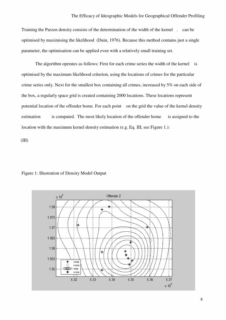
The algorithm operates as follows: First for each crime series the width of the kernel is

optimised by the maximum likelihood criterion, using the locations of crimes for the particular

crime series only. Next for the smallest box containing all crimes, increased by 5% on each side of

the box, a regularly space grid is created containing 2000 locations. These locations represent

potential location of the offender home. For each point on the grid the value of the kernel density

estimation is computed. The most likely location of the offender home is assigned to the

location with the maximum kernel density estimation (e.g. Eq. III; see Figure 1.):

(III)

Figure 1: Illustration of Density Model Output


9

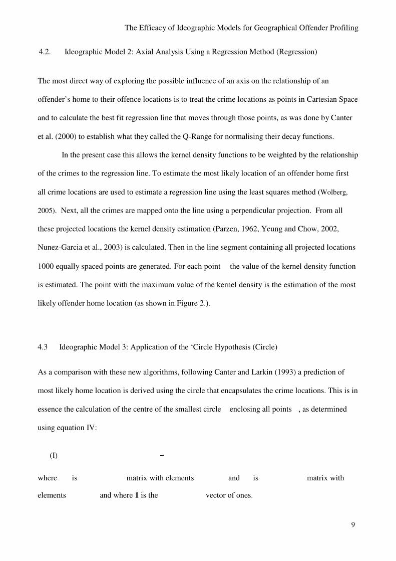
4.2. Ideographic Model 2: Axial Analysis Using a Regression Method (Regression)

The most direct way of exploring the possible influence of an axis on the relationship of an

offender’s home to their offence locations is to treat the crime locations as points in Cartesian Space

and to calculate the best fit regression line that moves through those points, as was done by Canter

et al. (2000) to establish what they called the Q-Range for normalising their decay functions.

In the present case this allows the kernel density functions to be weighted by the relationship

of the crimes to the regression line. To estimate the most likely location of an offender home first

all crime locations are used to estimate a regression line using the least squares method (Wolberg,

2005). Next, all the crimes are mapped onto the line using a perpendicular projection. From all

these projected locations the kernel density estimation (Parzen, 1962, Yeung and Chow, 2002,

Nunez-Garcia et al., 2003) is calculated. Then in the line segment containing all projected locations

1000 equally spaced points are generated. For each point the value of the kernel density function

is estimated. The point with the maximum value of the kernel density is the estimation of the most

likely offender home location (as shown in Figure 2.).

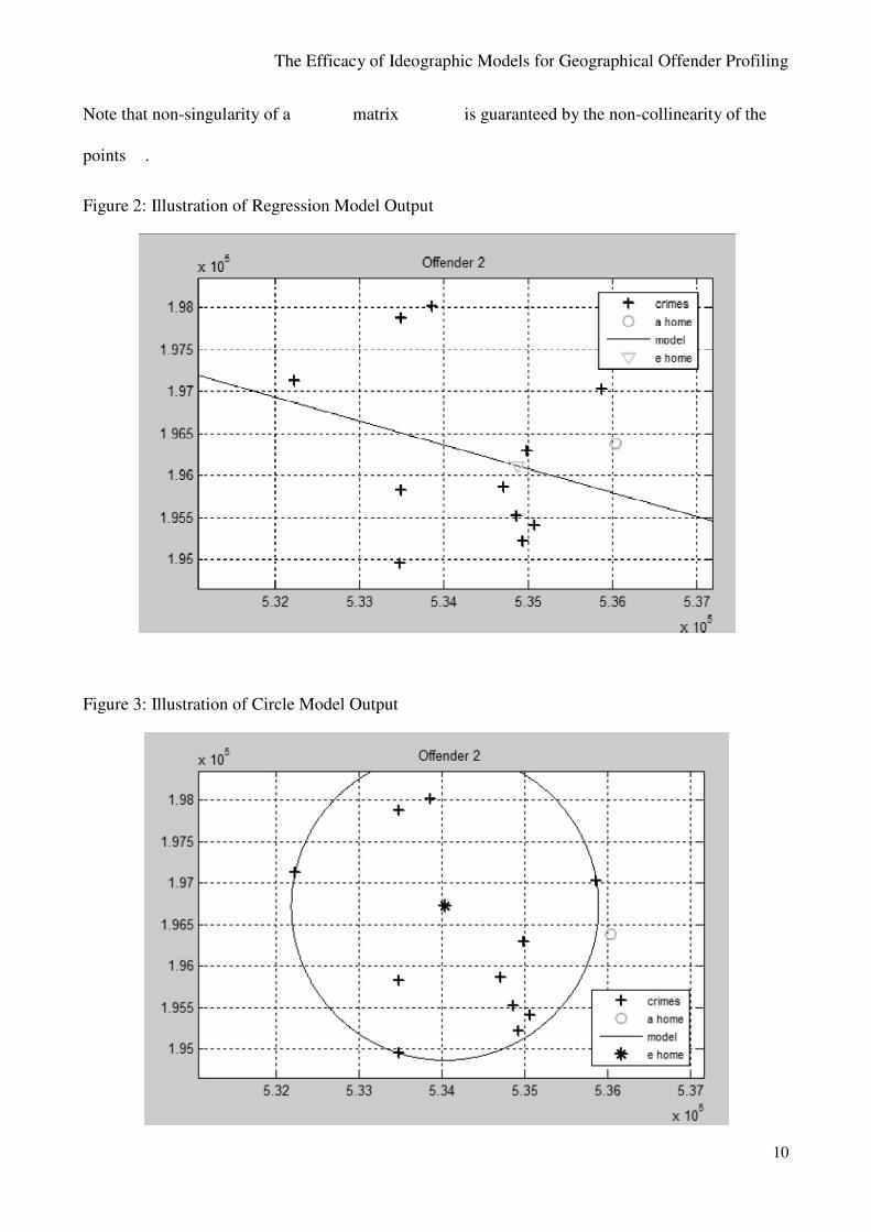
4.3 Ideographic Model 3: Application of the ‘Circle Hypothesis (Circle)

As a comparison with these new algorithms, following Canter and Larkin (1993) a prediction of

most likely home location is derived using the circle that encapsulates the crime locations. This is in

essence the calculation of the centre of the smallest circle enclosing all points , as determined

using equation IV:

(I)

where is matrix with elements and is matrix with

elements and where 1 is the vector of ones.


10

Note that non-singularity of a matrix is guaranteed by the non-collinearity of the

points .

Figure 2: Illustration of Regression Model Output

Figure 3: Illustration of Circle Model Output


11

In the application of this model we compute a circle with the smallest area that encloses all

crime locations. Previously the offence circle has been calculated by taking a line between the two

crimes that are furthest from each other as the diameter of the circle. This is not necessarily the

circle that covers the smallest area incorporating all the crimes, as is the case in the new algorithm

(illustrated in Figure 3).

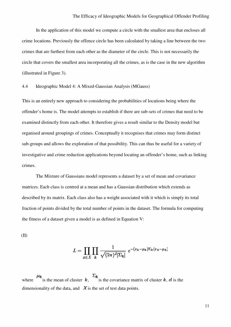
4.4 Ideographic Model 4: A Mixed-Gaussian Analysis (MGauss)

This is an entirely new approach to considering the probabilities of locations being where the

offender’s home is. The model attempts to establish if there are sub-sets of crimes that need to be

examined distinctly from each other. It therefore gives a result similar to the Density model but

organised around groupings of crimes. Conceptually it recognises that crimes may form distinct

sub-groups and allows the exploration of that possibility. This can thus be useful for a variety of

investigative and crime reduction applications beyond locating an offender’s home, such as linking

crimes.

The Mixture of Gaussians model represents a dataset by a set of mean and covariance

matrices. Each class is centred at a mean and has a Gaussian distribution which extends as

described by its matrix. Each class also has a weight associated with it which is simply its total

fraction of points divided by the total number of points in the dataset. The formula for computing

the fitness of a dataset given a model is as defined in Equation V:

(II)

where is the mean of cluster , is the covariance matrix of cluster , is the

dimensionality of the data, and is the set of test data points.


12

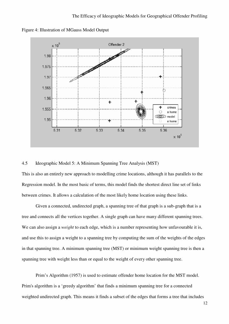
Figure 4: Illustration of MGauss Model Output

4.5 Ideographic Model 5: A Minimum Spanning Tree Analysis (MST)

This is also an entirely new approach to modelling crime locations, although it has parallels to the

Regression model. In the most basic of terms, this model finds the shortest direct line set of links

between crimes. It allows a calculation of the most likely home location using these links.

Given a connected, undirected graph, a spanning tree of that graph is a sub-graph that is a

tree and connects all the vertices together. A single graph can have many different spanning trees.

We can also assign a weight to each edge, which is a number representing how unfavourable it is,

and use this to assign a weight to a spanning tree by computing the sum of the weights of the edges

in that spanning tree. A minimum spanning tree (MST) or minimum weight spanning tree is then a

spanning tree with weight less than or equal to the weight of every other spanning tree.

Prim’s Algorithm (1957) is used to estimate offender home location for the MST model.

Prim's algorithm is a ‘greedy algorithm’ that finds a minimum spanning tree for a connected

weighted undirected graph. This means it finds a subset of the edges that forms a tree that includes


13

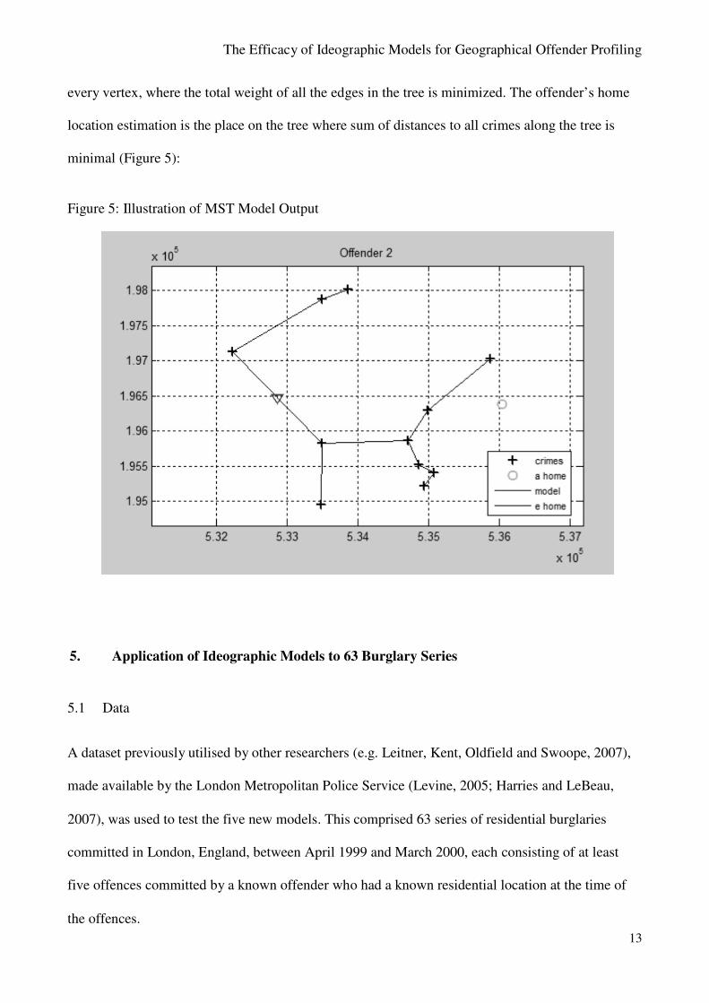
every vertex, where the total weight of all the edges in the tree is minimized. The offender’s home

location estimation is the place on the tree where sum of distances to all crimes along the tree is

minimal (Figure 5):

Figure 5: Illustration of MST Model Output

5. Application of Ideographic Models to 63 Burglary Series

5.1 Data

A dataset previously utilised by other researchers (e.g. Leitner, Kent, Oldfield and Swoope, 2007),

made available by the London Metropolitan Police Service (Levine, 2005; Harries and LeBeau,

2007), was used to test the five new models. This comprised 63 series of residential burglaries

committed in London, England, between April 1999 and March 2000, each consisting of at least

five offences committed by a known offender who had a known residential location at the time of

the offences.


14

5.2 Measuring GP Effectiveness:

Various measures of GP program output accuracy have been suggested (see, for example; Paulsen,

2004; Rich & Shively, 2004; Rich, Shively, & Adedokun, 2004). These generally consist of either

the distance from the most probable home location predicted by the algorithm to the known

residential base of the offender and/or the area of some putative search area that has to be searched,

starting from the location indicated as most probable, before the offenders’ actual base is reached.

These calculations are not as self-evident or unproblematic as may seem at first sight. The

distance measures could reasonably be on a Manhattan matrix or the nearest feasible route, both of

which could take account of land-use patterns. However, they are open to some arbitrariness

because the actual route an offender might take is not known. Indeed, as Canter and Hodge (2000)

and Canter and Shalev (2008) have shown through the study of offenders’ ‘mental maps’, there are

many reasons why an offender may not use the nearest direct route between home and crime

location. The direct ‘crow flight’ measurement may therefore remain the best estimate of the

distance that the predicted home is from the actual home. It is what most previous research has used

(e.g. Paulsen, 2005; 2006; Bennell et al., 2009), and is therefore used here.

The problem in calculating the area searched relates to the how the total search area is

defined and whether the actual area searched before the home is located is specified or some

proportion of the total, defined search area, as in Canter et al.’s (2000) ‘search cost’. Rossmo (2000)

proposed an area standard that involves the minimum bounding rectangle plus a slight addition and

distinguishes this from Dragnet, which increases the minimum bounding rectangle by 20%. But

how that bounding rectangle itself is defined is open to some arbitrariness.

In the present work the search area is computed as an area of the circle where a predicted

home is the centre of the circle and the true home defines the radius of the circle. For density and

MGauss methods the search area is computed along density levels from highest to lowest. Areas are

added to the search area until the actual home is located. This is an actual area measure, not a


15

proportion of any notional search area as in previous studies (e.g. Canter et al., 2000; Canter and

Hammond, 2006; Hammond and Youngs, 2011; Rossmo, 2000). Moreover, from an operational

perspective it is of course of much more value to know that, for example, 5km had to be searched,

rather than 10% of an arbitrary total area.

6. Results

6.1 Findings on the Efficacy of the Ideographic Models

6.1.1 Summary Descriptions of Efficacy Measures

Two efficacy measures were employed to make comparisons between the five ideographic models

presented previously; an error distance measure (shortest ‘crow flight’ distance between actual

home an estimated home location) and an area measure (the actual area that would need to be

searched to find the home, starting from the predicted home).

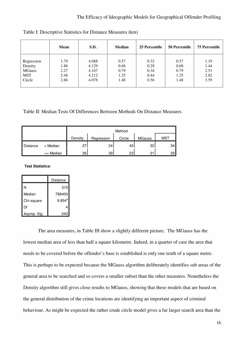
Table I gives the summary descriptions of the efficacy measures for the distance from home

to predicted home location. Because of the well established skewed distribution of the distances

offenders travel the median is the best estimate of the efficacy of the different measures, although

other indicators of central tendency are provided for comparison. The results show, interestingly,

that the regression model has the lowest median and mean, with the median being close to half a

kilometre. Also, a quarter of the sample have a median distance less than a third of a kilometre for

the regression model, but also for the Density and Mgauss models, This does show the significance

of dominant axes as also reported by Canter et al (2000) with their use of the Q range.

A median test does show that there are statistically significant differences between the

different models at p<.05. This supports the view that the different models are sensitive to different

aspects of the data and are worth considering independently of each other.


16

Table I: Descriptive Statistics for Distance Measures (km)

Mean

S.D.

Median

25 Percentile

50 Percentile

75 Percentile

Regression

Density

MGauss

MST

Circle

1.79

1.86

2.27

2.48

2.66

4.088

4.129

4.167

4.212

4.078

0.57

0.68

0.79

1.25

1.48

0.32

0.29

0.34

0.44

0.56

0.57

0.68

0.79

1.25

1.48

1.19

1.44

2.51

2.82

3.59

Table II: Median Tests Of Differences Between Methods On Distance Measures

Method

Density

Regression

Circle

MGauss

MST

Distance > Median

<= Median

27

24

40

32

34

36

39

23

31

29

Test Statistics:

Distance

N

Median

Chi-square

Df

Asymp. Sig.

315

.788400

9.854a

4

.043

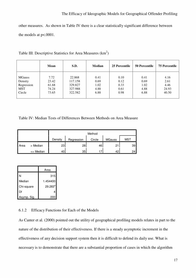
The area measures, in Table III show a slightly different picture. The MGauss has the

lowest median area of less than half a square kilometre. Indeed, in a quarter of case the area that

needs to be covered before the offender’s base is established is only one tenth of a square metre.

This is perhaps to be expected because the MGauss algorithm deliberately identifies sub areas of the

general area to be searched and so covers a smaller subset than the other measures. Nonetheless the

Density algorithm still gives close results to MGauss, showing that these models that are based on

the general distribution of the crime locations are identifying an important aspect of criminal

behaviour. As might be expected the rather crude circle model gives a far larger search area than the


17

other measures. As shown in Table IV there is a clear statistically significant difference between

the models at p<.0001.

Table III: Descriptive Statistics for Area Measures (km2)

Mean

S.D.

Median

25 Percentile

50 Percentile

75 Percentile

MGauss

Density

Regression

MST

Circle

7.72

23.42

61.68

74.24

73.65

22.868

117.158

329.827

327.988

322.582

0.41

0.69

1.02

4.88

6.88

0.10

0.12

0.33

0.61

0.98

0.41

0.69

1.02

4.88

6.88

4.16

2.61

4.46

24.93

40.50

Table IV: Median Tests of Differences Between Methods on Area Measure

Method

Density

Regression

Circle

MGauss

MST

Area > Median

<= Median

23

28

46

21

39

40

35

17

42

24

Area

N

Median

Chi-square

Df

Asymp. Sig.

315

1.454400

29.283a

4

.000

6.1.2 Efficacy Functions for Each of the Models

As Canter et al. (2000) pointed out the utility of geographical profiling models relates in part to the

nature of the distribution of their effectiveness. If there is a steady asymptotic increment in the

effectiveness of any decision support system then it is difficult to defend its daily use. What is

necessary is to demonstrate that there are a substantial proportion of cases in which the algorithm


18

0.5

1

1.5

2

2.5

3

3.5

4

4.5

5

5.5

6

6.5

7

7.5

8

8.5

9

9.5

1

0

10

.5

11

1

1.5

1

2

12

.5

13

1

3.5

1

4

14

.5

15

1

5.5

1

6

16

.5

17

1

7.5

1

8

18

.5

19

1

9.5

2

0

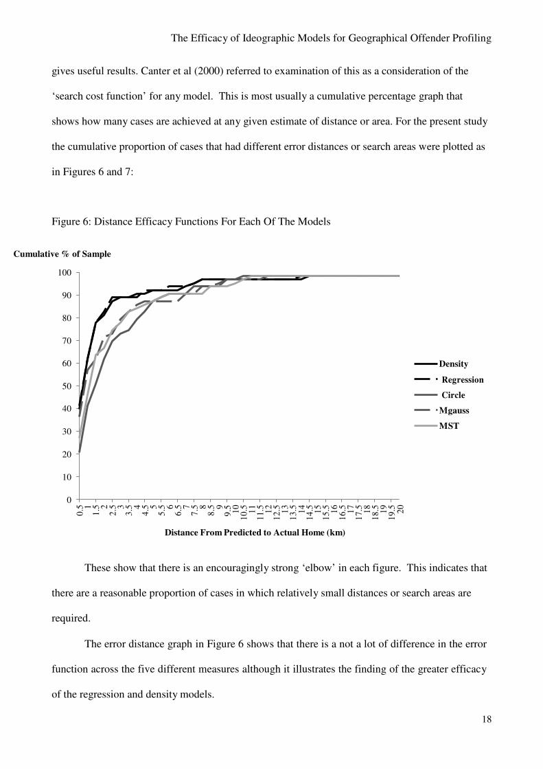
gives useful results. Canter et al (2000) referred to examination of this as a consideration of the

‘search cost function’ for any model. This is most usually a cumulative percentage graph that

shows how many cases are achieved at any given estimate of distance or area. For the present study

the cumulative proportion of cases that had different error distances or search areas were plotted as

in Figures 6 and 7:

Figure 6: Distance Efficacy Functions For Each Of The Models

Cumulative % of Sample

100

90

80

70

60 Density

Regression 50

Circle

40 Mgauss

30 MST

20

10

0

Distance From Predicted to Actual Home (km)

These show that there is an encouragingly strong ‘elbow’ in each figure. This indicates that

there are a reasonable proportion of cases in which relatively small distances or search areas are

required.

The error distance graph in Figure 6 shows that there is a not a lot of difference in the error

function across the five different measures although it illustrates the finding of the greater efficacy

of the regression and density models.


19

0.5

1

1.5

2

2.5

3

3.5

4

4.5

5

5.5

6

6.5

7

7.5

8

8.5

9

9.5

1

0

10

.5

11

1

1.5

1

2

12

.5

13

1

3.5

1

4

14

.5

15

1

5.5

1

6

16

.5

17

1

7.5

1

8

18

.5

19

1

9.5

2

0

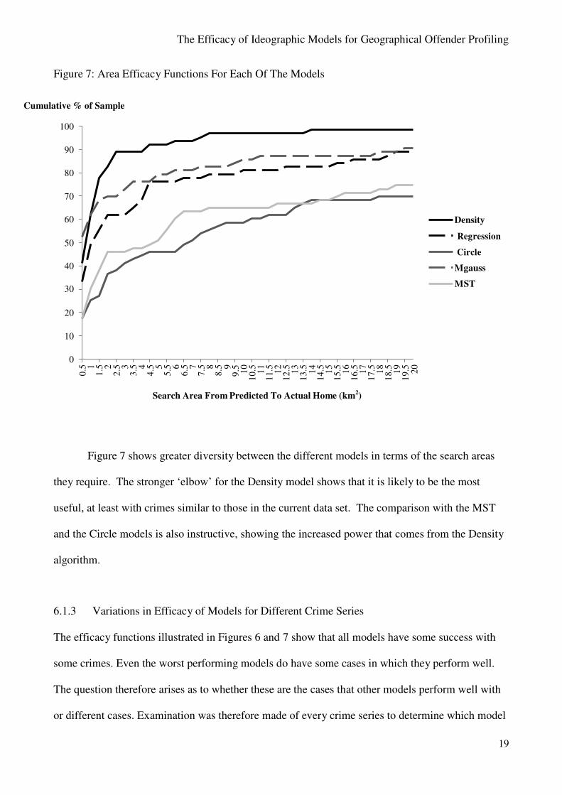
Figure 7: Area Efficacy Functions For Each Of The Models

Cumulative % of Sample

100

90

80

70

60 Density

Regression 50

Circle

40 Mgauss

30 MST

20

10

0

Search Area From Predicted To Actual Home (km2)

Figure 7 shows greater diversity between the different models in terms of the search areas

they require. The stronger ‘elbow’ for the Density model shows that it is likely to be the most

useful, at least with crimes similar to those in the current data set. The comparison with the MST

and the Circle models is also instructive, showing the increased power that comes from the Density

algorithm.

6.1.3 Variations in Efficacy of Models for Different Crime Series

The efficacy functions illustrated in Figures 6 and 7 show that all models have some success with

some crimes. Even the worst performing models do have some cases in which they perform well.

The question therefore arises as to whether these are the cases that other models perform well with

or different cases. Examination was therefore made of every crime series to determine which model


20

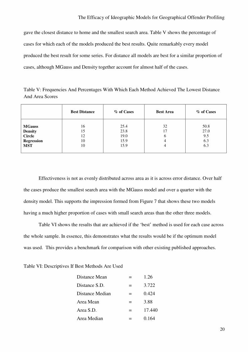
gave the closest distance to home and the smallest search area. Table V shows the percentage of

cases for which each of the models produced the best results. Quite remarkably every model

produced the best result for some series. For distance all models are best for a similar proportion of

cases, although MGauss and Density together account for almost half of the cases.

Table V: Frequencies And Percentages With Which Each Method Achieved The Lowest Distance

And Area Scores

Best Distance

% of Cases

Best Area

% of Cases

MGauss

Density

Circle

Regression

MST

16

15

12

10

10

25.4

23.8

19.0

15.9

15.9

32

17

6

4

4

50.8

27.0

9.5

6.3

6.3

Effectiveness is not as evenly distributed across area as it is across error distance. Over half

the cases produce the smallest search area with the MGauss model and over a quarter with the

density model. This supports the impression formed from Figure 7 that shows these two models

having a much higher proportion of cases with small search areas than the other three models.

Table VI shows the results that are achieved if the ‘best’ method is used for each case across

the whole sample. In essence, this demonstrates what the results would be if the optimum model

was used. This provides a benchmark for comparison with other existing published approaches.

Table VI: Descriptives If Best Methods Are Used

Distance Mean = 1.26

Distance S.D. = 3.722

Distance Median = 0.424

Area Mean = 3.88

Area S.D. = 17.440

Area Median = 0.164


21

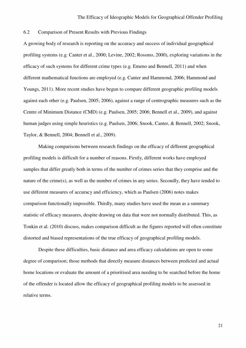
6.2 Comparison of Present Results with Previous Findings

A growing body of research is reporting on the accuracy and success of individual geographical

profiling systems (e.g. Canter et al., 2000; Levine, 2002; Rossmo, 2000), exploring variations in the

efficacy of such systems for different crime types (e.g. Emeno and Bennell, 2011) and when

different mathematical functions are employed (e.g. Canter and Hammond, 2006; Hammond and

Youngs, 2011). More recent studies have begun to compare different geographic profiling models

against each other (e.g. Paulsen, 2005; 2006), against a range of centrographic measures such as the

Centre of Minimum Distance (CMD) (e.g. Paulsen, 2005; 2006; Bennell et al., 2009), and against

human judges using simple heuristics (e.g. Paulsen, 2006; Snook, Canter, & Bennell, 2002; Snook,

Taylor, & Bennell, 2004; Bennell et al., 2009).

Making comparisons between research findings on the efficacy of different geographical

profiling models is difficult for a number of reasons. Firstly, different works have employed

samples that differ greatly both in terms of the number of crimes series that they comprise and the

nature of the crime(s), as well as the number of crimes in any series. Secondly, they have tended to

use different measures of accuracy and efficiency, which as Paulsen (2006) notes makes

comparison functionally impossible. Thirdly, many studies have used the mean as a summary

statistic of efficacy measures, despite drawing on data that were not normally distributed. This, as

Tonkin et al. (2010) discuss, makes comparison difficult as the figures reported will often constitute

distorted and biased representations of the true efficacy of geographical profiling models.

Despite these difficulties, basic distance and area efficacy calculations are open to some

degree of comparison; those methods that directly measure distances between predicted and actual

home locations or evaluate the amount of a prioritised area needing to be searched before the home

of the offender is located allow the efficacy of geographical profiling models to be assessed in

relative terms.


22

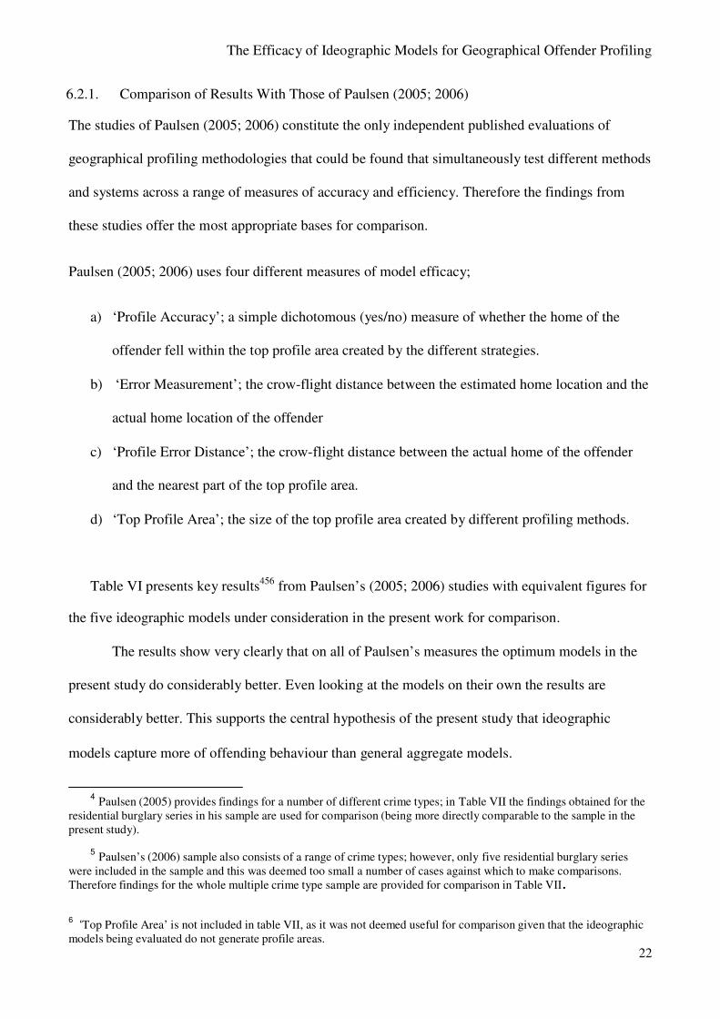
6.2.1. Comparison of Results With Those of Paulsen (2005; 2006)

The studies of Paulsen (2005; 2006) constitute the only independent published evaluations of

geographical profiling methodologies that could be found that simultaneously test different methods

and systems across a range of measures of accuracy and efficiency. Therefore the findings from

these studies offer the most appropriate bases for comparison.

Paulsen (2005; 2006) uses four different measures of model efficacy;

a) ‘Profile Accuracy’; a simple dichotomous (yes/no) measure of whether the home of the

offender fell within the top profile area created by the different strategies.

b) ‘Error Measurement’; the crow-flight distance between the estimated home location and the

actual home location of the offender

c) ‘Profile Error Distance’; the crow-flight distance between the actual home of the offender

and the nearest part of the top profile area.

d) ‘Top Profile Area’; the size of the top profile area created by different profiling methods.

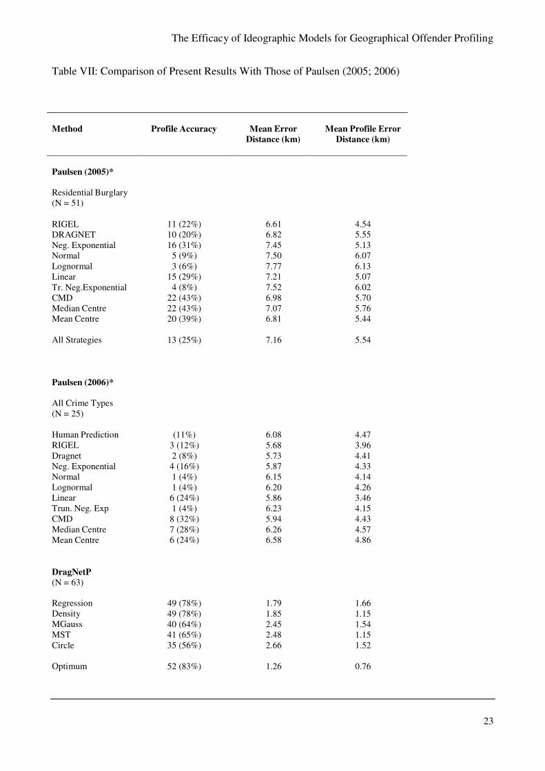
Table VI presents key results456

from Paulsen’s (2005; 2006) studies with equivalent figures for

the five ideographic models under consideration in the present work for comparison.

The results show very clearly that on all of Paulsen’s measures the optimum models in the

present study do considerably better. Even looking at the models on their own the results are

considerably better. This supports the central hypothesis of the present study that ideographic

models capture more of offending behaviour than general aggregate models.

4 Paulsen (2005) provides findings for a number of different crime types; in Table VII the findings obtained for the

residential burglary series in his sample are used for comparison (being more directly comparable to the sample in the

present study).

5 Paulsen’s (2006) sample also consists of a range of crime types; however, only five residential burglary series

were included in the sample and this was deemed too small a number of cases against which to make comparisons.

Therefore findings for the whole multiple crime type sample are provided for comparison in Table VII .

6

‘Top Profile Area’ is not included in table VII, as it was not deemed useful for comparison given that the ideographic

models being evaluated do not generate profile areas.


23

Table VII: Comparison of Present Results With Those of Paulsen (2005; 2006)

Method Profile Accuracy Mean Error

Distance (km)

Mean Profile Error

Distance (km)

Paulsen (2005)*

Residential Burglary

(N = 51)

RIGEL

DRAGNET

Neg. Exponential

Normal

Lognormal

Linear

Tr. Neg.Exponential

CMD

Median Centre

Mean Centre

All Strategies

Paulsen (2006)*

All Crime Types

(N = 25)

Human Prediction

RIGEL

Dragnet

Neg. Exponential

Normal

Lognormal

Linear

Trun. Neg. Exp

CMD

Median Centre

Mean Centre

DragNetP

(N = 63)

Regression

Density

MGauss

MST

Circle

Optimum

11 (22%)

10 (20%)

16 (31%)

5 (9%)

3 (6%)

15 (29%)

4 (8%)

22 (43%)

22 (43%)

20 (39%)

13 (25%)

(11%)

3 (12%)

2 (8%)

4 (16%)

1 (4%)

1 (4%)

6 (24%)

1 (4%)

8 (32%)

7 (28%)

6 (24%)

49 (78%)

49 (78%)

40 (64%)

41 (65%)

35 (56%)

52 (83%)

6.61

6.82

7.45

7.50

7.77

7.21

7.52

6.98

7.07

6.81

7.16

6.08

5.68

5.73

5.87

6.15

6.20

5.86

6.23

5.94

6.26

6.58

1.79

1.85

2.45

2.48

2.66

1.26

4.54

5.55

5.13

6.07

6.13

5.07

6.02

5.70

5.76

5.44

5.54

4.47

3.96

4.41

4.33

4.14

4.26

3.46

4.15

4.43

4.57

4.86

1.66

1.15

1.54

1.15

1.52

0.76


24

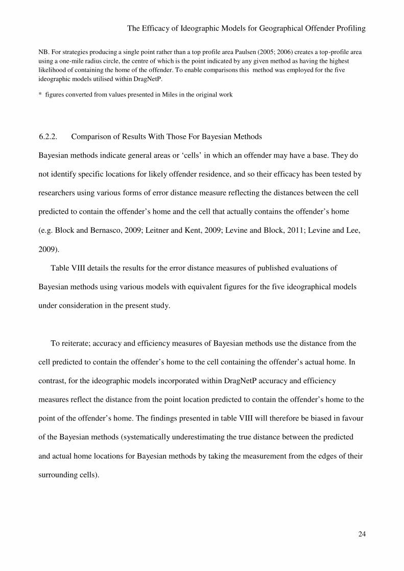
NB. For strategies producing a single point rather than a top profile area Paulsen (2005; 2006) creates a top -profile area

using a one-mile radius circle, the centre of which is the point indicated by any given method as having the highest

likelihood of containing the home of the offender. To enable comparisons this method was employed for the five

ideographic models utilised within DragNetP.

* figures converted from values presented in Miles in the original work

6.2.2. Comparison of Results With Those For Bayesian Methods

Bayesian methods indicate general areas or ‘cells’ in which an offender may have a base. They do

not identify specific locations for likely offender residence, and so their efficacy has been tested by

researchers using various forms of error distance measure reflecting the distances between the cell

predicted to contain the offender’s home and the cell that actually contains the offender’s home

(e.g. Block and Bernasco, 2009; Leitner and Kent, 2009; Levine and Block, 2011; Levine and Lee,

2009).

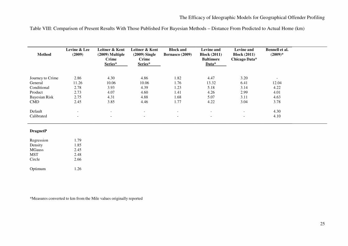
Table VIII details the results for the error distance measures of published evaluations of

Bayesian methods using various models with equivalent figures for the five ideographical models

under consideration in the present study.

To reiterate; accuracy and efficiency measures of Bayesian methods use the distance from the

cell predicted to contain the offender’s home to the cell containing the offender’s actual home. In

contrast, for the ideographic models incorporated within DragNetP accuracy and efficiency

measures reflect the distance from the point location predicted to contain the offender’s home to the

point of the offender’s home. The findings presented in table VIII will therefore be biased in favour

of the Bayesian methods (systematically underestimating the true distance between the predicted

and actual home locations for Bayesian methods by taking the measurement from the edges of their

surrounding cells).


25

Table VIII: Comparison of Present Results With Those Published For Bayesian Methods – Distance From Predicted to Actual Home (km)

Method

Levine & Lee

(2009)

Leitner & Kent

(2009) Multiple

Crime

Series*

Leitner & Kent

(2009) Single

Crime

Series*

Block and

Bernasco (2009)

Levine and

Block (2011)

Baltimore

Data*

Levine and

Block (2011)

Chicago Data*

Bennell et al.

(2009)*

Journey to Crime

General

Conditional

Product

Bayesian Risk

CMD

Default

Calibrated

2.86

11.26

2.78

2.73

2.75

2.45

-

-

4.30

10.06

3.93

4.07

4.31

3.85

-

-

4.86

10.06

4.39

4.60

4.88

4.46

-

-

1.82

1.76

1.23

1.41

1.68

1.77

-

-

4.47

13.32

5.18

4.26

5.07

4.22

-

-

3.20

6.41

3.14

2.99

3.11

3.04

-

-

-

12.04

4.22

4.01

4.63

3.78

4.30

4.10

DragnetP

Regression

Density

MGauss

MST

Circle

Optimum

1.79

1.85

2.45

2.48

2.66

1.26

*Measures converted to km from the Mile values originally reported


26

Table IX: Comparison of Present Results With Those Published For Bayesian Methods – Percentage of Offenders Living Less Than 1km From

Predicted Home

Method

Levine & Lee

(2009)

Leitner & Kent

(2009) Multiple

Crime Series

Leitner & Kent

(2009) Single

Crime Series

Block and

Bernasco (2009)

Journey to Crime

General

Conditional

Product

Bayesian Risk

CMD

45.03

1.17

42.69

46.78

49.12

43.27

41.88

1.06

36.35

41.53

42.35

38.94

35.47

1.06

31.65

34.47

33.88

32.59

40.3

35.5

64.5

51.6

50.0

35.5

DragnetP

Regression

Density

MGauss

MST

Circle

Optimum

61.9

61.9

52.4

46.0

41.3

61.1


27

Nonetheless, it is clear that the distance from home to predicted home is much smaller for the

models tested here than for the Bayesian studies. It is only for the Block & Bernasco (2009) study

that the average distances are at all close to those from the present study. Their best result is for their

‘conditional’ condition of 1.23 km. That is close to the optimum value for the present study of 1.26

km. However all the other values from the other studies are much higher.

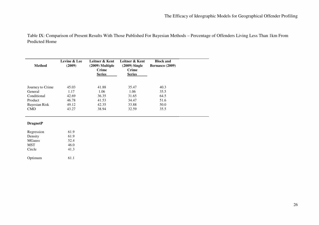
The variations in values across the different Bayesian studies are likely to be a direct

function of the distribution of crimes and criminals in any particular city. This is because Bayesian

analyses draw directly on the actual locations of offenders’ bases to develop their probabilities. In

order to counteract this problem measures are used that consider the proportion of offenders living

within any given distance from the predicted cell. These percentages are given in Table IX with

comparisons from the present study.

Again Block and Bernasco (2009) achieve the highest percentage for their ‘conditional’

model with 64% of their offenders within one kilometre of the cell designated by the Bayesian

analysis, but most of the other studies and models show much smaller figures, typically in the

region of 40% or less. By contrast the optimum result for the present study is 61%, with even the

simple circle model giving 41% of the offenders within one kilometre of the highest probability

designated location.

Discussion and Conclusions

Existing explorations of how an offender’s base may be related to where he or she commits crimes

have all drawn on general trends across a number of offenders. The dominant process has been to

apply geometric models based on aggregate probability distributions. These assume that the

likelihood surface can be applied to each individual crime series. However, growing empirical

evidence supports the commonsense perspective that each offender is likely to use surroundings in a

unique way.


28

An emerging approach that differs from the use of likelihood surfaces uses Bayesian

probability modelling. This relies on geographical examination of the actual locations in particular

cities of the areas in which offenders reside related to where they commit their crimes. This

implicitly takes account of differences in land use patterns and so can be more sensitive to local

issues than aggregate likelihood surfaces. However, it is entirely dependent on a particular data set

of a number of crimes and criminals from a specific location. It is thus also is essentially nomothetic

in dealing with general trends across a number of offenders.

In contrast to these existing approaches a number of models have been explored in the

present paper that are essentially ideographic, in that they only draw on information about the

location of the crimes in a unique crime series. Indeed, one of the earliest models of serial crime

distribution, often known as the ‘circle’ model (Canter and Larkin, 1993), was ideographic, utilising

only the two crimes furthest from each other to predict the base of the offender. A stronger

mathematical formula has been placed on that model in the present study and others have been

added that use density, dominant axes and routes applied to any specific crime series.

The results of applying these models to a set of 63 burglary series in London showed that

each was optimum for some series, but none was optimum for all series. The density models had the

highest number of series in which they were optimum giving median distances of close to 1

kilometre between the predicted home and the actual home. This indicates that these offenders did

tend to operate in an area that encompassed their home. However, the models that drew on

dominant axes or routes were also optimum for some series raising the prospect of some important

differences between offenders in the structure of their crime searches.

Comparisons of the results from the present study with those from the nomothetic models

showed that in virtually all cases the ideographic models out-performed them. For this data set at

least the density models tested here gave consistently and distinctly shorter distances to crime and

consistently and distinctly higher proportions of offenders within one kilometre of the designated

most probable base location. These results of course need to be tested further with other data sets


29

dealing with other sorts of crimes in other locations, but the results strongly indicate that offenders

need to be modelled individually if our understanding of their crime location choices is to be

improved. Such an understanding will also increase the effectiveness of geographical investigative

decision support tools.

References

Bennell, C., Emeno, K., Snook, B., Taylor, P. & Snook, B. (2009) The Precision, Accuracy and

Efficiency of Geographic Profiling Predictions: A Simple Heuristic Versus Mathematical

Algorithms. Crime Mapping: A Journal of Research and Practice, 1 (2); p.65-84.

Bennell, C., Snook, B., Taylor, P. J., Corey, S., & Keyton, J. (2007). It's No Riddle, Choose the

Middle: The Effect of Number of Crimes and Topographical Detail on Police Officer Predictions of

Serial Burglars' Home Locations. Criminal Justice and Behavior, 34 (1), 119-132.

Bennell, C., Taylor, P., & Snook, B. (2007). Clinical Versus Actuarial Geographic Profiling

Strategies: A Review of the Research. Police Practice and Research, 8(4), 335–345.

Block, R. & Bernasco, W. (2009) Finding A Serial Burglar’s Home Using Distance Decay and

Origin Destination Patterns: A Test of Empirical Bayes Journey-to-Crime Estimation in the Hague.

Journal of Investigative Psychology and Offender Profiling, 6 (3); 187-211.

Canter, D. (2009). Developments in Geographical Offender Profiling: Commentary on Bayesian

Journey-to-Crime Modelling. Journal of Investigative Psychology and Offender Profiling, 6; 161-

166.

Canter, D., Coffey, T., Huntley, M. & Missen, C. (2000). Predicting Serial Killers’ Home Base

Using a Decision Support System. Journal of Quantitative Criminology, 16, 4; 457 – 478.


30

Canter, D. & Hammond, L. (2006) A Comparison of the Efficacy of Different Decay Functions in

Geographical Profiling for a Sample of U.S. Serial Killers. Journal of Investigative Psychology and

Offender Profiling, 3; 91-103.

Canter, D. & Hammond, L. (2007) Prioritising Burglars: Comparing the Effectiveness of

Geographical Profiling Methods. Police, Practice and Research, 8(4); 371-384.

Canter, D. & Hodge, S. (2000). Criminal’s Mental Maps. In L.S. Turnball, E. Hallisey-Hendrix &

B.D. Dent (Eds). Atlas of Crime. Oryx Press; 187-191.

Canter, D. & Larkin, P. (1993). The Environmental Range of Serial Rapists. In Canter, D. & Alison,

L. (Eds.). Criminal Detection and the Psychology of Crime. Aldershot, Dartmouth: Ashgate.

Canter, D. & Shalev, K. (2008). Putting Crime in its Place: Psychological Process in Crime Site

Location. In D. Canter & D. Youngs (2008) Principles of Geographical Offender Profiling.

Aldershot, Ashgate.

Canter, D. & Youngs, D. (Eds.) (2008a) Principles of Geographical Offender Profiling. Aldershot,

Ashgate.

Canter, D. & Youngs, D. (Eds.) (2008b) Applications of Geographical Offender Profiling.

Aldershot, Ashgate.

Canter, D. & Youngs, D. (2009) Investigative Psychology: Offender Profiling and the Analysis of

Criminal Action. Chichester: Wiley.

C.M. Costanzo, W.C. Halperin, and N. Gale (1986). Criminal Mobility and the Directional

Component in Journeys to Crime, in R. Figlio, S. Hakim and G. Rengert (Eds.) Metropolitan Crime

Patterns. Monsey, N.Y.: Willow Tree Press.


31

Duin, R. (1976). On the Choice of the Smoothing Parameters for Parzen Estimators of Probability

Density Functions. IEEE Transactions on Computers, C-25(11); 1175–1179.

Emeno, K. & Bennell, C. (2011) The Effectiveness of Calibrated Versus Default Distance Decay

Functions for Geographic Profiling: A Preliminary Examination of Crime Type. Psychology, Crime

& Law, DOI:10.1080/1068316X.2011.621426

Goodwill, A.. & Alison, L. (2005) Sequential Angulation, Spatial Dispersion and Consistency of

Distance Attack Patterns from Home in Serial Murder, Rape and Burglary. Psychology, Crime &

Law, 11(2); 161-176.

Hammond, L. (2009) Spatial Patterns in Serial Crime: Modelling Offence Distribution and Home-

Crime Relationships For Prolific Individual Offenders. Unpublished Doctoral Thesis: University of

Liverpool.

Hammond, L. and Youngs, D. (2011) Decay Functions and Criminal Spatial Processes:

Geographical Offender Profiling of Volume Crime. Journal of Investigative Psychology and

Offender Profiling, 8; 90-102.

Harries, K. & Le Beau, J. (2007) Issues in the Geographic Profiling of Crime: Review and

Commentary. Police Practice and Research, 8 (4); 321-333.

Leitner, M. & Kent, J. (2009). Bayesian Journey to Crime Modelling of Single and Multiple Crime

Type Series in Baltimore County, MD. Journal of Investigative Psychology and Offender Profiling,

6; 213-236.

Leitner, M., Kent, J., Oldfield, I. & Swoope, E. (2007). Geoforensic Analysis Revisited – The

Application of Newton’s Geographic Profiling Method to Serial Burglaries in London, U.K. Police

Practice and Research, 8 (4); 359-370.


32

Levine, N. (2002). Crimestat II: Spatial Modeling. Report for the U.S. Department of Justice,

August 13th

, 2002.

Levine, N. (2005). CrimeStat III. Crime Mapping News. 7(2), Spring. 8-10.

Levine, N. (2009) Introduction to the Special Issue on Bayesian Journey-to-Crime Modelling.

Journal of Investigative Psychology and Offender Profiling, 6 (3); 167-185.

Levine, N. & Block, R. (2011) Bayesian Journey-to-Crime Estimation: An Improvement in

Geographic Profiling Methodology. The Professional Geographer, 63 (2); 213-229.

Levine, N. & Lee, P (2009). Bayesian Journey-to-Crime Modelling of Juvenile and Adult Offenders

by Gender in Manchester. Journal of Investigative Psychology and Offender Profiling, 6; 237-251.

Lundrigan, S. & Canter, D. (2001). Spatial Patterns of Serial Murder: An Analysis of Disposal Site

Location Choice. Behavioural Sciences and the Law, 19; 595-610.

Lundrigan, S. & Czarnomski, S. (2006). Spatial Characteristics of Serial Sexual Assault in New

Zealand. The Australian and New Zealand Journal of Criminology. 32 (2); 218-231.

Nunez-Garcia, J., Kutalik, Z., Cho, K.-H., and Wolkenhauer, O. (2003). Level Sets and Minimum

Volume Sets of Probability Density Functions. Journal of Approximate Reasoning, 34(1); 25–47.

Parzen, E. (1962). On the Estimation of a Probability Density Function and Mode. Annals of

Mathematical Statistics, 33:1065–1076.

Paulsen, D. J. (2004, March). Geographic profiling: Hype or hope? – Preliminary Results into the

Accuracy of Geographic Profiling Software. Paper presented at the UK Crime Mapping

Conference, London, UK.


33

Paulsen, D. (2005). Connecting the Dots: Assessing the Accuracy of Geographic Profiling

Software. Policing: An International Journal of Police Strategies and Management, 29 (2); 306-

334.

Paulsen, D. (2006). Human vs. Machine: A Comparison of the Accuracy of Geographic Profiling

Methods. Journal of Investigative Psychology and Offender Profiling, 3(2); 77-89.

Prim,R.J. (1957) Shortest Connection Networks and Some Generalizations. Bell System Technical

Journal, 36; 1389–1401.

Rich, T. & Shively, M. (2004). A Methodology for Evaluating Geographic Profiling Software: Final

Report. Cambridge, MA: Abt Associates Inc.

Rich, T., Shively, M., & Adedokun, L. (2004). NIJ Roundtable for Developing an Evaluation

Methodology for Geographic Profiling Software. Cambridge, MA: Abt Associates.

Rossmo, D.K. (2000). Geographic Profiling. Boca Raton, FL. CRC Press, LLC.

Smith, W., Bond, J.W. and Townsley, M. (2009). Determining How Journeys-to-Crime Vary

Measuring Inter- and Intra-Offender Crime Trip Distributions. In D. Weisburd, Bernasco, W.,

Gerben, J. & Bruinsma, N. (Eds). Putting Crime in its Place. London: Filiquarian Publishing.

Snook, B., Canter, D. V., & Bennell, C. (2002). Predicting the Home Location of Serial Offenders:

A Preliminary Comparison of the Accuracy of Human Judges with a Geographic Profiling System.

Behavioural Sciences and The Law, 20, 109-118.

Snook, B., Taylor, P. J., & Bennell, C. (2004). Geographic Profiling: The Fast, Frugal, and

Accurate Way. Applied Cognitive Psychology, 18, 105-121.


34

Snook, B., Zito, M., Bennell, C., & Taylor, P.J. (2005). On the Complexity and Accuracy of

Geographic Profiling Strategies. Journal of Quantitative Criminology, 21 (1); 1-26.

Taylor, P.J., Bennell, C., & Snook, B. (2009). The Bounds of Cognitive Heuristic Performance on

the Geographic Profiling Task. Applied Cognitive Psychology, 23, 410-430.

Tonkin, M., Woodhams, J., Bond, J.W. & Loe, T. (2010). A Theoretical and Practical Test of

Geographical Profiling With Serial Vehicle Theft in a U.K. Context. Behavioral Sciences and the

Law, 28; 442-460.

Townsley, M. & Sidebottom, A. (2010). All Offenders Are Equal, But Some Are More Equal Than

Others: Variation in Journeys to Crime Between Offenders. Criminology, 48 (3); 897-917.

Van Koppen, P.J. & De Keiser, J.W. (1997). Desisting Distance Decay: On the Aggregation of

Individual Crime Trips. Criminology, 35 (2); 505-513.

Van Koppen, M.V., Elffers, H. & Ruiter, S. (2011) When to Refrain From Using Likelihood

Surface Methods for Geographical Offender Profiling: An Ex Ante Test of Assumptions. Journal of

Investigative Psychology and Offender Profiling, 8 (3); p. 242-256.

Warren, J., Reboussin, R., Hazelwood, R.R., Cummings, A. Gibbs, N., and Trumbetta, S. (1998).

Crime Scene and Distance Correlates of Serial Rape. Journal of Quantitative Criminology. 14 (1);

35-59.

Wolberg, J. (2005) Data Analysis Using the Method of Least Squares: Extracting the Most

Information from Experiments. Springer: ISBN 3540256741.

Yeung, D. Y. and Chow, C. (2002). Parzen-Window Network Intrusion Detectors. Proceedings of

the Sixteenth International Conference on Pattern Recognition, 4; 385–388.

the efficacy of ideographic models for …eprints.hud.ac.uk/id/eprint/15273/1/the_efficacy_of...the...

Documents