ECONOMIC GROWTH CENTERYALE UNIVERSITY

P.O. Box 208629New Haven, CT 06520-8269

http://www.econ.yale.edu/~egcenter/

CENTER DISCUSSION PAPER NO. 964

The Efficacy of Parochial Politics:Caste, Commitment, and Competence in Indian Local

Governments

Kaivan MunshiBrown University and NBER

Mark RosenzweigYale University

September 2008

Notes: Center discussion papers are preliminary materials circulated to stimulate discussion andcritical comments.

We are grateful to Ashley Lester for initial collaboration on this project and to Pedro Dal Bo formany insights that improved this paper. We thank Brian Knight, Laura Schechter, andparticipants at NBER, SITE, and conferences in Amsterdam, Alicante, and Bangkok for helpfulcomments. Munshi acknowledges research support from the National Science Foundationthrough grant SES-0617847. We are responsible for any errors that may remain.

This paper can be downloaded without charge from the Social Science Research Networkelectronic library at: http://ssrn.com/abstract=1272500

An index to papers in the Economic Growth Center Discussion Paper Series is located at:http://www.econ.yale.edu/~egcenter/publications.html

Abstract

Parochial politics is typically associated with poor leadership and low levels of public

good provision. This paper explores the possibility that community involvement in politics need

not necessarily worsen governance and, indeed, can be efficiency-enhancing when the context is

appropriate. Complementing the new literature on the role of community networks in solving

market problems, we test the hypothesis that strong traditional social institutions can discipline

the leaders they put forward, successfully substituting for secular political institutions when they

are ineffective. Using new data on Indian local governments at the ward level over multiple

terms, and exploiting the randomized election reservation system, we find that the presence of a

numerically dominant sub-caste (caste equilibrium) is associated with the selection of leaders

with superior observed characteristics and with greater public good provision. This improvement

in leadership competence occurs without apparently diminishing leaders' responsiveness to their

constituency.

Key Words: Politics, Commitment, Governance

JEL Codes: H11, H44, O12

1 Introduction

Ethnic, linguistic, and caste identity dominate political life throughout the world. In India, the setting

for this paper, caste politics appears to have grown stronger over time (Banerjee and Pande 2007) and

a similar persistence in ethno-linguistic politics has been documented in countries at various stages

of economic development (e.g., Posner 2005). The standard explanation for the emergence and the

persistence of parochial politics is that social loyalty gives leaders leverage when political institutions

are weak, allowing them to appropriate substantial rents for themselves in return for the patronage

they provide to their supporters (Padro i Miquel 2007). Parochial politics is thus associated with

corrupt rulers (kleptocracies), wasteful patronage transfer, and low levels of public good provision.

Economists historically associated networks and other community-based economic institutions

with nepotism, rent-seeking, and inefficiency. In recent years, however, this view has been replaced by

a more moderated position, which recognizes that these institutions can under the right circumstances

facilitate economic activity when markets function imperfectly. Complementing the new literature

on non-market economic institutions, this paper documents, using new data on local public good

provision and electorate and elected leader characteristics, the role played by the community in solving

leadership commitment problems when the democratic system functions imperfectly and the context

is appropriate, providing a more complete assessment of parochial politics and its consequences.

The classical Downsian (1957) model of political competition is not concerned with leaders’ (or

candidates’) characteristics, focussing instead on the identity and the preferences of the pivotal voter.

Recently, however, citizen-candidate models in which leaders cannot commit to implementing policies

that diverge from their own preferences have generated much attention in the political economy

literature. Osborne and Slivinski (1996) and Besley and Coate (1997) are the early contributions

to this literature, which has now received empirical support both in the United States (Levitt 1996,

List and Sturm 2006) and in developing countries (Pande 2003, Chattopadhyay and Duflo 2004). To

understand the consequences of such an absence of leadership commitment, consider a political system

in which elected representatives allocate a fixed level of resources to two public goods, sanitation

and street lights, in their constituencies. Individuals are heterogeneous in their preferences for public

goods. With suitable restrictions on entry costs, the citizen-candidate model predicts that the winning

candidate will be endowed with the median level of ability in the constituency (in expectation) and

1

policy choices will coincide with the predictions of the Downsian model.1

The predictions of the two models start to diverge, however, once we endogenize the total level

of resources and allow individuals to differ on two dimensions – in their preference for public goods

and their leadership competence. Assume that these two characteristics are correlated such that

more competent individuals, who provide a higher level of resources for their constituency when

elected, prefer larger expenditures on, say, street lights. The tension that arises when commitment is

absent is that the pivotal median voter would like to endorse the most competent individual in the

constituency as the leader but at the same time is aware that the share of resources subsequently

allocated to street lights will exceed his own preferred allocation. Although the leader may now

be endowed with greater competence than the median voter, the most competent individual will

not necessarily be chosen. The distribution of resources will also fail to match the median voter’s

preferred distribution.

In a well-functioning polity, a party apparatus could solve this commitment problem. The po-

litical party has been seen to provide voters with information (Caillaud and Tirole 2002), to screen

candidates (Snyder and Ting 2002), and, most importantly, to ensure that candidates commit to the

party platform once they are elected to office (Alesina and Spear 1988, Harrington 1992). In countries

with weak parties, as in much of the developing world, existing social ties could be exploited instead

to ensure that elected leaders do not renege on their commitments. In India, networks organized

around the endogamous sub-caste or jati have been seen to solve information and commitment prob-

lems in the credit market (Banerjee and Munshi 2004), the labor market (Munshi and Rosenzweig

2006), and to provide mutual insurance (Munshi and Rosenzweig 2005). If the sub-caste were able

to extend the domain of its influence beyond the market to the political system, local leaders elected

with the support of their sub-caste would make decisions that reflect the preferences of the group,

even if they did not expect to be elected in the future, to avoid the social and economic punish-

ment they would face if they chose their individually optimal policies instead. This would allow the

numerically-dominant caste in a constituency to select its most competent member as the leader,

while at the same time ensuring that his choices reflected the preferences of the median individual

in the group (although not the entire constituency).

A number of recent papers have focused on the vertical (competence) dimension of leadership1Besley and Coate (2007) derive this result for single-candidate and two-candidate political equilibria. Their model

rules out equilibria with three or more candidates.

2

quality, studying how outside options and compensation in office shape the pool of candidates and

the subsequent effort that elected leaders exert (Caselli and Morelli 2004, Messner and Polborn 2004,

Ferraz and Finan 2008). Other studies, using data from India, have attempted to identify the misallo-

cation of resources due to corruption or elite capture, which can be interpreted as another dimension

of competence. These studies find some evidence that leaders appropriate resources for themselves

(Besley, Pande, and Rao 2007), but little support for the common perception that wealthy individ-

uals in the village or high castes receive a disproportionate share of the resources that are allocated

(Bardhan and Mookherjee 2006). Our analysis is concerned with the characteristics of elected leaders

and the resources that they provide to their constituency, net of any seepage through corruption or

targeting. By concentrating on the commitment problem, and its effect on leader selection, we link

the vertical dimension emphasized in the studies cited above to the literature on political competition

and political parties, which has otherwise restricted itself to the horizontal (valence) dimension of

leadership quality. In our framework, a social institution – the caste – decouples these two dimensions

of leadership quality, allowing the most competent leaders to be selected.

We exploit a unique local governance experiment that is currently under way in rural India

to test the hypothesis that parochial politics - organized around the sub-caste - can be efficiency-

enhancing. The 73rd Amendment of the Constitution, passed in 1991, established a three-tier system

of panchayats – at the village, block, and district level – with all seats to be filled by direct election.

The village panchayats, which in practice often cover multiple villages, were divided into 10-15 wards

in almost all states. Panchayats were given the power and the resources to make relatively substantial

expenditures on public goods, and regular elections for the position of panchayat president and for

each ward representative have been held every five years in most states. Reservation of seats for

historically disadvantaged groups – Scheduled Castes, Scheduled Tribes, Other Backward Castes,

and women – was also introduced in the 73rd Amendment. Seats for each reserved category are

assigned randomly across wards and, for the position of the president, randomly across panchayats,

from one election to the next. This affords a unique opportunity to study the effect of exogenous

leadership changes on the performance of the panchayat. Note that the changing requirements for

leader eligibility across elections means that the discipline of re-election is almost entirely absent,

making the commitment problem especially severe.2

Previous studies have exploited the transformation of the panchayat system with the 73rd Amend-2Our data indicate that only 13.9 percent of elected members of panchayats had run for office previously.

3

ment to test the citizen-candidate model by examining the distribution of public and private goods

across and within villages (Chattopadhyay and Duflo 2004, Bardhan, Mookherjee, and Torrado 2005).

Consistent with the absence of commitment, public good provision is higher in the panchayat presi-

dent’s village, and scheduled castes and tribes receive more resources when the president’s position is

reserved for a member of their group (Besley, Pande, Rahman, and Rao 2004, Bardhan, Mookherjee,

and Torrado 2005, Duflo, Fischer, and Chattopadhyay 2005). Our analysis differs from this research

in three important ways: First, we focus on political outcomes at the ward level because sub-castes

are too small to play a dominant role in state- or even panchyat-level elections in India (Chhibber

1999). Groups of sub-castes must form coalitions in those elections, appealing to a broader caste

identity among the voters. Without a mechanism to discipline leaders, caste-identity politics of this

sort can have serious negative consequences, as documented by Banerjee and Pande (2007). At the

ward level, however, a sub-caste acting independently can win an election and control the leader who

is elected. Second, in addition to testing for leadership commitment, we directly measure leader-

ship competence based on the level of resources channeled to the ward representative’s constituency.

Third, our analysis explicitly recognizes that reservation, by restricting the set of potential leaders,

changes not only the identity of the leader but the probability that a caste equilibrium that overcomes

the leadership commitment problem and serves the interest of a different pivotal voter will emerge

in the ward.

The data that we use in this paper are drawn from the sixth round of a nationally-representative

panel survey of rural Indian households carried out by the National Council of Applied Economic

Research (NCAER). The current round has three components that are relevant for this study: (i) a

census of all households in the approximately 250 villages covered by the survey, which enables the

identification of the pivotal voter at the ward level by sub-caste; (ii) a village module that includes

information on public good provision at the street level for each of three panchayat terms; and (iii)

the characteristics of elected leaders in each ward in those terms.

The survey data are indicative of the importance of local caste politics in India. Key informants

were asked to list the various sources of support that the elected ward representatives received in

each of the last three panchayat elections. As described in Table 1, caste is clearly the dominant

source of support: 82 percent of the elected ward leaders received support from their caste inside

the village and 29 percent received support from caste members outside the village. Religious groups

and wealthy individuals are evidently much less prevalent sources of support and, more importantly,

4

just 41 percent of local representatives are reported to have received support from a political party.

In section 2 of the paper we develop a citizen-candidate model with citizens who are heterogeneous

in their preferences for public goods and in leadership competence, and who belong to groups (castes)

that can discipline their leaders. The principal implication of the model is that the competence of the

leader, and thus the level of public goods received, should increase discontinuously when the share of

the most numerous caste in the ward crosses a threshold just below 0.5, allowing a caste equilibrium

to emerge. We test these predictions in subsequent sections using the new survey data, exploiting

the random change in the set of sub-castes that the leader can be drawn from across election terms

to estimate the effect of a shift to a caste equilibrium on the level of public goods provided within

each ward. We simultaneously estimate the relationships between the characteristics of pivotal voters

and the composition of local public goods. To assess whether the commitment problem is overcome

in a caste equilibrium, we exploit in addition the fact that gender reservation is overlayed on caste

reservation in India. The gender of the leader should have no effect on the composition of public

goods in a caste equilibrium, although it could if there is not a caste equilibrium, regardless of the

extent to which male and female preferences differ.

The results suggest that in the context of Indian local governments, parochial (caste) politics

appears to simultaneously increase both the competence and commitment of elected leaders, as

indicated by the characteristics of the elected representatives and their enhanced delivery of local

public goods in response to constituents’ preferences. We find that within a ward a change in the

gender of the leader has no effect on the composition of public goods in a caste equilibrium, but

changes the public goods portfolio when there is not a caste equilibrium. However, women appear to

be more competent representatives than men, obtaining more resources for their constituencies, when

there is a caste equilibrium despite having significantly lower education and relevant labor market

experience.3

2 The Model

This section describes leader selection and subsequent policy choices in political systems with different

levels of commitment. We begin by characterizing equilibrium outcomes for the canonical cases with

and without commitment. Subsequently we derive conditions under which a caste equilibrium with3These findings are broadly consistent with recent evidence in Chattopadhyay and Duflo (2004) and Beaman et al.

(2008). Their results, however, are obtained for panchayat-level elections, for which caste equilibria are less likely.

5

commitment will emerge.

2.1 Individual Preferences and Leadership Quality

N individuals reside in a political constituency. Each individual i is endowed with a unique level

of ability or competence ωi ∈ [0, 1]. Two public goods are provided in this economy. To highlight

the trade-off between leader competence and public good preferences in equilibrium and to keep the

model simple we assume that preferences and ability are isomorphic: individual i’s most preferred

share of resources to be allocated to the second good is ωi. Moreover, his utility is an additively

separable function of the level of resources received in the constituency and the share of these resources

allocated to the second good.4

The overall level of resources and the share of these resources allocated to the two goods is

determined by the political leader selected by the residents of the constituency. The level of resources

that this leader is able to provide is increasing in his ability. Without commitment, the leader will

choose his most preferred mix of goods. Individual i’s utility when individual j is selected as the

leader is then specified as βωj − γ|ωj − ωi|.The first term in the expression above represents the amount of resources (in utility units) that

the leader can generate for his constituency, which we assume is increasing linearly in his ability. The

second term represents the cost to individual i when a leader with different characteristics is chosen.

This disutility is specified to be a linear function of the distance in ability-space, or the difference

in the preferred allocation of total resources, between the two individuals. Individual i would like

the most able resident of the constituency to be the leader but is aware that this individual will also

choose a mix of projects ωj that differs from his own preferred mix ωi. If the horizontal dimension

dominates, γ > β, the linearity in our chosen specification implies that any individual i will prefer

himself to any other individual in the constituency as the leader.5 We assume that this condition holds4These assumptions can be shown to be consistent with utility maximizing behavior. Let individual i receive the

following utility from spending g1, g2 on the two goods:

U = (1− ωi)ln(g1) + ωiln(g2).

For a fixed amount of total resources, G ≡ g1 + g2, the preceding expression can be rewritten in terms of thecorresponding shares, S1, S2:

U = (1− ωi)ln(S1) + ωiln(S2) + ln(G).

Utility is separable in the level of resources and the mix of goods, and for a given G it is straightforward to verifythat utility is maximized at S2 = ωi.

5Individual i will certainly prefer himself to any individual with lower ability, since that individual will be dominated

6

in the discussion that follows to emphasize the importance of commitment in leadership selection.

2.2 The Political Equilibrium

Each resident in the constituency can choose to stand for election or not. The decision to stand is

accompanied by an entry cost that is close to zero. After all residents have simultaneously made

their entry decision, the election takes place and the candidate with the most votes is declared the

leader. For simplicity we restrict our attention to single-candidate equilibria.6 The discussion that

follows characterizes the identity of the leader, the level of public goods, and the mix of those goods

obtained for the canonical cases with and without leadership commitment.

A. Political Equilibrium without Commitment

With the cost of standing for election close to zero, the only strategy profile that can be supported

as a Nash equilibrium has the individual with median ability in the constituency, m, standing for

election, while all the other individuals stay out. This median individual will generate a level of

resources βm and allocate a share m of these resources to the second public good.

Normalizing so that the utility obtained in a constituency without a leader is zero, the median

individual will not wish to deviate from the equilibrium since βm > 0. No other individual wants

to deviate and stand for election (with its associated cost) since he would receive fewer votes than

the median individual. To see why even an individual with ability greater than m would not stand,

consider a candidate with ability ωj > m. For any individual i with ωi ≤ m, βm − γ(m − ωi) >

βωj − γ(ωj − ωi) for γ > β. A majority of the electorate will thus continue to vote for the median

individual.7

By a similar argument, no strategy profile in which someone other than the median voter stands

for election can be supported as an equilibrium. When the cost of standing is close to zero, the

median voter will always deviate from such an equilibrium, stand for election and subsequently get

elected.

B. Political Equilibrium with Commitment

on both the horizontal and the vertical dimension. He will prefer himself to any individual j with higher ability ifβωi > βωj − γ(ωj − ωi), which is satisfied for γ > β.

6In fact, the election was uncontested in over 50 percent of our ward elections.7Any individual with ability lower than m would certainly lose to the median individual since all individuals with

ability greater than m would vote for the median individual. He has greater ability (competence) than his rival and iscloser in ability-space (on the valence dimension) to them.

7

If all residents in the constituency belong to the same sub-caste and ex post commitment can be

ensured, the individual with maximum ability ω will be selected as the leader. He generates a level of

resources βω and allocates a share m of these resources to the second public good.

Allowing for lump-sum transfers between members of the sub-caste, the distribution of public

goods will be chosen to maximize community welfare. If individuals are located symmetrically on

each side of the median individual in ability-space and the social planner places equal weight on all

members of the group, the mix of goods under the caste equilibrium will coincide with the prediction

of the Downsian model, which is also the outcome without commitment when the cost of standing for

election is sufficiently low. The overall level of resources, however, will be higher in the equilibrium

with commitment, βω > βm.

In the caste equilibrium, the most able individual who is selected as the leader will make choices

that are aligned with the preferences of the pivotal individual in his group as long as the group can

punish him sufficiently severely for deviations from the socially optimal allocation. The basic marriage

rule in Hindu society is that individuals cannot marry outside their sub-caste or jati. The dense web of

marriage ties that forms over many generations in a sub-caste improves information flows and reduces

commitment problems. It is therefore not surprising that the sub-caste has historically organized,

and continues to organize, economic activity and support along many dimensions in India. Its ability

to punish deviating members is consequently substantial, ensuring that the leaders it nominates will

not renege on their commitments.

2.3 Equilibrium Selection

Although we assumed that all individuals in the constituency belonged to a single sub-caste when

characterizing the equilibrium with commitment above, in practice the most numerous caste will

account for a (possibly substantial) fraction of the population. The discussion that follows derives

conditions under which a caste equilibrium with a politically dominant caste will nevertheless be

obtained. We assume that all the members of this caste are concentrated in a single segment of

the ability distribution, ranging from ωc to ωc. They are located symmetrically on both sides of the

median member of their group, who is endowed with ability mc. The rest of the population is located

outside this segment and has no (alternative) caste affiliation.

Case 1: The most numerous caste accounts for the majority of the population in the constituency.

The most able member of the most numerous caste will stand unopposed for election. He will

8

generate a level of resources βωc and allocate a share mc of total resources to the second public good.

In the caste equilibrium all members of the dominant caste follow the command of the social

planner without deviating. Thus to ensure that the proposed strategy profile is an equilibrium, we

only need to verify that no other individual wants to deviate. Because the most numerous caste

has a majority and all members of that group will always vote for the selected candidate in a caste

equilibrium, no individual outside the caste can ever win and so will not stand for election.

We also need to verify that no other strategy profile can be supported as an equilibrium. A

strategy profile in which an individual with ability lower than ωc stands unopposed is clearly not

an equilibrium since the representative (median) individual in the dominant caste would be better

off on both the horizontal and the vertical dimension in the caste equilibrium. A strategy profile

in which an individual with ability ωj greater than ωc stands unopposed is also not an equilibrium.

The median member of the dominant caste would once again prefer the caste equilibrium since

βωc > βωj − γ(ωj −mc) for γ > β.8

Case 2: The most numerous caste falls short of a majority and ωc < m.

The median individual in the constituency will stand unopposed for election. He will generate a

level of resources βm and allocate a share m of these resources to the second public good.

No individual outside the most numerous caste wants to stand against the median individual since

he will certainly lose a straight contest, as described above. The caste representative with ability ωc

will also lose to the median individual because all individuals with ability greater than or equal to m

will prefer the median individual (he has greater ability and is closer in ability-space to them). By

the same argument, no other strategy profile can be an equilibrium since the median individual will

always deviate and stand against the proposed candidate.

Case 3: The most numerous caste falls short of a majority and ωc > m.

If the median individual in the ward prefers the caste representative to himself as the leader, then

a caste equilibrium will be obtained in which a level of resources βωc is provided and a share mc of

these resources is allocated to the second public good. If the median individual prefers himself as the

leader, the corresponding level of resources will be m and the share allocated to the second good m as8Rearranging terms, the inequality can be expressed as γ(ωj −mc)−β(ωj −ωc) > 0, which will be satisfied if γ > β

since ωj − mc > ωj − ωc. If members of the dominant caste are located symmetrically on either side of the medianindividual, then ωj − mc can be interpreted as the average distance in ability-space between members of that casteand the potential leader j. This would be the appropriate distance measure if the social planner in the dominant casteplaced equal weight on all members of that group.

9

well.

The median individual prefers the caste representative to himself as the leader if βωc − γ(mc −m) > βm. If this condition is satisfied, it is straightforward to verify that a strategy profile in

which the dominant-caste representative stands unopposed is an equilibrium. Individuals with ability

between m and ωc would prefer the caste representative to themselves and so would choose not to

deviate.9 Any individual with ability less than m would lose a straight contest with the dominant-

caste representative because everyone with ability greater than or equal to m would vote for the

representative.10 Finally, individuals with ability greater than ωc would not benefit from standing

since everyone with ability less than or equal to m would prefer the dominant-caste representative

when γ > β, following the same argument as in Case 1.

Verifying that no other equilibrium can be supported when βωc − γ(mc − m) > βm is also

straightforward. A strategy profile in which an individual, other than the median individual, from

outside the dominant caste stands unopposed is not an equilibrium since the median individual would

want to deviate and stand against him. A strategy profile in which the median individual stands

unopposed is also not an equilibrium because the dominant caste would put its representative forward

in that case and everyone with ability greater than or equal to m would vote for him.

Having established conditions under which a caste equilibrium is obtained, we now proceed to

show that the unique equilibrium when βωc − γ(mc − m) < βm is characterized by the median

individual standing for election unopposed. No individual outside the most numerous caste wants to

deviate from this equilibrium since he will certainly lose to the median individual in a direct contest.

The most numerous caste will also not put forward a candidate since its representative will now

lose to the median voter in a straight contest, with all individuals with ability less than or equal

to m voting for the median individual.11 By the same argument, no other strategy profile could be9We need to show that βωc − γ(mc − ωi) > βωi, for any individual with ωi ∈ (m, ωc). Rearranging the inequality,

it is straightforward to show that

β

γ(ωc − ωi)− (mc − ωi) >

(ωi −m)(ωc −mc)

ωc −m> 0

when the median individual prefers the caste representative to himself as the leader.10Individuals with ability between m and ωc prefer the caste representative to themselves as the leader and so would

certainly prefer the caste representative to an individual with lower ability than them. Members of the dominant caste,with ability ranging from ωc to ωc will always vote for the caste representative. Individuals with ability greater thanωc will prefer the caste representative to a candidate with ability lower than m since the caste representative dominateshis rival on both the vertical and the horizontal dimension.

11We need to show that βm − γ(m−ωi) > βωc − γ(mc − ωi), for any individual with ωi < m. Rearranging theinequality, the required condition is βωc−γ(mc−m) < βm, which is satisfied by definition when the median individualprefers himself to the caste representative.

10

supported as an equilibrium since the median individual would always deviate and stand for election.

Case 4: The median individual, with ability m, is a member of the most numerous caste.

A caste equilibrium will always be obtained in this case, regardless of the size of the most numerous

caste. The caste representative will generate a level of resources βωc and allocate a share mc of total

resources to the second public good.

To check whether a strategy profile in which the dominant-caste representative stands unopposed

is an equilibrium, we only need to verify that no individual outside that caste would want to deviate

(social pressures ensure that members of the dominant caste would never deviate). An individual

with ability lower than ωc would certainly lose a straight contest with the caste representative since

all members of the dominant caste and all individuals with ability greater than ωc would vote against

him. An individual with ability greater than ωc would also lose such a contest, since all members of

the dominant caste and individuals with ability less than ωc (using the same argument as in Case 1)

would vote against him. Having established that no one would deviate from the proposed strategy

profile, we finally rule out all other strategy profiles. A strategy profile in which any individual outside

the dominant caste stood unopposed would never be an equilibrium since the caste representative

would deviate and step forward, always winning the contest as described above.

2.4 Testable Predictions

Collecting the results from the previous section, a caste equilibrium will certainly be obtained if the

share of the most numerous caste exceeds 0.5. A caste equilibrium will also be obtained, even if the

most numerous caste falls short of a majority, if ωc > m and βωc − γ(mc − m) > βm. The caste

representative cannot commit to implementing policies that diverge from the preferred choice of the

median member of his group and so coalitions of sub-castes will generally be ruled out. Outsiders

with preferences sufficiently close the preferences of the median individual in the most numerous

caste could, nevertheless, vote with it under the conditions derived above.

To better understand the conditions under which a caste equilibrium can be obtained even when

the share of the most numerous caste falls below 0.5, we rewrite the preceding inequality as

β

γ>

dc

dc + Sc,

where dc ≡ mc−m is the distance in ability-space between the median individual in the ward and

the median individual in the dominant caste, and Sc ≡ ωc −mc measures the size or share of that

11

caste. It is straightforward to verify that the right hand side of the preceding inequality is increasing

in dc and decreasing in Sc. Holding the median-distance dc constant, a caste equilibrium is more

likely to be obtained with a larger caste. Holding caste size constant, a caste equilibrium is more

likely to be obtained when the most numerous caste occupies a position towards the center of the

ability distribution. In the extreme case, when the median individual in the ward is a member of

the most numerous caste, ωc < m < ωc, we saw in Case 4 above that a caste equilibrium was always

obtained, regardless of caste size.12

We will see below that the median-distance is declining monotonically with the share of the most

numerous caste in the range from 0 to 0.5. Based on the preceding discussion, this implies that there

exists a threshold S < 0.5 above which a dominant caste emerges and the non-caste equilibrium

switches discontinuously to the caste equilibrium. Let the median ability in the most numerous caste

be uncorrelated with its size, E(mc) = m, although we later relax this assumption in the empirical

analysis. The leader’s ability will then increase discontinuously from m to ωc at the threshold share

S. Holding the mean (or equivalently the median of the symmetric ability distribution) constant, the

leader’s ability will continue to grow steadily as the caste gets larger. Precisely the same relationship

should be obtained between the share of the most numerous caste and the overall level of resources

received by the ward, reflecting the mapping from the leader’s ability to the resources he can procure.

In the non-caste equilibrium without commitment, the mix of goods is aligned with the prefer-

ences of the median individual in the ward. In the caste equilibrium, the median individual in the

dominant caste assumes that pivotal position. Thus, although leadership competence and the overall

level of resources may increase in the caste equilibrium, the net effect on welfare is ambiguous. A

welfare comparison of the alternative political equilibria is beyond the scope of this paper. We will,

however, verify that the identity of the relevant pivotal individual, which varies across panchayat

terms with changes in reservation, does affect the mix of goods received in the ward. We also find

evidence consistent with the hypotheses that overall resources increase and that commitment can be

maintained in the caste equilibrium.12Once we allow for multiple sub-castes in the ward, a caste equilibrium could be enforced by a sub-caste that is

(somewhat) smaller than the most numerous caste but more centrally located in ability-space. In practice, however,there is a sharp drop in size from the numerically dominant caste in the ward to the next largest sub-caste. In our data,the average share of the most numerous caste across wards is 0.64 versus 0.17 for the next largest sub-caste. Amongthe 32 percent of wards without any caste with a share above 0.5, the difference in the share for the two largest castesnarrows but is still 0.13 (0.36 versus 0.23). It follows that the only feasible candidate to support a caste equilibrium ina ward will typically be the most numerous caste.

12

3 Empirical Analysis

3.1 The Data

The data that we use are unique in their geographic scope and detail. They are from the 2006 Rural

Economic and Development Survey, the most recent round of a nationally representative survey of

rural Indian households first carried out in 1968. The survey, administered by the National Council

of Applied Economic Research, covers over 250 villages in 17 major states of India. We make use of

two components of the survey data - the village census and the village inventory - for 13 states in

which there were ward-based elections and complete data in both components.13 The census obtained

information on all households in each of the sampled villages. These data indicate that on average

there are 67 households per ward and 7 wards per village.

The complete census of households in the sampled villages allows us to compute the population

share of the most numerous caste and to identify the pivotal household/individual in each ward and

panchayat term, depending on the political equilibrium that is in place. Households provided their

caste, sub-caste and religion. A sub-caste group is any set of households within a village reporting

the same sub-caste name. Most of the Muslim households provided sub-caste (biradari) names. We

also counted Muslim households within a village that were without a formal sub-caste name as a

unique sub-caste. On average, there are six sub-castes per ward. We use the census information

on the landholdings value of each household, the education (in years) of the household head, and

information on the head’s occupation to characterize the pivotal voter. The census data also reveal

for each household whether or not the household head or any family member was a candidate for

election for the two last panchayat elections preceding the survey.

The village inventory includes a special module that obtained information on the characteristics

of all of the elected leaders from each ward in each of the last three panchayat elections prior to

the survey (sub-caste, education, occupation) as well as information on whether new construction or

maintenance of specific public goods actually took place on each street in the village for each of the

three panchayat terms. These local public goods include drinking water, sanitation, improved roads,

electricity, street lights, and public telephones as well as schools, health and family planning centers

and irrigation facilities. The data permit the mapping of street-level information into wards so that13The states are Andhra Pradesh, Bihar, Chhattigarh, Gujarat, Haryana, Himachal Pradesh, Karnataka, Kerala,

Madhya Pradesh, Maharashtra, Orissa, Rajastan, Tamil Nadu, Uttar Pradesh, and West Bengal. Punjab and Jharkhanddid not have any ward-based elections and the election data are not available for Gujarat and Kerala.

13

public goods expenditures can be allocated to each ward, and its constituents, for each panchayat

term. The combined data set covers 1085 wards in 136 villages. Ninety-five percent of the wards

have information for at least two elections.

The main prediction of the model is that the presence of a dominant caste, with a population

share above a threshold level, increases public good provision by improving leader selection. A ward

that is more fractionalized along caste lines is mechanically less likely to have a dominant caste. A

positive dominant-caste effect could then simply reflect the well documented fact that fractionalized

populations tend to invest less in public goods (see, for example, Miguel and Gugerty 2005). This is

less of a concern in India because most of the resources available to a panchayat are received from

the state and central governments. Nevertheless, it is still possible that less fractionalized wards

could receive greater government transfers for a variety of reasons, in which case greater public good

provision would be erroneously attributed to the efforts of their leaders.

To allow for the possibility that the population characteristics of a ward could determine the level

of resources that it receives and to emphasize the role of leadership selection, we take advantage of

the randomized caste reservation in panchayat elections, which exogenously changes the set of castes

eligible to seek election and, hence, the probability that a dominant caste is present from one term

to the next within a ward. Our analysis thus always uses a ward fixed effect. Ward elections are

reserved for Scheduled Castes (SC), Scheduled Tribes (ST), and Other Backward Castes (OBC) in

proportion to the share of these groups in the population at the district level. Among the 3,300

ward-terms in our sample, 11 percent were reserved for Scheduled Castes, 6 percent were reserved

for Scheduled Tribes, and 23 percent were reserved for Other Backward Castes. The likelihood of

having a dominant caste in a ward mechanically declines when it is reserved since fewer sub-castes

are eligible to stand for election.

Panel A of Table 2 describes the share of the most numerous eligible caste in the ward by type of

election. These shares are generally quite large, reflecting the fact that neighborhoods in rural India

are often dominated by a single caste. For example, half the wards have a share greater than 0.6

and a quarter have a share greater than 0.85 in the unreserved elections. Although the shares are

lower in the reserved elections, the probability that the shares exceed 0.5 in these elections remains

high. Panel B of Table 2 displays the fraction of ward-terms in which a dominant caste is present,

for alternative thresholds above which the most numerous caste is assumed to be dominant, by the

type of election. Matching the descriptive statistics in Panel A, the proportion of elections with a

14

dominant caste is largest for unreserved elections, followed by elections in which the elected ward

candidates are restricted to ST, OBC, and SC in that order, regardless of the threshold that is

specified. Just as the likelihood that a dominant caste is present varies across different reservation

schemes in Table 2, there will be variation in the likelihood that a dominant caste is present from one

term to the next within a ward as the type of reservation changes. Thus in our empirical analysis we

can avoid biases due to cross-sectional heterogeneity in the population (inclusive of fractionalization)

by exploiting variation over time within a ward to estimate the effect of having a dominant caste

on leadership selection and public good provision. Notice from Table 2 that the likelihood that a

dominant caste is present varies substantially across the different thresholds ranging from 0.3 to 0.5.

This variation is also useful, allowing us to later experiment with alternative thresholds to identify

the share above which a dominant caste emerges and a caste equilibrium can be sustained.

3.2 Testing the Predictions of the Model

The model predicts that there exists a threshold share above which a caste equilibrium can be

sustained if the median-distance is negatively correlated with the share of the most numerous caste.

Figure 1 plots the relationship between these variables using ward-level data from three panchayat

terms. As discussed above, the empirical analysis exploits variation in the type of reservation within

wards to avoid bias due to cross-sectional population heterogeneity. The figure is thus constructed

in two steps. In the first step, we regress median-distance on the share of the most numerous caste

and a full set of ward fixed effects. To allow for a nonlinear relationship between the share and

the median distance, the share is constructed as a set of binary variables in 0.05 intervals over the

range from 0.05 to 1. In the second step, the estimated ward fixed effects are differenced from the

median-distance. The plot in Figure 1 represents the lowess-smoothed regression of the differenced

median-distance on the share of the most numerous caste, using a bandwidth of 0.4 over the interval

from 0.05 through 0.5. As can be seen, the difference in the level of education between the median

individual in the ward and the median individual in the dominant caste increases from one year to

2.5 years when we move from a share of 0.5 to a share of 0.05. The difference in the probability that

the median individuals are engaged in a managerial occupation increases from 0.03 to 0.13 over the

same range. Finally, the difference in the value of owned land between the two pivotal individuals

increases from 40 thousand Rupees to 90 thousand Rupees over the 0.5 to 0.25 range, flattening out

thereafter.

15

Given the strong negative relationship between the median-distance, regardless of how it is mea-

sured, and the share of the most numerous caste, we expect to find a threshold close to 0.5 above

which a caste equilibrium can be sustained. However, the theory gives no further guidance on where

this threshold is located. We will consequently experiment with a wide range of thresholds around

0.5, starting from 0.25 and extending till 0.75. For assumed thresholds close to 0.5, which we expect

to be close to the true threshold, the prediction is that the presence of a dominant caste with a

population share above those thresholds should be associated with an improvement in leadership

competence and a commensurate increase in public good provision.

For thresholds further away from 0.5, the estimated effect of a dominant caste is more difficult to

interpret. To better understand the results that we report below, we simulated the model to generate

a data set consisting of the actual share of the most numerous caste in each ward and election

term in our villages and a hypothetical leadership competence variable corresponding to each share.

Leadership competence maps directly into public good provision in our framework and so we focus

on competence in the discussion that follows for simplicity. Recall that the basic prediction of the

model is that leadership competence should remain constant over all shares below a threshold value

S, which we assume for convenience to be 0.5 in the simulations. There should be a discrete increase

in competence at S, followed by a steady increase for shares greater than S. We choose parameter

values that would generate this relationship between the hypothetical competence variable that we

constructed and the share, as described by the threshold model in Figure 2.14

To help us later compare our estimates with those that would be obtained if the underlying model

did not have this threshold property, we also generate data sets in which competence is assumed to

be a smoothly increasing concave or convex function of the most numerous caste’s share in each ward

and election term. The parameters for these alternative models are chosen so that the leadership

competence generated by all three models coincides when the share is zero or one, although Figure 2

presents the competence-share relationship from 0.25 to 0.75, matching the range over which we will14We assume the following relationship between competence in ward j in period t, yjt and the corresponding share

of the most numerous caste Sjt:

yjt = 0.05 + 0.2Mjt + 0.1Mjt(Sjt − 0.5) + 0.6Mjt(Sjt − 0.5)2,

where Mjt = 1 if Sjt ≥ 0.5, Mjt = 0 otherwise.

16

later estimate the model.15

The leadership selection regression that we later estimate has the following basic form:

yjt = λMjt + εjt, (1)

where yjt measures characteristics associated with the competence of the leader in ward j in term

t, Mjt takes the value one if the share of the most numerous caste in that term Sjt exceeds an assumed

threshold S and the value zero otherwise, and εjt is a mean-zero disturbance term. We will estimate

equation (1) with S ranging from 0.25 to 0.75, in increments of 0.05. To estimate the regression with

the data we have generated, a normally distributed mean-zero noise term with standard deviation

0.01 is added to each leadership competence value. The estimated λ coefficient for each model and

for each assumed threshold S is plotted in Figure 3.

When the underlying data are generated by the threshold model, the estimated λ coefficient

increases steeply at low thresholds, reaching its maximum when the assumed threshold S coincides

with the true threshold S, which was specified to be 0.5. The λ coefficient at this point can be

interpreted as the average effect of a caste equilibrium on leadership competence. There is an initial

decline for assumed thresholds just above 0.5, followed by a flattening out at higher thresholds.16

In contrast to the pattern of estimated regression coefficients that are obtained when the under-

lying model has a threshold property, the estimated λ coefficients are smoothly and monotonically

increasing (decreasing) in the assumed threshold when the data are generated by the convex (concave)

model.17 Leadership competence was assumed to be an increasing and convex function of the share

of the most numerous caste above S when generating the data for the threshold model. Although15We assume the following relationship between competence in ward j in period t, yjt and the corresponding share

of the most numerous caste Sjt for the convex and concave models, respectively:

yjt = 0.05 + 0.0025Sjt + 0.4S2jt,

yjt = 0.05 + 0.8Sjt − 0.4S2jt.

16An alternative and equivalent strategy to test the predictions of the threshold model would have been to estimatea series of local regressions, restricting the sample to a narrow range of shares on each side of the assumed threshold. Itis evident from Figure 2 that the estimated λ coefficient would then be close to zero for all thresholds below 0.5, wouldincrease discontinuously at the true threshold, and then would continue to be positive but with a smaller magnitudeat higher thresholds. The chief limitation of these local tests is that they lack statistical power. The λ estimates withthe full sample (global regressions) that we later report are just significant at their maximum point in some cases,preventing us from implementing the local tests of the threshold model.

17If we had assumed instead that leadership competence was a linear function of the share of the most numerouscaste over the entire 0.25-0.75 range, the estimated pattern of λ coefficients would have approximated a flat line inFigure 3.

17

not reported, if we had assumed a linear relationship instead, the estimated λ coefficient would have

continued to decline monotonically to the right of 0.5 in Figure 3 instead of flattening out. The

simulation results thus highlight a robust implication of the threshold model, which is that a trend

break in the estimated pattern of λ coefficients should be observed at the true threshold value S.

This observation will later allow us to rule out alternative explanations, based on alternative data

generating processes, for the results that are obtained.

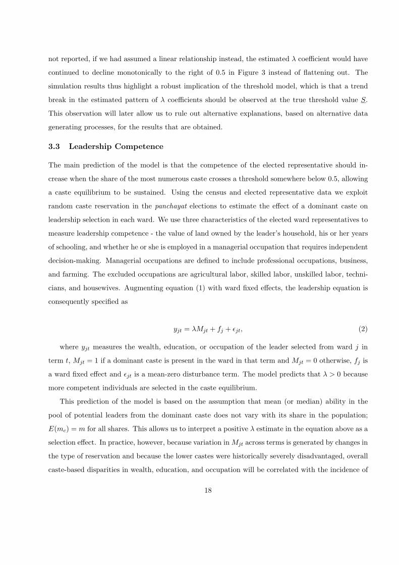
3.3 Leadership Competence

The main prediction of the model is that the competence of the elected representative should in-

crease when the share of the most numerous caste crosses a threshold somewhere below 0.5, allowing

a caste equilibrium to be sustained. Using the census and elected representative data we exploit

random caste reservation in the panchayat elections to estimate the effect of a dominant caste on

leadership selection in each ward. We use three characteristics of the elected ward representatives to

measure leadership competence - the value of land owned by the leader’s household, his or her years

of schooling, and whether he or she is employed in a managerial occupation that requires independent

decision-making. Managerial occupations are defined to include professional occupations, business,

and farming. The excluded occupations are agricultural labor, skilled labor, unskilled labor, techni-

cians, and housewives. Augmenting equation (1) with ward fixed effects, the leadership equation is

consequently specified as

yjt = λMjt + fj + εjt, (2)

where yjt measures the wealth, education, or occupation of the leader selected from ward j in

term t, Mjt = 1 if a dominant caste is present in the ward in that term and Mjt = 0 otherwise, fj is

a ward fixed effect and εjt is a mean-zero disturbance term. The model predicts that λ > 0 because

more competent individuals are selected in the caste equilibrium.

This prediction of the model is based on the assumption that mean (or median) ability in the

pool of potential leaders from the dominant caste does not vary with its share in the population;

E(mc) = m for all shares. This allows us to interpret a positive λ estimate in the equation above as a

selection effect. In practice, however, because variation in Mjt across terms is generated by changes in

the type of reservation and because the lower castes were historically severely disadvantaged, overall

caste-based disparities in wealth, education, and occupation will be correlated with the incidence of

18

a dominant caste. That is, even if leaders are randomly selected from eligible households there may

be variation in elected leader characteristics with Mjt solely because castes generally differ in wealth

or skills.

Panel A of Table 3 compares the characteristics of potential leaders for open, SC, ST, and OBC

elections as measured by the median characteristic of all households in each ward in each of these

reservation categories. The mean (with standard deviation in parentheses) of each median charac-

teristic is then computed across all wards. We see that there are substantial differences in median

household characteristics across reservation categories. For example, eligible households in open

elections have more land wealth, and heads of these households more education and experience as

decision-makers, compared with eligible households in restricted elections (particularly when they are

reserved for SC and ST candidates). This is because in open elections, unlike in the caste-restricted

elections, upper-caste households may also put up candidates.

The statistics in panel A suggest that the pool of potential leaders could vary substantially with

the type of caste reservation that is in place and this could account for variation in elected leader

characteristics with caste dominance even if there is no systematic leader selection. Note, however,

that the elected male leaders in Panel B are much more likely to have decision-making experience

and have substantially higher education than the (invariably male) representative household heads

in Panel A, within each caste reservation category. This suggests that there is systematic (non-

random) leader selection and rejects the hypothesis that the elected leader is always the median

voter, although variation in the pool of potential leaders across types of elections may still play a

role in determining leadership competence across terms within a ward. Moreover, notice that women

leaders are substantially disadvantaged with respect to decision-making experience and education in

Panel C. We will consequently include in equation (2) a full set of election reservation dummies – SC,

ST, OBC, and women – as well as measures of the distribution of characteristics among the potential

leaders in the ward in each term.18

Table 4 reports the estimates of the leadership equation with both the basic and the augmented

specification including measures of potential leaders’ characteristics. These estimates are based on

the assumption that 0.5 is the threshold share above which a caste equilibrium can be sustained. We

will display estimates of λ for the full range of assumed thresholds running from 0.25 to 0.75 below.18In addition, all the leadership regressions include a full set of term dummies as well as the election year, since

panchayat elections are not synchronized across the country.

19

The presence of a dominant caste, based on the assumed threshold of 0.5, has a large and significant

effect in Columns 1-2 on the land value of the elected representative - the elected leader’s land value

almost doubles when there is a dominant caste.19 The reservation dummies and the distribution

of potential leaders have little effect on the selected leader’s land value, and the dominant-caste

coefficient hardly changes from Column 1 to Column 2 when these additional controls are included.

The dependent variable in Columns 3-4 is a binary variable that takes the value one if the

leader is employed in a managerial occupation (farm operator, businessman, or professional) and zero

otherwise (technician, clerk, skilled or unskilled laborer, housewife). The presence of a dominant caste

has an insignificant effect on the occupation of the leader with the basic specification and actually

has the wrong sign, but a positive and statistically significant effect is obtained when we control for

the changing managerial experience of potential leaders across elections. This suggests strong within-

caste leadership selectivity. Although the distribution of potential leaders has little direct effect on

the selected leader’s characteristics once again, the female and SC dummies are now negative and

significant. With the appropriate controls included in Column 4, the presence of a dominant caste

has a large positive effect on whether the leader has managerial experience, increasing the probability

of a managerial occupation by 11 percentage points (a 16 percent increase above the mean for all

representatives).

The third leadership competence measure we use is the years of formal education of the elected

ward representative. The presence of a dominant caste, in both the basic and the augmented spec-

ification, has no effect on the leader’s education. Women and ST leaders have substantially lower

schooling than the reference category, unreserved men, and an increase in schooling for the median

potential leader has a significant effect on the selected leader’s education. The absence of an educa-

tion effect when a dominant caste is present in the ward suggests that education may not be strongly

associated with leadership competence. Indeed, this variable appears to have little power in predict-

ing competence across caste and gender lines, as we find below that elected women representatives

are actually more competent than men when there is a caste equilibrium despite having substantially

lower education.

The estimates in Table 4 are based on the assumption that the political regime switches when19The village inventory collected information over three election terms in each ward on the representative’s education

and occupation, but not the value of the land owned by his household. However, the census collected information onwhether the household had put forward a candidate in each of the last two elections. The value of landholdings isalso available for each household from the census. The regression in Columns 1-2 is thus estimated using data on allcandidates in each ward over the past two elections. Over half the elections had only one candidate.

20

the share of the most numerous caste crosses a threshold of 0.5. The theory, however, does not pin

down the precise location of the threshold. To verify the robustness of the results reported in Table

4, we experiment with alternative thresholds ranging from 0.25 to 0.75, for each of the leadership

characteristics using the augmented specification. We expect the pattern of estimated λ coefficients

to be similar to the simulated pattern for the threshold model in Figure 3.

Figures 4 and 5 report the dominant-caste (λ) coefficient estimates and their 95 percent con-

fidence intervals for land value and occupation.20 As predicted by the model, the dominant-caste

coefficient is positive and increasing for assumed thresholds below 0.5 in Figure 4 where leadership

competence is measured by land value. There is a weak trend-break in the point estimates as well

as the confidence band at 0.5, followed by a flattening out. Figure 5 with leadership competence

measured by managerial experience displays a similar pattern, with a steady increase in the estimated

λ coefficient at low thresholds followed by a trend-break around 0.6 and a subsequent flattening out.

Although the pattern of λ coefficients in Figures 4 and 5 broadly matches the pattern predicted

by the threshold model in Figure 3, leadership competence is only imperfectly measured by these

proxies for leadership experience and we will see a much sharper discontinuity, just around 0.5, when

competence is measured directly by actual public good provision in the ward.

3.4 Public Good Provision

In our framework, leadership competence maps directly into public good provision. Thus, we expect

the overall level of resources received by the ward to increase when the share of the most numerous

caste crosses a threshold just below 0.5, allowing a caste equilibrium to be sustained. The level of

public goods received by a ward in a given term will also depend on the political equilibria in other

wards, as well as the characteristics of the panchayat president. However, random reservation in

elections across wards and for the president’s position allows us to ignore the identity of other elected

representatives in the empirical analysis.21

According to the model the level and composition of public goods is also a function of the

characteristics of the pivotal voter. We consequently estimate the determinants of local public good

provision taking into account (median) voter preferences and leader competence with a specification20We do not show the figure for education. The dominant-caste coefficient was imprecisely estimated with education

as the dependent variable and an assumed threshold of 0.5 in Table 4. Small and statistically insignificant λ coefficientestimates are similarly obtained across the entire range of thresholds.

21Previous studies that focus on the role of the panchayat president have implicitly exploited the same randomnessto ignore the role played by ward representatives in their analyses.

21

of the form

Gkjt = (αk + δkXjt)(1 + θMjt) + hj + ξkjt (3)

where Gkjt measures the allocation of good k in ward j in term t, Xjt measures the characteristics

and, hence, the preferences of the pivotal household or individual in the ward-term, Mjt indicates

the presence of a dominant caste, and ξkjt is a mean-zero disturbance term.

When Mjt = 0, the pivotal household in the non-caste equilibrium is the median household in

the ward. When Mjt = 1 and the regime shifts to the caste equilibrium, the pivotal household

becomes the median household from the dominant caste in that ward-term. Note that the first term

in parentheses in equation (3) thus characterizes the (linear) demand for different types of public

goods, with the δk parameter identified off changes in the pivotal household within the ward over

time. The second term in parentheses reflects the ability of the leader to raise the overall level of

public goods received in the ward. Net of the ward fixed effects, hj , the competence parameter θ and

the demand parameters αk, δk can be estimated using nonlinear least squares.

The main prediction of the model is that θ > 0, reflecting the selection of more competent

individuals in the caste equilibrium. Because variation in Mjt within a ward is generated by changes

in caste reservation across terms, an alternative explanation for a positive θ estimate is that Mjt = 0

is disproportionately associated with less competent lower-caste leaders. We dealt with the same

concern in the leadership regression and our solution to the problem was to include a full set of

reservation dummies. Because Mjt enters multiplicatively in equation (3) above, the corresponding

augmented specification allows competence to vary by the type of reservation:

Gkjt =R∑

r=1

[w1r(αk + δkXjt) + w2rθMjt(αi + δkXjt)] + hj + ξkjt, (4)

where w1r, w2r estimate the effect of reservation, separately in the non-caste and caste equilibrium,

on overall resources. The reservation categories include SC, ST, OBC, and women, with unreserved

men occupying the reference category.

Gkjt is measured as the fraction of households in the ward who received a particular good k in

a given panchayat term, where public good provision is defined to include both new construction

and maintenance. The fraction of households in a ward in each term that benefited from a specific

public good was constructed by matching the locations of households and goods, based on the street

22

location of each public goods investment and the street addresses of the households. Our analysis

focuses on six goods for which the benefits have a significant local and spatial component; that is,

goods for which attachment or proximity to the household is desirable. The goods are: drinking

water, sanitation, improved roads, electricity, street lights, and public telephones.22 These six goods

account for 15.2 percent of all local public spending, which is four times the amount spent on schools

and health facilities.23

Table 5 reports the fraction of households in the ward that received each public good, averaged

across wards and panchayat terms, by type of election. Evidently, a large fraction of households

benefited directly from expenditures on water, roads, and sanitation, while a much smaller fraction

benefited in any term from expenditures on electricity, street lights, and public telephones. Notice,

in contrast with the leadership characteristics in Table 3, that public good provision does not appear

to vary systematically across castes, or between open and reserved elections in Table 5.

Table 6 reports the estimates of the public goods delivery equation, with the public goods demand

parameters reported in Table 6(a) and the competence parameters in Table 6(b). These estimates are

based on the assumption that 0.5 is the threshold above which a caste equilibrium can be sustained.

The first three columns of each table report estimates from the basic specification, measuring the

pivotal voter’s characteristics sequentially by owned land value, occupation, and education. The next

three columns of each table report estimates from the augmented specification allowing competence

to vary by gender and caste, with the same sequence of median voter characteristics.

The public good demand estimates in Table 6(a) are precisely estimated, with the intercepts αk

matching the pattern of public good provision in Table 5. Recall that a relatively large fraction of

households benefited from expenditures on water, sanitation, and roads in each ward-term. Public

telephones are the reference category in Table 6(a), and we see that the drinking water, sanitation,

and roads intercepts are relatively large in magnitude and very precisely estimated.

The estimates also indicate, consistent with our model, that the characteristics of the pivotal

household have a significant effect on the allocation of public goods in the ward. Relative to public22Public irrigation investments or school buildings, for example, are valued local public goods whose placement close

to a ward resident, or even within the ward (defined by place of residence) may not be desirable.23Key informants in the village were asked to rank 12 issues, by importance, that came under the purview of the

elected panchayat. Inadequate roads and drinking water were ranked 1 and 2, followed by health, schooling, sanitation,street lights and electrification. Note that the low spending on health and education and the relatively low level ofimportance assigned to these goods by the key informants reflects the fact that they are largely allocated at the statelevel and so fall outside the purview of the village panchayat.

23

telephone investment (the reference category), an increase in the value of the pivotal individual’s

landholdings increases the allocation of resources to roads and reduces the allocation to electricity.

When the pivotal individual (household head) is employed in a managerial occupation, we see a

relative increase in the resources allocated to electricity and street lights. The education of the pivotal

individual, in contrast, does not significantly affect the allocation to any single good. Nevertheless,

we can reject the joint hypothesis that the pivotal characteristic has no effect on the distribution of

public goods with 95 percent confidence for land value, occupation, and education.

The results in Table 6(a) indicate that elected ward representatives are responsive to the prefer-

ences of the pivotal individuals in their constituencies. The estimates, reported in table 6(b), also

indicate that leaders are more competent when there is a caste equilibrium. The competence param-

eter θ in Table 6(b) is positive and significant across both specifications and for all measures of the

pivotal voter’s characteristics, ranging in magnitude from 0.13 to 0.20. The presence of a dominant

caste in the ward thus appears to increase the overall level of local public resources the ward receives,

with respect to this set of local public goods, by about 16 percent.

The augmented specification in Columns 4-6 allows competence to vary by caste and gender.

Although some of the caste coefficients are individually significant, we cannot reject the hypothesis

that all the caste coefficients, uninteracted and interacted with θ as in equation (4), are jointly

zero. While a woman leader in the non-caste equilibrium is statistically indistinguishable from the

reference category (unreserved men), it is interesting to note that elected women are more competent

than elected male representatives when there is a caste equilibrium (when competence is more likely

to matter for election outcomes). Female representatives raise the overall level of resources by 10

percent compared to men who are elected in the same equilibrium.

We complete the analysis of leadership competence by estimating θ for different thresholds above

which a dominant caste is assumed to emerge. Because θ corresponds to λ in the leadership regression,

we expect the same pattern of θ coefficients across the range of assumed thresholds as in Figure 3.

Figure 6 reports the pattern of estimated θ’s and the accompanying 95 percent confidence bands, for

thresholds over the 0.25-0.75 range in 0.05 increments, using land value as the pivotal characteristic.

As in Figure 3, the estimated θ coefficient is increasing steeply at thresholds below 0.5 and then

subsequently increases at a slower rate, although a trend-break around that critical threshold is not

visually discernable. Figures 7 and 8 repeat this exercise with occupation and education, respectively,

as the pivotal characteristics. Once again we see a steep increase in the estimated θ coefficient at

24

thresholds below 0.5. However, there is now a sharp trend-break at 0.5 in both figures, followed by

a short decline and then a flattening out, precisely matching the predictions of the threshold model.

Ward fixed effects control for cross-sectional heterogeneity in population characteristics that could

independently determine public good delivery, net of leadership selection. The caste reservation

dummies control, in addition, for the possibility that the pool of potential leaders is weaker in reserved

(lower caste) elections where a caste equilibrium is mechanically less likely to be obtained. Suppose,

however, that the most competent individuals within each caste tend to cluster together in a relatively

small number of wards, while less competent individuals are spatially dispersed. The positive effect of

a dominant caste on public good provision could then simply reflect the fact that the most competent

members within each caste tend to be located in wards where they are disproportionately likely to

be politically dominant.

To rule out this unlikely possibility, we take advantage of the particular pattern of dominant-caste

coefficients implied by the threshold model of leadership selection in Figure 3. As noted, this pattern

matches reasonably well with the empirical results reported in Figures 6-8. Even if there was a

positive relationship between the share of the most numerous caste in the ward and the competence

of the pool of potential leaders, there is no reason why this relationship would display a discontinuity

just around 0.5. If the relationship were smooth and monotonically increasing instead, the pattern

of estimated dominant-caste coefficients would match with the predictions of the concave or convex

models in Figure 3, which are qualitatively quite different from the patterns in Figures 6-8.24

A final alternative explanation combines the preceding hypothesis of spatial heterogeneity within

castes with identity politics in which individuals vote mechanically on caste lines. This explanation

would also generate the patterns in Figures 6-8, with the most numerous caste in a ward-term

coming to power when its share exceeded 0.5, while being endowed at the same time with a superior

pool of potential leaders. What distinguishes our model of leadership selection from this alternative

explanation based on a superior pool of candidates is that the caste community overcomes the

leadership commitment problem, and this is what we turn to next.24Although not reported in Figure 3, if leadership competence were a linear function of the share of the most numerous

caste, the estimated dominant-caste coefficients would be approximately constant across the entire range of assumedthresholds. This is once again qualitatively quite different from the patterns reported in Figures 6-8.

25

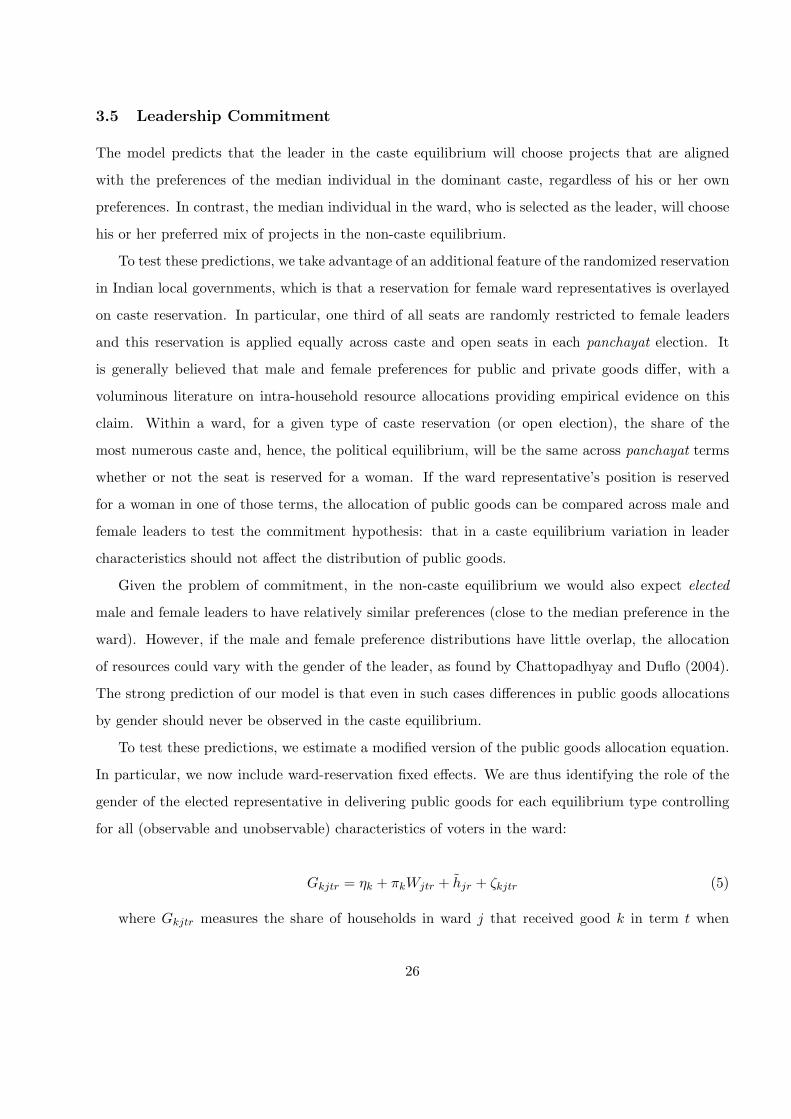
3.5 Leadership Commitment

The model predicts that the leader in the caste equilibrium will choose projects that are aligned

with the preferences of the median individual in the dominant caste, regardless of his or her own

preferences. In contrast, the median individual in the ward, who is selected as the leader, will choose

his or her preferred mix of projects in the non-caste equilibrium.

To test these predictions, we take advantage of an additional feature of the randomized reservation

in Indian local governments, which is that a reservation for female ward representatives is overlayed

on caste reservation. In particular, one third of all seats are randomly restricted to female leaders

and this reservation is applied equally across caste and open seats in each panchayat election. It

is generally believed that male and female preferences for public and private goods differ, with a

voluminous literature on intra-household resource allocations providing empirical evidence on this

claim. Within a ward, for a given type of caste reservation (or open election), the share of the

most numerous caste and, hence, the political equilibrium, will be the same across panchayat terms

whether or not the seat is reserved for a woman. If the ward representative’s position is reserved

for a woman in one of those terms, the allocation of public goods can be compared across male and

female leaders to test the commitment hypothesis: that in a caste equilibrium variation in leader

characteristics should not affect the distribution of public goods.

Given the problem of commitment, in the non-caste equilibrium we would also expect elected

male and female leaders to have relatively similar preferences (close to the median preference in the

ward). However, if the male and female preference distributions have little overlap, the allocation

of resources could vary with the gender of the leader, as found by Chattopadhyay and Duflo (2004).

The strong prediction of our model is that even in such cases differences in public goods allocations

by gender should never be observed in the caste equilibrium.

To test these predictions, we estimate a modified version of the public goods allocation equation.

In particular, we now include ward-reservation fixed effects. We are thus identifying the role of the

gender of the elected representative in delivering public goods for each equilibrium type controlling

for all (observable and unobservable) characteristics of voters in the ward:

Gkjtr = ηk + πkWjtr + h̃jr + ζkjtr (5)

where Gkjtr measures the share of households in ward j that received good k in term t when

26

reservation r was in place. Wjtr is a binary variable that takes the value one if the position was

reserved for a female leader in that ward-term, h̃jr is a ward-reservation fixed effect, and ζkjtr is a

mean-zero disturbance term. The reservation categories are SC, ST, OBC, and Open. The regression

is estimated separately for Mjt = 0 and Mjt = 1, and the prediction is that πk should be zero for all

public goods k when Mjt = 1. The female coefficient could be significant when Mjt = 0 if the male

and female preference distributions are sufficiently far apart, as discussed above.

Table 7 reports the estimates of equation (5) with ward-reservation fixed effects, separately for

Mjt = 0 and Mjt = 1. We consider three thresholds above which a dominant caste is assumed

to be present: 0.3, 0.4, 0.5. In the non-caste equilibrium (Mjt = 0), the woman representative

coefficient is always positive and significant for street lights, increasing the share of households that

receive that good by 0.07-0.09 relative to the reference good (public telephone). The woman-leader

coefficient is also positive and significant for electricity and the coefficients are jointly significant for

all public goods with the threshold set at 0.3, although the precision of the estimates declines at

higher thresholds. In contrast to the estimates for the non-caste equilibrium, the elected woman-

representative coefficient is never significant in the caste equilibrium (Mjt = 1) for any public good

or jointly for all public goods.25 Thus, while the presence of a female leader does appear to change

the mix of goods (the allocations are relative to the reference good) in the non-caste equilibrium, we

cannot reject the hypothesis of leadership commitment in the caste equilibrium.

4 Conclusion

In this paper we explore whether the involvement of communities in the political sphere always

worsens governance. In particular, complementary to the new literature on the role of community

networks in solving market problems, we test the hypothesis that strong traditional social institutions

can discipline the leaders they put forward, successfully substituting for secular political institutions

when they are ineffective. We do this by examining the interaction between an Indian institution

that is hundreds of years old – the caste system – with a new set of political institutions – local

democracy. Using detailed data on local public goods at the street level and Indian local governments25We cannot reject the hypothesis that all the female coefficients are zero with thresholds set at 0.4 and 0.5 in the

non-caste equilibrium as well. Notice, however, that the p-values for the test range from 0.5 to 0.8 for Mjt = 1 butare much lower, ranging from 0.02 to 0.15 for Mjt = 0. Our inability to reject the null hypothesis in the non-casteequilibrium for all thresholds might simply be a consequence of the low power of the statistical test. Note again thatwe are only identified off variation in the gender of the leader within wards and reservation categories.

27

at the ward level over multiple terms, we find that the presence of a numerically dominant sub-caste

(caste equilibrium) is associated with the selection of leaders with superior observed characteristics

and greater public goods provision. This improvement in leadership competence occurs without

apparently diminishing leaders’ responsiveness to their constituency.

Although these results suggest that parochial politics does not necessarily imply bad governance,

they need to be placed in the appropriate perspective. Although the sub-caste may be able to control

the leaders it nominates at the ward level, it will have less influence at higher levels of government

where a single sub-caste is rarely dominant. The negative effect of caste-identity politics on leadership

selection and outcomes has been documented at the state level in India and similar negative outcomes

have been associated with parochial politics in other parts of the world. Moreover, the leader in a

caste equilibrium is answerable to the social group she belongs to and so her choices will be aligned

with the preferences of the median voter in the dominant caste rather than the median voter in the

constituency. The welfare consequences of a caste equilibrium are thus ambiguous. Caste politics

is a second-best solution and, ultimately, there is no perfect substitute for well functioning political

institutions (parties) in a competitive democratic system.

Finally, our results shed new light on the efficiency consequences of political reservation in India.

Randomly-assigned caste reservation mechanically increases the commitment problem by inducing

exogenous turnover in the leadership. Reservation also reduces the likelihood that a numerically

dominant caste will emerge in any constituency, exacerbating the commitment problem. The obvious

equity advantage of any reservation system is that it favors historically-disadvantaged groups. The

multiple sources of inefficiency that we identify in this paper, however, suggest that a more systematic

appraisal of the costs and the benefits of political reservation in India may be warranted. One notable

exception to this qualified assessment of the reservation system is quotas for women. This particular

reservation scheme does not adversely affect the probability that a caste equilibrium will emerge and

we find that women leaders are significantly more competent than men in that equilibrium.

28

References

[1] Alesina, Alberto and Stephen E. Spear. 1988. “An Overlapping Generations Model of Electoral

Competition,” Journal of Public Economics 37: 359-379.

[2] Banerjee, Abhijit and Kaivan Munshi. 2004. How Efficiently is Capital Allocated? Evidence

from the Knitted Garment Industry in Tirupur, Review of Economic Studies 71(1):19-42.

[3] Banerjee, Abhijit and Rohini Pande. 2007. “Parochial Politics: Ethnic Preferences and Politician

Corruption,” Harvard University, Kennedy School of Government, typescript.

[4] Bardhan, Pranab, Dilip Mookherjee, and Monica Parra Torrado. 2005. “Impact of Reservations

of Panchayat Pradhans on Targeting in West Bengal,” University of California at Berkeley,

department of economics, typescript.

[5] Bardhan, Pranab and Dilip Mookherjee. 2006. “Pro-poor targeting and accountability of local

governments in West Bengal,” Journal of Development Economics 79: 303-327.

[6] Beaman, Lori, Raghabendra Chattopadhyay, Esther Duflo, Rohini Pande, and Petia Topalova.

2008. “Powerful Women: Does Exposure Reduce Prejudice?” MIT department of economics,

typescript.

[7] Besley, Timothy and Stephen Coate. 1997. “An Economic Model of Representative Democracy,”

Quarterly Journal of Economics 112(1): 85-114.

[8] Besley, Timothy, Rohini Pande, Lupin Rahman, and Vijayendra Rao. 2004. “The Politics of

Public Good Provision: Evidence from Indian Local Governments,” Journal of the European

Economic Association 2(2-3): 416-426.

[9] Besley, Timothy, Rohini Pande, and Vijayendra Rao. 2007. “Just Rewards? Local Politics and

Public Resource Allocation in South India,” Harvard University, Kennedy School of Government,

typescript.

[10] Caillaud, Bernard and Jean Tirole. 2002. “Parties as Political Intermediaries,” Quarterly Journal

of Economics 117(4): 1453-1489.

[11] Caselli, Francesco and Massimo Morelli. 2004. “Bad politicians,” Journal of Public Economics

88: 759-782.

29

[12] Chattopadhyay, Raghabendra and Esther Duflo. 2004. “Women as Policy Makers: Evidence

from a Randomized Policy Experiment in India,” Econometrica 72(5): 1409-1443.

[13] Chhibber, Pradeep K. 1999. Democracy without Associations: Transformation of the Party

System and Social Cleavages in India. Ann Arbor: University of Michigan Press.

[14] Downs, Anthony. 1957. An Economic Theory of Democracy. New York, NY: Harper and Row.

[15] Duflo, Esther, Greg Fischer, and Raghabendra Chattopadhyay. 2005. “Efficiency and rent seek-

ing in local government: Evidence from randomized policy experiments in India,” MIT depart-

ment of economics, typescript.

[16] Ferraz, Claudio and Frederico Finan. 2008. “Motivating Politicians: The Impacts of Monetary

Incentives on Quality and Performance,” UCLA department of economics, typescript.

[17] Harrington, Jr., Joseph E. 1992. “The role of party reputation in the formation of policy,”

Journal of Public Economics 49: 107-121.

[18] Levitt, Steven D. 1996. “How do Senators Vote? Disentangling the Role of Voter Preferences,

Party Affiliation and Senate Ideology,” American Economic Review 86(3): 425-441.

[19] List, John and Daniel Sturm. 2006. “How Elections Matter: Theory and Evidence from Envi-

ronmental Policy,” Quarterly Journal of Economics 121(4): 1249-1281.

[20] Messner, Matthias and Mattias Polborn. 2004. “Paying Politicians,” Journal of Public Eco-

nomics 88 : 2423-2445.

[21] Miguel, Edward and Mary Kay Gugerty. 2005. “Ethnic Diversity, Social Sanctions, and Public

Goods in Kenya,” Journal of Public Economics 89: 2325-2368.

[22] Munshi, Kaivan and Mark Rosenzweig. 2005. Why is Mobility in India so Low? Social Insurance,

Inequality and Growth, BREAD Working Paper No. 092.

[23] Munshi, Kaivan and Mark Rosenzweig. 2006. Traditional Institutions Meet the Modern World:

Caste, Gender and Schooling Choice in a Globalizing Economy, American Economic Review,

96(4):1225-1252.

30

[24] Osborne, Martin and Al Slivinski. 1996. “A Model of Political Competition with Citizen-

Candidates,” Quarterly Journal of Economics 111(1): 65-96.

[25] Padro i Miquel, Gerard. 2007. “The Control of Politicians in Divided Societies: The Politics of

Fear,” Review of Economic Studies 74: 1259-1274.

[26] Pande, Rohini. 2003. “Can Mandated Political Representation Increase Policy Influence for

Disadvantaged Minorities? Theory and Evidence from India,” American Economic Review 93(4):

1132-1151.

[27] Posner, Daniel N. 2005. Institutions and Ethnic Politics in Africa. Cambridge, MA: Cambridge

University Press.

[28] Snyder, Jr., James M. and Michael M. Ting. 2002. “An Informational Rationale for Political

Parties,” American Journal of Political Science 46(1): 90-110.

31

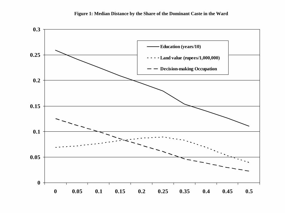
Figure 1: Median Distance by the Share of the Dominant Caste in the Ward

0

0.05

0.1

0.15

0.2

0.25

0.3

0 0.05 0.1 0.15 0.2 0.25 0.35 0.4 0.45 0.5

Education (years/10)

Land value (rupees/1,000,000)

Decision-making Occupation

Figure 2: Alternative Competence-Share Relationships

0

0.05

0.1

0.15

0.2

0.25

0.3

0.35

0.4

0.45

0.25 0.3 0.35 0.4 0.45 0.5 0.55 0.6 0.65 0.7 0.75

Threshold

Concave

Convex

Figure 3: Estimated Dominant Caste Coefficients for Alternative Thresholds Using Simulated Data

0.12

0.14

0.16

0.18

0.2

0.22

0.24

0.26

0.28

0.3

0.25 0.3 0.35 0.4 0.45 0.5 0.55 0.6 0.65 0.7 0.75

Convex Concave Threshold

-100

-50

0

50

100

150

200

250

300

350

0.25 0.3 0.35 0.4 0.45 0.5 0.55 0.6 0.65 0.7 0.75

Figure 4: Estimated Effect , with 95% Confidence Bounds, of a Dominant Caste onthe Landholding Value (1,000’s rupees) of the Ward Representative,

By Share Threshold

-0.1

-0.05

0

0.05

0.1

0.15

0.2

0.25

0.3

0.35

0.25 0.3 0.35 0.4 0.45 0.5 0.55 0.6 0.65 0.7 0.75

Figure 5: Estimated Effect, with 95% Confidence Bounds,of a Dominant Caste on Whether the Ward Representative is a Decision-Maker,

By Share Threshold

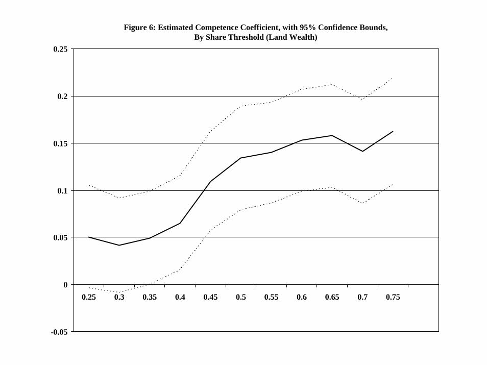
-0.05

0

0.05

0.1

0.15

0.2

0.25

0.25 0.3 0.35 0.4 0.45 0.5 0.55 0.6 0.65 0.7 0.75

Figure 6: Estimated Competence Coefficient, with 95% Confidence Bounds,By Share Threshold (Land Wealth)

-0.05

0

0.05

0.1

0.15

0.2

0.25

0.25 0.3 0.35 0.4 0.45 0.5 0.55 0.6 0.65 0.7 0.75

Figure 7: Estimated Competence Coefficient, with 95% Confidence Bounds,By Share Threshold (Occupation)

-0.05

0

0.05

0.1

0.15

0.2

0.25

0.25 0.3 0.35 0.4 0.45 0.5 0.55 0.6 0.65 0.7 0.75

Figure 8: Estimated Competence Coefficient, with 95% Confidence Bounds,By Share Threshold (Education)

Table 1: Sources of Support for Ward Leaders

Source of support: within village outside village(1) (2)

From caste 82 29

From religion 28 13

From wealthy individuals 38 --

From a political party -- 41

Note: The statistics are computed over the last three local governments in each ward.Each statistic reflects the percent of leaders who received support from a given source.

Table 2: Share of the Most Numerous Eligible Caste in the Ward

Type of election: Open SC ST OBC(1) (2) (3) (4)

Panel A: Distribution of shares

25 percentile 0.42 0.14 0.16 0.20

50 percentile 0.60 0.33 0.57 0.41

75 percentile 0.85 0.65 0.95 0.69

Panel B: Fraction of wards with a dominant caste

Threshold for dominance:

0.3 0.92 0.52 0.67 0.63

0.4 0.79 0.46 0.61 0.53

0.5 0.67 0.37 0.52 0.44

Total number of observations 1,973 373 187 769

Note: a caste is defined to be dominant if its share of the population in the ward exceeds the threshold.SC=scheduled caste, ST=scheduled tribe, OBC=other backward caste.Information on reservation and election outcomes is obtained for three terms in each ward.

Table 3: Pivotal Voter and Leader Characteristics

Election type: Unreserved SC ST OBC(1) (2) (3) (4)

Panel A: Median individuals

Land value 94.80 47.35 63.35 94.76(173.19) (105.85) (182.02) (157.49)

Decision-making occupation 0.36 0.18 0.33 0.39(0.47) (0.37) (0.46) (0.49)

Education 4.46 3.53 3.30 4.03(3.76) (3.59) (3.65) (3.36)

Panel B: Male leaders

Land value 99.55 81.50 58.36 83.21(23.69) (20.16) (19.91) (15.23)

Decision-making occupation 0.80 0.44 0.72 0.76(0.40) (0.50) (0.45) (0.43)

Education 7.42 6.01 5.30 7.05(4.43) (4.49) (3.99) (4.30)

Panel C: Female leaders

Land value 95.61 43.01 31.50 62.44(30.23) (10.10) (40.86) (91.83)

Decision-making occupation 0.17 0.29 0.33 0.57(0.38) (0.46) (0.49) (0.50)

Education 3.23 5.78 2.22 4.72(3.83) (4.39) (2.05) (4.17)

Note: all characteristics in Panel A are measured as the median value in the ward for the relevant caste category.The means (standard deviations) of these characteristics across all wards are reported in the table.Leaders' occupation and education is obtained for last three terms in each ward.Information on land value is based on all candidates in the ward over the last two terms. .Information on the landholdings of elected representatives was not collectedLand value is measured in thousands of Rupees. Decision-making occupation is a binary variable.This variable takes the value one for professional occupations, business and farming and zero for agricultural labor, skilled labor, unskilled labor, technicians, and housewife.Education is measured as years of schooling.SC=scheduled caste, ST=scheduled tribe, OBC=other backward caste.

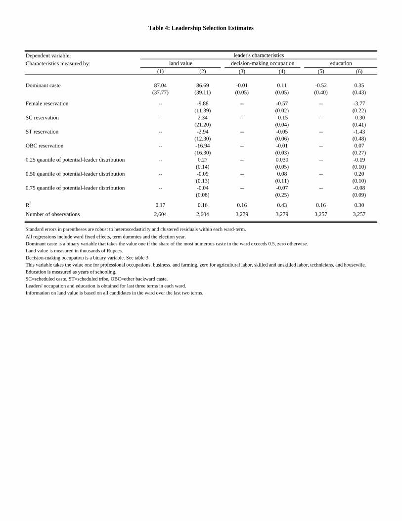
Table 4: Leadership Selection Estimates

Dependent variable: leader's characteristicsCharacteristics measured by: land value decision-making occupation education

(1) (2) (3) (4) (5) (6)

Dominant caste 87.04 86.69 -0.01 0.11 -0.52 0.35(37.77) (39.11) (0.05) (0.05) (0.40) (0.43)

Female reservation -- -9.88 -- -0.57 -- -3.77(11.39) (0.02) (0.22)

SC reservation -- 2.34 -- -0.15 -- -0.30(21.20) (0.04) (0.41)

ST reservation -- -2.94 -- -0.05 -- -1.43(12.30) (0.06) (0.48)

OBC reservation -- -16.94 -- -0.01 -- 0.07(16.30) (0.03) (0.27)

0.25 quantile of potential-leader distribution -- 0.27 -- 0.030 -- -0.19(0.14) (0.05) (0.10)

0.50 quantile of potential-leader distribution -- -0.09 -- 0.08 -- 0.20(0.13) (0.11) (0.10)

0.75 quantile of potential-leader distribution -- -0.04 -- -0.07 -- -0.08(0.08) (0.25) (0.09)

R2 0.17 0.16 0.16 0.43 0.16 0.30Number of observations 2,604 2,604 3,279 3,279 3,257 3,257

Standard errors in parentheses are robust to heteroscedasticity and clustered residuals within each ward-term.All regressions include ward fixed effects, term dummies and the election year.Dominant caste is a binary variable that takes the value one if the share of the most numerous caste in the ward exceeds 0.5, zero otherwise.Land value is measured in thousands of Rupees.Decision-making occupation is a binary variable. See table 3.This variable takes the value one for professional occupations, business, and farming, zero for agricultural labor, skilled and unskilled labor, technicians, and housewife.Education is measured as years of schooling.SC=scheduled caste, ST=scheduled tribe, OBC=other backward caste.Leaders' occupation and education is obtained for last three terms in each ward.Information on land value is based on all candidates in the ward over the last two terms.

Table 5: Fraction of Households in the Ward Receiving Public Goods in each Term

Type of election: Open SC ST OBC(1) (2) (3) (4)

water 0.69 0.73 0.78 0.72(0.40) (0.39) (0.71) (0.39)

sanitation 0.42 0.42 0.55 0.42(0.46) (0.46) (0.47) (0.46)

roads 0.69 0.72 0.74 0.73(0.41) (0.40) (0.41) (0.39)

telephones 0.07 0.12 0.08 0.10(0.24) (0.30) (0.25) (0.28)

electricity 0.14 0.20 0.17 0.20(0.34) (0.38) (0.36) (0.38)

street lighting 0.16 0.19 0.19 0.22(0.36) (0.38) (0.39) (0.40)

Number of observations 1,704 373 176 619

Note: means and standard deviations (in parentheses).SC=scheduled caste, ST=scheduled tribe, OBC=other backward caste.Statistics are based on the last three terms in each ward.

Table 6(a): Public Goods Demand Parameters

Dependent variable: public good provisionSpecification: no reservation interactions reservation interactions

Pivotal characteristic: land value managerial occupation education land value managerial

occupation education

(1) (2) (3) (4) (5) (6)

Water intercept 0.57 0.58 0.55 0.54 0.54 0.51(0.02) (0.04) (0.02) (0.02) (0.04) (0.03)

Sanitation intercept 0.31 0.34 0.31 0.29 0.32 0.28(0.02) (0.04) (0.02) (0.02) (0.04) (0.02)

Roads intercept 0.54 0.57 0.56 0.51 0.53 0.53(0.02) (0.04) (0.02) (0.02) (0.04) (0.03)

Electricity intercept 0.09 -0.03 0.08 0.08 -0.03 0.07(0.01) (0.03) (0.01) (0.01) (0.03) (0.01)

Street lights intercept 0.09 -0.03 0.09 0.08 -0.03 0.08(0.01) (0.03) (0.01) (0.01) (0.03) (0.01)

Pivotal char. - water 5.76 -0.02 2.82 5.57 -0.02 3.67(4.43) (0.04) (3.31) (4.26) (0.04) (3.20)

Pivotal char. - sanitation 2.20 -0.04 -1.05 2.07 -0.04 -0.24(4.85) (0.04) (3.49) (4.58) (0.04) (3.33)

Pivotal char. - roads 24.50 -0.005 -1.22 23.60 -0.004 -0.01(5.47) (0.04) (3.55) (5.22) (0.04) (3.40)

Pivotal char. - electricity -17.70 0.10 -4.44 -16.50 0.09 -3.64(3.21) (0.03) (2.62) (3.04) (0.03) (2.49)

Pivotal char. - street lights -6.44 0.12 -3.19 -5.87 0.11 -2.37(3.50) (0.03) (2.65) (3.28) (0.03) (2.51)

all pivotal char.-goods=0 (Fstatistic) 17.00

-10.68 2.32 14.62 12.99 2.49

(p value) 0.00 0.00 0.04 0.00 0.00 0.03

Standard errors in parentheses are robust to heteroscedasticity and clustered residuals within each ward-term.

The dependent variable is computed as the fraction of households in the ward who received a given public good in a given term. Public telephone is the excluded local public good.The pivotal characteristic is the median in the ward (dominant caste) when a dominant caste is absent (present).Land value is measured in thousands of Rupees. Coefficients on land value-goods in Columns 1 and 4 must be divided by 10 5.Managerial occupation takes the value one for professional occupations, business, and farming, zero for agricultural labor, skilled labor, unskilled labor, technician, and housewife.Education is measured as years of schooling. Coefficient on education-goods in Columns 3 and 6 must be divided by 10 3.All regressions include ward fixed effects, term dummies and the election year.Competence parameters are reported in Table 6(b).

Table 6(b): Leadership Competence Parameters

Dependent variable: public good provisionSpecification: no reservation interactions reservation interactions

Pivotal characteristic: land value managerial occupation education land value managerial

occupation education

(1) (2) (3) (4) (5) (6)

Theta 0.13 0.16 0.17 0.15 0.20 0.19(0.03) (0.03) (0.03) (0.05) (0.05) (0.05)

SC -- -- -- 0.08 0.12 0.12(0.05) (0.05) (0.05)

ST -- -- -- 0.09 0.11 0.13(0.07) (0.08) (0.08)

OBC -- -- -- 0.09 0.09 0.08(0.05) (0.05) (0.05)

Woman -- -- -- -0.02 -0.001 -0.02(0.04) (0.04) (0.04)

SC x Theta -- -- -- -0.02 -0.09 -0.04(0.08) (0.08) (0.08)

ST x Theta -- -- -- 0.09 0.04 0.02(0.10) (0.10) (0.10)

OBC x Theta -- -- -- -0.05 -0.05 -0.04(0.06) (0.06) (0.06)

Woman x Theta -- -- -- 0.10 0.08 0.10(0.05) (0.05) (0.05)

all caste dummies=0(F-statistic) -- -- -- 0.79 1.57 1.93

(p value) 0.50 0.19 0.12

all caste dummies-dominant caste=0

(F-statistic) -- -- -- 0.53 0.23 0.38(p value) 0.66 0.88 0.77

R2 0.37 0.36 0.36 0.37 0.36 0.36

Number of observations 14,270 14,215 14,255 14,270 14,215 14,255

Standard errors in parentheses are robust to heteroscedasticity and clustered residuals within each ward-term.The dependent variable is computed as the share of the households in the ward who received a given good in a given term: clean water(1), sanitation(2), improved roads(3), electricity(4), street lights(5). Public telephone is the excluded category.The pivotal characteristic is the median in the ward (dominant caste) when a dominant caste is absent (present).Land value is measured in thousands of Rupees.Managerial occupation takes the value one for professional occupations, business, and farming, zero for agricultural labor, unskilled labor, skilled labor, technician, and housewife.Education is measured as years of schooling. Reservation categories are SC, ST, OBC, and woman.All regressions include ward fixed effects, term dummies and the election year.

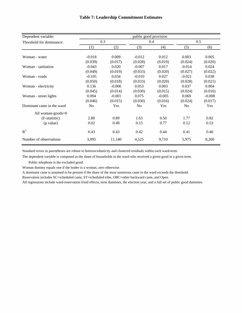
Table 7: Leadership Commitment Estimates

Dependent variable: public good provisionThreshold for dominance: 0.3 0.4 0.5

(1) (2) (3) (4) (5) (6)

Woman - water -0.018 0.009 -0.012 0.012 0.003 0.005(0.039) (0.017) (0.028) (0.019) (0.024) (0.020)

Woman - sanitation -0.043 0.020 -0.007 0.017 -0.014 0.024(0.049) (0.019) (0.033) (0.020) (0.027) (0.022)

Woman - roads -0.105 0.034 -0.010 0.027 -0.021 0.038(0.050) (0.018) (0.033) (0.020) (0.028) (0.021)

Woman - electricity 0.136 -0.006 0.053 0.003 0.037 0.004(0.045) (0.014) (0.030) (0.015) (0.024) (0.016)

Woman - street lights 0.094 -0.001 0.075 -0.005 0.069 -0.008(0.046) (0.015) (0.030) (0.016) (0.024) (0.017)

Dominant caste in the ward No Yes No Yes No Yes

All woman-goods=0(F-statistic) 2.80 0.89 1.63 0.50 1.77 0.82

(p value) 0.02 0.49 0.15 0.77 0.12 0.53

R2 0.43 0.43 0.42 0.44 0.41 0.46

Number of observations 3,095 11,140 4,525 9,710 5,975 8,260

Standard errors in parentheses are robust to heteroscedasticity and clustered residuals within each ward-term.The dependent variable is computed as the share of households in the ward who received a given good in a given term. Public telephone is the excluded good.Woman dummy equals one if the leader is a woman, zero otherwise.A dominant caste is assumed to be present if the share of the most numerous caste in the ward exceeds the threshold.Reservation includes SC=scheduled caste, ST=scheduled tribe, OBC=other backward caste, and Open.All regressions include ward-reservation fixed effects, term dummies, the election year, and a full set of public good dummies.