The ELM Survey South. I. An Effective Search for Extremely Low Mass White Dwarfs

Alekzander Kosakowski1 , Mukremin Kilic1 , Warren R. Brown2 , and Alexandros Gianninas31 Homer L. Dodge Department of Physics and Astronomy, University of Oklahoma, 440 W. Brooks St., Norman, OK 73019, USA

2 Smithsonian Astrophysical Observatory, 60 Garden St., Cambridge, MA 02138, USA3 Department of Physics and Astronomy, Amherst College, 25 East Dr., Amherst, MA 01002, USA

Received 2019 November 4; revised 2020 March 20; accepted 2020 March 23; published 2020 May 5

Abstract

We begin the search for extremely low mass (M� 0.3Me, ELM) white dwarfs (WDs) in the southern sky based onphotometry from the VST ATLAS and SkyMapper surveys. We use a similar color selection method as theHypervelocity star survey. We switched to an astrometric selection once Gaia Data Release 2 became available.We use the previously known sample of ELM white dwarfs to demonstrate that these objects occupy a uniqueparameter space in parallax and magnitude. We use the SOAR 4.1 m telescope to test the Gaia-based selection, andidentify more than two dozen low mass white dwarfs, including six new ELM white dwarf binaries with periods asshort as 2 h. The better efficiency of the Gaia-based selection enables us to extend the ELM Survey footprint to thesouthern sky. We confirm one of our candidates, J0500−0930, to be the brightest (G= 12.6 mag) and closest(d= 72 pc) ELM white dwarf binary currently known. Remarkably, the Transiting Exoplanet Survey Satellite(TESS) full-frame imaging data on this system reveals low-level (<0.1%) but significant variability at the orbitalperiod of this system (P= 9.5 hr), likely from the relativistic beaming effect. TESS data on another system, J0642−5605, reveals ellipsoidal variations due to a tidally distorted ELM WD. These demonstrate the power of TESSfull-frame images in confirming the orbital periods of relatively bright compact object binaries.

Unified Astronomy Thesaurus concepts: White dwarf stars (1799); Spectroscopy (1558); Radial velocity (1332);Compact objects (288)

Supporting material: machine-readable tables

1. Introduction

The single-star evolution of a solar-metallicity main-sequencestar with mass below about 8Me typically results in the formationof a CO-core white dwarf with mass of around 0.6–0.8 Me or anONe-core white dwarf with mass of around 1.0 Me (Woosley &Heger 2015; Lauffer et al. 2018). The formation of low mass He-core white dwarfs (M< 0.5Me) requires that the progenitor losesa significant amount of mass while on the red giant branch. Thismass loss can occur in metal-rich single stars (Kilic et al. 2007) orin close binary systems, in which the companion strips the lowmass white dwarf progenitor of its outer envelope before it beginshelium burning.

Extremely low mass white dwarfs (ELM WDs) are a relativelyrare population of M M0.3 He-core white dwarfs that formafter severe mass loss. Because the main-sequence lifetime of anELMWD progenitor through single-star evolution is longer than aHubble time, these ELM WD systems must form through binaryinteraction, typically following one of two dominant evolutionarychannels: Roche lobe overflow or common-envelope evolution(Li et al. 2019). While almost all of the known ELMWD systemsare found in compact binaries, Justham et al. (2009) predict apopulation of single ELM WDs that are the surviving cores ofgiant stars whose envelope was stripped by a companion during asupernova explosion.

In support of binary evolution models, virtually all knownELM WDs are found in binary systems, with about half of theknown systems expected to merge within a Hubble time due tothe emission of gravitational waves (Brown et al. 2010, 2020;Kilic et al. 2010). Compact double-degenerate merging systemsare the dominant sources of the gravitational wave foreground atmillihertz frequencies (Nelemans et al. 2001; Nissanke et al. 2012;Korol et al. 2017; Lamberts et al. 2019). Identification of

additional merging systems allows for better characterization ofthe gravitational wave foreground for the upcoming LaserInterferometer Space Antenna (LISA) mission. At the time ofwriting, three of the strongest seven LISA calibration sources arecompact double-degenerate binaries, all of which contain an ELMWD (Brown et al. 2011; Kilic et al. 2014; Burdge et al. 2019a).The fate of ELM WD systems is strongly dependent on the

mass ratio of the stars in the system. The system’s mass ratiodetermines whether eventual mass transfer is stable or unstable(Marsh et al. 2004; Kremer et al. 2017), which then determinesthe system’s merger timescale and merger outcomes. Potentialoutcomes for these merging systems include single massivewhite dwarfs, supernovae, helium-rich stars such as R CorBorstars, and AM CVn systems. While it is generally thought thatstable mass transfer results in an AM CVn, Shen (2015) haveshown that, through dynamical friction caused by novaoutbursts, all interacting double-degenerate white dwarfsystems may merge (see also Brown et al. 2016b). To fullyunderstand the formation channels of these various mergeroutcomes, a more complete sample of merging progenitorsystems is needed. Because ELMWD systems are signposts forcompact binary systems, increasing the ELM WD sampledirectly improves the sample of merging systems.Previous surveys targeting ELM WDs have taken advantage

of the abundance of photometric measurements of the northernsky to select candidate systems for follow-up observations. Atthe conclusion of the ELM Survey, Brown et al. (2020) hadidentified 98 double-degenerate white dwarf binary systemsthrough careful photometric cuts in SDSS photometry, whichaccount for over half of the known double-degenerate systemsin the Galaxy. With almost all of the currently known ELMsystems located in the northern sky, we begin the search forELM systems in the southern sky with two different target

The Astrophysical Journal, 894:53 (14pp), 2020 May 1 https://doi.org/10.3847/1538-4357/ab8300© 2020. The American Astronomical Society. All rights reserved.

1

selection methods based on ATLAS, SkyMapper, and Gaiaphotometry.

The layout of this paper is as follows. In Section 2, we beginby discussing our ATLAS+SkyMapper color target selectionmethod and observations. We discuss results and brieflycomment on the detection efficiency of our method. InSection 3, we discuss our Gaia parallax target selection methodand discuss the results and efficiency. Finally, we summarizeour conclusions in Section 4.

2. A Survey Based on ATLAS and SkyMapper Colors

The ELM Survey has been successful at identifying a largenumber of double white dwarfs based on the Sloan Digital SkySurvey (SDSS) photometry. The u−g and g−r colors areexcellent indicators of surface gravity and temperature,respectively. With the availability of the u-band data fromthe VST ATLAS and SkyMapper surveys in the southern sky,we based our target selection on color cuts to the VST ATLASData Release 2 and Data Release 3 (Shanks et al. 2015) andSkyMapper Data Release 1 (Wolf et al. 2018).

2.1. ATLAS Color Selection

VST ATLAS is a southern sky survey designed to image4500 deg2 of the southern sky at high galactic latitudes in theSDSS ugriz filter set with similar limiting magnitude to SDSS(r∼ 22). With the release of DR3 in 2017 March, each filterhas a total southern sky coverage of≈3000–3700 deg2.

We constructed our color cuts based on the results of theprevious ELM WD (Brown et al. 2016a) and HypervelocityStar (Brown et al. 2014) surveys. We defined our color cuts toinclude the region of color-space including late-B typehypervelocity star candidates, which coincidentally overlapswith the low mass white dwarf evolutionary tracks. Figure 1shows our color selection region.

To construct our VST ATLAS DR2+DR3 sample, we firstdereddened and converted the native ATLAS colors into SDSS(u0, g0, r0, and i0) using reddening values of Schlegel et al. (1998)and color conversion equations of Shanks et al. (2015). Weexclude targets located along the line of sight to the Galactic bulgeand restricted target g0 magnitude to 15�g0<20. We removequasars from the list by imposing a cut on r−i, and limit oursample to objects with 11,000 KTeff22,000 K by imposinga g−r color cut. While our temperature limits are chosen toavoid contamination from sdA and sdB stars, which are generallyfound outside of this temperature range, such a temperature cutintroduces a selection bias against ELM WD systems that formthrough stable Roche lobe overflow (Li et al. 2019). Our exactphotometric cuts are defined by

<- < - < -

- < -- <- < - - + - <- > - + - >

g

g rr iu gu g g r u gu g g r u g

15 20

0.42 0.20.051.152.67 0.25 0.97

2.0 1.21 0.65.

0

0

0

0

0 0 0

0 0 0

( )( )( )( ) ( ) ∣∣ ( )( ) ( ) ∣∣ ( )

2.2. SkyMapper Color Selection

SkyMapper is a southern sky survey designed to image theentire southern sky in the uvgriz filter set. SkyMapper DR1,released 2017 June, provides data on over 20,000 deg2 of the

southern sky, with approximately 17,200 deg2 covered by allsix filters. SkyMapper DR1 is a shallow survey with limitingmagnitude around 17.75 for each filter.From the SkyMapper DR1 data set, we selected all objects

with - <E B V 0.1( ) and stellarity index class_star>0.67, where class_star=1.0 represents a star. We thenremoved targets along the line of sight of the Galactic Bulge andthe Large and Small Magellanic Clouds. Finally, we dereddenedand applied the following color cuts in the native SkyMapperuvgriz system (Bessell et al. 2011) to create a clean sample.Figure 2 shows our target selection region.

>- < - < -

- + < - < - - +- + < - < - -- - < - < - - -

gg r

g r u v g rg r u g g rr i g r r i

10.50.42 0.15

0.7 0.25 1.4 0.353.5 1.0 0.80.91 0.16 0.425 0.28.

0

0 0 0

0 0 0

0 0 0

( )( ) ( ) ( )( ) ( ) ( )

( ) ( ) ( )

2.3. Observations

Because the previously known ELM WDs in the mainsurvey (Brown et al. 2020) display an average 240 km s−1

velocity semiamplitude, our observation setup is optimized toobtain radial velocity uncertainty of 10 km s−1, which allowsfor reliable orbital solutions. We initially observed candidatesbased on color information. We perform atmospheric fits toeach target at the end of each night. Targets with atmospheresolutions consistent with ELM WDs are followed up with atleast eight radial velocity measurements, including back-to-back exposures and exposures separated by 1 day to search for

Figure 1. Target selection region for the VST ATLAS data set as described inthe text. The colored dots mark every ATLAS object with 15<g0<20 magand with a follow-up spectrum (green points satisfy the target selection regionshown in blue bounds, and blue points are outside of our final target list), blackdots are all other objects in ATLAS, restricted to 17.5<g<19.5 mag for thesake of clarity. We overplot the DA white dwarf cooling tracks for logg=5, 6,and 7 as magenta lines. Excluding objects visually identified as “bad” (closedoubles, objects in globular clusters, etc.), our spectroscopic follow-up is 89%complete in the range of 16<g0<20 mag.

2

The Astrophysical Journal, 894:53 (14pp), 2020 May 1 Kosakowski et al.

short- and long-period variability. After our initial measure-ments, we attempt to sample the fitted RV curve to reduceperiod aliasing.

Our target selection and observing strategy lead to a biasagainst the ELMWDs that form through the stable Roche Lobeoverflow channel (see Figure 10 in Li et al. 2019). Some ofthese are predicted to be found in longer period systems withlower velocity semiamplitudes. Our observing strategy workswell for the ELM WDs that we discover, but we are less likelyto find the longer period systems by design.

A summary of our observing setup for each our ATLAS+SkyMapper target lists is available in Table 1.

We observed 532 unique systems over 14 nights across threeobserving campaigns on 2017 March (NOAO Program ID:2017A-0076), 2017 August (NOAO Program ID: 2017B-0173),and 2018 March (NOAO Program ID: 2018A-0233) using theSOAR 4.1m telescope located on Cerro Pachón, Chile. We usedthe Goodman high throughput spectrograph (Clemens et al. 2004)with the blue camera and 0 95 or 1 01 slits with 930 lines mm−1

grating resulting in spectral resolution of≈2.5Å covering thewavelength range 3550–5250Å, which includes all of the Balmerlines except Hα. To ensure accurate wavelength calibration, we

paired each target exposure with an FeAr or FeAr+CuArcalibration lamp exposure. We obtained multiple exposures ofspectrophotometric standard stars each night to facilitate fluxcalibration. The median seeing for each night ranged from 0 8to 1 0.We observed 134 additional systems using the Walter Baade

6.5 m telescope with the MagE spectrograph, located at the LasCampanas Observatory on Cerro Manqui, Chile. We used the0 7 slit with the 175 lines mm−1 grating resulting in spectralresolution of≈1.0Å covering 3600–7000Å.We observed 12 additional systems using the Fred Lawrence

Whipple Observatory (FLWO) 1.5 m Tillinghast telescope withthe FAST spectrograph, located on Mt. Hopkins, Arizona. Weused the 1 5 or 2 0 slits with the 600 lines mm−1 gratingresulting in spectral resolution of ≈1.7Å or ≈2.3Å between3600Å–5400Å.We observed 31 additional systems using the MMT 6.5 m

telescope with the Blue Channel Spectrograph, located on Mt.Hopkins, Arizona. We used the 1 0 or 1 25 slits with the 832lines mm−1 grating resulting in spectral resolution of 1.0Å or1.2Å covering the wavelength range of 3500–4500Å.

2.4. Radial Velocity and Orbital Fits

We used the IRAF cross-correlation package (RVSAO,Kurtz & Mink 1998) to calculate radial velocities. For eachobject, we first cross-correlated all spectra with a low masswhite dwarf template and then summed them to produce a zero-velocity spectrum unique to that object. We then measuredradial velocities for each exposure against the object-specificzero-velocity template and corrected for the solar systembarycentric motion. We obtained median radial velocityuncertainty of 10 km s−1. To confirm the binary nature ofour candidates, we performed orbital fitting to radial velocitymeasurements using a Monte Carlo approach based on Kenyon& Garcia (1986).

2.5. Stellar Atmosphere Fits

We obtained stellar atmosphere parameters by fitting all ofthe visible Balmer lines Hγ to H12 in the summed spectra to agrid of pure-hydrogen atmosphere models that cover the rangeof 4000 K�Teff�35,000 K and 4.5�logg�9.5 andinclude Stark broadening profiles of Tremblay & Bergeron(2009). Extrapolation was performed for targets with tempera-tures or logg outside of this range. Specifics for our fittingtechnique can be found in detail in Gianninas et al.(2011, 2014). For the systems in which the Ca II K line isvisible, we mask out the data in the wavelength regionsurrounding and including the Ca II 3933.66Å line fromour fits.

Figure 2. Target selection region for the SkyMapper DR1 data set as describedin the text. Blue lines mark our target selection region. Green points representall of our Skymapper candidates. We overplot the DA white dwarf coolingtracks for logg=5, 6, and 7 as magenta lines.

Table 1Observing Setup Summary for Our ATLAS + SkyMapper Observations

Telescope Instrument Grating Slit Resolution Spectral Coverage # Targets Observed(lines mm−1) (Å) (Å)

SOAR 4.1 m Goodman 930 0 95 2.4 3550–5250 481 01 2.6 3550–5250 487

Walter Baade 6.5 m MagE 175 0 70 1.0 3600–7000 134Tillinghast 1.5 m FAST 600 1 50 1.7 3600–5400 10

2 00 2.3 3600–5400 2MMT 6.5 m Blue Channel 832 1 00 1.0 3500–4500 21

1 25 1.2 3500–4500 10

3

The Astrophysical Journal, 894:53 (14pp), 2020 May 1 Kosakowski et al.

2.6. ELM WDs in ATLAS+SkyMapper

We fit pure-hydrogen atmosphere models to all 709 uniquetargets that show Balmer lines and note that only 33 of thesesystems are consistent with ELM WD temperature and surfacegravity. Of these systems, J0027−1516 and J1234−0228 arepreviously published ELMWDs (Kilic et al. 2011; Brown et al.2020). We obtained follow-up spectra and constrained the orbitof three of these systems and confirm that two (J123619.70−044437.90 and J151447.26−143626.77) are ELM WDs,while the third system (J142555.01−050808.60) is likely ametal-poor sdA star. We briefly discuss J1425−0508 in thefollowing section. Figures 3 and 4 show our orbital and modelatmosphere fits for J1236−0444 and J1514−1436.

J1236−0444 is an ELM WD with best-fit atmospheresolution of logg=6.28±0.02 and Teff=11,100±110 K.Istrate et al. (2016) He-core ELM WD evolutionary tracksindicate that J1236−0444 is a 0.156±0.01 Me white dwarf.Orbital fits to the 17 radial velocity measurements give a best-fit period of 0.68758±0.00327 day with velocity semiampli-tude of 138.0±6.6 km s−1 (Figure 3, left). Using the binarymass function

p+=

M i

M M

PK

G

sin

2, 12

3

1 22

3( )( )

( )

with primary ELM WD mass M1, orbital period P, velocitysemiamplitude K, and inclination i=90°, we calculate theminimum companion mass = M 0.37 0.042,min Me.J1514−1436 is an ELM WD with best-fit atmosphere

solution of logg=5.91±0.05 and Teff=9170±30 K.Istrate et al. (2016) He-core ELM WD evolutionary tracksindicate that J1514−1436 is a 0.167±0.01 Me white dwarf.Orbital fits to the 16 radial velocity measurements give a best-fit period of 0.58914±0.00244 day with velocity semiampli-tude 187.7±6.6 km s−1 (Figure 3, right). The minimumcompanion mass for this system is 0.64±0.06 Me.The orbit of compact double-degenerate systems slowly

decays due to the loss of angular moment caused by theemission of gravitational waves (Landau & Lifshitz 1958). Themerger timescale of these systems can be calculated if the massof each object and their orbital period is known by using theequation

t =+

´ -M M

M MP 10 Gyr 2merge

1 21 3

1 2

8 3 2( ) ( )

where M1 and M2 are the ELMWD and companion star massesin solar masses, and P is the period in hours. We useEquation (2) together with the minimum companion mass,M2,min, to estimate the maximum merger time for thesesystems. Neither J1236−0444 nor J1514−1436 will mergewithin a Hubble time.

Figure 3. Top: observed radial velocities for J1236–0444 (left) and J1514–1436 (right) with the best-fit orbit overplotted as a dotted line. Bottom: radial velocity dataphase-folded to best-fit period. A table of radial velocity measurements is available in Appendix B.

Figure 4. Normalized Balmer line profiles for J1236−0444 (left) and J1514−1436 (right) with best-fitting pure-hydrogen atmosphere model (up to H12)overplotted in red. Line profiles are shifted vertically for clarity. Thewavelength region surrounding the Ca II 3933.66 Å line was masked fromthe fit to J1514−1436.

4

The Astrophysical Journal, 894:53 (14pp), 2020 May 1 Kosakowski et al.

2.7. sdAs in ATLAS+SkyMapper

In addition to cool ELMWDs, there exists a large populationof subdwarf A-type (sdA) stars with 7000 K<Teff<20,000K (with most below 10,000 K) and 4.5<logg<6.0 (Kepleret al. 2016; Pelisoli et al. 2018a) that are often confused withELM WDs in low-resolution spectroscopy. Brown et al. (2017)and Pelisoli et al. (2018a, 2018b) have shown that the surfacegravities derived from pure-hydrogen atmosphere model fitssuffer from up to 1 dex error for sdA stars. This is likely due tometal line blanketing that is missing in the pure-hydrogenatmosphere models and the lower signal-to-noise ratio ofobserved spectra below 3700Å.

We note that while 33 of our objects appear to have atmospheresconsistent with ELMWDs, 29 are cool (Teff< 10,000 K) and sharetheir parameter space with sdA stars. Yu et al. (2019) have shownthrough binary population synthesis that only 1.5% of sdA stars in a10Gyr old population are ELM WDs, with the remaining 98.5%being metal-poor main-sequence stars (see also Pelisoli et al.2018a, 2019). Therefore, the majority of our 29 candidates withlogg=5–7 and Teff=8000–10,000 K are likely metal-poor main-sequence stars.

We obtained 25 radial velocity measurements for one ofthese candidates, J1425−0508. Figure 5 displays our best-fitmodel atmosphere and orbital fits. J1425−0508 is best-explained by a 8570 K and =glog 5.59 model based on theassumption of a pure-hydrogen atmosphere. Our radial velocitymeasurements result in the best-fit period of 0.798±0.005 daywith velocity semiamplitude K=54.1±3.4 km s−1. Asdemonstrated by Brown et al. (2017) and Pelisoli et al. (2018a),the surface gravity for such a cool object is likely over-estimated, and the relatively low semiamplitude of the velocityvariations and the Gaia parallax of 0.25±0.08 mas favors alow-metallicity main-sequence sdA star, rather than a coolELM WD.

Given the problems with distinguishing ELM WDs fromsdAs, we use the eclipsing system NLTT 11748 (Steinfadt et al.2010) as a prototype to estimate the radii of each of ourcandidates. NLTT 11748 is a well-studied eclipsing ELM WD

system with Teff≈8700 K and R≈0.043 Re (Kaplan et al.2014). We use a similar approach to what is done by Brownet al. (2020) and compare the Gaia parallax for each candidatewith its predicted parallax if it were similar in nature to NLTT11748, obtained by inverting the distance calculated from thecandidate’s apparent magnitude and the absolute magnitude ofNLTT 11748. This comparison provides a radius estimaterelative to a known ELM WD.Figure 6 shows the comparison between predicted parallax

and Gaia parallax for each of our 29 candidates with the 1:1and 50:1 lines overplotted. We note that most candidates areconsistent with the 50:1 line to within 2σ, suggesting that theyare∼50 times larger than NLTT 11748 with radii R∼2 Re.J0155−4148 is a strong ELM WD candidate; it lies along the4:1 line with a radius compatible with an ELM WD. We notethat there are four additional candidates that are consistent withthe 1:1 line, but their Gaia parallax values are uncertain withparallax_over_error<2. We will present our follow-up observations of J0155−4148 in a future publication.

2.8. Survey Efficiency

From our ATLAS+SkyMapper color selection method, weobserved 709 unique systems. Of these systems, we confirmonly four to contain an ELM WD, two of which werepreviously known. In addition to these four confirmed ELMWDs, we report 123 DA white dwarfs with logg>7.0(Table B1) and 29 additional candidates with 5.0<logg<7.0(Table B2). This low efficiency in our photometric selectionmay be due to potential color calibration issues in the ATLASDR3 data set. In addition, the low efficiency of the SkyMapperselection is likely due to the shallow depth of the SkyMapperDR1, which limits the survey volume for ELM WDs.Figure 7 shows the distribution of temperatures and surface

gravities for all targets observed as a part of our ATLAS +SkyMapper color selection with logg�5.0. We mark thelocations of the four observed ELMWD systems with red stars.We overplot the 0.2 Me (light blue) and 0.3 Me (purple) WDevolutionary tracks of Istrate et al. (2016).

Figure 5. Best-fit pure-hydrogen atmosphere model and radial velocity measurements of J1425−0508. A table of radial velocity measurements is available inAppendix B.

5

The Astrophysical Journal, 894:53 (14pp), 2020 May 1 Kosakowski et al.

In total, we confirm that only four of our systems (plus thecandidate system J0155−4148) contain an ELM WD, two ofwhich are new discoveries. Our ATLAS + SkyMapper targetselection method has an ELM WD detection efficiencyof∼0.6% and a white dwarf detection efficiency of about18%, making the majority of our targets unaligned with ourtargets of interest.

We note that all four of our confirmed ELM WDs originatedfrom our ATLAS sample. Given the surface density of ELMWDs between 17<g<20 in the SDSS footprint, we expectto find ∼10 ELM WDs in our observed ATLAS sample.However, the spatial distribution of our candidates variedsystematically over the ATLAS DR3 footprint, suggesting thatphotometric calibration in the VST ATLAS DR3 varied acrossthe survey. Similarly for the 15<g<17 ELM WD sample inthe SDSS footprint, we expect to find one ELM WD within ourobserved SkyMapper sample. While we have not yet confirmedthe nature of J0155−4148, this system originated from ourSkyMapper sample and is likely an ELM WD. Our SkyMapperresults are consistent with what is expected given the lowerlimiting magnitude.

3. Gaia Parallax Based Selection

The availability of Gaia DR2 in 2018 April opened a newwindow into ELM WD target selection. Gaia photometry andparallax measurements provide a direct measurement of theluminosity of each object, enabling a clear distinction betweenlow-luminosity WDs and brighter main-sequence stars. ELMWDs are a few times larger in radii compared to average 0.6Me WDs at the same temperature (color), but they are stillsignificantly smaller than A-type stars. Hence, Gaia parallaxesprovide a powerful method to create relatively clean samples ofELM WDs (see also Pelisoli & Vos 2019), and also for the firsttime enable an all-sky survey.

Since the ELM Survey has already observed the SDSSfootprint, here we focus on the southern sky, but exclude theGalactic plane ( < b 20∣ ∣ ) due to significant extinction and

avoid the Small and Large Magellanic Clouds. We also applycuts to astrometric noise and color excess based on recom-mendations from Lindegren et al. (2018). Figure 8 shows thedistances and Gaia magnitudes for sources with- < -G0.4 BP

<G 0.2RP . This color range corresponds to =T 8000 25,eff –000 K, where Balmer lines are relatively strong. Green linesmark the region for MG=6.0–9.7 mag objects, and blue andred triangles mark the previously confirmed normal WDs andELM WDs in this magnitude range, respectively. Magentatriangles mark other types of previously known objects, likesubdwarf B stars and cataclysmic variables (CVs).For a more intuitive look at our target selection region,

we plot the same sample on a color–magnitude diagram inFigure 9. The WD sequence stretches from MG=10 mag onthe left to about 12 mag on the right. Our Gaia-selected targetsare all overluminous compared to this sequence and aredominated by relatively hot WD candidates with bluer colors.Since we did not impose a cut on parallax errors, the top rightportion of this diagram is dominated by non-WD stars that arescattered into this region due to large parallax errors.To minimize contamination from main-sequence stars, we

limit our target selection to the region defined by parallax-distance (1/ϖ)<1.2 kpc, and to remove potential contam-ination from poorly calibrated colors on fainter targets, welimit the apparent Gaia G-band magnitude to G<18.6 mag.Because normal WDs dominate at larger absolute magni-tudes, we impose an absolute G-band magnitude limit ofMG<9.7 to avoid large numbers of normal WDs. Our Gaiatarget selection resulted in 573 candidates, 180 of whichwere also identified by Pelisoli & Vos (2019) as ELM WDcandidates.

Figure 6. Comparison between Gaia parallax and predicted NLTT 11748-likeparallax for the 29 sdA stars identified in our survey. 1:1 and 50:1 parallax ratiolines are marked as red dashed lines and labeled. Candidates consistent with the50:1 line have a radius estimate of R∼2Re and cannot be white dwarfs.Candidate J0155−4148 lies along the 4:1 line with a radius compatible with anELM WD. Figure 7. glog vs. Teff plot of our VST ATLAS DR2+DR3 and SkyMapper

DR1 targets with hydrogen-dominated atmospheres and log(g)>5.0. Redstars show the locations of the confirmed ELM systems identified through ourcolor selection. Evolutionary tracks for 0.205 Me (light blue) and 0.306 Me(purple) ELM WDs from Istrate et al. (2016) are overplotted. Hydrogen shellflashes during evolution cause loops seen in the model tracks. The silver andgold dashed lines show the locations of the helium main-sequence (HeMS) andzero-age extreme-horizontal branch (ZAEHB), respectively.

6

The Astrophysical Journal, 894:53 (14pp), 2020 May 1 Kosakowski et al.

Our Gaia target selection is defined by

v

<< <> < >-

>>

- -

<

bG

M

G G

2018.6 mag

6.0 9.7. . 100 or . . 100 & . 60

_ _ _ _ _ 10_ _ _ _ _ 10

0.4 0.21

1.2.

G

BP RP

∣ ∣

( )

( )

R A R A Decphot bp mean flux over errorphot rp mean flux over error

We observed a total of 82 unique systems over fourconsecutive nights in 2019 March (NOAO Program ID:2019A-0134). All observations were taken with the SOAR4.1 m telescope using the Goodman Blue Spectrograph with the1 01 long-slit resulting in a spectral resolution of 2.6Åcovering the wavelength range of 3550Å–5250Å. Medianseeing for each night was between 0 8 and 1 0. Radialvelocities, orbital solutions, and model atmosphere fits wereobtained identically to those described in Section 2.

3.1. Results

We fit pure-hydrogen atmosphere models to all 82 targetsand identify six systems consistent with ELM WDs. Figure 10shows our model fits to the Balmer line profiles for these sixsystems. All six are hotter than 10,000 K, have logg=5–7,and show significant velocity variability. However, we wereonly able to constrain the orbital period for four of thesesystems so far. Details for each system are discussed below.

3.2. J0500−0930

J050051.80−093056.98 (2MASS J05005185−0930549)was originally identified as an ELM WD candidate by Scholzet al. (2018) for its high proper motion. To explain its

Figure 8. Target selection region for Gaia parallax method described in text.Green lines mark the region for =M 6.0 9.7 magG – . Green triangles are theELM candidates identified through our Gaia parallax selection. Red trianglesare known ELMs. Blue triangles are known WDs. Yellow triangles are othertypes of previously known objects, like subdwarf B stars and cataclysmicvariables.

Figure 9. Color–magnitude diagram corresponding to our Gaia parallaxselection described in the text. The symbols are the same as those in Figure 8.We select objects with Gaia magnitude MG=6.0–9.7 mag.

Figure 10. Normalized Balmer line profiles for the six new ELM WD systemsidentified through our Gaia DR2 parallax selection. Best-fit pure-hydrogenatmosphere models are overplotted in red with best-fit parameters printed ineach subfigure. The Ca II K line at 3933.66 Å in the wing of Hò is masked fromfits where it is visible. Line profiles are shifted vertically for clarity. Due tolower signal-to-noise, we limit our fitting of J1239−2041 to include only upto H10.

7

The Astrophysical Journal, 894:53 (14pp), 2020 May 1 Kosakowski et al.

overluminous nature, Scholz et al. (2018) suggested that thesystem contains an ELM WD and estimate atmosphericparameters »glog 6 6.5– and Teff=11,880±1100 K.

We obtained = glog 6.39 0.02 and Teff=10,810±40K from fitting our SOAR spectra with pure H atmospheremodels, in agreement with the original estimates of Scholzet al. (2018). We obtained 7 radial velocity measurements ofJ0500−0930 with SOAR 4.1 m telescope using the Goodmanspectrograph, 50 with the FLWO 1.5 m telescope using FAST,and 1 with the MMT 6.5 m telescope with the Blue ChannelSpectrograph. Fitting an orbit to this combined data set of 58spectra resulted in a best-fit period of P=0.39435±0.00001day with velocity semiamplitude K=146.8±8.3 km s−1

(Figure 11). We use the ELM WD evolutionary models ofIstrate et al. (2016) to estimate its mass to be 0.163±0.01 Me

and calculated its minimum companion mass to be 0.30±0.04Me, potentially making this a double low mass WD system.With apparent Gaia G-band magnitude of 12.6 and Gaiaparallax of 13.97±0.05 mas, this is currently both thebrightest and closest known ELM WD system. This systemwill not merge within a Hubble time.

J0500−0930 was within the field of view of the TransitingExoplanet Survey Satellite (TESS; Ricker et al. 2015) duringSector 5 observations. TESS provides full-frame images (FFIs)of each sector at 30 minute cadence over a roughly 27 dayobserving window. We used the open source Python tooleleanor (Feinstein et al. 2019) to produce a light curve forJ0500−0930. We downloaded a time series of 15 by 15 pixel“postcards” containing TESS data for the target and itsimmediate surroundings from the Mikulski Archive at theSpace Telescope Science Institute (MAST). We then performbackground subtraction, aperture photometry, and correct forinstrumental systematic effects. We use the corrected fluxmeasurements with data quality flags set to 0 to remove data

points that are affected by issues like attitude tweaks or cosmicrays (Feinstein et al. 2019).We use the Astropy implementation of the Lomb–Scargle

periodogram to check for variability in the TESS data.Figure 12 shows the TESS FFI light curve of J0500−0930, itsLomb–Scargle periodogram, and phase-folded light curve atthe highest-peaked frequency. Remarkably, there is a small( -

+0.074 %0.0070.008 ) but significant peak at a frequency of 2.5391 ±

0.0025 cycles day−1. This frequency is within 1.3σ of theorbital frequency measured from our radial velocity data. Thepredicted amplitude of the relativistic beaming effect in J0500−0930 is ∼0.1% (Shporer et al. 2010). However, sincethe TESS pixels are relatively large (21″ pixel−1) and 90% ofthe point-spread function is spread over 4 pixel2, dilutionby neighboring sources is common in the TESS data. Thereare two relatively red sources with GRP=16.0 and 16.9 magwithin a 2 pixel radius of J0500−0930 that likely dilutethe variability signal. Hence, the observed photometricvariability is consistent with the relativistic beaming effect,confirming our orbital period measurement from the radialvelocity data.

3.3. J0517−1153

J051724.97−115325.85 has a best-fit atmosphere solution oflogg=5.82±0.02 and Teff=14,780±70 K (Figure 10),making this a clear ELM WD system. We obtained 13 spectraof this object over four nights and detect significant radialvelocity variations. However, due to significant period aliasingin the best-fit orbit, further follow-up is required to constrain itsorbit and determine companion mass and merger time. TESSfull-frame images of J0517−1153 do not reveal any significantphotometric variability.

3.4. J0642−5605

J064207.99−560547.44 is an ELM WD with logg=5.08±0.02 and Teff=10,460±70 K (Figure 10). We obtained 14spectra, resulting in a best-fit orbit with period P=0.13189±0.00006 day and velocity semiamplitude K=368.0±27.0 kms−1 (Figure 11). The minimum companion mass is 0.96±0.17Me. J0642−5605 will merge within 1.3 Gyr.

Figure 11. Best-fit orbital solutions plotted as a function of phase to the fourconstrained ELM WD systems based on data from SOAR, FLWO, and MMT.A table of radial velocity measurements is available in Appendix B.

Figure 12. TESS light curve (top), Lomb–Scargle periodogram (middle), andphase-folded light curve (bottom) of J0500−0930. We overplot the best-fitfrequency model onto the phase-folded light curve for clarity.

8

The Astrophysical Journal, 894:53 (14pp), 2020 May 1 Kosakowski et al.

J0642−5605 is within the continuous viewing zone of theTESS mission, and was observed as part of Sectors 1–13,excluding Sector 7. Figure 13 shows the TESS FFI light curveof J0642−5605 obtained over almost a year, its Lomb–Scargleperiodogram, and phase-folded light curve at the highest-peaked frequency. This WD shows 2.77% ± 0.02% photo-metric variability at a frequency of 15.1782 cycles day−1,which is roughly twice the orbital frequency measured from ourradial velocity data. In addition, there is a smaller butsignificant peak at the orbital period of the system as well.Hence, TESS data not only confirm the orbital period, but alsoreveal variability at half the orbital period, revealing ellipsoidalvariations in this system. These variations are intrinsic to thesource, and are also confirmed in the ASAS-SN data(Kochanek et al. 2017).

3.5. J0650−4925

J065051.48−492549.46 is an ELM WD with best-fit atmos-phere solution of logg=5.47±0.03 and Teff=11,210±90 K(Figure 10). From our 13 radial velocity measurements, weobtained a best-fit orbital period P=0.17453±0.00028 day withvelocity semiamplitude K=284.2±39.4 km s−1 (Figure 11).The minimum companion mass is 0.67±0.21 Me. J0650−4925will merge within a Hubble time, with a maximum gravitationalwave merger time of 3.6 Gyr. TESS full-frame images on J0650−4925 do not reveal any significant photometric variability.

3.6. J0930−8107

J093008.47−810738.32 is an ELM WD with best-fitatmosphere solution of logg=6.14±0.02 and Teff=23,350±120 K (Figure 10). Fitting 14 radial velocity measurements, weobtained for the best-fit period P=0.08837±0.00005 days withvelocity semiamplitude K=212.0±9.0 km s−1 (Figure 11).J0930−8107 has a mass of 0.24±0.01 Me with minimumcompanion mass of 0.29±0.02 Me, potentially making this adouble ELM WD system. J0930−8107 will merge within aHubble time, with a maximum gravitational wave merger time of0.9 Gyr.

J0930−8107 is included in Sectors 11, 12, and 13 of theTESS mission full-frame images. The combined light curve andits FT show a peak at 7.084 cycles day−1 with 0.035±0.006amplitude. However, this peak is only visible in the Sector 11data, indicating that it is most likely not intrinsic to the star.J0930−8107 is the shortest period system presented here, andthe observed variability in the TESS data does not match theorbital period (11.3 cycles day−1), and is likely caused bycontamination from neighboring sources in the TESS images.

3.7. J1239−2041

J123950.37−204142.28 has a best-fit atmosphere solution oflogg=7.03±0.04 and Teff=17,750±210 K (Figure 10).We obtained six spectra of J1239−2041 over three nights andmeasure significant radial velocity variations. However, due tosignificant period aliasing, additional follow-up is required toconstrain the orbit and determine companion mass and mergertime. Based on the Istrate et al. (2016) He-Core ELM WDmodels, J1239−2041 is a 0.30±0.01 Me He-core WD. TESSfull-frame images on J1239−2041 does not reveal anysignificant photometric variability.

3.8. Survey Efficiency

We observed 82 unique systems using our Gaia parallaxtarget selection method. Of these 82 systems, six contain anELM WD based on stellar atmosphere fits. We confirmed allsix of these to be in compact binary systems and obtainedprecise orbital periods for four systems, two of which willmerge within a Hubble time.Figure 14 shows a logg versus Teff plot of the objects fit with

hydrogen atmospheres and logg>5.0. Black points areobjects observed in this survey, identified through Gaiaparallax. Red stars mark the location of the six new ELMsystems identified through Gaia parallax. Blue stars mark thelocations of the two new ELM WDs identified in our ATLAS+ SkyMapper color selection discussed earlier in this work.Purple points mark the locations of the ELM WDs previouslypublished in the ELM Survey. We overlay the Istrate et al.(2016) 0.2 Me (light blue) and 0.3 Me (purple) He-core ELMWD evolutionary tracks, helium main-sequence (HeMS, silverdashed line) and zero-age extreme-horizontal branch (ZAEHB,gold dashed line) for reference.In addition to the six new ELM systems, we identify 49

white dwarfs (Table B3), 20 of which are low mass (0.3Me�MWD 0.5 Me), 7 subdwarf B stars (Table B4), and 4emission line systems. We present the spectra of the emissionline systems in Appendix A (Figure A1). We note that 37 of the49 white dwarfs in Table B3 are hotter than 25,000 K, theupper limit of our target selection criterion. We believe this isdue to reddening. Since extinction correction is problematic inGaia filters, it is not surprising that we are finding a largenumber of hot WDs contaminating our sample. The reducedspectra used for atmosphere and orbital fitting for all targetspublished here is archived in Zenodo in FITS format.4

4. Summary and Conclusions

We present the results from a targeted survey for ELM WDsin the southern sky using two different techniques. Prior to theGaia DR2, we relied on photometry from the VST ATLAS and

Figure 13. TESS light curve (top), Lomb–Scargle periodogram (middle), andphase-folded light curve (bottom) of J0642−5605. We include a zoomed insetplot showing the region surrounding the small peak at the orbital period of thesystem. We overplot the best-fit frequency model onto the phase-folded lightcurve for clarity.

4 doi:10.5281/zenodo.3635104

9

The Astrophysical Journal, 894:53 (14pp), 2020 May 1 Kosakowski et al.

SkyMapper surveys to select blue stars with low-surfacegravity. We note that the VST ATLAS DR4, released 2019April, offers an improved calibration based on Gaia photometryand a larger southern sky footprint over DR2+DR3 used in oursurvey. Similar to VST ATLAS DR4, SkyMapper DR2provides not only an extended southern sky footprint, butdeeper photometry in the uvgriz bands with limiting magni-tudes of about 19 mag in the g and r filters.With the release of Gaia DR2 astrometry, we developed a

new target selection method using Gaia parallax measurementsand tested it in 2019 March using 82 objects. We identified 6new ELM WD binary systems and 20 additional systems with

<M M0.5 , which correspond to ∼7% and ∼32% efficiencyfor ELM and low mass WDs with M<0.5Me, respectively. Intotal, we identified eight new ELM WD systems, andconstrained the orbital parameters for six of these systems,three of which will merge within 4 Gyr. We present a summaryof the physical and orbital parameters for these eight new ELMWD systems in Tables 2 and 3, respectively.While it appears that Gaia parallax is an efficient method for

targeting ELM WDs, we note that Pelisoli & Vos (2019) havecreated a target list of 5672 (including 2898 with decl. <0°)ELM WD candidates based on Gaia colors and astrometry withno restrictions on reddening. Five of our eight new ELM WDsystems are also included in Pelisoli & Vos (2019) as ELMWD candidates, but three are missing from their catalog asPelisoli & Vos (2019) applied stricter cuts to create theircatalog. In addition to these five ELM systems, 27 of our othertargets with SOAR spectra were also included in Pelisoli & Vos(2019). Almost all of these are normal DA white dwarfs or sdB

Figure 14. log(g) vs. Teff plot of the 82 systems observed through our Gaiaparallax selection. Red stars represent the six ELM systems identified from ourGaia parallax selection. Blue stars represent two new ELMs identified from ourATLAS+SkyMapper color selection. Purple points show the locations ofpreviously published ELMWDs from the ELM Survey. Evolutionary tracks for0.205 Me (light blue) and 0.306 Me (purple) ELM WDs from Istrate et al.(2016) are overplotted. Hydrogen shell flashes cause loops seen in the modeltracks. The silver and gold dashed lines show the locations of the helium mainsequence (HeMS) and zero-age extreme-horizontal branch (ZAEHB).

Table 2The Physical Parameters of the Eight New ELM WDs Identified in This Work

Gaia Source ID Object R.A. Decl. Gaia G Gaia Parallax Teff log(g) MWD

(mag) (mas) (K) (cm s−2) (Me)

3680368505418792320 J1236−0444 12:36:19.70 −04:44:37.90 17.29 1.91±0.12 11100±110 6.28±0.02 0.156±0.016308188582700310912 J1514−1436 15:14:47.26 −14:36:26.77 18.27 0.57±0.22 9170±30 5.91±0.05 0.167±0.013183166667278838656 J0500−0930 å 05:00:51.80 −09:30:56.98 12.62 13.97±0.05 10810±40 6.39±0.02 0.163±0.012989093214186918784 J0517−1153 å 05:17:24.97 −11:53:25.85 16.22 1.56±0.06 14780±70 5.82±0.02 0.179±0.015496812536854546432 J0642−5605 å 06:42:07.99 −56:05:47.44 15.26 1.42±0.03 10460±70 5.08±0.02 0.182±0.015503089133341793792 J0650−4925 å 06:50:51.48 −49:25:49.46 17.07 0.96±0.06 11210±90 5.47±0.03 0.182±0.015195888264601707392 J0930−8107 å 09:30:08.47 −81:07:38.32 16.25 1.17±0.04 23350±120 6.14±0.02 0.238±0.013503613283880705664 J1239−2041 12:39:50.37 −20:41:42.28 18.98 1.41±0.33 17750±210 7.03±0.04 0.305±0.01

Note. Targets marked with a å are also included in Pelisoli & Vos (2019) as ELM WD candidates.

(This table is available in machine-readable form.)

Table 3Orbital Parameters for the Six New Binaries Identified in This Work

Object P K M2,min τmax

(days) (km s−1) (Me) (Gyr)

J1236−0444 0.68758±0.00327 138.0±6.6 0.37±0.04 LJ1514−1436 0.58914±0.00244 187.7±6.6 0.63±0.06 LJ0500−0930 å 0.39435±0.00001 146.8±8.3 0.30±0.04 LJ0642−5605 0.13189±0.00006 368.0±27.0 0.96±0.17 1.3J0650−4925 å 0.17453±0.00028 284.2±39.4 0.67±0.21 3.6J0930−8107 0.08837±0.00005 212.0±9.0 0.29±0.03 0.9

Note. Radial velocity measurements for all targets are presented in Appendix B. Targets marked with a å are also included in Pelisoli & Vos (2019) as ELM WDcandidates.

(This table is available in machine-readable form.)

10

The Astrophysical Journal, 894:53 (14pp), 2020 May 1 Kosakowski et al.

stars, indicating a nonnegligible contamination of their ELMcandidate list.

The shortest period ELM WD binaries will serve as multi-messenger laboratories, when they are detected by the LaserInterferometer Space Antenna (LISA). Hence, the discovery ofadditional systems now is important for characterizing suchsystems before LISA is operational. We are continuing to observethe remaining Gaia-selected targets in our sample, and along withthe eclipsing and/or tidally distorted ELM WD discoveries fromthe Zwicky Transient Facility (Burdge et al. 2019b) and theupcoming Large Synoptic Survey Telescope, we hope tosignificantly increase the known population of ELM WDs inthe next few years.

We thank the anonymous referee for helpful comments andsuggestions that greatly improved the quality of this work. Thiswork was supported in part by the Smithsonian Institution, and inpart by the NSF under grant AST-1906379. This project makesuse of data obtained at the Southern Astrophysical Research(SOAR) telescope, which is a joint project of the Ministério daCiência, Tecnologia, Inovaçãos e Comunicaçãoes do Brasil, theU.S. National Optical Astronomy Observatory, the University ofNorth Carolina at Chapel Hill, and Michigan State University.This research made use of Astropy (http://www.astropy.org), acommunity-developed core Python package for Astronomy(Astropy Collaboration et al. 2013, 2018).Facilities: MMT (Blue Channel spectrograph), FLWO:1.5

m (FAST spectrograph), SOAR (Goodman spectrograph),Magellan (MagE).

Note added in proof. Kawka et al. (2020) have alsoindependently identified one of our binaries, J0500-0930, asthe closest ELM white dwarf binary currently known. Ourresults on the orbital period and photometric variations agreewithin the errors.

Appendix AAdditional Systems: Emission Line Objects

Among all of the systems observed throughout our survey,we identified a handful of emission line systems. Forcompleteness, here we display the optical spectrum for thesefour objects (Figure A1). J0409−7117 (Figure A1, top) showsevidence of an accretion disk in its Balmer and metal (e.g., Mg)emission lines. J0409−7117 was identified as a CV or WD+Mcandidate by Pelisoli & Vos (2019). One of these emission lineobjects, J1358−3556 (Figure A1, bottom), shows variability ata frequency of 12.3 cycles day−1 in the TESS full-frameimages. J1358−3556 was also identified as a CV or WD+Mcandidate by Pelisoli & Vos (2019). There are two additionaltargets in our sample that show variability in TESS data. J0950−2511 is a low mass WD with an estimated mass ofM=0.44±0.02Me, but with weak Balmer emission linesvisible in the line cores. The Catalina Sky Survey foundvariations with a period of 0.318654 days (Drake et al. 2017),and TESS full-frame images also show variability at the sameperiod. In addition, J0711−6727 shows significant variationsat a frequency of 4.86 cycles day−1. Follow-up spectroscopywould be useful to constrain the nature of variability in thesesystems.

Figure A1. Spectra of emission line objects observed as a part of the ELM Survey South: I. Hydrogen emission lines can be seen in the core of broad Balmer lines inall objects. J0409−7117 shows multipeaked hydrogen and metal emission lines. J0950−2511 shows faint emission lines systematically offset toward the red wing ofBalmer line cores. Both J0409−7117 and J1358−3556 were identified as CV or WD+M candidates by Pelisoli & Vos (2019).

11

The Astrophysical Journal, 894:53 (14pp), 2020 May 1 Kosakowski et al.

Appendix BData Tables

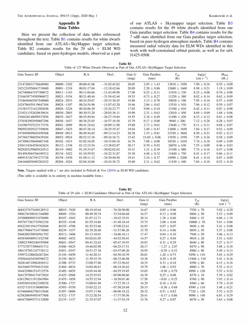
Here we present the collection of data tables referencedthroughout the text. Table B1 contains results for white dwarfsidentified from our ATLAS+SkyMapper target selection.Table B2 contains results for the 29 sdA + ELM WDcandidates, based on pure-hydrogen models, observed as a part

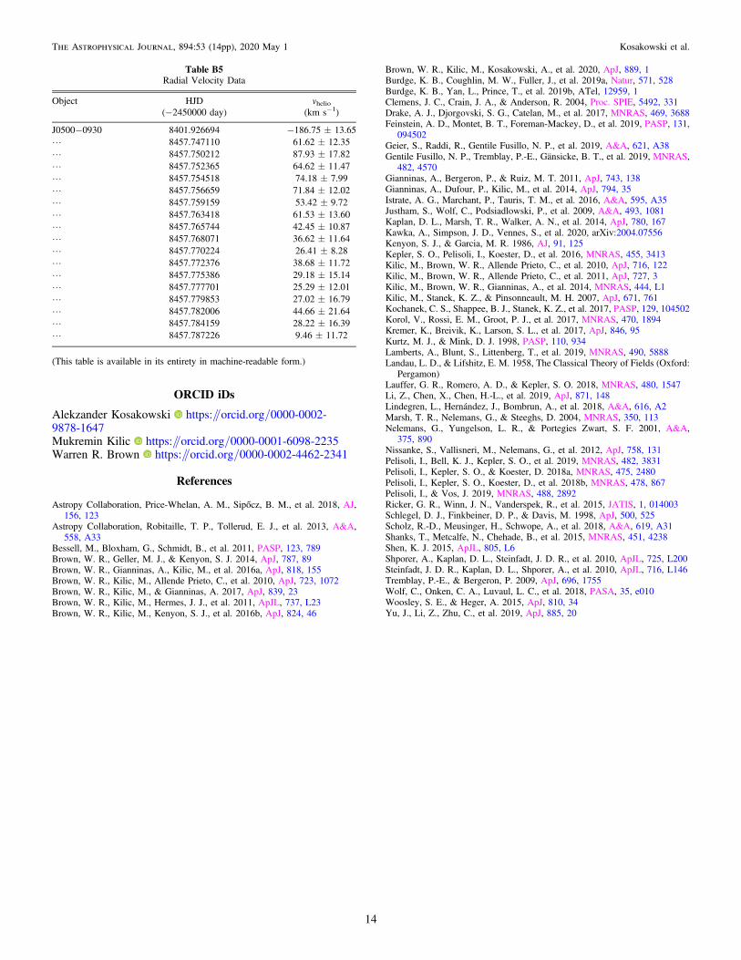
of our ATLAS + Skymapper target selection. Table B3contains results for the 49 white dwarfs identified from ourGaia parallax target selection. Table B4 contains results for the7 sdB stars identified from our Gaia parallax target selection,based on pure-hydrogen atmosphere models. Table B4 containsmeasured radial velocity data for ELM WDs identified in thiswork with well-constrained orbital periods, as well as for sdAJ1425-0508.

Table B1Table of 123 White Dwarfs Observed as Part of Our ATLAS+SkyMapper Target Selection

Gaia Source ID Object R.A. Decl. Gaia G Gaia Parallax Teff log(g) MWD

(mag) (mas) (K) (cm s−2) (Me)

2314720431736648960 J0000−3102 00:00:41.06 −31:02:45.82 20.05 2.95±1.43 13810±1950 7.90±0.16 0.55±0.092421224556841719680 J0001−1218 00:01:17.04 −12:18:42.66 20.09 2.28±0.86 12680±1660 8.98±0.21 1.19±0.092427460643197388672 J0011−1143 00:11:04.66 −11:43:49.98 17.08 0.25±0.11 11910±330 8.25±0.08 0.76±0.062316638774585068672 J0021−3154 00:21:40.44 −31:54:42.44 18.53 0.73±0.27 11250±380 8.02±0.14 0.62±0.092318640465567548800 J0024−2933 00:24:29.67 −29:33:38.45 19.88 3.13±0.78 10030±190 7.95±0.16 0.57±0.092424786459119647104 J0024−1107 00:24:54.96 −11:07:43.28 19.46 2.86±0.62 13510±910 7.96±0.12 0.59±0.072315815721412502656 J0026−3224 00:26:06.30 −32:24:23.77 17.05 9.09±0.10 13160±810 8.42±0.11 0.87±0.082319211352620639616 J0030−2803 00:30:53.20 −28:03:36.11 19.90 2.31±0.63 12010±450 8.69±0.09 1.04±0.062346428148058537856 J0035−2627 00:35:49.84 −26:27:19.84 19.55 2.18±0.49 11490±420 8.33±0.12 0.81±0.082370382902950807296 J0036−1657 00:36:25.85 −16:57:18.50 15.79 0.17±0.08 9940±200 7.12±0.28 0.28±0.072343867935233173376 J0041−2609 00:41:18.62 −26:09:11.88 19.88 2.73±0.61 13640±770 8.11±0.11 0.68±0.075005923029327350656 J0047−3425 00:47:28.14 −34:25:35.47 19.64 2.49±0.47 13600±1850 7.84±0.17 0.52±0.092474049699645450368 J0049−0913 00:49:44.65 −09:13:14.23 20.30 1.53±0.81 15350±3660 8.50±0.21 0.93±0.132473843786029439104 J0052−0924 00:52:15.36 −09:24:18.71 15.42 15.69±0.06 13930±1950 7.95±0.16 0.58±0.092473096358640407168 J0102−1015 01:02:16.05 −10:15:04.18 16.76 7.08±0.08 18520±1010 7.74±0.18 0.49±0.092456134364556362624 J0112−1338 01:12:15.54 −13:38:02.87 20.17 0.70±0.92 26070±630 7.55±0.09 0.46±0.035029203259605424512 J0119−3002 01:19:33.67 −30:02:02.62 19.31 1.31±0.39 13100±980 7.74±0.16 0.47±0.085014943044766189312 J0134−3422 01:34:59.92 −34:22:31.87 19.30 4.48±0.32 11840±750 8.41±0.17 0.86±0.114969151267391273728 J0158−3430 01:58:11.12 −34:30:40.50 19.41 2.34±0.37 14990±2200 8.41±0.14 0.87±0.092461668030485282432 J0204−1024 02:04:10.06 −10:24:36.72 19.60 2.11±0.62 11430±440 7.84±0.18 0.52±0.10

Note. Targets marked with a are also included in Pelisoli & Vos (2019) as ELM WD candidates.

(This table is available in its entirety in machine-readable form.)

Table B2Table of 29 sdA + ELM Candidates Observed as Part of Our ATLAS+SkyMapper Target Selection

Gaia Source ID Object R.A. Decl. Gaia G Gaia Parallax Teff log(g)(mag) (mas) (K) (cm s−2)

4684237675440128512 J0019−7620 00:19:45.64 −76:20:50.00 16.67 0.05±0.06 7520±70 5.02±0.205006336308261344000 J0049−3354 00:49:30.74 −33:54:04.68 16.57 0.13±0.08 8860±50 5.53±0.092470088090531076096 J0107−1042 01:07:12.71 −10:42:35.91 20.14 1.38±0.66 9460±43 6.06±1.344957677283735582336 J0155−4148 01:55:34.86 −41:48:18.44 15.75 2.08±0.04 10060±70 5.61±0.064942238319415762048 J0155−4708 01:55:53.66 −47:08:22.61 16.93 0.07±0.07 9040±40 5.41±0.085063798847514778880 J0239−3157 02:39:20.40 −31:57:06.26 15.70 0.14±0.06 8850±50 5.57±0.085048200350928561792 J0313−3406 03:13:10.01 −34:06:18.11 17.47 0.04±0.10 7940±50 5.06±0.134838360480913152768 J0402−4452 04:02:01.05 −44:52:56.01 14.57 0.27±0.04 9010±20 5.51±0.033200233905240195968 J0441−0547 04:41:32.62 −05:47:34.93 18.83 0.31±0.29 8640±80 5.27±0.173777278773096451712 J1046−0425 10:46:02.98 −04:25:17.51 20.17 −1.27±2.07 8470±90 5.88±0.183801357051247738112 J1051−0347 10:51:27.38 −03:47:09.20 18.95 −0.29±0.32 8960±80 5.49±0.133599721286026267264 J1144−0450 11:44:20.31 −04:50:10.39 20.01 1.28±0.73 9290±110 5.83±0.293595644434349398272 J1159−0633 11:59:35.70 −06:33:46.98 19.38 0.29±0.59 11960±510 5.41±0.163628140710962656512 J1308−0733 13:08:57.86 −07:33:56.63 18.35 0.33±0.18 8590±80 6.15±0.163643468379794415104 J1404−0634 14:04:40.81 −06:34:26.62 19.79 1.06±0.92 8880±70 5.52±0.113644329881514712576 J1405−0455 14:05:44.40 −04:55:19.85 19.65 −0.50±0.79 8990±120 5.53±0.323641707894175473024 J1425−0508 14:25:55.01 −05:08:08.60 16.39 0.25±0.08 8570±10 5.59±0.026281296211912043904 J1455−1858 14:55:32.94 −18:58:01.40 17.58 −0.01±0.25 8760±90 5.93±0.146305569103622390528 J1500−1727 15:00:01.98 −17:27:39.13 16.29 0.18±0.10 8560±60 5.79±0.106332713533156000384 J1503−0750 15:03:22.21 −07:50:24.68 20.33 −0.30±0.88 8590±110 5.48±0.216334668842786315648 J1507−0606 15:07:17.86 −06:06:18.22 20.32 0.51±0.82 7720±120 5.52±0.256258208494955477888 J1522−1737 15:22:20.54 −17:37:50.56 20.41 −0.17±0.86 9090±140 6.01±0.296844758095371132800 J2135−1137 21:35:47.07 −11:37:54.19 15.76 0.27±0.07 8670±50 5.63±0.08

12

The Astrophysical Journal, 894:53 (14pp), 2020 May 1 Kosakowski et al.

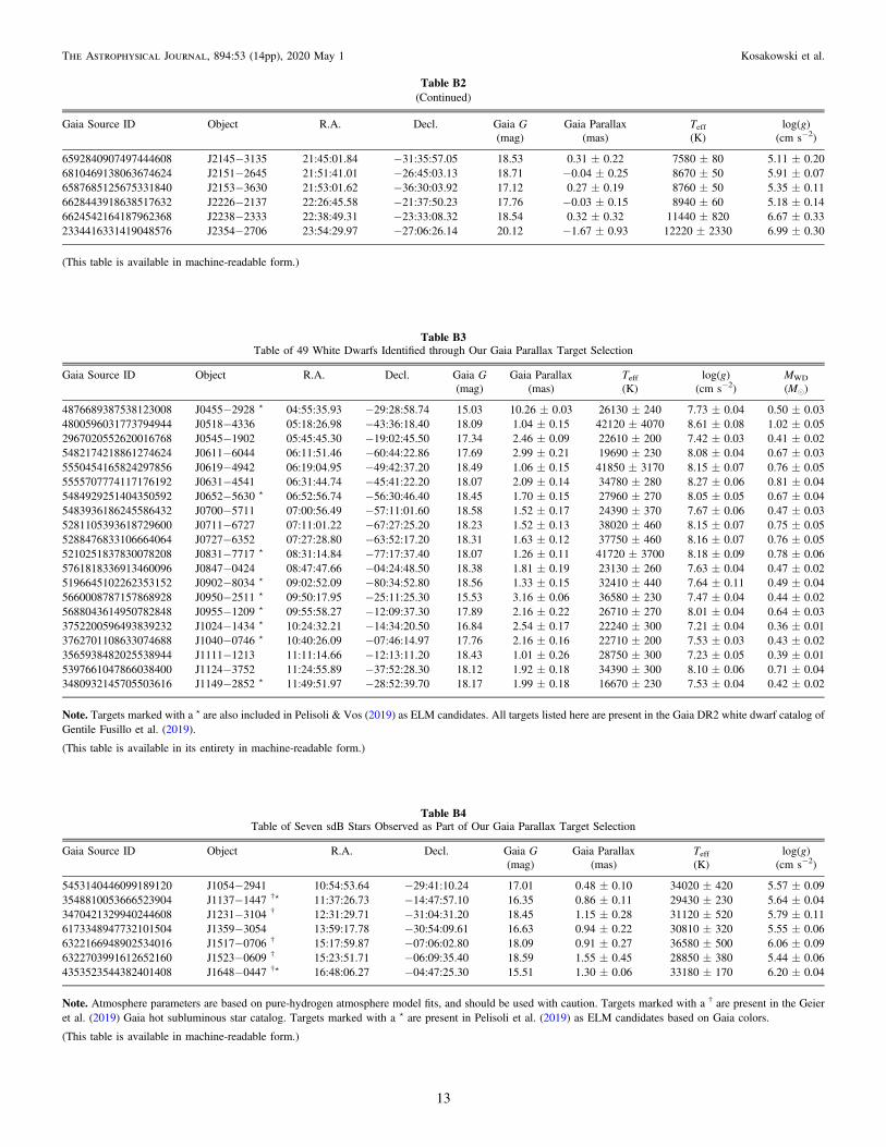
Table B2(Continued)

Gaia Source ID Object R.A. Decl. Gaia G Gaia Parallax Teff log(g)(mag) (mas) (K) (cm s−2)

6592840907497444608 J2145−3135 21:45:01.84 −31:35:57.05 18.53 0.31±0.22 7580±80 5.11±0.206810469138063674624 J2151−2645 21:51:41.01 −26:45:03.13 18.71 −0.04±0.25 8670±50 5.91±0.076587685125675331840 J2153−3630 21:53:01.62 −36:30:03.92 17.12 0.27±0.19 8760±50 5.35±0.116628443918638517632 J2226−2137 22:26:45.58 −21:37:50.23 17.76 −0.03±0.15 8940±60 5.18±0.146624542164187962368 J2238−2333 22:38:49.31 −23:33:08.32 18.54 0.32±0.32 11440±820 6.67±0.332334416331419048576 J2354−2706 23:54:29.97 −27:06:26.14 20.12 −1.67±0.93 12220±2330 6.99±0.30

(This table is available in machine-readable form.)

Table B3Table of 49 White Dwarfs Identified through Our Gaia Parallax Target Selection

Gaia Source ID Object R.A. Decl. Gaia G Gaia Parallax Teff log(g) MWD

(mag) (mas) (K) (cm s−2) (Me)

4876689387538123008 J0455−2928 å 04:55:35.93 −29:28:58.74 15.03 10.26±0.03 26130±240 7.73±0.04 0.50±0.034800596031773794944 J0518−4336 05:18:26.98 −43:36:18.40 18.09 1.04±0.15 42120±4070 8.61±0.08 1.02±0.052967020552620016768 J0545−1902 05:45:45.30 −19:02:45.50 17.34 2.46±0.09 22610±200 7.42±0.03 0.41±0.025482174218861274624 J0611−6044 06:11:51.46 −60:44:22.86 17.69 2.99±0.21 19690±230 8.08±0.04 0.67±0.035550454165824297856 J0619−4942 06:19:04.95 −49:42:37.20 18.49 1.06±0.15 41850±3170 8.15±0.07 0.76±0.055555707774117176192 J0631−4541 06:31:44.74 −45:41:22.20 18.07 2.09±0.14 34780±280 8.27±0.06 0.81±0.045484929251404350592 J0652−5630 å 06:52:56.74 −56:30:46.40 18.45 1.70±0.15 27960±270 8.05±0.05 0.67±0.045483936186245586432 J0700−5711 07:00:56.49 −57:11:01.60 18.58 1.52±0.17 24390±370 7.67±0.06 0.47±0.035281105393618729600 J0711−6727 07:11:01.22 −67:27:25.20 18.23 1.52±0.13 38020±460 8.15±0.07 0.75±0.055288476833106664064 J0727−6352 07:27:28.80 −63:52:17.20 18.31 1.63±0.12 37750±460 8.16±0.07 0.76±0.055210251837830078208 J0831−7717 å 08:31:14.84 −77:17:37.40 18.07 1.26±0.11 41720±3700 8.18±0.09 0.78±0.065761818336913460096 J0847−0424 08:47:47.66 −04:24:48.50 18.38 1.81±0.19 23130±260 7.63±0.04 0.47±0.025196645102262353152 J0902−8034 å 09:02:52.09 −80:34:52.80 18.56 1.33±0.15 32410±440 7.64±0.11 0.49±0.045660008787157868928 J0950−2511 å 09:50:17.95 −25:11:25.30 15.53 3.16±0.06 36580±230 7.47±0.04 0.44±0.025688043614950782848 J0955−1209 å 09:55:58.27 −12:09:37.30 17.89 2.16±0.22 26710±270 8.01±0.04 0.64±0.033752200596493839232 J1024−1434 å 10:24:32.21 −14:34:20.50 16.84 2.54±0.17 22240±300 7.21±0.04 0.36±0.013762701108633074688 J1040−0746 å 10:40:26.09 −07:46:14.97 17.76 2.16±0.16 22710±200 7.53±0.03 0.43±0.023565938482025538944 J1111−1213 11:11:14.66 −12:13:11.20 18.43 1.01±0.26 28750±300 7.23±0.05 0.39±0.015397661047866038400 J1124−3752 11:24:55.89 −37:52:28.30 18.12 1.92±0.18 34390±300 8.10±0.06 0.71±0.043480932145705503616 J1149−2852 å 11:49:51.97 −28:52:39.70 18.17 1.99±0.18 16670±230 7.53±0.04 0.42±0.02

Note. Targets marked with a å are also included in Pelisoli & Vos (2019) as ELM candidates. All targets listed here are present in the Gaia DR2 white dwarf catalog ofGentile Fusillo et al. (2019).

(This table is available in its entirety in machine-readable form.)

Table B4Table of Seven sdB Stars Observed as Part of Our Gaia Parallax Target Selection

Gaia Source ID Object R.A. Decl. Gaia G Gaia Parallax Teff log(g)(mag) (mas) (K) (cm s−2)

5453140446099189120 J1054−2941 10:54:53.64 −29:41:10.24 17.01 0.48±0.10 34020±420 5.57±0.093548810053666523904 J1137−1447 †å 11:37:26.73 −14:47:57.10 16.35 0.86±0.11 29430±230 5.64±0.043470421329940244608 J1231−3104 † 12:31:29.71 −31:04:31.20 18.45 1.15±0.28 31120±520 5.79±0.116173348947732101504 J1359−3054 13:59:17.78 −30:54:09.61 16.63 0.94±0.22 30810±320 5.55±0.066322166948902534016 J1517−0706 † 15:17:59.87 −07:06:02.80 18.09 0.91±0.27 36580±500 6.06±0.096322703991612652160 J1523−0609 † 15:23:51.71 −06:09:35.40 18.59 1.55±0.45 28850±380 5.44±0.064353523544382401408 J1648−0447 †å 16:48:06.27 −04:47:25.30 15.51 1.30±0.06 33180±170 6.20±0.04

Note. Atmosphere parameters are based on pure-hydrogen atmosphere model fits, and should be used with caution. Targets marked with a † are present in the Geieret al. (2019) Gaia hot subluminous star catalog. Targets marked with a å are present in Pelisoli et al. (2019) as ELM candidates based on Gaia colors.

(This table is available in machine-readable form.)

13

The Astrophysical Journal, 894:53 (14pp), 2020 May 1 Kosakowski et al.

ORCID iDs

Alekzander Kosakowski https://orcid.org/0000-0002-9878-1647Mukremin Kilic https://orcid.org/0000-0001-6098-2235Warren R. Brown https://orcid.org/0000-0002-4462-2341

References

Astropy Collaboration, Price-Whelan, A. M., Sipőcz, B. M., et al. 2018, AJ,156, 123

Astropy Collaboration, Robitaille, T. P., Tollerud, E. J., et al. 2013, A&A,558, A33

Bessell, M., Bloxham, G., Schmidt, B., et al. 2011, PASP, 123, 789Brown, W. R., Geller, M. J., & Kenyon, S. J. 2014, ApJ, 787, 89Brown, W. R., Gianninas, A., Kilic, M., et al. 2016a, ApJ, 818, 155Brown, W. R., Kilic, M., Allende Prieto, C., et al. 2010, ApJ, 723, 1072Brown, W. R., Kilic, M., & Gianninas, A. 2017, ApJ, 839, 23Brown, W. R., Kilic, M., Hermes, J. J., et al. 2011, ApJL, 737, L23Brown, W. R., Kilic, M., Kenyon, S. J., et al. 2016b, ApJ, 824, 46

Brown, W. R., Kilic, M., Kosakowski, A., et al. 2020, ApJ, 889, 1Burdge, K. B., Coughlin, M. W., Fuller, J., et al. 2019a, Natur, 571, 528Burdge, K. B., Yan, L., Prince, T., et al. 2019b, ATel, 12959, 1Clemens, J. C., Crain, J. A., & Anderson, R. 2004, Proc. SPIE, 5492, 331Drake, A. J., Djorgovski, S. G., Catelan, M., et al. 2017, MNRAS, 469, 3688Feinstein, A. D., Montet, B. T., Foreman-Mackey, D., et al. 2019, PASP, 131,

094502Geier, S., Raddi, R., Gentile Fusillo, N. P., et al. 2019, A&A, 621, A38Gentile Fusillo, N. P., Tremblay, P.-E., Gänsicke, B. T., et al. 2019, MNRAS,

482, 4570Gianninas, A., Bergeron, P., & Ruiz, M. T. 2011, ApJ, 743, 138Gianninas, A., Dufour, P., Kilic, M., et al. 2014, ApJ, 794, 35Istrate, A. G., Marchant, P., Tauris, T. M., et al. 2016, A&A, 595, A35Justham, S., Wolf, C., Podsiadlowski, P., et al. 2009, A&A, 493, 1081Kaplan, D. L., Marsh, T. R., Walker, A. N., et al. 2014, ApJ, 780, 167Kawka, A., Simpson, J. D., Vennes, S., et al. 2020, arXiv:2004.07556Kenyon, S. J., & Garcia, M. R. 1986, AJ, 91, 125Kepler, S. O., Pelisoli, I., Koester, D., et al. 2016, MNRAS, 455, 3413Kilic, M., Brown, W. R., Allende Prieto, C., et al. 2010, ApJ, 716, 122Kilic, M., Brown, W. R., Allende Prieto, C., et al. 2011, ApJ, 727, 3Kilic, M., Brown, W. R., Gianninas, A., et al. 2014, MNRAS, 444, L1Kilic, M., Stanek, K. Z., & Pinsonneault, M. H. 2007, ApJ, 671, 761Kochanek, C. S., Shappee, B. J., Stanek, K. Z., et al. 2017, PASP, 129, 104502Korol, V., Rossi, E. M., Groot, P. J., et al. 2017, MNRAS, 470, 1894Kremer, K., Breivik, K., Larson, S. L., et al. 2017, ApJ, 846, 95Kurtz, M. J., & Mink, D. J. 1998, PASP, 110, 934Lamberts, A., Blunt, S., Littenberg, T., et al. 2019, MNRAS, 490, 5888Landau, L. D., & Lifshitz, E. M. 1958, The Classical Theory of Fields (Oxford:

Pergamon)Lauffer, G. R., Romero, A. D., & Kepler, S. O. 2018, MNRAS, 480, 1547Li, Z., Chen, X., Chen, H.-L., et al. 2019, ApJ, 871, 148Lindegren, L., Hernández, J., Bombrun, A., et al. 2018, A&A, 616, A2Marsh, T. R., Nelemans, G., & Steeghs, D. 2004, MNRAS, 350, 113Nelemans, G., Yungelson, L. R., & Portegies Zwart, S. F. 2001, A&A,

375, 890Nissanke, S., Vallisneri, M., Nelemans, G., et al. 2012, ApJ, 758, 131Pelisoli, I., Bell, K. J., Kepler, S. O., et al. 2019, MNRAS, 482, 3831Pelisoli, I., Kepler, S. O., & Koester, D. 2018a, MNRAS, 475, 2480Pelisoli, I., Kepler, S. O., Koester, D., et al. 2018b, MNRAS, 478, 867Pelisoli, I., & Vos, J. 2019, MNRAS, 488, 2892Ricker, G. R., Winn, J. N., Vanderspek, R., et al. 2015, JATIS, 1, 014003Schlegel, D. J., Finkbeiner, D. P., & Davis, M. 1998, ApJ, 500, 525Scholz, R.-D., Meusinger, H., Schwope, A., et al. 2018, A&A, 619, A31Shanks, T., Metcalfe, N., Chehade, B., et al. 2015, MNRAS, 451, 4238Shen, K. J. 2015, ApJL, 805, L6Shporer, A., Kaplan, D. L., Steinfadt, J. D. R., et al. 2010, ApJL, 725, L200Steinfadt, J. D. R., Kaplan, D. L., Shporer, A., et al. 2010, ApJL, 716, L146Tremblay, P.-E., & Bergeron, P. 2009, ApJ, 696, 1755Wolf, C., Onken, C. A., Luvaul, L. C., et al. 2018, PASA, 35, e010Woosley, S. E., & Heger, A. 2015, ApJ, 810, 34Yu, J., Li, Z., Zhu, C., et al. 2019, ApJ, 885, 20

Table B5Radial Velocity Data

Object HJD vhelio(−2450000 day) (km s−1)

J0500−0930 8401.926694 −186.75±13.65L 8457.747110 61.62±12.35L 8457.750212 87.93±17.82L 8457.752365 64.62±11.47L 8457.754518 74.18±7.99L 8457.756659 71.84±12.02L 8457.759159 53.42±9.72L 8457.763418 61.53±13.60L 8457.765744 42.45±10.87L 8457.768071 36.62±11.64L 8457.770224 26.41±8.28L 8457.772376 38.68±11.72L 8457.775386 29.18±15.14L 8457.777701 25.29±12.01L 8457.779853 27.02±16.79L 8457.782006 44.66±21.64L 8457.784159 28.22±16.39L 8457.787226 9.46±11.72

(This table is available in its entirety in machine-readable form.)

14

The Astrophysical Journal, 894:53 (14pp), 2020 May 1 Kosakowski et al.