The Equilibrium Impact of Robots on Labor Markets∗

By NAREK ALEXANIAN†

April 2019

Abstract

We examine the impact of industrial robots on labor markets, focusing on changes

in skill-premia and real wages by skill-type. We hypothesize the existence of robot-

skill complementarity, appropriately embedding robots in our production function,

and develop a static Ricardian trade model to derive the equilibrium effects. The

model captures the displacement effect of robots as they compete with labor, as

well as the productivity effect that comes through decreases of costs and consump-

tion prices. We explicitly derive from our model a linearized equation which we

can directly use to estimate the key elasticity parameters. The ordering of the ob-

tained estimates supports our hypothesis of robot-skill complementarity, as well as

-the established in the literature- assumption of capital-skill complementarity. Our

estimates and derived equations suggest that automation benefits both skill-types.

Nevertheless, the relative gains are at least 2.3 times larger for the high-skilled la-

bor, widening the existing welfare gap. Our model allows us to use our estimates to

also quantify the impact of trade on labor markets. As in the case of robot adoption,

we find that while both skill-types gain from trade openness, the high-skilled are

benefited 2.25 times more than the low-skilled; our results agree with the existing

literature which claims that trade is skill-biased.

Keywords: automation, industrial robots, trade gains, skill-premium

JEL classification: E23; F11; F16; O33

∗I would like to thank my mentor and thesis advisor, Prof. Costas Arkolakis, for his invaluable guid-ance and support throughout my senior year. Many thanks to Max Perez Leon for his helpful commentsand technical support. All errors are my own.†Department of Economics & Department of Mathematics, Class of 2019, Yale University

1

2

Contents

1 Introduction 3

2 A Static Ricardian Model of Automation 102.1 The Set-up . . . . . . . . . . . . . . . . . . . . . . . . . . . . . . . . . . 10

2.2 Prices . . . . . . . . . . . . . . . . . . . . . . . . . . . . . . . . . . . . . 12

2.3 Firm Cost Minimization . . . . . . . . . . . . . . . . . . . . . . . . . . 13

2.4 Gravity equations-Trade Shares . . . . . . . . . . . . . . . . . . . . . . 14

2.5 Welfare . . . . . . . . . . . . . . . . . . . . . . . . . . . . . . . . . . . . 15

2.6 Equilibrium conditions . . . . . . . . . . . . . . . . . . . . . . . . . . . 16

3 Model Characterization & Further Derivations 173.1 The skill premium . . . . . . . . . . . . . . . . . . . . . . . . . . . . . . 17

3.2 Implementing Hat Algebra . . . . . . . . . . . . . . . . . . . . . . . . 18

3.2.1 First-order approximation for the change in the skill-premium 19

3.2.2 First-order approximation for the change in the real wages . . 21

4 Data description & Analysis 234.1 Data sources & description . . . . . . . . . . . . . . . . . . . . . . . . . 23

4.2 Analysis . . . . . . . . . . . . . . . . . . . . . . . . . . . . . . . . . . . 25

5 Results 275.1 Model accuracy . . . . . . . . . . . . . . . . . . . . . . . . . . . . . . . 30

5.2 Measuring the impact of automation . . . . . . . . . . . . . . . . . . . 31

5.3 Is trade mitigating or amplifying the change in the skill-premium? . 32

6 Conclusion 33

7 Appendix 377.1 Cost-minimization . . . . . . . . . . . . . . . . . . . . . . . . . . . . . 37

7.2 The skill-premium . . . . . . . . . . . . . . . . . . . . . . . . . . . . . 38

7.2.1 First-order approximation for the skill-premium . . . . . . . . 40

3

1 Introduction

With self-driving cars already roaming our streets and Artificial Intelligence (AI) get-

ting seats in company boardrooms in Hong-Kong1, the emergence of automation is

more tangible than ever before. Frey and Osborne (2017) report that 46 percent of U.S.

workers are at risk of losing jobs to automation over the course of the two next decades.

Ominous science-fiction stories that warn of the dominance of robots over humankind

seem to have perhaps influenced public opinion. According to a survey conducted by

the Pew Research Center2 twice as many Americans (72 percent) are expressing worry

rather than enthusiasm (36 percent) about a future in which robots can do tasks cur-

rently performed by humans. What is more, the steady contraction of the labor income

share during the last three decades (Karabarbounis and Neiman (2013)) seems to con-

firm the concerns about the future of automation (Brynjolfsson and McAfee (2014)). The

same pessimism was also conveyed by John Maynard Keynes, who in 1930 stated that,

“We are being addicted with a new disease of which some readers may not have heard

the name, but of which they will hear a great deal in the years to come—namely, tech-

nological unemployment” (Keynes (1930)). Fortunately, his predictions did not come

true, as technology, instead of substituting, has largely augmented the productivity of

labor, bringing tremendous economic growth since the Great Depression.

Some scholars think that the effects of automation and AI will not prove to be any

different. For example, consider that the introduction of automated teller machines

(ATMs) coincided with the expansion in the employment of bank tellers. According

to Bessen (2016) ATMs decreased substantially the cost of operations, inducing a scale

1 Nikkei Asian Review2 Pew Research Center

4

effect that encouraged banks to open more branches and to hire more bank tellers to

perform specialized tasks other than money withdrawals or deposits. Nevertheless,

European experts who participated at the Initiative on Global Markets (IGM) forum at

Chicago Booth are divided on whether “rising use of robots and artificial intelligence

is likely to increase substantially the number of workers in advanced countries who

are unemployed for long periods.”3 So, before we start planning a neo-Luddite move-

ment, let us use economic reasoning to understand whether an alarmist reaction is even

justified.

For our analysis we are going to develop a Ricardian trade model in a formulation

firstly suggested in Eaton and Kortum (2002), which captures the equilibrium impact

of robots on labor markets. As it has been clearly conceptualized in Acemoglu and

Restrepo (2018), the automation effect manifests itself into two countervailing forces: a

direct displacement effect and a productivity spillover effect. The displacement effect

is a natural consequence of robots’ substituting for human labor and therefore causes

a downward pressure on wages. Opposing to it stands the productivity effect that

results from decreases in the cost of production of intermediate goods and diffuses

across sectors and across countries through trade, pushing wages up while lowering

consumption prices. These countervailing forces exactly represent the dichotomy in

the views about the impact of automation with each side of the debate believing that

one of the effects will unambiguously dominate over the other. Our goal is to address

this dichotomy by deriving equations that describe the combined effects.

We will focus our attention on the impact of industrial robots using data released by the

International Federation of Robotics (2016). The IFR defines an industrial robot as an

“automatically controlled, reprogrammable, multipurpose manipulator programmable

in three or more axes, which may be either fixed in place or mobile for use in industrial

3 IGM 2017

5

automation applications.” Hence, we will not be concerned with examples of automa-

tion such as ATMs or AI applications, but we will limit ourselves to automation occur-

ring through industrial robots. This limitation is well-justified since industrial robots

have been the dominant form of automation technology for the last three decades (In-

ternational Federation of Robotics (2016)). The number of installed industrial robots in

Western Europe increased fourfold from 1993 to 2016. This increase was accompanied

by a spectacular decrease in robot prices of almost 80 percent from 1993 to 2005, if we

adjust the prices for quality improvements4. Current IFR reports put the number of

operational robots globally close to 2 million, and this number is anticipated to double

or triple by 2025 (BCG (2015)). To motivate our analysis, we plot the change of skill-

premium on the change of robot density (defined as robots over efficiency hours of

labor) in Germany from 1993 to 2005 as depicted in Figure 1. This positive correlation

between robot densification and the change in the skill-premium suggests that there

might be some sort of robot-skill complementarity, which we will now investigate in

depth.

Figure 1: Percentage Change in Skill-Premium over Robot Densification(Germany1993-2005)

4 IFR report(2006)

6

Our framework incorporates labor heterogeneity embedding a relative robot-skill com-

plementarity, similarly to Krusell, Ohanian, RÌos-Rull, and Violante (2000), who ana-

lyze capital-skill complementarity. Labor comes in two flavors: high-skilled and low-

skilled, and it is supplied inelastically. Although our approach does not separate be-

tween the two effects described above, it can completely characterize the aggregate

impact of robots on the skill-premium (a proxy for inequality) and on the real wages

for each skill-type (a proxy for welfare). We introduce this robot-skill complementar-

ity through a Constant Elasticity of Substitution (CES) production function, where we

hypothesize that the elasticity of substitution between robots and low-skilled labor is

higher than the respective elasticity between robots and high-skilled workers; hence,

robots and skill are relative complements. We maintain the capital-skill complementar-

ity hypothesis, as it was proposed in Krusell, Ohanian, RÌos-Rull, and Violante (2000).

We extend their specification by separating robots from the rest of intermediate capital

inputs and embedding the production in a Ricardian trade model to derive the appro-

priate equilibrium equations. The parameters that dictate the magnitude and the sign

of the effects on the skill-premia and the real wages are the elasticities of substitution

between the factors, as well as the elasticity of substitution of trade that captures the

productivity dispersion of the intermediate goods.

For our empirical analysis, we are going to estimate these parameters by using lin-

earized forms of our equilibrium equations and data on skill-premia, skill-supply and

volumes of intermediate capital inputs from the EUKLEMS data set (van Ark and Jäger

(2017)), as well as data on the stock of operational robots, as reported by the IFR. To ad-

dress potential endogeneity concerns, we use appropriate instruments for our regres-

sion analysis without sacrificing the statistical significance of our estimates. Obtaining

7

these estimates will help us determine the impact of robots on skill-premia and real

wages, in other words, whether there are gains from robotics and how they are dis-

tributed by skill-type. Moreover, they allow us to perform counterfactual exercises that

test whether trade mitigates or intensifies the impact of automation. The importance

of these considerations lies in their social and political implications. We have seen that

recently there has been a populist backlash supported by those who consider them-

selves the losers of globalization. Similar reactions can be prompted if the gains from

automation asymmetrically favor skilled-labor and capital-owners, sharpening the ex-

isting inequality.

Our results support the hypothesis of robot-skill complementarity, as well as the as-

sumption of capital-skill complementarity, which is well-established in the literature

(Krusell, Ohanian, RÌos-Rull, and Violante (2000),McAdam and Willman (2018)). Sub-

sequently, the obtained estimates are used to predict the change in skill premia through

equations that were not used for the regression. Our Ordinary Least Squares (OLS) esti-

mates achieve good model fit, in contrast to the estimates obtained by the IV regression.

As it is hinted by robot-skill complementarity, automation increases the skill-premium;

nevertheless it benefits everyone in terms of real wages. The impact of trade openness

is similar, as it is shown to be skill-biased staying consistent with the results of Burstein,

Cravino, and Vogel (2013) and Parro (2013).

The starting point and source of inspiration for this paper has been the recently pub-

lished series of papers by Acemoglu and Restrepo. Acemoglu and Restrepo (2017b)

estimate the impact of robots on employment and wages on local U.S. labor markets

(proxied by commuting zones) and find statistically significant negative effects that are

slightly mitigated when the locations are allowed to trade. Since their level of analysis

is local, they construct a measure of robot exposure from the IFR data, as the IFR does

8

not provide information at the granular level of commuting zones. To obtain these re-

sults, they set up a task-based static model in which robots compete with labor for the

performance of the tasks and increasing automation effectively improves the produc-

tivity of robots to a point that robots obtain the comparative advantage for performing

the task; this is the displacement effect. Cleverly, they also incorporate the creation of

new tasks in which labor has initially the comparative advantage; this is part of the

productivity effect. Since our model is not task-based, we fail to capture this aspect.

Moreover, Acemoglu and Restrepo (2018) complete their set-up by developing a dy-

namic model and characterizing the requirements for it to exhibit a balanced growth

path. Lastly, in Acemoglu and Restrepo (2017a) they extend their model to incorporate

labor heterogeneity by distinguishing between low-skill automation (through indus-

trial and service robots) and high-skill automation (mainly through the introduction of

AI).

Our paper adopts a static approach measuring changes across equilibrium states with

an international scope instead of a local one. To that end, we develop a Ricardian trade

model à la Eaton and Kortum (2002), where production is given through a nested CES

that intertwines the factors of production. Our model builds on the work of Burstein,

Cravino, and Vogel (2013) and Parro (2013), who employ the same Ricardian model to

characterize the skill-biased effect of trade. We extend their model to incorporate robots

in our production function. Our results are comparable to theirs since we find similar

effects of trade openness on the skill-premium and the real wages by skill-type.

More closely related to our work is the seminal on the topic paper of Graetz and

Michaels (2015), who were the first to bring attention to and use the IFR data. They

investigate the economic contributions of robots quantifying empirically the impact

of robot densification on labor productivity, output prices and employment by using

9

appropriate instruments. They provide a theoretical model of a task-based technolog-

ical choice from the firms’ side that predicts their results. In contrast, in our paper,

the equations used for our empirical analysis are not simply implied, but explicitly

derived. This enables us to recover the elasticities, whose cardinal order Graetz and

Michaels (2015) simply assume. Therefore, our value-added is to quantify the impact

of robots by estimating the key elasticity parameters. We do this by having developed

a trade model rather than a task-based one which fully captures the equilibrium impact

of robots while keeping our analysis at a cross-country level. Interestingly, our topic of

interest is included in the World Bank research agenda with the work of Artuc, Bastos,

and Rijkers (2018). They also use the Ricardian model of Eaton and Kortum (2002), but

a task-based production function, to investigate the impact of robot adoption on trade,

employment and welfare and how this effect percolates to economies that are not yet

automatized. Having used panel data and IV strategies, they find that robotization in-

creases volumes of trade and exhibits welfare gains for the automatized economy, gains

that can also reach countries that have not used industrial robots yet.

The rest of the paper is organized as follows: Section 2 presents our static Ricardian

trade model for automation, which incorporates robots in the production function and

helps us develop further intuition about the equilibrium impact of automation on labor

markets. In Section 3, we derive at a first-order approximation the equations that de-

scribe the changes in the skill-premium and real wages between two steady states and

will be used for our empirical analysis that is described in Section 4. In Section 5, we

get the results of our estimations, discuss their implications about our initial hypothe-

sis of robot-skill complementarity and consider some counterfactuals. Finally, Section

6 concludes, while the Appendix 7 provides analytical derivations of our expressions.

10

2 A Static Ricardian Model of Automation

To guide our empirical analysis, we are going to develop a Ricardian trade model based

on the model firstly described in Eaton and Kortum (2002). We follow the adaption of

this model by Burstein, Cravino, and Vogel (2013) making the appropriate modifica-

tions to accommodate the scope of our question. Specifically, we incorporate robots

in the production function. Then, we use this model to implement hat algebra for the

change in variables between two static equilibria, as done in Dekle, Eaton, and Kor-

tum (2007), and derive the equations that describe the change in skill-premium which

will be used for the regression estimation of key parameters and our counterfactual

analysis.

2.1 The Set-up

Our model describes a world economy with N countries that can freely engage in trade.

Each country i is endowed with inelastically supplied efficiency units of high-skilled

(Hi) and low-skilled (Li) labor. We assume that there are three sectors (s ∈ S): manu-

facturing (s = M), capital equipment (s = K) and non-tradable services (s = NT). For

each sector s there is a continuum of goods Ωs that is produced with different produc-

tivity A(ωs), where ωs ∈ Ωs. For simplicity, we take it to be have Lebesque measure

1, Ωs = [0, 1]. From each sector we can obtain the respective composite good given by

zs =

(∫Ωs

ωεs−1

εss dωs

) εsεs−1

, where εs is the elasticity of substitution between goods used

for production in sector s.

Every producer in these continua combines the composites of intermediate goods from

each sector with labor (high- and low-skilled) and robots, as described by the following

production function, which is a hybrid of a Cobb-Douglass and a nested CES, without

11

any spatial agglomeration forces. The output of good ωs in location i is given by:

Yi (ωs) = Ai (ωs) zM (ωs)γ1,i zNT (ωs)

1−γ1,i−γ2,i ×((zK (ωs)η′ + H (ωs)

η′) λ′

η′ + R (ωs)λ′) σ′

λ′

+ L (ωs)σ′

γ2,iσ′

(1)

, where where zs is the composite intermediate input from each sector, H(L) are the

high(low)-skilled labor hours, R is the number of industrial robots used, γ1,i and γ2,i are

the income shares of each factor, Ai (ωs) is the productivity of location i in producing

good ω, and η′ = η−1η with η being the elasticity of substitution between capital and

high-skilled labor (σ′ and λ′ are defined similarly).

A moment of reflection on the production function can be quite valuable. It is an ex-

tension of what was proposed in Krusell, Ohanian, RÌos-Rull, and Violante (2000) by

incorporating composite intermediate goods and robots. Krusell, Ohanian, RÌos-Rull,

and Violante (2000) by assuming a simpler functional form empirically confirmed the

existence of capital-skill complementarity have found that the elasticity of substitution

between capital and low-skilled labor is higher than the elasticity between capital and

high-skilled workers (in our model that is manifested as η < σ and R = 0). Similarly,

we aim to investigate the relative complementarity between robots and skill. Intu-

itively, the set-up of the function foreshadows that our elasticities will be ordered as

η < λ < σ, conforming with our robot-skill complementarity hypothesis. It remains to

derive the appropriate equations and use them to estimate these elasticity parameters.

The countries are free to trade with each other subject to some “iceberg” costs

τij,s

i,j∈N,s∈S,

where i is the source country and j is the destination ∀i, j ∈ N, τij ≥ 1 with τii = 1. Of

course, τij,NT = ∞ if i 6= j for all non-tradable services. The composite manufacturing

12

goods and services do not appear only as intermediate goods but also as final goods for

consumption. A representative consumer at each location j gets utility from consump-

tion according to:

Cj = CaMM CaNT

NT = CaMM C1−aM

NT (2)

where aM, aNT are the shares of consumption of every sector with aM + aNT = 1.

Households do not consume capital goods. For simplicity we can assume that the elas-

ticity of substitution for the composite final goods is the same as for the composite

intermediates (εs) . Moreover, assuming that there are not any amenities for consider-

ation this consumption can be considered as welfare. We do not allow for migration

in our model with efficiency units of each labor skill-type being exogenously provided.

Hence, we should not expect welfare equalization across locations.

2.2 Prices

Assuming that markets are operating under perfect competition, the price of a good

sent from a location i to a location j is given by:

pij (ωs) =ci,s

Ai,ωs

τij (3)

where ci,sAi,ω

is the marginal cost of one unit of ω in location i. Notice that the marginal

cost is country and sector specific. Since, each ωs ∈ Ωs, ∀s ∈ S is homogeneous across

locations, each location will choose the origin of each good by minimizing across prices,

hence pj (ωs) ≡ mini∈N pij (ωs)

Assume that for every location i and good ωs , Ai (ωs)is an identically independently

distributed random variable drawn by a Frechet distribution Fi (A) = exp

Ti A−θs

where Ti > 0 expresses the the idiosyncratic production of location i and θs > 1 governs

13

the heterogeneity of the distribution. θs is a comparative advantage parameter that

varies across sectors but not across locations (the higher it is the less heterogeneity

there is).

Now as in Eaton and Kortum (2002), we can define Φj,s ≡ ∑i∈N

[Ti(ci,sτij,s

)−θs]

and

obtain the price index:

Pj,s = Φ− 1

θsj,s

[Γ(

θs + 1− εs

θs

)] 11−εs

(4)

, where Γ (y) =∫ ∞

o xy−1e−xdx is the corresponding gamma function. For convenience

denote C (θ, χ) ≡ Γ(

θ+1−χθ

) 11−χ , where χ is the respective constant elasticity of substi-

tution.

We take the price of robots(ρj)

to be exogenously determined for each location, follow-

ing the approach of Graetz and Michaels (2015). Note that in our production function

we did not account for quality improvements of robots. We simply take these improve-

ments to be reflected through price discounts.

2.3 Firm Cost Minimization

Now we turn our attention to the cost of production ci,s which is key in the determina-

tion of prices and trade shares. Every firm chooses inputs such that it minimizes the

cost of production for a given amount of output.

Then we can put together the prices of inputs to get the following aggregate factor

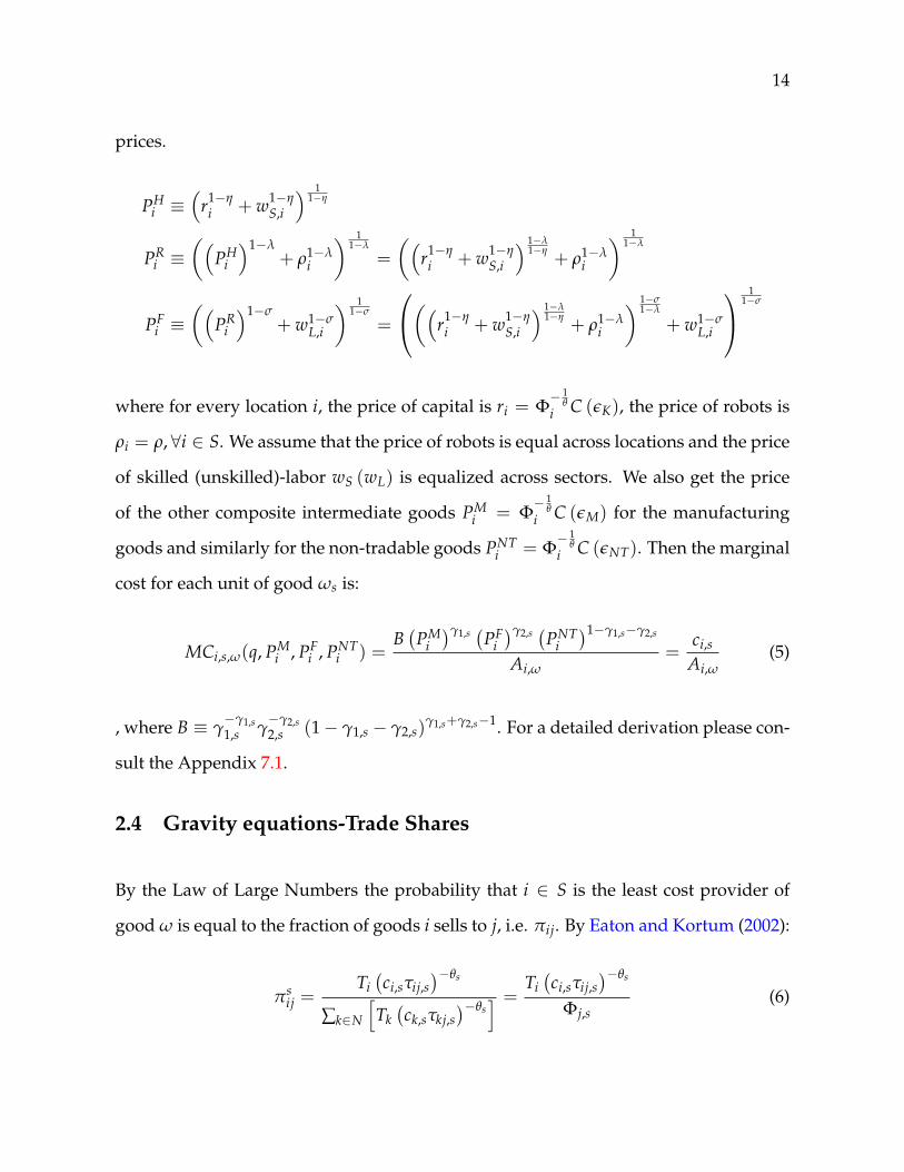
14

prices.

PHi ≡

(r1−η

i + w1−ηS,i

) 11−η

PRi ≡

((PH

i

)1−λ+ ρ1−λ

i

) 11−λ

=

((r1−η

i + w1−ηS,i

) 1−λ1−η

+ ρ1−λi

) 11−λ

PFi ≡

((PR

i

)1−σ+ w1−σ

L,i

) 11−σ

=

((r1−ηi + w1−η

S,i

) 1−λ1−η

+ ρ1−λi

) 1−σ1−λ

+ w1−σL,i

11−σ

where for every location i, the price of capital is ri = Φ− 1

θi C (εK), the price of robots is

ρi = ρ, ∀i ∈ S. We assume that the price of robots is equal across locations and the price

of skilled (unskilled)-labor wS (wL) is equalized across sectors. We also get the price

of the other composite intermediate goods PMi = Φ

− 1θ

i C (εM) for the manufacturing

goods and similarly for the non-tradable goods PNTi = Φ

− 1θ

i C (εNT). Then the marginal

cost for each unit of good ωs is:

MCi,s,ω(q, PMi , PF

i , PNTi ) =

B(

PMi)γ1,s

(PF

i)γ2,s (PNT

i)1−γ1,s−γ2,s

Ai,ω=

ci,s

Ai,ω(5)

, where B ≡ γ−γ1,s1,s γ

−γ2,s2,s (1− γ1,s − γ2,s)

γ1,s+γ2,s−1. For a detailed derivation please con-

sult the Appendix 7.1.

2.4 Gravity equations-Trade Shares

By the Law of Large Numbers the probability that i ∈ S is the least cost provider of

good ω is equal to the fraction of goods i sells to j, i.e. πij. By Eaton and Kortum (2002):

πsij =

Ti(ci,sτij,s

)−θs

∑k∈N

[Tk(ck,sτkj,s

)−θs] =

Ti(ci,sτij,s

)−θs

Φj,s(6)

15

It turns out that πij is equal to the fraction of j’s income spent on goods from i , λij ≡XijYj

= πij where Yj(total income)= Ej(total expenditure). Note that for sector S = NT,

the trade costs τij = +∞, ∀i 6= j. Hence, πij (NT) = 1.

By substituting, Φj = CθP−θj we get that

Xij = C−θτ−θij c−θ

i TiEjPθj

Most importantly, note that if we set i = j, then τii = 1. Hence we can obtain:

πii =Ti (ci,s)

−θ

Φi⇒ Φ

− 1θ

i =

(πii

Ti

) 1θ

ci,s

⇒ Pi = C(

πii

Ti

) 1θ

ci (7)

which is a pretty neat representation of the price index using only the domestic trade

shares, as done in Arkolakis, Costinot, and Rodriguez-Clare (2012).

2.5 Welfare

For simplicity, assume that the welfare of a representative consumer/worker at location

i is given by her real wage (i.e. consumption), -no amenities involved:

WS,i =wS,i

PCi

& WL,i =wL,i

PCi

where PCi =

(PMi )

aM(PNTi )

1−aM

aaMM (1−aM)1−aM

is the consumption price index at location i, as it is im-

plied by consumer welfare maximization. Since we have not allowed for labor mobility

across countries, we do not expect welfare equalization in equalibrium.

16

2.6 Equilibrium conditions

To close our model, we derive the equalibrium conditions of market clearing. I follow

Burstein, Cravino, and Vogel (2013) in their assumption of equalizing the parameters

γ1 and γ2 across all sectors. They claim that this approach comes at the only cost of

not modeling the Stolper-Samuelson effect, which has been estimated to be very close

to zero. Under this assumption, we can integrate over all goods and sectors for each

location.

Each equilibrium can be uniquely characterized by the following set of variables (8N

unknowns): (wS,i, wL,i, ci, Ri, zK,i, zM,i, zNT,i, Dii∈N

)where Si = ∑s∈S

∫Ωs

Si (ω) dω, Li = ∑s∈S∫

ΩsLi (ω) dω, Ri = ∑s∈S

∫Ωs

Ri (ω) dω, zK,i =

∑s∈S∫

ΩszK,i (ω) dω and zM,i = ∑s∈S

∫Ωs

zM,i (ω) dω.

For the price indices we have: Psi = Φ

− 1θ

i C (εs) , ∀s ∈ S, i ∈ N. Note that we do not

have to solve the price of robots(ρj), which as mentioned is determined exogenously.

You can imagine that robots are supplied by an exogenous agent that sets the prices for

each country and is committed to deliver the demanded quantity.

We can define the income at location i as Yi ≡ wS,iSi + wL,iLi + ρiRi. The composite

goods are not included because they are intermediate inputs. Then, from the feasibil-

ity/market clearing constraint, we obtain that:

Yi =

[∑j∈N

(πM

ij(γ1,j + aM

)+ πK

ij γK,j

)YJ + πM

ij aMDj

]+(1− γ1,j − γ2,j

)Yi +[1− aM] (Yi + Di)

(8)

where πsij =

Ti(ciτij)−θs

Φsj

are the trade shares for each sector πNTii = 1, where Di is the

deficit of i and γK is the income share of capital.

17

Moreover, total deficits clear:

∑i∈N

Di = 0

Having completely described the model, we will proceed by deriving the equations

that characterize the change in skill-premium and real wages by skill-type.

3 Model Characterization & Further Derivations

3.1 The skill premium

By cost minimization we can derive the skill premium at a steady state. We drop the

location subscripts to lighten up the notation. After some steps, which you can follow

analytically in the Appendix 7.2, we get the expression:

wS

wL=

(z

σ−1σ

K + Sσ−1

σ

) η−λλ(η−1)

(1S

) 1η(

zλ−1

λH + R

λ−1λ

) σ−λσ(λ−1)

L1σ (9)

We can compare this skill premium with what Burstein, Cravino, and Vogel (2013) got

without robots in their production function:

w′Sw′L

=

((zK

S

) η−1η

+ 1

) σ−ησ(1−η) (L

S

) 1σ

=

(z

η−1η

K + Sη−1

η

) σ−ησ(η−1)

L1σ

(1S

) 1η

Notice that the introduction of robots just adds the extra factor(

zλ−1

λH + R

λ−1λ

) σ−λσ(λ−1)

in

the expression of the skill premium.

18

3.2 Implementing Hat Algebra

We now follow the method of implementing hat algebra, which had been introduced

by Dekle, Eaton, and Kortum (2007). This approach capitalizes on the findings of Arko-

lakis, Costinot, and Rodriguez-Clare (2012) who link gains from trade to domestic trade

shares. We continue to operate under the assumption of equal γ’s across sections.

Having obtained our price index in equation7, let us define x ≡ x′x ; then we get:

ci =ˆ(PMi)γ1 ˆ(PF

i)γ2 ˆ(

PNTi)1−γ1−γ2

(10)

Pi = ci

(πii

Ti

) 1θ

(11)

Now taking PNTi = 1 to be our numeraire at all steady states, we obtain ˆPNT

i = 1 .

Moreover, we know that at every time, πNTii = 1⇒ ˆπNT

ii = 1

⇒ ci = Ti1θ ≡ Ai

⇒ ˆPMi =

(ˆπMii

) 1θ

⇒ ri = PKi =

(πK

ii

) 1θ

⇒ PFi =

Ai(ˆπMii

) γ1θ

1γ2

(12)

Moreover, PFi =

((PR

i

)1−σ+ ( ˆwL,i)

1−σ) 1

1−σ

, PRi =

((PH

i

)1−λ+ (ρ)1−λ

) 11−λ

, and PHi =(

(ri)1−η + (wH,i)

1−η) 1

1−η .

19

Most importantly, for the change in skill-premium we get that:

wSη

wLσ =

(PH)η−λ (

PR)λ−σ L

S(13)

Lastly, notice that the hat of the price of consumption is:

PCi =

(ˆPMi

)a ( ˆPNTi

)1−a =

(ˆπMii

)aθ (14)

, where a = aM from now on.

3.2.1 First-order approximation for the change in the skill-premium

Now, let us define x ≡ log (x); then we have that:

ri =πK

iiθ

ηwS − σwL = (η − λ) PH + (λ− σ) PR +(

L− S)

PFi =

Ai − γ1θ

˜πMii

γ2=

Ti − γ1˜πMii

θγ2

Taking to -a first-order approximation, that exp(x) = 1 + x, we can obtain (steps omit-

ted and presented thoroughly in the Appendix 7.2.1):

wS − wL =

(λ

σ− 1)

︸ ︷︷ ︸<0

ρ +(η

σ− 1)

︸ ︷︷ ︸<0

πKd

θ+

L− Sσ

+ constant (15)

where πKd = πK

ii is the domestic trade share. Hypothesizing robot-skill complementar-

ity (0 < η < λ < σ), we notice that the signs of the coefficients in the equation confirm

our intuition. A decline in the robot prices increases the skill-premium and so does

20

globalization (a.k.a. πKd < 0), concurring with the results of Burstein, Cravino, and Vo-

gel (2013) and Parro (2013). Moreover, the coefficient 1σ agrees with the intuitive impact

of changing the relative scarcity of the skill supplies (given σ > 0).

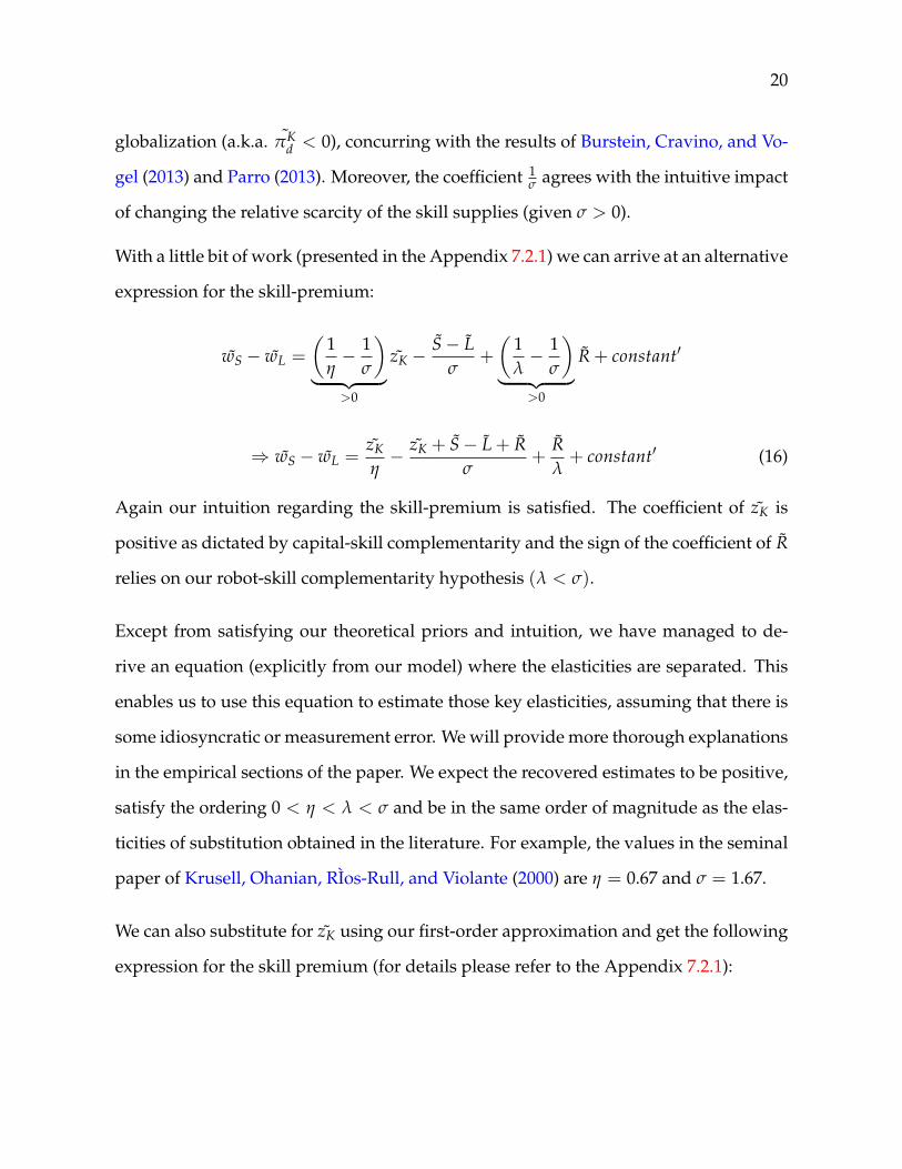
With a little bit of work (presented in the Appendix 7.2.1) we can arrive at an alternative

expression for the skill-premium:

wS − wL =

(1η− 1

σ

)︸ ︷︷ ︸

>0

zK −S− L

σ+

(1λ− 1

σ

)︸ ︷︷ ︸

>0

R + constant′

⇒ wS − wL =zK

η− zK + S− L + R

σ+

Rλ+ constant′ (16)

Again our intuition regarding the skill-premium is satisfied. The coefficient of zK is

positive as dictated by capital-skill complementarity and the sign of the coefficient of R

relies on our robot-skill complementarity hypothesis (λ < σ).

Except from satisfying our theoretical priors and intuition, we have managed to de-

rive an equation (explicitly from our model) where the elasticities are separated. This

enables us to use this equation to estimate those key elasticities, assuming that there is

some idiosyncratic or measurement error. We will provide more thorough explanations

in the empirical sections of the paper. We expect the recovered estimates to be positive,

satisfy the ordering 0 < η < λ < σ and be in the same order of magnitude as the elas-

ticities of substitution obtained in the literature. For example, the values in the seminal

paper of Krusell, Ohanian, RÌos-Rull, and Violante (2000) are η = 0.67 and σ = 1.67.

We can also substitute for zK using our first-order approximation and get the following

expression for the skill premium (for details please refer to the Appendix 7.2.1):

21

wS− wL =

(1η− 2

σ+

1λ

)︸ ︷︷ ︸

>0

R+

(λ

η− λ

σ

)︸ ︷︷ ︸

>0

ρ+

[(1η− 1

σ

)(λ− η

η

)− 1

σ

]S+

Lσ+

(λ

σ− λ

η

)︸ ︷︷ ︸

<0

πKd

θ+ cons

(17)

Again the signs of the coefficients are consistent with our assumptions. Consistent with

the results of Burstein, Cravino, and Vogel (2013) and Parro (2013) the skill-premium

increases with trade openness. The impact of change in stock of robots R and their

price ρ is positive. But, there is the caveat that these two changes are negatively related(R ↓↑ ρ

). Due to their simultaneous covariance, the counterfactuals of keeping the one

constant while changing the other are not that helpful. However, these counterfactuals

are not that meaningless if we revisit the idea presented in Arnaud (2018) that automa-

tion does not have to happen necessarily (i.e. change in R) but improvements in quality

(manifested as decreases in ρ) can increase the threat to automate and pressure wages

downward. This effect is manifested clearer in the following equations.

3.2.2 First-order approximation for the change in the real wages

We now use the same techniques to recover equations that describe changes in real

wage of each skill-type. We use equation 28 from the Appendix 7.2.1 and obtain the

following expressions. For the change in the real wage of the high-skilled labor we

have:

wS − PC =

(1η− 1

λ

)zK −

Sλ+

Rλ+

1η− 1

λ+ ρ− a

θ

(˜πMd

)and substituting for zK by equation 31 we get:

wS − PC =Rη+

λ

ηρ +

[1η

(λ

η− 2)]

S +

(1− λ

η

)︸ ︷︷ ︸

<0

πKd

θ− a

θ

(˜πMd

)+ constant′′ (18)

22

The coefficient to the supply of high-skilled labor is negative if λ and η are close enough.

While the real wage of skilled labor changes positively with trade openness since the

coefficient of the domestic trade shares are negative under the assumption of capital-

skill complementarity. The impact of change in stock of robots R and their price ρ is

positive. As we argued above, the positive coefficient in front of ρ suggests the down-

ward pressure on wages due to the threat to automate, as in discussed in Arnaud (2018).

Nevertheless, because of(

R ↓↑ ρ), it more instructive for our counterfactuals to substi-

tute for ρ by using the equation 30. Then we obtain:

wS − PC =zK

η+

(1λ− 2

η

)S− 1

θ

(a ˜πM

d − πKd

)+ constant′′′ (19)

Here, the impact of robots, which was manifested either through changes in prices or

quantities, is absent. The coefficients of the skill-supply and domestic trade shares of

manufacturing(

˜πMd

)is unambiguously negative as expected.

Lastly, we turn our attention the change in the real wage of the low-skilled labor is

obtained by:

wL − PC =(

wS − PC)− (wS − wL)

wL − PC =

(1σ− 1

λ

)︸ ︷︷ ︸

<0

zK +

(1σ− 1

λ

)︸ ︷︷ ︸

<0

S− Lσ + R

σ + ρ− aθ

(˜πMd

)+ const

⇒ wL− PC =zK

σ+

(1λ+

1σ− 2

η

)S− L

σ+

(1σ− 1

λ

)︸ ︷︷ ︸

<0

R+πK

dθ− a

θ

(˜πMd

)+ const′ (20)

Here, the coefficient of R is negative under our robot-skill complementarity assump-

23

tion.

wL − PC =

(2σ− 1

λ

)︸ ︷︷ ︸

>0<

R +λ

σρ +

1η

(η

λ+

λ

σ− 2)

S− Lσ+

(1− λ

σ

)︸ ︷︷ ︸

>0

πKd

θ− a

θ

(˜πMd

)+ cons (21)

When we substitute for zK we get that the impact of R is ambiguous depending on

the relative magnitude of the elasticities. The coefficient of ρ is positive but smaller

in scale than the respective impact for high-skilled labor, while the coefficient of πKd is

positive. Assuming πKd = πM

d the overall impact of trade openness depends on the sign

of a + λσ − 1.

All in all, with our assumptions of capital-skill and robot-skill complementarity, the in-

creasing usage of robots R is more beneficial to high-skilled labor. While improvements

in their quality (these can be thought as declines in ρ) affect negatively high-skilled la-

bor at a bigger extent. This is also true when it comes to trade openness: high-skilled

labor is benefited from globalization; this might not be the case for and the low-skilled

workers, as it depends on the exact magnitudes of the elasticity parameters.

4 Data description & Analysis

In this section we describe the data used and the exact steps for our empirical analysis

that includes estimation of key elasticity parameters

4.1 Data sources & description

For our estimations we need data on the operational stock of robots by country and

industry. The International Federation of Robotics (IFR) releases annual reports with

analytical data on both the number of robots delivered and stock of operational robots

24

for 50 countries at the industry level and by application, such as handling, dispensing,

processing or welding. For our purposes, we use the data on the operational stock of

robots. The data accounts for most countries starts since 1993. We also obtain data for

changes in price with or without adjusting for quality improvements from the 2006 IFR

World Robotics Report. At the industry level, a significant number of robots is denoted

as unspecified. Following Acemoglu and Restrepo (2017b), we classify these unspeci-

fied robots to each industry according to the proportions observed in the specified data.

We combine these with data that come from EUKLEMS (March 2008 edition). EUK-

LEMS, due to the work of van Ark and Jäger (2017), is a comprehensive database that

contains information on capital and labor inputs, outputs and growth accounting at an

industry-level for most OECD countries. From this database, we extract the compen-

sation share and hours-employed share by skill-type. Since, our model accounts for

two skill-types while EUKLEMS includes three types we combine their middle- and

low-skill type into one type. Hence, our skill characterization cut-off becomes high-

school graduation. Knowing these share variables are enough to construct the relative

skill-supply and the skill premium. We can also obtain data about the volumes of inter-

mediates goods (denoted as II_QI) and capital services volumes (CAP_QI), which are

readily available for every country at the industry level. Merging the data we have 24

observations at the country level and industry level observations for 8 countries (Ger-

many, Italy, the United Kingdom, France, Spain, Japan, Finland , and Sweden) and 9

manufacturing industries. This brings our total sample size to 96.

We also extract data on product exports by country from the Trade Map of the Inter-

national Trade Centre5. Specifically, we focus on exports of motor vehicles by Japan

5 Trade Map

25

and Germany, counties that dominate the global exports of industrial robots; these data

will be used for the construction of our instrumental variables. Lastly, we need data

on the domestic trade shares, which we find in Adao, Costinot, and Donaldson (2017).

Their data set includes all bilateral trade shares between a set of OECD countries, which

largely coincides with the list of countries covered by EUKLEMS and IFR. By putting

all data together we are left with 96 observations at the industry-sector–country level,

which we will use for our subsequent analysis.

4.2 Analysis

Our main analysis is going to be the estimation of the elasticity parameters. Having

recovered these parameters, their magnitude (or simply their relative order) can inform

us about the impact of automation through industrial robots on the skill-premium and

the real wages. Our work also allow us to conduct counterfactuals to determine the

impact of trade openness as well.

The key equation we have derived is:

wS − wL =zK

η− zK + S− L + R

σ+

Rλ+ constant

Assuming that there is some idiosyncratic error εi that is not captured by our model

(or information lost due to our approximation methods) we can uses this equation for

a regression analysis. We can perform a simple OLS regression assuming that εi sat-

isfies the moment condition. Since our equation is explicitly derived from a causal

model, our regression does not simply recover the coefficients of the best liner predic-

tor; these coefficients correspond to the key elasticity parameters of our model, which

have direct implications for our hypotheses of capital-skill and robot-skill complemen-

tarity. We also perform an OLS regression by controlling for the level of the observa-

26

tion (country-sector-industry). We recognize that this variation within country varia-

tion might partially contradict our model since we have argued that within a country

wages are equalized among sectors; hence, the skill-premium should vary only at the

country level. However, such a claim is not supported by the data. We leverage on this

fact and increase our sample size by constructing data at the industry-country level. If

we limited our analysis to the cross-country level we would have been left with just 24

observations. The small sample size would have given less credibility to our estimates;

making our subsequent analysis unreliable.

Even though our equation is derived from a causal model and there is not omitted vari-

able bias, there can be other causes of endogeneity. In addition to the potential mea-

surement error, a more serious consideration is reverse causality; robot adoption can be

influenced by the changes in the skill-premium. To address the banes of endogeneity

we need to come up with the appropriate instruments that safeguard us from biased

estimators, hoping that this will not come at the cost of losing statistical significance.

Since our observations come from the industry-country level, we need an instrument

that varies by country and one that varies by industry; by interacting the two we get

a valid instrument. We tried to follow Graetz and Michaels (2015) and instrument the

robot adoption by industry with a variable that measures the fraction of hours in an

industry that are replaceable given the replaceability of the occupations involved. The

failure of this approach at the first-stage led us to an instrument that leverages on the

fact that the idiosyncratic errors at the industry-country level are not correlated with

the global adoption trend. Under this IV moment assumption, we used the robot adop-

tion by industry at the global level, which yielded our instrument at the industry level

(it varies across industries, not countries).

For our instrument at the country level (it varies across countries, not industries) we

27

used the change in the exposure of countries to the top two exporters of industrial

robots, Japan and Germany6. Very conveniently, these two countries also export a lot

of vehicles. The changes in the imports of German and Japanese cars are used as instru-

ments for the changes in robot adoption. And since we have both Japan and Germany,

we effectively have two instruments (or even three if we take their average) to instru-

ment for robot adoption at the country level. Last step is two interact these two instru-

ment and obtain two (or even three) instrumental variables to use for a two-stage least

squares (2SLS) regression. Since robots(

R)

appear both alone and in zK + S− L + R

we can use two of these instruments for our analysis. Finally, for our third variable, zK,

we can instrument II_QI (intermediate input volumes) with CAP_QI (capital services

volumes). With three regressors and three instruments our 2SLS regression can be ex-

actly identified, which allows to proceed to our analysis having accounted for potential

endogeneity issues.

5 Results

We will be using the equation:

(wS − wL)i = constant +(zK)i

η−(zK + S− L + R

)i

σ+

(R)

iλ

+ εi

Since our model describes static equilibria we need to consider the changes between

two steady states. These states are the year 1996 and the year 2005 for all countries

to avoid variations related to time between our observations. We chose these steady

states since by 1995 all countries in our data set had already acquired some robots.

Furthermore, the two time periods cover a range of 10 years; while by stopping at 2005,

6 Top exporters of industrial robots

28

we avoid the distortions in the data because of the global financial crisis. Therefore, all

values are expressed as log changes, x = log(

x2005x1996

). Having all needed data in hand,

we proceed to our regression analysis.

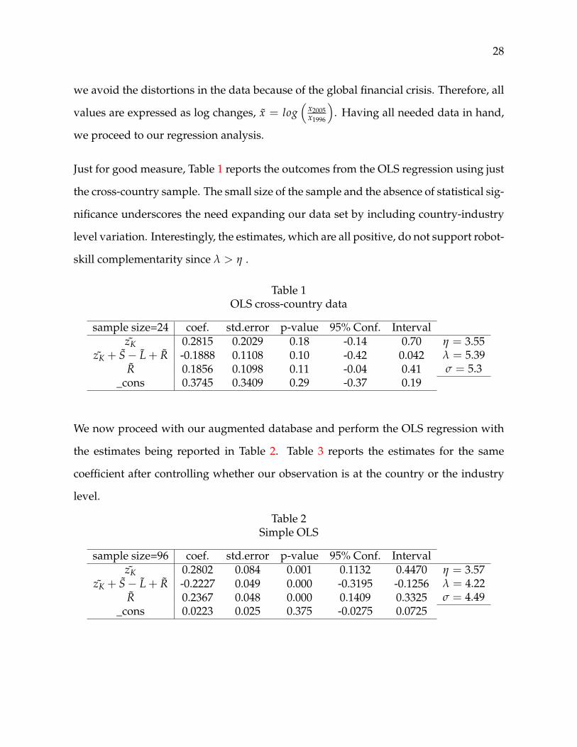
Just for good measure, Table 1 reports the outcomes from the OLS regression using just

the cross-country sample. The small size of the sample and the absence of statistical sig-

nificance underscores the need expanding our data set by including country-industry

level variation. Interestingly, the estimates, which are all positive, do not support robot-

skill complementarity since λ > η .

Table 1OLS cross-country data

sample size=24 coef. std.error p-value 95% Conf. IntervalzK 0.2815 0.2029 0.18 -0.14 0.70

zK + S− L + R -0.1888 0.1108 0.10 -0.42 0.042R 0.1856 0.1098 0.11 -0.04 0.41

_cons 0.3745 0.3409 0.29 -0.37 0.19

η = 3.55λ = 5.39σ = 5.3

We now proceed with our augmented database and perform the OLS regression with

the estimates being reported in Table 2. Table 3 reports the estimates for the same

coefficient after controlling whether our observation is at the country or the industry

level.

Table 2Simple OLS

sample size=96 coef. std.error p-value 95% Conf. IntervalzK 0.2802 0.084 0.001 0.1132 0.4470

zK + S− L + R -0.2227 0.049 0.000 -0.3195 -0.1256R 0.2367 0.048 0.000 0.1409 0.3325

_cons 0.0223 0.025 0.375 -0.0275 0.0725

η = 3.57λ = 4.22σ = 4.49

29

Table 3OLS with level-control

sample size=96 coef. std.error p-value 95% Conf. IntervalzK 0.2582 0.089 0.005 0.0797 0.4367

zK + S− L + R -0.2193 0.048 0.000 -0.3160 -0.1225R 0.2334 0.048 0.000 0.1379 0.3288

_cons 0.0506 0.028 0.375 -0.0275 0.0722

η = 3.87λ = 4.28σ = 4.55

We are pleased to see that the magnitudes of the elasticities are strongly positive and

are relatively close to one. Just as a reference point, Krusell, Ohanian, RÌos-Rull, and

Violante (2000) the corresponding elasticities, that they had recovered were η = 0.67

and σ = 1.67. Although the exact magnitudes will be also used for our subsequent

analysis, let us most importantly appreciate their cardinal order (η < λ < σ). This

ordering strongly and statistically significantly supports our robot-skill complementar-

ity hypothesis, while it also confirms the well-established capital-skill complementarity

assumption.

Given our concerns about endogeneity, we perform a 2SLS regression using the instru-

ments described above. The obtained estimates are moderately larger, hinting towards

the existence of attenuation bias due to measurement error. The estimates and the im-

plied elasticities are reported below in Table 4:

Table 4IV regression

sample size=96 coef. std.error p-value 95% Conf. IntervalzK 0.6493 0.258 0.012 0.143 1.155

zK + S− L + R -0.5388 0.228 0.018 -0.986 -0.091R 0.5514 0.24 0.022 0.081 1.021

_cons 0.136 0.09 0.134 -0.0275 0.0722

η = 1.54λ = 1.81σ = 1.85

The estimates obtained remain statistically significant with their ordering validating

the robot-skill complementarity hypothesis. Nevertheless, we cannot reject the null

30

hypothesis that λ > σ; hence the 2SLS estimates do not guarantee the existence of robot-

skill complementarity. Interestingly, Wooldridge (1995)’s robust score test that gives a

score of chi2(3) = 2.88831 (p-value=0.48), does not allow us to reject the exogeneity

hypothesis, leaving open the possibility that our regressors were exogenous in the first

place and that the OLS estimates were sufficient. In any case our estimates confirm the

existence of robot-skill and capital-skill complementarity.

5.1 Model accuracy

We can obtain the global average change in robot price from the IFR 2006 report to be

ρ = −0.372. When we use the estimates from our OLS[

η = 3.57, λ = 4.22, σ = 4.49

]and IV

[η = 1.54, λ = 1.81, σ = 1.85

]regressions and the equation

wS− wL =

(1η− 2

σ+

1λ

)R+

(λ

η− λ

σ

)ρ+

[(1η− 1

σ

)(λ− η

η

)− 1

σ

]S+

Lσ+

(λ

σ− λ

η

)πK

dθ

+ cons

, where cons = η−λλ(1−η)

+ λ−σσ(1−λ)

+ (σ−η)(λ−η)ση(η−1) . Then substituting for the respective values

of elasticities we get consOLS = 0.09 and consIV = 0.36. For the trade elasticity, we take

the value recovered by Simonovska and Waugh (2014) for the Eaton and Kortum (2002)

model of θ = 4.17. Then:

(wS − wL)OLSpred ' 0.07R + 0.24ρ− 0.22S + 0.22L− 0.06πK

d + 0.09 (22)

(wS − wL)IVpred ' 0.12R + 0.19ρ− 0.53S + 0.53L− 0.05πK

d + 0.36 (23)

According to our estimates and choice of parameters, we can see that the rising usage of

robots increases the skill premium, while the decline in prices ρ < 0, tends to decrease

the skill premium. Of course, as mentioned before these two forces function simulta-

neously and a “ceteris paribus” counterfactual is not that realistic, but it can have the

31

interpretation discussed by Arnaud (2018).

Comparing the predicted values with the observed log-changes in the skill-premium in

the cross-country-industry and cross-country level we obtain the respective model fits

in Figure 2 and Figure 3:

Figure 2: OLS model fit

Figure 3: IV model fit

We can evidently see that the OLS estimates have larger predicting power, which sup-ports the conjecture that our regressors are actually exogenous.

5.2 Measuring the impact of automation

It is easy to extract from our estimates the counterfactual impact of the increasing robot

adoption. “Ceteris paribus” (assuming prices do not change) a percentage increase in

the stock of robots will decrease welfare for the high-skilled by 0.28% (0.65%) and for

32

low-skilled by 0.21% (0.53%) according to our OLS (IV) estimates. We see that relative

gains are 2.32 (2.54) larger for the high-skilled. Hence, if our estimates are close to

reality the impact of robot is positive for the welfare of all consumers. Nevertheless, due

to our hypothesized and empirically validated robot-skill complementarity, increasing

automation widens the wage cap as they high-skilled claim a double share of the gains.

5.3 Is trade mitigating or amplifying the change in the skill-premium?

In our model, we did not have any direct interaction between the variables relevant

to robots (ρ and R) and domestic trade shares. However, there is an indirect link con-

nected with the decreases in cost. We find that in agreement with the results of Burstein,

Cravino, and Vogel (2013) and Parro (2013), trade openness amplifies the change in the

skill-premium. Due to lack of separate data on bilateral trade shares by sector, we

assume ˜πMii = πK

ii , ∀ ∈ N. Using equations 28 and 21, our elasticity estimates, a con-

sumption share of aM = 0.2 (as calibrated by Burstein, Cravino, and Vogel (2013) using

the OECD Input-Output Database), and a trade elasticity of θ = 4.17 (estimated for

the Eaton and Kortum (2002) model in Simonovska and Waugh (2014)), we measure

the impact of trade by skill-type. Using the OLS estimates, the impact of a percentage

decrease in the domestic trade share of capital(πK

ii)

benefits skilled-labor by 0.09% ,

compared to 0.03% for the low-skilled labor. These yield a ratio of 3; whereas, if we

use the IV estimates we find that the gains are 0.09% for the skilled-labor and 0.04% for

the unskilled labor, which give us a ratio of 2.25. Both are consistent with the 2.36 ratio

found by Burstein, Cravino, and Vogel (2013).

To illustrate our results we construct the counterfactual countries moving to autarky.

Since we do not have separate data on capital trade shares we assume due to greater

dependence on imported capital equipment that the domestic shares are half of the

33

respective manufacturing ones (πMii = 2πK

ii ). This assumption is supported by the trade

shares documented in Burstein, Cravino, and Vogel (2013); countries are more likely to

import capital equipment. For the πMii ’s we use the bilateral trade shares documented

in Adao, Costinot, and Donaldson (2017). Then, we plot the log-change in real wages

by skill-type over the log-change of trade shares from the 1996 levels to autarky. We can

get the following counterfactual results using our OLS estimates depicted in Figure 4.

As expected the return to autarky harms high-skilled labor more, but it is also harmful

to the low-skilled labor.

Figure 4: Move to Autarky

6 Conclusion

With the recent rise of automation, there is an increasing concern about the future of

jobs and wages. The clear displacement effect of robots is countervailed by their pro-

ductivity effect that can increase the value-added of labor while decreasing overall costs

of production and consumption. We enter this discussion by focusing our attention to a

specific but dominant form of automation, industrial robots. We develop a trade-based

34

model to capture the equilibrium impact of the increasing robot density in industries by

hypothesizing robot-skill complementarity in addition to capital-skill complementarity.

Our estimates which are obtained from a causal model regression support this conjec-

ture. Our approach shows that there are gains from automation for both skill-types;

these gains are favorably allocated to the high-skilled increasing the skill-premium.

Our model also predicts the impact of trade openness showing that the gains are larger

for the skilled-labor; this agrees with the existing literature. We hope that our anal-

ysis contributes interesting insights in the ongoing debate about automation and has

soothed fears about the future to some extent. Although we should pay attention to the

increasing inequality that can pose a serious challenge to social coherence, our findings

about the benefits of automation suggest that a Luddite revolution should wait for the

time being.

References

ACEMOGLU, D., AND P. RESTREPO (2017a): “Low-Skill and High-Skill Automation,”

NBER Working Papers 24119, National Bureau of Economic Research, Inc.

(2017b): “Robots and Jobs: Evidence from US Labor Markets,” Boston Univer-

sity - Department of Economics - Working Papers Series dp-297, Boston Univer-

sity - Department of Economics.

(2018): “The Race between Man and Machine: Implications of Technology

for Growth, Factor Shares, and Employment,” American Economic Review, 108(6),

1488–1542.

ADAO, R., A. COSTINOT, AND D. DONALDSON (2017): “Nonparametric Counterfactual

Predictions in Neoclassical Models of International Trade,” American Economic Re-

35

view, 107(3), 633–689.

ARKOLAKIS, C., A. COSTINOT, AND A. RODRIGUEZ-CLARE (2012): “New Trade Mod-

els, Same Old Gains?,” American Economic Review, 102(1), 94–130.

ARNAUD, A. (2018): “Automation Threat and Wage Bargaining,” Discussion paper,

Yale University.

ARTUC, E., P. S. R. BASTOS, AND B. RIJKERS (2018): “Robots, Tasks and Trade,” Policy

Research Working Paper Series 8674, The World Bank.

BCG (2015): “The Robotics Revolution: The Next Great Leap in Manufacturing,” Dis-

cussion paper, Boston Consulting Group.

BESSEN, J. (2016): Learning by Doing: The Real Connection Between Innova- tion, Wages,

and Wealth. Yale University Press.

BRYNJOLFSSON, E., AND A. MCAFEE (2014): The Second Machine Age: Work, Progress,

and Prosperity in a Time of Brilliant Technologies. W. W. Norton & Company.

BURSTEIN, A., J. CRAVINO, AND J. VOGEL (2013): “Importing Skill-Biased Technology,”

American Economic Journal: Macroeconomics, 5(2), 32–71.

DEKLE, R., J. EATON, AND S. KORTUM (2007): “Unbalanced Trade,” American Economic

Review, 97(2), 351–355.

EATON, J., AND S. KORTUM (2002): “Technology, Geography, and Trade,” Econometrica,

70(5), 1741–1779.

FREY, C. B., AND M. A. OSBORNE (2017): “The future of employment: How susceptible

are jobs to computerisation?,” Technological Forecasting and Social Change, 114(C),

254–280.

GRAETZ, G., AND G. MICHAELS (2015): “Robots at Work,” CEP Discussion Papers

dp1335, Centre for Economic Performance, LSE.

INTERNATIONAL FEDERATION OF ROBOTICS, I. (2016): “World Robotics: Industrial

Robots,” .

36

KARABARBOUNIS, L., AND B. NEIMAN (2013): “The Global Decline of the Labor Share,”

NBER Working Papers 19136, National Bureau of Economic Research, Inc.

KEYNES, J. M. (1930): Economic Possibilities for our Grandchildren.

KRUSELL, P., L. E. OHANIAN, J.-V. RÌOS-RULL, AND G. L. VIOLANTE (2000): “Capital-

Skill Complementarity and Inequality: A Macroeconomic Analysis,” Economet-

rica, 68(5), 1029–1054.

MCADAM, P., AND A. WILLMAN (2018): “Unraveling The Skill Premium,” Macroeco-

nomic Dynamics, 22(01), 33–62.

PARRO, F. (2013): “Capital-Skill Complementarity and the Skill Premium in a Quanti-

tative Model of Trade,” American Economic Journal: Macroeconomics, 5(2), 72–117.

SIMONOVSKA, I., AND M. E. WAUGH (2014): “The elasticity of trade: Estimates and

evidence,” Journal of International Economics, 92(1), 34–50.

VAN ARK, B., AND K. JÄGER (2017): “Recent Trends in Europe’s Output and Productiv-

ity Growth Performance at the Sector Level, 2002-2015,” International Productivity

Monitor, 33, 8–23.

WOOLDRIDGE, J. (1995): “Score diagnostics for linear models estimated by two stage

least squares,” Advances in Econometrics and Quantitative Economics: Essays in

Honor of Professor C. R. Rao, ed. G. S. Maddala, P. C. B. Phillips, and T. N. Srinivasan,.

37

7 Appendix

7.1 Cost-minimization

Given our production function: we can aggregate the factors as following:

zH ≡(

zη′

K + Hη′) 1

η′

zR ≡(

zλ′H + Rλ′

) 1λ

zF ≡(

zσ′R + Lσ′

) 1σ′

By cost minimization of a Cobb-Douglas production function for ∀ω, we can use the

Lagrangean to obtain:PF

iPM

i=

γ2,szM (ω)

γ1,szF (ω)

PNTi

PMi

=(1− γ1,s − γ2,s) zM (ω)

γ1,szNT (ω)

Also, by using Lagrangeans cost minimization implies:

zK (ω)

H (ω)=

(ri

wS,i

)−η

zH (ω)

R (ω)=

(PH

iρ

)−λ

zR (ω)

L (ω)=

(PR

iwL,i

)−σ

38

By proceeding through the calculation it can be shown that the cost function is

Ci,s,ω(q, PMi , PF

i , PNTi ) =

qB(

PMi)γ1,s

(PF

i)γ2,s (PNT

i)1−γ1,s−γ2,s

Ai,ω

where B ≡ γ−γ1,s1,s γ

−γ2,s2,s (1− γ1,s − γ2,s)

γ1,s+γ2,s−1

Then the marginal cost for each unit of good ωs is

MCi,s,ω(q, PMi , PF

i , PNTi ) =

B(

PMi)γ1,s

(PF

i)γ2,s (PNT

i)1−γ1,s−γ2,s

Ai,ω=

ci,s

Ai,ω(24)

7.2 The skill-premium

Given the total income at location i (i.e.GDPi − NXi = Xi − Di ), Yi = wS,iSi + wL,iLi +

ρRi + rizK,i + PMi zM,i + PNT

i zNT,iwe can obtain the following (to lighten up the notation

a little bit I have dropped the location subscripts i ):

wLL = γ2

(wL

PF

)1−σY

ρR = γ2

( ρ

PR

)1−λ(

PR

PF

)1−σ

Y

wSS = γ2

( ws

PH

)1−η(

PH

PR

)1−λ (PR

PF

)1−σ

Y

rzK = γ2

( rPH

)1−η(

PH

PR

)1−λ (PR

PF

)1−σ

Y

⇒wη

Swσ

L=(

PH)η−λ (

PR)λ−σ L

S(25)

39

We will be solving from bottom-up:

(r

wS

)1−η

=(zK

S

) η−1η

PH

wS=

((r

wS

)1−η

+ 1

) 11−η

=

((zK

S

) η−1η

+ 1

) 11−η

wS

ρ=

(PH

wS

) η−λλ(

RS

) 1λ

=

((zK

S

) η−1η

+ 1

) η−λλ(1−η) (R

S

) 1λ

(26)

rρ=

( SzK

) η−1η

+ 1

η−λ

λ(1−η) (RzK

) 1λ

(PH

ρ

)1−λ

=(zH

R

) λ−1λ

ρ

wL=

((zH

R

) λ−1λ

+ 1

) λ−σσ(1−λ) ( L

R

) 1σ

(27)

Hence the skill premium is given by:

wS

wL=

((zK

S

) η−1η

+ 1

) η−λλ(1−η) (R

S

) 1λ

((zH

R

) λ−1λ

+ 1

) λ−σσ(1−λ) ( L

R

) 1σ

⇒ wS

wL=

(z

σ−1σ

K + Sσ−1

σ

) η−λλ(η−1)

R1λ

(1S

) 1η(

zλ−1

λH + R

λ−1λ

) σ−λσ(λ−1)

L1σ

(1R

) 1λ

⇒ wS

wL=

(z

σ−1σ

K + Sσ−1

σ

) η−λλ(η−1)

(1S

) 1η(

zλ−1

λH + R

λ−1λ

) σ−λσ(λ−1)

L1σ

40

7.2.1 First-order approximation for the skill-premium

Given ηwS − σwL = (η − λ) PH + (λ− σ) PR +(

L− S), we can take the first-order

approximation that exp(x) = 1 + x and obtain that:

PRi = PF

i − wL,i +1

1− σ

PHi = ri + wS,i +

11− η

PRi = PH

i + ρ +1

1− λ

⇒ ηwS − σwL = (λ− σ)

(ρ +

11− λ

)+ (η − σ) PH +

(L− S

)⇒ ηwS − σwL = (λ− σ)

(ρ +

11− λ

)+ (η − σ)

(r + wS +

11− η

)+(

L− S)

⇒ wS − wL =

(λ− σ

σ

)(ρ +

11− λ

)+

(η − σ

σ

)(r +

11− η

)+

L− Sσ

⇒ wS − wL =

(λ

σ− 1)

ρ +(η

σ− 1) πK

dθ

+L− S

σ+ constant

We can also obtain a different expression. Given the relationship wSρ =

(z

η−1η

K + Sη−1

η

) η−λλ(1−η)

R1λ S−

1η ,

we apply our first-order approximation techniques to get:

wS − ρ =

(1η− 1

λ

)zK +

R− Sλ

+η − λ

λ (1− η)(28)

And from ρwL

=

(z

λ−1λ

H + Rλ−1

λ

) λ−σσ(1−λ)

L1σ R−

1λ we obtain:

ρ− wL =

(1λ− 1

σ

)zH +

L− Rσ

+λ− σ

σ(1− λ)

41

where ˜zH = zK + S + σσ−1

⇒ ρ− wL =

(1λ− 1

σ

)(zK + S +

σ

σ− 1

)+

L− Rσ

+λ− σ

σ(1− λ)

Hence, a different expression for the change in the skill-premium is:

wS − wL =

(1η− 1

σ

)zK −

S− Lσ

+

(1λ− 1

σ

)R + constant

⇒ wS − wL =zK

η− zK + S− L + R

σ+

Rλ+ constant (29)

Moreover, by the relationship rρ =

((SzK

) η−1η

+ 1

) η−λλ(1−η) (

RzK

) 1λ we obtain:

r− ρ =

(1η− 1

λ

)S +

η − λ

λ(1− η)+

R− zK

λ(30)

⇒ zK = R + λ (ρ− r) +(

λ− η

η

)S +

λ− η

η − 1(31)

Hence, the above expression for the skill-premium becomes:

wS− wL =

(1η− 2

σ+

1λ

)R+

[(1η− 1

σ

)(λ− η

η

)− 1

σ

]S+

Lσ+

(1η− 1

σ

)λ (ρ− r)+ constant

⇒ wS− wL =

(1η− 2

σ+

1λ

)R+

1η

(λ

η− λ

σ− 1)

S+Lσ+

(1σ− 1

η

)λ

(πK

dθ− ρ

)+ constant