Journal of Monetary Economics 24 (1989) 401-421. North-Holland

THE EQUITY PREMIUM PUZZLE AND THE RISK-FREE RATE PUZZLE

Philippe WEIL*

Harvard Unmmity, Cambridge, MA 02138, USA

Received August 1988, final version received July 1989

This paper studies the implications for general equilibnum asset pricing of a class of Kreps-Porteus nonexpected utility preferences characterized by a constant intertemporal elasticity of substitution and a constant, but unrelated, coefficient of relative risk aversion. It is shown that relaxing the parametric restriction on tastes imposed by the time-additive expected utility specification does not suffice to solve the Mehra-Prescott (1985) equity premium puzzle. An additional puzzle - the risk-free rate puzzle - emerges instead: why is the risk-free rate so low if agents are so averse to intertemporal substitution?

1. Introduction

The purpose of this paper is to study the implications for general equilib- rium asset pricing of the parametric class of Kreps-Porteus nonexpected utility preferences introduced recently by Epstein and Zin (1987a, b) and

myself [Weil (1987)l.l These preferences generalize, in a nonexpected utility framework, the commonly used time-additive, isoelastic expected utility speci- fication to allow for an independent parametrization of attitudes toward risk and attitudes toward intertemporal substitution. They are characterized by a constant intertemporal elasticity of substitution and a constant, but unrelated, coefficient of relative risk aversion, and thus relax the well-known constraint intrinsic to time-additive, isoelastic expected utility that the intemporal elastic- ity of substitution be the inverse of the constant coefficient of relative risk aversion.

Adopting this new class of preferences has clear benefits. Firstly, these preferences do not impose a behavioral restriction on tastes which is devoid of

*I thank Roger Farmer and RaJnish Mehra for helpful discussions, participants in the July 1988 NBER Summer Institute and in many workshops for useful comments, and the National Science Foundation (SES-8823040) for financial support.

‘See Kreps and Porteus (1978, 1979a, b) for the axiomatic foundations of these preferences.

0304-3932/89/$3,5O’Z’1989. Elsevier Science Publishers B.V. (North-Holland)

402 P Werl. Equity premmn and rrsk-free rate pales

any theoretical rationale and which has many unpleasant side-effects.’ Secondly, the data seem to reject the time-additive expected utility restriction, as established by Epstein and Zin (1987b) and Giovannini and Weil (1988). Thirdly, from an analytical point of view, this class of Kreps-Porteus prefer- ences is very simple to work with and a very natural generalization of isoelastic preferences to uncertainty.

In spite of these advantages, it is legitimate and necessary to wonder whether these new preferences contribute, even partially, to the resolution of any the many outstanding asset pricing or consumption theory puzzles. Do these puzzles disappear once preferences are ‘correctly’ specified and the expected, time-additive utility restriction lifted? Can we conclude that the role we had attributed, in the empirical difficulties of frictionless asset pricing or permanent income theories, to incomplete markets or liquidity constraints was misplaced, and that the only problem was in reality one of misspecification of preferences? It would be surprising that the answer to these purposefully provocative questions be positive - and indeed it is not, as this paper will suggest.

The test to which this study submits this new parametric class of nonex- petted utility preferences is the now standard one devised by Mehra and Prescott (1985): can an artificial representative agent economy, calibrated with plausible parameter values and output process, replicate the average secular level of the risk-free rate (0.75%) and of the risk premium on equity (6.20%)? We know, from Mehra and Prescott’s original work, that a representative agent economy with CES, time-additive, expected utility preferences and complete markets cannot pass this test - because of the inability of the model to fit both the level of the risk-free rate and the discrepancy between the safe and average risky rates. Does, however, an economy in which agents are endowed with the Kreps-Porteus generalization of CES preferences perform substantially better with respect to the Mehra-Prescott touchstone? While intuition suggests that it might - these new preferences afford an additional degree of freedom - the answer to this question is negative.

As I demonstrate below, the risk premium depends, for plausible calibra- tions of tastes and technology, almost exclusively on the coefficient of relative risk aversion. But this implies that relaxing the time-additive expected utility restriction on tastes does not substantially alter the fact, documented by Mehra and Prescott, that the model can replicate the risk premium only for astronomically high levels of risk aversion - thus leaving the equity premium

‘Among them figure prommently: (i) the impossibihty of replicatmg the behavior of agents who are both moderately risk-averse and yet very averse to intertemporal substitution (as most available empirical evrdence suggests is the case), and (u) the difficulty, pomted out by Hall (1985) of determining whether regressions of log growth rates of consumptron on mean log real interest rates provide an estimate of risk aversion or intertemporal substitution [see Well (1987) on this point].

P. Wed, Equity prenuum and risk-free rare puzzles 403

puzzle intact: there is simply not enough aggregate risk in the model to replicate the risk premium for plausibly risk-averse consumers. What emerges instead from the relaxation of this restriction and the appropriate calibration of tastes is, as we shall see, an additional puzzle, centered around the risk-free rate: why is it, if consumers are as averse to intertemporal substitution as some recent estimates suggest, that the risk-free rate is so low?

Epstein’s (1988) model - a Lucas tree economy peopled by consumers with Kreps-Porteus preferences - is very similar to the one developed here. While

the issues that he and I address are clearly related, they are distinct. His is a comparative statics study of the effects of risk aversion equilibrium asset prices in an economy with i.i.d. uncertainty, while my goal is to compare the equilibrium returns predicted by the model with historical data, and thus to provide a touchstone to evaluate the model.

The analysis proceeds as follows. Section 2 presents the model, and solves for equilibrium asset prices and rates of return. Section 3 establishes the main result of the paper: separating risk aversion from intertemporal substitution cannot, on its own, explain away the equity premium puzzle documented by Mehra and Prescott (1985). but instead highlights the existence of a risk-free rate puzzle. The conclusion summarizes the paper and outlines directions for further research.

2. The basic framework

The economy is similar, except for the agents’ preferences, to the one studied by Lucas (1978) and Mehra and Prescott (1985). I first describe technology and consumer behavior, and then compute equilibrium asset returns.

2.1, Technology

There is one perishable consumption good, a fruit, which is produced by nonreproducible identical trees whose number is normalized, without loss of

generality, to be equal to the size of the constant population. Let y, denote the number of fruits falling from a tree at time t, i.e., the dividend associated with holding a tree. It is assumed that the rate of growth of dividends, A,,, = y,+i/y,. is random and Markovian over a finite state space, with transition probabilities given by 3

with i, j = 1,2,. . . , Z -C cc, A, > 0, and c~=i+,, = 1, Vi. The uncertainty on

3The notation is purposefully smdar to the one used by Mehra and Prescott (1985)

404 P. Wed, Equty premum and risk-free rate puzzles

dividends at t + 1, and thus on y,+i/y,, is assumed to be resolved at the beginning of period t + 1, before time t + 1 consumption and savings deci- sions are made.

2.2. Consumers

The economy is inhabited by many identical infinitely-lived consumers. Let pt, x,, and c, denote, respectively, the fruit price of a tree at t, the number of (shares of) trees held at the beginning of period t, and consumption at t of a representative agent. The one-period budget constraint facing a representative consumer is then simply

c,+P,x,+l= (P,+Y,bt, t 2 0, (2)

with x0> 0 given. Letting R,+i = [ p,+ 1 + y,, J/p, denote the one-period (random) rate of return on a tree and rvI = ( pr + v,)x, represent beginning-of-

period wealth. the budget constraint (2) can be rewritten more compactly as

wr+1= fc+,b, - 4 (3)

I assume that agents are not indifferent to the timing of the resolution of uncertainty on temporal lotteries [as they are when preferences can be repre-

sented by a Von Neumann-Morgenstern (VNM) utility index] and that their preference ordering can be represented recursively as

v,= Lk,E,Y+i], (4

where E, denotes expectation conditional on information available at t.4 The aggregator function U[., .] is given by

qc, VI

= { (1 _ p)cl-p + p [l + (1 - P)(l _ y)v](l-~~~(‘-y)}(l-y)‘(l-p) - 1

(1 -P)(l -Y>

(5)

a parametrization of Kreps-Porteus preferences which, as Epstein and Zin (1987a) and Weil (1987) have independently shown, provides a generalization

%ee Kreps and Porteus (1978, 1979a, b) for an exposition of the axiomatic foundations of these preferences, and Attanasio and Weber (1989), Epstein and Zin (1987a, b), Epstein (1988), Farmer (1989). Giovannini and Weil (1988). and Weil (1987) for specific parametrizations and macroeco- nomic apphcations.

P. Weil, Equity premum and risk-free rate puzzles 405

of isoelastic utility which disentangles attitudes toward intertemporal substitu- tion and from behavior toward risk aversion.5

The parameter p > 0 represents the inverse of the (constant) elasticity of intertemporal substitution, y > 0 is the Arrow-Pratt (constant) coefficient of relative aversion for static gambles, and p E (0,l) measures the subjective discount factor under certainty. 6 The VNM time-additive expected utility specification emerges, up to a monotone transformation, as the special case in which y = p, i.e., as the special case in which the coefficient of relative risk aversion is restricted to be the inverse of the elasticity of intertemporal substitution.

To characterize the optimal consumption plan of the representative con- sumer, denote by V( w,, A,) the maximum utility attainable by an agent who has wealth w when the state of nature at t, summarized by the realized growth rate of dividends, is X,. This value function is the solution to the following functional equation:

V(w,, h,) = maxU[c,,E,V(w,+,, A,,,)] subject to (3). (6) CI

This functional equation of course reduces to the standard linear Bellman equation in the time-additive case y = p. The first-order condition for the maximization problem in (6) is simply

where U,, denotes the derivative of the aggregator function with respect to its i th argument (i = 1,2) evaluated at (c,, E,V,+ t), and V,, the derivative of the

value function with respect to wealth evaluated at (w,, X,). Using the envelope theorem and (7) one finds

Notice, from eq. (8), that while it remains true, with Kreps-Porteus prefer- ences, that an optimum program is characterized by the equalization of the marginal utility of wealth, Vu, to the marginal utility of consumption, Ur,,’ the latter depends (unless utility is time-additive) on expected future value. For our consumer, changes in the marginal utility of wealth do not solely reflect, in

‘The special cases p + 1 and y + 1 can be dealt with by applying de I’Hospttal’s rule to the aggregator function (5) Epstem (1988) chooses instead to write separate utility functions for these special cases.

6Under uncertamty, the subjective discount factor, 0; = au/l/aV, 1s in general time- and state-dependent: Kreps-Porteus preferences are a stochastic generalization of endogenous time preference.

‘For a framework in which this equality is violated, see Grossman and Laroque (1987).

406 P. Weil, Equuy premwn and risk-free rate puzzles

an optimal plan, changes in nondurable consumption, but also changes in expected future utility. Kreps-Porteus preferences thus introduce an effect very similar, at a formal level, to the one which would be associated with nonseparabilities in consumer durables or government purchases. This is the reason why they are, a priori, a good candidate for explaining asset pricing or consumption theory puzzles.

Substituting (8) into (7) yields the following Euler equation:

Et i

wJ1*+ 1 R

4 t+1 =

1

1.

which reduces to its familiar VNM form when the aggregator function is linear in its second argument, i.e., when U,, is a constant.

An analogous expression,

Et 1 uJJ1,+ 1 R

Ul, !Tr+1 =

I

1, (10)

applies to any asset with rate of return Rk,+l willingly held by our representa- tive consumer. Eq. (10) can be used, without rewriting the budget constraint (3) or redefining wealth, to price, in equilibrium, any inside asset in zero net

supply. To complete the characterization of the optimal consumption program, it

suffices to compute, from (3) and (5), the marginal rate of substitution

UJJ,,+,/U,, along an optimal consumption path. After some tedious but straightforward computations (see the appendix), one finds that, for any asset with rate of return R,, which is voluntarily held and for p # l,* it is the case that

an equation which holds, in particular, for the rate of return on trees

(Rk, = R,). As Epstein and Zin (1987a) emphasize, this equation shows that the covari-

ante between the return on asset k and the return on the market portfolio’ should be, in addition to covariance with consumption growth, a determinant of excess returns - unless, of course, utility is time- and state-additive, in

‘The functional form of the Euler equation 1s different when p = 1; see the appendix for detals.

9R f+, stands in for the rate of return on the market in this respectwe agent economy with only one type of tree and all other stores of value inside assets.

P. Wed, Equiy premrum und risk-free rate puzzles 407

which case the standard consumption capital asset pricing model (C-CAPM) obtains. While this observation can be used to explain the unsatisfactory empirical performance of the C-CAPM relative to the portfolio-based CAPM,” its general equilibrium implications, which I examine next, do not lend much overall support to the model - in the sense that the departure from the C-CAPM embodied in (11) does not solve the equity premium puzzle.

2.3. Equilibrium prrces and returns

In equilibrium, each representative agent must hold one tree (remember the normalization of section 2.1), i.e., x, = 1 for all t. By Walras’ law, this requires, from (2). that the entirety of period t (perishable) output be consumed during that period, so that

Turning first to the determination of the equilibrium price of tree, and proceeding as in Mehra and Prescott (1985), I look for a stationary equilib-

rium such that pt = w,); if the level output at t is yt and i is the state of state of nature at t (the realized rate of growth of output between t - 1 and t was h,). Note that this implies that the rate of return on a tree if state i is realized today and state J tomorrow is simply

p/+1 +Y,+l w +1 R r+1=

Pt = Lx,

Y (13)

Inserting this expression into the Euler equation (11) and using the market clearing condition (12) together with the specification (1) of the dividend process, one finds after a few straightforward manipulations that the w,‘s (i = 1,. . . , I ), which fully characterize equilibrium, are the nonnegative solu- tion, if it exists,” to the following system of 1 nonlinear equations:

i

(l-P)/(l--Y)

w, = p i Q-q “I/ + q’l-y”‘l-p) I for i=l,...,I. /=1

(14)

“See Giovanmm and Well (1988)

“Some restrictions on tastes and technology are of course necessary to ensure existence. They are henceforth assumed to be satlsfied

408 P. Weil, Equiy premium and risk-free rate puzzles

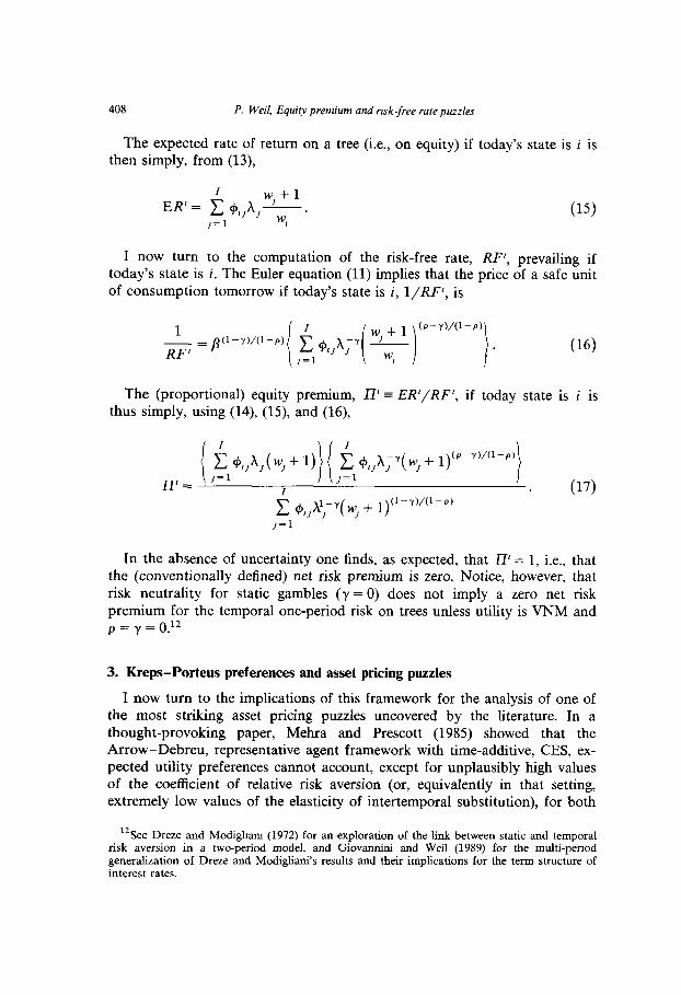
The expected rate of return on a tree (i.e., on equity) if today’s state is i is then simply, from (13),

w+l ER’ = i +,,$L

,=l w, .

I now turn to the computation of the risk-free rate, RF’, prevailing if today’s state is i. The Euler equation (11) implies that the price of a safe unit

of consumption tomorrow if today’s state is i, l/RF’, is

(16)

The (proportional) equity premium, LV = ER’/RF’, if today state is i is thus simply, using (14), (15) and (16),

:

I I

c +,,qw, + 1) c +,,A;‘( w, + l)(p--y)‘(l--p)

=,= J=l J=l

r (17)

1 $L$y WJ + ly)‘(l-) J=l

In the absence of uncertainty one finds, as expected, that II’ = 1, i.e., that the (conventionally defined) net risk premium is zero. Notice, however, that risk neutrality for static gambles (y = 0) does not imply a zero net risk premium for the temporal one-period risk on trees unless utility is VNM and p = y = 0.12

3. Kreps-Porteus preferences and asset pricing puzzles

I now turn to the implications of this framework for the analysis of one of the most striking asset pricing puzzles uncovered by the literature. In a thought-provoking paper, Mehra and Prescott (1985) showed that the Arrow-Debreu, representative agent framework with time-additive, CES, ex- pected utility preferences cannot account, except for unplausibly high values of the coefficient of relative risk aversion (or, equivalently in that setting, extremely low values of the elasticity of intertemporal substitution), for both

‘*See Dreze and Modigham (1972) for an exploration of the link between static and temporal risk aversion in a two-period model, and Giovannini and Weil (1989) for the multi-penod generalization of Dreze and Modigliani’s results and their implications for the term structure of interest rates.

P. Wed, Equity premium and risk-free rate puzzles 409

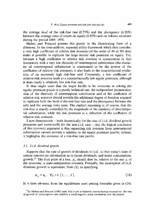
the average level of the risk-free rate (0.75%) and the discrepancv (6.20%) between the average rates of return on equity (6.95%) and on riskless securities during the period 1889-1978.

Mehra and Prescott present this puzzle in the illuminating form of a dilemma. In the time-additive, expected utility framework which they consider, a very high coefficient of relative risk aversion (of the order of 40 or 50) does make it possible to replicate the large secular risk premium on equity. Yet, because a high coefficient or relative risk aversion is synonymous in that framework with a very low elasticity of intertemporal substitution (the elastic- ity of intertemporal substitution is constrained to be the inverse of the coefficient of relative risk aversion), it also leads to the counterfactual predic- tion of an extremely high risk-free rate! Conversely, a low coefficient of relative risk aversion leads to a counterfactually low equity premium, although it does imply a relatively low risk-free rate.

It thus might seem that the major hurdle to be overcome in solving the equity premium puzzle is a purely technical one. An independent parametriza- tion of the elasticity of intertemporal substitution and of the coefficient of relative risk aversion should provide the additional degree of freedom required to replicate both the level of the risk-free rate and the discrepancy between the safe and the average risky rates. The implicit reasoning is, of course, that the risk-free is mainly controlled by the magnitude of the elasticity of intertempo- ral substitution, while the risk premium is a reflection of the coefficient of relative risk aversion.

I now demonstrate - both theoretically for the case of i.i.d. dividend growth processes and numerically for the non-i.i.d. case - that the logical conclusion of this (correct) argument is that separating risk aversion from intertemporal substitution cannot provide a solution to the equity premium puzzle: instead, it highlights the existence of a risk-free rate puzzle.

3.1. I.i.d. dividend growth

Suppose that the rate of growth of dividends is i.i.d., so that today’s state of nature conveys no information as to future dividends, and hence consumption, growth. l3 The fruit price of a tree, pt, should then be, relative to the size y, of the economy, a state-independent constant. Formally, the assumption of i.i.d. dividend growth is equivalent, from (1) to specifying

9,, = G, 1 Vj,iE{l,..., I}. (18)

It is then obvious, from the equilibrium asset pricing formulae given in (14),

13As Mehra and Prescott (1985) note, this is not a blatantly counterfactual assumption: the rate of growth of consumption only exhibits a small negative senal correlation over the period.

410

that

P. Well, Equgv premum and risk-free rate puzzles

U’, = K2’. Vi.

The equilibrium price function is simply pt = w);, where w is determined by substituting (19) into (14); the price-dividend constant when dividend growth is i.i.d.

09)

a constant ratio is a

An immediate implication of (19) is that, with i.i.d. dividend growth, the average risky and safe rates are state-independent [see eqs. (15) and (16)] and so is the equity premium II’. Its constant magnitude, denoted by 17. is, using eqs. (17) to (19).

(20)

From eq. (20) can be drawn an important conclusion: with i.i.d. drvidend growth, the equity premium, when defined in relative terms, is independent of the

elasticity of intertemporal suhstltution, and reflects only the properties of the dividend growth process and, of course, the magnitude of the coefficient of relative risk aversion.14

To understand this result, it suffices to remember that, with i.i.d. uncer- tainty, optimal consumption is a constant fraction of wealth.15 The rate of growth of consumption is, therefore, proportional to R,+l, the rate of return on the market portfolio [see eq. (3)]. As a consequence, the marginal rate of

substitution depends only on R,,, and the Euler equation (11) reduces to

(21)

which is the condition characterizing the static optimal portfolio allocation chosen by an agent with a coefficient of relative risk aversion equal to y! Eq. (21) simply establishes l6 that the intertemporal program reduces, in practice,

t4Analogous results have been obtamed by Barsky (1986) wtthm a two-penod framework based on Selden’s (1978) ordinal certainty eqmvalence preferences

“Preferences are homothettc - so that the ratio of consumption to wealth depends, at most, on the state of nature Dividend growth is i.t.d., so that this ratio (equal to the marginal und average propensity to consume) 1s a constant - because today’s state of nature conveys no mformatlon as to the future.

“See Huang and Litzenberger (1988) for a proof limited to the VNM case.

P. Wed, Equl[v premium and risk-free mte puzzles 411

to a sequence of disconnected static problems when underlying uncertainty is i i d l7 But then it is not surprising that, as eq. (20) shows, the risk premium on . . . equity depends only (for a given output process) on y, and that p is irrelevant - since intertemporal considerations play no role in the determina- tion of the optimal program with i.i.d. uncertainty.

While this result confirms the intuitive argument presented supru (the coefficient of relative risk aversion controls the risk premium and the elasticity of intertemporal substitution controls the level of the risk-free rate), it also proves that relaxing the time-additive expected utility restriction cannot possi- bly help solve the Mehra-Prescott equity premium puzzle when dividend growth is i.i.d. For any y, the equity premium is the same irrespective of whether p is equal to or different from y - i.e., irrespective of whether the expected, time-additive utility restriction is satisfied or not! Therefore, allow- ing attitudes toward risk to be parametrized independently from behavior towards intertemporal substitution cannot, with i.i.d. dividend growth, afford any improvement whatsoever over the results of Mehra and Prescott: indepen- dently of the value one might want to select for p (the inverse of the elasticity of intertemporal substitution), one will still need implausibly (of the order of 40) high values of y {the coefficient of relative risk aversion) to replicate the observed 6.20% risk premium on equity. The equity premium puzzle (‘why is the risk premium so large if consumers are only moderately risk-averse?‘) thus remains intact.

Another implication of the foregoing results is that relaxing, with i.i.d. uncertainty and for a given y, the time-additive, expected utility restriction in the direction of more plausible values might, while leaving the equity premium unchanged, deteriorate the ability of the model to replicate the level of the risk-free rate. It is commonly estimated that the coefficient of relative risk aversion is in the range of 1 to 5, with both theoretical [Arrow (1965)] and empirical [Epstein and Zin (1987b), Giovannini and Weil (1988)] grounds for thinking that it is in fact closer to 1. The implied value for the elasticity of intertemporal substitution under the expected, time-additive utility restriction, 0.2 to 1, runs counter to the belief that consumers are in fact very averse to intertemporal substitution, and thus seems to overestimate the ‘ true’ intertem- poral elasticity of substitution (i.e., underestimate the ‘true’ p). But it is easy to show [from (16) and the assumption of i.i.d. growth] that increasing p while maintaining y fixed may very well result, depending on the specification of the output process, in an increase in the predicted risk-free rate far over and above the already too high levels associated with the expected utility restriction!

The following section confirms and amplifies these results by turning to a numerical examination of the non-i.i.d. case.

“See Giovannmi and Wed (1988) for an elaboration of this and other related mues.

412 P. Werl. Equzty pretmum and rrsk-free rate puzzles

3.2. Non-i. i. d. dividend growth process

As the nonlinear nature of eq. (14) makes clear, one has to resort to numerical methods to solve for the equilibrium price function, as summarized by the u;‘s, when the dividend growth process is not i.i.d.

Mehra and Prescott observe that the evolution of the rate of growth of aggregate consumption (and thus, in this model, dividends) is well approxi- mated, over the period 1889-1978, by a two-state stochastic process:

A, = 1.054, h, = 0.984,

with transition probabilities

+it = +** = 0.43, @Ii2 = $21 = 0.57.

(22)

(23)

These magnitudes are used to solve for the W~‘S in (14) as well as for the state-dependent riskless and expected risky rates.

The Markov process in (22)-(23) has a probability @ = [l - $,,]/[2 - (ptl - +z2] = i of being in the good state, A,, in the long run. Given the three parameters p, y, and p which parametrize, respectively, consumers’ attitudes toward impatience, risk, and intertemporal substitution, this ergodic probabil- ity, @, can be used, as in Mehra and Prescott (1985) to compute the long-run

average risk-free rate, RF = @RF' + (1 - @)RF2, and the long-run average equity premium, IT = @LTI’ + (1 - @)n2, which are implied by the model.

Tables 1 and 2 report the average long-run risk premia and risk-free rate - for selected values of l/p between l/45 and infinity and y between 0 and 45 - for the cases j? = 0.95 and 0.98. The result are as distressing for the representative agent, complete market models as are Mehra and Prescott’s.

Under the expected time-additive utility restriction p = y,‘* decreasing the intertemporal elasticity of substitution amounts to increasing the coefficient of relative risk aversion, and results in the simultaneous rise of the risk premium and the risk-free rate - a property at the origin of the dilemma faced by Mehra and Prescott. There is no way to fit both the level of the risk-free rate and the risk premium when the VNM restrictions is imposed. If one wants to replicate the low observed secular risk-free rate, one needs to assume that the elasticity of intertemporal substitution is extremely large (by moving up the diagonal); but then agents are almost risk-neutral and the model cannot explain why the risk premium is so high. If one wants to fit the risk premium (by moving down the diagonal), one needs a coefficient of relative risk aversion of around 20: but the very small elasticity of intertemporal substitution which

lXThe correspondmg entries are read along the NW-SE diagonal of the tables.

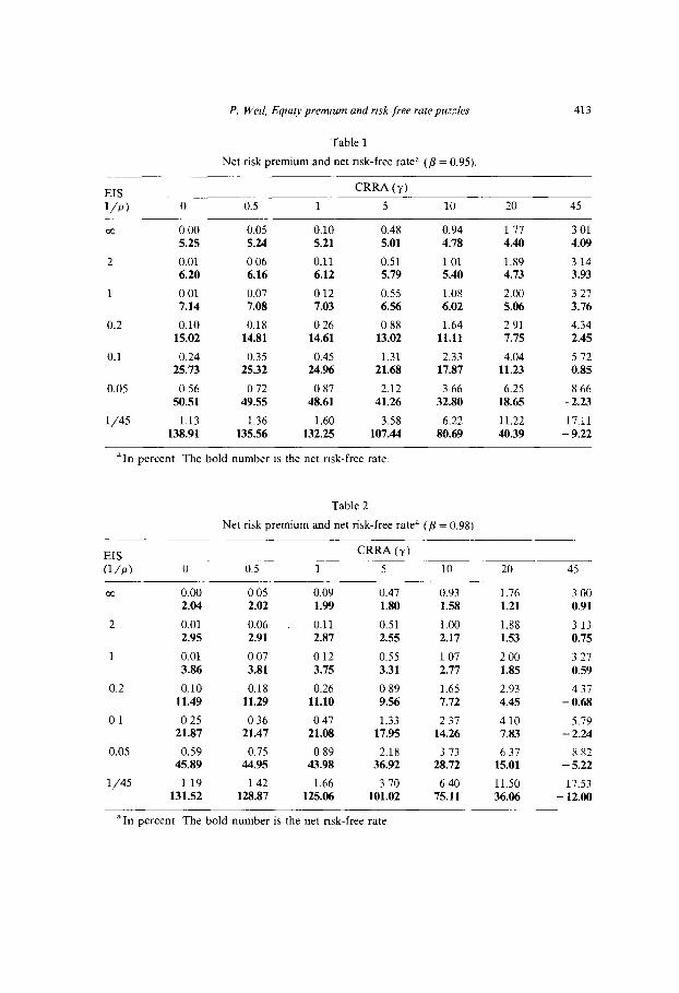
P. Wed, Eqtq premum and risk-free rate puzles 413

Table 1

Net risk premium and net risk-free ratea (/3 = 0.95)

EIS CRRA (u)

l/P) 0 0.5 1 5 10 20 45

m 0 00 0.05 0.10 5.25 5.24 5.21

2 0.01 006 0.11 6.20 6.16 6.12

1 001 0.07 012 7.14 7.08 7.03

0.2 0.10 0.18 0 26 15.02 14.81 14.61

0.1 0.24 0.35 0.45 25.73 25.32 24.96

0.05 0 56 0 72 0 87 50.51 49.55 48.61

l/45 1.13 1.36 1.60 138.91 135.56 132.25

0.48 0.94 1 17 5.01 4.78 4.40

0.51 101 1.89 5.79 5.40 4.73

0.55 1.08 2.00 6.56 6.02 5.06

0 88 1.64 2 91 13.02 11.11 7.75

1.31 2.33 4.04 21.68 17.87 11.23

2.12 3 66 6.25 41.26 32.80 18.65

3.58 6.22 11.22 107.44 80.69 40.39

3 01 4.99

3 14 3.93

3 21 3.76

4.34 2.45

5 72 0.85

8 66 - 2.23

17.11 - 9.22

‘In percent The bold number is the net risk-free rate.

EIS (l/P)

w

2

1

0.2

01

0.05

l/45

Table 2

Net risk premium and net risk-free ratea (/3 = 0.98)

CRRA (7)

0 0.5 1 5 10 20 45

0.00 005 0.09 0.47 0.93 1.76 3 00 2.94 2.02 1.99 1.80 1.58 1.21 0.91

0.01 0.06 . 0.11 0.51 1.00 1.88 3 13 2.95 2.91 2.87 2.55 2.17 1.53 0.75

0.01 007 0 12 0.55 1 07 2 00 3 27 3.86 3.81 3.75 3.31 2.77 1.85 0.59

0.10 0.18 0.26 0 89 1.65 2.93 4 37 11.49 11.29 11.10 9.56 7.12 4.4s -0.68

025 036 047 1.33 2 37 4 10 5.79 21.87 21.47 21.08 17.9s 14.26 7.83 - 2.24

0.59 0.75 0.89 2.18 3 73 6 37 8 82 45.89 44.95 43.98 36.92 28.72 15.01 - 5.22

119 142 1.66 3.70 6 40 11.50 17.53 131.52 128.87 125.96 101.02 75.11 36.96 - 12.00

“In percent The bold number is the net risk-free rate

414 P. Wed. Equity premrum and rrsk-free rate puzzles

this magnitude implies under the restriction p = y yields a much too large risk-free rate (at least 15%)!

Relaxing the restriction p = y clearly does eliminate, as hypothesized above. this dilemma. For any intertemporal elasticity of substitution l/p, increasing

the coefficient of relative risk aversion y raises the risk premium and lowers the risk-free rate. For any coefficient of relative risk aversion y, decreasing the intertemporal elasticity of substitution raises the risk-free rate and the risk premium. l9 For given p and y, an increase in p from 95% to 98% has almost no effect on the risk premium but, of course, decreases the risk-free rate by approximately 3%,.“O

One can exploit these properties to fit almost perfectly both the level of the risk-free rate and the risk premium on equity. For instance, choosing a very high coefficient of relative risk aversion (around 45) and an elasticity of intertemporal substitution not as small as the VNM would imply (around 0.10 instead of l/45 = 0.022) results, for p = 0.95, in a risk premium of 5.72% and a risk-free rate of 0.85%!”

While this clearly constitutes an improvement over what the Mehra- Prescott model with VNM utility could achieve, it is clear that this purported fit relies on an implausibly high coefficient of relative risk aversion. For more realistic configurations of the parameters, the numbers in tables 1 and 2 suggest instead that our representative agent, complete markets setup is unable to replicate the historical rates of return. If, for instance, one assumes that the coefficient of relative risk aversion is equal to 122 and the elasticity of intertemporal substitution is equal to 0.1, 23 the model predicts a risk premium of 0.45% (instead of 6.2%) and a risk-free rate between 20% and 25% (instead

of 0.75%)! This failure of the model is, in fact, more serious than when the VNM

restriction was imposed. It cannot be attributed anymore to the inability to control the levels of and the discrepancy between rates independently - since KP preferences lift this restriction and there is no dilemma anymore. It is now

“While the explanatton of the first effect ts straightforward m each of these two comparative statics general equilibrium experiments, the rattonale of the second result is more obscure These results are moreover not independent of the specification of the output process.

““A larger B stgnals less impattence. htgher savmgs, and thus results m a lower equihbrium nsk-free rate

lt1 do not allow for values of /3 above 1 - i.e., a negative subjective discount rate - although this 1s what one would find if one were to try to estimate /3. Analogously, in a Blanchard (1985) model with stochasttc lifetimes. estimates of the condttional death probabrhty are almost always negative - because thev decrease the effective subjective discount rate. A value of B above 1 or a negative death probability are a computer’s solution of the risk-free rate puzzle!

‘“See suprcr for the theoretical and empirical rationale of this choice. The argument also goes through with. say, y = 3.

‘3Thts is Hall’s (1988) estimate, as well as Campbell and Mankiw’s (1989).

P. Wed. Equrty premrum and risk-free rate puzhs 415

to be ascribed to two much more basic facts:

* there is not enough individual consumption riskz4 in this economy to explain why, if agents are only moderately risk-averse, the risk premium is so high;

l the average rate of growth of individual consumption is too high (1.8% per year) to be consistent, if agents are extremely averse to intertemporal substitution, with the very low risk-free rate.

There are, therefore, two distinct puzzles, which Mehra and Prescott could not clearly distinguish because of the restriction on preferences which they had imposed: the equity premium puzzle (H&Y is the risk predict so high?) and the risk-free rate puzzle (why the risk-free rate so iow?).

The latter puzzle is, of course, already apparent (but cannot be easily int~~reted) when the VNM restriction is imposed: for p = 0.98 and p = y = 1. the predicted safe rate is 4%. But it is made much starker when the elasticity of intertemporal substitution is allowed to decrease from the relatively high level implied by the VNM restriction towards smaller and more realistic values, as the safe rate increases very rapidly when l/p declines.

3.3. Robustness

The conclusion that there is both an equity premium puzzle and a risk-free rate puzzle is robust, as were Mehra and Prescott’s original results, to modifi- cations of the output growth process which maintain its first two moments set at their historical vafues. This is hardly surprising as, loosely speaking, the risk-free rate puzzle has to do with the average rate of growth of consumption and the equity premium puzzle with its variability.

It is not robust to the introduction of extremely catastrophic2s scenarios B la Rietz (1988). but survives, for reasonable degrees of risk aversion. the intro- duction of mildly disastrous states of nature - as do Mehra and Prescott’s results.26

An often raised question is whether the claims being priced correspond to the names being attached to them: is ‘equity’ truly equity? Within the confine of the model. yes.

Is the exchange economy assumption constraining? No, in the sense that, as Mehra (1987) has shown, the set of equilibrium asset returns obtained in a production economy is included in the set of equilibrium returns computed from an exchange economy. Yes, however. in the sense that the model is

“4The appropriate measure of risk is the one implied by the Euler equatlon (11)

“And, m my view, somewhat absurd

%ee their (1988) rejomder to Rietz, whxh applies, after suitable rn~i~eatl~ns of preferences. to the framework analyzed here.

416 P. Wed, Equtty premtum and risk-free rate puzzles

calibrated by assuming that aggregate dividends are equal to aggregate con- sumption of nondurables and services - a somewhat arbitrary and not incon- sequential choice.

The assumption that the economy is closed to foreign trade is restrictive, for it imposes that consumption be equal to domestic output - which clearly needs not be the case in a multi-country world.

Is the assumption of generalized isoelastic utility constraining? It is, for recent work by Constantinides (1987) suggests that habit formation prefer- ences (which yields time-nonseparable but state-separable representation of tastes) replicate first moments (but not second moments) of asset returns much more satisfactorily.

4. Conclusion

This paper has studied the implications for general equilibrium asset pricing of a recently introduced class of Kreps-Porteus nonexpected utility prefer- ences, which is characterized by a constant intertemporal elasticity of substitu- tion and a constant, but unrelated, coefficient of relative risk aversion.

It has been shown that the solution to the equity premium puzzle docu- mented by Mehra and Prescott (1985) cannot be found by simply separating risk aversion for intertemporal substitution. If the dividend growth process is i.i.d., the risk premium, when appropriately defined, is independent of the intertemporal elasticity of substitution, and thus is the same whether or not the time-additive, expected utility restriction is imposed. When the dividend growth process is non-i.i.d., relaxing the parametric restriction on tastes imposed by the time-additive, expected utility specification adds, for plausible parameter values, a risk-free rate puzzle to Mehra and Prescott’s equity

premium puzzle.

In the search for a solution to these puzzles, one could relax some of the simplifying assumptions pointed out in the previous section: this clearly cannot but improve the fit of the model. Nevertheless, the empirical potential of such modifications pales, in my view, before the extreme restrictiveness of two other fundamental tenets of the model: the existence of a representative agent and the assumption of complete Arrow-Debreu security markets.

As first hinted by Mehra and Prescott, and as confirmed by some recent results,27 introducing heterogeneity between agents in the form of undiversifi- able individual consumption risk goes a long way towards explaining both the equity premium and risk-free rate puzzles. If individual consumption is more risky than aggregate consumption, one can explain why the risk premium is large even though agents are only moderately risk-averse in the aggregate. At the same time, the price a consumer will be willing to pay for a safe unit of

“See Ma&w (1986), Ben Zvi and Sussmann (1988), or Kahn (1988)

P. Wed, Equr fy premrum and risk-free rate puzzles 417

consumption tomorrow will rise - i.e., the risk-free rate will decrease. There-

fore, the existence of heterogeneity and of market imperfections is likely to hold center stage in the explanation of the equity premium and risk-free rate puzzles.

Appendix A: Euler equation and outline of the numerical solution

This appendix derives eq. (11) in the text for the case p # 1, outlines the pecularities of the case p = 1, and sketches the procedure used to numerically solve the model.28

A. 1. General case (p # 1)

We need to compute the marginal rate of substitution,

M, = ~2*~,,+,/~,,1 (A.1)

and to prove that it can be written as in eq. (11). Because of the homogeneity properties of the aggregator function, of the

interpretation of y as the coefficient of relative risk aversion, and of the fact that preferences are isoelastic, guess that the value function can be written in the form

A(h)w’-Y- 1

T/(w,h)= (l-p)(I_+ 64.2)

where A(. ) is an unknown function, and that the consumption function is linear in wealth:

where p( A,) is the state-dependent marginal propensity to consume. It is easy to show, performing the maximization called for by (6), that the functions A( .) and p( .) are related by the following two conditions:

and

(1 - P)[PL(&)l -p= Pm- PO,)1 -p (A-4)

A(A,) = (1 _ p)(l-Y)/(iLP)[P(Xr)] -PKwA-P)l, (A4

28The Gauss programs are available on request.

418 P Wed. Equrty premum and risk-free rate puzzles

where 4= %{A(~,+l)[R,+lI - > ’ Y c1 -P)/(l -y). The solution to these functional equations is closed in only a few cases.

Using the budget constraint (3) along with (A.3) (A.4). and (AS) imply that, along an optimal program,

/j(l-Y)/(l-P)

(1 y)/(l--P) c,,1 [ 1

PN-Y)/(l--P)l

A;h,+,)R:;: = p - c, R$Y)/(~-P). (~.6)

an expression which will be used infra. From (5) it is straightforward to show that the marginal rate of substitution

defined in (A.1) is

(A.71

where y+ 1 denotes the value function evaluated at ( w~+~, A,,,). Using the budget constraint (3) along with (A.2) and (A.3) one finds that

WC+1 OCl-YM-P)

-= V lil &,+,)R:;: ’ (A-8)

so that, substituting (A.6) and (A.8) into (A.7) we find that

R[#t;:)/(l-P)l--l (A.9)

an expression which, inserted in (lo), yields the Euler equation (11). Given the specification in (1) of a discrete state space, this Euler equation

yields, in equilibrium, Z equations in the Z unknown price-dividend ratios (the w,‘s). This (in general nonlinear) system of equations must be solved numerically.

The special case of a unit coefficient of relative risk aversion can be dealt with by directly setting y = 1 (or, when necessary, using de 1’Hospital’s rule) in the above equations.

A.2. Unit elasticity of intertemporal substitution

For a unit elasticity of intertemporal substitution, the functional form of the consumer’s Euler equation is not the one given in eq. (11) and the solution procedure therefore differs slightly from what was outlined above. In the

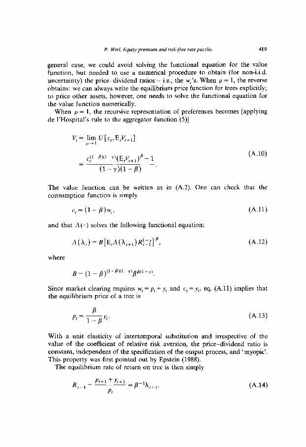
P. Wed, Equity prenuum and risk-free rate puzzles 419

general case, we could avoid solving the functional equation for the value function, but needed to use a numerical procedure to obtain (for non-i.i.d. uncertainty) the price-dividend ratios - i.e., the w,‘s. When p = 1. the reverse obtains: we can always write the equilibrium price function for trees explicitly; to price other assets, however, one needs to solve the functional equation for the value function numerically.

When p = 1, the recursive representation of preferences becomes [applying de 1’Hospital’s rule to the aggregator function (5)]

cjl-P)(‘-y)(E,~+,)‘- 1

(1 -Y)(l -P) .

(A.lO)

The value function can be written as in (A.2). One can check that the consumption function is simply

c,= (1 -P)w,, (A.ll)

and that A ( .) solves the following functional equation:

A(h) =BIW(X,,,)R:,:lp, (A.12)

where

B = (1 _ ,fj)(1-‘-y)p8(1-~).

Since market clearing requires w, = pt + y, and c, = y,, eq. (A.ll) implies that the equilibrium price of a tree is

P PI= l_ pJ+ (A.13)

With a unit elasticity of intertemporal substitution and irrespective of the value of the coefficient of relative risk aversion, the price-dividend ratio is constant, independent of the specification of the output process, and ‘myopic’. This property was first pointed out by Epstein (1988).

The equilibrium rate of return on tree is then simply

R 1+1= pt+1 +yt+1 = pA,+,_

Pt (A.14)

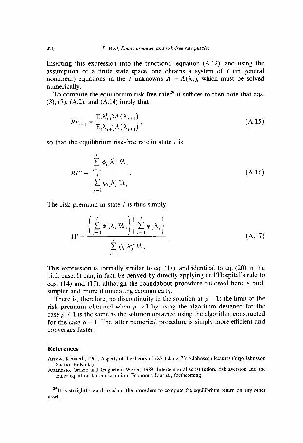
420 P. Wed, Equity premum and rrsk-free rate puzzles

Inserting this expression into the functional equation (A.12). and using the assumption of a finite state space, one obtains a system of I (in general nonlinear) equations in the I unknowns A, = A( A,), which must be solved numerically.

To compute the equilibrium risk-free rate 29 it suffices to then note that eqs. (3) (7). (A.2), and (A.14) imply that

so that the equilibrium risk-free rate in state i is

The risk premium in state i is thus simply

(A.15)

(~.i6)

(A- 17)

c +,J”J- yA, J=l

This expression is formally similar to eq. (17), and identical to eq. (20) in the i.i.d. case. It can, in fact, be derived by directly applying de 1’Hospital’s rule to eqs. (14) and (17) although the roundabout procedure followed here is both simpler and more illuminating economically.

There is, therefore, no discontinuity in the solution at p = 1: the limit of the risk premium obtained when p + 1 by using the algorithm designed for the

case p # 1 is the same as the solution obtained using the algorithm constructed for the case p = 1. The latter numerical procedure is simply more efficient and converges faster.

References

Arrow, Kenneth, 1965, Aspects of the theory of risk-taking, Yr~o Jahnsson lectures (Yr~o Jahnsson Saatio, Helsmki).

Attanaslo, Orazio and Gughelmo Weber, 1989, Intertemporal substitution, risk averslon and the Euler equation for consumption, Economic Journal, forthcoming

291t is straightforward to adapt the procedure to compute the equilibrium return on any other asset.

P. Wed, Equr(y premium and risk-free rate puzzles 421

Barsky, Robert, 1986. Why don’t the prices of stocks and bonds move together?, National Bureau of Economic Research working paper no. 2047.

Ben Zvi. Shmuel and Oren Sussmann, 1988, The equity premium and the volatility of the rate of return on stocks, Mimeo. (Center for the Study of the Israeli Economy, MIT.. Cambridge,

M“% Campbell, John and N. Gregory Mankiw, 1989, Consumption, income and mterest rates:

Reinterpretmg the time-series evidence. National Bureau of Economic Research working paper no. 2924.

Blanchard. Olivter. 1985. Debt, deficits, and finite horizons, Journal of Political Economy 93, 223-247.

Constantimdes. George, 1987. Habit formation: A resolution of the equity premium puzzle, Mtmeo. (University of Chicago, Chicago, IL).

Dreze. Jacques and Franc0 Modigliani, 1972, Consumption decisions under uncertainty, Journal of Economic Theory 5. 308-335.

Epstein, Larry, 1988, Risk aversion and asset prices, Journal of Monetary Economics 22. 177-192. Epstein, Larry and Stanley Zin, 1987a, Substitution, risk aversion, and the temporal behaviour of

consumption and asset returns I. A theoretical framework, Mimeo. (University of Toronto, Toronto, and Queens’ University, Kingston, Ont.).

Epstein, Larry and Stanley Zm, 1987b, Substitution, risk aversion, and the temporal behaviour of consumption and asset returns: II: An empirical investigation, Mimeo. (University of Toronto, Toronto, and Queens’ University, Kingston, Ont.).

Farmer. Roger, 1989, R I N C.E. preferences, Mmeo. (University of California, Los Angeles, CA). Giovannim, Albert0 and Philippe Weil. 1988, Risk averston, intertemporal substitution. and the

capital asset pricing model, Mimeo. (Columbia Umversity, New York, NY, and Harvard University, Cambridge, MA).

Giovanmni. Albert0 and Philippe Weil, 1989, Risk aversion, intertemporal substttution, and the term structure of interest rates, Mimeo. (Columbia Umversity, New York, NY, and Harvard University, Cambridge, MA).

Grossman, Sanford and Guy Laroque, 1987, Asset pncing and optimal portfolio choice m the presence of ilhquid durable consumption goods, National Bureau of Economic Research working paper no. 2369

Hall, Robert, 1985. Real interest and consumption, National Bureau of Economic Research workmg paper no. 1694

Hall, Robert, 1985, Intertemporal substitution in consumption, Journal of Political Economy 96, 221-273.

Huang, Chi-Fu and Robert Litzenberger, 1988, Foundations for financial economics (North- Holland, Amsterdam).

Kahn. James. 1988, Moral hazard, imperfect risk sharing, and the behavior of asset returns, Mimeo. (University of Rochester, Rochester, NY).

Kreps, David and E. Porteus, 1978, Temporal resolution of uncertamty and dynamic choice theory, Econometrica 36, 185-200.

Kreps, David and E Porteus. 1979a. Dynamic choice theory and dynamic programming, Econo- metrica 47, 91-100

Kreps, David and E. Porteus, 1979b, Temporal Von Neumann-Morgenstem and induced prefer- ences, Journal of Economic Theory 20, 81-109.

Lucas. Robert, 1978, Asset prices in an exchange economy. Econometrica 46, 1426-1445. Mankiw. N. Gregory. 1986, The equity premium and the concentration of aggregate shocks,

Journal of Financial Economics 17. 211-219. Mehra. RaJmsh, 1987, The equity premium in exchange and production economies, Mimeo.

(M LT.. Cambridge, MA). Mehra, RaJnish and Edward Prescott, 1985, The equity premium: A puzzle, Journal of Monetary

Economics 10, 335-359 Mehra. RaJnish and Edward Prescott, 1988, The equity risk premium: A solution?, Journal of

Monetary Economics 22.133-136 Rietz. Thomas, 1988. The equity nsk premium: A solution. Journal of Monetary Economics 22,

117-132. Weil, Philippe, 1987, Non-expected utility in macroeconomics, Quarterly Journal of Economics,

forthcoming.