Paper 124

HWWI Research

The Estimation of Reservation Wages: A Simulation-Based Comparison

Julian S. Leppin

Hamburg Institute of International Economics (HWWI) | 2012ISSN 1861-504X

Julian S. LeppinHamburg Institute of International Economics (HWWI)Heimhuder Str. 71 | 20148 Hamburg | GermanyPhone: +49 (0)40 34 05 76 - 669 | Fax: +49 (0)40 34 05 76 - 776leppin@hwwi.org

HWWI Research PaperHamburg Institute of International Economics (HWWI)Heimhuder Str. 71 | 20148 Hamburg | GermanyPhone: +49 (0)40 34 05 76 - 0 | Fax: +49 (0)40 34 05 76 - 776info@hwwi.org | www.hwwi.orgISSN 1861-504X

Editorial Board:Thomas Straubhaar (Chair)Michael BräuningerSilvia Stiller

© Hamburg Institute of International Economics (HWWI) April 2012All rights reserved. No part of this publication may be reproduced, stored in a retrieval system, or transmitted in any form or by any means (electronic, mechanical, photocopying, recording or otherwise) without the prior written permission of the publisher.

The Estimation of Reservation Wages: A

Simulation-Based Comparison

Julian S. Leppin∗

April 2012

Abstract This paper examines the predictive power of different es-

timation approaches for reservation wages. It applies stochastic frontier

models for employed workers and the approach from Kiefer and Neumann

(1979b) for unemployed workers. Furthermore, the question of whether

or not reservation wages decrease over the unemployment period is ad-

dressed. This is done by a pseudo-panel with known reservation wages

which uses data from the German Socio-Economic Panel as a basis. The

comparison of the estimators is carried out by a Monte Carlo simulation.

The best results are achieved by the cross-sectional stochastic frontier

model. The Kiefer-Neumann approach failed to predict the decreasing

reservation wages correctly.

Keywords: Job search theory, Monte Carlo simulation, reservation

wages, stochastic wage frontiers

JEL Classification: C21, C23, J64.

∗Hamburg Institute of International Economics (HWWI) and Christian-Albrechts-University Kiel. Email: leppin@hwwi.org.The author is grateful to Uwe Jensen and Bjorn Christensen for advice and sugges-tions.

1

1 Introduction

Unemployment and its determinants, this topic has been receiving increasing attention in

many western countries since the financial crisis and the following economic crisis. During

the crisis, unemployment, accompanied by all its negative impacts on the individual level as

well as on macroeconomic levels, started to rise in nearly all countries. Thus, it is essential

to reveal and understand the reasons for unemployment.

One theoretical model that tries to explain unemployment from a microeconomic point of

view is the Search Theory, introduced by McCall (1970), which models the decision process

to take up a job for unemployed persons with imperfect information. The Search Theory

assumes that each unemployed person is faced with the decision to accept a job offer at a

given wage or to remain unemployed and wait for a better offer in the next period. The final

decision to decline a job offer and to stay unemployed or to accept a job offer is made by

the use of individual reservation wages, which represent the minimum acceptable wage.

The reservation wages itself are not directly observable, so indirect measurement tech-

niques have to be applied. According to Jensen et al. (2010), one of the following three

possibilities can be chosen: direct questions, the approach of Kiefer and Neumann (1979b)

and the estimation of reservation wages with the use of stochastic frontier models. In this

paper, only the last two approaches are applied. The approach of Kiefer and Neumann uses

information on accepted wages after spells of unemployment and tries to infer reservation

wages for unemployed persons with the help of the Search Theory. This approach is used by

Boheim (2002) for British data from the British Household Panel Survey, by Schmidt and

Winkelmann (1993) for German data from the Zentralarchiv fuer Empirische Wirtschafts-

forschung and by Christensen (2005) for German data from the German Socio-Economic

Panel (GSOEP).

The second approach is the estimation of reservation wages for employed persons with

the use of stochastic frontier estimators, which was conducted for the first time by Hoffler

and Murphy (1994). It identifies reservation wages via the prediction of cost efficiency after a

frontier estimation. Application of frontier models for the estimation of reservation wages can

be found in Jensen et al. (2010) for German data from the Institute for Employment Research

(IAB) and in Cornwell and Schneider (2000) for Germany with the GSOEP. Furthermore,

two approaches of reservation wage estimation restricted to the financial service labor market

are available. Webb et al. (2003) estimated the overpayment in the banking sector of the

United Kingdom (UK) with data from the British Household Panel Survey by stochastic

frontier techniques. They defined the overpayment as any wage which is located above the

reservation wage. Closely related is the work from Watson and Webb (2008) which does the

same estimation for German and British data from the European Community Household

Panel Survey (ECHPS).

Apart from the estimation process, an often controversial issue is the behavior of persons

during the unemployment period. The question is if they lower their reservation wages

2

during the period of unemployment or if they keep the reservation wage constant until they

find an adequate job. The problem in estimation arises because constant reservation wages,

as stated by the basic Search Theory, could lead to rising observed reservation wages with

longer unemployment duration since only persons with high wage requests stay unemployed.

However, the Search Theory can in fact be adjusted to “produce” decreasing reservation

wages, for example by the use of duration-dependent stigmata of unemployed, such as found

in the work of Vishwanath (1989). Several empirical studies have examined the question

of constant reservation wages; to mention just two of them: Prasad (2003) using Dutch

data, found no relationship with a simple ordinary least square (OLS) regression, but a

positive relationship with instrumental variables (IV) regression, which could be interpreted

as support for the constant reservation wage hypothesis. On the other hand, Maani and

Studenmund (1986) found a decreasing reservation wage over the unemployment duration

for Chile. Thus, it remains unclear what underlying nature prevails for the reservation

wages. But the Kiefer-Neumann approach might be able to detect a decreasing or constant

reservation wage if it is applied to different time periods; Christensen (2005) used it in this

way.

Therefore, this paper examines the behavior of the different measurement techniques for

reservation wages and, at the same time, analyzes whether or not these estimators are able

to find the underlying reservation wage structure over the unemployment duration. This is

done by a Monte Carlo simulation where a pseudo-panel with observable reservation wages

is created. In a second step, the simulated data are used for the application of the different

estimators. The objective is to simulate a panel data set which is reasonably close to a

true panel like the GSOEP but with a known underlying process of employment transition.

The GSOEP served as a base for the simulation design, delivering starting values for the

simulation.

The plan of this paper is as follows. Sections 2 and 3 present the theoretical basis of the

estimation approaches. Section 4 introduces the data set and the preceding wage estimation.

Section 5 explains the simulation, which is built with the help of the obtained values from

the wage estimation and section 6 provides the results. The paper concludes with chapter 7.

2 Kiefer-Neumann Estimator

The section at hand briefly introduces the estimation approach of Kiefer and Neumann,

presented in the works of Kiefer and Neumann (1979a) and Kiefer and Neumann (1979b).

A more detailed derivation of the estimator can be found in the works of Christensen (2005)

and Schmidt and Winkelmann (1993). The approach is used to compare reservation wages

for unemployed persons, using interview data, with estimated ones. The objective of this

estimator is to not use requested reservation wage data, but to construct the reservation

wages with the use of observable accepted wages and concepts of the Search Theory. As

mentioned before, the estimation approach of Kiefer and Neumann is based on the reservation

3

wages derived from the Search Theory. This paper will present just the very basic thoughts

of the search theory, a detailed survey can be found in Devine and Kiefer (1991).

A successful match is achieved if an unemployed person receives and accepts a job offer

with a given wage offer. Normally, an unemployed person tries to find a new job during

his/her period of unemployment. A wage offer is considered to be sufficient if it exceeds the

reservation wage, which differs from one person to another since all labor market endowments

(education, age etc.) are variable.

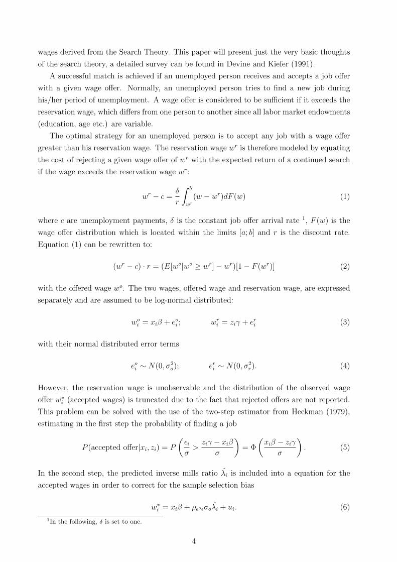
The optimal strategy for an unemployed person is to accept any job with a wage offer

greater than his reservation wage. The reservation wage wr is therefore modeled by equating

the cost of rejecting a given wage offer of wr with the expected return of a continued search

if the wage exceeds the reservation wage wr:

wr − c =δ

r

∫ b

wr

(w − wr)dF (w) (1)

where c are unemployment payments, δ is the constant job offer arrival rate 1, F (w) is the

wage offer distribution which is located within the limits [a; b] and r is the discount rate.

Equation (1) can be rewritten to:

(wr − c) · r = (E[wo|wo ≥ wr]− wr)[1− F (wr)] (2)

with the offered wage wo. The two wages, offered wage and reservation wage, are expressed

separately and are assumed to be log-normal distributed:

woi = xiβ + eoi ; wri = ziγ + eri (3)

with their normal distributed error terms

eoi ∼ N(0, σ2o); eri ∼ N(0, σ2

r). (4)

However, the reservation wage is unobservable and the distribution of the observed wage

offer w∗i (accepted wages) is truncated due to the fact that rejected offers are not reported.

This problem can be solved with the use of the two-step estimator from Heckman (1979),

estimating in the first step the probability of finding a job

P (accepted offer|xi, zi) = P

(εiσ>ziγ − xiβ

σ

)= Φ

(xiβ − ziγ

σ

). (5)

In the second step, the predicted inverse mills ratio λi is included into a equation for the

accepted wages in order to correct for the sample selection bias

w∗i = xiβ + ρeoεσoλi + ui. (6)

1In the following, δ is set to one.

4

Equation (6) is estimated for all employed persons using GLS since the error ui is het-

eroscedastic. With the attained estimation of the accepted wages, the next step is the

identification of the parameters in the reservation wage equation which could be realized by

the use of Search Theory and parameter restriction. Thus, the reservation wage equation in

(3) is decomposed to

wri = ziγ + eri = xo,ri γo,r + xoiγo + xriγr + eri (7)

in order to distinguish between variables that affect the reservation wage via the wage offer

only (xoi ), via the search costs only (xri ) and variables that affect the reservation wage via

both of them (xo,ri ). The partial derivations of equation (7) with respect to the variables

allow the replacement of the corresponding variables in the employment probit equation

wo − wr = (xo,rβo,r + xoβo)− [xo,r(mβo,r + co,r) + xomβo + xrcr]

= xo,r[(1−m)βo,r − co,r] + xo(1−m)βo − xrcr (8)

where m is the derivation ∂wr/∂xβ in this new structural model. The replacement of xβ by

its predicted value wo, attained by the estimation of equation (6), and some rearrangement

yields the structural probit

wo − wr

σ= wo

1−mσ− xo,r co,r

σ− xr cr

σ= woθ1 + xθ2 (9)

where

x = [xo,r, xr] and θ2 =[co,rσ,crσ

].

The parameters co,r and cr can be identified with external information about m or σ. For this

purpose, it is necessary to find an estimator for m by using the Search Theory. A connection

between the information on the mean duration of unemployment, the discount rate and the

shift of the reservation wage due to a change in the mean offered wage (m) is obtained by

equation

∂wr

∂µ=

[1− F (wr + µ)]

[1− F (wr + µ) + r]≈µ→0

[1− F (wr)]

r + [1− F (wr)](10)

which can be shown to be the derivation of (2). Since 1 − F (wr) is the probability of

accepting a given wage offer and every unemployed person receives one job offer per month,

the term 1/1 − F (wr) can be thought of as the expected duration of the unemployment

spell. Therefore, with assumed values for r, it is possible to identify all unknown parameters

and to predict the reservation wage. Finally, the estimated reservation wages are used in an

auxiliary regression for the true reservation wage in order to examine the predictive power.

5

3 Frontier Estimators

The stochastic frontier models are the second possibility for estimating reservation wages,

but with a focus on employed persons. The stochastic frontier models were introduced firstly

and independently from each other by Aigner et al. (1977) and Meeusen and Broeck (1977).

This section will give a very short view of into the topic, a good review of stochastic frontier

models can be found in Kumbhakar and Lovell (2003).

In general, a production frontier is the maximum output that can be produced with a

given input, or, as in case of a cost frontier, the minimum costs of input that are required for

a given output. This implies that production is only cost efficient if it takes place exactly at

the cost frontier (i.e. at minimum cost) because in all other cases the same amount of output

could be produced at a lower cost level. The basic concept of stochastic frontier functions

is transferred to reservation wages according to the work of Jensen et al. (2010); however,

the first application to reservation wages was made by Hoffler and Murphy (1994). The first

thing to notice is that the reservation wage W rit of worker i at time t can’t be higher than

his current wage Wit in the same period. Thus, the wage can be written as:

Wit = W rit · qit (11)

where qit is the wage gap between the wage and the reservation wage, named quasi-rent.

This wage gap qit is defined as the one sided efficiency term exp(uit), known from standard

application of stochastic frontier models. The assumed reservation wage

W rit = exp(βo) ·

k∏j=1

exp(βjxjit) · exp(vit) (12)

depends on a set of variables xjit, for worker i at time t and variable j, that determine the

reservation wage through search costs and wage offers. The error term exp(vit) is assumed

to be specific for each individual and contains random shocks at time t. Inserting (12) into

(11) and taking logs yields the stochastic wage frontier

wit = β0 +k∑j=1

βjxjit + vit + uit (13)

with wit = ln(Wit) and writ = ln(W rit). In the estimation process, the joint error εit = vit +uit

is used instead of the single components. They have to be disentangled afterwards in order to

identify the quasi-rent. The stochastic wage frontier can be estimated by different methods;

however, only three of them are considered in this work: the cross-sectional estimation with

a normal-half normal distributed error term, a panel model with time-varying decay and a

panel model with time-invariant error. Thereafter, the estimated reservation wages of the

different methods are compared with the true reservation wages by an auxiliary regression.

6

3.1 Cross Sectional Model

The first approach assumes that cross sectional data are used, therefore the index t is skipped

in this part. Moreover, distributional assumptions about the error terms are required to use

the model and to distinguish the error terms vi and ui. In general, vi is assumed to be normal

distributed but there exist four common possibilities to model the efficiency term ui: the

gamma distribution, the exponential distribution, the half normal distribution and the trun-

cated normal distribution. Ritter and Simar (1997) have shown the bad performance of the

gamma distribution. The truncated normal distribution often causes problems in achieving

convergence as Greene (2005) pointed out. The exponential distribution is excluded due to

weak results, as Jensen (2005) showed, leaving only the half-normal distribution for appli-

cation in this work. After the choice of the distributional form, the standard assumptions

on the error terms vi and ui are made, i.e. they are assumed to be independent from the xji

and each other

vi ∼ N(0, σ2v); ui ∼ N+(0, σ2

u) (14)

where N+ describes the chosen half normal distribution restricted to the positive number

range. Thus, the log-likelihood function for the estimation of the unknown parameters can

be constructed

lnL =N∑i=1

[1

2ln

(1

π

)− lnσ + ln Φ

(εiλ

σ

)− ε2i

2σ2

]. (15)

with σ =√σ2u + σ2

v , λ = σuσv

and the standard normal distribution function Φ(·). After the

iterative maximization of the log-likelihood, the problem remains to separate the variable of

interest ui from the joint error εi, i.e. identifying the quasi-rent qit. This is done according

to the approach from Jondrow et al. (1982), which uses the conditional distribution f(ui|ε)of ui given εi. But the final prediction of the cost efficiency is done by the more precise

estimator of Battese and Coelli (1988):

E[exp(ui)|εi] =

[1− Φ(−σ∗ − µ∗i/σ∗)

1− Φ(−µ∗i/σ∗)

]· exp

(µ∗i +

1

2σ2∗

)(16)

with σ∗ = σ2uσ

2v/σ

2 and µ∗ = εσ2u/σ

2. Finally, the prediction of the efficiency for each person

is used to get estimated reservation wages for all employed persons. Thereafter, the last step

is to compare the estimated reservation wages to the simulated reservation wages with the

use of a simple OLS regression.

3.2 Time-invariant Model

The next considered model is a panel model with time invariant efficiency. In general, the

panel data models have an advantage over the cross sectional models in that they require less

7

restrictions for the error term. However, the restriction that the efficiency will not change

over time is a difficult one as well.

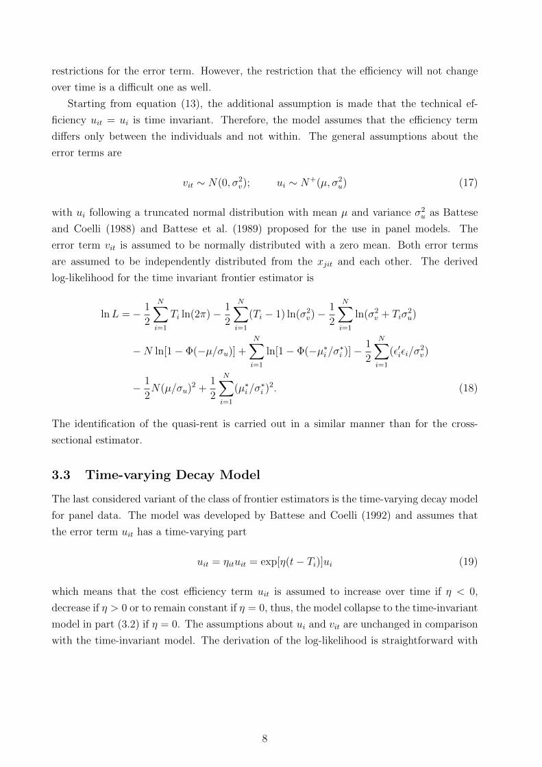
Starting from equation (13), the additional assumption is made that the technical ef-

ficiency uit = ui is time invariant. Therefore, the model assumes that the efficiency term

differs only between the individuals and not within. The general assumptions about the

error terms are

vit ∼ N(0, σ2v); ui ∼ N+(µ, σ2

u) (17)

with ui following a truncated normal distribution with mean µ and variance σ2u as Battese

and Coelli (1988) and Battese et al. (1989) proposed for the use in panel models. The

error term vit is assumed to be normally distributed with a zero mean. Both error terms

are assumed to be independently distributed from the xjit and each other. The derived

log-likelihood for the time invariant frontier estimator is

lnL =− 1

2

N∑i=1

Ti ln(2π)− 1

2

N∑i=1

(Ti − 1) ln(σ2v)−

1

2

N∑i=1

ln(σ2v + Tiσ

2u)

−N ln[1− Φ(−µ/σu)] +N∑i=1

ln[1− Φ(−µ∗i /σ∗i )]−1

2

N∑i=1

(ε′iεi/σ2v)

− 1

2N(µ/σu)

2 +1

2

N∑i=1

(µ∗i /σ∗i )

2. (18)

The identification of the quasi-rent is carried out in a similar manner than for the cross-

sectional estimator.

3.3 Time-varying Decay Model

The last considered variant of the class of frontier estimators is the time-varying decay model

for panel data. The model was developed by Battese and Coelli (1992) and assumes that

the error term uit has a time-varying part

uit = ηituit = exp[η(t− Ti)]ui (19)

which means that the cost efficiency term uit is assumed to increase over time if η < 0,

decrease if η > 0 or to remain constant if η = 0, thus, the model collapse to the time-invariant

model in part (3.2) if η = 0. The assumptions about ui and vit are unchanged in comparison

with the time-invariant model. The derivation of the log-likelihood is straightforward with

8

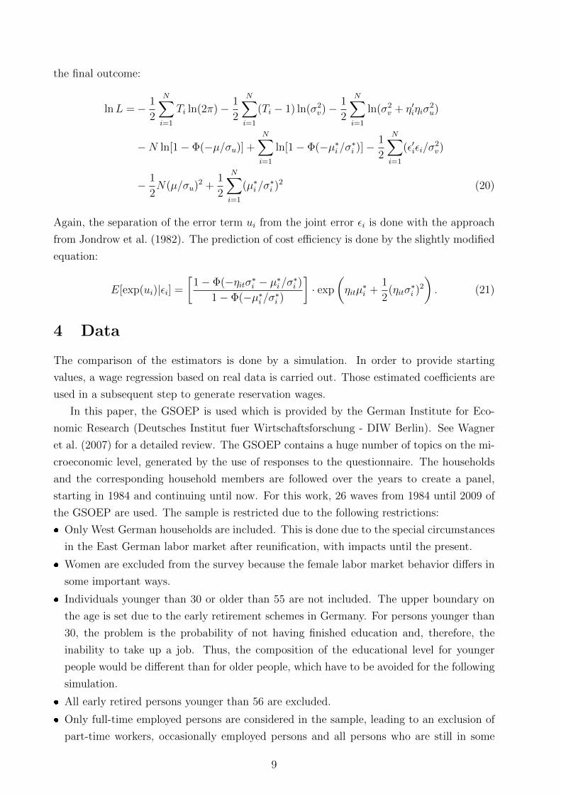
the final outcome:

lnL =− 1

2

N∑i=1

Ti ln(2π)− 1

2

N∑i=1

(Ti − 1) ln(σ2v)−

1

2

N∑i=1

ln(σ2v + η′iηiσ

2u)

−N ln[1− Φ(−µ/σu)] +N∑i=1

ln[1− Φ(−µ∗i /σ∗i )]−1

2

N∑i=1

(ε′iεi/σ2v)

− 1

2N(µ/σu)

2 +1

2

N∑i=1

(µ∗i /σ∗i )

2 (20)

Again, the separation of the error term ui from the joint error εi is done with the approach

from Jondrow et al. (1982). The prediction of cost efficiency is done by the slightly modified

equation:

E[exp(ui)|εi] =

[1− Φ(−ηitσ∗i − µ∗i /σ∗i )

1− Φ(−µ∗i /σ∗i )

]· exp

(ηitµ

∗i +

1

2(ηitσ

∗i )

2

). (21)

4 Data

The comparison of the estimators is done by a simulation. In order to provide starting

values, a wage regression based on real data is carried out. Those estimated coefficients are

used in a subsequent step to generate reservation wages.

In this paper, the GSOEP is used which is provided by the German Institute for Eco-

nomic Research (Deutsches Institut fuer Wirtschaftsforschung - DIW Berlin). See Wagner

et al. (2007) for a detailed review. The GSOEP contains a huge number of topics on the mi-

croeconomic level, generated by the use of responses to the questionnaire. The households

and the corresponding household members are followed over the years to create a panel,

starting in 1984 and continuing until now. For this work, 26 waves from 1984 until 2009 of

the GSOEP are used. The sample is restricted due to the following restrictions:

� Only West German households are included. This is done due to the special circumstances

in the East German labor market after reunification, with impacts until the present.

� Women are excluded from the survey because the female labor market behavior differs in

some important ways.

� Individuals younger than 30 or older than 55 are not included. The upper boundary on

the age is set due to the early retirement schemes in Germany. For persons younger than

30, the problem is the probability of not having finished education and, therefore, the

inability to take up a job. Thus, the composition of the educational level for younger

people would be different than for older people, which have to be avoided for the following

simulation.

� All early retired persons younger than 56 are excluded.

� Only full-time employed persons are considered in the sample, leading to an exclusion of

part-time workers, occasionally employed persons and all persons who are still in some

9

kind of education programs (trainees etc.).

� A minimum amount of 30 hours of work per week have to be reported in order to assume

a full-time employment.

� Only unemployed persons who are able to take up a job are included. Therefore, all

persons in active labor market schemes or in military services are excluded. Furthermore,

a regular secondary job but the lack of a primary job also leads to an exclusion because it

is questionable if they are really searching for a primary job due to their time constraints.

� All self-employed persons are excluded from the survey. They obviously face a very dif-

ferent employment pattern then regular employed workers.

� All persons with a country of origin other than Germany are excluded. The increased

problems of some groups of non-German residents in the labor market are well known and

could therefore lead to distorted results.

After all restrictions, 42,603 observations can be used for the estimation. For these persons,

corrected gross monthly wages are estimated to provide base values for the generation process

of the reservation wage in the simulation. The monthly gross wages are adjusted by additional

salary or bonuses: 13th and 14th monthly paychecks, Christmas bonus, vacation bonus, profit

sharing, travel grant and other bonuses. According to Boll (2011), the information about

the additional payments and the gross wages in the previous year can be used to correct the

current gross wage.

The choice of the exogenous variables is made with regard to the following simulation, the

chosen variables have to be applicable for this purpose as well. Finally, the following variables

are used for the regression: the weekly hours of work. Regional variables are included for the

south/north/west of Germany. The different qualification levels in Germany are measured

by the following variables: no qualifications, vocational training, high vocational training,

technical college and university. All persons without any qualifications different then the

school diploma are classified into the variable “no qualifications”. The variable “vocational

training” accounts for all persons with a “Hauptschulabschluss” (low vocational training) or

“Realschulabschluss” (medium vocational training) together with vocational training. “High

vocational training” includes all persons with “Abitur” alongside vocational training. The

last two qualification variables cover the different academic education in Germany. The

unemployment experience (linear and quadratic), full-time experience (linear and quadratic)

and tenure (linear and quadratic) are measured in years (month in decimal form) to cover

the working history of the persons. The marital status is included as a dummy variable.

Furthermore, the official unemployment rate for each year is implemented by external data

from Statistisches Bundesamt Deutschland (2011) (Federal Statistical Office of Germany).

The estimation of the log corrected gross wages is done with sample selection to correct for

non-participation in the labor market. Thereafter, the result of the estimation is used to

determine the personal reservation wages.

10

5 Simulation Design

The simulation of the labor market is built with the objective of getting a pseudo-panel

with known reservation wages in order to examine the predictive power of the estimation

approaches. The simulation is carried out nearly 1000 times, each time with a new randomly

drawn subsample of 5000 observations out of the 42,603 total observations for two different

scenarios of the reservation wages. The constant (decreasing) scenario assumes a stagnating

(decreasing) reservation wage over the unemployment duration. The idea behind decreasing

reservation wages is straightforward: an unsuccessful job searcher might lower his wage

requests in order to improve his chance for re-employment. Both scenarios are designed such

that they provide similar unemployment rates, since this would be observed in a real dataset

without any prior knowledge of the underlying nature of the reservation wages.

The simulation design is presented below, an overview of the starting values for the

constant (decreasing) scenario can be found in table 1. The simulation assumes that all

persons are either employed or unemployed and are searching for a new job.

To determine the logarithmic reservation wages, the estimated β from the previous wage

estimation are used 2. The constant term is reduced by 0.4 and the estimated standard

deviation has been shrunk by 90%. Furthermore, the reservation wages are set for 40 hours

of work weekly and an unemployment rate of 7%. But before the defined reservation wages

can be used, they have to be adjusted for outliers. Otherwise, very high reservation wages

would determine an unemployment problem especially for persons with good labor market

attraction. Thus, the reservation wages are cut for each of the qualification class at the mean

of its reservation wages distribution plus 1.2 times its standard deviation.

The next preparatory variable concerns the number of layoffs per month. The only

variable affecting the number of layoff is the assumed yearly GDP growth rate, which can

be found in table 1. Since the simulation is based on monthly data, the weighted averages

between the yearly assumed growth rates at time t and t + 1 (with t=year) are used. The

weights are set according to the position in time and will add up to one. The number of

layoffs are determined for the constant (decreasing) scenario by a fixed base rate of 1.6 %

(1.6%) of the total labor force and a variable rate of -0.1% (-0.1%) per 1% growth in the

GDP. The base rate in empirical data is similar, for example Bachmann (2005) found a

transition rate from employment to unemployment of 1.45% of the employed population

while Elsby et al. (2008) found a rate of only 0.5% of labor force for Germany.

The outflow rate of unemployment, measured as percentage of the currently unemployed,

consists of two different processes in this simulation: the probability of receiving a job offer

and the probability that the offer is acceptable. Only the probability of receiving a job offer

is determined in advance. The base rate is set to 25% (23%) of the unemployed while the

2The estimated β are: hours of work = 0.058; vocational training = 0.133; high vocational training =0.1844; technical college = 0.3409; university = 0.4515; married = 0.0477; unemployment experience =-0.0991; unemployment experience2 = 0.044; full-time experience = 0.0307; full-time experience2 = -0.0005;tenure = 0.0046; tenure2 = -0.0001; unemployment rate = -0.0029; lambda = 0.0705; constant = 7.3708.

11

variable component is set to 1 (1) percentage point per 1% change in the GDP growth. With

these preparations, all required variables for the simulation are available. The simulation

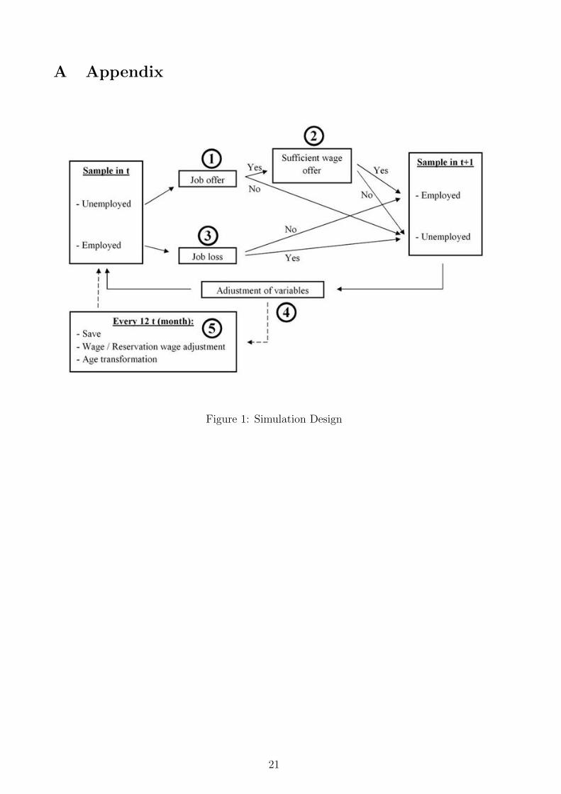
design is presented as a graphic in figure (1) and consists of 5 different steps, denoted by the

circled number.

Step 1

The first step of the simulation is the job offer function. Since the number of offers is

determined, only the allocation of the job offers to the unemployed persons remains. The

main variable is the duration of the current unemployment spell up to its cubic form, it is

assumed that people faces considerable problems reentering the labor market if they were

unemployed long-time. The values for the function are x ∗ (−0.05), x2 ∗ (−0.006) and x3 ∗(0.00028). Moreover, the whole function can be shifted upwards through higher education:

vocational training yields 0.4 points more, high vocational training 0.5, technical college 0.8

and university 0.9 points. To ensure that the process remains random, an error term is added

which is assumed to be normal distributed with mean 0 and standard deviation 4. The n

persons with the highest total scores receive an offer.

Step 2

The next step is the determination of the wage offers. They are based on the reservation

wage distribution for each qualification level in order to provide offers which are reasonable

close to the reservation wages. The mean of each qualification group distribution is used as

the mean of the corresponding wage offer distribution, whereas the standard deviation for

each group is increased by the factor 2.5.

Together, step 1 and step 2 are determining the process of job search. Each person with

a job offer decides thereafter to either accept the offer and to leave unemployment or to

decline and to search further. The choice depends, of course, on the individual reservation

wages.

Step 3

The third step covers the job loss process. Only the identification of the workers who lose

their jobs is left since the number of job losses is calculated in advance. This is done by a

function subject to the following variables and loadings: 0.5 for each year of unemployment

experience, -0.025 for the squared unemployment experience, -0.25 for the tenure, 0.004 for

the squared tenure. The idea behind choosing the unemployment experience is the concept

of scars from unemployment and that previously laid-off workers might have attributes which

make a new dismissal more likely. The tenure is working in the contrary direction since the

theory of human capital states those longer employed workers are more useful for a firm.

Furthermore, an error term and the qualification variables are included as well in the layoff

function, see table 1 for the values. Again, as in step 2 the workers with the highest combined

values in the above described variables lose their jobs.

Step 4

The fourth step covers the adjustment of variables. Most obviously, the employment status

is changed each month depending on the previously described steps. Also the variables on

12

tenure, squared tenure, full-time experience, squared full-time experience, unemployment

experience and squared unemployment experience are changed according to the employment

status of the person. Furthermore, the unemployment duration and tenure are adjusted.

The last thing to replace are the reservation wages for reemployed persons. This is done

in order to ensure that the overall level of reservation wages for employed workers is not

tending towards zero in the decreasing scenario. If the generated reservation wage is above

the accepted wage offer, the wage offer is used instead as the new reservation wage.

Step 5

Every 12 months, the age is increased by one which would lead to a problem with the age

distribution in the sample. Since the range of the sample is restricted to those aged of 30-

55, the first increase would delete the oldest workers and would simultaneously cause the

disappearance of the class of 30 year old persons. To solve this problem and to maintain the

original sample size of 5000 observations it is necessary to conduct an age transformation, i.e.

rewriting the age of all 56 year old people to 30. Most of their variables have to be changed

as well. What remains unchanged are the qualification level (and regional dummies, marital

status) for reasons of simplification but the tenure, unemployment experience, and full-time

experience are replaced. This is done according to the qualification level of the person. For

each of the replaced variables, the real distribution for the 30 year olds in its corresponding

qualification group in the GSOEP is analyzed. Based on this real distribution, each person

“draws” a value out of it. The employment status is arbitrarily set to the original status

of the person in the GSOEP. Of course, all transformed persons get a new reservation wage

and a new wage in the case that they are employed. Like before, new reservation wages are

controlled for outliers.

After the age transformation, some adjustments for all other persons in the sample are

made. Once every 12 months, their wages and reservation wages are adjusted in order

to accommodate changes in variables like tenure or full-time experience. This is done by

calculating the change from the previous year until the current year for all metric variables

and multiplying these changes by their corresponding coefficients.

The last step in the panel simulation is the storage of the data each year, given that the

calibration phase of 50 years is completed.

For decreasing reservation wages, an additional step is included in the simulation. In

this case, the duration of unemployment is assumed to have an influence on the reservation

wages. More precisely, the reservation wages are assumed to decrease by 1% every month of

unemployment for persons with medium or low reservation wages. High reservation wages are

decreasing by 2% each month. This is done since it is assumed that persons with comparable

high reservation wages will recognize their exaggerated wage requests and therefore lower the

level more quickly. The affiliation to the quickly decreasing group is determined through the

relative position of persons compared to all other persons in the same qualification group,

regardless of their labor market status. If a person exceeds the maximum reservation wage

defined by the group mean plus the group standard deviation, he will belong to the fast

13

decreasing group until he falls short of it again.

The final outcome in both scenarios is a panel of seven years, consisting of 35,000 ob-

servations by merging the saved data from each year together. But in advance of the seven

simulated years used, a calibration period of 50 years is conducted. Thereafter, the estima-

tors are applied on the pseudo-panel and the whole process is repeated approx. 1000 times

in the Monte Carlo simulation.

6 Results

The results of the Monte Carlo simulation are presented in two parts. The first part dis-

cusses the scenario with constant reservation wages and the second part with decreasing

reservation wages. For both scenarios, the results from the different estimation approaches

are compared. The subsample for the Kiefer-Neumann approach is restricted in a similar

manner to Christensen (2005). Thus, observations are only used if they are unemployed but

had a visible job spell before, or if they even found a new job. The restriction about the

existence of a previous employment spell is necessary since the wage before unemployment

is used as a regressor. Furthermore, the Kiefer-Neumann approach assumes that the reser-

vation wages are affected by three different groups of variables. The first group (denoted

by xoi ) is assumed to affect the search costs only, the second group (xoi ) to affect the wage

offer only and the third group (xo,ri ) to affect both. Search costs are assumed to have a di-

rect influence on reservation wages, which can be easily seen from equation (1). The second

group influences the reservation wages through a change in the mean wage offer and the third

group via both channels. The first group consists solely of the unemployment rate which

is separated by qualification levels. The second group consists of the (log) last wage before

unemployment and the marital status. The influence of the last wage before unemployment

is quite obvious, since newly employed persons will stay, in many cases, reasonably close to

their previous wage. The marital status is included as many studies estimate a relationship

between marriage and income, for example Antonovics and Town (2004) supports these find-

ings. The third group of variables is assumed to affect the reservation wage through both

possibilities and consists of the following variables: full-time experience, squared full-time

experience, tenure before unemployment, squared tenure before unemployment, unemploy-

ment experience, squared unemployment experience, qualification (low vocational, medium

vocational, high vocational, technical college, university) and the GDP growth rate.

The remainder of the paper presents the predictive power for the different estimation

approaches and different reservation wage scenarios3. This is examined by an auxiliary

regression of the predicted (log) reservation wages on the true simulated (log) reservation

wages, using the explained part of the total variance as a measure for the predicting power

alongside with the prediction itself. Prior to that, the individual reservation wages have to

3The estimated coefficients of both approaches in both scenarios are not presented in this work. Theyare available upon request from the author.

14

be calculated according to equation (11) by using the predicted cost efficiency qi. But in

order to improve the comparability with the Kiefer Neumann estimators, the log version of

equation (11) is taken

writ = wit − ln(qit) (22)

where wit and writ are the logarithm of the corresponding values.

The results are compared for different subsamples of the simulated data: five-year age-

group, for a boom cycle of the GDP growth in the simulation years 51-54 and for a bust cycle

in the years 55-57 4. Furthermore, a distinction between qualification groups is made where

“low qualification” corresponds to persons with low or medium vocational training, “medium

qualification” corresponds to persons with high vocational training and “high qualification”

to persons with academic qualification.

All wages and reservation wages are estimated in logs but presented in non-log to facilitate

the comparison. The r-squares in the outputs refer to a regression of the log-predicted

reservation wage on the log-simulated reservation wage.

6.1 Constant Reservation Wages

The constant scenario assumes stable reservation wages over the unemployment period. The

summary statistics over all 996 simulated samples can be found in the upper part of table 3.

The mean unemployment rate of 9.4% and the mean unemployment duration of 7.8 months

provide a sufficient base for an adequate transition between unemployment and employment.

The average simulated reservation wage is located at 1800.2e while the average simulated

labor income is located slightly higher at 2083.7e.

The results for the frontier estimators are presented first. For them in general, a correct

and sufficient skewness of the error term is essential. A negative skewness would lead to

production frontier estimators and a positive skewness to cost frontier estimators. Since the

objective is to predict reservation wages which are located below the log-wage, a regression

of all exogenous variables on the log-wage should result in positively skewed error terms.

Indeed, the results for the Monte Carlo simulation reveal a positive average skewness of 0.65

which is larger than 0 for all repetitions.

The results for the frontier estimator with normal-half normal distributed error terms in

column 3 of tables 4-6 indicate a fairly good prediction of the reservation wages. The mean

reservation wage is predicted in the main model with 1746.6e which is slightly lower than

the true mean reservation wage at 1833.4e. Nevertheless, the half-normal frontier model is

able to explain 83 % of the variance of the true simulated reservation wages. The subgroup

analysis reveals no remarkable drop in the quality of the prediction for the age-groups and

the business cycles, the r-squared stays always above or equal to 80%. A sharp drop in the

r-squared can be observed with regard to the qualification subgroups but with still a good

mean prediction of the reservation wage. The lower r-squared is caused by the dropout of

4The first 50 years are the calibration phase.

15

the qualification variables which was one of the most important variables in the simulation

design.

The second frontier model is the time-invariant model. Compared to the previous model,

the additional restriction is imposed that the cost efficiency will not change over time, i.e.

that the quasi-rents remain constant. Furthermore, the efficiency term is assumed to follow a

truncated normal distribution which necessitates the estimation of the additional parameter

µ, the mean of the efficiency term. The results for the prediction are presented in column 4

of tables 4-6 5. The first striking difference in the results is the higher underestimation of the

true average reservation wage with an outcome of 1697.2e in the main model. Furthermore,

the r-squared is low with only 53%. The different subgroups indicate a slightly decreasing

accuracy of the prediction for older age groups. The r-squared for the qualification groups

is practically zero, except for the highest two groups where 15% and 39% are attained.

Altogether, the results are disappointing if they are compared to the first frontier estimator.

The last model of the frontier class is the time-varying decay model whose results are

presented in column 5 of tables 4-66. The special assumption in this model is the decreasing,

increasing or constant efficiency term, thus the quasi-rents are allowed to differ over time

within one person according to uit = ηituit = exp[η(t−Ti)]ui. Compared to the cross sectional

normal-half normal model, the additional parameter of µ and η have to be estimated which

denotes the mean of the efficiency and time decay, respectively. The results for the main

model show a predicted mean reservation wage of 1668.7e which is even lower than the result

for the time-invariant model. Nevertheless, the r-squared is somewhat better with 65% but

still worse than the results from the half-normal frontier estimator. The subgroup analysis

reveals practically no differences between the main model and the different age groups and

business cycles. The division of the simulated sample in different qualification groups can be

found in in table 6. The results show a low r-squared and persistent underestimation of the

mean simulated reservation wage, comparable with the time-invariant model. The slightly

higher r-squared compared with the previous model does not hide the fact that the model

got most of its predictive power from the qualification model. Moreover, the time-varying

model has a higher standard deviation of its prediction over the Monte Carlo simulation,

even if the sample size is exactly the same as with the other two frontier models. This finding

of increased instability is underlined by the fact that the estimator did not converge for 13

repetitions.

The approach from Kiefer and Neumann focuses on the prediction of reservation wages for

unemployed persons. Three different realizations of the estimator are presented in this work7.

The results from the first one can be found in column 6 of tables 4-6, it uses all available

observations that fulfill the defined restrictions. In addition, the second model is restricted

5Results are based on 994 observations. The estimator did not converged for 2 repetitions.6Results are based on 983 observations. The estimator did not converged for 13 repetitions.7Repetitions are dropped if the estimated reservation wage is greater than 5000e which indicates problems

with estimation. First model: 7 repetitions dropped. Second model: 8 repetitions dropped. Third model:43 repetitions dropped.

16

to observations with less than 13 month of current unemployment duration or less than 13

month of completed unemployment duration. The results can be found in column 7 of tables

4-6. The third model is restricted to completed and current unemployment durations of 13

to 24 months and is presented in column 8 of tables 4-6. The separation in sub-models two

and three is done in order to examine the ability of the Kiefer-Neumann approach to detect

decreasing or constant reservation wages. The overall low level of the simulated reservation

wages in the Kiefer-Neumann sample of 1474.6e compared to the reservation wages in the

full sample of 1833.4e is caused by the lack of persons with good affiliation to the labor

market in the subsample. In the simulation, persons with good affiliation (wages) to the

labor market are very likely to stay employed or to quickly find a new job.

The full main model in column 6 reveals overestimation of the mean reservation wage.

The average prediction is with 1971.9e remarkably higher than the mean simulated reserva-

tion wage of 1474.6e. Nevertheless, the prediction from the full Kiefer-Neumann estimator is

able to explain 77 % of the variance of the true simulated reservation wages in the subsample

of 2046 unemployed observations. The subgroup analysis reveals a nearly constant r-squared

over the age groups with only small changes for the average predicted and simulated reserva-

tion wage. But the Kiefer-Neumann estimator seems to have increased problems estimating

the reservation wages in the case of higher education, a somewhat reversed result compared

to the frontier models.

The question of decreasing or constant reservation wages is addressed by the sub-models

for different length of unemployment duration, listed in the columns 7 and 8 of tables 4-6.

The difference of the real reservation wages between the short unemployment sub-model

and the long unemployment sub-model is small at 1449.6e to 1482e. The slight observable

increase is caused by the fact that persons with higher reservation wages are faced with more

problems finding a new job. However, the Kiefer-Neumann estimator predicts a decrease of

the average reservation wage from 1989.5e to 1946e and is less able to explain the true

reservation wages. The r-squared decreases from 76% for persons with a short unemploy-

ment period to 55% for persons a longer unemployment period. Furthermore, the standard

deviations increase remarkably for longer unemployment duration, which is caused by the

very small subsamples of data. The simulated sample offers on average only 359 observations

with current unemployment duration longer than 12 months, a fairly small number if it is

compared to the 31696.5 observations which could be used by the frontier models. Moreover,

the Monte Carlo simulation produces changing subgroups over the repetitions which cause

great volatility in the predicted reservation wages as well.

6.2 Decreasing Reservation Wages

The decreasing scenario assumes declining reservation wages over the unemployment period.

The summary statistics over the 969 simulated samples can be found in the lower part of

table 3. Compared to the constant reservation wages, some differences which are caused by

17

the simulation design can be observed. The average unemployment rate is, at 9.6%, nearly

similar to those of the constant scenario, but the average unemployment duration and the

average reservation wage is, unsurprisingly, lower. Furthermore, the simulated wage is, at

2077e, lower in the current scenario.

The results for the three frontier estimators can be found in columns 3 - 5 of tables 7 -

9. Again, the auxiliary regression (22) is used to determine the accuracy of the estimators

and the results are reported for different subgroups. The required skewness of the error term

distribution of a log-wage regression with all exogenous variables is given with a mean value

of 0.646. Thus, the cost frontier models are applicable.

The main model of the normal-half normal frontier estimator (column 3) shows a nearly

unchanged average prediction of the reservation wages, but with a higher r-squared of the

auxiliary regression compared to the constant scenario. More detailed, the average predicted

reservation wage is, at 1736.2e, again close to the true simulated value of 1837.7e, and the

model is able to explain 87% of the variance. The outcome of a better explanation of the

variance compared to the constant scenario carries over for the subgroup analysis of age,

business cycles and qualification groups.

The panel estimator with time-invariant quasi-rents is viewed next, results are listed in

column 4 of tables 7 - 9. The main model shows less evidence of underestimation in the

decreasing scenario, the mean predicted reservation wage is, at 1717e, closer to the true

value. Nevertheless, the r-squared of the auxiliary regression for the main model remains

low at 58%. Compared to the constant scenario, the results of the time-invariant estimator

are slightly improved for the different subgroups.

The same holds for the time-varying decay model whose results can be found in column

5 of tables 7 - 98. The quality of the predictions are slightly increased for all subgroups.

The main model exhibits an r-squared of 70% but still suffers from the problem of underes-

timation. Since better working stochastic frontier estimators are available, the result is not

impressively high.

The small differences between the reservation wage scenarios of the frontier estimators

are neither astonishing nor unexpected since the frontier estimator uses only information

on employed persons. Thus, a change in the reservation wages for unemployed persons can

hardly be detected. This is caused by the simulation design, since an unemployed person who

accepts a job offer will be paid with exactly that accepted wage. Thus, the only possibility for

the frontier estimator to detect lower reservation wages is through decreased accepted wages

but the fraction of newly employed workers in the sample is limited. Furthermore, it has to

be kept in mind that the reservation for new employed workers is set to some value below

the accepted wage but possibly above their current reservation wage during unemployment

which could have been markedly decreased. Altogether, the frontier models are faced with

similar problems than in the constant simulation scenario. The prediction quality from the

panel estimators is somewhat lower and their variance is significantly higher (on average

8Results are based on 931 observations. The estimator did not converged for 38 repetitions.

18

over all simulations), indicating problems with instability. Only the normal-half normal

stochastic frontier estimator shows acceptable results, but it overestimates the reservation

wages as well. However, the simplest model of the frontier estimators seems to produce the

best results.

The Kiefer-Neumann estimator, listed in columns 6 - 8 of tables 7 - 9, is faced with the

same problems as in the constant scenario9. A high overestimation of the average reservation

wage and a high standard deviation over the different repetition of the simulation through

changing subsamples can be seen. The sample size of unemployed persons which fulfill the

restrictions consists, on average, of 1874 observations with an unemployment duration lower

than 12 months and 326 observations with a duration longer than 24 months.

The results for the full main model reveal the nearly unchanged fraction of explained

variance of 73% compared to the constant reservation wage scenario. This carries over

to the analysis of the subsamples, neither of which exhibit much change. Concerning the

question of a detection of decreasing reservation wages, the Kiefer-Neumann estimator is

able to predict the direction correctly (column 7 and 8). But this was already attained for

nearly the same amount in the constant scenario where the real average reservation wage

stayed nearly constant for the different unemployment durations. In the current scenario,

the reservation wage is decreasing by construction which can be confirmed from average real

values. Thus, the Kiefer-Neumann estimator is, at least in the chosen simulation setting,

not a reliable predictor of decreasing reservation wages. But it has to be mentioned that the

standard deviations between the simulations are very high, thus even small changes in the

attributes of the persons in the sample would lead to significant differences in the estimation

outcome.

A striking fact of the Kiefer-Neumann estimator is the low r-squared of the auxiliary

regression for higher unemployment durations. Increased problems estimating the reserva-

tion wages for the long-term unemployed were found elsewhere as well, i.e. in the work

of Christensen (2005). One reason for the problem is, of course, the low number of obser-

vations compared to short-term unemployed estimation. But another reason might be the

estimation design. Like all other discussed works with an application of the Kiefer-Neumann

estimator, this work assumes that the offer arrival rate equals one even if it is known from

the simulation design that this is a wrong assumption. The Kiefer-Neumann approach tries

to estimate the probability of accepting a given job offer in the first step in order to detect

in a second step a sample selection bias in the accepted wage regression. But in the case of

an offer arrival rate smaller than one, the probit will estimate not only the probability that

the wage offer is greater than the reservation wage but also the probability of receiving an

job offer at the same time. This fact is very likely to occur in a real labor market as well

since it is known that long-term unemployed are faced with problems receiving any offers at

all. Altogether, these two facts might explain the problems the Kiefer-Neumann estimator

9Repetitions are dropped if the estimated reservation wage is greater than 5000e. First model: 36repetitions dropped. Second model: 42 repetitions dropped. Third model: 93 repetitions dropped.

19

has to find correct reservation wages for long-term unemployed persons and to provide an

reliable measure of constant or decreasing reservation wages.

7 Conclusion

This paper has analyzed the predictive power of different estimation methods for individual

reservation wages. The first class of models consisted of stochastic frontier models. More

precisely, a frontier model with normal-half normal error terms, a panel data stochastic

frontier with constant quasi-rent and a panel data stochastic frontier with time-invariant

quasi-rents were used. All of these models used a one-sided error to predict the reservation

wages for employed persons. The second class of models used the approach from Kiefer and

Neumann in order to predict the reservation wages for unemployed persons. This allowed

the consideration of the question of decreasing/constant reservation wages over the unem-

ployment duration. The comparison was carried out by a Monte Carlo simulation which

used the German Socio-Economic Panel as a basic framework for the simulation of a labor

market. The simulation itself modeled reservation wages and working wages alongside with a

transition path from unemployment to employment and vice versa. For testing the ability to

detect constant/decreasing reservation wages over the unemployment period, two different

simulation scenarios were considered with different specifications of the reservation wages.

The predictive power of all approaches in both scenarios was compared by the average results

over all repetitions from an auxiliary regression.

For employed persons, the paper showed the best results for the most simple stochastic

frontier model with normal-half normal distributed error terms. Both panel models failed

to attain the same level of explained variance and showed a higher underestimation of the

reservation wages. This finding held for both simulation designs and for all subgroup anal-

yses. For unemployed persons, the Kiefer-Neumann estimator was unable to provide the

same level of r-squared as the simple stochastic frontier model did for employed. Further-

more, the Kiefer-Neumann estimator suffered from a severe overestimation of the average

reservation wage in both scenarios. In addition, the paper showed the unreliability of the

Kiefer-Neumann estimator to detect decreasing reservation wages over the unemployment

period. The estimator predicted decreasing reservation wages for long-term unemployed in

both scenarios. However, the approach from Kiefer and Neumann suffered from two draw-

backs. The first was the known and wanted misspecification of the job offer probability,

which is used frequently in application. The second evolved from the fairly small number

of observations which could be used for the estimation, especially the lack of long-term

unemployed persons.

20

A Appendix

Figure 1: Simulation Design

21

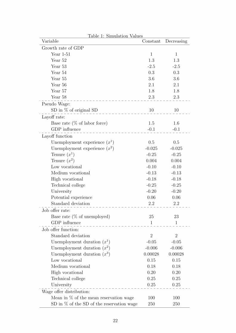
Table 1: Simulation ValuesVariable Constant Decreasing

Growth rate of GDP

Year 1-51 1 1

Year 52 1.3 1.3

Year 53 -2.5 -2.5

Year 54 0.3 0.3

Year 55 3.6 3.6

Year 56 2.1 2.1

Year 57 1.8 1.8

Year 58 2.3 2.3

Pseudo Wage:

SD in % of original SD 10 10

Layoff rate:

Base rate (% of labor force) 1.5 1.6

GDP influence -0.1 -0.1

Layoff function

Unemployment experience (x1) 0.5 0.5

Unemployment experience (x2) -0.025 -0.025

Tenure (x1) -0.25 -0.25

Tenure (x2) 0.004 0.004

Low vocational -0.10 -0.10

Medium vocational -0.13 -0.13

High vocational -0.18 -0.18

Technical college -0.25 -0.25

University -0.20 -0.20

Potential experience 0.06 0.06

Standard deviation 2.2 2.2

Job offer rate:

Base rate (% of unemployed) 25 23

GDP influence 1 1

Job offer function:

Standard deviation 2 2

Unemployment duration (x1) -0.05 -0.05

Unemployment duration (x2) -0.006 -0.006

Unemployment duration (x3) 0.00028 0.00028

Low vocational 0.15 0.15

Medium vocational 0.18 0.18

High vocational 0.20 0.20

Technical college 0.25 0.25

University 0.25 0.25

Wage offer distribution:

Mean in % of the mean reservation wage 100 100

SD in % of the SD of the reservation wage 250 250

22

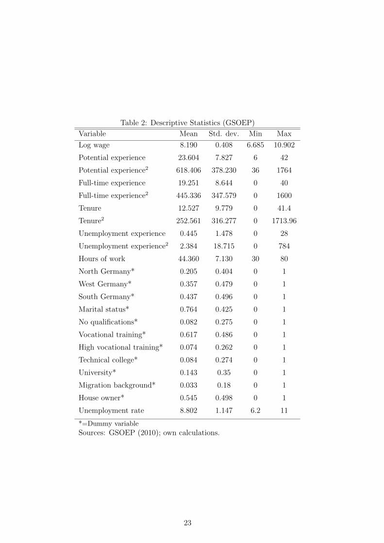
Table 2: Descriptive Statistics (GSOEP)

Variable Mean Std. dev. Min Max

Log wage 8.190 0.408 6.685 10.902

Potential experience 23.604 7.827 6 42

Potential experience2 618.406 378.230 36 1764

Full-time experience 19.251 8.644 0 40

Full-time experience2 445.336 347.579 0 1600

Tenure 12.527 9.779 0 41.4

Tenure2 252.561 316.277 0 1713.96

Unemployment experience 0.445 1.478 0 28

Unemployment experience2 2.384 18.715 0 784

Hours of work 44.360 7.130 30 80

North Germany* 0.205 0.404 0 1

West Germany* 0.357 0.479 0 1

South Germany* 0.437 0.496 0 1

Marital status* 0.764 0.425 0 1

No qualifications* 0.082 0.275 0 1

Vocational training* 0.617 0.486 0 1

High vocational training* 0.074 0.262 0 1

Technical college* 0.084 0.274 0 1

University* 0.143 0.35 0 1

Migration background* 0.033 0.18 0 1

House owner* 0.545 0.498 0 1

Unemployment rate 8.802 1.147 6.2 11

*=Dummy variable

Sources: GSOEP (2010); own calculations.

23

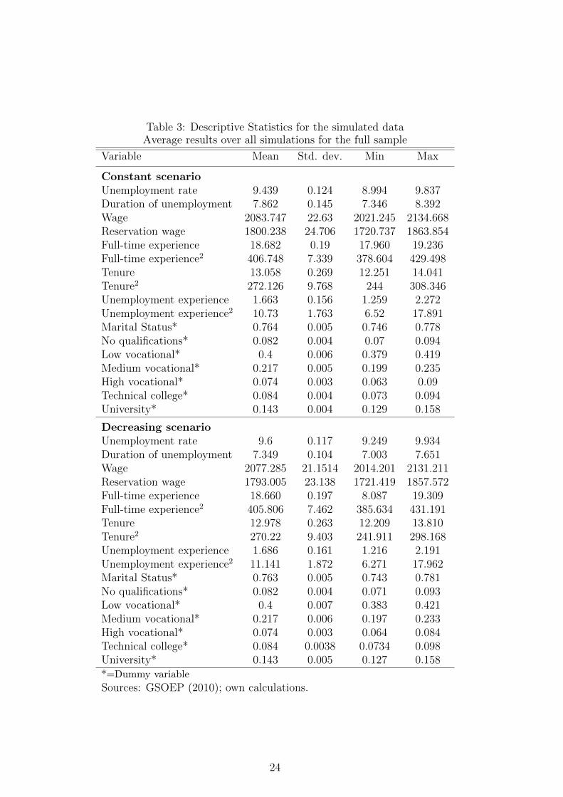
Table 3: Descriptive Statistics for the simulated dataAverage results over all simulations for the full sample

Variable Mean Std. dev. Min Max

Constant scenarioUnemployment rate 9.439 0.124 8.994 9.837Duration of unemployment 7.862 0.145 7.346 8.392Wage 2083.747 22.63 2021.245 2134.668Reservation wage 1800.238 24.706 1720.737 1863.854Full-time experience 18.682 0.19 17.960 19.236Full-time experience2 406.748 7.339 378.604 429.498Tenure 13.058 0.269 12.251 14.041Tenure2 272.126 9.768 244 308.346Unemployment experience 1.663 0.156 1.259 2.272Unemployment experience2 10.73 1.763 6.52 17.891Marital Status* 0.764 0.005 0.746 0.778No qualifications* 0.082 0.004 0.07 0.094Low vocational* 0.4 0.006 0.379 0.419Medium vocational* 0.217 0.005 0.199 0.235High vocational* 0.074 0.003 0.063 0.09Technical college* 0.084 0.004 0.073 0.094University* 0.143 0.004 0.129 0.158

Decreasing scenarioUnemployment rate 9.6 0.117 9.249 9.934Duration of unemployment 7.349 0.104 7.003 7.651Wage 2077.285 21.1514 2014.201 2131.211Reservation wage 1793.005 23.138 1721.419 1857.572Full-time experience 18.660 0.197 8.087 19.309Full-time experience2 405.806 7.462 385.634 431.191Tenure 12.978 0.263 12.209 13.810Tenure2 270.22 9.403 241.911 298.168Unemployment experience 1.686 0.161 1.216 2.191Unemployment experience2 11.141 1.872 6.271 17.962Marital Status* 0.763 0.005 0.743 0.781No qualifications* 0.082 0.004 0.071 0.093Low vocational* 0.4 0.007 0.383 0.421Medium vocational* 0.217 0.006 0.197 0.233High vocational* 0.074 0.003 0.064 0.084Technical college* 0.084 0.0038 0.0734 0.098University* 0.143 0.005 0.127 0.158*=Dummy variable

Sources: GSOEP (2010); own calculations.

24

Tab

le4:

Con

stan

tsc

enar

io:

com

par

ison

par

t1

Mea

ns

ofes

tim

ated

coeffi

cien

ts,

stan

dar

ddev

iati

ons

inpar

enth

esis

Fro

nti

eres

tim

ator

sK

iefe

r-N

eum

ann

esti

mat

ors

Var

iable

Hal

fN

orm

alT

ime-

inva

rian

tT

ime-

vary

ing

Full

model

Dura

tion≤

12D

ura

tion

>12

Main

model

Rea

lre

s.w

age

1833

.37

1833

.37

1833

.37

1474

.64

1449

.61

1482

.45

(24.

12)

(24.

12)

(24.

12)

(42.

37)

(40.

04)

(40.

73)

Est

.re

s.w

age

1746

.63

1697

.21

1668

.719

71.9

1989

.46

1945

.99

(25.

81)

(53.

06)

(94.

25)

(382

.18)

(422

.6)

(841

.23)

R-s

quar

ed0.

830.

530.

650.

770.

760.

55(0

.02)

(0.0

5)(0

.03)

(0.1

4)(0

.16)

(0.2

4)O

bs.

3169

6.49

3169

6.49

3169

6.49

2146

.23

1787

.02

359.

04(4

3.57

)(4

3.57

)(4

3.57

)(4

0.11

)(3

2.44

)(2

0.22

)A

ge<

36

Rea

lre

s.w

age

1814

.86

1814

.86

1814

.86

1553

.16

1534

.21

1651

.56

(25.

84)

(25.

84)

(25.

84)

(61.

54)

(61.

16)

(81.

22)

Est

.re

s.w

age

1716

.23

1814

.85

1640

.86

2014

.28

2034

.57

1983

.13

(27.

74)

(25.

86)

(92.

3)(3

59.2

7)(4

01.4

4)(8

02.1

3)R

-squar

ed0.

80.

550.

660.

750.

760.

56(0

.02)

(0.0

5)(0

.04)

(0.1

4)(0

.15)

(0.2

4)O

bs.

7291

.67

7291

.67

7291

.67

219.

3918

3.54

35.8

8(1

30.0

6)(1

30.0

6)(1

30.0

6)(2

1.45

)(1

7.66

)(7

.02)

35<

age<

41

Rea

lre

s.w

age

1823

.26

1823

.26

1823

.26

1482

.68

1461

.58

1581

.03

(24.

83)

(24.

83)

(24.

83)

(52.

87)

(51.

62)

(70.

73)

Est

.re

s.w

age

1735

.29

1685

.74

1659

.36

1980

.92

2002

.04

1963

.24

(26.

69)

(53.

09)

(93.

5)(3

68.6

5)(4

13.8

1)(8

19.6

2)R

-squar

ed0.

820.

540.

650.

760.

760.

57(0

.02)

(0.0

5)(0

.04)

(0.1

4)(0

.16)

(0.2

4)O

bs.

6881

.25

6881

.25

6881

.25

339.

1227

8.48

60.4

4(1

12.3

3)(1

12.3

3)(1

12.3

3)(2

8.08

)(2

2.61

)(9

.73)

40<

age<

46

Rea

lre

s.w

age

1840

.59

1840

.59

1840

.59

1471

.63

1448

.37

1583

.48

(24.

79)

(24.

79)

(24.

79)

(48.

73)

(46.

64)

(68.

89)

Est

.re

s.w

age

1752

.54

1703

.06

1675

.07

1968

.65

1989

.27

1971

.79

(26.

24)

(53.

73)

(94.

88)

(379

.36)

(421

.29)

(863

.34)

R-s

quar

ed0.

840.

530.

660.

770.

770.

59(0

.02)

(0.0

5)(0

.03)

(0.1

5)(0

.16)

(0.2

4)O

bs.

6533

.81

6533

.81

6533

.81

449.

9537

2.11

77.7

8(1

11.8

4)(1

11.8

4)(1

11.8

4)(2

8.49

)(2

3.96

)(1

0.06

)

25

Tab

le5:

Con

stan

tsc

enar

io:

com

par

ison

par

t2

Mea

ns

ofes

tim

ated

coeffi

cien

ts,

stan

dar

ddev

iati

ons

inpar

enth

esis

Fro

nti

eres

tim

ator

sK

iefe

r-N

eum

ann

esti

mat

ors

Var

iable

Hal

fN

orm

alT

ime-

inva

rian

tT

ime-

vary

ing

Full

model

Dura

tion≤

12D

ura

tion

>12

45<

age<

51

Rea

lre

s.w

age

1848

.56

1848

.56

1848

.56

1463

.92

1436

.64

1600

.35

(24.

42)

(24.

42)

(24.

42)

(45.

01)

(41.

24)

(73.

17)

Est

.re

s.w

age

1765

.91

1717

1686

.46

1962

.519

81.0

519

90.7

1(2

5.49

)(5

3.54

)(9

5.74

)(3

92.2

7)(4

28.3

3)(9

08.6

9)R

-squar

ed0.

860.

50.

660.

780.

770.

6(0

.01)

(0.0

5)(0

.03)

(0.1

5)(0

.16)

(0.2

)O

bs.

5886

.358

86.3

5886

.354

4.27

453.

5790

.64

(115

.26)

(115

.26)

(115

.26)

(30.

64)

(25.

82)

(10.

98)

Age>

50

Rea

lre

s.w

age

1846

.67

1846

.67

1846

.67

1453

.75

1425

.44

1603

.63

(25.

09)

(25.

09)

(25.

09)

(39.

79)

(35.

73)

(77.

04)

Est

.re

s.w

age

1775

.48

1722

.14

1692

.44

1963

.01

1974

.28

2012

.32

(25.

69)

(54.

41)

(96.

61)

(417

.94)

(434

.71)

(966

.63)

R-s

quar

ed0.

860.

50.

670.

770.

750.

59(0

.01)

(0.0

5)(0

.03)

(0.1

5)(0

.16)

(0.2

6)O

bs.

5103

.46

5103

.46

5103

.46

593.

4949

9.31

94.2

9(1

05.1

3)(1

05.1

3)(1

05.1

3)(3

4.14

)(2

9.25

)(1

1.24

)Y

ear

1-4

Rea

lre

s.w

age

1837

.47

1837

.47

1837

.47

1489

.414

75.8

615

80.2

2(2

4.16

)(2

4.16

)(2

4.16

)(4

4.61

)(4

3.37

)(5

8)E

st.

res.

wag

e17

48.3

816

98.1

616

70.0

919

89.1

920

13.5

719

88.7

1(2

5.79

)(5

3.23

)(9

4.41

)(4

27.1

8)(4

79.7

1)(8

93.4

1)R

-squar

ed0.

830.

540.

660.

780.

770.

58(0

.02)

(0.0

4)(0

.03)

(0.1

4)(0

.15)

(0.2

5)O

bs.

1794

1.87

1794

1.87

1794

1.87

1064

.92

926

138.

8(3

0.38

)(3

0.38

)(3

0.38

)(2

6.75

)(2

2.54

)(1

1.15

)Y

ear

5-7

Rea

lre

s.w

age

1828

.03

1828

.03

1828

.03

1460

.08

1421

.37

1611

.99

(24.

1)(2

4.1)

(24.

1)(4

1.2)

(37.

54)

(59.

33)

Est

.re

s.w

age

1744

.35

1695

.97

1666

.89

1954

.87

1963

.52

1985

.91

(25.

86)

(52.

86)

(94.

05)

(343

.6)

(364

.63)

(881

.40)

R-s

quar

ed0.

840.

510.

650.

770.

780.

57(0

.02)

(0.0

5)(0

.03)

(0.1

4)(0

.15)

(0.2

4)O

bs.

1375

4.62

1375

4.62

1375

4.62

1081

.31

861.

0222

0.23

(22.

58)

(22.

58)

(22.

58)

(23.

99)

(19.

42)

(15.

19)

26

Tab

le6:

Con

stan

tsc

enar

io:

com

par

ison

par

t3

Mea

ns

ofes

tim

ated

coeffi

cien

ts,

stan

dar

ddev

iati

ons

inpar

enth

esis

Fro

nti

eres

tim

ator

sK

iefe

r-N

eum

ann

esti

mat

ors

Var

iable

Hal

fN

orm

alT

ime-

inva

rian

tT

ime-

vary

ing

Full

model

Dura

tion≤

12D

ura

tion

>12

No

quali

fica

tions

Rea

lre

s.w

age

1474

.08

1474

.08

1474

.08

1275

.17

1257

.10

1351

.81

(57.

42)

(57.

42)

(57.

42)

(47.

49)

(45.

41)

(62.

69)

Est

.re

s.w

age

1462

.47

1488

.62

1417

.34

1818

.78

1841

.63

1824

.33

(47.

92)

(47.

62)

(80.

96)

(383

.25)

(414

.27)

(851

.18)

R-s

quar

ed0.

760.

040.

220.

690.

680.

46(0

.05)

(0.0

3)(0

.05)

(0.2

)(0

.21)

(0.2

7)O

bs.

2064

.41

2064

.41

2064

.41

488.

3939

3.43

94.6

8(1

61.6

)(1

61.6

)(1

61.6

)(7

7.83

)(6

1.48

)(1

9.13

)L

ow

quali

fica

tions

Rea

lre

s.w

age

1679

.26

1679

.26

1679

.26

1459

.92

1438

.27

1580

.18

(28.

99)

(28.

99)

(28.

99)

(43.

9)(4

1.43

)(5

8.22

)(l

owvo

cati

onal

and

Est

.re

s.w

age

1610

.26

1567

.84

1538

.619

55.8

419

73.3

519

58.5

2m

ediu

mvo

cati

onal

)(2

8.86

)(4

8.42

)(8

6.18

)(3

73.0

3)(4

12.7

9)(8

57.8

6)R

-squar

ed0.

590.

050.

190.

650.

630.

4(0

.06)

(0.0

3)(0

.06)

(0.1

8)(0

.2)

(0.2

4)O

bs.

1939

1.31

1939

1.31

1939

1.31

1469

.09

1245

.24

223.

81(2

54.2

2)(2

54.2

2)(2

54.2

2)(9

7.21

)(8

3.47

)(2

0.04

)M

ediu

mquali

fica

tions

Rea

lre

s.w

age

1932

.88

1932

.88

1932

.88

1863

.41

1829

.41

2001

.09

(49.

01)

(49.

01)

(49.

01)

(78.

129)

(72.

2)(1

15.4

7)(h

igh

voca

tion

al)

Est

.re

s.w

age

1818

.66

1747

.88

1730

.37

2243

.55

2270

2253

.97

(43.

05)

(66.

69)

(105

.65)

(427

.07)

(486

.9)

(100

5.94

)R

-squar

ed0.

490.

150.

230.

560.

60.

38(0

.08)

(0.0

6)(0

.07)

(0.2

)(0

.22)

(0.2

9)O

bs.

2505

.91

2505

.91

2505

.91

57.0

745

.91

11.1

2(1

19.0

1)(1

19.0

1)(1

19.0

1)(2

1.96

)(1

8.03

)(5

.23)

Hig

hquali

fica

tions

Rea

lre

s.w

age

2282

.09

2282

.09

2282

.09

2266

.04

2215

.09

2441

.49

(39.

63)

(39.

63)

(39.

63)

(77.

21)

(73.

54)

(96.

14)

(aca

dem

iced

uca

tion

)E

st.

res.

wag

e21

40.1

220

60.2

020

41.1

926

41.3

826

64.4

326

45.8

9(3

6.15

)(7

3.71

)(1

23.0

0)(5

12.1

6)(5

78.7

)(1

165.

37)

R-s

quar

ed0.

630.

390.

460.

510.

570.

30(0

.07)

(0.0

9)(0

.08)

(0.1

7)(0

.19)

(0.2

3)O

bs.

7734

.86

7734

.86

7734

.86

131.

6910

2.43

29.4

2(1

95.5

4)(1

95.5

4)(1

95.5

4)(3

8.85

)(3

1.54

)(9

.57)

27

Tab

le7:

Dec

reas

ing

scen

ario

:co

mpar

ison

par

t1

Mea

ns

ofes

tim

ated

coeffi

cien

ts,

stan

dar

ddev

iati

ons

inpar

enth

esis

Fro

nti

eres

tim

ator

sK

iefe

r-N

eum

ann

esti

mat

ors

Var

iable

Hal

fN

orm

alT

ime-

inva

rian

tT

ime-

vary

ing

Full

model

Dura

tion≤

12D

ura

tion

>12

Main

model

Rea

lre

s.w

age

1837

.72

1837

.72

1837

.72

1374

.31

1395

.513

71.8

1(2

2.68

)(2

2.68

)(2

2.68

)(3

7.63

)(3

7.67

)(3

5.76

)E

st.

res.

wag

e17

36.1

917

16.9

616

79.7

219

61.5

320

07.3

518

99.6

5(2

4.19

)(2

7.03

)(1

06.0

7)(4

18.7

7)(4

54.5

2)(8

26.2

2)R

-squar

ed0.

870.

580.

70.

730.

730.

5(0

.01)

(0.0

3)(0

.03)

(0.1

4)(0

.15)

(0)

Obs.

3163

9.86

3163

9.86

3163

9.86

2200

.34

1874

.29

325.

99(4

0.81

)(4

0.81

)(4

0.81

)(4

1.24

)(3

2.51

)(1

7.82

)A

ge<

36

Rea

lre

s.w

age

1817

.47

1817

.47

1817

.47

1444

.75

1466

.59

1313

.26

(24.

11)

(24.

11)

(24.

11)

(55.

09)

(56.

22)

(67.

45)

Est

.re

s.w

age

1705

.73

1686

.57

1651

.21

1989

.59

2035

.24

1896

.46

(25.

87)

(27.

74)

(103

.79)

(384

.84)

(432

.36)

(767

.25)

R-s

quar

ed0.

830.

60.

690.

760.

740.

53(0

.02)

(0.0

3)(0

.03)

(0.1

4)(0

.15)

(0.2

4)O

bs.

7299

.91

7299

.91

7299

.91

228.

5319

6.64

31.8

5(1

27.9

8)(1

27.9

8)(1

27.9

8)(2

3.14

)(1

9.43

)(6

.48)

35<

age<

41

Rea

lre

s.w

age

1827

.38

1827

.38

1827

.38

1378

.93

1402

.78

1253

.72

(23.

13)

(23.

13)

(23.

13)

(46.

69)

(47.

65)

(52.

78)

Est

.re

s.w

age

1724

.84

1704

.22

1669

.94

1961

.34

2009

.18

1878

.35

(24.

86)

(27.

42)

(105

.15)

(397

.33)

(445

.52)

(787

.55)

R-s

quar

ed0.

860.

590.

680.

750.

740.

54(0

.01)

(0.0

3)(0

.03)

(0.1

5)(0

.16)

(0.2

3)O

bs.

6869

.768

69.7

6869

.735

3.66

297.

7256

.08

(113

.14)

(113

.14)

(113

.14)

(27.

73)

(22.

93)

(8.6

9)40<

age<

46

Rea

lre

s.w

age

1844

.73

1844

.73

1844

.73

1369

.15

1391

.42

1247

.35

(23.

51)

(23.

51)

(23.

51)

(42.

98)

(43.

13)

(51.

36)

Est

.re

s.w

age

1741

.94

1722

.75

1685

.71

1956

.75

2003

.33

1885

.64

(24.

79)

(27.

42)

(106

.69)

(412

.39)

(452

.91)

(824

.68)

R-s

quar

ed0.

880.

580.

70.

750.

750.

55(0

.01)

(0.0

3)(0

.03)

(0.1

5)(0

.16)

(0.2

3)O

bs.

6521

.29

6521

.29

6521

.29

461.

8339

1.07

70.8

8(1

17.5

8)(1

17.5

8)(1

17.5

8)(2

8.62

)(2

4.23

)(9

.46)

28

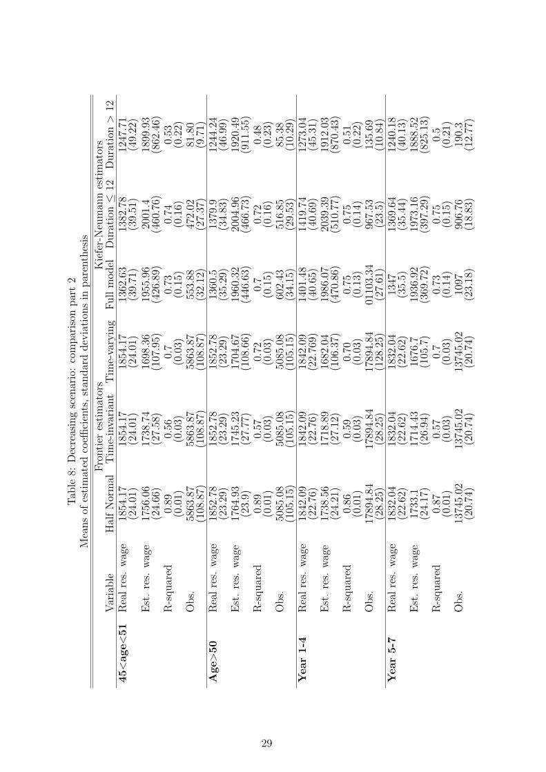
Tab

le8:

Dec

reas

ing

scen

ario

:co

mpar

ison

par

t2

Mea

ns

ofes

tim

ated

coeffi

cien

ts,

stan

dar

ddev

iati

ons

inpar

enth

esis

Fro

nti

eres

tim

ator

sK

iefe

r-N

eum

ann

esti

mat

ors

Var

iable

Hal

fN

orm

alT

ime-

inva

rian

tT

ime-

vary

ing

Full

model

Dura

tion≤

12D

ura

tion

>12

45<

age<

51

Rea

lre

s.w

age

1854

.17

1854

.17

1854

.17

1362

.63

1382

.78

1247

.71

(24.

01)

(24.

01)

(24.

01)

(39.

71)

(39.

51)

(49.

22)

Est

.re

s.w

age

1756

.06

1738

.74

1698

.36

1955

.96

2001

.418

99.9

3(2

4.66

)(2

7.58

)(1

07.9

5)(4

26.8

9)(4

60.7

6)(8

62.4

6)R

-squar

ed0.

890.

560.

70.

730.

740.

53(0

.01)

(0.0

3)(0

.03)

(0.1

5)(0

.16)

(0.2

2)O

bs.

5863

.87

5863

.87

5863

.87

553.

8847

2.02

81.8

0(1

08.8

7)(1

08.8

7)(1

08.8

7)(3

2.12

)(2

7.37

)(9

.71)

Age>

50

Rea

lre

s.w

age

1852

.78

1852

.78

1852

.78

1360

.513

79.9

1244

.24

(23.

29)

(23.

29)

(23.

29)

(35.

29)

(34.

83)

(46.

99)

Est

.re

s.w

age

1764

.93

1745

.23

1704

.67

1960

.32

2004

.96

1920

.49

(23.

9)(2

7.77

)(1

08.6

6)(4

46.6

3)(4

66.7

3)(9

11.5

5)R

-squar

ed0.

890.

570.

720.

70.

720.

48(0

.01)

(0.0

3)(0

.03)

(0.1

5)(0

.16)

(0.2

3)O

bs.

5085

.08

5085

.08

5085

.08

602.

4351

6.85

85.3

8(1

05.1

5)(1

05.1

5)(1

05.1

5)(3

4.15

)(2

9.53

)(1

0.29

)Y

ear

1-4

Rea

lre

s.w

age

1842

.09

1842

.09

1842

.09

1401

.48

1419

.74

1273

.04

(22.

76)

(22.

76)

(22.

769)

(40.

65)

(40.

69)

(45.

31)

Est

.re

s.w

age

1738

.56

1718

.89

1682

.04

1986

.07

2039

.39

1912

.03

(24.

21)

(27.

12)

(106

.37)

(470

.86)

(510

.77)

(870

.43)

R-s

quar

ed0.

860.

590.

700.

750.

750.

51(0

.01)

(0.0

3)(0

.03)

(0.1

3)(0

.14)

(0.2

2)O

bs.

1789

4.84

1789

4.84

1789

4.84

0110

3.34

967.

5313

5.69

(28.

25)

(28.

25)

(128

.25)

(27.

61)

(23.

5)(1

0.84

)Y

ear

5-7

Rea

lre

s.w

age

1832

.04

1832

.04

1832

.04

1347

1369

.64

1240

.18

(22.

62)

(22.

62)

(22.

62)

(35.

5)(3

5.44

)(4

0.13

)E

st.

res.

wag

e17

33.1

1714

.43

1676

.719

36.9

219

73.1

618

88.5

2(2

4.17

)(2

6.94

)(1

05.7

)(3

69.7

2)(3

97.2

9)(8

25.1

3)R

-squar

ed0.

870.

570.

70.

730.

750.

5(0

.01)

(0.0

3)(0

.03)

(0.1

4)(0

.15)

(0.2

1)O

bs.

1374

5.02

1374

5.02

1374

5.02

1097

906.

7619

0.3

(20.

74)

(20.

74)

(20.

74)

(23.

18)

(18.

83)

(12.

77)

29

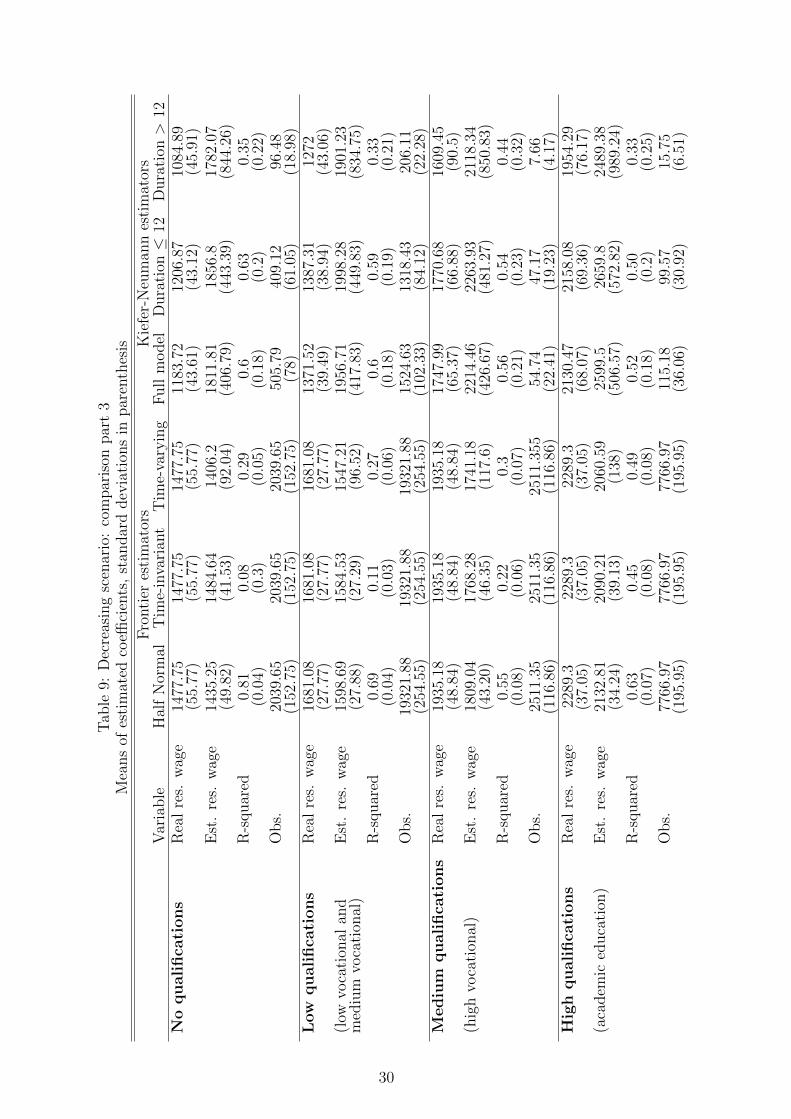
Tab

le9:

Dec

reas

ing

scen

ario

:co

mpar

ison

par

t3

Mea

ns

ofes

tim

ated

coeffi

cien

ts,

stan

dar

ddev

iati

ons

inpar

enth

esis

Fro

nti

eres

tim

ator

sK

iefe

r-N

eum

ann

esti

mat

ors

Var

iable

Hal

fN

orm

alT

ime-

inva

rian

tT

ime-

vary

ing

Full

model

Dura

tion≤

12D

ura

tion

>12

No

quali

fica

tions

Rea

lre

s.w

age

1477

.75

1477

.75

1477

.75

1183

.72

1206

.87

1084

.89

(55.

77)

(55.

77)

(55.

77)

(43.

61)

(43.

12)

(45.

91)

Est

.re

s.w

age

1435

.25

1484

.64

1406

.218

11.8

118

56.8

1782

.07

(49.

82)

(41.

53)

(92.

04)

(406

.79)

(443

.39)

(844

.26)

R-s

quar

ed0.

810.

080.

290.

60.

630.

35(0

.04)

(0.3

)(0

.05)

(0.1

8)(0

.2)

(0.2

2)O

bs.

2039

.65

2039

.65

2039

.65

505.

7940

9.12

96.4

8(1

52.7

5)(1

52.7

5)(1

52.7

5)(7

8)(6

1.05

)(1

8.98

)L

ow

quali

fica

tions

Rea

lre

s.w

age

1681

.08

1681

.08

1681

.08

1371

.52

1387

.31

1272

(27.

77)

(27.

77)

(27.

77)

(39.

49)

(38.

94)

(43.

06)

(low

voca

tion

alan

dE

st.

res.

wag

e15

98.6

915

84.5

315

47.2

119

56.7

119

98.2

819

01.2

3m

ediu

mvo

cati

onal

)(2

7.88

)(2

7.29

)(9

6.52

)(4

17.8

3)(4

49.8

3)(8

34.7

5)R

-squar

ed0.

690.

110.

270.

60.

590.

33(0

.04)

(0.0

3)(0

.06)

(0.1

8)(0

.19)

(0.2

1)O

bs.

1932

1.88

1932

1.88

1932

1.88

1524

.63

1318

.43

206.

11(2

54.5

5)(2

54.5

5)(2

54.5

5)(1

02.3

3)(8

4.12

)(2

2.28

)M

ediu

mquali

fica

tions

Rea

lre

s.w

age

1935

.18

1935

.18

1935

.18

1747

.99

1770

.68

1609

.45

(48.

84)

(48.

84)

(48.

84)

(65.

37)

(66.

88)

(90.

5)(h

igh

voca

tion

al)

Est

.re

s.w

age

1809

.04

1768

.28

1741

.18

2214

.46

2263

.93

2118

.34

(43.

20)

(46.

35)

(117

.6)

(426

.67)

(481

.27)

(850

.83)

R-s

quar

ed0.

550.

220.

30.

560.

540.

44(0

.08)

(0.0

6)(0

.07)

(0.2

1)(0

.23)

(0.3

2)O

bs.

2511

.35

2511

.35

2511

.355

54.7

447

.17

7.66

(116

.86)

(116

.86)

(116

.86)

(22.

41)

(19.

23)

(4.1

7)H

igh

quali

fica

tions

Rea

lre

s.w

age

2289

.322

89.3

2289

.321

30.4

721

58.0

819

54.2

9(3

7.05

)(3

7.05

)(3

7.05

)(6

8.07

)(6

9.36

)(7

6.17

)(a

cadem

iced

uca

tion

)E

st.

res.

wag

e21

32.8

120

90.2

120

60.5

925

99.5

2659

.824

89.3

8(3

4.24

)(3

9.13

)(1

38)

(506

.57)

(572

.82)

(989

.24)

R-s

quar

ed0.

630.

450.

490.

520.

500.

33(0

.07)

(0.0

8)(0

.08)

(0.1

8)(0

.2)

(0.2

5)O

bs.

7766

.97

7766

.97

7766

.97

115.

1899

.57

15.7

5(1

95.9

5)(1

95.9

5)(1

95.9

5)(3

6.06

)(3

0.92

)(6

.51)

30

References

Aigner, D., Lovell, C. A. K., and Schmidt, P. (1977). Formulation and estimation of stochas-

tic frontier production function models. Journal of Econometrics, 6(1):21–37.

Antonovics, K. and Town, R. (2004). Are all the good men married? uncovering the sources

of the marital wage premium. American Economic Review, 94(2):317–321.

Bachmann, R. (2005). Labour market dynamics in germany: Hirings, separations, and

job-to-job transitions over the business cycle. SFB 649 Discussion Papers 2005-045, Son-

derforschungsbereich 649, Humboldt University, Berlin, Germany.

Battese, G. E. and Coelli, T. J. (1988). Prediction of firm-level technical efficiencies with

a generalized frontier production function and panel data. Journal of Econometrics,

38(3):387 – 399.

Battese, G. E. and Coelli, T. J. (1992). Frontier production functions, technical efficiency

and panel data: With application to paddy farmers in india. Journal of Productivity

Analysis, 3:153–169.

Battese, G. E., Coelli, T. J., and Colby, T. (1989). Estimation of frontier production functions

and the efficiencies of indian farms using panel data from icrisat’s village level studies.

Journal of Quantitative Economics, 5:327–348.

Boheim, R. (2002). The association between reported and calculated reservation wages.

ISER Working Paper Series 2002-07, Institute for Social and Economic Research.

Boll, C. (2011). Lohneinbußen von Frauen durch geburtsbedingte Erwerbsunterbrechungen.

Sozialokonomische Schriften. Peter Lang, Frankfurt am Main, Berlin, Bern, Bruxelles,

New York, Oxford, Wien,.

Christensen, B. (2005). Die Lohnanspruche deutscher Arbeitsloser. Number 333 in Kieler

Studien. Springer, Berlin [u.a.].

Cornwell, C. and Schneider, K. (2000). Labor market policy and german reservation wages

in the 1990s: A stochastic frontier approach. University of Georgia and Dortmund.

Devine, T. J. and Kiefer, N. M. (1991). Empirical Labor Economics: The Search Approach.

Oxford University Press.

Elsby, M., Hobijn, B., and Sahin, A. (2008). Unemployment dynamics in the oecd. NBER

Working Papers 14617, National Bureau of Economic Research, Inc.

Greene, W. H. (2005). Efficiency of public spending in developing countries: A stochastic

frontier approach. Report for the World Bank.

31

Heckman, J. (1979.). Sample selection bias as a specification error. Econometrica,

47:153–161.

Hoffler, R. A. and Murphy, K. J. (1994). Estimating reservation wages of employed workers

using a stochastic frontier. Southern Economic Journal, 60(4):964–976.

Jensen, U. (2005). Misspecification preferred: The sensitivity of inefficiency rankings. Jour-

nal of Productivity Analysis, 23:223–244.

Jensen, U., Gartner, H., and Raessler, S. (2010). Estimating german reservation wages with

stochastic wage frontiers. Kiel, Nurnberg, Bamberg.

Jondrow, J., Lovell, C. A. K., Materov, I. S., and Schmidt, P. (1982). On the estimation

of technical inefficiency in the stochastic frontier production function model. Journal of

Econometrics, 19(2-3):233 – 238.

Kiefer, N. M. and Neumann, G. R. (1979a). An empirical job-search model, with a test of

the constant reservation-wage hypothesis. Journal of Political Economy, 87(1):89–107.

Kiefer, N. M. and Neumann, G. R. (1979b). Estimation of wage offer distribution and

reservation wages. In Lippman, S. A. and McCall, J. J., editors, Studies in the economics

of search. North Holland: Amsterdam.

Kumbhakar, S. C. and Lovell, C. A. K. (2003). Stochastic frontier analysis. Cambridge

University Press.

Maani, S. A. and Studenmund, A. H. (1986). The critical wage, unemployment duration,

and wage expectations: The case of chile. Industrial and Labor Relations Review, 39(2):pp.

264–276.

McCall, J. J. (1970). Economics of information and job search. The Quarterly Journal of

Economics, 84(1):pp. 113–126.

Meeusen, W. and Broeck, J. v. D. (1977). Efficiency estimation from cobb-douglas production

functions with composed error. International Economic Review, 18(2):pp. 435–444.

Prasad, E. S. (2003). What determines the reservation wages of unemployed workers? new

evidence from german micro data. IZA Discussion Papers 694, Institute for the Study of

Labor (IZA).

Ritter, C. and Simar, L. (1997). Pitfalls of normal-gamma stochastic frontier models. Journal

of Productivity Analysis, 8:167–182.

Schmidt, C. M. and Winkelmann, R. (1993). Reservation wages, wage offer distributions

and accepted wages. In Bunzel, H., Jensen, P., and Westergard-Nielsen, N., editors, Panel

Data and Labour Market Dynamics. Amsterdam.

32

Statistisches Bundesamt Deutschland (2011). Statistisches Bundesamt Deutschland - Reg-

istrierte Arbeitslose, Arbeitslosenquote nach Gebietsstand. [Online; accessed 23-August-

2011].

Vishwanath, T. (1989). Job search, stigma effect, and escape rate from unemployment.

Journal of Labor Economics, 7(4):487–502.

Wagner, G. G., Frick, J. R., and Schupp, J. (2007). The german socio-economic panel study

(soep): Scope, evolution and enhancements. SOEPpapers 1, DIW Berlin, The German

Socio-Economic Panel (SOEP).

Watson, D. and Webb, R. (2008). Reservation wage levels in uk and german financial services

sectors. The Service Industries Journal, 28(8):1167–1182.

Webb, R., Watson, D., and Hinks, T. (2003). Testing for wage overpayment in uk financial

services: A stochastic frontier approach. The Service Industries Journal, 23(5):123–136.

33

HWWI Research Papersseit 2011

123 Trade and Economic Growth: A Re-examination of the Empirical Evidence

Matthias Busse, Jens Königer, April 2012

122 Immigration and Election Outcomes − Evidence from City Districts in Hamburg

Alkis Henri Otto, Max Friedrich Steinhardt, April 2012

121 Renewables in the energy transition − Evidence on solar home systems and

lighting fuel choice in Kenya

Jann Lay, Janosch Ondraczek, Jana Stöver, April 2012

119 Creative professionals and high-skilled agents: Polarization of employment

growth?

Jan Wedemeier, March 2012

118 Unraveling the complexity of U.S. presidential approval. A multi-dimensional

semi-parametric approach

Michael Berlemann, Soeren Enkelmann, Torben Kuhlenkasper, February 2012

117 Policy Options for Climate Policy in the Residential Building Sector: The Case of

Germany

Sebastian Schröer, February 2012

116 Fathers’ Childcare: the Difference between Participation and Amount of Time

Nora Reich, February 2012

115 Fathers’ Childcare and Parental Leave Policies − Evidence from Western

European Countries and Canada

Nora Reich, Christina Boll, Julian Leppin, Hamburg, February 2012

114 What Drives FDI from Non-traditional Sources? A Comparative Analysis of the

Determinants of Bilateral FDI Flows

Maximiliano Sosa Andrés, Peter Nunnenkamp, Matthias Busse,

Hamburg, January 2012

113 On the predictive content of nonlinear transformations of lagged

autoregression residuals and time series observations

Anja Rossen, Hamburg, October 2011

112 Regional labor demand and national labor market institutions in the EU15

Helmut Herwartz, Annekatrin Niebuhr, Hamburg, October 2011

111 Unemployment Duration in Germany – A comprehensive study with dynamic

hazard models and P-Splines

Torben Kuhlenkasper, Max Friedrich Steinhardt, Hamburg, September 2011

110 Age, Life-satisfaction, and Relative Income

Felix FitzRoy, Michael Nolan, Max Friedrich Steinhardt, Hamburg, July 2011

109 The conjoint quest for a liberal positive program: “Old Chicago”, Freiburg and

Hayek

Ekkehard Köhler, Stefan Kolev, Hamburg, July 2011

108 Agglomeration, Congestion, and Regional Unemployment Disparities

Ulrich Zierahn, Hamburg, July 2011

107 Efficient Redistribution: Comparing Basic Income with Unemployment Benefit

Felix FitzRoy, Jim Jin, Hamburg, March 2011

106 The Resource Curse Revisited: Governance and Natural Resources

Matthias Busse, Steffen Gröning, Hamburg, March 2011

105 Regional Unemployment and New Economic Geography

Ulrich Zierahn, Hamburg, March 2011

104 The Taxation-Growth-Nexus Revisited

K. P. Arin, M. Berlemann, F. Koray, T. Kuhlenkasper, Hamburg, January 2011

The Hamburg Institute of International Economics (HWWI) is an independent economic research institute, based on a non-profit public-private partnership, which was founded in 2005. The University of Hamburg and the Hamburg Chamber of Commerce are shareholders in the Institute .

The HWWI’s main goals are to: • Promote economic sciences in research and teaching;• Conduct high-quality economic research; • Transfer and disseminate economic knowledge to policy makers, stakeholders and the general public.

The HWWI carries out interdisciplinary research activities in the context of the following research areas: • Economic Trends and Global Markets, • Regional Economics and Urban Development, • Sectoral Change: Maritime Industries and Aerospace, • Institutions and Institutional Change, • Energy and Raw Material Markets, • Environment and Climate, • Demography, Migration and Integration, • Labour and Family Economics, • Health and Sports Economics, • Family Owned Business, and• Real Estate and Asset Markets.

Hamburg Institute of International Economics (HWWI)

Heimhuder Str. 71 | 20148 Hamburg | GermanyPhone: +49 (0)40 34 05 76 - 0 | Fax: +49 (0)40 34 05 76 - 776info@hwwi.org | www.hwwi.org