the estimation of rock mass deformation modulus … · hamid mohammadi and reza rahmannejad 206 the...

Hamid Mohammadi and Reza Rahmannejad

January 2010 The Arabian Journal for Science and Engineering, Volume 35, Number 1A 205

THE ESTIMATION OF ROCK MASS DEFORMATION MODULUS USING REGRESSION AND ARTIFICIAL

NEURAL NETWORKS ANALYSIS

Hamid Mohammadi * and Reza Rahmannejad Mining Engineering Department

Bahonar University of Kerman, Iran

:الخالصـة

ة األساس لعاِمُمإن ا (EM) تفكك آتل ة هو عامل إدخ شاآل الجيوآيميائي م في الم ذا العامل نإحيث ، ل مه دان إليجاد ه ثمن فحوصات المي ة ال غاليل -في الطريقة األولى ف . (EM) تطوير طريقتين لحساب -في هذه الورقة العلمية -تم و. طويًال وقتًاتستهلك و ى - نحسار االباستخدام تحلي م الحصول عل ت

ة بعامل فتراضية اخمس معادالت ة األساس (EM) متعلق دد الحدود أفضل معامل حيث أ ، (RMR) و سرعة آتل اط اعطى تناسب متع م . رتب في -وتادا ا (EM)نموذج لحساب أ تطوير (ANN)باستخدام الشبكة الصناعية المحايدة -الطريقة األخرى ى نظام أساس وظيفي نصف قطري عتم م . عل د ت وق

ة و. الناتجة بنتائج في الموقع قيم مقارنة التتمآما . Karun IV لسد (EM) في حساب نيالطريقت نيهات تطبيق ًاأخير ة طريق ات أن دق قد أظهرت المقارنANN نحساراال هي أفضل من طريقة تحليل.

*Corresponding Author: E-mail: [email protected]

Paper Received April 1, 2008; Paper Revised October 24, 2009; Paper Accepted December 9, 2009


The Arabian Journal for Science and Engineering, Volume 35, Number 1A January 2010 206

ABSTRACT

Rock mass deformation modulus (EM) is an important input parameter in geomechanical problems. Field tests to determine this parameter are time consuming and expensive. In this paper, two methods have been developed to estimate EM. In the first method, using regression analysis, five empirical equations have been obtained relating EM and the rock mass rating (RMR), with the polynomial fitting having the best correlation coefficient. In the other method, using artificial neural network (ANN), a model has been obtained for estimating EM based on the radial basis function (RBF). Finally, both methods are applied to estimate EM of Karun IV dam. The obtained values are compared with the results of in-situ test. The comparisons have shown that the accuracy of the ANN method is better than of the regression analysis.

Key words: rock mass, RMR, deformation modulus, regression analysis, ANN



THE ESTIMATION OF ROCK MASS DEFORMATION MODULUS USING REGRESSION AND ARTIFICIAL NEURAL NETWORKS ANALYSIS

1. INTRODUCTION

The deformation modulus (EM) is one of the most important properties of rock masses used for designing many structures in and on rock, from underground openings to foundations [1–3]. This is why most numerical finite element and boundary element analyses for studies of the stress and displacement distribution around underground excavations are based on this parameter. Therefore, it is a cornerstone of many geomechanical analyses [4]. The equivalent continuum approach treats the jointed rock mass as an equivalent continuum with a deformability that reflects the properties of both the intact rock and the discontinuities [5,6]. However, the strength and deformation modulus of jointed rock masses can not be directly determined, since the dimensions of representative specimen are too large for a laboratory testing. To overcome this limitation, one should apply in situ tests, such as plate jacking, plate loading, radial jacking, flat jack, and cable jack, etc. [7].

Due to the difficulties encountered during in-situ tests, several authors have proposed empirical relations for estimating the deformation modulus of an isotropic rock mass on the basis of classification schemes such as the rock mass rating (RMR) [8], the tunneling quality index (Q) [9], the geological strength index (GSI) [10], rock quality designation RQD [3], and rock mass index (RMi) [4]. Also, some authors predicted the deformation modulus on the basis of the Mamdani fuzzy inference system and neuro-fuzzy model [7,11].

According to Table 1, the six relations were presented on the basis of RMR, showing that RMR is an important factor in the determination of deformation modulus both from the geologist’s and engineer’s point of view.

The RMR system was initially developed at the South African Council of Scientific and Industrial Research (CSIR) by Bieniawski (1973) on the basis of his experiences in shallow tunnels in sedimentary rocks (Kaiser et al., 1986) [12]. Since then, the classification has undergone several significant evolutions: in 1974 – reduction of classification parameters from 8 to 6; in 1975 – adjustment of ratings and reduction of recommended support requirements; in 1976 – modification of class boundaries to even multiples of 20; in 1979 – adoption of the ISRM (1978) rock mass description, etc. It is, therefore, important to state which version is used whenever RMR-values are quoted. The geomechanics classification reported by Bieniawski (1989) is referred to in this book [12].

To apply the geomechanics classification system, a given site should be divided into a number of geological structural units in such a way that each type of rock mass is represented by a separate geological structural unit. The following six parameters (representing causative factors) are determined for each structural unit [12]:

(i) Uniaxial compressive strength of the intact rock material, (Rating (Ri): 0–15),

(ii) Rock quality designation RQD, (Rating (Rii): 3–20),

(iii) Joint or discontinuity spacing, (Rating (Riii): 5–20),

(iv) Joint condition, (Rating (Riv): 0–30),

(v) Ground water condition, (Rating (Rv): 0–15), and

(vi) Joint orientation, (Rating (Rvi): -60–0).

The RMR (RMR(1989)) and RMRbasic should be determined as an algebraic sum of the rating parameters [12].

(1989) i ii iii iv v viRMR RMR R R R R R R= = + + + + + (1)

( )basic i ii iii iv vRMR R R R R R= + + + + (2)

On the basis of RMR values for a given engineering structure, the rock mass is classified into five classes, namely: very good (RMR 100–81), good (80–61), fair (60–41), poor (40–21), and very poor (<20) [12].

Hence, RMR will be used to determine the rock mass deformation modulus in this paper. The data used in the present study were obtained from Gokceoglu et al. [13] and from the field data of Bieniawski, Serafim & Pereira and Stephens [14–16].



Table 1. List of the Empirical Equations Suggested for Estimating the Deformation Modulus

Equation Range of Applicability Reference

2 100ME RMR= − 50>RMR [14] ( 10) / 4010 RMR

ME −= 50≤RMR [15] 2/100(0.0028 0.9exp( /22.82))M iE E RMR RMR= + _ [17]

(0.5(1 ( /100)))M iE E Cos RMRπ= − _ [18] 30.1( /10)ME RMR= _ [19]

( 10) / 40(1 / 2) /100 10 RMRM ciE D σ −= − × 100 UCS MPa≤ [20]

In this study, rock mass deformation modulus is determined using two methods. In the first one, new relations

between the rock mass deformation modulus and RMR have been derived using curve fitting and regression analysis. In the second method, artificial neural networks (ANN) were used. The ANN has been successfully used in the past decades in engineering problems [21,22]. For this reason, a new radial basis function (RBF) neural network was built to predict the deformation modulus of rock mass by the given value of RMR (1989). Plate-loading test data and the rock mass rating (RMR) obtained from Karun IV dam site in Iran [23] were used to test the results of the ANN model.

2. DEVELOPMENT OF EMPIRICAL RELATIONS OF ROCK MASS DEFORMATION MODULUS

When selecting from among the existing empirical equations for the estimation of deformation modulus, the following criteria suggested by Clerici [24] were considered:

(a) Equations must be based on parameters that can be acquired easily and at low cost;

(b) Equations must be widely used, or cited, in the literature.

As stated in the Introduction, there are several empirical approaches for predicting the rock masses' deformation modulus in rock mechanics literature. A rock mass classification system can be used to estimate mechanical properties such as the rock mass deformation modulus at a preliminary design stage. Bieniawski, Serafim and Pereira, and Read [14,15,19] estimated rock mass deformation modulus using the RMR of Bieniawski. The RMR system seems to be the best choice for the design because it contains many properties of rock masses. Therefore, the focus of this study is also on the use of a rock mass classification system RMR to estimate rock mass deformation modulus.

As mentioned, the (altogether 171) data employed in the present study were taken from [13–16] (Figure 1).

Figure 1. Rock mass deformation modulus-RMR data



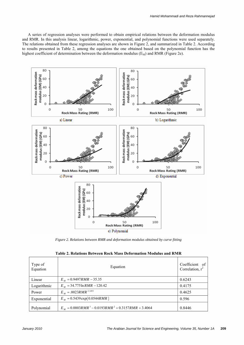
A series of regression analyses were performed to obtain empirical relations between the deformation modulus and RMR. In this analysis linear, logarithmic, power, exponential, and polynomial functions were used separately. The relations obtained from these regression analyses are shown in Figure 2, and summarized in Table 2. According to results presented in Table 2, among the equations the one obtained based on the polynomial function has the highest coefficient of determination between the deformation modulus (EM) and RMR (Figure 2e).

Figure 2. Relations between RMR and deformation modulus obtained by curve fitting

Table 2. Relations Between Rock Mass Deformation Modulus and RMR

Type of Equation Equation Coefficient of

Correlation, r2

Linear 0.9497 35.35ME RMR= − 0.6243 Logarithmic 34.775ln 120.42ME RMR= − 0.4175 Power 2.1455.0023ME RMR= 0.4625 Exponential ( )0.5439exp 0.0544ME RMR= 0.596

Polynomial 3 20.0003 0.0193 0.3157 3.4064ME RMR RMR RMR= − + + 0.8446



The comparison of the derived regression models with Bieniawski’s equation, Serafim and Pereira’s equation, and Read et al.’s equation are shown in Figure 3. In this comparison, the root mean square error (RMSE) was used to evaluate the qualification of suggested relations, prediction performance, and previous relations that were developed by other researchers such as Serafim and Pereira, Bieniawski, and Read et al. The equation of RMSE is

( ) ( )( )2

1

Nestimated measuredM Mi i

i

E ERMSE

N=

−=∑

(3)

where measuredME is the measured value of rock mass deformation modulus by in-situ test; estimatedME is the estimated value of rock mass deformation modulus by empirical equations; and N is the number of

dataset pairs.

The excellent prediction values are 0 RMSE errors. According to values in Figure 3, among the equations, the equation obtained by polynomial fitting has the lowest RMSE.

Figure 3. Comparison of obtained relations with the equations of:

a)Read et al., b) Serafim and Pereira, c) Bieniawski

3. A STUDY OF DEFORMATION MODULUS CLASSIFICATION

Clerici [24] expressed that, "When the value of the deformation modulus is determined, even by direct measurement, the aim can not be to define an absolute value, but rather to define a magnitude for the modulus.” Therefore, for designing geomechanics problems, it is logical to consider a range of values of the deformation modulus. This allows for a sensitivity analysis in the following calculations of the geomechanics problem. Bieniawski [9] classified the rock mass rating (RMR) into five classes and determined a range of values of rock mass geomechanical properties for each class, such as internal friction angle and cohesion of rock mass (Table 3). However, he did not include deformation modulus.



Table 3. Design Parameters and Engineering Properties of Rock Mass (Bieniawski, 1979)

Rock mass rating (Rock class) S. No

Parameter/properties of rock mass RMR = 81–100 RMR = 61–80 RMR = 41–60 RMR=21–40 RMR < 20

1. Classification of rock mass Very good Good Fair Poor Very poor

2. Cohesion of rock mass (MPa) >0.4 0.3–0.4 0.2–0.3 0.1–0.2 <0.1

3. Internal friction angle of rock mass (degree) >45 35–45 25–35 15–25 <15

As shown in Table 4 and Figure 4, the classes of internal friction angle together and cohesion of rock mass

together do not have any common aspect. Therefore, the internal friction angle and cohesion of rock mass can be classified based on the RMR classification.

Table 4. Relation of RMR Classes Together and Relation of Rock Mass Properties Classes (Cohesion and Internal Friction Angle) Together

Subscription of Class I to other

classes

Subscription of Class II to other

classes

Subscription of Class III to other

classes

Subscription of Class IV to other

classes

Subscription of Class V to other

classes

Class I∩Class II=Φ Class II∩Class I=Φ

Class III∩Class I=Φ Class IV∩Class I=Φ Class V∩Class I=Φ

Class I∩Class III=Φ

Class II∩Class III=Φ

Class III∩Class II=Φ

Class IV∩Class II=Φ

Class V∩Class II=Φ

Class I∩Class IV=Φ

Class II∩Class IV=Φ

Class III∩Class IV=Φ

Class IV∩Class III=Φ

Class V∩Class III=Φ

Class I∩Class V=Φ Class II∩Class V=Φ

Class III∩Class V=Φ

Class IV∩Class V=Φ

Class V∩Class IV=Φ

Figure 4. Classification of rock mass properties based on the RMR classification:

a) cohesion of rock mass, b) internal friction angle of rock mass

In Table 5 and Figure 5, the deformation modulus of rock masses were divided into 5 classes based on the RMR classification. As shown, the classes II, III, IV, and V have a subscription together. Therefore, the deformation modulus can not be classified based on the RMR classification.



Table 5. Relation of Rock Mass Deformation Modulus Classes (Cohesion and Internal Friction Angle) Together

Subscription of Class I to other

classes

Subscription of Class II to other

classes

Subscription of Class III to other

classes

Subscription of Class IV to other

classes

Subscription of Class V to other

classes

Class I∩Class II=Φ

Class II∩Class I=Φ

Class III∩Class I=Φ

Class IV∩Class I=Φ

Class V∩Class I=Φ

Class I∩Class III=Φ

Class II∩Class III= 0-24, (Class

III)

Class III∩Class II = 0-24, (Class III)

Class IV∩Class II = 0-8, (Class IV)

Class V∩Class II = 0-5, (Class V)

Class I∩Class IV=Φ

Class II∩Class IV= 0-8, (Class

IV)

Class III∩Class IV= 0-8, (Class

IV)

Class IV∩Class III = 0-8, (Class IV)

Class V∩Class III = 0-5, (Class V)

Class I∩Class V=Φ

Class II∩Class V= 0-5, (Class V)

Class III∩Class V= 0-5, (Class V)

Class IV∩Class V = 0-5, (Class V)

Class V∩Class IV = 0-5, (Class V)

Figure 5. Deformation modulus classification based on the RMR classification

4. ARTIFICIAL NEURAL NETWORKS

ANNs are highly simplified models of human nervous systems. These models consist of an interconnected assembly of simple processing elements, neurons, organized in a layered fashion. Each neuron in a layer is connected to the neurons in the subsequent layer and so on [25].

The propagation of information in ANNs starts at the first layer where the input data are presented. The inputs are weighted and received by each node in the next layer. The weighted inputs are then summed and passed through a transfer function to produce the nodal output, which is weighted and passed to processing elements in the next layer. The network adjusts its weights on presentation of a set of training data and uses a learning rule until it can find a set of weights that will produce the input-output mapping that has the smallest possible error. The above process is known as ‘learning’ or ‘training’ [26].

The most common and simplest type of neural networks consists of three layers: the input layer, the hidden layer, and the output layer. In general, neural networks can be categorized as either supervised or unsupervised. The fundamental difference between supervised and unsupervised networks depends on the known data set that must be used in order to train the network. Supervised neural networks are trained in order to produce the desired outputs in response to a training set of inputs. This is why they are typically used in the modelling and controlling of dynamic systems, classifying noisy data, and predicting future events. Unsupervised neural networks, on the other hand, are trained by letting the network continually adjusting itself to new inputs. They uncover non-linear relationships within data and can define classification schemes that adapt to changes in the new data [26]. Based on connections between processing elements, ANNs can be divided into feed-forward and feedback networks. In feed-forward networks, the



connections between processing elements are in the forward direction only, whereas in feedback networks, connections between processing elements are in both the forward and backward directions.

4.1. Radial Basis Function Networks

There are three layers in RBF networks: 1) the input layer, 2) the hidden layer, and 3) the output layer. The input layer is responsible for collecting the input information and formulating the input vector X. L hidden nodes of the hidden layer apply nonlinear transformations to the input vector. A vector ˆ

lX represents a typical hidden node 1 in an RBF network. Dimensionally, it is equal to the input vector and a scalar width lσ .

The activity ( )l Xν of the node is given by [27]

ˆ( )l lX X Xν = − (4)

It is computed as the Euclidean norm of the differences between the input vector and the node center. To determine the response of the hidden node, the activity should be passed through the radially symmetric Gaussian function [26]:

2

2( )( ) exp l

ll

Xf X νσ

⎛ ⎞= −⎜ ⎟⎜ ⎟

⎝ ⎠

(5)

The last network output values are calculated as linear combination of the hidden layer response:

, 1, ...,

1

ˆ( ) ( ) m ML

m m l lml

y g X f X w =∑=

= = (6)

where 1 2[ , ,..., ]L mm mw w w is the vector of weights. It multiplies the hidden node responses for calculating the network's m-th output. RBF network architecture methodologies are based on a set of input-output training pairs (x(k) ; y(k)) (k = 1,2,...,K). The procedure used in this study includes three separate steps [27]:

(i) Selection of the network structure and calculation of the hidden node centers.

(ii) The Gaussian activation function widths are calculated by the use of the p-nearest neighbor heuristic, after the determination of the hidden node centers (Equation (7)).

12

2

1

1 ˆ ˆp

l l i

i

X Xp

σ

=

= −⎛ ⎞⎜ ⎟⎜ ⎟⎝ ⎠∑ (7)

(iii) The connection weights are obtained by linear regression between responses of the hidden layer and the corresponding output training set.

4.2. Development of RBF Network

In this research, an RBF network was applied for the design of a model that could be able to predict the deformation modulus of rock masses.

In the RBF network, the spread value is affected based on the results. Therefore, a trial and error step is always used to find the best results. Because many properties of the rock mass affect the deformation modulus and some of the empirical relations are based on the RMR, the network input is selected as RMR (Figure 6).

The number of data in the dataset used for training is 171. In Figure 7, the result of application of the RBF network for predicting the deformation modulus is shown and compared with actual values. The RMSE obtained from network training is 5.84. The data from Karun IV dam site were used to test and investigate the efficiency of the ANN model.



Figure 6. RBF network architecture to estimate the deformation modulus

Figure 7. Results of RBF network for training data

5. DETERMINATION OF ROCK MASS DEFORMATION MODULUS OF KARUN IV DAM USING ANN

The Karun IV dam is located 180 km south-west of Shahrekord town in Chaharmahal-e-Bakhtiari province in Iran. Distance from dam site to the mouth of the Karun River is about 670 km.

The rock masses of the dam site are composed of limestone and marble rocks. The rock mass is intersected by

several bedding planes, joint sets, and faults. 17 plate loading tests were used for determining the rock mass deformation modulus (EM) of the site [23]. The results obtained from tests and the empirical equations [14,15] are presented in Table 6.



Table 6. Rock Masses Deformation Modulus of Karun IV Dam Site

Deformation modulus (GPa) Class RMR (basic) RMR=RMR(1989)

obtained from empirical equations [14,15]

obtained from plate loading tests

I 73 57 14 11 II 53 51 2 8 III 35 30 3.16 4 IV 26 22 1.88 2

The results of the deformation modulus calculation of Karun IV dam site using ANN's are shown in Table 7. The obtained results are also compared using the relative error level (∆) defined as

100measured EstimatedM M

EstimatedM

E EE

−∆ = × (8)

The obtained mean relative error level (∆) for the RBF network model and empirical equations are 23.25% and

32.25%, respectively. This shows that the RBF neural network model's efficiency is higher than that of the empirical equations.

Table 7. Determination of the Rock Mass Deformation Modulus of Karun IV Dam Using ANN'S

Deformation modulus (GPa) Relative error level (∆)

Class obtained from plate loading

tests

obtained from empirical equations

obtained from ANN model

between plate bearing test and

empirical equations

between plate bearing test and RBF network

I 11 14 12.56 27% 14% II 8 2 6.57 75% 18% III 4 3.16 5.49 21% 30% IV 2 1.88 2.63 6% 31%

6. CONCLUSIONS

The following conclusions can be drawn from the present study:

1. The different prediction models, regression equation and artificial neural network (ANN), were developed for the estimation of rock mass deformation modulus using a database including 173 data sets. A series of empirical relations to estimate the rock mass deformation modulus in terms of the RMR were derived using regression analyses. The root mean square errors (RMSE) and correlation coefficients revealed that the best predictive capability was provided by the equation obtained based on the polynomial function, among the obtained equations, Bieniawski’s equation, Serafim and Pereira’s equation, and Read et al.’s equation. Therefore, it can be reliably used to estimate deformation modulus.

2. The deformation modulus of rock masses were divided into 5 classes based on the RMR classification. The

classes II, III, IV, and V have a subscription together. Therefore, the deformation modulus can not be classified based on the RMR classification.

3. A model to estimate the deformation modulus was constructed using Redial Basis Function (RBF) Neural Networks, and tested using the data sets from the Karun IV dam. The results show that the RBF network model accuracy is higher than of the empirical equations.



ACKNOWLEDGMENT

The authors would like to acknowledge financial support from the Design and Calculation of Underground Structures Research Center at Bahonar University of Kerman-Iran. REFERENCES

[1] D. U. Deere, A. J. Hendron, F. D. Patton, and E. J. Cording, “Design of Surface and Near Surface Construction in Rock”, in Proceedings of the Eighth US Symposium on Rock Mechanics—Failure and Breakage of Rock, New York, 1976, pp. 237–302.

[2] K. M. Neaupane and N. R. Adhikari, “Prediction of Tunneling-Induced Ground Movement With the Multi-Layer Perceptron”, Tunneling and Underground Space Technol., 21(2006), pp. 151–159.

[3] L. Zhang and H. H. Einstein, “Using RQD to Estimate the Deformation Modulus of Rock Masses”, Int J. Rock Mech. Min. Sci., 4(2004), pp. 337–341.

[4] A. Palmstrom and R. Singh, “The Deformation Modulus of Rock Masses: Comparisons Between In Situ Tests and Indirect Estimates”, Tunnelling Underground Space Technol., 16(2001), pp. 115–131.

[5] [5] B. W. Amadei and Z. Savage, “Effect of Joints on Rock Mass Strength and Deformability: Comprehensive Rock Engineering Principle”, in Practice and Projects, ed. J. A. Hudson. Oxford: Pergamon Press, 1(1993), pp. 331–365.

[6] P. H. S. W. Kulatilake, S. Wang, and O. Stephansson, “Effect of Finite Size Joints on the Deformability of Jointed Rock in Three Dimensions”, Int. J. Rock Mech. Min. Sci. Geomech. Abstr., 30(1993), pp. 479–501.

[7] C. Gokceoglu, E. Yesilnacar, H. Sonmez, and A. Kayabasi, “A Neuro-Fuzzy Model for Modulus of Deformation of Jointed Rock Masses”, Computers and Geotechnics, 31(2004), pp. 375–383.

[8] Z. T. Bieniawski, “Engineering Classification of Rock Masses”, Trans. S. African Inst. Civ. Engrs., 15(12)(1973), pp. 335–344.

[9] N. Barton, R. Lien, and J. Lunde, “Engineering Classification of Rock Masses for the Design of Tunnel Support", Rock Mech. and Rock Eng., 6(4)(1974), pp. 189–236.

[10] E. Hoek and E. T. Brown, “Practical Estimates of Rock Mass Strength”, Int. J. Rock Mech. Min. Sci., 34(8)(1997), pp. 1165–1186.

[11] A. Kayabasi, C. Gokceoglu, and M. Ercanoglu, “Estimating the Deformation Modulus of Rock Masses: A Comparative Study”, Int. J. Rock Mech. Min. Sci., 40(2003), pp. 55–63.

[12] B. Singh and R. K. Goel, “Tunnelling in Weak Rocks”, Geo-Engineering Book. Elsevier, 2006, pp. 37–49.

[13] C. Gokceoglu, H. Sonmez, and A. Kayabasi, “Predicting the Deformation Moduli of Rock Masses”, Int. J. Rock Mech. Min. Sci., 40(2003), pp. 701–710.

[14] Z. T. Bieniawski, “Determining Rock Mass Deformability: Experience from Case Histories”, Int. J. Rock Mech. Min. Sci.Geomech. Abstr., 15(1978), pp. 237–247.

[15] J. L. Serafim and J. P. Pereira, “Considerations on the Geomechanical Classification of Bieniawski”, in Proc. Symp. on Engineering Geology and Underground Openings, Lisboa, 1983, pp. 1133–1144.

[16] R. E. Stephens and D. C. Banks, “Moduli for Deformation Studies of the Foundation and Abutments of the Portugues Dam—Puerto Rico”, Rock Mechanics as a Guide for Efficient Utilization of Natural Resources, in Proceedings of the 30th US Symposium, Morgantown. Rotterdam, Balkema, 1989, pp. 31–38.

[17] G. A. Nicholson and Z. T. Bieniawski, “A Nonlinear Deformation Modulus Based on Rock Mass Classification”, Int. J. Min. Geol. Eng., 8(1990), pp. 181–202.

[18] H. S. Mitri, R. Edrissi, and J. Henning, “Finite Element Modeling of Cablebolted Stopes in Hard Rock Ground Mines”, SME Annual Meeting, Albuquerque, New Mexico, 1994, pp. 94–116.

[19] S. A. L. Read, L. R. Richards, and N. D. Perrin, “Applicability of the Hoek–Brown Failure Criterion to New Zealand Greywacke Rocks”, in Proc. 9th International Congress on Rock Mechanics, Paris, eds. G. Vouille and P. Berest, August, 1999, pp. 655–660.

[20] E. Hoek, C. Carranza-Torres, and B. Corkum, “Hoek-Brown Failure Criterion-2002 Edition”, in Proc. 5th North American Rock Mechanics Symp., Toronto, Canada, 2002, pp. 267–273.

[21] M. A. Shahin and M. B. Jaksa, “Neural Network Prediction of Pullout Capacity of Marquee Ground Anchors”, Computers and Geotechnics, 32(2005), pp. 153–163.

[22] S. K. Kumar Das and P. K. Basudhar, “Undrained Lateral Load Capacity of Piles in Clay Using Artificial Neural Network”, Computers and Geotechnics, 33(2005), pp. 454–459.

[23] Mahab Ghodss Consulting Engineering Co., “Report of the Geotechnical Operations of Karun IV Dam”, 2003, Iran.



[24] A. Clerici, “Indirect Determination of Rock Masses—Case Histories”, in Proc. Symp. EUROCK, Rotterdam, A.A. Balkema, eds. L. M. Riberio e Sousa, and N. F. Grossman, 1993, pp. 509–517.

[25] S. Kahraman, H. Altun, B. S. Tezekici, and M. Fener, “Sawability Prediction of Carbonate Rocks from Shear Strength Parameters Using Artificial Neural Networks”, Int. J. Rock Mech. Min. Sci., 43(2006), pp. 157–164.

[26] M. G. Sakellariou and M. D. Ferentinou, “A Study of Slope Stability Prediction Using Neural Networks”, Geotech. Geol. Engng., 23(2005), pp. 419–445.

[27] A. Afantitis, G. Melagraki, K. Makridima, A. Alexandridis, H. Sarimveis, and O. Iglessi-Markopoulou, “Prediction of High Weight Polymers Glass Transition Temperature Using RBF Neural Networks”, Journal of Molecular Structure THEOCHEM, 716(2005), pp. 193–198.

the estimation of rock mass deformation modulus … · hamid mohammadi and reza rahmannejad 206 the...

Documents