the evaluation of bessel functions via exp-arc integrals · 1. introduction bessel functions are...
TRANSCRIPT

J. Math. Anal. Appl. 341 (2008) 478–500
www.elsevier.com/locate/jmaa
The evaluation of Bessel functions via exp-arc integrals
David Borwein a, Jonathan M. Borwein b,1, O-Yeat Chan c,∗,2
a Department of Mathematics, University of Western Ontario, London, Ontario, N6A 5B7, Canadab Faculty of Computer Science, Dalhousie University, Halifax, Nova Scotia, B3H 1W5, Canada
c Department of Mathematics and Statistics, Dalhousie University, Halifax, Nova Scotia, B3H 3J5, Canada
Received 10 July 2007
Available online 10 October 2007
Submitted by B.C. Berndt
Abstract
A standard method for computing values of Bessel functions has been to use the well-known ascending series for small argument,and to use an asymptotic series for large argument; with the choice of the series changing at some appropriate argument magnitude,depending on the number of digits required. In a recent paper, D. Borwein, J. Borwein, and R. Crandall [D. Borwein, J.M. Borwein,R. Crandall, Effective Laguerre asymptotics, preprint at http://locutus.cs.dal.ca:8088/archive/00000334/] derived a series for an“exp-arc” integral which gave rise to an absolutely convergent series for the J and I Bessel functions with integral order. Such seriescan be rapidly evaluated via recursion and elementary operations, and provide a viable alternative to the conventional ascending-asymptotic switching. In the present work, we extend the method to deal with Bessel functions of general (non-integral) order, aswell as to deal with the Y and K Bessel functions.© 2007 Elsevier Inc. All rights reserved.
Keywords: Bessel function; Uniform series expansion; Exponential-hyperbolic expansions
1. Introduction
Bessel functions are amongst the most important and most commonly occurring objects in mathematical physics.They arise as solutions to Bessel’s equation ([3, Eq. 10.2.1], [14, p. 38])
z2 d2y
dz2+ z
dy
dz+ (
z2 − ν2)y = 0, (1.1)
which is a special case of Laplace’s equation under cylindrical symmetry. The ordinary Bessel function of the firstkind of order ν is the solution Jν(z) given by the ascending series ([3, Eq. 10.2.2], [14, p. 40])
* Corresponding author.E-mail addresses: [email protected] (D. Borwein), [email protected] (J.M. Borwein), [email protected] (O-Y. Chan).
1 Research supported by NSERC and the Canada Research Chair program.2 Research partially supported by the NSERC PDF Program.
0022-247X/$ – see front matter © 2007 Elsevier Inc. All rights reserved.doi:10.1016/j.jmaa.2007.10.003

D. Borwein et al. / J. Math. Anal. Appl. 341 (2008) 478–500 479
Jν(z) :=(
z
2
)ν ∞∑m=0
(−1)m(z/2)2m
m!�(ν + m + 1). (1.2)
It is clear that although (1.2) converges rapidly for small |z|, it is computationally ineffective when |z/2|2 is muchgreater than ν. One approach to overcoming this difficulty is to use the ascending series (1.2) for small |z|, and to usethe asymptotic series below ([3, Eq. 10.17.3], [14, p. 199]) for large |z|:
Jν(z) ∼(
2
πz
)1/2(
cosω
∞∑k=0
(−1)kp2k(ν)
(2z)2k− sinω
∞∑k=0
(−1)kp2k+1(ν)
(2z)2k+1
), (1.3)
where
ω := z − πν
2− π
4,
and
pk(ν) := 1
k!k∏
m=1
4ν2 − (2m − 1)2
4= ( 1
2 − ν)k(12 + ν)k
k! ,
with the empty product that arises at k = 0 understood to be equal to 1 and
(a)n := a(a + 1) · · · (a + n − 1)
is the Pochhammer symbol. This approach is used in some texts on computation, for example in S. Zhang and J. Jin[15, p. 161]. However, one of the major drawbacks of using the asymptotic series (1.3) is that while it is known [14,p. 206] that when 2N > ν − 1
2 , the error from truncating the right-hand side of (1.3) at the N th term is bounded bythe absolute value of the N + 1st term, the right-hand side of (1.3) is divergent for fixed z. Therefore, the use of (1.3)imposes upon us a theoretical limit on the number of correct digits that can be obtained, which in turn forces us toswitch back to the ascending series (1.2) for very-high-precision computations.
The theory is similarly limited for the second (linearly independent of Jν ) solution of (1.1), known as the ordinaryBessel function of the second kind Yν(z), defined by
Yν(z) := Jν(z) cos(νπ) − J−ν(z)
sin(νπ), (1.4)
for non-integral ν, and defined as the limit of the above expression at integral ν. In particular, we have the followingexpression for Yn(z), where n is an integer [14, pp. 62, 64]:
Yn(z) = 1
π
(2(log(z/2) + γ
)Jn(z) −
n−1∑k=0
(n − k − 1)!(z/2)2k−n
k! −∞∑
k=0
(−1)k(z/2)2k+n(Hk + Hk+n)
k!(n + k)!
), (1.5)
where
Hk :=k∑
j=1
1
j
is the kth harmonic number. It also has an asymptotic expansion similar to (1.3)
Yν(z) ∼(
2
πz
)1/2(
sinω
∞∑k=0
(−1)kp2k(ν)
(2z)2k+ cosω
∞∑k=0
(−1)kp2k+1(ν)
(2z)2k+1
), (1.6)
with the same error bounds as indicated above.Similar expansions exist for the modified Bessel functions Iν(z) and Kν(z). For completeness, we state their defin-
itions below:
Iν(z) := e−νπi/2Jν(iz) =(
z
2
)ν ∞∑ (z/2)2m
m!�(ν + m + 1), (1.7)
m=0

480 D. Borwein et al. / J. Math. Anal. Appl. 341 (2008) 478–500
and
Kν(z) := π
2
I−ν(z) − Iν(z)
sin(νπ). (1.8)
It should be noted, however, that a convergent asymptotic expansion exists for Iν(z) due to Hadamard [14, p. 204]:
Iν(z) = ez
√2πz�(ν + 1
2 )
∞∑n=0
( 12 − ν)n
n!(2z)nγ
(ν + n + 1
2,2z
), (1.9)
where
γ (a, z) := za
1∫0
e−zssa−1 ds
is the incomplete gamma function. One should observe that for large n, the summands in (1.9) are of order O(n−ν−3/2)
and so although the series converges absolutely, it only does so algebraically (i.e., at polynomial rate) in the numberof summands.
In his extensive research into the theory of Hadamard expansions, R.B. Paris [4–11] found several variants of (1.9)that converge much more rapidly. In particular, in [9] he describes a general procedure for obtaining and acceleratingHadamard expansions that leads to the following geometrically convergent (i.e., at geometric rate) version of (1.9)[12]:
Iν(z) = ez
√2πz
∞∑k=0
pk(ν)
(2z)kP
(k + ν + 1
2, z
)+ e−z±πi(ν+ 1
2 )
√2πz
∞∑k=0
(−1)kpk(ν)
(2z)kP
(k + ν + 1
2,−z
), (1.10)
where
P(a, z) := γ (a, z)
�(a),
and the signs in the exponential are chosen depending on the sign of arg(z). In this paper, we approach series ex-pansions of Bessel functions from a different angle: through the evaluation of “exp-arc” integrals. The use of exp-arcintegrals was motivated by the recent work of D. Borwein, J. Borwein, and R. Crandall [1] in which these integralswere used to obtain explicit error bounds for asymptotic expansions of Laguerre polynomials. As a corollary of theirresults, they developed geometrically convergent series for the J and I Bessel functions at integral order, whose sum-mands can be computed recursively using elementary operations. These series are redolent of the modified Hadamardseries of Paris, but do not follow as special cases. Their independence from the Paris modifications is both theoreticallyand computationally interesting, and can be viewed as complementary to Paris’ investigations. We generalise theseideas to obtain exp-arc series for Bessel functions of non-integral order and for the Bessel functions of the secondkind.
At this point, perhaps a brief explanation of the term “exp-arc” is in order. Although originally (in [1]) exp-arcstood for “exponential-arcsine,” in the present work we shall use the term to indicate any of the functions
earcsin z, earcsinh z, earccos z, earccosh z.
Thus, an exp-arc integral is an integral involving a power of any of the above exp-arc functions. The main idea hereis to exploit the Taylor expansion of exp-arc functions to reduce exp-arc integrals to sums whose summands can becomputed recursively, as the Taylor coefficients of exp-arc functions satisfy second-order linear recurrences.
The rest of the paper is outlined as follows. In Section 2, we use exp-arc integrals to prove our series for Jν(z)
in detail. In Section 3, we prove analogous formulas for the other three Bessel functions mentioned above. Then inSection 4, we give an analysis of the effectiveness of our series and derive explicit error bounds on the tails. Finally, inSection 5, we provide some numerical calculations and compare our series with the traditional computation schemes.

D. Borwein et al. / J. Math. Anal. Appl. 341 (2008) 478–500 481
2. The evaluation of Jν(z)
To obtain our series for the Bessel function J , we evaluate the following integral representation of Jν(z) [14,p. 176], valid for Re(z) > 0:
Jν(z) = 1
π
π∫0
cos(νt − z sin t) dt − sin(νπ)
π
∞∫0
e−νt−z sinh t dt. (2.1)
The first integral has been dealt with in [1, Section 5]. We state the key result below.
Theorem 2.1 (Borwein–Borwein–Crandall). For any complex pair (p, q) and real numbers α, β ∈ (−π,π), let
I(p, q,α,β) :=β∫
α
e−iqωep cosω dω, (2.2)
and
r2m+1(ν) := ν
m∏j=1
(ν2 + (2j − 1)2), r2m(ν) :=
m∏j=1
(ν2 + (2j − 2)2). (2.3)
Then we have the absolutely convergent representation
I(p, q,α,β) = iep
q
∞∑k=0
rk+1(−2iq)
k!
sin β2∫
sin α2
xke−2px2dx. (2.4)
In particular, for the case where (α,β) = (−π/2,π/2), we have
I(p, q) := I(p, q,−π/2,π/2) = 2iep
q
∞∑k=0
r2k+1(−2iq)
(2k)! Bk(p), (2.5)
with
Bk(p) :=1/
√2∫
0
x2ke−2px2dx = 1
2k+1√
2
1∫0
e−puuk− 12 du = − e−p
p2k+1√
2+
(k − 1
2
)Bk−1(p)
2p. (2.6)
From Theorem 2.1 we easily deduce that
1
π
π∫0
cos(νt − z sin t) dt = 1
2π
π/2∫−π/2
ei(νt−z cos t)eiνπ/2 + e−i(νt−z cos t)e−iνπ/2 dt
= 1
2π
(e−iνπ/2I(iz, ν) + eiνπ/2I(−iz,−ν)
)= 1
2π
(e−iνπ/2I(iz, ν) + eiνπ/2I(−iz, ν)
). (2.7)
Our goal, therefore, is to find a rapidly converging series for the second (infinite domain) integral in (2.1). If we lets = sinh t so that dt = ds/
√1 + s2, we find that, for Re(z) > 0,
∞∫e−νt−z sinh t dt =
∞∫e−zse−ν arcsinh s
√1 + s2
ds
0 0

482 D. Borwein et al. / J. Math. Anal. Appl. 341 (2008) 478–500
= −1
νe−zse−ν arcsinh s
∣∣∣∣∞
0− z
ν
∞∫0
e−zse−ν arcsinh s ds
= 1
ν− z
ν
∞∫0
e−zse−ν arcsinh s ds (2.8)
and we are led to consider the integral
F(z, ν) :=∞∫
0
e−zse−ν arcsinh s ds.
To compute F(z, ν), we fix a positive integer N , subdivide [0,N + 12 ] into short intervals, and deal with the integral
on each interval separately. To that end, for an integer k � 0 define
Fk(z, ν) :=
⎧⎪⎪⎪⎪⎪⎪⎪⎪⎨⎪⎪⎪⎪⎪⎪⎪⎪⎩
1/2∫0
e−zse−ν arcsinh s ds, if k = 0,
k+1/2∫k−1/2
e−zse−ν arcsinh s ds, if k > 0,
(2.9)
and let
F∞(z, ν) :=∞∫
N+1/2
e−zse−ν arcsinh s ds. (2.10)
For each k > 0, we shift the integral to [−1/2,1/2] and expand the exp-arc factor as a power series about zero, thenintegrate term-by-term. In an analogous way, for F∞ we expand the exp-arc factor as a series at infinity and integrateterm-by-term. Here, and throughout the rest of this article, such interchanges are justified by Abel’s Limit Theorem[13, p. 425]. Since we are mainly interested in the computational aspect of the series, rather than explicit expressionswe aim for recurrence relations among the summands. Thus, we make use of the following two lemmas.
Lemma 2.2. For each integer k � 0 and any ν ∈ C, we may expand e−ν arcsinh(k+s) as a power series about s = 0 withradius of convergence r = |i − k| = √
k2 + 1. Moreover, the coefficients an(k, ν) given by
e−ν arcsinh(k+s) =∞∑
n=0
an(k, ν)sn
satisfy the recurrence relation
an+2(k, ν) = 1
k2 + 1
((ν2 − n2)an(k, ν) − k(n + 1)(2n + 1)an+1(k, ν)
(n + 1)(n + 2)
), (2.11)
with initial conditions
a0(k, ν) = (k +
√k2 + 1
)−ν, a1(k, ν) = −νa0(k, ν)√
k2 + 1. (2.12)
Proof. Since e−ν arcsinh(k+s) is analytic everywhere except when k + s = ±iy, y ∈ R�1, the Taylor expansion existswith radius of convergence as stated above. To compute the an(k, ν), let
fk(s) := e−ν arcsinh(k+s).

D. Borwein et al. / J. Math. Anal. Appl. 341 (2008) 478–500 483
Then one easily verifies that fk(s) satisfies the differential equation
f ′′k (s) = 1
k2 + 1 + 2ks + s2
(ν2fk(s) − (k + s)f ′
k(s)). (2.13)
Clearing denominators and equating coefficients of sn, we easily find that
n(n − 1)an + 2k(n + 1)nan+1 + (k2 + 1
)(n + 2)(n + 1)an+2 = ν2an − k(n + 1)an+1 − nan.
Rearranging, we obtain(k2 + 1
)(n + 2)(n + 1)an+2 = (
ν2 − n2)an − k(n + 1)(2n + 1)an+1,
with a0 = fk(0) = (k + √k2 + 1 )−ν and a1 = f ′
k(0) = −ν√k2+1
(k + √k2 + 1 )−ν , which is equivalent to (2.11)
and (2.12). �Lemma 2.3. Recall that (a)n := a(a + 1) · · · (a + n − 1) is the Pochhammer symbol. For ν ∈ C and |s| > 1, thefunction sνe−ν arcsinh s has the expansion
sνe−ν arcsinh s =∞∑
n=0
An(ν)
s2n, (2.14)
where A0(ν) = 2−ν and for n � 1,
An(ν) = (−1)nν2−ν(ν + n + 1)n−1
22nn! , (2.15)
provided that ν is not a negative integer. If ν is a negative integer, say ν = −m, m ∈ N, then (2.15) is valid for1 � n < m, and An(−m) = (−1)m+1An−m(m) for n � m.
Proof. Let
g(s) := sνe−ν arcsinh s = sν(s +
√1 + s2
)−ν = (1 +
√1 + s−2
)−ν =(
1 +∑k�0
(1/2
k
)s−2k
)−ν
.
When |s| > 1, we have |1 + s−2| < 2; so that |∑k�1
(1/2k
)s−2k| < 1. Therefore
g(s) = 2−ν
(1 +
∑k�1
(1/2
k
)s−2k
2
)−ν
= 2−ν∑m�0
(−ν
m
)(∑k�1
(1/2
k
)1
2s2k
)m
=∑n�0
An(ν)
s2n, (2.16)
for some constants An(ν) with A0(ν) = 2−ν . Let us find a recurrence for An(ν). Applying (2.13) with k = 0 we findthat
(1 + s2) d2
ds2
(s−νg(s)
) = ν2s−νg(s) − sd
ds
(s−νg(s)
).
Thus,
(2n − 2 + ν)(2n − 1 + ν)An−1 + (2n + ν)(2n + 1 + ν)An = ν2An − (2n + ν)An.
Rearranging, we find that((2n + ν)2 − ν2)An = −(ν + 2n − 2)(ν + 2n − 1)An−1, (2.17)
and so, when ν is not a negative integer, we have
An = − (ν + 2n − 2)(ν + 2n − 1)
4n(n + ν)An−1. (2.18)
It is easy to verify that (2.15) solves this recurrence. If ν = −m, m ∈ N, then the left-hand side of (2.17) is zero whenn = m = −ν; thus, we need to find another expression for An(−m) when n � m. However, note that

484 D. Borwein et al. / J. Math. Anal. Appl. 341 (2008) 478–500
∞∑n=−m
An+m(−m)
s2n+ (−1)m
∞∑n=0
An(m)
s2n= s2ms−mem arcsinh s + (−1)msme−m arcsinh s
= s2m(1 +
√1 + s−2
)m + (−1)m(1 +
√1 + s−2
)−m
= s2m(1 +
√1 + s−2
)m + (−1)m(s2(−1 +
√1 + s−2
))m
= sm((
s +√
s2 + 1)m + (−1)m
(−s +√
s2 + 1)m)
= sm
(m∑
k=0
(m
k
)sk
(√s2 + 1
)m−k(1 + (−1)m−k))
is a polynomial in s where the smallest power of s is at least m. Therefore, we conclude that all the terms in powersof s−2 (including the constant term) are zero, and thus An+m(−m) = −(−1)mAn(m) for n � 0, or equivalently,An(−m) = (−1)m+1An−m(m) for n � m. �
We are now ready to write down our expression for Jν(z).
Theorem 2.4 (Exp-arc series for Jν ). Let z, ν ∈ C with Re(z) > 0, and let N ∈ N. When ν �= 0, we have
Jν(z) = 1
2π
(e−iνπ/2I(iz, ν) + eiνπ/2I(−iz, ν)
)
+ z sin(νπ)
νπ
(−1
z+
∞∑n=0
(αn(z)an(0, ν) + βn(z)
N∑k=1
e−kzan(k, ν)
)
+∞∑
n=0
An(ν)In
(N + 1
2, z, ν
)), (2.19)
where I(p, q) is given by (2.5), an(k, ν) and An(ν) are given by Lemmas 2.2 and 2.3, while
αn(z) :=1/2∫0
e−zssn ds = −e−z/2
2nz+ n
zαn−1(z), (2.20)
βn(z) :=1/2∫
−1/2
e−zssn ds = (−1)nez/2 − e−z/2
2nz+ n
zβn−1(z), (2.21)
and
In(Θ, z, ν) := e−Θz
Θ2n+ν−1
∞∫0
e−Θzs(1 + s)−2n−ν ds
= 1
(ν + 2n − 1)(ν + 2n − 2)
(e−Θz(ν + 2n − 2 − Θz)
Θ2n+ν−1+ z2In−1(Θ, z, ν)
). (2.22)
For the case ν = 0, we have
Jν(z) = 1
2π
(I(iz,0) + I(−iz,0)
). (2.23)
Proof. By (2.1), (2.7), and (2.8), it suffices to show that
N∑Fk(z, ν) + F∞(z, ν) =
∞∑(αn(z)an(0, ν) + βn(z)
N∑e−kzan(k, ν)
)+
∞∑An(ν)In
(N + 1
2, z, ν
).
k=0 n=0 k=1 n=0

D. Borwein et al. / J. Math. Anal. Appl. 341 (2008) 478–500 485
For each k, we make a change of variable s → k + s and expand e−ν arcsinh(k+s) as in Lemma 2.2. This yields
F0(z, ν) =1/2∫0
e−zs∞∑
n=0
an(0, ν)sn ds =∞∑
n=0
αn(z)an(0, ν),
and, for k � 1,
Fk(z, ν) = e−kz
1/2∫−1/2
e−zs
∞∑n=0
an(k, ν)sn ds = e−kz
∞∑n=0
an(k, ν)βn(z).
For F∞, we first expand e−ν arcsinh s as in Lemma 2.3 and then make a change of variable s → (N + 12 )(1 + s). Thus
F∞(z, ν) = e−(N+1/2)z
∞∫0
e−(N+1/2)zs
∞∑n=0
An(ν)
(N + 12 )2n+ν(1 + s)2n+ν
(N + 1
2
)ds
=∞∑
n=0
An(ν)In
(N + 1
2, z, ν
).
The recurrence relations in (2.21) and (2.22) are easily obtained via integration by parts. �3. The Y , I , and K Bessel functions
Using our results from Section 2 we obtain similar evaluations for the Bessel function of the second kind Yν(z), aswell as for the modified Bessel functions Iν(z) and Kν(z). We make use of the integral representations [14, pp. 178,181]:
Yν(z) = 1
π
π∫0
sin(z sin t − νt) dt − 1
π
∞∫0
(eνt + e−νt cos(νπ)
)e−z sinh t dt, (3.1)
Iν(z) = 1
π
π∫0
ez cos t cos(νt) dt − sin(νπ)
π
∞∫0
e−z cosh t−νt dt, (3.2)
and
Kν(z) =∞∫
0
e−z cosh t cosh(νt) dt = 1
2
∞∫−∞
e−z cosh t−νt dt. (3.3)
We present our results below.
Theorem 3.1 (Exp-arc series for Yν ). Let z, ν ∈ C − {0} with Re(z) > 0, and let N ∈ N. Define
S(N, z, ν) :=∞∑
n=0
(αn(z)an(0, ν) + βn(z)
N∑k=1
e−kzan(k, ν)
)+
∞∑n=0
An(ν)In
(N + 1
2, z, ν
). (3.4)
Then we have
Yν(z) = 1
2πi
(e−iνπ/2I(iz, ν) − eiνπ/2I(−iz, ν)
)+ z
νπ
(1 − cos(νπ)
z+ S(N, z, ν) cos(νπ) − S(N, z,−ν)
), (3.5)
where I(p, q), an(k, ν), An(ν), αn(z), βn(z), and In(Θ, z, ν) are as in Theorem 2.4. When ν = 0, we have
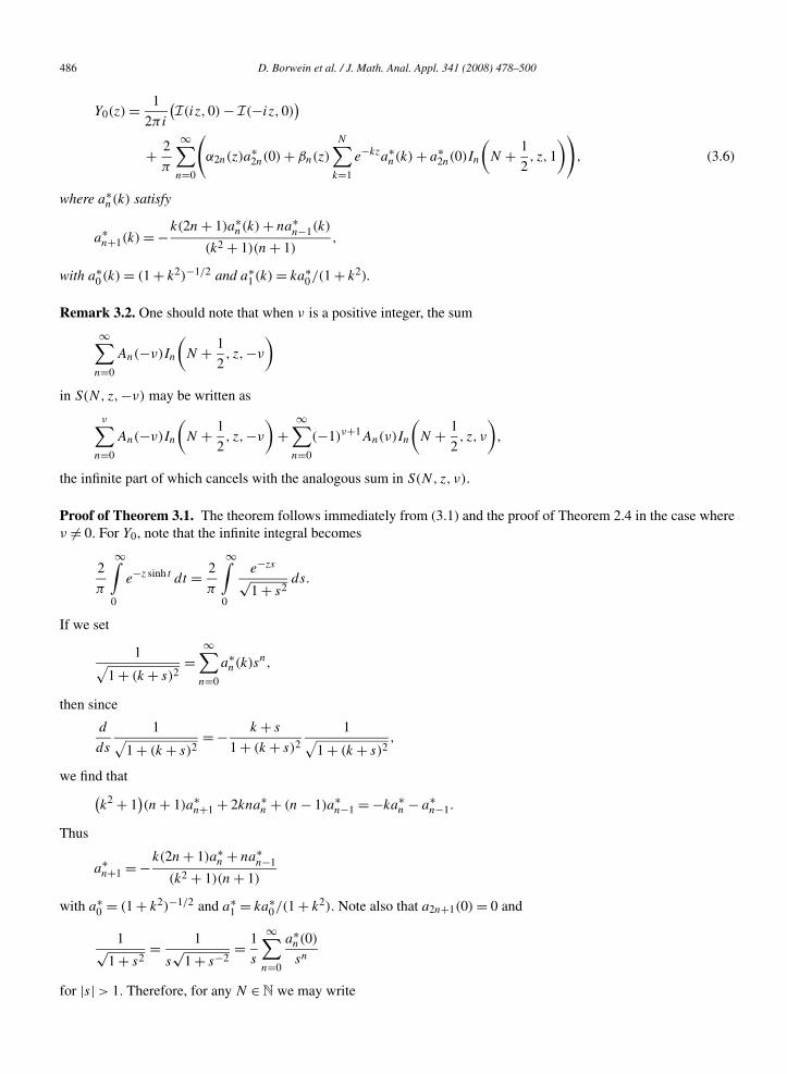
486 D. Borwein et al. / J. Math. Anal. Appl. 341 (2008) 478–500
Y0(z) = 1
2πi
(I(iz,0) − I(−iz,0)
)
+ 2
π
∞∑n=0
(α2n(z)a
∗2n(0) + βn(z)
N∑k=1
e−kza∗n(k) + a∗
2n(0)In
(N + 1
2, z,1
)), (3.6)
where a∗n(k) satisfy
a∗n+1(k) = −k(2n + 1)a∗
n(k) + na∗n−1(k)
(k2 + 1)(n + 1),
with a∗0(k) = (1 + k2)−1/2 and a∗
1(k) = ka∗0/(1 + k2).
Remark 3.2. One should note that when ν is a positive integer, the sum
∞∑n=0
An(−ν)In
(N + 1
2, z,−ν
)
in S(N, z,−ν) may be written as
ν∑n=0
An(−ν)In
(N + 1
2, z,−ν
)+
∞∑n=0
(−1)ν+1An(ν)In
(N + 1
2, z, ν
),
the infinite part of which cancels with the analogous sum in S(N, z, ν).
Proof of Theorem 3.1. The theorem follows immediately from (3.1) and the proof of Theorem 2.4 in the case whereν �= 0. For Y0, note that the infinite integral becomes
2
π
∞∫0
e−z sinh t dt = 2
π
∞∫0
e−zs
√1 + s2
ds.
If we set
1√1 + (k + s)2
=∞∑
n=0
a∗n(k)sn,
then since
d
ds
1√1 + (k + s)2
= − k + s
1 + (k + s)2
1√1 + (k + s)2
,
we find that(k2 + 1
)(n + 1)a∗
n+1 + 2kna∗n + (n − 1)a∗
n−1 = −ka∗n − a∗
n−1.
Thus
a∗n+1 = −k(2n + 1)a∗
n + na∗n−1
(k2 + 1)(n + 1)
with a∗0 = (1 + k2)−1/2 and a∗
1 = ka∗0/(1 + k2). Note also that a2n+1(0) = 0 and
1√1 + s2
= 1
s√
1 + s−2= 1
s
∞∑n=0
a∗n(0)
sn
for |s| > 1. Therefore, for any N ∈ N we may write
D. Borwein et al. / J. Math. Anal. Appl. 341 (2008) 478–500 487
∞∫0
e−zs
√1 + s2
ds =( 1/2∫
0
+N∑
k=1
e−ks
k+1/2∫k−1/2
+∞∫
N+1/2
)e−zs
√1 + s2
ds
=∞∑
n=0
(a∗
2n(0)α2n(z) +N∑
k=1
e−kza∗n(k)βn(z) + a∗
2n(0)
∞∫N+1/2
e−zss−2n−1 ds
)
=∞∑
n=0
(a∗
2n(0)α2n(z) +N∑
k=1
e−kza∗n(k)βn(z) + a∗
2n(0)In
(N + 1
2, z,1
)),
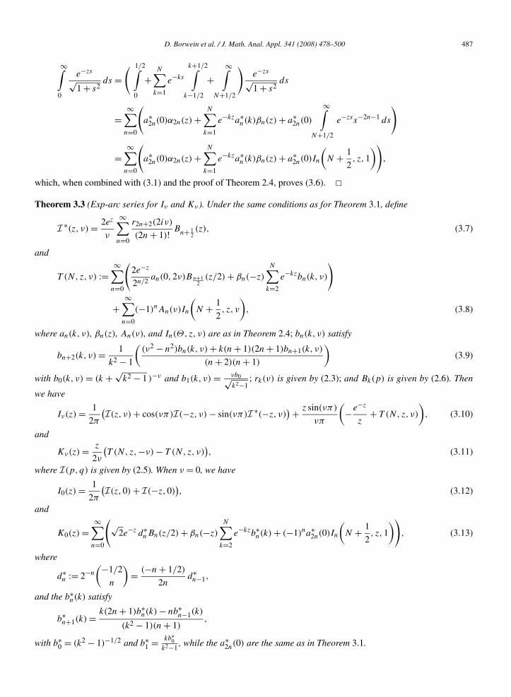
which, when combined with (3.1) and the proof of Theorem 2.4, proves (3.6). �Theorem 3.3 (Exp-arc series for Iν and Kν ). Under the same conditions as for Theorem 3.1, define
I ∗(z, ν) = 2ez
ν
∞∑n=0
r2n+2(2iν)
(2n + 1)! Bn+ 1
2(z), (3.7)
and
T (N, z, ν) :=∞∑
n=0
(2e−z
2n/2an(0,2ν)Bn+1
2(z/2) + βn(−z)
N∑k=2
e−kzbn(k, ν)
)
+∞∑
n=0
(−1)nAn(ν)In
(N + 1
2, z, ν
), (3.8)
where an(k, ν), βn(z), An(ν), and In(Θ, z, ν) are as in Theorem 2.4; bn(k, ν) satisfy
bn+2(k, ν) = 1
k2 − 1
((ν2 − n2)bn(k, ν) + k(n + 1)(2n + 1)bn+1(k, ν)
(n + 2)(n + 1)
)(3.9)
with b0(k, ν) = (k + √k2 − 1 )−ν and b1(k, ν) = νb0√
k2−1; rk(ν) is given by (2.3); and Bk(p) is given by (2.6). Then
we have
Iν(z) = 1
2π
(I(z, ν) + cos(νπ)I(−z, ν) − sin(νπ)I ∗(−z, ν)
) + z sin(νπ)
νπ
(−e−z
z+ T (N, z, ν)
), (3.10)
and
Kν(z) = z
2ν
(T (N, z,−ν) − T (N, z, ν)
), (3.11)
where I(p, q) is given by (2.5). When ν = 0, we have
I0(z) = 1
2π
(I(z,0) + I(−z,0)
), (3.12)
and
K0(z) =∞∑
n=0
(√2e−z d∗
nBn(z/2) + βn(−z)
N∑k=2
e−kzb∗n(k) + (−1)na∗
2n(0)In
(N + 1
2, z,1
)), (3.13)
where
d∗n := 2−n
(−1/2
n
)= (−n + 1/2)
2nd∗n−1,
and the b∗n(k) satisfy
b∗n+1(k) = k(2n + 1)b∗
n(k) − nb∗n−1(k)
(k2 − 1)(n + 1),
with b∗ = (k2 − 1)−1/2 and b∗ = kb∗0
2 , while the a∗ (0) are the same as in Theorem 3.1.
0 1 k −1 2n
488 D. Borwein et al. / J. Math. Anal. Appl. 341 (2008) 478–500
Remark 3.4. The reader may now be tempted to compare our series for Iν(z) with Paris’ formula (1.10). Indeed, forν = m ∈ Z, our series looks like
Iν(z) = 1
2π
(I (z,m) + (−1)mI(−z.m)
),
and both the summands of I as well as those of (1.10) have the form
(rising factorial) × (incomplete gamma)
power of z.
However, there are several key differences between the exp-arc series and (1.10):
• Although the summands in both the exp-arc and Paris’ series involve incomplete gamma functions that are recur-sively computable, Paris’ formula involves γ (k + ν + 1
2 ,±z) while our series only involve Bk(±z), which can beexpressed in terms of γ ( 1
2 ,±z). That is, our incomplete gamma evaluations are independent of ν.• When ν is not an integer, our series adjusts for the above independence with the sums T (N, z, ν). These sums
involve βn(z) which, although technically is an incomplete gamma function, is explicitly computable in closedform since it is the nth moment of the exponential. Thus, the only integral with ν dependence is In(N + 1
2 , z, ν),which, as we will see in the next section, can be ignored if one chooses a large enough N .
Proof. Since the proof is very similar to that of Theorems 2.4 and 3.1, we only highlight the differences here andrefer the reader to Appendix A for the details. Note that the integral on [0,π] in (3.2) simplifies to
π∫0
ez cos t cos(νt) dt = 1
2I(z, ν) +
π∫π/2
ez cos t cos(νt) dt
= 1
2
(I(z, ν) + eiνπI(−z, ν,0,π/2) + e−iνπI(−z,−ν,0,π/2)
).
Using (2.4) and combining the even (respectively odd) index terms into one sum, we obtain
π∫0
ez cos t cos(νt) dt = 1
2
(I(z, ν) + cos(νπ)I(−z, ν) − sin(νπ)
∞∑n=0
2e−zr2n+2(2iν)
(2n + 1)!ν Bn+ 1
2(−z)
).
Turning to the infinite integrals, after an integration by parts for ν �= 0 as in the previous theorems, it suffices toshow that
∞∫1
e−zse−ν arccosh s ds = T (N, z, ν)
for every N ∈ N. From the second order differential equation satisfied by e−ν arccosh s , it is easy to see that, for k � 2,
e−ν arccosh(k−s) =∞∑
n=0
bn(k, ν)sn,
where bn(k, ν) are given by (3.9). It is also easy to verify that
sνe−ν arccosh s =∞∑
n=0
(−1)nAn(ν)
s2n.
Thus, applying these expansions and interchanging summation and integration, we find
∞∫e−zse−ν arccosh s ds =
N∑k=2
e−kz∞∑
n=0
bn(k, ν)βn(−z) +∞∑
n=0
(−1)nAn(ν)In
(N + 1
2, z, ν
).
3/2

D. Borwein et al. / J. Math. Anal. Appl. 341 (2008) 478–500 489
Now all that remains is to show that3/2∫1
e−zse−ν arccosh s ds =∞∑
n=0
2e−z
2n/2an(0,2ν)Bn+1
2(z/2).
To do this, we note that e−ν arccosh s does not have a power series at the point s = 1. However, if we set u = √s − 1,
then it can be verified that
e−ν arccosh s =∞∑
n=0
an(0,2ν)un,
and so
3/2∫1
e−zse−ν arccosh s ds =1/
√2∫
0
e−z(u2+1)
∞∑n=0
an(0,2ν)un2udu = 2e−z
∞∑n=0
2−n/2an(0,2ν)B(n+1)/2(z/2).
This completes the proof for the case where ν �= 0. In the case where ν = 0, we now need only to evaluate K0 and sowe may follow the approach for the proof of (3.6). Expanding the function (1 + s2)−1/2 at each integer k � 2 as wellas at ∞ gives us the sums involving b∗
n and An in (3.13), while expanding (s + 1)−1/2 as a series in u = √s − 1 gives
the sum involving d∗n . �
4. Effectiveness of these series
We now turn our attention to the performance of our series in Theorems 2.4, 3.1, and 3.3. These series can beseparated into three parts: a pair of sums from the I function, a number of sums involving the moments of theexponential (given by αn and βn), and a series involving the incomplete gamma function arising from the tail of theinfinite integrals. Let us consider each of these separately. First, we look at the rate of convergence for the I sums.
Our series for Jν , Yν , and Iν involve terms of the form I(ikz, ν), which by Theorem 2.1 can be expressed as
I(ikz, ν
) = 4eikz
∞∑n=0
cn(ν)Bn
(ikz
),
where
cn(ν) := 1
(2n)!n∏
j=1
((2j − 1)2 − 4ν2) =
n∏j=1
(1 − 1
2j− 4ν2
(2j − 1)(2j)
),
with c0 := 1, and
Bn
(ikz
) = 1
2n+3/2
1∫0
e−ikzuun−1/2 du.
Thus it is clear that cn(ν) is bounded for fixed ν. In fact, it is easy to see that |cn(ν)| is strictly decreasing forn � 2|ν|2 − 1/2. It is also clear that for all n � 1 we have
∣∣Bn(ikz)
∣∣ � max(1, e−Re(ikz))
2n+3/2.
Therefore, for fixed k the error when the I(ikz, ν) sum is truncated after M terms can be bounded by∣∣∣∣4eikz∑
n�M+1
cn(ν)Bn
(ikz
)∣∣∣∣ �∣∣4eikz
∣∣ ∑n�M+1
C(ν)max(1, e−Re(ikz))
2n+3/2= 4C(ν)
2M+3/2· max
(eRe
(ikz
),1
)(4.1)
for some constant C(ν) depending only on ν.

490 D. Borwein et al. / J. Math. Anal. Appl. 341 (2008) 478–500
Our series for Iν also contains terms of the form I ∗(−z, ν). By a similar argument as above, there exists a constantC∗(ν) such that the tail of I ∗(−z, ν) when truncated after M terms is bounded by∣∣∣∣2e−z
ν
∑n�M+1
r2n+2(2iν)
(2n + 1)! Bn+1/2(−z)
∣∣∣∣ �∣∣2e−z
∣∣ ∑n�M+1
C∗(ν)max(1, eRe(z))
2n+2
= C∗(ν)
2M+1· max
(e−Re(z),1
). (4.2)
Now, let us consider the sums arising from the main contribution from the infinite exp-arc integrals. In the case ofthe J and Y Bessel functions, these sums are of the form
∑an(0, ν)αn(z) and e−kz
∑an(k, ν)βn(z), and in the case of
the I and K Bessel functions, they are of the form e−z∑
21−n/2an(0,2ν)B(n+1)/2(z/2) and e−kz∑
bn(k, ν)βn(−z).By (2.11), we deduce that, for n � 1,
a2n(0, ν) = 1
(2n)!n−1∏k=0
(ν2 − (2k)2) = (−1)n−1ν2
2n
n∏k=2
(1 − 1
2k − 1− ν2
(2k − 1)(2k − 2)
)
and
a2n+1(0, ν) = − ν
(2n + 1)!n−1∏k=0
(ν2 − (2k + 1)2) = (−1)n+1ν
2n + 1cn(ν/2).
Thus, we may conclude that for n > |ν|2/2, |nan(0, ν)| is decreasing, and that for all n � 2 there is a constant C∗0 (ν)
such that∣∣an(0, ν)∣∣ �
C∗0 (ν)
n. (4.3)
For the more general sequences an(k, ν) with k � 1, since the series∑
an(k, ν)sn has radius of convergence√k2 + 1, for sufficiently large n on using the root-test we have |an(k, ν)| < (k2 + 1)−n/2. Similarly, for each k > 2
we have |bn(k, ν)| < (k − 1)−n for sufficiently large n. We may make explicit the meaning of “sufficiently large”—at the expense of somewhat worse bounds—by using the recurrence relations (2.11) and (3.9). Note that when n >13 (|ν|2 + 4), we have | ν2−(n−2)2
n(n−1)| < 1. Thus in this range of n, we have
∣∣an(k, ν)∣∣ <
2k + 1
k2 + 1max
(∣∣an−2(k, ν)∣∣, ∣∣an−1(k, ν)
∣∣),and ∣∣bn(k, ν)
∣∣ <2k + 1
k2 − 1max
(∣∣bn−2(k, ν)∣∣, ∣∣bn−1(k, ν)
∣∣).We may conclude that there exist effectively computable constants C∗
k (ν) and D∗k (ν) such that when n > 1
3 (|ν|2 + 4),we have
∣∣an(k, ν)∣∣ <
⎧⎪⎪⎪⎨⎪⎪⎪⎩
(3
2
)n
C∗1 (ν), for k = 1,
(2k + 1
k2 + 1
)n/2
C∗k (ν), for k > 1,
and
∣∣bn(k, ν)∣∣ <
⎧⎪⎪⎪⎨⎪⎪⎪⎩
(5
3
)n
D∗2(ν), for k = 2,
(2k + 1
k2 − 1
)n/2
D∗k (ν), for k > 2.
Note that we may choose the constants such that these inequalities hold for all n > 0. We bound |αn(z)| and |βn(z)|trivially in the range Re(z) > 0, so that for all n > 0,∣∣αn(z)
∣∣ <1
and∣∣βn(±z)
∣∣ <eRe(z)/2
.
2n+1 2n
D. Borwein et al. / J. Math. Anal. Appl. 341 (2008) 478–500 491
Finally, we turn our attention to the series arising from the tails of the infinite integrals: that is, the sums
∞∑n=0
(±1)nAn(ν)In
(N + 1
2, z,±ν
).
Now, by (2.15) we have
|An| � |ν2−ν |n22n
(V + 2n − 1
n − 1
)<
|ν2−ν+V +2n−1|n22n
= |ν2V −ν−1|n
,
where V := �|ν|�, the smallest integer greater than or equal to |ν|. Also, when Re(z) > 0, we may trivially boundIn(N + 1
2 , z, ν) by
∣∣∣∣In
(N + 1
2, z, ν
)∣∣∣∣ � e−(N+ 12 )Re(z)
(N + 12 )2n+Re(ν)−1
∞∫0
e−(N+ 12 )Re(z)s(1 + s)−2n−Re(ν) ds,
which is bounded and monotonically decreasing as n increases. We can obtain a simpler bound when 2n > Re(ν),since by [2, Theorem 2.3] we have∣∣∣∣∣
∞∫0
e−zs(1 + s)a−1 ds
∣∣∣∣∣ � 1
|z|(
1 +∣∣∣∣ 1 − a
1 − Re(a)
∣∣∣∣)
whenever Re(a − 1) < 0. Thus, we find that, whenever 2n > Re(ν),∣∣∣∣In
(N + 1
2, z, ν
)∣∣∣∣ � e−(N+ 12 )Re(z)
(N + 12 )2n+Re(ν)−1
1
|(N + 12 )z|
(1 +
∣∣∣∣ 2n + ν
2n + Re(ν)
∣∣∣∣)
�(2 + | Im(ν)
2n+Re(ν)|
(N + 12 )Re(ν)
)e−(N+ 1
2 )Re(z)
|z|1
(N + 12 )2n
.
We summarize our discussion in the following theorem.
Theorem 4.1. Let z, ν ∈ C with Re(z) > 0. Then we obtain that:
(1) For each positive integer k there exist effectively computable constants C(ν), C∗(ν), C∗k (ν), D∗
k (ν) such that forany positive integer M ,∣∣∣∣4eikz
∑n>M
cn(ν)Bn
(ikz
)∣∣∣∣ � 4C(ν)
2M+3/2· max
(eRe(ikz),1
), (4.4)
∣∣∣∣2e−z
ν
∑n>M
r2n+2(2iν)
(2n + 1)! Bn+1/2(−z)
∣∣∣∣ = C∗(ν)
2M+1· max
(e−Re(z),1
), (4.5)
∣∣∣∣ ∑n>M
an(0, ν)αn(z)
∣∣∣∣ �C∗
0 (ν)
M2M+1, (4.6)
∣∣∣∣e−z∑n>M
an(1, ν)βn(z)
∣∣∣∣ � 3C∗1 (ν)e−Re(z)/2
(3
4
)M
, (4.7)
∣∣∣∣e−kz∑n>M
an(k, ν)βn(z)
∣∣∣∣ � C∗k (ν)e−(k− 1
2 )Re(z)(
1
2
√2k + 1
k2 + 1
)M+1(1 − 1
2
√2k + 1
k2 + 1
)−1
, (4.8)
∣∣∣∣2e−z∑ an(0,2ν)
2n/2B(n+1)/2(z/2)
∣∣∣∣ �C∗
0 (2ν)e−Re(z)
M2M+1, (4.9)
n>M

492 D. Borwein et al. / J. Math. Anal. Appl. 341 (2008) 478–500
∣∣∣∣e−z∑n>M
bn(2, ν)βn(−z)
∣∣∣∣ � 5D∗2(ν)e−Re(z)/2
(5
6
)M
, (4.10)
∣∣∣∣e−kz∑n>M
bn(k, ν)βn(−z)
∣∣∣∣ � D∗k (ν)e−(k− 1
2 )Re(z)(
1
2
√2k + 1
k2 − 1
)M+1(1 − 1
2
√2k + 1
k2 − 1
)−1
. (4.11)
We also obtain that:
(2) For any positive integer N there exists an effectively computable constant C∞(ν) such that for any positiveinteger M∣∣∣∣ ∑
n>M
(±1)nAn(ν)In
(N + 1
2, z,±ν
)∣∣∣∣ � C∞(ν)e−(N+ 12 )Re(z)
|z|1
M(N + 12 )2(M+1)
(1 − 1
(N + 12 )2
)−1
.
(4.12)
Moreover, if 2M > Re(ν) + 1, then we have the bound
∣∣C∞(ν)∣∣ � |ν2|ν||(2 + | Im(ν)|)
(2N + 1)Re(ν).
From Theorem 4.1 we can deduce the following bounds for the errors in computing Bessel functions using theseries in Theorems 2.4, 3.1, and 3.3. For simplicity of illustration, in the next corollary we set N = 1 in each of thetheorems, and truncate each infinite series at n = M .
Corollary 4.2. Let z, ν ∈ C with Re(z) > 0. For each integer M > 0, set
IM(z, ν) := 4ezM∑
n=0
cn(ν)Bn(z),
I ∗M(z, ν) := 2ez
M∑n=0
r2n+2(2iν)
(2n + 1)!ν Bn+ 1
2(z),
S∗(M,z, ν) :=M∑
n=0
(αn(z)an(0, ν) + e−zβn(z)an(1, ν) + An(ν)In
(3
2, z, ν
)),
T ∗(M,z, ν) :=M∑
n=0
(2e−z
2n/2an(0,2ν)Bn+1
2(z/2) + (−1)nAn(ν)In
(3
2, z, ν
)),
C∞(ν) :=∣∣∣∣ν2|ν|(2 + | Im(ν)|)
3Re(ν)
∣∣∣∣. (4.13)
Then for any M with 2M > |Re(ν)| + 1, the errors EJ , EY , EI , and EK from the truncation of the exp-arc seriesafter M terms at N = 1 defined by
EJ (M,z, ν) := Jν(z) − 1
2π
(e−iνπ/2IM(iz, ν) + eiνπ/2IM(−iz, ν)
)− z sin(νπ)
νπ
(−1
z+ S∗(M,z, ν)
), (4.14)
EY (M,z, ν) := Yν(z) − 1
2πi
(e−iνπ/2IM(iz, ν) − eiνπ/2IM(−iz, ν)
)− z
νπ
(1 − cos(νπ)
z+ S∗(M,z, ν) cos(νπ) − S∗(M,z,−ν)
), (4.15)
EI (M,z, ν) := Iν(z) − 1 (IM(z, ν) + eπiνI ∗
M(−z, ν) + e−πiνI ∗M(−z,−ν)
)
2π
D. Borwein et al. / J. Math. Anal. Appl. 341 (2008) 478–500 493
− z sin(νπ)
νπ
(−e−z
z+ T ∗(M,z, ν)
), (4.16)
EK(M,z, ν) := Kν(z) − z
2ν
(T ∗(M,z,−ν) − T ∗(M,z, ν)
), (4.17)
are bounded by∣∣EJ (M,z, ν)∣∣ � C(ν)
2M+1/2π
(eIm(ν)π/2 max
(e− Im(z),1
) + e− Im(ν)π/2 max(eIm(z),1
))+
∣∣∣∣z sin(νπ)
νπ
∣∣∣∣(
C∗0 (ν)
M2M+1+ 3C∗
1 (ν)e−Re(z)/2
(4/3)M+ 5
9
C∞(ν)e−3 Re(z)/2
M(9/4)M+1|z|)
, (4.18)
∣∣EY (M,z, ν)∣∣ � C(ν)
2M+1/2π
(eIm(ν)π/2 max
(e− Im(z),1
) + e− Im(ν)π/2 max(eIm(z),1
))+
∣∣∣∣ z
νπ
∣∣∣∣(
C∗0 (ν)| cos(νπ)| + C∗
0 (−ν)
M2M+1+ 3(C∗
1 (ν)| cos(νπ)| + C∗1 (−ν))e−Re(z)/2
(4/3)M
+ 5
9
(C∞(ν)| cos(νπ)| + C∞(−ν))e−3 Re(z)/2
M(9/4)M+1|z|)
, (4.19)
∣∣EI (M,z, ν)∣∣ � C(ν)eRe(z) + C∗(ν)| cos(νπ)|
2M+1/2π+ C∗(−ν)| sin(νπ)|
2M+2π
+∣∣∣∣z sin(νπ)
νπ
∣∣∣∣(
C∗0 (2ν)e−Re(z)
M2M+1+ 5
9
C∞(ν)e−3 Re(z)/2
M(9/4)M+1|z|)
, (4.20)
and
∣∣EK(M,z, ν)∣∣ �
∣∣∣∣ z
2ν
∣∣∣∣(
(C∗0 (2ν) + C∗
0 (−2ν))e−Re(z)
M2M+1+ 5(C∞(ν) + C∞(−ν))e−3 Re(z)/2
9M(9/4)M+1|z|)
. (4.21)
In consequence, as M tends to infinity, we have∣∣E(M,z, ν)∣∣ = Oν,z
(1
2M
), (4.22)
where E(M,z, ν) denotes any of the functions EJ , EY , EI , or EK , and the notation Oν,z indicates that the big-Oconstant depends on both ν and z.
Proof. As given above, the formulas for J,Y, I, and K are simply restatements of Theorems 2.4, 3.1, and 3.3 withN = 1 and truncation at M terms. The bounds for the errors follow immediately upon application of Theorem 4.1.Specifically, (4.18) and (4.19) follow from (4.4), (4.6), (4.7), and (4.12); (4.20) follows from (4.4), (4.9), and (4.12);and (4.21) follows from (4.9) and (4.12).
The asymptotic (4.22) for the error is easily deduced from the fact that an(1, ν) = O(2−n/2) as n tends to infinity,so that the (4/3)M in (4.18) and (4.19) may be replaced by 2M . �
We close this section with a few notes on the implementation of the series.
4.1. Notes on implementation
(1) First, we make a few remarks on the choice of N and the implementation of the S and T sums. Actually, welimit our discussion to S(N,ν, z), since the case T (N,ν, z) is similar. For a fixed N , we have N + 1 infinite sumsof the form Sk := e−kz
∑n an(k, ν)βn(z), 0 � k � N , and a sum S∞ := ∑
n AnIn for the tail of the infinite integral.Note that for each k, the size of Sk is of the order O(e−(k−1/2)z), and that S∞ is of the order O(e−(N+1/2)z). TheO-constants are explicitly computable by Theorem 4.1, and thus it is possible to determine at what point it becomesnecessary to begin summing the terms of Sk . Note also that as k increases, the rate of convergence of Sk also increases,and fewer terms are needed. As well, if one chooses a large enough N , it is possible to entirely avoid the error-functionevaluation that is necessary in computing S∞.

494 D. Borwein et al. / J. Math. Anal. Appl. 341 (2008) 478–500
(2) Second, we have stated our theorems for Re(z) > 0. To evaluate the Bessel functions when Re(z) < 0, oneshould use the well-known formulas [3, Sections 10.11, 10.34],
Jν
(zemπi
) = emνπiJν(z), Iν
(zemπi
) = emνπiIν(z),
Yν
(zemπi
) = e−mνπiYν(z) + 2i sin(mνπ) cot(νπ)Jν(z),
Kν
(zemπi
) = e−mνπiKν(z) − πi sin(mνπ) csc(νπ)Iν(z),
where m ∈ Z. For the details on how to choose m, see [14, p. 75]. Along the same lines, it is useful to use the identities[3, Section 10.27]
Iν(z) = e−νπi/2Jν(iz), −πiJν(z) = e−νπi/2Kν(−iz) − eνπi/2Kν(iz),
and
−πYν(z) = e−νπi/2Kν(−iz) + eνπi/2Kν(iz),
to evaluate Jν(z) and Yν(z) when Im(z) Re(z).(3) We also mention that in each of the sums I and Sk , the summands consist of a product of functions that depend
only on ν and on functions that depend only on z. This facilitates one-ν many-z or one-z many-ν computations byallowing us to pre-compute either the coefficients an(k, ν) or the exponential moments βn(z). Note also that all ofthese coefficients are either bounded or are converging to zero—as opposed to the analogous functions found in theascending series, where the dependence on z diverges to ∞, or those in the asymptotic series, where the dependenceon ν diverges to ∞.
(4) Finally, we note that the integrals Bk(p) and In(Θ, z, ν) in our series (the terms that cannot be evaluatedin closed form) are expressible in terms of the incomplete gamma function γ (a, z) and its complement �(a, z) :=�(a) − γ (a, z). Since the incomplete gamma functions have elegant continued-fraction representations, our resultstranslate to a continued-fraction computation scheme for the Bessel functions.
5. Numerical results
To give a more realistic idea of the effectiveness of our theorems, we implemented Corollary 4.2 in Maple tocompare it with the known ascending and asymptotic series. We remark that in addition to providing the numericaldata given in Tables 1 and 2, implementation of our theorems have helped us troubleshoot the theorems themselves.Not only have we corrected minor sign errors and typos, the computations also alerted us to more fundamental issuessuch as the fact that recurrence (2.17) needs to be restarted at the index n = −ν if ν is a negative integer.
Table 1 shows the absolute difference between the true value of Jν(z) and each of the values of (1.2) and (1.3) whentruncated at M terms, as well as the absolute error |EJ (M,z, ν)| given by (4.14). In the case of (1.3), “truncated at M
terms” means that both infinite sums are truncated at M terms. The data show that the exp-arc series converges like2−M as expected, giving one good digit approximately every three terms. Similar results can be seen in Table 2, wherewe compare the performance of the various series for the modified Bessel function Iν(z). Although it seems that inthe Jν(z) case the exp-arc series does not perform as well as either the ascending series (1.2) or the asymptotic series(1.3) in their respective domains of usefulness, both the exp-arc and Paris’ series for Iν(z) out-perform the ascendingand Hadamard series for sufficiently large argument z. The data also indicate that the accuracy of the exp-arc seriesdepends mainly on M , as the absolute errors do not seem to vary by much across values of z and ν. One should alsonote the following.
• For large z and small ν, to compute beyond the digital limit of the asymptotic series using the ascending seriesrequires higher precision arithmetic because of the cancellation of large numbers from the initial terms. These
terms are of size (z/2)k
k!(z/2)k+ν
�(k+ν+1), whose maximum occurs near k = z/2 if z ν. Compare this with the asymptotic
Jν(z) ∼√
2
πzcos
(z − πν
2− π
4
).

D. Borwein et al. / J. Math. Anal. Appl. 341 (2008) 478–500 495
Table 1Comparison between various series for Jν(z)
(ν, z) M Absolute value of the difference between the true value and
Ascending series (1.2) Asymptotic series (1.3) Exp-arc series (4.14)
ν = 12.3, z = 20 10 104 10−13 103
50 10−39 10−5 10−17
100 10−130 1051 10−33
150 10−242 10130 10−48
200 10−368 10223 10−64
ν = 12.3, z = 50 10 1018 10−23 102
30 1017 10−41 10−10
50 106 10−45 10−17
100 10−45 10−28 10−33
150 10−117 1011 10−48
ν = 12.3, z = 75 + 57i 10 1027 10−4 1013
50 1038 10−48 10−17
100 1014 10−59 10−33
120 10−2 10−56 10−39
150 10−31 10−47 10−48
200 10−89 10−20 10−64
Table 2Comparison between various series for Iν(z)
(ν, z) M Absolute value of the difference between the true value and
Ascending (1.7) Hadamard (1.9) Paris (1.10) Exp-arc (4.16)
ν = 4.2, z = 20 10 107 10−3 10−3 10−3
50 10−33 10−11 10−19 10−18
100 10−122 10−12 10−36 10−33
150 10−232 10−13 10−52 10−49
200 10−357 10−14 10−68 10−64
ν = 4.2, z = 50 10 1021 107 107 107
30 1019 10−9 10−9 10−9
50 109 10−17 10−17 10−17
100 10−40 10−23 10−34 10−33
150 10−110 10−24 10−51 10−49
ν = 4.2, z = 75 + 57i 10 1032 1013 1013 1013
50 1039 10−20 10−17 10−18
100 1017 10−33 10−33 10−33
120 102 10−34 10−40 10−39
150 10−26 10−34 10−49 10−49
200 10−84 10−35 10−65 10−64
• Switching from the asymptotic to the ascending series to obtain higher precision results requires that the com-putation using the asymptotic series be abandoned and the calculation restarted from scratch using the ascendingseries.
• It is not always obvious when to use the ascending series and when to use the asymptotic series, partly because itis not always obvious what amount of precision one requires before one begins a computation.
• To fairly compare the amount of work involved in our methods to that of Paris [4] or of the conventional ascending-asymptotic dichotomy depends on the context and on a level of implementation detail beyond the scope of thepresent article. That said, additional tabular comparison for the case of integer order is given in [1].

496 D. Borwein et al. / J. Math. Anal. Appl. 341 (2008) 478–500
6. Conclusion
The exp-arc expansion developed herein provides a geometrically convergent middle-ground between the asymp-totic and ascending series that avoids the issues raised in the previous section. It provides a uniform approach toevaluating Bessel functions that is universally convergent, with explicitly computable error bounds. It is therefore easyto predict the number of terms needed in our expansion to guarantee a given number of correct digits.
Appendix A
As promised we provide the details for the proof of Theorem 3.3 below.
Proof of Theorem 3.3. We wish to evaluate the integrals (3.2) and (3.3) as infinite series in the form of Theorem 3.3.As in the case for Jν and Yν , we express the integral on [0,π] in terms of I . One easily finds that
π∫0
ez cos t cos(νt) dt = 1
2I(z, ν) +
π∫π/2
ez cos t cos(νt) dt
= 1
2
(I(z, ν) + eiνπI(−z, ν,0,π/2) + e−iνπI(−z,−ν,0,π/2)
).
Now, by (2.4) we may write
I(−z,±ν,0,π/2) = ie−z
±ν
∞∑k=0
rk+1(∓2iν)
k! Bk/2(−z)
= ie−z
±ν
( ∞∑k=0
r2k+1(∓2iν)
(2k)! Bk(−z) + r2k+2(∓2iν)
(2k + 1)! Bk+1/2(−z)
).
Since r2k+1 is an odd function of ν and r2k+2 is an even function of ν, we find that
I(−z,±ν,0,π/2) = ie−z
ν
( ∞∑k=0
r2k+1(2iν)
(2k)! Bk(−z) ± r2k+2(2iν)
(2k + 1)! Bk+1/2(−z)
).
Thus, combining this with the expression for I(z, ν) in (2.5), we have
eπiνI(−z, ν,0,π/2) + e−πiνI(−z,−ν,0,π/2)
= cos(νπ)I(−z, ν) − 2 sin(νπ)e−z
ν
∞∑k=0
r2k+2(2iν)
(2k + 1)! Bk+ 1
2(−z).
The remainder of the proof is focused on evaluating the infinite integral. To that end, we make the change ofvariable s = cosh t so that dt = ds√
s2−1and obtain
∞∫0
e−z cosh t e−νt dt =∞∫
1
e−zse−ν arccosh s
√s2 − 1
ds = e−z
ν− z
ν
∞∫1
e−zse−ν arccosh s ds.
Thus for fixed N ∈ N we may write
∞∫1
e−zse−ν arccosh s ds =N∑
k=1
Gk(z, ν) + G∞(z, ν),
where

D. Borwein et al. / J. Math. Anal. Appl. 341 (2008) 478–500 497
Gk(z, ν) :=
⎧⎪⎪⎪⎪⎪⎪⎪⎪⎨⎪⎪⎪⎪⎪⎪⎪⎪⎩
3/2∫1
e−zse−ν arccosh s ds, for k = 1,
e−kz
1/2∫−1/2
ezse−ν arccosh(k−s) ds, for k � 2,
and
G∞(z, ν) :=∞∫
N+1/2
e−zse−ν arccosh s ds.
For each 2 � k � N , we expand e−ν arccosh(k−s) as a power series about s = 0, with radius of convergence k − 1. Set
hk(s) := e−ν arccosh(k−s) =∞∑
n=0
bn(k, ν)sn.
Then we easily find that(s2 − 2ks + k2 − 1
)h′′
k(s) = ν2hk(s) + (k − s)h′k(s).
Equating coefficients, we get
n(n − 1)bn − 2kn(n + 1)bn+1 + (k2 − 1
)(n + 2)(n + 1)bn+2 = ν2bn + k(n + 1)bn+1 − nbn,
and upon rearrangement we have
bn+2 = (ν2 − n2)bn + k(n + 1)(2n + 1)bn+1
(k2 − 1)(n + 2)(n + 1),
valid for n � 2 with initial conditions b0 = (k + √k2 − 1 )−ν and b1 = νb0/
√k2 − 1. Thus we easily deduce that, for
k � 2,
Gk(z, ν) =∞∑
n=0
e−kzbn(k, ν)βn(−z). (A.1)
For G∞(z, ν), note that
sνe−ν arccosh s = sν(s +
√s2 − 1
)−ν = (1 +
√1 − s−2
)−ν = (1 +
√1 + (is)−2
)−ν = (is)νe−ν arcsinh is . (A.2)
So by (2.16) we have
sνe−ν arccosh s =∞∑
n=0
(−1)nAn(ν)
s2n, (A.3)
where An(ν) are the same as in Lemma 2.3. Putting this into the expression for G∞ and interchanging the order ofsummation and integration, we get that
G∞(z, ν) =∞∑
n=0
(−1)nAn(ν)In
(N + 1
2, z, ν
). (A.4)
The evaluation of G1(z, ν) requires more care, as e−ν arccosh s does not have a Taylor expansion about s = 1 inpowers of s − 1. However, it does have an expansion in powers of u := √
s − 1, valid for |u| < √2. This is because
e−ν arccosh s = ((s2 − 1
)1/2 + s)−ν = (
(s − 1)1/2(s + 1)1/2 + s)−ν = (
u(u2 + 2
)1/2 + u2 + 1)−ν
is analytic and single-valued on |u| < √2, as u
√u2 + 2 + u2 + 1 is never zero. Now we let
h(s) := e−ν arccosh s = e−ν arccosh(u2+1) =: H(u),

498 D. Borwein et al. / J. Math. Anal. Appl. 341 (2008) 478–500
and expand
H(u) =∞∑
n=0
dn(ν)un.
Since h(s) = h0(−s), we have that(s2 − 1
)h′′(s) = ν2h(s) − sh′(s).
Then we have
dH
du= dh
ds
ds
du= 2u
dh
ds,
and
d2H
du2= d2h
ds2
(ds
du
)2
+ dh
ds
d2s
du2= 1
s2 − 1
(ν2h − s
dh
ds
)(ds
du
)2
+ dh
ds
d2s
du2.
Therefore,
u2(u2 + 2)d2H
du2=
(ν2H −
(u2 + 1
2u
)dH
du
)(4u2) + u2(u2 + 2)
2u
dH
du× 2 = 4u2ν2H − u3 dH
du.
Equating coefficients of un, we find that
n(n − 1) dn + 2(n + 2)(n + 1) dn+2 = 4ν2dn − ndn.
That is, for n � 0,
dn+2 = 4ν2 − n2
2(n + 2)(n + 1)dn, (A.5)
with d0 = 1 and d1 = −ν√
2. Comparing (A.5) with (2.11), we see that dn = 2−n/2an(0,2ν). Inserting this back intothe expression for G1, we obtain
G1(z, ν) =3/2∫1
e−zse−ν arccosh s ds =1/
√2∫
0
e−z(u2+1)H(u)2udu = 2e−z
∞∑n=0
dn(ν)
1/√
2∫0
e−zu2un+1 du
= 2e−z
∞∑n=0
2−n/2an(0,2ν)B(n+1)/2(z/2), (A.6)
where Bk(p) is defined by (2.6). Combining Theorem 2.1, (3.2), (A.1), (A.4), and (A.6) yields the series for Iν .Similarly, combining (3.3), (A.1), (A.4), and (A.6) yields the series for Kν .
Finally, we deal with the case ν = 0. The representation for I0(z) is obvious. For K0, we have by (3.3),
K0(z) =∞∫
0
e−z cosh t dt =∞∫
1
e−zs
√s2 − 1
ds
=3/2∫1
e−zs
√s − 1
√s + 1
ds +N∑
k=2
e−kz
k+1/2∫k−1/2
ezs√(k − s)2 − 1
ds +∞∫
N+1/2
e−zs
√s2 − 1
ds.
If we let
1√(k − s)2 − 1
=∞∑
b∗n(k)sn,
n=0

D. Borwein et al. / J. Math. Anal. Appl. 341 (2008) 478–500 499
then since
d
ds
1√(k − s)2 − 1
= k − s
(k − s)2 − 1
1√(k − s)2 − 1
,
we readily find that(k2 − 1
)(n + 1)b∗
n+1 − 2knb∗n + (n − 1)b∗
n−1 = kb∗n − b∗
n−1,
and thus
b∗n+1 = k(2n + 1)b∗
n − nb∗n−1
(k2 − 1)(n + 1),
with b∗0 = (k2 − 1)−1/2 and b∗
1 = kb∗0/(k2 − 1). Note also that
1√s2 − 1
= 1
s√
1 + (is)−2=
∞∑n=0
(−1)na∗2n(0)
s2n+1.
Therefore, for each N ∈ N,∞∫
3/2
e−zs
√s2 − 1
ds =∞∑
n=0
(βn(−z)
N∑k=2
e−kzb∗n(k) + (−1)na∗
2n(0)In
(N + 1
2, z,1
)).
So, to prove (3.13), it remains to show that
3/2∫1
e−zs
√s − 1
√s + 1
ds = √2e−z
∞∑n=0
d∗nBn(z/2).
To that end, we make a substitution u = √s − 1 and expand (u2 + 2)−1/2 as a series in u about u = 0. That is,
1√u2 + 2
= 1√2
(1 + u2
2
)−1/2
= 1√2
∞∑n=0
(−1/2
n
)u2n
2n,
valid for |u| < √2. Thus,
3/2∫1
e−zs
√s − 1
√s + 1
ds = e−z
1/√
2∫0
2e−zu2
√u2 + 2
du
= √2e−z
∞∑n=0
2−n
(−1/2
n
) 1/√
2∫0
e−zu2u2n du
= √2e−z
∞∑n=0
d∗nBn(z/2),
completing the proof. �References
[1] D. Borwein, J.M. Borwein, R. Crandall, Effective Laguerre asymptotics, preprint at http://locutus.cs.dal.ca:8088/archive/00000334/.[2] J.M. Borwein, O-Y. Chan, Uniform bounds for the complementary incomplete gamma function, preprint at http://locutus.cs.dal.ca:8088/
archive/00000335/.[3] The NIST Digital Library of Mathematical Functions, at http://dlmf.nist.gov.[4] R.B. Paris, On the use of Hadamard expansions in hyperasymptotic evaluation, I. Real variables, Proc. R. Soc. Lond. Ser. A 457 (2001)
2835–2853.

500 D. Borwein et al. / J. Math. Anal. Appl. 341 (2008) 478–500
[5] R.B. Paris, On the use of Hadamard expansions in hyperasymptotic evaluation, II. Complex variables, Proc. R. Soc. Lond. Ser. A 457 (2001)2855–2869.
[6] R.B. Paris, On the use of Hadamard expansions in hyperasymptotic evaluation of Laplace-type integrals, I. Real variable, J. Comput. Appl.Math. 167 (2004) 293–319.
[7] R.B. Paris, On the use of Hadamard expansions in hyperasymptotic evaluation of Laplace-type integrals, II. Complex variable, J. Comput.Appl. Math. 167 (2004) 321–343.
[8] R.B. Paris, On the use of Hadamard expansions in hyperasymptotic evaluation of Laplace-type integrals, III. Clusters of saddle points, J. Com-put. Appl. Math., in press.
[9] R.B. Paris, On the use of Hadamard expansions in hyperasymptotic evaluation of Laplace-type integrals, IV. Poles, J. Comput. Appl. Math.,in press.
[10] R.B. Paris, Exactification of the method of steepest descents: The Bessel functions of large order and argument, Proc. R. Soc. Lond. Ser. A 460(2004) 2737–2759.
[11] R.B. Paris, D. Kaminski, Hadamard expansions for integrals with saddles coalescing with an endpoint, Appl. Math. Lett. 18 (2005) 1389–1395.[12] R.B. Paris, private communication via R. Crandall, 2007.[13] K.R. Stromberg, Classical Real Analysis, Wadsworth, Belmont, CA, 1981.[14] G.N. Watson, A Treatise on the Theory of Bessel Functions, second ed., Cambridge Univ. Press, 1980.[15] S. Zhang, J. Jin, Computation of Special Functions, John Wiley & Sons, 1996.