the evolution of inflation in chile since 2000 papers no 89 93 the evolution of inflation in chile...

BIS Papers No 89 93

The evolution of inflation in Chile since 2000

Alberto Naudon1 and Joaquín Vial2

Abstract

We analyse the evolution of inflation in Chile over the last decade and a half through the lenses of the new keynesian theory. We do this first by reviewing the evidence relating to the main channels put forward by this framework: the output gap, inflation expectations, indexation to past inflation and the exchange rate. Based on the evidence gathered, we provide an interpretation of the inflation process in Chile. We show that in general terms the evolution of inflation can be explained consistently by the evolution of those elements. Critical to our finding is a differentiation of the dynamics of goods and services inflation.

Keywords: Monetary policy, inflation, Central Bank of Chile, Chile

JEL classification: E31, E52, E58

1 Chief Economist, Central Bank of Chile.

2 Member of the Board, Central Bank of Chile.

94 BIS Papers No 89

1. Introduction

We analyse the evolution of inflation in Chile over the last decade and a half through the lenses of the new keynesian theory. We do this first by reviewing the evidence relating to the main channels put forward by this framework: the output gap, inflation expectations, indexation to past inflation and the exchange rate. Based on this evidence, we then provide an interpretation of the inflation process in Chile. We show that, in general terms, the evolution of inflation can be explained consistently by the evolution of those elements. Critical to our findings is a differentiation of the dynamics of goods and services inflation.

The period analysed coincides with the implementation by Chile of a full-fledged inflation targeting (IT) framework, including a free floating exchange rate and the use of the short-term nominal interest rate as sole monetary policy instrument. The IT framework’s objective is to target an inflation rate of 3%, allowing for temporary deviations within a band of ±1% around the target. In practice, this means that the Central Bank of Chile (CBC) sets the interest rate in a way that is consistent with an inflation forecast of 3% two years ahead. The period is also interesting because it covers two significant developments for the global economy: the beginning and the end of the so-called supercycle of commodity prices, and the Great Financial Crisis (GFC) of 2008–2009 and its aftermath.

We begin in Section 2 with a description of the data showing the evolution of Chilean inflation and it main determinants. In Section 3, we briefly review the econometric evidence relating to the Phillips curve and, more generally, to the importance of the output gap, the exchange rate and inflation expectations for the inflation process. In Section 4, we follow up on our analysis by providing an interpretationof the evolution of inflation through the lenses of the evidence presented in the previous sections.

2. Evolution of inflation and its determinants since 2000

During most of the 20th century, Chile’s economic history, as was the case in several other South American countries, was marked by high and volatile inflation as well as failed attempts to control inflation. The reasons behind those failures are still open to debate but the fact is that until the second half of the 1990s it is difficult to find periods of one-digit inflation. 3 Things changed noticeably afterwards. During the past twenty years, annual inflation has not been above 10% for even a single month, and most of the time it has been close to the central bank’s target. There are two fundamental changes behind this remarkable improvement. First, a coherent fiscal policy was introduced in the late 1970s. It eradicated systematic public sector deficits and, with the implementation of increasingly sophisticated fiscal rules, it aligned fiscal

3 An example of this debate was the intense discussion that took place during a workshop organised

by the Central Bank of Chile and the Becker Friedman Institute for Research in Economics in December 2015. On that occasion, a group of Chilean economists were invited to discuss the chapter on Chile of the forthcoming book by Timothy Kehoe and Thomas Sargent on fiscal and monetary policy in Latin America.

BIS Papers No 89 95

expenditures with medium-term macroeconomic targets. This significantly reduced the procyclical behaviour of fiscal policy , in particular that linked to copper prices.4 The second element was the independence granted to the CBC in 1989 coupled with a clear mandate to keep inflation low and stable. Starting in 1990, the CBC implemented this mandate by setting a numerical target for inflation. The experience was highly successful and, over a period of ten years, the annual inflation rate was reduced from above 20% to around 3% in a context of strong growth and low unemployment.5 In 2000, the board of the CBC considered that the economy had reached a sufficient degree of maturity to implement a full-fledged IT regime, including a freely floating exchange rate and the use of the short-term nominal interest rate as sole monetary policy instrument.6 This change, supported by the fiscal policies described above, has been a key policy ingredient in dealing with the Chilean business cycle. In this Section, we describe the evolution of inflation and other relevant macroeconomic variables since the implementation of the IT regime in 2000.

Inflation

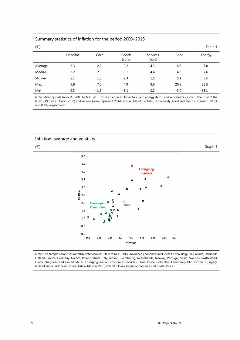
As shown in Table 1, since the implementation of IT, the inflation rate has stood on average at 3.3%, which has been slightly above the official target of 3%. Hidden behind this average, however, is an important degree of variability: during the last 15 years inflation has ranged between –2.3% and 9.9% with a standard deviation of 2.1%. Compared with inflation in Advanced Economies (AEs), inflation in Chile is more volatile (see Graph 1). Nevertheless, as shown by the same graph, high volatility of inflation is a common phenomenon in emerging market economies (EMEs). However, when compared with this group of economies, inflation in Chile ranks among the least volatile.

Graph 2 shows the evolution of inflation since 2000. It is evident from this graph that the period between mid-2007 and 2010 was one of particularly high volatility. This is not surprising given that those years were initially characterised by a significant increase in international commodity prices and then by an economic contraction during the GFC of 2008–2009. That said, even if one took those years out of the sample, it would still be true that inflation had fluctuated significantly, ranging between –1% and 6%.

4 From the early 1990s to the second half of the 2000s, gross public debt in Chile declined from 38%

of GDP to less than 10%. It now stands at about 17% of GDP. For a more detailed analysis of Chilean fiscal policy during that period, see Arellano (2005).

5 On the reduction of inflation in Chile see, for example, Corbo (1998), and Schmidt-Hebbel and Tapia (2002).

6 The severe recession of 1999, which followed the financial tensions created by attempts to limit the depreciation of the peso during the last phase of the Asian financial crisis, played a key role in convincing the Chilean authorities of the need to move to a freely floating exchange rate regime.

96 BIS Papers No 89

Summary statistics of inflation for the period 2000–2015

(%) Table 1

Headline Core Goods (core)

Services (core)

Food Energy

Average 3.3 2.5 –0.2 4.3 4.8 7.0

Median 3.2 2.5 –0.1 4.4 4.3 7.6

Std dev 2.1 1.5 2.3 1.5 5.1 9.5

Max 9.9 7.0 4.9 8.6 20.8 33.5

Min –2.3 –1.6 –6.1 0.2 –3.0 –18.1

Note: Monthly data from M1 2000 to M11 2015. Core inflation excludes food and energy items, and represents 72.2% of the total of the latest CPI basket. Good (core) and service (core) represent 28.6% and 43.6% of the total, respectively. Food and energy represent 19.1% and 8.7%, respectively.

Inflation: average and volatility

(%) Graph 1

Note: The sample comprises monthly data from M1 2000 to M 11 2015. Advanced economies includes: Austria, Belgium, Canada, Denmark, Finland, France, Germany, Greece, Ireland, Israel, Italy, Japan, Luxembourg, Netherlands, Norway, Portugal, Spain, Sweden, Switzerland, United Kingdom and United States. Emerging market economies includes: Chile, China, Colombia, Czech Republic, Estonia, Hungary, Iceland, India, Indonesia, Korea, Latvia, Mexico, Peru, Poland, Slovak Republic, Slovenia and South Africa.

BIS Papers No 89 97

Annual headline and core inflation

(%) Graph 2

Note: Monthly data from M1 2000 to M11 2015. Core inflation excludes food and energy items, and represents 72.2% of the total of the latest CPI basket.

Contribution to variance of inflation

(%) Table 2

Core Goods (Core)

Services (Core)

Food Energy

Share of variance 50.3 27.6 22.8 40.5 9.2

Share of CPI basket 72.3 28.6 43.6 19.1 8.7

Note: Monthly data from M1 2000 to M11 2015. The contribution reflects the fact that if 𝑦𝑦 = ∑𝑥𝑥𝑖𝑖 , then 𝑉𝑉𝑉𝑉𝑉𝑉(𝑦𝑦) = ∑𝐶𝐶𝐶𝐶𝐶𝐶(𝑦𝑦, 𝑥𝑥𝑖𝑖). The share of the variance is equal to COV (πCPI, πX)/ V(πCPI) where X is the incidence of the element X on CPI inflation. The share of the CPI basket is the same as in the 2013 basket.

Part of the variance is explained by the presence of highly volatile items in the CPI basket, such as food and energy. Indeed, as shown in Table 1, the standard deviation of these items is two and four times the standard deviation of the headline inflation rate. Table 2 shows the contribution to the variance of the headline inflation rate of four different sets of CPI items. It makes it clear that the contributions of food and energy items to the variance of inflation are larger than their respective shares in the CPI basket. Food, for example, contributes to 40% of the variance with an index weight of only 20%.

98 BIS Papers No 89

Annual goods and services inflation

(%) Graph 3

Note: Monthly data from M1 2000 to M11 2015. Good (core) and Service (core) represent 28.6% and 43.6% of the CPI basket respectively.

To better understand the dynamics of core and headline inflation, it is important to distinguish between the behaviour of tradable and non-tradable items within core inflation. This separation is to some extent arbitrary since in every item of the CPI basket there are tradable and non-tradable components. In addition, it must be kept in mind that non-core inflation comprises mainly tradable goods (energy and foodstuffs). Nonetheless, especially in a small open economy, the determinants of inflation for each of these items could vary quite significantly. In particular, non-tradable items are more strongly driven by domestic developments and more closely related to excess or deficient demand. On the other hand, tradable items are more strongly exposed to foreign competition and so to international prices and to the evolution of the exchange rate. In practice, in Chile as well as in other small open economies tradables are made up mainly of goods while non-tradables comprise mostly services. Bearing this in mind, we separate core items in these two broad groups. In terms of the share of CPI, these groups represent 28.6% and 43.6%, respectively, of the headline CPI index (and 40% and 60% of the core CPI index).

The behaviour of inflation for both goods and services is shown in Graph 3. It is evident that they have very different patterns, with both series cycling around their own averages but with quite dissimilar means. In particular, since the introduction of IT, the average inflation for core services, our proxy for non-tradables, has been 4.3% compared with only –0.2% for core goods (see Table 1). Services inflation is also less volatile than goods inflation, as shown in Table 2, and although the weight of services in the CPI basket is one and a half times the weight of goods its contribution to headline inflation is basically the same.7

7 The behaviour of the relative prices of tradable and non-tradable goods in Chile is not different from

that observed in other countries. See, for example, Jacobs and Williams (2014) who report a similar behaviour for Australia, Steenkamp (2013) for New Zealand, Coto-Martinez and Reboredo (2014) for several OECD countries, and Altissimo et al (2011) for a number of euro area countries.

BIS Papers No 89 99

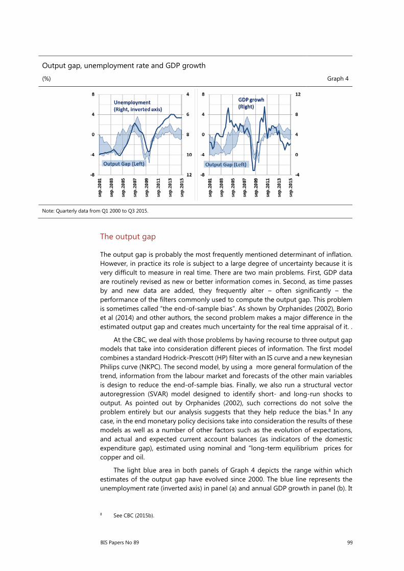
Output gap, unemployment rate and GDP growth

(%) Graph 4

Note: Quarterly data from Q1 2000 to Q3 2015.

The output gap

The output gap is probably the most frequently mentioned determinant of inflation. However, in practice its role is subject to a large degree of uncertainty because it is very difficult to measure in real time. There are two main problems. First, GDP data are routinely revised as new or better information comes in. Second, as time passes by and new data are added, they frequently alter – often significantly – the performance of the filters commonly used to compute the output gap. This problem is sometimes called “the end-of-sample bias”. As shown by Orphanides (2002), Borio et al (2014) and other authors, the second problem makes a major difference in the estimated output gap and creates much uncertainty for the real time appraisal of it. .

At the CBC, we deal with those problems by having recourse to three output gap models that take into consideration different pieces of information. The first model combines a standard Hodrick-Prescott (HP) filter with an IS curve and a new keynesian Philips curve (NKPC). The second model, by using a more general formulation of the trend, information from the labour market and forecasts of the other main variables is design to reduce the end-of-sample bias. Finally, we also run a structural vector autoregression (SVAR) model designed to identify short- and long-run shocks to output. As pointed out by Orphanides (2002), such corrections do not solve the problem entirely but our analysis suggests that they help reduce the bias.8 In any case, in the end monetary policy decisions take into consideration the results of these models as well as a number of other factors such as the evolution of expectations, and actual and expected current account balances (as indicators of the domestic expenditure gap), estimated using nominal and “long-term equilibrium prices for copper and oil.

The light blue area in both panels of Graph 4 depicts the range within which estimates of the output gap have evolved since 2000. The blue line represents the unemployment rate (inverted axis) in panel (a) and annual GDP growth in panel (b). It

8 See CBC (2015b).

100 BIS Papers No 89

is possible to identify five periods. The aftermath of the Asian financial crisis, during the early part of the 2000s, is characterised by a negative output gap, a high rate of unemployment and a low rate of growth. Next, the four years that preceded the GFC of 2008–2009 were marked by a remarkable recovery of growth and a reduction of the unemployment rate that made the output gap swing from around –3% to over 3%. This outstanding performance coincided with the beginning of the ‘supercycle’ of commodity prices. This ‘supercycle’ had long-lasting effects on the Chilean economy, especially through a delayed increase of investment in the mining sector. The effects of the GFC determined the evolution of the output gap during the period running from 2008 to 2010. However, in clear contrast with the Asian financial crisis, a combination of good macroeconomic management and a strong upsurge in copper prices led to a fast recovery of activity, which very quickly pushed the output gap back into positive territory. Finally, since mid-2013 we have seen a period of slower growth but persistently low unemployment. Even though this combination of weaker economic activity and low unemployment is somewhat puzzling, we think that it is consistent with a decline in potential output, which was partly hidden by the effects of the commodity price boom9 and some degree of labour hoarding in periods of deceleration.10 At any rate, we think that, in spite of the low rate of growth, the output gap was only slightly negative.11

The exchange rate

In small open economies such as Chile, a large share of the goods that are consumed (around 40%), as well as many intermediate goods, are imported. The retail prices of those goods are strongly correlated with the evolution of international prices and the exchange rate. Many locally produced goods also face competition from abroad which means that their prices are correlated with international prices. Empirical evidence suggests that the international price of goods and the exchange rate play an important role. However the evolution of the latter is particularly relevant when prices are invoiced in dollars, which is a common feature of EMEs (Gopinath (2015)).

9 See CBC (2015a).

10 The idea of “labour hoarding” is an old one in economics. It posits that because it is costly for firms to adjust employment, they will respond to short-run fluctuations in the demand for goods by changing the degree of effort required from workers. See, for example, Burnside et al (1993) and Sbordone (1996). Meza and Quintin (2007) study the behaviour of several Latin American and Asian economies during the Mexican Tequila crisis of 1994–1995, and report that labour hoarding may have accounted for much of the behaviour of working hours during this episode.

11 See CBC (2015c) for a discussion of the evolution of different measures of economic slack during the last cycle.

BIS Papers No 89 101

Nominal and real exchange rates

(Period average = 100) Graph 5

Note: Monthly data from M1 2000 to M11 2015.

Graph 5 shows the evolution of the nominal value of the peso against the US dollar, the multilateral nominal exchange rate and the real exchange rate. The last two are trade-based weighted averages, deflated by the CPI in the case of the latter. The co-movement between the three rates is evident but in periods characterised by a global appreciation of the US dollar, such as in the early 2000s and in the recent past, the simple nominal rate tends to move faster than both of its multilateral and real counterparts. What is remarkable is that, since Chile adopted a free floating exchange rate,the real exchange rate was very stable despite this was a period characterised by wide swings in commodity prices and capital flows. With the exception of a few brief episodes, the real exchange rate fluctuated within a relatively narrow band of 10%.

In line with our discussion of the output gap, it is possible to distinguish five periods of exchange rate movement12: a pronounced depreciation of the peso related to a large extent to a strengthening of the US dollar during the early 2000s; an intense real and nominal appreciation that started in around 2003 and was strongly related to the beginning of the supercycle of commodity prices; a sharp but short lived depreciation as a consequence of the GFC; a new period of appreciation associated with a recovery in copper prices and the increase in global liquidity; and finally a notable period of depreciation linked to the first signals of a reversal of monetary policy in the United States in mid-2013.

Inflation expectations

Graph 6 shows the evolution of inflation expectations one and two-year ahead. The numbers are taken from the Survey of Economic Analysts.13 Given that in our IT framework policy is operationalised by targeting a two-year-ahead inflation forecast of 3%, the two-year-ahead inflation expectations are a closely watched indicator of

12 Indeed, the correlation between both the real and the nominal exchange rate, and the output gap is

large, ranging between –0.3 and –0.6.

13 Results were similar when using inflation expectations derived from financial market prices.


policy.14 As shown by the red line in Graph 5 and by Table 3, during the past 172 months (the period covered by this survey) this indicator has been exactly at 3% for 85% of the time, and above 3.5% for only 1.7% of the time. So far it has never been outside the established range of 2% to 4%, not even in late 2008, when headline inflation reached close to 10%. This outcome has been achieved in spite of very volatile one-year-ahead inflation expectations, which reflected, as mentioned in Section 2, the volatile nature of inflation in Chile

The fact that one-year-ahead inflation expectations have been fairly volatile, but that two–year-ahead inflation expectations have not been, is commonly taken to reflect the credibility enjoyed by the CBC with respect to its commitment and ability to bring inflation back to target. If this is the case, shocks that affect inflation should be viewed as transitory and should therefore not influence long-term inflation expectations. The anchoring of inflation expectations since the introduction of the IT regime has been highlighted in various studies15 and is a central piece of the CBC’s monetary policy strategy. This allows the CBC to respond with flexibility when it thinks that shocks are transitory. However, the experience of 2008 (more on this in Section 4) shows that credibility is not something that should be taken for granted. Indeed, risks to credibility arise in periods when inflation is far from its target or when it remains beyond its band for an extended period of time.

Inflation expectations one and two years ahead Graph 6


14 For this purpose, we computed different measures of expected inflation that are implicit in financial

asset prices. We also used other surveys.

15 See, for example, De Pooter et al (2014), Rusticelli et al (2015) and Davis (2014).


Inflation expectations one and two years ahead Table 3

One year ahead Two years ahead

Average 3.1 3.0

Std dev 0.6 0.1

Max 6.0 3.9

Min 2.0 2.8

% of time at 3% 28.5 84.9

% of time out of [2.5%–3.5%] 20.3 1.7

% of time out of [2%–4%] 5.2 0


3. Determinants of inflation

In this Section, we present evidence relating to the main determinants of inflation in Chile. Our discussion is informed by a small open economy version of the NKPC. 16 In this context, the dynamics of inflation are related to the evolution of the output gap, the exchange rate, inflation expectations, past inflation and the price of foreign goods. More formally, the relationship among these variables and current inflation is usually described by an equation of the following type:

𝜋𝜋𝑡𝑡 = 𝜌𝜌𝐸𝐸𝑡𝑡𝜋𝜋𝑡𝑡+1 + (1 − 𝜌𝜌)𝜋𝜋𝑡𝑡−1 + 𝛽𝛽𝑥𝑥𝑡𝑡 + 𝛼𝛼∆𝑞𝑞𝑡𝑡 + 𝜀𝜀𝑡𝑡,

Where π is the inflation rate, x represents the output gap, q is the real exchange

rate (or something related to the relative prices of foreign goods) and ε is a residual term. In this equation, ρ is a parameter showing how forward-looking expectations influence the inflation process; β represents the slope of the NKPC; and α describes the degree of exchange rate pass-through (ERPT) typically associated with the openness of an economy.

As noted by Mavroeidis et al (2014) in their extensive review of the literature, the estimation of this kind of equation is subject to great uncertainty because ”seemingly innocuous specification changes lead to big differences in point estimates.” (p. 172). In particular, the pervasive problem of weak instruments led these authors to conclude that, at least using macro data, it was not possible to get reasonable assurance regarding the value of those parameters. This, of course, does not imply that the NKPC is not valid or relevant since there are good theoretical arguments behind this formulation. However, it is difficult to pin down the exact parameters. With this in mind, we do not attempt to conduct new estimations but we present the

16 As derived, for example, in Galí and Monacelli (2005). See also Razin and Yuen (2002), and Mihailov

et al (2011), In the case of Chile, there is large literature supporting NKPC models; see, for example, various studies conducted by current or ex CBC researchers, including Medina and Soto (2007), Caputo et al (2007) and Caputo (2009).


main conclusions of several studies already published for Chile within this framework.17

Output gap

Different estimations of the NKPC for the case of Chile show that the output gap has a positive and statistically significant effect on inflation but that this effect is relatively small.18 This conclusion is not different from that reached for other countries. More precisely, the coefficient β is typically somewhat below 0.2, meaning that, keeping everything else constant, a 1% increase in the output gap implies a less than 0.2% increase in (annualised) quarterly inflation. 19 Of course, this does not mean that the output gap is not important for inflation since what matters is the present value of all future output gaps. If changes in the output gap were persistent, the overall impact could be much larger.

Noticeably, there is evidence showing that the NKPC is now flatter than in the 1990s,20 which is in line with what has been found in several other countries.21 These changes are typically attributed to gains in central bank credibility.

Exchange rate

In any small open economy, especially if its production structure is more concentrated in commodities, an important share of consumption goods is produced abroad or faces a significant degree of competition from foreign producers. In this context, it is not surprising that the exchange rate plays a major role in the dynamics of inflation. What is surprising, however, is that many studies of the NKPC in Chile have not explicitly considered the role of the exchange rate. The CBC, by contrast, attaches great importance to exchange rate considerations and so it plays a central role in our models. In particular, models used at the central bank are consistent with an ERPT of around 0.1%–0.2% a year. As shown in Albagli et al (2015), this number is high when compared with AEs but not that different from coefficients founds in other EMEs.22

17 The most comprehensive analysis is contained in Cespedes et al (2005). See also Pincheira and Rubio

(2015), and Caputo (2009). The CBC redid much of those estimations and the main results remained valid.

18 It is possible that problems with the measurement of the output gap could be behind those small coefficients. After all, if one were using an incorrectly measured output gap, it would make sense for it not to appear very significant. However, it is important to note that studies that have used a real time ex post output gap have typically coincided in finding low output gap elasticities.

19 Mavroeidis et al (2014) report that most common numbers for AEs are even lower than this. Moreover, they show that, depending on the set of instruments, it is possible to find numbers that range from negative to positive values.

20 See Cespedes et al (2005) and Morandé and Tejeda (2008).

21 See Simon et al (2013).

22 In Albagli et al (2015), the authors analyse a sample of 48 AEs and EMEs and show that the pass-through is typically higher in the latter, and that within the group of EMEs Chile has a high level of pass-through. Indeed, they claim that the higher pass-through of Latin American countries, coupled with the sharp exchange rate depreciations associated with the end of the commodity price boom, could explain why this region has faced higher levels of inflation than other regions of the world.


Justel and Sansone (2015) used Chilean data from 1987 to 2013 to analyse the degree of ERPT to disaggregated CPI data: domestic energy, food and core consumer prices. They found that the ERPT to headline and core inflation was around 15% and 10% a year, respectively, for headline and core CPI. In both inflation measures, the effect of exchange rate movements took three to four quarters to fully take effect. Regarding the evolution of the ERPT, they found that it had decreased since the establishment of the IT regime and had remained fairly stable afterwards. They also reported a significant effect of changes in the exchange rate on food and energy prices, with an ERPT of close to 10% and 50%, respectively.

Bertinatto and Saravia (2015) analysed possible asymmetries in the ERPT. They reported that the ERPT depended on how persistent the exchange rate movement was and also on its direction. In particular, they found that the ERPT had been larger for devaluations than for appreciations of the peso,23 and that the ERPT was larger the more persistent was the exchange rate change. The authors failed to find a significant relationship between the level of ERPT and the output gap but they also noted that this result should be taken with care. In fact, even though there is no consensus in the literature about the importance of the output gap for the ERPT, several studies have previously found a positive relationship. For example, in a study of 12 euro area countries, Ben Cheikh (2013) found that the ERPT to CPI inflation depended positively on economic activity. In particular, when real GDP was growing above some threshold, the ERPT became larger. Similar results were reported by Goldfajn and Werlang (2000), and Brun-Aguerre et al (2012).

Of course, the degree of ERPT varies considerably across goods given that: (i) different amounts of local service inputs are added to prices; (ii) in some cases it is possible for consumers to switch from imported goods to lower-quality local substitutes; and (iii) there are also differences in the amount of intermediate foreign goods used in the production of local goods.24

In the case of Chile, Álvarez et al (2008) used monthly disaggregated import prices to show that such prices at the border and wholesale levels presented a high degree of long-run ERPT; that the ERPT had not declined and that in the short-run wholesale prices seemed to be less sensitive to exchange rate variations. On the other hand, using monthly data for the period ranging from December 1998 to April 2007, and prices for 156 items corresponding to the CPI basket, Álvarez et al (2008) found that the food and transport components exhibited significant ERPT but with a high degree of heterogeneity within the various elements of each category. They also reported a small ERPT for the other categories of the CPI.

Past and future inflation

Evidence regarding inflation expectations shows that they are relevant, with a ρ coefficient of 0.5–0.6.25 This means that the backward-looking component of the

23 Similar results are reported in Delatte et al (2012).

24 See Burstein and Gopinath (2014) for a complete survey of the relation between local and foreign prices.

25 It is difficult to determine the empirical relevance of inflation expectations for the current inflation rate. This is not only because of the identification problems discussed by Mavroeidis et al (2014) but also because a strong anchoring of inflation expectations leads to minimal movements in such expectations which makes it difficult to see how change in them could affect current inflation.


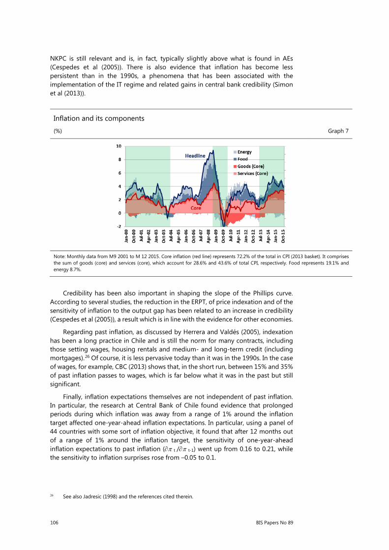
NKPC is still relevant and is, in fact, typically slightly above what is found in AEs (Cespedes et al (2005)). There is also evidence that inflation has become less persistent than in the 1990s, a phenomena that has been associated with the implementation of the IT regime and related gains in central bank credibility (Simon et al (2013)).

Inflation and its components

(%) Graph 7

Note: Monthly data from M9 2001 to M 12 2015. Core inflation (red line) represents 72.2% of the total in CPI (2013 basket). It comprises the sum of goods (core) and services (core), which account for 28.6% and 43.6% of total CPI, respectively. Food represents 19.1% and energy 8.7%.

Credibility has been also important in shaping the slope of the Phillips curve. According to several studies, the reduction in the ERPT, of price indexation and of the sensitivity of inflation to the output gap has been related to an increase in credibility (Cespedes et al (2005)), a result which is in line with the evidence for other economies.

Regarding past inflation, as discussed by Herrera and Valdés (2005), indexation has been a long practice in Chile and is still the norm for many contracts, including those setting wages, housing rentals and medium- and long-term credit (including mortgages).26 Of course, it is less pervasive today than it was in the 1990s. In the case of wages, for example, CBC (2013) shows that, in the short run, between 15% and 35% of past inflation passes to wages, which is far below what it was in the past but still significant.

Finally, inflation expectations themselves are not independent of past inflation. In particular, the research at Central Bank of Chile found evidence that prolonged periods during which inflation was away from a range of 1% around the inflation target affected one-year-ahead inflation expectations. In particular, using a panel of 44 countries with some sort of inflation objective, it found that after 12 months out of a range of 1% around the inflation target, the sensitivity of one-year-ahead inflation expectations to past inflation (∂π t /∂π t-1) went up from 0.16 to 0.21, while the sensitivity to inflation surprises rose from –0.05 to 0.1.

26 See also Jadresic (1998) and the references cited therein.


4. A view of the inflation process

Graph 7 depicts the evolution of headline inflation and the incidence of each of its components: goods, services, food and energy. The shaded areas divide the period under analysis into five different subperiods during which the direction of inflation changed. Table 4 provides numbers for average inflation in each of these subperiods and the values of several other macroeconomic variables.

The first subperiod covers the initial four years of the 2000s. During this time, headline inflation and, even more clearly, core inflation were on a decreasing path. Behind this behaviour was a sluggish economy fighting to recover from the Asian financial crisis and its aftermath, in addition to an external environment marked by unfavorable terms of trade (high oil and low copper prices) and adverse external financial conditions. In this context, unemployment remained high and the output gap became more negative on a quarter-by-quarter basis. This situation had an impact on non-tradables inflation, approximated in our analysis by the inflation rate for services, which went from above 7% at the end of 2000 to close to zero at the beginning of 2004.

The move to a freely floating exchange rate also played a role, helping the economy to absorb negative external shocks but creating upward pressure on inflation. Specifically, there was a significant depreciation of the peso in both nominal and real terms during the first period, in part as a response to a series of cuts in the Chilean policy rate (from 8.5% to 1.75%) in an environment of global appreciation of the US dollar. Although exchange rate movements put some pressure on inflation, especially on tradable items (such as food, energy and goods) the weak economy meant that inflation remained contained. While core inflation ended above 4% in 2000, it was below 1% by the beginning of 2004. Headline inflation was somewhat higher, because the price of oil increased appreciably in response to conflict in the Middle East, including the Iraq war of 2003.

At the end of this period, the price of copper started to rise and the ‘supercycle’ of commodity prices changed the course of the Chilean economy for the next decade. It is worth noting that, at the beginning, the change was viewed as a transitory phenomenon and, correspondingly, most of the extra government income was saved and there was no significant change in investment. The new fiscal rule played an important role in this respect since the savings that accrued were considered to be a counterpart to the deficits that allowed to maintain expenditure levels during the period of low copper prices. The fiscal balance went from –0.5% to 7.8% of GDP between 2003 and 2007.

However, as time passed by, both the government and private sector firms became convinced that high copper prices were there to stay. Consequently, internal demand increased, especially investment in the mining sector, helping to close the output gap and reducing unemployment. In particular, during the second period (Q2 2004 – Q3 2008), the output gap went from almost –3% at the beginning of 2004 to only –1% in 2005. By the end of this period (Q3 2008) it was 1.2%. Not surprisingly, non-tradables inflation climbed from 1.1% in Q2 2004 to 7.6% in Q3 2008 and nominal wage growth rose from around 3% to over 8%.27

27 Of course, the rise in the prices of energy and other natural resources in imported inputs also played

a role in the acceleration of inflation in the non-tradables sector.


Macroeconomic variables in selected subperiods

(%, average) Table 4

Panel (a): Inflation

Headline Core Goods (core)

Services (core) Food Energy

Q1 2000–Q1 2004 2.9 2.5 0.1 4.0 1.3 11.6

Q2 2004–Q3 2008 4.3 2.8 0.5 4.0 6.5 10.9

Q4 2008–Q1 2010 2.4 2.6 –0.8 5.0 5.8 –4.2

Q2 2010–Q2 2013 2.6 1.4 –2.8 4.6 5.8 5.2

Q3 2013–Q3 2015 3.9 3.6 2.0 4.8 6.7 0.8

Panel (b): Other macro variables

NER RER UR Employment GDP Output gap

Q1 2000–Q12004 5.6 4.6 9.8 2.1 3.8 –2.4 [–1.4 ; –2.8]

Q2 2004–Q3 2008 –5.8 –1.5 8.5 2.9 5.8 0.1 [–2.9 ; 1.2]

Q4 2008–Q1 2010 8.6 1.8 8.7 0.5 –0.3 –3.5 [–1.1 ; –5.1]

Q2 2010–Q2 2013 –3.2 –1.9 7.4 4.4 5.8 0.1 [–2.1 ; 1.1]

Q3 2013–Q3 2015 13.2 4.4 6.2 1.7 2.4 0.4 [1.4 ; 0.2]

Note: Quarterly data from Q3 2001 to Q3 2015. All data are period averages. In the case of the output gap, the numbers in brackets are the values of the output gap at the beginning and end of each period.

Ex post and real time output gaps of non-natural resources sectors

(%) Gaph 8

Note: Monthly data from M9 2001to M12 2015. The output gap is computed using an HP filter with a lambda of 1600.

The boom in commodity prices was accompanied by two additional developments that affected inflation during this second period. First, a sharp nominal appreciation of the peso and, to a lower extent, a real appreciation that helped to keep goods inflation under control. Second, the price of copper skyrocketed along with the price of other goods, including food and oil. In this context, with the exception of a few months at the end of 2006, during which the price of oil dropped, plus a transitory slowdown in activity, inflation increased steadily and by the end of


2008 headline inflation had reached almost 10%. At this point, for the first time since the implementation of IT, inflation expectations two years ahead moved significantly above the 3% target, calling into question the capacity of the central bank in bringing inflation back to its target.

From Graph 7 it is apparent that the surprise surge in the price of food was an important part of the escalation of inflation. However, core inflation (ie excluding food items) was also increasing at a fast rate. Indeed, between mid-2007 and the end of 2008 core inflation went from 1.9% to 6.6%. Looking back, it is not very difficult to explain this behavior: most of the determinants of inflation were tilting up, including the output gap which was at its highest level in years and increasing. The strengthening of the peso was helping, but the CBC decided to intervene by buying dollars in an attempt to curb what was seen as a too appreciated currency. (it was also a good opportunity to increase international reserves). Finally, actual and expected inflation started climbing very fast.

With the information at hand at the time, things looked somewhat different. In fact, this episode is a good example of the limitations of real time data. To begin with, computations of the output gap conducted with data to 2007 show that the economy had more economic slack than computations done with later data. This point is shown in Graph 8, where we computed the real-time and the ex-post output gaps for the non-natural resources sectors, a measure of GDP that is more closely related to inflation. One can clearly see from the graph the end-of-sample problem discussed in the previous Section. For 2007 and the initial part of 2008, the real time measure indicates a gap that is close to zero. After incorporating data until 2015, computation of the gap shows that it was between 2% and 4%, which is a considerable difference. Second, it was reasonable to expect a more important effect of the appreciation of the peso because the ERPT in the 1990s was much higher. Finally, the magnitude and persistence of the increase in the international prices of agricultural commodities came as a surprise. These considerations highlight the importance of keeping in mind the limitations imposed by the data and the difficulty in interpreting them when conducting monetary policy.

By the second part of 2007, the central bank initiated a contractionary monetary policy and during the next year and a half it raised the monetary policy rate (MPR) from 5% to 8.25%. However, inflation proved to be very stubborn and the MPR remained below the annual inflation rate throughout this period. In a worrisome development, by September 2008 the MPR had been increased by 300 bp but inflation expectations two years ahead measured at that time reached 3.9%, the highest level ever.

The GFC changed the game. Unemployment increased to almost 11% in a few months and the output gap went back into negative territory within one quarter. In this context, non-tradable goods inflation declined from 8% to less than 2% by the end of 2009. Probably reflecting the dependence of current inflation on past inflation, inflation took a longer time than activity to react. The reduction in the price of oil and food inflation of zero helped too. The peso depreciated quite a bit at the beginning of the third period (Q4 2008 – Q1 2010), keeping goods inflation into positive territory during the last quarter of 2008 and the first half of 2009 but after the recession and the later appreciation of the peso goods inflation became negative. In this context, inflation reached –2% by the end of 2009. A mix of good policies and good luck


quickly put the economy back on track.28 Monetary and fiscal policies were highly countercyclical; with a MPR that went from 8.25% to 0.5% in just seven months and a fiscal deficit that reached 4.4% of GDP. Good luck came in the form of a strong rebound in the price of copper (itself facilitated by the strong Chinese response to the crisis). Copper prices recovered from a minimum of around US$ 1.50 per pound to US$ 3.50 by April 2010. This convinced the government and the private sector that the supercycle was there to stay, propelling mining investment to record highs, which, in turn, reestablished internal demand growth. The output gap also recovered very fast, reaching positive numbers by the end of 2011. In this environment, non-tradable goods inflation recovered rapidly to around 5%, a level above its average of the first decade of the 2000s.

The years between 2010 and mid-2013, the fourth period,were also characterised by a weakness of the US dollar, which was in large part a consequence of the unprecedented expansiveness of US monetary policy and the persistence of high commodity prices. The associated appreciation of the peso pushed down the local price of tradable goods.29

Even though copper prices peaked in 2011, the international landscape began to change in mid-2013, the beginning of the fifth period, when the then Chairman of the Federal Reserve (Ben Bernanke) announced that US monetary policy was close to the beginning of a normalisation process. Even though it took a long time before the Federal Reserve actually increased the federal funds rate, the international financial environment for EMEs changed for worse. Additionally, China´s economy began to show signs of a moderation of growth and, consequently, the price of commodities declined. In the case of copper, as for several other industrial commodities, the expansion of supply resulting from the previous investment boom also played a role. In this context, growth in Chile shrunk significantly, coinciding with a major reduction in the investment plans of the large mining multinationals. At almost the same time, after more than a year with inflation (both headline and core) below the target band, the central bank began to signal a relaxation of policy. The first cut in the MPR came into effect on October 2013 and was followed by three additional cuts, for a total reduction of 100 bp by November 2014.

In this context, the nominal exchange rate depreciated by more than 45% with respect to mid-2013. This was one of the largest and most persistent periods of depreciation of the past 30 years. Not surprisingly, the effect on inflation was large. Tradable goods inflation was particularly notable, climbing from –2.5% to 5% between June 2013 and November 2015. The ERPT was a critical element in the evolution of inflation. Recent evidence suggests that it has remained within a range of values consistent with historic patterns but at the highest values within that range. This is also consistent with the empirical evidence discussed above since the ERPT tends to be larger when a depreciation is very persistent.

28 Bad luck also “helped”. The earthquake of 2010 prompted the incoming government into further

fiscal relaxation to facilitate reconstruction. Infrastructure under private concessions was insured and reconstruction was largely financed by foreign reinsurance companies.

29 Tradable goods inflation reached –6% in March 2010. It is difficult to explain such deflation by referring only to the behaviour of the exchange rate. In fact, there were measurement problems with the prices of some goods (for example, clothes) that introduced a downward bias to inflation during 2010. However, even after those problems were dealt with, goods inflation remained at a very low level (at an average of –2% between Mx 2011 and M6 2013.


In spite of the decline in growth, the output gap remained contained. Two factors explained this. First, by mid-2013 it was in positive territory. Second, potential growth had declined as the economy had become wealthier and productivity growth in natural resources-based sectors had slowed down or had even fallen (as in the case of mining). Our calculations show that Chile’s medium-term growth stands at around 3.5%, which is considerably less than the 5% estimated at the beginning of the 2000s. On top of that, several shocks and the necessity to reallocate resources between sectors with the fall in commodity prices have temporarily dampened potential growth to a number closer to 3%. This is consistent with the labour market remaining relatively tight despite low growth, with an unemployment rate of around 6%, net job creation of around 2% and wage growth in the vicinity of 6%. In this context, it is not surprising that non-tradable goods inflation has not declined.30

These are difficult times for monetary policy in EMEs. The end of the commodity price boom and of the extraordinary supply of liquidity in the AEs have obliged Latin American countries to confront “reality” faster than previously expected. The impact of the reduction in the price of copper on the economy, on inflation in particular, has already been discussed. We end this Section with considerations relating to the possibility of pursuing an independent monetary policy in the context of rising US policy rates.

Theoretically, provided that the monetary authorities are willing to let the exchange rate move freely, foreign monetary policy should not impose constraints on the local central bank. In practice, the experience of Chile shows that this is possible, at least to some extent. Graph 9 shows the evolution of Chilean and US MPRs since 2000. From the graph it is clear that during the last eight years movement in both rates have not been closely correlated: when the MPR in the US started to decline after the onset of the GFC, the MPR was increasing in Chile to curb inflation. During 2009, the Chilean MPR was cut aggressively, but in contrast to what happened in the US, by mid-2010 the CBC started to increase local rates as the economy was on a clear path of economic recovery. Finally in 2013, a few months after the Chairman of the Federal Reserve talked about the beginning of policy normalisation in the United States, the MPR was cut in Chile to confront the slowdown related to the end of the supercycle of commodity prices. As mentioned before, the real exchange rate fluctuated within a narrow range during this period of policy divergence, with almost no central bank intervention in foreign exchange markets.

30 There is also evidence showing that the tighter the economy is, the larger the ERPT will be. This could

have also played a role since, as mentioned before, the downward correction to the potential rate of growth implied a recognition that there was less slack in the economy. Actually, the ERPT has been somewhat above what was previously expected (and coincided with the revision of the numbers for potential growth).


Monetary policy rates

(%) Graph 9


The other side of the coin is, of course, the evolution of the nominal exchange rate, which in the case of Chile has shown important swings. Is this a reasonable course for monetary policy? In such matters one size definitely does not fit all, which means that it is not possible to make unconditional recommendations. The financial situation of different agents – including in particular the absence of large currency mismatches and a large pool of domestic savings managed by institutional investors – allows the central bank to let the exchange rate play its role of main shock absorber. The exchange rate is particularly important in an economy that requires significant changes in relative prices and where the degree of indexation to past inflation remains high.

Of course, monetary independence does not mean either a zero correlation with the foreign MPR or that international financial conditions are irrelevant. Regarding the first point, it is clear from Graph 9 that during the early 2000s there was a high degree of correlation between the US and Chilean MPRs. This is not unusual since during those years the business cycles in both economies were more or less in tune.

There has been a lot of debate in recent years regarding the second point.31 Our view is that international financial conditions assume greater relevance in a more financial integrated world but that this situation does not eliminate the benefits of an independent monetary policy. In particular, there is convincing evidence that long-term interest rates in EMEs are affected by developments in international financial markets and that the monetary policy of the Federal Reserve plays a major role.32 So local financial conditions clearly depend on what the Federal Reserve does. However, the idea that the local MPR has to react mechanically to changes in the US MPR is far from obvious. The best reaction to a movement in the fed funds rate will depend on the medium-term inflationary impact of that movement, and that movement, in turn, will depend on the many other elements shaping the economic landscape.

31 See Rey (2015a), Rey (2016) and Obstfeld (2015).

32 For instance, the Federal Reserve’s monetary policy has an effect either through its impact on expected future short-term interest rates or on the term premium on long-term interest rates.


5. Concluding remarks

Over the past 10 years, the Chilean economy has been affected to a large extent by the boom in commodity prices and, after 2008, by the GFC and the policy response of advanced economies and China to that episode. The impact of those events on internal demand and relative prices has left a clear mark on the evolution of tradable and non-tradable goods inflation.

In this paper, we reviewed the evolution of the main determinants of inflation in Chile and the empirical evidence that links those variables to the dynamics of inflation. We show that, in spite of significant issues relating to the new keynesian framework, in particular about the ability to identify the elasticities of the Phillips curve, the empirical evidence relating to Chile is broadly consistent with the relevance of the determinants of inflation highlighted by this framework: the output gap, the exchange rate, inflation expectations and past inflation. In the case of Chile, distinguishing between the behaviour of tradable and non-tradable goods inflation is of particular importance.

Our account of the evolution of inflation in Chile shows consistently that periods of low activity, high unemployment and negative output gaps coincide with low levels of inflation, especially in non-tradable items.

The exchange rate matters as well. It is true that the exchange rate pass-through is lower today than it was in the 1990s. But it is still significant. Periods of changes in relative prices as well as terms of trade are typically accompanied by movements in the exchange rate. Changes in the exchange rate are transmitted to local prices, especially those of tradable goods, feeding back into other prices through indexation mechanisms, even though such a channel is less important than it was in the 1990s. Finally, expectations matters too. In the case of Chile, they have been well anchored most of the time, helping to keep inflation under control.

References

Albagli, E, A Naudon and R Vergara (2015): “Inflation dynamics in LATAM: a comparison with global trends and implications for monetary policy”, Central Bank of Chile Economic Policy Papers, no 58, August.

Altissimo, F, P Benigno and D Palenzuela (2011): “Inflation differentials in a currency area: facts, explanations and policy”, Open Economies Review, vol 22, no 2, April, pp 189–233.

Álvarez, R, P Jaramillo and J Selaive (2008): “Exchange rate pass-through into import prices: the case of Chile”, Central Bank of Chile Working Papers, no 465, April.

Arellano, J (2005): “Del déficit al superávit estructural en Chile: razones para una transformación estructural en Chile”, Estudios Socio/Económicos de La Corporación de Investigaciones Económicas para Latinoamérica (CIEPLAN), no 25, April.

Ben Cheikh, N (2013): “Nonlinear mechanism of the exchange rate pass-through: does business cycle matter?”, Center for Research in Economics and Management Economics Working Paper, University of Rennes, January.


Bertinatto, L and D Saravia (2015): “El rol de asimetrías en el pass-through: evidencia para Chile”, Central bank of Chile Working Papers, no 750, February.

Borio, C, P Disnayat and M Juselius (2014): “A parsimonious approach to incorporating economic information in measures of potential output”, Bank for International Settlements Working Papers, no 442, February.

Brun-Aguerre, R, A Fuertes and K Phylaktis (2012): “Exchange rate pass-through into import prices revisited: what drives it?”, Journal of International Money and Finance, vol 31, no 4, June, pp 818–844.

Burnside, C, M Eichenbaum and S Rebelo (1993): “Labor hoarding and the business cycle”, Journal of Political Economy, vol 101, no 2, April, pp 245–273.

Burstein, A and G Gopinath (2014): "International prices and exchange rates", Handbook of International Economics, 4th edition, pp 391–451.

Caputo, R (2009): “External shocks and monetary policy. Does it pay to respond to exchange rate deviations?” Revista de Análisis Económico, vol 24, no 1, June, pp 55–99.

Caputo, R, F Liendo and J Medina (2007): “New keynesian models for Chile in the inflation-targeting period”, in Monetary Policy under Inflation Targeting, Central Banking, Analysis and Economic Policies Book Series of the Central Bank of Chile, edited by F Mishkin and K Schmidt-Hebbel, pp 507–546.

Central Bank of Chile (2013): “Salarios e indexación”, in Informe de política monetaria, September.

Central Bank of Chile (2014): “Índice de precios de vivienda en Chile: metodología y resultados”, Estudios Económicos Estadísticos, no 107, June.

Central Bank of Chile (2015a): “Crecimiento del PIB tendencial”, in Informe de política monetaria, September.

Central Bank of Chile (2015b): “PIB potencial, brecha de actividad e inflación”, in Informe de política monetaria, September.

Central Bank of Chile (2015c): “Evolución reciente de las holguras de capacidad”, Informe de política monetaria, September.

Céspedes, L, M Ochoa and C Soto (2005): “The new keynesian Phillips curve in an emerging market economy: the case of Chile”, Central Bank of Chile Working Papers, no 355, December.

Corbo, V (1998): “Reaching one-digit inflation: the Chilean experience”, Journal of Applied Economics, vol 1, no 1, November, pp 123–163.

Coto-Martinez, J and J Reboredo (2014): “The relative price of non-traded goods under imperfect competition”, Oxford Bulletin of Economics and Statistics, vol 76, no 1, February, pp 24–40.

Davis, J (2014): “Inflation targeting and the anchoring of inflation expectations: cross-country evidence from consensus forecasts”, Federal Reserve Bank of Dallas Working Paper, no 174, April.

De Pooter, M, P Robitaille, I Walker and M Zdinak (2014): “Are long-term inflation expectations well anchored in Brazil, Chile, and Mexico?”, International Journal of Central Banking, vol 10, no 2, June, pp 337–400.


Delatte, A and A López-Villavicencio (2012): “Asymmetric exchange rate pass-through: evidence from major countries”, Journal of Macroeconomics, vol 34, no 3, September, pp 833–844.

Esteban Jadresic (1998). "The Macroeconomic Consequences of Wage Indexation Revisited," Working Papers Central Bank of Chile 35, Central Bank

Gali, J and T Monacelli (2005): “Monetary policy and exchange rate volatility in a small open economy”, The Review of Economic Studies, vol 72, no 3, pp 707–734.

Goldfajn, I and S Werlang (2000): “The pass-through from depreciation to inflation: a panel study”, Banco Central do Brasil, Working Paper Series, no 5, September.

Gopinath, G (2015): “The international price system”, National Bureau of Economic Research Working Paper, no 21646, October.

Herrera, O and R Valdés (2005): “De-dollarization, indexation and nominalization: the Chilean experience”, The Journal of Policy Reform, vol 8, no 4, February, pp 281–312.

Jacobs, D and T Williams (2014): “The determinants of non-tradables inflation”, Reserve Bank of Australia Bulletin, September.

Justel, S and A Sansone (2015): “Exchange rate pass-through to prices: VAR evidence for Chile”, Central bank of Chile Working Papers, no 747, February.

Mavroeidis, S, M Plagborg-Møller and J Stock (2014): “Empirical evidence on inflation expectations in the new keynesian Phillips curve”, Journal of Economic Literature, vol 52, no 1, March, pp 124–188.

Medina, J and C Soto (2007): “The Chilean business cycles through the lens of a stochastic general equilibrium model”, Central Bank of Chile Working Papers, no 457, December.

Meza, F and E Quintin (2007): “Factor utilization and the real impact of financial crises”, The B.E. Journal of Macroeconomics, vol 7, no 1, September.

Mihailov, A, F Rumler and J Scharler (2011): “The small open-economy new keynesian Phillips curve: empirical evidence and implied inflation dynamics”, Open Economies Review, vol 22, no 2, April, pp 317–337.

Morandé, F and M Tejada (2008): “Sources of uncertainty for conducting monetary policy in Chile”, Central Bank of Chile Working Papers, no 492, December.

Obstfeld, M (2015): “Trilemmas and tradeoffs: living with financial globalization”, in Global Liquidity, Spillovers to Emerging Markets and Policy Responses, Central Banking, Analysis and Economic Policies Book Series of the Central Bank of Chile, edited by C Raddatz, D Saravia and J Ventura, pp 13–78.

Orphanides, A and S Van Norden (2002): “The unreliability of output-gap estimates in real time”, Review of Economics and Statistics, vol 84, no 4, November, pp 569–583.

Pincheira Brown, P and H Rubio Hurtado (2015): “The low predictive power of simple Phillips curves in Chile”, CEPAL Review, no 116, August.

Razin, A and C Yuen (2002): “The “new keynesian” Phillips curve: closed economy versus open economy”, Economics Letters, vol 75, no 1, March, pp 1–9.

Rey, H (2013): “International channels of transmission of monetary policy and the mundellian trilemma”, National Bureau of Economic Research Working Papers, no 21852, January.


Rey, H (2015): “Dilemma not trilemma: the global financial cycle and monetary policy independence”, National Bureau of Economic Research Working Papers, no 21162, May.

Rusticelli, E, D Turner and M Cavalleri (2015): “Incorporating anchored inflation expectations in the Phillips curve and in the derivation of OECD measures of the unemployment gap”, OECD Economics Department Working Papers, no 1231, May.

Sbordone, A (1996): “Cyclical productivity in a model of labor hoarding”, Journal of Monetary Economics, vol 38, no 2, October, pp 331–361

Simon, J, T Matheson D and Sandri (2013): “The dog that didn’t bark: has inflation been muzzled or was it just sleeping?”, World Economic Outlook, International Monetary Fund, April.

Schmidt-Hebbel, K and M Tapia (2002): “Inflation targeting in Chile”, The North American Journal of Economics and Finance, vol 13, no 2, February, pp 125–146.

Steenkamp D (2013): “Productivity and the New Zealand dollar: Balassa-Samuelson tests on sectoral data”, Reserve Bank of New Zealand Analytical Note Series, no AN 2013/0.

the evolution of inflation in chile since 2000 papers no 89 93 the evolution of inflation in chile...

Documents