The Evolution of Markets and the Revolution of Industry ∗

Klaus DesmetUniversidad Carlos III

and CEPR

Stephen L. ParenteUniversity of Illinoisand CRENoS

February 2008Preliminary and Incomplete

Abstract

Why did the Industrial Revolution start sometime in the 18th century in Englandand not earlier and in some other country? This paper argues that the key to thestart of the Industrial Revolution was the expansion and integration of markets thatpreceded it. Due to less regulation, increasing population, and declining trade costs,markets in England came to support an increasing variety of goods. As such, the de-mand became more elastic and competition intensified. This increased the benefits toprocess innovation. Sometime in the 18th century, these benefits became sufficientlylarge for firms to cover the fixed costs of innovation, giving rise to the IndustrialRevolution. We illustrate this mechanism in a model with endogenous innovationand population and show that it generates a transition from a Malthusian era to aModern Economic Growth era as well as a demographic transition and a structuraltransformation. We provide empirical support for our theory by documenting theevolution in markets in England prior to the Industrial Revolution and by document-ing that markets at the start of the 18th century were more developed in Englandthan in the rest of the world.JEL Classification:Keywords: Industrial Revolution, Innovation, Competition, Market Revolution

∗Desmet: Department of Economics, Universidad Carlos III. E-mail: klaus.desmet@uc3m.es; Parente:Department of Economics, University of Illinois at Urbana-Champaign. E-mail: parente@uiuc.edu.

1 Introduction

Sometime at the end of the 18th century England gradually escaped the Malthusian trap

of stagnant living standards. As technological progress accelerated, output started to

grow faster than population, and by the second half of the 19th century the country

transitioned to the modern era of sustained income per capita growth. During the same

time period two other important changes occurred: the demographic transition, with

population growth turning from being positively to negatively correlated with income

levels, and the structural transformation, with the share of manufacturing growing at the

expense of agriculture. Since then many other countries have gone through their own

industrial revolutions. Although different in time and place, these transitions to modern

growth have followed the same broad pattern as England during the 19th century.

This paper proposes a novel mechanism for the transition from Malthusian to

modern growth, based on the link between market size, competition and innovation.

During the late-Malthusian phase population was slowly, but steadily, increasing. This,

together with trade liberalization and improvements in transport infrastructure, led to

an expansion in the size of the market. As a result, the economy started to produce a

larger variety of products, making them more substitutable, raising the price elasticity

of demand, and strengthening competition. The mechanism linking tougher competition

to modern growth is as follows. The lower markups associated with greater competition

oblige firms to become larger to break even. As firms become larger, they find it easier to

cover the fixed cost of innovation and technology adoption. Therefore, once the market is

big enough, competition is strong enough, and firms are large enough, innovation endoge-

nously takes off. This, in turn, further increases the market size, providing additional

incentives for innovation. The economy thus graduates to the era of modern growth.

The key building block of our model is the Hotelling-Lancaster preference con-

struct. With such preferences, each household has an ideal variety that corresponds to his

location on the unit circle. As shown by Helpman and Krugman (1985) and Hummels and

Lugovskyy (2005), when the population increases, more varieties enter the market, mak-

1

ing them more substitutable, and thus increasing the price elasticity of demand. Desmet

and Parente (2007) exploit this feature and show in a one-period model how the higher

elasticity of demand, due to a larger population or more liberalized trade, facilitates

innovation.

The Hotelling-Lancaster construct naturally gives rise to a transition from stag-

nation to modern growth. As long as the market size experiences some minimal growth

during the Malthusian phase, at some point it reaches a sufficient size for innovation

to endogenously take off. This mechanism is by construction absent with Spence-Dixit-

Stiglitz preferences, since its constant elasticity feature precludes a link between market

size and elasticity. This difference is not only theoretically relevant, it is also empirically

important. Indeed, there is ample evidence of a positive relation between market size and

demand elasticity. This empirical regularity is present when markets expand because of

either population growth (Campbell and Hopenhayn, 2005) or trade liberalization (Ty-

bout, 2003; Hummels and Klenow, 2005).

The second building block of our model is a subsistence constraint in agriculture:

people need a minimum amount of food to survive. This is a standard way of introduc-

ing nonhomotheticities in preferences, implying that as consumers become richer, they

dedicate a decreasing share of their incomes to food consumption (Galor and Weil, 2000;

Caselli and Coleman, 2001). As economic growth takes off, this leads to a structural

transformation, with the share of labor employed in agriculture falling in favor of manu-

facturing.

The last building block reflects the evidence that child rearing is more costly in the

city than on the farm. It is well established that children are more likely to be involved

in home production on a farm than in a factory (Rosenzweig and Evensen, 1977; Hansen

and Prescott, 2002). In fact, the laws restricting child labor in England applied only to

factory work, and explicitly excluded farm work (Doepke and Zilibotti, 2005). Therefore,

whereas children could add to the family’s hours worked on the farm, this was much less

the case in the manufacturing towns. Although rising income increased the demand for

children, it also spurred the structural transformation, leading to a compositional effect,

2

decreasing the demand for children as a greater part of the labor force became employed

in factories. If this second force dominates, a demographic transition occurs, with higher

income levels reducing population growth.

In this model anything that affects the size of the market or the cost of innovation

will also affect the timing of the industrial revolution. Greater population size, higher

income per capita, longer working hours, better road infrastructure, and trade liberaliza-

tion all increase the size of the market, and thus speed up the arrival of the industrial

revolution. Some of these examples, such as trade liberalization, may be due to policy

changes. Others, such as an increase in population, may arise endogenously. For in-

stance, as in the standard Malthusian model, agricultural productivity growth allows the

economy to support a larger population. As for the cost of innovation, better institutions

and education may have played a role in stimulating R&D and the adoption of better

technologies.

Clearly, the novelty of our theory lies in the mechanism that links market size to

competition and innovation. The novelty is not in the list of factors we identify as being

important for the timing of the industrial revolution. For example, Simon (1977) and

Kremer (1993) have emphasized the importance of population growth for development.

Schultz (1971), and more recently Diamond (2007), have argued that an agricultural

revolution is a precondition for an industrial revolution. Williamson and O’Rourke (2005)

and O’Rourke and Findlay (2007) have been at the forefront of the camp that stresses

the role of international trade. Finally, North and Thomas (1973) have spearheaded the

literature that stresses the role of institutions for development.

There is a large and growing literature on unified growth models that set out

to show the transition from Malthusian to modern growth within a single framework.

Important contributions include, amongst others, Kremer (1993), Jones (2001), Galor and

Weil (2000), Hansen and Prescott (2002), and Voigtlander and Voth (2006). Once again,

the main difference with our work lies in the novelty of the mechanism we emphasize.

For example, whereas Hansen and Prescott (2002) is based on exogenous technological

progress, Galor and Weil (2000) relies on increasing returns and externalities associated

3

with human capital production to generate the industrial revolution. Our model, instead,

focuses on the link between market size, competition and innovation.

In light of the existing empirical evidence, our framework presents a number of

advantages. Voth (2003) has criticized part of the unified growth literature, because of

relying exclusively on a positive link between population size and innovation, when this

relation is empirically elusive. Instead, he suggests that the broader concept of market size

is more appropriate, because at the end of the 18th century England was more populous

than equally wealthy Holland, and much richer than more populous France. The key

mechanism in our paper addresses this criticism, as the relevant variable for take-off is

the size of the market.

Another point of debate is the role of human capital. The evidence shows that

during the industrial revolution the skill premium did not increase (Feinstein, 1988). In

our model, neither the industrial revolution nor the demographic transition depend on

human capital. Technological progress takes off when the market size becomes large

enough. The decrease in birth rates is not due to human capital changing the tradeoff

between quantity and quality. Instead, it is a compositional effect, due to people moving

from the farm to the city, where they face higher costs of raising kids.

The rest of the paper is organized as follows. Section 2 describes the model.

Section 3 reports the main results. Section 4 provides empirical support for the theory.

In particular, it shows that England’s markets were better integrated than any other

country in the world at that time. Section 5 concludes the paper.

2 The Model

Time is discrete and infinite. There are three sectors: a household sector, an agricultural

sector and an industrial sector. The agricultural sector is perfectly competitive. Techno-

logical change is exogenous there. The industrial sector is monopolistically competitive.

Each variety is located at a point on the unit circle. Technological change in the in-

dustrial sector is endogenous. Agents are distributed along the unit circle, and live for

two periods. The first period represents childhood, whereas the second period represents

4

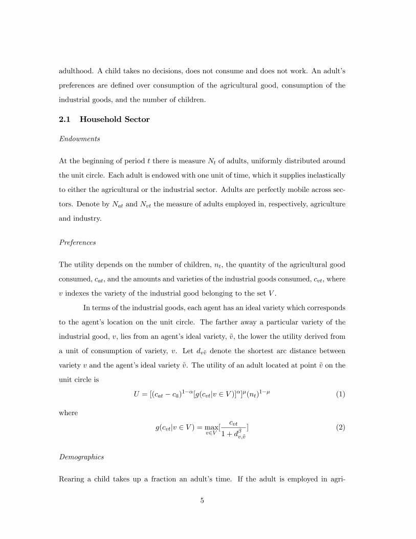
adulthood. A child takes no decisions, does not consume and does not work. An adult’s

preferences are defined over consumption of the agricultural good, consumption of the

industrial goods, and the number of children.

2.1 Household Sector

Endowments

At the beginning of period t there is measure Nt of adults, uniformly distributed around

the unit circle. Each adult is endowed with one unit of time, which it supplies inelastically

to either the agricultural or the industrial sector. Adults are perfectly mobile across sec-

tors. Denote by Nat and Nvt the measure of adults employed in, respectively, agriculture

and industry.

Preferences

The utility depends on the number of children, nt, the quantity of the agricultural good

consumed, cat, and the amounts and varieties of the industrial goods consumed, cvt, where

v indexes the variety of the industrial good belonging to the set V .

In terms of the industrial goods, each agent has an ideal variety which corresponds

to the agent’s location on the unit circle. The farther away a particular variety of the

industrial good, v, lies from an agent’s ideal variety, v, the lower the utility derived from

a unit of consumption of variety, v. Let dvv denote the shortest arc distance between

variety v and the agent’s ideal variety v. The utility of an adult located at point v on the

unit circle is

U = [(cat − ca)1−α[g(cvt|v ∈ V )]α]µ(nt)

1−µ (1)

where

g(cvt|v ∈ V ) = maxv∈V

[cvt

1 + dβv,v] (2)

Demographics

Rearing a child takes up a fraction an adult’s time. If the adult is employed in agri-

5

culture, this fraction of time is denoted by τa; if the adult is employed in industry, the

corresponding fraction is τv, where τv ≥ τa.

2.2 Agricultural Sector

The farming sector is perfectly competitive. Agricultural goods are produced with a con-

stant returns to scale technology, where labor and land are the inputs. For convenience,

we assume land rents are equally distributed amongst the entire adult population Nt.

The economy’s endowment of land is fixed and normalized to one. Let Qat denote the

quantity of agricultural output and let Lat denote the corresponding agricultural labor

input. Then

Qat = AatLθat (3)

where Aat is agricultural TFP, which grows exogenously at γa ≥ 0 between periods.

2.3 Industrial Sector

The industrial sector is monopolistically competitive, and produces a set of differentiated

goods. There is free entry and exit of firms. Each firm is located at a specific point on the

unit circle. Its location corresponds to the variety it produces. As in Lancaster (1979),

firms can costlessly relocate on the circle. Each period firms have a choice between using a

benchmark technology and upgrading to a more productive technology. The benchmark

technology in period t is the technology used by firms in period t − 1. We denote itsmarginal productivity of labor by At. Instead of using the benchmark technology, a firm

in period t can choose to improve its marginal productivity of labor to At(1 + γt). The

fixed labor cost associated with upgrading the marginal productivity by γt is

κeφ[(1+γt)(1+δt[

AtA0−1])−1] (4)

where the parameter δt refers to the strength of intertemporal spillovers. This can easily

be seen by considering the two extreme cases. If δt = 0, then spillovers are complete,

and the fixed cost simplifies to κeφγt . In that case, the fixed cost with operating the

benchmark technology in each period is κ, and the fixed cost associated with upgrading

the technology by γt is independent of the time period. If δ = 1, then there are no

6

intertemporal spillovers, and the expression simplifies to κeφ[(1+γt)AtA0−1]. In that case, the

fixed cost of operating a certain technology is determined by how much more productive

that technology is compared to the benchmark technology of period 0. Any δt strictly in

between 0 and 1 reflects a situation of incomplete spillovers. Note that in our specification

δt may change with time. For example, if the education system improves over time,

facilitating the intertemporal transfer of knowledge, this would imply δt becoming smaller

as time progresses. In the empirical section we assume that δt = δσ(t−s)+10 , where s is the

first period in which δs > 0.

Let Qvt be the quantity of variety v produced by a firm that chooses to upgrade

its marginal productivity by a fraction γt in period t and let Lvt denote the units of labor

it employs. Then,

Qvt = At(1 + γt)[Lv − κeφ[(1+γt)(1+δt[

AtA0−1])−1]

] (5)

2.4 Household Demand

We start by deriving the individual demand of an agent located at point v on the unit

circle. An agent working in sector i has two sources of income: labor income and land

rental income. Denote the wage level in sector i by wit and the rental price of land by rt.

Its budget constraint is then given by:

wit(1− τ int) +rtNt

= cat +

Zv∈V

pvtcvtdv (6)

where the price of the agricultural good has been normalized to 1.

Maximizing (1) subject to (6) gives:

cat = µ(1− α)(wit +rtNt− ca) + ca (7)Z

v∈Vpvtcvtdv = µα(wit +

rtNt− ca) (8)

ntτ i = (1− µ)(1 +1

wit(rtNt− ca)) (9)

We make the necessary assumptions to ensure that wit+rt/Nt > ca for all t ≥ 0. The sub-utility function given by equation (2) implies that each agent consumes a single industrial

7

variety. The variety v0 that an agent located at v buys is the one that minimizes the cost

of an equivalent unit of the agent’s ideal variety, pvt(1 + dβvv), so that

v0 = argmin[pvt(1 + dβv,v)|v ∈ V ]

A household located at v buys the following quantity of variety v0:

cv0t =µα(wit +

rtNt− ca)

pv0t(10)

In a symmetric equilibrium, aggregate demand is readily determined. Denote by

dt the distance between two neighboring varieties in period t, and by pvt the price of any

variety v. In that case, a fraction dt of agents consume each variety. Aggregate demand

for a given variety v is then

Qvt =dtµα(Nvtwvt +Natwat + rt −Ntca)

pvt(11)

Similarly, aggregate demand for the agricultural good is:

Qat = µ(1− α)(watNat + wvtNvt + rt −Ntca) +Ntca (12)

The demand for kids allow us to write down the law of motion of the population.

Nt+1 = (1− µ)(Nat

τa(1 +

1

wat(rtNt− ca)) +

Nvt

τv(1 +

1

wvt(rtNt− ca))) (13)

2.5 Agricultural Supply

If Lat is the labor input in the agricultural sector in period t, then the first order condition

of profit maximization implies that the agricultural wage rate is

wat = θAat(Lat)θ−1 (14)

The land rents generated by the agricultural sector are

rt = (1− θ)Aat(Lat)θ (15)

8

2.6 Industrial Supply

The fixed labor cost implies that each variety, regardless of the technology used, will be

produced by a single firm. In maximizing their profits, firms behave non-cooperatively,

taking the choices of other firms in both countries as given. Each firm chooses the price

and quantity of its good to be sold in the Home country, the price and quantity of its

good to be sold in the Foreign country, the number of workers to hire, and the technology

to be operated.

An industrial firm’s profits can be written as

Πvt = pvtQvt −wvt[κeφ[(1+γt)(1+δt[

AtA0−1])−1]

+Qvt

At(1 + γt)] (16)

where wvt is the wage in the industrial sector. A firm chooses (pvt, γt) to maximize

the above equation, subject to aggregate demand (11). As in the standard monopoly

problem, the profit maximizing price in each market is a markup over the marginal unit

cost wt/At(1 + γt), so that

pvt =wvt

At(1 + γt)

εvtεvt − 1 (17)

where εvt is the price elasticities of demand for variety v:

εvt = −∂Qvt

∂pvt

pvtQvt

Following the same procedure as in Hummels et al., it is easily shown that in a symmetric

equilibrium the elasticity is the same across all varieties:

εvt = εt = 1 +1

2β(2

dt)β +

1

2β(18)

The first order necessary condition associated with the choice of technology, γt, is

−φκeφ[(1+γt)(1+δt[AtA0−1])−1]

+Qvt

At(1 + γt)2≤ 0 (19)

where the inequality in the above expression corresponds to a corner solution, i.e., γt = 0.

2.7 Equilibrium

Free entry and exit gives us a zero profit condition, which can be written as

Qvt = κeφ[(1+γt)(1+δt[

AtA0−1])−1]

At(1 + γt)(εt − 1) (20)

9

Each firm therefore employs

Lvt = κeφ[(1+γt)(1+δt[

AtA0−1])−1]

εt (21)

The labor market clearing condition in the industrial sector is then

Nvt =1

dt[κe

φ[(1+γt)(1+δt[AtA0−1])−1]

εt] (22)

The labor market condition in the agricultural sector is

Lat = Nat (23)

The overall labor market clearing condition says that

Nt = Nat +Nvt (24)

Since workers can freely move across sectors, in equilibrium their utilities should be the

same:

uat = uvt (25)

This condition determines the number of agents in the two sectors, Nvt and Nat.

We are now ready to define the Symmetric Equilibrium.

Definition of Symmetric Equilibrium. A Symmetric Equilibrium is a vector of ele-

ments (Qat, Qvt, wat, wvt, rt, Nt, Nat, Nvt, pvt, dt, εt, and γt) that satisfies (11), (12),

(13), (14), (15), (17), (18), (19, (20), (22), (23), (24) and (25).

3 Numerical Results

Table 1 reports some relevant statistics for England and Western Europe between 1770

and 1913. GDP per capita growth before 1820 was positive, though very low; it then

picked up during the 19th century, to slow down somewhat in the decades before the

Great War. Over the same time period, population growth rates increased gradually.

Table 2 shows the same statistics for the longer time period 1760-2000. This gives a

slightly different picture. GDP per capita growth continues to increase, whereas popula-

tion growth rates increase during the 19th century, and then start dropping in the 20th

century.

10

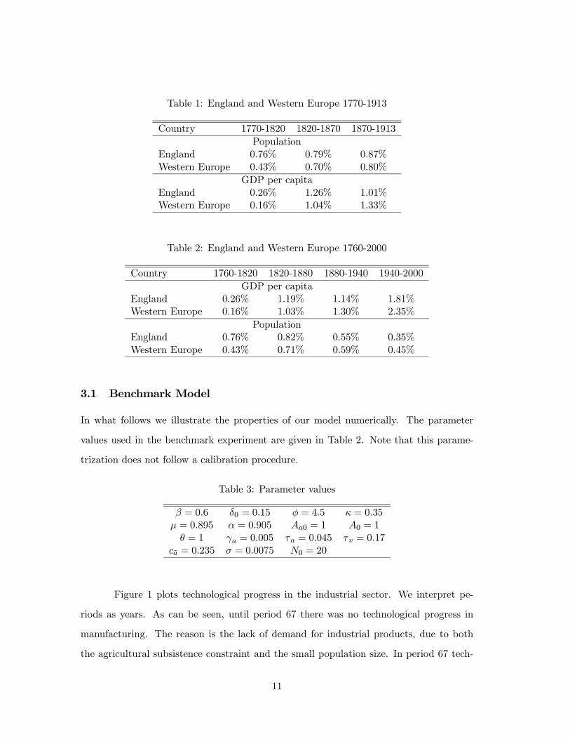
Table 1: England and Western Europe 1770-1913

Country 1770-1820 1820-1870 1870-1913Population

England 0.76% 0.79% 0.87%Western Europe 0.43% 0.70% 0.80%

GDP per capitaEngland 0.26% 1.26% 1.01%Western Europe 0.16% 1.04% 1.33%

Table 2: England and Western Europe 1760-2000

Country 1760-1820 1820-1880 1880-1940 1940-2000GDP per capita

England 0.26% 1.19% 1.14% 1.81%Western Europe 0.16% 1.03% 1.30% 2.35%

PopulationEngland 0.76% 0.82% 0.55% 0.35%Western Europe 0.43% 0.71% 0.59% 0.45%

3.1 Benchmark Model

In what follows we illustrate the properties of our model numerically. The parameter

values used in the benchmark experiment are given in Table 2. Note that this parame-

trization does not follow a calibration procedure.

Table 3: Parameter values

β = 0.6 δ0 = 0.15 φ = 4.5 κ = 0.35µ = 0.895 α = 0.905 Aa0 = 1 A0 = 1θ = 1 γa = 0.005 τa = 0.045 τv = 0.17

ca = 0.235 σ = 0.0075 N0 = 20

Figure 1 plots technological progress in the industrial sector. We interpret pe-

riods as years. As can be seen, until period 67 there was no technological progress in

manufacturing. The reason is the lack of demand for industrial products, due to both

the agricultural subsistence constraint and the small population size. In period 67 tech-

11

nological progress in the industrial sector takes off endogenously, and gradually increases

over time, before peaking at around 2.1%.

Technological Progress Industry

-0.5%

0.0%

0.5%

1.0%

1.5%

2.0%

2.5%

0 20 40 60 80 100 120 140 160 180 200Period

Ann

ual G

row

th R

ate

Figure 1: Technological Progess Industry

GDP per capita growth is initially close to zero. It is slightly positive though be-

cause agricultural TFP is assumed to growth at a rate of 0.5% per year. This corresponds

to the Malthusian phase.1 When technological progress takes off in the industrial sector,

GDP per capita growth starts to increase, from around 0.02% to 2%.

Because of the subsistence constraint, the increase in GDP per capita leads to

a relative decrease in the demand for agricultural goods. Figure 3 shows the share of

labor employed in agriculture. It steadily declines. Note that the structural transforma-

tion starts before the industrial revolution. This is because GDP per capita is already

increasing before.

The demand for kids is determined by two opposing forces. On the one hand, the

increase in GDP per capita increases the demand for children. On the other hand, the

move of people from the farm to the city, decreases the overall demand for children, as

1 In contrast to Galor and Weil (2000), we do not distinguish between Malthusian, Post-Malthusian,and modern growth, but only between Malthusian and modern gorwth.

12

Growth GDP per capita

0.0%

0.5%

1.0%

1.5%

2.0%

2.5%

0 20 40 60 80 100 120 140 160 180 200Period

Ann

ual G

row

th R

ate

Figure 2: Growth GDP per capita

Agricultural Employment Share

25.0%

27.0%

29.0%

31.0%

33.0%

35.0%

37.0%

39.0%

0 20 40 60 80 100 120 140 160 180 200Period

Agr

icul

tura

l Sha

re

Figure 3: Agricultural Employment Share

13

the time cost of child rearing is higher in the city. In Figure 4 we see how population

growth first increases and then decreases. This is the so-called demographic transition:

population growth decreases, even though income per capita is increasing.

Population Growth

0.0%

0.2%

0.4%

0.6%

0.8%

1.0%

1.2%

1.4%

0 20 40 60 80 100 120 140 160 180 200Period

Ann

ual G

row

th R

ate

Figure 4: Population Growth

3.2 Market Size

In our model the timing of the industrial revolution has to do with the size of the industrial

market. Several factors affect this market size, such as population size, GDP per capita,

and the subsistence constraint. This can easily be seen by doing a number of comparative

statics exercises.

If we increase the initial population, N0, by 25%, the industrial revolution starts

about 20 years earlier, in period 48 instead of 67. This can be seen in Figure 5. If we

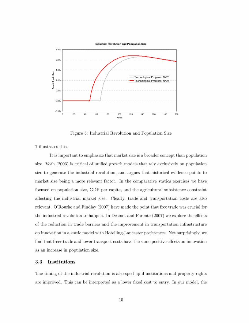
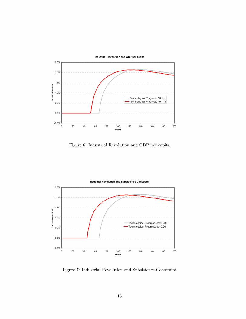
increase the initial GDP per capita by raising initial agricultural TFP by 10%, then the

industrial revolution starts 15 years earlier, in period 52 instead of 67. Figure 6 shows

this. Something similar occurs when we weaken the subsistence constraint by 15%, from

ca = 0.235 to ca = 0.20. This increases the demand for industrial goods, and as a result,

the industrial revolution starts about 20 years earlier, in period 45 instead of 67. Figure

14

Industrial Revolution and Population Size

-0.5%

0.0%

0.5%

1.0%

1.5%

2.0%

2.5%

0 20 40 60 80 100 120 140 160 180 200Period

Ann

ual G

row

th R

ate

Technological Progress, N=20Technological Progress, N=25

Figure 5: Industrial Revolution and Population Size

7 illustrates this.

It is important to emphasize that market size is a broader concept than population

size. Voth (2003) is critical of unified growth models that rely exclusively on population

size to generate the industrial revolution, and argues that historical evidence points to

market size being a more relevant factor. In the comparative statics exercises we have

focused on population size, GDP per capita, and the agricultural subsistence constraint

affecting the industrial market size. Clearly, trade and transportation costs are also

relevant. O’Rourke and Findlay (2007) have made the point that free trade was crucial for

the industrial revolution to happen. In Desmet and Parente (2007) we explore the effects

of the reduction in trade barriers and the improvement in transportation infrastructure

on innovation in a static model with Hotelling-Lancaster preferences. Not surprisingly, we

find that freer trade and lower transport costs have the same positive effects on innovation

as an increase in population size.

3.3 Institutions

The timing of the industrial revolution is also sped up if institutions and property rights

are improved. This can be interpreted as a lower fixed cost to entry. In our model, the

15

Industrial Revolution and GDP per capita

-0.5%

0.0%

0.5%

1.0%

1.5%

2.0%

2.5%

0 20 40 60 80 100 120 140 160 180 200Period

Ann

ual G

row

th R

ate

Technological Progress, A0=1Technological Progress, A0=1.1

Figure 6: Industrial Revolution and GDP per capita

Industrial Revolution and Subsistence Constraint

-0.5%

0.0%

0.5%

1.0%

1.5%

2.0%

2.5%

0 20 40 60 80 100 120 140 160 180 200Period

Ann

ual G

row

th R

ate

Technological Progress, ca=0.235Technological Progress, ca=0.20

Figure 7: Industrial Revolution and Subsistence Constraint

16

Industrial Revolution and Institutions

-0.5%

0.0%

0.5%

1.0%

1.5%

2.0%

2.5%

0 20 40 60 80 100 120 140 160 180 200Period

Ann

ual G

row

th R

ate

Technological Progress, kappa=0.35

Technological Progress, kappa=0.25

Figure 8: Industrial Revolution and Institutions: Effect of lower kappa

Industrial Revolution and Institutions II

-0.5%

0.0%

0.5%

1.0%

1.5%

2.0%

2.5%

0 20 40 60 80 100 120 140 160 180 200Period

Ann

ual G

row

th R

ate

Technological Progress, phi=4.5

Technological Progress, phi=0.4

Figure 9: Industrial Revolution and Institutions: Effect of lower phi

17

fixed cost is made up of two parameters, κ, which determines the fixed cost of determining

the benchmark technology, and φ, which determines how much the fixed cost increases

when adopting better technologies.

Decreases in κ and φ should have similar effects. Figure 8 shows that if we decrease

κ from 0.35 to 0.25, the industrial revolution starts 30 years earlier, in period 37 instead

of 67. Figure 9 shows how a drop in φ from 4.5 to 4 speeds up the industrial revolution

by about 20 years.

3.4 Agricultural Revolution

Some authors, such as Schultz (1971) and Diamond (1997), have argued that an agricul-

tural revolution is a precondition for an industrial revolution. This can easily be seen by

setting agricultural TFP growth to zero. In that case, population does not grow, and the

market never becomes big enough for the industrial revolution to take place.

4 Empirical support

In this section we use the model to interpret the historical experiences of various regions

and individual countries, and in doing so, hope to convince the reader that our theory

provides a reasonable answer to the question why the Industrial Revolution had to wait

until the 18th century and did not occur in some other country. Recall that at the core

of our theory is the mechanism by which various factors work to break down resistance.

This mechanism corresponds to more intense competition and more price elastic demand

for goods and services. The factors isolated by our theory as being critical for the degree

of competition are the size of the urban population, openness to trade, barriers to entry,

agricultural TFP and growth in that TFP.

We focus on two aspects of the historical experiences: the time series and the

cross section. The time series evidence concentrates on the experience of England, and

in particular, the developments in its institutions, agriculture, urban population, trans-

portation and trade in the centuries leading up to the Industrial Revolution. The cross

section compares other countries and regions to England along these same dimensions on

18

the eve of the Industrial Revolution. We start by providing empirical support for impor-

tant changes in these factors in England in the two centuries leading up to the Industrial

Revolution. We then show that England was further ahead along these dimensions than

other nations on the eve of the Industrial Revolution.

4.1 England, 1300-1800

Between 1300 and 1800 there were important improvements in England’s institutions,

agriculture, and transportation, in addition to large increases in the number of people

living in urban areas. These developments were almost surely dependent. For instance,

Acemoglu et al. (2005) argue that the rise in North Atlantic trade was an important

factor shaping institutions in England and other parts of Europe.

A key date for improvements in English institutions is the Glorious Revolution of

1688. North and Weingast (1989), in particular, have argued that the Glorious Revolution

was an important development because it made it far more difficult for the crown to

expropriate wealth, raise customs and sell monopolies. Ekelund and Tollison (1981)

argue that the balance of power brought on by the events of 1688 weakened the effects

of mercantilism, primarily, in the amount of effective regulation. In fact, Ekelend and

Tolllison characterize the situation in England as one of free trade as a result of the

balance of power.

There were also large increases in agricultural productivity in England between

1300 and 1800. According to Allen (2000, Table 8, p 21), agricultural output per agricul-

tural worker in England was stagnant from 1300 to 1600, but roughly doubled between

1600 and 1750. The reasons for these increases are numerous. Historians point to a

number of factors to explain this. The four most important developments were land en-

closure, mechanization, selective breeding and crop rotation. It is generally agreed that

each of these developments allowed for a significant population increase in England. Land

enclosure has also been related to the large increase in the urban population as tenant

farmers were evicted.

The transportation system in England likewise was improved in the period leading

19

up to the Industrial Revolution. In England, both roads and canals were important.

According to Szostak (1991, p. 60) a network of turnpikes linking almost every town

existed in England in the first half of the 18th century. The turnpike was a fairly recent

development, with the first one being built in the 17th century. Turnpike trusts were

an important institutional development for the English transportation system. Turnpike

Trusts replaced local parishes as the main body responsible for the maintenance of roads.

Before the creation of trusts, local parishes had responsibility for maintaining local roads.

This they did through property taxes and by requiring up to six days of unpaid labor

by residents. Trusts, in contrast, paid for maintenance by levying tolls and issuing debt.

Non-turn pike roads were also important in this period. In 1770, turnpikes covered 15,000

miles and non-turnpike roads covered approximately 60,000 miles.

Canals were also an important means of transporting goods in the period. Eng-

land was, in fact, blessed with a geographical advantage in this respect on account of

the abundance of natural waterways and the lack of dramatic changes in elevation and

seasonal temperatures which made water traffic profitable. According to Szostak (1991,

p 55), England had 1,100 kilometers of navigable rivers in 1660, rising to 1,900 in 1725,

to reach 3,400 km by 1830.

England was also blessed with a coastline that afforded natural ports. This con-

tributed to the growth in international trade over the 1300 to 1800 period. Acemoglu et

al. (2005) plot the dramatic rise in Atlantic voyages between 1500 and 1800. They show

that between 1700 and 1800 there was roughly an 8-fold factor increase in the number of

voyages per year.

Lastly, there was a large increase in England’s urban population between 1400 and

1750. In terms of total population, the English population in 1700 stood at approximately

the same number as in 1300, as it took 400 years for the total population to recover from

the Black Death in 1347 that killed off half of England’s population. While population

size was approximately the same in 1700 and 300, the distribution of the population across

rural and urban areas was radically different. In 1300, there were 220,000 people living

in urban areas, which represented 4 percent of the population. In 1700, this number was

20

880,000, representing almost 14 percent of the population. This increase in urbanization

occurred before the start of the Industrial Revolutions, and hence is not a result of an

increase in the living standard. Some of this increase is attributed to the English Acts of

Enclosure, which turned many common parcels of land into private holdings.

All of these developments are important in our theory. We see this as a virtue of

our theory. Clark (2005), for instance, has challenged the branch of the literature that

favors institutional developments, since the Glorious Revolution occurred 100 years before

the Industrial Revolution. Our theory offers an explanation for this lack of immediate

impact. Additionally, our theory would suggest that the Black Death was an important

event for the timing of the Industrial Revolution. Had there been no Black Death, the

Industrial Revolution would have likely occurred earlier. How much earlier, is a difficult

question to answer because institutions, openness, and urbanization in England were very

different in 1300 than in 1700.

4.2 England and the Rest of the World on the Eve of the IndustrialRevolution

We now present evidence that England on the eve of the Industrial Revolution was far

more advanced in the factors identified by our theory as being important than other

countries and regions. It is certainly true that England had a smaller land mass and

smaller total population than many other countries in the beginning of the 18th century.

However, as we shall argue, it compensated for this in terms of better transport, bet-

ter institutions, more open trade, and greater urbanization. These factors meant that

markets in England tended to more national in coverage, whereas markets in the larger

nations were much more regional. In fact, as we shall argue, in the case of China, the

relevant comparison is not with China as a whole, but the Jiangsu and Zhejiang regions

in the Lower Yangzi Province.

4.2.1 Western Europe

We begin with evidence in the form of price data from Shiu and Keller (2007) that suggests

that markets in England were far more national in nature compared to France, and the

21

rest of Western Europe. Shiue and Keller (2007) compute the variance of grain prices

across regions in Europe and China for the 17th, 18th and 19th centuries. What they

find is that grain prices in the 17th century were far less volatile in England compared

to the rest of Europe, or China that was on par with the rest of Europe. By the 19th

century, they find that this volatility declined for Europe, but remained more or less the

same for China.

Why were markets more national in England and more regional in the rest of the

world. One reason is that England possessed a much more developed system of roads

and canals. Szostak (1991) provides a thorough comparison of the English and French

transportation systems in the period leading up to the Industrial Revolution. He provides

estimates of the total mileage of roads and operating canals in England and France in

the 17th century, as well as the speed of transport by coach between cities. He also

characterizes the state of these roads. Essentially, England, despite having one fourth the

land mass as France, had the same amount of total road mileage. Whereas England by

the 18th century had a transportation system that linked every town in England, France

did not. Moreover, road in France were in a state of disrepair. (Szostak, 1991, p. 61).

The superiority of the English roads is reflected in the travel time of stage coaches. In

the 1760’s, the average coach in England traveled between 80 to 120 kilometers per day.

In France, in contrast, the average distance was between 40 and 55 kilometers per day.

Water transport also was far more prevalent and developed in England than France on

the eve of the Industrial Revolution. Additionally, France’s transportation system was

characterized by much larger tolls.

Why the transportation system was far more extensive and tolls significantly

lower in England than in France is good question. The answer most likely involves

geographical factors as well as political ones, including the greater power enjoyed by the

French crown. In terms of geography, England had a number of advantages. For one, it

was less mountainous. This was important not only for roads, but for water transport, as

it meant that the difference in the up-stream and down-stream currents was less. Also,

in contrast to England, France lacked any natural ports along its coastline, thus, making

22

sea transport more difficult.

There is thus strong evidence that markets in England were national but not in

France and the rest of Europe. Therefore, the relevant statistic is the amount of the

total population living in all urban areas. Despite its smaller population and land mass,

England by the 18th century was far more urbanized than any other country, having

experienced a large and steady increase in the number of cities over the previous five

centuries. According to Brewer (1988), the number of English towns with populations

between 5,000 and 10,000 doubled between 1600 and 1750. This was in contrast to con-

tinental Europe, which experienced an absolute decline in the number of such populated

towns. Bairoch (1976) presents data that shows that the fraction of the population living

in urban areas was significantly higher in England than France after 1600. By 1750, Eng-

land had 23 percent of the population living in cities, whereas in France only 13 percent of

the population lived in cities. (See Allen, R. Table 1, p Urban Development and Agrarian

Change in Early Modern Europe, 1998)

Institutions are generally viewed to have been more conducive to industrializa-

tion in England compared to the rest of Western Europe on the eve of the Industrial

Revolution. Ekelend and Tollison (1981) compare the forms of mercantilism practices

in England and France in the 16th through18th century and conclude that there were

dramatic differences in the amount of regulation, because of important institutional dif-

ferences determining the power of regulators. In France, this power was absolute, and

hence the barriers to entry were large. In England, the weaker power of the crown and

jurisdictional disputes with parliament meant that regulation was ineffective, and that

free trade reigned.

That France did not develop before is not hard to understand. What is harder

to understand is why the Netherlands and Belgium did not develop before or at the

same time as England. Allen (2000) documents that agricultural productivity was very

similar in the three countries on the eve of the Industrial Revolution. Additionally, the

fraction of the population in urban areas was similar. However, the absolute size of

that urban population in Belgium was about 50 percent the level of England and in the

23

Netherlands 80 percent the level of England. This may be one reason that Belgium and

the Netherlands had to wait longer for their industrial revolutions to begin

4.2.2 Asia

Much attention has been paid to China’s development between the 12th and 14th centuries

when China appeared to be on the verge of an industrial revolution. In our estimation,

the critical question is not why China failed to achieve an industrial revolution over

the Song Dynasty period, 900 to 1200 AD, but instead the critical question is why it

failed to realize and industrial revolution during the Qing period, 1600-1900 AD. It is

fairly obvious why the technological vibrancy that characterized the Song period was not

sustained. First, there is the Mongol invasion starting from 1205 and lasting to 1302 that

resulted in X million deaths and a general move of the population from the northeast

part of the country to the southwest. Second, there is Black death that similarly affected

China’s populations. Estimates of the fraction of the population who died in China from

the Bubonic plague are less specific than for Europe, but most historians think that the

effect was as large or larger, with possibly one third to two thirds of the population killed.

(There is also a third pandemic that starts around 1855 that kills 12 million people in

India and China.). In our theory, these two events certainly would have worked against

China fully industrializing. Nevertheless, the more important factor in the long-run was

the political developments in the middle 13th century associated with the start of the

Ming dynasty. The emperor, Name, was against the merchant class. Important during

this period was the outlawing of certain technologies, an increase in the number of state

monopolies, and a de-industrialization policy that was aimed at returning to a more

farm-based society.

The real question then is why didn’t China undergo an industrial revolution during

the Qing Dynasty, when it experienced a large increase in its population without any

associated increase in its living standard. On the surface, this large increase in population

without an industrial revolution would appear to be problematic for our theory. However,

if we look more closely at the nature of this population increase, it is not. According to

24

historians, the most vibrant region in China in the 17th century was the Lower Yangzi

Province that consists of Jiangsu and Zhejiang regions. The land mass of the LYP is only

slightly smaller than Britain. According to Pomeranz (2000), per capita GDP in the LYP

was approximately 1.5 times higher than the living standard for the rest of China. If an

industrial revolution were to start in China, the LYP is the logical place.

Interestingly enough, the LYP did not experience much by way of a population

increase during the Qing Dynasty. According to Pomeranz (2000), the population growth

in the LYP was approximately 0 while Ma (2006) estimates the average annual population

growth rate in the LYP to be .14 percent. The large increases in China’s population

occurred in the west and is associated with the opening of previously uninhabited land

and agriculture. In addition to land availability, important to this agricultural expansion

was the introduction of new plant varieties from the new world, particularly corn and

wheat.

Ma (2006) provides an interesting comparison between Qing LYP and Mejii Japan

in the 19th century and a theory for their subsequent divergent paths. His theory fits well

within our theory. In particular, Ma points out that in terms of land mass, population

levels, population changes, arable land, the LYP and Japan were very similar in 1850.

However, in the next 5 decades the two countries implemented very different policies,

which in our theory corresponds to a lowering of entry barriers and transportation costs in

Japan, but nothing like that in China. According to Ma, whereas the Japanese decided to

open up to the rest of the world, China under the leadership of the Qing Emperor decided

to return and strengthen its Neo-Confuscian ideology. The policies followed by the two

economies after 1850 were dramatically different. Japan’s ruling factions fully supported

private initiative, and even sold off some of the government enterprises. China in its

Self-Strengthening movement took nearly the opposite course of action, even opposing

private initiatives to improve the transportation system. Not surprisingly, whereas Japan

began its industrial revolution in the second half of the 19th century, China did not.

China, or more narrowly, the LYP had to wait nearly 50 years later to start an

industrialization. Following China’s naval defeat to Japan in the 1894-96, an industrial-

25

ization began in the LYP with Shanghai at the center of this revolution. The humiliating

defeat brought a sharp end to the Self-Strengthening movement. Additionally, the Treaty

of Shimonoseki gave foreigners the right to start up firms in the treaty ports. Thus, there

was both a lowering of entry costs and trade costs. As Ma (2006) documents, the growth

rate of per capita GDP in the LYP was essentially the same as Japan’s growth rate of

per capita GDP.

References

[1] Acemoglu, D., Johnson, S. and Robinson, J., 2005. The Rise of Europe: Atlantic

Trade, Institutional Change and Economic Growth. American Economic Review 95,

546-579.

[2] Aghion, P. and Howitt, P., 1992. A Model of Growth through Creative Destruction,

Econometrica, 60, 323-51.

[3] Allen, R.C. 2000. Economic Structure in and agricultural productivity in Europe,

1300-1800. European Review of Economic History, 3, 1-25.

[4] Brewer, J. 1988. The Sinews of War, Power and Money and the English State, 1688-

1783. Cambridge: Harvard University Press.

[5] Campbell, J.R. and Hopenhayn, H.A., 2005. Market Size Matters, Journal of Indus-

trial Economics, 53, 1-25

[6] Caselli, F. and Coleman, W.J., 2001. The U.S. Structural Tranformation and Re-

gional Convergence: A Reinterpretation, Journal of Political Economy, 109, 584-616.

[7] Clark, G. 2007. A Farewell to Alms. Trenton, N.J.: Princeton University Press

[8] Diamond, Jared. 1997. Guns, Germs, and Steel: The Fates of Human Societies. New

York: W.W. Norton.

[9] Desmet, K. and S.L. Parente. 2007. Bigger is Better: Market Size, Demand Elasticity

and Innovation.

26

[10] Doepke, M. and Zilibotti, F., 2005. The Macroeconomics of Child Labor Regulation,

American Economic Review, 95, 1492-1524.

[11] Ekelund, R. and R. Tollison. 1981. Mercantilism as a Rent-Seeking Society: Economic

Regulation in Historical Perspective. College Station, Texas: Texas A&M University.

[12] Findlay, R. and K. O’Rourke. 2007. Power and Plenty: Trade, War and the World

Economy in the Second Millennium. Princeton: Princeton University Press.

[13] Galor, Oded and David Weil. 2000. Population, Technology, and Growth: From the

Malthusian Regime to the Demographic Transition and Beyond. American Economic

Review. 90, 806-28.

[14] Goodfriend, Marvin and John McDermott. 1995. Early Development. American Eco-

nomic Review 85(1) 116-33.

[15] Hansen, Gary and Edward C. Prescott. 2002. Malthus to Solow. American Economic

Review 92(4): 1205-17.

[16] Helpman, E. and Krugman, P.R., 1985. Market Structure and Foreign Trade, MIT

Press.

[17] Hummels, D. and Klenow, P.J., 2005. The Variety and Quality of a Nation’s Exports,

American Economic Review, 95, 704-723.

[18] Hummels, D. and Lugovskyy, V., 2005. Trade in Ideal Varieties: Theory and Evi-

dence, mimeo.

[19] Hotelling, H. 1929. Stability in Competition. Economic Journal, 39, 41-57.

[20] Lancaster, K., 1979. Variety, Equity and Efficiency. New York: Columbia University

Press.

[21] Legros. P. A. Newman & E. Proto. 2006. ”Smithian Growth through Creative Organi-

zation,” Boston University - Department of Economics - The Institute for Economic

Development Working Papers dp-158, Boston University - Department of Economics.

27

[22] Mokyr. J. 1990. The Lever of Riche: Technological Creativity and Economic

Progress. New York: Oxford University Press.

[23] Mokyr, J. and Voth, H.-J., 2007. Understanding Growth in Europe, 1700-1870: The-

ory and Evidence, mimeo.

[24] Ma, D. 2006. Modern Economic Growth in the Lower Yangzi in 1911-37: a Quantita-

tive, Historical, and Institutional Analysis. Unpublished Manuscript, London School

of Economics.

[25] North, D.C. and R.P. Thomas. 1973. The Rise of the Western World: A New Eco-

nomic History. Cambridge: Cambridge University Press.

[26] North, D.C. and B. Weingast. 1989. The Evolution of Institutions Governing Public

Choice in Seventeenth Century England. Journal of Economic History 49 (4), 803-32.

[27] O’Rourke, K. and J. Williamson, 2005. ”From Malthus to Ohlin: Trade, Industri-

alisation and Distribution Since 1500,” Journal of Economic Growth, Springer, vol.

10(1), pages 5-34, 01

[28] Pomerantz, K. 2000. The Great Divergence: Europe, China and the Making of the

Modern World Economy. Princeton: Princeton University Press.

[29] Rosenzweig, M.S. and Evensen, R.E., 1977. Fertility, Schooling, and the Economic

Contribution of Children in Rural India: An Econometric Analysis, Econometrica,

45, 1065-1079.

[30] Schultz, T. W. 1968. Economic Growth and Agriculture. New York: McGraw-Hill.

[31] Shiue, C.H. and W. Keller. 2007. Markets in China and Europe on the Eve of the

Industrial Revolution. American Economic Review 97 (4):1189-1216.

[32] Szostak, R. 1991. The Role of Transportation in the Industrial Revolution. Buffalo,

NY: McGill-Queens University Press.

28

[33] Tybout, J., 2003. Plant- and Firm-level Evidence on the ‘New’ Trade Theories, in:

E. Kwan Choi and James Harrigan, ed., Handbook of International Trade, Oxford:

Basil-Blackwell.

[34] Voightlander, N. and H.J. Voth. 2006 Why England? Demographic Factors, Struc-

tural Change and Physical Capital Accumulation During the Industrial Revolution.

Universitat Pompeu Fabra Working Paper.

[35] Voth, H.-J., 2003. Living Standards During the Industrial Revolution: An Econo-

mist’s Guide, American Economic Review Papers and Proceedings, 93, 221-226.

29