WPS20S2POLICY RESEARCH WORKING PAPER 2052

The Macro Wage Curve The existence of a macrowage curve shows that

and Labor Market Flexibility wages in ZimbaDwe are

in Zimbabwe flexible. So, the labor marketadjusts to both negative and

positive economic shocks. The

Dorte Verner main cause of falling real

wages in Zimbabwe is

reduced economic activity.

The World Bank

Africa Technical Families

Human Development 3 UFebruary 1999

Pub

lic D

iscl

osur

e A

utho

rized

Pub

lic D

iscl

osur

e A

utho

rized

Pub

lic D

iscl

osur

e A

utho

rized

Pub

lic D

iscl

osur

e A

utho

rized

Pub

lic D

iscl

osur

e A

utho

rized

Pub

lic D

iscl

osur

e A

utho

rized

Pub

lic D

iscl

osur

e A

utho

rized

Pub

lic D

iscl

osur

e A

utho

rized

I POLICY RESEARCH WORKING PAPER 2052

Summary findings

There is little available information about what She finds that a macro wage curve does exist, so wagesdetermines money wages in Sub-Saharan Africa - or are flexible both generally and in the manuf:acturingindeed about whether there is a stable relationship sector. So, the labor market is able to adjust to bothbetween wages, productivity, GDP, inflation, activity in positive and negative shocks.the informal sector, policy changes, and unemployment. The main cause of falling real wages in Zimbabwe is

In studying how wages in Zimbabwe are affected by reduced economic activity.short- and long-run changes in variables, Verner asks: In the short term, wages are affected by c,aanges in theAre wages affected by prices, unemployment, increased unemployment rate. They are also affected positively byproductivity, economic activity, or policy changes? Does increases in productivity, prices, and econornic activity.a macro wage curve exist? Did structural adjustment The forecasting performance of thie wagecause a structural change in labor markets? determination models shows that they are valid after the

implementation of structural adjustment in 1991.

This paper - a product of Human Development 3, Africa Technical Families - is part of a larger effort in the region tounderstand how labor markets work in Africa. Copies of the paper are available free from the World Bank, 1 818 H StreetNW, Washington, DC 20433. Please contact Hazel Vargas, room 18-138, telephone 202-473-7871, fax 202-522-2119,Internet address hvargas@worldbank.org. The author may be contacted at dverner@v-worldbank.org. February 1999. (37pages)

The Policy Research Working Paper Series disseminates the findings of work in progress to enicourage the exchange of ideas aboutdevelopment issues. An objective of the series is to get the findings out quickly, euen if the presentations are less thani fully polished. Thepapers carry the names of the authors and should be cited accordingly. The findings, interpretations, and conclusions expressed in thispaper are entirely those of the authors. They do not necessarily represent the viewr' of the World Bank, its Executive Director, or thecountries they represent. |

Produced by the Policy Research Dissemination Center

The Macro Wage-Curve and LaborMarket Flexibility

in Zimbabwe

Dorte Verner*

The World Bank1818 H Street, N.W.

Washington, D.C. 20433e-mail: dverner@worldbank org

* I am grateful to Helena Ribe for invaluable support, to Niels-Hugo Blunch for excellent researchassistance, and to John Mclntire for comments.

1. Introduction

There is little available knowledge on what determines money wages in sub-Saharan

Africa, or indeed on whether there exists a stable relationship among wages, productivity,

GDP, inflation, policy changes and unemployment or informal sector activity. In this

paper, we study how wages are affected by short- and long-run changes in the

aforementioned variables in the case of Zimbabwe. The importance of knowing the

answer to this question may be illustrated by considering economic reforms. Structural

adjustment programs may cause reductions in aggregate demand due to decreased

government spending and increased real interest rates. If wages are downwards-rigid,

and, therefore, unable to adjust to changes in aggregate demand then the unemployment

rate or informal sector activity increase. On the other hand, if wages are flexible, then the

decrease in aggregate demand may be mitigated by falling wages and, therefore, causing a

more limited increase in unemployment or informal sector activity. In the latter case the

labor market is characterized by a macro-wage curve.

The main questions addressed are the following: (1) are wages affected by increased

productivity, economic activity, prices, policy changes and unemployment; (2) does there

exist a macro wage-curve; and, (3) did the economic structural adjustment program

(ESAP) cause a structural change in the labor markets. The main findings are that wages

are flexible-both upwards and downwards. Hence, the labor market is able to adjust to

economic shocks. The main cause of falling real wages in Zimbabwe is reduced

economic activity.

This paper is the first in a series of papers studying Zimbabwean labor markets. Another

paper analyzes wage and productivity determination in Zimbabwe but in contrast to this

paper, the study is based on findings from micro level data (see Verner, 1998). The

findings, using data on employees matched with data on firms, can be summarized as: (1)

female employees are paid less than males and the negative wage premium do not match

a corresponding negative productivity premium; (2) experience is reflected equally in

wages and productivity differentials over the life-cycle; (3) the wage premium increases

with level of education and with occupation title; (4) formal in-house training is found to

be associated with higher wages, while there does not seem to be any instant effect on

productlvity; (5) an additional wage and productivity premium exists if enterprises are

engaged in exporting activities; (6) ethnic origin of an employee is not important in the

determination of wages. However, Europeans are more productive than other ethnic

groups; (7) union members earn less than non-union members despite being found to be

more producive; (8) larger firms are more productive and pay higher wages than smaller

firms; (9) employees employed in the metal or textile sectors are paid higher wages than

colleagues in the food sector.

This paper gives a broad picture of developments in the labor market and it is organized

as fo'lows. Section two provides a brief presentation and discussion of economic

developments in Zimbabwe. This is followed by a presentation of wage theories and

empirical results. Sections three and four contain the estimated wage model and give

emppircal evidence of whether the labor market in Zimbabwe is characterized by a macro-

wage curve. I'he final section provides conclusions.

2. TLrends

This section contains a brief overview of Zimbabwean labor markets over the past three

decades. We apply time series data from 1964 to 1994 to show trends in output, wages,

productivity, and employment.

After the declaration of Tndependence by Rhodesia in 1965 most nations imposed trade

saactions against the regime. This caused a reduced flow of capital goods and industrial

inmcuts foro, abroad. In 1980 a new government led by Robert Mugabe introduced iimport

quotas and continued controlling prices introduced by the former regime. In the first

years after physical capital investment boomed but without investment in long-term

commitments to employees, meaning that the production was more capital intensive than

labor intensive (Failon and Lucas; 1993).

2

The average annual gross domestic product (GDP) growth rate was 7.5 percent in the

period from the declaration of Independence in 1965 until the first oil price increase in

1974. In the same period manufacturing employment increased at an annual rate close to

the GDP growth rate (7.2 percent) but the national employment level only grew around

3.7 percent per year. The main explanations of the low employment growth rate are the

composition of employment and the relatively low cost of capital as compared to labor

costs.

Until 1980, workers of African and European origin had very different opportunities,

given the political regime of the time. The latter group obtained the best education and

apprenticeships; and most white-collar jobs. African workers were excluded from

skilled occupation groups and had no access to training programs or labor unions.

Furthermore, wage grids and a minimum wage law did not exist until the 1980s. Fallon

and Lucas (1991) report that in 1978 earnings of Europeans were 10.4 times higher than

those of Africans. In manufacturing, workers of European origin earned 7.4 times more

than Africans. The transition to majority rule in 1980 and the war of Independence in the

1970s made numerous Europeans leave Zimbabwe. In 1992, Europeans represented only

one percent of the Zimbabwean population.

2.1 Output

Figure 1 shows real output in four sectors together with that of aggregate output in

Zimbabwe since 1964. The chart shows that the economic climate improved until the

first oil price increase. Afterwards, a recession set in and employment and output

declined. The causes of the recession were civil war, emigration, droughts, oil price

increases, and trade sanctions.

Whereas real output increased for most sectors over the 1964-94 period, the service and

agriculture sectors experienced major drops in output from 1991 onwards. The value of

output in the manufacturing sector lies substantially above that of agriculture-for the last

3

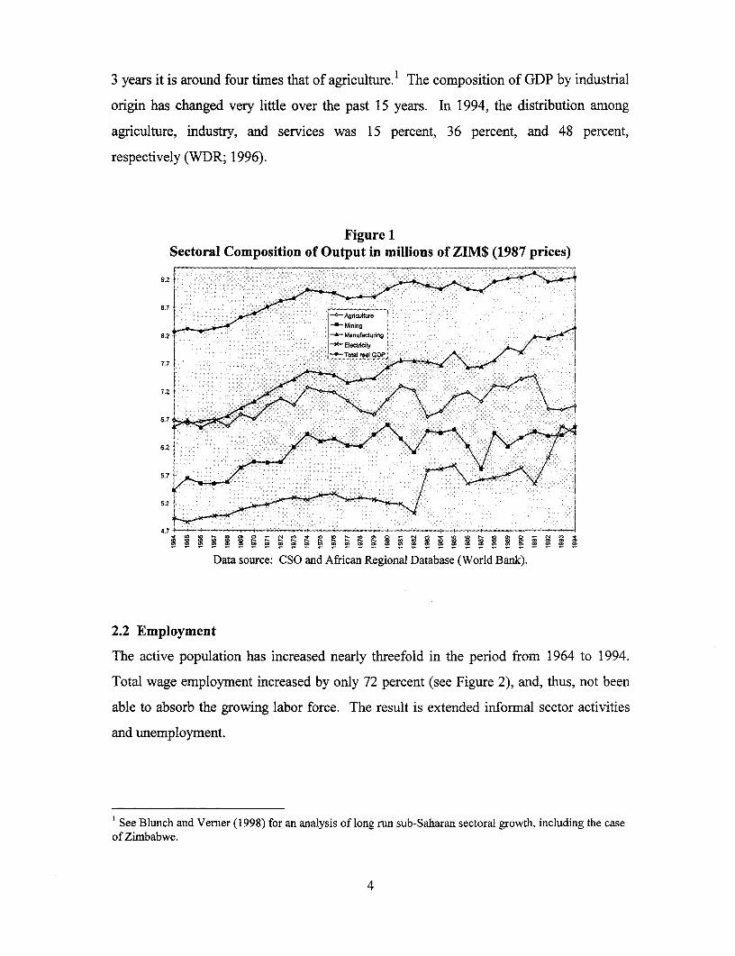
3 years it is around four times that of agriculture.' The composition of GDP by industrial

origin has changed very little over the past 15 years. In 1994, the distribution among

agriculture, industry, and services was 15 percent, 36 percent, and 48 perclent,

respectively (WDR; 1996).

Figure 1Sectoral Composition of Output in millions of ZIM$ (1987 prices)

9.2

8.7

8.2 Manufacturing

5.7

5.2

4.7% S o~ o S 0; - (N C' *n C C 0 ° 0 - EN Z' E 8 C E' ° ° o - (N o

Data source: CSO and African Regional Database (World Bank).

2.2 Employment

The active population has increased nearly threefold in the period from 1964 to 1994.

Total wage employment increased by only 72 percent (see Figure 2), and, thus, not been

able to absorb the growing labor force. The result is extended informal sector activities

and unemployment.

1 See Blunch and Verner (1998) for an analysis of long run sub-Saharan sectoral growth, including the caseof Zimbabwe.

4

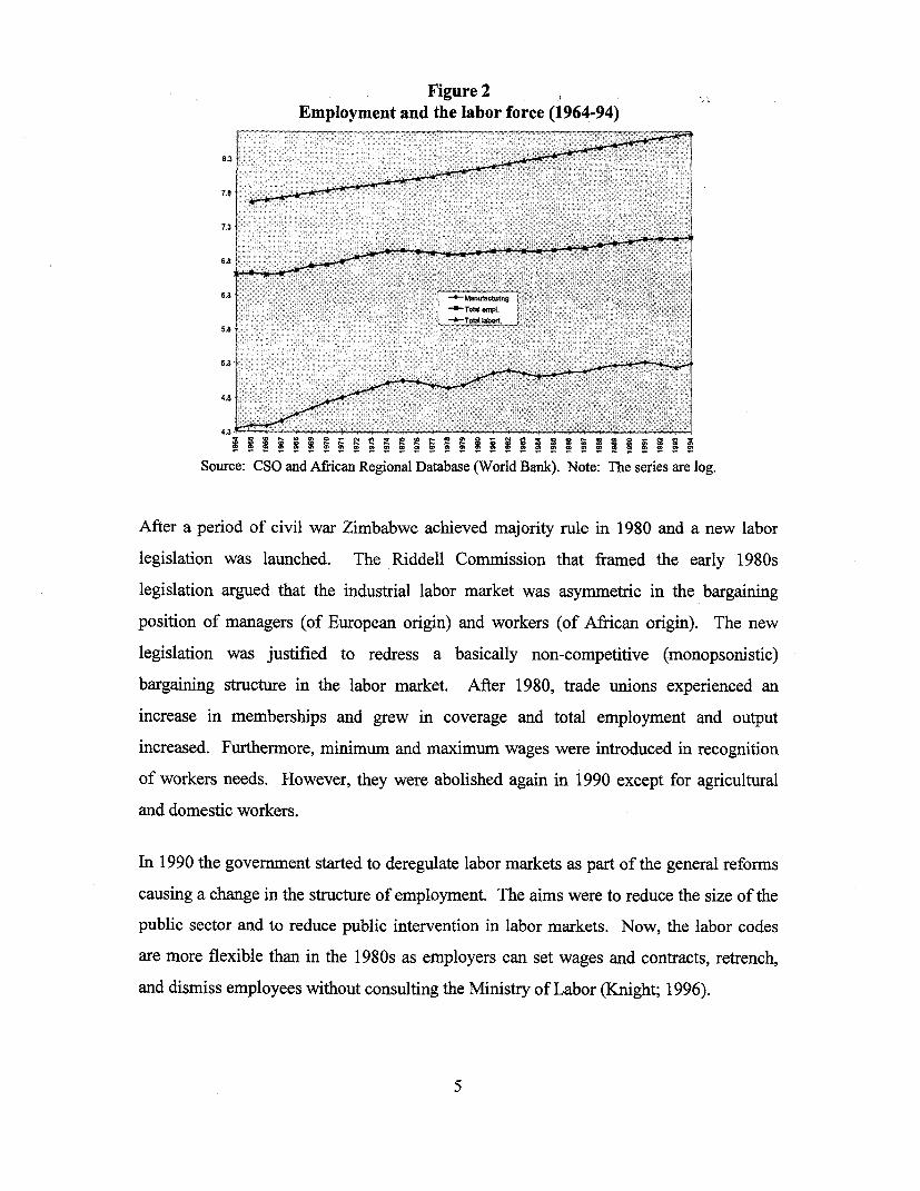
Figure 2Employment and the labor force (1964-94)

7.8 a a a a a r a a a

4.3

Source: CSO and African Regional Database (World Bank). Note: The series are log.

After a period of civil war Zimbabwe achieved majority rule in 1980 and a new labor

legislation was launched. The Riddell Commission that framed the early 1980s

legislation argued that the industrial labor market was asymmetric in the bargaining

position of managers (of European origin) and workers (of African origin). The new

legislation was justified to redress a basically non-competitive (monopsonistic)

bargaining structure in the labor market. After 1980, trade unions experienced an

increase in memberships and grew in coverage and total employment and output

increased. Furthermore, minimum and maximum wages were introduced in recognition

of workers needs. However, they were abolished again in 1990 except for agricultural

and domestic workers.

In 1990 the government started to deregulate labor markets as part of the general reforms

causing a change in the structure of employment. The aims were to reduce the size of the

public sector and to reduce public intervention in labor markets. Now, the labor codes

are more flexible than in the 1980s as employers can set wages and contracts, retrench,

and dismiss employees without consulting the Ministry of Labor (Knight; 1996).

5

Figure 3 shows the development in employment by industrial sector in the period from

1964 to 1994.2 The total number of formal employees in Zimbabwe reached 1.263.700 in

1994, starting at 736.600 in 1964.

The service sector is the largest employer followed by the agricultural and manufactwuing

sectors.3 Employment increased for all three major sectors over the thirty year period.

There is no clear trend in agriculture, leading to only a minor increase (10 percent') as

compared to 160 percent and 125 percent increase in the manufacturing and service

sectors, respectively.

Figure 3Employment by sector in thousands (1964-94)

6.5

5.5 Agricufture

~~~~~~~~~~~~~~~~~~~~~~~~~~~~~~anufacuturin_ > G_ t~~~~~~~~~~~~~~~~~~~~~~~~~~~~~~~~~~~~lectricity

4.5 Distribution

0 = _ > + ~~~~~~~~~~~~~~~~~~~~~~~~~~Mining

3.5 -~~~~~~~~~~~~~~~~~~~~~~~~~~~~~~Service

2.5

1.5C (CO C O N I ND CD Co N CD tO O (N

Data source: CSO. Note: Series are log (employees in thousands).

2 The service sector includes public administration, education, health, private domestic, and other.

3 Industry is an aggregation of the following seven sectors: mining and quarrying; manufacturing;electricity and water; construction; distribution, restaurants and hotels; finance; insurance and real estate;and, transport and communications.

6

Table 1Annual growth rates of employment in 3 major sectors (percentage)

1987-90 1991-94 1987-94Agriculture 2.9 2.1 2.8Industry 4.1 0.3 2.5Services 2.2 -0.3 1.4

Data source: own calculations based on CSO statistics.

After the economic structural adjustment program was introduced and droughts took

place, the rate of increase in employment slowed significantly in industry, as seen from

Table 1. It barely increased in the 1991-94 period. In the same period employment in the

service sector decreased yearly by 0.3 percent whereas in agriculture it increased 2.1

percent yearly. The employment loss has been concentrated in sectors vulnerable to

competition from trade liberalization and rise in interest rates, such as, for example,

textiles. The share of total employment in each sector in the 1987-94 period is pictured in

Figure 4.

Figure 4Employment by sector (1987-94)

Agric Mining Manuf Eiec Construc Finance Distrib Service Trrans&Comms

Data source: CSO

7

The share of total employment in agriculture, construction, finance, and.distribution

increased in the 1987-94 period while it decreased in manufacturing, mining,

transport/communication, and services; and slightly more in the latter than in the three

former sectors.

2.3 Earnings

Until 1982 real average wages across sectors as well as real wages in manufacturing were

characterized by a positive trend, which was reversed to a negative trend in 1982, see

Figure 5. The highest level of average real earnings was in 1982, being 39 percent above

the 1979 level (see Figure 6). This was mainly due to the launch of minimum wages (see

below).

Figure 5Total and manufacturing real wages (Zim $ per year)

7500

700000Totreal San ioge a ( B

4500 / \

4000 \

3500/

3000 - , I I I .

Source: CSO and African Regional Database (World Bank).

8

Figure 6Productivity (Real Output Per Employee ZIM$)

3.9

2.4

0.9{~ ~~~ N N N N N N° N C C C C C C - 0 0l Cl C 0000IS a9

Data source: CSO and African Regional Database (World Bank). Note: All series are log

Figure 6, continuedProductivity (Real Output Per Employee ZIM$)

1.4

0.9

Data source: CSO and African Regional Database (World Bank). Note: All series are log

9

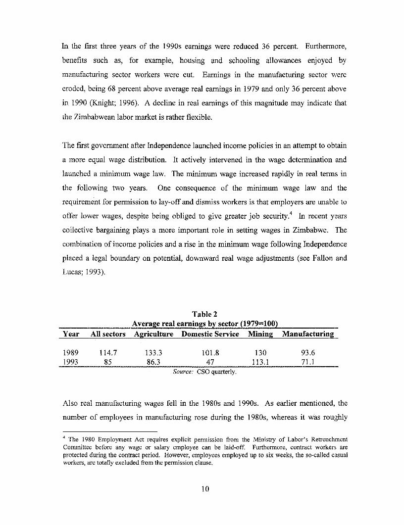
In the first three years of the 1990s earnings were reduced 36 percent. Eurthermore,

benefits such as, for examnple, housing and schooling allowances enjoyed by

manufacturing sector workers were cut. Earnings in the manufacturing sector were

eroded, being 68 percent above average real earnings in 1979 and only 36 percent above

in 1990 (Knight; 1996). A decline in real earnings of this magnitude may indicate that

the Zimbabwean labor market is rather flexible.

The first government after Independence launched income policies in an attempt to obtain

a more equal wage distribution. It actively intervened in the wage determination and

launched a minimum wage law. The minimum wage increased rapidly in real terms in

the following two years. One consequence of the minimum wage law and the

requirement for permission to lay-off and dismiss workers is that employers are unable to

offer lower wages, despite being obliged to give greater job security.4 In recent years

collective bargaining plays a more important role in setting wages in Zimbabwe. The

combination of income policies and a rise in the minimum wage following Independence

placed a legal boundary on potential, downward real wage adjustments (see Fallon and

Lucas; 1993).

Table 2Average real earnings by sector (1979=100)

Year All sectors Agriculture Domestic Service Mining Manufacturing_

1989 114.7 133.3 101.8 130 93.61993 85 86.3 47 113.1 71.1

Source: CSO quarterly.

Also real manufacturing wages fell in the 1980s and 1990s. As earlier mentioned, the

number of employees in manufacturing rose during the 1980s, whereas it was roughly

4 The 1980 Employment Act requires explicit permission from the Ministry of Labor's RetrenchmentCommittee before any wage or salary employee can be laid-off. Furthermore, contract workers areprotected during the contract period. However, employees employed up to six weeks, the so-called casualworkers, are totally excluded from the permission clause.

10

unchanged in the 1990s. In all sectors, real wages fell in the 1990s, whereas in the 1980s

real output increased in agriculture and mining, with a falling number of employees, and,

therefore, increasing productivity (see Figure 4 and Table 3).

Fallon and Lucas (1993) analyze job security, regulation and demand for industrial labor

in Zimbabwe. They find a reduction in demand for workers but no slowing in the

adjustrnent of the number of employees following enactment of the labor laws.

Furthermore, the drop in employment at the time of the new Employment Act is found

not to be associated with mounting European migration or with the structural change in

labor demand upon achieving Independence.

2.4 Productivity

Economy-wide econornic progress requires increased output per worker and it is expected

to expand employment opportunities and rise wages. Labor productivity for the 1964-94

period is presented in Figure 6. The charts show that the development in productivity is

sector specific. The highest level of productivity is found in electronics and finance. In

the mining sector, productivity increased around 162 percent over the period, whereas it

was reduced in construction by around 64 percent.

The manufacturing and agricultural sectors productivity show a steady positive trend,

having increased by 128 percent and 18 percent, respectively. The service sector,

experienced (as the only sector) a decrease in productivity-28 percent-indicating that

services may have absorbed the retrenched or less productive labor.

3. Wage curves

This subsection briefly describes theories concerned with wages and unemployment that

is used in the process of describing wage determination in Zimbabwe. The main

economic theories are the so-called Phillips curve (Phillips; 1958) and wage curve

(Blanchflower and Oswald; 1995).

11

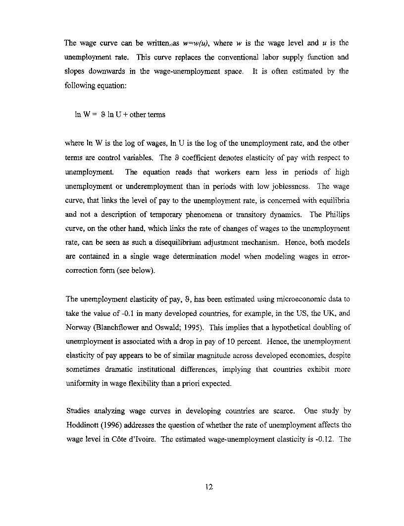
The wage curve can be writtenaas w=w(u), where w is the wage level and u is the

unemployment rate. This curve replaces the conventional labor supply function and

slopes downwards in the wage-unemployment space. It is often estimated by the

following equation:

ln W = a ln U + other terms

where In W is the log of wages, In U is the log of the unemployment rate, and the other

terms are control variables. The 9 coefficient denotes elasticity of pay with respect to

unemployment. The equation reads that workers earn less in periods of high

unemployment or underemployment than in periods with low joblessness. The wage

curve, that links the level of pay to the unemployment rate, is concerned with equilibria

and not a description of temporary phenomena or transitory dynamics. The Phillips

curve, on the other hand, which links the rate of changes of wages to the unemployrnent

rate, can be seen as such a disequilibrium adjustment mechanism. Hence, both models

are contained in a single wage determination model when modeling wages in error-

correction form (see below).

The unemployment elasticity of pay, X, has been estimated using microeconomic data to

take the value of -0.1 in many developed countries, for example, in the US, the UK, and

Norway (Blanchflower and Oswald; 1995). This implies that a hypothetical doubling of

unemployment is associated with a drop in pay of 10 percent. Hence, the unemployment

elasticity of pay appears to be of similar magnitude across developed economies, despite

sometimes dramatic institutional differences, implying that countries exhibit more

uniformity in wage flexibility than a priori expected.

Studies analyzing wage curves in developing countries are scarce. One study by

Hoddinott (1996) addresses the question of whether the rate of unemployment affects the

wage level in C6te d'Ivoire. The estimated wage-unemployment elasticity is -0.12. The

12

author also estimates the elasticity for the private and public sectors to be -0.18 and -0.11,

respectively.

In the following we apply a linear wage equation building on the above mentioned

theories to analyze questions related to the macro-wage curve in Zimbabwe. The model

is written:

wt= a+but+cpt+dyt+ft (1)

where lower case letters denote the natural logarithms of variables written in upper case

letters; w is wages, u is unemployment/informal sector activity and y is GDP (proxies for

pressure of demand), p is prices (proxy for macro economic stability and influence of

expectations), and t is a deterministic function of time, capturing productivity increases.

We predict that increased productivity impacts wages positively. The same holds for

enhanced economic activity and rising prices.

4. Wage curve estimation

The determination of Zimbabwean wages is estimated using an error-correction model

(ECM). This model allows for analyzing the impact of demand pressure, etc. on wages

both in the short and long run. The procedure we apply in estimating the ECM is the

Wicken and Breusch (1988) approach.5 Hence, this gives an eclectic macro wage model,

where we can simultaneously analyze the macro wage curve, the Phillips curve or other

economic models of wage determination. The linear wage equation (1) can be formulated

as an error correction regression model:

Awt = a + pAut + pApt + Ywt-M + Xut-l + 8Pt-I + Pt + st (2)

5 The reason for this choice is that there is some evidence that the small sample bias is smaller for the long-run estimators than, for example, in the Engle and Granger (1987) two-step procedure [see Kremers,Dolado, and Ericsson (1992)].

13

where A denotes first differences of the variable. The random disturbance e reflects all

other factors. The disturbance term may also reflect the fact that we cannot expect data to

have been measured with perfect accuracy. The possibility of errors in the measurement

of U, P and W is thus another reason for adding a random disturbance term.

The estimate of the long-run parameter, that measures the strength of demand in the labor

market on wages, can be obtained from the ratio of the estimated coefficients of wt-I and

uti. With the error correction interpretation of equation (1), X=O indicates that there is no

effect on wages from increased unemployment. This hypothesis does not preclude labor

market effects on wages altogether since changes in the unemployment rate, Au,

influence wages provided that ,3•O.

The real wage hypothesis, that is, real wages respond to the strength of demand in the

labor market, holds if there exists a co-integrating vector involving all long run variables

and the sum of the coefficients of w and p equal zero.

Equation (1) has other models of wage determination nested within, for example: (1) a

first order error correction model with wages adjusting towards a static equilibrium that

depends on prices only (B = X = p = 0); (2) a first order partial adjustment model with a

target value of wages depending on unemployment only (,B = 6 = p = 0); (3) a trend

stationary real wage model (p = 6 = 1 and ,B = k= 0); and, (4) a random walk with drift

model (o = p = y = 9= 0).

We model the economic time series using so-called general-to-specific modeling. This

approach has the twin advantages of avoiding unnecessary generality that may result in

loss of efficiency and can result in models being too finely tuned to the data.

Furthermore, it guarantees the coherence of the model with economic theory, i.e., ensures

that the model has an economic interpretation and is related to the phenomena being

analyzed.

14

5. Empirical Evidence

In the following subsection we analyze whether a macro wage curve exists in Zimbabwe

using aggregate data from 1964 to 1994. The statistical model in use is an autoregressive

distributed lag model for wages consisting of: (1) pressure of demand that we proxy by

the unemployment rate/informal sector and GDP; (2) expectational influences that we

proxy by prices; (3) productivity, captured by a deterministic, linear trend; and, (4)

important policy changes captured by including dummy variables.

The following three subsections present findings. Subsection 5.1 gives statistical

information and subsections 5.2 and 5.3 analyze wage determination in the total economy

and the manufacturing sector.

5.1 Statistical information

Visual inspections indicate that wages and unemployment have strong positive trends of a

similar magnitude, so that they may be modeled as stationary deviations from a linear

trend or alternatively as variables with stochastic trends within a co-integrated system

(see details in Banerjee, et al. (1993)). The unemployment or informal sector series also

exhibits deviations from the trend in form of cyclical movements that will be important to

capture in the modeling of wages. These properties, possibly resulting from changes in

economic policies and "autonomous" events such as droughts and changes in commodity

prices, e.g., crude oil, may be important to take into account when modeling wages.

The inspection of correlograms for the variables w, p, w-p, and u reveals high first order

serial correlation coefficients (around 0.9) with the higher order coefficients declining

extremely slowly, and correspondingly the spectra have peaks at the zero frequency. This

information is consistent with each of the series having a stochastic trend and, therefore,

being non-stationary and presumably integrated of order one, I(1). The result of the

Augmented Dickey-Fuller test supports these hypotheses (see Appendix A). Hence, in

modeling wages it will be important to choose models that can represent the

15

nonstationarities of the series with the possibility that they form a co-integration

relationship. That is, there is some linear combination of the series that is stationary, l(0).

5.2 Wage determination for the total economy

This section presents results on wage determination and it should be noted that we have

problems with regard to the number of data points when we want to introduce both

pressure-of-demand variables - the unemployment rate/informal sector and GDP. The

series are very highly correlated and, therefore, the high simple correlation may indicalte

multicollinearity problems. One way to solve this problem is to include all demand

pressure variables and the cross-products of these in the error correction specification of

the wage model. This is clearly the ideal scenario but data are only available for three

decades, therefore, it is not statistically feasible. Another way to model wages is by

including one demand pressure variable at a time, in both levels and changes, in the

model and subsequently perform encompassing tests to uncover which demand pressure

variable best explains wages.

5.2.1 The aggregate wage model with the unemployment rate

In this subsection, we explain wages by prices, the unemployment rate/informal sector

activity, productivity (trend), and policy dummy variables. Recursive estimation shovvs

that the pattern of wages in the period from 1980 to 1984 is out of line with the estimated

pattern of the wage model-they are too high.6 A congruent model is produced, by taking

into account that in this period, wages were set higher than could be sustained by

economic activity and productivity. There are no obvious signs of misspecifications for

the full data sample when including policy dummy variables: i1984 (an impulse dummy,

which takes the value one in 1984 and zero elsewhere) and i80-84 (step dummy, which

takes the value of one in each year in the 1980-84 period and zero else where). Policies

introduced after the Independence War (1980) appear to have led to a large acceleration

in wage inflation revealed by the positive parameter estimate (see Table 3).

6 This is revealed by recursive estimation followed by tests statistics for structural break points. One-ste(p-ahead Chow tests informed that changes took place in the labor market in the period from 1980 to 1984.

16

Table 3ECM for total wages

Variable Coefficient Std. Error t-value t-prob Part R2 Instab-U -1.392 0.521 -2.671 0.015 0.263 0.16CPI_1 0.103 0.058 1.782 0.090 0.137 0.03-CPI 0.098 0.135 0.727 0.476 0.026 0.03Trend 0.028 0.010 2.902 0.009 0.296 0.03Constant 2.765 1.295 2.135 0.045 0.186 0.03W_1 -0.253 0.112 -2.266 0.035 0.204 0.03U_1 -0.383 0.269 -1.423 0.170 0.092 0.04i80-84 0.086 0.019 4.505 0.000 0.504 0.03il984 -0.118 0.034 -3.492 0.002 0.379 0.07

Definitions of VariablesW_I is log total wages lagged once

U_1 is log total unemployment rate lagged once-U is the first order difference of U

CPI_I is the log of the consumer price index lagged once-CPI is the difference of CPI

iXXXX is a dummy variable for the(se) year(s)Test Statistics

R2 = 0.791 F(8, 20) = 9.436 [0.000] C = 0.029 DW = 2.54RSS = 0.017 for 9 variables and 29 observations

Variance instability test: 0.3 85 Joint instability test: 1.943Information Criteria: SC -6.393 HQ =-6.684 FPE =0.001

AR 1-2F(2, 18)= 1.825 [0.1901ARCH 1 F( 1, 18) = 0.047 [0.832]Normality Chi2(2)= 5.141 [0.077]

Xi2 F(16, 3) = 0.329 [0.94 1]RESET F( 1, 19) = 1.923 [0.182]

Additionally, Table 3 summarizes test statistics and based on these statistics; there is no

evidence of misspecification of the wage model. 7 The charts presented in Figure 7

substantiate these findings showing the actual and the fitted values, the residuals, the

7 The variance instability and the joint instability test statistics; a Lagrange multiplier (LM) test forautocorrelation in the residuals with the null of no serial correlation (AR); an LM statistic for testing thenull of no autoregressive conditional heteroscedasticity (ARCH); a statistic for testing the null hypothesis ofunconditional homoscedasticity against the alternative that the residuals are correlated with the model'sregressors and their squares (Xi2); a regression specification test which test the null of correct specificationagainst the alternative that the residuals are correlated with the squared fitted values of the regressand(RESET); and the test statistic for normality, where the null is that the residuals are normally distributed.

17

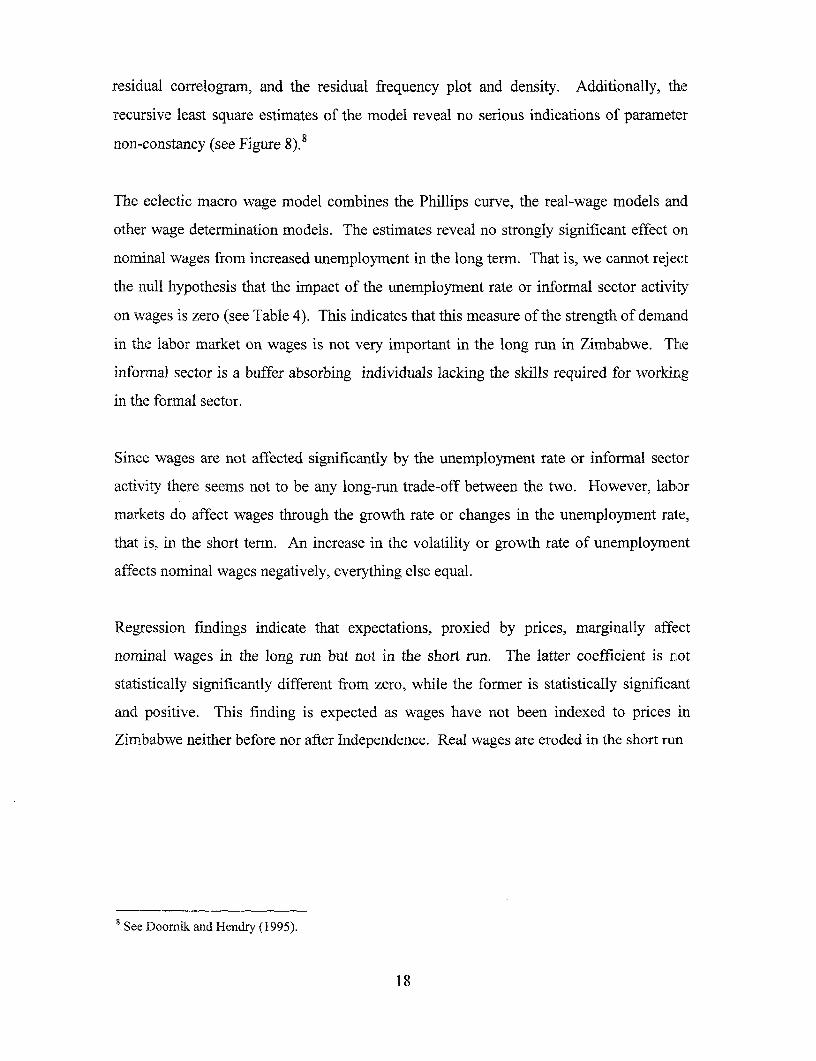
residual correlogram, and the residual frequency plot and density. Additionally, the

recursive least square estimates of the model reveal no serious indications of parameter

non-constancy (see Figure 8).8

The eclectic macro wage model combines the Phillips curve, the real-wage models and

other wage determination models. The estimates reveal no strongly significant effect on

nominal wages from increased unemployment in the long term. That is, we cannot reject

the null hypothesis that the impact of the unemployment rate or informal sector activity

on wages is zero (see Table 4). This indicates that this measure of the strength of demand

in the labor market on wages is not very important in the long run in Zimbabwe. The

infornal sector is a buffer absorbing individuals lacking the skills required for workir.g

in the formal sector.

Since wages are not affected significantly by the unemployment rate or informal sector

activity there seems not to be any long-mn trade-off between the two. However, labor

markets do affect wages through the growth rate or changes in the unemployment rate,

that is, in the short term. An increase in the volatility or growth rate of unemployment

affects nominal wages negatively, everything else equal.

Regression findings indicate that expectations, proxied by prices, marginally affect

nominal wages in the long run but not in the short run. The latter coefficient is riot

statistically significantly different from zero, while the former is statistically significant

and positive. This finding is expected as wages have not been indexed to prices in

Zimbabwe neither before nor after Independence. Real wages are eroded in the short run

' See Doomik and Hendry (1995).

18

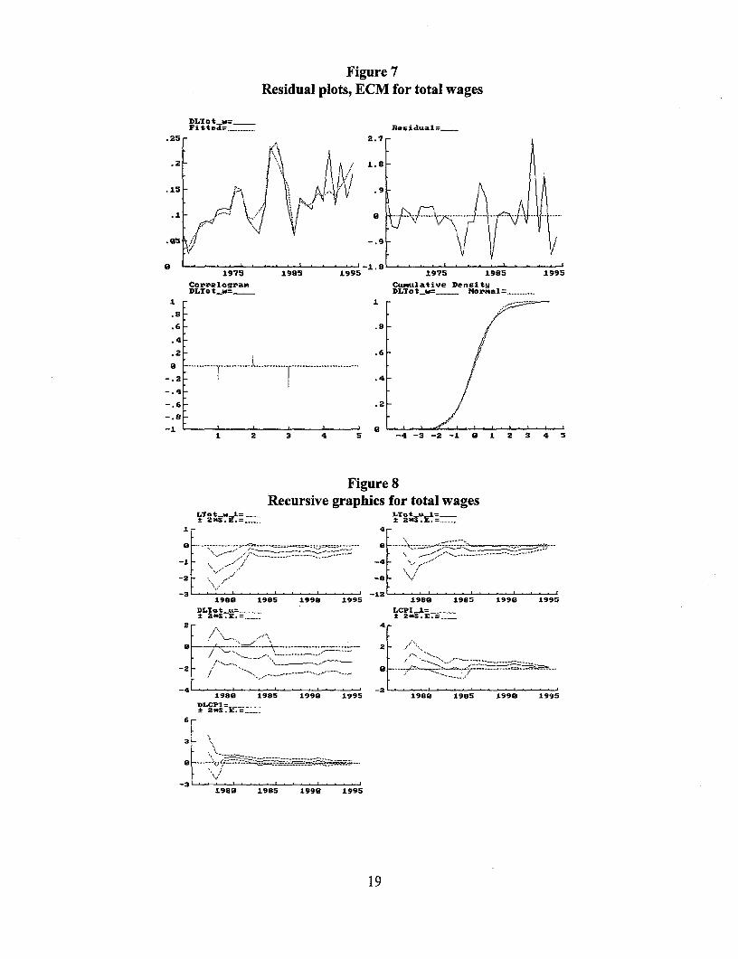
Figure 7Residual plots, ECM for total wages

DLTot_w=.Fitted=. ., Residual=_

. 25 2.?2

.1 ~~~~~~~~~~~9

* ~~~~~~~~-1.81975 1985 1995 1975 1985 1995

Corzrelog9XaM Cumulative DensitgDLTotw= . DLTot_w=_ Norzmal= ,,_....

.6 .8 t

.4 4

.2 _..6 /

. ................................ .4/

-. .2 /

-. 8p

1 2 3 4 5 -4 -3 -2 -1 0 1 2 3 4 5

Figure 8Recursive graphics for total wages

_- 4_

.......... . .\ ,-............... .-'.........

1980 1985 1998 1995 1986 1985 1998 1995

DLTot_ _ LP___= _t 2°*S.E. = t 2NSE.=,

2

2_ ..-.. .......... .......4

eLP __ -'_ _..... 198 198 1995.. ,'/ ~ . ~ . . ~ .............. .

-4 -2198e 1985 199e 1995 ls8e 1985 lsse 1995

:k 2 nS .E.-,::

3-

1986 1985 1998 1995

19

since wages are not instantaneously adjusted to price increases. Meanwhile, in the longer

term a price increase impacts nominal wages positively, ceteris paribus. The same is true

for productivity; estimated to be statistically significant and different from zero. Hence,

an increase in productivity leads to a wage increase.

The estimated coefficient on the level of nominal wages is negative, less than one and is

statistically significantly different from zero. The overall implication of a negative

coefficient estimate on the wage term (W_1) is that we can use the wage equation lto

obtain a "long-run equilibrium solution" of the error-correction type.9 The solved long-

run equation with zero autonomous growth (Aw = Aut = Apt = 0) for the model presented

in Table 3 is:

w = 10.9 - 1.5 u + 0.4 p + 0.llt (3)

which describes a highly significant error-correction mechanism between wages,

employment and prices (Wald test statistics for the hypothesis that all coefficienLts

including those of the 2 dummy variables but excluding the constant term are zero:

F(8,20) = 9.44 [0.00]). However, the unemployment rate seems to have no role to play in

the error correction mechanism as wages in the long term appear to be unaffected by the

level of unemployment in Zimbabwe. The hypothesis that the unemployment rate does

not affect wages, k=0 in equation (1), is not rejected (F(1,20) = 2.02 [0.17]).

Now we turn to the steady state solution of the wage model presented in Table 3 and

rewriting it gives the estimated steady state:

wt= 10.9+0.4pt+0.1 t- 1.5ut-5.5Au* +0.4Ap* (4)

9 See, e.g., Hendry (1980).

20

The steady state is consistent with the growth of wages implied by the long-run equation

(2). One implication for wages is that the equilibriurn value of nominal wages is smaller

ceteris paribus the larger the steady state growth rate of the unemployment rate when it is

positive. Hence, the equilibrium value of the nominal wage ceteris paribus is associated

negatively with increases in the unemployment growth rate. Another implication of the

steady state equation is that the equilibrium value of nominal wages is larger ceteris

paribus the larger is the steady state inflation rate when the latter is positive. The impact

on wages from increased inflation is not one to one. Ten percentage points increase in

inflation is associated with 4 percentage points increase in wages. Hence, inflation erodes

wages in the long run.

Is there a wage determination model that fits the Zimbabwean data? First, we test

whether the Zimbabwean data fit a real wage specification. The results indicate that real

wages do not respond to the strength of demand in the labor market. Furthermore, the

real wage hypothesis only holds if: (1) the restriction (w-p)=0 cannot be rejected; and (2)

there exists a co-integrating vector involving all three variables w, u and p which has the

sum of the coefficients equal zero. The first restriction cannot be rejected at a 1 percent

significance level but is rejected at 5 percent (F(1,20) = 4.84 [0.043*). Moreover, there

does not exist a co-integrating vector containing all three variables. Hence, the real wage

hypothesis can be rejected.

Second, we test other models of wage determination nested within the one presented in

Table 4: (1) a first order error-correction model with wages adjusting towards a static

equilibrium that depends on prices only (,B = X = p = 0) and this model cannot be rejected

at a 1 percent level of significance but is rejected at a 5 percent level (F(1,20) = 4.85

[0.04]*); (2) a first order partial adjustment model with a target value of wages

depending on unemployment only (1 = 8 = (p = 0) is highly rejected (F(3,20) = 6.89

[0.00]); and (3) a trend stationary real wage model (p = 6 = 1 and 3 = X = 0), this

hypothesis is highly rejected F(4,20) = 75.06 [0.00]);

21

Hence, no macro-wage curve can be revealed using unemployment as pressure of demand

variable as the level of unemployment plays no significant role in the longer term in

explaining nominal wages.

Table 4ECM for total wages (including GDP)

Variable Coefficient Std. Error t-value t-prob Part RP InstabW_1 -0.317 0.105 -3.008 0.007 0.301 0.05Constant 2.471 1.183 2.09 0.049 0.172 0.05CPI_1 0.089 0.053 1.664 0.111 0.117 0.05-CPI -0.023 0.131 -0.172 0.865 0.001 0.05GDP_1 0.099 0.038 2.649 0.015 0.250 0.05-GDP 0.083 0.036 2.312 0.031 0.203 0.04Trend 0.022 0.009 2.534 0.019 0.234 0.05i1984 -0.114 0.034 -3.364 0.003 0.350 0.05i80-84 0.086 0.019 4.613 0.000 0.503 0.03

Definitions of VariablesW_I is log total wages lagged once

U_1 is log total unemployment rate lagged once-U is the first order difference of U

CPI_1 is the log of the consumer price index lagged once-CPI is the difference of CPI

GDP_I is the log of GDP lagged once-GDP is the first order difference of GDP

iXXXX is a dummy for the(se) year(s)Test Statistics

R= 0.788 F(8, 21) =9.7442 [0.000] a = 0.029 DW = 2.33RSS = 0.018 for 9 variables and 30 observations

Variance instability test: 0.439 Joint instability test: 1.797Information Criteria: SC = -6.396 HQ = -6.682 FPE = 0.00111629

AR 1- 2F( 2, 19) = 0.869 [0.435]ARCH I F( 1, 19) = 0.035 [0.853]Normality Chi2 (2)= 6.940 [0.031]

Xi2 F(16, 4) = 0.416 [0.907]RESET F( 1, 20) = 0.165 [0.6891

22

5.2.2 Aggregate model with GDP

In this subsection we introduce GDP as the main pressure-of-demand variable, while in

the former sub-section we used the unemployment rate. We present our findings in Table

4. Again, nominal wages are explained by prices, a deterministic time trend, policy

dummy variables, and our pressure of demand variable, GDP. As above, the pattern of

wages in the beginning of the 1980s is out of line with the developments of the economy.

That is, wages are too high and to capture this, we include dummy variables (D1984 and

D80-84). On the basis of the diagnostic test statistics presented in the bottom of Table 4

and charts presented in Figures 9 and 10, we observe no evidence of model

misspecification.

The findings reveal that the pressure-of-demand variable affects wages positively both in

the short and long term, revealed by the statistically significant impact on wages from

both GDP growth and GDP in levels. This indicates that the strength of demand in the

labor market is important for Zimbabwean wages.

Figure 9Residual plots, ECM for total wages (including GDP)

DLT t_w

25~~~~~~~~~.

.2~~~~~~~~~.

.8elS75 1985 1995 1975 1985 1995

Corr." loUr; c"*leiw D ... i tsDLTot_* DSo= Sol

-. 6 .2 /

2 3 4 5 -4 -3 -2 -1 0 X 2 3 4 5

23

Figure 10Recursive plots, ECM for total wages (including GDP)

± 2"S. E.-_~ ±CP2 =

LTot._ _ = .. .. i... _,.._,...

- ~~~~~~~~~~~~~~~~~~~~~~~~~~~.5_-4 .......... ....

1989 1985 199D l995 198D 1985 1999 1995

DLCPI= LGDPcso_=i Z.. E ± 2S.E.=

± _z.......... ,3 _,._.......... .2 i i .... . -----.. ....... .

D_. ._._. , .............. _ %,..=,~~~~~~~~~~~~~~~~~. -. 1 S._.._.. . --......-

-2~~~~~~~~~~~~~~~~~~~~~~~~~~~~~~~~~~~~~~~~~.. . . _. ...... ....... _._ ......._.__._

-421989 1985 1999 1995 1988 1985 l99D 1995

DL'GDPeso= _

.18_.* ~~~~~~~~~~~~~~~~~~......... ... --

.12 _

.86 _ . , -.........

D~~~~~~~~~~~~~~~ . . . . . . .. .. . . . . .

1980 1985 l99D l99S

Expectations, measured by prices, marginally affect wages positively in the long run but

not in the short run. Furthermore, productivity affects the wage determination process

positively. These coefficients are estimated to be statistically significant and different

from zero.

We find that the wage term (W_i) is statistically significant and the coefficient is

negative, hinting at the existence of a long run relationship between GDP, prices,

productivity, and employment. Furthermore, the hypothesis that the sum of ihe

coefficients of w, u and p equals zero cannot be rejected (F(l, 21) = 4.27 [0.05]) and all

variables are significantly different from zero. Hence, there exists a co-integrating vector

involving all variables, and we can use the wage equation to obtain a long-run

equilibrium solution. The solved long-run equation with zero autonomous growth, Av=

AGDP = Ap = 0, is:

w=7.8+0.3GDP+0.3p+O.It (5)

24

which describes a significant error-correction mechanism between wages, GDP,

productivity and prices (the Wald test statistics for the hypothesis that all coefficients

including those of the 2 dummy variables but excluding the constant are zero: F(8,21) =

9.74 [0.00]). Hence, in the long term wages are affected positively by increases in

economic activity, prices, and productivity. A one percentage point increase in GDP is

associated with 0.3 percentage points increase in nominal wages, everything else equal.

Ten percentage points increase in prices or productivity impacts wages by 2.8 and 0.7

percentage points, respectively.

Therefore, the steady state for the model has the form:

wt=7.8 +0.3GDPt+0.3pt+0.lt+0.3 A GDP* -0.1 Ap* (6)

implying that the equilibrium value of nominal wages is larger the larger the steady state

growth rate of GDP, when it is positive, ceteris paribus. Hence, the equilibrium value of

the nominal wage is associated positively with increases in the GDP growth rate, ceteris

paribus. The other implication of the steady state equation is that the equilibrium value

of nominal wages is smaller the larger is the steady state inflation rate when the latter is

positive, ceteris paribus.

Does there exist a wage determination model that fit the Zimbabwean data using this

wage specification? We find that the real wage hypothesis cannot be rejected at a 5

percent level of significance (F(1, 21) = 6.98 [0.015]). Furthermore, this model explains

79 percent of the variation in wages in the last three decades. We test other models of

wage determination nested within the model shown in Table 5; all of these are rejected by

data.'0

10 The hypothesis that wages are determined by a first order error correction model with wages adjustingtowards a static equilibrium that depends on prices only can be rejected (F(3,2 1) = 6.90 [0.00]).Furthermore, the hypothesis that wages follows a first order partial adjustment model with target values ofwages depending on unemployment only can be rejected F(3,21) = 5.27 [0.01]; and so can the hypothesis ofa trend stationary real wage model (F(4,21) = 77.78 [0.00]).

25

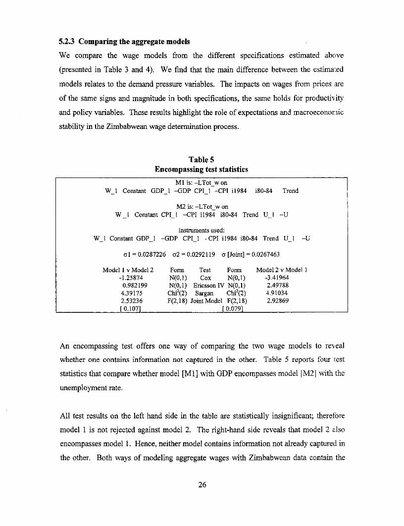
5.2.3 Comparing the aggregate models

We compare the wage models from the different specifications estimated above

(presented in Table 3 and 4). We find that the main difference between the estimated

models relates to the demand pressure variables. The impacts on wages from prices are

of the same signs and magnitude in both specifications, the same holds for productivity

and policy variables. These results highlight the role of expectations and macroeconomic

stability in the Zimbabwean wage determination process.

Table 5Encompassing test statistics

Ml is: -LTot_w onW_1 Constant GDP_1 -GDP CPI_1 -CPI i1984 i80-84 Trend

M2 is: -LTot_w onW_1 Constant CPI_1 -CPI il984 i80-84 Trend U_1 -U

Instruments used:W_1 Constant GDP_1 -GDP CPI_l -CPI i1984 i80-84 Trend U_1 -U

cl = 0.0287226 a2 = 0.0292119 a [Joint] = 0.0267463

Model 1 v Model 2 Forn Test Form Model 2 v Model 1-1.25874 N(0,1) Cox N(0,1) -3.41964

0.982199 N(0,1) Ericsson IV N(0,1) 2.497884.39175 Chi2(2) Sargan Chi2(2) 4.910342.53236 F(2,18) Joint Model F(2,18) 2.92869[ 0.107] [ 0.0791

An encompassing test offers one way of comparing the two wage models to reveal

whether one contains information not captured in the other. Table 5 reports four test

statistics that compare whether model [MI] with GDP encompasses model [M2] with the

unemployment rate.

All test results on the left hand side in the table are statistically insignificant; therefore

model 1 is not rejected against model 2. The right-hand side reveals that model 2 also

encompasses model 1. Hence, neither model contains information not already captured in

the other. Both ways of modeling aggregate wages with Zimbabwean data contain the

26

same information. Since we in MI find a long-run relationship between all the variables

this is our preferred and also final selected model.

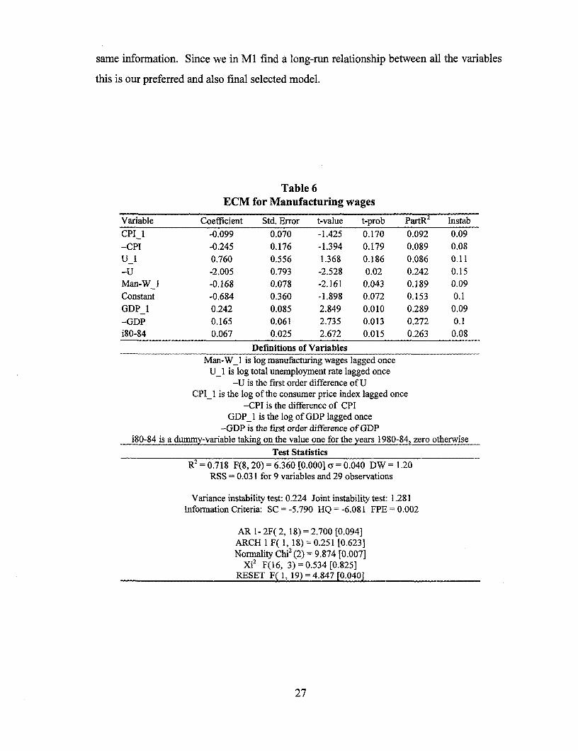
Table 6ECM for Manufacturing wages

Variable Coefficient Std. Error t-value t-prob PartR2 Instab

CPI_1 -0.099 0.070 -1.425 0.170 0.092 0.09-CPI -0.245 0.176 -1.394 0.179 0.089 0.08U_1 0.760 0.556 1.368 0.186 0.086 0.11-U -2.005 0.793 -2.528 0.02 0.242 0.15Man-W 1 -0.168 0.078 -2.161 0.043 0.189 0.09Constant -0.684 0.360 -1.898 0.072 0.153 0.1GDP_1 0.242 0.085 2.849 0.010 0.289 0.09-GDP 0.165 0.061 2.735 0.013 0.272 0.1i80-84 0.067 0.025 2.672 0.015 0.263 0.08

Definitions of VariablesMan-Wi1 is log manufacturing wages lagged onceU_1 is log total unemployment rate lagged once

-U is the first order difference of UCPI_1 is the log of the consumer price index lagged once

-CPI is the difference of CPIGDP_1 is the log of GDP lagged once

-GDP is the first order difference of GDPi80-84 is a dummy-variable taking on the value one for the years 1980-84, zero otherwise

Test StatisticsR2 0.718 F(8, 20) = 6.360 [0.000] a = 0.040 DW = 1.20

RSS = 0.031 for 9 variables and 29 observations

Variance instability test: 0.224 Joint instability test: 1.281Infornation Criteria: SC = -5.790 HQ = -6.081 FPE =0.002

AR 1- 2F( 2, 18) = 2.700 [0.094]ARCH 1 F( 1, 18) = 0.251 [0.623]Norrmality Chi2 (2) = 9.874 [0.007]

Xi2 F(16, 3) = 0.534 [0.825]RESET F( 1, 19) = 4.847 [0.040]

27

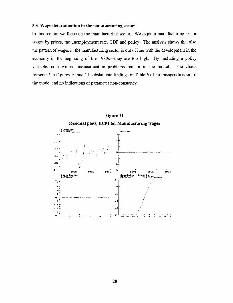
5.3 Wage determination in the manufacturing sector

In this section we focus on the manufacturing sector. We explain manufacturing sector

wages by prices, the unemployment rate, GDP and policy. The analysis shows that also

the pattern of wages in the manufacturing sector is out of line with the development in the

economy in the beginning of the 1980s-they are too high. By including a policy

variable, no obvious misspecification problems remain in the model. The charts

presented in Figures 10 and 11 substantiate findings in Table 6 of no misspecification of

the model and no indications of parameter non-constancy.

Figure 11

Residual plots, ECM for Manufacturing wagesDLNan_w=Fitted= ......... Res.ida

.3 3

.24 2

.12~~~~~~~~~~~~~~~~~~~~~~~~~1195 ;" 9 1

.12.4-~~~~~~~~~-,12 _---i.6_

.* 6 _ -2 . . . . , . . . . . . . .....

4 -31975 1985 199S 1975 1995 1995

Coppe1osr.a. Cu,,ulatiye DensityjDLMan.w.= DLMan_w Norpeal

.8~~~~~~~~~~~~.1 . 2. 4- 2- 1 2 3,

.6 _2.8

.4

.2 .6_.

8 _ ... ~. .._. ..... ...__. . ....

-.2 .4_

-.4.

-.6 .2

1 2 3 4 5 -4 -3 -2-1 8 1 2 3 4 5

28

Figure 12Recursive plots, ECM for manufacturing wages

LP___= _ DLCFI= LGDPcso =

I4

± 2 Z... ± __ DLCPI - _ 3 S .2.....

_ _ ~~~~ ; ~~ : -6 t 2 ...... .. .'' '

-2 -9eLT985 9 198 1995 1985 1995

± 2-*S.E =- -: . ..

+ ".4.,_ Mke- _LE.4 6- .. ..........=

_3 .4 <S.--,-------- 3 _

.2 . _ - v ...... _:

:4 ~~~~~~~~~~~-4. ........ .. . ........... ,| 6

1985 1995 1985 1995 1985 1995DLIo t_u=_ _I 2§SZ.E=_

-3_

1985 1995

Nominal wages in the manufacturing sector seem unaffected in the long term by increased

unemployment (see Table 6). This indicates that unemployment as a measure of the

strength of demand in the labor market is not very important for manufacturing wages in

the long run. Therefore, there exists no long-run trade-off between unemployment and

wages. On the other hand, the short-term dynamics of the labor market affect wages

through changes or growth in unemployment. The higher volatility or growth in the

unemployment rate or informal sector activity the lower nominal wages, ceteris paribus.

We now consider the other demand pressure measure, namely GDP. The estimates reveal

a positive effect on wages from increased demand. GDP affects wages both in the short

and long term and an increase in economic activity impacts manufacturing sector wages

positively.

Expectations and macro economic stability proxied by prices do only marginally affect

wages in the long run and in the short run. Hence, nominal wages are not adjusted to

price increases and, therefore, wages are eroded both in the short and long run.

29

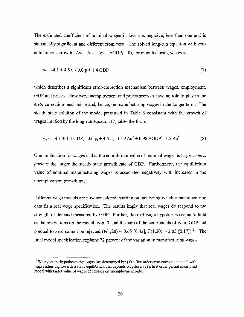
The estimated coefficient of nominal wages in levels is negative, less than one and is

statistically significant and different from zero. The solved long-run equation with zero

autonomous growth, (Aw = Aut = Apt = AGDPt = 0), for manufacturing wages is:

w = -4.1 + 4.5 u - 0.6 p + 1.4 GDP (7)

which describes a significant error-correction mechanism between wages, employment,

GDP and prices. However, unemployment and prices seem to have no role to play in the

error correction mechanism and, hence, on manufacturing wages in the longer term. The

steady state solution of the model presented in Table 6 consistent with the growth of

wages implied by the long-run equation (7) takes the form:

wt = - 4.1 + 1.4 GDPt - 0.6 Pt + 4.5 ut - 11.9 Au + 0.98 AGDP*- 1.5 Ap (8)

One implication for wages is that the equilibrium value of nominal wages is larger ceteris

paribus the larger the steady state growth rate of GDP. Furthermore, the equilibrium

value of nominal manufacturing wages is associated negatively with increases in the

unemployment growth rate.

Different wage models are now considered, starting out analyzing whether manufacturing

data fit a real wage specification. The results imply that real wages do respond to the

strength of demand measured by GDP. Further, the real wage hypothesis seems to hold

as the restrictions on the model, w-p=O, and the sum of t]he coefficients of w, u, GDP and

p equal to zero cannot be rejected (F(1,20) = 0.65 [0.43]; F(1,20) = 2.05 [0.17])." The

final model specification explains 72 percent of the variation in manufacturing wages.

'" We reject the hypotheses that wages are determined by: (1) a first order error correction model withwages adjusting towards a static equilibrium that depends on prices; (2) a first order partial adjustmnentmodel with target value of wages depending on unemployment only.

30

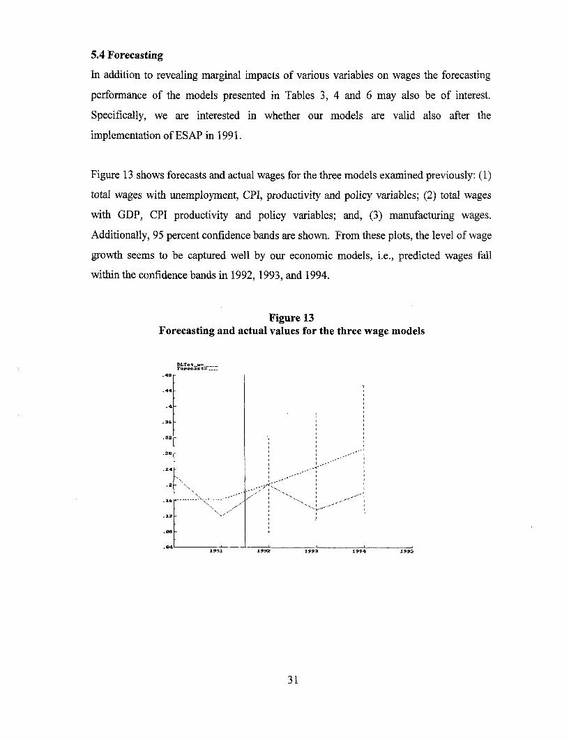
5.4 Forecasting

In addition to revealing marginal impacts of various variables on wages the forecasting

performance of the models presented in Tables 3, 4 and 6 may also be of interest.

Specifically, we are interested in whether our models are valid also after the

implementation of ESAP in 1991.

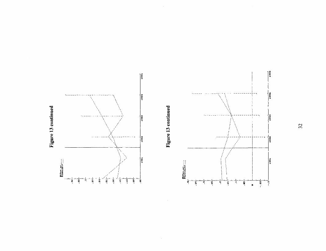
Figure 13 shows forecasts and actual wages for the three models examined previously: (1)

total wages with unemployment, CPI, productivity and policy variables; (2) total wages

with GDP, CPI productivity and policy variables; and, (3) manufacturing wages.

Additionally, 95 percent confidence bands are shown. From these plots, the level of wage

growth seems to be captured well by our economic models, i.e., predicted wages fall

within the confidence bands in 1992, 1993, and 1994.

Figure 13Forecasting and actual values for the three wage models

DLT.ot_.ror_ _st.48r

.44

.4

.36 -

.32

.28-

.24

.2 _

A.,, - ,,.-------

1991 1992 1993 1994 1995

31

LO~~~~~~~~~~~~~~~~~~~~~~~~~~~~~~~~~~~~~~~~~~~~~~U

L- - - _ -- - - - - .,_ - _-_-_-___ N|_______________0 -- N

0 -~~~~~~~-- - - - - - - - - - - -

- - - - - - - - - - - - - - -- - - - - - - - - U

-4 .4 0X ... Iti

. I i......aU~~4e lr er ,I,Ii

81N Nt1_1i 11 ' : q n 1 H5

6. Conclusion

One of the main questions analyzed in this study is whether wages are flexible and we

found that they are flexible both at the aggregate level and in the manufacturing sector.

Additionally, a macro wage-curve is present in Zimbabwe explaining the relationship

between nominal wage, productivity, economic activity, and prices. This is the case for

both the entire economy and the manufacturing sector. Furthermore, no visual structural

change has occurred in the labor markets after the ESAP was launched.

Inefficiencies due to loss in economic output are proxied by unemployment/informal

sector activity or GDP. Both at the aggregate level and in the manufacturing sector, we

find no significant negative effect on nominal wages from increased infornal sector

activity in the long term. This indicates that (institutional) rigidities are present in the

labor market as there seems not to be any long-run trade-off between

unemployment/informal sector activity and wages. One explanation may be that labor

market institutions still play an important role in the Zimbabwean economy. Other

explanations are that labor markets suffer from a so-called "insider-outsider" problem or

firms pay efficiency wages. This is further analyzed in Verner (1998). However, in the

short term wages are affected by changes in the unemployment rate. An increase affects

nominal wages negatively, all else equal. The equilibrium value of nominal wages is

smaller ceteris paribus the larger the steady state growth rate of the unemployment rate

when it is positive. Hence, the equilibrium value of the nominal wage is associated

negatively with increases in the unemployment growth rate or informal sector activity

growth.

Expectations and macro economic stability, proxied by prices, affect nominal wages

marginally in the long run but not in the short run. Wages do not instantaneously adjust

to price increases and wages are eroded in the short run. In the longer tern a price

increase impact nominal wages positively. The same is true for productivity. The

implication of the steady state equation is that the equilibrium value of nominal wages is

larger ceteris paribus the larger is the steady state inflation rate when the latter is positive.

33

Both in the short and long term wages are affected positively by increases in economnic

activity. The equilibrium value of nominal wages is larger the larger is the steady state

growth rate of GDP. A one percentage point increase in GDP is associated with 0.3

percentage points increase in nominal wages, everything else equal. A ten-percentage-

points increase in prices or productivity impacts wages by 2.8 and 0.7 percentage points,

respectively.

The forecasting performance indicates that the models are valid also after the

implementation of ESAP in 1991. Therefore, the labor market in Zimbabwe is not very

rigid and adjust to both positive and negative economic shocks.

34

References:

Banerjee, A., Dolado, J., Galbraith, J.W. and Hendry, D.F (1993). Co-integration, Error-correction, and the Econometric Analysis of Non-stationary Data, OxfordUniversity Press, Oxford.

Blanchflower, D. and Oswald, A. (1995). The Wage Curve, Cambridge: MIT Press.

Blunch, N.-H. and Vemer, D. (1998), "Sectoral Economic Growth and the Dual EconomyModel: Evidence from three Sub-Saharan Economies," Draft, World Bank,Washington, D.C.

Doornik, J. A. and Hendry, D. F (1995). PcGive 8.0 - An Interactive EconometricModelling System, Chapman & Hall.

Engle, R. F. and Granger, C. W. J. (1987). "Co-integration and Error Correction:Representation, Estimation and Testing," Econometrica, 55, 251-76.

Fallon, P. R. and R. E. Lucas (1991). "The Impact of Changes in Job Security in Indiaand Zimbabwe," World Bank Economic Review, Vol. 5, No. 3, 395-413.

Fallon, P. R. and R. E. Lucas (1993). "Job Security Regulations and the DynamicDemand for Industrial Labor in India and Zimbabwe," Journal of DevelopmentEconomics, Vol 40, No. 2, 241-76.

Hendry, D. F. (1976). "The Structure of Simultaneous Equations Estimators," Journal ofEconometrics, 4, 51-88.

Hendry, D. F. (1980). "Econometrics: Alchemy or Science?," Economica, 47, 387-406

Hoddinott, J. (1996). "Wages and Unemployment in an Urban African Labour Market,"Economic Journal, 106, 1610-1626.

Knight, John (1996). "Labour Market Policies and Outcomes in Zimbabwe," Oxford:University of Oxford, Centre for the Study of African Economies, Processed:March.

Kremers, J.J.M., N.R. Ericsson, and J. Dolado, (1992). "The Power of Co-integrationTests," Oxford Bulletin of Economics and Statistics, 54, 325-48.

Phillips, A. W. (1958). "The Relation between Unemployment and the Rate of Change ofMoney Wages in the United Kingdom, 1861-1957," Economica, 25, 283-299.

Sargan, J. D. (1980). "Some Tests of Dynamic Specification for a Single Equation,"Econometrica, 48, 879-97.

35

Vemer, D. (1998). "Are Wages and Productivity Affected by Human Capital Investmentand International Trade? The case of Zimbabwe," Draft, World Ba nk,Washington, D.C.

36

Appendix A

Unit root testsSeries t-adf a lag no t-lag t-prob

LTot_w -1.911 0.043 2 -0.035 0.973LTot_w -1.991 0.042 1 1.819 0.082LTot_w -1.761 0.044 0LMan_w -1.884 0.040 2 -2.199 0.039LMan_w -3.378 0.044 1 4.188 0.000LMan_w -1.6531 0.057 0LGDPcso -1.426 0.173 2 -0.777 0.446LGDPcso -2.283 0.172 1 1.425 0.168LGDPcso -1.770 0.175 0LTot_u -2.690 0.008 2 -0.257 0.800LTot_u -3.445 0.008 1 4.899 0.000LTot_u -2.311 0.011 0LCPI -0.397 0.053 2 -0.045 0.965LCPI -0.440 0.052 1 1.115 0.276LCPI -0.103 0.052 0Notes: Critical values: 5%=-3.587, 1%=-4.338; constant and trendincluded.

37

Policy Research Working Paper Series

ContactTitle Author Date for paper

WPS2034 Information, Accounting, and the Phil Burns December 1998 G. Chenet-SmithRegulation of Concessioned Antonio Estache 36370Infrastructure Monopolies

WPS2035 Macroeconomic Uncertainty and Luis Serven December 1998 H. VargasPrivate Investment in Developing 38546Countries: An Empirical Investigation

WPS2036 Vehicles, Roads, and Road Use: Gregory K. Ingram December 1998 J. PonchamniAlternative Empirical Specifications Zhi Liu 31022

WPS2037 Financial Regulation and James R. Barth January 1999 A. YaptencoPerformance: Cross-Country Gerard Caprio, Jr. 38526Evidence Ross Levine

WPS2038 Good Governance and Trade Policy: Francis Ng January 1999 L. TabadaAre They the Keys to Africa's Global Alexander Yeats 36896Integration and Growth?

WPS2039 Reforming Institutions for Service Navin Girishankar January 1999 B. Casely-HayfordDelivery: A Framework for Development 34672Assistance with an Application to thehealth, Nutrition, and PopulationPortfolio

WPS2040 Making Negotiated Land Reform Klaus Deininger January 1999 M. FernandezWork: Initial Experience from 33766Brazil, Colombia, and South Africa

WPS2041 Aid Allocation and Poverty Reduction Paul Collier January 1999 E. KhineDavid Dollar 37471

WPS2042 Determinants of Motorization and Gregory K. Ingram January 1999 J. PonchamniRoad Provision Zhi Liu 31022

PWS2043 Demand for Public Safety Menno Pradhan January 1999 P. SaderMartin Ravaltion 33902

WPS2044 Trade, Migration, and Welfare: Maurice Schiff January 1999 L. TabadaThe Impact of SociaI Capital 36896

WPS2045 Water Challenge and institutional R. Maria Saleth January 1999 F. ToppinResponse (A Cross-Country Ariei Dinar 30450Perspective)

WPS2046 Restructuring of insider-Dominated Simeon Djankov January 1999 R. VoFirms 33722

WPS2047 Ownership Structure and Enterprise Simeon Djankov February 1999 R. VoRestructuring in Six Newly 33722Independent States

Policy Research Working Paper Series

ContactTitle Author Date for paper

WPS2048 Corruption in Economic Shang-Jin Wei February 1999 C. BernardoDevelopment: Beneficial Grease, 31148Minor Annoyance, or Major Obstacle?

WPS2049 Household Labor Supply, Kaushik Basu February 1999 M. MasonUnemployment, and Minimum Wage Garance Genicot 30809Legislation Joseph E. Stiglitz

WPS2053 Measuring Aid Flows: A New Charles C. Chang February 1999 E. KhineApproach Eduardo Fern6ndez-Arias 37471

Luis Serven

WPS2051 How Stronger Protection of Carsten Fink February 1999 L, Willernsintellectual Property Rights Affects Carlos A. Primo Braga 85153International Trade Flows