the expected 060503

VATT-TUTKIMUKSIA99

VATT-RESEARCH REPORTS

Tarmo Räty - Kalevi LuomaErkki Mäkinen - Marja Vaarama

THE FACTORS AFFECTING THEUSE OF ELDERLY CARE ANDTHE NEED FOR RESOURCES

BY 2030 IN FINLAND

Valtion taloudellinen tutkimuskeskusGovernment Institute for Economic Research

Helsinki 2003

ISBN 951-561-454-6

ISSN 0788-5008

Valtion taloudellinen tutkimuskeskusGovernment Institute for Economic ResearchHämeentie 3, 00530 Helsinki, FinlandEmail: [email protected]

ISBN 951-563-441-5

Suomen itsenäisyyden juhlarahasto SitraFinnish National Fund for Research and Development SitraItämerentori 2, 00181 Helsinki, FinlandEmail: [email protected]

Oy Nord Print Ab

Helsinki, June 2003

RÄTY TARMO, LUOMA KALEVI, MÄKINEN ERKKI, VAARAMAMARJA: THE EXPECTED USAGE OF CARE AND RESOURCES INFINNISH ELDERLY CARE BY 2030. Helsinki, VATT, Valtion taloudellinentutkimuskeskus, Government Institute for Economic Research, 2003, (B, ISSN0788-5008, No 99). ISBN 951-561-454-6. ISBN 951-563-441-5.

Abstract: A nation-wide interview survey data is used to analyse by means ofordered logit models the impacts of age, dependency and other factors onprobabilities to use home and community care for the elderly. With these modelsand the age profile of the institutional care, we have made projections of servicespecific dependency, age and gender distributions by 2030. In our scenarios weassume that improvements in functional ability of the elderly will by 2030increase the average starting-age for using home and community care by three orfive years and delay the admission into institutional care by three years. We alsomake an assumption that quality of care is raised by increasing staffing levels inthe care of elderly to the level which was considered sufficient for good qualitycare according to recommendations made by a recent expert working group. Tomeet the resource needs caused by the rise in the projected number of elderlypopulation would require 1.9 % annual increase in operating costs. Increasingstaffing levels to correspond good quality care would increase costs by 2.6 %annually. However, postponing the average starting-age by three years wouldleave the annual increase to 1.2 %, even with better care quality. In case goodquality of care is desired already by 2010 operating costs would need to beincreased by 3.6 % annually.

Key words: Elderly care, dependency, quality of care, macrosimulation.

Tiivistelmä: Vanhuksille kotiin annettavien palvelujen käytön todennäköisyyk-siin vaikuttavia tekijöitä tutkittiin vuoden 1998 vanhusbarometriaineistolla. Näi-den mallien ja laitospalvelujen ikäjakauman perusteella laadittiin palvelu-kohtaiset arviot vanhusten vuoden 2030 toimintakyky-, sukupuoli- ja ikäjakau-masta. Tutkimuksen skenaarioissa oletettiin, SOMERA -toimikunnan mukaisesti,että avopalvelujen käytön aloitusikä siirtyy vuoteen 2030 mennessä kolme taiviisi vuotta ja laitospalvelujen kolme vuotta myöhemmäksi. Resurssiskenaariois-sa asetettiin tavoitteeksi nostaa sekä laitos-, että kotipalvelujen laatu tasolle "hy-vä", joka vastaa laitoshoidon osalta karkeasti muiden Pohjoismaiden tasoa.Pelkkä väestönkehitys merkitsisi aikajaksolla 1,9 prosentin vuosikasvua vanhus-tenhoidon kustannuksiin. Hyvä hoidon taso nostaisi vuosikasvun 2,6 prosenttiin.Toimintakyvyn paraneminen niin, että palvelujen käyttö myöhentyisi kolmellavuodella kuitenkin leikkaisi kustannusten kasvuvauhdin hyvälläkin hoidolla 1,2prosenttiin. Jos hoidon hyvä laatutaso halutaan saavuttaa jo vuoteen 2010 men-nessä, kasvaisivat vanhustenhuollon käyttökustannukset 3,6 prosenttia vuosittain.

Asiasanat: Vanhustenhuolto, toimintakyky, hoidon laatu, stimulointimallit

Foreword

The ageing of the population is a major challenge for Finland, where the popula-tion is ageing faster than in the other EU countries. This means that the need forinstitutional care, pension costs and the expenses of the social and health servicesare increasing.

The report analyses the factors influencing the use of social and health servicesby the elderly. On the basis of the analysis, scenarios for the growth in expendi-ture by the services are presented until the year 2030. The report is a scientificbackground report to the publication "Seniori-Suomi - ikääntyvän väestön talou-delliset vaikutukset" (Sitra's reports 30, written in Finnish), which was publishedin February 2003.

This new report is published in the series of the Government Institute forEconomic Research and the research work has been done with the support of Sit-ra. The advisory group for the project included Kalevi Luoma, Research Mana-ger, Reino Hjerppe, Director-General, and Aki Kangasharju, Research Director,from the Government Institute for Economic Research (VATT), Unto Häkkinen,Research Professor from the National Research and Development Centre forWelfare and Health (Stakes), Carita Putkonen, Fiscal Counsellor from the Fin-nish Ministry of Finance, Antti Hautamäki, Research Director from Sitra, and theundersigned. All of them to be complimented.

Helsinki, April 10, 2003

Vesa-Matti Lahti

Research Manager

Finnish National Fund for Research and Development Sitra

Esipuhe

Väestön ikääntyminen on suuri haaste Suomelle, jonka väestö ikääntyy muitaEU-maita nopeammin. Tämä merkitsee sitä, että hoitotarve, eläkemenot sekä so-siaali- ja terveyspalveluiden kustannukset kasvavat.

Tässä raportissa analysoidaan vanhusten sosiaali- ja terveyspalvelujen käyttöönvaikuttavia tekijöitä ja esitetään niiden pohjalta skenaariot palvelujen kustannus-kehityksestä vuoteen 2030 saakka. Raportti on helmikuussa 2003 julkistetun"Seniori-Suomi - ikääntyvän väestön taloudelliset vaikutukset" -julkaisun (Sitranraportteja 30) tieteellinen taustaraportti.

Raportti julkaistaan Valtion taloudellisen tutkimuskeskuksen sarjassa ja sen tut-kimustyö on tehty Sitran tuella. Hankkeen johtoryhmään kuuluivat allekirjoitta-neen lisäksi tutkimuspäällikkö Kalevi Luoma, ylijohtaja Reino Hjerppe jatutkimusjohtaja Aki Kangasharju Valtion taloudellisesta tutkimuskeskuksesta,tutkimusprofessori Unto Häkkinen Stakesista, finanssineuvos Carita Putkonenvaltiovarainministeriöstä ja tutkimusjohtaja Antti Hautamäki Sitrasta. He kaikkiansaitsevat suuren kiitoksen.

Helsingissä 10.4.2003

Vesa-Matti Lahti

Tutkimuspäällikkö

Suomen itsenäisyyden juhlarahasto Sitra

Contents

1. Introduction 1

2.The models for care utilisation 4

2.1 Data 42.1.1 Dependency measure 42.1.2 Age measure 62.1.3 Other variables 6

2.2 Home help services 72.3 Home nursing 102.4 Support services 11

2.4.1 Help with cleaning 112.4.2 Meals on wheels 122.4.3 Help with bathing 132.4.4 Services provided at service centres 14

2.5 Institutional care 14

3.Simulations 18

3.1 Predictions of the service use 183.2 Service profiles at 2030 183.3 Scenarios 203.4 Expected changes in resource usage 28

4.Discussion 33

Appendix 35

References 45

1. Introduction

During the next decades the demographic composition of the Finnish populationwill change dramatically. Due to the combined effects of increased longevity andageing of the large post-war baby boom cohorts the share of elderly populationwill rise considerably. The share of those aged 75 years or more will rise fromthe current 7 percent to approximately 14 percent in 2030, also their absolutenumber will double (Figure 1). Thereafter the population structure is expected tobe relatively stable.

Figure 1. Finnish population by age groups between 1900-2050. Popula-tion forecast based on population 2001, millions

2002

0,0

0,2

0,4

0,6

0,8

1,0

1,2

1,4

1,6

1,8

1900 1920 1940 1960 1980 2000 2020 204000,10,20,3

0,40,50,60,70,80,9

11,11,21,31,4

1,51,61,71,8

1900 1920 1940 1960 1980 2000 2020 2040

20-34 years

0-19 years

35-49 years

50-64 years

75 years and above

65-74 years

The baby-boom cohorts lived their economically most productive years from the1960s to the early 2000s. During that period Finland’s per capita GDP grew onaverage by three percent a year (OECD 2002). Thus, the expectations of the

Introduction2

increasing elderly population about future pension benefits level and availableelderly care may well be higher than the ones of the current elderly. A number ofstudies on economic consequences of ageing have already taken place. Thispaper deals only with elderly care. The pension benefits are extensively discussedin Sosiaali ja Terveysministeriö (2002) and Parkkinen (2002) and Lassila andValkonen (2002). These studies analyse also the impact of ageing on social andhealth care expenditure, based on population forecasts, expected economicgrowth and the age profiles of the social and health services. The results showthat with reasonable assumptions on future productivity growth, the GDP sharepublic expenditure on social and health care will grow about 2 percentage units,from the current 7.5 percent by 2030. In this paper we take into account a widerspectrum of factors connected to the use of these services. We concentrate solelyon the social and health services provided to the elderly making use of detaileddata on these services and their recipients.

The current service profile, the way in which services are distributed among theelderly, is multidimensional. In addition to demographic factors like age andgender the demand for health and elderly care is affected by dependency, socialand housing conditions of the elderly. Fiscal and resource constraints in thesupply of elderly care also have an effect on the quantity of care that is actuallyprovided. These factors are linked to each other, so that it is almost impossible tofigure out exactly what are the driving forces behind the need and receipt of care.In this paper, we examine the role of all the above-mentioned factors with twoindependent data sets. The role on fiscal factors is studied in institutional care,where municipal level panel data is used to find out how demography and theavailability of different funding sources contribute to the quantity anddistribution of service home, homes for the elderly, and long term inpatient care.A nation-wide interview study data of non-institutionalised elderly population isused to examine the role of age, gender, dependency and social environment.

Using the elderly population survey, we estimate the probabilities of receiving acertain type of care for 24 population cells, each describing a particularcombination of age, gender, and dependency group. These cell probabilities areused in conjunction with the national population forecasts to yield an estimate onthe future service usage. The main reference for this type of macrosimulationstudy is Wittenberg et. al. (1998), where the emphasis is on the links between thecircumstances of individuals and the receipt of services.

Given the results of the models we formulate predicted changes in the coverageof in-home domicile services and institutional care for elderly population. Togive an idea of what could be done to ease the adjustment of the elderly caresector we study consequences of a hypothetical improvement in the ability of theelderly to run their daily tasks independently. A comparable shift in entering thedomicile and institutional care is mirrored in the number of users within publiclyprovided care. EVERGREEN 2000 model (Vaarama et. al. 1998) is then used to

Introduction 3

calculate resources needed by 2030. The model uses detailed service specificinformation on the resources needed and unit costs. Assuming that moreworkforce per institutionalised client and more time used with an elderly livinghome means better care quality, we have used the figures from the nationalproposal for better elderly care quality (STM ja Kuntaliitto 2002) in theEVERGREEN 2000 model to see how much resources would be needed if therecommendations of the proposal were to be followed.

Our primary goal in this paper is to study what kind of changes in use of servicesand resources could be expected under two assumptions. First, the dependency ofthe elderly population is expected to diminish, pushing the starting-age ofdomicile and institutional service use upwards. Second, increasing the quality ofcare increases resources needed. The two assumptions induce opposite shifts inresource needs. From policy target setting point of view, we try to find an answerto the question how much dependency should be improved in order to makeenough resources available to increase the quality of care. These targets are notindependent of each other, but good quality of care will also contribute to thereduced dependency.

This report is not only a detailed version of the results reported in Luoma et. al.(2003) chapters 3.4 and 4, but includes some further analysis of the results.

The models for care utilisation4

2. The models for care utilisation

2.1 Data

The Ministry of Social Affairs and Health executed the national elderlybarometer survey in 1993 and 19981. In this study we exploit only the 1998survey. The gross sample of 1450 above 60 years old not receiving institutionalcare was drawn from the 1997 population. The Statistics Finland interviewedpersonally altogether 1036 respondents successfully. Weights for each genderand age groups were calculated to fix sample loss and make the obtained samplerepresentative for the non-institutionalised elderly population above 60 years in1997 in Finland. In service use model estimations we have limited the analysis tothe elderly above 65 years old. This sub-sample contains 895 respondentscorresponding to the population of 574500 elderly.

The survey data enables us to model the intensity of service use. It is measuredon ordinal scale [0,4] as no use, less than once a month, once or twice a month,once or twice a week and daily or almost daily respectively. We use orderedlogistic-model for home help services, support services, home nursing andcleaning; thus receipt and intensity of care is considered as a joint processdependent on the same set of variables. For the rest of the services binomiallogistic model is used to model whether the individual is a service recipients ornot. For the mathematical and stochastic specification of the models, seeAppendix I.

2.1.1 Dependency measure

Problems in activities in daily living (ADL) are classified into four ordinalcategories: no problems at all, minor problems, severe problems andinsurmountable problems. Originally the survey included 13 different ADLs, butonly ten of those were taken into the study. Of those cooking, laundry, cleaningand transactions outside home are classified as instrumental ADLs (IADL) andeating, washing, dressing and undressing, getting in and out of the bed, use ofbathroom and problems in urine continence are considered as personal ADLs(PADL).

The dichotomous variable DEPENDENCY summarises problems in activities ofdaily living. The variable got integer values [0,3] with no disabilities, only IADLdisabilities, minor problem in PADLs and severe or insurmountable disabilitiesrespectively. Increased dependency is considered as an immediate reason for the

1 See Vaarama, et. al. (1999) Vanhusbarometri 1998 for the detailed history of the survey. The data set isalso extensively analysed in Vaarama and Kaitsaari (2002).

The models for care utilisation 5

service use. Naturally, causes for altered dependency can be numerous. In theindependent ordered logistic regression of the DEPENDENCY on reportedsickness and injuries of the respondents in the Table 1, the role of mental andphysical factors is evident. The figures are average probabilities over the subsetof data covering the respondents with reported sickness or injury. Therefore theco-existence of the multiple physical or mental problems are taken into accountin proportion of their existence.

Table 1. Probabilities in having problems in activities of daily living forinterviewees with a certain sickness or injury. The average pre-dictions of the probability model

No disabilities IADL PADL1 PADL2Injured after an accident* 36.2 31 24.2 8.6Musculoskeletal diseases 28.8 31.8 28.6 10.8Cardiovascular diseases 34.6 31 25.2 9.1Respiratory organs 28.6 30.3 29.4 12.1Mental disorders* 24.1 30.2 32 13.7Skin diseases 26.6 30.1 30.4 12.9Metabolic disorders 28.8 30.4 29 11.8Digestive diseases* 27.5 30.2 29.8 12.4Impaired eyesight or audition 32.2 31.6 26.5 9.7Others 30.6 30.6 27.8 11.02IADL= Problems in instrumental activities of daily living.PADL1= Problems in two personal activities of daily living, at the most.PADL2= Problems in more than two activities of daily living.*Parameter not statistically significant at 10 % confidence level.

Respondents with cardiovascular diseases seem to have less PADL relatedproblems, on average, whereas skin problems seems to be connected to increaseddependency status. A noteworthy point is, that musculoskeletal diseases do notappear to raise dependency risk above other diseases and injuries.

In the rest of the study dependency is used as an explanatory variable for theservice usage. In those models partition of having minor or insurmountableproblems in personal ADL appeared to work poorly. Therefore we ended upusing two separate dummy variables to describe the presence of dependency. Inthe rest of the text, unit values of variables ADL1 and ADL2 denotes the presenceof instrumental ADL problems or presence of personal ADL problemsrespectively. The estimated parameters of these variables indicate response to theADL0 i.e. no disabilities.


2.1.2 Age measure

In the models of different service utilisation, in addition to dependency, theclient’s age is supposed to have a central role. However, it is not always clearhow age should enter into the models. A simple approach is to use age or amonotone transformation of it, but this was considered too restrictive, as changesin clients’ need may appear too abrupt for any sensible transformation. Instead,we let the impact of the age change according to the preselected age groups andif necessary also allow other variables to have a joint impact with age on serviceuse. The age related variables are denoted as AGE for the linear age, DAGEXX forthe age group dummy XX indicating the lower limit of the 5-age range (e.g.DAGE75 equal to 1 for the respondents between 75 and 79).

The simple dummy grouping of age does not usually work satisfactorily. Theway the client’s age enters in to the model is likely non-linear, however non-linearity may enter in the model in several ways. A parametric transformation,e.g. squaring, may work well, but implies a rather strong maintained hypothesis.An alternative is to use a discrete function, allowing the slope change at givenage nodes. Altering the set of nodes this gives an approximation to arbitrary non-linear function. However, our problem is that variation in service usage isdependent on also other factors related to age. To save degrees of freedom and tokeep model as simple as possible we have imposed non-linearity in age usingcross terms with other variables. The strongest emphasis in the model is on theimpact of gender (GENDER), age (AGE) and dependency (ADL1 and ADL2)structure of the population. Therefore age and dependency enter in the modelboth as independent variables and semi-continuous or dummy cross terms withgender. These variables are labelled as MADL1, MADL2 and FADL1AGE,FADL2AGE and MADL1AGE, MADL2AGE, where F and M are shortcuts forfemale and male respectively, ADL1 and ADL2 shortcuts for instrumental andpersonal disabilities in daily living respectively and AGE for the age of therespondent. MADL1 and MADL2 are dummies, FADL1AGE and other semi-continuos variables have value of AGE for the respondents in the reference group,otherwise zero.

2.1.3 Other variables

The other determinants of the service utilisation considered necessary are theclient’s gender (dummy variable GENDER, value 1 indicating a male respondent),living alone indicator (dummy variable ALONE, value 1 if living alone). Most ofthe services are arranged and/or subsidised by the municipalities. To indicate thissupply effect we have used several variables like government subsidies tomunicipalities (variable GOVGRANT) and municipal tax rate (variableTAXRATE). Government grants are somewhat problematic, as their amount isdependent on both demographic factors of the municipality and its financial


situation. A high tax rate usually indicates weak tax base of the municipality,perhaps due to unfavourable demographics structure or structural problems inlocal economy.

In the survey also availability of informal care was asked. Respondents were firstasked if they received any help in their daily activities, no matter what kind ofhelp. For those receiving some help, the sources of the help was asked. The listcovered both informal and formal care-givers and respondents were asked to listall of them and name one who helps the most. The structure allows a detailedmodelling of the informal care giving. However, to keep scenarios as simple aspossible we have used a dummy variable INFHELP, to describe, if therespondent considered having received any help in daily activities from relatives,friends and neighbourhood.

Finally, the economic position of the elderly is usually considered to have animpact on demand and use of services. However, the production costs ofintensive domicile care and all forms of institutional care usually exceed thecapacity of the elderly to pay for these services. For example operating costs perday range from 30 euros in regular service housing (not includingaccommodation) to 104 euros in health centre inpatient care (Rajala et. al. 2001).Domicile services are not necessary much cheaper, as home help services with10-29 visits a month costs about 17 euros a day, but with 30-79 visits already 52euros. The higher intensities of home help services are as expensive as inpatientcare (ibid.). The average amount of pensions in 2001 was 999 euros (SocialInsurance Institution (Kela, 2002, Table 11). If recipients of domicile serviceswere required to pay full price for services they consume, daily use of theseservices would be beyond the means of an average pensioner. However, theseservices are mainly financed by taxes. User charges cover only a fraction of theirproduction, or purchasing costs. In institutional care, the maximum service feecan not exceed 80 percent of the resident’s disposable income. Therefore,disposable income is not usually a constraining factor in service usage. Our dataset included an interviewee declared estimate on monthly disposable income.This had no explanatory power in any of the service usage models estimated.

2.2 Home help services

The survey covered questions about use, intensity and satisfaction of 19 differentservices that support respondents ability to live in their own home. Thesimulation program used in the next stage counts the number of users, intensityof use and costs of 11 domicile2 services. We can satisfactorily match only threeof the care options between survey and the model. However these services,namely home help services, support services and home nursing are considered as

2 By domicile or non-institutional services we mean the care given in the client’s own residence.


the most important ones. Home help services cover all the services and helpgiven at clients home (e.g. support in personal tasks, necessary dailyhousekeeping), whereas support services are typically either delivered to thehome (e.g. meals on wheels, grocery shopping, cleaning) or offered outside theresidence (day centre services, escorting, short-term institutional care). We modelhome help services and home nursing as independent tasks. Support services aresubdivided into cleaning help, meals on wheels, day centre services and bathingand later aggregated for the simulations.

The model estimates for the home help services are reported in Table 2. Age anddependency categories were statistically significant predictors for the receipt ofhome help service, whereas gender as independent variable failed the test.Therefore, gender appears in the model only in conjunction with disabilities andage. Except for informal help (INFHELP) and tax rate (TAXRATE), singleparameter gives only a partial impact of the variable considered.

Table 2. Ordered logit estimates for home help services

Survey ordered logistic regressionNumber of obs 1031 Population size 752236Sub-population no. of obs 895 Sub-population size 574901F(13,1018) 10.51 Prob > F 0Home help services Coef. Std. Err. T P>t Marginal effects by

intensities0 1 2 3 4

AGE 0.283 0.044 6.45 0 - + + + +ALONE 6.639 3.521 1.89 0.06 - + + + +ALONEAGE -0.072 0.045 -1.61 0.108 + - - - -ADL1 15.685 5.778 2.71 0.007 - + + + +ADL2 13.507 4.084 3.31 0.001 - + + + +MADL1 -15.273 5.805 -2.63 0.009 + - - - -MADL2 -11.277 3.984 -2.83 0.005 + - - - -FADL1AGE -0.189 0.074 -2.57 0.01 + - - - -FADL2AGE -0.150 0.051 -2.91 0.004 + - - - -MADL1AGE -0.021 0.012 -1.72 0.086 + - - - -MADL2AGE -0.027 0.009 -3.21 0.001 + - - - -INFHELP 1.165 0.297 3.92 0 - + + + +TAXRATE -0.035 0.012 -2.85 0.004 + - - - -

1κ 23.715 3.585 6.62 0

2κ 24.014 3.579 6.71 0

3κ 24.471 3.575 6.84 0

4κ 25.651 3.594 7.14 0


As noted in Appendix I the parameter values should be interpreted with care. Theprobability generated by an observation is dependent on the value of explanatoryvariables and the intensity of the care considered. As indicated in the five lastcolumns in the Table 2, the signs of the marginal values are choice specific. Thefull set of marginal values is reported in Appendix III.

Figure 2. Contribution of age to the probability to use home help services.Model predictions for a selected sets of elderly3

70 75 80 85

0.1

0.2

0.3

0.4

0.5

Healthy single

Healthy couple

Female with couple, ADL2

Single female, ADL2

Probability to get help

Age

AGE has a positive independent marginal effect on home help services. All theother age related cross terms, ALONEAGE, FADL1 and FADL2, MADL1 andMADL2 are negative, indicating the lower effect on probabilities to get help thanindependent variables suggest. As the value of these variables is always equal toAGE or zero, none of the cases has negative net marginal effect on service use.The highest marginal effect (but not the probability) is given to the healthyfemale or male elderly. The variable ALONEAGE is equal to AGE if respondentlived alone, otherwise zero. Thus the cross effect of living alone and age issomewhat lower than the independent parameter estimates suggests. Figure 2presents predicted contribution of age to probability levels to use help for fourdifferent cases, namely: 1) healthy females and males couples, 2) healthy females

3 Note that probabilities in the figure are not “complete”. Availability of informal help and supply factorswill shift the drawn lines.


and males living alone, 3) female couples having problems in personal activitiesof daily living (ADL2) and 4) female singles with ADL2 type problems.

As expected the healthy elderly living with a mate are the most likely to livewithout home help services. However, for them the probability of receiving helpincreases most rapidly with age. Females with a mate having problems inpersonal activities of daily living are more likely to report usage of home helpservices than their healthy peers. However the difference is rather small, athighest a little over 10 percent for elderly aged 80. Being single does not have agreat impact for healthy elderly, but really matters for singles with ADL2 typeproblems. Within age range 75 to 80, their probability to use (public) services ismore than 20 percent higher. The role of living alone decreases as people getolder and turns negative with the oldest elderly. However, the impact of ADLproblems and gender seems to disappear as people get older.

Independent dependency parameters ADL1 and ADL2 reflect the probabilitiesrelative to healthy population. Variables MADL1 and MADL2 indicate generallylower probabilities to use home help services for the male. As well as withvariable AGE, FADL1AGE and related variables strengthen the dependencyeffect.

Informal help has a positive effect on service use. This is a kind ofcomplementary relationship; a positive amount of informal help is expected withpublicly provided care.

The supply effect of service use is measured by the municipal tax rate. A highertax rate is connected to smaller probability to use home help services. There is anegative correlation between tax rate and population of the municipality (-0.22year 2000). Thus, it looks like small (and rural) communities are less likely tooffer services to homes.

It is already evident from the analysis of the Figure 2, that a lot of interestingfeatures are hidden in probability structures of the estimated models. However,the main goal of the models presented here is in their use for simulationpurposes. For that purpose, the analysis of the home help services, as well as theother service usage models, will be completed in the next section. We leave thedetailed study of the probability changes to the future studies, but present hereonly the estimated models and the basic statistical inference around the modelsfor other domicile services.

2.3 Home nursing

Having personal disabilities appeared as the only significant dependency measurefor the use of home nursing. The role of age is taken into account for clients


above 80 years as a dummy and a semi-continuous variable DAGE80 being equalto AGE if respondent was above 80 years old and 0 otherwise. No supply factorsappeared significant. The parameter estimates of ordered logit-model are reportedin table 3.

The dummy parameter of AGE is negative, but DAGE80 never gets value 1without variable AGE80 having a value above 80. Age does not have statisticallysignificant impact to the use of home nursing for the elderly younger than 80years. To the elderly that older, the net impact of the age variables is alwayspositive. Thus ageing as well as dependency increases the need for home nursing.From the appendix III, we can conclude, that personal disability has 15-20 timeshigher marginal effect than an additional year in life.

Table 3. Parameter estimates of home nursing

Survey ordered logistic regressionNumber of obs 1029 Population size 751781Sub-population no. of obs 893 Sub-population size 574446F(3,1026) 24.48 Prob > F 0Home nursing Coef. Std. Err. T P>|t| Marginal effects by intensitiesIntensity 0 1 2 3 4DAGE80 -10.436 4.903 -2.13 0.034 + - - - -AGE80 0.135 0.058 2.31 0.021 - + + + +ADL2 1.800 0.278 6.48 0 - + + + +

1κ 3.278 0.235 13.98 0

2κ 3.887 0.234 16.6 0

3κ 4.712 0.300 15.72 0

4κ 6.414 0.554 11.59 0

2.4 Support services

Support services consist of several different home and community care services.We have used the four main support services available from the survey, namelyhelp with cleaning, meals on wheels, help with bathing and services provided atday centres. This set of services is relatively heterogeneous, thus we haveconstructed for each service a model of its own, and the model predictions arelater added up for the simulations.

2.4.1 Help with cleaning

The intensity of cleaning services varies most among the support services and weare able to use the same ordered logit model as for the home help services and


home nursing. Even if the role of gender appears important, it has no independentexplanatory power. The greatest differences between genders appeared amongyounger elderly, where females were more likely to get help and among theoldest old where the converse holds. Table 4 reports the parameter estimates.

Table 4. Parameter estimates for the receipt of help with cleaning serv-ices

Survey ordered logistic regressionNumber of obs 1030 Population size 751929Sub-population no. Of obs 894 Sub-population size 574594F( 5, 1025) 29.69 Prob > F 0Cleaning services Coef. Std. Err. T P>|t| Marginal effects by

intensitiesIntensity 0 1 2 3 4FAGE 0.095 0.021 4.420 0.000 - + + + +MAGE 0.099 0.021 4.630 0.000 - + + + +Alone 1.305 0.292 4.480 0.000 - + + + +ADL2 1.351 0.252 5.350 0.000 - + + + +INFHELP 1.393 0.297 4.690 0.000 - + + + +

1κ 10.727 1.574 6.810 0.000

2κ 11.248 1.563 7.200 0.000

3κ 12.533 1.587 7.900 0.000

4κ 14.794 1.546 9.570 0.000

The male and female age patterns are, on average, very close to each other.Living alone, problems in personal activities and available informal helpincreases the need for cleaning help, the size of each effect being approximatelythe same. As well as in home help services, the availability of informal helpseems to be connected with increased need of support.

2.4.2 Meals on wheels

The same set of variables as for the cleaning services was found significant forthe meals on wheels, but the model is simplified to binomial logit. Againdifferences between genders are small, but both parameters are statisticallysignificant.


Table 5. Parameter estimates for the meals on wheels model

Survey logistics regressionNumber of obs 1031 Population size 752236Sub-population no. Of obs 894 Sub-population size 574901F(5,1026) 23.36 Prob > F 0Meals on wheels Coef. Std. Err. T P>|t| Marginal effectsFAGE 0.115 0.027 4.210 0.000 0.002MAGE 0.123 0.027 4.500 0.000 0.002Alone 1.407 0.334 4.220 0.000 0.032ADL2 1.065 0.310 3.430 0.001 0.024INFHELP 1.194 0.342 3.490 0.000 0.033CONSTANT -13.153 1.992 -6.600 0.000

According to the Appendix I, the marginal effects should be proportional toparameters. However, the parameter value of ALONE is higher than INFHELP,but the marginal value of INFHELP is slightly higher. This is because both of themarginal values are calculated independently using the means of otherexplanatory variables and change of dummy from 0 to 1. Thus the mean (orfrequency) of ALONE and INFHELP shift the range where each other’s marginaleffects are calculated.

2.4.3 Help with bathing

About 78% of those, who received help in daily hygiene received it once or twicea week. Just gender specific age, living alone and informal help appearedsignificant factors. The insignificance of dependency variables may also reflectthe social dimension of sauna-services. They are usually offered outside theresidence and are served also for recreational purposes.

Table 6. Parameter estimates for the bathing model

Survey logistics regressionNumber of obs 1031 Population size 752236Sub-population no. Of obs 895 Sub-population size 574901F(4,1027) 20.93 Prob > F 0Bathing Coef. Std. Err. T P>|t| Marginal effectsFAGE 0.135 0.036 3.720 0 0.001MAGE 0.122 0.037 3.250 0.001 0.001ALONE 0.810 0.464 1.750 0.081 0.009INFHELP 1.596 0.442 3.610 0 0.031CONSTANT -14.070 2.629 -5.350 0


2.4.4 Services provided at service centres

This group of services covers all the support given in day centres. They are notall recreational, but also physical rehabilitation and meals may be included indaily program. The intensity of support is distributed between seldom andweekly, but the total number of respondents using day centre services is only 43,giving rather small service intensity specific frequencies. Therefore day centreservices are modelled as binomial logit.

Table 7. Parameter estimates for the day centres’ model

Survey logistics regressionNumber of obs 1029 Population size 751781Sub-population no. of obs 893 Sub-population size 574446F(5,1024) 6.6 Prob > F 0Day centres Coef. Std. Err. T P>|t| Marginal effectsAGE 0.119 0.055 2.150 0.032 0.003DAGE80 -1.429 0.625 -2.280 0.023 -0.019DAGE85 -0.293 0.722 -0.410 0.685 -0.006ALONE 0.794 0.424 1.870 0.061 0.02INFHELP 1.234 0.448 2.750 0.006 0.045CONSTANT -12.325 3.961 -3.110 0.002

The two age dummies are overlapping. Thus age effect on service use for elderlyabove 85 years is a combination of all the three age variables. The use of servicesprovided in day centres increases with age but the for the elderly over 80 years ofage the effect decreases. Living alone and informal help increases the use of daycentre services.

Given models and estimated parameters it is easy to calculate any probabilityconditional on the values of explanatory variables. However, the strategies howto select values of explanatory variables differ. As noted in appendix I, in thediscussion of the statistical model, instead of using means or equivalent measuresof explanatory variables we will use sub-sample means of predictions.

2.5 Institutional care

Service homes, homes for the elderly and health centre hospitals constitute themain alternatives for providing institutional care for the elderly. They differ notonly in care intensity but also in the division of financial responsibility betweenclients, municipality and Social Insurance Institution (SII). Service homes do notnecessarily have a nurse available 24 hours a day and clients are living in theirown (or rented) flats and purchase the services they need either from the keeper


or the third party supplier. Clients are eligible for housing allowances and areentitled to reimbursements from SII for costs of prescribed medicines. In case aclient can not afford the entire care needed, municipal agency subsidises thepatient. In several cases the service housing is directly or indirectly undermunicipal control, and prices are bilaterally contracted. Homes for the elderlyhave nurses available 24 hours a day and clients are formally considered to be inneed of institutional care. Thus clients are “hospitalised” and they pay a mean-tested rate on all the care and pharmaceuticals they need. Elderly with severedisabilities and in need of constant long term care are taken care in municipalhealth centre hospitals for a mean-tested fixed rate. If only the health anddependency status of the elderly allows it, municipalities have great fiscalincentives to keep elderly in service homes.

These three institutional care alternatives are simultaneously related to eachother. Especially a client may be assigned to service home or a home for theelderly according to the places available. These relationships would be mostappropriately modelled as simultaneous equations, but we did not get enoughstatistical support for simultaneous relationships. Therefore, we use theseemingly unrelated (SUR) estimator to take account of the joint variation of theerror terms.

In all three estimated equations the dependent variable was expressed as a shareof the total elderly population aged 75 years. The data facilitated also the levelsof service use between 1994 – 1996, but using annual panel appearedproblematic, as the number of beds and places is not immediately affected byannual changes of demographic parameters and available finance. The data from1994 and 1995 was considered less reliable than data from 1996 onwards4.Therefore the dependent variables are expressed as differences from 1996 to2000. Also the explanatory variables are expressed in a comparable form. Thedemographic variables DiffAGE65-85 and DiffAGE85+ are percentagedifferences of the share of the age group. DiffTAXBASE is the change of(municipal) taxable income per capita (1000 FIM). As the Finnish Slot MachineAssociation grants are distributed annually for the next operation year, thevariable FSMAGRANT is the amount of grants per capita above 75 years old from1995-1999. Variable POORHOUSING is the share of elderly (75+ years old)households who reported having poor or very poor housing conditions in 1996.When all these variable get zero value, we do not expect to see any changes inthe share of elderly receiving the particular type of care, thus models areestimated without intercepts.

4 Most of the SOTKA database variables were first collected 1994. The municipals obviously have hadproblems in producing comparable data over the first years.


Table 8. Parameter estimates of the institutional care equations

Seemingly unrelated regressionsEquation (diff. of) Obs Parms χ2 Prob(>χ2)Service housing 436 5 181.2235 0Homes for the elderly 436 4 115.001 0Inpatient 436 2 42.83485 0Parameter estimates by equation

Coef. Std. Err. P>|t| MeanDiff service housing 0,017FSMAGRANT 0.0010 0.0004 2.8 2.5 (4.4)DiffTAXBASE 0.0009 0.0003 3.19 -1,78POORHOUSING 0.1019 0.0467 2.18 0.048DiffAGE65-84 0.4729 0.1893 2.5 0.0072DiffAGE85+ 2.9790 0.5932 5.02 0.0022

Diff homes for the elderly -0,011FSMAGRANT -0.0012 0.0003 -4.63 2.5 (4.4)POORHOUSING -0.1317 0.0323 -4.08 0.048DiffAGE65-84 -0.2654 0.1275 -2.08 0.0072DiffAGE85+ 0.4752 0.4175 1.14 0.0022

Diff Inpatient 0.006GOVSUB -0.0006 0.0003 -1.98DiffAGE65-84 -0.3512 0.0960 -3.66 -1,78DiffAGE85+ -0.7672 0.2992 -2.56 0.0022

A degree of symmetry in the SUR estimates is present, even if the parameters areunrestricted. The estimates of parameters FSMAGRANT, POORHOUSING andDiffAGE65-84 are approximately equal but have opposite signs to the servicehousing and homes for the elderly equations. This suggests that FMSA grantshave encouraged the replacement of care in homes for the elderly by servicehousing especially among younger elderly. From the oldest group, elderly above85 year old, both service housing and municipal hospitals take clients. The signsof the parameters confirm that the role of homes for the elderly in general havebeen declining in the late 90’s. As the DiffAGE85+ parameter is indefinite insign results do not indicate a pressure to increase the supply of care in homes forthe elderly.

The contribution of each independent variable to the form of care is easiest seenby comparing their contributions at the sample means (the last column of theparameter table). The size of FSMAGRANT tells that the average grants from theperiod of 1995-1999, about € 740 (4400 FIM) per elderly above 75 years old,increased the share of service housing residents of the total number of elderly


75+ by 0,5 percent. The initial level being 5,5 percent and average increase inshare being 1,7 percent. Thus the role of FSMA grants has not been particularlystrong, accounting less than 1/3 of the service housing share increase. The shareof oldest (DiffAGE85+) and poor housing conditions seem to explain slightlymore (0,6 percentage units) each in favour for the service housing.

The contribution of these variables for the homes for the elderly are reversed,with the difference that the oldest group does not have a significant impact.Therefore the FSMA grants have had relatively greater role in vacating homes forthe elderly than creating service housing.

For the health centre hospitals the share of the both age groups has had a negativeeffect on the share of hospitalised elderly. Obviously this is due to the chosenpolicy to favour service housing and health centres in short term care. Thegovernment subsidies on investments include also subsidies to day centrescombined with health centres, helping the elderly to postpone hospitalisation.

Even if the models of institutional care seem to explain reasonably well thechanges that took place in the late 1990’s, they are not that useful for predictingfuture use of care. The size of the elderly cohorts have changed only moderatelyover the estimation period compared to projected change by 2030. Also,promoting the supply of service homes has been a result of intentional nation-wide policy. Substituting the population forecasts over next 30 years to themodels easily yield perverse results. Thus, unlike the models for domicileservice, these models for institutional care will not be used for the simulation.However we should bear in mind from these models, that the role of fiscalincentives (government subsidies, FSMA grants and cost shifting) seem to haveless impact on final outcome than generally expected.

Simulations18

3. Simulations

3.1 Predictions of the service use

All the predictions of the service usage are conditional on the population forecastof Statistics Finland 2001 (see Figure 1). It is a demographic trend model basedon observed trends in birth rate, mortality and migration.

The basic tool used in simulations is EVERGREEN 2000 program (Vaarama et.al. 1998). It is a spreadsheet based program designed originally for a municipallevel follow up, assessment, planning and reporting of the elderly care, but it canbe used equally well in national level planning. In the target-setting section of themodel, user can feed in the desired, or expected, target levels of the service usersand intensity of service. It will use the current (or desired) labour and capitalproductivity as well as current investment and unit costs to calculate theoperating costs of each service.

3.2 Service profiles at 2030

EVERGREEN 2000 is a planning model, where the number of elderly usingservices, expressed as a share of population aged 65 years or more, is anexogenous variable. Also the intensity of service use is exogenous. To yield theservice profiles, the share of each cohort using services, we need to producepredictions of likely number of service users at target year 2030. The probabilitymodels estimated above are the natural starting points, but at least two alternativestrategies could be used to calculate the predictions for the service use.

The most straightforward way would be to substitute age in the models and useappropriate values, usually survey means, instead of other exogenous values.This is, however, somewhat problematic, as the probability model predictions arenon-linear, thus linear mean-estimator of the explanatory variable (or any otherestimate of expected value) does not yield average probability. This is a problemespecially for the dummy variables.

Alternatively, we could use the averages of fitted values or more precisely,average probabilities over the of appropriately selected sub-samples or cells. Ourmain interests are in the impact of age, dependency and gender distribution onfuture patterns of service use. We will let each cell express probability to useparticular service for a person with specified gender and dependencyclassification within certain range of age. As we need to count averageprobability of the cell, enough observations should be left in each cell afterdisaggregation of the data set. The respondents were of age 60-90. As the legalretirement age in Finland is 65 we will use range 65-90. As the level of service

Simulations 19

need is in general low and stable for those below 75 years, we divide therespondents into the following age categories: 65-74, 75-79, 80-84 and 85+. Thedependency variable consists of three ordered groups: non-ADL, onlyinstrumental ADL and personal ADL-disabilities. For some services the numberof personal ADL-disabilities and the type of disability appeared significant, butfor the simulation purposes the number of observations in each cell gets too low.

With two gender groups, three ADL groups and four age groups we can divideobservations in 24 cells. Even with that rough grouping the frequencies for theoldest age group are problematically low. The cell frequencies are reported inTable 9.

Table 9. Grouping of the probabilities and the cell frequencies from thesurvey

Survey cell frequencies Cell grouping for the simulationsAge65-74

Age75-79

Age80-84

Age85+

Age65-74

Age75-79

Age80-84

Age85+

Femalenon ADL

118 46 17 5 Femalenon ADL

118 46 22

FemaleIADL

52 31 28 7 FemaleIADL

52 31 35

FemalePADL

62 52 61 18 FemalePADL

62 52 61 18

Male nonADL

91 25 19 4 Male nonADL

91 25 23

MaleIADL

74 35 26 11 MaleIADL

74 35 37

MalePADL

49 31 22 14 MalePADL

49 31 36

From the left hand side panel in Table 9 it is clear that non ADL and IADL cellsfor both genders above 85 years old are too small for reliable estimates of themean. For the PADL cells the number of males above 85 years is also consideredtoo low. For the PADL disabled females above 85 years four more observationsand low variation in means of predictions suggest keeping the cell separate fromage 80-84.

The Statistics Finland population forecasts cover the whole population up to 100years in one year age groups and 100+. The survey was limited to the non-institutionalised elderly less than 91 years old. We will not try to expand modelpredictions beyond the sample range. Instead we give the same predictedprobability for elderly above 90 years, than those in the oldest ADL disabilitycell of the gender. This is a conservative guess having little effect on predictions,

Simulations20

since the share of elderly above 90 years old living home is relatively small. Wehave no information concerning future shares of non-institutionalised elderly. Allthe scenarios will be based on current shares (see Appendix IV).

The service patterns from the survey are reported in the Appendix II. For theordered logistic models each of the five service intensities have they ownprobability distribution. For each service, probabilities are organised in fivetables. The first table reports the probabilities for not using the service and therest of the tables give the probabilities for using the services with certainintensity. The EVERGREEN 2000 program does not use intensity groups, butuses aggregates, number of visits per week and the number of clients. Thus,instead of aggregating the intensity tables with exogenous weights5 we haveended up using the “residual” probability 1- (not receiving help) to calculate thenumber of clients receiving help or support in domestic daily life. Also for thebinomial logit models (i.e. bathing and day centres) the share of elderlypopulation projections are based on single table giving probability to get servicein hand.

3.3 Scenarios

In addition to the expected increase in the elderly population, the need for care,personnel and the cost of services in the future depends crucially on changes independency and service usage patterns, or to whom services are allocated. Thenumber of personnel needed depends not only on the number of servicerecipients, but also on the desired quality of care.

Expected dependency changes

The dependency rate of the future elderly cohorts depends on current healthstatus of the working age cohorts, and the future development of their health.Table 1 reported the predicted probabilities for dependency classificationsconditional on the different sicknesses and injuries. A remarkable point is thatvariation in the probabilities between them is low. This is probably due tosimultaneous occurrence of multiple illnesses.

According to the Terveys 2000 (Health 2000) study, the prevalence of healthproblems and functional limitations of adult Finns have decreased considerablyduring the last 20 years (Klaukka 2002, Aromaa and Koskinen 2002). Health ofelderly Finnish population has also significantly got better and their ability tocarry out activities of daily living improved. Development has been especially

5 The intensity tables could be aggregated to the weekly level using exogenous weights, e.g. Weekly users= 4 (daily) + 1 (weekly) + ½ (monthly) + ¼ (seldom), number of clients in intensity group in parenthesis..

Simulations 21

positive with regard to musculoskeletal and cardiovascular diseases. Thesechanges should show up in reduced levels of dependency.

Overall it seems that health and functional status of the elderly has improvedsignificantly over the last 20 years. Thus it seem reasonable to predict that alsothe physical dependency among the future elderly will be less common than it istoday. The expected longer life span will evidently increase the number ofarticular diseases, but this will have impact on the oldest old cohorts alreadylikely to be in need of more intensive care. The changes in mental dependency ismostly conditional on the occurrence of Altzheimer and related dementingdiseases. They seem to be strongly linked to the ageing process, without anyclear environmental or patients’ life cycle related reasons. Without significantadvances in the treatment of dementia, increased incidence of mental disabilitycaused by it endangers the total positive trend towards reduced dependency6.Anyway, advances in Altzheimer care have already taken place and are expectedin the future.

Also the SOMERA-commission7 has in its calculations assumed that improvedhealth and functional capacity of the elderly leads to the postponement in the useof care services on average by 3 – 5 years within next 30 years. The view israther optimistic, and especially in institutional care, it has little support from thepast trends. However, we will consider resource impacts of three and five yearsaverage shifts in age profile of service use. This would mean that by 2030 theelderly would have the same service patterns in domicile care as three or fiveyears younger elderly have today. Even if the entry into the institutional care overthe last 10 years has been postponed only by 0,3 years, we consider resourceconsequences that an increase by three years in the average age of enteringinpatient care would entail.

For the domicile care we used the elderly barometer data and the estimatedservice patterns to approximate the impact of reduced dependency of the elderly.First, a simple ordered logistic model for each gender, where the disability statusof the interviewee was explained by her age, was estimated. Second, the marginalvalues of the age at the group means (i.e. 69.5, 77, 82 and 87) were calculated(Table 10). Finally, the change in probability to have a certain dependency statusat a certain age group was calculated linearly by multiplying the marginal valueby the assumed number of years, the age profile of disability was supposed toshift.

6 See also Vaarama et. al. (2002) and references herein for the more detailed discussion on expected de-mentia figures.7 In April 2000 the Ministry of Social Affairs and Health in Finland established the commission for theevaluation of development of social expenditure SOMERA to define the long-term development of socialexpenditure and financing.

Simulations22

Table 10. The marginal impact of age on probabilities of disability statusby gender

Age65-74 Age75-79 Age80-84 Age85+FADL0 -2.10 % -1.91 % -1.62 % -1.29 %FADL1 0.45 % -0.12 % -0.48 % -0.70 %FADL2 1.66 % 2.03 % 2.10 % 1.99 %Sum, Females 0% 0% 0% 0%MADL0 -1.88 % -1.59 % -1.31 % -1.03 %MADL1 0.63 % -0.07 % -0.54 % -0.90 %MADL2 1.25 % 1.66 % 1.85 % 1.93 %Sum, Males 0% 0% 0% 0%

According to Table 10 females have a slightly higher marginal probability to gethighest dependency classification than males. This is especially the case for theelderly less than 80 years old. Also the probability of having no disabilitiesdecreases more rapidly with age for females than for males. For both genders, theprobability of instrumental disabilities (ADL1) increases only for the youngestage group, whereas for the elderly above 75 years old all the ADL1 marginalprobabilities are negative and all the personal disability (ADL2) marginalprobabilities are clearly positive. This is to say that, for the older peopleemergence of personal disabilities (ADL2) dominate and if instrumentaldisabilities appear, they coexist with the personal ones.

The survey based dependency distributions and assumed changes in tables arereported in Appendix IV.

Service usage patterns, prioritisation

For municipally provided services the receipt of services is needs-tested and thefinal number of clients and intensity of care provided depends on prioritisationand targeting decisions made by professionals who are responsible for caremanagement. Thus, the current patterns of home and community care servicesestimated from barometer data are already filtered by decisions made in caremanagement process. We have no reason to believe that domicile services arecurrently given out too easily, but in the future increased wealth of the elderlymay well make possible to let the clients with no or just minor disabilities takecare of the services by their own. As we have no definite rule on who should notreceive or should receive less care, we will not impose any prioritisation rules inscenarios.

Simulations 23

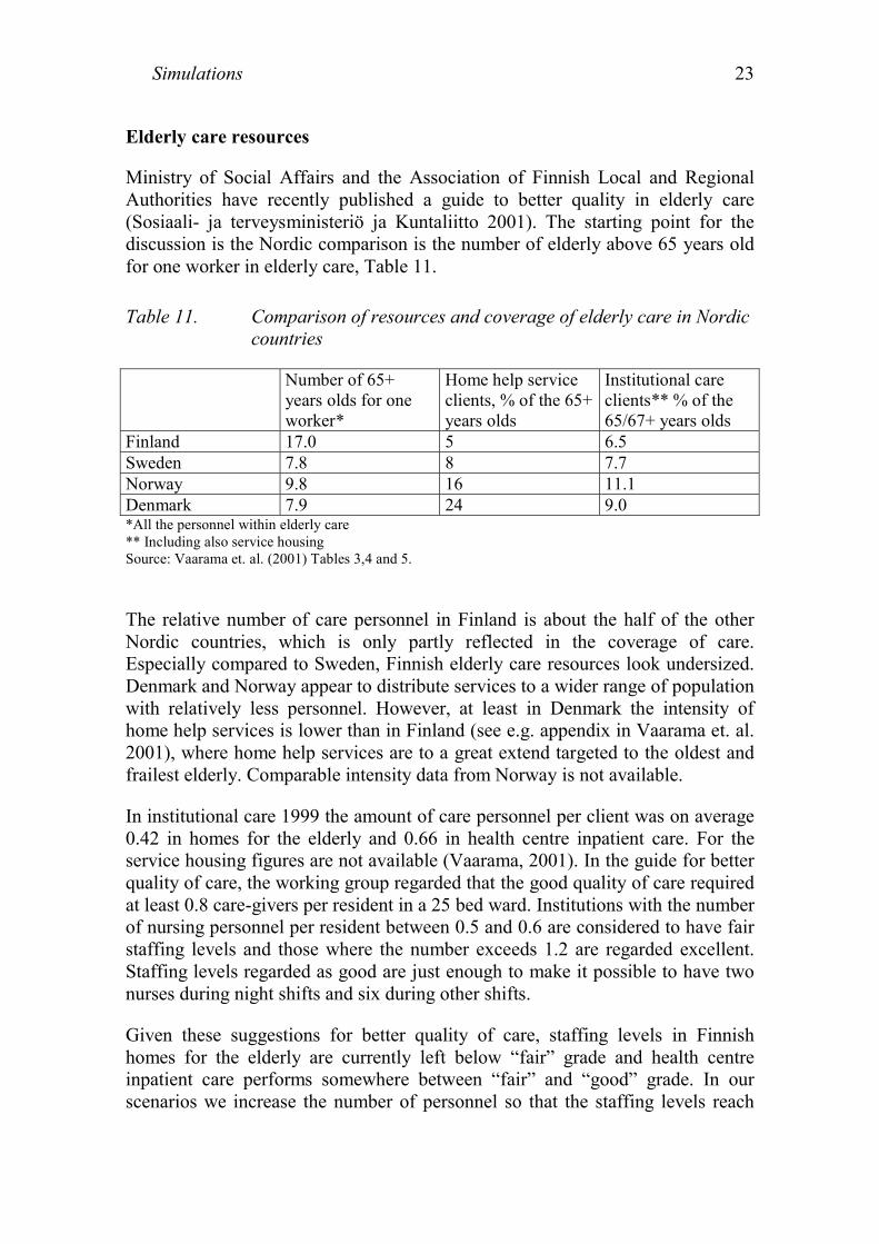
Elderly care resources

Ministry of Social Affairs and the Association of Finnish Local and RegionalAuthorities have recently published a guide to better quality in elderly care(Sosiaali- ja terveysministeriö ja Kuntaliitto 2001). The starting point for thediscussion is the Nordic comparison is the number of elderly above 65 years oldfor one worker in elderly care, Table 11.

Table 11. Comparison of resources and coverage of elderly care in Nordiccountries

Number of 65+years olds for oneworker*

Home help serviceclients, % of the 65+years olds

Institutional careclients** % of the65/67+ years olds

Finland 17.0 5 6.5Sweden 7.8 8 7.7Norway 9.8 16 11.1Denmark 7.9 24 9.0*All the personnel within elderly care** Including also service housingSource: Vaarama et. al. (2001) Tables 3,4 and 5.

The relative number of care personnel in Finland is about the half of the otherNordic countries, which is only partly reflected in the coverage of care.Especially compared to Sweden, Finnish elderly care resources look undersized.Denmark and Norway appear to distribute services to a wider range of populationwith relatively less personnel. However, at least in Denmark the intensity ofhome help services is lower than in Finland (see e.g. appendix in Vaarama et. al.2001), where home help services are to a great extend targeted to the oldest andfrailest elderly. Comparable intensity data from Norway is not available.

In institutional care 1999 the amount of care personnel per client was on average0.42 in homes for the elderly and 0.66 in health centre inpatient care. For theservice housing figures are not available (Vaarama, 2001). In the guide for betterquality of care, the working group regarded that the good quality of care requiredat least 0.8 care-givers per resident in a 25 bed ward. Institutions with the numberof nursing personnel per resident between 0.5 and 0.6 are considered to have fairstaffing levels and those where the number exceeds 1.2 are regarded excellent.Staffing levels regarded as good are just enough to make it possible to have twonurses during night shifts and six during other shifts.

Given these suggestions for better quality of care, staffing levels in Finnishhomes for the elderly are currently left below “fair” grade and health centreinpatient care performs somewhere between “fair” and “good” grade. In ourscenarios we increase the number of personnel so that the staffing levels reach

Simulations24

the working group recommendation for the “good” quality of institutional care byyear 2030.

Depending on the reference, an average either two hours a week8 or 2.8 visits aweek9 per client of home help services are currently given. As the average timeof a visit is something less than an hour10, the statistics give approximately anequal figure of care intensity. The workgroup suggestion is that intensity of homehelp services should be doubled, i.e. to 4 hours a week on average. In ourscenarios we have ended up to raise intensity from 2.8 visits to 4 visits a week.Given that we keep the number of visits per home help employee constant, this isnot as such enough to double the home help service resources. Therefore we alsoalter the intensity of the home nursing by increasing the time a nurse will spendwith each client roughly by 20%, letting the number of weekly visits decreasefrom 43.1 to 3511.

Table 12. The scenarios with respect to changes in dependency of the eld-erly and resources allocated to elderly care

Changes in dependencyCurrent 3 years shift on-

wards both indomicile andinstitutional care

5 years shift indomicile and 3years shift in in-stitutional care

Current I Trend II (Current3+3)Current resourcesand 3 years shiftin care needed by2030

III (Current3+5)Current resourcesand 3 or 5 yearsshift in institu-tional and domi-cile care neededrespectively by2030

Res

ourc

es a

lloca

ted

to e

lder

ly c

are

Resources allocated toreach care quality level“good” by 2030. Inten-sity of domicile serv-ices doubled.

IV Good care V (Good3+3)Good care and 3years shift in careneeded by 2030.

VI (Good3+5)Good care and 3 or5 years shift ininstitutional anddomicile careneeded respec-tively by 2030

8 Workgroup for guides to improve quality of elderly care, Vaarama et. al. (2001).9 SOTKA database.10 No reliable statistics are available.11 The estimate of 20% increased time per client is based on approximately 50% share of a nurses timebudget used to actual care, the rest of the time used to travelling and administrative tasks.

Simulations 25

Table 12 summarises the scenario framework used in the study. Keeping theinterpretation simple, scenarios differ from each other only in two dimensions,with respect to changes in dependency and resources allocated.

The trend scenario (I) is a straightforward projection using current servicepatterns and population forecasts. The scenario also fails accounting the impactof altering gender structure on service usage or resources needed.

The good care scenario (IV) imposes more resources to intensified servicehomes, homes for the elderly and inpatient care as well as to domicile care. Theexpected changes are summarised in Table 13. The care personnel in inpatientcare and homes for the elderly is sized according the quality criteria “good” to0.8 employees per patient. For the intensified service housing slightly lesspersonnel is suggested, 0.7 employees per resident. These changes also reflect theincreased dependency of the clients in service homes and homes for the elderly.We keep the staffing of the regular service houses at their current level, 0.32employees per resident, as their clients will partly rely on publicly or privatelysupplied domicile care. We have also increased the resources of long termsomatic and psychiatric care to the “good” level, although their role for elderlycare resource usage is currently low.

Table 13. Resources allocated to institutional care and domicile services inscenarios Good care, Good(3+3) and Good(3+5)

Currentlevel

Level by target year

Institutional care 1999 2010 2020 2030Service housing care personnel per bed 0.3 0.3 0.3 0.3Intensified service housing care personnel per bed 0.5 0.57 0.63 0.7Homes for elderly care personnel per bed 0.5 0.6 0.7 0.8Inpatient at health centres, inpatient ward employeesper bed

0.6 0.67 0.73 0.8

Somatic special care, inpatient ward employees perlong term care bed

0.4 0.53 0.67 0.8

Psychiatric care, inpatient ward employees per longterm care bed

0.7 0.73 0.78 0.8

Home help services and home nursingHome help service productivity: visits/employee /week 22 22 22 22Home help service: visits/client/week 2.8 3.2 3.6 4Home nursing productivity: visits/nurse/week 43.1 40.4 37.7 35

Simulations26

The actual coverage of the domicile services at target year depends on thenumber of elderly living home, their dependency and the expected usage of thecare. The numbers of users are calculated for each gender with their owncoefficients. Although, for the simplicity, the formula here for the number ofelderly receiving particular care is written without a subscript indicating thegender.

( ).Where

Population in age group , at target year .

Share of population with disability classigfication in age group .

Share (probability) in age group

j j j jt t i i

j Age i ADL

jtj

ij

i

USERS p d c NI

p j td i jc j

∈ ∈

= × × ×

=

=

=

∑ ∑

{ }

with disability classification to use particular service.

Share of non institutionalised elderly in age group .65-74 years, 75-79 years, 80-84 years,85+ years

Non ADL, Instrumental ADL,

j

i

NI jAge

ADL

==

= { }Personal ADL

The coefficients used in the formula are listed in Appendix II. In the scenariosdependency pattern is shifted 3 or 5 years onwards, altering the coefficients j

id ina way explained in Appendix IV. In the EVERGREEN 2000 model the coverageof a service is expressed as a share of the population above 65 years old. As theEVERGREEN and elderly barometer data bases are not exactly equal, we haveused EVERGREEN database as a starting value, but estimated the shifts inservice coverage according the models estimated from the barometer data.

To estimate the coverage of the institutional care, we have used SOTKA statisticson male and female residents and patients in care-giving institutions. Thestatistics seem to include measurement (or bookkeeping) errors and the agedistribution of patients naturally includes some stochastic variation. This type ofirregular variation of cohorts is troublesome, when age distributions are used topredict future service usage and shifts in it. In most of the cases the distribution isnot monotone, therefore we have smoothened the distributions by linear discretemodels. An example of smoothing the distribution of the short term homes forthe elderly is given in Appendix V. The smoothened age distributions andpopulation forecasts are used to calculate the expected numbers of patients ineach form of institutional care. For the scenarios, where shifts in dependencywere assumed, each cohort has a probability for care of 3 years younger cohort.

Simulations 27

Table 14 reports the resulting coverage of institutional and non-institutional careunder alternative assumptions.

Altogether the coverage of the institutional care, including service housing willdrop from 7.3 percent to 5.7 percent of the population aged 65 years. The mainchanges will take place in homes for the elderly and health centre’s inpatient carecoverage, which will drop by 50 – 60 percent. As the service housing coveragewill be kept constant their share of the institutional care will grow from 25percent to 36 percent. No changes are assumed between regular and intensifiedservice housing. In domicile care, 5 years shift in care by 2030 is needed todecrease the total coverage of help and support of the elderly population.However it seems evident, that gender/age/dependency structure of the ageingpopulation will decrease the relative number of domicile service users aroundyear 2020.

Table 14. Shifts in care coverage after given changes in dependency, sce-narios: Current3+3, Current3+5, Good3+3 and Good3+5

Currentlevel

Target year

1999 2010 2020 20303 years shift in care needed by 2030Domicile care Percent, relative to population aged 65

yearsHome help service clients 11 10.8 10.1 11.1Home nursing clients 8.2 8.1 7.5 7.8Support service clients 13.5 13.3 12.2 14.0Institutional careBeds in regular service housing 1.4 1.4 1.4 1.4Beds in intensified service housing 0.7 0.7 0.7 0.7Long term beds in homes for the elderly 2.6 2.0 1.5 1.0Short term beds in homes for the elderly 0.2 0.2 0.2 0.2Long term inpatient beds in health centres 2.2 1.6 1.3 1.0Short term inpatient beds in health centres 0.5 0.5 0.5 0.5Long term psychiatric care beds 0.1 0.1 0.1 0.1Long term somatic care beds 0.2 0.1 0.1 0.1Long term inpatient care altogether 5.6 4.5 3.7 2.9Inpatient and service housing altogether 8.4 7.3 6.5 5.75 years shift in care needed by 2030Domicile care Percent, relative to population aged 65

yearsHome help service clients 11 10.7 9.5 10.5Home nursing clients 8.2 7.9 7.1 7.3Support service clients 13.5 13.1 11.7 13.4

Simulations28

3.4 Expected changes in resource usage

The elderly population above 65 years old is expected to increase by 81% by2030. This is to say from 770 000 to 1 390 000 people. The time perspective islong, and the economy should be able to adjust to the corresponding proportionalrise in social and health related expenses, taken that economy-wide productivitygrowth will follow the historical trends (see e.g. Luoma et. al. 2003). Therefore,we will use the population forecast as a benchmark for the other scenarios.Improved functional ability of the ageing population will in part ease theadjustment to the population pressure, giving also room to improve the quality ofcare.

All the results are based on observed service usage at the end of the millennium.As the future cohorts are more wealthy and accustomed to a higher standard ofliving, the actual changes in services to be used are likely be higher thanpresented here. If we consider current supply with given quality improvements asa sufficient standard also for the future, these figures give estimate on care andresources needed for publicly provided elderly care services.

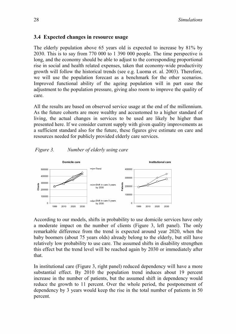
Figure 3. Number of elderly using care

Domicile care

0

100000

200000

300000

400000

500000

1999 2010 2020 2030

Clie

nts

Trend

Shift in care 3 yearsby 2030


Institutional care

0

100000

200000

300000

400000

1999 2010 2020 2030

Pat

ient

s

According to our models, shifts in probability to use domicile services have onlya moderate impact on the number of clients (Figure 3, left panel). The onlyremarkable difference from the trend is expected around year 2020, when thebaby boomers (about 75 years olds) already belong to the elderly, but still haverelatively low probability to use care. The assumed shifts in disability strengthenthis effect but the trend level will be reached again by 2030 or immediately afterthat.

In institutional care (Figure 3, right panel) reduced dependency will have a moresubstantial effect. By 2010 the population trend induces about 19 percentincrease in the number of patients, but the assumed shift in dependency wouldreduce the growth to 11 percent. Over the whole period, the postponement ofdependency by 3 years would keep the rise in the total number of patients in 50percent.

Simulations 29

Figure 4. Number of employees needed

Domicile care

05000

100001500020000

250003000035000

4000045000

1999 2010 2020 2030

Full

time

empl

oyee

s

Trend

Good care


Shift in care 3 yearsby 2030, good care



Institutional care

010000

2000030000

4000050000

6000070000

8000090000

1999 2010 2020 2030

Full

time

empl

oyee

s

The resources needed in social services, especially in services given at home, gohand in hand with the number of clients. Thus in domicile care with currentservice quality, number of care personnel needed will grow steadily with theelderly population (Figure 4, left panel). Increasing the number of visits perclient in home help services and extending the visits of home nursing willincrease the number of employees from 15500 to 40000 instead of 28000employees needed according to the current trend. Again at least 5 years shift incare probabilities is needed to give a noteworthy decrease in workforce undergood care scenario.

In institutional care the scenarios differ from each other more radically. Currently34000 employees take care of 190000 patients (Figure 4, right panel). Accordingto the trend almost 62000 employees will be needed to take care of 344 000patients. Three years postponement in the use of care would keep the requirednumber of employees approximately at current level, leaving room to improvethe quality of care. Even with good care and less dependent elderly population;just 44000 employees would be needed to run the required number of somaticand psychiatric inpatient care, as well as service housing and houses for theelderly.

Figure 5. Operating costs

Domicile care

0

200

400

600

800

1000

1200

1400

1999 2010 2020 2030

mill

lion

Euro

s

Trend

Good care





Institutional care

0

5001000

15002000

25003000

35004000

4500

1999 2010 2020 2030

mill

ion

Eur

os

Simulations30

The growth in operating costs is of the same order of magnitude as the rise in thenumber of care personnel. The € 508 million operating cost of the domicileelderly care in the year 1999 is expected to increase to € 920 millions (Figure 5,left panel). The good care option is about 35 percent more expensive without anychange in dependency, but only 18 percent more expensive if the targetpostponement of 5 years will be reached.

Reaching good quality of care within 30 years is rather unambitious target. Forexample safety reasons12 suggest accelerated schedule, e.g. 10 years, for qualityimprovements. Even if we had not directly simulated resources needed for thisscenario, we can use the linearity of the EVERGREEN 2000 model to deriveexpected need of resources. In the model the good would cost proportionallyabout the same in 10 years as in 30 years. This is to say that good care is about35 % more expensive also in 2010. Thus, taking into account the populationpressure, good domicile care at 2010 would cost about € 818 million, about 60percent more than today.

Institutional care operating costs are currently € 1910 millions and they areexpected to increase to € 3460 millions by 2030 (Figure 5, right panel). The goodcare quality would cost about € 4160 millions, only 20 percent more than thepopulation trend estimate gives. Counting the assumed shift in the care needed,operating costs will increase only moderately to € 2060 or € 2300 million withoutor with good care option respectively. Getting good care quality in acceleratedschedule by 2010 would mean institutional care operating costs of €2730millions instead of the population trend implied € 2280 millions.

The simulation results are summarised in Table 15, where both domicile andinstitutional care are summed up and the expected operating costs in alternativecases are expressed in annual growth percent required to match the populationinduced needs and/or targets set for the quality of care.

The operating cost growth estimates in Table 15 are based on the year 1999.Thus four budget years are already fixed and their contribution to the 2010 targetachievement is crucial. Unfortunately, no comparable nation-wide data isavailable after 1999. Also the figures do not assume any operating cost increasesdue to labour market pressure.

12 The current personnel in institutional care is not always enough to keep two persons a ward in nightshift. Service housing units usually do not have personnel available 24 hours a day.

Simulations 31

Table 15. The required annual growth in operating costs needed to matchelderly population growth and targets set for the good care

Target year2010 2030Domicile Institu-

tionalTotal Domicile Institu-

tionalTotal

Population trend 1.6 1.6 1.6 1.9 1.9 1.9Good care 4,4¹ 3.3¹ 3.6¹ 2.9 2.5 2.6Good care with 3 yearsimproved ability

2.9 0.5 1.2

Good care with 5 yearsimproved ability

2.5 1.1²

¹Assuming trend growth and an additional 35 % increase by 2010 in domicile care and 20% in institu-tional care to reach quality level “good care”.² Scenario Good3+5, i.e. 3 years improvement in institutional care by 2030.

If elderly population growth were the only factor affecting operating costs, theywould grow an average at annual speed of 1.6 percent by year 2010 and 1.9percent by 2030. Thus the population induced cost pressure will accelerate afteryear 2010 and will be on average 2.1 percent between 2010 - 2030. Targeting tothe year 2030 good quality of the care requires about 1 percent additionalincrease in annual growth in domicile care and 0.6 percent in institutional care.Improving the functional ability of the elderly so that dependency would bepostponed by three years does not seem to have any impact on domicile care, butit clearly affects the operating costs of institutional care. The required annualgrowth would be about 0.5 in real terms, far less than the population trendsuggests.

A far more attractive scenario from the welfare point of view is to accelerate thechange toward good care quality so that it would be reached already by 2010.Given that good care by 2010 is proportionally as expensive as it is by 2030, indomicile care the operating cost should be increased annually on average by 4.4percent and in institutional care by 3.3 percent. Total expenditures shouldincrease annually 3.6 percent from 1999 to 2010. In these figures both populationtrend and increased staffing levels required by good quality care are taken intoaccount. We can not read directly from the simulation results, how much reduceddependency of the elderly dependency would ease cost pressures, but the timeperiod is obviously relatively short for it to have a visible impact. This is alsoreflected in operating costs in Figure 5, where improvements in functional abilityof the elderly do not make a difference within first 11 years.

The expected growth of the operating costs due to the growth of elderlypopulation will be higher after 2020 than before. Therefore in order to reach bothtargets simulated in this paper, it looks like a good idea to invest to the improving

Simulations32

quality of the care now, when population pressure is weaker. Especially theinvestment in domicile care would be a good starting point to improveindependent ability in elderly daily living. In the long run it could help reachingeconomically a more affordable service mix by decreasing the need ofinstitutional care.

Discussion 33

4. Discussion

In this study we have projected assumptions on dependency of the elderly and thedesired improvements in the contents of elderly care to the expected number ofelderly within publicly provided care and the resources needed to produce them.Unlike in any previous studies using Finnish data, we have been able to modelthe impact of physical and social factors on the use of domicile care. Using theelderly barometer interview survey data, home help services, home nursing andthe set of four support services: cleaning, meals on wheels, bathing and servicesprovided at day centres all got their own models with service specific set ofexplanatory variables. The models and the data provide a detailed picture on howage, dependency, social environment and service supply related factorscontribute to the probabilities of for the elderly to use services. Together withpopulation forecasts these results were used to calculate expected number ofservice users at 2030.

According to the models estimated in this study dependency measured byproblems in personal activities of daily living and living alone are importantdeterminants for the use of domicile services. Their impact, however, varies withage of the elderly. For younger elderly the impact of dependency is clear, but forthe oldest group the impact of increased dependency cannot be separated fromthe impact of age. Even if analysis of the same data (Vaarama and Kaitsaari2002) show, that in some special groups informal help has substituted homehelp services, our analysis based on the whole data show, that informal helpcomplements publicly provided domicile services. They go hand in hand, butunfortunately analysis here is not enough to quantify this effect.

Regrettably, comparable data on institutional care was not available. We had tobe content with register data. However, we were able to compile institutional caredata (as well as domicile service data) into the form, where resource needed ofeach service and care form were computable in EVERGREEN 2000 -model. Themodel calculates for each service the number of users conditional on the size ofelderly population, resources needed with desired intensity of care and operatingcosts of the services. As usually in simulation models, the actual service andresource levels calculated are not that interesting, but scenarios should becompared to each other. Our key findings are, that good care scenario is likely toincrease required personnel, as well as operating cost, by 29 percent to the trendlevel and that reduced dependency decreases cost by 32 percent as such and evenwith more intensive good care by 19 percent. The compounded effect of goodcare and dependency shift is clearly cost saving. These results, expressed in theform of annual operation cost growth needed to match the target, are alsoreported in Table 15 (page 31).

Discussion34

According to our projections the increase in the number of care personnel shouldbe higher than what SOMERA commission presents in its report. Assumptionsabout dependency are the same as the commission’s, but our specification ofgood care quality increases considerably the need for care personnel. It is hard tofigure out from public sources the detailed (and comparable) figures of thecommission, but at least in home help services and home nursing the commissionassumes that 7500 more (not including replacements) workers are needed,whereas our specification suggests that about 12 000 more carers and nursesshould be hired. Although this means a substantial increase in the number ofworkers employed in elderly care, it should be economically possible givenenough time for the economy to adjust. However, increasing the number of socialand health sector employees at the time when labour supply is falling withoutrising their relative wages and salaries, is a difficult task. Therefore operatingcosts in elderly care will probably rise more rapidly than fixed price calculationsmade in our study suggest.

Policies how to decrease dependency are not discussed in detail here, but theobvious direction is a comprehensive view of the elderly care. According to thisview people are not just taken care of but the care plan takes into account thewhole social and physical environment an elderly belongs to and is also willingto invest in pre-emptive actions. The good quality of care is an essential part ofcomprehensive care, as it decreases dependency and makes it easier for theelderly to live in their familiar environments. The solution presented here is onlya partial one, but the message is clear; policies decreasing the dependency are aneffective tool to ease adjustment processes.

The approach here has been based on so called macrosimulation models. Theestimated probabilities of the population groups to use services are used togetherwith population forecasts to predict future demands. An alternative would be touse a microsimulation model, where behaviour of a representative sample isstudied over time. In addition to the sample, the main problem in themicrosimulation approach is the need of transfer probabilities e.g. from healthstatus to another or from domicile to institutional care. This type of researchwould aid especially in forecasting pre-mortal cost pressure, which is supposedto be one of the key elements of the future cost of care (for discussion seeZweifel et. al. 1999). Actually all the data needed to estimate transferprobabilities is already available. The elderly barometer studies from 1993 and1998 (Vaarama et. al. 1999) cover all the background and interview time healthand service use status information needed. Combining this information withnational HILMO-registers would give transfer probabilities to the institutionalcare. Also a local, but with larger population coverage executed TamELSA study(Jylhä et. al. 1992) could be used for these purposes.

Appendix 35

Appendix

APPENDIX I: Predictions from ordered logistic model

The survey data available allows a detailed probability modelling of the serviceuse. We have data available not only on selection, whether a respondent receiveda care, but also on the intensity of the care. In services like home help andcleaning the intensity varies enough to make sense for the ordered probabilisticmodel, whereas for example meals on wheels are usually received daily or not atall, a simple binomial probabilistic model suffices. In this chapter we discuss theordered probabilistic model, with a short review on the basic statistic model andgive the most emphasis on the interpretation of the results and the way modelprediction should be calculated.

The ordered probability models are developed to explain variation in ordereddiscrete choices, like choices of the care intensity. The measured probability isnot only conditional on the selection of explanatory variables but also on thechoice of probability function. The most usual choices are the logistic and normaldistribution with unit variance. Let ( )F ⋅ denote the cumulative distribution ofeither logistic or normal distribution and ( )f ⋅ its density function. The expectedvalue of the distribution is set as a function of explanatory variables( 1 vector k × x for each observation) and parameters ( 1k × vector β ) to beestimated and the cutting points [ ], 0,j j Jκ ∈ where J is equal to number ofdiscrete choices in endogenous variable y. The probability of a choice is set sothat

( ) ( ) [ ]1

0

Pr( 1) ' ' 1,

where and j j

J

y j F F j Jκ κκ κ

−= − = − − − ∀ ∈

= −∞ = ∞

β x β x(1)

The problem is to estimate k unknown parameters β and 1J − cutting points1 1, , Jκ κ −K . To keep probabilities always positive, it is supposed that

1 10 Jκ κ −< < <K .

The “slope” parameters β are somewhat tricky to explain. They do not get thetraditional marginal value interpretation. The derivatives (marginal values) w.r.t.x of the probability to choose y j= are

( ) ( ) ( )1

Pr' 'j j

y jf fκ κ −

∂ = = − − − ∂β x β x β

x(2)

Appendix36

For the given vector x, the marginal values of variables are proportional toparameter values β . However condition 1j jκ κ −> does not guarantee any signcondition for the bracketed expression. Instead, the marginal impact is likely tochange sign if the density function is quasi-concave (e.g. bell shaped). This is nota completely harmless condition. Consider for example a case, where most of thedensity is concentrated on the first choice in symmetric density function. Thus

1κ − β'x may be located right of the mean, so does all the densities for higherchoices of y. From (2) it follows, that all the marginal probabilities thereafterhave equal signs. This is a strong maintained hypothesis of the orderedprobability model that a modeller has to consider in advance. One way to takecontrol over the speed densities are accumulated is using non-linear (in variables)functions or discrete parameterisations of the explanatory variables.

The predicted probabilities and marginal values are conditional on the selectedvalues of independent variables. A common way is to report them in data means.This is a rough measure, giving an idea on the magnitudes, and will be used inthis study to report marginal values from the estimated models. However, ourprimary goal is to predict the probabilities of care in the population. Therefore,we use all the population to calculate probability predictions, and reportpopulation weighted means. The strategy selected makes also easy to calculatepredictions for the sub-samples selected according the subset of explanatoryvariables. The variation in the predicted probabilities is then conditional on thenon-controlled set of explanatory variables.

Using normal or logistic densities make only sense if all the choices may beconsidered emerging from the same distribution. For example the selectionprocesses whether to use services or not may be different from intensity ofservice use. To model this we should be able to identify factors independentlycontributing to the client’s enter to use facilities of the formal service sector.Unfortunately we have no data available on selection specific variables likeaccessibility of the certain service or service providers.

The choice of distribution is generally a matter of convenience as far as errorterm is plausibly modelled either as the logistic or normal distribution. Themodels give approximately equal results, even if logistic distribution givesgreater probability for small 'β x .

Appendix 37

APPENDIX II: Patterns of service use

The following tables refer to the coefficients in formula page 26.

Share of non-institutionalised elderly ( jNI )

Male FemaleAge 65-74 95% 97%Age 75-79 90% 92%Age 80-84 74% 74%Age 85+ 74% 74%

Disability distribution of the elderly ( jid )

The rows are

FADL0, Female with no reported disabilities

FADL1, Female with at least one reported instrumental disability, but noreported personal disabilities.

FADL2, Female with at least one reported personal disability

MADL0, MADL1 and MADL2 as above but for male elderly.

age65-74 age75-79 Age80-84

age85+

FADL0 50.862 % 35.659 % 16.038 % 16.667 %FADL1 22.414 % 24.031 % 26.415 % 23.333 %FADL2 26.724 % 40.310 % 57.547 % 60.000 %MADL0 42.523 % 27.473 % 28.358 % 13.793 %MADL1 34.579 % 38.462 % 38.806 % 37.931 %MADL2 22.897 % 34.066 % 32.836 % 48.276 %

Source: observed distribution from elderly barometer interview study.

Share (Probability) to use a particular service ( jic )

In each service, the first table (needs no help) reports coefficient 1 jic− . Home

help service and home nursing coefficient are used as reported. Support servicesis an adjusted sum of users of cleaning service, bathing, recreation centres andmeals on wheels, taking account that a female user uses on average 1.5 servicesand a male user uses 1.4 services.

Appendix38

Home help services

Needs no help, 1 jic− Needs help seldom

Age65-74

Age75-79

Age80-84

Age85+

Age65-74

Age5-79

Age80-84

Age85+

FADL0 0.992 0.962 0.822 0.822 FADL0 0.002 0.009 0.036 0.036FADL1 0.932 0.882 0.774 0.774 FADL1 0.016 0.027 0.045 0.045FADL2 0.815 0.667 0.588 0.547 FADL2 0.036 0.056 0.063 0.066MADL0 0.994 0.969 0.840 0.840 MADL0 0.001 0.008 0.034 0.034MADL1 0.989 0.966 0.823 0.823 MADL1 0.003 0.008 0.035 0.035MADL2 0.929 0.715 0.749 0.749 MADL2 0.016 0.048 0.042 0.042

Needs help monthly Needs help weeklyAge65-74

Age75-79

Age80-84

Age85+

Age65-74

Age5-79

Age80-84

Age85+


Needs help dailyAge65-74

Age75-79

Age80-84

Age85+

FADL0 0.001 0.006 0.034 0.034FADL1 0.011 0.020 0.044 0.044FADL2 0.037 0.077 0.107 0.123MADL0 0.001 0.005 0.029 0.029MADL1 0.002 0.005 0.035 0.035MADL2 0.012 0.068 0.061 0.061

Appendix 39

Cleaning services

Needs no help, 1 ijc− Needs help seldom

Age65-74

Age75-79

Age80-84

Age85+

Age65-74

Age5-79

Age80-84

Age85+



Age75-79

Age80-84

Age85+

Age65-74

Age5-79

Age80-84

Age85+



Age75-79

Age80-84

Age85+


Appendix40

Home nursing

Needs no help, 1 ijc− Needs help seldom

Age65-74

Age75-79

Age80-84

Age85+

Age65-74

Age5-79

Age80-84

Age85+



Age75-79

Age80-84

Age85+

Age65-74

Age5-79

Age80-84

Age85+



Age75-79

Age80-84

Age85+


Appendix 41

BathingProbability to get service, i

jcAge65-74

Age75-79

Age80-84

Age85+


Meals on wheelsProbability to get service, i

jcAge65-74

Age75-79

Age80-84

Age85+


Recreation centresProbability to get service, i

jcAge65-74

Age75-79

Age80-84

Age85+


Appendix42

Appendix III: Marginal values of domicile service models

Marginal values are evaluated at sample means. For the dummy variables as shiftfrom 0 to 1, for all the other variables as point derivatives.

Ordered logistic modelsHome help services

No help Seldom Mothly Weekly DailyAge -0.0033 0.0008 0.0009 0.0011 0.0005Alone -0.4991 0.0739 0.1059 0.1932 0.1261Aloneage 0.0008 -0.0002 -0.0002 -0.0003 -0.0001ADL1 -0.9988 0.0003 0.0007 0.0047 0.9931ADL2 -0.9961 0.0011 0.0026 0.0162 0.9762MADL1 0.0022 -0.0006 -0.0006 -0.0007 -0.0003MADL2 0.0017 -0.0004 -0.0005 -0.0006 -0.0003FADL1age 0.0002 -0.0001 -0.0001 -0.0001 0.0000FADL2age 0.0003 -0.0001 -0.0001 -0.0001 0.0000MADL1age 0.1060 -0.0252 -0.0281 -0.0359 -0.0168MADL2age 0.0303 -0.0077 -0.0082 -0.0100 -0.0045INFHELP -0.0224 0.0056 0.0060 0.0074 0.0034TAXRATE 0.0004 -0.0001 -0.0001 -0.0001 -0.0001Cleaning servicesFAGE -0.0039 0.0015 0.0017 0.0006 0.0001MAGE -0.0041 0.0016 0.0018 0.0006 0.0001Alone -0.0690 0.0258 0.0305 0.0113 0.0013ADL2 -0.0791 0.0293 0.0351 0.0131 0.0016INFHELP -0.0995 0.0359 0.0445 0.0170 0.0020Home nursingDAGE80 0.1324 -0.0557 -0.0416 -0.0285 -0.0066AGE80 -0.0076 0.0032 0.0024 0.0016 0.0004ADL2 -0.1570 0.0615 0.0501 0.0366 0.0087

Binomial logit modelsBathing Meals

onwheels

Recreationcentres

FAGE 0.001 0.002MAGE 0.001 0.002AGE 0.0026DAGE80 -0.0188DAGE85 -0.0056Alone 0.009 0.032 0.0199INFHELP 0.031 0.033 0.0450ADL2 0.024

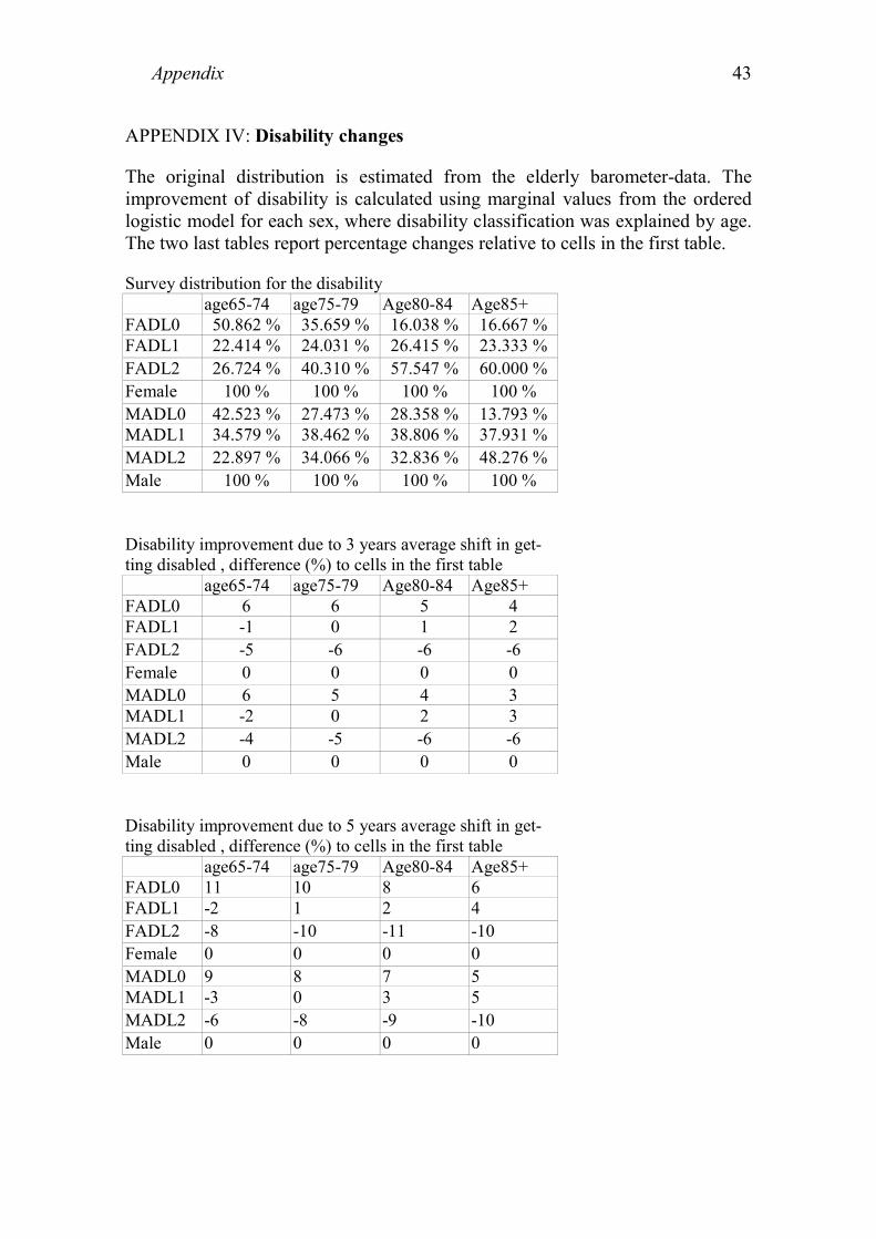
Appendix 43

APPENDIX IV: Disability changes

The original distribution is estimated from the elderly barometer-data. Theimprovement of disability is calculated using marginal values from the orderedlogistic model for each sex, where disability classification was explained by age.The two last tables report percentage changes relative to cells in the first table.

Survey distribution for the disabilityage65-74 age75-79 Age80-84 Age85+

FADL0 50.862 % 35.659 % 16.038 % 16.667 %FADL1 22.414 % 24.031 % 26.415 % 23.333 %FADL2 26.724 % 40.310 % 57.547 % 60.000 %Female 100 % 100 % 100 % 100 %MADL0 42.523 % 27.473 % 28.358 % 13.793 %MADL1 34.579 % 38.462 % 38.806 % 37.931 %MADL2 22.897 % 34.066 % 32.836 % 48.276 %Male 100 % 100 % 100 % 100 %

Disability improvement due to 3 years average shift in get-ting disabled , difference (%) to cells in the first table

age65-74 age75-79 Age80-84 Age85+FADL0 6 6 5 4FADL1 -1 0 1 2FADL2 -5 -6 -6 -6Female 0 0 0 0MADL0 6 5 4 3MADL1 -2 0 2 3MADL2 -4 -5 -6 -6Male 0 0 0 0

Disability improvement due to 5 years average shift in get-ting disabled , difference (%) to cells in the first table

age65-74 age75-79 Age80-84 Age85+FADL0 11 10 8 6FADL1 -2 1 2 4FADL2 -8 -10 -11 -10Female 0 0 0 0MADL0 9 8 7 5MADL1 -3 0 3 5MADL2 -6 -8 -9 -10Male 0 0 0 0

Appendix44

APPENDIX V: Age Distribution of Institutional Care

The first figure presents the number of beds per males between 65 - 100 years oldin the short-term homes for the eldelry. The second figure is the fit (or smooth)of the model.

Fitted

00.0020.0040.0060.0080.01

0.0120.0140.016

65 68 71 74 77 80 83 86 89 92 95 98

Observed

00.0020.0040.0060.0080.01

0.0120.0140.016

65 68 71 74 77 80 83 86 89 92 95 98

( ) { }

0. otherwise ,90 if age

0, otherwise ,90 if age

years, t aged maleper bedswhere

,100,,65,,0~,

2

1

21

>=

≤=

=

=+++=

txtx

y

tNxxy

t

t

t

ttttt Kσεεββα

The dependency shift is calculated by assigning to each cohort the bed frequencyof 3 years younger cohort.

References

Aromaa A. - Koskinen S. (ed.) (2002): Terveys ja toimintakyky Suomessa.Terveys 2000 tutkimuksen perustulokset. Kansanterveyslaitoksen julkaisujaB3/2002. Helsinki.

Jylhä M. - Jokela J. - Tolvanen E. - Heikkinen E. - Heikkinen R.L. - Koskinen S.- Leskinen E. - Lyyra A.L. - Pohjolainen P. (1992): The Tampere LongitudinalStudy on Ageing. Description of the study. Basic results on health andfunctional ability. Scandinavian Journal Soc. Med. Supplement 47, 1992

Kela (2002): Statistical Yearbook of the Social Insurance Institution, Finland.Publication by the Social Insurance Institution T1:37

Klaukka T. (ed.) (2002): Vaikka terveys on kohentunut, sosiaaliturvankustannukset kasvavat: Kelan näkökulma Terveys 2000 –hankkeen tuloksiin.Kelan tutkimusosasto, Sosiaali- ja terveysturvan selosteita 23/2002. Helsinki

Luoma K. - Räty T. - Parkkinen P. - Vaarama M. - Mäkinen E. (2003): Seniori -Suomi: Ikääntyvän väestön taloudelliset vaikutukset. Sitran raportteja 30.Helsinki.

OECD (2002): Economic Outlook, No 72.

Parkkinen P. (2002): Hoivapalvelut ja eläkemenot vuoteen 2050. VATT-tutkimuksia nro 94, Helsinki.

Rajala T. - Lahtinen Y. - Paunio P. (2001): Suurten kaupunkien 2. RAVA-tutkimus – Vanhuksien toimintakyky ja avun tarve. Suomen kuntaliitto,Helsinki.

Sosiaali- ja Terveysministeriö ja Kuntaliitto (2001): Ikäihmisten hoitoa japalveluja koskeva laatusuositus. Sosiaali- ja terveysministeriön oppaita 2001:4

Sosiaali- ja Terveysministeriö (2002): Sosiaalimenojen kehitys pitkälläaikavälillä. SOMERA toimikunnan taustaraportti. Helsinki

Vaarama M. - Hakkarainen A. - Laaksonen S. (1999): Vanhusbarometri.Sosiaali- ja terveysministeriön selvityksiä nro 3.

Vaarama M. - Kandelberg K. - Kitinoja A.-P. (1998): EVERGREEN 2000.Käyttäjän opas. Stakes, Helsinki.

Vaarama M. - Luomahaara J. - Peiponen A. - Voutilainen P. (2001): Koko kuntaikääntyneiden asialle: Näkökulmia ikääntyneiden itsenäisen selviytymisensekä hoidon ja palvelun kehittämiseen. Stakes, raportteja 259, Helsinki

Vaarama M. - Kaitsaari T. (2002): Ikääntyneiden toimintakyky ja koettuhyvinvointi. Teoksessa: Matti Heikkilä and Mikko Kautto (ed.) Suomalaistenhyvinvointi 2002, Stakes, Helsinki.

45

Vaarama M. - Voutilainen P. - Kauppinen S. (2002): Ikääntyneiden hyvinvointi.Teoksessa Sosiaali- ja terveydenhuollon palvelukatsaus 2002, Stakes,raportteja 268, Helsinki.

Wittenberg R. - Pickard L. - Comas-Herrera A. - Davies B. - Darton R. (1998):Demand for Long-term Care: Projections of Long-term Care Finance forElderly People. PSSRU, University of Kent at Canterbury.

Zweifel P. - Felder S. - Meiers M. (1999): Ageing of Population and Health CareExpenditure: A Red Herring? Health Economics 8.

46

VATT-TUTKIMUKSIA -SARJASSA ILMESTYNEITÄ

PUBLISHED VATT-RESEARCH REPORTS

65. Häkkinen Iida: Muuttopäätös ja aluevalinta Suomen sisäisessä muuttoliikkeessä. Helsinki2000.

66. Pyy-Martikainen Marjo: Työhön vai eläkkeelle? Ikääntyvien työttömien valinnattyömarkkinoilla. Helsinki 2000.

67. Kyllönen Lauri - Räty Tarmo: Asuntojen hinta-laatusuhde Joensuussa, semiparametrinenestimointi. Helsinki 2000.

68. Kyyrä Tomi: Welfare Differentials and Inequality in the Finnish Labour Market Over the1990s Recession. Helsinki 2000.

69. Perrels Adriaan: Selecting Instruments for a Greenhouse Gas Reduction Policy in Finland.Helsinki 2000.

70. Kröger Outi: Osakeyhtiöiden verotuksen investointikannustimet. Helsinki 2000.

71. Fridstrøm Lasse – Minken Harald – Moilanen Paavo – Shepherd Simon – Vold Arild:Economic and Equity Effects of Marginal Cost Pricing in Transport. Helsinki 2000.

72. Schade Jens – Schlag Bernhard: Acceptability of Urban Transport Pricing. Helsinki 2000.

73. Kemppi Heikki – Perrels Adriaan – Pohjola Johanna: Kasvihuonekaasupäästöjenalentamisen taloudelliset vaikutukset Suomessa. Vaiheen 1 Loppuraportti. Helsinki 2000.

74. Laine Veli – Uusitalo Roope: Kannustinloukku-uudistuksen vaikutukset työvoimantarjontaan. Helsinki 2001.

75. Kemppi Heikki – Lehtilä Antti – Perrels Adriaan: Suomen kansallisen ilmasto-ohjelmantaloudelliset vaikutukset. Vaiheen 2 loppuraportti. Helsinki 2001.

76. Milne David – Niskanen Esko – Verhoef Erik: Legal and Institutional Framework forMarginal Cost Pricing in Urban Transport in Europe. Helsinki 2001.

77. Ilmakunnas Seija – Romppanen Antti – Tuomala Juha: Työvoimapoliittistentoimenpiteiden vaikuttavuudesta ja ennakoinnista. Helsinki 2001.

78. Milne David – Niskanen Esko – Verhoef Erik: Acceptability of Fiscal and FinancialMeasures and Organisational Requirements for Demand Management. Helsinki 2001.(Not yet publiched).

79. Venetoklis Takis: Business Subsidies and Bureaucratic Behaviour. Helsinki 2001.

80. Riihelä Marja – Sullström Risto: Tuloerot ja eriarvoisuus suuralueilla pitkällä aikavälillä1971-1998 ja erityisesti 1990-luvulla. Helsinki 2001.

81. Ruuskanen Petri: Sosiaalinen pääoma – käsitteet, suuntaukset ja mekanismit. Helsinki2001.

82. Perrels Adriaan – Kemppi Heikki – Lehtilä Antti: Assessment of the Macro-economicEffects of Domestic Climate Policies for Finland. Helsinki 2001. Tulossa.

83. Venetoklis Takis: Business Subsidies and Bureaucratic Behaviour, A Revised Approach.Helsinki 2001.

84. Moisio Antti – Kangasharju Aki – Ahtonen Sanna-Mari: Menestyksen mitta?Vaihtoehtoisia mittareita aluetalouden kehitykselle. Helsinki 2001.

85. Tuomala Juha: Työvoimakoulutuksen vaikutus työttömien työllistymiseen. Helsinki 2002.

86. Ruotoistenmäki Riikka – Babygina Evgenia: The Actors and the Financial Affairs of theNorthern Dimension. Helsinki 2002.

87. Kyyrä Tomi: Funktionaalinen tulonjako Suomessa. Helsinki 2002.

88. Räty Tarmo – Luoma Kalevi – Koskinen Ville – Järviö Maija-Liisa: Terveyskeskustentuottavuus vuosina 1997 ja 1998 sekä tuottavuuseroja selittävät tekijät. Helsinki 2002.

89. Hakola Tuulia: Economic Incentives and Labour Market Transitions of the Aged FinnishWorkforce. Helsinki 2002.

90. Venetoklis Takis: Public Policy Evaluation: Introduction to Quantitative Methodologies.Helsinki 2002.

91. Berghäll Elina – Heikkilä Tuomo – Hjerppe Reino – Kiander Jaakko – Kilponen Juha –Lavrac Vladimir – Stanovnik Peter: The Role of Science and Technology Policy in SmallEconomies. Helsinki 2002.

92. Räisänen Heikki (toim.): Rakenteellinen työttömyys. Tutkimusinventaari japolitiikkajohtopäätökset. Helsinki 2002.

93. Moisio Antti: Essays on Finnish Municipal Finance and Intergovernmental Grants.Helsinki 2002.

94. Parkkinen Pekka: Hoivapalvelut ja eläkemenot vuoteen 2050. Helsinki 2002.

95. Junka Teuvo: Maailman kilpailukykyisin maa? Tuottavuus ja investoinnit Suomessa1975-2000. Helsinki 2003.

96. Cogan Josehp – McDevitt James: Science, Technology and Innovation Policies inSelected small European Countries. Helsinki 2003.

97. Perrels Adriaan – Kemppi Heikki: Liberalised Electricity Markets – Strengths andWeaknesses in Finland and Nordpool. Helsinki 2003.

98. Sarvimäki Matti: Euroopan Unionin itälaajentuminen ja maahanmuutto Suomeen.Helsinki 2003.

the expected 060503

Documents