Bank of Canada staff working papers provide a forum for staff to publish work-in-progress research independently from the Bank’s Governing Council. This research may support or challenge prevailing policy orthodoxy. Therefore, the views expressed in this paper are solely those of the authors and may differ from official Bank of Canada views. No responsibility for them should be attributed to the Bank.

www.bank-banque-canada.ca

Staff Working Paper/Document de travail du personnel 2018-37

The Extensive Margin of Trade and Monetary Policy

Yuko Imura and Malik Shukayev

ISSN 1701-9397 © 2018 Bank of Canada

Bank of Canada Staff Working Paper 2018-37

July 2018

The Extensive Margin of Trade and Monetary Policy

by

Yuko Imura1 and Malik Shukayev2

1 International Department Bank of Canada

Ottawa, Ontario, Canada K1A 0G9 2Department of Economics, University of Alberta

9-12 HM Tory Building Edmonton, AB T6G 2H4

yimura@bankofcanada.ca shukayev@ualberta.ca

i

Acknowledgements

We thank George Alessandria and Matthieu Bussière for insightful comments and

suggestions. We also thank seminar participants at the University of Alberta, the Bank of

Canada and Ohio State University; and conference participants at the 24th International

Conference on Computing in Economics and Finance, the 26th Annual Symposium of the

Society for Nonlinear Dynamics and Econometrics, the 2016 North American Summer

Meeting of the Econometric Society, the ECB-Banque de France workshop

“Understanding the Weakness in Global Trade: What Is the New Normal?”, the 2016

European Economics Association Annual Congress, and the 50th Annual Conference of

the Canadian Economics Association.

The views expressed in this paper are those of the authors, and do not reflect those of the

Bank of Canada. Any remaining errors are our own.

ii

Abstract

This paper studies the effects of monetary policy shocks on firms’ participation in exporting. We

develop a two-country dynamic stochastic general equilibrium model in which heterogeneous firms

make forward-looking decisions on whether to participate in the export market and prices are

staggered across firms and time. We show that while lower interest rates and a currency

depreciation associated with an expansionary monetary policy help to increase the value of

exporting, the inflationary effects of the policy stimulus weaken the competitiveness of some firms,

resulting in a contraction in firms’ export participation. In contrast, positive productivity shocks

lead to a currency depreciation and an expansion in export participation at the same time. We show

that, overall, the extensive margin is more sensitive to firms’ price competitiveness with other firms

in the export market than to exchange rate movements or interest rates.

Bank topics: Business fluctuations and cycles; Economic models; Firm dynamics; International

topics; Monetary policy

JEL codes: F44, E52, F12

Résumé

Dans cette étude, nous examinons les effets des chocs de politique monétaire sur la participation

des entreprises au marché de l’exportation. Nous élaborons à cette fin un modèle d’équilibre général

dynamique et stochastique à deux pays dans lequel 1) des entreprises hétérogènes prennent des

décisions prospectives quant à leur participation au marché de l’exportation et 2) les ajustements

des prix sont échelonnés entre les entreprises et dans le temps. Nous montrons que, si un repli des

taux d’intérêt et une dépréciation de la monnaie induits par une politique monétaire expansionniste

aident à accroître la valeur de la participation au marché de l’exportation, les effets inflationnistes

de la détente monétaire pèsent quant à eux sur la compétitivité de certaines entreprises, ce qui se

traduit par une diminution de la participation de ces entreprises au marché de l’exportation. En

revanche, les chocs de productivité positifs entraînent à la fois une dépréciation de la monnaie et

une augmentation de la participation à ce marché. Il ressort de notre étude que, dans l’ensemble, la

marge extensive est plus sensible à la compétitivité des prix des exportateurs qu’aux variations du

taux de change et des taux d’intérêt.

Sujets : Cycles et fluctuations économiques; Modèles économiques; Dynamique des entreprises;

Questions internationales; Politique monétaire

Codes JEL : F44, E52, F12

Non-technical summary With the exceptionally sluggish recovery from the Great Recession around the world, the prolonged period of expansionary monetary policy stances and the introduction of quantitative easing programs in a number of advanced economies reignited a debate over the role of a domestic-currency depreciation in stimulating the domestic economy through shifts in aggregate demand. While the standard beggar-thy-neighbour argument focuses on shifts in aggregate demand owing to changes in trade flows, little has been studied on its effects on the participation of individual firms in international trade. In this paper, we examine the effects of monetary policy shocks on firms’ participation in exporting. We extend the two-country dynamic-stochastic general equilibrium model of Imura (2016) in which firms make forward-looking decisions on whether and how much to export, and prices are staggered across firms and time. In addition to price rigidities, firms in our model face persistent shocks to their productivity each period, giving rise to firm-level heterogeneity in prices, productivity and export status. We find that lower interest rates and a depreciation of the domestic currency due to an expansionary monetary policy shock raise the value of exporting. However, the inflationary effects of the monetary stimulus increase production costs and weaken the competitiveness of some exporters, resulting in a contraction of export participation among domestic firms. In contrast, the shock increases aggregate export revenues for that country. The increase in aggregate exports and the contraction along the extensive margin thus imply a reallocation of production resources toward more competitive firms and larger market shares for those surviving exporters. This is unlike positive productivity shocks, which lead to a depreciation of the domestic currency and an expansion of export participation at the same time. Our results offer an important implication for the cyclicality of exporter dynamics. Naknoi (2015) reports that, for a median country in her sample, the extensive margin of exports is almost uncorrelated with the output of the exporters’ origin country. Our findings suggest that monetary policy shocks may partly contribute to the lack of positive comovement between the extensive margin and output. We provide suggestive empirical evidence that the extensive margin of exports declines persistently in response to an expansionary monetary policy shock for the United States.

1 Introduction

With the exceptionally sluggish recovery from the Great Recession around the world, the prolongedperiod of expansionary monetary policy stance and the introduction of quantitative easing programsin a number of advanced economies reignited a debate over the role of a domestic-currency depre-ciation in stimulating the domestic economy through shifts in aggregate demand. In particular,some policy-makers raised a concern that such stimulative monetary policy measures would leadto competitive devaluation of the currencies of these countries that would give an advantage to theexport sector in support of their domestic industry.

While the standard beggar-thy-neighbour argument focuses on shifts in aggregate demandtoward domestic goods and the resulting changes in trade flows, little has been studied on itseffects on individual firms’ participation in international trade. This, in part, may be due tothe perception that the adjustment along the extensive margin of trade is sluggish and hence itsrelevance to monetary policy transmission is limited. At first glance, previous empirical studiesusing low frequency trade data suggest that the evolution of the extensive margin of trade isgradual. For example, Bernard and Jensen (2004) report that firms’ export status exhibits highpersistence in the U.S. manufacturing sector. However, more recent studies have revealed that theextensive margin of trade is in fact highly volatile over business cycles and more so than output.Alessandria and Choi (2008) report that the extensive margin of exports is 1.5 times as volatile asGDP for the United States, and Naknoi (2015) reports that the extensive margin of exports to theUnited States is three times more volatile than the GDP of exporting countries. These findingsshed new light on the dynamics of firms’ export participation over business cycles and offers a newdimension of monetary policy transmission.

In this paper, we examine the effects of monetary policy shocks on firms’ participation inexporting using a two-country DSGE model and analyze different channels through which monetarypolicy affects firms’ export participation decisions. We show that, while lower interest rates and adepreciation of the domestic currency due to an expansionary monetary policy shock raise the valueof export participation, inflationary effects of the monetary stimulus raise domestic production costsand weaken the competitiveness of some exporters, resulting in their exit and discouraging entryof less productive firms.

For our analysis, we extend the two-country dynamic stochastic general equilibrium modelof Imura (2016) wherein firms make forward-looking decisions on whether and how much to export,and prices are staggered across firms and time. Following the exporter dynamics of Alessandriaand Choi (2007), the presence of a sunk cost of entering the export market implies that firms’export participation decisions are dynamic, as they evaluate the expected future profitability ofexporting against the alternative value of not exporting in the current period. As firms in ourmodel face price rigidities in addition to persistent shocks to their productivity each period, firm-level heterogeneity in prices, productivity and export status provides a more realistic framework to

1

study the implications of monetary policy for individual firms’ decisions to export.In our model economy, a firm’s value of export participation is directly influenced by rela-

tive export prices, the exchange rate, interest rates and foreign demand. The monetary authorityin each country follows a Taylor-rule interest rate policy function that reacts to domestic inflationand the real exchange rate. Since we assume that new entrants and incumbent exporters borrowto finance their respective export costs prior to production, a change in the policy rate directlyinfluences the profitability of export participation through changes in the financing costs. In addi-tion, the monetary authority indirectly influences the profitability of exporting and hence exportparticipation through general-equilibrium effects on the exchange rate, production costs and exportprices.

Our quantitative analysis reveals that, while an expansionary monetary policy shock in-creases aggregate export revenues for that country, it entails a contraction of export participationamong domestic firms. When exported goods are priced in the currency of the destination market(local currency pricing), for a given level of exported goods, a real depreciation of the producers’currency (or, equivalently, a real appreciation of the destination currency) increases export rev-enues in their currency. At the same time, the lower interest rate reduces the cost of financingexport costs. The depreciation and the lower interest rate both raise the profitability of exportparticipation, and hence have the potential to expand the extensive margin of trade. However, in-flationary effects of the monetary stimulus raise production costs and hence optimal export prices,thereby weakening the competitiveness of some firms in the export market. We find that, overall,firms’ decisions to participate in exporting are more sensitive to their price competitiveness againstother exporters and firms in the destination market. Therefore, for some potential entrants andincumbent exporters, the loss of competitiveness due to the rising production costs and higherprices dominates the positive effects of currency depreciation and lower interest rates, and we seea contraction in export participation. The increase in aggregate exports and the contraction alongthe extensive margin thus imply a reallocation of production resources toward more competitivefirms and larger market shares for those surviving exporters.

In contrast, we show that a positive productivity shock leads to a depreciation of thedomestic currency and an expansion of export participation at the same time. In this case, higherproductivity leads to a lower marginal cost of production and hence lower optimal prices, supportingthe competitiveness of home firms in the export market. In addition, the increasing consumptionin the home country relative to that of the foreign country leads to a real depreciation of the homecurrency, which further contributes to an increase in export profitability. In this case, we see botha depreciation of the currency and an expansion of export participation.

Our finding that a positive productivity shock encourages export participation but a mon-etary stimulus leads to a contraction in export participation has an important implication forexporter dynamics when an economy faces a downturn due to a negative productivity shock and

2

the monetary authority responds with an expansionary monetary policy shock. A negative pro-ductivity shock would reduce the country’s total exports and the number of firms participating inexporting. If the monetary authority responds to the recessionary effects of the negative produc-tivity shock with an expansionary policy shock, then our model predicts that it would reduce theextensive margin even further, while supporting the recovery of the domestic economy.

We also consider various Taylor-rule specifications and examine their effects on the dynamicpaths of the extensive margin of trade. We show that an interest rate rule that is more aggressiveon stabilizing domestic inflation moderates fluctuations in the extensive margin of the country’sexports. When inflation is more tightly controlled, it reduces fluctuations in the real exchange rate,which attenuates the changes in real export revenues. At the same time, the reduced inflationarypressures support the competitiveness of domestic firms in the export market, and the fluctuationsalong the extensive margin of trade are also dampened. Exploring a scope for an internationalpolicy cooperation, we show that when the monetary authority in both countries take exchangerate fluctuations into their policy considerations, neither margin of exports is affected relative tothe baseline case, but the GDP expansion is shared more evenly across the two countries, with asmaller expansion for the home country and a larger positive spillover to the foreign country.

The procyclical responses of the extensive margin to productivity shocks and its coun-tercyclical responses to monetary policy shocks that we show in this paper have an importantimplication for the cyclicality of exporter dynamics. Naknoi (2015) reports that, for a mediancountry in her sample of 99 countries, the extensive margin of exports to the United States is al-most uncorrelated with output of the exporters’ origin country. Our findings suggest that monetarypolicy shocks may play an important role in explaining the lack of positive comovement betweenthe extensive margin and output.

Finally, we provide suggestive empirical evidence from vector autoregression (VAR) analysisthat the extensive margin of U.S. exports declines persistently in response to an expansionary U.S.monetary policy shock. Qualitatively, this is consistent with the results of our model that theextensive margin of exports experiences a contraction in response to an expansionary monetarypolicy shock.

The remainder of the paper is organized as follows. Section 2 reviews the related literature.In section 3, we describe our model economy in detail. Section 4 summarizes calibration andsteady-state characteristics of the model. Results are presented in section 5. Section 6 concludes.

2 Related literature

Over the past decade, the extensive margin of trade has become an important dimension in theliterature of international business cycles, starting with the seminal work by Melitz (2003) and itsapplication to the general equilibrium analysis in Ghironi and Melitz (2005) and Alessandria andChoi (2007).

3

Alessandria and Choi (2007) developed a model of forward-looking export participationchoices by introducing large sunk costs of entry into the export market and per-period continuationcosts of exporting for incumbent exporters. They calibrated the model to match the entry and exitdynamics of U.S. exporters and showed that export decisions have negligible effects on the dynamicsof net exports and the real exchange rate. Imura (2016) extended their model by introducingprice rigidities and showed that when an aggregate shock has significant effects on optimal exportprices, the delay in intensive margin adjustments due to price rigidities leads to sizable shifts inthe profitability of export participation. This in turn generates larger responses in the number ofexporters and amplifies the responses of trade flows relative to a model without exporter entry andexit. In our present paper, we build upon her model and introduce working capital in the productionof tradable intermediate goods and an explicit monetary policy rule to study the transmission ofmonetary policy shocks to firms’ export decisions.

Some existing studies have examined the implications of domestic firm entry (or productcreation) for monetary policy in closed-economy settings. Bilbiie, Ghironi and Melitz (2007) studyoptimal monetary policy in a DSGE model with product creation, and Bilbiie, Fujiwara and Ghironi(2014) analyze the effects of variety creation on optimal inflation. Bergin and Corsetti (2008) reportempirical evidence that the extensive margin within the domestic market increases in response toexpansionary monetary policy shocks. They explain this finding using a general equilibrium modelwith price rigidities and firm entry into the domestic market and show that a fall in the realinterest rate raises the expected discounted profits from creating a new firm, thereby encouragingthe entry of new firms. In their environment, firms’ entry decisions are static, and all firms setthe same price one period ahead under their assumption of symmetry. Therefore, there is no pricedispersion between incumbent firms and potential entrants, and hence firms’ entry decisions donot depend on the pricing behavior of incumbent firms. In contrast, our model assumes firm-levelheterogeneity in productivity and the timing of price adjustment, and export participation decisionsare forward-looking due to sunk entry costs. Therefore, the evolution of price differentials amongincumbent exporters as well as between incumbents and potential entrants alters their market sharein the destination market, and hence monetary policy affects export entry/exit decisions throughits impact on the price dynamics. Using a two-country monetary model with firm entry into thedomestic market, Cavallari (2013) shows that firm entry in the domestic market amplifies theinternational transmission of monetary policy shocks because changes in the terms of trade affectthe relative price of investment to create a new firm.

Despite the growing number of studies on international business cycles with the extensivemargin of international trade, there is much less existing work analyzing the role of monetarypolicy in the presence of exporter entry and exit. Cooke (2014) examines the effects of monetaryshocks on entry of intermediate-good exporters using a framework of two-stage production andtrade where exchange rate pass-through to consumption-good products can be complete (under

4

producer currency pricing) or incomplete (under local currency pricing), while pass-through tointermediate-good prices, which are flexible, is complete. In his model, a depreciation of thedomestic currency due to a monetary expansion increases (decreases) entry of intermediate-goodexporters when pass-through to consumption-good prices is incomplete (complete). This is due tohis two-stage production structure wherein changes in home households’ demand for final goodsdirectly affect foreign producers’ demand for home exports of intermediate goods, and the degreeof the shift in household demand is determined by exchange rate pass-through to consumer-goodprices. In contrast, in our framework, the extensive margin of exports declines in response toan expansionary monetary policy regardless of the currency of pricing. In our model, the foreigndemand for the home country’s exports is not directly affected by the level of aggregate consumptionin the home country, as is the case in Cooke (2014), and only indirectly through its effects on thereal exchange rate. Therefore, changes in production costs and hence relative prices of exportshave more dominant effects on the foreign demand for home exports in our quantitative analysis.Further, exporters in our model make entry/exit decisions in the export market and also face pricerigidities at the same time, whereas Cooke’s framework assumes that prices are flexible for firmsmaking export entry/exit decisions. Therefore, our model generates important interactions betweenentry/exit decisions and the current and expected future rise in inflation, which gives rise to a moreprominent effect of the rising production costs on firms’ export decisions.

Cooke (2016) studies optimal monetary policy in a two-country model with exporter en-try/exit decisions, similar to the setup of Ghironi and Melitz (2005). He shows that as a homemonetary contraction improves the terms of trade, consumption increases, and policy-makers havean incentive to set higher interest rates, which lead to higher long-run inflation. Higher interestrates force less productive firms to exit the market, thereby raising the economy-wide productivity.In his model, prices are flexible, and monetary policy generates real effects because households facerestrictions in their choice of portfolio composition. In contrast, we explicitly model price rigiditiesand study the stabilizing effects of monetary policy on trade flows and firms’ export participation.

3 Model

The model economy consists of two symmetric countries: Home and Foreign. In each country,there is a continuum of identical households, a unit mass of monopolistically competitive firmseach producing a differentiated tradable intermediate good, and final-good producers who combinedomestically produced intermediate goods and imported intermediate goods. Final goods are non-tradable.

Intermediate-good firms are heterogeneous in productivity, export costs and the timing ofprice adjustment. Each period, they face persistent firm-level productivity shocks. All intermediate-good firms produce and sell in the domestic market; however, exporting is costly and involves exportcosts that depend on firms’ export status in the previous period. If a firm did not export in the

5

previous period, it must pay a sunk entry cost in order to start exporting.1 Once in the exportmarket, incumbent exporters pay a continuation cost every period in order to remain in the exportmarket. These export costs are i.i.d. across firms, time and countries. In any given period, firmsreset their domestic and export prices separately with some probability. This price-adjustmentprobability varies across firms depending on the number of periods since their most recent priceadjustment.

The following subsections describe the model economy from the perspective of the homecountry. Analogous conditions hold for the foreign country. Foreign counterparts to home-countryvariables are indicated by an asterisk.

3.1 Intermediate good producers

3.1.1 Static problem

Each intermediate good firm i has the following CES production technology:

yt(i) = z(i)AtKt(i)νLt(i)1−ν , (1)

where z(i) is firm-specific productivity in the current period, At is aggregate productivity, Kt(i) iscapital rented from domestic households, and Lt(i) is a labor input. The firm-specific productivityz(i) is discrete and follows a Markov switching process with transition probabilities prob(z′ = zc|z =zc) = πcc. The firm’s static problem minimizes the production cost:

minKt(i),Lt(i)

wtLt(i) + rtKt(i)

subject to equation (1), where wt is real wage and rt is the rental rate of capital.

3.1.2 Profits

Since the production function has constant returns to scale, we can decompose a firm’s total profitinto profits from domestic sales and those from exports. Consider a firm in the domestic marketwith current productivity zc and an effective price PDj,t(zs), which was set j periods ago when thisfirm had productivity zs. Let yHj,t(zs) denote domestic demand for this firm’s output. The realprofit of this firm from domestic sales is

dDt

(zc, P

Dj,t(zs)

)=PDj,t(zs)Pt

yHj,t(zs)− wtLDt(zc, P

Dj,t(zs)

)− rtKD

t

(zc, P

Dj,t(zs)

), (2)

1We assume that a firm that has exported at some point in the past and is resuming to export in the currentperiod also has to pay the same sunk entry cost as first-time exporters.

6

where Pt is the aggregate price index of the home country.2

In addition to selling in the domestic market, intermediate-good firms can choose to exportto the foreign country if they pay export costs that are paid as labor costs for hiring additionalworkers. Consider an exporter with current productivity zc. Let PXj,t(zs) denote an export pricethis firm set j periods ago when it had productivity zs. We assume local currency pricing, andhence PXj,t(zs) is denominated in the currency of the foreign country. The firm’s real export profit,excluding export costs, is

dXt

(zc, P

Xj,t(zs)

)= Qt

PXj,t(zs)P ∗t

yH∗j,t (zs)− wtLXt(zc, P

Xj,t(zs)

)− rtKX

t

(zc, P

Xj,t(zs)

), (3)

where yH∗j,t (zs) is the foreign demand for this firm’s exports, Qt is real exchange rate (home con-sumption good per unit of foreign consumption good), and P ∗t is the aggregate price index of theforeign country.

3.1.3 Domestic prices

Let αj be the probability of price adjustment in the current period given that the firm last adjustedits price j periods ago. We assume that all firms adjust their price with probability 1 within J

periods: αJ = 1.Let V D

0,t(zc) denote the value of a firm in the domestic market that has current productivitylevel zc and is currently adjusting its domestic-market price:

V D0,t(zc) = max

PD0,t(zc)dDt

(zc, P

D0,t(zc)

)+βEt

λt+1λt

[α1

nz∑c=1

πccVD

0,t+1(zc)+(1−α1)nz∑c=1

πccVD

1,t+1

(zc, P

D0,t(zc)

) ](4)

for c = 1, · · · , nz, where β is the household subjective discount factor, λt is the date-t householdmarginal utility of consumption, and V D

1,t+1(·) is the value of the firm next period if it cannot adjustits price next period. This firm chooses PD0,t(zc) in order to maximize (4).

The domestic-market value of a firm that is not currently adjusting its price and has currentproductivity zc and an effective price PDj,t(zs), is

V Dj,t

(zc, P

Dj,t(zs)

)= dDt

(zc, P

Dj,t(zs)

)+βEt

λt+1λt

[αj+1

nz∑c=1

πccVD

0,t+1(zc)+(1−αj+1)nz∑c=1

πccVDj+1,t+1

(zc, P

Dj,t(zs)

) ]

for c = 1, · · · , nz, s = 1, · · · , nz, and j = 1, · · · , J − 2, and

V DJ−1,t

(zc, P

DJ−1,t(zs)

)= dDt

(zc, P

DJ−1,t(zs)

)+ βEt

λt+1λt

nz∑c=1

πccVD

0,t+1(zc)

2If the firm adjusts its price in the current period, then j = 0 and zs = zc

7

for c = 1, · · · , nz, and s = 1, · · · , nz.

3.1.4 Export prices

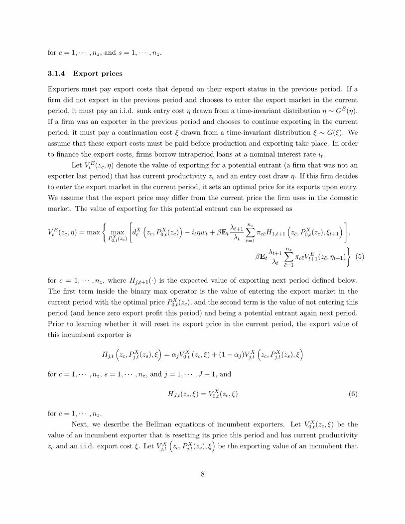
Exporters must pay export costs that depend on their export status in the previous period. If afirm did not export in the previous period and chooses to enter the export market in the currentperiod, it must pay an i.i.d. sunk entry cost η drawn from a time-invariant distribution η ∼ GE(η).If a firm was an exporter in the previous period and chooses to continue exporting in the currentperiod, it must pay a continuation cost ξ drawn from a time-invariant distribution ξ ∼ G(ξ). Weassume that these export costs must be paid before production and exporting take place. In orderto finance the export costs, firms borrow intraperiod loans at a nominal interest rate it.

Let V Et (zc, η) denote the value of exporting for a potential entrant (a firm that was not an

exporter last period) that has current productivity zc and an entry cost draw η. If this firm decidesto enter the export market in the current period, it sets an optimal price for its exports upon entry.We assume that the export price may differ from the current price the firm uses in the domesticmarket. The value of exporting for this potential entrant can be expressed as

V Et (zc, η) = max

{maxPX0,t(zc)

[dXt

(zc, P

X0,t(zc)

)− itηwt + βEt

λt+1λt

nz∑c=1

πccH1,t+1(zc, P

X0,t(zc), ξt+1

) ],

βEtλt+1λt

nz∑c=1

πccVEt+1(zc, ηt+1)

}(5)

for c = 1, · · · , nz, where Hj,t+1(·) is the expected value of exporting next period defined below.The first term inside the binary max operator is the value of entering the export market in thecurrent period with the optimal price PX0,t(zc), and the second term is the value of not entering thisperiod (and hence zero export profit this period) and being a potential entrant again next period.Prior to learning whether it will reset its export price in the current period, the export value ofthis incumbent exporter is

Hj,t

(zc, P

Xj,t(zs), ξ

)= αjV

X0,t (zc, ξ) + (1− αj)V X

j,t

(zc, P

Xj,t(zs), ξ

)for c = 1, · · · , nz, s = 1, · · · , nz, and j = 1, · · · , J − 1, and

HJ,t(zc, ξ) = V X0,t(zc, ξ) (6)

for c = 1, · · · , nz.Next, we describe the Bellman equations of incumbent exporters. Let V X

0,t(zc, ξ) be thevalue of an incumbent exporter that is resetting its price this period and has current productivityzc and an i.i.d. export cost ξ. Let V X

j,t

(zc, P

Xj,t(zs), ξ

)be the exporting value of an incumbent that

8

is not able to adjust its price this period and has current productivity zc, an effective price PXj,t(zs)and an i.i.d. export cost ξ. The export value for incumbent exporters conditional on price reset is

V X0,t(zc, ξ) = max

{maxPX0,t(zc)

[dXt

(zc, P

X0,t(zc)

)− itξwt + βEt

λt+1λt

nz∑c=1

πccH1,t+1(zc, P

X0,t(zc), ξt+1

) ],

βEtλt+1λt

nz∑c=1

πccVEt+1(zc, ηt+1)

}(7)

for c = 1, · · · , nz, and the values conditional on no price reset are

V Xj,t

(zc, P

Xj,t(zs), ξ

)= max

{dXt

(zc, P

Xj,t(zs)

)− itξwt + βEt

λt+1λt

nz∑c=1

πccHj+1,t+1(zc, P

Xj,t(zs), ξt+1

),

βEtλt+1λt

nz∑c=1

πccVEt+1(zc, ηt+1)

}(8)

for c = 1, · · · , nz, s = 1, · · · , nz, j = 1, · · · , J − 2, and

V XJ−1,t

(zc, P

XJ−1,t(zs), ξ

)= max

{dXt

(zc, P

XJ−1,t(zs)

)− itξwt + βEt

λt+1λt

nz∑c=1

πccHJ,t+1 (zc, ξt+1) ,

βEtλt+1λt

nz∑c=1

πccVEt+1(zc, ηt+1)

}(9)

for c = 1, · · · , nz, and s = 1, · · · , nz.Incumbent exporters with current productivity zc that are resetting prices in the current

period choose PX0,t(zc) so as to maximize equation (7). Entrants with current productivity zc choosePX0,t(zc) that solves equation (5). Since the optimal price does not depend on the export costs, for agiven level of current firm-specific productivity zc, entrants and price-resetting incumbent exporterschoose the same optimal price PX0,t(zc).

3.1.5 Exporter entry and exit decisions

We now turn to how firms make decisions on whether or not to participate in the export market. LetηEt (zc) denote the maximum entry cost that last period’s non-exporters with current productivityzc are willing to pay in order to start exporting this period. This threshold entry cost equates thevalue of entering the export market (the first element of the binary max operator in equation (5))to the value of not entering this period (the second element of the binary max operator):

βEtλt+1λt

nz∑c=1

πccVEt+1(zc, ηt+1) = dXt

(zc, P

X0,t(zc)

)−itηEt (zc)wt+βEt

λt+1λt

nz∑c=1

πccH1,t+1(zc, P

X0,t(zc), ξt+1

)

9

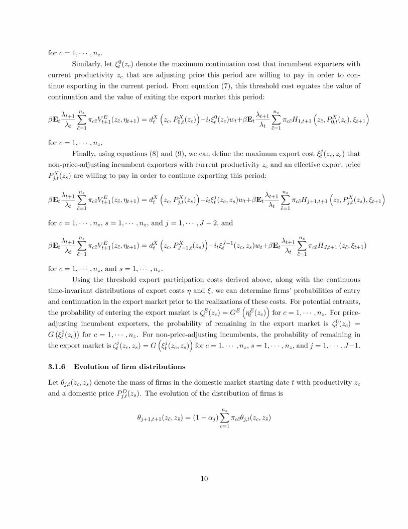
for c = 1, · · · , nz.Similarly, let ξ0

t (zc) denote the maximum continuation cost that incumbent exporters withcurrent productivity zc that are adjusting price this period are willing to pay in order to con-tinue exporting in the current period. From equation (7), this threshold cost equates the value ofcontinuation and the value of exiting the export market this period:

βEtλt+1λt

nz∑c=1

πccVEt+1(zc, ηt+1) = dXt

(zc, P

X0,t(zc)

)−itξ0

t (zc)wt+βEtλt+1λt

nz∑c=1

πccH1,t+1(zc, P

X0,t(zc), ξt+1

)for c = 1, · · · , nz.

Finally, using equations (8) and (9), we can define the maximum export cost ξjt (zc, zs) thatnon-price-adjusting incumbent exporters with current productivity zc and an effective export pricePXj,t(zs) are willing to pay in order to continue exporting this period:

βEtλt+1λt

nz∑c=1

πccVEt+1(zc, ηt+1) = dXt

(zc, P

Xj,t(zs)

)−itξjt (zc, zs)wt+βEt

λt+1λt

nz∑c=1

πccHj+1,t+1(zc, P

Xj,t(zs), ξt+1

)for c = 1, · · · , nz, s = 1, · · · , nz, and j = 1, · · · , J − 2, and

βEtλt+1λt

nz∑c=1

πccVEt+1(zc, ηt+1) = dXt

(zc, P

XJ−1,t(zs)

)−itξJ−1

t (zc, zs)wt+βEtλt+1λt

nz∑c=1

πccHJ,t+1 (zc, ξt+1)

for c = 1, · · · , nz, and s = 1, · · · , nz.Using the threshold export participation costs derived above, along with the continuous

time-invariant distributions of export costs η and ξ, we can determine firms’ probabilities of entryand continuation in the export market prior to the realizations of these costs. For potential entrants,the probability of entering the export market is ζEt (zc) = GE

(ηEt (zc)

)for c = 1, · · · , nz. For price-

adjusting incumbent exporters, the probability of remaining in the export market is ζ0t (zc) =

G(ξ0t (zc)

)for c = 1, · · · , nz. For non-price-adjusting incumbents, the probability of remaining in

the export market is ζjt (zc, zs) = G(ξjt (zc, zs)

)for c = 1, · · · , nz, s = 1, · · · , nz, and j = 1, · · · , J−1.

3.1.6 Evolution of firm distributions

Let θj,t(zc, zs) denote the mass of firms in the domestic market starting date t with productivity zcand a domestic price PDj,t(zs). The evolution of the distribution of firms is

θj+1,t+1(zc, zs) = (1− αj)nz∑c=1

πccθj,t(zc, zs)

10

for j = 1, · · · , J − 1, s = 1, · · · , nz, and c = 1, · · · , nz. The mass of firms in the domestic marketstarting t+ 1 with productivity zc and a domestic price PD1,t+1(zs) is

θ1,t+1(zc, zs) = πsc

J∑j=1

nz∑s=1

αjθj,t(zs, zs)

for s = 1, · · · , nz, and c = 1, · · · , nz. Since there is a unit mass of firms in the domestic market,θ(·) sums up to 1:

∑Jj=1

∑nzc=1

∑nzs=1 θj,t(zc, zs) = 1.

The evolution of the mass of exporters can be described in a similar way but taking intoaccount the probability of entry/exit in the export market. Let ψj,t(zc, zs) be the mass of incumbentsstarting date t with productivity zc and an export price PXj,t(zs), and let NE

t (zc) be the massof entrants with productivity zc at time t. The evolution of the distribution of price-adjustingincumbents is

ψ1,t+1(zc, zs) = πscζ0t (zs)

J∑j=1

nz∑s=1

αjψj,t(zs, zs) + πscNEt (zs)

for c = 1, · · · , nz, and s = 1, · · · , nz, where the first term on the right hand side of the equationis the mass of price-adjusting incumbents continuing to export at time t, and the second termrepresents the mass of entrants at time t. The evolution of the distribution of non-price-adjustingincumbents is

ψj+1,t+1(zc, zs) = (1− αj)nz∑c=1

ζjt (zc, zs)πccψj,t(zc, zs),

for j = 1, · · · , J − 1, s = 1, · · · , nz, and c = 1, · · · , nz. The mass of entrants with productivity zc

at time t is

NEt (zc) = ζEt (zc)

J∑j=1

nz∑s=1

θj,t(zc, zs)−J∑j=1

nz∑s=1

ψj,t(zc, zs)

for c = 1, · · · , nz.

3.2 Final good producers

Final good producers combine domestically produced intermediate goods and imported foreignintermediate goods to produce final goods Dt:

Dt =

ω[∫ 1

0yHt (i)

γ−1γ di

] γγ−1

ρ−1ρ

+ (1− ω)[∫i∈Θt

yFt (i)γ−1γ di

] γγ−1

ρ−1ρ

ρρ−1

, (10)

where ω is the home bias, γ is an elasticity of substitution between intermediate goods produced inthe same country, ρ is the elasticity of substitution between home and foreign intermediate goods(Armington elasticity), and Θt is a set of foreign intermediate goods available in the home countryin period t. Because firms enter and exit the export market over time, the variety of imported

11

products available in the country is time-varying. Final goods are sold at the price Pt to thedomestic household for consumption Ct and investment in physical capital It: Dt = Ct + It.

Final good producers choose yHt (i) and yFt (i) to solve

maxyHt (i),yFt (i)

PtDt −∫ 1

0PDt (i)yHt (i)di−

∫i∈Θ

PX∗t (i)yFt (i)di

subject to the production technology (10). This yields demand for each intermediate good i:

yHt (i) = ωρ(PDt (i)PDt

)−γ (PDtPt

)−ρDt,

and

yFt (i) = (1− ω)ρ(PX∗t (i)PX∗t

)−γ (PX∗t

Pt

)−ρDt,

where PDt =[∫ 1

0 PDt (i)1−γdi

] 11−γ is the price index of domestically produced intermediate goods

and P ∗t =[∫i∈Θt P

X∗t (i)1−γ

] 11−γ is the price index of intermediate goods imported from the foreign

country, which reflects the changes in the variety of imported goods available in the home country(Θt) due to endogenous entry and exit of foreign exporters over time.

Foreign final good producers solve an analogous problem. Their demand for imports fromthe home country is

yH∗t (i) = (1− ω)ρ(PXt (i)PXt

)−γ (PXtP ∗t

)−ρD∗t .

Therefore, the real exports for the home country are

EXt =∫i∈Θ∗t

QtPXt (i)P ∗t

yH∗t (i)di.

3.2.1 Price index

The aggregate price index across all goods available in the home country is

Pt =[ωρ(PDt

)1−ρ+ (1− ω)ρ

(PX∗t

)1−ρ] 1

1−ρ,

where the price index for domestically-produced goods PDt is

PDt =

J∑j=1

nz∑c=1

nz∑s=1

αjθj,t(zc, zs)PD0,t(zc)1−γ +J−1∑j=1

nz∑c=1

nz∑s=1

(1− αj)θj,t(zc, zs)PDj,t(zs)1−γ

11−γ

,

12

and the price index for imported goods PX∗t is

PX∗t =[nz∑c=1

NE∗t (zc)PX∗0,t (zc)1−γ +

J∑j=1

nz∑c=1

nz∑s=1

αjζ0∗t (zc)ψ∗j,t(zc, zs)PX∗0,t (zc)1−γ

+J−1∑j=1

nz∑c=1

nz∑s=1

(1− αj)ζj∗t (zc, zs)ψ∗j,t(zc, zs)PX∗j,t (zs)1−γ] 1

1−γ

.

Since γ > 1, PX∗t is decreasing in the number of available variety of exports, consistent with theresults in the literature on product variety (Feenstra, 1994; Ghironi and Melitz, 2005).

3.3 Household

There is a continuum of identical households in each country. They consume final goods, Ct; makeinvestment, It, in physical capital; and provide labor, Lt, to domestic intermediate-good producers.Households earn labor income, wtLt, and capital rental income, rtKt. They also purchase two typesof one-period bonds. One is a state-contingent international bond B(st+1), sold at price q(st+1|st)in units of the home currency, which yields payoffs contingent on the realization of a particularstate st+1 at time t+ 1. The other is domestically issued bonds BD

t with nominal return it.A representative household chooses Ct, Lt, Kt+1, Bt+1(st+1) and BD

t to solve

max Et

∞∑t=0

βt[ 1

1− σcC1−σct + χ

11− σL

(1− Lt)1−σL]

subject to a period budget constraint:

∑st+1

q(st+1|st)B(st+1) + PtCt + PtIt +BDt = B(st) + Ptdt + PtwtLt + PtrtKt + it−1B

Dt−1,

and the law of motion for capital:

Kt+1 = (1− δ)Kt + It −κ

2

(ItKt− δ

)2Kt.

Because we assume that the international bond markets are complete, the first-order condi-tion with respect to optimal purchases of international state-contingent bonds in the two countriesimplies that the real exchange rate is proportional to the relative marginal utility of consumption:

Qt = e0λ0λ∗0

P ∗0P0

λ∗tλt, (11)

13

where Qt ≡ et P∗tPt

and et is the nominal exchange rate.3

3.4 Monetary policy rule

The monetary authority in each country sets a nominal interest rate it according to a policy rulewith some persistence that reacts to fluctuations in domestic inflation and the real exchange rate:

it = ρiit−1 + (1− ρi)(φππt + φQQt

)+ µt, (12)

where variables with a hat denote percentage deviations from steady-state values, πt ≡ Pt/Pt−1 isdomestic inflation and µt is a monetary policy shock.

3.5 GDP and related variables

We define GDP as

Yt =ωρ(PDtPt

)1−ρDt +Qt(1− ω)ρ

(PXtP ∗t

)1−ρD∗t

PYtPt

,

where P Yt is the GDP deflator defined as

P YtPt≡ (1− gt)

PDtPt

+ gtQtPXtP ∗t

,

and gt is the export-to-GDP ratio defined as

gt ≡Qt(1− ω)ρ

(PXtP ∗t

)1−ρD∗t

PYtPtYt

.

4 Calibration

The model is calibrated to the quarterly frequency. The household subjective discount factor is0.99 to imply the annual real interest rate of 4 percent. We assume that the household periodutility is log in consumption (σc = 1) and linear in leisure (σL = 0). The weight on leisure in theutility function χ is set equal to 1.8 so that the households work 1/3 of their time in steady state.

The elasticity of substitution, ρ, between domestically produced intermediate goods andimported intermediate goods is 1.5 following the literature (see, for example, Backus, Kehoe andKydland (1994) and Chari, Kehoe and McGrattan (2002)). The intratemporal elasticity of substi-tution γ is 3.8 as in Ghironi and Melitz (2005).

3In our calibration, we normalize e0λ0λ∗

0

P∗0P0

= 1.

14

Table 1: Parameter values

Subjective discount factor β 0.99Exponent on consumption σc 1Exponent on leisure σL 0Weight on leisure in utility χ2 1.8Armington elasticity ρ 1.5Share of capital in production ν 0.4Capital depreciation rate δ 0.025Steady-state inflation π 1.021/4

Elasticity of substitution γ 3.8Capital adjustment cost κ 5.85Price adjustment probabilities αj [0.05 0.09 0.25 0.49 0.7 1]Home bias in final goods ω 0.762Upper support on entry cost dist. ηU 2.78Upper support on continuation cost dist. ξU 0.179

Firm-level productivitypersistence ρz 0.81standard deviation σz 0.085number of levels nz 2

Monetary policy rulepersistence ρi 0.8exponent on inflation φπ 2exponent on exchange rate φQ 0.1

15

Table 2: Target statistics and model moments

Data Model

Mass of exporters 0.21 0.23 Bernard et al. (2003)Continuation rate 0.97 0.87 Bernard & Jensen (2004)Entry rate 0.04 0.04 Bernard & Jensen (2004)Imports/GDP 0.12 0.12 Drozd & Nosal (2012)Productivity relative to 1.12–1.18 1.13 Bernard & Jensen (1999)nonexportersMean price adjustment 1.07–3.27 2.66 Bils & Klenow (2004)frequency (qtr) Nakamura & Steinsson (2008)

The share of capital in the production function ν is set equal to 0.4. The depreciation rateof capital δ is 0.025 so that capital depreciates by 10 percent annually. The investment adjustmentcost κ is set equal to 5.85 so that the standard deviation of investment relative to that of GDP is2.91 as in the data.4 We assume that there are two levels of firm-level productivity: nz = 2.

The price adjustment hazard is assumed to rise convexly in the time since last price resetand implies full adjustment by J = 6. The average age of domestic prices over the steady-statedistribution of firms is 2.7 quarters, to be within the estimated range of 1.4–4.3 quarters frommicro-level price adjustments in the recent literature (see, for example, Bils and Klenow (2004) andNakamura and Steinsson (2008)). The steady-state annual inflation rate is set to 2 percent.

We assume that entry and continuation costs (η and ξ, respectively) are both drawn fromuniform distributions with lower support 0. We jointly calibrate the home bias parameter ω, theupper support of entry costs ηU , that of continuation costs ξU , and the persistence and volatilityof the firm-level productivity (ρz and σz) to match (i) the mass of exporters, (ii) the average rateof entry, (iii) the average rate of exit, (iv) the average productivity of exporters relative to that ofnon-exporters, and (v) the imports-to-GDP ratio in the U.S. data. In our model, the steady-statemass of exporters is 23 percent of all the firms in the economy, to be in line with the findingsof Bernard et al. (2003) from data on U.S. manufacturers in 1992. For the entry and exit rates,Bernard and Jensen (2004) report that, on average each year, 87 percent of the exporters continuedexporting in the following year and 14 percent of non-exporters began exporting in the followingyear. These numbers translate to a 97 percent quarterly continuation rate and a 4 percent quarterly

4The simulation is driven by shocks to productivity and monetary policy in both countries. The process forproductivity shocks has persistence of 0.95, the standard deviation of 0.007, and the cross-country correlation of0.25, as in Kehoe and Perri (2002). The process for monetary policy shocks has persistence of 0.12, the standarddeviation of 0.0024, and no exogenous cross-country spillovers, as in Smets and Wouters (2007). The model statisticsare computed as the average of 100 simulations, each simulation with 1000 periods, where the relevant series havebeen logged and HP filtered.

16

entry rate. In our model, the probability that incumbent exporters continue exporting next periodis 87 percent quarterly while the probability of non-incumbent firms entering the export marketis 4 percent quarterly. Exporters are 13 percent more productive relative to non-exporters in oursteady state, to be in line with the observed range of 12 to 18 percent (Bernard and Jensen, 1999).The steady-state ratio of imports to GDP is 0.12, as in the data (Drozd and Nosal, 2012). Table1 summarizes the parameter values used in the baseline calibration, and the calibration targetmoments and the corresponding steady-state moments from our model are reported in Table 2.

5 Results

In this section, we examine a series of impulse responses of our model economy to country-specificaggregate shocks with a focus on the dynamics of the extensive margin of trade. As discussed insection 3.1.5, firms’ export decisions depend on the value of exporting (entry of new exporters, orcontinuation of incumbent exporters) relative to the value of not exporting (no entry for potentialentrants, or exit for incumbent exporters). Equations (5) and (7) suggest that the value of exportingis directly influenced by movements in certain aggregate variables, such as the exchange rate, exportprices, the interest rate, and the aggregate demand in the destination market. Of course, thesevariables are in turn affected by the evolution of the aggregate state of the economy through generalequilibrium effects.

5.1 Monetary policy shocks

We begin our analysis with an expansionary monetary policy shock. Figure 1 shows the impulseresponses of our model economy to a 1 percent expansionary monetary policy shock in the homecountry. The persistence of the shock is set to 0.12 as estimated by Smets and Wouters (2007),and there is no exogenous shock spillover to the foreign country.

With the policy stimulus, we see an immediate increase in the output of the home country.The rise in home consumption relative to that in the foreign country leads to a real depreciation ofthe home currency by 2.3 percent at the impact of the shock. At the same time, the inflationaryeffects of the expansionary shock exert an upward pressure on the current and expected futurecosts of production, and this leads firms to start raising their prices. In our local-currency-pricingsetting, the increase in the price of home exports (relative to the foreign CPI) reduces the foreigndemand for home exports; however, this decline is more than offset by the strong real appreciationof the foreign currency, and we see an increase in the home country’s real export revenues.

For individual firms making decisions on export participation, the lower interest rate reducesthe cost of financing export costs, and the real appreciation of the foreign currency raises theprofitability of exporting. However, we see that export participation (the extensive margin of trade)declines 2.7 percent at the impact of the shock. For incumbent exporters, the rising production

17

Figure 1: Impulse responses to an expansionary monetary policy shock in the home country

0 5 10 15 20-4

-2

0

2Mass of exporters (H)

% d

evia

tio

n

0 5 10 15 200

1

2Export revenues (H)

% d

evia

tio

n

0 5 10 15 200

1

2

3Real exchange rate

% d

evia

tio

n

0 5 10 15 20-1

0

1

2Export price index (H)

% d

evia

tio

n

0 5 10 15 20-1

-0.5

0

0.5Interest rate (H)

pp

t d

evia

tio

n

0 5 10 15 20

0

2

4

GDP

% d

evia

tio

n

Home

Foreign

Notes: Impulse responses to a 1 percent expansionary monetary policy shock in the home country. Thepersistence is set equal to 0.12, with no exogenous shock spillover to the foreign country.

costs imply lower profitability of exporting. The potential export-market share of potential entrantsis diminishing because their optimal prices chosen upon entry reflect rising costs of production andthus are higher than the average price of incumbent exporters whose prices adjust gradually as theresult of nominal rigidities. Therefore, despite the real depreciation of their currency and the lowerinterest rate, the loss of competitiveness due to the inflationary pressure dominates in some firms’export decisions. These results highlight the contrasting relative importance of a policy-induceddepreciation for a country’s aggregate exports and individual firms’ participation in internationaltrade. While the real depreciation contributes to increasing the value of a given unit of exportsales, the inflationary effects of the shock in the domestic economy reduce some firms’ market sharein the export market, thereby diminishing the value of their participation in international trade.As a result, the increased real exports are shared by fewer, more competitive exporters, with eachof them having a larger market share.

The importance of firms’ competitiveness over exchange rate movements in influencingthe dynamics of the extensive margin of trade becomes clearer when we consider simultaneousexpansionary monetary policy shocks in both home and foreign countries. In this case, becausethe dynamic path of consumption is symmetric in the two countries, the shocks cancel out theireffects on their respective currency, and the real exchange rate remains at the steady-state levelthroughout. In addition, relative to the impulse responses in figure 1, the foreign expansionary

18

Figure 2: Impulse responses to simultaneous expansionary monetary policy shocks in the home andforeign countries

0 5 10 15 20-6

-4

-2

0

2Mass of exporters (H)

% d

evia

tio

n

0 5 10 15 20

0

2

4Export revenues (H)

% d

evia

tio

n

0 5 10 15 20-0.1

0

0.1Real exchange rate

% d

evia

tio

n

0 5 10 15 200

1

2

3Export price index (H)

% d

evia

tio

n

0 5 10 15 20-1

-0.5

0

0.5Interest rate (H)

pp

t d

evia

tio

n

0 5 10 15 20

0

2

4

GDP

% d

evia

tio

n

Home

Foreign

Notes: Impulse responses to simultaneous 1 percent expansionary monetary policy shocks in the home andforeign countries. The persistence is set equal to 0.12, with no exogenous shock spillover to the other country.

19

monetary policy shock generates a sizable increase in foreign consumption, which increases foreigndemand for home exports.

In figure 2, we see that the higher aggregate demand in the foreign country due to theexpansionary monetary policy shock there leads to an immediate, sizable increase in home realexports relative to the level we saw in figure 1. In contrast, we continue to see a fall in exporterparticipation of home exporters despite the stronger foreign demand and the lower home interestrate. Since the real exchange rate remains at the steady-state level in this case, the changes inhome export prices are attributed to the rising current and expected future cost of production inthe home country, and the loss of competitiveness leads to fewer firms participating in internationaltrade.

When incumbent exporters face rising production costs, some of them find the real appre-ciation of their foreign sales insufficient to cover their production costs (because of productivityheterogeneity) and export costs (because of their i.i.d. continuation cost draw), and they exit theexport market. On the other hand, for average potential entrants, because they face sunk entrycosts that are on average substantially larger than the average continuation cost paid by incumbentexporters, their potential profit share from the rise in foreign demand is smaller than that of aver-age incumbent exporters. In addition, because of the rising production cost in the home country,the optimal export price chosen by potential exporters is higher than the average export price ofincumbent exporters, which further reduces the potential market share of potential exporters. Asa result, we see a contraction along the extensive margin of trade.

5.2 Productivity shock

We next examine the dynamic responses of our model economy to a positive productivity shockin the home country. We will see that, in contrast to the contraction of the extensive margin inresponse to an expansionary monetary policy shock as seen in figure 1, positive productivity shockslead to an expansion of the extensive margin of trade along with a depreciation of the currency.

Figure 3 shows the impulse responses of the same set of variables as in figures 1 and 2, toa 1 percent positive productivity shock in the home country, with persistence of 0.906 followingBackus, Kehoe and Kydland (1992) and without exogenous cross-country spillover to the foreigncountry. As the shock expands the home country’s production capacity, GDP increases. The higherconsumption in the home country relative to the foreign country implies that the real exchange ratedepreciates for the home currency. At the same time, the higher productivity lowers the marginalcost of production for home intermediate-good producers, and they start lowering their prices. Thelower price of home exports relative to the aggregate price index in the foreign country increasesthe demand for home exports, and, with the appreciation of the foreign currency, we see an increasein the home country’s exports.

Because potential entrants optimally set their prices upon entry, their prices are lower than

20

Figure 3: Impulse responses to a positive productivity shock in the home country

0 5 10 15 200

0.5

1

1.5Mass of exporters (H)

% d

evia

tio

n

0 5 10 15 200

0.5

1

1.5Export revenues (H)

% d

evia

tio

n

0 5 10 15 200

0.2

0.4

0.6Real exchange rate

% d

evia

tio

n

0 5 10 15 20-1

-0.5

0Export price index (H)

% d

evia

tio

n

0 5 10 15 20-0.1

-0.05

0Interest rate (H)

pp

t d

evia

tio

n

0 5 10 15 20

0

1

2GDP

% d

evia

tio

n

Home

Foreign

Notes: Impulse responses to a 1 percent positive productivity shock in the home country. The persistence ofthe shock is 0.906 as in Backus, Kehoe and Kydland (1992), and there is no exogenous spillover of the shockto the foreign productivity process.

21

the average export price of incumbent exporters facing price rigidities. As a result, the potentialmarket share of new entrants increases relative to that of an average incumbent exporter. Atthe same time, the lower domestic inflation leads the monetary authority to lower the interestrate, which contributes to lowering the borrowing costs for exporters to finance export costs. Theincreased price competitiveness of home exports, the real depreciation of the home currency, andthe lower home interest rate together increase the value of exporting, thereby encouraging exportparticipation.5

The procyclical responses of the extensive margin to productivity shocks and its counter-cyclical responses to monetary policy shocks that we saw in section 5.1 offer an important impli-cation for the cyclicality of exporter dynamics. Existing studies have reported that firm dynamicswithin the domestic market are procyclical (see, for example, Bergin and Corsetti, 2008); however,studies on international trade reveal that exporter dynamics in the export market do not necessarilycomove with aggregate output. For example, Naknoi (2015) reports that for a median country inher sample of 99 countries, the extensive margin of exports to the United States is almost uncor-related with output of the exporters’ origin country.6 Our findings suggest that monetary policyshocks may be a contributing factor for the lack of procyclicality in the extensive margin of exportsover business cycles.

Our results also have an interesting implication for the effects of monetary stimulus onthe extensive margin of trade in the face of an economic downturn. As we saw in figure 1, anexpansionary monetary policy can lead to increased real exports, but it also results in a contractionof export participation because of the rising costs of production. This implies that an expansionarymonetary policy shock designed to counteract an economic downturn (due to a negative productivityshock) may not lead to an increased participation of domestic firms in exporting. Such scenario ispresented in figure 4, which shows the dynamic responses of our model economy to a negative homeproductivity shock and a simultaneous expansionary monetary policy shock in the home country.The productivity shock is -1 percent with persistence of 0.5, and the monetary policy shock is-0.2 percent with the persistence of 0.12. We see that, while the expansionary monetary policyhelps to dampen the fall in export revenues, it amplifies the fall in the number of exporters as theinflationary effects of the shock raise production costs and erodes the value of exporting.

5In figure 3, we see that the mass of exporters changes immediately following the shock. This is in contrast tothe hump-shaped response of the extensive margin to a productivity shock in a flexible-price model of Alessandriaand Choi (2007). One may wonder that such a sharp fall in the mass of exporters is driven by incumbent exporterscircumventing price rigidities by exiting the export market and then re-entering next period with an optimal price(since entrant exporters are able to optimize their prices). We tested this possibility with a version of our model inwhich prices are adjusted with probability one within two periods, thus eliminating the benefits of strategic re-entry.We find that this model still exhibits an immediate peak response of the extensive margin to productivity shocks,ruling out the possibility of strategic re-entry as the reason for the absence of hump-shaped responses of the mass ofexporters in our model. We thank George Alessandria for the suggestion.

6Alessandria and Choi (2008) also report that the correlation between the number of exporters and output is-0.35 while that for the number of domestic establishments and output is 0.28 for the United States over the periodbetween 1975 and 2006.

22

Figure 4: Impulse responses to a negative home productivity shock and a simultaneous expansionarymonetary policy in the home country

0 5 10 15 20-2

-1

0

Mass of exporters (H)

% d

evia

tio

n

0 5 10 15 20

-0.6

-0.4

-0.2

0

Export revenues (H)

% d

evia

tio

n

0 5 10 15 20

-0.2

0

0.2

0.4

Real exchange rate

% d

evia

tio

n

0 5 10 15 20

0

0.5

1Export price index (H)

% d

evia

tio

n

0 5 10 15 20-0.2

-0.1

0

0.1Interest rate (H)

pp

t d

evia

tio

n

0 5 10 15 20

-0.5

0

0.5

GDP

% d

evia

tio

n

Negative TFP shock only

Negative TFP shock + Monetary stimulus

Notes: Blue lines: Impulse responses to a 1 percent negative productivity shock in the home country witha persistence of 0.5. Green lines: Impulse responses to a 1 percent negative productivity shock in the homecountry with a persistence of 0.5 and a simultaneous expansionary monetary policy shock in the home countryof the size 0.2 percent with persistence of 0.12.

23

Figure 5: Impulse responses to an expansionary monetary policy shock under various elasticitylevels for γ and ρ

(a) Varying γ

0 5 10 15 20-8

-6

-4

-2

0

2Mass of exporters (H)

% d

evia

tio

n

0 5 10 15 200

0.5

1

1.5

2

2.5Export revenues (H)

% d

evia

tio

n

=2 Baseline (=3.8) =7

(b) Varying ρ

0 5 10 15 20-3

-2

-1

0

1Mass of exporters (H)

% d

evia

tio

n

0 5 10 15 200

1

2

3Export revenues (H)

% d

evia

tio

n

Baseline (=1.5) =0.8

Notes: Panel (a): Impulse responses to a 1 percent expansionary monetary policy shock in the home country, underdifferent values of the elasticity of substitution, γ. The persistence of the shock is 0.12, with no exogenous spillover ofthe shock to the foreign monetary policy. Panel (b): Impulse responses to the same 1 percent expansionary monetarypolicy shock in the home country, from our baseline model and an otherwise identical model with a lower Armingtonelasticity (ρ = 0.8).

5.3 The role of the elasticity of substitution

In figures 1 and 2, we saw that firms’ export participation in our model is highly sensitive to theirprices relative to other exporters and the price level in the destination economy. The responsivenessof trade to changes in prices, at least quantitatively, depends on the elasticity of substitutionbetween different good varieties. There are two types of elasticity of substitution in our model:the elasticity of substitution between goods produced within the same country γ; and the elasticityof substitution between goods produced in different countries ρ (Armington elasticity). In thissubsection, we examine how various degrees of each elasticity affect export decisions.7

7When nz > 1 as in our baseline calibration, export probabilities of some firm types reach 0 (1) as we increase(decrease) γ or ρ, in which case the model cannot be solved using the linear method we employ. Therefore, in order toensure that an interior fraction of each firm type exports in any given period, we consider a special case with nz = 1for the analysis in this subsection.

24

We first vary the elasticity of substitution between goods produced in the same country γ,which is set to 3.8 in our baseline calibration. In figure 5a, we see that the responsiveness of theextensive margin of trade is increasing in this elasticity of substitution. Other things being equal,a higher elasticity implies that demand falls more for a given increase in the price of an exportedgood. Therefore, in the presence of price rigidities, potential and incumbent exporters with pricesthat are higher than the average export price face a reduced potential export market share andhence export profitability, and we see stronger selection effects among exporters as the elasticityof substitution increases. Qualitatively, however, lowering the elasticity of substitution does notincrease export participation in response to the monetary policy shock. The initial response ofthe extensive margin of trade is still negative (-0.7 percent at the impact of the shock) when theelasticity is lowered to 2, which implies a markup of 100 percent.

We next examine how the Armington elasticity ρ affects the dynamic responses of theextensive margin of trade. There is much debate regarding the estimates of this elasticity, andvarious values have been used in the literature on international business cycles.8 In our baselinecalibration, it is set to 1.5, implying that domestic and foreign goods are substitutes. We comparedour baseline results with those from an otherwise identical model with ρ = 0.8, where domestic andforeign goods are now complements. In figure 5b, we see that, similar to the case for γ above, themagnitude of the fall in the extensive margin of trade is increasing in the value of the Armingtonelasticity, but qualitatively, the negative response remains. With a lower Armington elasticity, totalforeign demand for home exports becomes less elastic to the deviation of the home export pricerelative to the foreign CPI, and firms’ export profitability is less affected by price increases. As aresult, we see a smaller fall along the extensive margin of trade.

5.4 Alternative Taylor-rule specifications and exporter dynamics

5.4.1 Inflation stabilization

Our results above suggest that inflationary effects of an expansionary monetary policy shock un-dermine the competitiveness of some exporters, discouraging their participation in internationaltrade, despite the currency depreciation and the lower interest rate. It has been shown in the mon-etary policy literature that the monetary authority that is systematically more aggressive towardstabilizing inflation is able to better anchor inflation expectations. In this subsection, we examinethe effects of monetary policy stance toward inflation stabilization on the dynamics of the extensivemargin of trade.

Figure 6 compares the impulse responses of our model economy with an expansionarymonetary policy shock in the benchmark calibration (φπ=2 in equation (12)) and in an otherwiseidentical model wherein the monetary authority in the home country is more aggressive towardinflation fluctuations (φπ=4). As expected, with a higher weight on inflation in the policy reaction

8See, for example, Backus, Kehoe and Kydland (1994), Heathcote and Perri (2002) and Ruhl (2008).

25

Figure 6: Impulse responses to a home expansionary monetary policy shock under different mone-tary policy responsiveness to inflation

0 5 10 15 20-4

-2

0

Mass of exporters (H)

% d

evia

tio

n

0 5 10 15 200

1

2 Export revenues (H)

% d

evia

tio

n

0 5 10 15 20-1

0

1

2

3 Real exchange rate

% d

evia

tio

n

0 5 10 15 20-1

0

1

2 Export price index (H)

% d

evia

tio

n

0 5 10 15 20-1

-0.5

0

0.5Interest rate (H)

pp

t d

evia

tio

n

0 5 10 15 20

0

2

4

GDP (H)

% d

evia

tio

n

Benchmark (=*

=2)

More aggressive on inflation stabilization (=4, *

=2)

Notes: Impulse responses to an expansionary monetary policy shock in the home country, from our baselinemodel and an otherwise identical model wherein the monetary authority in the home country is systematicallymore aggressive toward controlling inflation. The benchmark responses are the same as those in figure 1. Thealternative model assumes that the Taylor rule coefficient on inflation φπ is 4 for the home country.

26

Figure 7: Impulse responses to an expansionary monetary policy shock in the home country undervarying policy responsiveness to exchange rate movements

0 5 10 15 20-4

-2

0

Mass of exporters (H)

% d

evia

tio

n

0 5 10 15 20

0

1

2Export revenues (H)

% d

evia

tio

n

0 5 10 15 200

1

2

3Real exchange rate

% d

evia

tio

n

0 5 10 15 20-1

0

1

2Export price index (H)

% d

evia

tio

n

0 5 10 15 20-1

-0.5

0

0.5Interest rate (H)

pp

t d

evia

tio

n

0 5 10 15 20

0

2

4

GDP (H)

% d

evia

tio

n

Baseline (Q

=*Q

=0.1) Q

=*Q

=1

Notes: Impulse responses to an expansionary monetary policy shock in the home country, from our baselinemodel and an otherwise identical model wherein the monetary authority in both countries is systematicallymore responsive to real exchange rate movements. The benchmark responses are the same as those in figure 1.The alternative model assumes that the Taylor rule coefficient on the real exchange rate is 1 in both countries(φQ = φ∗Q = 1).

function, the expansion in the home country is moderated, and the real exchange rate depreciatesby less. This weaker inflationary pressure in the home country alleviates the loss of competitivenessfor home firms in the export market, and the fall in the extensive margin of trade is dampened.9

5.4.2 Policy responsiveness to exchange rate movements

In an open-economy environment, a country’s external position may be a concern for monetarypolicy-makers, and the monetary authority may respond to fluctuations in the exchange rate ofits currency, in addition to its inflation stabilization objective. In this subsection, we consider analternative Taylor-rule specification in which the monetary authority in both countries places asizable weight on exchange rate movements in their respective policy reaction function.

9We find that making the policy function in the foreign country also sensitive to inflation (φπ = φ∗π = 4) doesnot alter the dynamic responses of the export-related variables shown in figure 6 in any significant way. The figureis available upon request

27

Figure 8: Impulse responses to an expansionary monetary policy shock in the home country underproducer currency pricing

0 5 10 15 20-6

-4

-2

0

2Mass of exporters (H)

% d

evia

tio

n

0 5 10 15 200

1

2

3Export revenues (H)

% d

evia

tio

n

Notes: Impulse responses to an expansionary monetary policy shock in the home country from an otherwiseidentical model with producer currency pricing. The size and persistence of the shock are identical to those infigure 1.

In figure 7, we see that making the policy reaction function in both countries more responsiveto fluctuations in the real exchange rate has negligible effects on the extensive margin of tradein response to an expansionary monetary policy shock in the home country. In this case, inresponse to pressure for appreciation of the foreign currency due to the relative increase in homeconsumption, the foreign monetary authority responds by lowering its interest rate. This bringsexpansionary effects on foreign GDP and consumption, and foreign demand for home exportsexpands. This increase in foreign demand, however, is offset by the attenuated appreciation of theforeign currency. Further, we also see that the dynamic path of the export price index for thehome country is little affected by the alternative Taylor-rule specifications. This implies negligiblechanges in the competitiveness of home exporters relative to the baseline case, and the responseof exporter participation is little affected by the monetary authority’s stance to exchange ratefluctuations.

5.5 Comparison to the producer-currency-pricing setting

In our baseline model, we assumed that firms set the prices of their exports in the currency ofthe destination economy (local-currency pricing). In a recent study, Cooke (2014) shows that inresponse to a monetary expansion, the extensive margin of trade expands under local currencysetting, while it declines under producer currency pricing. We examined whether the extensivemargin responses are affected by the assumption of the currency in which exports are priced in ourmodel framework.

In figure 8, we find that, also under producer currency pricing, the extensive margin of tradefalls in response to an expansionary monetary policy shock. As in the case of local currency pricing,a rise in the marginal cost of production dominates the effects of the foreign currency appreciation,and the resulting rise in export prices reduces the demand for exports of some exporters. This is incontrast to the implications of Cooke’s model (2014), where expenditure switching due to exchangerate movements leads to changes in demand at upstream production, which in turn drives demand

28

for intermediate goods at the downstream production level where exporter entry and exit occur.

5.6 Suggestive evidence from U.S. export data

We provide suggestive empirical evidence supporting our theoretical results that the extensivemargin of exports declines in response to an expansionary monetary policy shock. Figure 9 showsthe VAR responses of the extensive margin of U.S. exports and the U.S. dollar exchange rateindex to a one standard deviation expansionary monetary policy shock. Following Armenter andKoren (2014), we measure the extensive margin of exports using monthly data on the number ofshipments collected through customs forms for each export shipment from the U.S. Census Bureau.The sample period covers from January 2002 to November 2017.10 The ordering of the variablesin our VAR specification is [U.S. monetary policy rate, foreign industrial production index, theextensive margin of U.S. exports, the U.S. exchange rate]. The foreign industrial production indexis a trade weighted average of industrial production indexes for 10 major trade partners for theUnited States, and is included to account for changes in foreign demand for U.S. exports. Basedon residual tests, we include four lags in the VAR.

We see that an expansionary monetary policy shock leads to a depreciation of the U.S.dollar in the short run, and the response is statistically significant during the peak responses (rightpanel). With the depreciation of the currency, we see a delayed but persistent negative responsein the extensive margin of U.S. exports (left panel), consistent with our theoretical results. Sinceour data are at the monthly frequency, the delayed response in the extensive margin is likely to bedue to the contractual nature of international trade. In the short- to medium-run, the extensivemargin contracts statistically significantly for about 10 months following the shock.11

6 Conclusions

In this paper, we examined the response of the extensive margin of trade to monetary policyshocks and the role of various aggregate factors affecting individual firms’ decision to participatein international trade. We developed a two-country dynamic stochastic general equilibrium modelwherein heterogeneous firms make state-contingent, dynamic decisions on whether and how muchto export and prices are staggered across firms and time.

We showed that while a lower interest rate and a currency depreciation associated with anexpansionary monetary policy both contribute to increasing the profitability of export participa-tion, inflationary effects of the policy stimulus weaken the competitiveness of exporters and lead to

10Detailed descriptions of the data are in Appendix A.11We also estimated a two-stage VAR specification, in which we first regressed the U.S. policy rate on domestic

inflation and output, and then estimated the response of the extensive margin of trade to the policy rates residualsobtained from the first-stage regression. We chose to estimate such a two-stage regression instead of including inflationand output directly in order to keep the number of variables in the final VAR specification at a minimum. The resultsare similar to our baseline specification. The figures are available upon request.

29

Figure 9: VAR responses of the extensive margin to an expansionary monetary policy shock1 5 10 15

-0.5

-0.4

-0.3

-0.2

-0.1

0Federal Funds Rate

1 5 10 15

-8

-6

-4

-2

0

Foreign IP index

1 5 10 15-10

-5

0

5Extensive margin of exports

1 5 10 15

-5

0

5

10US real exchange rate

Notes: VAR responses of the extensive margin of exports and the U.S. real exchange rate to a 1 standarddeviation, expansionary monetary policy shock in the United States. The dotted lines indicate the 68 percentconfidence intervals.

a contraction in firms’ export participation. This is in contrast to an implication of a productivityshock that generates an expansion along the extensive margin of trade while depreciating the cur-rency. Qualitatively, our findings are robust to the assumed degrees of the elasticity of substitutionbetween goods and whether exported goods are priced in the destination currency or the producers’currency. Further, our results lend support to empirical findings that the extensive margin of tradeis not necessarily procyclical, unlike the firm dynamics (or product creation) within the domesticmarket, and we provided suggestive empirical evidence using VAR that the extensive margin oftrade responds negatively to an expansionary monetary policy shock.

The current model framework can be extended in a number of ways to address some of therecent developments in the trade literature. One important direction may be an analysis of theimplication of global value chains for firms’ export participation. For example, recent empiricalstudies have reported that international input-output linkages contribute substantially to cross-country comovement of producer price inflation (Auer, Levchenko and Saure, 2017; Auer, Borioand Filardo, 2017). This finding implies that, in our framework, domestic monetary policy shocksmay have less impact on export participation by firms in its own country, but may have strongereffects on exporter dynamics in trade partners’ economies. Such an extension would allow for anew direction for the analysis of monetary policy transmission in open economies.

30

References

[1] Alessandria, George, and Horag Choi, “Do Sunk Costs of Exporting Matter for Net ExportDynamics,” Quarterly Journal of Economics, 122 (2007), 289-336.

[2] Alessandria, George, and Horag Choi, “The Role of Exporting and Trade for Entry over theBusiness Cycle,” working paper, 2008.

[3] Armenter, Roc, and Miklos Koren, “A Balls-and-Bins Model of Trade,” American EconomicReview, 104 (2014), 2127-2151.

[4] Auer, Raphael, Claudio Borio, and Andrew Filardo, “The Globalisation of Inflation: TheGrowing Importance of Global Value Chains,” BIS Working Papers, No. 602 (2017).

[5] Auer, Raphael, Andrei Levchenko, and Philip Saure, “International Inflation Spillovers throughInput Linkages,” NBER Working Paper 23246 (2017).

[6] Backus, David K., Patrick J. Kehoe, and Finn E. Kydland, “Dynamics of the Trade Balanceand the Terms of Trade: The J-Curve?” American Economic Review, 84 (1994), 84-103.

[7] Backus, David K., Patrick J. Kehoe, and Finn E. Kydland, “International Real BusinessCycles,” Journal of Political Economy, 100 (1992), 745-775.

[8] Bergin, Paul R., and Giancarlo Corsetti, “The Extensive Margin and Monetary Policy,” Jour-nal of Monetary Economics, 55 (2008), 1222-1237.

[9] Bernard, Andrew B., Jonathan Eaton, J. Bradford Jensen, and Samuel Kortum, “Plants andProductivity in International Trade,” American Economic Review, 93 (2003), 1268-1290.

[10] Bernard, Andrew B., and J. Bradford Jensen, “Exceptional Exporter Performance: Cause,Effect, or Both?” Journal of International Economics, 47 (1999), 1-25.

[11] Bernard, Andrew B., and J. Bradford Jensen, “Why Some Firms Export,” Review of Economicsand Statistics, 86 (2004), 561-69.

[12] Bilbiie, Florin O., Ippei Fujiwara, and Fabio Ghironi, “Optimal Monetary Policy with Endoge-nous Entry and Product Variety,” Journal of Monetary Economics, 64 (2014), 1-20.

[13] Bilbiie, Florin O., Fabio Ghironi, and Marc J. Melitz “Monetary Policy and Business Cycleswith Endogenous Entry and Product Variety,” NBER Macroeconomics Annual, 22 (2007),299-353.

[14] Bils, Mark, and Peter J. Klenow, “Some Evidence on the Importance of Sticky Prices,” Journalof Political Economy, 112 (2004), 947-985.

31

[15] Cavallari, Lilia, “Firms’ Entry, Monetary Policy and the International Business Cycle,” Journalof International Economics, 91 (2013), 263-274.

[16] Chari, V.V., Patrick J. Kehoe, and Ellen R. McGrattan, “Can Sticky Price Models GenerateVolatile and Persistent Real Exchange Rates?,” Review of Economic Studies, 69 (2002), 533-563.

[17] Cooke, Dudley, “Monetary Shocks, Exchange Rates, and the Extensive Margin of Exports,”Journal of International Money and Finance, 41 (2014), 128-145.

[18] Cooke, Dudley, “Optimal Monetary Policy with Endogenous Export Participation,” Review ofEconomic Dynamics, 21 (2016), 72-88.

[19] Drozd, Lukasz A., and Jaromir B. Nosal, “Pricing-to-Market in Business Cycle Models,” work-ing paper (2012).

[20] Feenstra, Robert C., “New Product Varieties and the Measurement of International Prices,”American Economic Review, 84 (1994), 157-177.

[21] Ghironi, Fabio, and Marc Melitz, “International Trade and Macroeconomic Dynamics withHeterogeneous Firms,” Quarterly Journal of Economics, 120 (2005), 865-915.

[22] Heathcote, Jonathan, and Fabrizio Perri, “Financial Autarky and International Business Cy-cles,” Journal of Monetary Economics, 49 (2002), 601-627.

[23] Imura, Yuko, “Endogenous Trade Participation with Price Rigidities,” Journal of InternationalEconomics, 100 (2016), 14-33.

[24] Kehoe, Patrick J., and Fabrizio Perri, “International Business Cycles with Endogenous Incom-plete Markets,” Econometrica, 70 (2002), 907-928.

[25] Krippner, Leo, “Measuring the Stance of Monetary Policy in Zero Lower Bound Environ-ments,” Economics Letters, 118 (2013), 135-138.

[26] Melitz, Marc, “The Impact of Trade on Intra-Industry Reallocations and Aggregate IndustryProductivity,” Econometrica, 71 (2003), 1695-1725.

[27] Nakamura, Emi, and Jon Steinsson, “Five Facts about Prices: A Reevaluation of Menu CostModels,” Quarterly Journal of Economics, 123 (2008), 1415-1464.

[28] Naknoi, Kanda, “Exchange Rate Volatility and Fluctuations in the Extensive Margin of Trade,”Journal of Economic Dynamics and Control, 52 (2015), 322-339.

[29] Ruhl, Kim J., “The International Elasticity Puzzle,” working paper (2008).

32

[30] Smets, Frank, and Rafael Wouters, “Shocks and Frictions in US Business Cycles: A BayesianDSGE Approach,” American Economic Review, 97 (2007), 586-606.

33

Appendix

A Data descriptions

The extensive margin of U.S. exports is measured by the count of U.S. export shipments from theU.S. Census Bureau, which is publicly available from January 2002 onward. Our sample periodcovers the period from January 2002 to November 2017. Since this sample period includes theperiod when the Federal Reserve used quantitative easing programs, we use Leo Krippner’s monthlyaverage Shadow Short Rate (SSR) estimates for the period between January 2002 and November2017. Leo Krippner’s series, available at www.rbnz.govt.nz/research-and-publications/research-programme/additional-research/measures-of-the-stance-of-united-states-monetary-policy, containsthree different summary measures of the the United States monetary policy stance (Krippner,2013). We focus our attention on SSR, which approximates an effective federal funds rate adjustedby the monetary policy stimulus implied by the Federal Reserve Bank’s balance sheet position. Theforeign industrial production index is an export-weighted industrial production index of 10 majortrade partners for the United States that include Canada, Japan, South Korea, Mexico, Turkey,UK, Brazil, India, Russia and EU19, reported by OECD. The exchange rate is a geometric U.S.export-weighted index of the following 16 bilateral exchange rates against the U.S. dollar: Argentinepeso, Australian dollar, Brazilian real, Canadian dollar, Chinese renminbi, Indian rupee, Indonesianrupiah, Japanese yen, Mexican peso, Russian ruble, Saudi riyal, South African rand, South Koreanwon, Turkish lira, British pound and the Euro. These 16 currencies are representative of the G20economies other than the United States. All series are seasonally adjusted and detrended using alinear trend.

34