1

The Fallacy of the Fiscal Theory of the Price Level – Once More

20 March 2017

Willem H. Buiter1

Global Chief Economist, Citigroup

Adjunct Professor of Economics, SIPA, Columbia University

Adjunct Senior Fellow, Council on Foreign Relations

1 The views and opinions expressed in this paper are those of the author alone. They cannot be taken to represent the views and opinions of Citigroup or of any other organization or entity I am affiliated with. I would like to thank Dirk Niepelt, Chris Sims, Mauricio Une and Ilker Domac for helpful comments on an earlier draft of this paper.

2

Abstract

Necessary conditions for valid general equilibrium analysis include: (1) the number of equations equals the number of unknowns; (2) if (1) holds, the resulting solution(s) make sense. The fiscal theory of the price level fails on both counts, both away from and at the ELB. The underlying fallacy is the confusion of the intertemporal budget constraint of the State with a misspecified government bond pricing equilibrium equation. This means overdetermined systems unless (a) the price level is flexible, (b) the interest rate is the monetary policy instrument and (c) there is a non-zero stock of nominal government bonds. Thus, a sticky price level or a nominal money stock rule imply inconsistency. When all three conditions are satisfied, unacceptable anomalies occur: negative price levels; the FTPL can price money when money does not exist; the logic of the FTPL applies equally to the intertemporal budget constraint of any household; when the bond pricing equation is specified correctly, there is no FTPL. The FTPL has nothing to do with monetary vs. fiscal dominance or active v. passive fiscal policy. The FTPL implies government debt is never a problem; the price level takes care of it, and not through unanticipated inflation or financial repression. If acted upon by fiscal authorities, the consequences could be severe. There is a correct fiscal theory of seigniorage. The issuance of return-dominated and/or irredeemable central bank money creates fiscal space and ensures that a combined monetary-fiscal stimulus always boosts nominal aggregate demand.

Keywords: Fiscal theory of the price level; intertemporal budget constraint; equilibrium bond pricing equation; monetary and fiscal policy coordination.

JEL Categories: E31, E40, E50, E58, E62, H62, H63 Willem H. Buiter Citigroup Global Markets, 390 Greenwich Street New York, NY 10069-0214, USA Tel. + 1 347 979 6067 E-mail: willem.buiter@citi.com E-mail2: whb1002@gmail.com Web: http://willembuiter.com

1

The Fallacy of the Fiscal Theory of the Price Level – Once More

(1) Introduction The so-called fiscal theory of the price level (FTPL) is making an unexpected and

undesirable comeback. On 1 April, 2016 a conference with “Next Steps for the Fiscal Theory of

the Price Level” as its theme was held at the Becker Friedman Institute for Research on Economics

at the University of Chicago.2 Many of the originators of the FTPL participated, including

Christopher Sims, John Cochrane and Eric Leeper and promoted it (see e.g. Sims (2016a),

Cochrane (2016a, b) and Jacobson, Leeper and Preston (2016)). As argued in this paper, there is

a good fiscal theory of the price level, or rather a fiscal theory of seigniorage (FTS), and a bad

fiscal theory of the price level. What was being promoted at this conference was the bad FTPL –

a false theory based on an elementary but fundamental fallacy: the confusion of the intertemporal

budget constraint (IBC) of the State with a misspecified equilibrium (nominal) government bond

pricing equation.

Two necessary conditions for valid general equilibrium analysis are: (1) make sure the

number of equations equals the number of unknowns; and (2), if condition (1) is satisfied, make

sure the resulting solution(s) make sense. The FTPL fails on both counts.

The FTPL was originally developed starting in the early 1990s, by Leeper (1991), Sims

(1994), Woodford (1994, 1995, 2001), Cochrane (1998, 2001, 2005) and Bassetto (2002)). It was

shown, in papers by Buiter (1998, 2001, 2002, 2005) and Niepelt (2004), to be logically

inconsistent in all but one class of models, and to be full of extreme, unacceptable anomalies in

that one class of models where it is not necessarily logically inconsistent: models with a flexible

nominal price level, an exogenous rule for the nominal interest rate and a non-zero stock of

nominal government bonds outstanding.

The argument that the FTPL rests on a fallacy and that the theory is consequently false was

never refuted. However, the FTPL was proposed and dismantled before risk-free nominal interest

rates in virtually all the advanced economies fell to unprecedentedly low levels following the Great

2 For the program and links to the presentations see https://bfi.uchicago.edu/events/next-steps-fiscal-theory-price-level.

2

Financial Crisis of 2007-2009. The zero lower bound (ZLB) or, more accurately, the effective

lower bound (ELB) for risk-free nominal interest rates did not play a role in the original discussion

of the FTPL. Some of the recent attempts by originators of the FTPL to resurrect it (see Sims

(2011, 2013, 2016a, b, c), Leeper (2015, 2016) and Cochrane (2016a, b, c)), contain suggestions

that it may be particularly relevant and powerful when the economy is at the ELB. This paper

proves that the FTPL fails for the same reasons at the ELB.

It is hard to understand how a theory that produces the manifest inconsistencies and

anomalies outlined in Section 1 below and proven in detail in the Appendix, could have survived

the normal academic refereeing process when it was first proposed. It is even harder to understand

how all the old mistakes are trotted out again in the recent attempts to resurrect the FTPL, including

the presentations given at the “Next Steps for the Fiscal Theory of the Price Level” conference.3

For instance, Eric Leeper, one of the original FTPL contributors, stated the following in a

note distributed at the “Next Steps…” conference (referring to the IBC of the consolidated general

government and central bank):

“The second condition is a valuation equation that equates the real market value of nominal

government liabilities to the expected present value of primary—net of interest payments— budget

surpluses.” (Leeper (2015, page 2)).

John Cochrane goes one further at the “Next Steps …” conference, where he referred to

the intertemporal budget constraint of the State as follows:

” This is a valuation equation, an equilibrium condition, not a budget constraint”. (Cochrane

(2016b, p. 1)).

Another example is Christopher Sims, who at the 2016 Jackson Hole Conference presented

a paper that emphasized the role of non-monetary nominally denominated government debt in the

FTPL:

“The fiscal theory of the price level is based on a simple notion.1 The price level is not only the

rate at which currency trades for goods in the economy, it is also the rate at which dollar-

denominated interest-bearing government liabilities trade for goods. Just as inflation reduces the

3 For a website containing information about this conference, and many of the presentations, see https://bfi.uchicago.edu/events/next-steps-fiscal-theory-price-level. The only (mildly) critical noise was made by Harald Uhlig (2016).

3

value of a 20-dollar bill, it reduces the value of a ten-thousand-dollar mature treasury bill.” (Sims

(2016c, page 4)).

The existence of non-monetary nominally denominated public debt is crucial for the FTPL to have

even a faint stab at appearing to be mathematically coherent (albeit under restrictive conditions

and plagued by the anomalies listed below in Section 1 and in the Appendix).

The most recent attempts to revive the FTPL are rather bereft of complete formal models.

Often only the misspecified government bond pricing equilibrium equation is provided. Only Sims

(2016a) provides an explicit Keynesian model which, when analyzed correctly, as is done in the

Appendix, Section A4, turns out to be overdetermined and therefore internally inconsistent when

the key assumption of the FTPL is imposed on it.

The case against the FTPL is not and never was an empirical one. Nor does it depend on

any of its assumptions being viewed as unrealistic. The rejection of the FTPL always rested, and

continues to rest, on its logical flaws, inconsistencies and egregious anomalies. An inconsistent

theory can have no empirical implications and the realism or lack of it of its assumptions is

irrelevant.

The outline of the rest of the paper is as follows. Section 1 gives a non-technical exposition

of the misspecified nominal government bond pricing equilibrium condition and the

inconsistencies and anomalies inherent in the FTPL. Section 2 explains that it is important to

expose the fatal flaws in the FTPL because, if taken seriously and acted upon by fiscal and

monetary policy makers, bad things could happen in the real world. Section 3 provides a brief,

non-technical discussion of the correct way to look at the inherent fiscal dimension of monetary

policy through the fiscal theory of seigniorage or FTS. The Appendix provides a formal analysis

of some simple models to establish in a rigorous manner the propositions and assertions in Sections

1 and 3.

1. The Bad Fiscal Theory of the Price Level As noted in the Introduction, the original sin of the FTPL is the confusion of the

intertemporal budget constraint of the State with a misspecified government nominal bond pricing

equilibrium condition. The IBC of the State and a correctly specified government bond pricing

equilibrium condition look similar but are quintessentially different.

4

The intertemporal budget constraint of the State constrains the fiscal-financial-monetary

program (FFMP) of the State – the paths of or rules for current and future public spending, taxation

and money issuance - to ensure that the contractual value (notional or face value) of the net non-

monetary debt (‘bonds’) of the State does not exceed the present discounted value (PDV) of current

and future primary (non-interest) surpluses of the State plus the PDV of current and future

seigniorage.4 Paths of or rules for current and future public spending, taxation and monetary

issuance must be consistent with all contractual obligations of the State being met in full.

Permissible FFMPs must satisfy the IBC identically, that is, for all possible values of prices,

quantities and other variables that enter into the IBC – not just in equilibrium. Rules for current

and future fiscal and monetary policy that ensure that the IBC of the State is always satisfied are

called Ricardian FFMPs.

Let ts denote the real value of the primary surplus of the state (the real value of taxes net

of transfers minus real government spending on goods and services, excluding interest); tσ is the

real value of seigniorage - central bank money issuance net of any interest paid on central bank

money; tB is the number of (one-period) nominal bonds issued by the government outstanding at

the beginning of period t; the contractual value of that nominal bond is 1 unit of money; tb is be

the number of (one period) index-linked bonds issued by the government outstanding at the

beginning of period t; in the Appendix, longer-maturity bonds are considered also, without this

changing any of the results; the general price level (in terms of money) in period t is tP ; the

contractual value in terms of money of an index-linked bond is tP ; ,t t jR + is the real risk-free

discount factor from period t+j to period t, that is ,0 , 1

1 if 11

j

t t jk t k t k

R jr+

= + + +

= ≥+∏ and , 1t tR = ,

where , 1j jr + is the risk-free real interest rate between periods j and j+1.

4 The nominal value of seigniorage in a period is the value of the change in the stock of central bank money minus any interest paid on central bank money during that period. Let tM be the nominal stock

of central bank money at the beginning of period t, , 1Mt ti − the own interest rate on central bank money

paid in period t on money carried over from period t-1 and tP the period t general price level then

1 , 1 , 1(1 )M Mt t t t t t t t

tt t

M i M M i MP P

σ + − −− + ∆ −≡ = .

5

The IBC of the State can be written as in equation (1.1):

( )0

,t

t t j t jjt

t t jB

b R sP

σ∞

+ +=

++ ≤ +∑ (1.1)

In equation (1) both the nominal bond and the index-linked bond are valued at their

contractual values. In period t, the quantities of the two bonds are inherited from the past and are

therefore given. The IBC imposes on the State the constraint that, whatever paths or rules it

chooses for current and future primary surpluses and seigniorage (henceforth augmented primary

surpluses), the present discounted value (PDV) of current and future augmented primary surpluses

must be at least equal to the contractual value of the government bonds outstanding. Paths of or

rules for augmented primary surpluses (or for their constituent components (taxes, public

spending, seigniorage) that satisfy equation (1) are Ricardian FFMPs.

A properly specified equilibrium bond pricing equation version instead states that the

market value or effective value of the net bond debt of the State equals the PDV of the actual

current and future primary surpluses of the State (whatever these are), plus the PDV of the actual

current and future seigniorage (whatever that may be). In the equilibrium bond pricing approach,

the FFMP is whatever it is. Essentially arbitrary sequences or rules for public spending, taxes,

monetary issuance and policy rates are permitted. Such overdetermined FFMPs that are not

required to satisfy the IBC of the State identically are called non-Ricardian FFMPs.

There is no reason to expect that a non-Ricardian FFMP will support a market value of the

outstanding net government bond debt that is equal to its contractual value. The PDV of current

and future augmented primary surpluses generated by a non-Ricardian FFMP could equal or

exceed the contractual value of the outstanding net stock of government bonds. In that case, the

market value of the bonds equals the contractual value of the bonds. The State is wasting ‘fiscal

space’.

It is also possible that the PDV of current and future primary surpluses plus seigniorage

generated by a non-Ricardian FFMP is less than the contractual value of the outstanding net stock

of government bonds. In that case, the market value of these bonds is less than their contractual

value. In the simple formal models that have been used to analyze the FTPL, the government is

in default or insolvent immediately. In more realistic and complex models the government could

6

merely be viewed as having a positive probability of default (that is, of not being able to meet its

contractual obligations) at some time in the future.5

When the equilibrium bond pricing equation generates a market value for the bonds that is

below their contractual value, the market price represents a discount on the contractual price. In

Buiter (2001, 2002) I referred to the ratio of the market value of a government bond to its

contractual value as the bond revaluation factor. The bond revaluation factor cannot be greater

than 1 or less than 0 (private creditors of the government cannot be turned into private debtors). I

shall denote the bond revaluation factor by tD , where 0 1tD≤ ≤ .

If we only consider Ricardian FFMPs, the bond revaluation factor will, by construction,

always be equal to 1 and can be ignored.

If we consider non-Ricardian FFMPs, we have to introduce the market value of government

debt or, equivalently, the bond revaluation factor, as an additional variable. This is shown in

equation (1.2) which differs from equation (1.1) in three ways. First, the weak inequality in

equation (1.1) becomes a strict equality in equation (1.2); second, the bond revaluation factor, tD ,

in equation (1.2) transforms the contractual values of the bonds into effective or market values;6

third, to emphasize the fact that we are dealing with arbitrary, non-Ricardian FFMPs, I put overbars

over the primary surpluses and seigniorage terms to emphasize that they are effectively exogenous

and will only by happenstance satisfy equation (1.2) with 1tD = .

5 In Niepelt (2004), the author argues that even if one accepts the valuation equation approach, this implies an intertemporal budget constraint if one imposes rational expectations and if one goes back to a truly initial period where debt is issued. Once this is accepted, the nominal anchor disappears and the possibility to run “arbitrary” (non-Ricardian) fiscal policies disappears as well—the price level cannot be relied upon to satisfy the IBC. If a bond revaluation factor less than 1 were to occur in the initial period when a government bond is issued, it would not be possible to price that bond at par. The State either sells it at the appropriate discount to its contractual value or the State cannot sell the bond. Niepelt’s analysis and mine are substantially the same. I am indebted to Dirk Niepelt for pointing this out to me. Of course, as pointed out in Daniel (2007), if, in that initial period, all the necessary conditions for the FTPL to generate an equilibrium price level sequence are satisfied (flexible prices, exogenous nominal interest rate, non-zero stock of government bonds), the FTPL might be able to pick a price level sequence that yields a unique, non-explosive equilibrium. This amounts to ‘relocating’ the FTPL to the initial period. Even if there is no inconsistency (overdeterminacy) in this case, the five anomalies introduced below still invalidate the FTPL. 6 I assume that nominal bonds and index-linked bonds have the same revaluation factor. This can easily be generalized to allow different revaluation factors for the two types of bonds.

7

( )0

,t

t t t j t jjt

t t jB

D b R sP

σ∞

+ +=

++ = +

∑ (1.2)

The FTPL considers non-Ricardian FFMPs but does not add a bond revaluation factor to

the model. So, equation (1.2) is replaced by:

( )0

,t

t t j t jjt

t t jB

b R sP

σ∞

+ +=

++ = +∑ (1.3)

Since the FTPL adds an additional equation (the bond pricing equilibrium condition) but

does not add another unknown, a model of the economy that has a determined (or determinate)

equilibrium under Ricardian FFMPs should be overdetermined under a non-Ricardian FFMP, that

is, mathematically inconsistent with more equations than unknowns,

And indeed, that is what happens for the vast majority of economic models that have been

studied. There is one class of models for which the imposition of a non-Ricardian FFMP does not

create an overdetermined system. Not surprisingly, that is the class of models for which the

equilibrium is underdetermined under Ricardian FFMPs. That class of model has fully flexible

nominal prices and a monetary policy that pegs the short nominal interest rate (the interest rate on

one-period nominal bonds with a contractual value of 1 unit of money). With Ricardian FFMPs,

both the general price level and the nominal money stock are indeterminate in such an economy.

With the nominal interest rate pegged, the nominal stock of money is endogenous – determined by

the demand for money. There is no nominal anchor. The stock of real money balances (the nominal

money stock deflated by the general price level) is, however, determinate.

Adding the bond pricing equilibrium condition to this economy, with a non-Ricardian

FFMP, leads to a determinate equilibrium, but only if a third condition is satisfied: there is a non-

zero stock of nominal government bonds outstanding. In that case the general price level tP can

(under certain conditions) play the role of the bond revaluation factor tD . The general price level

reconciles the real value of the outstanding stock of nominal government bonds, valued at their

contractual value of 1 unit of money, with the PDV of current and future primary surpluses and

seigniorage (which, under non-Ricardian FFMPs can be anything) minus the outstanding stock of

index-linked government bonds, also valued at their contractual value. Even if the FTPL-favorable

8

trinity of a flexible price level, and exogenous nominal interest rate and a non-zero stock of

government nominal bonds are present, the FTPL fails because it leads to unacceptable anomalies.7

A theory is only as good as the sum total of its logical implications and empirical

predictions. The anomalies and inconsistencies of the FTPL outlined below mean that it cannot

be taken seriously.

Anomalies

1. The FTPL can generate a negative price level unless its domain of validity is arbitrarily

restricted.

Even in the flexible price level, interest rate pegging world, there is a wide range of feasible

values of the exogenous variables, policy rules and inherited bond stocks for which the ‘nominal

7 Sims (2016a) does not actually contain the intertemporal budget constraint of the State – either in its true IBC incarnation or transmuted into a misspecified government bond pricing equilibrium equation by requiring it to hold with equality, yet insisting that all government bonds are priced at their contractual values. Both Sims (1994) and Sims (2016a) contain the single period budget identity of the State (in Sims (2016a) this is the continuous time version). In Sims (2016a) this instantaneous budget identity is never explicitly integrated forward in time, with the proper solvency constraint imposed. I assume in the Appendix (Section A4) that the IBC of the State is used as a misspecified nominal bond pricing equilibrium condition. In Sims (1994), there is an intertemporal budget constraint for the State (equations (48) and (49)), that incorporates what Sims calls the “social budget constraint” – which appears to be the goods market equilibrium condition (private consumption plus real resources used up in transactions equal the endowment). It is assumed to hold with equality and values government bonds at their contractual values. Sims (2016a) develops a standard flexible price level model of an endowment economy, with money introduced through a transactions technology function. Under any rule that sets the short nominal interest rate exogenously (or as a function of real variables alone, exogenous or endogenous) and that has the nominal money stock determined endogenously, such an economy will have an indeterminate nominal price level and nominal money stock if we either require the IBC of the State to hold always/identically because fiscal, financial and monetary policies are Ricardian, or if we permit non-Ricardian policies and specify the proper equilibrium government bond pricing condition - one that allows actual (market) bond prices to be less than their contractual values. Sims considers non-Ricardian policies (one of these, with real taxes going up when the real value of the public debt rises does, actually, look quite Ricardian). He then establishes that there is a unique sequence of values for the general price level that stops the economy (including the real debt stock) from exploding and thus violating the solvency condition of the State – Ponzi finance is not permitted in the long run. The Sims (1994) model is therefore a standard FTPL model, where, with flexible prices, an exogenous nominal interest rate and a non-zero stock of nominal bonds, the FTPL is not necessarily inconsistent. It does, of course, encounter the 5 anomalies outlined in this paper, which render it invalid even when it is not internally inconsistent. In Sims (2016a) the price level is predetermined, so there cannot be an FTPL.

9

bond pricing equilibrium equation’ generates a negative general price level. From equation (1.3)

this will be the case when

( ) ( )0 0

, ,0 and 0 or when 0 and 0t j t j t t t j t j t tj j

t t j t t jR s b B R s b Bσ σ∞ ∞

+ + + += =

+ ++ − < > + − > <∑ ∑ .

So, if there is a positive stock of nominal government bonds outstanding and the PDV of

current and future augmented primary surpluses minus the value of the outstanding stock of index-

linked debt is negative, the FTPL implies a negative price level. The same holds if there is a

negative stock of nominal government bonds outstanding and the PDV of current and future

augmented primary surpluses minus the value of the outstanding stock of index-linked debt is

positive. A negative general price level is generally considered an undesirable feature in a model

of a monetary economy.

2. There is no FTPL if all public debt is index-linked (or denominated in foreign currency).

The bond discount factor or bond revaluation factor approach given in equation (1.2) works

fine even without nominal bonds. From equation (1.3), the FTPL (which treats the IBC of the state

as a bond pricing equilibrium condition for arbitrary FFMPs, but still insists that bonds are priced

at their contractual value – the bond revaluation factor is omitted – this means that asserts

( )0

,t t j t jj

t t jb R s σ∞

+ +=

+= +∑ , which is likely to be a problem, because the stock of index-linked bonds

is given and the non-Ricardian FFMP would only by chance generate a PDV of current and future

augmented primary surplus that equals the value of those index-linked bonds, if they are valued at

their contractual values. This means that, in general, if there is only index-linked and/or foreign

currency denominated sovereign bond debt, there is an inconsistency (the bond pricing equation is

violated) and, in the flexible price level case with an exogenous nominal interest rate, the general

price level and the nominal stock of money are indeterminate.

Adding the bond revaluation factor, as in equation (1.2) resolves this inconsistency. The

equilibrium (real) bond pricing equation now determines the value of the bond revaluation factor:

( )0

,t t t j t jj

t t jD b R s σ∞

+ +=

+= +∑ . Note that the same argument can be made if government bonds are

denominated in foreign currency.

3. The FTPL can determine the price of phlogiston – it can determine an equilibrium price

without an associated quantity.

10

The FTPL can determine the general price level (the reciprocal of the price of money) even

if there is no money in the economy. Consider the case where there is no supply of or demand for

money balances. Money does not exist as an intrinsically valuable commodity, as paper money,

as a bookkeeping entry or as e-money or cyber money. It does not exist as a store of value, medium

of exchange or means of payment. The only way in which something named ‘money’ exists is as

an abstract or imaginary unit of account or numéraire. For some reason, government debt happens

to be denominated in terms of this numéraire. Instead of something non-existing called ‘money’,

we could use another abstract/imaginary numéraire – phlogiston, say, the substance formerly

believed to be embodied in all combustible materials. It this world, when the FTPL supports a

positive general price level, it manages to price non-existent phlogiston, just as it can price non-

existent money. I consider this to be an undesirable feature, not something to exult over.

To illustrate the deep conceptual bizarreness of the phlogiston economy, consider what a

one-period maturity pure discount nominal bond actually is in such an economy. It promises, in

period t, to pay the purchaser, ‘something’ in period t+1. That something cannot be one unit of

phlogiston, because phlogiston does not exist except as a unit of account. Instead it promises to

pay the holder in period t+1 something worth one unit of phlogiston in period t+1. How do we

know what one unit of phlogiston is worth in period t+1 – in terms of things that actually exist

other than as pure numéraires? Well, we have this phlogiston-denominated bond equilibrium

pricing condition in every period. It tells us that the real value (in terms of goods and services that

have intrinsic value) of the phlogiston-denominated bond, valued at its contractual value in terms

of phlogiston, has to be equal to the PDV of current and future real augmented primary budget

surpluses of the State.

So, in a world where money does not exist except as a pure numéraire, a nominal bond (a

bond promising a future payment worth 1 unit of money, say) is the ultimate non-deliverable

forward contract.8 I believe that it makes no sense to model a world where non-deliverable

contracts exist without there also being a deliverable benchmark. There must exist money as a

8 According to Investopedia “A non-deliverable forward (NDF) is a cash-settled, short-term forward contract in a thinly traded or nonconvertible foreign currency against a freely traded currency, where the profit or loss at the settlement date is calculated by taking the difference between the agreed upon exchange rate and the spot rate at the time of settlement, for an agreed upon notional amount of funds. The gain or loss is then settled in the freely traded currency”, http://www.investopedia.com/terms/n/ndf.asp. The key relevant point is that no payment in the thinly traded or nonconvertible currency is ever made. All payments are made in the freely traded currency. The amount of the freely traded currency paid is given by the notional amount of the contract times the difference between the agreed upon forward rate and the spot rate at the time of settlement.

11

commodity (with or without intrinsic value) or as a financial claim issued by some legal – or even

personal - entity. The has to be a benchmark spot market for money and a deliverable forward

contract for money for a non-deliverable forward contract for money to make sense. In the

preceding paragraph the word ‘money’ can be replaced by ‘phlogiston’.

The FTPL fails this test, insofar as it can price money (phlogiston) is a world where there

are no deliverable spot or forward contracts for money (phlogiston). I recognize this is an anomaly

rather than a logical inconsistency. I do, however, consider this anomaly to be as devastating as

the logical inconsistencies inherent in the FTPL: it is inconceivable to me to work with a model of

the economy that can determine an equilibrium price without an associated equilibrium quantity.

4. The FTPL makes as much sense as the HTPL or the ‘Mr Jones Theory of the Price Level.

The logic of turning the IBC of the State into a nominal bond pricing equilibrium condition,

but without introducing a bond discount factor or bond revaluation factor, can be applied to the

IBC of the household sector or even to that of a single household, as long as it holds a non-zero

stock of nominally denominated non-monetary financial assets or liabilities. Consider the IBC of

household i (Mr Jones, say). The stocks of nominal and index-linked household debt outstanding

at the beginning of period t are and i ih ht tB b ; , , and i i i ih h h h

t t t ty cτ σ are, respectively, the real factor

income, real taxes net of transfers, consumption and the real value of the accumulation of money

balances net of interest paid on money of Mr Jones in period t.

( ),0

ii i i i i

hh h h h htt t t j t j t j t j t j

jt

B b R y cP

τ σ∞

+ + + + +=

+ ≤ − − −∑ (1.4)

We can turn the IBC of Mr Jones into a Mr Jones equilibrium nominal bond pricing

equation by having equation (1.4) hold with equality. As with the FTPL, we don’t introduce a

bond revaluation factor but continue to price Mr Jones’s bond debt holdings at their contractual

values.

( ),0

ii i i i i

hh h h h htt t t j t j t j t j t j

jt

B b R y cP

τ σ∞

+ + + + +=

+ = − − −∑ (1.5)

Mr Jones could adopt an overdetermined or (non-Ricardian) consumption and asset

allocation program (as indicated by the overbars in equation (1.5)) and wait for the general price

level to take on the value that reconciles that non-Ricardian program with his outstanding stock of

nominal debt. If this household theory of the price level (HTPL) or even individual household/Mr

12

Jones theory of the price level is too weird to be taken seriously - as I believe it is - then so is the

FTPL, which uses identical logic.

5. When the equilibrium bond pricing equation is specified correctly, there is no FTPL.

Consider the case where we have an overdetermined, non-Ricardian FFMP, but we do the

proper thing of adding a debt revaluation factor to the bond pricing equilibrium condition. We are

in the world of equation (1.2). Assume that there is a non-zero stock of nominal government bonds

outstanding and that the conditions that would produce a negative price level (given under

Anomaly 1) are not satisfied. Now the FTPL cannot determine the general price level, even in a

flexible price level world with a pegged nominal interest rate and a non-Ricardian FFMP. We are

back where we should be – in a world without a nominal anchor and thus with an indeterminate

general price level and nominal money stock.

In addition to the list of unacceptable anomalies that are implied by the FTPL, even in the

single class of models where it is not internally inconsistent, it is easily shown that there is a very

wide range of models where the FTPL inevitably leads to internally inconsistencies –

overdetermined equilibria.

Inconsistencies 1. The FTPL implies an overdetermined system if there is an exogenous rule for the nominal

money stock.

If instead of pegging the nominal interest rate (or adopting some exogenous rule for the

nominal interest rate) the monetary authority adopts an exogenous rule for the nominal money

stock (with the nominal interest rate now endogenous), the system is overdetermined under the

non-Ricardian FFMP – mathematically inconsistent. This is true even if the price level is perfectly

flexible, because the price level is determined twice: once by the IBC of State doing the job of a

nominal bond equilibrium pricing equation and once by the monetary equilibrium condition – the

condition that the demand for real money balances equals the real value of the money supply.9

9In the Appendix I show that at the ELB, the FTPL creates an overdetermined system under an exogenous rule for the nominal money stock if the demand for real money balances does not have satiation at a finite stock of real money balances. If there is satiation in real money balances at a finite value of the stock of real money balances, is it possible, for certain values of the parameters and the nominal stock of bonds that the system is not overdetermined.

13

2. The FTPL implies an overdetermined system if the general price level is not freely

flexible.

If the general price level is not freely flexible (that is, in any Keynesian model where

nominal price and wage rigidities are present) the system is overdetermined under the non-

Ricardian FFMP – mathematically inconsistent. The price level at any point in time would be

determined twice, once by history and once by the IBC of the State, doing the job of a misspecified

nominal bond pricing equilibrium equation. An example of this is the Keynesian model developed

by Sims (2016a), as shown in detail in the Appendix, Section A4 below.

It is hard to understand how a theory that produces Inconsistencies 1 and 2 and Anomalies

1 through 5 could ever have survived the normal Academic refereeing process when it first hit the

professional journals. But it is worse than that: as noted in the Introduction, this logically defective

fiscal theory of the price level is making an unexpected and undesirable comeback

2. Why it matters The attempted resurrection of the FTPL matters not just for academic or scholarly reasons.

Clearly, propositions and theories that are internally inconsistent must be exposed and relegated to

the dustbin of intellectual history. However, in addition to these academic concerns, there are

material real-world policy risks associated with fiscal and monetary policy makers being

convinced that the FTPL is the appropriate way to consider the interaction of monetary and fiscal

policy in driving inflation, aggregate demand, real economic activity and sovereign default risk.

An implication of the FTPL is that monetary and fiscal policy makers – either acting in a

cooperative and coordinated manner or acting in an independent and uncoordinated manner – can

choose just about any paths or rules for real public spending on goods and services, real taxes net

of transfers, interest rates and/or monetary issuance, now and in the future, without having to be

concerned about meeting their contractual debt obligations. Somehow, the general price level is

guaranteed to take on the value required to ensure that the contractual value of the stock of nominal

non-monetary public debt outstanding, when deflated by that price level, is exactly consistent with

the State meeting its IBC, that is, consistent with it being solvent - meeting all its contractual

obligations.

Because this makes absolutely no sense at all, it could be dangerous if taken seriously and

acted upon by monetary and fiscal policy makers. After all, what could be more appealing to a

14

politician anxious to curry favor with the electorate through public spending increases and tax cuts,

than the reassurance provided by the FTPL, that solvency of the State is never a problem.

Regardless of the outstanding stocks of State assets and liabilities, the State can specify arbitrary

paths or (contingent) rules for public spending, taxation, monetary issuance and/or nominal policy

interest rates. Explosive sovereign bond trajectories will never threaten sovereign solvency. The

general price level will do whatever it takes to bring the real value of the stock of nominal

government bonds (valued at face value or contractual value) to the level required for government

solvency. If some misguided government were to take this delusional theory seriously and were

to act upon it, the result, when reality belatedly dawns, could be painful fiscal tightening,

government default, excessive recourse to inflationary financing and even hyperinflation.

The risk of the FTPL rubbing off on policy makers could well be real. In a recent note,

Katsushiko Aiba and Kiichi Murashima noted - referring to the FTPL as developed by Sims - that

“… the Nikkei and other media have recently reported his prescription for achieving the inflation

target based on the FTPL. We should keep a close eye on this theory because PM Abe’s economic

advisor Koichi Hamada is a believer, meaning that it might be adopted in Japan’s future

macroeconomic policies”. (Aiba and Murashima (2017, page 1).

In Brazil, André Lara Resende (2017) argues in a contribution to Valor Econômico, a

Brazilian financial newspaper, that high real interest rates in Brazil are simply the result of high

nominal interest rates. His analysis is based on the analysis of John Cochrane in Cochrane (2016a),

which has the FTPL as one of its key building blocks. If this argument ever gained traction among

monetary policy makers in Brazil, it could result in costly policy mistakes.

Note that in conventional (non-FTPL) monetary economics too, changes in the general

price level change the real value of the outstanding stock of nominal bonds (private as well as

public). Indeed, when faced with imminent default on its debt, a government may well opt for

excessive monetary financing of government deficits and driving up inflation. Unanticipated

inflation (that is, inflation that was unanticipated at the time the nominal debt was issued) can

cause the ex-post, realized real interest rate on nominal debt to be lower that the ex-ante, expected

real interest rate at the time the debt was issued. Financial repression (keeping nominal interest

rates below market rates) can further reinforce the ‘unanticipated inflation tax’ on holders of

nominally denominated government bonds. This indeed accounts for a sizeable part of the

15

reduction in the general government gross debt-to-GDP ratio after World War II in the UK, the US

and many other countries. As noted, this has nothing to do with the FTPL.

3. The Good Fiscal Theory There is a good fiscal theory of the price level, or rather a fiscal theory of seigniorage

(FTS). Fortunately, not all recent thinking about the interrelationships between monetary and

fiscal policy making or between the central bank and the national Treasury is invalidated by the

fallacy of the FTPL.

3.a. The fiscal theory of seigniorage

I will start with a brief characterization of the (good) fiscal theory of seigniorage. The FTS

starts from the recognition that central banking tends to be profitable and that the national Treasury

is the beneficial owner of the central bank. Regardless of the formal ownership arrangements for

the central bank and regardless of the degree of operational independence that a central bank may

have in the design and implementation of monetary policy, the Treasury is entitled to the profits of

the central bank. Because central banking is profitable, a monetized expansion of the central bank

balance sheet increases fiscal space – it relaxes the IBC of the consolidated central bank and central

government. If the fiscal authorities make use of this enhance fiscal space by cutting taxes and/or

raising public spending, nominal aggregate demand can be boosted. Monetary policy therefore

always and everywhere has a fiscal dimension.

The FTS insists that both the central bank and the national Treasury always satisfy their

IBCs. Their actions have to satisfy their IBCs identically, that is, for all possible values of prices,

quantities and other variables that enter into the IBCs – not just in equilibrium. For the central

bank, these actions are monetary issuance, asset purchases and sales, interest rate policies and

remittances to the Treasury. For the Treasury, actions are exhaustive public spending10, taxes net

of transfers, sales and purchases of Treasury debt and remittances paid by the central bank).

It should not come as a surprise that this is what a solvency constraint or (intertemporal)

budget constraint means in a market economy: an economic agent, including the Treasury and the

central bank, can only choose actions that will ensure that they live within their means if they want

10 Exhaustive public spending is public spending on real goods and services (consumption or investment) as opposed to transfer payments, which in what follows are treated as negative taxes.

16

to remain solvent and not have their debt valued at a discount to its contractual value. A hard

budget constraint is the defining characteristic of a functioning market economy.

Because the Treasury is the beneficial owner of the central bank, it makes sense to

consolidate the single-period budget constraints, balance sheets and IBCs of the central bank and

the Treasury and work with a consolidated single-period budget constraint, balance sheet and IBC

of the State.

Like the central bank and the Treasury severally, the consolidated State has to satisfy its

IBC identically if it wishes to see its debt trade at its contractual value. In simple models with

complete markets, this means that, for all admissible values of the variables entering the IBC that

are not choice variables of the State, the State has to design its fiscal-financial-monetary

programme in such a way that it satisfies its IBC. It must always be able to honor its contractual

obligations. In models with incomplete markets, default and insolvency are always possible in

principle, and the requirement that the State satisfies its IBC identically ex-ante has to be relaxed

in a way that does not violate the spirit of the hard budget constraint. An example would be the

requirement that the State always satisfies its IBC in expectation. The issue of the meaning and

enforcement of IBCs in a world with uncertainty and incomplete markets is important but not

relevant to the good FTS vs. bad FTPL issue.

3.b. The FTS and joint monetary-fiscal policy effectiveness – even at the ELB

There are two reasons why central banking is profitable. The first one is widely recognized:

because of the unique liquidity properties of central bank monetary liabilities (typically notes and

coin (currency) and central bank sight deposits held by commercial banks and similar eligible

counterparties (required reserves and excess reserves), private agents are willing to hold central

bank money even if it is ‘pecuniary rate-of-return-dominated’.

Households and firms hold currency with a zero nominal interest rate even when the short

risk-free nominal interest rate on non-monetary financial instruments (nominal bonds) is positive.

Commercial banks hold excess reserves with the central bank even though the risk-adjusted

financial rate of return on other investments open to these commercial banks exceeds the interest

rate on excess reserves held with the central bank. As long as the pecuniary rate of return on

central bank assets exceeds that on its liabilities, central banking will be profitable.

17

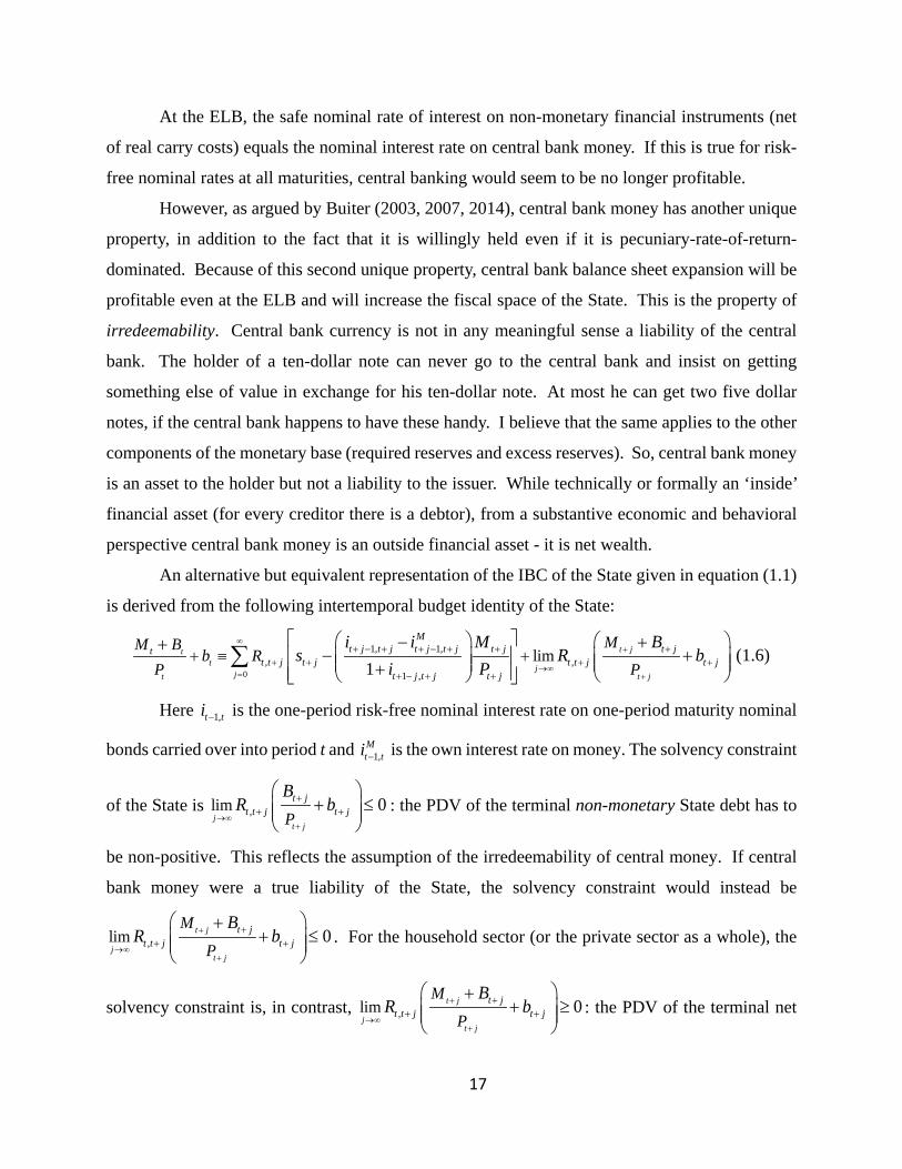
At the ELB, the safe nominal rate of interest on non-monetary financial instruments (net

of real carry costs) equals the nominal interest rate on central bank money. If this is true for risk-

free nominal rates at all maturities, central banking would seem to be no longer profitable.

However, as argued by Buiter (2003, 2007, 2014), central bank money has another unique

property, in addition to the fact that it is willingly held even if it is pecuniary-rate-of-return-

dominated. Because of this second unique property, central bank balance sheet expansion will be

profitable even at the ELB and will increase the fiscal space of the State. This is the property of

irredeemability. Central bank currency is not in any meaningful sense a liability of the central

bank. The holder of a ten-dollar note can never go to the central bank and insist on getting

something else of value in exchange for his ten-dollar note. At most he can get two five dollar

notes, if the central bank happens to have these handy. I believe that the same applies to the other

components of the monetary base (required reserves and excess reserves). So, central bank money

is an asset to the holder but not a liability to the issuer. While technically or formally an ‘inside’

financial asset (for every creditor there is a debtor), from a substantive economic and behavioral

perspective central bank money is an outside financial asset - it is net wealth.

An alternative but equivalent representation of the IBC of the State given in equation (1.1)

is derived from the following intertemporal budget identity of the State:

0

1, 1,, ,

1 ,

lim1

t jtt j

jt t j

Mt j t j t j t j t j t jt

t t j t j t t j t jt j t j t j

MM Bb R

P P

i i M Bs R b

i P

∞+

→∞= +

+ − + + − + + ++ + + +

+ − + +

+ ≡ + − ++

− + + ∑ (1.6)

Here 1,t ti − is the one-period risk-free nominal interest rate on one-period maturity nominal

bonds carried over into period t and 1,Mt ti − is the own interest rate on money. The solvency constraint

of the State is ,lim 0j

t j

t jt t j t jP

BR b

→∞+

++ +

+ ≤

: the PDV of the terminal non-monetary State debt has to

be non-positive. This reflects the assumption of the irredeemability of central money. If central

bank money were a true liability of the State, the solvency constraint would instead be

,lim 0t j

jt j

t jt t j t j

M

P

BR b+

→∞+

++ +

++ ≤

. For the household sector (or the private sector as a whole), the

solvency constraint is, in contrast, ,lim 0t j

jt j

t jt t j t j

M

P

BR b+

→∞+

++ +

++ ≥

: the PDV of the terminal net

18

financial assets of the private sectors, including its holdings of central bank money, has to be non-

negative. This reflects the assumption that central bank money is seen as an asset by the private

holders. This asymmetric treatment of central bank money in the solvency constraints of the

private sector and the public sector accounts for the ability of monetized central bank balance sheet

expansion to increase fiscal space even at the ELB. Substituting the solvency constraint of the

State into its intertemporal budget identity gives the IBC of the State:

0

1 , 1 ,, ,

1 ,

lim1

t jtt j

jt t j

Mt j t j t j t j t jt

t t j t j t t jt j t j t j

MM Bb

P P

i i MR s R

i P

∞+

→∞= +

− + + − + + ++ + +

− + + +

+ ≤ + −+

− + ∑ (1.7)11

Because central bank money is not a true liability of the State, fiscal space is increased (the

IBC of the State is relaxed) when the PDV of the ‘terminal’ stock of money balances increases.

Under normal conditions it is plausible that the long-run proportional growth rate of the nominal

money stock is less than the nominal interest rate. It that case ,lim 0t j

jt j

t t j t

M

PR +

→∞+

+ = . Consider,

however, the case where the economy is in a permanent liquidity trap, with the nominal interest

rate on bonds, i, equal to the nominal interest rate on central bank money: 1, 1, , 0Mt t t ti i t− −= ≥ . To

simplify the exposition further, assume that the nominal interest rate on central bank money is zero

(all central bank money is currency, say). say. In that case

, ,1 1

lim lim limt jt j t jj j j

t j t tt t j t t j

MM M

P P PR I+

+ +→∞ →∞ →∞

+

+ +≡ = , where ,t t jI + is the risk-free nominal discount factor

between period t+j and period t, with ,0 , 1

1 if 11

j

t t jk t k t k

I ji+

= + + +

= ≥+∏ and , 1t tI = . So, any

permanent increase in the monetized balance sheet of the central bank would relax the IBC of the

State one-for-one. It is up to the fiscal authorities to make use of this relaxation of the IBC of the

State by boosting public spending or cutting taxes.

11 The intertemporal budget identity of the State that results in the IBC given in (1.1) is

( )0

, ,limtt t j t j j

jt t j

t jt t j t t j t j

Bb R s

P P

BR bσ

∞

+ +→∞

= +

++ + ++ ≡ − +

+

∑ . Using the solvency constraint of the State that

recognizes the irredeemability of central bank money, ,lim 0j

t j

t jt t j t jP

BR b

→∞+

++ +

+ ≤

, results in the alternative but

equivalent representation of the IBC of the State given in equation (1.1).

19

From this it follows that a combined monetary-fiscal stimulus (a monetized tax cut or

increase in public spending) can always stimulate aggregate demand, even at the ELB (see Buiter

(2003, 2014)). Popularly known as ‘helicopter money’ (see Friedman (1969)), such a monetized

fiscal stimulus may well be the only thing that will lift a country like Japan out of its decades-old

liquidity trap.

The ability to stimulate aggregate demand through a helicopter money drop also exists

when the model of the economy exhibits ‘debt neutrality’ for non-monetary government debt.

Government bonds, even though they have the same interest rates as government money at the

ELB, don’t have this net wealth property. A government bond drop would only boost demand if

the future taxes required to service the increased public debt were to be paid by economic agents

that have lower propensities to spend than the beneficiaries of the bond drop – unborn future

generations, say. In that case, there is no ‘debt neutrality’.12

The ability to stimulate aggregate demand through a helicopter money drop exists away

from and at the ELB, and regardless of whether government bonds are nominal bonds, index-

linked bonds or foreign-currency-denominated bonds.13

The FTS goes back a long way. A classic example is the ‘Unpleasant Monetarist

Arithmetic’ paper of Sargent and Wallace (1981). That paper provides an example of an economy

in which inflation is always and everywhere a monetary phenomenon, but money itself is a fiscal

phenomenon. In the model, there is an upper bound on the ratio of non-monetary government debt

(bonds) to GDP. Once that bond ceiling is reached, the money supply becomes endogenous

because public spending and taxes are given exogenously. Such ‘fiscal dominance’ can be

contrasted with ‘monetary dominance’, where the central bank chooses the size and composition

of its balance sheet (including the stock of central bank money) over time and the fiscal authorities

take the central bank’s actions or rules of behavior as given and adjust their public spending and

taxes to them in such a way as to maintain sovereign solvency. Both monetary and fiscal

dominance are perfectly consistent with a non-FTPL view. Either we have Ricardian FFMPs - if

the IBC of the State must be satisfied always (identically), that is, if we impose a solvency

12 Assuming there is no operative intergenerational gift and bequest motive.

20

constraint restricting central bank and Treasury behavior to ensure that all outstanding debt can be

serviced on the original contractual terms - or we have non-Ricardian, overdetermined FFMPs, in

which case the IBC of the State, holding with equality and with a bond revaluation factor added,

morphs into a government bond pricing equation that determines a market price of bonds that can

be lower than their contractual value or face value. Ricardian FFMPs can have either monetary or

fiscal dominance, as the Unpleasant Monetarist Arithmetic Paper shows. Non-Ricardian FFMPs

(which I would not characterize as exhibiting either fiscal dominance or monetary dominance but

just as overdetermined FFMPs) don’t need the FTPL to produce a well-specified, consistent model.

All they need is an endogenous bond revaluation factor. The notion that the FTPL is about fiscal

dominance and the traditional approach about monetary dominance is incorrect.

The fiscal dimension of monetary policy (and specifically of central bank monetized

balance sheet expansion) exists even if the central bank is operationally independent and even if

there is ‘monetary dominance’ (or active monetary policy and passive fiscal policy) rather than the

‘fiscal dominance’ (or active fiscal policy and passive monetary policy), as assumed in the

‘Unpleasant Monetarist Arithmetic’ paper after the ceiling on the government debt-to-GDP ratio is

reached.14 The key insight is that, given the outstanding stocks of State assets and liabilities, you

cannot specify monetary policy (base money issuance) and fiscal policy (public spending and

taxes) independently if you want to ensure the State remains solvent. Either there is fiscal

dominance and monetary issuance becomes endogenously determined (the residual), or there is

monetary dominance and public spending and/or taxation have to adjust (becomes the residual) to

maintain sovereign solvency (to satisfy the IBC of the State.

4. Conclusion The fiscal theory of the price revel rests on a fundamental fallacy: the confusion of an IBC

with a misspecified equilibrium nominal bond pricing equation. This fundamental fallacy

generates a number of internal inconsistencies and anomalies that should have led to the rejection

14 Until the debt ceiling is reached in the Unpleasant Monetarist Arithmetic model, the money supply can be exogenous (monetary dominance). With public spending and taxes also exogenous, bond issuance is the mechanism through which the passive fiscal authority accommodates the active monetary authority.

21

of the FTPL as a logically coherent theory. This has not happened. This paper aims to rectify this

error.

The issue is not an empirical one. Neither does it concern the realism of the assumptions

that are made to obtain the FTPL. It is about the flawed internal logic of the FTPL.

The FTPL remains internally inconsistent and riven with unacceptable anomalies also when the

economy is at the ELB.

Monetary policy has an inevitable fiscal dimension – that has nothing to do with the failure

of the FTPL. Central bank money is irredeemable and, except at the ELB, is willingly held even

though it is pecuniary-rate-of-return dominated. Central banking therefore should be profitable,

not only away from the ELB but even at the ELB. The fiscal theory of seigniorage recognizes that

the national Treasury is the beneficial owner of the central bank and that, consequently, a

monetized balance sheet expansion by the central bank increases fiscal space. This fiscal space

can be filled with tax cuts or higher public spending. Helicopter money is the parable of the fiscal

dimension of monetary policy.

The issue is of more than academic interests. Policy makers convinced of the validity of

the FTPL could design and implement fiscal-financial-monetary programs that could waste fiscal

space or, more likely, lead to the explosive growth of public debt, followed by some combination

of a belated painful fiscal tightening, runaway inflation or even hyperinflation and sovereign

default. The FTPL is false theory. It could also be dangerous. It is time to rebury it.

The active use of concerted monetary and fiscal stimulus can always boost nominal

aggregate demand. The fiscal theory of the price level is dead, but the fiscal theory of seigniorage

is very much alive.

22

Appendix

A1. The model I use a very simple deterministic dynamic competitive equilibrium model of an

endowment economy (no physical capital, no firms) with a representative household and a

government sector. The government sector consists of a consolidated fiscal authority and central

bank, referred to as the State. There is no uncertainty and markets are complete. There is an

infinite number of discrete time periods, indexed by 1t ≥ .

A1.1. Households Households are price takers in the markets in which they transact. The representative

household receives an exogenous endowment of a perishable commodity, 0ty > each period,

consumes 0tc ≥ and pays net real lump-sum taxes tτ . The price of the commodity in terms of

money is 0tP ≥ . Households have access to four financial stores of value: fiat central bank base

money (henceforth ‘money’), which is issued by the State, with a one-period risk-free nominal

interest rate, , 1Mt ti + in period t, set by the State; a risk-free one-period maturity nominal bond with a

nominal interest rate , 1t ti + in period t; a one-period maturity real or index-linked (in terms of the

endowment commodity) bond with a one-period risk-free real rate of interest , 1t tr + in period t; and

an -period maturity risk-free nominal bond, 1> . All four securities are pure discount bonds.

The one-period nominal bond promises, in period t, a payment worth 1 unit of money in period

t+1. The -period nominal bond promises, in period t, a payment worth 1 unit of money in

period t + .15 The one-period index-linked bond promises, in period t, a payment worth 1 unit

of the commodity (or, equivalently, 1tP+ units of money) in period t+1.

15 This would not work for perpetuities or consols if the average future one-period risk-free

nominal interest rate were positive as a perpetuity promising, at time t, the payment of 1 unit of money in period t +∞ , would be zero. So, to introduce a consol in a positive risk-free nominal-interest rate world we would have to specify it as a promise, at time t, to pay a constant coupon, 0γ > , each period forever after.

23

The price in terms of period t money of one unit of money to be delivered at the

beginning of in period t+1 is , 1

11 M

t ti ++. The price in period t in terms of period t money of one

unit of money’s worth of the one-period nominal bond to be delivered in period t+1 is , 1

11 t ti ++

and the price in period t in terms of period t money of one unit of the real bond (promising the a

payment in period t+1 equal to 1tP+ , the value of one unit of the commodity in period t+1, is

, 11t

t t

Pr ++

. Let ,t j tP− be the contractual value (price) in period t of a nominal bond with original

maturity 1≥ issued in period , 0t j j− ≤ ≤ . In this world with efficient markets and no

uncertainty, the contractual price, in period t, in terms of period t money, of one unit of the -

period bond issued in period t-j is given by

, ,t j t t t jP I− − +=

(2.1) where

,0 , 1

1 if 1

1 if

j

t t jk t k t k

I ji

j

−

− += + + +

= >+

= =

∏

(2.2)

Until further notice, all bonds are valued at their contractual values.

The quantities of money, one-period nominal bonds, one-period real bonds and >1-

original maturity nominal bonds held by the households at the beginning of period t (and therefore

issued in period t − ) are denoted ,, , and , 0t t t t j tM B b B j− + ≤ <

, respectively.16 The State is

assumed to have the monopoly of the issuance of money, so 0, 1tM t≥ ≤ .

By arbitrage, the nominal and real risk-free interest rates are related as follows:

, 1 , 1 , 11 (1 )(1 )t t t t t ti r π+ + ++ = + + (2.3)

16 Note that 11,t t tB B −=

24

where 1, 1 1t

t tt

PP

π ++ ≡ − is the proportional rate of inflation between period t+1 and period t. The

period budget identity for the representative household is:

1 1 1 1

, 1 , 1 , 1

( ) ( )1 1 1

t t t t tt t t t t t t t tM

t t t t t t

M B V PbM B V Pb P y ci i r

τ+ + + +

+ + +

+− + − + + − ≡ − −

+ + +

(2.4)

where

1

, ,0

t t t j t j tj

V I B−

+ − +=

≡∑

(2.5)

is the value of the stock of bonds with original maturity 1> outstanding at the beginning of

period t. These are the bonds with original maturity 1> issued in periods t - 1, t - 2, …, t - .

Deflating equation (2.4) by the period t price level and rearranging yields:

1 1 11

, 1 1

, 1 , 11

, 1 , 1

11

11 1

t t t t t tt t

t t t t t

Mt t t tt

t t t Mt t t t t

M B V M B Vb bP P r P

i iMc yi P i

τ

+ + ++

+ +

+ ++

+ +

+ + ++ + ≡ + +

−+ + − + + +

(2.6)

Recursively solving (2.6) forward we get the N-period household budget identity. Taking

the limit as N →∞ yields:

1 , 1 , 1,

0 , 1 , 1

1 1, 1 1

1

(1 ) 1

lim

Mt j t j t j t j t jt t t

t t t j t j t j t j Mjt t t j t j t j t j t j

N N tt N NN

N

M i iM B V b R c yP P i P i

M B VR bP

τ∞

+ + + + + + + ++ + + +

= + + + + + + +

+ ++ +→∞

+

−++ + ≡ + − + + +

+ ++ +

∑

(2.7)

where the real discount factors ,t t jR + are defined as follows:

,0 , 1

1 if 11

1 if 0

j

t t jk t k t k

R jr

j

+= + + +

= ≥+

= =

∏ (2.8)

The multi-period household budget identity can also be writes as follows:

25

1 , 1,

0 , 1

1 1, 1 1

1

(1 )(1 )

lim

Mt j t j t j t jt t

t t t j t j t j t j Mjt t j t j t j

N Nt N NN

N

M i MB V b R c yP i P

B VR bP

τ∞

+ + + + + ++ + + +

= + + + +

+ ++ +→∞

+

− +++ ≡ + − + +

++ +

∑

(2.9)

Equations (2.7) and (2.9) are linked by the ‘seigniorage identity’, that the PDV of current

and future money issuance net-of-interest paid-on-money equals the PDV of current and future

interest saved through the issuance of fiat base money rather than one-period risk-free bonds, plus

the PDV of the terminal value of the stock of fiat base money, minus the value of the initial stock

of base money:

1 , 1 , 1 , 1

, , 1 10 0, 1 , 1

, 1 1

(1 )(1 ) 1

lim

M Mt j t j t j t j t j t j t j t j

t t j t t j t jM Mj jt j t j t j t j

t N N tN

M i M i iI I M

i i

I M M

∞ ∞+ + + + + + + + + + + +

+ + + + += =+ + + + + +

+ +→∞

− + −≡ + + + −

∑ ∑ (2.10)

or, equivalently

1 , 1 1 , 1 , 1, , 1

0 0, 1 1 , 1

1, 1

1

(1 )(1 ) 1

lim

M Mt j t j t j t j t j t j t j t j t j

t t j t t jM Mj jt j t j t j t j t j t j

N tt NN

N t

M i M M i iR R

i P P i

M MRP P

∞ ∞+ + + + + + + + + + + + + +

+ + += =+ + + + + + + + +

++→∞

+

− + −≡ + +

+ −

∑ ∑ (2.11)

In the infinite horizon case, the household solvency constraint is the ‘no Ponzi finance’

condition, that the present discounted value (PDV) of its terminal net financial debt cannot be

positive:

( ), 1 1 1 1 1 1lim 0t N N N N N NNI M B V P b+ + + + + +→∞

+ + + ≥ (2.12)

or

1 1 1, 1 1

1

lim 0N N Nt N NN

N

M B VR bP

+ + ++ +→∞

+

+ ++ ≥

(2.13)

The household’s IBC is obtained from equations (2.7) and (2.13) or, equivalently, by

equations (2.9) and (2.13):

1 , 1 , 1,

0 , 1 , 1(1 ) 1

Mt j t j t j t j t jt t t

t t t j t j t j t j Mjt t t j t j t j t j t j

M i iM B V b R c yP P i P i

τ∞

+ + + + + + + ++ + + +

= + + + + + + +

−++ + ≥ + − + + +

∑

(2.14)

26

or,

1 , 1,

0 , 1

1, 1

1

(1 )lim

(1 )

lim

Mt j t j t j t jt t

t t t j t j t j t j MN jt t j t j t j

Nt NN

N

M i MB V b R c yP i P

MRP

τ∞

+ + + + + ++ + + +→∞

= + + + +

++→∞

+

− +++ ≥ + − + +

−

∑

(2.15)

The household IBC will hold with strict equality if there is non-satiation in consumption

and/or real money balances. The household utility function introduced below does indeed have

that property.

Note for future reference that to the household - the holder/owner of central bank money -

central bank money definitely is an asset. It can be used to help meet the solvency constraint given

equations (2.12) or (2.13).

I ensure that, away from the ELB, central bank money is willingly held by private agents

despite being pecuniary-rate-of-return dominated by other financial assets (bonds), by making real

money balances an argument in the direct utility function. Making money an argument in a

transactions function or production function where it saves on real resources would produce a

similar demand for money function. Cash-in-advance or ‘legal restrictions’ approaches could also

be resorted to without materially changing the results. Because this paper is not about the ‘deep

microfoundations’ of money, I adopt the simplest approach, unappealing though it is in many

respects.

The representative consumer maximises the utility functional given in equation (2.16)

defined over non-negative sequences of consumption and end-of-period real money balances

subject to (2.14) or (2.15) and the initial financial asset stocks given in (2.17). It takes the tax

sequence and, prices and interest rates as given. The constant pure rate of time preference is δ.

1

11

0

1 1 11 1 1

, 0; , 0; 0

jN tt j

t t jj t j

t j t j

Mu c

P

c M

η

η φδ η η

δ η φ

−−

+ +−+

= +

+ +

= + + − − ≥ > ≥

∑ (2.16)

27

1 1

1 1

1 1

1 1 0

B BV Vb bM M

=

=

=

= >

(2.17)

Since utility is increasing in consumption and real money balances, the IBC of the

household will hold with equality.

The household optimal consumption and money holdings program is characterised by

equations (2.18) and (2.19), for 1t ≥ :.

, 11 11

t tt

t

rcc

η

δ++ +

= + (2.18)

( )

1

, 1 , 11

, 1 , 1

1 (1 )Mt t t tt

t Mt t t t t

i iM cP i i

η

φ + ++

+ +

+ + = −

(2.19)

A1.2. The State sector

The period budget identity of the State is given in equation (2.20). Real government

spending on the commodity is denoted tg

1 1 1 1

, 1 , 1 , 1 , 1

( )1 1 1 1

t t t t tt t t t t t t tM

t t t t t t t t

M B V PbM B V Pb P gi i i r

τ+ + + +

+ + + +

− + − + − + − ≡ −+ + + +

(2.20)

Dividing (2.20) by tP and solving it forward recursively yields the intertemporal budget

identity of the State:

1 , 1 , 1,

0 , 1 , 1

1 1 1, 1 1

1 1

(1 ) 1

lim

Mt j t j t j t j t jt t t

t t t j t j t j Mjt t t j t j t j t j t j

N N Nt N NN

N N

M i iM B V b R gP P i P i

M B VR bP P

τ∞

+ + + + + + + ++ + +

= + + + + + + +

+ + ++ +→∞

+ +

−++ + ≡ − + + +

++ + +

∑

(2.21)

(2.22)

or, equivalently

28

1 , 1,

0 , 1

1 1, 1 1

1

(1 )(1 )

lim

Mt j t j t j t jt t

t t t j t j t j Mjt t j t j t j

N Nt N NN

N

M i MB V b R gP i P

B VR bP

τ∞

+ + + + + ++ + +

= + + + +

+ ++ +→∞

+

− +++ ≡ − + +

++ +

∑

(2.23)

In the infinite horizon case, the solvency condition of the State is that the PDV of the

terminal value of its non-monetary liabilities is non-positive:

, 1 1 1 1 1lim ( ) 0t N N N N NNI B V P b+ + + + +→∞

+ + ≤ (2.24)

or

1 1, 1 1

1

lim ( ) 0N Nt N NN

N

B VR bP+ +

+ +→∞+

++ ≤

(2.25)

The IBC of the State in the infinite horizon case can therefore be written as:

1 , 1 , 1,

0 , 1 , 1

1, 1

1

(1 ) 1

lim

Mt j t j t j t j t jt t t

t t t j t j t j Mjt t t j t j t j t j t j

Nt NN

N

M i iM B V b R gP P i P i

MRP

τ∞

+ + + + + + + ++ + +

= + + + + + + +

++→∞

+

−++ + ≤ − + + +

+

∑

(2.26)

or, equivalently

1 , 1,

0 , 1

(1 )(1 )

Mt j t j t j t jt t

t t t j t j t j Mjt t j t j t j

M i MB V b R gP i P

τ∞

+ + + + + ++ + +

= + + + +

− +++ ≤ − + +

∑

(2.27)

A1.3. The irredeemability of central bank fiat base money

There is a key difference between the solvency constraint of the private sector

(households), given in equations (2.12) or (2.13) and the solvency constraint of the State, given in

equations (2.24) or (2.25). To the households, their holdings of central bank money are an asset.

It is the PDV of their terminal net financial assets, including central bank money, that has to be

non-negative.

For the State, the outstanding stock of central bank money does not constitute a liability in

any meaningful sense. Central bank money is irredeemable: the holder of central bank money

cannot insist at any time on the redemption of the base money he holds into anything else other

than the same amount of itself (base money). This means that for the State, it is the PDV of its

29

terminal net non-monetary liabilities that has to be non-positive.

This asymmetry turns central bank money, which technically is an ‘inside’ financial claim

(for every creditor there is a debtor) into what is, in substance, an ‘outside’ financial asset – or net

wealth, rather like a commodity money. It is the irredeemability of central bank money that

guarantees the effectiveness of ‘helicopter money drops’, a monetized fiscal stimulus – even if the

economy is in a permanent liquidity trap, that is, even if the economy is and is expected to be

permanently, at the ELB with , 1 , 1 , 1Mt t t ti i t+ += ≤ . We show this in Section A6.

A2. Equilibria away from the ELB

I will first (re)state the findings concerning the FTPL for the case where the economy is

never at the ELB. I will choose the sequence of nominal interest rates and/or the sequence of

nominal money stocks in such a way that the nominal interest rate on bonds exceeds the nominal

interest on money in each period:

, 1 , 1 , 1Mt t t ti i t+ +> ≤ (2.28)

For simplicity, I assume that the commodity endowment, real government spending on the

commodity and the nominal interest rate on money are constant in every period t, 1 t≤ :

, 1

00

t

tM Mt t

y yg g y

i i+

= >≤ = <

=

(2.29)

The following conditions will have to be satisfied in any equilibrium where the economy

is not at the ELB in any period: equation (2.17) and

,1tc c y g t= = − ≤ (2.30)

, 1 , 1t tr tδ+ = ≤ (2.31)

, 1 , 11 (1 )(1 ) , 1t t t ti tδ π+ ++ = + + ≤ (2.32)

1

, 1

, 1

(1 )(1 )( ) , 1

Mt tt

Mt t t

i iM y g tP i i

ηφ +

+

+ += − ≤

− (2.33)

A.2.1 Equilibria where the nominal interest rate is the exogenous monetary policy

30

instrument

I shall only consider exogenous (time-contingent or open-loop) rules for the nominal

interest rate. All results go through for feedback rules/closed-loop rules/contingent rules as long

as the nominal interest rate is not made a function of current, past or anticipated future values of

nominal variables like the nominal money stock or the nominal price level. For simplicity, I

assume that the nominal interest rate is constant:

, 1 , 1Mt ti i i t+ = > ≤ (2.34)

The equilibrium under a (constant) nominal interest rate rule simplifies to equations (2.30),

(2.31), (2.17) and:

, 111 , 11t t

i tπδ+

++ = = ≤

+ (2.35)

1

(1 )(1 )( ) , 1M

tM

t

M i iy g tP i i

ηφ + += − ≤ −

(2.36)

Note that equation (2.35) determines a constant rate of inflation equal to the difference

between the (constant) policy-determined nominal interest rate on bonds and the constant real

interest rate (equal to the constant rate of time preference, δ ). Equation (2.36) determines a

constant stock of real money balances for every period.

Thus far, I have not used the IBC of the State, holding with equality, as an equilibrium

condition. I am therefore assuming that with real government spending constant, and given the

initial stocks of nominal and index-linked debt, the authorities use taxes and monetary issuance to

ensure that the IBC of the State is satisfied – Ricardian FFMPs. In the next subsection, I will use

a specific Ricardian FFMP.

Neither the general price level nor the nominal money stock are determinate with a

Ricardian FFMP, although the real stock of money balances and the rate of inflation are uniquely

determined. With an interest rate pegging policy rule for the monetary authority, the nominal

money stock becomes endogenous: it is demand-determined.

A2.2. A Ricardian fiscal-financial-monetary program To make sure that the solvency constraint of the State is always satisfied, I will add a rule

for real tax revenues that makes sure it is satisfied, regardless of the initial financial asset stocks

31

outstanding and regardless of what the interest rate pegging policy implies for the behaviour of the

endogenous nominal money stock. The State solvency-ensuring tax rule is given in equation

(2.37).

In our simple economy, given the nominal money stock sequence or given the nominal

interest rate sequence, and given the (constant) real public spending sequence, at least one element

in the sequence of taxes must become endogenous. I will work with the following Ricardian tax

rule:

2 1,2 0 1 11 1

1 1

1 , 1

/ (1 )

/ (1 ), 2

M

Mt t t t

tt

M i M B Vg bP P

M i Mg t

P

τ

τ + +

+ − += − + +

+ −

= − ≤

(2.37)

In period 1, the tax rule retires the outstanding non-monetary public debt and covers period

1 real public spending minus the real value of the (endogenous when the interest rate is pegged)

net money issuance in period 1. Note that any interest to be paid on the end-of-period money stock

reduces the value of the net money issuance. In all subsequent periods tax revenues cover that

period’s public spending minus the (endogenous) value of the money issuance that period. This

ensures that there never is any net non-monetary public debt outstanding after the first period. The

solvency of the state is most definitely assured, regardless of what happens to the inflation rate and

to the real value of monetary issuance in any and every period.

Under the Ricardian fiscal-financial-monetary programme given in equation (2.37), the

State solvency constraint reduces to 0 0≤ , which is of course always satisfied. The same holds

for all subsequent periods.

It is not surprising that the general price level is indeterminate under a nominal interest rate

rule and a Ricardian fiscal-financial-monetary programme: the price level is freely flexible and the

nominal money stock is endogenous (demand-determined). There is no nominal anchor.

A2.3. Equilibria where the nominal money stock is the exogenous monetary policy

instrument

I will consider until the next section of the paper only monetary rules that ensure that the

(now endogenous) nominal interest on bonds rate is always above the nominal interest rate on

money, so the economy is never at the ELB. The following very simple rule with a constant

32

proportional growth rate, µ for the nominal money stock has that property:

, 11

1 1

11 , 1

10

Mt tt

t

iM tM

M M

µδ++ +

= + > ≤+

= >

(2.38)

The nominal interest rate is endogenous when the nominal stock of money is the policy

instrument.

It is well-known that, with flexible prices, there are infinitely many equilibria under this

policy rule. There is the barter equilibrium where money has no value in any period: 1 0, 1t

tP= ≤ .

Then there are infinitely many non-fundamental, bubble or sunspot equilibria where despite the

fact that all the exogenous variables of the model are constant, the rate of inflation is non-

stationary. I will not consider the barter equilibrium or the inflationary or deflationary bubbles

(see Buiter and Sibert (2007)). I will only consider the unique stationary equilibrium in which the

inflation rate is constant. In that equilibrium, the following conditions hold:

, 1 , 1t t tπ µ+ = ≤ (2.39)

, 1 , 11 (1 )(1 ) 1 ,1Mt t t ti i tµ δ+ ++ = + + > + ≤ (2.40)

The inflation rate equals the constant growth rate of the nominal money stock. The nominal

interest rate on bonds exceeds the interest rate on money. The sequences of the nominal money

stock and the general price level are obtained from (2.38) and

1

(1 )(1 )(1 )( ) , 1(1 )(1 ) (1 )

Mt

Mt

M iy g tP i

ηµ δφµ δ

+ + += − ≤ + + − +

(2.41)

The real money stock is constant and the price level sequence is uniquely determined. As

under the exogenous interest rate rule, I assume that taxes are endogenous and governed by

equation (2.37) to ensure that the IBC of the State is always satisfied.

A3. The FTPL at work A Non-Ricardian FFMP is an overdetermined FFMP that satisfies the government’s IBC

in equilibrium only, but for which outstanding contractual debt obligations must be met exactly.

A non-Ricardian FFMP with an exogenous nominal money rule will be defined by an exogenous

sequence of real public spending, an exogenous sequence of real net taxes plus real seigniorage,

33

and an exogenous strictly positive sequence of nominal money stocks. A non-Ricardian FFMP

with an exogenous nominal interest rate rule will be defined by an exogenous sequence of real

public spending, an exogenous sequence of real net taxes plus seigniorage, and an exogenous

sequence of nominal interest rates (and consequently an endogenous nominal money stock).

As noted, until we consider economies at the ELB in the next section, assumptions are

made that ensure that nominal bond interest rates, whether exogenous or endogenous, are always

higher than the nominal interest rate on money balances.

The above-mentioned non-Ricardian or overdetermined FFMP is the one proposed by

Woodford (1995) and used by Cochrane (1999a):

1 , 1/ (1 )Mt t t t

t tt

M i Ms

Pτ + ++ −

= + (2.42)

From the period budget identity of the State in equation (2.20), the non-Ricardian FFMP

implies the following dynamics for the real value of the non-monetary public debt:

1 11

, 1 , 1

1 11 1

t t t tt t t

t t t t t t

B V B Vb b g si P r P

+ ++

+ +

+ ++ − + ≡ − + +

(2.43)

The IBC of the State (assumed to hold with equality) in period t under the non-Ricardian

FFMP is:

,0

limN t

t tt t t j t jN jt

B V b R s gP

−

+ +→∞=

+ + = − ∑

(2.44)

Equilibrium is characterized by equations (2.17), (2.30), (2.31), (2.32), (2.33), (2.43) and

(2.44).

A3.1. An exogenous nominal interest rate rule with a non-Ricardian FFMP

Consider again the constant nominal interest rate rule , 1Mti i i t= > ≥ . To simplify the

analysis even further, assume that real taxes minus the real value of seigniorage is constant.

, 1ts s t= ≥ .

The two key equilibrium conditions are the monetary equilibrium condition and the IBC

of the State for 1t ≥ :

34

1

(1 )(1 )( )M

tM

t

M i iy gP i i

ηφ + += − −

(2.45)

( )1t tt

t

B V b s gP

δδ

+ + + = −

(2.46)

1 11

1 11 1

t t t tt t t

t t

B V B Vb b g si P Pδ

+ ++

+ + + − + ≡ − + +

(2.47)

The IBC of the State (equation (2.46)) determines the price level in every period. Given

the price level, the monetary equilibrium condition determines the endogenous nominal money

stock (equation (2.45)). It is the real value of the outstanding stock of nominal government debt at

the beginning of period t that adjusts, through the period t price level, to satisfy the IBC of the

State. Equation (2.47), the single-period budget identity of the State under the non-Ricardian

FFMP, updates the real value of the outstanding stock of government bonds. Because we have

both nominal bonds and index-linked bonds, we need a rule for the composition of the bond

financing by the State. For simplicity, I specify an exogenous sequence for the index-linked bond

stocks:

, 1t tb b t= ≥ (2.48)

The relevant equilibrium conditions are therefore given by (2.45) and:

( )1t tt

t

B V b s gP

δδ

+ + + = −

(2.49)

1 11

1 11 1

t t t tt t

t t

B V B Vb b g si P Pδ

+ ++

+ + + − + ≡ − + +

(2.50)

With an overdetermined FFMP and an IBC of the State that has been transformed into a

pseudo equilibrium bond pricing equation,17 we appear to have resolved the price level

indeterminacy problem of the flexible price model with an exogenous nominal interest rate. A

necessary condition for this to work is the trinity of (1) a flexible price level, (2) a pegged nominal

interest rate and (3) a non-zero stock of nominal government bonds. This is the FTPL. What we

have done in reality, is to create a host of logical inconsistencies and anomalies.

17 Pseudo, because a true equilibrium bond pricing equation would determine the market value of the bonds (or the bond revaluation factor). It would not value the bonds at their contractual value.

35

A3.2. Inconsistencies and anomalies Both inconsistencies and four of the five anomalies discussed in Section 1 of the paper can

now be established rigorously. Anomaly 5 has to be deferred until after the bond revaluation factor

is formally introduced in Section A3.3.

Inconsistency 1: The FTPL leads to an overdetermined system under an exogenous money

stock rule

When we have the exogenous money supply rule of equation (2.38), the relevant

equilibrium conditions given by equations (2.38), (2.39), (2.40), (2.41), (2.49) and (2.50) for 1t ≥ .

Again, the IBC of the State in equation (2.49) determines each period the price level for

that period, through the requirement that the real value of the outstanding stock of nominal

government bonds (priced at contractual values) exactly satisfies the IBC of the State. The stock

of nominal government bonds is updated through equation (2.50). We do however, have the

problem that the exogenous path of the nominal money stock also determines the price level each

period, through the monetary equilibrium condition (2.41). We have an overdetermined system –

a mathematical impossibility.

Why do we have to deactivate the non-Ricardian FFMP when we consider an economy

where the nominal money stock is the instrument? There seems to be no good economic reason.

Anomaly 1: Negative price levels or, an arbitrarily restricted domain of existence even under

an exogenous nominal interest rate rule

Consider again the equilibrium conditions for the exogenous interest rate rule under the

non-Ricardian FFMP, given by equations (2.45), (2.49) and (2.50). I rewrite the IBC of the State

as follows:

( )1t tt

t

B V s g bP

δδ

+ + = − −

The general price level cannot be negative. Therefore, if there is a positive stock of nominal

public debt outstanding ( 0t tB V+ > ), we require, in order to ensure 0tP > , that the PDV of

current and future primary State budget surpluses plus the PDV of current and future seigniorage

exceeds the value of the outstanding stock of index-linked debt. If the initial stock of nominal

government debt is negative (the State is a creditor as regards nominal bond instruments) the PDV

36

of current and future primary State budget surpluses plus the PDV of current and future seigniorage

minus the value of the outstanding stock of index-linked debt has to be negative. Both cases seem

to represent arbitrary restrictions on the feasible domain of non-Ricardian FFMPs and on the split

between nominal bond financing and index-linked bond financing.

Anomaly 2: Even under an exogenous nominal interest rate rule, the FTPL breaks down if

there is no nominal government bond debt outstanding

If there is only index-linked State bond debt outstanding, there are no nominal bonds that

can be priced to satisfy the IBC of the State. Note that monetary and fiscal effectiveness

propositions under the FTS hold even if all government bonds are index-linked (or, in an open

economy, denominated in foreign currency), as shown in Section A6.

Anomaly 3: Under an exogenous nominal interest rate rule, the FTPL can determine the

price of money in a world without money, that is, it can price phlogiston

Consider the special case of our model where there is no monetary asset. Money does not

exist as a store of value, means of payment or medium of exchange. It has no existence as a

physical currency, a book-keeping entry or as e-money. There is something called money that

serves as the unit of account, numéraire or invoicing unit. A government bond is denominated in

terms of that abstract, imaginary unit of account. In our model, we achieve this by setting

0 , 1tM t= ≥ and 0φ = . Equations (2.38) and (2.45) are gone, but the IBC of the State, equation

(2.49), and the single-period budget identity of the State, equation (2.50), still determine the

sequence of price levels – provided of course that the conditions for avoiding negative price levels

are satisfied.

Since in this world money does not exist as a physical object or as a disembodied financial

claim, it can be thought of as an imaginary substance, like phlogiston, the imaginary element

formerly believed to cause combustion. Private or public agents issue securities denominated in

terms of this abstract, imaginary numéraire, phlogiston It is troubling to me that the non-Ricardian

FFMP under an exogenous nominal interest rule might be able to determine the price of phlogiston.

Anomaly 4: Under an exogenous nominal interest rate rule, the FTPL can be replaced by the

HTPL

37

If the FTPL is deemed appealing, how about the household theory of the price level (or

HTPL) or even the Mr Jones TPL? Assume that the State follows a Ricardian FFMP and therefore

always satisfies its IBC. The exact specification of the State’s FFMP will be given below.

Consider the household’s IBC in equation (2.15).

Assume that the household follows a non-Ricardian consumption rule: it chooses an

exogenous constant sequence of real consumption net of real taxes and net of the real value of its

accumulation of money balances:

1 / (1 ) , 1M

t tt t

t

M i Mz c tP

τ + + −= − − ≥ (2.51)

Assume that the household also specifies an exogenous sequence for the index-linked bond

stock it wishes to hold.

For the moment, I will assume that the PDV of the terminal value of the stock of base

money is zero, as is typically assumed in the FTPL literature. The fact that it can be positive is,

however, an important element in driving the effectiveness of combined monetary and fiscal policy

at the ELB in the FTS world (see Section A6). Given these conditions, the IBC of the household

looks as follows in equilibrium:

( ) ( )0

1 11

jt t

tjt

B V b z y z yP

δδ δ

∞

=

+ + + ≡ − = − + ∑

(2.52)

( )1 1 1

1 1t t t t t

tt t

B V B V b b y zi P P δ

+ + + + +− + − ≡ − + +

(2.53)

Note that and t tB b in equation (2.52) and (2.53) refer to the nominal and index-linked

bond stocks held by the household sector. Either or both of these numbers could be negative if the

household sector were to be a net borrower (and, consequently, the State were to be a net non-

monetary creditor). Equation (2.53) is the household budget constraint under the non-Ricardian

household consumption rule. It shows the real value of the accumulation of nominal and index-

linked assets by the household. The monetary equilibrium condition on the exogenous nominal

interest rate rule is the same as under the FTPL, given in equation (2.45).

The sequence of IBCs holding as bond pricing equilibrium conditions for the household

sector (equation (2.52)) determines the price level in each period and equation (2.53) updates the

38

stock of nominal bonds held by the household. The monetary equilibrium condition (equation

(2.45)) then determines the endogenous nominal money stock.

As regards the State, the Ricardian FFMP given in equation (2.37) is consistent with

whatever sequence of nominal bond stocks the private sector holds. Remember that in period 1,

that tax rule retires the outstanding non-monetary public debt and covers period 1 real public

spending minus the real value of the net money issuance in period 1. In all subsequent periods tax

revenues cover that period’s public spending minus the value of the net money issuance that period.

Although there never is any net non-monetary public debt outstanding after the first period,

0, 2t tt

t

B V b tP+

+ = ≥

, the government can be a creditor in nominal bonds and an equal value

debtor in index-linked bonds or vice versa.

Note that the HTPL need not to apply to the IBC of the household sector as a whole. The

State could follow a Ricardian FFMP and every household but one could follow

“Ricardian“ consumption and asset allocation rules. The one exception, Mr. Jones, say, follows a

non-Ricardian consumption and asset allocation rule. Mr Jones’s IBC, holding with equality,

would be the equilibrium nominal bond pricing equation determining the general price level.

I would hope that anyone who considers the plausibility of the HTPL with its

overdetermined household consumption and asset accumulation programme concludes that it is a

without merit. And so it is, but it is formally identical to the FTPL.

Inconsistency 2: The FTPL implies an overdetermined model when the general price level is

sticky, even under an exogenous interest rate rule

Consider a world in which the general price level is predetermined every period, and

updated through a simple accelerationist Phillips curve:

( )

1 , 1

, 1 1,

0,1 0,1

(1 ) , 1

, 10

t t t t

t t t t t

P P t

y y t

π

π α π

απ π

+ +

+ −

≡ + ≥

= − + ≥

>=

(2.54)

Actual output, ty , can differ from the exogenous and constant level of potential output, y .

Actual output is demand-determined:

39

t ty c g= + (2.55)

We assume that the household follows a Ricardian consumption and asset accumulation

plan. The rest of the model remains unchanged and consists of equations (2.3) with , 1 , 1t ti i t+ = ≥

, (2.8), (2.42), (2.44) with , 1ts s t= ≥ , (2.56), (2.57) and (2.58). To simplify the notation further,

I assume 1η = .

(1 )(1 )Mt

t Mt

M i icP i i

φ + += −

(2.56)

( ),0(1 )(1 )

t t tt t t t j t j t j

jt

M B Vc b R yP

δ τδ φ

∞

+ + +=

+ += + + − + +

∑

(2.57)

1 1 1

, 11 1t t t t t

tt t t

B V B V b b g si P r

+ + +

+

+ +− + − ≡ − + +

(2.58)

Obviously, with the price level predetermined in every period, the price level cannot take

on whatever value is required to ensure that the IBC of the State, equation (2.44), holds in

equilibrium.

In this ‘Keynesian’ version of the model, the price level is predetermined and the level of

output is endogenous. Might it be possible to salvage the FTPL by turning it into the fiscal theory

of the level of economic activity (FTLEA)? It might seem that, if we made the level of real tax

revenues some increasing function of the level of real output, by replacing the non-Ricardian fiscal

rule in equation (2.42) by: 1 , 0(1 )

t tt t M

t t

M Myi P P

τ θ θ+ = − − > +

, the IBC of the State in equation

(2.44) and the period budget identity of the State in equation (2.58) get replaced by the following

two equations:

,0

limN t

t tt t t j t jN jt

B V b R y gP

θ−

+ +→∞=

+ + = − ∑

1 1 1

, 11 1t t t t t

t tt t t

B V B V b b g yi P r

θ+ + +

+

+ +− + − ≡ − + +

40

The rest of the equilibrium conditions (equations (2.3), (2.8), (2.54), (2.55), (2.56) and (2.57))

remain the same.

Could current and future levels of real output, , 0t jy j+ ≥ take on the values required to

ensure that the IBC of the State is satisfied? They cannot, because the system would be

overdetermined: we already have equation (2.55) for each period to determine the value of ty .

A3.3. How to resolve the FTPL inconsistencies: introduce a proper equilibrium

bond pricing equation. Can it ever make sense to view the IBC of the State as an equilibrium bond pricing

equation? Indeed, it can, and with very little work, but it destroys the FTPL.

First, we have to be able to view the “augmented” primary (non-interest) budget surpluses

of the State on the RHS of equations (2.26) and (2.27) as the resources available, now and in the

future to service the outstanding debt. The sequences of real taxes and real public spending and

the current and future money stocks issued by the State are senior to the claims of bond holders.

What’s left after these senior claims on the resources of the State, today and in the future, have

been met can and will be allocated to debt service (provided the PDV of current and future

augmented primary surpluses is non-negative).

Second, we have to distinguish between notional or contractual bond prices or face values

and effective bond prices or market values. Notional or contractual bond prices are the prices that

prevail if the contractual payments are certain to be made exactly. The effective bond prices are

the prices that actually prevail, including situations where the government does not meet its

contractual obligations exactly or is expected not to do so in the future. So far, the only bond

prices we have seen in the Appendix model are contractual bond prices. The Ricardian FFMPs by

construction ensure that all contractual debt obligations are met. With non-Ricardian FFMPs, the

FTPL hopes the general price level will value nominal bonds in such a way that all contractual

debt obligations can be met.

As in Buiter (2002) I now allow for possible sovereign default: contractual obligations may

not be met. I therefore introduce a debt revaluation factor, , 1tD t ≥ which measures the fraction

of the contractual bond prices that is actually covered by the PDV of the augmented primary

surpluses. For simplicity, I assume we have the same debt revaluation factor for both nominal and

41

index-linked bonds. The monetary liabilities are irredeemable. They therefore never receive a

‘haircut’ and never have a non-unitary revaluation factor applied to them.

The two representations of the IBC of the State, assumed to hold with strict equality, are

rewritten, with the debt revaluation factors included are:

1 , 1 , 1,

0 , 1 , 1

1, 1

1

(1 ) 1

lim

Mt j t j t j t j t jt t t

t t t t j t j t j Mjt t t j t j t j t j t j

Nt NN

N

M i iM B VD b R gP P i P i

MRP

τ∞

+ + + + + + + ++ + +

= + + + + + + +

++→∞

+

− ++ + = − + + +

+

∑

(2.59)

or, equivalently

1 , 1,

0 , 1

(1 )(1 )

Mt j t j t j t jt t

t t t t j t j t j Mjt t j t j t j

M i MB VD b R gP i P

τ∞

+ + + + + ++ + +

= + + + +

− + ++ = − + +

∑

(2.60)

The debt revaluation factor tD solves equation (2.59) or, equivalently, equation (2.60),

both under Ricardian and under non-Ricardian FFMPs, subject to the following self-evident

constraints:

1 , 1,

0 , 1

1 , 1,

0 , 1

0 1

(1 )1 if

(1 )

and , 0

(1 )0 if

(1 )

t

Mt j t j t j t jt t

t t t t j t j t j Mjt t j t j t j

t tt

t

Mt j t j t j t j

t t t j t j t j Mj t j t j t j

D

M i MB VD b R gP i P

B V bP

M i MD R g

i P

τ

τ

∞+ + + + + +

+ + += + + + +

∞+ + + + + +

+ + += + + + +

≤ ≤

− ++= + ≤ − + +

+≥

− += − + +

∑

∑

0 and , 0t tt

t

B V bP

+≤ ≥

(2.61)

Obviously, no government bondholder will get more than the contractual value of the bond

he owns: unused fiscal space is not paid out as a bonus to the bond holders. I assume that both the

nominal stock of bonds and the real stock of bonds are positive. If either were negative, we would

have to start considering the creditworthiness of the private borrowers. To simplify the analysis

and because the message concerning the FTPL does not depend on it, I have assumed thus far that

households always meet their contractual obligations. In the third line of (2.61), I also assume that

government bond holders have “limited liability”: they cannot lose more than the full contractual

value of the government bonds they own.

42

When the debt revaluation factor is included, the flexible price level economy with the

non-Ricardian FFPM under an exogenous monetary rule (equations (2.38), (2.39), (2.40), (2.41),

(2.49) and (2.50), which was overdetermined before, now becomes determinate. Equations (2.49)

and (2.50) are replaced by:

( )1t tt t

t

B VD b s gP

δδ

+ + + = −

(2.62)

1 11 1

1 11 1

t t t tt t t

t t t

B V B VD b D b g si P Pδ

+ ++ +

+ + + − − ≡ − + +

(2.63)

Because of the endogenous debt revaluation factor, the overdeterminacy disappears. The

FTPL tries to make the general price level play the role of the debt revaluation factor – and fails.

Clearly, if the debt revaluation factor is less than 1, we have to revisit the IBC of the households

who hold the sovereign debt and introduce the debt revaluation factor there also. The necessary

amendments are obvious.

The price level indeterminacy that is characteristic of the flexible price level model under

a Ricardian FFMP with contract fulfillment under an exogenous nominal interest rate rule, and

which disappears (subject to many caveats) when we consider a non-Ricardian FFMP with contract

fulfillment, reappears when we consider a non-Ricardian RRMP without contract fulfillment.

Equations (2.62), (2.63) and the monetary equilibrium condition (2.56) provide 3 equations in each

period t to determine 4 unknowns: 1 1, , andt t t t tM B V D P+ ++ . The only variable that is uniquely

determined (from the monetary equilibrium condition (2.56)) is the stock of real money balances,

t

t

MP

. If there were no nominally denominated bonds ( 0, 1t tB V t+ = ≥ ) the debt revaluation factor

(a real variable) would be determined by equations (2.61) and (2.62), but the nominal price level

and the nominal money stock would be indeterminate. The necessary discount on the public debt

can either be provided through a bond revaluation factor that is less than 1 or, if there is positive

nominal debt outstanding, through the general price level, or through some combination of the

two. The mix is indeterminate.

I summarize this as a fifth anomaly.

43

Anomaly 5: When the equilibrium bond pricing equation is specified properly, the FTPL

vanishes.

Even when the trinity of model characteristics necessary to give the FTPL a chance is

present (a flexible price level, and exogenous nominal interest rate rule and a non-zero stock of

nominal government bonds), introducing a bond revaluation factor (or distinguishing between the

contractual value of bonds and their market value) makes the price level indeterminate even with

a non-Ricardian FFMP.

A4.: The FTPL in the Keynesian model of Sims Sims (2016a) provides a simple Keynesian model that replicates all of the inconsistencies

of the FTPL established in previous sections for the New Classical model. Note that it only

contains zero maturity nominal government bonds. It can be summarized as follows (to maximize

similarity with the rest of my paper, the notation is slightly different from Sims’s but the model is

identical to his). For 0t ≥ :

( )ln ( ) ( )( )c c

d B tc t tdt P t i

τγ ε

= − +

(2.64)

( ) ( )( ) ( )( ) ( )

d B t B tr t tdt P t P t

τ

≡ −

(2.65)

( )( ) ( ) ( )f fd t t tdtτ γ τ τ ε= − + (2.66)

( )( ) ( ) ( )r md i t i i t tdt

γ ε= − + (2.67)

1ln ( ) ln ( ) ln ( ) ln( ) ln ( ) ( )p pd P t W t P t c t tdt

αγ α εα

− = − − + + (2.68)

ln ( ) ln ( ) ( )ww

d W t c t tdt

γ εα

= + (2.69)

( ) ( ) ln ( )dr t i t P tdt

= − (2.70)

44

Here W is the money wage. All other notation is as before. I assume that

, , , , 0 and 0 1c f r p nγ γ γ γ γ α> < < . The variables , , , and c f m p wε ε ε ε ε are disturbances. Sims

states about cε : “It can be thought of either as white noise (derivative of a Wiener process) or as

randomly arriving zero-mean discrete “lumps” that produce discontinuities in the time path of c.”

(Sims (2016a, p. 2). I assume that the same applies to the other disturbances. Note for future

reference that, even if , , , and c f m p wε ε ε ε ε are driven by exogenous ‘Dirac delta function’ -type

shocks, the values of the variables they shock (respectively ln , , , ln and lnc i P Wτ ) are

predetermined (as of course is B) and cannot move discretely or discontinuously except as those

instants when their own Dirac delta type disturbance hits. Therefore

( )

0

0

0

0

0

0

(0)(0)(0)0(0)(0)

c cB B

i iP PW W

τ τ

===

=

==

(2.71)

This is consistent with what Sims states: “Prices and wages contain a drifting component,

so have no unique steady state value, even though the system implies a unique value for them at

each date, given history and the steady state value of the real wage, w-n is unique.” (Sims (2016a,

footnote 1).18 Equation (2.66) is the rule for real taxes net of transfers. There is no real public

spending on goods and services. Equation (2.67) is the rule for the nominal interest rate on bonds.

and iτ are the steady state values of real taxes and the nominal interest rate, respectively. Note

that there is no money in the model. The bond is denominated in terms of something referred to

as ‘money’. This same ‘money’ is also the numeraire for the (nominal) wage and the nominal

price level.

The budget identity of the State can be integrated forward to yield:

( ) ( )( ) ( )( ) lim

( ) ( )

s s

t tr u du r u du

st

B t B ss e eP t P s

τ∞

− −

→∞

∫ ∫≡ +∫ (2.72)

18 Note that w = lnW and n = lnN in our notation; N, employment, was substituted out in our representation of Sims’s model using c Nα= ; I assume that, in the Sims quote, w n− should be w p− , where lnp P= .

45

The solvency constraint of the State is:

( ) ( )lim 0

( )

s

tr u du

s

B seP s

−

→∞

∫ ≤ (2.73)

Assuming this to hold FTPL-style - with strict equality - the IBC of the State (aka as the

misspecified equilibrium nominal bond pricing equation) is:

( )( ) ( )

( )

s

tr u du

t

B t s eP t

τ∞

−∫= ∫ (2.74)

Note that the tax rule in equation (2.66) is definitely non-Ricardian or overdetermined. The

behavior of current and future real taxes is independent of the outstanding stock of nominal debt.

There is no monetary issuance and there is no public spending. It would be a fortunate coincidence

if (2.74) were to hold at time t, with both the nominal stock of bonds B(t) and the general price

level P(t) predetermined.

So, the Sims model has the price level at time t determined twice. Once by history, with

the predetermined value of P(t) updated through the price-wage Phillips curve mechanism of

equations (2.68) and (2.69), and the rest of the model, given by equations (2.64) to (2.71), and

once by the IBC of the State given in equation (2.74). Sims only provides the flow budget identity

of the State (equation (2.65). He does not impose the solvency constraint of the State (equation

(2.73)) and does not explicitly require the IBC of the State to hold with equality, and with bonds

valued at their contractual values (equation (2.74)). So it is possible that Sims is not applying the

FTPL at all, that the equilibrium nominal bond pricing equation (2.74) is not part of the model,

and that the economy simply grinds along, in the traditional way, from given initial conditions,

occasionally perturbed by random shocks, with the real value of the stock of nominal government

bonds updated continuously through the flow budget identity of the State in equation (2.65). That

could work, if the debt dynamics are non-explosive. If the real value of the public debt were to

explode, which is certainly possible with the non-Ricardian fiscal rule given in equation (2.66),

and were to threaten to violate the solvency constraint (2.73) one would assume that, even in a

myopic world, private agents (or even the State itself) would eventually wake up to the reality of

State Ponzi finance. The behavioral relationships driving consumption and taxation would be

overridden, default risk would be priced in and the Sims model would break down.

46

In what follows I assume that Sims is offering an FTPL model and that equation (2.74)

holds. This means that all the Inconsistencies and Anomalies identified earlier apply to the Sims

model, except of course for Inconsistency 1, as the Sims model has no money in it.

(a) The general price level is overdetermined – the model is internally inconsistent –

Inconsistency 1.

That is easily established for a wide range of non-Ricardian tax and interest rate functions.

A simple example would be to replace equations (2.66) and (2.67) by the ultra non-Ricardian tax

( ) 0tτ τ= < , and by ( ) 0i t i= > , respectively. With ( ) 0B t < we would have an inconsistent

system unless the inherited, predetermined value of the price level, ( )P t , were by happenstance to

satisfy ( )( )

( )

s

tr u du

t

B t eP t

τ∞

−∫= ∫ . If ( ) 0B t > we would have the additional paradox of requiring a

negative value of ( )P t . Proving inconsistency requires a little more work with the specific non-

Ricardian policy rules and consumption function adopted by Sims.

Consider equation (2.74) and assume a particular combination of exogenous price and

wage shocks. Assume equation (2.74) is satisfied at time t. The price level, P, moves continuously

except at those instants that a ‘Dirac delta function’, discrete price level shock pε hits. The money

wage, W, also moves continuously, except at those instants that a ‘Dirac delta function’, discrete

money wage shock wε hits. Assume that both a price and wage shock hit at time t. The price level

shock lowers the (logarithm of the) general price level lnP(t) by some discrete amount ∆ and the

money wage shock lowers the logarithm of the nominal wage by the same amount (this requires

( ) ( )p p wt tε γ ε= ). The real wage is therefore unchanged at time t. Assume there are no other

shocks to the system at time t. Assume that, at time t, before the negative price level shock hits,

the system was in its deterministic steady state, with

( )( )

( )( )( ) 1

( )( )

B tP t i

ti t ic t cW t WP t P

τ

τ τ

α

=

=

== =

= =

(2.75)

47

From the tax equation (2.66), in the absence of exogenous shocks fε , real taxes will not

move from their steady state value τ following the downward shock to the general price level and

to the money wage at time t. Will the real interest rates change? From equation (2.67), as long as

there is no shock to the nominal interest rate equation ρε , the nominal interest rate will be stuck at

( )i t i= . What about the rate of inflation? From equation (2.68), the jump down in the price level

at time t and the equal proportional jump down in the money wage leave the real wage unchanged

at time t. So, from equation (2.68), the rate of inflation does not change at time t. Therefore, the

real interest rate does not change at time t.

In the absence of other exogenous shocks, real taxes and real interest rates will never

change. The discrete downward jump in the price level at time t has increased the real value of

the nominal government bonds. If before the shock equation (2.74) was satisfied, it no longer is

following the shock. The State is insolvent.

The combined price level and nominal wage shocks (with the real wage unchanged) will

trigger continuous dynamic adjustments in consumption and real public debt (see equations (2.64)

and (2.65)), but there can be no doubt that, following these shocks, the Sims model is inconsistent.

(b) Treating the price level as flexible instead of predetermined brings the possibility of

negative price levels - Anomaly 1.

Consider a flexible price level version of the Sims model (again assumed to incorporate

the FTPL). The general price level, P, instead of being predetermined at any point in time and

updated through the Phillips curve-type mechanism of equations (2.68) and (2.69) (and the rest of

the model given in equations (2.64) to (2.71)), is perfectly flexible and free to satisfy the IBC of

the State given in equation (2.74). So equations (2.68) and (2.69) would be dropped. The

consumption function (2.64) can be kept, but if we assume that the economy starts off in a steady

state, it could be replaced by the condition that consumption is at is steady-state equilibrium value

(determined by the full-employment level of output):

( ) 1c t = (2.76) The set of initial conditions in equation (2.71) is replaced by:

( )

0

0

0

(0)(0)0

B B

i iτ τ

==

=

(2.77)

48

This, however, of course only works if { } ( )sgn ( ) sgn ( )

s

tr u du

t

B t s eτ∞

− ∫= ∫ ; otherwise we would

have a negative price level.

(c) With only index-linked bonds, the ‘solution’ given in (b) does not work – Anomaly 2.

(d) If the solution given in (b) works, the Sims model can determine the price of phlogiston –

Anomaly 3.

(e) The ‘HTPL’ or ‘Mr. Jones theory of the price level’ could work as plausibly as the FTPL

in the Sims model – Anomaly 4.

Consider again the flexible price level version of the model, where y denotes household factor

income or real output. In the flexible price level version of the model, output is at its full-

employment level, so ( ) 1 ,y s s t= ≥ .19

The intertemporal budget identity of the household is:

( )( ) ( )( ) ( )( ) ( ) ( ) lim( ) ( )

s s

t tr u du r u du

st

B t B se c s s y s ds eP t P s

τ∞

− −

→∞

∫ ∫≡ + − +∫ (2.78)

The solvency constraint of the household is ( ) ( )lim 0

( )

s

tr u du

s

B seP s

−

→∞

∫ ≥ . Assuming the

household solvency constraint holds with strict equality, equation (2.78) can be substituted for

equation (2.74). We have the HTPL.

(f) Specifying the bond pricing equilibrium condition properly means there is no FTPL –

Anomaly 5.

The sensible way to re-specify equation (2.74) as part of a bond pricing equilibrium

condition is to introduce a bond default discount factor or bond revaluation factor, D:

19 Sims has output as demand-determined in his Keynesian model: ( ) ( )y t c t= , and

( ) ( )y t N t α=

49

( )

( )

( ) ( )

( ) ( ) ( )( )

0 ( ) 1

( )( ) 1 if ( ) and ( ) 0( )

( )( ) 0 if ( ) and ( ) 0, ( ) 0( )

s

t

s

t

s s

t t

r u du

t

r u du

t

r u du r u du

t t

D t B t s eP tD t

B tD t s e B tP t

B tD t s e B t s eP t

τ

τ

τ τ

∞−

∞−

∞ ∞− −

∫=

≤ ≤

∫= ≤ ≥

∫ ∫= > ≥ ≤

∫

∫

∫ ∫

(2.79)

The model now makes sense, with the price level predetermined and the IBC of the state

determining the bond default discount factor, both for Ricardian fiscal rules, when 1D ≡ and for

non-Ricardian fiscal rules, when D can take on any value from zero to 1. However, if the price

level is freely flexible, it now is indeterminate under an exogenous interest rate rule. If the price

level is predetermined (or if we have an exogenous money stock rule), we have a perfectly

conventional Keynesian model with none of the FTPL ‘(nominal-) public-debt-is-never-a-

problem’ implications.

A5. Equilibria at the ELB We now consider equilibria where the economy is at the ELB. We return to the discrete-

time, flexible price level version of the model. To make the point as dramatically as possible, we

assume that the economy is permanently at the ELB.

Under the exogenous nominal interest rate rule this requires:

, 1 , 1Mt ti i t+ = ≥ (2.80)

It is shown in what follows that there is a unique exogenous money stock rule that supports

the economy being permanently at the ELB only if there is satiation in real money balances at a

finite stock of real money balances at the ELB and the utility of holding real money balances

declines for real money holdings larger than the satiation level. In that case:

1

1 1

11 11

0

Mt

t

M i tM

M M

µδ

+ += + = ≥

+

= >

(2.81)

However, if there is an infinite demand for real money balances when the pecuniary

opportunity cost of holding money is zero, then, if the price level is non-zero, an infinite stock of

50

nominal money balances will always be demanded. Even if there is satiation in real money

balances at a finite stock of real money balances, but the utility of money remains constant at the

satiation level for real money balances when the stock of real money balances rises above the

minimum level at which satiation occurs, the monetary equilibrium condition does not in general

yield a unique price level when the nominal money stock is exogenous and the price level is freely

flexible.

We again consider the non-Ricardian FFMP in equation (2.42). The utility function (2.16)

has global non-satiation in real money balances, so the demand for real money balances is infinite

at the ELB (equation (2.82)). The following equilibrium conditions hold for 1t ≥ : equations (2.30)

, (2.31), (2.49), (2.50) and (2.80):

1

0t

t

PM +

= (2.82)

, 1111

M

t tiπδ+

++ =

+ (2.83)

Except for monetary equilibrium condition (2.82) and, of course, equation (2.80), these

are the same as they were away from the ELB.

Monetary equilibrium requires an infinite stock of real money balances because of the

non-satiation feature of the utility function. This can be generated either by a zero price level or

by a positive price level and an infinite stock of nominal money balances. In principle, at the

ELB the nominal money stock can be exogenous (policy-determined) or demand-determined and

endogenous.

The direct analogue with the FTPL under interest rate pegging away from the ELB is

where the nominal money stock is endogenously determined. If the misspecified ‘equilibrium

bond pricing equation’ (2.49) implies a positive price level, we have the FTPL again. Four of the

five anomalies that are present with a flexible price level, interest rate pegging and a non-zero

stock of nominal government bonds away from the ELB are present at the ELB also: the price

level can be negative, the FTPL cannot determine the price level if there are only index-linked or

51

foreign-currency denominated government bonds; the logic of the FTPL is no stronger than the

logic of the HTPL ; a correct specification of the equilibrium bond pricing equation causes the

FTPL to disappear. Of course, the ability to price money even if money only exists as an

abstract numeraire does not exist at the ELB, because there can be no ELB if money does not

exist as an asset …

A sticky general price level also makes the FTPL overdetermined at the ELB, even when

the misspecified bond equilibrium pricing equation implies a positive price level.

An exogenous and finite nominal money stock is only consistent with monetary

equilibrium if the price level is zero (equation (2.82)). That also would be inconsistent with

price level implied by the misspecified bond pricing equilibrium equation.

The infinite demand for real money balances (equation (2.82)) at the ELB is implausible

both a-priori and empirically. Japan, the Eurozone, Sweden and Denmark have been at the EBL

for a significant amount of time, and there has been no evidence of an infinite demand for central

bank money in any of these countries. To make sure that the results don’t depend on this feature,

I will also (briefly) consider the alternative household utility function in (2.84) below, which

exhibits satiation in real money balances when 1t

t

MP

βα

+ = .

11

0

2

1 1 1 1

21

1 11 1

if 02

if

, 0; , , , 0; 0

jt j

t t jj t j

t j t j t j t j

t j t j t j t j

t j

t j

t j t j

Mu c

P

M M M MP P P P

MP

c M

η ξδ η

α βξ ϕ βα

β βα α

α β δ η ϕ

∞+ +−

+= +

+ + + + + + + +

+ + + +

+ +

+

+ +

= + + − = − + ≤ ≤

= >2

≥ > >

∑

(2.84)

The only thing that changes as a result of this alternative utility function is the demand for

real money balances, which becomes:

52

, 11, 1

, 1

. 1

if (1 )(1 )

if

Mt t Mt t

t tMt t t

Mt t

i iM c a i iP i i

i i

ηβα αϕ

βα

−++

++

+

−= − > + +

≥ =

(2.85)

The monetary equilibrium condition at the ELB becomes, instead of equation (2.82):

1t

t

MP

βα

+ ≥ (2.86)20

Note that satiation in real money balances at a finite level of real money balances only

refers to the non-pecuniary, direct utility derived from money balances. Even at the ELB, money

remains a store of value and larger money balances make a household better off. If there is no

satiation in consumption (as I assume), this will boost household demand for consumption and the

household IBC will continue to hold with equality.

All but two of the results about the anomalies and the mathematic inconsistencies of the

FTPL when the economy is away from the ELB now remain entirely valid when the economy is

permanently at the ELB. One result does not carry over without qualification when there is

satiation at a finite stock of real money balances: the non-Ricardian FFMP does not necessarily

imply an overdetermined model when an exogenous monetary rule setting a finite nominal money

stock is followed. As we saw earlier, when there is no satiation in real money balances, the infinite

demand for real money balances at the ELB can only be satisfied at a zero general price level,

making the FTPL overdetermined, if the nominal money stock is finite. If there is satiation in real

money balances at a finite stock of real money balances (equation ((2.86) holds), the system is not

necessarily overdetermined under an exogenous money supply rule even at the ELB, because, as

long as the exogenous nominal money stock and the (positive) price level determined by the

misspecified bond pricing equilibrium condition satisfy (2.86), the monetary equilibrium condition

20 Equation (2.83) applies and we have a traditional ‘monetary’ theory of the price level only if we have

satiation in real money balances at a finite stock of real money balances and the utility of money starts declining when the actual level of money balances exceeds the satiation level. To capture this case, we can replace the utility

of real money balances in equation (2.86) by

2

1 1 1

2t j t j t j

t j t j t j

M M M

P P Pα

ξ ϕ β+ + + + + +

+ + +

= − +

, and the stock of real

money balances at the ELB would be 1t

t

MP

βα

+ = . I don’t consider negative marginal utility of money plausible.

53

will not determine the price level. If, at the price level determined by the misspecified bond pricing

equilibrium condition, the real money stock is smaller than /β α , we cannot be at the ELB.

And again, trivially, the phlogiston anomaly cannot occur because there is no ELB without

money existing as a store of value. The other anomalies and the occurrence of overdeterminacy

when the price level is sticky apply at the ELB also if there is satiation in real money balances at

a finite stock of real money balances.

A6. The good fiscal theory and aggregate demand The message of the FTS is that, at the ELB or away from the ELB, and regardless of

whether the demand for real money balances at the ELB is infinite or finite, it is always possible

with a Ricardian FFMP to boost nominal aggregate demand by any amount desired through a

monetized fiscal expansion. The fallacy of the FTPL is not necessary for the combined monetary

and fiscal authorities to be able to implement an effective helicopter money drop (that is, a

monetized fiscal stimulus that boosts nominal aggregate demand by any desired amount). The

only condition that needs to be satisfied for this result to be valid is that a monetized expansion of

the balance sheet of the central bank is profitable. This will be the case either if the interest rate

on money is below the yield on the central bank’s assets – when we are away from the ELB -

and/or if central bank money is irredeemable.

Away from the ELB both drivers of the profitability of central bank balance sheet

expansion are operative. At the ELB, only the irredeemability channel is operative. It is, however,

sufficient to ensure the effectiveness of a helicopter money drop in stimulating nominal aggregate

demand. This combined monetary and fiscal policy effectiveness at the ELB (or away from it)

depends in no way on the existence of nominal government bonds.

A6.1. The FTS away from the ELB Consider the consumption function in equation (2.57) and substitute out aggregate

household financial wealth using the IBC of the State in equation (2.26):

54

1 , 1,

0 , 1

1, 1

1

1 , 1,

, 1

(1 ) 1(1 )(1 )

lim

(1 ) 1(1 )(1 )

Mt j t j t j

t t j t j t j Mj t j t j t j

t

Nt NN

N

Mt j t j t j

t t j t j t jt j t j t j

M i iR y g

i P ic

MRP

M i iR y g

i P i

δδ φ

δδ φ

∞+ + + + +

+ + += + + + +

++→∞

+

+ + + + ++ + +

+ + + +

− − + + + = + +

−− +

+ +=

+ +

∑

0

, 1 11 lim

Mj

t N NNt

I MP

∞

=

+ +→∞

+

∑ (2.87)

The two ways in which central bank balance sheet expansion increases fiscal space

(potentially relaxes the IBC of the State) and the way in which the State can either use this

increased fiscal space to boost public spending on real goods and services or to cut taxes net of

transfers are clear from equations (2.87) and (2.26).

The first fiscal channel associated with a monetized expansion of the central bank balance

sheet is through the profits earned by the central bank by issuing liabilities that pay Mi and buying

assets yielding , 1N

t ti i+ ≥ . We are away from the ELB by assumption, so the interest rate on non-

monetary instruments exceeds the interest rate on central bank money. The PDV of these profits

is 1 , 1,

0 , 1(1 )(1 )

Mt j t j t j

t t j Mj t j t j t j

M i iR

P i i

∞+ + + + +

+= + + + +

− + +

∑ . These profits accrue to the Treasury, the beneficial

owner of the central bank. It disappears, of course, at the ELB.

Note that the State has to make use of the additional fiscal resources made available by a

monetized central bank balance sheet expansion for there to be an effect on nominal aggregate

demand. So, if the State cuts taxes or increases public spending on real goods and services and

monetizes this fiscal stimulus, the potential increase in fiscal space becomes an actual one. If

instead the central bank buys government bond debt and, say, holds it forever, rolling it over as it

matures, but the government does not use the PDV of the interest saved (or the increase in the

PDV of the terminal value of the money stock, to raise public spending or cut taxes – ever – this

QE will only increase potential, not actual fiscal space.21

21 If the State satisfies its intertemporal balance sheet exactly and if the state is not liquidity-constrained, the following financial actions of the central bank are equivalent. (1) The central bank buys X amount of N-period sovereign debt, paying for it with central bank money, and rolls it over forever when it matures; (2) The central bank buys X amount worth of perpetuities from the State, paying for it with central bank money, and holds them forever;

55

Because of the irredeemability of central bank money (it is an asset to the household but

not a liability in any meaningful sense to the central bank and the State) nominal aggregate demand

can be also be boosted by any amount by raising the PDV of the terminal stock of central bank

money, , 1 1lim t N NNI M+ +→∞

, by that amount. The central bank can boost the perceived wealth of the

consolidated household sector and State by increasing the value of the PDV of the terminal stock

of central bank money. Consider the case where the central bank expands the balance sheet in

period t by issuing money by an amount 0M∆ > relative to some benchmark path. From period

t on it forever grows the nominal money stock (relative to the benchmark path) by an amount equal

to the nominal interest rate on bonds times the period t increase in the money stock relative to the

benchmark. According to the consumption function in equation (2.87), holding constant the

current and future path of GDP and of government spending on goods and services, this will boost

nominal consumption demand in period t and forever after by (1 )(1 )

Mδδ φ

∆+ +

. The reason is

that the State has used the increased fiscal space for tax cuts or increased transfer payments. The

effect on real demand will depend on whether nominal prices are flexible or sticky and, if sticky,

on how far actual output is below or above potential output. Such a monetary stimulus is consistent

with the Ricardian FFMP in equation (2.37).

Note from the IBC of the State in equation (2.26), that an increase in the PDV of the

terminal stock of central bank money can be achieved either through a cut in the PDV of current

and future taxes or through an increase in the PDV of public spending on goods and services. Cuts

in ‘lump-sum’ taxes would be closest to Friedman’s original parable of helicopter money drops

(Friedman (1956)), but a monetized stimulus to exhaustive public spending (current or capital) is

equally feasible.

a. The FTS at the ELB

(3) the central bank buys X amount of sovereign debt of any maturity, paying for it with central bank money, and cancels it (forgives the debt); and (4) the central bank uses its money to buy X worth of assets from parties other than the State and holds them forever.

56

Consider the household consumption function when the economy is permanently at the

ELB ( , 1 , 1Mt ti i t+ = ≥ ). We change the utility function to the one given in equation (2.84) when

there is satiation in real money balances at βα

:

( ),01

t t tt t t t j t j t j

jt

M B Vc b R yP

δ τδ

∞

+ + +=

+ += + + − +

∑

(2.88)

The IBC of the State in this permanent liquidity trap is given by:

( )

( )

( )

1, , 1

0 1

, , 1 10

1

, 10

lim

1 lim

1 1lim1

t t t Nt t t j t j t j t NNjt t N

t t j t j t j t N NNj t

N t

t t j t j t j NMNj t

M B V Mb R g RP P P

R g I MP

R g MP i

τ

τ

τ

∞+

+ + + +→∞= +

∞

+ + + + +→∞=

+ −∞

+ + + +→∞=

++ + ≤ − +

= − +

= − + +

∑

∑

∑

(2.89)

Substituting equation (2.89) into (2.88) and assuming it to hold with equality yields:

( )1

, 10

1 1lim1 1

N tt t t

t t t t j t j t j NMNjt t

M B Vc b R y g MP P i

δδ

+ −∞

+ + + +→∞=

+ + = + + − + + + ∑

(2.90)

As was the case away from the ELB, because of the irredeemability of central bank money,

nominal aggregate demand can be boosted by any amount by raising the PDV of the terminal stock

of central bank money, 1

11lim

1

N t

NMNM

i

+ −

+→∞

+

, by that amount. If the nominal interest rate on

central bank money is zero, for example, 1

1 11lim lim

1

N t

N NMN NM M

i

+ −

+ +→∞ →∞

= + . A permanent

increase at time t in the stock of base money (relative to the benchmark) by M∆ will raise the

terminal value of the nominal stock of money balances by that amount. Holding constant the

current and future path of GDP and of government spending on goods and services, this will boost

nominal consumption demand by 1

Mδδ∆

+. The effect on real demand will depend on whether

nominal prices are flexible or sticky and, if sticky, on how far actual output is below or above

potential output.

57

These results concerning effective helicopter money drops at the ELB go through when the

own interest rate on central bank money is non-zero. Any increase in the money stock (relative to

some benchmark) that is followed by growth in the money stock at a proportional rate equal to or

greater than the own interest rate on money, will boost aggregate demand. This is clear from the

term 1

, 11

0

11lim1 1

N t N tt j t j

N tM MNj

M Mi i

µ+ − −+ + +

+→∞=

+ = + + ∏ .

Note also that helicopter bond drops will not boost nominal aggregate demand, since bonds

are assumed to be redeemable.

58

References Abai, Katsuhiki and Kiichi Murashima (2017), “On the Fiscal Theory of the Price Level”, Citi Research, Economics, Japan Economics Flash, 9 February, https://www.citivelocity.com/t/eppublic/12kGu. Bassetto, M. (2002). “A game-theoretic view of the fiscal theory of the price level”, Econometrica 70(6), 2167–2195. Buiter, Willem H. (1998), "The young person's guide to neutrality, price level indeterminacy, interest rate pegs, and fiscal theories of the price level," NBER Working Paper No. W6396, Feb. 1998 and CEPR Discussion Paper No. 1799, Mar. 1998. Buiter, Willem H. (2001), "The fallacy of the fiscal theory of the price level, again," Bank of England Working Paper Series No. 141, July 2001. For an abstract, click here. Buiter, Willem H. (2002), "The fiscal theory of the price level: A critique," Economic Journal 112, Jul. 2002, 459-480. For working paper version, click here. For an abstract, click here. Buiter, Willem H. (2003), "Helicopter money: Irredeemable fiat money and the liquidity trap," NBER Working Paper No. W10163, Dec. 2003. For an abstract, click here. Buiter, Willem H. (2005), “New developments in monetary economics: Two ghosts, two eccentricities, a fallacy, a mirage and a mythos, "Economic Journal 115(502), Mar. 2005, C1-C31, presented as the Royal Economic Society 2004 Hahn Lecture. For an abstract, click here. Buiter, Willem H. (2007), "Seigniorage," Economics, the Open-Access, Open-Assessment E-Journal, 2007-10. Buiter, Willem H. (2014), "The Simple Analytics of Helicopter Money: Why It Works - Always," in Economics, The Open-Access, Open-Assessment E-Journal, 8 (2014-28): 1-51. Buiter, Willem H. and Anne C. Sibert (2007), "Deflationary bubbles," Macroeconomic Dynamics 11(4), Sept., 431-454. For working paper version, click here. Cochrane, John H. (1998). “A frictionless model of U.S. inflation”, in (B.S. Bernanke and J.J. Rotemberg, eds.), NBER Macroeconomics Annual 1998, pp 323–84, Cambridge MA: MIT Press. Cochrane, John H. (2001). “Long term debt and optimal policy in the fiscal theory of the price level”, Econometrica, vol. 69, (January), pp. 69–116. Cochrane, John H. (2001). “Long term debt and optimal policy in the fiscal theory of the price level”, Econometrica 69(1), 69–116. Cochrane, John H. (2005). “Money as stock”, Journal of Monetary Economics 52(3), 501–528.

59

Cochrane, John H. (2016a), “Do higher interest rates raise or lower inflation”, Unpublished paper, February, https://faculty.chicagobooth.edu/john.cochrane/research/papers/fisher.pdf. Cochrane, John H. (2016b), “The Fiscal Theory of the Price Level and its Implications for Current Policy in the United States and Europe”, paper presented at the “Next Steps for the Fiscal Theory of the Price Level” conference at the Becker Friedman Institute for Research on Economics at the University of Chicago, 1 April. https://faculty.chicagobooth.edu/john.cochrane/research/papers/cochrane_fiscal_theory_panel_bfi.pdf. Cochrane, John. H. (2016c), “Next Steps for the FTPL”, The Grumpy Economist, John Cochrane’s Blog, http://johnhcochrane.blogspot.com/2016/04/next-steps-for-ftpl.html.

Daniel, Betty (2007), “The Fiscal Theory of the Price Level and Initial Government Debt”, Review of Economic Dynamics, vol. 10, issue 2, pages 193-206

Friedman, Milton (1969),” The Optimum Quantity of Money”, in Milton Friedman, The Optimum Quantity of Money and Other Essays, Chapter 1. Adline Publishing Company, Chicago. Jacobson, Margaret, Eric Leeper and Bruce Preston (2016), “Fiscal Inflation in 1933”, Lecture slides, https://bfi.uchicago.edu/sites/default/files/file_uploads/BFI_Jacobson_Leeper_Preston.pdf. Lara Resende, André (2017), “Juros e conservadorismo intellectual”, Valor Econômico, 13 January, http://www.valor.com.br/cultura/4834784/juros-e-conservadorismo-intelectual. Leeper, Eric E. M. (1991): “Equilibria under ‘Active’ and ‘Passive’ Monetary and Fiscal Policies,” Journal of Monetary Economics, 27, 129–47. Leeper, Eric E. M. (2015), Real Theory of the Price Level, Briefing, 21 September 2015, https://bfi.uchicago.edu/sites/default/files/file_uploads/Leeper_Background_3%20copy.pdf. LOYO, E. (2000): “Tight Money Paradox on the Loose: A Fiscalist Hyperinflation,” Discussion paper, John F. Kennedy School of Government, http://sims.princeton.edu/yftp/Loyo/LoyoTightLoose.pdf. Niepelt, D. (2004). ‘The fiscal myth of the price level’, Quarterly Journal of Economics, vol. 119(1) (February), pp. 277–300. Sargent, T. J. and N. Wallace (1981). “Some unpleasant monetarist arithmetic”. Federal Reserve Bank of Minneapolis Quarterly Review 5(3), 1–17. Sims, Christopher. A. (1994): “A Simple Model for Study of the Determination of the Price Level and the Interaction of Monetary and Fiscal Policy,” Economic Theory, 4, 381–99.

60

Sims, Christopher A. (2011): “Stepping on a Rake: The Role of Fiscal Policy in the Inflation of the 1970’s,” European Economic Review 55 (2011) 48â˘A ¸S56, 55, 48–56. Sims, Christopher A. (2013): “Paper Money,” American Economic Review, 103(2), 563–84. Sims, Christopher A. (2016a): “Active fiscal, passive money equilibrium in a purely backwardlooking model,” Discussion paper, Princeton University, http://yftp/OldKeynesianFTPL/BackwardAFPM.pdf. Sims, Christopher A. (2016b), “Making government paper a bad investment”, slides presented at the “Next Steps for the Fiscal Theory of the Price Level” conference at the Becker Friedman Institute for Research on Economics at the University of Chicago, 1 April. https://bfi.uchicago.edu/sites/default/files/file_uploads/6_MplsFedExpctns.pdf. Sims, Christopher A. (2016c), “Fiscal policy, monetary policy and central bank independence”, paper presented at the Kansas Citi Fed Jackson Hole Conference, August 26, 2016. Uhlig, Harald (2016), “The FTPL: some skeptical remarks”, slides presented at the “Next Steps for the Fiscal Theory of the Price Level” conference at the Becker Friedman Institute for Research on Economics at the University of Chicago, 1 April. https://bfi.uchicago.edu/sites/default/files/file_uploads/10_FTPL_Remarks_Uhlig.pdf. Woodford, Michael. (1994). “Monetary policy and price level determinacy in a cash-in-advance economy”. Economic Theory 4(3), 345–380. Woodford, Michael. (1995): “Price Level Determinacy Without Control of a Monetary Aggregate,” Carnegie-Rochester Conference Series on Public Policy, 43, 1–46. Woodford, Michael (2001): “Fiscal Requirements for Price Stability,” Journal of Money, Credit and Banking, 33(1), 669–728.