the financial and nonfinancial performance measures that
TRANSCRIPT

University of South Florida University of South Florida
Scholar Commons Scholar Commons
Graduate Theses and Dissertations Graduate School
October 2019
The Financial and Nonfinancial Performance Measures That Drive The Financial and Nonfinancial Performance Measures That Drive
Utility Abandonments and Transfers in the State of Florida Utility Abandonments and Transfers in the State of Florida
Daniel Acheampong University of South Florida
Follow this and additional works at: https://scholarcommons.usf.edu/etd
Part of the Accounting Commons
Scholar Commons Citation Scholar Commons Citation Acheampong, Daniel, "The Financial and Nonfinancial Performance Measures That Drive Utility Abandonments and Transfers in the State of Florida" (2019). Graduate Theses and Dissertations. https://scholarcommons.usf.edu/etd/8614
This Dissertation is brought to you for free and open access by the Graduate School at Scholar Commons. It has been accepted for inclusion in Graduate Theses and Dissertations by an authorized administrator of Scholar Commons. For more information, please contact [email protected].
The Financial and Nonfinancial Performance Measures
That Drive Utility Abandonments and Transfers in the State of Florida
by
Daniel Acheampong
A dissertation submitted in partial fulfillment
of the requirements for the degree of
Doctor of Business Administration
Muma College of Business
University of South Florida
Co-Major Professor: Christopher Pantzilis, Ph.D.
Co-Major Professor: Dahlia Robinson, Ph.D.
Hammond, Robert, D.B.A.
Janene Culumber, D.B.A.
Mohamad Ali Hasbini, D.B.A.
Date of Approval:
May 10, 2019
Keywords: Investor-Owned, Sustainability, Viability, Dominance, Deficiency communication
Copyright © 2019, Daniel Acheampong

Dedication
To God be the glory for the greater things He has accomplished, His grace and mercies
abound for us. This dissertation is dedicated to my family for their understanding, cooperation,
special love, prayers, and encouragement throughout this journey. Special gratitude to my
parents, Mr. and Mrs. Acheampong, for their wonderful care and prayers through this journey.
To my wife, Mrs. Gifty Acheampong, my daughters (Michelleine and Manuela) and my son
(Daniel, Jr.): their unflinching support, prayers, love, sacrifice, and understanding, made this
accomplishment a reality. To my sisters and brothers: their prayers and loving care shown during
this period are beyond reproach.
May God richly bless all of you (Lamentations 3:22-23).

i
Acknowledgments
I want to express my deepest gratitude and thanks to my committee members, Prof.
Christopher Pantzilis and Prof. Dahlia Robinson, (Co-major Professors), Dr. Robert Hammond,
Dr. Janene Culumber, and Dr. Mohamad Ali Hasbini. Their dedication, encouragement,
guidance, patience, and enthusiasm during the dissertation process are highly appreciated. I wish
to express my appreciation to the Accounting faculty members of Florida Gulf Coast University
for their encouragement to pursue an AACSB-accredited doctorate. For the support and
inspiration from my fellow graduate students in the 2019 DBA program, I will say, “Ayeeko!”
Thank you, “The DBA Team” Dr. Grandon Gill and Dr. Matthew Mullarkey, your
leadership, support, and vision for preparing students, beginning from the admission process
through graduation made this achievement possible, your supporting team Michele Walpole,
Lauren Baumgartner, and Donna Gonzalez, ensured a smooth process from the beginning till the
end. May the good God richly reward you in all your efforts. A final thank you goes to the DBA
faculty, you have provided an exceptional educational experience that has prepared us for both
academic and practitioner focus challenges. “Akpe na mi katah.”
i
Table of Contents
List of Figures ................................................................................................................................ iii
Chapter One .................................................................................................................................... 1
1.1 Introduction ................................................................................................................... 1
1.2 Problem Statement ........................................................................................................ 2
1.3 Overview: Problem Background................................................................................... 3
1.4 Purpose of the Study ..................................................................................................... 4
1.5 Practical Contribution ................................................................................................... 5
1.6 Definitions..................................................................................................................... 6
Chapter Two: Review of Elements of the Ratemaking Process ..................................................... 8
2.1 Introduction ................................................................................................................... 8
2.2 Theoretical Foundation ................................................................................................. 8
2.2.1 Financial Performance Measures ................................................................... 8
2.2.2 Financial Performance Variables: Financial Ratios ..................................... 11
2.2.3 Nonfinancial Performance Measures ........................................................... 18
2.2.4 Integration of Financial and Nonfinancial Performance Measures ............. 20
2.4 Regulation ................................................................................................................... 25
2.5 Ratemaking Process .................................................................................................... 29
2.5.1 Test-Period ................................................................................................... 30
2.5.2 Revenues ...................................................................................................... 32
2.5.3 Operation and Maintenance Expenses ......................................................... 34
2.5.4 Taxes ............................................................................................................ 39
2.5.5 Rate Base ..................................................................................................... 39
2.6 Capital Structure ......................................................................................................... 43
Chapter Three: Proposed Methodology ........................................................................................ 46
3.1 Background ................................................................................................................. 46
3.2 Research Design.......................................................................................................... 47
3.2.1 Data Collection ............................................................................................ 47
3.2.2 Population and Sample ................................................................................ 48
3.2.3 Research Question ....................................................................................... 49
3.2.4 Data Processing and Analysis ...................................................................... 49
3.2.5 Instrumentation Assumptions ...................................................................... 55

ii
Chapter Four: Presentation of Findings ........................................................................................ 57
4.1 The Purpose of the Study ............................................................................................ 57
4.2 Background of the Regulatory Industry ...................................................................... 58
4.2.1 Regulatory Approach to Sustaining Utilities ............................................... 59
4.3 Collection of Data ........................................................................................... 63
4.4 The Research Question-One ....................................................................................... 63
4.4.1 Abandonments and Transfers ...................................................................... 65
4.4.2 Hypothesis 1: Utility Abandonment Drivers ............................................... 70
4.4.3 Hypothesis 2: Utility Transfer Drivers ........................................................ 80
4.5 Research Question-Two .................................................................................. 90
4.5.1 Hypothesis 3................................................................................................. 92
4.5.2 Hypothesis 4................................................................................................. 93
Chapter Five: Discussion, Conclusions, and Recommendations .................................................. 95
5.1 Discussion ................................................................................................................... 95
5.2 Major Findings ............................................................................................................ 97
5.2.1 Major Findings: Question 1 ......................................................................... 98
5.2.2 Major Findings: Question 2 ....................................................................... 100
5.3 Conclusions ............................................................................................................... 101
5.3.1 Major Question 1 Related to the Purpose of the Study .............................. 102
5.3.2 Major Question 2 Related to the Purpose of the Study .............................. 103
5.4 Implications for Practitioners, Owners, and Regulators ............................... 103
5.5 Implications for Research ......................................................................................... 106
5.6 Limitations ................................................................................................................ 107
5.7 Recommendations ..................................................................................................... 108
5.7.1 Suggestions for Future Research ............................................................... 109
References ................................................................................................................................... 111

iii
List of Figures
Figure 1: Regulated Utilities from 1997-2018 ................................................................................ 5
Figure 2: Financial Performance Measures (Ratios) .................................................................... 18
Figure 3: Nonfinancial Performance Measures ............................................................................ 20
Figure 4: VIF: Qualified Predictors .............................................................................................. 64
Figure 5: Logistic Regression Output: Financial Performance Predictors ................................... 66
Figure 6: Logistic Regression Output: Nonfinancial Performance Predictors ............................. 67
Figure 7: Overall Model Linktest ................................................................................................. 69
Figure 8: Overall Model Output: Financial and Nonfinancial Performance Predictors ............... 69
Figure 9: VIF: Abandonment ........................................................................................................ 71
Figure 10: Abandonment Linktest ................................................................................................ 71
Figure 11: Abandonment Output: Financial & Nonfinancial Performance Predictors ................. 72
Figure 12: Abandonment Logistic Regression Standardized Coefficients ................................... 73
Figure 13: Abandoned, Goodness-of-fit Test ............................................................................... 74
Figure 14: Abandoned, Classification table .................................................................................. 75
Figure 15: Abandonment Logistic Regression Output for Class A Utilities ................................ 75
Figure 16: Abandonment Logistic Regression Output for Class B Utilities ................................ 76
Figure 17: Abandonment Logistic Regression Output for Class C Utilities ................................ 77
Figure 18: Abandonment Panel Logistic Regression with Random Effect .................................. 78
Figure 19: Abandonment Panel: Intra-class Correlation in Random Effects ............................... 78
iv
Figure 20: Abandonment Panel Logistic Regression Random Effect .......................................... 79
Figure 21: VIF Output: Without the Profit Margin ...................................................................... 80
Figure 22: Transfer Linktest ......................................................................................................... 81
Figure 23: Hosmer-Lemeshow Goodness of Fit Table ................................................................. 81
Figure 24:Transferred Output: Financial and Nonfinancial Performance Predictors ................... 82
Figure 25: Abandonment Logistic Regression Standardized Coefficients ................................... 83
Figure 26: Transferred Classification Table ................................................................................. 84
Figure 27: Abandonment Logistic Regression Output for Class A Utilities ................................ 85
Figure 28: Abandonment Logistic Regression Output for Class B Utilities ................................ 86
Figure 29: Abandonment Logistic Regression Output for Class C utilities ................................. 86
Figure 30: Transfer Panel Logistic Regression with Fixed Effect ................................................ 87
Figure 32: Transfer Panel Logistic Regression with Random Effect ........................................... 88
Figure 33: Abandonment Intra-class Correlation in Random Effects .......................................... 89
Figure 34: Abandonment Logistic Regression Random Effect .................................................... 89
Figure 35: Dominance Ranking-Overall Model ........................................................................... 91
Figure 36: Dominance Ranking-Abandoned Utilities .................................................................. 92
Figure 37: Dominance Ranking-Transferred Utilities .................................................................. 93
1
Chapter One
1.1 Introduction
Florida introduced commercial utilities in the supply of water and wastewater utilities in
1959 to promote the diversification of water and wastewater utility services to meet the growing
population. The State of Florida regulatory body for utility services is the Florida Public Service
Commission (FPSC); it currently regulates 131 investor-owned water and wastewater utilities in
38 of the 67 counties in the state. Investor-Owned Utilities (IOUs) are classified into three broad
groups, based on the annual revenues generated by the utilities. These classifications are outlined
by the National Association of Regulatory Utility Commissioners (NARUC). According to
NARUC (2012), class A utilities generate annual revenues of $1 million or more; class B utilities
make over $200,000, but not more than $1 million. Class C utilities generate less than $200,000
of annual revenues. Unlike local governments that issue bonds and receive government grants to
finance their utility infrastructure needs, IOUs primarily depend on owner financing or loans to
support plant replacements and operations.
Most states, including Florida, do not allow water and wastewater facilities to file for
bankruptcy; the utility is either abandoned or transferred if it cannot continue operations. Chapter
367.165 of Florida Statutes (2018) requires utility owners to file a 60-day notice of intent to
abandon a utility, and the statute requires the county in which the utility is located to take over
and ensure the continuous distribution of water and wastewater services. This process increases
the tax burden on counties and their citizens to continue utility operations, even if the utility is
placed in receivership. A review of FPSC annual reports shows a downward trend for utilities,

2
from 353 registered utilities in 1997 to 131 utilities in 2018. To investigate the problem, the
2012-187 Florida Legislature formed the “Study Committee on Investor-Owned Water and
Wastewater Utility Systems.” The committee completed its work and filed a final report on
February 15, 2013.
Many research studies attribute the current viability and sustainability issues within the
investor-owned water and wastewater industry to deferred maintenance decisions and the
inability of the utilities to raise capital. However, there is limited research on the viability and
sustainability of IOUs. This study focuses on IOUs, and it is motivated by the fact that the
investor-owned utilities do not have access to the capital funding and resources that are available
to municipal utilities. Municipal utilities have access to the bond market, technical expertise, and
the freedom of rate settings to maximize profitability. The ability to maximize profits encourages
public funding and investment in the municipal utility industry. In addition, most well-researched
studies focus on medium to large organizations, making it difficult for stakeholders to apply such
research findings to the small-scale utilities. The study analyzes the impact of financial and
nonfinancial performance measures on investor-owned water and wastewater utilities.
1.2 Problem Statement
Data compiled from annual FPSC reports indicate a downward trend of IOUs, though
these utilities play an essential role in serving rural communities and areas where city and
municipal utilities are not available; these IOUs serve anywhere from 50 to over 5,000
customers. Utility abandonments and transfers create burdens on the receiving counties,
especially with only a sixty-day notice regulatory requirement. Most of these abandoned and
transfer utilities require substantial investment by the receiving counties to sustain the utilities.
An improved rate-setting procedure, ensuring proper funding of the utilities, may avoid the
3
current down-trending of IOUs and reduce utility abandonments, thereby decreasing taxpayers’
cost.
1.3 Overview: Problem Background
The State of Florida currently regulates, under FPSC, 131 IOUs in 38 of its 67 counties.
The FPSC uses the NARUC classification of utilities and groups the utilities into three broad
categories (classes A, B, and C). The groupings are based on the annual gross revenues generated
by the utilities. IOUs with $1 million and over in revenues are classified as class A utilities;
IOUs with over $200,000, but less than $1million in revenues are categorized as class B, and
those with up to $200,000 in revenues are rated as class C utilities. Unlike local government
utilities that receive government grants and can (based on approval) raise bonds to finance the
capital improvement needs, IOUs primarily depend on owner financing or loans to support their
capital improvement.
The trending decrease in Florida IOUs (see Figure 1 below) may be associated with
various factors such as population growth leading to city expansions, aging infrastructure, lack of
information technology (data analysis leading to smart grids), economies of scale, etc.
Considering these issues, the Florida Legislature 2012-187’s “Study Committee on Investor-
Owned Water and Wastewater Utility Systems” recommended the following actions to improve
IOU water and wastewater systems:
➢ Economies of Scale
➢ Low-Interest Loans
➢ Tax Incentives or Exemptions
➢ Purchase of Existing Systems
➢ Resellers, Reserve Fund
4
➢ Interim Rates
➢ Rate Case Expense
➢ Quality of Service
➢ Public Service Commission’s Used and Useful Rule
➢ Use of Technology
➢ Public Service Commission’s Policies and Procedures.
Among the 2012 committee’s recommendations was the creation of a reserve fund, which
the committee capped at $75,000, but without any recommendations for funding the reserve
account. An analysis of Florida’s 2018-2019 appropriation bill reveals no funding provision for
IOUs.
The downward trend of the utilities had continued, from 140 in 2012, when the
Committee was formed to 131 utilities, five years after its report was issued. Abandonments and
transfers, which create a tax burden on Florida citizens, are at the epicenter of the problem. This
study analyzes the impact of financial and nonfinancial performance drivers on investor-owned
utility abandonments and transfers.
1.4 Purpose of the Study
The purpose of this study is to determine the financial and nonfinancial drivers of utility
abandonments and transfers among IOUs in the state of Florida. Primarily, the study will
examine the impact of seven financial performance measures (capital structure/equity ratios,
profitability ratios, solvency ratios, efficiency ratios, coverage ratios, leverage ratios, and activity
ratio) and four categories of nonfinancial performance measures (output measures, quality
measures, owner equity measures, and regulatory measures) on utility abandonments and
transfers.

5
Figure 1: Regulated Utilities from 1997-2018
The study attempts to validate the positive relationship between financial and nonfinancial
performance measures and IOUs’ failures and successes.
1.5 Practical Contribution
Continuous operations of utilities (both water and wastewater) are essential to ensure a
healthy economy. To meet the rapid population, an increase in the state of Florida, the quality
and sustainability of water resources require improvements to the operations of utilities. The
results of this study may create awareness and encourage regulators, investors, and local
governments to ensure proper rate settings and provision of resources to sustain viable investor-
owned utilities.
Regulators may have a different and fresh perspective on the treatment of both financial
and nonfinancial performance measures. This may encourage them to improve the method of rate
353 351331
206 207 199182 184 180 180
160 160 158 158148 140
149 149 146 151 150131
0
50
100
150
200
250
300
350
400
Number of Regulated Water & Wastewater Utilities
# of Utilities Linear (# of Utilities )

6
creation and revise the traditional allowable operating and maintenance costs (O&M) and
approved equity structure. Because the 60-day notice requirement for abandonment may lead to a
shifting of economic resources to save abandoned utilities and ensure the continuous provision of
services to Florida citizens, city governments and regulators may benefit from assisting investor-
owned utilities in improving nonfinancial performance measures.
This study contributes to prior research by expanding the existing theoretical framework
to include the impact of both financial and nonfinancial performance measures. Several studies
have explored the relationship between corporate economic returns and financial and
nonfinancial performance measures. However, this will be the first study to apply this framework
to the regulatory environment of the water and wastewater industry.
1.6 Definitions
Abandonment: Utilities deserting the facilities after sixty-day notification to the FPSC and/or the
municipality it operates. (Chapter 367.165 requires any individual, lessee, trustee, or
receiver owning, operating, managing, or controlling a utility to file a notice of intention
to abandon a utility).
Annual Operating Revenue Requirements: the sum of revenues essential for a utility to meet its
yearly allowable expenses and capital obligations.
Authorized Territory: an approved region or boundary assigned by the FPSC, exclusive to a
utility, to provide utility services, preventing competition from other utilities to provide
similar services in the assigned region.
Construction Work in Process (CWIP): new investment in a utility plant’s assets. The asset will
be under construction/yet to be completed, or if it is completed, it is not yet assigned to
the provision of utility services.
7
Contribution in Aid of Construction (CIAC): capital donated to a utility by a third party such as a
municipal, county, or state government, estate developers, ratepayers, etc. The
contributed capital or the donated capital, usually in the form of properties, is customarily
amortized and has a credit balance, offsetting the cost of the construction or the
acquisition costs. The utility usually has no recovery amount in the books.
Earnings Before Interest and Taxes (EBIT): the gross revenue of a utility minus the allowable
expenses.
Florida Public Service Commission (FPSC): the regulatory body responsible for rate setting in
the state of Florida.
Pass-Through: Approved annual allowable charges to recover the increase in operations and
maintenance costs. Utilities are required to file for a pass-through adjustment within
forty-five days of the utility’s annual financial statement filing requirement.
Price Index: each year, the FPSC is required to establish an annual price index for utilities by
March 31; utilities seeking to use the price index to increase or reduce rates are required
to apply within sixty days before the effective date of the change in rates.
Regulatory lag: the period of delay or the interval between a rate case filing and the approval or
denial of the tariff increase requested.
Ratemaking: the formal process for utilities to petition the FPSC for an increase in rate.
Transfer: changing ownership of the utility; it requires FPSC approval unless the transfer is made
pending FPSC approval. (The transferor is held responsible for all regulatory liabilities
such as regulatory assessment fees, penalties, or refunds before the transfer is finalized).

8
Chapter Two: Review of Elements of the Ratemaking Process
2.1 Introduction
Formerly, business performance was measured by theoretical, empirical, and managerial
dimensions (Schendel & Hofer, 1979). These dimensions were narrowly defined by financial
performance; to enlarge the scope of measurement requires the inclusion of operational
(nonfinancial) performance. The blend of financial and nonfinancial dimensions provides a
broader and more satisfactory analysis of organizational effectiveness (Venkatraman &
Ramanujam 1986). A reflection of the existing literature on the use of financial, nonfinancial,
and a combination of both financial and nonfinancial drivers of business performance motivates
this study to examine the regulated utility industry in Florida because the accounting basis for
financial and nonfinancial drivers is a function of Florida regulations on investor-owned utilities.
This section reviews Florida utility regulations and ratemaking processes.
2.2 Theoretical Foundation
The theoretical framework for the study includes an established positive correlation
between financial performance measures and the economic returns of an organization and a
positive correlation among nonfinancial performance measures and economic returns of an
organization. However, the combination of both financial and nonfinancial performance
measures drives the improvement of organizational performance measures.
2.2.1 Financial Performance Measures
Ratio analysis has been successfully used to predict a firm’s inability to adhere to its
current obligations, such as financial obligations as they come due, overdrawn bank accounts,

9
bond default, bankruptcy, etc. (Beaver, 1966). In predicting organizational failure, Beaver (1966)
organized six categories comprising thirty different financial ratios. Category 1 consists of cash
flow ratios; category two is made up of income ratios, category 3 comprises of debt to asset
ratios, category 4 contains liquid asset to total asset ratios, category 5 covers liquid asset to
current debt ratios, and category 6 includes turnover ratios. Neter’s (1966) study classified the
cash flow to total debt ratio as the most useful predictor of business failures. Neter (1966)
explained that financial ratios are used to predict failures and non-failures of organizations and
that the sample choice impacts results. To avoid sampling bias, Neter (1966) suggested that a
predictive criterion should be established by using calibrating samples. Ratios are good
predictors of business failures and success; however, using a statistical model to predict the
outcome of a study will better serve a particular industry (Wilcox, 1971).
Most of the statistically sophisticated research using ratio analysis to predict failures and
success has focused on medium to large organizations and tends to ignore small businesses
because of the difficulty of obtaining data from these entities. However, similar comprehensive
assessments of small businesses can be done by employing financial ratios as predictors of small
business failures and success (Edmister, 1972). Applying the four propositions from Beaver
(1966), Jordan, Carlson, and Wilson (1997) extracted 96 ratios from small-scale water utilities to
predict system failures. They modeled the financial health of a utility as a function of the four
groupings: financial health = f (size of liquid assets, cash flow, debt, expenditures).
Most states, including Florida, do not allow water and wastewater facilities to file
bankruptcy; the utility is either abandoned or transferred if they cannot continue operations. Most
models to predict water and wastewater utilities financial distress focus on failures and

10
bankruptcy; this does not directly apply to Florida; the study will determine the drivers of utility
abandonment and transfers, not bankruptcy.
Ratio analysis is a technique used to investigate corporate performance, and when
employed in a statistical model, it becomes a predictive tool for company performance (Altman,
1968). Most established ratio models are not designed with small water and wastewater utilities
in mind and are not suitable for predicting failure and success (abandonments and transfers) in
small utilities. The National Regulatory Research Institute (NRRI) identified seven ratios to be
used in the utility industry to predict failure and success (Acheampong et al. 2018).
Prior research suggests that financial ratios are good predictors of business failures and
success, be it a small, medium, or large organization. However, these ratios need to be part of a
statistical model to provide correct predictions. The study uses established financial ratios to
predict the impact of financial performance that drives utility abandonments and transfers. The
study adopts the seven financial ratios from NRRI enhanced by Acheampong et al. (2018). The
study includes other coverage ratios to expand the use of financial ratios to include more in-
depth measures of financial performance. Although financial ratios may be a useful tool to
predict failure or success, surrounding economic and decision determinants, may enhance the
current model. As Johnson (1970) noted, using historical data may explain the current status of
the utility ratios; however, it may not incorporate alternative strategies and regulatory impacts on
the firms’ successes or failures. Unlike other industries, which have competitive pricing, utilities
are required to comply with regulations and go through rate case proceedings to determine their
rates.
The study determines the drivers of utility abandonments and transfers. It adopts the
seven financial ratios from NRRI, enhanced by Acheampong et al. (2018), and includes other

11
coverage ratios to expand the use of financial ratios to include more in-depth measures of
financial performance. This study uses established financial ratios to predict the impact of
financial performance that drives utility abandonments and transfers and complements the
financial performance measures with other essential nonfinancial performance measures to
determine the drivers that impact utility abandonments and transfers. The nonfinancial factors
are designed to address activities that need to be corrected by both regulators and utility owners
to mitigate future occurrences of abandonments and transfers.
2.2.2 Financial Performance Variables: Financial Ratios
Using earnings trends with liquidity and leverage ratios, Wirick et al. (1997) suggested
that the evaluation of utility financial viability should be based on selected financial ratios. They
cited the Altman Z-score model as useful in the banking environment to predict bankruptcy
within two years. The model may be used to assess the general business performance in the
banking industry; however, it does not apply to the evaluation of the utility industry, particularly
not the water and wastewater industry. The Altman Z-score model employs multiple income
statements and balance sheets to evaluate the financial wellbeing of a business. Applying the Z-
score model to investor-owned utilities would require the use of multiple streams of income, but
most of these utilities do not have different series of income to satisfies the requirements of the
model. In addition, the application of the Altman's Z-score model requires consistent application
over time to predict bankruptcy. This may not be suitable for IOUs since they are not allowed to
file for bankruptcy. The ultimate goal of the model will not be achieved in the investor-owned
utility industry. Consequently, the utilization of the Altman Z-score may not be suitable to
predict distressed utility systems.

12
The Zeta model, which was developed by Professor Edward Altman in 1968, effectively
predicts bankruptcy within two years for publicly traded companies. The application of the Zeta
model by Wirick et al. (1997) required modification to meet the regulatory environment of the
investor-owned utility industry. Wirick et al. (1997) explained that without modification, the
Zeta model is not suitable for the investor-owned utility industry to determine the viability of
water and wastewater utilities. Among the ratios used by the Zeta model is the market value of
equity to total liabilities, a typical ratio used by publicly traded companies. However, most of
these utilities are not publicly traded, especially the class C utilities, most of which are "mom
and pop" businesses. Hence, the application of the Zeta model may not work well with a lack of
a significant indicator.
Wirick et al. (1997) further explained that the Platt and Platt model is not suitable neither
for the water industry since it is designed for bankruptcy, not specifically for the water industry;
however, they did not offer a detail explanation as to the inappropriateness of the model.
Contrary to Wirick et al. (1997) assertion, Beecher et al. (1992) offered support and motivation
for the use of the Platt and Platt model. They explained that the model employs industry-specific
ratios as the basis for comparison to the identified firm ratios, making it possible for its
application across industries. The Platt and Platt model reduces data variability over time and
incorporates the selected industry environment by comparing the selected ratios of the firm to the
available ratios in the industry, enhancing the comparison of the scores. (Beecher et al., 1992).
A statistical approach developed in the Platt and Platt model enhances the ability of the
model to be used by different industries. The model fundamentally uses logistic regression,
which is well recognized for using categorical variables in the prediction of its results
(Acheampong et al., 2018). The logistic regression has the flexibility of using either binomial or

13
multinomial variables, making the model flexible in its application. The formulation of the
model and its adaptability enhance the incorporation of different industry standards as well as
firm-specific standards into the model. Platt and Platt (2006) exhibited the model regression
analysis as:
𝑃𝑖 =1
[1 + exp. −(B0 + B1Xi1 + B2Xi2 + ⋯ BnXin)]
Pi represents the odds of failure of the ith item, and Xin is the nth industry-corresponding ratio of
the nth organization. The model’s flexibility allows the selection of particular variables for
comparison to the industry data. The downside is the estimation of the coefficient of the model if
there are no industry data (Beecher et al., 1992).
Currently, the investor-owned utility industry does not have any known industry ratios.
Consistent with Beecher et al. (1992), the current study explores the seven NRRI ratios and uses
logistic regression to predict the drivers of utility abandonments and transfers.
2.2.2.1 Capital Structure/Equity Ratios
Fair and competitive rates are needed to provide enough returns on utility owners’ equity
to encourage and promote satisfactory and quality service (West & Eubank, 1976). Nicdao-
Cuyugan (2014) identified capital structure ratios as an indicator of utility financial risk
assessment. The ratemaking procedures require the equity structure to be included in the rate
filing. NARUC identified the debt to equity as a ratio to represent the capital or equity structure
of a utility (Acheampong et al., 2018). NARUC defines the debt to equity ratio as the long-term
debt divided by the common stock equity of the utility. Equity and capital ratios such as the debt
capital and the level of total debt to equity are used to determine the creditworthiness of firms
within industries and may be used to measure the operating and financial performance of the
firm's management (Lucic, 2014). The outcomes of performance on capital structure depend on

14
the efficiency-risk of a firm; a more significant debt to equity ratio may be an indicator of an
efficient firm, and higher productivity decreases the expected costs of bankruptcy (abandonments
and transfers) (Margaritis & Psillaki, 2010). The cost of capital in the utility industry is higher
than the cost of debt recovered through rate proceedings; however, a default on a debt has higher
consequences. Hence, utilities should be encouraged to hold a high ratio of owner’s equity as
compared to debt ratios (Hempling, 2014). A lower equity ratio allows higher economical rates
to ratepayers by reducing the equity returns included in the rate base; some state commissioners
limit the equity percentage in the capital structure of a utility (Louiselle & Heilman, 1982). This
study will include the capital structure/equity ratios in the analysis to determine their impact on
abandonments and transfers; various authors emphasize the importance of the equity ratio as
compared to the debt ratio in the capital structure and its effects on abandonments and transfers.
2.2.2.2 Profitability Ratios
To assess the viability of the water industry, Beecher et al. (1992) used three profitability
ratios: the profit margin representing the return on sales, return on assets, and return on the net
worth. The profit margin in their model was used to estimate the earned profit per sales
generated, as well as the operating efficiency of the firm. They calculated the return on sales by
dividing net earnings by net sales; the ratio shows a firm’s ability to tolerate adverse conditions
in the business environment, such as declining rates, escalating operational costs, and
diminishing sales revenues. Return on assets (profitability ratio) divides the net profit by the total
assets (both current and long-term assets) of the organization. It explains the organization's
method of employing total assets to produce revenues (Beecher et al., 1992). Return on net worth
was described by Beecher et al. (1992) as the profitability ratio that is accomplished by dividing
the net income by the net worth of a firm; it measures management’s ability to employ the firm's

15
assets to produce enough returns on stockholders’ capital investment. Considering the
characteristics of investor-owned utilities, mostly “mom and pop” in nature, and the ratemaking
process set rates to assure them of a reasonable range of return on their invested capital, the
return on net worth may not be an appropriate ratio to assess the viability of these utilities or
determine the impact on utility abandonments and transfers.
2.2.2.3 Solvency Ratios/ Liquidity Ratios
Beecher et al. (1992) grouped the quick ratio, current ratio, total liabilities to net worth,
current liability to net worth, current liability to inventory, and fixed assets to net worth as the
solvency ratios. The quick ratio or the acid test ratio measures a firm's ability to meet its current
responsibilities. The quick ratio uses the cash balance, current investments, and the net account
receivables divided by the related current liabilities of the firm. The current ratio uses all the
current assets of the organization and divides it by the total current liabilities. The current ratio
determines the organization's ability to use its current assets to satisfies the short-term
obligations of the firm. A utility with a higher current ratio is an indication of more liquid utility,
holding more cash or short-term assets that can be converted to cash within ninety days; these
utilities are less likely to be abandoned or transferred to another utility (Beecher et al., 1992). If
industry standards exist, the ratio will be more effective if compared to the industry current ratio
standards, as suggested by Platt and Platt (2006). The debt to total assets ratio (total liabilities of
the utility divided by the total assets) measures the organization's strength of using its total assets
to satisfies the utility’s liabilities. The ratio assesses the utility’s risk of not meeting repayments
of interest and principal debt regularly.

16
2.2.2.4 Efficiency Ratios
Efficiency ratios measure the utility’s ability to use its assets efficiently and effectively to
generate revenues to meets obligations or withstand viability issues (Wirick et al., 1997). The
collection period ratio, revenues to net working capital, accounts payable to sales ratios, net
revenues to inventory, and total assets to sales revenues were recommended by Beecher et al.
(1992) as the efficiency ratios for the utility industry. The receivable collection period uses the
daily sales of the utility and the average account receivable in its calculation; the net account
receivable is divided by the daily revenues. The ratio measures the efficiency of collection on
accounts. The accounts payable to sales evaluates the firm’s strength to meet its obligations
towards creditors or suppliers; the ratio uses the total accounts payable and divides it by the
annual net sales.
2.2.2.5 Coverage Ratios
A coverage ratio assesses a utility's strength in servicing its debt. A higher coverage ratio
shows the ability of the firm to meet its interest payments and dividends. The coverage ratio is
used to predict the probability of default by a water utility. The ratio is known to have the
explanatory power to discriminate well-performing utilities from non-performing utilities
(Wibowo & Alfen, 2015). The coverage ratio is the most significant indicator to observe in
financial performance systems. It is determined by the net revenues after all nondebt expenses
(operating expenses have been covered), divided by the annual debt service expenses (principal
and interest payments) (Jordan, Witt, & Wilson, 1996). The significance of the ratio is the
measurement of the utility's cash flows to service debt and have excess to cover emergencies or
other unanticipated problems. Adequate coverage shows a utility that complies with its debt

17
covenant and has enough funds to cushion renewals and replacements (Jordan, Witt, & Wilson,
1996).
2.2.2.6 Leverage Ratios
The leverage scale is included in the rate proceedings to set utility rates. Commissioners
have encouraged utility owners over the years to increase their levels of leverage, from the
normal levels of 20% to as much as 90% (Myers, 1984). Leverage ratios evaluate the strength of
the utility's assets to protect its creditors. Creditors are more susceptible to the downturn in
utilities with little value of leverage (Lucic, 2014). A low-growth firm's leverage ratio has a
positive correlation with firm value, while high-growth firms have a negative correlation with the
utility's value (McConnell & Servaes, 1995). A firm's leverage ratio may impact the
determination of its efficiency and may affect its ability to file for bankruptcy (abandonments
and transfers) (Margaritis & Psillaki, 2010). Consistent with prior research, the leverage ratio is
used as a financial performance variable to determine drivers of utility abandonments and
transfers in the state of Florida.
Financial ratios were used by all the reviewed models, such as the Platt and Platt model,
the NRRI model, the Z-Score, and others, to forecast the failures/bankruptcy of firms. Both
Beecher et al. (1992) and Wirick et al. (1997) confirmed the use of financial performance
measures by recommending the liquidity ratios/solvency ratios, efficiency ratios, and
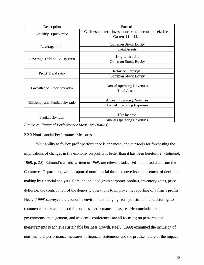
profitability ratios in assessing failures/bankruptcy. Based on the literature reviewed and the
availability of data, this study uses the NRRI and Acheampong et al. financial ratios as the
financial performance measures. These ratios have been confirmed by both the NRRI and
Acheampong et al. (2018) as predictors of IOUs’ viability variables. Figure 2 below presents the
financial performance or ratios used by this study.
18
Description Formula
Cash +short-term investments + net account receivables
Current Liabilities
Common Stock Equity
Total Assets
long-term debt
Common Stock Equity
Retained Earnings
Common Stock Equity
Annual operating Revenues
Total Assets
Annual Operating Revenues
Annual Operating Expenses
Net Income
Annual Operating Revenues Profitability ratio
Liquidity- Quick ratio
Leverage ratio
Leverage-Debt to Equity ratio
Profit Trend ratio
Growth and Efficiency ratio
Efficiency and Profitability ratio
Figure 2: Financial Performance Measures (Ratios)
2.2.3 Nonfinancial Performance Measures
“Our ability to follow profit performance is enhanced, and our tools for forecasting the
implications of changes in the economy on profits is better than it has been heretofore” (Edmund,
1969, p. 25). Edmund’s words, written in 1969, are relevant today. Edmund used data from the
Commerce Department, which captured nonfinancial data, to prove its enhancement of decision-
making by financial analysts. Edmund included gross corporate product, inventory gains, price
deflector, the contribution of the domestic operations to improve the reporting of a firm’s profits.
Neely (1999) surveyed the economic environment, ranging from politics to manufacturing, to
commerce, to assess the need for business performance measures. He concluded that
governments, management, and academic conferences are all focusing on performance
measurements to achieve sustainable business growth. Neely (1999) examined the inclusion of
non-financial performance measures in financial statements and the precise nature of the impact

19
of non-financial performance measures on the financial indicators discussed by the various Chief
Executive Officers (CEOs). Citing the 1996 MORI survey, Neely (1999) concluded that 72
percent of management concurs that focusing on nonfinancial performance measures such as the
needs of customers, employees, and suppliers will better serve shareholders.
In an attempt to address the question of whether nonfinancial measures such as customer
satisfaction lead to superior economic returns, Anderson, Fornell, and Lehmann (1994) surveyed
the Swedish market to identify the relationship between customer-based performance measures,
accounting performance measures and economic returns. They concluded that nonfinancial
measures have a positive correlation with the financial returns of an organization. In the past,
accounting financial data has been primarily used by external stakeholders to make decisions;
however, financial statement performance measures are not enough. Hence, there is a need for
nonfinancial performance measures to complement the financial measures and offer sufficient
information in determining the future economic value of an organization (Milost, 2013).
Although in the past, financial performance measures played a significant role in
providing historical accounting data regarding the financial performance of an organization, little
attention was given to the nonfinancial measures that impacted the historical data. More recently,
the management discussion and analysis (MDA) of several annual financial statements contain
more information on nonfinancial measures. The literature review above confirms that using
nonfinancial performance measures will enhance the analysis of every industry. However, the
IOU is a regulatory industry and may require different measures. Most of the research reviewed
highlights quality, size, customer satisfaction, etc. as nonfinancial performance measures. This
study substitutes some of these measures with factors that are known to be consistent with the
regulatory industry. Examples are management compensation, classification of the utility, type of

20
business registration, allowable depreciation and amortization, the number of customers served,
indirect business taxes (Taxes Other than Income), etc. These factors will be combined with the
financial ratios to determine the drivers of utility abandonments and transfers.
Consistent with the financial reporting required by FPSC (NARUC), Figure 3 below
provides the groupings of the nonfinancial performance measures identified for the study.
Classification Variables
Plant output /(gallonage per customer)
Plant output /Total Number of Meter Equivalents
Number of Customers served
Gross water Revenues per Customer
Compliance with FPSC Quality Measures
Compliance with DEP Quaility requirements
Compliance with CUP Quaility requirements
Type of Corporation for Tax filing purposes
Management Compensation
Owners Involvement of Direct operations of the Utility
Utility Classification
Donated Capital -CIAC
Indirect Business Taxes -Taxes Other than Income (PSC
compliance with the Uniform System Of
No deficiencies communications from regulatory agencies
Utility Compliance-annual report Filing
Output measures
Quality Measures
Owner's Equity Structure
Regulatory Measures
Figure 3: Nonfinancial Performance Measures
2.2.4 Integration of Financial and Nonfinancial Performance Measures
A survey of 128 manufacturing organizations revealed that financial and nonfinancial
performance measures have different roles in the determination of a firm’s overall performance.
Many studies consider periodic financial performance measures as too aggregated, historical in
nature, and lacking timely solutions to root problems within an organization (Chow & Van Der

21
Stede, 2006). In addition, periodic financial measures do not explain the root cause of the
problems. For example, an unfavorable variance may have different meanings and different
causes, but from a financial performance ratio point of view, it may have a different meaning and
total implications (Chow & Van Der Stede, 2006).
The combination of financial and nonfinancial (both quantitative and qualitative
nonfinancial measures) performance measures tends to yield a more comprehensive
understanding of the firm's performance on its viability. In an exploratory experiment, Schiff,
and Hoffman (1996) concluded that executives use both financial and nonfinancial measures in
making performance judgments, and to a certain extent, nonfinancial measures carry a greater
weight in decision-making than financial measures. They suggested that future research should
explore the generalizability of the combination of both financial and nonfinancial performance
measures to reach a better decision in different industries. The current study employs empirical
data from both financial and nonfinancial measures in the water and wastewater industry to
determine the impact on utility abandonments and transfers.
Testing the impact of financial and nonfinancial performance on employee clarity of job
expectations, Lau (2011) separated financial measures from nonfinancial measures and
determined that both financial and nonfinancial measures impact employee clarity and
nonfinancial measures had a stronger impact than financial measures. However, the integration
of both financial and nonfinancial measures yielded the best impact on employee role clarity.
Consistent with prior research, this study focuses on the integration of both financial and
nonfinancial performance measures and its impact on utility abandonments and transfers.

22
2.3 Business Failure Models
Many well-known ratio analysis models that predict overall business failures focus on
financial ratios. Models such as the Altman Z-Score model, the Platt and Platt model, the NRRI
Viability model, and the Zeta model, etc. focus on controlling and decreasing the risks correlated
with business failures, ensuring the continuity of business operations and the capability to attain
specific social and political objectives, such as addressing public safety and health concerns
(Acheampong et al., 2018). This section examines the applicability of these models to predict
utility transfers and abandonments.
Wirick et al. (1997) analyzed a Discounted Cash Flow (DCF) model using liquidity,
leverage ratios, and earnings trend. These financial ratios included measures such as the number
of utility customers, an average rate per customer, discount rate used in the leverage scale,
capital investment, etc. The analysis focused on utility viability and its access to the Drinking
Water State Revolving Fund (DWSRF). The model concentrated on cash flows and financial
indicators but not on nonfinancial performance measures. The objective of the model was to
ascertain the sustainability of utilities at market interest rate levels and which utilities need to
borrow from the market or obtain the subsidized loans from DWSFR. Ratio analysis naturally
strives to produce an insight into an organization's financial position by comparing differences in
financial relationships over time among similar firms (Wirick et al., 1997). Wirick et al. (1997)
advised the use of these ratios to assess the financial sustainability of small water systems, by
explaining that other financial ratios might not be suitable because those ratios are not explicitly
developed for the water industry. Wirick et al.’s (1997) model did not consider the impact of
nonfinancial performance measures. Additionally, the model focused on cash flows for loan
determination, not the sustainability of the utility as a whole. Thus, their recommendation is not

23
considered when determining which financial and nonfinancial factors are predictive of utility
transfers and abandonments.
Before the development of quantitative measures such as ratio analysis, qualitative
criteria were used to measure a firm's operating and financial challenges and establish its
creditworthiness (Altman, 1968). To predict creditworthiness, Altman (1968) established a
model employing multiple discriminant analysis (MDA), using financial ratios as the explanatory
variables for the prediction of potential bankruptcy. The model warns of multicollinearity among
the selected ratios and recommends scaling down to the least tolerable number of ratios. Using
MDA, with four to five financial ratios, Altman divided 66 firms into two groups, with average
assets of $6.4 million (ranging from $1M to $25M). The selected sample used in this model was
manufacturing firms, and the model’s Z score accurately predicted 95% of business failures
based on the sample used in the studies. The model was not designed for small-scale industries.
However, subsequent improvement led to the models "A and B" Z score.
The Altman Z-score model predicts bankruptcy or insolvency within two years, using
multiple income statements and the balance sheet items to estimate the financial strength of an
organization. Investor-owned water and wastewater utilities usually do not operate under
multiple income streams, making the applicability of the Altman Z-score model a challenge or
inappropriate in predicting distressed utilities (Acheampong et al., 2018). Beecher et al. (1992)
affirmed the need for an alternative to Altman’s Z-score model, by explaining that the Altman’s
Z-score model might not be suitable for an investor-owned or small water system since the
model requires a consistent application to predict filing for bankruptcy.
The NRRI 2009 annual report established a viability model employing two financial
ratios: profitability (net income divided by annual operating revenues) and profit trend. The
24
model included liquidity, measuring the utility's ability to meet short-term obligations as they
come due; the liquidity ratio was used to measure the utility’s total debt commitment to its total
assets. The growth and efficiency ratio, as well as the efficiency ratio, measured the utility's
ability to quickly turn over asserts to generate further resources for the firm. All seven ratios
were determined to be inversely related to a distressed utility system (Wirick et al., 1997). The
NRRI model used a simple addition of the results of the several ratios results to classify the
outcome into one of three categories. A utility with 2.0 or less was classified as distressed or
nonviable. A utility between 3.0 to 3.9 was rated as weak to marginal, and a utility that scored
4.0 or more was categorized as healthy and viable (Acheampong et al., 2018). The NRRI model
did not consider the effect of multicollinearity among the selected financial ratios and did not
employ a statistical approach in analyzing the results. The investor-owned utility industry lacks
industry standards for comparison. Employing simple additions, or the use of multivariate ratio
models, it will be a challenge to analyze the results to determine utility viability. In addition, the
NRRI model did not use any benchmarks from a related industry such as the Gas or the Electric
industry to measure viability or non-viability of utilities (Acheampong et al., 2018).
Acheampong et al. (2018) offered an improvement to the NRRI model by establishing a
two-step process in determining utility viability. To resolve multicollinearity issues among the
explanatory variables, the model used a stepwise multiple regression on 470 observations and
analyzed the variance inflation factor (VIF). Citing Mertler and Vannatta (2013), explanatory
variables with VIF of 10 and above were determined to be outliers and removed from the
explanatory variables. The second step used logistic regression to predict the viability of the
chosen utilities. The approach reclassified viable utilities by the NRRI model as non-viable and
25
vice versa. The current study improves the Acheampong et al. model (2018) by incorporating
nonfinancial performance measures.
2.4 Regulation
The utility manual created by the Deloitte Center for Energy Solutions (2012) explains
that the unique characteristics of utilities create global public attention in the establishment of
charges (rates) and their sustainability. The comprehensive public interest in utility operations
commands the regulation of these utilities. The uncertainty correlated with market breakdowns,
public safety, health interests, and delivering confident social and political goals, as well as the
financial considerations on both social and political objectives, plays an indispensable role in the
regulation of the utility industry (Jamison & Sanford, 2008). The Deloitte Center for Energy
Solutions confirms the need for regulation. It explained that the regulation of utilities would
ensure nondiscriminatory rates or charges and ensure satisfactory delivery of services.
Regulation is required since utilities operate under a natural monopoly theory. Utilities function
in organized territories (no real competition present); to stimulate conditions to support a
competitive environment, these utilities need to be regulated by a state board (American Water
Works Association, 2012. The FPSC (2018) explains that the Florida commission is committed
to guaranteeing that Florida's utility customers are offered the fundamental utility services,
including electric, natural gas, telephone, water, and wastewater, in a reliable, consistent, and
responsible way. The Florida commission regulates utility activities to establish rate base and
economic regulation such as competitive market oversight, protection, and the provision of
reliable service. The FPSC’s assertion reinforces Jamison and Sanford's (2008) declaration that
commissioners are required to govern the activities of utilities to ensure fair and competitive
pricing and reliable provision of service.

26
Regulatory system design should be focused on the long-term engagement and benefits of
both taxpayers (citizens) and investors (utility owners) but not on serving a short-term interest of
political program (Jamison & Sanford, 2008). This reinforces the need to ensure that utilities do
not abandon or transfer their facilities due to economic hardships such as dilapidated utility
assets: "To overcome such problems to the extent possible, countries adopt rules for regulation
and government institutions that support regulation under the law, as well as independence,
transparency, predictability, legitimacy, and credibility of the regulatory framework to help
ensure that regulation serves the long-term interests of the country" (Jamison & Berg, 2008, p.1).
The political intentions underlying the ratemaking process or rate creation for investor-
owned utilities create challenges thwarting the understanding of the consuming public in
establishing rates in Florida. The politicization of the overarching body (FPSC) has led to
incompetence in the provision of utility services, thereby leading to a lack of strategic investment
within the utility sector, for instance, the endorsement and approval process of utility
construction suffers strategical process for proper placements instead, is highly influenced by the
impulses of the utility regulators (Foster, Tiongson, & Caterina, 2003). The quality of the
utility’s provision of service is impacted by the allowable cost borne by ratepayers; the approval
of certain required types of equipment and supplies, which are generally approved for municipal
utilities, becomes an issue for investor-owned utilities. For instance, storage tanks, extra water
treatment equipment, generators for power, etc. to ensure an adequate and continuous supply of
services are considered extra costs for investor-owned utilities; politics play a significant role in
approving the need for utilities to have such extra equipment. Regulators focused more on cost-
cutting than on efficiencies and continuous provision of services. To be viable and to meet future
demands, the operations of the utilities should be cost-effective. Attracting capital investment to

27
run the utilities effectively depends on reasonable returns on investments and reporting of profit
by the utilities. Foster et al. (2003) recommended that reforms should focus on economic
theories; utilities are considered social goods, and their delivery and provision should be
accessible to all citizens. However, Foster et al. noted that most utility services are provided
under a natural monopoly theory. The cost of provisions of the services such as infrastructures
(main pipes and other distribution lines) serves as a barrier of entry. The required capital needed
to establish such infrastructure creates the obligation to protect the territory for a utility provider
to improve productivity and enhance efficient return on capital. The regulation of the utilities
ensures the protection of the territories, maintains reasonable prices to ensure a fair return on
investors’ capital, and stimulates capital investment required in the industry to ensure efficient
services (Foster et al., 2003).
To one degree or another, natural monopolies are classified as temporary, and most of
these utilities operate in an authorized territory avoiding competition within their territory. Some
utilities (e.g., electric utilities) also use economies of scale as a barrier to entry, preventing other
competitors from entering the market (Jones, 1988). Parker and Kirkpatrick (2005) contradict
Jones’s (1988) assertion by explaining that utilities show characteristics of a natural monopoly as
a result of economies of scale. Hence, the natural monopoly may be a result of the need for
capital, not necessarily a result of regulations. Citing the electric grid as an illustration, Parker,
and Kirkpatrick (2005) affirmed that the capital required to build the grid network is enormous,
to the extent that it discourages a competitive company from servicing the same territory. The
water and wastewater industry is similar: the capital requirements for main pipes are immense to
the extent that they discourage other utilities from competing in the same authorized territory; the
monopoly also avoids uneconomical duplication of financial resources. The public interest
28
hypothesis affirming regulating utilities serving the public has withstood the test of time: "That
regulation is undertaken to protect consumers from the abuses of market imperfections and for
the achievement of public interest related broad economic objectives remain viable creed"
(Jones, 1998, pp.1103).
An interesting notion in the ratemaking process is the concept of regulatory lag; this is
the timeline between the filing for a rate change and the approval process. The audit process, the
public hearing, and meetings of the commissioners to either support or disallow the requested
change in tariffs may take a while to complete; the range of time required to complete the
process is termed regulatory lag (Joskow,1989). While utilities are waiting for approval or denial
of their petition, they are required by the various legislative acts to continue the provision of
utility services at the current prices or sometimes at an interim approved rate.
Jones’s (1998) assertion of an increment in the cost of utility services during the
regulatory lag period requires thorough attention. The assertion of leaving utilities in the dark
during the regulatory lag period and the reimbursement of cost during the regulatory lag period
needs further review or study, since most states commissioners either denied the rate increase or
approved the rate increase with adjustments to recover the cost of the ratemaking process but not
the regulatory lag period increase in operating costs. The current study does not exclusively
address the regulatory lag period and its extensive implications on investor-owned utilities.
The regulation of utilities does not depend only on the social and political elements, but
also on the financing of utility assets becomes a challenge for most regulatory bodies. Regulated
utilities and regulators face the challenge of raising capital to finance projects. This requires a
financial strategy to ensure asset replacement to keep the utilities viable. Failure to acquire
sufficient funding and suitable capital investment for utilities to upgrade may damage the overall
29
profitability of the industry. One consequence may be avoiding compliance with environmental
regulations (Mann, 1999). These issues required the various states to put regulatory bodies in
place to ensure continuity of the utilities’ services to citizens.
Most literature reviews are focused on electrical utilities. For example, Dunn (2009)
illustrates the development and various preparations by electric utility companies to meet the
projected population growth of 12 million by 2030 in Florida. However, his study was focused
on electric companies. Dunn cited Progress Energy’s initiation of two new nuclear plants to meet
future demand. Regulators approved the construction of these plants and offered a rate increase
to support the provision of service in anticipation of future demand. Johnson (2013) reported a
$32 million rate increase request by Tampa Electric to construct five new generators as
preparation towards an anticipated increase in population. Most news articles about regulations
and rate developments in the state of Florida center on continued improvement in the electric and
gas companies. Because water and wastewater utilities also render valuable utility services to the
residents of Florida, they should receive equal consideration and attention.
2.5 Ratemaking Process
State commissioners have adopted innovative means of negotiating the ratemaking
process and energetically engaging the ratepayers. Some of the innovations include the adoption
of temporary rate increments, annual passthrough increases, and automatic adjustments of rate-
based on inflationary rates, as well as future test years to control and manage the ratemaking
processes (Joskow, 1974). The difficulty of managing ratemaking by the various state systems
has evolved to the current state of affairs by traditionally focusing on the income requirement for
a utility to be viable or sustainable. The ratemaking process established a rate adequate for
utilities to cover necessary expenses and generate allowable returns on owners’ investments.

30
However, the process seems superficial in that the establishment of customer rates depends
mainly on negotiations between utilities and the ratepayers' legislators (the General Counsel of
Florida) to agree on a negotiated price, instead of to establish the required rate to ensure viability
(Littlechild, 2009).
The costs of the ratemaking, the required audits, paper filing, and town hall meetings
required to obtain a rate increase practically persuade investor-owned utilities to habitually settle
for negotiated rates instead of the traditional ratemaking process (Littlechild, 2009). The question
to be addressed is whether the issue of financial vulnerability within the investor-owned utility
industry; a result of the settlement is or negotiated rates. Are the elements of the traditional
ratemaking process different from the negotiated rates or settled rates or the innovative
mechanism of establishing rates? Traditionally, the components of ratemaking have focused on
the creation of genuine opportunities for utilities to meet their revenue requirements (NRRI,
2009). An established rate for an investor-owned utility should yield moderate cost recovery and
a fair rate of return on equity (Deloitte & Touché, 2012). This assertion was affirmed by the
AAWA (2012), which explained that the establishment of rates for investor-owned water and
wastewater utilities should focus on the required revenues to meet the utility's allowable
expenses and equity returns (revenue requirement). The revenue obligations to establish a rate
for a utility should converge on the real revenues a utility generates within twelve calendar
months to cover its allowable cost of operations and the necessary funds to replace plant assets.
The test period may be based on past data or forecasted future estimates.
2.5.1 Test-Period
The choice of a test-period (thirteen months) is the most significant step in the
ratemaking process. The adopted period represents the recovery period for the utility if a

31
historical period is selected; the costs associated with the selected period with inflation
adjustments are used as the future recovery costs. Primarily, there are three selection methods.
All three methods involve twelve-months’ average costs as the basis for establishing a rate to
apply to future periods (Deloitte & Touché, 2012). The historical-average method is the most
customary test year; the method uses the most current preceding accounting twelve-months’
operating results of the utility as the test year (Deloitte & Touché, 2012). The establishment of
the rate base includes a thirteen-month plant asset average for the selected historical accounting
period and the expected adjustments to acknowledge the increase in costs related to recurring
expenses, such as labor costs, chemical supplies, etc.
The year-end test period or the point-in-time method, is the next commonly used method
compared to the historical-average method. The method adopts the elements of the historical-
average method and modifies the revenue and expenses to close the lag period between the
application process and the decision date (Deloitte & Touché, 2012; AAWA, 2012). The
generated revenues or income and the operating expenses of the most recent twelve months
preceding the decision date are used to establish the future rate for the utility.
The third method employs a projected twelve-month period in the future; the method
utilizes the utility's outstanding plant assets in service and twelve-month projected operating
results after the application date. For example, plant assets in service from August through
January are used and future assets added during the following six months (February through
July) as well as the projected operating budget (Deloitte & Touché, 2012). There are no
particular criteria set to select one method over the other. However, AAWA (2012) suggests that
states frequently employ one method and depend on the state rules and regulations with some
variations.

32
The Florida Administrative Code (FAC) acknowledges the use of two of the methods
discussed, the historical period or the forecasted future test-year method. The selection of the test
year is proposed by the utility sixty days before the filing date of the rate change, with evidence
supporting the selection of a particular method (FAC 25-6.140, 1994). The evidence to support
the selection of one method over the other should describe the impact of the selected method on
the rate establishment process and why it represents the interests of parties involved better than
the non-selected method. The impact assessment should outline the revenue requirements that
propelled the filling of the rate change. The selected twelve-month period is recommended to
correspond with the utility's calendar or annual fiscal filing period. The utility may deviate from
the regular filing year, with an appropriate explanation to support the departure from the annual
filing period.
2.5.2 Revenues
The number of investor-owned utilities undergoing financial difficulties, with revenues
falling below allowable operating expenses, may be an indicator of the effectiveness of an
implemented program to support investor-owned utility systems in recovering, gaining, or
identifying vulnerabilities in the system (Rubin, 2009). The United States General Accounting
Office (G.A.O.) (2002), determined that twenty-nine percent of water utilities deferred system
maintenance, due to inadequate funds generation (Stanford, 2008).
Beecher et al. (1996) suggested that the various state commissions should perform
financial sustainability tests on utilities focusing on the revenue generation abilities of the
utilities, as well as the reserves capabilities and the charging rates of the utilities. The investor-
owned utilities need to be permitted to generate adequate revenues to satisfy the allowable
operational and maintenance (O&M) requirements of their systems to meet the provision of
33
services (AAWA, 2012). The authors affirm the significance of the revenue required to meet
operating challenges to function efficiently and sustain utility operations.
An investor-owned utility generates revenue from either operations or non-operating
revenues. The classification of these revenues is based on the sources of the revenue generation
(AAWA, 2012). Operating revenues are generally revenues generated from the provision of
utility services to both residential and commercial ratepayers using the authorized rates by the
provider. Operating revenues also include the provision of other services to ratepayers using
approved standard rates or fixed contractual billing. Non-operating revenues composed of the
sale of merchandise and the associated sales taxes, profits, and losses from the sale of long-term
held properties, rental revenues not associated with utility plant assets, interest revenues, and
other contractual performance revenues not directly associated with the provision of utility
services (AAWA, 2012). The various state commissions regulate both metered and unmetered
operating revenues. The regulated revenues are the primary income contributor to the operations
of the investor-owned utilities.
NARUC (1996) classified utility incomes into five fundamental categories. Category one
represents the revenues generated from a flat-rate billing. Residential and commercial (industrial)
ratepayers received a monthly, quarterly, or annual billing that does not depend on the rate of
consumption; revenues in this category do not use metered or effluent output devices to
determine the cost of consumption. The metered consumption-based revenue is the second
category: residential and commercial (industrial) are billed based on the volume of consumption
using a metered or effluent output device to measure consumption. Category three measures
revenues not generated from residential and commercial (industrial) customers, but by the
provision of services to other utility services, such as the provision of bulk water supply to
34
another utility for distribution, or the use of main pipelines and a service agreement to service
them for other utilities. The fourth group is usually the guaranteed revenues from third parties
such as property developers or city governments before establishing the utility services.
Revenues from nonutility services were classified as the fifth group.
The FPSC revenue methods aligned with the AAWA 2012 category description. The
FPSC categorizes revenues into two groups: revenues related to the operations of the utility and
the non-operating revenues. The operating revenues are classified into metered and unmetered
for both residential and commercial customers. The FPSC uses the rate base of a utility to
establish the rate the utility is allowed to charge its customers. The rate base considers the
revenue requirement for allowable expenses and allowable returns on owners’ equity. F.A.C. 25-
30.415 empowers the FPSC to formulate a leverage scale at least once a year to offer a range of
returns on common equity (FPSC, 1986). The FPSC requires all investor-owned utilities to
comply with the NARUC uniform system of accounts. The annual filing requirement under
F.A.C. 25-30.445 requires utilities to indicate compliance with the NARUC revenue and
expenses structure in their annual filings.
2.5.3 Operation and Maintenance Expenses
State commissioners are authorized to implement adequate rate improvements for
investor-owned utilities to generate adequate revenues to satisfy operation and maintenance
expenses to sustain the operations of investor-owned utilities. The rate improvement should be
sufficient to cover debt obligations resulting from revolving loans used in the operations of the
utility (Stanford, 2008). Operations and maintenance (O&M) cost determinations should
consider the immediate interests for satisfying performance requirements and in the long run,
sustain the operations of the utility (Engelhardt, Skipworth, Savic, Cashman, & Al, 2002). O&M
35
costs are authorized, allowable operating costs required to sustain the utility operations. The
O&M expenses consist of semi-variable costs (mixed costs) and variable costs. The total variable
costs depend on the operating cycle, while the semi-variable costs are determined by the required
fixed expenses and the annual variable costs depending on the yearly operating cycle of the
utility; however, they are not proportional to the working hours of the plant assets (Vatavuk,
2005). Operating and supervisory labor costs and supplies such as chemicals were cited by
Vatavuk (2005) as examples of variable costs. However, overhead maintenance expenses,
charges related to laboratory testing, and servicing of the main pipelines were considered semi-
variable.
Deloitte and Touché (2004) emphasized that investor-owned utilities are mandated by the
various state regulators to use the NARUC uniform system of accounts. The NARUC system
fundamentally uses the U.S. “Generally Accepted Accounting Principles” (GAAP). The various
state regulators may use their discretion to change the NARUC pronouncements to meet the state
ordinance. The amendments to the NARUC accounts system are usually employed by the state to
meet the ratemaking aspirations. NARUC (1996) classifies investor-owned utility O&M
accounts into nineteen primary operating accounts subgroups: salaries and wages of utility
workers, salaries and wages of utility operating executive officers, administrators and majority
stockholders, workers’ benefits and pensions, the costs of purchasing water or the outsourcing
wastewater treatment, sludge removal costs, purchase power and fuel for power production,
chemical supplies, materials and general suppliers, contractual billing services, contractual
professional services (including engineering, accounting, etc.), contractual laboratory testing
services, other services outsourced, rent, transportation costs, insurance expenses, regulatory
commission fees, bad debt expenses, and miscellaneous expenses.
36
The accounts for salaries and wages for employees, officers, directors, and majority
shareholders include earnings covering salaries, bonuses, and other determined compensation of
service paid or accrued. Employee benefits and pensions incorporate irrevocable reserves
accumulated under pension systems and other payments covering workers’ compensation or
accidents on the job, illness, hospital admissions, and death benefits or insurance to employees.
The O&M also accounts for medical payments, educational reimbursement, or recreational
activities of utility workers. The purchased water account and the wastewater treatment account
accumulates costs related to the external provision of services by third parties supplying treated
water and treatment of wastewater (NARUC, 1996). Audit records for the purchased water
account and the wastewater treatment account exhibit the number of treated gallons purchased
and the quantity of wastewater treated and the related charges. The sludge removal account
accumulates the expenses related to the removal of sludge by an independent external utility or
service company. The purchase of electricity used in the provision of utility services is accounted
for by the purchased power account. The account for fuel for power production includes fuel
used to generate power for utility services or in connection with the provision of services such as
powering the pumps and other related equipment to ensure timely supply of services. The type
and quantity of fuel purchased need to be recorded as part of the record-keeping in the account
(NARUC, 1996).
The cost of chemical supplies used in the utility's operations for the provision of services
is accounted for in the chemical account. The accumulation of chemical costs comes from
chemicals purchased from third parties and those internally manufactured or extracted.
Employees’ salaries associated with the production of chemicals are not accounted for in the
chemical account; they are part of the wages and salary account. All supplies for the provision of

37
services not accounted for in other accounts are accumulated in the material and supplies
account, except materials used by third parties and professional services (professional-other
account). All contractual services performed by third parties for the utility, such as billing
services, audit services, etc., are accounted for in the contractual services account. The use of
rental properties, both equipment, and real property, associated with the provision of utility
services is accumulated by the rents account; rentals of trucks and automobiles are excluded
from the rents account but accounted for in the transport account. The total insurance expenses
for a utility cannot exceed twelve months of insurance payments or amortization of prepaid
insurance; refunds of canceled insurance policies and annual dividends associated with insurance
purchases are accumulated in the insurance expenses account. All rate case proceedings, as well
as all other cases related to the provision of services held before a state regulatory commission,
are accumulated in the regulatory commission expenses account. Wages and salaries of utility
employees and the related taxes associated with cases before the commission are part of the
salaries and wages expenses account, therefore not accounted for in the regulatory commission
expenses account. An account for miscellaneous expenses accumulates other recoverable costs
that are not accounted for by any other specific account, but for which the expenses are related to
the provision of the utility’s services, such as industry association dues, utility convention costs,
shareholders conference expenses and others (NARUC, 1996).
AAWA (2012) divided O&M expenses into recurring and nonrecurring categories. It
excluded all depreciation expenses and further maintenance expenses for plant assets that would
increase the life of the asset for more than a year. The utility needs to generate enough financial
resources regularly from operations to cover the O&M expenses for it to be sustainable or self-
sufficient. While AAWA was specific about the treatment of depreciation expenses, NARUC’s

38
(1996) documentation did not explain or classify the treatment of depreciation expenses as part
of O&M classification but highlighted the need to include it in the rate base (AAWA, 2012).
O&M costs are necessary and essential expenses required to effectively and efficiently manage
the operations and maintain and sustain the facility treatment plant’s assets, such as transmission
lines and distribution facilities (AAWA, 2012). According to AAWA, customer service expenses
related to billing and solving billing issues, serving ratepayers maintenance requirements, and
general administrative expenses should be expensed under O&M.
In the NARUC Uniform Systems of Accounts, the O&M account is classified into five
groups (AAWA, 2012). All expenses related to the in-house provision of water from the source
and the treatment of sewer or wastewater, the transmission and distribution lines, expenses
related to customer accounts, and general administrative expenses are grouped into one category.
A fourth digit might be adopted to expand the chart of accounts. AAWA (2000) indicates that
O&M costs that are infrequent annually, such as painting expenses or storage tank cleaning,
should be managed under O&M expenses. These costs are occasional and do increase the O&M
account substantially for the period. To resolve O&M cancellations and match expenses with
usage, these expenses need to be capitalized and amortized for a recommended period. F.A.C.
25-30.433 required O&M nonrecurring expenses to be amortized over five years. However, a
utility with supporting documentation may be able to deviate from the five-year amortization
period and justify either a shorter or more extended period. The time employed to amortize the
nonrecurring expenses should not skew the O&M expenses during rate case proceedings. O&M
expenses should be capitalized to match usage of the resources with expenses during the rate
case proceedings to reflect on the historical year (AAWA, 2012). F.A.C. 25-30.140 Subsection 1
(r), requires all direct labor costs for obtaining (building) plant assets, related materials, and
39
installation expenses to be accumulated as part of the costs of the acquired asset (FPSC, 2008).
F.A.C. 25-30.456 (11) requires FPSC to compare the O&M expenses of the applied utility to its
test-year operating revenues (FPSC, 2008). FPSC (2004) affirms the use of the NARUC chart of
accounts to include O&M accounts.
2.5.4 Taxes
The complicated nature of utility tax obligations and their inclusion in the rate case
proceedings focuses on state regulations. A large number of municipal utilities do not pay local
or state taxes and in some cases, are exempt from federal taxes. Most investor-owned utilities are
obligated to include local, state, and federal tax obligations in their daily operations. Taxes may
be treated as recurring expenses or nonrecurring expenses, depending on the state regulations.
AAWA (2000, 2012) emphasizes that the traditional forms of utility tax obligations are property
taxes but seldom franchise taxes. Taxes are likely the most vital component in the reporting
process for annual utility financials; they are recurring in nature and considered as an element of
service costs for the utility industry (Deloitte & Touché, 2004). Therefore, regulators should
consider them in establishing the utility's rates. This will enhance utilities’ ability to generate
enough revenues to sustain their operations (NARUC, 1996). Investor-owned utilities have both
recoverable and non-recoverable tax obligations. Income taxes and taxes other than income are
recoverable annual tax obligations (FPSC, 2008).
2.5.5 Rate Base
Rate case proceedings do not focus only on revenue generation to cover O&M expenses;
they also include returns on owners’ equity in the utility. They are considered a roadmap for
commissioners to plan towards capital expansion and its related rewards; hence, regulators
review the entire plant assets of the utility together with the operating costs of the utility to
40
include the satisfactory rate returns on capital investment (Forrer, Ehart, & Forrer, 2011). The
rate base takes into consideration the entire plant assets and all essential assets required for a
utility to provide services to ratepayers, and its returns are considered during ratemaking
(Deloitte & Touché, 2004). The determination of the rate of return takes into consideration the
net operating income created in the test year divided by the net plant assets used to generate the
income. An adequate return on invested capital is the percentage factor that generates sufficient
incomes to cover interest payments and equity earnings required by an invested capital to support
the sustainability of the utility (Deloitte & Touché, 2004).
F.A.C. 25-30.443 authorizes regulators to include the plant assets’ beginning balances
and the ending balances of the test year to determine the rate base. State regulators who employ
the utility approach include depreciation expenses as part of the measurement to assess the rate
base. The rate base is fundamentally a composition of the plant-in-service offset by CIAC and
the accumulated depreciation (AAWA, 2012).
2.5.5.1 Plant in Service
When there are disagreements about the positive and negative acquisition adjustments,
the utility is required to retrieve existing documents that were part of the acquisition to determine
the value of the asset. The supporting records should attest to the actual construction dates and
costs of the asset. Utilities are required to record the plant asset at their original cost (AWWA,
2012). When the acquisition costs differ from the original plant costs, the total costs of the plant
when it was first placed in service are used (AWWA, 2012). The difference between the
established acquired value and the original costs placed in service is considered as acquisition
adjustment.

41
2.5.5.2 Depreciation Expense and Accumulated Reserves
Accumulated and depreciation expenses associated with plant-in-service are practical
components for ratemaking proceedings in current acquisitions and the future acquisition of plant
assets (Mumm & Matthews, 2004). Depreciation estimates the decline of the plant assets’ value
resulting from usage and the justification for an increase in the asset value and reduction of the
net asset (Brazell & Mackie, 2000). Depreciation is the loss-in-service value not replaced by
general maintenance services of the plant assets. Utility plant assets connected with depreciation
expenses and accumulated depreciation result from the proposed usage and retirement of the
assets (AWWA, 2012). There are several depreciation practices, and different regulatory bodies
use different methods. For instance, the Internal Revenue Service may recommend a different
method for filing purposes. AWWA (2012) reveals that numerous utilities adopt the straight-line
method for simplicity or as recommended by the various state regulators. The straight-line
method utilizes a depreciable base’s cost (the acquisition cost and all other related costs that will
make the asset ready to be used) less the approximated salvage value at retirement. The
depreciable base is divided by the useful life of the asset. The results are an identical annual
depreciation expense for the asset over the useful of the asset. The straight-line method
normalizes costs of doing business, by avoiding fluctuations in expenses due to depreciation of
an asset. It facilitates an average costs range during rate case proceedings. F.A.C. 25-30.140
requires investor-owned utilities to adopt the NARUC depreciation expense and the accumulated
depreciation accounts and recommended calculations. The purpose of depreciation should be to
balance or normalize costs during ratemaking proceedings and project expected costs in the
future (AWWA, 2012).
42
2.5.5.3 Contribution in Aid of Construction (CIAC)
F.A.C. 367.021 describes Contribution in Aid of Construction (CIAC) as contributed
capital, maybe in the form of money, services, or plant assets (property) acquired by a utility at
no cost to the utility. The CIAC may be donated by an individual, a company, a governmental
institution, or an authority to assist the utility in its provision of services to ratepayers. The value
of the donated capital is used to offset the cost of construction or acquisition of plant assets.
Florida Administrative Rule 2530.515/ [14] supports the F.A.C. 367.021 statutes by clarifying
that CIAC constitutes utility system capacity costs, main pipe extension charges, and ratepayers’
connection assessments (Crahan, 1994). Estate developers evaluate the implementation of utility
systems as part of neighborhood development and they usually construct the utility system
(transmission lines, distribution systems, and to a certain extent, the plant to generate the
services) and donate the assets to an entity or a private individual to continue the provision of
utility services to the community. Such donation is acknowledged as CIAC. Estate developers
are obligated to develop and donate plant assets to offer the required continuous utility services
to the residents of the community (Crahan, 1994).
CIAC is donated capital that is included in a rate case proceeding by offsetting it in the
rate base. CIAC is treated as a credit balance to compensate for the donation by reducing the
plant asset in the rate base (AWWA, 2012). Ratepayer advances usually are deposits held by the
utility for a period before being refunded to customers. AWWA suggests the ratepayer deposits
should be included in CIAC for rate case proceedings purposes.
2.5.5.4 Construction Work in Progress (CWIP)
AWWA (2012) demonstrated that construction in progress/not yet finished or assets not
yet committed to the provision of utility but in the process of being completed for use in the
43
provision of utility services to consumers may be incorporated in the rate base. The inclusion in
the rate base acknowledges the utility’s yearly obligations for debt servicing and return on
owners’ equity. It recommends the use and useful test to persuade ratepayers that it is in their
interest to place the asset under construction in service in the future to enhance the provision of
utility services, hence, the need to include it in the rate base. Contrary to AWWA, F.A.C. 25-
30.116 declares that CWIP is not a rate base element and should not be included in it. However,
Allowance for Funds Used During Construction (AFUDC) may be justified as a rate base
element. An AFUDC that grosses $5,000 or more with a duration of over sixty days after the
initiation of a project or one which has exceeded the initial completion date by sixty days will be
considered AFUDC and be included in the rate base.
2.6 Capital Structure
The provision of satisfactory and quality utility service depends on the authorized rates to
enable investor-owned utilities to raise adequate revenues to be efficient and to pull capital
investment (economic resources) from the capital market (West & Eubank, 1976). Hence, utility
rates need to be adequate and competitive to generate a satisfactory rate of return on capital
investments competitive to the going market rates. However, investor-owned utility industry
rates are regulated and cannot charge a competitive market rate like non-regulated markets. The
equitable and fair treatment of ratepayers should be a significant determinant in the assessment
of the cost of capital (West & Eubank, 1976). Conine and Tamarkin (1985) revealed that many
dynamics might contribute to the assessment of the cost of capital in the regulated utility
industry. Citing regulatory lag as an example, they describe sudden price inflation and other
uncontrollable economic events as a probable impact on the determination of capital cost.

44
The cost of capital is affected by the weighted averages of multiple factors and classes of
capital, such as debt and equity financing. The equity financing is associated with common and
preferred stock representing the net assets owned by shareholders. The debt financing
customarily consists of borrowed capital (AWWA, 2012). Florida Statute 367.082(4) on Interim
rates; procedure reveals that the necessary rate of return assigned to utilities’ borrowed capital is
the most current twelve months’ weighted average cost of capital. The last approved rate of
return is required to be used until there is a new approved rate. However, if the debt element is
short-term, then the actual cost of debt is employed. The authorized rate of return is the
established rate between the least and highest approved rate of return authorized in the last rate
case proceeding of the utility. In that circumstance, the utility does not have an approved return
rate; the most current leverage scale formula is employed to comply with Section 367.081(4) (f),
F.S. FPSC Order No. PSC-2018-0327-PAA-WS, issued in June 2018, which issued a new
leverage scale, with return on common equity expressed as:
𝑅𝑒𝑡𝑢𝑟𝑛 𝑜𝑛 𝐶𝑜𝑚𝑚𝑜𝑛 𝐸𝑞𝑢𝑖𝑡𝑦 = 6.24% + 1.88
Equity Ratio and Range of Returns on Equity =
8.11% to 10.93%.
FPSC employs the equity ratio by dividing the sum of common and preferred equity,
added to the short-term and long-term liabilities. Investor-owned utilities are obligated to keep at
least 40% equity in the stockholdings to avoid imprudent monetary risk (abandonments and
transfers).
This study reviews the literature on failure models using financial and nonfinancial
performance measures; these studies confirmed the use of financial ratios, quality measures,
output measures, and other factors depending on the industry under study. The study followed
the suggestions of prior studies and identified financial and nonfinancial variables related to the

45
utility industry to develop an analysis of the drives of utility abandonments and transfers in the
state of Florida.

46
Chapter Three: Proposed Methodology
3.1 Background
The diversification strategy of most state governments for providing utility services led to
the creation of the investor-owned utility industry. The water and wastewater industry is
experiencing issues such as aging plant assets, abandonments, increases in operations and
maintenance costs, and transfers that require improvements and replacements (Beecher, Mann, &
Stanford, 1993). Rate improvement requests appear to be a useful mechanism to enhance the
financial position of the water and wastewater utility industry. However, due to the operating
characteristics of the industry, state commissioners have the responsibility to educate the general
populace on the costs and capital requirements for the provision of reliable water supply, and the
need to sustain these warrants the sustainability of these utilities (Beecher et al., 1993). Electric,
gas, and telecommunication utilities have been well-funded traditionally; in contrast, the
investor-owned water and wastewater utilities do not experience the same funding level as the
other utilities (Wirick, Borrows & Goldberg, 1997). According to Wirick et al., investor-owned
water and wastewater utilities operate under poor funding conditions, and they manage to survive
and sustain their facilities with underfunded capital assets. Confirming Wirick et al. (1997),
Wardrop (2000) demonstrated that the suffering of investor-owned utilities is an industry-
specific problem resulting from legislation guiding the operating conditions (state regulations).
Regarding this assertion, if the consuming public is well educated on the circumstances and
requirements, will legislators adopt a different approach to the ratemaking proceedings these
utilities go through to have a rate change to keep them viable or sustainable?

47
One general problem which has been approached in different research studies is the
sustainability of these utilities. This study approaches the current abandonment and transfer
problems, within the state of Florida, from the observation of the impact of both financial and
nonfinancial performance measurements. The study uses secondary data obtained from FPSC to
analyze the relationship between financial and nonfinancial performance measures impacting
utility transfers and abandonments.
3.2 Research Design
Quantitative research objectively tests theories by examining the correlations among
variables that are statistically investigated to make a determination (Creswell, 2009; Creswell &
Creswell, 2017). This study follows Creswell’s (2009) proposals and uses a quantitative
approach to investigate the impact of financial and nonfinancial performance measures on the
investor-owned utility industry, using evidence from the state of Florida. The study deductively
identifies the relationships of financial and nonfinancial performance measures of investor-
owned utilities, using a logistic regression model. It also identifies and explores the seven NRRI
ratios and sixteen nonfinancial measures as the explanatory variables to predict transfers and
abandonments within the utility industry. This research tests for multicollinearity among the
explanatory variables by using the Variance inflation factor analysis to rule out collinearity
issues.
3.2.1 Data Collection
This study used a quantitative design approach to analyze and investigate the collected
data from the state of Florida. The study employed financial and nonfinancial performance
measures to determine the drivers of utility abandonments and transfers in the state of Florida.
These measures consist of financial ratios and nonfinancial measures such as output, quality,

48
regulatory measures, and the owner's equity structure. The ratios are obtained from the annual
financial reporting of the investor-owned utilities and the annual rate structure compilation from
the annual filings of the FPSC. The nonfinancial performance measures are obtained from the
annual filings, confirmed by public document requests from FPSC and the Florida
Environmental Protection Agency (FDEP). Ten years of annual financial reporting (2008 to
2017) were used in the study.
3.2.2 Population and Sample
The study sampled all the financial and nonfinancial information of investor-owned
utilities (water and wastewater) in the state of Florida, from the 2008 to 2017 filing periods. The
“Rand” function in Excel was used to assign random numbers to the utilities, and the top 60% of
the utilities were randomly selected as the sample size for the study (87 utilities were randomly
selected, and 76 utilities qualified for the study). The researcher’s selection of the investor-
owned utilities in the state of Florida did not represent any exceptional importance to the
researcher. However, considering the water and wastewater industry, regulations about rate
making are state-specific, and most research on this industry is state-specific. Also, the state of
Florida is among the states experiencing both population growth and a downward trend in the
investor-owned utilities, making it an excellent fit for the proposed study. The data for the study
was readily available to the public.
F.A.C. 25-30.110 directs utilities to conserve and preserve utility records following
NARUC regulations. NARUC recommends 20 years of record retention, but due to updates in
the NARUC chart of accounts, the study used the ten years after the 2007 updates.

49
3.2.3 Research Question
The study focused on the drivers of investor-owned water and wastewater utility
abandonments and transfers. The primary purpose of the study is to examine the impact of
financial and nonfinancial performance measures on utility abandonments and transfers and
confirm the significance of financial and nonfinancial performance measures in the water and
wastewater industry. The study explored new nonfinancial measures and identified the best
combination of these measures to assist decision-makers (both regulators and owners) in future
decisions to prevent or sustain the current down-trending of investor-owned utilities in the state
of Florida. The study explored the research questions and related hypothesis below:
RQ1: What are the financial and nonfinancial performance drivers of utility abandonments and
transfers?
RQ2: Do the financial performance measures dominate the nonfinancial drivers of utility
abandonments and transfers?
3.2.3.1Research Hypothesis
Hypothesis 1: Financial and nonfinancial performance measures have no impact on IOU utility
abandonments.
Hypothesis 2: Financial and nonfinancial performance measures have no impact on utility
transfers.
Hypothesis 3: Nonfinancial performance measures do not dominate utility abandonments.
Hypothesis 4: Nonfinancial performance measures do not dominate utility transfers.
3.2.4 Data Processing and Analysis
The study used logistic regression to examine the secondary data, acquired from the
selected investor-owned utilities’ annual reporting from the state of Florida. The study used both

50
financial and nonfinancial performance data to predict utility abandonments and transfers.
Beaver (1966) used thirty financial ratios to predict the failures of firms, Wirick et al., (1997)
outlined seven ratios and the NRRI recommended these ratios for utility viability. Neter (1966)
confirmed the effectiveness of ratios to predict failures and nonfailures of firms. Wilcox (1971)
emphasized the use of ratios to predict firm failures and success. Considering the NRRI’s seven
ratios and other ratios used in a similar industry, as well as prior studies reviewed, the NRRI
ratios were selected as the financial ratios for the study.
The instability of financial ratios undermines the importance of the time interval in
distressed utility prediction models. To preserve and maintain the predictive capability of ratios,
the models should stabilize and sustain the predictors over time (Sormunen & Laitinen, 2012).
This affirmation demands a robust regression analysis to predict the drivers of utility
abandonments and transfers. The statistical importance of financial ratios shifts at various stages;
therefore, optimal cross-sectional models change at various stages (Balcaen & Ooghe, 2006).
The assertion above informed the adoption of the logistic regression to strengthen the predictive
power of the study's model.
The Variance Inflation Factor (VIF) assists in identifying the severity of multicollinearity
problems among explanatory variables. The VIF is one of the general, traditional collinearity
investigative techniques, directed at ordinary or weighted least squares regressions. The VIF
identifies the slope estimate caused by the nonorthogonality of the explanatory variables
(predictors) over and above the orthogonality variance (Liao & Valliant, 2012). Eliminating the
predictors with collinearity issues reduces the impact of one explanatory variable influencing the
other measures. The study explored the VIF to eliminate all predictors with VIF higher than
three.
51
This study used logistic regression on the remaining explanatory variables to predict
transfers and abandonments. The seven ratios recommended by the NRRI are employed in the
study, as well as the nonfinancial ratios. Logistic regression is a suitable statistical procedure to
employ when the dependent variable is categorical (Hair, Black, Babin, & Anderson, 2010).
Logistics regression analysis offers a fair assessment of the audit client’s failures by using a
conditional probability model (Sormunen & Laitinen, 2012). Models outside utilities have
employed the logistic regression study to predict failures and benchmarks. Hence, the study used
logistic regression to predict abandonments and transfers in the utility industry. Similar to other
regression analyses, logistic regression illustrates the causes and effects to identify the
correlation among a response variable and the associated explanatory variables (Sormunen and
Laitinen, 2012).
Many models face the assumption of multivariate commonality and equal variance-
covariance metrics across groups-assumptions. A logistics regression model is not required to
meet this strict assumption (Hair et al., 2010). Sormunen and Laitinen (2012) confirmed the
multivariate commonality assumption by explaining that logistic regression does not need to
have an explanatory variable to meet the multivariate normal or groups possessing equal
covariance matrices assumption. The logistics analysis generates a probability outcome that
weighs all the variables to generate a weighted average logit between 0 and 1. Furthermore, it
creates a solution based on the financial and nonfinancial variables to predict the abandonments
and transfers. The drivers of utility abandonments and transfers are based on selected financial
ratios and nonfinancial performance measures. Hence, the use of logistic regression to predict the
failures of utility or the transfers and abandonments is appropriate.
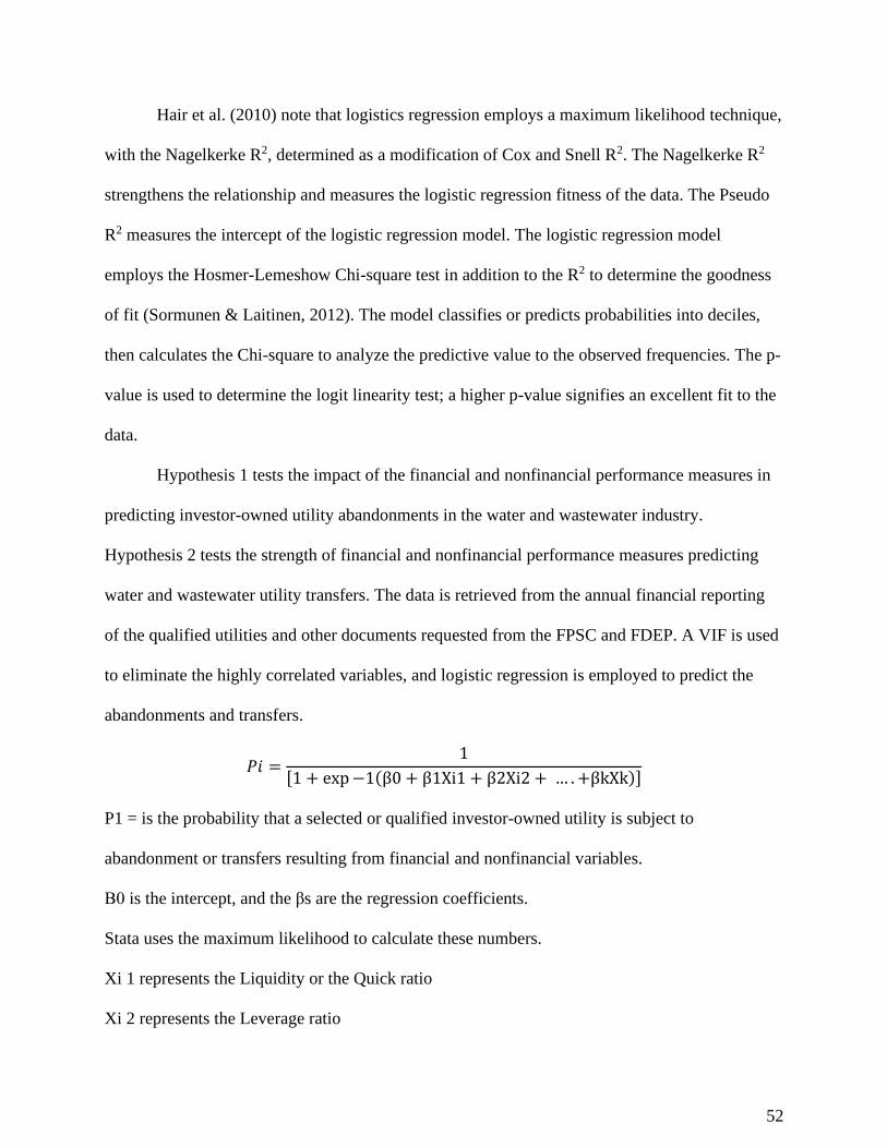
52
Hair et al. (2010) note that logistics regression employs a maximum likelihood technique,
with the Nagelkerke R2, determined as a modification of Cox and Snell R2. The Nagelkerke R2
strengthens the relationship and measures the logistic regression fitness of the data. The Pseudo
R2 measures the intercept of the logistic regression model. The logistic regression model
employs the Hosmer-Lemeshow Chi-square test in addition to the R2 to determine the goodness
of fit (Sormunen & Laitinen, 2012). The model classifies or predicts probabilities into deciles,
then calculates the Chi-square to analyze the predictive value to the observed frequencies. The p-
value is used to determine the logit linearity test; a higher p-value signifies an excellent fit to the
data.
Hypothesis 1 tests the impact of the financial and nonfinancial performance measures in
predicting investor-owned utility abandonments in the water and wastewater industry.
Hypothesis 2 tests the strength of financial and nonfinancial performance measures predicting
water and wastewater utility transfers. The data is retrieved from the annual financial reporting
of the qualified utilities and other documents requested from the FPSC and FDEP. A VIF is used
to eliminate the highly correlated variables, and logistic regression is employed to predict the
abandonments and transfers.
𝑃𝑖 =1
[1 + exp −1(β0 + β1Xi1 + β2Xi2 + … . +βkXk)]
P1 = is the probability that a selected or qualified investor-owned utility is subject to
abandonment or transfers resulting from financial and nonfinancial variables.
Β0 is the intercept, and the βs are the regression coefficients.
Stata uses the maximum likelihood to calculate these numbers.
Xi 1 represents the Liquidity or the Quick ratio
Xi 2 represents the Leverage ratio

53
Xi 3 represents the Leverage-Debt to Equity ratio
Xi 4 represents the Profit Trend ratio
Xi 5 represents the Growth and Efficiency ratio
Xi 6 represents the Efficiency and Profitability ratio
Xi 7 represents the Profitability ratio
Xi 8 represents the Output Measures category
Xi 9 represents the Quality Measures category
Xi 10 is the Owner's Equity Structure Measures category
Xi 11 represents Regulatory Measures category
E9 represents the random error in Y1 for data collection and observation. If the logistic
regression predicts utility abandonment, then the goodness of fit model is run to ascertain the
model fitness to the data, and the classification table is employed to determine the predictability
of the dependent variable. The impact of financial and nonfinancial performance measures on
transfers and abandonment within the water and wastewater utilities, for the selected 10-year
data, is tested by developing different models for the abandonment and transfers and an overall
model combining both transfers and abandonment.
The "Transferred utilities" are investor-owned utilities transferred to another utility or a
municipality within the ten-year study period. The transferred utility may be restructured into a
new utility with a new name or may retain the same name. "Non-transferred" utilities are utilities
that remained unchanged during the ten years. "Abandoned utilities" are all utilities that followed
FPSC procedures to be handed over the utility to the FPSC or the county it operated in and all
utilities that did not follow the procedure, but for which owners decided not to run the utility
anymore and left the facility. The abandonment and transfers are treated as dependent variables,
54
and the selected financial and nonfinancial measures after the VIF elimination process are
employed as independent variables. If the p ≤ α, the null hypothesis is rejected, and it indicates
that the transfers and abandonments of these utilities depend on the independent variables.
The logistic regression predicts or explains a model of financial and nonfinancial
performance measures in determining utility abandonment and transfers. This study used seven
ratios and sixteen non-ratio variables to assist decision-makers (regulators and owners) in
focusing on the most critical variables among the identified variables in their decision-making.
The study used the dominance analysis to distinguish between the most important explanatory
variables among the selected variables to abandonments and transfers (response variables).
Dominance analysis identifies the correct or the meaningful predictors or subsets of predictors
from the explanatory variables that offer the most satisfactory description of the response
variable (Azen & Budescu, 2003). Hypotheses 3 and 4 examine the dominance effect of financial
and nonfinancial performance measures.
Citing Pedhazur (1997), Azen and Budescu (2003) explained the need to analyze
predictors further to determine the most relevant among the full predictors of a response variable.
They note that the explanatory approach in prediction models needs further examination to
identify the most predictive model, while the prediction approach attempts merely to find the
explanatory variables that will correlate the response variables. The predictive model is less
concerned about the valid predictors of the response variable. The explanatory approach is
typically used in theory confirmation (Pedhazur, 1997). The framework of the study recognizes
the existence of numerous studies that have confirmed the prediction of failures in other
industries, using both financial and nonfinancial performance measures. Hence, the explanatory
55
approach is appropriate to establish the most valuable predictors for the water and wastewater
industry.
Dominance analysis is a valuable tool for practitioners and researchers to distinguish the
applicable significance of predictors in linear regression (Braun, Converse, & Oswald, 2018).
One of the most utilized appropriate metrics and straightforward procedures in averaging
outcomes across all feasible subset regression models is the dominance analysis (Budescu,
1993). The traditional assessment of predictor significance is conditional on the selection of a
model and its overall goodness of fit. However, the engagement of the criticality of predictors
offers the probability of misspecification of the model (Azen, Budescu, & Reiser, 2001).
Dominance analysis furthers the reliability of the predictors, and the study identifies new
nonfinancial variables as well as other ratios used in different industries. Hence, the dominance
analysis confirming the applicability of the identified explanatory variables strengthens the
findings of the study.
3.2.5 Instrumentation Assumptions
The study assumes that nonfinancial performance measures are connected with projected
financial performance measures. The study implies that ratemaking proceedings are a more
suitable alternative to change rates for utilities to enable the recovery of the required financial
resources needed for a utility to be sustainable. The study implies that FPSC will proactively
enhance utilities’ ability through rate case proceedings and deter them from abandonments. The
study assumes no specific requirement of a distributional format of the independent variables by
the logistic regression model. The logistic regression model assumes no heteroscedasticity
problems; that is, the study does not presume to overestimate the goodness of fit. The study
assumes minimum or no multicollinearity effects among the explanatory variables for the logistic

56
regression, after employing VIF to minimize multicollinearity issues among the explanatory
variables. The dependent variable and the explanatory variable are not required by the logistic
regression model to be linearly related; however, it assumes the explanatory variables or the
predictors to be linearly related to the log odds. The study expects the use of financial ratios to
normalize the explanatory variables to avoid strong influential outliers. Also, the sample size is
assumed to be large enough (76 utilities with unbalanced one to ten years of financial filings) per
explanatory or predictor to avoid an overfit model (Stoltzfus, 2011).

57
Chapter Four: Presentation of Findings
4.1 The Purpose of the Study
The purposes and motivation of the research are to determine the drivers of utility
abandonments and transfers in the state of Florida. The study uses both financial and
nonfinancial variables that impact utility transfers and abandonments. The study focuses on
changes in regulatory policies and awareness creation required to influence ratemaking
proceedings to enhance investor-owned water and wastewater utility sustainability and avoidance
of utility abandonments. The study enhances the understanding of regulators and utility owners
of the significance of planning to sustain the supply of quality water and the provision of
wastewater service in nation-building. It also enhances regulators’ understanding of the
sustainability of investor-owned utilities and their role in Florida’s current population growth.
The management of the water supply and wastewater treatment, given the population
growth in the state of Florida, is a crucial issue that requires the attention of the regulatory body.
Hence, a thorough plan and management system need to be established to avoid any water-borne
related disease explosion. The necessary upgrades and replacement of utility plant assets and
facilities pose a funding challenge to investor-owned water and wastewater utilities. Unlike the
electric and gas investor-owned utilities that have acquired funding through rate case
proceedings to increase their generation capacity for future population growth, the water and
wastewater industry is lagging behind on funding to sustain plant assets in the future. The study
intends to inform policymakers about the need to plan and manage the current investor-owned
utility plant assets, as well as replacement and further investment to meet the current challenges
58
and cater to the population growth. To sustain investor-owned utilities’ planned improvements,
regulators need to enable a business environment that promotes investments in the utility plant
assets and facilities. The results of this study should help policymakers, investor-owned utilities,
and oversight agencies to plan towards future investment in plant assets and facilities to enhance
the provision of water and wastewater utility services to Florida’s growing population.
4.2 Background of the Regulatory Industry
State of Florida Statute 2012-187 established the study committee with a primary
objective to investigate problems, issues, and challenges confronting investor-owned utilities in
the state of Florida, especially on the small water and wastewater utility systems (FPSC, 2012).
Among the problems was a significant outstanding issue for the committee to address: the
accomplishment of the economies of scale among investor-owned utilities. Other significant
objectives of the committee were to examine the availability of affordable loan provisions to
investor-owned utilities and investigate tax incentives or exemptions to enhance sustainability, as
well as the creation of a reserve account to enhance the financing of utility plant assets to
minimize the impact on rate settings and enhance utility affordability (FPSC, 2012).
The formation of the Study Committee was orchestrated by the results of the 2011
workshops conducted by the FPSC to address the various difficulties confronting the investor-
owned utilities. The principal objectives for the 2011 workshops were to gather information and
data to analyze the implementation and practicability of certain financial concepts to improve the
operations of investor-owned utilities. Overall the achievement of economies of scale to improve
financial stability and technical knowledge among investor-owned utilities was the primary goal.
However, other requirements by other regulatory bodies such as the Department of
Environmental Protection (DEP) surfaced during the workshops, and it became an integral part
59
of the sustainability of these utilities, thereby leading to a legislative instrument to establish the
Study Committee. Another factor that contributed to the formation of the Study Committee was
the need for an independent body to investigate the overall enforcement of different regulations
by different regulatory bodies. FPSC (2018) explained that it regulates 131 investor-owned
utilities within 36 counties, and the remaining 31 are regulated by other regulatory bodies such as
the municipality or the county. All utilities under FPSC jurisdiction were selected for the study.
The sample size for the study was based on all utilities within the ten selected years (2009-2018).
The randomly selected utilities’ annual financial statements filed with FPSC were extracted.
Qualified utilities for the study represent about 60% of all investor-owned water and wastewater
utilities regulated by the FPSC.
The Study Committee (2013) declared that all investor-owned utilities, in respect of what
agency, county, or regulatory body monitoring and controlling the quality of services and rate
settings proceedings, the FPSC have the overall jurisdiction of all investor-owned utilities. The
only exceptions to regulated utilities are systems that are owned and governed by
intergovernmental authorities. Examples are municipal utilities, cooperatives, and non-profit
utilities. The Study Committee (2013) results emphasized the rising cost of utility operations. It
recommended improving performances among utilities to reduce the charges of maintaining
water and wastewater utility operations to ensure more economical rates.
4.2.1 Regulatory Approach to Sustaining Utilities
The Study Committee (2013) identified twelve concerns and made recommendations to
improve the problems besieging the water and wastewater utility industry. The Study Committee
identified the following fundamental issues:
1) economics of scale
2) affordable loans
60
3) tax incentives or exemptions
4) purchasing of existing systems
5) resellers of water
6) creation of reserve fund
7) interim rates during the lag period
8) recovery of rate case expenses
9) quality of provision of service
10) the used and unused rule improvement
11) integration of technology
12) revision of policies, rules, and procedures of the FPSC on investor-owned water
and wastewater utilities.
These 12 issues confirm the problem framework of the study committee’s work. The
study's framework focuses on improvement, recovery, and reimbursement of allowable costs as
well as an efficient and effective revenue provision issues to address the sustainability of the
water and wastewater investor-owned utilities. Secondarily, the study emphasized the
accessibility of capital funding to renovate and replace the crumbling plant assets to improve
utility sustainability, minimize utility transfers, and possibly avoid utility abandonments among
the investor-owned utilities. The Study Committee focused on particular components (elements)
that may be resolved in financial terms for investor-owned utilities to be sustainable and viable.
The present study examines both financial and nonfinancial performance measures and their
relationships to the transfers and abandonments among the water and wastewater utilities.
The Study Committee recommended numerous actions to support the viability and
sustainability of the investor-owned water and wastewater, including bulk purchasing by utilities
to take advantage of volume discounts and the use of the Florida purchasing (supply) system for
investor-owned utilities, to negotiate standard affordable prices for supplies. It also
recommended the creation of a platform for utilities to exchange excess supplies, used plant
assets, and other related provisions for utility operations. The review of the financials indicates

61
that salaries and chemicals seem to be the highest costs for these utilities; however, the Study
Committee did not address salary issues.
The committee acknowledged the aging or deteriorating state of the plant assets of
utilities and the challenges associated with accessing capital funding at an affordable rate. They
proposed the creation of a state revolving fund for utilities to access funding for asset
replacement. The committee did not directly address CIAC. However, CIAC may be considered
one of the primary sources for the revolving fund. CIAC is a contra-expense account, and
consequently, utilities do not recoup the amount associated with the donated plant assets. Hence,
planned replacement of the donated assets is not funded by the current rate case proceedings. The
study committee did not address CIAC issues related to asset replacement of the donated assets.
Ad valorem, property taxes, and sales tax exemptions on investor-owned utilities operations were
suggested by the committee to improve utility sustainability and viability issues while enabling
an affordable provision of utility services to ratepayers. For water resellers, the committee
recommended preserving their exempt status and allowing them to retrieve metering and billing
expenses associated with the provision of services. The committee recommended the creation of
a reserve account by the FPSC and urged the state legislature to enact rules authorizing the FPSC
to do so.
The committee recognized that the current treatment of interim rates is an issue that needs
to be addressed; however, no modifications were recommended. The committee suggested the
costs and fees related to rate case consulting, including attorneys, accountants, and other
professionals, should be limited to services provided up to the initial staff report, as this may
discourage and reduce rate case proceedings costs. In terms of the impact of rate filing on utility
transfers and abandonments, the Study Committee’s recommendations may thwart the filing for
62
rate improvements, particularly with FPSC staff-assisted rate filings. This could ultimately affect
the choices of some of the utilities to transfer or abandon their facilities. On the other hand, if the
results of this study support the Study Committee’s recommendations, then steps need to be
taken to implement the recommendations to enhance the sustainability and viability of the
investor-owned utilities.
The underlying motivation of this study centers on FPSC’s methods and procedures,
implanted in both the financial and nonfinancial performance measures impacting utility
transfers and abandonments among investor-owned utilities. The profitability, viability, and
sustainability of the investor-owned water and wastewater utilities profoundly depend on the
policies, procedures, rules, and regulations established by the FPSC, since they are under their
jurisdiction. The committee suggested establishing enhanced communication to inform
policymaking needs between all parties involved in the ratemaking proceedings (ratepayers and
utility owners). The committee recommended a standard metric to evaluate the operations of
investor-owned utilities to inform the decision-making process of the ratemaking requirements. It
also requested that utilities have a long-term plan towards operations and provision of services. It
suggested a revision of the annual filing requirements and an improved system of filing for the
utilities.
The committee recommended that pass-through expenses be extended to include
additional expenses to be decided by the FPSC. The committee addressed all 12 pertinent issues
identified for the study; however, factors and determinants of revenue increases or the generation
of further revenues were not directly discussed by the Study Committee. It did not address an
empirical assessment of the operating effectiveness of the investor-owned utilities leading to
profit and losses that may impact utility transfers and abandonments. The Florida study was

63
handled from the viewpoint of the legislature, not addressing the impact on transfers and
abandonments. This study offers empirical evidence to determine the drives of utility transfers
and abandonments, employing logistic regression analysis.
4.3 Collection of Data
Data for the study was collected from the FPSC; most of the data is publicly available on
the FPSC website (http://www.floridapsc.com/UtilityRegulation/AnnualReport). The study
obtained the various FPSC annual reports to determine the total number of utilities currently
operating and regulated by FPSC. The available annual filings of the utility were obtained from
the annual utility filings; these reports are not audited financial statements but are the only
available financial and nonfinancial data available to support the study. Per chapter 1’s
discussion, the unaudited financial reports were addressed as a limitation to the study. A series of
public document requests between FPSC and FDEP were made to confirm some of the
nonfinancial performance measures that were self-reported on the financial statements. The
annual FPSC reports were also used to extract some of the nonfinancial performance variables. A
random selection using the “Rand” command in Excel was used to select about 94 utilities, of
which 88 utilities qualified for the study, representing about 60% of Florida water and
wastewater utilities between 2008 and 2017.
4.4 The Research Question-One
RQ1: What are the financial and nonfinancial performance drivers of utility
abandonments and transfers? This study approached the question by creating dummy variables to
represent transferred and utility abandonments. The study employed the NRRI and Acheampong
et al. financial ratios used in utility viability studies (liquidity ratio, leverage ratio, debt to equity
ratio, profit trend ratio, growth and efficiency ratio, efficiency ratio, and the profitability ratio).
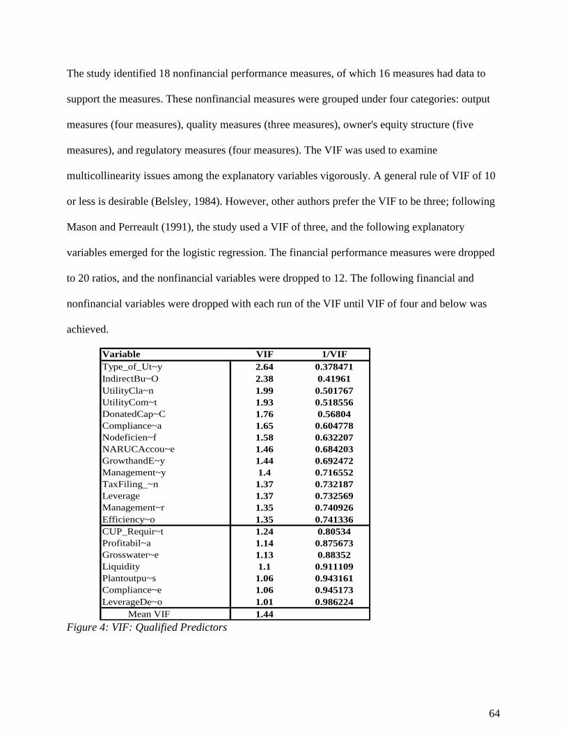
64
The study identified 18 nonfinancial performance measures, of which 16 measures had data to
support the measures. These nonfinancial measures were grouped under four categories: output
measures (four measures), quality measures (three measures), owner's equity structure (five
measures), and regulatory measures (four measures). The VIF was used to examine
multicollinearity issues among the explanatory variables vigorously. A general rule of VIF of 10
or less is desirable (Belsley, 1984). However, other authors prefer the VIF to be three; following
Mason and Perreault (1991), the study used a VIF of three, and the following explanatory
variables emerged for the logistic regression. The financial performance measures were dropped
to 20 ratios, and the nonfinancial variables were dropped to 12. The following financial and
nonfinancial variables were dropped with each run of the VIF until VIF of four and below was
achieved.
Variable VIF 1/VIF
Type_of_Ut~y 2.64 0.378471
IndirectBu~O 2.38 0.41961
UtilityCla~n 1.99 0.501767
UtilityCom~t 1.93 0.518556
DonatedCap~C 1.76 0.56804
Compliance~a 1.65 0.604778
Nodeficien~f 1.58 0.632207
NARUCAccou~e 1.46 0.684203
GrowthandE~y 1.44 0.692472
Management~y 1.4 0.716552
TaxFiling_~n 1.37 0.732187
Leverage 1.37 0.732569
Management~r 1.35 0.740926
Efficiency~o 1.35 0.741336
CUP_Requir~t 1.24 0.80534
Profitabil~a 1.14 0.875673
Grosswater~e 1.13 0.88352
Liquidity 1.1 0.911109
Plantoutpu~s 1.06 0.943161
Compliance~e 1.06 0.945173
LeverageDe~o 1.01 0.986224
Mean VIF 1.44 Figure 4: VIF: Qualified Predictors

65
The study used logistic regression analysis to predict the drivers of utility abandonments and
transfers, using the qualified predictors.
4.4.1 Abandonments and Transfers
Eighty-two utilities were randomly selected for the study, within the chosen utilities:
eight of them were abandoned, and 34 were transferred within the selected 10-year period (2008-
2017). Six utilities within the selected samples filed zero returns and did not have any
information to be used for the study. As explained in chapter 2, there are no specific models
designed to examine financial difficulty (sustainability) or viability for the investor-owned
utilities (Wirick et al., 1997). The Z score, Zeta, and the Platt and Platt models are good
predictors for financial sustainability or viability, as well as bankruptcy predictions; however, the
circumstances and industry standards required for these models to work effectively are not like
the regulatory environment in which the investor-owned utility operates. Hence, the application
of these models will need to be modified to fit the regulatory environment. The study employs
logistic regression analysis to examine the financial and nonfinancial performance measures
vigorously. The financial performance measures (ratios) were first examined in the detailed
panel data level, employing all 700 observations. Figure 5 presents the results of financial
performance measures.
Kremelberg (2011) declares that the “Variables in the Equation” table is the most
significant result of the logistic regression model, as it reveals the standardized and
unstandardized coefficients. At a significance probability level of 0.05 or 0.01, the explanatory
variable may be able to predict the result of a model without the interference of other predictors
(George & Mallery, 2010). The financial performance model on both transfers and
abandonments used 697 observations as compared to the 700 observations in the selected

66
sample. The likelihood ratio chi-square of 38.08 with a p-value of 0.0000 indicates a statistically
significant whole model for the financial performance measures, as compared to the null model
with no predictors.
Number of obs = 697.0000
LR chi2(20) = 38.0800
Prob > chi2 = 0.0000
Log likelihood = -586.3691 Pseudo R2 = 0.0314
TransferAbandoned Coef. Std. Err. z P>|z| [95% Conf. Interval
Liquidity -0.0136236 0.0052187 2.61 0.009 0.0238520 0.0033951
Leverage 0.0051862 0.0067612 0.77 0.443 0.0080655 0.0184378
LeverageDebttoEquityratio -0.0011753 0.0011528 1.02 0.308 0.0034348 0.0010841
ProfitabilityThenetprofitma 0.0003965 0.0003690 1.07 0.283 0.0003267 0.0011198
GrowthandEfficiency 0.0663878 0.051757 1.28 0.200 0.0350537 0.1678294
EfficiencyRatio -0.0050669 0.2424229 -0.02 0.983 0.4802071 0.4700733
ProfitabilityThenetprofitma -0.0067442 0.0054853 -1.23 0.219 0.0174951 0.0040067
/cut1 0.2551691 0.2249505 -0.1857258 0.6960639
/cut2 2.6041630 0.2612193 2.0921820 3.1161430
Ordered logistic regression
Figure 5: Logistic Regression Output: Financial Performance Predictors
However, only the “Liquidity” ratio is statistically significant; the rest of the explanatory
variables are not statistically significant. The liquidity ratio indicates the utilities’ ability to pay
current liabilities as they come due, without considering external financial resources. The
liquidity ratio enhances the utility’s ability to cover short-term obligations and cash flow needs.
The coefficient for the liquidity ratio is negative .013, evidence of an inverse relationship with
transfers/abandonment. For a one-unit increase (i.e., moving from 0 to 1), we expect 0.013
reductions in the log odds of being in the transfers and abandonments category, given all of the
other predictors in the model are held constant. The second run tested all the nonfinancial
performance measures on the detailed panel data level, using all 700 observations. Figure 6
presents the results of the nonfinancial performance measures.
The nonfinancial performance model on transfer/abandonment category used all 700
observations in the selected sample (dropped variables with insignificant coefficients), with a
likelihood ratio chi-square of 209.82 and a p-value of 0.0000, an overall statistically significant
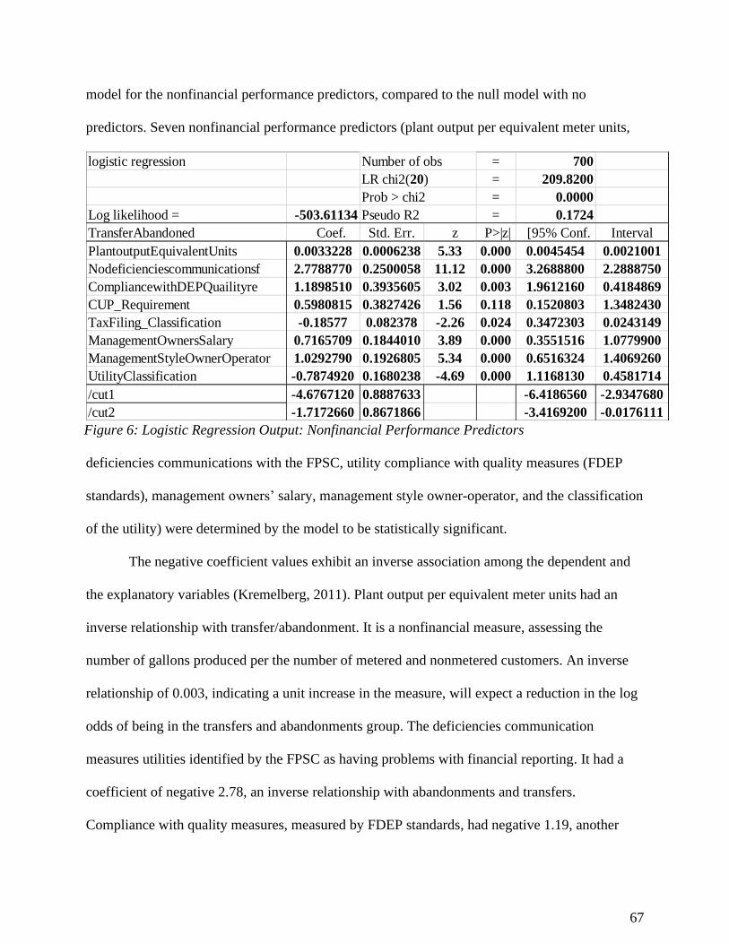
67
model for the nonfinancial performance predictors, compared to the null model with no
predictors. Seven nonfinancial performance predictors (plant output per equivalent meter units,
logistic regression = 700
= 209.8200
= 0.0000
Log likelihood = -503.61134 = 0.1724
TransferAbandoned Coef. Std. Err. z P>|z| [95% Conf. Interval
PlantoutputEquivalentUnits 0.0033228 0.0006238 5.33 0.000 0.0045454 0.0021001
Nodeficienciescommunicationsf 2.7788770 0.2500058 11.12 0.000 3.2688800 2.2888750
CompliancewithDEPQuailityre 1.1898510 0.3935605 3.02 0.003 1.9612160 0.4184869
CUP_Requirement 0.5980815 0.3827426 1.56 0.118 0.1520803 1.3482430
TaxFiling_Classification -0.18577 0.082378 -2.26 0.024 0.3472303 0.0243149
ManagementOwnersSalary 0.7165709 0.1844010 3.89 0.000 0.3551516 1.0779900
ManagementStyleOwnerOperator 1.0292790 0.1926805 5.34 0.000 0.6516324 1.4069260
UtilityClassification -0.7874920 0.1680238 -4.69 0.000 1.1168130 0.4581714
/cut1 -4.6767120 0.8887633 -6.4186560 -2.9347680
/cut2 -1.7172660 0.8671866 -3.4169200 -0.0176111
Pseudo R2
Number of obs
LR chi2(20)
Prob > chi2
Figure 6: Logistic Regression Output: Nonfinancial Performance Predictors
deficiencies communications with the FPSC, utility compliance with quality measures (FDEP
standards), management owners’ salary, management style owner-operator, and the classification
of the utility) were determined by the model to be statistically significant.
The negative coefficient values exhibit an inverse association among the dependent and
the explanatory variables (Kremelberg, 2011). Plant output per equivalent meter units had an
inverse relationship with transfer/abandonment. It is a nonfinancial measure, assessing the
number of gallons produced per the number of metered and nonmetered customers. An inverse
relationship of 0.003, indicating a unit increase in the measure, will expect a reduction in the log
odds of being in the transfers and abandonments group. The deficiencies communication
measures utilities identified by the FPSC as having problems with financial reporting. It had a
coefficient of negative 2.78, an inverse relationship with abandonments and transfers.
Compliance with quality measures, measured by FDEP standards, had negative 1.19, another

68
indicator that utilities who do not keep up with quality are likely to fall into the abandonment and
transfer category; the higher the quality compliance, the less likely that the utility may be
transferred or abandoned. The tax filing classification and utility class also had an inverse
relationship. Management operating style (owner operated-utility as compared to non-
shareholder operators) and management compensation (owners drawing a direct salary from the
utility), had a positive coefficient of 0.717 and 1.03 respectively, an indication that a one-unit
increase in these predictors will increase the log odds of being in the higher level of the
transfers/abandonment category by approximately 0.72 and 1.03, assuming all other predictors
are held constant in the model.
Wirick et al. (1997) explained that the utility industry does not have a precise model
design to examine financial difficulty or viability for water utilities. Acheampong et al. (2018)
improved the NRRI model to determine the viability or sustainability of utilities. This study
attempts to identify the drivers for transfers and abandonments, distinguishing it from other
studies that have solely relied on financial ratios. This study identified nonfinancial measures as
part of the comprehensive assessment of the drivers of transfers and abandonment. Considering
the Z score, the Zeta, and the Platt and Platt model approach to financial sustainability, a logistic
regression analysis was applied to the overall detailed panel data level. All 700 observations, the
NRRI, and Acheampong et al.’s improved financial ratios (five financial ratios), and 15 qualified
nonfinancial measures, after the application of the VIF, were used to predict utility
abandonments. In estimating the overall model, a linktest was run to determine a specified
model. Figure 7 below presents the results of the linktest.
The linktest detects specification error, and it is used to determine if a model possibly
included all the relevant variables. A specified model indicates no significant additional
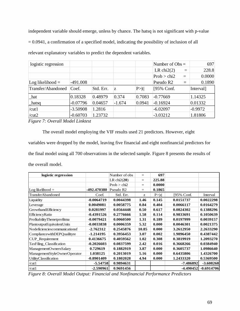
69
independent variable should emerge, unless by chance. The hatsq is not significant with p-value
= 0.0941, a confirmation of a specified model, indicating the possibility of inclusion of all
relevant explanatory variables to predict the dependent variables.
logistic regression Number of Obs = 697
LR chi2(2) = 228.8
Prob > chi2 = 0.0000
Log likelihood = -491.008 Pseudo R2 = 0.1890
Transfer/Abandoned Coef. Std. Err. z P>|t| [95% Conf. Interval]
_hat 0.18328 0.48979 0.374 0.7083 -0.77669 1.14325
_hatsq -0.07796 0.04657 -1.674 0.0941 -0.16924 0.01332
/cut1 -3.50908 1.2816 -6.02097 -0.9972
/cut2 -0.60703 1.23732 -3.03212 1.81806 Figure 7: Overall Model Linktest
The overall model employing the VIF results used 21 predictors. However, eight
variables were dropped by the model, leaving five financial and eight nonfinancial predictors for
the final model using all 700 observations in the selected sample. Figure 8 presents the results of
the overall model.
logistic regression Number of obs = 697
LR chi2(20) = 225.88
Prob > chi2 = 0.0000
Log likelihood = -492.470380 Pseudo R2 = 0.1865
TransferAbandoned Coef. Std. Err. z P>|z| [95% Conf. Interval
Liquidity -0.0064719 0.0044398 1.46 0.145 0.0151737 0.0022298
Leverage 0.0049081 0.0058775 0.84 0.404 0.0066117 0.0164279
GrowthandEfficiency 0.0281997 0.0564448 0.50 0.617 0.0824302 0.1388296
EfficiencyRatio -0.4391526 0.2776666 1.58 0.114 0.9833691 0.1050639
ProfitabilityThenetprofitma -0.0079421 0.0060500 1.31 0.189 0.0197999 0.0039157
PlantoutputEquivalentUnits -0.0033838 0.0006359 5.32 0.000 0.0046301 0.0021375
Nodeficienciescommunicationsf -2.762312 0.2545876 10.85 0.000 3.2612950 2.2633290
CompliancewithDEPQuailityre -1.214195 0.3956453 3.07 0.002 1.9896450 0.4387442
CUP_Requirement 0.4136675 0.4059562 1.02 0.308 0.3819919 1.2093270
TaxFiling_Classification -0.2026603 0.0837599 2.42 0.016 0.3668266 0.0384940
ManagementOwnersSalary 0.729619 0.1882919 3.87 0.000 0.3605737 1.0986640
ManagementStyleOwnerOperator 1.038125 0.2013019 5.16 0.000 0.6435806 1.4326700
UtilityClassification -0.8901409 0.1802028 4.94 0.000 1.2433320 0.5369500
/cut1 -5.54758 0.9894631 -7.486892 -3.608268
/cut1 -2.590961 0.9691456 -4.490452 -0.6914706
Figure 8: Overall Model Output: Financial and Nonfinancial Performance Predictors

70
The model results revealed a likelihood ratio chi-square of 225.88 and a p-value of 0.0000, an
overall statistically significant model. None of the financial performance measures were
significant. However, all the selected nonfinancial performance measures except the
Consumptive Use Permit (CUP) requirement were statistically significant. These nonfinancial
predictors were significant when they were analyzed separately from the financial predictors.
The plant output per equivalent meter units, the deficiencies communication, compliance with
quality measures, tax filing classification, and utility class, were inversely related to
transfer/abandonment. Management operating style and management compensation had a
positive relationship with transfer/abandonment.
4.4.2 Hypothesis 1: Utility Abandonment Drivers
The first hypothesis tests the financial and nonfinancial performance measures
relationship with IOU utility abandonments. The study used the selected samples and created a
dummy variable to represent utility abandonment. The overall model for abandonment/transfer
utilities used 21 explanatory variables (both financial and nonfinancial measures); the model was
statistically significant, employing ordered logistic regression. Abandonment and transfers were
tested separately to determine if the model for abandonment is significantly different from
transfers. The financial performance measures were tested independently from the nonfinancial
measures, and an overall model using both the financial and nonfinancial measures together was
established for utility abandonment; the overall model exhibits a statistically significant model.
A VIF of three was used to guide against multicollinearity issues. The profit trend was dropped
from the model; Figure 9 shows the results of the VIF.

71
Variable VIF 1/VIF
IndirectBu~O 2.38 0.41961
UtilityCla~n 1.99 0.501767
UtilityCom~t 1.93 0.518556
DonatedCap~C 1.76 0.56804
Compliance~a 1.65 0.604778
Nodeficien~f 1.58 0.632207
NARUCAccou~e 1.46 0.684203
GrowthandE~y 1.44 0.692472
Management~y 1.4 0.716552
TaxFiling_~n 1.37 0.732187
Leverage 1.37 0.732569
Management~r 1.35 0.740926
Efficiency~o 1.35 0.741336
CUP_Requir~t 1.24 0.80534
Profitabil~a 1.14 0.875673
Grosswater~e 1.13 0.88352
Liquidity 1.1 0.911109
Plantoutpu~s 1.06 0.943161
Compliance~e 1.06 0.945173
LeverageDe~o 1.01 0.986224
Mean VIF 1.44 Figure 9: VIF: Abandonment
A linktest to determine if the overall model is specified for utility abandonment was run.
Figure 10 presents the results of the linktest.
logistic regression Number of Obs = 700
LR chi2(2) = 135.43
Prob > chi2 = 0.0000
Log likelihood = -107.23269 Pseudo R2 = 0.3871
Abandonment Coef. Std. Err. z P>|t| [95% Conf. Interval]
_hat 0.99454 0.11362 8.753 0.0000 0.77185 1.21724
_hatsq 0.00042 0.00041 1.012 0.3114 -0.00039 0.00123
/cut1 8.38154 0.82146 6.7715 9.99158 Figure 10: Abandonment Linktest
The model is specified as indicated by the linktest presented in Figure 12. The variable _hatsq is
not significant with p-value = 0.3114, a confirmation of a specified model.
Logistic regression was used to build the overall model for utility abandonment. The
overall abandonment model was statistically significant, with Pseudo R2 of 0.387 and p-value =

72
0.0000. The results from all 700 variables indicate that three explanatory variables were
significant. The efficiency ratio, no deficiencies, and the utility class were significant in the
overall model for the utility abandonment. Figure 11 presents the outcome of the logistic
regression.
Logistic regression = 700
= 135.44
= 0.0000
Log likelihood = -107.231440 = 0.3871
Abandonment Coef. Std. Err. z P>|z| [95% Conf. Interval
EfficiencyRatio -1.05762 0.61169 -1.7300 0.0540 -2.25652 0.1412718
ProfitabilityThenetprofitma -0.03710 0.02408 -1.5400 0.1230 -0.08430 0.0100903
PlantoutputEquivalentUnits -0.00090 0.00184 -0.4900 0.6250 -0.00451 0.0027094
Nodeficienciescommunicationsf -3.41529 0.44868 -7.6100 0.0000 -4.29470 -2.5358870
UtilityComplianceannualreport -14.15841 919.22040 -0.0200 0.9880 -1815.797 1787.4800
CompliancewithFPSCQualityMea 14.60826 919.22020 0.0200 0.9870 -1787.030 1816.2470
TaxFiling_Classification 0.16547 0.17745 0.9300 0.3510 -0.18233 0.5132572
ManagementOwnersSalary 0.22920 0.40767 0.5600 0.5740 -0.56981 1.0282120
ManagementStyleOwnerOperator 0.17212 0.42820 0.4000 0.6880 -0.66713 1.0113690
UtilityClassification 2.67837 1.14809 2.3300 0.0200 0.42816 4.9285910
_cons 8.398216 3.62484 1.293656 15.50278
Number of obs
LR chi2(20)
Prob > chi2
Pseudo R2
Figure 11: Abandonment Output: Financial & Nonfinancial Performance Predictors
The efficiency ratio and the no deficiencies communications had a negative coefficient, an
inverse impact on the determination of utility abandonments; the null hypothesis assumes the
explanatory variables do not affect the dependent variable, assuming a coefficient of zero. The
utility class had a positive coefficient, an indication of direct prediction of utility abandonment.
A significant explanatory variable level indicates whether the explanatory variable significantly
impacted the dependent variable without interference from the other explanatory variables
(George & Mallery, 2010). The efficiency ratio and the no deficiencies communications
predicted utility abandonment at the .05 probability level, independent of the other ratios at
coefficients of negative 1.06 and negative 3.42. This means that a higher level of these variables
will expect a reduction of utility abandonments independent of the other variables. The utility
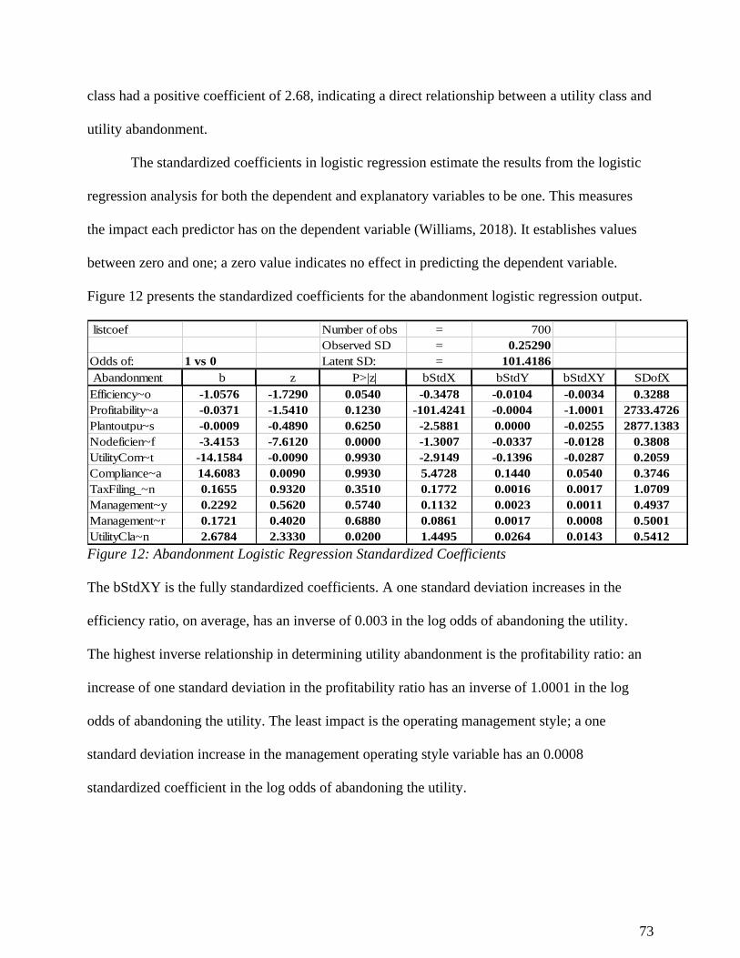
73
class had a positive coefficient of 2.68, indicating a direct relationship between a utility class and
utility abandonment.
The standardized coefficients in logistic regression estimate the results from the logistic
regression analysis for both the dependent and explanatory variables to be one. This measures
the impact each predictor has on the dependent variable (Williams, 2018). It establishes values
between zero and one; a zero value indicates no effect in predicting the dependent variable.
Figure 12 presents the standardized coefficients for the abandonment logistic regression output.
listcoef Number of obs = 700
Observed SD = 0.25290
Odds of: 1 vs 0 Latent SD: = 101.4186
Abandonment b z P>|z| bStdX bStdY bStdXY SDofX
Efficiency~o -1.0576 -1.7290 0.0540 -0.3478 -0.0104 -0.0034 0.3288
Profitability~a -0.0371 -1.5410 0.1230 -101.4241 -0.0004 -1.0001 2733.4726
Plantoutpu~s -0.0009 -0.4890 0.6250 -2.5881 0.0000 -0.0255 2877.1383
Nodeficien~f -3.4153 -7.6120 0.0000 -1.3007 -0.0337 -0.0128 0.3808
UtilityCom~t -14.1584 -0.0090 0.9930 -2.9149 -0.1396 -0.0287 0.2059
Compliance~a 14.6083 0.0090 0.9930 5.4728 0.1440 0.0540 0.3746
TaxFiling_~n 0.1655 0.9320 0.3510 0.1772 0.0016 0.0017 1.0709
Management~y 0.2292 0.5620 0.5740 0.1132 0.0023 0.0011 0.4937
Management~r 0.1721 0.4020 0.6880 0.0861 0.0017 0.0008 0.5001
UtilityCla~n 2.6784 2.3330 0.0200 1.4495 0.0264 0.0143 0.5412 Figure 12: Abandonment Logistic Regression Standardized Coefficients
The bStdXY is the fully standardized coefficients. A one standard deviation increases in the
efficiency ratio, on average, has an inverse of 0.003 in the log odds of abandoning the utility.
The highest inverse relationship in determining utility abandonment is the profitability ratio: an
increase of one standard deviation in the profitability ratio has an inverse of 1.0001 in the log
odds of abandoning the utility. The least impact is the operating management style; a one
standard deviation increase in the management operating style variable has an 0.0008
standardized coefficient in the log odds of abandoning the utility.
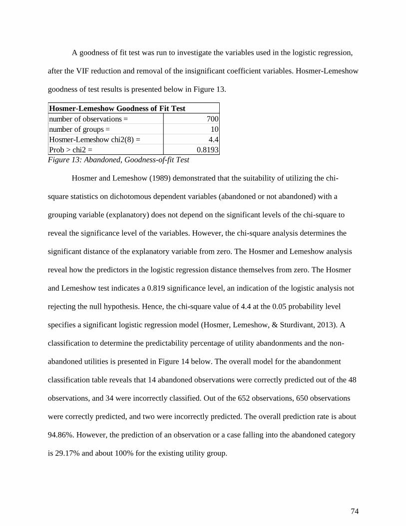
74
A goodness of fit test was run to investigate the variables used in the logistic regression,
after the VIF reduction and removal of the insignificant coefficient variables. Hosmer-Lemeshow
goodness of test results is presented below in Figure 13.
number of observations = 700
number of groups = 10
Hosmer-Lemeshow chi2(8) = 4.4
Prob > chi2 = 0.8193
Hosmer-Lemeshow Goodness of Fit Test
Figure 13: Abandoned, Goodness-of-fit Test
Hosmer and Lemeshow (1989) demonstrated that the suitability of utilizing the chi-
square statistics on dichotomous dependent variables (abandoned or not abandoned) with a
grouping variable (explanatory) does not depend on the significant levels of the chi-square to
reveal the significance level of the variables. However, the chi-square analysis determines the
significant distance of the explanatory variable from zero. The Hosmer and Lemeshow analysis
reveal how the predictors in the logistic regression distance themselves from zero. The Hosmer
and Lemeshow test indicates a 0.819 significance level, an indication of the logistic analysis not
rejecting the null hypothesis. Hence, the chi-square value of 4.4 at the 0.05 probability level
specifies a significant logistic regression model (Hosmer, Lemeshow, & Sturdivant, 2013). A
classification to determine the predictability percentage of utility abandonments and the non-
abandoned utilities is presented in Figure 14 below. The overall model for the abandonment
classification table reveals that 14 abandoned observations were correctly predicted out of the 48
observations, and 34 were incorrectly classified. Out of the 652 observations, 650 observations
were correctly predicted, and two were incorrectly predicted. The overall prediction rate is about
94.86%. However, the prediction of an observation or a case falling into the abandoned category
is 29.17% and about 100% for the existing utility group.
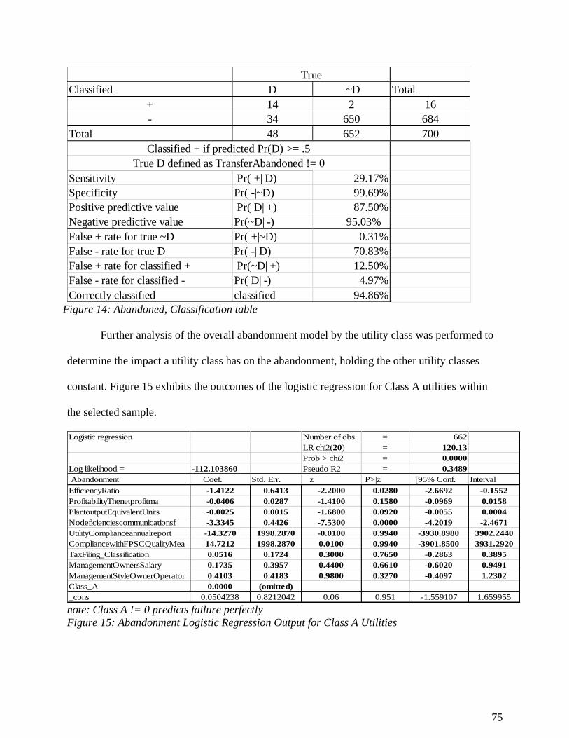
75
Classified D ~D Total
+ 14 2 16
- 34 650 684
Total 48 652 700
Sensitivity Pr( +| D) 29.17%
Specificity Pr( -|~D) 99.69%
Positive predictive value Pr( D| +) 87.50%
Negative predictive value Pr(~D| -) 95.03%
False + rate for true ~D Pr( +|~D) 0.31%
False - rate for true D Pr( -| D) 70.83%
False + rate for classified + Pr(~D| +) 12.50%
False - rate for classified - Pr( D| -) 4.97%
Correctly classified classified 94.86%
True
Classified + if predicted Pr(D) >= .5
True D defined as TransferAbandoned != 0
Figure 14: Abandoned, Classification table
Further analysis of the overall abandonment model by the utility class was performed to
determine the impact a utility class has on the abandonment, holding the other utility classes
constant. Figure 15 exhibits the outcomes of the logistic regression for Class A utilities within
the selected sample.
Logistic regression Number of obs = 662
LR chi2(20) = 120.13
Prob > chi2 = 0.0000
Log likelihood = -112.103860 Pseudo R2 = 0.3489
Abandonment Coef. Std. Err. z P>|z| [95% Conf. Interval
EfficiencyRatio -1.4122 0.6413 -2.2000 0.0280 -2.6692 -0.1552
ProfitabilityThenetprofitma -0.0406 0.0287 -1.4100 0.1580 -0.0969 0.0158
PlantoutputEquivalentUnits -0.0025 0.0015 -1.6800 0.0920 -0.0055 0.0004
Nodeficienciescommunicationsf -3.3345 0.4426 -7.5300 0.0000 -4.2019 -2.4671
UtilityComplianceannualreport -14.3270 1998.2870 -0.0100 0.9940 -3930.8980 3902.2440
CompliancewithFPSCQualityMea 14.7212 1998.2870 0.0100 0.9940 -3901.8500 3931.2920
TaxFiling_Classification 0.0516 0.1724 0.3000 0.7650 -0.2863 0.3895
ManagementOwnersSalary 0.1735 0.3957 0.4400 0.6610 -0.6020 0.9491
ManagementStyleOwnerOperator 0.4103 0.4183 0.9800 0.3270 -0.4097 1.2302
Class_A 0.0000 (omitted)
_cons 0.0504238 0.8212042 0.06 0.951 -1.559107 1.659955 note: Class A != 0 predicts failure perfectly
Figure 15: Abandonment Logistic Regression Output for Class A Utilities
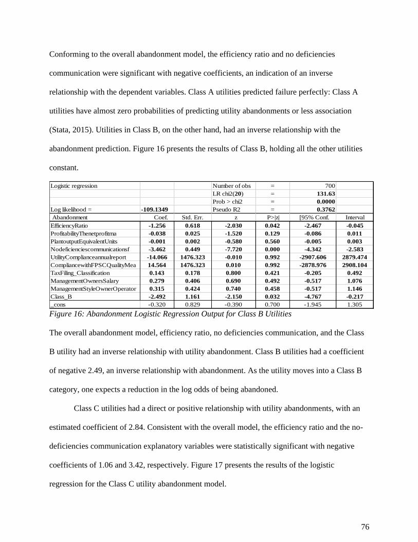
76
Conforming to the overall abandonment model, the efficiency ratio and no deficiencies
communication were significant with negative coefficients, an indication of an inverse
relationship with the dependent variables. Class A utilities predicted failure perfectly: Class A
utilities have almost zero probabilities of predicting utility abandonments or less association
(Stata, 2015). Utilities in Class B, on the other hand, had an inverse relationship with the
abandonment prediction. Figure 16 presents the results of Class B, holding all the other utilities
constant.
Logistic regression Number of obs = 700
LR chi2(20) = 131.63
Prob > chi2 = 0.0000
Log likelihood = -109.1349 Pseudo R2 = 0.3762
Abandonment Coef. Std. Err. z P>|z| [95% Conf. Interval
EfficiencyRatio -1.256 0.618 -2.030 0.042 -2.467 -0.045
ProfitabilityThenetprofitma -0.038 0.025 -1.520 0.129 -0.086 0.011
PlantoutputEquivalentUnits -0.001 0.002 -0.580 0.560 -0.005 0.003
Nodeficienciescommunicationsf -3.462 0.449 -7.720 0.000 -4.342 -2.583
UtilityComplianceannualreport -14.066 1476.323 -0.010 0.992 -2907.606 2879.474
CompliancewithFPSCQualityMea 14.564 1476.323 0.010 0.992 -2878.976 2908.104
TaxFiling_Classification 0.143 0.178 0.800 0.421 -0.205 0.492
ManagementOwnersSalary 0.279 0.406 0.690 0.492 -0.517 1.076
ManagementStyleOwnerOperator 0.315 0.424 0.740 0.458 -0.517 1.146
Class_B -2.492 1.161 -2.150 0.032 -4.767 -0.217
_cons -0.320 0.829 -0.390 0.700 -1.945 1.305 Figure 16: Abandonment Logistic Regression Output for Class B Utilities
The overall abandonment model, efficiency ratio, no deficiencies communication, and the Class
B utility had an inverse relationship with utility abandonment. Class B utilities had a coefficient
of negative 2.49, an inverse relationship with abandonment. As the utility moves into a Class B
category, one expects a reduction in the log odds of being abandoned.
Class C utilities had a direct or positive relationship with utility abandonments, with an
estimated coefficient of 2.84. Consistent with the overall model, the efficiency ratio and the no-
deficiencies communication explanatory variables were statistically significant with negative
coefficients of 1.06 and 3.42, respectively. Figure 17 presents the results of the logistic
regression for the Class C utility abandonment model.
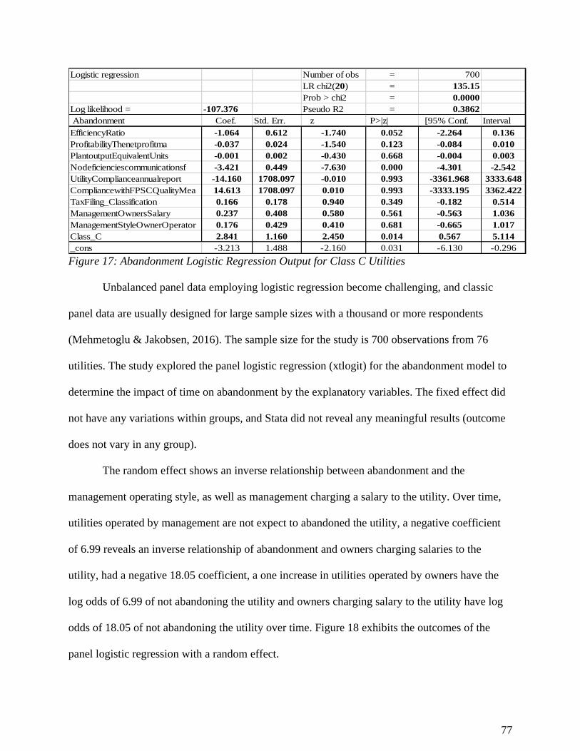
77
Logistic regression Number of obs = 700
LR chi2(20) = 135.15
Prob > chi2 = 0.0000
Log likelihood = -107.376 Pseudo R2 = 0.3862
Abandonment Coef. Std. Err. z P>|z| [95% Conf. Interval
EfficiencyRatio -1.064 0.612 -1.740 0.052 -2.264 0.136
ProfitabilityThenetprofitma -0.037 0.024 -1.540 0.123 -0.084 0.010
PlantoutputEquivalentUnits -0.001 0.002 -0.430 0.668 -0.004 0.003
Nodeficienciescommunicationsf -3.421 0.449 -7.630 0.000 -4.301 -2.542
UtilityComplianceannualreport -14.160 1708.097 -0.010 0.993 -3361.968 3333.648
CompliancewithFPSCQualityMea 14.613 1708.097 0.010 0.993 -3333.195 3362.422
TaxFiling_Classification 0.166 0.178 0.940 0.349 -0.182 0.514
ManagementOwnersSalary 0.237 0.408 0.580 0.561 -0.563 1.036
ManagementStyleOwnerOperator 0.176 0.429 0.410 0.681 -0.665 1.017
Class_C 2.841 1.160 2.450 0.014 0.567 5.114
_cons -3.213 1.488 -2.160 0.031 -6.130 -0.296 Figure 17: Abandonment Logistic Regression Output for Class C Utilities
Unbalanced panel data employing logistic regression become challenging, and classic
panel data are usually designed for large sample sizes with a thousand or more respondents
(Mehmetoglu & Jakobsen, 2016). The sample size for the study is 700 observations from 76
utilities. The study explored the panel logistic regression (xtlogit) for the abandonment model to
determine the impact of time on abandonment by the explanatory variables. The fixed effect did
not have any variations within groups, and Stata did not reveal any meaningful results (outcome
does not vary in any group).
The random effect shows an inverse relationship between abandonment and the
management operating style, as well as management charging a salary to the utility. Over time,
utilities operated by management are not expect to abandoned the utility, a negative coefficient
of 6.99 reveals an inverse relationship of abandonment and owners charging salaries to the
utility, had a negative 18.05 coefficient, a one increase in utilities operated by owners have the
log odds of 6.99 of not abandoning the utility and owners charging salary to the utility have log
odds of 18.05 of not abandoning the utility over time. Figure 18 exhibits the outcomes of the
panel logistic regression with a random effect.
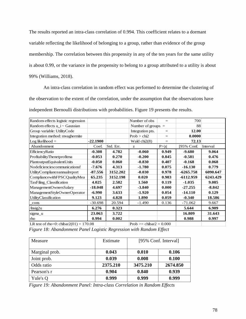
78
The results reported an intra-class correlation of 0.994. This coefficient relates to a dormant
variable reflecting the likelihood of belonging to a group, rather than evidence of the group
membership. The correlation between this propensity in any of the ten years for the same utility
is about 0.99, or the variance in the propensity to belong to a group attributed to a utility is about
99% (Williams, 2018).
An intra-class correlation in random effect was performed to determine the clustering of
the observation to the extent of the correlation, under the assumption that the observations have
independent Bernoulli distributions with probabilities. Figure 19 presents the results.
Random-effects logistic regression Number of obs = 700
Random effects u_i ~ Gaussian 88
Group variable: UtilityCode Integration pts. = 12.00
Integration method: mvaghermite Prob > chi2 = 0.0000
Log likelihood = -22.1900 Wald chi2(8) = 72.13
Abandonment Coef. Std. Err. z P>|z| [95% Conf. Interval
EfficiencyRatio -0.308 4.782 -0.060 0.949 -9.680 9.064
ProfitabilityThenetprofitma -0.053 0.270 -0.200 0.845 -0.581 0.476
PlantoutputEquivalentUnits -0.050 0.060 -0.830 0.407 -0.168 0.068
Nodeficienciescommunicationsf -7.676 4.313 -1.780 0.075 -16.130 0.779
UtilityComplianceannualreport -87.556 3152.202 -0.030 0.978 -6265.758 6090.647
CompliancewithFPSCQualityMea 65.235 3152.198 0.020 0.983 -6112.959 6243.429
TaxFiling_Classification 4.025 2.582 1.560 0.119 -1.035 9.085
ManagementOwnersSalary -18.048 4.697 -3.840 0.000 -27.255 -8.842
ManagementStyleOwnerOperator -6.990 3.633 -1.920 0.054 -14.110 0.129
UtilityClassification 9.123 4.828 1.890 0.059 -0.340 18.586
_cons -30.698 20.594 -1.490 0.136 -71.062 9.667
/lnsig2u 6.276 0.323 5.644 6.909
sigma_u 23.063 3.722 16.809 31.643
rho 0.994 0.002 0.988 0.997
LR test of rho=0: chibar2(01) = 170.08 Prob >= chibar2 = 0.000
Number of groups =
Figure 18: Abandonment Panel Logistic Regression with Random Effect
Measure Estimate [95% Conf. Interval]
Marginal prob. 0.043 0.010 0.106
Joint prob. 0.039 0.008 0.100
Odds ratio 2375.210 3475.210 2674.850
Pearson's r 0.904 0.840 0.939
Yule's Q 0.999 0.999 0.999
Figure 19: Abandonment Panel: Intra-class Correlation in Random Effects
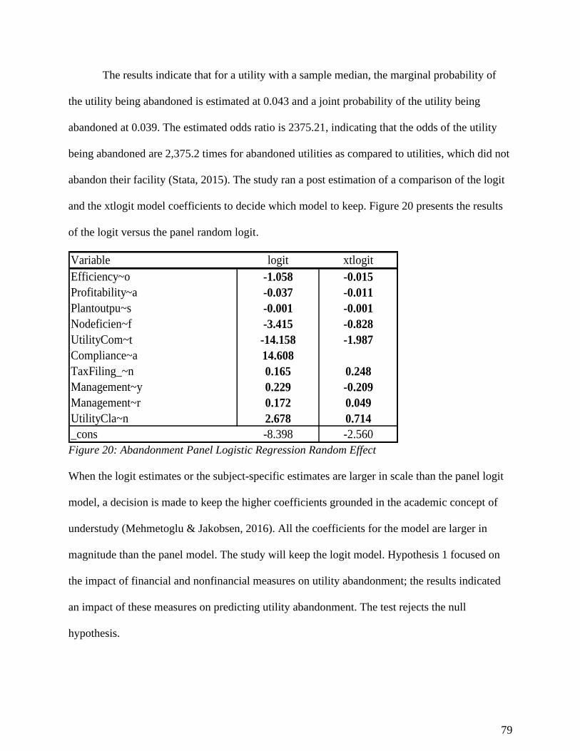
79
The results indicate that for a utility with a sample median, the marginal probability of
the utility being abandoned is estimated at 0.043 and a joint probability of the utility being
abandoned at 0.039. The estimated odds ratio is 2375.21, indicating that the odds of the utility
being abandoned are 2,375.2 times for abandoned utilities as compared to utilities, which did not
abandon their facility (Stata, 2015). The study ran a post estimation of a comparison of the logit
and the xtlogit model coefficients to decide which model to keep. Figure 20 presents the results
of the logit versus the panel random logit.
Variable logit xtlogit
Efficiency~o -1.058 -0.015
Profitability~a -0.037 -0.011
Plantoutpu~s -0.001 -0.001
Nodeficien~f -3.415 -0.828
UtilityCom~t -14.158 -1.987
Compliance~a 14.608
TaxFiling_~n 0.165 0.248
Management~y 0.229 -0.209
Management~r 0.172 0.049
UtilityCla~n 2.678 0.714
_cons -8.398 -2.560 Figure 20: Abandonment Panel Logistic Regression Random Effect
When the logit estimates or the subject-specific estimates are larger in scale than the panel logit
model, a decision is made to keep the higher coefficients grounded in the academic concept of
understudy (Mehmetoglu & Jakobsen, 2016). All the coefficients for the model are larger in
magnitude than the panel model. The study will keep the logit model. Hypothesis 1 focused on
the impact of financial and nonfinancial measures on utility abandonment; the results indicated
an impact of these measures on predicting utility abandonment. The test rejects the null
hypothesis.
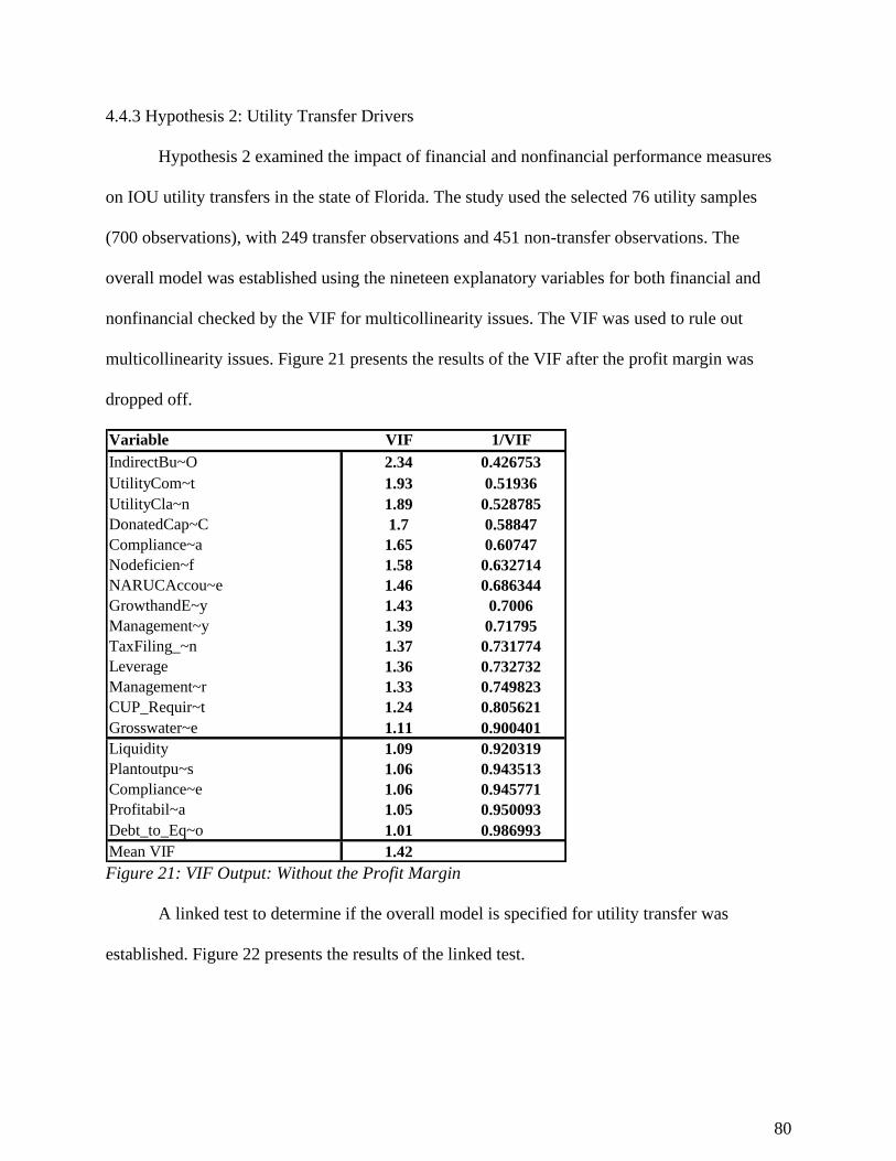
80
4.4.3 Hypothesis 2: Utility Transfer Drivers
Hypothesis 2 examined the impact of financial and nonfinancial performance measures
on IOU utility transfers in the state of Florida. The study used the selected 76 utility samples
(700 observations), with 249 transfer observations and 451 non-transfer observations. The
overall model was established using the nineteen explanatory variables for both financial and
nonfinancial checked by the VIF for multicollinearity issues. The VIF was used to rule out
multicollinearity issues. Figure 21 presents the results of the VIF after the profit margin was
dropped off.
Variable VIF 1/VIF
IndirectBu~O 2.34 0.426753
UtilityCom~t 1.93 0.51936
UtilityCla~n 1.89 0.528785
DonatedCap~C 1.7 0.58847
Compliance~a 1.65 0.60747
Nodeficien~f 1.58 0.632714
NARUCAccou~e 1.46 0.686344
GrowthandE~y 1.43 0.7006
Management~y 1.39 0.71795
TaxFiling_~n 1.37 0.731774
Leverage 1.36 0.732732
Management~r 1.33 0.749823
CUP_Requir~t 1.24 0.805621
Grosswater~e 1.11 0.900401
Liquidity 1.09 0.920319
Plantoutpu~s 1.06 0.943513
Compliance~e 1.06 0.945771
Profitabil~a 1.05 0.950093
Debt_to_Eq~o 1.01 0.986993
Mean VIF 1.42 Figure 21: VIF Output: Without the Profit Margin
A linked test to determine if the overall model is specified for utility transfer was
established. Figure 22 presents the results of the linked test.
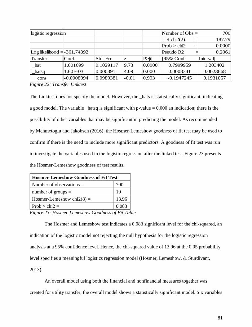
81
logistic regression Number of Obs = 700
LR chi2(2) = 187.79
Prob > chi2 = 0.0000
Log likelihood = -361.74392 Pseudo R2 = 0.2061
Transfer Coef. Std. Err. z P>|t| [95% Conf. Interval]
_hat 1.001699 0.1029117 9.73 0.0000 0.7999959 1.203402
_hatsq 1.60E-03 0.000391 4.09 0.000 0.0008341 0.0023668
_cons -0.0008094 0.0989381 -0.01 0.993 -0.1947245 0.1931057 Figure 22: Transfer Linktest
The Linktest does not specify the model. However, the _hats is statistically significant, indicating
a good model. The variable _hatsq is significant with p-value = 0.000 an indication; there is the
possibility of other variables that may be significant in predicting the model. As recommended
by Mehmetoglu and Jakobsen (2016), the Hosmer-Lemeshow goodness of fit test may be used to
confirm if there is the need to include more significant predictors. A goodness of fit test was run
to investigate the variables used in the logistic regression after the linked test. Figure 23 presents
the Hosmer-Lemeshow goodness of test results.
Hosmer-Lemeshow Goodness of Fit Test
Number of observations = 700
number of groups = 10
Hosmer-Lemeshow chi2(8) = 13.96
Prob > chi2 = 0.083
Figure 23: Hosmer-Lemeshow Goodness of Fit Table
The Hosmer and Lemeshow test indicates a 0.083 significant level for the chi-squared, an
indication of the logistic model not rejecting the null hypothesis for the logistic regression
analysis at a 95% confidence level. Hence, the chi-squared value of 13.96 at the 0.05 probability
level specifies a meaningful logistics regression model (Hosmer, Lemeshow, & Sturdivant,
2013).
An overall model using both the financial and nonfinancial measures together was
created for utility transfer; the overall model shows a statistically significant model. Six variables

82
were dropped from the VIF-suggested predictors due to either insignificant coefficients or
perfect predictions of failure (close to zero probability). The overall transfer model was
statistically significant, with Pseudo R2 of 0.2060 and p-value = 0.0000. The results from all 700
variables indicate that two financial variables and seven nonfinancial variables were statistically
significant. The liquidity and profit margin ratios had an inverse relationship with transfers,
liquidity had negative 0.116, and the profitability ratio had a negative 0.14 4.71. Figure 24
presents the results of the overall transfer model.
Logistic regression Number of = 700
LR chi2(20) = 187.72
Prob > chi2 = 0.0000
Log likelihood = -361.7779 Pseudo R2 = 0.2060
Transfer Coef. Std. Err. z P>|z| [95% Conf. Interval
Liquidity -0.11626 0.02682 -4.34000 0.00000 -0.16883 -0.06370
GrowthandEfficiency -0.02813 0.05157 -0.55000 0.58500 -0.12921 0.07295
ProfitabilityThenetprofitma -0.13977 0.04139 -3.38000 0.00100 -0.22088 -0.05865
PlantoutputEquivalentUnits -0.00194 0.00070 -2.79000 0.00500 -0.00331 -0.00058
GrosswaterRevenuesperCustome 0.00009 0.00011 0.76000 0.45000 -0.00014 0.00031
Nodeficienciescommunicationsf -0.45437 0.27189 -1.67000 0.09500 -0.98726 0.07852
NARUCAccountingCompliance -0.31130 0.21936 -1.42000 0.15600 -0.74124 0.11865
CompliancewithDEPQuailityre -1.82833 0.44711 -4.09000 0.00000 -2.70466 -0.95201
CUP_Requirement -2.42670 0.67909 -3.57000 0.00000 -3.75769 -1.09571
TaxFiling_Classification -0.39630 0.09968 -3.98000 0.00000 -0.59168 -0.20093
ManagementOwnersSalary 0.58527 0.20190 2.90000 0.00400 0.18955 0.98098
ManagementStyleOwnerOperator 0.96313 0.21299 4.52000 0.00000 0.54567 1.38059
UtilityClassification -1.32698 0.19533 -6.79000 0.00000 -1.70982 -0.94415
_cons 8.24020 1.17218 7.03000 0.00000 5.94278 10.53762 Figure 24:Transferred Output: Financial and Nonfinancial Performance Predictors
The seven statistically significant nonfinancial predictors all had an inverse relationship
predicting transfers, except management operating style and management-salary (owners
charging salary to the utility), which had a positive relationship with transfers, an indication of
utilities operated by owners and charging salaries to the utility expected to transfer the utility.
The standardized coefficients were used to compare the relative importance of each coefficient
of each predictor's impact on the dependent variable. Figure 25 presents the standardized
coefficients for the transfer logistic regression output.
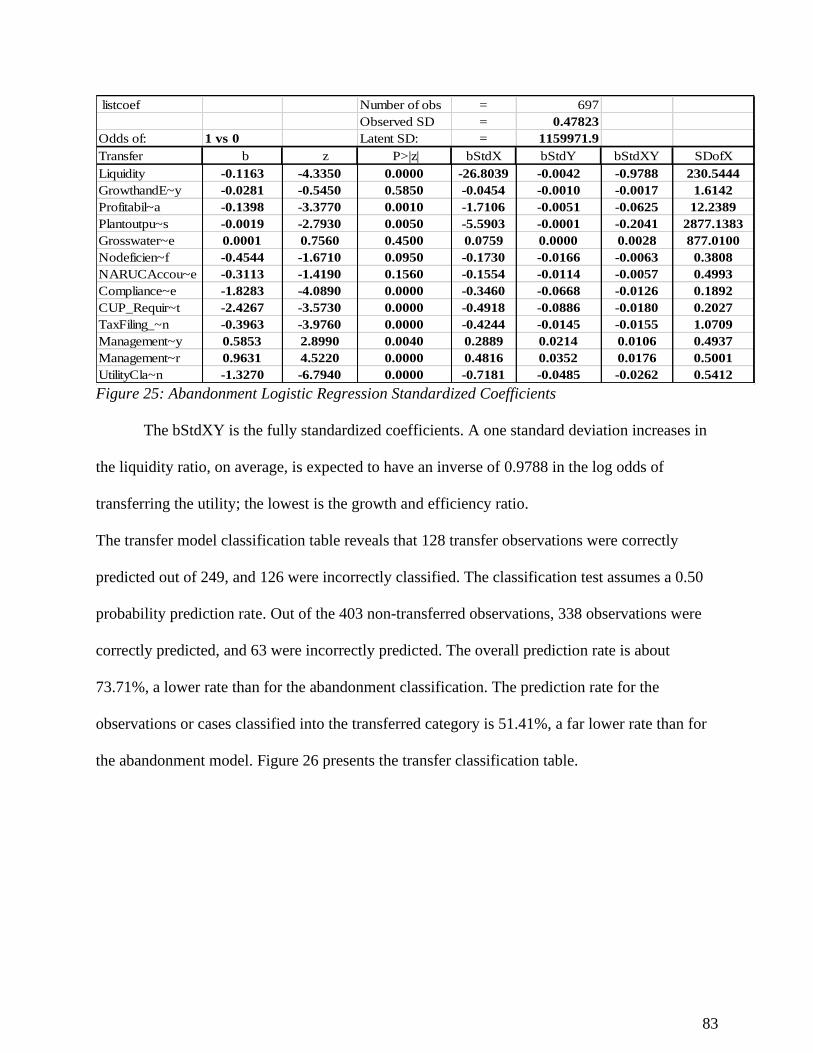
83
listcoef Number of obs = 697
Observed SD = 0.47823
Odds of: 1 vs 0 Latent SD: = 1159971.9
Transfer b z P>|z| bStdX bStdY bStdXY SDofX
Liquidity -0.1163 -4.3350 0.0000 -26.8039 -0.0042 -0.9788 230.5444
GrowthandE~y -0.0281 -0.5450 0.5850 -0.0454 -0.0010 -0.0017 1.6142
Profitabil~a -0.1398 -3.3770 0.0010 -1.7106 -0.0051 -0.0625 12.2389
Plantoutpu~s -0.0019 -2.7930 0.0050 -5.5903 -0.0001 -0.2041 2877.1383
Grosswater~e 0.0001 0.7560 0.4500 0.0759 0.0000 0.0028 877.0100
Nodeficien~f -0.4544 -1.6710 0.0950 -0.1730 -0.0166 -0.0063 0.3808
NARUCAccou~e -0.3113 -1.4190 0.1560 -0.1554 -0.0114 -0.0057 0.4993
Compliance~e -1.8283 -4.0890 0.0000 -0.3460 -0.0668 -0.0126 0.1892
CUP_Requir~t -2.4267 -3.5730 0.0000 -0.4918 -0.0886 -0.0180 0.2027
TaxFiling_~n -0.3963 -3.9760 0.0000 -0.4244 -0.0145 -0.0155 1.0709
Management~y 0.5853 2.8990 0.0040 0.2889 0.0214 0.0106 0.4937
Management~r 0.9631 4.5220 0.0000 0.4816 0.0352 0.0176 0.5001
UtilityCla~n -1.3270 -6.7940 0.0000 -0.7181 -0.0485 -0.0262 0.5412 Figure 25: Abandonment Logistic Regression Standardized Coefficients
The bStdXY is the fully standardized coefficients. A one standard deviation increases in
the liquidity ratio, on average, is expected to have an inverse of 0.9788 in the log odds of
transferring the utility; the lowest is the growth and efficiency ratio.
The transfer model classification table reveals that 128 transfer observations were correctly
predicted out of 249, and 126 were incorrectly classified. The classification test assumes a 0.50
probability prediction rate. Out of the 403 non-transferred observations, 338 observations were
correctly predicted, and 63 were incorrectly predicted. The overall prediction rate is about
73.71%, a lower rate than for the abandonment classification. The prediction rate for the
observations or cases classified into the transferred category is 51.41%, a far lower rate than for
the abandonment model. Figure 26 presents the transfer classification table.

84
Classified D ~D Total
+ 128 63 191
- 121 388 509
Total 249 451 700
True
Sensitivity Pr( +| D) 51.41%
Specificity Pr( -|~D) 86.03%
Positive predictive value Pr( D| +) 67.02%
Negative predictive value Pr(~D| -) 76.23%
False + rate for true ~D Pr( +|~D) 13.97%
False - rate for true D Pr( -| D) 48.59%
False + rate for classified + Pr(~D| +) 32.98%
False - rate for classified - Pr( D| -) 23.77%
Correctly classified classified 73.71%
Classified + if predicted Pr(D) >= .5
True D defined as TransferAbandoned != 0
Figure 26: Transferred Classification Table
The overall transfer model shows an inverse relationship between utility class and
transfers, a direct opposite to the utility abandonment model. Further analysis was performed by
utility class to determine the effect a utility class has on utility transfers, holding the other utility
classes constant. Figure 27 presents the results of the logistic regression for Class A utilities
within the selected sample. Consistent with the overall transfer model, the liquidity and
profitability ratios were significant, with an inverse relationship with a utility transfer. The plant
output per equivalent meters was not significant for Class A utilities as compared to the overall
transfer model. All the other nonfinancial predictors were significant; however, the Class A
utility had a positive coefficient as compared to the overall model.

85
Logistic regression Number of obs = 700
LR chi2(20) = 146.36
Prob > chi2 = 0.0000
Log likelihood = -382.4592 Pseudo R2 = 0.1606
Transfer Coef. Std. Err. z P>|z| [95%
Conf.
Interval
Liquidity -0.10220 0.02488 -4.11000 0.00000 -0.15097 -0.05343
GrowthandEfficiency -0.03736 0.05208 -0.72000 0.47300 -0.13943 0.06471
ProfitabilityThenetprofitma -0.08987 0.03913 -2.30000 0.02200 -0.16656 -0.01317
PlantoutputEquivalentUnits -0.00121 0.00064 -1.88000 0.06000 -0.00247 0.00005
GrosswaterRevenuesperCustome 0.00015 0.00011 1.29000 0.19600 -0.00008 0.00037
Nodeficienciescommunicationsf -0.44877 0.26183 -1.71000 0.08700 -0.96195 0.06440
NARUCAccountingCompliance -0.11982 0.20934 -0.57000 0.56700 -0.53013 0.29048
CompliancewithDEPQuailityre -1.37552 0.43898 -3.13000 0.00200 -2.23591 -0.51513
CUP_Requirement -2.36360 0.70443 -3.36000 0.00100 -3.74425 -0.98295
TaxFiling_Classification -0.18166 0.08864 -2.05000 0.04000 -0.35540 -0.00791
ManagementOwnersSalary 0.56717 0.19302 2.94000 0.00300 0.18885 0.94548
ManagementStyleOwnerOperator 0.64971 0.19592 3.32000 0.00100 0.26571 1.03371
Class_A 1.17851 0.37355 3.15000 0.00200 0.44635 1.91066
_cons 3.49434 0.90994 3.84000 0.00000 1.71088 5.27779 Figure 27: Abandonment Logistic Regression Output for Class A Utilities
The overall model predicted an inverse relationship between a utility class and transfers.
As a utility moves into the Class A category, there is more likelihood for the utility to transfer to
another entity. Class B utilities also had a positive relationship in predicting transfers. The results
of the Class B logistic regression shows an overall statistically significant model. The directions
and number of significant variables are the same as the overall model, except the Class B utility
classification, which has a positive outcome, as compared to a negative relationship by utility
class in the overall transfer model. Figure 28 presents the results of the Class B logistic
regression model. Class B utilities had a coefficient of positive 1.739, a direct relationship with
utility transfer. As a utility moves into a Class B category, one expects an increase in the log
odds of utility transfer to be higher.
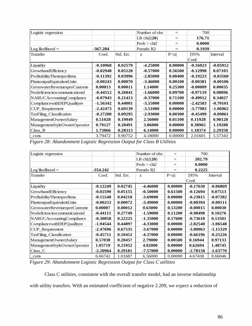
86
Logistic regression Number of obs = 700
LR chi2(20) = 176.71
Prob > chi2 = 0.0000
Log likelihood = -367.284 Pseudo R2 = 0.1939
Transfer Coef. Std. Err. z P>|z| [95%
Conf.
Interval
Liquidity -0.10968 0.02579 -4.25000 0.00000 -0.16023 -0.05912
GrowthandEfficiency -0.02948 0.05128 -0.57000 0.56500 -0.12998 0.07103
ProfitabilityThenetprofitma -0.11392 0.03996 -2.85000 0.00400 -0.19223 -0.03560
PlantoutputEquivalentUnits -0.00243 0.00070 -3.46000 0.00100 -0.00381 -0.00106
GrosswaterRevenuesperCustome 0.00013 0.00011 1.14000 0.25300 -0.00009 0.00035
Nodeficienciescommunicationsf -0.44512 0.26841 -1.66000 0.09700 -0.97119 0.08096
NARUCAccountingCompliance -0.07943 0.21413 -0.37000 0.71100 -0.49912 0.34027
CompliancewithDEPQuailityre -1.56342 0.44001 -3.55000 0.00000 -2.42583 -0.70101
CUP_Requirement -2.42473 0.69139 -3.51000 0.00000 -3.77983 -1.06962
TaxFiling_Classification -0.27280 0.09295 -2.93000 0.00300 -0.45499 -0.09061
ManagementOwnersSalary 0.51028 0.19949 2.56000 0.01100 0.11928 0.90128
ManagementStyleOwnerOperator 0.79127 0.20491 3.86000 0.00000 0.38965 1.19288
Class_B 1.73866 0.28313 6.14000 0.00000 1.18374 2.29358
_cons 3.79472 0.90752 4.18000 0.00000 2.01601 5.57343 Figure 28: Abandonment Logistic Regression Output for Class B Utilities
Logistic regression Number of obs = 700
LR chi2(20) = 202.79
Prob > chi2 = 0.0000
Log likelihood = -354.242 Pseudo R2 = 0.2225
Transfer Coef. Std. Err. z P>|z| [95%
Conf.
Interval
Liquidity -0.12249 0.02745 -4.46000 0.00000 -0.17630 -0.06869
GrowthandEfficiency -0.02590 0.05155 -0.50000 0.61500 -0.12694 0.07513
ProfitabilityThenetprofitma -0.15548 0.04218 -3.69000 0.00000 -0.23815 -0.07282
PlantoutputEquivalentUnits -0.00253 0.00072 -3.49000 0.00000 -0.00394 -0.00111
GrosswaterRevenuesperCustome 0.00007 0.00012 0.63000 0.53200 -0.00015 0.00030
Nodeficienciescommunicationsf -0.44111 0.27749 -1.59000 0.11200 -0.98498 0.10276
NARUCAccountingCompliance -0.30058 0.22225 -1.35000 0.17600 -0.73618 0.13501
CompliancewithDEPQuailityre -1.94544 0.44897 -4.33000 0.00000 -2.82540 -1.06548
CUP_Requirement -2.47696 0.67535 -3.67000 0.00000 -3.80063 -1.15329
TaxFiling_Classification -0.45711 0.10452 -4.37000 0.00000 -0.66196 -0.25226
ManagementOwnersSalary 0.57038 0.20457 2.79000 0.00500 0.16944 0.97133
ManagementStyleOwnerOperator 1.05719 0.21952 4.82000 0.00000 0.62694 1.48745
Class_C -2.20964 0.29181 -7.57000 0.00000 -2.78158 -1.63770
_cons 6.66742 1.01687 6.56000 0.00000 4.67438 8.66046 Figure 29: Abandonment Logistic Regression Output for Class C utilities
Class C utilities, consistent with the overall transfer model, had an inverse relationship
with utility transfers. With an estimated coefficient of negative 2.209, we expect a reduction of
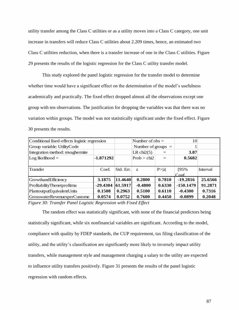
87
utility transfer among the Class C utilities or as a utility moves into a Class C category, one unit
increase in transfers will reduce Class C utilities about 2.209 times, hence, an estimated two
Class C utilities reduction, when there is a transfer increase of one in the Class C utilities. Figure
29 presents the results of the logistic regression for the Class C utility transfer model.
This study explored the panel logistic regression for the transfer model to determine
whether time would have a significant effect on the determination of the model’s usefulness
academically and practically. The fixed effect dropped almost all the observations except one
group with ten observations. The justification for dropping the variables was that there was no
variation within groups. The model was not statistically significant under the fixed effect. Figure
30 presents the results.
10
Group variable: UtilityCode 1
Integration method: mvaghermite LR chi2(5) = 3.87
Log likelihood = -1.871292 Prob > chi2 = 0.5682
Transfer Coef. Std. Err. z P>|z| [95%
Conf.
Interval
GrowthandEfficiency 3.1875 11.4640 0.2800 0.7810 -19.2816 25.6566
ProfitabilityThenetprofitma -29.4304 61.5917 -0.4800 0.6330 -150.1479 91.2871
PlantoutputEquivalentUnits 0.1508 0.2963 0.5100 0.6110 -0.4300 0.7316
GrosswaterRevenuesperCustome 0.0574 0.0752 0.7600 0.4450 -0.0899 0.2048
Number of groups =
Conditional fixed-effects logistic regression Number of obs =
Figure 30: Transfer Panel Logistic Regression with Fixed Effect
The random effect was statistically significant, with none of the financial predictors being
statistically significant, while six nonfinancial variables are significant. According to the model,
compliance with quality by FDEP standards, the CUP requirement, tax filing classification of the
utility, and the utility’s classification are significantly more likely to inversely impact utility
transfers, while management style and management charging a salary to the utility are expected
to influence utility transfers positively. Figure 31 presents the results of the panel logistic
regression with random effects.

88
Random-effects logistic regression Number of obs = 700
Random effects u_i ~ Gaussian 88
Group variable: UtilityCode Integration pts. = 12.00
Integration method: mvaghermite Prob > chi2 = 0.0000
Log likelihood = -67.389 Wald chi2(8) = 90.63
Transfer Coef. Std. Err. z P>|z| [95%
Conf.
Interval
Liquidity -0.14488 0.10101 -1.43000 0.15100 -0.34286 0.05310
GrowthandEfficiency 0.03479 0.43433 0.08000 0.93600 -0.81648 0.88605
ProfitabilityThenetprofitma -0.05714 0.25909 -0.22000 0.82500 -0.56494 0.45067
PlantoutputEquivalentUnits -0.00606 0.00533 -1.14000 0.25600 -0.01651 0.00440
GrosswaterRevenuesperCustome 0.00015 0.00096 0.15000 0.87900 -0.00174 0.00204
Nodeficienciescommunicationsf -1.20278 2.03717 -0.59000 0.55500 -5.19557 2.79000
NARUCAccountingCompliance 0.10660 1.42292 0.07000 0.94000 -2.68227 2.89547
CompliancewithDEPQuailityre -17.11922 3.94778 -4.34000 0.00000 -24.85673 -9.38171
CUP_Requirement -7.15021 3.58201 -2.00000 0.04600 -14.17082 -0.12959
TaxFiling_Classification -3.06127 0.84584 -3.62000 0.00000 -4.71908 -1.40345
ManagementOwnersSalary 3.93791 1.87284 2.10000 0.03500 0.26720 7.60861
ManagementStyleOwnerOperator 9.17968 1.81175 5.07000 0.00000 5.62871 12.73065
UtilityClassification -7.22446 1.67878 -4.30000 0.00000 -10.51481 -3.93411
_cons 42.44130 8.07101 5.26000 0.00000 26.62240 58.26019
/lnsig2u 5.711 0.300 5.123 6.299
sigma_u 17.383 2.610 12.952 23.329
rho 0.989 0.003 0.981 0.994
Number of groups =
Figure 31: Transfer Panel Logistic Regression with Random Effect
A highly significant intra-class correlation of 0.99 and a likelihood of -67.38 prompts a
higher prediction by the explanatory variables. The variance for a utility to be transferred within
any two years is about 99%. The intra-class “rho” correlation for the model is 0.989, a very high-
level intra-class correlation among transfers and the explanatory variables. An intra-class
correlation in random effect was performed to determine the correlation of a utility being
transferred within any two-year period. Figure 32 presents the results of the intra-class
correlation. Hypothesis 2 predicts no impacts of financial and nonfinancial measures on utility
transfers; the results rejected Hypothesis 2 since both financial and nonfinancial predictors
impacted utility transfers.
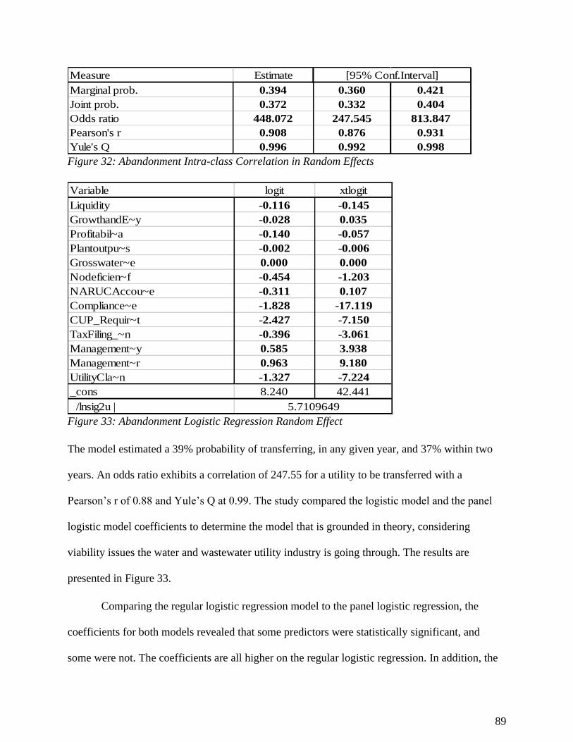
89
Measure Estimate
Marginal prob. 0.394 0.360 0.421
Joint prob. 0.372 0.332 0.404
Odds ratio 448.072 247.545 813.847
Pearson's r 0.908 0.876 0.931
Yule's Q 0.996 0.992 0.998
[95% Conf.Interval]
Figure 32: Abandonment Intra-class Correlation in Random Effects
Variable logit xtlogit
Liquidity -0.116 -0.145
GrowthandE~y -0.028 0.035
Profitabil~a -0.140 -0.057
Plantoutpu~s -0.002 -0.006
Grosswater~e 0.000 0.000
Nodeficien~f -0.454 -1.203
NARUCAccou~e -0.311 0.107
Compliance~e -1.828 -17.119
CUP_Requir~t -2.427 -7.150
TaxFiling_~n -0.396 -3.061
Management~y 0.585 3.938
Management~r 0.963 9.180
UtilityCla~n -1.327 -7.224
_cons 8.240 42.441
/lnsig2u | 5.7109649 Figure 33: Abandonment Logistic Regression Random Effect
The model estimated a 39% probability of transferring, in any given year, and 37% within two
years. An odds ratio exhibits a correlation of 247.55 for a utility to be transferred with a
Pearson’s r of 0.88 and Yule’s Q at 0.99. The study compared the logistic model and the panel
logistic model coefficients to determine the model that is grounded in theory, considering
viability issues the water and wastewater utility industry is going through. The results are
presented in Figure 33.
Comparing the regular logistic regression model to the panel logistic regression, the
coefficients for both models revealed that some predictors were statistically significant, and
some were not. The coefficients are all higher on the regular logistic regression. In addition, the

90
regular logistic regression has a broader explanation, including more statistically significant
predictors (nine predictors including both financial and nonfinancial variables), while the panel
logistic did not include any of the financial predictors and heavily emphasized six predictors with
compliance with quality measures having a negative coefficient of 17.119. Considering the
differences in the coefficients, it does not appear appropriate to compare the standard errors,
since they increase as a factor changes from the logit model to robust standard errors to the
estimates based on the random intercept model (Rodriguez & Elo, 2003). The study used the
logistic regression model results.
4.5 Research Question-Two
RQ2: Do financial performance measures dominate the nonfinancial drivers of utility
abandonments and transfers? The question assists decision-makers in paying attention to the
most prevalent issues among the numerous predictors identified and addressing the problems
accordingly. Question 2 examined two hypotheses about the domination of the financial or
nonfinancial predictors among the abandonment and transfer models. Models such as the NRRI,
Acheampong, et al., etc., focused on the financial ratios or financial performance measures with
six to seven specific ratios, initially identified by the NRRI. This study expanded on the NRRI
model and identified 16 nonfinancial performance measures. Using the data obtained from
FPSC, a VIF analysis was completed to avoid multicollinearity issues. After the VIF analysis,
the financial performance measures were reduced to five ratios, and the nonfinancial explanatory
variables decreased to 12.
Many studies have employed a dominance analysis to determine the relative importance
of the explanatory variables in predicting the dependent variable. In this study, the relative
importance of explanatory variables for transfers and abandonment is ranked using dominance

91
analysis. Dominance analysis selects a pair of predictors, uses the changes of the R2 of the
selected predictors, and runs the selected predictor against all possible subsets of the other
predictors (Azen, 2013). Figure 34 presents the results of the dominance analysis of the ten
categories of both financial and nonfinancial predictors.
Number of obs 697
Overall Fit Statistic 0.2445
TransferAbandoned Dominance Stat. Standardized Domin. Stat Ranking
Nodefici~f 0.1774 0.7256 1
Manageme~r 0.0239 0.0979 2
Manageme~y 0.0126 0.0516 3
Plantout~s 0.0046 0.0186 4
Liquidity 0.0045 0.0186 5
UtilityC~n 0.0045 0.0183 6
TaxFilin~n 0.0044 0.018 7
Complian~e 0.004 0.0164 8
Growthan~y 0.0037 0.0152 9
Profitab~a 0.0017 0.0071 10
CUP_Requ~t 0.0014 0.0056 11
Leverage 0.0013 0.0055 12
Efficien~o 0.0004 0.0015 13
Conditional dominance statistics
Dominance Analysis
Figure 34: Dominance Ranking-Overall Model
Luchman (2015) used the R2 in the dominance analysis. The R2 statistic is divided by the
overall fit statistic among the categories to determine the margin of dominance. A no
deficiencies communication predictor was ranked number one among the predictors. The margin
of dominance is about 73% (0.1774/ 0.2445), followed by the management operating style with a
margin of dominance of 10%, a substantial difference between the leading predictor and the
subsequent predictor. The efficiency ratio was ranked the least, with less than one percent
dominance margin.

92
4.5.1 Hypothesis 3
The study tested the hypothesis of financial performance measures dominating the
nonfinancial measures for utility abandonment. Hypothesis 3: Nonfinancial performance
measures do not dominate utility abandonment. Following Luchman (2015) and Kumar, Kee,
and Manshor, (2009). The study created an abandonment dummy, holding transfer and regular
utilities constant, within the selected sample and ran a dominance analysis on all the predictors
for utility abandonment. Figure 35 presents the results of the dominance analysis on utility
abandonment.
Number of obs 700
Overall Fit Statistic 0.2206
Abandonment Dominance Stat. Standardized Domin. Stat Ranking
Nodefici~f 0.1719 0.7793 1
UtilityC~t 0.0312 0.1415 2
UtilityC~n 0.0101 0.0456 3
Efficien~o 0.0025 0.0115 4
Complian~a 0.0024 0.011 5
Plantout~s 0.0008 0.0038 6
Manageme~y 0.0006 0.0028 7
TaxFilin~n 0.0004 0.002 8
Manageme~r 0.0003 0.0015 9
profitma~n 0.0002 0.001 10
Conditional dominance statistics
Abandonment Dominance Analysis
Figure 35: Dominance Ranking-Abandoned Utilities
The abandonment model predicted the nonfinancial variables as the dominating
predictors for utility abandonment. The no deficiencies communication predictor was ranked
number one among the predictors with a margin of dominance of 78%, consistent with the
overall model. Utility compliance with the annual report was ranked second with a margin of
dominance of 14%. The least dominant is the profitability ratio with less than one percent.
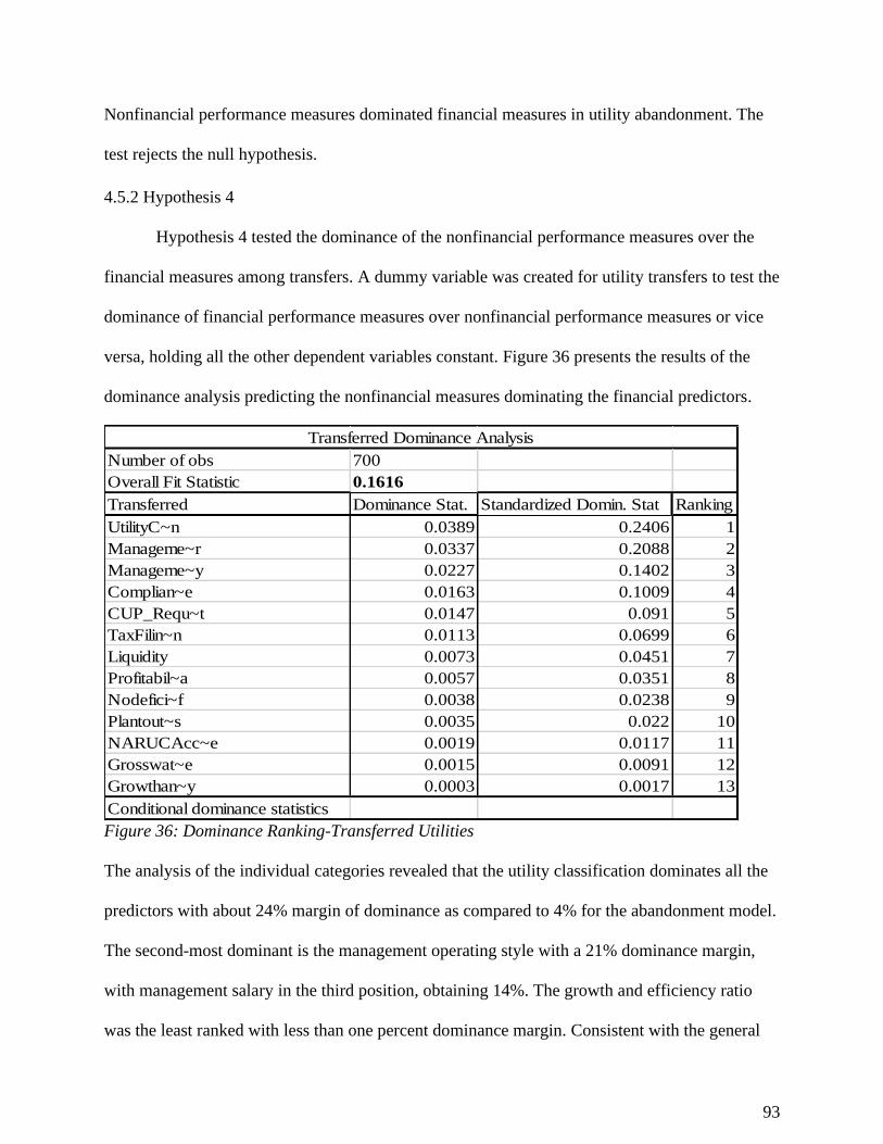
93
Nonfinancial performance measures dominated financial measures in utility abandonment. The
test rejects the null hypothesis.
4.5.2 Hypothesis 4
Hypothesis 4 tested the dominance of the nonfinancial performance measures over the
financial measures among transfers. A dummy variable was created for utility transfers to test the
dominance of financial performance measures over nonfinancial performance measures or vice
versa, holding all the other dependent variables constant. Figure 36 presents the results of the
dominance analysis predicting the nonfinancial measures dominating the financial predictors.
Number of obs 700
Overall Fit Statistic 0.1616
Transferred Dominance Stat. Standardized Domin. Stat Ranking
UtilityC~n 0.0389 0.2406 1
Manageme~r 0.0337 0.2088 2
Manageme~y 0.0227 0.1402 3
Complian~e 0.0163 0.1009 4
CUP_Requ~t 0.0147 0.091 5
TaxFilin~n 0.0113 0.0699 6
Liquidity 0.0073 0.0451 7
Profitabil~a 0.0057 0.0351 8
Nodefici~f 0.0038 0.0238 9
Plantout~s 0.0035 0.022 10
NARUCAcc~e 0.0019 0.0117 11
Grosswat~e 0.0015 0.0091 12
Growthan~y 0.0003 0.0017 13
Conditional dominance statistics
Transferred Dominance Analysis
Figure 36: Dominance Ranking-Transferred Utilities
The analysis of the individual categories revealed that the utility classification dominates all the
predictors with about 24% margin of dominance as compared to 4% for the abandonment model.
The second-most dominant is the management operating style with a 21% dominance margin,
with management salary in the third position, obtaining 14%. The growth and efficiency ratio
was the least ranked with less than one percent dominance margin. Consistent with the general

94
dominance analysis, the nonfinancial predictors dominated the financial predictors. Hypothesis 4
tested the dominance of financial performance measures on nonfinancial performance measures.
The results of the study rejected hypotheses 4. The nonfinancial performance measures
dominated the financial performance measures.
The results of both the logistic regression and the dominance analysis inform both
practitioners and academicians on the steps that may assist in evaluating transfers and
abandonments in the nonviable water and wastewater industry. Chapter five discusses the results
and their practical and theoretical implications, as well as the recommendations and suggestions
for future research.

95
Chapter Five: Discussion, Conclusions, and Recommendations
Chapter five concentrates on discussion, conclusions, practical and theoretical
implications on the research, recommendations, and suggestions for future study.
5.1 Discussion
This study is a primary empirical study examining and reviewing the drivers of water and
wastewater utility abandonments and transfers in the state of Florida. The investor-owned water
and wastewater utility industry is an increasing-cost industry; hence, the rate case proceedings
should enhance the long-term sustainability of utilities, by providing adequate resources for the
required services and a return on investment to protect the interest of investors and continuity of
services to the citizens (Beecher et al., 1993). The principal objective of the study is to determine
the drivers of utility abandonments and transfers using both financial and nonfinancial
performance measures by addressing the following objectives:
1. Determine the relationship between financial and nonfinancial performance measures on
utility abandonments.
2. Determine the relationship of both financial and nonfinancial performance measures on
utility transfers.
3. After identifying the financial and nonfinancial performance measures, rank their
dominance impact on abandonments and transfers.
4. Determine the overall dominance of financial or nonfinancial performance measures on
both abandonments and transfers.
These objectives were established within the framework of establishing the drivers of

96
utility abandonments and transfers and accomplishing the stated purposes that created the Study
Committee. To address the primary objectives, two research questions were identified: What are
the financial and nonfinancial performance drivers of utility abandonments and transfers, and do
the financial performance measures dominate the nonfinancial drivers of utility abandonments
and transfers?
Chapter three presented the methodology and data collection procedure. The study used a
quantitative approach, selecting seven ratios used by both NRRI and Acheampong et al. to
establish a utility viability model. These ratios are the liquidity, leverage, debt to equity,
profitability, and the growth and efficiency ratios, as well as the efficiency and profitability
ratios. Also, the study identified and used 14 nonfinancial performance measures. These
measures are plant output per equivalent units, the gross water revenues per customer,
compliance with FPSC quality measures, compliance with NARUC accounting standards,
deficiencies in communications with FPSC, compliance with annual financial reporting,
compliance with FDEP quality requirements, compliance with the CUP requirement, the tax
filing classification of the utility, management /owners charging salary to the utility, the
management operating style of the utility (owner/operator or management independent of
management), utility class, donated capital (CIAC), and indirect business taxes (i.e. taxes other
than income (PSC funding).
A total of 146 utilities existed within the study period of 2008-2017. This study used the
random sampling command in Excel to generate random numbers for the utility. The top 60%
(87 utilities) were randomly selected. Of the selected 87 utilities, 76 had enough information to
qualify for the study. A total of 11 utilities were dropped due to insufficient information, such as
zero annual filings or no financials filed by the utility. The study obtained the data used in the
97
study from the FPSC and the FDEP.
5.2 Major Findings
The two questions addressed by the study and the associated goals of the study revealed
interesting and intriguing findings. The drivers for utility abandonments were different from
those for the transfer models, and the dominance analysis revealed an opposite direction for
abandonments and transfers. Because utility regulations are state-specific, it is challenging to
have a general model. However, the study reveals a process that may be followed by each state
to establish a general model for its regulatory body. The first and second hypotheses tested the
financial and nonfinancial performance measures’ impacts on utility abandonments and transfers.
Among the seven selected financial ratios, the efficiency ratio was statistically significant.
Among the 14 selected nonfinancial predictors, two nonfinancial performance measures (no
deficiencies communication and utility classification) were statistically significant in
determining utility abandonment. Overall, ten variables were used to establish the abandonment
model. The transfer model used 13 financial and nonfinancial performance measures to establish
the transfer model. There were three financial and ten nonfinancial variables, with two financial
(liquidity and profitability) variables statistically significant in predicting transfers. Seven of the
ten nonfinancial variables were statistically significant in predicting transfers.
The dominance test used all 700 observations based on the variables used in each model.
The abandonment and transfer models separately ranked the variables in order of importance and
the contribution towards predicting abandonments and transfers. Nonfinancial predictors
dominated financial predictors for both the abandonment and transfer models. However, the
ranking of the nonfinancial predictors was different among the abandonments and transfer
models. For abandonments, no deficiencies communication ranked number one with about a
98
78% margin of dominance, while the transfer model ranked utility classification as number one
with a 24% margin of dominance. An indication of the treatment of abandonment and transfers
should be investigated differently. The transfer dominance analysis had a reasonable distribution
of variance among the ranking of the variables with no one particular variable dominating,
compared to the abandonment model in which the deficiencies communication variable
dominated all the other predictors.
5.2.1 Major Findings: Question 1
Seven nonfinancial performance measures of the nine qualified for the model were
significant in determining the abandonments and transfers. The plant output per the number of
meters served by a utility was determined to have an impact on both utility abandonments and
utility transfers; the more equivalent units a utility serves or the higher the output per meter, the
less likely that a utility will abandon or transfer the utility. The deficiency communication from
FPSC to utilities was another indicator that was influential in determining utility abandonment
and transfers. No deficiencies communication was good news for a utility. A company that does
not receive such communication is less likely to abandon or transfer its utilities. Utilities that
comply with the quality standards set by the FDEP were less likely to be abandoned or
transferred. The tax filing classification of a utility and the utility classification influenced
whether a utility was likely to be either abandoned or transferred. Utilities operated by owners
and /or owners charging a salary to the utility also were factors in the likelihood of a utility being
abandoned or transferred.
Overall, four financial performance measures—the liquidity, leverage, growth and
efficiency, and the efficiency ratios—together with nine nonfinancial ratios determined the
likelihood for a utility to abandoned or transferred. However, the impact of these measures was

99
different among abandonments and transfers. A utility is likely to abandon its facility if the
utility is not able to effectively employ its assets to generate enough financial resources to
manage its financial liabilities as they come due. Consistent with the overall assessment of the
industry, utilities that receive deficiency financial communications from the FPSC are likely to
abandon their facility. The utility classification under NARUC was a factor for utility
abandonments. Neither Class A nor Class B utilities are likely to abandon their facilities, as
compared to Class C utility. However, Class C utilities are three times more likely to abandon
their facilities as compared to Class A and B utilities. Overall, two financial performance
measures (the efficiency and profit margin ratios) combined with eight nonfinancial performance
measures (plant output per equivalent meters, deficiency communication, utility compliance with
annual report, utility compliance with FPSC quality measures, tax filing classification of the
utility, management operating style, and management compensation requirements) impact utility
abandonments in the state of Florida.
Thirteen financial and nonfinancial performance measures impacted the utility’s
likelihood to be transferred to new ownership. Three financial performance measures (the
liquidity, growth and efficiency, and the profitability ratios) and ten nonfinancial performance
measures influenced the decision to transfer the utility (the plant output per equivalent meter, the
gross water revenues per customer, the deficiency communication, compliance with NARUC
accounting standards, compliance with FDEP quality standards, compliance with the
consumptive use permit requirement, the tax filing classification, the utility classification, the
management operating style and management salary requirement). Utilities with less liquid
assets and/or utilities with downward profit trends are more likely to be transferred. Utilities with
less output per an equivalent number of meters are more likely to transfer the utility. Utilities
100
complying with the consumptive water use permit requirement (the ability to withdraw allowable
water from a water source), complying with FDEP quality standards, are more likely not to be
transferred. The tax classification of a utility impacts the factors for a utility to be transferred; the
management style and owners charging a salary to the utility influence a utility’s likelihood to
transfer the utility. Owners charging salaries to the utility are more likely to transfer the utility,
and utilities operated by owners are more likely to be transferred. The utility’s classification
influenced the decision to transfer to new ownership. Class A and Class B utilities (those with
over $200,000 in gross revenues) are likely to transfer the utility; unlike abandonment, Class C
utilities are not likely to be transferred.
5.2.2 Major Findings: Question 2
The study used the dominance analysis to prioritize the drivers of utility abandonment
and transfers, using evidence from the state of Florida. The study categorized the drivers into two
groups, the financial performance, and the nonfinancial performance measures, and ranked the
individual drivers for abandonments and transfers. The overall assessment rated FPSC deficiency
communication as the highest among the 13 financial and nonfinancial drivers. Utilities that
receive such communications from the FPSC need to follow the required steps to bring them up
to standard; this communication is typically issued after a thorough review of the utility’s
financials and other quality issues. Utilities run by owners and those charging salaries to the
utility were second and third, respectively. Utility regulators may have to assess these drivers,
since they are not allowable expenses and utility owners may overestimate or underestimate the
charges, making the utility seems nonviable, which eventually may lead to a transfer or
abandonment, costing taxpayer’s money. The top three accounted for about of the 85% variation
in explaining utility abandonments and transfers.

101
The nonfinancial performance measures for utility abandonments dominated financial
performance measures. Utility abandonment is most likely due to nonfinancial difficulties
encountered by the utility, leading to financial issues. The deficiency communication,
compliance with the annual reporting requirements, utility class, and the efficient operations of
the utility in generating cash to meet its present obligations were the major concerns for utility
abandonments. The profitability of a utility was the least concern for the utility to abandon its
facility.
The transfer of a utility either to a new utility or to an existing utility was not likely due
to financial performance measures. The nonfinancial performance measures dominated the
financial measures both in aggregate and individual drivers. The utility class was a primary
concern, followed by the operating style of the utility. Utilities run by the owners are most likely
to transfer. In addition, utilities in which the owners charge a salary to the utility are more likely
to be transferred compared to utilities in which the owners do not charge salaries to the utility.
Compliance with FDEP quality measures also plays a significant role in the decision of a utility
to transfer. Gross water revenues per customer and the growth trends of the utility as a result of
efficiency were the least among the drivers for a utility to transfer its facility to another utility or
a new utility.
Abandonments and transfers need to be assessed on their individual merits. Grouping
them yields a trend that seems to explain most utility abandonments, but considering them
separately, the drivers that dominate utility abandonments differ from the drivers dominating
utility transfers.
5.3 Conclusions
The study identified the drivers impacting transfers and abandonments in the investor-

102
owned water and wastewater utility industry. A review of the data exhibits some utilities
displaying long-term sustaining losses over the years, confirmation of viability and sustainability
problems. These problems were recognized by the state of Florida when House Bill No. 1389-
2012 formed the Study Committee to identify issues preventing investor-owned utilities from
being sustainable and making recommendations to avoid abandonments. The bill attempted to
identify a series of factors that addressed the sustainability issues within the investor-owned
water and wastewater utility industry. The committee identified a laundry list of items that, if
implemented, could improve the water and wastewater utility industry in the state of Florida.
This research used empirical evidence from the records and filings of the investor-owned
water and wastewater utility industry in the state of Florida to complement the work
accomplished by the state’s Study Committee, offering empirical evidence to substantiate its
findings. This study identified financial and nonfinancial performance measures that need to be
addressed to improve the current situation. In addition, the study ranked the significance of these
performance measures for abandonments and transfers independently. The study established that
both financial and nonfinancial performance measures should be given equal attention, compared
to prior studies that focused on financial performance measures only.
5.3.1 Major Question 1 Related to the Purpose of the Study
Question one’s purpose was to examine the financial and nonfinancial performance
factors that drive investor-owned utility abandonments and transfers by explaining the impact of
the financial and nonfinancial performance measures on utility abandonments and transfers. The
study employed logistic regression, using samples from the state of Florida water and wastewater
industry, to determine the impact of financial and nonfinancial factors that impact utility
abandonments and transfers. The logistic regression model reinforced the purpose of the study by

103
determining the drivers of utility abandonments and transfers. The question posed two
hypotheses to investigate the impacts of financial and nonfinancial performance abandonments
on utility abandonments and transfers. The first hypothesis tested the drivers for utility
abandonments, and the second hypothesis assessed the predictors for utility transfers. The study
found that the drivers for utility abandonments differ from those for utility transfers. Both
hypotheses exhibited the nonfinancial performance measures as the primary predictors for
abandonments and transfers of utilities.
5.3.2 Major Question 2 Related to the Purpose of the Study
Question one analyzed the significance of both financial and nonfinancial drivers of
utility abandonments and transfers, using the logistic regression model. The Z value for the
logistic regression shows the importance of the driver; the higher the Z value at the 95%
confidence level, the more significant the driver. However, it does not reveal the dominance of
the drivers. The second question was used to test the dominance of the drivers that were
determined by the first question. The overall model reveals that nonfinancial performance
measures need more attention compared to the financial measures; both the abandonment and
transfer models followed the same pattern. The dominance test determined the ranking of the
drivers, an essential element of the scope of the study. The purpose of the second question is to
promote regulatory policy changes needed to be considered for water and wastewater utilities to
be sustainable and possibly avoid abandonment, by analyzing the eminent drivers among those
reviewed. The dominance analysis will assist regulators, practitioners, and owners to effectively
use the limited resources to address the sustainability issues in the industry.
5.4 Implications for Practitioners, Owners, and Regulators
The outcomes of the research proposals showed remarkable implications for owners of

104
water and wastewater utilities. Owners, practitioners, regulators, ratepayers, and academicians
will benefit from the use of the dominance analysis to emphasize the drivers that are
distinguished among all the variables to assist the nonviable water and wastewater industry to be
sustainable to enhance the operations of the utilities to save taxpayers money. Regulators (state
commissioners) may create an enabling environment for academicians to examine the
vulnerabilities of the leverage scale; this will lead to the building of a more formidable model to
assist in establishing a rate base. A better model will help to account for the financial concerns
raised by the efficiency ratios, the growth and efficiency ratios, and the profit margin ratio. Also,
regulators may further explore management operating style and management charging a salary to
a utility to consider either authorizing salaries as allowable expenses or preventing utilities from
charging salaries, instead of leaving the issue in a gray area as “non-allowable expenses.”
Realizing that liquidity, among the financial performance measures, is vital in
determining the sustainability of the utilities, practitioners, and owners of investor-owned water
and wastewater utilities may reconsider the common practice within the industry that keeps less
cash at hand. This consideration is also supported by raising enough financial resources to be
able to meet the obligations of the utilities as they come due; the lack of such resources is a
driver that contributes to utility abandonments. The study encourages utilities to seek rate
changes and cut costs, among other means to increase the financial resources for these utilities to
avoid abandonments.
This study informs prospective utility purchasers about the liquidity issues revealed
within the ten years of data covered by the study; the fewer liquid financial resources a utility
carries, the more likely the utility will be transferred to a new entity. Practitioners should
consider the liquidity ratio during the appraisal of a utility. In addition, the profit margin
105
(profitability ratio) plays a significant role in utility transfers; the less profitable a utility is, the
more likely the utility will be transferred to another utility.
Owners and practitioners are informed by the study to consider nonfinancial measures
such as deficiency communications from the FPSC, the compliance with quality measures,
compliance with the required NARUC accounting standards, the CUP requirement, owner-
operator as compared to hiring certified professionals to run the utility, petitioning the FPSC
about the owners’ salary requirements, etc. in their annual assessments of the utility’s
performance and in a request for a rate increase or annual pass-throughs. A significant factor
revealed by the study is the profit trend of the industry. The study did not emphasize the details
since there are no known industry standards to compare averages. However, the net income for
the selected 76 utilities showed an average loss of $34,672 over the ten-year period from 2008
through 2017, concern practitioners and utility owners should jointly address with regulators.
The consequence may trigger unwarranted rate case proceedings; accordingly, regulators are
informed by the study results to prepare for an influx of rate case filings, by equipping and
improving the FPSC staff on oversight activities and rate filing activities.
This study informs the public about the need to sustain the water and wastewater utility
industry. Awareness of expected rate increases should be welcomed to assist these utilities in
sustaining their operations. A rate increase may not be the only factor needed to assist the
industry. However, FPSC oversight and requirements for utilities to meet some nonfinancial
performance measures may also assist the utilities in being sustainable. The public, through their
elected representatives, may require the FPSC to increase oversight activities to enhance the
abilities of these utilities to be sustainable. This study also furnishes ratepayers with the findings
that recovery of operating costs is not sufficient to improve the rate base and sustain utilities.

106
Owners are informed by the study to improve and incorporate nonfinancial performance
measures in their decision-making processes to improve the operations and sustainability of the
utilities.
The accounting profession may use the outcomes of the study in several different
avenues, as an opportunity for auditing engagements, preparing utilities for filing and testimony
appearance during rate hearings, and enhancing utilities’ abilities to comply with annual filing.
Consulting services may improve nonfinancial performance measures to augment utility
sustainability.
5.5 Implications for Research
The objectives of the research are to identify the drivers for utility abandonments and
transfers within the investor-owned water and wastewater industry and to rank the relevance of
the drivers. The study provides an informed contribution to the current literature and a future
platform analysis directed at the formulation of an enabling environment for the water and
wastewater industry to be sustainable and increase the oversight requirements by regulators to
ensure adequate funding through rate case proceedings. There are two essential revelations
associated with the drivers for utility abandonments and transfers and which of the drivers
dominated. The most important implication for the study is for academicians to distinguish the
treatment of utility abandonments from transfers. The second significant finding for researchers
is the applicability of both financial and nonfinancial performance measures in the determination
of firms’ performance in the utility industry.
Studies in the banking and finance industry, among others, have successfully used the
logistic regression in determining viable and nonviable firms. Beecher et al. (1992) emphasize
the need for an extensive model to examine the sustainability of the water industry. An attempt

107
to use the discounted method approach was employed, and recommendations about the use of the
Platt and Platt model alike were made. The outcome of the study has created an enabling
environment for researchers to explore the logistic regression as a more dependable method,
applying financial and nonfinancial performance factors to utility sustainability and viability
models, an extension of the modified model proposed by Acheampong et al.
5.6 Limitations
The literature review outlined the sustainability of water and wastewater utilities,
depending on other determinants instead of the financial and nonfinancial performance measures.
The research concentrated on financial ratios developed by the NRRI and improved by the model
developed by Acheampong et al., together with other nonfinancial performance measures in the
determination of utility abandonments and transfers. Prospective researchers may further
examine the detailed and inductive analyses on the different elements of the financial ratios,
exploring outside of the NRRI identified financial ratios in combination with the nonfinancial
performance measures.
The generalizability of the study outcomes is limited to the various states whose
regulations align with those of Florida and use rate base and annual pass-through to adjust utility
rates. The selection of 60% of utilities within ten years of annual filings poses a selection risk by
not including all Florida IOUs in the sample. The financial data were retrieved from unaudited
annual financial filings of the various utilities submitted to the FPSC. The study, at best, may
predict the relationship between financial and nonfinancial performance measures and utility
abandonments and transfers. However, the study does not address the level of capital funding
required by the investor-owned utilities to be sustainable. The study does not disclose or
acknowledge the provision of quality services to ratepayers.
108
Furthermore, the study does not examine or discuss the consequences and repercussions
of utility failures on ratepayers. One may anticipate the taxpayers’ burden to recover and upgrade
utility abandonments and transfers increases, but this study does not measure this increase. The
study is positioned to establish a correlation between financial and nonfinancial performance
measures on abandonments and transfers. The tax implications of tax shelters and the hobby rule
were not addressed as most of the sampled utilities had years of sustaining losses.
5.7 Recommendations
The following recommendations may assist regulators, practitioners, and owners of water
and wastewater utilities in improving the current sustainability and viability issues within the
water and wastewater industry in the state of Florida.
➢ FPSC regulators should consider the study to be empirical support for further
action on House Bill No. 1389-2012.
➢ FPSC regulators need to increase attention to nonfinancial performance in the
water and wastewater utilities to ensure consistent compliance with the various
rules, especially the quality measures by both FPSC and the FDEP. Compliance
with annual filing following the NARUC standards needs to be enforced with
penalties for noncompliance.
➢ FPSC regulators should improve annual financial reporting and offer
comprehensive audit oversight to improve the reliability of the reporting process
and the reported data.
➢ Owners and practitioners should be proactive in determining both financial and
nonfinancial performance measures that need to be improved to enhance a
utility’s sustainability.

109
➢ Utility owners should grow their equity base and be informed of the impact of
large equity base on rate base, improving the return on equity.
➢ Practitioners may have an excellent opportunity for a consulting role in this
industry to turn it around to be a viable utility by working with both regulators
and owners of these utilities.
5.7.1 Suggestions for Future Research
The empirical analysis outcomes, as complements to the literature review, have supported
the discussions and the conclusions of the study. The outcomes of the study have informed
numerous recommendations to enhance the subject matter. This study empirically complements
the Study Committee recommendations. There is still work to be done to include the perceptions
of ratepayers and improve the research activities in the water and wastewater industry to enhance
the sustainability and viability of investor-owned utilities. The implementation, further research,
and analysis by practitioners, regulators, and academicians will go further to improve the
sustainability of the utilities.
➢ The literature review did not offer substantive material on regulatory audit
oversight, so obtaining information about audit oversight was a challenge. This
study suggests a comprehensive assessment of the current audit oversight by
regulators and its impact on utility sustainability; the focus should be on
regulators.
➢ Debt and equity capital investment to replace dilapidated assets should be
researched to inform practitioners, regulators, and academicians about the
significance of the leverage-debt to equity ratios. Currently, the leverage-debt to
equity ratios for the selected sample averages about 3.68 with multiple negative

110
equities. There are no known industry standards across the various states for
comparison and no known research to ascertain the impact of equity or debt
financing on the profitability and sustainability of the investor-owned utilities. Is
debt financing a better option to improve profitability, as compared to equity
financing? Furthermore, will debt financing improve the current state of
crumbling plant assets within the industry? These questions need to be addressed
to improve the investor-owned utility industry.
➢ What is the association of net operating income to the type of business
registrations of investor-owned utilities? Are the years of sustained losses due to
tax shelter issues? A comprehensive study to investigate the correlation of the
business forms of these utilities and emerging tax shelters or existing unregistered
tax shelters, as well as the hobby rules, may offer a different perception about the
viability of the industry.
➢ Both ratepayers’ and utility owners’ perceptions about the effectiveness and
efficiency of regulators’ oversight tools should be considered in future studies.
➢ Empirical studies should explore changes in the regulatory environment and
financing, and ratepayers’ understanding should be explored to improve the
existing literature.
111
References
Acheampong, D., Benford, T., & Volkan, A. (2018). Modelling utility financial viability using
logistic regression: Evidence from Florida. Accounting & Taxation, 10(1), 87-96.
Altman, E. I. (1968). Financial ratios, discriminant analysis, and the prediction of corporate
bankruptcy. The Journal of Finance, 4, 589. https://doi-
org.ezproxy.lib.usf.edu/10.2307/2978933
America Society of Civil Engineers. (2017). Infrastructure report card. ASCE.
American Water Works Association (AWWA). (2012). Principles of water rates, fees, and
charges (6th). American Water Works Association. Retrieved from:
http://ezproxy.lib.usf.edu/login?url=http://search.ebscohost.com/login.aspx?direct=true&
db=edsgao&AN=edsgcl.298704895&site=eds-live
Anderson, E. W., Fornell, C., & Lehmann, D. R. (1994). Customer satisfaction, market share,
and profitability: Findings from Sweden. Journal of Marketing, 58(3), 53. Retrieved from
http://ezproxy.lib.usf.edu/login?url=http://search.ebscohost.com/login.aspx?direct=true&
db=buh&AN=9408160248&site=eds-live
Azen, R., Budescu, D. V., & Reiser, B. (2001). Criticality of predictors in multiple regression.
British Journal of Mathematical & Statistical Psychology, 54(2), 201. https://doi-
org.ezproxy.lib.usf.edu/10.1348/000711001159483
Azen, R., & Budescu, D. V. (2003). The dominance analysis approach for comparing predictors
in multiple regression. Psychological Methods, 2, 129. Retrieved from
http://ezproxy.lib.usf.edu/login?url=http://search.ebscohost.com/login.aspx?direct=true&
db=edsbl&AN=RN135549693&site=eds-live
Azen, R. (2013). Using dominance analysis to estimate predictor importance in multiple
regression. Applied Quantitative Analysis in Education and the Social Sciences, 34-64.
Balcaen, S. & H. Ooghe (2004). 35 years of studies on business failure: An overview of the
classic statistical methodologies and their related problems. The British Accounting
Review, 38, 63–93.
Beecher, J. A., Dreese, G. R., & Landers, J. R. (1992). Viability policies and assessment methods
for small water utilities (Vol. 91, No. 17). National Regulatory Research Institute, Ohio
State University.
Beecher, J. A., Mann, P. C., & Stanford, J. (1993). Meeting water utility revenue requirements:
financing and ratemaking alternatives. Retrieved from:
https://www.researchgate.net/profile/janice_beecher/publication/267796097_nrri_93-
13_meeting_water_utility_revenue_requirements_financing_and_ratemaking_alternative
s/links/569d351808ae950bd7a66bbd/nrri-93-13-meeting-water-utility-revenue-
requirements-financing-and-ratemaking-alternatives.pdf
Beecher, J. A., Higbee, J., Anthony, M., & Richard, D. (1996). The regionalization of water
utilities: perspectives, literature review, and annotated bibliography. The National
112
Regulatory Research Institute. Retrieved from http://nrri.org/download/1996-21-the-
regionalization-of-water-utilities_-perspectives-literature-review-and-annotated-
bibliography/
Beaver, W. (1966). Financial ratios as predictors of failure. Journal of Accounting Research, 4,
71-111. doi:10.2307/2490171
Belsley, D., (1984). Demeaning conditioning diagnostics through centering. The American
Statistician, 38(2), 73-77.
Bipartisan Policy Center. (2017). Understanding America’s water and wastewater challenges.
Washington, D.C.
Braun, M. T., Converse, P. D., & Oswald, F. L. (2018). The accuracy of dominance analysis as a
metric to assess relative importance: The joint impact of sampling error variance and
measurement unreliability. Journal of Applied Psychology. https://doi-
org.ezproxy.lib.usf.edu/10.1037/apl0000361.supp (Supplemental)
Brazell, D. W., & Mackie III, J. B. (2000). Depreciation lives and methods: current issues in the
US capital cost recovery system. National Tax Journal, 531-561. Retrieved from
http://search.proquest.com/docview/203275021?accountid=34899
Budescu, D. V (1993). Dominance analysis: a new approach to the problem of the relative
importance of predictors in multiple regression. Psychological Bulletin, 114(3), 542.
Chow, C. W., & Van Der Stede, W. A. (2006). The use and usefulness of nonfinancial
performance measures. Management accounting quarterly, 7(3), 1. Retrieved from
http://ezproxy.lib.usf.edu/login?url=http://search.ebscohost.com/login.aspx?direct=true&
db=edsgao&AN=edsgcl.190890169&site=eds-live
Collins, M., Dasgupta, S., & Schapire, R. E. (2002). A generalization of principal components
analysis to the exponential family. In Advances in neural information processing
systems (pp. 617-624).
Conine, T., Jr., & Tamarkin, M. (1985). Implications of skewness in returns for utilities' cost of
equity capital. Financial Management (Pre-1986), 14(4), 66. Retrieved from
http://search.proquest.com/docview/205237206?accountid=34899
Crahan, J. (1994). The value of contributed property in utility valuation. The Appraisal Journal,
62(2), 264-264. Retrieved from
http://search.proquest.com/docview/199946381?accountid=34899
Creswell, J. W. (2009) Research design: Qualitative, quantitative, and mixed methods approach.
Los Angeles California: Sage Publications, Inc.
Creswell, J. W., & Creswell, J. D. (2017). Research design: Qualitative, quantitative, and mixed
methods approach. Los Angeles California: Sage Publications, Inc.
Deloitte & Touché USA LLP. (2012). Regulated utility manual: A service for regulated utilities.
Retrieved from: https://www2.deloitte.com/content/dam/Deloitte/us/Documents/energy-
resources/us-er-power-utilities-accounting-financial-reporting-and-tax-research-guide.pdf
Dien, J. (2017). Best practices for repeated measures ANOVAs of ERP data: Reference, regional
channels, and robust ANOVAs. International Journal of Psychophysiology, 111, 42–56.
https://doi-org.ezproxy.lib.usf.edu/10.1016/j.ijpsycho.2016.09.006
Dien, J., & Santuzzi, A. M. (2004). Application of repeated measures ANOVA to high-density
ERP. Event-related potentials: A methods handbook, 57-81.
Dunn, J. M. (2009). Energizing prosperity. Florida Trend: 2009: Business, Florida, 23. Business
Module. (Document ID: 1883109681). Retrieved from:
https://www.floridatrend.com/article/5023/energizing-prosperity
113
Edmister, R. (1972). Financial ratios as discriminant predictors of small business failure. The
Journal of Finance, 27(1), 139-140. doi:10.2307/2978517
Engelhardt, M., Skipworth, P., Savic, D. A., Cashman, A., & Al, E. (2002).
Determining maintenance requirements of a water distribution network
using whole life costing. Journal of Quality in Maintenance Engineering,
8(2), 152-152. Retrieved from
http://search.proquest.com/docview/215570794?accountid=34899
FPSC. (1997). Florida public service commission 1998 annual report. Retrieved from
http://www.floridapsc.com/publications/pdf/general/annualreports/1997.pdf
FPSC. (1998). Florida public service commission 1998 annual report. Retrieved from:
http://www.psc.state.fl.us/Files/PDF/Publications/Reports/General/Annualreports/1998.p
df
FPSC. (1999). Florida public service commission 1999 annual report. Retrieved from
http://www.psc.state.fl.us/Files/PDF/Publications/Reports/General/Annualreports/1999.p
df
FPSC. (2000). Florida public service commission 2000 annual report. Retrieved from
http://www.psc.state.fl.us/Files/PDF/Publications/Reports/General/Annualreports/2000.p
df
FPSC. (2001). Florida public service commission 2001 annual report. Retrieved from
http://www.psc.state.fl.us/Files/PDF/Publications/Reports/General/Annualreports/2001.p
df
FPSC. (2002). Florida public service commission 2002 annual report. Retrieved from
http://www.psc.state.fl.us/Files/PDF/Publications/Reports/General/Annualreports/2002.p
df
FPSC. (2003). Florida public service commission 2003 annual report. Retrieved from
http://www.psc.state.fl.us/Files/PDF/Publications/Reports/General/Annualreports/2003.p
df
FPSC. (2004). Florida public service commission 2004 annual report. Retrieved from
http://www.floridapsc.com/publications/pdf/general/annualreports/2004.pdf
FPSC. (2005). Florida public service commission 2005 annual report. Retrieved from
http://www.floridapsc.com/publications/pdf/general/annualreports/2005.pdf
FPSC. (2006). Florida public service commission 2006 annual report. Retrieved from
http://www.floridapsc.com/publications/pdf/general/annualreports/2006.pdf
FPSC. (2007). Florida public service commission 2007 annual report. Retrieved from
http://www.floridapsc.com/publications/pdf/general/annualreports/2007.pdf
FPSC. (2008). Florida public service commission 2008 annual report. Retrieved from
http://www.floridapsc.com/publications/pdf/general/annualreports/2008.pdf
FPSC. (2009). Florida public service commission 2009 annual report. Retrieved from
http://www.floridapsc.com/publications/pdf/general/annualreports/2009.pdf
FPSC. (2010). Florida public service commission 2010 annual report. Retrieved from
http://www.floridapsc.com/publications/pdf/general/annualreports/2010.pdf
FPSC. (2011). Determining maintenance requirements of a water distribution network using
whole life costing. Journal of Quality in Maintenance Engineering, 8(2), 152-152.
Retrieved from http://search.proquest.com/docview/215570794?accountid=34899
FPSC. (2008) Chapter 25-30 water and wastewater utility rules (n.d.). Retrieved from
https://www.flrules.org/gateway/notice_Files.asp? ID=5653662
114
FPSC. (2011). Florida public service commission 2011 annual report. Retrieved from
http://www.floridapsc.com/publications/pdf/general/annualreports/2011.pdf
FPSC. (2008). Facts and figures of the Florida utility industry. Retrieved from
http://www.floridapsc.com/publications/pdf/general/factsandfigures2008.pdf
FPSC. (2008). Florida public service commission 2008 annual report. Retrieved from
http://www.floridapsc.com/publications/pdf/general/annualreports/2008.pdf
FPSC. (2009). Facts and figures of the Florida utility industry. Retrieved from
http://www.floridapsc.com/publications/pdf/general/factsandfigures2009.pdf
FPSC. (2009). Florida public service commission 2009 annual report. Retrieved from
http://www.floridapsc.com/publications/pdf/general/annualreports/2009.pdf
FPSC. (2010). Facts and figures of the Florida utility industry. Retrieved from
http://www.floridapsc.com/publications/pdf/general/factsandfigures2010.pdf
FPSC. (2010). Florida public service commission 2010 annual report. Retrieved from
http://www.floridapsc.com/publications/pdf/general/annualreports/2010.pdf
FPSC. (2011). Facts and figures of the Florida utility industry. Retrieved from
http://www.floridapsc.com/publications/pdf/general/factsandfigures2011.pdf
FPSC. (2011). Florida public service commission 2011 annual report. Retrieved from
http://www.floridapsc.com/publications/pdf/general/annualreports/2011.pdf
FPSC. (1993). F.A.C. 25-30.433 rate case proceedings. Retrieved from
https://www.flrules.org/gateway/ruleNo.asp?id=25-30.433
FPSC. (2008). F.A.C 25-30.456 staff assistance in alternative rate setting. Retrieved from
https://www.flrules.org/gateway/ruleNo.asp?id=25-30.456
FPSC. (2008). F.A.C. 25-30.140 depreciation. Retrieved from
https://www.flrules.org/gateway/ruleNo.asp?id=25-30.140
FPSC. (2010). F.A.C. 25-30.0371 acquisition adjustments. Retrieved from
https://www.flrules.org/gateway/ruleNo.asp?id=25-30.0371
FPSC. (2012). Study committee on investor-Owned water and wastewater utility systems.
Retrieved from http://flrules.eregulations.us/register/notice/7/27/2012/11790464
Florida Public Service Commission. (1994). Test year notification; proposed agency action
notification. Retrieved from https://www.flrules.org/gateway/ruleNo.asp?id=25-6.140.
FPSC. (2012). The PSC commissioners. The PSC's role. Retrieved October 25, 2018, from
http://www.psc.state.fl.us
FPSC. (2018). Water and wastewater industry annual reestablishment of authorized range of
return on common equity. Retrieved from
http://www.floridapsc.com/library/Orders/2018/04403-2018.pdf#search=leverage
FPSC. (2001). Refocusing on the commission's acquisition policy regarding water and
wastewater utilities. Retrieved from
http://www.floridapsc.com/publications/pdf/pai/refocusacqpolicy.pdf#xml=http://floridap
sc.com/search/pdfhi.aspx?query=rate+base&pr=default&prox=page&rorder=500&rprox
=500&rdfreq=500&rwfreq=500&rlead=500&rdepth=0&sufs=0&order=r&mode=&opts=
&cq=&id=4c45b46014Friedman, J., Hastie, T., & Tibshirani, R. (2001). The elements of
statistical learning (Vol. 1, No. 10). New York, NY, USA: Springer series in statistics.
Forrer, D., Ehart, C., & Forrer, A. (2011). Water and wastewater utility affordability: The Cape
Coral Florida experience. Journal of Business Case Studies (JBCS), 7(3), 37-48.
Foster, V., Tiongson, E. R., & Caterina, R. L. (2003). Utility Reforms [Analyzing the
distributional impact of reforms] (p. 74).
115
George, D., & Mallery, P. (2010). SPSS for windows step by step: A simple study guide and
reference. Boston, MA: Allyn & Bacon.
Hair, J. F. J., Black, W., Babin, B. J., & Anderson, R., E. (2010). Multivariate data analysis
(Seventh edition). New Jersey: Prentice Hall.
Hempling, S. (2014). Are regulators allowing returns on equity above the real cost of equity?
Retrieved from:
https://www.scotthemplinglaw.com/files/pdf/ppr_return_on_equity_hempling_0714_0.pd
f
Hosmer, D. W., Jr., Lemeshow, S., & Sturdivant, R. X. (2013). Applied logistic regression (Vol.
398). John Wiley & Sons.
Hosmer, D. W., Jr., & Lemeshow, S. (1989). Applied logistic regression. John Wiley & Sons.
Hukka, J. J., & Katko, T. S. (2015). Appropriate pricing policy needed worldwide for improving
water services infrastructure. Journal‐American Water Works Association, 107(1), E37-
E46.
Jamison, M. A., & Sanford, V. B. (2008). Annotated reading list for a body of knowledge on
infrastructure regulation. Public Utility Research Center, University of Florida.
Retrieved from: http://regulationbodyofknowledge.org/regulatory-process/
Johnson, C. (1970). Ratio analysis and the prediction of firm failure. The Journal of
Finance, 25(5), 1166-1168. doi:10.2307/2325590
Johnson, N. (2013). Agencies appealing TECO's rate increase: Retrieved from
https://www.tbo.com/business/breaking-news-business/2009/sep/15/agencies-appealing-
tecos-rate-increase-ar-74624/
Jolliffe, I. (2011). Principal component analysis. In International encyclopedia of statistical
science (pp. 1094-1096). Springer, Berlin, Heidelberg.
Jones, D. N. (1988). Regulatory concepts, propositions, and doctrines: casualties and
survivors. Journal of Economic Issues, 22(4), 1089-1108.
Jordan, J. L., Witt, H. J., & Wilson, J. R. (1996). Modeling water utility financial performance.
Water Resources Bulletin-American Water Resources Association, 1, 137. Retrieved from
http://ezproxy.lib.usf.edu/login?url=http://search.ebscohost.com/login.aspx?direct=true&
db=edsbl&AN=RN004079528&site=eds-live
Jordan, J. L., Carlson, C. N., & Wilson, J. R. (1997). Financial indicators measure fiscal health.
Journal-American Water Works Association, 89(8), Retrieved from
http://ezproxy.lib.usf.edu/login?url=http://search.ebscohost.com/login.aspx?direct=true&
db=aci&AN=500487642&site=eds-live
Joskow, P. L. (1974). Inflation and environmental concern: Structural change in the process of
public utility price regulation. The Journal of Law and Economics, 17(2), 291-327.
Joskow, P. L. (1989). Regulatory failure, regulatory reform, and structural change in the electric
power industry. Retrieved from:
https://dspace.mit.edu/bitstream/handle/1721.1/64103/regulatoryfailur00josk.pdf?sequenc
e=1
Kremelberg, D. (2011). Practical statistics: A quick and easy guide to IBM SPSS statistics,
SATA, and other statistical software. California: Sage Publications Ltd.
Kumar, M., Kee, F. T., & Manshor, A. T. (2009). Determining the relative importance of critical
factors in delivering service quality of banks: An application of dominance analysis in
SERVQUAL model. Managing Service Quality: An International Journal, 2, 211.
https://doi-org.ezproxy.lib.usf.edu/10.1108/09604520910943198
116
Lau, C. M. (2011). Nonfinancial and financial performance measures: How do they affect
employee role clarity and performance? Advances in Accounting, 27(2), 286-293.
Liao, D., & Valliant, R. (2012). Variance inflation factors in the analysis of complex survey data.
Survey Methodology, 38(1), 53-62.
Littlechild (2009) Stipulated settlements, the consumer advocate, and utility regulation in
Florida. Journal of Regulatory Economics, 35(1), 96-109. doi:10.1007/s11149-008-9071-
2. Retrieved from:
http://ezproxy.lib.usf.edu/login?url=http://search.ebscohost.com/login.aspx?direct=true&
db=edsbl&AN=RN241318540&site=eds-live. Accessed December 24, 2018.
Louiselle, B. M., & Heilman, J. E. (1982). The case for the use of an appropriate capital structure
in utility ratemaking: The general rule versus Minnesota. William Mitchell Law Review,
8, 423.
Luchman, J. N. (2015). Determining subgroup difference importance with complex survey
designs: An application of weighted dominance analysis: survey. Practice, 8(5).
Lucic, L. (2014). Financial ratios in the function of business risk assessment. Online Journal of
Applied Knowledge Management, 2(3), 21-34.
Mann, P. C. (1999). Financing mechanisms for capital improvements for regulated water
utilities. National Regulatory Research Institute.
Margaritis, D., & Psillaki, M. (2010). Capital structure, equity ownership, and firm performance.
Journal of Banking & Finance, 34(3), 621-632.
Mason, C. H., & Perreault Jr, W. D. (1991). Collinearity, power, and interpretation of multiple
regression analysis. Journal of Marketing Research, 28(3), 268-280.
McConnell, J. J., & Servaes, H. (1995). Equity ownership and the two faces of debt. Journal of
Financial Economics, 39(1), 131-157.
Mehmetoglu, M., & Jakobsen, T. G. (2016). Applied statistics using Stata: A guide for the social
sciences. Sage.
Mennis, E. A. (1969). New tools for profits analysis. Financial Analysts Journal, 25(1), 25-33.
Retrieved from http://www.jstor.org.ezproxy.lib.usf.edu/stable/4470455
Milost, F. (2013). Information power of non-financial performance measures. International
Journal of Business Management & Economic Research, 4(6), 823-828.
Mumm, J., & Matthews, P. (2004). Adapting GASB 34 for water utility ratemaking. American
Water Works Association Journal, 96(1), 65-65. Retrieved from
http://search.proquest.com/docview/221566436?accountid=34899
Myers, S. C. (1984). The capital structure puzzle. The Journal of Finance, 39(3), 574-592.
Neely, A. (1999). The performance measurement revolution: why now and what next?
International Journal of Operations & Production Management, 19(2), 205-228.
Neter, J. (1966). Discussion of financial ratios as predictors of failure. Journal of Accounting
Research, 4, 112-118. doi:10.2307/2490172
Nicdao-Cuyugan, J. (2014). Rate of return. National Association of Regulatory Utility
Commissioners. Retrieved from: https://pubs.naruc.org/pub.cfm?id=53725C25-2354-
D714-5199-32E95B58C1C9
Oaxaca, R. L., & Geisler, I. (2003). Fixed effects models with time-invariant variables: a
theoretical note. Economics Letters, 80(3), 373-377.
Parker, D., & Kirkpatrick, C. (2005). Regulating prices and profits in utility industries in low-
income economies: Rate of return, price cap, or sliding-scale regulation? International
Journal of Public Sector Management 3, 241. Retrieved from

117
http://ezproxy.lib.usf.edu/login?url=http://search.ebscohost.com/login.aspx?direct=true&
db=edsbl&AN=RN167137749&site=eds-live
Pedhazur, E. J. (1997). Multiple regression in behavioral research: Explanation and prediction.
Fort Worth: Harcourt Brace College Publishers.
Platt, H. D., & Platt, M. B. (1990). Development of a class of stable predictive variables: The
case of bankruptcy prediction. Journal of Business Finance & Accounting, 17(1), 31–51.
https://doi-org.ezproxy.lib.usf.edu/10.1111/j.1468-5957.1990.tb00548.x
Platt, H. D., & Platt, M. B. (2002). Predicting corporate financial distress: Reflections on choice-
based sample bias. Journal of Economics & Finance, 26(2), 184. https://doi-
org.ezproxy.lib.usf.edu/10.1007/BF02755985
Platt, H. D., & Platt, M. B. (2006). Understanding differences between financial distress and
bankruptcy. Review of Applied Economics, 2(2), 141–157. https://doi-
org.ezproxy.lib.usf.edu/http://serialsjournals.com/archives.php?journalspass:[_]id=244
Rodriguez, G., & Elo, I. (2003). Intra-class correlation in random-effects models for binary
data. The Stata Journal, 3(1), 32-46.
Salim, M., & Yadav, R. (2012). Capital structure and firm performance: Evidence from
Malaysian listed companies. Procedia-Social and Behavioral Sciences, 65, 156-166.
Schendel, D., & Hofer, C. W. (1979). Strategic management: A new view of business policy and
planning. Boston: Little, Brown.
Schiff, A. D., & Hoffman, L. R. (1996). An exploration of the use of financial and nonfinancial
measures of performance by executives in a service organization. Behavioral Research in
Accounting, 8,134-153. Retrieved from
http://ezproxy.lib.usf.edu/login?url=http://search.ebscohost.com/login.aspx?direct=true&
db=edsbl&AN=RN002169435&site=eds-liveSmalheiser, N. (2017). Data literacy: How
to make your experiments robust and reproducible. Academic Press.
Sormunen, N., & Laitinen, T. (2012). Late financial distress process stages and financial ratios:
Evidence for auditors’ going concern evaluation. Liiketaloudellinen Aikakauskirja (12,
Vol. 1, pp. 41-69). Retrieved from http://lta.hse.fi/2012/1/lta_2012_01_a2.pdfStanford,
M. J. (2008). Small water systems: Challenges and recommendations. National
Regulatory Research Institute, 08(02). Retrieved from: http://nrri.org/download/2008-02-
small-water-systems_-challenges-and-recommendations/
Stata, A. (2015). Stata base reference manual, release 14.
State of Florida (The Division of Bond Finance). (2016). State of Florida 2016 Debt Report.
Stoltzfus, J. C. (2011). Logistic regression: A brief primer. Academic Emergency Medicine, 10,
1099. Retrieved from
http://ezproxy.lib.usf.edu/login?url=http://search.ebscohost.com/login.aspx?direct=true&
db=edsbl&AN=RN300589910&site=eds-live
The Environmental Protection Agency (EPA). (2017). 2016 annual report clean water state
revolving fund programs.
The Study Committee (2013) Report of the study committee on investor-owned water &
wastewater utility systems. Retrieved from:
http://www.floridapsc.com/Files/PDF/Publications/Reports/Waterandwastewater/Water-
Wastewater%20Sub%20Committee%20Report.pdf
U.S. Conference of Mayors. (2018). Mayors, cities, and counties push for flexibility on water
infrastructure costs. Retrieved from: https://www.usmayors.org/2017/03/24/mayors-
cities-and-counties-push-for-flexibility-on-water-infrastructure-costs/

118
U.S. Conference of Mayors, American Water Works Association, and Water Environment
Federation. (2013). Affordability assessment tool for federal water mandates. Retrieved
from:
http://www.awwa.org/Portals/0/files/legreg/documents/affordability/AffordabilityAssess
mentTool.pdf.
Venkatraman, N., & Ramanujam, V. (1986). Measurement of business performance in strategy
research: A comparison of approaches. Academy of Management Review, 11(4), 801-814.
Retrieved from
http://ezproxy.lib.usf.edu/login?url=http://search.ebscohost.com/login.aspx?direct=true&
db=edsjsr&AN=edsjsr.258398&site=eds-live
Wardrop, A. (2000). Investor-owned utilities in financial distress: Re-organization options and
the public interest. University of Queensland Law Journal, 21, 42.
Wibowo, A., & Alfen, H. W. (2015). Predicting the probability of default for municipal water
utilities in Indonesia. Public Works Management & Policy, 20(4), 337-359.
Wilcox, J. (1971). A simple theory of financial ratios as predictors of failure. Journal of
Accounting Research, 9(2), 389-395. doi:10.2307/2489944
Williams, R. (2018). Standardized coefficients in logistic regression. University of Notre Dame.
Retrieved from: https://www3.nd.edu/~rwilliam/stats3/L04.pdf
Wirick, D. W., Borrows, J. D., & Goldberg, S. (1997). Evaluating water utility financial capacity
with ratio analysis and discounted cash flows. National Regulatory Research Institute.
Wold, S., Esbensen, K., & Geladi, P. (1987). Principal component analysis. Chemometrics and
Intelligent Laboratory Systems, 2(1-3), 37-52.
Woodley, M. (2012). Flushed away: Jefferson county, Alabama's sewer debt crisis. Journal of
Applied Finance, 22(1), 6-17. Retrieved from: https://search-proquest-
com.ezproxy.lib.usf.edu/docview/1350383019?accountid=14745
Vatavuk, W. M. (2005). How to estimate operating costs. Chemical Engineering, 112(7), 33-37.
Retrieved from http://search.proquest.com/docview/194437618?accou