the fingerprints of fraud: evidence from mexico s …
TRANSCRIPT

THE FINGERPRINTS OF FRAUD: EVIDENCE FROMMEXICO’S 1988 PRESIDENTIAL ELECTION∗
Francisco CantúUniversity of Houston
Abstract
This paper unpacks the formal and informal opportunities for fraud during the1988 presidential election in Mexico. In particular, I study how the alteration of votereturns came after an electoral reform that centralized the vote-counting process. Us-ing an original image database of the vote-tally sheets for that election, and applyingConvolutional Neural Networks (CNN) to analyze the sheets, I find evidence of bla-tant alterations in about a third of the tallies in the country. The empirical analysisshows that altered tallies were more prevalent in polling stations where the opposi-tion was not present and in states controlled by governors with grassroots experienceof managing the electoral operation. This research has implications for understandingthe ways in which autocrats control elections as well as introducing a new methodol-ogy to audit the integrity of vote tallies.
∗Angélica Alva and Pablo Hernández Aparicio provided great research assistance. I am grate-ful to Danis Boumer, Rodolfo Córdova, Ryan Kennedy, Jacob Montgomery, Marco Morales, JoséNewman, Pippa Norris, Gonzalo Rivero, Alex Ruiz, Jane Sumner, and Ricardo Vilalta for their use-ful feedback. This research also benefitted from feedback during presentations at the University ofOregon, the American Political Science Association 2016 Annual Meeting, the Southern PoliticalScience Association 2017 Annual Meeting, the Midwest Political Science Association 2017 AnnualMeeting, and the 2017 Conference of the Society for Political Methodology. All errors are my own.
1 Introduction
Elections are the norm to reach public legitimacy in modern dictatorships. Far from regu-
lating competition for power, authoritarian elections regulate access to spoils (Magaloni,
2006; Blaydes, 2011), mitigate intra-regime conflicts (Geddes, 2006; Boix and Svolik, 2013),
and gather information about the incumbent’s popularity (Lust-Okar, 2005; Brownlee,
2007; Cox, 2009; Malesky and Schuler, 2011). Autocrats working to achieve any or all
of these goals hold elections to enhance public legitimacy by allowing the opposition to
compete and by establishing a basic level of fairness in the process (Lindberg, 2006; My-
lonas and Roussias, 2007; Beaulieu, 2014). A regime’s success in masking its authoritarian
nature varies from case to case, but all dictators who hold elections aspire to balance lib-
eral concessions to the opposition with subtle control of the electoral process (Gandhi,
2008; Magaloni, 2008; Schedler, 2013).
Much less attention has been paid to the specific role that electoral institutions have on
authoritarian stability. The literature on comparative politics provides evidence on how
dictators tailor electoral institutions to their liking (Díaz-Cayeros and Magaloni, 2004;
Levitsky and Way, 2010; Higashijima and Chang, 2015). At the same time, recent works
demonstrate that authoritarian elections are frequently marked by electoral fraud (Birch,
2012; Simpser, 2013; Little, 2015; Rozenas, 2015). But if dictators contravene the rules they
created in first place, do electoral institutions shape the opportunities for fraud or they
are a mere façade for the autocrat to control the outcome?
This paper explores the opportunities for electoral manipulation using new data on
the 1988 presidential election in Mexico. In particular, I focus on the incentives to al-
ter the vote tallies after an electoral reform that allowed district officials to recount and
amend the results from polling stations. While this reform centralized the opportunities
for electoral manipulation, the ultimate execution of fraud depended on the resources
available to the governors of each state, who had the task of coordinating and monitoring
the performance of election officials under their jurisdiction. To understand the informal
1
incentives to commit fraud at the sub-national level, I analyze the variation in governors’
electoral experience and personal ties to the presidential candidate. Working at the in-
terface between formal and informal politics allows me to look for the constraints and
opportunities involved in manipulating the election results during the vote-aggregation
process.
I document the extent of aggregation fraud in the election using a novel database
with images of more than 50,000 vote tallies available for the election. Using Convo-
lutional Neural Networks (CNN)—a computer-aided detection system used for image-
recognition problems—I identify blatant alterations in about a third of the vote tallies in
the country. A complementary analysis suggests that these alterations were more likely
to occur in tallies from polling stations where the opposition was absent, and in the ju-
risdictions of the governors who had expertise in leading the electoral operations for the
ruling party.
This paper sheds light on the formal and informal opportunities for electoral fraud
during the vote-aggregation process (Myagkov, Ordeshook and Shakin, 2009; Ofosu and
Posner, 2015; Callen and Long, 2015; Ferrari and Mebane, 2017). The results demonstrate
that the inflation of vote returns occurred at the crossroads of the constraints established
by the electoral institutions and the informal incentives for governors to mobilize local
agents. Moreover, the findings provide evidence of the formal and informal conditions for
local officials to execute fraud (Ziblatt, 2009; Reuter and Robertson, 2012; Martinez Bravo,
2014; Mares, 2015).
The study also assesses the integrity of the vote tallies by introducing a CNN model
that can be used in the analysis of any contemporary election. The proposed approach
complements recent developments that look for statistical anomalies in vote returns (Myagkov,
Ordeshook and Shakin, 2009; Beber and Scacco, 2012; Mebane, 2015; Rozenas, 2017). In
particular, this work is most similar to the few works applying machine learning to iden-
tify patterns of electoral manipulation (Cantú and Saiegh, 2011; Montgomery et al., 2015;
2
Levin, Pomares and Alvarez, 2016). However, I depart from the aforementioned liter-
ature by using the images of the tallies, rather than their vote sums, to understand the
data-generating process behind the electoral irregularities.
The final contribution of this article is the documentation of an overlooked electoral
irregularity in a prototypical example of how authoritarian governments control electoral
outcomes (Schedler, 2002a; Levitsky and Way, 2010; Chernykh and Svolik, 2015). Prior
research on the 1988 election in Mexico has focused on its consequences for the country’s
gradual democratization process (Bruhn, 1997; Eisenstadt, 2004; Magaloni, 2006; Greene,
2007). Nevertheless, to this date there is little evidence of the existence and scope of fraud
in this election. This paper analyzes for the first time the results of all the polling stations
open on July 6, 1988, and shows that most of the electoral irregularities took place at the
district councils.
The structure of the rest of the paper is as follows. Section 2 provides a brief con-
textual background for the 1988 election in Mexico, describing the structural and insti-
tutional conditions for this election, as well as describing the main irregularities docu-
mented in the literature. Section 3 defines the conditions in which aggregation fraud is
more likely to occur and provides qualitative evidence from the study case. Section 4 de-
scribes the methodology and presents the results of the classification of all the images in
the database. Using this classification as the dependent variable, Section 5 proposes the
theoretical expectations and explores the determinants of this fraud technology. Finally,
Section 6 summarizes the findings and provides suggestions for future research.
2 Mexico 1988
2.1 Contextual Background
For most of the twentieth century, elections in Mexico were an instrument to the official
party to “rule perpetually and rule with consent” (Przeworski et al., 2000, p. 26). Al-
3
though multiparty elections were held uninterruptedly, a complex system of formal insti-
tutions and informal arrangements permitted the Institutional Revolutionary Party (PRI)
to win all the Senate, gubernatorial, and presidential elections from 1929 until 1988 (Scott,
1964; Johnson, 1978; Langston, 2017). The strength of the official party relied on the legit-
imacy gained by competing in elections and the uneven playing field for the opposition
parties (Schedler, 2002a, p. 37; Levitsky and Way, 2010).
By the second half of the 1980s, however, the PRI’s invincibility started to shatter. The
popularity of the official party gradually waned as a new generation of urban citizens,
unfamiliar with the country’s economic boom thirty years earlier, reached the voting age
(Craig and Cornelius, 1995). The erosion of the regime’s public support intensified with
the financial crisis of the early 1980s, which saw it lose support from popular sectors and
the businesspeople (Bruhn, 1997; Haber et al., 2008). Discontent with the government and
the official party became evident during the 1985 legislative election, where the PRI’s vote
share dropped to a new low of 64% (Molinar, 1991).
And yet, the most critical weakening factor for the regime may have sprung from
within the PRI itself. In the early 1980s, a group of young party members with more tech-
nical skills than political experience began occupying top positions in the federal admin-
istration (Camp, 2014, p. 134-137). The gradual influence of this group within the party
faced hostility from the traditional political bosses, who opposed the new pro-market
policies promoted by the government (Langston, 2017). The intra-party disagreements
escalated in 1987, when a handful of prominent PRI members spoke out against the gov-
ernment’s orthodox measures to deal with the economic crisis and the lack of democracy
within the party. When the president and party authorities did not attend the demands,
the dissident group left the PRI a year before the presidential election; this was the most
critical split in the party since 1940 (Magaloni, 2006).
4
2.2 Electoral process
The 1988 presidential race pitted the PRI’s Carlos Salinas against two main candidates
campaigning from opposite sides of the ideological spectrum.1 On the left, a number
of small parties and civic organizations created the Democratic National Front (FDN) to
endorse Cuauhtémoc Cárdenas’s candidacy. Cárdenas, who led the PRI’s splinter a year
earlier, aimed this campaign toward an electorate frustrated by declining living standards
and governmental corruption (Smith, 1989; Bruhn, 1997). On the right, the National Ac-
tion Party (PAN) nominated Manuel Clouthier, whose campaign targeted middle-class
voters disappointed with the country’s economic policies (Shirk, 2001; Wuhs, 2014). Fac-
ing unequal campaign resources and biased media coverage (Reding, 1988; Oppenheimer,
1996, p. 132; Lawson, 2002, p. 52, Greene, 2007), both opposition candidates focused on
mobilizing the protest vote and emphasizing that a PRI defeat was the first step toward
democratizing the country (Domínguez and McCann, 1996).
As soon as the voting started on July 6, 1988, opposition parties and news agencies
gave accounts of wide-ranging irregularities taking place throughout the country. The in-
cidents included, for example, polling stations opening with an undue delay (New York
Times, July 7, 1988), stolen and stuffed ballot boxes (La Jornada, July 7, 1988b), and de-
stroyed ballots marked for Cárdenas (Los Angeles Times, July 15, 1988). Later that day,
opposition candidates signed a letter documenting these and other irregularities—such
as absent election officials, inflated voter rolls, and voters casting multiple ballots—and
asked election officials to “reestablish the legality of the electoral process” (Cárdenas,
Clouthier and Ibarra, 1989).
Doubts about the legitimacy of the process escalated after electoral authorities sud-
1Besides Cárdenas and Clouthier, there were three other opposition candidates on theballot. Gumersindo Magaña from the Mexican Democratic Party, Rosario Ibarra from theRevolutionary Workers’ Party, and Heriberto Castillo from the Mexican Socialist Party.Castillo dropped out of the race a month before the election and endorsed Cárdenas’scandidacy. The vote shares for Magaña and Ibarra were 1% and 0.4%, respectively.
5

denly stopped publishing the results. A few hours after the polls closed, the first public
vote tallies showed adverse results for the PRI’s candidate, triggering the anxiety of gov-
ernment officials (Anaya, 2008). The news of the preliminary results reached President
Miguel de la Madrid, who—as he recognizes in his memoirs—urged Salinas to declare
himself the winner of the election and instructed election officials to interrupt the public
vote count (de la Madrid, 2004, p. 816). A few minutes later, the screens at the Ministry
of Interior went blank, an event that electoral authorities justified as a technical problem
caused by an overload on telephone lines (Castañeda, 2000, p. 83). Skeptical about the
official explanation, opposition representatives urged election officials to continue with
the public vote count after finding a computer in the building’s basement that continued
receiving electoral results (Valdés Zurita and Piekarewicz, 1990). The sudden interrup-
tion of public information and the refusal of electoral authorities to release further results
caused this incident to be referred to as “crash of the system,” suggesting that the inter-
ruption of the vote count allowed federal election officials in Mexico City to manipulate
the final results.
Electoral authorities resumed the public vote count three days later, on July 10, when
the official vote tabulation took place in each of the country’s 300 district councils. Later
that day, officials announced the victory of the PRI’s Carlos Salinas with 50.4% of the vote,
followed by Cárdenas with 31.1% and Clouthier with 17.1%. These results sparked mul-
tiple protests from opposition parties and citizens across the country. The confrontation
over the official results, however, gradually weakened in part because of disagreements
within the opposition (Gómez Tagle, 1990; Magaloni, 2010). This allowed the ratification
of Salinas’s victory by the Chamber of Deputies on September 10, 1988.
6

3 Aggregation Fraud
The focus of this paper is to identify the alteration of the vote tallies by officials when
adding up the vote totals from polling stations in the 1988 presidential election. This
irregularity, referred to in other works as aggregation fraud (Callen and Long, 2015), is a
prevalent problem in many modern elections and is a top concern of election observers
and international election experts.2 In the case of the 1988 election in Mexico, the existence
of this irregularity implies that the vote counts of the PRI’s candidate were inflated at
district councils after electoral authorities received the results from the polling stations
and before the officials reported the district vote totals to the Ministry of Interior in Mexico
City. The existence of aggregation fraud in the 1988 election proposes an overlooked
hypothesis for how electoral manipulation was carried out in this case.
The literature on electoral manipulation provides multiple accounts on the ways and
consequences of aggregation fraud. Caro (1991, p. 391-395), for example, offers an aston-
ishing description of how the Democratic political machine in southern Texas altered a
tally in Jim Wells County to give Lyndon B. Johnson 200 extra votes and flip the result of
the 1948 Senate primary election. In a study of the 2003 presidential election in Nigeria,
Beber and Scacco (2012) find a similar handwriting style across multiple tally sheets and
demonstrate that the last digits in vote totals significantly deviated from the uniform dis-
tribution, a pattern suggesting the alteration of the electoral results. Myagkov, Ordeshook
and Shakin (2009) detail the inflation of vote returns in contemporary Russian elections
and describe the incentives for local bosses to falsify the tallies under their jurisdiction.
In a carefully designed field experiment, Callen and Long (2015) photographed and com-
pared a random sample of tallies at several stages of the 2010 parliamentary elections in
Afghanistan. The authors find discrepancies on the vote results in 78% of the observa-
tions.
The prevalence of aggregation fraud in modern elections suggests its efficiency for
2See, for example: Democracy International (2011) and USAID (2015).
7

modifying vote results over other fraud resources. At one end of the process, incumbents
can delegate the execution of fraud to an army of vote agents who are able to manipulate
results at the polling-station level. Scholarly work provides examples of electoral manip-
ulation carried out by numerous agents—represented as local employers (Lehoucq and
Molina, 2002; Mares, 2015) or party bosses (Key, 1949)—with enough experience on the
ground to deliver votes in an effective and concealed way. Although decentralized fraud
relies on a group of experts in producing votes, this strategy faces two of drawbacks.
First, when local party agents can ultimately define the outcome of an election, they can
leverage their importance by demanding excessive material or political benefits from the
central party (Schattschneider, 1942, p. 162). Second, this fraud technology requires the
party to closely supervise and coordinate the activities of the agents. In the absence of
monitoring resources, agents are likely to undersupply fraud when the party needs it the
most (Rundlett and Svolik, 2016).
At the other end of the process, the incumbent can opt for centralized manipulation
and rig the final results just before their official announcement. In this case, electoral
fraud is carried out by a handful of top-level officials whose decisions determine on the
final outcome. Consider, for example, the case of Ukraine’s Central Electoral Commission
in 2004, whose decision to invalidate the votes in three districts flipped the outcome of
the presidential election (Birch, 2012, p. 123-130). Although it gives the incumbent greater
control over the election outcome, centralized manipulation is more likely to be noticed by
the opposition and electoral observers (Simpser, 2013). The blatancy of this irregularity,
therefore, can carry “legitimacy costs” related to social unrest (Tucker, 2007; Davecker,
2012; Beaulieu, 2014) or penalties from the international community (Hyde, 2011; Kelley,
2012). Therefore, centralized irregularities at the end of the process should be considered
only as a “last resort” for electoral manipulation (Birch, 2012, p. 131).
In comparison with highly localized or highly centralized manipulation, aggregation
fraud allows the political elite to rely on a compact group of decentralized agents, each
8
of them contributing to modify the outcome on the aggregate. This type of fraud is usu-
ally performed by a reduced number of middle-level officials with the expertise to carry
out manipulation and who have close links with the candidates (Callen and Long, 2015).
Given the perpetrators’ skills and their membership in the network, the ruling elite ben-
efit from electoral manipulation in a more efficient way.
3.1 Aggregation Fraud in Mexico’s 1988 Presidential Election
Before presenting the evidence of this irregularity for the case study, it is important to
understand its data-generating process. Beginning at 6 p.m. on Election Day, poll work-
ers counted the ballots and recorded the polling station results in the presence of party
representatives, who signed and got a carbon copy of the tally sheet. After finishing
the vote count, poll workers delivered the electoral material to one of the country’s 300
district councils, where election officials received the material and reported the prelimi-
nary results via telephone to the Ministry of Interior in Mexico City (Valdés Zurita and
Piekarewicz, 1990). Despite the interruption of the national vote count, district councils
continued receiving the tallies that were used three days later for the official vote tabula-
tion.
The formal structure of the Mexican electoral administration was concentrated in the
hands of the federal executive, which directly assigned the officials at the Federal Elec-
toral Commission (CFE) and poll workers across the nation (Molinar, 1991; Woldenberg,
2012). Furthermore, an electoral reform in 1987 shaped the incentives for aggregation
fraud in two ways.3 First, the amended law provided the PRI with the default majority
of votes in every district council, outnumbering those from the opposition by 19 to 12
seats (Krieger, 1990; Valdés Zurita and Piekarewicz, 1990). Second, the reformed law en-
titled district-level authorities to recount the votes of polling stations in their jurisdiction
3For a detailed description of the electoral reforms in the 1980s see Klesner (1997), andEisenstadt (2004, p. 42-44)
9
(Klesner, 1997, p. 44). Both changes in the rules gave party officials the legal faculty to
amend vote tallies without the opposition’s approval (Gómez-Tagle, 1993).
The electoral operation in Mexico during the PRI’s hegemonic regime was performed
by an informal chain of command leaded by the interior minister, who managed the elec-
tion process and held governors’ performance accountable. Governors, in turn, were
responsible for winning elections in their respective states, a goal that required them to
mobilize local brokers and to monitor election officials (Langston, 2017, Chapter 3). The
1988 election, however, departs from this description in two ways. First, the gradual en-
titlement of technocrats within the PRI structure allowed bureaucrats without political
skills and electoral experience to fill the governor’s post in several states (Centeno, 2004).
These inexperienced executives, however, lacked the means to mobilize local agents on
Election Day and deliver the expected results (Anaya, 2008, p. 15). Second, the interior
minister had wanted but did not get the PRI presidential nomination, causing him not to
coordinate governors’ electoral operation (Castañeda, 2000, p. 78-79). The bitterness of
his losing not being selected led the minister to focus on his formal task of administering
the electoral process, while leaving to the side his informal, yet critical, role of leading the
electoral machine. The absence of the Ministry of Interior as the leader of the electoral
operation left the control of electoral results to a few governors with the expertise and
motivation to deliver votes in an effective way.
Anecdotal evidence suggests the way in which aggregation fraud took part during the
tabulation of the votes. For example, Preston and Dillon (2004) describe the manipulation
of vote tallies in a district council on July 10, 1988:
An official would page through the pile of precinct tallies one by one, calling
out in a loud voice—in Spanish, cantando—the votes for each candidate as a
secretary wrote the totals onto the district spreadsheet. (...) Each time Salinas’s
votes from a precinct were read out loud, the PAN representative complained,
the district committee secretary was adding a zero to Salinas’s total on the
10
spreadsheet, changing 73 votes for Salinas to 730 votes, for instance. (p. 172)
The amendments to the tallies’ vote totals became evident when opposition represen-
tatives compared the results that they recorded at the polling stations on Election Day
with the few official results published at the polling-station level. Consider the following
quote from a member of the Popular Socialist Party describing the discrepancies in the
results documented in the Eighth District of Puebla:
In polling station number 2, the PRI obtained 232 votes, as it appears in the
certified copy provided to the political parties. However, Mr. Carlos Olvera,
the president of the Electoral Committee in the District, submitted an apparent
altered tally during the official vote count on Sunday the 10th, recording 1,422
instead of 232 votes. (...) In polling station number 3, the PRI actually got 184
votes, but the altered tally gives it 2,488. The real vote tally of polling station
No.4 shows 154 votes for the PRI, but the false tally shows 720. Meanwhile,
the the real number of votes for the Popular Socialist Party got 240 but the false
tally gave it only 140. (Senado de la República, 1988, p. 115)
The most straightforward way to assess the validity and extent of these examples
would be to compare the votes in every ballot box with the results reported by election
authorities. Unfortunately, this comparison turns out to be impossible as authorities only
published the results at the district level and the government destroyed the ballots in
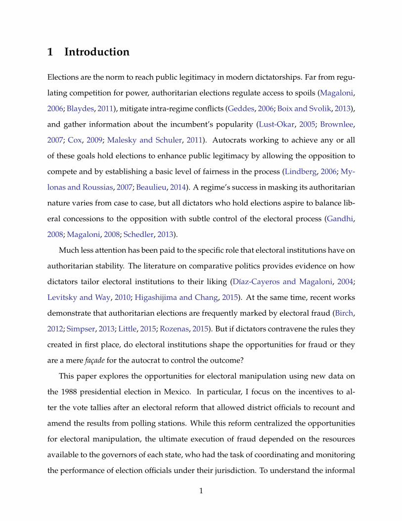
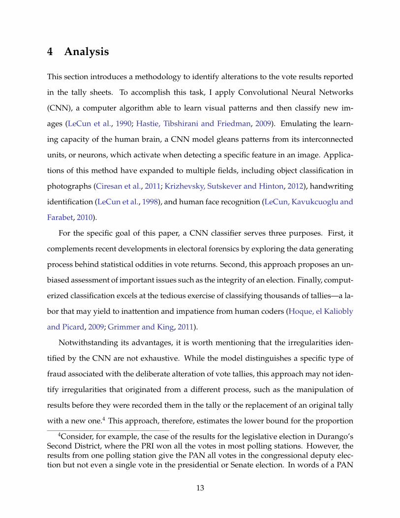
1992. Nevertheless, a close inspection of the vote tallies for the 1988 election shows that
numbers were changed. Figure 1 provides a few examples of vote tallies with vote totals
alterations. The examples at the top present crossed-out numbers as well as inconsisten-
cies in ink color and handwriting. Meanwhile, the images at the bottom illustrate those
altered tallies involving number insertions that have irregular slants and different pres-
sure. The next section presents quantitative evidence for this irregularity and estimates
the overall prevalence of the altered tallies in the election.
11
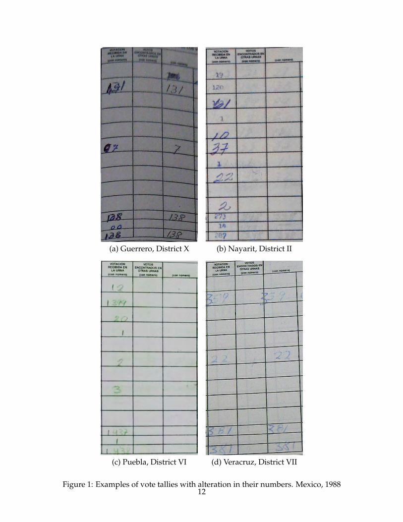
(a) Guerrero, District X (b) Nayarit, District II
(c) Puebla, District VI (d) Veracruz, District VII
Figure 1: Examples of vote tallies with alteration in their numbers. Mexico, 198812
4 Analysis
This section introduces a methodology to identify alterations to the vote results reported
in the tally sheets. To accomplish this task, I apply Convolutional Neural Networks
(CNN), a computer algorithm able to learn visual patterns and then classify new im-
ages (LeCun et al., 1990; Hastie, Tibshirani and Friedman, 2009). Emulating the learn-
ing capacity of the human brain, a CNN model gleans patterns from its interconnected
units, or neurons, which activate when detecting a specific feature in an image. Applica-
tions of this method have expanded to multiple fields, including object classification in
photographs (Ciresan et al., 2011; Krizhevsky, Sutskever and Hinton, 2012), handwriting
identification (LeCun et al., 1998), and human face recognition (LeCun, Kavukcuoglu and
Farabet, 2010).
For the specific goal of this paper, a CNN classifier serves three purposes. First, it
complements recent developments in electoral forensics by exploring the data generating
process behind statistical oddities in vote returns. Second, this approach proposes an un-
biased assessment of important issues such as the integrity of an election. Finally, comput-
erized classification excels at the tedious exercise of classifying thousands of tallies—a la-
bor that may yield to inattention and impatience from human coders (Hoque, el Kaliobly
and Picard, 2009; Grimmer and King, 2011).
Notwithstanding its advantages, it is worth mentioning that the irregularities iden-
tified by the CNN are not exhaustive. While the model distinguishes a specific type of
fraud associated with the deliberate alteration of vote tallies, this approach may not iden-
tify irregularities that originated from a different process, such as the manipulation of
results before they were recorded them in the tally or the replacement of an original tally
with a new one.4 This approach, therefore, estimates the lower bound for the proportion
4Consider, for example, the case of the results for the legislative election in Durango’sSecond District, where the PRI won all the votes in most polling stations. However, theresults from one polling station give the PAN all votes in the congressional deputy elec-tion but not even a single vote in the presidential or Senate election. In words of a PAN
13

of fraudulent tallies, and its results may complement alternative approaches for analyzing
the data.
I describe below the classification of the vote tallies in four steps. First, I collected,
organized, and pre-processed the tally images and their respective vote results. Second, I
inspected a subset of images and identified those with potential alterations in their num-
bers. Third, I used the labeled images to train and fine-tune the CNN model. Finally, I
used the trained model to label the rest of the images in the database.
4.1 Data Collection
This paper presents new data from more than 53,000 polling stations opened on July 6,
1988, whose respective vote tally sheets are stored at the National Archive in Mexico
City.5 The data collection and digitization process produced two databases. The first one
contains the images of all the vote tallies from the 1988 election.6 With the help of two
research assistants, I photographed, digitally edited, and organized by electoral district
every vote tally available in the archive. To minimize the noise of the images during the
classification stage, I manually cropped every picture to include only the area of the image
that contains the vote returns, as the examples in Figure 1 illustrate.
The second database includes the vote returns at the polling station level for every can-
official, “(O)bviously, the person who marked the vote tallies got it wrong” (La Jornada,August 6, 1988c).
5The closest analyses using this data are Barberán et al. (1988) and Báez Rodríguez(1994). The first one is a study by a group of scholars and political activists—CuauhtémocCárdenas himself included—analyzing the results of a sample of 30,000 polling stationsthat election officials made available to opposition parties. However, it remains unclearwhether the sample is representative of all the polling stations in the country and the dataused for this work became unavailable after the one of the authors died (Personal com-munication with two of the authors, January 2016.). The second one presents the results ofa quantitative analysis using a “computerized retrieval system” at the National Archive.However, staff members at the Archive denied the existence of such information (Eisen-stadt, 2004, p. xi-x). Moreover, the author acknowledges the impossibility to replicate theresults from the analysis (Personal communication with the author, June 2015.).
6See Figure A in the Appendix for an example.
14
didate. This information was entered by a team of professional data coders and double-
supervised by the coding team manager and me. The data-entry process proved impossi-
ble for a handful of images with faded writing or inadequate contrast. The total number
of observations in the database, thus, is 53,249. As Table A in the Appendix shows, these
vote totals are very similar to the official total votes reported at the national and district
level. The resemblance validates the information of my database and suggests that any
electoral manipulation occurred before officials compiled the results from the vote tallies.
Table B in the Appendix provides descriptive statistics of the database.
4.2 Data splitting
After preprocessing the images, I divided the database into three parts: a training set, a
validation set, and a test set. The first two sets came from a sample of 1,050 images that I
inspected and labeled as either “with alterations” (WA) or “without alterations” (WOA),
ending up with 525 images for each class. The training set contains 900 of these images,
which I use as inputs to fit my CNN model. The remaining 150 images constitute the
validation set, which I use to verify the accuracy of my model. Finally, the test set contains
almost 52,300 unlabeled images that help me to estimate the overall rate of aggregation
fraud.
To identify those tallies assigned to the WA class, I first used qualitative evidence from
interviews and legislative debates to find districts where aggregation fraud had been re-
ported.7 Then I inspected the tallies from those districts and labeled as WA those images
showing alterations suggested by the primary sources, such as the cross-outs or num-
ber insertions illustrated in Figure 1. The examples labeled as WOA were selected from
7The qualitative information includes interviews in January 2016, with José Newman,director of the Federal Electoral Commission (CFE) from 1982-1989 as well as Jorge Al-cocer and Leonardo Valdés, representatives of the Mexican Socialist Party (PMS) in theCFE (1986-1991). I also reviewed the stenographic record of the debates in the Chamberof Deputies to certify the election (Senado de la República, 1988).
15
images that did not present alterations in their numbers. To make sure that the model dis-
tinguishes the altered tallies by their amendments rather than by vote results, the sample
of WOA files include images where the PRI won all the votes but where there are no clear
patterns of alterations in their numbers, as Figure B in the Appendix shows.
I verified the reliability of the labels in two different tests. The first one used crowd-
sourcing to compare the labels provided by 200 respondents recruited through Amazon’s
Mechanical Turk (MTurk) for an online survey fielded in February 2017. The survey asked
respondents to identify tallies they perceived as altered from a random sample of 10 im-
ages. A second check recruited five undergraduate students at the University of Houston,
who were asked to identify altered tallies from a random sample of 50 images. In both
tests, subjects were never informed of the labels I had assigned to each of images. The
details of each experiment are available in the Appendix. The overall results show a sub-
stantial agreement with the original labeling.8
4.3 Classifier Training
The learning phase consists in allowing the CNN model to absorb the information of
the training set by passing random batches of images through the network. Each itera-
tion gradually calibrates the model’s inferences of the features that distinguish each class.
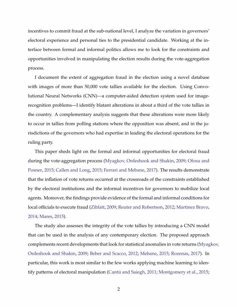
Figure 2 illustrates the network architecture of the model, and it is fully specified in Table
C in the Appendix.
To train the network, every image is first transformed into a numerical array of pixel
values. These inputs pass through a first convolutional layer, which contains 32 filters, or
neurons. Each of these filters slides across every 3× 3 pixel area of the image looking for
basic features, such as a straight line, an edge, or a curve. The 32 different image repre-
sentations are then used as inputs for the second convolutional layer, which also contains
32 filters. These filters slide across each representation searching for more complex fea-
8Youden’s J statistic numbers were 0.28 and 0.48, respectively.
16
Input: 3 x 227 X 227
Feature map: 32 @
229 X 229
Feature map: 32 @
118 X 118
Feature map: 64 @
63 X 63
Feature map: 64 @
35 X 35
Feature map:
128 @ 21 X 21
Feature map:
256 @ 14 X 14
Hidden units: 2048
Hidden units: 128
Outputs: 2
Convolution: 3x3
kernel
Max Pooling: 2x2
kernel
Flatten Fully connected
Convolution: 3x3
kernel
Max Pooling: 2x2
kernel
Convolution: 3x3
kernel
Max Pooling: 2x2
kernel
Convolution: 3x3
kernel
Max Pooling: 2x2
kernel
Convolution: 3x3
kernel
Max Pooling: 2x2
kernel
Convolution: 3x3
kernel
Max Pooling: 2x2
kernel
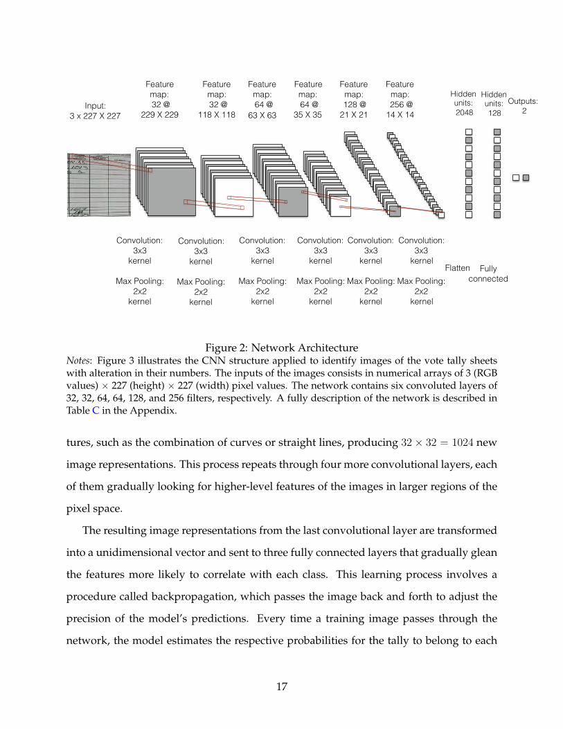
Figure 2: Network ArchitectureNotes: Figure 3 illustrates the CNN structure applied to identify images of the vote tally sheetswith alteration in their numbers. The inputs of the images consists in numerical arrays of 3 (RGBvalues) × 227 (height) × 227 (width) pixel values. The network contains six convoluted layers of32, 32, 64, 64, 128, and 256 filters, respectively. A fully description of the network is described inTable C in the Appendix.
tures, such as the combination of curves or straight lines, producing 32 × 32 = 1024 new
image representations. This process repeats through four more convolutional layers, each
of them gradually looking for higher-level features of the images in larger regions of the
pixel space.
The resulting image representations from the last convolutional layer are transformed
into a unidimensional vector and sent to three fully connected layers that gradually glean
the features more likely to correlate with each class. This learning process involves a
procedure called backpropagation, which passes the image back and forth to adjust the
precision of the model’s predictions. Every time a training image passes through the
network, the model estimates the respective probabilities for the tally to belong to each
17
class. These probabilities determine the value of the loss function, or the cost incurred by
those predictions after comparing the true image’s label. The lower the value of the loss
function, the better the accuracy classification of the model. To decrease this value, the
image passes back through the network, allowing the model to identify the features that
contributed to an incorrect prediction and to calibrate its filters’ weights accordingly.
I trained the network for 250 epochs, wherein each epoch stands for a set of forward
and backward passes for all images in the training set. After every epoch, I trace the
accuracy rates of the model in the validation set and saved its weights when there was
an improvement in the loss value. The final model thus contains the model weights that
reported the highest prediction accuracy in the validation set.
A common concern of using CNN is the risk of overfitting, which occurs when the
model “memorizes” image features that are not generalizable outside the training set. I
tackle this problem in two ways. First, I use data augmentation to artificially increase
the size of my training set. This technique produces new images derived from random
shears, flips, rotations, and zooms of the original pictures (Chatfield et al., 2014). Second,
I include a set of dropout layers to block a random set of filters throughout my network.
The inclusion of these layers during the training process detracts the model from focusing
on specific filter activations and instead consider those features that can be generalizable
to multiple images (Srivastava et al., 2014).
A final concern has to do with the political sensitivity of incorrectly assessing the in-
tegrity of a given vote tally. The predicting inaccuracies of the model face two types of
misclassification: labeling as WA those tallies with no clear patterns of manipulation (Er-
ror Type I) or labeling as WOA those tallies with potential altered features (Error Type
II). Faced with this trade-off, I chose to minimize the first error type. In other words, the
classifier would label a tally as altered only when its probability of belonging to the WA
category is at least twice its probability of belonging to the WOA category. This conserva-
tive approach thus labels a tally as WOA when its estimated probabilities are too close to
18
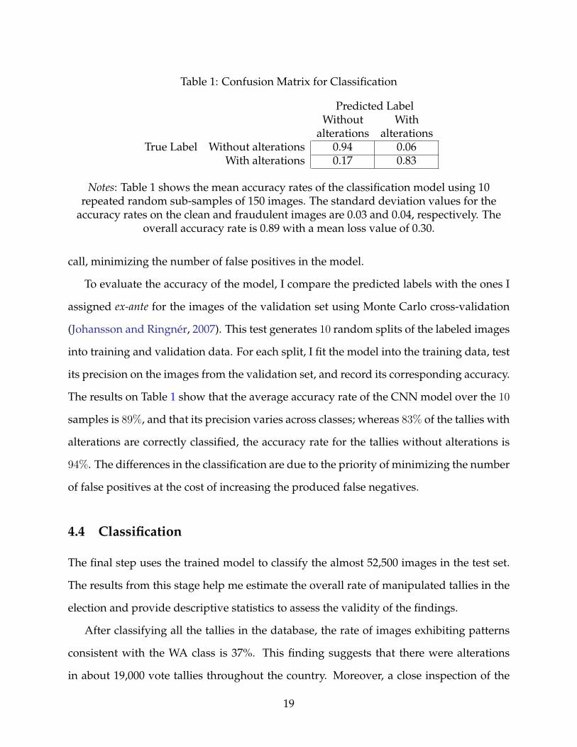
Table 1: Confusion Matrix for Classification
Predicted LabelWithout With
alterations alterationsTrue Label Without alterations 0.94 0.06
With alterations 0.17 0.83
Notes: Table 1 shows the mean accuracy rates of the classification model using 10repeated random sub-samples of 150 images. The standard deviation values for the
accuracy rates on the clean and fraudulent images are 0.03 and 0.04, respectively. Theoverall accuracy rate is 0.89 with a mean loss value of 0.30.
call, minimizing the number of false positives in the model.
To evaluate the accuracy of the model, I compare the predicted labels with the ones I
assigned ex-ante for the images of the validation set using Monte Carlo cross-validation
(Johansson and Ringnér, 2007). This test generates 10 random splits of the labeled images
into training and validation data. For each split, I fit the model into the training data, test
its precision on the images from the validation set, and record its corresponding accuracy.
The results on Table 1 show that the average accuracy rate of the CNN model over the 10
samples is 89%, and that its precision varies across classes; whereas 83% of the tallies with
alterations are correctly classified, the accuracy rate for the tallies without alterations is
94%. The differences in the classification are due to the priority of minimizing the number
of false positives at the cost of increasing the produced false negatives.
4.4 Classification
The final step uses the trained model to classify the almost 52,500 images in the test set.
The results from this stage help me estimate the overall rate of manipulated tallies in the
election and provide descriptive statistics to assess the validity of the findings.
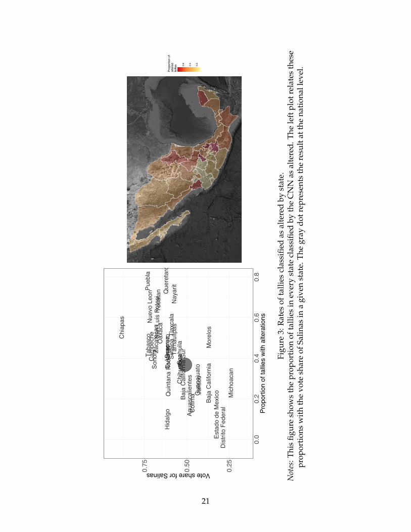
After classifying all the tallies in the database, the rate of images exhibiting patterns
consistent with the WA class is 37%. This finding suggests that there were alterations
in about 19,000 vote tallies throughout the country. Moreover, a close inspection of the
19
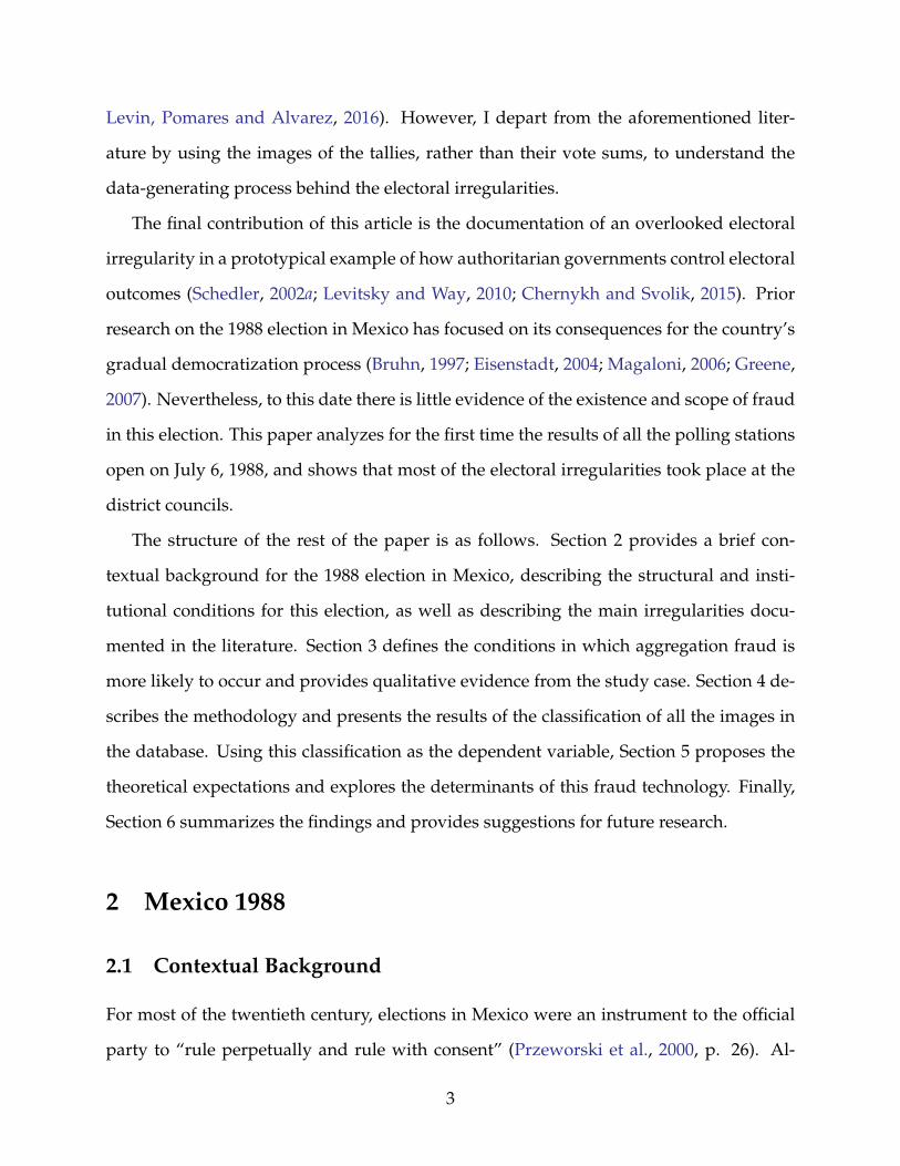
results suggests that the distribution of those tallies was uneven across the country. As
Figure 3 shows, the state-level rates of altered tallies range from less than 5% in Mexico
City to 78% in the state of Puebla.
The findings are consistent with the anecdotal and indirect evidence available about
the election. As the map in Figure 3 illustrates, most of the tallies with alterations are
placed in the south of the country, a region distinguished by its legacy of subnational
authoritarian enclaves during the last decade of the twentieth century (Cornelius, 1999;
Gibson, 2013). The results are also consistent with previous estimations of electoral ma-
nipulation at the subnational level. For example, Simpser (2012) compares the PRI’s vote
shares before and after the electoral reforms during the 1990s, identifying Jalisco, Chi-
huahua, the State of Mexico, and Baja California among the states with the lowest levels
of manipulation. By contrast, the states associated with the largest rates of manipulation
include Tlaxcala, San Luis Potosí, and Querétaro.
The results at the state level also provide a potential explanation for the career paths of
many governors after the 1988 election. Governors who were promoted to top-level posi-
tions in the PRI or the federal government—such as in Zacatecas, Tlaxcala, and Veracruz—
represented states with the largest rates of aggregation fraud during the 1988 election.9 By
contrast, during his first year in office, President Salinas removed three governors com-
ing from states with the lowest rates of altered tallies: Baja California, Michoacán, and the
State of Mexico.10
As an additional validation check for the labels, I used the database of electoral results
at the polling-station level, described in subsection 4.1, to determine whether the vote
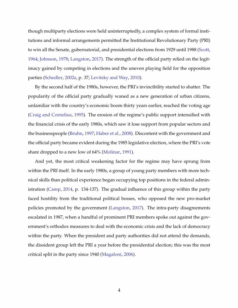
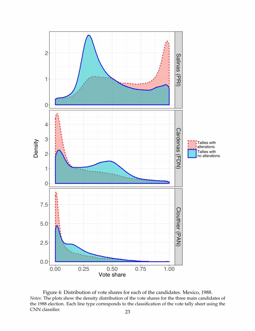
returns between the clean and altered tallies differ. The top, middle, and bottom plots of
Figure 4 show the vote share distributions for Salinas, Cárdenas, and Clouthier, respec-
9The governors who were promoted to top-level positions were: Genaro Borrego inZacatecas, Beatriz Paredes in Tlaxcala, and Fernando Gutiérrez Barrios in Veracruz.
10The removed governors were: Xicoténcatl Leyva Mortera in Baja California, LuisMartínez Villicaña in Michoacán, and Mario Ramón Beteta in the State of Mexico.
20
Ag
ua
sca
lien
tes
Ba
ja C
alif
orn
ia
Ba
ja C
alif
orn
ia S
ur
Ca
mp
ech
e
Ch
iap
as
Ch
ihu
ah
ua
Co
ah
uila
Co
lima
Dis
trito
Fe
de
ral
Du
ran
go
Esta
do
de
Me
xic
oGu
an
aju
ato
Gu
err
ero
Hid
alg
o
Ja
lisco
Mic
ho
aca
n
Mo
relo
s
Na
ya
rit
Nu
evo
Le
on
Oa
xa
ca
Pu
eb
la
Qu
ere
taro
Qu
inta
na
Ro
o
Sa
n L
uis
Po
tosi
Sin
alo
a
So
no
raTa
ba
sco
Ta
ma
ulip
as
Tla
xca
laV
era
cru
z
Yu
ca
tan
Za
ca
teca
s
0.2
5
0.5
0
0.7
5
0.0
0.2
0.4
0.6
0.8
Pro
po
rtio
n o
f ta
llie
s w
ith a
ltera
tion
s
Vote share for Salinas
0.2
0.4
0.6
Pro
po
rtio
n o
fa
ltere
dta
llie
s
Figu
re3:
Rat
esof
talli
escl
assi
fied
asal
tere
dby
stat
e.N
otes
:Thi
sfig
ure
show
sth
epr
opor
tion
ofta
llies
inev
ery
stat
ecl
assi
fied
byth
eC
NN
asal
tere
d.T
hele
ftpl
otre
late
sth
ese
prop
orti
ons
wit
hth
evo
tesh
are
ofSa
linas
ina
give
nst
ate.
The
gray
dotr
epre
sent
sth
ere
sult
atth
ena
tion
alle
vel.
21
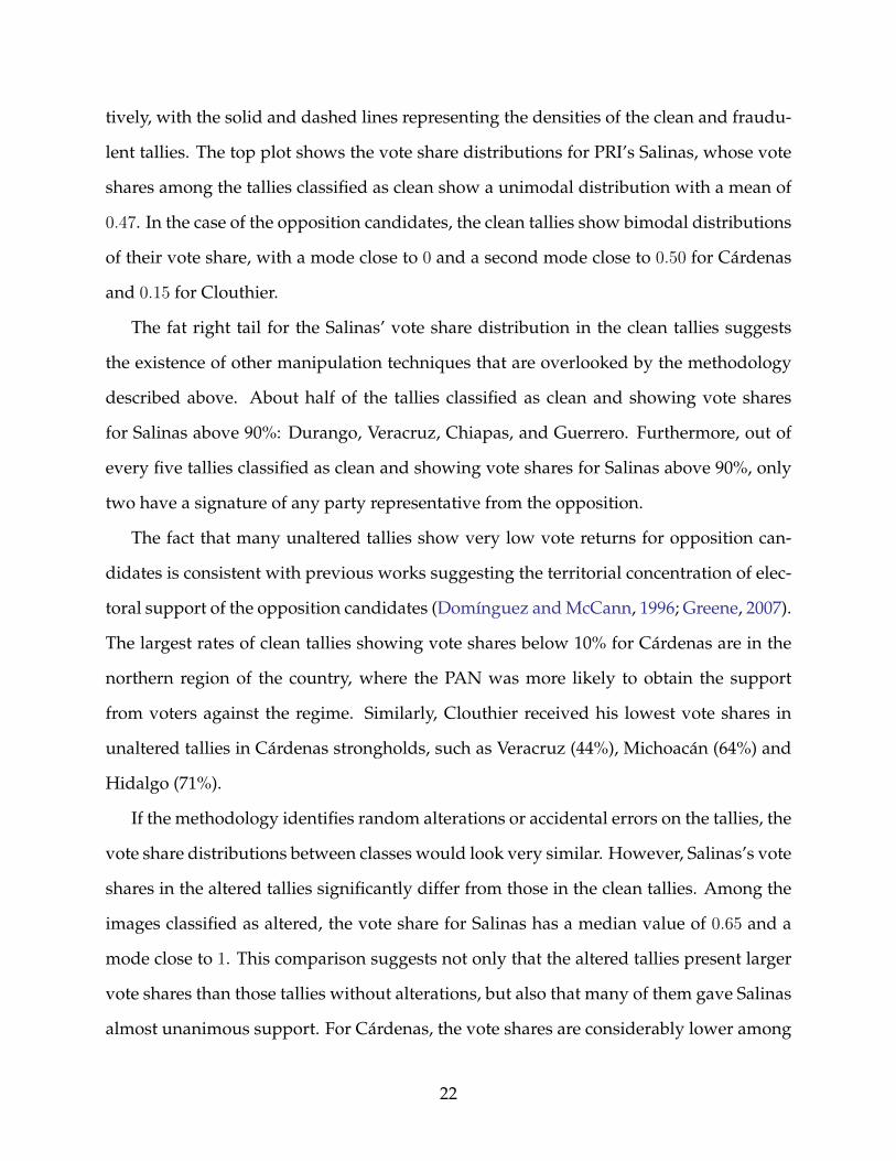
tively, with the solid and dashed lines representing the densities of the clean and fraudu-
lent tallies. The top plot shows the vote share distributions for PRI’s Salinas, whose vote
shares among the tallies classified as clean show a unimodal distribution with a mean of
0.47. In the case of the opposition candidates, the clean tallies show bimodal distributions
of their vote share, with a mode close to 0 and a second mode close to 0.50 for Cárdenas
and 0.15 for Clouthier.
The fat right tail for the Salinas’ vote share distribution in the clean tallies suggests
the existence of other manipulation techniques that are overlooked by the methodology
described above. About half of the tallies classified as clean and showing vote shares
for Salinas above 90%: Durango, Veracruz, Chiapas, and Guerrero. Furthermore, out of
every five tallies classified as clean and showing vote shares for Salinas above 90%, only
two have a signature of any party representative from the opposition.
The fact that many unaltered tallies show very low vote returns for opposition can-
didates is consistent with previous works suggesting the territorial concentration of elec-
toral support of the opposition candidates (Domínguez and McCann, 1996; Greene, 2007).
The largest rates of clean tallies showing vote shares below 10% for Cárdenas are in the
northern region of the country, where the PAN was more likely to obtain the support
from voters against the regime. Similarly, Clouthier received his lowest vote shares in
unaltered tallies in Cárdenas strongholds, such as Veracruz (44%), Michoacán (64%) and
Hidalgo (71%).
If the methodology identifies random alterations or accidental errors on the tallies, the
vote share distributions between classes would look very similar. However, Salinas’s vote
shares in the altered tallies significantly differ from those in the clean tallies. Among the
images classified as altered, the vote share for Salinas has a median value of 0.65 and a
mode close to 1. This comparison suggests not only that the altered tallies present larger
vote shares than those tallies without alterations, but also that many of them gave Salinas
almost unanimous support. For Cárdenas, the vote shares are considerably lower among
22
Sa
lina
s (P
RI)
Cá
rde
na
s (F
DN
)C
lou
thie
r (PA
N)
0.00 0.25 0.50 0.75 1.00
0
1
2
0
1
2
3
4
0.0
2.5
5.0
7.5
Vote share
De
nsity Tallies with
alterations
Tallies withno alterations
Figure 4: Distribution of vote shares for each of the candidates. Mexico, 1988.Notes: The plots show the density distribution of the vote shares for the three main candidates ofthe 1988 election. Each line type corresponds to the classification of the vote tally sheet using theCNN classifier. 23
the tallies classified as fraudulent than in those classified as clean, as the median values
for the distributions are 0.10 and 0.33, respectively. Moreover, while the vote shares for the
clean tallies follow a bimodal distribution, with a higher mode close to 0.5, the vote share
distribution of the fraudulent tallies has a unique mode close to 0. Similarly, Clouthier’s
median vote shares are about 0.14 in the clean ballots and only 0.04 among those classified
as fraudulent.
In sum, the CNN model is a useful tool to unveil the overall extent of aggregation
fraud. For the specific case of the 1988 presidential election in Mexico, the results suggest
that amendments of vote totals occurred in about a third of vote tallies. This finding
confirms the anecdotal evidence of aggregation fraud and supports the conjecture that
the institutional setup allowed election officials to inflate the vote returns.
5 The Determinants of Aggregation Fraud
This section explores the contextual characteristics of the tallies classified as fraudulent.
To accomplish this task, I conjecture that aggregation fraud is more likely to affect the
tallies from polling stations where opposition agents were absent and where local elites
had more resources and incentives to coordinate the irregularities. I propose below the
hypotheses to be tested, describe the set of variables used for this analysis, and discuss
the results.
5.1 Theoretical Expectations
The overarching hypothesis in this paper is that the opportunities for aggregation fraud
appear within the boundaries set by the electoral institutions, and its ultimate execution
depends on the resources available for local perpetrators to inflate vote counts. For the
Mexican case, Section 3.1 describes the consequences of an electoral reform that concen-
trated the vote aggregation process in the hands of district officials. However, as the
24
results in Figure 3 show, the prevalence of aggregation fraud was uneven across regions.
I explain the variance in this irregularity by the presence of the opposition, and the char-
acteristics of the networks required to manipulate vote tallies.
The first expectation is that aggregation fraud was less likely to occur in the presence
of opposition agents. This conjecture follows the existing works on the deterring effects
of election monitoring at the polling stations, where the costs of committing fraud in-
crease with the presence of opposition and independent agents (Hyde, 2007; Ichino and
Schundeln, 2012; Asunka et al., Forthcoming). As a result, perpetrators displace their
fraud efforts to places unreachable to observers other than those supporting the political
machine.
I extend this logic to the case of aggregation fraud and suggest that the deterrent ef-
fects of opposition representatives persist across further stages of the electoral process.
In particular, district officials were less likely to modify vote totals of tallies originally
recorded in the presence of opposition representatives, who could provide first-hand ev-
idence of the differences between the official results and those registered at the polling
station. In this case, the incentives for election officials to alter the tallies filled in presence
of the party representatives decreased after the 1987 electoral reform. This reform recog-
nized for the first time the legal figure of the party representatives and said the expulsion
of party representatives from a polling station constituted as reason to nullify the votes of
the polling place (Barquín, 1987, p. 52). Since the amended code strengthened the role of
party representatives to monitor the process and witness the tabulation at the polling sta-
tions, election officials had stronger incentives to amend the results of those tallies from
polling stations where opposition party representatives were absent.
The second expectation has to do with the influence of local power elites on the preva-
lence of aggregation fraud. As evidence from Russia (Myagkov, Ordeshook and Shakin,
2009; Kalinin and Mebane, 2011; Reuter and Robertson, 2012) and Indonesia (Martinez Bravo,
2014) show, electoral irregularities were carried out by subnational authorities, who took
25

this election as an opportunity to signal their loyalty to the central government. The
resources and incentives to manipulate the electoral result, however, may vary across
jurisdictions (Schattschneider, 1942; Key, 1949). Some local elites may have more experi-
ence and resources to coordinate the electoral operation. Others, meanwhile, may have
greater personal and career-based incentives to signal their loyalty to the central govern-
ment. Therefore, the local execution of fraud depends on the resources available to the
local elites for delivering votes in an effective way.
To verify this conjecture, I take advantage of the intrinsic characteristics of the state
governors during the election. As Section 3.1 describes, the electoral operation in Mexico
during the hegemonic party period was organized in every state by the governor who, at
the same time, was accountable to the minister of interior. The fact that the minister of
interior relinquished his oversight duty in 1988 left the success of the electoral operation
to the capacity and motivation of the governors to deliver votes.
I expect then to observe larger rates of aggregation fraud within the jurisdiction of
governors with previous electoral expertise. During the late 1980s, the pool of Mexican
governors was a mix of two types of politicians. On the one hand, there was a group
of young governors with technical skills but without the practical knowledge on how
to manage an election (Camp, 2014, p. 134-137). On the other hand, there was another
group of traditional political figures who advanced their political careers by working for
the party at the grassroots. Many of the governors in the last group learned the various
ways to deliver votes by running for election and holding multiple elective offices. We
can then expect that those governors who had a previous elected position were more
aware of what was necessary to lead an electoral operation and were more likely to use
aggregation fraud to favor the incumbent party.
A related expectation is that the altered tallies were more likely to appear under the ju-
risdiction of governors with personal ties with the presidential candidate. An alternative
explanation for vote operators’ efforts relies on their personal motivations for helping the
26
candidate win (Frye, Reuter and Szakonyi, 2014; Callen and Long, 2015; Larreguy, Mon-
tiel and Querubin, Forthcoming). During the hegemonic party period, the career of a
politician was defined by his affiliation to a political clique, or camarilla, which bonded
the loyalty of its members to a specific leader in exchange for patronage jobs (Smith, 1979,
p. 50-51; Camp, 2014, 128-139). Even when all governors in 1988 were members of the
official party, only a few of them belonged to the same intra-party group led by Carlos
Salinas. Therefore, if the prevalence of aggregation fraud in each state depended on the
governor’s ties with the presidential candidate, there should be more altered tallies in
those states led by members of Salinas’s political group.
5.2 Measures
I measure the explanatory variables as follows. First, No Opposition Representative is a bi-
nary variable indicating whether the tally lacks the signature of at least any representative
from the opposition. As the first theoretical expectation describes, election officials were
more likely to modify the vote returns of those tallies where results were not recorded
at the polling station by the opposition. Moreover, I build two variables regarding the
characteristics of the state governors. Governor’s Experience indicates whether the state
executive had previously held an elected public office. The information for this variable
comes from the Dictionary of Mexican Political Biographies (Camp, 2011), and I coded as 1
those tallies in states where governors were previously elected as Mayor, Deputy, or Sen-
ator, and 0 otherwise. Also, Camarilla identifies those governors within Salinas’s political
group. This information comes from Centeno (2004), who identifies 40 top-level officials
in the Salinas’s camarilla, out of which 7 were governors on the 1988 election.11
I consider alternative explanations on how fraud was carried out by including a bat-
tery of control variables. First, it could be the case that the number of altered tallies in a
district depends on the popularity of the incumbent party. The literature of electoral ma-
11See Centeno (2004, p. 166) for more details on the classification of this variable.
27

nipulation suggests that irregularities more commonly appear in tight races because they
yield larger marginal returns on the final outcome (Lehoucq, 2003; Mares, 2015; Golden
et al., 2015). I then operationalize the popularity of the incumbent party in two ways. PRI
1985 denotes the PRI’s district vote share during the 1985 legislative elections. A potential
concern in using this measure is that these results are plagued with irregularities similar
than those documented three years later, creating bias in the estimations. Alternatively, I
use the proportion of survey respondents in every state who identified with the PRI three
weeks prior to the election day (PRI’s Support from Polls). The data from this variable
comes from a survey of 4,414 respondents fielded during June 6-17, 1988, and published
by La Jornada newspaper a day before the election (La Jornada, July 5, 1988a).
The analysis also accounts for the possibility that the alteration of the tallies was not
accomplished at the district councils but rather at the polling stations by the incumbent
party’s manpower. The territorial base of the PRI relied on its affiliated workers’ unions,
which displayed their manpower and resources on election day in exchange for political
positions within the party (Murillo, 2001; Langston, 2017). However, given their resource
constraints, unions concentrated their electoral efforts in those districts where the party
endorsed the candidacy of a union member for a legislative seat (Langston and Morgen-
stern, 2009). To consider this possibility, Union membership identifies those districts where
the PRI nominated a union leader as a legislative candidate. If the tallies were altered
at the polling stations, those tallies classified as fraudulent would come from districts
where the PRI had enough human resources to accomplish it, causing the presence of
union candidates to correlate with the extent of fraud. The data for this variable comes
from Langston (2017).
Next, it could also be the case that the aggregation fraud operation was not led by
the governors but instead by those election officials with the most loyal ties to the federal
executive. To test for this possibility, and following a similar approach by Reuter and
Robertson (2012) and Martinez Bravo (2014), Reappointment identifies those districts that
28
had any reappointments of election officials during the six months prior to the election.
Since district election officials were directly appointed by the minister of interior, any
reappointment prior to the election would suggest the nomination of an agent closer to
the federal executive. The information from this variable comes from reviewing all the
issues of the Diario Oficial de la Federación, Mexico’s equivalent to the U.S. Federal Register
or the Canada Gazette, from January 1 to July 5, 1988.
I also consider two contextual factors that may affect the probability of observing alter-
ations in a vote tally. No Poll Worker’s Signature is a binary variable that accounts for those
tallies with no signatures of the election officials at the polling station. Tallies without sig-
nature suggest a replacement, rather than an amendment of the vote results. I expect then
that the vote returns from tallies with no signatures are less likely to present alterations
in their numbers. A final factor that may explain electoral fraud is whether it occurred in
a rural place. As the literature on Mexican politics suggests, electoral irregularities were
more difficult in urban areas than rural ones, where the opposition had fewer resources
to monitor polling stations and brokers had greater control over voters (Molinar, 1991).
To account for this possibility, Rural is the proportion of citizens in the district living in
communities with fewer than 50,000 inhabitants. I built this variable by aggregating to
the district level the municipal information available for the 1990 census.12
5.3 Results
Given the binary nature of my dependent variable and the nested structure of the data,
I specify a multilevel binomial logit-link model with district and state random effects.
Table 2 summarizes the main results. Models 1 and 2 show the estimates of the main
explanatory variables with and without controls, and Model 3 tests the robustness of the
results under an alternative variable specification.
12Given the multiple sample problems of the 1980 census, I used the 1990 census dataas a proxy of the rural population in 1988 rather than interpolating the data between thetwo data sources. I thank Alberto Díaz-Cayeros and René Zenteno for pointing this out.
29
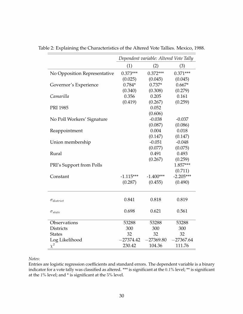
Table 2: Explaining the Characteristics of the Altered Vote Tallies. Mexico, 1988.
Dependent variable: Altered Vote Tally
(1) (2) (3)
No Opposition Representative 0.373*** 0.372*** 0.371***(0.025) (0.045) (0.045)
Governor’s Experience 0.784* 0.737* 0.667*(0.340) (0.308) (0.279)
Camarilla 0.356 0.205 0.161(0.419) (0.267) (0.259)
PRI 1985 0.052(0.606)
No Poll Workers’ Signature -0.038 -0.037(0.087) (0.086)
Reappointment 0.004 0.018(0.147) (0.147)
Union membership -0.051 -0.048(0.077) (0.075)
Rural 0.491 0.493(0.267) (0.259)
PRI’s Support from Polls 1.857***(0.711)
Constant -1.115*** -1.400*** -2.205***(0.287) (0.455) (0.490)
σdistrict 0.841 0.818 0.819
σstate 0.698 0.621 0.561
Observations 53288 53288 53288Districts 300 300 300States 32 32 32Log Likelihood −27374.42 −27369.80 −27367.64χ2 230.42 104.36 111.76
Notes:Entries are logistic regression coefficients and standard errors. The dependent variable is a binaryindicator for a vote tally was classified as altered. *** is significant at the 0.1% level; ** is significantat the 1% level; and * is significant at the 5% level.
30

The results for No Opposition Representative are positive and statistically significant,
suggesting that a tally coming from those polling stations with no signatures from at
least one opposition party agent is more likely to present alterations in its vote returns.
The size of this coefficient is quite consistent across models, 0.37, which the logit model
translates to a probability increase for a tally being altered of about 7%.
The results also provide evidence that the characteristics of the governors leading the
electoral operation affected the likelihood of observing an altered tally in the district.
The coefficient for Governor’s experience is positive and statistically significant. Among
those tallies under the jurisdiction of governors with previous electoral experience, their
probability of presenting alterations is about 14% larger than in those tallies from states
with electorally unexperienced governors. In contrast, although the sign of Camarilla is
positive across specifications, its estimated value is not statistically different from zero.
These results suggest that the extent of aggregation fraud in this election can be explained
by the governors’ resources available but not by their personal ties to the presidential
candidate.
As Models 2 and 3 show, the results hold after including the control variables that
account for alternative explanations. The evidence is inconclusive regarding the relation-
ship between the PRI’s electoral strength and the prevalence of aggregation fraud at the
district level, for the coefficient estimate of PRI 1985 is negligible and non-significant. On
the other hand, Model 3 shows that when substituting that variable for PRI’s Support from
Polls, the estimate is positive and significant, suggesting that the altered tallies were more
frequent in those districts with the largest vote shares.
Against the documented evidence of electoral irregularities in the rural areas of the
country (Molinar, 1991; Fox, 1994; Simpser, 2012), the effect of Rural is not statistically
different from zero. This finding suggests that the generating process of irregularities on
the tallies was not exclusive in rural areas or through the coercion of voters. The sign of
No poll workers’ signature is consistently negative, yet it is not statistically different from
31
zero. One potential explanation is the relatively small share of tallies with this character-
istic, about 3 percent of the observations, which makes this effect insufficient to reliably
estimate its effect. Similarly, the coefficients for Union present no statistically significant
effect, providing no evidence that aggregation fraud was more likely to occur in those dis-
tricts where unions provided manpower during on Election Day. Finally, Reappointments
show estimates not statistically different from zero. Suggesting no differences in the rates
of altered tallies between those districts with and without officials reappointments.
The results above are suggestive of the ways that aggregation fraud was carried out.
In order to inflate the results in an effective way, the alterations of the tallies were more
likely to occur where the opposition was unable to cross-check the results and those states
with a governor with the experience to lead and coordinate the operation. These findings
provide evidence of the opportunities for perpetrators to use this fraud technology.
6 Conclusion
In his memoirs, President Carlos Salinas (2002) defends the legality of his victory in the
1988 election based on two facts. First, the results reported by electoral authorities em-
anate from the vote sums in the tallies, which were filled out in the presence of opposition
party representatives in 72% of the polling stations. Second, the results of the polling sta-
tions are publicly available for corroboration. In the words of Salinas, “The actas (vote
tallies) stored in the National Archives confirm that the 1988 presidential elections are
fully documented” and validate his triumph in an election with “the major mobilization
to monitor the election that the opposition had in fact achieved” (p. 942-943).
This paper verifies both claims for the first time by examining the more than 50,000
tallies available in the National Archive. The analysis confirms that, indeed, the results
announced on July 9, 1988, mirror those recorded in the tallies. But the assessment of the
integrity of the election does not end there. Using recent developments in deep learning
32
and image analysis, I identify amendments of the vote returns in about a third of the
tallies. These alterations were more likely to appear in places where the opposition was
absent and within the jurisdiction of governors with enough experience to coordinate the
inflation of vote totals in an efficient way.
The results illustrate the formal opportunities for aggregation fraud after an elec-
toral reform that centralized the vote aggregation process and entitled district officials
to amend vote returns. Moreover, the electoral reform allowed party representatives to
be present at the polling stations, displacing the irregularities to places where the oppo-
sition was absent. On the other hand, informal opportunities for fraud appealed those
governors with the expertise to mobilize and coordinate the work of election officials in
their jurisdictions. The results illustrate the dynamics of electoral institutions in autocra-
cies, which develop from the tension between the demand of opposition parties to guar-
antee democratic uncertainty and the desire of autocrats to retain control over electoral
outcomes (Schedler, 2002b, p. 109).
While this study focuses on one of the most prototypical cases of electoral authori-
tarianism, the theoretical implications of the findings are generalizable beyond Mexico’s
hegemonic regime. The prevalence of manipulation and biased institutions has afflicted
many contemporary elections. In many of these cases, governments use elections to legit-
imize their regime while keeping full control of the electoral result. The emphasis of this
paper on the interaction between formal and informal incentives for fraud may inform
the dynamics of current electoral authoritarian cases involving authoritarian regimes.
Finally, this paper proposes an approach to identify electoral irregularities that can
be applied anywhere. The methodology is designed to complement existent develop-
ments on electoral forensics by focusing on the data-generating process behind statistical
anomalies in vote returns. Policy practitioners and scholars can use this test to audit the
integrity of tallies of any election. In fact, it is worth emphasizing that the methodology
I propose will become more accurate as it gathers more images from other elections and
33
accumulates the input from experts on the topic. This method, therefore, should be seen
as a steppingstone to identify electoral fraud in cases where, despite their efforts to keep
the irregularities hidden, the perpetrators left their fingerprints on the available evidence.
34
References
Anaya, Martha. 2008. 1988: el año que calló el sistema. Mexico City: Random House Mon-dadori.
Asunka, Joseph, Sarah Brierley, Miriam A. Golden, Eric Kramon and George Ofosu.Forthcoming. “Political Parties and Electoral Fraud in Ghana’s Competitive Democ-racy.” British Journal of Political Science . Working Paper.
Báez Rodríguez, Francisco. 1994. Las Piezas Perdidas (Ejercicios de Reconstrucción. InElecciones a Debate 1988, ed. Arturo Sánchez. Mexico City: Editorial Diana pp. 21–35.
Barberán, José, Cuauhtémoc Cárdenas, Adriana López Monjardin and Jorge Zavala. 1988.Radiografía del Fraude. Mexico City: Editorial Nuestro Tiempo.
Barquín, Manuel. 1987. La reforma electoral de 1986-1987 en México: retrospectiva y análisis.San José, Costa Rica: Centro Interamericano de Asesoría y Promoción Electoral.
Beaulieu, Emily. 2014. Electoral Protest and Democracy in the Developing World. New York:Cambridge University Press.
Beber, Bernd and Alexandra Scacco. 2012. “What the Numbers Say: A Digit-Based Testfor Election Fraud Using New Data from Nigeria.” Political Analysis 20:211–234.
Birch, Sarah. 2012. Electoral Malpractice. New York: Oxford University Press.
Blaydes, Lisa A. 2011. Elections and Distributive Politics in Mubarak’s Egypt. New York:Cambridge University Press.
Boix, Carles and Milan W. Svolik. 2013. “The Foundations of Limited Authoritarian Gov-ernment: Institutions, Commitment, and Power-Sharing in Dictatorships.” Journal ofPolitics 75(2):300–316.
Brownlee, Jason. 2007. Authoritarianism in an Age of Democratization. New York: Cam-bridge University Press.
Bruhn, Kathleen. 1997. Taking the Goliath: The emergence of a new left party and the strugglefor democracy in Mexico. University Park, PA: The Pennsylvania State University.
Callen, Michael and James D. Long. 2015. “Institutional Corruption and ElectionFraud: Evidence from a Field Experiment in Afghanistan.” American Economic Review105(1):354–381.
Camp, Roderic Ai. 2011. Mexican Political Biographies, 1935-2009. Fourth ed. Austin: Uni-versity of Texas Press.
Camp, Roderic Ai. 2014. Politics in Mexico. New York: Oxford University Press.
35
Cantú, Francisco and Sebastián Saiegh. 2011. “Fraudulent Democracy? An Analysis ofArgentina’s Infamous Decade using Supervised Machine Learning.” Political Analysis .Forthcoming.
Cárdenas, Cuauhtémoc, Manuel Clouthier and Rosario Ibarra. 1989. Llamado a la Legal-idad. In Las Elecciones de 1988 y la Crisis del Sistema Político, ed. Jaime González Graf.Mexico City: Editorial Diana.
Caro, Robert A. 1991. The Years of Lyndon Johnson. Means of Ascent. New York: VintageBooks.
Castañeda, Jorge G. 2000. Perpetuating Power. New York: The New Press.
Centeno, Miguel Angel. 2004. Democracy Within Reason. Technocratic Revolution in Mexico.University Park, PA: Penn State Press.
Chatfield, Ken, Karen Simonyan, Andrea Vedaldi and Andrew Zisserman. 2014. “Re-turn of the Devil in the Details: Delving Deep into Convolutional Nets.” eprintarXiv:1405.3531 .
Chernykh, Svitlana and Milan W. Svolik. 2015. “Third-Party Actors and the Success ofDemocracy: How Electoral Commissions, Courts, and Observers Shape Incentives forElectoral Manipulation and Post-Election Protests.” Journal of Politics 77(2):407–420.
Ciresan, Dan C., Ueli Meier, Jonathan Masci, Luca M. Gambardella and Jürgen Schmid-huber. 2011. Flexible, High Performance Convolutional Neural Networks for ImageClassification. In Proceedings of the Twenty-Second International Joint Conference on Artifi-cial Intelligence. Vol. 2 pp. 1237–1242.
Cornelius, Wayne A. 1999. Subnational Politics and Democratization: Tensions betweenCenter and Periphery in the Mexican Political System. In Subnational Politics and Democ-ratization in Mexico, ed. Wayne A. Cornelius, Todd A. Eisenstadt and Jane Hindley. LaJolla, CA: Center for U.S.-Mexican Studies.
Cox, Gary W. 2009. “Authoritarian elections and leadership succession, 1975-2000.”Working Paper.
Craig, Ann L. and Wayne A. Cornelius. 1995. Houses Divided. Parties and Political Re-form in Mexico. In Building Democratic Institutions: Party Systems in Latin America, ed.Scott Mainwaring and Timothy Scully. Stanford University Press.
Davecker, Ursula. 2012. “The cost of exposing cheating.” Journal of Peace Research49(4):503–516.
de la Madrid, Miguel. 2004. Cambio de Rumbo. Mexico City: Fondo de Cultura Económica.
Democracy International. 2011. “Vote Count Verification. A User’s Guide for Funders,Implementers, and Stakeholders.”.
36
Díaz-Cayeros, Alberto and Beatriz Magaloni. 2004. Mexico: Designing Electoral Rulesby a Dominant Party. In The Handbook of Electoral System Choice, ed. Josep M. Colomer.London: Palgrave Macmillan pp. 145–154.
Domínguez, Jorge I. and James A. McCann. 1996. Democratizing Mexico. Baltimore: TheJohn Hopkins University Press.
Eisenstadt, Todd A. 2004. Courting democracy in Mexico: party strategies and electoral insti-tutions. New York: Cambridge University Press.
Ferrari, Diogo and Walter Mebane. 2017. “Developments in Positive Empirical Models ofElection Frauds.” Working Paper.
Fox, Jonathan. 1994. “The Difficult Transition from Clientelism to Citizenship: Lessonsfrom Mexico.” World Politics 46(2):151–184.
Frye, Timothy, Ora John Reuter and David Szakonyi. 2014. “Political Machines at Work:Voter Mobilization and Electoral Subversion in the Workplace.” World Politics 66(2):195–228.
Gandhi, Jennifer. 2008. Political Institutions Under Dictatorships. New York: CambridgeUniversity Press.
Geddes, Barbara. 2006. “Why parties and elections in authoritarian regimes?” WorkingPaper.
Gibson, Edward L. 2013. Boundary Control: Subnational Authoritarianism in Federal Democ-racies. New York: Cambridge University Press.
Golden, Miriam A., Eric Kramon, George Ofosu and Luke Sonnet. 2015. “Biometric Iden-tification machine failure and Electoral Fraud in a Competitive Democracy.” WorkingPaper.
Gómez Tagle, Silvia. 1990. La Calificación de las Elecciones. In México, el 6 de julio de 1988:segundo informe sobre la democracia, ed. Pablo González Casanova. Mexico City: SigloXXI editores pp. 83–121.
Gómez-Tagle, Silvia. 1993. Electoral Reform and the Party System, 1977-90. In Mexico.Dilemmas of Transition, ed. Neil Harvey. London: University of London and BritishAcademic Press pp. 64–90.
Greene, Kenneth F. 2007. Why Dominant Parties Lose: Mexico’s Democratization in Compara-tive Perspective. New York: Cambridge University Press.
Grimmer, Justin and Gary King. 2011. “General purpose computer-assisted clustering andconceptualization.” Proceedings of the National Academy of Sciences of the United States ofAmerica 198(7):2643–2650.
Haber, Stephen, Hebert S. Klein, Noel Maurer and Kevin J. Middlebrook. 2008. MexicoSince 1980. New York: Cambridge University Press.
37
Hastie, Trevor, Robert Tibshirani and Jerome Friedman. 2009. The elements of statisticallearning. New York: Springer.
Higashijima, Masaaki and Eric C. Chang. 2015. “The Choice of Electoral Systems in Dic-tatorships.” Working Paper.
Hoque, Mohammed E., Rana el Kaliobly and Rosalind W. Picard. 2009. When Hu-man Coders (and Machines) Disagree on the Meaning of Facial Affect in SpontaneousVideos. In Intelligent Virtual Agents, ed. Zsófia Ruttkay, Michael Kipp, Anton Nijholtand Hannes Hogni Vilhjalmsson. Germany: Springer pp. 337–343.
Hyde, Susan D. 2007. “The Observer Effect in International Politics: Evidence from aNatural Experiment.” World Politics 50(1).
Hyde, Susan D. 2011. The Pseudo-Democrat’s Dilemma: Why Election Observation Became andInternational Norm. Ithaca, NY: Cornell University Press.
Ichino, Nahomi and Matthias Schundeln. 2012. “Deterring or Displacing Electoral Irreg-ularities? Spillover Effects of Observers in a Randomized Field Experiment in Ghana.”Journal of Politics 74(1):292–307.
Johansson, Peter and Markus Ringnér. 2007. Classification of Genomic and ProteomicData Using Support Vector Machines. In Fundamentals of Data Mining in Genomics andProteomics, ed. Werner Dubitzky, Martin Granzow and Daniel Berrar. Springer pp. 187–202.
Johnson, Kennetg F. 1978. Mexican Democracy: A Critical View. New York: Praeger Pub-lishers.
Kalinin, Kirill and Walter R. Mebane. 2011. “Understanding electoral frauds through evo-lution of Russian federalism: From ‘Bargaining Loyalty’ to ‘Signaling Loyalty.’.” Paperprepared for the 2011 Annual Meeting of the Midwest Political Science Association,Chicago, IL, March 31-April 2.
Kelley, Judith. 2012. Monitoring Democracy. Princeton, NJ: Princeton University Press.
Key, V.O. 1949. Southern politics in state and nation. Knoxville: The University of TennesseePress.
Klesner, Joseph L. 1997. “Electoral Reform in Mexico’s Hegemonic Party System: Perpet-uation of Privilege or Democratic Advance?” Presented at the Annual Meeting of theAmerican Political Science Association, Washington, D.C., 28-31 August 1997.
Krieger, Emilio. 1990. Derecho Electoral en Julio de 1988. In México, el 6 de julio de 1988:segundo informe sobre la democracia, ed. Pablo González Casanova. Mexico City: SigloXXI editores pp. 14–50.
Krizhevsky, Alex, Ilya Sutskever and Geoffrey Hinton. 2012. ImageNet Classification withDeep Convolutional Neural Networks. Technical report University of Toronto.
38
La Jornada. August 6, 1988c. “Se darán a conocer los resultados casilla por casilla:Bartlett.” p. 6.
La Jornada. July 5, 1988a. “Encuesta/I.” pp. i–vi.
La Jornada. July 7, 1988b. “La oposición debe fundamentar sus quejas, demanda Bartlett.”p. 3.
Langston, Joy. 2017. Democratization and Authoritarian Party Survival: Mexico’s PRI, 1982-2012. New York: Oxford University Press.
Langston, Joy and Scott Morgenstern. 2009. “Campaigning in an Electoral AuthoritarianRegime: The Case of Mexico.” Comparative Politics 41(2):165–181.
Larreguy, Horacio, Cesar Montiel and Pablo Querubin. Forthcoming. “Partisans orAgents? Evidence from the Mexican Teacher’s Union.” American Journal of Political Sci-ence .
Lawson, Chappell. 2002. Building the Fourth Estate. Democratization and the Rise of a FreePress in Mexico. Berkeley, CA: University of California Press.
LeCun, Yann, B. Boser, J. Denker, D. Henderson, R. Howard, W. Hubbard and L. Jackel.1990. Handwritten digit recognition with a back-propagation network. In Advances inNeural Information Processing Systems, ed. D. Touretzky. Vol. 2 Denver: Morgan Kaufmanpp. 386–404.
LeCun, Yann, Koray Kavukcuoglu and Clement Farabet. 2010. Convolutional networksand applications in vision. In Proceedings of 2010 IEEE International Symposium on Cir-cuits and Systems.
LeCun, Yann, Léon Bottou, Youshua Bengio and Patrick Haffner. 1998. “Gradient-BasedLearning Applied to Document Recognition.” Proceedings of the IEEE 86(11):2278–2324.
Lehoucq, Fabrice. 2003. “Electoral Fraud: Causes, Types, and Consequences.” AnnualReview of Political Science 6:233–256.
Lehoucq, Fabrice and Iván Molina. 2002. Stuffing the Ballot Box. New York: CambridgeUniversity Press.
Levin, Inés, Julia Pomares and R. Michael Alvarez. 2016. Using Machine Learning Algo-rithms to Detect Election Fraud. In Computational Social Science, ed. R. Michael Alvarez.New York: Cambridge University Press pp. 266–294.
Levitsky, Steven and Lucan A. Way. 2010. Competitive Authoritarianism. New York: Cam-bridge University Press.
Lindberg, Staffan I. 2006. Tragic Protest: Why Do Opposition Parties Boycott Elections?In Electoral Authoritarianism. Boulder, CO: Lynne Rienner Publishers.
39
Little, Andrew T. 2015. “Fraud and Monitoring in Noncompetitive Elections.” PoliticalScience Research and Methods 3(1):21–41.
Los Angeles Times. July 15, 1988. “Indications of Mexico Election Fraud Mount.”.
Lust-Okar, Ellen. 2005. Structuring Conflict in the Arab World. Incumbents, Opponents, andInstitutions. New York: Cambridge University Press.
Magaloni, Beatriz. 2006. Voting for Autocracy: Hegemonic Party Survival and Its Demise inMexico. New York: Cambridge University Press.
Magaloni, Beatriz. 2008. “Credible Power-Sharing and the Longevity of AuthoritarianRule.” Comparative Political Studies 41(4/5):715–741.
Magaloni, Beatriz. 2010. “The Game of Electoral Fraud and the Ousting of AuthoritarianRule.” American Journal of Political Science 54:751–765.
Malesky, Edmund J. and Paul Schuler. 2011. “The Single-Party Dictator’s Dilemma: In-formation in Elections without Opposition.” Legislative Studies Quarterly 36(4):491–530.
Mares, Isabela. 2015. From Open Secrets to Secret Voting: The Adoption of Electoral ReformsProtecting Voters Against Electoral Intimidation. New York: Cambridge University Press.
Martinez Bravo, Monica. 2014. “The Role of Local Officials in New Democracies: Evi-dence from Indonesia.” American Economic Review 104(4):1244–1287.
Mebane, Walter R. 2015. “Election Forensics Toolkit.” DRG Center Working Paper.
Molinar, Juan. 1991. El Tiempo de la Legitimidad. Mexico City: Cal y Arena.
Montgomery, Jacob M., Santiago Olivella, Joshua D. Potter and Brian F. Crisp. 2015.“An Informed Forensics Approach to Detecting Vote Irregularities.” Political Analysis23(4):488–505.
Murillo, María Victoria. 2001. Labor Unions, Partisan Coalitions, and Market Reforms in LatinAmerica. New York: Cambridge University Press.
Myagkov, Mikhail, Peter C. Ordeshook and Dimitri Shakin. 2009. The foresincs of electionfraud: Russia and Ukraine. New York: Cambridge University Press.
Mylonas, Harris and Nasos Roussias. 2007. “When Do Votes Count?: Regime Type,Electoral Conduct, and Political Competition in Africa.” Comparative Political Studies41(11):1466–1491.
New York Times. July 7, 1988. “As Mexicans Vote, Fraud is Alleged.”.
Ofosu, George and Daniel Posner. 2015. “Election Observers and Electoral Fraud inMalawi’s 2014 General Elections.” Working Paper.
Oppenheimer, Andrés. 1996. Bordering Chaos. New York: Little, Brown & Company.
40

Preston, Julia and Samuel Dillon. 2004. Opening Mexico: The Making of a Democracy. NewYork: Farrar Straus and Giroux.
Przeworski, Adam, Michael E. Alvarez, José Antonio Cheibub and Fernando Limongi.2000. Democracy and Development. New York: Cambridge University Press.
Reding, Andre. 1988. “Mexico at a Crossroads: The 1988 Election and Beyond.” WorldPolicy Journal 5(4):615–649.
Reuter, Ora John and Graeme B. Robertson. 2012. “Subnational Appointments in Author-itarian Regimes: Evidence from Russian Gubernatorial Appointments.” The Journal ofPolitics 74(4):1023–1037.
Rozenas, Arturas. 2015. “Office Insecurity and Electoral Manipulation.” Journal of Politics78(1):232–248.
Rozenas, Arturas. 2017. “Detecting Election Fraud from Irregularities in Vote-Share Dis-tributions.” Political Analysis 25(1):41–56.
Rundlett, Ashlea and Milan W. Svolik. 2016. “Deliver the Vote! Micromotives and Mac-robehavior in Electoral Fraud.” American Political Science Review 10(1):180–197. WorkingPaper.
Salinas, Carlos. 2002. México: The Policy and Politics of Modernization. Barcelona: Plaza &Janés Editores.
Schattschneider, Elmer Eric. 1942. Party Government. New York: Reinhart & Company.
Schedler, Andreas. 2002a. “The Menu of Manipulation.” Journal of Democracy 13(2):36–50.
Schedler, Andreas. 2002b. “The Nested Game of Democratization by Elections.” Interna-tional Political Science Review 23(1):103–122.
Schedler, Andreas. 2013. The Politics of Uncertainty. New York: Oxford University Press.
Scott, Robert E. 1964. Mexican Government in Transition. Urbana, IL: University of IllinoisPress.
Senado de la República. 1988. Colegio Electoral. Memoria.
Shirk, David. 2001. Mexico’s Democratization and the Organizational Development ofthe National Action Party. In Party Politics and the Struggle for Democracy in Mexico, ed.Kevin J. Middlebrook. La Jolla: Center for U.S.-Mexican Studies, University of Califor-nia, San Diego pp. 47–94.
Simpser, Alberto. 2012. “Does Electoral Manipulation Discourage Voter Turnout? Evi-dence from Mexico.” The Journal of Politics 74(3):782–795.
Simpser, Alberto. 2013. Why Governments and Parties Manipulate Elections: Theory, Practice,and Implications. New York: Cambridge University Press.
41
Smith, Peter H. 1979. Labyrinths of Power: Political Recruitment in Twentieth-Century Mexico.Princeton, NJ: Princeton University Press.
Smith, Peter H. 1989. The 1988 Presidential Succession in Historical Perspective. In Mex-ico’s Alternative Political Future, ed. Wayne A. Cornelius, Judith Gentleman and Peter H.Smith. Center for U.S.-Mexican Studies, University of California, San Diego pp. 391–416.
Srivastava, Nitish, Geoffrey Hinton, Alex Krizhevsky, Ilya Sutskever and RuslanSalakhutdinov. 2014. “Dropout: A Simple Way to Prevent Neural Networks from Over-fitting.” Journal of Machine Learning Research 15:1929–1958.
Tucker, Joshua. 2007. “Enough! Electoral Fraud, Collective Action Problems, and Post-Communist Colored Revolutions.” Perspectives on Politics 5(3):535–551.
USAID. 2015. “Assessing and Verifying Election Results. A Decision-Maker’s Guide toParallel Vote Tabulation and Other Tools.”.
Valdés Zurita, Leonardo and Mina Piekarewicz. 1990. La Organización de las Elec-ciones. In México, el 6 de julio de 1988: segundo informe sobre la democracia, ed. PabloGonzález Casanova. Mexico City: Siglo XXI editores pp. 51–82.
Woldenberg, José. 2012. Historia mínima de la transición en México. Mexico City: Fondo deCultura Económica.
Wuhs, Steven T. 2014. The Partido Acción Nacional as a Right Party. In The Resilience of theLatin American Right, ed. Juan Pablo Luna and Cristóbal Rovira Kaltwasser. Baltimore:John Hopkins University Press pp. 219–241.
Ziblatt, Daniel. 2009. “Shaping Democratic Practice and the Causes of Electoral Fraud:The Case of Nineteenth-Century Germany.” American Political Science Review 103(1):1–21.
42
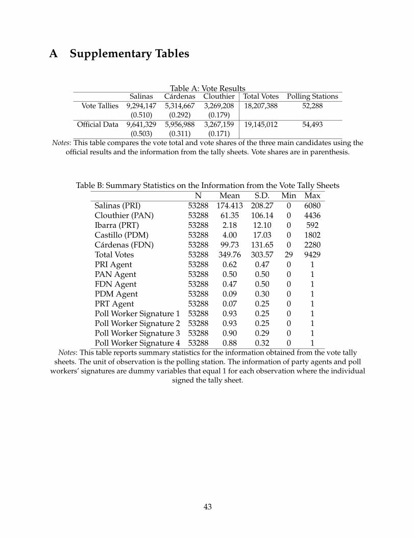
A Supplementary Tables
Table A: Vote ResultsSalinas Cárdenas Clouthier Total Votes Polling Stations
Vote Tallies 9,294,147 5,314,667 3,269,208 18,207,388 52,288(0.510) (0.292) (0.179)
Official Data 9,641,329 5,956,988 3,267,159 19,145,012 54,493(0.503) (0.311) (0.171)
Notes: This table compares the vote total and vote shares of the three main candidates using theofficial results and the information from the tally sheets. Vote shares are in parenthesis.
Table B: Summary Statistics on the Information from the Vote Tally SheetsN Mean S.D. Min Max
Salinas (PRI) 53288 174.413 208.27 0 6080Clouthier (PAN) 53288 61.35 106.14 0 4436Ibarra (PRT) 53288 2.18 12.10 0 592Castillo (PDM) 53288 4.00 17.03 0 1802Cárdenas (FDN) 53288 99.73 131.65 0 2280Total Votes 53288 349.76 303.57 29 9429PRI Agent 53288 0.62 0.47 0 1PAN Agent 53288 0.50 0.50 0 1FDN Agent 53288 0.47 0.50 0 1PDM Agent 53288 0.09 0.30 0 1PRT Agent 53288 0.07 0.25 0 1Poll Worker Signature 1 53288 0.93 0.25 0 1Poll Worker Signature 2 53288 0.93 0.25 0 1Poll Worker Signature 3 53288 0.90 0.29 0 1Poll Worker Signature 4 53288 0.88 0.32 0 1
Notes: This table reports summary statistics for the information obtained from the vote tallysheets. The unit of observation is the polling station. The information of party agents and poll
workers’ signatures are dummy variables that equal 1 for each observation where the individualsigned the tally sheet.
43

B Experiment Description
The survey experiment discussed in Section 4.2 used Qualtrics survey technology with
two population samples. The respondents for the first sample were recruited through
Amazon’s Mechanical Turk via a HIT advertised as “Find altered tallies. A 15 minute
survey” Respondents were restricted to those in the United States with HIT approval
rates greater than or equal to 95% and at least 1,000 HITs approved. Respondents were
provided $1.70 compensation for taking the survey. Survey data from 200 respondents
was collected on February 14, 2017. Each respondent was presented with 10 random
images from the Training Set and were asked to identify those files that present alterations
in their numbers. The average response time was 7.4 minutes (SD=2.8 minutes) and 62%
of the respondents correctly answered the attention check.
The second sample used the answers of 4 students at the University of Houston. Stu-
dents’ responses were collected during March 14 and July 8, 2017. Each respondent got
a sample of 50 random images from the Training Set and were asked to identify those
files that present alterations in their numbers. Respondents received $15 compensation
for taking the survey. The average response time was 92 minutes (SD=56.4 minutes). 75%
of the respondents correctly answered the attention check. This experiment was Neither
Amazon Turk respondents nor undergraduate students were informed about the label
that the images were originally assigned.
Both studies were approved by the University of Houston Institutional Review Board
(STUDY00000131 and STUDY00000301).
44

C Supplementary Figures
Figure A: Example of a Digitized Vote Tally Sheet. Mexico, 1988
45
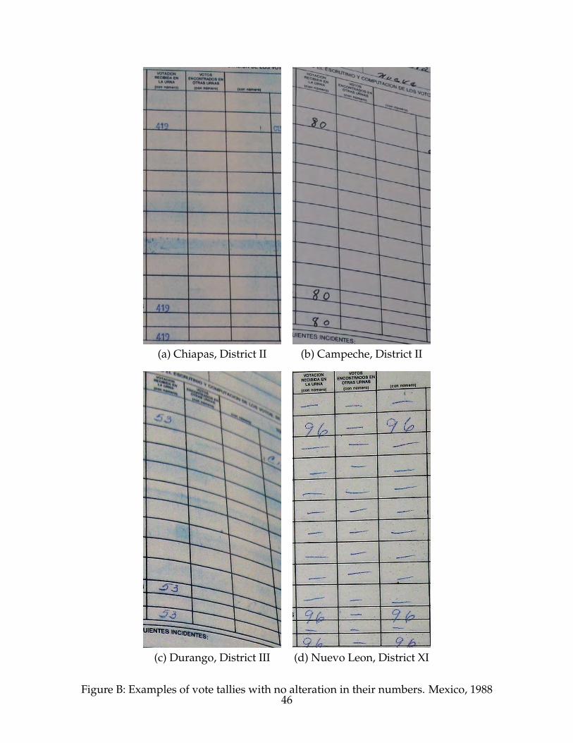
(a) Chiapas, District II (b) Campeche, District II
(c) Durango, District III (d) Nuevo Leon, District XI
Figure B: Examples of vote tallies with no alteration in their numbers. Mexico, 198846

D Network Structure
47
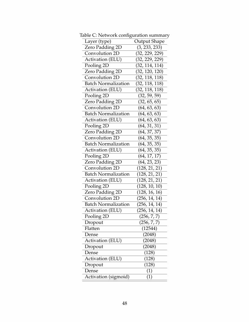
Table C: Network configuration summaryLayer (type) Output ShapeZero Padding 2D (3, 233, 233)Convolution 2D (32, 229, 229)Activation (ELU) (32, 229, 229)Pooling 2D (32, 114, 114)Zero Padding 2D (32, 120, 120)Convolution 2D (32, 118, 118)Batch Normalization (32, 118, 118)Activation (ELU) (32, 118, 118)Pooling 2D (32, 59, 59)Zero Padding 2D (32, 65, 65)Convolution 2D (64, 63, 63)Batch Normalization (64, 63, 63)Activation (ELU) (64, 63, 63)Pooling 2D (64, 31, 31)Zero Padding 2D (64, 37, 37)Convolution 2D (64, 35, 35)Batch Normalization (64, 35, 35)Activation (ELU) (64, 35, 35)Pooling 2D (64, 17, 17)Zero Padding 2D (64, 23, 23)Convolution 2D (128, 21, 21)Batch Normalization (128, 21, 21)Activation (ELU) (128, 21, 21)Pooling 2D (128, 10, 10)Zero Padding 2D (128, 16, 16)Convolution 2D (256, 14, 14)Batch Normalization (256, 14, 14)Activation (ELU) (256, 14, 14)Pooling 2D (256, 7, 7)Dropout (256, 7, 7)Flatten (12544)Dense (2048)Activation (ELU) (2048)Dropout (2048)Dense (128)Activation (ELU) (128)Dropout (128)Dense (1)Activation (sigmoid) (1)
48
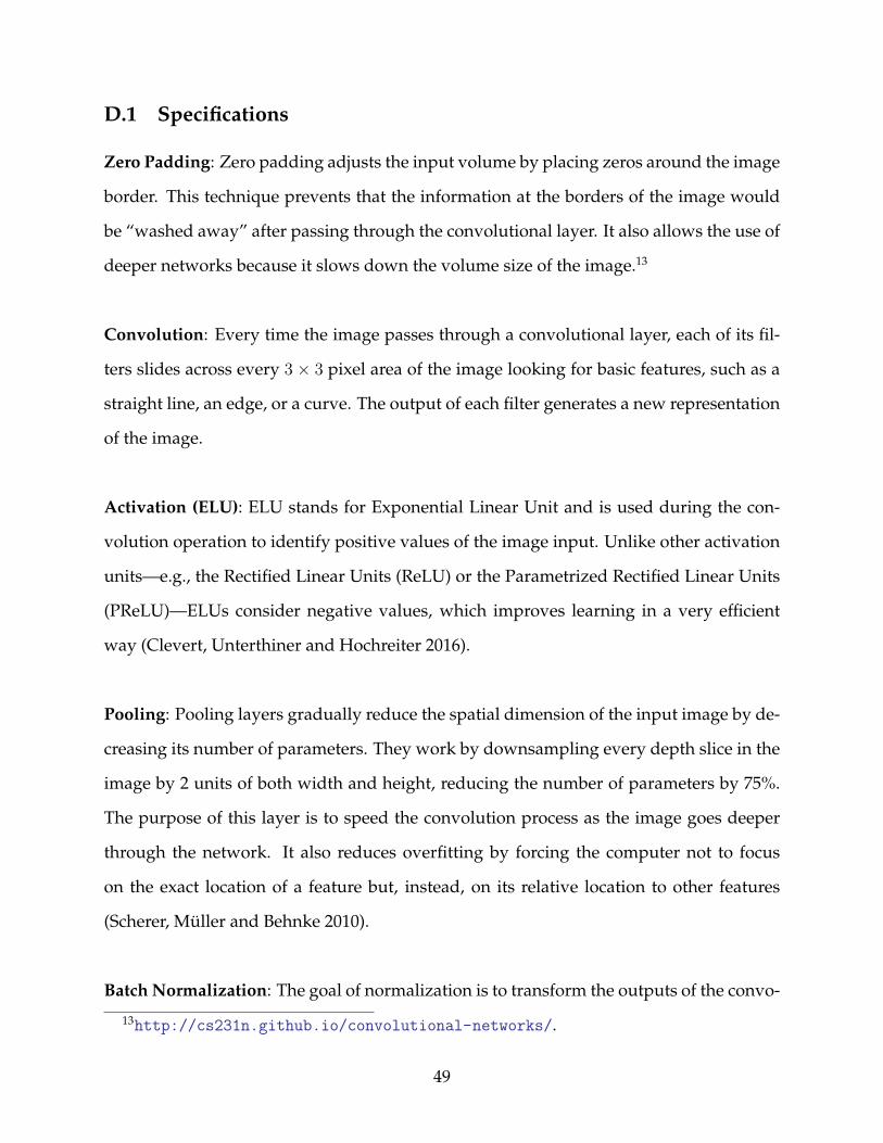
D.1 Specifications
Zero Padding: Zero padding adjusts the input volume by placing zeros around the image
border. This technique prevents that the information at the borders of the image would
be “washed away” after passing through the convolutional layer. It also allows the use of
deeper networks because it slows down the volume size of the image.13
Convolution: Every time the image passes through a convolutional layer, each of its fil-
ters slides across every 3 × 3 pixel area of the image looking for basic features, such as a
straight line, an edge, or a curve. The output of each filter generates a new representation
of the image.
Activation (ELU): ELU stands for Exponential Linear Unit and is used during the con-
volution operation to identify positive values of the image input. Unlike other activation
units—e.g., the Rectified Linear Units (ReLU) or the Parametrized Rectified Linear Units
(PReLU)—ELUs consider negative values, which improves learning in a very efficient
way (Clevert, Unterthiner and Hochreiter 2016).
Pooling: Pooling layers gradually reduce the spatial dimension of the input image by de-
creasing its number of parameters. They work by downsampling every depth slice in the
image by 2 units of both width and height, reducing the number of parameters by 75%.
The purpose of this layer is to speed the convolution process as the image goes deeper
through the network. It also reduces overfitting by forcing the computer not to focus
on the exact location of a feature but, instead, on its relative location to other features
(Scherer, Müller and Behnke 2010).
Batch Normalization: The goal of normalization is to transform the outputs of the convo-
13http://cs231n.github.io/convolutional-networks/.
49
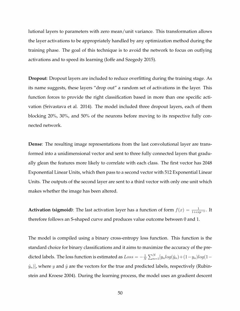
lutional layers to parameters with zero mean/unit variance. This transformation allows
the layer activations to be appropriately handled by any optimization method during the
training phase. The goal of this technique is to avoid the network to focus on outlying
activations and to speed its learning (Ioffe and Szegedy 2015).
Dropout: Dropout layers are included to reduce overfitting during the training stage. As
its name suggests, these layers “drop out” a random set of activations in the layer. This
function forces to provide the right classification based in more than one specific acti-
vation (Srivastava et al. 2014). The model included three dropout layers, each of them
blocking 20%, 30%, and 50% of the neurons before moving to its respective fully con-
nected network.
Dense: The resulting image representations from the last convolutional layer are trans-
formed into a unidimensional vector and sent to three fully connected layers that gradu-
ally glean the features more likely to correlate with each class. The first vector has 2048
Exponential Linear Units, which then pass to a second vector with 512 Exponential Linear
Units. The outputs of the second layer are sent to a third vector with only one unit which
makes whether the image has been altered.
Activation (sigmoid): The last activation layer has a function of form f(x) = 11+exp−x . It
therefore follows an S-shaped curve and produces value outcome between 0 and 1.
The model is compiled using a binary cross-entropy loss function. This function is the
standard choice for binary classifications and it aims to maximize the accuracy of the pre-
dicted labels. The loss function is estimated as Loss = − 1N
∑Nn=1[ynlog(yn)+(1−yn)log(1−
yn)], where y and y are the vectors for the true and predicted labels, respectively (Rubin-
stein and Kroese 2004). During the learning process, the model uses an gradient descent
50
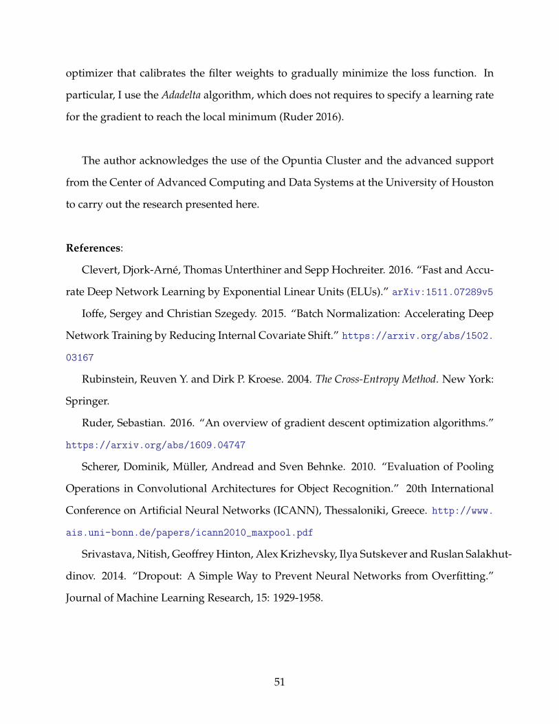
optimizer that calibrates the filter weights to gradually minimize the loss function. In
particular, I use the Adadelta algorithm, which does not requires to specify a learning rate
for the gradient to reach the local minimum (Ruder 2016).
The author acknowledges the use of the Opuntia Cluster and the advanced support
from the Center of Advanced Computing and Data Systems at the University of Houston
to carry out the research presented here.
References:
Clevert, Djork-Arné, Thomas Unterthiner and Sepp Hochreiter. 2016. “Fast and Accu-
rate Deep Network Learning by Exponential Linear Units (ELUs).” arXiv:1511.07289v5
Ioffe, Sergey and Christian Szegedy. 2015. “Batch Normalization: Accelerating Deep
Network Training by Reducing Internal Covariate Shift.” https://arxiv.org/abs/1502.
03167
Rubinstein, Reuven Y. and Dirk P. Kroese. 2004. The Cross-Entropy Method. New York:
Springer.
Ruder, Sebastian. 2016. “An overview of gradient descent optimization algorithms.”
https://arxiv.org/abs/1609.04747
Scherer, Dominik, Müller, Andread and Sven Behnke. 2010. “Evaluation of Pooling
Operations in Convolutional Architectures for Object Recognition.” 20th International
Conference on Artificial Neural Networks (ICANN), Thessaloniki, Greece. http://www.
ais.uni-bonn.de/papers/icann2010_maxpool.pdf
Srivastava, Nitish, Geoffrey Hinton, Alex Krizhevsky, Ilya Sutskever and Ruslan Salakhut-
dinov. 2014. “Dropout: A Simple Way to Prevent Neural Networks from Overfitting.”
Journal of Machine Learning Research, 15: 1929-1958.
51