.. ...

THE FINITE ELEMENT ANALYSIS

OF SHOCKS AND ACCELERATION WAVESIN NONLINEARLY ELASTIC SOLIDS

J. T. Oden -\landL. C. Wellford Jr.H

I~C

INTRODUCTION

Application of the finite element method to time-dependent problems, particularly mechanicalvibration problems of complex structures, datesback to the early 1960's. The use of "consis-tent" mass matrixes was proposed by Archer in1965, and mode superposition techniques becamepopular in the late 1960's for the analysis ofvibration problems. During the last half-decade,the need for studying transient dynamic phenom-ena in complex structures, particularly wavephenomena, has risen sharply. Prejudices thatdeveloped while studying vibration phenomenastill persist, and modern engineering literatureon finite element applications to wave problemsis still filled with discussions of various implicitschemes which had proved to be efficient for lowfrequency response or linear structures. Invery recent times, application of finite elementmethods to nonlinear dynamic problems havebegun to appear, but one rarely finds the men-tion or shocks or of numerical schemes capableof handling them.

In the present paper, we summarize some ofour recent work on finite element formulationsof shock and acceleration wave problems inconnection with nonlinearly elastic bodies, andcite at least one method for proving convergenceof the method at points away from wave frontswhere the solution is relatively smooth. Whatwe actually dwell on are not "pure" finite ele-ment techniques, since they are explicit in time,involve finite element approximations of thespatial dependencies, and various differenceschemes in time.

GLOBAL BALANCE LAWS WITH JUMPS

The finite element method is a variational meth-od of approximation. As such, it should featureall of the usual properties of variational tech-niques, namely, the intrinsic inclusion of bound-ary conditions and even jump conditions in asingle expression equi valent to and consistentwith systems of local equations describing phe-nomena at hand. The Iormulation of finite ele-ment equations of motion including this latterfeature, jump conditions, is something devel-oped only rec ently. In Ref. 1 we desc riOOd aone-dimensional formulation which is used in ashock-smearing scheme; in Ref. 2 an alternate,but equi valent three-dimensional version is de-scribed. The formulation itself suggests sev-eral numerical schemes, and we shall recordhere some of the essential features. To elimi-nate unnecessary detail, we shall limit our-selves to simpler onc-dimensional cases.

Consider a thin cylindrical rod of length Loand area Ao in motion relative to a fixed in-ertial (spatial) frame X, 0 being the massdensity per unit leTl!,Tlhin the reference configu-ration. We assume here that the mass densityo is constant. The motion of the body can bedescribed in terms of the longitudinal displace-ment field u, which is a function of time t andthe material particle X; u = u (X, t). As thebody moves, a surface of discontinuity alsotransverses the body, and its position at time tis gi ven by the material coordinate Y.

To describe this motion, and the propagation ofthe disturbance at yet) through Lo, we callupon the following global equations of physics:

Tllis work was undertaken at The University ofTexas at Austin under the support of the NationalScience Foundation through Grant GK-39071.

*Prof. Engr. Mech., Tex. Inst. ComputationalMech., Univ. Texas, Austin, Tex.

**Assistant Prof., Uni v. Soothern California,Los Angeles, Calif.

1. Balance of Linear Momentum

Ao S a"Ot(OU)dX+oAoV [Ii]y

Lo-y

= Ao(O(Lo,t) -0(0, t)) (1)

Reprint from THE SHOCK AND VIBRATION DIGEST - Vol. 7, No.2

1 -----------

Here V is the intrinsic wave speed, V = dy(t)1dt, a(X, t) is the first Piola-Kirchhoff stressat particle X at time t, e is the internalenergy density, and q(X, t) is the heat flux atX at time t. The notation [fJy denotes thejump in a field f at the wave front Y:

aU dXX

From which we obtain the amplitude equation,

(8)

[u]y + V [~~Jy2 ] a ["Ou]

= v2

a ~ y - 2V a t LaX y'axIt can be shown (see Ref. 1 for the details ofthis calculation) that the preceding equationsimply the alternate global law

(2)

2. Conservation of Energy

A f [ ~o "0 .2 1 .22 -at(ou +2e)dX+2"0AoV u yLo-Y

+AoV [e] y = Ao [a (X,t)Cl.(X,t)

/

X=L+q(X,t)} 0

x=o

·.

(3)

At particles X that do not fall upon the surfaceof discontinuity, Eqs. (1) and (2) lead to thelocal forms of the balance laws,

It is this form of the global balance of linearmomentum that we use to construct finite ele-ment models.

ou - aX=O

e - a iIx - qx = 0 (4)

F1NITE ELEMENT MODELSOF SHOCK WAVES

where a.x:: 0 IT lox, etc., whereas at the sur-face of discontinuity Y we obtain the jumpconditions,

oV[uJy + [a]y = 0

~oV [u2J y + V [e] y +[auJ y +[q] y = O. (5)

Following the procedure outlined in Ref. 1, wemay obtain an alternate form of Eq. (5):

To construct finite element models consistentwith Eq. (9), we begin, as usual (see for exam-ple, Ref. 4) by partitioning LQ into a finitenumber or subdomains L and applying theglobal physical law Eq. (~ to the restriction ofu and a to each subdomain. The final modelis ottained by appropriately connecting suchelements together. This approximation is es-sentially of the Galerkin type, applied indi vidu-ally to each element. When no jumps are pres-ent, it is customary to assume that the dis-placement field over a typical element Le isof the form.

where a = (a(y(t-),t) + a (y(t+),t))/2. In addi-tion, the kinematical compatibility equations(Ref. 3) imply that at a surface of discontinuity

(6)

(7)

Nue (X, t) = : u(~) (t) • ~e) (X) (10)

0.=1

where

• (e'cX)= local interpolation functions11 associated with the element,

u ()(t) = the displacement of node ae of L at time t,e

Ne = the number of nodes in Le'

In general, when the elements are reconnected,the • (e) (X) gererate global basis functions

0.eD (X) which have the following properties:

It

2

--

(i) w" (X), I{ = 1,2, .•. , G, are linearlyindependent, polynomials of degree :s; k, andprovide a basis for a G-dimensional spa c eSh(Lo)' Typically, the global basis functionsare of the form

are discontinuous, and satisfy the kinematicalcompatibility Eq. (7), then shocks can be in-cluded explicitly. Shock fitting schemes areobtained using this type finite element model.

(11)

,.

From this point on, we abandon the conventionof placing a subscript e to denote the elementof interest. Then. if we reformulate Eq. (9)for a finite element of lellj,Tth h we arrive atwhat we term the "consistent" finite elementequations for wave phenomena:

".(13)

'a= p (t) + r.R U + S6 a aa a

.. ar M u (t) + Ao a ~ a dXa a6 .... ,X

h-y

E New (X) = u r

I{ e=1 (1= 1

(e)where n a are entr ies in the Boolean matrixes

I{

describing the connectivity of the model.Generally

(e)n a = 1 or 0

I{

(see Ref. 4).

Here(ii) The wI{ (X) define an orthogonal pro-

jection ITh of functions v(X, t) in the spacecontaining the exact motion, into Sh(Lo)' (Hereh is the maximum diameter of an element inthe finite element model. )

(iii) If

IL 2(u, v)o = uvdX and II u 110:: (u, u)o'

o

the space She n) is designed so that, for eacht,

M aa• 6,XP (1) =

BRand

a8

the value of the local finite elementapproximation of the displacementfield at node a at ti~e t,the mass matrix,

a generalized force at node S.

S6 = amendments to Mas and Sadue to the presence of the rollowingjumps.

II a~ (v-lThv)II ~Khk+l-l{lvlk+1It 0

wherein I v I k+1 is a seminorm of It (seeRef. 4).

(12)

X=h

Unfortunately, a little thought about ~he discon-tinuous character of shock waves will soon leadto t he rea lizati on that the "usual" £i nite e lem entmodel Eq. (10) portrays too smooth a picture ofthe displacement field to be very realistic. Inparticular, if the

• (e)(X)a

are assumed to be continuous, then singularsurfaces of order one, (in particu11.r shocks)cannot be explicitly represented. Thus shocksmearing schemes are obtained from this typefinite element model. On the other hand, if the

(14)

Similarly, we obtain global equations corre-sponding to Eq. (13) by enforcing continuity atelement junctures,

(15)

3

where 0 = to < t1 < ..• < tr = T and tn+1 -

tn = ~t. Then the sequence {An}~=O repre-sents that values of the function A(t) cRh(LJevaluated at t = n6 1. Now we introduce twofinite difference operators to approximate 'j...First is the central difference operator,

FINITE ELEMENT MODELSOF THE SHOCK SMEARING TYPE

In this section, we introduce certain finite ele-ment models of the shock smearing type; Le.,we develop dissipative schemes in which nojump conditions are applied and the gradientsUx vary rapidly but continuously over a narrowband of elements.

n+1 n n-1A - 2A + A

(6 t)2(21)

We assume here that the material is hyperelas-tic, with a strain energy function W, and that

Secondly, we propose a Lax-Wendroff typescheme introduced in Ref. 1,

a = oW, A= extension ratio = 1 + uX' (16)a A

Two global forms of the finite element equationsare considered, one obtained from Eq. (15) bydeleting the jump terms, and another writtenin terms of a finite element approximation

t:.A (X, t) = 1: II (t) 'I. (X)

t:. 6

of the extension ratio A of Eq. (16),(23)

(22)

n n'I.2 0 + a(A , A ,Y. J

Introducing Eq. (21) into Eq. (18) leads to,

for every )( c Rh(L), whereas use of Eq. (22). II 0gives

n+1 .nA - 1\

(0 2' 'I. ll)0(ll t)

2An+1 = An + 6tAn + (~t) An + 0(t:.t3)

2. n+1 . n .. n (lit) ~.n 3A =A +6tA +~A +O(llt) .

(18)

(17)

(24)

.n 'i )1\ , 6

ILlit n 0n n 'X - - (0 'I.)+ a (II , II, 6) - 2 Xt 6 0

"1

"- (p-,;:{II

(19)

= acoustical wave speed.(20)

where2a (l "0 W

o c2 (A) = - = -,-a A OA

Here Eq. (17) holds for every lXl)t cSh(Lo) andEq. (18) holds for every Y. (X) in a subspaceRh(Lo) spanned by l)( 6(X)!lj. Also, we denote

I'Lo "O'{

a(A ,A, y. t:.) == C2 (A) ~ . ~ dXo

We next consider two schemes for approximatingthe temporal behavior of the ). -equation, Eq.(18). Similar schemes can be used for Eq. (17).First, we introduce a partition P of the inter-val [O,T] composed of a set {to,t1,···,tr)

(25)

4

•

where, for simplicity, we denote by 0 the in-terval (0, Lo); and of course,

J

~L 2o °uvdx::' (u,v)o and II u II

L2(0) = (u,u)o'

We shall also need SOme additional notation.We rollow standard practice and denote by

Hm (0, LJ the Sobolev space of order m on

(0, Lo); i. e., Hm(O, Lo) is the space of func-tions whose generalized derivatives of orderm are in ~(O, Lo)' The norm on Hm(O, Lo)is given by

ACCURACY AND CONVERGENCE STUDIES

We shall now describe briefly techniques thatcan be used to study the accuracy and conver-gence of the schemes described in the previoussection. We remark that efror estimates in an"energy" norm were deri ved in Ref. 5 for a re-stricted class of nonlinear hyperbolic equations.Here we develop estimates in the ~-norm,and thus extend some of the recent results ofDupont (Ref. 6) to nonlinear cases. Furtherdetails ofthe development to follow can be foundin Ref. 7.

We begin by making a few restrictive assump-tions concerning the wavespeed C(X) definedin Eq. (20); we assume that there exists:

II u I ~m(O) = (31)

(1) a positive constant M1 such that

C2 (X) ~ M1 I xl (26)

(2) a positive constant M2 such that

C2 (X) :!: M2 (27)

(3) a positive constant M3 such that

mWe also denote by L2(H (0)) the space offunctions u: [0,TJ - Hm(O) with finite L2norm:

and then to demonstrate using the triangle in-equality, that

(34)

Let

6 U I = ...!.... (Un+1 - Un)t n+ 2" 6 t .

II u IIL (Hm (0)) = sup I lu(t)1 I . (33)'" O:!:t~ Hm(O)

II 6t c Iii'" (L (0)) :!:C1 (II e: (0)1102

+ II c (0) IIHI (0) + II e:111H1 (0)

2+ II~II + liE II '"

at L2(L2(0)) L (L2(0))4

+ 612 IIU II } (35)at4 L2 (L2(0) )

Likewise L",(Hm(o)) is the space of functionsu: 0, T - Hm(O) with norm

Then we obtain a theorem specifying the be-havior of e: for the central difference approxi-mation, Eq. (23).

Theorem I: U ,,4>../at4 e: L2(L2(0)) thenthere exists a constant C1 such that

(30)

(29)

where

E = X - Wn e: "Wn = hnn n 'n

Our technique is to show that

Now the aPRroximation error e is defined byen = l.n - h • U we select an ar~itrary elementWn in Rh(O, Lo), we see that en can be de-composed into components

I C2

().) - C2 (X) I ~M3 Ix-I I (28)

and Eqs. (26) through (28) hold fOf all X, t,£ (0, LJ X (0, T). These conditions representpositive definiteness, boundedness, and Lipshitzcontinuity respectively. These are not unrea-sonable assu mptions physically.

5

where3

Theorem 3: If ~ I: ~ (~(o)), andat

then there exists a constant C 1 independent ofthe discretization parameters such that

(38)

where

II I: II i\ '" :!>C 1 [ II I: (0) II. L (~(O)) 0

+ II :; II~(~(n))

+ II :~ 11~(~(n)) + II :: IILCD(~(n))

I aE+ ITt IIL"'(~(n) ) + At IIE IIL"'(~(n))

3"2

+ At

then there exists a constant C2 independent ofh and At such that

2IIEll L'" (L2 (0)) + II "0 2

EIIL (L (0))at 2 2

:!>C2 (hk

+1 II xii L'" (Hk+1 (0))

hk+11ltx II ) (36)+ 2 L (Hk+1 (0) )at 2

This theorem is proved using the discreteGronwall inequality (Ref. 8). In addition wecite a fundamental approximation result whichcan be developed from the work of Nitsche(Ref. 9).

Lemma 1: If X I: L"'(Hk+1 (0)) and

2o X~ t L2 (H1t+1(0))

Now we establish the final error estimate forthe central difference approximation (Eq.( 23)) A similar theorem can be deri ved from Eq. (25).

Theorem 2: Suppose that the hypotheses ofTheorem 1 and Lemma 1 are satisfied, thenthere exists a constant C3 such that

116telli"'(L2(0)) :!>C3 (1Ie(0)llo+lle(0)/IH1(0)

+ IIe111Hl (0) + hk+

1(11 X I IL'" (Hk+1 (0))

2 4

+ II:t~IIL2(Hk+1 (0))) + 6t2 II:~11~(L2(0))}

(37)

This theorem is proved usi ng the resu Its ofTheorem 1, Lemma 1, and the triangle in-equality.

3Theorem 4: If a 3x

t ~(L2(0)) andat3

a X I: L'" (L(n))ax2 dt ~

then there exists a constant C2 such that

(39)

We have also studied the accuracy and conver-gence of the Lax-Wendroff type scheme. ForEq. (24) estimates of the type of Eq. (30) aregiven in the following theorem (detai ls of thisanalysis are given in Ref. 7).

Then we introduce an approximation theory re-sult due to Nitsche (Ref. 9).

6

•

(41 )

FlNITE ELEMENT MODELSOF THE SHOCK FITTING TYPE

In this section, we introduce certain finite ele-ment models of the shock fitting type; 1.e. , wedevelop schemes which effectively contain dis-continuous trial functions associated with cer-tain generalized coordinates and which explicit-ly represent shocks. As before, we illustratethe main ideas through a one-dimensional ex-ample. A more detailed account of this typescheme is given in Ref. 2.

x

(42)

jh

~~

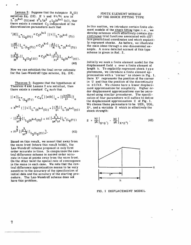
Initially we seek a finite element model for thedisplacement field u over a finite element oflength h, To explicitly represent shock t y P ephenomena, we introduce a finite element ap-proximation with a "corner" as shown in Fig. 1.Here X· represents the position of the cornerin U and thus the position of the disconti nuityin au/ax, We choose here a linear displace-ment approximation for simplicity. Higher or-der displacement approximations can be intro-duced using similar procedures. The specifi-cation of four parameters will suffice to definet he displacement approximation U of Fig. 1.We choose these parameters to be U(O) , U(h),X·, and a variable S which is effectively theshock strength:

I IEll s C h k+ 1 II A IIL"'(~(O)) 3 L"'(Hk+1 (0))

IIaE II k+1 0 >.at L "'(~(O)) ~ C3h 11-at,IIL'" (Hk+1(0))

2 2110 E II s C hk+1110 )..11;r ~(~(O») 3 ? ~(Hk+1(0»).

(40)

Based on this result, we assert that away fromthe wave front (where this result holds), theLax-Wendroff scheme proposed is only firstorder accurate in time. In comparison the cen-tral difference scheme is second order accu-rate in time at points away from the wave front.On the other hand the spatial rate of convergenceis the same in each case. We note that the cen-tral difference approximation seems to be verysensiti ve to the accuracy of the specification ofinitial data and the accuracy of the starting pro-cedure. The Lax-Wendroff scheme does nothave this problem.

Theorem 5: Suppose that the hypotheses ofTheorem 4 and Lemma 2 are satisfied, thenthere exists a constant C4 such that

Now we can establish the final error estimatefor the Lax-Wendroff type scheme, Eq. (24).

Lemma 2: Suppose that the subspace Rh (0)satisfies Eq. (12). If >. and ax/at are inL"'(Hk+l (O»)and a2x/at2 e:L (Hk+1 (0)), thefthere exists a constant C3 inJependent of thediscretization parameters such that

Ilell"", sC4[lle(0)/lo+ Ilo~~O) IIL (~(O)) u 0

+ hk+

1 (11).IIL'''(Hk+1(0))+ II :~ IIL"'(I-{k+l(O»)

2 . 3

.' 11:4-11L (Hk+1(0))) + lit II~IIL"'(T -(0))"Ot 2 ax at ~l

3~.D..+ ~t II ot311 ~(~(O)].

FIG. 1 DISPLACEMENT MODEL

7

•

t 1 (X) = 1 - ~h

where

/

*, X o ~X <X-ht'll(X) -., X· h-. X s:X s::1-,

... 1

x

x

x

rX 0 ~ X < x·1lO otherwise

B (X)

In terms of these four parameters, our localdisplacement approximation is, for example,

2U = r uct (t) t ct(X) + Set) 13(X) + x· Set) ('t, (X)

a. =1 (43)

1

In this representation Set) and X·S(t) aregeneralized coordinates and B(X) and t'll(X)are discontinuous trial functions associated withthese generalized coordinates. It can easi ly beshown that Eq. (43) satisfies the kinematicalcompatibility conditions of Eq. (7). The vari-ous trial functions are shown in Fig. 2.

.5

x

A more concise notation is obtained if we letU3(t) = Set) and U4(t) = X·S(t) and choose theassociated trial functions as t3(X) = 13(X) and•4 (X) = t'll(X). Then the displacement approxi-mation is

h

FIG. 2 DISCONTINUOUSTRIAL FUNCTIONS

Introducing this approximation into Eq. (9), wefind that

~ M tia(t) + A lot dXct =1 aBO B , X

h-Y4

=p (t)+ r. R UCl(t)+Sa (A=1, ... ,4)B a=1 as (45)

a= 1,2

n,a = 1,2

P3 = AoS(X) a IX=hX=O

P 4 = Aoq>(X)n IX=h

X=O

M 4 = M4 =AopJ' • t'lldX a= 1,2a a h- Y a

M34 = M43 =Aoo J~-y St'lldX

M44 = Aoo r q>2dXv h-Y

X=hp = A ~13(X) n I

S 0 x=O

1R =R =--oA Vi' 131

a3 30 2 0 a Y

(44)

0.=1,2

a,l3 = 1,2

• edXa

where

M = Aoo r t. dXnS Jh-Y a e

Maa = M3a = AOIJh_Y

M33 = Aoo Sh-Y s2dX

4 aU = r. u (t) t (X).

a=l a

8

•R33 = - iPAOV [a2Jy

R34 = R = - .! PA V [B (JlJ43 2 0 Y

R44 = - .!oAoV [m2J Y2

B = 1,2

This is the finitc element model for propagationof shock waves in a one-dimensional rod. Thefirst three equations are more or less typicalof finite element models in struct~ral dynamics;these represent the traditional inertially andelastically coopled equations of motion for thenodal displacement plus the shock strength.The fourth equation, turns out to be a finiteelement analog of the "amplitude equation" ofEq. (8). It effectively defines the interactionof the vclocity of the wave and the amplitude ofthe wave and governs thcir evolution in time.

CONCLUDING REMARKS

Therc are a number of important aspccts ofshock calculations using finite elcments onwhich space has not permitted us to elaborate.Among these, we list the following:

1. The important question of analyticalandlor numerical prediction of critical break-down times for the formation of shocks in non-linear materials from smooth or discontinuousinitial data needs furthcr study. It is possibleto develop closed form analytical estimates forbreakdown times in special cases, but the phe-nomena in general cases can be attacked onlywith the greatest difficully and generally in-volves estimates as to when characteristicscoalesce.

2. A less difficult problem, but onc notdealt with here, is the prediction of the growthand decay of shocks. Equations (7) and (8) canbe used to develop an ordinary differential equa-tion for the behavior of the shock strength, and

9

this equation can be handled numerically. Theredoes not appear to be any literature on the useof finite element methods to approximate thesolution of the shock strength equation. Wehope to investigate such calculations in subse-quent work.

3. In developing error estimates and con-vergence proofS in this paper, we have intro-duced a number of rather restricti ve assump-tions (e.g., Eqs. (26) to (28) which lead to somerather inflexible results. While our assump-tions can be shown to hold in a number of im-portant physical situations, they do not hold formany important nonlinear materials. To relaxthese assumptions means to consider theoriesallowing for nonlinear (e. g., polynomial) growthin nonlinearities. Test calculations seem toindicate that the use of more general constitu-tive laws can often make the difference in wheth-er or not the scheme is convergent. Indeed, byconsidering mild polynomial growth of nonlin-earities as is found in some rubberylike mate-rials, rates of convergence of some of theschemes considered herein can be improved.

4. The question of numerical stability stillremains to be answered. For certain monotoneoperators of thc type considered herein, it ispossible to develop sufficient conditions forstability. When more general forms of nonlin-earity are considered, the development of sta-bility criteria becomes an extremely difficultundertaking .

For more detai Is on these poi nts, see Refs. 1,3, and 5.

REFERENCES

1. Fost, R.B.;Oden, J.T.;andWellford,L.C., Jr., "A Finite Element Analysisof Shocks and Finite Amplitude Waves inOne-Dimensional Hyperelastic Bodies atFinite Strain", IntI. J. Solids Struc.(to appear).

2. We llford, L. C., Jr., "Variational Meth-ods for the Approximate Solution of WavePropagation Problems in HyperelasticSolids at Finite Strain", ComputationalMethods in Nonlinear Mech. 1, TexasTracts in Compo Mech., 1974 (to appear).

3. Chen, P., "Growth and Decay of Waves inSolids", Encyclopedia of Physics, VI a/3 -Mechanics of Solids, nI, Ed. S. Flugge,Springer-Verlag, New York, N. Y.,303-402 (1973).

~. &

4. aden, J. T., Finite Elements of NonlinearContinua, McGraw-Hill Book PublishingCo., Inc., New York, N. Y. (1972).

5. Oden, J. T. and Fost, R. B., "Conver-gence, Accuracy and Stability of FiniteElement Approximations of a Class orNon-Linear Hyperbolic Equations", IntI.J. Numerical Methods in Engr. 6,pp 357-365 (1973). -

6. Dupont, T., "L2 Estimates for GalerkinMethods for Second Order HyperbolicEquations", SIAM J. Numer. Anal. 10,pp 880-889 (1973). -

7. Wellford, L.C. and Oden, J.T., "OnSome Finite Element Methods for CertainNonlinear Second Order Hyperbolic Equa-tions", (in review).

8. Lees, M., "A Priori Estimates for theSolution of a Difference Approximation toParabolic Differential Equations", DukeMath. J. 27, pp297-312 (1960).

9. Nitsche, J., "Verfarbren Von Ritz andSpline - Interpolation bei Sturm -Liouvi lie - Randwertproblemen",Numeriske Matematik, 13, pp 260-265(1969). -

10