the finite element method analysis for assessing the...
TRANSCRIPT

The Finite Element Method Analysis for Assessing the Remaining Strength of Corroded Oil Field Casing and Tubing
Der Fakultät für Geowissenschaften, Geotechnik und Bergbau
der Technischen Universität Bergakademie Freiberg
eingereichte
Dissertation
zur Erlangung des akademischen Grades
Doktor-Ingenieur (Dr.-Ing.)
vorgelegt von
Dipl.-Ing. Tomasz Szary Geboren am 20.09.1975 in Gorlice
Freiberg, den 10.09.2006

i
Acknowledgements
This study has been performed under the supervision of Professor Volker Köckritz to
whom I would like to express my deepest gratitude. His guidance and assistance
during my entire work at the Freiberg University have been very helpful and
encouraging.
My thanks goes to all colleagues at the Institute of Drilling Engineering and Fluid
Mining for their friendship. They have contributed to my academic achievements and
provided a very good working atmosphere.
I am very grateful to Dr Rehmer and Mrs Hansen from USG Mittenwalde for their
cooperation during the development of this corrosion assessment method.
I also wish to thank the educational staff from the Drilling, Oil and Gas Faculty
(University of Science and Technology in Cracow) for the support which they offered
me during my MSc studies. Special thanks to Professor Danuta Bielewicz for her help
and for supervising my stay in Freiberg.
My work at Bergakademie Freiberg was made possible by the financial support from
the Kreissparkasse Freiberg, which awarded me with the �Freiherr-von-Friesen�
scholarship.
Finally, I would like to thank my family for standing by me and supporting me.

ii
Table of Contents
Acknowledgements .............................................................................i Table of Contents ............................................................................... ii List of Figures .....................................................................................v
List of Tables ................................................................................... viii Nomenclature .................................................................................... ix
Abbreviations .............................................................................................. ix Symbols .............................................................................................. ix
Remarks ............................................................................................. xii
1 Introduction ..................................................................................1
2 Corrosion in Petroleum Industry..................................................3
2.1 Corrosion mechanisms..........................................................................3 2.1.1 Electrochemical corrosion.........................................................................4 2.1.2 Chemical corrosion...................................................................................5 2.1.3 Mechanical assisted corrosion..................................................................5
2.2 Corrosion occurrence, causes and control ............................................7 2.2.1 Corrosion during developing and production.............................................7 2.2.2 Corrosion in gas and oil transmission pipelines ........................................9 2.2.3 Corrosion in petroleum refining.................................................................9
2.3 Corrosion rates and affecting factors...................................................10
2.4 Cost of corrosion .................................................................................11 2.4.1 Corrosion cost during development and production ................................11 2.4.2 Corrosion cost in gas and oil transmission pipelines...............................12 2.4.3 Corrosion cost in petroleum refining .......................................................13
3 Corrosion Detection...................................................................14
3.1 Mechanical methods of corrosion detection.........................................14 3.2 Electrical methods of corrosion detection ............................................15
3.3 Acoustic methods of corrosion detection .............................................15
4 Assessment of Corrosion Defects .............................................18
4.1 Semi-empirical methods of corrosion assessment ..............................18 4.1.1 ASME B31G corrosion assessment method...........................................19 4.1.2 Modified B31G corrosion assessment method........................................23 4.1.3 RSTRENG corrosion assessment method..............................................24 4.1.4 Kastner�s criterion for corrosion assessment of circum-ferentially
orientated defects ...................................................................................25

iii
4.2 Numerical methods of corrosion assessment ......................................26 4.2.1 British Gas procedure of corrosion assessment......................................26 4.2.2 Det Norske Veritas and other numerical corrosion assessment methods30
4.3 Probabilistic methods of corrosion assessment...................................31 4.3.1 DNV RP-F-101 standard.........................................................................31
5 Numerical Simulation Model......................................................34
5.1 ANSYS model......................................................................................34 5.2 Boundary condition..............................................................................37
5.2.1 Constraints and symmetry ......................................................................37 5.2.2 Applicable loads .....................................................................................39
5.3 Mesh and its accuracy.........................................................................41 5.3.1 Element number .....................................................................................42 5.3.2 Element size...........................................................................................42
5.4 Ovality implementation ........................................................................44 5.5 Defect generation ................................................................................46
5.6 Failure prediction .................................................................................51 5.6.1 Burst failure prediction............................................................................52 5.6.2 Collapse failure prediction ......................................................................54 5.6.3 Axial load failure prediction.....................................................................55
5.7 User-friendly interface .........................................................................56
5.8 Results representation and accuracy ..................................................59
6 Burst Analyses...........................................................................61
6.1 Burst model verification for intact pipes with the API formula ..............61 6.2 Defect influence on burst pressure ......................................................64
6.3 Comparison of burst simulation methods ............................................73 6.4 Discussion of the burst simulation model ............................................76
7 Collapse Analyses .....................................................................77
7.1 Collapse model verification for intact pipes with the API formulas.......77 7.2 Ovality influence on collapse pressure ................................................84
7.3 Defect influence on collapse pressure.................................................85 7.4 Collapse test data recalculation...........................................................88
7.5 Discussion of the collapse model ........................................................91
8 Critical Axial Load Analyses ......................................................92
8.1 Critical axial load model verification for intact pipes against the API formula .............................................................................................92
8.2 Discussion of the axial load model ......................................................94

iv
9 Summary ...................................................................................95
References .......................................................................................97
Appendices .....................................................................................105
Appendix 5.1 Typical elements sizes and their distribution in circumferential direction................................................................................105
Appendix 5.2 Nodes position after implementing 0.4% ovality...................107 Appendix 5.3 Close-up pictures of modelable defects ...............................109
Appendix 5.4 Typical result file of analysis with 2 layers............................112 Appendix 5.5 Typical result file of analysis with 4 layers............................113
Appendix 6.1 Comparison of the API and FEM critical internal pressures for intact pipes...........................................................................115
Appendix 6.2 Comparison of the API (with Dm) and FEM critical internal pressures for intact pipes .....................................................117
Appendix 6.3 Critical internal pressures / Yp (-) of variously corroded tubular (internal defect, depth 0.5t) ..................................................119
Appendix 6.4 Critical internal pressures / Yp (-) of variously corroded tubular (internal defect, depth 0.25t) ................................................120
Appendix 6.5 Critical internal pressures / Yp (-) of variously corroded tubular (internal defect, depth 0.75t) ................................................121
Appendix 6.5 Critical internal pressures / Yp (-) of variously corroded tubular (external defect, depth 0.5t) .................................................122
Appendix 7.1 The API critical external pressures for intact pipes ..............123 Appendix 7.2 Comparison of the API and FEM (ovality 0.4%) critical external
pressures for intact pipes .....................................................125 Appendix 7.3 Comparison of the API and FEM (ovality depended on D/t)
critical external pressures for intact pipes ............................127 Appendix 7.4 Ovality influence on the critical external pressure ................129
Appendix 7.5 Critical external pressures / Yp (-) of variously corroded tubular (external defect, depth 0.5t) .................................................130
Appendix 7.6 Critical external pressures / Yp (-) of variously corroded tubular (internal defect, depth 0.5t) ..................................................131
Appendix 8.1 Comparison of the API and FEM critical axial loads for intact pipes ....................................................................................132

v
List of Figures
Figure 2.1 Corrosion rates of steel compared to various concentrations of dissolved gases (from Brondel et al. /7/)................................................................... 7
Figure 3.1 Ultrasonic Casing Imager (from Schlumberger /25/) and hypothetical UCI log (from Brondel et al. /7/). .................................................................... 17
Figure 4.1 Part wall defect....................................................................................... 19 Figure 4.2 Longitudinal extend of the corroded area (according to ASME B31G /34/)
............................................................................................................... 20 Figure 4.3 Assumed parabolic corroded area for relatively short corrosion defect
(according to ASME B31G /34/).............................................................. 21 Figure 4.4 Assumed rectangular corroded area for longer corrosion defect (according
to ASME B31G /34/) ............................................................................... 22 Figure 4.5 Assumed rectangular corroded area for longer corrosion (according to
Kiefner /36/)............................................................................................ 23 Figure 4.6 Assumed rectangular corroded area for corrosion (according to Kiefner
and Vieth /36/) ........................................................................................ 24 Figure 4.7 3D FE model of pipe with internal corrosion groove (from Fu and Kirkwood
/42/) ........................................................................................................ 26 Figure 4.8 A three-level assessment frame work (from Fu and Batte /41/)............... 28 Figure 4.9 A three-level assessment frame work (from Saldanha and Bucherie /48/)
............................................................................................................... 30 Figure 4.10 Rectangular area of corrosion approximation (from Loureiro el al. /51/).. 31 Figure 5.1 Defect geometry (from Köckritz and Lippmann /64/) ............................... 35 Figure 5.2 Finite element model of the tubular......................................................... 36 Figure 5.3 A quarter model of the tubular. ............................................................... 37 Figure 5.4 A quarter model with constrains and symmetry expansion in xy and xz
planes..................................................................................................... 38 Figure 5.5 A full finite element model after symmetry expansions............................ 38 Figure 5.6 Internal pressure..................................................................................... 40 Figure 5.7 External pressure. .................................................................................. 40 Figure 5.8 Axial tension. .......................................................................................... 41 Figure 5.9 Typical finite element mesh of a quarter model....................................... 43 Figure 5.10 Ovality (red circles represent imperfect tubular)...................................... 44 Figure 5.11 Ovality implementation for collapse (top right) and burst (bottom left)
analyses (top left: without ovality). .......................................................... 45 Figure 5.12 Typical corrosion on the inner wall of tubing in a gas production well. .... 46 Figure 5.13 Surface approximation of the corroded area. .......................................... 47 Figure 5.14 Defect shape (I � top view, II and III � side views). ................................. 47 Figure 5.15 A typical corrosion defect generated on the inner wall of tubular. ........... 49 Figure 5.16 An internal and external defect generated on the wall of tubular............. 49

vi
Figure 5.17 Typical corrosion on the inner wall of tubing in a gas production well. .... 50 Figure 5.18 Typical corrosion on the inner wall of tubing in a gas production well. .... 51 Figure 5.19 Typical deformation stages of corroded pipe for a burst analysis............ 54 Figure 5.20 Typical deformation stages of non-corroded pipe for a collapse analysis.
............................................................................................................... 55 Figure 5.21 Typical stress distribution for critical tensional load analyses with a local
defect (left) and with a uniformly corroded circumferential area (right). ... 55 Figure 5.22 Input window with tubular and material properties. ................................. 56 Figure 5.23 Input windows with ovality information. ................................................... 57 Figure 5.24 Input window with defect parameters...................................................... 58 Figure 5.25 Input window with circumferential corroded area parameters.................. 58 Figure 5.26 Information carried by the filename......................................................... 59 Figure 5.27 Points at 0° and 90° for which results are presented in the result file...... 60 Figure 6.1 Comparison of the API and FEM critical internal pressures for intact pipes.
............................................................................................................... 62 Figure 6.2 Comparison of the API (with Dm) and FEM critical internal pressures for
intact pipes. ............................................................................................ 63 Figure 6.3 Influence of the defect circumferential extension (width) on burst pressure
(constant defect length of 0.2πD)............................................................ 67 Figure 6.4 Influence of the defect longitudinal extension (length) on burst pressure
(constant defect width of 0.2πD). ............................................................ 68 Figure 6.5 Influence of the defect (internal 0.5t) width on burst pressure. ................ 68 Figure 6.6 Influence of the defect (internal 0.5t) length on burst pressure................ 69 Figure 6.7 Influence of the defect (internal 0.25t) width on burst pressure. .............. 70 Figure 6.8 Influence of the defect (internal 0.25t) length on burst pressure.............. 70 Figure 6.9 Influence of the defect (internal 0.75t) width on burst pressure. .............. 71 Figure 6.10 Influence of the defect (internal 0.75t) length on burst pressure.............. 71 Figure 6.11 Influence of the defect (external 0.5t) width on burst pressure. ............... 72 Figure 6.12 Influence of the defect (external 0.5t) length on burst pressure............... 72 Figure 6.13 Comparison of the FEM and ASME B 31.8 results. ................................ 74 Figure 6.14 Comparison of the FEM and British Gas results. .................................... 75 Figure 7.1 The API critical external pressures for intact pipes (with safety margins).81 Figure 7.2 Comparison of the API and FEM critical external pressures for intact
pipes....................................................................................................... 81 Figure 7.3 Comparison of the API and FEM critical external pressures for intact pipes
with variable ovality dependent on D/t ratio............................................. 82 Figure 7.4 Ovality influence on the critical external pressure. .................................. 84 Figure 7.5 Influence of the defect (external 0.5t) width on collapse pressure........... 85 Figure 7.6 Influence of the defect (external 0.5t) length on collapse pressure.......... 86 Figure 7.7 Influence of the defect (internal 0.5t) width on collapse pressure............ 87 Figure 7.8 Influence of the defect (internal 0.5t) length on collapse pressure........... 87

vii
Figure 7.9 Strain-stress curve from one of the tensile tests (from Köckritz and Behrend /69/).......................................................................................... 88
Figure 7.10 A specimen after a collapse test (from Köckritz and Behrend /69/). ........ 90

viii
List of Tables
Table 2.1 Failures in oil and gas industry (from Kermanl and Harrop /3/) ................. 3 Table 2.2 Causes of corrosion-related failure within the oil and gas industry (from
Kermanl and Harrop /3/) ........................................................................... 6 Table 3.1 Surveying methods for corrosion detection (from UGS /26/) ................... 16 Table 6.1 Utilization of non-dimensional parameters. ............................................. 66 Table 6.2 Critical internal pressures (in MPa) of a variously corroded tubular......... 67 Table 6.3 Critical internal pressures calculated according to ASME B 31.8 ............ 73 Table 6.4 Critical internal pressures calculated according to the British Gas Equation
4.22. ....................................................................................................... 75 Table 7.1 Comparison of the API and FEM critical external pressures for intact pipes
within yield collapse range......................................................................83 Table 7.2 Comparison of critical external pressures calculated with the Barlow
equation and the FEM for intact pipes within yield collapse range. ......... 83 Table 7.3 Recalculated test data from collapse tests.............................................. 89

ix
Nomenclature
Abbreviations
APDL � ANSYS Parametric Design Language
API � American Petroleum Institute
ASME - The American Society of Mechanical Engineers
DNV � Det Norske Veritas
FEM � Finite Element Method
GDP � gross domestic product, $
GNP � gross national product, $
MAOP � maximum allowable operating pressure, Pa
PCORRC � Pipe Corrosion Failure Criterion
SI � International System of Units
SMTS � specified minimum tensile stress, Pa
SMYS � specified minimum yield stress, Pa
UTS � ultimate tensile strength, Pa
Symbols
φ � rotation angle, °
(2a)/(πD) � non-dimensional defect width for various defect widths, -
(2b)/(πD) � non-dimensional defect length for various defect lengths, -
(D/t)FEM � D/t ratio of already calculated case, -
(D/t)new � D/t ratio of a new case, -
(D/t)PT � D/t intersection between plastic collapse and transition collapse, -
(D/t)TE � D/t intersection between transition collapse and elastic collapse, -
(D/t)YP � D/t intersection between yield strength collapse and plastic collapse, -
∆u � average element extension, mm

x
∆ui_coord � node�s coordinate in circumferential direction, mm
a � half of defect�s width (½ value measured in hoop tubular direction), mm
A, B, C, F, G � formula factors, -
Ac � cross sectional area of corrosion metal loss in the longitudinal plane, mm
Ac0 � unflawed area in the longitudinal plane through the wall thickness, mm
Apc � projected corroded area in the longitudinal plane, mm
arg1 � variable width, mm
arg2 � variable width (corresponds to rotation angle), °
arg3 � variable length, mm
b � half of defect�s length (½ value measured in longitudinal tubular direction), mm
c � defect�s depth (maximum measured value in wall thickness direction), mm
c/t � non-dimensional defect depth for various tubular wall thicknesses and defect
depths, -
D � nominal outside diameter of the pipe, mm
Di � nominal inside diameter of the pipe, mm
Dm � middle diameter of the pipe, mm
E � elastic constant of the material, called the Modulus of Elasticity, Pa
i � coordinate number, -
L � measured longitudinal extent of the corroded area, mm
Lc � measured circumferentially-orientated extent of the corroded area, mm
M � Folias bulging factor, accounting for effect of stress concentration at notch, -
n � number of elements in circumferential direction, -
p � minimum internal yield pressure, Pa
p/YP � non-dimensional burst pressure for various steel grades, -
pAPI � API critical internal/external pressure, Pa
pe � external pressure, Pa
pE � minimum elastic collapse pressure, Pa
pf � failure pressure, Pa
pFEM � already calculated burst pressure for an old case, Pa
xi
pFEM � FEM critical internal/external pressure, Pa
pi � internal pressure, Pa
pnew � searched burst pressure of a new case, Pa
pP � minimum plastic collapse pressure, Pa
pT � minimum plastic/elastic transition collapse pressure, Pa
pY � minimum yield strength collapse pressure, Pa
py � pipe body yield strength (axial load required to yield the pipe), Pa
Q � length correction factor, -
r, φ, z � cylindrical coordinates, -
ra � nominal outside radius, mm
ro � imperfect tube radius, mm
Ry � radius of a sphere impression, mm
ry � radius of corroded area, mm
t � nominal wall thickness of the pipe, mm
Ty � maximum depth of corroded area, mm
x, y, z � Cartesian coordinates, also degrees of freedom, -
YP � minimum yield strength, Pa
YP(psi) � minimum yield strength, psi
YP_FEM � yield strength of already calculated case, Pa
YP_new � yield strength of a new case, Pa
σφ � tangential (hoop) stress, Pa
σaxial � ultimate axial stress, Pa
σflow � flow stress, Pa
σr � radial stress, Pa
σUTS � ultimate tensile stress, Pa
σv � equivalent (von Mises) stress, Pa
σyield � specified minimum yield stress (SMYS), Pa
σz � axial stress, Pa

xii
Remarks
billion � equal to 109
, (comma) � used to present large numbers in a more readable form e.g. 1,000,000
(one million)
. (full stop) � used as a decimal separator e.g. 1,000.00 (one thousand)

Chapter 1. Introduction
1
1 Introduction
It is hard to imagine life without energy, it may be stated that the mankind is addicted to
it. Today, principal sources of energy are hydrocarbons: crude oil and natural gas,
which are contained in the pore spaces of reservoir rocks deep in the earth. To
produce them, wells are drilled and stabilized with casing, which protect the holes from
collapsing, prevent contamination of fresh water sands, allow pressure control etc.
Additionally, in the centre of the wellbore, tubing is placed and stabilized by the means
of packers. Its job is to carry hydrocarbons to the surface where they are further
transported to refineries or plants where they finally generate energy.
Environmental conditions at the depth of several thousand meters are severe. There
are many factors, which may cause problems and one of the most serious of them is
corrosion. Corrosion, in spite of various kinds of protection, is inevitable. It may appear
in different forms, such as general corrosion with the uniform loss of the wall thickness
or pitting corrosion, which corresponds to the local wall thickness reduction. It leads to
deterioration of tubing/casing and jeopardizes production, facilities and even human
life. To avoid failures and ensure safe operation corrosion has to be detected,
measured and the remaining strength of this corroded area has to be determined.
This thesis deals with advanced simulation techniques of corroded tubular goods
based on the Finite Element Method (FEM). The purpose of this work was to develop a
user-friendly program for evaluating the remaining strength and to find out the influence
of material parameters and defect geometry on the failure pressure. The problem is
very complex and that is why Chapter 2 deals with corrosion in general, its origin,
types, occurrences and its economic consequences. It points out where and what kind
of corrosion is to be expected. Subsequently, Chapter 3 describes methods of
corrosion detection, because their precision influences any assessment method.
Chapter 4 gives an overview of the current strategies for pressure/stress evaluation of
corroded tubular goods. There is a variety of analytical tools, as well some numerical
assessment methods available. However, none of these methods meets all of the
upstream section�s needs. Some of them were developed many years ago and use
simplifications in the defect mapping or utilize failure criterions which are not in
accordance with American Petroleum Institute�s (API) norms. In addition, most of them
were developed for transmission pipelines and only allow burst pressure calculations.
Some of these methods are over conservative, while other too optimistic. The results of
the most widely used are compared later with simulation outcomes.

Chapter 1. Introduction
2
Chapter 5 highlights the development of the numerical model. The main purpose was
to create a tool that would enable the calculation of critical internal and critical external
pressure. It should additionally, make application of combined loads namely internal,
external pressure and axial load possible. Another important point was failure criterion
applicable to most materials. Special emphasis was put on realistic defect modelling.
Chapter 5 also contains descriptions of limitations, boundary conditions and FEM
model characteristics.
Chapters 6, 7 and 8 present respectively burst, collapse and critical axial load analysis.
Each chapter begins with the specific requirements and objectives. Subsequently,
model validations and comparison to tests and other existing corrosion method
assessments are presented. For burst analyses non-dimensional parameters are
introduced and failure curves constructed. They are dependent on defect geometry and
material properties. Chapter 9 concludes this thesis.

Chapter 2. Corrosion in Petroleum Industry
3
2 Corrosion in Petroleum Industry
Corrosion is defined as the natural deterioration of a material due to interaction with its
environment /1/. During this process the metal atoms are removed from the surface,
which leads to structure weakening and finally failures.
Corrosion is present in man�s everyday life and also within the oil and gas business, it
may be run into at every step. Corrosion attacks almost every component, as all metals
and alloys are subjected to it. It can appear downhole or above the ground, on internal
and external surfaces, destroying equipment and interrupting processes.
Corrosion is the main threat to the petroleum industry. Its enormous impact is shown in
Table 2.1. The values in the table may be assumed as average ones, because they
vary regarding to the country and region e.g. in Western Europe corrosion-related
failures come to ca. 25%, in the Gulf of Mexico and Poland about 50%, while in India
they reach 80% (Samant /2/).
Table 2.1 Failures in oil and gas industry (from Kermanl and Harrop /3/)
Type of failure Frequency [%]
Corrosion (all types) 33
Fatigue 18
Mechanical damage/overload 14
Brittle fracture 9
Fabrication defects (excluding welding defects) 9
Welding defects 7
Others 10
2.1 Corrosion mechanisms
Corrosion seems to be very simple, like the way in which it proceeds: it attacks every
metal thing. However, to fully understand this phenomenon a detailed study of
chemical, physical and mechanical properties of material is required. A general
overview can be found in works written by Fontana /4/, Uhlig and Revees /5/ or
Frankel /6/.
Chapter 2. Corrosion in Petroleum Industry
4
In the petroleum industry corrosion is initiated by a wide variety of mechanisms. They
can be grouped into three categories: electrochemical corrosion, chemical corrosion,
and mechanical assisted corrosion. In the following passages these groups are briefly
described, for a more detailed analysis see Brondel et al. /7/, Weeter /8/ and Truttle /9/.
2.1.1 Electrochemical corrosion
Electrochemical corrosion occurs above all on the outer casing wall. This type of
corrosion involves a flow of electrons between cathodic and anodic areas and can be
subdivided into the following three sub-groups.
Galvanic corrosion is the most widespread type of corrosion and comes into being
when two different metals or alloys develop a potential difference between them in a
conducting electrolyte. The metal with the lower positive electrochemical potential acts
as an anode and corrodes metal ions away to balance the electron flow. The second
metal with higher positive electrochemical potential acts as a cathode and is protected
from corrosion. If there were no electrical contact, both metals would be uniformly
attacked by the corrosion. The severity of galvanic corrosion depends primarily upon
the difference in potentials (the ranking of metal in galvanic series), their surface areas
and environment (conductivity of the corrosive medium).
Crevice corrosion is a form of localized corrosion and occurs at a narrow gap or
crevice between two metal (or metal and non-metal) surfaces. The metal does not have
access to oxygen, but only has contact with an electrolyte. This kind of corrosion
occurs at casing in poorly cemented sections as well as at drillpipe joints, tubing and
casing collars.
Pitting corrosion is similar to crevice corrosion and indicates a localized attack. Pitts
are caused by a scratch, defect or impurity in casing. Pitting is one of the most
dangerous forms of corrosion, because the metal loss can be rapid (even several mm
per year) and often results in fast penetration. This type of corrosion is strongly affected
by temperature.
Chapter 2. Corrosion in Petroleum Industry
5
2.1.2 Chemical corrosion
Chemical corrosion occurs mainly on the inner casing wall. It is governed by the
chemical reactions that can not generate the electrical current. Characteristic chemical
attacks are primary encouraged by hydrogen sulphide, carbon dioxide and organic or
inorganic acids.
H2S corrosion is caused by hydrogen sulphide dissolved in water, which reacts with
metal. Hydrogen ions are produced, which results in a more acidic environment, and
low pH accelerates corrosion (especially in deep wells, where pH is further reduced by
the pressure). Additionally iron sulphide is created, which at higher temperatures is
cathodic to iron and leads to galvanic corrosion.
CO2 corrosion called also sweet corrosion is produced by the carbon dioxide
dissolved in water and attacks the casing through a series of complex reactions.
Carbon dioxide dissolved in water decreases its pH by the formation of carbonic acid,
which acidify the water.
Strong acids corrosion results from acids, which are pumped into the wells. They are
mostly used to stimulate production like HCl in limestone formations or hydrofluoric
acid for sandstones reservoir.
Furthermore, dissolved oxygen stimulates corrosion in the presence of H2S and CO2.
2.1.3 Mechanical assisted corrosion
Stresses may increase corrosion especially on the casing joints and collars. They might
be caused by the weight of unsupported casing, high differential pressures across the
casing wall or pre-tension tubing force. This results in damage to the protective
corrosion films allowing localized corrosion to take place. This form of corrosion is
called corrosion fatigue.
Another common stress corrosion form is stress corrosion cracking, which occurs
under a tensile stress and is constant over time. This corrosion starts at a pit and
results in the formation of a crack. It is particularly dangerous, because it is difficult to
recognize and may proceed rapidly.

Chapter 2. Corrosion in Petroleum Industry
6
Tensile stress occurring in hydrogen sulphide environment may result in sulphide stress corrosion. In this case metal sulphides and elementary atomic hydrogen are
formed and atomic hydrogen diffuses into the metal matrix. A combination of tension
and chlorite may also produce failures (chlorite stress cracking). In saline water,
above 95°C, even tubular of austenitic stainless steels are not safe (Brondel et al. /7/).
Stress corrosion cracking and chlorite stress cracking are most probable in oil and gas
production.
Erosion corrosion covers the combined effect of corrosion and erosion. It is triggered
off by fast-moving fluids and abrasive solid particles, which remove the protective
coating and damage steel. In consequence, corrosion may occur at a faster rate and at
new spots.
It has to be added that the pure hydrocarbons are not corrosive themselves, so the
corrosion is always initiated by other factors (most important are mentioned above).
The �market� shares of individual corrosion mechanisms are presented in Table 2.2,
but naturally they may occur simultaneously.
Table 2.2 Causes of corrosion-related failure within the oil and gas industry (from
Kermanl and Harrop /3/)
Cause of failure Total failure [%]
CO2 related 28
H2S related 18
Preferential weld 18
Pitting 12
Erosion corrosion 9
Galvanic 6
Crevice 3
Impingement 3
Stress corrosion 3

Chapter 2. Corrosion in Petroleum Industry
7
2.2 Corrosion occurrence, causes and control
The above mentioned corrosion mechanisms accompany all phases of exploring,
producing, transmission and processing of oil and gas (Becker /10/). Although
corrosion is a phenomenon which cannot be eliminated its rates can be controlled. In
some cases it is possible to slow down corrosion process even to the negligible values.
2.2.1 Corrosion during developing and production
Corrosion may appear already at the very beginning, during the drilling phase, and the
most dangerous is fatigue and stress corrosion. Particularly drillpipes, due to the cyclic
tension loads, bending and vibrations are exposed to them. Drillpipes are attacked also
by the crevice corrosion, which is invited by the scars left by the makeup tongs.
At the drilling phase, drilling mud and formation fluids play crucial roles. Dissolved
gases such as oxygen, carbon dioxide and hydrogen sulphide result in chemical
corrosion. Most destructive of them, in the corrosion sense, is oxygen, which is
illustrated in Figure 2.1.
Figure 2.1 Corrosion rates of steel compared to various concentrations of dissolved
gases (from Brondel et al. /7/)

Chapter 2. Corrosion in Petroleum Industry
8
As a precaution, continuous mud monitoring for chemical and physical properties has
to be carried out. Direct corrosion control is done by raising the mud pH to more then
10 (Tuttle /9/), removing the oxygen or using the scavengers or oil-based mud.
Furthermore, it is possible to use internal coating for drillpipes, which is particularly
effective against pitting corrosion. The worst case is when various corrosion
mechanisms occur simultaneously and stimulate each other. For instance stress
corrosion cracking results from the effect of H2S and stresses.
Usually, each drilled section is protected by the cemented casing and cement provides
the first line of defense against corrosion. Therefore, the quality of the cementing job is
so important. Poor cementing exposes casing to saline formation water inviting almost
all corrosion mechanisms. Moreover, the water formation may include dissolved
oxygen, which as mentioned above, accelerates corrosion. In some cases, when the
cement fails, cathodic protection is used (not effective below salt layers). It guards
casing from external corrosion. With this type of protection corroding anodes are buried
deep in the hole filled with conductive material. This ensures electrical continuity
between them and the surrounding ground. The anodes are connected to the rectifier
to close the circuit and to prevent the reverse current flow, which would cause the
casing to corrode first.
Every well requires completion. Ideally its configuration should provide protection
against corrosion. Good completion design hinders not only external corrosion but also
internal one. It is carried out e.g. by means of gravel packs, which reduce sand
production. Blasting sand causes erosion corrosion, which destroys protective coatings
and opens the pipes to other corrosion mechanisms.
One of the most important roles plays material selection for tubing and casing. In a
corrosive environment corrosion-resistant alloys are used. Their application and
selection depends on surrounding conditions, especially on temperature. Nevertheless,
corrosion-resistant alloys are exposed to pitting attacks in the presence of oxygen.
Therefore, oxygen has to be neutralized first.
To grant a better protection against corrosion inhibitors are used. They are often
required where the severe conditions reign, especially in deep wells characterized by
high temperature and significant quantities of CO2 and H2S. Such kind of wells may
require continuous inhibition, which is done by introduction of the inhibitors through a
chemical injection line (runs along the outside of the tubing) or annulus between
tubings in case of the double tubing completion.

Chapter 2. Corrosion in Petroleum Industry
9
In the event of contamination with bacteria, biocides and bactericides can be used.
Biocides� task is to kill the bacteria, whereas bactericides suppress the growth of
biological activity (Samant /2/).
The surface equipment is protected mainly by the same inhibitors that are used to
protect the producing wells. Usually steel of a better quality in comparison to casing or
tubing steels are used.
2.2.2 Corrosion in gas and oil transmission pipelines
The following chapters concentrate on corrosion assessment in casing and tubing.
Therefore corrosion problems in the transport and refining phases are only outlined.
They are generally similar to those in producing wells. Transporting pipelines are
protected internally by inhibitors, and externally by coating systems and cathodic
protection systems. Continuous monitoring of the transported fluid or gases by the
means of various software programs, that are based on the fluid and gas parameters,
plays an important role to estimate the corrosivity of produced and transported
substances.
2.2.3 Corrosion in petroleum refining
In refinery oil components such as sulphur, hydrogen, salt water, chloride, nitrogen or
acid can cause corrosion. The basic protection is by the use of alloys as well as
successive monitoring of fluid and corrosion progress.
The corrosion of metals is a natural process and is difficult to stop. The fight already
begins during the design phase and lasts through the entire life of the well. Shrinking
resources force oil prospectors to search for oil and gas in severe conditions deep in
the ground, where high temperatures and high pressures dominate. That requires
adequate protection and controlling of the corrosion rates to find the most economical
and secure solution.

Chapter 2. Corrosion in Petroleum Industry
10
2.3 Corrosion rates and affecting factors
There are many ways of corrosion detection and some of them are discussed in
Chapter 3. However, it is not enough to detect and then to assess the corroded area. It
is also necessary to predict the deterioration of the defect and calculate the strength of
the pipe wall at the point of the next planned inspection. This prediction is based on
technical norms, which take into consideration not only material properties, but also
properties of oil, gas and the surrounding environment. Norms differ between countries,
regions or even companies. Examples and values can be found in internal companies�
norms e.g. Verbundnetz Gas AG norms /11/ for tubing and casing in Germany or can
be calculated on the basis of the models e.g. developed by Garber et al. /12/ for
predicting corrosion rates in oil wells with CO2.
Corrosion rates depend on many factors. One of the most important is temperature.
Generally it can be assumed that increasing temperature will lead to increased
corrosion rates. This is caused by the temperature effect on the reactions kinetic and
the higher diffusion rate of many corrosive by-products at increased temperatures. The
only exception is within an open system, when the corrosion is caused by dissolved
oxygen in water. In this case a rise in temperature decreases oxygen solubility in water
and lowers corrosion rates. In a closed system, oxygen cannot escape, and a
temperature increase results in increment of corrosion rates (Shreir /13/).
Another important factor is pH. It is the negative logarithm of the hydrogen ion
concentration and gives information about the acidity level. A decrease of pH values
results in an increase of the corrosion rate (Chilingarian /14/). It should be remembered
that other factors have an influence on pH e.g. the presence of carbon dioxide and
hydrogen sulphide lowers the pH level to acidic regions and consequently encourages
corrosion.
Oxygen concentration is another factor which affects corrosion. It increases rates of
diffusion and accelerate corrosion. Fluid velocity plays also a crucial role. In general,
the higher the velocity, the higher the corrosion rate, but as the limit of diffusion at a
particular temperature is reached, further increase in velocity has little effect on the
corrosion rate. Additionally, the solids carried by the oil or gas hasten corrosion rates.
Corrosion speed also depends on protection: selected material, coating, inhibitors.
Material selection is especially significant. It presents the possibility to pick out material
on their position in the galvanic series, which allows the control of the electrical current
and respectively corrosion speed. It has application in design of connections and joints
where different metals are used.

Chapter 2. Corrosion in Petroleum Industry
11
The above factors have to be considered when predicting the deterioration of metal. A
lot of questions, considering corrosion behaviour, can be answered in Heitz et al.
textbook /15/. It presents an extensive discussion of the corrosion types, protection
ways and experimental results. Each corrosion mechanism is characterised and
influenced by various factors discussed. This enables us to quantify these effects on
corrosion rates.
2.4 Cost of corrosion
Corrosion has spread to almost all branches of industry and became one of the most
serious problems worldwide. Countries have to dig deep into their pockets to cover the
consequence of corrosion. In several countries including the United States, the United
Kingdom, Japan, Australia, Germany, India, and China the corrosion costs have been
estimated. As a result of these studies, the annual corrosion costs, was ranged from
circa 1 to 5 percent of the gross national product (GNP) of each nation.
In this section, the corrosion cost for the United States will be summarised. According
to Koch�s report /16/ the total direct cost of corrosion in U.S. is estimated at $279 billion
per year, which corresponds to 3.2 percent of the gross domestic product (GDP). This
cost was determined by analyzing 26 industrial sectors, in which corrosion is known to
exist, and consists of the cost of design, manufacturing, construction and the cost of
management. However, there is also an indirect cost, and it is conservatively estimated
to be equal to the direct costs. This means that the overall cost in the United States
could be as much as 6.4 percent of the GDP.
2.4.1 Corrosion cost during development and production
Downhole tubing, surface pipelines or pressure vessels in oil and gas production are
subjected to corrosion. According to Ruschau and Al-Anezi /17/ the total estimated
annual cost of this corrosion in the United States reaches up to $1.4 billion.
There are two different approaches to corrosion problems in the U.S. The first is related
to onshore oil fields and is characterized by low mitigation costs, which results in poor
awareness. The second represents the offshore and arctic operations, in which the
high costs of production lost and replacement make corrosion prevention a higher

Chapter 2. Corrosion in Petroleum Industry
12
priority. The mitigation cost policy, in onshore operations, results in corrosion-related
failures of 30%. It is caused by the fact that only minor changes, in materials and
corrosion control technology, have taken place since the 1970s. However, according to
Ruschau and Al-Anezi /17/ the repair cost was valued at circa $3000 per well in 1999.
Considering that circa 153,000 oil and gas wells in the United States suffer corrosion-
related failures annually, this amounts to $0.5 billion. Another $0.5 billion are
consumed by inspection, monitoring and corrosion inhibitors. Nevertheless the above
well repair cost seems to be very low. Other sources estimate this value to be much
higher e.g. Bradshaw /18/ indicated continuous growth of the casing replacement cost
from $535 per well in 1946 to $250,000 in 1977.
Offshore operations may be up to 10 times more expensive than the same onshore
activities. Therefore, material costs only make up a small percentage of the total cost of
the corrosion mitigation operation. That is why better quality field equipment is used, to
last longer and to keep the operations economical. Finally, offshore subsea
completions or platforms need protection and maintenance. It is assumed that over
60% of maintenance costs are attributed to corrosion. Summarizing corrosion cost
amounts to $0.40 per barrel for offshore facilities in comparison to $0.20 for onshore
facilities (Ruschau and Al-Anezi /17/). This is however insignificant in light of the
amount of the offshore production for the U.S., which is about 2% of total domestic
production.
It has to be noted that the annual capital expenditures were $4.0 billion (Buck et al.
/19/), of which $320 million were directly related to corrosion control. The most
significant part was spent on the corrosion-resistant alloys in downhole tubing and
equipment, and the rest on galvanizing, coating, alloy valves etc.
2.4.2 Corrosion cost in gas and oil transmission pipelines
For the time being there are over 528,000 km of natural gas transmission and
gathering pipelines in the United States, 119,000 km of crude oil gas transmission and
gathering pipelines, and about 132,000 km of hazardous liquid transmission pipelines.
The average annual corrosion-related cost is approximately $5.4 to $8.6 billion
(Thompson /20/), which can be divided into the cost of capital (38%), operation and
maintenance (52%), and failures (10%).

Chapter 2. Corrosion in Petroleum Industry
13
As a result of a number of pipeline failures during the last years (411 between 1994
and 1999 caused by corrosion), new regulations forced operators to put into practice
in-line inspections. This technique allows finding corrosion flaws larger then 10% of
pipe wall thickness. As a consequence, it is possible to assess the remaining pipe
strength, and to avoid failures. The future cost of this pipeline inspection is estimated to
be as high as $35 billion over the next 5 years. It seems to be obvious that the
operators will search for some ways to save money, and this will be done by cutting
corrosion operation and maintenance costs. This will lead, in the long-term, to
increasing expenditures for pipeline replacement.
Corrosion is the primary reason for aging and deterioration of pipelines. It is assumed
that all of the replacement costs are related to corrosion. Generally about 25% of the
new capital costs are for the replacement of aging pipelines. The average cost of new
gas pipelines in U.S. in 1999 was $746,000 per km, and about 6% of this amount was
the cost of the corrosion protection (pipeline coating, cathodic protection system etc.)
(Thompson /20/). In order to optimize inspection frequency and maintenance, corrosion
growth and life-prediction models are required. This, among other things, means that at
the inspection stage, the cost-effective decision has to be made on the basis of
measured and assessed corrosion defects.
2.4.3 Corrosion cost in petroleum refining
A typical refinery consists of more then 3000 vessels and has about 3200 km of
pipeline. Nowadays the United States has 163 refineries, which have the largest
refining capacity in the world (circa 23 percent of the world's production). Such a large
amount of surface open to corrosion corresponds to the corrosion cost, which in the
refining sector is estimated at $3.7 billion per year (Ruschau and Al-Anezi /21/).
In summary, in the U.S. alone, all forms of corrosion constitute over $13 billion annually
for the oil and gas industry. Although the economical costs are enormous, there are
other, even more significant costs. If poorly controlled or ignored, corrosion may lead to
serious failures that may result in environmental contamination, human injury or even
fatalities.

Chapter 3. Corrosion Detection
14
3 Corrosion Detection
Most of the corrosion mechanisms and resulting metal losses can be predicted on the
basis of corrosive environment. However, some of them are difficult to detect and may
cause serious damage in a very short time. Therefore continuous corrosion monitoring
is required.
In the upstream oil and gas industry the corrosion attacks casing and tubing
particularly severe. This means the casing inspection plays the main role in corrosion
control. It provides a quantitative dimension assessment of corroded areas. For some
corrosion types, such as uniform corrosion, it is enough to estimate weight loss and
reduction in thickness, but for others, for example localized corrosion, the problem is
more complicated. This is caused by the role of the defect�s shape and depth. There
are various techniques, which can measure the defect�s dimensions using acoustic,
electrical or mechanical methods.
3.1 Mechanical methods of corrosion detection
The mechanical method of corrosion detection is a basic tried and tested technique.
The principal part is a calliper device. It is a multi-finger tool, which is run on the
wireline and logged out of the hole with its fingers spread out. This enables
measurement of the internal diameter. Depending on the diameter of the examined
tubular and the producers there are different numbers of fingers e.g. 24 for 1 11/16�
from Aker Kvaerner /21/ or 80 for 8� manufactured by Sondex /23/. The accuracy
depends on the number of fingers and casing/tubing diameter.
These tools can be run in any borehole fluid, but to measure corrosion defects the
fingers have to pass over them. This puts attention towards to the side-effects, as
fingers can damage protective film on the material surface and expose new locations to
corrosion.

Chapter 3. Corrosion Detection
15
3.2 Electrical methods of corrosion detection
An example of an electrical tool, which can be used for corrosion detection, is the
Corrosion Protection Evaluation Tool (CPET) from Schlumberger. It measures
potential differences and casing resistance between electrodes. This allows the current
calculation and general corrosion (uniform loss of material across the surface of a
component) rate can be computed. This technique is used to determine the magnitude
and direction of the axial current, which correspond to the efficiency of the corrosion
protection system (Watfa /24/). It is not suitable for detecting hollows and pits of
localised corrosion.
Another electrical corrosion detection device is the Multifrequency Electromagnetic Thickness Tool also manufactured by Schlumberger. It is used to detect large-scale
corrosion or splits and its working principle is similar to CPET. This electromagnetic
measurement provides data considering the average change of wall thickness, inner
diameter and conductivity.
Pipe Analysis Log tool has a completely different usage. It primarily detects small
holes and defects, although its accuracy and coverage are limited. During this
procedure a high-frequency eddy current detects flaws on the casing, and a magnetic-
flux-leakage test inspects the full casing thickness /25/.
3.3 Acoustic methods of corrosion detection
Acoustic tools are currently the best available on the market. A range of Schlumberger
products: UltraSonic Imager Tool (USIT), Cement Evaluation Tool (CET) and
Ultrasonic Casing Imager Tool (UCIT) are mentioned here. Until 1996 CET was the
most popular method, when its role was taken over by USIT method.
Ultrasonic Casing Imager Tool is one of the most precise methods. It uses ultrasonic
sound to measure both internal and external casing defects. Rotating transducer fires
an ultrasonic pulse at the casing and the arriving echoes produce an image of its
surface. UCIT can examine casings in diameter, ranging from 4 1/2� to 13 3/8� /25/.
Thanks to 180 measurements during each revolution and vertical resolution of 5 mm, it
is possible, according to Schlumberger�s specification /25/, to measure defects as small
as 8 mm in diameter on both the inside or outside casing surface.

Chapter 3. Corrosion Detection
16
Major characteristics of the above mentioned acoustic methods are presented in
Table 3.1. This table also contains some other methods commonly used for corrosion
detection.
Table 3.1 Surveying methods for corrosion detection (from UGS /26/)
To improve the accuracy of acoustic methods, companies manufacture them with
higher numbers of measurements (e.g. ABI 40 produced by ALT even has 288
measurements per revolution /27/). However, is should be kept in mind, that acoustic
measurements are affected by mud and scale.
The working principle for the other acoustic methods is similar to the one described for
UCIT. A typical ultrasonic tool and its log are presented in Figure 3.1. This log shows a
large hole in the middle, small perforation holes above and some corrosion defects in
the under part.
Corrosion monitoring, during drilling and production stages, means not only detection
and assessment of the existing defects. As stated in Chapter 2, continuous monitoring
of mud and oil and/or gas properties is vital. It helps to detect corrosion promoters such
as oxygen, CO2, H2S or bacteria. Moreover, flow velocity, operating pressure and
temperature have to be controlled. The first line of defense against corrosion �
cementation is also extremely important. Its condition may be proved by the use of a
Cement Bond Tool, which measures cement-to-casing and cement-to-formation
bonds.
Corrosion detection methods
Video Inspection - visual - no quantification
Acoustic survey methods
Stress measuring system - GR - relative measurements - strain gauges - on-line measurement
Cement Evaluation Tool
(CET)
UltraSonic Imager Tool
(USIT)
Ultrasonic Casinng ImagerTool
(UCIT)
450x2 in. Cement bond Wall thickness
+/- 3%
50x0.6 in. (high resol.)Cement bond Wall thickness
+/- 2%
20x0.2 in. (high resol.)-
Wall thickness +/- 4%
Standard Standard Special

Chapter 3. Corrosion Detection
17
Figure 3.1 Ultrasonic Casing Imager (from Schlumberger /25/) and hypothetical UCI
log (from Brondel et al. /7/).
In the midstream section, oil or gas leaving the production or storage well is
transported via pipelines. Above all they have to be regularly inspected to avoid
expensive repair jobs. The downhole monitoring techniques were adapted for logging
purposes by making them more flexible in order to allow the tool (called a smart pig) to
pass the sharp bends. These cylinder-shaped electronic devices are pumped through
the pipelines to detect and measure the metal losses. The inspection intervals are
based on risk-based models which include available pipeline data and failure models.
This helps to find out the most cost-effective approach (Burks et al. /28/, Palmer-Jones
and Paisley /29/). More information about pipelines pigging can be found e.g. in
Kristoffersen and Taberner�s work /30/.
The surveying methods described above allow good measurement of general and
localised corrosion. Nevertheless, it is difficult and expansive to obtain precise
information about the depth and the area of material loss. Especially troublesome to
measure are cracks, because of their shapes (depths).

Chapter 4. Assessment of Corrosion Defects
18
4 Assessment of Corrosion Defects
Tabular goods used in oil and gas wells, have to meet certain standards, which
concern burst, collapse and axial load. These criteria, after the corrosion has struck,
are not fulfilled anymore. It is because the corrosion results in strength deterioration
and shortens the casing/tubing life. To avoid and predict failures it is essential to
determine this strength decline.
There are various methods used for the assessment of remaining strength of corroded
pipes. Some of them are very simple and rely only upon the defect length and depth,
while the others are much more complicated, based on FEM modelling. The most well-
known methods are limited to internal pressure and internal corrosion, because they
originated from methods used for transmission pipelines. However, casing and tubing
are subjected to external pressure, axial and bending stresses as well as both internal
and external corrosion. In this chapter the most important methods are discussed in
regards to their strengths, weaknesses and limitations. Theses equations will then be
used to verify calculation results in the later chapters.
4.1 Semi-empirical methods of corrosion assessment
The semi-empirical methods are most extensively used. The main shortage, mentioned
earlier, is that they consider internal loads only. In addition, they take into account two
dimensions of defects: their length and depth, and define failure pressure as a function
of flow stress.
All methods have their origin in ASME B31.8 standard /31/, which was developed in
1955 for gas pipelines. In the early 70s some more empirical studies were performed to
give a better understanding of the failure mechanism of corroded pipes. This resulted in
the development of flow stress dependent and toughness dependent NG-18 equation
(Maxey et al. /32/, Kiefner et al. /33/). This equation was adapted to predict the
remaining strength of corroded pipe for axially-orientated defects with certain
simplifications. The remaining strength expressed as the failure pressure pf can be
calculated according to the general equation.

Chapter 4. Assessment of Corrosion Defects
19
⋅−
−⋅⋅⋅=
MAAAA
Dtp
c
c
c
c
flowf 11
12
0
0σ (Eq. 4.1)
Where:
t - nominal wall thickness of the pipe, mm
D - nominal outside diameter of the pipe, mm
flowσ - flow stress, Pa
cA - cross sectional area of corrosion metal loss in the longitudinal plane, mm
0cA - unflawed area in the longitudinal plane through the wall thickness, mm
M - Folias factor, accounting for effect of stress concentration at notch, -
The unflawed area Ac0 is expressed as:
LtAc ⋅=0 (Eq. 4.2)
Where:
L - measured longitudinal extent of the corroded area, mm
A typical part (not through) wall defect is illustrated in Figure 4.1.
Figure 4.1 Part wall defect
4.1.1 ASME B31G corrosion assessment method
The B31G manual /34/ is based on full scale tests of pressured to failure corroded
pipes completed by the Battelle Memorial Institute in 1971. Several hundred tests were
conducted, on various types of defect, to establish general defect behaviour. On the
basis of the tests mathematical expressions were developed.
t
L d
Ac0
Ac

Chapter 4. Assessment of Corrosion Defects
20
ASME B31G allows determination of the remaining strength of the corroded pipes and
estimating of the maximum allowable operating pressure (MAOP). However, the B31G
criterion contains some simplifications. First of all, it assumes that maximum pipe hoop
stress is equal to the pipe material yield strength. Next, the flow stress σflow in B31G is
approximated at 110% of the specified minimum yield stress (SMYS). Another
shortage, is the possibility of only proving the pipe integrity under internal pressure,
other stresses are not taken into account. There is also restriction in assessable
defects, namely the corroded area depth can not be greater than 80% of the wall
thickness and not less than 10%.
Test results pointed out that the failure was controlled by defect size and flow stress,
and not by the steel toughness. However, the tests were conducted on low, but
adequate, toughness steels /34/.
This method is based on the measurement of the longitudinal extent of the corroded
area (Figure 4.2). It considers the depth and longitudinal extent of corrosion, but
ignores its circumferential extent.
Figure 4.2 Longitudinal extend of the corroded area (according to ASME B31G /34/)
L
Longitudinal axis of pipe
Ac
t
d

Chapter 4. Assessment of Corrosion Defects
21
The corroded area is approximated. Depending on the defect length ASME B31G
assumes a parabolic or rectangular shape for corrosion. For shorter corrosion areas,
when the axial length of affected area L is lower or equal to tD ⋅⋅20 , the parabolic
shape is used (Figure 4.3).
tDL ⋅⋅≤ 20 (Eq. 4.3)
Figure 4.3 Assumed parabolic corroded area for relatively short corrosion defect
(according to ASME B31G /34/)
Hence the projected defect area Apc amounts:
LdAc ⋅⋅=32
(Eq. 4.4)
The maximum safe pressure for short defects is defined as:
⋅⋅⋅−
⋅⋅−
⋅⋅⋅⋅⋅⋅=
Mtdtd
DtTFp yieldf 1
321
32121.1 σ (Eq. 4.5)
Where:
yieldσ - specified minimum yield stress (SMYS), Pa
F - appropriate design factor from ASME B31.4, ASME B31.8, or ASME
B31.11, (normally equal to 0.72),
T - temperature derating factor from the appropriate B31 Code (if none listed,
T=1).
In the subsequent equations F and T factors are not taken into consideration. Most
authors assume that companies use their own safety factors anyway.
The Folias factor is defined as:
tDLM
⋅⋅+=
2
8.01 (Eq. 4.6)
L
Ac0
Ac
Apc t
d
Chapter 4. Assessment of Corrosion Defects
22
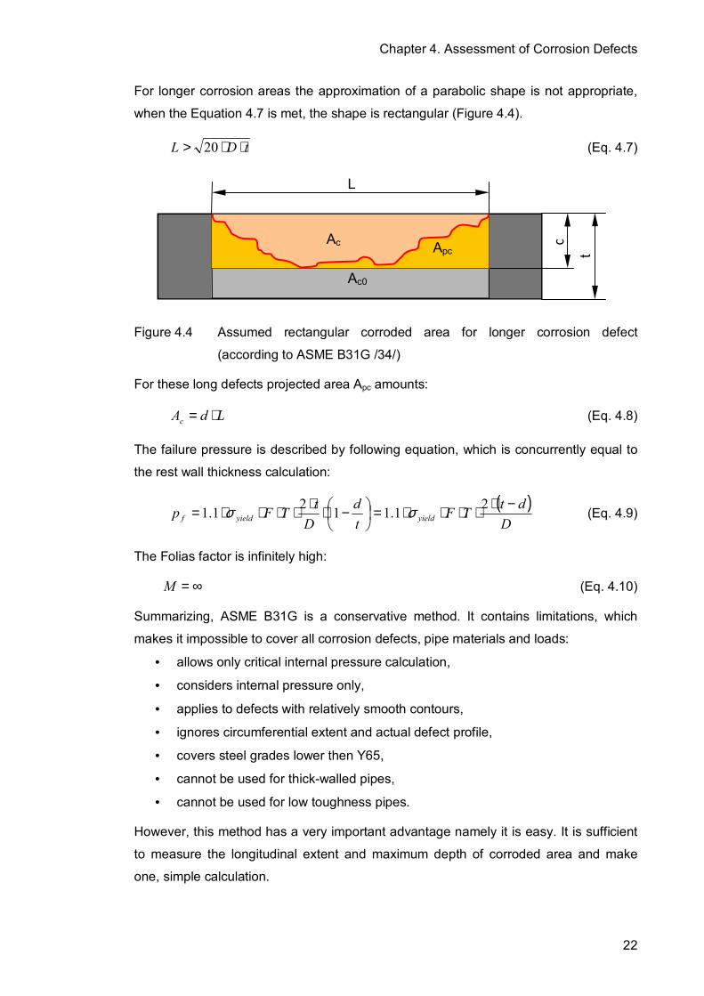
For longer corrosion areas the approximation of a parabolic shape is not appropriate,
when the Equation 4.7 is met, the shape is rectangular (Figure 4.4).
tDL ⋅⋅> 20 (Eq. 4.7)
Figure 4.4 Assumed rectangular corroded area for longer corrosion defect
(according to ASME B31G /34/)
For these long defects projected area Apc amounts:
LdAc ⋅= (Eq. 4.8)
The failure pressure is described by following equation, which is concurrently equal to
the rest wall thickness calculation:
( )DdtTF
td
DtTFp yieldyieldf
−⋅⋅⋅⋅⋅=
−⋅⋅⋅⋅⋅⋅= 21.1121.1 σσ (Eq. 4.9)
The Folias factor is infinitely high:
∞=M (Eq. 4.10)
Summarizing, ASME B31G is a conservative method. It contains limitations, which
makes it impossible to cover all corrosion defects, pipe materials and loads:
• allows only critical internal pressure calculation,
• considers internal pressure only,
• applies to defects with relatively smooth contours,
• ignores circumferential extent and actual defect profile,
• covers steel grades lower then Y65,
• cannot be used for thick-walled pipes,
• cannot be used for low toughness pipes.
However, this method has a very important advantage namely it is easy. It is sufficient
to measure the longitudinal extent and maximum depth of corroded area and make
one, simple calculation.
L
Ac0
t
dAc Apc

Chapter 4. Assessment of Corrosion Defects
23
4.1.2 Modified B31G corrosion assessment method
The B31G method was found to be too conservative and has been modified. The new
method is called Modified B31G or RSTRENG (Remaining Strength of Corroded Pipe)
0.85-area Method (Kiefner and Vieth /35/, /36/). This criterion has been confirmed
against 86 burst tests on pipes containing real corrosion defects. One of the most
significant changes to the original B31G method is the defect geometry approximation.
Corrosion shape is defined by 0.85dL (Figure 4.5).
Figure 4.5 Assumed rectangular corroded area for longer corrosion (according to
Kiefner /36/)
This method removes some conservation by changing the flow stress limit to SMYS
+ 69 MPa (10,000 PSI). This is very close to the conventional fracture mechanism
definition of the flow stress: the average of the yield and ultimate strength. This
modification results in the change of the failure equation, which is also dependent on
the limit on defect length.
tDL ⋅⋅≤ 50 (Eq. 4.11)
When the L value fulfils the Equation 4.11, than the failure equation is replaced by the
following one (failure pressure in Pa):
( )
⋅−
−⋅⋅⋅⋅+⋅=
Mtdtd
Dtp yieldf 185.01
85.01210691.1 6σ (Eq. 4.12)
The Folias factor is given by the following equation:
222
003375.06275.01
⋅
⋅−⋅
⋅+=tD
LtD
LM (Eq. 4.13)
L
Ac0
t
d
Ac Apc
Chapter 4. Assessment of Corrosion Defects
24
When the axial length of corroded area fulfils the Equation 4.14, then the failure
equation stays the same, but the Folias factor changes (Equation 4.15).
tDL ⋅⋅> 50 (Eq. 4.14)
tDLM
⋅⋅+=
2
032.03.3 (Eq. 4.15)
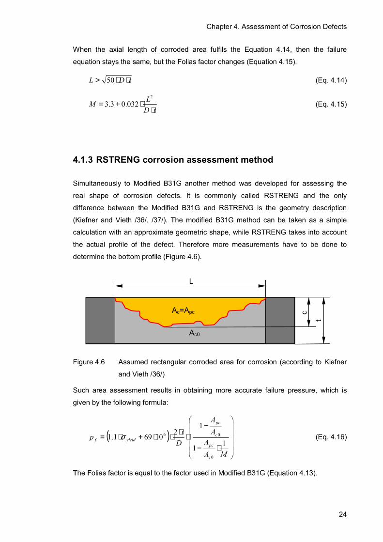
4.1.3 RSTRENG corrosion assessment method
Simultaneously to Modified B31G another method was developed for assessing the
real shape of corrosion defects. It is commonly called RSTRENG and the only
difference between the Modified B31G and RSTRENG is the geometry description
(Kiefner and Vieth /36/, /37/). The modified B31G method can be taken as a simple
calculation with an approximate geometric shape, while RSTRENG takes into account
the actual profile of the defect. Therefore more measurements have to be done to
determine the bottom profile (Figure 4.6).
Figure 4.6 Assumed rectangular corroded area for corrosion (according to Kiefner
and Vieth /36/)
Such area assessment results in obtaining more accurate failure pressure, which is
given by the following formula:
( )
⋅−
−⋅⋅⋅⋅+⋅=
MAAAA
Dtp
c
pc
c
pc
yieldf 11
1210691.1
0
06σ (Eq. 4.16)
The Folias factor is equal to the factor used in Modified B31G (Equation 4.13).
L
Ac0
Ac=Apc t
d
Chapter 4. Assessment of Corrosion Defects
25
Modified B31 Method and RSTRENG, are very similar to the original B31. They predict
failure by the calculation of the failure hoop stress. The allowable hoop stress is then
set at 0.72 percent.
Both methods have the same limitations as the primary B31 Method (Subchapter
4.1.1). They only improve the accuracy and it is done in three ways: changes in the
flow stress, modifications of the Folias factor, and approximation of the metal loss.
Budnik et al. /38/ have compared these approaches to the database of 80 burst tests.
The results for the B31G Method showed a standard deviation of circa 24% for the
average safety factor. The calculations were carried out with measured yield strength
not with the nominal one. Modified B31G method gave similar results. Accuracy
improvements achieved RSTRENG method with the standard deviation of 16% of the
average safety factor. It shows the conservatism of the above methods, because some
predicted burst pressure were even 2.5 times lower then test results. This however,
may be disputable, due to reading off the burst values from tests.
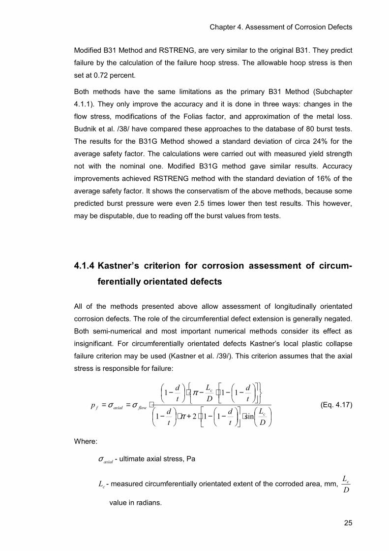
4.1.4 Kastner�s criterion for corrosion assessment of circum-
ferentially orientated defects
All of the methods presented above allow assessment of longitudinally orientated
corrosion defects. The role of the circumferential defect extension is generally negated.
Both semi-numerical and most important numerical methods consider its effect as
insignificant. For circumferentially orientated defects Kastner�s local plastic collapse
failure criterion may be used (Kastner et al. /39/). This criterion assumes that the axial
stress is responsible for failure:
⋅
−−⋅+⋅
−
−−⋅−⋅
−
⋅==
DL
td
td
td
DL
td
pc
c
flowaxialf
sin1121
111
π
πσσ (Eq. 4.17)
Where:
axialσ - ultimate axial stress, Pa
cL - measured circumferentially orientated extent of the corroded area, mm, DLc
value in radians.

Chapter 4. Assessment of Corrosion Defects
26
4.2 Numerical methods of corrosion assessment
Failure pressure of corroded tubular goods can also be predicted by the use of finite
element analysis. In recent years a number of studies concerning FE analysis have
been published. They present different approaches using various modelling and failure
criteria (Fu et al. /40/).
4.2.1 British Gas procedure of corrosion assessment
The best known numerical procedure has been developed by British Gas (later BG
Technology, and now Advantica). It has been done within the framework of a three-
year programme sponsored by a group of major oil and gas companies and European
regulatory authorities. The whole project cost approximately £1.2 million (Fu and Batte,
/41/) and was finished in 1997. The main task was to develop new guidelines for
integrity assessment for corroded pipes. This involved full scale burst tests, material
property determination and numerical studies of the failure behaviour. The project has
been discussed in a number of publications by Fu et al. /42/, /43/, /44/, /45/.
The analysis employs ABAQUS software with 3D model and 20-node hexahedral
elements. The defect geometry is simplified and takes into account its maximum
length, width and depth. The corrosion shape is approximated as a flat bottom with
circular corners (Figure 4.7). The mesh density and layer numbers depends on the
defect�s shape and ones own judgment.
Figure 4.7 3D FE model of pipe with internal corrosion groove (from Fu and
Kirkwood /42/)
Chapter 4. Assessment of Corrosion Defects
27
Analysis considers material nonlinearity and large displacements, and uses the plastic
collapse mechanism as the failure criterion. The failure occurs when the local
equivalent stresses von Mises reach the true ultimate tensile stress throughout the
remaining ligament of the corroded location. Three stages can be distinguished. The
first stage represents elastic deformation. The second, plastic stage is reached as the
elastic limit begins. During this stage plasticity spreads through the ligament, while the
maximum Mises stresses remain nearly constant. The third stage contains material
hardening after the yield strength exceeds Mises stresses and the whole ligament
deforms plastically.
The exact way in which this deformation process proceeds depends on material
parameters. In order to take into account the material behaviour over 200 material tests
with different steel grades were performed to fully understand the failure mechanism.
These tests allowed determining true stress/strain curves which were implemented into
the finite element analyses.
To validate the numerical procedure 81 full-scale pipe burst tests and 52 ring
expansion tests were completed. Isolated, interacting and combined corrosion defect
were considered for modelling corrosion in the form of pits, grooves (corrosion bands)
and uniform corroded areas (general corrosion). The defects depth ranged from 20% to
80% of wall thickness and only internal load was considered.
On the above basis almost 500 finite element analyses were performed with various
defect shapes, defect configurations and material properties. New methods of
analysing single, complex and interacting defect were developed and compared with
B31G method. This resulted into a three-level assessment procedure (Figure 4.8),
which depends on available information and on required assessment accuracy.
The failure pressure for single defects (Level-1) can be estimated using the simple
equation. It was derived from tests and nonlinear FE analyses. This equation requires
only defect sizes and basic material properties, and has the same basis as B31G
method.
Compared to the B31G the stress limit is defined by the minimum ultimate tensile
stress of the material not by the yield stress. This was decided on account of the test
results.
UTSflow σσ = (Eq. 4.20)

Chapter 4. Assessment of Corrosion Defects
28
Figure 4.8 A three-level assessment frame work (from Fu and Batte /41/)
There is also a difference in the geometry correction factor, which has been modified.
The Folias factor has been replaced by the length correction factor Q:
tDLQ
⋅⋅+=
2
31.01 (Eq. 4.21)
These changes result in the following failure equation:
⋅−
−⋅
−⋅⋅=
Qtdtd
tDtSMTSp f 11
12 (Eq. 4.22)
For the specified minimum tensile stress (SMTS), which is used in Equation 4.22, there
is no need to apply an additional safety factor regarding the accuracy. However, if
instead of SMTS the measured value of ultimate tensile strength (UTS) σUTS is used,
required factor amounts to 0.9.
Easy Complexity
Difficult
Con
serv
ativ
e Ac
cura
te
Acc
urac
y
Level-1(isolated defect)
simple material data simple geometry data
Level-2a(interacting defects) simple material data
simple geometry data
Level-2b(complex-shaped
defect) simple material data
Level-3 (numerical analysis)
detailed material data detailed geometry

Chapter 4. Assessment of Corrosion Defects
29
British Gas, within this project, developed a quantitative guidance for interacting
adjacent defects. The corrosion defect is regarded as an isolated one, when the axial
spacing to the nearest defect amounts to a minimum:
tDs ⋅⋅= 20 (Eq. 4.18)
An isolated defect has to be separated from other defects in circumferential direction
too. The minimum distance is as follows:
⋅⋅=
πφ 36030 D
t (Eq. 4.19)
For a group of defects, the failure pressure can be evaluated by taking the total length
of the group and effective depth based on an equal area. More information can be
found in Fu and Batte�s work /41/.
The project brought forwards these main outcomes:
• the internal and external defects have the same effect on failure pressure,
• short defects have no impact on pipe integrity,
• defects longer than tD ⋅⋅8 can be consider as infinite ones,
• defect circumferential width has no influence on the failure pressure,
• defect depth less then 10% of wall thickness has no influence on the failure
pressure,
• defects with depths less than 20% of wall thickness do not interact together.
Summarizing the limitations of this method:
• accuracy depends on the model (mesh, calculation steps, etc.),
• applicable to defects where plastic failure is expected,
• not for low toughness steels,
• max calculable defect depth 85% of not corroded wall thickness,
• considers internal pressure only,
• for smooth defect surfaces.
British Gas guidelines may also be applied to corrosion defects in seam welds and girth
welds, but there must not be any significant weld defect present and the fracture is not
likely to occur (Fu and Batte /41/).

Chapter 4. Assessment of Corrosion Defects
30
4.2.2 Det Norske Veritas and other numerical corrosion
assessment methods
Parallel to British Gas, Det Norske Veritas (DNV) was running a similar project. Authors
used 3D FE analyses to establish burst capacity and carried out some full-scale burst
tests with machined corrosion defects for calibration purposes. Numerical analysis is
comparable to that presented by British Gas (Subchapter 4.2.1). DNV carried out some
probabilistic evaluations to determine safety factors, applying the program PROBAN
(Bjornoy et al. /46/). This software enables, among other things, calculation of
probability of failure or parameter study, e.g. growth as function of time. As the result
DNV proposed its own method of corrosion assessment which evolved into the
equations that will be presented in the RP-F-101 description later in this chapter.
There are some other finite element analyses used for calculation of burst pressure,
but their descriptions contain only general statements e.g. use of non-linearity, large
displacement or ultimate strength as a failure criterion. Such information is insufficient
for evaluation. Most of the numerical methods predict failure using, the plastic collapse
criterion with ultimate tensile strength e.g. a procedure called PCORRC, which stands
for Pipe Corrosion Failure Criterion (Leis and Stephens /47/). Between these methods
the most significant differences are noticeable in implementation of the stress/strain
curve and defect modelling. The defect geometry approximation is very important not
only from an accuracy point of view, but it results in stress distribution and therefore
influences the remaining strength. One example of defect description has been already
presented in Figure 4.7. The same approach has been used by Saldanha and Bucherie
/48/, and its defect longitudinal section is presented in Figure 4.9.
Figure 4.9 A three-level assessment frame work (from Saldanha and Bucherie /48/)
The Lcyl and Lell stand correspondingly for the half length of the cylindrical region and
the half length of the ellipsoidal region. The total defect length amounts to 2Lcyl+2Lell.
Lcyl Lell
d t

Chapter 4. Assessment of Corrosion Defects
31
As previously mentioned there is a lack of information about pipe models with corrosion
defects, especially about boundary conditions and symmetries. Therefore, only various
defect shapes can be indicated here. Not all of these methods use spherical forms,
there are also simulations, with other shapes for example from Lee and Kim /49/, who
presented corrosion as a flat groove. Another idea is to use a rectangular area, as in
the Shell-92 method (Ritchie and Last /50/) or Loureiro el al. /51/. This is schematically
depicted in Figure 4.10.
Figure 4.10 Rectangular area of corrosion approximation (from Loureiro el al. /51/)
The shape of the defect has an impact on calculated remaining strength, so it is
important to map it as precisely as possible. However, there are limitations in numerical
programs and hardware, so the golden mean has to be found.
4.3 Probabilistic methods of corrosion assessment
4.3.1 DNV RP-F-101 standard
British Gas and DNV pooled their results to develop a unified guideline for corrosion
assessment (Bjornoy el al. /52/, /53/). In this guideline a probabilistic calibrated
equation should allow corroded pipelines operating for different safety classes. The
partial safety factors depend on the desired reliability level and assessment accuracy.
These levels are based on the offshore pipeline standard DNV-OS-F101, Submarine
Pipeline Systems, but are not limited to the offshore pipelines.

Chapter 4. Assessment of Corrosion Defects
32
The uncertainties of this approach are associated with:
• model,
• material properties,
• defect sizing and depth (three safety classes),
• inspection accuracy (four levels).
As a result a new equation for the longitudinal corrosion defects with internal pressure
loading only, has been developed:
⋅
⋅−
⋅−
⋅−⋅⋅⋅=
Qtdtd
tDtSMTSp
d
d
mf11
12
*
*
γ
γγ (Eq. 4.23)
Where:
mγ - partial safety factor for model prediction and safety class, -
dγ - partial safety factor for corrosion depth, -
The relative corrosion depth
⋅+
=
tdStD
td
td
dmeas
ε*
(Eq. 4.24)
Where:
meastd
- measured relative corrosion depth, -
dε - factor for defining a fractile value for the corrosion depth, -
tdStD - standard deviation of the measured d/t ratio (based on the
specification of the inspection tool), -
The Q factor is the same as that used by British Gas (Equation 4.12).
According to PETROBRAS (Benjamin el al. /54/) RP-F101 equation trends to give
results that depart from the tests when increasing defect length. The company
developed a new equation (Benjamin el al. /55/) for calculating the remaining strength
of tabular specimens containing longer defects (according to B31G). The major
difference refers to the Folias factor, which was modified to approach the laboratory
tests.

Chapter 4. Assessment of Corrosion Defects
33
DNV-RP-F101 contains one more approach for corrosion assessment. It is based on
allowable stress design, where the failure pressure of the pipe is calculated and
multiplied by safety factors (Equation 4.25). These factors may be based on design
factor and can consider uncertainties such as presented above. The uncertainties
caused by the presence of a corrosion defect, according to the authors, can be
described by the additional 0.9 factor. This is a commonly used approach because of
its simplicity.
⋅−
−⋅
−⋅⋅⋅⋅=
Qtdtd
tDtSMTSFp f 11
129.0 (Eq. 4.25)
DNV-RP-F101 also developed equations for single defects with longitudinal stress and
defects with complex shape. More information can be found in F101 manuals.
Nowadays, probability analyses are becoming more popular. Many of them were
developed for corroded transmission pipelines and more information can be found in
articles written by Francis and Geren /56/, McQueen el al. /57/ or Yahaya /58/.
This chapter presented assessment methods, which can be used with uniform or pitting
corrosion and not cracked corroded defects. Overviews of assessment methods for
other defect types i.e. mechanical ones, dents on welds or cracks are presented in
works written by Cosham and Kirkwood /59/, Cosham and Hopkins /60/, Osborn /61/,
/62/ or the MSL Report /63/. More inquiring readers will find, particularly in MSL Report,
many references regarding these topics.

Chapter 5. Numerical Simulation Model
34
5 Numerical Simulation Model
Current corrosion assessment methods, which are presented in Chapter 4, cannot be
used for assessing the remaining strength of corroded oil field tubulars. As mentioned
previously they were developed for transmission pipes and concentrate on predicting
the burst pressure only, while the tubular goods, used in wells, have to be additionally
checked for collapse and axial load criteria. Moreover, calculation criteria used in
midstream sector differ from those in upstream industry.
Chapter 4 pointed out that the most accurate methods for the assessment of corroded
tubes are FE analyses. These numerical methods enable the determination of
approximate solutions, which are even so better then others. There are also many
other advantages, such as the possibility of applying various loading conditions and
creations of almost exact shapes of the defects.
It is worth noting that this chapter contains information about the development of the
numerical model and describes it more from the user�s point of view. However, there is
hardly any information about the Finite Element Method. Readers not familiar with this
topic may find Zienkiewicz�s books /64/, /65/ interesting or take any other publications
on this subject.
5.1 ANSYS model
The idea of creating a numerical procedure for assessing the remaining strength of
corroded tubulars was taken from previous works completed by the Institute of Drilling
Engineering and Fluid Mining at Freiberg University. In numerous publications e.g.
Köckritz and Lippmann /66/, Behrend et al. /67/, Köckritz and Behrend /68/ authors
presented their experiences in the computation of tubes for burst and collapse
prediction. General purpose FE software ANSYS was used with the von Mises
calculation criterion: when equivalent stress exceeds the minimum yield stress. These
calculations were carried out in the 1990s and, as a result of limitations in early
versions of FE programs and computers� calculation power, were simplified in order to
perform analyses. Simultaneously, they were complicated at some level and required
more then a basic knowledge of ANSYS software to �choose� the right results.
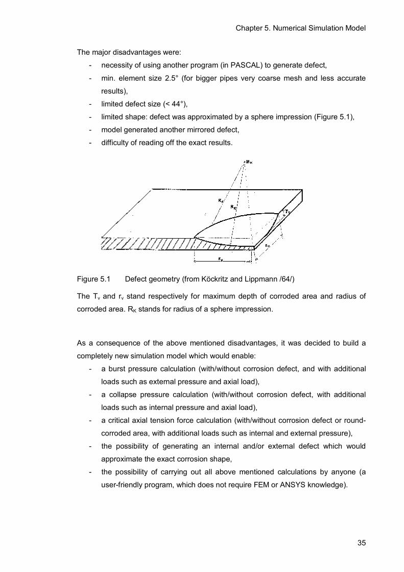
Chapter 5. Numerical Simulation Model
35
The major disadvantages were:
- necessity of using another program (in PASCAL) to generate defect,
- min. element size 2.5° (for bigger pipes very coarse mesh and less accurate
results),
- limited defect size (< 44°),
- limited shape: defect was approximated by a sphere impression (Figure 5.1),
- model generated another mirrored defect,
- difficulty of reading off the exact results.
Figure 5.1 Defect geometry (from Köckritz and Lippmann /64/)
The Tv and rv stand respectively for maximum depth of corroded area and radius of
corroded area. RK stands for radius of a sphere impression.
As a consequence of the above mentioned disadvantages, it was decided to build a
completely new simulation model which would enable:
- a burst pressure calculation (with/without corrosion defect, and with additional
loads such as external pressure and axial load),
- a collapse pressure calculation (with/without corrosion defect, with additional
loads such as internal pressure and axial load),
- a critical axial tension force calculation (with/without corrosion defect or round-
corroded area, with additional loads such as internal and external pressure),
- the possibility of generating an internal and/or external defect which would
approximate the exact corrosion shape,
- the possibility of carrying out all above mentioned calculations by anyone (a
user-friendly program, which does not require FEM or ANSYS knowledge).
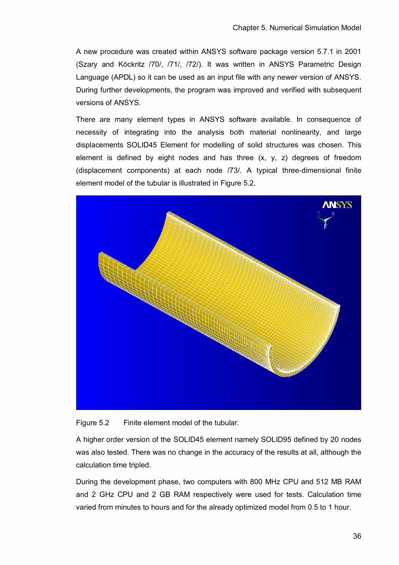
Chapter 5. Numerical Simulation Model
36
A new procedure was created within ANSYS software package version 5.7.1 in 2001
(Szary and Köckritz /70/, /71/, /72/). It was written in ANSYS Parametric Design
Language (APDL) so it can be used as an input file with any newer version of ANSYS.
During further developments, the program was improved and verified with subsequent
versions of ANSYS.
There are many element types in ANSYS software available. In consequence of
necessity of integrating into the analysis both material nonlinearity, and large
displacements SOLID45 Element for modelling of solid structures was chosen. This
element is defined by eight nodes and has three (x, y, z) degrees of freedom
(displacement components) at each node /73/. A typical three-dimensional finite
element model of the tubular is illustrated in Figure 5.2.
Figure 5.2 Finite element model of the tubular.
A higher order version of the SOLID45 element namely SOLID95 defined by 20 nodes
was also tested. There was no change in the accuracy of the results at all, although the
calculation time tripled.
During the development phase, two computers with 800 MHz CPU and 512 MB RAM
and 2 GHz CPU and 2 GB RAM respectively were used for tests. Calculation time
varied from minutes to hours and for the already optimized model from 0.5 to 1 hour.

Chapter 5. Numerical Simulation Model
37
5.2 Boundary condition
5.2.1 Constraints and symmetry
In order to keep the calculation time as low as possible and still get accurate results it
was decided to use advantage of symmetry and model only a quarter of the tubular.
Figure 5.3 shows this ¼ part with the appropriate constraints of degrees of freedom
generated from the symmetry planes.
Figure 5.3 A quarter model of the tubular.
Thanks to symmetry lying in xy and xz planes the number of nodes was reduced by
75%, and the calculation time decreased approximately 10 fold. As a picture says a
thousand words, symmetry expansions are presented in Figure 5.4. The picture in the
top left corner illustrates constraints with the xy plane which corresponds with the
expansion in this direction, illustrated in the top right picture. Bottom pictures
demonstrate constraints and expanded model in the xz plane.
The full model with both horizontal and vertical symmetry expansions is shown in
Figure 5.5.

Chapter 5. Numerical Simulation Model
38
Figure 5.4 A quarter model with constrains and symmetry expansion in xy and xz planes.
Figure 5.5 A full finite element model after symmetry expansions.

Chapter 5. Numerical Simulation Model
39
The only geometry limit, which had to be set, was the length of the examined tubular. It
was decided to set it equal to 2 outside diameters of the pipe (D) for a ¼ model part
which corresponds to 4D after symmetry expansion. Connecting this parameter with
the outside diameter of the pipe made possible to exclude it from input data and to
keep the model size proportional.
A main reason of setting the model length to the above value was the longitudinal
extent of the corrosion. On the one hand, various investigators (e.g. Fu and Batte, /41/)
have found that defects with longitudinal extent bigger then approx. 1-1.5 D can be
considered as infinite ones. FE calculations gave similar results and the maximum
modelable longitudinal defect extent was set at 2D (1D in a ¼ model). There was no
reason to build a model which would allow the creation of defects with longer then a 2D
axial extent, because the results stay the same. On the other hand, the model had to
be long enough to allow the stress distribution, and to prevent the model�s boundary
influence. It was proven that negligible differences are obtained when the non corroded
area, between defect and model border remains at a min of 1D in length.
5.2.2 Applicable loads
Generally speaking, FEM is based on approximations. As model geometry
approximates the real shape and constraints approximates how the structure is
supported similarly, loads approximate what happens in the real world. Considering the
operating condition of casing and tubing it was decided to implement three types of
loads:
- internal pressure (Figure 5.6),
- external pressure (Figure 5.7),
- axial tension (compression with ��� sign) (Figure 5.8),
Loads are applied in the numerical model over a surface as surface loads and it is
possible to apply them simultaneously. For visualisation purposes they are presented
separately (due to the elements� transparency) with appropriately placed arrows in the
figures overleaf.

Chapter 5. Numerical Simulation Model
40
Figure 5.6 Internal pressure.
Figure 5.7 External pressure.

Chapter 5. Numerical Simulation Model
41
Figure 5.8 Axial tension.
5.3 Mesh and its accuracy
The starting point of the finite element method is subdivision. The body has to be sub-
divided into a finite number of smaller pieces which are called elements (Figure 5.2).
These elements are defined by points at their edges called nodes. Nodes and elements
together form FEM mesh, which approximates the shape of the real body. The coarser
it is, the more simplified the body is and the results less accurate. A fine mesh gives
results that are closer to the exact solution, but the analysis is more time consuming.
There are two different ways in which a model in ANSYS can be created: top-down
solid modelling and bottom-up generation. In the first, the geometric model shape is
produced with points, lines, areas and volumes. After that, the mesh is automatically
generated according to the set up mesh controls. This way is very convenient, but, at
the time of developing this procedure, impossible to use. It was determined that the
calculating capacities were to low even to generate some more complicated shapes of
corrosion defects inscribed into an oval pipe. Therefore, it was necessary to follow a
so-called bottom-up generation way, in which the location of every node is defined, as
well as the shape and size of the elements.

Chapter 5. Numerical Simulation Model
42
5.3.1 Element number
The most challenging part was to build a model for a user non familiar with FEM and
ANSYS, who would be able to carry out calculations with various sizes of pipes and
corrosion defects. To combine this goal with the creation of well shaped and sized
elements, it was decided to a set a fixed number of nodes/element in axial and
circumferential directions and interlock their size with the pipe�s diameter.
As mentioned earlier, the finer the mesh is, the more exact the results are. However, at
some point, increasing the number of elements further does not improve accuracy
anymore. It was tested that 2 (in some cases 4) layers of elements through the
ligament of the pipe and defect, are enough to get reliable results. The difference
between 2 and 4 layer calculations for burst and collapse analyses stay in the range of
up to few percent (mostly 1-3%, see also Subchapter 5.8) and is dependent mainly on
the shape and size of the defects. As it was necessary to carry out thousands of
analyses to verify the model, a 2 layers model was chosen. In the procedure an option
was built in, which allows the user to choose the number of layers from 2 to 6.
However, for models with more then 4 layers, generally no accuracy improvement was
observed, only computational times increased considerably.
Analyses with different number of elements in circumferential and longitudinal tubular
direction were performed, to choose their optimal number. Due to the fact of using only
one model for different pipe sizes it was decided to take 61 elements in radial direction
and 69 elements in vertical direction. This configuration ensures a good approximation
of various shapes and sizes of corrosion defects, even for bigger pipes.
5.3.2 Element size
Elements sizes in this particular analysis are driven only by the pipe diameter, as the
number of elements stays the same. This relationship is directly proportional and for
the bigger pipes element sizes increase.
A typical element distribution is presented in Figure 5.9. The modelled pipe has a
diameter of 11 ¾�. The red arrow points at the corner where the defects start. At this
point, there is a centre of the future defect, which will also be created as a ¼ symmetric
part. To allow detailed modelling of any defects: small and large, the mesh density
gradually increases towards the corners.

Chapter 5. Numerical Simulation Model
43
Figure 5.9 Typical finite element mesh of a quarter model.
Elements sizes and their distribution in circumferential and axial direction are described
with the following equation:
1)1(
_ +∆⋅⋅−=∆
nuiiu coordi (Eq. 5.1)
Where:
coordiu _∆ - node�s coordinate in circumferential direction, mm
i - coordinate number, i = 1�(n+1)
n - number of elements in circumferential direction, -
u∆ - average element extension, mm
nDu
⋅⋅=∆
4π
(Eq. 5.2)
Equation 5.1 allows the creation of a very fine mesh in the middle (at the corner where
the defect generation starts) with a soft transition into coarser mesh. Typical results in
the circumferential direction for 61 elements and 11 ¾� pipe diameter are presented in
Appendix 5.1.

Chapter 5. Numerical Simulation Model
44
5.4 Ovality implementation
All tubular goods have some imperfections which usually come from dimensions or
weights and one of them is ovality (Figure 5.10), which can be relatively easily
determined during corrosion measurement. In the finite element model presented here,
a small initial ovality was introduced. The main reason was to allow the collapse
process to occur. A perfect pipe, without any defects and ovality would not collapse,
even if the external pressure were to be applied indefinitely. Another cause was
significant ovality influences on collapse pressure (even greater then defects).
Figure 5.10 Ovality (red circles represent imperfect tubular).
Ovality was calculated according to the following equation (Köckritz and Behrend /68/):
SDDDD
DDDD
O ⋅=+−
⋅=+−
= 22
2minmax
minmax
minmax
minmax (Eq. 5.3)
Where:
O - ovality, -
maxD - maximum outside diameter, mm
minD - minimum outside diameter, mm
S - half of the ovality, -
In this model the ovality was introduced by the equation presented by Issa /74/:
))2cos(1( φ⋅⋅+⋅= Srr ao (Eq. 5.4)
Where:
or - imperfect tube radius, mm
ar - nominal outside radius, mm
φ - rotation angle, °

Chapter 5. Numerical Simulation Model
45
In the numerical model ovality is implemented during the nodes generation phase.
It can be stated that nodes created according to the guideline presented in
Subchapter 5.3.2 were slightly moved from or into the pipe centre. This is shown on the
example in Appendix 5.2 of 11 ¾� pipe with an ovality of O= 0.004, which correspond
to 0.4%.
During the model development phase it was noted that ovality interact with defects
which influence the failure pressure. On the basis of calculation it was chosen to
introduce ovality in the way shown in Figure 5.11. The top left picture presents a pipe
without ovality and the red arrow points at the area where the defect can be generated.
A picture located on the right side illustrates a collapse example with an excessive
ovality equal to 10% (to make it visible). The minimum radius was created in the area
where defect can be generated. Although, failure collapse pressure depends on ovality
and particular defect parameters, for most cases such combination of ovality and
defect placement correspond with the worse case. For burst analyses, area with the
defect is most distant from the pipe centre (Figure 5.11 bottom left).
Figure 5.11 Ovality implementation for collapse (top right) and burst (bottom left)
analyses (top left: without ovality).

Chapter 5. Numerical Simulation Model
46
5.5 Defect generation
Defining the model geometry in FEM analysis indicates another approximation. Not
only a tubular but also corrosion defects have to be defined. It is obvious that material
losses reduce the tubular strength. However, not only the amount of removed material
is important, also the defect shape plays a significant role. It influences the stress
distribution around defects, and in turn, also influences the remaining strength.
Therefore, it is vital to create defects similar to real ones (Figure 5.12).
Figure 5.12 Typical corrosion on the inner wall of tubing in a gas production well.
On the other hand, to create a user-friendly program and to find out relationships
between defects shape and remaining strength it was necessary to approximate the
corroded volume. This was carried out by using the elliptical equations: one for the
surface and two others for material deterioration. That gives a good approach to the
real form and allows creation of the defect with only three parameters:
- �a� � half of defect�s width (½ of the value measured in hoop tubular direction),
- �b� � half of defect�s length (½ of the value measured in longitudinal tubular
direction),
- �c� � defect�s depth (maximum measured value in wall thickness direction).
Since the ellipsoid on the surface always depicts a larger region then the real corroded
area, results are also influenced and little conservative. Surface form (Figure 5.13) is
implemented by the following equation:
222222 bazab =+ϕ (Eq. 5.5)
The coordinate system is cylindrical with r, φ, and z coordinates.

Chapter 5. Numerical Simulation Model
47
Figure 5.13 Surface approximation of the corroded area.
It is enough to provide two parameters (defect width and length) to model a vertical or
horizontal orientated defect. For a complete defect depiction a third parameter, namely
defect depth, is necessary. This parameter corresponds with the maximal defect�s
immersion at its middle (Figure 5.14) and is described by the following elliptical
equations in horizontal and vertical direction respectively:
222222 cbzcrb =+ (Eq. 5.6)
222222 cacra =+ ϕ (Eq. 5.7)
Figure 5.14 Defect shape (I � top view, II and III � side views).
a
b z φ
a
b
a
b
c
c
z φ
r φ
z r
III
I II

Chapter 5. Numerical Simulation Model
48
In the numerical model nodes are generated with consideration of element sizes
(Subchapter 5.3.2) and ovality (Subchapter 5.4). It is possible to create an internally
and externally corroded tubular. The cylindrical coordinates for an externally corroded
one are implemented into the model by the subsequent equations:
- in r � direction:
( ) ( )( )
⋅−
⋅−⋅−⋅−−⋅⋅+⋅=
2
222
2
222
22
222
)1(arg
)1(arg
)3(arg)1(arg2arg2cos1,
abb
acc
accSrzr aϕ
(Eq. 5.8)
- in ϕ � direction:
2arg=ϕ (Eq. 5.9)
- in z � direction:
3arg=z (Eq. 5.10)
Where:
1arg - variable width, mm
2arg - variable width (corresponds to rotation angle) , °
3arg - variable length, mm
Parameters arg1, arg2 and arg3 are dependent on the element sizes (see
Subchapter 5.3.2).
For an internally corroded tubular Equation 5.8 has to be slightly modified:
( ) ( )( )
⋅−
⋅−⋅−⋅−+−⋅⋅+⋅=
2
222
2
222
22
222
)1(arg
)1(arg
)3(arg)1(arg2arg2cos1,
abb
acc
acctSrzr aϕ
(Eq. 5.11)
As mentioned at the beginning of this chapter the defect is created at the corner of the
¼ model, and also corresponds with ¼ of the defect (Figure 5.15). For visualisation
purposes the defect is presented without elements generated by ANSYS and only the
bottom right picture shows the finite element model with them. It is easy to notice that
the area where a defect is created has the finest mesh. This allows good shape
approximation, even of the small defects.

Chapter 5. Numerical Simulation Model
49
Figure 5.15 A typical corrosion defect generated on the inner wall of tubular.
Figure 5.16 An internal and external defect generated on the wall of tubular.

Chapter 5. Numerical Simulation Model
50
As mentioned earlier it is possible to generate an internal and external defect.
Moreover, it is possible to create both of them simultaneously (Figure 5.16).
There are almost no limitations in defects sizes. However, the following points should
be kept in mind:
- defect length should be limited to 2D (parameter �b� ≤ D) (defects that extend
longitudinally to more then 2D behave as infinite ones and results stay the
same; besides, for larger defects a longer model is required),
- defect width should be limited to πD (parameter �a� ≤ πD/2) for the external
defects and to πDi (parameter �a� ≤ πDi/2) for internal ones (defects with a
circumference of more then πD or πDi will not be elliptical anymore, but will
represent a uniformly corroded area around the tubular),
- defect depth must not extend wall thickness (parameter �c� < t) (if internal and
external defects are generated, their sums must stay below the t value).
In Figure 5.16 it can be noted that the internal defect is vertically orientated, while the
external one horizontally. This ability is presented in Figure 5.17 and 5.18. Elements
are presented only in bottom right pictures and without the symmetry extension due to
the fact that they make defects hardly visible.
Figure 5.17 Typical corrosion on the inner wall of tubing in a gas production well.

Chapter 5. Numerical Simulation Model
51
Figure 5.18 Typical corrosion on the inner wall of tubing in a gas production well.
A few additional pictures with close-ups of the defects are presented in Appendix 5.3.
5.6 Failure prediction
Failure may be defined as a certain limit above which material fails. It may occur as a
fracture, excessive deformation or just when an arbitrary set value of stress, strain or
energy is reached. It is relatively easy to predict the failure of a material with a simple
geometry and subjected to a single force, but the situation begins to become much
more complicated with complex shapes and with more loads acting from different
directions. Additionally, material behaviour and surroundings play a significant role.
Therefore, there are several failure theories and failure criteria which can be applied to
describe failure material�s failure phenomenon (Altenbach et al. /75/, Ugural and
Fenster /76/).

Chapter 5. Numerical Simulation Model
52
Most tubular goods used in the oil and gas industry are manufactured from ductile
steels and operate in environment where ductile failure occurs. To predict this kind of
failure, theories such as maximum principal stress theory (Lamè), maximum shear
stress theory (Tresca), maximum strain theory (Saint-Venant) or maximum distortion
energy theory (von Mises) may be used (Doege and Meyer-Nolkemper /77/, Lemaitre
/78/, Czichos /79/). In the case of corroded tubulars two of these are commonly used:
- the Tresca criterion, in which failure occur when the maximum shear stress
equals to the critical shear stress,
- the von Mises criterion, in which a three-dimensional stress is compared with an
effective stress.
The difference between both criteria becomes more significant after leaving the elastic
range and taking into consideration the hardening behaviour of the material (Zhu and
Leis /80/). The choice of which one to select was simple, as ANSYS uses only
von Mises criterion.
For pipe calculation it is more convenient to use this theory with cylindrical coordinates,
where stress components are combined into one effective stress according to the
following equation:
( ) ( ) ( ) vzrrz σσσσσσσ φφ =−+−+−⋅ 222
21
(Eq. 5.12)
Where:
zσ - axial stress, Pa
φσ - tangential (hoop) stress, Pa
rσ - radial stress, Pa
vσ - equivalent (von Mises) stress, Pa
5.6.1 Burst failure prediction
The von Mises theory has been extensively used for burst pressure prediction of
tubulars. Normally, combined stress is compared with yield strength, but for
transmitting pipes it was indicated by various stress values (as presented in Chapter 4).
This was so, because many people considered yield strength too conservative for burst
prediction and shifted the failure limit into the plastic region even to the tensile strength
value.

Chapter 5. Numerical Simulation Model
53
However, when applying this theory to wells, the yield strength seems to be a more
important property then tensile strength, because when it is passed, the structure
deforms permanently and beyond acceptable limits. Therefore, as a failure criterion,
the point of the initiation of the plastic behaviour was chosen. The failure occurs, when
the von Mises equivalent stress reaches the yield strength of the material throughout
the remaining ligament of the corroded tube (the analysis is also terminated if it
happens at any other point of the tubular). This criterion is consistent with the API
norms /81/ (Chapter 6).
As yield stress measures the resistance to the plastic deformation and resides at the
interaction between the elastic and plastic regions, the analysis also considers isotropic
work hardening to cover the plastic region. Material behaviour is controlled by an
integrated stress-strain curve for ductile materials. This curve is constructed to model
the material behaviour of common ductile steels that are used in the oil and gas
industry and it can be changed by changing the yield strength value alone (curve�s
upper part is adjusted automatically). In this way, simplifying, the program allows
modelling material nonlinearity. Geometric non-linearities are also taken into account
by permitting the occurrence of the large deformations.
Critical internal pressure is predicted by the line search option, which is an improved
Newton-Raphson procedure. The internal pressure is increasingly applied until the
convergence is achieved (Crisfield /82/, Belytschko et al. /83/). Calculation steps are
not uniform, but they rise to accelerate the analysis. Ultimately, when the failure
criterion is exceeded, the program automatically cuts the steps and solves the
equations until an accuracy of about 2% is achieved. This is the ideal case, but in
material science it is not always easy to determine the border between the elastic and
plastic regions. This problem occurred with some defect shapes and analyses were not
terminated, but using very small steps run further within the work hardening and plastic
regions. This was caused by the low differences in von Mises stresses between these
tiny steps. This problem was overcome by the use of a macro, which checks results
and removes those steps in the plastic region.
Not only small steps caused problems, but also big ones, as time step size determines
the accuracy of the solution. In some cases the analyses converged �too fast� and no
further divisions were done to improve accuracy. As a result of the ovality, various
tubular dimensions and different corroded areas it was not possible to employ 0.2%
offset from the linear region as a failure criterion (which is a common way of solving
problems in when the yield point is unknown). Therefore, another macro was created to
automatically assess results and when precision exceeds about 2% between the last
converted solutions a new analysis, with more steps in this region, is started.

Chapter 5. Numerical Simulation Model
54
To illustrate how the numerical model works the following sequence of pictures show
selected stages of burst simulation (Figure 5.19). For visualisation purposes, further
plastic stages up to the burst are shown. Normally, the program stops after the
equivalent stress von Mises exceeds the yield point value through the wall.
Figure 5.19 Typical deformation stages of corroded pipe for a burst analysis.
5.6.2 Collapse failure prediction
Collapse prediction is more difficult, because failure occurs under elastic, elastic-plastic
or plastic deformation (Chapter 7). It is also very sensitive to geometric imperfections
such as pipe�s ovality or corrosion defects. Failure prediction occurs in a similar way to
the burst failure prediction presented above. Material behaviour is modelled in elastic
and plastic regions with work hardening. Stresses are also compared to the von Mises
yield criterion. The main difference is that the created procedure stops if instability
occurs or the equivalent von Mises stress exceeds, at any point of the pipe, the yield
strength through the wall. For visualisation purposes (Figure 5.20) further stages of the
collapse analysis (without corrosion defects) are shown below.

Chapter 5. Numerical Simulation Model
55
Figure 5.20 Typical deformation stages of non-corroded pipe for a collapse analysis.
5.6.3 Axial load failure prediction
For the critical axial load analysis as a failure criterion yield strength of the pipe was
chosen. It was carried out according to the API regulations (Chapter 8). This analysis
allows prediction of the axial load, which is required to yield the pipe. Material
behaviour is specified in the same way as in the other analyses.
Figure 5.21 presents a typical stress distribution for an analysis with a local corrosion
defect (left) and an analysis with a uniformly corroded circumferential area (right).
Figure 5.21 Typical stress distribution for critical tensional load analyses with a local
defect (left) and with a uniformly corroded circumferential area (right).
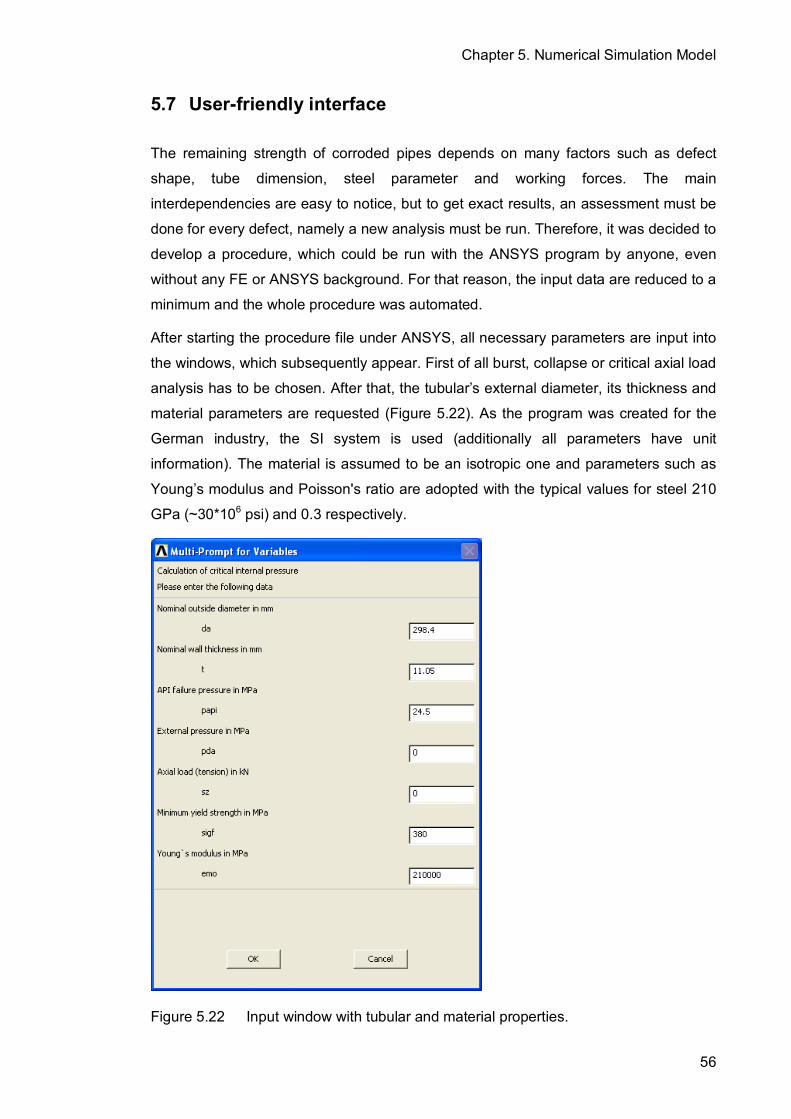
Chapter 5. Numerical Simulation Model
56
5.7 User-friendly interface
The remaining strength of corroded pipes depends on many factors such as defect
shape, tube dimension, steel parameter and working forces. The main
interdependencies are easy to notice, but to get exact results, an assessment must be
done for every defect, namely a new analysis must be run. Therefore, it was decided to
develop a procedure, which could be run with the ANSYS program by anyone, even
without any FE or ANSYS background. For that reason, the input data are reduced to a
minimum and the whole procedure was automated.
After starting the procedure file under ANSYS, all necessary parameters are input into
the windows, which subsequently appear. First of all burst, collapse or critical axial load
analysis has to be chosen. After that, the tubular�s external diameter, its thickness and
material parameters are requested (Figure 5.22). As the program was created for the
German industry, the SI system is used (additionally all parameters have unit
information). The material is assumed to be an isotropic one and parameters such as
Young�s modulus and Poisson's ratio are adopted with the typical values for steel 210
GPa (~30*106 psi) and 0.3 respectively.
Figure 5.22 Input window with tubular and material properties.

Chapter 5. Numerical Simulation Model
57
At this point it is necessary to provide, an expected failure pressure/load value (called
here the API failure pressure). It is not necessary to give the program the answer it is
merely an approximate value or the API value for a non corroded pipe. This speeds up
the calculations because the analysis searches for an answer within a smaller range of
pressures.
As discussed in Subchapter 5.4, all tubulars have a small initial ovality, and this can
also be also applied (Figure 5.23). If ovality is unknown the program automatically
takes an expected ovality (average) for this pipe diameter (Chapter 7).
Figure 5.23 Input windows with ovality information.
It is also possible to change the number of layers from 2 up to 6, but as the accuracy
changes insignificantly it is not recommended. Generally, it only increases the
computational time. A free change of the element number per layer was not
implemented.
In the next window defect dimensions have to be entered (Figure 5.24). As already
described in Subchapter 5.5, defects are created by the use of only three parameters.
External or/and internal defects are produced with their half width (measured in hoop
tubular direction), half length (measured in longitudinal tubular direction) and depth
(measured in wall thickness direction). For modelling purposes defect width and length
values must be greater then 0. To carry out an analysis without corrosion defects, their
depths are set to 0.

Chapter 5. Numerical Simulation Model
58
Figure 5.24 Input window with defect parameters.
In the case of an axial load analyses, there is a possibility to run an analysis with a
corrosion defect (local corrosion as presented above) or with a uniformly corroded
circumferential area. After choosing the second option only longitudinal value of the
circumferential corroded area and its depth are enter (Figure 5.25).
Figure 5.25 Input window with circumferential corroded area parameters.
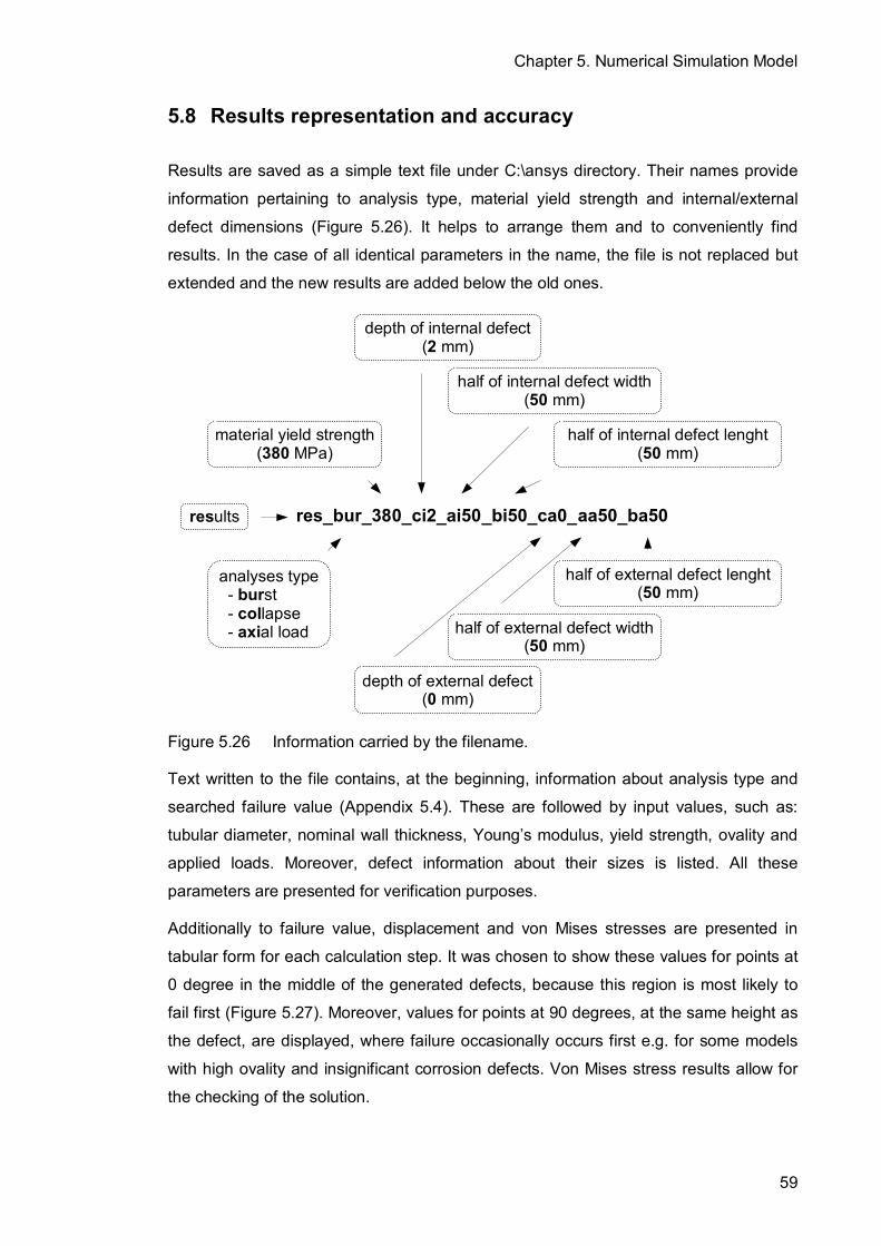
Chapter 5. Numerical Simulation Model
59
5.8 Results representation and accuracy
Results are saved as a simple text file under C:\ansys directory. Their names provide
information pertaining to analysis type, material yield strength and internal/external
defect dimensions (Figure 5.26). It helps to arrange them and to conveniently find
results. In the case of all identical parameters in the name, the file is not replaced but
extended and the new results are added below the old ones.
aa50_ba50_bi50_ca0_0_ci2_ai50res_bur_38
Figure 5.26 Information carried by the filename.
Text written to the file contains, at the beginning, information about analysis type and
searched failure value (Appendix 5.4). These are followed by input values, such as:
tubular diameter, nominal wall thickness, Young�s modulus, yield strength, ovality and
applied loads. Moreover, defect information about their sizes is listed. All these
parameters are presented for verification purposes.
Additionally to failure value, displacement and von Mises stresses are presented in
tabular form for each calculation step. It was chosen to show these values for points at
0 degree in the middle of the generated defects, because this region is most likely to
fail first (Figure 5.27). Moreover, values for points at 90 degrees, at the same height as
the defect, are displayed, where failure occasionally occurs first e.g. for some models
with high ovality and insignificant corrosion defects. Von Mises stress results allow for
the checking of the solution.
results
analyses type - burst - collapse - axial load
material yield strength(380 MPa)
depth of internal defect(2 mm)
depth of external defect(0 mm)
half of internal defect width (50 mm)
half of external defect width (50 mm)
half of external defect lenght (50 mm)
half of internal defect lenght (50 mm)

Chapter 5. Numerical Simulation Model
60
Figure 5.27 Points at 0° and 90° for which results are presented in the result file.
Appendix 5.4 presents the solution of an example analysis with two layers of elements
throughout the tabular wall. As mentioned previously, an analysis with more layers is
more accurate. However, comparing analyses with two and four layers (Appendix 5.5)
it can be noted that this accuracy amounts to approximately 2%. Results with a lower
number of layers are always more conservative (from 0 up to 3%). This is not
significant considering fact that solution accuracy also oscillates about 2%.
Thanks to presenting the results for all calculation steps their size can also be
controlled. This is important, because step size directly correlates to accuracy. As
mentioned earlier, some analyses converged to fast without dividing the last steps into
smaller ones. In such cases the procedure automatically starts an additional calculation
in this region (if the difference between last two steps is greater then approx. 2% of the
calculated failure value). There is only one disadvantage of this solution namely the
analysis requires more time.
Developing a simulation model is a very arduous process. Each time a limit or
dimension is set or changed all other constants and model parameters have to be
checked. It is done in this way in order to optimize the model, to make it as simple as
possible and also as accurate as necessary to reduce the computation time.
Chapter 6. Burst Analyses
61
6 Burst Analyses
Burst pressure of tubular goods is calculated by the use of the Barlow´s formula. This
formula is valid for thin-walled pipes where the wall thickness does not exceed 1/20 of
the pipe�s diameter. The failure itself is governed by the hoop stresses σφ, which are
two times larger then the axial stresses.
6.1 Burst model verification for intact pipes with the API formula
As mentioned in Chapter 5 API regulates the internal critical pressure in API Bulletin
5C3 /81/. The internal minimum yield pressure (p) is determined by the above
mentioned Barlow�s formula, reduced by factor 0.875. This factor allows for minimum
wall and corresponds with the -12.5 % tolerance for wall thickness as specified in the
API specification 5CT /84/.
⋅⋅⋅=
DtY
p p2875.0 (Eq. 6.1)
Where:
PY - specified minimum yield strength, Pa
To prove the numerical model presented earlier it was decided to verify calculated
critical internal pressure values for the entire range of D/t. It was done by recalculating
all casing sizes, for the steel grade J-55 from the Mannesmann casing catalogue /85/.
Results are presented in Figure 6.1 and 6.2 below and presented in tabular form in
Appendix 6.1. In this appendix the first three columns contain characteristic values,
such as outside diameter, wall thickness and D/t ratio. The fourth column has values
computed by the use of the API equation (Equation 6.1). As these values consider the
safety factor for minimum wall, for comparison purposes it was omitted (column 5). The
sixth column introduces simulation results, while the final, seventh column, shows the
deviation between API and FEM, calculated according to the equation presented
below.

Chapter 6. Burst Analyses
62
%100)( ⋅−=API
FEMAPI
pppdeviation (Eq. 6.2)
Where:
APIp - API critical internal pressure, Pa
FEMp - FEM critical internal pressure, Pa
Results show a good correlation between both methods, with the deviations between
-1% and -8% as presented in Figure 6.1. From this chart it is clear that the smaller the
D/t ratio, the larger the deviations become.
Critical internal pressure vs. D/t ratio Steel grade J55
0
10
20
30
40
50
60
0 10 20 30 40 50
D/t ratio
Crit
ical
inte
rnal
pre
ssur
e in
MPa
-11
-9
-7
-5
-3
-1
1
Dev
iatio
n in
%
APIFEMDeviation
Figure 6.1 Comparison of the API and FEM critical internal pressures for intact
pipes.
As stated earlier the Equation 6.1 for the critical internal pressure calculation comes
from the Barlow´s formula (known in Germany as Kesselformel). This equation can be
found in numerous publications, and interestingly they utilize outside, middle or inside
diameter. API use outside diameter, which affords additional safety and the lower
values of critical internal pressures. In the case of the numerical simulations the
calculations are carried out for average values. Therefore, the outside diameter was
replaced with the middle one, and the API values were recalculated once more with the
resulting equation (the safety factor for the minimum wall thickness 0.875 was omitted).

Chapter 6. Burst Analyses
63
⋅⋅=
m
p
DtY
p2
(Eq. 6.3)
Where:
mD � middle diameter of the pipe, m
Newly calculated burst pressures were compared to the numerical simulation results.
They are presented in Appendix 6.2 and can also be seen below in Figure 6.2. The
deviations up to -2.5% show a perfect match between the API and calculated numerical
values.
Critical internal pressure vs. D/t ratio Steel grade J55, API values calculated with Dm
0
10
20
30
40
50
60
0 10 20 30 40 50
D/t ratio
Crit
ical
inte
rnal
pre
ssur
e in
Mpa
-4
-3
-2
-1
0
1
2
Dev
iatio
n in
%
APIFEMDeviation
Figure 6.2 Comparison of the API (with Dm) and FEM critical internal pressures for
intact pipes.
It is easy to notice very good conformity between curves formed by the API (with
average tubular diameter) and FEM results. For those who prefer not to change the
API equation, an opposite way of comparing both methods can be proposed. Namely, it
is possible to achieve the same effect by multiplying the FEM results by the middle
diameters and dividing them by the outside ones.

Chapter 6. Burst Analyses
64
6.2 Defect influence on burst pressure
Subchapter 6.1 shows an excellent correlation between the numerical results and
Barlow´s formula for intact pipes. This simple equation covers all steel grades and pipe
diameters and there are some relationships, such as failure pressure dependence on
wall thickness, that are easy to notice. On this basis an attempt was made to create
non-dimensional parameters in order to transform the already calculated critical internal
pressures for other cases without the necessity of carrying out numerical simulations
again.
To cover all possible pipe dimensions, defect shapes and steel grades four parameters
are required:
• PYp
- non-dimensional burst pressure for various steel grades
• tc
- non-dimensional defect depth for various tubular wall thicknesses and
defect depths
• Da
⋅⋅
π2
- non-dimensional defect width for various defect widths
• Db
⋅⋅
π2
- non-dimensional defect length for various defect lengths
For example, for an intact tubular with the following parameters:
mmD 4.289=
mmt 05.11=
)55(380 JMPaYP =
Calculated with the numerical model critical internal pressure amounts to:
MPap 27.29= (Equation 6.3 gives: 29.23 MPa)
Using the above non-dimensional parameter:
077.0=PYp
For other tubulars with the same diameter and wall thickness this ratio stays the same,
so for instance for steel grade C75 the burst pressure amounts to:
MPaMPap 90.39518077.0 =⋅= (Equation 6.3 gives: 39.84 MPa)

Chapter 6. Burst Analyses
65
In a similar way, to the example presented above for intact tubular, non-dimensional
parameters can be used by transforming the calculated FE critical internal pressures of
corroded tubulars for other cases with other wall thickness, pipe diameter and steel
grade (Equation 6.4). However, the non-dimensional defect dimensions must be the
same.
new
FEM
FEMP
newPFEMnew
tDtD
YY
pp
⋅⋅=_
_ (Eq. 6.4)
Where:
newp � sought new burst pressure, Pa
FEMp � FEM burst pressure calculated for previously calculated example, Pa
newPY _ � yield strength of a new example, Pa
FEMPY _ � yield strength of previously calculated example, Pa
FEMtD
� D/t ratio of previously calculated example, -
newtD
� D/t ratio of a new example, -
Three examples utilizing this equation and non-dimensional parameters for other
tubular diameters and wall thicknesses are presented in Table 6.1. in order to cover
various defect sizes, Example 1 has a round defect, Example 2 a vertically orientated
one and Example 3 a defect of horizontal orientation. All examples were calculated with
the same steel grade and with yield strength of 380 MPa.
Deviations between results obtained by the use of Equation 6.4 and the FEM
calculations only amount to approximately 1%. This indicates that it is enough to know
only the critical internal pressures of one particular tubular with various corrosion defect
shapes and that all other corroded tubulars can be assessed with the help of
Equation 6.4. Moreover, by utilizing calculated examples it is possible to create non-
dimensional curves which may give a quick answer without the necessity of carrying
out any calculations whatsoever.

Chapter 6. Burst Analyses
66
Table 6.1 Utilization of non-dimensional parameters.
D t D/t Defect depth c/t Defect
width2a/
(π·D) Defect length
2b/ (π·D)
Critical internal
pressure
[mm] [mm] [-] [mm] [-] [mm] [-] [mm] [-] [MPa] Example 1a calculated with FEM
299.4 11.04 27.03 5.525 0.5 281.2 0.3 281.2 0.3 16.04Example 1b calculated using the non-dimensional parameters
220.1 8.94 24.51 4.47 0.5 206.4 0.3 206.4 0.3 17.69Example 1b recalculated with FEM
220.1 8.94 24.51 4.47 0.5 206.4 0.3 206.4 0.3 17.88Example 2a calculated with FEM
298.4 11.04 27.03 5.525 0.5 93.8 0.1 281.2 0.3 16.42Example 2b calculated using the non-dimensional parameters
220.1 8.94 24.51 4.47 0.5 68.8 0.1 206.4 0.3 18.11Example 2b recalculated with FEM
219.1 8.94 24.51 4.47 0.5 68.8 0.1 206.4 0.3 18.31Example 3a calculated with FEM
298.4 11.04 27.03 5.525 0.5 468.8 0.5 187.4 0.2 15.91Example 3b calculated using the non-dimensional parameters
220.1 8.94 24.51 4.47 0.5 344.2 0.5 137.6 0.2 17.55Example 3b recalculated with FEM
220.1 8.94 24.51 4.47 0.5 344.2 0.5 137.6 0.2 17.73
Exemplary curves were completed for a tubular with the following parameters:
mmD 4.289=
mmt 05.11=
)55(380 JMPaYP =
The built in defect was an internal defect calculated with various shapes. Critical
internal pressures calculated with different longitudinal and circumferential defect
extensions (all other parameters are constant) are presented in Table 6.2.

Chapter 6. Burst Analyses
67
Table 6.2 Critical internal pressures (in MPa) of a variously corroded tubular
internal defect c=0.5t Defect circumferential extent (width) 2a/(π·D) [-] 0.01 0.05 0.1 0.2 0.3 0.4 0.5 0.637
0.01 29.563 27.880 28.951 28.951 28.951 28.951 28.951 28.9510.05 28.951 23.290 22.780 22.780 22.780 22.780 21.760 21.7600.1 28.058 21.250 18.700 18.190 17.680 17.170 17.170 17.1700.2 24.361 18.700 16.660 15.640 15.640 15.130 15.130 15.1300.3 21.301 18.190 16.660 15.640 15.130 15.130 15.130 15.1300.4 19.924 17.579 16.558 15.640 15.130 15.130 15.130 15.130
Defect longitu-
dinal extent
(length) 2b/(π·D)
[-] 0.5 19.470 17.629 16.558 15.640 15.130 15.130 15.130 15.130 0.637 18.752 17.017 16.558 15.640 15.640 15.130 15.130 15.130
In this particular case the burst pressure of the intact tubular amounts to 29.670 MPa
whilst the failure pressure of the same tubular with the rest of the wall thickness (0.5t)
amounts to 14.235 MPa. Therefore, all results presented in Table 6.2 may be
considered as plausible, because they remain between these two values.
Results from Table 6.2 may be analysed in both a horizontal (Figure 6.3) and vertical
(Figure 6.4) direction. It is clear to see the logical dependence that the remaining
strength decreases for bigger defects.
Critical internal pressureinternal defect; c=0.5*t [-]; D=298.4 [mm]; t=11.05 [mm]; J55
14
16
18
20
22
24
26
28
30
0 0.1 0.2 0.3 0.4 0.5 0.6 0.72a/(PI*D) [-]
Crit
ical
inte
rnal
pre
ssur
e [M
Pa] 2b=0.02*D*PI
Figure 6.3 Influence of the defect circumferential extension (width) on burst
pressure (constant defect length of 0.2πD).
a1 a2 a3a1 a2 a3
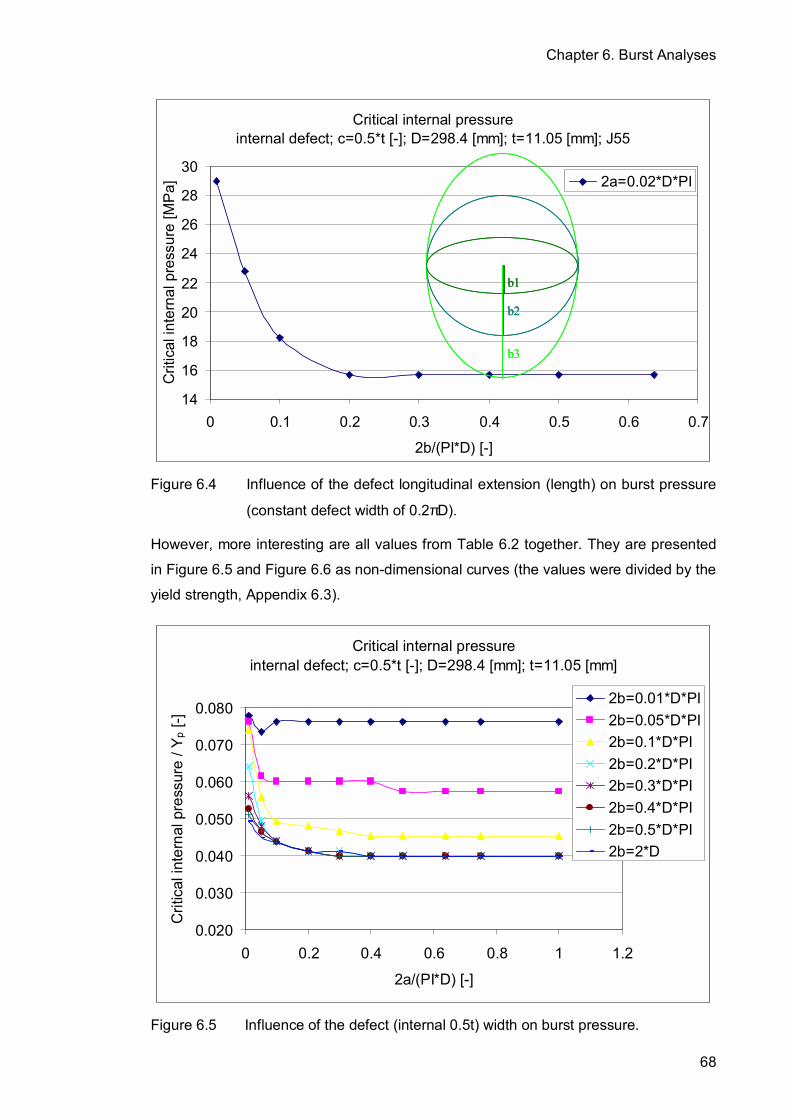
Chapter 6. Burst Analyses
68
Critical internal pressureinternal defect; c=0.5*t [-]; D=298.4 [mm]; t=11.05 [mm]; J55
14
16
18
20
22
24
26
28
30
0 0.1 0.2 0.3 0.4 0.5 0.6 0.7
2b/(PI*D) [-]
Crit
ical
inte
rnal
pre
ssur
e [M
Pa] 2a=0.02*D*PI
Figure 6.4 Influence of the defect longitudinal extension (length) on burst pressure
(constant defect width of 0.2πD).
However, more interesting are all values from Table 6.2 together. They are presented
in Figure 6.5 and Figure 6.6 as non-dimensional curves (the values were divided by the
yield strength, Appendix 6.3).
Critical internal pressureinternal defect; c=0.5*t [-]; D=298.4 [mm]; t=11.05 [mm]
0.020
0.030
0.040
0.050
0.060
0.070
0.080
0 0.2 0.4 0.6 0.8 1 1.2
2a/(PI*D) [-]
Crit
ical
inte
rnal
pre
ssur
e / Y
p [-]
2b=0.01*D*PI2b=0.05*D*PI2b=0.1*D*PI2b=0.2*D*PI2b=0.3*D*PI2b=0.4*D*PI2b=0.5*D*PI2b=2*D
Figure 6.5 Influence of the defect (internal 0.5t) width on burst pressure.
b1
b2
b3
b1
b2
b3
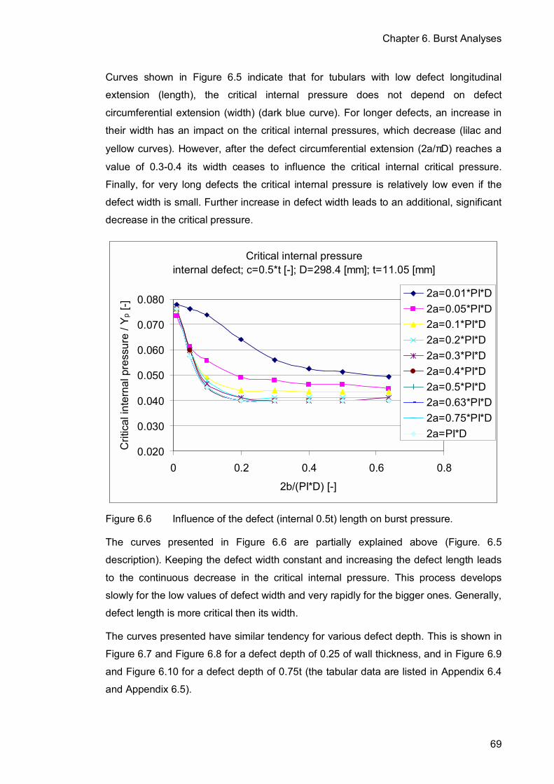
Chapter 6. Burst Analyses
69
Curves shown in Figure 6.5 indicate that for tubulars with low defect longitudinal
extension (length), the critical internal pressure does not depend on defect
circumferential extension (width) (dark blue curve). For longer defects, an increase in
their width has an impact on the critical internal pressures, which decrease (lilac and
yellow curves). However, after the defect circumferential extension (2a/πD) reaches a
value of 0.3-0.4 its width ceases to influence the critical internal critical pressure.
Finally, for very long defects the critical internal pressure is relatively low even if the
defect width is small. Further increase in defect width leads to an additional, significant
decrease in the critical pressure.
Critical internal pressureinternal defect; c=0.5*t [-]; D=298.4 [mm]; t=11.05 [mm]
0.020
0.030
0.040
0.050
0.060
0.070
0.080
0 0.2 0.4 0.6 0.8
2b/(PI*D) [-]
Crit
ical
inte
rnal
pre
ssur
e / Y
p [-]
2a=0.01*PI*D2a=0.05*PI*D2a=0.1*PI*D2a=0.2*PI*D2a=0.3*PI*D2a=0.4*PI*D2a=0.5*PI*D2a=0.63*PI*D2a=0.75*PI*D2a=PI*D
Figure 6.6 Influence of the defect (internal 0.5t) length on burst pressure.
The curves presented in Figure 6.6 are partially explained above (Figure. 6.5
description). Keeping the defect width constant and increasing the defect length leads
to the continuous decrease in the critical internal pressure. This process develops
slowly for the low values of defect width and very rapidly for the bigger ones. Generally,
defect length is more critical then its width.
The curves presented have similar tendency for various defect depth. This is shown in
Figure 6.7 and Figure 6.8 for a defect depth of 0.25 of wall thickness, and in Figure 6.9
and Figure 6.10 for a defect depth of 0.75t (the tabular data are listed in Appendix 6.4
and Appendix 6.5).

Chapter 6. Burst Analyses
70
Critical internal pressureinternal defect; c=0.25*t [-]; D=298.4 [mm]; t=11.05 [mm]
0.020
0.030
0.040
0.050
0.060
0.070
0.080
0 0.2 0.4 0.6 0.8 1 1.2
2a/(PI*D) [-]
Crit
ical
inte
rnal
pre
ssur
e / Y
p [-]
2b=0.01*D*PI2b=0.05*D*PI2b=0.1*D*PI2b=0.2*D*PI2b=0.3*D*PI2b=0.4*D*PI2b=0.5*D*PI2b=2*D
Figure 6.7 Influence of the defect (internal 0.25t) width on burst pressure.
Critical internal pressureinternal defect; c=0.25*t [-]; D=298.4 [mm]; t=11.05 [mm]
0.020
0.030
0.040
0.050
0.060
0.070
0.080
0 0.2 0.4 0.6 0.8
2b/(PI*D) [-]
Crit
ical
inte
rnal
pre
ssur
e / Y
p [-]
2a=0.01*PI*D2a=0.05*PI*D2a=0.1*PI*D2a=0.2*PI*D2a=0.3*PI*D2a=0.4*PI*D2a=0.5*PI*D2a=0.63*PI*D2a=0.75*PI*D2a=PI*D
Figure 6.8 Influence of the defect (internal 0.25t) length on burst pressure.
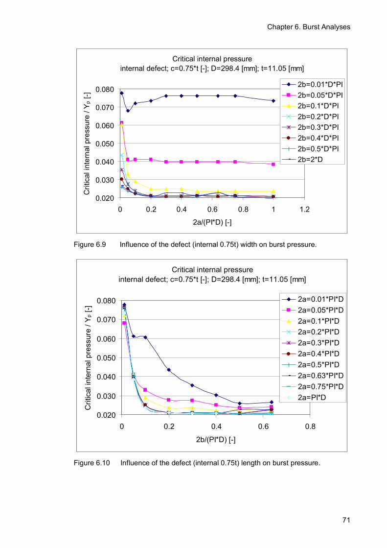
Chapter 6. Burst Analyses
71
Critical internal pressureinternal defect; c=0.75*t [-]; D=298.4 [mm]; t=11.05 [mm]
0.020
0.030
0.040
0.050
0.060
0.070
0.080
0 0.2 0.4 0.6 0.8 1 1.2
2a/(PI*D) [-]
Crit
ical
inte
rnal
pre
ssur
e / Y
p [-]
2b=0.01*D*PI2b=0.05*D*PI2b=0.1*D*PI2b=0.2*D*PI2b=0.3*D*PI2b=0.4*D*PI2b=0.5*D*PI2b=2*D
Figure 6.9 Influence of the defect (internal 0.75t) width on burst pressure.
Critical internal pressureinternal defect; c=0.75*t [-]; D=298.4 [mm]; t=11.05 [mm]
0.020
0.030
0.040
0.050
0.060
0.070
0.080
0 0.2 0.4 0.6 0.8
2b/(PI*D) [-]
Crit
ical
inte
rnal
pre
ssur
e / Y
p [-]
2a=0.01*PI*D2a=0.05*PI*D2a=0.1*PI*D2a=0.2*PI*D2a=0.3*PI*D2a=0.4*PI*D2a=0.5*PI*D2a=0.63*PI*D2a=0.75*PI*D2a=PI*D
Figure 6.10 Influence of the defect (internal 0.75t) length on burst pressure.

Chapter 6. Burst Analyses
72
Internal and external defects have a similar impact on critical internal pressure (Figure
6.11, Figure 6.12, Appendix 6.6). The results are approx. 5% (max 15%) lower for
defects with low width and slightly higher (2%) for the biggest defects. However, this
effect become more significant for deeper defects (c>0.5t).
Critical internal pressureexternal defect; c=0.5*t [-]; D=298.4 [mm]; t=11.05 [mm]
0.020
0.030
0.040
0.050
0.060
0.070
0.080
0 0.2 0.4 0.6 0.8 1 1.2
2a/(PI*D) [-]
Crit
ical
inte
rnal
pre
ssur
e / Y
p [-]
2b=0.01*D*PI2b=0.05*D*PI2b=0.1*D*PI2b=0.2*D*PI2b=0.3*D*PI2b=0.4*D*PI2b=0.5*D*PI2b=2*D
Figure 6.11 Influence of the defect (external 0.5t) width on burst pressure.
Critical internal pressureexternal defect; c=0.5*t [-]; D=298.4 [mm]; t=11.05 [mm]
0.020
0.030
0.040
0.050
0.060
0.070
0.080
0 0.2 0.4 0.6 0.8
2b/(PI*D) [-]
Crit
ical
inte
rnal
pre
ssur
e / Y
p [-]
2a=0.01*PI*D2a=0.05*PI*D2a=0.1*PI*D2a=0.2*PI*D2a=0.3*PI*D2a=0.4*PI*D2a=0.5*PI*D2a=0.63*PI*D2a=0.75*PI*D2a=PI*D
Figure 6.12 Influence of the defect (external 0.5t) length on burst pressure.
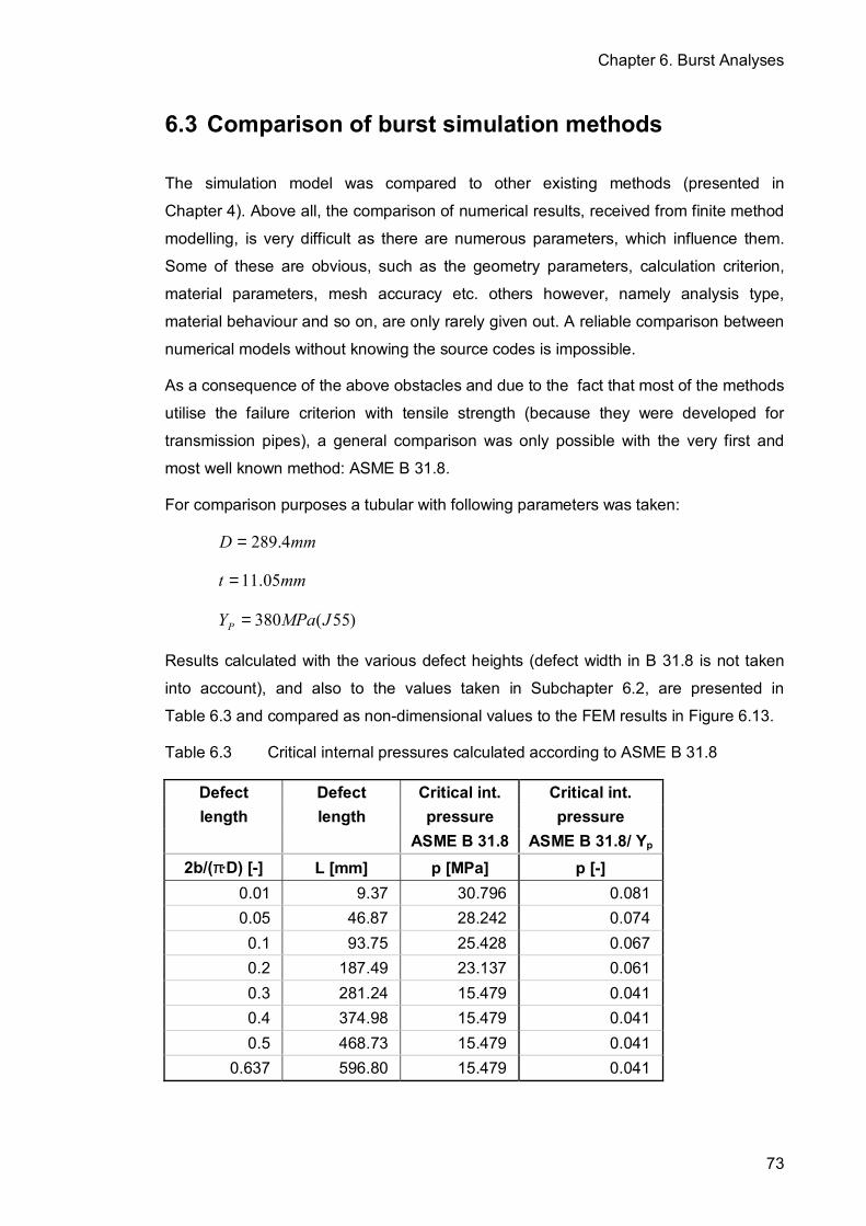
Chapter 6. Burst Analyses
73
6.3 Comparison of burst simulation methods
The simulation model was compared to other existing methods (presented in
Chapter 4). Above all, the comparison of numerical results, received from finite method
modelling, is very difficult as there are numerous parameters, which influence them.
Some of these are obvious, such as the geometry parameters, calculation criterion,
material parameters, mesh accuracy etc. others however, namely analysis type,
material behaviour and so on, are only rarely given out. A reliable comparison between
numerical models without knowing the source codes is impossible.
As a consequence of the above obstacles and due to the fact that most of the methods
utilise the failure criterion with tensile strength (because they were developed for
transmission pipes), a general comparison was only possible with the very first and
most well known method: ASME B 31.8.
For comparison purposes a tubular with following parameters was taken:
mmD 4.289=
mmt 05.11=
)55(380 JMPaYP =
Results calculated with the various defect heights (defect width in B 31.8 is not taken
into account), and also to the values taken in Subchapter 6.2, are presented in
Table 6.3 and compared as non-dimensional values to the FEM results in Figure 6.13.
Table 6.3 Critical internal pressures calculated according to ASME B 31.8
Defect Defect Critical int. Critical int. length length pressure pressure
ASME B 31.8 ASME B 31.8/ Yp 2b/(π·D) [-] L [mm] p [MPa] p [-]
0.01 9.37 30.796 0.081 0.05 46.87 28.242 0.074 0.1 93.75 25.428 0.067 0.2 187.49 23.137 0.061 0.3 281.24 15.479 0.041 0.4 374.98 15.479 0.041 0.5 468.73 15.479 0.041
0.637 596.80 15.479 0.041
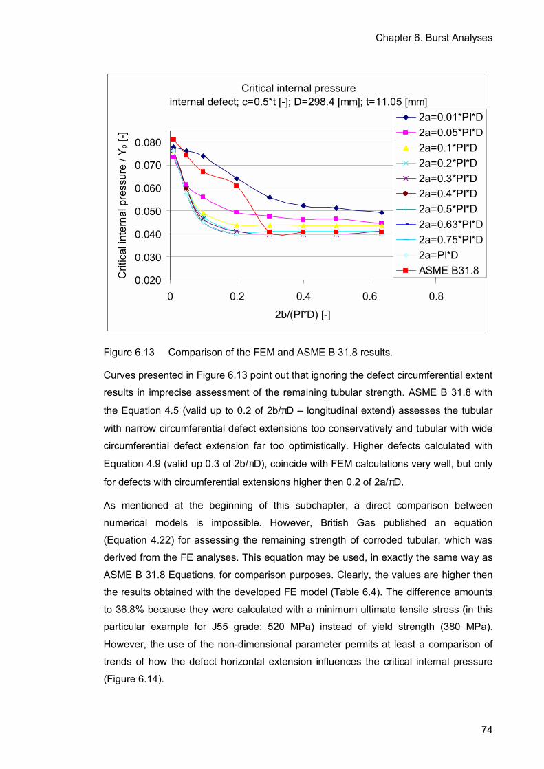
Chapter 6. Burst Analyses
74
Critical internal pressureinternal defect; c=0.5*t [-]; D=298.4 [mm]; t=11.05 [mm]
0.020
0.030
0.040
0.050
0.060
0.070
0.080
0 0.2 0.4 0.6 0.8
2b/(PI*D) [-]
Crit
ical
inte
rnal
pre
ssur
e / Y
p [-]
2a=0.01*PI*D2a=0.05*PI*D2a=0.1*PI*D2a=0.2*PI*D2a=0.3*PI*D2a=0.4*PI*D2a=0.5*PI*D2a=0.63*PI*D2a=0.75*PI*D2a=PI*DASME B31.8
Figure 6.13 Comparison of the FEM and ASME B 31.8 results.
Curves presented in Figure 6.13 point out that ignoring the defect circumferential extent
results in imprecise assessment of the remaining tubular strength. ASME B 31.8 with
the Equation 4.5 (valid up to 0.2 of 2b/πD � longitudinal extend) assesses the tubular
with narrow circumferential defect extensions too conservatively and tubular with wide
circumferential defect extension far too optimistically. Higher defects calculated with
Equation 4.9 (valid up 0.3 of 2b/πD), coincide with FEM calculations very well, but only
for defects with circumferential extensions higher then 0.2 of 2a/πD.
As mentioned at the beginning of this subchapter, a direct comparison between
numerical models is impossible. However, British Gas published an equation
(Equation 4.22) for assessing the remaining strength of corroded tubular, which was
derived from the FE analyses. This equation may be used, in exactly the same way as
ASME B 31.8 Equations, for comparison purposes. Clearly, the values are higher then
the results obtained with the developed FE model (Table 6.4). The difference amounts
to 36.8% because they were calculated with a minimum ultimate tensile stress (in this
particular example for J55 grade: 520 MPa) instead of yield strength (380 MPa).
However, the use of the non-dimensional parameter permits at least a comparison of
trends of how the defect horizontal extension influences the critical internal pressure
(Figure 6.14).

Chapter 6. Burst Analyses
75
Table 6.4 Critical internal pressures calculated according to the British Gas
Equation 4.22.
Defect Defect Critical int. Critical int. length length pressure pressure
BG Eq. BG Eq. / SMTS 2b/(π·D) [-] L [mm] p [MPa] p [-]
0.01 9.37 39.830 0.077 0.05 46.87 36.704 0.071 0.1 93.75 31.740 0.061 0.2 187.49 26.345 0.051 0.3 281.24 24.155 0.046 0.4 374.98 23.053 0.044 0.5 468.73 22.404 0.043
0.637 596.80 21.858 0.042
Critical internal pressureinternal defect; c=0.5*t [-]; D=298.4 [mm]; t=11.05 [mm]
0.020
0.030
0.040
0.050
0.060
0.070
0.080
0 0.2 0.4 0.6 0.8
2b/(PI*D) [-]
Crit
ical
inte
rnal
pre
ssur
e / Y
p
(SM
TS fo
r Brit
ish
Gas
equ
atio
n) [-
]
2a=0.01*PI*D2a=0.05*PI*D2a=0.1*PI*D2a=0.2*PI*D2a=0.3*PI*D2a=0.4*PI*D2a=0.5*PI*D2a=0.63*PI*D2a=0.75*PI*D2a=PI*DASME B31.8British Gas
Figure 6.14 Comparison of the FEM and British Gas results.
Non-dimensional values calculated with Equation 4.22 and presented in Figure 6.13 do
not differ a great deal from values obtained with the numerical model presented in this
thesis. It indicates comparable influence of the longitudinal defect extension. The
difference is caused by other material behaviour and geometry modelling. Besides,
British Gas tried, similar to ASME B 38.1, to cover all defects without considering their
circumferential extension, which is less accurate then proposed here numerical model.

Chapter 6. Burst Analyses
76
6.4 Discussion of the burst simulation model
Chapter 6 presents a new simulation model for burst calculations of intact and corroded
tubular goods. To fulfil API norms /81/ the model uses a relatively conservative failure
criterion and terminates analysis when the von Mises equivalent stress reaches the
yield strength of the material throughout the remaining ligament of the corroded tubular.
An advantage of using the FE analysis is that it provides more flexibility than semi-
empirical models. The burst calculations may be carried out with additional loads such
as external pressure and axial tension/compression load.
Defects are of upmost importance, and are generated with the help of elliptical
equations to get the exact shape of corroded areas. It is possible to create an internal
and an external defect separately or simultaneously. It should be kept in mind that:
- defect width should not be higher then πD (or πDi) otherwise it will not be
elliptical, but it will represent a uniformly corroded area around the tubular,
- defect length should not be longer than 2D, because bigger defects behave as
infinite ones and the results stay the same (there is no need to test them),
- defect depth must not extend the wall thickness, it is also recommended for
very deep defects to use more then 2 layers of elements for calculation.
A very fine mesh at the point where the defect generation starts ensures a good shape
approximation of even very small defects. The number of elements in a layer is
constant and their size depends on pipe diameter alone. The mesh density gradually
increases towards the corners to decrease computational time.
As presented in Subchapter 6.1, this numerical simulation model is even more precise
than API norm for intact pipes. Corroded tubular goods calculated with the semi-
empirical methods or numerical solutions with simplificated defects are by no means
perfect. They do not notice little differences between critical pressures of internal and
external corroded tubulars, which become more significant when the defect depth
extends to over 50% of wall thickness. The defect shape plays an important role
because it influences stress distribution.
Previous methods totally neglect the importance of the defect circumferential extent.
Corrosion may take various shapes and it is worth knowing how vertically and
horizontally orientated defects influence the burst pressure. Generally, critical internal
pressure decreases when both longitudinal and circumferential extension increases.
This process is influenced more by the length. It can also be observed to 0.2 of 2a/πD
(non-dimensional circumferential extension) and 0.2 of 2b/πD (non-dimensional
longitudinal extension). Bigger defects do not further decrease the failure pressure.

Chapter 7. Collapse Analyses
77
7 Collapse Analyses
Several formulas were developed for collapse pressure prediction. Firstly, elastic
expression was used in the 19th century. Due to the fact that in oil or gas wells
collapse occurs mainly in the plastic range, the Young´s modulus was replaced by a
�reduced modulus� (Timoshenko and Gere /87/). It turned out that this modulus is a
function of the stress-strain curve of the material and of the cross-section. A significant
step forward brought a formula for predicting critical external pressure of long cylinders
developed by Levy /88/ in 1884. Later, Clinedinst /89/, Holmquist and Nadai /90/
modified this equation on the basis of tests results, and new formulas were developed
for the API. Their evaluation can be traced in Clinedinst´s works /91/, /92/, /93/.
7.1 Collapse model verification for intact pipes with the API formulas
Collapse pressure of oil country tubular goods is calculated on the base of the API
standard 5C3 /81/. There are four main formulas, dependent on the D/t ratio, which
describe the collapse process. The API Bulletin 5C3 has its origin in 2488 collapse
tests for grades K-55, N-80 and P-110 for D/t ranges typically involved in plastic
collapse. In, the 1960s, collapse values for this region were calculated for the average
yield strength of materials and reduced by 25% (Clinedinst /91/) to give minimum
collapse pressures. Later, a new method was developed and the new minimum values
were determined by subtracting a constant pressure, determined for the particular
grade by the average /81/. From these studies the following plastic collapse (pp)
formula was empirically derived:
6895)( ⋅
−
−⋅= CB
tDAYp psiPP (Eq. 7.1)
Where:
)( psiPY - minimum yield strength, psi
A, B, C � formula factors, -

Chapter 7. Collapse Analyses
78
The A, B and C factors were derived from statistical regression analysis and also from
tests. To obtain formulas for other grades, these factors were curve fit. This resulted in
the creation of the following equations:
3)(
162)(
10)(
5 1053132.01021301.01010679.08762.2 psiPpsiPpsiP YYYA ⋅⋅−⋅⋅+⋅⋅+= −−−
(Eq. 7.2)
)(61050609.0026233.0 psiPYB ⋅⋅+= − (Eq. 7.3)
3)(
132)(
7)( 1036989.01010483.0030867.093.465 psiPpsiPpsiP YYYC ⋅⋅+⋅⋅−⋅+−= −−
(Eq. 7.4)
This plastic collapse formula can not be applied for every tubular. The range of validity
is determined by the D/t ratio. The lower D/t limit is given by the following equation:
( ) ( )
+⋅
−+
+⋅+−
=
)(
)(
2
2
282
psiP
psiP
YP
YCB
AYCBA
tD
(Eq. 7.5)
Where:
YPtD
- D/t intersection between yield strength collapse and plastic collapse
For lower D/t values, then calculated with the use of Equation 7.5, a yield strength collapse (PYp) formula for heavy wall pipe was derived on a theoretical basis
(Timoshenko and Gere /87/). The pressure, which generates a minimum yield stress on
the inside wall of the pipe, is the failure pressure and is given by the following equation:
−⋅⋅= 2
12
tDtD
Yp PYP (Eq. 7.6)
The upper limit for the use of plastic collapse relationship is determined by:
( )( )GBYCFAY
tD
P
P
PT −⋅+−⋅=
(Eq. 7.7)
Where:
PTtD
- D/t intersection between plastic collapse and transition collapse

Chapter 7. Collapse Analyses
79
For a higher D/t ratio a transition collapse (PT) formula has to be used. It was
introduced together with the plastic collapse formula (Equation 7.1) in the 1970s.
Earlier, when failure pressures in the plastic region were calculated by reducing
average values by 25%, using a transition collapse formula was not necessary. The
collapse curves were extended to higher D/t values and intersected with the elastic
collapse curve. However, extension of the new plastic collapse curves would give
minus values (Figure 7.1). Therefore, on an arbitrary basis, a new, transition formula
was derived to connect the plastic and elastic regions of collapse.
−⋅= G
tDFYp PT (Eq. 7.8)
Where:
F, G � formula factors, -
2
3
6
2
31
2
3
2
31095.46
+
⋅−⋅
−+
⋅⋅
+
⋅⋅⋅
=
ABAB
AB
ABAB
Y
ABAB
F
P
(Eq. 7.9)
ABF ⋅=G (Eq. 7.10)
For the greatest D/t values theoretical elastic collapse (PE) pressure formula was
derived on the basis of the Stewart equation (Stewart /94/). The formula was taken as
75% of the average elastic collapse /81/.
2
11
22
1
1046.3
1
11275.0
−⋅
⋅=
−⋅
⋅−⋅⋅=
tD
tD
tD
tD
EpE ν (Eq. 7.11)
This equation is valid for D/t ration greater than:

Chapter 7. Collapse Analyses
80
ABAB
tD
TE ⋅
+=
3
2 (Eq. 7.12)
Where:
TEtD
- D/t intersection between transition collapse and elastic collapse
Summarising, for collapse prediction, there are several formulas required, due to the
fact that failure is governed by various material behaviour. Which formula to use
depends on the D/t ratio.
There are also other formulas, but it was decided to validate the developed numerical
model with the API�s equations only. First of all, because they are based on empirical
results and are closest to the �real� values. Secondly, many other methods were
considered during the evaluation process of the above equations (e.g.
Timoshenko /79/) for particular D/t ranges. To prove the whole spectrum of D/t values a
similar way to Chapter 6 for burst calculations was chosen. Namely, it was decided to
recalculate collapse pressures for all casing sizes manufactured by Mannesmann for
the steel grade J-55 /85/. The characteristic size values are listed in Appendix 7.1 in
columns 1, 2 and 3. Columns 4, 5 and 6 contain the calculated critical external
pressures according to the API formulas /86/, for plastic, transition and elastic failure
respectively. There are not any values for yield strength collapse. As a result that no
pipe in grade J55 in this D/t range was found in the Mannesmann catalogue /85/ or in
the API Bulletin 5C2 /86/ (comparison for steel grade P110 was carried out and is
presented later in this chapter).
To compare the API values with the FEM results it was necessary to remove safety
margins. For the biggest D/t ratios, where failure is driven by the elastic equation, this
was done by omitting a 0.75 safety factor. In the plastic region, factor �C� from Equation
7.1 was omitted to obtain the average values. In the transition collapse region it was
decided to divide the API values by the factor 0.74, as the values were derived from the
basis of plastic (safety factor amounts to approx. 0.73) and elastic (safety factor 0.75)
formulas. All of these calculated values are presented in Figure 7.1 and in tabular form
in Appendix 7.2 (columns 4, 5 and 6). Various failure criteria are represented by
different colours for visualisation purposes in Figure 7.1.
The API results were compared to those calculated by the use of FEM (to be found in
the 7th column of Appendix 7.2) and showed graphically in Figure 7.2. The deviation
oscillates in the rage of +-5%, reaching 8% for pipes with the smallest D/t ratios.

Chapter 7. Collapse Analyses
81
Critical external pressure dependent on D/t ratio Ovality 0,004, steel grade J55
0
10
20
30
40
50
60
0 10 20 30 40 50D/t ratio
Crit
ical
ext
erna
l pre
ssur
e in
MP
ayield strength collapseplastic collapsetransition collapseelastic collapse
Figure 7.1 The API critical external pressures for intact pipes (with safety margins).
Critical external pressure vs. D/t ratio Ovality 0,004, steel grade J55
0
10
20
30
40
50
60
0 10 20 30 40 50D/t ratio
Crit
ical
ext
erna
l pre
ssur
e in
MPa
-6
-3
0
3
6
9
12
Dev
iatio
n in
%
APIFEMDeviation
Figure 7.2 Comparison of the API and FEM critical external pressures for intact
pipes.
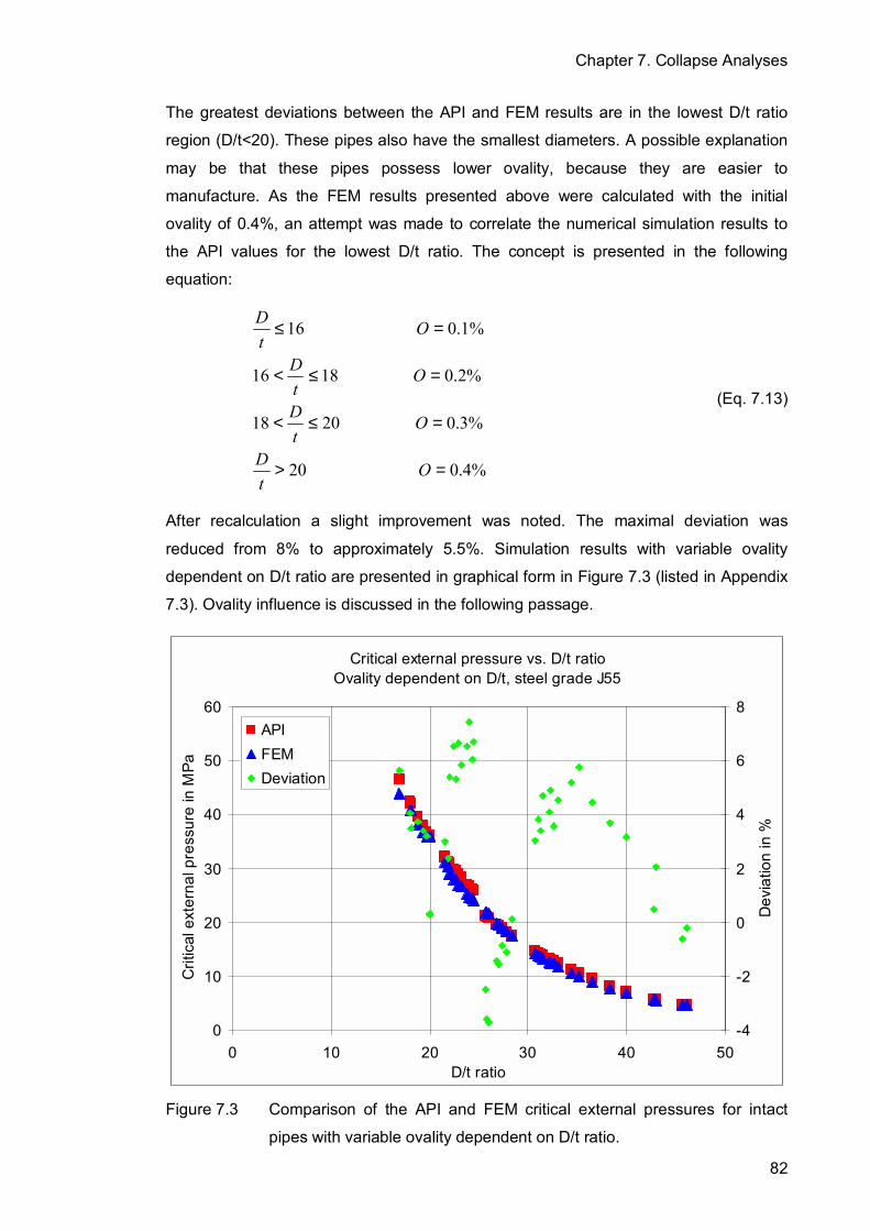
Chapter 7. Collapse Analyses
82
The greatest deviations between the API and FEM results are in the lowest D/t ratio
region (D/t<20). These pipes also have the smallest diameters. A possible explanation
may be that these pipes possess lower ovality, because they are easier to
manufacture. As the FEM results presented above were calculated with the initial
ovality of 0.4%, an attempt was made to correlate the numerical simulation results to
the API values for the lowest D/t ratio. The concept is presented in the following
equation:
%4.020
%3.02018
%2.01816
%1.016
=>
=≤<
=≤<
=≤
OtD
OtD
OtD
OtD
(Eq. 7.13)
After recalculation a slight improvement was noted. The maximal deviation was
reduced from 8% to approximately 5.5%. Simulation results with variable ovality
dependent on D/t ratio are presented in graphical form in Figure 7.3 (listed in Appendix
7.3). Ovality influence is discussed in the following passage.
Critical external pressure vs. D/t ratio Ovality dependent on D/t, steel grade J55
0
10
20
30
40
50
60
0 10 20 30 40 50D/t ratio
Crit
ical
ext
erna
l pre
ssur
e in
MPa
-4
-2
0
2
4
6
8
Dev
iatio
n in
%
APIFEMDeviation
Figure 7.3 Comparison of the API and FEM critical external pressures for intact
pipes with variable ovality dependent on D/t ratio.

Chapter 7. Collapse Analyses
83
To prove the simulation model within yield collapse range a group of P110 pipes was
taken from the API Bulletin 5C2 /86/ (Table 7.1). Due to the fact that they are in the low
range D/t it was decided to calculate them with 0.4% and 0.1% ovality.
Table 7.1 Comparison of the API and FEM critical external pressures for intact
pipes within yield collapse range.
1 2 3 4 5 6 7
D t D/t Ovality API yield FEM Deviation
[mm] [mm] [-] [-] [MPa] [MPa] [%] 127.00 9.19 13.81 0.004 92.84 105.42 -13.54 127.00 9.19 13.81 0.001 92.84 109.20 -17.62 127.00 11.10 11.44 0.004 120.97 134.64 -11.30 127.00 11.10 11.44 0.001 120.97 137.07 -13.31 127.00 12.14 10.46 0.004 131.10 147.60 -12.59 127.00 12.14 10.46 0.001 131.10 150.84 -15.06 127.00 12.70 10.00 0.004 136.48 156.51 -14.68 127.00 12.70 10.00 0.001 136.48 158.13 -15.87
The API results in yield collapse range differ from those simulated. They differ from the
test data, too (Clinedinst /92/). This is due to the fact, that during the development of
the first edition of the API Bulletin 5C3 /81/ in 1939, to ensure safety the Lamè equation
was taken. This equation specifies the initial yielding on the inside of a tube, and
seams to be too conservative. Therefore, similar to Clinedinst /92/ a Barlow formula
(Equation 6.1) was chosen. The results (calculated with outside diameter) show a good
correlation with the FEM analyses (Table 7.2).
Table 7.2 Comparison of critical external pressures calculated with the Barlow
equation and the FEM for intact pipes within yield collapse range.
1 2 3 4 5 6 7
D t D/t Ovality Barlow equation FEM Deviation
[mm] [mm] [-] [-] [MPa] [MPa] [%] 127.00 9.19 13.81 0.004 110.048 105.42 4.21 127.00 9.19 13.81 0.001 110.048 109.20 0.77 127.00 11.10 11.44 0.004 132.848 134.64 -1.35 127.00 11.10 11.44 0.001 132.848 137.07 -3.18 127.00 12.14 10.46 0.004 145.312 147.60 -1.57 127.00 12.14 10.46 0.001 145.312 150.84 -3.80 127.00 12.70 10.00 0.004 152 156.51 -2.97 127.00 12.70 10.00 0.001 152 158.13 -4.03

Chapter 7. Collapse Analyses
84
In a comparison of the API equations with simulation results for intact tubulars a very
good correlation in plastic, elastic, transition and yield collapse range was apparent.
This means that for any D/t ratio the FEM analyses provide reliable outcomes.
7.2 Ovality influence on collapse pressure
It has been already mentioned in Chapter 5 that it is impossible to carry out a FEM
collapse analyses for intact pipes. Therefore, the initial ovality or imperfection has to be
implemented. As presented here, numerical model initial ovality can be entered as an
input value. If it is unknown, the program takes an average ovality according to the
Equation 7.13.
To find out more about ovality influence, analyses with various ovality values were
performed. These results are illustrated by the following diagram (Figure 7.4). The
curve shows a rapid decrease of the collapse pressure caused by ovality increase. A
change of 0.1% of ovality in the lower region results in a 10% reduction of the
remaining strength, whilst the reduction is almost doubled at 2%. The outline of the
tested pipe parameters and ovality values is presented with the FEM results in
Appendix 7.4.
Ovality influenceSteel grade J55, D=298.4mm, t=11.05mm
0
5
10
15
20
25
30
0 2 4 6 8 10Ovality in %
Crit
ical
ext
erna
l pre
ssur
e in
MPa
Figure 7.4 Ovality influence on the critical external pressure.

Chapter 7. Collapse Analyses
85
7.3 Defect influence on collapse pressure
The critical collapse pressure is dependent not only on the material deterioration but
also to a high degree on ovality. Therefore, it is more difficult to construct non-
dimensional curves as in the case of burst calculations. On the basis of processed
examples it is recommended to calculate every case separately with ovality value
rather than to use non-dimensional curves. In order to demonstrate shape
dependences on critical external pressure, only results for external and internal defects
with 0.5t and ovality of 0.4% are presented below (Figures 7.5, 7.6, 7.7 and 7.8).
Critical external pressureexternal defect; c=0.5*t [-]; D=298.4 [mm]; t=11.05 [mm]
0.030
0.035
0.040
0.045
0.050
0.055
0.060
0 0.2 0.4 0.6 0.8 1 1.2
2a/(PI*D) [-]
Crit
ical
ext
erna
l pre
ssur
e / Y
p [-]
2b=0,001*D*PI2b=0,05*D*PI2b=0,1*D*PI2b=0,2*D*PI2b=0,3*D*PI2b=0,4*D*PI2b=0,5*D*PI2b=2*D
Figure 7.5 Influence of the defect (external 0.5t) width on collapse pressure.
The curves presented in Figure 7.5 and Figure 7.6 (the values were divided by the yield
strength, Appendix 7.5) have similar tendencies as these built for burst pressures.
Tubulars with low defect longitudinal extension (length) indicated that the critical
external pressure does not depend on defect circumferential extension (blue and lilac
curves). For higher defects, an increase in their width has an impact on collapse
pressure, which decreases until the defect reaches 0.2 of its radial extension (2a/πD).
Change in longitudinal extension has a relatively constant, decreasing influence on
collapse pressure (Figure 7.6).

Chapter 7. Collapse Analyses
86
Critical external pressureexternal defect; c=0.5*t [-]; D=298.4 [mm]; t=11.05 [mm]
0.030
0.035
0.040
0.045
0.050
0.055
0.060
0 0.2 0.4 0.6 0.8
2b/(PI*D) [-]
Crit
ical
ext
erna
l pre
ssur
e / Y
p [-] 2a=0,01*PI*D
2a=0,05*PI*D2a=0,1*PI*D2a=0,2*PI*D2a=0,3*PI*D2a=0,4*PI*D2a=0,5*PI*D2a=0,63*PI*D2a=0,75*PI*D2a=PI*D
Figure 7.6 Influence of the defect (external 0.5t) length on collapse pressure.
Tubulars with internal defects show comparable to tubulars with external defects trends
(Figure 7.7, Figure 7.8, Appendix 7.6). However, for vertically or horizontally orientated
narrow internal defects (blue and lilac curves) critical external pressure are equal or
even slightly higher than collapse pressure of an intact tubular. The reason may be the
stress distribution around elliptically shaped defect, which may work against collapse
forces.
Generally, internal and external defects have almost the same effect on the collapse
pressure. However, tubulars with vertically orientated narrow internal defects have
critical external pressures even 20% higher then tubulars with the same external
defects. This tendency is particularly easy to observe for longer (>0.3 of 2b/πD)
defects.

Chapter 7. Collapse Analyses
87
Critical external pressureinternal defect; c=0.5*t [-]; D=298.4 [mm]; t=11.05 [mm]
0.030
0.035
0.040
0.045
0.050
0.055
0.060
0 0.2 0.4 0.6 0.8 1 1.2
2a/(PI*D) [-]
Crit
ical
ext
erna
l pre
ssur
e / Y
p [-]
2b=0,001*D*PI2b=0,05*D*PI2b=0,1*D*PI2b=0,2*D*PI2b=0,3*D*PI2b=0,4*D*PI2b=0,5*D*PI2b=2*D
Figure 7.7 Influence of the defect (internal 0.5t) width on collapse pressure.
Critical external pressureinternal defect; c=0.5*t [-]; D=298.4 [mm]; t=11.05 [mm]
0.030
0.035
0.040
0.045
0.050
0.055
0.060
0 0.2 0.4 0.6 0.8
2b/(PI*D) [-]
Crit
ical
ext
erna
l pre
ssur
e / Y
p [-] 2a=0,01*PI*D
2a=0,05*PI*D2a=0,1*PI*D2a=0,2*PI*D2a=0,3*PI*D2a=0,4*PI*D2a=0,5*PI*D2a=0,63*PI*D2a=0,75*PI*D2a=PI*D
Figure 7.8 Influence of the defect (internal 0.5t) length on collapse pressure.

Chapter 7. Collapse Analyses
88
7.4 Collapse test data recalculation
In 1997 six specimens were tested in the Institute of Petroleum Engineering in
Clausthal. Their parameters are to be found in Table 7.3 below. Four specimens were
actually internally corroded pipes collected from a well. Two remaining were fabricated
with induced external defects, which circular shapes were very similar to those
produced by the numerical model (Subchapter 5.5).
To recalculate and assess these tests it was necessary to obtain the stress-strain curve
for the specimens� material. Therefore, tensile test were performed in the �Institut für
Füge- und Strahltechnik� at the Otto-von-Guericke-University Magdeburg (Köckritz and
Behrend /68/, /69/). Unfortunately, results were not clear and it was difficult to read off
the yield strength precisely, due to the specimens� constant expansion (Figure 7.9).
The minimum yield strength was set at 0.2% of the total displacement from the tension
test. A few samples from each pipe were tested and they gave various minimum yield
strengths (with differences up to 50 MPa). Therefore, it was decided to recalculate all
tests with the minimum, average and maximum read off yield points from tension tests
in order to provide an additional overview (Table 7.3).
Figure 7.9 Strain-stress curve from one of the tensile tests (from Köckritz and Behrend /69/).

Chapter 7. Collapse Analyses
89
Table 7.3 Recalculated test data from collapse tests. 1 Specimen 1 Specimen 2 Specimen 3 D [mm] 220.6 220.1 221.8 t [mm] 12.34 11.79 13.3 tmin [mm] 12 10.46 12.34 min of YP [MPa] 350 386.57 356 ave of YP [MPa] 381.37 446.25 380.65 max of YP [MPa] 406.25 484.38 400 axial tension [kN] 100 200 -200 ave Ovality [-] 0.0023 0.0016 0.0024 defect type internal internal internal ½ defect width [mm] round round round ½ defect length [mm] 220.6 220.1 221.8 defect depth [mm] 0.34 1.33 0.96 test result ITE [MPa] 36.4 36.1 48.8 FEM min YP [MPa] 36.80 36.08 41.48 (ITE-FEM)/ITE*100 [%] -1.10 0.06 15.00 FEM ave YP [MPa] 40.04 41.48 44.00 (ITE-FEM)/ITE*100 [%] -10.00 -14.90 9.84 FEM max YP [MPa] 42.92 44.00 45.44 (ITE-FEM)/ITE*100 [%] -17.91 -21.88 6.89
2 Specimen 4 Specimen 5 Specimen 6 D [mm] 220.4 220.8 220.6 t [mm] 12.15 8.96 8.96 tmin [mm] 11.2 4.2 5 min of YP [MPa] 400.64 400 400 ave of YP [MPa] 439.22 447.04 447.04 max of YP [MPa] 475 479.16 479.16 axial tension [kN] -200 120 80 ave Ovality [-] 0.0014 0.0013 0.0018 defect type internal external external ½ defect width [mm] round 108.45 108.25 ½ defect length [mm] 220.4 108.45 108.25 defect depth [mm] 0.95 4.76 3.96 test result ITE [MPa] 40.1 21.1 23 FEM min YP [MPa] 41.84 16.25 19.49 (ITE-FEM)/ITE*100 [%] -4.34 22.97 15.24 FEM ave YP [MPa] 45.44 17.72 21.68 (ITE-FEM)/ITE*100 [%] -13.32 16.02 5.74 FEM max YP [MPa] 48.68 19.40 23.36 (ITE-FEM)/ITE*100 [%] -21.40 8.06 -1.57

Chapter 7. Collapse Analyses
90
In Table 7.3 readings of min, mean and max yield strength are highlighted in different
colours. Simulation results are highlighted correspondingly, too. For the min. yield
strength values, calculations agree excellently with test results for Specimen 1 and 2
and concur well for Specimen 4. Values that are too low were obtained for Specimens
3, 5 and 6 (even up to 23%). A positive thing is however, that they do not exceed test
results, but stay on the conservative side. These deviations come, most probably, from
uncertainties in input data (yield point and steel elastic modulus). Assuming higher
values of the minimum yield strength, simulation results approached test outcomes
(Table 7.3).
However, it is not always the case that calculated results have to be wrong and test
result right. In this situation especially, the test result for Specimen 3 is dubious. It is
much higher then the FEM result and much higher in comparison to the result for
Specimen 4. Generally, both test are alike and should gave similar results. Both of
them were tested with the compression load of 200 kN and have the same corroded
area. Assuming that they have the same yield strength, Specimen 3 should be
approximately 4 MPa stronger then Specimen 4 because its wall is 1 mm thicker (D/t
ratio influence). However, its ovality is lower and therefore the critical pressure should
be approximately 2 MPa lower (ovality influence). Moreover, the yield stress reading
point out that it is about 50 MPa lower then for Specimen 4, and this should result in
nearly 4 MPa in its disadvantage (yield strength influence).
Summarizing, Specimen 3 should withstand lower external pressure than Specimen 4
(coarse estimation about 2 MPa) and not 8 MPa higher as it was during the test. This
brought the FEM analyses estimating critical collapse pressure, for mean value of
minimum yield strengths, exactly 1.5 MPa higher for Specimen 4 then for Specimen 3.
Overall, taking into consideration uncertainty about yield point determination, numerical
results concurred very well with results from the specimens tested (Figure 7.10).
Unfortunately, no data was found in literature and there were no other collapse test
results available for further validation.
Figure 7.10 A specimen after a collapse test (from Köckritz and Behrend /69/).

Chapter 7. Collapse Analyses
91
7.5 Discussion of the collapse model
Chapter 7 describes a new simulation model for collapse calculations of intact and
corroded tubulars. This model searches for instabilities and predicts failure according to
API norms, which was successfully demonstrated for intact pipes in Subchapter 7.1.
Collapse prediction of corroded tubulars is much more complicated. Generally the
failure criterion remains the same as for intact pipes, but the instability of the whole
pipe and corroded area has to be examined. In the corroded region the von Mises
equivalent stress is compared to the yield strength of the material throughout the
remaining ligament of the corroded tubular. As a consequence of different failure
criteria that depend on D/t ration, and fitting the tool for various defect depths, it is
suspected that for bigger defects the calculated values may be too optimistic. However,
this was not observed with the recalculation of test results.
The model takes advantage of the FEM and collapse calculations may be carried out
with additional loads such as internal pressure and axial tension/compression load.
Similar to the burst model, the elliptical shape of the defects is very important for
accurate corrosion replication. There are also the same advantages as with the burst
model such as the generation of an internal and external defect (separately or
simultaneously) or mesh optimization for various defect dimensions.
As mentioned earlier, this numerical simulation model enables even more exactly than
API collapse prediction for intact pipes. However, as oppose to the burst model it is
impossible to compare the collapse results of corroded tubulars. The reason being that
there are no methods available that enable prediction of the external critical pressures
of corroded tubulars. The only available validation is provided by collapse tests, which
were carried out in the Institute of Petroleum Engineering in Clausthal. Although, the
samples tested gave various minimum yield strengths, which slightly disturbed the
comparison, the numerical results concurred very well with the test results.
To carry out collapse analyses for intact pipes the ovality was implemented. It was also
proved that ovality has a significant influence on the collapse pressure results, which is
even higher than the impact of the shallow defects.
Only non-dimensional curves with 0.5t defect depths were constructed. The reason for
this is that not only material deterioration but also ovality impact on collapse pressures.
Generally, collapse pressures were higher than expected and for tubulars with shallow
and narrow defects they were even slightly higher than that for intact tubulars. An
explanation for this may be the stress distribution around elliptical defect shapes, which
may work against collapse forces.

Chapter 8. Critical Axial Load Analyses
92
8 Critical Axial Load Analyses
Axial load plays a significant role in casing and tubing calculations. Particular attention
is needed concerning tubing which hangs in well, casing which pulled in tension and
surface casing, which supports the weight of all subsequent strings. The worst case is
when the corrosion takes place just below the well head and the entire tubing/casing
weight works on the weakened area. Such failures happens from time to time (Gair and
Moulds /95/), but remains mainly unpublished.
8.1 Critical axial load model verification for intact pipes against the API formula
The API criterion for pipe body yield strength calculation is given by following
equation /81/:
( )P
iy Y
DDp ⋅
−⋅=
4
22π (Eq. 8.1)
This strength is directly dependent on the cross section area of the tubular and
minimum yield strength of the particular steel grade.
The numerical model enables calculation of the critical tension load only and no critical
compression load. This function was not implemented in the procedure because of
insignificant application purposes. A similar way of validating these calculations has
was chosen, as in the burst and collapse predictions. Critical axial load was calculated
for the whole spectrum of D/t values. These results are presented graphically in figure
8.1 (in tabular form in Appendix 8.1). The deviation oscillates from 0 to 3%.

Chapter 8. Critical Axial Load Analyses
93
Critical axial load vs. D/t ratio Steel grade J55
0
2000
4000
6000
8000
10000
12000
0 10 20 30 40 50D/t ratio
Pipe
bod
y yi
eld
stre
ngth
in k
N
0
1
2
3
Dev
iatio
n in
%
APIFEMDeviation
Figure 8.1 Comparison of the API and FEM critical axial loads for intact pipes.
As an example a tubular with the following parameters was recalculated:
mmD 4.289=
mmt 05.11=
)55(380 JMPaYP =
For an intact tubular calculated critical axial load by FEM amounts to:
kNp y 3725= (Equation 8.1 gives: 3761kN)
For a uniformly corroded circumferential area (depth 0.5t = 5.525 mm; height 100 mm)
the FEM calculation gives:
kNp y 1914= (Equation 8.1 gives: 1859kN)
Deviation between results obtained by the use of Equation 8.1 and the FEM calculation
amounts to only -2.97%.

Chapter 8. Critical Axial Load Analyses
94
8.2 Discussion of the axial load model Critical axial last calculation model utilizes failure criterion according to API norm and is
relatively conservative. The analysis is terminated when the von Mises equivalent
stress reaches the yield strength of the material throughout the remaining ligament of
the corroded tubular.
It is possible to carry out the critical axial last calculation with additional loads such as
internal and external pressures.
The defects may be created, similarly to the burst and collapse models, as elliptical
ones or as a uniformly corroded circumferential area. Circumferential corroded areas
are especially dangerous to casing integrity and as presented on an example in
Subchapter 8.1 predicted with a good correlation. Generally, such calculations are not
complicated and only depend on the cross section area of the corroded tubular.

Chapter Error! Reference source not found.. Summary
95
9 Summary
The present thesis focuses on the development of the simulation tool for calculating the
critical pressures/loads of corroded tubulars. The model uses the von Mises distortion
energy theory in order to compare three-dimensional stress with effective stress. On
this basis, failure criteria in accordance with API norms /81/, to desired calculation load,
are utilized respectively. It is possible to calculate:
- critical internal (burst) pressure,
- critical external (collapse) pressure,
- critical axial tension force.
Calculations may be carried out with additional loads:
- burst calculation with external pressure and/or axial tension/compression,
- collapse calculation with internal pressure and/or axial tension/compression,
- axial strength calculation with internal and/or external pressure.
Corroded defects can be generated on the internal and/or external tubular wall. To
provide an exact approximation of the real shape elliptical equations are used to
describe material deterioration and defect shape. These equations enable the
modelling of horizontally or vertically orientated defects, as well as round defects. The
following limitation should be kept in mind whilst creating defects:
- defect width should not be higher then πD (or πDi) otherwise it will not be
elliptical, but will represent a uniformly corroded area around the tubular,
- defect length should not be longer than 2D, because bigger defects behave as
infinite ones and the results stay the same (there is no need to test them),
- defect depth must not extend the wall thickness, it is also recommended for
very deep defects to use more then 2 layers of elements for calculation.
Program accuracy depends on mesh preciseness i.e. element number and element
sizes as well as the number of layers. Thanks to a very fine mesh at the spot where the
defect generation starts it is possible to outline even small defects very precisely. The
mesh is only interlocked with the pipe�s diameter and is created automatically.
Another factor which influences the accuracy applies to the calculation steps which are
used for convergence calculations. The finer the steps are, the more exact the solution
is. Several models with different meshes and calculation profiles were tested and the
best were chosen and implemented in the procedure. They provide reliable results for
any defect configurations within a reasonable time.

Chapter Error! Reference source not found.. Summary
96
Validation of the burst, collapse and critical axial load model were carried out and
compared to the API equations /81/ for intact pipes. For all models, minor deviations
showed a very good match between the API and FEM results. Additionally, some
conservativism of API was demonstrated e.g. for burst calculations where API uses the
Barlow�s formula with outside diameter or for collapse calculations in yield collapse
range where API uses Lamè equation. Calculated numerical values are more precise
and closer to the test data.
Burst model of corroded tubular goods in comparison to other assessment methods
brought the important outcome that defect circumferential width has an influence on the
failure pressure. Generally, this pressure decreases when both circumferential and
longitudinal defect extension increases. However, this process is more influenced by
the longitudinal extension and proceeds faster. Defects with dimensions bigger then
0.2 of 2a/πD (non-dimensional circumferential extension) and 0.2 of 2b/πD (non-
dimensional longitudinal extension) do not decrease the failure pressure anymore.
Additionally, tubulars with external defects have slightly lower critical internal pressures
than tubulars with internal defects.
Comparison of the collapse model of corroded tubulars to other methods was not
possible, because such models do not exist. Fortunately, there were some test data
available, and the numerical results concurred very well with the test results. Similar to
burst model the increase of the circumferential and longitudinal defect extension
causes a decrease in the collapse strength. This process, however, is not as rapid as
in the case of the burst model, besides, tubulars with very short longitudinal defect
extension shows only marginal decrease of collapse pressure. Generally, the collapse
pressures were higher than expected. Moreover, a very strong ovality influence on the
collapse pressure was observed.
Prediction of the critical axial load of corroded tubulars gave a very good correlation to
API criterion. In this calculation failure depends only on the cross section of the
corroded tubular and minimum yield strength of the material.
Not only current defects can be assessed but it is also possible, on the basis of
predicted corrosion rates, to assess corroded tubular in the future, calculating it with
bigger and deeper defects. It enables planning, setting the next inspection interval or
renewal point.
The simulation model possesses its own interface, which enables an easy input of
necessary data. The procedure can be run by anyone and FE or ANSYS background is
not necessary. Model and defect generation, loads application, calculation and even
presenting results all proceeds automatically.

References
97
References
/1/ Anon; DOE Fundamentals Handbook, Material Science, Volume 1 of 2, DOE-
HDBK-1017/1-93, U.S. Department of Energy, January 1993.
/2/ Samant, A.; Corrosion Problems in Oil Industry Need More Attention, technical
paper from Oil and Natural Gas Corporation Limited, February 2003
/3/ Keranl, M., Harrop, D.; The Impact of Corrosion on the Oil and Gas Industry,
SPE, Production and Facilities, August 1996.
/4/ Fontana, M.; Corrosion Engineering, McGraw Hill, New York, USA, 1986.
/5/ Uhlig, H., Revees, R., Corrosion and Corrosion Control, John Wiley and Sons
Publishing Co., New York, 1985.
/6/ Frankel, G.; Localized Corrosion of Metals; A Review of the Rate-Controlling
Factors in Initiation and Growth, published in the proceedings of the 8th
International Conference of Passivity of Metals and Semiconductors, Jasper,
Canada, May 1999.
/7/ Brondel, D. et al.; Corrosion in the Oil Industry, Oilfield Review, April 1994.
/8/ Weeter, F.; Downhole Corrosion � Prevention and Treatment, (SPE-Paper
9984), 1982. presented at the SPE meeting held in Bejing, China, March 1982.
/9/ Tuttle, R.; Corrosion in Oil and Gas Production, (SPE-Paper 17004), Jurnal of
Petroleum Technology, July 1987.
/10/ Becker, J.; Corrosion and Scale Handbook, PennWell Publishing Company,
Tulsa, USA, 1998.
/11/ Anon; Bewertung von Untertagekomplettierungen, internal VNG guideline,
January 2003.
/12/ Garber, J. et al.; A Model for Predicting Corrosion Rates in Oil Wells Containing
Carbon Dioxide, (SPE-Paper 66651), presented at the SPE/EPA/DOE
Exploration and Production Environmental Conference held in San Antonio,
Texas, USA, 26�28 February 2001.
/13/ Shreir, L.; Corrosion, Vol. 1, John Wiley and Sons Publishing Co., New York,
1963.
/14/ Chilingarian, V.; Drilling and Drilling Fluids, Elsevier Publishing Co.,
Amsterdam, Holland, 1983.

References
98
/15/ Heitz, E., Henkhaus, R., Rahmel, A.; Corrosion Science, An Experimental
Approach, Ellis Horwood Limited, Chichester, England, 1992.
/16/ Koch, G. et al..; Corrosion Costs and Preventive Strategies in the United
States, Report FHWA-RD-01-156, September 2001.
/17/ Ruschau, G., Al-Anezi, M.; Corrosion Costs and Preventive Strategies in the
United States, APPENDIX S: Oil and Gas Exploration and Production, Report
FHWA-RD-01-156, September 2001.
/18/ Bradshaw, J.; Production Cost Reduction Through Casing Corrosion
Monitoring, (SPE-Paper 7704), presented at the SPE of AIME Production
Technology Symposium held in Hobbs, New Mexico, October 1978.
/19/ Buck, E., Maddux, G., L. Sullivan, R.; Internal Corrosion Cost Impact Study �
United States Natural Gas Exploration and Production Industry, GRI-96/0056
document no. 96-146,. Gas Research Institute, Des Plaines, 1996.
/20/ Thompson, N.; Corrosion Costs and Preventive Strategies in the United States,
APPENDIX E: Gas and Liquid Transmission Pipelines, Report FHWA-RD-01-
156, September 2001.
/21/ Ruschau, G., Al-Anezi, M.; Corrosion Costs and Preventive Strategies in the
United States, APPENDIX U: Petroleum Refining, Report FHWA-RD-01-156,
September 2001.
/22/ Aker Kvaerner; Wireline Logging Service: Multifinger Caliper, URL=http://www.akerkvaerner.com, May 2004.
/23/ Sondex plc; Multi Finger Imaging Tool � User Guide V1.0,
URL=http://www.sondex.co.uk, May 2004.
/24/ Watfa, M.; Downhole Casing Corrosion Monitoring and Interpretation
Techniques to Evaluate Corrosion in Multiple Casing Strings, (SPE-Paper
17931), August 1991, presented at the SPE of Middle East Oil Technical
Conference and Exhibition held in Bahrain, March 1989.
/25/ Schlumberger; Well Integrity, www.schlumberger.com, May 2004.
/26/ Anon; Bewertung von Untertagekomplettierungen, internal Untergrundspeicher-
und Geotechnologie-Systeme GmbH guideline, 2003.
/27/ Advanced Logic Technology; Slimhole Acoustic Televiewer, www.alt.lu; ABI 40,
May 2004.

References
99
/28/ Burks, W., Hicks, R., McQueen, M.; How to Get More Out of Your Pigging
Runs, Pipeline & Gas Journal, August 2002.
/29/ Palmer-Jones, R., Paisley, D.; Repairing Internal Corrosion Defects in Pipelines
� a Case Study, presented at the 4th International Pipeline Rehabilitation and
Maintenance Conference held in Prague, September 2000.
/30/ Kristoffersen, K., Taberner, D.; Internal Corrosion in Submarine Pipelines-
Methods of Detection, Mapping of Attacks and Procedures to Predict The
Lifetime and Allowable Operating Pressure, (SPE-Paper 12442), 1984,
presented at the 5th Offshore South East Asia Conference held in Singapore,
February 1989.
/31/ Anon; Gas Transmission Distribution and Piping Systems, ASME B31.8-2000,
The American Society of Mechanical Engineers, 2000.
/32/ Maxey, W. et al.; Ductile Fracture Initiation, Propagation and Arrest in
Cylindrical Vessels, Fracture Toughness, Proceedings of the 1971 National
Symposium on Fracture Mechanics, Part II, ASTM STP 514, 1971.
/33/ Kiefner, J. et al.; Failure Stress Levels of Flaws in Pressurized Cylinders, ASTM
STP 536, American Society for Testing and Materials, Philadelphia, 1973, pp.
461-481.
/34/ Anon; Manual for Determining the Remaining Strength of Corroded Pipelines -
A Supplement to ASME B31 Code for Pressure Piping, ANSI/ASME B31G-
1991, The American Society of Mechanical Engineers, New York, 1991.
/35/ Kiefner, J., Vieth, P.; A Modified Criterion for Evaluating the Strenght of
Corroded Pipe, Final Report for PR 3-805 project to the Pipeline Supervisory
Committee of the American Gas Association, Battelle, Ohio, 1989.
/36/ Kiefner, J., Vieth, P.; Evaluating Pipe-1 New Method Corrects Criterion for
Evaluating Corroded Pipe, Oil & Gas Journal, 6 August, 1990.
/37/ Kiefner and Associates Inc; http://www.kiefner.com/, April, 2004.
/38/ Bubenik, A. el al.; Analysing the Pressure Strength of Corroded Line Pipe, 11th
International Conference on Offshore Mechanics and Arctic Engineering,
Calgary, 1992.
/39/ Kastner, W. el al.; Critical Crack Sizes in Ductile Piping, International Journal of
Pressure Vessels and Piping, 9, 1981, pp. 197-219.
/40/ Fu, B. el al.; Methods for assessing corroded pipeline � review, validation and
recommendations, Advantica Technologies, 2000.
References
100
/41/ Fu, B., Batte, A.; An Overview of Advanced Methods for the Assessment of
Corrosion in Linepipe, Offshore Technology Report - OTO 1999 051, August
1999.
/42/ Fu, B., Kirkwood, M.; Predicting Failure Pressure of Internally Corroded
Linepipe Using the Finite Element Method, OMAE � Volume V, Pipeline
Technology, 1995.
/43/ Kirkwood, M. et al.; Assessing the Integrity of Corroded Linepipe � An Industry
Initiative, Advances in Subsea Pipeline Engineering and Technology
(ASPECT�96), Aberdeen, UK, 27-28 November 1996, Society for Underwater
Technology, 1996, pp. 55-68.
/44/ Batte, A. et al.; Advanced Methods for Integrity Assessment of Corroded
Pipelines, Pipes & Pipelines International, Jan/Feb 1997.
/45/ Kirkwood, M., et al.; New Methods for Determining the Remaining Strength of
corroded Pipelines, OMAE � Volume V, Pipeline Technology, 1997.
/46/ Bjornoy, O., Cramer, H., Sigurdsson, G.; Probabilistic Calibrated Design
Equation for Burst Strength Assessment of Corroded Pipelines, ISOPE 1997.
/47/ Leis. B., Stephens D.; An Alternative Approach to Assess the Integrity of
Corroded Line Pipe Part II: Alternative Criterion, ISOPE 1997.
/48/ Saldanha, S., Bucherie, C.; Integrity of non Crack Like Corroded Pipelines
Submited to Internal Pressure, presentet at the 3th Seminar on Pipeline, held in
Rio de Janerio, Brazil, 21-23 November, 2001.
/49/ Lee, O., Kim, D.; Reliability of Buried Pipelines with Corrosion Defects under
Varying Boundary Conditions, The 15th European Conference of Fracture,
Stockholm, Sweden, 11-13August, 2004.
/50/ Ritchie, D., Last, S.; Burst criteria of corroded pipelines - defect acceptance
criteria, presented at 10th Biennial Joint Technical Meeting on Line Pipe
Research held in Cambridge, UK, 18-21 April, 1995.
/51/ Loureiro, J., Netto, T., Estefen, S.; On the Effect of Corrosion Defects in the
Burst Pressure of Pipelines, presented at 20th International Conference on
OMAE held in Rio de Janerio, Brazil, 3-8 June, 2001.
/52/ Bjornoy, O. el al.; Introduction and Background to DNV RP-F101 �Corroded
Pipelines�, ISOPE 1999, vol. II, pp. 117-124.
/53/ Bjornoy, O., Sigurdsson, G., Marley, M.; Background and Development of DNV-
RP-F101 �Corroded Pipelines�, ISOPE 2001, vol. II, pp. 102-109.

References
101
/54/ Benjamin, A. el al.; Burst Tests on Pipeline with Long External Corrosion,
International Pipeline Conference ASME IPC 2000, Vol. 2, pp. 793-799.
/55/ Benjamin, A. el al.; Modified Equation for the Assessment of Long Corrosion
Defects, International Conference on Offshore Mechanics and Arctic
Engineering, OMAE2001/PIPE-4111, 2001.
/56/ Francis, A., Geren, P.; New Method Helps Operators Assess Line Integrity, Oil
and Gas Journal, November 2001.
/57/ McQueen, M. el al.; Quantitative probabilistic Approach to External Corrosion
Direct Assessment Using Structural Reliability Analysis, presented at National
Association of Corrosion Engineers, Las Vegas, USA, November 2003.
/58/ Yahaya, N.; Risk-based Maintenance Management of Corroded Pipelines,
research paper for Global Dialog EXPO 2000.
/59/ Cosham, A., Kirkwood, M.; Best Practice in Pipeline Defect Assessment,
IPC00-0205, Calgary, Canada, October 2000.
/60/ Cosham, A., Hopkins, P.; The Pipeline Defect Assessment Manual, IPC02-
27067, International Pipeline Conference, Calgary, Canada, 29 September � 3
October, 2002.
/61/ Osborne, B.; A Review of Current Practice in Pipeline Defect Assessment,
Offshore Technology Report - OTO 1999 002, February 1999.
/62/ Osborne, B.; Review of Current Practice in Pipeline Defect Assessment � User
Guide, Offshore Technology Report - OTO 1999 004, February 1999.
/63/ Anon; Appraisal and Development of Pipeline Defect Assessment
Methodologies, Final Report Phases I& II, DOC REF CH109R001 Rev 0, MSL
Engineering Limited, June 2000.
/64/ Zienkiewicz, C.; The Finite Element Method, Butterworth-Heinemann, 5th
edition, September 2000.
/65/ Zienkiewicz, C.; Finite Element Method: Volume 2, Solid Mechanics,
Butterworth-Heinemann; 5th edition, September 2000.
/66/ Köckritz, V., Lippmann, G.; Numerische Bemessung von Rohrtouren mit
Verschwächungszonen, TU Bergakademie Freiberg, Institut für Bohrtechnik
und Fluidbergbau, Oktober 1996.
References
102
/67/ Behrend, J. el al.; Untersuchung der Beanspruchung von länger in Betrieb
befindlichen Futterrohren unter Einsatz der FEM, Erdöl Erdgas Kohle,
Hamburg/Wien 113, 1997, Vol 10, p. 421�424.
/68/ Köckritz, V.; Behrend, J.; Berechnung des kritischen Außendruckes für Rohre
mit Exzentrizitäten, Ovalitäten und Korrosionsmulden, TU Bergakademie
Freiberg, Institut für Bohrtechnik und Fluidbergbau, 31. Dezember 1997.
/69/ Köckritz, V.; Behrend, J.: Untersuchungen zum Festigkeitsverhalten an
untertänigen Bauteilen sowie Spannungs- und Verformugsmessungen, TU
Bergakademie Freiberg, Institut für Bohrtechnik und Fluidbergbau, Januar
1998.
/70/ Szary, T.; Köckritz, V.; 3D-Simulation von Spannungen und Verformungen in
Futterrohren von Erdgasbohrungen � Festigkeits- und Stabilitätsberechnungen
mittels FEM (Modellierung und Berechnung von Korrosionsmulden in
Futterrohren), TU Bergakademie Freiberg, Institut für Bohrtechnik und
Fluidbergbau, 16. Dezember 2002.
/71/ Szary, T.; Köckritz, V.; Numerische Bewertung lokaler Verschwächungen in
Ölfeldrohren, DGMK Tagungsbericht 2004, Vol 2.
/72/ Szary, T.; Köckritz, V.; Numerische Bewertung lokaler Verschwächungen in
Ölfeldrohren, Erdöl, Erdgas Kohle, Hammburg/Wien 120, 2004, Vol 11, p. 403-
407.
/73/ Anon; ANSYS Documentation (Help), all Versions.
/74/ Issa, A.; Crawford, D.; An Improved Design for Tubular Collapse � presented at
the 68th Annual Technical Conference and Exhibition of the Society of
Petroleum Engineers held in Houston, Texas, 3-6 October 1993.
/75/ Altenbach, H., Altenbach, J., Zolochovsky, A.; Erweiterte Deformationsmodelle
und Versagenskriterien der Werkstoffmechanik, Deutscher Verlag für
Grundstoffindustrie, Stuttgart, 1995.
/76/ Ugural, A., Fenster, S.; Advanced Strength and Applied Elasticity, Elsevier,
New York, 1987.
/77/ Doege, E., Meyer-Nolkemper, H.; Fließkurvenatlas metallischer Werkstoffe und
einer grundlegenden Einführung, Hanser, München, 1986.
/78/ Lemaitre, J.; A Course on Damage Mechanics, Springer, Berlin, 1996.
/79/ Czichos, H. el al.; Hütte: Die Grundlagen der Ingenieurwissenschaften,
Springer, Berlin, 2000.

References
103
/80/ Zhu, X-K., Leis, B.; Strenght Criteria and Analytic Predictions of Failure
Pressure in Corroded Line Pipes, presented at the 13th Interanaional Offshore
and Polar Engineering Conference, Honolulu, Hawaii, USA, 25-30 May, 2003.
/81/ Anon; Bulletin on Formulas and Calculations for Casing, Tubing, Drill Pipe, and
Line Pipe Properties, API Bulletin 5C3, Sixth edition, October, 1994.
/82/ Crisfield, M.; Non-linear Finite Element Analysis of Solids and Structures, John
Wiley & Sons Ltd., Chichester, 2001.
/83/ Belytschko, T., Liu, W., Moran, B.; Nonlinear Finite Elements for Continua and
Structures, John Wiley & Sons Ltd., Chichester, 2003.
/84/ Annon; Specification for Casing and Tubing, API Specification 5CT, Seventh
Edition, October, 2001.
/85/ Anon; Tubular Goods for Oil and Fields, Casing, Mannesmannröhren-Werke
AG, Düsseldorf, Germany, 1980.
/86/ Annon; Bulletin on Performance Properties of Casing, Tubing, and Drill Pipe,
API Bulletin 5C2, Twenty-first edition, October, 1999.
/87/ Timoshenko, S., Gere, J.; Theory of Elastic Stability, McGraw-Hill Book
Company, 1933.
/88/ Levy, M.; The Journal de Mathematiques Pure et Appliquees, 1884.
/89/ Clinedinst, W.; A Rational Expression for the Critical Collapsing Pressure of
Pipe under External Pressure, Drilling and Production Practice, API, 1939.
/90/ Holmquist, J., Nadai, A.; A Theoretical and Experimental Approach to the
Problem of Collapse of Deep-Well Casing, Drilling and Production Practice,
API, 1939.
/91/ Clinedinst, W.; Development of API Collapse Pressure Formulas, presented at
API Meeting, December, 1963.
/92/ Clinedinst, W.; Analysis of API Collapse Test Data and Development of New
Collapse Resistance Formulas, presented to the API Task Group on
Performance Properties, October, 1977.
/93/ Clinedinst, W.; New Collapse Resistance Formulas Based on the Data of the
Round Robin Collapse Test Program and the 1981 API Sponsored Test
Program on the effect of axial loading on Collapse Resistance, presented at the
API Meeting, April, 1987.

References
104
/94/ Stewart, R.; Collapsing Pressures of Lap-Welded Tubes, Western University,
Allegheny, USA, ASME Vol. 27, 1906.
/95/ Gair, D., Moulds, T.; Tubular Corrosion in the West Sole Gas Field, SPE, May,
1988. SPE 11879 first presented at the 1983 SPE Offshore Europe Conference
held in Aberdeen, Sept. 6-9. 1983.

Appendices
105
Appendices
Appendix 5.1 Typical elements sizes and their distribution in
circumferential direction
D 298.4 mm ∆u 5.450 mm ∆u` 7.684 mm n 43 - n` 61 - n+1 44 - n`+1 62 -
i ∆u Sum ∆u ∆u Sum ∆u [-] [degree] [degree] [mm] [mm]
1 0.00 0.00 0.00 0.00 2 0.10 0.10 0.25 0.25 3 0.19 0.29 0.50 0.74 4 0.29 0.57 0.74 1.49 5 0.38 0.95 0.99 2.48 6 0.48 1.43 1.24 3.72 7 0.57 2.00 1.49 5.20 8 0.67 2.66 1.73 6.94 9 0.76 3.42 1.98 8.92
10 0.86 4.28 2.23 11.15 11 0.95 5.23 2.48 13.63 12 1.05 6.28 2.73 16.35 13 1.14 7.42 2.97 19.32 14 1.24 8.66 3.22 22.54 15 1.33 9.99 3.47 26.01 16 1.43 11.42 3.72 29.73 17 1.52 12.94 3.96 33.69 18 1.62 14.56 4.21 37.90 19 1.71 16.27 4.46 42.36 20 1.81 18.08 4.71 47.07 21 1.90 19.98 4.95 52.03 22 2.00 21.98 5.20 57.23 23 2.09 24.07 5.45 62.68 24 2.19 26.26 5.70 68.38 25 2.28 28.54 5.95 74.32
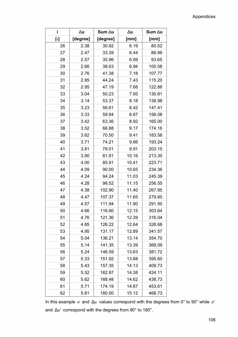
Appendices
106
i ∆u Sum ∆u ∆u Sum ∆u [-] [degree] [degree] [mm] [mm]
26 2.38 30.92 6.19 80.52 27 2.47 33.39 6.44 86.96 28 2.57 35.96 6.69 93.65 29 2.66 38.63 6.94 100.58 30 2.76 41.38 7.18 107.77 31 2.85 44.24 7.43 115.20 32 2.95 47.19 7.68 122.88 33 3.04 50.23 7.93 130.81 34 3.14 53.37 8.18 138.98 35 3.23 56.61 8.42 147.41 36 3.33 59.94 8.67 156.08 37 3.42 63.36 8.92 165.00 38 3.52 66.88 9.17 174.16 39 3.62 70.50 9.41 183.58 40 3.71 74.21 9.66 193.24 41 3.81 78.01 9.91 203.15 42 3.90 81.91 10.16 213.30 43 4.00 85.91 10.41 223.71 44 4.09 90.00 10.65 234.36 45 4.24 94.24 11.03 245.39 46 4.28 98.52 11.15 256.55 47 4.38 102.90 11.40 267.95 48 4.47 107.37 11.65 279.60 49 4.57 111.94 11.90 291.50 50 4.66 116.60 12.15 303.64 51 4.76 121.36 12.39 316.04 52 4.85 126.22 12.64 328.68 53 4.95 131.17 12.89 341.57 54 5.04 136.21 13.14 354.70 55 5.14 141.35 13.39 368.09 56 5.24 146.59 13.63 381.72 57 5.33 151.92 13.88 395.60 58 5.43 157.35 14.13 409.73 59 5.52 162.87 14.38 424.11 60 5.62 168.48 14.62 438.73 61 5.71 174.19 14.87 453.61 62 5.81 180.00 15.12 468.73
In this example n and u∆ values correspond with the degrees from 0° to 90° while 'n
and 'u∆ correspond with the degrees from 90° to 180°.

Appendices
107
Appendix 5.2 Nodes position after implementing 0.4% ovality
D 298.4 mm ra 149.2 mm S 0.002 -
O .004 -
i φ ro ro/ra Displa-cement
[-] [degree] [mm] [-] [mm] 1 0.00 149.498 1.002 0.298 2 0.10 149.498 1.002 0.298 3 0.29 149.498 1.002 0.298 4 0.57 149.498 1.002 0.298 5 0.95 149.498 1.002 0.298 6 1.43 149.498 1.002 0.298 7 2.00 149.498 1.002 0.298 8 2.66 149.497 1.002 0.297 9 3.42 149.496 1.002 0.296
10 4.28 149.495 1.002 0.295 11 5.23 149.493 1.002 0.293 12 6.28 149.491 1.002 0.291 13 7.42 149.488 1.002 0.288 14 8.66 149.485 1.002 0.285 15 9.99 149.480 1.002 0.280 16 11.42 149.475 1.002 0.275 17 12.94 149.468 1.002 0.268 18 14.56 149.461 1.002 0.261 19 16.27 149.452 1.002 0.252 20 18.08 149.441 1.002 0.241 21 19.98 149.429 1.002 0.229 22 21.98 149.415 1.001 0.215 23 24.07 149.399 1.001 0.199 24 26.26 149.382 1.001 0.182 25 28.54 149.362 1.001 0.162 26 30.92 149.341 1.001 0.141 27 33.39 149.318 1.001 0.118 28 35.96 149.293 1.001 0.093 29 38.63 149.266 1.000 0.066 30 41.38 149.238 1.000 0.038

Appendices
108
i φ ro ro/ra Displa-cement
[-] [degree] [mm] [-] [mm] 31 44.24 149.208 1.000 0.008 32 47.19 149.177 1.000 -0.023 33 50.23 149.146 1.000 -0.054 34 53.37 149.114 0.999 -0.086 35 56.61 149.082 0.999 -0.118 36 59.94 149.051 0.999 -0.149 37 63.36 149.022 0.999 -0.178 38 66.88 148.994 0.999 -0.206 39 70.50 148.968 0.998 -0.232 40 74.21 148.946 0.998 -0.254 41 78.01 148.927 0.998 -0.273 42 81.91 148.913 0.998 -0.287 43 85.91 148.905 0.998 -0.295 44 90.00 148.902 0.998 -0.298 45 94.24 148.905 0.998 -0.295 46 98.52 148.915 0.998 -0.285 47 102.90 148.931 0.998 -0.269 48 107.37 148.955 0.998 -0.245 49 111.94 148.985 0.999 -0.215 50 116.60 149.021 0.999 -0.179 51 121.36 149.063 0.999 -0.137 52 126.22 149.110 0.999 -0.090 53 131.17 149.160 1.000 -0.040 54 136.21 149.213 1.000 0.013 55 141.35 149.266 1.000 0.066 56 146.59 149.317 1.001 0.117 57 151.92 149.366 1.001 0.166 58 157.35 149.410 1.001 0.210 59 162.87 149.447 1.002 0.247 60 168.48 149.475 1.002 0.275 61 174.19 149.492 1.002 0.292 62 180.00 149.498 1.002 0.298
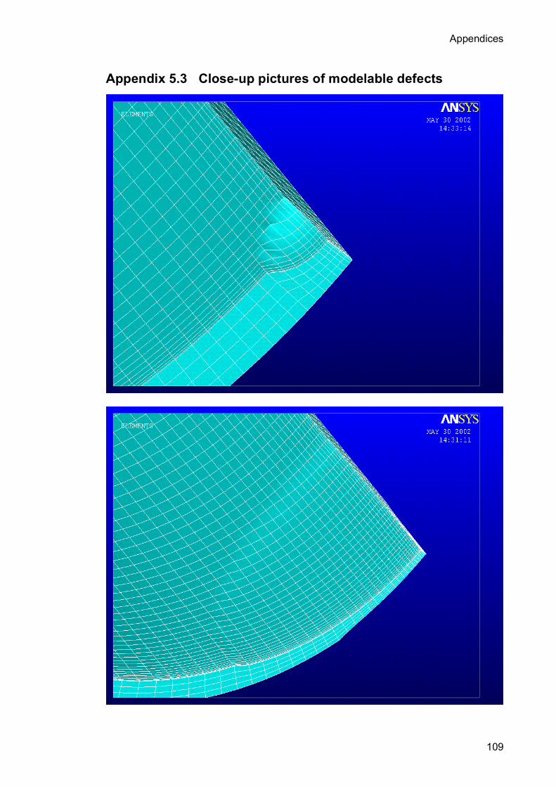
Appendices
109
Appendix 5.3 Close-up pictures of modelable defects

Appendices
110

Appendices
111

Appendices
112
Appendix 5.4 Typical result file of analysis with 2 layers
---------------------Burst pressure ---------------------- 28.416 MPa ----------------------------------------------------------------- Critical internal pressure calculation (D = 298.4 mm, t = 11.05 mm, E = 210000 MPa, sigf = 380 MPa) (Ovality = 4.E-03, External pressure = 0 MPa, Axial load (tension) = 0 kN) Internal defect (Depth = 1 mm, Rad. half-axis = 50 mm, Ver. half-axis = 50 mm) External defect (Depth = 0 mm, Rad. half-axis = 50 mm, Ver. half-axis = 50 mm) ----------------------------------------------------------------- -----------Displacement in mm by 0 degrees----------- TIME 1 UX NSOL UX NSOL UX D_0_1lo D_0_1l D_0_2l 0.24000E-02 -0.817528E-05 -0.797355E-05 -0.766371E-05 2.4012 -0.817369E-02 -0.797190E-02 -0.766197E-02 4.8000 -0.823604E-02 -0.782401E-02 -0.721092E-02 16.356 0.139798E-01 0.154301E-01 0.174862E-01 27.912 0.366604E-01 0.393387E-01 0.441626E-01 28.416 0.166347E-01 0.198286E-01 0.256434E-01 ----------------------------------------------------------------- -----------Displacement in mm by 90 degrees----------- TIME 1401 UX NSOL UX NSOL UX D_90_1lo D_90_1l D_90_2l 0.24000E-02 0.469871E-04 0.472241E-04 0.474525E-04 2.4012 0.469972E-01 0.472343E-01 0.474627E-01 4.8000 0.861627E-01 0.866397E-01 0.871145E-01 16.356 0.253503 0.255144 0.256856 27.912 0.403066 0.405886 0.408909 28.416 0.424328 0.427193 0.430254 ----------------------------------------------------------------- -------Von Mises stresses in MPa by 0 degrees------- TIME 1 S EQV 521 S EQV 521 S EQV S_0_1lo S_0_1l S_0_2l 0.24000E-02 0.251839E-01 0.329656E-01 0.414645E-01 2.4012 25.1910 32.9737 41.4733 4.8000 51.6889 66.0018 81.5455 16.356 191.562 234.835 260.960 27.912 350.709 380.000 380.000 28.416 380.000 380.000 380.000 ----------------------------------------------------------------- -------Von Mises stresses in MPa by 90 degrees------- TIME 339 S EQV 859 S EQV 859 S EQV S_90_1lo S_90_1l S_90_2l 0.24000E-02 0.329230E-01 0.307287E-01 0.280116E-01 2.4012 32.9305 30.7364 28.0195 4.8000 64.6797 61.4862 57.3444 16.356 213.122 208.395 204.102 27.912 359.315 357.811 354.543 28.416 366.757 364.368 360.537

Appendices
113
Appendix 5.5 Typical result file of analysis with 4 layers
---------------------Burst pressure ---------------------- 28.920 MPa ----------------------------------------------------------------- Critical internal pressure calculation (D = 298.4 mm, t = 11.05 mm, E = 210000 MPa, sigf = 380 MPa) (Ovality = 4.E-03, External pressure = %pda% MPa, Axial load (tension) = 0 kN) Internal defect (Depth = 1 mm, Rad. half-axis = 50 mm, Ver. half-axis = 50 mm) External defect (Depth = 0 mm, Rad. half-axis = 140.617687 mm, Ver. half-axis = 140.617687 mm) ----------------------------------------------------------------- -----------Displacement in mm by 0 degrees----------- TIME 1 UX NSOL UX NSOL UX NSOL UX NSOL UX D_0_1lo D_0_1l D_0_2l D_0_3l D_0_4l 0.24000E-02 -0.817511E-05 -0.808656E-05 -0.797302E-05 -0.783263E-05 -0.766307E-05 2.4012 -0.817352E-02 -0.808494E-02 -0.797136E-02 -0.783093E-02 -0.766133E-02 4.8000 -0.823359E-02 -0.805048E-02 -0.782087E-02 -0.754134E-02 -0.720759E-02 16.356 0.140006E-01 0.146567E-01 0.154530E-01 0.163997E-01 0.175097E-01 27.912 0.357721E-01 0.369543E-01 0.384576E-01 0.405677E-01 0.432927E-01 28.416 0.144784E-01 0.157659E-01 0.176465E-01 0.201631E-01 0.234101E-01 28.920 0.541356E-02 0.715331E-02 0.955743E-02 0.126592E-01 0.165587E-01 ----------------------------------------------------------------- -----------Displacement in mm by 90 degrees----------- TIME 1401 UX NSOL UX NSOL UX NSOL UX NSOL UX D_90_1lo D_90_1l D_90_2l D_90_3l D_90_4l 0.24000E-02 0.469899E-04 0.471092E-04 0.472269E-04 0.473424E-04 0.474553E-04 2.4012 0.470000E-01 0.471193E-01 0.472370E-01 0.473526E-01 0.474655E-01 4.8000 0.861684E-01 0.864068E-01 0.866454E-01 0.868835E-01 0.871203E-01 16.356 0.253522 0.254334 0.255164 0.256011 0.256876 27.912 0.403652 0.405037 0.406472 0.407958 0.409496 28.416 0.426539 0.427947 0.429403 0.430907 0.432461 28.920 0.445397 0.446826 0.448304 0.449831 0.451408 ----------------------------------------------------------------- -------Von Mises stresses in MPa by 0 degrees------- TIME 1 S EQV 521 S EQV 521 S EQV 1041 S EQV 1561 S EQV S_0_1lo S_0_1l S_0_2l S_0_3l S_0_4l 0.24000E-02 0.251719E-01 0.289077E-01 0.327515E-01 0.370179E-01 0.416449E-01 2.4012 25.1790 28.9153 32.7595 37.0263 41.6537 4.8000 51.6545 58.5312 65.5650 73.3974 81.8924 16.356 187.120 207.616 219.443 242.142 266.702 27.912 339.934 380.000 380.000 380.000 380.000 28.416 367.683 380.000 380.000 380.000 380.000 28.920 380.000 380.000 380.000 380.000 380.000

Appendices
114
----------------------------------------------------------------- -------Von Mises stresses in MPa by 90 degrees------- TIME 339 S EQV 859 S EQV 859 S EQV 1379 S EQV 1899 S EQV S_90_1lo S_90_1l S_90_2l S_90_3l S_90_4l 0.24000E-02 0.328287E-01 0.317590E-01 0.304808E-01 0.293137E-01 0.280736E-01 2.4012 32.8362 31.7666 30.4885 29.3215 28.0815 4.8000 64.4992 62.9399 60.9884 59.2899 57.4830 16.356 213.278 210.969 208.927 206.490 203.914 27.912 358.966 358.159 356.562 355.783 354.997 28.416 366.686 365.374 363.453 362.134 360.765 28.920 373.934 372.551 370.574 369.178 367.746 -----------------------------------------------------------------

Appendices
115
Appendix 6.1 Comparison of the API and FEM critical internal
pressures for intact pipes
1 2 3 4 5 6 7
D
t
D/t
API w/ factor 0.875
API w/o factor 0.875
FEM
Deviation
[mm] [mm] [-] [MPa] [MPa] [MPa] [%] 114.3 5.21 21.94 30.31 34.64 37.05 -6.95 114.3 5.69 20.09 33.10 37.83 39.77 -5.10 114.3 6.35 18.00 36.94 42.22 45.70 -8.23
127 5.59 22.72 29.27 33.45 34.95 -4.46 127 6.43 19.75 33.67 38.48 41.50 -7.84 127 7.52 16.89 39.38 45.00 48.40 -7.55
139.7 6.2 22.53 29.51 33.73 35.31 -4.69 139.7 6.98 20.01 33.23 37.97 40.70 -7.18 139.7 7.72 18.10 36.75 42.00 45.10 -7.38 168.3 7.32 22.99 28.92 33.06 35.15 -6.33 168.3 8.94 18.83 35.32 40.37 42.80 -6.02 177.8 6.91 25.73 25.84 29.54 30.88 -4.53 177.8 8.05 22.09 30.11 34.41 36.15 -5.06 177.8 9.19 19.35 34.37 39.28 42.41 -7.95 193.7 8.33 23.25 28.60 32.68 34.58 -5.80 219.1 6.71 32.65 20.37 23.28 24.10 -3.54 219.1 7.72 28.38 23.43 26.78 28.05 -4.75 219.1 8.94 24.51 27.13 31.01 32.54 -4.92 219.1 10.16 21.56 30.84 35.24 37.05 -5.13 244.5 8.94 27.35 24.32 27.79 28.92 -4.07 244.5 10.03 24.38 27.28 31.18 32.54 -4.36
273 8.89 30.71 21.66 24.75 25.94 -4.79 273 10.16 26.87 24.75 28.28 29.64 -4.79 273 11.43 23.88 27.84 31.82 33.35 -4.79
298.4 9.52 31.34 21.22 24.25 25.08 -3.45 298.4 11.05 27.00 24.63 28.14 29.27 -3.99 298.4 12.42 24.03 27.68 31.63 33.35 -5.41 339.7 9.65 35.20 18.89 21.59 22.23 -2.97 339.7 10.92 31.11 21.38 24.43 25.31 -3.58 339.7 12.19 27.87 23.86 27.27 28.41 -4.15 339.7 13.06 26.01 25.57 29.22 30.09 -2.96
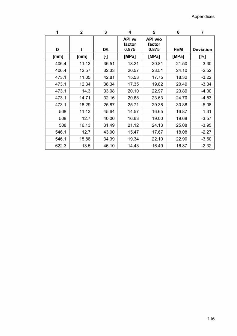
Appendices
116
1 2 3 4 5 6 7
D
t
D/t
API w/ factor 0.875
API w/o factor 0.875
FEM
Deviation
[mm] [mm] [-] [MPa] [MPa] [MPa] [%] 406.4 11.13 36.51 18.21 20.81 21.50 -3.30 406.4 12.57 32.33 20.57 23.51 24.10 -2.52 473.1 11.05 42.81 15.53 17.75 18.32 -3.22 473.1 12.34 38.34 17.35 19.82 20.49 -3.34 473.1 14.3 33.08 20.10 22.97 23.89 -4.00 473.1 14.71 32.16 20.68 23.63 24.70 -4.53 473.1 18.29 25.87 25.71 29.38 30.88 -5.08
508 11.13 45.64 14.57 16.65 16.87 -1.31 508 12.7 40.00 16.63 19.00 19.68 -3.57 508 16.13 31.49 21.12 24.13 25.08 -3.95
546.1 12.7 43.00 15.47 17.67 18.08 -2.27 546.1 15.88 34.39 19.34 22.10 22.90 -3.60 622.3 13.5 46.10 14.43 16.49 16.87 -2.32

Appendices
117
Appendix 6.2 Comparison of the API (with Dm) and FEM
critical internal pressures for intact pipes
1 2 3 4 5 6
D t D/t API with
Dm FEM Deviation [mm] [mm] [-] [MPa} [MPa] [%]
114.3 5.21 21.94 36.30 37.05 -2.08 114.3 5.69 20.09 39.82 39.77 0.13 114.3 6.35 18.00 44.71 45.70 -2.21
127 5.59 22.72 34.99 34.95 0.13 127 6.43 19.75 40.53 41.50 -2.38 127 7.52 16.89 47.83 48.40 -1.18
139.7 6.2 22.53 35.30 35.31 -0.04 139.7 6.98 20.01 39.97 40.70 -1.83 139.7 7.72 18.10 44.46 45.10 -1.45 168.3 7.32 22.99 34.56 35.15 -1.71 168.3 8.94 18.83 42.64 42.80 -0.39 177.8 6.91 25.73 30.73 30.88 -0.47 177.8 8.05 22.09 36.04 36.15 -0.30 177.8 9.19 19.35 41.42 42.41 -2.37 193.7 8.33 23.25 34.15 34.58 -1.25 219.1 6.71 32.65 24.01 24.10 -0.37 219.1 7.72 28.38 27.76 28.05 -1.06 219.1 8.94 24.51 32.33 32.54 -0.64 219.1 10.16 21.56 36.96 37.05 -0.25 244.5 8.94 27.35 28.84 28.92 -0.26 244.5 10.03 24.38 32.51 32.54 -0.07
273 8.89 30.71 25.58 25.94 -1.38 273 10.16 26.87 29.38 29.64 -0.89 273 11.43 23.88 33.21 33.35 -0.41
298.4 9.52 31.34 25.05 25.08 -0.15 298.4 11.05 27.00 29.23 29.27 -0.13 298.4 12.42 24.03 33.01 33.35 -1.03 339.7 9.65 35.20 22.22 22.23 -0.04 339.7 10.92 31.11 25.24 25.31 -0.25 339.7 12.19 27.87 28.29 28.41 -0.42 339.7 13.06 26.01 30.39 30.09 0.99

Appendices
118
1 2 3 4 5 6
D t D/t API with
Dm FEM Deviation [mm] [mm] [-] [MPa} [MPa] [%]
406.4 11.13 36.51 21.40 21.50 -0.47 406.4 12.57 32.33 24.26 24.10 0.65 473.1 11.05 42.81 18.18 18.32 -0.81 473.1 12.34 38.34 20.35 20.49 -0.64 473.1 14.3 33.08 23.69 23.89 -0.85 473.1 14.71 32.16 24.39 24.70 -1.28 473.1 18.29 25.87 30.56 30.88 -1.02
508 11.13 45.64 17.02 16.87 0.91 508 12.7 40.00 19.49 19.68 -0.98 508 16.13 31.49 24.92 25.08 -0.65
546.1 12.7 43.00 18.10 18.08 0.11 546.1 15.88 34.39 22.76 22.90 -0.58 622.3 13.5 46.10 16.85 16.87 -0.10

Appendices
119
Appendix 6.3 Critical internal pressures / Yp (-) of variously
corroded tubular (internal defect, depth 0.5t)
c/t 0.5 Defect circumferential extent (width) 2a/(π·D) [-] 0.01 0.05 0.1 0.2 0.3
0.01 0.078 0.073 0.076 0.076 0.076 0.05 0.076 0.061 0.060 0.060 0.060 0.1 0.074 0.056 0.049 0.048 0.047 0.2 0.064 0.049 0.044 0.041 0.041 0.3 0.056 0.048 0.044 0.041 0.040
Defect longitudinal
extent (length) 2b/(π·D)
[-] 0.4 0.052 0.046 0.044 0.041 0.040 0.5 0.051 0.046 0.044 0.041 0.040 0.637 0.049 0.045 0.044 0.041 0.041 c/t 0.5 Defect circumferential extent (width) 2a/(π·D) [-] 0.4 0.5 0.637 0.75 1
0.01 0.076 0.076 0.076 0.076 0.076 0.05 0.060 0.057 0.057 0.057 0.057 0.1 0.045 0.045 0.045 0.045 0.045 0.2 0.040 0.040 0.040 0.040 0.040 0.3 0.040 0.040 0.040 0.040 0.040
Defect longitudinal
extent (length) 2b/(π·D)
[-] 0.4 0.040 0.040 0.040 0.040 0.040 0.5 0.040 0.040 0.040 0.040 0.040 0.637 0.040 0.040 0.040 0.040 0.040

Appendices
120
Appendix 6.4 Critical internal pressures / Yp (-) of variously
corroded tubular (internal defect, depth 0.25t)
c/t 0.25 Defect circumferential extent (width) 2a/(π·D) [-] 0.01 0.05 0.1 0.2 0.3
0.01 0.078 0.076 0.078 0.078 0.078 0.05 0.078 0.073 0.072 0.071 0.071
0.1 0.076 0.071 0.068 0.065 0.065 0.2 0.076 0.068 0.063 0.061 0.060 0.3 0.073 0.068 0.063 0.060 0.060
Defect longitudinal
extent (length) 2b/(π·D)
[-] 0.4 0.071 0.065 0.063 0.060 0.060 0.5 0.069 0.065 0.063 0.060 0.060 0.637 0.069 0.065 0.064 0.061 0.060 c/t 0.25 Defect circumferential extent (width) 2a/(π·D) [-] 0.4 0.5 0.637 0.75 1
0.01 0.078 0.078 0.078 0.078 0.078 0.05 0.071 0.071 0.071 0.071 0.071 0.1 0.064 0.064 0.064 0.064 0.064 0.2 0.060 0.060 0.060 0.060 0.060 0.3 0.060 0.060 0.060 0.060 0.060
Defect longitudinal
extent (length) 2b/(π·D)
[-] 0.4 0.060 0.060 0.060 0.060 0.060 0.5 0.060 0.060 0.060 0.060 0.060 0.637 0.060 0.060 0.060 0.060 0.060

Appendices
121
Appendix 6.5 Critical internal pressures / Yp (-) of variously
corroded tubular (internal defect, depth 0.75t)
c/t 0.75 Defect circumferential extent (width) 2a/(π·D) [-] 0.01 0.05 0.1 0.2 0.3
0.01 0.078 0.068 0.072 0.073 0.076 0.05 0.061 0.041 0.041 0.041 0.040 0.1 0.060 0.033 0.029 0.025 0.025 0.2 0.044 0.028 0.024 0.021 0.021 0.3 0.036 0.027 0.024 0.021 0.021
Defect longitudinal
extent (length) 2b/(π·D)
[-] 0.4 0.030 0.025 0.022 0.021 0.021 0.5 0.026 0.024 0.023 0.021 0.021 0.637 0.027 0.024 0.022 0.021 0.023 c/t 0.75 Defect circumferential extent (width) 2a/(π·D) [-] 0.4 0.5 0.637 0.75 1
0.01 0.076 0.076 0.076 0.076 0.073 0.05 0.040 0.040 0.040 0.040 0.038 0.1 0.025 0.024 0.024 0.024 0.024 0.2 0.021 0.021 0.021 0.021 0.021 0.3 0.021 0.021 0.021 0.021 0.021
Defect longitudinal
extent (length) 2b/(π·D)
[-] 0.4 0.021 0.021 0.021 0.021 0.021 0.5 0.021 0.021 0.023 0.021 0.020 0.637 0.023 0.021 0.023 0.021 0.020

Appendices
122
Appendix 6.5 Critical internal pressures / Yp (-) of variously
corroded tubular (external defect, depth 0.5t)
c/t 0.5 Defect circumferential extent (width) 2a/(π·D) [-] 0.01 0.05 0.1 0.2 0.3
0.01 0.078 0.065 0.069 0.071 0.071 0.05 0.076 0.053 0.052 0.052 0.053 0.1 0.072 0.052 0.044 0.041 0.044 0.2 0.062 0.048 0.044 0.040 0.040 0.3 0.056 0.047 0.044 0.041 0.041
Defect longitudinal
extent (length) 2b/(π·D)
[-] 0.4 0.050 0.047 0.044 0.041 0.041 0.5 0.050 0.045 0.044 0.044 0.041 0.637 0.048 0.045 0.044 0.044 0.041 c/t 0.5 Defect circumferential extent (width) 2a/(π·D) [-] 0.4 0.5 0.637 0.75 1
0.01 0.072 0.072 0.072 0.072 0.072 0.05 0.053 0.053 0.053 0.053 0.053 0.1 0.044 0.044 0.044 0.044 0.044 0.2 0.041 0.041 0.041 0.041 0.041 0.3 0.041 0.041 0.041 0.040 0.041
Defect longitudinal
extent (length) 2b/(π·D)
[-] 0.4 0.041 0.041 0.041 0.041 0.041 0.5 0.041 0.041 0.041 0.041 0.040 0.637 0.041 0.041 0.041 0.041 0.041

Appendices
123
Appendix 7.1 The API critical external pressures for intact
pipes
1 2 3 4 5 6
D t D/t API
plastic API
transitionAPI
elastic [mm] [mm] [-] [MPa] [MPa] [MPa]
114.3 5.21 21.94 22.89 114.3 5.69 20.09 27.65 114.3 6.35 18.00 34.21
127 5.59 22.72 21.11 127 6.43 19.75 28.62 127 7.52 16.89 38.36
139.7 6.2 22.53 21.52 139.7 6.98 20.01 27.86 139.7 7.72 18.10 33.87 168.3 7.32 22.99 20.52 168.3 8.94 18.83 31.44 177.8 6.91 25.73 15.67 177.8 8.05 22.09 22.54 177.8 9.19 19.35 29.82 193.7 8.33 23.25 19.96 219.1 6.71 32.65 9.45 219.1 7.72 28.38 12.93 219.1 8.94 24.51 17.46 219.1 10.16 21.56 23.78 244.5 8.94 27.35 13.94 244.5 10.03 24.38 17.71
273 8.89 30.71 10.92 273 10.16 26.87 14.43 273 11.43 23.88 18.67
298.4 9.52 31.34 10.42 298.4 11.05 27.00 14.29 298.4 12.42 24.03 18.39 339.7 9.65 35.20 7.78 339.7 10.92 31.11 10.60 339.7 12.19 27.87 13.42 339.7 13.06 26.01 15.36

Appendices
124
1 2 3 4 5 6
D t D/t API
plastic API
transitionAPI
elastic [mm] [mm] [-] [MPa] [MPa] [MPa]
406.4 11.13 36.51 7.01 406.4 12.57 32.33 9.68 473.1 11.05 42.81 4.33 473.1 12.34 38.34 6.06 473.1 14.3 33.08 9.15 473.1 14.71 32.16 9.81 473.1 18.29 25.87 15.52
508 11.13 45.64 3.56 508 12.7 40.00 5.32 508 16.13 31.49 10.31
546.1 12.7 43.00 4.27 546.1 15.88 34.39 8.29 622.3 13.5 46.10 3.46

Appendices
125
Appendix 7.2 Comparison of the API and FEM (ovality 0.4%)
critical external pressures for intact pipes
1 2 3 4 5 6 7 8
D t D/t
API w/o safety margin plastic
API w/o safety margin
transition
API w/o safety margin elastic FEM Deviation
[mm] [mm] [-] [MPa] [MPa] [MPa] [MPa] [%] 114.3 5.21 21.94 31.18 29.10 6.67 114.3 5.69 20.09 35.94 33.81 5.92 114.3 6.35 18.00 42.48 39.47 7.11
127 5.59 22.72 29.40 27.84 5.30 127 6.43 19.75 36.90 34.81 5.65 127 7.52 16.89 46.63 42.94 7.92
139.7 6.2 22.53 29.81 27.86 6.56 139.7 6.98 20.01 36.14 34.20 5.37 139.7 7.72 18.10 42.15 39.47 6.37 168.3 7.32 22.99 28.81 26.89 6.67 168.3 8.94 18.83 39.72 36.98 6.91 177.8 6.91 25.73 20.88 21.69 -3.90 177.8 8.05 22.09 30.83 29.17 5.39 177.8 9.19 19.35 38.10 35.92 5.71 193.7 8.33 23.25 28.25 26.60 5.85 219.1 6.71 32.65 12.59 12.31 2.25 219.1 7.72 28.38 17.23 17.44 -1.22 219.1 8.94 24.51 25.76 24.04 6.69 219.1 10.16 21.56 32.07 30.51 4.87 244.5 8.94 27.35 18.56 18.98 -2.21 244.5 10.03 24.38 26.01 24.43 6.06
273 8.89 30.71 14.54 14.29 1.74 273 10.16 26.87 19.22 19.76 -2.81 273 11.43 23.88 26.96 25.20 6.54
298.4 9.52 31.34 13.88 13.59 2.11 298.4 11.05 27.00 19.03 19.59 -2.93 298.4 12.42 24.03 26.69 24.70 7.44 339.7 9.65 35.20 10.36 9.90 4.47 339.7 10.92 31.11 14.12 13.77 2.51 339.7 12.19 27.87 17.88 18.32 -2.47 339.7 13.06 26.01 20.46 21.51 -5.13

Appendices
126
1 2 3 4 5 6 7 8
D t D/t
API w/o safety margin plastic
API w/o safety margin
transition
API w/o safety margin elastic FEM Deviation
[mm] [mm] [-] [MPa] [MPa] [MPa] [MPa] [%] 406.4 11.13 36.51 9.34 9.04 3.18 406.4 12.57 32.33 12.90 12.43 3.64 473.1 11.05 42.81 5.76 5.74 0.48 473.1 12.34 38.34 8.07 7.77 3.69 473.1 14.3 33.08 12.19 11.80 3.24 473.1 14.71 32.16 13.06 12.70 2.79 473.1 18.29 25.87 20.67 21.70 -4.98
508 11.13 45.64 4.74 4.77 -0.62 508 12.7 40.00 7.09 6.87 3.17 508 16.13 31.49 13.73 13.26 3.41
546.1 12.7 43.00 5.69 5.57 2.05 546.1 15.88 34.39 11.04 10.61 3.92 622.3 13.5 46.10 4.60 4.61 -0.20

Appendices
127
Appendix 7.3 Comparison of the API and FEM (ovality
depended on D/t) critical external pressures for
intact pipes
1 2 3 4 5 7 8
D t D/t
API w/o safety margin Ovality FEM Deviation
[mm] [mm] [-] [MPa] [-] [MPa] [%] 114.3 5.21 21.94 30.52 0.004 30.43 2.41 114.3 5.69 20.09 36.87 0.004 35.83 0.31 114.3 6.35 18.00 45.61 0.003 40.76 4.06
127 5.59 22.72 28.15 0.004 27.84 5.30 127 6.43 19.75 38.16 0.003 35.72 3.20 127 7.52 16.89 51.15 0.002 44.00 5.64
139.7 6.2 22.53 28.70 0.004 27.86 6.56 139.7 6.98 20.01 37.15 0.004 36.05 0.26 139.7 7.72 18.10 45.17 0.003 40.69 3.47 168.3 7.32 22.99 27.36 0.004 26.89 6.67 168.3 8.94 18.83 41.92 0.003 38.24 3.73 177.8 6.91 25.73 20.90 0.004 21.69 -2.51 177.8 8.05 22.09 30.05 0.004 29.17 5.39 177.8 9.19 19.35 39.76 0.003 36.80 3.41 193.7 8.33 23.25 26.62 0.004 26.60 0.06 219.1 6.71 32.65 12.61 0.004 12.31 2.35 219.1 7.72 28.38 17.25 0.004 17.44 -1.11 219.1 8.94 24.51 23.28 0.004 24.04 -3.23 219.1 10.16 21.56 31.71 0.003 31.11 1.90 244.5 8.94 27.35 18.58 0.004 18.98 -2.11 244.5 10.03 24.38 23.62 0.004 24.43 -3.45
273 8.89 30.71 14.56 0.004 14.29 1.85 273 10.16 26.87 19.24 0.004 19.76 -2.71 273 11.43 23.88 24.90 0.004 25.20 -1.22
298.4 9.52 31.34 13.89 0.004 13.59 2.22 298.4 11.05 27.00 19.05 0.004 19.59 -2.82 298.4 12.42 24.03 24.52 0.004 24.70 -0.72 339.7 9.65 35.20 10.37 0.004 9.90 4.57 339.7 10.92 31.11 14.14 0.004 13.77 2.62 339.7 12.19 27.87 17.90 0.004 18.32 -2.36 339.7 13.06 26.01 20.48 0.004 21.51 -5.02

Appendices
128
1 2 3 4 5 7 8
D t D/t
API w/o safety margin Ovality FEM Deviation
[mm] [mm] [-] [MPa] [-] [MPa] [%] 406.4 11.13 36.51 9.35 0.004 9.04 3.28 406.4 12.57 32.33 12.91 0.004 12.43 3.74 473.1 11.05 42.81 5.77 0.004 5.74 0.58 473.1 12.34 38.34 8.08 0.004 7.77 3.79 473.1 14.3 33.08 12.20 0.004 11.80 3.34 473.1 14.71 32.16 13.08 0.004 12.70 2.90 473.1 18.29 25.87 20.69 0.004 21.70 -4.87
508 11.13 45.64 4.75 0.004 4.77 -0.51 508 12.7 40.00 7.10 0.004 6.87 3.27 508 16.13 31.49 13.74 0.004 13.26 3.51
546.1 12.7 43.00 5.69 0.004 5.57 2.16 546.1 15.88 34.39 11.05 0.004 10.61 4.02 622.3 13.5 46.10 4.61 0.004 4.61 -0.10
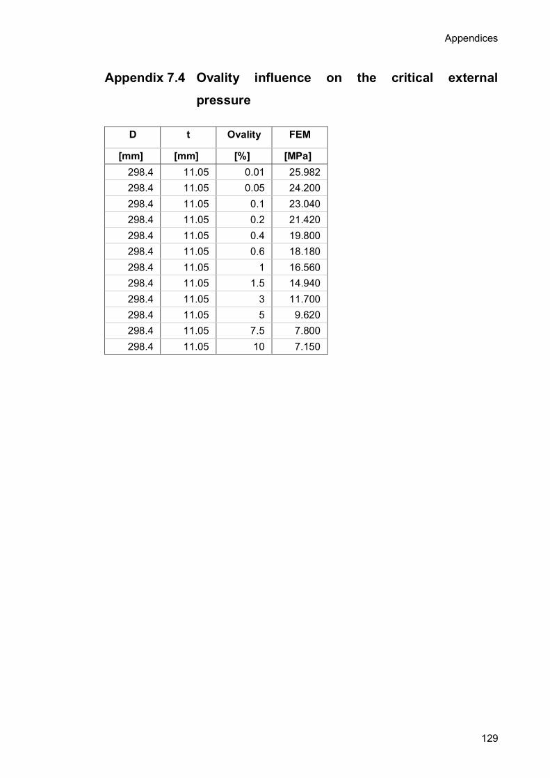
Appendices
129
Appendix 7.4 Ovality influence on the critical external
pressure
D t Ovality FEM
[mm] [mm] [%] [MPa] 298.4 11.05 0.01 25.982 298.4 11.05 0.05 24.200 298.4 11.05 0.1 23.040 298.4 11.05 0.2 21.420 298.4 11.05 0.4 19.800 298.4 11.05 0.6 18.180 298.4 11.05 1 16.560 298.4 11.05 1.5 14.940 298.4 11.05 3 11.700 298.4 11.05 5 9.620 298.4 11.05 7.5 7.800 298.4 11.05 10 7.150
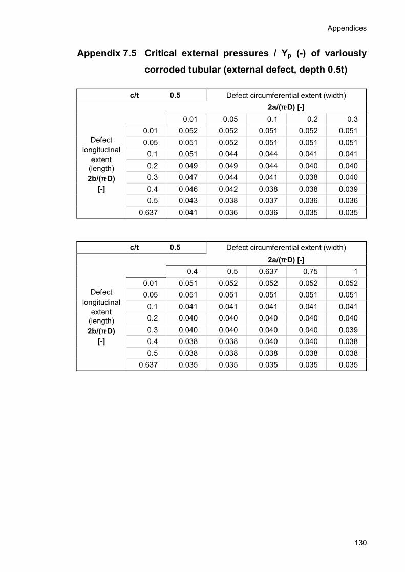
Appendices
130
Appendix 7.5 Critical external pressures / Yp (-) of variously
corroded tubular (external defect, depth 0.5t)
c/t 0.5 Defect circumferential extent (width) 2a/(π·D) [-] 0.01 0.05 0.1 0.2 0.3
0.01 0.052 0.052 0.051 0.052 0.051 0.05 0.051 0.052 0.051 0.051 0.051 0.1 0.051 0.044 0.044 0.041 0.041 0.2 0.049 0.049 0.044 0.040 0.040 0.3 0.047 0.044 0.041 0.038 0.040
Defect longitudinal
extent (length) 2b/(π·D)
[-] 0.4 0.046 0.042 0.038 0.038 0.039 0.5 0.043 0.038 0.037 0.036 0.036 0.637 0.041 0.036 0.036 0.035 0.035 c/t 0.5 Defect circumferential extent (width) 2a/(π·D) [-] 0.4 0.5 0.637 0.75 1
0.01 0.051 0.052 0.052 0.052 0.052 0.05 0.051 0.051 0.051 0.051 0.051 0.1 0.041 0.041 0.041 0.041 0.041 0.2 0.040 0.040 0.040 0.040 0.040 0.3 0.040 0.040 0.040 0.040 0.039
Defect longitudinal
extent (length) 2b/(π·D)
[-] 0.4 0.038 0.038 0.040 0.040 0.038 0.5 0.038 0.038 0.038 0.038 0.038 0.637 0.035 0.035 0.035 0.035 0.035

Appendices
131
Appendix 7.6 Critical external pressures / Yp (-) of variously
corroded tubular (internal defect, depth 0.5t)
c/t 0.5 Defect circumferential extent (width) 2a/(π·D) [-] 0.01 0.05 0.1 0.2 0.3
0.01 0.052 0.052 0.052 0.052 0.052 0.05 0.052 0.049 0.049 0.049 0.049 0.1 0.052 0.049 0.045 0.043 0.043 0.2 0.053 0.050 0.043 0.039 0.039 0.3 0.053 0.049 0.045 0.040 0.039
Defect longitudinal
extent (length) 2b/(π·D)
[-] 0.4 0.053 0.049 0.045 0.040 0.039 0.5 0.050 0.046 0.043 0.042 0.040 0.637 0.050 0.044 0.040 0.038 0.039 c/t 0.5 Defect circumferential extent (width) 2a/(π·D) [-] 0.4 0.5 0.637 0.75 1
0.01 0.052 0.052 0.052 0.052 0.052 0.05 0.049 0.049 0.049 0.049 0.051 0.1 0.043 0.040 0.040 0.040 0.041 0.2 0.039 0.039 0.039 0.039 0.040 0.3 0.039 0.039 0.040 0.039 0.040
Defect longitudinal
extent (length) 2b/(π·D)
[-] 0.4 0.040 0.040 0.040 0.040 0.040 0.5 0.040 0.038 0.038 0.037 0.038 0.637 0.040 0.037 0.035 0.035 0.035
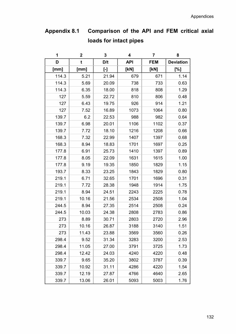
Appendices
132
Appendix 8.1 Comparison of the API and FEM critical axial
loads for intact pipes
1 2 3 4 7 8 D t D/t API FEM Deviation
[mm] [mm] [-] [kN] [kN] [%] 114.3 5.21 21.94 679 671 1.14 114.3 5.69 20.09 738 733 0.63 114.3 6.35 18.00 818 808 1.29
127 5.59 22.72 810 806 0.48 127 6.43 19.75 926 914 1.21 127 7.52 16.89 1073 1064 0.80
139.7 6.2 22.53 988 982 0.64 139.7 6.98 20.01 1106 1102 0.37 139.7 7.72 18.10 1216 1208 0.66 168.3 7.32 22.99 1407 1397 0.68 168.3 8.94 18.83 1701 1697 0.25 177.8 6.91 25.73 1410 1397 0.89 177.8 8.05 22.09 1631 1615 1.00 177.8 9.19 19.35 1850 1829 1.15 193.7 8.33 23.25 1843 1829 0.80 219.1 6.71 32.65 1701 1696 0.31 219.1 7.72 28.38 1948 1914 1.75 219.1 8.94 24.51 2243 2225 0.78 219.1 10.16 21.56 2534 2508 1.04 244.5 8.94 27.35 2514 2508 0.24 244.5 10.03 24.38 2808 2783 0.86
273 8.89 30.71 2803 2720 2.96 273 10.16 26.87 3188 3140 1.51 273 11.43 23.88 3569 3560 0.26
298.4 9.52 31.34 3283 3200 2.53 298.4 11.05 27.00 3791 3725 1.73 298.4 12.42 24.03 4240 4220 0.48 339.7 9.65 35.20 3802 3787 0.39 339.7 10.92 31.11 4286 4220 1.54 339.7 12.19 27.87 4766 4640 2.65 339.7 13.06 26.01 5093 5003 1.76

Appendices
133
1 2 3 4 7 8 D t D/t API FEM Deviation
[mm] [mm] [-] [kN] [kN] [%] 406.4 11.13 36.51 5252 5224 0.54 406.4 12.57 32.33 5910 5840 1.18 473.1 11.05 42.81 6095 6083 0.20 473.1 12.34 38.34 6788 6743 0.66 473.1 14.3 33.08 7832 7808 0.31 473.1 14.71 32.16 8050 8009 0.51 473.1 18.29 25.87 9931 9803 1.29
508 11.13 45.64 6602 6500 1.54 508 12.7 40.00 7509 7403 1.42 508 16.13 31.49 9471 9440 0.33
546.1 12.7 43.00 8087 8051 0.45 546.1 15.88 34.39 10052 9980 0.71 622.3 13.5 46.10 9812 9683 1.31