the finite element method for the analyyysis of linear...
TRANSCRIPT

Swiss Federal Institute of Technology Page 1
The Finite Element Method for the Analysis of Linear Systemsy y
Prof. Dr. Michael Havbro FaberSwiss Federal Institute of Technology
ETH Zurich, Switzerland
Method of Finite Elements 1
Swiss Federal Institute of Technology Page 2
C t t f T d ' L tContents of Today's Lecture
• Q d il t l l t• Quadrilateral elements
- Bi-linear four node element- Singularity of Jacobian matrixSingularity of Jacobian matrix
• Element matrices in global coordinate system
Method of Finite Elements 1

Swiss Federal Institute of Technology Page 3
Q d il t l l tQuadrilateral elements
Bi li f d l tBi-linear four node element:
In the following we will for matters of convenience consider the iso parametric representationiso-parametric representation:
Displacement fields as well as the geometrical representation of the finite elements are approximated using the same approximating functions – shape functions
y
s1, 1-1, 1
ˆ ˆ
4 4ˆ ˆ,u v4
x
r
1, -1-1, -1
1 1ˆ ˆ,u v
2 2ˆ ˆ,u v
3 3ˆ ˆ,u v1
2
3
Method of Finite Elements 1

Swiss Federal Institute of Technology Page 4
Q d il t l l tQuadrilateral elements
Bi li f d l tBi-linear four node element:
For the bi-linear four node element the shape functions in this coordinate s stem becomecoordinate system become:
s1 1(1 ) (1 )h s1, 1-1, 1
1
2
(1 ) (1 )2 21 1(1 ) (1 )
h r s
h r s
= − −
= + − 34
r
2
3
(1 ) (1 )2 21 1(1 ) (1 )2 2
h r s
h r s
+
= + +1 2
1, -1-1, -14
2 21 1(1 ) (1 )2 2
h r s= − +1 2
Method of Finite Elements 1

Swiss Federal Institute of Technology Page 5
Q d il t l l t
Bi li f d l t
Quadrilateral elements
Bi-linear four node element:
Numerical integration: Gauss rule (2x2)s
3 (1, 1)4 (‐1, 1)
r
Stiffness matrix: T dV= ∫K B CB
2 (1, ‐1)1 (‐1, ‐1)
det V
dV dr ds dt=
∫J
det T
V
dr ds dt= ∫K B CB J
Method of Finite Elements 125-Apr-08
Swiss Federal Institute of Technology Page 6
Q d il t l l tQuadrilateral elements
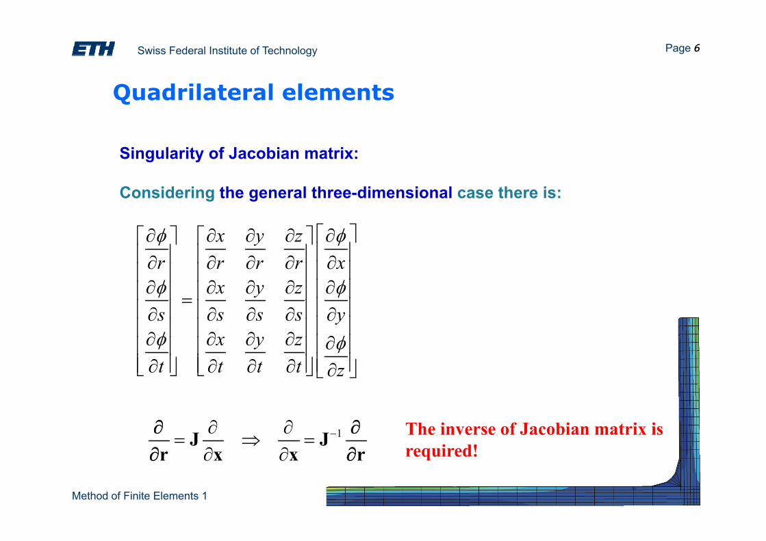
Si l it f J bi t iSingularity of Jacobian matrix:
Considering the general three-dimensional case there is:
x y zr r r r xφ φ⎡ ⎤∂ ∂ ∂ ∂ ∂⎡ ⎤ ⎡ ⎤
⎢ ⎥⎢ ⎥ ⎢ ⎥∂ ∂ ∂ ∂ ∂⎢ ⎥⎢ ⎥ ⎢ ⎥x y z
s s s s yφ φ
φ
⎢ ⎥⎢ ⎥ ⎢ ⎥∂ ∂ ∂ ∂ ∂⎢ ⎥⎢ ⎥ ⎢ ⎥= ⎢ ⎥⎢ ⎥ ⎢ ⎥∂ ∂ ∂ ∂ ∂
⎢ ⎥⎢ ⎥ ⎢ ⎥∂ ∂ ∂ ∂x y zt t t t zφ φ
⎢ ⎥⎢ ⎥ ⎢ ⎥∂ ∂ ∂ ∂ ∂⎢ ⎥⎢ ⎥ ⎢ ⎥⎢ ⎥⎢ ⎥ ⎢ ⎥∂ ∂ ∂ ∂⎣ ⎦ ⎣ ⎦ ∂⎣ ⎦
1 −∂ ∂= ⇒ =
∂ ∂J J
r x x r∂ ∂∂ ∂
The inverse of Jacobian matrix isrequired!
Method of Finite Elements 125-Apr-08
∂ ∂r x x r∂ ∂ required!

Swiss Federal Institute of Technology Page 7
Q d il t l l tQuadrilateral elements
Si l it f J bi t iSingularity of Jacobian matrix:
The existence of the inverse of Jacobian matrix provides the unique correspondence bet een nat ral and local coordinatescorrespondence between natural and local coordinates.
Let us consider a quadrilateral element
y
s1, 1-1, 134
x
r
1, -1-1, -11 2
( )
( )
1 2 3 41( , ) (1 )(1 ) (1 )(1 ) (1 )(1 ) (1 )(1 )41( ) (1 )(1 ) (1 )(1 ) (1 )(1 ) (1 )(1 )
x r s r s x r s x r s x r s x
y r s r s y r s y r s y r s y
= − − + + − + + + + − +
= − − + + − + + + + − +
Method of Finite Elements 125-Apr-08
( )1 2 3 4( , ) (1 )(1 ) (1 )(1 ) (1 )(1 ) (1 )(1 )4
y r s r s y r s y r s y r s y= − − + + − + + + + − +

Swiss Federal Institute of Technology Page 8
Q d il t l l tQuadrilateral elements
Si l it f J bi t iSingularity of Jacobian matrix:
Let us consider a quadrilateral elementy
r
s
1 1
1, 1-1, 1
1 11 2
34
x1, -1-1, -1
( )1 2 3 41( , ) (1 )(1 ) (1 )(1 ) (1 )(1 ) (1 )(1 )4
x r s r s x r s x r s x r s x= − − + + − + + + + − +
( )1 2 3 41( , ) (1 )(1 ) (1 )(1 ) (1 )(1 ) (1 )(1 )4
y r s r s y r s y r s y r s y= − − + + − + + + + − +
det
x yr rx y
∂ ∂∂ ∂=∂ ∂
J
1 2 3 4 1 2 3 4 1 2 3 4 1 2 3 4( ) ( )1 =( ) ( )4
s sx x x x s x x x x y y y y s y y y yx x x x r x x x x y y y y r y y y y
∂ ∂− + + − + − + − − + + − + − + −
+ + + + + + + +
Method of Finite Elements 125-Apr-08
1 2 3 4 1 2 3 4 1 2 3 4 1 2 3 4( ) ( )4 x x x x r x x x x y y y y r y y y y− − + + + − + − − − + + + − + −

Swiss Federal Institute of Technology Page 9
Q d il t l l tQuadrilateral elements
Si l it f J bi t iSingularity of Jacobian matrix:
Let us consider a quadrilateral elementy
r
s
1 1
1, 1-1, 1
1 11 2
34
det J is a linear function of the coordinates r and s. Therefore, det J≠0 in the element only if its values in all nodes are positive or negative.
x1, -1-1, -1
We have to inspect the values at the nodes.
node 1:
( )( ) ( )( )( )( ) ( )( )2 1 4 1 2 1 4 1det x x y y y y x x= − − − − −J
Method of Finite Elements 125-Apr-08
Swiss Federal Institute of Technology Page 10
Q d il t l l tQuadrilateral elements
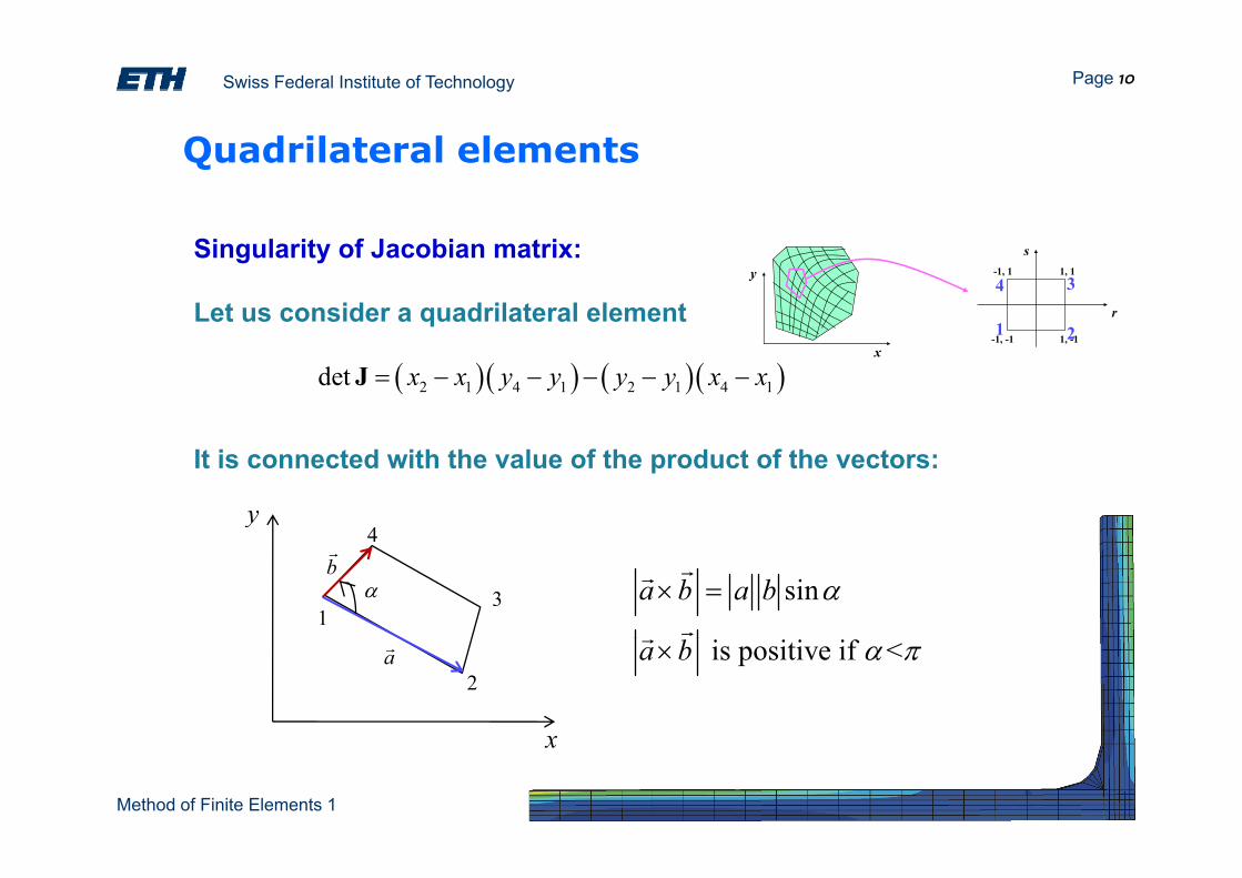
Si l it f J bi t iSingularity of Jacobian matrix:
Let us consider a quadrilateral elementy
r
s
1 1
1, 1-1, 1
1 11 2
34
x1, -1-1, -1
( )( ) ( )( )2 1 4 1 2 1 4 1det x x y y y y x x= − − − − −J
It is connected with the value of the product of the vectors:
y4
3
4
1
bα sina b a b α× =
x
2a is positive if <a b α π×
Method of Finite Elements 125-Apr-08
x
Swiss Federal Institute of Technology Page 11
Q d il t l l tQuadrilateral elements
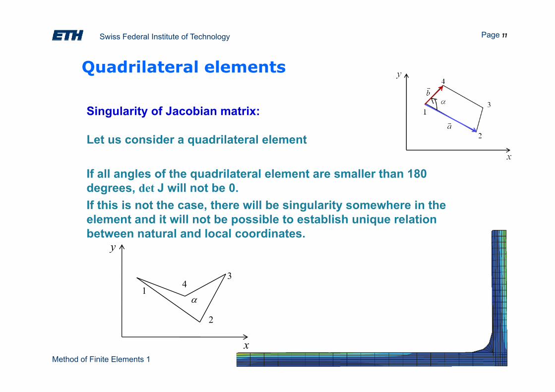
Si l it f J bi t iSingularity of Jacobian matrix:
Let us consider a quadrilateral element
If all angles of the quadrilateral element are smaller than 180 degrees, det J will not be 0.If this is not the case, there will be singularity somewhere in the element and it will not be possible to establish unique relation between natural and local coordinates.
34
y
2
41
α
Method of Finite Elements 125-Apr-08
x

Swiss Federal Institute of Technology Page 12
Q d il t l l tQuadrilateral elements
Following the same principle one may define isoparametric shape functions for three-dimensional quadrilateral elements (see Bathe pp. 344 345 )344-345.)
zt
s
r
x y
Method of Finite Elements 1

Swiss Federal Institute of Technology Page 13
Q d il t l l tQuadrilateral elements
We can also construct the triangular element directly from the quadrilateral element – by so-called collapsing:
1
2
1
23
3
44
Method of Finite Elements 1

Swiss Federal Institute of Technology Page 14
Q d il t l l tQuadrilateral elements
We can also construct the triangular element directly from the quadrilateral element – by so-called collapsing:
1 1 2 2 3 3 4 4ˆ ˆ ˆ ˆˆ ˆ ˆ ˆ
x h x h x h x h xh h h h
= + + ++ + +
3 2ˆ ˆˆ ˆx x=
1 1 2 2 3 3 4 4y h y h y h y h y= + + + 3 2y y=
1 1 2 3 2 4 4ˆ ˆ ˆ( )ˆ ˆ ˆ( )
x h x h h x h xy h y h h y h y= + + += + + +
1
2
3
1
2
1 1 2 3 2 4 4( )y h y h h y h y= + + +
44
Method of Finite Elements 1

Swiss Federal Institute of Technology Page 15
El t t i i l b l di t Element matrices in global coordinate system
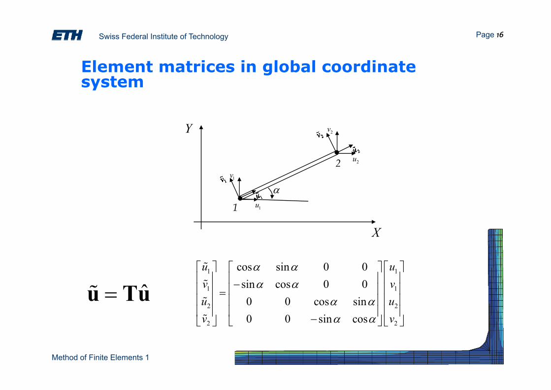
Local to global coordinate transformations:
It is often more convenient to define the element stiffness relations and to calculate their contributions to the load vector in a local coordinate system (e.g. displacements ũ) – this is often specific for each individual elementelement.
In this case we need to transform the element matrixes into global coordinates (e.g. displacements û) before we can assemble the global stiffness relation. Transformation relationship can be written as:
ˆ=u TuT being a transformation matrix.
u Tu
Method of Finite Elements 1
Swiss Federal Institute of Technology Page 16
El t t i i l b l di t Element matrices in global coordinate system
Y 2v
1v
2u
α
2
X
1u1
1 1cos sin 0 0sin cos 0 0
u uv v
α αα α
⎡ ⎤ ⎡ ⎤⎡ ⎤⎢ ⎥ ⎢ ⎥⎢ ⎥⎢ ⎥ ⎢ ⎥⎢ ⎥ˆ =u Tu 1 1
2 2
2 2
sin cos 0 00 0 cos sin0 0 sin cos
v vu uv v
α αα αα α
−⎢ ⎥ ⎢ ⎥⎢ ⎥=⎢ ⎥ ⎢ ⎥⎢ ⎥⎢ ⎥ ⎢ ⎥⎢ ⎥−⎣ ⎦⎣ ⎦ ⎣ ⎦
Method of Finite Elements 1
Swiss Federal Institute of Technology Page 17
El t t i i l b l di t Element matrices in global coordinate system
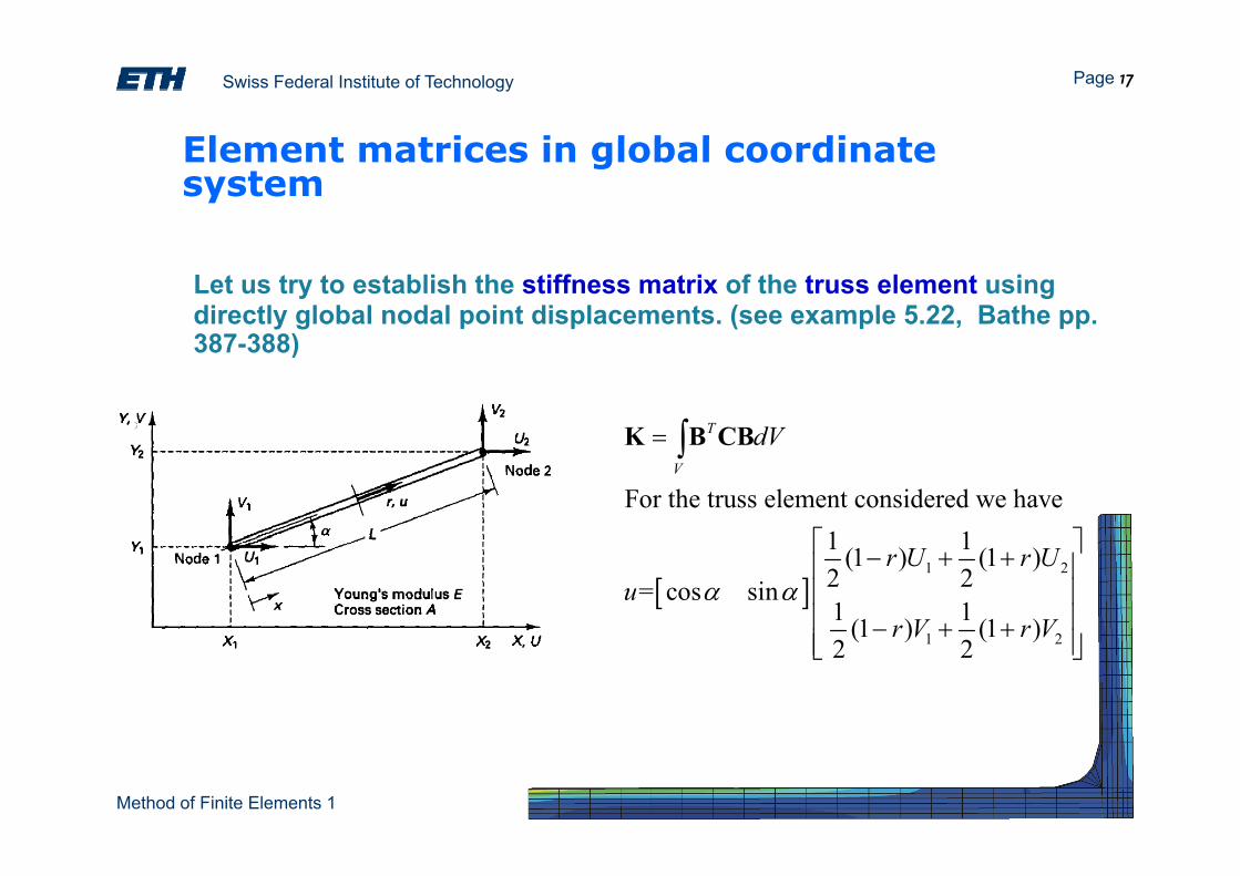
Let us try to establish the stiffness matrix of the truss element using directly global nodal point displacements. (see example 5.22, Bathe pp. 387 388)387-388)
T dV= ∫K B CB
For the truss element considered we have1 1
V
dV=
⎡ ⎤
∫K B CB
[ ]1 2
1 2
1 1(1 ) (1 )2 2= cos sin1 1(1 ) (1 )
r U r Uu
r V r Vα α
⎡ ⎤− + +⎢ ⎥⎢ ⎥⎢ ⎥− + +⎢ ⎥⎣ ⎦1 2( ) ( )
2 2V V⎢ ⎥⎣ ⎦
Method of Finite Elements 1
Swiss Federal Institute of Technology Page 18
El t t i i l b l di t Element matrices in global coordinate system
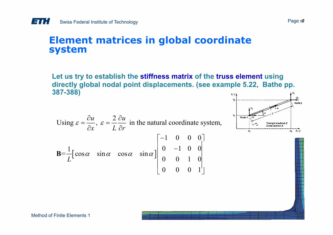
Let us try to establish the stiffness matrix of the truss element using directly global nodal point displacements. (see example 5.22, Bathe pp. 387 388)387-388)
2u u∂ ∂2Using , in the natural coordinate system,
1 0 0 0
u ux L r
ε ε∂ ∂= =∂ ∂
−⎡ ⎤⎢ ⎥
[ ] 0 1 0 01= cos sin cos sin0 0 1 00 0 0 1
Lα α α α
⎢ ⎥−⎢ ⎥⎢ ⎥⎢ ⎥⎣ ⎦
B
0 0 0 1⎣ ⎦
Method of Finite Elements 1
Swiss Federal Institute of Technology Page 19
El t t i i l b l di t Element matrices in global coordinate system
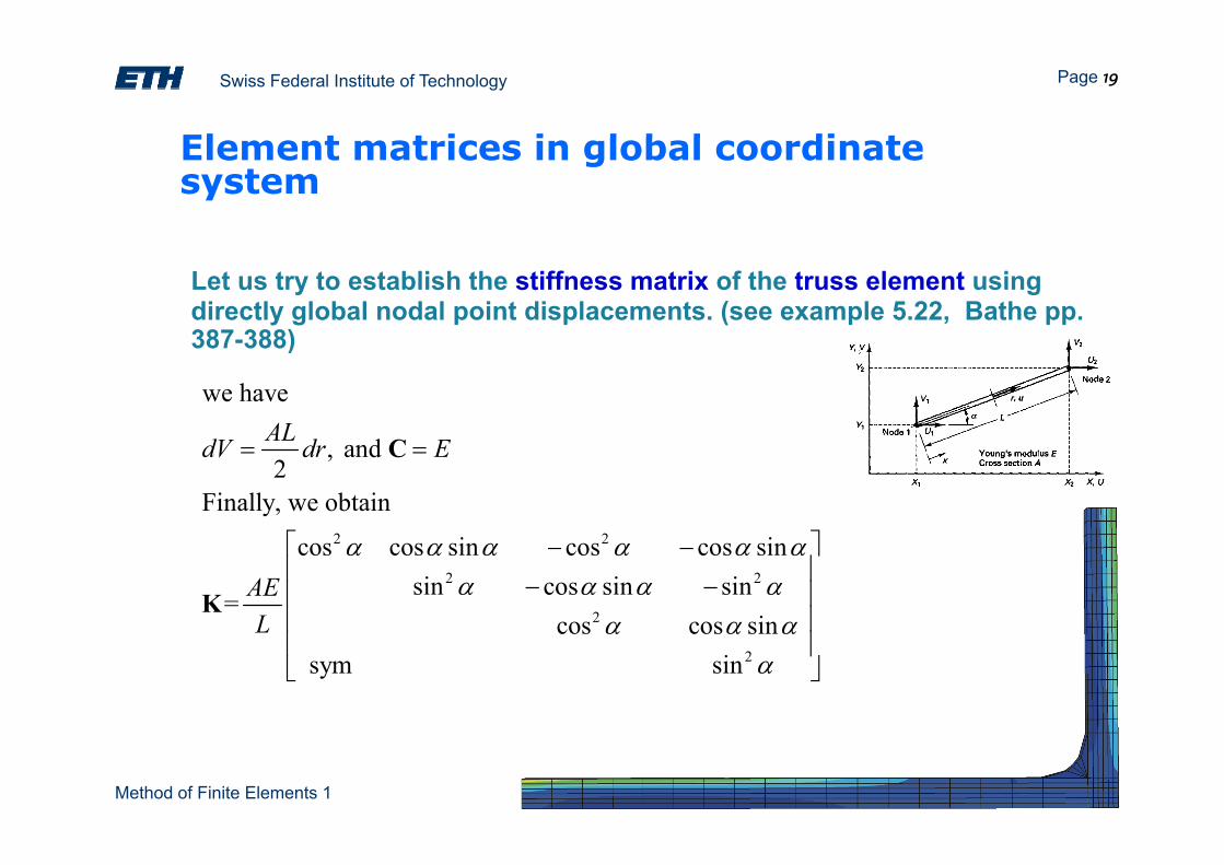
Let us try to establish the stiffness matrix of the truss element using directly global nodal point displacements. (see example 5.22, Bathe pp. 387 388)387-388)
we haveAL , and 2
Finally, we obtain
ALdV dr E= =
⎡ ⎤
C
2 2
2 2
2
cos cos sin cos cos sinsin cos sin sin
=cos cos sin
AEL
α α α α α αα α α α
α α α
⎡ ⎤− −⎢ ⎥− −⎢ ⎥⎢ ⎥
K
2
cos cos sinsym sin
L α α αα
⎢ ⎥⎢ ⎥⎣ ⎦
Method of Finite Elements 1