The First Fermi Large Area Telescope Catalog of Gamma-ray Pulsars

A. A. Abdo2,3, M. Ackermann4, M. Ajello4, W. B. Atwood5, M. Axelsson6,7, L. Baldini8,

J. Ballet9, G. Barbiellini10,11, M. G. Baring12, D. Bastieri13,14, B. M. Baughman15, K. Bechtol4,

R. Bellazzini8, B. Berenji4, R. D. Blandford4, E. D. Bloom4, E. Bonamente16,17, A. W. Borgland4,

J. Bregeon8, A. Brez8, M. Brigida18,19, P. Bruel20, T. H. Burnett21, S. Buson14,

G. A. Caliandro18,19,1, R. A. Cameron4, F. Camilo22, P. A. Caraveo23, J. M. Casandjian9,

C. Cecchi16,17, O. Celik24,25,26, E. Charles4, A. Chekhtman2,27, C. C. Cheung24, J. Chiang4,

S. Ciprini16,17, R. Claus4, I. Cognard28, J. Cohen-Tanugi29, L. R. Cominsky30, J. Conrad31,7,32,

R. Corbet24,26, S. Cutini33, P. R. den Hartog4, C. D. Dermer2, A. de Angelis34, A. de Luca23,35,

F. de Palma18,19, S. W. Digel4, M. Dormody5, E. do Couto e Silva4, P. S. Drell4, R. Dubois4,

D. Dumora36,37, C. Espinoza38, C. Farnier29, C. Favuzzi18,19, S. J. Fegan20, E. C. Ferrara24,1,

W. B. Focke4, P. Fortin20, M. Frailis34, P. C. C. Freire39, Y. Fukazawa40, S. Funk4, P. Fusco18,19,

F. Gargano19, D. Gasparrini33, N. Gehrels24,41, S. Germani16,17, G. Giavitto42, B. Giebels20,

N. Giglietto18,19 , P. Giommi33, F. Giordano18,19, T. Glanzman4, G. Godfrey4, E. V. Gotthelf22,

I. A. Grenier9, M.-H. Grondin36,37, J. E. Grove2, L. Guillemot36,37, S. Guiriec43, C. Gwon2,

Y. Hanabata40, A. K. Harding24, M. Hayashida4, E. Hays24, R. E. Hughes15, M. S. Jackson31,7,44,

G. Johannesson4, A. S. Johnson4, R. P. Johnson5, T. J. Johnson24,41, W. N. Johnson2,

S. Johnston45, T. Kamae4, G. Kanbach46, V. M. Kaspi47, H. Katagiri40, J. Kataoka48,49,

N. Kawai48,50, M. Kerr21, J. Knodlseder51, M. L. Kocian4, M. Kramer38,52, M. Kuss8, J. Lande4,

L. Latronico8, M. Lemoine-Goumard36,37, M. Livingstone47, F. Longo10,11, F. Loparco18,19,

B. Lott36,37, M. N. Lovellette2 , P. Lubrano16,17, A. G. Lyne38, G. M. Madejski4, A. Makeev2,27,

R. N. Manchester45, M. Marelli23, M. N. Mazziotta19 , W. McConville24,41, J. E. McEnery24,

S. McGlynn44,7, C. Meurer31,7, P. F. Michelson4, T. Mineo53, W. Mitthumsiri4, T. Mizuno40,

A. A. Moiseev25,41, C. Monte18,19, M. E. Monzani4, A. Morselli54, I. V. Moskalenko4, S. Murgia4,

T. Nakamori48, P. L. Nolan4, J. P. Norris55, A. Noutsos38, E. Nuss29, T. Ohsugi40, N. Omodei8,

E. Orlando46, J. F. Ormes55, M. Ozaki56, D. Paneque4, J. H. Panetta4, D. Parent36,37,1,

V. Pelassa29, M. Pepe16,17, M. Pesce-Rollins8, F. Piron29, T. A. Porter5, S. Raino18,19,

R. Rando13,14, S. M. Ransom57, P. S. Ray2, M. Razzano8, N. Rea58,59, A. Reimer60,4,

O. Reimer60,4, T. Reposeur36,37, S. Ritz5, A. Y. Rodriguez58, R. W. Romani4,1, M. Roth21,

F. Ryde44,7, H. F.-W. Sadrozinski5, D. Sanchez20, A. Sander15, P. M. Saz Parkinson5,

J. D. Scargle61, T. L. Schalk5, A. Sellerholm31,7, C. Sgro8, E. J. Siskind62, D. A. Smith36,37,

P. D. Smith15, G. Spandre8, P. Spinelli18,19, B. W. Stappers38, J.-L. Starck9, E. Striani54,63,

M. S. Strickman2, A. W. Strong46, D. J. Suson64, H. Tajima4, H. Takahashi40, T. Takahashi56,

T. Tanaka4, J. B. Thayer4, J. G. Thayer4, G. Theureau28, D. J. Thompson24, S. E. Thorsett5,

L. Tibaldo13,9,14, O. Tibolla65, D. F. Torres66,58, G. Tosti16,17, A. Tramacere4,67, Y. Uchiyama56,4,

T. L. Usher4, A. Van Etten4, V. Vasileiou24,25,26, C. Venter24,68, N. Vilchez51, V. Vitale54,63,

A. P. Waite4, P. Wang4, N. Wang69, K. Watters4, P. Weltevrede45, B. L. Winer15, K. S. Wood2,

T. Ylinen44,70,7, M. Ziegler5

SLAC-PUB-14907

Work supported in part by US Department of Energy contract DE-AC02-76SF00515.

SLAC National Accelerator Laboratory, Menlo Park, CA 94025

– 2 –

1Corresponding authors: G. A. Caliandro, andrea.caliandro@ba.infn.it; E. C. Ferrara, eliza-

beth.c.ferrara@nasa.gov; D. Parent, parent@cenbg.in2p3.fr; R. W. Romani, rwr@astro.stanford.edu.

2Space Science Division, Naval Research Laboratory, Washington, DC 20375, USA

3National Research Council Research Associate, National Academy of Sciences, Washington, DC 20001, USA

4W. W. Hansen Experimental Physics Laboratory, Kavli Institute for Particle Astrophysics and Cosmology, De-

partment of Physics and SLAC National Accelerator Laboratory, Stanford University, Stanford, CA 94305, USA

5Santa Cruz Institute for Particle Physics, Department of Physics and Department of Astronomy and Astrophysics,

University of California at Santa Cruz, Santa Cruz, CA 95064, USA

6Department of Astronomy, Stockholm University, SE-106 91 Stockholm, Sweden

7The Oskar Klein Centre for Cosmoparticle Physics, AlbaNova, SE-106 91 Stockholm, Sweden

8Istituto Nazionale di Fisica Nucleare, Sezione di Pisa, I-56127 Pisa, Italy

9Laboratoire AIM, CEA-IRFU/CNRS/Universite Paris Diderot, Service d’Astrophysique, CEA Saclay, 91191 Gif

sur Yvette, France

10Istituto Nazionale di Fisica Nucleare, Sezione di Trieste, I-34127 Trieste, Italy

11Dipartimento di Fisica, Universita di Trieste, I-34127 Trieste, Italy

12Rice University, Department of Physics and Astronomy, MS-108, P. O. Box 1892, Houston, TX 77251, USA

13Istituto Nazionale di Fisica Nucleare, Sezione di Padova, I-35131 Padova, Italy

14Dipartimento di Fisica “G. Galilei”, Universita di Padova, I-35131 Padova, Italy

15Department of Physics, Center for Cosmology and Astro-Particle Physics, The Ohio State University, Columbus,

OH 43210, USA

16Istituto Nazionale di Fisica Nucleare, Sezione di Perugia, I-06123 Perugia, Italy

17Dipartimento di Fisica, Universita degli Studi di Perugia, I-06123 Perugia, Italy

18Dipartimento di Fisica “M. Merlin” dell’Universita e del Politecnico di Bari, I-70126 Bari, Italy

19Istituto Nazionale di Fisica Nucleare, Sezione di Bari, 70126 Bari, Italy

20Laboratoire Leprince-Ringuet, Ecole polytechnique, CNRS/IN2P3, Palaiseau, France

21Department of Physics, University of Washington, Seattle, WA 98195-1560, USA

22Columbia Astrophysics Laboratory, Columbia University, New York, NY 10027, USA

23INAF-Istituto di Astrofisica Spaziale e Fisica Cosmica, I-20133 Milano, Italy

24NASA Goddard Space Flight Center, Greenbelt, MD 20771, USA

25Center for Research and Exploration in Space Science and Technology (CRESST), NASA Goddard Space Flight

Center, Greenbelt, MD 20771, USA

26University of Maryland, Baltimore County, Baltimore, MD 21250, USA

27George Mason University, Fairfax, VA 22030, USA

28Laboratoire de Physique et Chemie de l’Environnement, LPCE UMR 6115 CNRS, F-45071 Orleans Cedex 02,

– 3 –

and Station de radioastronomie de Nancay, Observatoire de Paris, CNRS/INSU, F-18330 Nancay, France

29Laboratoire de Physique Theorique et Astroparticules, Universite Montpellier 2, CNRS/IN2P3, Montpellier,

France

30Department of Physics and Astronomy, Sonoma State University, Rohnert Park, CA 94928-3609, USA

31Department of Physics, Stockholm University, AlbaNova, SE-106 91 Stockholm, Sweden

32Royal Swedish Academy of Sciences Research Fellow, funded by a grant from the K. A. Wallenberg Foundation

33Agenzia Spaziale Italiana (ASI) Science Data Center, I-00044 Frascati (Roma), Italy

34Dipartimento di Fisica, Universita di Udine and Istituto Nazionale di Fisica Nucleare, Sezione di Trieste, Gruppo

Collegato di Udine, I-33100 Udine, Italy

35Istituto Universitario di Studi Superiori (IUSS), I-27100 Pavia, Italy

36Universite de Bordeaux, Centre d’Etudes Nucleaires Bordeaux Gradignan, UMR 5797, Gradignan, 33175, France

37CNRS/IN2P3, Centre d’Etudes Nucleaires Bordeaux Gradignan, UMR 5797, Gradignan, 33175, France

38Jodrell Bank Centre for Astrophysics, School of Physics and Astronomy, The University of Manchester, M13

9PL, UK

39Arecibo Observatory, Arecibo, Puerto Rico 00612, USA

40Department of Physical Sciences, Hiroshima University, Higashi-Hiroshima, Hiroshima 739-8526, Japan

41University of Maryland, College Park, MD 20742, USA

42Istituto Nazionale di Fisica Nucleare, Sezione di Trieste, and Universita di Trieste, I-34127 Trieste, Italy

43University of Alabama in Huntsville, Huntsville, AL 35899, USA

44Department of Physics, Royal Institute of Technology (KTH), AlbaNova, SE-106 91 Stockholm, Sweden

45Australia Telescope National Facility, CSIRO, Epping NSW 1710, Australia

46Max-Planck Institut fur extraterrestrische Physik, 85748 Garching, Germany

47Department of Physics, McGill University, Montreal, PQ, Canada H3A 2T8

48Department of Physics, Tokyo Institute of Technology, Meguro City, Tokyo 152-8551, Japan

49Waseda University, 1-104 Totsukamachi, Shinjuku-ku, Tokyo, 169-8050, Japan

50Cosmic Radiation Laboratory, Institute of Physical and Chemical Research (RIKEN), Wako, Saitama 351-0198,

Japan

51Centre d’Etude Spatiale des Rayonnements, CNRS/UPS, BP 44346, F-30128 Toulouse Cedex 4, France

52Max-Planck-Institut fur Radioastronomie, Auf dem Hugel 69, 53121 Bonn, Germany

53IASF Palermo, 90146 Palermo, Italy

54Istituto Nazionale di Fisica Nucleare, Sezione di Roma “Tor Vergata”, I-00133 Roma, Italy

55Department of Physics and Astronomy, University of Denver, Denver, CO 80208, USA

56Institute of Space and Astronautical Science, JAXA, 3-1-1 Yoshinodai, Sagamihara, Kanagawa 229-8510, Japan

57National Radio Astronomy Observatory (NRAO), Charlottesville, VA 22903, USA

– 4 –

ABSTRACT

The dramatic increase in the number of known gamma-ray pulsars since the launch

of the Fermi Gamma-ray Space Telescope (formerly GLAST) offers the first opportu-

nity to study a sizable population of these high-energy objects. This catalog summa-

rizes 46 high-confidence pulsed detections using the first six months of data taken by

the Large Area Telescope (LAT), Fermi ’s main instrument. Sixteen previously un-

known pulsars were discovered by searching for pulsed signals at the positions of bright

gamma-ray sources seen with the LAT, or at the positions of objects suspected to be

neutron stars based on observations at other wavelengths. The dimmest observed flux

among these gamma-ray-selected pulsars is 6.0× 10−8 ph cm−2 s−1 (for E >100 MeV).

Pulsed gamma-ray emission was discovered from twenty-four known pulsars by using

ephemerides (timing solutions) derived from monitoring radio pulsars. Eight of these

new gamma-ray pulsars are millisecond pulsars. The dimmest observed flux among the

radio-selected pulsars is 1.4 × 10−8 ph cm−2 s−1 (for E >100 MeV). The remaining six

gamma-ray pulsars were known since the Compton Gamma Ray Observatory mission,

or before. The limiting flux for pulse detection is non-uniform over the sky owing to

different background levels, especially near the Galactic plane. The pulsed energy spec-

tra can be described by a power law with an exponential cutoff, with cutoff energies in

the range ∼ 1−5 GeV. The rotational energy loss rate (E) of these neutron stars spans

5 decades, from ∼3 × 1033 erg s−1 to 5 × 1038 erg s−1, and the apparent efficiencies

for conversion to gamma-ray emission range from ∼ 0.1% to ∼ unity, although dis-

tance uncertainties complicate efficiency estimates. The pulse shapes show substantial

58Institut de Ciencies de l’Espai (IEEC-CSIC), Campus UAB, 08193 Barcelona, Spain

59Sterrenkundig Institut “Anton Pannekoek”, 1098 SJ Amsterdam, Netherlands

60Institut fur Astro- und Teilchenphysik and Institut fur Theoretische Physik, Leopold-Franzens-Universitat Inns-

bruck, A-6020 Innsbruck, Austria

61Space Sciences Division, NASA Ames Research Center, Moffett Field, CA 94035-1000, USA

62NYCB Real-Time Computing Inc., Lattingtown, NY 11560-1025, USA

63Dipartimento di Fisica, Universita di Roma “Tor Vergata”, I-00133 Roma, Italy

64Department of Chemistry and Physics, Purdue University Calumet, Hammond, IN 46323-2094, USA

65Max-Planck-Institut fur Kernphysik, D-69029 Heidelberg, Germany

66Institucio Catalana de Recerca i Estudis Avancats, Barcelona, Spain

67Consorzio Interuniversitario per la Fisica Spaziale (CIFS), I-10133 Torino, Italy

68North-West University, Potchefstroom Campus, Potchefstroom 2520, South Africa

69National Astronomical Observatories-CAS, Urumqi 830011, China

70School of Pure and Applied Natural Sciences, University of Kalmar, SE-391 82 Kalmar, Sweden

– 5 –

diversity, but roughly 75% of the gamma-ray pulse profiles have two peaks, separated

by & 0.2 of rotational phase. For most of the pulsars, gamma-ray emission appears to

come mainly from the outer magnetosphere, while polar-cap emission remains plausi-

ble for a remaining few. Spatial associations imply that many of these pulsars power

pulsar wind nebulae. Finally, these discoveries suggest that gamma-ray-selected young

pulsars are born at a rate comparable to that of their radio-selected cousins and that

the birthrate of all young gamma-ray-detected pulsars is a substantial fraction of the

expected Galactic supernova rate.

Subject headings: catalogs – gamma rays: observations – pulsars: general – stars: neu-

tron

1. Introduction

Following the 1967 discovery of pulsars by Bell and Hewish (Hewish et al. 1968), Gold (1968)

and Pacini (1968) identified these objects as rapidly rotating neutron stars whose observable emis-

sion is powered by the slow-down of the rotation. With their strong electric, magnetic, and gravita-

tional fields, pulsars offer an opportunity to study physics under extreme conditions. As endpoints

of stellar evolution, these neutron stars, together with their associated supernova remnants (SNRs)

and pulsar wind nebulae (PWNe), help probe the life cycles of stars.

Over 1800 rotation-powered pulsars are now listed in the ATNF pulsar catalog (Manchester et al.

2005)1, as illustrated in Figure 1. The vast majority of these pulsars were discovered by radio tele-

scopes. Small numbers of pulsars have also been seen in the optical band, with more in the X-ray

bands (see e.g. Becker 2009).

In the high-energy gamma-ray domain (≥ 30 MeV) the first indications for pulsar emission

were obtained for the Crab pulsar by balloon-borne detectors (e.g. Browning et al. 1971), and

confirmed by the SAS-2 satellite (Kniffen et al. 1974), which also found gamma radiation from the

Vela pulsar (Thompson et al. 1975). The COS-B satellite provided additional details about these

two gamma-ray pulsars, including a confirmation that the Vela pulsar gamma-ray emission was not

in phase with the radio nor did it have the same emission pattern (light curve) as seen in the radio

(see e.g. Kanbach et al. 1980).

The Compton Gamma Ray Observatory (CGRO) expanded the number of gamma-ray pulsars

to at least seven, with six clearly seen by the CGRO high-energy instrument, EGRET. This gamma-

ray pulsar population allowed a search for trends, such as the increase in efficiency η = Lγ/E with

decreasing values of the open field line voltage of the pulsar, first noted by Arons (1996), for gamma-

ray luminosity Lγ and spin-down luminosity E. A summary of gamma-ray pulsar results in the

1http://www.atnf.csiro.au/research/pulsar/psrcat

– 6 –

CGRO era is given by Thompson (2004).

The third EGRET catalog (3EG; Hartman et al. 1999) included 271 sources of which ∼170 re-

mained unidentified. Determining the nature of these unidentified sources is one of the outstanding

problems in high-energy astrophysics. Many of them are at high Galactic latitude and are most

likely active galactic nuclei or blazars. However, most of the sources at low Galactic latitudes (|b| ≤

5) are associated with star-forming regions and hence may be pulsars, PWNe, SNRs, winds from

massive stars, or high-mass X-ray binaries (e.g. Kaaret & Cottam 1996; Yadigaroglu & Romani

1997; Romero et al. 1999). A number of radio pulsars were subsequently discovered in EGRET

error boxes (e.g. Kramer et al. 2003), but gamma-ray pulsations in the archival EGRET data were

never clearly seen. Solving the puzzle of the unidentified sources will constrain pulsar emission mod-

els: pulsar population synthesis studies, such as those by Cheng & Zhang (1998), Gonthier et al.

(2002), and McLaughlin & Cordes (2000), indicate that the number of detectable pulsars in ei-

ther EGRET or Fermi data, as well as the expected ratio of radio-loud and radio-quiet pulsars

(Harding et al. 2007), strongly depends on the assumed emission model.

The Large Area Telescope (LAT) on the Fermi Gamma-ray Space Telescope has provided a

major increase in the known gamma-ray pulsar population, including pulsars discovered first in

gamma-rays (Abdo et al. 2009i) and millisecond pulsars (MSPs) (Abdo et al. 2009h). The first

aim of this paper is to summarize the properties of the gamma-ray pulsars detected by Fermi-LAT

during its first six months of data taking. The second primary goal is to use this gamma-ray pulsar

catalog to address astrophysical questions such as:

1. Are all the gamma-ray pulsars consistent with one type of emission model?

2. How do the gamma-ray pulsars compare to the radio pulsars in terms of physical properties

such as age, magnetic field, spin-down luminosity, and other parameters?

3. Are the trends suggested by the CGRO pulsars confirmed by the LAT gamma-ray pulsars?

4. Which of the LAT pulsars are associated with SNRs, PWNe, unidentified EGRET sources,

or TeV sources?

The structure of this paper is as follows: Section 2 describes the LAT and the pulsar data

analysis procedures; Section 3 presents the catalog and derives some population statistics from our

sample; Section 4 studies the LAT sensitivity for gamma-ray pulsar detection, while in Section 5

the implications of our results are briefly discussed. Finally, our conclusions are summarized in

Section 6.

– 7 –

2. Observations and Analysis

The Fermi Gamma-ray Space Telescope was successfully launched on 2008 June 11, carry-

ing two gamma-ray instruments: the LAT and the Gamma-ray Burst Monitor (GBM). The LAT,

Fermi ’s main instrument, is described in detail in Atwood et al. (2009), with early on-orbit per-

formance reported in Abdo et al. (2009q). It is a pair-production telescope composed of a 4 × 4

grid of towers. Each tower consists of a silicon-strip detector and a tungsten-foil tracker/converter,

mated with a hodoscopic cesium-iodide calorimeter. This grid of towers is covered by a segmented

plastic scintillator anti-coincidence detector. The LAT is sensitive to gamma rays with energies in

the range from 20 MeV to greater than 300 GeV, and its on-axis effective area is ∼ 8000 cm2 for

E > 1 GeV. The gamma-ray point spread function (PSF) is energy dependent, and 68% of photons

have reconstructed directions within θ68 ≃ 0.8E−0.8 of a point source, with E in GeV, leveling off

to θ68 . 0.1 for E > 10 GeV . Effective area, PSF, and energy resolution are tabulated into bins of

photon energy and angle of incidence relative to the LAT axis. The tables are called “instrument

response functions”. This work uses the version called P6 v3 diffuse.

Gamma-ray events recorded with the LAT have time stamps that are derived from a GPS-

synchronized clock on board the Fermi satellite. The accuracy of the time stamps relative to UTC

is < 1 µs (Abdo et al. 2009q). The timing chain from the GPS-based satellite clock through the

barycentering and epoch folding software has been shown to be accurate to better than a few µs

for binary orbits, and significantly better for isolated pulsars (Smith et al. 2008).

The LAT field-of-view is about 2.4 sr. Nearly the entire first year in orbit has been dedi-

cated to an all-sky survey, imaging the entire sky every two orbits, i.e. every 3 hours. Any given

point on the sky is observed roughly 1/6th of the time. The LAT’s large effective area and ex-

cellent source localization coupled with improved cosmic-ray rejection led to the detection of 46

gamma-ray pulsars in the first six months of LAT observations. These include the six gamma-

ray pulsars clearly seen with EGRET (Thompson 2004), two young pulsars seen marginally with

EGRET (Ramanamurthy et al. 1996; Kaspi et al. 2000), the MSP seen marginally with EGRET

(Kuiper et al. 2000), PSR J2021+3651 discovered in gamma-rays by AGILE (Halpern et al. 2008),

and some of the other pulsars also studied by AGILE (Pellizzoni et al. 2009).

During the LAT commissioning period, several configuration settings were tested that affected

the LAT energy resolution and reconstruction. However, these changes had no effect on the LAT

timing. Therefore, for the spectral analyses, the data were collected from the start of the Fermi

sky-survey observations (2008 August 4, shortly before the end of the commissioning period) until

2009 February 1, while the light curve and periodicity test analysis starts from the first events

recorded by the LAT after launch (2008 June 25) and also extends through 2009 February 1.

– 8 –

2.1. Timing Analysis

We have conducted two distinct pulsation searches of Fermi LAT data. One search uses the

ephemerides of known pulsars, obtained from radio and X-ray observations. The other method

searches for periodicity in the arrival times of gamma-rays coming from the direction of neutron

star candidates (“blind period searches”). Both search strategies have advantages. The former is

sensitive to lower gamma-ray fluxes, and the comparison of phase-aligned pulse profiles at different

wavelengths is a powerful diagnostic of beam geometry. The blind period search allows for the

discovery of new pulsars with selection biases different from those of radio searches, such as, for

example, favoring pulsars with a broader range of inclinations between the rotation and magnetic

axes.

For each gamma-ray event (index i), the topocentric gamma-ray arrival time recorded by the

LAT is transferred to times at the solar-system barycenter ti by correcting for the position of Fermi

in the solar-system frame. The rotation phase φi(ti) of the neutron star is calculated from a timing

model, such as a truncated Taylor series expansion,

φi(ti) = φ0 +

j=N∑

j=0

fj × (ti − T0)j+1

(j + 1)!. (1)

Here, T0 is the reference epoch of the pulsar ephemeris and φ0 is the pulsar phase at t = T0. The

coefficients fj are the rotation frequency derivatives of order j. The rotation period is P = 1/f0.

Different timing models, described in detail in Edwards et al. (2006), can take into account various

physical effects. Most germane to the present work is accurate φi(ti) computations, even in the

presence of the rotational instabilities of the neutron star called “timing noise”. “Phase-folding” a

light curve, or pulse profile, means filling a histogram with the fractional part of the φi values. An

ephemeris includes the pulsar coordinates necessary for barycentering, the fj and T0 values, and

may include parameters describing the pulsar proper motion, glitch epochs, and more. The radio

dispersion measure (DM) is used to extrapolate the radio pulse arrival time to infinite frequency,

and uncertainties in the DM translate to an uncertainty in the phase offset between the radio and

gamma-ray peaks.

2.1.1. Pulsars with Known Rotation Ephemerides

The ATNF database (version 1.36, Manchester et al. 2005) lists 1826 pulsars, and more have

been discovered and await publication (Figure 1). The LAT observes them continuously during

the all-sky survey. Phase-folding the gamma rays coming from the positions of all of these pulsars

(consistent with the energy-dependent LAT PSF) requires only modest computational resources.

However, the best candidates for gamma-ray emission are the pulsars with high E, which often

have substantial timing noise. Ephemerides accurate enough to allow phase-folding into, at a

minimum, 25-bin phase histograms can degrade within days to months. The challenge is to have

– 9 –

contemporaneous ephemerides.

We have obtained 762 contemporaneous pulsar ephemerides from radio observatories, and 5

from X-ray telescopes, in two distinct groups. The first consists of 218 pulsars with high spin-down

power (E > 1034 erg s−1) timed regularly as part of a campaign by a consortium of astronomers

for the Fermi mission, as described in Smith et al. (2008). With one exception (PSR J1124−5916,

which is a faint radio source with large timing noise), all of the 218 targets of the campaign have

been monitored since shortly before Fermi launch. Some results from the timing campaign can be

found in Weltevrede et al. (2009b).

The second group is a sample of 544 pulsars from nearly the entire P − P plane (Figure 2)

being timed for other purposes for which ephemerides were shared with the LAT team. These

pulsars reduce possible bias of the LAT pulsar searches created by our focus on the high E sample

requiring frequent monitoring. Gamma-ray pulsations from six radio pulsars with E < 1034 erg s−1

were discovered in this manner, all of which are MSPs.

Table 1 lists properties of the 46 detected gamma-ray pulsars. Five of the 46 pulsars, all MSPs,

are in binary systems. The period first derivative P is corrected for the kinematic Shklovskii effect

(Shklovskii 1970): P = Pobs − µ2Pobsd/c, where µ is the pulsar proper motion, and d the distance.

The correction is small except for a few MSPs (Abdo et al. 2009h). The characteristic age is

τc = P/2P and the spin-down luminosity is

E = 4π2IPP−3, (2)

taking the neutron star’s moment of inertia I to be 1045g cm2. The magnetic field at the light

cylinder (radius RLC = cP/2π) is

BLC =

(

3I8π4P

c3P 5

)1/2

≈ 2.94 × 108(PP−5)1/2 G. (3)

Table 2 lists which observatories provided ephemerides for the gamma-ray pulsars. An “L”

indicates that the pulsar was timed using LAT gamma rays, as described in the next Section.

“P” is the Parkes radio telescope (Manchester 2008; Weltevrede et al. 2009b). The majority

of the Parkes observations were carried out at intervals of 4 – 6 weeks using the 20 cm Multibeam

receiver (Staveley-Smith et al. 1996) with a 256 MHz band centered at 1369 MHz. At 6 month

intervals observations were also made at frequencies near 0.7 and 3.1 GHz with bandwidths of 32

and 1024 MHz respectively. The required frequency resolution to avoid dispersive smearing across

the band was provided by a digital spectrometer system.

“N” is the Nancay radio telescope (Theureau et al. 2005). Nancay observations are carried

out every three weeks on average. The recent version of the BON backend is a GPU-based coher-

ent dedispersor allowing the processing of a 128 MHz bandwidth over two complex polarizations

(Desvignes et al. 2009). The majority of the data are collected at 1398 MHz, while for MSPs in

particular, observations are duplicated at 2048 MHz to allow DM monitoring.

– 10 –

“J” is the 76-m Lovell radio telescope at Jodrell Bank in the United Kingdom. Jodrell Bank

observations (Hobbs et al. 2004) were carried out at typical intervals of between 2 days and 10

days in a 64-MHz band centered on 1404 MHz, using an analog filterbank to provide the frequency

resolution required to remove interstellar dispersive broadening. Occasionally, observations are also

carried out in a band centered on 610 MHz to monitor the interstellar dispersion delay.

“G” is the 100-m NRAO Green Bank Telescope (GBT). PSR J1833–1034 was observed monthly

at 0.8 GHz with a bandwidth of 48 MHz using the BCPM filter bank (Backer et al. 1997). The other

pulsars monitored at the GBT were observed every two weeks at a frequency of 2 GHz across a

600 MHz band with the Spigot spectrometer (Kaplan et al. 2005). Individual integration times

ranged between 5 minutes and 1 hour.

Arecibo (“A”) timing observations of two pulsars (PSRs J1930+1852 and J2021+3651, among

the faintest within the Arecibo declination range) are carried out every two weeks, with the L-

wide receiver (which is sensitive to radio waves from 1100 to 1730 MHz). The back-ends used are

the Wideband Arecibo Pulsar Processor (WAPP) correlators (Dowd et al. 2000), each capable of

processing a 100 MHz-wide band. These are normally centered at 1170, 1410, 1510 and 1610 MHz

to minimize the adverse effects of radio frequency interference. For the purposes of this program,

the antenna voltages are 3-level digitized and then auto-correlated with a total of 512 lags. The

results are accumulated every 128 µs and written to disk as 16-bit sums. During processing these

are Fourier-transformed to obtain power spectra, which are then dedispersed at the pulsar’s DM

and folded at the pulsar’s spin period. The resultant average pulse profiles are cross-correlated

with a low-noise template profile to obtain topocentric times of arrival.

“W” is the Westerbork Synthesis Radio Telescope, with which observations were made approx-

imately monthly at central frequencies of 328, 382 and 1380 MHz with bandwidths of 10 MHz at the

lower frequencies and 80 MHz at the higher frequencies. The PuMa pulsar backend (Voute et al.

2002) was used to record all the observations. Folding and dedispersion were performed offline.

The rms of the radio timing residuals for most of the solutions used in this paper is < 0.5%

of a rotation period, but ranges as high as 1.2% for five pulsars. This is adequate for the 50- or

25-bin phase histograms used in this paper. The ephemerides used for this catalog will be available

on the Fermi Science Support Center data servers2.

2.1.2. Pulsars Discovered in Blind Periodicity Searches

For all 16 of the pulsars found in the blind searches of the LAT data, we determined the timing

ephemerides used in this catalog directly from the LAT data as described below. In addition, for

two other pulsars the LAT data provided the best available timing model. The first is the radio-

2http://fermi.gsfc.nasa.gov/ssc/

– 11 –

quiet pulsar Geminga. Since Geminga is such a bright gamma-ray pulsar, it is best timed directly

using gamma-ray observations. During the period between EGRET and Fermi, occasional XMM-

Newton observations maintained the timing model (Jackson & Halpern 2005) but a substantially

improved ephemeris has now been derived from the LAT data (Abdo et al. 2009a). The second is

PSR J1124−5916, which is extremely faint in the radio (see Table 1) and exhibits a large amount

of timing noise (Camilo et al. 2002c). In this Section, we briefly describe the blind pulsar searches

and how the timing models for these pulsars are created. These pulsars have an “L” in the “ObsID”

column of Table 2.

Even though Lγ of a young pulsar can be several percent of E, the gamma-ray counting rates

are low. As an example, the LAT detects a gamma ray from the Crab pulsar approximately every

500 rotations, when the Crab is well within the LAT’s field-of-view. Such sparse photon arrivals

make periodicity searches difficult. Extensive searches for pulsations performed on EGRET data

(Chandler et al. 2001; Ziegler et al. 2008) were just sensitive enough to detect the very bright

pulsars Vela, Crab, and Geminga in a blind search, had they not already been known as pulsars.

Blind periodicity searches of all other EGRET sources proved fruitless.

By contrast, the improvements afforded by the LAT have enabled highly successful blind

searches for pulsars. In the first six months of operation, we discovered a total of 16 new pulsars

in direct pulsation searches of the LAT data (see e.g. Abdo et al. 2008, 2009i). A computation-

ally efficient time-difference search technique made these searches possible (Atwood et al. 2006),

enabling searches of hundreds of Fermi sources to be performed on a small computer cluster with

only a modest loss in sensitivity compared to fully coherent search techniques. Still, owing to the

large number of frequency and frequency derivative trials required to search a broad parameter

space, the minimum gamma-ray flux needed for a statistically significant detection is considerably

higher than the minimum flux needed for the phase-folding technique using a known ephemeris (as

in Section 2.1, Eq. 1).

We performed these blind searches on ∼ 100 candidate sources identified before launch and on

another ∼ 200 newly detected LAT sources. Of the 16 pulsars detected in these searches, 13 are

associated with previously known EGRET sources. The discoveries include several long-suspected

pulsars in SNRs and PWNe.

These 16 pulsars are gamma-ray selected, as they were discovered by the LAT and thus the

population is subject to very different selection effects than the general radio pulsar population.

However, this does not necessarily imply that they are radio quiet. For several cases, deep radio

searches have already been performed on known PWNe or X-ray point sources suspected of harbor-

ing pulsars. In most cases, new radio searches are required to ensure that there is no radio pulsar

counterpart down to a meaningful luminosity limit. These searches are now being undertaken and

are yielding the first results (Camilo et al. 2009b).

For these 18 pulsars (16 new plus Geminga and PSR J1124−5916), we derived timing models

from the LAT data using the procedure summarized here. A more detailed description of pulsar

– 12 –

timing using LAT data can be found in Ray et al. (2009).

The LAT timing analysis starts from the first events recorded by the LAT after launch (2008

June 25) and extends through about 2009 May 1. During the commissioning period, several config-

uration settings were tested that affected the LAT energy resolution and reconstruction. However,

these changes had no effect on the LAT timing. We selected photons from a small radius of interest

(ROI) around the pulsar of < 0.5 or < 1 (see further Section 2.1.3 and Table 2). For this pulsar

timing analysis, we used diffuse class photons with energies above a cutoff (typically E > 300 MeV)

selected to optimize the signal-to-noise ratio for that particular pulsar. We converted the photon

arrival times to the geocenter using the gtbary science tool2. This correction removes the effects

of the spacecraft motion about the Earth, resulting in times as would be observed by a virtual

observatory at the geocenter.

Using an initial timing model for the pulsar, we then used Tempo2 (Hobbs et al. 2006) in its

predictive mode to generate polynomial coefficients describing the pulse phase as a function of time

for an observatory at the geocenter. Using these predicted phases, we produced folded pulse profiles

over segments of the LAT observation. The length of the segments depends on the brightness of the

pulsar but are typically 10–20 days. We then produced a pulse time of arrival (TOA) for each data

segment by Fourier domain cross-correlation with a template profile (Taylor 1992). The template

profile for most of the pulsars is based on a multi-Gaussian fit to the observed LAT pulse profile.

However, in the case of Geminga, which has very high signal-to-noise and a complex profile not

well described by a small number of Gaussians, we used a template profile that was the full mission

light curve itself.

Finally, we used Tempo2 to fit a timing model to each pulsar. For most of the pulsars, the

model includes pulsar celestial coordinates, frequency and frequency derivative. In several cases,

the fit also required a frequency second derivative term to account for timing noise. In the case

of PSR J1124−5916, we required three sinusoidal terms (Hobbs et al. 2006) to model the effects of

the strong timing noise in this source. Two pulsars (J1741−2054 and J1809−2332) have positions

too close to the ecliptic plane for the Declination to be well-constrained by pulsar timing and thus

we fixed the positions based on X-ray observations of the presumed counterparts3. For Geminga

and PSR J1124−5916 we also used known, fixed positions (Caraveo et al. 1998; Faherty et al. 2007;

Camilo et al. 2002c) because they were of much higher precision than could be determined from

less than one year of Fermi timing. The rms of the timing residuals are between 0.5 and 2.9% of a

rotation period, with the highest being for PSR J1459−60. The Tempo2 timing models used for

the catalog analysis will be made available online at the FSSC web site2.

3Pulsar timing positions are measured by fitting the sinusoidal delays of the pulse arrival times associated with the

Earth moving along its orbit. For pulsars very close to the ecliptic plane the derivative of this delay with respect to

ecliptic latitude is greatly reduced and thus such pulsars have one spatial dimension poorly constrained, as discussed

in Ray et al. (2009).

– 13 –

2.1.3. Light Curves

The light curves of 46 gamma-ray pulsars detected by the LAT are appended to the end of

this paper, in Figures A-1 to A-46. The gray light curve in the top panel includes all photons with

E > 0.1 GeV, while the other panels show the profiles in exclusive energy ranges: E > 1.0 GeV

(with E > 3.0 GeV in black) in the second panel from the top; 0.3 to 1.0 GeV in the next panel;

and 0.1 to 0.3 GeV in the fourth panel. Phase-aligned radio profiles for the radio-selected pulsars

are in the bottom panel. The light curves are plotted with N = 25 or 50 bins, with 25 bins used

when required to keep at least 50 counts per bin in the peak of the light curve or to prevent undue

smearing due to the accuracy of the timing model.

Table 3 lists light curve parameters, taken from the > 100 MeV profiles (top panel of Figures

A-1–A-46). For some pulsars (e.g. PSR J1420−6048) the peak multiplicity is unclear: the data are

consistent with both a single, broad peak and with two closely spaced narrow peaks.

Table 2 lists the Z22 (Buccheri et al. 1983) and H (de Jager et al. 1989) periodicity test values

for E > 0.3 GeV. Only one trial is made for each pulsar, and the significance calculations do not take

into account the trials factor for the ∼ 800 pulsars searched. Detection of gamma-ray pulsations

are claimed when the significance of the periodicity test exceeds 5σ (i.e. a chance probability of

< 6 × 10−7). We have used the Z-test with m = 2 harmonics (Z22 ) which provides an analytical

distribution function for the null hypothesis described by a χ2 distribution with 2m degrees of

freedom. The H-test uses Monte-Carlo simulations to calculate probabilities, limited to a minimum

of 4 × 10−8 (equivalent to 5.37σ). Each method is sensitive to different pulse profile shapes. Four

pulsars in the catalog fall short of the 5σ significance threshold in the six-month data set with the

selection cuts applied here: the 3 MSPs J0218+4232, J0751+1807, and J1744−1134 reported in

Abdo et al. (2009h), and the radio pulsar PSR J2043+2740. The characteristic pulse shape as well

as the trend of the significance versus time lead us to include these four in the catalog.

Table 2 also lists “maxROI”, the maximum angular radius around the pulsar position within

which gamma-ray events were kept, generally 1.0, but 0.5 in some cases. The choice was made

by using the energy spectrum for the phase-averaged source, described in Section 2.2, to maximize

S2/N over a grid of maximum radii and minimum energy thresholds (where S is the number of

counts attributed to the point source, and N is the number of counts due to the diffuse background

and neighboring sources). We selected photons within a radius θ68 of the pulsar position, requiring

a radius of at least 0.35, but no larger than the reported maxROI.

We estimated the background level represented by the dashed horizontal lines in Figures A-1

to A-46 from an annulus between 1< θ <2 surrounding the source. Nearby sources were removed,

and we normalized to the same solid angle as the source ROI. The poor spatial resolution of the

LAT at low energies can blur structured diffuse emission and bias this background estimate. The

levels shown are intended only to guide the eye. Detailed analyses of off-pulse emission will be

discussed in future work.

– 14 –

2.2. Spectral Analysis

The pulsar spectra were fitted with an exponentially cutoff power-law model of the form

dN

dE= KE−Γ

GeV exp

(

−E

Ecutoff

)

(4)

in which the three parameters are the photon index at low energy Γ, the cutoff energy Ecutoff , and

a normalization factor K (in units of ph cm−2 s−1 MeV−1), in keeping with the observed spectral

shape of bright pulsars (Abdo et al. 2009l). The energy at which the normalization factor K is

defined is arbitrary. We chose 1 GeV because it is, for most pulsars, close to the energy at which

the relative uncertainty on the differential flux is minimal.

We wish to extract the spectra down to 100 MeV in order to constrain the power-law part of

the spectrum, and to measure the flux above 100 MeV directly. Because the spatial resolution of

Fermi is not very good at low energies (∼ 5 at 100 MeV), we need to account for all neighboring

sources and the diffuse emission together with each pulsar. This was done using the framework

used for the LAT Bright Source List (Abdo et al. 2009n). A 6-month source list was generated

in the same way as the 3-month source list described in Abdo et al. (2009n), but covering the

extended period of time used for the pulsar analysis. We used a Galactic diffuse model designated

54 77Xvarh7S calculated using GALPROP4, an evolution of that used in Abdo et al. (2009n). A

similar model, gll iem v02, is publicly available2.

We kept events with E > 100 MeV belonging to the diffuse event class, which has the tightest

cosmic-ray background rejection (Atwood et al. 2009). To avoid contamination by gamma-rays

produced by cosmic-ray interactions in the Earth’s atmosphere, we select time intervals when the

entire ROI, of radius 10 around the source, has a zenith angle < 105. We extracted events in a

circle of radius 10 around each pulsar, and included all sources up to 17 into the model (sources

outside the extraction region can contribute at low energy). Sources further away than 3 from

the pulsar were assigned fixed spectra, taken from the all-sky analysis. Spectral parameters for the

pulsar and sources within 3 of it were left free for the analysis.

The fit was performed by maximizing unbinned likelihood (direction and energy of each event

is considered) as described in Abdo et al. (2009n) and using the minuit fitting engine5. The un-

certainties on the parameters were estimated from the quadratic development of the log(likelihood)

surface around the best fit. In addition to the index Γ and the cutoff energy Ecutoff which are

explicit parameters of the fit, the important physical quantities are the photon flux F100 (in units

of ph cm−2 s−1) and the energy flux G100 (in units of erg cm−2 s−1),

F100 =

∫ 100 GeV

100 MeV

dN

dEdE, and (5)

4http://galprop.stanford.edu/

5http://lcgapp.cern.ch/project/cls/work-packages/mathlibs/minuit/doc/doc.html

– 15 –

G100 =

∫ 100GeV

100 MeVE

dN

dEdE. (6)

These derived quantities are obtained from the primary fit parameters. Their statistical uncertain-

ties are obtained using their derivatives with respect to the primary parameters and the covariance

matrix obtained from the fitting process.

For a number of pulsars, an exponentially cutoff power-law spectral model is not significantly

better than a simple power-law. We identified these by computing TScutoff = 2∆log(likelihood)

(comparable to a χ2 distribution with one degree of freedom) between the models with and without

the cutoff. Pulsars with TScutoff < 10 have poorly measured cutoff energies. TScutoff is reported in

Table 4.

The above analysis yields a fit to the overall spectrum, including both the pulsar and any

unpulsed emission, such as from a PWN. To do better we split the data into on-pulse and off-pulse

samples and modeled the off-pulse spectrum by a simple power-law. The off-pulse window used for

this background estimation is defined in the last column of Table 3.

In a second step we re-fitted the on-pulse emission to the exponentially cutoff power-law as

before, with the off-pulse emission (scaled to the on-pulse phase interval) added to the model and

fixed to the off-pulse result. In many cases the off-pulse emission was not significant at the 5σ or

even 3σ level, but we kept the formal best fit anyway, in order to not bias the pulsed emission

upwards. The results summarized in Table 4 come from this on-pulse analysis.

Using an off-pulse pure power law is not ideal for the Crab or any other PWN with synchrotron

and inverse Compton components within the Fermi energy range. Judging from the Crab pulsar,

using a simple power-law to model the off-pulse emission mainly affects the value of the cutoff

energy. The analysis specific to the Crab, with a model adapted to the pulsar synchrotron compo-

nent low energies and to the high energy nebular component, yields Ecutoff ∼ 6 GeV (Abdo et al.

2009b). This is the value listed in Table 4. The cutoff value obtained with the simplified model

applied to most pulsars in this paper is higher (> 10 GeV). The photon and energy fluxes given

by the two analyses are within 10% of each other. Additional exceptions in Table 4 are for PSRs

J1836+5925 and J2021+4026. The off-pulse phase definition for these pulsars is unclear, so the

spectral parameters reported in the Table are from the initial, phase-averaged spectral analysis.

We have checked whether our imperfect knowledge of the Galactic diffuse emission may impact

the pulsar parameters by applying the same analysis with a different diffuse model, as was done in

Abdo et al. (2009n). The phase-averaged emission is affected. Seven (relatively faint) pulsars see

their flux move up or down by more than a factor of 1.5. On the other hand, the pulsed flux is

much more robust, because the off-pulse component absorbs part of the background difference, and

the source-to-background ratio is better after on-pulse phase selection. Only two pulsars see their

pulsed flux move up or down by more than a factor of 1.2, and none shift by more than a factor of 1.4

when changing the diffuse model. Overall, the systematic uncertainties due to the diffuse model on

the fluxes F100 and G100, on the photon index Γ, and on Ecutoff scale with the statistical uncertainty.

– 16 –

Adding the statistical and systematic errors in quadrature amounts, to a good approximation, to

multiplying the statistical errors on F100, G100, and Γ by 1.2. The uncertainties listed in Table 4

and plotted in the figures include this correction. The increase in the uncertainty on Ecutoff due to

the diffuse model is < 5% and is neglected.

Systematic uncertainties on the LAT effective area are of order 5% near 1 GeV, 10% below 0.1

GeV, and 20% above 10 GeV. To propagate their effect on the spectral parameters in Equation 4, we

modify the instrument response functions to bracket the nominal values, and repeat the likelihood

calculations. This is reported in detail for most of the individual LAT pulsars already referenced.

The bias values reported in Abdo et al. (2009h) well describe our current knowledge of the effect of

the uncertainties in the instrument response functions on the spectral parameters: they are δΓ =

(+0.3, −0.1), δEcutoff = (+20%, −10%), δF100 = (+30%, −10%), and δG100 = (+20%, −10%).

The bias on the integral energy flux is somewhat less than that of the integral photon flux, due to

the weighting by photons in the energy range where the effective area uncertainties are smallest.

We do not sum these uncertainties in quadrature with the others, since a change in instrument

response will tend to shift all spectral parameters similarly.

The pulsar spectra were also evaluated using an unfolding method (D’Agostini 1995; Mazziotta

2009), that takes into account the energy dispersion introduced by the instrument response function

and does not assume any model for the spectral shapes. “Unfolding” is essentially a deconvolution

of the observed data from the instrument response functions. For each pulsar we selected photons

within 68% of the PSF with a minimum radius of 0.35 and a maximum of 5.

The observed pulsed spectrum was built by selecting the events in the on-pulse phase interval

and subtracting the events in the off-pulse interval, properly scaled for the phase ratio. The

instrument response function, expressed as a smearing matrix, was evaluated using the LAT Geant4 -

based6 Monte Carlo simulation package called Gleam (Boinee et al. 2003), taking into account the

pointing history of the source.

The true pulsar energy spectra were then reconstructed from the observed ones using an

iterative procedure based on Bayes’ theorem (Mazziotta 2009). Typically, convergence is reached

after a few iterations. When the procedure has converged, both statistical and systematic errors

on the observed energy distribution can be easily propagated to the unfolded spectra. The results

obtained from the unfolding analysis were consistent within errors with the likelihood analysis

results.

6http://geant4.web.cern.ch/geant4/

– 17 –

3. The LAT Pulsar Sample

We describe here the astronomical context of the observed LAT pulsars, including our current

best understanding of the source distances, the Galactic distribution and possible associations.

We also note correlations among some observables which may help probe the origin of the pulsar

emission.

3.1. Distances

Converting measured pulsar fluxes to radiated power requires reliable distance estimates. An-

nual trigonometric parallax measurements are the most reliable, but are generally only available

for a few relatively nearby pulsars.

The most commonly used technique to obtain radio pulsar distances exploits the pulse de-

lay as a function of wavelength by free electrons along the path to Earth. A distance can be

computed from the DM coupled to an electron density distribution model. We use the NE2001

model (Cordes & Lazio 2002) unless noted otherwise. It assumes uniform electron densities in and

between the Galactic spiral arms, with smooth transitions between zones, and spheres of greater

density for specific regions such as the Gum nebula, or surrounding Vela. Specific lines-of-sight can

traverse unmodeled regions of over- (or under-) density, as, for example, along the tangents of the

spiral arms, causing significant discrepancies between the true pulsar distances and those inferred

from the electron-column density.

A third method, kinematic, associates the pulsar with objects whose distance can be measured

from the Doppler shift of absorption or emission lines in the neutral hydrogen (HI) spectrum,

together with a rotation curve of the Galaxy. It breaks down where the velocity gradients are

very small or where the distance-velocity relation has double values. The associations are often

uncertain, and these distance measurements can be controversial.

In a small number of cases, the distance is evaluated either from X-ray measurements of the

absorbing column at low energies (below 1 keV), or from consideration of the X-ray flux assuming

some standard parameters for the neutron star.

Table 5 presents the best known distances of 37 pulsars detected by Fermi, the methods used

to obtain them, and the references. For distances obtained from the NE2001 model and the DM,

the reference indicates the DM measurement. We assume a minimum DM distance uncertainty

of 30%. When distances from different methods disagree and no method is more convincing than

the other, a range is given, and 30% uncertainties on the upper and lower values are used. For

the remaining 9 Fermi-discovered pulsars no distance estimates have been established so far. Here

follow comments for some of the distance values reported in Table 5:

PSR J0205+6449 – The pulsar is in the PWN 3C 58. NE2001 gives 4.5 kpc for DM=141

– 18 –

cm−3 pc in this direction (Camilo et al. 2002d). Using HI absorption and emission lines from the

PWN yields from 2.6 kpc (Green & Gull 1982) to 3.2 kpc (Roberts et al. 1993). The lower V-

band reddening (Fesen et al. 1988, 2008) compared to the Galactic-disk edge (Schlegel et al. 1998)

suggests that the PWN is in the range 3–4 kpc. Table 5 quotes the distance range found by

Green & Gull (1982) and Roberts et al. (1993).

PSR J0218+4232 – The DM measurements from Navarro et al. (1995) together with NE2001

yield 2.7 ± 0.8 kpc. Comparing the pulsar characteristic age with the cooling models of its white-

dwarf companion gives a distance range of 2.5 to 4 kpc (Bassa et al. 2003).

PSR J0248+6021 – The DM of 376 cm−3 pc (Cognard et al. 2009) puts this pulsar beyond

the edge of the Galaxy for this line-of-sight. The line-of-sight, however, borders the giant HII region

W5 in the Perseus Arm. We bracket the pulsar distance as being between W5 (2 kpc) and the

Galaxy edge (9 kpc).

PSR J0631+1036 – The DM = 125.3 cm−3 pc (Zepka et al. 1996) is large for a source in the

direction of the Galactic anticenter. The dark cloud LDN 1605, part of the active star-forming

region 3 Mon, is in the line-of-sight. The pulsar could be inside the cloud, at ∼0.75 kpc. Ionized

material in the cloud could cause NE2001 to overestimate the distance.

PSR J1124−5916 – It lies towards the Carina arm where NE2001 biases are acute. The DM dis-

tance is 5.7 kpc (Camilo et al. 2002c). The kinematic distance of the associated SNR (G292.0+1.8)

indicates a lower limit of 6.2±0.9 kpc (Gaensler & Wallace 2003). The value in Table 5 is derived

by Gonzalez & Safi-Harb (2003) linking the X-ray absorption column with the extinction along the

pulsar direction.

PSR J1418−6058 – This pulsar is likely associated with the PWN G313.3+0.1, near the

Kookaburra complex. A nearby HII region is at 13.4 kpc (Caswell & Haynes 1987) but could easily

be in the background. Such a large distance implies an unreasonably large gamma-ray efficiency.

Table 5 lists a crude estimate of the distance range with the lower limit (Yadigaroglu & Romani

1997) taking the pulsar to be related to one of the near objects (Clust 3, Cl Lunga 2 or SNR

G312.4−0.4), and the higher limit (Ng et al. 2005) determined by applying the relation found by

Possenti et al. (2002) and the correlation between pulsar X-ray photon index and luminosity given

by Gotthelf (2003).

PSR J1709−4429 – The NE2001 DM distance is 2.3±0.7 kpc (Koribalski et al. 1995). Kine-

matic distances give upper and lower limits of 3.2±0.4 kpc and 2.4±0.6 kpc, respectively (Koribalski et al.

1995). The X-ray flux from the neutron star detected by Chandra (Romani et al. 2005) and XMM-

Newton (McGowan et al. 2004) is compatible with a distance of 1.4–2.0 kpc. We assume the range

1.4–3.6 kpc.

PSR J1747−2958 – The pulsar is associated with the PWN G359.23−0.82. HI measurements

yield a distance upper limit of 5.5 kpc (Uchida et al. 1992), but the DM (101 pc cm−3) suggests

2.0±0.6 kpc (Camilo et al. 2002b). The X-ray absorbing column detected by Chandra is between 4

– 19 –

and 5 kpc, while the closer value of 2 kpc would imply that an otherwise unknown molecular cloud

lies in front of the pulsar (Gaensler et al. 2004). A range of 2–5 kpc is used in our analysis.

PSR J2021+3651 – The DM distance of ∼12 kpc implies a high gamma-ray conversion effi-

ciency (Roberts et al. 2002; Abdo et al. 2009o). The open cluster Berkeley 87 near the line-of-sight

could be responsible for an electron column density higher than modeled by NE2001. The dis-

tance in Table 5 comes from a Chandra X-ray observation of the pulsar and its surrounding nebula

(Van Etten et al. 2008). A similar range (1.3–4.1 kpc) was obtained for the X-ray flux detected

from the associated PWN.

PSR J2032+4127 – The DM value (115 pc cm−3) gives an NE2001 distance of 3.6 kpc. If

the pulsar belongs to the star cluster Cyg OB2, it would be located at approximately 1.6 kpc

(Camilo et al. 2009b). In this text we use a range of 1.6–3.6 kpc for this source.

PSR J2229+6114 – The distance derived from the X-ray absorption is ∼3 kpc (Halpern et al.

2001b), between the values from the DM (6.5 kpc; Halpern et al. 2001a) and from the kinematic

method (0.8 kpc; Kothes et al. 2001).

Figure 3 shows a polar view of the distribution of known pulsars over the Galactic plane. When

two different distances are listed, we plot the closer one.

3.2. Spatial Distributions, Luminosity, and Other Pulse Properties

Figure 1 shows the pulsars projected on the sky. A Gaussian fit to the Galactic latitude

distribution for those with |b| < 10 and having distance estimates yields a standard deviation of

σb = 3.5 ± 0.8 degrees. The distances range from d = 0.25 to 5.6 kpc, and we can use the most

distant to place an upper limit on the scale height, obtaining h < d sin 3.5 = 340 pc, close to the

typical scale height for all radio pulsars.

The light curve peak separations ∆ and the radio lags δ from Table 3 are summarized in Figure

4. As we will discuss in Section 5, outer magnetosphere emission models predict correlations between

these parameters. Figure 5 shows BLC versus the characteristic age (τc). The magnetic fields at

the light cylinder for the detected MSPs are comparable to those of the other gamma-ray pulsars,

suggesting that the emission mechanism for the two families may be similar.

Table 4 lists Lγ and η, while Figure 6 plots Lγ vs. E. The dashed line indicates Lγ = E, while

the dot-dashed line indicates Lγ ∝ E1/2, where

Lγ ≡ 4πd2fΩG100. (7)

The flux correction factor fΩ (Watters et al. 2009) is model-dependent and depends on the magnetic

inclination and observer angles α and ζ. Both the outer gap and slot gap models predict fΩ ∼ 1,

in contrast to earlier use of fΩ = 1/4π ≈ 0.08 (in e.g. Thompson et al. 1994), or fΩ = 0.5 for

MSPs (in e.g. Fierro et al. 1995). For simplicity, we use fΩ = 1 throughout the paper, which

– 20 –

presumably induces an artificial spread in the quoted Lγ values. However, it is the quadratic

distance dependence for Lγ that dominates the uncertainty in Lγ in nearly all cases.

Gamma-rays dominate the total power Ltot radiated by most known high-energy pulsars, that

is, Ltot ≈ Lγ . The Crab is a notable exception, with X-ray luminosity LX ∼ 10Lγ . In Figure 6 we

plot both Lγ and LX + Lγ . LX for E < 100 MeV is taken from Figure 9 of Kuiper et al. (2001).

3.3. Associations

Table 6 provides some alternate names and positional associations of the pulsars in this catalog

with other astrophysical sources.

We see that 23 of the 46 pulsars are associated with sources in the 3EG and EGR catalogs

of EGRET sources, though 17 were seen only as unidentified unpulsed sources. A number of

these unidentified EGRET sources had previously been associated with SNRs, PWNe, or other

objects (e.g. Walker et al. 2003; De Becker et al. 2005). In all cases, the gamma-ray emission seen

with the LAT is dominated by the pulsed emission. Of the 23 EGRET sources, 12 are gamma-

ray-selected pulsars, and 11 are radio-selected, including 2 MSPs. All 6 high-confidence EGRET

pulsars (Nolan et al. 1996) are detected, and the 3 marginal EGRET detections are confirmed as

pulsars (Ramanamurthy et al. 1996; Kaspi et al. 2000; Kuiper et al. 2000). The 23 sources without

3EG or EGR counterparts include 18 previously detected radio pulsars (6 of which are MSPs) and

5 gamma-ray selected pulsars. However, we note that two of these 5 gamma-ray selected pulsars

(PSRs J1813−1246 and J1907+06) are associated with sources in the catalog of point sources above

1 GeV by Lamb & Macomb (1997).

Not surprisingly, many of the young pulsars have SNR or PWN associations. At least 19 of

the 46 pulsars are associated with a PWN and/or SNR (Roberts et al. 2005; Green 2009). We do

not test here whether the gamma-ray flux from any of these pulsars includes a non-magnetospheric

component, as might be indicated by spatially extended emission or a spectrum at pulse minimum

not characteristic of a pulsar. Such studies are underway.

At least 12 of the pulsars are associated with TeV sources, 9 of which are also associated with

PWNe. Those pulsars with both TeV and PWN associations are typically young, with ages less

than 20 kyr.

4. Pulsar Flux Sensitivity

In order to interpret the population of gamma-ray pulsars discovered with the LAT, we need

to evaluate the sensitivity of our searches for pulsed emission. While the precise sensitivity at any

location is a function of the local background flux, the pulsar spectrum, and the pulse shape, we can

derive an approximate pulsed sensitivity by calculating the unpulsed flux sensitivity for a typical

– 21 –

pulsar spectrum at all locations in the sky and correlating with the observed Z22 test statistic for

the ensemble of detected pulsars.

Figures 7 and 8 show the distributions of the cutoff energy and the photon index, respectively,

for all the LAT-detected pulsars. The distribution of photon indices peaks in the range Γ = 1 − 2,

and the distribution of cutoffs peaks at Ecutoff = 1−3 GeV. For a typical spectrum, we used Γ = 1.4

and Ecutoff = 2.2 GeV, values approximately equal to their respective weighted averages.

We then generated a sensitivity map for unpulsed emission for the six-month data set used

here. For each (l,b) location in the sky, we computed the DC flux sensitivity at a threshold

likelihood test statistic TS = 25 integrated above 100 MeV, assuming the typical pulsar spectrum

within the source PSF and an underlying diffuse gamma-ray flux from the rings Galaxy v0 model

(Abdo et al. 2009c). This is an earlier version of the publicly available2 model gll iem v02, similar

to the model used for the spectral analysis. We note that the likelihood calculation assumes that the

source flux is small compared to the diffuse background flux within the PSF, which is appropriate

for a source just at the detection limit. Finally, we converted this map to pulsed sensitivity by a

simple scale factor that accounts for the correspondence between the Z22 periodicity test confidence

level and the unpulsed likelihood TS for the detected pulsars.

The resulting 5σ sensitivity map for pulsed emission is shown in Figure 9. Comparing the

measured fluxes with the predicted sensitivities at the pulsar locations (Figure 10), we see that this

5σ limit indeed provides a reasonable lower envelope to the pulsed detections in this catalog. Thus

the effective sensitivity for high latitude (e.g. millisecond) pulsars with known rotation ephemerides

is 1− 2× 10−8 cm−2 s−1; at low latitude there is large variation, with typical detection thresholds

3 − 5× higher. We expect the threshold to be somewhat higher for pulsars found in blind period

searches. Figure 10 suggests that this threshold is 2 − 3× higher than that for pulsars discovered

in folding searches, with resulting values as high as 2 × 10−7 cm−2 s−1 on the Galactic plane.

The Log N–Log S plot is shown in Figure 11. The dashed line is for all the detected pulsars,

the radio-selected gamma-ray pulsars (including MSPs) are colored gray, and the blue histogram

is for the gamma-ray-selected pulsars. The approximate N ∝ 1/S dependence expected for a disk

population is apparent for the higher flux objects. This shows that while radio-selected pulsars

are detected down to a threshold of 2 × 10−8 cm−2 s−1, the faintest gamma-ray-selected pulsar

detected has a flux ∼ 3× higher at 6 × 10−8 cm−2 s−1. It is interesting to note that, aside from

the lower flux threshold for the former, the radio-selected and gamma-ray-selected histograms are

well matched, suggesting similar underlying populations.

5. Discussion

The striking results of the early Fermi pulsar discoveries demonstrate the LAT’s excellent

power for pulsed gamma-ray detection. By increasing the gamma-ray pulsar sample size by nearly

an order of magnitude and by firmly establishing the gamma-ray-selected (radio-quiet Geminga-

– 22 –

type) and millisecond gamma-ray pulsar populations, we have promoted GeV pulsar astronomy to

a major probe of the energetic pulsar population and its magnetospheric physics. Our large pulsar

sample allows us both to establish patterns in the pulse emission possibly pointing to a common

origin of pulsar gamma-rays and to find anomalous systems that may point to exceptional pulsar

geometries and/or unusual emission physics. In this Section we discuss some initial conclusions

drawn from the sample, recognizing that the full exploitation of these new results will flow from

the detailed population and emission physics studies to follow.

5.1. Pulsar Detectability

A widely-cited predictor of gamma-ray pulsar detectability is the spin-down flux at Earth E/d2

(see e.g. Smith et al. 2008). However, as argued by Arons (2006) (see also Harding & Muslimov

2002), it is natural in many models for the gamma-ray emitting gap to maintain a fixed voltage

drop. This implies that Lγ is simply proportional to the particle current (Harding 1981), which

gives Lγ ∝ E1/2, i.e. gamma-ray efficiency increases with decreasing spin-down power down to

E ∼ 1034 − 1035 erg s−1 where the gap saturates at large efficiency. In Figure 12 we show how our

detected pulsars rank in E1/2/d2 against the set of searched pulsars. We see that for both MSPs

and young pulsars, the detected objects have among the largest values of this metric. The presence

of missing objects among the detected pulsars is interesting, but must be treated with caution,

as the detectability metric may be inflated by poor DM distances, or the sensitivity of the pulse

search might be anomalously low due to high local background or unfavorable pulsar spectrum

or pulse profile. Alternatively, some missing objects may be truly gamma-ray faint for the Earth

line-of-sight. A more complete study of the implications of the pulsar non-detections and upper

limits is in progress.

To study the luminosity evolution in the observed pulsar population, we plot in Figure 6 our

present best estimate of Lγ against E, based on the pulsed flux measured for each pulsar. Two

important caveats must be emphasized here. First, the inferred luminosities are quadratically

sensitive to the often large distance uncertainties. Indeed, for many radio selected pulsars (green

points) we have only DM-based distance estimates. For many gamma-ray-selected pulsars we have

only rather tenuous SNR or birth cluster associations with rough distance bounds. Only a handful

of pulsars have secure parallax-based distances. Second, we have assumed here uniform phase-

averaged beaming across the sky (fΩ=1). This is not realized for many emission models, especially

for low E pulsars (Watters et al. 2009).

To guide the eye, Figure 6 shows lines for 100% conversion efficiency (Lγ = E) and a heuristic

constant voltage line Lγ = (1033 erg s−1E)1/2. In view of the large luminosity uncertainties, we

must conclude that it is not yet possible to test the details of the luminosity evolution. However,

some trends are apparent and individual objects highlight possible complicating factors. For the

highest E pulsars, there does seem to be rough agreement with the E1/2 trend. However, large

variance between different distance estimates for the Vela-like PSRs J2021+3651 and J1709−4429

– 23 –

complicate the interpretation. In the range 1035 erg s−1 < E < 1036.5 erg s−1, the Lγ seems

nearly constant, although the lack of precise distance measurements limits our ability to draw

conclusions. For example, the very large nominal DM distance of PSR J0248+6021 would require

> 100% efficiency, and so is unlikely to be correct. Two other pulsars with apparent high efficiency

(J1836+5925 and J2021+4026) are plotted including relatively bright unpulsed emission; this may

be magnetospheric, but may also be a surrounding or nearby source. The association distances

for the gamma-ray-selected pulsars must additionally be treated with caution. For example PSR

J2021+4026 has a τc ∼ 10× larger than the age of the putative associated SNR γ Cygni. Improved

distance estimates in this range are the key to probing luminosity evolution.

From 1034 erg s−1 < E < 1035 erg s−1 we have several nearby pulsars with reasonably ac-

curate parallax distance estimates. However we see a wide range of gamma-ray efficiencies. This

is the range over which, for both slot gap and outer gap models, the gap is expected to ‘satu-

rate’ and use most of the available potential to maintain the pair cascade. In slot gap models

(Muslimov & Harding 2003), the break occurs at about 1035 erg s−1, when the gap is limited by

screening of the accelerating field by pairs. The efficiency below this saturation is predicted to

be ∼ 10%. In outer gap models (Zhang et al. 2004), the break is predicted to occur at somewhat

lower E ∼ 1034 erg s−1. With the present statistics and uncertainties, it is not possible to discrim-

inate between these model predictions except to note that both are consistent with the observed

results. In some models the gap saturation dramatically affects the shape of the beam on the sky

and accordingly the flux conversion factor fΩ; for outer gap models Watters et al. (2009) estimate

fΩ ∼ 0.1−0.15 for Geminga (similar values are obtained for J1836+5925), driving down the rather

high inferred luminosity of these pulsars by an order of magnitude. In contrast, another pulsar

with an accurate parallax distance, PSR J0659+1414, has an inferred luminosity 30× lower than

the E1/2 prediction. Clearly, some parameter in addition to E controls the observed Lγ . Finally,

for < 1034 erg s−1 the sample is dominated by the MSPs. These nearby, low luminosity objects

clearly lie below the E1/2 trend, and in fact seem more consistent with Lγ ∝ E.

Upper limits on radio pulsars with high values of the spin-down flux at Earth or large E1/2/d2

can help constrain viable efficiency models. In practice, the modest present exposure, the large

background in the Galactic plane and the need to rely on uncertain dispersion-based distance

estimates limit the value of such constraints. Still, a few pulsars are already interesting; for example,

using the DM-based distance, the sensitivity in Figure 9, and an assumed fΩ = 1, we find that PSR

J1740+1000 shows less than 1/5 of the flux expected from the E1/2 (constant voltage) line in Figure

6. Similarly, PSRs J1357−6429 and J1930+1852 have upper limits just below the expected fluxes.

Further, some detected pulsars, e.g. PSRs J0659+1414 and J0205+6449, lie significantly below

the constant voltage trend. We expect that as LAT exposure and the significance of such limits

increase, we should obtain additional constraints on the factors controlling pulsar detectability.

One likely candidate for the additional factor affecting gamma-ray detectability is beaming. For

PSR J1930+1852 (Camilo et al. 2002a), X-ray torus fitting (Ng & Romani 2008) suggests a small

viewing angle |ζ| ∼ 33. In outer gap models this makes it highly unlikely that the pulsar will pro-

– 24 –

duce strong emission on the Earth line-of-sight. Similarly it has been argued that PSR J0659+1414

has a small viewing angle ζ < 20 (Everett & Weisberg 2001) (but see Weltevrede & Wright (2009)

for a discussion of uncertainties). Again, strong emission from above the null charge surface is not

expected for this ζ. One possible interpretation is that we are seeing slot gap or even polar cap

emission from this pulsar, which is expected at this ζ. The unusual pulse profile and spectrum of

this pulsar may allow us to test this idea of alternate emission zones.

In discussing non-detections, we should also note that the only binary pulsar systems reported

in this paper are the radio-timed MSPs. In particular, our blind searches are not, as yet, sensitive

to pulsars that are undergoing strong acceleration in binary systems. However, we do expect such

objects to exist. Population syntheses (Pfahl et al. 2002) suggest that several percent of the young

pulsars are born while retained in massive star binary systems. A few such systems are known in

the radio pulsar sample (e.g. the TeV-detected PSR B1259−63); we expect that with the gamma-

ray signal immune to dispersion effects an appreciable number of pulsar massive-star binaries will

eventually be discovered. Indeed, it is entirely possible that the bright gamma-ray binaries LSI

+61 303 (Abdo et al. 2009m) and LS 5039 (Abdo et al. 2009d) may host pulsed GeV signals that

have not yet been found.

5.2. Pulsar Population

With the above caveats about missing binary systems in mind, we can already draw some

conclusions about the single gamma-ray pulsar population. For example, we have 21 non-millisecond

radio-selected pulsars and 17 gamma-ray selected pulsars to the shallower flux limit (∼ 6 × 10−8

cm−2 s−1) of the latter. Of course, some gamma-ray-selected objects can indeed be detected in the

radio (Camilo et al. 2009b). Indeed, the detection of PSR J1741−2054 at L1.4GHz ≈ 0.03 mJy kpc2

underlines the fact that the radio emission can be very faint. Deep searches for additional radio

counterparts are underway. However, with deep radio observations of several objects, e.g. Geminga,

PSR J0007+7303, PSR J1836+5925 (Kassim & Lazio 1999; Halpern et al. 2004, 2007), providing

no convincing detections, it is clear that some objects are truly radio faint. The substantial number

of radio faint objects suggests that gamma-ray emission has an appreciably larger extent than the

radio beams, such as expected in the outer gap (OG) and slot-gap/two pole caustic (SG/TPC)

models.

Population synthesis studies for normal (non-millisecond) pulsars predicted that LAT would

detect from 40–80 radio loud pulsars and comparable numbers of radio quiet pulsars in the first

year (Gonthier et al. 2004; Zhang et al. 2007). The ratio of radio-selected to gamma-ray-selected

gamma-ray pulsars has been noted as a particularly sensitive discriminator of models, since the

outer magnetosphere models predict much smaller ratios than polar cap models (Harding et al.

2007). Studies of the MSP population (Story et al. 2007) predicted that LAT would detect around

12 radio-selected and 33–40 gamma-ray-selected MSPs in the first year, in rough agreement with the

number of radio-selected MSPs seen to date (searches for gamma-ray selected MSPs have not yet

– 25 –

been conducted). Thus, in the first six months the numbers of LAT pulsar detections are consistent

with the predicted range, and the large number of gamma-ray selected pulsars discovered so early

in the mission points towards the outer magnetosphere models.

We can in fact use our sample of detected gamma-ray pulsars to estimate the Galactic birthrates.

For each object with an available distance estimate, we compute the maximum distance for detec-

tion from Dmax = Dest(Fγ/Fmin)1/2, where Dest comes from Table 5, the photon flux F100 from

Table 4 and Fmin from Figure 9. We limit Dmax to 15 kpc, and compare V , the volume enclosed

within the estimated source distance, to Vmax, that enclosed within the maximum distance, for a

Galactic disk with radius 10 kpc and thickness 1 kpc. If we assume a blind search threshold 2×

higher than that for a folding search at a given sky position, the inferred values of 〈V/Vmax〉 are

0.49, 0.59 and 0.55 for the radio-selected young pulsars, millisecond pulsars and gamma-ray-selected

pulsars, respectively. These are close to the expected value of 0.5 (Schmidt 1968); the MSP value

is somewhat high as our sample includes three objects detected at < 5σ. The value for the gamma-

ray-selected pulsars is also high but is controlled by PSR J2032+4127. If we exclude this object

from the sample, we get 〈V/Vmax〉 = 0.5 at an effective threshold of 3× the ephemeris-folding value.

Although we do not attempt a full population synthesis here, if we assume that the pulsar

characteristic ages are the true ages, our sample can give rough estimates for local volume birthrates:

8.4×10−5 kpc−3 yr−1 (young radio-selected), 3.7×10−5 kpc−3 yr−1 (young gamma-ray-selected, 2×

threshold) and 1.7×10−8 kpc−3 yr−1 (MSP). Note that only half of the gamma-ray-selected objects

have distance estimates. If we assume that the set without distance information has comparable

luminosity, the gamma-ray-selected birthrate is ∼ 2× larger. These estimates retain appreciable

uncertainty; for example if the effective blind search detection threshold is 3× that for folding, the

inferred gamma-ray-selected birthrate increases by an additional ∼ 65%. If we extrapolate these

local birthrates to a full disk with an effective radius of 10 kpc we get 1/120 yr (radio-selected young

pulsars), 1/140 yr to 1/85 yr (gamma-ray-selected pulsars, 2×− or 3×− threshold) and 1/(6×105

yr) (radio-selected MSPs). Normally in estimating radio pulsar birthrates one would correct for the

radio beaming fraction. However if young gamma-ray-selected pulsars are simply similar objects

viewed outside of the radio beam, this would result in double-counting. In any case one infers a total

Galactic birthrate for energetic pulsars of ∼ 1/50 yr, with gamma-ray-selected objects representing

half or more. This represents a large fraction of the estimated Galactic supernova rate, so clearly

more careful population syntheses will be needed to see if these numbers are compatible.

5.3. Trends in Light Curves and Other Observables

The pulse shape properties can also help us to probe the geometry and physics of the emission

region. The great majority of the pulsars show two dominant, relatively sharp peaks, suggesting

that we are seeing caustics from the edge of a hollow cone. When a single peak is seen, it tends to

be broader, suggesting a tangential cut through an emission cone. This picture is realized in the

OG and the high altitude portion of the SG models.

– 26 –

For the radio-emitting pulsars, we can compare the phase lag between the radio and first

gamma-ray peak δ with the separation of the two gamma-ray peaks ∆. As first pointed out in

Romani & Yadigaroglu (1995), these should be correlated in outer magnetosphere models — this

is indeed seen (Figure 4). The distribution can be compared with predictions of the TPC and

OG models shown in Watters et al. (2009). The δ − ∆ distribution and in particular the presence

of ∆ ∼ 0.2 − 0.3 values appear to favor the OG picture. However, there are a greater number

having ∆ ∼ 0.4 − 0.5, which favors TPC models. In Figure 13 we show the peak separation as a

function of pulsar spin-down luminosity — the ∆ distribution appears to be bimodal, with no strong

dependence on pulsar E (or age). A full comparison will require detailed population models, which

are being created. It may also be hoped that the precise distribution of measured values can help

probe details of the emission geometry. In particular, whenever we have external constraints on the

viewing angle ζ (typically from X-ray images of the PWN) or magnetic inclination α (occasionally

measured from radio polarization), then the observed values of δ and ∆ become a powerful probe

of the precise location of the emission sheet within the magnetosphere. This can be sensitive to the

field perturbations from magnetospheric currents and hence can probe the global electrodynamics

of the pulsar magnetosphere.

If one examines the energy dependence of the light curves of both the radio-selected and

gamma-ray-selected pulsars, a decrease in the P1/P2 ratio with increasing energy seems to be

a common feature. However, the P1/P2 ratio evolution does not occur for all pulsars, notably

J1028−5819, J2021+3651, J0633+0632, J1124−5916, J1813−1246, J1826−1256, J1836+5925, and

J2238+59. Most of these pulsars have two peaks with phase separation of ∼0.5 and little or no

bridge emission between the peaks. Perhaps the lack of P1/P2 energy evolution is connected with

an overall symmetry of the light curve.

The LAT pulsar sample also shows evidence of trends in other observables that may offer

additional clues to the pulsar physics. While the detected objects have a wide range of surface

magnetic fields, their inferred light cylinder magnetic fields BLC are uniformly relatively large

(& 103 G). Indeed, the LAT-detected MSPs are those with the highest light cylinder fields with

values very similar to those of the detected normal pulsars. Comparison of the spectral cut-off

Ecutoff with surface magnetic field shows no significant correlation. This evidence argues against

classical low altitude polar cap models supported by γ-B cascades. However, there is a weak

correlation of Ecutoff with BLC, as shown in Figure 7. It is interesting that the values of Ecutoff

have a range of only about a decade, from 1 to 10 GeV, and that all the different types of pulsars

seem to follow the same correlation. This strongly implies that the gamma-ray emission originates

in similar locations in the magnetosphere relative to the light cylinder. Such a correlation of Ecutoff

with BLC is actually expected in all outer magnetosphere models where the gamma-ray emission

primarily comes from curvature radiation of electrons whose acceleration is balanced by radiation

losses. In this case,

Ecutoff = 0.32λc

(

E‖

e

)3/4

ρ1/2c (8)

– 27 –

in mec2, where λc is the electron Compton wavelength, E‖ is the electric field that accelerates

particles parallel to the magnetic field and ρc is the magnetic field radius of curvature. In both

SG (Muslimov & Harding 2004) and OG (Zhang et al. 2004; Hirotani 2008) models, E‖ ∝ BLC w2,

where w is the gap width. All these models give values of Ecutoff that are roughly consistent with

those measured for the LAT pulsars. Although ρc ∼ RLC, the gap widths are expected to decrease

with increasing BLC, so that Ecutoff is predicted to be only weakly dependent on BLC in most outer

magnetosphere models, as observed.

The detection of pulsed flux at Emax > a few GeV provides additional, physical motivation for

high altitude emission, since one expects strong (hyper-exponential) attenuation from γ-B−→ e+e−

absorption in the high magnetic fields at low altitudes of a near-surface polar gap. For a polar

cap model with spin period P and surface field 1012B12G, Equation 1 of Baring (2004) gives

r & (EmaxB12/1.76GeV)2/7 P−1/7 106cm. While the largest minimum r is derived from the 25 GeV

detection of the Crab by MAGIC (Albert et al. 2008), significant minimum altitudes of 2 to 3 stellar

radii are found for many LAT pulsars with large B12 and high Ecutoff , assuming maximum energies

set at around 2.5Ecutoff . Such altitudes are inconsistent with the r . 1− 2 stellar radii of polar cap

models, hence implicating outer magnetosphere (e.g. TPC or OG) models where the bulk of the

emission occurs at tens to hundreds of stellar radii.

In Figure 8, we see a general trend for the young pulsars to show a softer spectrum at large

E, although there is a great deal of scatter; a similar trend was noted in Thompson et al. (1999).

This may be indicative of higher pair multiplicity, which would steepen the spectrum for the more

energetic pulsars, either by steepening the spectrum of the curvature radiation-generating primary

electrons (Romani 1996) or by inclusion of an additional soft spectral component associated with

robust pair formation (Takata & Chang 2007; Harding et al. 2008). In either case, one would expect

steepening from the simple monoenergetic curvature radiation spectrum Γ = 2/3 for the higher E

pulsars. Interestingly, the MSPs do not extend the trend to lower E. Of course EGRET (and

now the LAT) find strong variations of photon index with phase for the brighter pulsars. A full

understanding of photon index trends will doubtless require phase-resolved modeling.

6. Conclusion

The new gamma-ray pulsar populations established by early LAT observations show that we

are detecting many nearby young pulsars. In addition we are detecting the millisecond pulsars

with the highest spin-down flux at Earth. Thus we see that the LAT is providing a new, local,

but relatively unbiased view of the energetic pulsar population (see Figures 1, 2, and 3). These

detections provide a new window into pulsar demographics and physics.

We conclude that a large fraction of the local energetic pulsars are GeV emitters. There is also

a significant correlation with X-ray and TeV bright pulsar wind nebulae. Conversely, we have now

uncovered the pulsar origin of a large fraction of the bright unidentified Galactic EGRET sources,

– 28 –

as proposed by several authors (Kaaret & Cottam 1996; Yadigaroglu & Romani 1997). We have

also found plausible pulsar counterparts for several previously detected TeV sources. In this sense

the “mystery” of the unidentified EGRET sources is largely solved. It is possible that the two

LAT-detected massive binaries (LSI +61 303, LS 5059) and some of the remaining unidentified

sources also contain spin-powered pulsars. Thus we expect that the LAT pulsar population will

increase, with both the detection of binary gamma-ray pulsars and fainter and more distant pulsars.

The light curve and spectral evidence summarized above suggests that these pulsars have high

altitude emission zones whose fan-like beams scan over a large portion of the celestial sphere. This

means that they should provide a relatively unbiased census of energetic neutron star formation.

A rough estimate of the young gamma-ray pulsar birthrate extrapolating from our local sample

suggests a Galactic birthrate as high as ∼ 1/50 yr, a large fraction of the estimated Galactic

supernova rate. Gamma-ray detectable MSPs in the Galactic field are born rarely, ∼ 1/6× 105 yr,

but with their long lifetimes are inferred to contribute comparably to the number of (in principle)

detectable Galactic gamma-ray pulsars.

The data also advance our understanding of emission zone physics. It is now clear that the

gamma-ray emission from the brightest pulsars arises largely in the outer magnetosphere. The pho-

ton emission also accounts for a large fraction of the spin-down luminosity, increasing as the pulsars

approach E ∼ 1033−34 erg s−1. While these wide, bright beams are a boon for population studies, as

noted above, they represent a challenge for theorists trying to understand pulsar magnetospheres.

Further LAT pulsar observations and, in particular, the high quality, highly phase-resolved spectra

now being obtained for the brightest LAT pulsars will surely sharpen this challenge.

The Fermi LAT Collaboration acknowledges the generous support of a number of agencies

and institutes that have supported the Fermi LAT Collaboration. These include the National

Aeronautics and Space Administration and the Department of Energy in the United States, the

Commissariat a l’Energie Atomique and the Centre National de la Recherche Scientifique / Institut

National de Physique Nucleaire et de Physique des Particules in France, the Agenzia Spaziale

Italiana and the Istituto Nazionale di Fisica Nucleare in Italy, the Ministry of Education, Culture,

Sports, Science and Technology (MEXT), High Energy Accelerator Research Organization (KEK)

and Japan Aerospace Exploration Agency (JAXA) in Japan, and the K. A. Wallenberg Foundation

and the Swedish National Space Board in Sweden.

Additional support for science analysis during the operations phase is gratefully acknowledged

from the Istituto Nazionale di Astrofisica in Italy and the Centre National d’Etudes Spatiales in

France.

The Parkes radio telescope is part of the Australia Telescope which is funded by the Com-

monwealth Government for operation as a National Facility managed by CSIRO. The Green Bank

Telescope is operated by the National Radio Astronomy Observatory, a facility of the National

Science Foundation operated under cooperative agreement by Associated Universities, Inc. The

– 29 –

Arecibo Observatory is part of the National Astronomy and Ionosphere Center (NAIC), a national

research center operated by Cornell University under a cooperative agreement with the National

Science Foundation. The Nancay Radio Observatory is operated by the Paris Observatory, associ-

ated with the French Centre National de la Recherche Scientifique (CNRS). The Lovell Telescope

is owned and operated by the University of Manchester as part of the Jodrell Bank Centre for

Astrophysics with support from the Science and Technology Facilities Council of the United King-

dom. The Westerbork Synthesis Radio Telescope is operated by Netherlands Foundation for Radio

Astronomy, ASTRON.

REFERENCES

Abdo, A. A. et al. 2008, Science, 322, 1218, (CTA1)

—. 2009a, ApJ, in prep (Geminga)

—. 2009b, ApJ, submitted (Crab)

—. 2009c, ApJ, submitted (PSRs J1048−5832 and J2229+6114)

—. 2009d, ApJ, submitted (LS5039)

—. 2009e, ApJ, in prep (Three EGRET Pulsars)

—. 2009f, ApJ, in prep (PSR J1907+0602)

—. 2009g, ApJ, in prep (γ-Cygni)

—. 2009h, Science, 325, 848, (Millisecond Pulsars)

—. 2009i, Science, 325, 840, (Blind Search Pulsars)

—. 2009j, ApJ, 699, L102, (PSR J0205+6449)

—. 2009k, ApJ, 695, L72, (PSR J1028−5819)

—. 2009l, ApJ, 696, 1084, (Vela)

—. 2009m, ApJ, 701, L123, (LSI+61303)

—. 2009n, ApJS, 183, 46, (Bright Source List)

—. 2009o, ApJ, 700, 1059, (PSR J2021+3651)

—. 2009p, ApJ, 699, 1171, (PSR J0030+0451)

—. 2009q, Astropart. Phys., accepted (On-orbit calibrations, arXiv:0904.2226)

– 30 –

—. 2009r, ApJ, 700, L127, (Milagro Observations of Bright Source List)

Aharonian, F. et al. 2009, A&A, 499, 723

—. 2007, A&A, 472, 489

—. 2006a, A&A, 457, 899

—. 2006b, A&A, 448, L43

—. 2006c, A&A, 456, 245

Albert, J. et al. 2008, ApJ, 674, 1037

Arons, J. 1996, A&AS, 120, C49

—. 2006, On the Present and Future of Pulsar Astronomy, 26th meeting of the IAU, Joint Discussion

2, 16-17 August, 2006, Prague, Czech Republic, JD02, #39, 2

Atwood, W. B. et al. 2009, ApJ, 697, 1071, (LAT)

Atwood, W. B., Ziegler, M., Johnson, R. P., & Baughman, B. M. 2006, ApJ, 652, L49

Backer, D. C., Dexter, M. R., Zepka, A., Ng, D., Werthimer, D. J., Ray, P. S., & Foster, R. S.

1997, PASP, 109, 61

Baring, M. G. 2004, Advances in Space Research, 33, 552

Bassa, C. G., van Kerkwijk, M. H., & Kulkarni, S. R. 2003, A&A, 403, 1067

Becker, W. 2009, in Astrophysics and Space Science Library, Vol. 357, Astrophysics and Space

Science Library, ed. W. Becker

Boinee, P. et al. 2003, in Science with the New Generation of High Energy Gamma-Ray Exper-

iments: Between Astrophysics and Astroparticle Physics, ed. S. Ciprini, A. de Angelis,

P. Lubrano, & O. Mansutti, 141

Brisken, W. F., Fruchter, A. S., Goss, W. M., Herrnstein, R. M., & Thorsett, S. E. 2003, AJ, 126,

3090

Browning, R., Ramsden, D., & Wright, P. J. 1971, Nature, 232, 99

Buccheri, R. et al. 1983, A&A, 128, 245

Camilo, F. et al. 2009a, ApJ, in prep (PSRs J1833−1034 and J1747−2958)

Camilo, F., Lorimer, D. R., Bhat, N. D. R., Gotthelf, E. V., Halpern, J. P., Wang, Q. D., Lu, F. J.,

& Mirabal, N. 2002a, ApJ, 574, L71

– 31 –

Camilo, F., Manchester, R. N., Gaensler, B. M., & Lorimer, D. R. 2002b, ApJ, 579, L25

Camilo, F., Manchester, R. N., Gaensler, B. M., Lorimer, D. R., & Sarkissian, J. 2002c, ApJ, 567,

L71

Camilo, F., Ransom, S. M., Gaensler, B. M., Slane, P. O., Lorimer, D. R., Reynolds, J., Manchester,

R. N., & Murray, S. S. 2006, ApJ, 637, 456

Camilo, F. et al. 2009b, ApJ, 709, 1

—. 2002d, ApJ, 571, L41

Caraveo, P. A., Lattanzi, M. G., Massone, G., Mignani, R. P., Makarov, V. V., Perryman, M. A. C.,

& Bignami, G. F. 1998, A&A, 329, L1

Casandjian, J.-M., & Grenier, I. A. 2008, A&A, 489, 849

Caswell, J. L., & Haynes, R. F. 1987, A&A, 171, 261

Chandler, A. M., Koh, D. T., Lamb, R. C., Macomb, D. J., Mattox, J. R., Prince, T. A., & Ray,

P. S. 2001, ApJ, 556, 59

Cheng, K. S., & Zhang, L. 1998, ApJ, 498, 327

Cognard, I. et al. 2009, A&A, in prep - PSR J0248+6021, a young pulsar in the northern Galactic

plane

Cordes, J. M., & Lazio, T. J. W. 2002, ArXiv e-prints, (arXiv:astro-ph/0207156)

Crawford, F., Roberts, M. S. E., Hessels, J. W. T., Ransom, S. M., Livingstone, M., Tam, C. R.,

& Kaspi, V. M. 2006, ApJ, 652, 1499

D’Agostini, G. 1995, Nuclear Instruments and Methods in Physics Research A, 362, 487

D’Amico, N. et al. 2001, ApJ, 552, L45

De Becker, M., Rauw, G., & Swings, J.-P. 2005, Ap&SS, 297, 291

de Jager, O. C., Raubenheimer, B. C., & Swanepoel, J. W. H. 1989, A&A, 221, 180

Deller, A. T., Verbiest, J. P. W., Tingay, S. J., & Bailes, M. 2008, ApJ, 685, L67

Desvignes, G., et al. 2009, A&A, in prep - Graphic Processor Unit based dedispersor for the Nancay

Radiotelescope

Djannati-Ataı, A., De Jager, O. C., Terrier, R., Gallant, Y. A., & Hoppe, S. 2007, ArXiv e-prints,

(arXiv:0710.2247)

Dodson, R., Legge, D., Reynolds, J. E., & McCulloch, P. M. 2003, ApJ, 596, 1137

– 32 –

Dowd, A., Sisk, W., & Hagen, J. 2000, in Astronomical Society of the Pacific Conference Series,

Vol. 202, IAU Colloq. 177: Pulsar Astronomy - 2000 and Beyond, ed. M. Kramer, N. Wex,

& R. Wielebinski, 275

Edwards, R. T., Hobbs, G. B., & Manchester, R. N. 2006, MNRAS, 372, 1549

Everett, J. E., & Weisberg, J. M. 2001, ApJ, 553, 341

Faherty, J., Walter, F. M., & Anderson, J. 2007, Ap&SS, 308, 225

Fesen, R., Rudie, G., Hurford, A., & Soto, A. 2008, ApJS, 174, 379

Fesen, R. A., Kirshner, R. P., & Becker, R. H. 1988, in IAU Colloq. 101: Supernova Remnants and

the Interstellar Medium, ed. R. S. Roger & T. L. Landecker, 55

Fierro, J. M. et al. 1995, ApJ, 447, 807

Gaensler, B. M., van der Swaluw, E., Camilo, F., Kaspi, V. M., Baganoff, F. K., Yusef-Zadeh, F.,

& Manchester, R. N. 2004, ApJ, 616, 383

Gaensler, B. M., & Wallace, B. J. 2003, ApJ, 594, 326

Gold, T. 1968, Nature, 218, 731

Gonthier, P. L., Ouellette, M. S., Berrier, J., O’Brien, S., & Harding, A. K. 2002, ApJ, 565, 482

Gonthier, P. L., Van Guilder, R., & Harding, A. K. 2004, ApJ, 604, 775

Gonzalez, M., & Safi-Harb, S. 2003, ApJ, 583, L91

Goodman, J., & Sinnis, G. 2009, The Astronomer’s Telegram, 2172, 1

Gotthelf, E. V. 2003, ApJ, 591, 361

Green, D. A. 2009, Bulletin of the Astronomical Society of India, 37, 45

Green, D. A., & Gull, S. F. 1982, Nature, 299, 606

Greidanus, H., & Strom, R. G. 1990, A&A, 240, 376

Halpern, J. P. et al. 2008, ApJ, 688, L33

Halpern, J. P., Camilo, F., & Gotthelf, E. V. 2007, ApJ, 668, 1154

Halpern, J. P., Camilo, F., Gotthelf, E. V., Helfand, D. J., Kramer, M., Lyne, A. G., Leighly,

K. M., & Eracleous, M. 2001a, ApJ, 552, L125

Halpern, J. P., Gotthelf, E. V., Camilo, F., Helfand, D. J., & Ransom, S. M. 2004, ApJ, 612, 398

Halpern, J. P., Gotthelf, E. V., Leighly, K. M., & Helfand, D. J. 2001b, ApJ, 547, 323

– 33 –

Harding, A. K. 1981, ApJ, 245, 267

Harding, A. K., Grenier, I. A., & Gonthier, P. L. 2007, Ap&SS, 309, 221

Harding, A. K., & Muslimov, A. G. 2002, ApJ, 568, 862

Harding, A. K., Stern, J. V., Dyks, J., & Frackowiak, M. 2008, ApJ, 680, 1378

Hartman, R. C. et al. 1999, ApJS, 123, 79

Hewish, A., Bell, S. J., Pilkington, J. D. H., Scott, P. F., & Collins, R. A. 1968, Nature, 217, 709

Hirotani, K. 2008, ApJ, 688, L25

Hobbs, G., Edwards, R., & Manchester, R. 2006, Chinese Journal of Astronomy and Astrophysics

Supplement, 6, 189

Hobbs, G. B., Lyne, A. G., Kramer, M., Martin, C. E., & Jordan, C. 2004, MNRAS, 353, 1311

Hoppe, S., de Ona-Wilhemi, E., Khelifi, B., Chaves, R. C. G., de Jager, O. C., Stegmann, C.,

Terrier, R., & for the H. E. S. S. Collaboration. 2009, ArXiv e-prints, (arXiv:0906.5574)

Hotan, A. W., Bailes, M., & Ord, S. M. 2006, MNRAS, 369, 1502

Hui, C. Y., & Becker, W. 2007, A&A, 470, 965

Jackson, M. S., & Halpern, J. P. 2005, ApJ, 633, 1114

Johnston, S., Manchester, R. N., Lyne, A. G., D’Amico, N., Bailes, M., Gaensler, B. M., & Nicastro,

L. 1996, MNRAS, 279, 1026

Kaaret, P., & Cottam, J. 1996, ApJ, 462, L35

Kanbach, G. et al. 1980, A&A, 90, 163

Kaplan, D. L. et al. 2005, PASP, 117, 643

Kaspi, V. M., Lackey, J. R., Mattox, J., Manchester, R. N., Bailes, M., & Pace, R. 2000, ApJ, 528,

445

Kassim, N. E., & Lazio, T. J. W. 1999, ApJ, 527, L101

Keith, M. J., Johnston, S., Kramer, M., Weltevrede, P., Watters, K. P., & Stappers, B. W. 2008,

MNRAS, 389, 1881

Kniffen, D. A., Hartman, R. C., Thompson, D. J., Bignami, G. F., & Fichtel, C. E. 1974, Nature,

251, 397

Koribalski, B., Johnston, S., Weisberg, J. M., & Wilson, W. 1995, ApJ, 441, 756

– 34 –

Kothes, R., Uyaniker, B., & Pineault, S. 2001, ApJ, 560, 236

Kramer, M. et al. 2003, MNRAS, 342, 1299

Kuiper, L., Hermsen, W., Cusumano, G., Diehl, R., Schonfelder, V., Strong, A., Bennett, K., &

McConnell, M. L. 2001, A&A, 378, 918

Kuiper, L., Hermsen, W., Krijger, J. M., Bennett, K., Carraminana, A., Schonfelder, V., Bailes,

M., & Manchester, R. N. 1999, A&A, 351, 119

Kuiper, L., Hermsen, W., Verbunt, F., Thompson, D. J., Stairs, I. H., Lyne, A. G., Strickman,

M. S., & Cusumano, G. 2000, A&A, 359, 615

Lamb, R. C., & Macomb, D. J. 1997, ApJ, 488, 872

Landecker, T. L., Roger, R. S., & Higgs, L. A. 1980, A&AS, 39, 133

Lommen, A. N., Kipphorn, R. A., Nice, D. J., Splaver, E. M., Stairs, I. H., & Backer, D. C. 2006,

ApJ, 642, 1012

Manchester, R. N. 2008, in American Institute of Physics Conference Series, Vol. 983, 40 Years of

Pulsars: Millisecond Pulsars, Magnetars and More, ed. C. Bassa, Z. Wang, A. Cumming, &

V. M. Kaspi, 584

Manchester, R. N., Hobbs, G. B., Teoh, A., & Hobbs, M. 2005, AJ, 129, 1993

Manchester, R. N. et al. 2001, MNRAS, 328, 17

Mazziotta, M. N. 2009, ArXiv e-prints, (arXiv:0907.0638)

McGowan, K. E., Zane, S., Cropper, M., Kennea, J. A., Cordova, F. A., Ho, C., Sasseen, T., &

Vestrand, W. T. 2004, ApJ, 600, 343

McLaughlin, M. A., & Cordes, J. M. 2000, ApJ, 538, 818

Muslimov, A. G., & Harding, A. K. 2003, ApJ, 588, 430

—. 2004, ApJ, 606, 1143

Navarro, J., de Bruyn, A. G., Frail, D. A., Kulkarni, S. R., & Lyne, A. G. 1995, ApJ, 455, L55+

Ng, C.-Y., Roberts, M. S. E., & Romani, R. W. 2005, ApJ, 627, 904

Ng, C.-Y., & Romani, R. W. 2008, ApJ, 673, 411

Nice, D. J., Splaver, E. M., Stairs, I. H., Lohmer, O., Jessner, A., Kramer, M., & Cordes, J. M.

2005, ApJ, 634, 1242

Nolan, P. L. et al. 1996, A&AS, 120, C61

– 35 –

Noutsos, A. et al. 2009, ApJ, in prep (PSR J2043+2740)

Oka, T., Kawai, N., Naito, T., Horiuchi, T., Namiki, M., Saito, Y., Romani, R. W., & Kifune, T.

1999, ApJ, 526, 764

Pacini, F. 1968, Nature, 219, 145

Pellizzoni, A. et al. 2009, ApJ, 695, L115

Pfahl, E., Rappaport, S., Podsiadlowski, P., & Spruit, H. 2002, ApJ, 574, 364

Pineault, S., Landecker, T. L., Madore, B., & Gaumont-Guay, S. 1993, AJ, 105, 1060

Pittori, C. et al. 2009, A&A, in press (arXiv:0902.2959)

Possenti, A., Cerutti, R., Colpi, M., & Mereghetti, S. 2002, A&A, 387, 993

Ramanamurthy, P. V., Fichtel, C. E., Kniffen, D. A., Sreekumar, P., & Thompson, D. J. 1996,

ApJ, 458, 755

Ray, P. S., Thorsett, S. E., Jenet, F. A., van Kerkwijk, M. H., Kulkarni, S. R., Prince, T. A.,

Sandhu, J. S., & Nice, D. J. 1996, ApJ, 470, 1103

Ray, P. S., et al. 2009, ApJ, in prep (Precise Timing of Fermi Gamma-Ray Pulsars)

Roberts, D. A., Goss, W. M., Kalberla, P. M. W., Herbstmeier, U., & Schwarz, U. J. 1993, A&A,

274, 427

Roberts, M. S. E., Brogan, C. L., Gaensler, B. M., Hessels, J. W. T., Ng, C.-Y., & Romani, R. W.

2005, Ap&SS, 297, 93

Roberts, M. S. E., Hessels, J. W. T., Ransom, S. M., Kaspi, V. M., Freire, P. C. C., Crawford, F.,

& Lorimer, D. R. 2002, ApJ, 577, L19

Romani, R. W. 1996, ApJ, 470, 469

Romani, R. W., Ng, C.-Y., Dodson, R., & Brisken, W. 2005, ApJ, 631, 480

Romani, R. W., & Yadigaroglu, I.-A. 1995, ApJ, 438, 314

Romero, G. E., Benaglia, P., & Torres, D. F. 1999, A&A, 348, 868

Schlegel, D. J., Finkbeiner, D. P., & Davis, M. 1998, ApJ, 500, 525

Schmidt, M. 1968, ApJ, 151, 393

Shklovskii, I. S. 1970, Soviet Astronomy, 13, 562

Smith, D. A. et al. 2008, A&A, 492, 923

– 36 –

Staveley-Smith, L. et al. 1996, Publications of the Astronomical Society of Australia, 13, 243

Story, S. A., Gonthier, P. L., & Harding, A. K. 2007, ApJ, 671, 713

Takata, J., & Chang, H.-K. 2007, ApJ, 670, 677

Taylor, J. H. 1992, Royal Society of London Philosophical Transactions Series A, 341, 117

Theureau, G. et al. 2005, A&A, 430, 373

Thompson, D. J. 2004, in Astrophysics and Space Science Library, Vol. 304, Cosmic Gamma-Ray

Sources, ed. K. S. Cheng & G. E. Romero, 149

Thompson, D. J. et al. 1994, ApJ, 436, 229

—. 1999, ApJ, 516, 297

Thompson, D. J., Fichtel, C. E., Kniffen, D. A., & Ogelman, H. B. 1975, ApJ, 200, L79

Toscano, M., Britton, M. C., Manchester, R. N., Bailes, M., Sandhu, J. S., Kulkarni, S. R., &

Anderson, S. B. 1999, ApJ, 523, L171

Trimble, V. 1973, PASP, 85, 579

Uchida, K., Morris, M., & Yusef-Zadeh, F. 1992, AJ, 104, 1533

Van Etten, A., Romani, R. W., & Ng, C.-Y. 2008, ApJ, 680, 1417

Voute, J. L. L., Kouwenhoven, M. L. A., van Haren, P. C., Langerak, J. J., Stappers, B. W.,

Driesens, D., Ramachandran, R., & Beijaard, T. D. 2002, A&A, 385, 733

Walker, M., Mori, M., & Ohishi, M. 2003, ApJ, 589, 810

Watters, K. P., Romani, R. W., Weltevrede, P., & Johnston, S. 2009, ApJ, 695, 1289

Weltevrede, P. et al. 2009a, ApJ, submitted - Gamma-ray and Radio Properties of Six Pulsars

Detetcted by the Fermi LAT

Weltevrede, P., & Wright, G. 2009, MNRAS, 395, 2117

Weltevrede, P., et al. 2009b, PASA, submitted

Yadigaroglu, I.-A., & Romani, R. W. 1997, ApJ, 476, 347

Zepka, A., Cordes, J. M., Wasserman, I., & Lundgren, S. C. 1996, ApJ, 456, 305

Zhang, L., Cheng, K. S., Jiang, Z. J., & Leung, P. 2004, ApJ, 604, 317

Zhang, L., Fang, J., & Chen, S. B. 2007, ApJ, 666, 1165

– 37 –

Ziegler, M., Baughman, B. M., Johnson, R. P., & Atwood, W. B. 2008, ApJ, 680, 620

This preprint was prepared with the AAS LATEX macros v5.2.

– 38 –

Table 1. Measured and intrinsic parameters of LAT-detected pulsars

PSR Type, l b P P age τc E BLC S1400

Ref. () () (ms) (10−15) (kyr) (1034 erg s−1) (kG) (mJy)

J0007+7303 g a,b 119.7 10.5 316 361 14 45.2 3.1 1 < 0.1

J0030+0451 m c,d 113.1 −57.6 4.9 10×10−6 7.7×106 0.3 17.8 0.6

J0205+6449 r e 130.7 3.1 65.7 194 5 2700 115.9 0.04

J0218+4232 mb d 139.5 −17.5 2.3 77×10−6 0.5×106 24 313.1 0.9

J0248+6021 r f 137.0 0.4 217 55.1 63 21 3.1 9

J0357+32 g b 162.7 −16.0 444 12.0 590 0.5 0.2 · · ·

J0437−4715 mb d 253.4 −42.0 5.8 14×10−6 6.6×106 0.3 13.7 140

J0534+2200 r h 184.6 −5.8 33.1 423 1 46100 950.0 14

J0613−0200 mb d 210.4 −9.3 3.1 9×10−6 5.3×106 1.3 54.3 1.4

J0631+1036 r i 201.2 0.5 288 105 44 17.3 2.1 0.8

J0633+0632 g b 205.0 −1.0 297 79.5 59 11.9 1.7 2 < 0.2

J0633+1746 g h 195.1 4.3 237 11.0 340 3.3 1.1 < 1

J0659+1414 r i 201.1 8.3 385 55.0 110 3.8 0.7 3.7

J0742−2822 r i 243.8 −2.4 167 16.8 160 14.3 3.3 15

J0751+1807 mb d 202.7 21.1 3.5 6×10−6 8.0×106 0.6 32.3 3.2

J0835−4510 r k 263.6 −2.8 89.3 124 11 688 43.4 1100

J1028−5819 r l 285.1 −0.5 91.4 16.1 90 83.2 14.6 0.36

J1048−5832 r m 287.4 0.6 124 96.3 20 201 16.8 6.5

J1057−5226 r n 286.0 6.6 197 5.8 540 3.0 1.3 11

J1124−5916 r 292.0 1.8 135 747 3 1190 37.3 0.08

J1418−6058 g b 313.3 0.1 111 170 10 495 29.4 2,3 < 0.06

J1420−6048 r i 313.5 0.2 68.2 83.2 13 1000 69.1 0.9

J1459−60 g b 317.9 −1.8 103 25.5 64 91.9 13.6 2 < 0.2

J1509−5850 r i 320.0 −0.6 88.9 9.2 150 51.5 11.8 0.15

J1614−2230 mb d 352.5 20.3 3.2 4×10−6 1.2×106 0.5 33.7 · · ·

J1709−4429 r n 343.1 −2.7 102 93.0 18 341 26.4 7.3

J1718−3825 r i 349.0 −0.4 74.7 13.2 90 125 21.9 1.3

J1732−31 g b 356.2 0.9 197 26.1 120 13.6 2.7 2 < 0.2

J1741−2054 g b,t 6.4 4.6 414 16.9 390 0.9 0.3 2 0.16

J1744−1134 m d 14.8 9.2 4.1 7×10−6 9×106 0.4 24.0 3

J1747−2958 r o 359.3 −0.8 98.8 61.3 26 251 23.5 0.25

J1809−2332 g b 7.4 −2.0 147 34.4 68 43.0 6.5 2,3 < 0.06

J1813−1246 g b 17.2 2.4 48.1 17.6 43 626 76.2 2 < 0.2

J1826−1256 g b 18.5 −0.4 110 121 14 358 25.2 2,3 < 0.06

J1833−1034 r o 21.5 −0.9 61.9 202 5 3370 137.3 0.07

J1836+5925 g b 88.9 25.0 173 1.5 1800 1.2 0.9 4 < 0.007

J1907+06 g b,r 40.2 −0.9 107 87.3 19 284 23.2 < 0.02

J1952+3252 r n 68.8 2.8 39.5 5.8 110 374 71.6 1

J1958+2846 g b 65.9 −0.2 290 222 21 35.8 3.0 · · ·

J2021+3651 r p 75.2 0.1 104 95.6 17 338 26.0 0.1

J2021+4026 g b,s 78.2 2.1 265 54.8 77 11.6 1.9 · · ·

J2032+4127 g b,t 80.2 1.0 143 19.6 120 26.3 5.3 2 0.24

J2043+2740 r q 70.6 −9.2 96.1 1.3 1200 5.6 3.6 5 3

J2124−3358 m d 10.9 −45.4 4.9 12×10−6 0.6×106 0.4 18.8 1.6

J2229+6114 r m 106.6 2.9 51.6 78.3 11 2250 134.5 0.25

– 39 –

Table 1—Continued

PSR Type, l b P P age τc E BLC S1400

Ref. () () (ms) (10−15) (kyr) (1034 erg s−1) (kG) (mJy)

J2238+59 g b 106.5 0.5 163 98.6 26 90.3 8.6 · · ·

Note. — The first two columns are pulsar names and types: r for radio-selected, g for gamma-ray-

selected, m for MSPs, and b for binary pulsars. The 3rd and 4th columns are Galactic coordinates for

each pulsar. The 5th and 6th columns list the period (P ) and its first derivative (P ), corrected for the

Shklovskii effect (see text). Following are the characteristic age τc (column 7), the spin-down luminosity

E (column 8), and the magnetic field at the light cylinder BLC (column 9) . The last column is the

radio flux density at 1400 MHz, or an upper limit when one is available. These values are taken from the

ATNF database (Manchester et al. 2005) except for the noted entries where: (1) (Halpern et al. 2004); (2)

(Camilo et al. 2009b); (3) (Roberts et al. 2002); (4) (Halpern et al. 2007); (5) (Ray et al. 1996). Note that

PSR J1509−5850 should not be confused with PSR B1509−58 observed by CGRO.

References. — References to Fermi LAT publications specific to these pulsars: a (Abdo et al. 2008) ; b

(Abdo et al. 2009i) ; c (Abdo et al. 2009p) ; d (Abdo et al. 2009h) ; e (Abdo et al. 2009j) ; f (Cognard et al.

2009) ; h (Abdo et al. 2009b) ; i (Weltevrede et al. 2009a) ; j (Abdo et al. 2009a) ; k (Abdo et al. 2009l) ; l

(Abdo et al. 2009k) ; m (Abdo et al. 2009c) ; n (Abdo et al. 2009e) ; o (Camilo et al. 2009a) ; p (Abdo et al.

2009o) ; q (Noutsos et al. 2009) ; r (Abdo et al. 2009f) ; s (Abdo et al. 2009g) ; t (Camilo et al. 2009b).

– 40 –

Table 2. Pulsation detection significances for LAT-detected pulsars

PSR Z22 value H value maxROI() ObsID

J0007+7303 2072.1 2371.8 1.0 L

J0030+0451 121.1 362.7 1.0 N

J0205+6449 90.9 206.0 1.0 G, J

J0218+4232 24.7 22.5 1.0 N, W

J0248+6021 57.5 75.1 0.5 N

J0357+32 422.7 450.7 1.0 L

J0437−4715 126.9 153.6 1.0 P

J0534+2200 4397.8 15285.0 1.0 N, J

J0613−0200 93.6 139.9 1.0 N

J0631+1036 48.6 44.8 1.0 N, J

J0633+0632 230.2 573.3 1.0 L

J0633+1746 10053.6 20346.4 1.0 L

J0659+1414 80.5 99.0 1.0 N, J

J0742−2822 38.9 44.9 1.0 N, J

J0751+1807 29.7 26.5 1.0 N

J0835−4510 26903.9 74716.7 1.0 P

J1028−5819 291.5 915.9 0.5 P

J1048−5832 208.5 634.0 1.0 P

J1057−5226 1668.9 1772.4 1.0 P

J1124−5916 93.5 179.9 1.0 L

J1418−6058 230.1 343.7 1.0 L

J1420−6048 104.7 114.4 1.0 P

J1459−60 148.2 159.3 1.0 L

J1509−5850 71.6 73.3 0.5 P

J1614−2230 36.2 69.5 0.5 G

J1709−4429 4680.1 5612.1 1.0 P

J1718−3825 111.9 109.8 0.5 N, P

J1732−31 141.2 279.6 1.0 L

J1741−2054 332.6 355.9 1.0 L

J1744−1134 28.4 38.1 1.0 N

J1747−2958 47.2 69.0 0.5 G

J1809−2332 589.3 1562.5 1.0 L

J1813−1246 140.0 162.0 1.0 L

J1826−1256 442.4 979.0 1.0 L

J1833−1034 35.2 87.6 1.0 G

J1836+5925 349.2 385.3 1.0 L

J1907+06 257.1 521.0 1.0 L

J1952+3252 464.8 1008.8 1.0 J, N

J1958+2846 146.9 233.1 1.0 L

J2021+3651 1433.5 4603.7 1.0 G, A

J2021+4026 222.0 275.8 1.0 L

J2032+4127 224.9 485.9 0.5 L

J2043+2740 28.2 38.2 1.0 N, J

J2124−3358 77.8 80.9 1.0 N

J2229+6114 1026.0 1237.4 1.0 G, J

J2238+59 135.8 373.0 1.0 L

– 41 –

Table 2—Continued

PSR Z22 value H value maxROI() ObsID

Note. — Columns 2 and 3 list the Z22 (Buccheri et al.

1983) and H (de Jager et al. 1989) periodicity test values

for E > 0.3 GeV respectively. Detection of gamma-ray pul-

sations are claimed when the significance of the periodic-

ity test exceeds 5σ. A significance greater than 5σ corre-

sponds to Z22 > 36 and H > 42 ; greater than 7σ corre-

sponds to Z22 > 61 ; and greater than 10σ corresponds to

Z22 > 114 (see Section 2.1.3). Column 4 gives the maxi-

mum angular radius (maxROI) around the pulsar position

within which gamma-ray events were searched for pulsa-

tions. The final column indicates the observatories that

provided ephemerides (see Section 2.1.1 for details): “A”

– Arecibo telescope; “G” – Green Bank Telescope; “J” –

Lovell telescope at Jodrell Bank; “L” – Large Area Tele-

scope; “N” – Nancay Radio Telescope; “P” – Parkes radio

telescope; “W” – Westerbork Synthesis Radio Telescope.

– 42 –

Table 3. Pulse shape parameters of LAT-detected pulsars

PSR Typea Peak Radio lag γ-ray peak separation Off-pulse definition

multiplicity δ ∆ φ

J0007+7303 g 2 ... 0.23 ± 0.01 0.29 – 0.87

J0030+0451 m 2 0.18 ± 0.01 0.44 ± 0.01 0.68 – 0.12

J0205+6449 r 2 0.08 ± 0.01 0.50 ± 0.01 0.64 – 0.02

J0218+4232 m 2 0.32 ± 0.02 0.36 ± 0.02 0.84 – 0.16

J0248+6021 r 1 0.35 ± 0.01 ... 0.71 – 0.19

J0357+32 g 1 ... ... 0.34 – 0.86

J0437−4715 m 1 0.43 ± 0.02 ... 0.60 – 0.20

J0534+2200 r 2 0.09 ± 0.01 0.40 ± 0.01 0.62 – 0.98

J0613−0200 m 1 0.42 ± 0.01 ... 0.56 – 0.16

J0631+1036 r 1 0.54 ± 0.02 ... 0.80 – 0.20

J0633+0632 g 2 ... 0.48 ± 0.01 0.09 – 0.45

J0633+1746 g 2 ... 0.50 ± 0.01 0.24 – 0.54

J0659+1414 r 1 0.21 ± 0.01 ... 0.40 – 1.00

J0742−2822 r 1 0.61 ± 0.02 ... 0.84 – 0.44

J0751+1807 m 1 0.43 ± 0.02 ... 0.63 – 0.99

J0835−4510 r 2 0.13 ± 0.01 0.43 ± 0.01 0.66 – 0.06

J1028−5819 r 2 0.19 ± 0.01 0.47 ± 0.01 0.76 – 0.12

J1048−5832 r 2 0.15 ± 0.01 0.42 ± 0.02 0.64 – 0.04

J1057−5226 r 2 0.35 ± 0.05 0.20 ± 0.07 0.72 – 0.20

J1124−5916 r 2 0.23 ± 0.01 0.49 ± 0.01 0.60 – 0.96

J1418−6058 g 2 ... 0.47 ± 0.01 0.54 – 0.90

J1420−6048 r 2b 0.26 ± 0.02 0.18 ± 0.02 0.60 – 0.10

J1459−60 g 2 ... 0.15 ± 0.03 0.34 – 0.78

J1509−5850 r 2b 0.18 ± 0.03 0.20 ± 0.03 0.52 – 1.00

J1614−2230 m 2 0.19 ± 0.01 0.51 ± 0.01 0.92 – 0.14

J1709−4429 r 2 0.24 ± 0.01 0.25 ± 0.01 0.66 – 0.14

J1718−3825 r 1 0.42 ± 0.02 ... 0.68 – 0.20

J1732−31 g 2 ... 0.42 ± 0.02 0.49 – 0.93

J1741−2054 g 2 0.30 ± 0.01 0.18 ± 0.02 0.67 – 0.19

J1744−1134 m 1 0.83 ± 0.02 ... 0.08 – 0.44

J1747−2958 r 2 0.18 ± 0.01 0.42 ± 0.04 0.64 – 0.10

J1809−2332 g 2 ... 0.35 ± 0.01 0.41 – 0.89

J1813−1246 g 2 ... 0.47 ± 0.02 0.56 – 0.90

J1826−1256 g 2 ... 0.47 ± 0.01 0.54 – 0.94

J1833−1034 r 2 0.15 ± 0.01 0.44 ± 0.01 0.68 – 0.10

J1836+5925 g 2 ... 0.48 ± 0.01 ...

J1907+06 g 2 ... 0.40 ± 0.01 0.46 – 0.94

J1952+3252 r 2 0.15 ± 0.01 0.49 ± 0.01 0.68 – 0.08

J1958+2846 g 2 ... 0.45 ± 0.01 0.55 – 0.95

J2021+3651 r 2 0.17 ± 0.01 0.47 ± 0.01 0.70 – 0.04

J2021+4026 g 2 ... 0.48 ± 0.01 ...

J2032+4127 g 2 0.15 ± 0.01 0.50 ± 0.01 0.60 – 0.92

J2043+2740 r 2 0.20 ± 0.01 0.36 ± 0.01 0.64 – 0.08

J2124−3358 m 1 0.86 ± 0.02 ... 0.92 – 0.58

J2229+6114 r 1 0.49 ± 0.01 ... 0.64 – 0.14

– 43 –

Table 3—Continued

PSR Typea Peak Radio lag γ-ray peak separation Off-pulse definition

multiplicity δ ∆ φ

J2238+59 g 2 ... 0.50 ± 0.01 0.60 – 0.92

aTypes are r=radio-selected, g=gamma-ray-selected, m=millisecond

bFor some pulse profiles the current dataset does not allow clear discrimination between a single,

broad pulse and two unresolved pulses. See the discussion in Weltevrede et al. (2009a) regarding

PSRs J1420−6048 and J1509−5850.

Note. — Light curve shape parameters evaluated from the full energy range light curve (see Section

2.1.3). These include the peak multiplicity (3rd column), the lag δ of the first gamma peak from the

main radio peak for the radio-detected pulsars (4th column), and the phase difference ∆ between the

main gamma-ray peaks (5th column). Column 6 lists the off-pulse phase range used in the spectral

analysis.

–44

–

Table 4. Spectral fitting results for LAT-detected pulsars

PSR Typea Photon Flux (F100) Energy Flux (G100) Γ Ecutoff TS TScutoff Luminosity Efficiencyb

(10−8 ph cm−2 s−1) (10−11 erg cm−2 s−1) (GeV) (1033 erg s−1) (fΩ = 1)

J0007+7303 g 30.7 ± 1.3 38.2 ± 1.3 1.38 ± 0.05 4.6 ± 0.4 7384 274.7 89 ± 38 0.20 ± 0.08

J0030+0451 m 5.83 ± 0.78 5.26 ± 0.42 1.22 ± 0.19 1.8 ± 0.4 960 59.2 0.57 ± 0.35 0.17 ± 0.10

J0205+6449 r 13.2 ± 2.0 6.64 ± 0.65 2.09 ± 0.17 3.5 ± 1.4 346 12.5 54 – 81 0.002 – 0.003

J0218+4232 m 6.2 ± 1.7 3.62 ± 0.64 2.02 ± 0.28 5.1 ± 4.2 119 4.7 27 – 69 0.11 – 0.29

J0248+6021 r 3.7 ± 1.8 3.07 ± 0.70 1.15 ± 0.59 1.4 ± 0.6 103 18.5 15 – 300 0.07 – 1.4

J0357+32 g 10.4 ± 1.2 6.38 ± 0.44 1.29 ± 0.22 0.9 ± 0.2 949 71.6 · · · · · ·

J0437−4715 m 3.65 ± 0.84 1.86 ± 0.26 1.74 ± 0.38 1.3 ± 0.7 172 9.9 0.054 ± 0.008 0.02 ± 0.003

J0534+2200c r 209 ± 4 130.6 ± 3.4 1.97 ± 0.02 5.8 ± 0.5 21507 80.2 620 ± 310 0.001 ± 0.001

J0613−0200 m 3.38 ± 0.85 3.23 ± 0.42 1.38 ± 0.29 2.7 ± 1.0 285 18.5 0.89 +0.71−0.42 0.07 +0.06

−0.03

J0631+1036 r 2.8 ± 1.2 3.04 ± 0.61 1.38 ± 0.42 3.6 ± 1.8 86 10.0 2.0 – 48 0.01 – 0.27

J0633+0632 g 8.4 ± 1.4 8.0 ± 0.77 1.29 ± 0.22 2.2 ± 0.6 370 50.8 · · · · · ·

J0633+1746 g 305.3 ± 3.5 338.1 ± 3.5 1.08 ± 0.02 1.9 ± 0.05 62307 5120.4 25+24−12 0.78 +0.74

−0.38

J0659+1414 r 10 ± 1.4 3.17 ± 0.36 2.37 ± 0.50 0.7 ± 0.5 206 6.9 0.31 ± 0.08 0.01 ± 0.002

J0742−2822 r 3.18 ± 1.2 1.82 ± 0.42 1.76 ± 0.48 2.0 ± 1.4 47 4.2 9.0 +12−9 0.07 +0.09

−0.07

J0751+1807 m 1.35 ± 0.66 1.09 ± 0.38 1.56 ± 0.70 3.0 ± 4.3 37 3.8 0.47 +1−0.35 0.08 +0.17

−0.06

J0835−4510 r 1061 ± 7.0 879.4 ± 5.4 1.57 ± 0.01 3.2 ± 0.1 219585 5971.0 87 ± 12 0.01 ± 0.002

J1028−5819 r 19.6 ± 3.1 17.7 ± 1.4 1.25 ± 0.20 1.9 ± 0.5 620 75.1 120 ± 73 0.14 ± 0.09

J1048−5832 r 19.7 ± 3.0 17.2 ± 1.3 1.31 ± 0.18 2.0 ± 0.4 881 81.8 150 ± 90 0.08 ± 0.05

J1057−5226 r 30.45 ± 1.7 27.2 ± 0.98 1.06 ± 0.10 1.3 ± 0.1 4961 366.3 17 ± 9 0.56 ± 0.31

J1124−5916 r 5.2 ± 1.8 3.79 ± 0.70 1.43 ± 0.40 1.7 ± 0.7 111 16.7 100 +34−53 0.01 +0.003

−0.004

J1418−6058 g 27.7 ± 8.3 23.5 ± 3.8 1.32 ± 0.24 1.9 ± 0.4 162 54.1 110 – 700 0.02 – 0.14

J1420−6048 r 24.2 ± 7.9 15.8 ± 3.5 1.73 ± 0.24 2.7 ± 1.0 63 21.4 590 ± 380 0.06 ± 0.04

J1459−60 g 17.8 ± 3.4 10.56 ± 1.2 1.83 ± 0.24 2.7 ± 1.1 337 21.1 · · · · · ·

J1509−5850 r 8.7 ± 1.4 9.7 ± 1.2 1.36 ± 0.28 3.5 ± 1.1 262 26.3 78 ± 49 0.15 ± 0.10

J1614−2230 m 2.89 ± 1.2 2.74 ± 0.50 1.34 ± 0.43 2.4 ± 1.0 149 13.3 5.3 ±3.4 1.0 ± 0.7

J1709−4429 r 149.8 ± 4.1 124 ± 2.6 1.70 ± 0.04 4.9 ± 0.4 16009 373.6 290 – 1900 0.09 – 0.57

J1718−3825 r 9.1 ± 5.8 6.7 ± 1.9 1.26 ± 0.74 1.3 ± 0.6 105 19.7 120 ± 80 0.09 ± 0.06

J1732−31 g 25.3 ± 3.0 24.2 ± 1.4 1.27 ± 0.14 2.2 ± 0.3 1002 131.2 · · · · · ·

J1741−2054 g 20.3 ± 2.0 12.8 ± 0.8 1.39 ± 0.17 1.2 ± 0.2 935 92.6 2.2 ± 1.3 0.24 ± 0.14

J1744−1134 m 4.3 ± 1.6 2.8 ± 0.6 1.02 ± 0.71 0.7 ± 0.4 78 20.0 0.43 ± 0.13 0.1 ± 0.03

J1747−2958 r 18.2 ± 4.2 13.1 ± 1.7 1.11 ± 0.34 1.0 ± 0.2 213 59.3 63 – 390 0.02 – 0.16

J1809−2332 g 49.5 ± 3.0 41.3 ± 1.6 1.52 ± 0.07 2.9 ± 0.3 3451 201.9 140 ± 140 0.33 ± 0.33

J1813−1246 g 28.1 ± 3.5 16.9 ± 1.3 1.83 ± 0.14 2.9 ± 0.8 482 39.7 · · · · · ·

J1826−1256 g 41.8 ± 4.1 33.4 ± 1.8 1.49 ± 0.11 2.4 ± 0.3 1152 138 · · · · · ·

–45

–

Table 4—Continued

PSR Typea Photon Flux (F100) Energy Flux (G100) Γ Ecutoff TS TScutoff Luminosity Efficiencyb

(10−8 ph cm−2 s−1) (10−11 erg cm−2 s−1) (GeV) (1033 erg s−1) (fΩ = 1)

J1833−1034 r 20.5 ± 4.6 10.1 ± 1.4 2.24 ± 0.18 7.7 ± 4.8 110 4.9 270 ± 60 0.01 ± 0.002

J1836+5925d g 65.6 ± 1.8 59.9 ± 1.3 1.35 ± 0.04 2.3 ± 0.1 20982 674.6 <46 <4.0

J1907+06 g 40.25 ± 3.8 27.5 ± 1.6 1.84 ± 0.10 4.6 ± 1.0 1209 59.3 · · · · · ·

J1952+3252 r 17.6 ± 1.9 13.4 ± 0.9 1.75 ± 0.12 4.5 ± 1.2 1008 36.4 64 ± 32 0.02 ± 0.01

J1958+2846 g 7.65 ± 1.6 8.45 ± 0.83 0.77 ± 0.31 1.2 ± 0.2 491 89.2 · · · · · ·

J2021+3651 r 67.35 ± 4.4 47.0 ± 1.8 1.65 ± 0.07 2.6 ± 0.3 3138 223.5 250 +500−240 0.07 +0.15

−0.07

J2021+4026d g 152.6 ± 4.9 97.6 ± 2.0 1.79 ± 0.04 3.0 ± 0.2 10180 331.4 260 ± 150 2.2 ± 1.3

J2032+4127 g 6 ± 2.3 11.1 ± 1.4 0.68 ± 0.46 2.1 ± 0.6 487 56.3 34 – 170 0.13 – 0.64

J2043+2740 r 2.41 ± 0.90 1.55 ± 0.32 1.07 ± 0.66 0.8 ± 0.3 79 15.1 6.0 ± 3.8 0.09 ± 0.06

J2124−3358 m 1.95 ± 0.49 2.75 ± 0.42 1.05 ± 0.34 2.7 ± 1.0 226 22.9 0.21 +0.42−0.14 0.05 +0.11

−0.04

J2229+6114 r 32.6 ± 2.2 22.0 ± 1.0 1.74 ± 0.08 3.0 ± 0.5 1929 96.0 17 – 1100 0.001 – 0.05

J2238+59 g 6.8 ± 1.8 5.44 ± 0.71 1.00 ± 0.43 1.0 ± 0.3 219 37.2 · · · · · ·

aTypes are r=radio-selected, g=gamma-ray-selected, m=millisecond.

bHere, fΩ is assumed to be 1, which can result in an efficiency > 1.

cFor the Crab the spectral parameters come from Abdo et al. (2009b).

dFor J1836+5925 and J2021+4026 the spectral parameters come from the phase-averaged analysis (see Section 2.2).

Note. — Results of the unbinned maximum likelihood spectral fits for the LAT gamma-ray pulsars (see Section 2.2). Columns 3 and 4 list the on-pulse photon

flux F100 and on-pulse energy flux G100 respectively. The fits used an exponentially cutoff power-law model (see Eq. 4) with photon index Γ and cutoff energy

Ecutoff given in columns 5 and 6. The systematic uncertainties on F100, G100, and Γ due to uncertainties in the Galactic diffuse emission model have been added

in quadrature with the statistical errors. Uncertainties in the instrument response induce additional biases of δF100 = (+30%, −10%), δG100 = (+20%, −10%),

δΓ = (+0.3, −0.1), and δEcutoff = (+20%, −10%). The test statistic (TS) for the source significance is provided in column 7. The significance of an exponential

cutoff (as compared to a simple power-law) is indicated by TScutoff in column 8, where a value < 10 indicates that the two models are comparable. The total

gamma-ray luminosity Lγ and the resulting calculated gamma-ray conversion efficiency ηγ ≡ Lγ/E (where fΩ = 1 as described in Section 3.2) are listed in

columns 9 and 10, respectively. The uncertainties in Lγ and η include the flux and distance uncertainties. Nevertheless, the strong dependence of these variables

on the measured distance (see Table 5) and beaming factor means that they should be considered with care.

– 46 –

Table 5. Pulsar distance estimates

Pulsar Name Distance (kpc) Methoda (Refb)

J0007+7303 1.4±0.3 K (31)

J0030+0451 0.300±0.090 P (25)

J0205+6449 2.6–3.2 K (14,33)

J0218+4232 2.5–4 O (1)

J0248+6021 2–9 O (6)

J0437−4715 0.1563±0.0013 P (9)

J0534+2200 2.0±0.5 O (35)

J0613−0200 0.48+0.19−0.11 P (18)

J0631+1036 0.75–3.62 O (39)

J0633+1746 0.250+0.120−0.062 P (11)

J0659+1414 0.288+0.033−0.027 P (2)

J0742−2822 2.07+1.38−1.07 DM (21)

J0751+1807 0.6+0.6−0.2 P (29)

J0835−4510 0.287+0.019−0.017 P (10)

J1028−5819 2.33±0.70 DM (20)

J1048−5832 2.71±0.81 DM (23)

J1057−5226 0.72 ±0.2 DM (37)

J1124−5916 4.8+0.7−1.2 O (13)

J1418−6058 2–5 O (28,38)

J1420−6048 5.6±1.7 DM (8)

J1509−5850 2.6±0.8 DM (19)

J1614−2230 1.27±0.39 DM (7)

J1709−4429 1.4–3.6 O (21,27)

J1718−3825 3.82±1.15 DM (26)

J1741−2054 0.38±0.11 DM (3)

J1744−1134 0.357+0.043−0.035 P (34)

J1747−2958 2–5 O (5,12)

J1809−2332 1.7±1.0 K (30)

J1833−1034 4.7±0.4 K (4)

J1836+5925 <0.8 O (16)

J1952+3252 2.0±0.5 K (15)

J2021+3651 2.1+2.1−1.0 O (36)

J2021+4026 1.5±0.45 K (24)

J2032+4127 1.6–3.6 O (3)

J2043+2740 1.80±0.54 DM (32)

J2124−3358 0.25+0.25−0.08 P (18)

J2229+6114 0.8–6.5 O (17,22)

aK distance evaluation from kinematic model; P

from parallax; DM from dispersion measure using the

Cordes & Lazio (2002) model; O from other measurements.

For DM measurements, we assume a minimum distance un-

certainty of 30%, as discussed in Section 3.1.

bFor DM, the reference gives the DM measurement.

Note. — The best known distances of 37 pulsars detected

by Fermi. Nine of the pulsars in the catalog have no dis-

– 47 –

tance estimate and are not included in this table.

References. — (1) Bassa et al. (2003); (2) Brisken et al.

(2003); (3) Camilo et al. (2009b); (4) Camilo et al.

(2006); (5) Camilo et al. (2002b); (6) Cognard et al.

(2009); (7) Crawford et al. (2006); (8) D’Amico et al.

(2001); (9) Deller et al. (2008); (10) Dodson et al. (2003);

(11) Faherty et al. (2007); (12) Gaensler et al. (2004);

(13) Gonzalez & Safi-Harb (2003); (14) Green & Gull

(1982); (15) Greidanus & Strom (1990); (16) Halpern et al.

(2007); (17) Halpern et al. (2001a); (18) Hotan et al.

(2006); (19) Hui & Becker (2007); (20) Keith et al.

(2008); (21) Koribalski et al. (1995); (22) Kothes et al.

(2001); (23) Johnston et al. (1996); (24) Landecker et al.

(1980); (25) Lommen et al. (2006); (26) Manchester et al.

(2001); (27) McGowan et al. (2004); (28) Ng et al.

(2005); (29) Nice et al. (2005); (30) Oka et al. (1999);

(31) Pineault et al. (1993); (32) Ray et al. (1996); (33)

Roberts et al. (1993); (34) Toscano et al. (1999); (35)

Trimble (1973); (36) Van Etten et al. (2008); (37)

Weltevrede & Wright (2009); (38) Yadigaroglu & Romani

(1997); (39) Zepka et al. (1996)

– 48 –

Table 6. Positional associations with known GeV and TeV sources for LAT-detected pulsars

PSR Alt. name LAT BSL associationa GeV associationsb Other associations

J0007+7303 · · · 0FGL J0007.4+7303 3EG J0010+7309 SNR CTA 1 2

EGR J0008+7308 PWN G119.5+10.2 1

1AGL J0006+7311

J0030+0451 · · · 0FGL J0030.3+0450 EGR J0028+0457 · · ·

J0205+6449 · · · · · · · · · SNR/PWN 3C 58 2

PWN G119.5+10.2 1

J0218+4232 · · · · · · · · · · · ·

J0248+6021 · · · · · · · · · · · ·

J0357+32 · · · 0FGL J0357.5+3205 · · · · · ·

J0437−4715 · · · · · · · · · PWN G253.4−42.0 1

J0534+2200 Crab 0FGL J0534.6+2201 3EG J0534+2200 SNR/PWN G184.6−5.8 1,2

PSR B0531+21 EGR J0534+2159 HESS J0534+220 4

1AGL J0535+2205

J0613−0200 · · · 0FGL J0613.9−0202 · · · · · ·

J0631+1036 · · · 0FGL J0631.8+1034 · · · · · ·

J0633+0632 · · · 0FGL J0633.5+0634 3EG J0631+0642 · · ·

EGR J0633+0646

J0633+1746 Geminga 0FGL J0634.0+1745 3EG J0633+1751 PWN G195.1+4.3 1

EGR J0633+1750 MGRO J0632+17 3,11

1AGL J0634+1748

J0659+1414 PSR B0656+14 · · · · · · SNR 203.0+12.0

J0742−2822 PSR B0740−28 · · · · · · · · ·

J0751+1807 · · · · · · · · · · · ·

J0835−4510 Vela 0FGL J0835.4−4510 3EG J0834−4511 SNR/PWN G263.9−3.3 1,2

PSR B0833−45 EGR J0834−4512 HESS J0835−455 5

1AGL J0835−4509

J1028−5819 · · · 0FGL J1028.6−5817 3EG J1027−5817 · · ·

J1048−5832 PSR B1046−58 0FGL J1047.6−5834 3EG J1048−5840 PWN G287.4+0.58 1

EGR J1048−5839

J1057−5226 PSR B1055−52 0FGL J1058.1−5225 3EG J1058−5234 · · ·

EGR J1058−5221

1AGL J1058−5239

J1124−5916 · · · · · · · · · MSH 11−54

SNR/PWN G292.0+1.8 1,2

J1418−6058 · · · 0FGL J1418.8−6058 3EG J1420−6038 PWN G313.3+0.1 1

1AGL J1419−6055 HESS J1418−609 6

J1420−6048 · · · · · · 3EG J1420−6038 PWN G313.6+0.3 1

EGR J1418−6040 HESS J1420−607 6

1AGL J1419−6055

J1459−60 · · · 0FGL J1459.4−6056 · · · · · ·

J1509−5850c · · · 0FGL J1509.5−5848 1AGL J1506−5859 PWN G319.97−0.62 1

J1614−2230 · · · · · · 3EG J1616−2221 · · ·

J1709−4429 PSR B1706−44 0FGL J1709.7−4428 3EG J1710−4439 SNR/PWN G343.1−2.3 1,2

EGR J1710−4435 HESS J1708−443 7

1AGL J1709−4428

J1718−3825 · · · · · · · · · HESS J1718−385 8

– 49 –

Table 6—Continued

PSR Alt. name LAT BSL associationa GeV associationsb Other associations

J1732−31 · · · 0FGL J1732.8−3135 3EG J1734−3232 · · ·

EGR J1732−3126

J1741−2054 · · · 0FGL J1742.1−2054 3EG J1741−2050 · · ·

J1744−1134 · · · · · · · · · · · ·

J1747−2958 · · · · · · 1AGL J1746−3017 PWN G359.23−0.82 1

J1809−2332 · · · 0FGL J1809.5−2331 3EG J1809−2328 PWN G7.4−2.0 1

1AGL J1809−2333

J1813−1246 · · · 0FGL J1813.5−1248 · · ·

J1826−1256 · · · 0FGL J1825.9−1256 3EG J1826−1302 PWN G18.5−0.4 1

1AGL J1827−1277

J1833−1034 · · · · · · · · · SNR/PWN G21.5−0.9 1,2

HESS J1833−105 9

J1836+5925 · · · 0FGL J1836.2+5924 3EG J1835+5918 · · ·

1AGL J1836+5923

J1907+06 · · · 0FGL J1907.5+0602 1AGL J1908+0613 MGRO J1908+063 3

HESS J1908+06 10

J1952+3252 PSR B1951+32 0FGL J1953.2+3249 · · · SNR CTB 80 2

PWN G69.0+2.7 1

J1958+2846 · · · 0FGL J1958.1+2848 3EG J1958+2909 · · ·

J2021+3651 · · · 0FGL J2020.8+3649 1AGL J2021+3652 PWN G75.2+0.1 1

· · · MGRO J2019+37 3

J2021+4026 · · · 0FGL J2021.5+4026 3EG J2020+4017 SNR γ Cygni 2

1AGL J2021+3652 SNR G78.2+2.1 2

J2032+4127 · · · 0FGL J2032.2+4122 3EG J2033+4118 MGRO J2031+41 3

EGR J2033+4117

1AGL J2032+4102

J2043+2740 · · · · · · · · · · · ·

J2124−3358 · · · 0FGL J2124.7−3358 · · · PWN G10.9−45.4 1

J2229+6114 · · · 0FGL J2229.0+6114 3EG J2227+6122 PWN G106.6+2.9 1

EGR J2227+6114 MGRO J2228+61 3,11

1AGL J2231+6109

J2238+59 · · · · · · · · · · · ·

aSource designator from the LAT Bright Source List (Abdo et al. 2009n).

bSource designator(s) from the 3rd EGRET (3EG: Hartman et al. 1999), Revised EGRET (EGR:

Casandjian & Grenier 2008) and/or the first AGILE (1AGL: Pittori et al. 2009) catalogs.

cPSR J1509−5850 should not be confused with PSR B1509−58 observed by CGRO (Kuiper et al. 1999).

Note. — Alternate names for the pulsars in this catalog are given in column 2. Positional associations with

SNRs, PWNe and selected TeV sources are provided in column 5.

References. — 1. Roberts et al. (2005), 2. Green (2009), 3. Abdo et al. (2009r), 4. Aharonian et al. (2006a),

5. Aharonian et al. (2006b), 6. Aharonian et al. (2006c), 7. Hoppe et al. (2009), 8. Aharonian et al. (2007), 9.

Djannati-Ataı et al. (2007), 10. Aharonian et al. (2009), 11. Goodman & Sinnis (2009) .

– 50 –

Fig. 1.— Pulsar sky map in Galactic coordinates. Blue squares: gamma-ray-selected pulsars.

Red triangles: millisecond gamma-ray pulsars. Green circles: all other radio loud gamma-ray pul-

sars. Black dots: Pulsars for which gamma-ray pulsation searches were conducted using rotational

ephemerides. Gray dots: Known pulsars which were not searched for pulsations.

– 51 –

Log [P(s)]−3 −2.5 −2 −1.5 −1 −0.5 0 0.5 1 1.5

Lo

g[d

P/d

t]

−20

−18

−16

−14

−12

−10

erg

/s

3410

erg

/s

3510

erg

/s

3610

erg

/s

3710

erg

/s

3810

erg

/s

3910

y310

y410

y510

y610

y710

y810

Fig. 2.— P − P diagram. Dashed lines: characteristic age τc. Dot-dashed lines: rotational energy

loss rate E. Blue squares: gamma-ray-selected pulsars. Red triangles: millisecond gamma-ray

pulsars. Green circles: all other radio loud gamma-ray pulsars. Black dots: Pulsars for which

gamma-ray pulsation searches were conducted using rotational ephemerides. Gray dots: Known

pulsars which were not searched for pulsations.

– 52 –

X [kpc]-14 -12 -10 -8 -6 -4 -2 0 2 4 6

Y [k

pc]

-10

-8

-6

-4

-2

0

2

4

6

8

10

Fig. 3.— Galactic plane pulsar distribution (polar view). The star represents the Galactic center.

The two circles centered at the Earth’s position have radii of 3 kpc and 5 kpc. For pulsars with dif-

ferent possible distances, the nearer values from Table 5 are used. Note that the millisecond pulsars

(MSPs), while having a significantly lower E than the other pulsars (see Figure 8), are detectable

due to their close proximity. The one exception (PSR J0218+4232) also exhibits a significantly

higher E than the other MSPs. Blue squares: gamma-ray-selected pulsars. Red triangles: millisec-

ond gamma-ray pulsars. Green circles: all other radio loud gamma-ray pulsars. Black dots: Pulsars

for which gamma-ray pulsation searches were conducted using rotational ephemerides. Gray dots:

Known pulsars which were not searched for pulsations.

– 53 –

Fig. 4.— Phase difference ∆ between the gamma-ray peaks, versus the phase lag δ between the

main radio peak and the nearest gamma-ray peak. Pulsars without a radio detection are plotted

with δ = 0. With present light curves we cannot generally measure ∆ < 0.15; objects classified as

single-peaked are plotted with ∆=0. Two such objects, both MSPs, are off the plot at δ > 0.8.

Blue squares: gamma-ray-selected pulsars. Red triangles: millisecond gamma-ray pulsars. Green

circles: all other radio loud gamma-ray pulsars.

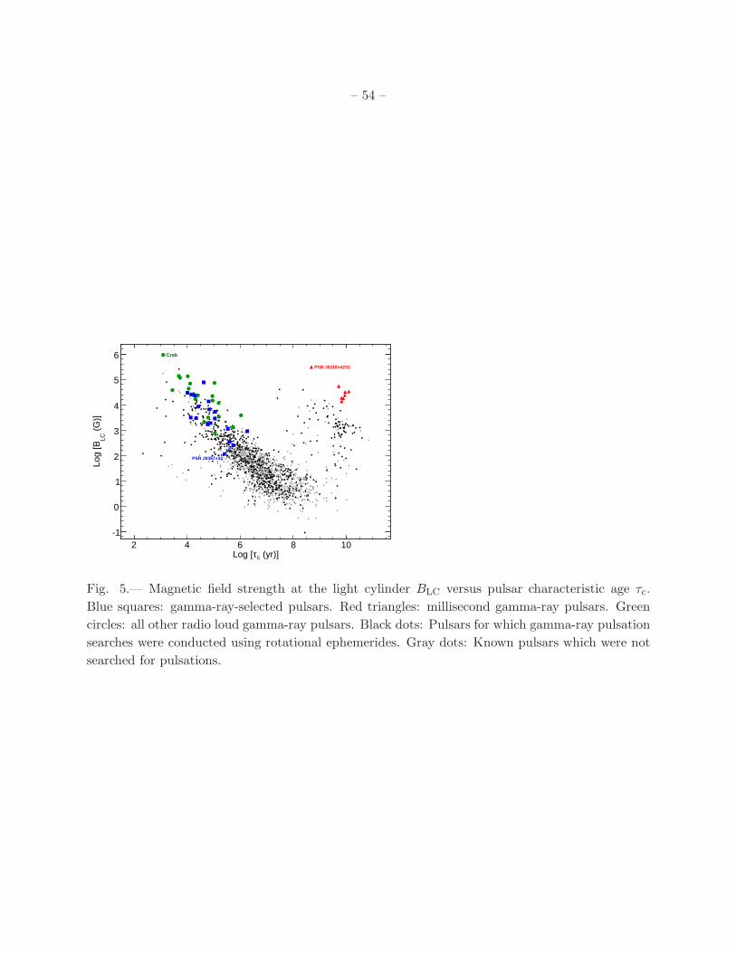
– 54 –

(yr)]cτLog [2 4 6 8 10

(G

)]LC

Log

[B

-1

0

1

2

3

4

5

6 Crab

PSR J0357+32

PSR J0218+4232

Fig. 5.— Magnetic field strength at the light cylinder BLC versus pulsar characteristic age τc.

Blue squares: gamma-ray-selected pulsars. Red triangles: millisecond gamma-ray pulsars. Green

circles: all other radio loud gamma-ray pulsars. Black dots: Pulsars for which gamma-ray pulsation

searches were conducted using rotational ephemerides. Gray dots: Known pulsars which were not

searched for pulsations.

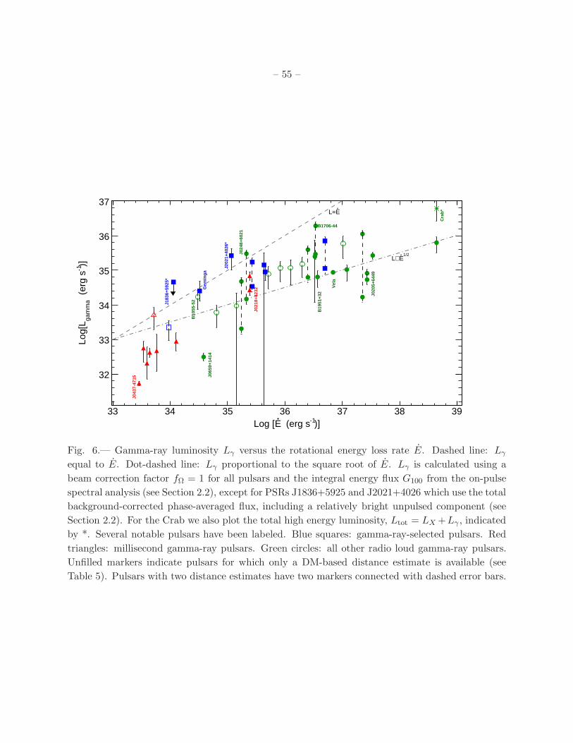
– 55 –

)]-1 (erg sELog [33 34 35 36 37 38 39

)]-1

(er

g s

gam

ma

Log[

L

32

33

34

35

36

37

J183

6+59

25*

Gem

ing

a

Vel

a

Cra

b*

B10

55-5

2

B19

51+3

2

B1706-44

J043

7-47

15

J021

8+42

32

J024

8+60

21

EL=

1/2E∝L

J202

1+40

26*

J065

9+14

14

J020

5+64

49

Fig. 6.— Gamma-ray luminosity Lγ versus the rotational energy loss rate E. Dashed line: Lγ

equal to E. Dot-dashed line: Lγ proportional to the square root of E. Lγ is calculated using a

beam correction factor fΩ = 1 for all pulsars and the integral energy flux G100 from the on-pulse

spectral analysis (see Section 2.2), except for PSRs J1836+5925 and J2021+4026 which use the total

background-corrected phase-averaged flux, including a relatively bright unpulsed component (see

Section 2.2). For the Crab we also plot the total high energy luminosity, Ltot = LX +Lγ , indicated

by *. Several notable pulsars have been labeled. Blue squares: gamma-ray-selected pulsars. Red

triangles: millisecond gamma-ray pulsars. Green circles: all other radio loud gamma-ray pulsars.

Unfilled markers indicate pulsars for which only a DM-based distance estimate is available (see

Table 5). Pulsars with two distance estimates have two markers connected with dashed error bars.

– 56 –

Fig. 7.— Value of the exponential cutoff Ecutoff versus the magnetic field at the light cylinder, BLC.

The statistical uncertainties on Ecutoff are shown. An additional systematic bias of (+20%, −10%)

may affect Ecutoff (see text). The histogram of Ecutoff values is projected along the right-hand axis.

Blue squares: gamma-ray-selected pulsars. Red triangles: millisecond gamma-ray pulsars. Green

circles: all other radio loud gamma-ray pulsars.

Fig. 8.— Photon index Γ versus the rotational energy loss rate, E. For Γ, the statistical uncertain-

ties combined with the systematic uncertainties due to the diffuse emission model are shown. An

additional systematic bias of (+0.3, −0.1) affects Γ (see text). The histogram of the photon indices

is projected along the right-hand axis. Blue squares: gamma-ray-selected pulsars. Red triangles:

millisecond gamma-ray pulsars. Green circles: all other radio loud gamma-ray pulsars.

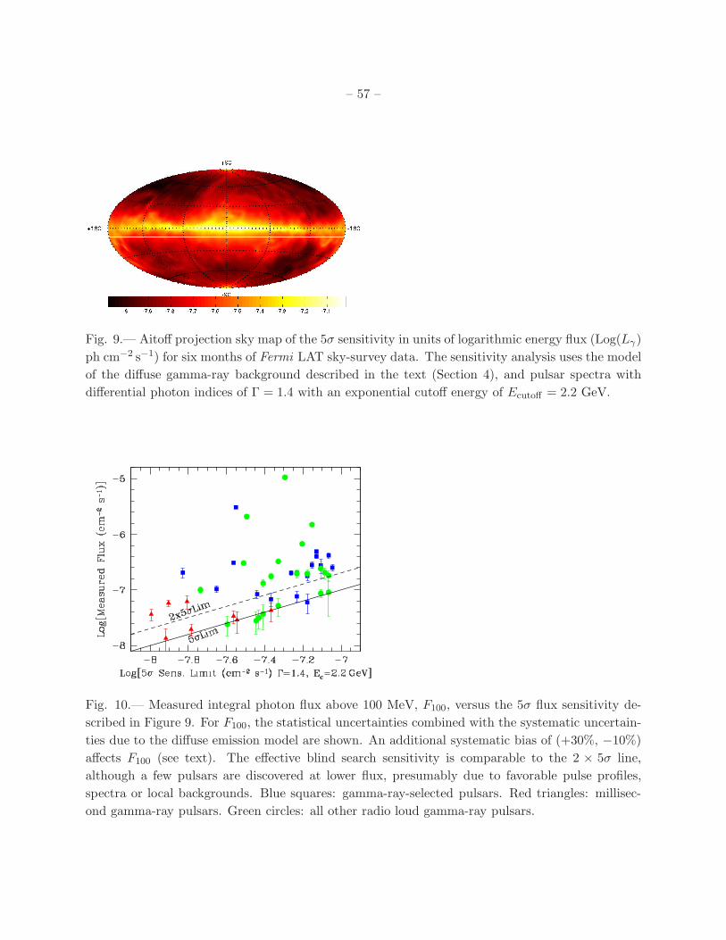
– 57 –

Fig. 9.— Aitoff projection sky map of the 5σ sensitivity in units of logarithmic energy flux (Log(Lγ)

ph cm−2 s−1) for six months of Fermi LAT sky-survey data. The sensitivity analysis uses the model

of the diffuse gamma-ray background described in the text (Section 4), and pulsar spectra with

differential photon indices of Γ = 1.4 with an exponential cutoff energy of Ecutoff = 2.2 GeV.

Fig. 10.— Measured integral photon flux above 100 MeV, F100, versus the 5σ flux sensitivity de-

scribed in Figure 9. For F100, the statistical uncertainties combined with the systematic uncertain-

ties due to the diffuse emission model are shown. An additional systematic bias of (+30%, −10%)

affects F100 (see text). The effective blind search sensitivity is comparable to the 2 × 5σ line,

although a few pulsars are discovered at lower flux, presumably due to favorable pulse profiles,

spectra or local backgrounds. Blue squares: gamma-ray-selected pulsars. Red triangles: millisec-

ond gamma-ray pulsars. Green circles: all other radio loud gamma-ray pulsars.

– 58 –

)-1 s-2Log Flux (ph cm-8 -7.5 -7 -6.5 -6 -5.5 -5 -4.5

Num

ber

with

Flu

x >

F

1

10

All gamma-ray psr

Radio selected

Gamma selected

Fig. 11.— Log N–Log S distribution as described in Section 4 for all the detected pulsars (black

dashed line), the radio-selected gamma-ray pulsars including MSPs (grey histogram), and the

gamma-ray-selected pulsars (blue hatched histogram).

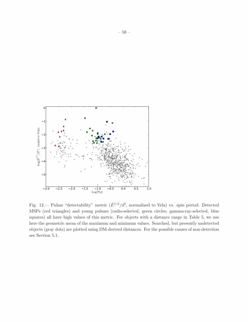
– 59 –

3.0 2.5 2.0 1.5 1.0 0.5 0.0 0.5 1.0Log[P(s)]

5

4

3

2

1

0

Log[E

1/2/D

2]

(sca

led

toVela)

Fig. 12.— Pulsar “detectability” metric (E1/2/d2, normalized to Vela) vs. spin period. Detected

MSPs (red triangles) and young pulsars (radio-selected, green circles; gamma-ray-selected, blue

squares) all have high values of this metric. For objects with a distance range in Table 5, we use

here the geometric mean of the maximum and minimum values. Searched, but presently undetected

objects (gray dots) are plotted using DM-derived distances. For the possible causes of non-detection

see Section 5.1.

– 60 –

Fig. 13.— Separations ∆ between the gamma-ray peaks, for those pulsars with two identified

peaks, versus the spin-down power E. The histogram of peak separations is projected along the

right-hand axis. Blue squares: gamma-ray-selected pulsars. Red triangles: millisecond gamma-ray

pulsars. Green circles: all other radio loud gamma-ray pulsars.

– 61 –

Appendix: Gamma-ray Pulsar Light Curves

–62

–

Co

un

ts

20

40

60

80

100

120

140

160>0.1 GeV J0007+7303

0 0.2 0.4 0.6 0.8 1 1.2 1.4 1.6 1.8 2

Co

un

ts

102030405060708090 >1.0 GeV

Co

un

ts

10

20304050607080

900.3−1.0 GeV

Pulsar Phase0 0.2 0.4 0.6 0.8 1 1.2 1.4 1.6 1.8 2

Co

un

ts

5

10

15

20

25

30

350.1−0.3 GeV

Fig. A-1.— Light curves for PSR J0007+7303 (P =

316 ms).

Co

un

ts

10

20

30

40

50

60

>0.1 GeV J0030+0451

0 0.2 0.4 0.6 0.8 1 1.2 1.4 1.6 1.8 2

Co

un

ts

5

10

15

20

25

30

35

>1.0 GeV

Co

un

ts

5

10

15

20

25 0.3−1.0 GeV

Co

un

ts2

4

6

8

10

12

140.1−0.3 GeV

Pulsar Phase0 0.2 0.4 0.6 0.8 1 1.2 1.4 1.6 1.8 2

Rad

io F

lux

(au

)

−0.20

0.20.40.60.8

1 Nancay 1.4 GHz

Fig. A-2.— Light curves for PSR J0030+0451 (P =

4.87 ms).

–63

–

Cou

nts

20

40

60

80

100 >0.1 GeV J0205+6449

0 0.2 0.4 0.6 0.8 1 1.2 1.4 1.6 1.8 2

Cou

nts

5

10

15

20

25

30

>1.0 GeV

Cou

nts

510

1520

2530

35

4045

0.3−1.0 GeV

Cou

nts

5

10

15

20

25

30

35 0.1−0.3 GeV

Pulsar Phase0 0.2 0.4 0.6 0.8 1 1.2 1.4 1.6 1.8 2

Rad

io F

lux

(au)

−0.20

0.20.40.60.8

1 GBT 2 GHz

Fig. A-3.— Light curves for PSR J0205+6449 (P =

65.7 ms).

Cou

nts

10

20

30

40

50>0.1 GeV J0218+4232

0 0.2 0.4 0.6 0.8 1 1.2 1.4 1.6 1.8 2

Cou

nts

2

4

6

8

10

12

>1.0 GeV

Cou

nts

5

10

15

20

25

30 0.3−1.0 GeV

Cou

nts

5

10

15

20

25 0.1−0.3 GeV

Pulsar Phase0 0.2 0.4 0.6 0.8 1 1.2 1.4 1.6 1.8 2

Rad

io F

lux

(au)

−0.20

0.20.40.60.8

1 Nancay 1.4 GHz

Fig. A-4.— Light curves for PSR J0218+4232 (P =

2.32 ms).

–64

–

Cou

nts

10

20

30

40

50

60

70

80>0.1 GeV J0248+6021

0 0.2 0.4 0.6 0.8 1 1.2 1.4 1.6 1.8 2

Cou

nts

5

10

15

20

25

30 >1.0 GeV

Cou

nts

5

10

15

20

25

30

35

40

45

0.3−1.0 GeV

Cou

nts

2468

10121416182022 0.1−0.3 GeV

Pulsar Phase0 0.2 0.4 0.6 0.8 1 1.2 1.4 1.6 1.8 2

Rad

io F

lux

(au)

00.20.40.60.8

1 Nancay 1.4 GHz

Fig. A-5.— Light curves for PSR J0248+6021 (P =

217 ms).

Cou

nts

20

40

60

80

100 >0.1 GeV J0357+32

0 0.2 0.4 0.6 0.8 1 1.2 1.4 1.6 1.8 2

Cou

nts

5

10

15

20

25 >1.0 GeV

Cou

nts

10

20

30

40

50

600.3−1.0 GeV

Pulsar Phase0 0.2 0.4 0.6 0.8 1 1.2 1.4 1.6 1.8 2

Cou

nts

5

10

15

20

25 0.1−0.3 GeV

Fig. A-6.— Light curves for PSR J0357+32 (P = 444 ms).

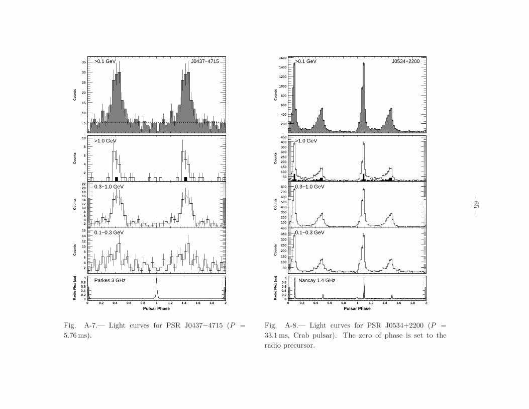
–65

–

Cou

nts

5

10

15

20

25

30

35 >0.1 GeV J0437−4715

0 0.2 0.4 0.6 0.8 1 1.2 1.4 1.6 1.8 2

Cou

nts

2

4

6

8

10>1.0 GeV

Cou

nts

2468

10121416182022

0.3−1.0 GeV

Cou

nts

2

4

6

8

10

12

14

16 0.1−0.3 GeV

Pulsar Phase0 0.2 0.4 0.6 0.8 1 1.2 1.4 1.6 1.8 2

Rad

io F

lux

(au)

00.20.40.60.8

1 Parkes 3 GHz

Fig. A-7.— Light curves for PSR J0437−4715 (P =

5.76 ms).

Cou

nts

200

400

600

800

1000

1200

1400

1600>0.1 GeV J0534+2200

0 0.2 0.4 0.6 0.8 1 1.2 1.4 1.6 1.8 2

Cou

nts

50100

150

200250

300350

400450

>1.0 GeV

Cou

nts

100

200

300

400

500

600

700

800 0.3−1.0 GeV

Cou

nts

50

100

150

200

250

300

350

4000.1−0.3 GeV

Pulsar Phase0 0.2 0.4 0.6 0.8 1 1.2 1.4 1.6 1.8 2

Rad

io F

lux

(au)

00.20.40.60.8

1 Nancay 1.4 GHz

Fig. A-8.— Light curves for PSR J0534+2200 (P =

33.1 ms, Crab pulsar). The zero of phase is set to the

radio precursor.

–66

–

Cou

nts

10

20

30

40

50

60

70

80 >0.1 GeV J0613−0200

0 0.2 0.4 0.6 0.8 1 1.2 1.4 1.6 1.8 2

Cou

nts

5

10

15

20

25

30 >1.0 GeV

Cou

nts

5

10

15

20

25

30

35

40 0.3−1.0 GeV

Cou

nts

2468

10121416182022 0.1−0.3 GeV

Pulsar Phase0 0.2 0.4 0.6 0.8 1 1.2 1.4 1.6 1.8 2

Rad

io F

lux

(au)

−0.20

0.20.40.60.8

1 Nancay 1.4 GHz

Fig. A-9.— Light curves for PSR J0613−0200 (P =

3.06 ms).

Cou

nts

10

20

30

40

50

60

70

80>0.1 GeV J0631+1036

0 0.2 0.4 0.6 0.8 1 1.2 1.4 1.6 1.8 2

Cou

nts

2468

101214161820

>1.0 GeV

Cou

nts

5

10

1520

25

30

35

4045

0.3−1.0 GeV

Cou

nts

5

10

15

20

25 0.1−0.3 GeV

Pulsar Phase0 0.2 0.4 0.6 0.8 1 1.2 1.4 1.6 1.8 2

Rad

io F

lux

(au)

00.20.40.60.8

1 Nancay 1.4 GHz

Fig. A-10.— Light curves for PSR J0631+1036 (P =

288 ms).

–67

–

Cou

nts

20

40

60

80

100

120

140>0.1 GeV J0633+0632

0 0.2 0.4 0.6 0.8 1 1.2 1.4 1.6 1.8 2

Cou

nts

10

20

30

40

50

60>1.0 GeV

Cou

nts

10203040

506070

8090

0.3−1.0 GeV

Pulsar Phase0 0.2 0.4 0.6 0.8 1 1.2 1.4 1.6 1.8 2

Cou

nts

5

10

15

20

25

30 0.1−0.3 GeV

Fig. A-11.— Light curves for PSR J0633+0632 (P =

297 ms).

Cou

nts

200

400

600

800

1000

1200

1400

1600

1800

2000

2200>0.1 GeV J0633+1746

0 0.2 0.4 0.6 0.8 1 1.2 1.4 1.6 1.8 2

Cou

nts

200

400

600

800

1000 >1.0 GeV

Cou

nts

200

400

600

800

1000 0.3−1.0 GeV

Pulsar Phase0 0.2 0.4 0.6 0.8 1 1.2 1.4 1.6 1.8 2

Cou

nts

20406080

100120140160180200 0.1−0.3 GeV

Fig. A-12.— Light curves for PSR J0633+1746 (P =

237 ms, Geminga pulsar).

–68

–

Cou

nts

10

20

30

40

50

60>0.1 GeV J0659+1414

0 0.2 0.4 0.6 0.8 1 1.2 1.4 1.6 1.8 2

Cou

nts

1

2

3

4

5

6

7

8 >1.0 GeV

Cou

nts

5

10

15

20

25

30

350.3−1.0 GeV

Cou

nts

5

10

15

20

25

30 0.1−0.3 GeV

Pulsar Phase0 0.2 0.4 0.6 0.8 1 1.2 1.4 1.6 1.8 2

Rad

io F

lux

(au)

0.20.40.60.8

1Nancay 1.4 GHz

Fig. A-13.— Light curves for PSR J0659+1414 (P =

385 ms).

Cou

nts

10

20

30

40

50

60

70>0.1 GeV J0742−2822

0 0.2 0.4 0.6 0.8 1 1.2 1.4 1.6 1.8 2

Cou

nts

2

4

6

8

10

12>1.0 GeV

Cou

nts

5101520253035404550

0.3−1.0 GeV

Cou

nts

5

10

15

20

25 0.1−0.3 GeV

Pulsar Phase0 0.2 0.4 0.6 0.8 1 1.2 1.4 1.6 1.8 2

Rad

io F

lux

(au)

00.20.40.60.8

1 Nancay 1.4 GHz

Fig. A-14.— Light curves for PSR J0742−2822 (P =

167 ms).

–69

–

Cou

nts

5

10

15

20

25 >0.1 GeV J0751+1807

0 0.2 0.4 0.6 0.8 1 1.2 1.4 1.6 1.8 2

Cou

nts

123456789 >1.0 GeV

Cou

nts

2

4

6

8

10

12

14 0.3−1.0 GeV

Cou

nts

2

4

6

8

10 0.1−0.3 GeV

Pulsar Phase0 0.2 0.4 0.6 0.8 1 1.2 1.4 1.6 1.8 2

Rad

io F

lux

(au)

00.20.40.60.8

1 Nancay 1.4 GHz

Fig. A-15.— Light curves for PSR J0751+1807 (P =

3.48 ms).

Cou

nts

1000

2000

3000

4000

5000

6000 >0.1 GeV J0835−4510

0 0.2 0.4 0.6 0.8 1 1.2 1.4 1.6 1.8 2

Cou

nts

200400600800

100012001400160018002000

>1.0 GeV

Cou

nts

500

1000

1500

2000

2500

3000 0.3−1.0 GeV

Cou

nts

200

400

600

800

1000

1200 0.1−0.3 GeV

Pulsar Phase0 0.2 0.4 0.6 0.8 1 1.2 1.4 1.6 1.8 2

Rad

io F

lux

(au)

00.20.40.60.8

1 Parkes 1.4 GHz

Fig. A-16.— Light curves for PSR J0835−4510 (P =

89.3 ms, Vela pulsar).

–70

–

Cou

nts

20

40

60

80

100

120

140

160 >0.1 GeV J1028−5820

0 0.2 0.4 0.6 0.8 1 1.2 1.4 1.6 1.8 2

Cou

nts

10

20

30

40

50 >1.0 GeV

Cou

nts

102030405060708090 0.3−1.0 GeV

Cou

nts

5

10

15

20

25

30

35

400.1−0.3 GeV

Pulsar Phase0 0.2 0.4 0.6 0.8 1 1.2 1.4 1.6 1.8 2

Rad

io F

lux

(au)

00.20.40.60.8

1 Parkes 1.4 GHz

Fig. A-17.— Light curves for PSR J1028−5819 (P =

91.4 ms).

Cou

nts

20

40

60

80

100

120

140

160

180

200

220 >0.1 GeV J1048−5832

0 0.2 0.4 0.6 0.8 1 1.2 1.4 1.6 1.8 2

Cou

nts

10

20

30

40

50

60 >1.0 GeV

Cou

nts

20

40

60

80

100

120 0.3−1.0 GeV

Cou

nts

51015202530354045 0.1−0.3 GeV

Pulsar Phase0 0.2 0.4 0.6 0.8 1 1.2 1.4 1.6 1.8 2

Rad

io F

lux

(au)

00.20.40.60.8

1 Parkes 1.4 GHz

Fig. A-18.— Light curves for PSR J1048−5832 (P =

124 ms).

–71

–

Cou

nts

50

100

150

200

250>0.1 GeV J1057−5226

0 0.2 0.4 0.6 0.8 1 1.2 1.4 1.6 1.8 2

Cou

nts

10

20

30

40

50

60

70

80

90>1.0 GeV

Cou

nts

20

40

60

80

100

120

140 0.3−1.0 GeV

Cou

nts

10

20

30

40

50

600.1−0.3 GeV

Pulsar Phase0 0.2 0.4 0.6 0.8 1 1.2 1.4 1.6 1.8 2

Rad

io F

lux

(au)

00.20.40.60.8

1 Parkes 1.4 GHz

Fig. A-19.— Light curves for PSR J1057−5226 (P =

197 ms, PSR B1055−52).

Cou

nts

20

40

60

80

100

>0.1 GeV J1124−5916

0 0.2 0.4 0.6 0.8 1 1.2 1.4 1.6 1.8 2

Cou

nts

2468

10121416182022 >1.0 GeV

Cou

nts

10

20

30

40

50

60

70

0.3−1.0 GeV

Cou

nts

5

10

15

20

25

30

35

0.1−0.3 GeV

Pulsar Phase0 0.2 0.4 0.6 0.8 1 1.2 1.4 1.6 1.8 2

Rad

io F

lux

(au)

−0.20

0.20.40.60.8

1 Parkes 1.4 GHz

Fig. A-20.— Light curves for PSR J1124−5916 (P =

135 ms).

–72

–

Cou

nts

50

100

150

200

250

300

350

400

450>0.1 GeV J1418−6058

0 0.2 0.4 0.6 0.8 1 1.2 1.4 1.6 1.8 2

Cou

nts

102030405060708090 >1.0 GeV

Cou

nts

50

100

150

200

250

3000.3−1.0 GeV

Pulsar Phase0 0.2 0.4 0.6 0.8 1 1.2 1.4 1.6 1.8 2

Cou

nts

20

40

60

80

100

120 0.1−0.3 GeV

Fig. A-21.— Light curves for PSR J1418−6058 (P =

111 ms).

Cou

nts

20

40

60

80

100

120

140

160>0.1 GeV J1420−6048

0 0.2 0.4 0.6 0.8 1 1.2 1.4 1.6 1.8 2

Cou

nts

10

20

30

40

50

60

70>1.0 GeV

Cou

nts

10

20

30

40

50

60

70

80 0.3−1.0 GeV

Cou

nts

5

10

15

20

25

30

35 0.1−0.3 GeV

Pulsar Phase0 0.2 0.4 0.6 0.8 1 1.2 1.4 1.6 1.8 2

Rad

io F

lux

(au)

−0.20

0.20.40.60.8

1 Parkes 1.4 GHz

Fig. A-22.— Light curves for PSR J1420−6048 (P =

68.2 ms).

–73

–

Cou

nts

20

40

60

80

100

120

140

160

180 >0.1 GeV J1459−60

0 0.2 0.4 0.6 0.8 1 1.2 1.4 1.6 1.8 2

Cou

nts

5

10

15

20

25 >1.0 GeV

Cou

nts

20

40

60

80

100 0.3−1.0 GeV

Pulsar Phase0 0.2 0.4 0.6 0.8 1 1.2 1.4 1.6 1.8 2

Cou

nts

10

20

30

40

50

60

70 0.1−0.3 GeV

Fig. A-23.— Light curves for PSR J1459−60 (P =

103 ms).

Cou

nts

20

40

60

80

100 >0.1 GeV J1509−5850

0 0.2 0.4 0.6 0.8 1 1.2 1.4 1.6 1.8 2

Cou

nts

5

10

15

20

25

30

35

40 >1.0 GeV

Cou

nts

10

20

30

40

50 0.3−1.0 GeV

Cou

nts

5

10

15

20

25

300.1−0.3 GeV

Pulsar Phase0 0.2 0.4 0.6 0.8 1 1.2 1.4 1.6 1.8 2

Rad

io F

lux

(au)

−0.4−0.2

00.20.40.60.8

1 Parkes 1.4 GHz

Fig. A-24.— Light curves for PSR J1509−5850 (P =

88.9 ms).

–74

–

Cou

nts

5

10

15

20

25

30

35 >0.1 GeV J1614−2230

0 0.2 0.4 0.6 0.8 1 1.2 1.4 1.6 1.8 2

Cou

nts

2468

1012141618202224

>1.0 GeV

Cou

nts

2

4

6

8

10

120.3−1.0 GeV

Cou

nts

1

2

3

4

5

6

7 0.1−0.3 GeV

Pulsar Phase0 0.2 0.4 0.6 0.8 1 1.2 1.4 1.6 1.8 2

Rad

io F

lux

(au)

00.20.40.60.8

1 GBT 2 GHz

Fig. A-25.— Light curves for PSR J1614−2230 (P =

3.15 ms).

Cou

nts

50

100

150

200

250

300

350

400

450>0.1 GeV J1709−4429

0 0.2 0.4 0.6 0.8 1 1.2 1.4 1.6 1.8 2

Cou

nts

20

40

60

80

100

120

140

160 >1.0 GeV

Cou

nts

50

100

150

200

2500.3−1.0 GeV

Cou

nts

1020

30

4050

6070

8090

0.1−0.3 GeV

Pulsar Phase0 0.2 0.4 0.6 0.8 1 1.2 1.4 1.6 1.8 2

Rad

io F

lux

(au)

00.20.40.60.8

1 Parkes 1.4 GHz

Fig. A-26.— Light curves for PSR J1709−4429 (P =

102 ms, PSR B1706−44).

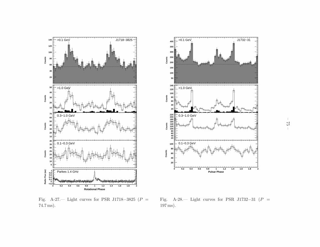
–75

–

Cou

nts

20

40

60

80

100

120

140 >0.1 GeV J1718−3825

0 0.2 0.4 0.6 0.8 1 1.2 1.4 1.6 1.8 2

Cou

nts

10

20

30

40

50 >1.0 GeV

Cou

nts

10

20

30

40

50

60

700.3−1.0 GeV

Cou

nts

5

10

15

20

25

30

35

400.1−0.3 GeV

Rotational Phase0 0.2 0.4 0.6 0.8 1 1.2 1.4 1.6 1.8 2

Rad

io F

lux

(au)

−0.20

0.20.40.60.8

1 Parkes 1.4 GHz

Fig. A-27.— Light curves for PSR J1718−3825 (P =

74.7 ms).

Cou

nts

50

100

150

200

250

300

350

400 >0.1 GeV J1732−31

0 0.2 0.4 0.6 0.8 1 1.2 1.4 1.6 1.8 2

Cou

nts

20

40

60

80

100

120

140>1.0 GeV

Cou

nts

20406080

100120140160180200220 0.3−1.0 GeV

Pulsar Phase0 0.2 0.4 0.6 0.8 1 1.2 1.4 1.6 1.8 2

Cou

nts

20

40

60

80

100 0.1−0.3 GeV

Fig. A-28.— Light curves for PSR J1732−31 (P =

197 ms).

–76

–

Cou

nts

20

40

60

80

100

120

140

160 >0.1 GeV J1741−2054

0 0.2 0.4 0.6 0.8 1 1.2 1.4 1.6 1.8 2

Cou

nts

5

10

15

20

25

30

35

40>1.0 GeV

Cou

nts

20

40

60

80

100 0.3−1.0 GeV

Cou

nts

10

20

30

40

50

60

70

0.1−0.3 GeV

Pulsar Phase0 0.2 0.4 0.6 0.8 1 1.2 1.4 1.6 1.8 2

Rad

io F

lux

(au)

−0.20

0.20.40.60.8

1 GBT 2 GHz

Fig. A-29.— Light curves for PSR J1741−2054 (P =

414 ms). While this pulsar is detected in the radio

(Camilo et al. 2009b), it was discovered by the LAT and

is considered a gamma-ray-selected pulsar.

Cou

nts

10

20

30

40

50

60

70

80

90 >0.1 GeV J1744−1134

0 0.2 0.4 0.6 0.8 1 1.2 1.4 1.6 1.8 2

Cou

nts

2

4

6

8

10

12 >1.0 GeV

Cou

nts

10

20

30

40

500.3−1.0 GeV

Cou

nts

5

101520253035

4045

0.1−0.3 GeV

Pulsar Phase0 0.2 0.4 0.6 0.8 1 1.2 1.4 1.6 1.8 2

Rad

io F

lux

(au)

00.20.40.60.8

1 Nancay 1.4 GHz

Fig. A-30.— Light curves for PSR J1744−1134 (P =

4.08 ms).

–77

–

Cou

nts

20

40

60

80

100>0.1 GeV J1747−2958

0 0.2 0.4 0.6 0.8 1 1.2 1.4 1.6 1.8 2

Cou

nts

5

10

15

20

25

30 >1.0 GeV

Cou

nts

10

20

30

40

50

60 0.3−1.0 GeV

Cou

nts

5

10

15

20

25

30 0.1−0.3 GeV

Pulsar Phase0 0.2 0.4 0.6 0.8 1 1.2 1.4 1.6 1.8 2

Rad

io F

lux

(au)

−0.20

0.20.40.60.8

1 GBT 2 GHz

Fig. A-31.— Light curves for PSR J1747−2958 (P =

98.8 ms).

Cou

nts

50

100

150

200

250

300>0.1 GeV J1809−2332

0 0.2 0.4 0.6 0.8 1 1.2 1.4 1.6 1.8 2

Cou

nts

20

40

60

80

100>1.0 GeV

Cou

nts

2040

60

80100

120140

160180

0.3−1.0 GeV

Pulsar Phase0 0.2 0.4 0.6 0.8 1 1.2 1.4 1.6 1.8 2

Cou

nts

10

2030

40

50

60

70

800.1−0.3 GeV

Fig. A-32.— Light curves for PSR J1809−2332 (P =

147 ms).

–78

–

Cou

nts

50

100

150

200

250

300 >0.1 GeV J1813−1246

0 0.2 0.4 0.6 0.8 1 1.2 1.4 1.6 1.8 2

Cou

nts

10

20

30

40

50 >1.0 GeV

Cou

nts

20406080

100120140160180 0.3−1.0 GeV

Pulsar Phase0 0.2 0.4 0.6 0.8 1 1.2 1.4 1.6 1.8 2

Cou

nts

20

40

60

80

100

120 0.1−0.3 GeV

Fig. A-33.— Light curves for PSR J1813−1246 (P =

48.1 ms).

Cou

nts

50

100

150

200

250

300

350

400>0.1 GeV J1826−1256

0 0.2 0.4 0.6 0.8 1 1.2 1.4 1.6 1.8 2

Cou

nts

20

40

60

80

100 >1.0 GeV

Cou

nts

20406080

100120140160180200220 0.3−1.0 GeV

Pulsar Phase0 0.2 0.4 0.6 0.8 1 1.2 1.4 1.6 1.8 2

Cou

nts

20

40

60

80

100 0.1−0.3 GeV

Fig. A-34.— Light curves for PSR J1826−1256 (P =

110 ms).

–79

–

Cou

nts

50

100

150

200

250 >0.1 GeV J1833−1034

0 0.2 0.4 0.6 0.8 1 1.2 1.4 1.6 1.8 2

Cou

nts

5

1015

20

2530

3540

45>1.0 GeV

Cou

nts

20

40

60

80

100

120 0.3−1.0 GeV

Cou

nts

10

20

30

40

50

60

70

80 0.1−0.3 GeV

Pulsar Phase0 0.2 0.4 0.6 0.8 1 1.2 1.4 1.6 1.8 2

Rad

io F

lux

(au)

00.20.40.60.8

1 GBT 0.8 GHz

Fig. A-35.— Light curves for PSR J1833−1034 (P =

61.9 ms).

Cou

nts

50

100

150

200

250

300

>0.1 GeV J1836+5925

0 0.2 0.4 0.6 0.8 1 1.2 1.4 1.6 1.8 2

Cou

nts

20

40

60

80

100

120

140 >1.0 GeV

Cou

nts

20

40

60

80

100

120

140

160 0.3−1.0 GeV

Pulsar Phase0 0.2 0.4 0.6 0.8 1 1.2 1.4 1.6 1.8 2

Cou

nts

10

20

30

40

50

600.1−0.3 GeV

Fig. A-36.— Light curves for PSR J1836+5925 (P =

173 ms).

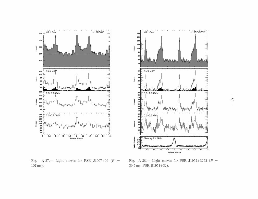
–80

–

Cou

nts

100

200

300

400

500>0.1 GeV J1907+06

0 0.2 0.4 0.6 0.8 1 1.2 1.4 1.6 1.8 2

Cou

nts

20

40

60

80

100

120 >1.0 GeV

Cou

nts

50

100

150

200

250

3000.3−1.0 GeV

Pulsar Phase0 0.2 0.4 0.6 0.8 1 1.2 1.4 1.6 1.8 2

Cou

nts

20406080

100120140160180 0.1−0.3 GeV

Fig. A-37.— Light curves for PSR J1907+06 (P =

107 ms).

Cou

nts

20

40

60

80

100

120

140

160

180 >0.1 GeV J1952+3252

0 0.2 0.4 0.6 0.8 1 1.2 1.4 1.6 1.8 2

Cou

nts

10

20

30

40

50

60 >1.0 GeV

Cou

nts

102030405060708090 0.3−1.0 GeV

Cou

nts

5

10

15

20

25

30

35

400.1−0.3 GeV

Pulsar Phase0 0.2 0.4 0.6 0.8 1 1.2 1.4 1.6 1.8 2

Rad

io F

lux

(au)

−0.20

0.20.40.60.8

1 Nancay 1.4 GHz

Fig. A-38.— Light curves for PSR J1952+3252 (P =

39.5 ms, PSR B1951+32).

–81

–

Cou

nts

50

100

150

200

250 >0.1 GeV J1958+2846

0 0.2 0.4 0.6 0.8 1 1.2 1.4 1.6 1.8 2

Cou

nts

10

20

30

40

50

60 >1.0 GeV

Cou

nts

20

40

60

80

100

120

140

160 0.3−1.0 GeV

Pulsar Phase0 0.2 0.4 0.6 0.8 1 1.2 1.4 1.6 1.8 2

Cou

nts

10

20

30

40

50

60

70 0.1−0.3 GeV

Fig. A-39.— Light curves for PSR J1958+2846 (P =

290 ms).

Cou

nts

100

200

300

400

500

600

>0.1 GeV J2021+3651

0 0.2 0.4 0.6 0.8 1 1.2 1.4 1.6 1.8 2

Cou

nts

2040

6080

100120140160180

>1.0 GeV

Cou

nts

50

100

150

200

250

300

350

4000.3−1.0 GeV

Cou

nts

20

40

60

80

100

120

140 0.1−0.3 GeV

Pulsar Phase0 0.2 0.4 0.6 0.8 1 1.2 1.4 1.6 1.8 2

Rad

io F

lux

(au)

00.20.40.60.8

1 GBT 2 GHz

Fig. A-40.— Light curves for PSR J2021+3651 (P =

104 ms).

–82

–

Cou

nts

50

100

150

200

250

300 >0.1 GeV J2021+4026

0 0.2 0.4 0.6 0.8 1 1.2 1.4 1.6 1.8 2

Cou

nts

20

40

60

80

100

120 >1.0 GeV

Cou

nts

20

40

60

80

100

120

140 0.3−1.0 GeV

Pulsar Phase0 0.2 0.4 0.6 0.8 1 1.2 1.4 1.6 1.8 2

Cou

nts

10

20

30

40

50 0.1−0.3 GeV

Fig. A-41.— Light curves for PSR J2021+4026 (P =

265 ms).

Cou

nts

20

40

60

80

100

120

140

160

180

200

220>0.1 GeV J2032+4127

0 0.2 0.4 0.6 0.8 1 1.2 1.4 1.6 1.8 2

Cou

nts

20

40

60

80

100 >1.0 GeV

Cou

nts

10

20

30

40

50

60

70

80 0.3−1.0 GeV

Cou

nts

5

10

15

20

25

30

35

400.1−0.3 GeV

Pulsar Phase0 0.2 0.4 0.6 0.8 1 1.2 1.4 1.6 1.8 2

Rad

io F

lux

(au)

00.20.40.60.8

1 GBT 2 GHz

Fig. A-42.— Light curves for PSR J2032+4127 (P =

143 ms). While this pulsar is detected in the radio

(Camilo et al. 2009b), it was discovered by the LAT and

is considered a gamma-ray-selected pulsar.

–83

–

Cou

nts

10

20

30

40

50

60>0.1 GeV J2043+2740

0 0.2 0.4 0.6 0.8 1 1.2 1.4 1.6 1.8 2

Cou

nts

2

4

6

8

10

12

14

16>1.0 GeV

Cou

nts

5

10

15

20

25

300.3−1.0 GeV

Cou

nts

5

10

15

20

250.1−0.3 GeV

Pulsar Phase0 0.2 0.4 0.6 0.8 1 1.2 1.4 1.6 1.8 2

Rad

io F

lux

(au)

00.20.40.60.8

1 Nancay 1.4 GHz

Fig. A-43.— Light curves for PSR J2043+2740 (P =

96.1 ms).

Cou

nts

5

10

15

20

25

30

35

40

45 >0.1 GeV J2124−3358

0 0.2 0.4 0.6 0.8 1 1.2 1.4 1.6 1.8 2

Cou

nts

2468

101214161820 >1.0 GeV

Cou

nts

2468

1012141618

0.3−1.0 GeV

Cou

nts

2

4

6

8

10

12 0.1−0.3 GeV

Pulsar Phase0 0.2 0.4 0.6 0.8 1 1.2 1.4 1.6 1.8 2

Rad

io F

lux

(au)

−0.20

0.20.40.60.8

1 Nancay 1.4 GHz

Fig. A-44.— Light curves for PSR J2124−3358 (P =

4.93 ms).

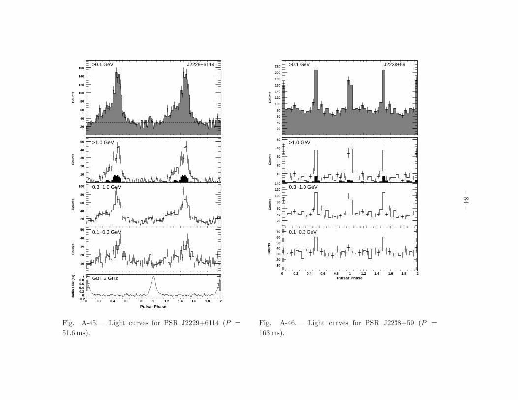
–84

–

Cou

nts

20

40

60

80

100

120

140

160>0.1 GeV J2229+6114

0 0.2 0.4 0.6 0.8 1 1.2 1.4 1.6 1.8 2

Cou

nts

10

20

30

40

50 >1.0 GeV

Cou

nts

20

40

60

80

100 0.3−1.0 GeV

Cou

nts

10

20

30

40

500.1−0.3 GeV

Pulsar Phase0 0.2 0.4 0.6 0.8 1 1.2 1.4 1.6 1.8 2

Rad

io F

lux

(au)

−0.20

0.20.40.60.8

1 GBT 2 GHz

Fig. A-45.— Light curves for PSR J2229+6114 (P =

51.6 ms).

Cou

nts

20

40

60

80

100

120

140

160

180

200

220 >0.1 GeV J2238+59

0 0.2 0.4 0.6 0.8 1 1.2 1.4 1.6 1.8 2

Cou

nts

10

20

30

40

50>1.0 GeV

Cou

nts

20

40

60

80

100

120

1400.3−1.0 GeV

Pulsar Phase0 0.2 0.4 0.6 0.8 1 1.2 1.4 1.6 1.8 2

Cou

nts

10

20

30

40

50

60

70 0.1−0.3 GeV

Fig. A-46.— Light curves for PSR J2238+59 (P =

163 ms).