the fluorescence transient as a tool to characterize … · chapter 25the fluorescence transient as...

The fluorescence transient as a tool to characterize and screen photosynthetic samples 445Chapter 25

The fluorescence transient as a tool tocharacterize and screen photosyntheticsamples

R.J. Strasser, A. Srivastava and M. Tsimilli-Michael

Introduction

Photosynthesis is the process by which plants, algae, cyanobacteria and photosyntheticbacteria convert radiant energy into a chemically stable form. The pathway of thisenergy transduction is complex, involving several physical and chemical mechanismsand many components. The process is initiated when light is absorbed by the antennamolecules within the photosynthetic membrane. The absorbed energy is transferred asexcitation energy and is either trapped at a reaction centre and used to do chemicallyuseful work, or dissipated mainly as heat and less as emitted radiation – fluorescence.The features of the emitted fluorescence are basically determined by the absorbingpigments, the excitation energy transfer, and the nature and orientation of the fluorescingpigments. However, fluorescence is also affected by the redox state of the reactioncenters and of the donors and acceptors of PSII, and is moreover sensitive to a widevariety of photosynthetic events, e.g., proton translocation, thylakoid stacking andunstacking, ionic strength, and the midpoint potential of cyt b-559, to name a few.Although the effect of each factor on fluorescence is often indirect and they are noteasily quantified and distinguished from one another, fluorescence measurements havebeen successfully used to monitor and characterize a wide variety of photosyntheticevents.

The first significant realization of the relationship between primary reactions ofphotosynthesis and Chl a fluorescence came from Kautsky and Hirsh (1931). Theywere the first to report that, upon illumination of a dark adapted photosynthetic sample,the Chl a fluorescence emission is not constant but exhibits a fast rise to a maximumfollowed by a decline to reach finally, in a range of some minutes, a steady level. Theypostulated that the rising phase of this transient, found to be unaffected by temperaturechanges (up to 30ºC) and the presence of poison (potassium cyanide), reflects theprimary reactions of photosynthesis. They further showed that the declining phase ofthe fluorescence transient is correlated with an increase in the CO2 assimilation.

Since this first report, which is a landmark in the history of photosynthesis research,our knowledge on the relationship between primary reactions of photosynthesis andChl a fluorescence has increased tremendously, as this aspect attracted the interest ofmany research groups due to its significance for basic biophysical research as well asapplied research. During these decades the investigations became more and morethorough utilizing also the advancement in instrumentation, and the number ofpublications on this topic has rapidly increased. For reviews on Chl a fluorescence,readers may consult, among others, the following: Rabinowitch (1951), Wassink (1951),

446 Probing photosynthesis

Govindjee et al. (1967), Goedheer (1972), Papageorgiou (1975), Lavorel and Etienne(1977), Butler (1978), Govindjee and Jursinic (1979), several chapters in Govindjee etal. (1986), Govindjee and Wasielewski (1989), several chapters in Lichtenthaler (1988),Holzwarth (1991), Karukstis (1991), Krause and Weis (1991), Dau (1994a,b), Govindjee(1995), Joshi and Mohanty (1995), Schreiber et al. (1995), Sauer and Debreczeny(1996), Owens (1996) and Strasser et al. (1997).

This chapter is not a general review on Chl a fluorescence and is not written forspecialists in the field of fluorescence. It rather aims to give a general introduction tonon-specialists about the Chl a fluorescence kinetics and how their analysis and inter-pretation can provide information about the photosynthetic capacity and the vitalityof the plant material. Furthermore, this chapter describes analytically a real screeningprocedure by which the fluorescence transient, easily measured with handy, commerciallyavailable, instruments, is analysed providing a description of the dynamic capacities ofthe photosynthetic sample. This procedure satisfies the demand for rapid, non-invasivescreening tests, and can be thus easily applied to approach also questions of commercialor economical interest concerning the physiological condition of plants.

The fluorescence transient

A typical fluorescence transient, exhibited upon illumination of a dark-adapted photo-synthetic sample by saturating light, is shown in Figure 25.1. The same transient ispresented here on different time scales. It is clearly demonstrated that on a logarithmictime scale the full transient from 50 µs to many minutes can be presented in one graph,revealing both the fast polyphasic rise from F0 to FP (where FP = FM under saturatingexcitation light) and the subsequent slower decline from FP to a steady state FS. Thefluorometer here used, a PEA (Plant Efficiency Analyser from Hansatech), has a hightime resolution (10 µs) and a data acquisition capacity over several orders of magnitude(Strasser et al., 1995). With an instrument of lower time resolution the shape of thefast rise of this transient would not reveal the steps 0-J-I-P so clearly.

Not only dark-adapted samples upon illumination, but also light-adapted samples,upon any change of the quality (Strasser, 1985) or the intensity (Srivastava et al., 1995)of the light they are exposed to, exhibit a fluorescence transient which levels off at anew steady state. More generally, under natural in vivo conditions, the fluorescencebehaviour of any photosynthetic system changes continuously following its adaptationto a perpetually changing environment (Srivastava et al., 1995).

Based on several observations, we can conclude that, at a given moment, the shapeof the fluorescence transient of any sample is determined by the physiological state ofthe sample at that moment and the physical and chemical environmental conditionsaround the sample. It must also be pointed out that the actual physiological state of asample at a given moment is a function of all the states the sample went through in thepast (Strasser, 1985; Krüger et al., 1997).

Scenario for a practical application of the fluorescence transient

Based on the general conclusions stated above, the fluorescence transient becomes apotential tool for several basic and applied projects. Four basic groups of questions thatsuch projects could aim to tackle are presented in Table 25.1. Examples for each groupare:

The fluorescence transient as a tool to characterize and screen photosynthetic samples 447

I A well-defined plant material is used under well-defined physical conditions toanalyse its response to chemical changes in the environment (chemical stress). Severalexperiments can be designed in the laboratory, using, e.g., inhibitors, fertilizers,gases like CO2, O2, O3 or any other chemical stressor.

II A well-defined plant material is used to analyse its response to changes of physicalparameters of the environment (physical stress), e.g., light quality and intensity,

6

4

2

0

6

4

2

0

6

4

2

0

6

4

2

0

0 50 100 150 200

0 5 10 0 0.5 1.0

0 0.05 0.1 0 0.005 0.01

10–5 10–4 10–3 10–2 10–1 100 101 102 103

Time (second)

0

J

IP

StFmax

F300µs

FJ

F0F0

FJ

FI

dArea

F0

FJ

FI

FM FM

FI

F0

FJ

F0

FJ

FI

FM

0 0.001

2

0

F0

FS

Chl

a F

luor

esce

nce

inte

nsity

(re

l.)

Figure 25.1 A typical fluorescence transient exhibited upon illumination of a dark-adaptedphotosynthetic sample by saturating light. The transient is presented on different time scales.


temperature, etc. (Srivastava and Strasser, 1996; Srivastava et al., 1997).III A well-defined plant material is used to analyse its response to a combination of

chemical and physical stress. The synergism and antagonism of the physical andchemical co-stress can be studied (Ouzounidou et al., 1997).

IV Biosensing: under well-defined experimental conditions fluorescence tests areelaborated (a) to describe a system (plant or ecosystem) in terms of, e.g., (i) vitality,(ii) productivity, (iii) sensitivity and resistance to stress; (b) to study the structure –function relationship in transgenic plants; (c) to investigate the ecodynamics ofcomplex systems, like trees, horticulture, forests and even whole ecosystems (VanRensburg et al., 1996; Srivasta and Strasser, 1997).

The above examples give only an indication of the wide diversity in addressing possiblequestions and designing the appropriate experiments. Further applications of interestcan be enumerated:

• Testing of productivity in agriculture as a function of:

– style of culture (sustainable agriculture etc.)– regulator (herbicides, pesticides, hormones etc.)– selection of cultivar (transgenic etc.)– drought, heat, cold, light, salt stress etc.

• Testing of the behaviour of a commercialized product. Freshness, taste, colour andconsistency of vegetables, flowers and fruits as a function of storage and homeconditions; moreover, the decision for the optimal moment for such products tobe put on the shelves in the supermarket can be made by utilizing the fluorescencetechniques.

• Testing greenhouse conditions concerning light, temperature etc.; economicoptimization.

• Testing the formation and ripening of fruits from the flower to the commercialproduct by means of residual chlorophyll fluorescence.

• Testing environmental conditions influenced by pollution.• Testing the behaviour of ecosystems upon global changes (e.g. of CO2, O3,

temperature, volatile organic compounds, UV).

Table 25.1 Four basic groups of questions that can be tackled through a practical application of thefluorescence transient.

Plants Test conditions (1) Test conditions (2) Test signals

The physical and The physical The chemical Fluorescence transientchemical conditions conditions in the conditions in the as a tool to analyse theduring the culture of environment during environment during following groups of

the samples the fluorescence test the fluorescence test questions

constant constant variable Iconstant variable constant IIconstant variable variable IIIvariable constant constant IV


Requirements for a useful fluorescence test

Anyone who goes into a forest with good ideas, created in the laboratory in order toanalyse a tree, recognizes that it does not take long before many problems, which werenot predictable, become apparent. Whatever the tree is, a sample has to be selectedfirst. There is no such problem in the laboratory, as nice, homogeneous material can begrown there. But standing in front of a tree we have to take many subjective decisionsconcerning which leaf or branch to choose, since every type of leaf material, fromgreen to brown, with or without parasites, may be found on every tree. The choicebecomes even more complicated when dealing with an ecosystem.

The answer is that many samples have to be chosen. However, measuring all thesemany samples takes a lot of time during which the samples may change their behaviourdue at least to diurnal changes. Therefore, a fast screening procedure is needed toprovide an overall picture of the vitality and the fitness of the samples. Deviation fromnormality can then be localized so that eventually the time-consuming more specificand accurate investigations can be done. For such a fast screening procedure, a singlemeasurement must take not more than 20 seconds, so that 100 or more samples can bemeasured per working hour. The instrument has to be lightweight and the batterieshave to hold many hours in the field under any weather conditions. It should also beeasily handled so that even non-specialists can collect and store the data.

There is not a big choice of instruments and assays fulfilling these requirements. Wehave chosen the portable fluorometer PEA (Plant Efficiency Analyser, built by Hansatech,King’s Lynn, UK) by which the fast Chl a fluorescence kinetics can be measured, invivo and in situ, with a 10 µs time resolution and a measuring time of one second. Inthis way a new sample can be measured every 10 seconds.

Reduction and standardization of parameters

The fluorescence transient is a signal extremely rich in terms of quality and quantity ofdifferent information. This complexity bears already a problem concerning the inter-pretation of the signal, to which the heterogeneity of the biological sample is added. Itis therefore necessary to reduce and standardize other parameters, otherwise it wouldbe impossible to interpret the transients from a big scale screening field experiment.

In the following we will describe the physiological state of the sample as dark-adapted (marked as d ) or light-adapted (marked as l ). However, for each case theconditions have to be defined and standardized, i.e. the duration of the dark or the lightadaptation, as well as the light quality and intensity for the light adaptation. Concerningthe latter, the light sources incorporated in the fluorometer must be used to illuminatethe sample in the field in a well-defined way, as the actual light conditions vary all thetime.

A light-adapted ( l ) or dark adapted ( d ) sample is treated by two types of calibratedlight sources:

(a) Saturating light: The physiological reactions are light saturated. Higher light dosesmay result in photodamage. In many situations, even under strong light conditions,an adaptation may be achieved and, thus, a steady state may be observed.


(b) Light-limiting conditions: The sample adapts to the given light intensity, exhibitinga steady state behaviour in the (limited) light-adapted state.

The polyphasic fluorescence rise from F0 to FM

Any photosynthetic sample at any physiological state exhibits upon illumination a fastfluorescence rise from an initial fluorescence intensity F0 to a maximal intensity FP. Thelatter depends on the intensity of the illumination and becomes highest under saturatinglight conditions, denoted then as FM . Between these two extrema the fluorescenceintensity Ft was found to show intermediate steps like I1 and I2 (Neubauer and Schreiber,1987) or FJ at about 2 ms and FI at about 30 ms (Strasser and Govindjee 1992a,b;Strasser et al., 1995), while FM is reached after about 300 ms. There are also cases thatthe full transient shows a sequence of more steps, e.g. F0-J-I-H-G (Tsimilli-Michael etal., 1998). In some heat-stressed samples an additional step K (Guissé et al., 1995;Srivastava et al., 1997; Strasser, 1997) appears at about 300 µs leading to a transientF0-K-J-I-P. The K-step appears also in plants in their natural habitat (Srivastava et al.,1997). The labeling of the steps follows an alphabetic order, from the slower to thefaster part of the transient. Any step could be the highest and would then become FP, oreven FM under saturating light conditions.

Physiological state changes

A physiological state is defined by the molecular composition and the conformation ofthe sample and it can be described by a constellation of structural and conformationalparameters. Every environmental change forces the photosynthetic system to adapt bychanging its physiological state (for an extended paper see Tsimilli-Michael et al., 1996).This is also reflected in the shape of the fast polyphasic fluorescence transient whichhas been shown to change upon changes in various environmental conditions, such aslight intensity (Tsimilli-Michael et al., 1995; Srivastava and Strasser, 1996; Krüger etal., 1997), temperature (Guissé, et al.,1995; Srivastava et al., 1997; Strasser, 1997),drought (Van Rensberg et al., 1996) or chemical influences (Ouzounidou et al., 1997).

Adaptation is an expression of a survival strategy and, therefore, the vitality of aphotosynthetic system can be investigated by studying its adaptability, for example tochanging light conditions.

It is assumed that the fluorescence rise is very fast to permit any change of thephysiological state of the sample. This means that the structure and conformation ofthe sample remain constant and the variation in the fluorescence intensity are solelydue to changes in the redox state of the reaction centre complex of PSII. Thus, for adark-adapted sample all the steps in the transient refer to the same dark-adapted stateand can be denoted as dF0 , dFJ ,

dFI , dFP or dFM , or any other dFt , and for a light-adapted

sample all the steps refer to the same light-adapted physiological state and can bedenoted as lFS , lFJ ,

lFI , lFM or any other lFt . Therefore, by performing the fluorescence

tests of a sample when it is dark-adapted and after being light-adapted, the comparisonof the two transients and of the corresponding parameters which can be calculatedfrom the raw data allows to estimate the capability of a sample to adapt from dark tocertain light conditions. A similar test can be done to follow the adaptation from onelight condition to another.


The experimental fluorescence signal

How to measure the fluorescence transient

Fluorescence spectroscopy is today of high importance for many research fields. Manyfluorescence techniques have been developed and a large number of fluorometers arecommercially available. In many laboratories additional home-made instruments withparticular performances can be found. However, in this report we will only concentrateon techniques for measuring fluorescence kinetics suitable for a screening test of alarge number of samples.

Two techniques remain practical: direct fluorescence and modulated fluorescence.Both techniques have advantages and limitations which, upon the continuoustechnological development, have favoured the one or the other technique in a somehowperiodic manner. For a given state any fluorescence signal is proportional to theexcitation light intensity. Therefore, low sensitivity of photocells and photomultipliersrequired high excitation light intensity. This favoured the use of direct fluorescencetechniques (for the principle of direct fluorescence, see any textbook on fluorescence),however, with two limitations: (a) the strong excitation light provokes a very fastfluorescence rise; (b) the initial fluorescence F0 was mostly not measurable due to thelong opening time (about 1 ms) of the light shutter.

The development of sensitive photocells, photodiodes and high performanceamplifiers allowed the measurement of fluorescence signals with very low excitationlight intensity. A low intensity modulated light beam excites measurable fluorescence.The initial and maximal fluorescence can now be measured with high precision. Still,there are two limitations: (a) the time resolution is limited by the modulation anddemodulation frequencies; (b) a low cost modulated fluorometer with 10 µs timeresolution and 12 bit signal resolution is not available. Today, shutterless systems withoptoelectronic parts make the direct fluorescence measurements very fast with 10 µstime resolution and 12 bit signal resolution, as for example the Plant Efficiency Analyser(PEA, by Hansatech; resolution of 1 to 5 µs for the commercial version of 1998). Itconsumes very low power and is of low cost. The high resolution of the fluorescencerise allows one to observe the several steps, F0 , K, J, I, P, etc. New LEDs (light emittingdiodes) allow to select the light quality (even white light). The only limitation is thatshielding of ambient light is needed. So, at the present time the direct fluorescencetechnique has several advantages over the modulated technique:

• much more information per measuring time• longer independence while working in the field (low power consumption)• high sample testing rate (~ 100–300 samples per working hour)• data collection under any weather conditions (under sea as well)• light weight• less than half the cost of any comparable modulated system.

Laser-induced modulated fluorescence imaging is and will remain helpful (like modulatedfluorescence kinetics) in tackling many specific questions. The major advantage ofmodulated fluorescence is the fact that the redox state of the reaction centre complexof PSII can be measured (after a strong light pulse) in the dark (only with a very weakmodulated excitation beam).


In the near future, new systems for routine analysis and screening will be available,by which imaging of a dynamic 3D fluorescence will be possible, each pixel of theimage behaving like a direct fluorescence signal. Mass storage and data handling willallow remote sensing of fluorescence imaging by satellites.

The experimental signals F0 to FM

To obtain an experimental signal between F0 to FM , a dark-adapted leaf is illuminatedwith a saturating light pulse (duration of saturating light pulse: 500 ms to 10 s). Theduration of the light pulse has to be chosen in such a way that the maximal fluorescencecan be detected (FM is reached mostly before 500 ms). The information gathered by thetwo systems (modulated and direct) are as follows.

Modulated fluorescence signal with two strong light pulses

Figure 25.2 shows the modulated fluorescence measurements on a pea (Pisum sativum)leaf. The saturating light pulse makes it possible to measure dF0 and dFM of the dark-adapted sample and lFS and lFM of the light-adapted sample (the real F0 fluorescence forthe light-adapted state can only be measured by using an additional far-red light source).Often lF0 is estimated to be close to dF0 . Only a few expressions need this value and forroutine measurements such an approximation is acceptable. Between the two saturatinglight pulses the light-adaptation transient under light-limiting conditions is shown inFigure 25.2. In a routine test the four values dF0 , dFM , lFS and lFM can be easily measured

7

6

5

4

3

2

1

00 2 4 6 8 10

Time (min)

Chl

a F

luor

esce

nce

inte

nsity

(re

l.)

dFM

dFI

dFJ

dF300µs

dFP

IFMIFI

IFJ

IFS

IF0

dF0

SLSLAL on AL off

Figure 25.2 An example of a modulated fluorescence measurement. The selected fluorescencevalues on the fast rise are taken from the direct fluorescence measurement of the same sample(transient of Figure 25.1). SL, saturating light; AL, actinic light.


by the 1s pulses with a modulated fluorometer (Table 25.2, shaded field only). Thelight state, however, depends on the light intensity used during the light adaptation(Havaux et al., 1991).

Direct fluorescence signals with two strong light pulses

Parallel measurements with those of Figure 25.2 were carried out by the fast directfluorometer PEA (Figure 25.3). The time resolution is 10 µs with the first reliable datapoint at 40 µs. The transient from F0 to FP or FM , which appears only as a spike in thecurrently used modulated techniques, reveals now clearly the steps J and I whenpresented on a logarithmic time scale. Moreover, very accurate fluorescence slopes canbe measured at any time.

Table 25.2 Fluorescence data from a routine test carried out with modulated fluorescencemeasurements (shaded field) or direct fluorescence measurements (white and shaded field) usingtwo strong light pulses, one before and one after 10 min of light adaptation.

Dark adapted dF0dF300µs

dFJdFI

dFPdFM

dArea dtFmaxdF0 / dFM

1 2.56 3.56 5.43 4.72 ∗ 6.52 97.0 203 ms 0.15

Light adapted lF0 ∗∗ lF300µs

lFJlFI

lFSlFM

lArea ltFmaxdF0 / lFM

– 1.96 2.33 2.80 1.62 2.92 22.2 873 ms 0.35

* See second strong light pulse in Figure 25.2.* * A far-red light source is needed.

5

4

3

2

1

010–2 10–1 100 101 102 103 104

Time (ms)

J

I

P2

1

0 2 8 32Light %

0%

1%

2%

4%8%16%32%64%

I FS

/d F0

Ft/

I FS

Figure 25.3 Examples of direct fluorescence measurements with a PEA instrument. Thefluorescence transients (measured with 100% light), plotted on a logarithmic time scale, weremeasured on pea leaves at different light adapted states (0% to 64% of 600 Wm–2 for 10 sec).


In Figure 25.3, beside the fluorescence transient of the dark-adapted sample (indicatedby 0%), the transients after light adaptation are also presented (see also Srivastava etal., 1995). The actinic light used for the light adaptation was provided by the lightsource of the PEA instrument (red light with peak at 650 nm, of maximum 600 Wm–2

intensity = 100%). The different intensities of actinic light used for light adaptation,expressed as percentages of the maximum intensity provided by the source, are shownfor each transient. The easily obtainable data of the fluorescence rise during a lightpulse are shown in Table 25.2 (white and shaded areas). F0 is measured at 50 µs.Therefore, the slope at the origin can be calculated as a fluorescence increment per ms,e.g., from 50 µs to 300 µs as (∆F/∆t)0 = 4*(F300µs – F50µs ).

Several expressions utilizing such a selection of data have been derived, and aredescribed below. These expressions are shown in Table 25.3 which also presents, as anexample, their values calculated from the data of Table 25.2. The expressions andvalues utilizing the raw data from the modulated fluorescence measurement are indicatedby shaded areas while the whole of the expressions and values of Table 25.3 (whiteand shaded areas) can be calculated from a direct, as above presented, fluorescencemeasurement.

Direct fluorescence signals with multiple strong light pulses

The full fluorescence transient under a given actinic light intensity (light-adaptationtransient) is usually measured by modulated fluorescence techniques. Repetitive highlight pulses of 0.5 to 1 s duration are applied to detect for each light pulse the maximalfluorescence intensity FM of the sample, i.e. the fluorescence intensity when all thereaction centers are closed.

Fast fluorescence techniques (light measurements with the PEA instrument) allowone to measure this information as well. Moreover, they provide in digital form thefluorescence kinetics of the full closure of the reaction centers, i.e., the kinetics fromthe actual fluorescence intensity under actinic light up to the fluorescence intensity FM

(e.g., F0 , FJ , FI , FM ). However if a strong light pulse is given to a sample alreadyexcited with actinic light the initial fluorescence signal F0 becomes a measure for themaximum FP or steady state fluorescence signal, FS. The same is valid for any statebetween dFP and dFS (see Figure 25.4). Such an example of a full light-adaptation transientis shown in Figure 25.4. The adaptation time was 10 min and the actinic light intensitywas set at 3% of the maximal intensity, 600 Wm–2, provided by the light source of thePEA instrument. Every 10 sec a light pulse of 1 sec duration with an intensity of 100%was given. Each such pulse created a fast closure of all reaction centers, reflected in afast fluorescence transient which was recorded as more than 1000 digitized pointswith the PEA instrument. The insert of Figure 25.4 shows (A) the first (dark-adapted)and (B) the last (10 min light-adapted) fast fluorescence transient. Each vertical tracein Figure 25.4 corresponds to such a transient F0 (or FS ) FJ , FI , FM. For clarity onlyevery 5th data point is plotted in these transients.

From Figure 25.4 the following raw data are selected:

Curve A: dF0 = 0.453 dFV = 2.975 dFM = 3.428 lF0 = 0.453Curve B: lFS = 0.85 lFV = 1.081 lFM = 1.534


Table 25.3 Calculated expressions using the data of Table 25.2, from modulated fluorescencemeasurements (shaded field) or direct fluorescence measurements (white and shaded field).

Dark adapted dSmdVJ

dVI (d dV/dt)0dϕPo

dABS / RC d TR0 / RC dET0 / RC N17.57 0.46 0.80 0.28 0.85 2.87 2.43 1.30 10.7

Light adapted lSS ∗ lVJ

lVIlVS

lϕPolϕPs

lqNlqP

lSS / ltFmax

11.55 0.69 0.94 0.32 0.66 0.45 0.65 0.68 0.013

* The index “S” in lSS refers to the light-adapted stationary state and not to the single turnover situationdefined in the section “The area growth above the fast fluorescence rise”.

4

3

2

1

0

Chl

a F

luor

esce

nce

inte

nsity

(re

l.)

3

2

1

0

0 100 200 300 400 500 600Time (seconds)

(A)

(B)

10–2 10–1 100 101 102 103

(A)

(B)

dFM

dFI

dFP

dFJ

dF0

dF0

IFS

dFJ

dFI

dFM

IFM

Flu

ores

cenc

e (r

el.)

Time (ms)

IFS

IFJ

IFI

IFM

Figure 25.4 The light-adaptation transient of a dark-adapted pea leaf. The adaptation time was10 min and the actinic light intensity was set at 3% of the maximal intensity, 600 Wm–2, providedby the light source of the PEA instrument. Every 10 s during the actinic illumination, a light pulseof 1 s with an intensity of 100% was applied which provoked a fast fluorescence rise, measuredand digitized between 10 µs to 1 s by the PEA instrument. The inset shows the fast fluorescencerise of the first (A) and the last (B) light pulses. Each vertical trace in the main figure correspondsto a complete fast fluorescence rise. The two envelop lines, of all the highest and all the lowestfluorescence values, correspond to the fluorescence transients under actinic light of FM and FPrespectively. The latter reaches finally a stationary value labeled lFS . All intermediary steps FJ orFI are available from the data files.


Based on these data several expressions can be calculated which describe the behaviourof the sample (Table 25.4). These expressions will be discussed on the following pages.However, it is worth pointing out here that the most fashionable expressions qN and qP

(the so-called nonphotochemical and photochemical quenching, respectively) can beeasily obtained by direct fast fluorescence techniques as shown in Table 25.4, and notonly from modulated fluorescence measurements, as mostly reported.

Processing fluorescence data

Empirical processing of data

Only the extrema F0 and FM are used

The fast fluorescence rise starts at the initial low value F0 and reaches a maximal valueFM . From these two values, several expressions can be calculated. The basis of all theseexpressions is the ratio F0 / FM and the difference FV = FM – F0 of the two values. Figure25.5 shows how all formulations combining the fluorescence signals of F0 and FM canbe converted into one another. This equivalency points out that the several expressionscannot be used independently and, further, cannot lead to different interpretationswhen fluorescence data are discussed. Each of these expressions is a combination ofthe two signals F0 and FM . Therefore, all these combinations carry one identical pieceof information. The only difference is in the scaling of the values.

Full kinetics of Ft from F0 to FM

The full kinetics of the fluorescence rise is given by the fluorescence values Ft at anytime t. Different samples may exhibit fluorescence signals of different amplitude.

Table 25.4 Expressions describing the behaviour of a sample and their calculated values from the dataof Figure 25.4, obtained by direct fast fluorescence techniques.

Biophysical meanings Correlation of symbols and Empirical Values from Data offluorescencesignals definition figure curves

Maximum yields of primary dϕPo = dkP / (dkP + dkN) = 1 – dF0 / dFM 0.87 Aphotochemistry (dark-adapted)Maximum yield of primary lϕPo = lkP / (lkP + lkN) = 1 – lF0 / lFM 0.70 Bphotochemistry (light-adapted)Actual yield of primary lϕPs = lϕPo (1 – lVS) = 1 – lFS /

lFM 0.45 Bphotochemistry (light-adapted)Relative ratio of photochemical lkp /

lkNlϕPo / (1 – lϕPo) lFV / lF0 1 – qN 0.36 A, B

and non-photochemical rateconstants

dkP / dkNdϕPo / (1 – dϕPo) dFV / dF0

Relative variable fluorescence B lFs – lF0(light-adapted) *

lVs = 1 – qP 0.36 B1 + pG ( kP / kN ) (1 – B ) = lFM / lF0

Here, kP and kN refer to the de-excitation rate constants of photochemical and non-photochemical events.In the formula expressing lVS. B is the fraction of closed reaction centers and pG is the overall probability forthe energetic cooperativity between PSII antenna of different photosynthetic units (grouping).

* Replacing lF0 by dF0 and lFM by dFM and dFS by FP of the second light pulse allows to calculate the highestrelative variable fluorescence (dVP) which can be reached by the actinic light intensity used for a dark-adapted sample. For definition of other symbols, see the next section.

= =

=


However, with proper normalization it is possible to bring these signals into such aform that they can be compared with one another. In Figure 25.6 a combination ofnormalization methods is shown. New symbols can be used to substitute fluorescenceexpressions:

• ϕPo substitutes expressions containing only F0 and FM

• ϕPt substitutes expressions containing only Ft and FM

• Vt substitutes expressions containing F0, Ft and FM .

Empirical equation of any fluorescence rise

It is a challenge to describe the fluorescence rise in an empirical way, i.e., withoutknowing what the components of an expression mean in terms of physics and biology.Even so, a phenomenological quantification of the fluorescence behaviour of a samplecan be made and used to compare and classify different samples. Such an empiricalexpression for any signal Ft or any normalization of it, like Ft / FM or Ft / F0 , is presentedin Figure 25.7.

It appears that all the information needed to describe the shape of the variable partof a fluorescence kinetics is given by the kinetics of the relative variable fluorescence,defined as Vt = (Ft – F0 ) / (FM – F0 ). The variable part of any fluorescence inductionkinetics can thus be presented on a scale from zero to unity (0 ≤ Vt ≤ 1). The biophysicalunderstanding of this function, Vt , is therefore at the centre of interest. (For moredetails, see energy flux theory in biomembranes by Strasser, 1978.)

Primary information Derived information

FM F0

F0FM

– FV

FVFM

FVF0

oror

=

F0FM

–1 =FVFM

=FVF0

– 1F0/FM

1

=FVFM

FV/F01+FV/F0

Figure 25.5 A demonstration of how the several expressions combining the extrema F0 and FMare converted into one another.


As in any field of science, the experimental signals can be processed in a purelyphenomenological way, so that practical expressions can be derived and defined. Figure25.8 shows such phenomenological signal processing. Two phenomenologicalpresentations are given. First the experimental signals are directly used and second thefluorescence signals Ft are converted into ϕPt signals according to the substitution ϕPt =(FM – Ft ) / FM . It is thus possible to draw all fluorescence signals, measured at any time,as a function of ϕPt versus Vt . Both parameters, ϕPt and Vt , can take values between 0and unity only.

÷FM – Ft

FM

Any fluorescencevalue in time

Only extremaof fluorescence

Complement to unityof relative variable

fluorescence

=FM – F0

FM

FM – FtFM – F0

÷FtFM

=Ft – F0FM – F0

÷ϕPt = 1 – Vt

1 –F0FM

1 – 1 –

ϕPo

| | | | | |

| | | | | |

Figure 25.6 Expressions normalizing the full kinetics of Ft from F0 to FM , where the relative variablefluorescence Vt = (Ft – F0 ) / (FM – F0 ).

Figure 25.7 The derivation of the relative variable fluorescence Vt for an empirical quantificationof the fluorescence signal. Only Vt determines the dynamic shape of any fluorescence transient.

1 –Ft – F0FM – F0

F0FM

=FVFM

FMF0

FV = FM – F0

FM FM

F0 F0

FMF0

– 1 =FVF0

F0FM

Ft – F0FM – F0

FVF0

FtFM

FtF0

+ (1 – )F0FM

=

Ft = +F0 FV Vt

·

·

·

||

||

Only extrema of fluorescence:F0 and FM

Full fluorescence kinetics:Ft from F0 to FM

= +1


The empirical behaviour of a plant during light-adaptation

At each physiological state a sample is characterized generally by F0 , Ft and FM . However,in Figure 25.1 we have seen that the full fluorescence rise exhibits particular steps likeFJ (at about 2 ms) and FI (at about 30 ms). In the light we have, in addition, thestationary state FS .

Therefore, the infinite points of a fast fluorescence rise can be reduced to the followingfluorescence signals for each physiological state:

dark-adapted state: dF0dFJ

dFIdFM

light-adapted state: lFSlFJ

lFIlFM

From the normalized expressions,• of the extrema: ϕPo = 1 – F0 / FM and• the relative variable fluorescence: VJ = ( FJ – F0 ) / ( FM – F0 )

VI = ( FI – F0 ) / ( FM – F0 )VS = ( FS – F0 ) / ( FM – F0 )

and applying the relation ϕPx = ϕPo . ( 1 – Vx )we get: ϕPJ = ϕPo . ( 1 – VJ )

ϕPI = ϕPo . ( 1 – VI )ϕPS = ϕPo . ( 1 – VS )

all belonging to the same physiological state (Havaux et al., 1991).

Signal

Ratio

Complementto unity

Ratio

Complementto unity

Definition

Experimental signal Substitutions

relative variablefluorescence

F0 Ft FM

Ft/FM F0/FMresp. = 1 – ϕPo resp. 1 – ϕPt =

(FM – Ft) / FM = ϕPt

Ft/FM

=1 – Ft/FM resp. 1 – F0/FM ϕPo ϕPtresp. 1 – Ft/FM

= =1 – Ft/FM

1 – F0/FMϕPt/ϕPo

1 – Ft/FM

1 – F0/FM= =1 – 1 – ϕPt/ϕPo

Ft – F0

FM – F0

FM – Ft

FM – F0

Ft – F0

FM – F0= = Vt

||||||

Ft = F0 + (FM – F0) Vt ϕPt = ϕPo (1 – Vt)

F0 < Ft < FM 0 < ϕPt < ϕPo < 1 0 < Vt < 10 < t < ∞

=

Figure 25.8 A phenomenological signal processing by which the experimental signals Ft are eitherdirectly used or converted into ϕPt or Vt signals.


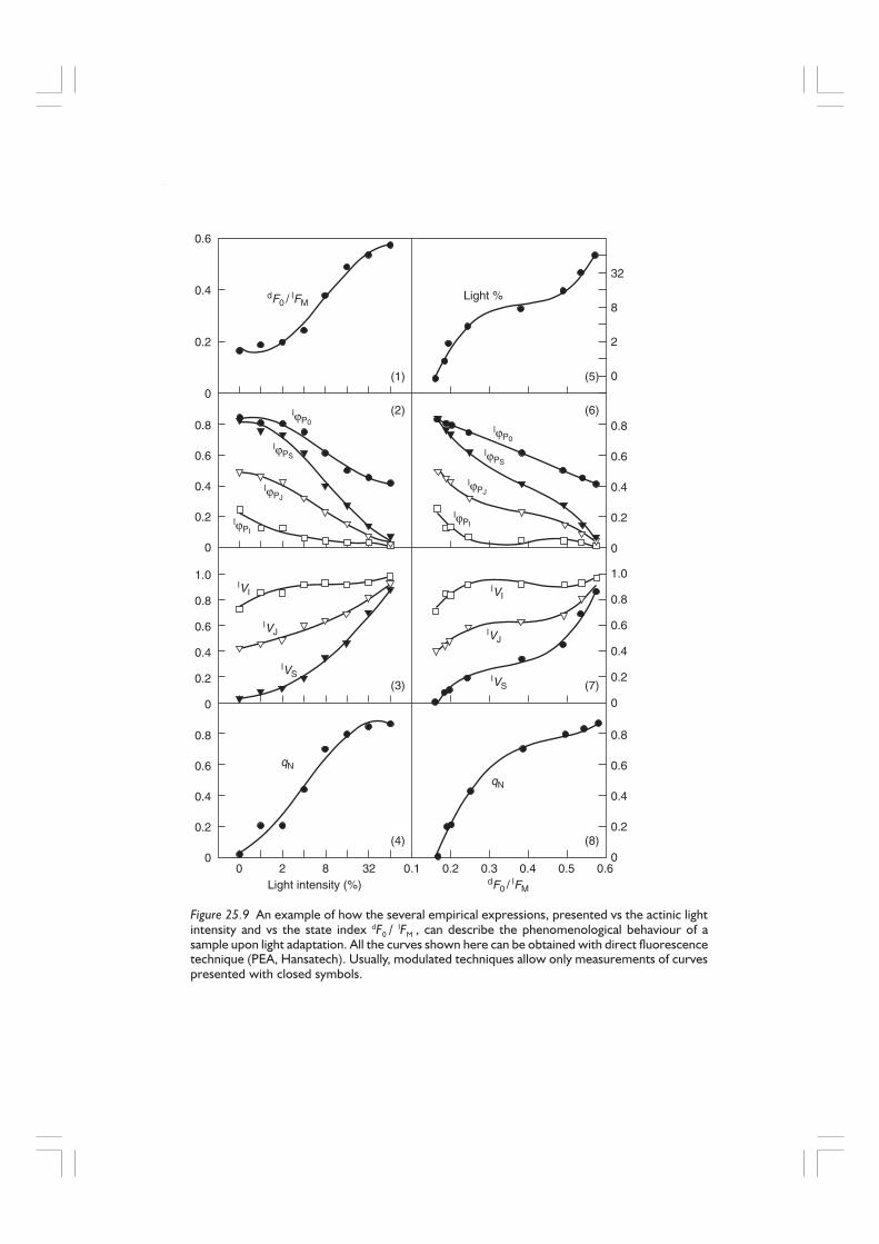
We show here, as an example, how these expressions can be used to describe thephenomenological behaviour of a sample upon light adaptation. A dark-adapted samplewas exposed and adapted to different light intensities (actinic light intensities). Atevery adapted physiological state the fluorescence transient was recorded and all of theabove expressions were calculated from the selected fluorescence signals. A firstobservation is that the ratio F0 / FM is higher in the light-adapted states and that, thehigher the actinic light intensity the more pronounced this increase is. Theoreticallythe ratio F0 / FM can take any value between 0 and 1. Therefore, the ratio F0 / FM can beused as an indicator of the physiological state (state change index) which is thus calibratedon an axis between 0 and 1.

Figure 25.9 shows these empirical expressions, for each light-adapted state, as afunction of the light intensity of adaptation (actinic light intensity) and also as a functionof the state index dF0 /

lFM . The light intensity is expressed as a percentage of thehighest light intensity used (600 Wm–2 of red light of 650 ± 30 nm).

Any expression describing one physiological state can be compared with the corre-sponding expression referring to another physiological state. The dark-adapted statecan well serve as a reference state for the normalization of the light-adapted states. Anexample is the expression

qN = 1 – [( FV / F0 )light / ( FV / F0 )dark ]

which is often used in the literature.All expressions thus far, have been derived in a purely empirical way, i.e. no theory

at all has been applied and up to now no biological or biophysical meaning has beengiven to any of them. However, all these expressions can be used to present and comparea biological sample in many types of experiments.

Conceptual processing of data

In order to link the experimental signals to biological reaction mechanisms, one has tochoose and apply a theory. Any theory, however, is based on certain concepts in termsof physics and chemistry and their link to the behaviour of a sample. The theory chosenmay describe the sample in a general or in a well-defined way. The investigator has todecide which level of complexity is appropriate for the given situation.

The actual dogmatics of the fluorescence emission of PSII

The knowledge in this field is very advanced. In this chapter, however, we just focus onthe concepts which help to understand the in vivo fluorescence transient of plants. Asa simplification we consider the following components of PSII:

• all absorbing pigments (mainly chlorophylls, Chl)• the reaction centre, RC• the primary quinone electron acceptor, QA

• all the electron carriers beyond QA.

The photon flux absorbed by the pigments is indicated as ABS; the dissipated flux (all


0.6

0.4

0.2

0

0.8

0.6

0.4

0.2

0

1.0

0.8

0.6

0.4

0.2

0

0.8

0.6

0.4

0.2

0

0.8

0.6

0.4

0.2

0

0.8

0.6

0.4

0.2

0

1.0

0.8

0.6

0.4

0.2

0

32

8

2

0

Light %dF0 / lFM

lϕP0

lϕPS

lϕPJ

lϕPI

lϕPI

lϕPJ

lϕPS

lϕP0

lVI lVI

lVJ lVJ

lVS lVS

qN

qN

(1) (5)

(2) (6)

(3) (7)

(4) (8)

0 2 8 32 0.1 0.2 0.3 0.4 0.5 0.6Light intensity (%) dF0 / lFM

Figure 25.9 An example of how the several empirical expressions, presented vs the actinic lightintensity and vs the state index dF0 / lFM , can describe the phenomenological behaviour of asample upon light adaptation. All the curves shown here can be obtained with direct fluorescencetechnique (PEA, Hansatech). Usually, modulated techniques allow only measurements of curvespresented with closed symbols.


the de-excitations except the photochemical one) is indicated as DI, which includes aswell the fluorescence emission, indicated as F; the excitation energy flux which reachesthe RC and gets trapped there (in the sense of leading to QA reduction) is indicated astrapping flux TR; the energy flux corresponding to the electron transport beyond QA

–

is indicated as ET.When QA is in its oxidized form the excited reaction centre is called open ( RCop ), as

it can promote the reduction of QA to QA– , thus converting excitation energy into free

energy of the redox couple QA– / QA. If QA is already reduced, then the excited reaction

centre is called closed (RCcl). Therefore, a PSII unit with open RC can be indicated asChl.RC.QA and a PSII unit with closed RC as Chl.RC.QA

– .Dogmatically, it is accepted that, for the same physiological state (i.e. dark-adapted

or light-adapted):

• an excited PSII with an open RC shows a low fluorescence emission;• an excited PSII with a closed RC shows a high fluorescence emission.

As a working hypothesis it has been generally considered that a sample in darkness hasonly open RCs and that a sample in strong light has only closed RCs. Therefore, thefluorescence rise from F0 to FM corresponds to the reduction of QA to QA

–, starting withall RCs open until all the RCs are closed. One has to keep in mind that the redox stateof plastoquinone (PQ or PQH2 ) can influence the fluorescence intensity mainly at FM .For simplicity, the possible quenching by PQ is not considered in the following equations.

Correlation of fluorescence signals with energy fluxes

The total light energy flux absorbed by a sample can be split into two fractions:

• the energy flux which is conserved as free energy by the primary photochemicalreaction, denoted as trapping flux TR; and

• the energy flux which is dissipated, DI, as heat and fluorescence, or transferred toother systems.

We can, therefore, write:

ABS = TRt + DIt (25.1)

For samples which, previous to their excitation, had all reaction centers open (e.g., inthe dark state) we can make the following link to the fluorescence rise:

• at t = 0, F ≡ F0 is minimal and TR ≡ TR0 is maximal;• at t = ∞ (practically at t = tFmax ), F ≡ FM is maximal and TR ≡ TRM = 0.

Assuming that the fluorescence emission is proportional to the total dissipation, Ft ~DIt , and introducing a proportionality factor α, we can write: DIt = α Ft . Therefore,

ABS = TRt + αFt ⇒ Ft = (ABS – ) / α ⇒ FM = ABS/ α (25.2)


Hence, the normalized signal Ft / FM is linked with the flux ratio TRt /ABS:

Ft / FM = 1 – ( TRt /ABS) (25.3)

However, the flux ratio TRt /ABS expresses the ratio of an energy output from theantenna pigments to the photon input into the antenna pigments and, therefore,corresponds to the yield of excitation energy trapping ϕPt , known also as the yield ofprimary photochemistry or the photon use efficiency. Hence,

ϕPt = TRt / ABS = 1– Ft / FM (25.4)

(Note that ϕPt is not any more an empirical expression but a biophysical one).The maximum yield of primary photochemistry, ϕPo , is therefore written as:

ϕPo = TR0 /ABS = 1 – F0 / FM (25.5)

Dividing equation (25.4) by equation (25.5) we get:

ϕPt / ϕPo = ( FM – Ft ) / ( FM – F0 ) = 1 – [ ( Ft – F0 ) / ( FM – F0 ) ] = 1 – Vt (25.6)

where Vt is the relative (or normalized) variable fluorescence.For the general case and at any time we can therefore write for ϕPt the following

equation:

ϕPt = ϕPo ( 1 – Vt ) (25.7)

The term ϕPo contains only the fluorescence extrema F0 and FM and the term ϕPt contains

the fluorescence expressions FM and Ft . Therefore, Vt contains all the three fluorescencesignals F0, Ft and FM .

Figure 25.10 shows the historical sequence of appearance in the literature of theequations 25.4 to 25.7 which all link experimental fluorescence signals with the quantumyield of primary photochemistry ϕP .

For the initial conditions of the fluorescence transient (light on and t ≅ 0) the maximalyield for primary photochemistry expressed as exciton trapped that triggers the reductionof one QA to QA

– per one photon absorbed, can be expressed entirely by using the ratioof the extrema F0 and FM , as shown by equation (25.5). Note that from this equation,several expressions combining the extrema F0 and FM in a different way can be derived,all containing the term ϕPo . Such expressions are the following, all containing the sameinformation:

1 – ( F0 / FM ) = ϕPo

F0 / FM = 1 – ϕPo

FV / F0 = ϕPo / ( 1 – ϕPo ) = ( FM / F0 ) – 1


The above analysis is valid for any physiological state. Among the different physiologicalstates we are here interested mainly in the dark-adapted state (index d, e.g., dF, dϕP etc.)and in the light-adapted state (index l, e.g., lF, lϕP etc).

The correlation of a fluorescence ratio and a ratio of rate constants

Each energy flux, TR, or DI or F, is proportional to the concentration of the excitedantenna chlorophyll Chl* and to the corresponding de-excitation rate constant:

fluxi = Chl*. ki

Denoting the sum of all non-photochemical rate constants as kN and the photochemicalrate constant as kP, the sum of all rate constants is written as:

Σ ki = kP + kN (25.8)

Therefore, the absorption flux ABS, being equal to the sum of all the de-excitationfluxes ki .

Chl*, can be written as:

Figure 25.10 The historical sequence of the appearance in the literature of equations (25.4) to(25.7) which all link experimental fluorescence signals to the quantum yield of primaryphotochemistry ϕp .

TRt

ABS= ϕPt ϕPo

ϕPo

25.7 25.7

25.5

25.6

25.6

(1–Vt) 1 –==

=

= =

Ft

FM·

Strasser 1978: Energy flux theory

FV

FM

= =FM – Ft

FV

FM – Ft

FM – F0

FM – Ft

FM=·

·

= = ==

∆FFM

Kitajima and Butler 1975Butler and Kitajima 1975

Paillotin 1976

Genty et al. 1989


ABS = ( kN + kP ) . [Chl*] (25.9)

while the maximal trapping flux TR0 (when all reaction centers are open) is:

TR0 = kP [Chl*] (25.10)

Hence, equation (25.5) can be now linked to a ratio of the rate constants, as:

TR0 /ABS = ϕPo = kP / ( kN + kP ) = 1 – ( F0 /

FM ) = FV / FM (25.11)

Different ways to express the same thing

Under in vivo conditions it is usually very difficult to measure the concentration of achemical compound in a photosynthetic sample. However it is possible to record thedynamic behaviour of the sample by its activities and energy fluxes. Thereafter, theratio of energy fluxes can be correlated with the ratio of fluorescence signals, the quan-tum yields and the ratio of de-excitation rate constants. Every physiological state canbe described in this way. Any expression describing any physiological state can becompared with the corresponding expression referring to another physiological state.Such a comparison can be quantified by the ratio of the two values which thus serves asan index of the state change capability, i.e. of the capability for change from one physio-logical state to another. This dynamics can be expressed identically in terms of ratios offluorescence signals, rate constants, yields or energy fluxes, as shown in Figure 25.11for the change from a dark-adapted to a light-adapted state.

In Figure 25.11 a definition of the expression qN is shown as:

( FV / F0 )light / (

FV / F0 )dark = 1 – qN

where FV = FM – F0 .In many situations lF0 (F0 in the light) is considered to be close to dF0 (F0 in the dark).

Therefore, qN can be approximated as:

“qN” = 1 – lFV / dFV

The biological and biophysical meaning of the expression qN is shown in Figure 25.11in terms of ratio of fluxes, ratio of yields, ratio of rate constants and ratio of fluorescencesignals. Note that qN was mentioned in the section “The empirical behaviour of a plantduring light adaptation”, however as a purely phenomenological expression.

The meaning of qP and qN

The expression qN is usually called in the literature “non-photochemical quenching” toindicate that it quantifies a decrease in fluorescence of an origin different from that ofthe photochemical quenching qP = ( FM – F ) / ( FM – F0 ). However, the naming andsymbolization lead to confusion, as they give the impression that the two terms arecomplementary and, moreover, that they refer to the same state. In addition, thecharacterization “non-photochemical” as such is quite misleading, since qN contains as


much photochemical information (through kP ) as non-photochemical information(through kN) and, therefore, is not at all a specific index for non-photochemical events(for more details, see Havaux et al., 1991). More arguments can be stated andsummarized as follows.

Concerning qP :

• qP is directly defined by the relative variable fluorescence as: 1 – qP = V = (F – F0)/(FM – F0);

• qP refers to only one physiological state;• qP depends on the redox state QA

– / QA of the sample in a given physiological state;and

• qP refers by name to the well-defined physical events of photochemical quenching.In other words, the name “photochemical quenching” corresponds precisely to aconceptual interpretation. Even so, it must be pointed out that, when a cooperativitybetween the PSUs is considered, qP depends on the non-photochemical rate constantkN as much as on the photochemical one kP . This dependence arises from therelation V = B / [1 + K(1–B)] between the relative variable fluorescence V and thefraction of closed reaction centers B, where K is a constant containing, beside theprobability pG for cooperativity (grouping), both kP and kN . If no cooperativity isassumed, the relative variable fluorescence V is identical assumed, the relativevariable fluorescence V is identical to the fraction of closed RC indicated as B andtherefore V = B = 1– qP . However, the rate constant for photochemical quenchingkP does not change at all, while qP can take all values between zero and unity.

• qP indicates a relative concentration, i.e. the fraction of the open reaction centre(1–B) if no grouping (pG = 0) is considered.

Physiologicalstatee.g.

Ratio offluxes

Ratio ofyields

Ratio ofrate

constants

Ratio offluorescence

signals

Dark adapted

Lightadapted

Normalizationon a referencestate, e.g. onthe dark state

dTR0dDI0

dϕPo

1 – dϕPo

dkPdkN

dFVdF0

lTR0lDI0

lϕPo

1 – lϕPo

lkPlkN

lFVlF0

l(TR0/DI0)d(TR0/DI0)

l(kP/kN)d(kP/kN)

l[ϕPo/(1–ϕPo)]d[ϕPo/(1–ϕPo)]

l(FV/F0)d(FV/F0)

1 – qN====

===

===

Figure 25.11 The derivation of the expression 1 – qN , expressed identically in terms of ratios offluorescence signals, rate constants, yields or energy fluxes. As an example, it is shown here forthe change from a dark-adapted to a light-adapted state.


Concerning qN :

• qN refers to two physiological states; it is an index of the change from the dark-adapted to a light-adapted state;

• qN does not refer to any intermediate redox state QA– / QA of the sample; it is

defined only by the fluorescence signals when the reaction centers are all open (F0)and all closed (FM), as in the case of the maximum quantum yield of primaryphotochemistry, ϕPo ;

• qN depends on kN as much as on kP (see Table 25.4); and• qN is not a specific expression for non-photochemical events. However, in terms

of rate constants, changes concerning non-photochemical events can be describedby the ratio dkN /

lkN = lFM /

dFM and compared with photochemical events by theratio kP / kN = FV / F0 .

Misleading advertisement of qP and qN

qP and qN can be used like any useful expression. However care should be taken ifinterpretations are made. The intensity of the fluorescence from a PSII is higher if theRC does not contribute to photochemistry (hence the definition: closed) than if it does(hence the definition: open). For any fluorescence signal between F0 and FM , one cancalculate the relative variable fluorescence V = (F – F0) / (FM – F0), which provides adirect measure of the fraction of closed RCs. Therefore, an increase of qP is not due toan increase of a photochemical rate constant, but simply to an increase of the concen-tration of open RCs which, by definition, are those exhibiting a lower fluorescenceintensity. Moreover, any sample exhibits at any moment after any light condition acertain relative variable fluorescence 0 ≤ V ≤ 1 which is determined by many parameters;photochemical quenching (in terms of physics) is only one of them.

Both the naming of qP and qN and the symbols used, make the impression that theyare describing complementary actions or mechanisms. This however is not at all thecase. qP is an expression which refers to one single state in which the fraction of openRCs can take only values between zero and unity. On the other hand, qN is only definedby the extrema F0 and FM (for all open and all closed RCs) at a particular state relativeto the same expression obtained in the dark-adapted state. It is trivial that, if the quantumyield of primary photochemistry can be calculated only by the values F0 and FM asϕPo = 1 – F0 /

FM , any acrobatic expression which contains only the F0 and FM can also

be expressed in terms of ϕPo. The quantum yield of primary photochemistry however,is a function of kN and kP as ϕPo sample this may be because lkN is bigger, dkN is smaller,dkP is bigger or lkP is smaller, etc. This means that any change of qN can be due tochanges of kP or/and kN . The non-photochemical events can be described by non-photochemical de-excitation rate constants but not by the fashionable expression qN =1 – ( lFV /

lF0 ) / ( dFV /

dF0 ).

The meaning of the slope at the origin of the fast fluorescence rise

The slope at the origin of the fluorescence rise (dF/dt)0 can be approximated by (∆F/∆t)0; the shorter the ∆t, better is the approximation. This can be obtained with aninstrument of a high time resolution (10 µs or faster). The initial slope of the relative


variable fluorescence can then be expressed as the initial increment per ms, using, forexample, the time interval of 250 or 100 µs:

(dV/dt)0 ≅ (∆V/∆t)0

= { [ ∆F / ( FM – F0 ) ] / ∆t }0

≅ 4 . ( F300µs – F50µs ) / ( FM – F50µs )

≅ 10 . ( F150µs – F50µs ) / ( FM – F50µs )

However, this expression corresponds to the maximal rate of the accumulation of thefraction of closed reaction centers, (dV/dt)0 = (dB/dt)0 , and considering

• one QA per reaction centre,• that one trapped exciton by an open RC triggers the reduction of QA to QA

–, and• that the reoxidation of QA

– to QA is inhibited,

we can write:

(dV/dt)0 = (dB/dt)0

= [d(QA–/ QA (total))

/ dt] 0

= flux of excitons trapped per RC

= TR0 / RC .

Thus, in cases that the reoxidation of QA– to QA is inhibited, as, for example, in the

presence of DCMU (3-(3,4-dichlorophenyl)-1,1-dimethylurea), the initial slope of therelative variable fluorescence (dV/dt)0 directly describes the trapping flux TR0 /RC.However, it has been shown (Strasser and Strasser, 1995) that when the reoxidation ofQA

– to QA proceeds normally, the initial slope of the relative variable fluorescence hasto be normalized by the value of VJ in order to describe the specific trapping flux TR0 /RC:

TR0 / RC = [ (dV/dt)0 / VJ ] ≅ 4 . ( F300µs – F50µs ) / ( F2ms – F50µs )

The area growth above the fast fluorescence rise

Once a fluorescence rise from F0 to FM is digitized and stored, the area growth betweenthe measured fluorescence signal Ft and the maximal measured fluorescence can becalculated. The maximal area, i.e. the area up to the time tFmax that Ft reaches FM,denoted as “Area”, is given by:


��

�

��

� �� −∫

In order to compare different samples, the Area has to be normalized by FV. Thenormalized expression is defined as: Sm ≡ Area / ( FM – F0 ). The parameter Sm expressesa work-integral; in other words, it is a measure of the energy needed to close all reactioncenters. Subscript “m” stands for “multiple”, referring to the multiple turn-over in theclosure of the reaction centers. The more the electrons from QA

– are transferred intothe electron transport chain ET, the longer the fluorescence signals remain lower thanFM and the bigger Sm becomes. The smallest Sm corresponds to the case when every QA

is reduced only once, as in the presence of DCMU, and it can then be denoted as SS

indicating single turn-over. Thereafter, the so-called turn-over number N, calculated as

� ��

� ��

�

��

�=

indicates how many times QA has been reduced in the time span from 0 to tFmax .If we consider an exponential fluorescence rise for the single turn-over situation,

then the normalized area SS would be inversely proportional to the initial slope of therelative variable fluorescence. However, as mentioned under “The meaning of the slopeat the origin of the fast fluorescence rise”, the value of this slope can also be calculatedin the absence of DCMU by dividing the actual initial slope of the relative variablefluorescence transient by VJ (Strasser and Strasser, 1995). Hence, the turn-over numbercan be given by a formula utilizing only data from the fluorescence transient of samplesmeasured under physiological conditions, without the need of additional measurementsin the presence of DCMU:

N = Sm . [ (dV/dt)0 ] / VJ

The time tFmax to reach FM

The time to reach the maximal fluorescence intensity makes sense only if it can bemeasured accurately. A clear FM has to appear in the fluorescence transient. Underthese situations the ratio Sm /

tFmax expresses the average redox state of QA in the timespan from 0 to tFmax and, concomitantly, the average fraction of open reaction centersduring the time needed to complete their closure:

Sm / tFmax = [ QA /

QA (total) ]av = [ 1 – (QA– / QA (total)) ]av = 1 – Bav

Therefore, this expression can be used for quantitation of the electron transport activity.

The basic information obtainable from the fluorescence rise

A fluorescence rise of high time resolution (10 µs or faster) provides the followingbasic elements of information:


• ratio of the extrema ( F0 / FM )

• fluorescence intensity at any time ( Ft )• shape of the fluorescence kinetics ( Vt )• time to reach the maximal fluorescence ( tFmax ), and• area above the fluorescence transient (Area).

Due to the typical shape of the fluorescence rise which shows the steps 0, (K), J, I, P,the following information can easily be selected and used in screening tests:

(1) ratio of the extrema, F0 / FM

(2) normalized slope at the origin, (dV/dt)0

(3) intermediate step, VJ

(4) intermediate step, VI

(5) time to reach the maximal fluorescence, tFmax, and(6) normalized area, Sm.

The information (1) to (3) refer to the structure and function of PSII only, while theinformation (4) to (6) refer to the activity of the electron transport beyond QA

– and tothe activity of the photosynthetic metabolism. Therefore, it is possible to localize thesetwo sites of responses of a sample to a physical or chemical stress from outside.

The JIP-test: a tool for screening

Based on the analysis of how the data from the 0-J-I-P fluorescence transient can beprocessed, a test has been developed and called the “JIP-test” after the steps of thetransient. This test can be used as a tool for rapid screening of many samples providingadequate information about the structure, conformation and function of theirphotosynthetic apparatus (Strasser and Strasser, 1995; Strasser et al., 1996).

We judged that it would be useful if this section on the JIP-test were not limited toa description of how the JIP-test can be applied, but integrated also the conceptualbasis, even though some of the elements of this basis have already been analysed in theprevious section.

From the data stored during the first second, the following values are selected to beused by the JIP-test for the calculation of several phenomenological and biophysicalexpressions leading to the dynamic description of a photosynthetic sample at a givenphysiological state:

• the maximal measured fluorescence intensity FP, provided that the excitationintensity is high enough to permit the closure of all RCs so that FP = FM ;

• the fluorescence intensity at 50 µs, considered to be F0 , i.e. the intensity when allRCs are open;

• the fluorescence intensity at 150 µs, at 300 µs, at 2 ms (denoted as FJ) and at 60 ms(denoted as FI);

• the time to reach FM tFmax; and• the area between the fluorescence transient and the line F = FM.


A highly simplified working model of the energy fluxes in a photosynthetic apparatusis shown in Figure 25.12 (from Strasser and Strasser, 1995). Based on the theory ofenergy fluxes in biomembranes, formulae for the specific energy fluxes (per reactioncentre RC) and the phenomenological energy fluxes (per excited cross-section CS), aswell as for the flux ratios or yields, have been derived using the experimental valuesprovided from the JIP-test. The constellation of their values at any instant can beconsidered as expressing the behaviour of the system (Krüger et al., 1997). ABS refersto the flux of photons absorbed by the antenna pigments Chl*. Part of this excitationenergy is dissipated, mainly as heat and less as fluorescence emission F, and anotherpart is channelled as trapping flux TR to the reaction centre RC and converted toredox energy by reducing the electron acceptor QA

to QA–, which is then reoxidized to

QA thus creating an electron transport ET that leads ultimately to CO2 fixation.The specific energy fluxes at time zero (at the onset of excitation) ABS / RC, TR0 /

RC and ET0 / RC, can be derived from the experiments as shown below. The maximum

quantum yield of primary photochemistry (note that trapping refers to the energy fluxleading to photochemistry) TR0 /ABS ≡ ϕPo , the efficiency that a trapped exciton canmove an electron further than QA

– into the electron transport chain ET0 / TR0 ≡ ψ0 , or

the probability that an absorbed photon will move an electron into the electron transportchain ET0 /ABS ≡ ϕEo , are directly related to the three fluxes, as the ratios of any two ofthem. TR / RC expresses the rate by which an exciton is trapped by the RC resulting inthe reduction of QA to QA

–. The maximal value of this rate is given by TR0 / RC, because

at time zero all RCs are open. The link of TR0 / RC with the experimental data is

derived as follows. If the reoxidation of QA– would be blocked, as happens in DCMU-

treated samples, TR0 / RC would be given by the normalization of the initial slope of

the fluorescence induction curve (between 50 and 300 µs or 50 and 150 µs) on themaximal variable fluorescence FV = FM – F0. This normalized value is denoted as M0,DCMU .However, if the reoxidation of QA

– is not blocked, the normalized value of the initialslope, M0 , indicates the net rate of closure of the RCs, where trapping increases thenumber of closed centers and electron transport decreases it:

ABSRC

TR0

RC

ET0

RC

TR0

ABS

ET0

TR0

= ϕPo

= ψ0

ϕEo =ET0

ABS

RCQA QA–

Ne–

F

ABS

TRt

ETt

Chl*

(N–1)e–

Figure 25.12 A highly simplified working model of the energy fluxes in the photosyntheticapparatus.


M0 = TR0 / RC – ET0 /

RC (25.12)

A thorough investigation carried out in our laboratory (Strasser and Strasser, 1995)revealed clearly that M0 in DCMU-treated samples can be simulated by the amplificationof the measured M0 in samples without DCMU by a factor reciprocal to VJ. Thus,

TR0 / RC = M0,DCMU = M0 /

VJ (25.13)

From equations 25.12 and 25.13 we get:

ET0 / RC = TR0 /

RC – M0

= (M0 / VJ) – M0

= (M0 / VJ) . (1 – VJ)

= (TR0 / RC) . (1 – VJ) (25.14)

Hence,

ψ0 ≡ ET0 / TR0 = 1 – VJ (25.15)

and

ϕEo ≡ ET0 /ABS = (TR0 /ABS) . ( ET0 / TR0) = ϕPo . ψ0 (25.16)

where ϕPo is calculated from the values at the extrema F0 and FM of the fluorescencetransient:

ϕPo = (FM – F0) / FM = 1 – (F0 / FM) (25.17)

Based on equations (25.16) and (25.17), equation (25.15) can now be written as:

ϕEo = [ 1 – (F0 / FM) ] . (1 – VJ) (25.18)

Concerning the expression ABS / RC, it is derived as follows:

TR0 / RC = (TR0 /

ABS) . (ABS / RC) = ϕPo . (ABS / RC) (25.19)

ABS / RC = (TR0 / RC) / ϕPo = (M0 /

VJ) / [ 1 – (F0 /

FM) ] (25.20)

It has to be pointed out that TR0 / RC expresses the initial rate of the closure of RCs as

a fractional expression over the total number of RCs that can be closed. We point thisout clearly, because it is possible that under stress conditions some RCs are inactivatedin the sense of being transformed to quenching sinks (Krause et al., 1990) withoutreducing QA to QA

–. In such a case, TR0 / RC still refers only to the active (QA to QA

–

reducing) centers. The same is valid for the other two specific fluxes, since theirderivation is based on TR0 /

RC.


The phenomenological fluxes are, accordingly, ABS / CS, TR0 / CS and ET0 /

CS,where CS stands for the excited cross-section of the tested sample. The value of theinitial fluorescence F0 has been proposed to serve as a measure (in arbitrary units) ofthe phenomenological absorption flux ABS / CS (Strasser and Strasser, 1995). However,since the initial fluorescence value is affected by conformational changes, care shouldbe taken (Krüger et al., 1997) to use the value F0

dark that the sample exhibits whilebeing in its dark-adapted state:

ABS / CS0 = F0dark (25.21)

TR0/CS0 and ET0/CS0 can then be calculated, in the same arbitrary units:

TR0 / CS0 = ϕPo . F0

dark = [ 1 – (F0 /

FM) ] . F0dark (25.22)

ET0 / CS0 = ϕEo . F0

dark = [ 1 – (F0 /

FM) ] . (1 – VJ) . F0dark (25.23)

The expression RC / CS0 (active RCs per excited cross-section) for the concentration ofthe reaction centers is easily derived using equations (25.20) and (25.21):

RC / CS0 = (ABS / CS) / (ABS / RC) = { F0dark. [ 1 – (F0 /

FM) ] } / (M0 / VJ) (25.24)

The value of the maximal fluorescence FM can also serve as a measure (in arbitraryunits) of the phenomenological absorption flux, provided that the same care is takento avoid the interference of conformational changes. In order to distinguish the twoways of calculation, the following notations are used: ABS / CS0 = F0

dark and ABS / CSM

= Fmdark.

All these formulae for the JIP-test are summarized in Table 25.5.Based on the theory of energy fluxes in biomembranes, expressions relating the

photochemical rate constant kP and the nonphotochemical rate constant kN summingup kH (for heat dissipation), kF (for fluorescence emission) and kX (for energy migrationto PSI) with the fluorescence values F0 and FM have been derived (see Havaux et al.,1991):

kN = (ABS/CS) . kF . (1 / FM) (25.25)

kN + kP = (ABS/CS) . kF . (1 / F0) (25.26)

kP = (ABS/CS) . kF . {(1 / F0) – (1 / FM)} (25.27)

Note that

ϕPo = 1– (F0 / FM) = kP / (kP + kN) (25.28)

The presentation of the JIP-test data

A screening test has to be able to present a large amount of data in an integrated way,in order to allow a clear approach to the situation under study. As an example we show


here how the effect of a mild heat-treatment (10 min at 40ºC or 44ºC) on the behaviourof pea leaves can be presented in such an integrated way. The JIP-test of one singleexcitation of 1 sec light was used for both the heat-treated samples and the non-treatedsamples (25ºC) which served as the control. The fast fluorescence transients are shownin Figure 25.13. All expressions were calculated according to the equations of Table25.5 and the calculated values are summarized in Tables 25.6 and 25.7, both as absolutevalues and relative to the corresponding values of the control. All measured information(all obtained from one single sample and an experimental excitation time of one secondonly) is summarized in two types of presentation: the spider-plot presentation and theenergy pipeline model. The experiment shows clearly most of the well-known responsesto a mild heat treatment.

Table 25.5 Summary of the JIP-test formulae, using data extractedfrom the fast fluorescence transient

Extracted and technical fluorescence parameters

F0 = F50µs , fluorescence intensity at 50 µsF150 = fluorescence intensity at 150 µsF300 = fluorescence intensity at 300 µsFJ = fluorescence intensity at the J-step (at 2 ms)FM = maximal fluorescence intensitytfmax = time to reach FM , in msVJ = ( F2ms – F0 ) / ( FM – F0 )Area = area between fluorescence curve and FM

(dV/dt)0 or M0 = 4 . ( F300 – F0 ) / ( FM – F0 )Sm = Area / ( FM – F0 )Bav = 1 – ( Sm / tFmax )N = Sm . M0 . ( 1 / VJ ) turn-over number QA

Quantum efficiencies or flux ratiosϕPo or TR0 / ABS = (1 – F0 ) / FM or Fv / FM

ϕEo or ET0 / ABS = (1 – F0 / FM ) . ψ0

ψ0 or ET0 / TR0 = 1 – VJ

Specific fluxes or specific activitiesABS / RC = M0 . (1 / VJ ) . ( 1 / ϕPo)TR0 / RC = M0 . (1 / VJ )ET0 / RC = M0 . (1 / VJ ) . ψ0

DI0 / RC = ( ABS / RC ) – ( TR0 / RC )

Phenomenological fluxes or phenomenological activitiesABS / CS0 = F0 or other useful expression ∗TR0 / CS0 = ϕPo ( ABS / CS0 )ET0 / CS0 = ϕPo . ψ0 . ( ABS / CS0 )DI0 / CS0 = ( ABS / CS0) – (TR0 / CS0 )RC / CS0 = ϕPo . ( VJ / M0 ) . F0 *

∗ when expressed per CSM , F0 is replaced by FM


The spider-plot presentation

The relative values (relative to the corresponding value of the control, which thusbecome equal to unity) of selected expressions, such as the specific fluxes (ABS / RC,TR0 /

RC and ET0 / RC), the flux ratio TR0 /

ABS = ϕPo , and the density of the activereaction centers per excited cross-section (RC / CS), can be plotted using a spider-plotpresentation (Figure 25.14). This is a multiparametric description of structure andfunction of each photosynthetic sample, presented by an octagonal line. This type ofpresentation provides a direct visualization of the behaviour of a sample and thusfacilitates the comparison of plant material as well as the classification of the effect ofdifferent environmental stressors on it in terms of the modifications it undergoes toadapt to new conditions.

Energy pipeline models

The derived parameters can also be visualized by means of an energy pipeline model ofthe photosynthetic apparatus (Strasser, 1987; Strasser et al., 1996; Krüger et al., 1997).This is a dynamic model in which the value of each energy flux, either changing as a

2

1

010–1 100 101 102 103

Time (ms)

0 0.5 1.0

1.6

1.2

0.8 Flu

ores

cenc

e (r

el.)

44 °C40 °C25 °C

Time (ms)

25 °C

40 °C

44 °C

0

K

J

I

P

Figure 25.13 The fast fluorescence rise (measured with the PEA instrument) in pea leaves subjectedfor 10 min to a heat treatment at 40ºC and 44ºC. The fast fluorescence rise of the control sample(25ºC) is also shown. Insert shows the same curves but plotted on linear time scale up to 1 ms.


Table 25.6 The experimental expressions of the JIP-test and their calculated values from the data ofFigure 25.13. Pea (Pisum sativum) leaves were heated at 40ºC and 44ºC for 10 min. Fluorescencemeasurements were performed immediately after heat treatment at room temperature. Numbers inparentheses express the normalized values over the control.

Pisum sativum Control 10 min heat treatment

25ºC 40ºC 44ºC

F extremesF0 663 (1) 759 (1.14) 873 (1.32)FM 3357 (1) 2734 (0.81) 2465 (0.73)

FV / F0 4.06 (1) 2.60 (0.64) 1.82 (0.45)

F dynamicsVJ 0.43 (1) 0.44 (1.04) 0.49 (1.14)VI 0.73 (1) 0.65 (0.89) 0.37 (0.50)

(dV / dt)0 0.97 (1) 1.42 (1.46) 1.83 (1.89)

Areaslog Sm 1.37 (1) 1.68 (1.22) 2.01 (1.47)

Sm / tFmax 98.9 (1) 65.9 (0.67) 150 1.52

log N 1.73 (1) 2.19 (1.27) 2.59 (1.50)

Table 25.7 The specific and phenomenological expressions of the JIP-test and their calculated valuesfrom the data of Figure 25.13. Pea (Pisum sativum) leaves were heated at 40ºC and 44ºC for 10 min.Fluorescence measurements were performed immediately after heat treatment at room temperature.Numbers in parentheses express the normalized values over the control.

Pisum sativum Control 10 min heat treatment

25ºC 40ºC 44ºC

Flux per RCABS / RC = AS 2.84 (1) 4.45 (1.57) 5.85 (2.06)TR0

/ RC 2.28 (1) 3.21 (1.41) 3.78 (1.66)ET0

/ RC 1.31 (1) 1.79 (1.37) 1.94 (1.48)

Flux-ratio = YieldTR0 / ABS = ϕPo 0.80 (1) 0.72 (0.90) 0.65 (0.80)

•ET0 / TR0 = ψ0 0.57 (1) 0.56 (0.97) 0.51 (0.89)

IIET0 / ABS = ϕEo 0.46 (1) 0.40 (0.87) 0.33 (0.72)

Density of RCsRC / CS0 = (Chl / CS) : (Chl / RC)

= F0 / AS 234 (1) 171 (0.73) 149 (0.64)

RC / CSM = (Chl / CS) : (Chl / RC)= FM / AS 1183 (1) 615 (0.52) 421 (0.36)

ActivitiesABS / CS0 = F0 663 (1) 759 (1.14) 873 (1.32)TR0 / CS0 = F0 • ϕPo 532 (1) 548 (1.03) 564 (1.06)ET0 / CS0 = F0 • ϕPo • ψ0 306 (1) 306 (1.00) 290 (0.95)ABS / CSM = FM 3357 (1) 2734 (0.81) 2465 (0.73)TR0 / CSM = FM • ϕPo 2694 (1) 1975 (0.73) 1592 (0.59)ET0 / CSSM = FM • ϕPo• ψ0 1549 (1) 1103 (0.71) 819 (0.53)


2.0

1.5

1.0

0.5

0

F0

VI

VJ

FM

FV/F0

N

Mo

log (Sm)

2.0

1.5

1.0

0.5

0

TR0/CS

ABS/CS

ABS/RC

ϕPo

ET0/CS

RC/CS

ET0/RC

TR0/RC

0 5 10 15Time (min)

1.5

1.3

1.1

0.9Tran

smis

sion

(re

l.)40 °C

25 °C40 °C44 °C

Figure 25.14 An example of a spider-plot presentation of a constellation of selected parametersquantifying the behaviour of PSII of pea leaves exposed for 10 min to 40ºC ( � ) or 44ºC ( o ),relative to that of pea leaves at 25ºC (regular octagon, ---- ). Top: technical spider-plot showingnormalized experimental expressions. Bottom: flux spider-plot showing specific and pheno-menological fluxes which have been calculated from the values of the technical spider-plotaccording to the equations given in Table 25.5. The effect of heat treatment on the lighttransmission of the tested leaves is shown in the insert.


function of time or modified by the different imposed environmental conditions, isexpressed by the appropriately adjusted width of the corresponding arrow.

For each sample and/or state of the sample, two types of models can be presented(Figure 25.15); the one refers to the reaction centre in the membrane and thus dealswith the specific energy fluxes (per RC) and the other refers to the excited cross-sectionof a leaf and thus deals with the phenomenological energy fluxes (per CS). The flux ofdissipated excitation energy at time zero ( DI0 = ABS – TR0 ) is also shown both per RCand per CS. The membrane model includes also a demonstration of the average “antennasize”, which follows the value of the ABS / RC. This value expresses the total absorptionof PSII antenna chlorophylls divided by the number of active (in the sense of QA reducing)reaction centres. Therefore, the antenna of inactivated reaction centres (non-QA

reducing, here due to the depletion of the oxygen-evolving side) are mathematically

Membrane model Leaf model

ABS/RCABS/CS

TR0/RC

TR0/CS

ET0/RCET0/CS

DI0/CSDI0/RC

25 °C

40 °C

RC

RC

TR0/RC

ABS/RC

ET0/RC

DI0/RCDI0/CS

ET0/CS

TR0/CS

ABS/CS

44 °CTR0/RC

RCET0/RC

DI0/RC

ABS/RC

ET0/CS

TR0/CS

ABS/CS

DI0/CS

Figure 25.15 Pipeline models for specific fluxes (membrane model) or phenomenological fluxes(leaf model).


added to the antenna of the active reaction centres. In the leaf model the active reactioncenters per cross-section (RC/CS) are indicated by open circles and those that havebeen inactivated are indicated by closed circles.

Upon heating, the data show the following:

• Phenomenologically per excited cross-section CS (i.e., per active measured leafarea):

– Decrease of electron transport per excited cross-section (ET0 / CS) due to theinactivation of reaction centre complexes (here due to the inactivation of theoxygen-evolving system).

– Decrease of the density of active reaction centers RC /CS (indicated as opencircles in Figure 25.15).

– Increase of the energy dissipation per excited cross-section DI0 / CS.

– Decrease of the energy absorbed per excited cross-section ABS / CS. This findinghas been confirmed by independent parallel transmission measurements whichshowed an increase of the transmitted light through the leaf (insert in Figure25.14).

• Specifically per active reaction centre RC:

– Average absorption per active reaction centre increases (ABS / RC) due to theinactivation of some RCs.

– The ratio of total dissipation to the amount of active RCs increases (DI0 / RC)

due to the high dissipation of the inactive RCs.– Electron transport per active reaction centre increases due to a thermal

activation of the dark reactions.

Concluding remarks

In this overview we have discussed some of the properties of the chlorophyll fluorescenceinduction curves and showed how they can be utilized to derive information about thebehaviour of PSII. However, the recorded fluorescence transients carry much moreinformation than those used by the JIP-test. The whole of this information can beutilized by means of the powerful methods of numerical simulations (Stirbet and Strasser,1995, 1996; Stirbet et al., 1998). The application of these methods is being furtherexplored in our laboratory.

The fluorescence kinetic is so rich in information that since its discovery in 1931 newproperties are continuously being detected. New instrumentation has made it possibleto measure fast changes in a way that one can follow the electron transfer from thewater splitting side to QA, then to QB and later to plastoquinone. As this transfer is verysensitive to stressors and highly dependent on the need of electrons for metabolism, PSIIfluorescence can become a biosensing device for stress detection in plants. For suchdetection, it is very useful to establish and apply tests that can screen many samples ina short time. At a second stage, more time-consuming and specific tests can be made onselected samples. In the future, the newer fluorescence imaging techniques and numericalsimulations will have to be calibrated by accurate kinetic tests like the JIP-test.

Basic fluorescence understanding combined with the JIP-test are a tool to analyseany plant material in any situation, even by non-fluorescence specialists. We hope that


many young scientists will try the JIP-test presented in this report to probe photo-synthesis.

Remarks

While this paper has been processed we derived a so called performance index, PI, ofany photosynthetic sample. For its derivation see Strasser et al. (1999) and Srivastavaet al. (1999).

This index groups the bifurcations of the energy cascades:

or in experimental terms, based on the cross section or leaf area

or

or based on the equal absorption

To present the different components we defined a driving force of the primaryphotosynthetic reactions as

DF(x) = log PI(x) which is the sum of the logarithms of the components above.

For many situations the expressions PI(x) and DF(x) appeared to be a very sensitiveindex for any stress and therefore, a practical index to use for physiological, environ-mental and biotechnological screenings.

Acknowledgments

This work was supported by Swiss National Foundation grant (3100-046860-96; 3100-052541-97) to RJS and AS.

References

Butler, W.L. 1978. Energy distribution in the photochemical apparatus of photosynthesis. Annu.Rev. Plant Physiol. 29: 345–378.

Butler, W.L. and Kitajima, M. 1975. Fluorescence quenching in photosystem II of chloroplast.Biochim. Biophys. Acta 376: 116–125.

Dau, H. 1994a. Molecular mechanisms and quantitative models of variable photosystem IIfluorescence. Photochem. Photobiol. 60: 1–23.

��

�� ! "!#$

�� $ % &� ��= i i i

#� ��

#� �

�#$ '

�� ( (

ϕ ψϕ ψ− −

i i i

#� ��

#� �

�#$ '

�� ( (

ϕ ψϕ ψ− −

i i i

#� ��

#� �

�#$

�� ( (

ϕ ψϕ ψ− −

i i


Dau, H. 1994b. Short-term adaptation of plants to changing light intensities and its relation tophotosystem II photochemistry and fluorescence emission. J. Photochem. Photobiol. 26:3–27.

Genty, B., Briantais, J.-M. and Baker, N.R. 1989. The relationship between the quantum yieldof photosynthetic electron transport and quenching of chlorophyll fluorescence. Biochim.Biophys. Acta 990: 87–92.

Goedheer, J.H.C. 1972 Fluorescence in relation to photosynthesis. Annu. Rev. Plant Physiol.23: 87–112.

Govindjee. 1995. Sixty-three years since Kautsky: chlorophyll a fluorescence. Aust. J. PlantPhysiol. 22: 131–160.

Govindjee and Jursinic, P. 1979. Photosynthesis and fast changes in light emission by greenplants. Photochem. Photobiol. Rev. 4: 125–205.

Govindjee and Wasielewski, M.R. 1989. Photosystem II: from femtosecond to a millisecond. InBriggs, W.R. (ed.) Photosynthesis: 71–103. Alan R. Liss, New York.

Govindjee, Papageorgiou, G. and Rabinowitch, E. 1967. Chlorophyll fluorescence and photo-synthesis. In Guibault, G.G. (ed.) Fluorescence Theory, Instrumentation and Practice: 511–564. Marcel Dekker, New York.

Govindjee, Amesz, J. and Fork, D.C. 1986. Light Emission by Plants and Bacteria. AcademicPress, Orlando.

Guissé, B., Srivastava, A. and Strasser, R.J. 1995. The polyphasic rise of the chlorophyll afluorescence (O-K-J-I-P) in heat stressed leaves. Arch. Sci. Genève 48: 147–160.

Havaux, M., Strasser, R.J. and Greppin, G. 1991. A theoretical and experimental analysis ofthe qP and qN coefficients of chlorophyll fluorescence quenching and their relation tophotochemical and nonphotochemical events. Photosynth. Res. 27: 41–55.

Holzwarth, A.R. 1991. Excited state kinetics in chlorophyll systems and its relationship to thefundamental organization of the photosystems. In Scheer, H. (ed.) Chlorophylls: 1125–1151.CRC Press, Boca Raton.

Joshi, M.K. and Mohanty, P. 1995. Probing photosynthetic performance by chlorophyll afluorescence: Analysis and interpretation of fluorescence parameters. J. Sci. Indust. Res. 54:155–174.

Karukstis, K.K. 1991. Chlorophyll fluorescence as a physiological probe of the photosyntheticapparatus. In Scheer, H. (ed.) Chlorophylls: 769–795. CRC Press, Boca Raton.

Kautsky, H. and Hirsch, A. 1931. Neue Versuche zur Kohlensäureassimilation. Natur-wissenschaften 19: 96.

Kitajima, M. and Butler, W.L. 1975. Quenching of chlorophyll fluorescence and primaryphotochemistry in chloroplasts by dibromothymoquinone. Biochim. Biophys. Acta 376:105–115.

Krause, G.H. and Weis, E. 1991. Chlorophyll fluorescence and photosynthesis: the basics. Annu.Rev. Plant Physiol. Plant Mol. Biol. 42: 313–349.

Krause, G.H., Somersalo, S., Zumbusch, E., Weyers, B. and Laasch, H. 1990. On the mechanismof photoinhibition in chloroplasts. Relationship between changes in fluorescence and activityof photosystem II. J. Plant Physiol. 136: 472–479.

Krüger, G.H.J., Tsimilli-Michael, M. and Strasser, R.J. 1997. Light stress provokes plastic andelastic modifications in structure and function of photosystem II in camellia leaves. Physiol.Plant. 101: 265–277.

Lavorel, J. and Etienne, A.-L. 1977. In vivo chlorophyll fluorescence. Top. Photosynth. 2:203–268.

Lichtenthaler, H.K. 1988. Application of Chlorophyll Fluorescence in Photosynthetic Research,Stress Physiology, Hydrobiology and Remote Sensing. Kluwer Academic, Dordrecht.

Neubauer, C. and Schreiber, U. 1987. The polyphasic rise of chlorophyll fluorescence upononset of strong continuous illumination: Saturation characteristics and partial control by thephotosystem II acceptor side. Z. Naturforsch. 42c: 1246–1254.


Ouzounidou, G., Moustakas, M. and Strasser, R.J. 1997. Sites of action of copper in thephotosynthetic apparatus of maize leaves: Kinetic analysis of chlorophyll fluorescence, oxygenevolution, absorption changes and thermal dissipation as monitored by photoacoustic signals.Aust. J. Plant Physiol. 24: 81–90.

Owens, T.G. 1996. Processing of excitation energy by antenna pigments. In Baker, N.R. (ed.)Photosynthesis and the Environment: 1–23. Kluwer Academic, The Netherlands.

Paillotin, G. 1976. Movement of excitations in the photosynthesis domain of photosystem II. J.Theor. Biol. 58: 237–252.

Papageorgiou, G. 1975. Chlorophyll fluorescence: an intrinsic probe of photosynthesis. InGovindjee (ed.) Bioenergetics of Photosynthesis: 319–371. Academic Press, New York.

Rabinowitch, E. 1951. Spectroscopy and fluorescence of photosynthetic pigments, in Photo-synthesis and Related Processes, Vol 2 Part 1: 740–820. Interscience Publishers, New York.

Sauer, K. and Debreczeny, M. 1996. Fluorescence. In Amesz, J. and Hoff, A.J. (eds) BiophysicalTechniques in Photosynthesis: 41–61. Kluwer Academic, The Netherlands.

Schreiber, U., Bilger, W. and Neubauer, C. 1995. Chlorophyll fluorescence as a nonintrusiveindicator for rapid assessment of in vivo photosynthesis. In Schulze, E.-D. and Cladwell,M.M. (eds) Ecophysiology of Photosynthesis: 49–70. Springer-Verlag, Berlin.

Srivastava, A. and Strasser, A. 1996. Stress and stress management of land plants during aregular day. J. Plant Physiol. 148: 445–455.

Srivastava, A. and Strasser, R.J. 1997. Constructive and destructive actions of light on thephotosynthetic apparatus. J. Sci. Indust. Res. 56: 133–148.

Srivastava, A., Greppin, G. and Strasser, R.J. 1995. The steady-state chlorophyll a fluorescenceexhibits in vivo an optimum as a function of light intensity which reflects the physiologicalstate of the plant. Plant Cell Physiol. 36: 839–848.

Srivastava, A., Guissé, B., Greppin, H. and Strasser, R.J. 1997. Regulation of antenna structureand electron transport in PSII of Pisum sativum under elevated temperature probed by thefast polyphasic chlorophyll a fluorescence transient: OKJIP. Biochim. Biophys. Acta 1320:95–106.

Srivastava, A., Strasser, R.J. and Govindjee. 1999. Greening of peas: parallel measurements on77k emission spectra, OJIP chlorophyll a fluorescence transient, period four oscillation ofthe initial flourescence level, delayed light emission, and P700. Photosynthetica 37: 365–392.

Stirbet, A. and Strasser, R.J. 1995. Numerical simulation of the fluorescence induction in plants.Arch. Sci. Genève 48: 42–59.

Stirbet, A. and Strasser, R.J. 1996. Numerical simulation of the in vivo fluorescence in plants.Math. Compu. Simul. 42: 245–253.

Stirbet, A., Govindjee, Strasser, B.J. and Strasser R.J. 1998. Chlorophyll a fluorescence inductionin higher plants: modelling and numerical simulation. J. Theor. Biol. 193: 131–151.

Strasser, B.J. 1997. Donor side capacity of photosystem II probed by chlorophyll a fluorescencetransients. Photosynth. Res. 52: 147–155.

Strasser, B.J. and Strasser, R.J. 1995. Measuring fast fluorescence transients to address environ-mental questions: The JIP test. In Mathis, P. (ed.) Photosynthesis: From Light to Biosphere,Vol 5: 977–980. Kluwer Academic, The Netherlands.

Strasser, R.J. 1978. The grouping model of plant photosynthesis. In Akoyunoglou, G. andArgyroudi-Akoyunoglou, J.H. (eds) Chloroplast Development: 513–538. Elsevier BiomedicalPress, North-Holland.

Strasser, R.J. 1985. Dissipative strukturen als thermodynamischer regelkreis des photosyntheseapparates. Berichte Deutsche Botanische Gesellschaft 98: 53–72.

Strasser, R.J. 1987. Energy pipeline model of the photosynthetic apparatus. In Biggins, J. (ed.)Progress in Photosynthesis Research, Vol 2: 717–720. Martinus Nijhoff Publisher, Dordrecht.


Strasser, R.J. and Govindjee. 1992a. The Fo and the O-J-I-P fluorescence rise in higher plantsand algae. In Argyroudi-Akoyunoglou, J.H. (ed.) Regulation of Chloroplast Biogenesis: 423–426. Plenum Press, New York.

Strasser, R.J. and Govindjee. 1992b. On the O-J-I-P fluorescence transient in leaves and D1mutants of Chlamydomonas reinhardtii. In Murata, N. (ed.) Research in Photosynthesis, Vol.4: 29–32. Kluwer Academic, Dordrecht.

Strasser, R.J., Srivastava, A. and Govindjee. 1995. Polyphasic chlorophyll a fluorescence transientin plants and cyanobacteria. Photochem. Photobiol. 61: 32–42.

Strasser, R.J., Eggenberg, P. and Strasser, B.J. 1996. How to work without stress but withfluorescence. Bull. Royal Soc. Liege 65: 330–349.

Strasser, R.J., Tsimilli-Michael, M. and Greppin, H. 1997. How excitation energy distributionindicates the complexity of a developing and to the environment adapting photosyntheticapparatus. In Greppin, H., Penel, C. and P. Simon, P. (eds) Travelling Shot on Plant Develop-ment: 99–129. Rochat-Baumann, Imprimerie Nationale, Genève.

Strasser, R.J., Srivastava, A. and Tsimilli-Michael, M. 1999. Screening the vitality and photo-synthetic activity of plants by fluorescent transient. In Behl, R.K., Punia, M.S. and Lather,B.P.S (eds) Crop Improvement for Food Security: 72–115. SSARM, Hisar, India.

Tsimilli-Michael, M., Krüger, G.H.J. and Strasser, R.J. 1995. Suboptimality as driving force foradaptation: A study about the correlation of excitation light intensity and the dynamicfluorescence emission in plants. In Mathis, P. (ed.) Photosynthesis: From Light to Biosphere,Vol 5: 981–984. Kluwer Academic, The Netherlands.

Tsimilli-Michael, M., Krüger, G.H.J. and Strasser, R.J. 1996. About the perpetual state changesin plants approaching harmony with their environment. Arch. Sci. Genève 49: 173–203.

Tsimilli-Michael, M., Pêcheux, M. and Strasser, R.J. 1998. Vitality and stress adaptation of thesymbionts of coral reef and temperate foraminifers probed in hospite by the fluorescencekinetics O-J-I-P. Arch. Sci. Genève 51 (2): 1–36.

Van Rensberg, L., Krüger, G.H.J., Eggenberg, P. and Strasser, R.J. 1996. Can screening criteriafor drought resistance in Nicotiana tabacum L. be derived from the polyphasic rise of thechlorophyll a fluorescence transient (OJIP)? South African J. Bot. 62: 337–341.

Wassink, E.C. 1951. Chlorophyll fluorescence and photosynthesis. Advances in Enzymol. 11:91–199.

the fluorescence transient as a tool to characterize … · chapter 25the fluorescence transient as...

Documents