The Fortran Parallel Transformer and itsProgramming Environment

Erik H. D’Hollander, Fubo Zhang and Qi Wang

University of Ghent

Department of Electrical Engineering

Parallel Information Systems group

St.-Pietersnieuwstraat 41

B-9000 Gent, Belgium

email: {dhollander,wang}@elis.rug.ac.bezfb@platform.com

tel: +32-9-264.33.75

keywords: programming environment, program restructuring, PVM,

Fortran parallelizer, automatic code generation

DOALL, distributed computing

Abstract

The Fortran Parallel Transformer (FPT) is a Parallel Programming Environ-

ment for Fortran-77 programs. It is used for the automatic parallelization of

loops, program transformations, dependence analysis, performance tuning and

code generation for various platforms. FPT is able to deal with GOTO’s by

restructuring ill-structured code using hammock graph transformations. In this

way more parallelism becomes detectable.

The X-window based Programming Environment, PEFPT, extends FPT with

interactive dependence analysis, the iteration space graph and guided loop opti-

mization.

FPT contains a PVM (Parallel Virtual Machine) code generator which con-

verts the parallel loops into PVM master- and slave-code for a network of work-

stations. This includes job scheduling, synchronization and optimized data com-

munication. The productivity gained is about a factor of ten in programming

time and a significant speedup of the execution.

1

Journal of Information Sciences 106 (1998) 293..317

1 Introduction

The Fortran Parallel Transformer is a compilation system which analyzes serial source

code and finds parallel loops. Output is generated for shared memory multiprocessors

and message passing distributed computers. In addition, PEFPT, a Programming

Environment for FPT, is a X-Window based parallel program development tool which

assists the user with graphical views of the program. The X-Window programming

system is presented in section 2. The highlights of the FPT environment are the user

assisted dependence analysis based on the iteration space graph, the code restructuring

and the generation of distributed PVM-code.

FPT recognizes parallel loop iterations using well known dependence analysis techniques[8].

Sometimes however, the analytical techniques fail to discover even obvious parallel iter-

ations. In that case, the iteration space graph (ISG) is used to depict the dependences

by type and by variable. The ISG shows how iterations interfere and this allows users

to safely parallelize code which is otherwise intractable by analytical tests. The depen-

dence analysis and the use of the iteration space graph and are presented in section

3.

Code restructuring is concerned with repairing the ill-structured control flow caused

by non-blocked branches. The presence of goto’s or if-goto’s obscures the execution

trajectory and prevents the detection of the parallelism. Using hammock graph trans-

formations, the so-called spaghetti code is transformed into well-structured code blocks,

amenable for parallel execution. This is discussed in section 4.

Distributed computing provides high performance computing by assigning relatively

independent components of a program to a cluster of computers and executing them

in parallel. The Parallel Virtual Machine (PVM) concept is a powerful programming

model to distribute a parallel application on a network of cooperative computers. In

section 5 the techniques employed by FPT to discover and amplify the parallelism

in a program are extended with a code and message passing generator for PVM. An

algorithm to minimize data communication is presented and example programs are

given. In section 6 the techniques used in FPT to detect and exploit the parallelism

are illustrated for a number of typical programs, such as the Jacobi and Fast Fourier

Transform and a PVM benchmark. In section 7 the concluding remarks and future

directions of this work are given.

2

Figure 1: The opening canvas of the FPT Programming Environment contains a pro-

gram window, a graphical window for visual program analysis and the textual output

window. When clicking a dependence arc in the graphic window, the corresponding

statements are highlighted.

2 The FPT parallel programming environment

FPT is a >40.000 lines toolkit for the parallelization of f77 programs. In its non-

interactive form, FPT detects parallel loops using well-known dependence analysis

techniques[8], and generates a number of output files:

.prg = generated code (multithreaded, PVM, Fortran/MP...)

.tsk = annotated assembly code

why = explains dependences preventing parallel execution

call.ps = call graph

dep.ps = dependence graph

In its interactive form, an X canvas is offered with three panes: the program, the

output and the graphical window (see figure 1).

After opening a program file, the user selects the main or subprogram and a pretty-

3

printed code is displayed. In semi-automatic mode, the user selects Transform →Parallelize to find the parallel loops. When automatic parallelization fails, program and

loop restructuring filters are available. These include: loop unrolling and unimodular

parallelization[13]. Also a link is offered to the loop restructuring Tiny tool developed

by M. Wolfe[30]. However, in the presence of GOTO’s and non-structured branches,

loop analysis fails, because execution trajectories interfere and the scope of a loop body

is ill defined. Therefore, FPT has a program restructurer which removes forward or

backward branches and converts them into while loops. Next the while loops may be

converted into do-loops by converting the induction variables into a function of the

loop index. Finally, the resulting do-loops are tested for parallel iterations. These

program transformations are described in detail in section 4.

In the graphic pane, the user views the call graph, the dependence graph, the task

graph and the iteration space. The graph is kept synchronized with the program

segment displayed. E.g. clicking a node or a dependence arc in the dependence graph

will highlight the corresponding statements in the program.

3 Dependence analysis

3.1 Analytical tests

Dependences are analyzed using the Banerjee tests[8], taking into account if-statements,

trapezoidal loop boundaries, and constant propagation where possible.

Example 1 shows the parallelism found in the Gauss-Jordan program, taking into

account the if-test.

Besides the automatic detection of parallel loops, the user can ask specific dependence

information, e.g. the dependences between statements and variables, the dependence

type (a=anti, f=flow, o=output) and the direction vector. Dependences occur when

a variable is written (W ) and read (R) in the same (=) or different (<,>) iterations.

The sequence of W and R determines the dependence type: flow (W → R), output

(W → W ) or anti (R → W ). The direction vector indicates the iteration order for

each dependence, e.g. a dependence between iterations (2,3,4) and (5,6,4) is indicated

by a direction vector (<,<,=). If the order cannot be determined, the corresponding

loop index is (*).

4

Example 1 Gauss-Jordan program

1 SUBROUTINE gauss(a,x,n)

2 DIMENSION a(n,n+1),x(n)

3 DO i = 1,n

4 DOALL j = 1,n

5 IF (j.ne.i) THEN

6 f=a(j,i)/a(i,i)

7 DOALL k = i+1,n+1

8 a(j,k)=a(j,k)-f*a(i,k)

9 ENDDO

10 ENDIF

11 ENDDO

12 ENDDO

13 DOALL i = 1,n

14 x(i)=a(i,n+1)/a(i,i)

15 ENDDO

16 END

3.2 Iteration space graph

In many real programs the dependence relations are far from obvious. In this case,

analytical methods fail or are too conservative for an efficient loop parallelization. Fur-

thermore, the huge list of dependences and the dependence graph become intractable.

In PEFPT the iteration space graph (ISG) is used as a complementary tool which gives

detailed dependence information in an easy graphical form. This allows the user to rec-

ognize parallel loops and safely insert parallelizing directives. In a single loop, the ISG

shows the dependences between statements. In a nested loop, the ISG represents the

dependences between the iterations. Flow-, anti- and output-dependences are shown

by red, blue and green edges respectively. Black nodes in the rectangular iteration

region indicate that the corresponding iteration is executed. If the dependences can

be determined analytically, the ISG is calculated, otherwise, the ISG is built from an

instrumented program run.

5

Figure 2: Iteration space graph of example 1 showing the flow dependences of array a

in the area (i, j) ∈ (1 : 10, 1 : 10).

In a nested loop, the ISG shows the dependences between iterations. Consider the

Gauss-Jordan elimination program in example 1. The flow dependences of variable a

occurring in loops i and j are shown in figure 2. From this iteration space graph, it

appears that all flow dependences of variable a are directed from lower to higher values

of i. Since there are no flow dependences between the iterations j for any particular

i, all iterations in the j loop are independent and can be executed in parallel. Note

that the dependences of the k loop are projected onto the (i,j)-plane. Consequently,

the ISG takes also into account possible dependences in the (i,j)-plane generated

from the inner loop k. Scalar f generates dependences between the iterations of the

j-loop. However, f can be privatized per processor, and thus loop j is a DOALL.

Likewise the iteration space graph of the (j,k)-plane shows that there is no dependence

between the k-iterations, and therefore loop k is also a DOALL. This is also found

by automatic parallelization, as shown in the example program 1. The Fast Fourier

Transform program is a prominent example where the dependence analysis fails to

recognize parallel loops and the iteration space graph helps the user to recognize the

parallel loops. This example is discussed in section 6.1.

6

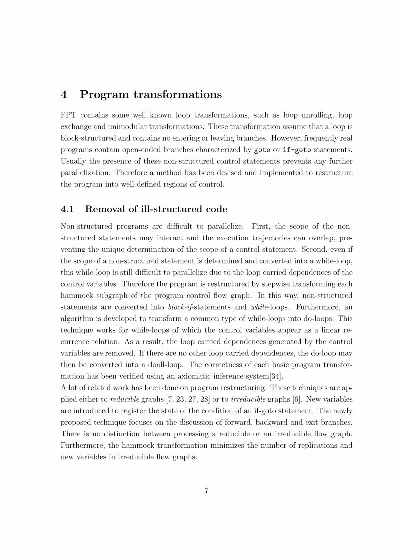
4 Program transformations

FPT contains some well known loop transformations, such as loop unrolling, loop

exchange and unimodular transformations. These transformation assume that a loop is

block-structured and contains no entering or leaving branches. However, frequently real

programs contain open-ended branches characterized by goto or if-goto statements.

Usually the presence of these non-structured control statements prevents any further

parallelization. Therefore a method has been devised and implemented to restructure

the program into well-defined regions of control.

4.1 Removal of ill-structured code

Non-structured programs are difficult to parallelize. First, the scope of the non-

structured statements may interact and the execution trajectories can overlap, pre-

venting the unique determination of the scope of a control statement. Second, even if

the scope of a non-structured statement is determined and converted into a while-loop,

this while-loop is still difficult to parallelize due to the loop carried dependences of the

control variables. Therefore the program is restructured by stepwise transforming each

hammock subgraph of the program control flow graph. In this way, non-structured

statements are converted into block-if-statements and while-loops. Furthermore, an

algorithm is developed to transform a common type of while-loops into do-loops. This

technique works for while-loops of which the control variables appear as a linear re-

currence relation. As a result, the loop carried dependences generated by the control

variables are removed. If there are no other loop carried dependences, the do-loop may

then be converted into a doall-loop. The correctness of each basic program transfor-

mation has been verified using an axiomatic inference system[34].

A lot of related work has been done on program restructuring. These techniques are ap-

plied either to reducible graphs [7, 23, 27, 28] or to irreducible graphs [6]. New variables

are introduced to register the state of the condition of an if-goto statement. The newly

proposed technique focuses on the discussion of forward, backward and exit branches.

There is no distinction between processing a reducible or an irreducible flow graph.

Furthermore, the hammock transformation minimizes the number of replications and

new variables in irreducible flow graphs.

7

4.2 Hammock graph transformations

There exist several approaches to restructure programs and many unstructured pro-

gram forms have been discussed in the literature. However, principally there are two

types of branches: backward and forward. Because the goto’s which jump out of one

or more loops are different from backward and forward branches, we call those goto’s

exit-jump.

Informally, a hammock graph [17] is a region of the program bounded by two state-

ments, n0 and ne, such that all possible execution trajectories enter the hammock graph

at its initial statement n0 and leave it at the terminal statement ne. Consequently, a

correct transformation of the hammock graph maintains the correctness of the whole

program. We define the following:

Definition 1 Branch and target.

A branch is a control statement of the following type:

[ if (< exp >) ] goto < label >

The < label > is the target of the branch. 2

If a branch is lexically preceding its target, it is called a forward branch. Otherwise, it

is called a backward branch.

Definition 2 Scope of an unstructured branch, SC(ib).

The scope of an if-statement, SC(ib), is the block of statements between the if-

statement and the target, excluding ”if” and including the ”target”. 2

Definition 3 Interacting branches.

When two branches and its targets overlap, the branches interact, i.e. their scopes

intersect:

SC(ib) ∩ SC(jb) 6= 0

2

Definition 4 Hammock graph of a branch ib, HGib

A hammock graph of a branch is the union of all scopes which directly or indirectly

overlap with SC(ib). A hammock graph has a single entry point n0 and a single exit

point ne. 2

8

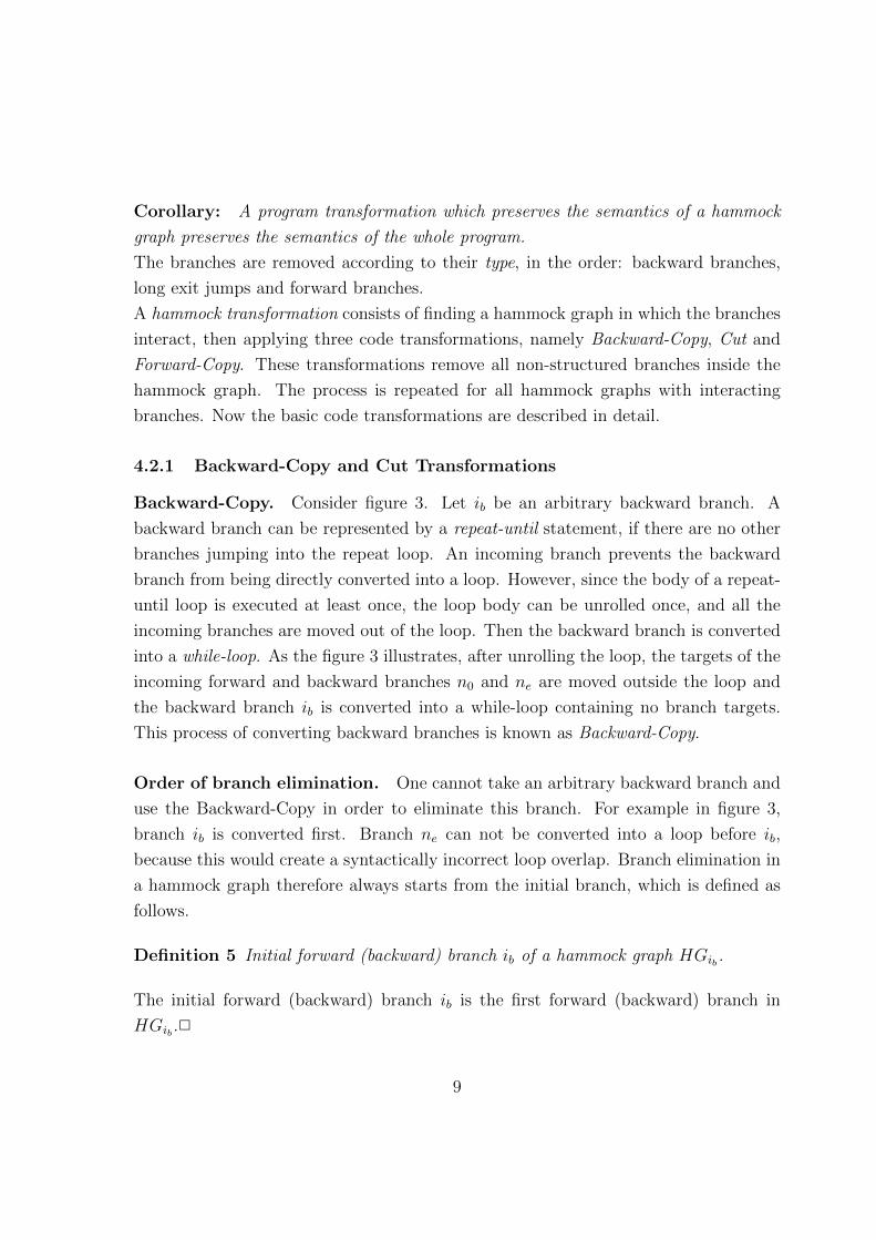
Corollary: A program transformation which preserves the semantics of a hammock

graph preserves the semantics of the whole program.

The branches are removed according to their type, in the order: backward branches,

long exit jumps and forward branches.

A hammock transformation consists of finding a hammock graph in which the branches

interact, then applying three code transformations, namely Backward-Copy, Cut and

Forward-Copy. These transformations remove all non-structured branches inside the

hammock graph. The process is repeated for all hammock graphs with interacting

branches. Now the basic code transformations are described in detail.

4.2.1 Backward-Copy and Cut Transformations

Backward-Copy. Consider figure 3. Let ib be an arbitrary backward branch. A

backward branch can be represented by a repeat-until statement, if there are no other

branches jumping into the repeat loop. An incoming branch prevents the backward

branch from being directly converted into a loop. However, since the body of a repeat-

until loop is executed at least once, the loop body can be unrolled once, and all the

incoming branches are moved out of the loop. Then the backward branch is converted

into a while-loop. As the figure 3 illustrates, after unrolling the loop, the targets of the

incoming forward and backward branches n0 and ne are moved outside the loop and

the backward branch ib is converted into a while-loop containing no branch targets.

This process of converting backward branches is known as Backward-Copy.

Order of branch elimination. One cannot take an arbitrary backward branch and

use the Backward-Copy in order to eliminate this branch. For example in figure 3,

branch ib is converted first. Branch ne can not be converted into a loop before ib,

because this would create a syntactically incorrect loop overlap. Branch elimination in

a hammock graph therefore always starts from the initial branch, which is defined as

follows.

Definition 5 Initial forward (backward) branch ib of a hammock graph HGib.

The initial forward (backward) branch ib is the first forward (backward) branch in

HGib .2

9

Figure 3: Removal of interacting backward branches. (a) The hammock graph HGib

of backward branch ib with beginning and end nodes n0 and ne. SC(ib) is the scope of

branch ib. (b) After converting ib into a while-statement, the targets of n0 and ne are

moved outside the loop.

E.g. backward branch ib precedes ne and is therefore the initial backward branch of the

surrounding hammock graph, HGib . When branch ib is the initial backward branch,

there are no other backward branches going out of its scope, SC(ib). Since there

are no preceding backward branches, the Backward-Copy transformation creates no

interaction with other backward branches. Furthermore, by construction, the targets

of all other branches are moved outside the while-loop.

Next, the second initial backward branch is selected and eliminated. This procedure

is repeated until there are no more backward branches.

Code duplication. In order to structure the program, some code duplications are

needed when the control graph is irreducible. Consider the program (2.a). The scope

of initial backward branch S5, SC(S5), is S3-S4. However, since S4 is the target

of incoming forward branch S1, the scope SC(S5) is duplicated and a while-loop is

generated around S3’ and S4’ (see (2.b)). Then the next backward branch S7 is

converted into a repeat-until loop and finally the forward branch S1 reverts to a block-

if (see next section).

10

Example 2 Cut transformation

S1 IF (P1) GOTO 200 S1 IF (.not.p1) THEN

S2 S1=1 S2 s1=1

S3 100 S2=2 S3 100 s2=2

S4 200 S3=3 ENDIF

S5 IF (P2) GOTO 100 200 REPEAT

S6 S4=4 S4 s3=3

S7 IF (P3) GOTO 200 S5 WHILE(p2)

S3’ 15 s2=2

S4’ 20 s3=3

ENDDO

S6 s4=4

S7 UNTIL (p3)

(a) interacting forward and (b) branches removed

backward branches

Backward branch optimization. If the scope of a backward branch SC(ib) con-

tains no incoming branches, the branch can be replaced by a repeat-until loop, without

duplicating the scope SC(ib) in front of the loop.

Cut Transformation. After eliminating the backward branches, there may be loops

with forward branches jumping out of the newly created while-loops. In order to remove

these branches, the Cut conversion is applied as follows: 1) a new variable bri is used

to register the state of the branch condition and the loop control expression is modified

by adding the new variable bri; 2) the long jump is cut into two parts, one starts within

the loop and jumps to the end of the loop, using EXIT, which is similar to a break

statement in C. The other is located outside the loop and jumps to its original target.

See example 3.

11

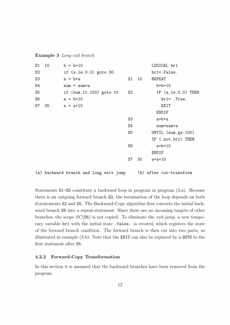
Example 3 Long exit branch

S1 10 b = b+10 LOGICAL br1

S2 if (a.le.0.0) goto 30 br1=.False.

S3 a = b+a S1 10 REPEAT

S4 sum = sum+a b=b+10

S5 if (sum.lt.100) goto 10 S2 IF (a.le.0.0) THEN

S6 a = b+10 br1= .True.

S7 30 a = a+10 EXIT

ENDIF

S3 a=b+a

S4 sum=sum+a

S5 UNTIL (sum.ge.100)

IF (.not.br1) THEN

S6 a=b+10

ENDIF

S7 30 a=a+10

(a) backward branch and long exit jump (b) after cut-transform

Statements S1-S5 constitute a backward loop in program in program (3.a). Because

there is an outgoing forward branch S2, the termination of the loop depends on both

if-statements S2 and S5. The Backward-Copy algorithm first converts the initial back-

ward branch S5 into a repeat-statement. Since there are no incoming targets of other

branches, the scope SC(S5) is not copied. To eliminate the exit-jump, a new tempo-

rary variable br1 with the initial state .false. is created, which registers the state

of the forward branch condition. The forward branch is then cut into two parts, as

illustrated in example (3.b). Note that the EXIT can also be replaced by a GOTO to the

first statement after S5.

4.2.2 Forward-Copy Transformation

In this section it is assumed that the backward branches have been removed from the

program.

12

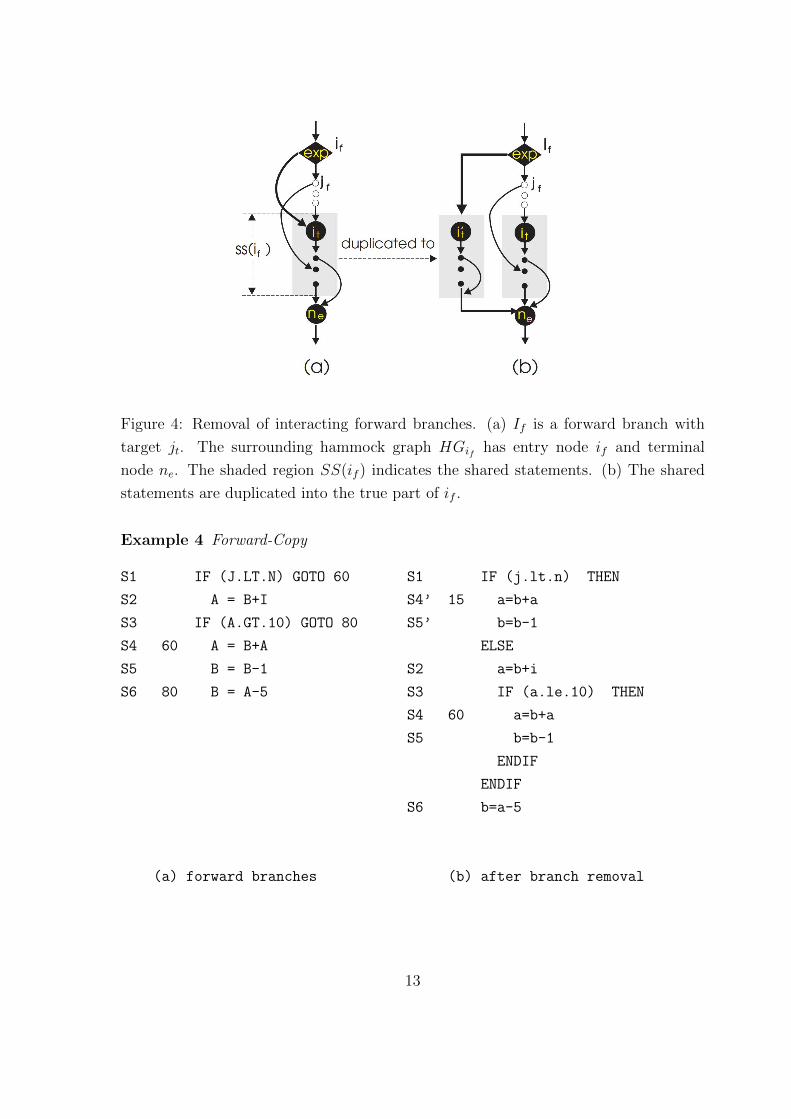
Figure 4: Removal of interacting forward branches. (a) If is a forward branch with

target jt. The surrounding hammock graph HGif has entry node if and terminal

node ne. The shaded region SS(if ) indicates the shared statements. (b) The shared

statements are duplicated into the true part of if .

Example 4 Forward-Copy

S1 IF (J.LT.N) GOTO 60 S1 IF (j.lt.n) THEN

S2 A = B+I S4’ 15 a=b+a

S3 IF (A.GT.10) GOTO 80 S5’ b=b-1

S4 60 A = B+A ELSE

S5 B = B-1 S2 a=b+i

S6 80 B = A-5 S3 IF (a.le.10) THEN

S4 60 a=b+a

S5 b=b-1

ENDIF

ENDIF

S6 b=a-5

(a) forward branches (b) after branch removal

13

Duplication of shared statements. A forward branch transfers the control flow

according to a Boolean condition. The first path is called the true part while the other

is called the false part. Assume that an initial forward branch if interacts with an

other forward branch (see figure 4). The statements on the path between the target of

if and the terminal node ne are called the shared statements, SS(if ). Forward branch

if is converted into a block-if by duplicating the shared statements into the true part.

This process is called Forward-Copy.

To illustrate the method, refer to the program (4.a). The two forward branches S1 and

S3 interact. The shared statements S4, S5 are duplicated to S4’, S5’ as the true

part of S1, while the statements S2, S3, S4, S5 are located in the false part of S1.

After the Forward Copy, both block-if’s are hammock graphs (see the program (4.b)

and figure 4).

4.3 Converting a while-loop into a do loop

Y. Wu [32] has formalized a while-loop as follows:

while b(T )

T = g(T )

U = h(D,T )

endwhile

(1)

Here T is the set of variables controlling Boolean condition b(T ) and D are the other

variables. U is the set of output variables, excluding T . The control variables T are

modified by the function g and the data are modified by the function h. A while-

statement establishes a loop of which the Boolean expression b(T ) is modified during

an iteration. Therefore, the number of iterations depends on b(T ). The key to the

translation of while-loops into do-loops is to determine the number of iterations. This

requires that b(T ) can be represented as a function of a loop counter k. If b(T ) = bf (k),

the number of iterations Nit is the smallest integer which makes bf (Nit) = false. As

a result, the while-loop (1) is converted into a do-loop by replacing while b(T ) by do

k = 1, Nit.

When the induction statements T = g(T ) create loop carried dependences, the resulting

do-loop cannot be parallelized. Often the induction statements represent a set of

coupled linear recurrence relations, for which an analytical solution exists. In this

14

case FPT converts the control variable T into a function f(k) of the loop counter k.

As a result, the loop carried induction dependence is eliminated. Next, the Boolean

expression b(T ) is represented as a function bf (k) by substituting f(k) into b(T ), where

bf = b◦f . Finally, the number of iterations Nit is found by calculating the first integer

value of n such that bf (n) = false. The number n can be determined by a binary

search, or solved explicitly when the Boolean function is of the form f(n) ≥ 0, such as

in the FFT-program (see section 6.1). If there are no other loop carried dependences,

the loop is converted into a DOALL-loop.

4.4 Loop transformations

When the array subscripts are linear and differ only by a constant, a unimodular

transformation exists which generates outermost DOALLs with a large granularity[13].

The available loop transformations in the interactive mode are extended by a link to the

well-known Tiny-tool developed by Michael Wolfe [30]. The user can select and clip any

particular loop or nested loop, edit, modify and apply the loop transformations such as

interchange, skewing, strip mining, wavefront as well as unimodular transformations.

In each step the user can perform a dependence test and verify the parallelism gained

by the transformation.

5 PVM interface

5.1 Code generation

After detecting the parallel loops, FPT generates code for different platforms, i.e.

Fortran/MP for Sun Sparc, assembly code for a multiprocessor prototype (VPS[14]),

threaded-code and PVM. The PVM software [15, 18] creates a Parallel Virtual Ma-

chine on a network of workstations. Basically PVM consists of a C- or Fortran-callable

message passing library and a communication daemon which greatly facilitates the ex-

ecution of a parallel application on distributed computers. However, users still need to

find the parallelism and to program the data exchange and the task synchronization

explicitly. During the process, new errors may be introduced when a sequential pro-

gram is translated into the PVM code. Recently, a few tools have been developed for

generating PVM code from a user’s application.

15

ADAPTOR of GMD [11] is an Automatic DAta Parallelism TranslatOR for trans-

forming data parallel programs written in Fortran with array extensions, parallel loops,

and layout directives to parallel programs with explicit message passing. It supports

the data parallel languages Connection Machine Fortran and High Performance For-

tran (HPF). The user has to express the parallelism explicitly using HPF statements.

The resulting code is linked with the Adaptor libraries, which hide the PVM-code.

PARADDAPT of Washington state university [24] is another compilation system

which converts a sequential program to parallel PVM code. PARADDAPT consists

of several cooperating tools i.e. the Parafrase-2 parallelizing compiler, a data distri-

bution tool ADDT, and a HPF compiler, ADAPTOR. Sequential programs are paral-

lelized into parallel PVM codes using the HPF code generator. Here the user may use

Parafrase to analyze and parallelize the loops.

FPT, the Fortran Parallel Transformer developed at the University of Ghent, is an

integrated interactive parallel programming environment for parallelizing programs.

Besides the parallelization tools, the generation of PVM code is simple and transparent

to the user. Furthermore, no extra libraries or tools are needed, apart from the public

domain PVM system. The PVM-code generator of FPT converts the serial program

into master and slave programs. The parallel loops are partitioned to be executed

by the number of available servers. The communication is optimized by using a data

broadcast from the master to all slaves and by minimizing the amount of data sent.

A PVM application consists of a master program and several slave programs. Each

outer DOALL loop found by FPT constitutes a separate job executed by the slaves.

Therefore the N independent iterations are partitioned over the p processors in bands

of dN/pe iterations. The granularity can be refined by selecting p > pmax, where pmax

is the maximum number of available processors for the job.

Each parallel loop is executed in three steps.

1. In the prologue, the input data for all slaves is gathered and put into a single

message. The number of iterations in one task is calculated and included in the

message. Finally, the sequence number of every slave is added. Then this message

is broadcast.

16

2. In the execution phase, the slave program unpacks the message and executes the

loop body corresponding to its sequence number sent by the master. During

this phase there is no communication between the slaves, because the inner loop

iterations are independent.

3. In the epilogue, each slave packs and sends back the results and the master stores

the received data in the proper locations. Care is taken that the data results of

each slave do not overlap.

5.2 Data distribution

Data packing. Let lhs and rhs be the data references at the left hand side and the

right hand side of the assign statements in a parallel loop. Then the input data and

the output data for a slave are rhs and lhs respectively. The input data rhs is packed

one by one in a message buffer using the command

call pvmfpack(type, name, n, stride, info).

Here type is a constant representing the variable type, name represents a scalar or an

array element. As a result n elements at distance stride are added to the message

buffer, info. Similarly, at the slave, the pvmfunpack routine unloads the message

buffer. This PVM-call allows arrays with linear index expressions to be packed in a

single call. E.g., the input for the following parallel loop

doall i=1,n

b(i)=a(i)+c(2*i)

enddo

is packed and broadcast to the slaves by

call pvmfpack(3,a,n,1,info)

call pvmfpack(3,c,n/2,2,info)

call pvmfmcast(info)

17

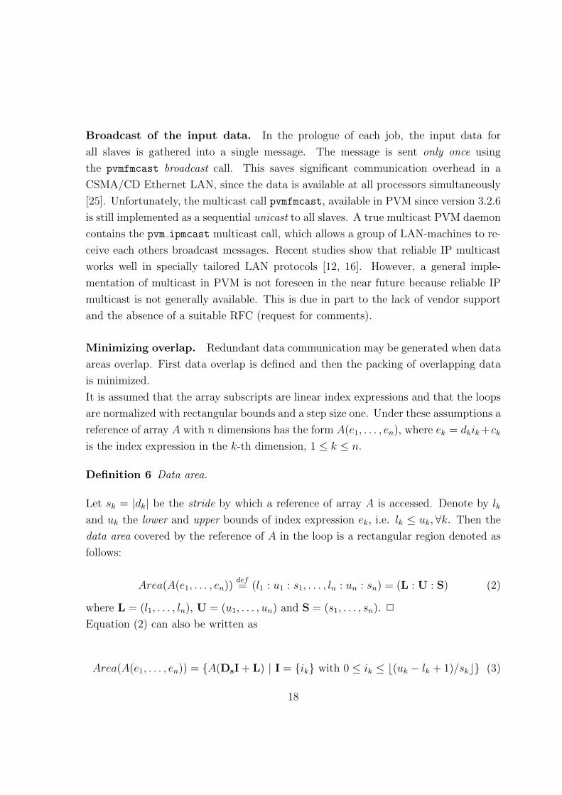
Broadcast of the input data. In the prologue of each job, the input data for

all slaves is gathered into a single message. The message is sent only once using

the pvmfmcast broadcast call. This saves significant communication overhead in a

CSMA/CD Ethernet LAN, since the data is available at all processors simultaneously

[25]. Unfortunately, the multicast call pvmfmcast, available in PVM since version 3.2.6

is still implemented as a sequential unicast to all slaves. A true multicast PVM daemon

contains the pvm ipmcast multicast call, which allows a group of LAN-machines to re-

ceive each others broadcast messages. Recent studies show that reliable IP multicast

works well in specially tailored LAN protocols [12, 16]. However, a general imple-

mentation of multicast in PVM is not foreseen in the near future because reliable IP

multicast is not generally available. This is due in part to the lack of vendor support

and the absence of a suitable RFC (request for comments).

Minimizing overlap. Redundant data communication may be generated when data

areas overlap. First data overlap is defined and then the packing of overlapping data

is minimized.

It is assumed that the array subscripts are linear index expressions and that the loops

are normalized with rectangular bounds and a step size one. Under these assumptions a

reference of array A with n dimensions has the form A(e1, . . . , en), where ek = dkik +ck

is the index expression in the k-th dimension, 1 ≤ k ≤ n.

Definition 6 Data area.

Let sk = |dk| be the stride by which a reference of array A is accessed. Denote by lk

and uk the lower and upper bounds of index expression ek, i.e. lk ≤ uk,∀k. Then the

data area covered by the reference of A in the loop is a rectangular region denoted as

follows:

Area(A(e1, . . . , en))def= (l1 : u1 : s1, . . . , ln : un : sn) = (L : U : S) (2)

where L = (l1, . . . , ln), U = (u1, . . . , un) and S = (s1, . . . , sn). 2

Equation (2) can also be written as

Area(A(e1, . . . , en)) = {A(DsI + L) | I = {ik} with 0 ≤ ik ≤ b(uk − lk + 1)/skc} (3)

18

Here Ds is a constant diagonal matrix with elements the stride vector S=(s1, . . . , sn).

Definition 7 Overlapping data areas.

Two areas A1 and A2 overlap if they have at least one common element. 2

FPT checks the following sufficient overlap conditions:

Lemma 1 Sufficient overlap conditions.

Let A1 = (L:U:S) and A2 = (L’:U’:S’) be two data areas. A1 and A2 overlap if the

following conditions are true:

max (L,L′) ≤ min (U,U′) (4)

gcd (S,S′) divides |L− L′| (5)

and

lcm (S,S′) ≤ min (U,U′)−max (L,L′). (6)

2

Here the operators max, min, gcd (greatest common divisor) and lcm (least common

multiple) operate on pairwise elements of the two vector arguments, e.g.

max(lk, l′k) ≤ min(uk, u

′k),∀k

Proof: Assume condition (4) is not true. Then there exists a bound k such that

max(lk, l′k) > min(uk, u

′k). Without loss of generality, suppose lk = max(lk, l

′k). Since

by definition 6, lk ≤ uk, one has lk > u′k or ek > e′k,∀k, and A1 and A2 cannot have

common elements in dimension k. Therefore condition (4) is necessary. Furthermore,

in order to A1 and A2 have at least one element in common, a solution of the set of

n Diophantine equations ek = e′k,∀k, must exist. In other words, there exist integer

indices I and J such that

DsI + L = Ds′J + L′. (7)

Since Ds and Ds′ are diagonal matrices, the Diophantine equations (7) are independent.

An integer solution exists iff gcd (S,S′) divides |L− L′|[8]. This is condition (5).

19

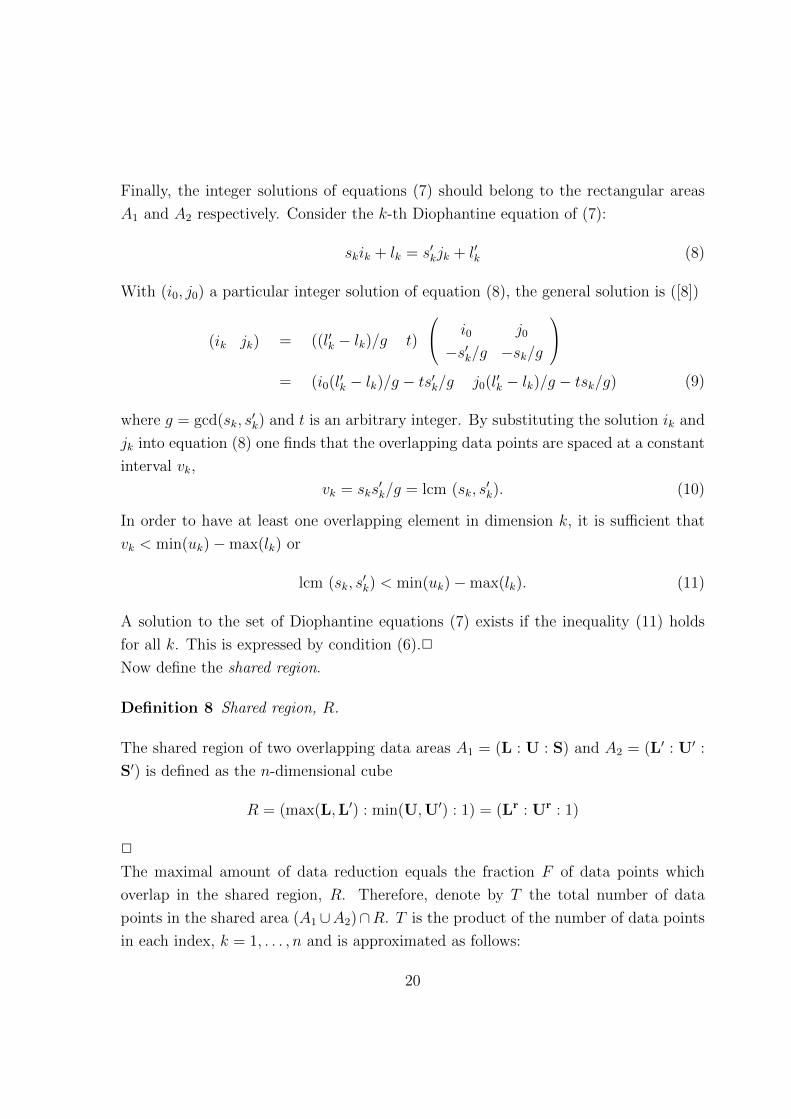
Finally, the integer solutions of equations (7) should belong to the rectangular areas

A1 and A2 respectively. Consider the k-th Diophantine equation of (7):

skik + lk = s′kjk + l′k (8)

With (i0, j0) a particular integer solution of equation (8), the general solution is ([8])

(ik jk) = ((l′k − lk)/g t)

i0 j0

−s′k/g −sk/g

= (i0(l

′k − lk)/g − ts′k/g j0(l

′k − lk)/g − tsk/g) (9)

where g = gcd(sk, s′k) and t is an arbitrary integer. By substituting the solution ik and

jk into equation (8) one finds that the overlapping data points are spaced at a constant

interval vk,

vk = sks′k/g = lcm (sk, s

′k). (10)

In order to have at least one overlapping element in dimension k, it is sufficient that

vk < min(uk)−max(lk) or

lcm (sk, s′k) < min(uk)−max(lk). (11)

A solution to the set of Diophantine equations (7) exists if the inequality (11) holds

for all k. This is expressed by condition (6).2

Now define the shared region.

Definition 8 Shared region, R.

The shared region of two overlapping data areas A1 = (L : U : S) and A2 = (L′ : U′ :

S′) is defined as the n-dimensional cube

R = (max(L,L′) : min(U,U′) : 1) = (Lr : Ur : 1)

2

The maximal amount of data reduction equals the fraction F of data points which

overlap in the shared region, R. Therefore, denote by T the total number of data

points in the shared area (A1 ∪A2)∩R. T is the product of the number of data points

in each index, k = 1, . . . , n and is approximated as follows:

20

T =n∏

k=1

((ur

k − lrk + 1)

sk+

(urk − lrk + 1)

s′k)

=n∏

k=1

(sk + s′k)

sks′k(ur

k − lrk + 1)

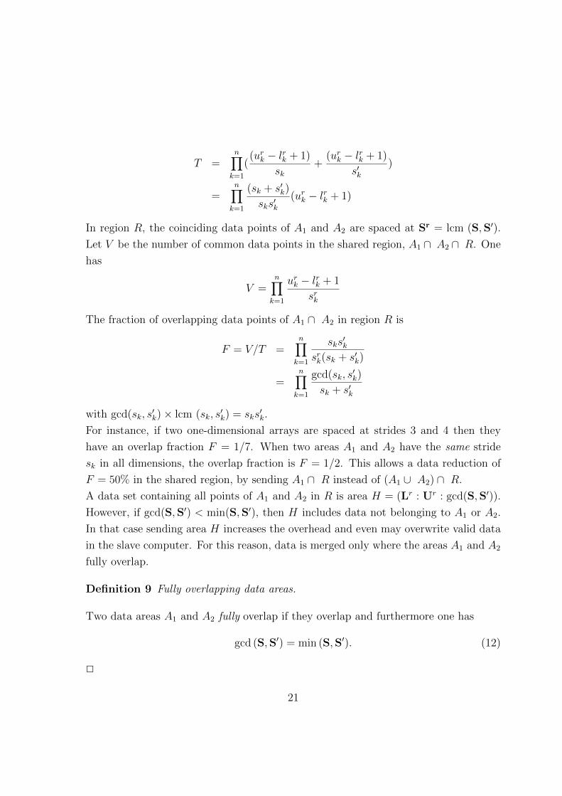
In region R, the coinciding data points of A1 and A2 are spaced at Sr = lcm (S,S′).

Let V be the number of common data points in the shared region, A1 ∩ A2 ∩ R. One

has

V =n∏

k=1

urk − lrk + 1

srk

The fraction of overlapping data points of A1 ∩ A2 in region R is

F = V/T =n∏

k=1

sks′k

srk(sk + s′k)

=n∏

k=1

gcd(sk, s′k)

sk + s′k

with gcd(sk, s′k)× lcm (sk, s

′k) = sks

′k.

For instance, if two one-dimensional arrays are spaced at strides 3 and 4 then they

have an overlap fraction F = 1/7. When two areas A1 and A2 have the same stride

sk in all dimensions, the overlap fraction is F = 1/2. This allows a data reduction of

F = 50% in the shared region, by sending A1 ∩ R instead of (A1 ∪ A2) ∩ R.

A data set containing all points of A1 and A2 in R is area H = (Lr : Ur : gcd(S,S′)).

However, if gcd(S,S′) < min(S,S′), then H includes data not belonging to A1 or A2.

In that case sending area H increases the overhead and even may overwrite valid data

in the slave computer. For this reason, data is merged only where the areas A1 and A2

fully overlap.

Definition 9 Fully overlapping data areas.

Two data areas A1 and A2 fully overlap if they overlap and furthermore one has

gcd (S,S′) = min (S,S′). (12)

2

21

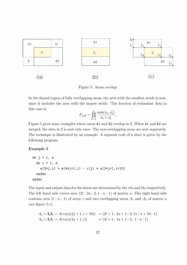
Figure 5: Areas overlap

In the shared region of fully overlapping areas, the area with the smallest stride is sent,

since it includes the area with the largest stride. The fraction of redundant data in

this case is:

Ffull =n∏

k=1

min(sk, s′k)

sk + s′k.

Figure 5 gives some examples where areas A1 and A2 overlap in C. When A1 and A2 are

merged, the data in C is sent only once. The non-overlapping areas are sent separately.

The technique is illustrated by an example. A segment code of a slave is given by the

following program.

Example 5

do j = l, u

do i = 1, n

a(2*j,i) = a(4*j+1,i) - c(j) * a(2*j+1,i+10)

enddo

enddo

The input and output data for the slaves are determined by the rhs and lhs respectively.

The left hand side covers area (2l : 2u : 2, 1 : n : 1) of matrix a. The right hand side

contains area (l : u : 1) of array c and two overlapping areas A1 and A2 of matrix a

(see figure 5.c):

A1 = I0I5 = Area(a(2j + 1, i + 10)) = (2l + 1 : 2u + 1 : 2, 11 : n + 10 : 1)

A2 = I2I7 = Area(a(4j + 1, i)) = (4l + 1 : 4u + 1 : 4, 1 : n : 1)

22

Areas A1 and A2 overlap when n > 10. The overlap is full, since the strides (2,1)

(A1) and (4,1) (A2) satisfy equation (12). By a merging operation, the input data area

consists of three data regions:

I0I5 = (2l + 1 : 2u + 1 : 2, 11 : n + 10 : 1)

I3I6 = (2u + 1 : 4u + 1 : 4, 11 : n : 1)

I4I7 = (4l + 1 : 4u + 1 : 4, 1 : 11 : 1)

Since vector c is only input data, the master sends vector c only once. Using the input

and output areas of matrix a, the generation of PVM code for sending and receiving

data is straight forward.

6 Results

6.1 Parallelizing the FFT kernel using the ISG

The iteration space graph can help the programmer to find less obvious parallelism.

Consider the FFT kernel in example 6. After restructuring the FFT kernel by remov-

ing the GOTO’s and converting the resulting WHILE into a DO-loop, the program 6(b)

results. Automatic parallelization is not able to detect parallel loops in this case. The

flow dependences for the array data are shown in figure 6 for n=16. It immediately

becomes clear that all loop-carried dependences point from iteration k1 to iteration

k1+1. Consequently, the k1 loop has to be executed sequentially. At the other hand,

there are no dependences between the iterations of loop i or loop m for a particular

value of k1. Therefore, the i- and the m-loops can be executed in parallel.

6.2 PVM benchmark

Generating PVM code is an important aspect of the FPT environment. PVM code

is generated from a serial users’ application first by extracting parallel loops via the

data and control dependence analysis, next by partitioning the code and distributing

the data to the slaves. Furthermore, redundant data communication is minimized by

merging overlapping data areas.

Three examples, GJ (Gauss-Jordan Elimination), MM (Matrix Multiplication) and

CONVOL, a convolution program, illustrate the use of FPT-generated PVM code.

23

Table 1 gives speedups when problems with dimensions 400 and 800 are executed on

1 to 4 processors. The codes were executed on HP7XX workstations connected by an

Ethernet 10Mb/s network.

Example 6 Fast Fourier Kernel program

mmax=1 mmax=1

90 if (mmax-n .ge. 0 ) goto 130 n1=log(dble(n))/log(dble(2))+0.9

100 istep=2*mmax 90 DO k1 = 1,n1

do m=1, mmax v2=mmax-1

theta=pi*isi*(m-1)/float(mmax) v3=n-1

w=cmplx(cos(theta), sin(theta)) v4=2**(k1-1)

do i=m,n, istep v1=2**k1

j=i+mmax mmax=v4

temp = w*data(j) 100 istep=2*mmax

data(j)=data(i)-temp DOALL m = 1,mmax

data(i)=data(i)+temp theta=pi*isi*(m-1)/float(mmax)

enddo w=cmplx(cos(theta),sin(theta))

enddo DOALL i = m,n,istep

mmax=istep j=i+mmax

goto 90 temp=w*data(j)

130 continue data(j)=data(i)-temp

data(i)=data(i)+temp

ENDDO

ENDDO

mmax=v1

ENDDO

(a) original FFT kernel (b) restructured FFT kernel

24

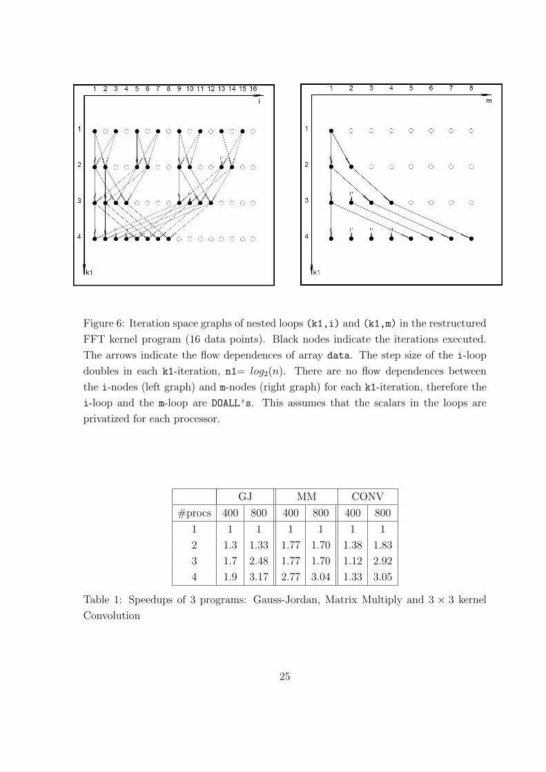
Figure 6: Iteration space graphs of nested loops (k1,i) and (k1,m) in the restructured

FFT kernel program (16 data points). Black nodes indicate the iterations executed.

The arrows indicate the flow dependences of array data. The step size of the i-loop

doubles in each k1-iteration, n1= log2(n). There are no flow dependences between

the i-nodes (left graph) and m-nodes (right graph) for each k1-iteration, therefore the

i-loop and the m-loop are DOALL’s. This assumes that the scalars in the loops are

privatized for each processor.

GJ MM CONV

#procs 400 800 400 800 400 800

1 1 1 1 1 1 1

2 1.3 1.33 1.77 1.70 1.38 1.83

3 1.7 2.48 1.77 1.70 1.12 2.92

4 1.9 3.17 2.77 3.04 1.33 3.05

Table 1: Speedups of 3 programs: Gauss-Jordan, Matrix Multiply and 3 × 3 kernel

Convolution

25

6.3 PVM code generation for the Jacobi kernel

The following example illustrates the PVM-code productivity gain. Consider the fol-

lowing 19-line Jacobi program as parallelized by FPT:

Example 7 Jacobi kernel

SUBROUTINE jacobi(a,b,n,ncycles)

REAL a(n+2,n+2),b(n+2,n+2)

DO k = 1,ncycles

c Job 1

DOALL j = 2,n+1

DOALL i = 2,n+1

a(i,j)=(b(i-1,j)+b(i+1,j)+b(i,j-1)+b(i,j+1))/4

ENDDO

ENDDO

c Job 2

DOALL j = 2,n+1

DOALL i = 2,n+1

b(i,j)=a(i,j)

ENDDO

ENDDO

ENDDO

END

The outer DOALL-loops are partitioned as Job 1 and 2. The original program is 19 lines,

the resulting PVM-codes for master and slave contain respectively 107 and 91 lines. If

one roughly assumes that the programming time is proportional to the number of lines

in a program, the productivity gained by the automatic PVM-code generation and

data distribution is about a factor of ten. With respect to data compaction, the areas

of matrix b in Job 1 are B1 = (1 : n : 1, 2 : n + 1 : 1), B2 = (3 : n + 2 : 1, 2 : n + 1 : 1),

B3 = (2 : n + 1 : 1, 1 : n : 1) and B4 = (2 : n + 1 : 1, 3 : n + 2 : 1). Since the strides in

both dimensions i and j are si = sj = 1, areas B1, B2, B3 and B4 fully overlap in the

shared region R = (3 : n : 1, 3 : n : 1). Consequently, the PVM generator sends the

26

data in region R once, resulting in a data reduction of 4. After merging region R with

the boundary rows and columns, matrix b is packed into the message buffer info by

the following code:

C** Master sends the input data

DO i_0 = 1,n+2,1

call pvmfpack(4,b(1,i_0),n+2,1,info)

ENDDO

7 Conclusion

FPT contains many of the dependence tests described in Banerjee’s comprehensive

work [8] and in addition includes the analysis of IF statements by sharpening the itera-

tion space and constant propagation. Backward GOTO’s are converted into DOWHILE

loops and these are furthermore changed into DO-loops when the while condition can

be expressed by a linear induction variable[33].

The treatment of loop transformations in the interactive mode is inspired by the well-

known tiny-tool developed by Wolfe [30]. The user can select and clip any particular

loop or nested loop, edit, modify and apply the loop transformations such as inter-

change, skewing, strip mining, wavefront as well as unimodular transformations. In

each step the user can perform a dependence test and verify the parallelism gained by

the transformation.

At the end of the interactive phase, an annotated pretty printed source code is gen-

erated, instrumented with parallel directives for several platforms. These include a

shared memory Solaris machine, a parallel intermediate language for a multiprocessor

prototype (VPS) as well as threaded code and PVM.

FPT-PVM facilitates high performance computing in a distributed network of com-

puters by translating a sequential application into parallel PVM code. The resulting

program uses only standard f77 and PVM library calls. Furthermore, the program is

highly readable and informative to the user. Finally, the application of the FPT-PVM

system is straightforward and has been demonstrated to allow efficient distributed

computing.

27

References

[1] Aho, A. V., and Ullman, J. D., Compilers: Principles, Techniques, and tools. Addison-

Wesley, Reading, MA, 1986.

[2] Allen, J.R., “Automated Environments for Parallel Programming”, IEEE Software

February, Vol 7, pp. 21-29, 1985.

[3] Allen, J.R., “Dependence Analysis for subscript Variables and Its Application to Pro-

gram Transformations”, Ph.D. Dissertation, Department of Mathematical Sciences, Rice

University, Houston, Texas(April), 1983.

[4] Allen, J.R., Kennedy, K., Porterfield, C., and Warren, J., “Conversion of Control De-

pendence to Data Dependence”, in Conference Proceedings – The 10th Annual ACM

Symposium on Principles of Programming Languages, 1983, pp. 177-189.

[5] Allen, J.R., and Kennedy, K., “Automatic Translation of FORTRAN Programs to Vector

Form”. ACM Transaction on programming Language& Systems. Vol. 9, No. 4(October),

pp. 491-542, 1984.

[6] Ammarguellat Zahira, A Control-Flow Normalization Algorithm and its Complexity,

IEEE Transactions on Software Engineering, Vol. 18, 3, pp. 237-251, 1992

[7] Baker, B., “An algorithm for structuring flowgraphs,” JACM, vol 24, no. 1, 1977.

[8] Banerjee U., Loop Transformations for Restructuring Compilers, Kluwer Academic Pub-

lishers, Boston (Mass.), 305 pp., 1993.

[9] Banerjee U., Eigenmann R., Nicolau A., Padua D., Automatic Program Parallelization,

IEEE Proceedings, Vol. 81, 2, pp. 211-243, 1993.

[10] Banerjee, U., Dependence Analysis for Supercomputing, The Kluwer international series

in engineering and computer science. Parallel processing and fifth generation computing.

ISBN 0-89838-289-0. Kluwer Academic Publishers, 1988.

[11] Brandes, T., ADAPTOR Programmer’s Guide (Version 3.1) Technical documen-

tation, GMD, Oct., 1995. Available via anonymous ftp from ftp.gmd.de as

gmd/adaptor/docs/pguide.ps.

[12] Chang S-L., Du D.H-C., Hsieh J., Tsang R.P., Lin M., Enhanced PVM Communications

over a High-Speed LAN, IEEE Parallel & Distributed Technology, Fall ’95, pp. 20-32,

1995.

28

[13] D’Hollander E.H., Partitioning and Labeling of Loops by Unimodular Transformations,

IEEE Transactions on Parallel and Distributed Systems, Vol. 3, 7, pp. 465-476, 1992.

[14] D’Hollander E.H., The VPS, a Virtual MIMD Processor and its Software Environment,

Workshop on Compiling Techniques and Compiler Construction, for Parallel Computers,

Oxford UK, 13-15 September 1989, 19-36, 1989.

[15] Dongarra J., Geist G.A., Manchek R., Sunderam V.S., Integrated PVM framework

supports heterogeneous network, Tennessee Univ., Knoxville, TN, USA Computers in

Physics Vol: 7 Iss:2 pp. 166-74, 1993.

[16] Dunigan T.H., Hall K.A., PVM and IP Multicast, Oak Ridge National Laboratory,

Technical Report ORNL/TM-13030, 28 pp., 1996.

[17] Ferrante, J., Ottenstein, K. J., and Warren, J. D., “The Program Dependence Graph

and Its use Optimization”, ACM Trans. on Programming Languages and Systems. vol.

9 no. 3, July, pp. 319-349, 1987.

[18] Geist A., Beguelin A., Dongarra J., Jiang W., Manchek R., Sunder,PVM 3 User’s Guide

and Reference Manual, Oak Ridge National Laboratory, Oak Ridge TN 37831-6367

Technical Report, ORNL/TM-12187, May, 108pp., 1993.

[19] Gupta M., Banerjee P., Demonstration of Automatic Data Partitioning Techniques for

Parallelizing Compilers on Multicomputers, IEEE Trans. on Parallel Distributed System.

Vol. 3, No. 2, March, pp. 179-93, 1992.

[20] Kuck, D.J., Kuhn, R.H., and Padua, D.A., Leasure, B.R., and Wolfe, M.J. “Dependence

Graphs and Compiler Optimizations”, Conference Proceedings– The 8th Annual ACM

Symposium on Principles of Programming Languages (Williamsburgh, Virginia, January

26-28), ACM Press, pp. 207-218, 1981.

[21] Lundstrom Stephen F. and Barnes George H., “A Controllable MIMD Architecture”,

International Conference on Parallel Processing, pp. 19-27, 1980.

[22] Polychronopoulos, C., Girkar, M., Haghighat, M.R., Lee, C.H., Leungg, “Parafrase-2:

An Environment for Parallelizing, Partitioning, Synchronizing and Scheduling Programs

on Multiprocessors”, CSRD Urbana-Champaign IL 61801 USA, ICPP’89, II - Software,

pp. 39-48, 1989.

[23] Ramshaw, L., “Eliminating go to’s while Preserving Program Structure”, JACM. Vol.

35, No. 4, October, pp. 893-920, 1988.

29

[24] Sivaraman, H., Raghavendra, C.S., Parallelizing sequential programs to a cluster of

workstations, Proceedings of the 1995 Workshop on Challenges for Parallel Processing,

Raleigh, NC, USA. 14 Aug., pp. 38-41, 1995.

[25] Sunderam V.S., Geist G.A., Dongarra J., Manchek R., The PVM Concurrent Computing

System: Evolution, Experiences, and Trends, Parallel Computing, 1992.

[26] Tarjan, R. E., “Testing Flow Graph Reducibility”, Computer Journal. vol. 9, pp. 355-

365, 1974.

[27] Williams, M. H., “Generating structured flow diagrams: the nature of unstructuredness”,

Computer Journal. vol 20, no. 1, pp. 45-50, 1977.

[28] Williams M. H, and Ossher, H. L., “Conversion of Unstructured flow diagrams to struc-

tured form”, Computer Journal. vol. 21, no. 2, pp. 161-167, 1978.

[29] Wolfe, M.J., “Optimizing Supercompilers for Supercomputers”, PhD. Thesis, the Grad-

uate College of the University of Illinois at Urbana-Champaign, 1982.

[30] Wolfe M., The Tiny Loop Restructuring Research Tool, Proceedings of the International

Conference on Parallel Processing, vol. II - Software, pp. 46-53, 1991.

[31] Wolfe, M., “Beyond Induction Variables”, ACM SIGPLAN’92, SIGPLAN Notices. Vol.

27, No. 7 (July), pp. 162-174, 1992.

[32] Wu, Y., Lewis, T.G., “Parallelizing While Loops”, Proceedings of the International Con-

ference on Parallel Processing ’90, II - Software, August 13-17, pp. 1-8, 1990.

[33] Zhang Fubo, D’Hollander E.H., Extracting the Parallelism in Programs with Unstruc-

tured Control Statements, International Conference on Parallel and Distributed Systems,

ICPADS’94, Taipei, December, 1994.

[34] Zhang Fubo, FPT: A Parallel Programming Environment, PhD. Thesis, September, 26,

pp. 203, 1996.

[35] Zhu, C.Q., and Yew, P.C., “A Scheme to Enforce Data Dependence on Large Multipro-

cessor System”, IEEE Trans. on Software and Engineering, 13, 6, pp. 352-358, 1987.

30