THE FOUNDATIONS OF QUANTUMMECHANICS AND THE EVOLUTION OF

THE CALCULUS.

Jose G. Vargas ∗

Abstract

In 1960-62, E. Kahler enriched Cartan’s exterior calculus, mak-ing it suitable to address the needs, not only of quantum mechanics,but also of general relativity. Using his calculus, Kahler produceda “Kahler-Dirac” (KD) equation with which he reproduced the finestructure of the hydrogen atom. In addition, he showed that his equa-tion’s positron solutions correspond to the same positive energy aselectrons.

In this paper, we present some basic concepts of differential ge-ometry from a Cartan-Kahler perspective in order to understand, forinstance, why the components of Kahler’s tensor-valued differentialforms have three series of indices. After a summary of some high-lights of his calculus, we demonstrate its power by developing for theelectron’s large components their standard Hamiltonian beyond thePauli approximation, but without resort to Foldy-Wouthuysen trans-formations or ad hoc alternatives. The same Hamiltonian is also de-rived for the large components of positrons, the latter particles notbeing identified with small components. Hamiltonians in closed form(i.e. exact through a finite number of terms) are obtained for bothlarge and small components. The emergence of negative energies forpositrons in the Dirac theory is interpreted from the perspective ofthe KD equation.

∗PST Associates, 48 Hamptonwood Way, Columbia, SC 29209.

1

1 Introduction

In the mid to late 1920’s, a few very gifted scientists developed the present

formalism of quantum mechanics, and of QED. The merits of such formalism

not withstanding, it has to be seen as an ad hoc response to the needs of

the physics of the time. Eventually the calculus of differential forms evolved

to the point where it could address the needs of quantum physics. In the

last sections of this paper, we shall show that such a calculus constitutes a

much better way to compute in quantum mechanics, specifically in relativistic

quantum mechanics. But it is not only a matter of easier computing, as will

transpire from the first sections of the paper.

The first of the two most important highlights in the evolution of the

calculus is constituted by Cartan’s introduction in a paper on differential

equations of his exterior calculus of differential forms [1]. It is the modern

language of differential geometry, differential topology and other branches

of mathematics. It is based on exterior algebra. For decades, this calculus

remained basically ignored except in Cartan and Kahler’s work. The latter

used it in 1934 to generalize the former’s theory of exterior differential sys-

tems [2]. In 1960, Kahler generalized the exterior calculus itself, by endowing

differential forms with the richer “Clifford” structure [3],.[4], [5].

Kahler’s sophisticated calculus revolves around a basic equation that par-

allels the equation df/dx = gf , and df/dx = 0 in particular. It is called

2

the Kahler-Dirac or (simply) Kahler equation, to which he still referred as

Dirac’s. Among the many differences between the Dirac and Kahler equa-

tions (both give the same fine structure constant for the hydrogen atom, [4],

[5]), there is the replacement of spinors with inhomogeneous differential forms

with complex coefficients, differential forms which span a 32-dimensional dif-

ferentiable manifold. All these are very significant features, with ab-initio-

important consequences for quantum mechanics and even the foundations

of geometry. As we shall show, there are several tantalizing (certainly in-

triguing) features in his calculus, which Kahler already showed and which we

report in section 3.

His work, written in German and not yet translated, constitutes a formidable

piece of mathematics. His theory is relativistic ab initio, but one does not

need to know relativity to be able to use it. In fact, dealing with the issues

that are normally associated with relativistic quantum mechanics (exception

made of solving the hydrogen atom) requires just the simple version of this

calculus that results when the use of Cartesian coordinates suffices. Being

equation-based, a prior theory of physical observables is not needed, at least

for the purposes that occupied Kahler and that will occupy us in this paper.

Absent are also the gamma matrices.

In addition to the language barrier, an understanding of the Kahler calcu-

lus encounters the further barrier that one should be familiar with Cartan’s

3

methods, which Kahler largely follows. A related complication is that the

general quantities in his calculus have components with one series of super-

scripts and two series of subscripts. It is then clear that the widely held view

that the calculus of differential forms pertains to antisymmetric covariant

tensors clashes with the realities of this calculus, as it would appear that

there are two types of antisymmetric covariant tensors. For this reason, we

shall present in section 2 the Cartan-Kahler approach to vector fields, tensor-

valued differential forms, and exterior, interior, covariant and Lie derivatives

from. Fortunately, quantities with just one series of indices are sufficient

to deal with problems such as the fine structure of the hydrogen atom and

everything that we shall do in this paper.

In section 3, we summarize several outstanding features of his calculus

and his equation, features which he himself discussed. In section 4, we briefly

present further developments of this calculus, like removing the constraint

of Levi-Civita affine connection of the space, explaining some of its ad hoc

features and the rationale for some of its ansatzs. In the same section, we

also raise the issue of the two “Dirac” equations that Kahler proposed, re-

spectively in 1960 and 1962, for tensor-valued input differential form. Except

for some minor reporting, the whole paper will be confined to scalar-valued

input, whose components have just one series of indices. Kahler did not

study any particular problem where the input required the use of more than

4

one series of indices.

In section 5, we discuss rotations, angular momentum, spinors and plane

waves, all of it in the context of the two important concepts of Killing sym-

metries and constant differentials.

Readers thoroughly familiar with this calculus could just go directly to

sections 6 to 8. They might even try to solve themselves the “graduate

problems” that we proceed to formulate. The main contribution in this paper

to the use of the Kahler calculus in physics is precisely the formulation of

those problems, which are not difficult to solve, and which show the enormous

power to do what the Dirac theory can only do with hole theory plus Foldy-

Wouthuysen transformations, or similar paraphernalia.

Problem 1: At low energy, we write the wave form u of an electron in a

slowly constant electromagnetic field as e−imc2t/~R(x, t)∨ ε−, where m is the

mass of the electron and ε− suppresses positrons (i.e. projects on electrons).

Find the system of equations satisfied by the even (ϕ) and odd (χ) parts of

R.

Problem 2: Let us define χ1 ≡ − i2m

P ∨ϕ, where P denotes dxj ∨ (−i∂j−

eAj) as P. Replacing χ with χ1 in the system of problem 1, obtain the Pauli

equation for ϕ.

Problem 3: Show that, in the next order of approximation for χ, one

obtains in essence the same development of the Hamiltonian for ϕ as, say, in

5

Bjorken and Drell [8].

Problem 4: With positrons given in the form e−imc2t/~S(x, t)∨ε+, develop

the Hamiltonian for the large components (now even) of S.

Problem 5: The wave form u of an electron in a constant electromagnetic

field may also be written as u = e−iEc2t/~<(x)∨ ε−, where E is the energy of

the system. Equate the R and < forms of u to obtain simple expressions for

ϕ,t (also χ,t) in terms of ϕ (respectively χ). Use that to readily obtain an

exact Hamiltonian for χ containing just a few terms.

Problem 6: Transform the coupled system of equations for ϕ and χ so

that their roles in that system will be exchanged. Relate to the negative

energy solutions of the Dirac theory the term that jumps equation in that

transformation.

Problem 7: Based on the treatment of problems 1 and 2, develop the

iterative procedure that suggests itself to obtain χ,and then the Hamiltonian

for ϕ, in ever increasing orders.

Problem 8: Obtain an exact (i.e. in closed form) Hamiltonian for ϕ

using the idea given in problem 5. Compare the result with the also exact

Hamiltonian for χ previously obtained.

A point about terminology follows. There are subtleties familiar to al-

gebraists (a) between the concepts that go by the terms of exterior and

Grassmann algebras, and more so (b) with the use of the terms Grassmann

6

algebra, Clifford algebra and Clifford-Atiyah algebra. To follow Graff [6], in

(a), the difference is that, whereas exterior algebra is based just on the exte-

rior product, Grassman algebra contains the additional structure conferred

by an inner product induced by a quadratic form. Clifford algebra contains

only the Clifford product (example, the algebra of Dirac gamma matrices).

The Kahler-Atiyah contains both the Grassmann and Clifford algebras as

substructures [6]. However, the Clifford product of two vectors (similarly for

vector and multivector, but not for two general multivectors) can be decom-

posed into their symmetric and antisymmetric parts, identifiable with the

exterior and interior products in this case. There is not, therefore, much

point for physicists in making such subtle differences as to what constitutes

Clifford algebra. Hence, we shall adopt the practical perspective, common in

the literature, of using the term Grassmann algebra for exterior algebra and

the term Clifford algebra for the Kahler-Atiyah algebra. The term Kahler

algebra will be reserved for the so understood Clifford algebra (i.e. Kahler-

Atiyah algebra) of cochains, i.e. of functions of hypersurfaces. As we shall

explain later in the paper, we shall use the term differential forms for these

cochains, in accordance with Kahler, and because the cochains rather than

the antisymmetric multilinear functions of vectors are of the essence of his

calculus [7].

7

2 The Cartan-Kahler View of Basic Concepts

of Geometry and the Calculus

A comprehensive treatment of tangent vectors is given in an authoritative

book by Choquet-Bruhat et al. [9]. They define them (a) as sets of quan-

tities that transform in a particular way, (b) as linear operators on spaces

of functions (active vectors) and (c) as equivalence classes of curves (passive

vectors). Defining concepts by their transformation properties is clearly in-

adequate. For instance, a 1-cochain, i.e. a function of curves, and a field of

linear functions of vectors transform in the same way. Similarly, a tangent

vector field referred to the reciprocal basis ei (defined by ei = gijej) has

components which transform like 1-cochains and fields of linear functions of

vectors. Based just on transformation properties, there would be no point in

distinguishing between the two series of subscripts in the Kahler calculus

The vectors defined in (b) are operators consisting of linear combinations

of the partial derivatives with respect to the coordinates. Cartan refers to

them as infinitesimal transformations [10]. Both he and Kahler do not refer

to those operators as vectors, theirs being of type (c), as they do not act

on anything. In other words, they do not play the active role that the in-

finitesimal operators play. When Cartan generates a differential (r−1)-form

from a pair constituted by a differential r-form together with an infinitesimal

operator, he is doing what in the modern language is called the evaluation

8

of a differential form on a vector field [10]. But he does not refer to the

infinitesimal operator as a vector field. Nor does he so when he makes that

operator act on the differential r-form to obtain another differential r-form

(operation nowadays called the Lie derivative of a differential form).

The point just made is very clear in Cartan’s approach to differential

geometry. He starts [11] with the concept of what nowadays is known as an

elementary or Klein geometry [12], [13], [14], [15]. These are flat spaces, but

are not viewed as just the easiest examples of general spaces (affine, projec-

tive, conformal, etc.). Retrospectively, the Klein geometries certainly fit this

mold of being the easiest examples, but they constitute the primary concept.

Given a “flat space” of a given type, one differentiates twice the group equa-

tions defining it. These are the equations of structure, which, in this case

make the connection integrable ab initio. The generalized case corresponds

to when equations of structure of the same form but with different input

no longer amount to integrability conditions (in other words, when these

conditions are broken) [14].

We proceed to explain the approaches to differentiation by Cartan and

Kahler. The former uses exterior derivatives. Kahler uses more general differ-

entiations, containing interior and exterior parts. The latter part constitutes

Cartan’s exterior derivative, or simply Cartan’s derivative. It gives the ex-

terior derivative when acting on scalar-valued differential forms, and the co-

9

variant derivative on tensor-valued differential 0−forms , i.e. on tensor fields

(His rather casual approach to differentiation has been formalized by Flanders

[16]). Those authors use the term exterior even when d acts on vector-valued

forms, dd then not yielding zero in general (see Eq. (3)). Kahler’s com-

bined exterior-interior derivative (which he called interior derivative) does

not satisfy the Leibniz rule, not even when applied to scalar-valued differ-

ential forms. Those operations can still be viewed as derivatives from some

more general perspective.

We return to vector fields. They are passive in books on the theory of

curves and surfaces in Euclidean space (typical representatives being Struik

[17] and Henri Cartan [18]), or in books like Elements of the Tensor Calculus

by Lichnerowicz [19]. Of course, one can do flat space geometry with active

vector fields, but it is not intuitive and runs counter to what one learned in,

say, courses on the multivariable calculus. The key point here is that the

passive concept of vector field in generalized spaces as equivalence classes of

curves bodes well with the simple concept of vector field that is standard

in the study of Euclidean space. In both cases we are dealing with passive

vector fields, however defined.

Exterior differentiation of v in the extended sense of Cartan, Kahler and

Flanders yields

dv = d(viei) = dviei + videi = dviei + viωjiej. (1)

10

Differentiating again, one gets

ddv = (0− dvi ∧ ω.ji ej) + (dvi ∧ ω.j

i ej + vidω.ki ek − viω.j

i ∧ ω.kj ek). (2)

We have used parentheses to make clear the origin of each of the five terms

on th eright of Eq. (2), respectively from dviei and viωjiej. We further write

ddv = vi(dω.ji − ω.j

i ∧ ω.kj )ek = viΩ.k

i ek, (3)

where the Ω.ki constitute the differential forms.defining the affine curvature

Next, consider the concept itself of differential forms. Modernly, these are

defined as fields of antisymmetric multilinear functions of vectors, though,

in the same breath, some authors say that they are integrands. However,

an integrand is above all a function of hypersurfaces, whose evaluation is its

integration. It is in this way that Rudin [20] defines differential forms, which

is consistent with the Kahler calculus, where, as in the Cartan calculus, the

same operator yields different derivatives depending on the mathematical

object it acts upon.

As we said, the components of Kahler’s tensor-valued differential forms

have one series of superscripts and two series of subscripts [3], [5]. The general

formula that he gives for the derivatives speaks of the nature of the object to

which each series of subscripts refers. The exterior part d of this derivative

is the usual covariant one if the second series of subscripts is empty. But d is

the exterior derivative if the series of superscripts and first series of subscripts

11

are empty. It is clear that, since the action of d on tangent tensors (in the

sense of Cartan, Kahler and Flanders) depends on connection, it must also

depend on connection for multilinear functions of tangent vectors, whether

antisymmetric or not. On the other hand, functions of hypersurfaces do not

depend on connection, since they live on the base manifold, not on its tangent

bundles. Hence, the differential forms of Kahler, like those of Cartan and

Rudin, are essentially cochains, not antisymmetric multilinear functions of

vectors.

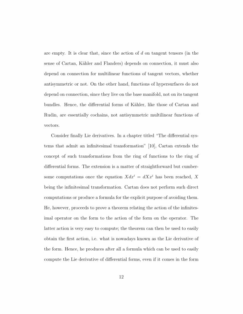
Consider finally Lie derivatives. In a chapter titled “The differential sys-

tems that admit an infinitesimal transformation” [10], Cartan extends the

concept of such transformations from the ring of functions to the ring of

differential forms. The extension is a matter of straightforward but cumber-

some computations once the equation Xdxi = dXxi has been reached, X

being the infinitesimal transformation. Cartan does not perform such direct

computations or produce a formula for the explicit purpose of avoiding them.

He, however, proceeds to prove a theorem relating the action of the infinites-

imal operator on the form to the action of the form on the operator. The

latter action is very easy to compute; the theorem can then be used to easily

obtain the first action, i.e. what is nowadays known as the Lie derivative of

the form. Hence, he produces after all a formula which can be used to easily

compute the Lie derivative of differential forms, even if it comes in the form

12

of a theorem with a different purpose.

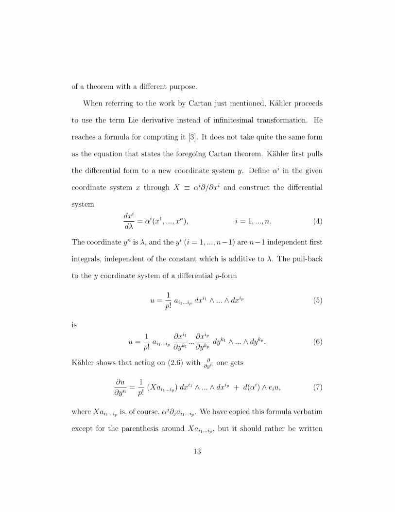
When referring to the work by Cartan just mentioned, Kahler proceeds

to use the term Lie derivative instead of infinitesimal transformation. He

reaches a formula for computing it [3]. It does not take quite the same form

as the equation that states the foregoing Cartan theorem. Kahler first pulls

the differential form to a new coordinate system y. Define αi in the given

coordinate system x through X ≡ αi∂/∂xi and construct the differential

system

dxi

dλ= αi(x1, ..., xn), i = 1, ..., n. (4)

The coordinate yn is λ, and the yi (i = 1, ..., n−1) are n−1 independent first

integrals, independent of the constant which is additive to λ. The pull-back

to the y coordinate system of a differential p-form

u =1

p!ai1...ip dxi1 ∧ ... ∧ dxip (5)

is

u =1

p!ai1...ip

∂xi1

∂yk1...

∂xip

∂ykpdyk1 ∧ ... ∧ dykp . (6)

Kahler shows that acting on (2.6) with ∂∂yn one gets

∂u

∂yn=

1

p!(Xai1...ip) dxi1 ∧ ... ∧ dxip + d(αi) ∧ eiu, (7)

where Xai1...ip is, of course, αj∂jai1...ip . We have copied this formula verbatim

except for the parenthesis around Xai1...ip , but it should rather be written

13

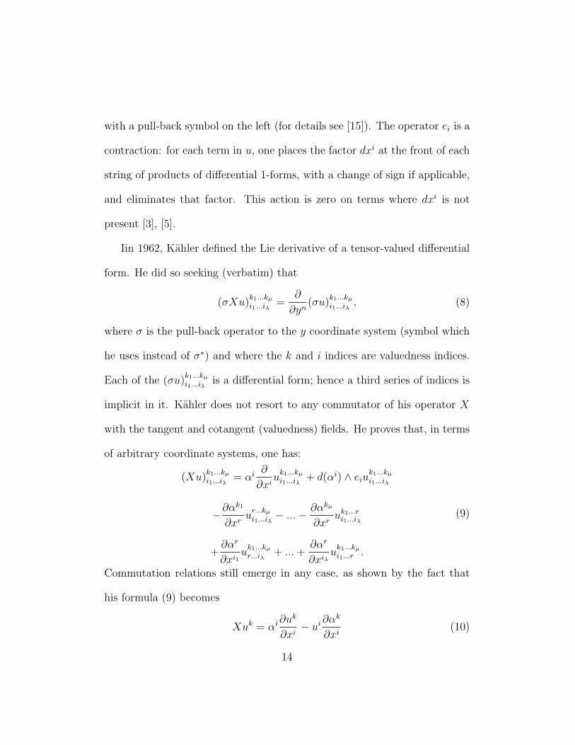
with a pull-back symbol on the left (for details see [15]). The operator ei is a

contraction: for each term in u, one places the factor dxi at the front of each

string of products of differential 1-forms, with a change of sign if applicable,

and eliminates that factor. This action is zero on terms where dxi is not

present [3], [5].

Iin 1962, Kahler defined the Lie derivative of a tensor-valued differential

form. He did so seeking (verbatim) that

(σXu)k1...kµ

i1...iλ=

∂

∂yn(σu)

k1...kµ

i1...iλ, (8)

where σ is the pull-back operator to the y coordinate system (symbol which

he uses instead of σ∗) and where the k and i indices are valuedness indices.

Each of the (σu)k1...kµ

i1...iλis a differential form; hence a third series of indices is

implicit in it. Kahler does not resort to any commutator of his operator X

with the tangent and cotangent (valuedness) fields. He proves that, in terms

of arbitrary coordinate systems, one has:

(Xu)k1...kµ

i1...iλ= αi ∂

∂xiu

k1...kµ

i1...iλ+ d(αi) ∧ eiu

k1...kµ

i1...iλ

−∂αk1

∂xru

r...kµ

i1...iλ− ...− ∂αkµ

∂xruk1...r

i1...iλ

+∂αr

∂xi1u

k1...kµ

r...iλ+ ... +

∂αr

∂xiλu

k1...kµ

i1...r .

(9)

Commutation relations still emerge in any case, as shown by the fact that

his formula (9) becomes

Xuk = αi ∂uk

∂xi− ui ∂αk

∂xi(10)

14

for a vector field uk. Thus formula (9) is consistent with the modern concept

of Lie derivative of a vector field as the commutator,

LXY = [X, Y ] ≡ XY − Y X. (11)

In spite of the correspondence between equations (10) and (11), the right

hand side of equation (8) may give the a first impression that something is

wrong with it, given the absence of the commutator. This absence reflects

that the −Y X term is zero in the y coordinate system, where the components

of X are (0, 0, ..., 1). Finally, as previously reported, Cartan did not deal with

Lie derivatives (i.e. infinitesimal operators) of vector fields, and one wonders

what Kahler would need them for, since he does not use them.

It is worth recalling in connection with equation (9) the important point

made before to the effect that the symbol for differential form represents

cochains in Kahler’s work. In this regard it is very instructive to consider

Slebodzinski’s treatment of the subject [21]. Let v be a vector field. He

obtains Xv using that the contraction of u and the differential 1-form β is a

scalar. He uses for that the Lie derivative of β and the Leibniz rule. However,

in first obtaining the formula for the Lie derivative of differential forms,

Slebodzinski treats them as integrands, i.e. as functions of hypersurfaces,

whose d derivative in the sense of Kahler does not depend on connection. He

does not consider them as fields of multilinear functions of vectors, whose

d derivative, like that of vectors fields, depends on connection. Thus, he

15

actually contracts the vector field with a cochain, not with a linear function

of vector fields.

Our observations with regards to Lie derivatives of vector fields point to

the fact that there is nothing in them of geometric significance, even though

they are used in the most common modern definition of the affine curvature

and torsion, from which one then obtains the equations of structure (This

approach need not be the best, since one can obtain those equations in a

much simpler yet rigorous way and fully in the spirit of Cartan) [22]. The

lack of significance has to do with the fact that equality of two tangent

vectors at two different points of a differentiable manifold (and, therefore,

any significant derivative of vector fields and their duals) is determined by

the affine connection, and we can define any we want. Sure enough one could

have two different concepts of derivatives of vector fields, like one has the

concept of exterior and Lie derivatives of scalar-valued differential forms. The

question arises, however, of what is the geometric value of having a partial

differentiation (see Eq. (8)) of a tensor-valued differential form (i.e. the limit

of a quotient of increments) if the increment in the numerator lacks meaning

because the tangent spaces at the points x and x+dx are not comparable. For

comparison one needs a connection. No connection enters the Lie derivative

equations, (8)-(11). The existence of symmetries is irrelevant in this respect,

since one can choose any connection one wants regardless of what symmetries

16

one has. A truly geometrically significant Lie derivative of vector fields would

have to involve the connection. Of course, there are many applications where

the connection is zero in some particular frame field; ignoring the connection

in such a field when it should not be ignored then amounts to making it zero

and thus to postulating teleparallelism (TP), but not necessarily global, i.e.

strict TP.

3 Quantum Mechanical Issues Raised by Kahler’s

Own Work

The combination of Dirac’s authoritative formalization of the principles of

quantum mechanics [23] and the Copenhagen interpretation did not consti-

tute a solid enough foundation to preempt what Mead [24] (page 5) refers

to as the “muddle and fuss over theory” in the decades that followed. With

regards to the Dirac equation in particular, Thaller [25] had this to say in

the preface of his book on this subject:

“Perhaps one reason that there are comparatively few books

on the Dirac equation is the lack of an unambiguous quantum me-

chanical interpretation. Dirac’s electron theory seems to remain a

theory with no clearly defined range of validity, with peculiarities

at its limits which are not completely understood.”

17

All this is not surprising since the development of those principles and

interpretation took place to accommodate the new experimental evidence

about matter through the adoption of new versions of concepts inherited

from a tradition where matter is particles to the exclusion of any wave con-

cept. The need for new versions of those concepts rather than altogether new

concepts may be unavoidable in any useful quantum physics. However, more

refined perspectives on their use may arise if those concepts are not intro-

duced like with forceps, as happened in the 1920’s, in order to reach evolution

equations of observables, and wave equations. In contrast, the Kahler equa-

tion requires none of this. It emerges on its own right in his calculus. The

different placement of the unit imaginary in the Kahler and Dirac equations

should be more than enough illustration of this point. Following Kahler, we

shall not presuppose interpretations. We shall rather let the mathematics

speak, like he did in the matter of spin and total angular momentum, and of

particles and antiparticles, with striking consequences in both cases. But we

shall not try to rush responses to issues that the present development of the

calculus does not yet wish to speak of.

We proceed to report on some highlights of this calculus that are (almost0

explicit and not emphasized in Kahler’s papers of 1960 and 1962. From now

on, and because of the physical applications, we shall use Latin indices for

3-space, and Greek indices otherwise.

18

(a) The Kahler equation is

∂u = a ∨ u, (12)

where ∨ stands for Clifford product of differential forms, a is the input differ-

ential form and u is the output differential form. In this paper, ∂ designates

Kahler’s general derivative operator (not partial differentiation unless used

as in ∂/∂uk). It constitutes what we shall refer to as the sum of the exterior

and interior derivatives (or exterior and interior covariant derivatives when

∂ acts on tensor-valued differential forms):

∂u = du + δu, (13)

where

du = dxµ ∧ dµu (14)

and

δu = dxµ · dµu. (15)

and where “·” stands for interior product. Kahler proves that, for the Levi-

Civita connection, δu becomes ∗d∗ or -∗d∗ , the sign depending on signature

and dimensionality of the space. For present purposes, we do not need the

details of what goes into the making of the operator dµ, which Kahler calls

the covariant derivative. Suffice to say that it allows one to view the exterior

derivative d and (in the case of the Levi-Civita connection) the coderivative δ

19

in the new light of equations (14) and (15). The operators d and dµ satisfy the

Leibniz rule, but ∂ and δ do not. Equations (13)-(15) should be motivation

enough to still use the term derivative in those cases, disregarding the modern

use of the term.

It is to be noted that, if the exterior-interior calculus of differential forms

had been formulated before the advent of quantum mechanics, the natural

order of differential equations to be solved that involve ∂ might have been

as follows: ∂u = 0 (definition of strict harmonic differential), ∂∂u = 0 (defi-

nition of harmonic differential), ∂u = a (of this type is the Maxwell system,

with a of grade 3 and u of grade 2) and ∂u = a∨u. In other words, the basic

equation of quantum mechanics would have emerged in the calculus without

input from the physics, had humans had greater mathematical ability.

Let eµ be the operator as in Eq. (8) and define eµ as gµνeν . The operator

∂ satisfies [5]

∂∂u = gµνdµdνu + Rµνdxµ ∨ eνu− Ωµν ∨ eµeνu, (16)

regardless of whether u is scalar-valued or not. Rµν stands for the components

of the Ricci tensor and Ωµν stands for the curvature 2-forms This suggests

that the generalization to curved spacetime of the Laplacian of a differential

form should not be viewed as just the generally covariant form gµνdµdν , unless

20

the curvature is zero. Using here the Kahler equation, we have

∂(a ∨ u) = gµνdµdνu + Rµνdxµ ∨ eνu− Ωµν ∨ eµeνu (17)

which one would further develop on the left, showing the entanglement of

the curvature with the Kahler equation. Of special interest would be the

case when a and u were geometric quantities themselves, but this exceeds

the scope of this paper.

To summarize, Kahler’s common mathematical formalism for QM and

general relativity is constituted by his generalization of Cartan’s calculus of

differential forms, and may actually entangle those branches of physics, as

intimated by the combination of the pair of equations (12) and (16). This

entanglement, if and when it is physically found, will have to be interpreted

as the need to represent quantum mechanical states by differential forms

rather than by functions (or even by spinors, under the old concept of the

Laplacian operator).

(b) The Kahler equation has a conservation law built into it. Let r and

s be any two differentiable differential forms. He defined

〈r, s〉 ≡ (ζs ∨ r)0 z, 〈r, s〉1 ≡ (ζs ∨ dxµ ∨ r)0 eµz, (18)

where ( )0 denotes the 0-form part of the contents of the parenthesis, where

ζ denotes reversion of the order of all the 1−form factors in the differential

forms, and where z is the unit differential n−form. 〈r, s〉 and 〈r, s〉1 are

21

respective n−forms and (n− 1)−forms. For later use in subsection (f), it is

worth pointing out that

〈r, s〉 =n∑

m=0

〈rm, sm〉 , (19)

and

〈rm, sm〉 =

( ∑i1<...<im

eµ1...eµm

rm ∧ eµ1 ...eµmsm

)z, (20)

where rm and sm denote the terms of degree m in the generally inhomoge-

neous differential forms r and s respectively. The last two equations together

imply that, if the metric is positive definite, the coefficient of z in the corre-

sponding expression for 〈r, r〉 is positive definite if r is not null.

A generalized Green’s formula of this calculus reads:

〈r, ∂s〉+ 〈s, ∂r〉 = d 〈r, s〉1 . (21)

The Kahler equation admits a conjugate equation

∂v = −ζa ∨ v (22)

whose relevance lies in that the sum 〈u, ∂v〉 + 〈v, ∂u〉 is zero if u and v are

respective solutions of a Kahler equation and its conjugate. The conservation

law

d 〈u, v〉1 = 0, (23)

thus follows. Notice that the unit imaginary does not enter here at this point.

22

To summarize: in principle, the existence of a conservation law associated

with the main equation of relativistic quantum mechanics does not require a

complex algebra.

(c) In 1961 and again in 1962, Kahler solved the fine structure of the

hydrogen atom with the specific equation

∂u = − 1

~c(mc2 + iceφdt) ∨ u (24)

and signature +2. Here φ denotes the Coulomb potential and m is the mass

of the electron. Notice the mismatch with the Dirac theory in what concerns

the non-standard position of the unit imaginary.

The relation between the solutions to the fine structure of the hydrogen

atom through the Dirac and Kahler equations emerges as one exploits the

time translation and cylindrical rotational symmetries in the latter of the two

equations. Four different mutually annulling primitive idempotents arise as

factors in respective four terms into which the general solution decomposes

(details provided under (e)). They make the difference between those indi-

vidual solutions and the solution of the Dirac equation, which lacks a similar

structure, and to which they are otherwise equivalent. The larger spherical

symmetry does not give rise to additional primitive idempotents and thus to

further decomposition of the general Kahler solution.

To summarize, the Kahler equation has a much richer structure of so-

lutions than the Dirac equation. This coexistence of equations shows that

23

the location of the unit imaginary is formalism dependent. The argument

that leads to a unit imaginary in the four momentum operator –and thus

on the left hand side of the Dirac equation– was based on the search for a

Hamiltonian written in terms of quantum mechanical operators that parallels

corresponding classical mechanical operators. That argument is, therefore,

begging for an explanation that might one day come from further develop-

ment of Kahler’s theory.

(d) Equation (7) does not involve metric structure, much less symmetries

of the metric. The latter give rise to Killing equations, dµαν+dνα

µ = 0, which

allow one in turn to further write the rotations’ Lie operator on differential

forms, (7), as [5]

Xu = αµdµu +1

4dα ∨ u− 1

4u ∨ dα. (25)

where α is defined by

α = gµναµdxν . (26)

When this formula is applied to the rotation operator around the axis xi, one

gets [5]

Xiu = xk ∂u

∂xl− xl ∂u

∂xk+

1

2wi ∨ u− 1

2u ∨ wi, i = 1, 2, 3 (27)

where

wi ≡ dxk ∧ dxl = dxi ∨ w = w ∨ dxi, (28)

24

with (i, k, l) a cyclic permutation of (1,2,3) in (27) and (28), and with w

defined as dx1 ∧ dx2 ∧ dx3 (i.e. the z of three dimensions). The action of the

spin operator is to be read from the last two terms of Eq. (27), which we use

to summarize this subsection with Kahler’s statement that “the spin of the

electron is interpreted as the need to represent the state of the electron by a

differential form rather than by a function”.

(e) The considerations in the present and next subsections are related to

the particle/antiparticle issue. Time-translation symmetry is of the essence

of the argument. It is important, however, to keep track of the point at which

that symmetry plays a role.

Following Kahler, any spacetime differential can be written as u = u′ +

u′′ ∧ dt, where u′ and u′′ are uniquely defined by the condition that they be

spatial differentials, i.e. that they do not contain dt as a factor. Define then

the mutually annulling constant differential idempotents

ε± ≡ 1

2∓ ic

2dt (29)

(a constant differential u is defined by the condition dµu = 0). The i factor

would not have been necessary to make a dt related idempotent if the sig-

nature had been -2. We wish, however, to follow Kahler in using +2, since

we are reproducing in more targeted form some of the implications of his

25

computations. One readily finds that

ε+ + ε− = 1, dt = iε+ − ε−

c. (30)

Substitution of these equations in u = u′ + u′′ ∧ dt = u′ ∨ 1 + u′′ ∨ dt yields

an expression of the form

u =+ u ∨ ε+ +− u ∨ ε−, (31)

where +u and −u are uniquely defined by the process just stated. Although

both +u and −u are different from u, one still has

u ∨ ε± =± u ∨ ε±. (32)

as follows from multiplication of Eq. (31) by ε± on the right, and taking into

account that ε+ and ε− are mutually annulling idempotents.

Constant differentials, c, satisfy the property that, if u is a solution of

a Kahler equation, u ∨ c also is a solution of the same equation.. Thus the

u ∨ ε± are solutions of the same equation as u, and so are then the ±u ∨ ε±

by virtue of equations (32). Since

u ∨ ε± ∨ ε± = u ∨ ε±, u ∨ ε± ∨ ε∓ = 0, (33)

we may view u ∨ ε± as proper differential forms with proper value 1 (cor-

responding to right multiplication by ε±), and with proper value 0 (corre-

sponding to right multiplication by ε∓).

26

Up to this point no assumption has been made about the symmetries

of the factor a in the Kahler equation. When a does not depend on time,

the action on a differential form of the Lie operator corresponding to time

translations is a constant times ∂u/∂t. Without justification, Kahler selects

the constant so that this operator is the standard energy operator i~(∂u/∂t)

of the Dirac formalism. It is then clear that the solutions of the Kahler

equation that are eigen solutions of this operator are of the form

u = p+ ∨ T+ + p− ∨ T−, (34)

where

T± = e−i~Et

(1

2∓ ic

2dt

), (35)

and where the spatial differentials p± do not depend on t either (thus called

pure spatial differentials). Both solutions

+u = p+ ∨ T+, −u = p− ∨ T−, (36)

pertain to the same sign of the energy, which is chosen as positive.

We summarize this subsection with a partial paraphrasing of a Kahler

statement on spin. Negative energy solutions and the inseparability of pure-

particle and pure-antiparticle solutions for bound systems are spurious effects

of representing the state of electrons and positrons by spinors rather than by

differential forms.

27

(f) The argument outlined under (e) is not enough to justify the use of the

term antiparticle. Kahler shows that, for minimal electromagnetic coupling,

ηu is a solution of the conjugate Kahler equation, where η is the operator

that reverses the sign of each 1−form factor in differential forms and where

overbar stands for complex conjugate. The conservation law d 〈u, v〉1 = 0

then includes d 〈u, ηu〉1 = 0. He then shows that

[u, v] = [+u ∨ ε+, +v ∨ ε+] + [−u ∨ ε−, −v ∨ ε−], (37)

where the notational simplification [u, v] ≡ 〈u, ηv〉1 has been used. Spatial

differentials (p, q,...) satisfy that [p, q] ≡ p, ηq)1 ∧ icdt, where curly brackets

play with respect to the spatial metric the same role as 〈 〉 plays with regards

to the spacetime metric. He finally shows that

[u, u] =[+u, + u

]+

[−u, −u], (38)

where

[±u, ±u]

= ±1

2±u, ±u+

1

2±u, η±u1 ∨ icdt. (39)

The ± sign at the front of the first term on the right (while the second

sign remains the same) is interpreted to mean that, for the same sign of the

energy, the two solutions in ±u are each other’s antiparticle.

Equations (39) have to be compared with the general form for currents

which, as explained in the previous paper, are given by

j = ρw − (jxdy ∧ dz + jydz ∧ dx + jzdx ∧ dy) ∧ dt. (40)

28

Hence, following Kahler, the 4-current has to be identified with |e| 〈u, ηu〉1 .

Thus, for the electron, we have:

ρw = −|e|2−u,− u, (41)

and, since −u,− u is proportional to w, and w2 = 1, the density is given by

ρ =|e|2−u,− uw, (42)

where the symbol of Clifford product by w is not required, for obvious reasons.

In the same way as we have read a density, we can read a corresponding

3−current for the electron (really a 3−form) by identifying the 3-current part

of (40) with |e| times the 3-current part of (39). For the electron, we have,

−jidxk ∧ dxl ∧ dt =|e|2−u, η−u1 ∨ icdt, (43)

where the presence of the ordered triple (i, k, l) means sum over cyclic per-

mutations of (1, 2, 3) (and similarly ρw = |e|2+u,+ u for the positron).

4 Further Developments of the Kahler Cal-

culus

The success with the fine structure constant of the hydrogen atom and the

just reported results by Kahler speak of the potential significance for physics

of his calculus. Before we discuss it further and in order to provide perspec-

tive, let us consider recent extensions of the Kahler calculus.

29

In subsections (a) to (b), we deal with some unexplained issues in Kahler’s

work on this subject, namely (a) the three series of indices in components

of his tensor-valued differential forms, (b) his ansatz for differentiation and

(c) the dependence of the interior derivative on connection. In subsections

(d) and (e), we deal with the replacement of tensor-valuedness with Clifford-

valuedness of his differential forms, thus incorporating the product ei.ej,

which is one of the cornerstones of Cartan’s theory of moving frames. In

subsection (f), we argue that the results obtained in (d) and (e) address an

issue raised in Cartan’s writing on geometry and that he left unresolved. We

also provide a geometric context to a Cartan innovative way of writing the

equations of the physics in a five dimensional space.

(a) Kahler’s tensor-valued differential forms have three series of indices,

one of them being of superscripts and the other two of subscripts. This

difference with everybody else’s differential forms has to be inferred from

some of his main formulas, since he gives no reason for it. For an explanation

as to what those three series of indices refer to see [7]. Readers can also find

there the justification of why his differential expressions do not mean the

usual elements of the exterior cotangent algebra, i.e. antisymmetric covariant

tensors, but rather functions of hypersurfaces. One can imagine that Kahler’s

silence on this intended to avoid polemics.

(b) Kahler produces cumbersome ad hoc expressions for what he calls

30

the covariant derivative, dµu. As reported in section 3, he contracts the lat-

ter’s exterior and interior products with dxµ to obtain the exterior covariant

and interior covariant derivatives respectively (In the following, these deriva-

tives will be called simply exterior and interior). Since these products come

together into the Clifford product, the corresponding derivatives also come

together into what we shall call Kahler derivative, to which he refers as inte-

rior. Those intimate relationships may have constituted his justification for

the use of the term derivative, disregarding whether the Leibniz rule is sat-

isfied or not. In addition to their ad hoc character, the lengthy expressions

proposed by Kahler apply only to manifolds endowed with the Levi-Civita

connection. The following alternative course of action is possible.

The exterior product of two unknown differential forms does not imply

what their interior product is. Hence, the exterior derivative does not imply

what the interior derivative is. However, once a connection is given, one

can use covariance constraints to determine canonical covariant and interior

derivatives, thus removing the aforementioned ad hoc character. This can be

done with arbitrary affine connection through the first equation of structure

[26], [27].

(c) The interior derivative of even scalar-valued functions of hypersur-

faces depends on connection (In the case of Levi-Civita’s connection, this is

disguised by the fact that the interior derivative becomes the coderivative,

31

a prior concept introduced directly through the metric). We have shown

that said dependence is a concomitant of requiring that the equations of the

derivatives of the connection will associate bases of 1-cochains with bases of

tangent vectors [27].

(d) Though the Kahler equation of 1960 is well defined also when the input

differential form a is tensor valued, it has the unpleasant feature of run-away

valuedness, arising from the fact that a∨ is a degree-changing operator and

∂ is not [7]. Without explanation but likely because of that feature, Kahler

produced in 1962 a different equation for tensor-valued “a” (For a detailed

discussion see [28]). Unaware of his 1962 equation, the same situation was

addressed [29] ain the alternative way that we proceed to summarize. When

Kahler writes u∨v for two tensor-valued differential forms, he actually means

u(∨,⊗)v, where ∨ takes place in the algebra of differential forms and ⊗

takes place in the algebra of valuedness tensors. For different reasons, we

proposed to replace the tensor-valuedness with Clifford-valuedness. A “new

Kahler equation”, ∂u = a(∨,∨)u, results [29]. The tangent Clifford product

includes the product eµ.eν (= gµν), which gives rise through differentiation

to the relation of compatibility of metric and affine connection.

(e) The tangent Clifford algebra resolves the problem of run-away val-

uedness but creates a new one. Consider the translation form dP of the

theory of moving frames. It is a vector-valued differential 1-form. The prod-

32

uct dP(∨,∨)dP yields dxµ ∧ dxνeµ.eν + 4. This last term lacks geometric

interpretation other than the trivial one, the dimension of the space. For

this reason, among other, a double Clifford algebra was not introduced in

spacetime itself, but rather in a Kaluza-Klein type of space suggested by

Finslerian TP [29], where the horizontal differential invariants are (ωµ, ωi0)

[22]. In appropriate frame fields of the Finsler bundle, the ωij (and not just

their pull-back to the fibers) become the left-invariant forms of the rotation

group in three dimensions. d℘ (≡ dP + udτ) is the translation element in

that 5-dimensional space, τ being proper time, u being its dual tangent vector

field and dP being the translation element in spacetime. We then have

d℘(∨,∨)d℘ = d℘(∧,∧)d℘, (44)

with

0 = d℘(., .)d℘ = c2dτ 2 ± [c2dt2 − Σi(dxi)2], (45)

the choice of sign amounting to a choice of signature. This resolves an issue

that, as we said, Cartan raised but did not address [30], namely that his

theory of moving frames is simply what its name indicates; the motion of

points in that theory is represented by the motion of the origin of frames,

and not of points viewed as objects unrelated to the frames [14].

To summarize this section up to here, points (a) to (d) have to do directly

with limitations of the Kahler calculus. (e) has to do with eliminating a

33

difficulty introduced in (d) in the process of solving old difficulties. Issues of

geometry also are positively impacted by these developments. The ones that

follow speak of the potential of the Kahler calculus for the advancement of

physics.

(f) Practitioners of Clifford algebras have proposed a variation of them

claimed to be specific to quantum field theory, and to which they refer as

quantum Clifford algebra, or Clifford algebra of non-symmetric quadratic

differential forms [31] (and references therein). In a paper in this journal, it

has been shown that such algebras arise naturally in the Kaluza-Klein space

to which we have referred above [32].

In another development, Schmeikal has shown how to represent SU(3) in

the Clifford algebra of spacetime [33], quarks emerging in families of mutually

annulling primitive idempotents. An equivalent family arises in the problem

of solving the Kahler equation for systems with a couple of commuting one-

parameter symmetries, like in the hydrogen atom. As shown elsewhere [27],

simple observation of any of Schmeikal’s families and comparison with the

one that emerges in solving the hydrogen atom prompts one to think of

nucleons as Kahler equation solutions that are not a sum of solutions of

Dirac equations. We shall return to this later.

Finally, it is worth mentioning a most intriguing option for unification

of gravitation and, at least, electrodynamics. It is made possible by a con-

34

fluence of the Kahler calculus and geometry. Consider Finsler bundles on

the usual pseudo-Riemannian metrics. Regardless of what torsion Ωµ one

postulates, only Ω0 contributes to the equations of the autoparallels [?],[35].

It does so in such way that the pre-Finslerian components of Ω0 enter the

autoparallels in the same way as the electric and magnetic fields enter the

Lorentz force. Those components of Ω0 also play, in the linear part of the

first Bianchi identity for TP connections, the same role as the electromagnetic

form in the homogeneous Maxwell’s equations [35]. In our Kaluza-Klein-type

space associated with Finslerian TP, that specific part of Ω0 is represented

by Ω4. The second equation of structure (affine curvature equal to zero) be-

comes the statement that the metric curvature equals terms that depend

on the (con)torsion and derivative thereof. The contribution of Ω4 to the

Einstein contraction of that equation virtually amounts to the standard elec-

tromagnetic energy-momentum tensor [36]. The inhomogeneous Maxwell’s

equations are still missing in this geometric picture, which unifies the grav-

itational interaction with whatever interaction(s) is(are) represented by the

torsion. Suppose that Maxwell’s equations were a degeneration of a geomet-

ric Kahler equation resulting from the replacement of its right hand side with

a phenomenological alternative [24]. The geometrization of electrodynamics

would lie, in the last instance in a totally geometric Kahler equation [37],

[35].

35

5 Killing Symmetries and Constant Differen-

tials: Spinors and Plane Waves.

In this section, we discuss two methods to generate new solutions of the

Kahler equation, once a solution has been given. These methods are (a)

the action of Killing operators and (b) products by constant differentials.

We also make a few considerations meant to replace cumbersome relativistic

quantum mechanics theory, like spinors and their transformations.

The term Killing operator is used here to refer to Lie operators that satisfy

the Killing relation and leave invariant the input differential form of a given

Kahler equation. A most important class of Killing operators are rotation

operators. Kahler produced two remarkable results about it. One of them,

already mentioned, is that spin is a manifestation of the need to represent

the state of an electron by a differential form. A second and related feature

is his proposal that the total angular momentum operator appears to assign

the electron spin ~ rather than (1/2)~. Since his mathematical argument

is incontrovertible and so is the experiment evidences for spin 1/2, a “new

picture” for the role of the wave equation emerges, whose potential remains

to be examined.

We start with a general remark about rotations in Clifford algebra (In the

following, juxtaposition means Clifford product). The action of a rotation

on any “Clifford number”, whether homogeneous or not, can be given in the

36

following two ways:

u′ = eϕA ∨ u = e(ϕ/2)A ∨ u ∨ e−(ϕ/2)A (46)

where A is a unit bivector in the plane of the rotation. Let us define

α ≡ e(ϕ/2)A. Under a rotation, a product u (≡ xy...z) of vectors or vec-

tor operators becomes u′ given by

u′ = (αxα−1)(αyα−1) ∨ ... ∨ (αzα−1), (47)

where we have suppressed several Clifford product symbols to minimize clut-

ter, after adding parentheses for emphasis. The Clifford equation in the

rotated frame, ∂α = a ∨ u, then becomes

(α∂α−1)αu = (αaα−1) ∨ αu, (48)

after multiplication by α on the right. Hence, u maybe viewed as being

transformed by the half angle of the rotation, regardless of whether it is

spinor or not. What counts is his placement within a differential equation

such as the Kahler or Dirac equation.

Next, consider spinors. Corresponding to rotation around an axis, we

have the two mutually annulling idempotents

τ± =1

2(1± idx ∧ dy) =

1

2(1± iω3) (49)

The operators τ± correspond to opposite senses of rotation. They annul each

other, and so do the ε±. The τ± and ε± commute with each other. It easily

37

follows that the complex algebra of scalar-valued differential forms can be

viewed as composed of four left ideals:

u =+ u+ ∨ τ+ ∨ ε+ ++ u− ∨ τ− ∨ ε+ +− u+ ∨ τ+ ∨ ε− +− u− ∨ τ− ∨ ε− (50)

We use the symbol ±u∗ to refer to both ±u± and ±u∓. If u is a solution of the

Kahler equation, each of the four ±u∗ ∨ τ ∗ ∨ ε± also is a solution. If a system

has time-translational and cylindrical symmetry (spherical in particular) each

of the solutions corresponds to a solution of the Dirac equation for the same

problem. At least such is the case for the hydrogen atom and one may expect

similar correspondence in other problems with two “commuting” 1-parameter

groups of symmetries. In the Kahler calculus the non-commutativity mani-

fests itself in the impossibility of simultaneously implementing a decomposi-

tion into ideals in the sense that we are about to explain.

The decomposition into ideals in (50) is possible because of the commu-

tativity of τ± and ε± and that 1 = ε+ + ε− = τ+ + τ− :

u = u ∨ (τ+ + τ−) ∨ (ε+ + ε−) (51)

That defines the ±u∗∨τ ∗∨ε±, not the ±u∗ themselves, as is clear for example

that

+u+ ∨ τ+ ∨ ε+ = (+u+ + v ∨ τ− ∨ ε+) ∨ τ+ ∨ ε+. (52)

Hence, we should more appropriately referred to the ±u∗∨τ ∗∨ε± as u∨τ ∗∨ε±.

38

One can define unique coefficients ±u∗ as follows. One first proceeds as

in obtaining (31). Let a differential form α not depend on dt. We use a

basis of polar 1-forms, (dρ, dφ, dz) and decompose α as α′ + α′′ ∨ dφ, where

neither α′ nor α′′ contain dφ as a factor, which defines them uniquely. α

can then be expressed as the linear combination of τ+ and τ− using that

1 = τ+ and τ− and dφ = i(dρ/ρ)∨ (τ−− τ+). Hence Eq. (31) can further be

expanded to obtain expression (50) with the coefficients ±u∗ that this process

uniquely defines. They still depend on t and φ, dependence which reduces

to exponentials on these variables if there is time-translation and cylindrical

symmetry.

Consider now how the non-commutativity of rotations around different

axes manifests itself in this calculus. For simplicity, let the differential forms

be spatial, and the axes of rotation be orthogonal. We substitute dφ in terms

of τ+ and τ−. Using tan θ = ρ/z, we can express dθ in terms of dρ and dz.

There is the problem, however, that ρ and z do not determine a constant

plane, which causes dρ and dz to not be a constant differential. Hence,

one can not deal with two rotations as if one had a time translation and a

rotation.

We now turn to the mathematical point made by Kahler with regards

to total angular momentum. For this purpose, we first need to consider the

spin terms in Xiu (See Eq. (27), namely (1/2)wi ∨ u− (1/2)u ∨ wi. Let the

39

subscript i be 3. We then have

±u∗ ∨ τ ∗ ∨ ε± ∨ ω3 =± u∗ ∨ ω3 ∨ τ ∗ ∨ ε± = −ω±3 ∨± u∗ ∨ τ ∗ ∨ ε± (53)

For the first step in (53) we have used that ω3 commutes with τ± and ε±. The

last step follows from the fact that ω3 and u∗ are respectively proportional

to dρ ∨ dφ and dρ ∨ dz and, therefore,

dρ ∨ dz ∨ dρ ∨ dφ = −dρ ∨ dφ ∨ dρ ∨ dz (54)

We thus obtain that

1

2ω3 ∨ u = −1

2u ∨ ω3, (55)

and that, therefore, the last two terms in (27) are equal.

Consider next the issue of proper values of the spin operator. Since

±u∗ ∨ τ ∗ ∨ ε± ∨ ω3 equals ±u∗ ∨ τ ∗ ∨ ω3 ∨ ε±, we have

τ± ∨ ω3 =1

2(1± idx ∧ dy) ∨ (dx ∧ dy) = ∓iτ± (56)

It is then clear that, here as in the standard formalism, we need to multiply

by −i~ the expression (27) for the operator Xi, so that the proper value of

both, orbital angular momentum and spin be real. In particular, the spin

term for rotations around the z axes will amount to

−i~2

(ω3 ∨ u± − u± ∨ ωi) = i~u ∨ ω3 = i~(∓u±) = ±~u± (57)

Dirac particles in general, and electrons in particular, would thus appear to

acquire spin values of ±~, rather than ±~/2. The way out of this conclusion

40

could be simply that the Kahler equation does not represent an electron in

isolation but rather an electron in an external field, and that the external

field constitutes in turn a simplified representation of a second Dirac system

(say, the nucleus of the hydrogen atom). In this way, the spin of the two

interacting Dirac particles would be represented respectively by each of the

two terms in equation (27). This will be clear in later sections from consid-

eration of the standard expanded Hamiltonian for the large components of

the wave form. For comparison purposes, let us use the language a little bit

freeley, as follows. In the Dirac theory, the large components represent the

“electron separated from the positron”, the latter being given by the small

components. In the Kahler theory, on the other hand, both the large and

small components represent the electron, but only the large components obey

the Hamiltonian to which we are used. Be as it may, the fine structure of the

hydrogen atom obtained with the Kahler equation yields exactly the same

result as with the Dirac equation.

Let us proceed with plane waves. We have here four commuting transla-

tional symmetries. They allow one to obtain the solutions which are proper

functions of energy momentum:

u = ei(pldxl−Et) 1

24(1± dx) ∨ (1± dy) ∨ (1± dz) ∨ (1± idt). (58)

The two signs in (1± idt) correspond to electrons and positrons respectively.

Postmultiplying by (1/2)(1±idx∨dy), one obtains the projection upon proper

41

states of angular momentum corresponding to opposite senses of rotation.

In the Dirac theory, the spinor entries of plane wave solutions depend on

the components of the energy-momentum 4-vector. Here, the dependence

on orientation is implicit in the exponential factor at the front. We project

upon electron (respectively positron) states by multiplying on the right by

ε−(respectively ε+). The information contained in the components of the

spinors that reflect the relative orientations of velocity and spin and which

is obtained through complicated spinor transformations (even when Clifford

algebra formalism is used) will emerge spontaneously through multiplication

by τ± on the right. For instance, let z be the spin axis. We project on that

axis through multiplication on the right by (1/2)(1± idx∨dy). This is much

simpler than applying rotation operators to the spinors, since these operators

are exponentials of terms like (1/2)(1± idx∨ dy). In other words, operating

with these constant differentials amounts to working in the Lie algebra of the

Lorentz group rather than in the group itself.

This greater simplicity of Kahler’s than Dirac’s formalism will be encoun-

tered time and again as we deal with a variety of issues later in this and, we

hope, future papers.

42

6 Minimal Electromagnetic Coupling: Expan-

sion of the Hamiltonian for Large Compo-

nents

The Kahler equation with minimal electromagnetic coupling is [3], [4], [5]

−i~∂u =1

c(imc2 − ecφdt + eAidxi) ∨ u. (59)

Since the mass term dominates at low energies, we write u as

u = e−imc2t/~R(x, t) ∨ ε−, (60)

R depending slowly on time. In the following, we make ~ = c = 1.We

substitute (60) in

∂u = dt ∨ u,t +dxi ∨ u,i , (61)

and the resulting expression is replaced in (59). Premultiplying then by −idt

and using that dt ∨ dt = −1, we get

u,t = −imu + e−imtR,t ∨ε− = −dxi ∨ (dt ∨ u,i ) +

+m(dt ∨ u) + ieAidxi ∨ (dt ∨ u)− ieφu. (62)

We absorb the factor dt in u and simplify to get

R,t = −P ∨ ηR− ieφR + im(R− ηR), (63)

where P ≡ dxj(−i∂j − eAj). Applying η to (63) on the left, and combining

the resulting equation with (63) itself, we obtain:

ϕ,t = P ∨ χ− ieφϕ, (64)

43

χ,t = −P ∨ ϕ− ieφχ + 2imχ, (65)

where ϕ ≡ 12(R + ηR) and χ ≡ 1

2(R− ηR). Since m is the dominant energy,

Eq. (65) shows that χ is small relative to ϕ. We define:

χ1 ≡ − i

2mP ∨ ϕ, χ′1 ≡ χ− χ1. (66)

Using (65) and (66), we write:

χ,t = −ieφχ + 2imχ′1, (67)

which implies that χ′1 is small relative to χ. We thus have

χ′1 = − i

2mχ,t +

eφ

2mχ = χ2 + χ′2, (68)

where

(χ2, χ′2) = − i

2m(χ1, χ′1),t +

eφ

2m(χ1, χ′1), (69)

and, therefore

χ = χ1 + χ2 + χ′2. (70)

Notice that χ′2 ¿ χ2 ¿ χ1 ¿ ϕ.

We proceed to write down the equation

iϕ,t = iP ∨ Y − ieφϕ, (71)

and to develop Eq. (71) with Y = χ1. Taking into account the first of (66),

we further get

iϕ,t =1

2mP ∨ (P ∨ ϕ)− ieφϕ. (72)

44

Expand P ∨ (P ∨ ϕ) :

P ∨ (P ∨ ϕ) = dxi ∨ dxj ∨ Pi(Pjϕ) = (dxi ∧ dxj) ∨ Pi(Pjϕ) +

+δijPi(Pjϕ) = (dxi ∧ dxj) ∨ [(PiPj)ϕ + Pi(PCj ϕ)] + P 2ϕ, (73)

where the subscript C denotes that the derivative operators in Pi do not act

on Pj, this action already being taken care of by

(PkPj)ϕ ≡ −i∂k(−eAj) = ieAj,k . (74)

The antisymmetry of dxi ∧ dxj causes the product (dxi ∧ dxj) ∨ Pi(PCj ϕ) to

vanish, since Pi(PCj ϕ) is symmetric. It also causes the symmetric part of

ieAj,k to be ineffectual. Thus, finally,

P ∨ (P ∨ ϕ) =ie

2

∑i,j

(dxi ∧ dxj) ∨ (Aj,i−Ai,j )ϕ + P 2ϕ =

= ieBkdxi ∨ dxj ∨ ϕ + P 2ϕ. (75)

In the Bk term, one assumes cyclic sum of the three even permutations of

(i = 1, j = 2, k = 3), just once each (thus the disappearance of the factor

1/2). We thus get, from (72) and (75),

iϕ,t =1

2mP 2ϕ +

ie

2mBkdxi ∨ dxj ∨ ϕ + eφϕ, (76)

which is the Pauli equation in terms of differential forms.

The next approximation is now a simple exercise. We readily get:

iP ∨ χ2 = I1 + I2 + II, (77)

45

where

I1 ≡ − i

4m2P ∨ (P,t ∨ϕ), (78)

I2 ≡ − i

4m2P ∨ (P ∨ ϕ,t ), (79)

and

II ≡ ie

2mP ∨ (φχ1) =

ie

2m

(− i

2m

)P ∨ (φP ∨ ϕ). (80)

We rewrite Eq. (78) as

I1 ≡ − i

4m2(P ∨ P,t ) ∨ ϕ)− i

4m2P ∨ (P,t )C ∨ ϕ), (81)

where the notation parallels that of Eq. (73). We substitute (64) in (79) with

P ∨χ replaced with P ∨χ1 in order to stay in the same order as in standard

treatments of this problem with the Foldy-Wouthuysen transformation (say

as in Bjorken and Drell). Using then (66), we get

I2 ≡ − i

4m2P ∨

P ∨

[− i

2mP ∨ (P ∨ ϕ)

]−

− i

4m2P ∨ [P ∨ (−ieφϕ)] . (82)

The last term in (82) cancels with II. We thus obtain

I2 + II ≡

= − 1

8m3P ∨ P ∨ [P ∨ (P ∨ φ)] − e

4m2P ∨ [(Pφ) ∨ ϕ)] =

=−1

8m3p4 − e

4m2[P ∨ (Pφ)] ∨ ϕ− e

4m2P ∨ (Pφ)C ∨ ϕ), (83)

46

where the approximation allowed us to replace the P∨4 term with−(8m3)−1p4,

and where p2 is as in non-relativistic quantum mechanics. Using (83) and

(81), we finally have

iP ∨ χ2 =−1

8m3p4 − ie

4m2P ∨ EC ∨ ϕ− e

4m2Ei,j (dxj ∧ dxi) ∨ ϕ. (84)

The second term on the right hand side of (84) results from combining the

(P,t )C term of Eq. (81) with the (Pφ)C term of (Eq. (83)). Similarly, the

third term results from combining the P,t (Eq. (81)) and Pφ terms (Eq.

(83)). Once again for the purpose of comparison, we drop higher order terms

in further expanding iP ∨ χ2. We thus have

− ie

4m2P ∨ EC ∨ ϕ = − ie

4m2dxi ∧ dxj ∨ Ej(−i∂i)ϕ =

= − ie

4m2dxi ∨ dxj ∨ [Ej(−i∂i)− Ei(−i∂j)] ϕ− ie

4m2Eipi. (85)

In more conventional language, these are σ · E× p terms. Finally

− e

4m2Ei,j (dxj ∧ dxi) ∨ ϕ =

− e

4m2Ei,i ∨ϕ− e

8m2(Ej,i−Ei,j )dxj ∧ dxi ∨ ϕ. (86)

These are the div E and σ · curl E terms.

7 Antiparticles, Small Components and “Neg-

ative” Energies

In this section, we develop for the large components of positrons the same

expanded Hamiltonian equation as for electrons. We then return to the equa-

47

tions for the electrons of the previous section in order to obtain the Hamil-

tonian that applies to the small components. We finally show that negative

energies constitute a spurious effect arising from the fact that, interpreted

from the perspective of the Kahler calculus, the Dirac theory makes the small

components of electron wave forms appear as if they belonged to positrons.

In parallel to Eqs. (59)-(61) we now have

−i∂u′ = imu′ + qAu′, (87)

u′ = e−imtS(x, t) ∨ ε+, (88)

and

u′,t = −imu′ + e−im′tS,t ∨ε+ = −dxi ∨ (dt ∨ u′,i ) +

+m(dt ∨ u′) + iqAidxi ∨ (dt ∨ u′)− iqφu′. (89)

where S depends slowly on t, but not on dt. At this point, the computation

changes slightly relative to the previous section in that, whereas we then

encountered the product dt ∨ ε− (= −ε−), we now contend with dt ∨ ε+

(= −ε+). Hence, we have

S,t = P ∨ ηS − iqφS + im(S + ηS), (90)

ηS,t = −P ∨ ηS − iqφηS + im(S + ηS), (91)

The even part ϕ′ (= (S + ηS)/2) is now small. Clearly,

ϕ′,t = −P ∨ χ′ − iqφϕ′ + 2imϕ′, (92)

48

χ′,t = P ∨ ϕ′ − iqφχ′. (93)

The system (92)-(93) is for (χ′, ϕ′) what the system (63)-(64) is for (ϕ, χ).

We have thus shown that the large part, now odd, of the positron has the

same Hamiltonian as the large part, then even, of the electron, both in an

electromagnetic field.

Let us now deal with the issue of the small components. We return

to the equations of the previous section, where we were able to develop an

approximating process for obtaining the Hamiltonian for ϕ thanks to the fact

that we could solve (65) approximately for χ, which was then substituted in

(64). But, the system of differential equations being what it was, it did not

let us proceed similarly to obtain an equation for χ. It is possible, however,

to proceed in the following alternative way.

For an electron in a time-homogeneous electromagnetic field, we can write

the solution of the Kahler equation, not only as in (60), but also as

e−imtR(x, t) = e−iEt<(x), (94)

where E is the actual energy of the electron in a time-independent electro-

magnetic field. This readily implies:

ϕ,tχ,t

= i(m− E)

ϕχ

. (95)

Substituting the first of (95) in (92) and solving for ϕ we get

ϕ = µP ∨ χ (96)

49

where

µ ≡ − i

m− E + eφ(97)

It readily follows that

P ∨ ϕ = (Pµ) ∨ (P ∨ χ) + µP ∨ (P ∨ χ) (98)

and, therefore,

iχ,t = −iµP ∨ (P ∨ χ)− i(Pµ) ∨ (P ∨ χ) + eφχ− 2mχ, (99)

which involves only the small components and is an exact equation for the

system of an electron in a time-independent electromagnetic field.

We finally ask whether we can transform the system (64)-(65) into another

system where the roles of ϕ and χ are reversed. In order to achieve this, one

has to reverse the signs of the first terms on the right hand sides relative

to the left hand sides, which is achieved by replacing t with t′(=−t) and

multiplying the equations by −1. One thus obtains

ϕ,t′ = −P ∨ χ + ieφϕ, (100)

χ,t′ = P ∨ ϕ + ieφχ− 2imχ (101)

In order to restore the sign of the ieφϕ terms, we replace e with e′ (=−e).

We further replace −ie′φ− 2im with −ie′φ′. We thus get:

ϕ,t′ = −P ∨ χ− ie′φ′ϕ + 2imϕ, (102)

χ,t′ = P ∨ ϕ− ie′φ′χ. (103)

50

These equations are formally identical to Eqs. (64)-(65) with the roles of ϕ

and χ exchanged by time reversal and change conjugation. It is important

to remark that the transformation performed does not allow us to follow for

this system the process of the previous section. The reason is that −ie′φ′

is of the order of 2im. The changes made do not affect the fact that χ was

small relative to ϕ in the system (64)-(65); it remains so.

Kahler already showed that electrons and positrons come with the same

sign of the energy. We now show why positrons appear with negative energy,

a spurious effect that has not impeded the Dirac theory, complemented by

hole theory, to yield the right results when doing quantum electrodynamics

(QED). The equation u,t = −imu + e−imtR,t ∨ε− (see (62)) says that rest

mass energy is an energy term additional to the terms that appear in R,t,

which is the reason why it does not appear in the Pauli equation. Let us

rewrite the equation (102) as

ϕ,t′ = −P ∨ χ− i(e′φ′ − 2im)ϕ. (104)

If e′φ′ (not small) is taken inadvertently as if it were the real e′φ (small), we

then have the additional contribution −2m to the energy equation in order

to handle positrons properly in the Dirac theory and, consequently, in QED

based on hole theory.

51

8 Exact Closed Form of the Minimal-Coupling

Electromagnetic Hamiltonian for the Large

Components of the Wave Form

Although there is no direct important consequence of obtaining a closed

form for the development of the Hamiltonian that we started in Section 6,

we proceed to obtain one such expression to illustrate the use of techniques

related to the Kahler equation. We have in mind solving other problems with

that equation in future papers. We define

B ≡ − i

2m∂t +

eφ

2m(105)

and, for integer i ≥ 2,

χi ≡ Bχi−1 = BBχi−2 = ... = Bi−2χ2. (106)

For the same range of i’s, define further χ′i ≡ χ′i−1 − χi, and thus

χ′i−1 = χi + χ′i, (107)

so that the equations

χ = χ1 + χ2 + χ′2 =n∑

i=1

χi + χ′n (108)

follow. Define χ′0 ≡ χ. Thus χ′1 ≡ B∨χ0. We use complete induction to show

that χ′i+1 ≡ B ∨ χ′i. Correspondingly, we assume χ′i ≡ B ∨ χ′i−1. Clearly,

χi+1 + χ′i+1 = χ′i = Bχ′i−1 = B(χi + χ′i) = χi+1 + Bχ′i, (109)

52

and, therefore,

χ′i+1 = Bχ′i (= Bi+1χ′0 = Bi+1χ). (110)

Let us develop χ2 without the approximations used after Eq. (81) in

developing iP ∨ χ2. We have:

χ2 = − 1

4m2(P,t ∨ϕ + P ∨ ϕ,t )− ieφ

4m2P ∨ ϕ. (111)

The first term on the right of (111), can be further developed as:

− 1

4m2

[−edxjAj,t ∨ϕ + P ∨ (P ∨ χ− ieφϕ)]. (112)

The φ terms in (111) and (112) combine to yield 14m2 (−edxjφ,j ), so that we

finally have:

χ2 = − 1

4m2[eξ ∨ ϕ + P ∨ (P ∨ χ)] , (113)

where ξ is Ejdxj. We could now apply B to this relatively compact expression

to get χ3 and so on. But that is not of special interest, once we have shown

the way.

We proceed to obtain a closed expression, as per the title of this section.

Using the first of (95) in (65) we get

χ = −iγP ∨ ϕ, (114)

where γ = 1/(E + m− eφ). We substitute back in (65) to obtain

− i

2mχ,t = −iCγP ∨ ϕ, (115)

53

where C ≡ (m− E)/2m. Through the use of equations (114)-(115), we get,

denoting, for brevity π ≡ P ∨ ϕ and λ ≡ eφ/2m,

iP ∨ χ′1 = P ∨ (Cγπ + γλπ) =

= C(Pγ) ∨ π + CγP ∨ π + P (γλ) ∨ (Pϕ) + γλP ∨ π =

= [(C + λ)(Pγ) + γ(Pλ)] ∨ (Pϕ) + (Cλ)γP ∨ π, (116)

where. From equation (64) and the second of equations (66), we finally have,

restoring the P ∨ ϕ’s,

iϕ,t = i(ϕ,t )Pauli + iP ∨ χ′1 =

= MP ∨ (P ∨ ϕ) + N ∨ (P ∨ ϕ) + eφϕ, (117)

where

M ≡ 1

2m+ (C + λ)γ, N ≡ (C + λ)Pγ + γ(Pλ). (118)

In order to analyze this result, we consider the term iP∨χ′1 that complements

the Pauli equation. Equation (68) gives χ′1. Its first term on the right is

− i2m

χ,t. Equation (64) for χ,t shows th epresence of P in from of ϕ, which

together with the P in front of χ′1 yields two P ’s in front of ϕ. This is not

the case with terms arising from the second term on (68), (eφ/2m)χ, which

yields only one P acting on ϕ. Thus, in Eq. (117), contributions to the

magnetic moment of the electron come exclusively from the M term. Such

54

contributions (other than Pauli’s) are of too high an order relative to QED

predictions. Of course, this is no substitute for QED.

The Lamb shift term is of the type Ei,i (see comparison in [8] of the

explicit Ei,i term obtained in the expansion of the Hamiltonian with the

implicit Ei,i in the Lamb shift term provided by QED). In order to get the

contribution to Ei,i from φ, one needs two P ’s acting on it. This is not

explicit in Eqs. (117)-(118). But we know that an Ei,i term must be hidden

on the right hand side of (117), the reason being that we actually obtained

one such term in section 6. Equation (94) allowed us to bring together and

metamorphose the sum of an infinite number of terms.

The Lamb shift corresponds to the difference in behavior of two specific

states at the origin. In the last instance, what matters is the terms that con-

tribute to the specific energy levels. If, for the sake of the sample, we assumed

that Eq. (117) happened to contain the anomalous magnetic moment and

the Lamb shift effects (it certainly does not), it would take place by virtue of

respectively the first and second terms on its right hand side. It would then

be advisable to speak of type P ∨ (P ∨ ϕ) and P ∨ ϕ terms, rather than the

multiple “effects” represented by Feynman diagrams or combinations thereof.

The preceding considerations would seem to be preposterous given that

the anomalous magnetic moment and Lamb shift effects are too large to be

contained in Eq. (117). In the next section, we shall argue that one should

55

not dismiss ab initio the possibility that QED results could be replaced by

some other approach with the help of Kahler theory, at least until small

components are understood. Our computations show that the Dirac theory

does not even reveal the existence of a situation to be explained.

The structural similarity between Eqs. (99) and (117) is to be noticed,

abstraction made of the difference in the coefficients. The most important

difference is the role of the term eφϕ, role played by eφχ−2mχ. Once again,

one may interpret that by saying that, if one insists on incorrectly interpreting

χ (i.e. the small components in the case of electrons) as positrons, these

appear to be endowed with energy mc2 + eφ − 2mc2, i.e. -mc2 + eφ. The

emergence of the negative energy −mc2 is interpreted by Kahler theory as

a spurious effect of Dirac’s theory.

9 Closing Remarks

The computations of sections 6 to 8 show that Kahler’s is an approach to

quantum physics far more powerful than Dirac’s. Gone is the need for nega-

tive energy solutions to represent positrons in pre-QED quantum physics[5].

Gone also is the need for Foldy-Wouthuysen transformations. This calcu-

lus thus is advantageous for physicists. It should be clear that doing QED

without explicit field quantization can be repeated with this new calculus in

approximate parallelism with the approach to quantum electrodynamics in

56

the first volume of Bjorken and Drell [8]). Work in that direction would be

said to constitute “QED based on Kahler”. Such course of action, though

important, may not even be the most relevant one, as we now explain.

In 1928, simultaneously with the birth of the Dirac’s theory and his equa-

tion for the electron, Iwanenko and Landau produced an alternative theory

based on the use of inhomogeneous antisymmetric tensors in lieu of wave

functions. Their work may be viewed as a very crude and ad hoc precursor

of the physical part of Kahler’s theory [38]. As pointed out by those authors,

their theory was more amenable than Dirac’s to the treatment of multipar-

ticle systems. That advantage is to be expected for Kahler theory also. In

addition, the facts that ϕ and χ satisfy different differential equations and

that the (developed) Hamiltonian that appears to represent the physics is

that of ϕ (not of χ for the electron; not of R; not of u) raise the issues of why

this is so, and what does χ represent. Hence the present paper should be

viewed as just the beginning of a field of research on Kahler equations, not

the last step prior to “QED based on Kahler”. The reach of Kahler equations

remains to be determined. And there is more.

Work on TP (see [36] and references therein) suggests that the develop-

ment of Kahler theory may have enormous implications for the philosophy of

science, and philosophy itself. For the sake of the argument, let us start with

the crude remark that the approach of Heisenberg to quantum mechanics

57

is operator-based, and that of Schrodinger is based on finding appropriate

differential equations (We said crude because he actually found his namesake

equation and the one nowadays known as Klein-Gordon’s through replace-

ment of physical magnitudes with appropriate operators). In any case, a

substantial difference in that general direction has been formalized in the

literature: Heisenbergs and Schrodinger pictures.

The first systematic, text-book-level exposition of the principles of quan-

tum mechanics appears to be, happily enough for our purposes, Dirac’s clas-

sic [23]. His approach with regards to his equation of motion was similar

in spirit to Schrodinger’s (namely, replace physical magnitudes with corre-

sponding operators). However, his approach is sharply focussed on operators,

representations and transformation theory; equations of motion appear al-

most as an afterthought. It is not a coincidence that QED was born mainly

from the efforts of Dirac, on the one hand, and Heisenberg and collaborators

on the other. Let us bring now Landau back into our story.

In Landau and Lifchitz’s approach to the principles of quantum mechan-

ics [39], there is even less resort to operators, at least implicitly. A profes-

sional physicist might easily dismiss these differences as trivial, since all the

approaches end up in the same place. The best argument would be the frus-

tration experienced by a student, however bright, asked to learn quantum

mechanics by reading [23] and [39] in parallel.

58

Let us bring now Kahler into the picture and consider the following

ordered series: Heisenberg/Dirac, Schrodinger, Landau/Iwanenko/Lifchitz,

Kahler. As we move from left to right in this series, the operator flavor

decreases and the differential equation flavor increases. In Kahler, the oper-

ators emerge from the theory, rather than being used to create it. See our

generation of Hamiltonians in sections (6)-(8), as well as the appearance of

dxj(−i∂j − eAj). Contrast that with the form in which corresponding oper-

ators were introduced by Dirac [23]. The physical part of Kahler’s theory

is about a continuous u field whose physical significance is left undefined.

Hamiltonians and momenta emerge from the Kahler equation only after one

replaces the a in his equation with an input differential form that relates

specifically to particles through the mass term.

It first occurred to Einstein to postulate TP for geometrization of the

physics. But it was Cartan who made first, correct and easy headway with

it. Our work in this regard (see specially [28], [37], [35]) connects Kahler equa-

tions whose input differential forms are Clifford valued with the geometry of a

Kaluza-Klein type space that we have derived from Finslerian TP. Any addi-

tional progress in this direction would make increasingly possible the expan-

sion of the aforementioned series to the right as follows: Heisenberg/Dirac,

Schrodinger, Landau/Iwanenko/Lifchitz, Kahler, Cartan/Einstein. The step

from Kahler to Cartan/Einstein still remains a huge gap to bridge, which

59

certainly is not possible if one does not try. Let us provide direction.

The first equation of structure (FES) is the specification of the torsion. In

TP, the first Bianchi identity (FBI) states that the exterior covariant deriva-

tive of the torsion is zero. Hence it constitutes a constraint (specifically a

necessary integrability condition), so that a connection with such a torsion

may exist. The FBI may also be viewed as a down payment on the specifi-

cation of the torsion, given by the FES, However, such specification can be

approached differently. Since the FBI already goes some way towards spec-

ifying the torsion, one need only complement it, i.e. add to the FBI. That

complement is the specification of the interior covariant derivative. Together,

they constitute the Kahler derivative, which specifies via integration the dif-

ferential form of which that derivative is given. Hence the Cartan/Einstein

project would meet quantum mechanics if one were to get some kind of Kahler

equation canonically determined by the differential invariants of teleparallel

structures of some kind. The sought equation should be such that the exte-

rior covariant derivative part of it should become zero when the wave form is

meant to represent the torsion in a theory of moving frames (i.e. geometry

a la Cartan). This is an approach based on classical techniques, meaning

differential equations, which is th eway that Einstein would have wanted it.

The promising but still untested possibilities that the Kahler calculus has to

offer make unnecessary further advocacy of such a course of action. May this

60

paper help reduce that gap.

10 Acknowledgements

The author acknowledges interesting conversations with Professors P. Mazur,

Z. Oziewicz and A. Staruskewicz on matters related to this paper. Generous

funding by PST Associates is deeply appreciated.

References

[1] E. Cartan, Ann. Ec. Normale, 16, 239 (1899). Reprinted in Œuvres

Completes (CNRS, Paris, 1984). Vol. II, 239-332.

[2] E. Kahler, Einfuhrung in die Theorie der Systeme von Differential-

gleichungen (Hamburger Math. Einzelschrifte, 16, 1934). Reprinted

(Chelsea Publishing Company, New York, 1949).

[3] E. Kahler, Abh. Dtsch. Akad. Wiss. Berlin, Kl. fur Math. Phys. Tech.,

No. 4 (1960).

[4] E. Kahler, Abh. Dtsch. Akad. Wiss. Berlin, Kl. fur Math. Phys. Tech.,

No. 1 (1961).

[5] E. Kahler, Rendiconti di Matematica, 21 (1962).

[6] W. Graf, Ann. Inst. Henri Poincare 19, 85 (1978).

61

[7] J. G. Vargas and D. G. Torr, In Conference Proceedings of Clifford alge-

bras and their Applications in Mathematical Physics, Ixtapa, 1999, Mex-

ico, edited by R. Ablamowicz and B. Fauser (BirKahlerauser, Boston,

2000), Vol. 1, 135-154.

[8] J. D. Bjorken and S. D. Drell, Relativistic Quantum Mechanics (Mc-

Graw Hill, New York, 1964).

[9] Y. Choquet-Bruhat, C. DeWitt-Morette and M. Dillard-Bleick, Analy-

sis, Manifolds and Physics (North Holland, Amsterdam, 1982).

[10] E. Cartan, Le cons sur les invariants integraux (Hermann, Paris, 1922).

[11] E. Cartan, Ann. Ec. Norm. 40, 325 (1923); Reprinted in Œuvres

Completes, Vol. III.

[12] Y. H. Clifton, J. of Math. and Mechanics 16 (1966), 569-576.

[13] R. W. Sharpe, Differential Geometry: Cartan’s Generalization of Klein’s

Erlangen Program ( Springer, New York, 1996).

[14] J. G. Vargas and D. G. Torr, Balkan Geometry Society Proceed-

ings 13 (Geometry Balkan Press, Bucharest, 2006) pp. 173-182.

www.mathem.pub.ro/dept/confer05/M-VAA.PDF.

62

[15] J. G. Vargas, Klein Geometries, Spin and Erratum. Submitted to

the Journal of the Balkan Geometry Society www.cartan-einstein-

unification.com/pdf/IX.pdf.

[16] H. Flanders, Differential Forms with Applications to the Physical Sci-

ences (Dover, New York, 1989).

[17] D. J. Struik, Lectures on Classical Differential Geometry (Addison Wes-

ley, Cambridge, MassacHusetts, 1950).

[18] H. Cartan, Differential Forms, (Hermann, Paris, 1970) Reprinted

(Dover, New York, 2006).

[19] A. Lichnerowicz, Elements de calcul tensoriel (Jacques Gabay, Paris,

1987).

[20] W. Rudin, Principles of Mathematical Analysis (Mc-Graw Hill, New

York, 1976).

[21] W. Slebodzinski, Formes exterieures et leurs applications, Vol. 2 (Panst-

wowe Wydawnictwo Naukowe, Warsaw, 1963).

[22] J. G. Vargas and D. G. Torr, J. Math. Phys. 34 (10), 4898 (1993).

[23] P. A. M. Dirac, The Principles of Quantum Mechanics (Oxford at the

Clarendon Press, London, 1966).

63

[24] C. A. Mead, Collective Electrodynamics: Quantum Foundations of Elec-

tromagnetism (The MIT Press, Cambridge, Massachusetts, 2000).

[25] B. Thaller, The Dirac Equation (Springer-Verlag, New York, 1992).

[26] J. G. Vargas and D. G. Torr, Found. Phys. 28, 931 (1998).

[27] J. G. Vargas and D. G. Torr, New Perspectives on the Kahler Cal-

culus and Wave Functions. Submitted to the Proceedings of the 7th

International Conference on Clifford Algebras. www.cartan-einstein-

unification.com/pdf/I.pdf

[28] J. G. Vargas and D. G. Torr, The Kahler-Dirac Equation with Non-

Scalar-Valued Input Differential Form, Submitted to the Proceedings

of the 7th International Conference on Clifford Algebras. www.cartan-

einstein-unification.com/pdf/II.pdf

[29] J G. Vargas and D. G. Torr, Found. Phys. 27, 533 (1997)

[30] E. Cartan, J. Math. pures et appl. 1, 141 (1922). Reprinted Œuvres

Completes, Vol. III.1 (Editions du C.N.R.S., Paris, 1983), pp 549-611,

[31] B. Fauser and A. Ablamowicz, in “Clifford Algebras and their Applica-

tions in Mathematical Physics”, edited by B. Fauser and A. Ablamowicz

(Birkhauser, Boston, 2000), Vol. 2, pp.341-365.

64

[32] J. G. Vargas and D. G. Torr, J. Math. Phys. 43, 1353 (2002).

[33] B. Schmeikal, in Conference Proceedings of Clifford Algebras and their

Applications in Mathematical Physics, Cookeville, 2002, USA, edited by

R. Ablamowicz (Birkhauser, Boston, 2003), 355-377.

[34] J. G. Vargas and D. G. Torr, Found. Phys. 29, 1543 (1999).

[35] J. G. Vargas and D. G. Torr, The Idiosyncrasies of Anticipation in Demi-

urgic Physical Unification with Teleparallelism. To be published in the

July-August 2006 issue of the International Journal of Computing An-

ticipatory Systems. www.cartan-einstein-unification.com/pdf/VI.pdf.

[36] J. G. Vargas, Energy-Momentum Tensors: Perspective from Post-

Riemannian Geometry. An accompanying paper. www.cartan-einstein-

unification.com/pdf/VIII.pdf

[37] J. G. Vargas and D. G. Torr, Balkan Geometry Society Proceed-

ings 13 (Geometry Balkan Press, Bucharest, 2006) pp. 183-191.

www.mathem.pub.ro/dept/confer05/M-VAO.PDF

[38] D. Iwanenko and L. D. Landau, Z. Phys. 48, 340 (1928).

[39] L. Landau and E. Lifchitz, Mecanique Quantique (Editions Mir,

Moscow, 1966).

65