The fractal geometry of Brownian motion

by

Paul Potgieter

THE FRACTAL GEOMETRY OF BROWNIAN

MOTION

by

PAUL POTGIETER

submitted in accordance with the requirements for the

degree of

DOCTOR OF PHILOSOPHY

in the subject

MATHEMATICS

at the

UNIVERSITY OF SOUTH AFRICA

PROMOTER: PROF W L FOUCHE

30 NOVEMBER 2004

The fractal geometry of Brownian motion

by P Potgieter

Degree: Doctor of Philosophy

Subject: Mathematics

Promoter: Prof W L Fouche

Summary

After an introduction to Brownian motion, Hausdorff dimension, nonstan-

dard analysis and Loeb measure theory, we explore the notion of a nonstan-

dard formulation of Hausdorff dimension. By considering an adapted form of

the counting measure formulation of Lebesgue measure, we find that Hausdorff

dimension can be computed through a counting argument rather than the tra-

ditional way. This formulation is then applied to obtain simple proofs of some

of the dimensional properties of Brownian motion, such as the doubling of the

dimension of a set of dimension smaller than 1/2 under Brownian motion, by

utilising Anderson’s formulation of Brownian motion as a hyperfinite random

walk. We also use the technique to refine a theorem of Orey and Taylor’s on

the Hausdorff dimension of the rapid points of Brownian motion. The result is

somewhat stronger than the original. Lastly, we give a corrected proof of Kauf-

man’s result that the rapid points of Brownian motion have similar Hausdorff

and Fourier dimensions, implying that they constitute a Salem set.

Contents

1 Introduction to Brownian motion and Hausdorff dimension 11.1 Properties of Brownian motion . . . . . . . . . . . . . . . . . . . 11.2 Hausdorff dimension . . . . . . . . . . . . . . . . . . . . . . . . . 51.3 Some fractal properties of Brownian paths . . . . . . . . . . . . . 7

2 Introduction to nonstandard analysis and Loeb measure theory 92.1 The hyperreals . . . . . . . . . . . . . . . . . . . . . . . . . . . . 92.2 The nonstandard universe . . . . . . . . . . . . . . . . . . . . . . 112.3 Nonstandard topology . . . . . . . . . . . . . . . . . . . . . . . . 132.4 Loeb measure . . . . . . . . . . . . . . . . . . . . . . . . . . . . . 152.5 Loeb counting measure . . . . . . . . . . . . . . . . . . . . . . . . 16

3 A nonstandard version of Hausdorff dimension 18

4 Some applications to the fractal geometry of Brownian motion 254.1 Anderson’s construction of Brownian motion . . . . . . . . . . . 254.2 Brownian local time . . . . . . . . . . . . . . . . . . . . . . . . . 264.3 The image of a set under Brownian motion . . . . . . . . . . . . 27

5 Nonstandard analysis of rapid points of functions 28

6 The Fourier dimension of rapid points 336.1 Introduction . . . . . . . . . . . . . . . . . . . . . . . . . . . . . . 33

6.1.1 Construction of a deterministic Salem set . . . . . . . . . 356.1.2 The occurrence of Salem sets in Brownian motion . . . . 36

6.2 Large increments of Brownian motion . . . . . . . . . . . . . . . 37

7 Appendix 45

i

Preface

This thesis grew from a study of Brownian motion and its relation to descriptivecomplexity, initially undertaken by my supervisor, Willem Fouche [11]. I cameinto contact with the fractal geometric aspects of Brownian motion through alecture series given by Prof. Fouche. Also inspired by the book of Kahane [21]and the classic paper of Orey and Taylor [31], I undertook a study of the sub-ject, specifically regarding the rapid points of Brownian motion, the points ofexceptional growth on a Brownian path. After familiarising myself with thebasics of nonstandard analysis and Loeb measure theory (at the suggestion ofmy supervisor) and unaware of any work relating Hausdorff dimension and non-standard analysis, I found a very simple and intuitive method of approachingcertain dimensional problems through hyperfinite counting arguments. By us-ing Anderson’s construction of Brownian motion on a hyperfinite time line [7],I found that these methods were suitable for providing a clear explanation ofthe dimensional behaviour of certain sets under Brownian motion.

The rapid points of Brownian motion turn out to have other interesting andmore subtle properties, specifically regarding Fourier dimension. This consid-ers the asymptotic behaviour of Fourier transforms of measures on exceptionalsets. These properties have been intensively investigated by Kahane [21] andKaufman [22], but the subject is by no means exhausted. In fact, many funda-mental questions remain unanswered. For instance, the Fourier dimension of thezero set of Brownian motion is unknown, even though its Hausdorff dimensionwas calculated almost 50 years ago. It is even unknown whether it is a set ofmultiplicity.

This thesis starts with a basic introduction to Brownian motion and Haus-dorff dimension, with a more thorough historical sketch being provided of thelatter. Although the history of Brownian motion makes fascinating reading initself, I felt that focusing on Hausdorff dimension provides a good segue into adiscussion of nonstandard analysis and Loeb measure theory, which comprisesthe second chapter. This part, especially, is heavily indebted to Cutland’s veryclear survey of the subject [7].

The third chapter deals with Hausdorff dimension in a nonstandard con-text, initially inspired by the construction of Lebesgue measure as a countingmeasure utilising Loeb measure theory. I have only recently become aware ofthe treatment of the subject by Wattenberg [36], though our approaches aresomewhat different. It is to be expected that the results in this chapter couldalso be expanded to Hausdorff measure with respect to arbitrary functions, butthis was not necessary in the context of this thesis. The chapter also discussescapacity and Hausdorff dimension and provides a nonstandard version of Frost-man’s lemma. This provides an initial glimpse of Chapter 6, since it is the firstencounter in this thesis of the behaviour of Fourier transforms of measures onexceptional sets.

The fourth chapter applies the previous three to the study of the fractalgeometry of Brownian motion. Some of the well-known fractal properties ofBrownian motion are mentioned and some are proved using nonstandard no-

ii

tions. Although none of the results in this section are new, to my knowledgethis is the first time they have been proved using nonstandard methods. In lightof Anderson’s construction of Brownian motion, the results attain a certain in-tuitive clarity.

The paper of Orey and Taylor [31] was the major inspiration for the fifthchapter. Although their result is a consequence of the results in the chapter, Iprovide a more constructive proof, dealing with certain properties of coveringthe set of rapid points of Brownian motion with dyadic intervals. (This part isalso indebted to Kaufman’s treatment of Fourier dimension, to be discussed inChapter 6.) The nature of the proof lends it applicability to the study of rapidpoints of complex oscillations (for some initial results in this regard, see [11]).This theme will be pursued in an upcoming paper with Fouche.

The difficult and subtle study of the Fourier dimension of the rapid points isthe subject of Chapter 6. It is shown that the Hausdorff and Fourier dimensionsof the set of rapid points of Brownian motion are equal, implying that theyform a so-called Salem set. Raphael Salem first constructed a random set withthis property [34]. Kaufman later constructed a deterministic Salem set, aconstruction which was clarified in 1996 by Bluhm [5]. This chapter is essentiallya reworking of Kaufman’s original [22] proof that the rapid points of Brownianmotion form a Salem set. I felt that not all Kaufman’s conclusions are entirelysupported in his original paper, although the fundamental ideas are sound. HereI endeavoured to provide his argument with the necessary mathematical rigourand to clarify the underlying intuition.

This thesis is merely an introduction to a fascinating and important math-ematical investigation. The idea of a Salem set is not yet fully understood, buthopefully the study of Brownian motions and their constructive counterparts,complex oscillations, will yield greater understanding.

iii

1 Introduction to Brownian motion and Haus-

dorff dimension

1.1 Properties of Brownian motion

Brownian motion is a phenomenon with an essentially simple definition, butwhich possesses varied and surprising properties. It is well known that the namederives from the biologist Robert Brown, who observed the motion of a grainof pollen suspended in a drop of water in 1828. Although this phenomenonhad been observed well before 1800, Brown’s contribution was his conclusionthat the process was not biological, but physical in nature. Although Brown isnot otherwise famous in physics or mathematics, he made many contributions tobiology, and his biographical entry in the Encyclopaedia Britannicas of 1878 didnot even mention Brownian motion. Further illustrious names associated withthe development of Brownian motion are Bachelier, Perrin and Einstein. Thetrue theory of mathematical (as opposed to physical) Brownian motion beganwith Wiener, who in 1923 defined Brownian motion in the space of continuousfunctions [37].

In this thesis we will be interested in those properties of the sample paths(trajectories) that can be described in terms of Hausdorff and Fourier dimensionsand specifically sets where those are the same, or the so-called Salem sets. Westart with an introduction to Brownian motion, not a comprehensive one by anymeans, but one which highlights the properties we will use for our investigation.

Definition 1.1. Given a probability space (Ω,B,P), a Brownian motion is astochastic process X from Ω × [0, 1] to R satisfying the following properties:

1. Each path X(ω, ·) : [0, 1] → R is almost surely continuous

2. X(ω, 0) = 0 almost surely

3. For 0 ≤ t1 < t2 · · · < tn ≤ 1, the random variables X(ω, t1),X(ω, t2) −X(ω, t1), . . . ,X(ω, tn)−X(ω, tn−1) are independent and normally distrib-uted with mean 0 and variance t1, t2 − t1, . . . , tn − tn−1.

This means that for 0 ≤ t1 < t2 < · · · < tn ≤ 1 and if the sets A1, A2, . . . , An

are Borel subsets of the reals, the probability of the event

ω ∈ Ω : (X(t1), . . . ,X(tn)) ∈ A1 × · · · ×An (1.1)

is given by

∫

A1

· · ·∫

An

n∏

j=1

1√

2π(tj − tj−1)exp

[−(yj − yj−1)2

2(tj − tj−1)

]

dyn . . . dy1, (1.2)

where we have set t0 = y0 = 0.Note that we will from now on denote a Brownian path X(ω, t) by X(t).

1

To explore this definition in a familiar context we turn to C[0, 1], the set ofreal-valued continuous functions on the unit interval. We denote by Σ the Borelσ-algebra of subsets of C[0, 1], where C[0, 1] has the uniform norm topology.We will now show how to construct Brownian motion on this space in a waywhich captures the notion that Brownian motion may sometimes be viewed asa limit of random walks. A similar construction will be used in Chapter 3 tofind a hyperfinite version of Brownian motion.

We first state the Central Limit Theorem [4], since we will later present atheorem of Donsker, which is an extension of it.

Theorem 1.1. Let Xj : j ≥ 1 be a sequence of identically distributed randomvariables on the probability space (Ω,P,A). Assume that each of these randomvariables has mean 0 and variance 1. If A is a Borel set of real numbers whosefrontier, ∂A, has Lebesgue measure 0, then

P

(

X1 + · · · +Xn√n

∈ A

)

−→ 1√2π

∫

A

e−t2/2dt,

as n → ∞. (The frontier of a set A in a topological space is the set of pointswhich are limit points for both the set and its complement.)

Now suppose that we have independent, identically distributed random vari-ables y1, y2, . . . with mean 0 and variance 1. Let Sn =

∑ni=1 yi. For fixed n we

want to define a process Xn(t) such that Xn(k/n) = n−12Sk, for 0 ≤ k ≤ n. In

between the fractions we interpolate linearly:

Xn(t) =1√n

(S[nt] + (nt− [nt])y[nt]+1), 0 ≤ t ≤ 1, (1.3)

where [a] denotes the largest integer smaller than a. By the central limit theoremwe expect that the functions Xn(t) will have a limiting distribution on C[0, 1]such that a continuous function X(t) will have X(t) = 0 almost surely, and for0 ≤ t1 < · · · < tn ≤ 1 the increments X(t1), X(t2)−X(t1), . . . , X(tn)−X(tn−1)will be independent and normally distributed with means 0 and variances t1,t2−t1, . . . , tn−tn−1. For such a distribution the probability of the finitary event[X(tj) ∈ Aj for 1 ≤ j ≤ n] would be given by Equation (1.2), where t0 = y0 = 0and A1,. . . ,An are Borel subsets of R. This would uniquely determine thelimiting distribution. These remarks are made precise by Donsker’s invarianceprinciple:

Theorem 1.2. Donsker [8] There is a probability measure W on Σ, the Borel-algebra of C[0, 1], such that, for a Borel subset A with W (∂A) = 0, we have

P(Xn ∈ A) →W (A)

as n → ∞, where the functions Xn are the functions defined above by (1.3).Also, for X ∈ C[0, 1], almost surely X(0) = 0, and for 0 ≤ t1 < · · · < tn ≤ 1the events X(t1), X(t2) − X(t1), . . . , X(tn) − X(tn−1) are independent andhave normal distributions all of mean 0 and variances t1, t2− t1, . . . , tn − tn−1,respectively.

2

The density function

g(t1, . . . , tn, x1, . . . , xn) =

n∏

k=1

[2π(tk − tk−1)]−1/2 exp

[−(xk − xk−1)2

2(tk − tk−1)

]

,

where t0 = x0 = 0, is called the Gauss kernel. The measure in Donsker’stheorem of which existence is guaranteed is known as Wiener measure. ForBorel subsets A1, . . . , An of R and for 0 ≤ t1 < · · · < tn ≤ 1, the probability

W (X ∈ C[0, 1] : (X(t1), . . . ,X(tn)) ∈ A1 × · · · ×An)

is given by (1.2).Note that we use [0, 1] as our time line purely for convenience; Brownian

motion can be defined for any interval or for all of R (for each ω).Brownian motion in n dimensions on a probability space (Ω,B,P) is defined

as the process

X = (X1, . . . ,Xn) : [0, 1] × Ω → Rn,

where the Xi are mutually independant one-dimensional Brownian motions.It is sometimes useful to know how new Brownian motions can be obtained

from old; the following will be used in Chapter 6.

Proposition 1.3. Let X(t) : t ∈ [0, 1] be a Brownian motion as definedabove. For fixed real numbers s > 0 and λ 6= 0, the following process is also aBrownian motion:

λ−1X(λ2t) : t ∈ [0, 1].

Also, X(t) : t ∈ [0, 1] and tX(1/t) : t ∈ [0, 1] have the same distribution.Another fundamental property of Brownian motion we will depend on heav-

ily later is the Markov property. Suppose (for the moment) that we are workingwith a Brownian motion X on [0,∞) instead of [0, 1] as usual. In its weakerform, the Markov property asserts that Brownian motion can be seen as “start-ing over” at each t ∈ R. The future of the path in a sense just depends onthe present, not on the past. Specifically, if the probability measure associatedwith the process is denoted by P (as in the definition) and s ∈ R, there exists aprobability Ps such that the process starting at time s has the same distributionas the original process; i.e.

Pω : X(·) ∈ A = Psω : X(· + s) ∈ A,

where A is a Borel subset of R. Furthermore, the process X(t+s)−X(s) has thesame distribution as X(t). The strong Markov property states that Brownianmotion also starts over at Markov times. A Markov time for Brownian motionis a measurable function σ(ω) on Ω with values in the positive reals satisfying

ω : σ(ω) < t ∈ Bt

3

for all t, where Bt is the σ-algebra generated by X(s) : s < t. The strongMarkov property asserts that for a Markov time τ(ω), the process

X(τ(ω) + t) −X(τ(ω)), 0 ≤ t ≤ 1

is a Brownian motion.We will mostly be focusing on the sample paths (or trajectories) of Brownian

motion, that is, the maps X(·) from [0, 1] to R for each ω. We now go on tolook at a few sample path properties, some of which will be used in the sequel.

Proposition 1.4. Almost all sample paths of a Brownian motion are nowheredifferentiable.

The original proof of this is due to Dvoretzky, Erdos and Kakutani [9]. Al-though this result has no immediate bearing on this thesis, it does serve asan indication of the interesting fractal properties Brownian paths may have.A more complete introduction to such matters is given in Chapter 3; for nowit suffices to mention that some of the earliest exceptional sets (what are nowcalled fractals) occurred in the construction of functions that are nowhere differ-entiable. Later we shall be considering the structure of the sets of rapid pointsof a Brownian motion X. Given 0 < α < 1, these are the elements t of [0,1] forwhich

lim suph→0

|X(t+ h) −X(t)|√

2|h| log 1/|h|≥ α. (1.4)

These sets have Lebesgue measure 0 almost surely and have rather unusualproperties. They are exceptional points of rapid growth, since the usual localgrowth behaviour is described by Khintchine’s law of the iterated logarithm [25]:

P

lim suph→0

|X(t0 + h) −X(t0)|√

2|h| log log 1/|h|= 1

= 1,

for any prescribed t0 ∈ [0, 1]. The modulus of continuity of a continuous functionf is given by

ωf (h) = sup|t2−t1|≤h

|f(t1) − f(t2)|.

For Brownian motion we find that, for small enough h,

ω(h) ≤√

2C|h| log |h|−1,

for some constant C > 0. If we set

S(h, a, b) = supa≤t≤b

|X(t+ h) −X(t)|,

then for any 0 ≤ b < a we have, almost surely, that

lim suph→0

S(h, a, b)√

2|h| log 1/|h|= 1.

4

This result was established by Levy [19]. With some changes in Levy’s proof,the result can be strengthened such that the following holds, almost surely [31]:

limh→0

S(h, a, b)√

2|h| log 1/|h|= 1.

Our study will be concerned primarily with the so-called fractal properties asso-ciated with these paths, that is, the Hausdorff dimensional properties. Towardthe end we will also consider so-called Fourier dimensional properties. In thefollowing section we give a brief introduction to Hausdorff dimension.

1.2 Hausdorff dimension

Before we introduce Hausdorff dimension, it might be worthwhile to brieflydiscuss the notion of topological dimension. Although the topological dimensionis not much used in the sequel, we present a short discussion of it here in orderto contrast it with the subtler Hausdorff dimension, and to hopefully providesome indication of why (and how) the second concept was a consequence of theshortcomings of the first.

The intuition behind topological dimension is an old one and can be tracedback to Euclid, although his notions were somewhat imprecise. Also, the veryname presupposes the existence of topology (in which field Hausdorff accom-plished his most famous work [17]).Although it is easily proved that the dimen-sions coincide for certain sets, it is not so obvious how the two dimensions arelinked in any intuitive way. It does however seem likely that the precise formu-lation of topological dimension (as given below), which shifts attention to theidea of topological cover, may have led to the consideration of the “size” of thecover, which leads us naturally to Hausdorff dimension. The notion had to beseparately formulated, since the size of the cover is of no interest in the case ofinteger dimensions.

The main players in the story of topological dimension were Brouwer, Lebesgue,Menger and Urysohn. An important role was certainly also played by Cantor.In showing that the line and the plane have a one-to-one correspondence (Je levois, mais je ne le crois pas - “I see it but I don’t believe it” [28]), Cantor putto rest the notion that n-dimensionality is the same as saying that a set can bedescribed by n parameters. In what is in retrospect a prelude to the subtletiesof Brownian motion to follow, he also constructed a function that is continuousand non-constant but has a derivative 0 except on a set of Lebesgue measure 0—a so-called singular function, known as the “devil’s staircase”. A fuller accountof the fascinating history of the concept of dimension is given in [28].

Formally, we can define the dimension of a set as follows [28]: The topologicaldimension (defined in a way also now known as the “covering dimension”) ofa compact metric space F is ≤ r iff for every ε > 0, there is a cover of order≤ r + 1 of F by finitely many closed sets with diameter < ε. A cover has order≤ r + 1 iff every r + 2 distinct sets in the cover has empty intersection.

It is not hard to apply this definition in simple cases; given a closed intervalof R, any finite cover by intervals with diameter < ε can reduce to a “better”, or

5

more efficient, cover in which none of the covering intervals will intersect morethan 2 of the others.

We now turn to Hausdorff measure and dimension. In the definition thatfollows, note that if we only allowed for exponents of integer value, we wouldobtain something not far removed, and not richer than, topological dimension.Allowing for real numbers as exponents allows Hausdorff measure and dimensionto assign non-zero values to sets which would have had a Lebesgue measure anda topological dimension of zero.

Given a compact set A on the unit interval (or any bounded subset of R)and ε > 0, we consider all coverings of the set by open balls Bn of diametersmaller than or equal to ε. For each cover we form the sum

∞∑

n=0

|Bn|α,

where | · | denotes the diameter of a set (i.e., the maximum distance betweenany two points). We will call these the α-Hausdorff sums for A, always withreference to a given cover. For each A we can take the infimum over all suchsums, as Bn ranges over all possible covers of A:

Sεα(B) = inf

Bn

∑

n

|Bn|α.

As ε decreases to 0, Sεα(B) increases to a limit Hα(A) (which might be infinite)

which is called the α-Hausdorff measure of A, or the Hausdorff measure of Ain dimension α (we will refer to this as just “the measure” when the context isclear). Since Hα is σ-subadditive but otherwise satisfies the requirements of ameasure, it is an outer measure.

Definition 1.2. The Hausdorff dimension, dimA, of a compact set A ⊆ [0, 1] isthe supremum of all the α ∈ [0, 1] for which, for any cover B of A, Sα(B) = ∞.This is equal to the infimum of all β ∈ [0, 1] for which there exists a cover C ofA such that Sα(B) = 0.

To see that the supremum of the one set of values is indeed equal to theinfimum of the other, let 0 < α < β ≤ 1 and consider the following:

∑

n

|Bn|β ≤ supn

|Bn|β−α∑

n

|Bn|α.

Hence, if Sα(A) <∞, Sβ(A) = 0, or equivalently, Sα(A) = ∞ if Sβ(A) > 0.We can now also see why the size of the cover is of no interest for integer

dimensions; the α-Hausdorff sums simply diverge or are 0 on any non-integerreal, as can be easily seen by dividing the unite interval into n pieces, andconsidering the sums

∑

n−α as n→ ∞.Usually, little is known about the value of the measure Hα where α = dimA.It might be valuable at this point just to give some motivation behind the

creation and use of Hausdorff dimension. From Hausdorff’s original paper [16]

6

we may infer that his original intention was somewhat akin to some of themotivation behind the creation of non-standard analysis (which we shall soonbe using in this context). In this paper he states:

In this way,the dimension becomes a sort of characteristic measure ofgraduality similar to the ‘order’ of convergence to zero, the ‘strength’of convergence, and related concepts.

When we formulate the basic concepts of nonstandard analysis, we shall see thatit too discriminates between different rates of convergence. Hausdorff amusinglycalled the concept a “small contribution” to the measure theory of Lebesgueand Caratheodory. His concern seemed to be that the usual Lebesgue measurewould simply assign a value of 0 to many perfect linear sets which exhibit inter-esting behaviour, thus effectively preventing the study of its structure accordingto usual measure theory. His dimension does go some way towards giving anindication of the structure of the set being studied, thus yielding far more infor-mation than Lebesgue measure (or any measure absolutely continuous thereto)would. The different measures do coincide sometimes. For instance, the Haus-dorff dimension of the interval [0, 1] is 1, and the corresponding measure H1 isalso 1. It should not be hard to guess what the Hausdorff dimension and corre-sponding measure for the empty set is, seen as a subset of [0, 1]. The Hausdorffdimension of the rational numbers in [0, 1], or indeed of any countable set, is 0.This can be seen by ordering the set and, for any given α ∈ (0, 1], covering the

kth point by an open ball of diameter 1/2kα . Thus, for any α, there is a cover

of which the α-Hausdorff sum is 1. The supremum of the set for which a coveryields an infinite sum is therefore 0.

Although we work almost exclusively with compact sets in one (topological)dimension, it is possible to do so in any number of dimensions. The principlesremain exactly the same and the Hausdorff dimension of a set is the samewhether we consider it as a subset of R or Rn.

An interesting class of sets one often encounters in studying Hausdorff di-mension is the so-called Cantor-like sets, the most famous of which is the triadicCantor set. These will be explained more fully in Chapter 3. For now we brieflymention some properties of Brownian paths. Hopefully this will furnish somemotivation as to why these are fascinating objects of study. Nonstandard proofsof some of these will be offered in Chapter 4.

1.3 Some fractal properties of Brownian paths

A proper study of Brownian motion and Hausdorff dimension would fill far morethan this introduction. It is fascinating how Brownian motion seems to yieldsets with interesting dimensional properties around every corner, and also to seewhat its effect is on already interesting sets. We will just mention some of themore relevant “highlights” in this section. For a more complete introductionthe reader is referred to Kahane’s book [21].

7

For a Brownian path X(t) and a given a ∈ R the set t ∈ [0, 1] : X(t) = ais called the level set of X associated to a. It is well known that these sets havea Hausdorff dimension of 1/2, almost surely, as can be seen on pp. 250-255 ofKahane’s book [21]. The images of subsets of [0, 1] with dimensions differentfrom 1/2 have more interesting properties: If such a set has dimension α < 1/2,its image has dimension 2α with probability 1, and if it has dimension β > 1/2,its image is almost surely of dimension 1 and has positive Lebesgue measure.Furthermore, such a set will almost surely have an interior point (i.e., it hasa non-void interior) [21]. It will become a little clearer why the dividing lineis 1/2 when we consider nonstandard proofs of the above. These results canbe generalised to n dimensions by replacing 1/2 by n/2. We shall attempt tounderstand some of these properties in an intuitively satisfying way by usingLoeb’s nonstandard measure theory. An introduction to the basics makes upChapter 2, after which we will define Hausdorff dimension in a hyperfinite con-text. The remaining chapters will study first Hausdorff and then the Fourierdimensional properties, specifically of the rapid points of Brownian motion. Thefourth chapter reproves some widely known results, but in what is hopefully aclearer and more “hands-on” way. In the fifth chapter we give a nonstandardproof of a theorem by Orey and Taylor [31]. What is somewhat surprisingabout the proof is that certain probabilities are reflected almost surely withinthe paths themselves; when we consider ratios of intervals chosen (with a certainproperty) to the total number of intervals, these are almost surely similar tothe probability that an subinterval will have the required property. The sixthchapter is a study of Kaufman’s proof that the rapid points give rise to so-calledSalem sets. There is some departure from the original, since much of it is verysketchy and requires further clarification, a task which was undertaken in thefinal chapter of this thesis.

8

2 Introduction to nonstandard analysis and Loeb

measure theory

Before defining Loeb measures, we briefly introduce the nonstandard universein which we will be working. This exposition is largely based on the very clearmonograph of Cutland [7]. Although Loeb measures are standard measures,their construction involves nonstandard analysis (NSA).

2.1 The hyperreals

We construct a real line ∗R which is richer than the standard reals R. This isan ordered field which extends the real numbers in two notable ways:

(i) ∗R contains non-zero infinitesimals; that is, numbers of which the absolutevalues are smaller than any real number; and

(ii) ∗R contains positive and negative infinite numbers; that is, numbers whichin absolute value are larger than any real number.

We say that x, y ∈ ∗R are infinitely close whenever x − y is infinitesimal anddenote it by x ≈ y. Thus, x ≈ y if for every ε > 0 in R, |x− y| < ε. The set ofall such y that are infinitesimally close to x is called the monad of x.

There are several ways of constructing the extended universe. We shall use anultrapower construction. An axiomatic approach is also possible, as developedby E. Nelson; see for instance [30]. We prefer to use the ultrapower constructionbecause it is pertinent to later constructions.

Definition 2.1. A free ultrafilter U on N is a collection of subsets of N that isclosed under finite intersections and supersets, contains no finite sets and forevery A ⊆ N has either A ∈ U or N \A ∈ U .

Given such a free ultrafilter U on N we construct ∗R as an ultrapower of thereals

∗R = RN/U .

The set ∗R that we obtain therefore consists of equivalence classes of sequencesof reals under the equivalence relation ≡U , where

(an) ≡U (bn) ⇔ n : an = bn ∈ U .

The equivalence class of a sequence (an) is denoted by either (an)U or, in thesequel, by 〈an〉U . It is clear that ∗R is then an extension of R, the usual realnumbers represented by equivalence classes of constant sequences. The usualalgebraic operations such as +,×, < are easily extended, but shall be denoted inthe usual way. Functions and relations on R can be extended pointwise withoutdifficulty. Exactly which properties of ∗R are inherited from R is specified in thefollowing theorem, a restricted version of the more general transfer principle:

9

Theorem 2.1. Let ϕ be any first order statement. Then ϕ holds in R if andonly if ∗ϕ holds in ∗R.

A first order statement ϕ (or ∗ϕ in ∗R) is one referring to elements (fixedor variable) of R (respectively, ∗R) and to fixed functions and relations on R

(respectively, ∗R), that uses the usual logical connectives and (∧), or (∨), implies(→) and not (¬). Quantification may be done over elements but not overrelations or functions; that is, ∀x, ∃y are allowed, but ∀f , ∃R are not. As anexample, the density of the rationals in the reals can be written as

∀x ∈ R∀y ∈ R(x < y → ∃z ∈ R(z ∈ Q ∧ (x < z < y))),

an expression meaning, “between every two reals is a rational”. From the trans-fer principle we can therefore immediately conclude that the statement is truein ∗R, that is, that the hyperrationals are dense in the hyperreals. The corre-sponding transferred statement is as follows:

∀X ∈ ∗R∀Y ∈ ∗R(X < Y → ∃Z ∈ ∗R(Z ∈ ∗Q ∧ (X < Z < Y ))),

In transferring, every set, relation and function in the original statement isreplaced by its nonstandard extension, according to the ultrapower construction.

We say that an element x of ∗R is finite if there is some r ∈ R such thatx < |∗r|. A simple but important theorem is the following:

Theorem 2.2. If x ∈ ∗R is finite, then there is a unique r ∈ R such thatx ≈ r. Any finite hyperreal is thus expressible as x = r + δ with r ∈ R and δinfinitesimal.

Proof. [1]Suppose x ∈ ∗R is finite. Let D1 be the set of r ∈ R such that∗r < x and D2 the set of r′ ∈ R such that x < ∗r′. The pair (D1,D2) formsa Dedekind cut in R, hence determines a unique r0 ∈ R. A simple argumentshows that |x− ∗r0| is infinitesimal.

We call r0 in the above theorem the standard part of x and denote it as eitherx or as st(x). Both are used, sometimes in conjunction, to improve readability.

The following theorem will find application in the next chapter.

Theorem 2.3. Let (sn) be a sequence of real numbers and let l ∈ R. Then

sn → l as n→ ∞ ⇐⇒ ∗sK ≈ l for all infinite K ∈ ∗N.

Proof. [7] Suppose that sn → l and let K ∈ ∗N be a fixed infinite number.We must show, for all real ε > 0, that |∗sK − l| < ε. From ordinary real analysiswe know that there exists some n0 ∈ N such that

∀n ∈ N [n ≥ n0 → |sn − l| < ε].

According to the transfer principle, the following is true in ∗R:

∀N ∈ ∗N [N ≥ n0 → |∗sN − l| ≤ ε].

10

In particular, |∗sK − l| < ε as required.Conversely, suppose that ∗sK ≈ l for all infinite K ∈ ∗N. For any given realε > 0 we have

∃K ∈ ∗N∀N ∈ ∗N [N ≥ K → |∗sN − l| < ε].

By transferring this “down” to R, we get

∃k ∈ N ∀n ∈ N [n ≥ k → |sn − l| < ε].

By then taking n0 any of such extant k, we have that sn → l.

2.2 The nonstandard universe

The principles of the previous section can be used in a much broader contextthan just real analysis. Given any mathematical object M (whether it is agroup, ring, vector space, etc.), we can construct a nonstandard version ∗M.We use a somewhat more economical construction however, by starting witha working portion of the mathematical universe V and ending up with a ∗V

which will contain ∗M for every M ∈ V. This has the added advantage ofpreserving some of the relations between structures through the more generaltransfer principle.

We start with the superstructure over R, denoted by V = V (R). It is definedas follows:

V0(R) = R

Vn+1(R) = Vn(R) ∪ P(Vn(R)), n ∈ N

V =⋃

n∈N

Vn(R).

(P(A) denotes the power set of the set A.)If a larger (or simply different) universe is required, start the same process

with a more suitable set than R.Next one must construct a mapping ∗ : V (R) → V (∗R) associating to an

M ∈ V a nonstandard extension ∗M ∈ V (∗R). The nonstandard universe cannow be constructed by means of an ultrapower

VN/U ,

and then utilising a “Mostowski collapse” [1]. This is somewhat more compli-cated to do than in the case of ∗R and we do not go into detail here. It issufficient to consider the nonstandard universe as the set of objects

∗V = x : x ∈∗M for some M ∈ V.

Sets in ∗V are called internal sets. It should be noted that ∗V ∈ V (∗R), butthat V (∗R) contains sets that are not internal.

11

We now also have a transfer principle which specifies which statements maybe moved from one structure to the other. A bounded quantifier statement isa statement which can be written so that all quantifiers range over a fixed set.Thus, quantifiers like ∀x ∈ A or ∃y ∈ B are allowed, but not unbounded quanti-fiers such as ∀x and ∃y. Note that often boundedness is implied in the expositionand is not always specifically indicated in the statement. When given a boundedquantifier statement ϕ, we obtain its nonstandard version ∗ϕ by replacing everyset, function or relation in ϕ by its nonstandard counterpart. Specifically, sincewe can consider relations and functions as sets as well, we replace each set A byits nonstandard counterpart ∗A, whilst the logical connectives in the statementϕ remain the same. Thus, a variable x ranging over R becomes a variable Xranging over ∗R, a function f is replaced by its extension ∗f , and a relation Ris replaced by its extension ∗R.

Theorem 2.4. A bounded quantifier statement ϕ holds in V if and only if ∗ϕholds in ∗V.

The transfer principle can after some consideration be seen to apply only tointernal sets. For instance, the concept of supremum implies that each boundedset will have a least upper bound. However, N seen as a member of ∗R isbounded, but has no supremum. It is therefore an external (i.e. non-internal)set.

We show now that the concept of supremum transfers. The proof also pro-vides an illustration of how to change a bounded quantifier statement ϕ into∗ϕ.

Proposition 2.5. Every nonempty internal subset of ∗R with an upper boundhas a least upper bound.

Proof. The notation used in this proof refers back to our construction ofthe nonstandard universe. We express the fact that any nonempty subset of thestandard real numbers has a least upper bound by the statement

Φ(R, V2(R)) = ∀A ∈ V2(R)[A 6= ∅ ∧ (∃x ∈ R(∀y ∈ A(y < x))) →∃z ∈ R(∀y ∈ A(y < x) ∧ ∀u ∈ R∀y ∈ A (y ≤ u→ z ≤ u))].

Since the statement Φ = Φ(R, V2(R)) is true in V (R), the transferred ∗Φ =Φ(∗R, ∗V2(R)) condition is true in V (∗R). The nonstandard version of the abovestatement that will hold is

Φ(∗R,∗V2(R)) = ∀A ∈∗V2(R)[A 6= ∅ ∧ (∃X ∈∗R (∀Y ∈ A(Y < X))) →∃Z ∈∗R (∀Y ∈ A(Y < X) ∧ ∀u ∈∗R∀Y ∈ A (Y ≤ U → Z ≤ U))].

(The capitals for the variables are not necessary and just serve to indicate thatthe statement is indeed nonstandard.)

The transfer principle yields the following properties, which will be usedlater:

12

Proposition 2.6. Let A ⊆∗R be an internal set.

(i) If A contains arbitrarily large finite numbers, then it also contains aninfinite number.

(ii) If A contains arbitrarily small positive infinite numbers, then it containsa positive finite number.

These two are known as the overflow and underflow properties, respectively.We give the proof as another illustration of the use of the Transfer Principle.

Proof.

(i) Since A is an internal set, if it has an upper bound, it must have a leastupper bound. However, if it did not contain an infinite number, it wouldbe bounded by any infinite number. Such a number would necessarily beinfinite, leading to a contradiction.

(ii) The same type of proof as in (i) holds here, once it is recognised that thetransfer principle guarantees that an internal set bounded from below hasan infimum.

Note that these properties are also easily obtained from the ultrafilter con-struction. By taking reciprocals, similar properties can be seen to hold forinfinitesimals.

An important property of any nonstandard universe constructed as an ul-trapower is that of ℵ1-saturation:

Proposition 2.7. If (Am)m∈N is a countable decreasing sequence of nonemptyinternal sets, then ∩m∈NAm 6= ∅.

A useful reformulation of this is known as countable comprehension: Givenany sequence (An)n∈N of internal subsets of an internal set A, there is an internalsequence (An)n∈∗N of subsets of A that extends the original sequence. Thisproperty will be used in the construction of Loeb measure.

2.3 Nonstandard topology

Before doing analysis in a nonstandard universe, we must clearly understand thetopology. Firstly, we see that the concept of being infinitely close, and thereforethe idea of a monad, can be extended:

Definition 2.2. Let (X, τ) be a topological space.

(i) For a ∈ X the monad of a is

monad(a) =⋂

a∈U∈τ

∗U.

(ii) For x ∈ ∗X, we write x ≈ a if x ∈ monad(a).

13

(iii) x ∈∗X is said to be nearstandard if x ≈ a for some a ∈ X.

(iv) For any Y ⊆ ∗X, we denote the nearstandard points in Y by ns(Y ).

(v) st(Y ) = a ∈ X : x ≈ a for some x ∈ Y is called the standard part of Y .

The following result allows us to generalise the pointwise standard part map-ping:

Proposition 2.8. A topological space X is Hausdorff if and only if

monad(a) ∩ monad(b) = ∅ for a 6= b, a, b ∈ X.

This means we can define the function

st : ns(∗X) → X

as

st(x) = the unique a ∈ X with a ≈ x.

Again, we use the notation x = st(x) interchangeably.We mention some general topological results.

Proposition 2.9. Let (X, τ) be separable and Hausdorff. Suppose Y ⊆ ∗X isinternal and A ⊆ X. Then

(i) st(Y ) is closed,

(ii) if X is regular and Y ⊆ ns(∗X), then st(Y ) is compact,

(iii) st(∗A) = A (closure of A),

(iv) if X is regular, then A is relatively compact iff ∗A ⊆ ns(∗X).

Since we will be dealing almost exclusively with continuous functions, weshould introduce corresponding notions in the nonstandard universe.

Definition 2.3. Let Y be a subset of ∗X for some topological space X and letF : ∗X → ∗R be an internal function. Then F is said to be S-continuous on Yif for all x, y ∈ Y we have

x ≈ y ⇒ F (x) ≈ F (y).

The following result allows us to switch from the one notion of continuity toanother.

Theorem 2.10. If F : ∗X → ∗X is S-continuous on an interval ∗[a, b] for reala, b and F (x) is finite for some x ∈ ∗[a, b], then the standard function defined in[a, b] by

f(t) =F (t)

is continuous and ∗f(τ) ≈ F (τ) for all τ ∈ ∗[a, b].

Given a real function f defined on an interval [a, b], we shall call any functionF on ∗[a, b] such that f(t) =F (t), a lifting of f .

14

2.4 Loeb measure

A Loeb measure is a standard measure, but constructed from a nonstandardone. That is, the Loeb measure exists on a σ-algebra and obeys all the usualrules for a measure, for example countable additivity.

We start with a given internal set Ω, an algebra A of internal subsets of Ωand a finite internal finitely additive measure µ on A. Thus µ is a function fromA to ∗[0,∞) such that µ(Ω) < ∞ and µ(A ∪ B) = µ(A) + µ(B) for disjointA,B ∈ A. (We focus only on bounded Loeb measures; infinite ones shall notconcern us in the sequel.) We can then define the mapping

µ : A → [0,∞)

by µ(A) =(µ(A)). This is finitely additive and therefore (Ω,A, µ) is a stan-dard finitely additive measure space. This is not usually a measure, since µ isnot always σ-additive. We shall see shortly, however, that it is almost a mea-sure. The following crucial theorem was proved by Loeb [27]. It is possible togive a quick proof using Caratheodory’s extension theorem, but we shall followCutland [7] and give a more straightforward approach.

Theorem 2.11. There is a unique σ-additive extension of µ to the σ-algebraσ(A) generated by A. The measure theoretic completion of this measure is theLoeb measure associated with µ, denoted by µL. The completion of σ(A) is theLoeb σ-algebra, denoted by L(A).

The more straightforward proof depends on the notion of a Loeb null set:

Definition 2.4. Let B ⊆ Ω, where B is not necessarily internal. We call B aLoeb null set if for each standard real ε > 0 there is a set A ∈ A with B ⊆ Aand µ(A) < ε.

This allows us to make precise the notion that A is almost a σ-algebra:

Lemma 2.12. Let (An)n∈N be an increasing family of sets, with each An in Aand let B =

⋃

n∈NAn. Then there is a set A ∈ A such that

(i) B ⊆ A

(ii) µ(A) = limn→∞µ(An) and

(iii) A \B is null

Proof. Let α = limn→∞µ(An). For any finite n,

µ(An) ≤ µ(An) +1

n≤ α+

1

n.

Let (AN )N∈∗N be a sequence of sets in A extending the sequence (An)n∈N, madepossible by ℵ1 saturation (see 2.2). The overflow principle then guarantees aninfinite N such that

µ(AN ) ≤ α+1

N.

15

If we now let A = AN , (i) will hold because An ⊆ A for each n. Also, µ(An) ≤µ(A) for finite n, so µ(An) ≤ µ(A) ≤ α and therefore µ(A) = α. This gives(ii). For (iii), note that A \ B ⊆ A \ An and µ(A \ An) = µ(A) − µ(An) → 0as n→ ∞.

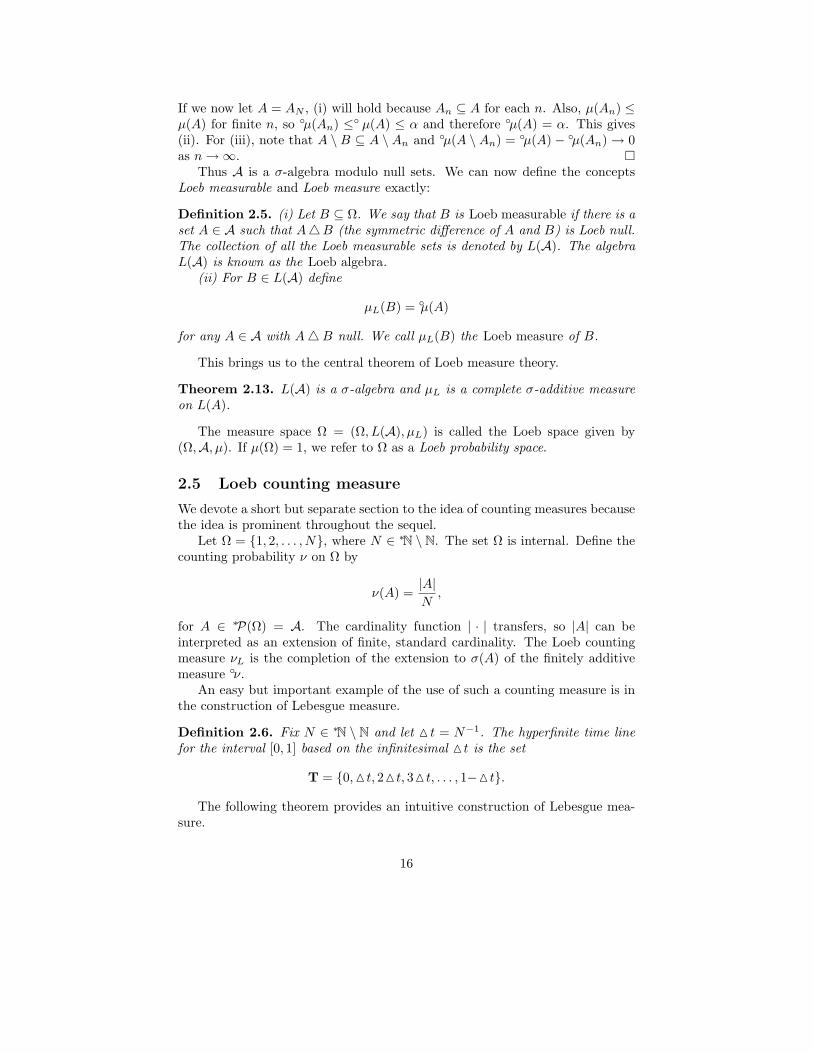
Thus A is a σ-algebra modulo null sets. We can now define the conceptsLoeb measurable and Loeb measure exactly:

Definition 2.5. (i) Let B ⊆ Ω. We say that B is Loeb measurable if there is aset A ∈ A such that A4B (the symmetric difference of A and B) is Loeb null.The collection of all the Loeb measurable sets is denoted by L(A). The algebraL(A) is known as the Loeb algebra.

(ii) For B ∈ L(A) define

µL(B) = µ(A)

for any A ∈ A with A4B null. We call µL(B) the Loeb measure of B.

This brings us to the central theorem of Loeb measure theory.

Theorem 2.13. L(A) is a σ-algebra and µL is a complete σ-additive measureon L(A).

The measure space Ω = (Ω, L(A), µL) is called the Loeb space given by(Ω,A, µ). If µ(Ω) = 1, we refer to Ω as a Loeb probability space.

2.5 Loeb counting measure

We devote a short but separate section to the idea of counting measures becausethe idea is prominent throughout the sequel.

Let Ω = 1, 2, . . . , N, where N ∈ ∗N \ N. The set Ω is internal. Define thecounting probability ν on Ω by

ν(A) =|A|N,

for A ∈ ∗P(Ω) = A. The cardinality function | · | transfers, so |A| can beinterpreted as an extension of finite, standard cardinality. The Loeb countingmeasure νL is the completion of the extension to σ(A) of the finitely additivemeasure ν.

An easy but important example of the use of such a counting measure is inthe construction of Lebesgue measure.

Definition 2.6. Fix N ∈ ∗N \ N and let M t = N−1. The hyperfinite time linefor the interval [0, 1] based on the infinitesimal M t is the set

T = 0,M t, 2M t, 3M t, . . . , 1−M t.

The following theorem provides an intuitive construction of Lebesgue mea-sure.

16

Theorem 2.14. Let νL be the Loeb counting measure on T. Define

(i) M = B ⊆ [0, 1] : st−1T

(B) is Loeb measurable, where st−1T

(B) = t ∈T : t ∈ B.

(ii) λ(B) = νL(st−1T

(B)) for B ∈ M.

Then M is the completion of the Borel sets B[0, 1] and λ is Lebesgue measureon M.

Proof. We only need to sketch the proof here. A more complete proof canbe found in [1]. To check that M is a σ-algebra is not difficult. Furthermore, Mcontains each standard interval [a, b], since st−1

T([a, b]) = ∩n ∈ N(∗[a − 1/n, b +

1/n]∩T), a countable intersection of internal sets. It can also be shown that λ isa complete probability measure on M. We can then show that λ is translationinvariant and λ([a, b]) = b−a. The measure is therefore an extension of Lebesguemeasure. Now take B ∈ M and an internal A such that A ⊆ st−1

T(B) is an inner

approximation. The set st(A) is a closed inner approximation of B; enough toshow that B is Lebesgue measurable.

In Chapter 4 we will encounter another important use of counting measurein constructing Wiener measure.

17

3 A nonstandard version of Hausdorff dimen-

sion

In this chapter we show that a formulation of Hausdorff measure as a nonstan-dard counting measure, similar to Loeb’s formulation of Lebesgue measure, ispossible and prove some well-known theorems using these nonstandard tech-niques. It turns out that some interesting dimensional properties of Brownianpaths become quite easy to prove using hyperfinite counting arguments.

Before we start the proof, we need a nonstandard version of the followingresult known as Frostman’s lemma [13]. We denote the β-dimensional Hausdorffmeasure of a set A by measβA.

Theorem 3.1. (Frostman’s lemma) Let A be a compact subset of [0, 1] andβ ∈ (0, 1). Then measβA > 0 if and only if there exists a probability measure µon A such that µ(B) ≤ C|B|β for each interval B ⊆ [0, 1] and some positive C.

This is often used to prove Frostman’s theorem, which we will include at theend of this chapter. A version of the lemma on the hyperfinite time line is as

follows. Note that we abuse the notation slightly by using (

|A′|2Nα

)

> 0 to mean

either that the standard part of the expression in brackets exists and is largerthan 0, or that the expression is infinite.

Theorem 3.2. Let A be a compact subset of [0, 1]. Suppose T is a hyperfinitetime line based on the dyadic sequence 2n and A′ ⊆ T is such that its standard

part is A. If (

|A′|2Nα

)

> 0 , there exists a nonstandard measure µ on a hyperfinite

time line on [0, 1] such that the Loeb measure µL ∈ M+(A) (the set of strictlypositive measures on A) associated to µ has the property that for an absoluteconstant C and an arbitrary interval B ⊆ [0, 1], it is true that µL(B) ≤ ‖B‖α.

Proof. The measure in question is not quite as simple as, for instance, thecounting measure we used to generate Lebesgue measure. In this case we haveto take into account how “close” elements of A are to each other and a uniformcounting measure cannot provide that information. Thus the construction ofthe measure is not generic but will depend specifically on the nature of A.

We use a time line based on the hyperfinite number 2N , whereN = 〈1, 2, 3, ...〉U .The measure is constructed in a number of stages, at each stage ensuring thatthe inequality µm(B) ≤ ‖B‖α holds, and then showing that the total measureof the interval is larger than 0 and normalising. On a dyadic interval B of orderm, meaning that the interval has length 2−m, count the number of elements ofBT ∩ AT and distribute the mass ‖B‖α evenly over the elements of BT ∩ AT.Thus each element of AT in BT receives a weight of

‖B‖α

|BT ∩AT|.

This does guarantee that the required inequality is true for this interval, but wemust bear in mind that the measure must be additive. To this effect we go back

18

one step, to dyadic intervals of order m− 1. Suppose that the above interval Bis contained in an interval B′ of order m− 1. We must now check whether

µ(B′) ≤ 2α‖B‖α

|B′T ∩AT|

.

If adjacent intervals of order m both contain elements of AT, we will need tomultiply the measure on each of these intervals by a factor of 2α

2 . We continuedoing this until we cover all dyadic intervals on the time line, both standard andnonstandard. Thus the measure is finitely additive in the nonstandard context.Also, the smallest the measure of any element of AT can be, will be

2α

22−(N−1)α = 22α−12−Nα.

Thus, the smallest the total mass over all of AT can be is

22α−1 |AT|2Nα

.

But since we have that (

|AT|2Nα

)

> 0, we know there will exist some finite (but

not infinitesimal) γ such that

22α−1 |AT|2Nα

> 22α−1γ.

We normalise using the total mass and obtain, for any dyadic interval B that

µ(B) ≤ 1

γ‖B‖α.

The inequality will then also hold for µL. An arbitrary interval D will alwaysbe contained in two such dyadic intervals and therefore

µL(D) ≤ 2

γ‖D‖α.

We prove the main result of this chapter in two separate theorems. The firstguarantees the existence of a subset of a time line from which we can computethe dimension and the second shows that the choice of set is not very important.It is proved for subsets of [0, 1] only, but note that it can easily be extended toany compact interval and arbitrary (finite) dimension.

Theorem 3.3. Given a compact subset A of [0, 1], there is a subset AT on thehyperfinite time line T and a hyperfinite number N ∈ ∗N \N such that AT = Aand

( |AT|Nβ

)

= ∞ for β < α

( |AT|Nβ

)

= 0 for β > α

if and only if dimA = α.

19

Proof. Suppose that β < dimA. We know that the sum diverges to infinityas the sizes of the intervals decrease. Thus there will be some N ∈ N such thatthe β-Hausdorff sum will be larger than 1 for covers constituting of sets withdiameter smaller than 2−K , for all K > N .

In the following we will state as a bounded quantifier statement that this willhold for any cover and that such a cover always exists, a seemingly trivial pointin the standard case, but not as obvious in the nonstandard. We also use thefact that we may require our intervals not to border on each other, for otherwisethe Hausdorff sum may be made smaller, and we require that even the smallestsum must be larger than 1. The use of K > J is justified by the compactnessof the set A; that is, the cover will have a finite subcover, and therefore therewill be a set of diameter no smaller than 2−K for some K > J .

Let S = S(A,X,K, J) be the following statement, where X ⊂ N × N:

S = ∀x ∈ A∃(i, j) ∈ X(

x ∈(

i2K ,

j2K

])

∧ ∀(i, j) ∈ X∃x ∈ A(

x ∈(

i2K ,

j2K

])

∧∀(i, j) ∈ X(

2−K ≤ (j − i)2−K ≤ 2−J)

∧[

(i, j) ∈ X ⇒ ¬(∃k ∈ 0, 1, . . . , 2K − 1((j, k) ∈ X))]

,

and let T = T (X,K, β) be the statement

∑

(i,j)∈X

(

j − i

2K

)β

> 1.

We then express β < dimA as:

[∃N ∈ N∀J > N∀K ≥ J∀X ⊆ 0, 1, . . . , 2K − 1 × 0, 1, . . . , 2K − 1(S ⇒ T )] ∧

[∃N ∈ N∀J > N∀K ≥ J∃X ⊆ 0, 1, . . . , 2K − 1 × 0, 1, . . . , 2K − 1(S ⇒ T )].

The transferred statement now reads as

[∃N ∈ ∗N∀J > N∀K ≥ J∀X ⊆ 0, 1, . . . , 2K − 1 × 0, 1, . . . , 2K − 1(∗S ⇒ ∗T )] ∧

[∃N ∈ ∗N∀J > N∀K ≥ J∃X ⊆ 0, 1, . . . , 2K − 1 × 0, 1, . . . , 2K − 1(∗S ⇒ ∗T )],

where ∗S and ∗T are the transferred versions of the statements S and T . Notethat this necessitates replacing only A with ∗A in the original.

We now choose any sufficiently large J ∈ ∗N \ N. The statement will stillhold if we set K = J . This results in a “cover” of ∗A by intervals of diameter2−K . Set

AT =

j

2K: (j − 1, j) ∈ X

,

20

where X is the set the existence of which is guaranteed in the second line of theprevious transferred statement.

By the transferred statement we know that∑

(i,j)∈X

(

j−i2K

)β> 1, but j− i =

1 because of the choice of K — all the infinitesimal intervals are now of thesame size. Also, |AT| = |X|; therefore |AT|

2Kβ > 1. Thus,

measβA > 0 ⇒ ∃AT ⊆ T,K ∈ ∗N \ N such that AT = A and

( |AT|2Kβ

)

> 0.

Since the converse holds by the nonstandard Frostman lemma, the theoremis proved.

We now show that any set which satisfies certain of the above properties isrich enough to yield Hausdorff dimension.

Theorem 3.4. Consider a hyperfinite time line T based on the infinitesimal2N , for a given N ∈ ∗N \ N. Suppose that a subset A′ of the time line is suchthat st(A′) = A and for some α > 0

( |A′|2Nβ

)

> 0 for β < α and (3.1)

( |A′|2Nβ

)

= 0 for β > α. (3.2)

Then α = dimA.

Proof. Given (1), the nonstandard version of Frostman’s lemma immedi-ately implies that dimA ≥ α. For the converse inequality, notice that the secondcondition implies that for each ε ∈ R, ε > 0,

|A′|2Nβ

< ε,

which implies the following nonstandard statement for each positive ε ∈ R:

∃N ∈ ∗N∃Y ⊆ 0, 1, . . . , 2N − 1∀x ∈ A′∃i ∈ Y(

x ∈ (i2−N , (i+ 1)2−N ])

∧(

|Y |2Nβ < ε

)

.

Transferring down to the standard case, we find that for each ε > 0,

∃n ∈ N∃y ∈ 0, 1, . . . , 2n − 1∀x ∈ A′∃i ∈ y (x ∈ (i2−n, (i+ 1)2−n])∧(

|y|2nβ < ε

)

.

This implies that measβA = 0 and therefore that dimA ≤ α.

For computational purposes it is therefore enough to find a set in the timeline with standard part A that satisfies the conditions in the above theorem.This fact will be used in subsequent chapters. In the sequel we refer to |AT| M tβ

as nonstandard (or NS) β-Hausdorff measure and to measβA as just β-Hausdorffmeasure.

21

Several of the properties of the standard β-Hausdorff measure can easily beseen to be valid in the nonstandard case, such as its outer measure properties,invariance under translation (and rotation, in the multidimensional case) andhomogeneity of degree β with respect to dilation.

To illustrate some applications of this formulation, we first turn to the peren-nial example of a set of non-integer dimension, the triadic Cantor set (construc-tion described in any book on fractals). We did not prove that its dimension wasα = log 2/ log 3, but do so now. The “base-infinitesimal” of the constructionis 〈1, 3−1, 3−2, . . . , 3−k, . . .〉U =M t = 1/N . The cardinality of the NS Cantorset |AT| is given by |AT|〈1, 2/3, 4/9, . . . , (2/3)k, . . .〉UN . The NS β-Hausdorffmeasure of A is then given by

|AT| M tβ = 〈(2/3)k〉UN〈(1/3)kβ〉U= 〈(2/3β)k〉U ,

where we have used the obvious notation, 〈ak〉U instead of 〈a, a2, . . . , ak, . . .〉U .The above expression then has value 1 for β = log 2/ log 3, which is then dimAby our previous theorems. Since the standard β-Hausdorff sum for the triadicCantor set is also 1 for β = dimA, we suspect that the standard parts of thenonstandard sum will be equal to the standard sum at dimA for other sets aswell. This remains to be proved. We now turn to Cantor-like sets in general.In [31], a Cantor-like set K is a set generated by nested intervals in the followingway:

1. Let, for each m, Im,i be an interval contained in [0, 1], where i ≤Mm, andsuppose these intervals are disjoint.

2. Let Em =⋃

1≤i≤MmIm,i; it is also required that Em ⊇ Em+1.

3. Let K =⋂

m∈NEm.

We can further assume that K has Lebesgue measure 0, to avoid triviality. Oreyand Taylor proved the following theorem for such sets:

Theorem 3.5. Suppose that c > 0, δ > 0. The measβK > 0 if, for everyinterval J ⊆ [0, 1] with |J | < δ, there is a finite integer m(J) such that

Mm(J) ≤ c|J |βMm for m ≥ m(J),

where Mm(J) denotes the number of intervals Im,i, 1 ≤ i ≤Mm contained in J .

Clearly, each of the intervals used in the construction gives rise to someinfinitesimals, depending on the rate at which their lengths converge to 0. Inthe case of the triadic Cantor set, these are all the same, which makes theconstruction so simple.

We can therefore consider a Cantor-like set as some union of infinitesimals.The β-Hausdorff measure will not be as simple to calculate as the Cantor set,since we cannot base the hyperfinite time line on a single one of the infinitesi-mals.

22

The above theorem in the nonstandard context is actually a restricted ver-sion of Frostman’s Lemma. For the sake of completeness, we now present Frost-man’s theorem [21], an important tool in the study of capacity and Hausdorffdimension. The proof itself is so simple that little extra insight is gained froma nonstandard approach. But first we have to define the notion of capacity:

Definition 3.1. A compact set A ⊂ Rd is said to have a positive capacity if itcarries a positive measure µ such that the following integral is finite:

Iα(µ) =

∫ ∫

dµ(x)dµ(y)

|x− y|α .

If there is no such measure, we say that A has capacity 0. The capacitariandimension of A is

dimC(A) = supα : CapαA > 0 = α : CapαA = 0.In a sense, this is the exact opposite of Hausdorff measure, in that the integralis finite exactly where measαA is infinite, and infinite where measαA is 0. Thisnotion is made precise in the following:

Theorem 3.6. Let A be a compact set in Rd and 0 < α < β < d. Then

measβA > 0 ⇒ CapαA > 0 ⇒ measαA > 0.

This implies that the capacitarian and Hausdorff dimensions of A are the same.

Proof. First we show that measβA > 0 ⇒ CapαA > 0. If measβA > 0, Acarries a measure µ such that

∫

|x−y|≤ρ

dµ(x) < Cρβ

for every y ∈ Rd and ρ > 0, dependant only on µ. Integrating on sphericalrings,

∫

dµ(x)

|x− y|αis uniformly bounded with respect to y, and therefore Iα(µ) < ∞, implyingCapαA > 0.

We now show that CapαA > 0 ⇒ measαA > 0. If CapαA > 0 there is aµ ∈M+(A) such that Iα(µ) <∞. Let At be the subset of A defined by

y ∈ At if and only if

∫

dµ(x)

|x− y|α ≤ t.

For large enough t, µ(At) > 0. Let A ⊆ ∪nBn such that At ∩ Bn 6= ∅ for eachn. Choose yn ∈ At ∩Bn. Then

µ(Bn) ≤ |Bn|α∫

Bn

dµ(x)

|x− yn|α≤ t|Bn|α and

∑

|Bn|α ≥ t−1µ(At),

implying that measαAt > 0 and therefore measαA > 0.

Note that this theorem and Frostman’s lemma, are also valid when A isσ-compact instead of compact.

23

4 Some applications to the fractal geometry of

Brownian motion

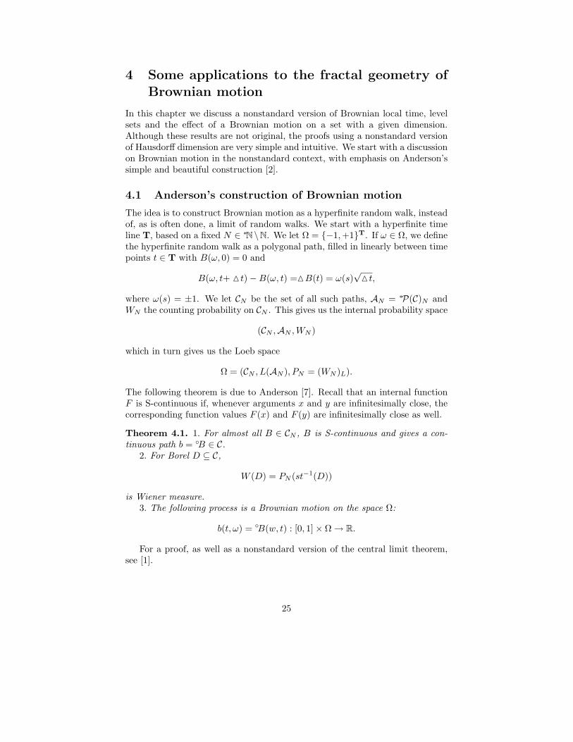
In this chapter we discuss a nonstandard version of Brownian local time, levelsets and the effect of a Brownian motion on a set with a given dimension.Although these results are not original, the proofs using a nonstandard versionof Hausdorff dimension are very simple and intuitive. We start with a discussionon Brownian motion in the nonstandard context, with emphasis on Anderson’ssimple and beautiful construction [2].

4.1 Anderson’s construction of Brownian motion

The idea is to construct Brownian motion as a hyperfinite random walk, insteadof, as is often done, a limit of random walks. We start with a hyperfinite timeline T, based on a fixed N ∈ ∗N\N. We let Ω = −1,+1T. If ω ∈ Ω, we definethe hyperfinite random walk as a polygonal path, filled in linearly between timepoints t ∈ T with B(ω, 0) = 0 and

B(ω, t+ M t) −B(ω, t) =MB(t) = ω(s)√

M t,

where ω(s) = ±1. We let CN be the set of all such paths, AN = ∗P(C)N andWN the counting probability on CN . This gives us the internal probability space

(CN ,AN ,WN )

which in turn gives us the Loeb space

Ω = (CN , L(AN ), PN = (WN )L).

The following theorem is due to Anderson [7]. Recall that an internal functionF is S-continuous if, whenever arguments x and y are infinitesimally close, thecorresponding function values F (x) and F (y) are infinitesimally close as well.

Theorem 4.1. 1. For almost all B ∈ CN , B is S-continuous and gives a con-tinuous path b = B ∈ C.

2. For Borel D ⊆ C,

W (D) = PN (st−1(D))

is Wiener measure.3. The following process is a Brownian motion on the space Ω:

b(t, ω) = B(w, t) : [0, 1] × Ω → R.

For a proof, as well as a nonstandard version of the central limit theorem,see [1].

25

4.2 Brownian local time

The local time of a Brownian motion gives a measure of the time a Brownianmotion spends at x. The Lebesgue measure of this set is 0, but it can bedescribed using Hausdorff measure, as we shall see shortly.

Definition 4.1. We define the local time l(t, x) as

l(t, x) =

∫ t

0

δ(x− b(s))ds,

where b is a Brownian motion and δ the delta function.

The integral therefore “counts” how many times the Brownian path visits xup till the time t. The standard approach (which can be found in detail in [?])is to show there exists a jointly continuous process l(t, x) such that

l(t, x) =d

dx

∫ t

0

I(−∞,x](b(s))ds,

for almost all (t, x) ∈ [0, 1] × R, where IA is the characteristic function of theset A. Note that although the definition is valid for a time line [0,∞) as well as[0, 1], we use a bounded interval throughout. The nonstandard approach, dueto Perkins [1], is clearer and more intuitive. We think of the Brownian pathb as the standard part of a hyperfinite random walk. The following expositionfollows [1]. We start by approximating l(t, x) by

(M x)−1

∫ t

0

I[x,x+Mx](b(s))ds.

Now replace the time line [0, 1] by a discrete hyperfinite time line T and thespace R by Γ = 0,±

√M t, . . . ,±n

√M t, . . . ,±N

√M t and define the internal

process L : T × Γ → ∗R by

L(t, x) =∑

s<t

Ix(B(s))(M t)1/2.

Perkins showed that L(t, x) has a standard part which is Brownian local time.He used the nonstandard formulation to prove the following global characterisa-tion of local time, which was previously known to hold only for each x separately:Let λ(t, x, δ) be the Lebesgue measure of the set of points within a distance ofδ/2 of s ≤ t|b(s) = x. Then for almost all ω ∈ Ω and each t0 > 0,

limδ→0+

supt≤t0,x∈R

|m(t, x, δ)δ−1/2 − 2(2/π)1/2l(t, x)| = 0.

It is shown in [?] that local time is the same as 12 -dimensional Hausdorff measure.

From the nonstandard formulation, however, it is immediately clear. If wedefine the set A as the set of all t ∈ [0, 1] such that b(t) = x, the nonstandard

26

local time becomes simply |AT| M t1/2. But this is exactly the nonstandardformulation of 1

2 -dimensional Hausdorff measure (up to a finite constant factor— which depends on which author you read) We must now show that level setshave dimension 1/2. We just show this for x = 0, since they all have similardimension. Denote the zero set of a Brownian path b(ω) by Aω. We now turnto a standard property of local time to show that the dimension of this set is1/2. It can be shown (as for instance in [?]) that local time is identical in lawto the function

Mω(t) = maxs≤t

b(s).

This implies that P [l(1, 0) > 0] = 1. By the nonstandard formulation of localtime, this immediately implies that dimA ≤ 1/2, almost surely. By the sametoken, however, l(1, 0) is almost certainly finite, implying that dim(A) = 1/2.The following lemma will be used in the subsequent section. In this case thestandard approach is easier than the hyperfinite, by using the Holder conditionfor Brownian motion.

Lemma 4.2. If A is a level set and D ⊆ A, then D has dimension 1/2 or 0.

Corollary 4.3. If dimA < 1/2, then the inverse image of any element in b(A)(where b is a Brownian motion) has dimension 0.

4.3 The image of a set under Brownian motion

A very interesting property of Brownian motion is what it does to sets of acertain Hausdorff dimension. If a compact subset of [0, 1] has dimension α <1/2, its image under Brownian motion is a set of dimension 2α. (This set isa Salem set as well, meaning it has equal Hausdorff and Fourier dimensions.This notion will be explored in more depth in Chapter 6.) A set of dimensionα > 1/2 will have dimension 1 and will almost surely contain an interval. Asfor sets of dimension 1/2, we have seen above that they may have an imageof dimension 0. No hard and fast rule exists for such sets. We now look atnonstandard proofs of these results. The advantage of this approach is a moreintuitive (counting) argument. The following was first proved by Kaufman [21].

Theorem 4.4. Let A ⊂ [0, 1] be a compact set. If dimA = α < 1/2 and b is aBrownian motion, dimb(A) = 2α.

Proof. The basis for the time line of the image is no longer M t, but√

M t.Since |B(AT )| ≤ |AT | and we know that |AT | M tβ ≈ 0 for β > α, we willhave that |B(AT )| M tβ ≈ 0 for any β > α. Therefore, |B(AT )|(

√M t)γ ≈ 0 for

γ > 2α and we conclude that dimb(A) ≤ 2dimA (because of the continuity ofthe functions involved we can conclude that |[b(A)]T | = |B(AT )|). It is left toshow that dimb(A) ≥ 2dimA. This is not quite as simple as the previous proof,since the matter of possible level sets complicates the question of the cardinalityof the image. We overcome this by considering only the first elements of level

27

sets and discarding the rest. The remaining set will have the same dimension asthe original and the image will have the same cardinality. This is made possiblebecause the set A has a dimension of less than 1/2. Any subsets of level setsin A are small enough to be left out (mostly) without affecting the dimension.For any x ∈ b(A), let Lx denote the part of the level set of x contained in Aand let L denote the collection of all these sets. We want to show now that thestandard parts of the sums

∑

Lx∈L

1

Nα,

∑

Lx∈L

|Lx,T|Nα

are 0 and ∞ for the same values of α. To do this, all that is necessary is toshow that the first one is infinite whenever the second one is. So suppose that

(

∑

Lx∈L

|Lx,T|Nα

)

= ∞.

We know that

|Lx,T|Nα

= sβx ≈ 0

for any β > 0. This implies that

∑

Lx∈L

sβxN

β

Nα=∑

Lx∈L

sβx

Nα−β≤∑

Lx∈L

1

Nα−β= ∞,

for β arbitrarily close to 0. Thus we may conclude that the number of level setsis important and not the cardinality of each. But the number of level sets isequal to the cardinality of the range, thus the standard parts of

|B(AT )|Nα

and|AT |Nα

are 0 and ∞ for the same values of α. Keeping in mind that the time line ofthe image is based on

√M t and not M t, we can conclude that the dimensions

are equal.

28

5 Nonstandard analysis of rapid points of func-

tions

Orey and Taylor found the exact Hausdorff dimension of rapid points of Brown-ian paths [31]. Because of the importance of the result and the beauty of itsproof (utilising Cantor-type sets), we present a sketch of the proof in the ap-pendix. We show in this chapter that the result holds for a more general classof functions satisfying a few conditions which hold almost surely for Brown-ian paths. Specifically, any function that satisfies these conditions will have aset of rapid points of a given dimension, and Brownian motion satisfies theseconditions with probability 1.

First, we need a some definitions. Given an interval I = [a, b], we define

Rf (I) = supa≤s<t≤b

|f(t) − f(s)|.

When it is clear which function we are using, we usually write just R(I). Fora function f and a given 0 < α < 1, let I = I(α) denote the collection of all

intervals I in [0, 1] such that R(I) > α√

2h log h−1, where h > 0 denotes thelength of the interval I. Given such an I, we denote by Ik the collection of allthe intervals of the form [i2−k, (i+ 1)2−k) (for i = 0, 1, . . . , 2k − 1) contained inI. The set of α-rapid points of Brownian motion, Eα, is defined in (1.4).

We first turn to a requirement which will allow certain sets to have a dimen-sion of, or more than, 1 − α2.

Lemma 5.1. Suppose 0 < α < 1. Let f be a continuous function and consideran equipartition of [0, 1] into 2n pieces, each of which is further subdivided in afurther 2j pieces. If there exists some c > 0, dependant only on f , such that therelation

|0 ≤ k ≤ 2n − 1 : ∃t ∈ [k2−n−j , (k + 1)2−n + 2−j ](2n/2|f(k + 1)2−n) − f(t)|≥ α

√

2n log 2| ≥ c2(1−α2)(n+j)(5.1)

is satisfied for large enough n, the α-rapid points of f have dimension largerthan or equal to 1 − α2.

Although the formulation may seem somewhat cumbersome, we do it as suchto facilitate the application to Brownian motion at a later stage.

Proof. Consider the relation

|0 ≤ k ≤ 2n+j − 1 : ∃t ∈ [kb2−n, (k + 1)b2−n](2n/2|f(k2−n + 2−n) − f(t))|≥ α

√

2n log 2| ≥ c2(1−α2)(n+j).(5.2)

Everything in this relation is first order and can be transferred to a hyperfinitecontext; it follows that there are infinite numbers N and J for which the relationalso holds; for convenience we set M = N + J :

|1 ≤ K ≤ 2M : 2N/2|F ((K + 1)2−N ) − F (T ))| ≥ α√

2M log 2| ≥ c2(1−α2)M .

28

(F is the S-continuous nonstandard extension of f ; see Section 2.3.) Now,instead of seeing the division of [0, 1] as an equipartition, we can consider it ahyperfinite time line. Also, remembering the ultrapower construction, each Kfor which the above holds implies the existence of a sequence of dyadic rationalswhich converges to a rapid point. The hyperfinite dyadic rationals included inthe transferred relation therefore exist in the monad of an α-rapid point. Butwe know that there are ≥ c2(1−α2)N points on our time line of 2N elements. Tolet the quotient

|Eα|Nβ

therefore have real part 0, N would have to be raised to a power larger than1 − α2, for the quotient would then be a constant. Thus, dimEα ≥ 1 − α2.

We now confirm that Brownian motion does indeed have these properties,almost surely, and that the α-rapid points of Brownian motion therefore havedimension 1−α2. In the following two lemmas we assume we are working witha Brownian motion X on a space (Ω,B,P).

Lemma 5.2. If A is the set of α-rapid points of X(t), A has a Hausdorffdimension of at most 1 − α2.

Proof. We consider a partial covering of Eα by dyadic intervals not unlikethose considered in the previous lemma. Since each member of Eα can beapproached through dyadic rationals, this will indeed form a cover in the limit.Let n, j ∈ N and let α1 < α. We will consider j to be fixed. Define Bα1,n(ω) tobe the random set

0 ≤ k ≤ 2n+j − 1 : ∃t ∈ [k2−n−j , (k + 1)2−n−j ](2n/2|f(k2−n + 2−n) − f(t)|≥ α1

√

2n log 2Note that we can either consider these sets as subsets of the integers or ascollections of the dyadic intervals these integers represent. We shall use theseinterchangeably, since it will always be clear from the context which we mean.Let Aα1,n be the event

|Bα1,n(ω)| ≥ 2(n+j)(1−α21).

The sets of the form Bα1,n(ω) do not form a cover of the rapid points, but it iseasily seen that the α-rapid points are contained in the limit superior of suchsets, indexed by n.

We now estimate the probability of Aα1,n. The distribution of Aα1,n isbinomial and the probability of a success is calculated in Theorem 6.4 to belarger than 2−α2

1n2o(1). We now want to calculate the probability P(Aα1,n).For this we use an estimate from [10] for the tail of the binomial distribution.If S2n denotes the sum of 2n variables which may take value 1 with probabilityp and 0 with probability q = 1 − p, then we have that

PS2n ≥ r ≤ rq

(r − 2np)2, (5.3)

29

when r > 2np. To see that we may use this estimate, using the approximations inthe proof of Lemma 6.4, we find that p < 2−nα2

1(1+o(1)) (using Feller’s estimate ofthe maximum fluctuation over an interval as upper bound). We let the constant

c be determined by j in the form c ≥ 2−jα2

. Then it will be true that r > np,for fixed j. Using the lower bound for p it is clear that

p ≥ 2−α21n2o(1)

> 2−α21(n+j) >

2−mα21

m, (5.4)

where m = n+ j. Our estimate becomes

P(Aα1,n) <2m(1−α2

1)(1 − p)

(2m(1−α21) − 2mp)2

.

through the use of (5.4), and using (5.5) we obtain

P(Aα1,n) ≤ 2m(1−α21)(1 − 2mα2

1/m)

(2m(1−α21) − 2mp)2

.

Not only can some quick calculation show that this term tends to zero as n tendsto infinity, but we also have that the sum of all the terms converges, because ofthe inequalities

P(Aα1,n) <2m(1−α2

1)(1 − 2mα21/m)

(2m(1−α21) − 2mp)2

<2m(m2−mα2

1 − 2m(α21−α12))

m(2m(1−α21) − 2m)2

≤ 2(1−α21)m

m(2m(1−α21) − 2m)2

< 22(1−α2

1)m

2msince (2−α2

1m − 1)2 >1

2for m large

=2

2m(1+α21).

Seeing the above as the first step in constructing our cover, we can now proceedto larger values of n and α1 to find intervals of smaller diameter. For such largervalues the above inequalities will still hold. We also consider, for each largervalue of n, a larger value αi, where α1 < αi−1 < αi < α. If we now consider, fora specific sequence αii∈N, the collection of intervals given by all the Bα1,n, weobtain a cover of A. Although we have constructed the sets as unions of closedintervals, they may as well be considered to be made up of open intervals, sincethe set of dyadic rationals which are also rapid points have Hausdorff dimension0. Although the compactness of the set ensures that we could find a finitesubcover, we do not actually need to find such a cover here, since the number

30

of intervals used is small enough. If we now consider the α1-Hausdorff sum forthe cover of A obtained by the above process, we get an expression smaller than

∑

|Bαi,n|21−α21(n+j)

<∑

2(n+j)(1−α2i )2(−1−α2

1)(n+j)

= 2(α21−α2

i )(n+j)

which is bounded, with an exceptional probability which is as close to 0 as wewish (since the sum of the probabilities of each exceptional case can be madearbitrarily small by simply starting our construction at a larger value of n).This holds for all the 1 − α2

i -Hausdorff sums. Since A is contained in the setwhose dimension we are now approximating, it must follow that dimA ≤ 1−α2,with probability 1.

Lemma 5.3. There exists a constant c < 1 such that Brownian motion almostsurely satisfies relation 5.2; that is, for large enough n,

|0 ≤ k ≤ b2n − 1 : ∃t ∈ [kb2−n, (k + 1)2−n + 2−j ](2n/2|f(k + 1)2−n) − f(t)|≥ α

√

2n log 2| ≥ c2(1−α2)(n+j).(5.5)

Proof. We again use a binomial distribution on the set of intervals, viewingit as a Bernoulli trial with probability of success p (as calculated in Theorem6.5) and using another estimate of the binomial tail from [10], we find that

P

(

Sm ≤ 1

22(1−β2)m

)

≤ (m− r)p

(mp− r)2

=(2m − 1

22(1−β2)m)2−β2m2o(1)

(2(1−β2)m2o(1) − 122(1−β2)m)2

=2o(1)(2(1−β2)m − 1

22(1−β2)m)

(2o(1)2(1−β2)m − 122(1−β2)n)2

.

This clearly tends to 0 and thus the probability of more than 122(1−β2)m successes

in 2m trials goes to 1, which proves the lemma.

It now follows trivially from the previous two lemmas that the α-rapid pointsof a Brownian motion have almost surely a Hausdorff dimension of 1 − α2.

This theorem has the following interesting (but simple) result as conse-quence [31]:

Corollary 5.4. For a Brownian path Xω = X,

dim

t : lim suph→o

X(t+ h) −X(t)

(2h log log h−1)12

= ∞

= 1

with probability 1.

31

Proof. It is easily seen that that for each α, the set of α-rapid points hasthe property of the above set, with probability 1 (the iterated logarithm is tooweak to “contain” the growth at the rapid points). The above set thereforecontains all the E(α) and has dimension 1, with probability 1.

We also remark that the theorem can quite easily be extended to higherdimensions, with the most notable change being the replacement of X(t+ h)−X(t) by the Euclidean distance |X(t+ h) −X(t)|.

As mentioned in the introduction, the notable feature of this version of theproof is the pathwise approach it takes. In the next section we will repeatedlyuse the probability that a section contains an α-rapid point, approximated byhα2

ho(1), where h is the length of the interval. This is very close to our approxi-mation of the ratio of intervals which are picked at any stage. The probability ofthe paths having a certain property is therefore somehow reflected in each path.This ratio is used in Section 6.2 to find upper and lower bounds on the totalmass of a measure, while the probability will lead us to the domain of validityof the measure. As we shall see, these two in combination give us a Salem set.

32

6 The Fourier dimension of rapid points

6.1 Introduction

In this chapter we explore a subtler property of the rapid points of Brown-ian motion than their Hausdorff dimension. The main result of this chapter isattributable to Kaufman [22], but since his proof is perhaps not entirely trans-parent (and sometimes inaccurate) we feel it is worthwhile giving an expositionthereof.

The Hausdorff dimension of a set gives us a measure of the “thinness” of theset. As we shall show shortly, when it is regarded as a capacitarian dimension, itcan also yield information on the asymptotic behaviour of the Fourier transformof measures supported by the set.

Given a measure µ on our usual set [0, 1], we define the Fourier transform ofµ as

µ(ξ) =

∫

[0,1]

eiξxdµ(x).

We then have the following result, which is a statement about capacity in termsof Fourier transforms:

Theorem 6.1. If A ⊆ Rd is a compact set, then the dimension of A is thesupremum of all α for which there exist a positive measure µ such that

∫

Rn

|µ(ξ)|2|ξ|α−ddξ <∞.

Proof. Recall from Definition 3.1 that a compact set A ⊂ Rd is said tohave a positive capacity if it carries a positive measure µ such that the followingintegral is finite:

Iα(µ) =

∫ ∫

dµ(x)dµ(y)

|x− y|α .

It follows from the Fourier analysis of Schwartz distributions that there is aconstant C = C(d, α) such that

Iα(µ) = C

∫

Rd

|µ(ξ)|2|ξ|α−ddξ,

as for example on p.162 of [29]. The result follows.

Sometimes more precise information about µ is required. In harmonic analy-sis, one of the most important problems is that of the uniqueness and multiplicityof sets. A compact set E ⊆ T = R/Z is called a set of (restricted) multiplicityif there is a measure supported on T such that the trigonometric series

∑

n∈Z

µ(n)e2πinx

vanishes everywhere outside E. These sets are sometimes called M0-sets. Theconcept can be extended:

33

Definition 6.1. An Mβ-set is a compact set in Rn which carries a measureµ such that µ(ξ) = o(|ξ|−β) as |ξ| → ∞. For a compact set E, we call thesupremum of the α such that E is an Mα/2-set, the Fourier dimension of E.We shall denote this by dimFE.

The Fourier dimension is a somewhat more elusive character than Hausdorffdimension (dimE). They are usually different, as for instance in the case ofthe triadic Cantor set, which has positive Hausdorff dimension but a Fourierdimension of 0 [24]. The following lemma shows that the dimensions are related;specifically, that the Fourier dimension is majorised by the Hausdorff dimension.

Lemma 6.2. For a compact set E ⊆ Rd, dimEF ≤ dimE.

Proof. We use the previous theorem. Suppose that dimFE > 0. Choose0 < α < β < dimFA. Then there exists some µ ∈ M+(E) (the set of strictlypositive measures on E) with |µ(ξ)|2 = o(|ξ|−β) as ξ → ∞. In addition thereare constants C and C1 such that

Iα(µ) = C

∫

|µ(ξ)|2|ξ|2−ddξ

≤ C1

∫

|ξ|≥1

dξ

|ξ|d+(β−α)+ O(1).

Thus, CapαE > 0, and dimE ≥ dimFE.

One of the interesting aspects of Fourier, as opposed to Hausdorff, dimensionis its arithmetical properties, as illustrated by the following theorem.

Theorem 6.3. If E has a strictly positive Fourier dimension, then the abeliangroup generated by E is the entire ambient Euclidean space Rn.

Proof. We use the following result of Steinhaus [35] in the proof: If E ⊆ Rn

is such that its Lebesgue measure exists and is non-zero, then for some ε > 0,

B(ε) = x : ‖x‖ < ε ⊂ E − E,

where E − E is defined as the set x− y : x, y ∈ E.Let α > 0 be such that for some µ ∈M+(E),

|µ(ξ)|2 = o(|ξ|−α) for |ξ| ≥ 1.

Set ν = µ ? · · · ? µ, the convolution product of µ with itself, k times, where k islarge enough that kα > n. From the well-known properties of convolution wehave

|ν(ξ)|2 = |µ(ξ)|2k = o(|ξ|−kα),

implying that suppν has positive Lebesgue measure (through the use of Parse-val’s theorem). But suppν ⊂ suppµ + · · · + suppµ (k times) and therefore, forsome ε > 0,

B(ε) ⊂ (E + · · · + E) − (E + · · · + E)

34

(the difference of E summed k times and itself). Since R =⋃

n≥1 nB(ε), we canconclude that the abelian group generated by E is Rn. .

When the Fourier and Hausdorff dimensions of a set coincide, it is calleda Salem set, after Raphael Salem. The first (nontrivial) set known to havethis property almost surely was constructed by Salem [34]. Trivial examplesof such sets are the balls in any dimension; for example, the interval [0, 1] hasboth dimension equal to one (as a subset of R), and the appropriate measure inboth cases is the Lebesgue measure. For quite a while the only Salem sets wererandom sets. Gatesoupe [14] showed how to construct Salem sets of arbitrarydimension 0 < α < d for d > 1 by using rotations, given Salem sets in R ofFourier dimension β, 0 < β < 1. Only in 1981 did Kaufman [23] devise a way toconstruct Salem sets of arbitrary dimension 0 < α < 1, with certainty. In 1996C. Bluhm [5] expanded this construction. We give a summary of Bluhm’s resultin the following section, since in section 6.2 we will consider the probabilisticconstruction of Salem sets. Also worth mentioning is the result of Rudin [33],using a set introduced by Salem: There exist M0-sets which are independent inRd over the rationals. Such a set carries a pseudomeasure which is not a measure,but all discrete measures it carries have the same norm whether considered aspseudomeasures or measures. For a wide class of thin sets, the Brownian imageof the set is a Rudin set, i.e. an M0-set independent over the rationals.

6.1.1 Construction of a deterministic Salem set

First, we fix some notation to be used in this section. For x ∈ R,

‖x‖ = minm∈Z|x−m|.The set of prime numbers will be denoted by P, and we let PM = P ∩ [M, 2M ].The inspiration for the construction is the set of α-well-approximable number,defined as

F (α) =

∞⋂

k=1

∞⋃

q=k

x ∈ [0, 1] : ‖qx‖ < q−1−α.

The Hausdorff dimension of this set is 2/(2 + α). This has been known forquite some time, since the work of Jarnik [20] and Besicovitch [3]. Althoughthe set Sα to be defined momentarily resembles F (α) strongly, the set of α-well-approximable number is dense in [0, 1], which Sα is not. Also used in thepaper of Bluhm is the prime number theorem in the following by Hardy andWright [15]:

limM→∞

#PM

M/ logM= 1

where #PM denotes the number of prime numbers smaller than M . For theCantor-type construction that is used, a sequence of integers (Mk)k∈N is con-structed recursively, satisfying

M1 < 2M1 < M2 < 2M2 < M3 < 2M3 < · · · .

35

Furthermore, according to the prime number theorem we can find such a se-quence which also satisfies, for every k ∈ N,

PMk6= ∅ and #PMk

≥Mk/(2 logMk).

We now consider the following set:

Fq(α) = x ∈ [0, 1] : ‖qx‖ ≤ q−1−α.

We conclude that the set is compact by writing it as a union of closed intervals:

Fq(α) = [0, q−2−α] ∪(

q−1⋃

m=1

[

m

q− q−2−α,

m

q+ q−2−α

]

)

∪ [1 − q−2−α].

The set which then carries an appropriate measure for it to be a Salem set ofdimension 2/(2 + α) is defined by

Sα =

∞⋂

k=1

⋃

p∈PMk

Fp(α).

The nonzero measure µα constructed by Bluhm on the set Sα satisfies the decaycondition

µα(x) = o(log |x|)|x| −1

2+α , |x| → ∞.

6.1.2 The occurrence of Salem sets in Brownian motion

Thus far it may appear that Salem sets are extremely rare and possibly of littleintrinsic value. However, once we turn to random sets, specifically those associ-ated with Brownian motion, Salem sets seem to arise naturally and often. Forinstance, consider any subset of [0, 1] of Hausdorff dimension (strictly) between0 and 1/2. We have seen in Chapter 4 that the dimension doubles under theaction of Brownian motion; perhaps even more interestingly, the set has be-come a Salem set [21]. When the dimension of the original set is larger than1/2, its dimension clearly cannot be doubled, since both Hausdorff and Fourierdimensions are bounded by 1. The image does however attain this maximum,and what is more, will contain a set of positive Lebesgue measure [21] (clearly,Brownian motion does not respect topological dimension either). For a thoroughstudy of Brownian images and Salem sets, there is a whole series of (difficult)papers by Kaufman, as listed on p.289 of [21].

There is another instance where the Brownian motion brings forth Salemsets which we will examine closely in the next section (again, due to Kaufman).We have already concerned ourselves with the Hausdorff dimension of the rapidpoints. What is more surprising than these properties is the fact that this“encoding” of the dynamics of Brownian motion as a linear set also generates aset with similar Fourier dimension, almost surely.

36

There are still many questions remaining in the study of Fourier dimensionalproperties of Brownian motion. It is (to the author’s knowledge) not yet knownwhat the Fourier dimension of the zeroset of Brownian motion is, although wehave seen in an earlier chapter that it has a Hausdorff dimension of 1/2. Wehave clearer results for sets of Hausdorff dimension unequal to 1/2, but still donot entirely understand why this dividing line has such an effect on dimension.

6.2 Large increments of Brownian motion

The main result of this section is the following:

Theorem 6.4. (Kaufman [22]) With probability 1, a certain compact subsetof Eα, the α-rapid points of a given Brownian motion X, carries a probabilitymeasure µ such that µ(ξ) = o(ξ

12(α2−1)), 1 ≤ ξ < ∞. That is, Eα is a set of

Fourier dimension 1 − α2.

In proving this we will need a lemma. Suppose that ξn;n ≥ 1 is a set ofindependent random variables with a common distribution

Pξn = 1 = p = 1 − Pξn = 0.

We want estimates for sums of the form∑

(p − ξn)an. Let σ2 =∑ |an|2. We

let B = max|an|.

Lemma 6.5. Provided that Y B < 2pσ2 and all else as above,

P|∑

(p− ξn)an| ≥ Y ≤ 4

(

exp−1

4p−1σ−2Y 2

)

. (6.1)

Proof. We use a basic inequality that can be easily obtained by writing outthe series expansion of e:

pet(1−p) + (1 − p)e−pt ≤ 1 + p(1 − p)t2 ≤ et2p,

which is valid for 0 ≤ p ≤ 1, −1 ≤ t ≤ 1. We now turn to Chebyshev’sinequality, which states that

PX ≥ k ≤ 1

kE(X)

for any random variable X with finite expectation. Kaufman mentions that hededuces the final inequality by using Chebyshev, but it is never indicated howthis should be done. We now give the details required to obtain an estimate ofthe probability

P|∑

(p− ξn)an| ≤ Y .

Note that this will be the same as the probability

Pe|

(p−ξn)an| ≤ eY .

37

Set X =∑

(p − ξn)an. Because of the assumed independence of the ξn, theexpected value of etX can be evaluated by the integral

∫

etXdP =

n∏

i=1

∫

e−(p−ξn)antdP

=∏

(pe−(1−p)ant + (1 − p)epant)

≤∏

ept|an|2

= eptσ2

.

Note that we have used the basic inequality repeatedly with ant instead of justt, and must require that 0 ≤ max |an|t ≤ 1. It then follows that

PX ≥ Y ≤ et2pσ−tY .

By symmetry we can conclude that

P|X| ≥ Y ≤ 2 exp(ptσ2) exp(−tY ). (6.2)

We now choose a specific value of t to minimise the right-hand side of theinequality. It is easily seen that t = Y/2pσ2 is such a value. This yields

P|X| ≤ Y ≤ 2 exp

(

−1

4p−1σ−2Y 2

)

,

as long as Y B ≤ 2pσ2. We do still require an inequality for complex values ofan and can obtain a rough but useful one by considering the above for separatereal values and considering the probabilities of |X| ≤ Y/2, and then doublingthe right hand side. We then obtain

P|X| ≤ Y ≤ 4 exp

(

−1

4p−1σ−2Y 2

)

.

To proceed with the proof of the theorem we need some further inequalities.Let

S = max |X(b) −X(a)|, 0 ≤ a < b ≤ 1.

The exact distribution of S was found by Feller [10], but we need only anapproximation of the following form:

PS ≥ Y = exp(−1

2Y 2) exp o(Y 2), Y → ∞.

In the original paper it is never mentioned how one arrives at this probability(except for indicating that it is a consequence of the reflection principle andthe Gaussian distribution). We obtain this estimate from the distribution ofBrownian motion and from the reflection principle as follows: The maximum

38

difference will clearly exceed Y if M(1) (the maximum of a path over [0, 1])exceeds Y , since m(1) (the minimum over [0, 1]) is almost surely less than 0.By Andre’s reflection principle (see, for instance [19]), we have

PM(1) ≥ Y = 2PB(1) ≥ Y .

The probability we want to estimate is clearly larger than this (obviously morethan twice as large, again by the reflection principle).To get an upper bound, consider the two Markov times τm(ω) and τM (ω) whichsignify the t ∈ [0, 1] on which the Brownian path reaches its minimum andmaximum for the first time, respectively. (These passage times are well-defined;see for instance p.25 of [18].) We create a new time by taking the least of thetwo:

τ(ω) = min(τm(ω), τM (ω)).

With this Markov time we form a new Brownian motion, which is the old onereflected about τ :

B1(t) = 2B(τ(ω)) −B(t).

Now, all paths for which S ≥ Y will have the property that the correspondingpaths of B1 have maxima or minima exceeding Y . However, all of the reflectedpaths which have this property do not necessarily have that S ≥ Y for theoriginal Brownian motion. The probability of this set therefore provides theupper bound we seek. Explicitly, the probability is given by

PM(1) ≥ Y or m(1) ≤ Y = PM(1) ≥ Y + Pm(1) ≤ −Y − PM(1) ≥ Y and m(1) ≤ −Y = 4PX(1) ≥ Y − PM(1) ≥ Y and m(1) ≤ −Y ≤ 4PX(1) ≥ Y

We have therefore that the desired probability is bounded from above and belowby terms which are both e−

12Y 2

eo(Y 2) (since that is also the distribution of thetail of Brownian motion) and can therefore be approximated by the same form.

Suppose now that

g(h) =√

2h log h−1

Next we want to use this to find the probability of the event

X(h) −X(t) ≥ (β − 2b12 )g(h),

where h tends to 0, 0 < β < 1 and b is the reciprocal of an integer (which wewill later assume to be large enough for our purposes).Kaufman obtains this by combining the probabilities of two events. His reason-ing, however, is not clear, since the events are very much not independent, and

39

do not necessarily lead to the desired approximation. We now indicate how thisprobability can be estimated.

We will need the estimate of the tail of Brownian motion in the followingform [31]:

PX(t+ h) −X(t) > λh12 = e−

12λ2(1+o(1)). (6.3)

The desired probability will be larger than the probability of the maximumfluctuation over [0, h] being greater than βg(h) and the maximum over 0 ≤ t ≤bh being less than 2b

12 . This is given by

PS([0, h]) ≥ βg(h) − PM([0, bh]) ≥ 2b12 g(h).

Using 6.3, we approximate the first part by

PS([0, h]) ≥ βg(h) = exp [β2 log h+ o(β2 log h−1)]

= hβ2

(1 + 0(1)). (6.4)

In approximating the second part, we use the fact that the probability ofX(bh

12 ) ≥ b

12Y is equal to that of X(h) ≥ Y (see Proposition 1.3.2). Setting

Y = 2b12 g(h), we get

PM([0, bh]) ≥ 2b12 g(h) = 2PX(bh) ≥ 2b

12 g(h)

= 2PX(h) ≥ 2bg(h)= e−

12Y 2

eo(Y 2)

= exp [(4 log h)(1 + o(1))]

= h4(1+o(1)). (6.5)

Subtracting 6.5 from 6.4, we find a probability of hβ2

(1+ o(1)−h4ho(1)). In his

paper, Kaufman uses the fact that the probability is larger than hβ2

ho(1). Notethat, as the second term in our probability also approaches 1, we may use thesame approximation.

We can now start our construction. Let 0 ≤ r < s ≤ 1 and let In be adivision of the interval (r, s) into N equal intervals of length (s − r)N−1. Wefurther subdivide each interval In into intervals Iq

n of length (s− r)bN−1, wherewe assume that b−1 ∈ Z and 1 ≤ q ≤ b−1. We select Iq

n with lower extremity xif

X(x+ h) −X(t) ≤ (β − 2b12 )g(h) on x ≤ t ≤ x+ bh,

where h is the length of the interval. The selection of the intervals Iqn (1 ≤

n ≤ N) are mutually independant for each q, with the probability p = pN ≥N−β2

No(1) for large N , as shown above. Let µ0 be Lebesgue measure on [r, s]and let ξ be the characteristic function of the selected intervals. For a Borelsubset A of [r, s], define

µ1(A) = p−1ξ(A)µ0(A).

40

(We suppose that ξ(A) = 1 if there is some x ∈ A such that ξ(x) = 1, andξ(A) = 0 otherwise.)

Lemma 6.6. For any ε > 0 and large enough N , the inequality

|µ1(u) − µ0(u)| < ε(1 + u)12(α2−1)

holds for all u > 0, with probability approaching 1 as N → ∞.

Proof. Each q = 1, . . . , b determines a decomposition µ1 =∑b−1

q=1 µq1 and

µ0 =∑b−1

q=1 µq0. Because b is fixed it suffices to prove the inequality for each

pair µq1 and µq

0 (each of which is already a summation over 1, . . . , N) and wedrop the superscript from now on. By letting fn(u) be the Fourier transform ofLebesgue measure, we get that

µ0(u) − µ1(u) =

N∑

n=1

(1 − p−1ξn(u))fn(u),

where |fn(u)| ≤ 2|u|−1. We set C(u) = max |fn(u)| and rewrite the sum as inLemma 6.5:

∣

∣

∣

∣

∣

N∑

n=1

(p− ξn)fn(u)

∣

∣

∣

∣

∣

< εp(1 + u)12(α2−1), (6.6)

where B = C(u) and σ = NC2(u). We now divide up the positive reals andprove inequality 6.6 for each section.

Suppose 0 < u ≤ N . On this interval we replace fn(u) with an upper boundfor max |fn(u)|, which is 2N−1 and σ2 with the upper bound N−1. Since thenew sum is larger, proving the new inequality will imply the original one. Wecan also easily enough get rid of the factor 2 and replace the upper bound formax |fn(u)| by N−1. Now let Y = εpN

12(α2−1). We are therefore considering

the inequality

P∣

∣

∣

∑

(p− ξn)N−1∣

∣

∣≥ εpN

12(α2−1)

. (6.7)

Lemma 6.5 is applicable because

Y B = εpN−1N12(α2−1) < pN−1 = pσ2.

Lemma 6.5 then gives us a probability of less than 4e−12p−1N2Y 2

. Some quickcalculation shows that

p−1N2Y 2 ≥ cε2Nα2β2−1No(1), (6.8)

which is larger than N δ for some positive value of δ. For u > N we need aslightly finer approximation, but the same principle is in operation. We setB = 2u−1, σ2 = 4Nu−2 and Y = εpu

12(α2−1). Again, to apply Lemma 6.5

41

we must verify that Y B < 2pσ2: Comparing the two sides we find that it willcertainly be true when uα2+1 < N2. Calculating the probability we find anexponent of

1

4cε2pN−1uα2+1, (6.9)

which because of our estimation of p and the fact that u > N , is larger than N δ

for some δ > 0.When uα2+1 ≥ N2, we choose a small constant 0 < η < 1 and set t = ηB−1.

Using this in 6.2, we find that the exponent of the probability is

t2pσ2 − tY = η2pN − 1

2ηuεpu

12(α2−1)

≤ η2pN − 1

2ηuεN1+β2

No(1)

≤ η2N − 1

2ηεN2+β2

No(1). (6.10)

The inequality will then hold for the finite number of u which can be representedas u = jN−2, 0 ≤ j ≤ N4, except on a set of measure exp(−N δ1), whereδ1 = minδ(u)|u = jN−2; 0 ≤ j ≤ N4. Because the expression µ1(u) − µ0(u)has derivative of at most 2, we interpolate between the fractions to find that forall u in the interval,

|µ1(u) − µ0(u)| < ε(1 + u)12(α2−1) +

2

N2

with probability at least 1− exp(−N δ), which still implies the statement of thelemma.

For those u > N2, we find in inequality 6.9 an upper bound of

η2N − 1

2ηεN3+β2

No(1), (6.11)

which is independent of u and also tends to 0 as N → ∞. Originally, this casewas handled by the inequality

‖µ1‖ < 2u−1p−1∑

ξn < 4u−1N = o(u−12 ).

We fail to see how this leads to the required result. It can, however, be done asfollows: We find the largest of the estimates 6.8 - 6.11, which gives us a certainupper bound on the probability of the extraordinary event. This upper boundtends to 0. The implication is, of course, that by enlarging N we can make theprobability arbitrarily small. Thus follows the lemma.

We now proceed to the proof of Theorem 6.4.We let β1 = β − 2b−12 tend to

α such that the difference is a sequence η1, η2 = η2, η3 = η3, . . . converging to0, where η1 < 1/2. Now assume that the construction in the lemma has beenaccomplished on the interval [0, 1], with N = N1 such that the lemma holds

42

except on a set of probability at most η1. We then create a measure µ2(A) =p−12 ξ2(X)µ1(A), with p2 and ξ2 being the probability and characteristic function

applicable to a difference (between α and β1) of smaller than η2, respectively.Note that p2 here refers to the probability associated with a division of into N2

intervals (since we use the number of intervals to approximate the probability),and therefore p1 is still taken into account. Lemma 6.6 is not shown in [22] tolead to similar results for all n. How the iterated construction of µn (which iscrucial to the theorem) is accomplished is not mentioned either.

The lemma can now be applied to show that

|µ2(u) − µ1(u)| <ε

4(1 + u)

12(α2−1)

with probability approaching 1. The difference in applying the lemma with a“starting measure” of µ1 as opposed to µ0 is a factor p−1

1 ξn. We can factor outp1 and bound the characteristic function by 1, and since p1 is fixed (since N1

is) we can adjust the ε to obtain the necessary inequality. We suppose that N2

is chosen large enough so that the lemma holds except on a set of maximummeasure η2 = η2.

A direct consequence of Lemmas 5.2 and 5.3 is that the total mass of theconsecutive measures are bounded from above by 1 and from below by someconstant c strictly larger than 0, for all N large enough. This follows becausethe proofs of the lemmas are still valid when the interval-ratio hβ2

is replacedby a term hβ2

ho(1). The constant c is absolute, thus we can be assured thatnone of the measures converge to zero. At each stage we then normalise themeasures to maintain a total mass of 1 throughout. It is asserted in [22] thatthe measures have weight smaller than 1 + η + · · · + ηn at each stage, but noargument supporting this is given.

Taking into account that the supports are nested as well, these measuresconverge to a measure µ on a subset of Eα. This satisfies

|µ1(u) − µn(u)| < ε2−n(1 + u)12(α2−1).

This measure has the required property, because

|µ(u) − 0| ≤ |µ(u) − µn(u)| + |µ0 − 0|≤ ε(2−n + · · · + 2−2 + 1)(1 + u)

12(α2−1) + |µ0(u)|

and therefore

|µ(u)|(1 + u)

12(α2−1)

≤ 2ε+2u−1

(1 + u)12(α2−1)

.

This last expression clearly approaches 2ε as u → ∞. We therefore have, forarbitrarily small ε and η, a measure µ which has the desired property excepton a set of measure less than 2η. Here is where Kaufman concludes his proof ofthe theorem. We feel, however, that it is necessary to complete the argumentas follows.

43

Our measure was determined by our choices of ε and η. These basicallydetermine how large N should be chosen at each stage. The question now iswhether different choices of (ε, η) yield different measures µ. Given a sequenceεi, ηi, where both components tend to 0, we can find a sequence of measuresµ(εi, ηi), each of which satisfies the same relations as the measure we haveconstructed above. We have obtained a sequence N1

i for the constructionof the measure µ(ε1, η1). In the construction of µ(ε2, η2), we can assume thatthe sequence N2

i is a subsequence of N1i , since the size of the chosen N at

each stage is really all that matters. Because of the nature of the construction,this implies that smaller ηi and εi simply assume that the same construction isstarted with a larger Ni, but will have the same limit. This implies that µ isindeed the required measure.

44

7 Appendix

As a short digression we will give a summary here of part of Orey and Taylor’sproof that the α-rapid points of Brownian motion have dimension 1− α2. Thisis a beautiful application of the power that Cantor-like sets may indeed posses(Mandelbrot [28] employs the term “Cantor dusts”), since the lower bound ofdimension is determined through that of a Cantor-like subset. We will needthe concept of a Hausdorff measure function. In our previous use of Hausdorffsums we merely raised the diameter of each set in the cover to a power α.This corresponds to a Hausdorff measure function ψ(x) = xα. We define theψ-Hausdorff measure of a set a in exactly the same way as the α-Hausdorffmeasure in Chapter 1, except that the terms |B|α in the sums are replaced byψ(|B|). The ψ-Hausdorff measure of A is denoted as ψ −m(A).

Before we start the proof proper, we present a lemma concerning Cantor-likesets.

Lemma 7.1. Suppose that ψ is a Hausdorff measure function and c > 0, δ > 0.Let K be a Cantor-like set with representation

K =

∞⋂

m=1

Em, Em+1 ⊆ Em, Em =

Mm⋃

i=1

Im,i,

where the Im,i (1 leqi ≤Mm) are disjoint closed subintervals of [0, 1]. Then

ψ −m(K) > 0

if, for every interval J ⊆ [0, 1] with |J | < δ, there is a finite integer m(J) suchthat

Mm(J) ≤ cψ(|J |)Mm for m ≥ m(J), (7.12)

where Mm(J) denotes the number of intervals Im,i (1 ≤ i ≤ Mm) contained inJ .

This lemma can be used to show that ψ −m(K) = 1 for the classic Cantortriadic set, as shown in Chapter 3.

The easier part of the proof, which we consider first, considers the upper boundfor the dimension. We define, as in Chapter 6,

S(a, b) = maxa≤<s<t≤b

|X(t) −X(s)|,

where X of course represents a Brownian motion. When [a, b] = I, we defineS(I) in the obvious way. We let E(α) (α > 0) denote the set of α-rapid pointsof X, as usual. Take α2 < α1 < α and consider the collection I = I(α1) ofintervals I ⊆ [0, 1] such that

S(I) > α1(2h log h−1)12 , |I| = h.

45

Using the estimate

PS(I) > λ|I| 12 = e−12λ2(1+o(1))

for the upper tail of S(I), we can conclude that there is a δ = δ(α2) such that

PI ∈ I < |I|α22 , 0 < |I| < δ.

Let Cn consist of all closed intervals of length hn = exp−n/ log n and left-handendpoints ih/ log n (i = 0, 1, 2, . . . , [h−1

n log n]). To any point t ∈ E(α) therecorresponds a sequence of intervals In = [t, t+ un] such that un → 0 and

S(In) >1

2(α1 + α)(2un log u−1

n )12 .

For small enough un, each such In is contained in one of the intervals Cm∩I forsuitable m. Each point of E(α) is therefore covered infinitely often by intervalsfrom the collection

⋃∞m=1 Cm∩I. The above estimate for the tail of S now yields

ETm ≤ (h−1m logm)h

α22−1

m logm.

Thus, for each ε > 0,

PTm > hα2

2−1−εm ≤ hε

m logm.

By using the Borel-Cantelli lemma we can show that almost surely there is aninteger m0 = m0(ω) such that

Tm ≤ hα2

2−1−εm , m ≥ m0.

Therefore∑

Tmhsm <∞, s > 1 − α2

2 + ε

and dimE(α) ≤ 1 − α22 + ε. Letting ε→ 0 and α2 → α through countable sets,

we find that

dimE(α) ≤ 1 − α2.

To prove the opposite inequality, they consider a collection I of intervals [u, v] ⊆[0, 1] such that

X(v) −X(u) ≥ α√

2(v − u) log (v − u)−1,

whereX of course represents a Brownian motion. The Levy modulus (mentionedin Chapter 1) tells us that

|X(t) −X(s)| < 2√

|t− s| log |t− s|−1

46

for |s− t| small enough. Given some α0 > α, this then guarantees the existenceof some b = b(α, α0) such that for a sufficiently small interval I = [u, v] ⊆ [0, 1],

X(v) −X(u) > α0

√

2(v − u) log (v − u)−1 (7.13)

implies that [t, v] ∈ I for all t ∈ I(b) = [u, u+ b(v−u)] ⊆ [u, v]. We can assumeb to be the reciprocal of an integer. Now, suppose that ρm is the reciprocal of aninteger, ρm+1 < bρm and bρm/ρm+1 is an integer for all integer m. We then letFm be the class of all intervals of the form [iρm, (i+1)ρm], i = 0, 1, 2, . . . , p−1

m −1and let F+

m denote the sequence of those intervals in Fm which satisfy (7.2) withα0 replaced be α. Let

F+m(b) = (I(b) : I ∈ F+

m).

A sparse subsequence of F+m(b) is then used to construct a Cantor-like subset of

the set of α-rapid points, which may be quite sparse but still has large enoughdimension.

Now, if J is a sub-interval of [0, 1], we denote by Nm(J) the random variableswhich count the number of intervals I of F+

m contained in J and we let Nm =Nm([0, 1]). These variables have a binomial distribution, which leads to thefollowing:

Lemma 7.2. Given ε > 0, δ > 0, then there almost surely exists an integer m0

such that

|Nm(J) − ENm(J)| < εENm(J)

for all J ⊆ [0, 1] such that |J | ≥ δ, and all m ≥ m0(ε, δ).

This takes care of the intervals that are large compared to ρm, but does notquite work for the small ones. For these we use the following:

Lemma 7.3. Given β0 < β = 1− α20, there is an absolute constant c such that

almost surely there is an m1 such that

Nm(J) ≤ c|J |β0Nm

for all J ⊆ [0, 1] with |J | ≤ ρm, m ≥ m1.

Combining these we have constructed a Cantor-like set which has dimensionclose to 1 − α2. By then having α0 converge to α and ε converge to zero,the theorem is proved. It should be noted that these are significant steps bythemselves, since convergence in the area of dimension is not always clear cut.For instance, a nested sequence of Cantor-like sets of dimension 1 can converge(by taking the intersection) to a set of dimension 0.

47

References

[1] S. Albeverio, J.E. Fenstad, R. Hoegh-Krohn, T. Lindstrom, “Nonstan-dard Methods in Stochastic Analysis and Mathematical Physics”, Acad-emic Press, 1986.

[2] R.M. Anderson, A nonstandard representation for Brownian motion andIto integration, Israel J. Math. 25 (1976).

[3] A.S. Besicovitch, Sets of fractional dimensions (IV): On rational approxi-mation to real numbers, J. Lond. Math. Soc. 9 (1934), 126-131.

[4] P. Billingsley, “Convergence of Probability Measures”, Wiley, New York,1968.

[5] C. Bluhm, On a theorem of Kaufman: Cantor-type construction of linearfractal Salem sets, Ark. Mat., 36 (1998), 307-316.

[6] G. Cantor and R. Dedekind, “Briefwechsel”, Ed. E. Noether and J. Cav-alles, Paris: Hermann, 1937.

[7] NJ Cutland, “Loeb Measures in Practice: Recent Advances”, Springer-Verlag, 1997.

[8] M.D. Donsker, An invariance principle for certain probability limit theo-rems, Memoirs of the American Mathematical Society 6 (1951).

[9] A. Dvoretsky, P. Erdos, S. Kakutani, Nonincreasing everywhere of theBrownian motion process, Proc. Fourth Berkeley Symp. on Math. Stat.and Probability II, 103-116, Univ. of Cali. Press, 1961.

[10] W. Feller, “An Introduction to Probability Theory and Its Applications”,Vol. I, 3d ed., John Wiley & Sons, Inc., 1968.

[11] W.L. Fouche, Arithmetical representations of Brownian motion 1, J. Sym-bolic Logic 65 (2000), 421-442.

[12] W.L. Fouche, Local properties of oscillations of high Kolmogorov complex-ity, preprint.

[13] O. Frostman, Potentiel d’equilibre et capacite des ensembles, These, Lund,1935.

[14] M. Gatesoupe, Sur un theoreme de R. Salem, Bull. Soc. Math. Fr. 91(1967), 125-127.

[15] G.H. Hardy and E.M. Wright, “An Introduction to the Theory of Num-bers”, Oxford University Press, 4th ed., 1971.

[16] F. Hausdorff, Dimension und ausseres Mass, Mathematische Annalen 79(1919), 157-179.

48

[17] F. Hausdorff, “Grundzuge der Mengenlehre”, Leipzig, 1914. Reprinted byChelsea, New York, 1941.

[18] T. Hida, “Brownian Motion”, Springer-Verlag, 1980.

[19] K. Ito and H.P. McKean, Jr., “Diffusion Processes”, Springer-Verlag, 1974.

[20] V. Jarnik, Zur metrischen Theorie der diophantischen Approximation,Prace Mat.-Fiz. 36 (1928/29), 91-106.

[21] J-P. Kahane, “Some Random Series of Functions” 2nd ed., Cambridge Uni-versity Press, 1985.

[22] R. Kaufman, Large increments of Brownian motion, Nagoya Math. J. 56(1974), 139-145.

[23] R. Kaufman, On the theorem of Jarnik and Besicovitch, Acta Arithm. 39(1981), 265-267.

[24] A.S. Kechris and A. Louveau, “Descriptive Set Theory and the Structureof Sets of Uniqueness”, Cambridge University Press, 1987.

[25] A.I. Khintchine, Uber dyadische Bruche, Mathematische Zeitschrift 18(1923), 109-116.

[26] P. Levy, “Theorie de l’Addition des Variables Aleatoires”, 2nd ed., Paris,Gauthier-Villars, 1954.

[27] P.A. Loeb, Conversion from nonstandard to standard measure spaces andapplications in probability theory, Trans. Amer. Math. Soc. 211 (1975).

[28] B. Mandelbrot, “The Fractal Geometry of Nature”, Freeman, 1983.

[29] P. Mattila, “Geometry of Sets and Measures in Euclidean Spaces: Fractalsand Rectifiability”, Cambridge University Press, 1995.

[30] R. Alain, “ Nonstandard Analysis”, John Wiley & Sons, 1985.

[31] S. Orey and S.J. Taylor, How often on a Brownian path does the law ofiterated logarithm fail?, Proc. Lond. Math. Soc. 28(3) (1974), 174-192.

[32] E. Perkins, A global intrinsic characterisation of Brownian local time, Ann.Prob. 9 (1981).

[33] W. Rudin, Fourier-Stieltjes transforms of measures on independent sets,Bull. Amer. Math. Soc. 66 (1960), 199-202.

[34] R. Salem, On singular monotonic functions whose spectrum has a givenHausdorff dimension, Arkiv. Mat. 1 (1950), 353-365.

[35] H. Steinhaus, Sur les distances des points des ensembles de mesure positive,Fundementa Mathematicae 1 (1920), 93-104.

49

[36] Wattenberg, Nonstandard measure theory — Hausdorff measure, Proc.AMS 65 (1977), 326-331.

[37] N. Wiener, Differential space, J. Math. Phys. 2 (1923), 131-174.

50