Websters Dictionary defines funda-mentalism as a movement or pointof view marked by a rigid adherenceto fundamental or basic principles AtMcGill AirFlow we take pride in havingparticipated since 1951 in the develop-ment and establishment of duct sys-tem design fundamentals This hasincluded active participation in techni-cal and standards committees for pro-fessional organizations that serve theHVAC industry such as ASHRAEASTM AMCA and SMACNA

This is the first Design Advisory forMcGill AirFlows new Duct SystemDesign Guide being issued inbimonthly installments to CAS sub-scribers These releases address real-world applications and design topicsSubmit comments and questionsabout these releases to our Ask AnHVAC Expert service

Chapter One of the Duct SystemDesign Guide presents the fundamen-tals of duct system design mdash establish-ing a strong technical foundation that will aid in understanding and persevering over future topics

Design Advisory 1 CAS-DA1-2003

The Fundamentals of Duct System Design

copy2003 McGill AirFlow Corporation

190 East BroadwayWesterville OH 43081614882-5455 Fax 614797-2175E-mail mafengineeringmcgillairflowcom

To request the new Duct System Design Guide on CD

along with McGill AirFlows Products amp Services Catalog please email us at

marketingmcgillairflowcomSubject DSDG CAS subscriber

Be sure to include your complete mailing address

Visit wwwductexpresscomRequest a quotation through our securesite A bill of material is forwarded to oursales staff who will respond to your orderwithin one business day

Over 300 products available for order online

Duct System Design

Page 11

CHAPTER 1 Airflow Fundamentals for Supply Duct Systems 11 Overview This section presents basic airflow principles and equations for supply systems Students or novice designers should read and study this material thoroughly before proceeding with the design sections Experienced designers may find a review of these principles helpful Those who are comfortable with their knowledge of airflow fundamentals may proceed to Chapter 2 Whatever the level of experience the reader should find the material about derivations in Appendix A3 interesting and informative The two fundamental concepts which govern the flow of air in ducts are the laws of conservation of mass and conservation of energy From these principles are derived the basic continuity and pressure equations which are the basis for duct system designs 12 Conservation of Mass The law of conservation of mass for a steady flow states that the mass flowing into a control volume must equal the mass flowing out of the control volume For a one-dimensional flow of constant density this mass flow is proportional to the product of the local average velocity and the cross-sectional area of the duct Appendix A31 shows how these relationships are combined to derive the continuity equation 121 Continuity Equation The volume flow rate of air is the product of the cross-sectional area of the duct through which it flows and its average velocity As an equation this is written

Q = A x V Equation 11 where

Q = Volume flow rate (cubic feet per minute or cfm) A = Duct cross-sectional area (ft2) (=πD2576 where D is diameter in

inches) V = Velocity (feet per minute or fpm)

The volume flow rate velocity and area are related as shown in Equation 11 Knowing any two of these properties the equation can be solved to yield the value of the third The following sample problems illustrate the usefulness of the continuity equation

Duct System Design

Page 12

Sample Problem 1-1

If the average velocity in a 20-inch diameter duct section is measured and found to be 1700 feet per minute what is the volume flow rate at that point Answer A = π x (202) 576 = 218 ft2 V = 1700 fpm Q = A x V = 218 ft2 x 1700 fpm = 3706 cfm

Sample Problem 1-2

If the volume flow rate in a section of 24-inch duct is 5500 cfm what will be the average velocity of the air at that point What would be the velocity if the same volume of air were flowing through a 20-inch duct Answer A24 = π x (242) 576 = 314 ft2 Q = 5500 cfm Q = A x V therefore V = QA V = (5500 cfm) 314 ft2 = 1752 fpm (for 24- inch duct) A20 = π x (202) 576 = 218 ft2

V = (5500 cfm) 218 ft2 = 2523 fpm (for 20- inch duct)

Sample Problem 1-3

If the volume flow rate in a section of duct is required to be 5500 cfm and it is desired to maintain a velocity of 2000 fpm what size duct will be required Answer V = 2000 fpm Q = 5500 cfm A = (5500 cfm) (2000 fpm) = 275 ft2 D = (576 x Aπ)05 = (576 x 275 ft2π)05 = 2245 inches Use D = 22 inches then Vactual = (5500 cfm)( π x (222) 576) = 2083 fpm

Duct System Design

Page 13

122 Diverging Flows According to the law of conservation of mass the volume flow rate before a flow divergence is equal to the sum of the volume flows after the divergence Figure 11 and Equation 12 illustrate this point

Figure 11

Diverging Flow

Qc = Qb + Qs Equation 12 where

Qc = Common (upstream) volume flow rate (cfm) Qb = Branch volume flow rate (cfm) Qs = Straight-through (downstream) volume flow rate (cfm)

Duct System Design

Page 14

Sample Problem 1-4

Figure 12 Multiple Diverging Flow The system segment shown in Figure 12 has four outlets each delivering 200 cfm What is the volume flow rate at points A B and C Answer A = 800 cfm

B = 600 cfm C = 400 cfm

The total volume flow rate at any point is simply the sum of all the downstream volume flow rates The volume flow rate of all branches andor trunks of any system can be determined in this way and combined to obtain the total volume flow rate of the system

13 Conservation of Energy The total energy per unit volume of air flowing in a duct system is equal to the sum of the static energy kinetic energy and potential energy When applied to airflow in ducts the flow work or static energy is represented by the static pressure of the air and the velocity pressure of the air represents the kinetic energy Potential

Duct System Design

Page 15

energy is due to elevation above a reference datum and is often negligible in HVAC duct design systems Consequently the total pressure (or total energy) of air flowing in a duct system is generally equal to the sum of the static pressure and the velocity pressure As an equation this is written

TP = SP + VP Equation 13

where

TP = Total pressure SP = Static pressure VP = Velocity pressure

Furthermore when elevation changes are negligible from the law of conservation of energy written for a steady non-compressible flow for a fixed control volume the change in total pressure between any two points of a system is equal to the sum of the change in static pressure between the points and the change in velocity pressure between the points This relationship is represented in the following equation

∆∆TP = ∆∆SP + ∆∆VP Equation 14 Appendix A32 shows the derivation of Equation 14 from the general equation of the first law of thermodynamics Pressure (or pressure loss) is important to all duct designs and sizing methods Many times systems are sized to operate at a certain pressure or not in excess of a certain pressure Higher pressure at the same volume flow rate means that more energy is required from the fan and this will raise the operating cost The English unit most commonly used to describe pressure in a duct system is the inch of water gauge (inch wg) One pound per square inch (psi ) the standard measure of atmospheric pressure equals approximately 277 inches wg 131 Static Pressure Static pressure is a measure of the static energy of the air flowing in a duct system It is static in that it can exist without a movement of the air stream The air which fills a balloon is a good example of static pressure it is exerted equally in all directions and the magnitude of the pressure is reflected by the size of the balloon The atmospheric pressure of air is a static pressure At sea level this pressure is equal to approximately 147 pounds per square inch For air to flow in a duct system a pressure differential must exist That is energy must be imparted to the system (by a fan or air handling device) to raise the pressure above or below atmospheric pressure Air always flows from an area of higher pressure to an area of lower pressure Because the static pressure is above atmospheric at a fan outlet air will flow from the fan through any connecting ductwork until it reaches atmospheric pressure at the discharge Because the static pressure is below atmospheric at a fan inlet air will flow from the higher atmospheric pressure

Duct System Design

Page 16

ρρ

4005V

= 1097

V = VP

2 2

through an intake and any connecting ductwork until it reaches the area of lowest static pressure at the fan inlet The first type of system is referred to as a positive pressure or supply air system and the second type as a negative pressure exhaust or return air system Static Pressure Losses The initial static pressure differential (from atmospheric) is produced by adding energy at the fan This pressure differential is completely dissipated by losses as the air flows from the fan to the system discharge Static pressure losses are caused by increases in velocity pressure as well as friction and dynamic losses Sign Convention When a static pressure measurement is expressed as a positive number it means the pressure is greater than the local atmospheric pressure Negative static pressure measurements indicate a pressure less than local atmospheric pressure By convention positive changes in static pressure represent losses and negative changes represent regains or increases For example if the static pressure change as air flows from point A to point B in a system i s a positive number then there is a static pressure loss between points A and B and the static pressure at A must be greater than the static pressure at B Conversely if the static pressure change as air flows between these points is negative the static pressure at B must be greater than the static pressure at A 132 Velocity Pressure Velocity pressure is a measure of the kinetic energy of the air flowing in a duct system It is directly proportional to the velocity of the air For air at standard density (0075 pounds per cubic foot) the relationship is

Equation 15 where

VP = Velocity pressure (inches wg) V = Air velocity (fpm) ρρ = Density (lbmft3)

Appendix A33 provides a derivation of this relationship from the kinetic energy term This derivation also provides an equation for determining velocity pressures at nonstandard densities Appendix A16 provides a table of velocities and corresponding velocity pressures at standard conditions Velocity pressure is always a positive number and the sign convention for changes in velocity pressure is the same as that described for static pressure From Equation 11 it can be seen that velocity must increase if the duct diameter (area) is reduced without a corresponding reduction in air volume Similarly the velocity must decrease if the air volume is reduced without a corresponding reduction in duct diameter Thus the

Duct System Design

Page 17

velocity and the velocity pressure in a duct system are constantly changing 133 Total Pressure Total pressure represents the energy of the air flowing in a duct system Because energy cannot be created or increased except by adding work or heat there is no way to increase the total pressure once the air leaves the fan The total pressure is at its maximum value at the fan outlet and must continually decrease as the air moves through the duct system toward the outlets Total pressure losses represent the irreversible conversion of static and kinetic energy to internal energy in the form of heat These losses are classified as either friction losses or dynamic losses Friction losses are produced whenever moving air flows in contact with a fixed boundary These are discussed in Section 14 Dynamic losses are the result of turbulence or changes in size shape direction or volume flow rate in a duct system These losses are discussed in Section 15 Referring to Equation 14 note that if the decrease in velocity pressure between two points in a system is greater than the total pressure loss t he static pressure must increase to maintain the equality Alternatively an increase in velocity pressure will result in a reduction in static pressure equal to the sum of the velocity pressure increase and the total pressure loss When there is both a decrease in velocity and a reduction in static pressure the total pressure will be reduced by the sum of these losses These three concepts are illustrated in Figure 13

Figure 13

Conservation of Energy Relationship 14 Pressure Loss In Duct (Friction Loss) When air flows through a duct friction is generated between the flowing air and the stationary duct wall Energy must be provided to overcome this friction and any energy converted irreversibly to heat is known as a friction loss The fan initially provides this energy in the form of pressure The amount of pressure necessary to overcome the friction in any section of duct depends on (1) the length of the duct (2) the diameter of the duct (3) the velocity (or volume) of the air flowing in the duct and (4) the friction factor of the duct

Duct System Design

Page 18

1000V

D1

256= 100ft

P 18118∆

100ftP∆

The friction factor is a function of duct diameter velocity fluid viscosity air density and surface roughness For nonstandard conditions see Section 15 The surface roughness can have a substantial impact on pressure loss and this is discussed in Appendix A35 These factors are combined in the Darcy equation to yield the pressure loss or the energy requirement for a particular section of duct Appendix A34 discusses the use and application of the Darcy equation 141 Round Duct One of the most important and useful tools available to the designer of duct systems is a friction loss chart (see Appendix A411) This chart is based on the Darcy equation and combines duct diameter velocity volume flow rate and pressure loss The chart is arranged in such a manner that knowing any two of these properties (at standard conditions) it is possible to determine the other two

The chart is arranged with pressure loss (per 100 feet of duct length) on the horizontal axis volume flow rate on the vertical axis duct diameter on diagonals sloping upward from left to right and velocity on diagonals sloping downward from left to right

Examination of this chart (or the Darcy equation) reveals several interesting air flow properties (1) at a constant volume flow rate reducing the duct diameter will increase the pressure loss (2) to maintain a constant pressure loss in ducts of different size larger volume flow rates require larger duct diameters and (3) for a given duct diameter larger volume flow rates will increase the pressure loss The following sample problems will give the reader a feel for these important relationships Although there are many nomographs or duct calculators available to speed the calculation of duct friction loss problems novice designers should use the friction loss charts to better visualize the relationships The friction loss chart in the Appendix is approximated by Equation 16

Equation 16

where = the friction loss per 100 ft of duct (inches wg)

D = the duct diameter (inches) V = the velocity of the air flow in the duct (fpm)

Sample Problem 1-5

What is the friction loss of a 150-foot long section of 18-inch diameter duct carrying 2500 cfm What is the air velocity in this duct Answer From the friction loss chart find the horizontal line that represents 2500 cfm

Move across this line to the point where it intersects the diagonal line which represents an 18-inch diameter duct From this point drop down to the horizontal

Duct System Design

Page 19

wginches 100ft

P016 =

1000

1412

18

1256 =

18118

∆

(pressure) axis and read the friction loss This value is approximately 016 inches wg This represents the pressure loss of a 100-foot section of 18-inch diameter duct carrying 2500 cfm To determine the pressure loss for a 150-foot duct section it is necessary to multiply the 100-foot loss by a factor of 15 Therefore the pressure loss is 024 inches wg

At the intersection of the 2500 cfm line and the 18-inch diameter line locate the nearest velocity diagonal The velocity is approximately 1400 fpm

Equation 16 could have also been used to solve this problem To use Equation 16 we must first calculate the velocity using Equation 11 To calculate the velocity we have to determine the cross-sectional area of the 18-inch diameter duct A = π x 182 576 = 177 ft2 The calculated velocity is QA = 2500177 = 1412 fpm The pressure loss per 100 ft is calculated as For a 150 ft section the pressure is 15 x 016 = 024 inches wg

Sample Problem 1-6

Part of a system you have designed includes a 20-inch diameter 500-foot duct run carrying 3000 cfm You now discover there is only 16 inches of space in which to install this section What will be the increase in pressure loss of the duct section if 16-inch duct is used in place of 20-inch Answer From the friction loss chart or Equation 16 find the pressure loss per 100 feet for

3000 cfm flowing through a 20-inch diameter duct This value is 014 inches wg or 070 inches wg for 500 feet Similarly the friction loss for 500 feet of 16-inch diameter duct carrying 3000 cfm is found to be 195 inches wg

Reducing this duct diameter by 4 inches results in an increase of pressure loss of 125 inches wg

Sample Problem 1-7

An installed system includes a 20-inch diameter 500-foot duct run carrying 3000 cfm Due to unanticipated conditions downstream it has become necessary to increase the volume flow rate in this duct section to 3600 cfm What will be the impact on the pressure loss of the section Answer From Sample Problem 1-6 the pressure drop of this section as installed is 070

inches wg To find the new pressure drop move up the 20-inch diameter line until it intersects the 3600 cfm volume flow rate line At this point read down to the friction loss axis and find that the new friction loss is 019 inches wg per 100

Duct System Design

Page 110

feet or 095 inches wg for 500 feet Therefore this 20 percent increase in volume will result in a 36 percent increase in the pressure loss for the duct section

Sample Problem 1-8

A system is being designed so that the pressure loss in all duct sections is equal to 02 inches wg per 100 feet What size duct will be required to carry (a) 500 cfm (b) 1500 cfm (c) 5000 cfm (d) 15000 cfm Answer From the friction loss chart find the vertical line that represents 020 inches wg per

100 feet friction loss Move up this line to the point where it intersects the horizontal line which represents a volume flow rate of 500 cfm At this point locate the nearest diagonal line representing duct diameter It will either be 9-inch duct or 95-inch duct (if half-inch duct sizes are available)

Similarly for the other volumes find the line representing duct size which is nearest to the intersection of the 020 inches wg per 100 feet friction loss line and the appropriate volume At 1500 cfm 14-inch duct is required at 5000 cfm 22-inch duct is required and at 15000 cfm 33-inch duct is required In each case the duct will carry the specified volume with a pressure loss of approximately 020 inches wg per 100 feet

142 Flat Oval Duct Flat oval duct has the advantage of allowing a greater duct cross-sectional area to be accommodated in areas with reduced vertical clearances Figure 14 shows a typical cross section of flat oval duct References in Appendices A1 A2 and A9 provide additional information about flat oval duct

Figure 14 Flat Oval Dimensions The Darcy equation is not applicable to flat oval duct and there are no friction loss charts available for non-round duct shapes To calculate the friction loss for flat oval duct it is necessary to determine the equivalent round diameter of the flat oval size and then determine the friction loss for the equivalent round duct

Duct System Design

Page 111

)(P)(A 155

= D 025

0625

eq

1444

)minx (+)minx (FS

= A

2ππ

12x FS) 2( + )minx (

= Pππ

The equivalent round diameter of flat oval duct is the diameter of round duct that has the same pressure loss per unit length at the same volume flow rate as the flat oval duct Equation 17 can be used to calculate the equivalent round diameter for flat oval duct with cross-sectional area A and perimeter P The equivalent round diameters for many standard sizes of flat oval duct are given in Appendix A132

Equation 17

where

Deq = Equivalent round diameter (ft) A = Flat oval cross-sectional area (ft2) P = Flat oval perimeter (ft)

The flat oval cross-sectional area is calculated using Equation 18

Equation 18

where

A = Cross-sectional area (ft2) FS = Flat Span (inches) = maj - min min = Minor axis (inches) maj = Major axis (inches)

The perimeter of flat oval is calculated using Equation 19

Equation 19

where

P = Flat oval perimeter (ft)

When calculating the air velocity in flat oval duct it is necessary to use the actual cross-sectional area of the flat oval shape not the area of the equivalent round duct To use Equation 16 however the air velocity is calculated using the equivalent round diameter cross sectional area

Duct System Design

Page 112

Sample Problem 1-9

A 12-inch x 45-inch flat oval duct is designed to carry 10000 cfm What is the pressure loss per 100 feet of this section What is the velocity Answer Equations 18 and 19 are used to calculate the area and perimeter of the flat

oval duct For 12 x 45 duct A = 354 ft2 from (45 - 12) x 12 + (π x 122)4144 and P = 864 ft from (π x 12) + (2 x (45-12))12 Substituting into Equation 17 Deq = 199 ft 24 inches From the friction loss chart the pressure loss of 10000 cfm air flowing in a 24-inch round duct is 050 inch wg per 100 feet

The velocity can be calculated from Equation 11

V = QA = 10000 354 = 2825 fpm

Note that the velocity of the same air volume flowing in the 24-inch diameter round duct is 10000 314 or 3185 fpm

Alternatively to use Equation 16 we must first calculate the velocity assuming the cross-sectional area is determined from the equivalent round

ftA2

Deq 314 = 576

)24x ( 2π=

fpm V Deq 3185 = 314

10000 =

wginches 100ft

P 048=

1000

3185

24

1256 =

18118

∆

Which is close to the 050 incheswg determined from the friction loss chart

Sample Problem 1-10

In Sample Problem 1-6 what size flat oval duct would be required in order to maintain the original (070 inches wg) pressure drop and still fit within the 16-inch space allowance Answer In this situation the available space will dictate the minor axis dimension of the

Duct System Design

Page 113

flat oval duct It is always advisable to allow at least 2 to 4 inches for the reinforcement which may be required on any flat oval or rectangular duct product Therefore we will assume that the largest minor axis that can be accommodated is 12 inches

Since we want to select a flat oval size which will have the same pressure loss as a 20-inch round duct the major axis dimension can be determined by solving Equation 17 with Deq = 167 feet (20 inches) and min = 12 inches Using Equations 18 and 19 for determining A and P as functions of the major axis dimension (maj) and the minor axis dimension (min) Unfortunately this requires an iterative solution

A simpler solution is to refer to the tables in Appendix A132 These tables list the various available flat oval sizes and their respective equivalent round diameters Since we already know that the minor axis must be 12 inches we look for a flat oval size with a 12-inch minor axis and an equivalent round diameter of 20 inches The required flat oval size is 12 inches x 31 inches

If it is determined that there is room for a 14-inch minor axis duct the required size would be 14 inches x 27 inches (Deq = 20 inches)

143 Rectangular Duct Rectangular duct is fabricated by breaking two individual sheets of sheet metal (called L-sections) that have the appropriate duct dimensions (side and side adjacent) and joining them together by one of several techniques Rectangular duct is also used when height restrictions are employed in a duct design Equation 110 can be used to calculate the equivalent round diameter Deq of rectangular duct The equivalent round diameter Deq for many standard sizes of rectangular duct are given in Appendix 14

Equation 110

where

Deq = Equivalent round diameter (inches)

a = Duct side length (inches) b = Other duct side length (inches)

When calculating air velocity in rectangular duct it is necessary to use the actual cross-sectional area of the rectangular shape not the area of the equivalent round diameter

)b+(a)(ab 130

= D 0250

0625

eq

Duct System Design

Page 114

Sample Problem 1-11

A 12-inch x 45-inch rectangular duct is designed to carry 10000 cfm What is the pressure loss per 100 feet of this section What is the velocity Answer Using Equation 110 Deq = 24 inches From the friction loss chart the loss of

10000 cfm air flowing in a 24-inch round duct is 050 inch wg per 100 feet

The velocity can be calculated from Equation 11

fpmA

Q = V 2667=

45)144 x (12

10000 =

Note that the velocity in the rectangular duct is less than in the flat oval with the same major and minor dimensions (See Sample Problem 1-9)

144 Acoustically Lined and Double-wall Duct Applying an inner liner or a perforated inner metal shell sandwiching insulation between an inner and outer wall increases the surface roughness that air sees and thus increases the friction losses of duct Acoustically lined round and rectangular duct consist of a single-wall duct with an internal insulation liner but no inner metal shell Double-wall duct that is acoustically insulated consists of a solid outer shell a thermalacoustical insulation and a metal inner liner (either solid or perforated) The inner dimensions of lined duct or the metal inner liner dimensions of double-wall duct are the nominal duct size dimensions that are used to determine the cross-sectional area for airflow calculations The single-wall dimensions of lined duct or outer shell dimensions of double-wall duct depend on the insulation thickness For a 1-inch thick insulation the dimensions are 2 inches larger than the inner dimensions of lined duct or metal inner liner dimensions Acoustically Lined Duct Correction factors to the friction loss determined from the friction loss chart or for Equation 16 have not been developed for internally insulated duct Therefore the designer must use the Darcey equation as given in Appendix A34 Assume an absolute roughness of ε = 0015 Double-wall Duct

Corrections factors to the friction loss determined from the friction loss chart or Equation 16 have been developed for when a perforated metal inner liner is used Figure 15 is a chart which gives the correction factors This information is repeated in Appendix A412 Note that these corrections are a function of duct diameter and velocity If the duct shape is flat oval or rectangular use the equivalent round diameter based on the perforated metal inner liner dimensions If the inner shell of the double-wall duct does not use perforated metal use the same friction loss as a single-wall duct of the same dimensions as the metal inner shell

Duct System Design

Page 115

13

12

11

10

4rdquo 8rdquo

12rdquo

18rdquo

36rdquo

72rdquo

2000 3000 4000 5000 6000

Correction factor to be applied to the friction loss of single-wall duct to calculate the friction loss of double-wall duct with a perforated metal inner liner

Velocity (fpm)

Figure 15 Correction Factors for Double-Wall Duct with Perforated Metal Inne r Liner When only thermal insulation is required the metal inner liner may be specified as solid rather than perforated metal In this case the friction losses are identical to those for single-wall duct with a diameter equal to the metal inner liner diameter For acoustically insulated flat oval or rectangular duct with a perforated metal inner liner use the correction factors of the equivalent round diameter and the actual velocity (based on the metal inner liner of the flat oval or rectangular cross section) The reference in Appendix A92 addresses friction losses for lined rectangular duct

Sample Problem 1-12

What is the friction loss of a 100-foot section of 22-inch diameter double-wall duct (with perforated metal inner liner) carrying 8000 cfm Answer The pressure loss for 100 feet of 22-inch single-wall duct carrying 8000 cfm is

found from the friction loss chart to be 050 inches wg The velocity is 3000 fpm

From Figure 15 the correction factor for 22-inch duct (interpolated) at 3000 fpm is approximately116Therefore the pressure loss of this section of double-wall duct is 050 x 116 or 058 inches wg

145 Nonstandard Conditions All loss calculations thus far have been made assuming a standard air density of 0075 pounds per cubic foot When the actual design conditions vary appreciably from standard (ie temperature is 30degF from 70degF elevation above 1500 feet or moisture greater than 002 pounds water per pound dry air) the air density and viscosity will change If the Darcy equation is used to calculate friction losses and the friction factor and velocity pressure are calculated using

Duct System Design

Page 116

actual conditions no additional corrections are necessary If a nomograph or friction chart is used to calculate friction losses at standard conditions correction factors should be applied The corrections for nonstandard conditions discussed above apply to duct friction losses only Other corrections are applicable to the dynamic losses of fittings as will be explained in the following section For a more in-depth presentation of these and other correction factors see Reference in Appendix A92 Tables for determining correction factors are included in Appendix A15 A temperature correction factor Kt can be calculated as follows

460) + T(

530= K

a

0825

t Equation 111

where

Kt = Nonstandard temperature correction factor Ta = Actual temperature of air in the duct (degF)

An elevation correction factor Ke can be calculated as follows

](Z) )10x (68754 -1[= K473-6

e Equation 112a

Equation 112a can also be written as follows

ββ29921

= K09

e Equation 112b

where

Ke = Nonstandard elevation correction factor Z = Elevation above sea level (feet) ββ = Actual barometric pressure (inches Hg)

When both a nonstandard temperature and a nonstandard elevation are present the correction factors are multiplicative As an equation

Kx K= K etf Equation 113

where

Kf = Total friction loss correction factor

The calculated duct friction pressure loss should be multiplied by the appropriate correction factor Kt Ke or Kf to obtain the actual pressure loss at the nonstandard conditions

Duct System Design

Page 117

Sample Problem 1-13

The friction loss for a certain segment of a duct system is calculated to be 25 inches wg at standard conditions What is the corrected friction loss if (a) the design temperature is 30degF (b) the design temperature is 110degF (c) the design elevation is 5000 feet above sea level (d) both (b) and (c) Answer 1 Substituting into Equation 111 Kt = [530(30 + 460)]0825 = 107

Corrected friction loss = 25 x 107 = 268 inches wg

2 Kt = [530(110 + 460)]0825 = 094 Corrected friction loss = 235 inches wg

3 Substituting into Equation 112a Ke = [1 - (68754 x 10-6)(5000)] 473 = 085 Corrected friction loss = 213 inches wg

4 Substituting into Equation 113 Kf = 094 x 085 = 080 Corrected

friction loss = 200 inches wg

If moisture in the airstream is a concern a humidity correction factor Kh can be calculated as follows

(( )) 90

wsh

P37801K

ββ

minusminus== Equation 114

where

Pws = Saturation pressure of water vapor at the dew point

temperature (inches Hg) ββ = Actual barometric pressure (inches Hg)

The total friction loss correction factor Kf is expressed as

hetf Kx Kx K= K Equation 115

15 Pressure Loss in Supply Fittings As mentioned in Section 13 pressure losses can be the result of either friction losses or dynamic losses Section 14 discussed friction losses produced by air flowing over a fixed boundary This section will address dynamic losses Friction losses are primarily associated with duct sections while dynamic losses are exclusively attributable to fittings or obstructions Dynamic losses will result whenever the direction or volume of air flowing in a duct is altered or when the size or shape of the duct carrying the air is altered Fittings of any type will produce dynamic losses The dynamic loss of a fitting is generally proportional to the severity of the airflow disturbance A smooth large radius elbow for example will have a much lower dynamic

Duct System Design

Page 118

loss than a mitered (two-piece) sharp-bend elbow Similarly a 45deg branch fitting will usually have lower dynamic losses than a straight 90deg tee branch 151 Loss Coefficients In order to quantify fitting losses a dimensionless parameter known as a loss coefficient has been developed Every fitting has associated loss coefficients which can be det ermined experimentally by measuring the total pressure loss through the fitting for varying flow conditions Equation 116a is the general equation for the loss coefficient of a fitting

VPTP

= C∆

Equation 116a

where C = Fitting loss coeffi cient ∆∆TP = Change in total pressure of air flowing through the fitting (inches

wg) VP = Velocity pressure of air flowing through the fitting (inches wg)

Once the loss coefficient for a particular fitting or class of fittings has been experimentally determined the total pressure loss for any flow condition can be determined Rewriting Equation 116a we obtain

VPx C= TP∆ Equation 116b

From this equation it can be seen that the total pressure loss is directly proportional to both the loss coefficient and the velocity pressure Higher loss coefficient values or increases in velocity will result in higher total pressure losses for a fitting A less efficient fitting will have a higher loss coefficient (ie for a given velocity the tot al pressure loss is greater) 152 Elbows Table 11 shows typical loss coefficients for 8-inch diameter elbows of various construction Table 11 Loss Coefficient Comparisons for Abrupt-Turn Fittings

90EE Elbows 8-inch Diameter Fitting

Loss Coefficient

Die-StampedPressed 15 Centerline Radius

011 Five-Piece 15 Centerline Radius

022

Mitered with Turning Vanes

052 Mitered

124

From Equation 14 we can determine the pressure loss

∆∆TP = ∆∆SP + ∆∆VP

Duct System Design

Page 119

Since the elbow diameter and volume flow rate are constant the continuity equation (Equation 11) tells us that the velocity will be constant From Equation 15 the velocity pressure is a direct function of velocity and so ∆∆VP = 0 Therefore ∆∆SP = ∆∆TP Note that whenever there is no change in velocity as is the case in duct and constant diameter elbows the change in static pressure is equal to the change in total pressure

Sample Problem 1-14

What is the total pressure loss of an 8-inch diameter die-stamped elbow carrying 600 cfm What is the static pressure loss Answer From Equation 11

Q = A x V or V = QA A = πD2576 = π (8)2 576 = 035 ft2 V = 600 035 V = 1714 fpm

From Equation 15 or Appendix A16

wginches VP 018= 40051714

=2

From Table 11

C = 011 (die-stamped elbow) From Equation 116b

∆TP = C x VP = 011 x 018 = 002 inches wg

Sample Problem 1-15

A designer is trying to determine which 8-inch elbow to select for a location which will have a design velocity of 1714 fpm What will be the implications in terms of pressure loss if the designer chooses (1) a die-stamped elbow (2) a five-gore elbow (3) a mitered elbow with turning vanes or (4) a mitered elbow without turning vanes Answer From Sample Problem 1-14 we calculated the total pressure loss of an 8-inch

die-stamped elbow at 1714 fpm to be 002 inches wg

For the other elbows we can determine the pressure loss from loss coefficients given in Table 11

Duct System Design

Page 120

C2 = 022 C3 = 052 C4 = 124

From Equation 116b

∆TP2 = ∆SP2 = 022 x 018 = 004 inches wg (five-gore)

∆TP3 = ∆SP3 = 052 x 018 = 009 inches wg (mitered with turning vanes)

∆TP4 = ∆SP4 = 124 x 018 = 022 inches wg (mitered without turning vanes)

Therefore using a five-gore elbow will increase the total pressure loss by 100 percent but it will be a very modest 004 inches wg Using the mitered elbow with vanes would result in a 350 percent increase over the die-stamped elbow or a 125 percent increase over the five-gore elbow The mitered elbow without turning vanes would have a loss of 022 inches wg which is a tenfold increase over the die-stamped elbow

The increased pressure losses associated with the use of les s efficient fittings may or may not be critical to the operation of the system depending on the location of the fittings Succeeding chapters will note when there could be locations in a system where it is desirable to increase the losses of certain fittings In general unless the system has been carefully analyzed to determine the location of the critical path(s) and the excess pressures present in other paths it is wise to always select fittings with the lowest pressure drop The loss coefficients of most elbows vary as a function of diameter The ASHRAE Duct Fitting Database Program (Appendix A82) presents loss coefficients as a function of diameter for various elbow constructions The loss coefficient drops sharply as diameters increase through approximately 24 inches then only slightly from 24 inches through 60 inches Also eliminating turning vanes in mitered elbows more than doubles the pressure loss Flat Oval Elbows Although the use of equivalent duct lengths as a measure of dynamic fitting losses is usually strongly discouraged it provides acceptable approximations in the case of flat oval elbows Data indicates that flat oval 90deg elbows (hard or easy bend) with 15 centerline radius bends have a pressure loss approximately equal to the friction loss of a flat oval duct with an identical cross section and a length equal to nine times the elbow major axis dimension calculated at the same air velocity that is flowing through the elbow For example a 12-inch x 31-inch flat oval elbow would have a pressure loss approximately equal to that of a 12-inch x 31-inch flat oval duct 23 feet long (9 x 31 inches) at the same velocity For flat oval elbows that do not have a 15 centerline radius bend use the loss coefficient for a round elbow of similar construction with the diameter equal to the flat oval minor axis Rectangular Elbows (see ASHRAE== s Duct Fitting Database Program)

Duct System Design

Page 121

VPTP= C

b

b-cb

∆

Acoustically LinedDouble-wall Elbows For acoustically lined elbows or double-wall elbows with either a solid or perforated metal inner liner the losses are the same as for standard single-wall elbows with dimensions equal to the metal inner liner dimensions of the acoustically lined or double-wall elbow Elbows With Bend Angles Less Than 90deg For elbows constructed with bend angles less than 90deg multiply the calculated pressure loss for a 90deg elbow by the correction factor given in Table 12

Table 12 Elbow Bend Angle Correction Factor

Angle CFelb

225deg 031

30deg 045

45deg 060

60deg 078

75deg 090 153 Diverging-Flow Fittings Branches The pressure losses in diverging-flow fittings are somewhat more complicated than elbows for two reasons (1) there are multiple flow paths and (2) there will almost always be velocity changes First consider the case of air flowing from the common (upstream) section to the branch Referring to Figure 11 this is from c to b (Refer to Appendix A11 for clarification of upstream and downstream) As is the case for elbows loss coefficients are determined experimentally for diverging-flow fittings However it is now necessary to specify which flow paths the equation parameters refer to By definition

Equation 117a

where

Cb = Branch loss coefficient ∆TPc-b = Total pressure loss common-to-branch (inches wg) VPb = Branch velocity pressure (inches wg)

Rewriting in terms of total pressure loss

∆TPc-b = Cb x VPb Equation 117b Therefore the total pressure loss of air flowing into the branch leg of a diverging-flow fitting is

Duct System Design

Page 122

directly proportional to the branch loss coefficient and the branch velocity pressure For duct and elbows the total pressure loss is always equal to the static pressure loss because there is no change in velocity However diverging-flow fittings almost always have velocity changes associated with them If ∆VP is not zero then the total and static pressure losses cannot be equal (Equation 14) For diverging-flow fittings the static pressure loss of air flowing into the branch leg can be determined from Equation 117c

∆SPc-b = VPb (Cb + 1) - VPc Equation 117c where

∆SPc-b = Static pressure loss common-to-branch (inches wg) VPb = Branch velocity pressure (inches wg) VPc = Common velocity pressure (inches wg) Cb = Branch loss coefficient (dimensionless)

Equation 117c is derived from Equations 117a and 117b as shown in Appendix A36

As is the case for elbows a comparison of loss coefficients gives a good indication of relative fitting efficiencies The following samples compare loss coefficients of various diverging-flow fittings

Duct System Design

Page 123

Table 13 Loss Coefficient Comparisons for Diverging-Flow Fittings

Fitting Loss Coefficient

(Cb) Y-Branch plus 45deg Elbows

022

Vee Fitting

030

Tee with Turning Vanes plus Branch Reducers (Bullhead Tee with Vanes)

045

Tee plus Branch Reducers

108

Capped Cross with Straight Branches

445

Capped Cross with Conical Branches

445

Capped Cross with 1-foot Cushion Head

54

Capped Cross with 2-foot Cushion Head

60

Capped Cross with 3-foot Cushion Head

64

The loss coefficient Cb is for a VbVc ratio of approximately 10

Duct System Design

Page 124

AA

Q

Q VP V VP V

c

b

c

bbbcc

Sample Problem 1-16

What is the total pressure loss for flow from c to b in the straight tee shown below What is the static pressure loss Answer ∆TPc-b = Cb x VPb From Equation 117b

∆SPc-b = VPb (Cb + 1) - VPc From Equation 117c Reference ASHRAE Duct Fitting Database Number SD5-9 Given Qc = 5000 cfm Dc = 24 inches

Qb = 2000 cfm Db = 18 inches

Qs = 3000 cfm Ds = 24 inches Calculate

fpmA

Q V

c

cc 1592 =

314

5000 ==

c

s

b

Duct System Design

Page 125

wginches4005

VVP c

2

c 016 = 40051592

==2

fpmA

Q V

b

bb 1130 =

177

2000 ==

wginches4005

VVP b

2

b 008 = 40051130

==2

040 = 50002000

= Q

Q

c

b

056 = 314

177 =

A

A

c

b

Determine Cb - Interpolated from the ASHRAE table = 214

Answer ∆TPc-b = 214 x 008 = 017 inches wg

∆SPc-b = 008 (214 + 1) - 016 = 009 inches wg

Duct System Design

Page 126

Sample Problem 1-17

What would be the static and total pressure losses in Sample Problem 1-16 if a conical tee were substituted for the straight tee A LO-LOSSTM tee Reference Conical Tee ASHRAE Fitting SD5-10

LO-LOSST M Tee ASHRAE Fitting SD5-12 Determine Cb (conical) = 135

Cb (LO-LOSST M) = 079 Answer ∆TPc-b (conical) = 011 inches wg

∆SPc-b (conical) = 003 inches wg ∆TPc-b (LO-LOSST M) = 006 inches wg ∆SPc-b (LO-LOSST M) = -002 inches wg

In the preceding problem the static pressure loss for a LO-LOSST M tee at the given conditions resulted in a negative number Recall from Section 131 that a pressure change expressed as a positive number is a loss while a pressure change expressed as a negative number represents an increase in pressure This pressure increase is a common phenomenon in air handling systems and is known as static regain It occurs for the LO-LOSST M fitting because the decrease in velocity pressure is greater than the total pressure loss of the fitting Total Pressure Losses versus Static Pressure Losses Just as total pressure represents the total energy present at any point in a system the total pressure loss of a fitting represents the true energy loss of the fitting for a given flow situation Static pressure losses are useful for certain design methods as we shall see later however they do not give an accurate indication of fitting efficiency Sample Problem 1-18 illustrates this concept

Duct System Design

Page 127

Sample Problem 1-18

Change the branch size in Sample 1-17 from 18 inches diameter to 12 inches diameter and recalculate the total and static pressure losses of the LO-LOSS TM tee

Reference ASHRAE Fitting SD5-12 Given Qc = 5000 cfm Dc = 24 inches

Qb = 2000 cfm Db = 12 inches Qs = 3000 cfm Ds = 24 inches

Calculate AA

Q

Q VP V VP V

c

b

c

bbbcc

Vc = 1592 fpm VPc = 016 inches wg Vb = 2548 fpm VPb = 040 inches wg Qb Qc = 040 Ab Ac = 025

Determine Cb Interpolate from ASHRAE Fitting SD5-12 = 021 Answer ∆TPc-b = CbxVPb (from Equation 117b) = 021x040 = 008 inches wg ∆SPc-b = VPb (Cb + 1) - VPc (from Equation 117c) = 040(021+1)-016 = 032 inches wg In this problem the total pressure loss is 008 inches wg but the static pressure loss is 032 inches wg If one were to look only at the static pressure this would seem to be a very inefficient fitting However notice that due to flow and pressure conditions in the system the velocity increased as the air moved from the common section into the branch resulting in a velocity pressure increase of 024 inches wg

c s

b

Duct System Design

Page 128

This situation is shown in Figure 13 Case II The apparently large decrease in static pressure was caused by a large increase in velocity pressure As Equation 14 this becomes

008 = 032 + -024 (∆TP = ∆SP + ∆VP )

Conversely when certain flow conditions are present it is possible for a fitting to have a small static pressure loss but a relatively large total pressure loss It is always advisable to calculate the total pressure loss in order to determine the total energy consumption of a fitting Manifold Fittings The single-branch fittings discussed thus far are assumed to be factory fabricated and constructed as a separate unit from the duct to which t hey would be attached Occasionally it is desirable to construct a manifold fitting with a tap attached directly to the duct This construction will generally result in a less efficient fitting especially if the manifold is constructed in the field Flat Oval Diverging-Flow Fittings Diverging-flow fittings of similar construction generally exhibit the same pressure loss for the same volume flow rate ratios and area ratios Flat oval fittings exhibit similar pressure losses as round fittings Testing is under way to develop a database of loss coefficients for flat oval diverging-flow fittings Until this data is available use the same loss coefficients as for the same construction of round Acoustically Lined and Double-wall Diverging-Flow Fittings Whether a fitting has been acoustically lined or has a perforated metal inner shell the difference in surface roughness is accounted for in the friction loss determination since all friction loss calculations are base on fitting-to-fitting centerline dimensions Therefore there is no need to increase the dynamic loss of a diverging flow-fitting that is either acoustically lined or one that has an inner metal shell even if the shell is perforated Determine the loss coefficient of the fitting as if it were a single-wall fitting with the dimension of the inner liner or metal inner shell Rectangular Diverging-Flow Fittings (see ASHRAE== s Duct Fitting Database Program) 154 Diverging-Flow Fittings Straight-Throughs Reducers and Transitions Straight-Throughs The straight-through (downstream) leg of a diverging-flow fitting is that path followed by air flowing from c to s as represented in Figure 11 The straight -through may have a constant diameter such that Dc = Ds or there may be a reducer attached to the straight -through such that Dc gt Ds In the case of a constant diameter straight -through there will always be a velocity reduction caused by a reduced volume (after the branch) flowing through the same diameter duct If a reducer is attac hed to the straight -through it can be sized to reduce maintain or increase the downstream velocity relative to the common velocity Dynamic losses associated with air flowing straight through a diverging-flow fitting andor a

Duct System Design

Page 129

reducer is very slight This is understandable since there is little physical disturbance of the airflow The total pressure loss in a straight -through leg or reducer is often only a few hundredths of an inch wg Perhaps the most important phenomenon associated with the straight-through flow situation is the potential for static regain This situation is illustrated in Figure 13 Case I A large reduction in velocity pressure and a small reduction in total pressure must (by Equation 14) result in an increase in static pressure or static regain The regain will be equal in magnitude to the velocity pressure loss minus the total pressure loss Of course if the total pressure loss is greater than the reduction in velocity pressure as shown in Figure 13 Case III there can be no static regain Referring again to Sample Problem 1-16 we see that the velocity in the constant diameter straight -through leg is reduced from 1592 fpm (VPc = 016 inches wg) in the duct before the straight -through to 955 fpm (VPs = 006 inches wg) in the duct after the straight -through due to the reduced volume flow This is a velocity pressure reduction of ∆VPc-s = 010 inches wg If we assume a total pressure loss of ∆TPc-s = 001 inches wg then from Equation 14 we get

001 = ∆SPc-s + 010 or ∆SPc-s = -009 inches wg The negative result indicates a static regain or that the static pressure at point s will be 009 inches wg higher than the static pressure at point c The loss coefficient data for reducers and straight -throughs is found in the ASHRAE Duct Fitting Database When using loss coefficients to determine straight -through losses Equations 117b and 117c are rewritten as follows

∆∆TPc-s = Cs x VPs Equation 118a ∆∆SPc-s = VPs (Cs + 1) - VPc Equation 118b

where

∆∆TPc-s = Total pressure loss common-to-straight-through (inches wg) ∆∆SPc-s = Static pressure loss common-to-straight-through (inches wg) VPc = Common velocity pressure (inches wg) VPs = Straight-through velocity pressure (inches wg) Cs = Straight-through loss coefficient

Sample Problem 1-19

Calculate the total and static pressure losses for the straight-through portion of the straight tee in Sample Problem 1-16

Reference ASHRAE Fitting SD5-9

Duct System Design

Page 130

Calculate AA

Q

Q VP V VP V

c

s

c

ssscc

Vc = 1592 fpm VPc = 016 inches wg

Vs = 955 fpm VPs= 006 inches wg

Qs Qc = 060 As Ac = 10

Determine Cs Interpolate from ASHRAE Fitting SD5-9 = 020 Answer

∆TPc-s = Cs x VPs (Equation 118a ) = 020 x 006 = 001 inches wg ∆SPc-s = VPs (Cs + 1) - VPc (Equation 118b) = 006(020 + 1) - 016 = -009 inches wg

Reducers A stand-alone reducer will cause the velocity to increase since after the reducer the same volume of air will be flowing through a smaller diameter duct (see Sample Problem 1-2) The use of a reducer on its own is not consistent with any design methods presented in this manual and should be fairly rare in most duct systems However when this fitting is used the losses are calculated using the same charts and in the same manner as the straight -throughs Losses are a function of upstream and downstream velocity Reducing fittings should be constructed as shown in Figure 17 such that the length of the taper portion (L) is equal to the difference between the common diameter and the straight -through diameter (Dc - Ds) Verify this with manufacturers dimension sheets Since reducers are very efficient fittings the use of a longer taper section will not necessarily provide a significant improvement in performance

Figure 17 Reducing Fitting Construction Transitions Transitions between round and flat oval duct also produce dynamic pressure losses As with other fittings these losses can be quantified in terms of a loss coefficient The loss coefficient

Duct System Design

Page 131

for round-to-flat oval or flat oval-to-round transitions depends on the flat oval aspect ratio (major axisminor axis) the direction of airflow and the air velocity When round duct transitions to flat oval the flat oval minor axis dimension is usually less than the original round diameter while the flat oval major axis dimension is greater than the round diameter The reverse is true in transitions from flat oval to round Therefore roundflat oval transitions usually involve both a reducer effect (round to flat oval minor or flat oval major to round) and an enlarger effect (round to flat oval major or flat oval minor to round) The change in dimension involving the flat oval major axis is normally much greater than the change tofrom the flat oval minor axis Therefore in round-to-flat oval transitions the enlarger effect predominates while in flat oval-to-round transitions the reducer effect predominates Dynamic losses which result from expanding areas (decreasing velocities) are always more severe than losses from reducing areas (increasing velocities) Therefore the flat oval-to-round transition is more efficient than the round-to-flat oval fitting Figure A24 in Appendix A4 2 is a plot of loss coefficient (Cs ) versus round duct velocity for both round-to-flat oval and flat oval-to-round transitions The curves are valid for any size flat oval and will be conservative for transitions involving flat oval with a low aspect ratio Use the appropriate loss coefficient value in the following equations to determine static and total pressure losses for transition fittings

∆∆TPc-s = Cs x VPs Equation 119a ∆∆SPc-s = VPs (Cs + 1) - VPc Equation 119b where

∆∆TPc-s = Total pressure loss common-to-straight-through (inches wg) ∆∆SPc-s = Static pressure loss common-to-straight-through (inches wg) VPc = Common velocity pressure (inches wg) VPs = Straight-through velocity pressure (inches wg) Cs = Straight-through loss coefficient

Sample Problem 1-20

In Sample Problem 1-10 we determined that a 12-inch H 31-inch flat oval duct would have the same pressure loss per unit length as a 20-inch round duct What would be the impact on total and static pressure losses in a 100-foot section of 20-inch round duct carrying 5000 cfm if 40 feet of this duct were replaced by a 12-inch H 31-inch flat oval duct Assume the first 30 feet of duct is round next 40 feet is flat oval and the last 30 feet is round Answer Since the duct sizes are equivalent 40 feet of 12-inch H 31-inch flat oval would

have the same pressure loss per 100 feet as the section of 20-inch round duct it replaced The addition of two transitions one round-to-flat oval at the start of the

Duct System Design

Page 132

40-foot section and the other flat oval-to-round at the transition back to round duct would cause the only change in pressure loss

The velocity in the 20-inch round duct carrying 5000 cfm is 2294 fpm (VP = 033 inches wg) The flat oval duct cross-sectional area from Appendix A13 is 236 ft2 therefore the velocity in the flat oval duct is 2119 fpm (VP = 028 inches wg) From Appendix A434 the loss coefficients at 2294 fpm are Cr-o = 017 and Co-r = 006

Substituting into Equations 119a and 119b

∆TPc-sr-o = 017 x 028 = 005 inches wg ∆TP c-so-r = 006 x 033 = 002 inches wg ∆SPc-sr-o = 028 (017 + 1) - 033 = -000 (-0002) inches wg ∆SP c-so-r = 033 (006 + 1) - 028 = -007 inches wg

The flat oval section will therefore increase the total pressure loss by an additional 007 inches wg (005 + 002) due to the combined effects of both transitions As expected since there was no net change in velocity in the round duct ∆VP = 0 and (by Equation 14) the combined static pressure loss (007 inches wg) is equal to the combined total pressure loss

155 Miscellaneous Fittings Heel-Tapped Elbows The tee-type diverging-flow fittings discussed in Section 153 are generally used where the designer desires to direct a relatively small quantity of air at some angle relative to the main trunk duct while maintaining a straight -through flow for the majority of the air Occasionally situations arise where the main air stream must be diverted at some angle while a smaller quantity of air is required in a straight -through direction In these situations the use of a heel -tapped elbow will generally result in lower pressure losses in both common and branch directions ASHRAE Fitting SD5-21 presents loss coefficients (Cb) for both the straight-through tap and the elbow section of heel -tapped elbows as a function of velocity ratio Use Equations 117b and 117c for determining the total and static pressure losses If 65 percent or more of the airflow is diverted then it is advisable to use a heel-tapped elbow

Sample Problem 1-21

A diverging-flow fitting must be selected which will split 10000 cfm volume flow rate such that 7000 cfm will flow at a 90E angle relative to the upstream direction and 3000 cfm will continue in the same direction as the upstream flow Compare the performance of a (a) straight tee (b) conical tee (c) LOLOSSTM tee and (d) heel-tapped elbow and select the most efficient fitting for this situation Assume it is desired to

Duct System Design

Page 133

maintain approximately constant velocity Given

Qc = 10000 cfm Qb = 7000 cfm Qs = 3000 cfm Dc = 28 inches Db = 23 inches Ds = 15 inches Ac = 428 sq ft Ab = 289 sq ft As = 123 sq ft Vc = 2336 fpm Vb = 2422 fpm Vs = 2439 fpm VP = 034 inches wg VPb = 037 inches wg VPs = 037 inches wg QbQc = 070 QsQc = 030 AbAc = 068 AsAc = 029

Reference

Straight Tee ASHRAE Fitting SD5-9 Conical Tee ASHRAE Fitting SD5-10 LO-LOSST MTee ASHRAE Fitting SD5-12 Heel-tapped Elbow ASHRAE Fitting SD5-21

Determine

Coefficients Cb Cs

Straight Tee 115 013 Conical Tee 062 013 LO-LOSST M Tee 033 013 Heel-tapped Elbow 065 009

Answer

Pressure Losses (inches wg)

∆TPc-b ∆TPc-s ∆SPc-b ∆SPc-s

Straight Tee 043 005 046 008 Conical Tee 023 005 026 008 LO-LOSST M Tee 012 005 015 008 Heel-tapped Elbow 024 003 027 006

Duct System Design

Page 134

In this case the heel-tapped elbow and the conical tee will have nearly the same total pressure loss in the 90E bend direction The heel-tapped elbow provides a significant performance increase over the straight tee but has a higher loss than the LO-LOSST M tee branch The straight-through leg of the heel-tapped elbow is slightly more efficient than the straight -throughs of the tees

The best fitting though based strictly on efficiency would appear to be the LO-LOSST M tee However bear in mind that all three tee fittings will require substantial strai ght-through reducers (28 inches to 15 inches) which will generally be at least 12 inches long (Figure 17) and will add substantially to the cost of the fitting If a compromise between cost and performance is desired the heel-tapped elbow may still be the best choice for these flow situations Also increased loss may help balance the leg in which this fitting resides

Note that in Sample Problem 1-21 the total pressure is lower than the static pressure by 003 inches wg in all cases due to the increase in velocity pressure (003 inches wg) from common to both straight-through and branch In the form of Equation 14

∆TPc-b = ∆SPc-b - 003 ∆TPc-s = ∆SPc-s - 003

Crosses Cross fittings are those which have two taps located at the same cross section of a main or trunk duct Usually these taps will be constructed so that they discharge air in diametrically opposed directions The pressure loss of the taps on a cross fitting depends to a large extent on the cross-sectional area reduction of the straight-through duct For straight -through area reductions of less that 20 percent the branch losses through either tap of a cross fitting will be the same as those for a single-branch fitting with identical tap construction For example a conical cross (a cross with conical taps) that has a straight -through of 24 inches reducing to 22 inches would have an area reduction of 16 percent Since this is less than 20 percent the branch losses for either tap would be found from the direct-read charts in ASHRAE Fittings SD5-9 through SD5-17 For crosses where the straight -through area reduction exceeds 20 percent use the loss coefficients presented in ASHRAE Fittings SD5-23 through SD5-26 The three curves shown are for varying percentage area reductions and apply for all tap constructions Use interpolation to find loss coefficients for area reductions between these curves Use Equations 117b and 117c for determining the total and static pressure losses of each branch Split Fittings Split fittings are diverging-flow fittings where the air divides into two branches each of which turns at 90E to the main There is no straight-through leg The most common types of split fittings are the Vee Y-branch and the bullhead tee The Y-branches are the most efficient split fittings however they are more expensive than Vees and may be more expensive than bullhead tees Bullhead tees should always be specified with turning vanes ASHRAE Fittings SD5-18 19 and 21 presents drawings and loss

Duct System Design

Page 135

coefficients data for Y-branches bullhead tees with turning vanes bullhead tees without turning vanes and capped crosses The capped cross is discussed in the following section Use Equations 117b and 117c for determining the total and static pressure losses Capped Fittings Capped fittings are those in which the main or straight -through is completely closed off The most common use for a capped fitting is in locations where it is expected that future expansion will require additional ducting at which time the cap can be removed and the duct run continued In general the use of capped fittings is strongly discouraged For both single-branch fittings and crosses the performance is severely degraded if the main is capped Where these fittings are unavoidable SD5-2 includes a curve for capped crosses Use Equations 117b and 117c for determining the total and static pressure losses Close -Coupled Fittings After air flows through any type of fitting a certain length of straight duct is required to re-establish the flow profile of the airstream Simply stated it takes a certain distance for air to recover from a disturbance produced by a fitting If the airstream encounters a second fitting before it has had a chance to recover from a previous disturbance the effect of the second fitting will be more pronounced than if it had been located in a long run of straight duct Generally two elbows in series will have the same loss as the sum of the individual elbows The exception to this is when the second elbow has an additional change in direction such that the air is not flowing parallel to the first flow For this case as much as an additional 100 percent of the combined losses should be added unless the elbows are at least 10 diameters apart The loss of two tees in series is a function of the spacing between the tees although the loss coefficient of the upstream tee is not significantly affected The loss coefficient of the downstream tee actually decreases at half-diameter spacing At two-diameter spacing however the downstream loss coefficient is significantly higher The loss coeffi cient gradually decreases back to its original value at 10 diameters To account for the increased pressure loss at two-diameter spacing add 100 percent of the calculated loss This can be decreased as the diameter spacing between tees becomes greater Appendix A99 has a more detailed discussion of the effect of spacing of tees Couplings Slip couplings which are inserted inside duct sections and are therefore exposed to the air stream are generally used to join two adjacent duct sections Fittings which connect directly to duct sections do not require couplings and fittings which are connected directly to other fittings usually have an outside coupling Losses associated with duct couplings are very low When slip couplings are separated by 10 to 20 feet of duct their effects are negligible However in the event it is necessary to calculate the loss due to duct couplings Appendix A42 presents a table of loss coefficients versus coupling diameter Use Equations 117b and 117c for determining the total and static pressure losses As can be seen from the loss coefficient values it is normally quite acceptable to ignore these losses when calculating system pressure losses Experience has shown that even poorly made and undersized couplings have negligible losses The resulting loss coefficient may be two to three times that of a slip coupling

Duct System Design

Page 136

but this is still a very low value Offsets Offsets are required to change the location of a duct run horizontally vertically or both This is most often necessary to avoid interference with some obstruction along the duct run Offsets are usually constructed with two or more elbows joined by a suitable length of straight duct Due to the almost limitless number of offsets that could be created there are no tables or charts in this manual for the calculation of these losses It is suggested that offset losses be obtained by adding the losses of the individual elbows and duct which form the offset and if necessary adding a factor for any close-coupling effects that may exist Bellmouths The bellmouth fitting is used as an intake or entrance to a duct usually from a plenum or fan housing There is a substantial advantage in having a smooth radiused entrance as opposed to a square-edged entrance Loss coefficients for bellmouths are presented in ASHRAE Fittings SD1-1 SD1-2 and SD1-3 To calculate the total and static pressure losses use (transition loss) Equations 119a and 119b Expanders Increasing the duct diameter upstream-to-downstream in a supply air system is not a recommended design practice Abrupt expanders are very inefficient fittings in that their loss coefficients are always 10 or greater This means that the entire upstream velocity head is lost and unrecoverable This can be shown by substituting a unity loss coefficient into Equations 118a and 118b

∆TPc-s = 10 x VPc = VPc ∆SPc-s = VPc (10 - 10) + VPs = VPs

Therefore although the static pressure loss may be small the total pressure loss is equal to (at least) the entire upstream velocity pressure Exits Exits are fittings that discharge air into the surrounding environment Refer to ASHRAE Fittings SD1-1 and SD1-2 (plenums) SD2-1 to SD2-6 (atmosphere) and SD7-1 to SD7-5 (fans) for loss coefficients of round exits Refer to SR1-1 (plenums) SR2-1 to SR2-6 (atmosphere) and SR7-1 to SR7-17 (fans) for loss coefficients of rectangular exits Increasing the duct size at an exit is advantageous in minimizing pressure loss Obstructions In-line losses common to supply systems also must be taken into account Refer to ASHRAE=s Duct Fitting Database CD9-1 to CD9-3 for loss coefficients of round dampers CR9-1 to CR9-7 for loss coefficients of rectangular dampers CD8-1 to CD8-8 for loss coefficients of round silencers CR8-1 to CR8-4 for loss coefficients of rectangular silencers CR8-5 to CR8-8 for loss coefficients of coils CR8-9 to CR8-11 for loss coefficients of VAV boxes and CD6-1 to CD6-4 for loss coefficients of other round obstructions

Duct System Design

Page 137

156 Nonstandard Conditions In Section 145 equations were given for correcting the calculated friction loss of a system for nonstandard conditions of temperature andor elevation Since velocity pressure is a function of air density (see Appendix A33) and since all dynamic fitting losses are a function of velocity pressure an additional correction must be made to the calculated fitting losses whenever there are substantial variations from standard conditions If a density-corrected velocity pressure (Appendix A33) is used to calculate all dynamic fitting losses then no further corrections (except friction loss corrections) are required If the pressure losses are calculated assuming standard conditions the results can be corrected by multiplying by the ratio of actual density diverging by standard density For most HVAC applications this ratio can be calculated as shown in Equation 120

ββ

ρρρρ

29921x

460) + T(530

= astd

act Equation 120

where

ρρact = Actual density (lbmft3) ρρstd = Standard density (lbmft3) Ta = Actual air temperature (EF ) ββ = Actual barometric pressure (inches Hg)

The corrected total static and velocity pressure can be calculated as follows

ρρρρ

std

actstdact x TP= TP ∆∆ Equation 121

ρρρρ

std

actstdact x SP= SP ∆∆ Equation 122

ρρρρ

std

actstdact x VP= VP ∆∆ Equation 123

where

∆∆TPact = Total pressure loss at actual conditions (inches wg) ∆∆TPstd = Total pressure loss at standard conditions (inches wg)

Duct System Design

Page 138

wginches x TPTPstd

act stdb-cact b-c 015= 086 x 017 ==

ρρρρ

∆∆

wginches x SPSPstd

act stdb-cact b-c 008 = 086 x 009 ==

ρρρρ

∆∆

∆∆SPact = Static pressure loss at actual conditions (inches wg) ∆∆SPstd = Static pressure loss at standard conditions (inches wg) ∆∆VPact = Change in velocity pressure calculated at actual conditions (inches

wg) ∆∆VPstd = Change in velocity pressure calculated at standard conditions (inches

wg) Density correction factors are tabulated in Appendix A15 Often for systems operating at normal HVAC temperatures (70E 30EF ) and elevations less than 1500 feet above sea level these corrections can be neglected When Equations 121 andor 122 are applied to the aggregate pressure loss of an entire system instead of to the individual fi tting components the resulting pressures are not necessarily accurate This is because the friction correction factors (Section 145) are calculated in a different manner from the dynamic loss correction factors discussed above The accuracy depends on the ratio of duct length versus number of fittings and on the deviation from standard conditions

Sample Problem 1-22

Determine the effect on the total and static pressure losses of the straight tee of Sample Problem 1-16 if the air temperature is 55EF and the elevation is 5000 feet Answer From Sample Problem 1-16 at standard conditions

wginchesSP

wginchesTP

stdb-c

stdb-c

009 =

017 =

∆

∆

From Appendix A15

086 = ρρρρ

std

act (interpolation required)

From Equation 121

From Equation 122

Duct System Design

Page 12

Sample Problem 1-1

If the average velocity in a 20-inch diameter duct section is measured and found to be 1700 feet per minute what is the volume flow rate at that point Answer A = π x (202) 576 = 218 ft2 V = 1700 fpm Q = A x V = 218 ft2 x 1700 fpm = 3706 cfm

Sample Problem 1-2

If the volume flow rate in a section of 24-inch duct is 5500 cfm what will be the average velocity of the air at that point What would be the velocity if the same volume of air were flowing through a 20-inch duct Answer A24 = π x (242) 576 = 314 ft2 Q = 5500 cfm Q = A x V therefore V = QA V = (5500 cfm) 314 ft2 = 1752 fpm (for 24- inch duct) A20 = π x (202) 576 = 218 ft2

V = (5500 cfm) 218 ft2 = 2523 fpm (for 20- inch duct)

Sample Problem 1-3

If the volume flow rate in a section of duct is required to be 5500 cfm and it is desired to maintain a velocity of 2000 fpm what size duct will be required Answer V = 2000 fpm Q = 5500 cfm A = (5500 cfm) (2000 fpm) = 275 ft2 D = (576 x Aπ)05 = (576 x 275 ft2π)05 = 2245 inches Use D = 22 inches then Vactual = (5500 cfm)( π x (222) 576) = 2083 fpm

Duct System Design

Page 13

122 Diverging Flows According to the law of conservation of mass the volume flow rate before a flow divergence is equal to the sum of the volume flows after the divergence Figure 11 and Equation 12 illustrate this point

Figure 11

Diverging Flow

Qc = Qb + Qs Equation 12 where

Qc = Common (upstream) volume flow rate (cfm) Qb = Branch volume flow rate (cfm) Qs = Straight-through (downstream) volume flow rate (cfm)

Duct System Design

Page 14

Sample Problem 1-4

Figure 12 Multiple Diverging Flow The system segment shown in Figure 12 has four outlets each delivering 200 cfm What is the volume flow rate at points A B and C Answer A = 800 cfm

B = 600 cfm C = 400 cfm

The total volume flow rate at any point is simply the sum of all the downstream volume flow rates The volume flow rate of all branches andor trunks of any system can be determined in this way and combined to obtain the total volume flow rate of the system

13 Conservation of Energy The total energy per unit volume of air flowing in a duct system is equal to the sum of the static energy kinetic energy and potential energy When applied to airflow in ducts the flow work or static energy is represented by the static pressure of the air and the velocity pressure of the air represents the kinetic energy Potential

Duct System Design

Page 15

energy is due to elevation above a reference datum and is often negligible in HVAC duct design systems Consequently the total pressure (or total energy) of air flowing in a duct system is generally equal to the sum of the static pressure and the velocity pressure As an equation this is written

TP = SP + VP Equation 13

where

TP = Total pressure SP = Static pressure VP = Velocity pressure

Furthermore when elevation changes are negligible from the law of conservation of energy written for a steady non-compressible flow for a fixed control volume the change in total pressure between any two points of a system is equal to the sum of the change in static pressure between the points and the change in velocity pressure between the points This relationship is represented in the following equation

∆∆TP = ∆∆SP + ∆∆VP Equation 14 Appendix A32 shows the derivation of Equation 14 from the general equation of the first law of thermodynamics Pressure (or pressure loss) is important to all duct designs and sizing methods Many times systems are sized to operate at a certain pressure or not in excess of a certain pressure Higher pressure at the same volume flow rate means that more energy is required from the fan and this will raise the operating cost The English unit most commonly used to describe pressure in a duct system is the inch of water gauge (inch wg) One pound per square inch (psi ) the standard measure of atmospheric pressure equals approximately 277 inches wg 131 Static Pressure Static pressure is a measure of the static energy of the air flowing in a duct system It is static in that it can exist without a movement of the air stream The air which fills a balloon is a good example of static pressure it is exerted equally in all directions and the magnitude of the pressure is reflected by the size of the balloon The atmospheric pressure of air is a static pressure At sea level this pressure is equal to approximately 147 pounds per square inch For air to flow in a duct system a pressure differential must exist That is energy must be imparted to the system (by a fan or air handling device) to raise the pressure above or below atmospheric pressure Air always flows from an area of higher pressure to an area of lower pressure Because the static pressure is above atmospheric at a fan outlet air will flow from the fan through any connecting ductwork until it reaches atmospheric pressure at the discharge Because the static pressure is below atmospheric at a fan inlet air will flow from the higher atmospheric pressure

Duct System Design

Page 16

ρρ

4005V

= 1097

V = VP

2 2

through an intake and any connecting ductwork until it reaches the area of lowest static pressure at the fan inlet The first type of system is referred to as a positive pressure or supply air system and the second type as a negative pressure exhaust or return air system Static Pressure Losses The initial static pressure differential (from atmospheric) is produced by adding energy at the fan This pressure differential is completely dissipated by losses as the air flows from the fan to the system discharge Static pressure losses are caused by increases in velocity pressure as well as friction and dynamic losses Sign Convention When a static pressure measurement is expressed as a positive number it means the pressure is greater than the local atmospheric pressure Negative static pressure measurements indicate a pressure less than local atmospheric pressure By convention positive changes in static pressure represent losses and negative changes represent regains or increases For example if the static pressure change as air flows from point A to point B in a system i s a positive number then there is a static pressure loss between points A and B and the static pressure at A must be greater than the static pressure at B Conversely if the static pressure change as air flows between these points is negative the static pressure at B must be greater than the static pressure at A 132 Velocity Pressure Velocity pressure is a measure of the kinetic energy of the air flowing in a duct system It is directly proportional to the velocity of the air For air at standard density (0075 pounds per cubic foot) the relationship is

Equation 15 where

VP = Velocity pressure (inches wg) V = Air velocity (fpm) ρρ = Density (lbmft3)

Appendix A33 provides a derivation of this relationship from the kinetic energy term This derivation also provides an equation for determining velocity pressures at nonstandard densities Appendix A16 provides a table of velocities and corresponding velocity pressures at standard conditions Velocity pressure is always a positive number and the sign convention for changes in velocity pressure is the same as that described for static pressure From Equation 11 it can be seen that velocity must increase if the duct diameter (area) is reduced without a corresponding reduction in air volume Similarly the velocity must decrease if the air volume is reduced without a corresponding reduction in duct diameter Thus the

Duct System Design

Page 17

velocity and the velocity pressure in a duct system are constantly changing 133 Total Pressure Total pressure represents the energy of the air flowing in a duct system Because energy cannot be created or increased except by adding work or heat there is no way to increase the total pressure once the air leaves the fan The total pressure is at its maximum value at the fan outlet and must continually decrease as the air moves through the duct system toward the outlets Total pressure losses represent the irreversible conversion of static and kinetic energy to internal energy in the form of heat These losses are classified as either friction losses or dynamic losses Friction losses are produced whenever moving air flows in contact with a fixed boundary These are discussed in Section 14 Dynamic losses are the result of turbulence or changes in size shape direction or volume flow rate in a duct system These losses are discussed in Section 15 Referring to Equation 14 note that if the decrease in velocity pressure between two points in a system is greater than the total pressure loss t he static pressure must increase to maintain the equality Alternatively an increase in velocity pressure will result in a reduction in static pressure equal to the sum of the velocity pressure increase and the total pressure loss When there is both a decrease in velocity and a reduction in static pressure the total pressure will be reduced by the sum of these losses These three concepts are illustrated in Figure 13

Figure 13

Conservation of Energy Relationship 14 Pressure Loss In Duct (Friction Loss) When air flows through a duct friction is generated between the flowing air and the stationary duct wall Energy must be provided to overcome this friction and any energy converted irreversibly to heat is known as a friction loss The fan initially provides this energy in the form of pressure The amount of pressure necessary to overcome the friction in any section of duct depends on (1) the length of the duct (2) the diameter of the duct (3) the velocity (or volume) of the air flowing in the duct and (4) the friction factor of the duct

Duct System Design

Page 18

1000V

D1

256= 100ft

P 18118∆

100ftP∆

The friction factor is a function of duct diameter velocity fluid viscosity air density and surface roughness For nonstandard conditions see Section 15 The surface roughness can have a substantial impact on pressure loss and this is discussed in Appendix A35 These factors are combined in the Darcy equation to yield the pressure loss or the energy requirement for a particular section of duct Appendix A34 discusses the use and application of the Darcy equation 141 Round Duct One of the most important and useful tools available to the designer of duct systems is a friction loss chart (see Appendix A411) This chart is based on the Darcy equation and combines duct diameter velocity volume flow rate and pressure loss The chart is arranged in such a manner that knowing any two of these properties (at standard conditions) it is possible to determine the other two

The chart is arranged with pressure loss (per 100 feet of duct length) on the horizontal axis volume flow rate on the vertical axis duct diameter on diagonals sloping upward from left to right and velocity on diagonals sloping downward from left to right

Examination of this chart (or the Darcy equation) reveals several interesting air flow properties (1) at a constant volume flow rate reducing the duct diameter will increase the pressure loss (2) to maintain a constant pressure loss in ducts of different size larger volume flow rates require larger duct diameters and (3) for a given duct diameter larger volume flow rates will increase the pressure loss The following sample problems will give the reader a feel for these important relationships Although there are many nomographs or duct calculators available to speed the calculation of duct friction loss problems novice designers should use the friction loss charts to better visualize the relationships The friction loss chart in the Appendix is approximated by Equation 16

Equation 16

where = the friction loss per 100 ft of duct (inches wg)

D = the duct diameter (inches) V = the velocity of the air flow in the duct (fpm)

Sample Problem 1-5

What is the friction loss of a 150-foot long section of 18-inch diameter duct carrying 2500 cfm What is the air velocity in this duct Answer From the friction loss chart find the horizontal line that represents 2500 cfm

Move across this line to the point where it intersects the diagonal line which represents an 18-inch diameter duct From this point drop down to the horizontal

Duct System Design

Page 19

wginches 100ft

P016 =

1000

1412

18

1256 =

18118

∆

(pressure) axis and read the friction loss This value is approximately 016 inches wg This represents the pressure loss of a 100-foot section of 18-inch diameter duct carrying 2500 cfm To determine the pressure loss for a 150-foot duct section it is necessary to multiply the 100-foot loss by a factor of 15 Therefore the pressure loss is 024 inches wg

At the intersection of the 2500 cfm line and the 18-inch diameter line locate the nearest velocity diagonal The velocity is approximately 1400 fpm

Equation 16 could have also been used to solve this problem To use Equation 16 we must first calculate the velocity using Equation 11 To calculate the velocity we have to determine the cross-sectional area of the 18-inch diameter duct A = π x 182 576 = 177 ft2 The calculated velocity is QA = 2500177 = 1412 fpm The pressure loss per 100 ft is calculated as For a 150 ft section the pressure is 15 x 016 = 024 inches wg

Sample Problem 1-6

Part of a system you have designed includes a 20-inch diameter 500-foot duct run carrying 3000 cfm You now discover there is only 16 inches of space in which to install this section What will be the increase in pressure loss of the duct section if 16-inch duct is used in place of 20-inch Answer From the friction loss chart or Equation 16 find the pressure loss per 100 feet for

3000 cfm flowing through a 20-inch diameter duct This value is 014 inches wg or 070 inches wg for 500 feet Similarly the friction loss for 500 feet of 16-inch diameter duct carrying 3000 cfm is found to be 195 inches wg

Reducing this duct diameter by 4 inches results in an increase of pressure loss of 125 inches wg

Sample Problem 1-7

An installed system includes a 20-inch diameter 500-foot duct run carrying 3000 cfm Due to unanticipated conditions downstream it has become necessary to increase the volume flow rate in this duct section to 3600 cfm What will be the impact on the pressure loss of the section Answer From Sample Problem 1-6 the pressure drop of this section as installed is 070

inches wg To find the new pressure drop move up the 20-inch diameter line until it intersects the 3600 cfm volume flow rate line At this point read down to the friction loss axis and find that the new friction loss is 019 inches wg per 100

Duct System Design

Page 110

feet or 095 inches wg for 500 feet Therefore this 20 percent increase in volume will result in a 36 percent increase in the pressure loss for the duct section

Sample Problem 1-8

A system is being designed so that the pressure loss in all duct sections is equal to 02 inches wg per 100 feet What size duct will be required to carry (a) 500 cfm (b) 1500 cfm (c) 5000 cfm (d) 15000 cfm Answer From the friction loss chart find the vertical line that represents 020 inches wg per

100 feet friction loss Move up this line to the point where it intersects the horizontal line which represents a volume flow rate of 500 cfm At this point locate the nearest diagonal line representing duct diameter It will either be 9-inch duct or 95-inch duct (if half-inch duct sizes are available)

Similarly for the other volumes find the line representing duct size which is nearest to the intersection of the 020 inches wg per 100 feet friction loss line and the appropriate volume At 1500 cfm 14-inch duct is required at 5000 cfm 22-inch duct is required and at 15000 cfm 33-inch duct is required In each case the duct will carry the specified volume with a pressure loss of approximately 020 inches wg per 100 feet

142 Flat Oval Duct Flat oval duct has the advantage of allowing a greater duct cross-sectional area to be accommodated in areas with reduced vertical clearances Figure 14 shows a typical cross section of flat oval duct References in Appendices A1 A2 and A9 provide additional information about flat oval duct

Figure 14 Flat Oval Dimensions The Darcy equation is not applicable to flat oval duct and there are no friction loss charts available for non-round duct shapes To calculate the friction loss for flat oval duct it is necessary to determine the equivalent round diameter of the flat oval size and then determine the friction loss for the equivalent round duct

Duct System Design

Page 111

)(P)(A 155

= D 025

0625

eq

1444

)minx (+)minx (FS

= A

2ππ

12x FS) 2( + )minx (

= Pππ

The equivalent round diameter of flat oval duct is the diameter of round duct that has the same pressure loss per unit length at the same volume flow rate as the flat oval duct Equation 17 can be used to calculate the equivalent round diameter for flat oval duct with cross-sectional area A and perimeter P The equivalent round diameters for many standard sizes of flat oval duct are given in Appendix A132

Equation 17

where

Deq = Equivalent round diameter (ft) A = Flat oval cross-sectional area (ft2) P = Flat oval perimeter (ft)

The flat oval cross-sectional area is calculated using Equation 18

Equation 18

where

A = Cross-sectional area (ft2) FS = Flat Span (inches) = maj - min min = Minor axis (inches) maj = Major axis (inches)

The perimeter of flat oval is calculated using Equation 19

Equation 19

where

P = Flat oval perimeter (ft)

When calculating the air velocity in flat oval duct it is necessary to use the actual cross-sectional area of the flat oval shape not the area of the equivalent round duct To use Equation 16 however the air velocity is calculated using the equivalent round diameter cross sectional area

Duct System Design

Page 112

Sample Problem 1-9

A 12-inch x 45-inch flat oval duct is designed to carry 10000 cfm What is the pressure loss per 100 feet of this section What is the velocity Answer Equations 18 and 19 are used to calculate the area and perimeter of the flat

oval duct For 12 x 45 duct A = 354 ft2 from (45 - 12) x 12 + (π x 122)4144 and P = 864 ft from (π x 12) + (2 x (45-12))12 Substituting into Equation 17 Deq = 199 ft 24 inches From the friction loss chart the pressure loss of 10000 cfm air flowing in a 24-inch round duct is 050 inch wg per 100 feet

The velocity can be calculated from Equation 11

V = QA = 10000 354 = 2825 fpm

Note that the velocity of the same air volume flowing in the 24-inch diameter round duct is 10000 314 or 3185 fpm

Alternatively to use Equation 16 we must first calculate the velocity assuming the cross-sectional area is determined from the equivalent round

ftA2

Deq 314 = 576

)24x ( 2π=

fpm V Deq 3185 = 314

10000 =

wginches 100ft

P 048=

1000

3185

24

1256 =

18118

∆

Which is close to the 050 incheswg determined from the friction loss chart

Sample Problem 1-10

In Sample Problem 1-6 what size flat oval duct would be required in order to maintain the original (070 inches wg) pressure drop and still fit within the 16-inch space allowance Answer In this situation the available space will dictate the minor axis dimension of the

Duct System Design

Page 113

flat oval duct It is always advisable to allow at least 2 to 4 inches for the reinforcement which may be required on any flat oval or rectangular duct product Therefore we will assume that the largest minor axis that can be accommodated is 12 inches

Since we want to select a flat oval size which will have the same pressure loss as a 20-inch round duct the major axis dimension can be determined by solving Equation 17 with Deq = 167 feet (20 inches) and min = 12 inches Using Equations 18 and 19 for determining A and P as functions of the major axis dimension (maj) and the minor axis dimension (min) Unfortunately this requires an iterative solution

A simpler solution is to refer to the tables in Appendix A132 These tables list the various available flat oval sizes and their respective equivalent round diameters Since we already know that the minor axis must be 12 inches we look for a flat oval size with a 12-inch minor axis and an equivalent round diameter of 20 inches The required flat oval size is 12 inches x 31 inches

If it is determined that there is room for a 14-inch minor axis duct the required size would be 14 inches x 27 inches (Deq = 20 inches)

143 Rectangular Duct Rectangular duct is fabricated by breaking two individual sheets of sheet metal (called L-sections) that have the appropriate duct dimensions (side and side adjacent) and joining them together by one of several techniques Rectangular duct is also used when height restrictions are employed in a duct design Equation 110 can be used to calculate the equivalent round diameter Deq of rectangular duct The equivalent round diameter Deq for many standard sizes of rectangular duct are given in Appendix 14

Equation 110

where

Deq = Equivalent round diameter (inches)

a = Duct side length (inches) b = Other duct side length (inches)

When calculating air velocity in rectangular duct it is necessary to use the actual cross-sectional area of the rectangular shape not the area of the equivalent round diameter

)b+(a)(ab 130

= D 0250

0625

eq

Duct System Design

Page 114

Sample Problem 1-11

A 12-inch x 45-inch rectangular duct is designed to carry 10000 cfm What is the pressure loss per 100 feet of this section What is the velocity Answer Using Equation 110 Deq = 24 inches From the friction loss chart the loss of

10000 cfm air flowing in a 24-inch round duct is 050 inch wg per 100 feet

The velocity can be calculated from Equation 11

fpmA

Q = V 2667=

45)144 x (12

10000 =

Note that the velocity in the rectangular duct is less than in the flat oval with the same major and minor dimensions (See Sample Problem 1-9)

144 Acoustically Lined and Double-wall Duct Applying an inner liner or a perforated inner metal shell sandwiching insulation between an inner and outer wall increases the surface roughness that air sees and thus increases the friction losses of duct Acoustically lined round and rectangular duct consist of a single-wall duct with an internal insulation liner but no inner metal shell Double-wall duct that is acoustically insulated consists of a solid outer shell a thermalacoustical insulation and a metal inner liner (either solid or perforated) The inner dimensions of lined duct or the metal inner liner dimensions of double-wall duct are the nominal duct size dimensions that are used to determine the cross-sectional area for airflow calculations The single-wall dimensions of lined duct or outer shell dimensions of double-wall duct depend on the insulation thickness For a 1-inch thick insulation the dimensions are 2 inches larger than the inner dimensions of lined duct or metal inner liner dimensions Acoustically Lined Duct Correction factors to the friction loss determined from the friction loss chart or for Equation 16 have not been developed for internally insulated duct Therefore the designer must use the Darcey equation as given in Appendix A34 Assume an absolute roughness of ε = 0015 Double-wall Duct

Corrections factors to the friction loss determined from the friction loss chart or Equation 16 have been developed for when a perforated metal inner liner is used Figure 15 is a chart which gives the correction factors This information is repeated in Appendix A412 Note that these corrections are a function of duct diameter and velocity If the duct shape is flat oval or rectangular use the equivalent round diameter based on the perforated metal inner liner dimensions If the inner shell of the double-wall duct does not use perforated metal use the same friction loss as a single-wall duct of the same dimensions as the metal inner shell

Duct System Design

Page 115

13

12

11

10

4rdquo 8rdquo

12rdquo

18rdquo

36rdquo

72rdquo

2000 3000 4000 5000 6000

Correction factor to be applied to the friction loss of single-wall duct to calculate the friction loss of double-wall duct with a perforated metal inner liner

Velocity (fpm)

Figure 15 Correction Factors for Double-Wall Duct with Perforated Metal Inne r Liner When only thermal insulation is required the metal inner liner may be specified as solid rather than perforated metal In this case the friction losses are identical to those for single-wall duct with a diameter equal to the metal inner liner diameter For acoustically insulated flat oval or rectangular duct with a perforated metal inner liner use the correction factors of the equivalent round diameter and the actual velocity (based on the metal inner liner of the flat oval or rectangular cross section) The reference in Appendix A92 addresses friction losses for lined rectangular duct

Sample Problem 1-12

What is the friction loss of a 100-foot section of 22-inch diameter double-wall duct (with perforated metal inner liner) carrying 8000 cfm Answer The pressure loss for 100 feet of 22-inch single-wall duct carrying 8000 cfm is

found from the friction loss chart to be 050 inches wg The velocity is 3000 fpm

From Figure 15 the correction factor for 22-inch duct (interpolated) at 3000 fpm is approximately116Therefore the pressure loss of this section of double-wall duct is 050 x 116 or 058 inches wg

145 Nonstandard Conditions All loss calculations thus far have been made assuming a standard air density of 0075 pounds per cubic foot When the actual design conditions vary appreciably from standard (ie temperature is 30degF from 70degF elevation above 1500 feet or moisture greater than 002 pounds water per pound dry air) the air density and viscosity will change If the Darcy equation is used to calculate friction losses and the friction factor and velocity pressure are calculated using

Duct System Design

Page 116

actual conditions no additional corrections are necessary If a nomograph or friction chart is used to calculate friction losses at standard conditions correction factors should be applied The corrections for nonstandard conditions discussed above apply to duct friction losses only Other corrections are applicable to the dynamic losses of fittings as will be explained in the following section For a more in-depth presentation of these and other correction factors see Reference in Appendix A92 Tables for determining correction factors are included in Appendix A15 A temperature correction factor Kt can be calculated as follows

460) + T(

530= K

a

0825

t Equation 111

where

Kt = Nonstandard temperature correction factor Ta = Actual temperature of air in the duct (degF)

An elevation correction factor Ke can be calculated as follows

](Z) )10x (68754 -1[= K473-6

e Equation 112a

Equation 112a can also be written as follows

ββ29921

= K09

e Equation 112b

where

Ke = Nonstandard elevation correction factor Z = Elevation above sea level (feet) ββ = Actual barometric pressure (inches Hg)

When both a nonstandard temperature and a nonstandard elevation are present the correction factors are multiplicative As an equation

Kx K= K etf Equation 113

where

Kf = Total friction loss correction factor

The calculated duct friction pressure loss should be multiplied by the appropriate correction factor Kt Ke or Kf to obtain the actual pressure loss at the nonstandard conditions

Duct System Design

Page 117

Sample Problem 1-13

The friction loss for a certain segment of a duct system is calculated to be 25 inches wg at standard conditions What is the corrected friction loss if (a) the design temperature is 30degF (b) the design temperature is 110degF (c) the design elevation is 5000 feet above sea level (d) both (b) and (c) Answer 1 Substituting into Equation 111 Kt = [530(30 + 460)]0825 = 107

Corrected friction loss = 25 x 107 = 268 inches wg

2 Kt = [530(110 + 460)]0825 = 094 Corrected friction loss = 235 inches wg

3 Substituting into Equation 112a Ke = [1 - (68754 x 10-6)(5000)] 473 = 085 Corrected friction loss = 213 inches wg

4 Substituting into Equation 113 Kf = 094 x 085 = 080 Corrected

friction loss = 200 inches wg

If moisture in the airstream is a concern a humidity correction factor Kh can be calculated as follows

(( )) 90

wsh

P37801K

ββ

minusminus== Equation 114

where

Pws = Saturation pressure of water vapor at the dew point

temperature (inches Hg) ββ = Actual barometric pressure (inches Hg)

The total friction loss correction factor Kf is expressed as

hetf Kx Kx K= K Equation 115

15 Pressure Loss in Supply Fittings As mentioned in Section 13 pressure losses can be the result of either friction losses or dynamic losses Section 14 discussed friction losses produced by air flowing over a fixed boundary This section will address dynamic losses Friction losses are primarily associated with duct sections while dynamic losses are exclusively attributable to fittings or obstructions Dynamic losses will result whenever the direction or volume of air flowing in a duct is altered or when the size or shape of the duct carrying the air is altered Fittings of any type will produce dynamic losses The dynamic loss of a fitting is generally proportional to the severity of the airflow disturbance A smooth large radius elbow for example will have a much lower dynamic

Duct System Design

Page 118

loss than a mitered (two-piece) sharp-bend elbow Similarly a 45deg branch fitting will usually have lower dynamic losses than a straight 90deg tee branch 151 Loss Coefficients In order to quantify fitting losses a dimensionless parameter known as a loss coefficient has been developed Every fitting has associated loss coefficients which can be det ermined experimentally by measuring the total pressure loss through the fitting for varying flow conditions Equation 116a is the general equation for the loss coefficient of a fitting

VPTP

= C∆

Equation 116a

where C = Fitting loss coeffi cient ∆∆TP = Change in total pressure of air flowing through the fitting (inches

wg) VP = Velocity pressure of air flowing through the fitting (inches wg)

Once the loss coefficient for a particular fitting or class of fittings has been experimentally determined the total pressure loss for any flow condition can be determined Rewriting Equation 116a we obtain

VPx C= TP∆ Equation 116b

From this equation it can be seen that the total pressure loss is directly proportional to both the loss coefficient and the velocity pressure Higher loss coefficient values or increases in velocity will result in higher total pressure losses for a fitting A less efficient fitting will have a higher loss coefficient (ie for a given velocity the tot al pressure loss is greater) 152 Elbows Table 11 shows typical loss coefficients for 8-inch diameter elbows of various construction Table 11 Loss Coefficient Comparisons for Abrupt-Turn Fittings

90EE Elbows 8-inch Diameter Fitting

Loss Coefficient

Die-StampedPressed 15 Centerline Radius

011 Five-Piece 15 Centerline Radius

022

Mitered with Turning Vanes

052 Mitered

124

From Equation 14 we can determine the pressure loss

∆∆TP = ∆∆SP + ∆∆VP

Duct System Design

Page 119

Since the elbow diameter and volume flow rate are constant the continuity equation (Equation 11) tells us that the velocity will be constant From Equation 15 the velocity pressure is a direct function of velocity and so ∆∆VP = 0 Therefore ∆∆SP = ∆∆TP Note that whenever there is no change in velocity as is the case in duct and constant diameter elbows the change in static pressure is equal to the change in total pressure

Sample Problem 1-14

What is the total pressure loss of an 8-inch diameter die-stamped elbow carrying 600 cfm What is the static pressure loss Answer From Equation 11

Q = A x V or V = QA A = πD2576 = π (8)2 576 = 035 ft2 V = 600 035 V = 1714 fpm

From Equation 15 or Appendix A16

wginches VP 018= 40051714

=2

From Table 11

C = 011 (die-stamped elbow) From Equation 116b

∆TP = C x VP = 011 x 018 = 002 inches wg

Sample Problem 1-15

A designer is trying to determine which 8-inch elbow to select for a location which will have a design velocity of 1714 fpm What will be the implications in terms of pressure loss if the designer chooses (1) a die-stamped elbow (2) a five-gore elbow (3) a mitered elbow with turning vanes or (4) a mitered elbow without turning vanes Answer From Sample Problem 1-14 we calculated the total pressure loss of an 8-inch

die-stamped elbow at 1714 fpm to be 002 inches wg

For the other elbows we can determine the pressure loss from loss coefficients given in Table 11

Duct System Design

Page 120

C2 = 022 C3 = 052 C4 = 124

From Equation 116b

∆TP2 = ∆SP2 = 022 x 018 = 004 inches wg (five-gore)

∆TP3 = ∆SP3 = 052 x 018 = 009 inches wg (mitered with turning vanes)

∆TP4 = ∆SP4 = 124 x 018 = 022 inches wg (mitered without turning vanes)

Therefore using a five-gore elbow will increase the total pressure loss by 100 percent but it will be a very modest 004 inches wg Using the mitered elbow with vanes would result in a 350 percent increase over the die-stamped elbow or a 125 percent increase over the five-gore elbow The mitered elbow without turning vanes would have a loss of 022 inches wg which is a tenfold increase over the die-stamped elbow

The increased pressure losses associated with the use of les s efficient fittings may or may not be critical to the operation of the system depending on the location of the fittings Succeeding chapters will note when there could be locations in a system where it is desirable to increase the losses of certain fittings In general unless the system has been carefully analyzed to determine the location of the critical path(s) and the excess pressures present in other paths it is wise to always select fittings with the lowest pressure drop The loss coefficients of most elbows vary as a function of diameter The ASHRAE Duct Fitting Database Program (Appendix A82) presents loss coefficients as a function of diameter for various elbow constructions The loss coefficient drops sharply as diameters increase through approximately 24 inches then only slightly from 24 inches through 60 inches Also eliminating turning vanes in mitered elbows more than doubles the pressure loss Flat Oval Elbows Although the use of equivalent duct lengths as a measure of dynamic fitting losses is usually strongly discouraged it provides acceptable approximations in the case of flat oval elbows Data indicates that flat oval 90deg elbows (hard or easy bend) with 15 centerline radius bends have a pressure loss approximately equal to the friction loss of a flat oval duct with an identical cross section and a length equal to nine times the elbow major axis dimension calculated at the same air velocity that is flowing through the elbow For example a 12-inch x 31-inch flat oval elbow would have a pressure loss approximately equal to that of a 12-inch x 31-inch flat oval duct 23 feet long (9 x 31 inches) at the same velocity For flat oval elbows that do not have a 15 centerline radius bend use the loss coefficient for a round elbow of similar construction with the diameter equal to the flat oval minor axis Rectangular Elbows (see ASHRAE== s Duct Fitting Database Program)

Duct System Design

Page 121

VPTP= C

b

b-cb

∆

Acoustically LinedDouble-wall Elbows For acoustically lined elbows or double-wall elbows with either a solid or perforated metal inner liner the losses are the same as for standard single-wall elbows with dimensions equal to the metal inner liner dimensions of the acoustically lined or double-wall elbow Elbows With Bend Angles Less Than 90deg For elbows constructed with bend angles less than 90deg multiply the calculated pressure loss for a 90deg elbow by the correction factor given in Table 12

Table 12 Elbow Bend Angle Correction Factor

Angle CFelb

225deg 031

30deg 045

45deg 060

60deg 078

75deg 090 153 Diverging-Flow Fittings Branches The pressure losses in diverging-flow fittings are somewhat more complicated than elbows for two reasons (1) there are multiple flow paths and (2) there will almost always be velocity changes First consider the case of air flowing from the common (upstream) section to the branch Referring to Figure 11 this is from c to b (Refer to Appendix A11 for clarification of upstream and downstream) As is the case for elbows loss coefficients are determined experimentally for diverging-flow fittings However it is now necessary to specify which flow paths the equation parameters refer to By definition

Equation 117a

where

Cb = Branch loss coefficient ∆TPc-b = Total pressure loss common-to-branch (inches wg) VPb = Branch velocity pressure (inches wg)

Rewriting in terms of total pressure loss

∆TPc-b = Cb x VPb Equation 117b Therefore the total pressure loss of air flowing into the branch leg of a diverging-flow fitting is

Duct System Design

Page 122

directly proportional to the branch loss coefficient and the branch velocity pressure For duct and elbows the total pressure loss is always equal to the static pressure loss because there is no change in velocity However diverging-flow fittings almost always have velocity changes associated with them If ∆VP is not zero then the total and static pressure losses cannot be equal (Equation 14) For diverging-flow fittings the static pressure loss of air flowing into the branch leg can be determined from Equation 117c

∆SPc-b = VPb (Cb + 1) - VPc Equation 117c where

∆SPc-b = Static pressure loss common-to-branch (inches wg) VPb = Branch velocity pressure (inches wg) VPc = Common velocity pressure (inches wg) Cb = Branch loss coefficient (dimensionless)

Equation 117c is derived from Equations 117a and 117b as shown in Appendix A36

As is the case for elbows a comparison of loss coefficients gives a good indication of relative fitting efficiencies The following samples compare loss coefficients of various diverging-flow fittings

Duct System Design

Page 123

Table 13 Loss Coefficient Comparisons for Diverging-Flow Fittings

Fitting Loss Coefficient

(Cb) Y-Branch plus 45deg Elbows

022

Vee Fitting

030

Tee with Turning Vanes plus Branch Reducers (Bullhead Tee with Vanes)

045

Tee plus Branch Reducers

108

Capped Cross with Straight Branches

445

Capped Cross with Conical Branches

445

Capped Cross with 1-foot Cushion Head

54

Capped Cross with 2-foot Cushion Head

60

Capped Cross with 3-foot Cushion Head

64

The loss coefficient Cb is for a VbVc ratio of approximately 10

Duct System Design

Page 124

AA

Q

Q VP V VP V

c

b

c

bbbcc

Sample Problem 1-16

What is the total pressure loss for flow from c to b in the straight tee shown below What is the static pressure loss Answer ∆TPc-b = Cb x VPb From Equation 117b

∆SPc-b = VPb (Cb + 1) - VPc From Equation 117c Reference ASHRAE Duct Fitting Database Number SD5-9 Given Qc = 5000 cfm Dc = 24 inches

Qb = 2000 cfm Db = 18 inches

Qs = 3000 cfm Ds = 24 inches Calculate

fpmA

Q V

c

cc 1592 =

314

5000 ==

c

s

b

Duct System Design

Page 125

wginches4005

VVP c

2

c 016 = 40051592

==2

fpmA

Q V

b

bb 1130 =

177

2000 ==

wginches4005

VVP b

2

b 008 = 40051130

==2

040 = 50002000

= Q

Q

c

b

056 = 314

177 =

A

A

c

b

Determine Cb - Interpolated from the ASHRAE table = 214

Answer ∆TPc-b = 214 x 008 = 017 inches wg

∆SPc-b = 008 (214 + 1) - 016 = 009 inches wg

Duct System Design

Page 126

Sample Problem 1-17

What would be the static and total pressure losses in Sample Problem 1-16 if a conical tee were substituted for the straight tee A LO-LOSSTM tee Reference Conical Tee ASHRAE Fitting SD5-10

LO-LOSST M Tee ASHRAE Fitting SD5-12 Determine Cb (conical) = 135

Cb (LO-LOSST M) = 079 Answer ∆TPc-b (conical) = 011 inches wg

∆SPc-b (conical) = 003 inches wg ∆TPc-b (LO-LOSST M) = 006 inches wg ∆SPc-b (LO-LOSST M) = -002 inches wg

In the preceding problem the static pressure loss for a LO-LOSST M tee at the given conditions resulted in a negative number Recall from Section 131 that a pressure change expressed as a positive number is a loss while a pressure change expressed as a negative number represents an increase in pressure This pressure increase is a common phenomenon in air handling systems and is known as static regain It occurs for the LO-LOSST M fitting because the decrease in velocity pressure is greater than the total pressure loss of the fitting Total Pressure Losses versus Static Pressure Losses Just as total pressure represents the total energy present at any point in a system the total pressure loss of a fitting represents the true energy loss of the fitting for a given flow situation Static pressure losses are useful for certain design methods as we shall see later however they do not give an accurate indication of fitting efficiency Sample Problem 1-18 illustrates this concept

Duct System Design

Page 127

Sample Problem 1-18

Change the branch size in Sample 1-17 from 18 inches diameter to 12 inches diameter and recalculate the total and static pressure losses of the LO-LOSS TM tee

Reference ASHRAE Fitting SD5-12 Given Qc = 5000 cfm Dc = 24 inches

Qb = 2000 cfm Db = 12 inches Qs = 3000 cfm Ds = 24 inches

Calculate AA

Q

Q VP V VP V

c

b

c

bbbcc

Vc = 1592 fpm VPc = 016 inches wg Vb = 2548 fpm VPb = 040 inches wg Qb Qc = 040 Ab Ac = 025

Determine Cb Interpolate from ASHRAE Fitting SD5-12 = 021 Answer ∆TPc-b = CbxVPb (from Equation 117b) = 021x040 = 008 inches wg ∆SPc-b = VPb (Cb + 1) - VPc (from Equation 117c) = 040(021+1)-016 = 032 inches wg In this problem the total pressure loss is 008 inches wg but the static pressure loss is 032 inches wg If one were to look only at the static pressure this would seem to be a very inefficient fitting However notice that due to flow and pressure conditions in the system the velocity increased as the air moved from the common section into the branch resulting in a velocity pressure increase of 024 inches wg

c s

b

Duct System Design

Page 128

This situation is shown in Figure 13 Case II The apparently large decrease in static pressure was caused by a large increase in velocity pressure As Equation 14 this becomes

008 = 032 + -024 (∆TP = ∆SP + ∆VP )

Conversely when certain flow conditions are present it is possible for a fitting to have a small static pressure loss but a relatively large total pressure loss It is always advisable to calculate the total pressure loss in order to determine the total energy consumption of a fitting Manifold Fittings The single-branch fittings discussed thus far are assumed to be factory fabricated and constructed as a separate unit from the duct to which t hey would be attached Occasionally it is desirable to construct a manifold fitting with a tap attached directly to the duct This construction will generally result in a less efficient fitting especially if the manifold is constructed in the field Flat Oval Diverging-Flow Fittings Diverging-flow fittings of similar construction generally exhibit the same pressure loss for the same volume flow rate ratios and area ratios Flat oval fittings exhibit similar pressure losses as round fittings Testing is under way to develop a database of loss coefficients for flat oval diverging-flow fittings Until this data is available use the same loss coefficients as for the same construction of round Acoustically Lined and Double-wall Diverging-Flow Fittings Whether a fitting has been acoustically lined or has a perforated metal inner shell the difference in surface roughness is accounted for in the friction loss determination since all friction loss calculations are base on fitting-to-fitting centerline dimensions Therefore there is no need to increase the dynamic loss of a diverging flow-fitting that is either acoustically lined or one that has an inner metal shell even if the shell is perforated Determine the loss coefficient of the fitting as if it were a single-wall fitting with the dimension of the inner liner or metal inner shell Rectangular Diverging-Flow Fittings (see ASHRAE== s Duct Fitting Database Program) 154 Diverging-Flow Fittings Straight-Throughs Reducers and Transitions Straight-Throughs The straight-through (downstream) leg of a diverging-flow fitting is that path followed by air flowing from c to s as represented in Figure 11 The straight -through may have a constant diameter such that Dc = Ds or there may be a reducer attached to the straight -through such that Dc gt Ds In the case of a constant diameter straight -through there will always be a velocity reduction caused by a reduced volume (after the branch) flowing through the same diameter duct If a reducer is attac hed to the straight -through it can be sized to reduce maintain or increase the downstream velocity relative to the common velocity Dynamic losses associated with air flowing straight through a diverging-flow fitting andor a

Duct System Design

Page 129

reducer is very slight This is understandable since there is little physical disturbance of the airflow The total pressure loss in a straight -through leg or reducer is often only a few hundredths of an inch wg Perhaps the most important phenomenon associated with the straight-through flow situation is the potential for static regain This situation is illustrated in Figure 13 Case I A large reduction in velocity pressure and a small reduction in total pressure must (by Equation 14) result in an increase in static pressure or static regain The regain will be equal in magnitude to the velocity pressure loss minus the total pressure loss Of course if the total pressure loss is greater than the reduction in velocity pressure as shown in Figure 13 Case III there can be no static regain Referring again to Sample Problem 1-16 we see that the velocity in the constant diameter straight -through leg is reduced from 1592 fpm (VPc = 016 inches wg) in the duct before the straight -through to 955 fpm (VPs = 006 inches wg) in the duct after the straight -through due to the reduced volume flow This is a velocity pressure reduction of ∆VPc-s = 010 inches wg If we assume a total pressure loss of ∆TPc-s = 001 inches wg then from Equation 14 we get

001 = ∆SPc-s + 010 or ∆SPc-s = -009 inches wg The negative result indicates a static regain or that the static pressure at point s will be 009 inches wg higher than the static pressure at point c The loss coefficient data for reducers and straight -throughs is found in the ASHRAE Duct Fitting Database When using loss coefficients to determine straight -through losses Equations 117b and 117c are rewritten as follows

∆∆TPc-s = Cs x VPs Equation 118a ∆∆SPc-s = VPs (Cs + 1) - VPc Equation 118b

where

∆∆TPc-s = Total pressure loss common-to-straight-through (inches wg) ∆∆SPc-s = Static pressure loss common-to-straight-through (inches wg) VPc = Common velocity pressure (inches wg) VPs = Straight-through velocity pressure (inches wg) Cs = Straight-through loss coefficient

Sample Problem 1-19

Calculate the total and static pressure losses for the straight-through portion of the straight tee in Sample Problem 1-16

Reference ASHRAE Fitting SD5-9

Duct System Design

Page 130

Calculate AA

Q

Q VP V VP V

c

s

c

ssscc

Vc = 1592 fpm VPc = 016 inches wg

Vs = 955 fpm VPs= 006 inches wg

Qs Qc = 060 As Ac = 10

Determine Cs Interpolate from ASHRAE Fitting SD5-9 = 020 Answer

∆TPc-s = Cs x VPs (Equation 118a ) = 020 x 006 = 001 inches wg ∆SPc-s = VPs (Cs + 1) - VPc (Equation 118b) = 006(020 + 1) - 016 = -009 inches wg

Reducers A stand-alone reducer will cause the velocity to increase since after the reducer the same volume of air will be flowing through a smaller diameter duct (see Sample Problem 1-2) The use of a reducer on its own is not consistent with any design methods presented in this manual and should be fairly rare in most duct systems However when this fitting is used the losses are calculated using the same charts and in the same manner as the straight -throughs Losses are a function of upstream and downstream velocity Reducing fittings should be constructed as shown in Figure 17 such that the length of the taper portion (L) is equal to the difference between the common diameter and the straight -through diameter (Dc - Ds) Verify this with manufacturers dimension sheets Since reducers are very efficient fittings the use of a longer taper section will not necessarily provide a significant improvement in performance

Figure 17 Reducing Fitting Construction Transitions Transitions between round and flat oval duct also produce dynamic pressure losses As with other fittings these losses can be quantified in terms of a loss coefficient The loss coefficient

Duct System Design

Page 131

for round-to-flat oval or flat oval-to-round transitions depends on the flat oval aspect ratio (major axisminor axis) the direction of airflow and the air velocity When round duct transitions to flat oval the flat oval minor axis dimension is usually less than the original round diameter while the flat oval major axis dimension is greater than the round diameter The reverse is true in transitions from flat oval to round Therefore roundflat oval transitions usually involve both a reducer effect (round to flat oval minor or flat oval major to round) and an enlarger effect (round to flat oval major or flat oval minor to round) The change in dimension involving the flat oval major axis is normally much greater than the change tofrom the flat oval minor axis Therefore in round-to-flat oval transitions the enlarger effect predominates while in flat oval-to-round transitions the reducer effect predominates Dynamic losses which result from expanding areas (decreasing velocities) are always more severe than losses from reducing areas (increasing velocities) Therefore the flat oval-to-round transition is more efficient than the round-to-flat oval fitting Figure A24 in Appendix A4 2 is a plot of loss coefficient (Cs ) versus round duct velocity for both round-to-flat oval and flat oval-to-round transitions The curves are valid for any size flat oval and will be conservative for transitions involving flat oval with a low aspect ratio Use the appropriate loss coefficient value in the following equations to determine static and total pressure losses for transition fittings

∆∆TPc-s = Cs x VPs Equation 119a ∆∆SPc-s = VPs (Cs + 1) - VPc Equation 119b where

∆∆TPc-s = Total pressure loss common-to-straight-through (inches wg) ∆∆SPc-s = Static pressure loss common-to-straight-through (inches wg) VPc = Common velocity pressure (inches wg) VPs = Straight-through velocity pressure (inches wg) Cs = Straight-through loss coefficient

Sample Problem 1-20

In Sample Problem 1-10 we determined that a 12-inch H 31-inch flat oval duct would have the same pressure loss per unit length as a 20-inch round duct What would be the impact on total and static pressure losses in a 100-foot section of 20-inch round duct carrying 5000 cfm if 40 feet of this duct were replaced by a 12-inch H 31-inch flat oval duct Assume the first 30 feet of duct is round next 40 feet is flat oval and the last 30 feet is round Answer Since the duct sizes are equivalent 40 feet of 12-inch H 31-inch flat oval would

have the same pressure loss per 100 feet as the section of 20-inch round duct it replaced The addition of two transitions one round-to-flat oval at the start of the

Duct System Design

Page 132

40-foot section and the other flat oval-to-round at the transition back to round duct would cause the only change in pressure loss

The velocity in the 20-inch round duct carrying 5000 cfm is 2294 fpm (VP = 033 inches wg) The flat oval duct cross-sectional area from Appendix A13 is 236 ft2 therefore the velocity in the flat oval duct is 2119 fpm (VP = 028 inches wg) From Appendix A434 the loss coefficients at 2294 fpm are Cr-o = 017 and Co-r = 006

Substituting into Equations 119a and 119b

∆TPc-sr-o = 017 x 028 = 005 inches wg ∆TP c-so-r = 006 x 033 = 002 inches wg ∆SPc-sr-o = 028 (017 + 1) - 033 = -000 (-0002) inches wg ∆SP c-so-r = 033 (006 + 1) - 028 = -007 inches wg

The flat oval section will therefore increase the total pressure loss by an additional 007 inches wg (005 + 002) due to the combined effects of both transitions As expected since there was no net change in velocity in the round duct ∆VP = 0 and (by Equation 14) the combined static pressure loss (007 inches wg) is equal to the combined total pressure loss

155 Miscellaneous Fittings Heel-Tapped Elbows The tee-type diverging-flow fittings discussed in Section 153 are generally used where the designer desires to direct a relatively small quantity of air at some angle relative to the main trunk duct while maintaining a straight -through flow for the majority of the air Occasionally situations arise where the main air stream must be diverted at some angle while a smaller quantity of air is required in a straight -through direction In these situations the use of a heel -tapped elbow will generally result in lower pressure losses in both common and branch directions ASHRAE Fitting SD5-21 presents loss coefficients (Cb) for both the straight-through tap and the elbow section of heel -tapped elbows as a function of velocity ratio Use Equations 117b and 117c for determining the total and static pressure losses If 65 percent or more of the airflow is diverted then it is advisable to use a heel-tapped elbow

Sample Problem 1-21

A diverging-flow fitting must be selected which will split 10000 cfm volume flow rate such that 7000 cfm will flow at a 90E angle relative to the upstream direction and 3000 cfm will continue in the same direction as the upstream flow Compare the performance of a (a) straight tee (b) conical tee (c) LOLOSSTM tee and (d) heel-tapped elbow and select the most efficient fitting for this situation Assume it is desired to

Duct System Design

Page 133

maintain approximately constant velocity Given

Qc = 10000 cfm Qb = 7000 cfm Qs = 3000 cfm Dc = 28 inches Db = 23 inches Ds = 15 inches Ac = 428 sq ft Ab = 289 sq ft As = 123 sq ft Vc = 2336 fpm Vb = 2422 fpm Vs = 2439 fpm VP = 034 inches wg VPb = 037 inches wg VPs = 037 inches wg QbQc = 070 QsQc = 030 AbAc = 068 AsAc = 029

Reference

Straight Tee ASHRAE Fitting SD5-9 Conical Tee ASHRAE Fitting SD5-10 LO-LOSST MTee ASHRAE Fitting SD5-12 Heel-tapped Elbow ASHRAE Fitting SD5-21

Determine

Coefficients Cb Cs

Straight Tee 115 013 Conical Tee 062 013 LO-LOSST M Tee 033 013 Heel-tapped Elbow 065 009

Answer

Pressure Losses (inches wg)

∆TPc-b ∆TPc-s ∆SPc-b ∆SPc-s

Straight Tee 043 005 046 008 Conical Tee 023 005 026 008 LO-LOSST M Tee 012 005 015 008 Heel-tapped Elbow 024 003 027 006

Duct System Design

Page 134

In this case the heel-tapped elbow and the conical tee will have nearly the same total pressure loss in the 90E bend direction The heel-tapped elbow provides a significant performance increase over the straight tee but has a higher loss than the LO-LOSST M tee branch The straight-through leg of the heel-tapped elbow is slightly more efficient than the straight -throughs of the tees

The best fitting though based strictly on efficiency would appear to be the LO-LOSST M tee However bear in mind that all three tee fittings will require substantial strai ght-through reducers (28 inches to 15 inches) which will generally be at least 12 inches long (Figure 17) and will add substantially to the cost of the fitting If a compromise between cost and performance is desired the heel-tapped elbow may still be the best choice for these flow situations Also increased loss may help balance the leg in which this fitting resides

Note that in Sample Problem 1-21 the total pressure is lower than the static pressure by 003 inches wg in all cases due to the increase in velocity pressure (003 inches wg) from common to both straight-through and branch In the form of Equation 14

∆TPc-b = ∆SPc-b - 003 ∆TPc-s = ∆SPc-s - 003

Crosses Cross fittings are those which have two taps located at the same cross section of a main or trunk duct Usually these taps will be constructed so that they discharge air in diametrically opposed directions The pressure loss of the taps on a cross fitting depends to a large extent on the cross-sectional area reduction of the straight-through duct For straight -through area reductions of less that 20 percent the branch losses through either tap of a cross fitting will be the same as those for a single-branch fitting with identical tap construction For example a conical cross (a cross with conical taps) that has a straight -through of 24 inches reducing to 22 inches would have an area reduction of 16 percent Since this is less than 20 percent the branch losses for either tap would be found from the direct-read charts in ASHRAE Fittings SD5-9 through SD5-17 For crosses where the straight -through area reduction exceeds 20 percent use the loss coefficients presented in ASHRAE Fittings SD5-23 through SD5-26 The three curves shown are for varying percentage area reductions and apply for all tap constructions Use interpolation to find loss coefficients for area reductions between these curves Use Equations 117b and 117c for determining the total and static pressure losses of each branch Split Fittings Split fittings are diverging-flow fittings where the air divides into two branches each of which turns at 90E to the main There is no straight-through leg The most common types of split fittings are the Vee Y-branch and the bullhead tee The Y-branches are the most efficient split fittings however they are more expensive than Vees and may be more expensive than bullhead tees Bullhead tees should always be specified with turning vanes ASHRAE Fittings SD5-18 19 and 21 presents drawings and loss

Duct System Design

Page 135

coefficients data for Y-branches bullhead tees with turning vanes bullhead tees without turning vanes and capped crosses The capped cross is discussed in the following section Use Equations 117b and 117c for determining the total and static pressure losses Capped Fittings Capped fittings are those in which the main or straight -through is completely closed off The most common use for a capped fitting is in locations where it is expected that future expansion will require additional ducting at which time the cap can be removed and the duct run continued In general the use of capped fittings is strongly discouraged For both single-branch fittings and crosses the performance is severely degraded if the main is capped Where these fittings are unavoidable SD5-2 includes a curve for capped crosses Use Equations 117b and 117c for determining the total and static pressure losses Close -Coupled Fittings After air flows through any type of fitting a certain length of straight duct is required to re-establish the flow profile of the airstream Simply stated it takes a certain distance for air to recover from a disturbance produced by a fitting If the airstream encounters a second fitting before it has had a chance to recover from a previous disturbance the effect of the second fitting will be more pronounced than if it had been located in a long run of straight duct Generally two elbows in series will have the same loss as the sum of the individual elbows The exception to this is when the second elbow has an additional change in direction such that the air is not flowing parallel to the first flow For this case as much as an additional 100 percent of the combined losses should be added unless the elbows are at least 10 diameters apart The loss of two tees in series is a function of the spacing between the tees although the loss coefficient of the upstream tee is not significantly affected The loss coefficient of the downstream tee actually decreases at half-diameter spacing At two-diameter spacing however the downstream loss coefficient is significantly higher The loss coeffi cient gradually decreases back to its original value at 10 diameters To account for the increased pressure loss at two-diameter spacing add 100 percent of the calculated loss This can be decreased as the diameter spacing between tees becomes greater Appendix A99 has a more detailed discussion of the effect of spacing of tees Couplings Slip couplings which are inserted inside duct sections and are therefore exposed to the air stream are generally used to join two adjacent duct sections Fittings which connect directly to duct sections do not require couplings and fittings which are connected directly to other fittings usually have an outside coupling Losses associated with duct couplings are very low When slip couplings are separated by 10 to 20 feet of duct their effects are negligible However in the event it is necessary to calculate the loss due to duct couplings Appendix A42 presents a table of loss coefficients versus coupling diameter Use Equations 117b and 117c for determining the total and static pressure losses As can be seen from the loss coefficient values it is normally quite acceptable to ignore these losses when calculating system pressure losses Experience has shown that even poorly made and undersized couplings have negligible losses The resulting loss coefficient may be two to three times that of a slip coupling

Duct System Design

Page 136

but this is still a very low value Offsets Offsets are required to change the location of a duct run horizontally vertically or both This is most often necessary to avoid interference with some obstruction along the duct run Offsets are usually constructed with two or more elbows joined by a suitable length of straight duct Due to the almost limitless number of offsets that could be created there are no tables or charts in this manual for the calculation of these losses It is suggested that offset losses be obtained by adding the losses of the individual elbows and duct which form the offset and if necessary adding a factor for any close-coupling effects that may exist Bellmouths The bellmouth fitting is used as an intake or entrance to a duct usually from a plenum or fan housing There is a substantial advantage in having a smooth radiused entrance as opposed to a square-edged entrance Loss coefficients for bellmouths are presented in ASHRAE Fittings SD1-1 SD1-2 and SD1-3 To calculate the total and static pressure losses use (transition loss) Equations 119a and 119b Expanders Increasing the duct diameter upstream-to-downstream in a supply air system is not a recommended design practice Abrupt expanders are very inefficient fittings in that their loss coefficients are always 10 or greater This means that the entire upstream velocity head is lost and unrecoverable This can be shown by substituting a unity loss coefficient into Equations 118a and 118b

∆TPc-s = 10 x VPc = VPc ∆SPc-s = VPc (10 - 10) + VPs = VPs

Therefore although the static pressure loss may be small the total pressure loss is equal to (at least) the entire upstream velocity pressure Exits Exits are fittings that discharge air into the surrounding environment Refer to ASHRAE Fittings SD1-1 and SD1-2 (plenums) SD2-1 to SD2-6 (atmosphere) and SD7-1 to SD7-5 (fans) for loss coefficients of round exits Refer to SR1-1 (plenums) SR2-1 to SR2-6 (atmosphere) and SR7-1 to SR7-17 (fans) for loss coefficients of rectangular exits Increasing the duct size at an exit is advantageous in minimizing pressure loss Obstructions In-line losses common to supply systems also must be taken into account Refer to ASHRAE=s Duct Fitting Database CD9-1 to CD9-3 for loss coefficients of round dampers CR9-1 to CR9-7 for loss coefficients of rectangular dampers CD8-1 to CD8-8 for loss coefficients of round silencers CR8-1 to CR8-4 for loss coefficients of rectangular silencers CR8-5 to CR8-8 for loss coefficients of coils CR8-9 to CR8-11 for loss coefficients of VAV boxes and CD6-1 to CD6-4 for loss coefficients of other round obstructions

Duct System Design

Page 137

156 Nonstandard Conditions In Section 145 equations were given for correcting the calculated friction loss of a system for nonstandard conditions of temperature andor elevation Since velocity pressure is a function of air density (see Appendix A33) and since all dynamic fitting losses are a function of velocity pressure an additional correction must be made to the calculated fitting losses whenever there are substantial variations from standard conditions If a density-corrected velocity pressure (Appendix A33) is used to calculate all dynamic fitting losses then no further corrections (except friction loss corrections) are required If the pressure losses are calculated assuming standard conditions the results can be corrected by multiplying by the ratio of actual density diverging by standard density For most HVAC applications this ratio can be calculated as shown in Equation 120

ββ

ρρρρ

29921x

460) + T(530

= astd

act Equation 120

where

ρρact = Actual density (lbmft3) ρρstd = Standard density (lbmft3) Ta = Actual air temperature (EF ) ββ = Actual barometric pressure (inches Hg)

The corrected total static and velocity pressure can be calculated as follows

ρρρρ

std

actstdact x TP= TP ∆∆ Equation 121

ρρρρ

std

actstdact x SP= SP ∆∆ Equation 122

ρρρρ

std

actstdact x VP= VP ∆∆ Equation 123

where

∆∆TPact = Total pressure loss at actual conditions (inches wg) ∆∆TPstd = Total pressure loss at standard conditions (inches wg)

Duct System Design

Page 138

wginches x TPTPstd

act stdb-cact b-c 015= 086 x 017 ==

ρρρρ

∆∆

wginches x SPSPstd

act stdb-cact b-c 008 = 086 x 009 ==

ρρρρ

∆∆

∆∆SPact = Static pressure loss at actual conditions (inches wg) ∆∆SPstd = Static pressure loss at standard conditions (inches wg) ∆∆VPact = Change in velocity pressure calculated at actual conditions (inches

wg) ∆∆VPstd = Change in velocity pressure calculated at standard conditions (inches

wg) Density correction factors are tabulated in Appendix A15 Often for systems operating at normal HVAC temperatures (70E 30EF ) and elevations less than 1500 feet above sea level these corrections can be neglected When Equations 121 andor 122 are applied to the aggregate pressure loss of an entire system instead of to the individual fi tting components the resulting pressures are not necessarily accurate This is because the friction correction factors (Section 145) are calculated in a different manner from the dynamic loss correction factors discussed above The accuracy depends on the ratio of duct length versus number of fittings and on the deviation from standard conditions

Sample Problem 1-22

Determine the effect on the total and static pressure losses of the straight tee of Sample Problem 1-16 if the air temperature is 55EF and the elevation is 5000 feet Answer From Sample Problem 1-16 at standard conditions

wginchesSP

wginchesTP

stdb-c

stdb-c

009 =

017 =

∆

∆

From Appendix A15

086 = ρρρρ

std

act (interpolation required)

From Equation 121

From Equation 122

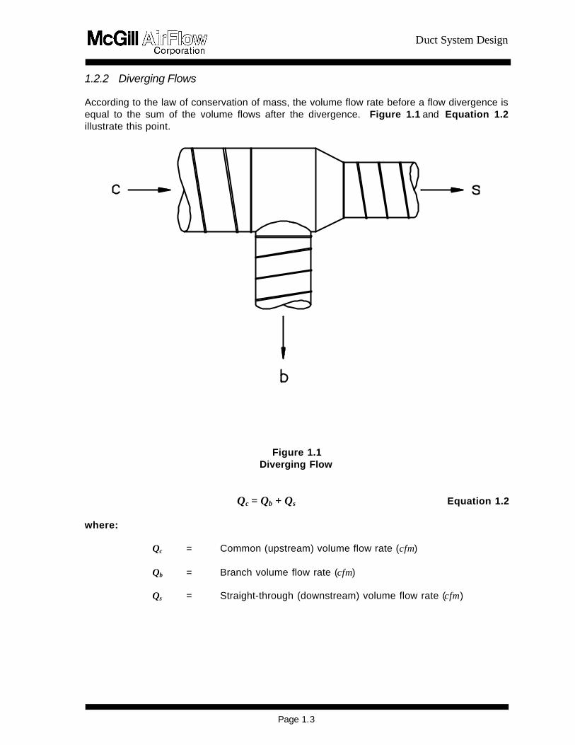
Duct System Design

Page 13

122 Diverging Flows According to the law of conservation of mass the volume flow rate before a flow divergence is equal to the sum of the volume flows after the divergence Figure 11 and Equation 12 illustrate this point

Figure 11

Diverging Flow

Qc = Qb + Qs Equation 12 where

Qc = Common (upstream) volume flow rate (cfm) Qb = Branch volume flow rate (cfm) Qs = Straight-through (downstream) volume flow rate (cfm)

Duct System Design

Page 14

Sample Problem 1-4

Figure 12 Multiple Diverging Flow The system segment shown in Figure 12 has four outlets each delivering 200 cfm What is the volume flow rate at points A B and C Answer A = 800 cfm

B = 600 cfm C = 400 cfm

The total volume flow rate at any point is simply the sum of all the downstream volume flow rates The volume flow rate of all branches andor trunks of any system can be determined in this way and combined to obtain the total volume flow rate of the system

13 Conservation of Energy The total energy per unit volume of air flowing in a duct system is equal to the sum of the static energy kinetic energy and potential energy When applied to airflow in ducts the flow work or static energy is represented by the static pressure of the air and the velocity pressure of the air represents the kinetic energy Potential

Duct System Design

Page 15

energy is due to elevation above a reference datum and is often negligible in HVAC duct design systems Consequently the total pressure (or total energy) of air flowing in a duct system is generally equal to the sum of the static pressure and the velocity pressure As an equation this is written

TP = SP + VP Equation 13

where

TP = Total pressure SP = Static pressure VP = Velocity pressure

Furthermore when elevation changes are negligible from the law of conservation of energy written for a steady non-compressible flow for a fixed control volume the change in total pressure between any two points of a system is equal to the sum of the change in static pressure between the points and the change in velocity pressure between the points This relationship is represented in the following equation

∆∆TP = ∆∆SP + ∆∆VP Equation 14 Appendix A32 shows the derivation of Equation 14 from the general equation of the first law of thermodynamics Pressure (or pressure loss) is important to all duct designs and sizing methods Many times systems are sized to operate at a certain pressure or not in excess of a certain pressure Higher pressure at the same volume flow rate means that more energy is required from the fan and this will raise the operating cost The English unit most commonly used to describe pressure in a duct system is the inch of water gauge (inch wg) One pound per square inch (psi ) the standard measure of atmospheric pressure equals approximately 277 inches wg 131 Static Pressure Static pressure is a measure of the static energy of the air flowing in a duct system It is static in that it can exist without a movement of the air stream The air which fills a balloon is a good example of static pressure it is exerted equally in all directions and the magnitude of the pressure is reflected by the size of the balloon The atmospheric pressure of air is a static pressure At sea level this pressure is equal to approximately 147 pounds per square inch For air to flow in a duct system a pressure differential must exist That is energy must be imparted to the system (by a fan or air handling device) to raise the pressure above or below atmospheric pressure Air always flows from an area of higher pressure to an area of lower pressure Because the static pressure is above atmospheric at a fan outlet air will flow from the fan through any connecting ductwork until it reaches atmospheric pressure at the discharge Because the static pressure is below atmospheric at a fan inlet air will flow from the higher atmospheric pressure

Duct System Design

Page 16

ρρ

4005V

= 1097

V = VP

2 2

through an intake and any connecting ductwork until it reaches the area of lowest static pressure at the fan inlet The first type of system is referred to as a positive pressure or supply air system and the second type as a negative pressure exhaust or return air system Static Pressure Losses The initial static pressure differential (from atmospheric) is produced by adding energy at the fan This pressure differential is completely dissipated by losses as the air flows from the fan to the system discharge Static pressure losses are caused by increases in velocity pressure as well as friction and dynamic losses Sign Convention When a static pressure measurement is expressed as a positive number it means the pressure is greater than the local atmospheric pressure Negative static pressure measurements indicate a pressure less than local atmospheric pressure By convention positive changes in static pressure represent losses and negative changes represent regains or increases For example if the static pressure change as air flows from point A to point B in a system i s a positive number then there is a static pressure loss between points A and B and the static pressure at A must be greater than the static pressure at B Conversely if the static pressure change as air flows between these points is negative the static pressure at B must be greater than the static pressure at A 132 Velocity Pressure Velocity pressure is a measure of the kinetic energy of the air flowing in a duct system It is directly proportional to the velocity of the air For air at standard density (0075 pounds per cubic foot) the relationship is

Equation 15 where

VP = Velocity pressure (inches wg) V = Air velocity (fpm) ρρ = Density (lbmft3)

Appendix A33 provides a derivation of this relationship from the kinetic energy term This derivation also provides an equation for determining velocity pressures at nonstandard densities Appendix A16 provides a table of velocities and corresponding velocity pressures at standard conditions Velocity pressure is always a positive number and the sign convention for changes in velocity pressure is the same as that described for static pressure From Equation 11 it can be seen that velocity must increase if the duct diameter (area) is reduced without a corresponding reduction in air volume Similarly the velocity must decrease if the air volume is reduced without a corresponding reduction in duct diameter Thus the

Duct System Design

Page 17

velocity and the velocity pressure in a duct system are constantly changing 133 Total Pressure Total pressure represents the energy of the air flowing in a duct system Because energy cannot be created or increased except by adding work or heat there is no way to increase the total pressure once the air leaves the fan The total pressure is at its maximum value at the fan outlet and must continually decrease as the air moves through the duct system toward the outlets Total pressure losses represent the irreversible conversion of static and kinetic energy to internal energy in the form of heat These losses are classified as either friction losses or dynamic losses Friction losses are produced whenever moving air flows in contact with a fixed boundary These are discussed in Section 14 Dynamic losses are the result of turbulence or changes in size shape direction or volume flow rate in a duct system These losses are discussed in Section 15 Referring to Equation 14 note that if the decrease in velocity pressure between two points in a system is greater than the total pressure loss t he static pressure must increase to maintain the equality Alternatively an increase in velocity pressure will result in a reduction in static pressure equal to the sum of the velocity pressure increase and the total pressure loss When there is both a decrease in velocity and a reduction in static pressure the total pressure will be reduced by the sum of these losses These three concepts are illustrated in Figure 13

Figure 13

Conservation of Energy Relationship 14 Pressure Loss In Duct (Friction Loss) When air flows through a duct friction is generated between the flowing air and the stationary duct wall Energy must be provided to overcome this friction and any energy converted irreversibly to heat is known as a friction loss The fan initially provides this energy in the form of pressure The amount of pressure necessary to overcome the friction in any section of duct depends on (1) the length of the duct (2) the diameter of the duct (3) the velocity (or volume) of the air flowing in the duct and (4) the friction factor of the duct

Duct System Design

Page 18

1000V

D1

256= 100ft

P 18118∆

100ftP∆

The friction factor is a function of duct diameter velocity fluid viscosity air density and surface roughness For nonstandard conditions see Section 15 The surface roughness can have a substantial impact on pressure loss and this is discussed in Appendix A35 These factors are combined in the Darcy equation to yield the pressure loss or the energy requirement for a particular section of duct Appendix A34 discusses the use and application of the Darcy equation 141 Round Duct One of the most important and useful tools available to the designer of duct systems is a friction loss chart (see Appendix A411) This chart is based on the Darcy equation and combines duct diameter velocity volume flow rate and pressure loss The chart is arranged in such a manner that knowing any two of these properties (at standard conditions) it is possible to determine the other two

The chart is arranged with pressure loss (per 100 feet of duct length) on the horizontal axis volume flow rate on the vertical axis duct diameter on diagonals sloping upward from left to right and velocity on diagonals sloping downward from left to right

Examination of this chart (or the Darcy equation) reveals several interesting air flow properties (1) at a constant volume flow rate reducing the duct diameter will increase the pressure loss (2) to maintain a constant pressure loss in ducts of different size larger volume flow rates require larger duct diameters and (3) for a given duct diameter larger volume flow rates will increase the pressure loss The following sample problems will give the reader a feel for these important relationships Although there are many nomographs or duct calculators available to speed the calculation of duct friction loss problems novice designers should use the friction loss charts to better visualize the relationships The friction loss chart in the Appendix is approximated by Equation 16

Equation 16

where = the friction loss per 100 ft of duct (inches wg)

D = the duct diameter (inches) V = the velocity of the air flow in the duct (fpm)

Sample Problem 1-5

What is the friction loss of a 150-foot long section of 18-inch diameter duct carrying 2500 cfm What is the air velocity in this duct Answer From the friction loss chart find the horizontal line that represents 2500 cfm

Move across this line to the point where it intersects the diagonal line which represents an 18-inch diameter duct From this point drop down to the horizontal

Duct System Design

Page 19

wginches 100ft

P016 =

1000

1412

18

1256 =

18118

∆

(pressure) axis and read the friction loss This value is approximately 016 inches wg This represents the pressure loss of a 100-foot section of 18-inch diameter duct carrying 2500 cfm To determine the pressure loss for a 150-foot duct section it is necessary to multiply the 100-foot loss by a factor of 15 Therefore the pressure loss is 024 inches wg

At the intersection of the 2500 cfm line and the 18-inch diameter line locate the nearest velocity diagonal The velocity is approximately 1400 fpm

Equation 16 could have also been used to solve this problem To use Equation 16 we must first calculate the velocity using Equation 11 To calculate the velocity we have to determine the cross-sectional area of the 18-inch diameter duct A = π x 182 576 = 177 ft2 The calculated velocity is QA = 2500177 = 1412 fpm The pressure loss per 100 ft is calculated as For a 150 ft section the pressure is 15 x 016 = 024 inches wg

Sample Problem 1-6

Part of a system you have designed includes a 20-inch diameter 500-foot duct run carrying 3000 cfm You now discover there is only 16 inches of space in which to install this section What will be the increase in pressure loss of the duct section if 16-inch duct is used in place of 20-inch Answer From the friction loss chart or Equation 16 find the pressure loss per 100 feet for

3000 cfm flowing through a 20-inch diameter duct This value is 014 inches wg or 070 inches wg for 500 feet Similarly the friction loss for 500 feet of 16-inch diameter duct carrying 3000 cfm is found to be 195 inches wg

Reducing this duct diameter by 4 inches results in an increase of pressure loss of 125 inches wg

Sample Problem 1-7

An installed system includes a 20-inch diameter 500-foot duct run carrying 3000 cfm Due to unanticipated conditions downstream it has become necessary to increase the volume flow rate in this duct section to 3600 cfm What will be the impact on the pressure loss of the section Answer From Sample Problem 1-6 the pressure drop of this section as installed is 070

inches wg To find the new pressure drop move up the 20-inch diameter line until it intersects the 3600 cfm volume flow rate line At this point read down to the friction loss axis and find that the new friction loss is 019 inches wg per 100

Duct System Design

Page 110

feet or 095 inches wg for 500 feet Therefore this 20 percent increase in volume will result in a 36 percent increase in the pressure loss for the duct section

Sample Problem 1-8

A system is being designed so that the pressure loss in all duct sections is equal to 02 inches wg per 100 feet What size duct will be required to carry (a) 500 cfm (b) 1500 cfm (c) 5000 cfm (d) 15000 cfm Answer From the friction loss chart find the vertical line that represents 020 inches wg per

100 feet friction loss Move up this line to the point where it intersects the horizontal line which represents a volume flow rate of 500 cfm At this point locate the nearest diagonal line representing duct diameter It will either be 9-inch duct or 95-inch duct (if half-inch duct sizes are available)

Similarly for the other volumes find the line representing duct size which is nearest to the intersection of the 020 inches wg per 100 feet friction loss line and the appropriate volume At 1500 cfm 14-inch duct is required at 5000 cfm 22-inch duct is required and at 15000 cfm 33-inch duct is required In each case the duct will carry the specified volume with a pressure loss of approximately 020 inches wg per 100 feet

142 Flat Oval Duct Flat oval duct has the advantage of allowing a greater duct cross-sectional area to be accommodated in areas with reduced vertical clearances Figure 14 shows a typical cross section of flat oval duct References in Appendices A1 A2 and A9 provide additional information about flat oval duct

Figure 14 Flat Oval Dimensions The Darcy equation is not applicable to flat oval duct and there are no friction loss charts available for non-round duct shapes To calculate the friction loss for flat oval duct it is necessary to determine the equivalent round diameter of the flat oval size and then determine the friction loss for the equivalent round duct

Duct System Design

Page 111

)(P)(A 155

= D 025

0625

eq

1444

)minx (+)minx (FS

= A

2ππ

12x FS) 2( + )minx (

= Pππ

The equivalent round diameter of flat oval duct is the diameter of round duct that has the same pressure loss per unit length at the same volume flow rate as the flat oval duct Equation 17 can be used to calculate the equivalent round diameter for flat oval duct with cross-sectional area A and perimeter P The equivalent round diameters for many standard sizes of flat oval duct are given in Appendix A132

Equation 17

where

Deq = Equivalent round diameter (ft) A = Flat oval cross-sectional area (ft2) P = Flat oval perimeter (ft)

The flat oval cross-sectional area is calculated using Equation 18

Equation 18

where

A = Cross-sectional area (ft2) FS = Flat Span (inches) = maj - min min = Minor axis (inches) maj = Major axis (inches)

The perimeter of flat oval is calculated using Equation 19

Equation 19

where

P = Flat oval perimeter (ft)

When calculating the air velocity in flat oval duct it is necessary to use the actual cross-sectional area of the flat oval shape not the area of the equivalent round duct To use Equation 16 however the air velocity is calculated using the equivalent round diameter cross sectional area

Duct System Design

Page 112

Sample Problem 1-9

A 12-inch x 45-inch flat oval duct is designed to carry 10000 cfm What is the pressure loss per 100 feet of this section What is the velocity Answer Equations 18 and 19 are used to calculate the area and perimeter of the flat

oval duct For 12 x 45 duct A = 354 ft2 from (45 - 12) x 12 + (π x 122)4144 and P = 864 ft from (π x 12) + (2 x (45-12))12 Substituting into Equation 17 Deq = 199 ft 24 inches From the friction loss chart the pressure loss of 10000 cfm air flowing in a 24-inch round duct is 050 inch wg per 100 feet

The velocity can be calculated from Equation 11

V = QA = 10000 354 = 2825 fpm

Note that the velocity of the same air volume flowing in the 24-inch diameter round duct is 10000 314 or 3185 fpm

Alternatively to use Equation 16 we must first calculate the velocity assuming the cross-sectional area is determined from the equivalent round

ftA2

Deq 314 = 576

)24x ( 2π=

fpm V Deq 3185 = 314

10000 =

wginches 100ft

P 048=

1000

3185

24

1256 =

18118

∆

Which is close to the 050 incheswg determined from the friction loss chart

Sample Problem 1-10

In Sample Problem 1-6 what size flat oval duct would be required in order to maintain the original (070 inches wg) pressure drop and still fit within the 16-inch space allowance Answer In this situation the available space will dictate the minor axis dimension of the

Duct System Design

Page 113

flat oval duct It is always advisable to allow at least 2 to 4 inches for the reinforcement which may be required on any flat oval or rectangular duct product Therefore we will assume that the largest minor axis that can be accommodated is 12 inches

Since we want to select a flat oval size which will have the same pressure loss as a 20-inch round duct the major axis dimension can be determined by solving Equation 17 with Deq = 167 feet (20 inches) and min = 12 inches Using Equations 18 and 19 for determining A and P as functions of the major axis dimension (maj) and the minor axis dimension (min) Unfortunately this requires an iterative solution

A simpler solution is to refer to the tables in Appendix A132 These tables list the various available flat oval sizes and their respective equivalent round diameters Since we already know that the minor axis must be 12 inches we look for a flat oval size with a 12-inch minor axis and an equivalent round diameter of 20 inches The required flat oval size is 12 inches x 31 inches

If it is determined that there is room for a 14-inch minor axis duct the required size would be 14 inches x 27 inches (Deq = 20 inches)

143 Rectangular Duct Rectangular duct is fabricated by breaking two individual sheets of sheet metal (called L-sections) that have the appropriate duct dimensions (side and side adjacent) and joining them together by one of several techniques Rectangular duct is also used when height restrictions are employed in a duct design Equation 110 can be used to calculate the equivalent round diameter Deq of rectangular duct The equivalent round diameter Deq for many standard sizes of rectangular duct are given in Appendix 14

Equation 110

where

Deq = Equivalent round diameter (inches)

a = Duct side length (inches) b = Other duct side length (inches)

When calculating air velocity in rectangular duct it is necessary to use the actual cross-sectional area of the rectangular shape not the area of the equivalent round diameter

)b+(a)(ab 130

= D 0250

0625

eq

Duct System Design

Page 114

Sample Problem 1-11

A 12-inch x 45-inch rectangular duct is designed to carry 10000 cfm What is the pressure loss per 100 feet of this section What is the velocity Answer Using Equation 110 Deq = 24 inches From the friction loss chart the loss of

10000 cfm air flowing in a 24-inch round duct is 050 inch wg per 100 feet

The velocity can be calculated from Equation 11

fpmA

Q = V 2667=

45)144 x (12

10000 =

Note that the velocity in the rectangular duct is less than in the flat oval with the same major and minor dimensions (See Sample Problem 1-9)

144 Acoustically Lined and Double-wall Duct Applying an inner liner or a perforated inner metal shell sandwiching insulation between an inner and outer wall increases the surface roughness that air sees and thus increases the friction losses of duct Acoustically lined round and rectangular duct consist of a single-wall duct with an internal insulation liner but no inner metal shell Double-wall duct that is acoustically insulated consists of a solid outer shell a thermalacoustical insulation and a metal inner liner (either solid or perforated) The inner dimensions of lined duct or the metal inner liner dimensions of double-wall duct are the nominal duct size dimensions that are used to determine the cross-sectional area for airflow calculations The single-wall dimensions of lined duct or outer shell dimensions of double-wall duct depend on the insulation thickness For a 1-inch thick insulation the dimensions are 2 inches larger than the inner dimensions of lined duct or metal inner liner dimensions Acoustically Lined Duct Correction factors to the friction loss determined from the friction loss chart or for Equation 16 have not been developed for internally insulated duct Therefore the designer must use the Darcey equation as given in Appendix A34 Assume an absolute roughness of ε = 0015 Double-wall Duct

Corrections factors to the friction loss determined from the friction loss chart or Equation 16 have been developed for when a perforated metal inner liner is used Figure 15 is a chart which gives the correction factors This information is repeated in Appendix A412 Note that these corrections are a function of duct diameter and velocity If the duct shape is flat oval or rectangular use the equivalent round diameter based on the perforated metal inner liner dimensions If the inner shell of the double-wall duct does not use perforated metal use the same friction loss as a single-wall duct of the same dimensions as the metal inner shell

Duct System Design

Page 115

13

12

11

10

4rdquo 8rdquo

12rdquo

18rdquo

36rdquo

72rdquo

2000 3000 4000 5000 6000

Correction factor to be applied to the friction loss of single-wall duct to calculate the friction loss of double-wall duct with a perforated metal inner liner

Velocity (fpm)

Figure 15 Correction Factors for Double-Wall Duct with Perforated Metal Inne r Liner When only thermal insulation is required the metal inner liner may be specified as solid rather than perforated metal In this case the friction losses are identical to those for single-wall duct with a diameter equal to the metal inner liner diameter For acoustically insulated flat oval or rectangular duct with a perforated metal inner liner use the correction factors of the equivalent round diameter and the actual velocity (based on the metal inner liner of the flat oval or rectangular cross section) The reference in Appendix A92 addresses friction losses for lined rectangular duct

Sample Problem 1-12

What is the friction loss of a 100-foot section of 22-inch diameter double-wall duct (with perforated metal inner liner) carrying 8000 cfm Answer The pressure loss for 100 feet of 22-inch single-wall duct carrying 8000 cfm is

found from the friction loss chart to be 050 inches wg The velocity is 3000 fpm

From Figure 15 the correction factor for 22-inch duct (interpolated) at 3000 fpm is approximately116Therefore the pressure loss of this section of double-wall duct is 050 x 116 or 058 inches wg

145 Nonstandard Conditions All loss calculations thus far have been made assuming a standard air density of 0075 pounds per cubic foot When the actual design conditions vary appreciably from standard (ie temperature is 30degF from 70degF elevation above 1500 feet or moisture greater than 002 pounds water per pound dry air) the air density and viscosity will change If the Darcy equation is used to calculate friction losses and the friction factor and velocity pressure are calculated using

Duct System Design

Page 116

actual conditions no additional corrections are necessary If a nomograph or friction chart is used to calculate friction losses at standard conditions correction factors should be applied The corrections for nonstandard conditions discussed above apply to duct friction losses only Other corrections are applicable to the dynamic losses of fittings as will be explained in the following section For a more in-depth presentation of these and other correction factors see Reference in Appendix A92 Tables for determining correction factors are included in Appendix A15 A temperature correction factor Kt can be calculated as follows

460) + T(

530= K

a

0825

t Equation 111

where

Kt = Nonstandard temperature correction factor Ta = Actual temperature of air in the duct (degF)

An elevation correction factor Ke can be calculated as follows

](Z) )10x (68754 -1[= K473-6

e Equation 112a

Equation 112a can also be written as follows

ββ29921

= K09

e Equation 112b

where

Ke = Nonstandard elevation correction factor Z = Elevation above sea level (feet) ββ = Actual barometric pressure (inches Hg)

When both a nonstandard temperature and a nonstandard elevation are present the correction factors are multiplicative As an equation

Kx K= K etf Equation 113

where

Kf = Total friction loss correction factor

The calculated duct friction pressure loss should be multiplied by the appropriate correction factor Kt Ke or Kf to obtain the actual pressure loss at the nonstandard conditions

Duct System Design

Page 117

Sample Problem 1-13

The friction loss for a certain segment of a duct system is calculated to be 25 inches wg at standard conditions What is the corrected friction loss if (a) the design temperature is 30degF (b) the design temperature is 110degF (c) the design elevation is 5000 feet above sea level (d) both (b) and (c) Answer 1 Substituting into Equation 111 Kt = [530(30 + 460)]0825 = 107

Corrected friction loss = 25 x 107 = 268 inches wg

2 Kt = [530(110 + 460)]0825 = 094 Corrected friction loss = 235 inches wg

3 Substituting into Equation 112a Ke = [1 - (68754 x 10-6)(5000)] 473 = 085 Corrected friction loss = 213 inches wg

4 Substituting into Equation 113 Kf = 094 x 085 = 080 Corrected

friction loss = 200 inches wg

If moisture in the airstream is a concern a humidity correction factor Kh can be calculated as follows

(( )) 90

wsh

P37801K

ββ

minusminus== Equation 114

where

Pws = Saturation pressure of water vapor at the dew point

temperature (inches Hg) ββ = Actual barometric pressure (inches Hg)

The total friction loss correction factor Kf is expressed as

hetf Kx Kx K= K Equation 115

15 Pressure Loss in Supply Fittings As mentioned in Section 13 pressure losses can be the result of either friction losses or dynamic losses Section 14 discussed friction losses produced by air flowing over a fixed boundary This section will address dynamic losses Friction losses are primarily associated with duct sections while dynamic losses are exclusively attributable to fittings or obstructions Dynamic losses will result whenever the direction or volume of air flowing in a duct is altered or when the size or shape of the duct carrying the air is altered Fittings of any type will produce dynamic losses The dynamic loss of a fitting is generally proportional to the severity of the airflow disturbance A smooth large radius elbow for example will have a much lower dynamic

Duct System Design

Page 118

loss than a mitered (two-piece) sharp-bend elbow Similarly a 45deg branch fitting will usually have lower dynamic losses than a straight 90deg tee branch 151 Loss Coefficients In order to quantify fitting losses a dimensionless parameter known as a loss coefficient has been developed Every fitting has associated loss coefficients which can be det ermined experimentally by measuring the total pressure loss through the fitting for varying flow conditions Equation 116a is the general equation for the loss coefficient of a fitting

VPTP

= C∆

Equation 116a

where C = Fitting loss coeffi cient ∆∆TP = Change in total pressure of air flowing through the fitting (inches

wg) VP = Velocity pressure of air flowing through the fitting (inches wg)

Once the loss coefficient for a particular fitting or class of fittings has been experimentally determined the total pressure loss for any flow condition can be determined Rewriting Equation 116a we obtain

VPx C= TP∆ Equation 116b

From this equation it can be seen that the total pressure loss is directly proportional to both the loss coefficient and the velocity pressure Higher loss coefficient values or increases in velocity will result in higher total pressure losses for a fitting A less efficient fitting will have a higher loss coefficient (ie for a given velocity the tot al pressure loss is greater) 152 Elbows Table 11 shows typical loss coefficients for 8-inch diameter elbows of various construction Table 11 Loss Coefficient Comparisons for Abrupt-Turn Fittings

90EE Elbows 8-inch Diameter Fitting

Loss Coefficient

Die-StampedPressed 15 Centerline Radius

011 Five-Piece 15 Centerline Radius

022

Mitered with Turning Vanes

052 Mitered

124

From Equation 14 we can determine the pressure loss

∆∆TP = ∆∆SP + ∆∆VP

Duct System Design

Page 119

Since the elbow diameter and volume flow rate are constant the continuity equation (Equation 11) tells us that the velocity will be constant From Equation 15 the velocity pressure is a direct function of velocity and so ∆∆VP = 0 Therefore ∆∆SP = ∆∆TP Note that whenever there is no change in velocity as is the case in duct and constant diameter elbows the change in static pressure is equal to the change in total pressure

Sample Problem 1-14

What is the total pressure loss of an 8-inch diameter die-stamped elbow carrying 600 cfm What is the static pressure loss Answer From Equation 11

Q = A x V or V = QA A = πD2576 = π (8)2 576 = 035 ft2 V = 600 035 V = 1714 fpm

From Equation 15 or Appendix A16

wginches VP 018= 40051714

=2

From Table 11

C = 011 (die-stamped elbow) From Equation 116b

∆TP = C x VP = 011 x 018 = 002 inches wg

Sample Problem 1-15

A designer is trying to determine which 8-inch elbow to select for a location which will have a design velocity of 1714 fpm What will be the implications in terms of pressure loss if the designer chooses (1) a die-stamped elbow (2) a five-gore elbow (3) a mitered elbow with turning vanes or (4) a mitered elbow without turning vanes Answer From Sample Problem 1-14 we calculated the total pressure loss of an 8-inch

die-stamped elbow at 1714 fpm to be 002 inches wg

For the other elbows we can determine the pressure loss from loss coefficients given in Table 11

Duct System Design

Page 120

C2 = 022 C3 = 052 C4 = 124

From Equation 116b

∆TP2 = ∆SP2 = 022 x 018 = 004 inches wg (five-gore)

∆TP3 = ∆SP3 = 052 x 018 = 009 inches wg (mitered with turning vanes)

∆TP4 = ∆SP4 = 124 x 018 = 022 inches wg (mitered without turning vanes)

Therefore using a five-gore elbow will increase the total pressure loss by 100 percent but it will be a very modest 004 inches wg Using the mitered elbow with vanes would result in a 350 percent increase over the die-stamped elbow or a 125 percent increase over the five-gore elbow The mitered elbow without turning vanes would have a loss of 022 inches wg which is a tenfold increase over the die-stamped elbow

The increased pressure losses associated with the use of les s efficient fittings may or may not be critical to the operation of the system depending on the location of the fittings Succeeding chapters will note when there could be locations in a system where it is desirable to increase the losses of certain fittings In general unless the system has been carefully analyzed to determine the location of the critical path(s) and the excess pressures present in other paths it is wise to always select fittings with the lowest pressure drop The loss coefficients of most elbows vary as a function of diameter The ASHRAE Duct Fitting Database Program (Appendix A82) presents loss coefficients as a function of diameter for various elbow constructions The loss coefficient drops sharply as diameters increase through approximately 24 inches then only slightly from 24 inches through 60 inches Also eliminating turning vanes in mitered elbows more than doubles the pressure loss Flat Oval Elbows Although the use of equivalent duct lengths as a measure of dynamic fitting losses is usually strongly discouraged it provides acceptable approximations in the case of flat oval elbows Data indicates that flat oval 90deg elbows (hard or easy bend) with 15 centerline radius bends have a pressure loss approximately equal to the friction loss of a flat oval duct with an identical cross section and a length equal to nine times the elbow major axis dimension calculated at the same air velocity that is flowing through the elbow For example a 12-inch x 31-inch flat oval elbow would have a pressure loss approximately equal to that of a 12-inch x 31-inch flat oval duct 23 feet long (9 x 31 inches) at the same velocity For flat oval elbows that do not have a 15 centerline radius bend use the loss coefficient for a round elbow of similar construction with the diameter equal to the flat oval minor axis Rectangular Elbows (see ASHRAE== s Duct Fitting Database Program)

Duct System Design

Page 121

VPTP= C

b

b-cb

∆

Acoustically LinedDouble-wall Elbows For acoustically lined elbows or double-wall elbows with either a solid or perforated metal inner liner the losses are the same as for standard single-wall elbows with dimensions equal to the metal inner liner dimensions of the acoustically lined or double-wall elbow Elbows With Bend Angles Less Than 90deg For elbows constructed with bend angles less than 90deg multiply the calculated pressure loss for a 90deg elbow by the correction factor given in Table 12

Table 12 Elbow Bend Angle Correction Factor

Angle CFelb

225deg 031

30deg 045

45deg 060

60deg 078

75deg 090 153 Diverging-Flow Fittings Branches The pressure losses in diverging-flow fittings are somewhat more complicated than elbows for two reasons (1) there are multiple flow paths and (2) there will almost always be velocity changes First consider the case of air flowing from the common (upstream) section to the branch Referring to Figure 11 this is from c to b (Refer to Appendix A11 for clarification of upstream and downstream) As is the case for elbows loss coefficients are determined experimentally for diverging-flow fittings However it is now necessary to specify which flow paths the equation parameters refer to By definition

Equation 117a

where

Cb = Branch loss coefficient ∆TPc-b = Total pressure loss common-to-branch (inches wg) VPb = Branch velocity pressure (inches wg)

Rewriting in terms of total pressure loss

∆TPc-b = Cb x VPb Equation 117b Therefore the total pressure loss of air flowing into the branch leg of a diverging-flow fitting is

Duct System Design

Page 122

directly proportional to the branch loss coefficient and the branch velocity pressure For duct and elbows the total pressure loss is always equal to the static pressure loss because there is no change in velocity However diverging-flow fittings almost always have velocity changes associated with them If ∆VP is not zero then the total and static pressure losses cannot be equal (Equation 14) For diverging-flow fittings the static pressure loss of air flowing into the branch leg can be determined from Equation 117c

∆SPc-b = VPb (Cb + 1) - VPc Equation 117c where

∆SPc-b = Static pressure loss common-to-branch (inches wg) VPb = Branch velocity pressure (inches wg) VPc = Common velocity pressure (inches wg) Cb = Branch loss coefficient (dimensionless)

Equation 117c is derived from Equations 117a and 117b as shown in Appendix A36

As is the case for elbows a comparison of loss coefficients gives a good indication of relative fitting efficiencies The following samples compare loss coefficients of various diverging-flow fittings

Duct System Design

Page 123

Table 13 Loss Coefficient Comparisons for Diverging-Flow Fittings

Fitting Loss Coefficient

(Cb) Y-Branch plus 45deg Elbows

022

Vee Fitting

030

Tee with Turning Vanes plus Branch Reducers (Bullhead Tee with Vanes)

045

Tee plus Branch Reducers

108

Capped Cross with Straight Branches

445

Capped Cross with Conical Branches

445

Capped Cross with 1-foot Cushion Head

54

Capped Cross with 2-foot Cushion Head

60

Capped Cross with 3-foot Cushion Head

64

The loss coefficient Cb is for a VbVc ratio of approximately 10

Duct System Design

Page 124

AA

Q

Q VP V VP V

c

b

c

bbbcc

Sample Problem 1-16

What is the total pressure loss for flow from c to b in the straight tee shown below What is the static pressure loss Answer ∆TPc-b = Cb x VPb From Equation 117b

∆SPc-b = VPb (Cb + 1) - VPc From Equation 117c Reference ASHRAE Duct Fitting Database Number SD5-9 Given Qc = 5000 cfm Dc = 24 inches

Qb = 2000 cfm Db = 18 inches

Qs = 3000 cfm Ds = 24 inches Calculate

fpmA

Q V

c

cc 1592 =

314

5000 ==

c

s

b

Duct System Design

Page 125

wginches4005

VVP c

2

c 016 = 40051592

==2

fpmA

Q V

b

bb 1130 =

177

2000 ==

wginches4005

VVP b

2

b 008 = 40051130

==2

040 = 50002000

= Q

Q

c

b

056 = 314

177 =

A

A

c

b

Determine Cb - Interpolated from the ASHRAE table = 214

Answer ∆TPc-b = 214 x 008 = 017 inches wg

∆SPc-b = 008 (214 + 1) - 016 = 009 inches wg

Duct System Design

Page 126

Sample Problem 1-17

What would be the static and total pressure losses in Sample Problem 1-16 if a conical tee were substituted for the straight tee A LO-LOSSTM tee Reference Conical Tee ASHRAE Fitting SD5-10

LO-LOSST M Tee ASHRAE Fitting SD5-12 Determine Cb (conical) = 135

Cb (LO-LOSST M) = 079 Answer ∆TPc-b (conical) = 011 inches wg

∆SPc-b (conical) = 003 inches wg ∆TPc-b (LO-LOSST M) = 006 inches wg ∆SPc-b (LO-LOSST M) = -002 inches wg

In the preceding problem the static pressure loss for a LO-LOSST M tee at the given conditions resulted in a negative number Recall from Section 131 that a pressure change expressed as a positive number is a loss while a pressure change expressed as a negative number represents an increase in pressure This pressure increase is a common phenomenon in air handling systems and is known as static regain It occurs for the LO-LOSST M fitting because the decrease in velocity pressure is greater than the total pressure loss of the fitting Total Pressure Losses versus Static Pressure Losses Just as total pressure represents the total energy present at any point in a system the total pressure loss of a fitting represents the true energy loss of the fitting for a given flow situation Static pressure losses are useful for certain design methods as we shall see later however they do not give an accurate indication of fitting efficiency Sample Problem 1-18 illustrates this concept

Duct System Design

Page 127

Sample Problem 1-18

Change the branch size in Sample 1-17 from 18 inches diameter to 12 inches diameter and recalculate the total and static pressure losses of the LO-LOSS TM tee

Reference ASHRAE Fitting SD5-12 Given Qc = 5000 cfm Dc = 24 inches

Qb = 2000 cfm Db = 12 inches Qs = 3000 cfm Ds = 24 inches

Calculate AA

Q

Q VP V VP V

c

b

c

bbbcc

Vc = 1592 fpm VPc = 016 inches wg Vb = 2548 fpm VPb = 040 inches wg Qb Qc = 040 Ab Ac = 025

Determine Cb Interpolate from ASHRAE Fitting SD5-12 = 021 Answer ∆TPc-b = CbxVPb (from Equation 117b) = 021x040 = 008 inches wg ∆SPc-b = VPb (Cb + 1) - VPc (from Equation 117c) = 040(021+1)-016 = 032 inches wg In this problem the total pressure loss is 008 inches wg but the static pressure loss is 032 inches wg If one were to look only at the static pressure this would seem to be a very inefficient fitting However notice that due to flow and pressure conditions in the system the velocity increased as the air moved from the common section into the branch resulting in a velocity pressure increase of 024 inches wg

c s

b

Duct System Design

Page 128

This situation is shown in Figure 13 Case II The apparently large decrease in static pressure was caused by a large increase in velocity pressure As Equation 14 this becomes

008 = 032 + -024 (∆TP = ∆SP + ∆VP )

Conversely when certain flow conditions are present it is possible for a fitting to have a small static pressure loss but a relatively large total pressure loss It is always advisable to calculate the total pressure loss in order to determine the total energy consumption of a fitting Manifold Fittings The single-branch fittings discussed thus far are assumed to be factory fabricated and constructed as a separate unit from the duct to which t hey would be attached Occasionally it is desirable to construct a manifold fitting with a tap attached directly to the duct This construction will generally result in a less efficient fitting especially if the manifold is constructed in the field Flat Oval Diverging-Flow Fittings Diverging-flow fittings of similar construction generally exhibit the same pressure loss for the same volume flow rate ratios and area ratios Flat oval fittings exhibit similar pressure losses as round fittings Testing is under way to develop a database of loss coefficients for flat oval diverging-flow fittings Until this data is available use the same loss coefficients as for the same construction of round Acoustically Lined and Double-wall Diverging-Flow Fittings Whether a fitting has been acoustically lined or has a perforated metal inner shell the difference in surface roughness is accounted for in the friction loss determination since all friction loss calculations are base on fitting-to-fitting centerline dimensions Therefore there is no need to increase the dynamic loss of a diverging flow-fitting that is either acoustically lined or one that has an inner metal shell even if the shell is perforated Determine the loss coefficient of the fitting as if it were a single-wall fitting with the dimension of the inner liner or metal inner shell Rectangular Diverging-Flow Fittings (see ASHRAE== s Duct Fitting Database Program) 154 Diverging-Flow Fittings Straight-Throughs Reducers and Transitions Straight-Throughs The straight-through (downstream) leg of a diverging-flow fitting is that path followed by air flowing from c to s as represented in Figure 11 The straight -through may have a constant diameter such that Dc = Ds or there may be a reducer attached to the straight -through such that Dc gt Ds In the case of a constant diameter straight -through there will always be a velocity reduction caused by a reduced volume (after the branch) flowing through the same diameter duct If a reducer is attac hed to the straight -through it can be sized to reduce maintain or increase the downstream velocity relative to the common velocity Dynamic losses associated with air flowing straight through a diverging-flow fitting andor a

Duct System Design

Page 129

reducer is very slight This is understandable since there is little physical disturbance of the airflow The total pressure loss in a straight -through leg or reducer is often only a few hundredths of an inch wg Perhaps the most important phenomenon associated with the straight-through flow situation is the potential for static regain This situation is illustrated in Figure 13 Case I A large reduction in velocity pressure and a small reduction in total pressure must (by Equation 14) result in an increase in static pressure or static regain The regain will be equal in magnitude to the velocity pressure loss minus the total pressure loss Of course if the total pressure loss is greater than the reduction in velocity pressure as shown in Figure 13 Case III there can be no static regain Referring again to Sample Problem 1-16 we see that the velocity in the constant diameter straight -through leg is reduced from 1592 fpm (VPc = 016 inches wg) in the duct before the straight -through to 955 fpm (VPs = 006 inches wg) in the duct after the straight -through due to the reduced volume flow This is a velocity pressure reduction of ∆VPc-s = 010 inches wg If we assume a total pressure loss of ∆TPc-s = 001 inches wg then from Equation 14 we get

001 = ∆SPc-s + 010 or ∆SPc-s = -009 inches wg The negative result indicates a static regain or that the static pressure at point s will be 009 inches wg higher than the static pressure at point c The loss coefficient data for reducers and straight -throughs is found in the ASHRAE Duct Fitting Database When using loss coefficients to determine straight -through losses Equations 117b and 117c are rewritten as follows

∆∆TPc-s = Cs x VPs Equation 118a ∆∆SPc-s = VPs (Cs + 1) - VPc Equation 118b

where

∆∆TPc-s = Total pressure loss common-to-straight-through (inches wg) ∆∆SPc-s = Static pressure loss common-to-straight-through (inches wg) VPc = Common velocity pressure (inches wg) VPs = Straight-through velocity pressure (inches wg) Cs = Straight-through loss coefficient

Sample Problem 1-19

Calculate the total and static pressure losses for the straight-through portion of the straight tee in Sample Problem 1-16

Reference ASHRAE Fitting SD5-9

Duct System Design

Page 130

Calculate AA

Q

Q VP V VP V

c

s

c

ssscc

Vc = 1592 fpm VPc = 016 inches wg

Vs = 955 fpm VPs= 006 inches wg

Qs Qc = 060 As Ac = 10

Determine Cs Interpolate from ASHRAE Fitting SD5-9 = 020 Answer

∆TPc-s = Cs x VPs (Equation 118a ) = 020 x 006 = 001 inches wg ∆SPc-s = VPs (Cs + 1) - VPc (Equation 118b) = 006(020 + 1) - 016 = -009 inches wg

Reducers A stand-alone reducer will cause the velocity to increase since after the reducer the same volume of air will be flowing through a smaller diameter duct (see Sample Problem 1-2) The use of a reducer on its own is not consistent with any design methods presented in this manual and should be fairly rare in most duct systems However when this fitting is used the losses are calculated using the same charts and in the same manner as the straight -throughs Losses are a function of upstream and downstream velocity Reducing fittings should be constructed as shown in Figure 17 such that the length of the taper portion (L) is equal to the difference between the common diameter and the straight -through diameter (Dc - Ds) Verify this with manufacturers dimension sheets Since reducers are very efficient fittings the use of a longer taper section will not necessarily provide a significant improvement in performance

Figure 17 Reducing Fitting Construction Transitions Transitions between round and flat oval duct also produce dynamic pressure losses As with other fittings these losses can be quantified in terms of a loss coefficient The loss coefficient

Duct System Design

Page 131

for round-to-flat oval or flat oval-to-round transitions depends on the flat oval aspect ratio (major axisminor axis) the direction of airflow and the air velocity When round duct transitions to flat oval the flat oval minor axis dimension is usually less than the original round diameter while the flat oval major axis dimension is greater than the round diameter The reverse is true in transitions from flat oval to round Therefore roundflat oval transitions usually involve both a reducer effect (round to flat oval minor or flat oval major to round) and an enlarger effect (round to flat oval major or flat oval minor to round) The change in dimension involving the flat oval major axis is normally much greater than the change tofrom the flat oval minor axis Therefore in round-to-flat oval transitions the enlarger effect predominates while in flat oval-to-round transitions the reducer effect predominates Dynamic losses which result from expanding areas (decreasing velocities) are always more severe than losses from reducing areas (increasing velocities) Therefore the flat oval-to-round transition is more efficient than the round-to-flat oval fitting Figure A24 in Appendix A4 2 is a plot of loss coefficient (Cs ) versus round duct velocity for both round-to-flat oval and flat oval-to-round transitions The curves are valid for any size flat oval and will be conservative for transitions involving flat oval with a low aspect ratio Use the appropriate loss coefficient value in the following equations to determine static and total pressure losses for transition fittings

∆∆TPc-s = Cs x VPs Equation 119a ∆∆SPc-s = VPs (Cs + 1) - VPc Equation 119b where

∆∆TPc-s = Total pressure loss common-to-straight-through (inches wg) ∆∆SPc-s = Static pressure loss common-to-straight-through (inches wg) VPc = Common velocity pressure (inches wg) VPs = Straight-through velocity pressure (inches wg) Cs = Straight-through loss coefficient

Sample Problem 1-20

In Sample Problem 1-10 we determined that a 12-inch H 31-inch flat oval duct would have the same pressure loss per unit length as a 20-inch round duct What would be the impact on total and static pressure losses in a 100-foot section of 20-inch round duct carrying 5000 cfm if 40 feet of this duct were replaced by a 12-inch H 31-inch flat oval duct Assume the first 30 feet of duct is round next 40 feet is flat oval and the last 30 feet is round Answer Since the duct sizes are equivalent 40 feet of 12-inch H 31-inch flat oval would

have the same pressure loss per 100 feet as the section of 20-inch round duct it replaced The addition of two transitions one round-to-flat oval at the start of the

Duct System Design

Page 132

40-foot section and the other flat oval-to-round at the transition back to round duct would cause the only change in pressure loss

The velocity in the 20-inch round duct carrying 5000 cfm is 2294 fpm (VP = 033 inches wg) The flat oval duct cross-sectional area from Appendix A13 is 236 ft2 therefore the velocity in the flat oval duct is 2119 fpm (VP = 028 inches wg) From Appendix A434 the loss coefficients at 2294 fpm are Cr-o = 017 and Co-r = 006

Substituting into Equations 119a and 119b

∆TPc-sr-o = 017 x 028 = 005 inches wg ∆TP c-so-r = 006 x 033 = 002 inches wg ∆SPc-sr-o = 028 (017 + 1) - 033 = -000 (-0002) inches wg ∆SP c-so-r = 033 (006 + 1) - 028 = -007 inches wg

The flat oval section will therefore increase the total pressure loss by an additional 007 inches wg (005 + 002) due to the combined effects of both transitions As expected since there was no net change in velocity in the round duct ∆VP = 0 and (by Equation 14) the combined static pressure loss (007 inches wg) is equal to the combined total pressure loss

155 Miscellaneous Fittings Heel-Tapped Elbows The tee-type diverging-flow fittings discussed in Section 153 are generally used where the designer desires to direct a relatively small quantity of air at some angle relative to the main trunk duct while maintaining a straight -through flow for the majority of the air Occasionally situations arise where the main air stream must be diverted at some angle while a smaller quantity of air is required in a straight -through direction In these situations the use of a heel -tapped elbow will generally result in lower pressure losses in both common and branch directions ASHRAE Fitting SD5-21 presents loss coefficients (Cb) for both the straight-through tap and the elbow section of heel -tapped elbows as a function of velocity ratio Use Equations 117b and 117c for determining the total and static pressure losses If 65 percent or more of the airflow is diverted then it is advisable to use a heel-tapped elbow

Sample Problem 1-21

A diverging-flow fitting must be selected which will split 10000 cfm volume flow rate such that 7000 cfm will flow at a 90E angle relative to the upstream direction and 3000 cfm will continue in the same direction as the upstream flow Compare the performance of a (a) straight tee (b) conical tee (c) LOLOSSTM tee and (d) heel-tapped elbow and select the most efficient fitting for this situation Assume it is desired to

Duct System Design

Page 133

maintain approximately constant velocity Given

Qc = 10000 cfm Qb = 7000 cfm Qs = 3000 cfm Dc = 28 inches Db = 23 inches Ds = 15 inches Ac = 428 sq ft Ab = 289 sq ft As = 123 sq ft Vc = 2336 fpm Vb = 2422 fpm Vs = 2439 fpm VP = 034 inches wg VPb = 037 inches wg VPs = 037 inches wg QbQc = 070 QsQc = 030 AbAc = 068 AsAc = 029

Reference

Straight Tee ASHRAE Fitting SD5-9 Conical Tee ASHRAE Fitting SD5-10 LO-LOSST MTee ASHRAE Fitting SD5-12 Heel-tapped Elbow ASHRAE Fitting SD5-21

Determine

Coefficients Cb Cs

Straight Tee 115 013 Conical Tee 062 013 LO-LOSST M Tee 033 013 Heel-tapped Elbow 065 009

Answer

Pressure Losses (inches wg)

∆TPc-b ∆TPc-s ∆SPc-b ∆SPc-s

Straight Tee 043 005 046 008 Conical Tee 023 005 026 008 LO-LOSST M Tee 012 005 015 008 Heel-tapped Elbow 024 003 027 006

Duct System Design

Page 134

In this case the heel-tapped elbow and the conical tee will have nearly the same total pressure loss in the 90E bend direction The heel-tapped elbow provides a significant performance increase over the straight tee but has a higher loss than the LO-LOSST M tee branch The straight-through leg of the heel-tapped elbow is slightly more efficient than the straight -throughs of the tees

The best fitting though based strictly on efficiency would appear to be the LO-LOSST M tee However bear in mind that all three tee fittings will require substantial strai ght-through reducers (28 inches to 15 inches) which will generally be at least 12 inches long (Figure 17) and will add substantially to the cost of the fitting If a compromise between cost and performance is desired the heel-tapped elbow may still be the best choice for these flow situations Also increased loss may help balance the leg in which this fitting resides

Note that in Sample Problem 1-21 the total pressure is lower than the static pressure by 003 inches wg in all cases due to the increase in velocity pressure (003 inches wg) from common to both straight-through and branch In the form of Equation 14

∆TPc-b = ∆SPc-b - 003 ∆TPc-s = ∆SPc-s - 003

Crosses Cross fittings are those which have two taps located at the same cross section of a main or trunk duct Usually these taps will be constructed so that they discharge air in diametrically opposed directions The pressure loss of the taps on a cross fitting depends to a large extent on the cross-sectional area reduction of the straight-through duct For straight -through area reductions of less that 20 percent the branch losses through either tap of a cross fitting will be the same as those for a single-branch fitting with identical tap construction For example a conical cross (a cross with conical taps) that has a straight -through of 24 inches reducing to 22 inches would have an area reduction of 16 percent Since this is less than 20 percent the branch losses for either tap would be found from the direct-read charts in ASHRAE Fittings SD5-9 through SD5-17 For crosses where the straight -through area reduction exceeds 20 percent use the loss coefficients presented in ASHRAE Fittings SD5-23 through SD5-26 The three curves shown are for varying percentage area reductions and apply for all tap constructions Use interpolation to find loss coefficients for area reductions between these curves Use Equations 117b and 117c for determining the total and static pressure losses of each branch Split Fittings Split fittings are diverging-flow fittings where the air divides into two branches each of which turns at 90E to the main There is no straight-through leg The most common types of split fittings are the Vee Y-branch and the bullhead tee The Y-branches are the most efficient split fittings however they are more expensive than Vees and may be more expensive than bullhead tees Bullhead tees should always be specified with turning vanes ASHRAE Fittings SD5-18 19 and 21 presents drawings and loss

Duct System Design

Page 135

coefficients data for Y-branches bullhead tees with turning vanes bullhead tees without turning vanes and capped crosses The capped cross is discussed in the following section Use Equations 117b and 117c for determining the total and static pressure losses Capped Fittings Capped fittings are those in which the main or straight -through is completely closed off The most common use for a capped fitting is in locations where it is expected that future expansion will require additional ducting at which time the cap can be removed and the duct run continued In general the use of capped fittings is strongly discouraged For both single-branch fittings and crosses the performance is severely degraded if the main is capped Where these fittings are unavoidable SD5-2 includes a curve for capped crosses Use Equations 117b and 117c for determining the total and static pressure losses Close -Coupled Fittings After air flows through any type of fitting a certain length of straight duct is required to re-establish the flow profile of the airstream Simply stated it takes a certain distance for air to recover from a disturbance produced by a fitting If the airstream encounters a second fitting before it has had a chance to recover from a previous disturbance the effect of the second fitting will be more pronounced than if it had been located in a long run of straight duct Generally two elbows in series will have the same loss as the sum of the individual elbows The exception to this is when the second elbow has an additional change in direction such that the air is not flowing parallel to the first flow For this case as much as an additional 100 percent of the combined losses should be added unless the elbows are at least 10 diameters apart The loss of two tees in series is a function of the spacing between the tees although the loss coefficient of the upstream tee is not significantly affected The loss coefficient of the downstream tee actually decreases at half-diameter spacing At two-diameter spacing however the downstream loss coefficient is significantly higher The loss coeffi cient gradually decreases back to its original value at 10 diameters To account for the increased pressure loss at two-diameter spacing add 100 percent of the calculated loss This can be decreased as the diameter spacing between tees becomes greater Appendix A99 has a more detailed discussion of the effect of spacing of tees Couplings Slip couplings which are inserted inside duct sections and are therefore exposed to the air stream are generally used to join two adjacent duct sections Fittings which connect directly to duct sections do not require couplings and fittings which are connected directly to other fittings usually have an outside coupling Losses associated with duct couplings are very low When slip couplings are separated by 10 to 20 feet of duct their effects are negligible However in the event it is necessary to calculate the loss due to duct couplings Appendix A42 presents a table of loss coefficients versus coupling diameter Use Equations 117b and 117c for determining the total and static pressure losses As can be seen from the loss coefficient values it is normally quite acceptable to ignore these losses when calculating system pressure losses Experience has shown that even poorly made and undersized couplings have negligible losses The resulting loss coefficient may be two to three times that of a slip coupling

Duct System Design

Page 136

but this is still a very low value Offsets Offsets are required to change the location of a duct run horizontally vertically or both This is most often necessary to avoid interference with some obstruction along the duct run Offsets are usually constructed with two or more elbows joined by a suitable length of straight duct Due to the almost limitless number of offsets that could be created there are no tables or charts in this manual for the calculation of these losses It is suggested that offset losses be obtained by adding the losses of the individual elbows and duct which form the offset and if necessary adding a factor for any close-coupling effects that may exist Bellmouths The bellmouth fitting is used as an intake or entrance to a duct usually from a plenum or fan housing There is a substantial advantage in having a smooth radiused entrance as opposed to a square-edged entrance Loss coefficients for bellmouths are presented in ASHRAE Fittings SD1-1 SD1-2 and SD1-3 To calculate the total and static pressure losses use (transition loss) Equations 119a and 119b Expanders Increasing the duct diameter upstream-to-downstream in a supply air system is not a recommended design practice Abrupt expanders are very inefficient fittings in that their loss coefficients are always 10 or greater This means that the entire upstream velocity head is lost and unrecoverable This can be shown by substituting a unity loss coefficient into Equations 118a and 118b

∆TPc-s = 10 x VPc = VPc ∆SPc-s = VPc (10 - 10) + VPs = VPs

Therefore although the static pressure loss may be small the total pressure loss is equal to (at least) the entire upstream velocity pressure Exits Exits are fittings that discharge air into the surrounding environment Refer to ASHRAE Fittings SD1-1 and SD1-2 (plenums) SD2-1 to SD2-6 (atmosphere) and SD7-1 to SD7-5 (fans) for loss coefficients of round exits Refer to SR1-1 (plenums) SR2-1 to SR2-6 (atmosphere) and SR7-1 to SR7-17 (fans) for loss coefficients of rectangular exits Increasing the duct size at an exit is advantageous in minimizing pressure loss Obstructions In-line losses common to supply systems also must be taken into account Refer to ASHRAE=s Duct Fitting Database CD9-1 to CD9-3 for loss coefficients of round dampers CR9-1 to CR9-7 for loss coefficients of rectangular dampers CD8-1 to CD8-8 for loss coefficients of round silencers CR8-1 to CR8-4 for loss coefficients of rectangular silencers CR8-5 to CR8-8 for loss coefficients of coils CR8-9 to CR8-11 for loss coefficients of VAV boxes and CD6-1 to CD6-4 for loss coefficients of other round obstructions

Duct System Design

Page 137

156 Nonstandard Conditions In Section 145 equations were given for correcting the calculated friction loss of a system for nonstandard conditions of temperature andor elevation Since velocity pressure is a function of air density (see Appendix A33) and since all dynamic fitting losses are a function of velocity pressure an additional correction must be made to the calculated fitting losses whenever there are substantial variations from standard conditions If a density-corrected velocity pressure (Appendix A33) is used to calculate all dynamic fitting losses then no further corrections (except friction loss corrections) are required If the pressure losses are calculated assuming standard conditions the results can be corrected by multiplying by the ratio of actual density diverging by standard density For most HVAC applications this ratio can be calculated as shown in Equation 120

ββ

ρρρρ

29921x

460) + T(530

= astd

act Equation 120

where

ρρact = Actual density (lbmft3) ρρstd = Standard density (lbmft3) Ta = Actual air temperature (EF ) ββ = Actual barometric pressure (inches Hg)

The corrected total static and velocity pressure can be calculated as follows

ρρρρ

std

actstdact x TP= TP ∆∆ Equation 121

ρρρρ

std

actstdact x SP= SP ∆∆ Equation 122

ρρρρ

std

actstdact x VP= VP ∆∆ Equation 123

where

∆∆TPact = Total pressure loss at actual conditions (inches wg) ∆∆TPstd = Total pressure loss at standard conditions (inches wg)

Duct System Design

Page 138

wginches x TPTPstd

act stdb-cact b-c 015= 086 x 017 ==

ρρρρ

∆∆

wginches x SPSPstd

act stdb-cact b-c 008 = 086 x 009 ==

ρρρρ

∆∆

∆∆SPact = Static pressure loss at actual conditions (inches wg) ∆∆SPstd = Static pressure loss at standard conditions (inches wg) ∆∆VPact = Change in velocity pressure calculated at actual conditions (inches

wg) ∆∆VPstd = Change in velocity pressure calculated at standard conditions (inches

wg) Density correction factors are tabulated in Appendix A15 Often for systems operating at normal HVAC temperatures (70E 30EF ) and elevations less than 1500 feet above sea level these corrections can be neglected When Equations 121 andor 122 are applied to the aggregate pressure loss of an entire system instead of to the individual fi tting components the resulting pressures are not necessarily accurate This is because the friction correction factors (Section 145) are calculated in a different manner from the dynamic loss correction factors discussed above The accuracy depends on the ratio of duct length versus number of fittings and on the deviation from standard conditions

Sample Problem 1-22

Determine the effect on the total and static pressure losses of the straight tee of Sample Problem 1-16 if the air temperature is 55EF and the elevation is 5000 feet Answer From Sample Problem 1-16 at standard conditions

wginchesSP

wginchesTP

stdb-c

stdb-c

009 =

017 =

∆

∆

From Appendix A15

086 = ρρρρ

std

act (interpolation required)

From Equation 121

From Equation 122

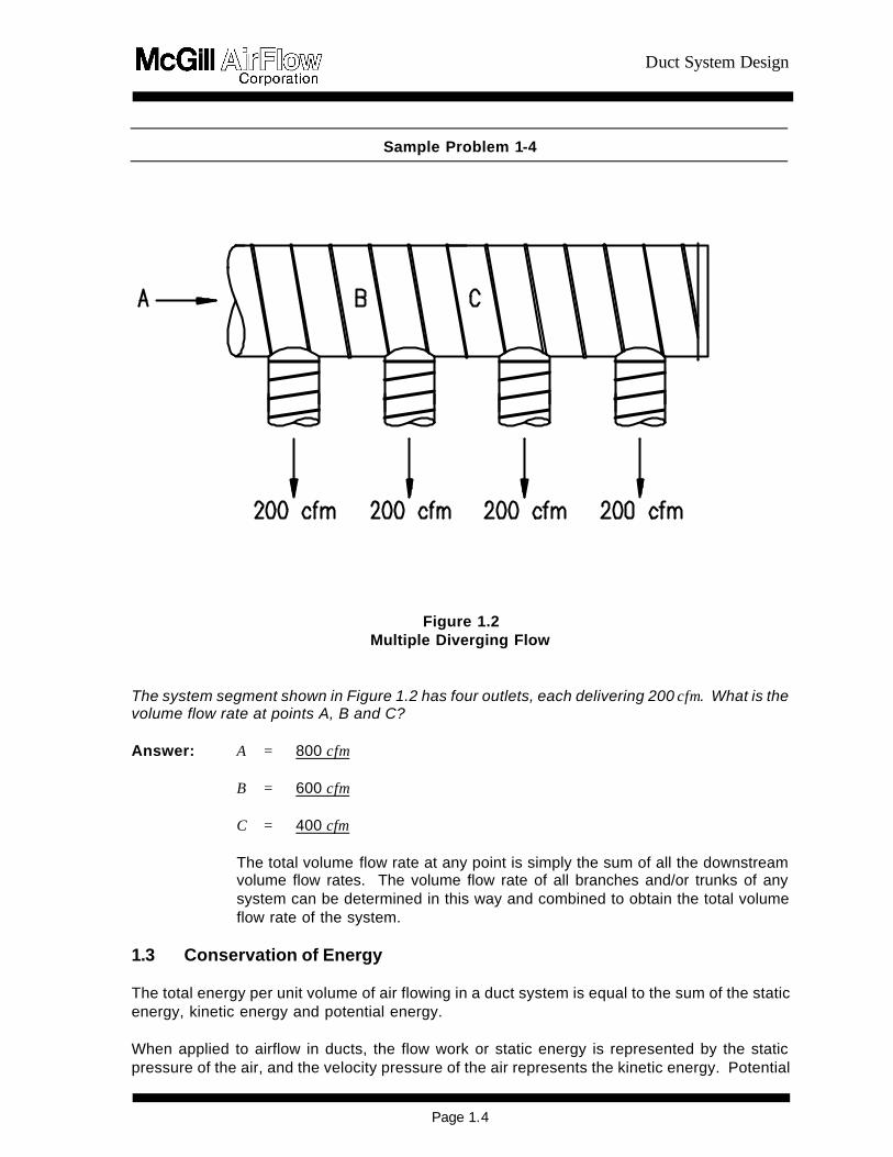
Duct System Design

Page 14

Sample Problem 1-4

Figure 12 Multiple Diverging Flow The system segment shown in Figure 12 has four outlets each delivering 200 cfm What is the volume flow rate at points A B and C Answer A = 800 cfm

B = 600 cfm C = 400 cfm

The total volume flow rate at any point is simply the sum of all the downstream volume flow rates The volume flow rate of all branches andor trunks of any system can be determined in this way and combined to obtain the total volume flow rate of the system

13 Conservation of Energy The total energy per unit volume of air flowing in a duct system is equal to the sum of the static energy kinetic energy and potential energy When applied to airflow in ducts the flow work or static energy is represented by the static pressure of the air and the velocity pressure of the air represents the kinetic energy Potential

Duct System Design

Page 15

energy is due to elevation above a reference datum and is often negligible in HVAC duct design systems Consequently the total pressure (or total energy) of air flowing in a duct system is generally equal to the sum of the static pressure and the velocity pressure As an equation this is written

TP = SP + VP Equation 13

where

TP = Total pressure SP = Static pressure VP = Velocity pressure

Furthermore when elevation changes are negligible from the law of conservation of energy written for a steady non-compressible flow for a fixed control volume the change in total pressure between any two points of a system is equal to the sum of the change in static pressure between the points and the change in velocity pressure between the points This relationship is represented in the following equation

∆∆TP = ∆∆SP + ∆∆VP Equation 14 Appendix A32 shows the derivation of Equation 14 from the general equation of the first law of thermodynamics Pressure (or pressure loss) is important to all duct designs and sizing methods Many times systems are sized to operate at a certain pressure or not in excess of a certain pressure Higher pressure at the same volume flow rate means that more energy is required from the fan and this will raise the operating cost The English unit most commonly used to describe pressure in a duct system is the inch of water gauge (inch wg) One pound per square inch (psi ) the standard measure of atmospheric pressure equals approximately 277 inches wg 131 Static Pressure Static pressure is a measure of the static energy of the air flowing in a duct system It is static in that it can exist without a movement of the air stream The air which fills a balloon is a good example of static pressure it is exerted equally in all directions and the magnitude of the pressure is reflected by the size of the balloon The atmospheric pressure of air is a static pressure At sea level this pressure is equal to approximately 147 pounds per square inch For air to flow in a duct system a pressure differential must exist That is energy must be imparted to the system (by a fan or air handling device) to raise the pressure above or below atmospheric pressure Air always flows from an area of higher pressure to an area of lower pressure Because the static pressure is above atmospheric at a fan outlet air will flow from the fan through any connecting ductwork until it reaches atmospheric pressure at the discharge Because the static pressure is below atmospheric at a fan inlet air will flow from the higher atmospheric pressure

Duct System Design

Page 16

ρρ

4005V

= 1097

V = VP

2 2

through an intake and any connecting ductwork until it reaches the area of lowest static pressure at the fan inlet The first type of system is referred to as a positive pressure or supply air system and the second type as a negative pressure exhaust or return air system Static Pressure Losses The initial static pressure differential (from atmospheric) is produced by adding energy at the fan This pressure differential is completely dissipated by losses as the air flows from the fan to the system discharge Static pressure losses are caused by increases in velocity pressure as well as friction and dynamic losses Sign Convention When a static pressure measurement is expressed as a positive number it means the pressure is greater than the local atmospheric pressure Negative static pressure measurements indicate a pressure less than local atmospheric pressure By convention positive changes in static pressure represent losses and negative changes represent regains or increases For example if the static pressure change as air flows from point A to point B in a system i s a positive number then there is a static pressure loss between points A and B and the static pressure at A must be greater than the static pressure at B Conversely if the static pressure change as air flows between these points is negative the static pressure at B must be greater than the static pressure at A 132 Velocity Pressure Velocity pressure is a measure of the kinetic energy of the air flowing in a duct system It is directly proportional to the velocity of the air For air at standard density (0075 pounds per cubic foot) the relationship is

Equation 15 where

VP = Velocity pressure (inches wg) V = Air velocity (fpm) ρρ = Density (lbmft3)

Appendix A33 provides a derivation of this relationship from the kinetic energy term This derivation also provides an equation for determining velocity pressures at nonstandard densities Appendix A16 provides a table of velocities and corresponding velocity pressures at standard conditions Velocity pressure is always a positive number and the sign convention for changes in velocity pressure is the same as that described for static pressure From Equation 11 it can be seen that velocity must increase if the duct diameter (area) is reduced without a corresponding reduction in air volume Similarly the velocity must decrease if the air volume is reduced without a corresponding reduction in duct diameter Thus the

Duct System Design

Page 17

velocity and the velocity pressure in a duct system are constantly changing 133 Total Pressure Total pressure represents the energy of the air flowing in a duct system Because energy cannot be created or increased except by adding work or heat there is no way to increase the total pressure once the air leaves the fan The total pressure is at its maximum value at the fan outlet and must continually decrease as the air moves through the duct system toward the outlets Total pressure losses represent the irreversible conversion of static and kinetic energy to internal energy in the form of heat These losses are classified as either friction losses or dynamic losses Friction losses are produced whenever moving air flows in contact with a fixed boundary These are discussed in Section 14 Dynamic losses are the result of turbulence or changes in size shape direction or volume flow rate in a duct system These losses are discussed in Section 15 Referring to Equation 14 note that if the decrease in velocity pressure between two points in a system is greater than the total pressure loss t he static pressure must increase to maintain the equality Alternatively an increase in velocity pressure will result in a reduction in static pressure equal to the sum of the velocity pressure increase and the total pressure loss When there is both a decrease in velocity and a reduction in static pressure the total pressure will be reduced by the sum of these losses These three concepts are illustrated in Figure 13

Figure 13

Conservation of Energy Relationship 14 Pressure Loss In Duct (Friction Loss) When air flows through a duct friction is generated between the flowing air and the stationary duct wall Energy must be provided to overcome this friction and any energy converted irreversibly to heat is known as a friction loss The fan initially provides this energy in the form of pressure The amount of pressure necessary to overcome the friction in any section of duct depends on (1) the length of the duct (2) the diameter of the duct (3) the velocity (or volume) of the air flowing in the duct and (4) the friction factor of the duct

Duct System Design

Page 18

1000V

D1

256= 100ft

P 18118∆

100ftP∆

The friction factor is a function of duct diameter velocity fluid viscosity air density and surface roughness For nonstandard conditions see Section 15 The surface roughness can have a substantial impact on pressure loss and this is discussed in Appendix A35 These factors are combined in the Darcy equation to yield the pressure loss or the energy requirement for a particular section of duct Appendix A34 discusses the use and application of the Darcy equation 141 Round Duct One of the most important and useful tools available to the designer of duct systems is a friction loss chart (see Appendix A411) This chart is based on the Darcy equation and combines duct diameter velocity volume flow rate and pressure loss The chart is arranged in such a manner that knowing any two of these properties (at standard conditions) it is possible to determine the other two

The chart is arranged with pressure loss (per 100 feet of duct length) on the horizontal axis volume flow rate on the vertical axis duct diameter on diagonals sloping upward from left to right and velocity on diagonals sloping downward from left to right

Examination of this chart (or the Darcy equation) reveals several interesting air flow properties (1) at a constant volume flow rate reducing the duct diameter will increase the pressure loss (2) to maintain a constant pressure loss in ducts of different size larger volume flow rates require larger duct diameters and (3) for a given duct diameter larger volume flow rates will increase the pressure loss The following sample problems will give the reader a feel for these important relationships Although there are many nomographs or duct calculators available to speed the calculation of duct friction loss problems novice designers should use the friction loss charts to better visualize the relationships The friction loss chart in the Appendix is approximated by Equation 16

Equation 16

where = the friction loss per 100 ft of duct (inches wg)

D = the duct diameter (inches) V = the velocity of the air flow in the duct (fpm)

Sample Problem 1-5

What is the friction loss of a 150-foot long section of 18-inch diameter duct carrying 2500 cfm What is the air velocity in this duct Answer From the friction loss chart find the horizontal line that represents 2500 cfm

Move across this line to the point where it intersects the diagonal line which represents an 18-inch diameter duct From this point drop down to the horizontal

Duct System Design

Page 19

wginches 100ft

P016 =

1000

1412

18

1256 =

18118

∆

(pressure) axis and read the friction loss This value is approximately 016 inches wg This represents the pressure loss of a 100-foot section of 18-inch diameter duct carrying 2500 cfm To determine the pressure loss for a 150-foot duct section it is necessary to multiply the 100-foot loss by a factor of 15 Therefore the pressure loss is 024 inches wg

At the intersection of the 2500 cfm line and the 18-inch diameter line locate the nearest velocity diagonal The velocity is approximately 1400 fpm

Equation 16 could have also been used to solve this problem To use Equation 16 we must first calculate the velocity using Equation 11 To calculate the velocity we have to determine the cross-sectional area of the 18-inch diameter duct A = π x 182 576 = 177 ft2 The calculated velocity is QA = 2500177 = 1412 fpm The pressure loss per 100 ft is calculated as For a 150 ft section the pressure is 15 x 016 = 024 inches wg

Sample Problem 1-6

Part of a system you have designed includes a 20-inch diameter 500-foot duct run carrying 3000 cfm You now discover there is only 16 inches of space in which to install this section What will be the increase in pressure loss of the duct section if 16-inch duct is used in place of 20-inch Answer From the friction loss chart or Equation 16 find the pressure loss per 100 feet for

3000 cfm flowing through a 20-inch diameter duct This value is 014 inches wg or 070 inches wg for 500 feet Similarly the friction loss for 500 feet of 16-inch diameter duct carrying 3000 cfm is found to be 195 inches wg

Reducing this duct diameter by 4 inches results in an increase of pressure loss of 125 inches wg

Sample Problem 1-7

An installed system includes a 20-inch diameter 500-foot duct run carrying 3000 cfm Due to unanticipated conditions downstream it has become necessary to increase the volume flow rate in this duct section to 3600 cfm What will be the impact on the pressure loss of the section Answer From Sample Problem 1-6 the pressure drop of this section as installed is 070

inches wg To find the new pressure drop move up the 20-inch diameter line until it intersects the 3600 cfm volume flow rate line At this point read down to the friction loss axis and find that the new friction loss is 019 inches wg per 100

Duct System Design

Page 110

feet or 095 inches wg for 500 feet Therefore this 20 percent increase in volume will result in a 36 percent increase in the pressure loss for the duct section

Sample Problem 1-8

A system is being designed so that the pressure loss in all duct sections is equal to 02 inches wg per 100 feet What size duct will be required to carry (a) 500 cfm (b) 1500 cfm (c) 5000 cfm (d) 15000 cfm Answer From the friction loss chart find the vertical line that represents 020 inches wg per

100 feet friction loss Move up this line to the point where it intersects the horizontal line which represents a volume flow rate of 500 cfm At this point locate the nearest diagonal line representing duct diameter It will either be 9-inch duct or 95-inch duct (if half-inch duct sizes are available)

Similarly for the other volumes find the line representing duct size which is nearest to the intersection of the 020 inches wg per 100 feet friction loss line and the appropriate volume At 1500 cfm 14-inch duct is required at 5000 cfm 22-inch duct is required and at 15000 cfm 33-inch duct is required In each case the duct will carry the specified volume with a pressure loss of approximately 020 inches wg per 100 feet

142 Flat Oval Duct Flat oval duct has the advantage of allowing a greater duct cross-sectional area to be accommodated in areas with reduced vertical clearances Figure 14 shows a typical cross section of flat oval duct References in Appendices A1 A2 and A9 provide additional information about flat oval duct

Figure 14 Flat Oval Dimensions The Darcy equation is not applicable to flat oval duct and there are no friction loss charts available for non-round duct shapes To calculate the friction loss for flat oval duct it is necessary to determine the equivalent round diameter of the flat oval size and then determine the friction loss for the equivalent round duct

Duct System Design

Page 111

)(P)(A 155

= D 025

0625

eq

1444

)minx (+)minx (FS

= A

2ππ

12x FS) 2( + )minx (

= Pππ

The equivalent round diameter of flat oval duct is the diameter of round duct that has the same pressure loss per unit length at the same volume flow rate as the flat oval duct Equation 17 can be used to calculate the equivalent round diameter for flat oval duct with cross-sectional area A and perimeter P The equivalent round diameters for many standard sizes of flat oval duct are given in Appendix A132

Equation 17

where

Deq = Equivalent round diameter (ft) A = Flat oval cross-sectional area (ft2) P = Flat oval perimeter (ft)

The flat oval cross-sectional area is calculated using Equation 18

Equation 18

where

A = Cross-sectional area (ft2) FS = Flat Span (inches) = maj - min min = Minor axis (inches) maj = Major axis (inches)

The perimeter of flat oval is calculated using Equation 19

Equation 19

where

P = Flat oval perimeter (ft)

When calculating the air velocity in flat oval duct it is necessary to use the actual cross-sectional area of the flat oval shape not the area of the equivalent round duct To use Equation 16 however the air velocity is calculated using the equivalent round diameter cross sectional area

Duct System Design

Page 112

Sample Problem 1-9

A 12-inch x 45-inch flat oval duct is designed to carry 10000 cfm What is the pressure loss per 100 feet of this section What is the velocity Answer Equations 18 and 19 are used to calculate the area and perimeter of the flat

oval duct For 12 x 45 duct A = 354 ft2 from (45 - 12) x 12 + (π x 122)4144 and P = 864 ft from (π x 12) + (2 x (45-12))12 Substituting into Equation 17 Deq = 199 ft 24 inches From the friction loss chart the pressure loss of 10000 cfm air flowing in a 24-inch round duct is 050 inch wg per 100 feet

The velocity can be calculated from Equation 11

V = QA = 10000 354 = 2825 fpm

Note that the velocity of the same air volume flowing in the 24-inch diameter round duct is 10000 314 or 3185 fpm

Alternatively to use Equation 16 we must first calculate the velocity assuming the cross-sectional area is determined from the equivalent round

ftA2

Deq 314 = 576

)24x ( 2π=

fpm V Deq 3185 = 314

10000 =

wginches 100ft

P 048=

1000

3185

24

1256 =

18118

∆

Which is close to the 050 incheswg determined from the friction loss chart

Sample Problem 1-10

In Sample Problem 1-6 what size flat oval duct would be required in order to maintain the original (070 inches wg) pressure drop and still fit within the 16-inch space allowance Answer In this situation the available space will dictate the minor axis dimension of the

Duct System Design

Page 113

flat oval duct It is always advisable to allow at least 2 to 4 inches for the reinforcement which may be required on any flat oval or rectangular duct product Therefore we will assume that the largest minor axis that can be accommodated is 12 inches

Since we want to select a flat oval size which will have the same pressure loss as a 20-inch round duct the major axis dimension can be determined by solving Equation 17 with Deq = 167 feet (20 inches) and min = 12 inches Using Equations 18 and 19 for determining A and P as functions of the major axis dimension (maj) and the minor axis dimension (min) Unfortunately this requires an iterative solution

A simpler solution is to refer to the tables in Appendix A132 These tables list the various available flat oval sizes and their respective equivalent round diameters Since we already know that the minor axis must be 12 inches we look for a flat oval size with a 12-inch minor axis and an equivalent round diameter of 20 inches The required flat oval size is 12 inches x 31 inches

If it is determined that there is room for a 14-inch minor axis duct the required size would be 14 inches x 27 inches (Deq = 20 inches)

143 Rectangular Duct Rectangular duct is fabricated by breaking two individual sheets of sheet metal (called L-sections) that have the appropriate duct dimensions (side and side adjacent) and joining them together by one of several techniques Rectangular duct is also used when height restrictions are employed in a duct design Equation 110 can be used to calculate the equivalent round diameter Deq of rectangular duct The equivalent round diameter Deq for many standard sizes of rectangular duct are given in Appendix 14

Equation 110

where

Deq = Equivalent round diameter (inches)

a = Duct side length (inches) b = Other duct side length (inches)

When calculating air velocity in rectangular duct it is necessary to use the actual cross-sectional area of the rectangular shape not the area of the equivalent round diameter

)b+(a)(ab 130

= D 0250

0625

eq

Duct System Design

Page 114

Sample Problem 1-11

A 12-inch x 45-inch rectangular duct is designed to carry 10000 cfm What is the pressure loss per 100 feet of this section What is the velocity Answer Using Equation 110 Deq = 24 inches From the friction loss chart the loss of

10000 cfm air flowing in a 24-inch round duct is 050 inch wg per 100 feet

The velocity can be calculated from Equation 11

fpmA

Q = V 2667=

45)144 x (12

10000 =

Note that the velocity in the rectangular duct is less than in the flat oval with the same major and minor dimensions (See Sample Problem 1-9)

144 Acoustically Lined and Double-wall Duct Applying an inner liner or a perforated inner metal shell sandwiching insulation between an inner and outer wall increases the surface roughness that air sees and thus increases the friction losses of duct Acoustically lined round and rectangular duct consist of a single-wall duct with an internal insulation liner but no inner metal shell Double-wall duct that is acoustically insulated consists of a solid outer shell a thermalacoustical insulation and a metal inner liner (either solid or perforated) The inner dimensions of lined duct or the metal inner liner dimensions of double-wall duct are the nominal duct size dimensions that are used to determine the cross-sectional area for airflow calculations The single-wall dimensions of lined duct or outer shell dimensions of double-wall duct depend on the insulation thickness For a 1-inch thick insulation the dimensions are 2 inches larger than the inner dimensions of lined duct or metal inner liner dimensions Acoustically Lined Duct Correction factors to the friction loss determined from the friction loss chart or for Equation 16 have not been developed for internally insulated duct Therefore the designer must use the Darcey equation as given in Appendix A34 Assume an absolute roughness of ε = 0015 Double-wall Duct

Corrections factors to the friction loss determined from the friction loss chart or Equation 16 have been developed for when a perforated metal inner liner is used Figure 15 is a chart which gives the correction factors This information is repeated in Appendix A412 Note that these corrections are a function of duct diameter and velocity If the duct shape is flat oval or rectangular use the equivalent round diameter based on the perforated metal inner liner dimensions If the inner shell of the double-wall duct does not use perforated metal use the same friction loss as a single-wall duct of the same dimensions as the metal inner shell

Duct System Design

Page 115

13

12

11

10

4rdquo 8rdquo

12rdquo

18rdquo

36rdquo

72rdquo

2000 3000 4000 5000 6000

Correction factor to be applied to the friction loss of single-wall duct to calculate the friction loss of double-wall duct with a perforated metal inner liner

Velocity (fpm)

Figure 15 Correction Factors for Double-Wall Duct with Perforated Metal Inne r Liner When only thermal insulation is required the metal inner liner may be specified as solid rather than perforated metal In this case the friction losses are identical to those for single-wall duct with a diameter equal to the metal inner liner diameter For acoustically insulated flat oval or rectangular duct with a perforated metal inner liner use the correction factors of the equivalent round diameter and the actual velocity (based on the metal inner liner of the flat oval or rectangular cross section) The reference in Appendix A92 addresses friction losses for lined rectangular duct

Sample Problem 1-12

What is the friction loss of a 100-foot section of 22-inch diameter double-wall duct (with perforated metal inner liner) carrying 8000 cfm Answer The pressure loss for 100 feet of 22-inch single-wall duct carrying 8000 cfm is

found from the friction loss chart to be 050 inches wg The velocity is 3000 fpm

From Figure 15 the correction factor for 22-inch duct (interpolated) at 3000 fpm is approximately116Therefore the pressure loss of this section of double-wall duct is 050 x 116 or 058 inches wg

145 Nonstandard Conditions All loss calculations thus far have been made assuming a standard air density of 0075 pounds per cubic foot When the actual design conditions vary appreciably from standard (ie temperature is 30degF from 70degF elevation above 1500 feet or moisture greater than 002 pounds water per pound dry air) the air density and viscosity will change If the Darcy equation is used to calculate friction losses and the friction factor and velocity pressure are calculated using

Duct System Design

Page 116

actual conditions no additional corrections are necessary If a nomograph or friction chart is used to calculate friction losses at standard conditions correction factors should be applied The corrections for nonstandard conditions discussed above apply to duct friction losses only Other corrections are applicable to the dynamic losses of fittings as will be explained in the following section For a more in-depth presentation of these and other correction factors see Reference in Appendix A92 Tables for determining correction factors are included in Appendix A15 A temperature correction factor Kt can be calculated as follows

460) + T(

530= K

a

0825

t Equation 111

where

Kt = Nonstandard temperature correction factor Ta = Actual temperature of air in the duct (degF)

An elevation correction factor Ke can be calculated as follows

](Z) )10x (68754 -1[= K473-6

e Equation 112a

Equation 112a can also be written as follows

ββ29921

= K09

e Equation 112b

where

Ke = Nonstandard elevation correction factor Z = Elevation above sea level (feet) ββ = Actual barometric pressure (inches Hg)

When both a nonstandard temperature and a nonstandard elevation are present the correction factors are multiplicative As an equation

Kx K= K etf Equation 113

where

Kf = Total friction loss correction factor

The calculated duct friction pressure loss should be multiplied by the appropriate correction factor Kt Ke or Kf to obtain the actual pressure loss at the nonstandard conditions

Duct System Design

Page 117

Sample Problem 1-13

The friction loss for a certain segment of a duct system is calculated to be 25 inches wg at standard conditions What is the corrected friction loss if (a) the design temperature is 30degF (b) the design temperature is 110degF (c) the design elevation is 5000 feet above sea level (d) both (b) and (c) Answer 1 Substituting into Equation 111 Kt = [530(30 + 460)]0825 = 107

Corrected friction loss = 25 x 107 = 268 inches wg

2 Kt = [530(110 + 460)]0825 = 094 Corrected friction loss = 235 inches wg

3 Substituting into Equation 112a Ke = [1 - (68754 x 10-6)(5000)] 473 = 085 Corrected friction loss = 213 inches wg

4 Substituting into Equation 113 Kf = 094 x 085 = 080 Corrected

friction loss = 200 inches wg

If moisture in the airstream is a concern a humidity correction factor Kh can be calculated as follows

(( )) 90

wsh

P37801K

ββ

minusminus== Equation 114

where

Pws = Saturation pressure of water vapor at the dew point

temperature (inches Hg) ββ = Actual barometric pressure (inches Hg)

The total friction loss correction factor Kf is expressed as

hetf Kx Kx K= K Equation 115

15 Pressure Loss in Supply Fittings As mentioned in Section 13 pressure losses can be the result of either friction losses or dynamic losses Section 14 discussed friction losses produced by air flowing over a fixed boundary This section will address dynamic losses Friction losses are primarily associated with duct sections while dynamic losses are exclusively attributable to fittings or obstructions Dynamic losses will result whenever the direction or volume of air flowing in a duct is altered or when the size or shape of the duct carrying the air is altered Fittings of any type will produce dynamic losses The dynamic loss of a fitting is generally proportional to the severity of the airflow disturbance A smooth large radius elbow for example will have a much lower dynamic

Duct System Design

Page 118

loss than a mitered (two-piece) sharp-bend elbow Similarly a 45deg branch fitting will usually have lower dynamic losses than a straight 90deg tee branch 151 Loss Coefficients In order to quantify fitting losses a dimensionless parameter known as a loss coefficient has been developed Every fitting has associated loss coefficients which can be det ermined experimentally by measuring the total pressure loss through the fitting for varying flow conditions Equation 116a is the general equation for the loss coefficient of a fitting

VPTP

= C∆

Equation 116a

where C = Fitting loss coeffi cient ∆∆TP = Change in total pressure of air flowing through the fitting (inches

wg) VP = Velocity pressure of air flowing through the fitting (inches wg)

Once the loss coefficient for a particular fitting or class of fittings has been experimentally determined the total pressure loss for any flow condition can be determined Rewriting Equation 116a we obtain

VPx C= TP∆ Equation 116b

From this equation it can be seen that the total pressure loss is directly proportional to both the loss coefficient and the velocity pressure Higher loss coefficient values or increases in velocity will result in higher total pressure losses for a fitting A less efficient fitting will have a higher loss coefficient (ie for a given velocity the tot al pressure loss is greater) 152 Elbows Table 11 shows typical loss coefficients for 8-inch diameter elbows of various construction Table 11 Loss Coefficient Comparisons for Abrupt-Turn Fittings

90EE Elbows 8-inch Diameter Fitting

Loss Coefficient

Die-StampedPressed 15 Centerline Radius

011 Five-Piece 15 Centerline Radius

022

Mitered with Turning Vanes

052 Mitered

124

From Equation 14 we can determine the pressure loss

∆∆TP = ∆∆SP + ∆∆VP

Duct System Design

Page 119

Since the elbow diameter and volume flow rate are constant the continuity equation (Equation 11) tells us that the velocity will be constant From Equation 15 the velocity pressure is a direct function of velocity and so ∆∆VP = 0 Therefore ∆∆SP = ∆∆TP Note that whenever there is no change in velocity as is the case in duct and constant diameter elbows the change in static pressure is equal to the change in total pressure

Sample Problem 1-14

What is the total pressure loss of an 8-inch diameter die-stamped elbow carrying 600 cfm What is the static pressure loss Answer From Equation 11

Q = A x V or V = QA A = πD2576 = π (8)2 576 = 035 ft2 V = 600 035 V = 1714 fpm

From Equation 15 or Appendix A16

wginches VP 018= 40051714

=2

From Table 11

C = 011 (die-stamped elbow) From Equation 116b

∆TP = C x VP = 011 x 018 = 002 inches wg

Sample Problem 1-15

A designer is trying to determine which 8-inch elbow to select for a location which will have a design velocity of 1714 fpm What will be the implications in terms of pressure loss if the designer chooses (1) a die-stamped elbow (2) a five-gore elbow (3) a mitered elbow with turning vanes or (4) a mitered elbow without turning vanes Answer From Sample Problem 1-14 we calculated the total pressure loss of an 8-inch

die-stamped elbow at 1714 fpm to be 002 inches wg

For the other elbows we can determine the pressure loss from loss coefficients given in Table 11

Duct System Design

Page 120

C2 = 022 C3 = 052 C4 = 124

From Equation 116b

∆TP2 = ∆SP2 = 022 x 018 = 004 inches wg (five-gore)

∆TP3 = ∆SP3 = 052 x 018 = 009 inches wg (mitered with turning vanes)

∆TP4 = ∆SP4 = 124 x 018 = 022 inches wg (mitered without turning vanes)

Therefore using a five-gore elbow will increase the total pressure loss by 100 percent but it will be a very modest 004 inches wg Using the mitered elbow with vanes would result in a 350 percent increase over the die-stamped elbow or a 125 percent increase over the five-gore elbow The mitered elbow without turning vanes would have a loss of 022 inches wg which is a tenfold increase over the die-stamped elbow

The increased pressure losses associated with the use of les s efficient fittings may or may not be critical to the operation of the system depending on the location of the fittings Succeeding chapters will note when there could be locations in a system where it is desirable to increase the losses of certain fittings In general unless the system has been carefully analyzed to determine the location of the critical path(s) and the excess pressures present in other paths it is wise to always select fittings with the lowest pressure drop The loss coefficients of most elbows vary as a function of diameter The ASHRAE Duct Fitting Database Program (Appendix A82) presents loss coefficients as a function of diameter for various elbow constructions The loss coefficient drops sharply as diameters increase through approximately 24 inches then only slightly from 24 inches through 60 inches Also eliminating turning vanes in mitered elbows more than doubles the pressure loss Flat Oval Elbows Although the use of equivalent duct lengths as a measure of dynamic fitting losses is usually strongly discouraged it provides acceptable approximations in the case of flat oval elbows Data indicates that flat oval 90deg elbows (hard or easy bend) with 15 centerline radius bends have a pressure loss approximately equal to the friction loss of a flat oval duct with an identical cross section and a length equal to nine times the elbow major axis dimension calculated at the same air velocity that is flowing through the elbow For example a 12-inch x 31-inch flat oval elbow would have a pressure loss approximately equal to that of a 12-inch x 31-inch flat oval duct 23 feet long (9 x 31 inches) at the same velocity For flat oval elbows that do not have a 15 centerline radius bend use the loss coefficient for a round elbow of similar construction with the diameter equal to the flat oval minor axis Rectangular Elbows (see ASHRAE== s Duct Fitting Database Program)

Duct System Design

Page 121

VPTP= C

b

b-cb

∆

Acoustically LinedDouble-wall Elbows For acoustically lined elbows or double-wall elbows with either a solid or perforated metal inner liner the losses are the same as for standard single-wall elbows with dimensions equal to the metal inner liner dimensions of the acoustically lined or double-wall elbow Elbows With Bend Angles Less Than 90deg For elbows constructed with bend angles less than 90deg multiply the calculated pressure loss for a 90deg elbow by the correction factor given in Table 12

Table 12 Elbow Bend Angle Correction Factor

Angle CFelb

225deg 031

30deg 045

45deg 060

60deg 078

75deg 090 153 Diverging-Flow Fittings Branches The pressure losses in diverging-flow fittings are somewhat more complicated than elbows for two reasons (1) there are multiple flow paths and (2) there will almost always be velocity changes First consider the case of air flowing from the common (upstream) section to the branch Referring to Figure 11 this is from c to b (Refer to Appendix A11 for clarification of upstream and downstream) As is the case for elbows loss coefficients are determined experimentally for diverging-flow fittings However it is now necessary to specify which flow paths the equation parameters refer to By definition

Equation 117a

where

Cb = Branch loss coefficient ∆TPc-b = Total pressure loss common-to-branch (inches wg) VPb = Branch velocity pressure (inches wg)

Rewriting in terms of total pressure loss

∆TPc-b = Cb x VPb Equation 117b Therefore the total pressure loss of air flowing into the branch leg of a diverging-flow fitting is

Duct System Design

Page 122

directly proportional to the branch loss coefficient and the branch velocity pressure For duct and elbows the total pressure loss is always equal to the static pressure loss because there is no change in velocity However diverging-flow fittings almost always have velocity changes associated with them If ∆VP is not zero then the total and static pressure losses cannot be equal (Equation 14) For diverging-flow fittings the static pressure loss of air flowing into the branch leg can be determined from Equation 117c

∆SPc-b = VPb (Cb + 1) - VPc Equation 117c where

∆SPc-b = Static pressure loss common-to-branch (inches wg) VPb = Branch velocity pressure (inches wg) VPc = Common velocity pressure (inches wg) Cb = Branch loss coefficient (dimensionless)

Equation 117c is derived from Equations 117a and 117b as shown in Appendix A36

As is the case for elbows a comparison of loss coefficients gives a good indication of relative fitting efficiencies The following samples compare loss coefficients of various diverging-flow fittings

Duct System Design

Page 123

Table 13 Loss Coefficient Comparisons for Diverging-Flow Fittings

Fitting Loss Coefficient

(Cb) Y-Branch plus 45deg Elbows

022

Vee Fitting

030

Tee with Turning Vanes plus Branch Reducers (Bullhead Tee with Vanes)

045

Tee plus Branch Reducers

108

Capped Cross with Straight Branches

445

Capped Cross with Conical Branches

445

Capped Cross with 1-foot Cushion Head

54

Capped Cross with 2-foot Cushion Head

60

Capped Cross with 3-foot Cushion Head

64

The loss coefficient Cb is for a VbVc ratio of approximately 10

Duct System Design

Page 124

AA

Q

Q VP V VP V

c

b

c

bbbcc

Sample Problem 1-16

What is the total pressure loss for flow from c to b in the straight tee shown below What is the static pressure loss Answer ∆TPc-b = Cb x VPb From Equation 117b

∆SPc-b = VPb (Cb + 1) - VPc From Equation 117c Reference ASHRAE Duct Fitting Database Number SD5-9 Given Qc = 5000 cfm Dc = 24 inches

Qb = 2000 cfm Db = 18 inches

Qs = 3000 cfm Ds = 24 inches Calculate

fpmA

Q V

c

cc 1592 =

314

5000 ==

c

s

b

Duct System Design

Page 125

wginches4005

VVP c

2

c 016 = 40051592

==2

fpmA

Q V

b

bb 1130 =

177

2000 ==

wginches4005

VVP b

2

b 008 = 40051130

==2

040 = 50002000

= Q

Q

c

b

056 = 314

177 =

A

A

c

b

Determine Cb - Interpolated from the ASHRAE table = 214

Answer ∆TPc-b = 214 x 008 = 017 inches wg

∆SPc-b = 008 (214 + 1) - 016 = 009 inches wg

Duct System Design

Page 126

Sample Problem 1-17

What would be the static and total pressure losses in Sample Problem 1-16 if a conical tee were substituted for the straight tee A LO-LOSSTM tee Reference Conical Tee ASHRAE Fitting SD5-10

LO-LOSST M Tee ASHRAE Fitting SD5-12 Determine Cb (conical) = 135

Cb (LO-LOSST M) = 079 Answer ∆TPc-b (conical) = 011 inches wg

∆SPc-b (conical) = 003 inches wg ∆TPc-b (LO-LOSST M) = 006 inches wg ∆SPc-b (LO-LOSST M) = -002 inches wg

In the preceding problem the static pressure loss for a LO-LOSST M tee at the given conditions resulted in a negative number Recall from Section 131 that a pressure change expressed as a positive number is a loss while a pressure change expressed as a negative number represents an increase in pressure This pressure increase is a common phenomenon in air handling systems and is known as static regain It occurs for the LO-LOSST M fitting because the decrease in velocity pressure is greater than the total pressure loss of the fitting Total Pressure Losses versus Static Pressure Losses Just as total pressure represents the total energy present at any point in a system the total pressure loss of a fitting represents the true energy loss of the fitting for a given flow situation Static pressure losses are useful for certain design methods as we shall see later however they do not give an accurate indication of fitting efficiency Sample Problem 1-18 illustrates this concept

Duct System Design

Page 127

Sample Problem 1-18

Change the branch size in Sample 1-17 from 18 inches diameter to 12 inches diameter and recalculate the total and static pressure losses of the LO-LOSS TM tee

Reference ASHRAE Fitting SD5-12 Given Qc = 5000 cfm Dc = 24 inches

Qb = 2000 cfm Db = 12 inches Qs = 3000 cfm Ds = 24 inches

Calculate AA

Q

Q VP V VP V

c

b

c

bbbcc

Vc = 1592 fpm VPc = 016 inches wg Vb = 2548 fpm VPb = 040 inches wg Qb Qc = 040 Ab Ac = 025

Determine Cb Interpolate from ASHRAE Fitting SD5-12 = 021 Answer ∆TPc-b = CbxVPb (from Equation 117b) = 021x040 = 008 inches wg ∆SPc-b = VPb (Cb + 1) - VPc (from Equation 117c) = 040(021+1)-016 = 032 inches wg In this problem the total pressure loss is 008 inches wg but the static pressure loss is 032 inches wg If one were to look only at the static pressure this would seem to be a very inefficient fitting However notice that due to flow and pressure conditions in the system the velocity increased as the air moved from the common section into the branch resulting in a velocity pressure increase of 024 inches wg

c s

b

Duct System Design

Page 128

This situation is shown in Figure 13 Case II The apparently large decrease in static pressure was caused by a large increase in velocity pressure As Equation 14 this becomes

008 = 032 + -024 (∆TP = ∆SP + ∆VP )

Conversely when certain flow conditions are present it is possible for a fitting to have a small static pressure loss but a relatively large total pressure loss It is always advisable to calculate the total pressure loss in order to determine the total energy consumption of a fitting Manifold Fittings The single-branch fittings discussed thus far are assumed to be factory fabricated and constructed as a separate unit from the duct to which t hey would be attached Occasionally it is desirable to construct a manifold fitting with a tap attached directly to the duct This construction will generally result in a less efficient fitting especially if the manifold is constructed in the field Flat Oval Diverging-Flow Fittings Diverging-flow fittings of similar construction generally exhibit the same pressure loss for the same volume flow rate ratios and area ratios Flat oval fittings exhibit similar pressure losses as round fittings Testing is under way to develop a database of loss coefficients for flat oval diverging-flow fittings Until this data is available use the same loss coefficients as for the same construction of round Acoustically Lined and Double-wall Diverging-Flow Fittings Whether a fitting has been acoustically lined or has a perforated metal inner shell the difference in surface roughness is accounted for in the friction loss determination since all friction loss calculations are base on fitting-to-fitting centerline dimensions Therefore there is no need to increase the dynamic loss of a diverging flow-fitting that is either acoustically lined or one that has an inner metal shell even if the shell is perforated Determine the loss coefficient of the fitting as if it were a single-wall fitting with the dimension of the inner liner or metal inner shell Rectangular Diverging-Flow Fittings (see ASHRAE== s Duct Fitting Database Program) 154 Diverging-Flow Fittings Straight-Throughs Reducers and Transitions Straight-Throughs The straight-through (downstream) leg of a diverging-flow fitting is that path followed by air flowing from c to s as represented in Figure 11 The straight -through may have a constant diameter such that Dc = Ds or there may be a reducer attached to the straight -through such that Dc gt Ds In the case of a constant diameter straight -through there will always be a velocity reduction caused by a reduced volume (after the branch) flowing through the same diameter duct If a reducer is attac hed to the straight -through it can be sized to reduce maintain or increase the downstream velocity relative to the common velocity Dynamic losses associated with air flowing straight through a diverging-flow fitting andor a

Duct System Design

Page 129

reducer is very slight This is understandable since there is little physical disturbance of the airflow The total pressure loss in a straight -through leg or reducer is often only a few hundredths of an inch wg Perhaps the most important phenomenon associated with the straight-through flow situation is the potential for static regain This situation is illustrated in Figure 13 Case I A large reduction in velocity pressure and a small reduction in total pressure must (by Equation 14) result in an increase in static pressure or static regain The regain will be equal in magnitude to the velocity pressure loss minus the total pressure loss Of course if the total pressure loss is greater than the reduction in velocity pressure as shown in Figure 13 Case III there can be no static regain Referring again to Sample Problem 1-16 we see that the velocity in the constant diameter straight -through leg is reduced from 1592 fpm (VPc = 016 inches wg) in the duct before the straight -through to 955 fpm (VPs = 006 inches wg) in the duct after the straight -through due to the reduced volume flow This is a velocity pressure reduction of ∆VPc-s = 010 inches wg If we assume a total pressure loss of ∆TPc-s = 001 inches wg then from Equation 14 we get

001 = ∆SPc-s + 010 or ∆SPc-s = -009 inches wg The negative result indicates a static regain or that the static pressure at point s will be 009 inches wg higher than the static pressure at point c The loss coefficient data for reducers and straight -throughs is found in the ASHRAE Duct Fitting Database When using loss coefficients to determine straight -through losses Equations 117b and 117c are rewritten as follows

∆∆TPc-s = Cs x VPs Equation 118a ∆∆SPc-s = VPs (Cs + 1) - VPc Equation 118b

where

∆∆TPc-s = Total pressure loss common-to-straight-through (inches wg) ∆∆SPc-s = Static pressure loss common-to-straight-through (inches wg) VPc = Common velocity pressure (inches wg) VPs = Straight-through velocity pressure (inches wg) Cs = Straight-through loss coefficient

Sample Problem 1-19

Calculate the total and static pressure losses for the straight-through portion of the straight tee in Sample Problem 1-16

Reference ASHRAE Fitting SD5-9

Duct System Design

Page 130

Calculate AA

Q

Q VP V VP V

c

s

c

ssscc

Vc = 1592 fpm VPc = 016 inches wg

Vs = 955 fpm VPs= 006 inches wg

Qs Qc = 060 As Ac = 10

Determine Cs Interpolate from ASHRAE Fitting SD5-9 = 020 Answer

∆TPc-s = Cs x VPs (Equation 118a ) = 020 x 006 = 001 inches wg ∆SPc-s = VPs (Cs + 1) - VPc (Equation 118b) = 006(020 + 1) - 016 = -009 inches wg

Reducers A stand-alone reducer will cause the velocity to increase since after the reducer the same volume of air will be flowing through a smaller diameter duct (see Sample Problem 1-2) The use of a reducer on its own is not consistent with any design methods presented in this manual and should be fairly rare in most duct systems However when this fitting is used the losses are calculated using the same charts and in the same manner as the straight -throughs Losses are a function of upstream and downstream velocity Reducing fittings should be constructed as shown in Figure 17 such that the length of the taper portion (L) is equal to the difference between the common diameter and the straight -through diameter (Dc - Ds) Verify this with manufacturers dimension sheets Since reducers are very efficient fittings the use of a longer taper section will not necessarily provide a significant improvement in performance

Figure 17 Reducing Fitting Construction Transitions Transitions between round and flat oval duct also produce dynamic pressure losses As with other fittings these losses can be quantified in terms of a loss coefficient The loss coefficient

Duct System Design

Page 131

for round-to-flat oval or flat oval-to-round transitions depends on the flat oval aspect ratio (major axisminor axis) the direction of airflow and the air velocity When round duct transitions to flat oval the flat oval minor axis dimension is usually less than the original round diameter while the flat oval major axis dimension is greater than the round diameter The reverse is true in transitions from flat oval to round Therefore roundflat oval transitions usually involve both a reducer effect (round to flat oval minor or flat oval major to round) and an enlarger effect (round to flat oval major or flat oval minor to round) The change in dimension involving the flat oval major axis is normally much greater than the change tofrom the flat oval minor axis Therefore in round-to-flat oval transitions the enlarger effect predominates while in flat oval-to-round transitions the reducer effect predominates Dynamic losses which result from expanding areas (decreasing velocities) are always more severe than losses from reducing areas (increasing velocities) Therefore the flat oval-to-round transition is more efficient than the round-to-flat oval fitting Figure A24 in Appendix A4 2 is a plot of loss coefficient (Cs ) versus round duct velocity for both round-to-flat oval and flat oval-to-round transitions The curves are valid for any size flat oval and will be conservative for transitions involving flat oval with a low aspect ratio Use the appropriate loss coefficient value in the following equations to determine static and total pressure losses for transition fittings

∆∆TPc-s = Cs x VPs Equation 119a ∆∆SPc-s = VPs (Cs + 1) - VPc Equation 119b where

∆∆TPc-s = Total pressure loss common-to-straight-through (inches wg) ∆∆SPc-s = Static pressure loss common-to-straight-through (inches wg) VPc = Common velocity pressure (inches wg) VPs = Straight-through velocity pressure (inches wg) Cs = Straight-through loss coefficient

Sample Problem 1-20

In Sample Problem 1-10 we determined that a 12-inch H 31-inch flat oval duct would have the same pressure loss per unit length as a 20-inch round duct What would be the impact on total and static pressure losses in a 100-foot section of 20-inch round duct carrying 5000 cfm if 40 feet of this duct were replaced by a 12-inch H 31-inch flat oval duct Assume the first 30 feet of duct is round next 40 feet is flat oval and the last 30 feet is round Answer Since the duct sizes are equivalent 40 feet of 12-inch H 31-inch flat oval would

have the same pressure loss per 100 feet as the section of 20-inch round duct it replaced The addition of two transitions one round-to-flat oval at the start of the

Duct System Design

Page 132

40-foot section and the other flat oval-to-round at the transition back to round duct would cause the only change in pressure loss

The velocity in the 20-inch round duct carrying 5000 cfm is 2294 fpm (VP = 033 inches wg) The flat oval duct cross-sectional area from Appendix A13 is 236 ft2 therefore the velocity in the flat oval duct is 2119 fpm (VP = 028 inches wg) From Appendix A434 the loss coefficients at 2294 fpm are Cr-o = 017 and Co-r = 006

Substituting into Equations 119a and 119b

∆TPc-sr-o = 017 x 028 = 005 inches wg ∆TP c-so-r = 006 x 033 = 002 inches wg ∆SPc-sr-o = 028 (017 + 1) - 033 = -000 (-0002) inches wg ∆SP c-so-r = 033 (006 + 1) - 028 = -007 inches wg

The flat oval section will therefore increase the total pressure loss by an additional 007 inches wg (005 + 002) due to the combined effects of both transitions As expected since there was no net change in velocity in the round duct ∆VP = 0 and (by Equation 14) the combined static pressure loss (007 inches wg) is equal to the combined total pressure loss

155 Miscellaneous Fittings Heel-Tapped Elbows The tee-type diverging-flow fittings discussed in Section 153 are generally used where the designer desires to direct a relatively small quantity of air at some angle relative to the main trunk duct while maintaining a straight -through flow for the majority of the air Occasionally situations arise where the main air stream must be diverted at some angle while a smaller quantity of air is required in a straight -through direction In these situations the use of a heel -tapped elbow will generally result in lower pressure losses in both common and branch directions ASHRAE Fitting SD5-21 presents loss coefficients (Cb) for both the straight-through tap and the elbow section of heel -tapped elbows as a function of velocity ratio Use Equations 117b and 117c for determining the total and static pressure losses If 65 percent or more of the airflow is diverted then it is advisable to use a heel-tapped elbow

Sample Problem 1-21

A diverging-flow fitting must be selected which will split 10000 cfm volume flow rate such that 7000 cfm will flow at a 90E angle relative to the upstream direction and 3000 cfm will continue in the same direction as the upstream flow Compare the performance of a (a) straight tee (b) conical tee (c) LOLOSSTM tee and (d) heel-tapped elbow and select the most efficient fitting for this situation Assume it is desired to

Duct System Design

Page 133

maintain approximately constant velocity Given

Qc = 10000 cfm Qb = 7000 cfm Qs = 3000 cfm Dc = 28 inches Db = 23 inches Ds = 15 inches Ac = 428 sq ft Ab = 289 sq ft As = 123 sq ft Vc = 2336 fpm Vb = 2422 fpm Vs = 2439 fpm VP = 034 inches wg VPb = 037 inches wg VPs = 037 inches wg QbQc = 070 QsQc = 030 AbAc = 068 AsAc = 029

Reference

Straight Tee ASHRAE Fitting SD5-9 Conical Tee ASHRAE Fitting SD5-10 LO-LOSST MTee ASHRAE Fitting SD5-12 Heel-tapped Elbow ASHRAE Fitting SD5-21

Determine

Coefficients Cb Cs

Straight Tee 115 013 Conical Tee 062 013 LO-LOSST M Tee 033 013 Heel-tapped Elbow 065 009

Answer

Pressure Losses (inches wg)

∆TPc-b ∆TPc-s ∆SPc-b ∆SPc-s

Straight Tee 043 005 046 008 Conical Tee 023 005 026 008 LO-LOSST M Tee 012 005 015 008 Heel-tapped Elbow 024 003 027 006

Duct System Design

Page 134

In this case the heel-tapped elbow and the conical tee will have nearly the same total pressure loss in the 90E bend direction The heel-tapped elbow provides a significant performance increase over the straight tee but has a higher loss than the LO-LOSST M tee branch The straight-through leg of the heel-tapped elbow is slightly more efficient than the straight -throughs of the tees

The best fitting though based strictly on efficiency would appear to be the LO-LOSST M tee However bear in mind that all three tee fittings will require substantial strai ght-through reducers (28 inches to 15 inches) which will generally be at least 12 inches long (Figure 17) and will add substantially to the cost of the fitting If a compromise between cost and performance is desired the heel-tapped elbow may still be the best choice for these flow situations Also increased loss may help balance the leg in which this fitting resides

Note that in Sample Problem 1-21 the total pressure is lower than the static pressure by 003 inches wg in all cases due to the increase in velocity pressure (003 inches wg) from common to both straight-through and branch In the form of Equation 14

∆TPc-b = ∆SPc-b - 003 ∆TPc-s = ∆SPc-s - 003

Crosses Cross fittings are those which have two taps located at the same cross section of a main or trunk duct Usually these taps will be constructed so that they discharge air in diametrically opposed directions The pressure loss of the taps on a cross fitting depends to a large extent on the cross-sectional area reduction of the straight-through duct For straight -through area reductions of less that 20 percent the branch losses through either tap of a cross fitting will be the same as those for a single-branch fitting with identical tap construction For example a conical cross (a cross with conical taps) that has a straight -through of 24 inches reducing to 22 inches would have an area reduction of 16 percent Since this is less than 20 percent the branch losses for either tap would be found from the direct-read charts in ASHRAE Fittings SD5-9 through SD5-17 For crosses where the straight -through area reduction exceeds 20 percent use the loss coefficients presented in ASHRAE Fittings SD5-23 through SD5-26 The three curves shown are for varying percentage area reductions and apply for all tap constructions Use interpolation to find loss coefficients for area reductions between these curves Use Equations 117b and 117c for determining the total and static pressure losses of each branch Split Fittings Split fittings are diverging-flow fittings where the air divides into two branches each of which turns at 90E to the main There is no straight-through leg The most common types of split fittings are the Vee Y-branch and the bullhead tee The Y-branches are the most efficient split fittings however they are more expensive than Vees and may be more expensive than bullhead tees Bullhead tees should always be specified with turning vanes ASHRAE Fittings SD5-18 19 and 21 presents drawings and loss

Duct System Design

Page 135

coefficients data for Y-branches bullhead tees with turning vanes bullhead tees without turning vanes and capped crosses The capped cross is discussed in the following section Use Equations 117b and 117c for determining the total and static pressure losses Capped Fittings Capped fittings are those in which the main or straight -through is completely closed off The most common use for a capped fitting is in locations where it is expected that future expansion will require additional ducting at which time the cap can be removed and the duct run continued In general the use of capped fittings is strongly discouraged For both single-branch fittings and crosses the performance is severely degraded if the main is capped Where these fittings are unavoidable SD5-2 includes a curve for capped crosses Use Equations 117b and 117c for determining the total and static pressure losses Close -Coupled Fittings After air flows through any type of fitting a certain length of straight duct is required to re-establish the flow profile of the airstream Simply stated it takes a certain distance for air to recover from a disturbance produced by a fitting If the airstream encounters a second fitting before it has had a chance to recover from a previous disturbance the effect of the second fitting will be more pronounced than if it had been located in a long run of straight duct Generally two elbows in series will have the same loss as the sum of the individual elbows The exception to this is when the second elbow has an additional change in direction such that the air is not flowing parallel to the first flow For this case as much as an additional 100 percent of the combined losses should be added unless the elbows are at least 10 diameters apart The loss of two tees in series is a function of the spacing between the tees although the loss coefficient of the upstream tee is not significantly affected The loss coefficient of the downstream tee actually decreases at half-diameter spacing At two-diameter spacing however the downstream loss coefficient is significantly higher The loss coeffi cient gradually decreases back to its original value at 10 diameters To account for the increased pressure loss at two-diameter spacing add 100 percent of the calculated loss This can be decreased as the diameter spacing between tees becomes greater Appendix A99 has a more detailed discussion of the effect of spacing of tees Couplings Slip couplings which are inserted inside duct sections and are therefore exposed to the air stream are generally used to join two adjacent duct sections Fittings which connect directly to duct sections do not require couplings and fittings which are connected directly to other fittings usually have an outside coupling Losses associated with duct couplings are very low When slip couplings are separated by 10 to 20 feet of duct their effects are negligible However in the event it is necessary to calculate the loss due to duct couplings Appendix A42 presents a table of loss coefficients versus coupling diameter Use Equations 117b and 117c for determining the total and static pressure losses As can be seen from the loss coefficient values it is normally quite acceptable to ignore these losses when calculating system pressure losses Experience has shown that even poorly made and undersized couplings have negligible losses The resulting loss coefficient may be two to three times that of a slip coupling

Duct System Design

Page 136

but this is still a very low value Offsets Offsets are required to change the location of a duct run horizontally vertically or both This is most often necessary to avoid interference with some obstruction along the duct run Offsets are usually constructed with two or more elbows joined by a suitable length of straight duct Due to the almost limitless number of offsets that could be created there are no tables or charts in this manual for the calculation of these losses It is suggested that offset losses be obtained by adding the losses of the individual elbows and duct which form the offset and if necessary adding a factor for any close-coupling effects that may exist Bellmouths The bellmouth fitting is used as an intake or entrance to a duct usually from a plenum or fan housing There is a substantial advantage in having a smooth radiused entrance as opposed to a square-edged entrance Loss coefficients for bellmouths are presented in ASHRAE Fittings SD1-1 SD1-2 and SD1-3 To calculate the total and static pressure losses use (transition loss) Equations 119a and 119b Expanders Increasing the duct diameter upstream-to-downstream in a supply air system is not a recommended design practice Abrupt expanders are very inefficient fittings in that their loss coefficients are always 10 or greater This means that the entire upstream velocity head is lost and unrecoverable This can be shown by substituting a unity loss coefficient into Equations 118a and 118b

∆TPc-s = 10 x VPc = VPc ∆SPc-s = VPc (10 - 10) + VPs = VPs

Therefore although the static pressure loss may be small the total pressure loss is equal to (at least) the entire upstream velocity pressure Exits Exits are fittings that discharge air into the surrounding environment Refer to ASHRAE Fittings SD1-1 and SD1-2 (plenums) SD2-1 to SD2-6 (atmosphere) and SD7-1 to SD7-5 (fans) for loss coefficients of round exits Refer to SR1-1 (plenums) SR2-1 to SR2-6 (atmosphere) and SR7-1 to SR7-17 (fans) for loss coefficients of rectangular exits Increasing the duct size at an exit is advantageous in minimizing pressure loss Obstructions In-line losses common to supply systems also must be taken into account Refer to ASHRAE=s Duct Fitting Database CD9-1 to CD9-3 for loss coefficients of round dampers CR9-1 to CR9-7 for loss coefficients of rectangular dampers CD8-1 to CD8-8 for loss coefficients of round silencers CR8-1 to CR8-4 for loss coefficients of rectangular silencers CR8-5 to CR8-8 for loss coefficients of coils CR8-9 to CR8-11 for loss coefficients of VAV boxes and CD6-1 to CD6-4 for loss coefficients of other round obstructions

Duct System Design

Page 137

156 Nonstandard Conditions In Section 145 equations were given for correcting the calculated friction loss of a system for nonstandard conditions of temperature andor elevation Since velocity pressure is a function of air density (see Appendix A33) and since all dynamic fitting losses are a function of velocity pressure an additional correction must be made to the calculated fitting losses whenever there are substantial variations from standard conditions If a density-corrected velocity pressure (Appendix A33) is used to calculate all dynamic fitting losses then no further corrections (except friction loss corrections) are required If the pressure losses are calculated assuming standard conditions the results can be corrected by multiplying by the ratio of actual density diverging by standard density For most HVAC applications this ratio can be calculated as shown in Equation 120

ββ

ρρρρ

29921x

460) + T(530

= astd

act Equation 120

where

ρρact = Actual density (lbmft3) ρρstd = Standard density (lbmft3) Ta = Actual air temperature (EF ) ββ = Actual barometric pressure (inches Hg)

The corrected total static and velocity pressure can be calculated as follows

ρρρρ

std

actstdact x TP= TP ∆∆ Equation 121

ρρρρ

std

actstdact x SP= SP ∆∆ Equation 122

ρρρρ

std

actstdact x VP= VP ∆∆ Equation 123

where

∆∆TPact = Total pressure loss at actual conditions (inches wg) ∆∆TPstd = Total pressure loss at standard conditions (inches wg)

Duct System Design

Page 138

wginches x TPTPstd

act stdb-cact b-c 015= 086 x 017 ==

ρρρρ

∆∆

wginches x SPSPstd

act stdb-cact b-c 008 = 086 x 009 ==

ρρρρ

∆∆

∆∆SPact = Static pressure loss at actual conditions (inches wg) ∆∆SPstd = Static pressure loss at standard conditions (inches wg) ∆∆VPact = Change in velocity pressure calculated at actual conditions (inches

wg) ∆∆VPstd = Change in velocity pressure calculated at standard conditions (inches

wg) Density correction factors are tabulated in Appendix A15 Often for systems operating at normal HVAC temperatures (70E 30EF ) and elevations less than 1500 feet above sea level these corrections can be neglected When Equations 121 andor 122 are applied to the aggregate pressure loss of an entire system instead of to the individual fi tting components the resulting pressures are not necessarily accurate This is because the friction correction factors (Section 145) are calculated in a different manner from the dynamic loss correction factors discussed above The accuracy depends on the ratio of duct length versus number of fittings and on the deviation from standard conditions

Sample Problem 1-22

Determine the effect on the total and static pressure losses of the straight tee of Sample Problem 1-16 if the air temperature is 55EF and the elevation is 5000 feet Answer From Sample Problem 1-16 at standard conditions

wginchesSP

wginchesTP

stdb-c

stdb-c

009 =

017 =

∆

∆

From Appendix A15

086 = ρρρρ

std

act (interpolation required)

From Equation 121

From Equation 122

Duct System Design

Page 15

energy is due to elevation above a reference datum and is often negligible in HVAC duct design systems Consequently the total pressure (or total energy) of air flowing in a duct system is generally equal to the sum of the static pressure and the velocity pressure As an equation this is written

TP = SP + VP Equation 13

where

TP = Total pressure SP = Static pressure VP = Velocity pressure

Furthermore when elevation changes are negligible from the law of conservation of energy written for a steady non-compressible flow for a fixed control volume the change in total pressure between any two points of a system is equal to the sum of the change in static pressure between the points and the change in velocity pressure between the points This relationship is represented in the following equation

∆∆TP = ∆∆SP + ∆∆VP Equation 14 Appendix A32 shows the derivation of Equation 14 from the general equation of the first law of thermodynamics Pressure (or pressure loss) is important to all duct designs and sizing methods Many times systems are sized to operate at a certain pressure or not in excess of a certain pressure Higher pressure at the same volume flow rate means that more energy is required from the fan and this will raise the operating cost The English unit most commonly used to describe pressure in a duct system is the inch of water gauge (inch wg) One pound per square inch (psi ) the standard measure of atmospheric pressure equals approximately 277 inches wg 131 Static Pressure Static pressure is a measure of the static energy of the air flowing in a duct system It is static in that it can exist without a movement of the air stream The air which fills a balloon is a good example of static pressure it is exerted equally in all directions and the magnitude of the pressure is reflected by the size of the balloon The atmospheric pressure of air is a static pressure At sea level this pressure is equal to approximately 147 pounds per square inch For air to flow in a duct system a pressure differential must exist That is energy must be imparted to the system (by a fan or air handling device) to raise the pressure above or below atmospheric pressure Air always flows from an area of higher pressure to an area of lower pressure Because the static pressure is above atmospheric at a fan outlet air will flow from the fan through any connecting ductwork until it reaches atmospheric pressure at the discharge Because the static pressure is below atmospheric at a fan inlet air will flow from the higher atmospheric pressure

Duct System Design

Page 16

ρρ

4005V

= 1097

V = VP

2 2

through an intake and any connecting ductwork until it reaches the area of lowest static pressure at the fan inlet The first type of system is referred to as a positive pressure or supply air system and the second type as a negative pressure exhaust or return air system Static Pressure Losses The initial static pressure differential (from atmospheric) is produced by adding energy at the fan This pressure differential is completely dissipated by losses as the air flows from the fan to the system discharge Static pressure losses are caused by increases in velocity pressure as well as friction and dynamic losses Sign Convention When a static pressure measurement is expressed as a positive number it means the pressure is greater than the local atmospheric pressure Negative static pressure measurements indicate a pressure less than local atmospheric pressure By convention positive changes in static pressure represent losses and negative changes represent regains or increases For example if the static pressure change as air flows from point A to point B in a system i s a positive number then there is a static pressure loss between points A and B and the static pressure at A must be greater than the static pressure at B Conversely if the static pressure change as air flows between these points is negative the static pressure at B must be greater than the static pressure at A 132 Velocity Pressure Velocity pressure is a measure of the kinetic energy of the air flowing in a duct system It is directly proportional to the velocity of the air For air at standard density (0075 pounds per cubic foot) the relationship is

Equation 15 where

VP = Velocity pressure (inches wg) V = Air velocity (fpm) ρρ = Density (lbmft3)

Appendix A33 provides a derivation of this relationship from the kinetic energy term This derivation also provides an equation for determining velocity pressures at nonstandard densities Appendix A16 provides a table of velocities and corresponding velocity pressures at standard conditions Velocity pressure is always a positive number and the sign convention for changes in velocity pressure is the same as that described for static pressure From Equation 11 it can be seen that velocity must increase if the duct diameter (area) is reduced without a corresponding reduction in air volume Similarly the velocity must decrease if the air volume is reduced without a corresponding reduction in duct diameter Thus the

Duct System Design

Page 17

velocity and the velocity pressure in a duct system are constantly changing 133 Total Pressure Total pressure represents the energy of the air flowing in a duct system Because energy cannot be created or increased except by adding work or heat there is no way to increase the total pressure once the air leaves the fan The total pressure is at its maximum value at the fan outlet and must continually decrease as the air moves through the duct system toward the outlets Total pressure losses represent the irreversible conversion of static and kinetic energy to internal energy in the form of heat These losses are classified as either friction losses or dynamic losses Friction losses are produced whenever moving air flows in contact with a fixed boundary These are discussed in Section 14 Dynamic losses are the result of turbulence or changes in size shape direction or volume flow rate in a duct system These losses are discussed in Section 15 Referring to Equation 14 note that if the decrease in velocity pressure between two points in a system is greater than the total pressure loss t he static pressure must increase to maintain the equality Alternatively an increase in velocity pressure will result in a reduction in static pressure equal to the sum of the velocity pressure increase and the total pressure loss When there is both a decrease in velocity and a reduction in static pressure the total pressure will be reduced by the sum of these losses These three concepts are illustrated in Figure 13

Figure 13

Conservation of Energy Relationship 14 Pressure Loss In Duct (Friction Loss) When air flows through a duct friction is generated between the flowing air and the stationary duct wall Energy must be provided to overcome this friction and any energy converted irreversibly to heat is known as a friction loss The fan initially provides this energy in the form of pressure The amount of pressure necessary to overcome the friction in any section of duct depends on (1) the length of the duct (2) the diameter of the duct (3) the velocity (or volume) of the air flowing in the duct and (4) the friction factor of the duct

Duct System Design

Page 18

1000V

D1

256= 100ft

P 18118∆

100ftP∆

The friction factor is a function of duct diameter velocity fluid viscosity air density and surface roughness For nonstandard conditions see Section 15 The surface roughness can have a substantial impact on pressure loss and this is discussed in Appendix A35 These factors are combined in the Darcy equation to yield the pressure loss or the energy requirement for a particular section of duct Appendix A34 discusses the use and application of the Darcy equation 141 Round Duct One of the most important and useful tools available to the designer of duct systems is a friction loss chart (see Appendix A411) This chart is based on the Darcy equation and combines duct diameter velocity volume flow rate and pressure loss The chart is arranged in such a manner that knowing any two of these properties (at standard conditions) it is possible to determine the other two

The chart is arranged with pressure loss (per 100 feet of duct length) on the horizontal axis volume flow rate on the vertical axis duct diameter on diagonals sloping upward from left to right and velocity on diagonals sloping downward from left to right

Examination of this chart (or the Darcy equation) reveals several interesting air flow properties (1) at a constant volume flow rate reducing the duct diameter will increase the pressure loss (2) to maintain a constant pressure loss in ducts of different size larger volume flow rates require larger duct diameters and (3) for a given duct diameter larger volume flow rates will increase the pressure loss The following sample problems will give the reader a feel for these important relationships Although there are many nomographs or duct calculators available to speed the calculation of duct friction loss problems novice designers should use the friction loss charts to better visualize the relationships The friction loss chart in the Appendix is approximated by Equation 16

Equation 16

where = the friction loss per 100 ft of duct (inches wg)

D = the duct diameter (inches) V = the velocity of the air flow in the duct (fpm)

Sample Problem 1-5

What is the friction loss of a 150-foot long section of 18-inch diameter duct carrying 2500 cfm What is the air velocity in this duct Answer From the friction loss chart find the horizontal line that represents 2500 cfm

Move across this line to the point where it intersects the diagonal line which represents an 18-inch diameter duct From this point drop down to the horizontal

Duct System Design

Page 19

wginches 100ft

P016 =

1000

1412

18

1256 =

18118

∆

(pressure) axis and read the friction loss This value is approximately 016 inches wg This represents the pressure loss of a 100-foot section of 18-inch diameter duct carrying 2500 cfm To determine the pressure loss for a 150-foot duct section it is necessary to multiply the 100-foot loss by a factor of 15 Therefore the pressure loss is 024 inches wg

At the intersection of the 2500 cfm line and the 18-inch diameter line locate the nearest velocity diagonal The velocity is approximately 1400 fpm

Equation 16 could have also been used to solve this problem To use Equation 16 we must first calculate the velocity using Equation 11 To calculate the velocity we have to determine the cross-sectional area of the 18-inch diameter duct A = π x 182 576 = 177 ft2 The calculated velocity is QA = 2500177 = 1412 fpm The pressure loss per 100 ft is calculated as For a 150 ft section the pressure is 15 x 016 = 024 inches wg

Sample Problem 1-6

Part of a system you have designed includes a 20-inch diameter 500-foot duct run carrying 3000 cfm You now discover there is only 16 inches of space in which to install this section What will be the increase in pressure loss of the duct section if 16-inch duct is used in place of 20-inch Answer From the friction loss chart or Equation 16 find the pressure loss per 100 feet for

3000 cfm flowing through a 20-inch diameter duct This value is 014 inches wg or 070 inches wg for 500 feet Similarly the friction loss for 500 feet of 16-inch diameter duct carrying 3000 cfm is found to be 195 inches wg

Reducing this duct diameter by 4 inches results in an increase of pressure loss of 125 inches wg

Sample Problem 1-7

An installed system includes a 20-inch diameter 500-foot duct run carrying 3000 cfm Due to unanticipated conditions downstream it has become necessary to increase the volume flow rate in this duct section to 3600 cfm What will be the impact on the pressure loss of the section Answer From Sample Problem 1-6 the pressure drop of this section as installed is 070

inches wg To find the new pressure drop move up the 20-inch diameter line until it intersects the 3600 cfm volume flow rate line At this point read down to the friction loss axis and find that the new friction loss is 019 inches wg per 100

Duct System Design

Page 110

feet or 095 inches wg for 500 feet Therefore this 20 percent increase in volume will result in a 36 percent increase in the pressure loss for the duct section

Sample Problem 1-8

A system is being designed so that the pressure loss in all duct sections is equal to 02 inches wg per 100 feet What size duct will be required to carry (a) 500 cfm (b) 1500 cfm (c) 5000 cfm (d) 15000 cfm Answer From the friction loss chart find the vertical line that represents 020 inches wg per

100 feet friction loss Move up this line to the point where it intersects the horizontal line which represents a volume flow rate of 500 cfm At this point locate the nearest diagonal line representing duct diameter It will either be 9-inch duct or 95-inch duct (if half-inch duct sizes are available)

Similarly for the other volumes find the line representing duct size which is nearest to the intersection of the 020 inches wg per 100 feet friction loss line and the appropriate volume At 1500 cfm 14-inch duct is required at 5000 cfm 22-inch duct is required and at 15000 cfm 33-inch duct is required In each case the duct will carry the specified volume with a pressure loss of approximately 020 inches wg per 100 feet

142 Flat Oval Duct Flat oval duct has the advantage of allowing a greater duct cross-sectional area to be accommodated in areas with reduced vertical clearances Figure 14 shows a typical cross section of flat oval duct References in Appendices A1 A2 and A9 provide additional information about flat oval duct

Figure 14 Flat Oval Dimensions The Darcy equation is not applicable to flat oval duct and there are no friction loss charts available for non-round duct shapes To calculate the friction loss for flat oval duct it is necessary to determine the equivalent round diameter of the flat oval size and then determine the friction loss for the equivalent round duct

Duct System Design

Page 111

)(P)(A 155

= D 025

0625

eq

1444

)minx (+)minx (FS

= A

2ππ

12x FS) 2( + )minx (

= Pππ

The equivalent round diameter of flat oval duct is the diameter of round duct that has the same pressure loss per unit length at the same volume flow rate as the flat oval duct Equation 17 can be used to calculate the equivalent round diameter for flat oval duct with cross-sectional area A and perimeter P The equivalent round diameters for many standard sizes of flat oval duct are given in Appendix A132

Equation 17

where

Deq = Equivalent round diameter (ft) A = Flat oval cross-sectional area (ft2) P = Flat oval perimeter (ft)

The flat oval cross-sectional area is calculated using Equation 18

Equation 18

where

A = Cross-sectional area (ft2) FS = Flat Span (inches) = maj - min min = Minor axis (inches) maj = Major axis (inches)

The perimeter of flat oval is calculated using Equation 19

Equation 19

where

P = Flat oval perimeter (ft)

When calculating the air velocity in flat oval duct it is necessary to use the actual cross-sectional area of the flat oval shape not the area of the equivalent round duct To use Equation 16 however the air velocity is calculated using the equivalent round diameter cross sectional area

Duct System Design

Page 112

Sample Problem 1-9

A 12-inch x 45-inch flat oval duct is designed to carry 10000 cfm What is the pressure loss per 100 feet of this section What is the velocity Answer Equations 18 and 19 are used to calculate the area and perimeter of the flat

oval duct For 12 x 45 duct A = 354 ft2 from (45 - 12) x 12 + (π x 122)4144 and P = 864 ft from (π x 12) + (2 x (45-12))12 Substituting into Equation 17 Deq = 199 ft 24 inches From the friction loss chart the pressure loss of 10000 cfm air flowing in a 24-inch round duct is 050 inch wg per 100 feet

The velocity can be calculated from Equation 11

V = QA = 10000 354 = 2825 fpm

Note that the velocity of the same air volume flowing in the 24-inch diameter round duct is 10000 314 or 3185 fpm

Alternatively to use Equation 16 we must first calculate the velocity assuming the cross-sectional area is determined from the equivalent round

ftA2

Deq 314 = 576

)24x ( 2π=

fpm V Deq 3185 = 314

10000 =

wginches 100ft

P 048=

1000

3185

24

1256 =

18118

∆

Which is close to the 050 incheswg determined from the friction loss chart

Sample Problem 1-10

In Sample Problem 1-6 what size flat oval duct would be required in order to maintain the original (070 inches wg) pressure drop and still fit within the 16-inch space allowance Answer In this situation the available space will dictate the minor axis dimension of the

Duct System Design

Page 113

flat oval duct It is always advisable to allow at least 2 to 4 inches for the reinforcement which may be required on any flat oval or rectangular duct product Therefore we will assume that the largest minor axis that can be accommodated is 12 inches

Since we want to select a flat oval size which will have the same pressure loss as a 20-inch round duct the major axis dimension can be determined by solving Equation 17 with Deq = 167 feet (20 inches) and min = 12 inches Using Equations 18 and 19 for determining A and P as functions of the major axis dimension (maj) and the minor axis dimension (min) Unfortunately this requires an iterative solution

A simpler solution is to refer to the tables in Appendix A132 These tables list the various available flat oval sizes and their respective equivalent round diameters Since we already know that the minor axis must be 12 inches we look for a flat oval size with a 12-inch minor axis and an equivalent round diameter of 20 inches The required flat oval size is 12 inches x 31 inches

If it is determined that there is room for a 14-inch minor axis duct the required size would be 14 inches x 27 inches (Deq = 20 inches)

143 Rectangular Duct Rectangular duct is fabricated by breaking two individual sheets of sheet metal (called L-sections) that have the appropriate duct dimensions (side and side adjacent) and joining them together by one of several techniques Rectangular duct is also used when height restrictions are employed in a duct design Equation 110 can be used to calculate the equivalent round diameter Deq of rectangular duct The equivalent round diameter Deq for many standard sizes of rectangular duct are given in Appendix 14

Equation 110

where

Deq = Equivalent round diameter (inches)

a = Duct side length (inches) b = Other duct side length (inches)

When calculating air velocity in rectangular duct it is necessary to use the actual cross-sectional area of the rectangular shape not the area of the equivalent round diameter

)b+(a)(ab 130

= D 0250

0625

eq

Duct System Design

Page 114

Sample Problem 1-11

A 12-inch x 45-inch rectangular duct is designed to carry 10000 cfm What is the pressure loss per 100 feet of this section What is the velocity Answer Using Equation 110 Deq = 24 inches From the friction loss chart the loss of

10000 cfm air flowing in a 24-inch round duct is 050 inch wg per 100 feet

The velocity can be calculated from Equation 11

fpmA

Q = V 2667=

45)144 x (12

10000 =

Note that the velocity in the rectangular duct is less than in the flat oval with the same major and minor dimensions (See Sample Problem 1-9)

144 Acoustically Lined and Double-wall Duct Applying an inner liner or a perforated inner metal shell sandwiching insulation between an inner and outer wall increases the surface roughness that air sees and thus increases the friction losses of duct Acoustically lined round and rectangular duct consist of a single-wall duct with an internal insulation liner but no inner metal shell Double-wall duct that is acoustically insulated consists of a solid outer shell a thermalacoustical insulation and a metal inner liner (either solid or perforated) The inner dimensions of lined duct or the metal inner liner dimensions of double-wall duct are the nominal duct size dimensions that are used to determine the cross-sectional area for airflow calculations The single-wall dimensions of lined duct or outer shell dimensions of double-wall duct depend on the insulation thickness For a 1-inch thick insulation the dimensions are 2 inches larger than the inner dimensions of lined duct or metal inner liner dimensions Acoustically Lined Duct Correction factors to the friction loss determined from the friction loss chart or for Equation 16 have not been developed for internally insulated duct Therefore the designer must use the Darcey equation as given in Appendix A34 Assume an absolute roughness of ε = 0015 Double-wall Duct

Corrections factors to the friction loss determined from the friction loss chart or Equation 16 have been developed for when a perforated metal inner liner is used Figure 15 is a chart which gives the correction factors This information is repeated in Appendix A412 Note that these corrections are a function of duct diameter and velocity If the duct shape is flat oval or rectangular use the equivalent round diameter based on the perforated metal inner liner dimensions If the inner shell of the double-wall duct does not use perforated metal use the same friction loss as a single-wall duct of the same dimensions as the metal inner shell

Duct System Design

Page 115

13

12

11

10

4rdquo 8rdquo

12rdquo

18rdquo

36rdquo

72rdquo

2000 3000 4000 5000 6000

Correction factor to be applied to the friction loss of single-wall duct to calculate the friction loss of double-wall duct with a perforated metal inner liner

Velocity (fpm)

Figure 15 Correction Factors for Double-Wall Duct with Perforated Metal Inne r Liner When only thermal insulation is required the metal inner liner may be specified as solid rather than perforated metal In this case the friction losses are identical to those for single-wall duct with a diameter equal to the metal inner liner diameter For acoustically insulated flat oval or rectangular duct with a perforated metal inner liner use the correction factors of the equivalent round diameter and the actual velocity (based on the metal inner liner of the flat oval or rectangular cross section) The reference in Appendix A92 addresses friction losses for lined rectangular duct

Sample Problem 1-12

What is the friction loss of a 100-foot section of 22-inch diameter double-wall duct (with perforated metal inner liner) carrying 8000 cfm Answer The pressure loss for 100 feet of 22-inch single-wall duct carrying 8000 cfm is

found from the friction loss chart to be 050 inches wg The velocity is 3000 fpm

From Figure 15 the correction factor for 22-inch duct (interpolated) at 3000 fpm is approximately116Therefore the pressure loss of this section of double-wall duct is 050 x 116 or 058 inches wg

145 Nonstandard Conditions All loss calculations thus far have been made assuming a standard air density of 0075 pounds per cubic foot When the actual design conditions vary appreciably from standard (ie temperature is 30degF from 70degF elevation above 1500 feet or moisture greater than 002 pounds water per pound dry air) the air density and viscosity will change If the Darcy equation is used to calculate friction losses and the friction factor and velocity pressure are calculated using

Duct System Design

Page 116

actual conditions no additional corrections are necessary If a nomograph or friction chart is used to calculate friction losses at standard conditions correction factors should be applied The corrections for nonstandard conditions discussed above apply to duct friction losses only Other corrections are applicable to the dynamic losses of fittings as will be explained in the following section For a more in-depth presentation of these and other correction factors see Reference in Appendix A92 Tables for determining correction factors are included in Appendix A15 A temperature correction factor Kt can be calculated as follows

460) + T(

530= K

a

0825

t Equation 111

where

Kt = Nonstandard temperature correction factor Ta = Actual temperature of air in the duct (degF)

An elevation correction factor Ke can be calculated as follows

](Z) )10x (68754 -1[= K473-6

e Equation 112a

Equation 112a can also be written as follows

ββ29921

= K09

e Equation 112b

where

Ke = Nonstandard elevation correction factor Z = Elevation above sea level (feet) ββ = Actual barometric pressure (inches Hg)

When both a nonstandard temperature and a nonstandard elevation are present the correction factors are multiplicative As an equation

Kx K= K etf Equation 113

where

Kf = Total friction loss correction factor

The calculated duct friction pressure loss should be multiplied by the appropriate correction factor Kt Ke or Kf to obtain the actual pressure loss at the nonstandard conditions

Duct System Design

Page 117

Sample Problem 1-13

The friction loss for a certain segment of a duct system is calculated to be 25 inches wg at standard conditions What is the corrected friction loss if (a) the design temperature is 30degF (b) the design temperature is 110degF (c) the design elevation is 5000 feet above sea level (d) both (b) and (c) Answer 1 Substituting into Equation 111 Kt = [530(30 + 460)]0825 = 107

Corrected friction loss = 25 x 107 = 268 inches wg

2 Kt = [530(110 + 460)]0825 = 094 Corrected friction loss = 235 inches wg

3 Substituting into Equation 112a Ke = [1 - (68754 x 10-6)(5000)] 473 = 085 Corrected friction loss = 213 inches wg

4 Substituting into Equation 113 Kf = 094 x 085 = 080 Corrected

friction loss = 200 inches wg

If moisture in the airstream is a concern a humidity correction factor Kh can be calculated as follows

(( )) 90

wsh

P37801K

ββ

minusminus== Equation 114

where

Pws = Saturation pressure of water vapor at the dew point

temperature (inches Hg) ββ = Actual barometric pressure (inches Hg)

The total friction loss correction factor Kf is expressed as

hetf Kx Kx K= K Equation 115

15 Pressure Loss in Supply Fittings As mentioned in Section 13 pressure losses can be the result of either friction losses or dynamic losses Section 14 discussed friction losses produced by air flowing over a fixed boundary This section will address dynamic losses Friction losses are primarily associated with duct sections while dynamic losses are exclusively attributable to fittings or obstructions Dynamic losses will result whenever the direction or volume of air flowing in a duct is altered or when the size or shape of the duct carrying the air is altered Fittings of any type will produce dynamic losses The dynamic loss of a fitting is generally proportional to the severity of the airflow disturbance A smooth large radius elbow for example will have a much lower dynamic

Duct System Design

Page 118

loss than a mitered (two-piece) sharp-bend elbow Similarly a 45deg branch fitting will usually have lower dynamic losses than a straight 90deg tee branch 151 Loss Coefficients In order to quantify fitting losses a dimensionless parameter known as a loss coefficient has been developed Every fitting has associated loss coefficients which can be det ermined experimentally by measuring the total pressure loss through the fitting for varying flow conditions Equation 116a is the general equation for the loss coefficient of a fitting

VPTP

= C∆

Equation 116a

where C = Fitting loss coeffi cient ∆∆TP = Change in total pressure of air flowing through the fitting (inches

wg) VP = Velocity pressure of air flowing through the fitting (inches wg)

Once the loss coefficient for a particular fitting or class of fittings has been experimentally determined the total pressure loss for any flow condition can be determined Rewriting Equation 116a we obtain

VPx C= TP∆ Equation 116b

From this equation it can be seen that the total pressure loss is directly proportional to both the loss coefficient and the velocity pressure Higher loss coefficient values or increases in velocity will result in higher total pressure losses for a fitting A less efficient fitting will have a higher loss coefficient (ie for a given velocity the tot al pressure loss is greater) 152 Elbows Table 11 shows typical loss coefficients for 8-inch diameter elbows of various construction Table 11 Loss Coefficient Comparisons for Abrupt-Turn Fittings

90EE Elbows 8-inch Diameter Fitting

Loss Coefficient

Die-StampedPressed 15 Centerline Radius

011 Five-Piece 15 Centerline Radius

022

Mitered with Turning Vanes

052 Mitered

124

From Equation 14 we can determine the pressure loss

∆∆TP = ∆∆SP + ∆∆VP

Duct System Design

Page 119

Since the elbow diameter and volume flow rate are constant the continuity equation (Equation 11) tells us that the velocity will be constant From Equation 15 the velocity pressure is a direct function of velocity and so ∆∆VP = 0 Therefore ∆∆SP = ∆∆TP Note that whenever there is no change in velocity as is the case in duct and constant diameter elbows the change in static pressure is equal to the change in total pressure

Sample Problem 1-14

What is the total pressure loss of an 8-inch diameter die-stamped elbow carrying 600 cfm What is the static pressure loss Answer From Equation 11

Q = A x V or V = QA A = πD2576 = π (8)2 576 = 035 ft2 V = 600 035 V = 1714 fpm

From Equation 15 or Appendix A16

wginches VP 018= 40051714

=2

From Table 11

C = 011 (die-stamped elbow) From Equation 116b

∆TP = C x VP = 011 x 018 = 002 inches wg

Sample Problem 1-15

A designer is trying to determine which 8-inch elbow to select for a location which will have a design velocity of 1714 fpm What will be the implications in terms of pressure loss if the designer chooses (1) a die-stamped elbow (2) a five-gore elbow (3) a mitered elbow with turning vanes or (4) a mitered elbow without turning vanes Answer From Sample Problem 1-14 we calculated the total pressure loss of an 8-inch

die-stamped elbow at 1714 fpm to be 002 inches wg

For the other elbows we can determine the pressure loss from loss coefficients given in Table 11

Duct System Design

Page 120

C2 = 022 C3 = 052 C4 = 124

From Equation 116b

∆TP2 = ∆SP2 = 022 x 018 = 004 inches wg (five-gore)

∆TP3 = ∆SP3 = 052 x 018 = 009 inches wg (mitered with turning vanes)

∆TP4 = ∆SP4 = 124 x 018 = 022 inches wg (mitered without turning vanes)

Therefore using a five-gore elbow will increase the total pressure loss by 100 percent but it will be a very modest 004 inches wg Using the mitered elbow with vanes would result in a 350 percent increase over the die-stamped elbow or a 125 percent increase over the five-gore elbow The mitered elbow without turning vanes would have a loss of 022 inches wg which is a tenfold increase over the die-stamped elbow

The increased pressure losses associated with the use of les s efficient fittings may or may not be critical to the operation of the system depending on the location of the fittings Succeeding chapters will note when there could be locations in a system where it is desirable to increase the losses of certain fittings In general unless the system has been carefully analyzed to determine the location of the critical path(s) and the excess pressures present in other paths it is wise to always select fittings with the lowest pressure drop The loss coefficients of most elbows vary as a function of diameter The ASHRAE Duct Fitting Database Program (Appendix A82) presents loss coefficients as a function of diameter for various elbow constructions The loss coefficient drops sharply as diameters increase through approximately 24 inches then only slightly from 24 inches through 60 inches Also eliminating turning vanes in mitered elbows more than doubles the pressure loss Flat Oval Elbows Although the use of equivalent duct lengths as a measure of dynamic fitting losses is usually strongly discouraged it provides acceptable approximations in the case of flat oval elbows Data indicates that flat oval 90deg elbows (hard or easy bend) with 15 centerline radius bends have a pressure loss approximately equal to the friction loss of a flat oval duct with an identical cross section and a length equal to nine times the elbow major axis dimension calculated at the same air velocity that is flowing through the elbow For example a 12-inch x 31-inch flat oval elbow would have a pressure loss approximately equal to that of a 12-inch x 31-inch flat oval duct 23 feet long (9 x 31 inches) at the same velocity For flat oval elbows that do not have a 15 centerline radius bend use the loss coefficient for a round elbow of similar construction with the diameter equal to the flat oval minor axis Rectangular Elbows (see ASHRAE== s Duct Fitting Database Program)

Duct System Design

Page 121

VPTP= C

b

b-cb

∆

Acoustically LinedDouble-wall Elbows For acoustically lined elbows or double-wall elbows with either a solid or perforated metal inner liner the losses are the same as for standard single-wall elbows with dimensions equal to the metal inner liner dimensions of the acoustically lined or double-wall elbow Elbows With Bend Angles Less Than 90deg For elbows constructed with bend angles less than 90deg multiply the calculated pressure loss for a 90deg elbow by the correction factor given in Table 12

Table 12 Elbow Bend Angle Correction Factor

Angle CFelb

225deg 031

30deg 045

45deg 060

60deg 078

75deg 090 153 Diverging-Flow Fittings Branches The pressure losses in diverging-flow fittings are somewhat more complicated than elbows for two reasons (1) there are multiple flow paths and (2) there will almost always be velocity changes First consider the case of air flowing from the common (upstream) section to the branch Referring to Figure 11 this is from c to b (Refer to Appendix A11 for clarification of upstream and downstream) As is the case for elbows loss coefficients are determined experimentally for diverging-flow fittings However it is now necessary to specify which flow paths the equation parameters refer to By definition

Equation 117a

where

Cb = Branch loss coefficient ∆TPc-b = Total pressure loss common-to-branch (inches wg) VPb = Branch velocity pressure (inches wg)

Rewriting in terms of total pressure loss

∆TPc-b = Cb x VPb Equation 117b Therefore the total pressure loss of air flowing into the branch leg of a diverging-flow fitting is

Duct System Design

Page 122

directly proportional to the branch loss coefficient and the branch velocity pressure For duct and elbows the total pressure loss is always equal to the static pressure loss because there is no change in velocity However diverging-flow fittings almost always have velocity changes associated with them If ∆VP is not zero then the total and static pressure losses cannot be equal (Equation 14) For diverging-flow fittings the static pressure loss of air flowing into the branch leg can be determined from Equation 117c

∆SPc-b = VPb (Cb + 1) - VPc Equation 117c where

∆SPc-b = Static pressure loss common-to-branch (inches wg) VPb = Branch velocity pressure (inches wg) VPc = Common velocity pressure (inches wg) Cb = Branch loss coefficient (dimensionless)

Equation 117c is derived from Equations 117a and 117b as shown in Appendix A36

As is the case for elbows a comparison of loss coefficients gives a good indication of relative fitting efficiencies The following samples compare loss coefficients of various diverging-flow fittings

Duct System Design

Page 123

Table 13 Loss Coefficient Comparisons for Diverging-Flow Fittings

Fitting Loss Coefficient

(Cb) Y-Branch plus 45deg Elbows

022

Vee Fitting

030

Tee with Turning Vanes plus Branch Reducers (Bullhead Tee with Vanes)

045

Tee plus Branch Reducers

108

Capped Cross with Straight Branches

445

Capped Cross with Conical Branches

445

Capped Cross with 1-foot Cushion Head

54

Capped Cross with 2-foot Cushion Head

60

Capped Cross with 3-foot Cushion Head

64

The loss coefficient Cb is for a VbVc ratio of approximately 10

Duct System Design

Page 124

AA

Q

Q VP V VP V

c

b

c

bbbcc

Sample Problem 1-16

What is the total pressure loss for flow from c to b in the straight tee shown below What is the static pressure loss Answer ∆TPc-b = Cb x VPb From Equation 117b

∆SPc-b = VPb (Cb + 1) - VPc From Equation 117c Reference ASHRAE Duct Fitting Database Number SD5-9 Given Qc = 5000 cfm Dc = 24 inches

Qb = 2000 cfm Db = 18 inches

Qs = 3000 cfm Ds = 24 inches Calculate

fpmA

Q V

c

cc 1592 =

314

5000 ==

c

s

b

Duct System Design

Page 125

wginches4005

VVP c

2

c 016 = 40051592

==2

fpmA

Q V

b

bb 1130 =

177

2000 ==

wginches4005

VVP b

2

b 008 = 40051130

==2

040 = 50002000

= Q

Q

c

b

056 = 314

177 =

A

A

c

b

Determine Cb - Interpolated from the ASHRAE table = 214

Answer ∆TPc-b = 214 x 008 = 017 inches wg

∆SPc-b = 008 (214 + 1) - 016 = 009 inches wg

Duct System Design

Page 126

Sample Problem 1-17

What would be the static and total pressure losses in Sample Problem 1-16 if a conical tee were substituted for the straight tee A LO-LOSSTM tee Reference Conical Tee ASHRAE Fitting SD5-10

LO-LOSST M Tee ASHRAE Fitting SD5-12 Determine Cb (conical) = 135

Cb (LO-LOSST M) = 079 Answer ∆TPc-b (conical) = 011 inches wg

∆SPc-b (conical) = 003 inches wg ∆TPc-b (LO-LOSST M) = 006 inches wg ∆SPc-b (LO-LOSST M) = -002 inches wg

In the preceding problem the static pressure loss for a LO-LOSST M tee at the given conditions resulted in a negative number Recall from Section 131 that a pressure change expressed as a positive number is a loss while a pressure change expressed as a negative number represents an increase in pressure This pressure increase is a common phenomenon in air handling systems and is known as static regain It occurs for the LO-LOSST M fitting because the decrease in velocity pressure is greater than the total pressure loss of the fitting Total Pressure Losses versus Static Pressure Losses Just as total pressure represents the total energy present at any point in a system the total pressure loss of a fitting represents the true energy loss of the fitting for a given flow situation Static pressure losses are useful for certain design methods as we shall see later however they do not give an accurate indication of fitting efficiency Sample Problem 1-18 illustrates this concept

Duct System Design

Page 127

Sample Problem 1-18

Change the branch size in Sample 1-17 from 18 inches diameter to 12 inches diameter and recalculate the total and static pressure losses of the LO-LOSS TM tee

Reference ASHRAE Fitting SD5-12 Given Qc = 5000 cfm Dc = 24 inches

Qb = 2000 cfm Db = 12 inches Qs = 3000 cfm Ds = 24 inches

Calculate AA

Q

Q VP V VP V

c

b

c

bbbcc

Vc = 1592 fpm VPc = 016 inches wg Vb = 2548 fpm VPb = 040 inches wg Qb Qc = 040 Ab Ac = 025

Determine Cb Interpolate from ASHRAE Fitting SD5-12 = 021 Answer ∆TPc-b = CbxVPb (from Equation 117b) = 021x040 = 008 inches wg ∆SPc-b = VPb (Cb + 1) - VPc (from Equation 117c) = 040(021+1)-016 = 032 inches wg In this problem the total pressure loss is 008 inches wg but the static pressure loss is 032 inches wg If one were to look only at the static pressure this would seem to be a very inefficient fitting However notice that due to flow and pressure conditions in the system the velocity increased as the air moved from the common section into the branch resulting in a velocity pressure increase of 024 inches wg

c s

b

Duct System Design

Page 128

This situation is shown in Figure 13 Case II The apparently large decrease in static pressure was caused by a large increase in velocity pressure As Equation 14 this becomes

008 = 032 + -024 (∆TP = ∆SP + ∆VP )

Conversely when certain flow conditions are present it is possible for a fitting to have a small static pressure loss but a relatively large total pressure loss It is always advisable to calculate the total pressure loss in order to determine the total energy consumption of a fitting Manifold Fittings The single-branch fittings discussed thus far are assumed to be factory fabricated and constructed as a separate unit from the duct to which t hey would be attached Occasionally it is desirable to construct a manifold fitting with a tap attached directly to the duct This construction will generally result in a less efficient fitting especially if the manifold is constructed in the field Flat Oval Diverging-Flow Fittings Diverging-flow fittings of similar construction generally exhibit the same pressure loss for the same volume flow rate ratios and area ratios Flat oval fittings exhibit similar pressure losses as round fittings Testing is under way to develop a database of loss coefficients for flat oval diverging-flow fittings Until this data is available use the same loss coefficients as for the same construction of round Acoustically Lined and Double-wall Diverging-Flow Fittings Whether a fitting has been acoustically lined or has a perforated metal inner shell the difference in surface roughness is accounted for in the friction loss determination since all friction loss calculations are base on fitting-to-fitting centerline dimensions Therefore there is no need to increase the dynamic loss of a diverging flow-fitting that is either acoustically lined or one that has an inner metal shell even if the shell is perforated Determine the loss coefficient of the fitting as if it were a single-wall fitting with the dimension of the inner liner or metal inner shell Rectangular Diverging-Flow Fittings (see ASHRAE== s Duct Fitting Database Program) 154 Diverging-Flow Fittings Straight-Throughs Reducers and Transitions Straight-Throughs The straight-through (downstream) leg of a diverging-flow fitting is that path followed by air flowing from c to s as represented in Figure 11 The straight -through may have a constant diameter such that Dc = Ds or there may be a reducer attached to the straight -through such that Dc gt Ds In the case of a constant diameter straight -through there will always be a velocity reduction caused by a reduced volume (after the branch) flowing through the same diameter duct If a reducer is attac hed to the straight -through it can be sized to reduce maintain or increase the downstream velocity relative to the common velocity Dynamic losses associated with air flowing straight through a diverging-flow fitting andor a

Duct System Design

Page 129

reducer is very slight This is understandable since there is little physical disturbance of the airflow The total pressure loss in a straight -through leg or reducer is often only a few hundredths of an inch wg Perhaps the most important phenomenon associated with the straight-through flow situation is the potential for static regain This situation is illustrated in Figure 13 Case I A large reduction in velocity pressure and a small reduction in total pressure must (by Equation 14) result in an increase in static pressure or static regain The regain will be equal in magnitude to the velocity pressure loss minus the total pressure loss Of course if the total pressure loss is greater than the reduction in velocity pressure as shown in Figure 13 Case III there can be no static regain Referring again to Sample Problem 1-16 we see that the velocity in the constant diameter straight -through leg is reduced from 1592 fpm (VPc = 016 inches wg) in the duct before the straight -through to 955 fpm (VPs = 006 inches wg) in the duct after the straight -through due to the reduced volume flow This is a velocity pressure reduction of ∆VPc-s = 010 inches wg If we assume a total pressure loss of ∆TPc-s = 001 inches wg then from Equation 14 we get

001 = ∆SPc-s + 010 or ∆SPc-s = -009 inches wg The negative result indicates a static regain or that the static pressure at point s will be 009 inches wg higher than the static pressure at point c The loss coefficient data for reducers and straight -throughs is found in the ASHRAE Duct Fitting Database When using loss coefficients to determine straight -through losses Equations 117b and 117c are rewritten as follows

∆∆TPc-s = Cs x VPs Equation 118a ∆∆SPc-s = VPs (Cs + 1) - VPc Equation 118b

where

∆∆TPc-s = Total pressure loss common-to-straight-through (inches wg) ∆∆SPc-s = Static pressure loss common-to-straight-through (inches wg) VPc = Common velocity pressure (inches wg) VPs = Straight-through velocity pressure (inches wg) Cs = Straight-through loss coefficient

Sample Problem 1-19

Calculate the total and static pressure losses for the straight-through portion of the straight tee in Sample Problem 1-16

Reference ASHRAE Fitting SD5-9

Duct System Design

Page 130

Calculate AA

Q

Q VP V VP V

c

s

c

ssscc

Vc = 1592 fpm VPc = 016 inches wg

Vs = 955 fpm VPs= 006 inches wg

Qs Qc = 060 As Ac = 10

Determine Cs Interpolate from ASHRAE Fitting SD5-9 = 020 Answer

∆TPc-s = Cs x VPs (Equation 118a ) = 020 x 006 = 001 inches wg ∆SPc-s = VPs (Cs + 1) - VPc (Equation 118b) = 006(020 + 1) - 016 = -009 inches wg

Reducers A stand-alone reducer will cause the velocity to increase since after the reducer the same volume of air will be flowing through a smaller diameter duct (see Sample Problem 1-2) The use of a reducer on its own is not consistent with any design methods presented in this manual and should be fairly rare in most duct systems However when this fitting is used the losses are calculated using the same charts and in the same manner as the straight -throughs Losses are a function of upstream and downstream velocity Reducing fittings should be constructed as shown in Figure 17 such that the length of the taper portion (L) is equal to the difference between the common diameter and the straight -through diameter (Dc - Ds) Verify this with manufacturers dimension sheets Since reducers are very efficient fittings the use of a longer taper section will not necessarily provide a significant improvement in performance

Figure 17 Reducing Fitting Construction Transitions Transitions between round and flat oval duct also produce dynamic pressure losses As with other fittings these losses can be quantified in terms of a loss coefficient The loss coefficient

Duct System Design

Page 131

for round-to-flat oval or flat oval-to-round transitions depends on the flat oval aspect ratio (major axisminor axis) the direction of airflow and the air velocity When round duct transitions to flat oval the flat oval minor axis dimension is usually less than the original round diameter while the flat oval major axis dimension is greater than the round diameter The reverse is true in transitions from flat oval to round Therefore roundflat oval transitions usually involve both a reducer effect (round to flat oval minor or flat oval major to round) and an enlarger effect (round to flat oval major or flat oval minor to round) The change in dimension involving the flat oval major axis is normally much greater than the change tofrom the flat oval minor axis Therefore in round-to-flat oval transitions the enlarger effect predominates while in flat oval-to-round transitions the reducer effect predominates Dynamic losses which result from expanding areas (decreasing velocities) are always more severe than losses from reducing areas (increasing velocities) Therefore the flat oval-to-round transition is more efficient than the round-to-flat oval fitting Figure A24 in Appendix A4 2 is a plot of loss coefficient (Cs ) versus round duct velocity for both round-to-flat oval and flat oval-to-round transitions The curves are valid for any size flat oval and will be conservative for transitions involving flat oval with a low aspect ratio Use the appropriate loss coefficient value in the following equations to determine static and total pressure losses for transition fittings

∆∆TPc-s = Cs x VPs Equation 119a ∆∆SPc-s = VPs (Cs + 1) - VPc Equation 119b where

∆∆TPc-s = Total pressure loss common-to-straight-through (inches wg) ∆∆SPc-s = Static pressure loss common-to-straight-through (inches wg) VPc = Common velocity pressure (inches wg) VPs = Straight-through velocity pressure (inches wg) Cs = Straight-through loss coefficient

Sample Problem 1-20

In Sample Problem 1-10 we determined that a 12-inch H 31-inch flat oval duct would have the same pressure loss per unit length as a 20-inch round duct What would be the impact on total and static pressure losses in a 100-foot section of 20-inch round duct carrying 5000 cfm if 40 feet of this duct were replaced by a 12-inch H 31-inch flat oval duct Assume the first 30 feet of duct is round next 40 feet is flat oval and the last 30 feet is round Answer Since the duct sizes are equivalent 40 feet of 12-inch H 31-inch flat oval would

have the same pressure loss per 100 feet as the section of 20-inch round duct it replaced The addition of two transitions one round-to-flat oval at the start of the

Duct System Design

Page 132

40-foot section and the other flat oval-to-round at the transition back to round duct would cause the only change in pressure loss

The velocity in the 20-inch round duct carrying 5000 cfm is 2294 fpm (VP = 033 inches wg) The flat oval duct cross-sectional area from Appendix A13 is 236 ft2 therefore the velocity in the flat oval duct is 2119 fpm (VP = 028 inches wg) From Appendix A434 the loss coefficients at 2294 fpm are Cr-o = 017 and Co-r = 006

Substituting into Equations 119a and 119b

∆TPc-sr-o = 017 x 028 = 005 inches wg ∆TP c-so-r = 006 x 033 = 002 inches wg ∆SPc-sr-o = 028 (017 + 1) - 033 = -000 (-0002) inches wg ∆SP c-so-r = 033 (006 + 1) - 028 = -007 inches wg

The flat oval section will therefore increase the total pressure loss by an additional 007 inches wg (005 + 002) due to the combined effects of both transitions As expected since there was no net change in velocity in the round duct ∆VP = 0 and (by Equation 14) the combined static pressure loss (007 inches wg) is equal to the combined total pressure loss

155 Miscellaneous Fittings Heel-Tapped Elbows The tee-type diverging-flow fittings discussed in Section 153 are generally used where the designer desires to direct a relatively small quantity of air at some angle relative to the main trunk duct while maintaining a straight -through flow for the majority of the air Occasionally situations arise where the main air stream must be diverted at some angle while a smaller quantity of air is required in a straight -through direction In these situations the use of a heel -tapped elbow will generally result in lower pressure losses in both common and branch directions ASHRAE Fitting SD5-21 presents loss coefficients (Cb) for both the straight-through tap and the elbow section of heel -tapped elbows as a function of velocity ratio Use Equations 117b and 117c for determining the total and static pressure losses If 65 percent or more of the airflow is diverted then it is advisable to use a heel-tapped elbow

Sample Problem 1-21

A diverging-flow fitting must be selected which will split 10000 cfm volume flow rate such that 7000 cfm will flow at a 90E angle relative to the upstream direction and 3000 cfm will continue in the same direction as the upstream flow Compare the performance of a (a) straight tee (b) conical tee (c) LOLOSSTM tee and (d) heel-tapped elbow and select the most efficient fitting for this situation Assume it is desired to

Duct System Design

Page 133

maintain approximately constant velocity Given

Qc = 10000 cfm Qb = 7000 cfm Qs = 3000 cfm Dc = 28 inches Db = 23 inches Ds = 15 inches Ac = 428 sq ft Ab = 289 sq ft As = 123 sq ft Vc = 2336 fpm Vb = 2422 fpm Vs = 2439 fpm VP = 034 inches wg VPb = 037 inches wg VPs = 037 inches wg QbQc = 070 QsQc = 030 AbAc = 068 AsAc = 029

Reference

Straight Tee ASHRAE Fitting SD5-9 Conical Tee ASHRAE Fitting SD5-10 LO-LOSST MTee ASHRAE Fitting SD5-12 Heel-tapped Elbow ASHRAE Fitting SD5-21

Determine

Coefficients Cb Cs

Straight Tee 115 013 Conical Tee 062 013 LO-LOSST M Tee 033 013 Heel-tapped Elbow 065 009

Answer

Pressure Losses (inches wg)

∆TPc-b ∆TPc-s ∆SPc-b ∆SPc-s

Straight Tee 043 005 046 008 Conical Tee 023 005 026 008 LO-LOSST M Tee 012 005 015 008 Heel-tapped Elbow 024 003 027 006

Duct System Design

Page 134

In this case the heel-tapped elbow and the conical tee will have nearly the same total pressure loss in the 90E bend direction The heel-tapped elbow provides a significant performance increase over the straight tee but has a higher loss than the LO-LOSST M tee branch The straight-through leg of the heel-tapped elbow is slightly more efficient than the straight -throughs of the tees

The best fitting though based strictly on efficiency would appear to be the LO-LOSST M tee However bear in mind that all three tee fittings will require substantial strai ght-through reducers (28 inches to 15 inches) which will generally be at least 12 inches long (Figure 17) and will add substantially to the cost of the fitting If a compromise between cost and performance is desired the heel-tapped elbow may still be the best choice for these flow situations Also increased loss may help balance the leg in which this fitting resides

Note that in Sample Problem 1-21 the total pressure is lower than the static pressure by 003 inches wg in all cases due to the increase in velocity pressure (003 inches wg) from common to both straight-through and branch In the form of Equation 14

∆TPc-b = ∆SPc-b - 003 ∆TPc-s = ∆SPc-s - 003

Crosses Cross fittings are those which have two taps located at the same cross section of a main or trunk duct Usually these taps will be constructed so that they discharge air in diametrically opposed directions The pressure loss of the taps on a cross fitting depends to a large extent on the cross-sectional area reduction of the straight-through duct For straight -through area reductions of less that 20 percent the branch losses through either tap of a cross fitting will be the same as those for a single-branch fitting with identical tap construction For example a conical cross (a cross with conical taps) that has a straight -through of 24 inches reducing to 22 inches would have an area reduction of 16 percent Since this is less than 20 percent the branch losses for either tap would be found from the direct-read charts in ASHRAE Fittings SD5-9 through SD5-17 For crosses where the straight -through area reduction exceeds 20 percent use the loss coefficients presented in ASHRAE Fittings SD5-23 through SD5-26 The three curves shown are for varying percentage area reductions and apply for all tap constructions Use interpolation to find loss coefficients for area reductions between these curves Use Equations 117b and 117c for determining the total and static pressure losses of each branch Split Fittings Split fittings are diverging-flow fittings where the air divides into two branches each of which turns at 90E to the main There is no straight-through leg The most common types of split fittings are the Vee Y-branch and the bullhead tee The Y-branches are the most efficient split fittings however they are more expensive than Vees and may be more expensive than bullhead tees Bullhead tees should always be specified with turning vanes ASHRAE Fittings SD5-18 19 and 21 presents drawings and loss

Duct System Design

Page 135

coefficients data for Y-branches bullhead tees with turning vanes bullhead tees without turning vanes and capped crosses The capped cross is discussed in the following section Use Equations 117b and 117c for determining the total and static pressure losses Capped Fittings Capped fittings are those in which the main or straight -through is completely closed off The most common use for a capped fitting is in locations where it is expected that future expansion will require additional ducting at which time the cap can be removed and the duct run continued In general the use of capped fittings is strongly discouraged For both single-branch fittings and crosses the performance is severely degraded if the main is capped Where these fittings are unavoidable SD5-2 includes a curve for capped crosses Use Equations 117b and 117c for determining the total and static pressure losses Close -Coupled Fittings After air flows through any type of fitting a certain length of straight duct is required to re-establish the flow profile of the airstream Simply stated it takes a certain distance for air to recover from a disturbance produced by a fitting If the airstream encounters a second fitting before it has had a chance to recover from a previous disturbance the effect of the second fitting will be more pronounced than if it had been located in a long run of straight duct Generally two elbows in series will have the same loss as the sum of the individual elbows The exception to this is when the second elbow has an additional change in direction such that the air is not flowing parallel to the first flow For this case as much as an additional 100 percent of the combined losses should be added unless the elbows are at least 10 diameters apart The loss of two tees in series is a function of the spacing between the tees although the loss coefficient of the upstream tee is not significantly affected The loss coefficient of the downstream tee actually decreases at half-diameter spacing At two-diameter spacing however the downstream loss coefficient is significantly higher The loss coeffi cient gradually decreases back to its original value at 10 diameters To account for the increased pressure loss at two-diameter spacing add 100 percent of the calculated loss This can be decreased as the diameter spacing between tees becomes greater Appendix A99 has a more detailed discussion of the effect of spacing of tees Couplings Slip couplings which are inserted inside duct sections and are therefore exposed to the air stream are generally used to join two adjacent duct sections Fittings which connect directly to duct sections do not require couplings and fittings which are connected directly to other fittings usually have an outside coupling Losses associated with duct couplings are very low When slip couplings are separated by 10 to 20 feet of duct their effects are negligible However in the event it is necessary to calculate the loss due to duct couplings Appendix A42 presents a table of loss coefficients versus coupling diameter Use Equations 117b and 117c for determining the total and static pressure losses As can be seen from the loss coefficient values it is normally quite acceptable to ignore these losses when calculating system pressure losses Experience has shown that even poorly made and undersized couplings have negligible losses The resulting loss coefficient may be two to three times that of a slip coupling

Duct System Design

Page 136

but this is still a very low value Offsets Offsets are required to change the location of a duct run horizontally vertically or both This is most often necessary to avoid interference with some obstruction along the duct run Offsets are usually constructed with two or more elbows joined by a suitable length of straight duct Due to the almost limitless number of offsets that could be created there are no tables or charts in this manual for the calculation of these losses It is suggested that offset losses be obtained by adding the losses of the individual elbows and duct which form the offset and if necessary adding a factor for any close-coupling effects that may exist Bellmouths The bellmouth fitting is used as an intake or entrance to a duct usually from a plenum or fan housing There is a substantial advantage in having a smooth radiused entrance as opposed to a square-edged entrance Loss coefficients for bellmouths are presented in ASHRAE Fittings SD1-1 SD1-2 and SD1-3 To calculate the total and static pressure losses use (transition loss) Equations 119a and 119b Expanders Increasing the duct diameter upstream-to-downstream in a supply air system is not a recommended design practice Abrupt expanders are very inefficient fittings in that their loss coefficients are always 10 or greater This means that the entire upstream velocity head is lost and unrecoverable This can be shown by substituting a unity loss coefficient into Equations 118a and 118b

∆TPc-s = 10 x VPc = VPc ∆SPc-s = VPc (10 - 10) + VPs = VPs

Therefore although the static pressure loss may be small the total pressure loss is equal to (at least) the entire upstream velocity pressure Exits Exits are fittings that discharge air into the surrounding environment Refer to ASHRAE Fittings SD1-1 and SD1-2 (plenums) SD2-1 to SD2-6 (atmosphere) and SD7-1 to SD7-5 (fans) for loss coefficients of round exits Refer to SR1-1 (plenums) SR2-1 to SR2-6 (atmosphere) and SR7-1 to SR7-17 (fans) for loss coefficients of rectangular exits Increasing the duct size at an exit is advantageous in minimizing pressure loss Obstructions In-line losses common to supply systems also must be taken into account Refer to ASHRAE=s Duct Fitting Database CD9-1 to CD9-3 for loss coefficients of round dampers CR9-1 to CR9-7 for loss coefficients of rectangular dampers CD8-1 to CD8-8 for loss coefficients of round silencers CR8-1 to CR8-4 for loss coefficients of rectangular silencers CR8-5 to CR8-8 for loss coefficients of coils CR8-9 to CR8-11 for loss coefficients of VAV boxes and CD6-1 to CD6-4 for loss coefficients of other round obstructions

Duct System Design

Page 137

156 Nonstandard Conditions In Section 145 equations were given for correcting the calculated friction loss of a system for nonstandard conditions of temperature andor elevation Since velocity pressure is a function of air density (see Appendix A33) and since all dynamic fitting losses are a function of velocity pressure an additional correction must be made to the calculated fitting losses whenever there are substantial variations from standard conditions If a density-corrected velocity pressure (Appendix A33) is used to calculate all dynamic fitting losses then no further corrections (except friction loss corrections) are required If the pressure losses are calculated assuming standard conditions the results can be corrected by multiplying by the ratio of actual density diverging by standard density For most HVAC applications this ratio can be calculated as shown in Equation 120

ββ

ρρρρ

29921x

460) + T(530

= astd

act Equation 120

where

ρρact = Actual density (lbmft3) ρρstd = Standard density (lbmft3) Ta = Actual air temperature (EF ) ββ = Actual barometric pressure (inches Hg)

The corrected total static and velocity pressure can be calculated as follows

ρρρρ

std

actstdact x TP= TP ∆∆ Equation 121

ρρρρ

std

actstdact x SP= SP ∆∆ Equation 122

ρρρρ

std

actstdact x VP= VP ∆∆ Equation 123

where

∆∆TPact = Total pressure loss at actual conditions (inches wg) ∆∆TPstd = Total pressure loss at standard conditions (inches wg)

Duct System Design

Page 138

wginches x TPTPstd

act stdb-cact b-c 015= 086 x 017 ==

ρρρρ

∆∆

wginches x SPSPstd

act stdb-cact b-c 008 = 086 x 009 ==

ρρρρ

∆∆

∆∆SPact = Static pressure loss at actual conditions (inches wg) ∆∆SPstd = Static pressure loss at standard conditions (inches wg) ∆∆VPact = Change in velocity pressure calculated at actual conditions (inches

wg) ∆∆VPstd = Change in velocity pressure calculated at standard conditions (inches

wg) Density correction factors are tabulated in Appendix A15 Often for systems operating at normal HVAC temperatures (70E 30EF ) and elevations less than 1500 feet above sea level these corrections can be neglected When Equations 121 andor 122 are applied to the aggregate pressure loss of an entire system instead of to the individual fi tting components the resulting pressures are not necessarily accurate This is because the friction correction factors (Section 145) are calculated in a different manner from the dynamic loss correction factors discussed above The accuracy depends on the ratio of duct length versus number of fittings and on the deviation from standard conditions

Sample Problem 1-22

Determine the effect on the total and static pressure losses of the straight tee of Sample Problem 1-16 if the air temperature is 55EF and the elevation is 5000 feet Answer From Sample Problem 1-16 at standard conditions

wginchesSP

wginchesTP

stdb-c

stdb-c

009 =

017 =

∆

∆

From Appendix A15

086 = ρρρρ

std

act (interpolation required)

From Equation 121

From Equation 122

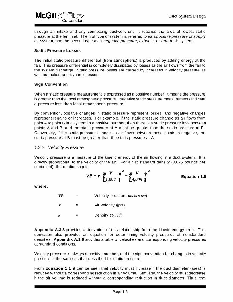
Duct System Design

Page 16

ρρ

4005V

= 1097

V = VP

2 2

through an intake and any connecting ductwork until it reaches the area of lowest static pressure at the fan inlet The first type of system is referred to as a positive pressure or supply air system and the second type as a negative pressure exhaust or return air system Static Pressure Losses The initial static pressure differential (from atmospheric) is produced by adding energy at the fan This pressure differential is completely dissipated by losses as the air flows from the fan to the system discharge Static pressure losses are caused by increases in velocity pressure as well as friction and dynamic losses Sign Convention When a static pressure measurement is expressed as a positive number it means the pressure is greater than the local atmospheric pressure Negative static pressure measurements indicate a pressure less than local atmospheric pressure By convention positive changes in static pressure represent losses and negative changes represent regains or increases For example if the static pressure change as air flows from point A to point B in a system i s a positive number then there is a static pressure loss between points A and B and the static pressure at A must be greater than the static pressure at B Conversely if the static pressure change as air flows between these points is negative the static pressure at B must be greater than the static pressure at A 132 Velocity Pressure Velocity pressure is a measure of the kinetic energy of the air flowing in a duct system It is directly proportional to the velocity of the air For air at standard density (0075 pounds per cubic foot) the relationship is

Equation 15 where

VP = Velocity pressure (inches wg) V = Air velocity (fpm) ρρ = Density (lbmft3)

Appendix A33 provides a derivation of this relationship from the kinetic energy term This derivation also provides an equation for determining velocity pressures at nonstandard densities Appendix A16 provides a table of velocities and corresponding velocity pressures at standard conditions Velocity pressure is always a positive number and the sign convention for changes in velocity pressure is the same as that described for static pressure From Equation 11 it can be seen that velocity must increase if the duct diameter (area) is reduced without a corresponding reduction in air volume Similarly the velocity must decrease if the air volume is reduced without a corresponding reduction in duct diameter Thus the

Duct System Design

Page 17

velocity and the velocity pressure in a duct system are constantly changing 133 Total Pressure Total pressure represents the energy of the air flowing in a duct system Because energy cannot be created or increased except by adding work or heat there is no way to increase the total pressure once the air leaves the fan The total pressure is at its maximum value at the fan outlet and must continually decrease as the air moves through the duct system toward the outlets Total pressure losses represent the irreversible conversion of static and kinetic energy to internal energy in the form of heat These losses are classified as either friction losses or dynamic losses Friction losses are produced whenever moving air flows in contact with a fixed boundary These are discussed in Section 14 Dynamic losses are the result of turbulence or changes in size shape direction or volume flow rate in a duct system These losses are discussed in Section 15 Referring to Equation 14 note that if the decrease in velocity pressure between two points in a system is greater than the total pressure loss t he static pressure must increase to maintain the equality Alternatively an increase in velocity pressure will result in a reduction in static pressure equal to the sum of the velocity pressure increase and the total pressure loss When there is both a decrease in velocity and a reduction in static pressure the total pressure will be reduced by the sum of these losses These three concepts are illustrated in Figure 13

Figure 13

Conservation of Energy Relationship 14 Pressure Loss In Duct (Friction Loss) When air flows through a duct friction is generated between the flowing air and the stationary duct wall Energy must be provided to overcome this friction and any energy converted irreversibly to heat is known as a friction loss The fan initially provides this energy in the form of pressure The amount of pressure necessary to overcome the friction in any section of duct depends on (1) the length of the duct (2) the diameter of the duct (3) the velocity (or volume) of the air flowing in the duct and (4) the friction factor of the duct

Duct System Design

Page 18

1000V

D1

256= 100ft

P 18118∆

100ftP∆

The friction factor is a function of duct diameter velocity fluid viscosity air density and surface roughness For nonstandard conditions see Section 15 The surface roughness can have a substantial impact on pressure loss and this is discussed in Appendix A35 These factors are combined in the Darcy equation to yield the pressure loss or the energy requirement for a particular section of duct Appendix A34 discusses the use and application of the Darcy equation 141 Round Duct One of the most important and useful tools available to the designer of duct systems is a friction loss chart (see Appendix A411) This chart is based on the Darcy equation and combines duct diameter velocity volume flow rate and pressure loss The chart is arranged in such a manner that knowing any two of these properties (at standard conditions) it is possible to determine the other two

The chart is arranged with pressure loss (per 100 feet of duct length) on the horizontal axis volume flow rate on the vertical axis duct diameter on diagonals sloping upward from left to right and velocity on diagonals sloping downward from left to right

Examination of this chart (or the Darcy equation) reveals several interesting air flow properties (1) at a constant volume flow rate reducing the duct diameter will increase the pressure loss (2) to maintain a constant pressure loss in ducts of different size larger volume flow rates require larger duct diameters and (3) for a given duct diameter larger volume flow rates will increase the pressure loss The following sample problems will give the reader a feel for these important relationships Although there are many nomographs or duct calculators available to speed the calculation of duct friction loss problems novice designers should use the friction loss charts to better visualize the relationships The friction loss chart in the Appendix is approximated by Equation 16

Equation 16

where = the friction loss per 100 ft of duct (inches wg)

D = the duct diameter (inches) V = the velocity of the air flow in the duct (fpm)

Sample Problem 1-5

What is the friction loss of a 150-foot long section of 18-inch diameter duct carrying 2500 cfm What is the air velocity in this duct Answer From the friction loss chart find the horizontal line that represents 2500 cfm

Move across this line to the point where it intersects the diagonal line which represents an 18-inch diameter duct From this point drop down to the horizontal

Duct System Design

Page 19

wginches 100ft

P016 =

1000

1412

18

1256 =

18118

∆

(pressure) axis and read the friction loss This value is approximately 016 inches wg This represents the pressure loss of a 100-foot section of 18-inch diameter duct carrying 2500 cfm To determine the pressure loss for a 150-foot duct section it is necessary to multiply the 100-foot loss by a factor of 15 Therefore the pressure loss is 024 inches wg

At the intersection of the 2500 cfm line and the 18-inch diameter line locate the nearest velocity diagonal The velocity is approximately 1400 fpm

Equation 16 could have also been used to solve this problem To use Equation 16 we must first calculate the velocity using Equation 11 To calculate the velocity we have to determine the cross-sectional area of the 18-inch diameter duct A = π x 182 576 = 177 ft2 The calculated velocity is QA = 2500177 = 1412 fpm The pressure loss per 100 ft is calculated as For a 150 ft section the pressure is 15 x 016 = 024 inches wg

Sample Problem 1-6

Part of a system you have designed includes a 20-inch diameter 500-foot duct run carrying 3000 cfm You now discover there is only 16 inches of space in which to install this section What will be the increase in pressure loss of the duct section if 16-inch duct is used in place of 20-inch Answer From the friction loss chart or Equation 16 find the pressure loss per 100 feet for

3000 cfm flowing through a 20-inch diameter duct This value is 014 inches wg or 070 inches wg for 500 feet Similarly the friction loss for 500 feet of 16-inch diameter duct carrying 3000 cfm is found to be 195 inches wg

Reducing this duct diameter by 4 inches results in an increase of pressure loss of 125 inches wg

Sample Problem 1-7

An installed system includes a 20-inch diameter 500-foot duct run carrying 3000 cfm Due to unanticipated conditions downstream it has become necessary to increase the volume flow rate in this duct section to 3600 cfm What will be the impact on the pressure loss of the section Answer From Sample Problem 1-6 the pressure drop of this section as installed is 070

inches wg To find the new pressure drop move up the 20-inch diameter line until it intersects the 3600 cfm volume flow rate line At this point read down to the friction loss axis and find that the new friction loss is 019 inches wg per 100

Duct System Design

Page 110

feet or 095 inches wg for 500 feet Therefore this 20 percent increase in volume will result in a 36 percent increase in the pressure loss for the duct section

Sample Problem 1-8

A system is being designed so that the pressure loss in all duct sections is equal to 02 inches wg per 100 feet What size duct will be required to carry (a) 500 cfm (b) 1500 cfm (c) 5000 cfm (d) 15000 cfm Answer From the friction loss chart find the vertical line that represents 020 inches wg per

100 feet friction loss Move up this line to the point where it intersects the horizontal line which represents a volume flow rate of 500 cfm At this point locate the nearest diagonal line representing duct diameter It will either be 9-inch duct or 95-inch duct (if half-inch duct sizes are available)

Similarly for the other volumes find the line representing duct size which is nearest to the intersection of the 020 inches wg per 100 feet friction loss line and the appropriate volume At 1500 cfm 14-inch duct is required at 5000 cfm 22-inch duct is required and at 15000 cfm 33-inch duct is required In each case the duct will carry the specified volume with a pressure loss of approximately 020 inches wg per 100 feet

142 Flat Oval Duct Flat oval duct has the advantage of allowing a greater duct cross-sectional area to be accommodated in areas with reduced vertical clearances Figure 14 shows a typical cross section of flat oval duct References in Appendices A1 A2 and A9 provide additional information about flat oval duct

Figure 14 Flat Oval Dimensions The Darcy equation is not applicable to flat oval duct and there are no friction loss charts available for non-round duct shapes To calculate the friction loss for flat oval duct it is necessary to determine the equivalent round diameter of the flat oval size and then determine the friction loss for the equivalent round duct

Duct System Design

Page 111

)(P)(A 155

= D 025

0625

eq

1444

)minx (+)minx (FS

= A

2ππ

12x FS) 2( + )minx (

= Pππ

The equivalent round diameter of flat oval duct is the diameter of round duct that has the same pressure loss per unit length at the same volume flow rate as the flat oval duct Equation 17 can be used to calculate the equivalent round diameter for flat oval duct with cross-sectional area A and perimeter P The equivalent round diameters for many standard sizes of flat oval duct are given in Appendix A132

Equation 17

where

Deq = Equivalent round diameter (ft) A = Flat oval cross-sectional area (ft2) P = Flat oval perimeter (ft)

The flat oval cross-sectional area is calculated using Equation 18

Equation 18

where

A = Cross-sectional area (ft2) FS = Flat Span (inches) = maj - min min = Minor axis (inches) maj = Major axis (inches)

The perimeter of flat oval is calculated using Equation 19

Equation 19

where

P = Flat oval perimeter (ft)

When calculating the air velocity in flat oval duct it is necessary to use the actual cross-sectional area of the flat oval shape not the area of the equivalent round duct To use Equation 16 however the air velocity is calculated using the equivalent round diameter cross sectional area

Duct System Design

Page 112

Sample Problem 1-9

A 12-inch x 45-inch flat oval duct is designed to carry 10000 cfm What is the pressure loss per 100 feet of this section What is the velocity Answer Equations 18 and 19 are used to calculate the area and perimeter of the flat

oval duct For 12 x 45 duct A = 354 ft2 from (45 - 12) x 12 + (π x 122)4144 and P = 864 ft from (π x 12) + (2 x (45-12))12 Substituting into Equation 17 Deq = 199 ft 24 inches From the friction loss chart the pressure loss of 10000 cfm air flowing in a 24-inch round duct is 050 inch wg per 100 feet

The velocity can be calculated from Equation 11

V = QA = 10000 354 = 2825 fpm

Note that the velocity of the same air volume flowing in the 24-inch diameter round duct is 10000 314 or 3185 fpm

Alternatively to use Equation 16 we must first calculate the velocity assuming the cross-sectional area is determined from the equivalent round

ftA2

Deq 314 = 576

)24x ( 2π=

fpm V Deq 3185 = 314

10000 =

wginches 100ft

P 048=

1000

3185

24

1256 =

18118

∆

Which is close to the 050 incheswg determined from the friction loss chart

Sample Problem 1-10

In Sample Problem 1-6 what size flat oval duct would be required in order to maintain the original (070 inches wg) pressure drop and still fit within the 16-inch space allowance Answer In this situation the available space will dictate the minor axis dimension of the

Duct System Design

Page 113

flat oval duct It is always advisable to allow at least 2 to 4 inches for the reinforcement which may be required on any flat oval or rectangular duct product Therefore we will assume that the largest minor axis that can be accommodated is 12 inches

Since we want to select a flat oval size which will have the same pressure loss as a 20-inch round duct the major axis dimension can be determined by solving Equation 17 with Deq = 167 feet (20 inches) and min = 12 inches Using Equations 18 and 19 for determining A and P as functions of the major axis dimension (maj) and the minor axis dimension (min) Unfortunately this requires an iterative solution

A simpler solution is to refer to the tables in Appendix A132 These tables list the various available flat oval sizes and their respective equivalent round diameters Since we already know that the minor axis must be 12 inches we look for a flat oval size with a 12-inch minor axis and an equivalent round diameter of 20 inches The required flat oval size is 12 inches x 31 inches

If it is determined that there is room for a 14-inch minor axis duct the required size would be 14 inches x 27 inches (Deq = 20 inches)

143 Rectangular Duct Rectangular duct is fabricated by breaking two individual sheets of sheet metal (called L-sections) that have the appropriate duct dimensions (side and side adjacent) and joining them together by one of several techniques Rectangular duct is also used when height restrictions are employed in a duct design Equation 110 can be used to calculate the equivalent round diameter Deq of rectangular duct The equivalent round diameter Deq for many standard sizes of rectangular duct are given in Appendix 14

Equation 110

where

Deq = Equivalent round diameter (inches)

a = Duct side length (inches) b = Other duct side length (inches)

When calculating air velocity in rectangular duct it is necessary to use the actual cross-sectional area of the rectangular shape not the area of the equivalent round diameter

)b+(a)(ab 130

= D 0250

0625

eq

Duct System Design

Page 114

Sample Problem 1-11

A 12-inch x 45-inch rectangular duct is designed to carry 10000 cfm What is the pressure loss per 100 feet of this section What is the velocity Answer Using Equation 110 Deq = 24 inches From the friction loss chart the loss of

10000 cfm air flowing in a 24-inch round duct is 050 inch wg per 100 feet

The velocity can be calculated from Equation 11

fpmA

Q = V 2667=

45)144 x (12

10000 =

Note that the velocity in the rectangular duct is less than in the flat oval with the same major and minor dimensions (See Sample Problem 1-9)

144 Acoustically Lined and Double-wall Duct Applying an inner liner or a perforated inner metal shell sandwiching insulation between an inner and outer wall increases the surface roughness that air sees and thus increases the friction losses of duct Acoustically lined round and rectangular duct consist of a single-wall duct with an internal insulation liner but no inner metal shell Double-wall duct that is acoustically insulated consists of a solid outer shell a thermalacoustical insulation and a metal inner liner (either solid or perforated) The inner dimensions of lined duct or the metal inner liner dimensions of double-wall duct are the nominal duct size dimensions that are used to determine the cross-sectional area for airflow calculations The single-wall dimensions of lined duct or outer shell dimensions of double-wall duct depend on the insulation thickness For a 1-inch thick insulation the dimensions are 2 inches larger than the inner dimensions of lined duct or metal inner liner dimensions Acoustically Lined Duct Correction factors to the friction loss determined from the friction loss chart or for Equation 16 have not been developed for internally insulated duct Therefore the designer must use the Darcey equation as given in Appendix A34 Assume an absolute roughness of ε = 0015 Double-wall Duct

Corrections factors to the friction loss determined from the friction loss chart or Equation 16 have been developed for when a perforated metal inner liner is used Figure 15 is a chart which gives the correction factors This information is repeated in Appendix A412 Note that these corrections are a function of duct diameter and velocity If the duct shape is flat oval or rectangular use the equivalent round diameter based on the perforated metal inner liner dimensions If the inner shell of the double-wall duct does not use perforated metal use the same friction loss as a single-wall duct of the same dimensions as the metal inner shell

Duct System Design

Page 115

13

12

11

10

4rdquo 8rdquo

12rdquo

18rdquo

36rdquo

72rdquo

2000 3000 4000 5000 6000

Correction factor to be applied to the friction loss of single-wall duct to calculate the friction loss of double-wall duct with a perforated metal inner liner

Velocity (fpm)

Figure 15 Correction Factors for Double-Wall Duct with Perforated Metal Inne r Liner When only thermal insulation is required the metal inner liner may be specified as solid rather than perforated metal In this case the friction losses are identical to those for single-wall duct with a diameter equal to the metal inner liner diameter For acoustically insulated flat oval or rectangular duct with a perforated metal inner liner use the correction factors of the equivalent round diameter and the actual velocity (based on the metal inner liner of the flat oval or rectangular cross section) The reference in Appendix A92 addresses friction losses for lined rectangular duct

Sample Problem 1-12

What is the friction loss of a 100-foot section of 22-inch diameter double-wall duct (with perforated metal inner liner) carrying 8000 cfm Answer The pressure loss for 100 feet of 22-inch single-wall duct carrying 8000 cfm is

found from the friction loss chart to be 050 inches wg The velocity is 3000 fpm

From Figure 15 the correction factor for 22-inch duct (interpolated) at 3000 fpm is approximately116Therefore the pressure loss of this section of double-wall duct is 050 x 116 or 058 inches wg

145 Nonstandard Conditions All loss calculations thus far have been made assuming a standard air density of 0075 pounds per cubic foot When the actual design conditions vary appreciably from standard (ie temperature is 30degF from 70degF elevation above 1500 feet or moisture greater than 002 pounds water per pound dry air) the air density and viscosity will change If the Darcy equation is used to calculate friction losses and the friction factor and velocity pressure are calculated using

Duct System Design

Page 116

actual conditions no additional corrections are necessary If a nomograph or friction chart is used to calculate friction losses at standard conditions correction factors should be applied The corrections for nonstandard conditions discussed above apply to duct friction losses only Other corrections are applicable to the dynamic losses of fittings as will be explained in the following section For a more in-depth presentation of these and other correction factors see Reference in Appendix A92 Tables for determining correction factors are included in Appendix A15 A temperature correction factor Kt can be calculated as follows

460) + T(

530= K

a

0825

t Equation 111

where

Kt = Nonstandard temperature correction factor Ta = Actual temperature of air in the duct (degF)

An elevation correction factor Ke can be calculated as follows

](Z) )10x (68754 -1[= K473-6

e Equation 112a

Equation 112a can also be written as follows

ββ29921

= K09

e Equation 112b

where

Ke = Nonstandard elevation correction factor Z = Elevation above sea level (feet) ββ = Actual barometric pressure (inches Hg)

When both a nonstandard temperature and a nonstandard elevation are present the correction factors are multiplicative As an equation

Kx K= K etf Equation 113

where

Kf = Total friction loss correction factor

The calculated duct friction pressure loss should be multiplied by the appropriate correction factor Kt Ke or Kf to obtain the actual pressure loss at the nonstandard conditions

Duct System Design

Page 117

Sample Problem 1-13

The friction loss for a certain segment of a duct system is calculated to be 25 inches wg at standard conditions What is the corrected friction loss if (a) the design temperature is 30degF (b) the design temperature is 110degF (c) the design elevation is 5000 feet above sea level (d) both (b) and (c) Answer 1 Substituting into Equation 111 Kt = [530(30 + 460)]0825 = 107

Corrected friction loss = 25 x 107 = 268 inches wg

2 Kt = [530(110 + 460)]0825 = 094 Corrected friction loss = 235 inches wg

3 Substituting into Equation 112a Ke = [1 - (68754 x 10-6)(5000)] 473 = 085 Corrected friction loss = 213 inches wg

4 Substituting into Equation 113 Kf = 094 x 085 = 080 Corrected

friction loss = 200 inches wg

If moisture in the airstream is a concern a humidity correction factor Kh can be calculated as follows

(( )) 90

wsh

P37801K

ββ

minusminus== Equation 114

where

Pws = Saturation pressure of water vapor at the dew point

temperature (inches Hg) ββ = Actual barometric pressure (inches Hg)

The total friction loss correction factor Kf is expressed as

hetf Kx Kx K= K Equation 115

15 Pressure Loss in Supply Fittings As mentioned in Section 13 pressure losses can be the result of either friction losses or dynamic losses Section 14 discussed friction losses produced by air flowing over a fixed boundary This section will address dynamic losses Friction losses are primarily associated with duct sections while dynamic losses are exclusively attributable to fittings or obstructions Dynamic losses will result whenever the direction or volume of air flowing in a duct is altered or when the size or shape of the duct carrying the air is altered Fittings of any type will produce dynamic losses The dynamic loss of a fitting is generally proportional to the severity of the airflow disturbance A smooth large radius elbow for example will have a much lower dynamic

Duct System Design

Page 118

loss than a mitered (two-piece) sharp-bend elbow Similarly a 45deg branch fitting will usually have lower dynamic losses than a straight 90deg tee branch 151 Loss Coefficients In order to quantify fitting losses a dimensionless parameter known as a loss coefficient has been developed Every fitting has associated loss coefficients which can be det ermined experimentally by measuring the total pressure loss through the fitting for varying flow conditions Equation 116a is the general equation for the loss coefficient of a fitting

VPTP

= C∆

Equation 116a

where C = Fitting loss coeffi cient ∆∆TP = Change in total pressure of air flowing through the fitting (inches

wg) VP = Velocity pressure of air flowing through the fitting (inches wg)

Once the loss coefficient for a particular fitting or class of fittings has been experimentally determined the total pressure loss for any flow condition can be determined Rewriting Equation 116a we obtain

VPx C= TP∆ Equation 116b

From this equation it can be seen that the total pressure loss is directly proportional to both the loss coefficient and the velocity pressure Higher loss coefficient values or increases in velocity will result in higher total pressure losses for a fitting A less efficient fitting will have a higher loss coefficient (ie for a given velocity the tot al pressure loss is greater) 152 Elbows Table 11 shows typical loss coefficients for 8-inch diameter elbows of various construction Table 11 Loss Coefficient Comparisons for Abrupt-Turn Fittings

90EE Elbows 8-inch Diameter Fitting

Loss Coefficient

Die-StampedPressed 15 Centerline Radius

011 Five-Piece 15 Centerline Radius

022

Mitered with Turning Vanes

052 Mitered

124

From Equation 14 we can determine the pressure loss

∆∆TP = ∆∆SP + ∆∆VP

Duct System Design

Page 119

Since the elbow diameter and volume flow rate are constant the continuity equation (Equation 11) tells us that the velocity will be constant From Equation 15 the velocity pressure is a direct function of velocity and so ∆∆VP = 0 Therefore ∆∆SP = ∆∆TP Note that whenever there is no change in velocity as is the case in duct and constant diameter elbows the change in static pressure is equal to the change in total pressure

Sample Problem 1-14

What is the total pressure loss of an 8-inch diameter die-stamped elbow carrying 600 cfm What is the static pressure loss Answer From Equation 11

Q = A x V or V = QA A = πD2576 = π (8)2 576 = 035 ft2 V = 600 035 V = 1714 fpm

From Equation 15 or Appendix A16

wginches VP 018= 40051714

=2

From Table 11

C = 011 (die-stamped elbow) From Equation 116b

∆TP = C x VP = 011 x 018 = 002 inches wg

Sample Problem 1-15

A designer is trying to determine which 8-inch elbow to select for a location which will have a design velocity of 1714 fpm What will be the implications in terms of pressure loss if the designer chooses (1) a die-stamped elbow (2) a five-gore elbow (3) a mitered elbow with turning vanes or (4) a mitered elbow without turning vanes Answer From Sample Problem 1-14 we calculated the total pressure loss of an 8-inch

die-stamped elbow at 1714 fpm to be 002 inches wg

For the other elbows we can determine the pressure loss from loss coefficients given in Table 11

Duct System Design

Page 120

C2 = 022 C3 = 052 C4 = 124

From Equation 116b

∆TP2 = ∆SP2 = 022 x 018 = 004 inches wg (five-gore)

∆TP3 = ∆SP3 = 052 x 018 = 009 inches wg (mitered with turning vanes)

∆TP4 = ∆SP4 = 124 x 018 = 022 inches wg (mitered without turning vanes)

Therefore using a five-gore elbow will increase the total pressure loss by 100 percent but it will be a very modest 004 inches wg Using the mitered elbow with vanes would result in a 350 percent increase over the die-stamped elbow or a 125 percent increase over the five-gore elbow The mitered elbow without turning vanes would have a loss of 022 inches wg which is a tenfold increase over the die-stamped elbow

The increased pressure losses associated with the use of les s efficient fittings may or may not be critical to the operation of the system depending on the location of the fittings Succeeding chapters will note when there could be locations in a system where it is desirable to increase the losses of certain fittings In general unless the system has been carefully analyzed to determine the location of the critical path(s) and the excess pressures present in other paths it is wise to always select fittings with the lowest pressure drop The loss coefficients of most elbows vary as a function of diameter The ASHRAE Duct Fitting Database Program (Appendix A82) presents loss coefficients as a function of diameter for various elbow constructions The loss coefficient drops sharply as diameters increase through approximately 24 inches then only slightly from 24 inches through 60 inches Also eliminating turning vanes in mitered elbows more than doubles the pressure loss Flat Oval Elbows Although the use of equivalent duct lengths as a measure of dynamic fitting losses is usually strongly discouraged it provides acceptable approximations in the case of flat oval elbows Data indicates that flat oval 90deg elbows (hard or easy bend) with 15 centerline radius bends have a pressure loss approximately equal to the friction loss of a flat oval duct with an identical cross section and a length equal to nine times the elbow major axis dimension calculated at the same air velocity that is flowing through the elbow For example a 12-inch x 31-inch flat oval elbow would have a pressure loss approximately equal to that of a 12-inch x 31-inch flat oval duct 23 feet long (9 x 31 inches) at the same velocity For flat oval elbows that do not have a 15 centerline radius bend use the loss coefficient for a round elbow of similar construction with the diameter equal to the flat oval minor axis Rectangular Elbows (see ASHRAE== s Duct Fitting Database Program)

Duct System Design

Page 121

VPTP= C

b

b-cb

∆

Acoustically LinedDouble-wall Elbows For acoustically lined elbows or double-wall elbows with either a solid or perforated metal inner liner the losses are the same as for standard single-wall elbows with dimensions equal to the metal inner liner dimensions of the acoustically lined or double-wall elbow Elbows With Bend Angles Less Than 90deg For elbows constructed with bend angles less than 90deg multiply the calculated pressure loss for a 90deg elbow by the correction factor given in Table 12

Table 12 Elbow Bend Angle Correction Factor

Angle CFelb

225deg 031

30deg 045

45deg 060

60deg 078

75deg 090 153 Diverging-Flow Fittings Branches The pressure losses in diverging-flow fittings are somewhat more complicated than elbows for two reasons (1) there are multiple flow paths and (2) there will almost always be velocity changes First consider the case of air flowing from the common (upstream) section to the branch Referring to Figure 11 this is from c to b (Refer to Appendix A11 for clarification of upstream and downstream) As is the case for elbows loss coefficients are determined experimentally for diverging-flow fittings However it is now necessary to specify which flow paths the equation parameters refer to By definition

Equation 117a

where

Cb = Branch loss coefficient ∆TPc-b = Total pressure loss common-to-branch (inches wg) VPb = Branch velocity pressure (inches wg)

Rewriting in terms of total pressure loss

∆TPc-b = Cb x VPb Equation 117b Therefore the total pressure loss of air flowing into the branch leg of a diverging-flow fitting is

Duct System Design

Page 122

directly proportional to the branch loss coefficient and the branch velocity pressure For duct and elbows the total pressure loss is always equal to the static pressure loss because there is no change in velocity However diverging-flow fittings almost always have velocity changes associated with them If ∆VP is not zero then the total and static pressure losses cannot be equal (Equation 14) For diverging-flow fittings the static pressure loss of air flowing into the branch leg can be determined from Equation 117c

∆SPc-b = VPb (Cb + 1) - VPc Equation 117c where

∆SPc-b = Static pressure loss common-to-branch (inches wg) VPb = Branch velocity pressure (inches wg) VPc = Common velocity pressure (inches wg) Cb = Branch loss coefficient (dimensionless)

Equation 117c is derived from Equations 117a and 117b as shown in Appendix A36

As is the case for elbows a comparison of loss coefficients gives a good indication of relative fitting efficiencies The following samples compare loss coefficients of various diverging-flow fittings

Duct System Design

Page 123

Table 13 Loss Coefficient Comparisons for Diverging-Flow Fittings

Fitting Loss Coefficient

(Cb) Y-Branch plus 45deg Elbows

022

Vee Fitting

030

Tee with Turning Vanes plus Branch Reducers (Bullhead Tee with Vanes)

045

Tee plus Branch Reducers

108

Capped Cross with Straight Branches

445

Capped Cross with Conical Branches

445

Capped Cross with 1-foot Cushion Head

54

Capped Cross with 2-foot Cushion Head

60

Capped Cross with 3-foot Cushion Head

64

The loss coefficient Cb is for a VbVc ratio of approximately 10

Duct System Design

Page 124

AA

Q

Q VP V VP V

c

b

c

bbbcc

Sample Problem 1-16

What is the total pressure loss for flow from c to b in the straight tee shown below What is the static pressure loss Answer ∆TPc-b = Cb x VPb From Equation 117b

∆SPc-b = VPb (Cb + 1) - VPc From Equation 117c Reference ASHRAE Duct Fitting Database Number SD5-9 Given Qc = 5000 cfm Dc = 24 inches

Qb = 2000 cfm Db = 18 inches

Qs = 3000 cfm Ds = 24 inches Calculate

fpmA

Q V

c

cc 1592 =

314

5000 ==

c

s

b

Duct System Design

Page 125

wginches4005

VVP c

2

c 016 = 40051592

==2

fpmA

Q V

b

bb 1130 =

177

2000 ==

wginches4005

VVP b

2

b 008 = 40051130

==2

040 = 50002000

= Q

Q

c

b

056 = 314

177 =

A

A

c

b

Determine Cb - Interpolated from the ASHRAE table = 214

Answer ∆TPc-b = 214 x 008 = 017 inches wg

∆SPc-b = 008 (214 + 1) - 016 = 009 inches wg

Duct System Design

Page 126

Sample Problem 1-17

What would be the static and total pressure losses in Sample Problem 1-16 if a conical tee were substituted for the straight tee A LO-LOSSTM tee Reference Conical Tee ASHRAE Fitting SD5-10

LO-LOSST M Tee ASHRAE Fitting SD5-12 Determine Cb (conical) = 135

Cb (LO-LOSST M) = 079 Answer ∆TPc-b (conical) = 011 inches wg

∆SPc-b (conical) = 003 inches wg ∆TPc-b (LO-LOSST M) = 006 inches wg ∆SPc-b (LO-LOSST M) = -002 inches wg

In the preceding problem the static pressure loss for a LO-LOSST M tee at the given conditions resulted in a negative number Recall from Section 131 that a pressure change expressed as a positive number is a loss while a pressure change expressed as a negative number represents an increase in pressure This pressure increase is a common phenomenon in air handling systems and is known as static regain It occurs for the LO-LOSST M fitting because the decrease in velocity pressure is greater than the total pressure loss of the fitting Total Pressure Losses versus Static Pressure Losses Just as total pressure represents the total energy present at any point in a system the total pressure loss of a fitting represents the true energy loss of the fitting for a given flow situation Static pressure losses are useful for certain design methods as we shall see later however they do not give an accurate indication of fitting efficiency Sample Problem 1-18 illustrates this concept

Duct System Design

Page 127

Sample Problem 1-18

Change the branch size in Sample 1-17 from 18 inches diameter to 12 inches diameter and recalculate the total and static pressure losses of the LO-LOSS TM tee

Reference ASHRAE Fitting SD5-12 Given Qc = 5000 cfm Dc = 24 inches

Qb = 2000 cfm Db = 12 inches Qs = 3000 cfm Ds = 24 inches

Calculate AA

Q

Q VP V VP V

c

b

c

bbbcc

Vc = 1592 fpm VPc = 016 inches wg Vb = 2548 fpm VPb = 040 inches wg Qb Qc = 040 Ab Ac = 025

Determine Cb Interpolate from ASHRAE Fitting SD5-12 = 021 Answer ∆TPc-b = CbxVPb (from Equation 117b) = 021x040 = 008 inches wg ∆SPc-b = VPb (Cb + 1) - VPc (from Equation 117c) = 040(021+1)-016 = 032 inches wg In this problem the total pressure loss is 008 inches wg but the static pressure loss is 032 inches wg If one were to look only at the static pressure this would seem to be a very inefficient fitting However notice that due to flow and pressure conditions in the system the velocity increased as the air moved from the common section into the branch resulting in a velocity pressure increase of 024 inches wg

c s

b

Duct System Design

Page 128

This situation is shown in Figure 13 Case II The apparently large decrease in static pressure was caused by a large increase in velocity pressure As Equation 14 this becomes

008 = 032 + -024 (∆TP = ∆SP + ∆VP )

Conversely when certain flow conditions are present it is possible for a fitting to have a small static pressure loss but a relatively large total pressure loss It is always advisable to calculate the total pressure loss in order to determine the total energy consumption of a fitting Manifold Fittings The single-branch fittings discussed thus far are assumed to be factory fabricated and constructed as a separate unit from the duct to which t hey would be attached Occasionally it is desirable to construct a manifold fitting with a tap attached directly to the duct This construction will generally result in a less efficient fitting especially if the manifold is constructed in the field Flat Oval Diverging-Flow Fittings Diverging-flow fittings of similar construction generally exhibit the same pressure loss for the same volume flow rate ratios and area ratios Flat oval fittings exhibit similar pressure losses as round fittings Testing is under way to develop a database of loss coefficients for flat oval diverging-flow fittings Until this data is available use the same loss coefficients as for the same construction of round Acoustically Lined and Double-wall Diverging-Flow Fittings Whether a fitting has been acoustically lined or has a perforated metal inner shell the difference in surface roughness is accounted for in the friction loss determination since all friction loss calculations are base on fitting-to-fitting centerline dimensions Therefore there is no need to increase the dynamic loss of a diverging flow-fitting that is either acoustically lined or one that has an inner metal shell even if the shell is perforated Determine the loss coefficient of the fitting as if it were a single-wall fitting with the dimension of the inner liner or metal inner shell Rectangular Diverging-Flow Fittings (see ASHRAE== s Duct Fitting Database Program) 154 Diverging-Flow Fittings Straight-Throughs Reducers and Transitions Straight-Throughs The straight-through (downstream) leg of a diverging-flow fitting is that path followed by air flowing from c to s as represented in Figure 11 The straight -through may have a constant diameter such that Dc = Ds or there may be a reducer attached to the straight -through such that Dc gt Ds In the case of a constant diameter straight -through there will always be a velocity reduction caused by a reduced volume (after the branch) flowing through the same diameter duct If a reducer is attac hed to the straight -through it can be sized to reduce maintain or increase the downstream velocity relative to the common velocity Dynamic losses associated with air flowing straight through a diverging-flow fitting andor a

Duct System Design

Page 129

reducer is very slight This is understandable since there is little physical disturbance of the airflow The total pressure loss in a straight -through leg or reducer is often only a few hundredths of an inch wg Perhaps the most important phenomenon associated with the straight-through flow situation is the potential for static regain This situation is illustrated in Figure 13 Case I A large reduction in velocity pressure and a small reduction in total pressure must (by Equation 14) result in an increase in static pressure or static regain The regain will be equal in magnitude to the velocity pressure loss minus the total pressure loss Of course if the total pressure loss is greater than the reduction in velocity pressure as shown in Figure 13 Case III there can be no static regain Referring again to Sample Problem 1-16 we see that the velocity in the constant diameter straight -through leg is reduced from 1592 fpm (VPc = 016 inches wg) in the duct before the straight -through to 955 fpm (VPs = 006 inches wg) in the duct after the straight -through due to the reduced volume flow This is a velocity pressure reduction of ∆VPc-s = 010 inches wg If we assume a total pressure loss of ∆TPc-s = 001 inches wg then from Equation 14 we get

001 = ∆SPc-s + 010 or ∆SPc-s = -009 inches wg The negative result indicates a static regain or that the static pressure at point s will be 009 inches wg higher than the static pressure at point c The loss coefficient data for reducers and straight -throughs is found in the ASHRAE Duct Fitting Database When using loss coefficients to determine straight -through losses Equations 117b and 117c are rewritten as follows

∆∆TPc-s = Cs x VPs Equation 118a ∆∆SPc-s = VPs (Cs + 1) - VPc Equation 118b

where

∆∆TPc-s = Total pressure loss common-to-straight-through (inches wg) ∆∆SPc-s = Static pressure loss common-to-straight-through (inches wg) VPc = Common velocity pressure (inches wg) VPs = Straight-through velocity pressure (inches wg) Cs = Straight-through loss coefficient

Sample Problem 1-19

Calculate the total and static pressure losses for the straight-through portion of the straight tee in Sample Problem 1-16

Reference ASHRAE Fitting SD5-9

Duct System Design

Page 130

Calculate AA

Q

Q VP V VP V

c

s

c

ssscc

Vc = 1592 fpm VPc = 016 inches wg

Vs = 955 fpm VPs= 006 inches wg

Qs Qc = 060 As Ac = 10

Determine Cs Interpolate from ASHRAE Fitting SD5-9 = 020 Answer

∆TPc-s = Cs x VPs (Equation 118a ) = 020 x 006 = 001 inches wg ∆SPc-s = VPs (Cs + 1) - VPc (Equation 118b) = 006(020 + 1) - 016 = -009 inches wg

Reducers A stand-alone reducer will cause the velocity to increase since after the reducer the same volume of air will be flowing through a smaller diameter duct (see Sample Problem 1-2) The use of a reducer on its own is not consistent with any design methods presented in this manual and should be fairly rare in most duct systems However when this fitting is used the losses are calculated using the same charts and in the same manner as the straight -throughs Losses are a function of upstream and downstream velocity Reducing fittings should be constructed as shown in Figure 17 such that the length of the taper portion (L) is equal to the difference between the common diameter and the straight -through diameter (Dc - Ds) Verify this with manufacturers dimension sheets Since reducers are very efficient fittings the use of a longer taper section will not necessarily provide a significant improvement in performance

Figure 17 Reducing Fitting Construction Transitions Transitions between round and flat oval duct also produce dynamic pressure losses As with other fittings these losses can be quantified in terms of a loss coefficient The loss coefficient

Duct System Design

Page 131

for round-to-flat oval or flat oval-to-round transitions depends on the flat oval aspect ratio (major axisminor axis) the direction of airflow and the air velocity When round duct transitions to flat oval the flat oval minor axis dimension is usually less than the original round diameter while the flat oval major axis dimension is greater than the round diameter The reverse is true in transitions from flat oval to round Therefore roundflat oval transitions usually involve both a reducer effect (round to flat oval minor or flat oval major to round) and an enlarger effect (round to flat oval major or flat oval minor to round) The change in dimension involving the flat oval major axis is normally much greater than the change tofrom the flat oval minor axis Therefore in round-to-flat oval transitions the enlarger effect predominates while in flat oval-to-round transitions the reducer effect predominates Dynamic losses which result from expanding areas (decreasing velocities) are always more severe than losses from reducing areas (increasing velocities) Therefore the flat oval-to-round transition is more efficient than the round-to-flat oval fitting Figure A24 in Appendix A4 2 is a plot of loss coefficient (Cs ) versus round duct velocity for both round-to-flat oval and flat oval-to-round transitions The curves are valid for any size flat oval and will be conservative for transitions involving flat oval with a low aspect ratio Use the appropriate loss coefficient value in the following equations to determine static and total pressure losses for transition fittings

∆∆TPc-s = Cs x VPs Equation 119a ∆∆SPc-s = VPs (Cs + 1) - VPc Equation 119b where

∆∆TPc-s = Total pressure loss common-to-straight-through (inches wg) ∆∆SPc-s = Static pressure loss common-to-straight-through (inches wg) VPc = Common velocity pressure (inches wg) VPs = Straight-through velocity pressure (inches wg) Cs = Straight-through loss coefficient

Sample Problem 1-20

In Sample Problem 1-10 we determined that a 12-inch H 31-inch flat oval duct would have the same pressure loss per unit length as a 20-inch round duct What would be the impact on total and static pressure losses in a 100-foot section of 20-inch round duct carrying 5000 cfm if 40 feet of this duct were replaced by a 12-inch H 31-inch flat oval duct Assume the first 30 feet of duct is round next 40 feet is flat oval and the last 30 feet is round Answer Since the duct sizes are equivalent 40 feet of 12-inch H 31-inch flat oval would

have the same pressure loss per 100 feet as the section of 20-inch round duct it replaced The addition of two transitions one round-to-flat oval at the start of the

Duct System Design

Page 132

40-foot section and the other flat oval-to-round at the transition back to round duct would cause the only change in pressure loss

The velocity in the 20-inch round duct carrying 5000 cfm is 2294 fpm (VP = 033 inches wg) The flat oval duct cross-sectional area from Appendix A13 is 236 ft2 therefore the velocity in the flat oval duct is 2119 fpm (VP = 028 inches wg) From Appendix A434 the loss coefficients at 2294 fpm are Cr-o = 017 and Co-r = 006

Substituting into Equations 119a and 119b

∆TPc-sr-o = 017 x 028 = 005 inches wg ∆TP c-so-r = 006 x 033 = 002 inches wg ∆SPc-sr-o = 028 (017 + 1) - 033 = -000 (-0002) inches wg ∆SP c-so-r = 033 (006 + 1) - 028 = -007 inches wg

The flat oval section will therefore increase the total pressure loss by an additional 007 inches wg (005 + 002) due to the combined effects of both transitions As expected since there was no net change in velocity in the round duct ∆VP = 0 and (by Equation 14) the combined static pressure loss (007 inches wg) is equal to the combined total pressure loss

155 Miscellaneous Fittings Heel-Tapped Elbows The tee-type diverging-flow fittings discussed in Section 153 are generally used where the designer desires to direct a relatively small quantity of air at some angle relative to the main trunk duct while maintaining a straight -through flow for the majority of the air Occasionally situations arise where the main air stream must be diverted at some angle while a smaller quantity of air is required in a straight -through direction In these situations the use of a heel -tapped elbow will generally result in lower pressure losses in both common and branch directions ASHRAE Fitting SD5-21 presents loss coefficients (Cb) for both the straight-through tap and the elbow section of heel -tapped elbows as a function of velocity ratio Use Equations 117b and 117c for determining the total and static pressure losses If 65 percent or more of the airflow is diverted then it is advisable to use a heel-tapped elbow

Sample Problem 1-21

A diverging-flow fitting must be selected which will split 10000 cfm volume flow rate such that 7000 cfm will flow at a 90E angle relative to the upstream direction and 3000 cfm will continue in the same direction as the upstream flow Compare the performance of a (a) straight tee (b) conical tee (c) LOLOSSTM tee and (d) heel-tapped elbow and select the most efficient fitting for this situation Assume it is desired to

Duct System Design

Page 133

maintain approximately constant velocity Given

Qc = 10000 cfm Qb = 7000 cfm Qs = 3000 cfm Dc = 28 inches Db = 23 inches Ds = 15 inches Ac = 428 sq ft Ab = 289 sq ft As = 123 sq ft Vc = 2336 fpm Vb = 2422 fpm Vs = 2439 fpm VP = 034 inches wg VPb = 037 inches wg VPs = 037 inches wg QbQc = 070 QsQc = 030 AbAc = 068 AsAc = 029

Reference

Straight Tee ASHRAE Fitting SD5-9 Conical Tee ASHRAE Fitting SD5-10 LO-LOSST MTee ASHRAE Fitting SD5-12 Heel-tapped Elbow ASHRAE Fitting SD5-21

Determine

Coefficients Cb Cs

Straight Tee 115 013 Conical Tee 062 013 LO-LOSST M Tee 033 013 Heel-tapped Elbow 065 009

Answer

Pressure Losses (inches wg)

∆TPc-b ∆TPc-s ∆SPc-b ∆SPc-s

Straight Tee 043 005 046 008 Conical Tee 023 005 026 008 LO-LOSST M Tee 012 005 015 008 Heel-tapped Elbow 024 003 027 006

Duct System Design

Page 134

In this case the heel-tapped elbow and the conical tee will have nearly the same total pressure loss in the 90E bend direction The heel-tapped elbow provides a significant performance increase over the straight tee but has a higher loss than the LO-LOSST M tee branch The straight-through leg of the heel-tapped elbow is slightly more efficient than the straight -throughs of the tees

The best fitting though based strictly on efficiency would appear to be the LO-LOSST M tee However bear in mind that all three tee fittings will require substantial strai ght-through reducers (28 inches to 15 inches) which will generally be at least 12 inches long (Figure 17) and will add substantially to the cost of the fitting If a compromise between cost and performance is desired the heel-tapped elbow may still be the best choice for these flow situations Also increased loss may help balance the leg in which this fitting resides

Note that in Sample Problem 1-21 the total pressure is lower than the static pressure by 003 inches wg in all cases due to the increase in velocity pressure (003 inches wg) from common to both straight-through and branch In the form of Equation 14

∆TPc-b = ∆SPc-b - 003 ∆TPc-s = ∆SPc-s - 003

Crosses Cross fittings are those which have two taps located at the same cross section of a main or trunk duct Usually these taps will be constructed so that they discharge air in diametrically opposed directions The pressure loss of the taps on a cross fitting depends to a large extent on the cross-sectional area reduction of the straight-through duct For straight -through area reductions of less that 20 percent the branch losses through either tap of a cross fitting will be the same as those for a single-branch fitting with identical tap construction For example a conical cross (a cross with conical taps) that has a straight -through of 24 inches reducing to 22 inches would have an area reduction of 16 percent Since this is less than 20 percent the branch losses for either tap would be found from the direct-read charts in ASHRAE Fittings SD5-9 through SD5-17 For crosses where the straight -through area reduction exceeds 20 percent use the loss coefficients presented in ASHRAE Fittings SD5-23 through SD5-26 The three curves shown are for varying percentage area reductions and apply for all tap constructions Use interpolation to find loss coefficients for area reductions between these curves Use Equations 117b and 117c for determining the total and static pressure losses of each branch Split Fittings Split fittings are diverging-flow fittings where the air divides into two branches each of which turns at 90E to the main There is no straight-through leg The most common types of split fittings are the Vee Y-branch and the bullhead tee The Y-branches are the most efficient split fittings however they are more expensive than Vees and may be more expensive than bullhead tees Bullhead tees should always be specified with turning vanes ASHRAE Fittings SD5-18 19 and 21 presents drawings and loss

Duct System Design

Page 135

coefficients data for Y-branches bullhead tees with turning vanes bullhead tees without turning vanes and capped crosses The capped cross is discussed in the following section Use Equations 117b and 117c for determining the total and static pressure losses Capped Fittings Capped fittings are those in which the main or straight -through is completely closed off The most common use for a capped fitting is in locations where it is expected that future expansion will require additional ducting at which time the cap can be removed and the duct run continued In general the use of capped fittings is strongly discouraged For both single-branch fittings and crosses the performance is severely degraded if the main is capped Where these fittings are unavoidable SD5-2 includes a curve for capped crosses Use Equations 117b and 117c for determining the total and static pressure losses Close -Coupled Fittings After air flows through any type of fitting a certain length of straight duct is required to re-establish the flow profile of the airstream Simply stated it takes a certain distance for air to recover from a disturbance produced by a fitting If the airstream encounters a second fitting before it has had a chance to recover from a previous disturbance the effect of the second fitting will be more pronounced than if it had been located in a long run of straight duct Generally two elbows in series will have the same loss as the sum of the individual elbows The exception to this is when the second elbow has an additional change in direction such that the air is not flowing parallel to the first flow For this case as much as an additional 100 percent of the combined losses should be added unless the elbows are at least 10 diameters apart The loss of two tees in series is a function of the spacing between the tees although the loss coefficient of the upstream tee is not significantly affected The loss coefficient of the downstream tee actually decreases at half-diameter spacing At two-diameter spacing however the downstream loss coefficient is significantly higher The loss coeffi cient gradually decreases back to its original value at 10 diameters To account for the increased pressure loss at two-diameter spacing add 100 percent of the calculated loss This can be decreased as the diameter spacing between tees becomes greater Appendix A99 has a more detailed discussion of the effect of spacing of tees Couplings Slip couplings which are inserted inside duct sections and are therefore exposed to the air stream are generally used to join two adjacent duct sections Fittings which connect directly to duct sections do not require couplings and fittings which are connected directly to other fittings usually have an outside coupling Losses associated with duct couplings are very low When slip couplings are separated by 10 to 20 feet of duct their effects are negligible However in the event it is necessary to calculate the loss due to duct couplings Appendix A42 presents a table of loss coefficients versus coupling diameter Use Equations 117b and 117c for determining the total and static pressure losses As can be seen from the loss coefficient values it is normally quite acceptable to ignore these losses when calculating system pressure losses Experience has shown that even poorly made and undersized couplings have negligible losses The resulting loss coefficient may be two to three times that of a slip coupling

Duct System Design

Page 136

but this is still a very low value Offsets Offsets are required to change the location of a duct run horizontally vertically or both This is most often necessary to avoid interference with some obstruction along the duct run Offsets are usually constructed with two or more elbows joined by a suitable length of straight duct Due to the almost limitless number of offsets that could be created there are no tables or charts in this manual for the calculation of these losses It is suggested that offset losses be obtained by adding the losses of the individual elbows and duct which form the offset and if necessary adding a factor for any close-coupling effects that may exist Bellmouths The bellmouth fitting is used as an intake or entrance to a duct usually from a plenum or fan housing There is a substantial advantage in having a smooth radiused entrance as opposed to a square-edged entrance Loss coefficients for bellmouths are presented in ASHRAE Fittings SD1-1 SD1-2 and SD1-3 To calculate the total and static pressure losses use (transition loss) Equations 119a and 119b Expanders Increasing the duct diameter upstream-to-downstream in a supply air system is not a recommended design practice Abrupt expanders are very inefficient fittings in that their loss coefficients are always 10 or greater This means that the entire upstream velocity head is lost and unrecoverable This can be shown by substituting a unity loss coefficient into Equations 118a and 118b

∆TPc-s = 10 x VPc = VPc ∆SPc-s = VPc (10 - 10) + VPs = VPs

Therefore although the static pressure loss may be small the total pressure loss is equal to (at least) the entire upstream velocity pressure Exits Exits are fittings that discharge air into the surrounding environment Refer to ASHRAE Fittings SD1-1 and SD1-2 (plenums) SD2-1 to SD2-6 (atmosphere) and SD7-1 to SD7-5 (fans) for loss coefficients of round exits Refer to SR1-1 (plenums) SR2-1 to SR2-6 (atmosphere) and SR7-1 to SR7-17 (fans) for loss coefficients of rectangular exits Increasing the duct size at an exit is advantageous in minimizing pressure loss Obstructions In-line losses common to supply systems also must be taken into account Refer to ASHRAE=s Duct Fitting Database CD9-1 to CD9-3 for loss coefficients of round dampers CR9-1 to CR9-7 for loss coefficients of rectangular dampers CD8-1 to CD8-8 for loss coefficients of round silencers CR8-1 to CR8-4 for loss coefficients of rectangular silencers CR8-5 to CR8-8 for loss coefficients of coils CR8-9 to CR8-11 for loss coefficients of VAV boxes and CD6-1 to CD6-4 for loss coefficients of other round obstructions

Duct System Design

Page 137

156 Nonstandard Conditions In Section 145 equations were given for correcting the calculated friction loss of a system for nonstandard conditions of temperature andor elevation Since velocity pressure is a function of air density (see Appendix A33) and since all dynamic fitting losses are a function of velocity pressure an additional correction must be made to the calculated fitting losses whenever there are substantial variations from standard conditions If a density-corrected velocity pressure (Appendix A33) is used to calculate all dynamic fitting losses then no further corrections (except friction loss corrections) are required If the pressure losses are calculated assuming standard conditions the results can be corrected by multiplying by the ratio of actual density diverging by standard density For most HVAC applications this ratio can be calculated as shown in Equation 120

ββ

ρρρρ

29921x

460) + T(530

= astd

act Equation 120

where

ρρact = Actual density (lbmft3) ρρstd = Standard density (lbmft3) Ta = Actual air temperature (EF ) ββ = Actual barometric pressure (inches Hg)

The corrected total static and velocity pressure can be calculated as follows

ρρρρ

std

actstdact x TP= TP ∆∆ Equation 121

ρρρρ

std

actstdact x SP= SP ∆∆ Equation 122

ρρρρ

std

actstdact x VP= VP ∆∆ Equation 123

where

∆∆TPact = Total pressure loss at actual conditions (inches wg) ∆∆TPstd = Total pressure loss at standard conditions (inches wg)

Duct System Design

Page 138

wginches x TPTPstd

act stdb-cact b-c 015= 086 x 017 ==

ρρρρ

∆∆

wginches x SPSPstd

act stdb-cact b-c 008 = 086 x 009 ==

ρρρρ

∆∆

∆∆SPact = Static pressure loss at actual conditions (inches wg) ∆∆SPstd = Static pressure loss at standard conditions (inches wg) ∆∆VPact = Change in velocity pressure calculated at actual conditions (inches

wg) ∆∆VPstd = Change in velocity pressure calculated at standard conditions (inches

wg) Density correction factors are tabulated in Appendix A15 Often for systems operating at normal HVAC temperatures (70E 30EF ) and elevations less than 1500 feet above sea level these corrections can be neglected When Equations 121 andor 122 are applied to the aggregate pressure loss of an entire system instead of to the individual fi tting components the resulting pressures are not necessarily accurate This is because the friction correction factors (Section 145) are calculated in a different manner from the dynamic loss correction factors discussed above The accuracy depends on the ratio of duct length versus number of fittings and on the deviation from standard conditions

Sample Problem 1-22

Determine the effect on the total and static pressure losses of the straight tee of Sample Problem 1-16 if the air temperature is 55EF and the elevation is 5000 feet Answer From Sample Problem 1-16 at standard conditions

wginchesSP

wginchesTP

stdb-c

stdb-c

009 =

017 =

∆

∆

From Appendix A15

086 = ρρρρ

std

act (interpolation required)

From Equation 121

From Equation 122

Duct System Design

Page 17

velocity and the velocity pressure in a duct system are constantly changing 133 Total Pressure Total pressure represents the energy of the air flowing in a duct system Because energy cannot be created or increased except by adding work or heat there is no way to increase the total pressure once the air leaves the fan The total pressure is at its maximum value at the fan outlet and must continually decrease as the air moves through the duct system toward the outlets Total pressure losses represent the irreversible conversion of static and kinetic energy to internal energy in the form of heat These losses are classified as either friction losses or dynamic losses Friction losses are produced whenever moving air flows in contact with a fixed boundary These are discussed in Section 14 Dynamic losses are the result of turbulence or changes in size shape direction or volume flow rate in a duct system These losses are discussed in Section 15 Referring to Equation 14 note that if the decrease in velocity pressure between two points in a system is greater than the total pressure loss t he static pressure must increase to maintain the equality Alternatively an increase in velocity pressure will result in a reduction in static pressure equal to the sum of the velocity pressure increase and the total pressure loss When there is both a decrease in velocity and a reduction in static pressure the total pressure will be reduced by the sum of these losses These three concepts are illustrated in Figure 13

Figure 13

Conservation of Energy Relationship 14 Pressure Loss In Duct (Friction Loss) When air flows through a duct friction is generated between the flowing air and the stationary duct wall Energy must be provided to overcome this friction and any energy converted irreversibly to heat is known as a friction loss The fan initially provides this energy in the form of pressure The amount of pressure necessary to overcome the friction in any section of duct depends on (1) the length of the duct (2) the diameter of the duct (3) the velocity (or volume) of the air flowing in the duct and (4) the friction factor of the duct

Duct System Design

Page 18

1000V

D1

256= 100ft

P 18118∆

100ftP∆

The friction factor is a function of duct diameter velocity fluid viscosity air density and surface roughness For nonstandard conditions see Section 15 The surface roughness can have a substantial impact on pressure loss and this is discussed in Appendix A35 These factors are combined in the Darcy equation to yield the pressure loss or the energy requirement for a particular section of duct Appendix A34 discusses the use and application of the Darcy equation 141 Round Duct One of the most important and useful tools available to the designer of duct systems is a friction loss chart (see Appendix A411) This chart is based on the Darcy equation and combines duct diameter velocity volume flow rate and pressure loss The chart is arranged in such a manner that knowing any two of these properties (at standard conditions) it is possible to determine the other two

The chart is arranged with pressure loss (per 100 feet of duct length) on the horizontal axis volume flow rate on the vertical axis duct diameter on diagonals sloping upward from left to right and velocity on diagonals sloping downward from left to right

Examination of this chart (or the Darcy equation) reveals several interesting air flow properties (1) at a constant volume flow rate reducing the duct diameter will increase the pressure loss (2) to maintain a constant pressure loss in ducts of different size larger volume flow rates require larger duct diameters and (3) for a given duct diameter larger volume flow rates will increase the pressure loss The following sample problems will give the reader a feel for these important relationships Although there are many nomographs or duct calculators available to speed the calculation of duct friction loss problems novice designers should use the friction loss charts to better visualize the relationships The friction loss chart in the Appendix is approximated by Equation 16

Equation 16

where = the friction loss per 100 ft of duct (inches wg)

D = the duct diameter (inches) V = the velocity of the air flow in the duct (fpm)

Sample Problem 1-5

What is the friction loss of a 150-foot long section of 18-inch diameter duct carrying 2500 cfm What is the air velocity in this duct Answer From the friction loss chart find the horizontal line that represents 2500 cfm

Move across this line to the point where it intersects the diagonal line which represents an 18-inch diameter duct From this point drop down to the horizontal

Duct System Design

Page 19

wginches 100ft

P016 =

1000

1412

18

1256 =

18118

∆

(pressure) axis and read the friction loss This value is approximately 016 inches wg This represents the pressure loss of a 100-foot section of 18-inch diameter duct carrying 2500 cfm To determine the pressure loss for a 150-foot duct section it is necessary to multiply the 100-foot loss by a factor of 15 Therefore the pressure loss is 024 inches wg

At the intersection of the 2500 cfm line and the 18-inch diameter line locate the nearest velocity diagonal The velocity is approximately 1400 fpm

Equation 16 could have also been used to solve this problem To use Equation 16 we must first calculate the velocity using Equation 11 To calculate the velocity we have to determine the cross-sectional area of the 18-inch diameter duct A = π x 182 576 = 177 ft2 The calculated velocity is QA = 2500177 = 1412 fpm The pressure loss per 100 ft is calculated as For a 150 ft section the pressure is 15 x 016 = 024 inches wg

Sample Problem 1-6

Part of a system you have designed includes a 20-inch diameter 500-foot duct run carrying 3000 cfm You now discover there is only 16 inches of space in which to install this section What will be the increase in pressure loss of the duct section if 16-inch duct is used in place of 20-inch Answer From the friction loss chart or Equation 16 find the pressure loss per 100 feet for

3000 cfm flowing through a 20-inch diameter duct This value is 014 inches wg or 070 inches wg for 500 feet Similarly the friction loss for 500 feet of 16-inch diameter duct carrying 3000 cfm is found to be 195 inches wg

Reducing this duct diameter by 4 inches results in an increase of pressure loss of 125 inches wg

Sample Problem 1-7

An installed system includes a 20-inch diameter 500-foot duct run carrying 3000 cfm Due to unanticipated conditions downstream it has become necessary to increase the volume flow rate in this duct section to 3600 cfm What will be the impact on the pressure loss of the section Answer From Sample Problem 1-6 the pressure drop of this section as installed is 070

inches wg To find the new pressure drop move up the 20-inch diameter line until it intersects the 3600 cfm volume flow rate line At this point read down to the friction loss axis and find that the new friction loss is 019 inches wg per 100

Duct System Design

Page 110

feet or 095 inches wg for 500 feet Therefore this 20 percent increase in volume will result in a 36 percent increase in the pressure loss for the duct section

Sample Problem 1-8

A system is being designed so that the pressure loss in all duct sections is equal to 02 inches wg per 100 feet What size duct will be required to carry (a) 500 cfm (b) 1500 cfm (c) 5000 cfm (d) 15000 cfm Answer From the friction loss chart find the vertical line that represents 020 inches wg per

100 feet friction loss Move up this line to the point where it intersects the horizontal line which represents a volume flow rate of 500 cfm At this point locate the nearest diagonal line representing duct diameter It will either be 9-inch duct or 95-inch duct (if half-inch duct sizes are available)

Similarly for the other volumes find the line representing duct size which is nearest to the intersection of the 020 inches wg per 100 feet friction loss line and the appropriate volume At 1500 cfm 14-inch duct is required at 5000 cfm 22-inch duct is required and at 15000 cfm 33-inch duct is required In each case the duct will carry the specified volume with a pressure loss of approximately 020 inches wg per 100 feet

142 Flat Oval Duct Flat oval duct has the advantage of allowing a greater duct cross-sectional area to be accommodated in areas with reduced vertical clearances Figure 14 shows a typical cross section of flat oval duct References in Appendices A1 A2 and A9 provide additional information about flat oval duct

Figure 14 Flat Oval Dimensions The Darcy equation is not applicable to flat oval duct and there are no friction loss charts available for non-round duct shapes To calculate the friction loss for flat oval duct it is necessary to determine the equivalent round diameter of the flat oval size and then determine the friction loss for the equivalent round duct

Duct System Design

Page 111

)(P)(A 155

= D 025

0625

eq

1444

)minx (+)minx (FS

= A

2ππ

12x FS) 2( + )minx (

= Pππ

The equivalent round diameter of flat oval duct is the diameter of round duct that has the same pressure loss per unit length at the same volume flow rate as the flat oval duct Equation 17 can be used to calculate the equivalent round diameter for flat oval duct with cross-sectional area A and perimeter P The equivalent round diameters for many standard sizes of flat oval duct are given in Appendix A132

Equation 17

where

Deq = Equivalent round diameter (ft) A = Flat oval cross-sectional area (ft2) P = Flat oval perimeter (ft)

The flat oval cross-sectional area is calculated using Equation 18

Equation 18

where

A = Cross-sectional area (ft2) FS = Flat Span (inches) = maj - min min = Minor axis (inches) maj = Major axis (inches)

The perimeter of flat oval is calculated using Equation 19

Equation 19

where

P = Flat oval perimeter (ft)

When calculating the air velocity in flat oval duct it is necessary to use the actual cross-sectional area of the flat oval shape not the area of the equivalent round duct To use Equation 16 however the air velocity is calculated using the equivalent round diameter cross sectional area

Duct System Design

Page 112

Sample Problem 1-9

A 12-inch x 45-inch flat oval duct is designed to carry 10000 cfm What is the pressure loss per 100 feet of this section What is the velocity Answer Equations 18 and 19 are used to calculate the area and perimeter of the flat

oval duct For 12 x 45 duct A = 354 ft2 from (45 - 12) x 12 + (π x 122)4144 and P = 864 ft from (π x 12) + (2 x (45-12))12 Substituting into Equation 17 Deq = 199 ft 24 inches From the friction loss chart the pressure loss of 10000 cfm air flowing in a 24-inch round duct is 050 inch wg per 100 feet

The velocity can be calculated from Equation 11

V = QA = 10000 354 = 2825 fpm

Note that the velocity of the same air volume flowing in the 24-inch diameter round duct is 10000 314 or 3185 fpm

Alternatively to use Equation 16 we must first calculate the velocity assuming the cross-sectional area is determined from the equivalent round

ftA2

Deq 314 = 576

)24x ( 2π=

fpm V Deq 3185 = 314

10000 =

wginches 100ft

P 048=

1000

3185

24

1256 =

18118

∆

Which is close to the 050 incheswg determined from the friction loss chart

Sample Problem 1-10

In Sample Problem 1-6 what size flat oval duct would be required in order to maintain the original (070 inches wg) pressure drop and still fit within the 16-inch space allowance Answer In this situation the available space will dictate the minor axis dimension of the

Duct System Design

Page 113

flat oval duct It is always advisable to allow at least 2 to 4 inches for the reinforcement which may be required on any flat oval or rectangular duct product Therefore we will assume that the largest minor axis that can be accommodated is 12 inches

Since we want to select a flat oval size which will have the same pressure loss as a 20-inch round duct the major axis dimension can be determined by solving Equation 17 with Deq = 167 feet (20 inches) and min = 12 inches Using Equations 18 and 19 for determining A and P as functions of the major axis dimension (maj) and the minor axis dimension (min) Unfortunately this requires an iterative solution

A simpler solution is to refer to the tables in Appendix A132 These tables list the various available flat oval sizes and their respective equivalent round diameters Since we already know that the minor axis must be 12 inches we look for a flat oval size with a 12-inch minor axis and an equivalent round diameter of 20 inches The required flat oval size is 12 inches x 31 inches

If it is determined that there is room for a 14-inch minor axis duct the required size would be 14 inches x 27 inches (Deq = 20 inches)

143 Rectangular Duct Rectangular duct is fabricated by breaking two individual sheets of sheet metal (called L-sections) that have the appropriate duct dimensions (side and side adjacent) and joining them together by one of several techniques Rectangular duct is also used when height restrictions are employed in a duct design Equation 110 can be used to calculate the equivalent round diameter Deq of rectangular duct The equivalent round diameter Deq for many standard sizes of rectangular duct are given in Appendix 14

Equation 110

where

Deq = Equivalent round diameter (inches)

a = Duct side length (inches) b = Other duct side length (inches)

When calculating air velocity in rectangular duct it is necessary to use the actual cross-sectional area of the rectangular shape not the area of the equivalent round diameter

)b+(a)(ab 130

= D 0250

0625

eq

Duct System Design

Page 114

Sample Problem 1-11

A 12-inch x 45-inch rectangular duct is designed to carry 10000 cfm What is the pressure loss per 100 feet of this section What is the velocity Answer Using Equation 110 Deq = 24 inches From the friction loss chart the loss of

10000 cfm air flowing in a 24-inch round duct is 050 inch wg per 100 feet

The velocity can be calculated from Equation 11

fpmA

Q = V 2667=

45)144 x (12

10000 =

Note that the velocity in the rectangular duct is less than in the flat oval with the same major and minor dimensions (See Sample Problem 1-9)

144 Acoustically Lined and Double-wall Duct Applying an inner liner or a perforated inner metal shell sandwiching insulation between an inner and outer wall increases the surface roughness that air sees and thus increases the friction losses of duct Acoustically lined round and rectangular duct consist of a single-wall duct with an internal insulation liner but no inner metal shell Double-wall duct that is acoustically insulated consists of a solid outer shell a thermalacoustical insulation and a metal inner liner (either solid or perforated) The inner dimensions of lined duct or the metal inner liner dimensions of double-wall duct are the nominal duct size dimensions that are used to determine the cross-sectional area for airflow calculations The single-wall dimensions of lined duct or outer shell dimensions of double-wall duct depend on the insulation thickness For a 1-inch thick insulation the dimensions are 2 inches larger than the inner dimensions of lined duct or metal inner liner dimensions Acoustically Lined Duct Correction factors to the friction loss determined from the friction loss chart or for Equation 16 have not been developed for internally insulated duct Therefore the designer must use the Darcey equation as given in Appendix A34 Assume an absolute roughness of ε = 0015 Double-wall Duct

Corrections factors to the friction loss determined from the friction loss chart or Equation 16 have been developed for when a perforated metal inner liner is used Figure 15 is a chart which gives the correction factors This information is repeated in Appendix A412 Note that these corrections are a function of duct diameter and velocity If the duct shape is flat oval or rectangular use the equivalent round diameter based on the perforated metal inner liner dimensions If the inner shell of the double-wall duct does not use perforated metal use the same friction loss as a single-wall duct of the same dimensions as the metal inner shell

Duct System Design

Page 115

13

12

11

10

4rdquo 8rdquo

12rdquo

18rdquo

36rdquo

72rdquo

2000 3000 4000 5000 6000

Correction factor to be applied to the friction loss of single-wall duct to calculate the friction loss of double-wall duct with a perforated metal inner liner

Velocity (fpm)

Figure 15 Correction Factors for Double-Wall Duct with Perforated Metal Inne r Liner When only thermal insulation is required the metal inner liner may be specified as solid rather than perforated metal In this case the friction losses are identical to those for single-wall duct with a diameter equal to the metal inner liner diameter For acoustically insulated flat oval or rectangular duct with a perforated metal inner liner use the correction factors of the equivalent round diameter and the actual velocity (based on the metal inner liner of the flat oval or rectangular cross section) The reference in Appendix A92 addresses friction losses for lined rectangular duct

Sample Problem 1-12

What is the friction loss of a 100-foot section of 22-inch diameter double-wall duct (with perforated metal inner liner) carrying 8000 cfm Answer The pressure loss for 100 feet of 22-inch single-wall duct carrying 8000 cfm is

found from the friction loss chart to be 050 inches wg The velocity is 3000 fpm

From Figure 15 the correction factor for 22-inch duct (interpolated) at 3000 fpm is approximately116Therefore the pressure loss of this section of double-wall duct is 050 x 116 or 058 inches wg

145 Nonstandard Conditions All loss calculations thus far have been made assuming a standard air density of 0075 pounds per cubic foot When the actual design conditions vary appreciably from standard (ie temperature is 30degF from 70degF elevation above 1500 feet or moisture greater than 002 pounds water per pound dry air) the air density and viscosity will change If the Darcy equation is used to calculate friction losses and the friction factor and velocity pressure are calculated using

Duct System Design

Page 116

actual conditions no additional corrections are necessary If a nomograph or friction chart is used to calculate friction losses at standard conditions correction factors should be applied The corrections for nonstandard conditions discussed above apply to duct friction losses only Other corrections are applicable to the dynamic losses of fittings as will be explained in the following section For a more in-depth presentation of these and other correction factors see Reference in Appendix A92 Tables for determining correction factors are included in Appendix A15 A temperature correction factor Kt can be calculated as follows

460) + T(

530= K

a

0825

t Equation 111

where

Kt = Nonstandard temperature correction factor Ta = Actual temperature of air in the duct (degF)

An elevation correction factor Ke can be calculated as follows

](Z) )10x (68754 -1[= K473-6

e Equation 112a

Equation 112a can also be written as follows

ββ29921

= K09

e Equation 112b

where

Ke = Nonstandard elevation correction factor Z = Elevation above sea level (feet) ββ = Actual barometric pressure (inches Hg)

When both a nonstandard temperature and a nonstandard elevation are present the correction factors are multiplicative As an equation

Kx K= K etf Equation 113

where

Kf = Total friction loss correction factor

The calculated duct friction pressure loss should be multiplied by the appropriate correction factor Kt Ke or Kf to obtain the actual pressure loss at the nonstandard conditions

Duct System Design

Page 117

Sample Problem 1-13

The friction loss for a certain segment of a duct system is calculated to be 25 inches wg at standard conditions What is the corrected friction loss if (a) the design temperature is 30degF (b) the design temperature is 110degF (c) the design elevation is 5000 feet above sea level (d) both (b) and (c) Answer 1 Substituting into Equation 111 Kt = [530(30 + 460)]0825 = 107

Corrected friction loss = 25 x 107 = 268 inches wg

2 Kt = [530(110 + 460)]0825 = 094 Corrected friction loss = 235 inches wg

3 Substituting into Equation 112a Ke = [1 - (68754 x 10-6)(5000)] 473 = 085 Corrected friction loss = 213 inches wg

4 Substituting into Equation 113 Kf = 094 x 085 = 080 Corrected

friction loss = 200 inches wg

If moisture in the airstream is a concern a humidity correction factor Kh can be calculated as follows

(( )) 90

wsh

P37801K

ββ

minusminus== Equation 114

where

Pws = Saturation pressure of water vapor at the dew point

temperature (inches Hg) ββ = Actual barometric pressure (inches Hg)

The total friction loss correction factor Kf is expressed as

hetf Kx Kx K= K Equation 115

15 Pressure Loss in Supply Fittings As mentioned in Section 13 pressure losses can be the result of either friction losses or dynamic losses Section 14 discussed friction losses produced by air flowing over a fixed boundary This section will address dynamic losses Friction losses are primarily associated with duct sections while dynamic losses are exclusively attributable to fittings or obstructions Dynamic losses will result whenever the direction or volume of air flowing in a duct is altered or when the size or shape of the duct carrying the air is altered Fittings of any type will produce dynamic losses The dynamic loss of a fitting is generally proportional to the severity of the airflow disturbance A smooth large radius elbow for example will have a much lower dynamic

Duct System Design

Page 118

loss than a mitered (two-piece) sharp-bend elbow Similarly a 45deg branch fitting will usually have lower dynamic losses than a straight 90deg tee branch 151 Loss Coefficients In order to quantify fitting losses a dimensionless parameter known as a loss coefficient has been developed Every fitting has associated loss coefficients which can be det ermined experimentally by measuring the total pressure loss through the fitting for varying flow conditions Equation 116a is the general equation for the loss coefficient of a fitting

VPTP

= C∆

Equation 116a

where C = Fitting loss coeffi cient ∆∆TP = Change in total pressure of air flowing through the fitting (inches

wg) VP = Velocity pressure of air flowing through the fitting (inches wg)

Once the loss coefficient for a particular fitting or class of fittings has been experimentally determined the total pressure loss for any flow condition can be determined Rewriting Equation 116a we obtain

VPx C= TP∆ Equation 116b

From this equation it can be seen that the total pressure loss is directly proportional to both the loss coefficient and the velocity pressure Higher loss coefficient values or increases in velocity will result in higher total pressure losses for a fitting A less efficient fitting will have a higher loss coefficient (ie for a given velocity the tot al pressure loss is greater) 152 Elbows Table 11 shows typical loss coefficients for 8-inch diameter elbows of various construction Table 11 Loss Coefficient Comparisons for Abrupt-Turn Fittings

90EE Elbows 8-inch Diameter Fitting

Loss Coefficient

Die-StampedPressed 15 Centerline Radius

011 Five-Piece 15 Centerline Radius

022

Mitered with Turning Vanes

052 Mitered

124

From Equation 14 we can determine the pressure loss

∆∆TP = ∆∆SP + ∆∆VP

Duct System Design

Page 119

Since the elbow diameter and volume flow rate are constant the continuity equation (Equation 11) tells us that the velocity will be constant From Equation 15 the velocity pressure is a direct function of velocity and so ∆∆VP = 0 Therefore ∆∆SP = ∆∆TP Note that whenever there is no change in velocity as is the case in duct and constant diameter elbows the change in static pressure is equal to the change in total pressure

Sample Problem 1-14

What is the total pressure loss of an 8-inch diameter die-stamped elbow carrying 600 cfm What is the static pressure loss Answer From Equation 11

Q = A x V or V = QA A = πD2576 = π (8)2 576 = 035 ft2 V = 600 035 V = 1714 fpm

From Equation 15 or Appendix A16

wginches VP 018= 40051714

=2

From Table 11

C = 011 (die-stamped elbow) From Equation 116b

∆TP = C x VP = 011 x 018 = 002 inches wg

Sample Problem 1-15

A designer is trying to determine which 8-inch elbow to select for a location which will have a design velocity of 1714 fpm What will be the implications in terms of pressure loss if the designer chooses (1) a die-stamped elbow (2) a five-gore elbow (3) a mitered elbow with turning vanes or (4) a mitered elbow without turning vanes Answer From Sample Problem 1-14 we calculated the total pressure loss of an 8-inch

die-stamped elbow at 1714 fpm to be 002 inches wg

For the other elbows we can determine the pressure loss from loss coefficients given in Table 11

Duct System Design

Page 120

C2 = 022 C3 = 052 C4 = 124

From Equation 116b

∆TP2 = ∆SP2 = 022 x 018 = 004 inches wg (five-gore)

∆TP3 = ∆SP3 = 052 x 018 = 009 inches wg (mitered with turning vanes)

∆TP4 = ∆SP4 = 124 x 018 = 022 inches wg (mitered without turning vanes)

Therefore using a five-gore elbow will increase the total pressure loss by 100 percent but it will be a very modest 004 inches wg Using the mitered elbow with vanes would result in a 350 percent increase over the die-stamped elbow or a 125 percent increase over the five-gore elbow The mitered elbow without turning vanes would have a loss of 022 inches wg which is a tenfold increase over the die-stamped elbow

The increased pressure losses associated with the use of les s efficient fittings may or may not be critical to the operation of the system depending on the location of the fittings Succeeding chapters will note when there could be locations in a system where it is desirable to increase the losses of certain fittings In general unless the system has been carefully analyzed to determine the location of the critical path(s) and the excess pressures present in other paths it is wise to always select fittings with the lowest pressure drop The loss coefficients of most elbows vary as a function of diameter The ASHRAE Duct Fitting Database Program (Appendix A82) presents loss coefficients as a function of diameter for various elbow constructions The loss coefficient drops sharply as diameters increase through approximately 24 inches then only slightly from 24 inches through 60 inches Also eliminating turning vanes in mitered elbows more than doubles the pressure loss Flat Oval Elbows Although the use of equivalent duct lengths as a measure of dynamic fitting losses is usually strongly discouraged it provides acceptable approximations in the case of flat oval elbows Data indicates that flat oval 90deg elbows (hard or easy bend) with 15 centerline radius bends have a pressure loss approximately equal to the friction loss of a flat oval duct with an identical cross section and a length equal to nine times the elbow major axis dimension calculated at the same air velocity that is flowing through the elbow For example a 12-inch x 31-inch flat oval elbow would have a pressure loss approximately equal to that of a 12-inch x 31-inch flat oval duct 23 feet long (9 x 31 inches) at the same velocity For flat oval elbows that do not have a 15 centerline radius bend use the loss coefficient for a round elbow of similar construction with the diameter equal to the flat oval minor axis Rectangular Elbows (see ASHRAE== s Duct Fitting Database Program)

Duct System Design

Page 121

VPTP= C

b

b-cb

∆

Acoustically LinedDouble-wall Elbows For acoustically lined elbows or double-wall elbows with either a solid or perforated metal inner liner the losses are the same as for standard single-wall elbows with dimensions equal to the metal inner liner dimensions of the acoustically lined or double-wall elbow Elbows With Bend Angles Less Than 90deg For elbows constructed with bend angles less than 90deg multiply the calculated pressure loss for a 90deg elbow by the correction factor given in Table 12

Table 12 Elbow Bend Angle Correction Factor

Angle CFelb

225deg 031

30deg 045

45deg 060

60deg 078

75deg 090 153 Diverging-Flow Fittings Branches The pressure losses in diverging-flow fittings are somewhat more complicated than elbows for two reasons (1) there are multiple flow paths and (2) there will almost always be velocity changes First consider the case of air flowing from the common (upstream) section to the branch Referring to Figure 11 this is from c to b (Refer to Appendix A11 for clarification of upstream and downstream) As is the case for elbows loss coefficients are determined experimentally for diverging-flow fittings However it is now necessary to specify which flow paths the equation parameters refer to By definition

Equation 117a

where

Cb = Branch loss coefficient ∆TPc-b = Total pressure loss common-to-branch (inches wg) VPb = Branch velocity pressure (inches wg)

Rewriting in terms of total pressure loss

∆TPc-b = Cb x VPb Equation 117b Therefore the total pressure loss of air flowing into the branch leg of a diverging-flow fitting is

Duct System Design

Page 122

directly proportional to the branch loss coefficient and the branch velocity pressure For duct and elbows the total pressure loss is always equal to the static pressure loss because there is no change in velocity However diverging-flow fittings almost always have velocity changes associated with them If ∆VP is not zero then the total and static pressure losses cannot be equal (Equation 14) For diverging-flow fittings the static pressure loss of air flowing into the branch leg can be determined from Equation 117c

∆SPc-b = VPb (Cb + 1) - VPc Equation 117c where

∆SPc-b = Static pressure loss common-to-branch (inches wg) VPb = Branch velocity pressure (inches wg) VPc = Common velocity pressure (inches wg) Cb = Branch loss coefficient (dimensionless)

Equation 117c is derived from Equations 117a and 117b as shown in Appendix A36

As is the case for elbows a comparison of loss coefficients gives a good indication of relative fitting efficiencies The following samples compare loss coefficients of various diverging-flow fittings

Duct System Design

Page 123

Table 13 Loss Coefficient Comparisons for Diverging-Flow Fittings

Fitting Loss Coefficient

(Cb) Y-Branch plus 45deg Elbows

022

Vee Fitting

030

Tee with Turning Vanes plus Branch Reducers (Bullhead Tee with Vanes)

045

Tee plus Branch Reducers

108

Capped Cross with Straight Branches

445

Capped Cross with Conical Branches

445

Capped Cross with 1-foot Cushion Head

54

Capped Cross with 2-foot Cushion Head

60

Capped Cross with 3-foot Cushion Head

64

The loss coefficient Cb is for a VbVc ratio of approximately 10

Duct System Design

Page 124

AA

Q

Q VP V VP V

c

b

c

bbbcc

Sample Problem 1-16

What is the total pressure loss for flow from c to b in the straight tee shown below What is the static pressure loss Answer ∆TPc-b = Cb x VPb From Equation 117b

∆SPc-b = VPb (Cb + 1) - VPc From Equation 117c Reference ASHRAE Duct Fitting Database Number SD5-9 Given Qc = 5000 cfm Dc = 24 inches

Qb = 2000 cfm Db = 18 inches

Qs = 3000 cfm Ds = 24 inches Calculate

fpmA

Q V

c

cc 1592 =

314

5000 ==

c

s

b

Duct System Design

Page 125

wginches4005

VVP c

2

c 016 = 40051592

==2

fpmA

Q V

b

bb 1130 =

177

2000 ==

wginches4005

VVP b

2

b 008 = 40051130

==2

040 = 50002000

= Q

Q

c

b

056 = 314

177 =

A

A

c

b

Determine Cb - Interpolated from the ASHRAE table = 214

Answer ∆TPc-b = 214 x 008 = 017 inches wg

∆SPc-b = 008 (214 + 1) - 016 = 009 inches wg

Duct System Design

Page 126

Sample Problem 1-17

What would be the static and total pressure losses in Sample Problem 1-16 if a conical tee were substituted for the straight tee A LO-LOSSTM tee Reference Conical Tee ASHRAE Fitting SD5-10

LO-LOSST M Tee ASHRAE Fitting SD5-12 Determine Cb (conical) = 135

Cb (LO-LOSST M) = 079 Answer ∆TPc-b (conical) = 011 inches wg

∆SPc-b (conical) = 003 inches wg ∆TPc-b (LO-LOSST M) = 006 inches wg ∆SPc-b (LO-LOSST M) = -002 inches wg

In the preceding problem the static pressure loss for a LO-LOSST M tee at the given conditions resulted in a negative number Recall from Section 131 that a pressure change expressed as a positive number is a loss while a pressure change expressed as a negative number represents an increase in pressure This pressure increase is a common phenomenon in air handling systems and is known as static regain It occurs for the LO-LOSST M fitting because the decrease in velocity pressure is greater than the total pressure loss of the fitting Total Pressure Losses versus Static Pressure Losses Just as total pressure represents the total energy present at any point in a system the total pressure loss of a fitting represents the true energy loss of the fitting for a given flow situation Static pressure losses are useful for certain design methods as we shall see later however they do not give an accurate indication of fitting efficiency Sample Problem 1-18 illustrates this concept

Duct System Design

Page 127

Sample Problem 1-18

Change the branch size in Sample 1-17 from 18 inches diameter to 12 inches diameter and recalculate the total and static pressure losses of the LO-LOSS TM tee

Reference ASHRAE Fitting SD5-12 Given Qc = 5000 cfm Dc = 24 inches

Qb = 2000 cfm Db = 12 inches Qs = 3000 cfm Ds = 24 inches

Calculate AA

Q

Q VP V VP V

c

b

c

bbbcc

Vc = 1592 fpm VPc = 016 inches wg Vb = 2548 fpm VPb = 040 inches wg Qb Qc = 040 Ab Ac = 025

Determine Cb Interpolate from ASHRAE Fitting SD5-12 = 021 Answer ∆TPc-b = CbxVPb (from Equation 117b) = 021x040 = 008 inches wg ∆SPc-b = VPb (Cb + 1) - VPc (from Equation 117c) = 040(021+1)-016 = 032 inches wg In this problem the total pressure loss is 008 inches wg but the static pressure loss is 032 inches wg If one were to look only at the static pressure this would seem to be a very inefficient fitting However notice that due to flow and pressure conditions in the system the velocity increased as the air moved from the common section into the branch resulting in a velocity pressure increase of 024 inches wg

c s

b

Duct System Design

Page 128

This situation is shown in Figure 13 Case II The apparently large decrease in static pressure was caused by a large increase in velocity pressure As Equation 14 this becomes

008 = 032 + -024 (∆TP = ∆SP + ∆VP )

Conversely when certain flow conditions are present it is possible for a fitting to have a small static pressure loss but a relatively large total pressure loss It is always advisable to calculate the total pressure loss in order to determine the total energy consumption of a fitting Manifold Fittings The single-branch fittings discussed thus far are assumed to be factory fabricated and constructed as a separate unit from the duct to which t hey would be attached Occasionally it is desirable to construct a manifold fitting with a tap attached directly to the duct This construction will generally result in a less efficient fitting especially if the manifold is constructed in the field Flat Oval Diverging-Flow Fittings Diverging-flow fittings of similar construction generally exhibit the same pressure loss for the same volume flow rate ratios and area ratios Flat oval fittings exhibit similar pressure losses as round fittings Testing is under way to develop a database of loss coefficients for flat oval diverging-flow fittings Until this data is available use the same loss coefficients as for the same construction of round Acoustically Lined and Double-wall Diverging-Flow Fittings Whether a fitting has been acoustically lined or has a perforated metal inner shell the difference in surface roughness is accounted for in the friction loss determination since all friction loss calculations are base on fitting-to-fitting centerline dimensions Therefore there is no need to increase the dynamic loss of a diverging flow-fitting that is either acoustically lined or one that has an inner metal shell even if the shell is perforated Determine the loss coefficient of the fitting as if it were a single-wall fitting with the dimension of the inner liner or metal inner shell Rectangular Diverging-Flow Fittings (see ASHRAE== s Duct Fitting Database Program) 154 Diverging-Flow Fittings Straight-Throughs Reducers and Transitions Straight-Throughs The straight-through (downstream) leg of a diverging-flow fitting is that path followed by air flowing from c to s as represented in Figure 11 The straight -through may have a constant diameter such that Dc = Ds or there may be a reducer attached to the straight -through such that Dc gt Ds In the case of a constant diameter straight -through there will always be a velocity reduction caused by a reduced volume (after the branch) flowing through the same diameter duct If a reducer is attac hed to the straight -through it can be sized to reduce maintain or increase the downstream velocity relative to the common velocity Dynamic losses associated with air flowing straight through a diverging-flow fitting andor a

Duct System Design

Page 129

reducer is very slight This is understandable since there is little physical disturbance of the airflow The total pressure loss in a straight -through leg or reducer is often only a few hundredths of an inch wg Perhaps the most important phenomenon associated with the straight-through flow situation is the potential for static regain This situation is illustrated in Figure 13 Case I A large reduction in velocity pressure and a small reduction in total pressure must (by Equation 14) result in an increase in static pressure or static regain The regain will be equal in magnitude to the velocity pressure loss minus the total pressure loss Of course if the total pressure loss is greater than the reduction in velocity pressure as shown in Figure 13 Case III there can be no static regain Referring again to Sample Problem 1-16 we see that the velocity in the constant diameter straight -through leg is reduced from 1592 fpm (VPc = 016 inches wg) in the duct before the straight -through to 955 fpm (VPs = 006 inches wg) in the duct after the straight -through due to the reduced volume flow This is a velocity pressure reduction of ∆VPc-s = 010 inches wg If we assume a total pressure loss of ∆TPc-s = 001 inches wg then from Equation 14 we get

001 = ∆SPc-s + 010 or ∆SPc-s = -009 inches wg The negative result indicates a static regain or that the static pressure at point s will be 009 inches wg higher than the static pressure at point c The loss coefficient data for reducers and straight -throughs is found in the ASHRAE Duct Fitting Database When using loss coefficients to determine straight -through losses Equations 117b and 117c are rewritten as follows

∆∆TPc-s = Cs x VPs Equation 118a ∆∆SPc-s = VPs (Cs + 1) - VPc Equation 118b

where

∆∆TPc-s = Total pressure loss common-to-straight-through (inches wg) ∆∆SPc-s = Static pressure loss common-to-straight-through (inches wg) VPc = Common velocity pressure (inches wg) VPs = Straight-through velocity pressure (inches wg) Cs = Straight-through loss coefficient

Sample Problem 1-19

Calculate the total and static pressure losses for the straight-through portion of the straight tee in Sample Problem 1-16

Reference ASHRAE Fitting SD5-9

Duct System Design

Page 130

Calculate AA

Q

Q VP V VP V

c

s

c

ssscc

Vc = 1592 fpm VPc = 016 inches wg

Vs = 955 fpm VPs= 006 inches wg

Qs Qc = 060 As Ac = 10

Determine Cs Interpolate from ASHRAE Fitting SD5-9 = 020 Answer

∆TPc-s = Cs x VPs (Equation 118a ) = 020 x 006 = 001 inches wg ∆SPc-s = VPs (Cs + 1) - VPc (Equation 118b) = 006(020 + 1) - 016 = -009 inches wg

Reducers A stand-alone reducer will cause the velocity to increase since after the reducer the same volume of air will be flowing through a smaller diameter duct (see Sample Problem 1-2) The use of a reducer on its own is not consistent with any design methods presented in this manual and should be fairly rare in most duct systems However when this fitting is used the losses are calculated using the same charts and in the same manner as the straight -throughs Losses are a function of upstream and downstream velocity Reducing fittings should be constructed as shown in Figure 17 such that the length of the taper portion (L) is equal to the difference between the common diameter and the straight -through diameter (Dc - Ds) Verify this with manufacturers dimension sheets Since reducers are very efficient fittings the use of a longer taper section will not necessarily provide a significant improvement in performance

Figure 17 Reducing Fitting Construction Transitions Transitions between round and flat oval duct also produce dynamic pressure losses As with other fittings these losses can be quantified in terms of a loss coefficient The loss coefficient

Duct System Design

Page 131

for round-to-flat oval or flat oval-to-round transitions depends on the flat oval aspect ratio (major axisminor axis) the direction of airflow and the air velocity When round duct transitions to flat oval the flat oval minor axis dimension is usually less than the original round diameter while the flat oval major axis dimension is greater than the round diameter The reverse is true in transitions from flat oval to round Therefore roundflat oval transitions usually involve both a reducer effect (round to flat oval minor or flat oval major to round) and an enlarger effect (round to flat oval major or flat oval minor to round) The change in dimension involving the flat oval major axis is normally much greater than the change tofrom the flat oval minor axis Therefore in round-to-flat oval transitions the enlarger effect predominates while in flat oval-to-round transitions the reducer effect predominates Dynamic losses which result from expanding areas (decreasing velocities) are always more severe than losses from reducing areas (increasing velocities) Therefore the flat oval-to-round transition is more efficient than the round-to-flat oval fitting Figure A24 in Appendix A4 2 is a plot of loss coefficient (Cs ) versus round duct velocity for both round-to-flat oval and flat oval-to-round transitions The curves are valid for any size flat oval and will be conservative for transitions involving flat oval with a low aspect ratio Use the appropriate loss coefficient value in the following equations to determine static and total pressure losses for transition fittings

∆∆TPc-s = Cs x VPs Equation 119a ∆∆SPc-s = VPs (Cs + 1) - VPc Equation 119b where

∆∆TPc-s = Total pressure loss common-to-straight-through (inches wg) ∆∆SPc-s = Static pressure loss common-to-straight-through (inches wg) VPc = Common velocity pressure (inches wg) VPs = Straight-through velocity pressure (inches wg) Cs = Straight-through loss coefficient

Sample Problem 1-20

In Sample Problem 1-10 we determined that a 12-inch H 31-inch flat oval duct would have the same pressure loss per unit length as a 20-inch round duct What would be the impact on total and static pressure losses in a 100-foot section of 20-inch round duct carrying 5000 cfm if 40 feet of this duct were replaced by a 12-inch H 31-inch flat oval duct Assume the first 30 feet of duct is round next 40 feet is flat oval and the last 30 feet is round Answer Since the duct sizes are equivalent 40 feet of 12-inch H 31-inch flat oval would

have the same pressure loss per 100 feet as the section of 20-inch round duct it replaced The addition of two transitions one round-to-flat oval at the start of the

Duct System Design

Page 132

40-foot section and the other flat oval-to-round at the transition back to round duct would cause the only change in pressure loss

The velocity in the 20-inch round duct carrying 5000 cfm is 2294 fpm (VP = 033 inches wg) The flat oval duct cross-sectional area from Appendix A13 is 236 ft2 therefore the velocity in the flat oval duct is 2119 fpm (VP = 028 inches wg) From Appendix A434 the loss coefficients at 2294 fpm are Cr-o = 017 and Co-r = 006

Substituting into Equations 119a and 119b

∆TPc-sr-o = 017 x 028 = 005 inches wg ∆TP c-so-r = 006 x 033 = 002 inches wg ∆SPc-sr-o = 028 (017 + 1) - 033 = -000 (-0002) inches wg ∆SP c-so-r = 033 (006 + 1) - 028 = -007 inches wg

The flat oval section will therefore increase the total pressure loss by an additional 007 inches wg (005 + 002) due to the combined effects of both transitions As expected since there was no net change in velocity in the round duct ∆VP = 0 and (by Equation 14) the combined static pressure loss (007 inches wg) is equal to the combined total pressure loss

155 Miscellaneous Fittings Heel-Tapped Elbows The tee-type diverging-flow fittings discussed in Section 153 are generally used where the designer desires to direct a relatively small quantity of air at some angle relative to the main trunk duct while maintaining a straight -through flow for the majority of the air Occasionally situations arise where the main air stream must be diverted at some angle while a smaller quantity of air is required in a straight -through direction In these situations the use of a heel -tapped elbow will generally result in lower pressure losses in both common and branch directions ASHRAE Fitting SD5-21 presents loss coefficients (Cb) for both the straight-through tap and the elbow section of heel -tapped elbows as a function of velocity ratio Use Equations 117b and 117c for determining the total and static pressure losses If 65 percent or more of the airflow is diverted then it is advisable to use a heel-tapped elbow

Sample Problem 1-21

A diverging-flow fitting must be selected which will split 10000 cfm volume flow rate such that 7000 cfm will flow at a 90E angle relative to the upstream direction and 3000 cfm will continue in the same direction as the upstream flow Compare the performance of a (a) straight tee (b) conical tee (c) LOLOSSTM tee and (d) heel-tapped elbow and select the most efficient fitting for this situation Assume it is desired to

Duct System Design

Page 133

maintain approximately constant velocity Given

Qc = 10000 cfm Qb = 7000 cfm Qs = 3000 cfm Dc = 28 inches Db = 23 inches Ds = 15 inches Ac = 428 sq ft Ab = 289 sq ft As = 123 sq ft Vc = 2336 fpm Vb = 2422 fpm Vs = 2439 fpm VP = 034 inches wg VPb = 037 inches wg VPs = 037 inches wg QbQc = 070 QsQc = 030 AbAc = 068 AsAc = 029

Reference

Straight Tee ASHRAE Fitting SD5-9 Conical Tee ASHRAE Fitting SD5-10 LO-LOSST MTee ASHRAE Fitting SD5-12 Heel-tapped Elbow ASHRAE Fitting SD5-21

Determine

Coefficients Cb Cs

Straight Tee 115 013 Conical Tee 062 013 LO-LOSST M Tee 033 013 Heel-tapped Elbow 065 009

Answer

Pressure Losses (inches wg)

∆TPc-b ∆TPc-s ∆SPc-b ∆SPc-s

Straight Tee 043 005 046 008 Conical Tee 023 005 026 008 LO-LOSST M Tee 012 005 015 008 Heel-tapped Elbow 024 003 027 006

Duct System Design

Page 134

In this case the heel-tapped elbow and the conical tee will have nearly the same total pressure loss in the 90E bend direction The heel-tapped elbow provides a significant performance increase over the straight tee but has a higher loss than the LO-LOSST M tee branch The straight-through leg of the heel-tapped elbow is slightly more efficient than the straight -throughs of the tees

The best fitting though based strictly on efficiency would appear to be the LO-LOSST M tee However bear in mind that all three tee fittings will require substantial strai ght-through reducers (28 inches to 15 inches) which will generally be at least 12 inches long (Figure 17) and will add substantially to the cost of the fitting If a compromise between cost and performance is desired the heel-tapped elbow may still be the best choice for these flow situations Also increased loss may help balance the leg in which this fitting resides

Note that in Sample Problem 1-21 the total pressure is lower than the static pressure by 003 inches wg in all cases due to the increase in velocity pressure (003 inches wg) from common to both straight-through and branch In the form of Equation 14

∆TPc-b = ∆SPc-b - 003 ∆TPc-s = ∆SPc-s - 003

Crosses Cross fittings are those which have two taps located at the same cross section of a main or trunk duct Usually these taps will be constructed so that they discharge air in diametrically opposed directions The pressure loss of the taps on a cross fitting depends to a large extent on the cross-sectional area reduction of the straight-through duct For straight -through area reductions of less that 20 percent the branch losses through either tap of a cross fitting will be the same as those for a single-branch fitting with identical tap construction For example a conical cross (a cross with conical taps) that has a straight -through of 24 inches reducing to 22 inches would have an area reduction of 16 percent Since this is less than 20 percent the branch losses for either tap would be found from the direct-read charts in ASHRAE Fittings SD5-9 through SD5-17 For crosses where the straight -through area reduction exceeds 20 percent use the loss coefficients presented in ASHRAE Fittings SD5-23 through SD5-26 The three curves shown are for varying percentage area reductions and apply for all tap constructions Use interpolation to find loss coefficients for area reductions between these curves Use Equations 117b and 117c for determining the total and static pressure losses of each branch Split Fittings Split fittings are diverging-flow fittings where the air divides into two branches each of which turns at 90E to the main There is no straight-through leg The most common types of split fittings are the Vee Y-branch and the bullhead tee The Y-branches are the most efficient split fittings however they are more expensive than Vees and may be more expensive than bullhead tees Bullhead tees should always be specified with turning vanes ASHRAE Fittings SD5-18 19 and 21 presents drawings and loss

Duct System Design

Page 135

coefficients data for Y-branches bullhead tees with turning vanes bullhead tees without turning vanes and capped crosses The capped cross is discussed in the following section Use Equations 117b and 117c for determining the total and static pressure losses Capped Fittings Capped fittings are those in which the main or straight -through is completely closed off The most common use for a capped fitting is in locations where it is expected that future expansion will require additional ducting at which time the cap can be removed and the duct run continued In general the use of capped fittings is strongly discouraged For both single-branch fittings and crosses the performance is severely degraded if the main is capped Where these fittings are unavoidable SD5-2 includes a curve for capped crosses Use Equations 117b and 117c for determining the total and static pressure losses Close -Coupled Fittings After air flows through any type of fitting a certain length of straight duct is required to re-establish the flow profile of the airstream Simply stated it takes a certain distance for air to recover from a disturbance produced by a fitting If the airstream encounters a second fitting before it has had a chance to recover from a previous disturbance the effect of the second fitting will be more pronounced than if it had been located in a long run of straight duct Generally two elbows in series will have the same loss as the sum of the individual elbows The exception to this is when the second elbow has an additional change in direction such that the air is not flowing parallel to the first flow For this case as much as an additional 100 percent of the combined losses should be added unless the elbows are at least 10 diameters apart The loss of two tees in series is a function of the spacing between the tees although the loss coefficient of the upstream tee is not significantly affected The loss coefficient of the downstream tee actually decreases at half-diameter spacing At two-diameter spacing however the downstream loss coefficient is significantly higher The loss coeffi cient gradually decreases back to its original value at 10 diameters To account for the increased pressure loss at two-diameter spacing add 100 percent of the calculated loss This can be decreased as the diameter spacing between tees becomes greater Appendix A99 has a more detailed discussion of the effect of spacing of tees Couplings Slip couplings which are inserted inside duct sections and are therefore exposed to the air stream are generally used to join two adjacent duct sections Fittings which connect directly to duct sections do not require couplings and fittings which are connected directly to other fittings usually have an outside coupling Losses associated with duct couplings are very low When slip couplings are separated by 10 to 20 feet of duct their effects are negligible However in the event it is necessary to calculate the loss due to duct couplings Appendix A42 presents a table of loss coefficients versus coupling diameter Use Equations 117b and 117c for determining the total and static pressure losses As can be seen from the loss coefficient values it is normally quite acceptable to ignore these losses when calculating system pressure losses Experience has shown that even poorly made and undersized couplings have negligible losses The resulting loss coefficient may be two to three times that of a slip coupling

Duct System Design

Page 136

but this is still a very low value Offsets Offsets are required to change the location of a duct run horizontally vertically or both This is most often necessary to avoid interference with some obstruction along the duct run Offsets are usually constructed with two or more elbows joined by a suitable length of straight duct Due to the almost limitless number of offsets that could be created there are no tables or charts in this manual for the calculation of these losses It is suggested that offset losses be obtained by adding the losses of the individual elbows and duct which form the offset and if necessary adding a factor for any close-coupling effects that may exist Bellmouths The bellmouth fitting is used as an intake or entrance to a duct usually from a plenum or fan housing There is a substantial advantage in having a smooth radiused entrance as opposed to a square-edged entrance Loss coefficients for bellmouths are presented in ASHRAE Fittings SD1-1 SD1-2 and SD1-3 To calculate the total and static pressure losses use (transition loss) Equations 119a and 119b Expanders Increasing the duct diameter upstream-to-downstream in a supply air system is not a recommended design practice Abrupt expanders are very inefficient fittings in that their loss coefficients are always 10 or greater This means that the entire upstream velocity head is lost and unrecoverable This can be shown by substituting a unity loss coefficient into Equations 118a and 118b

∆TPc-s = 10 x VPc = VPc ∆SPc-s = VPc (10 - 10) + VPs = VPs

Therefore although the static pressure loss may be small the total pressure loss is equal to (at least) the entire upstream velocity pressure Exits Exits are fittings that discharge air into the surrounding environment Refer to ASHRAE Fittings SD1-1 and SD1-2 (plenums) SD2-1 to SD2-6 (atmosphere) and SD7-1 to SD7-5 (fans) for loss coefficients of round exits Refer to SR1-1 (plenums) SR2-1 to SR2-6 (atmosphere) and SR7-1 to SR7-17 (fans) for loss coefficients of rectangular exits Increasing the duct size at an exit is advantageous in minimizing pressure loss Obstructions In-line losses common to supply systems also must be taken into account Refer to ASHRAE=s Duct Fitting Database CD9-1 to CD9-3 for loss coefficients of round dampers CR9-1 to CR9-7 for loss coefficients of rectangular dampers CD8-1 to CD8-8 for loss coefficients of round silencers CR8-1 to CR8-4 for loss coefficients of rectangular silencers CR8-5 to CR8-8 for loss coefficients of coils CR8-9 to CR8-11 for loss coefficients of VAV boxes and CD6-1 to CD6-4 for loss coefficients of other round obstructions

Duct System Design

Page 137

156 Nonstandard Conditions In Section 145 equations were given for correcting the calculated friction loss of a system for nonstandard conditions of temperature andor elevation Since velocity pressure is a function of air density (see Appendix A33) and since all dynamic fitting losses are a function of velocity pressure an additional correction must be made to the calculated fitting losses whenever there are substantial variations from standard conditions If a density-corrected velocity pressure (Appendix A33) is used to calculate all dynamic fitting losses then no further corrections (except friction loss corrections) are required If the pressure losses are calculated assuming standard conditions the results can be corrected by multiplying by the ratio of actual density diverging by standard density For most HVAC applications this ratio can be calculated as shown in Equation 120

ββ

ρρρρ

29921x

460) + T(530

= astd

act Equation 120

where

ρρact = Actual density (lbmft3) ρρstd = Standard density (lbmft3) Ta = Actual air temperature (EF ) ββ = Actual barometric pressure (inches Hg)

The corrected total static and velocity pressure can be calculated as follows

ρρρρ

std

actstdact x TP= TP ∆∆ Equation 121

ρρρρ

std

actstdact x SP= SP ∆∆ Equation 122

ρρρρ

std

actstdact x VP= VP ∆∆ Equation 123

where

∆∆TPact = Total pressure loss at actual conditions (inches wg) ∆∆TPstd = Total pressure loss at standard conditions (inches wg)

Duct System Design

Page 138

wginches x TPTPstd

act stdb-cact b-c 015= 086 x 017 ==

ρρρρ

∆∆

wginches x SPSPstd

act stdb-cact b-c 008 = 086 x 009 ==

ρρρρ

∆∆

∆∆SPact = Static pressure loss at actual conditions (inches wg) ∆∆SPstd = Static pressure loss at standard conditions (inches wg) ∆∆VPact = Change in velocity pressure calculated at actual conditions (inches

wg) ∆∆VPstd = Change in velocity pressure calculated at standard conditions (inches

wg) Density correction factors are tabulated in Appendix A15 Often for systems operating at normal HVAC temperatures (70E 30EF ) and elevations less than 1500 feet above sea level these corrections can be neglected When Equations 121 andor 122 are applied to the aggregate pressure loss of an entire system instead of to the individual fi tting components the resulting pressures are not necessarily accurate This is because the friction correction factors (Section 145) are calculated in a different manner from the dynamic loss correction factors discussed above The accuracy depends on the ratio of duct length versus number of fittings and on the deviation from standard conditions

Sample Problem 1-22

Determine the effect on the total and static pressure losses of the straight tee of Sample Problem 1-16 if the air temperature is 55EF and the elevation is 5000 feet Answer From Sample Problem 1-16 at standard conditions

wginchesSP

wginchesTP

stdb-c

stdb-c

009 =

017 =

∆

∆

From Appendix A15

086 = ρρρρ

std

act (interpolation required)

From Equation 121

From Equation 122

Duct System Design

Page 18

1000V

D1

256= 100ft

P 18118∆

100ftP∆

The friction factor is a function of duct diameter velocity fluid viscosity air density and surface roughness For nonstandard conditions see Section 15 The surface roughness can have a substantial impact on pressure loss and this is discussed in Appendix A35 These factors are combined in the Darcy equation to yield the pressure loss or the energy requirement for a particular section of duct Appendix A34 discusses the use and application of the Darcy equation 141 Round Duct One of the most important and useful tools available to the designer of duct systems is a friction loss chart (see Appendix A411) This chart is based on the Darcy equation and combines duct diameter velocity volume flow rate and pressure loss The chart is arranged in such a manner that knowing any two of these properties (at standard conditions) it is possible to determine the other two

The chart is arranged with pressure loss (per 100 feet of duct length) on the horizontal axis volume flow rate on the vertical axis duct diameter on diagonals sloping upward from left to right and velocity on diagonals sloping downward from left to right

Examination of this chart (or the Darcy equation) reveals several interesting air flow properties (1) at a constant volume flow rate reducing the duct diameter will increase the pressure loss (2) to maintain a constant pressure loss in ducts of different size larger volume flow rates require larger duct diameters and (3) for a given duct diameter larger volume flow rates will increase the pressure loss The following sample problems will give the reader a feel for these important relationships Although there are many nomographs or duct calculators available to speed the calculation of duct friction loss problems novice designers should use the friction loss charts to better visualize the relationships The friction loss chart in the Appendix is approximated by Equation 16

Equation 16

where = the friction loss per 100 ft of duct (inches wg)

D = the duct diameter (inches) V = the velocity of the air flow in the duct (fpm)

Sample Problem 1-5

What is the friction loss of a 150-foot long section of 18-inch diameter duct carrying 2500 cfm What is the air velocity in this duct Answer From the friction loss chart find the horizontal line that represents 2500 cfm

Move across this line to the point where it intersects the diagonal line which represents an 18-inch diameter duct From this point drop down to the horizontal

Duct System Design

Page 19

wginches 100ft

P016 =

1000

1412

18

1256 =

18118

∆

(pressure) axis and read the friction loss This value is approximately 016 inches wg This represents the pressure loss of a 100-foot section of 18-inch diameter duct carrying 2500 cfm To determine the pressure loss for a 150-foot duct section it is necessary to multiply the 100-foot loss by a factor of 15 Therefore the pressure loss is 024 inches wg

At the intersection of the 2500 cfm line and the 18-inch diameter line locate the nearest velocity diagonal The velocity is approximately 1400 fpm

Equation 16 could have also been used to solve this problem To use Equation 16 we must first calculate the velocity using Equation 11 To calculate the velocity we have to determine the cross-sectional area of the 18-inch diameter duct A = π x 182 576 = 177 ft2 The calculated velocity is QA = 2500177 = 1412 fpm The pressure loss per 100 ft is calculated as For a 150 ft section the pressure is 15 x 016 = 024 inches wg

Sample Problem 1-6

Part of a system you have designed includes a 20-inch diameter 500-foot duct run carrying 3000 cfm You now discover there is only 16 inches of space in which to install this section What will be the increase in pressure loss of the duct section if 16-inch duct is used in place of 20-inch Answer From the friction loss chart or Equation 16 find the pressure loss per 100 feet for

3000 cfm flowing through a 20-inch diameter duct This value is 014 inches wg or 070 inches wg for 500 feet Similarly the friction loss for 500 feet of 16-inch diameter duct carrying 3000 cfm is found to be 195 inches wg

Reducing this duct diameter by 4 inches results in an increase of pressure loss of 125 inches wg

Sample Problem 1-7

An installed system includes a 20-inch diameter 500-foot duct run carrying 3000 cfm Due to unanticipated conditions downstream it has become necessary to increase the volume flow rate in this duct section to 3600 cfm What will be the impact on the pressure loss of the section Answer From Sample Problem 1-6 the pressure drop of this section as installed is 070

inches wg To find the new pressure drop move up the 20-inch diameter line until it intersects the 3600 cfm volume flow rate line At this point read down to the friction loss axis and find that the new friction loss is 019 inches wg per 100

Duct System Design

Page 110

feet or 095 inches wg for 500 feet Therefore this 20 percent increase in volume will result in a 36 percent increase in the pressure loss for the duct section

Sample Problem 1-8

A system is being designed so that the pressure loss in all duct sections is equal to 02 inches wg per 100 feet What size duct will be required to carry (a) 500 cfm (b) 1500 cfm (c) 5000 cfm (d) 15000 cfm Answer From the friction loss chart find the vertical line that represents 020 inches wg per

100 feet friction loss Move up this line to the point where it intersects the horizontal line which represents a volume flow rate of 500 cfm At this point locate the nearest diagonal line representing duct diameter It will either be 9-inch duct or 95-inch duct (if half-inch duct sizes are available)

Similarly for the other volumes find the line representing duct size which is nearest to the intersection of the 020 inches wg per 100 feet friction loss line and the appropriate volume At 1500 cfm 14-inch duct is required at 5000 cfm 22-inch duct is required and at 15000 cfm 33-inch duct is required In each case the duct will carry the specified volume with a pressure loss of approximately 020 inches wg per 100 feet

142 Flat Oval Duct Flat oval duct has the advantage of allowing a greater duct cross-sectional area to be accommodated in areas with reduced vertical clearances Figure 14 shows a typical cross section of flat oval duct References in Appendices A1 A2 and A9 provide additional information about flat oval duct

Figure 14 Flat Oval Dimensions The Darcy equation is not applicable to flat oval duct and there are no friction loss charts available for non-round duct shapes To calculate the friction loss for flat oval duct it is necessary to determine the equivalent round diameter of the flat oval size and then determine the friction loss for the equivalent round duct

Duct System Design

Page 111

)(P)(A 155

= D 025

0625

eq

1444

)minx (+)minx (FS

= A

2ππ

12x FS) 2( + )minx (

= Pππ

The equivalent round diameter of flat oval duct is the diameter of round duct that has the same pressure loss per unit length at the same volume flow rate as the flat oval duct Equation 17 can be used to calculate the equivalent round diameter for flat oval duct with cross-sectional area A and perimeter P The equivalent round diameters for many standard sizes of flat oval duct are given in Appendix A132

Equation 17

where

Deq = Equivalent round diameter (ft) A = Flat oval cross-sectional area (ft2) P = Flat oval perimeter (ft)

The flat oval cross-sectional area is calculated using Equation 18

Equation 18

where

A = Cross-sectional area (ft2) FS = Flat Span (inches) = maj - min min = Minor axis (inches) maj = Major axis (inches)

The perimeter of flat oval is calculated using Equation 19

Equation 19

where

P = Flat oval perimeter (ft)

When calculating the air velocity in flat oval duct it is necessary to use the actual cross-sectional area of the flat oval shape not the area of the equivalent round duct To use Equation 16 however the air velocity is calculated using the equivalent round diameter cross sectional area

Duct System Design

Page 112

Sample Problem 1-9

A 12-inch x 45-inch flat oval duct is designed to carry 10000 cfm What is the pressure loss per 100 feet of this section What is the velocity Answer Equations 18 and 19 are used to calculate the area and perimeter of the flat

oval duct For 12 x 45 duct A = 354 ft2 from (45 - 12) x 12 + (π x 122)4144 and P = 864 ft from (π x 12) + (2 x (45-12))12 Substituting into Equation 17 Deq = 199 ft 24 inches From the friction loss chart the pressure loss of 10000 cfm air flowing in a 24-inch round duct is 050 inch wg per 100 feet

The velocity can be calculated from Equation 11

V = QA = 10000 354 = 2825 fpm

Note that the velocity of the same air volume flowing in the 24-inch diameter round duct is 10000 314 or 3185 fpm

Alternatively to use Equation 16 we must first calculate the velocity assuming the cross-sectional area is determined from the equivalent round

ftA2

Deq 314 = 576

)24x ( 2π=

fpm V Deq 3185 = 314

10000 =

wginches 100ft

P 048=

1000

3185

24

1256 =

18118

∆

Which is close to the 050 incheswg determined from the friction loss chart

Sample Problem 1-10

In Sample Problem 1-6 what size flat oval duct would be required in order to maintain the original (070 inches wg) pressure drop and still fit within the 16-inch space allowance Answer In this situation the available space will dictate the minor axis dimension of the

Duct System Design

Page 113

flat oval duct It is always advisable to allow at least 2 to 4 inches for the reinforcement which may be required on any flat oval or rectangular duct product Therefore we will assume that the largest minor axis that can be accommodated is 12 inches

Since we want to select a flat oval size which will have the same pressure loss as a 20-inch round duct the major axis dimension can be determined by solving Equation 17 with Deq = 167 feet (20 inches) and min = 12 inches Using Equations 18 and 19 for determining A and P as functions of the major axis dimension (maj) and the minor axis dimension (min) Unfortunately this requires an iterative solution

A simpler solution is to refer to the tables in Appendix A132 These tables list the various available flat oval sizes and their respective equivalent round diameters Since we already know that the minor axis must be 12 inches we look for a flat oval size with a 12-inch minor axis and an equivalent round diameter of 20 inches The required flat oval size is 12 inches x 31 inches

If it is determined that there is room for a 14-inch minor axis duct the required size would be 14 inches x 27 inches (Deq = 20 inches)

143 Rectangular Duct Rectangular duct is fabricated by breaking two individual sheets of sheet metal (called L-sections) that have the appropriate duct dimensions (side and side adjacent) and joining them together by one of several techniques Rectangular duct is also used when height restrictions are employed in a duct design Equation 110 can be used to calculate the equivalent round diameter Deq of rectangular duct The equivalent round diameter Deq for many standard sizes of rectangular duct are given in Appendix 14

Equation 110

where

Deq = Equivalent round diameter (inches)

a = Duct side length (inches) b = Other duct side length (inches)

When calculating air velocity in rectangular duct it is necessary to use the actual cross-sectional area of the rectangular shape not the area of the equivalent round diameter

)b+(a)(ab 130

= D 0250

0625

eq

Duct System Design

Page 114

Sample Problem 1-11

A 12-inch x 45-inch rectangular duct is designed to carry 10000 cfm What is the pressure loss per 100 feet of this section What is the velocity Answer Using Equation 110 Deq = 24 inches From the friction loss chart the loss of

10000 cfm air flowing in a 24-inch round duct is 050 inch wg per 100 feet

The velocity can be calculated from Equation 11

fpmA

Q = V 2667=

45)144 x (12

10000 =

Note that the velocity in the rectangular duct is less than in the flat oval with the same major and minor dimensions (See Sample Problem 1-9)

144 Acoustically Lined and Double-wall Duct Applying an inner liner or a perforated inner metal shell sandwiching insulation between an inner and outer wall increases the surface roughness that air sees and thus increases the friction losses of duct Acoustically lined round and rectangular duct consist of a single-wall duct with an internal insulation liner but no inner metal shell Double-wall duct that is acoustically insulated consists of a solid outer shell a thermalacoustical insulation and a metal inner liner (either solid or perforated) The inner dimensions of lined duct or the metal inner liner dimensions of double-wall duct are the nominal duct size dimensions that are used to determine the cross-sectional area for airflow calculations The single-wall dimensions of lined duct or outer shell dimensions of double-wall duct depend on the insulation thickness For a 1-inch thick insulation the dimensions are 2 inches larger than the inner dimensions of lined duct or metal inner liner dimensions Acoustically Lined Duct Correction factors to the friction loss determined from the friction loss chart or for Equation 16 have not been developed for internally insulated duct Therefore the designer must use the Darcey equation as given in Appendix A34 Assume an absolute roughness of ε = 0015 Double-wall Duct

Corrections factors to the friction loss determined from the friction loss chart or Equation 16 have been developed for when a perforated metal inner liner is used Figure 15 is a chart which gives the correction factors This information is repeated in Appendix A412 Note that these corrections are a function of duct diameter and velocity If the duct shape is flat oval or rectangular use the equivalent round diameter based on the perforated metal inner liner dimensions If the inner shell of the double-wall duct does not use perforated metal use the same friction loss as a single-wall duct of the same dimensions as the metal inner shell

Duct System Design

Page 115

13

12

11

10

4rdquo 8rdquo

12rdquo

18rdquo

36rdquo

72rdquo

2000 3000 4000 5000 6000

Correction factor to be applied to the friction loss of single-wall duct to calculate the friction loss of double-wall duct with a perforated metal inner liner

Velocity (fpm)

Figure 15 Correction Factors for Double-Wall Duct with Perforated Metal Inne r Liner When only thermal insulation is required the metal inner liner may be specified as solid rather than perforated metal In this case the friction losses are identical to those for single-wall duct with a diameter equal to the metal inner liner diameter For acoustically insulated flat oval or rectangular duct with a perforated metal inner liner use the correction factors of the equivalent round diameter and the actual velocity (based on the metal inner liner of the flat oval or rectangular cross section) The reference in Appendix A92 addresses friction losses for lined rectangular duct

Sample Problem 1-12

What is the friction loss of a 100-foot section of 22-inch diameter double-wall duct (with perforated metal inner liner) carrying 8000 cfm Answer The pressure loss for 100 feet of 22-inch single-wall duct carrying 8000 cfm is

found from the friction loss chart to be 050 inches wg The velocity is 3000 fpm

From Figure 15 the correction factor for 22-inch duct (interpolated) at 3000 fpm is approximately116Therefore the pressure loss of this section of double-wall duct is 050 x 116 or 058 inches wg

145 Nonstandard Conditions All loss calculations thus far have been made assuming a standard air density of 0075 pounds per cubic foot When the actual design conditions vary appreciably from standard (ie temperature is 30degF from 70degF elevation above 1500 feet or moisture greater than 002 pounds water per pound dry air) the air density and viscosity will change If the Darcy equation is used to calculate friction losses and the friction factor and velocity pressure are calculated using

Duct System Design

Page 116

actual conditions no additional corrections are necessary If a nomograph or friction chart is used to calculate friction losses at standard conditions correction factors should be applied The corrections for nonstandard conditions discussed above apply to duct friction losses only Other corrections are applicable to the dynamic losses of fittings as will be explained in the following section For a more in-depth presentation of these and other correction factors see Reference in Appendix A92 Tables for determining correction factors are included in Appendix A15 A temperature correction factor Kt can be calculated as follows

460) + T(

530= K

a

0825

t Equation 111

where

Kt = Nonstandard temperature correction factor Ta = Actual temperature of air in the duct (degF)

An elevation correction factor Ke can be calculated as follows

](Z) )10x (68754 -1[= K473-6

e Equation 112a

Equation 112a can also be written as follows

ββ29921

= K09

e Equation 112b

where

Ke = Nonstandard elevation correction factor Z = Elevation above sea level (feet) ββ = Actual barometric pressure (inches Hg)

When both a nonstandard temperature and a nonstandard elevation are present the correction factors are multiplicative As an equation

Kx K= K etf Equation 113

where

Kf = Total friction loss correction factor

The calculated duct friction pressure loss should be multiplied by the appropriate correction factor Kt Ke or Kf to obtain the actual pressure loss at the nonstandard conditions

Duct System Design

Page 117

Sample Problem 1-13

The friction loss for a certain segment of a duct system is calculated to be 25 inches wg at standard conditions What is the corrected friction loss if (a) the design temperature is 30degF (b) the design temperature is 110degF (c) the design elevation is 5000 feet above sea level (d) both (b) and (c) Answer 1 Substituting into Equation 111 Kt = [530(30 + 460)]0825 = 107

Corrected friction loss = 25 x 107 = 268 inches wg

2 Kt = [530(110 + 460)]0825 = 094 Corrected friction loss = 235 inches wg

3 Substituting into Equation 112a Ke = [1 - (68754 x 10-6)(5000)] 473 = 085 Corrected friction loss = 213 inches wg

4 Substituting into Equation 113 Kf = 094 x 085 = 080 Corrected

friction loss = 200 inches wg

If moisture in the airstream is a concern a humidity correction factor Kh can be calculated as follows

(( )) 90

wsh

P37801K

ββ

minusminus== Equation 114

where

Pws = Saturation pressure of water vapor at the dew point

temperature (inches Hg) ββ = Actual barometric pressure (inches Hg)

The total friction loss correction factor Kf is expressed as

hetf Kx Kx K= K Equation 115

15 Pressure Loss in Supply Fittings As mentioned in Section 13 pressure losses can be the result of either friction losses or dynamic losses Section 14 discussed friction losses produced by air flowing over a fixed boundary This section will address dynamic losses Friction losses are primarily associated with duct sections while dynamic losses are exclusively attributable to fittings or obstructions Dynamic losses will result whenever the direction or volume of air flowing in a duct is altered or when the size or shape of the duct carrying the air is altered Fittings of any type will produce dynamic losses The dynamic loss of a fitting is generally proportional to the severity of the airflow disturbance A smooth large radius elbow for example will have a much lower dynamic

Duct System Design

Page 118

loss than a mitered (two-piece) sharp-bend elbow Similarly a 45deg branch fitting will usually have lower dynamic losses than a straight 90deg tee branch 151 Loss Coefficients In order to quantify fitting losses a dimensionless parameter known as a loss coefficient has been developed Every fitting has associated loss coefficients which can be det ermined experimentally by measuring the total pressure loss through the fitting for varying flow conditions Equation 116a is the general equation for the loss coefficient of a fitting

VPTP

= C∆

Equation 116a

where C = Fitting loss coeffi cient ∆∆TP = Change in total pressure of air flowing through the fitting (inches

wg) VP = Velocity pressure of air flowing through the fitting (inches wg)

Once the loss coefficient for a particular fitting or class of fittings has been experimentally determined the total pressure loss for any flow condition can be determined Rewriting Equation 116a we obtain

VPx C= TP∆ Equation 116b

From this equation it can be seen that the total pressure loss is directly proportional to both the loss coefficient and the velocity pressure Higher loss coefficient values or increases in velocity will result in higher total pressure losses for a fitting A less efficient fitting will have a higher loss coefficient (ie for a given velocity the tot al pressure loss is greater) 152 Elbows Table 11 shows typical loss coefficients for 8-inch diameter elbows of various construction Table 11 Loss Coefficient Comparisons for Abrupt-Turn Fittings

90EE Elbows 8-inch Diameter Fitting

Loss Coefficient

Die-StampedPressed 15 Centerline Radius

011 Five-Piece 15 Centerline Radius

022

Mitered with Turning Vanes

052 Mitered

124

From Equation 14 we can determine the pressure loss

∆∆TP = ∆∆SP + ∆∆VP

Duct System Design

Page 119

Since the elbow diameter and volume flow rate are constant the continuity equation (Equation 11) tells us that the velocity will be constant From Equation 15 the velocity pressure is a direct function of velocity and so ∆∆VP = 0 Therefore ∆∆SP = ∆∆TP Note that whenever there is no change in velocity as is the case in duct and constant diameter elbows the change in static pressure is equal to the change in total pressure

Sample Problem 1-14

What is the total pressure loss of an 8-inch diameter die-stamped elbow carrying 600 cfm What is the static pressure loss Answer From Equation 11

Q = A x V or V = QA A = πD2576 = π (8)2 576 = 035 ft2 V = 600 035 V = 1714 fpm

From Equation 15 or Appendix A16

wginches VP 018= 40051714

=2

From Table 11

C = 011 (die-stamped elbow) From Equation 116b

∆TP = C x VP = 011 x 018 = 002 inches wg

Sample Problem 1-15

A designer is trying to determine which 8-inch elbow to select for a location which will have a design velocity of 1714 fpm What will be the implications in terms of pressure loss if the designer chooses (1) a die-stamped elbow (2) a five-gore elbow (3) a mitered elbow with turning vanes or (4) a mitered elbow without turning vanes Answer From Sample Problem 1-14 we calculated the total pressure loss of an 8-inch

die-stamped elbow at 1714 fpm to be 002 inches wg

For the other elbows we can determine the pressure loss from loss coefficients given in Table 11

Duct System Design

Page 120

C2 = 022 C3 = 052 C4 = 124

From Equation 116b

∆TP2 = ∆SP2 = 022 x 018 = 004 inches wg (five-gore)

∆TP3 = ∆SP3 = 052 x 018 = 009 inches wg (mitered with turning vanes)

∆TP4 = ∆SP4 = 124 x 018 = 022 inches wg (mitered without turning vanes)

Therefore using a five-gore elbow will increase the total pressure loss by 100 percent but it will be a very modest 004 inches wg Using the mitered elbow with vanes would result in a 350 percent increase over the die-stamped elbow or a 125 percent increase over the five-gore elbow The mitered elbow without turning vanes would have a loss of 022 inches wg which is a tenfold increase over the die-stamped elbow

The increased pressure losses associated with the use of les s efficient fittings may or may not be critical to the operation of the system depending on the location of the fittings Succeeding chapters will note when there could be locations in a system where it is desirable to increase the losses of certain fittings In general unless the system has been carefully analyzed to determine the location of the critical path(s) and the excess pressures present in other paths it is wise to always select fittings with the lowest pressure drop The loss coefficients of most elbows vary as a function of diameter The ASHRAE Duct Fitting Database Program (Appendix A82) presents loss coefficients as a function of diameter for various elbow constructions The loss coefficient drops sharply as diameters increase through approximately 24 inches then only slightly from 24 inches through 60 inches Also eliminating turning vanes in mitered elbows more than doubles the pressure loss Flat Oval Elbows Although the use of equivalent duct lengths as a measure of dynamic fitting losses is usually strongly discouraged it provides acceptable approximations in the case of flat oval elbows Data indicates that flat oval 90deg elbows (hard or easy bend) with 15 centerline radius bends have a pressure loss approximately equal to the friction loss of a flat oval duct with an identical cross section and a length equal to nine times the elbow major axis dimension calculated at the same air velocity that is flowing through the elbow For example a 12-inch x 31-inch flat oval elbow would have a pressure loss approximately equal to that of a 12-inch x 31-inch flat oval duct 23 feet long (9 x 31 inches) at the same velocity For flat oval elbows that do not have a 15 centerline radius bend use the loss coefficient for a round elbow of similar construction with the diameter equal to the flat oval minor axis Rectangular Elbows (see ASHRAE== s Duct Fitting Database Program)

Duct System Design

Page 121

VPTP= C

b

b-cb

∆

Acoustically LinedDouble-wall Elbows For acoustically lined elbows or double-wall elbows with either a solid or perforated metal inner liner the losses are the same as for standard single-wall elbows with dimensions equal to the metal inner liner dimensions of the acoustically lined or double-wall elbow Elbows With Bend Angles Less Than 90deg For elbows constructed with bend angles less than 90deg multiply the calculated pressure loss for a 90deg elbow by the correction factor given in Table 12

Table 12 Elbow Bend Angle Correction Factor

Angle CFelb

225deg 031

30deg 045

45deg 060

60deg 078

75deg 090 153 Diverging-Flow Fittings Branches The pressure losses in diverging-flow fittings are somewhat more complicated than elbows for two reasons (1) there are multiple flow paths and (2) there will almost always be velocity changes First consider the case of air flowing from the common (upstream) section to the branch Referring to Figure 11 this is from c to b (Refer to Appendix A11 for clarification of upstream and downstream) As is the case for elbows loss coefficients are determined experimentally for diverging-flow fittings However it is now necessary to specify which flow paths the equation parameters refer to By definition

Equation 117a

where

Cb = Branch loss coefficient ∆TPc-b = Total pressure loss common-to-branch (inches wg) VPb = Branch velocity pressure (inches wg)

Rewriting in terms of total pressure loss

∆TPc-b = Cb x VPb Equation 117b Therefore the total pressure loss of air flowing into the branch leg of a diverging-flow fitting is

Duct System Design

Page 122

directly proportional to the branch loss coefficient and the branch velocity pressure For duct and elbows the total pressure loss is always equal to the static pressure loss because there is no change in velocity However diverging-flow fittings almost always have velocity changes associated with them If ∆VP is not zero then the total and static pressure losses cannot be equal (Equation 14) For diverging-flow fittings the static pressure loss of air flowing into the branch leg can be determined from Equation 117c

∆SPc-b = VPb (Cb + 1) - VPc Equation 117c where

∆SPc-b = Static pressure loss common-to-branch (inches wg) VPb = Branch velocity pressure (inches wg) VPc = Common velocity pressure (inches wg) Cb = Branch loss coefficient (dimensionless)

Equation 117c is derived from Equations 117a and 117b as shown in Appendix A36

As is the case for elbows a comparison of loss coefficients gives a good indication of relative fitting efficiencies The following samples compare loss coefficients of various diverging-flow fittings

Duct System Design

Page 123

Table 13 Loss Coefficient Comparisons for Diverging-Flow Fittings

Fitting Loss Coefficient

(Cb) Y-Branch plus 45deg Elbows

022

Vee Fitting

030

Tee with Turning Vanes plus Branch Reducers (Bullhead Tee with Vanes)

045

Tee plus Branch Reducers

108

Capped Cross with Straight Branches

445

Capped Cross with Conical Branches

445

Capped Cross with 1-foot Cushion Head

54

Capped Cross with 2-foot Cushion Head

60

Capped Cross with 3-foot Cushion Head

64

The loss coefficient Cb is for a VbVc ratio of approximately 10

Duct System Design

Page 124

AA

Q

Q VP V VP V

c

b

c

bbbcc

Sample Problem 1-16

What is the total pressure loss for flow from c to b in the straight tee shown below What is the static pressure loss Answer ∆TPc-b = Cb x VPb From Equation 117b

∆SPc-b = VPb (Cb + 1) - VPc From Equation 117c Reference ASHRAE Duct Fitting Database Number SD5-9 Given Qc = 5000 cfm Dc = 24 inches

Qb = 2000 cfm Db = 18 inches

Qs = 3000 cfm Ds = 24 inches Calculate

fpmA

Q V

c

cc 1592 =

314

5000 ==

c

s

b

Duct System Design

Page 125

wginches4005

VVP c

2

c 016 = 40051592

==2

fpmA

Q V

b

bb 1130 =

177

2000 ==

wginches4005

VVP b

2

b 008 = 40051130

==2

040 = 50002000

= Q

Q

c

b

056 = 314

177 =

A

A

c

b

Determine Cb - Interpolated from the ASHRAE table = 214

Answer ∆TPc-b = 214 x 008 = 017 inches wg

∆SPc-b = 008 (214 + 1) - 016 = 009 inches wg

Duct System Design

Page 126

Sample Problem 1-17

What would be the static and total pressure losses in Sample Problem 1-16 if a conical tee were substituted for the straight tee A LO-LOSSTM tee Reference Conical Tee ASHRAE Fitting SD5-10

LO-LOSST M Tee ASHRAE Fitting SD5-12 Determine Cb (conical) = 135

Cb (LO-LOSST M) = 079 Answer ∆TPc-b (conical) = 011 inches wg

∆SPc-b (conical) = 003 inches wg ∆TPc-b (LO-LOSST M) = 006 inches wg ∆SPc-b (LO-LOSST M) = -002 inches wg

In the preceding problem the static pressure loss for a LO-LOSST M tee at the given conditions resulted in a negative number Recall from Section 131 that a pressure change expressed as a positive number is a loss while a pressure change expressed as a negative number represents an increase in pressure This pressure increase is a common phenomenon in air handling systems and is known as static regain It occurs for the LO-LOSST M fitting because the decrease in velocity pressure is greater than the total pressure loss of the fitting Total Pressure Losses versus Static Pressure Losses Just as total pressure represents the total energy present at any point in a system the total pressure loss of a fitting represents the true energy loss of the fitting for a given flow situation Static pressure losses are useful for certain design methods as we shall see later however they do not give an accurate indication of fitting efficiency Sample Problem 1-18 illustrates this concept

Duct System Design

Page 127

Sample Problem 1-18

Change the branch size in Sample 1-17 from 18 inches diameter to 12 inches diameter and recalculate the total and static pressure losses of the LO-LOSS TM tee

Reference ASHRAE Fitting SD5-12 Given Qc = 5000 cfm Dc = 24 inches

Qb = 2000 cfm Db = 12 inches Qs = 3000 cfm Ds = 24 inches

Calculate AA

Q

Q VP V VP V

c

b

c

bbbcc

Vc = 1592 fpm VPc = 016 inches wg Vb = 2548 fpm VPb = 040 inches wg Qb Qc = 040 Ab Ac = 025

Determine Cb Interpolate from ASHRAE Fitting SD5-12 = 021 Answer ∆TPc-b = CbxVPb (from Equation 117b) = 021x040 = 008 inches wg ∆SPc-b = VPb (Cb + 1) - VPc (from Equation 117c) = 040(021+1)-016 = 032 inches wg In this problem the total pressure loss is 008 inches wg but the static pressure loss is 032 inches wg If one were to look only at the static pressure this would seem to be a very inefficient fitting However notice that due to flow and pressure conditions in the system the velocity increased as the air moved from the common section into the branch resulting in a velocity pressure increase of 024 inches wg

c s

b

Duct System Design

Page 128

This situation is shown in Figure 13 Case II The apparently large decrease in static pressure was caused by a large increase in velocity pressure As Equation 14 this becomes

008 = 032 + -024 (∆TP = ∆SP + ∆VP )

Conversely when certain flow conditions are present it is possible for a fitting to have a small static pressure loss but a relatively large total pressure loss It is always advisable to calculate the total pressure loss in order to determine the total energy consumption of a fitting Manifold Fittings The single-branch fittings discussed thus far are assumed to be factory fabricated and constructed as a separate unit from the duct to which t hey would be attached Occasionally it is desirable to construct a manifold fitting with a tap attached directly to the duct This construction will generally result in a less efficient fitting especially if the manifold is constructed in the field Flat Oval Diverging-Flow Fittings Diverging-flow fittings of similar construction generally exhibit the same pressure loss for the same volume flow rate ratios and area ratios Flat oval fittings exhibit similar pressure losses as round fittings Testing is under way to develop a database of loss coefficients for flat oval diverging-flow fittings Until this data is available use the same loss coefficients as for the same construction of round Acoustically Lined and Double-wall Diverging-Flow Fittings Whether a fitting has been acoustically lined or has a perforated metal inner shell the difference in surface roughness is accounted for in the friction loss determination since all friction loss calculations are base on fitting-to-fitting centerline dimensions Therefore there is no need to increase the dynamic loss of a diverging flow-fitting that is either acoustically lined or one that has an inner metal shell even if the shell is perforated Determine the loss coefficient of the fitting as if it were a single-wall fitting with the dimension of the inner liner or metal inner shell Rectangular Diverging-Flow Fittings (see ASHRAE== s Duct Fitting Database Program) 154 Diverging-Flow Fittings Straight-Throughs Reducers and Transitions Straight-Throughs The straight-through (downstream) leg of a diverging-flow fitting is that path followed by air flowing from c to s as represented in Figure 11 The straight -through may have a constant diameter such that Dc = Ds or there may be a reducer attached to the straight -through such that Dc gt Ds In the case of a constant diameter straight -through there will always be a velocity reduction caused by a reduced volume (after the branch) flowing through the same diameter duct If a reducer is attac hed to the straight -through it can be sized to reduce maintain or increase the downstream velocity relative to the common velocity Dynamic losses associated with air flowing straight through a diverging-flow fitting andor a

Duct System Design

Page 129

reducer is very slight This is understandable since there is little physical disturbance of the airflow The total pressure loss in a straight -through leg or reducer is often only a few hundredths of an inch wg Perhaps the most important phenomenon associated with the straight-through flow situation is the potential for static regain This situation is illustrated in Figure 13 Case I A large reduction in velocity pressure and a small reduction in total pressure must (by Equation 14) result in an increase in static pressure or static regain The regain will be equal in magnitude to the velocity pressure loss minus the total pressure loss Of course if the total pressure loss is greater than the reduction in velocity pressure as shown in Figure 13 Case III there can be no static regain Referring again to Sample Problem 1-16 we see that the velocity in the constant diameter straight -through leg is reduced from 1592 fpm (VPc = 016 inches wg) in the duct before the straight -through to 955 fpm (VPs = 006 inches wg) in the duct after the straight -through due to the reduced volume flow This is a velocity pressure reduction of ∆VPc-s = 010 inches wg If we assume a total pressure loss of ∆TPc-s = 001 inches wg then from Equation 14 we get

001 = ∆SPc-s + 010 or ∆SPc-s = -009 inches wg The negative result indicates a static regain or that the static pressure at point s will be 009 inches wg higher than the static pressure at point c The loss coefficient data for reducers and straight -throughs is found in the ASHRAE Duct Fitting Database When using loss coefficients to determine straight -through losses Equations 117b and 117c are rewritten as follows

∆∆TPc-s = Cs x VPs Equation 118a ∆∆SPc-s = VPs (Cs + 1) - VPc Equation 118b

where

∆∆TPc-s = Total pressure loss common-to-straight-through (inches wg) ∆∆SPc-s = Static pressure loss common-to-straight-through (inches wg) VPc = Common velocity pressure (inches wg) VPs = Straight-through velocity pressure (inches wg) Cs = Straight-through loss coefficient

Sample Problem 1-19

Calculate the total and static pressure losses for the straight-through portion of the straight tee in Sample Problem 1-16

Reference ASHRAE Fitting SD5-9

Duct System Design

Page 130

Calculate AA

Q

Q VP V VP V

c

s

c

ssscc

Vc = 1592 fpm VPc = 016 inches wg

Vs = 955 fpm VPs= 006 inches wg

Qs Qc = 060 As Ac = 10

Determine Cs Interpolate from ASHRAE Fitting SD5-9 = 020 Answer

∆TPc-s = Cs x VPs (Equation 118a ) = 020 x 006 = 001 inches wg ∆SPc-s = VPs (Cs + 1) - VPc (Equation 118b) = 006(020 + 1) - 016 = -009 inches wg

Reducers A stand-alone reducer will cause the velocity to increase since after the reducer the same volume of air will be flowing through a smaller diameter duct (see Sample Problem 1-2) The use of a reducer on its own is not consistent with any design methods presented in this manual and should be fairly rare in most duct systems However when this fitting is used the losses are calculated using the same charts and in the same manner as the straight -throughs Losses are a function of upstream and downstream velocity Reducing fittings should be constructed as shown in Figure 17 such that the length of the taper portion (L) is equal to the difference between the common diameter and the straight -through diameter (Dc - Ds) Verify this with manufacturers dimension sheets Since reducers are very efficient fittings the use of a longer taper section will not necessarily provide a significant improvement in performance

Figure 17 Reducing Fitting Construction Transitions Transitions between round and flat oval duct also produce dynamic pressure losses As with other fittings these losses can be quantified in terms of a loss coefficient The loss coefficient

Duct System Design

Page 131

for round-to-flat oval or flat oval-to-round transitions depends on the flat oval aspect ratio (major axisminor axis) the direction of airflow and the air velocity When round duct transitions to flat oval the flat oval minor axis dimension is usually less than the original round diameter while the flat oval major axis dimension is greater than the round diameter The reverse is true in transitions from flat oval to round Therefore roundflat oval transitions usually involve both a reducer effect (round to flat oval minor or flat oval major to round) and an enlarger effect (round to flat oval major or flat oval minor to round) The change in dimension involving the flat oval major axis is normally much greater than the change tofrom the flat oval minor axis Therefore in round-to-flat oval transitions the enlarger effect predominates while in flat oval-to-round transitions the reducer effect predominates Dynamic losses which result from expanding areas (decreasing velocities) are always more severe than losses from reducing areas (increasing velocities) Therefore the flat oval-to-round transition is more efficient than the round-to-flat oval fitting Figure A24 in Appendix A4 2 is a plot of loss coefficient (Cs ) versus round duct velocity for both round-to-flat oval and flat oval-to-round transitions The curves are valid for any size flat oval and will be conservative for transitions involving flat oval with a low aspect ratio Use the appropriate loss coefficient value in the following equations to determine static and total pressure losses for transition fittings

∆∆TPc-s = Cs x VPs Equation 119a ∆∆SPc-s = VPs (Cs + 1) - VPc Equation 119b where

∆∆TPc-s = Total pressure loss common-to-straight-through (inches wg) ∆∆SPc-s = Static pressure loss common-to-straight-through (inches wg) VPc = Common velocity pressure (inches wg) VPs = Straight-through velocity pressure (inches wg) Cs = Straight-through loss coefficient

Sample Problem 1-20

In Sample Problem 1-10 we determined that a 12-inch H 31-inch flat oval duct would have the same pressure loss per unit length as a 20-inch round duct What would be the impact on total and static pressure losses in a 100-foot section of 20-inch round duct carrying 5000 cfm if 40 feet of this duct were replaced by a 12-inch H 31-inch flat oval duct Assume the first 30 feet of duct is round next 40 feet is flat oval and the last 30 feet is round Answer Since the duct sizes are equivalent 40 feet of 12-inch H 31-inch flat oval would

have the same pressure loss per 100 feet as the section of 20-inch round duct it replaced The addition of two transitions one round-to-flat oval at the start of the

Duct System Design

Page 132

40-foot section and the other flat oval-to-round at the transition back to round duct would cause the only change in pressure loss

The velocity in the 20-inch round duct carrying 5000 cfm is 2294 fpm (VP = 033 inches wg) The flat oval duct cross-sectional area from Appendix A13 is 236 ft2 therefore the velocity in the flat oval duct is 2119 fpm (VP = 028 inches wg) From Appendix A434 the loss coefficients at 2294 fpm are Cr-o = 017 and Co-r = 006

Substituting into Equations 119a and 119b

∆TPc-sr-o = 017 x 028 = 005 inches wg ∆TP c-so-r = 006 x 033 = 002 inches wg ∆SPc-sr-o = 028 (017 + 1) - 033 = -000 (-0002) inches wg ∆SP c-so-r = 033 (006 + 1) - 028 = -007 inches wg

The flat oval section will therefore increase the total pressure loss by an additional 007 inches wg (005 + 002) due to the combined effects of both transitions As expected since there was no net change in velocity in the round duct ∆VP = 0 and (by Equation 14) the combined static pressure loss (007 inches wg) is equal to the combined total pressure loss

155 Miscellaneous Fittings Heel-Tapped Elbows The tee-type diverging-flow fittings discussed in Section 153 are generally used where the designer desires to direct a relatively small quantity of air at some angle relative to the main trunk duct while maintaining a straight -through flow for the majority of the air Occasionally situations arise where the main air stream must be diverted at some angle while a smaller quantity of air is required in a straight -through direction In these situations the use of a heel -tapped elbow will generally result in lower pressure losses in both common and branch directions ASHRAE Fitting SD5-21 presents loss coefficients (Cb) for both the straight-through tap and the elbow section of heel -tapped elbows as a function of velocity ratio Use Equations 117b and 117c for determining the total and static pressure losses If 65 percent or more of the airflow is diverted then it is advisable to use a heel-tapped elbow

Sample Problem 1-21

A diverging-flow fitting must be selected which will split 10000 cfm volume flow rate such that 7000 cfm will flow at a 90E angle relative to the upstream direction and 3000 cfm will continue in the same direction as the upstream flow Compare the performance of a (a) straight tee (b) conical tee (c) LOLOSSTM tee and (d) heel-tapped elbow and select the most efficient fitting for this situation Assume it is desired to

Duct System Design

Page 133

maintain approximately constant velocity Given

Qc = 10000 cfm Qb = 7000 cfm Qs = 3000 cfm Dc = 28 inches Db = 23 inches Ds = 15 inches Ac = 428 sq ft Ab = 289 sq ft As = 123 sq ft Vc = 2336 fpm Vb = 2422 fpm Vs = 2439 fpm VP = 034 inches wg VPb = 037 inches wg VPs = 037 inches wg QbQc = 070 QsQc = 030 AbAc = 068 AsAc = 029

Reference

Straight Tee ASHRAE Fitting SD5-9 Conical Tee ASHRAE Fitting SD5-10 LO-LOSST MTee ASHRAE Fitting SD5-12 Heel-tapped Elbow ASHRAE Fitting SD5-21

Determine

Coefficients Cb Cs

Straight Tee 115 013 Conical Tee 062 013 LO-LOSST M Tee 033 013 Heel-tapped Elbow 065 009

Answer

Pressure Losses (inches wg)

∆TPc-b ∆TPc-s ∆SPc-b ∆SPc-s

Straight Tee 043 005 046 008 Conical Tee 023 005 026 008 LO-LOSST M Tee 012 005 015 008 Heel-tapped Elbow 024 003 027 006

Duct System Design

Page 134

In this case the heel-tapped elbow and the conical tee will have nearly the same total pressure loss in the 90E bend direction The heel-tapped elbow provides a significant performance increase over the straight tee but has a higher loss than the LO-LOSST M tee branch The straight-through leg of the heel-tapped elbow is slightly more efficient than the straight -throughs of the tees

The best fitting though based strictly on efficiency would appear to be the LO-LOSST M tee However bear in mind that all three tee fittings will require substantial strai ght-through reducers (28 inches to 15 inches) which will generally be at least 12 inches long (Figure 17) and will add substantially to the cost of the fitting If a compromise between cost and performance is desired the heel-tapped elbow may still be the best choice for these flow situations Also increased loss may help balance the leg in which this fitting resides

Note that in Sample Problem 1-21 the total pressure is lower than the static pressure by 003 inches wg in all cases due to the increase in velocity pressure (003 inches wg) from common to both straight-through and branch In the form of Equation 14

∆TPc-b = ∆SPc-b - 003 ∆TPc-s = ∆SPc-s - 003

Crosses Cross fittings are those which have two taps located at the same cross section of a main or trunk duct Usually these taps will be constructed so that they discharge air in diametrically opposed directions The pressure loss of the taps on a cross fitting depends to a large extent on the cross-sectional area reduction of the straight-through duct For straight -through area reductions of less that 20 percent the branch losses through either tap of a cross fitting will be the same as those for a single-branch fitting with identical tap construction For example a conical cross (a cross with conical taps) that has a straight -through of 24 inches reducing to 22 inches would have an area reduction of 16 percent Since this is less than 20 percent the branch losses for either tap would be found from the direct-read charts in ASHRAE Fittings SD5-9 through SD5-17 For crosses where the straight -through area reduction exceeds 20 percent use the loss coefficients presented in ASHRAE Fittings SD5-23 through SD5-26 The three curves shown are for varying percentage area reductions and apply for all tap constructions Use interpolation to find loss coefficients for area reductions between these curves Use Equations 117b and 117c for determining the total and static pressure losses of each branch Split Fittings Split fittings are diverging-flow fittings where the air divides into two branches each of which turns at 90E to the main There is no straight-through leg The most common types of split fittings are the Vee Y-branch and the bullhead tee The Y-branches are the most efficient split fittings however they are more expensive than Vees and may be more expensive than bullhead tees Bullhead tees should always be specified with turning vanes ASHRAE Fittings SD5-18 19 and 21 presents drawings and loss

Duct System Design

Page 135

coefficients data for Y-branches bullhead tees with turning vanes bullhead tees without turning vanes and capped crosses The capped cross is discussed in the following section Use Equations 117b and 117c for determining the total and static pressure losses Capped Fittings Capped fittings are those in which the main or straight -through is completely closed off The most common use for a capped fitting is in locations where it is expected that future expansion will require additional ducting at which time the cap can be removed and the duct run continued In general the use of capped fittings is strongly discouraged For both single-branch fittings and crosses the performance is severely degraded if the main is capped Where these fittings are unavoidable SD5-2 includes a curve for capped crosses Use Equations 117b and 117c for determining the total and static pressure losses Close -Coupled Fittings After air flows through any type of fitting a certain length of straight duct is required to re-establish the flow profile of the airstream Simply stated it takes a certain distance for air to recover from a disturbance produced by a fitting If the airstream encounters a second fitting before it has had a chance to recover from a previous disturbance the effect of the second fitting will be more pronounced than if it had been located in a long run of straight duct Generally two elbows in series will have the same loss as the sum of the individual elbows The exception to this is when the second elbow has an additional change in direction such that the air is not flowing parallel to the first flow For this case as much as an additional 100 percent of the combined losses should be added unless the elbows are at least 10 diameters apart The loss of two tees in series is a function of the spacing between the tees although the loss coefficient of the upstream tee is not significantly affected The loss coefficient of the downstream tee actually decreases at half-diameter spacing At two-diameter spacing however the downstream loss coefficient is significantly higher The loss coeffi cient gradually decreases back to its original value at 10 diameters To account for the increased pressure loss at two-diameter spacing add 100 percent of the calculated loss This can be decreased as the diameter spacing between tees becomes greater Appendix A99 has a more detailed discussion of the effect of spacing of tees Couplings Slip couplings which are inserted inside duct sections and are therefore exposed to the air stream are generally used to join two adjacent duct sections Fittings which connect directly to duct sections do not require couplings and fittings which are connected directly to other fittings usually have an outside coupling Losses associated with duct couplings are very low When slip couplings are separated by 10 to 20 feet of duct their effects are negligible However in the event it is necessary to calculate the loss due to duct couplings Appendix A42 presents a table of loss coefficients versus coupling diameter Use Equations 117b and 117c for determining the total and static pressure losses As can be seen from the loss coefficient values it is normally quite acceptable to ignore these losses when calculating system pressure losses Experience has shown that even poorly made and undersized couplings have negligible losses The resulting loss coefficient may be two to three times that of a slip coupling

Duct System Design

Page 136

but this is still a very low value Offsets Offsets are required to change the location of a duct run horizontally vertically or both This is most often necessary to avoid interference with some obstruction along the duct run Offsets are usually constructed with two or more elbows joined by a suitable length of straight duct Due to the almost limitless number of offsets that could be created there are no tables or charts in this manual for the calculation of these losses It is suggested that offset losses be obtained by adding the losses of the individual elbows and duct which form the offset and if necessary adding a factor for any close-coupling effects that may exist Bellmouths The bellmouth fitting is used as an intake or entrance to a duct usually from a plenum or fan housing There is a substantial advantage in having a smooth radiused entrance as opposed to a square-edged entrance Loss coefficients for bellmouths are presented in ASHRAE Fittings SD1-1 SD1-2 and SD1-3 To calculate the total and static pressure losses use (transition loss) Equations 119a and 119b Expanders Increasing the duct diameter upstream-to-downstream in a supply air system is not a recommended design practice Abrupt expanders are very inefficient fittings in that their loss coefficients are always 10 or greater This means that the entire upstream velocity head is lost and unrecoverable This can be shown by substituting a unity loss coefficient into Equations 118a and 118b

∆TPc-s = 10 x VPc = VPc ∆SPc-s = VPc (10 - 10) + VPs = VPs

Therefore although the static pressure loss may be small the total pressure loss is equal to (at least) the entire upstream velocity pressure Exits Exits are fittings that discharge air into the surrounding environment Refer to ASHRAE Fittings SD1-1 and SD1-2 (plenums) SD2-1 to SD2-6 (atmosphere) and SD7-1 to SD7-5 (fans) for loss coefficients of round exits Refer to SR1-1 (plenums) SR2-1 to SR2-6 (atmosphere) and SR7-1 to SR7-17 (fans) for loss coefficients of rectangular exits Increasing the duct size at an exit is advantageous in minimizing pressure loss Obstructions In-line losses common to supply systems also must be taken into account Refer to ASHRAE=s Duct Fitting Database CD9-1 to CD9-3 for loss coefficients of round dampers CR9-1 to CR9-7 for loss coefficients of rectangular dampers CD8-1 to CD8-8 for loss coefficients of round silencers CR8-1 to CR8-4 for loss coefficients of rectangular silencers CR8-5 to CR8-8 for loss coefficients of coils CR8-9 to CR8-11 for loss coefficients of VAV boxes and CD6-1 to CD6-4 for loss coefficients of other round obstructions

Duct System Design

Page 137

156 Nonstandard Conditions In Section 145 equations were given for correcting the calculated friction loss of a system for nonstandard conditions of temperature andor elevation Since velocity pressure is a function of air density (see Appendix A33) and since all dynamic fitting losses are a function of velocity pressure an additional correction must be made to the calculated fitting losses whenever there are substantial variations from standard conditions If a density-corrected velocity pressure (Appendix A33) is used to calculate all dynamic fitting losses then no further corrections (except friction loss corrections) are required If the pressure losses are calculated assuming standard conditions the results can be corrected by multiplying by the ratio of actual density diverging by standard density For most HVAC applications this ratio can be calculated as shown in Equation 120

ββ

ρρρρ

29921x

460) + T(530

= astd

act Equation 120

where

ρρact = Actual density (lbmft3) ρρstd = Standard density (lbmft3) Ta = Actual air temperature (EF ) ββ = Actual barometric pressure (inches Hg)

The corrected total static and velocity pressure can be calculated as follows

ρρρρ

std

actstdact x TP= TP ∆∆ Equation 121

ρρρρ

std

actstdact x SP= SP ∆∆ Equation 122

ρρρρ

std

actstdact x VP= VP ∆∆ Equation 123

where

∆∆TPact = Total pressure loss at actual conditions (inches wg) ∆∆TPstd = Total pressure loss at standard conditions (inches wg)

Duct System Design

Page 138

wginches x TPTPstd

act stdb-cact b-c 015= 086 x 017 ==

ρρρρ

∆∆

wginches x SPSPstd

act stdb-cact b-c 008 = 086 x 009 ==

ρρρρ

∆∆

∆∆SPact = Static pressure loss at actual conditions (inches wg) ∆∆SPstd = Static pressure loss at standard conditions (inches wg) ∆∆VPact = Change in velocity pressure calculated at actual conditions (inches

wg) ∆∆VPstd = Change in velocity pressure calculated at standard conditions (inches

wg) Density correction factors are tabulated in Appendix A15 Often for systems operating at normal HVAC temperatures (70E 30EF ) and elevations less than 1500 feet above sea level these corrections can be neglected When Equations 121 andor 122 are applied to the aggregate pressure loss of an entire system instead of to the individual fi tting components the resulting pressures are not necessarily accurate This is because the friction correction factors (Section 145) are calculated in a different manner from the dynamic loss correction factors discussed above The accuracy depends on the ratio of duct length versus number of fittings and on the deviation from standard conditions

Sample Problem 1-22

Determine the effect on the total and static pressure losses of the straight tee of Sample Problem 1-16 if the air temperature is 55EF and the elevation is 5000 feet Answer From Sample Problem 1-16 at standard conditions

wginchesSP

wginchesTP

stdb-c

stdb-c

009 =

017 =

∆

∆

From Appendix A15

086 = ρρρρ

std

act (interpolation required)

From Equation 121

From Equation 122

Duct System Design

Page 19

wginches 100ft

P016 =

1000

1412

18

1256 =

18118

∆

(pressure) axis and read the friction loss This value is approximately 016 inches wg This represents the pressure loss of a 100-foot section of 18-inch diameter duct carrying 2500 cfm To determine the pressure loss for a 150-foot duct section it is necessary to multiply the 100-foot loss by a factor of 15 Therefore the pressure loss is 024 inches wg

At the intersection of the 2500 cfm line and the 18-inch diameter line locate the nearest velocity diagonal The velocity is approximately 1400 fpm

Equation 16 could have also been used to solve this problem To use Equation 16 we must first calculate the velocity using Equation 11 To calculate the velocity we have to determine the cross-sectional area of the 18-inch diameter duct A = π x 182 576 = 177 ft2 The calculated velocity is QA = 2500177 = 1412 fpm The pressure loss per 100 ft is calculated as For a 150 ft section the pressure is 15 x 016 = 024 inches wg

Sample Problem 1-6

Part of a system you have designed includes a 20-inch diameter 500-foot duct run carrying 3000 cfm You now discover there is only 16 inches of space in which to install this section What will be the increase in pressure loss of the duct section if 16-inch duct is used in place of 20-inch Answer From the friction loss chart or Equation 16 find the pressure loss per 100 feet for

3000 cfm flowing through a 20-inch diameter duct This value is 014 inches wg or 070 inches wg for 500 feet Similarly the friction loss for 500 feet of 16-inch diameter duct carrying 3000 cfm is found to be 195 inches wg

Reducing this duct diameter by 4 inches results in an increase of pressure loss of 125 inches wg

Sample Problem 1-7

An installed system includes a 20-inch diameter 500-foot duct run carrying 3000 cfm Due to unanticipated conditions downstream it has become necessary to increase the volume flow rate in this duct section to 3600 cfm What will be the impact on the pressure loss of the section Answer From Sample Problem 1-6 the pressure drop of this section as installed is 070

inches wg To find the new pressure drop move up the 20-inch diameter line until it intersects the 3600 cfm volume flow rate line At this point read down to the friction loss axis and find that the new friction loss is 019 inches wg per 100

Duct System Design

Page 110

feet or 095 inches wg for 500 feet Therefore this 20 percent increase in volume will result in a 36 percent increase in the pressure loss for the duct section

Sample Problem 1-8

A system is being designed so that the pressure loss in all duct sections is equal to 02 inches wg per 100 feet What size duct will be required to carry (a) 500 cfm (b) 1500 cfm (c) 5000 cfm (d) 15000 cfm Answer From the friction loss chart find the vertical line that represents 020 inches wg per

100 feet friction loss Move up this line to the point where it intersects the horizontal line which represents a volume flow rate of 500 cfm At this point locate the nearest diagonal line representing duct diameter It will either be 9-inch duct or 95-inch duct (if half-inch duct sizes are available)

Similarly for the other volumes find the line representing duct size which is nearest to the intersection of the 020 inches wg per 100 feet friction loss line and the appropriate volume At 1500 cfm 14-inch duct is required at 5000 cfm 22-inch duct is required and at 15000 cfm 33-inch duct is required In each case the duct will carry the specified volume with a pressure loss of approximately 020 inches wg per 100 feet

142 Flat Oval Duct Flat oval duct has the advantage of allowing a greater duct cross-sectional area to be accommodated in areas with reduced vertical clearances Figure 14 shows a typical cross section of flat oval duct References in Appendices A1 A2 and A9 provide additional information about flat oval duct

Figure 14 Flat Oval Dimensions The Darcy equation is not applicable to flat oval duct and there are no friction loss charts available for non-round duct shapes To calculate the friction loss for flat oval duct it is necessary to determine the equivalent round diameter of the flat oval size and then determine the friction loss for the equivalent round duct

Duct System Design

Page 111

)(P)(A 155

= D 025

0625

eq

1444

)minx (+)minx (FS

= A

2ππ

12x FS) 2( + )minx (

= Pππ

The equivalent round diameter of flat oval duct is the diameter of round duct that has the same pressure loss per unit length at the same volume flow rate as the flat oval duct Equation 17 can be used to calculate the equivalent round diameter for flat oval duct with cross-sectional area A and perimeter P The equivalent round diameters for many standard sizes of flat oval duct are given in Appendix A132

Equation 17

where

Deq = Equivalent round diameter (ft) A = Flat oval cross-sectional area (ft2) P = Flat oval perimeter (ft)

The flat oval cross-sectional area is calculated using Equation 18

Equation 18

where

A = Cross-sectional area (ft2) FS = Flat Span (inches) = maj - min min = Minor axis (inches) maj = Major axis (inches)

The perimeter of flat oval is calculated using Equation 19

Equation 19

where

P = Flat oval perimeter (ft)

When calculating the air velocity in flat oval duct it is necessary to use the actual cross-sectional area of the flat oval shape not the area of the equivalent round duct To use Equation 16 however the air velocity is calculated using the equivalent round diameter cross sectional area

Duct System Design

Page 112

Sample Problem 1-9

A 12-inch x 45-inch flat oval duct is designed to carry 10000 cfm What is the pressure loss per 100 feet of this section What is the velocity Answer Equations 18 and 19 are used to calculate the area and perimeter of the flat

oval duct For 12 x 45 duct A = 354 ft2 from (45 - 12) x 12 + (π x 122)4144 and P = 864 ft from (π x 12) + (2 x (45-12))12 Substituting into Equation 17 Deq = 199 ft 24 inches From the friction loss chart the pressure loss of 10000 cfm air flowing in a 24-inch round duct is 050 inch wg per 100 feet

The velocity can be calculated from Equation 11

V = QA = 10000 354 = 2825 fpm

Note that the velocity of the same air volume flowing in the 24-inch diameter round duct is 10000 314 or 3185 fpm

Alternatively to use Equation 16 we must first calculate the velocity assuming the cross-sectional area is determined from the equivalent round

ftA2

Deq 314 = 576

)24x ( 2π=

fpm V Deq 3185 = 314

10000 =

wginches 100ft

P 048=

1000

3185

24

1256 =

18118

∆

Which is close to the 050 incheswg determined from the friction loss chart

Sample Problem 1-10

In Sample Problem 1-6 what size flat oval duct would be required in order to maintain the original (070 inches wg) pressure drop and still fit within the 16-inch space allowance Answer In this situation the available space will dictate the minor axis dimension of the

Duct System Design

Page 113

flat oval duct It is always advisable to allow at least 2 to 4 inches for the reinforcement which may be required on any flat oval or rectangular duct product Therefore we will assume that the largest minor axis that can be accommodated is 12 inches

Since we want to select a flat oval size which will have the same pressure loss as a 20-inch round duct the major axis dimension can be determined by solving Equation 17 with Deq = 167 feet (20 inches) and min = 12 inches Using Equations 18 and 19 for determining A and P as functions of the major axis dimension (maj) and the minor axis dimension (min) Unfortunately this requires an iterative solution

A simpler solution is to refer to the tables in Appendix A132 These tables list the various available flat oval sizes and their respective equivalent round diameters Since we already know that the minor axis must be 12 inches we look for a flat oval size with a 12-inch minor axis and an equivalent round diameter of 20 inches The required flat oval size is 12 inches x 31 inches

If it is determined that there is room for a 14-inch minor axis duct the required size would be 14 inches x 27 inches (Deq = 20 inches)

143 Rectangular Duct Rectangular duct is fabricated by breaking two individual sheets of sheet metal (called L-sections) that have the appropriate duct dimensions (side and side adjacent) and joining them together by one of several techniques Rectangular duct is also used when height restrictions are employed in a duct design Equation 110 can be used to calculate the equivalent round diameter Deq of rectangular duct The equivalent round diameter Deq for many standard sizes of rectangular duct are given in Appendix 14

Equation 110

where

Deq = Equivalent round diameter (inches)

a = Duct side length (inches) b = Other duct side length (inches)

When calculating air velocity in rectangular duct it is necessary to use the actual cross-sectional area of the rectangular shape not the area of the equivalent round diameter

)b+(a)(ab 130

= D 0250

0625

eq

Duct System Design

Page 114

Sample Problem 1-11

A 12-inch x 45-inch rectangular duct is designed to carry 10000 cfm What is the pressure loss per 100 feet of this section What is the velocity Answer Using Equation 110 Deq = 24 inches From the friction loss chart the loss of

10000 cfm air flowing in a 24-inch round duct is 050 inch wg per 100 feet

The velocity can be calculated from Equation 11

fpmA

Q = V 2667=

45)144 x (12

10000 =

Note that the velocity in the rectangular duct is less than in the flat oval with the same major and minor dimensions (See Sample Problem 1-9)

144 Acoustically Lined and Double-wall Duct Applying an inner liner or a perforated inner metal shell sandwiching insulation between an inner and outer wall increases the surface roughness that air sees and thus increases the friction losses of duct Acoustically lined round and rectangular duct consist of a single-wall duct with an internal insulation liner but no inner metal shell Double-wall duct that is acoustically insulated consists of a solid outer shell a thermalacoustical insulation and a metal inner liner (either solid or perforated) The inner dimensions of lined duct or the metal inner liner dimensions of double-wall duct are the nominal duct size dimensions that are used to determine the cross-sectional area for airflow calculations The single-wall dimensions of lined duct or outer shell dimensions of double-wall duct depend on the insulation thickness For a 1-inch thick insulation the dimensions are 2 inches larger than the inner dimensions of lined duct or metal inner liner dimensions Acoustically Lined Duct Correction factors to the friction loss determined from the friction loss chart or for Equation 16 have not been developed for internally insulated duct Therefore the designer must use the Darcey equation as given in Appendix A34 Assume an absolute roughness of ε = 0015 Double-wall Duct

Corrections factors to the friction loss determined from the friction loss chart or Equation 16 have been developed for when a perforated metal inner liner is used Figure 15 is a chart which gives the correction factors This information is repeated in Appendix A412 Note that these corrections are a function of duct diameter and velocity If the duct shape is flat oval or rectangular use the equivalent round diameter based on the perforated metal inner liner dimensions If the inner shell of the double-wall duct does not use perforated metal use the same friction loss as a single-wall duct of the same dimensions as the metal inner shell

Duct System Design

Page 115

13

12

11

10

4rdquo 8rdquo

12rdquo

18rdquo

36rdquo

72rdquo

2000 3000 4000 5000 6000

Correction factor to be applied to the friction loss of single-wall duct to calculate the friction loss of double-wall duct with a perforated metal inner liner

Velocity (fpm)

Figure 15 Correction Factors for Double-Wall Duct with Perforated Metal Inne r Liner When only thermal insulation is required the metal inner liner may be specified as solid rather than perforated metal In this case the friction losses are identical to those for single-wall duct with a diameter equal to the metal inner liner diameter For acoustically insulated flat oval or rectangular duct with a perforated metal inner liner use the correction factors of the equivalent round diameter and the actual velocity (based on the metal inner liner of the flat oval or rectangular cross section) The reference in Appendix A92 addresses friction losses for lined rectangular duct

Sample Problem 1-12

What is the friction loss of a 100-foot section of 22-inch diameter double-wall duct (with perforated metal inner liner) carrying 8000 cfm Answer The pressure loss for 100 feet of 22-inch single-wall duct carrying 8000 cfm is

found from the friction loss chart to be 050 inches wg The velocity is 3000 fpm

From Figure 15 the correction factor for 22-inch duct (interpolated) at 3000 fpm is approximately116Therefore the pressure loss of this section of double-wall duct is 050 x 116 or 058 inches wg

145 Nonstandard Conditions All loss calculations thus far have been made assuming a standard air density of 0075 pounds per cubic foot When the actual design conditions vary appreciably from standard (ie temperature is 30degF from 70degF elevation above 1500 feet or moisture greater than 002 pounds water per pound dry air) the air density and viscosity will change If the Darcy equation is used to calculate friction losses and the friction factor and velocity pressure are calculated using

Duct System Design

Page 116

actual conditions no additional corrections are necessary If a nomograph or friction chart is used to calculate friction losses at standard conditions correction factors should be applied The corrections for nonstandard conditions discussed above apply to duct friction losses only Other corrections are applicable to the dynamic losses of fittings as will be explained in the following section For a more in-depth presentation of these and other correction factors see Reference in Appendix A92 Tables for determining correction factors are included in Appendix A15 A temperature correction factor Kt can be calculated as follows

460) + T(

530= K

a

0825

t Equation 111

where

Kt = Nonstandard temperature correction factor Ta = Actual temperature of air in the duct (degF)

An elevation correction factor Ke can be calculated as follows

](Z) )10x (68754 -1[= K473-6

e Equation 112a

Equation 112a can also be written as follows

ββ29921

= K09

e Equation 112b

where

Ke = Nonstandard elevation correction factor Z = Elevation above sea level (feet) ββ = Actual barometric pressure (inches Hg)

When both a nonstandard temperature and a nonstandard elevation are present the correction factors are multiplicative As an equation

Kx K= K etf Equation 113

where

Kf = Total friction loss correction factor

The calculated duct friction pressure loss should be multiplied by the appropriate correction factor Kt Ke or Kf to obtain the actual pressure loss at the nonstandard conditions

Duct System Design

Page 117

Sample Problem 1-13

The friction loss for a certain segment of a duct system is calculated to be 25 inches wg at standard conditions What is the corrected friction loss if (a) the design temperature is 30degF (b) the design temperature is 110degF (c) the design elevation is 5000 feet above sea level (d) both (b) and (c) Answer 1 Substituting into Equation 111 Kt = [530(30 + 460)]0825 = 107

Corrected friction loss = 25 x 107 = 268 inches wg

2 Kt = [530(110 + 460)]0825 = 094 Corrected friction loss = 235 inches wg

3 Substituting into Equation 112a Ke = [1 - (68754 x 10-6)(5000)] 473 = 085 Corrected friction loss = 213 inches wg

4 Substituting into Equation 113 Kf = 094 x 085 = 080 Corrected

friction loss = 200 inches wg

If moisture in the airstream is a concern a humidity correction factor Kh can be calculated as follows

(( )) 90

wsh

P37801K

ββ

minusminus== Equation 114

where

Pws = Saturation pressure of water vapor at the dew point

temperature (inches Hg) ββ = Actual barometric pressure (inches Hg)

The total friction loss correction factor Kf is expressed as

hetf Kx Kx K= K Equation 115

15 Pressure Loss in Supply Fittings As mentioned in Section 13 pressure losses can be the result of either friction losses or dynamic losses Section 14 discussed friction losses produced by air flowing over a fixed boundary This section will address dynamic losses Friction losses are primarily associated with duct sections while dynamic losses are exclusively attributable to fittings or obstructions Dynamic losses will result whenever the direction or volume of air flowing in a duct is altered or when the size or shape of the duct carrying the air is altered Fittings of any type will produce dynamic losses The dynamic loss of a fitting is generally proportional to the severity of the airflow disturbance A smooth large radius elbow for example will have a much lower dynamic

Duct System Design

Page 118

loss than a mitered (two-piece) sharp-bend elbow Similarly a 45deg branch fitting will usually have lower dynamic losses than a straight 90deg tee branch 151 Loss Coefficients In order to quantify fitting losses a dimensionless parameter known as a loss coefficient has been developed Every fitting has associated loss coefficients which can be det ermined experimentally by measuring the total pressure loss through the fitting for varying flow conditions Equation 116a is the general equation for the loss coefficient of a fitting

VPTP

= C∆

Equation 116a

where C = Fitting loss coeffi cient ∆∆TP = Change in total pressure of air flowing through the fitting (inches

wg) VP = Velocity pressure of air flowing through the fitting (inches wg)

Once the loss coefficient for a particular fitting or class of fittings has been experimentally determined the total pressure loss for any flow condition can be determined Rewriting Equation 116a we obtain

VPx C= TP∆ Equation 116b

From this equation it can be seen that the total pressure loss is directly proportional to both the loss coefficient and the velocity pressure Higher loss coefficient values or increases in velocity will result in higher total pressure losses for a fitting A less efficient fitting will have a higher loss coefficient (ie for a given velocity the tot al pressure loss is greater) 152 Elbows Table 11 shows typical loss coefficients for 8-inch diameter elbows of various construction Table 11 Loss Coefficient Comparisons for Abrupt-Turn Fittings

90EE Elbows 8-inch Diameter Fitting

Loss Coefficient

Die-StampedPressed 15 Centerline Radius

011 Five-Piece 15 Centerline Radius

022

Mitered with Turning Vanes

052 Mitered

124

From Equation 14 we can determine the pressure loss

∆∆TP = ∆∆SP + ∆∆VP

Duct System Design

Page 119

Since the elbow diameter and volume flow rate are constant the continuity equation (Equation 11) tells us that the velocity will be constant From Equation 15 the velocity pressure is a direct function of velocity and so ∆∆VP = 0 Therefore ∆∆SP = ∆∆TP Note that whenever there is no change in velocity as is the case in duct and constant diameter elbows the change in static pressure is equal to the change in total pressure

Sample Problem 1-14

What is the total pressure loss of an 8-inch diameter die-stamped elbow carrying 600 cfm What is the static pressure loss Answer From Equation 11

Q = A x V or V = QA A = πD2576 = π (8)2 576 = 035 ft2 V = 600 035 V = 1714 fpm

From Equation 15 or Appendix A16

wginches VP 018= 40051714

=2

From Table 11

C = 011 (die-stamped elbow) From Equation 116b

∆TP = C x VP = 011 x 018 = 002 inches wg

Sample Problem 1-15

A designer is trying to determine which 8-inch elbow to select for a location which will have a design velocity of 1714 fpm What will be the implications in terms of pressure loss if the designer chooses (1) a die-stamped elbow (2) a five-gore elbow (3) a mitered elbow with turning vanes or (4) a mitered elbow without turning vanes Answer From Sample Problem 1-14 we calculated the total pressure loss of an 8-inch

die-stamped elbow at 1714 fpm to be 002 inches wg

For the other elbows we can determine the pressure loss from loss coefficients given in Table 11

Duct System Design

Page 120

C2 = 022 C3 = 052 C4 = 124

From Equation 116b

∆TP2 = ∆SP2 = 022 x 018 = 004 inches wg (five-gore)

∆TP3 = ∆SP3 = 052 x 018 = 009 inches wg (mitered with turning vanes)

∆TP4 = ∆SP4 = 124 x 018 = 022 inches wg (mitered without turning vanes)

Therefore using a five-gore elbow will increase the total pressure loss by 100 percent but it will be a very modest 004 inches wg Using the mitered elbow with vanes would result in a 350 percent increase over the die-stamped elbow or a 125 percent increase over the five-gore elbow The mitered elbow without turning vanes would have a loss of 022 inches wg which is a tenfold increase over the die-stamped elbow

The increased pressure losses associated with the use of les s efficient fittings may or may not be critical to the operation of the system depending on the location of the fittings Succeeding chapters will note when there could be locations in a system where it is desirable to increase the losses of certain fittings In general unless the system has been carefully analyzed to determine the location of the critical path(s) and the excess pressures present in other paths it is wise to always select fittings with the lowest pressure drop The loss coefficients of most elbows vary as a function of diameter The ASHRAE Duct Fitting Database Program (Appendix A82) presents loss coefficients as a function of diameter for various elbow constructions The loss coefficient drops sharply as diameters increase through approximately 24 inches then only slightly from 24 inches through 60 inches Also eliminating turning vanes in mitered elbows more than doubles the pressure loss Flat Oval Elbows Although the use of equivalent duct lengths as a measure of dynamic fitting losses is usually strongly discouraged it provides acceptable approximations in the case of flat oval elbows Data indicates that flat oval 90deg elbows (hard or easy bend) with 15 centerline radius bends have a pressure loss approximately equal to the friction loss of a flat oval duct with an identical cross section and a length equal to nine times the elbow major axis dimension calculated at the same air velocity that is flowing through the elbow For example a 12-inch x 31-inch flat oval elbow would have a pressure loss approximately equal to that of a 12-inch x 31-inch flat oval duct 23 feet long (9 x 31 inches) at the same velocity For flat oval elbows that do not have a 15 centerline radius bend use the loss coefficient for a round elbow of similar construction with the diameter equal to the flat oval minor axis Rectangular Elbows (see ASHRAE== s Duct Fitting Database Program)

Duct System Design

Page 121

VPTP= C

b

b-cb

∆

Acoustically LinedDouble-wall Elbows For acoustically lined elbows or double-wall elbows with either a solid or perforated metal inner liner the losses are the same as for standard single-wall elbows with dimensions equal to the metal inner liner dimensions of the acoustically lined or double-wall elbow Elbows With Bend Angles Less Than 90deg For elbows constructed with bend angles less than 90deg multiply the calculated pressure loss for a 90deg elbow by the correction factor given in Table 12

Table 12 Elbow Bend Angle Correction Factor

Angle CFelb

225deg 031

30deg 045

45deg 060

60deg 078

75deg 090 153 Diverging-Flow Fittings Branches The pressure losses in diverging-flow fittings are somewhat more complicated than elbows for two reasons (1) there are multiple flow paths and (2) there will almost always be velocity changes First consider the case of air flowing from the common (upstream) section to the branch Referring to Figure 11 this is from c to b (Refer to Appendix A11 for clarification of upstream and downstream) As is the case for elbows loss coefficients are determined experimentally for diverging-flow fittings However it is now necessary to specify which flow paths the equation parameters refer to By definition

Equation 117a

where

Cb = Branch loss coefficient ∆TPc-b = Total pressure loss common-to-branch (inches wg) VPb = Branch velocity pressure (inches wg)

Rewriting in terms of total pressure loss

∆TPc-b = Cb x VPb Equation 117b Therefore the total pressure loss of air flowing into the branch leg of a diverging-flow fitting is

Duct System Design

Page 122

directly proportional to the branch loss coefficient and the branch velocity pressure For duct and elbows the total pressure loss is always equal to the static pressure loss because there is no change in velocity However diverging-flow fittings almost always have velocity changes associated with them If ∆VP is not zero then the total and static pressure losses cannot be equal (Equation 14) For diverging-flow fittings the static pressure loss of air flowing into the branch leg can be determined from Equation 117c

∆SPc-b = VPb (Cb + 1) - VPc Equation 117c where

∆SPc-b = Static pressure loss common-to-branch (inches wg) VPb = Branch velocity pressure (inches wg) VPc = Common velocity pressure (inches wg) Cb = Branch loss coefficient (dimensionless)

Equation 117c is derived from Equations 117a and 117b as shown in Appendix A36

As is the case for elbows a comparison of loss coefficients gives a good indication of relative fitting efficiencies The following samples compare loss coefficients of various diverging-flow fittings

Duct System Design

Page 123

Table 13 Loss Coefficient Comparisons for Diverging-Flow Fittings

Fitting Loss Coefficient

(Cb) Y-Branch plus 45deg Elbows

022

Vee Fitting

030

Tee with Turning Vanes plus Branch Reducers (Bullhead Tee with Vanes)

045

Tee plus Branch Reducers

108

Capped Cross with Straight Branches

445

Capped Cross with Conical Branches

445

Capped Cross with 1-foot Cushion Head

54

Capped Cross with 2-foot Cushion Head

60

Capped Cross with 3-foot Cushion Head

64

The loss coefficient Cb is for a VbVc ratio of approximately 10

Duct System Design

Page 124

AA

Q

Q VP V VP V

c

b

c

bbbcc

Sample Problem 1-16

What is the total pressure loss for flow from c to b in the straight tee shown below What is the static pressure loss Answer ∆TPc-b = Cb x VPb From Equation 117b

∆SPc-b = VPb (Cb + 1) - VPc From Equation 117c Reference ASHRAE Duct Fitting Database Number SD5-9 Given Qc = 5000 cfm Dc = 24 inches

Qb = 2000 cfm Db = 18 inches

Qs = 3000 cfm Ds = 24 inches Calculate

fpmA

Q V

c

cc 1592 =

314

5000 ==

c

s

b

Duct System Design

Page 125

wginches4005

VVP c

2

c 016 = 40051592

==2

fpmA

Q V

b

bb 1130 =

177

2000 ==

wginches4005

VVP b

2

b 008 = 40051130

==2

040 = 50002000

= Q

Q

c

b

056 = 314

177 =

A

A

c

b

Determine Cb - Interpolated from the ASHRAE table = 214

Answer ∆TPc-b = 214 x 008 = 017 inches wg

∆SPc-b = 008 (214 + 1) - 016 = 009 inches wg

Duct System Design

Page 126

Sample Problem 1-17

What would be the static and total pressure losses in Sample Problem 1-16 if a conical tee were substituted for the straight tee A LO-LOSSTM tee Reference Conical Tee ASHRAE Fitting SD5-10

LO-LOSST M Tee ASHRAE Fitting SD5-12 Determine Cb (conical) = 135

Cb (LO-LOSST M) = 079 Answer ∆TPc-b (conical) = 011 inches wg

∆SPc-b (conical) = 003 inches wg ∆TPc-b (LO-LOSST M) = 006 inches wg ∆SPc-b (LO-LOSST M) = -002 inches wg

In the preceding problem the static pressure loss for a LO-LOSST M tee at the given conditions resulted in a negative number Recall from Section 131 that a pressure change expressed as a positive number is a loss while a pressure change expressed as a negative number represents an increase in pressure This pressure increase is a common phenomenon in air handling systems and is known as static regain It occurs for the LO-LOSST M fitting because the decrease in velocity pressure is greater than the total pressure loss of the fitting Total Pressure Losses versus Static Pressure Losses Just as total pressure represents the total energy present at any point in a system the total pressure loss of a fitting represents the true energy loss of the fitting for a given flow situation Static pressure losses are useful for certain design methods as we shall see later however they do not give an accurate indication of fitting efficiency Sample Problem 1-18 illustrates this concept

Duct System Design

Page 127

Sample Problem 1-18

Change the branch size in Sample 1-17 from 18 inches diameter to 12 inches diameter and recalculate the total and static pressure losses of the LO-LOSS TM tee

Reference ASHRAE Fitting SD5-12 Given Qc = 5000 cfm Dc = 24 inches

Qb = 2000 cfm Db = 12 inches Qs = 3000 cfm Ds = 24 inches

Calculate AA

Q

Q VP V VP V

c

b

c

bbbcc

Vc = 1592 fpm VPc = 016 inches wg Vb = 2548 fpm VPb = 040 inches wg Qb Qc = 040 Ab Ac = 025

Determine Cb Interpolate from ASHRAE Fitting SD5-12 = 021 Answer ∆TPc-b = CbxVPb (from Equation 117b) = 021x040 = 008 inches wg ∆SPc-b = VPb (Cb + 1) - VPc (from Equation 117c) = 040(021+1)-016 = 032 inches wg In this problem the total pressure loss is 008 inches wg but the static pressure loss is 032 inches wg If one were to look only at the static pressure this would seem to be a very inefficient fitting However notice that due to flow and pressure conditions in the system the velocity increased as the air moved from the common section into the branch resulting in a velocity pressure increase of 024 inches wg

c s

b

Duct System Design

Page 128

This situation is shown in Figure 13 Case II The apparently large decrease in static pressure was caused by a large increase in velocity pressure As Equation 14 this becomes

008 = 032 + -024 (∆TP = ∆SP + ∆VP )

Conversely when certain flow conditions are present it is possible for a fitting to have a small static pressure loss but a relatively large total pressure loss It is always advisable to calculate the total pressure loss in order to determine the total energy consumption of a fitting Manifold Fittings The single-branch fittings discussed thus far are assumed to be factory fabricated and constructed as a separate unit from the duct to which t hey would be attached Occasionally it is desirable to construct a manifold fitting with a tap attached directly to the duct This construction will generally result in a less efficient fitting especially if the manifold is constructed in the field Flat Oval Diverging-Flow Fittings Diverging-flow fittings of similar construction generally exhibit the same pressure loss for the same volume flow rate ratios and area ratios Flat oval fittings exhibit similar pressure losses as round fittings Testing is under way to develop a database of loss coefficients for flat oval diverging-flow fittings Until this data is available use the same loss coefficients as for the same construction of round Acoustically Lined and Double-wall Diverging-Flow Fittings Whether a fitting has been acoustically lined or has a perforated metal inner shell the difference in surface roughness is accounted for in the friction loss determination since all friction loss calculations are base on fitting-to-fitting centerline dimensions Therefore there is no need to increase the dynamic loss of a diverging flow-fitting that is either acoustically lined or one that has an inner metal shell even if the shell is perforated Determine the loss coefficient of the fitting as if it were a single-wall fitting with the dimension of the inner liner or metal inner shell Rectangular Diverging-Flow Fittings (see ASHRAE== s Duct Fitting Database Program) 154 Diverging-Flow Fittings Straight-Throughs Reducers and Transitions Straight-Throughs The straight-through (downstream) leg of a diverging-flow fitting is that path followed by air flowing from c to s as represented in Figure 11 The straight -through may have a constant diameter such that Dc = Ds or there may be a reducer attached to the straight -through such that Dc gt Ds In the case of a constant diameter straight -through there will always be a velocity reduction caused by a reduced volume (after the branch) flowing through the same diameter duct If a reducer is attac hed to the straight -through it can be sized to reduce maintain or increase the downstream velocity relative to the common velocity Dynamic losses associated with air flowing straight through a diverging-flow fitting andor a

Duct System Design

Page 129

reducer is very slight This is understandable since there is little physical disturbance of the airflow The total pressure loss in a straight -through leg or reducer is often only a few hundredths of an inch wg Perhaps the most important phenomenon associated with the straight-through flow situation is the potential for static regain This situation is illustrated in Figure 13 Case I A large reduction in velocity pressure and a small reduction in total pressure must (by Equation 14) result in an increase in static pressure or static regain The regain will be equal in magnitude to the velocity pressure loss minus the total pressure loss Of course if the total pressure loss is greater than the reduction in velocity pressure as shown in Figure 13 Case III there can be no static regain Referring again to Sample Problem 1-16 we see that the velocity in the constant diameter straight -through leg is reduced from 1592 fpm (VPc = 016 inches wg) in the duct before the straight -through to 955 fpm (VPs = 006 inches wg) in the duct after the straight -through due to the reduced volume flow This is a velocity pressure reduction of ∆VPc-s = 010 inches wg If we assume a total pressure loss of ∆TPc-s = 001 inches wg then from Equation 14 we get

001 = ∆SPc-s + 010 or ∆SPc-s = -009 inches wg The negative result indicates a static regain or that the static pressure at point s will be 009 inches wg higher than the static pressure at point c The loss coefficient data for reducers and straight -throughs is found in the ASHRAE Duct Fitting Database When using loss coefficients to determine straight -through losses Equations 117b and 117c are rewritten as follows

∆∆TPc-s = Cs x VPs Equation 118a ∆∆SPc-s = VPs (Cs + 1) - VPc Equation 118b

where

∆∆TPc-s = Total pressure loss common-to-straight-through (inches wg) ∆∆SPc-s = Static pressure loss common-to-straight-through (inches wg) VPc = Common velocity pressure (inches wg) VPs = Straight-through velocity pressure (inches wg) Cs = Straight-through loss coefficient

Sample Problem 1-19

Calculate the total and static pressure losses for the straight-through portion of the straight tee in Sample Problem 1-16

Reference ASHRAE Fitting SD5-9

Duct System Design

Page 130

Calculate AA

Q

Q VP V VP V

c

s

c

ssscc

Vc = 1592 fpm VPc = 016 inches wg

Vs = 955 fpm VPs= 006 inches wg

Qs Qc = 060 As Ac = 10

Determine Cs Interpolate from ASHRAE Fitting SD5-9 = 020 Answer

∆TPc-s = Cs x VPs (Equation 118a ) = 020 x 006 = 001 inches wg ∆SPc-s = VPs (Cs + 1) - VPc (Equation 118b) = 006(020 + 1) - 016 = -009 inches wg

Reducers A stand-alone reducer will cause the velocity to increase since after the reducer the same volume of air will be flowing through a smaller diameter duct (see Sample Problem 1-2) The use of a reducer on its own is not consistent with any design methods presented in this manual and should be fairly rare in most duct systems However when this fitting is used the losses are calculated using the same charts and in the same manner as the straight -throughs Losses are a function of upstream and downstream velocity Reducing fittings should be constructed as shown in Figure 17 such that the length of the taper portion (L) is equal to the difference between the common diameter and the straight -through diameter (Dc - Ds) Verify this with manufacturers dimension sheets Since reducers are very efficient fittings the use of a longer taper section will not necessarily provide a significant improvement in performance

Figure 17 Reducing Fitting Construction Transitions Transitions between round and flat oval duct also produce dynamic pressure losses As with other fittings these losses can be quantified in terms of a loss coefficient The loss coefficient

Duct System Design

Page 131

for round-to-flat oval or flat oval-to-round transitions depends on the flat oval aspect ratio (major axisminor axis) the direction of airflow and the air velocity When round duct transitions to flat oval the flat oval minor axis dimension is usually less than the original round diameter while the flat oval major axis dimension is greater than the round diameter The reverse is true in transitions from flat oval to round Therefore roundflat oval transitions usually involve both a reducer effect (round to flat oval minor or flat oval major to round) and an enlarger effect (round to flat oval major or flat oval minor to round) The change in dimension involving the flat oval major axis is normally much greater than the change tofrom the flat oval minor axis Therefore in round-to-flat oval transitions the enlarger effect predominates while in flat oval-to-round transitions the reducer effect predominates Dynamic losses which result from expanding areas (decreasing velocities) are always more severe than losses from reducing areas (increasing velocities) Therefore the flat oval-to-round transition is more efficient than the round-to-flat oval fitting Figure A24 in Appendix A4 2 is a plot of loss coefficient (Cs ) versus round duct velocity for both round-to-flat oval and flat oval-to-round transitions The curves are valid for any size flat oval and will be conservative for transitions involving flat oval with a low aspect ratio Use the appropriate loss coefficient value in the following equations to determine static and total pressure losses for transition fittings

∆∆TPc-s = Cs x VPs Equation 119a ∆∆SPc-s = VPs (Cs + 1) - VPc Equation 119b where

∆∆TPc-s = Total pressure loss common-to-straight-through (inches wg) ∆∆SPc-s = Static pressure loss common-to-straight-through (inches wg) VPc = Common velocity pressure (inches wg) VPs = Straight-through velocity pressure (inches wg) Cs = Straight-through loss coefficient

Sample Problem 1-20

In Sample Problem 1-10 we determined that a 12-inch H 31-inch flat oval duct would have the same pressure loss per unit length as a 20-inch round duct What would be the impact on total and static pressure losses in a 100-foot section of 20-inch round duct carrying 5000 cfm if 40 feet of this duct were replaced by a 12-inch H 31-inch flat oval duct Assume the first 30 feet of duct is round next 40 feet is flat oval and the last 30 feet is round Answer Since the duct sizes are equivalent 40 feet of 12-inch H 31-inch flat oval would

have the same pressure loss per 100 feet as the section of 20-inch round duct it replaced The addition of two transitions one round-to-flat oval at the start of the

Duct System Design

Page 132

40-foot section and the other flat oval-to-round at the transition back to round duct would cause the only change in pressure loss

The velocity in the 20-inch round duct carrying 5000 cfm is 2294 fpm (VP = 033 inches wg) The flat oval duct cross-sectional area from Appendix A13 is 236 ft2 therefore the velocity in the flat oval duct is 2119 fpm (VP = 028 inches wg) From Appendix A434 the loss coefficients at 2294 fpm are Cr-o = 017 and Co-r = 006

Substituting into Equations 119a and 119b

∆TPc-sr-o = 017 x 028 = 005 inches wg ∆TP c-so-r = 006 x 033 = 002 inches wg ∆SPc-sr-o = 028 (017 + 1) - 033 = -000 (-0002) inches wg ∆SP c-so-r = 033 (006 + 1) - 028 = -007 inches wg

The flat oval section will therefore increase the total pressure loss by an additional 007 inches wg (005 + 002) due to the combined effects of both transitions As expected since there was no net change in velocity in the round duct ∆VP = 0 and (by Equation 14) the combined static pressure loss (007 inches wg) is equal to the combined total pressure loss

155 Miscellaneous Fittings Heel-Tapped Elbows The tee-type diverging-flow fittings discussed in Section 153 are generally used where the designer desires to direct a relatively small quantity of air at some angle relative to the main trunk duct while maintaining a straight -through flow for the majority of the air Occasionally situations arise where the main air stream must be diverted at some angle while a smaller quantity of air is required in a straight -through direction In these situations the use of a heel -tapped elbow will generally result in lower pressure losses in both common and branch directions ASHRAE Fitting SD5-21 presents loss coefficients (Cb) for both the straight-through tap and the elbow section of heel -tapped elbows as a function of velocity ratio Use Equations 117b and 117c for determining the total and static pressure losses If 65 percent or more of the airflow is diverted then it is advisable to use a heel-tapped elbow

Sample Problem 1-21

A diverging-flow fitting must be selected which will split 10000 cfm volume flow rate such that 7000 cfm will flow at a 90E angle relative to the upstream direction and 3000 cfm will continue in the same direction as the upstream flow Compare the performance of a (a) straight tee (b) conical tee (c) LOLOSSTM tee and (d) heel-tapped elbow and select the most efficient fitting for this situation Assume it is desired to

Duct System Design

Page 133

maintain approximately constant velocity Given

Qc = 10000 cfm Qb = 7000 cfm Qs = 3000 cfm Dc = 28 inches Db = 23 inches Ds = 15 inches Ac = 428 sq ft Ab = 289 sq ft As = 123 sq ft Vc = 2336 fpm Vb = 2422 fpm Vs = 2439 fpm VP = 034 inches wg VPb = 037 inches wg VPs = 037 inches wg QbQc = 070 QsQc = 030 AbAc = 068 AsAc = 029

Reference

Straight Tee ASHRAE Fitting SD5-9 Conical Tee ASHRAE Fitting SD5-10 LO-LOSST MTee ASHRAE Fitting SD5-12 Heel-tapped Elbow ASHRAE Fitting SD5-21

Determine

Coefficients Cb Cs

Straight Tee 115 013 Conical Tee 062 013 LO-LOSST M Tee 033 013 Heel-tapped Elbow 065 009

Answer

Pressure Losses (inches wg)

∆TPc-b ∆TPc-s ∆SPc-b ∆SPc-s

Straight Tee 043 005 046 008 Conical Tee 023 005 026 008 LO-LOSST M Tee 012 005 015 008 Heel-tapped Elbow 024 003 027 006

Duct System Design

Page 134

In this case the heel-tapped elbow and the conical tee will have nearly the same total pressure loss in the 90E bend direction The heel-tapped elbow provides a significant performance increase over the straight tee but has a higher loss than the LO-LOSST M tee branch The straight-through leg of the heel-tapped elbow is slightly more efficient than the straight -throughs of the tees

The best fitting though based strictly on efficiency would appear to be the LO-LOSST M tee However bear in mind that all three tee fittings will require substantial strai ght-through reducers (28 inches to 15 inches) which will generally be at least 12 inches long (Figure 17) and will add substantially to the cost of the fitting If a compromise between cost and performance is desired the heel-tapped elbow may still be the best choice for these flow situations Also increased loss may help balance the leg in which this fitting resides

Note that in Sample Problem 1-21 the total pressure is lower than the static pressure by 003 inches wg in all cases due to the increase in velocity pressure (003 inches wg) from common to both straight-through and branch In the form of Equation 14

∆TPc-b = ∆SPc-b - 003 ∆TPc-s = ∆SPc-s - 003

Crosses Cross fittings are those which have two taps located at the same cross section of a main or trunk duct Usually these taps will be constructed so that they discharge air in diametrically opposed directions The pressure loss of the taps on a cross fitting depends to a large extent on the cross-sectional area reduction of the straight-through duct For straight -through area reductions of less that 20 percent the branch losses through either tap of a cross fitting will be the same as those for a single-branch fitting with identical tap construction For example a conical cross (a cross with conical taps) that has a straight -through of 24 inches reducing to 22 inches would have an area reduction of 16 percent Since this is less than 20 percent the branch losses for either tap would be found from the direct-read charts in ASHRAE Fittings SD5-9 through SD5-17 For crosses where the straight -through area reduction exceeds 20 percent use the loss coefficients presented in ASHRAE Fittings SD5-23 through SD5-26 The three curves shown are for varying percentage area reductions and apply for all tap constructions Use interpolation to find loss coefficients for area reductions between these curves Use Equations 117b and 117c for determining the total and static pressure losses of each branch Split Fittings Split fittings are diverging-flow fittings where the air divides into two branches each of which turns at 90E to the main There is no straight-through leg The most common types of split fittings are the Vee Y-branch and the bullhead tee The Y-branches are the most efficient split fittings however they are more expensive than Vees and may be more expensive than bullhead tees Bullhead tees should always be specified with turning vanes ASHRAE Fittings SD5-18 19 and 21 presents drawings and loss

Duct System Design

Page 135

coefficients data for Y-branches bullhead tees with turning vanes bullhead tees without turning vanes and capped crosses The capped cross is discussed in the following section Use Equations 117b and 117c for determining the total and static pressure losses Capped Fittings Capped fittings are those in which the main or straight -through is completely closed off The most common use for a capped fitting is in locations where it is expected that future expansion will require additional ducting at which time the cap can be removed and the duct run continued In general the use of capped fittings is strongly discouraged For both single-branch fittings and crosses the performance is severely degraded if the main is capped Where these fittings are unavoidable SD5-2 includes a curve for capped crosses Use Equations 117b and 117c for determining the total and static pressure losses Close -Coupled Fittings After air flows through any type of fitting a certain length of straight duct is required to re-establish the flow profile of the airstream Simply stated it takes a certain distance for air to recover from a disturbance produced by a fitting If the airstream encounters a second fitting before it has had a chance to recover from a previous disturbance the effect of the second fitting will be more pronounced than if it had been located in a long run of straight duct Generally two elbows in series will have the same loss as the sum of the individual elbows The exception to this is when the second elbow has an additional change in direction such that the air is not flowing parallel to the first flow For this case as much as an additional 100 percent of the combined losses should be added unless the elbows are at least 10 diameters apart The loss of two tees in series is a function of the spacing between the tees although the loss coefficient of the upstream tee is not significantly affected The loss coefficient of the downstream tee actually decreases at half-diameter spacing At two-diameter spacing however the downstream loss coefficient is significantly higher The loss coeffi cient gradually decreases back to its original value at 10 diameters To account for the increased pressure loss at two-diameter spacing add 100 percent of the calculated loss This can be decreased as the diameter spacing between tees becomes greater Appendix A99 has a more detailed discussion of the effect of spacing of tees Couplings Slip couplings which are inserted inside duct sections and are therefore exposed to the air stream are generally used to join two adjacent duct sections Fittings which connect directly to duct sections do not require couplings and fittings which are connected directly to other fittings usually have an outside coupling Losses associated with duct couplings are very low When slip couplings are separated by 10 to 20 feet of duct their effects are negligible However in the event it is necessary to calculate the loss due to duct couplings Appendix A42 presents a table of loss coefficients versus coupling diameter Use Equations 117b and 117c for determining the total and static pressure losses As can be seen from the loss coefficient values it is normally quite acceptable to ignore these losses when calculating system pressure losses Experience has shown that even poorly made and undersized couplings have negligible losses The resulting loss coefficient may be two to three times that of a slip coupling

Duct System Design

Page 136

but this is still a very low value Offsets Offsets are required to change the location of a duct run horizontally vertically or both This is most often necessary to avoid interference with some obstruction along the duct run Offsets are usually constructed with two or more elbows joined by a suitable length of straight duct Due to the almost limitless number of offsets that could be created there are no tables or charts in this manual for the calculation of these losses It is suggested that offset losses be obtained by adding the losses of the individual elbows and duct which form the offset and if necessary adding a factor for any close-coupling effects that may exist Bellmouths The bellmouth fitting is used as an intake or entrance to a duct usually from a plenum or fan housing There is a substantial advantage in having a smooth radiused entrance as opposed to a square-edged entrance Loss coefficients for bellmouths are presented in ASHRAE Fittings SD1-1 SD1-2 and SD1-3 To calculate the total and static pressure losses use (transition loss) Equations 119a and 119b Expanders Increasing the duct diameter upstream-to-downstream in a supply air system is not a recommended design practice Abrupt expanders are very inefficient fittings in that their loss coefficients are always 10 or greater This means that the entire upstream velocity head is lost and unrecoverable This can be shown by substituting a unity loss coefficient into Equations 118a and 118b

∆TPc-s = 10 x VPc = VPc ∆SPc-s = VPc (10 - 10) + VPs = VPs

Therefore although the static pressure loss may be small the total pressure loss is equal to (at least) the entire upstream velocity pressure Exits Exits are fittings that discharge air into the surrounding environment Refer to ASHRAE Fittings SD1-1 and SD1-2 (plenums) SD2-1 to SD2-6 (atmosphere) and SD7-1 to SD7-5 (fans) for loss coefficients of round exits Refer to SR1-1 (plenums) SR2-1 to SR2-6 (atmosphere) and SR7-1 to SR7-17 (fans) for loss coefficients of rectangular exits Increasing the duct size at an exit is advantageous in minimizing pressure loss Obstructions In-line losses common to supply systems also must be taken into account Refer to ASHRAE=s Duct Fitting Database CD9-1 to CD9-3 for loss coefficients of round dampers CR9-1 to CR9-7 for loss coefficients of rectangular dampers CD8-1 to CD8-8 for loss coefficients of round silencers CR8-1 to CR8-4 for loss coefficients of rectangular silencers CR8-5 to CR8-8 for loss coefficients of coils CR8-9 to CR8-11 for loss coefficients of VAV boxes and CD6-1 to CD6-4 for loss coefficients of other round obstructions

Duct System Design

Page 137

156 Nonstandard Conditions In Section 145 equations were given for correcting the calculated friction loss of a system for nonstandard conditions of temperature andor elevation Since velocity pressure is a function of air density (see Appendix A33) and since all dynamic fitting losses are a function of velocity pressure an additional correction must be made to the calculated fitting losses whenever there are substantial variations from standard conditions If a density-corrected velocity pressure (Appendix A33) is used to calculate all dynamic fitting losses then no further corrections (except friction loss corrections) are required If the pressure losses are calculated assuming standard conditions the results can be corrected by multiplying by the ratio of actual density diverging by standard density For most HVAC applications this ratio can be calculated as shown in Equation 120

ββ

ρρρρ

29921x

460) + T(530

= astd

act Equation 120

where

ρρact = Actual density (lbmft3) ρρstd = Standard density (lbmft3) Ta = Actual air temperature (EF ) ββ = Actual barometric pressure (inches Hg)

The corrected total static and velocity pressure can be calculated as follows

ρρρρ

std

actstdact x TP= TP ∆∆ Equation 121

ρρρρ

std

actstdact x SP= SP ∆∆ Equation 122

ρρρρ

std

actstdact x VP= VP ∆∆ Equation 123

where

∆∆TPact = Total pressure loss at actual conditions (inches wg) ∆∆TPstd = Total pressure loss at standard conditions (inches wg)

Duct System Design

Page 138

wginches x TPTPstd

act stdb-cact b-c 015= 086 x 017 ==

ρρρρ

∆∆

wginches x SPSPstd

act stdb-cact b-c 008 = 086 x 009 ==

ρρρρ

∆∆

∆∆SPact = Static pressure loss at actual conditions (inches wg) ∆∆SPstd = Static pressure loss at standard conditions (inches wg) ∆∆VPact = Change in velocity pressure calculated at actual conditions (inches

wg) ∆∆VPstd = Change in velocity pressure calculated at standard conditions (inches

wg) Density correction factors are tabulated in Appendix A15 Often for systems operating at normal HVAC temperatures (70E 30EF ) and elevations less than 1500 feet above sea level these corrections can be neglected When Equations 121 andor 122 are applied to the aggregate pressure loss of an entire system instead of to the individual fi tting components the resulting pressures are not necessarily accurate This is because the friction correction factors (Section 145) are calculated in a different manner from the dynamic loss correction factors discussed above The accuracy depends on the ratio of duct length versus number of fittings and on the deviation from standard conditions

Sample Problem 1-22

Determine the effect on the total and static pressure losses of the straight tee of Sample Problem 1-16 if the air temperature is 55EF and the elevation is 5000 feet Answer From Sample Problem 1-16 at standard conditions

wginchesSP

wginchesTP

stdb-c

stdb-c

009 =

017 =

∆

∆

From Appendix A15

086 = ρρρρ

std

act (interpolation required)

From Equation 121

From Equation 122

Duct System Design

Page 110

feet or 095 inches wg for 500 feet Therefore this 20 percent increase in volume will result in a 36 percent increase in the pressure loss for the duct section

Sample Problem 1-8

A system is being designed so that the pressure loss in all duct sections is equal to 02 inches wg per 100 feet What size duct will be required to carry (a) 500 cfm (b) 1500 cfm (c) 5000 cfm (d) 15000 cfm Answer From the friction loss chart find the vertical line that represents 020 inches wg per

100 feet friction loss Move up this line to the point where it intersects the horizontal line which represents a volume flow rate of 500 cfm At this point locate the nearest diagonal line representing duct diameter It will either be 9-inch duct or 95-inch duct (if half-inch duct sizes are available)

Similarly for the other volumes find the line representing duct size which is nearest to the intersection of the 020 inches wg per 100 feet friction loss line and the appropriate volume At 1500 cfm 14-inch duct is required at 5000 cfm 22-inch duct is required and at 15000 cfm 33-inch duct is required In each case the duct will carry the specified volume with a pressure loss of approximately 020 inches wg per 100 feet

142 Flat Oval Duct Flat oval duct has the advantage of allowing a greater duct cross-sectional area to be accommodated in areas with reduced vertical clearances Figure 14 shows a typical cross section of flat oval duct References in Appendices A1 A2 and A9 provide additional information about flat oval duct

Figure 14 Flat Oval Dimensions The Darcy equation is not applicable to flat oval duct and there are no friction loss charts available for non-round duct shapes To calculate the friction loss for flat oval duct it is necessary to determine the equivalent round diameter of the flat oval size and then determine the friction loss for the equivalent round duct

Duct System Design

Page 111

)(P)(A 155

= D 025

0625

eq

1444

)minx (+)minx (FS

= A

2ππ

12x FS) 2( + )minx (

= Pππ

The equivalent round diameter of flat oval duct is the diameter of round duct that has the same pressure loss per unit length at the same volume flow rate as the flat oval duct Equation 17 can be used to calculate the equivalent round diameter for flat oval duct with cross-sectional area A and perimeter P The equivalent round diameters for many standard sizes of flat oval duct are given in Appendix A132

Equation 17

where

Deq = Equivalent round diameter (ft) A = Flat oval cross-sectional area (ft2) P = Flat oval perimeter (ft)

The flat oval cross-sectional area is calculated using Equation 18

Equation 18

where

A = Cross-sectional area (ft2) FS = Flat Span (inches) = maj - min min = Minor axis (inches) maj = Major axis (inches)

The perimeter of flat oval is calculated using Equation 19

Equation 19

where

P = Flat oval perimeter (ft)

When calculating the air velocity in flat oval duct it is necessary to use the actual cross-sectional area of the flat oval shape not the area of the equivalent round duct To use Equation 16 however the air velocity is calculated using the equivalent round diameter cross sectional area

Duct System Design

Page 112

Sample Problem 1-9

A 12-inch x 45-inch flat oval duct is designed to carry 10000 cfm What is the pressure loss per 100 feet of this section What is the velocity Answer Equations 18 and 19 are used to calculate the area and perimeter of the flat

oval duct For 12 x 45 duct A = 354 ft2 from (45 - 12) x 12 + (π x 122)4144 and P = 864 ft from (π x 12) + (2 x (45-12))12 Substituting into Equation 17 Deq = 199 ft 24 inches From the friction loss chart the pressure loss of 10000 cfm air flowing in a 24-inch round duct is 050 inch wg per 100 feet

The velocity can be calculated from Equation 11

V = QA = 10000 354 = 2825 fpm

Note that the velocity of the same air volume flowing in the 24-inch diameter round duct is 10000 314 or 3185 fpm

Alternatively to use Equation 16 we must first calculate the velocity assuming the cross-sectional area is determined from the equivalent round

ftA2

Deq 314 = 576

)24x ( 2π=

fpm V Deq 3185 = 314

10000 =

wginches 100ft

P 048=

1000

3185

24

1256 =

18118

∆

Which is close to the 050 incheswg determined from the friction loss chart

Sample Problem 1-10

In Sample Problem 1-6 what size flat oval duct would be required in order to maintain the original (070 inches wg) pressure drop and still fit within the 16-inch space allowance Answer In this situation the available space will dictate the minor axis dimension of the

Duct System Design

Page 113

flat oval duct It is always advisable to allow at least 2 to 4 inches for the reinforcement which may be required on any flat oval or rectangular duct product Therefore we will assume that the largest minor axis that can be accommodated is 12 inches

Since we want to select a flat oval size which will have the same pressure loss as a 20-inch round duct the major axis dimension can be determined by solving Equation 17 with Deq = 167 feet (20 inches) and min = 12 inches Using Equations 18 and 19 for determining A and P as functions of the major axis dimension (maj) and the minor axis dimension (min) Unfortunately this requires an iterative solution

A simpler solution is to refer to the tables in Appendix A132 These tables list the various available flat oval sizes and their respective equivalent round diameters Since we already know that the minor axis must be 12 inches we look for a flat oval size with a 12-inch minor axis and an equivalent round diameter of 20 inches The required flat oval size is 12 inches x 31 inches

If it is determined that there is room for a 14-inch minor axis duct the required size would be 14 inches x 27 inches (Deq = 20 inches)

143 Rectangular Duct Rectangular duct is fabricated by breaking two individual sheets of sheet metal (called L-sections) that have the appropriate duct dimensions (side and side adjacent) and joining them together by one of several techniques Rectangular duct is also used when height restrictions are employed in a duct design Equation 110 can be used to calculate the equivalent round diameter Deq of rectangular duct The equivalent round diameter Deq for many standard sizes of rectangular duct are given in Appendix 14

Equation 110

where

Deq = Equivalent round diameter (inches)

a = Duct side length (inches) b = Other duct side length (inches)

When calculating air velocity in rectangular duct it is necessary to use the actual cross-sectional area of the rectangular shape not the area of the equivalent round diameter

)b+(a)(ab 130

= D 0250

0625

eq

Duct System Design

Page 114

Sample Problem 1-11

A 12-inch x 45-inch rectangular duct is designed to carry 10000 cfm What is the pressure loss per 100 feet of this section What is the velocity Answer Using Equation 110 Deq = 24 inches From the friction loss chart the loss of

10000 cfm air flowing in a 24-inch round duct is 050 inch wg per 100 feet

The velocity can be calculated from Equation 11

fpmA

Q = V 2667=

45)144 x (12

10000 =

Note that the velocity in the rectangular duct is less than in the flat oval with the same major and minor dimensions (See Sample Problem 1-9)

144 Acoustically Lined and Double-wall Duct Applying an inner liner or a perforated inner metal shell sandwiching insulation between an inner and outer wall increases the surface roughness that air sees and thus increases the friction losses of duct Acoustically lined round and rectangular duct consist of a single-wall duct with an internal insulation liner but no inner metal shell Double-wall duct that is acoustically insulated consists of a solid outer shell a thermalacoustical insulation and a metal inner liner (either solid or perforated) The inner dimensions of lined duct or the metal inner liner dimensions of double-wall duct are the nominal duct size dimensions that are used to determine the cross-sectional area for airflow calculations The single-wall dimensions of lined duct or outer shell dimensions of double-wall duct depend on the insulation thickness For a 1-inch thick insulation the dimensions are 2 inches larger than the inner dimensions of lined duct or metal inner liner dimensions Acoustically Lined Duct Correction factors to the friction loss determined from the friction loss chart or for Equation 16 have not been developed for internally insulated duct Therefore the designer must use the Darcey equation as given in Appendix A34 Assume an absolute roughness of ε = 0015 Double-wall Duct

Corrections factors to the friction loss determined from the friction loss chart or Equation 16 have been developed for when a perforated metal inner liner is used Figure 15 is a chart which gives the correction factors This information is repeated in Appendix A412 Note that these corrections are a function of duct diameter and velocity If the duct shape is flat oval or rectangular use the equivalent round diameter based on the perforated metal inner liner dimensions If the inner shell of the double-wall duct does not use perforated metal use the same friction loss as a single-wall duct of the same dimensions as the metal inner shell

Duct System Design

Page 115

13

12

11

10

4rdquo 8rdquo

12rdquo

18rdquo

36rdquo

72rdquo

2000 3000 4000 5000 6000

Correction factor to be applied to the friction loss of single-wall duct to calculate the friction loss of double-wall duct with a perforated metal inner liner

Velocity (fpm)

Figure 15 Correction Factors for Double-Wall Duct with Perforated Metal Inne r Liner When only thermal insulation is required the metal inner liner may be specified as solid rather than perforated metal In this case the friction losses are identical to those for single-wall duct with a diameter equal to the metal inner liner diameter For acoustically insulated flat oval or rectangular duct with a perforated metal inner liner use the correction factors of the equivalent round diameter and the actual velocity (based on the metal inner liner of the flat oval or rectangular cross section) The reference in Appendix A92 addresses friction losses for lined rectangular duct

Sample Problem 1-12

What is the friction loss of a 100-foot section of 22-inch diameter double-wall duct (with perforated metal inner liner) carrying 8000 cfm Answer The pressure loss for 100 feet of 22-inch single-wall duct carrying 8000 cfm is

found from the friction loss chart to be 050 inches wg The velocity is 3000 fpm

From Figure 15 the correction factor for 22-inch duct (interpolated) at 3000 fpm is approximately116Therefore the pressure loss of this section of double-wall duct is 050 x 116 or 058 inches wg

145 Nonstandard Conditions All loss calculations thus far have been made assuming a standard air density of 0075 pounds per cubic foot When the actual design conditions vary appreciably from standard (ie temperature is 30degF from 70degF elevation above 1500 feet or moisture greater than 002 pounds water per pound dry air) the air density and viscosity will change If the Darcy equation is used to calculate friction losses and the friction factor and velocity pressure are calculated using

Duct System Design

Page 116

actual conditions no additional corrections are necessary If a nomograph or friction chart is used to calculate friction losses at standard conditions correction factors should be applied The corrections for nonstandard conditions discussed above apply to duct friction losses only Other corrections are applicable to the dynamic losses of fittings as will be explained in the following section For a more in-depth presentation of these and other correction factors see Reference in Appendix A92 Tables for determining correction factors are included in Appendix A15 A temperature correction factor Kt can be calculated as follows

460) + T(

530= K

a

0825

t Equation 111

where

Kt = Nonstandard temperature correction factor Ta = Actual temperature of air in the duct (degF)

An elevation correction factor Ke can be calculated as follows

](Z) )10x (68754 -1[= K473-6

e Equation 112a

Equation 112a can also be written as follows

ββ29921

= K09

e Equation 112b

where

Ke = Nonstandard elevation correction factor Z = Elevation above sea level (feet) ββ = Actual barometric pressure (inches Hg)

When both a nonstandard temperature and a nonstandard elevation are present the correction factors are multiplicative As an equation

Kx K= K etf Equation 113

where

Kf = Total friction loss correction factor

The calculated duct friction pressure loss should be multiplied by the appropriate correction factor Kt Ke or Kf to obtain the actual pressure loss at the nonstandard conditions

Duct System Design

Page 117

Sample Problem 1-13

The friction loss for a certain segment of a duct system is calculated to be 25 inches wg at standard conditions What is the corrected friction loss if (a) the design temperature is 30degF (b) the design temperature is 110degF (c) the design elevation is 5000 feet above sea level (d) both (b) and (c) Answer 1 Substituting into Equation 111 Kt = [530(30 + 460)]0825 = 107

Corrected friction loss = 25 x 107 = 268 inches wg

2 Kt = [530(110 + 460)]0825 = 094 Corrected friction loss = 235 inches wg

3 Substituting into Equation 112a Ke = [1 - (68754 x 10-6)(5000)] 473 = 085 Corrected friction loss = 213 inches wg

4 Substituting into Equation 113 Kf = 094 x 085 = 080 Corrected

friction loss = 200 inches wg

If moisture in the airstream is a concern a humidity correction factor Kh can be calculated as follows

(( )) 90

wsh

P37801K

ββ

minusminus== Equation 114

where

Pws = Saturation pressure of water vapor at the dew point

temperature (inches Hg) ββ = Actual barometric pressure (inches Hg)

The total friction loss correction factor Kf is expressed as

hetf Kx Kx K= K Equation 115

15 Pressure Loss in Supply Fittings As mentioned in Section 13 pressure losses can be the result of either friction losses or dynamic losses Section 14 discussed friction losses produced by air flowing over a fixed boundary This section will address dynamic losses Friction losses are primarily associated with duct sections while dynamic losses are exclusively attributable to fittings or obstructions Dynamic losses will result whenever the direction or volume of air flowing in a duct is altered or when the size or shape of the duct carrying the air is altered Fittings of any type will produce dynamic losses The dynamic loss of a fitting is generally proportional to the severity of the airflow disturbance A smooth large radius elbow for example will have a much lower dynamic

Duct System Design

Page 118

loss than a mitered (two-piece) sharp-bend elbow Similarly a 45deg branch fitting will usually have lower dynamic losses than a straight 90deg tee branch 151 Loss Coefficients In order to quantify fitting losses a dimensionless parameter known as a loss coefficient has been developed Every fitting has associated loss coefficients which can be det ermined experimentally by measuring the total pressure loss through the fitting for varying flow conditions Equation 116a is the general equation for the loss coefficient of a fitting

VPTP

= C∆

Equation 116a

where C = Fitting loss coeffi cient ∆∆TP = Change in total pressure of air flowing through the fitting (inches

wg) VP = Velocity pressure of air flowing through the fitting (inches wg)

Once the loss coefficient for a particular fitting or class of fittings has been experimentally determined the total pressure loss for any flow condition can be determined Rewriting Equation 116a we obtain

VPx C= TP∆ Equation 116b

From this equation it can be seen that the total pressure loss is directly proportional to both the loss coefficient and the velocity pressure Higher loss coefficient values or increases in velocity will result in higher total pressure losses for a fitting A less efficient fitting will have a higher loss coefficient (ie for a given velocity the tot al pressure loss is greater) 152 Elbows Table 11 shows typical loss coefficients for 8-inch diameter elbows of various construction Table 11 Loss Coefficient Comparisons for Abrupt-Turn Fittings

90EE Elbows 8-inch Diameter Fitting

Loss Coefficient

Die-StampedPressed 15 Centerline Radius

011 Five-Piece 15 Centerline Radius

022

Mitered with Turning Vanes

052 Mitered

124

From Equation 14 we can determine the pressure loss

∆∆TP = ∆∆SP + ∆∆VP

Duct System Design

Page 119

Since the elbow diameter and volume flow rate are constant the continuity equation (Equation 11) tells us that the velocity will be constant From Equation 15 the velocity pressure is a direct function of velocity and so ∆∆VP = 0 Therefore ∆∆SP = ∆∆TP Note that whenever there is no change in velocity as is the case in duct and constant diameter elbows the change in static pressure is equal to the change in total pressure

Sample Problem 1-14

What is the total pressure loss of an 8-inch diameter die-stamped elbow carrying 600 cfm What is the static pressure loss Answer From Equation 11

Q = A x V or V = QA A = πD2576 = π (8)2 576 = 035 ft2 V = 600 035 V = 1714 fpm

From Equation 15 or Appendix A16

wginches VP 018= 40051714

=2

From Table 11

C = 011 (die-stamped elbow) From Equation 116b

∆TP = C x VP = 011 x 018 = 002 inches wg

Sample Problem 1-15

A designer is trying to determine which 8-inch elbow to select for a location which will have a design velocity of 1714 fpm What will be the implications in terms of pressure loss if the designer chooses (1) a die-stamped elbow (2) a five-gore elbow (3) a mitered elbow with turning vanes or (4) a mitered elbow without turning vanes Answer From Sample Problem 1-14 we calculated the total pressure loss of an 8-inch

die-stamped elbow at 1714 fpm to be 002 inches wg

For the other elbows we can determine the pressure loss from loss coefficients given in Table 11

Duct System Design

Page 120

C2 = 022 C3 = 052 C4 = 124

From Equation 116b

∆TP2 = ∆SP2 = 022 x 018 = 004 inches wg (five-gore)

∆TP3 = ∆SP3 = 052 x 018 = 009 inches wg (mitered with turning vanes)

∆TP4 = ∆SP4 = 124 x 018 = 022 inches wg (mitered without turning vanes)

Therefore using a five-gore elbow will increase the total pressure loss by 100 percent but it will be a very modest 004 inches wg Using the mitered elbow with vanes would result in a 350 percent increase over the die-stamped elbow or a 125 percent increase over the five-gore elbow The mitered elbow without turning vanes would have a loss of 022 inches wg which is a tenfold increase over the die-stamped elbow

The increased pressure losses associated with the use of les s efficient fittings may or may not be critical to the operation of the system depending on the location of the fittings Succeeding chapters will note when there could be locations in a system where it is desirable to increase the losses of certain fittings In general unless the system has been carefully analyzed to determine the location of the critical path(s) and the excess pressures present in other paths it is wise to always select fittings with the lowest pressure drop The loss coefficients of most elbows vary as a function of diameter The ASHRAE Duct Fitting Database Program (Appendix A82) presents loss coefficients as a function of diameter for various elbow constructions The loss coefficient drops sharply as diameters increase through approximately 24 inches then only slightly from 24 inches through 60 inches Also eliminating turning vanes in mitered elbows more than doubles the pressure loss Flat Oval Elbows Although the use of equivalent duct lengths as a measure of dynamic fitting losses is usually strongly discouraged it provides acceptable approximations in the case of flat oval elbows Data indicates that flat oval 90deg elbows (hard or easy bend) with 15 centerline radius bends have a pressure loss approximately equal to the friction loss of a flat oval duct with an identical cross section and a length equal to nine times the elbow major axis dimension calculated at the same air velocity that is flowing through the elbow For example a 12-inch x 31-inch flat oval elbow would have a pressure loss approximately equal to that of a 12-inch x 31-inch flat oval duct 23 feet long (9 x 31 inches) at the same velocity For flat oval elbows that do not have a 15 centerline radius bend use the loss coefficient for a round elbow of similar construction with the diameter equal to the flat oval minor axis Rectangular Elbows (see ASHRAE== s Duct Fitting Database Program)

Duct System Design

Page 121

VPTP= C

b

b-cb

∆

Acoustically LinedDouble-wall Elbows For acoustically lined elbows or double-wall elbows with either a solid or perforated metal inner liner the losses are the same as for standard single-wall elbows with dimensions equal to the metal inner liner dimensions of the acoustically lined or double-wall elbow Elbows With Bend Angles Less Than 90deg For elbows constructed with bend angles less than 90deg multiply the calculated pressure loss for a 90deg elbow by the correction factor given in Table 12

Table 12 Elbow Bend Angle Correction Factor

Angle CFelb

225deg 031

30deg 045

45deg 060

60deg 078

75deg 090 153 Diverging-Flow Fittings Branches The pressure losses in diverging-flow fittings are somewhat more complicated than elbows for two reasons (1) there are multiple flow paths and (2) there will almost always be velocity changes First consider the case of air flowing from the common (upstream) section to the branch Referring to Figure 11 this is from c to b (Refer to Appendix A11 for clarification of upstream and downstream) As is the case for elbows loss coefficients are determined experimentally for diverging-flow fittings However it is now necessary to specify which flow paths the equation parameters refer to By definition

Equation 117a

where

Cb = Branch loss coefficient ∆TPc-b = Total pressure loss common-to-branch (inches wg) VPb = Branch velocity pressure (inches wg)

Rewriting in terms of total pressure loss

∆TPc-b = Cb x VPb Equation 117b Therefore the total pressure loss of air flowing into the branch leg of a diverging-flow fitting is

Duct System Design

Page 122

directly proportional to the branch loss coefficient and the branch velocity pressure For duct and elbows the total pressure loss is always equal to the static pressure loss because there is no change in velocity However diverging-flow fittings almost always have velocity changes associated with them If ∆VP is not zero then the total and static pressure losses cannot be equal (Equation 14) For diverging-flow fittings the static pressure loss of air flowing into the branch leg can be determined from Equation 117c

∆SPc-b = VPb (Cb + 1) - VPc Equation 117c where

∆SPc-b = Static pressure loss common-to-branch (inches wg) VPb = Branch velocity pressure (inches wg) VPc = Common velocity pressure (inches wg) Cb = Branch loss coefficient (dimensionless)

Equation 117c is derived from Equations 117a and 117b as shown in Appendix A36

As is the case for elbows a comparison of loss coefficients gives a good indication of relative fitting efficiencies The following samples compare loss coefficients of various diverging-flow fittings

Duct System Design

Page 123

Table 13 Loss Coefficient Comparisons for Diverging-Flow Fittings

Fitting Loss Coefficient

(Cb) Y-Branch plus 45deg Elbows

022

Vee Fitting

030

Tee with Turning Vanes plus Branch Reducers (Bullhead Tee with Vanes)

045

Tee plus Branch Reducers

108

Capped Cross with Straight Branches

445

Capped Cross with Conical Branches

445

Capped Cross with 1-foot Cushion Head

54

Capped Cross with 2-foot Cushion Head

60

Capped Cross with 3-foot Cushion Head

64

The loss coefficient Cb is for a VbVc ratio of approximately 10

Duct System Design

Page 124

AA

Q

Q VP V VP V

c

b

c

bbbcc

Sample Problem 1-16

What is the total pressure loss for flow from c to b in the straight tee shown below What is the static pressure loss Answer ∆TPc-b = Cb x VPb From Equation 117b

∆SPc-b = VPb (Cb + 1) - VPc From Equation 117c Reference ASHRAE Duct Fitting Database Number SD5-9 Given Qc = 5000 cfm Dc = 24 inches

Qb = 2000 cfm Db = 18 inches

Qs = 3000 cfm Ds = 24 inches Calculate

fpmA

Q V

c

cc 1592 =

314

5000 ==

c

s

b

Duct System Design

Page 125

wginches4005

VVP c

2

c 016 = 40051592

==2

fpmA

Q V

b

bb 1130 =

177

2000 ==

wginches4005

VVP b

2

b 008 = 40051130

==2

040 = 50002000

= Q

Q

c

b

056 = 314

177 =

A

A

c

b

Determine Cb - Interpolated from the ASHRAE table = 214

Answer ∆TPc-b = 214 x 008 = 017 inches wg

∆SPc-b = 008 (214 + 1) - 016 = 009 inches wg

Duct System Design

Page 126

Sample Problem 1-17

What would be the static and total pressure losses in Sample Problem 1-16 if a conical tee were substituted for the straight tee A LO-LOSSTM tee Reference Conical Tee ASHRAE Fitting SD5-10

LO-LOSST M Tee ASHRAE Fitting SD5-12 Determine Cb (conical) = 135

Cb (LO-LOSST M) = 079 Answer ∆TPc-b (conical) = 011 inches wg

∆SPc-b (conical) = 003 inches wg ∆TPc-b (LO-LOSST M) = 006 inches wg ∆SPc-b (LO-LOSST M) = -002 inches wg

In the preceding problem the static pressure loss for a LO-LOSST M tee at the given conditions resulted in a negative number Recall from Section 131 that a pressure change expressed as a positive number is a loss while a pressure change expressed as a negative number represents an increase in pressure This pressure increase is a common phenomenon in air handling systems and is known as static regain It occurs for the LO-LOSST M fitting because the decrease in velocity pressure is greater than the total pressure loss of the fitting Total Pressure Losses versus Static Pressure Losses Just as total pressure represents the total energy present at any point in a system the total pressure loss of a fitting represents the true energy loss of the fitting for a given flow situation Static pressure losses are useful for certain design methods as we shall see later however they do not give an accurate indication of fitting efficiency Sample Problem 1-18 illustrates this concept

Duct System Design

Page 127

Sample Problem 1-18

Change the branch size in Sample 1-17 from 18 inches diameter to 12 inches diameter and recalculate the total and static pressure losses of the LO-LOSS TM tee

Reference ASHRAE Fitting SD5-12 Given Qc = 5000 cfm Dc = 24 inches

Qb = 2000 cfm Db = 12 inches Qs = 3000 cfm Ds = 24 inches

Calculate AA

Q

Q VP V VP V

c

b

c

bbbcc

Vc = 1592 fpm VPc = 016 inches wg Vb = 2548 fpm VPb = 040 inches wg Qb Qc = 040 Ab Ac = 025

Determine Cb Interpolate from ASHRAE Fitting SD5-12 = 021 Answer ∆TPc-b = CbxVPb (from Equation 117b) = 021x040 = 008 inches wg ∆SPc-b = VPb (Cb + 1) - VPc (from Equation 117c) = 040(021+1)-016 = 032 inches wg In this problem the total pressure loss is 008 inches wg but the static pressure loss is 032 inches wg If one were to look only at the static pressure this would seem to be a very inefficient fitting However notice that due to flow and pressure conditions in the system the velocity increased as the air moved from the common section into the branch resulting in a velocity pressure increase of 024 inches wg

c s

b

Duct System Design

Page 128

This situation is shown in Figure 13 Case II The apparently large decrease in static pressure was caused by a large increase in velocity pressure As Equation 14 this becomes

008 = 032 + -024 (∆TP = ∆SP + ∆VP )

Conversely when certain flow conditions are present it is possible for a fitting to have a small static pressure loss but a relatively large total pressure loss It is always advisable to calculate the total pressure loss in order to determine the total energy consumption of a fitting Manifold Fittings The single-branch fittings discussed thus far are assumed to be factory fabricated and constructed as a separate unit from the duct to which t hey would be attached Occasionally it is desirable to construct a manifold fitting with a tap attached directly to the duct This construction will generally result in a less efficient fitting especially if the manifold is constructed in the field Flat Oval Diverging-Flow Fittings Diverging-flow fittings of similar construction generally exhibit the same pressure loss for the same volume flow rate ratios and area ratios Flat oval fittings exhibit similar pressure losses as round fittings Testing is under way to develop a database of loss coefficients for flat oval diverging-flow fittings Until this data is available use the same loss coefficients as for the same construction of round Acoustically Lined and Double-wall Diverging-Flow Fittings Whether a fitting has been acoustically lined or has a perforated metal inner shell the difference in surface roughness is accounted for in the friction loss determination since all friction loss calculations are base on fitting-to-fitting centerline dimensions Therefore there is no need to increase the dynamic loss of a diverging flow-fitting that is either acoustically lined or one that has an inner metal shell even if the shell is perforated Determine the loss coefficient of the fitting as if it were a single-wall fitting with the dimension of the inner liner or metal inner shell Rectangular Diverging-Flow Fittings (see ASHRAE== s Duct Fitting Database Program) 154 Diverging-Flow Fittings Straight-Throughs Reducers and Transitions Straight-Throughs The straight-through (downstream) leg of a diverging-flow fitting is that path followed by air flowing from c to s as represented in Figure 11 The straight -through may have a constant diameter such that Dc = Ds or there may be a reducer attached to the straight -through such that Dc gt Ds In the case of a constant diameter straight -through there will always be a velocity reduction caused by a reduced volume (after the branch) flowing through the same diameter duct If a reducer is attac hed to the straight -through it can be sized to reduce maintain or increase the downstream velocity relative to the common velocity Dynamic losses associated with air flowing straight through a diverging-flow fitting andor a

Duct System Design

Page 129

reducer is very slight This is understandable since there is little physical disturbance of the airflow The total pressure loss in a straight -through leg or reducer is often only a few hundredths of an inch wg Perhaps the most important phenomenon associated with the straight-through flow situation is the potential for static regain This situation is illustrated in Figure 13 Case I A large reduction in velocity pressure and a small reduction in total pressure must (by Equation 14) result in an increase in static pressure or static regain The regain will be equal in magnitude to the velocity pressure loss minus the total pressure loss Of course if the total pressure loss is greater than the reduction in velocity pressure as shown in Figure 13 Case III there can be no static regain Referring again to Sample Problem 1-16 we see that the velocity in the constant diameter straight -through leg is reduced from 1592 fpm (VPc = 016 inches wg) in the duct before the straight -through to 955 fpm (VPs = 006 inches wg) in the duct after the straight -through due to the reduced volume flow This is a velocity pressure reduction of ∆VPc-s = 010 inches wg If we assume a total pressure loss of ∆TPc-s = 001 inches wg then from Equation 14 we get

001 = ∆SPc-s + 010 or ∆SPc-s = -009 inches wg The negative result indicates a static regain or that the static pressure at point s will be 009 inches wg higher than the static pressure at point c The loss coefficient data for reducers and straight -throughs is found in the ASHRAE Duct Fitting Database When using loss coefficients to determine straight -through losses Equations 117b and 117c are rewritten as follows

∆∆TPc-s = Cs x VPs Equation 118a ∆∆SPc-s = VPs (Cs + 1) - VPc Equation 118b

where

∆∆TPc-s = Total pressure loss common-to-straight-through (inches wg) ∆∆SPc-s = Static pressure loss common-to-straight-through (inches wg) VPc = Common velocity pressure (inches wg) VPs = Straight-through velocity pressure (inches wg) Cs = Straight-through loss coefficient

Sample Problem 1-19

Calculate the total and static pressure losses for the straight-through portion of the straight tee in Sample Problem 1-16

Reference ASHRAE Fitting SD5-9

Duct System Design

Page 130

Calculate AA

Q

Q VP V VP V

c

s

c

ssscc

Vc = 1592 fpm VPc = 016 inches wg

Vs = 955 fpm VPs= 006 inches wg

Qs Qc = 060 As Ac = 10

Determine Cs Interpolate from ASHRAE Fitting SD5-9 = 020 Answer

∆TPc-s = Cs x VPs (Equation 118a ) = 020 x 006 = 001 inches wg ∆SPc-s = VPs (Cs + 1) - VPc (Equation 118b) = 006(020 + 1) - 016 = -009 inches wg

Reducers A stand-alone reducer will cause the velocity to increase since after the reducer the same volume of air will be flowing through a smaller diameter duct (see Sample Problem 1-2) The use of a reducer on its own is not consistent with any design methods presented in this manual and should be fairly rare in most duct systems However when this fitting is used the losses are calculated using the same charts and in the same manner as the straight -throughs Losses are a function of upstream and downstream velocity Reducing fittings should be constructed as shown in Figure 17 such that the length of the taper portion (L) is equal to the difference between the common diameter and the straight -through diameter (Dc - Ds) Verify this with manufacturers dimension sheets Since reducers are very efficient fittings the use of a longer taper section will not necessarily provide a significant improvement in performance

Figure 17 Reducing Fitting Construction Transitions Transitions between round and flat oval duct also produce dynamic pressure losses As with other fittings these losses can be quantified in terms of a loss coefficient The loss coefficient

Duct System Design

Page 131

for round-to-flat oval or flat oval-to-round transitions depends on the flat oval aspect ratio (major axisminor axis) the direction of airflow and the air velocity When round duct transitions to flat oval the flat oval minor axis dimension is usually less than the original round diameter while the flat oval major axis dimension is greater than the round diameter The reverse is true in transitions from flat oval to round Therefore roundflat oval transitions usually involve both a reducer effect (round to flat oval minor or flat oval major to round) and an enlarger effect (round to flat oval major or flat oval minor to round) The change in dimension involving the flat oval major axis is normally much greater than the change tofrom the flat oval minor axis Therefore in round-to-flat oval transitions the enlarger effect predominates while in flat oval-to-round transitions the reducer effect predominates Dynamic losses which result from expanding areas (decreasing velocities) are always more severe than losses from reducing areas (increasing velocities) Therefore the flat oval-to-round transition is more efficient than the round-to-flat oval fitting Figure A24 in Appendix A4 2 is a plot of loss coefficient (Cs ) versus round duct velocity for both round-to-flat oval and flat oval-to-round transitions The curves are valid for any size flat oval and will be conservative for transitions involving flat oval with a low aspect ratio Use the appropriate loss coefficient value in the following equations to determine static and total pressure losses for transition fittings

∆∆TPc-s = Cs x VPs Equation 119a ∆∆SPc-s = VPs (Cs + 1) - VPc Equation 119b where

∆∆TPc-s = Total pressure loss common-to-straight-through (inches wg) ∆∆SPc-s = Static pressure loss common-to-straight-through (inches wg) VPc = Common velocity pressure (inches wg) VPs = Straight-through velocity pressure (inches wg) Cs = Straight-through loss coefficient

Sample Problem 1-20

In Sample Problem 1-10 we determined that a 12-inch H 31-inch flat oval duct would have the same pressure loss per unit length as a 20-inch round duct What would be the impact on total and static pressure losses in a 100-foot section of 20-inch round duct carrying 5000 cfm if 40 feet of this duct were replaced by a 12-inch H 31-inch flat oval duct Assume the first 30 feet of duct is round next 40 feet is flat oval and the last 30 feet is round Answer Since the duct sizes are equivalent 40 feet of 12-inch H 31-inch flat oval would

have the same pressure loss per 100 feet as the section of 20-inch round duct it replaced The addition of two transitions one round-to-flat oval at the start of the

Duct System Design

Page 132

40-foot section and the other flat oval-to-round at the transition back to round duct would cause the only change in pressure loss

The velocity in the 20-inch round duct carrying 5000 cfm is 2294 fpm (VP = 033 inches wg) The flat oval duct cross-sectional area from Appendix A13 is 236 ft2 therefore the velocity in the flat oval duct is 2119 fpm (VP = 028 inches wg) From Appendix A434 the loss coefficients at 2294 fpm are Cr-o = 017 and Co-r = 006

Substituting into Equations 119a and 119b

∆TPc-sr-o = 017 x 028 = 005 inches wg ∆TP c-so-r = 006 x 033 = 002 inches wg ∆SPc-sr-o = 028 (017 + 1) - 033 = -000 (-0002) inches wg ∆SP c-so-r = 033 (006 + 1) - 028 = -007 inches wg

The flat oval section will therefore increase the total pressure loss by an additional 007 inches wg (005 + 002) due to the combined effects of both transitions As expected since there was no net change in velocity in the round duct ∆VP = 0 and (by Equation 14) the combined static pressure loss (007 inches wg) is equal to the combined total pressure loss

155 Miscellaneous Fittings Heel-Tapped Elbows The tee-type diverging-flow fittings discussed in Section 153 are generally used where the designer desires to direct a relatively small quantity of air at some angle relative to the main trunk duct while maintaining a straight -through flow for the majority of the air Occasionally situations arise where the main air stream must be diverted at some angle while a smaller quantity of air is required in a straight -through direction In these situations the use of a heel -tapped elbow will generally result in lower pressure losses in both common and branch directions ASHRAE Fitting SD5-21 presents loss coefficients (Cb) for both the straight-through tap and the elbow section of heel -tapped elbows as a function of velocity ratio Use Equations 117b and 117c for determining the total and static pressure losses If 65 percent or more of the airflow is diverted then it is advisable to use a heel-tapped elbow

Sample Problem 1-21

A diverging-flow fitting must be selected which will split 10000 cfm volume flow rate such that 7000 cfm will flow at a 90E angle relative to the upstream direction and 3000 cfm will continue in the same direction as the upstream flow Compare the performance of a (a) straight tee (b) conical tee (c) LOLOSSTM tee and (d) heel-tapped elbow and select the most efficient fitting for this situation Assume it is desired to

Duct System Design

Page 133

maintain approximately constant velocity Given

Qc = 10000 cfm Qb = 7000 cfm Qs = 3000 cfm Dc = 28 inches Db = 23 inches Ds = 15 inches Ac = 428 sq ft Ab = 289 sq ft As = 123 sq ft Vc = 2336 fpm Vb = 2422 fpm Vs = 2439 fpm VP = 034 inches wg VPb = 037 inches wg VPs = 037 inches wg QbQc = 070 QsQc = 030 AbAc = 068 AsAc = 029

Reference

Straight Tee ASHRAE Fitting SD5-9 Conical Tee ASHRAE Fitting SD5-10 LO-LOSST MTee ASHRAE Fitting SD5-12 Heel-tapped Elbow ASHRAE Fitting SD5-21

Determine

Coefficients Cb Cs

Straight Tee 115 013 Conical Tee 062 013 LO-LOSST M Tee 033 013 Heel-tapped Elbow 065 009

Answer

Pressure Losses (inches wg)

∆TPc-b ∆TPc-s ∆SPc-b ∆SPc-s

Straight Tee 043 005 046 008 Conical Tee 023 005 026 008 LO-LOSST M Tee 012 005 015 008 Heel-tapped Elbow 024 003 027 006

Duct System Design

Page 134

In this case the heel-tapped elbow and the conical tee will have nearly the same total pressure loss in the 90E bend direction The heel-tapped elbow provides a significant performance increase over the straight tee but has a higher loss than the LO-LOSST M tee branch The straight-through leg of the heel-tapped elbow is slightly more efficient than the straight -throughs of the tees

The best fitting though based strictly on efficiency would appear to be the LO-LOSST M tee However bear in mind that all three tee fittings will require substantial strai ght-through reducers (28 inches to 15 inches) which will generally be at least 12 inches long (Figure 17) and will add substantially to the cost of the fitting If a compromise between cost and performance is desired the heel-tapped elbow may still be the best choice for these flow situations Also increased loss may help balance the leg in which this fitting resides

Note that in Sample Problem 1-21 the total pressure is lower than the static pressure by 003 inches wg in all cases due to the increase in velocity pressure (003 inches wg) from common to both straight-through and branch In the form of Equation 14

∆TPc-b = ∆SPc-b - 003 ∆TPc-s = ∆SPc-s - 003

Crosses Cross fittings are those which have two taps located at the same cross section of a main or trunk duct Usually these taps will be constructed so that they discharge air in diametrically opposed directions The pressure loss of the taps on a cross fitting depends to a large extent on the cross-sectional area reduction of the straight-through duct For straight -through area reductions of less that 20 percent the branch losses through either tap of a cross fitting will be the same as those for a single-branch fitting with identical tap construction For example a conical cross (a cross with conical taps) that has a straight -through of 24 inches reducing to 22 inches would have an area reduction of 16 percent Since this is less than 20 percent the branch losses for either tap would be found from the direct-read charts in ASHRAE Fittings SD5-9 through SD5-17 For crosses where the straight -through area reduction exceeds 20 percent use the loss coefficients presented in ASHRAE Fittings SD5-23 through SD5-26 The three curves shown are for varying percentage area reductions and apply for all tap constructions Use interpolation to find loss coefficients for area reductions between these curves Use Equations 117b and 117c for determining the total and static pressure losses of each branch Split Fittings Split fittings are diverging-flow fittings where the air divides into two branches each of which turns at 90E to the main There is no straight-through leg The most common types of split fittings are the Vee Y-branch and the bullhead tee The Y-branches are the most efficient split fittings however they are more expensive than Vees and may be more expensive than bullhead tees Bullhead tees should always be specified with turning vanes ASHRAE Fittings SD5-18 19 and 21 presents drawings and loss

Duct System Design

Page 135

coefficients data for Y-branches bullhead tees with turning vanes bullhead tees without turning vanes and capped crosses The capped cross is discussed in the following section Use Equations 117b and 117c for determining the total and static pressure losses Capped Fittings Capped fittings are those in which the main or straight -through is completely closed off The most common use for a capped fitting is in locations where it is expected that future expansion will require additional ducting at which time the cap can be removed and the duct run continued In general the use of capped fittings is strongly discouraged For both single-branch fittings and crosses the performance is severely degraded if the main is capped Where these fittings are unavoidable SD5-2 includes a curve for capped crosses Use Equations 117b and 117c for determining the total and static pressure losses Close -Coupled Fittings After air flows through any type of fitting a certain length of straight duct is required to re-establish the flow profile of the airstream Simply stated it takes a certain distance for air to recover from a disturbance produced by a fitting If the airstream encounters a second fitting before it has had a chance to recover from a previous disturbance the effect of the second fitting will be more pronounced than if it had been located in a long run of straight duct Generally two elbows in series will have the same loss as the sum of the individual elbows The exception to this is when the second elbow has an additional change in direction such that the air is not flowing parallel to the first flow For this case as much as an additional 100 percent of the combined losses should be added unless the elbows are at least 10 diameters apart The loss of two tees in series is a function of the spacing between the tees although the loss coefficient of the upstream tee is not significantly affected The loss coefficient of the downstream tee actually decreases at half-diameter spacing At two-diameter spacing however the downstream loss coefficient is significantly higher The loss coeffi cient gradually decreases back to its original value at 10 diameters To account for the increased pressure loss at two-diameter spacing add 100 percent of the calculated loss This can be decreased as the diameter spacing between tees becomes greater Appendix A99 has a more detailed discussion of the effect of spacing of tees Couplings Slip couplings which are inserted inside duct sections and are therefore exposed to the air stream are generally used to join two adjacent duct sections Fittings which connect directly to duct sections do not require couplings and fittings which are connected directly to other fittings usually have an outside coupling Losses associated with duct couplings are very low When slip couplings are separated by 10 to 20 feet of duct their effects are negligible However in the event it is necessary to calculate the loss due to duct couplings Appendix A42 presents a table of loss coefficients versus coupling diameter Use Equations 117b and 117c for determining the total and static pressure losses As can be seen from the loss coefficient values it is normally quite acceptable to ignore these losses when calculating system pressure losses Experience has shown that even poorly made and undersized couplings have negligible losses The resulting loss coefficient may be two to three times that of a slip coupling

Duct System Design

Page 136

but this is still a very low value Offsets Offsets are required to change the location of a duct run horizontally vertically or both This is most often necessary to avoid interference with some obstruction along the duct run Offsets are usually constructed with two or more elbows joined by a suitable length of straight duct Due to the almost limitless number of offsets that could be created there are no tables or charts in this manual for the calculation of these losses It is suggested that offset losses be obtained by adding the losses of the individual elbows and duct which form the offset and if necessary adding a factor for any close-coupling effects that may exist Bellmouths The bellmouth fitting is used as an intake or entrance to a duct usually from a plenum or fan housing There is a substantial advantage in having a smooth radiused entrance as opposed to a square-edged entrance Loss coefficients for bellmouths are presented in ASHRAE Fittings SD1-1 SD1-2 and SD1-3 To calculate the total and static pressure losses use (transition loss) Equations 119a and 119b Expanders Increasing the duct diameter upstream-to-downstream in a supply air system is not a recommended design practice Abrupt expanders are very inefficient fittings in that their loss coefficients are always 10 or greater This means that the entire upstream velocity head is lost and unrecoverable This can be shown by substituting a unity loss coefficient into Equations 118a and 118b

∆TPc-s = 10 x VPc = VPc ∆SPc-s = VPc (10 - 10) + VPs = VPs

Therefore although the static pressure loss may be small the total pressure loss is equal to (at least) the entire upstream velocity pressure Exits Exits are fittings that discharge air into the surrounding environment Refer to ASHRAE Fittings SD1-1 and SD1-2 (plenums) SD2-1 to SD2-6 (atmosphere) and SD7-1 to SD7-5 (fans) for loss coefficients of round exits Refer to SR1-1 (plenums) SR2-1 to SR2-6 (atmosphere) and SR7-1 to SR7-17 (fans) for loss coefficients of rectangular exits Increasing the duct size at an exit is advantageous in minimizing pressure loss Obstructions In-line losses common to supply systems also must be taken into account Refer to ASHRAE=s Duct Fitting Database CD9-1 to CD9-3 for loss coefficients of round dampers CR9-1 to CR9-7 for loss coefficients of rectangular dampers CD8-1 to CD8-8 for loss coefficients of round silencers CR8-1 to CR8-4 for loss coefficients of rectangular silencers CR8-5 to CR8-8 for loss coefficients of coils CR8-9 to CR8-11 for loss coefficients of VAV boxes and CD6-1 to CD6-4 for loss coefficients of other round obstructions

Duct System Design

Page 137

156 Nonstandard Conditions In Section 145 equations were given for correcting the calculated friction loss of a system for nonstandard conditions of temperature andor elevation Since velocity pressure is a function of air density (see Appendix A33) and since all dynamic fitting losses are a function of velocity pressure an additional correction must be made to the calculated fitting losses whenever there are substantial variations from standard conditions If a density-corrected velocity pressure (Appendix A33) is used to calculate all dynamic fitting losses then no further corrections (except friction loss corrections) are required If the pressure losses are calculated assuming standard conditions the results can be corrected by multiplying by the ratio of actual density diverging by standard density For most HVAC applications this ratio can be calculated as shown in Equation 120

ββ

ρρρρ

29921x

460) + T(530

= astd

act Equation 120

where

ρρact = Actual density (lbmft3) ρρstd = Standard density (lbmft3) Ta = Actual air temperature (EF ) ββ = Actual barometric pressure (inches Hg)

The corrected total static and velocity pressure can be calculated as follows

ρρρρ

std

actstdact x TP= TP ∆∆ Equation 121

ρρρρ

std

actstdact x SP= SP ∆∆ Equation 122

ρρρρ

std

actstdact x VP= VP ∆∆ Equation 123

where

∆∆TPact = Total pressure loss at actual conditions (inches wg) ∆∆TPstd = Total pressure loss at standard conditions (inches wg)

Duct System Design

Page 138

wginches x TPTPstd

act stdb-cact b-c 015= 086 x 017 ==

ρρρρ

∆∆

wginches x SPSPstd

act stdb-cact b-c 008 = 086 x 009 ==

ρρρρ

∆∆

∆∆SPact = Static pressure loss at actual conditions (inches wg) ∆∆SPstd = Static pressure loss at standard conditions (inches wg) ∆∆VPact = Change in velocity pressure calculated at actual conditions (inches

wg) ∆∆VPstd = Change in velocity pressure calculated at standard conditions (inches

wg) Density correction factors are tabulated in Appendix A15 Often for systems operating at normal HVAC temperatures (70E 30EF ) and elevations less than 1500 feet above sea level these corrections can be neglected When Equations 121 andor 122 are applied to the aggregate pressure loss of an entire system instead of to the individual fi tting components the resulting pressures are not necessarily accurate This is because the friction correction factors (Section 145) are calculated in a different manner from the dynamic loss correction factors discussed above The accuracy depends on the ratio of duct length versus number of fittings and on the deviation from standard conditions

Sample Problem 1-22

Determine the effect on the total and static pressure losses of the straight tee of Sample Problem 1-16 if the air temperature is 55EF and the elevation is 5000 feet Answer From Sample Problem 1-16 at standard conditions

wginchesSP

wginchesTP

stdb-c

stdb-c

009 =

017 =

∆

∆

From Appendix A15

086 = ρρρρ

std

act (interpolation required)

From Equation 121

From Equation 122

Duct System Design

Page 111

)(P)(A 155

= D 025

0625

eq

1444

)minx (+)minx (FS

= A

2ππ

12x FS) 2( + )minx (

= Pππ

The equivalent round diameter of flat oval duct is the diameter of round duct that has the same pressure loss per unit length at the same volume flow rate as the flat oval duct Equation 17 can be used to calculate the equivalent round diameter for flat oval duct with cross-sectional area A and perimeter P The equivalent round diameters for many standard sizes of flat oval duct are given in Appendix A132

Equation 17

where

Deq = Equivalent round diameter (ft) A = Flat oval cross-sectional area (ft2) P = Flat oval perimeter (ft)

The flat oval cross-sectional area is calculated using Equation 18

Equation 18

where

A = Cross-sectional area (ft2) FS = Flat Span (inches) = maj - min min = Minor axis (inches) maj = Major axis (inches)

The perimeter of flat oval is calculated using Equation 19

Equation 19

where

P = Flat oval perimeter (ft)

When calculating the air velocity in flat oval duct it is necessary to use the actual cross-sectional area of the flat oval shape not the area of the equivalent round duct To use Equation 16 however the air velocity is calculated using the equivalent round diameter cross sectional area

Duct System Design

Page 112

Sample Problem 1-9

A 12-inch x 45-inch flat oval duct is designed to carry 10000 cfm What is the pressure loss per 100 feet of this section What is the velocity Answer Equations 18 and 19 are used to calculate the area and perimeter of the flat

oval duct For 12 x 45 duct A = 354 ft2 from (45 - 12) x 12 + (π x 122)4144 and P = 864 ft from (π x 12) + (2 x (45-12))12 Substituting into Equation 17 Deq = 199 ft 24 inches From the friction loss chart the pressure loss of 10000 cfm air flowing in a 24-inch round duct is 050 inch wg per 100 feet

The velocity can be calculated from Equation 11

V = QA = 10000 354 = 2825 fpm

Note that the velocity of the same air volume flowing in the 24-inch diameter round duct is 10000 314 or 3185 fpm

Alternatively to use Equation 16 we must first calculate the velocity assuming the cross-sectional area is determined from the equivalent round

ftA2

Deq 314 = 576

)24x ( 2π=

fpm V Deq 3185 = 314

10000 =

wginches 100ft

P 048=

1000

3185

24

1256 =

18118

∆

Which is close to the 050 incheswg determined from the friction loss chart

Sample Problem 1-10

In Sample Problem 1-6 what size flat oval duct would be required in order to maintain the original (070 inches wg) pressure drop and still fit within the 16-inch space allowance Answer In this situation the available space will dictate the minor axis dimension of the

Duct System Design

Page 113

flat oval duct It is always advisable to allow at least 2 to 4 inches for the reinforcement which may be required on any flat oval or rectangular duct product Therefore we will assume that the largest minor axis that can be accommodated is 12 inches

Since we want to select a flat oval size which will have the same pressure loss as a 20-inch round duct the major axis dimension can be determined by solving Equation 17 with Deq = 167 feet (20 inches) and min = 12 inches Using Equations 18 and 19 for determining A and P as functions of the major axis dimension (maj) and the minor axis dimension (min) Unfortunately this requires an iterative solution

A simpler solution is to refer to the tables in Appendix A132 These tables list the various available flat oval sizes and their respective equivalent round diameters Since we already know that the minor axis must be 12 inches we look for a flat oval size with a 12-inch minor axis and an equivalent round diameter of 20 inches The required flat oval size is 12 inches x 31 inches

If it is determined that there is room for a 14-inch minor axis duct the required size would be 14 inches x 27 inches (Deq = 20 inches)

143 Rectangular Duct Rectangular duct is fabricated by breaking two individual sheets of sheet metal (called L-sections) that have the appropriate duct dimensions (side and side adjacent) and joining them together by one of several techniques Rectangular duct is also used when height restrictions are employed in a duct design Equation 110 can be used to calculate the equivalent round diameter Deq of rectangular duct The equivalent round diameter Deq for many standard sizes of rectangular duct are given in Appendix 14

Equation 110

where

Deq = Equivalent round diameter (inches)

a = Duct side length (inches) b = Other duct side length (inches)

When calculating air velocity in rectangular duct it is necessary to use the actual cross-sectional area of the rectangular shape not the area of the equivalent round diameter

)b+(a)(ab 130

= D 0250

0625

eq

Duct System Design

Page 114

Sample Problem 1-11

A 12-inch x 45-inch rectangular duct is designed to carry 10000 cfm What is the pressure loss per 100 feet of this section What is the velocity Answer Using Equation 110 Deq = 24 inches From the friction loss chart the loss of

10000 cfm air flowing in a 24-inch round duct is 050 inch wg per 100 feet

The velocity can be calculated from Equation 11

fpmA

Q = V 2667=

45)144 x (12

10000 =

Note that the velocity in the rectangular duct is less than in the flat oval with the same major and minor dimensions (See Sample Problem 1-9)

144 Acoustically Lined and Double-wall Duct Applying an inner liner or a perforated inner metal shell sandwiching insulation between an inner and outer wall increases the surface roughness that air sees and thus increases the friction losses of duct Acoustically lined round and rectangular duct consist of a single-wall duct with an internal insulation liner but no inner metal shell Double-wall duct that is acoustically insulated consists of a solid outer shell a thermalacoustical insulation and a metal inner liner (either solid or perforated) The inner dimensions of lined duct or the metal inner liner dimensions of double-wall duct are the nominal duct size dimensions that are used to determine the cross-sectional area for airflow calculations The single-wall dimensions of lined duct or outer shell dimensions of double-wall duct depend on the insulation thickness For a 1-inch thick insulation the dimensions are 2 inches larger than the inner dimensions of lined duct or metal inner liner dimensions Acoustically Lined Duct Correction factors to the friction loss determined from the friction loss chart or for Equation 16 have not been developed for internally insulated duct Therefore the designer must use the Darcey equation as given in Appendix A34 Assume an absolute roughness of ε = 0015 Double-wall Duct

Corrections factors to the friction loss determined from the friction loss chart or Equation 16 have been developed for when a perforated metal inner liner is used Figure 15 is a chart which gives the correction factors This information is repeated in Appendix A412 Note that these corrections are a function of duct diameter and velocity If the duct shape is flat oval or rectangular use the equivalent round diameter based on the perforated metal inner liner dimensions If the inner shell of the double-wall duct does not use perforated metal use the same friction loss as a single-wall duct of the same dimensions as the metal inner shell

Duct System Design

Page 115

13

12

11

10

4rdquo 8rdquo

12rdquo

18rdquo

36rdquo

72rdquo

2000 3000 4000 5000 6000

Correction factor to be applied to the friction loss of single-wall duct to calculate the friction loss of double-wall duct with a perforated metal inner liner

Velocity (fpm)

Figure 15 Correction Factors for Double-Wall Duct with Perforated Metal Inne r Liner When only thermal insulation is required the metal inner liner may be specified as solid rather than perforated metal In this case the friction losses are identical to those for single-wall duct with a diameter equal to the metal inner liner diameter For acoustically insulated flat oval or rectangular duct with a perforated metal inner liner use the correction factors of the equivalent round diameter and the actual velocity (based on the metal inner liner of the flat oval or rectangular cross section) The reference in Appendix A92 addresses friction losses for lined rectangular duct

Sample Problem 1-12

What is the friction loss of a 100-foot section of 22-inch diameter double-wall duct (with perforated metal inner liner) carrying 8000 cfm Answer The pressure loss for 100 feet of 22-inch single-wall duct carrying 8000 cfm is

found from the friction loss chart to be 050 inches wg The velocity is 3000 fpm

From Figure 15 the correction factor for 22-inch duct (interpolated) at 3000 fpm is approximately116Therefore the pressure loss of this section of double-wall duct is 050 x 116 or 058 inches wg

145 Nonstandard Conditions All loss calculations thus far have been made assuming a standard air density of 0075 pounds per cubic foot When the actual design conditions vary appreciably from standard (ie temperature is 30degF from 70degF elevation above 1500 feet or moisture greater than 002 pounds water per pound dry air) the air density and viscosity will change If the Darcy equation is used to calculate friction losses and the friction factor and velocity pressure are calculated using

Duct System Design

Page 116

actual conditions no additional corrections are necessary If a nomograph or friction chart is used to calculate friction losses at standard conditions correction factors should be applied The corrections for nonstandard conditions discussed above apply to duct friction losses only Other corrections are applicable to the dynamic losses of fittings as will be explained in the following section For a more in-depth presentation of these and other correction factors see Reference in Appendix A92 Tables for determining correction factors are included in Appendix A15 A temperature correction factor Kt can be calculated as follows

460) + T(

530= K

a

0825

t Equation 111

where

Kt = Nonstandard temperature correction factor Ta = Actual temperature of air in the duct (degF)

An elevation correction factor Ke can be calculated as follows

](Z) )10x (68754 -1[= K473-6

e Equation 112a

Equation 112a can also be written as follows

ββ29921

= K09

e Equation 112b

where

Ke = Nonstandard elevation correction factor Z = Elevation above sea level (feet) ββ = Actual barometric pressure (inches Hg)

When both a nonstandard temperature and a nonstandard elevation are present the correction factors are multiplicative As an equation

Kx K= K etf Equation 113

where

Kf = Total friction loss correction factor

The calculated duct friction pressure loss should be multiplied by the appropriate correction factor Kt Ke or Kf to obtain the actual pressure loss at the nonstandard conditions

Duct System Design

Page 117

Sample Problem 1-13

The friction loss for a certain segment of a duct system is calculated to be 25 inches wg at standard conditions What is the corrected friction loss if (a) the design temperature is 30degF (b) the design temperature is 110degF (c) the design elevation is 5000 feet above sea level (d) both (b) and (c) Answer 1 Substituting into Equation 111 Kt = [530(30 + 460)]0825 = 107

Corrected friction loss = 25 x 107 = 268 inches wg

2 Kt = [530(110 + 460)]0825 = 094 Corrected friction loss = 235 inches wg

3 Substituting into Equation 112a Ke = [1 - (68754 x 10-6)(5000)] 473 = 085 Corrected friction loss = 213 inches wg

4 Substituting into Equation 113 Kf = 094 x 085 = 080 Corrected

friction loss = 200 inches wg

If moisture in the airstream is a concern a humidity correction factor Kh can be calculated as follows

(( )) 90

wsh

P37801K

ββ

minusminus== Equation 114

where

Pws = Saturation pressure of water vapor at the dew point

temperature (inches Hg) ββ = Actual barometric pressure (inches Hg)

The total friction loss correction factor Kf is expressed as

hetf Kx Kx K= K Equation 115

15 Pressure Loss in Supply Fittings As mentioned in Section 13 pressure losses can be the result of either friction losses or dynamic losses Section 14 discussed friction losses produced by air flowing over a fixed boundary This section will address dynamic losses Friction losses are primarily associated with duct sections while dynamic losses are exclusively attributable to fittings or obstructions Dynamic losses will result whenever the direction or volume of air flowing in a duct is altered or when the size or shape of the duct carrying the air is altered Fittings of any type will produce dynamic losses The dynamic loss of a fitting is generally proportional to the severity of the airflow disturbance A smooth large radius elbow for example will have a much lower dynamic

Duct System Design

Page 118

loss than a mitered (two-piece) sharp-bend elbow Similarly a 45deg branch fitting will usually have lower dynamic losses than a straight 90deg tee branch 151 Loss Coefficients In order to quantify fitting losses a dimensionless parameter known as a loss coefficient has been developed Every fitting has associated loss coefficients which can be det ermined experimentally by measuring the total pressure loss through the fitting for varying flow conditions Equation 116a is the general equation for the loss coefficient of a fitting

VPTP

= C∆

Equation 116a

where C = Fitting loss coeffi cient ∆∆TP = Change in total pressure of air flowing through the fitting (inches

wg) VP = Velocity pressure of air flowing through the fitting (inches wg)

Once the loss coefficient for a particular fitting or class of fittings has been experimentally determined the total pressure loss for any flow condition can be determined Rewriting Equation 116a we obtain

VPx C= TP∆ Equation 116b

From this equation it can be seen that the total pressure loss is directly proportional to both the loss coefficient and the velocity pressure Higher loss coefficient values or increases in velocity will result in higher total pressure losses for a fitting A less efficient fitting will have a higher loss coefficient (ie for a given velocity the tot al pressure loss is greater) 152 Elbows Table 11 shows typical loss coefficients for 8-inch diameter elbows of various construction Table 11 Loss Coefficient Comparisons for Abrupt-Turn Fittings

90EE Elbows 8-inch Diameter Fitting

Loss Coefficient

Die-StampedPressed 15 Centerline Radius

011 Five-Piece 15 Centerline Radius

022

Mitered with Turning Vanes

052 Mitered

124

From Equation 14 we can determine the pressure loss

∆∆TP = ∆∆SP + ∆∆VP

Duct System Design

Page 119

Since the elbow diameter and volume flow rate are constant the continuity equation (Equation 11) tells us that the velocity will be constant From Equation 15 the velocity pressure is a direct function of velocity and so ∆∆VP = 0 Therefore ∆∆SP = ∆∆TP Note that whenever there is no change in velocity as is the case in duct and constant diameter elbows the change in static pressure is equal to the change in total pressure

Sample Problem 1-14

What is the total pressure loss of an 8-inch diameter die-stamped elbow carrying 600 cfm What is the static pressure loss Answer From Equation 11

Q = A x V or V = QA A = πD2576 = π (8)2 576 = 035 ft2 V = 600 035 V = 1714 fpm

From Equation 15 or Appendix A16

wginches VP 018= 40051714

=2

From Table 11

C = 011 (die-stamped elbow) From Equation 116b

∆TP = C x VP = 011 x 018 = 002 inches wg

Sample Problem 1-15

A designer is trying to determine which 8-inch elbow to select for a location which will have a design velocity of 1714 fpm What will be the implications in terms of pressure loss if the designer chooses (1) a die-stamped elbow (2) a five-gore elbow (3) a mitered elbow with turning vanes or (4) a mitered elbow without turning vanes Answer From Sample Problem 1-14 we calculated the total pressure loss of an 8-inch

die-stamped elbow at 1714 fpm to be 002 inches wg

For the other elbows we can determine the pressure loss from loss coefficients given in Table 11

Duct System Design

Page 120

C2 = 022 C3 = 052 C4 = 124

From Equation 116b

∆TP2 = ∆SP2 = 022 x 018 = 004 inches wg (five-gore)

∆TP3 = ∆SP3 = 052 x 018 = 009 inches wg (mitered with turning vanes)

∆TP4 = ∆SP4 = 124 x 018 = 022 inches wg (mitered without turning vanes)

Therefore using a five-gore elbow will increase the total pressure loss by 100 percent but it will be a very modest 004 inches wg Using the mitered elbow with vanes would result in a 350 percent increase over the die-stamped elbow or a 125 percent increase over the five-gore elbow The mitered elbow without turning vanes would have a loss of 022 inches wg which is a tenfold increase over the die-stamped elbow

The increased pressure losses associated with the use of les s efficient fittings may or may not be critical to the operation of the system depending on the location of the fittings Succeeding chapters will note when there could be locations in a system where it is desirable to increase the losses of certain fittings In general unless the system has been carefully analyzed to determine the location of the critical path(s) and the excess pressures present in other paths it is wise to always select fittings with the lowest pressure drop The loss coefficients of most elbows vary as a function of diameter The ASHRAE Duct Fitting Database Program (Appendix A82) presents loss coefficients as a function of diameter for various elbow constructions The loss coefficient drops sharply as diameters increase through approximately 24 inches then only slightly from 24 inches through 60 inches Also eliminating turning vanes in mitered elbows more than doubles the pressure loss Flat Oval Elbows Although the use of equivalent duct lengths as a measure of dynamic fitting losses is usually strongly discouraged it provides acceptable approximations in the case of flat oval elbows Data indicates that flat oval 90deg elbows (hard or easy bend) with 15 centerline radius bends have a pressure loss approximately equal to the friction loss of a flat oval duct with an identical cross section and a length equal to nine times the elbow major axis dimension calculated at the same air velocity that is flowing through the elbow For example a 12-inch x 31-inch flat oval elbow would have a pressure loss approximately equal to that of a 12-inch x 31-inch flat oval duct 23 feet long (9 x 31 inches) at the same velocity For flat oval elbows that do not have a 15 centerline radius bend use the loss coefficient for a round elbow of similar construction with the diameter equal to the flat oval minor axis Rectangular Elbows (see ASHRAE== s Duct Fitting Database Program)

Duct System Design

Page 121

VPTP= C

b

b-cb

∆

Acoustically LinedDouble-wall Elbows For acoustically lined elbows or double-wall elbows with either a solid or perforated metal inner liner the losses are the same as for standard single-wall elbows with dimensions equal to the metal inner liner dimensions of the acoustically lined or double-wall elbow Elbows With Bend Angles Less Than 90deg For elbows constructed with bend angles less than 90deg multiply the calculated pressure loss for a 90deg elbow by the correction factor given in Table 12

Table 12 Elbow Bend Angle Correction Factor

Angle CFelb

225deg 031

30deg 045

45deg 060

60deg 078

75deg 090 153 Diverging-Flow Fittings Branches The pressure losses in diverging-flow fittings are somewhat more complicated than elbows for two reasons (1) there are multiple flow paths and (2) there will almost always be velocity changes First consider the case of air flowing from the common (upstream) section to the branch Referring to Figure 11 this is from c to b (Refer to Appendix A11 for clarification of upstream and downstream) As is the case for elbows loss coefficients are determined experimentally for diverging-flow fittings However it is now necessary to specify which flow paths the equation parameters refer to By definition

Equation 117a

where

Cb = Branch loss coefficient ∆TPc-b = Total pressure loss common-to-branch (inches wg) VPb = Branch velocity pressure (inches wg)

Rewriting in terms of total pressure loss

∆TPc-b = Cb x VPb Equation 117b Therefore the total pressure loss of air flowing into the branch leg of a diverging-flow fitting is

Duct System Design

Page 122

directly proportional to the branch loss coefficient and the branch velocity pressure For duct and elbows the total pressure loss is always equal to the static pressure loss because there is no change in velocity However diverging-flow fittings almost always have velocity changes associated with them If ∆VP is not zero then the total and static pressure losses cannot be equal (Equation 14) For diverging-flow fittings the static pressure loss of air flowing into the branch leg can be determined from Equation 117c

∆SPc-b = VPb (Cb + 1) - VPc Equation 117c where

∆SPc-b = Static pressure loss common-to-branch (inches wg) VPb = Branch velocity pressure (inches wg) VPc = Common velocity pressure (inches wg) Cb = Branch loss coefficient (dimensionless)

Equation 117c is derived from Equations 117a and 117b as shown in Appendix A36

As is the case for elbows a comparison of loss coefficients gives a good indication of relative fitting efficiencies The following samples compare loss coefficients of various diverging-flow fittings

Duct System Design

Page 123

Table 13 Loss Coefficient Comparisons for Diverging-Flow Fittings

Fitting Loss Coefficient

(Cb) Y-Branch plus 45deg Elbows

022

Vee Fitting

030

Tee with Turning Vanes plus Branch Reducers (Bullhead Tee with Vanes)

045

Tee plus Branch Reducers

108

Capped Cross with Straight Branches

445

Capped Cross with Conical Branches

445

Capped Cross with 1-foot Cushion Head

54

Capped Cross with 2-foot Cushion Head

60

Capped Cross with 3-foot Cushion Head

64

The loss coefficient Cb is for a VbVc ratio of approximately 10

Duct System Design

Page 124

AA

Q

Q VP V VP V

c

b

c

bbbcc

Sample Problem 1-16

What is the total pressure loss for flow from c to b in the straight tee shown below What is the static pressure loss Answer ∆TPc-b = Cb x VPb From Equation 117b

∆SPc-b = VPb (Cb + 1) - VPc From Equation 117c Reference ASHRAE Duct Fitting Database Number SD5-9 Given Qc = 5000 cfm Dc = 24 inches

Qb = 2000 cfm Db = 18 inches

Qs = 3000 cfm Ds = 24 inches Calculate

fpmA

Q V

c

cc 1592 =

314

5000 ==

c

s

b

Duct System Design

Page 125

wginches4005

VVP c

2

c 016 = 40051592

==2

fpmA

Q V

b

bb 1130 =

177

2000 ==

wginches4005

VVP b

2

b 008 = 40051130

==2

040 = 50002000

= Q

Q

c

b

056 = 314

177 =

A

A

c

b

Determine Cb - Interpolated from the ASHRAE table = 214

Answer ∆TPc-b = 214 x 008 = 017 inches wg

∆SPc-b = 008 (214 + 1) - 016 = 009 inches wg

Duct System Design

Page 126

Sample Problem 1-17

What would be the static and total pressure losses in Sample Problem 1-16 if a conical tee were substituted for the straight tee A LO-LOSSTM tee Reference Conical Tee ASHRAE Fitting SD5-10

LO-LOSST M Tee ASHRAE Fitting SD5-12 Determine Cb (conical) = 135

Cb (LO-LOSST M) = 079 Answer ∆TPc-b (conical) = 011 inches wg

∆SPc-b (conical) = 003 inches wg ∆TPc-b (LO-LOSST M) = 006 inches wg ∆SPc-b (LO-LOSST M) = -002 inches wg

In the preceding problem the static pressure loss for a LO-LOSST M tee at the given conditions resulted in a negative number Recall from Section 131 that a pressure change expressed as a positive number is a loss while a pressure change expressed as a negative number represents an increase in pressure This pressure increase is a common phenomenon in air handling systems and is known as static regain It occurs for the LO-LOSST M fitting because the decrease in velocity pressure is greater than the total pressure loss of the fitting Total Pressure Losses versus Static Pressure Losses Just as total pressure represents the total energy present at any point in a system the total pressure loss of a fitting represents the true energy loss of the fitting for a given flow situation Static pressure losses are useful for certain design methods as we shall see later however they do not give an accurate indication of fitting efficiency Sample Problem 1-18 illustrates this concept

Duct System Design

Page 127

Sample Problem 1-18

Change the branch size in Sample 1-17 from 18 inches diameter to 12 inches diameter and recalculate the total and static pressure losses of the LO-LOSS TM tee

Reference ASHRAE Fitting SD5-12 Given Qc = 5000 cfm Dc = 24 inches

Qb = 2000 cfm Db = 12 inches Qs = 3000 cfm Ds = 24 inches

Calculate AA

Q

Q VP V VP V

c

b

c

bbbcc

Vc = 1592 fpm VPc = 016 inches wg Vb = 2548 fpm VPb = 040 inches wg Qb Qc = 040 Ab Ac = 025

Determine Cb Interpolate from ASHRAE Fitting SD5-12 = 021 Answer ∆TPc-b = CbxVPb (from Equation 117b) = 021x040 = 008 inches wg ∆SPc-b = VPb (Cb + 1) - VPc (from Equation 117c) = 040(021+1)-016 = 032 inches wg In this problem the total pressure loss is 008 inches wg but the static pressure loss is 032 inches wg If one were to look only at the static pressure this would seem to be a very inefficient fitting However notice that due to flow and pressure conditions in the system the velocity increased as the air moved from the common section into the branch resulting in a velocity pressure increase of 024 inches wg

c s

b

Duct System Design

Page 128

This situation is shown in Figure 13 Case II The apparently large decrease in static pressure was caused by a large increase in velocity pressure As Equation 14 this becomes

008 = 032 + -024 (∆TP = ∆SP + ∆VP )

Conversely when certain flow conditions are present it is possible for a fitting to have a small static pressure loss but a relatively large total pressure loss It is always advisable to calculate the total pressure loss in order to determine the total energy consumption of a fitting Manifold Fittings The single-branch fittings discussed thus far are assumed to be factory fabricated and constructed as a separate unit from the duct to which t hey would be attached Occasionally it is desirable to construct a manifold fitting with a tap attached directly to the duct This construction will generally result in a less efficient fitting especially if the manifold is constructed in the field Flat Oval Diverging-Flow Fittings Diverging-flow fittings of similar construction generally exhibit the same pressure loss for the same volume flow rate ratios and area ratios Flat oval fittings exhibit similar pressure losses as round fittings Testing is under way to develop a database of loss coefficients for flat oval diverging-flow fittings Until this data is available use the same loss coefficients as for the same construction of round Acoustically Lined and Double-wall Diverging-Flow Fittings Whether a fitting has been acoustically lined or has a perforated metal inner shell the difference in surface roughness is accounted for in the friction loss determination since all friction loss calculations are base on fitting-to-fitting centerline dimensions Therefore there is no need to increase the dynamic loss of a diverging flow-fitting that is either acoustically lined or one that has an inner metal shell even if the shell is perforated Determine the loss coefficient of the fitting as if it were a single-wall fitting with the dimension of the inner liner or metal inner shell Rectangular Diverging-Flow Fittings (see ASHRAE== s Duct Fitting Database Program) 154 Diverging-Flow Fittings Straight-Throughs Reducers and Transitions Straight-Throughs The straight-through (downstream) leg of a diverging-flow fitting is that path followed by air flowing from c to s as represented in Figure 11 The straight -through may have a constant diameter such that Dc = Ds or there may be a reducer attached to the straight -through such that Dc gt Ds In the case of a constant diameter straight -through there will always be a velocity reduction caused by a reduced volume (after the branch) flowing through the same diameter duct If a reducer is attac hed to the straight -through it can be sized to reduce maintain or increase the downstream velocity relative to the common velocity Dynamic losses associated with air flowing straight through a diverging-flow fitting andor a

Duct System Design

Page 129

reducer is very slight This is understandable since there is little physical disturbance of the airflow The total pressure loss in a straight -through leg or reducer is often only a few hundredths of an inch wg Perhaps the most important phenomenon associated with the straight-through flow situation is the potential for static regain This situation is illustrated in Figure 13 Case I A large reduction in velocity pressure and a small reduction in total pressure must (by Equation 14) result in an increase in static pressure or static regain The regain will be equal in magnitude to the velocity pressure loss minus the total pressure loss Of course if the total pressure loss is greater than the reduction in velocity pressure as shown in Figure 13 Case III there can be no static regain Referring again to Sample Problem 1-16 we see that the velocity in the constant diameter straight -through leg is reduced from 1592 fpm (VPc = 016 inches wg) in the duct before the straight -through to 955 fpm (VPs = 006 inches wg) in the duct after the straight -through due to the reduced volume flow This is a velocity pressure reduction of ∆VPc-s = 010 inches wg If we assume a total pressure loss of ∆TPc-s = 001 inches wg then from Equation 14 we get

001 = ∆SPc-s + 010 or ∆SPc-s = -009 inches wg The negative result indicates a static regain or that the static pressure at point s will be 009 inches wg higher than the static pressure at point c The loss coefficient data for reducers and straight -throughs is found in the ASHRAE Duct Fitting Database When using loss coefficients to determine straight -through losses Equations 117b and 117c are rewritten as follows

∆∆TPc-s = Cs x VPs Equation 118a ∆∆SPc-s = VPs (Cs + 1) - VPc Equation 118b

where

∆∆TPc-s = Total pressure loss common-to-straight-through (inches wg) ∆∆SPc-s = Static pressure loss common-to-straight-through (inches wg) VPc = Common velocity pressure (inches wg) VPs = Straight-through velocity pressure (inches wg) Cs = Straight-through loss coefficient

Sample Problem 1-19

Calculate the total and static pressure losses for the straight-through portion of the straight tee in Sample Problem 1-16

Reference ASHRAE Fitting SD5-9

Duct System Design

Page 130

Calculate AA

Q

Q VP V VP V

c

s

c

ssscc

Vc = 1592 fpm VPc = 016 inches wg

Vs = 955 fpm VPs= 006 inches wg

Qs Qc = 060 As Ac = 10

Determine Cs Interpolate from ASHRAE Fitting SD5-9 = 020 Answer

∆TPc-s = Cs x VPs (Equation 118a ) = 020 x 006 = 001 inches wg ∆SPc-s = VPs (Cs + 1) - VPc (Equation 118b) = 006(020 + 1) - 016 = -009 inches wg

Reducers A stand-alone reducer will cause the velocity to increase since after the reducer the same volume of air will be flowing through a smaller diameter duct (see Sample Problem 1-2) The use of a reducer on its own is not consistent with any design methods presented in this manual and should be fairly rare in most duct systems However when this fitting is used the losses are calculated using the same charts and in the same manner as the straight -throughs Losses are a function of upstream and downstream velocity Reducing fittings should be constructed as shown in Figure 17 such that the length of the taper portion (L) is equal to the difference between the common diameter and the straight -through diameter (Dc - Ds) Verify this with manufacturers dimension sheets Since reducers are very efficient fittings the use of a longer taper section will not necessarily provide a significant improvement in performance

Figure 17 Reducing Fitting Construction Transitions Transitions between round and flat oval duct also produce dynamic pressure losses As with other fittings these losses can be quantified in terms of a loss coefficient The loss coefficient

Duct System Design

Page 131

for round-to-flat oval or flat oval-to-round transitions depends on the flat oval aspect ratio (major axisminor axis) the direction of airflow and the air velocity When round duct transitions to flat oval the flat oval minor axis dimension is usually less than the original round diameter while the flat oval major axis dimension is greater than the round diameter The reverse is true in transitions from flat oval to round Therefore roundflat oval transitions usually involve both a reducer effect (round to flat oval minor or flat oval major to round) and an enlarger effect (round to flat oval major or flat oval minor to round) The change in dimension involving the flat oval major axis is normally much greater than the change tofrom the flat oval minor axis Therefore in round-to-flat oval transitions the enlarger effect predominates while in flat oval-to-round transitions the reducer effect predominates Dynamic losses which result from expanding areas (decreasing velocities) are always more severe than losses from reducing areas (increasing velocities) Therefore the flat oval-to-round transition is more efficient than the round-to-flat oval fitting Figure A24 in Appendix A4 2 is a plot of loss coefficient (Cs ) versus round duct velocity for both round-to-flat oval and flat oval-to-round transitions The curves are valid for any size flat oval and will be conservative for transitions involving flat oval with a low aspect ratio Use the appropriate loss coefficient value in the following equations to determine static and total pressure losses for transition fittings

∆∆TPc-s = Cs x VPs Equation 119a ∆∆SPc-s = VPs (Cs + 1) - VPc Equation 119b where

∆∆TPc-s = Total pressure loss common-to-straight-through (inches wg) ∆∆SPc-s = Static pressure loss common-to-straight-through (inches wg) VPc = Common velocity pressure (inches wg) VPs = Straight-through velocity pressure (inches wg) Cs = Straight-through loss coefficient

Sample Problem 1-20

In Sample Problem 1-10 we determined that a 12-inch H 31-inch flat oval duct would have the same pressure loss per unit length as a 20-inch round duct What would be the impact on total and static pressure losses in a 100-foot section of 20-inch round duct carrying 5000 cfm if 40 feet of this duct were replaced by a 12-inch H 31-inch flat oval duct Assume the first 30 feet of duct is round next 40 feet is flat oval and the last 30 feet is round Answer Since the duct sizes are equivalent 40 feet of 12-inch H 31-inch flat oval would

have the same pressure loss per 100 feet as the section of 20-inch round duct it replaced The addition of two transitions one round-to-flat oval at the start of the

Duct System Design

Page 132

40-foot section and the other flat oval-to-round at the transition back to round duct would cause the only change in pressure loss

The velocity in the 20-inch round duct carrying 5000 cfm is 2294 fpm (VP = 033 inches wg) The flat oval duct cross-sectional area from Appendix A13 is 236 ft2 therefore the velocity in the flat oval duct is 2119 fpm (VP = 028 inches wg) From Appendix A434 the loss coefficients at 2294 fpm are Cr-o = 017 and Co-r = 006

Substituting into Equations 119a and 119b

∆TPc-sr-o = 017 x 028 = 005 inches wg ∆TP c-so-r = 006 x 033 = 002 inches wg ∆SPc-sr-o = 028 (017 + 1) - 033 = -000 (-0002) inches wg ∆SP c-so-r = 033 (006 + 1) - 028 = -007 inches wg

The flat oval section will therefore increase the total pressure loss by an additional 007 inches wg (005 + 002) due to the combined effects of both transitions As expected since there was no net change in velocity in the round duct ∆VP = 0 and (by Equation 14) the combined static pressure loss (007 inches wg) is equal to the combined total pressure loss

155 Miscellaneous Fittings Heel-Tapped Elbows The tee-type diverging-flow fittings discussed in Section 153 are generally used where the designer desires to direct a relatively small quantity of air at some angle relative to the main trunk duct while maintaining a straight -through flow for the majority of the air Occasionally situations arise where the main air stream must be diverted at some angle while a smaller quantity of air is required in a straight -through direction In these situations the use of a heel -tapped elbow will generally result in lower pressure losses in both common and branch directions ASHRAE Fitting SD5-21 presents loss coefficients (Cb) for both the straight-through tap and the elbow section of heel -tapped elbows as a function of velocity ratio Use Equations 117b and 117c for determining the total and static pressure losses If 65 percent or more of the airflow is diverted then it is advisable to use a heel-tapped elbow

Sample Problem 1-21

A diverging-flow fitting must be selected which will split 10000 cfm volume flow rate such that 7000 cfm will flow at a 90E angle relative to the upstream direction and 3000 cfm will continue in the same direction as the upstream flow Compare the performance of a (a) straight tee (b) conical tee (c) LOLOSSTM tee and (d) heel-tapped elbow and select the most efficient fitting for this situation Assume it is desired to

Duct System Design

Page 133

maintain approximately constant velocity Given

Qc = 10000 cfm Qb = 7000 cfm Qs = 3000 cfm Dc = 28 inches Db = 23 inches Ds = 15 inches Ac = 428 sq ft Ab = 289 sq ft As = 123 sq ft Vc = 2336 fpm Vb = 2422 fpm Vs = 2439 fpm VP = 034 inches wg VPb = 037 inches wg VPs = 037 inches wg QbQc = 070 QsQc = 030 AbAc = 068 AsAc = 029

Reference

Straight Tee ASHRAE Fitting SD5-9 Conical Tee ASHRAE Fitting SD5-10 LO-LOSST MTee ASHRAE Fitting SD5-12 Heel-tapped Elbow ASHRAE Fitting SD5-21

Determine

Coefficients Cb Cs

Straight Tee 115 013 Conical Tee 062 013 LO-LOSST M Tee 033 013 Heel-tapped Elbow 065 009

Answer

Pressure Losses (inches wg)

∆TPc-b ∆TPc-s ∆SPc-b ∆SPc-s

Straight Tee 043 005 046 008 Conical Tee 023 005 026 008 LO-LOSST M Tee 012 005 015 008 Heel-tapped Elbow 024 003 027 006

Duct System Design

Page 134

In this case the heel-tapped elbow and the conical tee will have nearly the same total pressure loss in the 90E bend direction The heel-tapped elbow provides a significant performance increase over the straight tee but has a higher loss than the LO-LOSST M tee branch The straight-through leg of the heel-tapped elbow is slightly more efficient than the straight -throughs of the tees

The best fitting though based strictly on efficiency would appear to be the LO-LOSST M tee However bear in mind that all three tee fittings will require substantial strai ght-through reducers (28 inches to 15 inches) which will generally be at least 12 inches long (Figure 17) and will add substantially to the cost of the fitting If a compromise between cost and performance is desired the heel-tapped elbow may still be the best choice for these flow situations Also increased loss may help balance the leg in which this fitting resides

Note that in Sample Problem 1-21 the total pressure is lower than the static pressure by 003 inches wg in all cases due to the increase in velocity pressure (003 inches wg) from common to both straight-through and branch In the form of Equation 14

∆TPc-b = ∆SPc-b - 003 ∆TPc-s = ∆SPc-s - 003

Crosses Cross fittings are those which have two taps located at the same cross section of a main or trunk duct Usually these taps will be constructed so that they discharge air in diametrically opposed directions The pressure loss of the taps on a cross fitting depends to a large extent on the cross-sectional area reduction of the straight-through duct For straight -through area reductions of less that 20 percent the branch losses through either tap of a cross fitting will be the same as those for a single-branch fitting with identical tap construction For example a conical cross (a cross with conical taps) that has a straight -through of 24 inches reducing to 22 inches would have an area reduction of 16 percent Since this is less than 20 percent the branch losses for either tap would be found from the direct-read charts in ASHRAE Fittings SD5-9 through SD5-17 For crosses where the straight -through area reduction exceeds 20 percent use the loss coefficients presented in ASHRAE Fittings SD5-23 through SD5-26 The three curves shown are for varying percentage area reductions and apply for all tap constructions Use interpolation to find loss coefficients for area reductions between these curves Use Equations 117b and 117c for determining the total and static pressure losses of each branch Split Fittings Split fittings are diverging-flow fittings where the air divides into two branches each of which turns at 90E to the main There is no straight-through leg The most common types of split fittings are the Vee Y-branch and the bullhead tee The Y-branches are the most efficient split fittings however they are more expensive than Vees and may be more expensive than bullhead tees Bullhead tees should always be specified with turning vanes ASHRAE Fittings SD5-18 19 and 21 presents drawings and loss

Duct System Design

Page 135

coefficients data for Y-branches bullhead tees with turning vanes bullhead tees without turning vanes and capped crosses The capped cross is discussed in the following section Use Equations 117b and 117c for determining the total and static pressure losses Capped Fittings Capped fittings are those in which the main or straight -through is completely closed off The most common use for a capped fitting is in locations where it is expected that future expansion will require additional ducting at which time the cap can be removed and the duct run continued In general the use of capped fittings is strongly discouraged For both single-branch fittings and crosses the performance is severely degraded if the main is capped Where these fittings are unavoidable SD5-2 includes a curve for capped crosses Use Equations 117b and 117c for determining the total and static pressure losses Close -Coupled Fittings After air flows through any type of fitting a certain length of straight duct is required to re-establish the flow profile of the airstream Simply stated it takes a certain distance for air to recover from a disturbance produced by a fitting If the airstream encounters a second fitting before it has had a chance to recover from a previous disturbance the effect of the second fitting will be more pronounced than if it had been located in a long run of straight duct Generally two elbows in series will have the same loss as the sum of the individual elbows The exception to this is when the second elbow has an additional change in direction such that the air is not flowing parallel to the first flow For this case as much as an additional 100 percent of the combined losses should be added unless the elbows are at least 10 diameters apart The loss of two tees in series is a function of the spacing between the tees although the loss coefficient of the upstream tee is not significantly affected The loss coefficient of the downstream tee actually decreases at half-diameter spacing At two-diameter spacing however the downstream loss coefficient is significantly higher The loss coeffi cient gradually decreases back to its original value at 10 diameters To account for the increased pressure loss at two-diameter spacing add 100 percent of the calculated loss This can be decreased as the diameter spacing between tees becomes greater Appendix A99 has a more detailed discussion of the effect of spacing of tees Couplings Slip couplings which are inserted inside duct sections and are therefore exposed to the air stream are generally used to join two adjacent duct sections Fittings which connect directly to duct sections do not require couplings and fittings which are connected directly to other fittings usually have an outside coupling Losses associated with duct couplings are very low When slip couplings are separated by 10 to 20 feet of duct their effects are negligible However in the event it is necessary to calculate the loss due to duct couplings Appendix A42 presents a table of loss coefficients versus coupling diameter Use Equations 117b and 117c for determining the total and static pressure losses As can be seen from the loss coefficient values it is normally quite acceptable to ignore these losses when calculating system pressure losses Experience has shown that even poorly made and undersized couplings have negligible losses The resulting loss coefficient may be two to three times that of a slip coupling

Duct System Design

Page 136

but this is still a very low value Offsets Offsets are required to change the location of a duct run horizontally vertically or both This is most often necessary to avoid interference with some obstruction along the duct run Offsets are usually constructed with two or more elbows joined by a suitable length of straight duct Due to the almost limitless number of offsets that could be created there are no tables or charts in this manual for the calculation of these losses It is suggested that offset losses be obtained by adding the losses of the individual elbows and duct which form the offset and if necessary adding a factor for any close-coupling effects that may exist Bellmouths The bellmouth fitting is used as an intake or entrance to a duct usually from a plenum or fan housing There is a substantial advantage in having a smooth radiused entrance as opposed to a square-edged entrance Loss coefficients for bellmouths are presented in ASHRAE Fittings SD1-1 SD1-2 and SD1-3 To calculate the total and static pressure losses use (transition loss) Equations 119a and 119b Expanders Increasing the duct diameter upstream-to-downstream in a supply air system is not a recommended design practice Abrupt expanders are very inefficient fittings in that their loss coefficients are always 10 or greater This means that the entire upstream velocity head is lost and unrecoverable This can be shown by substituting a unity loss coefficient into Equations 118a and 118b

∆TPc-s = 10 x VPc = VPc ∆SPc-s = VPc (10 - 10) + VPs = VPs

Therefore although the static pressure loss may be small the total pressure loss is equal to (at least) the entire upstream velocity pressure Exits Exits are fittings that discharge air into the surrounding environment Refer to ASHRAE Fittings SD1-1 and SD1-2 (plenums) SD2-1 to SD2-6 (atmosphere) and SD7-1 to SD7-5 (fans) for loss coefficients of round exits Refer to SR1-1 (plenums) SR2-1 to SR2-6 (atmosphere) and SR7-1 to SR7-17 (fans) for loss coefficients of rectangular exits Increasing the duct size at an exit is advantageous in minimizing pressure loss Obstructions In-line losses common to supply systems also must be taken into account Refer to ASHRAE=s Duct Fitting Database CD9-1 to CD9-3 for loss coefficients of round dampers CR9-1 to CR9-7 for loss coefficients of rectangular dampers CD8-1 to CD8-8 for loss coefficients of round silencers CR8-1 to CR8-4 for loss coefficients of rectangular silencers CR8-5 to CR8-8 for loss coefficients of coils CR8-9 to CR8-11 for loss coefficients of VAV boxes and CD6-1 to CD6-4 for loss coefficients of other round obstructions

Duct System Design

Page 137

156 Nonstandard Conditions In Section 145 equations were given for correcting the calculated friction loss of a system for nonstandard conditions of temperature andor elevation Since velocity pressure is a function of air density (see Appendix A33) and since all dynamic fitting losses are a function of velocity pressure an additional correction must be made to the calculated fitting losses whenever there are substantial variations from standard conditions If a density-corrected velocity pressure (Appendix A33) is used to calculate all dynamic fitting losses then no further corrections (except friction loss corrections) are required If the pressure losses are calculated assuming standard conditions the results can be corrected by multiplying by the ratio of actual density diverging by standard density For most HVAC applications this ratio can be calculated as shown in Equation 120

ββ

ρρρρ

29921x

460) + T(530

= astd

act Equation 120

where

ρρact = Actual density (lbmft3) ρρstd = Standard density (lbmft3) Ta = Actual air temperature (EF ) ββ = Actual barometric pressure (inches Hg)

The corrected total static and velocity pressure can be calculated as follows

ρρρρ

std

actstdact x TP= TP ∆∆ Equation 121

ρρρρ

std

actstdact x SP= SP ∆∆ Equation 122

ρρρρ

std

actstdact x VP= VP ∆∆ Equation 123

where

∆∆TPact = Total pressure loss at actual conditions (inches wg) ∆∆TPstd = Total pressure loss at standard conditions (inches wg)

Duct System Design

Page 138

wginches x TPTPstd

act stdb-cact b-c 015= 086 x 017 ==

ρρρρ

∆∆

wginches x SPSPstd

act stdb-cact b-c 008 = 086 x 009 ==

ρρρρ

∆∆

∆∆SPact = Static pressure loss at actual conditions (inches wg) ∆∆SPstd = Static pressure loss at standard conditions (inches wg) ∆∆VPact = Change in velocity pressure calculated at actual conditions (inches

wg) ∆∆VPstd = Change in velocity pressure calculated at standard conditions (inches

wg) Density correction factors are tabulated in Appendix A15 Often for systems operating at normal HVAC temperatures (70E 30EF ) and elevations less than 1500 feet above sea level these corrections can be neglected When Equations 121 andor 122 are applied to the aggregate pressure loss of an entire system instead of to the individual fi tting components the resulting pressures are not necessarily accurate This is because the friction correction factors (Section 145) are calculated in a different manner from the dynamic loss correction factors discussed above The accuracy depends on the ratio of duct length versus number of fittings and on the deviation from standard conditions

Sample Problem 1-22

Determine the effect on the total and static pressure losses of the straight tee of Sample Problem 1-16 if the air temperature is 55EF and the elevation is 5000 feet Answer From Sample Problem 1-16 at standard conditions

wginchesSP

wginchesTP

stdb-c

stdb-c

009 =

017 =

∆

∆

From Appendix A15

086 = ρρρρ

std

act (interpolation required)

From Equation 121

From Equation 122

Duct System Design

Page 112

Sample Problem 1-9

A 12-inch x 45-inch flat oval duct is designed to carry 10000 cfm What is the pressure loss per 100 feet of this section What is the velocity Answer Equations 18 and 19 are used to calculate the area and perimeter of the flat

oval duct For 12 x 45 duct A = 354 ft2 from (45 - 12) x 12 + (π x 122)4144 and P = 864 ft from (π x 12) + (2 x (45-12))12 Substituting into Equation 17 Deq = 199 ft 24 inches From the friction loss chart the pressure loss of 10000 cfm air flowing in a 24-inch round duct is 050 inch wg per 100 feet

The velocity can be calculated from Equation 11

V = QA = 10000 354 = 2825 fpm

Note that the velocity of the same air volume flowing in the 24-inch diameter round duct is 10000 314 or 3185 fpm

Alternatively to use Equation 16 we must first calculate the velocity assuming the cross-sectional area is determined from the equivalent round

ftA2

Deq 314 = 576

)24x ( 2π=

fpm V Deq 3185 = 314

10000 =

wginches 100ft

P 048=

1000

3185

24

1256 =

18118

∆

Which is close to the 050 incheswg determined from the friction loss chart

Sample Problem 1-10

In Sample Problem 1-6 what size flat oval duct would be required in order to maintain the original (070 inches wg) pressure drop and still fit within the 16-inch space allowance Answer In this situation the available space will dictate the minor axis dimension of the

Duct System Design

Page 113

flat oval duct It is always advisable to allow at least 2 to 4 inches for the reinforcement which may be required on any flat oval or rectangular duct product Therefore we will assume that the largest minor axis that can be accommodated is 12 inches

Since we want to select a flat oval size which will have the same pressure loss as a 20-inch round duct the major axis dimension can be determined by solving Equation 17 with Deq = 167 feet (20 inches) and min = 12 inches Using Equations 18 and 19 for determining A and P as functions of the major axis dimension (maj) and the minor axis dimension (min) Unfortunately this requires an iterative solution

A simpler solution is to refer to the tables in Appendix A132 These tables list the various available flat oval sizes and their respective equivalent round diameters Since we already know that the minor axis must be 12 inches we look for a flat oval size with a 12-inch minor axis and an equivalent round diameter of 20 inches The required flat oval size is 12 inches x 31 inches

If it is determined that there is room for a 14-inch minor axis duct the required size would be 14 inches x 27 inches (Deq = 20 inches)

143 Rectangular Duct Rectangular duct is fabricated by breaking two individual sheets of sheet metal (called L-sections) that have the appropriate duct dimensions (side and side adjacent) and joining them together by one of several techniques Rectangular duct is also used when height restrictions are employed in a duct design Equation 110 can be used to calculate the equivalent round diameter Deq of rectangular duct The equivalent round diameter Deq for many standard sizes of rectangular duct are given in Appendix 14

Equation 110

where

Deq = Equivalent round diameter (inches)

a = Duct side length (inches) b = Other duct side length (inches)

When calculating air velocity in rectangular duct it is necessary to use the actual cross-sectional area of the rectangular shape not the area of the equivalent round diameter

)b+(a)(ab 130

= D 0250

0625

eq

Duct System Design

Page 114

Sample Problem 1-11

A 12-inch x 45-inch rectangular duct is designed to carry 10000 cfm What is the pressure loss per 100 feet of this section What is the velocity Answer Using Equation 110 Deq = 24 inches From the friction loss chart the loss of

10000 cfm air flowing in a 24-inch round duct is 050 inch wg per 100 feet

The velocity can be calculated from Equation 11

fpmA

Q = V 2667=

45)144 x (12

10000 =

Note that the velocity in the rectangular duct is less than in the flat oval with the same major and minor dimensions (See Sample Problem 1-9)

144 Acoustically Lined and Double-wall Duct Applying an inner liner or a perforated inner metal shell sandwiching insulation between an inner and outer wall increases the surface roughness that air sees and thus increases the friction losses of duct Acoustically lined round and rectangular duct consist of a single-wall duct with an internal insulation liner but no inner metal shell Double-wall duct that is acoustically insulated consists of a solid outer shell a thermalacoustical insulation and a metal inner liner (either solid or perforated) The inner dimensions of lined duct or the metal inner liner dimensions of double-wall duct are the nominal duct size dimensions that are used to determine the cross-sectional area for airflow calculations The single-wall dimensions of lined duct or outer shell dimensions of double-wall duct depend on the insulation thickness For a 1-inch thick insulation the dimensions are 2 inches larger than the inner dimensions of lined duct or metal inner liner dimensions Acoustically Lined Duct Correction factors to the friction loss determined from the friction loss chart or for Equation 16 have not been developed for internally insulated duct Therefore the designer must use the Darcey equation as given in Appendix A34 Assume an absolute roughness of ε = 0015 Double-wall Duct

Corrections factors to the friction loss determined from the friction loss chart or Equation 16 have been developed for when a perforated metal inner liner is used Figure 15 is a chart which gives the correction factors This information is repeated in Appendix A412 Note that these corrections are a function of duct diameter and velocity If the duct shape is flat oval or rectangular use the equivalent round diameter based on the perforated metal inner liner dimensions If the inner shell of the double-wall duct does not use perforated metal use the same friction loss as a single-wall duct of the same dimensions as the metal inner shell

Duct System Design

Page 115

13

12

11

10

4rdquo 8rdquo

12rdquo

18rdquo

36rdquo

72rdquo

2000 3000 4000 5000 6000

Correction factor to be applied to the friction loss of single-wall duct to calculate the friction loss of double-wall duct with a perforated metal inner liner

Velocity (fpm)

Figure 15 Correction Factors for Double-Wall Duct with Perforated Metal Inne r Liner When only thermal insulation is required the metal inner liner may be specified as solid rather than perforated metal In this case the friction losses are identical to those for single-wall duct with a diameter equal to the metal inner liner diameter For acoustically insulated flat oval or rectangular duct with a perforated metal inner liner use the correction factors of the equivalent round diameter and the actual velocity (based on the metal inner liner of the flat oval or rectangular cross section) The reference in Appendix A92 addresses friction losses for lined rectangular duct

Sample Problem 1-12

What is the friction loss of a 100-foot section of 22-inch diameter double-wall duct (with perforated metal inner liner) carrying 8000 cfm Answer The pressure loss for 100 feet of 22-inch single-wall duct carrying 8000 cfm is

found from the friction loss chart to be 050 inches wg The velocity is 3000 fpm

From Figure 15 the correction factor for 22-inch duct (interpolated) at 3000 fpm is approximately116Therefore the pressure loss of this section of double-wall duct is 050 x 116 or 058 inches wg

145 Nonstandard Conditions All loss calculations thus far have been made assuming a standard air density of 0075 pounds per cubic foot When the actual design conditions vary appreciably from standard (ie temperature is 30degF from 70degF elevation above 1500 feet or moisture greater than 002 pounds water per pound dry air) the air density and viscosity will change If the Darcy equation is used to calculate friction losses and the friction factor and velocity pressure are calculated using

Duct System Design

Page 116

actual conditions no additional corrections are necessary If a nomograph or friction chart is used to calculate friction losses at standard conditions correction factors should be applied The corrections for nonstandard conditions discussed above apply to duct friction losses only Other corrections are applicable to the dynamic losses of fittings as will be explained in the following section For a more in-depth presentation of these and other correction factors see Reference in Appendix A92 Tables for determining correction factors are included in Appendix A15 A temperature correction factor Kt can be calculated as follows

460) + T(

530= K

a

0825

t Equation 111

where

Kt = Nonstandard temperature correction factor Ta = Actual temperature of air in the duct (degF)

An elevation correction factor Ke can be calculated as follows

](Z) )10x (68754 -1[= K473-6

e Equation 112a

Equation 112a can also be written as follows

ββ29921

= K09

e Equation 112b

where

Ke = Nonstandard elevation correction factor Z = Elevation above sea level (feet) ββ = Actual barometric pressure (inches Hg)

When both a nonstandard temperature and a nonstandard elevation are present the correction factors are multiplicative As an equation

Kx K= K etf Equation 113

where

Kf = Total friction loss correction factor

The calculated duct friction pressure loss should be multiplied by the appropriate correction factor Kt Ke or Kf to obtain the actual pressure loss at the nonstandard conditions

Duct System Design

Page 117

Sample Problem 1-13

The friction loss for a certain segment of a duct system is calculated to be 25 inches wg at standard conditions What is the corrected friction loss if (a) the design temperature is 30degF (b) the design temperature is 110degF (c) the design elevation is 5000 feet above sea level (d) both (b) and (c) Answer 1 Substituting into Equation 111 Kt = [530(30 + 460)]0825 = 107

Corrected friction loss = 25 x 107 = 268 inches wg

2 Kt = [530(110 + 460)]0825 = 094 Corrected friction loss = 235 inches wg

3 Substituting into Equation 112a Ke = [1 - (68754 x 10-6)(5000)] 473 = 085 Corrected friction loss = 213 inches wg

4 Substituting into Equation 113 Kf = 094 x 085 = 080 Corrected

friction loss = 200 inches wg

If moisture in the airstream is a concern a humidity correction factor Kh can be calculated as follows

(( )) 90

wsh

P37801K

ββ

minusminus== Equation 114

where

Pws = Saturation pressure of water vapor at the dew point

temperature (inches Hg) ββ = Actual barometric pressure (inches Hg)

The total friction loss correction factor Kf is expressed as

hetf Kx Kx K= K Equation 115

15 Pressure Loss in Supply Fittings As mentioned in Section 13 pressure losses can be the result of either friction losses or dynamic losses Section 14 discussed friction losses produced by air flowing over a fixed boundary This section will address dynamic losses Friction losses are primarily associated with duct sections while dynamic losses are exclusively attributable to fittings or obstructions Dynamic losses will result whenever the direction or volume of air flowing in a duct is altered or when the size or shape of the duct carrying the air is altered Fittings of any type will produce dynamic losses The dynamic loss of a fitting is generally proportional to the severity of the airflow disturbance A smooth large radius elbow for example will have a much lower dynamic

Duct System Design

Page 118

loss than a mitered (two-piece) sharp-bend elbow Similarly a 45deg branch fitting will usually have lower dynamic losses than a straight 90deg tee branch 151 Loss Coefficients In order to quantify fitting losses a dimensionless parameter known as a loss coefficient has been developed Every fitting has associated loss coefficients which can be det ermined experimentally by measuring the total pressure loss through the fitting for varying flow conditions Equation 116a is the general equation for the loss coefficient of a fitting

VPTP

= C∆

Equation 116a

where C = Fitting loss coeffi cient ∆∆TP = Change in total pressure of air flowing through the fitting (inches

wg) VP = Velocity pressure of air flowing through the fitting (inches wg)

Once the loss coefficient for a particular fitting or class of fittings has been experimentally determined the total pressure loss for any flow condition can be determined Rewriting Equation 116a we obtain

VPx C= TP∆ Equation 116b

From this equation it can be seen that the total pressure loss is directly proportional to both the loss coefficient and the velocity pressure Higher loss coefficient values or increases in velocity will result in higher total pressure losses for a fitting A less efficient fitting will have a higher loss coefficient (ie for a given velocity the tot al pressure loss is greater) 152 Elbows Table 11 shows typical loss coefficients for 8-inch diameter elbows of various construction Table 11 Loss Coefficient Comparisons for Abrupt-Turn Fittings

90EE Elbows 8-inch Diameter Fitting

Loss Coefficient

Die-StampedPressed 15 Centerline Radius

011 Five-Piece 15 Centerline Radius

022

Mitered with Turning Vanes

052 Mitered

124

From Equation 14 we can determine the pressure loss

∆∆TP = ∆∆SP + ∆∆VP

Duct System Design

Page 119

Since the elbow diameter and volume flow rate are constant the continuity equation (Equation 11) tells us that the velocity will be constant From Equation 15 the velocity pressure is a direct function of velocity and so ∆∆VP = 0 Therefore ∆∆SP = ∆∆TP Note that whenever there is no change in velocity as is the case in duct and constant diameter elbows the change in static pressure is equal to the change in total pressure

Sample Problem 1-14

What is the total pressure loss of an 8-inch diameter die-stamped elbow carrying 600 cfm What is the static pressure loss Answer From Equation 11

Q = A x V or V = QA A = πD2576 = π (8)2 576 = 035 ft2 V = 600 035 V = 1714 fpm

From Equation 15 or Appendix A16

wginches VP 018= 40051714

=2

From Table 11

C = 011 (die-stamped elbow) From Equation 116b

∆TP = C x VP = 011 x 018 = 002 inches wg

Sample Problem 1-15

A designer is trying to determine which 8-inch elbow to select for a location which will have a design velocity of 1714 fpm What will be the implications in terms of pressure loss if the designer chooses (1) a die-stamped elbow (2) a five-gore elbow (3) a mitered elbow with turning vanes or (4) a mitered elbow without turning vanes Answer From Sample Problem 1-14 we calculated the total pressure loss of an 8-inch

die-stamped elbow at 1714 fpm to be 002 inches wg

For the other elbows we can determine the pressure loss from loss coefficients given in Table 11

Duct System Design

Page 120

C2 = 022 C3 = 052 C4 = 124

From Equation 116b

∆TP2 = ∆SP2 = 022 x 018 = 004 inches wg (five-gore)

∆TP3 = ∆SP3 = 052 x 018 = 009 inches wg (mitered with turning vanes)

∆TP4 = ∆SP4 = 124 x 018 = 022 inches wg (mitered without turning vanes)

Therefore using a five-gore elbow will increase the total pressure loss by 100 percent but it will be a very modest 004 inches wg Using the mitered elbow with vanes would result in a 350 percent increase over the die-stamped elbow or a 125 percent increase over the five-gore elbow The mitered elbow without turning vanes would have a loss of 022 inches wg which is a tenfold increase over the die-stamped elbow

The increased pressure losses associated with the use of les s efficient fittings may or may not be critical to the operation of the system depending on the location of the fittings Succeeding chapters will note when there could be locations in a system where it is desirable to increase the losses of certain fittings In general unless the system has been carefully analyzed to determine the location of the critical path(s) and the excess pressures present in other paths it is wise to always select fittings with the lowest pressure drop The loss coefficients of most elbows vary as a function of diameter The ASHRAE Duct Fitting Database Program (Appendix A82) presents loss coefficients as a function of diameter for various elbow constructions The loss coefficient drops sharply as diameters increase through approximately 24 inches then only slightly from 24 inches through 60 inches Also eliminating turning vanes in mitered elbows more than doubles the pressure loss Flat Oval Elbows Although the use of equivalent duct lengths as a measure of dynamic fitting losses is usually strongly discouraged it provides acceptable approximations in the case of flat oval elbows Data indicates that flat oval 90deg elbows (hard or easy bend) with 15 centerline radius bends have a pressure loss approximately equal to the friction loss of a flat oval duct with an identical cross section and a length equal to nine times the elbow major axis dimension calculated at the same air velocity that is flowing through the elbow For example a 12-inch x 31-inch flat oval elbow would have a pressure loss approximately equal to that of a 12-inch x 31-inch flat oval duct 23 feet long (9 x 31 inches) at the same velocity For flat oval elbows that do not have a 15 centerline radius bend use the loss coefficient for a round elbow of similar construction with the diameter equal to the flat oval minor axis Rectangular Elbows (see ASHRAE== s Duct Fitting Database Program)

Duct System Design

Page 121

VPTP= C

b

b-cb

∆

Acoustically LinedDouble-wall Elbows For acoustically lined elbows or double-wall elbows with either a solid or perforated metal inner liner the losses are the same as for standard single-wall elbows with dimensions equal to the metal inner liner dimensions of the acoustically lined or double-wall elbow Elbows With Bend Angles Less Than 90deg For elbows constructed with bend angles less than 90deg multiply the calculated pressure loss for a 90deg elbow by the correction factor given in Table 12

Table 12 Elbow Bend Angle Correction Factor

Angle CFelb

225deg 031

30deg 045

45deg 060

60deg 078

75deg 090 153 Diverging-Flow Fittings Branches The pressure losses in diverging-flow fittings are somewhat more complicated than elbows for two reasons (1) there are multiple flow paths and (2) there will almost always be velocity changes First consider the case of air flowing from the common (upstream) section to the branch Referring to Figure 11 this is from c to b (Refer to Appendix A11 for clarification of upstream and downstream) As is the case for elbows loss coefficients are determined experimentally for diverging-flow fittings However it is now necessary to specify which flow paths the equation parameters refer to By definition

Equation 117a

where

Cb = Branch loss coefficient ∆TPc-b = Total pressure loss common-to-branch (inches wg) VPb = Branch velocity pressure (inches wg)

Rewriting in terms of total pressure loss

∆TPc-b = Cb x VPb Equation 117b Therefore the total pressure loss of air flowing into the branch leg of a diverging-flow fitting is

Duct System Design

Page 122

directly proportional to the branch loss coefficient and the branch velocity pressure For duct and elbows the total pressure loss is always equal to the static pressure loss because there is no change in velocity However diverging-flow fittings almost always have velocity changes associated with them If ∆VP is not zero then the total and static pressure losses cannot be equal (Equation 14) For diverging-flow fittings the static pressure loss of air flowing into the branch leg can be determined from Equation 117c

∆SPc-b = VPb (Cb + 1) - VPc Equation 117c where

∆SPc-b = Static pressure loss common-to-branch (inches wg) VPb = Branch velocity pressure (inches wg) VPc = Common velocity pressure (inches wg) Cb = Branch loss coefficient (dimensionless)

Equation 117c is derived from Equations 117a and 117b as shown in Appendix A36

As is the case for elbows a comparison of loss coefficients gives a good indication of relative fitting efficiencies The following samples compare loss coefficients of various diverging-flow fittings

Duct System Design

Page 123

Table 13 Loss Coefficient Comparisons for Diverging-Flow Fittings

Fitting Loss Coefficient

(Cb) Y-Branch plus 45deg Elbows

022

Vee Fitting

030

Tee with Turning Vanes plus Branch Reducers (Bullhead Tee with Vanes)

045

Tee plus Branch Reducers

108

Capped Cross with Straight Branches

445

Capped Cross with Conical Branches

445

Capped Cross with 1-foot Cushion Head

54

Capped Cross with 2-foot Cushion Head

60

Capped Cross with 3-foot Cushion Head

64

The loss coefficient Cb is for a VbVc ratio of approximately 10

Duct System Design

Page 124

AA

Q

Q VP V VP V

c

b

c

bbbcc

Sample Problem 1-16

What is the total pressure loss for flow from c to b in the straight tee shown below What is the static pressure loss Answer ∆TPc-b = Cb x VPb From Equation 117b

∆SPc-b = VPb (Cb + 1) - VPc From Equation 117c Reference ASHRAE Duct Fitting Database Number SD5-9 Given Qc = 5000 cfm Dc = 24 inches

Qb = 2000 cfm Db = 18 inches

Qs = 3000 cfm Ds = 24 inches Calculate

fpmA

Q V

c

cc 1592 =

314

5000 ==

c

s

b

Duct System Design

Page 125

wginches4005

VVP c

2

c 016 = 40051592

==2

fpmA

Q V

b

bb 1130 =

177

2000 ==

wginches4005

VVP b

2

b 008 = 40051130

==2

040 = 50002000

= Q

Q

c

b

056 = 314

177 =

A

A

c

b

Determine Cb - Interpolated from the ASHRAE table = 214

Answer ∆TPc-b = 214 x 008 = 017 inches wg

∆SPc-b = 008 (214 + 1) - 016 = 009 inches wg

Duct System Design

Page 126

Sample Problem 1-17

What would be the static and total pressure losses in Sample Problem 1-16 if a conical tee were substituted for the straight tee A LO-LOSSTM tee Reference Conical Tee ASHRAE Fitting SD5-10

LO-LOSST M Tee ASHRAE Fitting SD5-12 Determine Cb (conical) = 135

Cb (LO-LOSST M) = 079 Answer ∆TPc-b (conical) = 011 inches wg

∆SPc-b (conical) = 003 inches wg ∆TPc-b (LO-LOSST M) = 006 inches wg ∆SPc-b (LO-LOSST M) = -002 inches wg

In the preceding problem the static pressure loss for a LO-LOSST M tee at the given conditions resulted in a negative number Recall from Section 131 that a pressure change expressed as a positive number is a loss while a pressure change expressed as a negative number represents an increase in pressure This pressure increase is a common phenomenon in air handling systems and is known as static regain It occurs for the LO-LOSST M fitting because the decrease in velocity pressure is greater than the total pressure loss of the fitting Total Pressure Losses versus Static Pressure Losses Just as total pressure represents the total energy present at any point in a system the total pressure loss of a fitting represents the true energy loss of the fitting for a given flow situation Static pressure losses are useful for certain design methods as we shall see later however they do not give an accurate indication of fitting efficiency Sample Problem 1-18 illustrates this concept

Duct System Design

Page 127

Sample Problem 1-18

Change the branch size in Sample 1-17 from 18 inches diameter to 12 inches diameter and recalculate the total and static pressure losses of the LO-LOSS TM tee

Reference ASHRAE Fitting SD5-12 Given Qc = 5000 cfm Dc = 24 inches

Qb = 2000 cfm Db = 12 inches Qs = 3000 cfm Ds = 24 inches

Calculate AA

Q

Q VP V VP V

c

b

c

bbbcc

Vc = 1592 fpm VPc = 016 inches wg Vb = 2548 fpm VPb = 040 inches wg Qb Qc = 040 Ab Ac = 025

Determine Cb Interpolate from ASHRAE Fitting SD5-12 = 021 Answer ∆TPc-b = CbxVPb (from Equation 117b) = 021x040 = 008 inches wg ∆SPc-b = VPb (Cb + 1) - VPc (from Equation 117c) = 040(021+1)-016 = 032 inches wg In this problem the total pressure loss is 008 inches wg but the static pressure loss is 032 inches wg If one were to look only at the static pressure this would seem to be a very inefficient fitting However notice that due to flow and pressure conditions in the system the velocity increased as the air moved from the common section into the branch resulting in a velocity pressure increase of 024 inches wg

c s

b

Duct System Design

Page 128

This situation is shown in Figure 13 Case II The apparently large decrease in static pressure was caused by a large increase in velocity pressure As Equation 14 this becomes

008 = 032 + -024 (∆TP = ∆SP + ∆VP )

Conversely when certain flow conditions are present it is possible for a fitting to have a small static pressure loss but a relatively large total pressure loss It is always advisable to calculate the total pressure loss in order to determine the total energy consumption of a fitting Manifold Fittings The single-branch fittings discussed thus far are assumed to be factory fabricated and constructed as a separate unit from the duct to which t hey would be attached Occasionally it is desirable to construct a manifold fitting with a tap attached directly to the duct This construction will generally result in a less efficient fitting especially if the manifold is constructed in the field Flat Oval Diverging-Flow Fittings Diverging-flow fittings of similar construction generally exhibit the same pressure loss for the same volume flow rate ratios and area ratios Flat oval fittings exhibit similar pressure losses as round fittings Testing is under way to develop a database of loss coefficients for flat oval diverging-flow fittings Until this data is available use the same loss coefficients as for the same construction of round Acoustically Lined and Double-wall Diverging-Flow Fittings Whether a fitting has been acoustically lined or has a perforated metal inner shell the difference in surface roughness is accounted for in the friction loss determination since all friction loss calculations are base on fitting-to-fitting centerline dimensions Therefore there is no need to increase the dynamic loss of a diverging flow-fitting that is either acoustically lined or one that has an inner metal shell even if the shell is perforated Determine the loss coefficient of the fitting as if it were a single-wall fitting with the dimension of the inner liner or metal inner shell Rectangular Diverging-Flow Fittings (see ASHRAE== s Duct Fitting Database Program) 154 Diverging-Flow Fittings Straight-Throughs Reducers and Transitions Straight-Throughs The straight-through (downstream) leg of a diverging-flow fitting is that path followed by air flowing from c to s as represented in Figure 11 The straight -through may have a constant diameter such that Dc = Ds or there may be a reducer attached to the straight -through such that Dc gt Ds In the case of a constant diameter straight -through there will always be a velocity reduction caused by a reduced volume (after the branch) flowing through the same diameter duct If a reducer is attac hed to the straight -through it can be sized to reduce maintain or increase the downstream velocity relative to the common velocity Dynamic losses associated with air flowing straight through a diverging-flow fitting andor a

Duct System Design

Page 129

reducer is very slight This is understandable since there is little physical disturbance of the airflow The total pressure loss in a straight -through leg or reducer is often only a few hundredths of an inch wg Perhaps the most important phenomenon associated with the straight-through flow situation is the potential for static regain This situation is illustrated in Figure 13 Case I A large reduction in velocity pressure and a small reduction in total pressure must (by Equation 14) result in an increase in static pressure or static regain The regain will be equal in magnitude to the velocity pressure loss minus the total pressure loss Of course if the total pressure loss is greater than the reduction in velocity pressure as shown in Figure 13 Case III there can be no static regain Referring again to Sample Problem 1-16 we see that the velocity in the constant diameter straight -through leg is reduced from 1592 fpm (VPc = 016 inches wg) in the duct before the straight -through to 955 fpm (VPs = 006 inches wg) in the duct after the straight -through due to the reduced volume flow This is a velocity pressure reduction of ∆VPc-s = 010 inches wg If we assume a total pressure loss of ∆TPc-s = 001 inches wg then from Equation 14 we get

001 = ∆SPc-s + 010 or ∆SPc-s = -009 inches wg The negative result indicates a static regain or that the static pressure at point s will be 009 inches wg higher than the static pressure at point c The loss coefficient data for reducers and straight -throughs is found in the ASHRAE Duct Fitting Database When using loss coefficients to determine straight -through losses Equations 117b and 117c are rewritten as follows

∆∆TPc-s = Cs x VPs Equation 118a ∆∆SPc-s = VPs (Cs + 1) - VPc Equation 118b

where

∆∆TPc-s = Total pressure loss common-to-straight-through (inches wg) ∆∆SPc-s = Static pressure loss common-to-straight-through (inches wg) VPc = Common velocity pressure (inches wg) VPs = Straight-through velocity pressure (inches wg) Cs = Straight-through loss coefficient

Sample Problem 1-19

Calculate the total and static pressure losses for the straight-through portion of the straight tee in Sample Problem 1-16

Reference ASHRAE Fitting SD5-9

Duct System Design

Page 130

Calculate AA

Q

Q VP V VP V

c

s

c

ssscc

Vc = 1592 fpm VPc = 016 inches wg

Vs = 955 fpm VPs= 006 inches wg

Qs Qc = 060 As Ac = 10

Determine Cs Interpolate from ASHRAE Fitting SD5-9 = 020 Answer

∆TPc-s = Cs x VPs (Equation 118a ) = 020 x 006 = 001 inches wg ∆SPc-s = VPs (Cs + 1) - VPc (Equation 118b) = 006(020 + 1) - 016 = -009 inches wg

Reducers A stand-alone reducer will cause the velocity to increase since after the reducer the same volume of air will be flowing through a smaller diameter duct (see Sample Problem 1-2) The use of a reducer on its own is not consistent with any design methods presented in this manual and should be fairly rare in most duct systems However when this fitting is used the losses are calculated using the same charts and in the same manner as the straight -throughs Losses are a function of upstream and downstream velocity Reducing fittings should be constructed as shown in Figure 17 such that the length of the taper portion (L) is equal to the difference between the common diameter and the straight -through diameter (Dc - Ds) Verify this with manufacturers dimension sheets Since reducers are very efficient fittings the use of a longer taper section will not necessarily provide a significant improvement in performance

Figure 17 Reducing Fitting Construction Transitions Transitions between round and flat oval duct also produce dynamic pressure losses As with other fittings these losses can be quantified in terms of a loss coefficient The loss coefficient

Duct System Design

Page 131

for round-to-flat oval or flat oval-to-round transitions depends on the flat oval aspect ratio (major axisminor axis) the direction of airflow and the air velocity When round duct transitions to flat oval the flat oval minor axis dimension is usually less than the original round diameter while the flat oval major axis dimension is greater than the round diameter The reverse is true in transitions from flat oval to round Therefore roundflat oval transitions usually involve both a reducer effect (round to flat oval minor or flat oval major to round) and an enlarger effect (round to flat oval major or flat oval minor to round) The change in dimension involving the flat oval major axis is normally much greater than the change tofrom the flat oval minor axis Therefore in round-to-flat oval transitions the enlarger effect predominates while in flat oval-to-round transitions the reducer effect predominates Dynamic losses which result from expanding areas (decreasing velocities) are always more severe than losses from reducing areas (increasing velocities) Therefore the flat oval-to-round transition is more efficient than the round-to-flat oval fitting Figure A24 in Appendix A4 2 is a plot of loss coefficient (Cs ) versus round duct velocity for both round-to-flat oval and flat oval-to-round transitions The curves are valid for any size flat oval and will be conservative for transitions involving flat oval with a low aspect ratio Use the appropriate loss coefficient value in the following equations to determine static and total pressure losses for transition fittings

∆∆TPc-s = Cs x VPs Equation 119a ∆∆SPc-s = VPs (Cs + 1) - VPc Equation 119b where

∆∆TPc-s = Total pressure loss common-to-straight-through (inches wg) ∆∆SPc-s = Static pressure loss common-to-straight-through (inches wg) VPc = Common velocity pressure (inches wg) VPs = Straight-through velocity pressure (inches wg) Cs = Straight-through loss coefficient

Sample Problem 1-20

In Sample Problem 1-10 we determined that a 12-inch H 31-inch flat oval duct would have the same pressure loss per unit length as a 20-inch round duct What would be the impact on total and static pressure losses in a 100-foot section of 20-inch round duct carrying 5000 cfm if 40 feet of this duct were replaced by a 12-inch H 31-inch flat oval duct Assume the first 30 feet of duct is round next 40 feet is flat oval and the last 30 feet is round Answer Since the duct sizes are equivalent 40 feet of 12-inch H 31-inch flat oval would

have the same pressure loss per 100 feet as the section of 20-inch round duct it replaced The addition of two transitions one round-to-flat oval at the start of the

Duct System Design

Page 132

40-foot section and the other flat oval-to-round at the transition back to round duct would cause the only change in pressure loss

The velocity in the 20-inch round duct carrying 5000 cfm is 2294 fpm (VP = 033 inches wg) The flat oval duct cross-sectional area from Appendix A13 is 236 ft2 therefore the velocity in the flat oval duct is 2119 fpm (VP = 028 inches wg) From Appendix A434 the loss coefficients at 2294 fpm are Cr-o = 017 and Co-r = 006

Substituting into Equations 119a and 119b

∆TPc-sr-o = 017 x 028 = 005 inches wg ∆TP c-so-r = 006 x 033 = 002 inches wg ∆SPc-sr-o = 028 (017 + 1) - 033 = -000 (-0002) inches wg ∆SP c-so-r = 033 (006 + 1) - 028 = -007 inches wg

The flat oval section will therefore increase the total pressure loss by an additional 007 inches wg (005 + 002) due to the combined effects of both transitions As expected since there was no net change in velocity in the round duct ∆VP = 0 and (by Equation 14) the combined static pressure loss (007 inches wg) is equal to the combined total pressure loss

155 Miscellaneous Fittings Heel-Tapped Elbows The tee-type diverging-flow fittings discussed in Section 153 are generally used where the designer desires to direct a relatively small quantity of air at some angle relative to the main trunk duct while maintaining a straight -through flow for the majority of the air Occasionally situations arise where the main air stream must be diverted at some angle while a smaller quantity of air is required in a straight -through direction In these situations the use of a heel -tapped elbow will generally result in lower pressure losses in both common and branch directions ASHRAE Fitting SD5-21 presents loss coefficients (Cb) for both the straight-through tap and the elbow section of heel -tapped elbows as a function of velocity ratio Use Equations 117b and 117c for determining the total and static pressure losses If 65 percent or more of the airflow is diverted then it is advisable to use a heel-tapped elbow

Sample Problem 1-21

A diverging-flow fitting must be selected which will split 10000 cfm volume flow rate such that 7000 cfm will flow at a 90E angle relative to the upstream direction and 3000 cfm will continue in the same direction as the upstream flow Compare the performance of a (a) straight tee (b) conical tee (c) LOLOSSTM tee and (d) heel-tapped elbow and select the most efficient fitting for this situation Assume it is desired to

Duct System Design

Page 133

maintain approximately constant velocity Given

Qc = 10000 cfm Qb = 7000 cfm Qs = 3000 cfm Dc = 28 inches Db = 23 inches Ds = 15 inches Ac = 428 sq ft Ab = 289 sq ft As = 123 sq ft Vc = 2336 fpm Vb = 2422 fpm Vs = 2439 fpm VP = 034 inches wg VPb = 037 inches wg VPs = 037 inches wg QbQc = 070 QsQc = 030 AbAc = 068 AsAc = 029

Reference

Straight Tee ASHRAE Fitting SD5-9 Conical Tee ASHRAE Fitting SD5-10 LO-LOSST MTee ASHRAE Fitting SD5-12 Heel-tapped Elbow ASHRAE Fitting SD5-21

Determine

Coefficients Cb Cs

Straight Tee 115 013 Conical Tee 062 013 LO-LOSST M Tee 033 013 Heel-tapped Elbow 065 009

Answer

Pressure Losses (inches wg)

∆TPc-b ∆TPc-s ∆SPc-b ∆SPc-s

Straight Tee 043 005 046 008 Conical Tee 023 005 026 008 LO-LOSST M Tee 012 005 015 008 Heel-tapped Elbow 024 003 027 006

Duct System Design

Page 134

In this case the heel-tapped elbow and the conical tee will have nearly the same total pressure loss in the 90E bend direction The heel-tapped elbow provides a significant performance increase over the straight tee but has a higher loss than the LO-LOSST M tee branch The straight-through leg of the heel-tapped elbow is slightly more efficient than the straight -throughs of the tees

The best fitting though based strictly on efficiency would appear to be the LO-LOSST M tee However bear in mind that all three tee fittings will require substantial strai ght-through reducers (28 inches to 15 inches) which will generally be at least 12 inches long (Figure 17) and will add substantially to the cost of the fitting If a compromise between cost and performance is desired the heel-tapped elbow may still be the best choice for these flow situations Also increased loss may help balance the leg in which this fitting resides

Note that in Sample Problem 1-21 the total pressure is lower than the static pressure by 003 inches wg in all cases due to the increase in velocity pressure (003 inches wg) from common to both straight-through and branch In the form of Equation 14

∆TPc-b = ∆SPc-b - 003 ∆TPc-s = ∆SPc-s - 003

Crosses Cross fittings are those which have two taps located at the same cross section of a main or trunk duct Usually these taps will be constructed so that they discharge air in diametrically opposed directions The pressure loss of the taps on a cross fitting depends to a large extent on the cross-sectional area reduction of the straight-through duct For straight -through area reductions of less that 20 percent the branch losses through either tap of a cross fitting will be the same as those for a single-branch fitting with identical tap construction For example a conical cross (a cross with conical taps) that has a straight -through of 24 inches reducing to 22 inches would have an area reduction of 16 percent Since this is less than 20 percent the branch losses for either tap would be found from the direct-read charts in ASHRAE Fittings SD5-9 through SD5-17 For crosses where the straight -through area reduction exceeds 20 percent use the loss coefficients presented in ASHRAE Fittings SD5-23 through SD5-26 The three curves shown are for varying percentage area reductions and apply for all tap constructions Use interpolation to find loss coefficients for area reductions between these curves Use Equations 117b and 117c for determining the total and static pressure losses of each branch Split Fittings Split fittings are diverging-flow fittings where the air divides into two branches each of which turns at 90E to the main There is no straight-through leg The most common types of split fittings are the Vee Y-branch and the bullhead tee The Y-branches are the most efficient split fittings however they are more expensive than Vees and may be more expensive than bullhead tees Bullhead tees should always be specified with turning vanes ASHRAE Fittings SD5-18 19 and 21 presents drawings and loss

Duct System Design

Page 135

coefficients data for Y-branches bullhead tees with turning vanes bullhead tees without turning vanes and capped crosses The capped cross is discussed in the following section Use Equations 117b and 117c for determining the total and static pressure losses Capped Fittings Capped fittings are those in which the main or straight -through is completely closed off The most common use for a capped fitting is in locations where it is expected that future expansion will require additional ducting at which time the cap can be removed and the duct run continued In general the use of capped fittings is strongly discouraged For both single-branch fittings and crosses the performance is severely degraded if the main is capped Where these fittings are unavoidable SD5-2 includes a curve for capped crosses Use Equations 117b and 117c for determining the total and static pressure losses Close -Coupled Fittings After air flows through any type of fitting a certain length of straight duct is required to re-establish the flow profile of the airstream Simply stated it takes a certain distance for air to recover from a disturbance produced by a fitting If the airstream encounters a second fitting before it has had a chance to recover from a previous disturbance the effect of the second fitting will be more pronounced than if it had been located in a long run of straight duct Generally two elbows in series will have the same loss as the sum of the individual elbows The exception to this is when the second elbow has an additional change in direction such that the air is not flowing parallel to the first flow For this case as much as an additional 100 percent of the combined losses should be added unless the elbows are at least 10 diameters apart The loss of two tees in series is a function of the spacing between the tees although the loss coefficient of the upstream tee is not significantly affected The loss coefficient of the downstream tee actually decreases at half-diameter spacing At two-diameter spacing however the downstream loss coefficient is significantly higher The loss coeffi cient gradually decreases back to its original value at 10 diameters To account for the increased pressure loss at two-diameter spacing add 100 percent of the calculated loss This can be decreased as the diameter spacing between tees becomes greater Appendix A99 has a more detailed discussion of the effect of spacing of tees Couplings Slip couplings which are inserted inside duct sections and are therefore exposed to the air stream are generally used to join two adjacent duct sections Fittings which connect directly to duct sections do not require couplings and fittings which are connected directly to other fittings usually have an outside coupling Losses associated with duct couplings are very low When slip couplings are separated by 10 to 20 feet of duct their effects are negligible However in the event it is necessary to calculate the loss due to duct couplings Appendix A42 presents a table of loss coefficients versus coupling diameter Use Equations 117b and 117c for determining the total and static pressure losses As can be seen from the loss coefficient values it is normally quite acceptable to ignore these losses when calculating system pressure losses Experience has shown that even poorly made and undersized couplings have negligible losses The resulting loss coefficient may be two to three times that of a slip coupling

Duct System Design

Page 136

but this is still a very low value Offsets Offsets are required to change the location of a duct run horizontally vertically or both This is most often necessary to avoid interference with some obstruction along the duct run Offsets are usually constructed with two or more elbows joined by a suitable length of straight duct Due to the almost limitless number of offsets that could be created there are no tables or charts in this manual for the calculation of these losses It is suggested that offset losses be obtained by adding the losses of the individual elbows and duct which form the offset and if necessary adding a factor for any close-coupling effects that may exist Bellmouths The bellmouth fitting is used as an intake or entrance to a duct usually from a plenum or fan housing There is a substantial advantage in having a smooth radiused entrance as opposed to a square-edged entrance Loss coefficients for bellmouths are presented in ASHRAE Fittings SD1-1 SD1-2 and SD1-3 To calculate the total and static pressure losses use (transition loss) Equations 119a and 119b Expanders Increasing the duct diameter upstream-to-downstream in a supply air system is not a recommended design practice Abrupt expanders are very inefficient fittings in that their loss coefficients are always 10 or greater This means that the entire upstream velocity head is lost and unrecoverable This can be shown by substituting a unity loss coefficient into Equations 118a and 118b

∆TPc-s = 10 x VPc = VPc ∆SPc-s = VPc (10 - 10) + VPs = VPs

Therefore although the static pressure loss may be small the total pressure loss is equal to (at least) the entire upstream velocity pressure Exits Exits are fittings that discharge air into the surrounding environment Refer to ASHRAE Fittings SD1-1 and SD1-2 (plenums) SD2-1 to SD2-6 (atmosphere) and SD7-1 to SD7-5 (fans) for loss coefficients of round exits Refer to SR1-1 (plenums) SR2-1 to SR2-6 (atmosphere) and SR7-1 to SR7-17 (fans) for loss coefficients of rectangular exits Increasing the duct size at an exit is advantageous in minimizing pressure loss Obstructions In-line losses common to supply systems also must be taken into account Refer to ASHRAE=s Duct Fitting Database CD9-1 to CD9-3 for loss coefficients of round dampers CR9-1 to CR9-7 for loss coefficients of rectangular dampers CD8-1 to CD8-8 for loss coefficients of round silencers CR8-1 to CR8-4 for loss coefficients of rectangular silencers CR8-5 to CR8-8 for loss coefficients of coils CR8-9 to CR8-11 for loss coefficients of VAV boxes and CD6-1 to CD6-4 for loss coefficients of other round obstructions

Duct System Design

Page 137

156 Nonstandard Conditions In Section 145 equations were given for correcting the calculated friction loss of a system for nonstandard conditions of temperature andor elevation Since velocity pressure is a function of air density (see Appendix A33) and since all dynamic fitting losses are a function of velocity pressure an additional correction must be made to the calculated fitting losses whenever there are substantial variations from standard conditions If a density-corrected velocity pressure (Appendix A33) is used to calculate all dynamic fitting losses then no further corrections (except friction loss corrections) are required If the pressure losses are calculated assuming standard conditions the results can be corrected by multiplying by the ratio of actual density diverging by standard density For most HVAC applications this ratio can be calculated as shown in Equation 120

ββ

ρρρρ

29921x

460) + T(530

= astd

act Equation 120

where

ρρact = Actual density (lbmft3) ρρstd = Standard density (lbmft3) Ta = Actual air temperature (EF ) ββ = Actual barometric pressure (inches Hg)

The corrected total static and velocity pressure can be calculated as follows

ρρρρ

std

actstdact x TP= TP ∆∆ Equation 121

ρρρρ

std

actstdact x SP= SP ∆∆ Equation 122

ρρρρ

std

actstdact x VP= VP ∆∆ Equation 123

where

∆∆TPact = Total pressure loss at actual conditions (inches wg) ∆∆TPstd = Total pressure loss at standard conditions (inches wg)

Duct System Design

Page 138

wginches x TPTPstd

act stdb-cact b-c 015= 086 x 017 ==

ρρρρ

∆∆

wginches x SPSPstd

act stdb-cact b-c 008 = 086 x 009 ==

ρρρρ

∆∆

∆∆SPact = Static pressure loss at actual conditions (inches wg) ∆∆SPstd = Static pressure loss at standard conditions (inches wg) ∆∆VPact = Change in velocity pressure calculated at actual conditions (inches

wg) ∆∆VPstd = Change in velocity pressure calculated at standard conditions (inches

wg) Density correction factors are tabulated in Appendix A15 Often for systems operating at normal HVAC temperatures (70E 30EF ) and elevations less than 1500 feet above sea level these corrections can be neglected When Equations 121 andor 122 are applied to the aggregate pressure loss of an entire system instead of to the individual fi tting components the resulting pressures are not necessarily accurate This is because the friction correction factors (Section 145) are calculated in a different manner from the dynamic loss correction factors discussed above The accuracy depends on the ratio of duct length versus number of fittings and on the deviation from standard conditions

Sample Problem 1-22

Determine the effect on the total and static pressure losses of the straight tee of Sample Problem 1-16 if the air temperature is 55EF and the elevation is 5000 feet Answer From Sample Problem 1-16 at standard conditions

wginchesSP

wginchesTP

stdb-c

stdb-c

009 =

017 =

∆

∆

From Appendix A15

086 = ρρρρ

std

act (interpolation required)

From Equation 121

From Equation 122

Duct System Design

Page 113

flat oval duct It is always advisable to allow at least 2 to 4 inches for the reinforcement which may be required on any flat oval or rectangular duct product Therefore we will assume that the largest minor axis that can be accommodated is 12 inches

Since we want to select a flat oval size which will have the same pressure loss as a 20-inch round duct the major axis dimension can be determined by solving Equation 17 with Deq = 167 feet (20 inches) and min = 12 inches Using Equations 18 and 19 for determining A and P as functions of the major axis dimension (maj) and the minor axis dimension (min) Unfortunately this requires an iterative solution

A simpler solution is to refer to the tables in Appendix A132 These tables list the various available flat oval sizes and their respective equivalent round diameters Since we already know that the minor axis must be 12 inches we look for a flat oval size with a 12-inch minor axis and an equivalent round diameter of 20 inches The required flat oval size is 12 inches x 31 inches

If it is determined that there is room for a 14-inch minor axis duct the required size would be 14 inches x 27 inches (Deq = 20 inches)

143 Rectangular Duct Rectangular duct is fabricated by breaking two individual sheets of sheet metal (called L-sections) that have the appropriate duct dimensions (side and side adjacent) and joining them together by one of several techniques Rectangular duct is also used when height restrictions are employed in a duct design Equation 110 can be used to calculate the equivalent round diameter Deq of rectangular duct The equivalent round diameter Deq for many standard sizes of rectangular duct are given in Appendix 14

Equation 110

where

Deq = Equivalent round diameter (inches)

a = Duct side length (inches) b = Other duct side length (inches)

When calculating air velocity in rectangular duct it is necessary to use the actual cross-sectional area of the rectangular shape not the area of the equivalent round diameter

)b+(a)(ab 130

= D 0250

0625

eq

Duct System Design

Page 114

Sample Problem 1-11

A 12-inch x 45-inch rectangular duct is designed to carry 10000 cfm What is the pressure loss per 100 feet of this section What is the velocity Answer Using Equation 110 Deq = 24 inches From the friction loss chart the loss of

10000 cfm air flowing in a 24-inch round duct is 050 inch wg per 100 feet

The velocity can be calculated from Equation 11

fpmA

Q = V 2667=

45)144 x (12

10000 =

Note that the velocity in the rectangular duct is less than in the flat oval with the same major and minor dimensions (See Sample Problem 1-9)

144 Acoustically Lined and Double-wall Duct Applying an inner liner or a perforated inner metal shell sandwiching insulation between an inner and outer wall increases the surface roughness that air sees and thus increases the friction losses of duct Acoustically lined round and rectangular duct consist of a single-wall duct with an internal insulation liner but no inner metal shell Double-wall duct that is acoustically insulated consists of a solid outer shell a thermalacoustical insulation and a metal inner liner (either solid or perforated) The inner dimensions of lined duct or the metal inner liner dimensions of double-wall duct are the nominal duct size dimensions that are used to determine the cross-sectional area for airflow calculations The single-wall dimensions of lined duct or outer shell dimensions of double-wall duct depend on the insulation thickness For a 1-inch thick insulation the dimensions are 2 inches larger than the inner dimensions of lined duct or metal inner liner dimensions Acoustically Lined Duct Correction factors to the friction loss determined from the friction loss chart or for Equation 16 have not been developed for internally insulated duct Therefore the designer must use the Darcey equation as given in Appendix A34 Assume an absolute roughness of ε = 0015 Double-wall Duct

Corrections factors to the friction loss determined from the friction loss chart or Equation 16 have been developed for when a perforated metal inner liner is used Figure 15 is a chart which gives the correction factors This information is repeated in Appendix A412 Note that these corrections are a function of duct diameter and velocity If the duct shape is flat oval or rectangular use the equivalent round diameter based on the perforated metal inner liner dimensions If the inner shell of the double-wall duct does not use perforated metal use the same friction loss as a single-wall duct of the same dimensions as the metal inner shell

Duct System Design

Page 115

13

12

11

10

4rdquo 8rdquo

12rdquo

18rdquo

36rdquo

72rdquo

2000 3000 4000 5000 6000

Correction factor to be applied to the friction loss of single-wall duct to calculate the friction loss of double-wall duct with a perforated metal inner liner

Velocity (fpm)

Figure 15 Correction Factors for Double-Wall Duct with Perforated Metal Inne r Liner When only thermal insulation is required the metal inner liner may be specified as solid rather than perforated metal In this case the friction losses are identical to those for single-wall duct with a diameter equal to the metal inner liner diameter For acoustically insulated flat oval or rectangular duct with a perforated metal inner liner use the correction factors of the equivalent round diameter and the actual velocity (based on the metal inner liner of the flat oval or rectangular cross section) The reference in Appendix A92 addresses friction losses for lined rectangular duct

Sample Problem 1-12

What is the friction loss of a 100-foot section of 22-inch diameter double-wall duct (with perforated metal inner liner) carrying 8000 cfm Answer The pressure loss for 100 feet of 22-inch single-wall duct carrying 8000 cfm is

found from the friction loss chart to be 050 inches wg The velocity is 3000 fpm

From Figure 15 the correction factor for 22-inch duct (interpolated) at 3000 fpm is approximately116Therefore the pressure loss of this section of double-wall duct is 050 x 116 or 058 inches wg

145 Nonstandard Conditions All loss calculations thus far have been made assuming a standard air density of 0075 pounds per cubic foot When the actual design conditions vary appreciably from standard (ie temperature is 30degF from 70degF elevation above 1500 feet or moisture greater than 002 pounds water per pound dry air) the air density and viscosity will change If the Darcy equation is used to calculate friction losses and the friction factor and velocity pressure are calculated using

Duct System Design

Page 116

actual conditions no additional corrections are necessary If a nomograph or friction chart is used to calculate friction losses at standard conditions correction factors should be applied The corrections for nonstandard conditions discussed above apply to duct friction losses only Other corrections are applicable to the dynamic losses of fittings as will be explained in the following section For a more in-depth presentation of these and other correction factors see Reference in Appendix A92 Tables for determining correction factors are included in Appendix A15 A temperature correction factor Kt can be calculated as follows

460) + T(

530= K

a

0825

t Equation 111

where

Kt = Nonstandard temperature correction factor Ta = Actual temperature of air in the duct (degF)

An elevation correction factor Ke can be calculated as follows

](Z) )10x (68754 -1[= K473-6

e Equation 112a

Equation 112a can also be written as follows

ββ29921

= K09

e Equation 112b

where

Ke = Nonstandard elevation correction factor Z = Elevation above sea level (feet) ββ = Actual barometric pressure (inches Hg)

When both a nonstandard temperature and a nonstandard elevation are present the correction factors are multiplicative As an equation

Kx K= K etf Equation 113

where

Kf = Total friction loss correction factor

The calculated duct friction pressure loss should be multiplied by the appropriate correction factor Kt Ke or Kf to obtain the actual pressure loss at the nonstandard conditions

Duct System Design

Page 117

Sample Problem 1-13

The friction loss for a certain segment of a duct system is calculated to be 25 inches wg at standard conditions What is the corrected friction loss if (a) the design temperature is 30degF (b) the design temperature is 110degF (c) the design elevation is 5000 feet above sea level (d) both (b) and (c) Answer 1 Substituting into Equation 111 Kt = [530(30 + 460)]0825 = 107

Corrected friction loss = 25 x 107 = 268 inches wg

2 Kt = [530(110 + 460)]0825 = 094 Corrected friction loss = 235 inches wg

3 Substituting into Equation 112a Ke = [1 - (68754 x 10-6)(5000)] 473 = 085 Corrected friction loss = 213 inches wg

4 Substituting into Equation 113 Kf = 094 x 085 = 080 Corrected

friction loss = 200 inches wg

If moisture in the airstream is a concern a humidity correction factor Kh can be calculated as follows

(( )) 90

wsh

P37801K

ββ

minusminus== Equation 114

where

Pws = Saturation pressure of water vapor at the dew point

temperature (inches Hg) ββ = Actual barometric pressure (inches Hg)

The total friction loss correction factor Kf is expressed as

hetf Kx Kx K= K Equation 115

15 Pressure Loss in Supply Fittings As mentioned in Section 13 pressure losses can be the result of either friction losses or dynamic losses Section 14 discussed friction losses produced by air flowing over a fixed boundary This section will address dynamic losses Friction losses are primarily associated with duct sections while dynamic losses are exclusively attributable to fittings or obstructions Dynamic losses will result whenever the direction or volume of air flowing in a duct is altered or when the size or shape of the duct carrying the air is altered Fittings of any type will produce dynamic losses The dynamic loss of a fitting is generally proportional to the severity of the airflow disturbance A smooth large radius elbow for example will have a much lower dynamic

Duct System Design

Page 118

loss than a mitered (two-piece) sharp-bend elbow Similarly a 45deg branch fitting will usually have lower dynamic losses than a straight 90deg tee branch 151 Loss Coefficients In order to quantify fitting losses a dimensionless parameter known as a loss coefficient has been developed Every fitting has associated loss coefficients which can be det ermined experimentally by measuring the total pressure loss through the fitting for varying flow conditions Equation 116a is the general equation for the loss coefficient of a fitting

VPTP

= C∆

Equation 116a

where C = Fitting loss coeffi cient ∆∆TP = Change in total pressure of air flowing through the fitting (inches

wg) VP = Velocity pressure of air flowing through the fitting (inches wg)

Once the loss coefficient for a particular fitting or class of fittings has been experimentally determined the total pressure loss for any flow condition can be determined Rewriting Equation 116a we obtain

VPx C= TP∆ Equation 116b

From this equation it can be seen that the total pressure loss is directly proportional to both the loss coefficient and the velocity pressure Higher loss coefficient values or increases in velocity will result in higher total pressure losses for a fitting A less efficient fitting will have a higher loss coefficient (ie for a given velocity the tot al pressure loss is greater) 152 Elbows Table 11 shows typical loss coefficients for 8-inch diameter elbows of various construction Table 11 Loss Coefficient Comparisons for Abrupt-Turn Fittings

90EE Elbows 8-inch Diameter Fitting

Loss Coefficient

Die-StampedPressed 15 Centerline Radius

011 Five-Piece 15 Centerline Radius

022

Mitered with Turning Vanes

052 Mitered

124

From Equation 14 we can determine the pressure loss

∆∆TP = ∆∆SP + ∆∆VP

Duct System Design

Page 119

Since the elbow diameter and volume flow rate are constant the continuity equation (Equation 11) tells us that the velocity will be constant From Equation 15 the velocity pressure is a direct function of velocity and so ∆∆VP = 0 Therefore ∆∆SP = ∆∆TP Note that whenever there is no change in velocity as is the case in duct and constant diameter elbows the change in static pressure is equal to the change in total pressure

Sample Problem 1-14

What is the total pressure loss of an 8-inch diameter die-stamped elbow carrying 600 cfm What is the static pressure loss Answer From Equation 11

Q = A x V or V = QA A = πD2576 = π (8)2 576 = 035 ft2 V = 600 035 V = 1714 fpm

From Equation 15 or Appendix A16

wginches VP 018= 40051714

=2

From Table 11

C = 011 (die-stamped elbow) From Equation 116b

∆TP = C x VP = 011 x 018 = 002 inches wg

Sample Problem 1-15

A designer is trying to determine which 8-inch elbow to select for a location which will have a design velocity of 1714 fpm What will be the implications in terms of pressure loss if the designer chooses (1) a die-stamped elbow (2) a five-gore elbow (3) a mitered elbow with turning vanes or (4) a mitered elbow without turning vanes Answer From Sample Problem 1-14 we calculated the total pressure loss of an 8-inch

die-stamped elbow at 1714 fpm to be 002 inches wg

For the other elbows we can determine the pressure loss from loss coefficients given in Table 11

Duct System Design

Page 120

C2 = 022 C3 = 052 C4 = 124

From Equation 116b

∆TP2 = ∆SP2 = 022 x 018 = 004 inches wg (five-gore)

∆TP3 = ∆SP3 = 052 x 018 = 009 inches wg (mitered with turning vanes)

∆TP4 = ∆SP4 = 124 x 018 = 022 inches wg (mitered without turning vanes)

Therefore using a five-gore elbow will increase the total pressure loss by 100 percent but it will be a very modest 004 inches wg Using the mitered elbow with vanes would result in a 350 percent increase over the die-stamped elbow or a 125 percent increase over the five-gore elbow The mitered elbow without turning vanes would have a loss of 022 inches wg which is a tenfold increase over the die-stamped elbow

The increased pressure losses associated with the use of les s efficient fittings may or may not be critical to the operation of the system depending on the location of the fittings Succeeding chapters will note when there could be locations in a system where it is desirable to increase the losses of certain fittings In general unless the system has been carefully analyzed to determine the location of the critical path(s) and the excess pressures present in other paths it is wise to always select fittings with the lowest pressure drop The loss coefficients of most elbows vary as a function of diameter The ASHRAE Duct Fitting Database Program (Appendix A82) presents loss coefficients as a function of diameter for various elbow constructions The loss coefficient drops sharply as diameters increase through approximately 24 inches then only slightly from 24 inches through 60 inches Also eliminating turning vanes in mitered elbows more than doubles the pressure loss Flat Oval Elbows Although the use of equivalent duct lengths as a measure of dynamic fitting losses is usually strongly discouraged it provides acceptable approximations in the case of flat oval elbows Data indicates that flat oval 90deg elbows (hard or easy bend) with 15 centerline radius bends have a pressure loss approximately equal to the friction loss of a flat oval duct with an identical cross section and a length equal to nine times the elbow major axis dimension calculated at the same air velocity that is flowing through the elbow For example a 12-inch x 31-inch flat oval elbow would have a pressure loss approximately equal to that of a 12-inch x 31-inch flat oval duct 23 feet long (9 x 31 inches) at the same velocity For flat oval elbows that do not have a 15 centerline radius bend use the loss coefficient for a round elbow of similar construction with the diameter equal to the flat oval minor axis Rectangular Elbows (see ASHRAE== s Duct Fitting Database Program)

Duct System Design

Page 121

VPTP= C

b

b-cb

∆

Acoustically LinedDouble-wall Elbows For acoustically lined elbows or double-wall elbows with either a solid or perforated metal inner liner the losses are the same as for standard single-wall elbows with dimensions equal to the metal inner liner dimensions of the acoustically lined or double-wall elbow Elbows With Bend Angles Less Than 90deg For elbows constructed with bend angles less than 90deg multiply the calculated pressure loss for a 90deg elbow by the correction factor given in Table 12

Table 12 Elbow Bend Angle Correction Factor

Angle CFelb

225deg 031

30deg 045

45deg 060

60deg 078

75deg 090 153 Diverging-Flow Fittings Branches The pressure losses in diverging-flow fittings are somewhat more complicated than elbows for two reasons (1) there are multiple flow paths and (2) there will almost always be velocity changes First consider the case of air flowing from the common (upstream) section to the branch Referring to Figure 11 this is from c to b (Refer to Appendix A11 for clarification of upstream and downstream) As is the case for elbows loss coefficients are determined experimentally for diverging-flow fittings However it is now necessary to specify which flow paths the equation parameters refer to By definition

Equation 117a

where

Cb = Branch loss coefficient ∆TPc-b = Total pressure loss common-to-branch (inches wg) VPb = Branch velocity pressure (inches wg)

Rewriting in terms of total pressure loss

∆TPc-b = Cb x VPb Equation 117b Therefore the total pressure loss of air flowing into the branch leg of a diverging-flow fitting is

Duct System Design

Page 122

directly proportional to the branch loss coefficient and the branch velocity pressure For duct and elbows the total pressure loss is always equal to the static pressure loss because there is no change in velocity However diverging-flow fittings almost always have velocity changes associated with them If ∆VP is not zero then the total and static pressure losses cannot be equal (Equation 14) For diverging-flow fittings the static pressure loss of air flowing into the branch leg can be determined from Equation 117c

∆SPc-b = VPb (Cb + 1) - VPc Equation 117c where

∆SPc-b = Static pressure loss common-to-branch (inches wg) VPb = Branch velocity pressure (inches wg) VPc = Common velocity pressure (inches wg) Cb = Branch loss coefficient (dimensionless)

Equation 117c is derived from Equations 117a and 117b as shown in Appendix A36

As is the case for elbows a comparison of loss coefficients gives a good indication of relative fitting efficiencies The following samples compare loss coefficients of various diverging-flow fittings

Duct System Design

Page 123

Table 13 Loss Coefficient Comparisons for Diverging-Flow Fittings

Fitting Loss Coefficient

(Cb) Y-Branch plus 45deg Elbows

022

Vee Fitting

030

Tee with Turning Vanes plus Branch Reducers (Bullhead Tee with Vanes)

045

Tee plus Branch Reducers

108

Capped Cross with Straight Branches

445

Capped Cross with Conical Branches

445

Capped Cross with 1-foot Cushion Head

54

Capped Cross with 2-foot Cushion Head

60

Capped Cross with 3-foot Cushion Head

64

The loss coefficient Cb is for a VbVc ratio of approximately 10

Duct System Design

Page 124

AA

Q

Q VP V VP V

c

b

c

bbbcc

Sample Problem 1-16

What is the total pressure loss for flow from c to b in the straight tee shown below What is the static pressure loss Answer ∆TPc-b = Cb x VPb From Equation 117b

∆SPc-b = VPb (Cb + 1) - VPc From Equation 117c Reference ASHRAE Duct Fitting Database Number SD5-9 Given Qc = 5000 cfm Dc = 24 inches

Qb = 2000 cfm Db = 18 inches

Qs = 3000 cfm Ds = 24 inches Calculate

fpmA

Q V

c

cc 1592 =

314

5000 ==

c

s

b

Duct System Design

Page 125

wginches4005

VVP c

2

c 016 = 40051592

==2

fpmA

Q V

b

bb 1130 =

177

2000 ==

wginches4005

VVP b

2

b 008 = 40051130

==2

040 = 50002000

= Q

Q

c

b

056 = 314

177 =

A

A

c

b

Determine Cb - Interpolated from the ASHRAE table = 214

Answer ∆TPc-b = 214 x 008 = 017 inches wg

∆SPc-b = 008 (214 + 1) - 016 = 009 inches wg

Duct System Design

Page 126

Sample Problem 1-17

What would be the static and total pressure losses in Sample Problem 1-16 if a conical tee were substituted for the straight tee A LO-LOSSTM tee Reference Conical Tee ASHRAE Fitting SD5-10

LO-LOSST M Tee ASHRAE Fitting SD5-12 Determine Cb (conical) = 135

Cb (LO-LOSST M) = 079 Answer ∆TPc-b (conical) = 011 inches wg

∆SPc-b (conical) = 003 inches wg ∆TPc-b (LO-LOSST M) = 006 inches wg ∆SPc-b (LO-LOSST M) = -002 inches wg

In the preceding problem the static pressure loss for a LO-LOSST M tee at the given conditions resulted in a negative number Recall from Section 131 that a pressure change expressed as a positive number is a loss while a pressure change expressed as a negative number represents an increase in pressure This pressure increase is a common phenomenon in air handling systems and is known as static regain It occurs for the LO-LOSST M fitting because the decrease in velocity pressure is greater than the total pressure loss of the fitting Total Pressure Losses versus Static Pressure Losses Just as total pressure represents the total energy present at any point in a system the total pressure loss of a fitting represents the true energy loss of the fitting for a given flow situation Static pressure losses are useful for certain design methods as we shall see later however they do not give an accurate indication of fitting efficiency Sample Problem 1-18 illustrates this concept

Duct System Design

Page 127

Sample Problem 1-18

Change the branch size in Sample 1-17 from 18 inches diameter to 12 inches diameter and recalculate the total and static pressure losses of the LO-LOSS TM tee

Reference ASHRAE Fitting SD5-12 Given Qc = 5000 cfm Dc = 24 inches

Qb = 2000 cfm Db = 12 inches Qs = 3000 cfm Ds = 24 inches

Calculate AA

Q

Q VP V VP V

c

b

c

bbbcc

Vc = 1592 fpm VPc = 016 inches wg Vb = 2548 fpm VPb = 040 inches wg Qb Qc = 040 Ab Ac = 025

Determine Cb Interpolate from ASHRAE Fitting SD5-12 = 021 Answer ∆TPc-b = CbxVPb (from Equation 117b) = 021x040 = 008 inches wg ∆SPc-b = VPb (Cb + 1) - VPc (from Equation 117c) = 040(021+1)-016 = 032 inches wg In this problem the total pressure loss is 008 inches wg but the static pressure loss is 032 inches wg If one were to look only at the static pressure this would seem to be a very inefficient fitting However notice that due to flow and pressure conditions in the system the velocity increased as the air moved from the common section into the branch resulting in a velocity pressure increase of 024 inches wg

c s

b

Duct System Design

Page 128

This situation is shown in Figure 13 Case II The apparently large decrease in static pressure was caused by a large increase in velocity pressure As Equation 14 this becomes

008 = 032 + -024 (∆TP = ∆SP + ∆VP )

Conversely when certain flow conditions are present it is possible for a fitting to have a small static pressure loss but a relatively large total pressure loss It is always advisable to calculate the total pressure loss in order to determine the total energy consumption of a fitting Manifold Fittings The single-branch fittings discussed thus far are assumed to be factory fabricated and constructed as a separate unit from the duct to which t hey would be attached Occasionally it is desirable to construct a manifold fitting with a tap attached directly to the duct This construction will generally result in a less efficient fitting especially if the manifold is constructed in the field Flat Oval Diverging-Flow Fittings Diverging-flow fittings of similar construction generally exhibit the same pressure loss for the same volume flow rate ratios and area ratios Flat oval fittings exhibit similar pressure losses as round fittings Testing is under way to develop a database of loss coefficients for flat oval diverging-flow fittings Until this data is available use the same loss coefficients as for the same construction of round Acoustically Lined and Double-wall Diverging-Flow Fittings Whether a fitting has been acoustically lined or has a perforated metal inner shell the difference in surface roughness is accounted for in the friction loss determination since all friction loss calculations are base on fitting-to-fitting centerline dimensions Therefore there is no need to increase the dynamic loss of a diverging flow-fitting that is either acoustically lined or one that has an inner metal shell even if the shell is perforated Determine the loss coefficient of the fitting as if it were a single-wall fitting with the dimension of the inner liner or metal inner shell Rectangular Diverging-Flow Fittings (see ASHRAE== s Duct Fitting Database Program) 154 Diverging-Flow Fittings Straight-Throughs Reducers and Transitions Straight-Throughs The straight-through (downstream) leg of a diverging-flow fitting is that path followed by air flowing from c to s as represented in Figure 11 The straight -through may have a constant diameter such that Dc = Ds or there may be a reducer attached to the straight -through such that Dc gt Ds In the case of a constant diameter straight -through there will always be a velocity reduction caused by a reduced volume (after the branch) flowing through the same diameter duct If a reducer is attac hed to the straight -through it can be sized to reduce maintain or increase the downstream velocity relative to the common velocity Dynamic losses associated with air flowing straight through a diverging-flow fitting andor a

Duct System Design

Page 129

reducer is very slight This is understandable since there is little physical disturbance of the airflow The total pressure loss in a straight -through leg or reducer is often only a few hundredths of an inch wg Perhaps the most important phenomenon associated with the straight-through flow situation is the potential for static regain This situation is illustrated in Figure 13 Case I A large reduction in velocity pressure and a small reduction in total pressure must (by Equation 14) result in an increase in static pressure or static regain The regain will be equal in magnitude to the velocity pressure loss minus the total pressure loss Of course if the total pressure loss is greater than the reduction in velocity pressure as shown in Figure 13 Case III there can be no static regain Referring again to Sample Problem 1-16 we see that the velocity in the constant diameter straight -through leg is reduced from 1592 fpm (VPc = 016 inches wg) in the duct before the straight -through to 955 fpm (VPs = 006 inches wg) in the duct after the straight -through due to the reduced volume flow This is a velocity pressure reduction of ∆VPc-s = 010 inches wg If we assume a total pressure loss of ∆TPc-s = 001 inches wg then from Equation 14 we get

001 = ∆SPc-s + 010 or ∆SPc-s = -009 inches wg The negative result indicates a static regain or that the static pressure at point s will be 009 inches wg higher than the static pressure at point c The loss coefficient data for reducers and straight -throughs is found in the ASHRAE Duct Fitting Database When using loss coefficients to determine straight -through losses Equations 117b and 117c are rewritten as follows

∆∆TPc-s = Cs x VPs Equation 118a ∆∆SPc-s = VPs (Cs + 1) - VPc Equation 118b

where

∆∆TPc-s = Total pressure loss common-to-straight-through (inches wg) ∆∆SPc-s = Static pressure loss common-to-straight-through (inches wg) VPc = Common velocity pressure (inches wg) VPs = Straight-through velocity pressure (inches wg) Cs = Straight-through loss coefficient

Sample Problem 1-19

Calculate the total and static pressure losses for the straight-through portion of the straight tee in Sample Problem 1-16

Reference ASHRAE Fitting SD5-9

Duct System Design

Page 130

Calculate AA

Q

Q VP V VP V

c

s

c

ssscc

Vc = 1592 fpm VPc = 016 inches wg

Vs = 955 fpm VPs= 006 inches wg

Qs Qc = 060 As Ac = 10

Determine Cs Interpolate from ASHRAE Fitting SD5-9 = 020 Answer

∆TPc-s = Cs x VPs (Equation 118a ) = 020 x 006 = 001 inches wg ∆SPc-s = VPs (Cs + 1) - VPc (Equation 118b) = 006(020 + 1) - 016 = -009 inches wg

Reducers A stand-alone reducer will cause the velocity to increase since after the reducer the same volume of air will be flowing through a smaller diameter duct (see Sample Problem 1-2) The use of a reducer on its own is not consistent with any design methods presented in this manual and should be fairly rare in most duct systems However when this fitting is used the losses are calculated using the same charts and in the same manner as the straight -throughs Losses are a function of upstream and downstream velocity Reducing fittings should be constructed as shown in Figure 17 such that the length of the taper portion (L) is equal to the difference between the common diameter and the straight -through diameter (Dc - Ds) Verify this with manufacturers dimension sheets Since reducers are very efficient fittings the use of a longer taper section will not necessarily provide a significant improvement in performance

Figure 17 Reducing Fitting Construction Transitions Transitions between round and flat oval duct also produce dynamic pressure losses As with other fittings these losses can be quantified in terms of a loss coefficient The loss coefficient

Duct System Design

Page 131

for round-to-flat oval or flat oval-to-round transitions depends on the flat oval aspect ratio (major axisminor axis) the direction of airflow and the air velocity When round duct transitions to flat oval the flat oval minor axis dimension is usually less than the original round diameter while the flat oval major axis dimension is greater than the round diameter The reverse is true in transitions from flat oval to round Therefore roundflat oval transitions usually involve both a reducer effect (round to flat oval minor or flat oval major to round) and an enlarger effect (round to flat oval major or flat oval minor to round) The change in dimension involving the flat oval major axis is normally much greater than the change tofrom the flat oval minor axis Therefore in round-to-flat oval transitions the enlarger effect predominates while in flat oval-to-round transitions the reducer effect predominates Dynamic losses which result from expanding areas (decreasing velocities) are always more severe than losses from reducing areas (increasing velocities) Therefore the flat oval-to-round transition is more efficient than the round-to-flat oval fitting Figure A24 in Appendix A4 2 is a plot of loss coefficient (Cs ) versus round duct velocity for both round-to-flat oval and flat oval-to-round transitions The curves are valid for any size flat oval and will be conservative for transitions involving flat oval with a low aspect ratio Use the appropriate loss coefficient value in the following equations to determine static and total pressure losses for transition fittings

∆∆TPc-s = Cs x VPs Equation 119a ∆∆SPc-s = VPs (Cs + 1) - VPc Equation 119b where

∆∆TPc-s = Total pressure loss common-to-straight-through (inches wg) ∆∆SPc-s = Static pressure loss common-to-straight-through (inches wg) VPc = Common velocity pressure (inches wg) VPs = Straight-through velocity pressure (inches wg) Cs = Straight-through loss coefficient

Sample Problem 1-20

In Sample Problem 1-10 we determined that a 12-inch H 31-inch flat oval duct would have the same pressure loss per unit length as a 20-inch round duct What would be the impact on total and static pressure losses in a 100-foot section of 20-inch round duct carrying 5000 cfm if 40 feet of this duct were replaced by a 12-inch H 31-inch flat oval duct Assume the first 30 feet of duct is round next 40 feet is flat oval and the last 30 feet is round Answer Since the duct sizes are equivalent 40 feet of 12-inch H 31-inch flat oval would

have the same pressure loss per 100 feet as the section of 20-inch round duct it replaced The addition of two transitions one round-to-flat oval at the start of the

Duct System Design

Page 132

40-foot section and the other flat oval-to-round at the transition back to round duct would cause the only change in pressure loss

The velocity in the 20-inch round duct carrying 5000 cfm is 2294 fpm (VP = 033 inches wg) The flat oval duct cross-sectional area from Appendix A13 is 236 ft2 therefore the velocity in the flat oval duct is 2119 fpm (VP = 028 inches wg) From Appendix A434 the loss coefficients at 2294 fpm are Cr-o = 017 and Co-r = 006

Substituting into Equations 119a and 119b

∆TPc-sr-o = 017 x 028 = 005 inches wg ∆TP c-so-r = 006 x 033 = 002 inches wg ∆SPc-sr-o = 028 (017 + 1) - 033 = -000 (-0002) inches wg ∆SP c-so-r = 033 (006 + 1) - 028 = -007 inches wg

The flat oval section will therefore increase the total pressure loss by an additional 007 inches wg (005 + 002) due to the combined effects of both transitions As expected since there was no net change in velocity in the round duct ∆VP = 0 and (by Equation 14) the combined static pressure loss (007 inches wg) is equal to the combined total pressure loss

155 Miscellaneous Fittings Heel-Tapped Elbows The tee-type diverging-flow fittings discussed in Section 153 are generally used where the designer desires to direct a relatively small quantity of air at some angle relative to the main trunk duct while maintaining a straight -through flow for the majority of the air Occasionally situations arise where the main air stream must be diverted at some angle while a smaller quantity of air is required in a straight -through direction In these situations the use of a heel -tapped elbow will generally result in lower pressure losses in both common and branch directions ASHRAE Fitting SD5-21 presents loss coefficients (Cb) for both the straight-through tap and the elbow section of heel -tapped elbows as a function of velocity ratio Use Equations 117b and 117c for determining the total and static pressure losses If 65 percent or more of the airflow is diverted then it is advisable to use a heel-tapped elbow

Sample Problem 1-21

A diverging-flow fitting must be selected which will split 10000 cfm volume flow rate such that 7000 cfm will flow at a 90E angle relative to the upstream direction and 3000 cfm will continue in the same direction as the upstream flow Compare the performance of a (a) straight tee (b) conical tee (c) LOLOSSTM tee and (d) heel-tapped elbow and select the most efficient fitting for this situation Assume it is desired to

Duct System Design

Page 133

maintain approximately constant velocity Given

Qc = 10000 cfm Qb = 7000 cfm Qs = 3000 cfm Dc = 28 inches Db = 23 inches Ds = 15 inches Ac = 428 sq ft Ab = 289 sq ft As = 123 sq ft Vc = 2336 fpm Vb = 2422 fpm Vs = 2439 fpm VP = 034 inches wg VPb = 037 inches wg VPs = 037 inches wg QbQc = 070 QsQc = 030 AbAc = 068 AsAc = 029

Reference

Straight Tee ASHRAE Fitting SD5-9 Conical Tee ASHRAE Fitting SD5-10 LO-LOSST MTee ASHRAE Fitting SD5-12 Heel-tapped Elbow ASHRAE Fitting SD5-21

Determine

Coefficients Cb Cs

Straight Tee 115 013 Conical Tee 062 013 LO-LOSST M Tee 033 013 Heel-tapped Elbow 065 009

Answer

Pressure Losses (inches wg)

∆TPc-b ∆TPc-s ∆SPc-b ∆SPc-s

Straight Tee 043 005 046 008 Conical Tee 023 005 026 008 LO-LOSST M Tee 012 005 015 008 Heel-tapped Elbow 024 003 027 006

Duct System Design

Page 134

In this case the heel-tapped elbow and the conical tee will have nearly the same total pressure loss in the 90E bend direction The heel-tapped elbow provides a significant performance increase over the straight tee but has a higher loss than the LO-LOSST M tee branch The straight-through leg of the heel-tapped elbow is slightly more efficient than the straight -throughs of the tees

The best fitting though based strictly on efficiency would appear to be the LO-LOSST M tee However bear in mind that all three tee fittings will require substantial strai ght-through reducers (28 inches to 15 inches) which will generally be at least 12 inches long (Figure 17) and will add substantially to the cost of the fitting If a compromise between cost and performance is desired the heel-tapped elbow may still be the best choice for these flow situations Also increased loss may help balance the leg in which this fitting resides

Note that in Sample Problem 1-21 the total pressure is lower than the static pressure by 003 inches wg in all cases due to the increase in velocity pressure (003 inches wg) from common to both straight-through and branch In the form of Equation 14

∆TPc-b = ∆SPc-b - 003 ∆TPc-s = ∆SPc-s - 003

Crosses Cross fittings are those which have two taps located at the same cross section of a main or trunk duct Usually these taps will be constructed so that they discharge air in diametrically opposed directions The pressure loss of the taps on a cross fitting depends to a large extent on the cross-sectional area reduction of the straight-through duct For straight -through area reductions of less that 20 percent the branch losses through either tap of a cross fitting will be the same as those for a single-branch fitting with identical tap construction For example a conical cross (a cross with conical taps) that has a straight -through of 24 inches reducing to 22 inches would have an area reduction of 16 percent Since this is less than 20 percent the branch losses for either tap would be found from the direct-read charts in ASHRAE Fittings SD5-9 through SD5-17 For crosses where the straight -through area reduction exceeds 20 percent use the loss coefficients presented in ASHRAE Fittings SD5-23 through SD5-26 The three curves shown are for varying percentage area reductions and apply for all tap constructions Use interpolation to find loss coefficients for area reductions between these curves Use Equations 117b and 117c for determining the total and static pressure losses of each branch Split Fittings Split fittings are diverging-flow fittings where the air divides into two branches each of which turns at 90E to the main There is no straight-through leg The most common types of split fittings are the Vee Y-branch and the bullhead tee The Y-branches are the most efficient split fittings however they are more expensive than Vees and may be more expensive than bullhead tees Bullhead tees should always be specified with turning vanes ASHRAE Fittings SD5-18 19 and 21 presents drawings and loss

Duct System Design

Page 135

coefficients data for Y-branches bullhead tees with turning vanes bullhead tees without turning vanes and capped crosses The capped cross is discussed in the following section Use Equations 117b and 117c for determining the total and static pressure losses Capped Fittings Capped fittings are those in which the main or straight -through is completely closed off The most common use for a capped fitting is in locations where it is expected that future expansion will require additional ducting at which time the cap can be removed and the duct run continued In general the use of capped fittings is strongly discouraged For both single-branch fittings and crosses the performance is severely degraded if the main is capped Where these fittings are unavoidable SD5-2 includes a curve for capped crosses Use Equations 117b and 117c for determining the total and static pressure losses Close -Coupled Fittings After air flows through any type of fitting a certain length of straight duct is required to re-establish the flow profile of the airstream Simply stated it takes a certain distance for air to recover from a disturbance produced by a fitting If the airstream encounters a second fitting before it has had a chance to recover from a previous disturbance the effect of the second fitting will be more pronounced than if it had been located in a long run of straight duct Generally two elbows in series will have the same loss as the sum of the individual elbows The exception to this is when the second elbow has an additional change in direction such that the air is not flowing parallel to the first flow For this case as much as an additional 100 percent of the combined losses should be added unless the elbows are at least 10 diameters apart The loss of two tees in series is a function of the spacing between the tees although the loss coefficient of the upstream tee is not significantly affected The loss coefficient of the downstream tee actually decreases at half-diameter spacing At two-diameter spacing however the downstream loss coefficient is significantly higher The loss coeffi cient gradually decreases back to its original value at 10 diameters To account for the increased pressure loss at two-diameter spacing add 100 percent of the calculated loss This can be decreased as the diameter spacing between tees becomes greater Appendix A99 has a more detailed discussion of the effect of spacing of tees Couplings Slip couplings which are inserted inside duct sections and are therefore exposed to the air stream are generally used to join two adjacent duct sections Fittings which connect directly to duct sections do not require couplings and fittings which are connected directly to other fittings usually have an outside coupling Losses associated with duct couplings are very low When slip couplings are separated by 10 to 20 feet of duct their effects are negligible However in the event it is necessary to calculate the loss due to duct couplings Appendix A42 presents a table of loss coefficients versus coupling diameter Use Equations 117b and 117c for determining the total and static pressure losses As can be seen from the loss coefficient values it is normally quite acceptable to ignore these losses when calculating system pressure losses Experience has shown that even poorly made and undersized couplings have negligible losses The resulting loss coefficient may be two to three times that of a slip coupling

Duct System Design

Page 136

but this is still a very low value Offsets Offsets are required to change the location of a duct run horizontally vertically or both This is most often necessary to avoid interference with some obstruction along the duct run Offsets are usually constructed with two or more elbows joined by a suitable length of straight duct Due to the almost limitless number of offsets that could be created there are no tables or charts in this manual for the calculation of these losses It is suggested that offset losses be obtained by adding the losses of the individual elbows and duct which form the offset and if necessary adding a factor for any close-coupling effects that may exist Bellmouths The bellmouth fitting is used as an intake or entrance to a duct usually from a plenum or fan housing There is a substantial advantage in having a smooth radiused entrance as opposed to a square-edged entrance Loss coefficients for bellmouths are presented in ASHRAE Fittings SD1-1 SD1-2 and SD1-3 To calculate the total and static pressure losses use (transition loss) Equations 119a and 119b Expanders Increasing the duct diameter upstream-to-downstream in a supply air system is not a recommended design practice Abrupt expanders are very inefficient fittings in that their loss coefficients are always 10 or greater This means that the entire upstream velocity head is lost and unrecoverable This can be shown by substituting a unity loss coefficient into Equations 118a and 118b

∆TPc-s = 10 x VPc = VPc ∆SPc-s = VPc (10 - 10) + VPs = VPs

Therefore although the static pressure loss may be small the total pressure loss is equal to (at least) the entire upstream velocity pressure Exits Exits are fittings that discharge air into the surrounding environment Refer to ASHRAE Fittings SD1-1 and SD1-2 (plenums) SD2-1 to SD2-6 (atmosphere) and SD7-1 to SD7-5 (fans) for loss coefficients of round exits Refer to SR1-1 (plenums) SR2-1 to SR2-6 (atmosphere) and SR7-1 to SR7-17 (fans) for loss coefficients of rectangular exits Increasing the duct size at an exit is advantageous in minimizing pressure loss Obstructions In-line losses common to supply systems also must be taken into account Refer to ASHRAE=s Duct Fitting Database CD9-1 to CD9-3 for loss coefficients of round dampers CR9-1 to CR9-7 for loss coefficients of rectangular dampers CD8-1 to CD8-8 for loss coefficients of round silencers CR8-1 to CR8-4 for loss coefficients of rectangular silencers CR8-5 to CR8-8 for loss coefficients of coils CR8-9 to CR8-11 for loss coefficients of VAV boxes and CD6-1 to CD6-4 for loss coefficients of other round obstructions

Duct System Design

Page 137

156 Nonstandard Conditions In Section 145 equations were given for correcting the calculated friction loss of a system for nonstandard conditions of temperature andor elevation Since velocity pressure is a function of air density (see Appendix A33) and since all dynamic fitting losses are a function of velocity pressure an additional correction must be made to the calculated fitting losses whenever there are substantial variations from standard conditions If a density-corrected velocity pressure (Appendix A33) is used to calculate all dynamic fitting losses then no further corrections (except friction loss corrections) are required If the pressure losses are calculated assuming standard conditions the results can be corrected by multiplying by the ratio of actual density diverging by standard density For most HVAC applications this ratio can be calculated as shown in Equation 120

ββ

ρρρρ

29921x

460) + T(530

= astd

act Equation 120

where

ρρact = Actual density (lbmft3) ρρstd = Standard density (lbmft3) Ta = Actual air temperature (EF ) ββ = Actual barometric pressure (inches Hg)

The corrected total static and velocity pressure can be calculated as follows

ρρρρ

std

actstdact x TP= TP ∆∆ Equation 121

ρρρρ

std

actstdact x SP= SP ∆∆ Equation 122

ρρρρ

std

actstdact x VP= VP ∆∆ Equation 123

where

∆∆TPact = Total pressure loss at actual conditions (inches wg) ∆∆TPstd = Total pressure loss at standard conditions (inches wg)

Duct System Design

Page 138

wginches x TPTPstd

act stdb-cact b-c 015= 086 x 017 ==

ρρρρ

∆∆

wginches x SPSPstd

act stdb-cact b-c 008 = 086 x 009 ==

ρρρρ

∆∆

∆∆SPact = Static pressure loss at actual conditions (inches wg) ∆∆SPstd = Static pressure loss at standard conditions (inches wg) ∆∆VPact = Change in velocity pressure calculated at actual conditions (inches

wg) ∆∆VPstd = Change in velocity pressure calculated at standard conditions (inches

wg) Density correction factors are tabulated in Appendix A15 Often for systems operating at normal HVAC temperatures (70E 30EF ) and elevations less than 1500 feet above sea level these corrections can be neglected When Equations 121 andor 122 are applied to the aggregate pressure loss of an entire system instead of to the individual fi tting components the resulting pressures are not necessarily accurate This is because the friction correction factors (Section 145) are calculated in a different manner from the dynamic loss correction factors discussed above The accuracy depends on the ratio of duct length versus number of fittings and on the deviation from standard conditions

Sample Problem 1-22

Determine the effect on the total and static pressure losses of the straight tee of Sample Problem 1-16 if the air temperature is 55EF and the elevation is 5000 feet Answer From Sample Problem 1-16 at standard conditions

wginchesSP

wginchesTP

stdb-c

stdb-c

009 =

017 =

∆

∆

From Appendix A15

086 = ρρρρ

std

act (interpolation required)

From Equation 121

From Equation 122

Duct System Design

Page 114

Sample Problem 1-11

A 12-inch x 45-inch rectangular duct is designed to carry 10000 cfm What is the pressure loss per 100 feet of this section What is the velocity Answer Using Equation 110 Deq = 24 inches From the friction loss chart the loss of

10000 cfm air flowing in a 24-inch round duct is 050 inch wg per 100 feet

The velocity can be calculated from Equation 11

fpmA

Q = V 2667=

45)144 x (12

10000 =

Note that the velocity in the rectangular duct is less than in the flat oval with the same major and minor dimensions (See Sample Problem 1-9)

144 Acoustically Lined and Double-wall Duct Applying an inner liner or a perforated inner metal shell sandwiching insulation between an inner and outer wall increases the surface roughness that air sees and thus increases the friction losses of duct Acoustically lined round and rectangular duct consist of a single-wall duct with an internal insulation liner but no inner metal shell Double-wall duct that is acoustically insulated consists of a solid outer shell a thermalacoustical insulation and a metal inner liner (either solid or perforated) The inner dimensions of lined duct or the metal inner liner dimensions of double-wall duct are the nominal duct size dimensions that are used to determine the cross-sectional area for airflow calculations The single-wall dimensions of lined duct or outer shell dimensions of double-wall duct depend on the insulation thickness For a 1-inch thick insulation the dimensions are 2 inches larger than the inner dimensions of lined duct or metal inner liner dimensions Acoustically Lined Duct Correction factors to the friction loss determined from the friction loss chart or for Equation 16 have not been developed for internally insulated duct Therefore the designer must use the Darcey equation as given in Appendix A34 Assume an absolute roughness of ε = 0015 Double-wall Duct

Corrections factors to the friction loss determined from the friction loss chart or Equation 16 have been developed for when a perforated metal inner liner is used Figure 15 is a chart which gives the correction factors This information is repeated in Appendix A412 Note that these corrections are a function of duct diameter and velocity If the duct shape is flat oval or rectangular use the equivalent round diameter based on the perforated metal inner liner dimensions If the inner shell of the double-wall duct does not use perforated metal use the same friction loss as a single-wall duct of the same dimensions as the metal inner shell

Duct System Design

Page 115

13

12

11

10

4rdquo 8rdquo

12rdquo

18rdquo

36rdquo

72rdquo

2000 3000 4000 5000 6000

Correction factor to be applied to the friction loss of single-wall duct to calculate the friction loss of double-wall duct with a perforated metal inner liner

Velocity (fpm)

Figure 15 Correction Factors for Double-Wall Duct with Perforated Metal Inne r Liner When only thermal insulation is required the metal inner liner may be specified as solid rather than perforated metal In this case the friction losses are identical to those for single-wall duct with a diameter equal to the metal inner liner diameter For acoustically insulated flat oval or rectangular duct with a perforated metal inner liner use the correction factors of the equivalent round diameter and the actual velocity (based on the metal inner liner of the flat oval or rectangular cross section) The reference in Appendix A92 addresses friction losses for lined rectangular duct

Sample Problem 1-12

What is the friction loss of a 100-foot section of 22-inch diameter double-wall duct (with perforated metal inner liner) carrying 8000 cfm Answer The pressure loss for 100 feet of 22-inch single-wall duct carrying 8000 cfm is

found from the friction loss chart to be 050 inches wg The velocity is 3000 fpm

From Figure 15 the correction factor for 22-inch duct (interpolated) at 3000 fpm is approximately116Therefore the pressure loss of this section of double-wall duct is 050 x 116 or 058 inches wg

145 Nonstandard Conditions All loss calculations thus far have been made assuming a standard air density of 0075 pounds per cubic foot When the actual design conditions vary appreciably from standard (ie temperature is 30degF from 70degF elevation above 1500 feet or moisture greater than 002 pounds water per pound dry air) the air density and viscosity will change If the Darcy equation is used to calculate friction losses and the friction factor and velocity pressure are calculated using

Duct System Design

Page 116

actual conditions no additional corrections are necessary If a nomograph or friction chart is used to calculate friction losses at standard conditions correction factors should be applied The corrections for nonstandard conditions discussed above apply to duct friction losses only Other corrections are applicable to the dynamic losses of fittings as will be explained in the following section For a more in-depth presentation of these and other correction factors see Reference in Appendix A92 Tables for determining correction factors are included in Appendix A15 A temperature correction factor Kt can be calculated as follows

460) + T(

530= K

a

0825

t Equation 111

where

Kt = Nonstandard temperature correction factor Ta = Actual temperature of air in the duct (degF)

An elevation correction factor Ke can be calculated as follows

](Z) )10x (68754 -1[= K473-6

e Equation 112a

Equation 112a can also be written as follows

ββ29921

= K09

e Equation 112b

where

Ke = Nonstandard elevation correction factor Z = Elevation above sea level (feet) ββ = Actual barometric pressure (inches Hg)

When both a nonstandard temperature and a nonstandard elevation are present the correction factors are multiplicative As an equation

Kx K= K etf Equation 113

where

Kf = Total friction loss correction factor

The calculated duct friction pressure loss should be multiplied by the appropriate correction factor Kt Ke or Kf to obtain the actual pressure loss at the nonstandard conditions

Duct System Design

Page 117

Sample Problem 1-13

The friction loss for a certain segment of a duct system is calculated to be 25 inches wg at standard conditions What is the corrected friction loss if (a) the design temperature is 30degF (b) the design temperature is 110degF (c) the design elevation is 5000 feet above sea level (d) both (b) and (c) Answer 1 Substituting into Equation 111 Kt = [530(30 + 460)]0825 = 107

Corrected friction loss = 25 x 107 = 268 inches wg

2 Kt = [530(110 + 460)]0825 = 094 Corrected friction loss = 235 inches wg

3 Substituting into Equation 112a Ke = [1 - (68754 x 10-6)(5000)] 473 = 085 Corrected friction loss = 213 inches wg

4 Substituting into Equation 113 Kf = 094 x 085 = 080 Corrected

friction loss = 200 inches wg

If moisture in the airstream is a concern a humidity correction factor Kh can be calculated as follows

(( )) 90

wsh

P37801K

ββ

minusminus== Equation 114

where

Pws = Saturation pressure of water vapor at the dew point

temperature (inches Hg) ββ = Actual barometric pressure (inches Hg)

The total friction loss correction factor Kf is expressed as

hetf Kx Kx K= K Equation 115

15 Pressure Loss in Supply Fittings As mentioned in Section 13 pressure losses can be the result of either friction losses or dynamic losses Section 14 discussed friction losses produced by air flowing over a fixed boundary This section will address dynamic losses Friction losses are primarily associated with duct sections while dynamic losses are exclusively attributable to fittings or obstructions Dynamic losses will result whenever the direction or volume of air flowing in a duct is altered or when the size or shape of the duct carrying the air is altered Fittings of any type will produce dynamic losses The dynamic loss of a fitting is generally proportional to the severity of the airflow disturbance A smooth large radius elbow for example will have a much lower dynamic

Duct System Design

Page 118

loss than a mitered (two-piece) sharp-bend elbow Similarly a 45deg branch fitting will usually have lower dynamic losses than a straight 90deg tee branch 151 Loss Coefficients In order to quantify fitting losses a dimensionless parameter known as a loss coefficient has been developed Every fitting has associated loss coefficients which can be det ermined experimentally by measuring the total pressure loss through the fitting for varying flow conditions Equation 116a is the general equation for the loss coefficient of a fitting

VPTP

= C∆

Equation 116a

where C = Fitting loss coeffi cient ∆∆TP = Change in total pressure of air flowing through the fitting (inches

wg) VP = Velocity pressure of air flowing through the fitting (inches wg)

Once the loss coefficient for a particular fitting or class of fittings has been experimentally determined the total pressure loss for any flow condition can be determined Rewriting Equation 116a we obtain

VPx C= TP∆ Equation 116b

From this equation it can be seen that the total pressure loss is directly proportional to both the loss coefficient and the velocity pressure Higher loss coefficient values or increases in velocity will result in higher total pressure losses for a fitting A less efficient fitting will have a higher loss coefficient (ie for a given velocity the tot al pressure loss is greater) 152 Elbows Table 11 shows typical loss coefficients for 8-inch diameter elbows of various construction Table 11 Loss Coefficient Comparisons for Abrupt-Turn Fittings

90EE Elbows 8-inch Diameter Fitting

Loss Coefficient

Die-StampedPressed 15 Centerline Radius

011 Five-Piece 15 Centerline Radius

022

Mitered with Turning Vanes

052 Mitered

124

From Equation 14 we can determine the pressure loss

∆∆TP = ∆∆SP + ∆∆VP

Duct System Design

Page 119

Since the elbow diameter and volume flow rate are constant the continuity equation (Equation 11) tells us that the velocity will be constant From Equation 15 the velocity pressure is a direct function of velocity and so ∆∆VP = 0 Therefore ∆∆SP = ∆∆TP Note that whenever there is no change in velocity as is the case in duct and constant diameter elbows the change in static pressure is equal to the change in total pressure

Sample Problem 1-14

What is the total pressure loss of an 8-inch diameter die-stamped elbow carrying 600 cfm What is the static pressure loss Answer From Equation 11

Q = A x V or V = QA A = πD2576 = π (8)2 576 = 035 ft2 V = 600 035 V = 1714 fpm

From Equation 15 or Appendix A16

wginches VP 018= 40051714

=2

From Table 11

C = 011 (die-stamped elbow) From Equation 116b

∆TP = C x VP = 011 x 018 = 002 inches wg

Sample Problem 1-15

A designer is trying to determine which 8-inch elbow to select for a location which will have a design velocity of 1714 fpm What will be the implications in terms of pressure loss if the designer chooses (1) a die-stamped elbow (2) a five-gore elbow (3) a mitered elbow with turning vanes or (4) a mitered elbow without turning vanes Answer From Sample Problem 1-14 we calculated the total pressure loss of an 8-inch

die-stamped elbow at 1714 fpm to be 002 inches wg

For the other elbows we can determine the pressure loss from loss coefficients given in Table 11

Duct System Design

Page 120

C2 = 022 C3 = 052 C4 = 124

From Equation 116b

∆TP2 = ∆SP2 = 022 x 018 = 004 inches wg (five-gore)

∆TP3 = ∆SP3 = 052 x 018 = 009 inches wg (mitered with turning vanes)

∆TP4 = ∆SP4 = 124 x 018 = 022 inches wg (mitered without turning vanes)

Therefore using a five-gore elbow will increase the total pressure loss by 100 percent but it will be a very modest 004 inches wg Using the mitered elbow with vanes would result in a 350 percent increase over the die-stamped elbow or a 125 percent increase over the five-gore elbow The mitered elbow without turning vanes would have a loss of 022 inches wg which is a tenfold increase over the die-stamped elbow

The increased pressure losses associated with the use of les s efficient fittings may or may not be critical to the operation of the system depending on the location of the fittings Succeeding chapters will note when there could be locations in a system where it is desirable to increase the losses of certain fittings In general unless the system has been carefully analyzed to determine the location of the critical path(s) and the excess pressures present in other paths it is wise to always select fittings with the lowest pressure drop The loss coefficients of most elbows vary as a function of diameter The ASHRAE Duct Fitting Database Program (Appendix A82) presents loss coefficients as a function of diameter for various elbow constructions The loss coefficient drops sharply as diameters increase through approximately 24 inches then only slightly from 24 inches through 60 inches Also eliminating turning vanes in mitered elbows more than doubles the pressure loss Flat Oval Elbows Although the use of equivalent duct lengths as a measure of dynamic fitting losses is usually strongly discouraged it provides acceptable approximations in the case of flat oval elbows Data indicates that flat oval 90deg elbows (hard or easy bend) with 15 centerline radius bends have a pressure loss approximately equal to the friction loss of a flat oval duct with an identical cross section and a length equal to nine times the elbow major axis dimension calculated at the same air velocity that is flowing through the elbow For example a 12-inch x 31-inch flat oval elbow would have a pressure loss approximately equal to that of a 12-inch x 31-inch flat oval duct 23 feet long (9 x 31 inches) at the same velocity For flat oval elbows that do not have a 15 centerline radius bend use the loss coefficient for a round elbow of similar construction with the diameter equal to the flat oval minor axis Rectangular Elbows (see ASHRAE== s Duct Fitting Database Program)

Duct System Design

Page 121

VPTP= C

b

b-cb

∆

Acoustically LinedDouble-wall Elbows For acoustically lined elbows or double-wall elbows with either a solid or perforated metal inner liner the losses are the same as for standard single-wall elbows with dimensions equal to the metal inner liner dimensions of the acoustically lined or double-wall elbow Elbows With Bend Angles Less Than 90deg For elbows constructed with bend angles less than 90deg multiply the calculated pressure loss for a 90deg elbow by the correction factor given in Table 12

Table 12 Elbow Bend Angle Correction Factor

Angle CFelb

225deg 031

30deg 045

45deg 060

60deg 078

75deg 090 153 Diverging-Flow Fittings Branches The pressure losses in diverging-flow fittings are somewhat more complicated than elbows for two reasons (1) there are multiple flow paths and (2) there will almost always be velocity changes First consider the case of air flowing from the common (upstream) section to the branch Referring to Figure 11 this is from c to b (Refer to Appendix A11 for clarification of upstream and downstream) As is the case for elbows loss coefficients are determined experimentally for diverging-flow fittings However it is now necessary to specify which flow paths the equation parameters refer to By definition

Equation 117a

where

Cb = Branch loss coefficient ∆TPc-b = Total pressure loss common-to-branch (inches wg) VPb = Branch velocity pressure (inches wg)

Rewriting in terms of total pressure loss

∆TPc-b = Cb x VPb Equation 117b Therefore the total pressure loss of air flowing into the branch leg of a diverging-flow fitting is

Duct System Design

Page 122

directly proportional to the branch loss coefficient and the branch velocity pressure For duct and elbows the total pressure loss is always equal to the static pressure loss because there is no change in velocity However diverging-flow fittings almost always have velocity changes associated with them If ∆VP is not zero then the total and static pressure losses cannot be equal (Equation 14) For diverging-flow fittings the static pressure loss of air flowing into the branch leg can be determined from Equation 117c

∆SPc-b = VPb (Cb + 1) - VPc Equation 117c where

∆SPc-b = Static pressure loss common-to-branch (inches wg) VPb = Branch velocity pressure (inches wg) VPc = Common velocity pressure (inches wg) Cb = Branch loss coefficient (dimensionless)

Equation 117c is derived from Equations 117a and 117b as shown in Appendix A36

As is the case for elbows a comparison of loss coefficients gives a good indication of relative fitting efficiencies The following samples compare loss coefficients of various diverging-flow fittings

Duct System Design

Page 123

Table 13 Loss Coefficient Comparisons for Diverging-Flow Fittings

Fitting Loss Coefficient

(Cb) Y-Branch plus 45deg Elbows

022

Vee Fitting

030

Tee with Turning Vanes plus Branch Reducers (Bullhead Tee with Vanes)

045

Tee plus Branch Reducers

108

Capped Cross with Straight Branches

445

Capped Cross with Conical Branches

445

Capped Cross with 1-foot Cushion Head

54

Capped Cross with 2-foot Cushion Head

60

Capped Cross with 3-foot Cushion Head

64

The loss coefficient Cb is for a VbVc ratio of approximately 10

Duct System Design

Page 124

AA

Q

Q VP V VP V

c

b

c

bbbcc

Sample Problem 1-16

What is the total pressure loss for flow from c to b in the straight tee shown below What is the static pressure loss Answer ∆TPc-b = Cb x VPb From Equation 117b

∆SPc-b = VPb (Cb + 1) - VPc From Equation 117c Reference ASHRAE Duct Fitting Database Number SD5-9 Given Qc = 5000 cfm Dc = 24 inches

Qb = 2000 cfm Db = 18 inches

Qs = 3000 cfm Ds = 24 inches Calculate

fpmA

Q V

c

cc 1592 =

314

5000 ==

c

s

b

Duct System Design

Page 125

wginches4005

VVP c

2

c 016 = 40051592

==2

fpmA

Q V

b

bb 1130 =

177

2000 ==

wginches4005

VVP b

2

b 008 = 40051130

==2

040 = 50002000

= Q

Q

c

b

056 = 314

177 =

A

A

c

b

Determine Cb - Interpolated from the ASHRAE table = 214

Answer ∆TPc-b = 214 x 008 = 017 inches wg

∆SPc-b = 008 (214 + 1) - 016 = 009 inches wg

Duct System Design

Page 126

Sample Problem 1-17

What would be the static and total pressure losses in Sample Problem 1-16 if a conical tee were substituted for the straight tee A LO-LOSSTM tee Reference Conical Tee ASHRAE Fitting SD5-10

LO-LOSST M Tee ASHRAE Fitting SD5-12 Determine Cb (conical) = 135

Cb (LO-LOSST M) = 079 Answer ∆TPc-b (conical) = 011 inches wg

∆SPc-b (conical) = 003 inches wg ∆TPc-b (LO-LOSST M) = 006 inches wg ∆SPc-b (LO-LOSST M) = -002 inches wg

In the preceding problem the static pressure loss for a LO-LOSST M tee at the given conditions resulted in a negative number Recall from Section 131 that a pressure change expressed as a positive number is a loss while a pressure change expressed as a negative number represents an increase in pressure This pressure increase is a common phenomenon in air handling systems and is known as static regain It occurs for the LO-LOSST M fitting because the decrease in velocity pressure is greater than the total pressure loss of the fitting Total Pressure Losses versus Static Pressure Losses Just as total pressure represents the total energy present at any point in a system the total pressure loss of a fitting represents the true energy loss of the fitting for a given flow situation Static pressure losses are useful for certain design methods as we shall see later however they do not give an accurate indication of fitting efficiency Sample Problem 1-18 illustrates this concept

Duct System Design

Page 127

Sample Problem 1-18

Change the branch size in Sample 1-17 from 18 inches diameter to 12 inches diameter and recalculate the total and static pressure losses of the LO-LOSS TM tee

Reference ASHRAE Fitting SD5-12 Given Qc = 5000 cfm Dc = 24 inches

Qb = 2000 cfm Db = 12 inches Qs = 3000 cfm Ds = 24 inches

Calculate AA

Q

Q VP V VP V

c

b

c

bbbcc

Vc = 1592 fpm VPc = 016 inches wg Vb = 2548 fpm VPb = 040 inches wg Qb Qc = 040 Ab Ac = 025

Determine Cb Interpolate from ASHRAE Fitting SD5-12 = 021 Answer ∆TPc-b = CbxVPb (from Equation 117b) = 021x040 = 008 inches wg ∆SPc-b = VPb (Cb + 1) - VPc (from Equation 117c) = 040(021+1)-016 = 032 inches wg In this problem the total pressure loss is 008 inches wg but the static pressure loss is 032 inches wg If one were to look only at the static pressure this would seem to be a very inefficient fitting However notice that due to flow and pressure conditions in the system the velocity increased as the air moved from the common section into the branch resulting in a velocity pressure increase of 024 inches wg

c s

b

Duct System Design

Page 128

This situation is shown in Figure 13 Case II The apparently large decrease in static pressure was caused by a large increase in velocity pressure As Equation 14 this becomes

008 = 032 + -024 (∆TP = ∆SP + ∆VP )

Conversely when certain flow conditions are present it is possible for a fitting to have a small static pressure loss but a relatively large total pressure loss It is always advisable to calculate the total pressure loss in order to determine the total energy consumption of a fitting Manifold Fittings The single-branch fittings discussed thus far are assumed to be factory fabricated and constructed as a separate unit from the duct to which t hey would be attached Occasionally it is desirable to construct a manifold fitting with a tap attached directly to the duct This construction will generally result in a less efficient fitting especially if the manifold is constructed in the field Flat Oval Diverging-Flow Fittings Diverging-flow fittings of similar construction generally exhibit the same pressure loss for the same volume flow rate ratios and area ratios Flat oval fittings exhibit similar pressure losses as round fittings Testing is under way to develop a database of loss coefficients for flat oval diverging-flow fittings Until this data is available use the same loss coefficients as for the same construction of round Acoustically Lined and Double-wall Diverging-Flow Fittings Whether a fitting has been acoustically lined or has a perforated metal inner shell the difference in surface roughness is accounted for in the friction loss determination since all friction loss calculations are base on fitting-to-fitting centerline dimensions Therefore there is no need to increase the dynamic loss of a diverging flow-fitting that is either acoustically lined or one that has an inner metal shell even if the shell is perforated Determine the loss coefficient of the fitting as if it were a single-wall fitting with the dimension of the inner liner or metal inner shell Rectangular Diverging-Flow Fittings (see ASHRAE== s Duct Fitting Database Program) 154 Diverging-Flow Fittings Straight-Throughs Reducers and Transitions Straight-Throughs The straight-through (downstream) leg of a diverging-flow fitting is that path followed by air flowing from c to s as represented in Figure 11 The straight -through may have a constant diameter such that Dc = Ds or there may be a reducer attached to the straight -through such that Dc gt Ds In the case of a constant diameter straight -through there will always be a velocity reduction caused by a reduced volume (after the branch) flowing through the same diameter duct If a reducer is attac hed to the straight -through it can be sized to reduce maintain or increase the downstream velocity relative to the common velocity Dynamic losses associated with air flowing straight through a diverging-flow fitting andor a

Duct System Design

Page 129

reducer is very slight This is understandable since there is little physical disturbance of the airflow The total pressure loss in a straight -through leg or reducer is often only a few hundredths of an inch wg Perhaps the most important phenomenon associated with the straight-through flow situation is the potential for static regain This situation is illustrated in Figure 13 Case I A large reduction in velocity pressure and a small reduction in total pressure must (by Equation 14) result in an increase in static pressure or static regain The regain will be equal in magnitude to the velocity pressure loss minus the total pressure loss Of course if the total pressure loss is greater than the reduction in velocity pressure as shown in Figure 13 Case III there can be no static regain Referring again to Sample Problem 1-16 we see that the velocity in the constant diameter straight -through leg is reduced from 1592 fpm (VPc = 016 inches wg) in the duct before the straight -through to 955 fpm (VPs = 006 inches wg) in the duct after the straight -through due to the reduced volume flow This is a velocity pressure reduction of ∆VPc-s = 010 inches wg If we assume a total pressure loss of ∆TPc-s = 001 inches wg then from Equation 14 we get

001 = ∆SPc-s + 010 or ∆SPc-s = -009 inches wg The negative result indicates a static regain or that the static pressure at point s will be 009 inches wg higher than the static pressure at point c The loss coefficient data for reducers and straight -throughs is found in the ASHRAE Duct Fitting Database When using loss coefficients to determine straight -through losses Equations 117b and 117c are rewritten as follows

∆∆TPc-s = Cs x VPs Equation 118a ∆∆SPc-s = VPs (Cs + 1) - VPc Equation 118b

where

∆∆TPc-s = Total pressure loss common-to-straight-through (inches wg) ∆∆SPc-s = Static pressure loss common-to-straight-through (inches wg) VPc = Common velocity pressure (inches wg) VPs = Straight-through velocity pressure (inches wg) Cs = Straight-through loss coefficient

Sample Problem 1-19

Calculate the total and static pressure losses for the straight-through portion of the straight tee in Sample Problem 1-16

Reference ASHRAE Fitting SD5-9

Duct System Design

Page 130

Calculate AA

Q

Q VP V VP V

c

s

c

ssscc

Vc = 1592 fpm VPc = 016 inches wg

Vs = 955 fpm VPs= 006 inches wg

Qs Qc = 060 As Ac = 10

Determine Cs Interpolate from ASHRAE Fitting SD5-9 = 020 Answer

∆TPc-s = Cs x VPs (Equation 118a ) = 020 x 006 = 001 inches wg ∆SPc-s = VPs (Cs + 1) - VPc (Equation 118b) = 006(020 + 1) - 016 = -009 inches wg

Reducers A stand-alone reducer will cause the velocity to increase since after the reducer the same volume of air will be flowing through a smaller diameter duct (see Sample Problem 1-2) The use of a reducer on its own is not consistent with any design methods presented in this manual and should be fairly rare in most duct systems However when this fitting is used the losses are calculated using the same charts and in the same manner as the straight -throughs Losses are a function of upstream and downstream velocity Reducing fittings should be constructed as shown in Figure 17 such that the length of the taper portion (L) is equal to the difference between the common diameter and the straight -through diameter (Dc - Ds) Verify this with manufacturers dimension sheets Since reducers are very efficient fittings the use of a longer taper section will not necessarily provide a significant improvement in performance

Figure 17 Reducing Fitting Construction Transitions Transitions between round and flat oval duct also produce dynamic pressure losses As with other fittings these losses can be quantified in terms of a loss coefficient The loss coefficient

Duct System Design

Page 131

for round-to-flat oval or flat oval-to-round transitions depends on the flat oval aspect ratio (major axisminor axis) the direction of airflow and the air velocity When round duct transitions to flat oval the flat oval minor axis dimension is usually less than the original round diameter while the flat oval major axis dimension is greater than the round diameter The reverse is true in transitions from flat oval to round Therefore roundflat oval transitions usually involve both a reducer effect (round to flat oval minor or flat oval major to round) and an enlarger effect (round to flat oval major or flat oval minor to round) The change in dimension involving the flat oval major axis is normally much greater than the change tofrom the flat oval minor axis Therefore in round-to-flat oval transitions the enlarger effect predominates while in flat oval-to-round transitions the reducer effect predominates Dynamic losses which result from expanding areas (decreasing velocities) are always more severe than losses from reducing areas (increasing velocities) Therefore the flat oval-to-round transition is more efficient than the round-to-flat oval fitting Figure A24 in Appendix A4 2 is a plot of loss coefficient (Cs ) versus round duct velocity for both round-to-flat oval and flat oval-to-round transitions The curves are valid for any size flat oval and will be conservative for transitions involving flat oval with a low aspect ratio Use the appropriate loss coefficient value in the following equations to determine static and total pressure losses for transition fittings

∆∆TPc-s = Cs x VPs Equation 119a ∆∆SPc-s = VPs (Cs + 1) - VPc Equation 119b where

∆∆TPc-s = Total pressure loss common-to-straight-through (inches wg) ∆∆SPc-s = Static pressure loss common-to-straight-through (inches wg) VPc = Common velocity pressure (inches wg) VPs = Straight-through velocity pressure (inches wg) Cs = Straight-through loss coefficient

Sample Problem 1-20

In Sample Problem 1-10 we determined that a 12-inch H 31-inch flat oval duct would have the same pressure loss per unit length as a 20-inch round duct What would be the impact on total and static pressure losses in a 100-foot section of 20-inch round duct carrying 5000 cfm if 40 feet of this duct were replaced by a 12-inch H 31-inch flat oval duct Assume the first 30 feet of duct is round next 40 feet is flat oval and the last 30 feet is round Answer Since the duct sizes are equivalent 40 feet of 12-inch H 31-inch flat oval would

have the same pressure loss per 100 feet as the section of 20-inch round duct it replaced The addition of two transitions one round-to-flat oval at the start of the

Duct System Design

Page 132

40-foot section and the other flat oval-to-round at the transition back to round duct would cause the only change in pressure loss

The velocity in the 20-inch round duct carrying 5000 cfm is 2294 fpm (VP = 033 inches wg) The flat oval duct cross-sectional area from Appendix A13 is 236 ft2 therefore the velocity in the flat oval duct is 2119 fpm (VP = 028 inches wg) From Appendix A434 the loss coefficients at 2294 fpm are Cr-o = 017 and Co-r = 006

Substituting into Equations 119a and 119b

∆TPc-sr-o = 017 x 028 = 005 inches wg ∆TP c-so-r = 006 x 033 = 002 inches wg ∆SPc-sr-o = 028 (017 + 1) - 033 = -000 (-0002) inches wg ∆SP c-so-r = 033 (006 + 1) - 028 = -007 inches wg

The flat oval section will therefore increase the total pressure loss by an additional 007 inches wg (005 + 002) due to the combined effects of both transitions As expected since there was no net change in velocity in the round duct ∆VP = 0 and (by Equation 14) the combined static pressure loss (007 inches wg) is equal to the combined total pressure loss

155 Miscellaneous Fittings Heel-Tapped Elbows The tee-type diverging-flow fittings discussed in Section 153 are generally used where the designer desires to direct a relatively small quantity of air at some angle relative to the main trunk duct while maintaining a straight -through flow for the majority of the air Occasionally situations arise where the main air stream must be diverted at some angle while a smaller quantity of air is required in a straight -through direction In these situations the use of a heel -tapped elbow will generally result in lower pressure losses in both common and branch directions ASHRAE Fitting SD5-21 presents loss coefficients (Cb) for both the straight-through tap and the elbow section of heel -tapped elbows as a function of velocity ratio Use Equations 117b and 117c for determining the total and static pressure losses If 65 percent or more of the airflow is diverted then it is advisable to use a heel-tapped elbow

Sample Problem 1-21

A diverging-flow fitting must be selected which will split 10000 cfm volume flow rate such that 7000 cfm will flow at a 90E angle relative to the upstream direction and 3000 cfm will continue in the same direction as the upstream flow Compare the performance of a (a) straight tee (b) conical tee (c) LOLOSSTM tee and (d) heel-tapped elbow and select the most efficient fitting for this situation Assume it is desired to

Duct System Design

Page 133

maintain approximately constant velocity Given

Qc = 10000 cfm Qb = 7000 cfm Qs = 3000 cfm Dc = 28 inches Db = 23 inches Ds = 15 inches Ac = 428 sq ft Ab = 289 sq ft As = 123 sq ft Vc = 2336 fpm Vb = 2422 fpm Vs = 2439 fpm VP = 034 inches wg VPb = 037 inches wg VPs = 037 inches wg QbQc = 070 QsQc = 030 AbAc = 068 AsAc = 029

Reference

Straight Tee ASHRAE Fitting SD5-9 Conical Tee ASHRAE Fitting SD5-10 LO-LOSST MTee ASHRAE Fitting SD5-12 Heel-tapped Elbow ASHRAE Fitting SD5-21

Determine

Coefficients Cb Cs

Straight Tee 115 013 Conical Tee 062 013 LO-LOSST M Tee 033 013 Heel-tapped Elbow 065 009

Answer

Pressure Losses (inches wg)

∆TPc-b ∆TPc-s ∆SPc-b ∆SPc-s

Straight Tee 043 005 046 008 Conical Tee 023 005 026 008 LO-LOSST M Tee 012 005 015 008 Heel-tapped Elbow 024 003 027 006

Duct System Design

Page 134

In this case the heel-tapped elbow and the conical tee will have nearly the same total pressure loss in the 90E bend direction The heel-tapped elbow provides a significant performance increase over the straight tee but has a higher loss than the LO-LOSST M tee branch The straight-through leg of the heel-tapped elbow is slightly more efficient than the straight -throughs of the tees

The best fitting though based strictly on efficiency would appear to be the LO-LOSST M tee However bear in mind that all three tee fittings will require substantial strai ght-through reducers (28 inches to 15 inches) which will generally be at least 12 inches long (Figure 17) and will add substantially to the cost of the fitting If a compromise between cost and performance is desired the heel-tapped elbow may still be the best choice for these flow situations Also increased loss may help balance the leg in which this fitting resides

Note that in Sample Problem 1-21 the total pressure is lower than the static pressure by 003 inches wg in all cases due to the increase in velocity pressure (003 inches wg) from common to both straight-through and branch In the form of Equation 14

∆TPc-b = ∆SPc-b - 003 ∆TPc-s = ∆SPc-s - 003

Crosses Cross fittings are those which have two taps located at the same cross section of a main or trunk duct Usually these taps will be constructed so that they discharge air in diametrically opposed directions The pressure loss of the taps on a cross fitting depends to a large extent on the cross-sectional area reduction of the straight-through duct For straight -through area reductions of less that 20 percent the branch losses through either tap of a cross fitting will be the same as those for a single-branch fitting with identical tap construction For example a conical cross (a cross with conical taps) that has a straight -through of 24 inches reducing to 22 inches would have an area reduction of 16 percent Since this is less than 20 percent the branch losses for either tap would be found from the direct-read charts in ASHRAE Fittings SD5-9 through SD5-17 For crosses where the straight -through area reduction exceeds 20 percent use the loss coefficients presented in ASHRAE Fittings SD5-23 through SD5-26 The three curves shown are for varying percentage area reductions and apply for all tap constructions Use interpolation to find loss coefficients for area reductions between these curves Use Equations 117b and 117c for determining the total and static pressure losses of each branch Split Fittings Split fittings are diverging-flow fittings where the air divides into two branches each of which turns at 90E to the main There is no straight-through leg The most common types of split fittings are the Vee Y-branch and the bullhead tee The Y-branches are the most efficient split fittings however they are more expensive than Vees and may be more expensive than bullhead tees Bullhead tees should always be specified with turning vanes ASHRAE Fittings SD5-18 19 and 21 presents drawings and loss

Duct System Design

Page 135

coefficients data for Y-branches bullhead tees with turning vanes bullhead tees without turning vanes and capped crosses The capped cross is discussed in the following section Use Equations 117b and 117c for determining the total and static pressure losses Capped Fittings Capped fittings are those in which the main or straight -through is completely closed off The most common use for a capped fitting is in locations where it is expected that future expansion will require additional ducting at which time the cap can be removed and the duct run continued In general the use of capped fittings is strongly discouraged For both single-branch fittings and crosses the performance is severely degraded if the main is capped Where these fittings are unavoidable SD5-2 includes a curve for capped crosses Use Equations 117b and 117c for determining the total and static pressure losses Close -Coupled Fittings After air flows through any type of fitting a certain length of straight duct is required to re-establish the flow profile of the airstream Simply stated it takes a certain distance for air to recover from a disturbance produced by a fitting If the airstream encounters a second fitting before it has had a chance to recover from a previous disturbance the effect of the second fitting will be more pronounced than if it had been located in a long run of straight duct Generally two elbows in series will have the same loss as the sum of the individual elbows The exception to this is when the second elbow has an additional change in direction such that the air is not flowing parallel to the first flow For this case as much as an additional 100 percent of the combined losses should be added unless the elbows are at least 10 diameters apart The loss of two tees in series is a function of the spacing between the tees although the loss coefficient of the upstream tee is not significantly affected The loss coefficient of the downstream tee actually decreases at half-diameter spacing At two-diameter spacing however the downstream loss coefficient is significantly higher The loss coeffi cient gradually decreases back to its original value at 10 diameters To account for the increased pressure loss at two-diameter spacing add 100 percent of the calculated loss This can be decreased as the diameter spacing between tees becomes greater Appendix A99 has a more detailed discussion of the effect of spacing of tees Couplings Slip couplings which are inserted inside duct sections and are therefore exposed to the air stream are generally used to join two adjacent duct sections Fittings which connect directly to duct sections do not require couplings and fittings which are connected directly to other fittings usually have an outside coupling Losses associated with duct couplings are very low When slip couplings are separated by 10 to 20 feet of duct their effects are negligible However in the event it is necessary to calculate the loss due to duct couplings Appendix A42 presents a table of loss coefficients versus coupling diameter Use Equations 117b and 117c for determining the total and static pressure losses As can be seen from the loss coefficient values it is normally quite acceptable to ignore these losses when calculating system pressure losses Experience has shown that even poorly made and undersized couplings have negligible losses The resulting loss coefficient may be two to three times that of a slip coupling

Duct System Design

Page 136

but this is still a very low value Offsets Offsets are required to change the location of a duct run horizontally vertically or both This is most often necessary to avoid interference with some obstruction along the duct run Offsets are usually constructed with two or more elbows joined by a suitable length of straight duct Due to the almost limitless number of offsets that could be created there are no tables or charts in this manual for the calculation of these losses It is suggested that offset losses be obtained by adding the losses of the individual elbows and duct which form the offset and if necessary adding a factor for any close-coupling effects that may exist Bellmouths The bellmouth fitting is used as an intake or entrance to a duct usually from a plenum or fan housing There is a substantial advantage in having a smooth radiused entrance as opposed to a square-edged entrance Loss coefficients for bellmouths are presented in ASHRAE Fittings SD1-1 SD1-2 and SD1-3 To calculate the total and static pressure losses use (transition loss) Equations 119a and 119b Expanders Increasing the duct diameter upstream-to-downstream in a supply air system is not a recommended design practice Abrupt expanders are very inefficient fittings in that their loss coefficients are always 10 or greater This means that the entire upstream velocity head is lost and unrecoverable This can be shown by substituting a unity loss coefficient into Equations 118a and 118b

∆TPc-s = 10 x VPc = VPc ∆SPc-s = VPc (10 - 10) + VPs = VPs

Therefore although the static pressure loss may be small the total pressure loss is equal to (at least) the entire upstream velocity pressure Exits Exits are fittings that discharge air into the surrounding environment Refer to ASHRAE Fittings SD1-1 and SD1-2 (plenums) SD2-1 to SD2-6 (atmosphere) and SD7-1 to SD7-5 (fans) for loss coefficients of round exits Refer to SR1-1 (plenums) SR2-1 to SR2-6 (atmosphere) and SR7-1 to SR7-17 (fans) for loss coefficients of rectangular exits Increasing the duct size at an exit is advantageous in minimizing pressure loss Obstructions In-line losses common to supply systems also must be taken into account Refer to ASHRAE=s Duct Fitting Database CD9-1 to CD9-3 for loss coefficients of round dampers CR9-1 to CR9-7 for loss coefficients of rectangular dampers CD8-1 to CD8-8 for loss coefficients of round silencers CR8-1 to CR8-4 for loss coefficients of rectangular silencers CR8-5 to CR8-8 for loss coefficients of coils CR8-9 to CR8-11 for loss coefficients of VAV boxes and CD6-1 to CD6-4 for loss coefficients of other round obstructions

Duct System Design

Page 137

156 Nonstandard Conditions In Section 145 equations were given for correcting the calculated friction loss of a system for nonstandard conditions of temperature andor elevation Since velocity pressure is a function of air density (see Appendix A33) and since all dynamic fitting losses are a function of velocity pressure an additional correction must be made to the calculated fitting losses whenever there are substantial variations from standard conditions If a density-corrected velocity pressure (Appendix A33) is used to calculate all dynamic fitting losses then no further corrections (except friction loss corrections) are required If the pressure losses are calculated assuming standard conditions the results can be corrected by multiplying by the ratio of actual density diverging by standard density For most HVAC applications this ratio can be calculated as shown in Equation 120

ββ

ρρρρ

29921x

460) + T(530

= astd

act Equation 120

where

ρρact = Actual density (lbmft3) ρρstd = Standard density (lbmft3) Ta = Actual air temperature (EF ) ββ = Actual barometric pressure (inches Hg)

The corrected total static and velocity pressure can be calculated as follows

ρρρρ

std

actstdact x TP= TP ∆∆ Equation 121

ρρρρ

std

actstdact x SP= SP ∆∆ Equation 122

ρρρρ

std

actstdact x VP= VP ∆∆ Equation 123

where

∆∆TPact = Total pressure loss at actual conditions (inches wg) ∆∆TPstd = Total pressure loss at standard conditions (inches wg)

Duct System Design

Page 138

wginches x TPTPstd

act stdb-cact b-c 015= 086 x 017 ==

ρρρρ

∆∆

wginches x SPSPstd

act stdb-cact b-c 008 = 086 x 009 ==

ρρρρ

∆∆

∆∆SPact = Static pressure loss at actual conditions (inches wg) ∆∆SPstd = Static pressure loss at standard conditions (inches wg) ∆∆VPact = Change in velocity pressure calculated at actual conditions (inches

wg) ∆∆VPstd = Change in velocity pressure calculated at standard conditions (inches

wg) Density correction factors are tabulated in Appendix A15 Often for systems operating at normal HVAC temperatures (70E 30EF ) and elevations less than 1500 feet above sea level these corrections can be neglected When Equations 121 andor 122 are applied to the aggregate pressure loss of an entire system instead of to the individual fi tting components the resulting pressures are not necessarily accurate This is because the friction correction factors (Section 145) are calculated in a different manner from the dynamic loss correction factors discussed above The accuracy depends on the ratio of duct length versus number of fittings and on the deviation from standard conditions

Sample Problem 1-22

Determine the effect on the total and static pressure losses of the straight tee of Sample Problem 1-16 if the air temperature is 55EF and the elevation is 5000 feet Answer From Sample Problem 1-16 at standard conditions

wginchesSP

wginchesTP

stdb-c

stdb-c

009 =

017 =

∆

∆

From Appendix A15

086 = ρρρρ

std

act (interpolation required)

From Equation 121

From Equation 122

Duct System Design

Page 115

13

12

11

10

4rdquo 8rdquo

12rdquo

18rdquo

36rdquo

72rdquo

2000 3000 4000 5000 6000

Correction factor to be applied to the friction loss of single-wall duct to calculate the friction loss of double-wall duct with a perforated metal inner liner

Velocity (fpm)

Figure 15 Correction Factors for Double-Wall Duct with Perforated Metal Inne r Liner When only thermal insulation is required the metal inner liner may be specified as solid rather than perforated metal In this case the friction losses are identical to those for single-wall duct with a diameter equal to the metal inner liner diameter For acoustically insulated flat oval or rectangular duct with a perforated metal inner liner use the correction factors of the equivalent round diameter and the actual velocity (based on the metal inner liner of the flat oval or rectangular cross section) The reference in Appendix A92 addresses friction losses for lined rectangular duct

Sample Problem 1-12

What is the friction loss of a 100-foot section of 22-inch diameter double-wall duct (with perforated metal inner liner) carrying 8000 cfm Answer The pressure loss for 100 feet of 22-inch single-wall duct carrying 8000 cfm is

found from the friction loss chart to be 050 inches wg The velocity is 3000 fpm

From Figure 15 the correction factor for 22-inch duct (interpolated) at 3000 fpm is approximately116Therefore the pressure loss of this section of double-wall duct is 050 x 116 or 058 inches wg

145 Nonstandard Conditions All loss calculations thus far have been made assuming a standard air density of 0075 pounds per cubic foot When the actual design conditions vary appreciably from standard (ie temperature is 30degF from 70degF elevation above 1500 feet or moisture greater than 002 pounds water per pound dry air) the air density and viscosity will change If the Darcy equation is used to calculate friction losses and the friction factor and velocity pressure are calculated using

Duct System Design

Page 116

actual conditions no additional corrections are necessary If a nomograph or friction chart is used to calculate friction losses at standard conditions correction factors should be applied The corrections for nonstandard conditions discussed above apply to duct friction losses only Other corrections are applicable to the dynamic losses of fittings as will be explained in the following section For a more in-depth presentation of these and other correction factors see Reference in Appendix A92 Tables for determining correction factors are included in Appendix A15 A temperature correction factor Kt can be calculated as follows

460) + T(

530= K

a

0825

t Equation 111

where

Kt = Nonstandard temperature correction factor Ta = Actual temperature of air in the duct (degF)

An elevation correction factor Ke can be calculated as follows

](Z) )10x (68754 -1[= K473-6

e Equation 112a

Equation 112a can also be written as follows

ββ29921

= K09

e Equation 112b

where

Ke = Nonstandard elevation correction factor Z = Elevation above sea level (feet) ββ = Actual barometric pressure (inches Hg)

When both a nonstandard temperature and a nonstandard elevation are present the correction factors are multiplicative As an equation

Kx K= K etf Equation 113

where

Kf = Total friction loss correction factor

The calculated duct friction pressure loss should be multiplied by the appropriate correction factor Kt Ke or Kf to obtain the actual pressure loss at the nonstandard conditions

Duct System Design

Page 117

Sample Problem 1-13

The friction loss for a certain segment of a duct system is calculated to be 25 inches wg at standard conditions What is the corrected friction loss if (a) the design temperature is 30degF (b) the design temperature is 110degF (c) the design elevation is 5000 feet above sea level (d) both (b) and (c) Answer 1 Substituting into Equation 111 Kt = [530(30 + 460)]0825 = 107

Corrected friction loss = 25 x 107 = 268 inches wg

2 Kt = [530(110 + 460)]0825 = 094 Corrected friction loss = 235 inches wg

3 Substituting into Equation 112a Ke = [1 - (68754 x 10-6)(5000)] 473 = 085 Corrected friction loss = 213 inches wg

4 Substituting into Equation 113 Kf = 094 x 085 = 080 Corrected

friction loss = 200 inches wg

If moisture in the airstream is a concern a humidity correction factor Kh can be calculated as follows

(( )) 90

wsh

P37801K

ββ

minusminus== Equation 114

where

Pws = Saturation pressure of water vapor at the dew point

temperature (inches Hg) ββ = Actual barometric pressure (inches Hg)

The total friction loss correction factor Kf is expressed as

hetf Kx Kx K= K Equation 115

15 Pressure Loss in Supply Fittings As mentioned in Section 13 pressure losses can be the result of either friction losses or dynamic losses Section 14 discussed friction losses produced by air flowing over a fixed boundary This section will address dynamic losses Friction losses are primarily associated with duct sections while dynamic losses are exclusively attributable to fittings or obstructions Dynamic losses will result whenever the direction or volume of air flowing in a duct is altered or when the size or shape of the duct carrying the air is altered Fittings of any type will produce dynamic losses The dynamic loss of a fitting is generally proportional to the severity of the airflow disturbance A smooth large radius elbow for example will have a much lower dynamic

Duct System Design

Page 118

loss than a mitered (two-piece) sharp-bend elbow Similarly a 45deg branch fitting will usually have lower dynamic losses than a straight 90deg tee branch 151 Loss Coefficients In order to quantify fitting losses a dimensionless parameter known as a loss coefficient has been developed Every fitting has associated loss coefficients which can be det ermined experimentally by measuring the total pressure loss through the fitting for varying flow conditions Equation 116a is the general equation for the loss coefficient of a fitting

VPTP

= C∆

Equation 116a

where C = Fitting loss coeffi cient ∆∆TP = Change in total pressure of air flowing through the fitting (inches

wg) VP = Velocity pressure of air flowing through the fitting (inches wg)

Once the loss coefficient for a particular fitting or class of fittings has been experimentally determined the total pressure loss for any flow condition can be determined Rewriting Equation 116a we obtain

VPx C= TP∆ Equation 116b

From this equation it can be seen that the total pressure loss is directly proportional to both the loss coefficient and the velocity pressure Higher loss coefficient values or increases in velocity will result in higher total pressure losses for a fitting A less efficient fitting will have a higher loss coefficient (ie for a given velocity the tot al pressure loss is greater) 152 Elbows Table 11 shows typical loss coefficients for 8-inch diameter elbows of various construction Table 11 Loss Coefficient Comparisons for Abrupt-Turn Fittings

90EE Elbows 8-inch Diameter Fitting

Loss Coefficient

Die-StampedPressed 15 Centerline Radius

011 Five-Piece 15 Centerline Radius

022

Mitered with Turning Vanes

052 Mitered

124

From Equation 14 we can determine the pressure loss

∆∆TP = ∆∆SP + ∆∆VP

Duct System Design

Page 119

Since the elbow diameter and volume flow rate are constant the continuity equation (Equation 11) tells us that the velocity will be constant From Equation 15 the velocity pressure is a direct function of velocity and so ∆∆VP = 0 Therefore ∆∆SP = ∆∆TP Note that whenever there is no change in velocity as is the case in duct and constant diameter elbows the change in static pressure is equal to the change in total pressure

Sample Problem 1-14

What is the total pressure loss of an 8-inch diameter die-stamped elbow carrying 600 cfm What is the static pressure loss Answer From Equation 11

Q = A x V or V = QA A = πD2576 = π (8)2 576 = 035 ft2 V = 600 035 V = 1714 fpm

From Equation 15 or Appendix A16

wginches VP 018= 40051714

=2

From Table 11

C = 011 (die-stamped elbow) From Equation 116b

∆TP = C x VP = 011 x 018 = 002 inches wg

Sample Problem 1-15

A designer is trying to determine which 8-inch elbow to select for a location which will have a design velocity of 1714 fpm What will be the implications in terms of pressure loss if the designer chooses (1) a die-stamped elbow (2) a five-gore elbow (3) a mitered elbow with turning vanes or (4) a mitered elbow without turning vanes Answer From Sample Problem 1-14 we calculated the total pressure loss of an 8-inch

die-stamped elbow at 1714 fpm to be 002 inches wg

For the other elbows we can determine the pressure loss from loss coefficients given in Table 11

Duct System Design

Page 120

C2 = 022 C3 = 052 C4 = 124

From Equation 116b

∆TP2 = ∆SP2 = 022 x 018 = 004 inches wg (five-gore)

∆TP3 = ∆SP3 = 052 x 018 = 009 inches wg (mitered with turning vanes)

∆TP4 = ∆SP4 = 124 x 018 = 022 inches wg (mitered without turning vanes)

Therefore using a five-gore elbow will increase the total pressure loss by 100 percent but it will be a very modest 004 inches wg Using the mitered elbow with vanes would result in a 350 percent increase over the die-stamped elbow or a 125 percent increase over the five-gore elbow The mitered elbow without turning vanes would have a loss of 022 inches wg which is a tenfold increase over the die-stamped elbow

The increased pressure losses associated with the use of les s efficient fittings may or may not be critical to the operation of the system depending on the location of the fittings Succeeding chapters will note when there could be locations in a system where it is desirable to increase the losses of certain fittings In general unless the system has been carefully analyzed to determine the location of the critical path(s) and the excess pressures present in other paths it is wise to always select fittings with the lowest pressure drop The loss coefficients of most elbows vary as a function of diameter The ASHRAE Duct Fitting Database Program (Appendix A82) presents loss coefficients as a function of diameter for various elbow constructions The loss coefficient drops sharply as diameters increase through approximately 24 inches then only slightly from 24 inches through 60 inches Also eliminating turning vanes in mitered elbows more than doubles the pressure loss Flat Oval Elbows Although the use of equivalent duct lengths as a measure of dynamic fitting losses is usually strongly discouraged it provides acceptable approximations in the case of flat oval elbows Data indicates that flat oval 90deg elbows (hard or easy bend) with 15 centerline radius bends have a pressure loss approximately equal to the friction loss of a flat oval duct with an identical cross section and a length equal to nine times the elbow major axis dimension calculated at the same air velocity that is flowing through the elbow For example a 12-inch x 31-inch flat oval elbow would have a pressure loss approximately equal to that of a 12-inch x 31-inch flat oval duct 23 feet long (9 x 31 inches) at the same velocity For flat oval elbows that do not have a 15 centerline radius bend use the loss coefficient for a round elbow of similar construction with the diameter equal to the flat oval minor axis Rectangular Elbows (see ASHRAE== s Duct Fitting Database Program)

Duct System Design

Page 121

VPTP= C

b

b-cb

∆

Acoustically LinedDouble-wall Elbows For acoustically lined elbows or double-wall elbows with either a solid or perforated metal inner liner the losses are the same as for standard single-wall elbows with dimensions equal to the metal inner liner dimensions of the acoustically lined or double-wall elbow Elbows With Bend Angles Less Than 90deg For elbows constructed with bend angles less than 90deg multiply the calculated pressure loss for a 90deg elbow by the correction factor given in Table 12

Table 12 Elbow Bend Angle Correction Factor

Angle CFelb

225deg 031

30deg 045

45deg 060

60deg 078

75deg 090 153 Diverging-Flow Fittings Branches The pressure losses in diverging-flow fittings are somewhat more complicated than elbows for two reasons (1) there are multiple flow paths and (2) there will almost always be velocity changes First consider the case of air flowing from the common (upstream) section to the branch Referring to Figure 11 this is from c to b (Refer to Appendix A11 for clarification of upstream and downstream) As is the case for elbows loss coefficients are determined experimentally for diverging-flow fittings However it is now necessary to specify which flow paths the equation parameters refer to By definition

Equation 117a

where

Cb = Branch loss coefficient ∆TPc-b = Total pressure loss common-to-branch (inches wg) VPb = Branch velocity pressure (inches wg)

Rewriting in terms of total pressure loss

∆TPc-b = Cb x VPb Equation 117b Therefore the total pressure loss of air flowing into the branch leg of a diverging-flow fitting is

Duct System Design

Page 122

directly proportional to the branch loss coefficient and the branch velocity pressure For duct and elbows the total pressure loss is always equal to the static pressure loss because there is no change in velocity However diverging-flow fittings almost always have velocity changes associated with them If ∆VP is not zero then the total and static pressure losses cannot be equal (Equation 14) For diverging-flow fittings the static pressure loss of air flowing into the branch leg can be determined from Equation 117c

∆SPc-b = VPb (Cb + 1) - VPc Equation 117c where

∆SPc-b = Static pressure loss common-to-branch (inches wg) VPb = Branch velocity pressure (inches wg) VPc = Common velocity pressure (inches wg) Cb = Branch loss coefficient (dimensionless)

Equation 117c is derived from Equations 117a and 117b as shown in Appendix A36

As is the case for elbows a comparison of loss coefficients gives a good indication of relative fitting efficiencies The following samples compare loss coefficients of various diverging-flow fittings

Duct System Design

Page 123

Table 13 Loss Coefficient Comparisons for Diverging-Flow Fittings

Fitting Loss Coefficient

(Cb) Y-Branch plus 45deg Elbows

022

Vee Fitting

030

Tee with Turning Vanes plus Branch Reducers (Bullhead Tee with Vanes)

045

Tee plus Branch Reducers

108

Capped Cross with Straight Branches

445

Capped Cross with Conical Branches

445

Capped Cross with 1-foot Cushion Head

54

Capped Cross with 2-foot Cushion Head

60

Capped Cross with 3-foot Cushion Head

64

The loss coefficient Cb is for a VbVc ratio of approximately 10

Duct System Design

Page 124

AA

Q

Q VP V VP V

c

b

c

bbbcc

Sample Problem 1-16

What is the total pressure loss for flow from c to b in the straight tee shown below What is the static pressure loss Answer ∆TPc-b = Cb x VPb From Equation 117b

∆SPc-b = VPb (Cb + 1) - VPc From Equation 117c Reference ASHRAE Duct Fitting Database Number SD5-9 Given Qc = 5000 cfm Dc = 24 inches

Qb = 2000 cfm Db = 18 inches

Qs = 3000 cfm Ds = 24 inches Calculate

fpmA

Q V

c

cc 1592 =

314

5000 ==

c

s

b

Duct System Design

Page 125

wginches4005

VVP c

2

c 016 = 40051592

==2

fpmA

Q V

b

bb 1130 =

177

2000 ==

wginches4005

VVP b

2

b 008 = 40051130

==2

040 = 50002000

= Q

Q

c

b

056 = 314

177 =

A

A

c

b

Determine Cb - Interpolated from the ASHRAE table = 214

Answer ∆TPc-b = 214 x 008 = 017 inches wg

∆SPc-b = 008 (214 + 1) - 016 = 009 inches wg

Duct System Design

Page 126

Sample Problem 1-17

What would be the static and total pressure losses in Sample Problem 1-16 if a conical tee were substituted for the straight tee A LO-LOSSTM tee Reference Conical Tee ASHRAE Fitting SD5-10

LO-LOSST M Tee ASHRAE Fitting SD5-12 Determine Cb (conical) = 135

Cb (LO-LOSST M) = 079 Answer ∆TPc-b (conical) = 011 inches wg

∆SPc-b (conical) = 003 inches wg ∆TPc-b (LO-LOSST M) = 006 inches wg ∆SPc-b (LO-LOSST M) = -002 inches wg

In the preceding problem the static pressure loss for a LO-LOSST M tee at the given conditions resulted in a negative number Recall from Section 131 that a pressure change expressed as a positive number is a loss while a pressure change expressed as a negative number represents an increase in pressure This pressure increase is a common phenomenon in air handling systems and is known as static regain It occurs for the LO-LOSST M fitting because the decrease in velocity pressure is greater than the total pressure loss of the fitting Total Pressure Losses versus Static Pressure Losses Just as total pressure represents the total energy present at any point in a system the total pressure loss of a fitting represents the true energy loss of the fitting for a given flow situation Static pressure losses are useful for certain design methods as we shall see later however they do not give an accurate indication of fitting efficiency Sample Problem 1-18 illustrates this concept

Duct System Design

Page 127

Sample Problem 1-18

Change the branch size in Sample 1-17 from 18 inches diameter to 12 inches diameter and recalculate the total and static pressure losses of the LO-LOSS TM tee

Reference ASHRAE Fitting SD5-12 Given Qc = 5000 cfm Dc = 24 inches

Qb = 2000 cfm Db = 12 inches Qs = 3000 cfm Ds = 24 inches

Calculate AA

Q

Q VP V VP V

c

b

c

bbbcc

Vc = 1592 fpm VPc = 016 inches wg Vb = 2548 fpm VPb = 040 inches wg Qb Qc = 040 Ab Ac = 025

Determine Cb Interpolate from ASHRAE Fitting SD5-12 = 021 Answer ∆TPc-b = CbxVPb (from Equation 117b) = 021x040 = 008 inches wg ∆SPc-b = VPb (Cb + 1) - VPc (from Equation 117c) = 040(021+1)-016 = 032 inches wg In this problem the total pressure loss is 008 inches wg but the static pressure loss is 032 inches wg If one were to look only at the static pressure this would seem to be a very inefficient fitting However notice that due to flow and pressure conditions in the system the velocity increased as the air moved from the common section into the branch resulting in a velocity pressure increase of 024 inches wg

c s

b

Duct System Design

Page 128

This situation is shown in Figure 13 Case II The apparently large decrease in static pressure was caused by a large increase in velocity pressure As Equation 14 this becomes

008 = 032 + -024 (∆TP = ∆SP + ∆VP )

Conversely when certain flow conditions are present it is possible for a fitting to have a small static pressure loss but a relatively large total pressure loss It is always advisable to calculate the total pressure loss in order to determine the total energy consumption of a fitting Manifold Fittings The single-branch fittings discussed thus far are assumed to be factory fabricated and constructed as a separate unit from the duct to which t hey would be attached Occasionally it is desirable to construct a manifold fitting with a tap attached directly to the duct This construction will generally result in a less efficient fitting especially if the manifold is constructed in the field Flat Oval Diverging-Flow Fittings Diverging-flow fittings of similar construction generally exhibit the same pressure loss for the same volume flow rate ratios and area ratios Flat oval fittings exhibit similar pressure losses as round fittings Testing is under way to develop a database of loss coefficients for flat oval diverging-flow fittings Until this data is available use the same loss coefficients as for the same construction of round Acoustically Lined and Double-wall Diverging-Flow Fittings Whether a fitting has been acoustically lined or has a perforated metal inner shell the difference in surface roughness is accounted for in the friction loss determination since all friction loss calculations are base on fitting-to-fitting centerline dimensions Therefore there is no need to increase the dynamic loss of a diverging flow-fitting that is either acoustically lined or one that has an inner metal shell even if the shell is perforated Determine the loss coefficient of the fitting as if it were a single-wall fitting with the dimension of the inner liner or metal inner shell Rectangular Diverging-Flow Fittings (see ASHRAE== s Duct Fitting Database Program) 154 Diverging-Flow Fittings Straight-Throughs Reducers and Transitions Straight-Throughs The straight-through (downstream) leg of a diverging-flow fitting is that path followed by air flowing from c to s as represented in Figure 11 The straight -through may have a constant diameter such that Dc = Ds or there may be a reducer attached to the straight -through such that Dc gt Ds In the case of a constant diameter straight -through there will always be a velocity reduction caused by a reduced volume (after the branch) flowing through the same diameter duct If a reducer is attac hed to the straight -through it can be sized to reduce maintain or increase the downstream velocity relative to the common velocity Dynamic losses associated with air flowing straight through a diverging-flow fitting andor a

Duct System Design

Page 129

reducer is very slight This is understandable since there is little physical disturbance of the airflow The total pressure loss in a straight -through leg or reducer is often only a few hundredths of an inch wg Perhaps the most important phenomenon associated with the straight-through flow situation is the potential for static regain This situation is illustrated in Figure 13 Case I A large reduction in velocity pressure and a small reduction in total pressure must (by Equation 14) result in an increase in static pressure or static regain The regain will be equal in magnitude to the velocity pressure loss minus the total pressure loss Of course if the total pressure loss is greater than the reduction in velocity pressure as shown in Figure 13 Case III there can be no static regain Referring again to Sample Problem 1-16 we see that the velocity in the constant diameter straight -through leg is reduced from 1592 fpm (VPc = 016 inches wg) in the duct before the straight -through to 955 fpm (VPs = 006 inches wg) in the duct after the straight -through due to the reduced volume flow This is a velocity pressure reduction of ∆VPc-s = 010 inches wg If we assume a total pressure loss of ∆TPc-s = 001 inches wg then from Equation 14 we get

001 = ∆SPc-s + 010 or ∆SPc-s = -009 inches wg The negative result indicates a static regain or that the static pressure at point s will be 009 inches wg higher than the static pressure at point c The loss coefficient data for reducers and straight -throughs is found in the ASHRAE Duct Fitting Database When using loss coefficients to determine straight -through losses Equations 117b and 117c are rewritten as follows

∆∆TPc-s = Cs x VPs Equation 118a ∆∆SPc-s = VPs (Cs + 1) - VPc Equation 118b

where

∆∆TPc-s = Total pressure loss common-to-straight-through (inches wg) ∆∆SPc-s = Static pressure loss common-to-straight-through (inches wg) VPc = Common velocity pressure (inches wg) VPs = Straight-through velocity pressure (inches wg) Cs = Straight-through loss coefficient

Sample Problem 1-19

Calculate the total and static pressure losses for the straight-through portion of the straight tee in Sample Problem 1-16

Reference ASHRAE Fitting SD5-9

Duct System Design

Page 130

Calculate AA

Q

Q VP V VP V

c

s

c

ssscc

Vc = 1592 fpm VPc = 016 inches wg

Vs = 955 fpm VPs= 006 inches wg

Qs Qc = 060 As Ac = 10

Determine Cs Interpolate from ASHRAE Fitting SD5-9 = 020 Answer

∆TPc-s = Cs x VPs (Equation 118a ) = 020 x 006 = 001 inches wg ∆SPc-s = VPs (Cs + 1) - VPc (Equation 118b) = 006(020 + 1) - 016 = -009 inches wg

Reducers A stand-alone reducer will cause the velocity to increase since after the reducer the same volume of air will be flowing through a smaller diameter duct (see Sample Problem 1-2) The use of a reducer on its own is not consistent with any design methods presented in this manual and should be fairly rare in most duct systems However when this fitting is used the losses are calculated using the same charts and in the same manner as the straight -throughs Losses are a function of upstream and downstream velocity Reducing fittings should be constructed as shown in Figure 17 such that the length of the taper portion (L) is equal to the difference between the common diameter and the straight -through diameter (Dc - Ds) Verify this with manufacturers dimension sheets Since reducers are very efficient fittings the use of a longer taper section will not necessarily provide a significant improvement in performance

Figure 17 Reducing Fitting Construction Transitions Transitions between round and flat oval duct also produce dynamic pressure losses As with other fittings these losses can be quantified in terms of a loss coefficient The loss coefficient

Duct System Design

Page 131

for round-to-flat oval or flat oval-to-round transitions depends on the flat oval aspect ratio (major axisminor axis) the direction of airflow and the air velocity When round duct transitions to flat oval the flat oval minor axis dimension is usually less than the original round diameter while the flat oval major axis dimension is greater than the round diameter The reverse is true in transitions from flat oval to round Therefore roundflat oval transitions usually involve both a reducer effect (round to flat oval minor or flat oval major to round) and an enlarger effect (round to flat oval major or flat oval minor to round) The change in dimension involving the flat oval major axis is normally much greater than the change tofrom the flat oval minor axis Therefore in round-to-flat oval transitions the enlarger effect predominates while in flat oval-to-round transitions the reducer effect predominates Dynamic losses which result from expanding areas (decreasing velocities) are always more severe than losses from reducing areas (increasing velocities) Therefore the flat oval-to-round transition is more efficient than the round-to-flat oval fitting Figure A24 in Appendix A4 2 is a plot of loss coefficient (Cs ) versus round duct velocity for both round-to-flat oval and flat oval-to-round transitions The curves are valid for any size flat oval and will be conservative for transitions involving flat oval with a low aspect ratio Use the appropriate loss coefficient value in the following equations to determine static and total pressure losses for transition fittings

∆∆TPc-s = Cs x VPs Equation 119a ∆∆SPc-s = VPs (Cs + 1) - VPc Equation 119b where

∆∆TPc-s = Total pressure loss common-to-straight-through (inches wg) ∆∆SPc-s = Static pressure loss common-to-straight-through (inches wg) VPc = Common velocity pressure (inches wg) VPs = Straight-through velocity pressure (inches wg) Cs = Straight-through loss coefficient

Sample Problem 1-20

In Sample Problem 1-10 we determined that a 12-inch H 31-inch flat oval duct would have the same pressure loss per unit length as a 20-inch round duct What would be the impact on total and static pressure losses in a 100-foot section of 20-inch round duct carrying 5000 cfm if 40 feet of this duct were replaced by a 12-inch H 31-inch flat oval duct Assume the first 30 feet of duct is round next 40 feet is flat oval and the last 30 feet is round Answer Since the duct sizes are equivalent 40 feet of 12-inch H 31-inch flat oval would

have the same pressure loss per 100 feet as the section of 20-inch round duct it replaced The addition of two transitions one round-to-flat oval at the start of the

Duct System Design

Page 132

40-foot section and the other flat oval-to-round at the transition back to round duct would cause the only change in pressure loss

The velocity in the 20-inch round duct carrying 5000 cfm is 2294 fpm (VP = 033 inches wg) The flat oval duct cross-sectional area from Appendix A13 is 236 ft2 therefore the velocity in the flat oval duct is 2119 fpm (VP = 028 inches wg) From Appendix A434 the loss coefficients at 2294 fpm are Cr-o = 017 and Co-r = 006

Substituting into Equations 119a and 119b

∆TPc-sr-o = 017 x 028 = 005 inches wg ∆TP c-so-r = 006 x 033 = 002 inches wg ∆SPc-sr-o = 028 (017 + 1) - 033 = -000 (-0002) inches wg ∆SP c-so-r = 033 (006 + 1) - 028 = -007 inches wg

The flat oval section will therefore increase the total pressure loss by an additional 007 inches wg (005 + 002) due to the combined effects of both transitions As expected since there was no net change in velocity in the round duct ∆VP = 0 and (by Equation 14) the combined static pressure loss (007 inches wg) is equal to the combined total pressure loss

155 Miscellaneous Fittings Heel-Tapped Elbows The tee-type diverging-flow fittings discussed in Section 153 are generally used where the designer desires to direct a relatively small quantity of air at some angle relative to the main trunk duct while maintaining a straight -through flow for the majority of the air Occasionally situations arise where the main air stream must be diverted at some angle while a smaller quantity of air is required in a straight -through direction In these situations the use of a heel -tapped elbow will generally result in lower pressure losses in both common and branch directions ASHRAE Fitting SD5-21 presents loss coefficients (Cb) for both the straight-through tap and the elbow section of heel -tapped elbows as a function of velocity ratio Use Equations 117b and 117c for determining the total and static pressure losses If 65 percent or more of the airflow is diverted then it is advisable to use a heel-tapped elbow

Sample Problem 1-21

A diverging-flow fitting must be selected which will split 10000 cfm volume flow rate such that 7000 cfm will flow at a 90E angle relative to the upstream direction and 3000 cfm will continue in the same direction as the upstream flow Compare the performance of a (a) straight tee (b) conical tee (c) LOLOSSTM tee and (d) heel-tapped elbow and select the most efficient fitting for this situation Assume it is desired to

Duct System Design

Page 133

maintain approximately constant velocity Given

Qc = 10000 cfm Qb = 7000 cfm Qs = 3000 cfm Dc = 28 inches Db = 23 inches Ds = 15 inches Ac = 428 sq ft Ab = 289 sq ft As = 123 sq ft Vc = 2336 fpm Vb = 2422 fpm Vs = 2439 fpm VP = 034 inches wg VPb = 037 inches wg VPs = 037 inches wg QbQc = 070 QsQc = 030 AbAc = 068 AsAc = 029

Reference

Straight Tee ASHRAE Fitting SD5-9 Conical Tee ASHRAE Fitting SD5-10 LO-LOSST MTee ASHRAE Fitting SD5-12 Heel-tapped Elbow ASHRAE Fitting SD5-21

Determine

Coefficients Cb Cs

Straight Tee 115 013 Conical Tee 062 013 LO-LOSST M Tee 033 013 Heel-tapped Elbow 065 009

Answer

Pressure Losses (inches wg)

∆TPc-b ∆TPc-s ∆SPc-b ∆SPc-s

Straight Tee 043 005 046 008 Conical Tee 023 005 026 008 LO-LOSST M Tee 012 005 015 008 Heel-tapped Elbow 024 003 027 006

Duct System Design

Page 134

In this case the heel-tapped elbow and the conical tee will have nearly the same total pressure loss in the 90E bend direction The heel-tapped elbow provides a significant performance increase over the straight tee but has a higher loss than the LO-LOSST M tee branch The straight-through leg of the heel-tapped elbow is slightly more efficient than the straight -throughs of the tees

The best fitting though based strictly on efficiency would appear to be the LO-LOSST M tee However bear in mind that all three tee fittings will require substantial strai ght-through reducers (28 inches to 15 inches) which will generally be at least 12 inches long (Figure 17) and will add substantially to the cost of the fitting If a compromise between cost and performance is desired the heel-tapped elbow may still be the best choice for these flow situations Also increased loss may help balance the leg in which this fitting resides

Note that in Sample Problem 1-21 the total pressure is lower than the static pressure by 003 inches wg in all cases due to the increase in velocity pressure (003 inches wg) from common to both straight-through and branch In the form of Equation 14

∆TPc-b = ∆SPc-b - 003 ∆TPc-s = ∆SPc-s - 003

Crosses Cross fittings are those which have two taps located at the same cross section of a main or trunk duct Usually these taps will be constructed so that they discharge air in diametrically opposed directions The pressure loss of the taps on a cross fitting depends to a large extent on the cross-sectional area reduction of the straight-through duct For straight -through area reductions of less that 20 percent the branch losses through either tap of a cross fitting will be the same as those for a single-branch fitting with identical tap construction For example a conical cross (a cross with conical taps) that has a straight -through of 24 inches reducing to 22 inches would have an area reduction of 16 percent Since this is less than 20 percent the branch losses for either tap would be found from the direct-read charts in ASHRAE Fittings SD5-9 through SD5-17 For crosses where the straight -through area reduction exceeds 20 percent use the loss coefficients presented in ASHRAE Fittings SD5-23 through SD5-26 The three curves shown are for varying percentage area reductions and apply for all tap constructions Use interpolation to find loss coefficients for area reductions between these curves Use Equations 117b and 117c for determining the total and static pressure losses of each branch Split Fittings Split fittings are diverging-flow fittings where the air divides into two branches each of which turns at 90E to the main There is no straight-through leg The most common types of split fittings are the Vee Y-branch and the bullhead tee The Y-branches are the most efficient split fittings however they are more expensive than Vees and may be more expensive than bullhead tees Bullhead tees should always be specified with turning vanes ASHRAE Fittings SD5-18 19 and 21 presents drawings and loss

Duct System Design

Page 135

coefficients data for Y-branches bullhead tees with turning vanes bullhead tees without turning vanes and capped crosses The capped cross is discussed in the following section Use Equations 117b and 117c for determining the total and static pressure losses Capped Fittings Capped fittings are those in which the main or straight -through is completely closed off The most common use for a capped fitting is in locations where it is expected that future expansion will require additional ducting at which time the cap can be removed and the duct run continued In general the use of capped fittings is strongly discouraged For both single-branch fittings and crosses the performance is severely degraded if the main is capped Where these fittings are unavoidable SD5-2 includes a curve for capped crosses Use Equations 117b and 117c for determining the total and static pressure losses Close -Coupled Fittings After air flows through any type of fitting a certain length of straight duct is required to re-establish the flow profile of the airstream Simply stated it takes a certain distance for air to recover from a disturbance produced by a fitting If the airstream encounters a second fitting before it has had a chance to recover from a previous disturbance the effect of the second fitting will be more pronounced than if it had been located in a long run of straight duct Generally two elbows in series will have the same loss as the sum of the individual elbows The exception to this is when the second elbow has an additional change in direction such that the air is not flowing parallel to the first flow For this case as much as an additional 100 percent of the combined losses should be added unless the elbows are at least 10 diameters apart The loss of two tees in series is a function of the spacing between the tees although the loss coefficient of the upstream tee is not significantly affected The loss coefficient of the downstream tee actually decreases at half-diameter spacing At two-diameter spacing however the downstream loss coefficient is significantly higher The loss coeffi cient gradually decreases back to its original value at 10 diameters To account for the increased pressure loss at two-diameter spacing add 100 percent of the calculated loss This can be decreased as the diameter spacing between tees becomes greater Appendix A99 has a more detailed discussion of the effect of spacing of tees Couplings Slip couplings which are inserted inside duct sections and are therefore exposed to the air stream are generally used to join two adjacent duct sections Fittings which connect directly to duct sections do not require couplings and fittings which are connected directly to other fittings usually have an outside coupling Losses associated with duct couplings are very low When slip couplings are separated by 10 to 20 feet of duct their effects are negligible However in the event it is necessary to calculate the loss due to duct couplings Appendix A42 presents a table of loss coefficients versus coupling diameter Use Equations 117b and 117c for determining the total and static pressure losses As can be seen from the loss coefficient values it is normally quite acceptable to ignore these losses when calculating system pressure losses Experience has shown that even poorly made and undersized couplings have negligible losses The resulting loss coefficient may be two to three times that of a slip coupling

Duct System Design

Page 136

but this is still a very low value Offsets Offsets are required to change the location of a duct run horizontally vertically or both This is most often necessary to avoid interference with some obstruction along the duct run Offsets are usually constructed with two or more elbows joined by a suitable length of straight duct Due to the almost limitless number of offsets that could be created there are no tables or charts in this manual for the calculation of these losses It is suggested that offset losses be obtained by adding the losses of the individual elbows and duct which form the offset and if necessary adding a factor for any close-coupling effects that may exist Bellmouths The bellmouth fitting is used as an intake or entrance to a duct usually from a plenum or fan housing There is a substantial advantage in having a smooth radiused entrance as opposed to a square-edged entrance Loss coefficients for bellmouths are presented in ASHRAE Fittings SD1-1 SD1-2 and SD1-3 To calculate the total and static pressure losses use (transition loss) Equations 119a and 119b Expanders Increasing the duct diameter upstream-to-downstream in a supply air system is not a recommended design practice Abrupt expanders are very inefficient fittings in that their loss coefficients are always 10 or greater This means that the entire upstream velocity head is lost and unrecoverable This can be shown by substituting a unity loss coefficient into Equations 118a and 118b

∆TPc-s = 10 x VPc = VPc ∆SPc-s = VPc (10 - 10) + VPs = VPs

Therefore although the static pressure loss may be small the total pressure loss is equal to (at least) the entire upstream velocity pressure Exits Exits are fittings that discharge air into the surrounding environment Refer to ASHRAE Fittings SD1-1 and SD1-2 (plenums) SD2-1 to SD2-6 (atmosphere) and SD7-1 to SD7-5 (fans) for loss coefficients of round exits Refer to SR1-1 (plenums) SR2-1 to SR2-6 (atmosphere) and SR7-1 to SR7-17 (fans) for loss coefficients of rectangular exits Increasing the duct size at an exit is advantageous in minimizing pressure loss Obstructions In-line losses common to supply systems also must be taken into account Refer to ASHRAE=s Duct Fitting Database CD9-1 to CD9-3 for loss coefficients of round dampers CR9-1 to CR9-7 for loss coefficients of rectangular dampers CD8-1 to CD8-8 for loss coefficients of round silencers CR8-1 to CR8-4 for loss coefficients of rectangular silencers CR8-5 to CR8-8 for loss coefficients of coils CR8-9 to CR8-11 for loss coefficients of VAV boxes and CD6-1 to CD6-4 for loss coefficients of other round obstructions

Duct System Design

Page 137

156 Nonstandard Conditions In Section 145 equations were given for correcting the calculated friction loss of a system for nonstandard conditions of temperature andor elevation Since velocity pressure is a function of air density (see Appendix A33) and since all dynamic fitting losses are a function of velocity pressure an additional correction must be made to the calculated fitting losses whenever there are substantial variations from standard conditions If a density-corrected velocity pressure (Appendix A33) is used to calculate all dynamic fitting losses then no further corrections (except friction loss corrections) are required If the pressure losses are calculated assuming standard conditions the results can be corrected by multiplying by the ratio of actual density diverging by standard density For most HVAC applications this ratio can be calculated as shown in Equation 120

ββ

ρρρρ

29921x

460) + T(530

= astd

act Equation 120

where

ρρact = Actual density (lbmft3) ρρstd = Standard density (lbmft3) Ta = Actual air temperature (EF ) ββ = Actual barometric pressure (inches Hg)

The corrected total static and velocity pressure can be calculated as follows

ρρρρ

std

actstdact x TP= TP ∆∆ Equation 121

ρρρρ

std

actstdact x SP= SP ∆∆ Equation 122

ρρρρ

std

actstdact x VP= VP ∆∆ Equation 123

where

∆∆TPact = Total pressure loss at actual conditions (inches wg) ∆∆TPstd = Total pressure loss at standard conditions (inches wg)

Duct System Design

Page 138

wginches x TPTPstd

act stdb-cact b-c 015= 086 x 017 ==

ρρρρ

∆∆

wginches x SPSPstd

act stdb-cact b-c 008 = 086 x 009 ==

ρρρρ

∆∆

∆∆SPact = Static pressure loss at actual conditions (inches wg) ∆∆SPstd = Static pressure loss at standard conditions (inches wg) ∆∆VPact = Change in velocity pressure calculated at actual conditions (inches

wg) ∆∆VPstd = Change in velocity pressure calculated at standard conditions (inches

wg) Density correction factors are tabulated in Appendix A15 Often for systems operating at normal HVAC temperatures (70E 30EF ) and elevations less than 1500 feet above sea level these corrections can be neglected When Equations 121 andor 122 are applied to the aggregate pressure loss of an entire system instead of to the individual fi tting components the resulting pressures are not necessarily accurate This is because the friction correction factors (Section 145) are calculated in a different manner from the dynamic loss correction factors discussed above The accuracy depends on the ratio of duct length versus number of fittings and on the deviation from standard conditions

Sample Problem 1-22

Determine the effect on the total and static pressure losses of the straight tee of Sample Problem 1-16 if the air temperature is 55EF and the elevation is 5000 feet Answer From Sample Problem 1-16 at standard conditions

wginchesSP

wginchesTP

stdb-c

stdb-c

009 =

017 =

∆

∆

From Appendix A15

086 = ρρρρ

std

act (interpolation required)

From Equation 121

From Equation 122

Duct System Design

Page 116

actual conditions no additional corrections are necessary If a nomograph or friction chart is used to calculate friction losses at standard conditions correction factors should be applied The corrections for nonstandard conditions discussed above apply to duct friction losses only Other corrections are applicable to the dynamic losses of fittings as will be explained in the following section For a more in-depth presentation of these and other correction factors see Reference in Appendix A92 Tables for determining correction factors are included in Appendix A15 A temperature correction factor Kt can be calculated as follows

460) + T(

530= K

a

0825

t Equation 111

where

Kt = Nonstandard temperature correction factor Ta = Actual temperature of air in the duct (degF)

An elevation correction factor Ke can be calculated as follows

](Z) )10x (68754 -1[= K473-6

e Equation 112a

Equation 112a can also be written as follows

ββ29921

= K09

e Equation 112b

where

Ke = Nonstandard elevation correction factor Z = Elevation above sea level (feet) ββ = Actual barometric pressure (inches Hg)

When both a nonstandard temperature and a nonstandard elevation are present the correction factors are multiplicative As an equation

Kx K= K etf Equation 113

where

Kf = Total friction loss correction factor

The calculated duct friction pressure loss should be multiplied by the appropriate correction factor Kt Ke or Kf to obtain the actual pressure loss at the nonstandard conditions

Duct System Design

Page 117

Sample Problem 1-13

The friction loss for a certain segment of a duct system is calculated to be 25 inches wg at standard conditions What is the corrected friction loss if (a) the design temperature is 30degF (b) the design temperature is 110degF (c) the design elevation is 5000 feet above sea level (d) both (b) and (c) Answer 1 Substituting into Equation 111 Kt = [530(30 + 460)]0825 = 107

Corrected friction loss = 25 x 107 = 268 inches wg

2 Kt = [530(110 + 460)]0825 = 094 Corrected friction loss = 235 inches wg

3 Substituting into Equation 112a Ke = [1 - (68754 x 10-6)(5000)] 473 = 085 Corrected friction loss = 213 inches wg

4 Substituting into Equation 113 Kf = 094 x 085 = 080 Corrected

friction loss = 200 inches wg

If moisture in the airstream is a concern a humidity correction factor Kh can be calculated as follows

(( )) 90

wsh

P37801K

ββ

minusminus== Equation 114

where

Pws = Saturation pressure of water vapor at the dew point

temperature (inches Hg) ββ = Actual barometric pressure (inches Hg)

The total friction loss correction factor Kf is expressed as

hetf Kx Kx K= K Equation 115

15 Pressure Loss in Supply Fittings As mentioned in Section 13 pressure losses can be the result of either friction losses or dynamic losses Section 14 discussed friction losses produced by air flowing over a fixed boundary This section will address dynamic losses Friction losses are primarily associated with duct sections while dynamic losses are exclusively attributable to fittings or obstructions Dynamic losses will result whenever the direction or volume of air flowing in a duct is altered or when the size or shape of the duct carrying the air is altered Fittings of any type will produce dynamic losses The dynamic loss of a fitting is generally proportional to the severity of the airflow disturbance A smooth large radius elbow for example will have a much lower dynamic

Duct System Design

Page 118

loss than a mitered (two-piece) sharp-bend elbow Similarly a 45deg branch fitting will usually have lower dynamic losses than a straight 90deg tee branch 151 Loss Coefficients In order to quantify fitting losses a dimensionless parameter known as a loss coefficient has been developed Every fitting has associated loss coefficients which can be det ermined experimentally by measuring the total pressure loss through the fitting for varying flow conditions Equation 116a is the general equation for the loss coefficient of a fitting

VPTP

= C∆

Equation 116a

where C = Fitting loss coeffi cient ∆∆TP = Change in total pressure of air flowing through the fitting (inches

wg) VP = Velocity pressure of air flowing through the fitting (inches wg)

Once the loss coefficient for a particular fitting or class of fittings has been experimentally determined the total pressure loss for any flow condition can be determined Rewriting Equation 116a we obtain

VPx C= TP∆ Equation 116b

From this equation it can be seen that the total pressure loss is directly proportional to both the loss coefficient and the velocity pressure Higher loss coefficient values or increases in velocity will result in higher total pressure losses for a fitting A less efficient fitting will have a higher loss coefficient (ie for a given velocity the tot al pressure loss is greater) 152 Elbows Table 11 shows typical loss coefficients for 8-inch diameter elbows of various construction Table 11 Loss Coefficient Comparisons for Abrupt-Turn Fittings

90EE Elbows 8-inch Diameter Fitting

Loss Coefficient

Die-StampedPressed 15 Centerline Radius

011 Five-Piece 15 Centerline Radius

022

Mitered with Turning Vanes

052 Mitered

124

From Equation 14 we can determine the pressure loss

∆∆TP = ∆∆SP + ∆∆VP

Duct System Design

Page 119

Since the elbow diameter and volume flow rate are constant the continuity equation (Equation 11) tells us that the velocity will be constant From Equation 15 the velocity pressure is a direct function of velocity and so ∆∆VP = 0 Therefore ∆∆SP = ∆∆TP Note that whenever there is no change in velocity as is the case in duct and constant diameter elbows the change in static pressure is equal to the change in total pressure

Sample Problem 1-14

What is the total pressure loss of an 8-inch diameter die-stamped elbow carrying 600 cfm What is the static pressure loss Answer From Equation 11

Q = A x V or V = QA A = πD2576 = π (8)2 576 = 035 ft2 V = 600 035 V = 1714 fpm

From Equation 15 or Appendix A16

wginches VP 018= 40051714

=2

From Table 11

C = 011 (die-stamped elbow) From Equation 116b

∆TP = C x VP = 011 x 018 = 002 inches wg

Sample Problem 1-15

A designer is trying to determine which 8-inch elbow to select for a location which will have a design velocity of 1714 fpm What will be the implications in terms of pressure loss if the designer chooses (1) a die-stamped elbow (2) a five-gore elbow (3) a mitered elbow with turning vanes or (4) a mitered elbow without turning vanes Answer From Sample Problem 1-14 we calculated the total pressure loss of an 8-inch

die-stamped elbow at 1714 fpm to be 002 inches wg

For the other elbows we can determine the pressure loss from loss coefficients given in Table 11

Duct System Design

Page 120

C2 = 022 C3 = 052 C4 = 124

From Equation 116b

∆TP2 = ∆SP2 = 022 x 018 = 004 inches wg (five-gore)

∆TP3 = ∆SP3 = 052 x 018 = 009 inches wg (mitered with turning vanes)

∆TP4 = ∆SP4 = 124 x 018 = 022 inches wg (mitered without turning vanes)

Therefore using a five-gore elbow will increase the total pressure loss by 100 percent but it will be a very modest 004 inches wg Using the mitered elbow with vanes would result in a 350 percent increase over the die-stamped elbow or a 125 percent increase over the five-gore elbow The mitered elbow without turning vanes would have a loss of 022 inches wg which is a tenfold increase over the die-stamped elbow

The increased pressure losses associated with the use of les s efficient fittings may or may not be critical to the operation of the system depending on the location of the fittings Succeeding chapters will note when there could be locations in a system where it is desirable to increase the losses of certain fittings In general unless the system has been carefully analyzed to determine the location of the critical path(s) and the excess pressures present in other paths it is wise to always select fittings with the lowest pressure drop The loss coefficients of most elbows vary as a function of diameter The ASHRAE Duct Fitting Database Program (Appendix A82) presents loss coefficients as a function of diameter for various elbow constructions The loss coefficient drops sharply as diameters increase through approximately 24 inches then only slightly from 24 inches through 60 inches Also eliminating turning vanes in mitered elbows more than doubles the pressure loss Flat Oval Elbows Although the use of equivalent duct lengths as a measure of dynamic fitting losses is usually strongly discouraged it provides acceptable approximations in the case of flat oval elbows Data indicates that flat oval 90deg elbows (hard or easy bend) with 15 centerline radius bends have a pressure loss approximately equal to the friction loss of a flat oval duct with an identical cross section and a length equal to nine times the elbow major axis dimension calculated at the same air velocity that is flowing through the elbow For example a 12-inch x 31-inch flat oval elbow would have a pressure loss approximately equal to that of a 12-inch x 31-inch flat oval duct 23 feet long (9 x 31 inches) at the same velocity For flat oval elbows that do not have a 15 centerline radius bend use the loss coefficient for a round elbow of similar construction with the diameter equal to the flat oval minor axis Rectangular Elbows (see ASHRAE== s Duct Fitting Database Program)

Duct System Design

Page 121

VPTP= C

b

b-cb

∆

Acoustically LinedDouble-wall Elbows For acoustically lined elbows or double-wall elbows with either a solid or perforated metal inner liner the losses are the same as for standard single-wall elbows with dimensions equal to the metal inner liner dimensions of the acoustically lined or double-wall elbow Elbows With Bend Angles Less Than 90deg For elbows constructed with bend angles less than 90deg multiply the calculated pressure loss for a 90deg elbow by the correction factor given in Table 12

Table 12 Elbow Bend Angle Correction Factor

Angle CFelb

225deg 031

30deg 045

45deg 060

60deg 078

75deg 090 153 Diverging-Flow Fittings Branches The pressure losses in diverging-flow fittings are somewhat more complicated than elbows for two reasons (1) there are multiple flow paths and (2) there will almost always be velocity changes First consider the case of air flowing from the common (upstream) section to the branch Referring to Figure 11 this is from c to b (Refer to Appendix A11 for clarification of upstream and downstream) As is the case for elbows loss coefficients are determined experimentally for diverging-flow fittings However it is now necessary to specify which flow paths the equation parameters refer to By definition

Equation 117a

where

Cb = Branch loss coefficient ∆TPc-b = Total pressure loss common-to-branch (inches wg) VPb = Branch velocity pressure (inches wg)

Rewriting in terms of total pressure loss

∆TPc-b = Cb x VPb Equation 117b Therefore the total pressure loss of air flowing into the branch leg of a diverging-flow fitting is

Duct System Design

Page 122

directly proportional to the branch loss coefficient and the branch velocity pressure For duct and elbows the total pressure loss is always equal to the static pressure loss because there is no change in velocity However diverging-flow fittings almost always have velocity changes associated with them If ∆VP is not zero then the total and static pressure losses cannot be equal (Equation 14) For diverging-flow fittings the static pressure loss of air flowing into the branch leg can be determined from Equation 117c

∆SPc-b = VPb (Cb + 1) - VPc Equation 117c where

∆SPc-b = Static pressure loss common-to-branch (inches wg) VPb = Branch velocity pressure (inches wg) VPc = Common velocity pressure (inches wg) Cb = Branch loss coefficient (dimensionless)

Equation 117c is derived from Equations 117a and 117b as shown in Appendix A36

As is the case for elbows a comparison of loss coefficients gives a good indication of relative fitting efficiencies The following samples compare loss coefficients of various diverging-flow fittings

Duct System Design

Page 123

Table 13 Loss Coefficient Comparisons for Diverging-Flow Fittings

Fitting Loss Coefficient

(Cb) Y-Branch plus 45deg Elbows

022

Vee Fitting

030

Tee with Turning Vanes plus Branch Reducers (Bullhead Tee with Vanes)

045

Tee plus Branch Reducers

108

Capped Cross with Straight Branches

445

Capped Cross with Conical Branches

445

Capped Cross with 1-foot Cushion Head

54

Capped Cross with 2-foot Cushion Head

60

Capped Cross with 3-foot Cushion Head

64

The loss coefficient Cb is for a VbVc ratio of approximately 10

Duct System Design

Page 124

AA

Q

Q VP V VP V

c

b

c

bbbcc

Sample Problem 1-16

What is the total pressure loss for flow from c to b in the straight tee shown below What is the static pressure loss Answer ∆TPc-b = Cb x VPb From Equation 117b

∆SPc-b = VPb (Cb + 1) - VPc From Equation 117c Reference ASHRAE Duct Fitting Database Number SD5-9 Given Qc = 5000 cfm Dc = 24 inches

Qb = 2000 cfm Db = 18 inches

Qs = 3000 cfm Ds = 24 inches Calculate

fpmA

Q V

c

cc 1592 =

314

5000 ==

c

s

b

Duct System Design

Page 125

wginches4005

VVP c

2

c 016 = 40051592

==2

fpmA

Q V

b

bb 1130 =

177

2000 ==

wginches4005

VVP b

2

b 008 = 40051130

==2

040 = 50002000

= Q

Q

c

b

056 = 314

177 =

A

A

c

b

Determine Cb - Interpolated from the ASHRAE table = 214

Answer ∆TPc-b = 214 x 008 = 017 inches wg

∆SPc-b = 008 (214 + 1) - 016 = 009 inches wg

Duct System Design

Page 126

Sample Problem 1-17

What would be the static and total pressure losses in Sample Problem 1-16 if a conical tee were substituted for the straight tee A LO-LOSSTM tee Reference Conical Tee ASHRAE Fitting SD5-10

LO-LOSST M Tee ASHRAE Fitting SD5-12 Determine Cb (conical) = 135

Cb (LO-LOSST M) = 079 Answer ∆TPc-b (conical) = 011 inches wg

∆SPc-b (conical) = 003 inches wg ∆TPc-b (LO-LOSST M) = 006 inches wg ∆SPc-b (LO-LOSST M) = -002 inches wg

In the preceding problem the static pressure loss for a LO-LOSST M tee at the given conditions resulted in a negative number Recall from Section 131 that a pressure change expressed as a positive number is a loss while a pressure change expressed as a negative number represents an increase in pressure This pressure increase is a common phenomenon in air handling systems and is known as static regain It occurs for the LO-LOSST M fitting because the decrease in velocity pressure is greater than the total pressure loss of the fitting Total Pressure Losses versus Static Pressure Losses Just as total pressure represents the total energy present at any point in a system the total pressure loss of a fitting represents the true energy loss of the fitting for a given flow situation Static pressure losses are useful for certain design methods as we shall see later however they do not give an accurate indication of fitting efficiency Sample Problem 1-18 illustrates this concept

Duct System Design

Page 127

Sample Problem 1-18

Change the branch size in Sample 1-17 from 18 inches diameter to 12 inches diameter and recalculate the total and static pressure losses of the LO-LOSS TM tee

Reference ASHRAE Fitting SD5-12 Given Qc = 5000 cfm Dc = 24 inches

Qb = 2000 cfm Db = 12 inches Qs = 3000 cfm Ds = 24 inches

Calculate AA

Q

Q VP V VP V

c

b

c

bbbcc

Vc = 1592 fpm VPc = 016 inches wg Vb = 2548 fpm VPb = 040 inches wg Qb Qc = 040 Ab Ac = 025

Determine Cb Interpolate from ASHRAE Fitting SD5-12 = 021 Answer ∆TPc-b = CbxVPb (from Equation 117b) = 021x040 = 008 inches wg ∆SPc-b = VPb (Cb + 1) - VPc (from Equation 117c) = 040(021+1)-016 = 032 inches wg In this problem the total pressure loss is 008 inches wg but the static pressure loss is 032 inches wg If one were to look only at the static pressure this would seem to be a very inefficient fitting However notice that due to flow and pressure conditions in the system the velocity increased as the air moved from the common section into the branch resulting in a velocity pressure increase of 024 inches wg

c s

b

Duct System Design

Page 128

This situation is shown in Figure 13 Case II The apparently large decrease in static pressure was caused by a large increase in velocity pressure As Equation 14 this becomes

008 = 032 + -024 (∆TP = ∆SP + ∆VP )

Conversely when certain flow conditions are present it is possible for a fitting to have a small static pressure loss but a relatively large total pressure loss It is always advisable to calculate the total pressure loss in order to determine the total energy consumption of a fitting Manifold Fittings The single-branch fittings discussed thus far are assumed to be factory fabricated and constructed as a separate unit from the duct to which t hey would be attached Occasionally it is desirable to construct a manifold fitting with a tap attached directly to the duct This construction will generally result in a less efficient fitting especially if the manifold is constructed in the field Flat Oval Diverging-Flow Fittings Diverging-flow fittings of similar construction generally exhibit the same pressure loss for the same volume flow rate ratios and area ratios Flat oval fittings exhibit similar pressure losses as round fittings Testing is under way to develop a database of loss coefficients for flat oval diverging-flow fittings Until this data is available use the same loss coefficients as for the same construction of round Acoustically Lined and Double-wall Diverging-Flow Fittings Whether a fitting has been acoustically lined or has a perforated metal inner shell the difference in surface roughness is accounted for in the friction loss determination since all friction loss calculations are base on fitting-to-fitting centerline dimensions Therefore there is no need to increase the dynamic loss of a diverging flow-fitting that is either acoustically lined or one that has an inner metal shell even if the shell is perforated Determine the loss coefficient of the fitting as if it were a single-wall fitting with the dimension of the inner liner or metal inner shell Rectangular Diverging-Flow Fittings (see ASHRAE== s Duct Fitting Database Program) 154 Diverging-Flow Fittings Straight-Throughs Reducers and Transitions Straight-Throughs The straight-through (downstream) leg of a diverging-flow fitting is that path followed by air flowing from c to s as represented in Figure 11 The straight -through may have a constant diameter such that Dc = Ds or there may be a reducer attached to the straight -through such that Dc gt Ds In the case of a constant diameter straight -through there will always be a velocity reduction caused by a reduced volume (after the branch) flowing through the same diameter duct If a reducer is attac hed to the straight -through it can be sized to reduce maintain or increase the downstream velocity relative to the common velocity Dynamic losses associated with air flowing straight through a diverging-flow fitting andor a

Duct System Design

Page 129

reducer is very slight This is understandable since there is little physical disturbance of the airflow The total pressure loss in a straight -through leg or reducer is often only a few hundredths of an inch wg Perhaps the most important phenomenon associated with the straight-through flow situation is the potential for static regain This situation is illustrated in Figure 13 Case I A large reduction in velocity pressure and a small reduction in total pressure must (by Equation 14) result in an increase in static pressure or static regain The regain will be equal in magnitude to the velocity pressure loss minus the total pressure loss Of course if the total pressure loss is greater than the reduction in velocity pressure as shown in Figure 13 Case III there can be no static regain Referring again to Sample Problem 1-16 we see that the velocity in the constant diameter straight -through leg is reduced from 1592 fpm (VPc = 016 inches wg) in the duct before the straight -through to 955 fpm (VPs = 006 inches wg) in the duct after the straight -through due to the reduced volume flow This is a velocity pressure reduction of ∆VPc-s = 010 inches wg If we assume a total pressure loss of ∆TPc-s = 001 inches wg then from Equation 14 we get

001 = ∆SPc-s + 010 or ∆SPc-s = -009 inches wg The negative result indicates a static regain or that the static pressure at point s will be 009 inches wg higher than the static pressure at point c The loss coefficient data for reducers and straight -throughs is found in the ASHRAE Duct Fitting Database When using loss coefficients to determine straight -through losses Equations 117b and 117c are rewritten as follows

∆∆TPc-s = Cs x VPs Equation 118a ∆∆SPc-s = VPs (Cs + 1) - VPc Equation 118b

where

∆∆TPc-s = Total pressure loss common-to-straight-through (inches wg) ∆∆SPc-s = Static pressure loss common-to-straight-through (inches wg) VPc = Common velocity pressure (inches wg) VPs = Straight-through velocity pressure (inches wg) Cs = Straight-through loss coefficient

Sample Problem 1-19

Calculate the total and static pressure losses for the straight-through portion of the straight tee in Sample Problem 1-16

Reference ASHRAE Fitting SD5-9

Duct System Design

Page 130

Calculate AA

Q

Q VP V VP V

c

s

c

ssscc

Vc = 1592 fpm VPc = 016 inches wg

Vs = 955 fpm VPs= 006 inches wg

Qs Qc = 060 As Ac = 10

Determine Cs Interpolate from ASHRAE Fitting SD5-9 = 020 Answer

∆TPc-s = Cs x VPs (Equation 118a ) = 020 x 006 = 001 inches wg ∆SPc-s = VPs (Cs + 1) - VPc (Equation 118b) = 006(020 + 1) - 016 = -009 inches wg

Reducers A stand-alone reducer will cause the velocity to increase since after the reducer the same volume of air will be flowing through a smaller diameter duct (see Sample Problem 1-2) The use of a reducer on its own is not consistent with any design methods presented in this manual and should be fairly rare in most duct systems However when this fitting is used the losses are calculated using the same charts and in the same manner as the straight -throughs Losses are a function of upstream and downstream velocity Reducing fittings should be constructed as shown in Figure 17 such that the length of the taper portion (L) is equal to the difference between the common diameter and the straight -through diameter (Dc - Ds) Verify this with manufacturers dimension sheets Since reducers are very efficient fittings the use of a longer taper section will not necessarily provide a significant improvement in performance

Figure 17 Reducing Fitting Construction Transitions Transitions between round and flat oval duct also produce dynamic pressure losses As with other fittings these losses can be quantified in terms of a loss coefficient The loss coefficient

Duct System Design

Page 131

for round-to-flat oval or flat oval-to-round transitions depends on the flat oval aspect ratio (major axisminor axis) the direction of airflow and the air velocity When round duct transitions to flat oval the flat oval minor axis dimension is usually less than the original round diameter while the flat oval major axis dimension is greater than the round diameter The reverse is true in transitions from flat oval to round Therefore roundflat oval transitions usually involve both a reducer effect (round to flat oval minor or flat oval major to round) and an enlarger effect (round to flat oval major or flat oval minor to round) The change in dimension involving the flat oval major axis is normally much greater than the change tofrom the flat oval minor axis Therefore in round-to-flat oval transitions the enlarger effect predominates while in flat oval-to-round transitions the reducer effect predominates Dynamic losses which result from expanding areas (decreasing velocities) are always more severe than losses from reducing areas (increasing velocities) Therefore the flat oval-to-round transition is more efficient than the round-to-flat oval fitting Figure A24 in Appendix A4 2 is a plot of loss coefficient (Cs ) versus round duct velocity for both round-to-flat oval and flat oval-to-round transitions The curves are valid for any size flat oval and will be conservative for transitions involving flat oval with a low aspect ratio Use the appropriate loss coefficient value in the following equations to determine static and total pressure losses for transition fittings

∆∆TPc-s = Cs x VPs Equation 119a ∆∆SPc-s = VPs (Cs + 1) - VPc Equation 119b where

∆∆TPc-s = Total pressure loss common-to-straight-through (inches wg) ∆∆SPc-s = Static pressure loss common-to-straight-through (inches wg) VPc = Common velocity pressure (inches wg) VPs = Straight-through velocity pressure (inches wg) Cs = Straight-through loss coefficient

Sample Problem 1-20

In Sample Problem 1-10 we determined that a 12-inch H 31-inch flat oval duct would have the same pressure loss per unit length as a 20-inch round duct What would be the impact on total and static pressure losses in a 100-foot section of 20-inch round duct carrying 5000 cfm if 40 feet of this duct were replaced by a 12-inch H 31-inch flat oval duct Assume the first 30 feet of duct is round next 40 feet is flat oval and the last 30 feet is round Answer Since the duct sizes are equivalent 40 feet of 12-inch H 31-inch flat oval would

have the same pressure loss per 100 feet as the section of 20-inch round duct it replaced The addition of two transitions one round-to-flat oval at the start of the

Duct System Design

Page 132

40-foot section and the other flat oval-to-round at the transition back to round duct would cause the only change in pressure loss

The velocity in the 20-inch round duct carrying 5000 cfm is 2294 fpm (VP = 033 inches wg) The flat oval duct cross-sectional area from Appendix A13 is 236 ft2 therefore the velocity in the flat oval duct is 2119 fpm (VP = 028 inches wg) From Appendix A434 the loss coefficients at 2294 fpm are Cr-o = 017 and Co-r = 006

Substituting into Equations 119a and 119b

∆TPc-sr-o = 017 x 028 = 005 inches wg ∆TP c-so-r = 006 x 033 = 002 inches wg ∆SPc-sr-o = 028 (017 + 1) - 033 = -000 (-0002) inches wg ∆SP c-so-r = 033 (006 + 1) - 028 = -007 inches wg

The flat oval section will therefore increase the total pressure loss by an additional 007 inches wg (005 + 002) due to the combined effects of both transitions As expected since there was no net change in velocity in the round duct ∆VP = 0 and (by Equation 14) the combined static pressure loss (007 inches wg) is equal to the combined total pressure loss

155 Miscellaneous Fittings Heel-Tapped Elbows The tee-type diverging-flow fittings discussed in Section 153 are generally used where the designer desires to direct a relatively small quantity of air at some angle relative to the main trunk duct while maintaining a straight -through flow for the majority of the air Occasionally situations arise where the main air stream must be diverted at some angle while a smaller quantity of air is required in a straight -through direction In these situations the use of a heel -tapped elbow will generally result in lower pressure losses in both common and branch directions ASHRAE Fitting SD5-21 presents loss coefficients (Cb) for both the straight-through tap and the elbow section of heel -tapped elbows as a function of velocity ratio Use Equations 117b and 117c for determining the total and static pressure losses If 65 percent or more of the airflow is diverted then it is advisable to use a heel-tapped elbow

Sample Problem 1-21

A diverging-flow fitting must be selected which will split 10000 cfm volume flow rate such that 7000 cfm will flow at a 90E angle relative to the upstream direction and 3000 cfm will continue in the same direction as the upstream flow Compare the performance of a (a) straight tee (b) conical tee (c) LOLOSSTM tee and (d) heel-tapped elbow and select the most efficient fitting for this situation Assume it is desired to

Duct System Design

Page 133

maintain approximately constant velocity Given

Qc = 10000 cfm Qb = 7000 cfm Qs = 3000 cfm Dc = 28 inches Db = 23 inches Ds = 15 inches Ac = 428 sq ft Ab = 289 sq ft As = 123 sq ft Vc = 2336 fpm Vb = 2422 fpm Vs = 2439 fpm VP = 034 inches wg VPb = 037 inches wg VPs = 037 inches wg QbQc = 070 QsQc = 030 AbAc = 068 AsAc = 029

Reference

Straight Tee ASHRAE Fitting SD5-9 Conical Tee ASHRAE Fitting SD5-10 LO-LOSST MTee ASHRAE Fitting SD5-12 Heel-tapped Elbow ASHRAE Fitting SD5-21

Determine

Coefficients Cb Cs

Straight Tee 115 013 Conical Tee 062 013 LO-LOSST M Tee 033 013 Heel-tapped Elbow 065 009

Answer

Pressure Losses (inches wg)

∆TPc-b ∆TPc-s ∆SPc-b ∆SPc-s

Straight Tee 043 005 046 008 Conical Tee 023 005 026 008 LO-LOSST M Tee 012 005 015 008 Heel-tapped Elbow 024 003 027 006

Duct System Design

Page 134

In this case the heel-tapped elbow and the conical tee will have nearly the same total pressure loss in the 90E bend direction The heel-tapped elbow provides a significant performance increase over the straight tee but has a higher loss than the LO-LOSST M tee branch The straight-through leg of the heel-tapped elbow is slightly more efficient than the straight -throughs of the tees

The best fitting though based strictly on efficiency would appear to be the LO-LOSST M tee However bear in mind that all three tee fittings will require substantial strai ght-through reducers (28 inches to 15 inches) which will generally be at least 12 inches long (Figure 17) and will add substantially to the cost of the fitting If a compromise between cost and performance is desired the heel-tapped elbow may still be the best choice for these flow situations Also increased loss may help balance the leg in which this fitting resides

Note that in Sample Problem 1-21 the total pressure is lower than the static pressure by 003 inches wg in all cases due to the increase in velocity pressure (003 inches wg) from common to both straight-through and branch In the form of Equation 14

∆TPc-b = ∆SPc-b - 003 ∆TPc-s = ∆SPc-s - 003

Crosses Cross fittings are those which have two taps located at the same cross section of a main or trunk duct Usually these taps will be constructed so that they discharge air in diametrically opposed directions The pressure loss of the taps on a cross fitting depends to a large extent on the cross-sectional area reduction of the straight-through duct For straight -through area reductions of less that 20 percent the branch losses through either tap of a cross fitting will be the same as those for a single-branch fitting with identical tap construction For example a conical cross (a cross with conical taps) that has a straight -through of 24 inches reducing to 22 inches would have an area reduction of 16 percent Since this is less than 20 percent the branch losses for either tap would be found from the direct-read charts in ASHRAE Fittings SD5-9 through SD5-17 For crosses where the straight -through area reduction exceeds 20 percent use the loss coefficients presented in ASHRAE Fittings SD5-23 through SD5-26 The three curves shown are for varying percentage area reductions and apply for all tap constructions Use interpolation to find loss coefficients for area reductions between these curves Use Equations 117b and 117c for determining the total and static pressure losses of each branch Split Fittings Split fittings are diverging-flow fittings where the air divides into two branches each of which turns at 90E to the main There is no straight-through leg The most common types of split fittings are the Vee Y-branch and the bullhead tee The Y-branches are the most efficient split fittings however they are more expensive than Vees and may be more expensive than bullhead tees Bullhead tees should always be specified with turning vanes ASHRAE Fittings SD5-18 19 and 21 presents drawings and loss

Duct System Design

Page 135

coefficients data for Y-branches bullhead tees with turning vanes bullhead tees without turning vanes and capped crosses The capped cross is discussed in the following section Use Equations 117b and 117c for determining the total and static pressure losses Capped Fittings Capped fittings are those in which the main or straight -through is completely closed off The most common use for a capped fitting is in locations where it is expected that future expansion will require additional ducting at which time the cap can be removed and the duct run continued In general the use of capped fittings is strongly discouraged For both single-branch fittings and crosses the performance is severely degraded if the main is capped Where these fittings are unavoidable SD5-2 includes a curve for capped crosses Use Equations 117b and 117c for determining the total and static pressure losses Close -Coupled Fittings After air flows through any type of fitting a certain length of straight duct is required to re-establish the flow profile of the airstream Simply stated it takes a certain distance for air to recover from a disturbance produced by a fitting If the airstream encounters a second fitting before it has had a chance to recover from a previous disturbance the effect of the second fitting will be more pronounced than if it had been located in a long run of straight duct Generally two elbows in series will have the same loss as the sum of the individual elbows The exception to this is when the second elbow has an additional change in direction such that the air is not flowing parallel to the first flow For this case as much as an additional 100 percent of the combined losses should be added unless the elbows are at least 10 diameters apart The loss of two tees in series is a function of the spacing between the tees although the loss coefficient of the upstream tee is not significantly affected The loss coefficient of the downstream tee actually decreases at half-diameter spacing At two-diameter spacing however the downstream loss coefficient is significantly higher The loss coeffi cient gradually decreases back to its original value at 10 diameters To account for the increased pressure loss at two-diameter spacing add 100 percent of the calculated loss This can be decreased as the diameter spacing between tees becomes greater Appendix A99 has a more detailed discussion of the effect of spacing of tees Couplings Slip couplings which are inserted inside duct sections and are therefore exposed to the air stream are generally used to join two adjacent duct sections Fittings which connect directly to duct sections do not require couplings and fittings which are connected directly to other fittings usually have an outside coupling Losses associated with duct couplings are very low When slip couplings are separated by 10 to 20 feet of duct their effects are negligible However in the event it is necessary to calculate the loss due to duct couplings Appendix A42 presents a table of loss coefficients versus coupling diameter Use Equations 117b and 117c for determining the total and static pressure losses As can be seen from the loss coefficient values it is normally quite acceptable to ignore these losses when calculating system pressure losses Experience has shown that even poorly made and undersized couplings have negligible losses The resulting loss coefficient may be two to three times that of a slip coupling

Duct System Design

Page 136

but this is still a very low value Offsets Offsets are required to change the location of a duct run horizontally vertically or both This is most often necessary to avoid interference with some obstruction along the duct run Offsets are usually constructed with two or more elbows joined by a suitable length of straight duct Due to the almost limitless number of offsets that could be created there are no tables or charts in this manual for the calculation of these losses It is suggested that offset losses be obtained by adding the losses of the individual elbows and duct which form the offset and if necessary adding a factor for any close-coupling effects that may exist Bellmouths The bellmouth fitting is used as an intake or entrance to a duct usually from a plenum or fan housing There is a substantial advantage in having a smooth radiused entrance as opposed to a square-edged entrance Loss coefficients for bellmouths are presented in ASHRAE Fittings SD1-1 SD1-2 and SD1-3 To calculate the total and static pressure losses use (transition loss) Equations 119a and 119b Expanders Increasing the duct diameter upstream-to-downstream in a supply air system is not a recommended design practice Abrupt expanders are very inefficient fittings in that their loss coefficients are always 10 or greater This means that the entire upstream velocity head is lost and unrecoverable This can be shown by substituting a unity loss coefficient into Equations 118a and 118b

∆TPc-s = 10 x VPc = VPc ∆SPc-s = VPc (10 - 10) + VPs = VPs

Therefore although the static pressure loss may be small the total pressure loss is equal to (at least) the entire upstream velocity pressure Exits Exits are fittings that discharge air into the surrounding environment Refer to ASHRAE Fittings SD1-1 and SD1-2 (plenums) SD2-1 to SD2-6 (atmosphere) and SD7-1 to SD7-5 (fans) for loss coefficients of round exits Refer to SR1-1 (plenums) SR2-1 to SR2-6 (atmosphere) and SR7-1 to SR7-17 (fans) for loss coefficients of rectangular exits Increasing the duct size at an exit is advantageous in minimizing pressure loss Obstructions In-line losses common to supply systems also must be taken into account Refer to ASHRAE=s Duct Fitting Database CD9-1 to CD9-3 for loss coefficients of round dampers CR9-1 to CR9-7 for loss coefficients of rectangular dampers CD8-1 to CD8-8 for loss coefficients of round silencers CR8-1 to CR8-4 for loss coefficients of rectangular silencers CR8-5 to CR8-8 for loss coefficients of coils CR8-9 to CR8-11 for loss coefficients of VAV boxes and CD6-1 to CD6-4 for loss coefficients of other round obstructions

Duct System Design

Page 137

156 Nonstandard Conditions In Section 145 equations were given for correcting the calculated friction loss of a system for nonstandard conditions of temperature andor elevation Since velocity pressure is a function of air density (see Appendix A33) and since all dynamic fitting losses are a function of velocity pressure an additional correction must be made to the calculated fitting losses whenever there are substantial variations from standard conditions If a density-corrected velocity pressure (Appendix A33) is used to calculate all dynamic fitting losses then no further corrections (except friction loss corrections) are required If the pressure losses are calculated assuming standard conditions the results can be corrected by multiplying by the ratio of actual density diverging by standard density For most HVAC applications this ratio can be calculated as shown in Equation 120

ββ

ρρρρ

29921x

460) + T(530

= astd

act Equation 120

where

ρρact = Actual density (lbmft3) ρρstd = Standard density (lbmft3) Ta = Actual air temperature (EF ) ββ = Actual barometric pressure (inches Hg)

The corrected total static and velocity pressure can be calculated as follows

ρρρρ

std

actstdact x TP= TP ∆∆ Equation 121

ρρρρ

std

actstdact x SP= SP ∆∆ Equation 122

ρρρρ

std

actstdact x VP= VP ∆∆ Equation 123

where

∆∆TPact = Total pressure loss at actual conditions (inches wg) ∆∆TPstd = Total pressure loss at standard conditions (inches wg)

Duct System Design

Page 138

wginches x TPTPstd

act stdb-cact b-c 015= 086 x 017 ==

ρρρρ

∆∆

wginches x SPSPstd

act stdb-cact b-c 008 = 086 x 009 ==

ρρρρ

∆∆

∆∆SPact = Static pressure loss at actual conditions (inches wg) ∆∆SPstd = Static pressure loss at standard conditions (inches wg) ∆∆VPact = Change in velocity pressure calculated at actual conditions (inches

wg) ∆∆VPstd = Change in velocity pressure calculated at standard conditions (inches

wg) Density correction factors are tabulated in Appendix A15 Often for systems operating at normal HVAC temperatures (70E 30EF ) and elevations less than 1500 feet above sea level these corrections can be neglected When Equations 121 andor 122 are applied to the aggregate pressure loss of an entire system instead of to the individual fi tting components the resulting pressures are not necessarily accurate This is because the friction correction factors (Section 145) are calculated in a different manner from the dynamic loss correction factors discussed above The accuracy depends on the ratio of duct length versus number of fittings and on the deviation from standard conditions

Sample Problem 1-22

Determine the effect on the total and static pressure losses of the straight tee of Sample Problem 1-16 if the air temperature is 55EF and the elevation is 5000 feet Answer From Sample Problem 1-16 at standard conditions

wginchesSP

wginchesTP

stdb-c

stdb-c

009 =

017 =

∆

∆

From Appendix A15

086 = ρρρρ

std

act (interpolation required)

From Equation 121

From Equation 122

Duct System Design

Page 117

Sample Problem 1-13

The friction loss for a certain segment of a duct system is calculated to be 25 inches wg at standard conditions What is the corrected friction loss if (a) the design temperature is 30degF (b) the design temperature is 110degF (c) the design elevation is 5000 feet above sea level (d) both (b) and (c) Answer 1 Substituting into Equation 111 Kt = [530(30 + 460)]0825 = 107

Corrected friction loss = 25 x 107 = 268 inches wg

2 Kt = [530(110 + 460)]0825 = 094 Corrected friction loss = 235 inches wg

3 Substituting into Equation 112a Ke = [1 - (68754 x 10-6)(5000)] 473 = 085 Corrected friction loss = 213 inches wg

4 Substituting into Equation 113 Kf = 094 x 085 = 080 Corrected

friction loss = 200 inches wg

If moisture in the airstream is a concern a humidity correction factor Kh can be calculated as follows

(( )) 90

wsh

P37801K

ββ

minusminus== Equation 114

where

Pws = Saturation pressure of water vapor at the dew point

temperature (inches Hg) ββ = Actual barometric pressure (inches Hg)

The total friction loss correction factor Kf is expressed as

hetf Kx Kx K= K Equation 115

15 Pressure Loss in Supply Fittings As mentioned in Section 13 pressure losses can be the result of either friction losses or dynamic losses Section 14 discussed friction losses produced by air flowing over a fixed boundary This section will address dynamic losses Friction losses are primarily associated with duct sections while dynamic losses are exclusively attributable to fittings or obstructions Dynamic losses will result whenever the direction or volume of air flowing in a duct is altered or when the size or shape of the duct carrying the air is altered Fittings of any type will produce dynamic losses The dynamic loss of a fitting is generally proportional to the severity of the airflow disturbance A smooth large radius elbow for example will have a much lower dynamic

Duct System Design

Page 118

loss than a mitered (two-piece) sharp-bend elbow Similarly a 45deg branch fitting will usually have lower dynamic losses than a straight 90deg tee branch 151 Loss Coefficients In order to quantify fitting losses a dimensionless parameter known as a loss coefficient has been developed Every fitting has associated loss coefficients which can be det ermined experimentally by measuring the total pressure loss through the fitting for varying flow conditions Equation 116a is the general equation for the loss coefficient of a fitting

VPTP

= C∆

Equation 116a

where C = Fitting loss coeffi cient ∆∆TP = Change in total pressure of air flowing through the fitting (inches

wg) VP = Velocity pressure of air flowing through the fitting (inches wg)

Once the loss coefficient for a particular fitting or class of fittings has been experimentally determined the total pressure loss for any flow condition can be determined Rewriting Equation 116a we obtain

VPx C= TP∆ Equation 116b

From this equation it can be seen that the total pressure loss is directly proportional to both the loss coefficient and the velocity pressure Higher loss coefficient values or increases in velocity will result in higher total pressure losses for a fitting A less efficient fitting will have a higher loss coefficient (ie for a given velocity the tot al pressure loss is greater) 152 Elbows Table 11 shows typical loss coefficients for 8-inch diameter elbows of various construction Table 11 Loss Coefficient Comparisons for Abrupt-Turn Fittings

90EE Elbows 8-inch Diameter Fitting

Loss Coefficient

Die-StampedPressed 15 Centerline Radius

011 Five-Piece 15 Centerline Radius

022

Mitered with Turning Vanes

052 Mitered

124

From Equation 14 we can determine the pressure loss

∆∆TP = ∆∆SP + ∆∆VP

Duct System Design

Page 119

Since the elbow diameter and volume flow rate are constant the continuity equation (Equation 11) tells us that the velocity will be constant From Equation 15 the velocity pressure is a direct function of velocity and so ∆∆VP = 0 Therefore ∆∆SP = ∆∆TP Note that whenever there is no change in velocity as is the case in duct and constant diameter elbows the change in static pressure is equal to the change in total pressure

Sample Problem 1-14

What is the total pressure loss of an 8-inch diameter die-stamped elbow carrying 600 cfm What is the static pressure loss Answer From Equation 11

Q = A x V or V = QA A = πD2576 = π (8)2 576 = 035 ft2 V = 600 035 V = 1714 fpm

From Equation 15 or Appendix A16

wginches VP 018= 40051714

=2

From Table 11

C = 011 (die-stamped elbow) From Equation 116b

∆TP = C x VP = 011 x 018 = 002 inches wg

Sample Problem 1-15

A designer is trying to determine which 8-inch elbow to select for a location which will have a design velocity of 1714 fpm What will be the implications in terms of pressure loss if the designer chooses (1) a die-stamped elbow (2) a five-gore elbow (3) a mitered elbow with turning vanes or (4) a mitered elbow without turning vanes Answer From Sample Problem 1-14 we calculated the total pressure loss of an 8-inch

die-stamped elbow at 1714 fpm to be 002 inches wg

For the other elbows we can determine the pressure loss from loss coefficients given in Table 11

Duct System Design

Page 120

C2 = 022 C3 = 052 C4 = 124

From Equation 116b

∆TP2 = ∆SP2 = 022 x 018 = 004 inches wg (five-gore)

∆TP3 = ∆SP3 = 052 x 018 = 009 inches wg (mitered with turning vanes)

∆TP4 = ∆SP4 = 124 x 018 = 022 inches wg (mitered without turning vanes)

Therefore using a five-gore elbow will increase the total pressure loss by 100 percent but it will be a very modest 004 inches wg Using the mitered elbow with vanes would result in a 350 percent increase over the die-stamped elbow or a 125 percent increase over the five-gore elbow The mitered elbow without turning vanes would have a loss of 022 inches wg which is a tenfold increase over the die-stamped elbow

The increased pressure losses associated with the use of les s efficient fittings may or may not be critical to the operation of the system depending on the location of the fittings Succeeding chapters will note when there could be locations in a system where it is desirable to increase the losses of certain fittings In general unless the system has been carefully analyzed to determine the location of the critical path(s) and the excess pressures present in other paths it is wise to always select fittings with the lowest pressure drop The loss coefficients of most elbows vary as a function of diameter The ASHRAE Duct Fitting Database Program (Appendix A82) presents loss coefficients as a function of diameter for various elbow constructions The loss coefficient drops sharply as diameters increase through approximately 24 inches then only slightly from 24 inches through 60 inches Also eliminating turning vanes in mitered elbows more than doubles the pressure loss Flat Oval Elbows Although the use of equivalent duct lengths as a measure of dynamic fitting losses is usually strongly discouraged it provides acceptable approximations in the case of flat oval elbows Data indicates that flat oval 90deg elbows (hard or easy bend) with 15 centerline radius bends have a pressure loss approximately equal to the friction loss of a flat oval duct with an identical cross section and a length equal to nine times the elbow major axis dimension calculated at the same air velocity that is flowing through the elbow For example a 12-inch x 31-inch flat oval elbow would have a pressure loss approximately equal to that of a 12-inch x 31-inch flat oval duct 23 feet long (9 x 31 inches) at the same velocity For flat oval elbows that do not have a 15 centerline radius bend use the loss coefficient for a round elbow of similar construction with the diameter equal to the flat oval minor axis Rectangular Elbows (see ASHRAE== s Duct Fitting Database Program)

Duct System Design

Page 121

VPTP= C

b

b-cb

∆

Acoustically LinedDouble-wall Elbows For acoustically lined elbows or double-wall elbows with either a solid or perforated metal inner liner the losses are the same as for standard single-wall elbows with dimensions equal to the metal inner liner dimensions of the acoustically lined or double-wall elbow Elbows With Bend Angles Less Than 90deg For elbows constructed with bend angles less than 90deg multiply the calculated pressure loss for a 90deg elbow by the correction factor given in Table 12

Table 12 Elbow Bend Angle Correction Factor

Angle CFelb

225deg 031

30deg 045

45deg 060

60deg 078

75deg 090 153 Diverging-Flow Fittings Branches The pressure losses in diverging-flow fittings are somewhat more complicated than elbows for two reasons (1) there are multiple flow paths and (2) there will almost always be velocity changes First consider the case of air flowing from the common (upstream) section to the branch Referring to Figure 11 this is from c to b (Refer to Appendix A11 for clarification of upstream and downstream) As is the case for elbows loss coefficients are determined experimentally for diverging-flow fittings However it is now necessary to specify which flow paths the equation parameters refer to By definition

Equation 117a

where

Cb = Branch loss coefficient ∆TPc-b = Total pressure loss common-to-branch (inches wg) VPb = Branch velocity pressure (inches wg)

Rewriting in terms of total pressure loss

∆TPc-b = Cb x VPb Equation 117b Therefore the total pressure loss of air flowing into the branch leg of a diverging-flow fitting is

Duct System Design

Page 122

directly proportional to the branch loss coefficient and the branch velocity pressure For duct and elbows the total pressure loss is always equal to the static pressure loss because there is no change in velocity However diverging-flow fittings almost always have velocity changes associated with them If ∆VP is not zero then the total and static pressure losses cannot be equal (Equation 14) For diverging-flow fittings the static pressure loss of air flowing into the branch leg can be determined from Equation 117c

∆SPc-b = VPb (Cb + 1) - VPc Equation 117c where

∆SPc-b = Static pressure loss common-to-branch (inches wg) VPb = Branch velocity pressure (inches wg) VPc = Common velocity pressure (inches wg) Cb = Branch loss coefficient (dimensionless)

Equation 117c is derived from Equations 117a and 117b as shown in Appendix A36

As is the case for elbows a comparison of loss coefficients gives a good indication of relative fitting efficiencies The following samples compare loss coefficients of various diverging-flow fittings

Duct System Design

Page 123

Table 13 Loss Coefficient Comparisons for Diverging-Flow Fittings

Fitting Loss Coefficient

(Cb) Y-Branch plus 45deg Elbows

022

Vee Fitting

030

Tee with Turning Vanes plus Branch Reducers (Bullhead Tee with Vanes)

045

Tee plus Branch Reducers

108

Capped Cross with Straight Branches

445

Capped Cross with Conical Branches

445

Capped Cross with 1-foot Cushion Head

54

Capped Cross with 2-foot Cushion Head

60

Capped Cross with 3-foot Cushion Head

64

The loss coefficient Cb is for a VbVc ratio of approximately 10

Duct System Design

Page 124

AA

Q

Q VP V VP V

c

b

c

bbbcc

Sample Problem 1-16

What is the total pressure loss for flow from c to b in the straight tee shown below What is the static pressure loss Answer ∆TPc-b = Cb x VPb From Equation 117b

∆SPc-b = VPb (Cb + 1) - VPc From Equation 117c Reference ASHRAE Duct Fitting Database Number SD5-9 Given Qc = 5000 cfm Dc = 24 inches

Qb = 2000 cfm Db = 18 inches

Qs = 3000 cfm Ds = 24 inches Calculate

fpmA

Q V

c

cc 1592 =

314

5000 ==

c

s

b

Duct System Design

Page 125

wginches4005

VVP c

2

c 016 = 40051592

==2

fpmA

Q V

b

bb 1130 =

177

2000 ==

wginches4005

VVP b

2

b 008 = 40051130

==2

040 = 50002000

= Q

Q

c

b

056 = 314

177 =

A

A

c

b

Determine Cb - Interpolated from the ASHRAE table = 214

Answer ∆TPc-b = 214 x 008 = 017 inches wg

∆SPc-b = 008 (214 + 1) - 016 = 009 inches wg

Duct System Design

Page 126

Sample Problem 1-17

What would be the static and total pressure losses in Sample Problem 1-16 if a conical tee were substituted for the straight tee A LO-LOSSTM tee Reference Conical Tee ASHRAE Fitting SD5-10

LO-LOSST M Tee ASHRAE Fitting SD5-12 Determine Cb (conical) = 135

Cb (LO-LOSST M) = 079 Answer ∆TPc-b (conical) = 011 inches wg

∆SPc-b (conical) = 003 inches wg ∆TPc-b (LO-LOSST M) = 006 inches wg ∆SPc-b (LO-LOSST M) = -002 inches wg

In the preceding problem the static pressure loss for a LO-LOSST M tee at the given conditions resulted in a negative number Recall from Section 131 that a pressure change expressed as a positive number is a loss while a pressure change expressed as a negative number represents an increase in pressure This pressure increase is a common phenomenon in air handling systems and is known as static regain It occurs for the LO-LOSST M fitting because the decrease in velocity pressure is greater than the total pressure loss of the fitting Total Pressure Losses versus Static Pressure Losses Just as total pressure represents the total energy present at any point in a system the total pressure loss of a fitting represents the true energy loss of the fitting for a given flow situation Static pressure losses are useful for certain design methods as we shall see later however they do not give an accurate indication of fitting efficiency Sample Problem 1-18 illustrates this concept

Duct System Design

Page 127

Sample Problem 1-18

Change the branch size in Sample 1-17 from 18 inches diameter to 12 inches diameter and recalculate the total and static pressure losses of the LO-LOSS TM tee

Reference ASHRAE Fitting SD5-12 Given Qc = 5000 cfm Dc = 24 inches

Qb = 2000 cfm Db = 12 inches Qs = 3000 cfm Ds = 24 inches

Calculate AA

Q

Q VP V VP V

c

b

c

bbbcc

Vc = 1592 fpm VPc = 016 inches wg Vb = 2548 fpm VPb = 040 inches wg Qb Qc = 040 Ab Ac = 025

Determine Cb Interpolate from ASHRAE Fitting SD5-12 = 021 Answer ∆TPc-b = CbxVPb (from Equation 117b) = 021x040 = 008 inches wg ∆SPc-b = VPb (Cb + 1) - VPc (from Equation 117c) = 040(021+1)-016 = 032 inches wg In this problem the total pressure loss is 008 inches wg but the static pressure loss is 032 inches wg If one were to look only at the static pressure this would seem to be a very inefficient fitting However notice that due to flow and pressure conditions in the system the velocity increased as the air moved from the common section into the branch resulting in a velocity pressure increase of 024 inches wg

c s

b

Duct System Design

Page 128

This situation is shown in Figure 13 Case II The apparently large decrease in static pressure was caused by a large increase in velocity pressure As Equation 14 this becomes

008 = 032 + -024 (∆TP = ∆SP + ∆VP )

Conversely when certain flow conditions are present it is possible for a fitting to have a small static pressure loss but a relatively large total pressure loss It is always advisable to calculate the total pressure loss in order to determine the total energy consumption of a fitting Manifold Fittings The single-branch fittings discussed thus far are assumed to be factory fabricated and constructed as a separate unit from the duct to which t hey would be attached Occasionally it is desirable to construct a manifold fitting with a tap attached directly to the duct This construction will generally result in a less efficient fitting especially if the manifold is constructed in the field Flat Oval Diverging-Flow Fittings Diverging-flow fittings of similar construction generally exhibit the same pressure loss for the same volume flow rate ratios and area ratios Flat oval fittings exhibit similar pressure losses as round fittings Testing is under way to develop a database of loss coefficients for flat oval diverging-flow fittings Until this data is available use the same loss coefficients as for the same construction of round Acoustically Lined and Double-wall Diverging-Flow Fittings Whether a fitting has been acoustically lined or has a perforated metal inner shell the difference in surface roughness is accounted for in the friction loss determination since all friction loss calculations are base on fitting-to-fitting centerline dimensions Therefore there is no need to increase the dynamic loss of a diverging flow-fitting that is either acoustically lined or one that has an inner metal shell even if the shell is perforated Determine the loss coefficient of the fitting as if it were a single-wall fitting with the dimension of the inner liner or metal inner shell Rectangular Diverging-Flow Fittings (see ASHRAE== s Duct Fitting Database Program) 154 Diverging-Flow Fittings Straight-Throughs Reducers and Transitions Straight-Throughs The straight-through (downstream) leg of a diverging-flow fitting is that path followed by air flowing from c to s as represented in Figure 11 The straight -through may have a constant diameter such that Dc = Ds or there may be a reducer attached to the straight -through such that Dc gt Ds In the case of a constant diameter straight -through there will always be a velocity reduction caused by a reduced volume (after the branch) flowing through the same diameter duct If a reducer is attac hed to the straight -through it can be sized to reduce maintain or increase the downstream velocity relative to the common velocity Dynamic losses associated with air flowing straight through a diverging-flow fitting andor a

Duct System Design

Page 129

reducer is very slight This is understandable since there is little physical disturbance of the airflow The total pressure loss in a straight -through leg or reducer is often only a few hundredths of an inch wg Perhaps the most important phenomenon associated with the straight-through flow situation is the potential for static regain This situation is illustrated in Figure 13 Case I A large reduction in velocity pressure and a small reduction in total pressure must (by Equation 14) result in an increase in static pressure or static regain The regain will be equal in magnitude to the velocity pressure loss minus the total pressure loss Of course if the total pressure loss is greater than the reduction in velocity pressure as shown in Figure 13 Case III there can be no static regain Referring again to Sample Problem 1-16 we see that the velocity in the constant diameter straight -through leg is reduced from 1592 fpm (VPc = 016 inches wg) in the duct before the straight -through to 955 fpm (VPs = 006 inches wg) in the duct after the straight -through due to the reduced volume flow This is a velocity pressure reduction of ∆VPc-s = 010 inches wg If we assume a total pressure loss of ∆TPc-s = 001 inches wg then from Equation 14 we get

001 = ∆SPc-s + 010 or ∆SPc-s = -009 inches wg The negative result indicates a static regain or that the static pressure at point s will be 009 inches wg higher than the static pressure at point c The loss coefficient data for reducers and straight -throughs is found in the ASHRAE Duct Fitting Database When using loss coefficients to determine straight -through losses Equations 117b and 117c are rewritten as follows

∆∆TPc-s = Cs x VPs Equation 118a ∆∆SPc-s = VPs (Cs + 1) - VPc Equation 118b

where

∆∆TPc-s = Total pressure loss common-to-straight-through (inches wg) ∆∆SPc-s = Static pressure loss common-to-straight-through (inches wg) VPc = Common velocity pressure (inches wg) VPs = Straight-through velocity pressure (inches wg) Cs = Straight-through loss coefficient

Sample Problem 1-19

Calculate the total and static pressure losses for the straight-through portion of the straight tee in Sample Problem 1-16

Reference ASHRAE Fitting SD5-9

Duct System Design

Page 130

Calculate AA

Q

Q VP V VP V

c

s

c

ssscc

Vc = 1592 fpm VPc = 016 inches wg

Vs = 955 fpm VPs= 006 inches wg

Qs Qc = 060 As Ac = 10

Determine Cs Interpolate from ASHRAE Fitting SD5-9 = 020 Answer

∆TPc-s = Cs x VPs (Equation 118a ) = 020 x 006 = 001 inches wg ∆SPc-s = VPs (Cs + 1) - VPc (Equation 118b) = 006(020 + 1) - 016 = -009 inches wg

Reducers A stand-alone reducer will cause the velocity to increase since after the reducer the same volume of air will be flowing through a smaller diameter duct (see Sample Problem 1-2) The use of a reducer on its own is not consistent with any design methods presented in this manual and should be fairly rare in most duct systems However when this fitting is used the losses are calculated using the same charts and in the same manner as the straight -throughs Losses are a function of upstream and downstream velocity Reducing fittings should be constructed as shown in Figure 17 such that the length of the taper portion (L) is equal to the difference between the common diameter and the straight -through diameter (Dc - Ds) Verify this with manufacturers dimension sheets Since reducers are very efficient fittings the use of a longer taper section will not necessarily provide a significant improvement in performance

Figure 17 Reducing Fitting Construction Transitions Transitions between round and flat oval duct also produce dynamic pressure losses As with other fittings these losses can be quantified in terms of a loss coefficient The loss coefficient

Duct System Design

Page 131

for round-to-flat oval or flat oval-to-round transitions depends on the flat oval aspect ratio (major axisminor axis) the direction of airflow and the air velocity When round duct transitions to flat oval the flat oval minor axis dimension is usually less than the original round diameter while the flat oval major axis dimension is greater than the round diameter The reverse is true in transitions from flat oval to round Therefore roundflat oval transitions usually involve both a reducer effect (round to flat oval minor or flat oval major to round) and an enlarger effect (round to flat oval major or flat oval minor to round) The change in dimension involving the flat oval major axis is normally much greater than the change tofrom the flat oval minor axis Therefore in round-to-flat oval transitions the enlarger effect predominates while in flat oval-to-round transitions the reducer effect predominates Dynamic losses which result from expanding areas (decreasing velocities) are always more severe than losses from reducing areas (increasing velocities) Therefore the flat oval-to-round transition is more efficient than the round-to-flat oval fitting Figure A24 in Appendix A4 2 is a plot of loss coefficient (Cs ) versus round duct velocity for both round-to-flat oval and flat oval-to-round transitions The curves are valid for any size flat oval and will be conservative for transitions involving flat oval with a low aspect ratio Use the appropriate loss coefficient value in the following equations to determine static and total pressure losses for transition fittings

∆∆TPc-s = Cs x VPs Equation 119a ∆∆SPc-s = VPs (Cs + 1) - VPc Equation 119b where

∆∆TPc-s = Total pressure loss common-to-straight-through (inches wg) ∆∆SPc-s = Static pressure loss common-to-straight-through (inches wg) VPc = Common velocity pressure (inches wg) VPs = Straight-through velocity pressure (inches wg) Cs = Straight-through loss coefficient

Sample Problem 1-20

In Sample Problem 1-10 we determined that a 12-inch H 31-inch flat oval duct would have the same pressure loss per unit length as a 20-inch round duct What would be the impact on total and static pressure losses in a 100-foot section of 20-inch round duct carrying 5000 cfm if 40 feet of this duct were replaced by a 12-inch H 31-inch flat oval duct Assume the first 30 feet of duct is round next 40 feet is flat oval and the last 30 feet is round Answer Since the duct sizes are equivalent 40 feet of 12-inch H 31-inch flat oval would

have the same pressure loss per 100 feet as the section of 20-inch round duct it replaced The addition of two transitions one round-to-flat oval at the start of the

Duct System Design

Page 132

40-foot section and the other flat oval-to-round at the transition back to round duct would cause the only change in pressure loss

The velocity in the 20-inch round duct carrying 5000 cfm is 2294 fpm (VP = 033 inches wg) The flat oval duct cross-sectional area from Appendix A13 is 236 ft2 therefore the velocity in the flat oval duct is 2119 fpm (VP = 028 inches wg) From Appendix A434 the loss coefficients at 2294 fpm are Cr-o = 017 and Co-r = 006

Substituting into Equations 119a and 119b

∆TPc-sr-o = 017 x 028 = 005 inches wg ∆TP c-so-r = 006 x 033 = 002 inches wg ∆SPc-sr-o = 028 (017 + 1) - 033 = -000 (-0002) inches wg ∆SP c-so-r = 033 (006 + 1) - 028 = -007 inches wg

The flat oval section will therefore increase the total pressure loss by an additional 007 inches wg (005 + 002) due to the combined effects of both transitions As expected since there was no net change in velocity in the round duct ∆VP = 0 and (by Equation 14) the combined static pressure loss (007 inches wg) is equal to the combined total pressure loss

155 Miscellaneous Fittings Heel-Tapped Elbows The tee-type diverging-flow fittings discussed in Section 153 are generally used where the designer desires to direct a relatively small quantity of air at some angle relative to the main trunk duct while maintaining a straight -through flow for the majority of the air Occasionally situations arise where the main air stream must be diverted at some angle while a smaller quantity of air is required in a straight -through direction In these situations the use of a heel -tapped elbow will generally result in lower pressure losses in both common and branch directions ASHRAE Fitting SD5-21 presents loss coefficients (Cb) for both the straight-through tap and the elbow section of heel -tapped elbows as a function of velocity ratio Use Equations 117b and 117c for determining the total and static pressure losses If 65 percent or more of the airflow is diverted then it is advisable to use a heel-tapped elbow

Sample Problem 1-21

A diverging-flow fitting must be selected which will split 10000 cfm volume flow rate such that 7000 cfm will flow at a 90E angle relative to the upstream direction and 3000 cfm will continue in the same direction as the upstream flow Compare the performance of a (a) straight tee (b) conical tee (c) LOLOSSTM tee and (d) heel-tapped elbow and select the most efficient fitting for this situation Assume it is desired to

Duct System Design

Page 133

maintain approximately constant velocity Given

Qc = 10000 cfm Qb = 7000 cfm Qs = 3000 cfm Dc = 28 inches Db = 23 inches Ds = 15 inches Ac = 428 sq ft Ab = 289 sq ft As = 123 sq ft Vc = 2336 fpm Vb = 2422 fpm Vs = 2439 fpm VP = 034 inches wg VPb = 037 inches wg VPs = 037 inches wg QbQc = 070 QsQc = 030 AbAc = 068 AsAc = 029

Reference

Straight Tee ASHRAE Fitting SD5-9 Conical Tee ASHRAE Fitting SD5-10 LO-LOSST MTee ASHRAE Fitting SD5-12 Heel-tapped Elbow ASHRAE Fitting SD5-21

Determine

Coefficients Cb Cs

Straight Tee 115 013 Conical Tee 062 013 LO-LOSST M Tee 033 013 Heel-tapped Elbow 065 009

Answer

Pressure Losses (inches wg)

∆TPc-b ∆TPc-s ∆SPc-b ∆SPc-s

Straight Tee 043 005 046 008 Conical Tee 023 005 026 008 LO-LOSST M Tee 012 005 015 008 Heel-tapped Elbow 024 003 027 006

Duct System Design

Page 134

In this case the heel-tapped elbow and the conical tee will have nearly the same total pressure loss in the 90E bend direction The heel-tapped elbow provides a significant performance increase over the straight tee but has a higher loss than the LO-LOSST M tee branch The straight-through leg of the heel-tapped elbow is slightly more efficient than the straight -throughs of the tees

The best fitting though based strictly on efficiency would appear to be the LO-LOSST M tee However bear in mind that all three tee fittings will require substantial strai ght-through reducers (28 inches to 15 inches) which will generally be at least 12 inches long (Figure 17) and will add substantially to the cost of the fitting If a compromise between cost and performance is desired the heel-tapped elbow may still be the best choice for these flow situations Also increased loss may help balance the leg in which this fitting resides

Note that in Sample Problem 1-21 the total pressure is lower than the static pressure by 003 inches wg in all cases due to the increase in velocity pressure (003 inches wg) from common to both straight-through and branch In the form of Equation 14

∆TPc-b = ∆SPc-b - 003 ∆TPc-s = ∆SPc-s - 003

Crosses Cross fittings are those which have two taps located at the same cross section of a main or trunk duct Usually these taps will be constructed so that they discharge air in diametrically opposed directions The pressure loss of the taps on a cross fitting depends to a large extent on the cross-sectional area reduction of the straight-through duct For straight -through area reductions of less that 20 percent the branch losses through either tap of a cross fitting will be the same as those for a single-branch fitting with identical tap construction For example a conical cross (a cross with conical taps) that has a straight -through of 24 inches reducing to 22 inches would have an area reduction of 16 percent Since this is less than 20 percent the branch losses for either tap would be found from the direct-read charts in ASHRAE Fittings SD5-9 through SD5-17 For crosses where the straight -through area reduction exceeds 20 percent use the loss coefficients presented in ASHRAE Fittings SD5-23 through SD5-26 The three curves shown are for varying percentage area reductions and apply for all tap constructions Use interpolation to find loss coefficients for area reductions between these curves Use Equations 117b and 117c for determining the total and static pressure losses of each branch Split Fittings Split fittings are diverging-flow fittings where the air divides into two branches each of which turns at 90E to the main There is no straight-through leg The most common types of split fittings are the Vee Y-branch and the bullhead tee The Y-branches are the most efficient split fittings however they are more expensive than Vees and may be more expensive than bullhead tees Bullhead tees should always be specified with turning vanes ASHRAE Fittings SD5-18 19 and 21 presents drawings and loss

Duct System Design

Page 135

coefficients data for Y-branches bullhead tees with turning vanes bullhead tees without turning vanes and capped crosses The capped cross is discussed in the following section Use Equations 117b and 117c for determining the total and static pressure losses Capped Fittings Capped fittings are those in which the main or straight -through is completely closed off The most common use for a capped fitting is in locations where it is expected that future expansion will require additional ducting at which time the cap can be removed and the duct run continued In general the use of capped fittings is strongly discouraged For both single-branch fittings and crosses the performance is severely degraded if the main is capped Where these fittings are unavoidable SD5-2 includes a curve for capped crosses Use Equations 117b and 117c for determining the total and static pressure losses Close -Coupled Fittings After air flows through any type of fitting a certain length of straight duct is required to re-establish the flow profile of the airstream Simply stated it takes a certain distance for air to recover from a disturbance produced by a fitting If the airstream encounters a second fitting before it has had a chance to recover from a previous disturbance the effect of the second fitting will be more pronounced than if it had been located in a long run of straight duct Generally two elbows in series will have the same loss as the sum of the individual elbows The exception to this is when the second elbow has an additional change in direction such that the air is not flowing parallel to the first flow For this case as much as an additional 100 percent of the combined losses should be added unless the elbows are at least 10 diameters apart The loss of two tees in series is a function of the spacing between the tees although the loss coefficient of the upstream tee is not significantly affected The loss coefficient of the downstream tee actually decreases at half-diameter spacing At two-diameter spacing however the downstream loss coefficient is significantly higher The loss coeffi cient gradually decreases back to its original value at 10 diameters To account for the increased pressure loss at two-diameter spacing add 100 percent of the calculated loss This can be decreased as the diameter spacing between tees becomes greater Appendix A99 has a more detailed discussion of the effect of spacing of tees Couplings Slip couplings which are inserted inside duct sections and are therefore exposed to the air stream are generally used to join two adjacent duct sections Fittings which connect directly to duct sections do not require couplings and fittings which are connected directly to other fittings usually have an outside coupling Losses associated with duct couplings are very low When slip couplings are separated by 10 to 20 feet of duct their effects are negligible However in the event it is necessary to calculate the loss due to duct couplings Appendix A42 presents a table of loss coefficients versus coupling diameter Use Equations 117b and 117c for determining the total and static pressure losses As can be seen from the loss coefficient values it is normally quite acceptable to ignore these losses when calculating system pressure losses Experience has shown that even poorly made and undersized couplings have negligible losses The resulting loss coefficient may be two to three times that of a slip coupling

Duct System Design

Page 136

but this is still a very low value Offsets Offsets are required to change the location of a duct run horizontally vertically or both This is most often necessary to avoid interference with some obstruction along the duct run Offsets are usually constructed with two or more elbows joined by a suitable length of straight duct Due to the almost limitless number of offsets that could be created there are no tables or charts in this manual for the calculation of these losses It is suggested that offset losses be obtained by adding the losses of the individual elbows and duct which form the offset and if necessary adding a factor for any close-coupling effects that may exist Bellmouths The bellmouth fitting is used as an intake or entrance to a duct usually from a plenum or fan housing There is a substantial advantage in having a smooth radiused entrance as opposed to a square-edged entrance Loss coefficients for bellmouths are presented in ASHRAE Fittings SD1-1 SD1-2 and SD1-3 To calculate the total and static pressure losses use (transition loss) Equations 119a and 119b Expanders Increasing the duct diameter upstream-to-downstream in a supply air system is not a recommended design practice Abrupt expanders are very inefficient fittings in that their loss coefficients are always 10 or greater This means that the entire upstream velocity head is lost and unrecoverable This can be shown by substituting a unity loss coefficient into Equations 118a and 118b

∆TPc-s = 10 x VPc = VPc ∆SPc-s = VPc (10 - 10) + VPs = VPs

Therefore although the static pressure loss may be small the total pressure loss is equal to (at least) the entire upstream velocity pressure Exits Exits are fittings that discharge air into the surrounding environment Refer to ASHRAE Fittings SD1-1 and SD1-2 (plenums) SD2-1 to SD2-6 (atmosphere) and SD7-1 to SD7-5 (fans) for loss coefficients of round exits Refer to SR1-1 (plenums) SR2-1 to SR2-6 (atmosphere) and SR7-1 to SR7-17 (fans) for loss coefficients of rectangular exits Increasing the duct size at an exit is advantageous in minimizing pressure loss Obstructions In-line losses common to supply systems also must be taken into account Refer to ASHRAE=s Duct Fitting Database CD9-1 to CD9-3 for loss coefficients of round dampers CR9-1 to CR9-7 for loss coefficients of rectangular dampers CD8-1 to CD8-8 for loss coefficients of round silencers CR8-1 to CR8-4 for loss coefficients of rectangular silencers CR8-5 to CR8-8 for loss coefficients of coils CR8-9 to CR8-11 for loss coefficients of VAV boxes and CD6-1 to CD6-4 for loss coefficients of other round obstructions

Duct System Design

Page 137

156 Nonstandard Conditions In Section 145 equations were given for correcting the calculated friction loss of a system for nonstandard conditions of temperature andor elevation Since velocity pressure is a function of air density (see Appendix A33) and since all dynamic fitting losses are a function of velocity pressure an additional correction must be made to the calculated fitting losses whenever there are substantial variations from standard conditions If a density-corrected velocity pressure (Appendix A33) is used to calculate all dynamic fitting losses then no further corrections (except friction loss corrections) are required If the pressure losses are calculated assuming standard conditions the results can be corrected by multiplying by the ratio of actual density diverging by standard density For most HVAC applications this ratio can be calculated as shown in Equation 120

ββ

ρρρρ

29921x

460) + T(530

= astd

act Equation 120

where

ρρact = Actual density (lbmft3) ρρstd = Standard density (lbmft3) Ta = Actual air temperature (EF ) ββ = Actual barometric pressure (inches Hg)

The corrected total static and velocity pressure can be calculated as follows

ρρρρ

std

actstdact x TP= TP ∆∆ Equation 121

ρρρρ

std

actstdact x SP= SP ∆∆ Equation 122

ρρρρ

std

actstdact x VP= VP ∆∆ Equation 123

where

∆∆TPact = Total pressure loss at actual conditions (inches wg) ∆∆TPstd = Total pressure loss at standard conditions (inches wg)

Duct System Design

Page 138

wginches x TPTPstd

act stdb-cact b-c 015= 086 x 017 ==

ρρρρ

∆∆

wginches x SPSPstd

act stdb-cact b-c 008 = 086 x 009 ==

ρρρρ

∆∆

∆∆SPact = Static pressure loss at actual conditions (inches wg) ∆∆SPstd = Static pressure loss at standard conditions (inches wg) ∆∆VPact = Change in velocity pressure calculated at actual conditions (inches

wg) ∆∆VPstd = Change in velocity pressure calculated at standard conditions (inches

wg) Density correction factors are tabulated in Appendix A15 Often for systems operating at normal HVAC temperatures (70E 30EF ) and elevations less than 1500 feet above sea level these corrections can be neglected When Equations 121 andor 122 are applied to the aggregate pressure loss of an entire system instead of to the individual fi tting components the resulting pressures are not necessarily accurate This is because the friction correction factors (Section 145) are calculated in a different manner from the dynamic loss correction factors discussed above The accuracy depends on the ratio of duct length versus number of fittings and on the deviation from standard conditions

Sample Problem 1-22

Determine the effect on the total and static pressure losses of the straight tee of Sample Problem 1-16 if the air temperature is 55EF and the elevation is 5000 feet Answer From Sample Problem 1-16 at standard conditions

wginchesSP

wginchesTP

stdb-c

stdb-c

009 =

017 =

∆

∆

From Appendix A15

086 = ρρρρ

std

act (interpolation required)

From Equation 121

From Equation 122

Duct System Design

Page 118

loss than a mitered (two-piece) sharp-bend elbow Similarly a 45deg branch fitting will usually have lower dynamic losses than a straight 90deg tee branch 151 Loss Coefficients In order to quantify fitting losses a dimensionless parameter known as a loss coefficient has been developed Every fitting has associated loss coefficients which can be det ermined experimentally by measuring the total pressure loss through the fitting for varying flow conditions Equation 116a is the general equation for the loss coefficient of a fitting

VPTP

= C∆

Equation 116a

where C = Fitting loss coeffi cient ∆∆TP = Change in total pressure of air flowing through the fitting (inches

wg) VP = Velocity pressure of air flowing through the fitting (inches wg)

Once the loss coefficient for a particular fitting or class of fittings has been experimentally determined the total pressure loss for any flow condition can be determined Rewriting Equation 116a we obtain

VPx C= TP∆ Equation 116b

From this equation it can be seen that the total pressure loss is directly proportional to both the loss coefficient and the velocity pressure Higher loss coefficient values or increases in velocity will result in higher total pressure losses for a fitting A less efficient fitting will have a higher loss coefficient (ie for a given velocity the tot al pressure loss is greater) 152 Elbows Table 11 shows typical loss coefficients for 8-inch diameter elbows of various construction Table 11 Loss Coefficient Comparisons for Abrupt-Turn Fittings

90EE Elbows 8-inch Diameter Fitting

Loss Coefficient

Die-StampedPressed 15 Centerline Radius

011 Five-Piece 15 Centerline Radius

022

Mitered with Turning Vanes

052 Mitered

124

From Equation 14 we can determine the pressure loss

∆∆TP = ∆∆SP + ∆∆VP

Duct System Design

Page 119

Since the elbow diameter and volume flow rate are constant the continuity equation (Equation 11) tells us that the velocity will be constant From Equation 15 the velocity pressure is a direct function of velocity and so ∆∆VP = 0 Therefore ∆∆SP = ∆∆TP Note that whenever there is no change in velocity as is the case in duct and constant diameter elbows the change in static pressure is equal to the change in total pressure

Sample Problem 1-14

What is the total pressure loss of an 8-inch diameter die-stamped elbow carrying 600 cfm What is the static pressure loss Answer From Equation 11

Q = A x V or V = QA A = πD2576 = π (8)2 576 = 035 ft2 V = 600 035 V = 1714 fpm

From Equation 15 or Appendix A16

wginches VP 018= 40051714

=2

From Table 11

C = 011 (die-stamped elbow) From Equation 116b

∆TP = C x VP = 011 x 018 = 002 inches wg

Sample Problem 1-15

A designer is trying to determine which 8-inch elbow to select for a location which will have a design velocity of 1714 fpm What will be the implications in terms of pressure loss if the designer chooses (1) a die-stamped elbow (2) a five-gore elbow (3) a mitered elbow with turning vanes or (4) a mitered elbow without turning vanes Answer From Sample Problem 1-14 we calculated the total pressure loss of an 8-inch

die-stamped elbow at 1714 fpm to be 002 inches wg

For the other elbows we can determine the pressure loss from loss coefficients given in Table 11

Duct System Design

Page 120

C2 = 022 C3 = 052 C4 = 124

From Equation 116b

∆TP2 = ∆SP2 = 022 x 018 = 004 inches wg (five-gore)

∆TP3 = ∆SP3 = 052 x 018 = 009 inches wg (mitered with turning vanes)

∆TP4 = ∆SP4 = 124 x 018 = 022 inches wg (mitered without turning vanes)

Therefore using a five-gore elbow will increase the total pressure loss by 100 percent but it will be a very modest 004 inches wg Using the mitered elbow with vanes would result in a 350 percent increase over the die-stamped elbow or a 125 percent increase over the five-gore elbow The mitered elbow without turning vanes would have a loss of 022 inches wg which is a tenfold increase over the die-stamped elbow

The increased pressure losses associated with the use of les s efficient fittings may or may not be critical to the operation of the system depending on the location of the fittings Succeeding chapters will note when there could be locations in a system where it is desirable to increase the losses of certain fittings In general unless the system has been carefully analyzed to determine the location of the critical path(s) and the excess pressures present in other paths it is wise to always select fittings with the lowest pressure drop The loss coefficients of most elbows vary as a function of diameter The ASHRAE Duct Fitting Database Program (Appendix A82) presents loss coefficients as a function of diameter for various elbow constructions The loss coefficient drops sharply as diameters increase through approximately 24 inches then only slightly from 24 inches through 60 inches Also eliminating turning vanes in mitered elbows more than doubles the pressure loss Flat Oval Elbows Although the use of equivalent duct lengths as a measure of dynamic fitting losses is usually strongly discouraged it provides acceptable approximations in the case of flat oval elbows Data indicates that flat oval 90deg elbows (hard or easy bend) with 15 centerline radius bends have a pressure loss approximately equal to the friction loss of a flat oval duct with an identical cross section and a length equal to nine times the elbow major axis dimension calculated at the same air velocity that is flowing through the elbow For example a 12-inch x 31-inch flat oval elbow would have a pressure loss approximately equal to that of a 12-inch x 31-inch flat oval duct 23 feet long (9 x 31 inches) at the same velocity For flat oval elbows that do not have a 15 centerline radius bend use the loss coefficient for a round elbow of similar construction with the diameter equal to the flat oval minor axis Rectangular Elbows (see ASHRAE== s Duct Fitting Database Program)

Duct System Design

Page 121

VPTP= C

b

b-cb

∆

Acoustically LinedDouble-wall Elbows For acoustically lined elbows or double-wall elbows with either a solid or perforated metal inner liner the losses are the same as for standard single-wall elbows with dimensions equal to the metal inner liner dimensions of the acoustically lined or double-wall elbow Elbows With Bend Angles Less Than 90deg For elbows constructed with bend angles less than 90deg multiply the calculated pressure loss for a 90deg elbow by the correction factor given in Table 12

Table 12 Elbow Bend Angle Correction Factor

Angle CFelb

225deg 031

30deg 045

45deg 060

60deg 078

75deg 090 153 Diverging-Flow Fittings Branches The pressure losses in diverging-flow fittings are somewhat more complicated than elbows for two reasons (1) there are multiple flow paths and (2) there will almost always be velocity changes First consider the case of air flowing from the common (upstream) section to the branch Referring to Figure 11 this is from c to b (Refer to Appendix A11 for clarification of upstream and downstream) As is the case for elbows loss coefficients are determined experimentally for diverging-flow fittings However it is now necessary to specify which flow paths the equation parameters refer to By definition

Equation 117a

where

Cb = Branch loss coefficient ∆TPc-b = Total pressure loss common-to-branch (inches wg) VPb = Branch velocity pressure (inches wg)

Rewriting in terms of total pressure loss

∆TPc-b = Cb x VPb Equation 117b Therefore the total pressure loss of air flowing into the branch leg of a diverging-flow fitting is

Duct System Design

Page 122

directly proportional to the branch loss coefficient and the branch velocity pressure For duct and elbows the total pressure loss is always equal to the static pressure loss because there is no change in velocity However diverging-flow fittings almost always have velocity changes associated with them If ∆VP is not zero then the total and static pressure losses cannot be equal (Equation 14) For diverging-flow fittings the static pressure loss of air flowing into the branch leg can be determined from Equation 117c

∆SPc-b = VPb (Cb + 1) - VPc Equation 117c where

∆SPc-b = Static pressure loss common-to-branch (inches wg) VPb = Branch velocity pressure (inches wg) VPc = Common velocity pressure (inches wg) Cb = Branch loss coefficient (dimensionless)

Equation 117c is derived from Equations 117a and 117b as shown in Appendix A36

As is the case for elbows a comparison of loss coefficients gives a good indication of relative fitting efficiencies The following samples compare loss coefficients of various diverging-flow fittings

Duct System Design

Page 123

Table 13 Loss Coefficient Comparisons for Diverging-Flow Fittings

Fitting Loss Coefficient

(Cb) Y-Branch plus 45deg Elbows

022

Vee Fitting

030

Tee with Turning Vanes plus Branch Reducers (Bullhead Tee with Vanes)

045

Tee plus Branch Reducers

108

Capped Cross with Straight Branches

445

Capped Cross with Conical Branches

445

Capped Cross with 1-foot Cushion Head

54

Capped Cross with 2-foot Cushion Head

60

Capped Cross with 3-foot Cushion Head

64

The loss coefficient Cb is for a VbVc ratio of approximately 10

Duct System Design

Page 124

AA

Q

Q VP V VP V

c

b

c

bbbcc

Sample Problem 1-16

What is the total pressure loss for flow from c to b in the straight tee shown below What is the static pressure loss Answer ∆TPc-b = Cb x VPb From Equation 117b

∆SPc-b = VPb (Cb + 1) - VPc From Equation 117c Reference ASHRAE Duct Fitting Database Number SD5-9 Given Qc = 5000 cfm Dc = 24 inches

Qb = 2000 cfm Db = 18 inches

Qs = 3000 cfm Ds = 24 inches Calculate

fpmA

Q V

c

cc 1592 =

314

5000 ==

c

s

b

Duct System Design

Page 125

wginches4005

VVP c

2

c 016 = 40051592

==2

fpmA

Q V

b

bb 1130 =

177

2000 ==

wginches4005

VVP b

2

b 008 = 40051130

==2

040 = 50002000

= Q

Q

c

b

056 = 314

177 =

A

A

c

b

Determine Cb - Interpolated from the ASHRAE table = 214

Answer ∆TPc-b = 214 x 008 = 017 inches wg

∆SPc-b = 008 (214 + 1) - 016 = 009 inches wg

Duct System Design

Page 126

Sample Problem 1-17

What would be the static and total pressure losses in Sample Problem 1-16 if a conical tee were substituted for the straight tee A LO-LOSSTM tee Reference Conical Tee ASHRAE Fitting SD5-10

LO-LOSST M Tee ASHRAE Fitting SD5-12 Determine Cb (conical) = 135

Cb (LO-LOSST M) = 079 Answer ∆TPc-b (conical) = 011 inches wg

∆SPc-b (conical) = 003 inches wg ∆TPc-b (LO-LOSST M) = 006 inches wg ∆SPc-b (LO-LOSST M) = -002 inches wg

In the preceding problem the static pressure loss for a LO-LOSST M tee at the given conditions resulted in a negative number Recall from Section 131 that a pressure change expressed as a positive number is a loss while a pressure change expressed as a negative number represents an increase in pressure This pressure increase is a common phenomenon in air handling systems and is known as static regain It occurs for the LO-LOSST M fitting because the decrease in velocity pressure is greater than the total pressure loss of the fitting Total Pressure Losses versus Static Pressure Losses Just as total pressure represents the total energy present at any point in a system the total pressure loss of a fitting represents the true energy loss of the fitting for a given flow situation Static pressure losses are useful for certain design methods as we shall see later however they do not give an accurate indication of fitting efficiency Sample Problem 1-18 illustrates this concept

Duct System Design

Page 127

Sample Problem 1-18

Change the branch size in Sample 1-17 from 18 inches diameter to 12 inches diameter and recalculate the total and static pressure losses of the LO-LOSS TM tee

Reference ASHRAE Fitting SD5-12 Given Qc = 5000 cfm Dc = 24 inches

Qb = 2000 cfm Db = 12 inches Qs = 3000 cfm Ds = 24 inches

Calculate AA

Q

Q VP V VP V

c

b

c

bbbcc

Vc = 1592 fpm VPc = 016 inches wg Vb = 2548 fpm VPb = 040 inches wg Qb Qc = 040 Ab Ac = 025

Determine Cb Interpolate from ASHRAE Fitting SD5-12 = 021 Answer ∆TPc-b = CbxVPb (from Equation 117b) = 021x040 = 008 inches wg ∆SPc-b = VPb (Cb + 1) - VPc (from Equation 117c) = 040(021+1)-016 = 032 inches wg In this problem the total pressure loss is 008 inches wg but the static pressure loss is 032 inches wg If one were to look only at the static pressure this would seem to be a very inefficient fitting However notice that due to flow and pressure conditions in the system the velocity increased as the air moved from the common section into the branch resulting in a velocity pressure increase of 024 inches wg

c s

b

Duct System Design

Page 128

This situation is shown in Figure 13 Case II The apparently large decrease in static pressure was caused by a large increase in velocity pressure As Equation 14 this becomes

008 = 032 + -024 (∆TP = ∆SP + ∆VP )

Conversely when certain flow conditions are present it is possible for a fitting to have a small static pressure loss but a relatively large total pressure loss It is always advisable to calculate the total pressure loss in order to determine the total energy consumption of a fitting Manifold Fittings The single-branch fittings discussed thus far are assumed to be factory fabricated and constructed as a separate unit from the duct to which t hey would be attached Occasionally it is desirable to construct a manifold fitting with a tap attached directly to the duct This construction will generally result in a less efficient fitting especially if the manifold is constructed in the field Flat Oval Diverging-Flow Fittings Diverging-flow fittings of similar construction generally exhibit the same pressure loss for the same volume flow rate ratios and area ratios Flat oval fittings exhibit similar pressure losses as round fittings Testing is under way to develop a database of loss coefficients for flat oval diverging-flow fittings Until this data is available use the same loss coefficients as for the same construction of round Acoustically Lined and Double-wall Diverging-Flow Fittings Whether a fitting has been acoustically lined or has a perforated metal inner shell the difference in surface roughness is accounted for in the friction loss determination since all friction loss calculations are base on fitting-to-fitting centerline dimensions Therefore there is no need to increase the dynamic loss of a diverging flow-fitting that is either acoustically lined or one that has an inner metal shell even if the shell is perforated Determine the loss coefficient of the fitting as if it were a single-wall fitting with the dimension of the inner liner or metal inner shell Rectangular Diverging-Flow Fittings (see ASHRAE== s Duct Fitting Database Program) 154 Diverging-Flow Fittings Straight-Throughs Reducers and Transitions Straight-Throughs The straight-through (downstream) leg of a diverging-flow fitting is that path followed by air flowing from c to s as represented in Figure 11 The straight -through may have a constant diameter such that Dc = Ds or there may be a reducer attached to the straight -through such that Dc gt Ds In the case of a constant diameter straight -through there will always be a velocity reduction caused by a reduced volume (after the branch) flowing through the same diameter duct If a reducer is attac hed to the straight -through it can be sized to reduce maintain or increase the downstream velocity relative to the common velocity Dynamic losses associated with air flowing straight through a diverging-flow fitting andor a

Duct System Design

Page 129

reducer is very slight This is understandable since there is little physical disturbance of the airflow The total pressure loss in a straight -through leg or reducer is often only a few hundredths of an inch wg Perhaps the most important phenomenon associated with the straight-through flow situation is the potential for static regain This situation is illustrated in Figure 13 Case I A large reduction in velocity pressure and a small reduction in total pressure must (by Equation 14) result in an increase in static pressure or static regain The regain will be equal in magnitude to the velocity pressure loss minus the total pressure loss Of course if the total pressure loss is greater than the reduction in velocity pressure as shown in Figure 13 Case III there can be no static regain Referring again to Sample Problem 1-16 we see that the velocity in the constant diameter straight -through leg is reduced from 1592 fpm (VPc = 016 inches wg) in the duct before the straight -through to 955 fpm (VPs = 006 inches wg) in the duct after the straight -through due to the reduced volume flow This is a velocity pressure reduction of ∆VPc-s = 010 inches wg If we assume a total pressure loss of ∆TPc-s = 001 inches wg then from Equation 14 we get

001 = ∆SPc-s + 010 or ∆SPc-s = -009 inches wg The negative result indicates a static regain or that the static pressure at point s will be 009 inches wg higher than the static pressure at point c The loss coefficient data for reducers and straight -throughs is found in the ASHRAE Duct Fitting Database When using loss coefficients to determine straight -through losses Equations 117b and 117c are rewritten as follows

∆∆TPc-s = Cs x VPs Equation 118a ∆∆SPc-s = VPs (Cs + 1) - VPc Equation 118b

where

∆∆TPc-s = Total pressure loss common-to-straight-through (inches wg) ∆∆SPc-s = Static pressure loss common-to-straight-through (inches wg) VPc = Common velocity pressure (inches wg) VPs = Straight-through velocity pressure (inches wg) Cs = Straight-through loss coefficient

Sample Problem 1-19

Calculate the total and static pressure losses for the straight-through portion of the straight tee in Sample Problem 1-16

Reference ASHRAE Fitting SD5-9

Duct System Design

Page 130

Calculate AA

Q

Q VP V VP V

c

s

c

ssscc

Vc = 1592 fpm VPc = 016 inches wg

Vs = 955 fpm VPs= 006 inches wg

Qs Qc = 060 As Ac = 10

Determine Cs Interpolate from ASHRAE Fitting SD5-9 = 020 Answer

∆TPc-s = Cs x VPs (Equation 118a ) = 020 x 006 = 001 inches wg ∆SPc-s = VPs (Cs + 1) - VPc (Equation 118b) = 006(020 + 1) - 016 = -009 inches wg

Reducers A stand-alone reducer will cause the velocity to increase since after the reducer the same volume of air will be flowing through a smaller diameter duct (see Sample Problem 1-2) The use of a reducer on its own is not consistent with any design methods presented in this manual and should be fairly rare in most duct systems However when this fitting is used the losses are calculated using the same charts and in the same manner as the straight -throughs Losses are a function of upstream and downstream velocity Reducing fittings should be constructed as shown in Figure 17 such that the length of the taper portion (L) is equal to the difference between the common diameter and the straight -through diameter (Dc - Ds) Verify this with manufacturers dimension sheets Since reducers are very efficient fittings the use of a longer taper section will not necessarily provide a significant improvement in performance

Figure 17 Reducing Fitting Construction Transitions Transitions between round and flat oval duct also produce dynamic pressure losses As with other fittings these losses can be quantified in terms of a loss coefficient The loss coefficient

Duct System Design

Page 131

for round-to-flat oval or flat oval-to-round transitions depends on the flat oval aspect ratio (major axisminor axis) the direction of airflow and the air velocity When round duct transitions to flat oval the flat oval minor axis dimension is usually less than the original round diameter while the flat oval major axis dimension is greater than the round diameter The reverse is true in transitions from flat oval to round Therefore roundflat oval transitions usually involve both a reducer effect (round to flat oval minor or flat oval major to round) and an enlarger effect (round to flat oval major or flat oval minor to round) The change in dimension involving the flat oval major axis is normally much greater than the change tofrom the flat oval minor axis Therefore in round-to-flat oval transitions the enlarger effect predominates while in flat oval-to-round transitions the reducer effect predominates Dynamic losses which result from expanding areas (decreasing velocities) are always more severe than losses from reducing areas (increasing velocities) Therefore the flat oval-to-round transition is more efficient than the round-to-flat oval fitting Figure A24 in Appendix A4 2 is a plot of loss coefficient (Cs ) versus round duct velocity for both round-to-flat oval and flat oval-to-round transitions The curves are valid for any size flat oval and will be conservative for transitions involving flat oval with a low aspect ratio Use the appropriate loss coefficient value in the following equations to determine static and total pressure losses for transition fittings

∆∆TPc-s = Cs x VPs Equation 119a ∆∆SPc-s = VPs (Cs + 1) - VPc Equation 119b where

∆∆TPc-s = Total pressure loss common-to-straight-through (inches wg) ∆∆SPc-s = Static pressure loss common-to-straight-through (inches wg) VPc = Common velocity pressure (inches wg) VPs = Straight-through velocity pressure (inches wg) Cs = Straight-through loss coefficient

Sample Problem 1-20

In Sample Problem 1-10 we determined that a 12-inch H 31-inch flat oval duct would have the same pressure loss per unit length as a 20-inch round duct What would be the impact on total and static pressure losses in a 100-foot section of 20-inch round duct carrying 5000 cfm if 40 feet of this duct were replaced by a 12-inch H 31-inch flat oval duct Assume the first 30 feet of duct is round next 40 feet is flat oval and the last 30 feet is round Answer Since the duct sizes are equivalent 40 feet of 12-inch H 31-inch flat oval would

have the same pressure loss per 100 feet as the section of 20-inch round duct it replaced The addition of two transitions one round-to-flat oval at the start of the

Duct System Design

Page 132

40-foot section and the other flat oval-to-round at the transition back to round duct would cause the only change in pressure loss

The velocity in the 20-inch round duct carrying 5000 cfm is 2294 fpm (VP = 033 inches wg) The flat oval duct cross-sectional area from Appendix A13 is 236 ft2 therefore the velocity in the flat oval duct is 2119 fpm (VP = 028 inches wg) From Appendix A434 the loss coefficients at 2294 fpm are Cr-o = 017 and Co-r = 006

Substituting into Equations 119a and 119b

∆TPc-sr-o = 017 x 028 = 005 inches wg ∆TP c-so-r = 006 x 033 = 002 inches wg ∆SPc-sr-o = 028 (017 + 1) - 033 = -000 (-0002) inches wg ∆SP c-so-r = 033 (006 + 1) - 028 = -007 inches wg

The flat oval section will therefore increase the total pressure loss by an additional 007 inches wg (005 + 002) due to the combined effects of both transitions As expected since there was no net change in velocity in the round duct ∆VP = 0 and (by Equation 14) the combined static pressure loss (007 inches wg) is equal to the combined total pressure loss

155 Miscellaneous Fittings Heel-Tapped Elbows The tee-type diverging-flow fittings discussed in Section 153 are generally used where the designer desires to direct a relatively small quantity of air at some angle relative to the main trunk duct while maintaining a straight -through flow for the majority of the air Occasionally situations arise where the main air stream must be diverted at some angle while a smaller quantity of air is required in a straight -through direction In these situations the use of a heel -tapped elbow will generally result in lower pressure losses in both common and branch directions ASHRAE Fitting SD5-21 presents loss coefficients (Cb) for both the straight-through tap and the elbow section of heel -tapped elbows as a function of velocity ratio Use Equations 117b and 117c for determining the total and static pressure losses If 65 percent or more of the airflow is diverted then it is advisable to use a heel-tapped elbow

Sample Problem 1-21

A diverging-flow fitting must be selected which will split 10000 cfm volume flow rate such that 7000 cfm will flow at a 90E angle relative to the upstream direction and 3000 cfm will continue in the same direction as the upstream flow Compare the performance of a (a) straight tee (b) conical tee (c) LOLOSSTM tee and (d) heel-tapped elbow and select the most efficient fitting for this situation Assume it is desired to

Duct System Design

Page 133

maintain approximately constant velocity Given

Qc = 10000 cfm Qb = 7000 cfm Qs = 3000 cfm Dc = 28 inches Db = 23 inches Ds = 15 inches Ac = 428 sq ft Ab = 289 sq ft As = 123 sq ft Vc = 2336 fpm Vb = 2422 fpm Vs = 2439 fpm VP = 034 inches wg VPb = 037 inches wg VPs = 037 inches wg QbQc = 070 QsQc = 030 AbAc = 068 AsAc = 029

Reference

Straight Tee ASHRAE Fitting SD5-9 Conical Tee ASHRAE Fitting SD5-10 LO-LOSST MTee ASHRAE Fitting SD5-12 Heel-tapped Elbow ASHRAE Fitting SD5-21

Determine

Coefficients Cb Cs

Straight Tee 115 013 Conical Tee 062 013 LO-LOSST M Tee 033 013 Heel-tapped Elbow 065 009

Answer

Pressure Losses (inches wg)

∆TPc-b ∆TPc-s ∆SPc-b ∆SPc-s

Straight Tee 043 005 046 008 Conical Tee 023 005 026 008 LO-LOSST M Tee 012 005 015 008 Heel-tapped Elbow 024 003 027 006

Duct System Design

Page 134

In this case the heel-tapped elbow and the conical tee will have nearly the same total pressure loss in the 90E bend direction The heel-tapped elbow provides a significant performance increase over the straight tee but has a higher loss than the LO-LOSST M tee branch The straight-through leg of the heel-tapped elbow is slightly more efficient than the straight -throughs of the tees

The best fitting though based strictly on efficiency would appear to be the LO-LOSST M tee However bear in mind that all three tee fittings will require substantial strai ght-through reducers (28 inches to 15 inches) which will generally be at least 12 inches long (Figure 17) and will add substantially to the cost of the fitting If a compromise between cost and performance is desired the heel-tapped elbow may still be the best choice for these flow situations Also increased loss may help balance the leg in which this fitting resides

Note that in Sample Problem 1-21 the total pressure is lower than the static pressure by 003 inches wg in all cases due to the increase in velocity pressure (003 inches wg) from common to both straight-through and branch In the form of Equation 14

∆TPc-b = ∆SPc-b - 003 ∆TPc-s = ∆SPc-s - 003

Crosses Cross fittings are those which have two taps located at the same cross section of a main or trunk duct Usually these taps will be constructed so that they discharge air in diametrically opposed directions The pressure loss of the taps on a cross fitting depends to a large extent on the cross-sectional area reduction of the straight-through duct For straight -through area reductions of less that 20 percent the branch losses through either tap of a cross fitting will be the same as those for a single-branch fitting with identical tap construction For example a conical cross (a cross with conical taps) that has a straight -through of 24 inches reducing to 22 inches would have an area reduction of 16 percent Since this is less than 20 percent the branch losses for either tap would be found from the direct-read charts in ASHRAE Fittings SD5-9 through SD5-17 For crosses where the straight -through area reduction exceeds 20 percent use the loss coefficients presented in ASHRAE Fittings SD5-23 through SD5-26 The three curves shown are for varying percentage area reductions and apply for all tap constructions Use interpolation to find loss coefficients for area reductions between these curves Use Equations 117b and 117c for determining the total and static pressure losses of each branch Split Fittings Split fittings are diverging-flow fittings where the air divides into two branches each of which turns at 90E to the main There is no straight-through leg The most common types of split fittings are the Vee Y-branch and the bullhead tee The Y-branches are the most efficient split fittings however they are more expensive than Vees and may be more expensive than bullhead tees Bullhead tees should always be specified with turning vanes ASHRAE Fittings SD5-18 19 and 21 presents drawings and loss

Duct System Design

Page 135

coefficients data for Y-branches bullhead tees with turning vanes bullhead tees without turning vanes and capped crosses The capped cross is discussed in the following section Use Equations 117b and 117c for determining the total and static pressure losses Capped Fittings Capped fittings are those in which the main or straight -through is completely closed off The most common use for a capped fitting is in locations where it is expected that future expansion will require additional ducting at which time the cap can be removed and the duct run continued In general the use of capped fittings is strongly discouraged For both single-branch fittings and crosses the performance is severely degraded if the main is capped Where these fittings are unavoidable SD5-2 includes a curve for capped crosses Use Equations 117b and 117c for determining the total and static pressure losses Close -Coupled Fittings After air flows through any type of fitting a certain length of straight duct is required to re-establish the flow profile of the airstream Simply stated it takes a certain distance for air to recover from a disturbance produced by a fitting If the airstream encounters a second fitting before it has had a chance to recover from a previous disturbance the effect of the second fitting will be more pronounced than if it had been located in a long run of straight duct Generally two elbows in series will have the same loss as the sum of the individual elbows The exception to this is when the second elbow has an additional change in direction such that the air is not flowing parallel to the first flow For this case as much as an additional 100 percent of the combined losses should be added unless the elbows are at least 10 diameters apart The loss of two tees in series is a function of the spacing between the tees although the loss coefficient of the upstream tee is not significantly affected The loss coefficient of the downstream tee actually decreases at half-diameter spacing At two-diameter spacing however the downstream loss coefficient is significantly higher The loss coeffi cient gradually decreases back to its original value at 10 diameters To account for the increased pressure loss at two-diameter spacing add 100 percent of the calculated loss This can be decreased as the diameter spacing between tees becomes greater Appendix A99 has a more detailed discussion of the effect of spacing of tees Couplings Slip couplings which are inserted inside duct sections and are therefore exposed to the air stream are generally used to join two adjacent duct sections Fittings which connect directly to duct sections do not require couplings and fittings which are connected directly to other fittings usually have an outside coupling Losses associated with duct couplings are very low When slip couplings are separated by 10 to 20 feet of duct their effects are negligible However in the event it is necessary to calculate the loss due to duct couplings Appendix A42 presents a table of loss coefficients versus coupling diameter Use Equations 117b and 117c for determining the total and static pressure losses As can be seen from the loss coefficient values it is normally quite acceptable to ignore these losses when calculating system pressure losses Experience has shown that even poorly made and undersized couplings have negligible losses The resulting loss coefficient may be two to three times that of a slip coupling

Duct System Design

Page 136

but this is still a very low value Offsets Offsets are required to change the location of a duct run horizontally vertically or both This is most often necessary to avoid interference with some obstruction along the duct run Offsets are usually constructed with two or more elbows joined by a suitable length of straight duct Due to the almost limitless number of offsets that could be created there are no tables or charts in this manual for the calculation of these losses It is suggested that offset losses be obtained by adding the losses of the individual elbows and duct which form the offset and if necessary adding a factor for any close-coupling effects that may exist Bellmouths The bellmouth fitting is used as an intake or entrance to a duct usually from a plenum or fan housing There is a substantial advantage in having a smooth radiused entrance as opposed to a square-edged entrance Loss coefficients for bellmouths are presented in ASHRAE Fittings SD1-1 SD1-2 and SD1-3 To calculate the total and static pressure losses use (transition loss) Equations 119a and 119b Expanders Increasing the duct diameter upstream-to-downstream in a supply air system is not a recommended design practice Abrupt expanders are very inefficient fittings in that their loss coefficients are always 10 or greater This means that the entire upstream velocity head is lost and unrecoverable This can be shown by substituting a unity loss coefficient into Equations 118a and 118b

∆TPc-s = 10 x VPc = VPc ∆SPc-s = VPc (10 - 10) + VPs = VPs

Therefore although the static pressure loss may be small the total pressure loss is equal to (at least) the entire upstream velocity pressure Exits Exits are fittings that discharge air into the surrounding environment Refer to ASHRAE Fittings SD1-1 and SD1-2 (plenums) SD2-1 to SD2-6 (atmosphere) and SD7-1 to SD7-5 (fans) for loss coefficients of round exits Refer to SR1-1 (plenums) SR2-1 to SR2-6 (atmosphere) and SR7-1 to SR7-17 (fans) for loss coefficients of rectangular exits Increasing the duct size at an exit is advantageous in minimizing pressure loss Obstructions In-line losses common to supply systems also must be taken into account Refer to ASHRAE=s Duct Fitting Database CD9-1 to CD9-3 for loss coefficients of round dampers CR9-1 to CR9-7 for loss coefficients of rectangular dampers CD8-1 to CD8-8 for loss coefficients of round silencers CR8-1 to CR8-4 for loss coefficients of rectangular silencers CR8-5 to CR8-8 for loss coefficients of coils CR8-9 to CR8-11 for loss coefficients of VAV boxes and CD6-1 to CD6-4 for loss coefficients of other round obstructions

Duct System Design

Page 137

156 Nonstandard Conditions In Section 145 equations were given for correcting the calculated friction loss of a system for nonstandard conditions of temperature andor elevation Since velocity pressure is a function of air density (see Appendix A33) and since all dynamic fitting losses are a function of velocity pressure an additional correction must be made to the calculated fitting losses whenever there are substantial variations from standard conditions If a density-corrected velocity pressure (Appendix A33) is used to calculate all dynamic fitting losses then no further corrections (except friction loss corrections) are required If the pressure losses are calculated assuming standard conditions the results can be corrected by multiplying by the ratio of actual density diverging by standard density For most HVAC applications this ratio can be calculated as shown in Equation 120

ββ

ρρρρ

29921x

460) + T(530

= astd

act Equation 120

where

ρρact = Actual density (lbmft3) ρρstd = Standard density (lbmft3) Ta = Actual air temperature (EF ) ββ = Actual barometric pressure (inches Hg)

The corrected total static and velocity pressure can be calculated as follows

ρρρρ

std

actstdact x TP= TP ∆∆ Equation 121

ρρρρ

std

actstdact x SP= SP ∆∆ Equation 122

ρρρρ

std

actstdact x VP= VP ∆∆ Equation 123

where

∆∆TPact = Total pressure loss at actual conditions (inches wg) ∆∆TPstd = Total pressure loss at standard conditions (inches wg)

Duct System Design

Page 138

wginches x TPTPstd

act stdb-cact b-c 015= 086 x 017 ==

ρρρρ

∆∆

wginches x SPSPstd

act stdb-cact b-c 008 = 086 x 009 ==

ρρρρ

∆∆

∆∆SPact = Static pressure loss at actual conditions (inches wg) ∆∆SPstd = Static pressure loss at standard conditions (inches wg) ∆∆VPact = Change in velocity pressure calculated at actual conditions (inches

wg) ∆∆VPstd = Change in velocity pressure calculated at standard conditions (inches

wg) Density correction factors are tabulated in Appendix A15 Often for systems operating at normal HVAC temperatures (70E 30EF ) and elevations less than 1500 feet above sea level these corrections can be neglected When Equations 121 andor 122 are applied to the aggregate pressure loss of an entire system instead of to the individual fi tting components the resulting pressures are not necessarily accurate This is because the friction correction factors (Section 145) are calculated in a different manner from the dynamic loss correction factors discussed above The accuracy depends on the ratio of duct length versus number of fittings and on the deviation from standard conditions

Sample Problem 1-22

Determine the effect on the total and static pressure losses of the straight tee of Sample Problem 1-16 if the air temperature is 55EF and the elevation is 5000 feet Answer From Sample Problem 1-16 at standard conditions

wginchesSP

wginchesTP

stdb-c

stdb-c

009 =

017 =

∆

∆

From Appendix A15

086 = ρρρρ

std

act (interpolation required)

From Equation 121

From Equation 122

Duct System Design

Page 119

Since the elbow diameter and volume flow rate are constant the continuity equation (Equation 11) tells us that the velocity will be constant From Equation 15 the velocity pressure is a direct function of velocity and so ∆∆VP = 0 Therefore ∆∆SP = ∆∆TP Note that whenever there is no change in velocity as is the case in duct and constant diameter elbows the change in static pressure is equal to the change in total pressure

Sample Problem 1-14

What is the total pressure loss of an 8-inch diameter die-stamped elbow carrying 600 cfm What is the static pressure loss Answer From Equation 11

Q = A x V or V = QA A = πD2576 = π (8)2 576 = 035 ft2 V = 600 035 V = 1714 fpm

From Equation 15 or Appendix A16

wginches VP 018= 40051714

=2

From Table 11

C = 011 (die-stamped elbow) From Equation 116b

∆TP = C x VP = 011 x 018 = 002 inches wg

Sample Problem 1-15

A designer is trying to determine which 8-inch elbow to select for a location which will have a design velocity of 1714 fpm What will be the implications in terms of pressure loss if the designer chooses (1) a die-stamped elbow (2) a five-gore elbow (3) a mitered elbow with turning vanes or (4) a mitered elbow without turning vanes Answer From Sample Problem 1-14 we calculated the total pressure loss of an 8-inch

die-stamped elbow at 1714 fpm to be 002 inches wg

For the other elbows we can determine the pressure loss from loss coefficients given in Table 11

Duct System Design

Page 120

C2 = 022 C3 = 052 C4 = 124

From Equation 116b

∆TP2 = ∆SP2 = 022 x 018 = 004 inches wg (five-gore)

∆TP3 = ∆SP3 = 052 x 018 = 009 inches wg (mitered with turning vanes)

∆TP4 = ∆SP4 = 124 x 018 = 022 inches wg (mitered without turning vanes)

Therefore using a five-gore elbow will increase the total pressure loss by 100 percent but it will be a very modest 004 inches wg Using the mitered elbow with vanes would result in a 350 percent increase over the die-stamped elbow or a 125 percent increase over the five-gore elbow The mitered elbow without turning vanes would have a loss of 022 inches wg which is a tenfold increase over the die-stamped elbow

The increased pressure losses associated with the use of les s efficient fittings may or may not be critical to the operation of the system depending on the location of the fittings Succeeding chapters will note when there could be locations in a system where it is desirable to increase the losses of certain fittings In general unless the system has been carefully analyzed to determine the location of the critical path(s) and the excess pressures present in other paths it is wise to always select fittings with the lowest pressure drop The loss coefficients of most elbows vary as a function of diameter The ASHRAE Duct Fitting Database Program (Appendix A82) presents loss coefficients as a function of diameter for various elbow constructions The loss coefficient drops sharply as diameters increase through approximately 24 inches then only slightly from 24 inches through 60 inches Also eliminating turning vanes in mitered elbows more than doubles the pressure loss Flat Oval Elbows Although the use of equivalent duct lengths as a measure of dynamic fitting losses is usually strongly discouraged it provides acceptable approximations in the case of flat oval elbows Data indicates that flat oval 90deg elbows (hard or easy bend) with 15 centerline radius bends have a pressure loss approximately equal to the friction loss of a flat oval duct with an identical cross section and a length equal to nine times the elbow major axis dimension calculated at the same air velocity that is flowing through the elbow For example a 12-inch x 31-inch flat oval elbow would have a pressure loss approximately equal to that of a 12-inch x 31-inch flat oval duct 23 feet long (9 x 31 inches) at the same velocity For flat oval elbows that do not have a 15 centerline radius bend use the loss coefficient for a round elbow of similar construction with the diameter equal to the flat oval minor axis Rectangular Elbows (see ASHRAE== s Duct Fitting Database Program)

Duct System Design

Page 121

VPTP= C

b

b-cb

∆

Acoustically LinedDouble-wall Elbows For acoustically lined elbows or double-wall elbows with either a solid or perforated metal inner liner the losses are the same as for standard single-wall elbows with dimensions equal to the metal inner liner dimensions of the acoustically lined or double-wall elbow Elbows With Bend Angles Less Than 90deg For elbows constructed with bend angles less than 90deg multiply the calculated pressure loss for a 90deg elbow by the correction factor given in Table 12

Table 12 Elbow Bend Angle Correction Factor

Angle CFelb

225deg 031

30deg 045

45deg 060

60deg 078

75deg 090 153 Diverging-Flow Fittings Branches The pressure losses in diverging-flow fittings are somewhat more complicated than elbows for two reasons (1) there are multiple flow paths and (2) there will almost always be velocity changes First consider the case of air flowing from the common (upstream) section to the branch Referring to Figure 11 this is from c to b (Refer to Appendix A11 for clarification of upstream and downstream) As is the case for elbows loss coefficients are determined experimentally for diverging-flow fittings However it is now necessary to specify which flow paths the equation parameters refer to By definition

Equation 117a

where

Cb = Branch loss coefficient ∆TPc-b = Total pressure loss common-to-branch (inches wg) VPb = Branch velocity pressure (inches wg)

Rewriting in terms of total pressure loss

∆TPc-b = Cb x VPb Equation 117b Therefore the total pressure loss of air flowing into the branch leg of a diverging-flow fitting is

Duct System Design

Page 122

directly proportional to the branch loss coefficient and the branch velocity pressure For duct and elbows the total pressure loss is always equal to the static pressure loss because there is no change in velocity However diverging-flow fittings almost always have velocity changes associated with them If ∆VP is not zero then the total and static pressure losses cannot be equal (Equation 14) For diverging-flow fittings the static pressure loss of air flowing into the branch leg can be determined from Equation 117c

∆SPc-b = VPb (Cb + 1) - VPc Equation 117c where

∆SPc-b = Static pressure loss common-to-branch (inches wg) VPb = Branch velocity pressure (inches wg) VPc = Common velocity pressure (inches wg) Cb = Branch loss coefficient (dimensionless)

Equation 117c is derived from Equations 117a and 117b as shown in Appendix A36

As is the case for elbows a comparison of loss coefficients gives a good indication of relative fitting efficiencies The following samples compare loss coefficients of various diverging-flow fittings

Duct System Design

Page 123

Table 13 Loss Coefficient Comparisons for Diverging-Flow Fittings

Fitting Loss Coefficient

(Cb) Y-Branch plus 45deg Elbows

022

Vee Fitting

030

Tee with Turning Vanes plus Branch Reducers (Bullhead Tee with Vanes)

045

Tee plus Branch Reducers

108

Capped Cross with Straight Branches

445

Capped Cross with Conical Branches

445

Capped Cross with 1-foot Cushion Head

54

Capped Cross with 2-foot Cushion Head

60

Capped Cross with 3-foot Cushion Head

64

The loss coefficient Cb is for a VbVc ratio of approximately 10

Duct System Design

Page 124

AA

Q

Q VP V VP V

c

b

c

bbbcc

Sample Problem 1-16

What is the total pressure loss for flow from c to b in the straight tee shown below What is the static pressure loss Answer ∆TPc-b = Cb x VPb From Equation 117b

∆SPc-b = VPb (Cb + 1) - VPc From Equation 117c Reference ASHRAE Duct Fitting Database Number SD5-9 Given Qc = 5000 cfm Dc = 24 inches

Qb = 2000 cfm Db = 18 inches

Qs = 3000 cfm Ds = 24 inches Calculate

fpmA

Q V

c

cc 1592 =

314

5000 ==

c

s

b

Duct System Design

Page 125

wginches4005

VVP c

2

c 016 = 40051592

==2

fpmA

Q V

b

bb 1130 =

177

2000 ==

wginches4005

VVP b

2

b 008 = 40051130

==2

040 = 50002000

= Q

Q

c

b

056 = 314

177 =

A

A

c

b

Determine Cb - Interpolated from the ASHRAE table = 214

Answer ∆TPc-b = 214 x 008 = 017 inches wg

∆SPc-b = 008 (214 + 1) - 016 = 009 inches wg

Duct System Design

Page 126

Sample Problem 1-17

What would be the static and total pressure losses in Sample Problem 1-16 if a conical tee were substituted for the straight tee A LO-LOSSTM tee Reference Conical Tee ASHRAE Fitting SD5-10

LO-LOSST M Tee ASHRAE Fitting SD5-12 Determine Cb (conical) = 135

Cb (LO-LOSST M) = 079 Answer ∆TPc-b (conical) = 011 inches wg

∆SPc-b (conical) = 003 inches wg ∆TPc-b (LO-LOSST M) = 006 inches wg ∆SPc-b (LO-LOSST M) = -002 inches wg

In the preceding problem the static pressure loss for a LO-LOSST M tee at the given conditions resulted in a negative number Recall from Section 131 that a pressure change expressed as a positive number is a loss while a pressure change expressed as a negative number represents an increase in pressure This pressure increase is a common phenomenon in air handling systems and is known as static regain It occurs for the LO-LOSST M fitting because the decrease in velocity pressure is greater than the total pressure loss of the fitting Total Pressure Losses versus Static Pressure Losses Just as total pressure represents the total energy present at any point in a system the total pressure loss of a fitting represents the true energy loss of the fitting for a given flow situation Static pressure losses are useful for certain design methods as we shall see later however they do not give an accurate indication of fitting efficiency Sample Problem 1-18 illustrates this concept

Duct System Design

Page 127

Sample Problem 1-18

Change the branch size in Sample 1-17 from 18 inches diameter to 12 inches diameter and recalculate the total and static pressure losses of the LO-LOSS TM tee

Reference ASHRAE Fitting SD5-12 Given Qc = 5000 cfm Dc = 24 inches

Qb = 2000 cfm Db = 12 inches Qs = 3000 cfm Ds = 24 inches

Calculate AA

Q

Q VP V VP V

c

b

c

bbbcc

Vc = 1592 fpm VPc = 016 inches wg Vb = 2548 fpm VPb = 040 inches wg Qb Qc = 040 Ab Ac = 025

Determine Cb Interpolate from ASHRAE Fitting SD5-12 = 021 Answer ∆TPc-b = CbxVPb (from Equation 117b) = 021x040 = 008 inches wg ∆SPc-b = VPb (Cb + 1) - VPc (from Equation 117c) = 040(021+1)-016 = 032 inches wg In this problem the total pressure loss is 008 inches wg but the static pressure loss is 032 inches wg If one were to look only at the static pressure this would seem to be a very inefficient fitting However notice that due to flow and pressure conditions in the system the velocity increased as the air moved from the common section into the branch resulting in a velocity pressure increase of 024 inches wg

c s

b

Duct System Design

Page 128

This situation is shown in Figure 13 Case II The apparently large decrease in static pressure was caused by a large increase in velocity pressure As Equation 14 this becomes

008 = 032 + -024 (∆TP = ∆SP + ∆VP )

Conversely when certain flow conditions are present it is possible for a fitting to have a small static pressure loss but a relatively large total pressure loss It is always advisable to calculate the total pressure loss in order to determine the total energy consumption of a fitting Manifold Fittings The single-branch fittings discussed thus far are assumed to be factory fabricated and constructed as a separate unit from the duct to which t hey would be attached Occasionally it is desirable to construct a manifold fitting with a tap attached directly to the duct This construction will generally result in a less efficient fitting especially if the manifold is constructed in the field Flat Oval Diverging-Flow Fittings Diverging-flow fittings of similar construction generally exhibit the same pressure loss for the same volume flow rate ratios and area ratios Flat oval fittings exhibit similar pressure losses as round fittings Testing is under way to develop a database of loss coefficients for flat oval diverging-flow fittings Until this data is available use the same loss coefficients as for the same construction of round Acoustically Lined and Double-wall Diverging-Flow Fittings Whether a fitting has been acoustically lined or has a perforated metal inner shell the difference in surface roughness is accounted for in the friction loss determination since all friction loss calculations are base on fitting-to-fitting centerline dimensions Therefore there is no need to increase the dynamic loss of a diverging flow-fitting that is either acoustically lined or one that has an inner metal shell even if the shell is perforated Determine the loss coefficient of the fitting as if it were a single-wall fitting with the dimension of the inner liner or metal inner shell Rectangular Diverging-Flow Fittings (see ASHRAE== s Duct Fitting Database Program) 154 Diverging-Flow Fittings Straight-Throughs Reducers and Transitions Straight-Throughs The straight-through (downstream) leg of a diverging-flow fitting is that path followed by air flowing from c to s as represented in Figure 11 The straight -through may have a constant diameter such that Dc = Ds or there may be a reducer attached to the straight -through such that Dc gt Ds In the case of a constant diameter straight -through there will always be a velocity reduction caused by a reduced volume (after the branch) flowing through the same diameter duct If a reducer is attac hed to the straight -through it can be sized to reduce maintain or increase the downstream velocity relative to the common velocity Dynamic losses associated with air flowing straight through a diverging-flow fitting andor a

Duct System Design

Page 129

reducer is very slight This is understandable since there is little physical disturbance of the airflow The total pressure loss in a straight -through leg or reducer is often only a few hundredths of an inch wg Perhaps the most important phenomenon associated with the straight-through flow situation is the potential for static regain This situation is illustrated in Figure 13 Case I A large reduction in velocity pressure and a small reduction in total pressure must (by Equation 14) result in an increase in static pressure or static regain The regain will be equal in magnitude to the velocity pressure loss minus the total pressure loss Of course if the total pressure loss is greater than the reduction in velocity pressure as shown in Figure 13 Case III there can be no static regain Referring again to Sample Problem 1-16 we see that the velocity in the constant diameter straight -through leg is reduced from 1592 fpm (VPc = 016 inches wg) in the duct before the straight -through to 955 fpm (VPs = 006 inches wg) in the duct after the straight -through due to the reduced volume flow This is a velocity pressure reduction of ∆VPc-s = 010 inches wg If we assume a total pressure loss of ∆TPc-s = 001 inches wg then from Equation 14 we get

001 = ∆SPc-s + 010 or ∆SPc-s = -009 inches wg The negative result indicates a static regain or that the static pressure at point s will be 009 inches wg higher than the static pressure at point c The loss coefficient data for reducers and straight -throughs is found in the ASHRAE Duct Fitting Database When using loss coefficients to determine straight -through losses Equations 117b and 117c are rewritten as follows

∆∆TPc-s = Cs x VPs Equation 118a ∆∆SPc-s = VPs (Cs + 1) - VPc Equation 118b

where

∆∆TPc-s = Total pressure loss common-to-straight-through (inches wg) ∆∆SPc-s = Static pressure loss common-to-straight-through (inches wg) VPc = Common velocity pressure (inches wg) VPs = Straight-through velocity pressure (inches wg) Cs = Straight-through loss coefficient

Sample Problem 1-19

Calculate the total and static pressure losses for the straight-through portion of the straight tee in Sample Problem 1-16

Reference ASHRAE Fitting SD5-9

Duct System Design

Page 130

Calculate AA

Q

Q VP V VP V

c

s

c

ssscc

Vc = 1592 fpm VPc = 016 inches wg

Vs = 955 fpm VPs= 006 inches wg

Qs Qc = 060 As Ac = 10

Determine Cs Interpolate from ASHRAE Fitting SD5-9 = 020 Answer

∆TPc-s = Cs x VPs (Equation 118a ) = 020 x 006 = 001 inches wg ∆SPc-s = VPs (Cs + 1) - VPc (Equation 118b) = 006(020 + 1) - 016 = -009 inches wg

Reducers A stand-alone reducer will cause the velocity to increase since after the reducer the same volume of air will be flowing through a smaller diameter duct (see Sample Problem 1-2) The use of a reducer on its own is not consistent with any design methods presented in this manual and should be fairly rare in most duct systems However when this fitting is used the losses are calculated using the same charts and in the same manner as the straight -throughs Losses are a function of upstream and downstream velocity Reducing fittings should be constructed as shown in Figure 17 such that the length of the taper portion (L) is equal to the difference between the common diameter and the straight -through diameter (Dc - Ds) Verify this with manufacturers dimension sheets Since reducers are very efficient fittings the use of a longer taper section will not necessarily provide a significant improvement in performance

Figure 17 Reducing Fitting Construction Transitions Transitions between round and flat oval duct also produce dynamic pressure losses As with other fittings these losses can be quantified in terms of a loss coefficient The loss coefficient

Duct System Design

Page 131

for round-to-flat oval or flat oval-to-round transitions depends on the flat oval aspect ratio (major axisminor axis) the direction of airflow and the air velocity When round duct transitions to flat oval the flat oval minor axis dimension is usually less than the original round diameter while the flat oval major axis dimension is greater than the round diameter The reverse is true in transitions from flat oval to round Therefore roundflat oval transitions usually involve both a reducer effect (round to flat oval minor or flat oval major to round) and an enlarger effect (round to flat oval major or flat oval minor to round) The change in dimension involving the flat oval major axis is normally much greater than the change tofrom the flat oval minor axis Therefore in round-to-flat oval transitions the enlarger effect predominates while in flat oval-to-round transitions the reducer effect predominates Dynamic losses which result from expanding areas (decreasing velocities) are always more severe than losses from reducing areas (increasing velocities) Therefore the flat oval-to-round transition is more efficient than the round-to-flat oval fitting Figure A24 in Appendix A4 2 is a plot of loss coefficient (Cs ) versus round duct velocity for both round-to-flat oval and flat oval-to-round transitions The curves are valid for any size flat oval and will be conservative for transitions involving flat oval with a low aspect ratio Use the appropriate loss coefficient value in the following equations to determine static and total pressure losses for transition fittings

∆∆TPc-s = Cs x VPs Equation 119a ∆∆SPc-s = VPs (Cs + 1) - VPc Equation 119b where

∆∆TPc-s = Total pressure loss common-to-straight-through (inches wg) ∆∆SPc-s = Static pressure loss common-to-straight-through (inches wg) VPc = Common velocity pressure (inches wg) VPs = Straight-through velocity pressure (inches wg) Cs = Straight-through loss coefficient

Sample Problem 1-20

In Sample Problem 1-10 we determined that a 12-inch H 31-inch flat oval duct would have the same pressure loss per unit length as a 20-inch round duct What would be the impact on total and static pressure losses in a 100-foot section of 20-inch round duct carrying 5000 cfm if 40 feet of this duct were replaced by a 12-inch H 31-inch flat oval duct Assume the first 30 feet of duct is round next 40 feet is flat oval and the last 30 feet is round Answer Since the duct sizes are equivalent 40 feet of 12-inch H 31-inch flat oval would

have the same pressure loss per 100 feet as the section of 20-inch round duct it replaced The addition of two transitions one round-to-flat oval at the start of the

Duct System Design

Page 132

40-foot section and the other flat oval-to-round at the transition back to round duct would cause the only change in pressure loss

The velocity in the 20-inch round duct carrying 5000 cfm is 2294 fpm (VP = 033 inches wg) The flat oval duct cross-sectional area from Appendix A13 is 236 ft2 therefore the velocity in the flat oval duct is 2119 fpm (VP = 028 inches wg) From Appendix A434 the loss coefficients at 2294 fpm are Cr-o = 017 and Co-r = 006

Substituting into Equations 119a and 119b

∆TPc-sr-o = 017 x 028 = 005 inches wg ∆TP c-so-r = 006 x 033 = 002 inches wg ∆SPc-sr-o = 028 (017 + 1) - 033 = -000 (-0002) inches wg ∆SP c-so-r = 033 (006 + 1) - 028 = -007 inches wg

The flat oval section will therefore increase the total pressure loss by an additional 007 inches wg (005 + 002) due to the combined effects of both transitions As expected since there was no net change in velocity in the round duct ∆VP = 0 and (by Equation 14) the combined static pressure loss (007 inches wg) is equal to the combined total pressure loss

155 Miscellaneous Fittings Heel-Tapped Elbows The tee-type diverging-flow fittings discussed in Section 153 are generally used where the designer desires to direct a relatively small quantity of air at some angle relative to the main trunk duct while maintaining a straight -through flow for the majority of the air Occasionally situations arise where the main air stream must be diverted at some angle while a smaller quantity of air is required in a straight -through direction In these situations the use of a heel -tapped elbow will generally result in lower pressure losses in both common and branch directions ASHRAE Fitting SD5-21 presents loss coefficients (Cb) for both the straight-through tap and the elbow section of heel -tapped elbows as a function of velocity ratio Use Equations 117b and 117c for determining the total and static pressure losses If 65 percent or more of the airflow is diverted then it is advisable to use a heel-tapped elbow

Sample Problem 1-21

A diverging-flow fitting must be selected which will split 10000 cfm volume flow rate such that 7000 cfm will flow at a 90E angle relative to the upstream direction and 3000 cfm will continue in the same direction as the upstream flow Compare the performance of a (a) straight tee (b) conical tee (c) LOLOSSTM tee and (d) heel-tapped elbow and select the most efficient fitting for this situation Assume it is desired to

Duct System Design

Page 133

maintain approximately constant velocity Given

Qc = 10000 cfm Qb = 7000 cfm Qs = 3000 cfm Dc = 28 inches Db = 23 inches Ds = 15 inches Ac = 428 sq ft Ab = 289 sq ft As = 123 sq ft Vc = 2336 fpm Vb = 2422 fpm Vs = 2439 fpm VP = 034 inches wg VPb = 037 inches wg VPs = 037 inches wg QbQc = 070 QsQc = 030 AbAc = 068 AsAc = 029

Reference

Straight Tee ASHRAE Fitting SD5-9 Conical Tee ASHRAE Fitting SD5-10 LO-LOSST MTee ASHRAE Fitting SD5-12 Heel-tapped Elbow ASHRAE Fitting SD5-21

Determine

Coefficients Cb Cs

Straight Tee 115 013 Conical Tee 062 013 LO-LOSST M Tee 033 013 Heel-tapped Elbow 065 009

Answer

Pressure Losses (inches wg)

∆TPc-b ∆TPc-s ∆SPc-b ∆SPc-s

Straight Tee 043 005 046 008 Conical Tee 023 005 026 008 LO-LOSST M Tee 012 005 015 008 Heel-tapped Elbow 024 003 027 006

Duct System Design

Page 134

In this case the heel-tapped elbow and the conical tee will have nearly the same total pressure loss in the 90E bend direction The heel-tapped elbow provides a significant performance increase over the straight tee but has a higher loss than the LO-LOSST M tee branch The straight-through leg of the heel-tapped elbow is slightly more efficient than the straight -throughs of the tees

The best fitting though based strictly on efficiency would appear to be the LO-LOSST M tee However bear in mind that all three tee fittings will require substantial strai ght-through reducers (28 inches to 15 inches) which will generally be at least 12 inches long (Figure 17) and will add substantially to the cost of the fitting If a compromise between cost and performance is desired the heel-tapped elbow may still be the best choice for these flow situations Also increased loss may help balance the leg in which this fitting resides

Note that in Sample Problem 1-21 the total pressure is lower than the static pressure by 003 inches wg in all cases due to the increase in velocity pressure (003 inches wg) from common to both straight-through and branch In the form of Equation 14

∆TPc-b = ∆SPc-b - 003 ∆TPc-s = ∆SPc-s - 003

Crosses Cross fittings are those which have two taps located at the same cross section of a main or trunk duct Usually these taps will be constructed so that they discharge air in diametrically opposed directions The pressure loss of the taps on a cross fitting depends to a large extent on the cross-sectional area reduction of the straight-through duct For straight -through area reductions of less that 20 percent the branch losses through either tap of a cross fitting will be the same as those for a single-branch fitting with identical tap construction For example a conical cross (a cross with conical taps) that has a straight -through of 24 inches reducing to 22 inches would have an area reduction of 16 percent Since this is less than 20 percent the branch losses for either tap would be found from the direct-read charts in ASHRAE Fittings SD5-9 through SD5-17 For crosses where the straight -through area reduction exceeds 20 percent use the loss coefficients presented in ASHRAE Fittings SD5-23 through SD5-26 The three curves shown are for varying percentage area reductions and apply for all tap constructions Use interpolation to find loss coefficients for area reductions between these curves Use Equations 117b and 117c for determining the total and static pressure losses of each branch Split Fittings Split fittings are diverging-flow fittings where the air divides into two branches each of which turns at 90E to the main There is no straight-through leg The most common types of split fittings are the Vee Y-branch and the bullhead tee The Y-branches are the most efficient split fittings however they are more expensive than Vees and may be more expensive than bullhead tees Bullhead tees should always be specified with turning vanes ASHRAE Fittings SD5-18 19 and 21 presents drawings and loss

Duct System Design

Page 135

coefficients data for Y-branches bullhead tees with turning vanes bullhead tees without turning vanes and capped crosses The capped cross is discussed in the following section Use Equations 117b and 117c for determining the total and static pressure losses Capped Fittings Capped fittings are those in which the main or straight -through is completely closed off The most common use for a capped fitting is in locations where it is expected that future expansion will require additional ducting at which time the cap can be removed and the duct run continued In general the use of capped fittings is strongly discouraged For both single-branch fittings and crosses the performance is severely degraded if the main is capped Where these fittings are unavoidable SD5-2 includes a curve for capped crosses Use Equations 117b and 117c for determining the total and static pressure losses Close -Coupled Fittings After air flows through any type of fitting a certain length of straight duct is required to re-establish the flow profile of the airstream Simply stated it takes a certain distance for air to recover from a disturbance produced by a fitting If the airstream encounters a second fitting before it has had a chance to recover from a previous disturbance the effect of the second fitting will be more pronounced than if it had been located in a long run of straight duct Generally two elbows in series will have the same loss as the sum of the individual elbows The exception to this is when the second elbow has an additional change in direction such that the air is not flowing parallel to the first flow For this case as much as an additional 100 percent of the combined losses should be added unless the elbows are at least 10 diameters apart The loss of two tees in series is a function of the spacing between the tees although the loss coefficient of the upstream tee is not significantly affected The loss coefficient of the downstream tee actually decreases at half-diameter spacing At two-diameter spacing however the downstream loss coefficient is significantly higher The loss coeffi cient gradually decreases back to its original value at 10 diameters To account for the increased pressure loss at two-diameter spacing add 100 percent of the calculated loss This can be decreased as the diameter spacing between tees becomes greater Appendix A99 has a more detailed discussion of the effect of spacing of tees Couplings Slip couplings which are inserted inside duct sections and are therefore exposed to the air stream are generally used to join two adjacent duct sections Fittings which connect directly to duct sections do not require couplings and fittings which are connected directly to other fittings usually have an outside coupling Losses associated with duct couplings are very low When slip couplings are separated by 10 to 20 feet of duct their effects are negligible However in the event it is necessary to calculate the loss due to duct couplings Appendix A42 presents a table of loss coefficients versus coupling diameter Use Equations 117b and 117c for determining the total and static pressure losses As can be seen from the loss coefficient values it is normally quite acceptable to ignore these losses when calculating system pressure losses Experience has shown that even poorly made and undersized couplings have negligible losses The resulting loss coefficient may be two to three times that of a slip coupling

Duct System Design

Page 136

but this is still a very low value Offsets Offsets are required to change the location of a duct run horizontally vertically or both This is most often necessary to avoid interference with some obstruction along the duct run Offsets are usually constructed with two or more elbows joined by a suitable length of straight duct Due to the almost limitless number of offsets that could be created there are no tables or charts in this manual for the calculation of these losses It is suggested that offset losses be obtained by adding the losses of the individual elbows and duct which form the offset and if necessary adding a factor for any close-coupling effects that may exist Bellmouths The bellmouth fitting is used as an intake or entrance to a duct usually from a plenum or fan housing There is a substantial advantage in having a smooth radiused entrance as opposed to a square-edged entrance Loss coefficients for bellmouths are presented in ASHRAE Fittings SD1-1 SD1-2 and SD1-3 To calculate the total and static pressure losses use (transition loss) Equations 119a and 119b Expanders Increasing the duct diameter upstream-to-downstream in a supply air system is not a recommended design practice Abrupt expanders are very inefficient fittings in that their loss coefficients are always 10 or greater This means that the entire upstream velocity head is lost and unrecoverable This can be shown by substituting a unity loss coefficient into Equations 118a and 118b

∆TPc-s = 10 x VPc = VPc ∆SPc-s = VPc (10 - 10) + VPs = VPs

Therefore although the static pressure loss may be small the total pressure loss is equal to (at least) the entire upstream velocity pressure Exits Exits are fittings that discharge air into the surrounding environment Refer to ASHRAE Fittings SD1-1 and SD1-2 (plenums) SD2-1 to SD2-6 (atmosphere) and SD7-1 to SD7-5 (fans) for loss coefficients of round exits Refer to SR1-1 (plenums) SR2-1 to SR2-6 (atmosphere) and SR7-1 to SR7-17 (fans) for loss coefficients of rectangular exits Increasing the duct size at an exit is advantageous in minimizing pressure loss Obstructions In-line losses common to supply systems also must be taken into account Refer to ASHRAE=s Duct Fitting Database CD9-1 to CD9-3 for loss coefficients of round dampers CR9-1 to CR9-7 for loss coefficients of rectangular dampers CD8-1 to CD8-8 for loss coefficients of round silencers CR8-1 to CR8-4 for loss coefficients of rectangular silencers CR8-5 to CR8-8 for loss coefficients of coils CR8-9 to CR8-11 for loss coefficients of VAV boxes and CD6-1 to CD6-4 for loss coefficients of other round obstructions

Duct System Design

Page 137

156 Nonstandard Conditions In Section 145 equations were given for correcting the calculated friction loss of a system for nonstandard conditions of temperature andor elevation Since velocity pressure is a function of air density (see Appendix A33) and since all dynamic fitting losses are a function of velocity pressure an additional correction must be made to the calculated fitting losses whenever there are substantial variations from standard conditions If a density-corrected velocity pressure (Appendix A33) is used to calculate all dynamic fitting losses then no further corrections (except friction loss corrections) are required If the pressure losses are calculated assuming standard conditions the results can be corrected by multiplying by the ratio of actual density diverging by standard density For most HVAC applications this ratio can be calculated as shown in Equation 120

ββ

ρρρρ

29921x

460) + T(530

= astd

act Equation 120

where

ρρact = Actual density (lbmft3) ρρstd = Standard density (lbmft3) Ta = Actual air temperature (EF ) ββ = Actual barometric pressure (inches Hg)

The corrected total static and velocity pressure can be calculated as follows

ρρρρ

std

actstdact x TP= TP ∆∆ Equation 121

ρρρρ

std

actstdact x SP= SP ∆∆ Equation 122

ρρρρ

std

actstdact x VP= VP ∆∆ Equation 123

where

∆∆TPact = Total pressure loss at actual conditions (inches wg) ∆∆TPstd = Total pressure loss at standard conditions (inches wg)

Duct System Design

Page 138

wginches x TPTPstd

act stdb-cact b-c 015= 086 x 017 ==

ρρρρ

∆∆

wginches x SPSPstd

act stdb-cact b-c 008 = 086 x 009 ==

ρρρρ

∆∆

∆∆SPact = Static pressure loss at actual conditions (inches wg) ∆∆SPstd = Static pressure loss at standard conditions (inches wg) ∆∆VPact = Change in velocity pressure calculated at actual conditions (inches

wg) ∆∆VPstd = Change in velocity pressure calculated at standard conditions (inches

wg) Density correction factors are tabulated in Appendix A15 Often for systems operating at normal HVAC temperatures (70E 30EF ) and elevations less than 1500 feet above sea level these corrections can be neglected When Equations 121 andor 122 are applied to the aggregate pressure loss of an entire system instead of to the individual fi tting components the resulting pressures are not necessarily accurate This is because the friction correction factors (Section 145) are calculated in a different manner from the dynamic loss correction factors discussed above The accuracy depends on the ratio of duct length versus number of fittings and on the deviation from standard conditions

Sample Problem 1-22

Determine the effect on the total and static pressure losses of the straight tee of Sample Problem 1-16 if the air temperature is 55EF and the elevation is 5000 feet Answer From Sample Problem 1-16 at standard conditions

wginchesSP

wginchesTP

stdb-c

stdb-c

009 =

017 =

∆

∆

From Appendix A15

086 = ρρρρ

std

act (interpolation required)

From Equation 121

From Equation 122

Duct System Design

Page 120

C2 = 022 C3 = 052 C4 = 124

From Equation 116b

∆TP2 = ∆SP2 = 022 x 018 = 004 inches wg (five-gore)

∆TP3 = ∆SP3 = 052 x 018 = 009 inches wg (mitered with turning vanes)

∆TP4 = ∆SP4 = 124 x 018 = 022 inches wg (mitered without turning vanes)

Therefore using a five-gore elbow will increase the total pressure loss by 100 percent but it will be a very modest 004 inches wg Using the mitered elbow with vanes would result in a 350 percent increase over the die-stamped elbow or a 125 percent increase over the five-gore elbow The mitered elbow without turning vanes would have a loss of 022 inches wg which is a tenfold increase over the die-stamped elbow

The increased pressure losses associated with the use of les s efficient fittings may or may not be critical to the operation of the system depending on the location of the fittings Succeeding chapters will note when there could be locations in a system where it is desirable to increase the losses of certain fittings In general unless the system has been carefully analyzed to determine the location of the critical path(s) and the excess pressures present in other paths it is wise to always select fittings with the lowest pressure drop The loss coefficients of most elbows vary as a function of diameter The ASHRAE Duct Fitting Database Program (Appendix A82) presents loss coefficients as a function of diameter for various elbow constructions The loss coefficient drops sharply as diameters increase through approximately 24 inches then only slightly from 24 inches through 60 inches Also eliminating turning vanes in mitered elbows more than doubles the pressure loss Flat Oval Elbows Although the use of equivalent duct lengths as a measure of dynamic fitting losses is usually strongly discouraged it provides acceptable approximations in the case of flat oval elbows Data indicates that flat oval 90deg elbows (hard or easy bend) with 15 centerline radius bends have a pressure loss approximately equal to the friction loss of a flat oval duct with an identical cross section and a length equal to nine times the elbow major axis dimension calculated at the same air velocity that is flowing through the elbow For example a 12-inch x 31-inch flat oval elbow would have a pressure loss approximately equal to that of a 12-inch x 31-inch flat oval duct 23 feet long (9 x 31 inches) at the same velocity For flat oval elbows that do not have a 15 centerline radius bend use the loss coefficient for a round elbow of similar construction with the diameter equal to the flat oval minor axis Rectangular Elbows (see ASHRAE== s Duct Fitting Database Program)

Duct System Design

Page 121

VPTP= C

b

b-cb

∆

Acoustically LinedDouble-wall Elbows For acoustically lined elbows or double-wall elbows with either a solid or perforated metal inner liner the losses are the same as for standard single-wall elbows with dimensions equal to the metal inner liner dimensions of the acoustically lined or double-wall elbow Elbows With Bend Angles Less Than 90deg For elbows constructed with bend angles less than 90deg multiply the calculated pressure loss for a 90deg elbow by the correction factor given in Table 12

Table 12 Elbow Bend Angle Correction Factor

Angle CFelb

225deg 031

30deg 045

45deg 060

60deg 078

75deg 090 153 Diverging-Flow Fittings Branches The pressure losses in diverging-flow fittings are somewhat more complicated than elbows for two reasons (1) there are multiple flow paths and (2) there will almost always be velocity changes First consider the case of air flowing from the common (upstream) section to the branch Referring to Figure 11 this is from c to b (Refer to Appendix A11 for clarification of upstream and downstream) As is the case for elbows loss coefficients are determined experimentally for diverging-flow fittings However it is now necessary to specify which flow paths the equation parameters refer to By definition

Equation 117a

where

Cb = Branch loss coefficient ∆TPc-b = Total pressure loss common-to-branch (inches wg) VPb = Branch velocity pressure (inches wg)

Rewriting in terms of total pressure loss

∆TPc-b = Cb x VPb Equation 117b Therefore the total pressure loss of air flowing into the branch leg of a diverging-flow fitting is

Duct System Design

Page 122

directly proportional to the branch loss coefficient and the branch velocity pressure For duct and elbows the total pressure loss is always equal to the static pressure loss because there is no change in velocity However diverging-flow fittings almost always have velocity changes associated with them If ∆VP is not zero then the total and static pressure losses cannot be equal (Equation 14) For diverging-flow fittings the static pressure loss of air flowing into the branch leg can be determined from Equation 117c

∆SPc-b = VPb (Cb + 1) - VPc Equation 117c where

∆SPc-b = Static pressure loss common-to-branch (inches wg) VPb = Branch velocity pressure (inches wg) VPc = Common velocity pressure (inches wg) Cb = Branch loss coefficient (dimensionless)

Equation 117c is derived from Equations 117a and 117b as shown in Appendix A36

As is the case for elbows a comparison of loss coefficients gives a good indication of relative fitting efficiencies The following samples compare loss coefficients of various diverging-flow fittings

Duct System Design

Page 123

Table 13 Loss Coefficient Comparisons for Diverging-Flow Fittings

Fitting Loss Coefficient

(Cb) Y-Branch plus 45deg Elbows

022

Vee Fitting

030

Tee with Turning Vanes plus Branch Reducers (Bullhead Tee with Vanes)

045

Tee plus Branch Reducers

108

Capped Cross with Straight Branches

445

Capped Cross with Conical Branches

445

Capped Cross with 1-foot Cushion Head

54

Capped Cross with 2-foot Cushion Head

60

Capped Cross with 3-foot Cushion Head

64

The loss coefficient Cb is for a VbVc ratio of approximately 10

Duct System Design

Page 124

AA

Q

Q VP V VP V

c

b

c

bbbcc

Sample Problem 1-16

What is the total pressure loss for flow from c to b in the straight tee shown below What is the static pressure loss Answer ∆TPc-b = Cb x VPb From Equation 117b

∆SPc-b = VPb (Cb + 1) - VPc From Equation 117c Reference ASHRAE Duct Fitting Database Number SD5-9 Given Qc = 5000 cfm Dc = 24 inches

Qb = 2000 cfm Db = 18 inches

Qs = 3000 cfm Ds = 24 inches Calculate

fpmA

Q V

c

cc 1592 =

314

5000 ==

c

s

b

Duct System Design

Page 125

wginches4005

VVP c

2

c 016 = 40051592

==2

fpmA

Q V

b

bb 1130 =

177

2000 ==

wginches4005

VVP b

2

b 008 = 40051130

==2

040 = 50002000

= Q

Q

c

b

056 = 314

177 =

A

A

c

b

Determine Cb - Interpolated from the ASHRAE table = 214

Answer ∆TPc-b = 214 x 008 = 017 inches wg

∆SPc-b = 008 (214 + 1) - 016 = 009 inches wg

Duct System Design

Page 126

Sample Problem 1-17

What would be the static and total pressure losses in Sample Problem 1-16 if a conical tee were substituted for the straight tee A LO-LOSSTM tee Reference Conical Tee ASHRAE Fitting SD5-10

LO-LOSST M Tee ASHRAE Fitting SD5-12 Determine Cb (conical) = 135

Cb (LO-LOSST M) = 079 Answer ∆TPc-b (conical) = 011 inches wg

∆SPc-b (conical) = 003 inches wg ∆TPc-b (LO-LOSST M) = 006 inches wg ∆SPc-b (LO-LOSST M) = -002 inches wg

In the preceding problem the static pressure loss for a LO-LOSST M tee at the given conditions resulted in a negative number Recall from Section 131 that a pressure change expressed as a positive number is a loss while a pressure change expressed as a negative number represents an increase in pressure This pressure increase is a common phenomenon in air handling systems and is known as static regain It occurs for the LO-LOSST M fitting because the decrease in velocity pressure is greater than the total pressure loss of the fitting Total Pressure Losses versus Static Pressure Losses Just as total pressure represents the total energy present at any point in a system the total pressure loss of a fitting represents the true energy loss of the fitting for a given flow situation Static pressure losses are useful for certain design methods as we shall see later however they do not give an accurate indication of fitting efficiency Sample Problem 1-18 illustrates this concept

Duct System Design

Page 127

Sample Problem 1-18

Change the branch size in Sample 1-17 from 18 inches diameter to 12 inches diameter and recalculate the total and static pressure losses of the LO-LOSS TM tee

Reference ASHRAE Fitting SD5-12 Given Qc = 5000 cfm Dc = 24 inches

Qb = 2000 cfm Db = 12 inches Qs = 3000 cfm Ds = 24 inches

Calculate AA

Q

Q VP V VP V

c

b

c

bbbcc

Vc = 1592 fpm VPc = 016 inches wg Vb = 2548 fpm VPb = 040 inches wg Qb Qc = 040 Ab Ac = 025

Determine Cb Interpolate from ASHRAE Fitting SD5-12 = 021 Answer ∆TPc-b = CbxVPb (from Equation 117b) = 021x040 = 008 inches wg ∆SPc-b = VPb (Cb + 1) - VPc (from Equation 117c) = 040(021+1)-016 = 032 inches wg In this problem the total pressure loss is 008 inches wg but the static pressure loss is 032 inches wg If one were to look only at the static pressure this would seem to be a very inefficient fitting However notice that due to flow and pressure conditions in the system the velocity increased as the air moved from the common section into the branch resulting in a velocity pressure increase of 024 inches wg

c s

b

Duct System Design

Page 128

This situation is shown in Figure 13 Case II The apparently large decrease in static pressure was caused by a large increase in velocity pressure As Equation 14 this becomes

008 = 032 + -024 (∆TP = ∆SP + ∆VP )

Conversely when certain flow conditions are present it is possible for a fitting to have a small static pressure loss but a relatively large total pressure loss It is always advisable to calculate the total pressure loss in order to determine the total energy consumption of a fitting Manifold Fittings The single-branch fittings discussed thus far are assumed to be factory fabricated and constructed as a separate unit from the duct to which t hey would be attached Occasionally it is desirable to construct a manifold fitting with a tap attached directly to the duct This construction will generally result in a less efficient fitting especially if the manifold is constructed in the field Flat Oval Diverging-Flow Fittings Diverging-flow fittings of similar construction generally exhibit the same pressure loss for the same volume flow rate ratios and area ratios Flat oval fittings exhibit similar pressure losses as round fittings Testing is under way to develop a database of loss coefficients for flat oval diverging-flow fittings Until this data is available use the same loss coefficients as for the same construction of round Acoustically Lined and Double-wall Diverging-Flow Fittings Whether a fitting has been acoustically lined or has a perforated metal inner shell the difference in surface roughness is accounted for in the friction loss determination since all friction loss calculations are base on fitting-to-fitting centerline dimensions Therefore there is no need to increase the dynamic loss of a diverging flow-fitting that is either acoustically lined or one that has an inner metal shell even if the shell is perforated Determine the loss coefficient of the fitting as if it were a single-wall fitting with the dimension of the inner liner or metal inner shell Rectangular Diverging-Flow Fittings (see ASHRAE== s Duct Fitting Database Program) 154 Diverging-Flow Fittings Straight-Throughs Reducers and Transitions Straight-Throughs The straight-through (downstream) leg of a diverging-flow fitting is that path followed by air flowing from c to s as represented in Figure 11 The straight -through may have a constant diameter such that Dc = Ds or there may be a reducer attached to the straight -through such that Dc gt Ds In the case of a constant diameter straight -through there will always be a velocity reduction caused by a reduced volume (after the branch) flowing through the same diameter duct If a reducer is attac hed to the straight -through it can be sized to reduce maintain or increase the downstream velocity relative to the common velocity Dynamic losses associated with air flowing straight through a diverging-flow fitting andor a

Duct System Design

Page 129

reducer is very slight This is understandable since there is little physical disturbance of the airflow The total pressure loss in a straight -through leg or reducer is often only a few hundredths of an inch wg Perhaps the most important phenomenon associated with the straight-through flow situation is the potential for static regain This situation is illustrated in Figure 13 Case I A large reduction in velocity pressure and a small reduction in total pressure must (by Equation 14) result in an increase in static pressure or static regain The regain will be equal in magnitude to the velocity pressure loss minus the total pressure loss Of course if the total pressure loss is greater than the reduction in velocity pressure as shown in Figure 13 Case III there can be no static regain Referring again to Sample Problem 1-16 we see that the velocity in the constant diameter straight -through leg is reduced from 1592 fpm (VPc = 016 inches wg) in the duct before the straight -through to 955 fpm (VPs = 006 inches wg) in the duct after the straight -through due to the reduced volume flow This is a velocity pressure reduction of ∆VPc-s = 010 inches wg If we assume a total pressure loss of ∆TPc-s = 001 inches wg then from Equation 14 we get

001 = ∆SPc-s + 010 or ∆SPc-s = -009 inches wg The negative result indicates a static regain or that the static pressure at point s will be 009 inches wg higher than the static pressure at point c The loss coefficient data for reducers and straight -throughs is found in the ASHRAE Duct Fitting Database When using loss coefficients to determine straight -through losses Equations 117b and 117c are rewritten as follows

∆∆TPc-s = Cs x VPs Equation 118a ∆∆SPc-s = VPs (Cs + 1) - VPc Equation 118b

where

∆∆TPc-s = Total pressure loss common-to-straight-through (inches wg) ∆∆SPc-s = Static pressure loss common-to-straight-through (inches wg) VPc = Common velocity pressure (inches wg) VPs = Straight-through velocity pressure (inches wg) Cs = Straight-through loss coefficient

Sample Problem 1-19

Calculate the total and static pressure losses for the straight-through portion of the straight tee in Sample Problem 1-16

Reference ASHRAE Fitting SD5-9

Duct System Design

Page 130

Calculate AA

Q

Q VP V VP V

c

s

c

ssscc

Vc = 1592 fpm VPc = 016 inches wg

Vs = 955 fpm VPs= 006 inches wg

Qs Qc = 060 As Ac = 10

Determine Cs Interpolate from ASHRAE Fitting SD5-9 = 020 Answer

∆TPc-s = Cs x VPs (Equation 118a ) = 020 x 006 = 001 inches wg ∆SPc-s = VPs (Cs + 1) - VPc (Equation 118b) = 006(020 + 1) - 016 = -009 inches wg

Reducers A stand-alone reducer will cause the velocity to increase since after the reducer the same volume of air will be flowing through a smaller diameter duct (see Sample Problem 1-2) The use of a reducer on its own is not consistent with any design methods presented in this manual and should be fairly rare in most duct systems However when this fitting is used the losses are calculated using the same charts and in the same manner as the straight -throughs Losses are a function of upstream and downstream velocity Reducing fittings should be constructed as shown in Figure 17 such that the length of the taper portion (L) is equal to the difference between the common diameter and the straight -through diameter (Dc - Ds) Verify this with manufacturers dimension sheets Since reducers are very efficient fittings the use of a longer taper section will not necessarily provide a significant improvement in performance

Figure 17 Reducing Fitting Construction Transitions Transitions between round and flat oval duct also produce dynamic pressure losses As with other fittings these losses can be quantified in terms of a loss coefficient The loss coefficient

Duct System Design

Page 131

for round-to-flat oval or flat oval-to-round transitions depends on the flat oval aspect ratio (major axisminor axis) the direction of airflow and the air velocity When round duct transitions to flat oval the flat oval minor axis dimension is usually less than the original round diameter while the flat oval major axis dimension is greater than the round diameter The reverse is true in transitions from flat oval to round Therefore roundflat oval transitions usually involve both a reducer effect (round to flat oval minor or flat oval major to round) and an enlarger effect (round to flat oval major or flat oval minor to round) The change in dimension involving the flat oval major axis is normally much greater than the change tofrom the flat oval minor axis Therefore in round-to-flat oval transitions the enlarger effect predominates while in flat oval-to-round transitions the reducer effect predominates Dynamic losses which result from expanding areas (decreasing velocities) are always more severe than losses from reducing areas (increasing velocities) Therefore the flat oval-to-round transition is more efficient than the round-to-flat oval fitting Figure A24 in Appendix A4 2 is a plot of loss coefficient (Cs ) versus round duct velocity for both round-to-flat oval and flat oval-to-round transitions The curves are valid for any size flat oval and will be conservative for transitions involving flat oval with a low aspect ratio Use the appropriate loss coefficient value in the following equations to determine static and total pressure losses for transition fittings

∆∆TPc-s = Cs x VPs Equation 119a ∆∆SPc-s = VPs (Cs + 1) - VPc Equation 119b where

∆∆TPc-s = Total pressure loss common-to-straight-through (inches wg) ∆∆SPc-s = Static pressure loss common-to-straight-through (inches wg) VPc = Common velocity pressure (inches wg) VPs = Straight-through velocity pressure (inches wg) Cs = Straight-through loss coefficient

Sample Problem 1-20

In Sample Problem 1-10 we determined that a 12-inch H 31-inch flat oval duct would have the same pressure loss per unit length as a 20-inch round duct What would be the impact on total and static pressure losses in a 100-foot section of 20-inch round duct carrying 5000 cfm if 40 feet of this duct were replaced by a 12-inch H 31-inch flat oval duct Assume the first 30 feet of duct is round next 40 feet is flat oval and the last 30 feet is round Answer Since the duct sizes are equivalent 40 feet of 12-inch H 31-inch flat oval would

have the same pressure loss per 100 feet as the section of 20-inch round duct it replaced The addition of two transitions one round-to-flat oval at the start of the

Duct System Design

Page 132

40-foot section and the other flat oval-to-round at the transition back to round duct would cause the only change in pressure loss

The velocity in the 20-inch round duct carrying 5000 cfm is 2294 fpm (VP = 033 inches wg) The flat oval duct cross-sectional area from Appendix A13 is 236 ft2 therefore the velocity in the flat oval duct is 2119 fpm (VP = 028 inches wg) From Appendix A434 the loss coefficients at 2294 fpm are Cr-o = 017 and Co-r = 006

Substituting into Equations 119a and 119b

∆TPc-sr-o = 017 x 028 = 005 inches wg ∆TP c-so-r = 006 x 033 = 002 inches wg ∆SPc-sr-o = 028 (017 + 1) - 033 = -000 (-0002) inches wg ∆SP c-so-r = 033 (006 + 1) - 028 = -007 inches wg

The flat oval section will therefore increase the total pressure loss by an additional 007 inches wg (005 + 002) due to the combined effects of both transitions As expected since there was no net change in velocity in the round duct ∆VP = 0 and (by Equation 14) the combined static pressure loss (007 inches wg) is equal to the combined total pressure loss

155 Miscellaneous Fittings Heel-Tapped Elbows The tee-type diverging-flow fittings discussed in Section 153 are generally used where the designer desires to direct a relatively small quantity of air at some angle relative to the main trunk duct while maintaining a straight -through flow for the majority of the air Occasionally situations arise where the main air stream must be diverted at some angle while a smaller quantity of air is required in a straight -through direction In these situations the use of a heel -tapped elbow will generally result in lower pressure losses in both common and branch directions ASHRAE Fitting SD5-21 presents loss coefficients (Cb) for both the straight-through tap and the elbow section of heel -tapped elbows as a function of velocity ratio Use Equations 117b and 117c for determining the total and static pressure losses If 65 percent or more of the airflow is diverted then it is advisable to use a heel-tapped elbow

Sample Problem 1-21

A diverging-flow fitting must be selected which will split 10000 cfm volume flow rate such that 7000 cfm will flow at a 90E angle relative to the upstream direction and 3000 cfm will continue in the same direction as the upstream flow Compare the performance of a (a) straight tee (b) conical tee (c) LOLOSSTM tee and (d) heel-tapped elbow and select the most efficient fitting for this situation Assume it is desired to

Duct System Design

Page 133

maintain approximately constant velocity Given

Qc = 10000 cfm Qb = 7000 cfm Qs = 3000 cfm Dc = 28 inches Db = 23 inches Ds = 15 inches Ac = 428 sq ft Ab = 289 sq ft As = 123 sq ft Vc = 2336 fpm Vb = 2422 fpm Vs = 2439 fpm VP = 034 inches wg VPb = 037 inches wg VPs = 037 inches wg QbQc = 070 QsQc = 030 AbAc = 068 AsAc = 029

Reference

Straight Tee ASHRAE Fitting SD5-9 Conical Tee ASHRAE Fitting SD5-10 LO-LOSST MTee ASHRAE Fitting SD5-12 Heel-tapped Elbow ASHRAE Fitting SD5-21

Determine

Coefficients Cb Cs

Straight Tee 115 013 Conical Tee 062 013 LO-LOSST M Tee 033 013 Heel-tapped Elbow 065 009

Answer

Pressure Losses (inches wg)

∆TPc-b ∆TPc-s ∆SPc-b ∆SPc-s

Straight Tee 043 005 046 008 Conical Tee 023 005 026 008 LO-LOSST M Tee 012 005 015 008 Heel-tapped Elbow 024 003 027 006

Duct System Design

Page 134

In this case the heel-tapped elbow and the conical tee will have nearly the same total pressure loss in the 90E bend direction The heel-tapped elbow provides a significant performance increase over the straight tee but has a higher loss than the LO-LOSST M tee branch The straight-through leg of the heel-tapped elbow is slightly more efficient than the straight -throughs of the tees

The best fitting though based strictly on efficiency would appear to be the LO-LOSST M tee However bear in mind that all three tee fittings will require substantial strai ght-through reducers (28 inches to 15 inches) which will generally be at least 12 inches long (Figure 17) and will add substantially to the cost of the fitting If a compromise between cost and performance is desired the heel-tapped elbow may still be the best choice for these flow situations Also increased loss may help balance the leg in which this fitting resides

Note that in Sample Problem 1-21 the total pressure is lower than the static pressure by 003 inches wg in all cases due to the increase in velocity pressure (003 inches wg) from common to both straight-through and branch In the form of Equation 14

∆TPc-b = ∆SPc-b - 003 ∆TPc-s = ∆SPc-s - 003

Crosses Cross fittings are those which have two taps located at the same cross section of a main or trunk duct Usually these taps will be constructed so that they discharge air in diametrically opposed directions The pressure loss of the taps on a cross fitting depends to a large extent on the cross-sectional area reduction of the straight-through duct For straight -through area reductions of less that 20 percent the branch losses through either tap of a cross fitting will be the same as those for a single-branch fitting with identical tap construction For example a conical cross (a cross with conical taps) that has a straight -through of 24 inches reducing to 22 inches would have an area reduction of 16 percent Since this is less than 20 percent the branch losses for either tap would be found from the direct-read charts in ASHRAE Fittings SD5-9 through SD5-17 For crosses where the straight -through area reduction exceeds 20 percent use the loss coefficients presented in ASHRAE Fittings SD5-23 through SD5-26 The three curves shown are for varying percentage area reductions and apply for all tap constructions Use interpolation to find loss coefficients for area reductions between these curves Use Equations 117b and 117c for determining the total and static pressure losses of each branch Split Fittings Split fittings are diverging-flow fittings where the air divides into two branches each of which turns at 90E to the main There is no straight-through leg The most common types of split fittings are the Vee Y-branch and the bullhead tee The Y-branches are the most efficient split fittings however they are more expensive than Vees and may be more expensive than bullhead tees Bullhead tees should always be specified with turning vanes ASHRAE Fittings SD5-18 19 and 21 presents drawings and loss

Duct System Design

Page 135

coefficients data for Y-branches bullhead tees with turning vanes bullhead tees without turning vanes and capped crosses The capped cross is discussed in the following section Use Equations 117b and 117c for determining the total and static pressure losses Capped Fittings Capped fittings are those in which the main or straight -through is completely closed off The most common use for a capped fitting is in locations where it is expected that future expansion will require additional ducting at which time the cap can be removed and the duct run continued In general the use of capped fittings is strongly discouraged For both single-branch fittings and crosses the performance is severely degraded if the main is capped Where these fittings are unavoidable SD5-2 includes a curve for capped crosses Use Equations 117b and 117c for determining the total and static pressure losses Close -Coupled Fittings After air flows through any type of fitting a certain length of straight duct is required to re-establish the flow profile of the airstream Simply stated it takes a certain distance for air to recover from a disturbance produced by a fitting If the airstream encounters a second fitting before it has had a chance to recover from a previous disturbance the effect of the second fitting will be more pronounced than if it had been located in a long run of straight duct Generally two elbows in series will have the same loss as the sum of the individual elbows The exception to this is when the second elbow has an additional change in direction such that the air is not flowing parallel to the first flow For this case as much as an additional 100 percent of the combined losses should be added unless the elbows are at least 10 diameters apart The loss of two tees in series is a function of the spacing between the tees although the loss coefficient of the upstream tee is not significantly affected The loss coefficient of the downstream tee actually decreases at half-diameter spacing At two-diameter spacing however the downstream loss coefficient is significantly higher The loss coeffi cient gradually decreases back to its original value at 10 diameters To account for the increased pressure loss at two-diameter spacing add 100 percent of the calculated loss This can be decreased as the diameter spacing between tees becomes greater Appendix A99 has a more detailed discussion of the effect of spacing of tees Couplings Slip couplings which are inserted inside duct sections and are therefore exposed to the air stream are generally used to join two adjacent duct sections Fittings which connect directly to duct sections do not require couplings and fittings which are connected directly to other fittings usually have an outside coupling Losses associated with duct couplings are very low When slip couplings are separated by 10 to 20 feet of duct their effects are negligible However in the event it is necessary to calculate the loss due to duct couplings Appendix A42 presents a table of loss coefficients versus coupling diameter Use Equations 117b and 117c for determining the total and static pressure losses As can be seen from the loss coefficient values it is normally quite acceptable to ignore these losses when calculating system pressure losses Experience has shown that even poorly made and undersized couplings have negligible losses The resulting loss coefficient may be two to three times that of a slip coupling

Duct System Design

Page 136

but this is still a very low value Offsets Offsets are required to change the location of a duct run horizontally vertically or both This is most often necessary to avoid interference with some obstruction along the duct run Offsets are usually constructed with two or more elbows joined by a suitable length of straight duct Due to the almost limitless number of offsets that could be created there are no tables or charts in this manual for the calculation of these losses It is suggested that offset losses be obtained by adding the losses of the individual elbows and duct which form the offset and if necessary adding a factor for any close-coupling effects that may exist Bellmouths The bellmouth fitting is used as an intake or entrance to a duct usually from a plenum or fan housing There is a substantial advantage in having a smooth radiused entrance as opposed to a square-edged entrance Loss coefficients for bellmouths are presented in ASHRAE Fittings SD1-1 SD1-2 and SD1-3 To calculate the total and static pressure losses use (transition loss) Equations 119a and 119b Expanders Increasing the duct diameter upstream-to-downstream in a supply air system is not a recommended design practice Abrupt expanders are very inefficient fittings in that their loss coefficients are always 10 or greater This means that the entire upstream velocity head is lost and unrecoverable This can be shown by substituting a unity loss coefficient into Equations 118a and 118b

∆TPc-s = 10 x VPc = VPc ∆SPc-s = VPc (10 - 10) + VPs = VPs

Therefore although the static pressure loss may be small the total pressure loss is equal to (at least) the entire upstream velocity pressure Exits Exits are fittings that discharge air into the surrounding environment Refer to ASHRAE Fittings SD1-1 and SD1-2 (plenums) SD2-1 to SD2-6 (atmosphere) and SD7-1 to SD7-5 (fans) for loss coefficients of round exits Refer to SR1-1 (plenums) SR2-1 to SR2-6 (atmosphere) and SR7-1 to SR7-17 (fans) for loss coefficients of rectangular exits Increasing the duct size at an exit is advantageous in minimizing pressure loss Obstructions In-line losses common to supply systems also must be taken into account Refer to ASHRAE=s Duct Fitting Database CD9-1 to CD9-3 for loss coefficients of round dampers CR9-1 to CR9-7 for loss coefficients of rectangular dampers CD8-1 to CD8-8 for loss coefficients of round silencers CR8-1 to CR8-4 for loss coefficients of rectangular silencers CR8-5 to CR8-8 for loss coefficients of coils CR8-9 to CR8-11 for loss coefficients of VAV boxes and CD6-1 to CD6-4 for loss coefficients of other round obstructions

Duct System Design

Page 137

156 Nonstandard Conditions In Section 145 equations were given for correcting the calculated friction loss of a system for nonstandard conditions of temperature andor elevation Since velocity pressure is a function of air density (see Appendix A33) and since all dynamic fitting losses are a function of velocity pressure an additional correction must be made to the calculated fitting losses whenever there are substantial variations from standard conditions If a density-corrected velocity pressure (Appendix A33) is used to calculate all dynamic fitting losses then no further corrections (except friction loss corrections) are required If the pressure losses are calculated assuming standard conditions the results can be corrected by multiplying by the ratio of actual density diverging by standard density For most HVAC applications this ratio can be calculated as shown in Equation 120

ββ

ρρρρ

29921x

460) + T(530

= astd

act Equation 120

where

ρρact = Actual density (lbmft3) ρρstd = Standard density (lbmft3) Ta = Actual air temperature (EF ) ββ = Actual barometric pressure (inches Hg)

The corrected total static and velocity pressure can be calculated as follows

ρρρρ

std

actstdact x TP= TP ∆∆ Equation 121

ρρρρ

std

actstdact x SP= SP ∆∆ Equation 122

ρρρρ

std

actstdact x VP= VP ∆∆ Equation 123

where

∆∆TPact = Total pressure loss at actual conditions (inches wg) ∆∆TPstd = Total pressure loss at standard conditions (inches wg)

Duct System Design

Page 138

wginches x TPTPstd

act stdb-cact b-c 015= 086 x 017 ==

ρρρρ

∆∆

wginches x SPSPstd

act stdb-cact b-c 008 = 086 x 009 ==

ρρρρ

∆∆

∆∆SPact = Static pressure loss at actual conditions (inches wg) ∆∆SPstd = Static pressure loss at standard conditions (inches wg) ∆∆VPact = Change in velocity pressure calculated at actual conditions (inches

wg) ∆∆VPstd = Change in velocity pressure calculated at standard conditions (inches

wg) Density correction factors are tabulated in Appendix A15 Often for systems operating at normal HVAC temperatures (70E 30EF ) and elevations less than 1500 feet above sea level these corrections can be neglected When Equations 121 andor 122 are applied to the aggregate pressure loss of an entire system instead of to the individual fi tting components the resulting pressures are not necessarily accurate This is because the friction correction factors (Section 145) are calculated in a different manner from the dynamic loss correction factors discussed above The accuracy depends on the ratio of duct length versus number of fittings and on the deviation from standard conditions

Sample Problem 1-22

Determine the effect on the total and static pressure losses of the straight tee of Sample Problem 1-16 if the air temperature is 55EF and the elevation is 5000 feet Answer From Sample Problem 1-16 at standard conditions

wginchesSP

wginchesTP

stdb-c

stdb-c

009 =

017 =

∆

∆

From Appendix A15

086 = ρρρρ

std

act (interpolation required)

From Equation 121

From Equation 122

Duct System Design

Page 121

VPTP= C

b

b-cb

∆

Acoustically LinedDouble-wall Elbows For acoustically lined elbows or double-wall elbows with either a solid or perforated metal inner liner the losses are the same as for standard single-wall elbows with dimensions equal to the metal inner liner dimensions of the acoustically lined or double-wall elbow Elbows With Bend Angles Less Than 90deg For elbows constructed with bend angles less than 90deg multiply the calculated pressure loss for a 90deg elbow by the correction factor given in Table 12

Table 12 Elbow Bend Angle Correction Factor

Angle CFelb

225deg 031

30deg 045

45deg 060

60deg 078

75deg 090 153 Diverging-Flow Fittings Branches The pressure losses in diverging-flow fittings are somewhat more complicated than elbows for two reasons (1) there are multiple flow paths and (2) there will almost always be velocity changes First consider the case of air flowing from the common (upstream) section to the branch Referring to Figure 11 this is from c to b (Refer to Appendix A11 for clarification of upstream and downstream) As is the case for elbows loss coefficients are determined experimentally for diverging-flow fittings However it is now necessary to specify which flow paths the equation parameters refer to By definition

Equation 117a

where

Cb = Branch loss coefficient ∆TPc-b = Total pressure loss common-to-branch (inches wg) VPb = Branch velocity pressure (inches wg)

Rewriting in terms of total pressure loss

∆TPc-b = Cb x VPb Equation 117b Therefore the total pressure loss of air flowing into the branch leg of a diverging-flow fitting is

Duct System Design

Page 122

directly proportional to the branch loss coefficient and the branch velocity pressure For duct and elbows the total pressure loss is always equal to the static pressure loss because there is no change in velocity However diverging-flow fittings almost always have velocity changes associated with them If ∆VP is not zero then the total and static pressure losses cannot be equal (Equation 14) For diverging-flow fittings the static pressure loss of air flowing into the branch leg can be determined from Equation 117c

∆SPc-b = VPb (Cb + 1) - VPc Equation 117c where

∆SPc-b = Static pressure loss common-to-branch (inches wg) VPb = Branch velocity pressure (inches wg) VPc = Common velocity pressure (inches wg) Cb = Branch loss coefficient (dimensionless)

Equation 117c is derived from Equations 117a and 117b as shown in Appendix A36

As is the case for elbows a comparison of loss coefficients gives a good indication of relative fitting efficiencies The following samples compare loss coefficients of various diverging-flow fittings

Duct System Design

Page 123

Table 13 Loss Coefficient Comparisons for Diverging-Flow Fittings

Fitting Loss Coefficient

(Cb) Y-Branch plus 45deg Elbows

022

Vee Fitting

030

Tee with Turning Vanes plus Branch Reducers (Bullhead Tee with Vanes)

045

Tee plus Branch Reducers

108

Capped Cross with Straight Branches

445

Capped Cross with Conical Branches

445

Capped Cross with 1-foot Cushion Head

54

Capped Cross with 2-foot Cushion Head

60

Capped Cross with 3-foot Cushion Head

64

The loss coefficient Cb is for a VbVc ratio of approximately 10

Duct System Design

Page 124

AA

Q

Q VP V VP V

c

b

c

bbbcc

Sample Problem 1-16

What is the total pressure loss for flow from c to b in the straight tee shown below What is the static pressure loss Answer ∆TPc-b = Cb x VPb From Equation 117b

∆SPc-b = VPb (Cb + 1) - VPc From Equation 117c Reference ASHRAE Duct Fitting Database Number SD5-9 Given Qc = 5000 cfm Dc = 24 inches

Qb = 2000 cfm Db = 18 inches

Qs = 3000 cfm Ds = 24 inches Calculate

fpmA

Q V

c

cc 1592 =

314

5000 ==

c

s

b

Duct System Design

Page 125

wginches4005

VVP c

2

c 016 = 40051592

==2

fpmA

Q V

b

bb 1130 =

177

2000 ==

wginches4005

VVP b

2

b 008 = 40051130

==2

040 = 50002000

= Q

Q

c

b

056 = 314

177 =

A

A

c

b

Determine Cb - Interpolated from the ASHRAE table = 214

Answer ∆TPc-b = 214 x 008 = 017 inches wg

∆SPc-b = 008 (214 + 1) - 016 = 009 inches wg

Duct System Design

Page 126

Sample Problem 1-17

What would be the static and total pressure losses in Sample Problem 1-16 if a conical tee were substituted for the straight tee A LO-LOSSTM tee Reference Conical Tee ASHRAE Fitting SD5-10

LO-LOSST M Tee ASHRAE Fitting SD5-12 Determine Cb (conical) = 135

Cb (LO-LOSST M) = 079 Answer ∆TPc-b (conical) = 011 inches wg

∆SPc-b (conical) = 003 inches wg ∆TPc-b (LO-LOSST M) = 006 inches wg ∆SPc-b (LO-LOSST M) = -002 inches wg

In the preceding problem the static pressure loss for a LO-LOSST M tee at the given conditions resulted in a negative number Recall from Section 131 that a pressure change expressed as a positive number is a loss while a pressure change expressed as a negative number represents an increase in pressure This pressure increase is a common phenomenon in air handling systems and is known as static regain It occurs for the LO-LOSST M fitting because the decrease in velocity pressure is greater than the total pressure loss of the fitting Total Pressure Losses versus Static Pressure Losses Just as total pressure represents the total energy present at any point in a system the total pressure loss of a fitting represents the true energy loss of the fitting for a given flow situation Static pressure losses are useful for certain design methods as we shall see later however they do not give an accurate indication of fitting efficiency Sample Problem 1-18 illustrates this concept

Duct System Design

Page 127

Sample Problem 1-18

Change the branch size in Sample 1-17 from 18 inches diameter to 12 inches diameter and recalculate the total and static pressure losses of the LO-LOSS TM tee

Reference ASHRAE Fitting SD5-12 Given Qc = 5000 cfm Dc = 24 inches

Qb = 2000 cfm Db = 12 inches Qs = 3000 cfm Ds = 24 inches

Calculate AA

Q

Q VP V VP V

c

b

c

bbbcc

Vc = 1592 fpm VPc = 016 inches wg Vb = 2548 fpm VPb = 040 inches wg Qb Qc = 040 Ab Ac = 025

Determine Cb Interpolate from ASHRAE Fitting SD5-12 = 021 Answer ∆TPc-b = CbxVPb (from Equation 117b) = 021x040 = 008 inches wg ∆SPc-b = VPb (Cb + 1) - VPc (from Equation 117c) = 040(021+1)-016 = 032 inches wg In this problem the total pressure loss is 008 inches wg but the static pressure loss is 032 inches wg If one were to look only at the static pressure this would seem to be a very inefficient fitting However notice that due to flow and pressure conditions in the system the velocity increased as the air moved from the common section into the branch resulting in a velocity pressure increase of 024 inches wg

c s

b

Duct System Design

Page 128

This situation is shown in Figure 13 Case II The apparently large decrease in static pressure was caused by a large increase in velocity pressure As Equation 14 this becomes

008 = 032 + -024 (∆TP = ∆SP + ∆VP )

Conversely when certain flow conditions are present it is possible for a fitting to have a small static pressure loss but a relatively large total pressure loss It is always advisable to calculate the total pressure loss in order to determine the total energy consumption of a fitting Manifold Fittings The single-branch fittings discussed thus far are assumed to be factory fabricated and constructed as a separate unit from the duct to which t hey would be attached Occasionally it is desirable to construct a manifold fitting with a tap attached directly to the duct This construction will generally result in a less efficient fitting especially if the manifold is constructed in the field Flat Oval Diverging-Flow Fittings Diverging-flow fittings of similar construction generally exhibit the same pressure loss for the same volume flow rate ratios and area ratios Flat oval fittings exhibit similar pressure losses as round fittings Testing is under way to develop a database of loss coefficients for flat oval diverging-flow fittings Until this data is available use the same loss coefficients as for the same construction of round Acoustically Lined and Double-wall Diverging-Flow Fittings Whether a fitting has been acoustically lined or has a perforated metal inner shell the difference in surface roughness is accounted for in the friction loss determination since all friction loss calculations are base on fitting-to-fitting centerline dimensions Therefore there is no need to increase the dynamic loss of a diverging flow-fitting that is either acoustically lined or one that has an inner metal shell even if the shell is perforated Determine the loss coefficient of the fitting as if it were a single-wall fitting with the dimension of the inner liner or metal inner shell Rectangular Diverging-Flow Fittings (see ASHRAE== s Duct Fitting Database Program) 154 Diverging-Flow Fittings Straight-Throughs Reducers and Transitions Straight-Throughs The straight-through (downstream) leg of a diverging-flow fitting is that path followed by air flowing from c to s as represented in Figure 11 The straight -through may have a constant diameter such that Dc = Ds or there may be a reducer attached to the straight -through such that Dc gt Ds In the case of a constant diameter straight -through there will always be a velocity reduction caused by a reduced volume (after the branch) flowing through the same diameter duct If a reducer is attac hed to the straight -through it can be sized to reduce maintain or increase the downstream velocity relative to the common velocity Dynamic losses associated with air flowing straight through a diverging-flow fitting andor a

Duct System Design

Page 129

reducer is very slight This is understandable since there is little physical disturbance of the airflow The total pressure loss in a straight -through leg or reducer is often only a few hundredths of an inch wg Perhaps the most important phenomenon associated with the straight-through flow situation is the potential for static regain This situation is illustrated in Figure 13 Case I A large reduction in velocity pressure and a small reduction in total pressure must (by Equation 14) result in an increase in static pressure or static regain The regain will be equal in magnitude to the velocity pressure loss minus the total pressure loss Of course if the total pressure loss is greater than the reduction in velocity pressure as shown in Figure 13 Case III there can be no static regain Referring again to Sample Problem 1-16 we see that the velocity in the constant diameter straight -through leg is reduced from 1592 fpm (VPc = 016 inches wg) in the duct before the straight -through to 955 fpm (VPs = 006 inches wg) in the duct after the straight -through due to the reduced volume flow This is a velocity pressure reduction of ∆VPc-s = 010 inches wg If we assume a total pressure loss of ∆TPc-s = 001 inches wg then from Equation 14 we get

001 = ∆SPc-s + 010 or ∆SPc-s = -009 inches wg The negative result indicates a static regain or that the static pressure at point s will be 009 inches wg higher than the static pressure at point c The loss coefficient data for reducers and straight -throughs is found in the ASHRAE Duct Fitting Database When using loss coefficients to determine straight -through losses Equations 117b and 117c are rewritten as follows

∆∆TPc-s = Cs x VPs Equation 118a ∆∆SPc-s = VPs (Cs + 1) - VPc Equation 118b

where

∆∆TPc-s = Total pressure loss common-to-straight-through (inches wg) ∆∆SPc-s = Static pressure loss common-to-straight-through (inches wg) VPc = Common velocity pressure (inches wg) VPs = Straight-through velocity pressure (inches wg) Cs = Straight-through loss coefficient

Sample Problem 1-19

Calculate the total and static pressure losses for the straight-through portion of the straight tee in Sample Problem 1-16

Reference ASHRAE Fitting SD5-9

Duct System Design

Page 130

Calculate AA

Q

Q VP V VP V

c

s

c

ssscc

Vc = 1592 fpm VPc = 016 inches wg

Vs = 955 fpm VPs= 006 inches wg

Qs Qc = 060 As Ac = 10

Determine Cs Interpolate from ASHRAE Fitting SD5-9 = 020 Answer

∆TPc-s = Cs x VPs (Equation 118a ) = 020 x 006 = 001 inches wg ∆SPc-s = VPs (Cs + 1) - VPc (Equation 118b) = 006(020 + 1) - 016 = -009 inches wg

Reducers A stand-alone reducer will cause the velocity to increase since after the reducer the same volume of air will be flowing through a smaller diameter duct (see Sample Problem 1-2) The use of a reducer on its own is not consistent with any design methods presented in this manual and should be fairly rare in most duct systems However when this fitting is used the losses are calculated using the same charts and in the same manner as the straight -throughs Losses are a function of upstream and downstream velocity Reducing fittings should be constructed as shown in Figure 17 such that the length of the taper portion (L) is equal to the difference between the common diameter and the straight -through diameter (Dc - Ds) Verify this with manufacturers dimension sheets Since reducers are very efficient fittings the use of a longer taper section will not necessarily provide a significant improvement in performance

Figure 17 Reducing Fitting Construction Transitions Transitions between round and flat oval duct also produce dynamic pressure losses As with other fittings these losses can be quantified in terms of a loss coefficient The loss coefficient

Duct System Design

Page 131

for round-to-flat oval or flat oval-to-round transitions depends on the flat oval aspect ratio (major axisminor axis) the direction of airflow and the air velocity When round duct transitions to flat oval the flat oval minor axis dimension is usually less than the original round diameter while the flat oval major axis dimension is greater than the round diameter The reverse is true in transitions from flat oval to round Therefore roundflat oval transitions usually involve both a reducer effect (round to flat oval minor or flat oval major to round) and an enlarger effect (round to flat oval major or flat oval minor to round) The change in dimension involving the flat oval major axis is normally much greater than the change tofrom the flat oval minor axis Therefore in round-to-flat oval transitions the enlarger effect predominates while in flat oval-to-round transitions the reducer effect predominates Dynamic losses which result from expanding areas (decreasing velocities) are always more severe than losses from reducing areas (increasing velocities) Therefore the flat oval-to-round transition is more efficient than the round-to-flat oval fitting Figure A24 in Appendix A4 2 is a plot of loss coefficient (Cs ) versus round duct velocity for both round-to-flat oval and flat oval-to-round transitions The curves are valid for any size flat oval and will be conservative for transitions involving flat oval with a low aspect ratio Use the appropriate loss coefficient value in the following equations to determine static and total pressure losses for transition fittings

∆∆TPc-s = Cs x VPs Equation 119a ∆∆SPc-s = VPs (Cs + 1) - VPc Equation 119b where

∆∆TPc-s = Total pressure loss common-to-straight-through (inches wg) ∆∆SPc-s = Static pressure loss common-to-straight-through (inches wg) VPc = Common velocity pressure (inches wg) VPs = Straight-through velocity pressure (inches wg) Cs = Straight-through loss coefficient

Sample Problem 1-20

In Sample Problem 1-10 we determined that a 12-inch H 31-inch flat oval duct would have the same pressure loss per unit length as a 20-inch round duct What would be the impact on total and static pressure losses in a 100-foot section of 20-inch round duct carrying 5000 cfm if 40 feet of this duct were replaced by a 12-inch H 31-inch flat oval duct Assume the first 30 feet of duct is round next 40 feet is flat oval and the last 30 feet is round Answer Since the duct sizes are equivalent 40 feet of 12-inch H 31-inch flat oval would

have the same pressure loss per 100 feet as the section of 20-inch round duct it replaced The addition of two transitions one round-to-flat oval at the start of the

Duct System Design

Page 132

40-foot section and the other flat oval-to-round at the transition back to round duct would cause the only change in pressure loss

The velocity in the 20-inch round duct carrying 5000 cfm is 2294 fpm (VP = 033 inches wg) The flat oval duct cross-sectional area from Appendix A13 is 236 ft2 therefore the velocity in the flat oval duct is 2119 fpm (VP = 028 inches wg) From Appendix A434 the loss coefficients at 2294 fpm are Cr-o = 017 and Co-r = 006

Substituting into Equations 119a and 119b

∆TPc-sr-o = 017 x 028 = 005 inches wg ∆TP c-so-r = 006 x 033 = 002 inches wg ∆SPc-sr-o = 028 (017 + 1) - 033 = -000 (-0002) inches wg ∆SP c-so-r = 033 (006 + 1) - 028 = -007 inches wg

The flat oval section will therefore increase the total pressure loss by an additional 007 inches wg (005 + 002) due to the combined effects of both transitions As expected since there was no net change in velocity in the round duct ∆VP = 0 and (by Equation 14) the combined static pressure loss (007 inches wg) is equal to the combined total pressure loss

155 Miscellaneous Fittings Heel-Tapped Elbows The tee-type diverging-flow fittings discussed in Section 153 are generally used where the designer desires to direct a relatively small quantity of air at some angle relative to the main trunk duct while maintaining a straight -through flow for the majority of the air Occasionally situations arise where the main air stream must be diverted at some angle while a smaller quantity of air is required in a straight -through direction In these situations the use of a heel -tapped elbow will generally result in lower pressure losses in both common and branch directions ASHRAE Fitting SD5-21 presents loss coefficients (Cb) for both the straight-through tap and the elbow section of heel -tapped elbows as a function of velocity ratio Use Equations 117b and 117c for determining the total and static pressure losses If 65 percent or more of the airflow is diverted then it is advisable to use a heel-tapped elbow

Sample Problem 1-21

A diverging-flow fitting must be selected which will split 10000 cfm volume flow rate such that 7000 cfm will flow at a 90E angle relative to the upstream direction and 3000 cfm will continue in the same direction as the upstream flow Compare the performance of a (a) straight tee (b) conical tee (c) LOLOSSTM tee and (d) heel-tapped elbow and select the most efficient fitting for this situation Assume it is desired to

Duct System Design

Page 133

maintain approximately constant velocity Given

Qc = 10000 cfm Qb = 7000 cfm Qs = 3000 cfm Dc = 28 inches Db = 23 inches Ds = 15 inches Ac = 428 sq ft Ab = 289 sq ft As = 123 sq ft Vc = 2336 fpm Vb = 2422 fpm Vs = 2439 fpm VP = 034 inches wg VPb = 037 inches wg VPs = 037 inches wg QbQc = 070 QsQc = 030 AbAc = 068 AsAc = 029

Reference

Straight Tee ASHRAE Fitting SD5-9 Conical Tee ASHRAE Fitting SD5-10 LO-LOSST MTee ASHRAE Fitting SD5-12 Heel-tapped Elbow ASHRAE Fitting SD5-21

Determine

Coefficients Cb Cs

Straight Tee 115 013 Conical Tee 062 013 LO-LOSST M Tee 033 013 Heel-tapped Elbow 065 009

Answer

Pressure Losses (inches wg)

∆TPc-b ∆TPc-s ∆SPc-b ∆SPc-s

Straight Tee 043 005 046 008 Conical Tee 023 005 026 008 LO-LOSST M Tee 012 005 015 008 Heel-tapped Elbow 024 003 027 006

Duct System Design

Page 134

In this case the heel-tapped elbow and the conical tee will have nearly the same total pressure loss in the 90E bend direction The heel-tapped elbow provides a significant performance increase over the straight tee but has a higher loss than the LO-LOSST M tee branch The straight-through leg of the heel-tapped elbow is slightly more efficient than the straight -throughs of the tees

The best fitting though based strictly on efficiency would appear to be the LO-LOSST M tee However bear in mind that all three tee fittings will require substantial strai ght-through reducers (28 inches to 15 inches) which will generally be at least 12 inches long (Figure 17) and will add substantially to the cost of the fitting If a compromise between cost and performance is desired the heel-tapped elbow may still be the best choice for these flow situations Also increased loss may help balance the leg in which this fitting resides

Note that in Sample Problem 1-21 the total pressure is lower than the static pressure by 003 inches wg in all cases due to the increase in velocity pressure (003 inches wg) from common to both straight-through and branch In the form of Equation 14

∆TPc-b = ∆SPc-b - 003 ∆TPc-s = ∆SPc-s - 003

Crosses Cross fittings are those which have two taps located at the same cross section of a main or trunk duct Usually these taps will be constructed so that they discharge air in diametrically opposed directions The pressure loss of the taps on a cross fitting depends to a large extent on the cross-sectional area reduction of the straight-through duct For straight -through area reductions of less that 20 percent the branch losses through either tap of a cross fitting will be the same as those for a single-branch fitting with identical tap construction For example a conical cross (a cross with conical taps) that has a straight -through of 24 inches reducing to 22 inches would have an area reduction of 16 percent Since this is less than 20 percent the branch losses for either tap would be found from the direct-read charts in ASHRAE Fittings SD5-9 through SD5-17 For crosses where the straight -through area reduction exceeds 20 percent use the loss coefficients presented in ASHRAE Fittings SD5-23 through SD5-26 The three curves shown are for varying percentage area reductions and apply for all tap constructions Use interpolation to find loss coefficients for area reductions between these curves Use Equations 117b and 117c for determining the total and static pressure losses of each branch Split Fittings Split fittings are diverging-flow fittings where the air divides into two branches each of which turns at 90E to the main There is no straight-through leg The most common types of split fittings are the Vee Y-branch and the bullhead tee The Y-branches are the most efficient split fittings however they are more expensive than Vees and may be more expensive than bullhead tees Bullhead tees should always be specified with turning vanes ASHRAE Fittings SD5-18 19 and 21 presents drawings and loss

Duct System Design

Page 135

coefficients data for Y-branches bullhead tees with turning vanes bullhead tees without turning vanes and capped crosses The capped cross is discussed in the following section Use Equations 117b and 117c for determining the total and static pressure losses Capped Fittings Capped fittings are those in which the main or straight -through is completely closed off The most common use for a capped fitting is in locations where it is expected that future expansion will require additional ducting at which time the cap can be removed and the duct run continued In general the use of capped fittings is strongly discouraged For both single-branch fittings and crosses the performance is severely degraded if the main is capped Where these fittings are unavoidable SD5-2 includes a curve for capped crosses Use Equations 117b and 117c for determining the total and static pressure losses Close -Coupled Fittings After air flows through any type of fitting a certain length of straight duct is required to re-establish the flow profile of the airstream Simply stated it takes a certain distance for air to recover from a disturbance produced by a fitting If the airstream encounters a second fitting before it has had a chance to recover from a previous disturbance the effect of the second fitting will be more pronounced than if it had been located in a long run of straight duct Generally two elbows in series will have the same loss as the sum of the individual elbows The exception to this is when the second elbow has an additional change in direction such that the air is not flowing parallel to the first flow For this case as much as an additional 100 percent of the combined losses should be added unless the elbows are at least 10 diameters apart The loss of two tees in series is a function of the spacing between the tees although the loss coefficient of the upstream tee is not significantly affected The loss coefficient of the downstream tee actually decreases at half-diameter spacing At two-diameter spacing however the downstream loss coefficient is significantly higher The loss coeffi cient gradually decreases back to its original value at 10 diameters To account for the increased pressure loss at two-diameter spacing add 100 percent of the calculated loss This can be decreased as the diameter spacing between tees becomes greater Appendix A99 has a more detailed discussion of the effect of spacing of tees Couplings Slip couplings which are inserted inside duct sections and are therefore exposed to the air stream are generally used to join two adjacent duct sections Fittings which connect directly to duct sections do not require couplings and fittings which are connected directly to other fittings usually have an outside coupling Losses associated with duct couplings are very low When slip couplings are separated by 10 to 20 feet of duct their effects are negligible However in the event it is necessary to calculate the loss due to duct couplings Appendix A42 presents a table of loss coefficients versus coupling diameter Use Equations 117b and 117c for determining the total and static pressure losses As can be seen from the loss coefficient values it is normally quite acceptable to ignore these losses when calculating system pressure losses Experience has shown that even poorly made and undersized couplings have negligible losses The resulting loss coefficient may be two to three times that of a slip coupling

Duct System Design

Page 136

but this is still a very low value Offsets Offsets are required to change the location of a duct run horizontally vertically or both This is most often necessary to avoid interference with some obstruction along the duct run Offsets are usually constructed with two or more elbows joined by a suitable length of straight duct Due to the almost limitless number of offsets that could be created there are no tables or charts in this manual for the calculation of these losses It is suggested that offset losses be obtained by adding the losses of the individual elbows and duct which form the offset and if necessary adding a factor for any close-coupling effects that may exist Bellmouths The bellmouth fitting is used as an intake or entrance to a duct usually from a plenum or fan housing There is a substantial advantage in having a smooth radiused entrance as opposed to a square-edged entrance Loss coefficients for bellmouths are presented in ASHRAE Fittings SD1-1 SD1-2 and SD1-3 To calculate the total and static pressure losses use (transition loss) Equations 119a and 119b Expanders Increasing the duct diameter upstream-to-downstream in a supply air system is not a recommended design practice Abrupt expanders are very inefficient fittings in that their loss coefficients are always 10 or greater This means that the entire upstream velocity head is lost and unrecoverable This can be shown by substituting a unity loss coefficient into Equations 118a and 118b

∆TPc-s = 10 x VPc = VPc ∆SPc-s = VPc (10 - 10) + VPs = VPs

Therefore although the static pressure loss may be small the total pressure loss is equal to (at least) the entire upstream velocity pressure Exits Exits are fittings that discharge air into the surrounding environment Refer to ASHRAE Fittings SD1-1 and SD1-2 (plenums) SD2-1 to SD2-6 (atmosphere) and SD7-1 to SD7-5 (fans) for loss coefficients of round exits Refer to SR1-1 (plenums) SR2-1 to SR2-6 (atmosphere) and SR7-1 to SR7-17 (fans) for loss coefficients of rectangular exits Increasing the duct size at an exit is advantageous in minimizing pressure loss Obstructions In-line losses common to supply systems also must be taken into account Refer to ASHRAE=s Duct Fitting Database CD9-1 to CD9-3 for loss coefficients of round dampers CR9-1 to CR9-7 for loss coefficients of rectangular dampers CD8-1 to CD8-8 for loss coefficients of round silencers CR8-1 to CR8-4 for loss coefficients of rectangular silencers CR8-5 to CR8-8 for loss coefficients of coils CR8-9 to CR8-11 for loss coefficients of VAV boxes and CD6-1 to CD6-4 for loss coefficients of other round obstructions

Duct System Design

Page 137

156 Nonstandard Conditions In Section 145 equations were given for correcting the calculated friction loss of a system for nonstandard conditions of temperature andor elevation Since velocity pressure is a function of air density (see Appendix A33) and since all dynamic fitting losses are a function of velocity pressure an additional correction must be made to the calculated fitting losses whenever there are substantial variations from standard conditions If a density-corrected velocity pressure (Appendix A33) is used to calculate all dynamic fitting losses then no further corrections (except friction loss corrections) are required If the pressure losses are calculated assuming standard conditions the results can be corrected by multiplying by the ratio of actual density diverging by standard density For most HVAC applications this ratio can be calculated as shown in Equation 120

ββ

ρρρρ

29921x

460) + T(530

= astd

act Equation 120

where

ρρact = Actual density (lbmft3) ρρstd = Standard density (lbmft3) Ta = Actual air temperature (EF ) ββ = Actual barometric pressure (inches Hg)

The corrected total static and velocity pressure can be calculated as follows

ρρρρ

std

actstdact x TP= TP ∆∆ Equation 121

ρρρρ

std

actstdact x SP= SP ∆∆ Equation 122

ρρρρ

std

actstdact x VP= VP ∆∆ Equation 123

where

∆∆TPact = Total pressure loss at actual conditions (inches wg) ∆∆TPstd = Total pressure loss at standard conditions (inches wg)

Duct System Design

Page 138

wginches x TPTPstd

act stdb-cact b-c 015= 086 x 017 ==

ρρρρ

∆∆

wginches x SPSPstd

act stdb-cact b-c 008 = 086 x 009 ==

ρρρρ

∆∆

∆∆SPact = Static pressure loss at actual conditions (inches wg) ∆∆SPstd = Static pressure loss at standard conditions (inches wg) ∆∆VPact = Change in velocity pressure calculated at actual conditions (inches

wg) ∆∆VPstd = Change in velocity pressure calculated at standard conditions (inches

wg) Density correction factors are tabulated in Appendix A15 Often for systems operating at normal HVAC temperatures (70E 30EF ) and elevations less than 1500 feet above sea level these corrections can be neglected When Equations 121 andor 122 are applied to the aggregate pressure loss of an entire system instead of to the individual fi tting components the resulting pressures are not necessarily accurate This is because the friction correction factors (Section 145) are calculated in a different manner from the dynamic loss correction factors discussed above The accuracy depends on the ratio of duct length versus number of fittings and on the deviation from standard conditions

Sample Problem 1-22

Determine the effect on the total and static pressure losses of the straight tee of Sample Problem 1-16 if the air temperature is 55EF and the elevation is 5000 feet Answer From Sample Problem 1-16 at standard conditions

wginchesSP

wginchesTP

stdb-c

stdb-c

009 =

017 =

∆

∆

From Appendix A15

086 = ρρρρ

std

act (interpolation required)

From Equation 121

From Equation 122

Duct System Design

Page 122

directly proportional to the branch loss coefficient and the branch velocity pressure For duct and elbows the total pressure loss is always equal to the static pressure loss because there is no change in velocity However diverging-flow fittings almost always have velocity changes associated with them If ∆VP is not zero then the total and static pressure losses cannot be equal (Equation 14) For diverging-flow fittings the static pressure loss of air flowing into the branch leg can be determined from Equation 117c

∆SPc-b = VPb (Cb + 1) - VPc Equation 117c where

∆SPc-b = Static pressure loss common-to-branch (inches wg) VPb = Branch velocity pressure (inches wg) VPc = Common velocity pressure (inches wg) Cb = Branch loss coefficient (dimensionless)

Equation 117c is derived from Equations 117a and 117b as shown in Appendix A36

As is the case for elbows a comparison of loss coefficients gives a good indication of relative fitting efficiencies The following samples compare loss coefficients of various diverging-flow fittings

Duct System Design

Page 123

Table 13 Loss Coefficient Comparisons for Diverging-Flow Fittings

Fitting Loss Coefficient

(Cb) Y-Branch plus 45deg Elbows

022

Vee Fitting

030

Tee with Turning Vanes plus Branch Reducers (Bullhead Tee with Vanes)

045

Tee plus Branch Reducers

108

Capped Cross with Straight Branches

445

Capped Cross with Conical Branches

445

Capped Cross with 1-foot Cushion Head

54

Capped Cross with 2-foot Cushion Head

60

Capped Cross with 3-foot Cushion Head

64

The loss coefficient Cb is for a VbVc ratio of approximately 10

Duct System Design

Page 124

AA

Q

Q VP V VP V

c

b

c

bbbcc

Sample Problem 1-16

What is the total pressure loss for flow from c to b in the straight tee shown below What is the static pressure loss Answer ∆TPc-b = Cb x VPb From Equation 117b

∆SPc-b = VPb (Cb + 1) - VPc From Equation 117c Reference ASHRAE Duct Fitting Database Number SD5-9 Given Qc = 5000 cfm Dc = 24 inches

Qb = 2000 cfm Db = 18 inches

Qs = 3000 cfm Ds = 24 inches Calculate

fpmA

Q V

c

cc 1592 =

314

5000 ==

c

s

b

Duct System Design

Page 125

wginches4005

VVP c

2

c 016 = 40051592

==2

fpmA

Q V

b

bb 1130 =

177

2000 ==

wginches4005

VVP b

2

b 008 = 40051130

==2

040 = 50002000

= Q

Q

c

b

056 = 314

177 =

A

A

c

b

Determine Cb - Interpolated from the ASHRAE table = 214

Answer ∆TPc-b = 214 x 008 = 017 inches wg

∆SPc-b = 008 (214 + 1) - 016 = 009 inches wg

Duct System Design

Page 126

Sample Problem 1-17

What would be the static and total pressure losses in Sample Problem 1-16 if a conical tee were substituted for the straight tee A LO-LOSSTM tee Reference Conical Tee ASHRAE Fitting SD5-10

LO-LOSST M Tee ASHRAE Fitting SD5-12 Determine Cb (conical) = 135

Cb (LO-LOSST M) = 079 Answer ∆TPc-b (conical) = 011 inches wg

∆SPc-b (conical) = 003 inches wg ∆TPc-b (LO-LOSST M) = 006 inches wg ∆SPc-b (LO-LOSST M) = -002 inches wg

In the preceding problem the static pressure loss for a LO-LOSST M tee at the given conditions resulted in a negative number Recall from Section 131 that a pressure change expressed as a positive number is a loss while a pressure change expressed as a negative number represents an increase in pressure This pressure increase is a common phenomenon in air handling systems and is known as static regain It occurs for the LO-LOSST M fitting because the decrease in velocity pressure is greater than the total pressure loss of the fitting Total Pressure Losses versus Static Pressure Losses Just as total pressure represents the total energy present at any point in a system the total pressure loss of a fitting represents the true energy loss of the fitting for a given flow situation Static pressure losses are useful for certain design methods as we shall see later however they do not give an accurate indication of fitting efficiency Sample Problem 1-18 illustrates this concept

Duct System Design

Page 127

Sample Problem 1-18

Change the branch size in Sample 1-17 from 18 inches diameter to 12 inches diameter and recalculate the total and static pressure losses of the LO-LOSS TM tee

Reference ASHRAE Fitting SD5-12 Given Qc = 5000 cfm Dc = 24 inches

Qb = 2000 cfm Db = 12 inches Qs = 3000 cfm Ds = 24 inches

Calculate AA

Q

Q VP V VP V

c

b

c

bbbcc

Vc = 1592 fpm VPc = 016 inches wg Vb = 2548 fpm VPb = 040 inches wg Qb Qc = 040 Ab Ac = 025

Determine Cb Interpolate from ASHRAE Fitting SD5-12 = 021 Answer ∆TPc-b = CbxVPb (from Equation 117b) = 021x040 = 008 inches wg ∆SPc-b = VPb (Cb + 1) - VPc (from Equation 117c) = 040(021+1)-016 = 032 inches wg In this problem the total pressure loss is 008 inches wg but the static pressure loss is 032 inches wg If one were to look only at the static pressure this would seem to be a very inefficient fitting However notice that due to flow and pressure conditions in the system the velocity increased as the air moved from the common section into the branch resulting in a velocity pressure increase of 024 inches wg

c s

b

Duct System Design

Page 128

This situation is shown in Figure 13 Case II The apparently large decrease in static pressure was caused by a large increase in velocity pressure As Equation 14 this becomes

008 = 032 + -024 (∆TP = ∆SP + ∆VP )

Conversely when certain flow conditions are present it is possible for a fitting to have a small static pressure loss but a relatively large total pressure loss It is always advisable to calculate the total pressure loss in order to determine the total energy consumption of a fitting Manifold Fittings The single-branch fittings discussed thus far are assumed to be factory fabricated and constructed as a separate unit from the duct to which t hey would be attached Occasionally it is desirable to construct a manifold fitting with a tap attached directly to the duct This construction will generally result in a less efficient fitting especially if the manifold is constructed in the field Flat Oval Diverging-Flow Fittings Diverging-flow fittings of similar construction generally exhibit the same pressure loss for the same volume flow rate ratios and area ratios Flat oval fittings exhibit similar pressure losses as round fittings Testing is under way to develop a database of loss coefficients for flat oval diverging-flow fittings Until this data is available use the same loss coefficients as for the same construction of round Acoustically Lined and Double-wall Diverging-Flow Fittings Whether a fitting has been acoustically lined or has a perforated metal inner shell the difference in surface roughness is accounted for in the friction loss determination since all friction loss calculations are base on fitting-to-fitting centerline dimensions Therefore there is no need to increase the dynamic loss of a diverging flow-fitting that is either acoustically lined or one that has an inner metal shell even if the shell is perforated Determine the loss coefficient of the fitting as if it were a single-wall fitting with the dimension of the inner liner or metal inner shell Rectangular Diverging-Flow Fittings (see ASHRAE== s Duct Fitting Database Program) 154 Diverging-Flow Fittings Straight-Throughs Reducers and Transitions Straight-Throughs The straight-through (downstream) leg of a diverging-flow fitting is that path followed by air flowing from c to s as represented in Figure 11 The straight -through may have a constant diameter such that Dc = Ds or there may be a reducer attached to the straight -through such that Dc gt Ds In the case of a constant diameter straight -through there will always be a velocity reduction caused by a reduced volume (after the branch) flowing through the same diameter duct If a reducer is attac hed to the straight -through it can be sized to reduce maintain or increase the downstream velocity relative to the common velocity Dynamic losses associated with air flowing straight through a diverging-flow fitting andor a

Duct System Design

Page 129

reducer is very slight This is understandable since there is little physical disturbance of the airflow The total pressure loss in a straight -through leg or reducer is often only a few hundredths of an inch wg Perhaps the most important phenomenon associated with the straight-through flow situation is the potential for static regain This situation is illustrated in Figure 13 Case I A large reduction in velocity pressure and a small reduction in total pressure must (by Equation 14) result in an increase in static pressure or static regain The regain will be equal in magnitude to the velocity pressure loss minus the total pressure loss Of course if the total pressure loss is greater than the reduction in velocity pressure as shown in Figure 13 Case III there can be no static regain Referring again to Sample Problem 1-16 we see that the velocity in the constant diameter straight -through leg is reduced from 1592 fpm (VPc = 016 inches wg) in the duct before the straight -through to 955 fpm (VPs = 006 inches wg) in the duct after the straight -through due to the reduced volume flow This is a velocity pressure reduction of ∆VPc-s = 010 inches wg If we assume a total pressure loss of ∆TPc-s = 001 inches wg then from Equation 14 we get

001 = ∆SPc-s + 010 or ∆SPc-s = -009 inches wg The negative result indicates a static regain or that the static pressure at point s will be 009 inches wg higher than the static pressure at point c The loss coefficient data for reducers and straight -throughs is found in the ASHRAE Duct Fitting Database When using loss coefficients to determine straight -through losses Equations 117b and 117c are rewritten as follows

∆∆TPc-s = Cs x VPs Equation 118a ∆∆SPc-s = VPs (Cs + 1) - VPc Equation 118b

where

∆∆TPc-s = Total pressure loss common-to-straight-through (inches wg) ∆∆SPc-s = Static pressure loss common-to-straight-through (inches wg) VPc = Common velocity pressure (inches wg) VPs = Straight-through velocity pressure (inches wg) Cs = Straight-through loss coefficient

Sample Problem 1-19

Calculate the total and static pressure losses for the straight-through portion of the straight tee in Sample Problem 1-16

Reference ASHRAE Fitting SD5-9

Duct System Design

Page 130

Calculate AA

Q

Q VP V VP V

c

s

c

ssscc

Vc = 1592 fpm VPc = 016 inches wg

Vs = 955 fpm VPs= 006 inches wg

Qs Qc = 060 As Ac = 10

Determine Cs Interpolate from ASHRAE Fitting SD5-9 = 020 Answer

∆TPc-s = Cs x VPs (Equation 118a ) = 020 x 006 = 001 inches wg ∆SPc-s = VPs (Cs + 1) - VPc (Equation 118b) = 006(020 + 1) - 016 = -009 inches wg

Reducers A stand-alone reducer will cause the velocity to increase since after the reducer the same volume of air will be flowing through a smaller diameter duct (see Sample Problem 1-2) The use of a reducer on its own is not consistent with any design methods presented in this manual and should be fairly rare in most duct systems However when this fitting is used the losses are calculated using the same charts and in the same manner as the straight -throughs Losses are a function of upstream and downstream velocity Reducing fittings should be constructed as shown in Figure 17 such that the length of the taper portion (L) is equal to the difference between the common diameter and the straight -through diameter (Dc - Ds) Verify this with manufacturers dimension sheets Since reducers are very efficient fittings the use of a longer taper section will not necessarily provide a significant improvement in performance

Figure 17 Reducing Fitting Construction Transitions Transitions between round and flat oval duct also produce dynamic pressure losses As with other fittings these losses can be quantified in terms of a loss coefficient The loss coefficient

Duct System Design

Page 131

for round-to-flat oval or flat oval-to-round transitions depends on the flat oval aspect ratio (major axisminor axis) the direction of airflow and the air velocity When round duct transitions to flat oval the flat oval minor axis dimension is usually less than the original round diameter while the flat oval major axis dimension is greater than the round diameter The reverse is true in transitions from flat oval to round Therefore roundflat oval transitions usually involve both a reducer effect (round to flat oval minor or flat oval major to round) and an enlarger effect (round to flat oval major or flat oval minor to round) The change in dimension involving the flat oval major axis is normally much greater than the change tofrom the flat oval minor axis Therefore in round-to-flat oval transitions the enlarger effect predominates while in flat oval-to-round transitions the reducer effect predominates Dynamic losses which result from expanding areas (decreasing velocities) are always more severe than losses from reducing areas (increasing velocities) Therefore the flat oval-to-round transition is more efficient than the round-to-flat oval fitting Figure A24 in Appendix A4 2 is a plot of loss coefficient (Cs ) versus round duct velocity for both round-to-flat oval and flat oval-to-round transitions The curves are valid for any size flat oval and will be conservative for transitions involving flat oval with a low aspect ratio Use the appropriate loss coefficient value in the following equations to determine static and total pressure losses for transition fittings

∆∆TPc-s = Cs x VPs Equation 119a ∆∆SPc-s = VPs (Cs + 1) - VPc Equation 119b where

∆∆TPc-s = Total pressure loss common-to-straight-through (inches wg) ∆∆SPc-s = Static pressure loss common-to-straight-through (inches wg) VPc = Common velocity pressure (inches wg) VPs = Straight-through velocity pressure (inches wg) Cs = Straight-through loss coefficient

Sample Problem 1-20

In Sample Problem 1-10 we determined that a 12-inch H 31-inch flat oval duct would have the same pressure loss per unit length as a 20-inch round duct What would be the impact on total and static pressure losses in a 100-foot section of 20-inch round duct carrying 5000 cfm if 40 feet of this duct were replaced by a 12-inch H 31-inch flat oval duct Assume the first 30 feet of duct is round next 40 feet is flat oval and the last 30 feet is round Answer Since the duct sizes are equivalent 40 feet of 12-inch H 31-inch flat oval would

have the same pressure loss per 100 feet as the section of 20-inch round duct it replaced The addition of two transitions one round-to-flat oval at the start of the

Duct System Design

Page 132

40-foot section and the other flat oval-to-round at the transition back to round duct would cause the only change in pressure loss

The velocity in the 20-inch round duct carrying 5000 cfm is 2294 fpm (VP = 033 inches wg) The flat oval duct cross-sectional area from Appendix A13 is 236 ft2 therefore the velocity in the flat oval duct is 2119 fpm (VP = 028 inches wg) From Appendix A434 the loss coefficients at 2294 fpm are Cr-o = 017 and Co-r = 006

Substituting into Equations 119a and 119b

∆TPc-sr-o = 017 x 028 = 005 inches wg ∆TP c-so-r = 006 x 033 = 002 inches wg ∆SPc-sr-o = 028 (017 + 1) - 033 = -000 (-0002) inches wg ∆SP c-so-r = 033 (006 + 1) - 028 = -007 inches wg

The flat oval section will therefore increase the total pressure loss by an additional 007 inches wg (005 + 002) due to the combined effects of both transitions As expected since there was no net change in velocity in the round duct ∆VP = 0 and (by Equation 14) the combined static pressure loss (007 inches wg) is equal to the combined total pressure loss

155 Miscellaneous Fittings Heel-Tapped Elbows The tee-type diverging-flow fittings discussed in Section 153 are generally used where the designer desires to direct a relatively small quantity of air at some angle relative to the main trunk duct while maintaining a straight -through flow for the majority of the air Occasionally situations arise where the main air stream must be diverted at some angle while a smaller quantity of air is required in a straight -through direction In these situations the use of a heel -tapped elbow will generally result in lower pressure losses in both common and branch directions ASHRAE Fitting SD5-21 presents loss coefficients (Cb) for both the straight-through tap and the elbow section of heel -tapped elbows as a function of velocity ratio Use Equations 117b and 117c for determining the total and static pressure losses If 65 percent or more of the airflow is diverted then it is advisable to use a heel-tapped elbow

Sample Problem 1-21

A diverging-flow fitting must be selected which will split 10000 cfm volume flow rate such that 7000 cfm will flow at a 90E angle relative to the upstream direction and 3000 cfm will continue in the same direction as the upstream flow Compare the performance of a (a) straight tee (b) conical tee (c) LOLOSSTM tee and (d) heel-tapped elbow and select the most efficient fitting for this situation Assume it is desired to

Duct System Design

Page 133

maintain approximately constant velocity Given

Qc = 10000 cfm Qb = 7000 cfm Qs = 3000 cfm Dc = 28 inches Db = 23 inches Ds = 15 inches Ac = 428 sq ft Ab = 289 sq ft As = 123 sq ft Vc = 2336 fpm Vb = 2422 fpm Vs = 2439 fpm VP = 034 inches wg VPb = 037 inches wg VPs = 037 inches wg QbQc = 070 QsQc = 030 AbAc = 068 AsAc = 029

Reference

Straight Tee ASHRAE Fitting SD5-9 Conical Tee ASHRAE Fitting SD5-10 LO-LOSST MTee ASHRAE Fitting SD5-12 Heel-tapped Elbow ASHRAE Fitting SD5-21

Determine

Coefficients Cb Cs

Straight Tee 115 013 Conical Tee 062 013 LO-LOSST M Tee 033 013 Heel-tapped Elbow 065 009

Answer

Pressure Losses (inches wg)

∆TPc-b ∆TPc-s ∆SPc-b ∆SPc-s

Straight Tee 043 005 046 008 Conical Tee 023 005 026 008 LO-LOSST M Tee 012 005 015 008 Heel-tapped Elbow 024 003 027 006

Duct System Design

Page 134

In this case the heel-tapped elbow and the conical tee will have nearly the same total pressure loss in the 90E bend direction The heel-tapped elbow provides a significant performance increase over the straight tee but has a higher loss than the LO-LOSST M tee branch The straight-through leg of the heel-tapped elbow is slightly more efficient than the straight -throughs of the tees

The best fitting though based strictly on efficiency would appear to be the LO-LOSST M tee However bear in mind that all three tee fittings will require substantial strai ght-through reducers (28 inches to 15 inches) which will generally be at least 12 inches long (Figure 17) and will add substantially to the cost of the fitting If a compromise between cost and performance is desired the heel-tapped elbow may still be the best choice for these flow situations Also increased loss may help balance the leg in which this fitting resides

Note that in Sample Problem 1-21 the total pressure is lower than the static pressure by 003 inches wg in all cases due to the increase in velocity pressure (003 inches wg) from common to both straight-through and branch In the form of Equation 14

∆TPc-b = ∆SPc-b - 003 ∆TPc-s = ∆SPc-s - 003

Crosses Cross fittings are those which have two taps located at the same cross section of a main or trunk duct Usually these taps will be constructed so that they discharge air in diametrically opposed directions The pressure loss of the taps on a cross fitting depends to a large extent on the cross-sectional area reduction of the straight-through duct For straight -through area reductions of less that 20 percent the branch losses through either tap of a cross fitting will be the same as those for a single-branch fitting with identical tap construction For example a conical cross (a cross with conical taps) that has a straight -through of 24 inches reducing to 22 inches would have an area reduction of 16 percent Since this is less than 20 percent the branch losses for either tap would be found from the direct-read charts in ASHRAE Fittings SD5-9 through SD5-17 For crosses where the straight -through area reduction exceeds 20 percent use the loss coefficients presented in ASHRAE Fittings SD5-23 through SD5-26 The three curves shown are for varying percentage area reductions and apply for all tap constructions Use interpolation to find loss coefficients for area reductions between these curves Use Equations 117b and 117c for determining the total and static pressure losses of each branch Split Fittings Split fittings are diverging-flow fittings where the air divides into two branches each of which turns at 90E to the main There is no straight-through leg The most common types of split fittings are the Vee Y-branch and the bullhead tee The Y-branches are the most efficient split fittings however they are more expensive than Vees and may be more expensive than bullhead tees Bullhead tees should always be specified with turning vanes ASHRAE Fittings SD5-18 19 and 21 presents drawings and loss

Duct System Design

Page 135

coefficients data for Y-branches bullhead tees with turning vanes bullhead tees without turning vanes and capped crosses The capped cross is discussed in the following section Use Equations 117b and 117c for determining the total and static pressure losses Capped Fittings Capped fittings are those in which the main or straight -through is completely closed off The most common use for a capped fitting is in locations where it is expected that future expansion will require additional ducting at which time the cap can be removed and the duct run continued In general the use of capped fittings is strongly discouraged For both single-branch fittings and crosses the performance is severely degraded if the main is capped Where these fittings are unavoidable SD5-2 includes a curve for capped crosses Use Equations 117b and 117c for determining the total and static pressure losses Close -Coupled Fittings After air flows through any type of fitting a certain length of straight duct is required to re-establish the flow profile of the airstream Simply stated it takes a certain distance for air to recover from a disturbance produced by a fitting If the airstream encounters a second fitting before it has had a chance to recover from a previous disturbance the effect of the second fitting will be more pronounced than if it had been located in a long run of straight duct Generally two elbows in series will have the same loss as the sum of the individual elbows The exception to this is when the second elbow has an additional change in direction such that the air is not flowing parallel to the first flow For this case as much as an additional 100 percent of the combined losses should be added unless the elbows are at least 10 diameters apart The loss of two tees in series is a function of the spacing between the tees although the loss coefficient of the upstream tee is not significantly affected The loss coefficient of the downstream tee actually decreases at half-diameter spacing At two-diameter spacing however the downstream loss coefficient is significantly higher The loss coeffi cient gradually decreases back to its original value at 10 diameters To account for the increased pressure loss at two-diameter spacing add 100 percent of the calculated loss This can be decreased as the diameter spacing between tees becomes greater Appendix A99 has a more detailed discussion of the effect of spacing of tees Couplings Slip couplings which are inserted inside duct sections and are therefore exposed to the air stream are generally used to join two adjacent duct sections Fittings which connect directly to duct sections do not require couplings and fittings which are connected directly to other fittings usually have an outside coupling Losses associated with duct couplings are very low When slip couplings are separated by 10 to 20 feet of duct their effects are negligible However in the event it is necessary to calculate the loss due to duct couplings Appendix A42 presents a table of loss coefficients versus coupling diameter Use Equations 117b and 117c for determining the total and static pressure losses As can be seen from the loss coefficient values it is normally quite acceptable to ignore these losses when calculating system pressure losses Experience has shown that even poorly made and undersized couplings have negligible losses The resulting loss coefficient may be two to three times that of a slip coupling

Duct System Design

Page 136

but this is still a very low value Offsets Offsets are required to change the location of a duct run horizontally vertically or both This is most often necessary to avoid interference with some obstruction along the duct run Offsets are usually constructed with two or more elbows joined by a suitable length of straight duct Due to the almost limitless number of offsets that could be created there are no tables or charts in this manual for the calculation of these losses It is suggested that offset losses be obtained by adding the losses of the individual elbows and duct which form the offset and if necessary adding a factor for any close-coupling effects that may exist Bellmouths The bellmouth fitting is used as an intake or entrance to a duct usually from a plenum or fan housing There is a substantial advantage in having a smooth radiused entrance as opposed to a square-edged entrance Loss coefficients for bellmouths are presented in ASHRAE Fittings SD1-1 SD1-2 and SD1-3 To calculate the total and static pressure losses use (transition loss) Equations 119a and 119b Expanders Increasing the duct diameter upstream-to-downstream in a supply air system is not a recommended design practice Abrupt expanders are very inefficient fittings in that their loss coefficients are always 10 or greater This means that the entire upstream velocity head is lost and unrecoverable This can be shown by substituting a unity loss coefficient into Equations 118a and 118b

∆TPc-s = 10 x VPc = VPc ∆SPc-s = VPc (10 - 10) + VPs = VPs

Therefore although the static pressure loss may be small the total pressure loss is equal to (at least) the entire upstream velocity pressure Exits Exits are fittings that discharge air into the surrounding environment Refer to ASHRAE Fittings SD1-1 and SD1-2 (plenums) SD2-1 to SD2-6 (atmosphere) and SD7-1 to SD7-5 (fans) for loss coefficients of round exits Refer to SR1-1 (plenums) SR2-1 to SR2-6 (atmosphere) and SR7-1 to SR7-17 (fans) for loss coefficients of rectangular exits Increasing the duct size at an exit is advantageous in minimizing pressure loss Obstructions In-line losses common to supply systems also must be taken into account Refer to ASHRAE=s Duct Fitting Database CD9-1 to CD9-3 for loss coefficients of round dampers CR9-1 to CR9-7 for loss coefficients of rectangular dampers CD8-1 to CD8-8 for loss coefficients of round silencers CR8-1 to CR8-4 for loss coefficients of rectangular silencers CR8-5 to CR8-8 for loss coefficients of coils CR8-9 to CR8-11 for loss coefficients of VAV boxes and CD6-1 to CD6-4 for loss coefficients of other round obstructions

Duct System Design

Page 137

156 Nonstandard Conditions In Section 145 equations were given for correcting the calculated friction loss of a system for nonstandard conditions of temperature andor elevation Since velocity pressure is a function of air density (see Appendix A33) and since all dynamic fitting losses are a function of velocity pressure an additional correction must be made to the calculated fitting losses whenever there are substantial variations from standard conditions If a density-corrected velocity pressure (Appendix A33) is used to calculate all dynamic fitting losses then no further corrections (except friction loss corrections) are required If the pressure losses are calculated assuming standard conditions the results can be corrected by multiplying by the ratio of actual density diverging by standard density For most HVAC applications this ratio can be calculated as shown in Equation 120

ββ

ρρρρ

29921x

460) + T(530

= astd

act Equation 120

where

ρρact = Actual density (lbmft3) ρρstd = Standard density (lbmft3) Ta = Actual air temperature (EF ) ββ = Actual barometric pressure (inches Hg)

The corrected total static and velocity pressure can be calculated as follows

ρρρρ

std

actstdact x TP= TP ∆∆ Equation 121

ρρρρ

std

actstdact x SP= SP ∆∆ Equation 122

ρρρρ

std

actstdact x VP= VP ∆∆ Equation 123

where

∆∆TPact = Total pressure loss at actual conditions (inches wg) ∆∆TPstd = Total pressure loss at standard conditions (inches wg)

Duct System Design

Page 138

wginches x TPTPstd

act stdb-cact b-c 015= 086 x 017 ==

ρρρρ

∆∆

wginches x SPSPstd

act stdb-cact b-c 008 = 086 x 009 ==

ρρρρ

∆∆

∆∆SPact = Static pressure loss at actual conditions (inches wg) ∆∆SPstd = Static pressure loss at standard conditions (inches wg) ∆∆VPact = Change in velocity pressure calculated at actual conditions (inches

wg) ∆∆VPstd = Change in velocity pressure calculated at standard conditions (inches

wg) Density correction factors are tabulated in Appendix A15 Often for systems operating at normal HVAC temperatures (70E 30EF ) and elevations less than 1500 feet above sea level these corrections can be neglected When Equations 121 andor 122 are applied to the aggregate pressure loss of an entire system instead of to the individual fi tting components the resulting pressures are not necessarily accurate This is because the friction correction factors (Section 145) are calculated in a different manner from the dynamic loss correction factors discussed above The accuracy depends on the ratio of duct length versus number of fittings and on the deviation from standard conditions

Sample Problem 1-22

Determine the effect on the total and static pressure losses of the straight tee of Sample Problem 1-16 if the air temperature is 55EF and the elevation is 5000 feet Answer From Sample Problem 1-16 at standard conditions

wginchesSP

wginchesTP

stdb-c

stdb-c

009 =

017 =

∆

∆

From Appendix A15

086 = ρρρρ

std

act (interpolation required)

From Equation 121

From Equation 122

Duct System Design

Page 123

Table 13 Loss Coefficient Comparisons for Diverging-Flow Fittings

Fitting Loss Coefficient

(Cb) Y-Branch plus 45deg Elbows

022

Vee Fitting

030

Tee with Turning Vanes plus Branch Reducers (Bullhead Tee with Vanes)

045

Tee plus Branch Reducers

108

Capped Cross with Straight Branches

445

Capped Cross with Conical Branches

445

Capped Cross with 1-foot Cushion Head

54

Capped Cross with 2-foot Cushion Head

60

Capped Cross with 3-foot Cushion Head

64

The loss coefficient Cb is for a VbVc ratio of approximately 10

Duct System Design

Page 124

AA

Q

Q VP V VP V

c

b

c

bbbcc

Sample Problem 1-16

What is the total pressure loss for flow from c to b in the straight tee shown below What is the static pressure loss Answer ∆TPc-b = Cb x VPb From Equation 117b

∆SPc-b = VPb (Cb + 1) - VPc From Equation 117c Reference ASHRAE Duct Fitting Database Number SD5-9 Given Qc = 5000 cfm Dc = 24 inches

Qb = 2000 cfm Db = 18 inches

Qs = 3000 cfm Ds = 24 inches Calculate

fpmA

Q V

c

cc 1592 =

314

5000 ==

c

s

b

Duct System Design

Page 125

wginches4005

VVP c

2

c 016 = 40051592

==2

fpmA

Q V

b

bb 1130 =

177

2000 ==

wginches4005

VVP b

2

b 008 = 40051130

==2

040 = 50002000

= Q

Q

c

b

056 = 314

177 =

A

A

c

b

Determine Cb - Interpolated from the ASHRAE table = 214

Answer ∆TPc-b = 214 x 008 = 017 inches wg

∆SPc-b = 008 (214 + 1) - 016 = 009 inches wg

Duct System Design

Page 126

Sample Problem 1-17

What would be the static and total pressure losses in Sample Problem 1-16 if a conical tee were substituted for the straight tee A LO-LOSSTM tee Reference Conical Tee ASHRAE Fitting SD5-10

LO-LOSST M Tee ASHRAE Fitting SD5-12 Determine Cb (conical) = 135

Cb (LO-LOSST M) = 079 Answer ∆TPc-b (conical) = 011 inches wg

∆SPc-b (conical) = 003 inches wg ∆TPc-b (LO-LOSST M) = 006 inches wg ∆SPc-b (LO-LOSST M) = -002 inches wg

In the preceding problem the static pressure loss for a LO-LOSST M tee at the given conditions resulted in a negative number Recall from Section 131 that a pressure change expressed as a positive number is a loss while a pressure change expressed as a negative number represents an increase in pressure This pressure increase is a common phenomenon in air handling systems and is known as static regain It occurs for the LO-LOSST M fitting because the decrease in velocity pressure is greater than the total pressure loss of the fitting Total Pressure Losses versus Static Pressure Losses Just as total pressure represents the total energy present at any point in a system the total pressure loss of a fitting represents the true energy loss of the fitting for a given flow situation Static pressure losses are useful for certain design methods as we shall see later however they do not give an accurate indication of fitting efficiency Sample Problem 1-18 illustrates this concept

Duct System Design

Page 127

Sample Problem 1-18

Change the branch size in Sample 1-17 from 18 inches diameter to 12 inches diameter and recalculate the total and static pressure losses of the LO-LOSS TM tee

Reference ASHRAE Fitting SD5-12 Given Qc = 5000 cfm Dc = 24 inches

Qb = 2000 cfm Db = 12 inches Qs = 3000 cfm Ds = 24 inches

Calculate AA

Q

Q VP V VP V

c

b

c

bbbcc

Vc = 1592 fpm VPc = 016 inches wg Vb = 2548 fpm VPb = 040 inches wg Qb Qc = 040 Ab Ac = 025

Determine Cb Interpolate from ASHRAE Fitting SD5-12 = 021 Answer ∆TPc-b = CbxVPb (from Equation 117b) = 021x040 = 008 inches wg ∆SPc-b = VPb (Cb + 1) - VPc (from Equation 117c) = 040(021+1)-016 = 032 inches wg In this problem the total pressure loss is 008 inches wg but the static pressure loss is 032 inches wg If one were to look only at the static pressure this would seem to be a very inefficient fitting However notice that due to flow and pressure conditions in the system the velocity increased as the air moved from the common section into the branch resulting in a velocity pressure increase of 024 inches wg

c s

b

Duct System Design

Page 128

This situation is shown in Figure 13 Case II The apparently large decrease in static pressure was caused by a large increase in velocity pressure As Equation 14 this becomes

008 = 032 + -024 (∆TP = ∆SP + ∆VP )

Conversely when certain flow conditions are present it is possible for a fitting to have a small static pressure loss but a relatively large total pressure loss It is always advisable to calculate the total pressure loss in order to determine the total energy consumption of a fitting Manifold Fittings The single-branch fittings discussed thus far are assumed to be factory fabricated and constructed as a separate unit from the duct to which t hey would be attached Occasionally it is desirable to construct a manifold fitting with a tap attached directly to the duct This construction will generally result in a less efficient fitting especially if the manifold is constructed in the field Flat Oval Diverging-Flow Fittings Diverging-flow fittings of similar construction generally exhibit the same pressure loss for the same volume flow rate ratios and area ratios Flat oval fittings exhibit similar pressure losses as round fittings Testing is under way to develop a database of loss coefficients for flat oval diverging-flow fittings Until this data is available use the same loss coefficients as for the same construction of round Acoustically Lined and Double-wall Diverging-Flow Fittings Whether a fitting has been acoustically lined or has a perforated metal inner shell the difference in surface roughness is accounted for in the friction loss determination since all friction loss calculations are base on fitting-to-fitting centerline dimensions Therefore there is no need to increase the dynamic loss of a diverging flow-fitting that is either acoustically lined or one that has an inner metal shell even if the shell is perforated Determine the loss coefficient of the fitting as if it were a single-wall fitting with the dimension of the inner liner or metal inner shell Rectangular Diverging-Flow Fittings (see ASHRAE== s Duct Fitting Database Program) 154 Diverging-Flow Fittings Straight-Throughs Reducers and Transitions Straight-Throughs The straight-through (downstream) leg of a diverging-flow fitting is that path followed by air flowing from c to s as represented in Figure 11 The straight -through may have a constant diameter such that Dc = Ds or there may be a reducer attached to the straight -through such that Dc gt Ds In the case of a constant diameter straight -through there will always be a velocity reduction caused by a reduced volume (after the branch) flowing through the same diameter duct If a reducer is attac hed to the straight -through it can be sized to reduce maintain or increase the downstream velocity relative to the common velocity Dynamic losses associated with air flowing straight through a diverging-flow fitting andor a

Duct System Design

Page 129

reducer is very slight This is understandable since there is little physical disturbance of the airflow The total pressure loss in a straight -through leg or reducer is often only a few hundredths of an inch wg Perhaps the most important phenomenon associated with the straight-through flow situation is the potential for static regain This situation is illustrated in Figure 13 Case I A large reduction in velocity pressure and a small reduction in total pressure must (by Equation 14) result in an increase in static pressure or static regain The regain will be equal in magnitude to the velocity pressure loss minus the total pressure loss Of course if the total pressure loss is greater than the reduction in velocity pressure as shown in Figure 13 Case III there can be no static regain Referring again to Sample Problem 1-16 we see that the velocity in the constant diameter straight -through leg is reduced from 1592 fpm (VPc = 016 inches wg) in the duct before the straight -through to 955 fpm (VPs = 006 inches wg) in the duct after the straight -through due to the reduced volume flow This is a velocity pressure reduction of ∆VPc-s = 010 inches wg If we assume a total pressure loss of ∆TPc-s = 001 inches wg then from Equation 14 we get

001 = ∆SPc-s + 010 or ∆SPc-s = -009 inches wg The negative result indicates a static regain or that the static pressure at point s will be 009 inches wg higher than the static pressure at point c The loss coefficient data for reducers and straight -throughs is found in the ASHRAE Duct Fitting Database When using loss coefficients to determine straight -through losses Equations 117b and 117c are rewritten as follows

∆∆TPc-s = Cs x VPs Equation 118a ∆∆SPc-s = VPs (Cs + 1) - VPc Equation 118b

where

∆∆TPc-s = Total pressure loss common-to-straight-through (inches wg) ∆∆SPc-s = Static pressure loss common-to-straight-through (inches wg) VPc = Common velocity pressure (inches wg) VPs = Straight-through velocity pressure (inches wg) Cs = Straight-through loss coefficient

Sample Problem 1-19

Calculate the total and static pressure losses for the straight-through portion of the straight tee in Sample Problem 1-16

Reference ASHRAE Fitting SD5-9

Duct System Design

Page 130

Calculate AA

Q

Q VP V VP V

c

s

c

ssscc

Vc = 1592 fpm VPc = 016 inches wg

Vs = 955 fpm VPs= 006 inches wg

Qs Qc = 060 As Ac = 10

Determine Cs Interpolate from ASHRAE Fitting SD5-9 = 020 Answer

∆TPc-s = Cs x VPs (Equation 118a ) = 020 x 006 = 001 inches wg ∆SPc-s = VPs (Cs + 1) - VPc (Equation 118b) = 006(020 + 1) - 016 = -009 inches wg

Reducers A stand-alone reducer will cause the velocity to increase since after the reducer the same volume of air will be flowing through a smaller diameter duct (see Sample Problem 1-2) The use of a reducer on its own is not consistent with any design methods presented in this manual and should be fairly rare in most duct systems However when this fitting is used the losses are calculated using the same charts and in the same manner as the straight -throughs Losses are a function of upstream and downstream velocity Reducing fittings should be constructed as shown in Figure 17 such that the length of the taper portion (L) is equal to the difference between the common diameter and the straight -through diameter (Dc - Ds) Verify this with manufacturers dimension sheets Since reducers are very efficient fittings the use of a longer taper section will not necessarily provide a significant improvement in performance

Figure 17 Reducing Fitting Construction Transitions Transitions between round and flat oval duct also produce dynamic pressure losses As with other fittings these losses can be quantified in terms of a loss coefficient The loss coefficient

Duct System Design

Page 131

for round-to-flat oval or flat oval-to-round transitions depends on the flat oval aspect ratio (major axisminor axis) the direction of airflow and the air velocity When round duct transitions to flat oval the flat oval minor axis dimension is usually less than the original round diameter while the flat oval major axis dimension is greater than the round diameter The reverse is true in transitions from flat oval to round Therefore roundflat oval transitions usually involve both a reducer effect (round to flat oval minor or flat oval major to round) and an enlarger effect (round to flat oval major or flat oval minor to round) The change in dimension involving the flat oval major axis is normally much greater than the change tofrom the flat oval minor axis Therefore in round-to-flat oval transitions the enlarger effect predominates while in flat oval-to-round transitions the reducer effect predominates Dynamic losses which result from expanding areas (decreasing velocities) are always more severe than losses from reducing areas (increasing velocities) Therefore the flat oval-to-round transition is more efficient than the round-to-flat oval fitting Figure A24 in Appendix A4 2 is a plot of loss coefficient (Cs ) versus round duct velocity for both round-to-flat oval and flat oval-to-round transitions The curves are valid for any size flat oval and will be conservative for transitions involving flat oval with a low aspect ratio Use the appropriate loss coefficient value in the following equations to determine static and total pressure losses for transition fittings

∆∆TPc-s = Cs x VPs Equation 119a ∆∆SPc-s = VPs (Cs + 1) - VPc Equation 119b where

∆∆TPc-s = Total pressure loss common-to-straight-through (inches wg) ∆∆SPc-s = Static pressure loss common-to-straight-through (inches wg) VPc = Common velocity pressure (inches wg) VPs = Straight-through velocity pressure (inches wg) Cs = Straight-through loss coefficient

Sample Problem 1-20

In Sample Problem 1-10 we determined that a 12-inch H 31-inch flat oval duct would have the same pressure loss per unit length as a 20-inch round duct What would be the impact on total and static pressure losses in a 100-foot section of 20-inch round duct carrying 5000 cfm if 40 feet of this duct were replaced by a 12-inch H 31-inch flat oval duct Assume the first 30 feet of duct is round next 40 feet is flat oval and the last 30 feet is round Answer Since the duct sizes are equivalent 40 feet of 12-inch H 31-inch flat oval would

have the same pressure loss per 100 feet as the section of 20-inch round duct it replaced The addition of two transitions one round-to-flat oval at the start of the

Duct System Design

Page 132

40-foot section and the other flat oval-to-round at the transition back to round duct would cause the only change in pressure loss

The velocity in the 20-inch round duct carrying 5000 cfm is 2294 fpm (VP = 033 inches wg) The flat oval duct cross-sectional area from Appendix A13 is 236 ft2 therefore the velocity in the flat oval duct is 2119 fpm (VP = 028 inches wg) From Appendix A434 the loss coefficients at 2294 fpm are Cr-o = 017 and Co-r = 006

Substituting into Equations 119a and 119b

∆TPc-sr-o = 017 x 028 = 005 inches wg ∆TP c-so-r = 006 x 033 = 002 inches wg ∆SPc-sr-o = 028 (017 + 1) - 033 = -000 (-0002) inches wg ∆SP c-so-r = 033 (006 + 1) - 028 = -007 inches wg

The flat oval section will therefore increase the total pressure loss by an additional 007 inches wg (005 + 002) due to the combined effects of both transitions As expected since there was no net change in velocity in the round duct ∆VP = 0 and (by Equation 14) the combined static pressure loss (007 inches wg) is equal to the combined total pressure loss

155 Miscellaneous Fittings Heel-Tapped Elbows The tee-type diverging-flow fittings discussed in Section 153 are generally used where the designer desires to direct a relatively small quantity of air at some angle relative to the main trunk duct while maintaining a straight -through flow for the majority of the air Occasionally situations arise where the main air stream must be diverted at some angle while a smaller quantity of air is required in a straight -through direction In these situations the use of a heel -tapped elbow will generally result in lower pressure losses in both common and branch directions ASHRAE Fitting SD5-21 presents loss coefficients (Cb) for both the straight-through tap and the elbow section of heel -tapped elbows as a function of velocity ratio Use Equations 117b and 117c for determining the total and static pressure losses If 65 percent or more of the airflow is diverted then it is advisable to use a heel-tapped elbow

Sample Problem 1-21

A diverging-flow fitting must be selected which will split 10000 cfm volume flow rate such that 7000 cfm will flow at a 90E angle relative to the upstream direction and 3000 cfm will continue in the same direction as the upstream flow Compare the performance of a (a) straight tee (b) conical tee (c) LOLOSSTM tee and (d) heel-tapped elbow and select the most efficient fitting for this situation Assume it is desired to

Duct System Design

Page 133

maintain approximately constant velocity Given

Qc = 10000 cfm Qb = 7000 cfm Qs = 3000 cfm Dc = 28 inches Db = 23 inches Ds = 15 inches Ac = 428 sq ft Ab = 289 sq ft As = 123 sq ft Vc = 2336 fpm Vb = 2422 fpm Vs = 2439 fpm VP = 034 inches wg VPb = 037 inches wg VPs = 037 inches wg QbQc = 070 QsQc = 030 AbAc = 068 AsAc = 029

Reference

Straight Tee ASHRAE Fitting SD5-9 Conical Tee ASHRAE Fitting SD5-10 LO-LOSST MTee ASHRAE Fitting SD5-12 Heel-tapped Elbow ASHRAE Fitting SD5-21

Determine

Coefficients Cb Cs

Straight Tee 115 013 Conical Tee 062 013 LO-LOSST M Tee 033 013 Heel-tapped Elbow 065 009

Answer

Pressure Losses (inches wg)

∆TPc-b ∆TPc-s ∆SPc-b ∆SPc-s

Straight Tee 043 005 046 008 Conical Tee 023 005 026 008 LO-LOSST M Tee 012 005 015 008 Heel-tapped Elbow 024 003 027 006

Duct System Design

Page 134

In this case the heel-tapped elbow and the conical tee will have nearly the same total pressure loss in the 90E bend direction The heel-tapped elbow provides a significant performance increase over the straight tee but has a higher loss than the LO-LOSST M tee branch The straight-through leg of the heel-tapped elbow is slightly more efficient than the straight -throughs of the tees

The best fitting though based strictly on efficiency would appear to be the LO-LOSST M tee However bear in mind that all three tee fittings will require substantial strai ght-through reducers (28 inches to 15 inches) which will generally be at least 12 inches long (Figure 17) and will add substantially to the cost of the fitting If a compromise between cost and performance is desired the heel-tapped elbow may still be the best choice for these flow situations Also increased loss may help balance the leg in which this fitting resides

Note that in Sample Problem 1-21 the total pressure is lower than the static pressure by 003 inches wg in all cases due to the increase in velocity pressure (003 inches wg) from common to both straight-through and branch In the form of Equation 14

∆TPc-b = ∆SPc-b - 003 ∆TPc-s = ∆SPc-s - 003

Crosses Cross fittings are those which have two taps located at the same cross section of a main or trunk duct Usually these taps will be constructed so that they discharge air in diametrically opposed directions The pressure loss of the taps on a cross fitting depends to a large extent on the cross-sectional area reduction of the straight-through duct For straight -through area reductions of less that 20 percent the branch losses through either tap of a cross fitting will be the same as those for a single-branch fitting with identical tap construction For example a conical cross (a cross with conical taps) that has a straight -through of 24 inches reducing to 22 inches would have an area reduction of 16 percent Since this is less than 20 percent the branch losses for either tap would be found from the direct-read charts in ASHRAE Fittings SD5-9 through SD5-17 For crosses where the straight -through area reduction exceeds 20 percent use the loss coefficients presented in ASHRAE Fittings SD5-23 through SD5-26 The three curves shown are for varying percentage area reductions and apply for all tap constructions Use interpolation to find loss coefficients for area reductions between these curves Use Equations 117b and 117c for determining the total and static pressure losses of each branch Split Fittings Split fittings are diverging-flow fittings where the air divides into two branches each of which turns at 90E to the main There is no straight-through leg The most common types of split fittings are the Vee Y-branch and the bullhead tee The Y-branches are the most efficient split fittings however they are more expensive than Vees and may be more expensive than bullhead tees Bullhead tees should always be specified with turning vanes ASHRAE Fittings SD5-18 19 and 21 presents drawings and loss

Duct System Design

Page 135

coefficients data for Y-branches bullhead tees with turning vanes bullhead tees without turning vanes and capped crosses The capped cross is discussed in the following section Use Equations 117b and 117c for determining the total and static pressure losses Capped Fittings Capped fittings are those in which the main or straight -through is completely closed off The most common use for a capped fitting is in locations where it is expected that future expansion will require additional ducting at which time the cap can be removed and the duct run continued In general the use of capped fittings is strongly discouraged For both single-branch fittings and crosses the performance is severely degraded if the main is capped Where these fittings are unavoidable SD5-2 includes a curve for capped crosses Use Equations 117b and 117c for determining the total and static pressure losses Close -Coupled Fittings After air flows through any type of fitting a certain length of straight duct is required to re-establish the flow profile of the airstream Simply stated it takes a certain distance for air to recover from a disturbance produced by a fitting If the airstream encounters a second fitting before it has had a chance to recover from a previous disturbance the effect of the second fitting will be more pronounced than if it had been located in a long run of straight duct Generally two elbows in series will have the same loss as the sum of the individual elbows The exception to this is when the second elbow has an additional change in direction such that the air is not flowing parallel to the first flow For this case as much as an additional 100 percent of the combined losses should be added unless the elbows are at least 10 diameters apart The loss of two tees in series is a function of the spacing between the tees although the loss coefficient of the upstream tee is not significantly affected The loss coefficient of the downstream tee actually decreases at half-diameter spacing At two-diameter spacing however the downstream loss coefficient is significantly higher The loss coeffi cient gradually decreases back to its original value at 10 diameters To account for the increased pressure loss at two-diameter spacing add 100 percent of the calculated loss This can be decreased as the diameter spacing between tees becomes greater Appendix A99 has a more detailed discussion of the effect of spacing of tees Couplings Slip couplings which are inserted inside duct sections and are therefore exposed to the air stream are generally used to join two adjacent duct sections Fittings which connect directly to duct sections do not require couplings and fittings which are connected directly to other fittings usually have an outside coupling Losses associated with duct couplings are very low When slip couplings are separated by 10 to 20 feet of duct their effects are negligible However in the event it is necessary to calculate the loss due to duct couplings Appendix A42 presents a table of loss coefficients versus coupling diameter Use Equations 117b and 117c for determining the total and static pressure losses As can be seen from the loss coefficient values it is normally quite acceptable to ignore these losses when calculating system pressure losses Experience has shown that even poorly made and undersized couplings have negligible losses The resulting loss coefficient may be two to three times that of a slip coupling

Duct System Design

Page 136

but this is still a very low value Offsets Offsets are required to change the location of a duct run horizontally vertically or both This is most often necessary to avoid interference with some obstruction along the duct run Offsets are usually constructed with two or more elbows joined by a suitable length of straight duct Due to the almost limitless number of offsets that could be created there are no tables or charts in this manual for the calculation of these losses It is suggested that offset losses be obtained by adding the losses of the individual elbows and duct which form the offset and if necessary adding a factor for any close-coupling effects that may exist Bellmouths The bellmouth fitting is used as an intake or entrance to a duct usually from a plenum or fan housing There is a substantial advantage in having a smooth radiused entrance as opposed to a square-edged entrance Loss coefficients for bellmouths are presented in ASHRAE Fittings SD1-1 SD1-2 and SD1-3 To calculate the total and static pressure losses use (transition loss) Equations 119a and 119b Expanders Increasing the duct diameter upstream-to-downstream in a supply air system is not a recommended design practice Abrupt expanders are very inefficient fittings in that their loss coefficients are always 10 or greater This means that the entire upstream velocity head is lost and unrecoverable This can be shown by substituting a unity loss coefficient into Equations 118a and 118b

∆TPc-s = 10 x VPc = VPc ∆SPc-s = VPc (10 - 10) + VPs = VPs

Therefore although the static pressure loss may be small the total pressure loss is equal to (at least) the entire upstream velocity pressure Exits Exits are fittings that discharge air into the surrounding environment Refer to ASHRAE Fittings SD1-1 and SD1-2 (plenums) SD2-1 to SD2-6 (atmosphere) and SD7-1 to SD7-5 (fans) for loss coefficients of round exits Refer to SR1-1 (plenums) SR2-1 to SR2-6 (atmosphere) and SR7-1 to SR7-17 (fans) for loss coefficients of rectangular exits Increasing the duct size at an exit is advantageous in minimizing pressure loss Obstructions In-line losses common to supply systems also must be taken into account Refer to ASHRAE=s Duct Fitting Database CD9-1 to CD9-3 for loss coefficients of round dampers CR9-1 to CR9-7 for loss coefficients of rectangular dampers CD8-1 to CD8-8 for loss coefficients of round silencers CR8-1 to CR8-4 for loss coefficients of rectangular silencers CR8-5 to CR8-8 for loss coefficients of coils CR8-9 to CR8-11 for loss coefficients of VAV boxes and CD6-1 to CD6-4 for loss coefficients of other round obstructions

Duct System Design

Page 137

156 Nonstandard Conditions In Section 145 equations were given for correcting the calculated friction loss of a system for nonstandard conditions of temperature andor elevation Since velocity pressure is a function of air density (see Appendix A33) and since all dynamic fitting losses are a function of velocity pressure an additional correction must be made to the calculated fitting losses whenever there are substantial variations from standard conditions If a density-corrected velocity pressure (Appendix A33) is used to calculate all dynamic fitting losses then no further corrections (except friction loss corrections) are required If the pressure losses are calculated assuming standard conditions the results can be corrected by multiplying by the ratio of actual density diverging by standard density For most HVAC applications this ratio can be calculated as shown in Equation 120

ββ

ρρρρ

29921x

460) + T(530

= astd

act Equation 120

where

ρρact = Actual density (lbmft3) ρρstd = Standard density (lbmft3) Ta = Actual air temperature (EF ) ββ = Actual barometric pressure (inches Hg)

The corrected total static and velocity pressure can be calculated as follows

ρρρρ

std

actstdact x TP= TP ∆∆ Equation 121

ρρρρ

std

actstdact x SP= SP ∆∆ Equation 122

ρρρρ

std

actstdact x VP= VP ∆∆ Equation 123

where

∆∆TPact = Total pressure loss at actual conditions (inches wg) ∆∆TPstd = Total pressure loss at standard conditions (inches wg)

Duct System Design

Page 138

wginches x TPTPstd

act stdb-cact b-c 015= 086 x 017 ==

ρρρρ

∆∆

wginches x SPSPstd

act stdb-cact b-c 008 = 086 x 009 ==

ρρρρ

∆∆

∆∆SPact = Static pressure loss at actual conditions (inches wg) ∆∆SPstd = Static pressure loss at standard conditions (inches wg) ∆∆VPact = Change in velocity pressure calculated at actual conditions (inches

wg) ∆∆VPstd = Change in velocity pressure calculated at standard conditions (inches

wg) Density correction factors are tabulated in Appendix A15 Often for systems operating at normal HVAC temperatures (70E 30EF ) and elevations less than 1500 feet above sea level these corrections can be neglected When Equations 121 andor 122 are applied to the aggregate pressure loss of an entire system instead of to the individual fi tting components the resulting pressures are not necessarily accurate This is because the friction correction factors (Section 145) are calculated in a different manner from the dynamic loss correction factors discussed above The accuracy depends on the ratio of duct length versus number of fittings and on the deviation from standard conditions

Sample Problem 1-22

Determine the effect on the total and static pressure losses of the straight tee of Sample Problem 1-16 if the air temperature is 55EF and the elevation is 5000 feet Answer From Sample Problem 1-16 at standard conditions

wginchesSP

wginchesTP

stdb-c

stdb-c

009 =

017 =

∆

∆

From Appendix A15

086 = ρρρρ

std

act (interpolation required)

From Equation 121

From Equation 122

Duct System Design

Page 124

AA

Q

Q VP V VP V

c

b

c

bbbcc

Sample Problem 1-16

What is the total pressure loss for flow from c to b in the straight tee shown below What is the static pressure loss Answer ∆TPc-b = Cb x VPb From Equation 117b

∆SPc-b = VPb (Cb + 1) - VPc From Equation 117c Reference ASHRAE Duct Fitting Database Number SD5-9 Given Qc = 5000 cfm Dc = 24 inches

Qb = 2000 cfm Db = 18 inches

Qs = 3000 cfm Ds = 24 inches Calculate

fpmA

Q V

c

cc 1592 =

314

5000 ==

c

s

b

Duct System Design

Page 125

wginches4005

VVP c

2

c 016 = 40051592

==2

fpmA

Q V

b

bb 1130 =

177

2000 ==

wginches4005

VVP b

2

b 008 = 40051130

==2

040 = 50002000

= Q

Q

c

b

056 = 314

177 =

A

A

c

b

Determine Cb - Interpolated from the ASHRAE table = 214

Answer ∆TPc-b = 214 x 008 = 017 inches wg

∆SPc-b = 008 (214 + 1) - 016 = 009 inches wg

Duct System Design

Page 126

Sample Problem 1-17

What would be the static and total pressure losses in Sample Problem 1-16 if a conical tee were substituted for the straight tee A LO-LOSSTM tee Reference Conical Tee ASHRAE Fitting SD5-10

LO-LOSST M Tee ASHRAE Fitting SD5-12 Determine Cb (conical) = 135

Cb (LO-LOSST M) = 079 Answer ∆TPc-b (conical) = 011 inches wg

∆SPc-b (conical) = 003 inches wg ∆TPc-b (LO-LOSST M) = 006 inches wg ∆SPc-b (LO-LOSST M) = -002 inches wg

In the preceding problem the static pressure loss for a LO-LOSST M tee at the given conditions resulted in a negative number Recall from Section 131 that a pressure change expressed as a positive number is a loss while a pressure change expressed as a negative number represents an increase in pressure This pressure increase is a common phenomenon in air handling systems and is known as static regain It occurs for the LO-LOSST M fitting because the decrease in velocity pressure is greater than the total pressure loss of the fitting Total Pressure Losses versus Static Pressure Losses Just as total pressure represents the total energy present at any point in a system the total pressure loss of a fitting represents the true energy loss of the fitting for a given flow situation Static pressure losses are useful for certain design methods as we shall see later however they do not give an accurate indication of fitting efficiency Sample Problem 1-18 illustrates this concept

Duct System Design

Page 127

Sample Problem 1-18

Change the branch size in Sample 1-17 from 18 inches diameter to 12 inches diameter and recalculate the total and static pressure losses of the LO-LOSS TM tee

Reference ASHRAE Fitting SD5-12 Given Qc = 5000 cfm Dc = 24 inches

Qb = 2000 cfm Db = 12 inches Qs = 3000 cfm Ds = 24 inches

Calculate AA

Q

Q VP V VP V

c

b

c

bbbcc

Vc = 1592 fpm VPc = 016 inches wg Vb = 2548 fpm VPb = 040 inches wg Qb Qc = 040 Ab Ac = 025

Determine Cb Interpolate from ASHRAE Fitting SD5-12 = 021 Answer ∆TPc-b = CbxVPb (from Equation 117b) = 021x040 = 008 inches wg ∆SPc-b = VPb (Cb + 1) - VPc (from Equation 117c) = 040(021+1)-016 = 032 inches wg In this problem the total pressure loss is 008 inches wg but the static pressure loss is 032 inches wg If one were to look only at the static pressure this would seem to be a very inefficient fitting However notice that due to flow and pressure conditions in the system the velocity increased as the air moved from the common section into the branch resulting in a velocity pressure increase of 024 inches wg

c s

b

Duct System Design

Page 128

This situation is shown in Figure 13 Case II The apparently large decrease in static pressure was caused by a large increase in velocity pressure As Equation 14 this becomes

008 = 032 + -024 (∆TP = ∆SP + ∆VP )

Conversely when certain flow conditions are present it is possible for a fitting to have a small static pressure loss but a relatively large total pressure loss It is always advisable to calculate the total pressure loss in order to determine the total energy consumption of a fitting Manifold Fittings The single-branch fittings discussed thus far are assumed to be factory fabricated and constructed as a separate unit from the duct to which t hey would be attached Occasionally it is desirable to construct a manifold fitting with a tap attached directly to the duct This construction will generally result in a less efficient fitting especially if the manifold is constructed in the field Flat Oval Diverging-Flow Fittings Diverging-flow fittings of similar construction generally exhibit the same pressure loss for the same volume flow rate ratios and area ratios Flat oval fittings exhibit similar pressure losses as round fittings Testing is under way to develop a database of loss coefficients for flat oval diverging-flow fittings Until this data is available use the same loss coefficients as for the same construction of round Acoustically Lined and Double-wall Diverging-Flow Fittings Whether a fitting has been acoustically lined or has a perforated metal inner shell the difference in surface roughness is accounted for in the friction loss determination since all friction loss calculations are base on fitting-to-fitting centerline dimensions Therefore there is no need to increase the dynamic loss of a diverging flow-fitting that is either acoustically lined or one that has an inner metal shell even if the shell is perforated Determine the loss coefficient of the fitting as if it were a single-wall fitting with the dimension of the inner liner or metal inner shell Rectangular Diverging-Flow Fittings (see ASHRAE== s Duct Fitting Database Program) 154 Diverging-Flow Fittings Straight-Throughs Reducers and Transitions Straight-Throughs The straight-through (downstream) leg of a diverging-flow fitting is that path followed by air flowing from c to s as represented in Figure 11 The straight -through may have a constant diameter such that Dc = Ds or there may be a reducer attached to the straight -through such that Dc gt Ds In the case of a constant diameter straight -through there will always be a velocity reduction caused by a reduced volume (after the branch) flowing through the same diameter duct If a reducer is attac hed to the straight -through it can be sized to reduce maintain or increase the downstream velocity relative to the common velocity Dynamic losses associated with air flowing straight through a diverging-flow fitting andor a

Duct System Design

Page 129

reducer is very slight This is understandable since there is little physical disturbance of the airflow The total pressure loss in a straight -through leg or reducer is often only a few hundredths of an inch wg Perhaps the most important phenomenon associated with the straight-through flow situation is the potential for static regain This situation is illustrated in Figure 13 Case I A large reduction in velocity pressure and a small reduction in total pressure must (by Equation 14) result in an increase in static pressure or static regain The regain will be equal in magnitude to the velocity pressure loss minus the total pressure loss Of course if the total pressure loss is greater than the reduction in velocity pressure as shown in Figure 13 Case III there can be no static regain Referring again to Sample Problem 1-16 we see that the velocity in the constant diameter straight -through leg is reduced from 1592 fpm (VPc = 016 inches wg) in the duct before the straight -through to 955 fpm (VPs = 006 inches wg) in the duct after the straight -through due to the reduced volume flow This is a velocity pressure reduction of ∆VPc-s = 010 inches wg If we assume a total pressure loss of ∆TPc-s = 001 inches wg then from Equation 14 we get

001 = ∆SPc-s + 010 or ∆SPc-s = -009 inches wg The negative result indicates a static regain or that the static pressure at point s will be 009 inches wg higher than the static pressure at point c The loss coefficient data for reducers and straight -throughs is found in the ASHRAE Duct Fitting Database When using loss coefficients to determine straight -through losses Equations 117b and 117c are rewritten as follows

∆∆TPc-s = Cs x VPs Equation 118a ∆∆SPc-s = VPs (Cs + 1) - VPc Equation 118b

where

∆∆TPc-s = Total pressure loss common-to-straight-through (inches wg) ∆∆SPc-s = Static pressure loss common-to-straight-through (inches wg) VPc = Common velocity pressure (inches wg) VPs = Straight-through velocity pressure (inches wg) Cs = Straight-through loss coefficient

Sample Problem 1-19

Calculate the total and static pressure losses for the straight-through portion of the straight tee in Sample Problem 1-16

Reference ASHRAE Fitting SD5-9

Duct System Design

Page 130

Calculate AA

Q

Q VP V VP V

c

s

c

ssscc

Vc = 1592 fpm VPc = 016 inches wg

Vs = 955 fpm VPs= 006 inches wg

Qs Qc = 060 As Ac = 10

Determine Cs Interpolate from ASHRAE Fitting SD5-9 = 020 Answer

∆TPc-s = Cs x VPs (Equation 118a ) = 020 x 006 = 001 inches wg ∆SPc-s = VPs (Cs + 1) - VPc (Equation 118b) = 006(020 + 1) - 016 = -009 inches wg

Reducers A stand-alone reducer will cause the velocity to increase since after the reducer the same volume of air will be flowing through a smaller diameter duct (see Sample Problem 1-2) The use of a reducer on its own is not consistent with any design methods presented in this manual and should be fairly rare in most duct systems However when this fitting is used the losses are calculated using the same charts and in the same manner as the straight -throughs Losses are a function of upstream and downstream velocity Reducing fittings should be constructed as shown in Figure 17 such that the length of the taper portion (L) is equal to the difference between the common diameter and the straight -through diameter (Dc - Ds) Verify this with manufacturers dimension sheets Since reducers are very efficient fittings the use of a longer taper section will not necessarily provide a significant improvement in performance

Figure 17 Reducing Fitting Construction Transitions Transitions between round and flat oval duct also produce dynamic pressure losses As with other fittings these losses can be quantified in terms of a loss coefficient The loss coefficient

Duct System Design

Page 131

for round-to-flat oval or flat oval-to-round transitions depends on the flat oval aspect ratio (major axisminor axis) the direction of airflow and the air velocity When round duct transitions to flat oval the flat oval minor axis dimension is usually less than the original round diameter while the flat oval major axis dimension is greater than the round diameter The reverse is true in transitions from flat oval to round Therefore roundflat oval transitions usually involve both a reducer effect (round to flat oval minor or flat oval major to round) and an enlarger effect (round to flat oval major or flat oval minor to round) The change in dimension involving the flat oval major axis is normally much greater than the change tofrom the flat oval minor axis Therefore in round-to-flat oval transitions the enlarger effect predominates while in flat oval-to-round transitions the reducer effect predominates Dynamic losses which result from expanding areas (decreasing velocities) are always more severe than losses from reducing areas (increasing velocities) Therefore the flat oval-to-round transition is more efficient than the round-to-flat oval fitting Figure A24 in Appendix A4 2 is a plot of loss coefficient (Cs ) versus round duct velocity for both round-to-flat oval and flat oval-to-round transitions The curves are valid for any size flat oval and will be conservative for transitions involving flat oval with a low aspect ratio Use the appropriate loss coefficient value in the following equations to determine static and total pressure losses for transition fittings

∆∆TPc-s = Cs x VPs Equation 119a ∆∆SPc-s = VPs (Cs + 1) - VPc Equation 119b where

∆∆TPc-s = Total pressure loss common-to-straight-through (inches wg) ∆∆SPc-s = Static pressure loss common-to-straight-through (inches wg) VPc = Common velocity pressure (inches wg) VPs = Straight-through velocity pressure (inches wg) Cs = Straight-through loss coefficient

Sample Problem 1-20

In Sample Problem 1-10 we determined that a 12-inch H 31-inch flat oval duct would have the same pressure loss per unit length as a 20-inch round duct What would be the impact on total and static pressure losses in a 100-foot section of 20-inch round duct carrying 5000 cfm if 40 feet of this duct were replaced by a 12-inch H 31-inch flat oval duct Assume the first 30 feet of duct is round next 40 feet is flat oval and the last 30 feet is round Answer Since the duct sizes are equivalent 40 feet of 12-inch H 31-inch flat oval would

have the same pressure loss per 100 feet as the section of 20-inch round duct it replaced The addition of two transitions one round-to-flat oval at the start of the

Duct System Design

Page 132

40-foot section and the other flat oval-to-round at the transition back to round duct would cause the only change in pressure loss

The velocity in the 20-inch round duct carrying 5000 cfm is 2294 fpm (VP = 033 inches wg) The flat oval duct cross-sectional area from Appendix A13 is 236 ft2 therefore the velocity in the flat oval duct is 2119 fpm (VP = 028 inches wg) From Appendix A434 the loss coefficients at 2294 fpm are Cr-o = 017 and Co-r = 006

Substituting into Equations 119a and 119b

∆TPc-sr-o = 017 x 028 = 005 inches wg ∆TP c-so-r = 006 x 033 = 002 inches wg ∆SPc-sr-o = 028 (017 + 1) - 033 = -000 (-0002) inches wg ∆SP c-so-r = 033 (006 + 1) - 028 = -007 inches wg

The flat oval section will therefore increase the total pressure loss by an additional 007 inches wg (005 + 002) due to the combined effects of both transitions As expected since there was no net change in velocity in the round duct ∆VP = 0 and (by Equation 14) the combined static pressure loss (007 inches wg) is equal to the combined total pressure loss

155 Miscellaneous Fittings Heel-Tapped Elbows The tee-type diverging-flow fittings discussed in Section 153 are generally used where the designer desires to direct a relatively small quantity of air at some angle relative to the main trunk duct while maintaining a straight -through flow for the majority of the air Occasionally situations arise where the main air stream must be diverted at some angle while a smaller quantity of air is required in a straight -through direction In these situations the use of a heel -tapped elbow will generally result in lower pressure losses in both common and branch directions ASHRAE Fitting SD5-21 presents loss coefficients (Cb) for both the straight-through tap and the elbow section of heel -tapped elbows as a function of velocity ratio Use Equations 117b and 117c for determining the total and static pressure losses If 65 percent or more of the airflow is diverted then it is advisable to use a heel-tapped elbow

Sample Problem 1-21

A diverging-flow fitting must be selected which will split 10000 cfm volume flow rate such that 7000 cfm will flow at a 90E angle relative to the upstream direction and 3000 cfm will continue in the same direction as the upstream flow Compare the performance of a (a) straight tee (b) conical tee (c) LOLOSSTM tee and (d) heel-tapped elbow and select the most efficient fitting for this situation Assume it is desired to

Duct System Design

Page 133

maintain approximately constant velocity Given

Qc = 10000 cfm Qb = 7000 cfm Qs = 3000 cfm Dc = 28 inches Db = 23 inches Ds = 15 inches Ac = 428 sq ft Ab = 289 sq ft As = 123 sq ft Vc = 2336 fpm Vb = 2422 fpm Vs = 2439 fpm VP = 034 inches wg VPb = 037 inches wg VPs = 037 inches wg QbQc = 070 QsQc = 030 AbAc = 068 AsAc = 029

Reference

Straight Tee ASHRAE Fitting SD5-9 Conical Tee ASHRAE Fitting SD5-10 LO-LOSST MTee ASHRAE Fitting SD5-12 Heel-tapped Elbow ASHRAE Fitting SD5-21

Determine

Coefficients Cb Cs

Straight Tee 115 013 Conical Tee 062 013 LO-LOSST M Tee 033 013 Heel-tapped Elbow 065 009

Answer

Pressure Losses (inches wg)

∆TPc-b ∆TPc-s ∆SPc-b ∆SPc-s

Straight Tee 043 005 046 008 Conical Tee 023 005 026 008 LO-LOSST M Tee 012 005 015 008 Heel-tapped Elbow 024 003 027 006

Duct System Design

Page 134

In this case the heel-tapped elbow and the conical tee will have nearly the same total pressure loss in the 90E bend direction The heel-tapped elbow provides a significant performance increase over the straight tee but has a higher loss than the LO-LOSST M tee branch The straight-through leg of the heel-tapped elbow is slightly more efficient than the straight -throughs of the tees

The best fitting though based strictly on efficiency would appear to be the LO-LOSST M tee However bear in mind that all three tee fittings will require substantial strai ght-through reducers (28 inches to 15 inches) which will generally be at least 12 inches long (Figure 17) and will add substantially to the cost of the fitting If a compromise between cost and performance is desired the heel-tapped elbow may still be the best choice for these flow situations Also increased loss may help balance the leg in which this fitting resides

Note that in Sample Problem 1-21 the total pressure is lower than the static pressure by 003 inches wg in all cases due to the increase in velocity pressure (003 inches wg) from common to both straight-through and branch In the form of Equation 14

∆TPc-b = ∆SPc-b - 003 ∆TPc-s = ∆SPc-s - 003

Crosses Cross fittings are those which have two taps located at the same cross section of a main or trunk duct Usually these taps will be constructed so that they discharge air in diametrically opposed directions The pressure loss of the taps on a cross fitting depends to a large extent on the cross-sectional area reduction of the straight-through duct For straight -through area reductions of less that 20 percent the branch losses through either tap of a cross fitting will be the same as those for a single-branch fitting with identical tap construction For example a conical cross (a cross with conical taps) that has a straight -through of 24 inches reducing to 22 inches would have an area reduction of 16 percent Since this is less than 20 percent the branch losses for either tap would be found from the direct-read charts in ASHRAE Fittings SD5-9 through SD5-17 For crosses where the straight -through area reduction exceeds 20 percent use the loss coefficients presented in ASHRAE Fittings SD5-23 through SD5-26 The three curves shown are for varying percentage area reductions and apply for all tap constructions Use interpolation to find loss coefficients for area reductions between these curves Use Equations 117b and 117c for determining the total and static pressure losses of each branch Split Fittings Split fittings are diverging-flow fittings where the air divides into two branches each of which turns at 90E to the main There is no straight-through leg The most common types of split fittings are the Vee Y-branch and the bullhead tee The Y-branches are the most efficient split fittings however they are more expensive than Vees and may be more expensive than bullhead tees Bullhead tees should always be specified with turning vanes ASHRAE Fittings SD5-18 19 and 21 presents drawings and loss

Duct System Design

Page 135

coefficients data for Y-branches bullhead tees with turning vanes bullhead tees without turning vanes and capped crosses The capped cross is discussed in the following section Use Equations 117b and 117c for determining the total and static pressure losses Capped Fittings Capped fittings are those in which the main or straight -through is completely closed off The most common use for a capped fitting is in locations where it is expected that future expansion will require additional ducting at which time the cap can be removed and the duct run continued In general the use of capped fittings is strongly discouraged For both single-branch fittings and crosses the performance is severely degraded if the main is capped Where these fittings are unavoidable SD5-2 includes a curve for capped crosses Use Equations 117b and 117c for determining the total and static pressure losses Close -Coupled Fittings After air flows through any type of fitting a certain length of straight duct is required to re-establish the flow profile of the airstream Simply stated it takes a certain distance for air to recover from a disturbance produced by a fitting If the airstream encounters a second fitting before it has had a chance to recover from a previous disturbance the effect of the second fitting will be more pronounced than if it had been located in a long run of straight duct Generally two elbows in series will have the same loss as the sum of the individual elbows The exception to this is when the second elbow has an additional change in direction such that the air is not flowing parallel to the first flow For this case as much as an additional 100 percent of the combined losses should be added unless the elbows are at least 10 diameters apart The loss of two tees in series is a function of the spacing between the tees although the loss coefficient of the upstream tee is not significantly affected The loss coefficient of the downstream tee actually decreases at half-diameter spacing At two-diameter spacing however the downstream loss coefficient is significantly higher The loss coeffi cient gradually decreases back to its original value at 10 diameters To account for the increased pressure loss at two-diameter spacing add 100 percent of the calculated loss This can be decreased as the diameter spacing between tees becomes greater Appendix A99 has a more detailed discussion of the effect of spacing of tees Couplings Slip couplings which are inserted inside duct sections and are therefore exposed to the air stream are generally used to join two adjacent duct sections Fittings which connect directly to duct sections do not require couplings and fittings which are connected directly to other fittings usually have an outside coupling Losses associated with duct couplings are very low When slip couplings are separated by 10 to 20 feet of duct their effects are negligible However in the event it is necessary to calculate the loss due to duct couplings Appendix A42 presents a table of loss coefficients versus coupling diameter Use Equations 117b and 117c for determining the total and static pressure losses As can be seen from the loss coefficient values it is normally quite acceptable to ignore these losses when calculating system pressure losses Experience has shown that even poorly made and undersized couplings have negligible losses The resulting loss coefficient may be two to three times that of a slip coupling

Duct System Design

Page 136

but this is still a very low value Offsets Offsets are required to change the location of a duct run horizontally vertically or both This is most often necessary to avoid interference with some obstruction along the duct run Offsets are usually constructed with two or more elbows joined by a suitable length of straight duct Due to the almost limitless number of offsets that could be created there are no tables or charts in this manual for the calculation of these losses It is suggested that offset losses be obtained by adding the losses of the individual elbows and duct which form the offset and if necessary adding a factor for any close-coupling effects that may exist Bellmouths The bellmouth fitting is used as an intake or entrance to a duct usually from a plenum or fan housing There is a substantial advantage in having a smooth radiused entrance as opposed to a square-edged entrance Loss coefficients for bellmouths are presented in ASHRAE Fittings SD1-1 SD1-2 and SD1-3 To calculate the total and static pressure losses use (transition loss) Equations 119a and 119b Expanders Increasing the duct diameter upstream-to-downstream in a supply air system is not a recommended design practice Abrupt expanders are very inefficient fittings in that their loss coefficients are always 10 or greater This means that the entire upstream velocity head is lost and unrecoverable This can be shown by substituting a unity loss coefficient into Equations 118a and 118b

∆TPc-s = 10 x VPc = VPc ∆SPc-s = VPc (10 - 10) + VPs = VPs

Therefore although the static pressure loss may be small the total pressure loss is equal to (at least) the entire upstream velocity pressure Exits Exits are fittings that discharge air into the surrounding environment Refer to ASHRAE Fittings SD1-1 and SD1-2 (plenums) SD2-1 to SD2-6 (atmosphere) and SD7-1 to SD7-5 (fans) for loss coefficients of round exits Refer to SR1-1 (plenums) SR2-1 to SR2-6 (atmosphere) and SR7-1 to SR7-17 (fans) for loss coefficients of rectangular exits Increasing the duct size at an exit is advantageous in minimizing pressure loss Obstructions In-line losses common to supply systems also must be taken into account Refer to ASHRAE=s Duct Fitting Database CD9-1 to CD9-3 for loss coefficients of round dampers CR9-1 to CR9-7 for loss coefficients of rectangular dampers CD8-1 to CD8-8 for loss coefficients of round silencers CR8-1 to CR8-4 for loss coefficients of rectangular silencers CR8-5 to CR8-8 for loss coefficients of coils CR8-9 to CR8-11 for loss coefficients of VAV boxes and CD6-1 to CD6-4 for loss coefficients of other round obstructions

Duct System Design

Page 137

156 Nonstandard Conditions In Section 145 equations were given for correcting the calculated friction loss of a system for nonstandard conditions of temperature andor elevation Since velocity pressure is a function of air density (see Appendix A33) and since all dynamic fitting losses are a function of velocity pressure an additional correction must be made to the calculated fitting losses whenever there are substantial variations from standard conditions If a density-corrected velocity pressure (Appendix A33) is used to calculate all dynamic fitting losses then no further corrections (except friction loss corrections) are required If the pressure losses are calculated assuming standard conditions the results can be corrected by multiplying by the ratio of actual density diverging by standard density For most HVAC applications this ratio can be calculated as shown in Equation 120

ββ

ρρρρ

29921x

460) + T(530

= astd

act Equation 120

where

ρρact = Actual density (lbmft3) ρρstd = Standard density (lbmft3) Ta = Actual air temperature (EF ) ββ = Actual barometric pressure (inches Hg)

The corrected total static and velocity pressure can be calculated as follows

ρρρρ

std

actstdact x TP= TP ∆∆ Equation 121

ρρρρ

std

actstdact x SP= SP ∆∆ Equation 122

ρρρρ

std

actstdact x VP= VP ∆∆ Equation 123

where

∆∆TPact = Total pressure loss at actual conditions (inches wg) ∆∆TPstd = Total pressure loss at standard conditions (inches wg)

Duct System Design

Page 138

wginches x TPTPstd

act stdb-cact b-c 015= 086 x 017 ==

ρρρρ

∆∆

wginches x SPSPstd

act stdb-cact b-c 008 = 086 x 009 ==

ρρρρ

∆∆

∆∆SPact = Static pressure loss at actual conditions (inches wg) ∆∆SPstd = Static pressure loss at standard conditions (inches wg) ∆∆VPact = Change in velocity pressure calculated at actual conditions (inches

wg) ∆∆VPstd = Change in velocity pressure calculated at standard conditions (inches

wg) Density correction factors are tabulated in Appendix A15 Often for systems operating at normal HVAC temperatures (70E 30EF ) and elevations less than 1500 feet above sea level these corrections can be neglected When Equations 121 andor 122 are applied to the aggregate pressure loss of an entire system instead of to the individual fi tting components the resulting pressures are not necessarily accurate This is because the friction correction factors (Section 145) are calculated in a different manner from the dynamic loss correction factors discussed above The accuracy depends on the ratio of duct length versus number of fittings and on the deviation from standard conditions

Sample Problem 1-22

Determine the effect on the total and static pressure losses of the straight tee of Sample Problem 1-16 if the air temperature is 55EF and the elevation is 5000 feet Answer From Sample Problem 1-16 at standard conditions

wginchesSP

wginchesTP

stdb-c

stdb-c

009 =

017 =

∆

∆

From Appendix A15

086 = ρρρρ

std

act (interpolation required)

From Equation 121

From Equation 122

Duct System Design

Page 125

wginches4005

VVP c

2

c 016 = 40051592

==2

fpmA

Q V

b

bb 1130 =

177

2000 ==

wginches4005

VVP b

2

b 008 = 40051130

==2

040 = 50002000

= Q

Q

c

b

056 = 314

177 =

A

A

c

b

Determine Cb - Interpolated from the ASHRAE table = 214

Answer ∆TPc-b = 214 x 008 = 017 inches wg

∆SPc-b = 008 (214 + 1) - 016 = 009 inches wg

Duct System Design

Page 126

Sample Problem 1-17

What would be the static and total pressure losses in Sample Problem 1-16 if a conical tee were substituted for the straight tee A LO-LOSSTM tee Reference Conical Tee ASHRAE Fitting SD5-10

LO-LOSST M Tee ASHRAE Fitting SD5-12 Determine Cb (conical) = 135

Cb (LO-LOSST M) = 079 Answer ∆TPc-b (conical) = 011 inches wg

∆SPc-b (conical) = 003 inches wg ∆TPc-b (LO-LOSST M) = 006 inches wg ∆SPc-b (LO-LOSST M) = -002 inches wg

In the preceding problem the static pressure loss for a LO-LOSST M tee at the given conditions resulted in a negative number Recall from Section 131 that a pressure change expressed as a positive number is a loss while a pressure change expressed as a negative number represents an increase in pressure This pressure increase is a common phenomenon in air handling systems and is known as static regain It occurs for the LO-LOSST M fitting because the decrease in velocity pressure is greater than the total pressure loss of the fitting Total Pressure Losses versus Static Pressure Losses Just as total pressure represents the total energy present at any point in a system the total pressure loss of a fitting represents the true energy loss of the fitting for a given flow situation Static pressure losses are useful for certain design methods as we shall see later however they do not give an accurate indication of fitting efficiency Sample Problem 1-18 illustrates this concept

Duct System Design

Page 127

Sample Problem 1-18

Change the branch size in Sample 1-17 from 18 inches diameter to 12 inches diameter and recalculate the total and static pressure losses of the LO-LOSS TM tee

Reference ASHRAE Fitting SD5-12 Given Qc = 5000 cfm Dc = 24 inches

Qb = 2000 cfm Db = 12 inches Qs = 3000 cfm Ds = 24 inches

Calculate AA

Q

Q VP V VP V

c

b

c

bbbcc

Vc = 1592 fpm VPc = 016 inches wg Vb = 2548 fpm VPb = 040 inches wg Qb Qc = 040 Ab Ac = 025

Determine Cb Interpolate from ASHRAE Fitting SD5-12 = 021 Answer ∆TPc-b = CbxVPb (from Equation 117b) = 021x040 = 008 inches wg ∆SPc-b = VPb (Cb + 1) - VPc (from Equation 117c) = 040(021+1)-016 = 032 inches wg In this problem the total pressure loss is 008 inches wg but the static pressure loss is 032 inches wg If one were to look only at the static pressure this would seem to be a very inefficient fitting However notice that due to flow and pressure conditions in the system the velocity increased as the air moved from the common section into the branch resulting in a velocity pressure increase of 024 inches wg

c s

b

Duct System Design

Page 128

This situation is shown in Figure 13 Case II The apparently large decrease in static pressure was caused by a large increase in velocity pressure As Equation 14 this becomes

008 = 032 + -024 (∆TP = ∆SP + ∆VP )

Conversely when certain flow conditions are present it is possible for a fitting to have a small static pressure loss but a relatively large total pressure loss It is always advisable to calculate the total pressure loss in order to determine the total energy consumption of a fitting Manifold Fittings The single-branch fittings discussed thus far are assumed to be factory fabricated and constructed as a separate unit from the duct to which t hey would be attached Occasionally it is desirable to construct a manifold fitting with a tap attached directly to the duct This construction will generally result in a less efficient fitting especially if the manifold is constructed in the field Flat Oval Diverging-Flow Fittings Diverging-flow fittings of similar construction generally exhibit the same pressure loss for the same volume flow rate ratios and area ratios Flat oval fittings exhibit similar pressure losses as round fittings Testing is under way to develop a database of loss coefficients for flat oval diverging-flow fittings Until this data is available use the same loss coefficients as for the same construction of round Acoustically Lined and Double-wall Diverging-Flow Fittings Whether a fitting has been acoustically lined or has a perforated metal inner shell the difference in surface roughness is accounted for in the friction loss determination since all friction loss calculations are base on fitting-to-fitting centerline dimensions Therefore there is no need to increase the dynamic loss of a diverging flow-fitting that is either acoustically lined or one that has an inner metal shell even if the shell is perforated Determine the loss coefficient of the fitting as if it were a single-wall fitting with the dimension of the inner liner or metal inner shell Rectangular Diverging-Flow Fittings (see ASHRAE== s Duct Fitting Database Program) 154 Diverging-Flow Fittings Straight-Throughs Reducers and Transitions Straight-Throughs The straight-through (downstream) leg of a diverging-flow fitting is that path followed by air flowing from c to s as represented in Figure 11 The straight -through may have a constant diameter such that Dc = Ds or there may be a reducer attached to the straight -through such that Dc gt Ds In the case of a constant diameter straight -through there will always be a velocity reduction caused by a reduced volume (after the branch) flowing through the same diameter duct If a reducer is attac hed to the straight -through it can be sized to reduce maintain or increase the downstream velocity relative to the common velocity Dynamic losses associated with air flowing straight through a diverging-flow fitting andor a

Duct System Design

Page 129

reducer is very slight This is understandable since there is little physical disturbance of the airflow The total pressure loss in a straight -through leg or reducer is often only a few hundredths of an inch wg Perhaps the most important phenomenon associated with the straight-through flow situation is the potential for static regain This situation is illustrated in Figure 13 Case I A large reduction in velocity pressure and a small reduction in total pressure must (by Equation 14) result in an increase in static pressure or static regain The regain will be equal in magnitude to the velocity pressure loss minus the total pressure loss Of course if the total pressure loss is greater than the reduction in velocity pressure as shown in Figure 13 Case III there can be no static regain Referring again to Sample Problem 1-16 we see that the velocity in the constant diameter straight -through leg is reduced from 1592 fpm (VPc = 016 inches wg) in the duct before the straight -through to 955 fpm (VPs = 006 inches wg) in the duct after the straight -through due to the reduced volume flow This is a velocity pressure reduction of ∆VPc-s = 010 inches wg If we assume a total pressure loss of ∆TPc-s = 001 inches wg then from Equation 14 we get

001 = ∆SPc-s + 010 or ∆SPc-s = -009 inches wg The negative result indicates a static regain or that the static pressure at point s will be 009 inches wg higher than the static pressure at point c The loss coefficient data for reducers and straight -throughs is found in the ASHRAE Duct Fitting Database When using loss coefficients to determine straight -through losses Equations 117b and 117c are rewritten as follows

∆∆TPc-s = Cs x VPs Equation 118a ∆∆SPc-s = VPs (Cs + 1) - VPc Equation 118b

where

∆∆TPc-s = Total pressure loss common-to-straight-through (inches wg) ∆∆SPc-s = Static pressure loss common-to-straight-through (inches wg) VPc = Common velocity pressure (inches wg) VPs = Straight-through velocity pressure (inches wg) Cs = Straight-through loss coefficient

Sample Problem 1-19

Calculate the total and static pressure losses for the straight-through portion of the straight tee in Sample Problem 1-16

Reference ASHRAE Fitting SD5-9

Duct System Design

Page 130

Calculate AA

Q

Q VP V VP V

c

s

c

ssscc

Vc = 1592 fpm VPc = 016 inches wg

Vs = 955 fpm VPs= 006 inches wg

Qs Qc = 060 As Ac = 10

Determine Cs Interpolate from ASHRAE Fitting SD5-9 = 020 Answer

∆TPc-s = Cs x VPs (Equation 118a ) = 020 x 006 = 001 inches wg ∆SPc-s = VPs (Cs + 1) - VPc (Equation 118b) = 006(020 + 1) - 016 = -009 inches wg

Reducers A stand-alone reducer will cause the velocity to increase since after the reducer the same volume of air will be flowing through a smaller diameter duct (see Sample Problem 1-2) The use of a reducer on its own is not consistent with any design methods presented in this manual and should be fairly rare in most duct systems However when this fitting is used the losses are calculated using the same charts and in the same manner as the straight -throughs Losses are a function of upstream and downstream velocity Reducing fittings should be constructed as shown in Figure 17 such that the length of the taper portion (L) is equal to the difference between the common diameter and the straight -through diameter (Dc - Ds) Verify this with manufacturers dimension sheets Since reducers are very efficient fittings the use of a longer taper section will not necessarily provide a significant improvement in performance

Figure 17 Reducing Fitting Construction Transitions Transitions between round and flat oval duct also produce dynamic pressure losses As with other fittings these losses can be quantified in terms of a loss coefficient The loss coefficient

Duct System Design

Page 131

for round-to-flat oval or flat oval-to-round transitions depends on the flat oval aspect ratio (major axisminor axis) the direction of airflow and the air velocity When round duct transitions to flat oval the flat oval minor axis dimension is usually less than the original round diameter while the flat oval major axis dimension is greater than the round diameter The reverse is true in transitions from flat oval to round Therefore roundflat oval transitions usually involve both a reducer effect (round to flat oval minor or flat oval major to round) and an enlarger effect (round to flat oval major or flat oval minor to round) The change in dimension involving the flat oval major axis is normally much greater than the change tofrom the flat oval minor axis Therefore in round-to-flat oval transitions the enlarger effect predominates while in flat oval-to-round transitions the reducer effect predominates Dynamic losses which result from expanding areas (decreasing velocities) are always more severe than losses from reducing areas (increasing velocities) Therefore the flat oval-to-round transition is more efficient than the round-to-flat oval fitting Figure A24 in Appendix A4 2 is a plot of loss coefficient (Cs ) versus round duct velocity for both round-to-flat oval and flat oval-to-round transitions The curves are valid for any size flat oval and will be conservative for transitions involving flat oval with a low aspect ratio Use the appropriate loss coefficient value in the following equations to determine static and total pressure losses for transition fittings

∆∆TPc-s = Cs x VPs Equation 119a ∆∆SPc-s = VPs (Cs + 1) - VPc Equation 119b where

∆∆TPc-s = Total pressure loss common-to-straight-through (inches wg) ∆∆SPc-s = Static pressure loss common-to-straight-through (inches wg) VPc = Common velocity pressure (inches wg) VPs = Straight-through velocity pressure (inches wg) Cs = Straight-through loss coefficient

Sample Problem 1-20

In Sample Problem 1-10 we determined that a 12-inch H 31-inch flat oval duct would have the same pressure loss per unit length as a 20-inch round duct What would be the impact on total and static pressure losses in a 100-foot section of 20-inch round duct carrying 5000 cfm if 40 feet of this duct were replaced by a 12-inch H 31-inch flat oval duct Assume the first 30 feet of duct is round next 40 feet is flat oval and the last 30 feet is round Answer Since the duct sizes are equivalent 40 feet of 12-inch H 31-inch flat oval would

have the same pressure loss per 100 feet as the section of 20-inch round duct it replaced The addition of two transitions one round-to-flat oval at the start of the

Duct System Design

Page 132

40-foot section and the other flat oval-to-round at the transition back to round duct would cause the only change in pressure loss

The velocity in the 20-inch round duct carrying 5000 cfm is 2294 fpm (VP = 033 inches wg) The flat oval duct cross-sectional area from Appendix A13 is 236 ft2 therefore the velocity in the flat oval duct is 2119 fpm (VP = 028 inches wg) From Appendix A434 the loss coefficients at 2294 fpm are Cr-o = 017 and Co-r = 006

Substituting into Equations 119a and 119b

∆TPc-sr-o = 017 x 028 = 005 inches wg ∆TP c-so-r = 006 x 033 = 002 inches wg ∆SPc-sr-o = 028 (017 + 1) - 033 = -000 (-0002) inches wg ∆SP c-so-r = 033 (006 + 1) - 028 = -007 inches wg

The flat oval section will therefore increase the total pressure loss by an additional 007 inches wg (005 + 002) due to the combined effects of both transitions As expected since there was no net change in velocity in the round duct ∆VP = 0 and (by Equation 14) the combined static pressure loss (007 inches wg) is equal to the combined total pressure loss

155 Miscellaneous Fittings Heel-Tapped Elbows The tee-type diverging-flow fittings discussed in Section 153 are generally used where the designer desires to direct a relatively small quantity of air at some angle relative to the main trunk duct while maintaining a straight -through flow for the majority of the air Occasionally situations arise where the main air stream must be diverted at some angle while a smaller quantity of air is required in a straight -through direction In these situations the use of a heel -tapped elbow will generally result in lower pressure losses in both common and branch directions ASHRAE Fitting SD5-21 presents loss coefficients (Cb) for both the straight-through tap and the elbow section of heel -tapped elbows as a function of velocity ratio Use Equations 117b and 117c for determining the total and static pressure losses If 65 percent or more of the airflow is diverted then it is advisable to use a heel-tapped elbow

Sample Problem 1-21

A diverging-flow fitting must be selected which will split 10000 cfm volume flow rate such that 7000 cfm will flow at a 90E angle relative to the upstream direction and 3000 cfm will continue in the same direction as the upstream flow Compare the performance of a (a) straight tee (b) conical tee (c) LOLOSSTM tee and (d) heel-tapped elbow and select the most efficient fitting for this situation Assume it is desired to

Duct System Design

Page 133

maintain approximately constant velocity Given

Qc = 10000 cfm Qb = 7000 cfm Qs = 3000 cfm Dc = 28 inches Db = 23 inches Ds = 15 inches Ac = 428 sq ft Ab = 289 sq ft As = 123 sq ft Vc = 2336 fpm Vb = 2422 fpm Vs = 2439 fpm VP = 034 inches wg VPb = 037 inches wg VPs = 037 inches wg QbQc = 070 QsQc = 030 AbAc = 068 AsAc = 029

Reference

Straight Tee ASHRAE Fitting SD5-9 Conical Tee ASHRAE Fitting SD5-10 LO-LOSST MTee ASHRAE Fitting SD5-12 Heel-tapped Elbow ASHRAE Fitting SD5-21

Determine

Coefficients Cb Cs

Straight Tee 115 013 Conical Tee 062 013 LO-LOSST M Tee 033 013 Heel-tapped Elbow 065 009

Answer

Pressure Losses (inches wg)

∆TPc-b ∆TPc-s ∆SPc-b ∆SPc-s

Straight Tee 043 005 046 008 Conical Tee 023 005 026 008 LO-LOSST M Tee 012 005 015 008 Heel-tapped Elbow 024 003 027 006

Duct System Design

Page 134

In this case the heel-tapped elbow and the conical tee will have nearly the same total pressure loss in the 90E bend direction The heel-tapped elbow provides a significant performance increase over the straight tee but has a higher loss than the LO-LOSST M tee branch The straight-through leg of the heel-tapped elbow is slightly more efficient than the straight -throughs of the tees

The best fitting though based strictly on efficiency would appear to be the LO-LOSST M tee However bear in mind that all three tee fittings will require substantial strai ght-through reducers (28 inches to 15 inches) which will generally be at least 12 inches long (Figure 17) and will add substantially to the cost of the fitting If a compromise between cost and performance is desired the heel-tapped elbow may still be the best choice for these flow situations Also increased loss may help balance the leg in which this fitting resides

Note that in Sample Problem 1-21 the total pressure is lower than the static pressure by 003 inches wg in all cases due to the increase in velocity pressure (003 inches wg) from common to both straight-through and branch In the form of Equation 14

∆TPc-b = ∆SPc-b - 003 ∆TPc-s = ∆SPc-s - 003

Crosses Cross fittings are those which have two taps located at the same cross section of a main or trunk duct Usually these taps will be constructed so that they discharge air in diametrically opposed directions The pressure loss of the taps on a cross fitting depends to a large extent on the cross-sectional area reduction of the straight-through duct For straight -through area reductions of less that 20 percent the branch losses through either tap of a cross fitting will be the same as those for a single-branch fitting with identical tap construction For example a conical cross (a cross with conical taps) that has a straight -through of 24 inches reducing to 22 inches would have an area reduction of 16 percent Since this is less than 20 percent the branch losses for either tap would be found from the direct-read charts in ASHRAE Fittings SD5-9 through SD5-17 For crosses where the straight -through area reduction exceeds 20 percent use the loss coefficients presented in ASHRAE Fittings SD5-23 through SD5-26 The three curves shown are for varying percentage area reductions and apply for all tap constructions Use interpolation to find loss coefficients for area reductions between these curves Use Equations 117b and 117c for determining the total and static pressure losses of each branch Split Fittings Split fittings are diverging-flow fittings where the air divides into two branches each of which turns at 90E to the main There is no straight-through leg The most common types of split fittings are the Vee Y-branch and the bullhead tee The Y-branches are the most efficient split fittings however they are more expensive than Vees and may be more expensive than bullhead tees Bullhead tees should always be specified with turning vanes ASHRAE Fittings SD5-18 19 and 21 presents drawings and loss

Duct System Design

Page 135

coefficients data for Y-branches bullhead tees with turning vanes bullhead tees without turning vanes and capped crosses The capped cross is discussed in the following section Use Equations 117b and 117c for determining the total and static pressure losses Capped Fittings Capped fittings are those in which the main or straight -through is completely closed off The most common use for a capped fitting is in locations where it is expected that future expansion will require additional ducting at which time the cap can be removed and the duct run continued In general the use of capped fittings is strongly discouraged For both single-branch fittings and crosses the performance is severely degraded if the main is capped Where these fittings are unavoidable SD5-2 includes a curve for capped crosses Use Equations 117b and 117c for determining the total and static pressure losses Close -Coupled Fittings After air flows through any type of fitting a certain length of straight duct is required to re-establish the flow profile of the airstream Simply stated it takes a certain distance for air to recover from a disturbance produced by a fitting If the airstream encounters a second fitting before it has had a chance to recover from a previous disturbance the effect of the second fitting will be more pronounced than if it had been located in a long run of straight duct Generally two elbows in series will have the same loss as the sum of the individual elbows The exception to this is when the second elbow has an additional change in direction such that the air is not flowing parallel to the first flow For this case as much as an additional 100 percent of the combined losses should be added unless the elbows are at least 10 diameters apart The loss of two tees in series is a function of the spacing between the tees although the loss coefficient of the upstream tee is not significantly affected The loss coefficient of the downstream tee actually decreases at half-diameter spacing At two-diameter spacing however the downstream loss coefficient is significantly higher The loss coeffi cient gradually decreases back to its original value at 10 diameters To account for the increased pressure loss at two-diameter spacing add 100 percent of the calculated loss This can be decreased as the diameter spacing between tees becomes greater Appendix A99 has a more detailed discussion of the effect of spacing of tees Couplings Slip couplings which are inserted inside duct sections and are therefore exposed to the air stream are generally used to join two adjacent duct sections Fittings which connect directly to duct sections do not require couplings and fittings which are connected directly to other fittings usually have an outside coupling Losses associated with duct couplings are very low When slip couplings are separated by 10 to 20 feet of duct their effects are negligible However in the event it is necessary to calculate the loss due to duct couplings Appendix A42 presents a table of loss coefficients versus coupling diameter Use Equations 117b and 117c for determining the total and static pressure losses As can be seen from the loss coefficient values it is normally quite acceptable to ignore these losses when calculating system pressure losses Experience has shown that even poorly made and undersized couplings have negligible losses The resulting loss coefficient may be two to three times that of a slip coupling

Duct System Design

Page 136

but this is still a very low value Offsets Offsets are required to change the location of a duct run horizontally vertically or both This is most often necessary to avoid interference with some obstruction along the duct run Offsets are usually constructed with two or more elbows joined by a suitable length of straight duct Due to the almost limitless number of offsets that could be created there are no tables or charts in this manual for the calculation of these losses It is suggested that offset losses be obtained by adding the losses of the individual elbows and duct which form the offset and if necessary adding a factor for any close-coupling effects that may exist Bellmouths The bellmouth fitting is used as an intake or entrance to a duct usually from a plenum or fan housing There is a substantial advantage in having a smooth radiused entrance as opposed to a square-edged entrance Loss coefficients for bellmouths are presented in ASHRAE Fittings SD1-1 SD1-2 and SD1-3 To calculate the total and static pressure losses use (transition loss) Equations 119a and 119b Expanders Increasing the duct diameter upstream-to-downstream in a supply air system is not a recommended design practice Abrupt expanders are very inefficient fittings in that their loss coefficients are always 10 or greater This means that the entire upstream velocity head is lost and unrecoverable This can be shown by substituting a unity loss coefficient into Equations 118a and 118b

∆TPc-s = 10 x VPc = VPc ∆SPc-s = VPc (10 - 10) + VPs = VPs

Therefore although the static pressure loss may be small the total pressure loss is equal to (at least) the entire upstream velocity pressure Exits Exits are fittings that discharge air into the surrounding environment Refer to ASHRAE Fittings SD1-1 and SD1-2 (plenums) SD2-1 to SD2-6 (atmosphere) and SD7-1 to SD7-5 (fans) for loss coefficients of round exits Refer to SR1-1 (plenums) SR2-1 to SR2-6 (atmosphere) and SR7-1 to SR7-17 (fans) for loss coefficients of rectangular exits Increasing the duct size at an exit is advantageous in minimizing pressure loss Obstructions In-line losses common to supply systems also must be taken into account Refer to ASHRAE=s Duct Fitting Database CD9-1 to CD9-3 for loss coefficients of round dampers CR9-1 to CR9-7 for loss coefficients of rectangular dampers CD8-1 to CD8-8 for loss coefficients of round silencers CR8-1 to CR8-4 for loss coefficients of rectangular silencers CR8-5 to CR8-8 for loss coefficients of coils CR8-9 to CR8-11 for loss coefficients of VAV boxes and CD6-1 to CD6-4 for loss coefficients of other round obstructions

Duct System Design

Page 137

156 Nonstandard Conditions In Section 145 equations were given for correcting the calculated friction loss of a system for nonstandard conditions of temperature andor elevation Since velocity pressure is a function of air density (see Appendix A33) and since all dynamic fitting losses are a function of velocity pressure an additional correction must be made to the calculated fitting losses whenever there are substantial variations from standard conditions If a density-corrected velocity pressure (Appendix A33) is used to calculate all dynamic fitting losses then no further corrections (except friction loss corrections) are required If the pressure losses are calculated assuming standard conditions the results can be corrected by multiplying by the ratio of actual density diverging by standard density For most HVAC applications this ratio can be calculated as shown in Equation 120

ββ

ρρρρ

29921x

460) + T(530

= astd

act Equation 120

where

ρρact = Actual density (lbmft3) ρρstd = Standard density (lbmft3) Ta = Actual air temperature (EF ) ββ = Actual barometric pressure (inches Hg)

The corrected total static and velocity pressure can be calculated as follows

ρρρρ

std

actstdact x TP= TP ∆∆ Equation 121

ρρρρ

std

actstdact x SP= SP ∆∆ Equation 122

ρρρρ

std

actstdact x VP= VP ∆∆ Equation 123

where

∆∆TPact = Total pressure loss at actual conditions (inches wg) ∆∆TPstd = Total pressure loss at standard conditions (inches wg)

Duct System Design

Page 138

wginches x TPTPstd

act stdb-cact b-c 015= 086 x 017 ==

ρρρρ

∆∆

wginches x SPSPstd

act stdb-cact b-c 008 = 086 x 009 ==

ρρρρ

∆∆

∆∆SPact = Static pressure loss at actual conditions (inches wg) ∆∆SPstd = Static pressure loss at standard conditions (inches wg) ∆∆VPact = Change in velocity pressure calculated at actual conditions (inches

wg) ∆∆VPstd = Change in velocity pressure calculated at standard conditions (inches

wg) Density correction factors are tabulated in Appendix A15 Often for systems operating at normal HVAC temperatures (70E 30EF ) and elevations less than 1500 feet above sea level these corrections can be neglected When Equations 121 andor 122 are applied to the aggregate pressure loss of an entire system instead of to the individual fi tting components the resulting pressures are not necessarily accurate This is because the friction correction factors (Section 145) are calculated in a different manner from the dynamic loss correction factors discussed above The accuracy depends on the ratio of duct length versus number of fittings and on the deviation from standard conditions

Sample Problem 1-22

Determine the effect on the total and static pressure losses of the straight tee of Sample Problem 1-16 if the air temperature is 55EF and the elevation is 5000 feet Answer From Sample Problem 1-16 at standard conditions

wginchesSP

wginchesTP

stdb-c

stdb-c

009 =

017 =

∆

∆

From Appendix A15

086 = ρρρρ

std

act (interpolation required)

From Equation 121

From Equation 122

Duct System Design

Page 126

Sample Problem 1-17

What would be the static and total pressure losses in Sample Problem 1-16 if a conical tee were substituted for the straight tee A LO-LOSSTM tee Reference Conical Tee ASHRAE Fitting SD5-10

LO-LOSST M Tee ASHRAE Fitting SD5-12 Determine Cb (conical) = 135

Cb (LO-LOSST M) = 079 Answer ∆TPc-b (conical) = 011 inches wg

∆SPc-b (conical) = 003 inches wg ∆TPc-b (LO-LOSST M) = 006 inches wg ∆SPc-b (LO-LOSST M) = -002 inches wg

In the preceding problem the static pressure loss for a LO-LOSST M tee at the given conditions resulted in a negative number Recall from Section 131 that a pressure change expressed as a positive number is a loss while a pressure change expressed as a negative number represents an increase in pressure This pressure increase is a common phenomenon in air handling systems and is known as static regain It occurs for the LO-LOSST M fitting because the decrease in velocity pressure is greater than the total pressure loss of the fitting Total Pressure Losses versus Static Pressure Losses Just as total pressure represents the total energy present at any point in a system the total pressure loss of a fitting represents the true energy loss of the fitting for a given flow situation Static pressure losses are useful for certain design methods as we shall see later however they do not give an accurate indication of fitting efficiency Sample Problem 1-18 illustrates this concept

Duct System Design

Page 127

Sample Problem 1-18

Change the branch size in Sample 1-17 from 18 inches diameter to 12 inches diameter and recalculate the total and static pressure losses of the LO-LOSS TM tee

Reference ASHRAE Fitting SD5-12 Given Qc = 5000 cfm Dc = 24 inches

Qb = 2000 cfm Db = 12 inches Qs = 3000 cfm Ds = 24 inches

Calculate AA

Q

Q VP V VP V

c

b

c

bbbcc

Vc = 1592 fpm VPc = 016 inches wg Vb = 2548 fpm VPb = 040 inches wg Qb Qc = 040 Ab Ac = 025

Determine Cb Interpolate from ASHRAE Fitting SD5-12 = 021 Answer ∆TPc-b = CbxVPb (from Equation 117b) = 021x040 = 008 inches wg ∆SPc-b = VPb (Cb + 1) - VPc (from Equation 117c) = 040(021+1)-016 = 032 inches wg In this problem the total pressure loss is 008 inches wg but the static pressure loss is 032 inches wg If one were to look only at the static pressure this would seem to be a very inefficient fitting However notice that due to flow and pressure conditions in the system the velocity increased as the air moved from the common section into the branch resulting in a velocity pressure increase of 024 inches wg

c s

b

Duct System Design

Page 128

This situation is shown in Figure 13 Case II The apparently large decrease in static pressure was caused by a large increase in velocity pressure As Equation 14 this becomes

008 = 032 + -024 (∆TP = ∆SP + ∆VP )

Conversely when certain flow conditions are present it is possible for a fitting to have a small static pressure loss but a relatively large total pressure loss It is always advisable to calculate the total pressure loss in order to determine the total energy consumption of a fitting Manifold Fittings The single-branch fittings discussed thus far are assumed to be factory fabricated and constructed as a separate unit from the duct to which t hey would be attached Occasionally it is desirable to construct a manifold fitting with a tap attached directly to the duct This construction will generally result in a less efficient fitting especially if the manifold is constructed in the field Flat Oval Diverging-Flow Fittings Diverging-flow fittings of similar construction generally exhibit the same pressure loss for the same volume flow rate ratios and area ratios Flat oval fittings exhibit similar pressure losses as round fittings Testing is under way to develop a database of loss coefficients for flat oval diverging-flow fittings Until this data is available use the same loss coefficients as for the same construction of round Acoustically Lined and Double-wall Diverging-Flow Fittings Whether a fitting has been acoustically lined or has a perforated metal inner shell the difference in surface roughness is accounted for in the friction loss determination since all friction loss calculations are base on fitting-to-fitting centerline dimensions Therefore there is no need to increase the dynamic loss of a diverging flow-fitting that is either acoustically lined or one that has an inner metal shell even if the shell is perforated Determine the loss coefficient of the fitting as if it were a single-wall fitting with the dimension of the inner liner or metal inner shell Rectangular Diverging-Flow Fittings (see ASHRAE== s Duct Fitting Database Program) 154 Diverging-Flow Fittings Straight-Throughs Reducers and Transitions Straight-Throughs The straight-through (downstream) leg of a diverging-flow fitting is that path followed by air flowing from c to s as represented in Figure 11 The straight -through may have a constant diameter such that Dc = Ds or there may be a reducer attached to the straight -through such that Dc gt Ds In the case of a constant diameter straight -through there will always be a velocity reduction caused by a reduced volume (after the branch) flowing through the same diameter duct If a reducer is attac hed to the straight -through it can be sized to reduce maintain or increase the downstream velocity relative to the common velocity Dynamic losses associated with air flowing straight through a diverging-flow fitting andor a

Duct System Design

Page 129

reducer is very slight This is understandable since there is little physical disturbance of the airflow The total pressure loss in a straight -through leg or reducer is often only a few hundredths of an inch wg Perhaps the most important phenomenon associated with the straight-through flow situation is the potential for static regain This situation is illustrated in Figure 13 Case I A large reduction in velocity pressure and a small reduction in total pressure must (by Equation 14) result in an increase in static pressure or static regain The regain will be equal in magnitude to the velocity pressure loss minus the total pressure loss Of course if the total pressure loss is greater than the reduction in velocity pressure as shown in Figure 13 Case III there can be no static regain Referring again to Sample Problem 1-16 we see that the velocity in the constant diameter straight -through leg is reduced from 1592 fpm (VPc = 016 inches wg) in the duct before the straight -through to 955 fpm (VPs = 006 inches wg) in the duct after the straight -through due to the reduced volume flow This is a velocity pressure reduction of ∆VPc-s = 010 inches wg If we assume a total pressure loss of ∆TPc-s = 001 inches wg then from Equation 14 we get

001 = ∆SPc-s + 010 or ∆SPc-s = -009 inches wg The negative result indicates a static regain or that the static pressure at point s will be 009 inches wg higher than the static pressure at point c The loss coefficient data for reducers and straight -throughs is found in the ASHRAE Duct Fitting Database When using loss coefficients to determine straight -through losses Equations 117b and 117c are rewritten as follows

∆∆TPc-s = Cs x VPs Equation 118a ∆∆SPc-s = VPs (Cs + 1) - VPc Equation 118b

where

∆∆TPc-s = Total pressure loss common-to-straight-through (inches wg) ∆∆SPc-s = Static pressure loss common-to-straight-through (inches wg) VPc = Common velocity pressure (inches wg) VPs = Straight-through velocity pressure (inches wg) Cs = Straight-through loss coefficient

Sample Problem 1-19

Calculate the total and static pressure losses for the straight-through portion of the straight tee in Sample Problem 1-16

Reference ASHRAE Fitting SD5-9

Duct System Design

Page 130

Calculate AA

Q

Q VP V VP V

c

s

c

ssscc

Vc = 1592 fpm VPc = 016 inches wg

Vs = 955 fpm VPs= 006 inches wg

Qs Qc = 060 As Ac = 10

Determine Cs Interpolate from ASHRAE Fitting SD5-9 = 020 Answer

∆TPc-s = Cs x VPs (Equation 118a ) = 020 x 006 = 001 inches wg ∆SPc-s = VPs (Cs + 1) - VPc (Equation 118b) = 006(020 + 1) - 016 = -009 inches wg

Reducers A stand-alone reducer will cause the velocity to increase since after the reducer the same volume of air will be flowing through a smaller diameter duct (see Sample Problem 1-2) The use of a reducer on its own is not consistent with any design methods presented in this manual and should be fairly rare in most duct systems However when this fitting is used the losses are calculated using the same charts and in the same manner as the straight -throughs Losses are a function of upstream and downstream velocity Reducing fittings should be constructed as shown in Figure 17 such that the length of the taper portion (L) is equal to the difference between the common diameter and the straight -through diameter (Dc - Ds) Verify this with manufacturers dimension sheets Since reducers are very efficient fittings the use of a longer taper section will not necessarily provide a significant improvement in performance

Figure 17 Reducing Fitting Construction Transitions Transitions between round and flat oval duct also produce dynamic pressure losses As with other fittings these losses can be quantified in terms of a loss coefficient The loss coefficient

Duct System Design

Page 131

for round-to-flat oval or flat oval-to-round transitions depends on the flat oval aspect ratio (major axisminor axis) the direction of airflow and the air velocity When round duct transitions to flat oval the flat oval minor axis dimension is usually less than the original round diameter while the flat oval major axis dimension is greater than the round diameter The reverse is true in transitions from flat oval to round Therefore roundflat oval transitions usually involve both a reducer effect (round to flat oval minor or flat oval major to round) and an enlarger effect (round to flat oval major or flat oval minor to round) The change in dimension involving the flat oval major axis is normally much greater than the change tofrom the flat oval minor axis Therefore in round-to-flat oval transitions the enlarger effect predominates while in flat oval-to-round transitions the reducer effect predominates Dynamic losses which result from expanding areas (decreasing velocities) are always more severe than losses from reducing areas (increasing velocities) Therefore the flat oval-to-round transition is more efficient than the round-to-flat oval fitting Figure A24 in Appendix A4 2 is a plot of loss coefficient (Cs ) versus round duct velocity for both round-to-flat oval and flat oval-to-round transitions The curves are valid for any size flat oval and will be conservative for transitions involving flat oval with a low aspect ratio Use the appropriate loss coefficient value in the following equations to determine static and total pressure losses for transition fittings

∆∆TPc-s = Cs x VPs Equation 119a ∆∆SPc-s = VPs (Cs + 1) - VPc Equation 119b where

∆∆TPc-s = Total pressure loss common-to-straight-through (inches wg) ∆∆SPc-s = Static pressure loss common-to-straight-through (inches wg) VPc = Common velocity pressure (inches wg) VPs = Straight-through velocity pressure (inches wg) Cs = Straight-through loss coefficient

Sample Problem 1-20

In Sample Problem 1-10 we determined that a 12-inch H 31-inch flat oval duct would have the same pressure loss per unit length as a 20-inch round duct What would be the impact on total and static pressure losses in a 100-foot section of 20-inch round duct carrying 5000 cfm if 40 feet of this duct were replaced by a 12-inch H 31-inch flat oval duct Assume the first 30 feet of duct is round next 40 feet is flat oval and the last 30 feet is round Answer Since the duct sizes are equivalent 40 feet of 12-inch H 31-inch flat oval would

have the same pressure loss per 100 feet as the section of 20-inch round duct it replaced The addition of two transitions one round-to-flat oval at the start of the

Duct System Design

Page 132

40-foot section and the other flat oval-to-round at the transition back to round duct would cause the only change in pressure loss

The velocity in the 20-inch round duct carrying 5000 cfm is 2294 fpm (VP = 033 inches wg) The flat oval duct cross-sectional area from Appendix A13 is 236 ft2 therefore the velocity in the flat oval duct is 2119 fpm (VP = 028 inches wg) From Appendix A434 the loss coefficients at 2294 fpm are Cr-o = 017 and Co-r = 006

Substituting into Equations 119a and 119b

∆TPc-sr-o = 017 x 028 = 005 inches wg ∆TP c-so-r = 006 x 033 = 002 inches wg ∆SPc-sr-o = 028 (017 + 1) - 033 = -000 (-0002) inches wg ∆SP c-so-r = 033 (006 + 1) - 028 = -007 inches wg

The flat oval section will therefore increase the total pressure loss by an additional 007 inches wg (005 + 002) due to the combined effects of both transitions As expected since there was no net change in velocity in the round duct ∆VP = 0 and (by Equation 14) the combined static pressure loss (007 inches wg) is equal to the combined total pressure loss

155 Miscellaneous Fittings Heel-Tapped Elbows The tee-type diverging-flow fittings discussed in Section 153 are generally used where the designer desires to direct a relatively small quantity of air at some angle relative to the main trunk duct while maintaining a straight -through flow for the majority of the air Occasionally situations arise where the main air stream must be diverted at some angle while a smaller quantity of air is required in a straight -through direction In these situations the use of a heel -tapped elbow will generally result in lower pressure losses in both common and branch directions ASHRAE Fitting SD5-21 presents loss coefficients (Cb) for both the straight-through tap and the elbow section of heel -tapped elbows as a function of velocity ratio Use Equations 117b and 117c for determining the total and static pressure losses If 65 percent or more of the airflow is diverted then it is advisable to use a heel-tapped elbow

Sample Problem 1-21

A diverging-flow fitting must be selected which will split 10000 cfm volume flow rate such that 7000 cfm will flow at a 90E angle relative to the upstream direction and 3000 cfm will continue in the same direction as the upstream flow Compare the performance of a (a) straight tee (b) conical tee (c) LOLOSSTM tee and (d) heel-tapped elbow and select the most efficient fitting for this situation Assume it is desired to

Duct System Design

Page 133

maintain approximately constant velocity Given

Qc = 10000 cfm Qb = 7000 cfm Qs = 3000 cfm Dc = 28 inches Db = 23 inches Ds = 15 inches Ac = 428 sq ft Ab = 289 sq ft As = 123 sq ft Vc = 2336 fpm Vb = 2422 fpm Vs = 2439 fpm VP = 034 inches wg VPb = 037 inches wg VPs = 037 inches wg QbQc = 070 QsQc = 030 AbAc = 068 AsAc = 029

Reference

Straight Tee ASHRAE Fitting SD5-9 Conical Tee ASHRAE Fitting SD5-10 LO-LOSST MTee ASHRAE Fitting SD5-12 Heel-tapped Elbow ASHRAE Fitting SD5-21

Determine

Coefficients Cb Cs

Straight Tee 115 013 Conical Tee 062 013 LO-LOSST M Tee 033 013 Heel-tapped Elbow 065 009

Answer

Pressure Losses (inches wg)

∆TPc-b ∆TPc-s ∆SPc-b ∆SPc-s

Straight Tee 043 005 046 008 Conical Tee 023 005 026 008 LO-LOSST M Tee 012 005 015 008 Heel-tapped Elbow 024 003 027 006

Duct System Design

Page 134

In this case the heel-tapped elbow and the conical tee will have nearly the same total pressure loss in the 90E bend direction The heel-tapped elbow provides a significant performance increase over the straight tee but has a higher loss than the LO-LOSST M tee branch The straight-through leg of the heel-tapped elbow is slightly more efficient than the straight -throughs of the tees

The best fitting though based strictly on efficiency would appear to be the LO-LOSST M tee However bear in mind that all three tee fittings will require substantial strai ght-through reducers (28 inches to 15 inches) which will generally be at least 12 inches long (Figure 17) and will add substantially to the cost of the fitting If a compromise between cost and performance is desired the heel-tapped elbow may still be the best choice for these flow situations Also increased loss may help balance the leg in which this fitting resides

Note that in Sample Problem 1-21 the total pressure is lower than the static pressure by 003 inches wg in all cases due to the increase in velocity pressure (003 inches wg) from common to both straight-through and branch In the form of Equation 14

∆TPc-b = ∆SPc-b - 003 ∆TPc-s = ∆SPc-s - 003

Crosses Cross fittings are those which have two taps located at the same cross section of a main or trunk duct Usually these taps will be constructed so that they discharge air in diametrically opposed directions The pressure loss of the taps on a cross fitting depends to a large extent on the cross-sectional area reduction of the straight-through duct For straight -through area reductions of less that 20 percent the branch losses through either tap of a cross fitting will be the same as those for a single-branch fitting with identical tap construction For example a conical cross (a cross with conical taps) that has a straight -through of 24 inches reducing to 22 inches would have an area reduction of 16 percent Since this is less than 20 percent the branch losses for either tap would be found from the direct-read charts in ASHRAE Fittings SD5-9 through SD5-17 For crosses where the straight -through area reduction exceeds 20 percent use the loss coefficients presented in ASHRAE Fittings SD5-23 through SD5-26 The three curves shown are for varying percentage area reductions and apply for all tap constructions Use interpolation to find loss coefficients for area reductions between these curves Use Equations 117b and 117c for determining the total and static pressure losses of each branch Split Fittings Split fittings are diverging-flow fittings where the air divides into two branches each of which turns at 90E to the main There is no straight-through leg The most common types of split fittings are the Vee Y-branch and the bullhead tee The Y-branches are the most efficient split fittings however they are more expensive than Vees and may be more expensive than bullhead tees Bullhead tees should always be specified with turning vanes ASHRAE Fittings SD5-18 19 and 21 presents drawings and loss

Duct System Design

Page 135

coefficients data for Y-branches bullhead tees with turning vanes bullhead tees without turning vanes and capped crosses The capped cross is discussed in the following section Use Equations 117b and 117c for determining the total and static pressure losses Capped Fittings Capped fittings are those in which the main or straight -through is completely closed off The most common use for a capped fitting is in locations where it is expected that future expansion will require additional ducting at which time the cap can be removed and the duct run continued In general the use of capped fittings is strongly discouraged For both single-branch fittings and crosses the performance is severely degraded if the main is capped Where these fittings are unavoidable SD5-2 includes a curve for capped crosses Use Equations 117b and 117c for determining the total and static pressure losses Close -Coupled Fittings After air flows through any type of fitting a certain length of straight duct is required to re-establish the flow profile of the airstream Simply stated it takes a certain distance for air to recover from a disturbance produced by a fitting If the airstream encounters a second fitting before it has had a chance to recover from a previous disturbance the effect of the second fitting will be more pronounced than if it had been located in a long run of straight duct Generally two elbows in series will have the same loss as the sum of the individual elbows The exception to this is when the second elbow has an additional change in direction such that the air is not flowing parallel to the first flow For this case as much as an additional 100 percent of the combined losses should be added unless the elbows are at least 10 diameters apart The loss of two tees in series is a function of the spacing between the tees although the loss coefficient of the upstream tee is not significantly affected The loss coefficient of the downstream tee actually decreases at half-diameter spacing At two-diameter spacing however the downstream loss coefficient is significantly higher The loss coeffi cient gradually decreases back to its original value at 10 diameters To account for the increased pressure loss at two-diameter spacing add 100 percent of the calculated loss This can be decreased as the diameter spacing between tees becomes greater Appendix A99 has a more detailed discussion of the effect of spacing of tees Couplings Slip couplings which are inserted inside duct sections and are therefore exposed to the air stream are generally used to join two adjacent duct sections Fittings which connect directly to duct sections do not require couplings and fittings which are connected directly to other fittings usually have an outside coupling Losses associated with duct couplings are very low When slip couplings are separated by 10 to 20 feet of duct their effects are negligible However in the event it is necessary to calculate the loss due to duct couplings Appendix A42 presents a table of loss coefficients versus coupling diameter Use Equations 117b and 117c for determining the total and static pressure losses As can be seen from the loss coefficient values it is normally quite acceptable to ignore these losses when calculating system pressure losses Experience has shown that even poorly made and undersized couplings have negligible losses The resulting loss coefficient may be two to three times that of a slip coupling

Duct System Design

Page 136

but this is still a very low value Offsets Offsets are required to change the location of a duct run horizontally vertically or both This is most often necessary to avoid interference with some obstruction along the duct run Offsets are usually constructed with two or more elbows joined by a suitable length of straight duct Due to the almost limitless number of offsets that could be created there are no tables or charts in this manual for the calculation of these losses It is suggested that offset losses be obtained by adding the losses of the individual elbows and duct which form the offset and if necessary adding a factor for any close-coupling effects that may exist Bellmouths The bellmouth fitting is used as an intake or entrance to a duct usually from a plenum or fan housing There is a substantial advantage in having a smooth radiused entrance as opposed to a square-edged entrance Loss coefficients for bellmouths are presented in ASHRAE Fittings SD1-1 SD1-2 and SD1-3 To calculate the total and static pressure losses use (transition loss) Equations 119a and 119b Expanders Increasing the duct diameter upstream-to-downstream in a supply air system is not a recommended design practice Abrupt expanders are very inefficient fittings in that their loss coefficients are always 10 or greater This means that the entire upstream velocity head is lost and unrecoverable This can be shown by substituting a unity loss coefficient into Equations 118a and 118b

∆TPc-s = 10 x VPc = VPc ∆SPc-s = VPc (10 - 10) + VPs = VPs

Therefore although the static pressure loss may be small the total pressure loss is equal to (at least) the entire upstream velocity pressure Exits Exits are fittings that discharge air into the surrounding environment Refer to ASHRAE Fittings SD1-1 and SD1-2 (plenums) SD2-1 to SD2-6 (atmosphere) and SD7-1 to SD7-5 (fans) for loss coefficients of round exits Refer to SR1-1 (plenums) SR2-1 to SR2-6 (atmosphere) and SR7-1 to SR7-17 (fans) for loss coefficients of rectangular exits Increasing the duct size at an exit is advantageous in minimizing pressure loss Obstructions In-line losses common to supply systems also must be taken into account Refer to ASHRAE=s Duct Fitting Database CD9-1 to CD9-3 for loss coefficients of round dampers CR9-1 to CR9-7 for loss coefficients of rectangular dampers CD8-1 to CD8-8 for loss coefficients of round silencers CR8-1 to CR8-4 for loss coefficients of rectangular silencers CR8-5 to CR8-8 for loss coefficients of coils CR8-9 to CR8-11 for loss coefficients of VAV boxes and CD6-1 to CD6-4 for loss coefficients of other round obstructions

Duct System Design

Page 137

156 Nonstandard Conditions In Section 145 equations were given for correcting the calculated friction loss of a system for nonstandard conditions of temperature andor elevation Since velocity pressure is a function of air density (see Appendix A33) and since all dynamic fitting losses are a function of velocity pressure an additional correction must be made to the calculated fitting losses whenever there are substantial variations from standard conditions If a density-corrected velocity pressure (Appendix A33) is used to calculate all dynamic fitting losses then no further corrections (except friction loss corrections) are required If the pressure losses are calculated assuming standard conditions the results can be corrected by multiplying by the ratio of actual density diverging by standard density For most HVAC applications this ratio can be calculated as shown in Equation 120

ββ

ρρρρ

29921x

460) + T(530

= astd

act Equation 120

where

ρρact = Actual density (lbmft3) ρρstd = Standard density (lbmft3) Ta = Actual air temperature (EF ) ββ = Actual barometric pressure (inches Hg)

The corrected total static and velocity pressure can be calculated as follows

ρρρρ

std

actstdact x TP= TP ∆∆ Equation 121

ρρρρ

std

actstdact x SP= SP ∆∆ Equation 122

ρρρρ

std

actstdact x VP= VP ∆∆ Equation 123

where

∆∆TPact = Total pressure loss at actual conditions (inches wg) ∆∆TPstd = Total pressure loss at standard conditions (inches wg)

Duct System Design

Page 138

wginches x TPTPstd

act stdb-cact b-c 015= 086 x 017 ==

ρρρρ

∆∆

wginches x SPSPstd

act stdb-cact b-c 008 = 086 x 009 ==

ρρρρ

∆∆

∆∆SPact = Static pressure loss at actual conditions (inches wg) ∆∆SPstd = Static pressure loss at standard conditions (inches wg) ∆∆VPact = Change in velocity pressure calculated at actual conditions (inches

wg) ∆∆VPstd = Change in velocity pressure calculated at standard conditions (inches

wg) Density correction factors are tabulated in Appendix A15 Often for systems operating at normal HVAC temperatures (70E 30EF ) and elevations less than 1500 feet above sea level these corrections can be neglected When Equations 121 andor 122 are applied to the aggregate pressure loss of an entire system instead of to the individual fi tting components the resulting pressures are not necessarily accurate This is because the friction correction factors (Section 145) are calculated in a different manner from the dynamic loss correction factors discussed above The accuracy depends on the ratio of duct length versus number of fittings and on the deviation from standard conditions

Sample Problem 1-22

Determine the effect on the total and static pressure losses of the straight tee of Sample Problem 1-16 if the air temperature is 55EF and the elevation is 5000 feet Answer From Sample Problem 1-16 at standard conditions

wginchesSP

wginchesTP

stdb-c

stdb-c

009 =

017 =

∆

∆

From Appendix A15

086 = ρρρρ

std

act (interpolation required)

From Equation 121

From Equation 122

Duct System Design

Page 127

Sample Problem 1-18

Change the branch size in Sample 1-17 from 18 inches diameter to 12 inches diameter and recalculate the total and static pressure losses of the LO-LOSS TM tee

Reference ASHRAE Fitting SD5-12 Given Qc = 5000 cfm Dc = 24 inches

Qb = 2000 cfm Db = 12 inches Qs = 3000 cfm Ds = 24 inches

Calculate AA

Q

Q VP V VP V

c

b

c

bbbcc

Vc = 1592 fpm VPc = 016 inches wg Vb = 2548 fpm VPb = 040 inches wg Qb Qc = 040 Ab Ac = 025

Determine Cb Interpolate from ASHRAE Fitting SD5-12 = 021 Answer ∆TPc-b = CbxVPb (from Equation 117b) = 021x040 = 008 inches wg ∆SPc-b = VPb (Cb + 1) - VPc (from Equation 117c) = 040(021+1)-016 = 032 inches wg In this problem the total pressure loss is 008 inches wg but the static pressure loss is 032 inches wg If one were to look only at the static pressure this would seem to be a very inefficient fitting However notice that due to flow and pressure conditions in the system the velocity increased as the air moved from the common section into the branch resulting in a velocity pressure increase of 024 inches wg

c s

b

Duct System Design

Page 128

This situation is shown in Figure 13 Case II The apparently large decrease in static pressure was caused by a large increase in velocity pressure As Equation 14 this becomes

008 = 032 + -024 (∆TP = ∆SP + ∆VP )

Conversely when certain flow conditions are present it is possible for a fitting to have a small static pressure loss but a relatively large total pressure loss It is always advisable to calculate the total pressure loss in order to determine the total energy consumption of a fitting Manifold Fittings The single-branch fittings discussed thus far are assumed to be factory fabricated and constructed as a separate unit from the duct to which t hey would be attached Occasionally it is desirable to construct a manifold fitting with a tap attached directly to the duct This construction will generally result in a less efficient fitting especially if the manifold is constructed in the field Flat Oval Diverging-Flow Fittings Diverging-flow fittings of similar construction generally exhibit the same pressure loss for the same volume flow rate ratios and area ratios Flat oval fittings exhibit similar pressure losses as round fittings Testing is under way to develop a database of loss coefficients for flat oval diverging-flow fittings Until this data is available use the same loss coefficients as for the same construction of round Acoustically Lined and Double-wall Diverging-Flow Fittings Whether a fitting has been acoustically lined or has a perforated metal inner shell the difference in surface roughness is accounted for in the friction loss determination since all friction loss calculations are base on fitting-to-fitting centerline dimensions Therefore there is no need to increase the dynamic loss of a diverging flow-fitting that is either acoustically lined or one that has an inner metal shell even if the shell is perforated Determine the loss coefficient of the fitting as if it were a single-wall fitting with the dimension of the inner liner or metal inner shell Rectangular Diverging-Flow Fittings (see ASHRAE== s Duct Fitting Database Program) 154 Diverging-Flow Fittings Straight-Throughs Reducers and Transitions Straight-Throughs The straight-through (downstream) leg of a diverging-flow fitting is that path followed by air flowing from c to s as represented in Figure 11 The straight -through may have a constant diameter such that Dc = Ds or there may be a reducer attached to the straight -through such that Dc gt Ds In the case of a constant diameter straight -through there will always be a velocity reduction caused by a reduced volume (after the branch) flowing through the same diameter duct If a reducer is attac hed to the straight -through it can be sized to reduce maintain or increase the downstream velocity relative to the common velocity Dynamic losses associated with air flowing straight through a diverging-flow fitting andor a

Duct System Design

Page 129

reducer is very slight This is understandable since there is little physical disturbance of the airflow The total pressure loss in a straight -through leg or reducer is often only a few hundredths of an inch wg Perhaps the most important phenomenon associated with the straight-through flow situation is the potential for static regain This situation is illustrated in Figure 13 Case I A large reduction in velocity pressure and a small reduction in total pressure must (by Equation 14) result in an increase in static pressure or static regain The regain will be equal in magnitude to the velocity pressure loss minus the total pressure loss Of course if the total pressure loss is greater than the reduction in velocity pressure as shown in Figure 13 Case III there can be no static regain Referring again to Sample Problem 1-16 we see that the velocity in the constant diameter straight -through leg is reduced from 1592 fpm (VPc = 016 inches wg) in the duct before the straight -through to 955 fpm (VPs = 006 inches wg) in the duct after the straight -through due to the reduced volume flow This is a velocity pressure reduction of ∆VPc-s = 010 inches wg If we assume a total pressure loss of ∆TPc-s = 001 inches wg then from Equation 14 we get

001 = ∆SPc-s + 010 or ∆SPc-s = -009 inches wg The negative result indicates a static regain or that the static pressure at point s will be 009 inches wg higher than the static pressure at point c The loss coefficient data for reducers and straight -throughs is found in the ASHRAE Duct Fitting Database When using loss coefficients to determine straight -through losses Equations 117b and 117c are rewritten as follows

∆∆TPc-s = Cs x VPs Equation 118a ∆∆SPc-s = VPs (Cs + 1) - VPc Equation 118b

where

∆∆TPc-s = Total pressure loss common-to-straight-through (inches wg) ∆∆SPc-s = Static pressure loss common-to-straight-through (inches wg) VPc = Common velocity pressure (inches wg) VPs = Straight-through velocity pressure (inches wg) Cs = Straight-through loss coefficient

Sample Problem 1-19

Calculate the total and static pressure losses for the straight-through portion of the straight tee in Sample Problem 1-16

Reference ASHRAE Fitting SD5-9

Duct System Design

Page 130

Calculate AA

Q

Q VP V VP V

c

s

c

ssscc

Vc = 1592 fpm VPc = 016 inches wg

Vs = 955 fpm VPs= 006 inches wg

Qs Qc = 060 As Ac = 10

Determine Cs Interpolate from ASHRAE Fitting SD5-9 = 020 Answer

∆TPc-s = Cs x VPs (Equation 118a ) = 020 x 006 = 001 inches wg ∆SPc-s = VPs (Cs + 1) - VPc (Equation 118b) = 006(020 + 1) - 016 = -009 inches wg

Reducers A stand-alone reducer will cause the velocity to increase since after the reducer the same volume of air will be flowing through a smaller diameter duct (see Sample Problem 1-2) The use of a reducer on its own is not consistent with any design methods presented in this manual and should be fairly rare in most duct systems However when this fitting is used the losses are calculated using the same charts and in the same manner as the straight -throughs Losses are a function of upstream and downstream velocity Reducing fittings should be constructed as shown in Figure 17 such that the length of the taper portion (L) is equal to the difference between the common diameter and the straight -through diameter (Dc - Ds) Verify this with manufacturers dimension sheets Since reducers are very efficient fittings the use of a longer taper section will not necessarily provide a significant improvement in performance

Figure 17 Reducing Fitting Construction Transitions Transitions between round and flat oval duct also produce dynamic pressure losses As with other fittings these losses can be quantified in terms of a loss coefficient The loss coefficient

Duct System Design

Page 131

for round-to-flat oval or flat oval-to-round transitions depends on the flat oval aspect ratio (major axisminor axis) the direction of airflow and the air velocity When round duct transitions to flat oval the flat oval minor axis dimension is usually less than the original round diameter while the flat oval major axis dimension is greater than the round diameter The reverse is true in transitions from flat oval to round Therefore roundflat oval transitions usually involve both a reducer effect (round to flat oval minor or flat oval major to round) and an enlarger effect (round to flat oval major or flat oval minor to round) The change in dimension involving the flat oval major axis is normally much greater than the change tofrom the flat oval minor axis Therefore in round-to-flat oval transitions the enlarger effect predominates while in flat oval-to-round transitions the reducer effect predominates Dynamic losses which result from expanding areas (decreasing velocities) are always more severe than losses from reducing areas (increasing velocities) Therefore the flat oval-to-round transition is more efficient than the round-to-flat oval fitting Figure A24 in Appendix A4 2 is a plot of loss coefficient (Cs ) versus round duct velocity for both round-to-flat oval and flat oval-to-round transitions The curves are valid for any size flat oval and will be conservative for transitions involving flat oval with a low aspect ratio Use the appropriate loss coefficient value in the following equations to determine static and total pressure losses for transition fittings

∆∆TPc-s = Cs x VPs Equation 119a ∆∆SPc-s = VPs (Cs + 1) - VPc Equation 119b where

∆∆TPc-s = Total pressure loss common-to-straight-through (inches wg) ∆∆SPc-s = Static pressure loss common-to-straight-through (inches wg) VPc = Common velocity pressure (inches wg) VPs = Straight-through velocity pressure (inches wg) Cs = Straight-through loss coefficient

Sample Problem 1-20

In Sample Problem 1-10 we determined that a 12-inch H 31-inch flat oval duct would have the same pressure loss per unit length as a 20-inch round duct What would be the impact on total and static pressure losses in a 100-foot section of 20-inch round duct carrying 5000 cfm if 40 feet of this duct were replaced by a 12-inch H 31-inch flat oval duct Assume the first 30 feet of duct is round next 40 feet is flat oval and the last 30 feet is round Answer Since the duct sizes are equivalent 40 feet of 12-inch H 31-inch flat oval would

have the same pressure loss per 100 feet as the section of 20-inch round duct it replaced The addition of two transitions one round-to-flat oval at the start of the

Duct System Design

Page 132

40-foot section and the other flat oval-to-round at the transition back to round duct would cause the only change in pressure loss

The velocity in the 20-inch round duct carrying 5000 cfm is 2294 fpm (VP = 033 inches wg) The flat oval duct cross-sectional area from Appendix A13 is 236 ft2 therefore the velocity in the flat oval duct is 2119 fpm (VP = 028 inches wg) From Appendix A434 the loss coefficients at 2294 fpm are Cr-o = 017 and Co-r = 006

Substituting into Equations 119a and 119b

∆TPc-sr-o = 017 x 028 = 005 inches wg ∆TP c-so-r = 006 x 033 = 002 inches wg ∆SPc-sr-o = 028 (017 + 1) - 033 = -000 (-0002) inches wg ∆SP c-so-r = 033 (006 + 1) - 028 = -007 inches wg

The flat oval section will therefore increase the total pressure loss by an additional 007 inches wg (005 + 002) due to the combined effects of both transitions As expected since there was no net change in velocity in the round duct ∆VP = 0 and (by Equation 14) the combined static pressure loss (007 inches wg) is equal to the combined total pressure loss

155 Miscellaneous Fittings Heel-Tapped Elbows The tee-type diverging-flow fittings discussed in Section 153 are generally used where the designer desires to direct a relatively small quantity of air at some angle relative to the main trunk duct while maintaining a straight -through flow for the majority of the air Occasionally situations arise where the main air stream must be diverted at some angle while a smaller quantity of air is required in a straight -through direction In these situations the use of a heel -tapped elbow will generally result in lower pressure losses in both common and branch directions ASHRAE Fitting SD5-21 presents loss coefficients (Cb) for both the straight-through tap and the elbow section of heel -tapped elbows as a function of velocity ratio Use Equations 117b and 117c for determining the total and static pressure losses If 65 percent or more of the airflow is diverted then it is advisable to use a heel-tapped elbow

Sample Problem 1-21

A diverging-flow fitting must be selected which will split 10000 cfm volume flow rate such that 7000 cfm will flow at a 90E angle relative to the upstream direction and 3000 cfm will continue in the same direction as the upstream flow Compare the performance of a (a) straight tee (b) conical tee (c) LOLOSSTM tee and (d) heel-tapped elbow and select the most efficient fitting for this situation Assume it is desired to

Duct System Design

Page 133

maintain approximately constant velocity Given

Qc = 10000 cfm Qb = 7000 cfm Qs = 3000 cfm Dc = 28 inches Db = 23 inches Ds = 15 inches Ac = 428 sq ft Ab = 289 sq ft As = 123 sq ft Vc = 2336 fpm Vb = 2422 fpm Vs = 2439 fpm VP = 034 inches wg VPb = 037 inches wg VPs = 037 inches wg QbQc = 070 QsQc = 030 AbAc = 068 AsAc = 029

Reference

Straight Tee ASHRAE Fitting SD5-9 Conical Tee ASHRAE Fitting SD5-10 LO-LOSST MTee ASHRAE Fitting SD5-12 Heel-tapped Elbow ASHRAE Fitting SD5-21

Determine

Coefficients Cb Cs

Straight Tee 115 013 Conical Tee 062 013 LO-LOSST M Tee 033 013 Heel-tapped Elbow 065 009

Answer

Pressure Losses (inches wg)

∆TPc-b ∆TPc-s ∆SPc-b ∆SPc-s

Straight Tee 043 005 046 008 Conical Tee 023 005 026 008 LO-LOSST M Tee 012 005 015 008 Heel-tapped Elbow 024 003 027 006

Duct System Design

Page 134

In this case the heel-tapped elbow and the conical tee will have nearly the same total pressure loss in the 90E bend direction The heel-tapped elbow provides a significant performance increase over the straight tee but has a higher loss than the LO-LOSST M tee branch The straight-through leg of the heel-tapped elbow is slightly more efficient than the straight -throughs of the tees

The best fitting though based strictly on efficiency would appear to be the LO-LOSST M tee However bear in mind that all three tee fittings will require substantial strai ght-through reducers (28 inches to 15 inches) which will generally be at least 12 inches long (Figure 17) and will add substantially to the cost of the fitting If a compromise between cost and performance is desired the heel-tapped elbow may still be the best choice for these flow situations Also increased loss may help balance the leg in which this fitting resides

Note that in Sample Problem 1-21 the total pressure is lower than the static pressure by 003 inches wg in all cases due to the increase in velocity pressure (003 inches wg) from common to both straight-through and branch In the form of Equation 14

∆TPc-b = ∆SPc-b - 003 ∆TPc-s = ∆SPc-s - 003

Crosses Cross fittings are those which have two taps located at the same cross section of a main or trunk duct Usually these taps will be constructed so that they discharge air in diametrically opposed directions The pressure loss of the taps on a cross fitting depends to a large extent on the cross-sectional area reduction of the straight-through duct For straight -through area reductions of less that 20 percent the branch losses through either tap of a cross fitting will be the same as those for a single-branch fitting with identical tap construction For example a conical cross (a cross with conical taps) that has a straight -through of 24 inches reducing to 22 inches would have an area reduction of 16 percent Since this is less than 20 percent the branch losses for either tap would be found from the direct-read charts in ASHRAE Fittings SD5-9 through SD5-17 For crosses where the straight -through area reduction exceeds 20 percent use the loss coefficients presented in ASHRAE Fittings SD5-23 through SD5-26 The three curves shown are for varying percentage area reductions and apply for all tap constructions Use interpolation to find loss coefficients for area reductions between these curves Use Equations 117b and 117c for determining the total and static pressure losses of each branch Split Fittings Split fittings are diverging-flow fittings where the air divides into two branches each of which turns at 90E to the main There is no straight-through leg The most common types of split fittings are the Vee Y-branch and the bullhead tee The Y-branches are the most efficient split fittings however they are more expensive than Vees and may be more expensive than bullhead tees Bullhead tees should always be specified with turning vanes ASHRAE Fittings SD5-18 19 and 21 presents drawings and loss

Duct System Design

Page 135

coefficients data for Y-branches bullhead tees with turning vanes bullhead tees without turning vanes and capped crosses The capped cross is discussed in the following section Use Equations 117b and 117c for determining the total and static pressure losses Capped Fittings Capped fittings are those in which the main or straight -through is completely closed off The most common use for a capped fitting is in locations where it is expected that future expansion will require additional ducting at which time the cap can be removed and the duct run continued In general the use of capped fittings is strongly discouraged For both single-branch fittings and crosses the performance is severely degraded if the main is capped Where these fittings are unavoidable SD5-2 includes a curve for capped crosses Use Equations 117b and 117c for determining the total and static pressure losses Close -Coupled Fittings After air flows through any type of fitting a certain length of straight duct is required to re-establish the flow profile of the airstream Simply stated it takes a certain distance for air to recover from a disturbance produced by a fitting If the airstream encounters a second fitting before it has had a chance to recover from a previous disturbance the effect of the second fitting will be more pronounced than if it had been located in a long run of straight duct Generally two elbows in series will have the same loss as the sum of the individual elbows The exception to this is when the second elbow has an additional change in direction such that the air is not flowing parallel to the first flow For this case as much as an additional 100 percent of the combined losses should be added unless the elbows are at least 10 diameters apart The loss of two tees in series is a function of the spacing between the tees although the loss coefficient of the upstream tee is not significantly affected The loss coefficient of the downstream tee actually decreases at half-diameter spacing At two-diameter spacing however the downstream loss coefficient is significantly higher The loss coeffi cient gradually decreases back to its original value at 10 diameters To account for the increased pressure loss at two-diameter spacing add 100 percent of the calculated loss This can be decreased as the diameter spacing between tees becomes greater Appendix A99 has a more detailed discussion of the effect of spacing of tees Couplings Slip couplings which are inserted inside duct sections and are therefore exposed to the air stream are generally used to join two adjacent duct sections Fittings which connect directly to duct sections do not require couplings and fittings which are connected directly to other fittings usually have an outside coupling Losses associated with duct couplings are very low When slip couplings are separated by 10 to 20 feet of duct their effects are negligible However in the event it is necessary to calculate the loss due to duct couplings Appendix A42 presents a table of loss coefficients versus coupling diameter Use Equations 117b and 117c for determining the total and static pressure losses As can be seen from the loss coefficient values it is normally quite acceptable to ignore these losses when calculating system pressure losses Experience has shown that even poorly made and undersized couplings have negligible losses The resulting loss coefficient may be two to three times that of a slip coupling

Duct System Design

Page 136

but this is still a very low value Offsets Offsets are required to change the location of a duct run horizontally vertically or both This is most often necessary to avoid interference with some obstruction along the duct run Offsets are usually constructed with two or more elbows joined by a suitable length of straight duct Due to the almost limitless number of offsets that could be created there are no tables or charts in this manual for the calculation of these losses It is suggested that offset losses be obtained by adding the losses of the individual elbows and duct which form the offset and if necessary adding a factor for any close-coupling effects that may exist Bellmouths The bellmouth fitting is used as an intake or entrance to a duct usually from a plenum or fan housing There is a substantial advantage in having a smooth radiused entrance as opposed to a square-edged entrance Loss coefficients for bellmouths are presented in ASHRAE Fittings SD1-1 SD1-2 and SD1-3 To calculate the total and static pressure losses use (transition loss) Equations 119a and 119b Expanders Increasing the duct diameter upstream-to-downstream in a supply air system is not a recommended design practice Abrupt expanders are very inefficient fittings in that their loss coefficients are always 10 or greater This means that the entire upstream velocity head is lost and unrecoverable This can be shown by substituting a unity loss coefficient into Equations 118a and 118b

∆TPc-s = 10 x VPc = VPc ∆SPc-s = VPc (10 - 10) + VPs = VPs

Therefore although the static pressure loss may be small the total pressure loss is equal to (at least) the entire upstream velocity pressure Exits Exits are fittings that discharge air into the surrounding environment Refer to ASHRAE Fittings SD1-1 and SD1-2 (plenums) SD2-1 to SD2-6 (atmosphere) and SD7-1 to SD7-5 (fans) for loss coefficients of round exits Refer to SR1-1 (plenums) SR2-1 to SR2-6 (atmosphere) and SR7-1 to SR7-17 (fans) for loss coefficients of rectangular exits Increasing the duct size at an exit is advantageous in minimizing pressure loss Obstructions In-line losses common to supply systems also must be taken into account Refer to ASHRAE=s Duct Fitting Database CD9-1 to CD9-3 for loss coefficients of round dampers CR9-1 to CR9-7 for loss coefficients of rectangular dampers CD8-1 to CD8-8 for loss coefficients of round silencers CR8-1 to CR8-4 for loss coefficients of rectangular silencers CR8-5 to CR8-8 for loss coefficients of coils CR8-9 to CR8-11 for loss coefficients of VAV boxes and CD6-1 to CD6-4 for loss coefficients of other round obstructions

Duct System Design

Page 137

156 Nonstandard Conditions In Section 145 equations were given for correcting the calculated friction loss of a system for nonstandard conditions of temperature andor elevation Since velocity pressure is a function of air density (see Appendix A33) and since all dynamic fitting losses are a function of velocity pressure an additional correction must be made to the calculated fitting losses whenever there are substantial variations from standard conditions If a density-corrected velocity pressure (Appendix A33) is used to calculate all dynamic fitting losses then no further corrections (except friction loss corrections) are required If the pressure losses are calculated assuming standard conditions the results can be corrected by multiplying by the ratio of actual density diverging by standard density For most HVAC applications this ratio can be calculated as shown in Equation 120

ββ

ρρρρ

29921x

460) + T(530

= astd

act Equation 120

where

ρρact = Actual density (lbmft3) ρρstd = Standard density (lbmft3) Ta = Actual air temperature (EF ) ββ = Actual barometric pressure (inches Hg)

The corrected total static and velocity pressure can be calculated as follows

ρρρρ

std

actstdact x TP= TP ∆∆ Equation 121

ρρρρ

std

actstdact x SP= SP ∆∆ Equation 122

ρρρρ

std

actstdact x VP= VP ∆∆ Equation 123

where

∆∆TPact = Total pressure loss at actual conditions (inches wg) ∆∆TPstd = Total pressure loss at standard conditions (inches wg)

Duct System Design

Page 138

wginches x TPTPstd

act stdb-cact b-c 015= 086 x 017 ==

ρρρρ

∆∆

wginches x SPSPstd

act stdb-cact b-c 008 = 086 x 009 ==

ρρρρ

∆∆

∆∆SPact = Static pressure loss at actual conditions (inches wg) ∆∆SPstd = Static pressure loss at standard conditions (inches wg) ∆∆VPact = Change in velocity pressure calculated at actual conditions (inches

wg) ∆∆VPstd = Change in velocity pressure calculated at standard conditions (inches

wg) Density correction factors are tabulated in Appendix A15 Often for systems operating at normal HVAC temperatures (70E 30EF ) and elevations less than 1500 feet above sea level these corrections can be neglected When Equations 121 andor 122 are applied to the aggregate pressure loss of an entire system instead of to the individual fi tting components the resulting pressures are not necessarily accurate This is because the friction correction factors (Section 145) are calculated in a different manner from the dynamic loss correction factors discussed above The accuracy depends on the ratio of duct length versus number of fittings and on the deviation from standard conditions

Sample Problem 1-22

Determine the effect on the total and static pressure losses of the straight tee of Sample Problem 1-16 if the air temperature is 55EF and the elevation is 5000 feet Answer From Sample Problem 1-16 at standard conditions

wginchesSP

wginchesTP

stdb-c

stdb-c

009 =

017 =

∆

∆

From Appendix A15

086 = ρρρρ

std

act (interpolation required)

From Equation 121

From Equation 122

Duct System Design

Page 128

This situation is shown in Figure 13 Case II The apparently large decrease in static pressure was caused by a large increase in velocity pressure As Equation 14 this becomes

008 = 032 + -024 (∆TP = ∆SP + ∆VP )

Conversely when certain flow conditions are present it is possible for a fitting to have a small static pressure loss but a relatively large total pressure loss It is always advisable to calculate the total pressure loss in order to determine the total energy consumption of a fitting Manifold Fittings The single-branch fittings discussed thus far are assumed to be factory fabricated and constructed as a separate unit from the duct to which t hey would be attached Occasionally it is desirable to construct a manifold fitting with a tap attached directly to the duct This construction will generally result in a less efficient fitting especially if the manifold is constructed in the field Flat Oval Diverging-Flow Fittings Diverging-flow fittings of similar construction generally exhibit the same pressure loss for the same volume flow rate ratios and area ratios Flat oval fittings exhibit similar pressure losses as round fittings Testing is under way to develop a database of loss coefficients for flat oval diverging-flow fittings Until this data is available use the same loss coefficients as for the same construction of round Acoustically Lined and Double-wall Diverging-Flow Fittings Whether a fitting has been acoustically lined or has a perforated metal inner shell the difference in surface roughness is accounted for in the friction loss determination since all friction loss calculations are base on fitting-to-fitting centerline dimensions Therefore there is no need to increase the dynamic loss of a diverging flow-fitting that is either acoustically lined or one that has an inner metal shell even if the shell is perforated Determine the loss coefficient of the fitting as if it were a single-wall fitting with the dimension of the inner liner or metal inner shell Rectangular Diverging-Flow Fittings (see ASHRAE== s Duct Fitting Database Program) 154 Diverging-Flow Fittings Straight-Throughs Reducers and Transitions Straight-Throughs The straight-through (downstream) leg of a diverging-flow fitting is that path followed by air flowing from c to s as represented in Figure 11 The straight -through may have a constant diameter such that Dc = Ds or there may be a reducer attached to the straight -through such that Dc gt Ds In the case of a constant diameter straight -through there will always be a velocity reduction caused by a reduced volume (after the branch) flowing through the same diameter duct If a reducer is attac hed to the straight -through it can be sized to reduce maintain or increase the downstream velocity relative to the common velocity Dynamic losses associated with air flowing straight through a diverging-flow fitting andor a

Duct System Design

Page 129

reducer is very slight This is understandable since there is little physical disturbance of the airflow The total pressure loss in a straight -through leg or reducer is often only a few hundredths of an inch wg Perhaps the most important phenomenon associated with the straight-through flow situation is the potential for static regain This situation is illustrated in Figure 13 Case I A large reduction in velocity pressure and a small reduction in total pressure must (by Equation 14) result in an increase in static pressure or static regain The regain will be equal in magnitude to the velocity pressure loss minus the total pressure loss Of course if the total pressure loss is greater than the reduction in velocity pressure as shown in Figure 13 Case III there can be no static regain Referring again to Sample Problem 1-16 we see that the velocity in the constant diameter straight -through leg is reduced from 1592 fpm (VPc = 016 inches wg) in the duct before the straight -through to 955 fpm (VPs = 006 inches wg) in the duct after the straight -through due to the reduced volume flow This is a velocity pressure reduction of ∆VPc-s = 010 inches wg If we assume a total pressure loss of ∆TPc-s = 001 inches wg then from Equation 14 we get

001 = ∆SPc-s + 010 or ∆SPc-s = -009 inches wg The negative result indicates a static regain or that the static pressure at point s will be 009 inches wg higher than the static pressure at point c The loss coefficient data for reducers and straight -throughs is found in the ASHRAE Duct Fitting Database When using loss coefficients to determine straight -through losses Equations 117b and 117c are rewritten as follows

∆∆TPc-s = Cs x VPs Equation 118a ∆∆SPc-s = VPs (Cs + 1) - VPc Equation 118b

where

∆∆TPc-s = Total pressure loss common-to-straight-through (inches wg) ∆∆SPc-s = Static pressure loss common-to-straight-through (inches wg) VPc = Common velocity pressure (inches wg) VPs = Straight-through velocity pressure (inches wg) Cs = Straight-through loss coefficient

Sample Problem 1-19

Calculate the total and static pressure losses for the straight-through portion of the straight tee in Sample Problem 1-16

Reference ASHRAE Fitting SD5-9

Duct System Design

Page 130

Calculate AA

Q

Q VP V VP V

c

s

c

ssscc

Vc = 1592 fpm VPc = 016 inches wg

Vs = 955 fpm VPs= 006 inches wg

Qs Qc = 060 As Ac = 10

Determine Cs Interpolate from ASHRAE Fitting SD5-9 = 020 Answer

∆TPc-s = Cs x VPs (Equation 118a ) = 020 x 006 = 001 inches wg ∆SPc-s = VPs (Cs + 1) - VPc (Equation 118b) = 006(020 + 1) - 016 = -009 inches wg

Reducers A stand-alone reducer will cause the velocity to increase since after the reducer the same volume of air will be flowing through a smaller diameter duct (see Sample Problem 1-2) The use of a reducer on its own is not consistent with any design methods presented in this manual and should be fairly rare in most duct systems However when this fitting is used the losses are calculated using the same charts and in the same manner as the straight -throughs Losses are a function of upstream and downstream velocity Reducing fittings should be constructed as shown in Figure 17 such that the length of the taper portion (L) is equal to the difference between the common diameter and the straight -through diameter (Dc - Ds) Verify this with manufacturers dimension sheets Since reducers are very efficient fittings the use of a longer taper section will not necessarily provide a significant improvement in performance

Figure 17 Reducing Fitting Construction Transitions Transitions between round and flat oval duct also produce dynamic pressure losses As with other fittings these losses can be quantified in terms of a loss coefficient The loss coefficient

Duct System Design

Page 131

for round-to-flat oval or flat oval-to-round transitions depends on the flat oval aspect ratio (major axisminor axis) the direction of airflow and the air velocity When round duct transitions to flat oval the flat oval minor axis dimension is usually less than the original round diameter while the flat oval major axis dimension is greater than the round diameter The reverse is true in transitions from flat oval to round Therefore roundflat oval transitions usually involve both a reducer effect (round to flat oval minor or flat oval major to round) and an enlarger effect (round to flat oval major or flat oval minor to round) The change in dimension involving the flat oval major axis is normally much greater than the change tofrom the flat oval minor axis Therefore in round-to-flat oval transitions the enlarger effect predominates while in flat oval-to-round transitions the reducer effect predominates Dynamic losses which result from expanding areas (decreasing velocities) are always more severe than losses from reducing areas (increasing velocities) Therefore the flat oval-to-round transition is more efficient than the round-to-flat oval fitting Figure A24 in Appendix A4 2 is a plot of loss coefficient (Cs ) versus round duct velocity for both round-to-flat oval and flat oval-to-round transitions The curves are valid for any size flat oval and will be conservative for transitions involving flat oval with a low aspect ratio Use the appropriate loss coefficient value in the following equations to determine static and total pressure losses for transition fittings

∆∆TPc-s = Cs x VPs Equation 119a ∆∆SPc-s = VPs (Cs + 1) - VPc Equation 119b where

∆∆TPc-s = Total pressure loss common-to-straight-through (inches wg) ∆∆SPc-s = Static pressure loss common-to-straight-through (inches wg) VPc = Common velocity pressure (inches wg) VPs = Straight-through velocity pressure (inches wg) Cs = Straight-through loss coefficient

Sample Problem 1-20

In Sample Problem 1-10 we determined that a 12-inch H 31-inch flat oval duct would have the same pressure loss per unit length as a 20-inch round duct What would be the impact on total and static pressure losses in a 100-foot section of 20-inch round duct carrying 5000 cfm if 40 feet of this duct were replaced by a 12-inch H 31-inch flat oval duct Assume the first 30 feet of duct is round next 40 feet is flat oval and the last 30 feet is round Answer Since the duct sizes are equivalent 40 feet of 12-inch H 31-inch flat oval would

have the same pressure loss per 100 feet as the section of 20-inch round duct it replaced The addition of two transitions one round-to-flat oval at the start of the

Duct System Design

Page 132

40-foot section and the other flat oval-to-round at the transition back to round duct would cause the only change in pressure loss

The velocity in the 20-inch round duct carrying 5000 cfm is 2294 fpm (VP = 033 inches wg) The flat oval duct cross-sectional area from Appendix A13 is 236 ft2 therefore the velocity in the flat oval duct is 2119 fpm (VP = 028 inches wg) From Appendix A434 the loss coefficients at 2294 fpm are Cr-o = 017 and Co-r = 006

Substituting into Equations 119a and 119b

∆TPc-sr-o = 017 x 028 = 005 inches wg ∆TP c-so-r = 006 x 033 = 002 inches wg ∆SPc-sr-o = 028 (017 + 1) - 033 = -000 (-0002) inches wg ∆SP c-so-r = 033 (006 + 1) - 028 = -007 inches wg

The flat oval section will therefore increase the total pressure loss by an additional 007 inches wg (005 + 002) due to the combined effects of both transitions As expected since there was no net change in velocity in the round duct ∆VP = 0 and (by Equation 14) the combined static pressure loss (007 inches wg) is equal to the combined total pressure loss

155 Miscellaneous Fittings Heel-Tapped Elbows The tee-type diverging-flow fittings discussed in Section 153 are generally used where the designer desires to direct a relatively small quantity of air at some angle relative to the main trunk duct while maintaining a straight -through flow for the majority of the air Occasionally situations arise where the main air stream must be diverted at some angle while a smaller quantity of air is required in a straight -through direction In these situations the use of a heel -tapped elbow will generally result in lower pressure losses in both common and branch directions ASHRAE Fitting SD5-21 presents loss coefficients (Cb) for both the straight-through tap and the elbow section of heel -tapped elbows as a function of velocity ratio Use Equations 117b and 117c for determining the total and static pressure losses If 65 percent or more of the airflow is diverted then it is advisable to use a heel-tapped elbow

Sample Problem 1-21

A diverging-flow fitting must be selected which will split 10000 cfm volume flow rate such that 7000 cfm will flow at a 90E angle relative to the upstream direction and 3000 cfm will continue in the same direction as the upstream flow Compare the performance of a (a) straight tee (b) conical tee (c) LOLOSSTM tee and (d) heel-tapped elbow and select the most efficient fitting for this situation Assume it is desired to

Duct System Design

Page 133

maintain approximately constant velocity Given

Qc = 10000 cfm Qb = 7000 cfm Qs = 3000 cfm Dc = 28 inches Db = 23 inches Ds = 15 inches Ac = 428 sq ft Ab = 289 sq ft As = 123 sq ft Vc = 2336 fpm Vb = 2422 fpm Vs = 2439 fpm VP = 034 inches wg VPb = 037 inches wg VPs = 037 inches wg QbQc = 070 QsQc = 030 AbAc = 068 AsAc = 029

Reference

Straight Tee ASHRAE Fitting SD5-9 Conical Tee ASHRAE Fitting SD5-10 LO-LOSST MTee ASHRAE Fitting SD5-12 Heel-tapped Elbow ASHRAE Fitting SD5-21

Determine

Coefficients Cb Cs

Straight Tee 115 013 Conical Tee 062 013 LO-LOSST M Tee 033 013 Heel-tapped Elbow 065 009

Answer

Pressure Losses (inches wg)

∆TPc-b ∆TPc-s ∆SPc-b ∆SPc-s

Straight Tee 043 005 046 008 Conical Tee 023 005 026 008 LO-LOSST M Tee 012 005 015 008 Heel-tapped Elbow 024 003 027 006

Duct System Design

Page 134

In this case the heel-tapped elbow and the conical tee will have nearly the same total pressure loss in the 90E bend direction The heel-tapped elbow provides a significant performance increase over the straight tee but has a higher loss than the LO-LOSST M tee branch The straight-through leg of the heel-tapped elbow is slightly more efficient than the straight -throughs of the tees

The best fitting though based strictly on efficiency would appear to be the LO-LOSST M tee However bear in mind that all three tee fittings will require substantial strai ght-through reducers (28 inches to 15 inches) which will generally be at least 12 inches long (Figure 17) and will add substantially to the cost of the fitting If a compromise between cost and performance is desired the heel-tapped elbow may still be the best choice for these flow situations Also increased loss may help balance the leg in which this fitting resides

Note that in Sample Problem 1-21 the total pressure is lower than the static pressure by 003 inches wg in all cases due to the increase in velocity pressure (003 inches wg) from common to both straight-through and branch In the form of Equation 14

∆TPc-b = ∆SPc-b - 003 ∆TPc-s = ∆SPc-s - 003

Crosses Cross fittings are those which have two taps located at the same cross section of a main or trunk duct Usually these taps will be constructed so that they discharge air in diametrically opposed directions The pressure loss of the taps on a cross fitting depends to a large extent on the cross-sectional area reduction of the straight-through duct For straight -through area reductions of less that 20 percent the branch losses through either tap of a cross fitting will be the same as those for a single-branch fitting with identical tap construction For example a conical cross (a cross with conical taps) that has a straight -through of 24 inches reducing to 22 inches would have an area reduction of 16 percent Since this is less than 20 percent the branch losses for either tap would be found from the direct-read charts in ASHRAE Fittings SD5-9 through SD5-17 For crosses where the straight -through area reduction exceeds 20 percent use the loss coefficients presented in ASHRAE Fittings SD5-23 through SD5-26 The three curves shown are for varying percentage area reductions and apply for all tap constructions Use interpolation to find loss coefficients for area reductions between these curves Use Equations 117b and 117c for determining the total and static pressure losses of each branch Split Fittings Split fittings are diverging-flow fittings where the air divides into two branches each of which turns at 90E to the main There is no straight-through leg The most common types of split fittings are the Vee Y-branch and the bullhead tee The Y-branches are the most efficient split fittings however they are more expensive than Vees and may be more expensive than bullhead tees Bullhead tees should always be specified with turning vanes ASHRAE Fittings SD5-18 19 and 21 presents drawings and loss

Duct System Design

Page 135

coefficients data for Y-branches bullhead tees with turning vanes bullhead tees without turning vanes and capped crosses The capped cross is discussed in the following section Use Equations 117b and 117c for determining the total and static pressure losses Capped Fittings Capped fittings are those in which the main or straight -through is completely closed off The most common use for a capped fitting is in locations where it is expected that future expansion will require additional ducting at which time the cap can be removed and the duct run continued In general the use of capped fittings is strongly discouraged For both single-branch fittings and crosses the performance is severely degraded if the main is capped Where these fittings are unavoidable SD5-2 includes a curve for capped crosses Use Equations 117b and 117c for determining the total and static pressure losses Close -Coupled Fittings After air flows through any type of fitting a certain length of straight duct is required to re-establish the flow profile of the airstream Simply stated it takes a certain distance for air to recover from a disturbance produced by a fitting If the airstream encounters a second fitting before it has had a chance to recover from a previous disturbance the effect of the second fitting will be more pronounced than if it had been located in a long run of straight duct Generally two elbows in series will have the same loss as the sum of the individual elbows The exception to this is when the second elbow has an additional change in direction such that the air is not flowing parallel to the first flow For this case as much as an additional 100 percent of the combined losses should be added unless the elbows are at least 10 diameters apart The loss of two tees in series is a function of the spacing between the tees although the loss coefficient of the upstream tee is not significantly affected The loss coefficient of the downstream tee actually decreases at half-diameter spacing At two-diameter spacing however the downstream loss coefficient is significantly higher The loss coeffi cient gradually decreases back to its original value at 10 diameters To account for the increased pressure loss at two-diameter spacing add 100 percent of the calculated loss This can be decreased as the diameter spacing between tees becomes greater Appendix A99 has a more detailed discussion of the effect of spacing of tees Couplings Slip couplings which are inserted inside duct sections and are therefore exposed to the air stream are generally used to join two adjacent duct sections Fittings which connect directly to duct sections do not require couplings and fittings which are connected directly to other fittings usually have an outside coupling Losses associated with duct couplings are very low When slip couplings are separated by 10 to 20 feet of duct their effects are negligible However in the event it is necessary to calculate the loss due to duct couplings Appendix A42 presents a table of loss coefficients versus coupling diameter Use Equations 117b and 117c for determining the total and static pressure losses As can be seen from the loss coefficient values it is normally quite acceptable to ignore these losses when calculating system pressure losses Experience has shown that even poorly made and undersized couplings have negligible losses The resulting loss coefficient may be two to three times that of a slip coupling

Duct System Design

Page 136

but this is still a very low value Offsets Offsets are required to change the location of a duct run horizontally vertically or both This is most often necessary to avoid interference with some obstruction along the duct run Offsets are usually constructed with two or more elbows joined by a suitable length of straight duct Due to the almost limitless number of offsets that could be created there are no tables or charts in this manual for the calculation of these losses It is suggested that offset losses be obtained by adding the losses of the individual elbows and duct which form the offset and if necessary adding a factor for any close-coupling effects that may exist Bellmouths The bellmouth fitting is used as an intake or entrance to a duct usually from a plenum or fan housing There is a substantial advantage in having a smooth radiused entrance as opposed to a square-edged entrance Loss coefficients for bellmouths are presented in ASHRAE Fittings SD1-1 SD1-2 and SD1-3 To calculate the total and static pressure losses use (transition loss) Equations 119a and 119b Expanders Increasing the duct diameter upstream-to-downstream in a supply air system is not a recommended design practice Abrupt expanders are very inefficient fittings in that their loss coefficients are always 10 or greater This means that the entire upstream velocity head is lost and unrecoverable This can be shown by substituting a unity loss coefficient into Equations 118a and 118b

∆TPc-s = 10 x VPc = VPc ∆SPc-s = VPc (10 - 10) + VPs = VPs

Therefore although the static pressure loss may be small the total pressure loss is equal to (at least) the entire upstream velocity pressure Exits Exits are fittings that discharge air into the surrounding environment Refer to ASHRAE Fittings SD1-1 and SD1-2 (plenums) SD2-1 to SD2-6 (atmosphere) and SD7-1 to SD7-5 (fans) for loss coefficients of round exits Refer to SR1-1 (plenums) SR2-1 to SR2-6 (atmosphere) and SR7-1 to SR7-17 (fans) for loss coefficients of rectangular exits Increasing the duct size at an exit is advantageous in minimizing pressure loss Obstructions In-line losses common to supply systems also must be taken into account Refer to ASHRAE=s Duct Fitting Database CD9-1 to CD9-3 for loss coefficients of round dampers CR9-1 to CR9-7 for loss coefficients of rectangular dampers CD8-1 to CD8-8 for loss coefficients of round silencers CR8-1 to CR8-4 for loss coefficients of rectangular silencers CR8-5 to CR8-8 for loss coefficients of coils CR8-9 to CR8-11 for loss coefficients of VAV boxes and CD6-1 to CD6-4 for loss coefficients of other round obstructions

Duct System Design

Page 137

156 Nonstandard Conditions In Section 145 equations were given for correcting the calculated friction loss of a system for nonstandard conditions of temperature andor elevation Since velocity pressure is a function of air density (see Appendix A33) and since all dynamic fitting losses are a function of velocity pressure an additional correction must be made to the calculated fitting losses whenever there are substantial variations from standard conditions If a density-corrected velocity pressure (Appendix A33) is used to calculate all dynamic fitting losses then no further corrections (except friction loss corrections) are required If the pressure losses are calculated assuming standard conditions the results can be corrected by multiplying by the ratio of actual density diverging by standard density For most HVAC applications this ratio can be calculated as shown in Equation 120

ββ

ρρρρ

29921x

460) + T(530

= astd

act Equation 120

where

ρρact = Actual density (lbmft3) ρρstd = Standard density (lbmft3) Ta = Actual air temperature (EF ) ββ = Actual barometric pressure (inches Hg)

The corrected total static and velocity pressure can be calculated as follows

ρρρρ

std

actstdact x TP= TP ∆∆ Equation 121

ρρρρ

std

actstdact x SP= SP ∆∆ Equation 122

ρρρρ

std

actstdact x VP= VP ∆∆ Equation 123

where

∆∆TPact = Total pressure loss at actual conditions (inches wg) ∆∆TPstd = Total pressure loss at standard conditions (inches wg)

Duct System Design

Page 138

wginches x TPTPstd

act stdb-cact b-c 015= 086 x 017 ==

ρρρρ

∆∆

wginches x SPSPstd

act stdb-cact b-c 008 = 086 x 009 ==

ρρρρ

∆∆

∆∆SPact = Static pressure loss at actual conditions (inches wg) ∆∆SPstd = Static pressure loss at standard conditions (inches wg) ∆∆VPact = Change in velocity pressure calculated at actual conditions (inches

wg) ∆∆VPstd = Change in velocity pressure calculated at standard conditions (inches

wg) Density correction factors are tabulated in Appendix A15 Often for systems operating at normal HVAC temperatures (70E 30EF ) and elevations less than 1500 feet above sea level these corrections can be neglected When Equations 121 andor 122 are applied to the aggregate pressure loss of an entire system instead of to the individual fi tting components the resulting pressures are not necessarily accurate This is because the friction correction factors (Section 145) are calculated in a different manner from the dynamic loss correction factors discussed above The accuracy depends on the ratio of duct length versus number of fittings and on the deviation from standard conditions

Sample Problem 1-22

Determine the effect on the total and static pressure losses of the straight tee of Sample Problem 1-16 if the air temperature is 55EF and the elevation is 5000 feet Answer From Sample Problem 1-16 at standard conditions

wginchesSP

wginchesTP

stdb-c

stdb-c

009 =

017 =

∆

∆

From Appendix A15

086 = ρρρρ

std

act (interpolation required)

From Equation 121

From Equation 122

Duct System Design

Page 129

reducer is very slight This is understandable since there is little physical disturbance of the airflow The total pressure loss in a straight -through leg or reducer is often only a few hundredths of an inch wg Perhaps the most important phenomenon associated with the straight-through flow situation is the potential for static regain This situation is illustrated in Figure 13 Case I A large reduction in velocity pressure and a small reduction in total pressure must (by Equation 14) result in an increase in static pressure or static regain The regain will be equal in magnitude to the velocity pressure loss minus the total pressure loss Of course if the total pressure loss is greater than the reduction in velocity pressure as shown in Figure 13 Case III there can be no static regain Referring again to Sample Problem 1-16 we see that the velocity in the constant diameter straight -through leg is reduced from 1592 fpm (VPc = 016 inches wg) in the duct before the straight -through to 955 fpm (VPs = 006 inches wg) in the duct after the straight -through due to the reduced volume flow This is a velocity pressure reduction of ∆VPc-s = 010 inches wg If we assume a total pressure loss of ∆TPc-s = 001 inches wg then from Equation 14 we get

001 = ∆SPc-s + 010 or ∆SPc-s = -009 inches wg The negative result indicates a static regain or that the static pressure at point s will be 009 inches wg higher than the static pressure at point c The loss coefficient data for reducers and straight -throughs is found in the ASHRAE Duct Fitting Database When using loss coefficients to determine straight -through losses Equations 117b and 117c are rewritten as follows

∆∆TPc-s = Cs x VPs Equation 118a ∆∆SPc-s = VPs (Cs + 1) - VPc Equation 118b

where

∆∆TPc-s = Total pressure loss common-to-straight-through (inches wg) ∆∆SPc-s = Static pressure loss common-to-straight-through (inches wg) VPc = Common velocity pressure (inches wg) VPs = Straight-through velocity pressure (inches wg) Cs = Straight-through loss coefficient

Sample Problem 1-19

Calculate the total and static pressure losses for the straight-through portion of the straight tee in Sample Problem 1-16

Reference ASHRAE Fitting SD5-9

Duct System Design

Page 130

Calculate AA

Q

Q VP V VP V

c

s

c

ssscc

Vc = 1592 fpm VPc = 016 inches wg

Vs = 955 fpm VPs= 006 inches wg

Qs Qc = 060 As Ac = 10

Determine Cs Interpolate from ASHRAE Fitting SD5-9 = 020 Answer

∆TPc-s = Cs x VPs (Equation 118a ) = 020 x 006 = 001 inches wg ∆SPc-s = VPs (Cs + 1) - VPc (Equation 118b) = 006(020 + 1) - 016 = -009 inches wg

Reducers A stand-alone reducer will cause the velocity to increase since after the reducer the same volume of air will be flowing through a smaller diameter duct (see Sample Problem 1-2) The use of a reducer on its own is not consistent with any design methods presented in this manual and should be fairly rare in most duct systems However when this fitting is used the losses are calculated using the same charts and in the same manner as the straight -throughs Losses are a function of upstream and downstream velocity Reducing fittings should be constructed as shown in Figure 17 such that the length of the taper portion (L) is equal to the difference between the common diameter and the straight -through diameter (Dc - Ds) Verify this with manufacturers dimension sheets Since reducers are very efficient fittings the use of a longer taper section will not necessarily provide a significant improvement in performance

Figure 17 Reducing Fitting Construction Transitions Transitions between round and flat oval duct also produce dynamic pressure losses As with other fittings these losses can be quantified in terms of a loss coefficient The loss coefficient

Duct System Design

Page 131

for round-to-flat oval or flat oval-to-round transitions depends on the flat oval aspect ratio (major axisminor axis) the direction of airflow and the air velocity When round duct transitions to flat oval the flat oval minor axis dimension is usually less than the original round diameter while the flat oval major axis dimension is greater than the round diameter The reverse is true in transitions from flat oval to round Therefore roundflat oval transitions usually involve both a reducer effect (round to flat oval minor or flat oval major to round) and an enlarger effect (round to flat oval major or flat oval minor to round) The change in dimension involving the flat oval major axis is normally much greater than the change tofrom the flat oval minor axis Therefore in round-to-flat oval transitions the enlarger effect predominates while in flat oval-to-round transitions the reducer effect predominates Dynamic losses which result from expanding areas (decreasing velocities) are always more severe than losses from reducing areas (increasing velocities) Therefore the flat oval-to-round transition is more efficient than the round-to-flat oval fitting Figure A24 in Appendix A4 2 is a plot of loss coefficient (Cs ) versus round duct velocity for both round-to-flat oval and flat oval-to-round transitions The curves are valid for any size flat oval and will be conservative for transitions involving flat oval with a low aspect ratio Use the appropriate loss coefficient value in the following equations to determine static and total pressure losses for transition fittings

∆∆TPc-s = Cs x VPs Equation 119a ∆∆SPc-s = VPs (Cs + 1) - VPc Equation 119b where

∆∆TPc-s = Total pressure loss common-to-straight-through (inches wg) ∆∆SPc-s = Static pressure loss common-to-straight-through (inches wg) VPc = Common velocity pressure (inches wg) VPs = Straight-through velocity pressure (inches wg) Cs = Straight-through loss coefficient

Sample Problem 1-20

In Sample Problem 1-10 we determined that a 12-inch H 31-inch flat oval duct would have the same pressure loss per unit length as a 20-inch round duct What would be the impact on total and static pressure losses in a 100-foot section of 20-inch round duct carrying 5000 cfm if 40 feet of this duct were replaced by a 12-inch H 31-inch flat oval duct Assume the first 30 feet of duct is round next 40 feet is flat oval and the last 30 feet is round Answer Since the duct sizes are equivalent 40 feet of 12-inch H 31-inch flat oval would

have the same pressure loss per 100 feet as the section of 20-inch round duct it replaced The addition of two transitions one round-to-flat oval at the start of the

Duct System Design

Page 132

40-foot section and the other flat oval-to-round at the transition back to round duct would cause the only change in pressure loss

The velocity in the 20-inch round duct carrying 5000 cfm is 2294 fpm (VP = 033 inches wg) The flat oval duct cross-sectional area from Appendix A13 is 236 ft2 therefore the velocity in the flat oval duct is 2119 fpm (VP = 028 inches wg) From Appendix A434 the loss coefficients at 2294 fpm are Cr-o = 017 and Co-r = 006

Substituting into Equations 119a and 119b

∆TPc-sr-o = 017 x 028 = 005 inches wg ∆TP c-so-r = 006 x 033 = 002 inches wg ∆SPc-sr-o = 028 (017 + 1) - 033 = -000 (-0002) inches wg ∆SP c-so-r = 033 (006 + 1) - 028 = -007 inches wg

The flat oval section will therefore increase the total pressure loss by an additional 007 inches wg (005 + 002) due to the combined effects of both transitions As expected since there was no net change in velocity in the round duct ∆VP = 0 and (by Equation 14) the combined static pressure loss (007 inches wg) is equal to the combined total pressure loss

155 Miscellaneous Fittings Heel-Tapped Elbows The tee-type diverging-flow fittings discussed in Section 153 are generally used where the designer desires to direct a relatively small quantity of air at some angle relative to the main trunk duct while maintaining a straight -through flow for the majority of the air Occasionally situations arise where the main air stream must be diverted at some angle while a smaller quantity of air is required in a straight -through direction In these situations the use of a heel -tapped elbow will generally result in lower pressure losses in both common and branch directions ASHRAE Fitting SD5-21 presents loss coefficients (Cb) for both the straight-through tap and the elbow section of heel -tapped elbows as a function of velocity ratio Use Equations 117b and 117c for determining the total and static pressure losses If 65 percent or more of the airflow is diverted then it is advisable to use a heel-tapped elbow

Sample Problem 1-21

A diverging-flow fitting must be selected which will split 10000 cfm volume flow rate such that 7000 cfm will flow at a 90E angle relative to the upstream direction and 3000 cfm will continue in the same direction as the upstream flow Compare the performance of a (a) straight tee (b) conical tee (c) LOLOSSTM tee and (d) heel-tapped elbow and select the most efficient fitting for this situation Assume it is desired to

Duct System Design

Page 133

maintain approximately constant velocity Given

Qc = 10000 cfm Qb = 7000 cfm Qs = 3000 cfm Dc = 28 inches Db = 23 inches Ds = 15 inches Ac = 428 sq ft Ab = 289 sq ft As = 123 sq ft Vc = 2336 fpm Vb = 2422 fpm Vs = 2439 fpm VP = 034 inches wg VPb = 037 inches wg VPs = 037 inches wg QbQc = 070 QsQc = 030 AbAc = 068 AsAc = 029

Reference

Straight Tee ASHRAE Fitting SD5-9 Conical Tee ASHRAE Fitting SD5-10 LO-LOSST MTee ASHRAE Fitting SD5-12 Heel-tapped Elbow ASHRAE Fitting SD5-21

Determine

Coefficients Cb Cs

Straight Tee 115 013 Conical Tee 062 013 LO-LOSST M Tee 033 013 Heel-tapped Elbow 065 009

Answer

Pressure Losses (inches wg)

∆TPc-b ∆TPc-s ∆SPc-b ∆SPc-s

Straight Tee 043 005 046 008 Conical Tee 023 005 026 008 LO-LOSST M Tee 012 005 015 008 Heel-tapped Elbow 024 003 027 006

Duct System Design

Page 134

In this case the heel-tapped elbow and the conical tee will have nearly the same total pressure loss in the 90E bend direction The heel-tapped elbow provides a significant performance increase over the straight tee but has a higher loss than the LO-LOSST M tee branch The straight-through leg of the heel-tapped elbow is slightly more efficient than the straight -throughs of the tees

The best fitting though based strictly on efficiency would appear to be the LO-LOSST M tee However bear in mind that all three tee fittings will require substantial strai ght-through reducers (28 inches to 15 inches) which will generally be at least 12 inches long (Figure 17) and will add substantially to the cost of the fitting If a compromise between cost and performance is desired the heel-tapped elbow may still be the best choice for these flow situations Also increased loss may help balance the leg in which this fitting resides

Note that in Sample Problem 1-21 the total pressure is lower than the static pressure by 003 inches wg in all cases due to the increase in velocity pressure (003 inches wg) from common to both straight-through and branch In the form of Equation 14

∆TPc-b = ∆SPc-b - 003 ∆TPc-s = ∆SPc-s - 003

Crosses Cross fittings are those which have two taps located at the same cross section of a main or trunk duct Usually these taps will be constructed so that they discharge air in diametrically opposed directions The pressure loss of the taps on a cross fitting depends to a large extent on the cross-sectional area reduction of the straight-through duct For straight -through area reductions of less that 20 percent the branch losses through either tap of a cross fitting will be the same as those for a single-branch fitting with identical tap construction For example a conical cross (a cross with conical taps) that has a straight -through of 24 inches reducing to 22 inches would have an area reduction of 16 percent Since this is less than 20 percent the branch losses for either tap would be found from the direct-read charts in ASHRAE Fittings SD5-9 through SD5-17 For crosses where the straight -through area reduction exceeds 20 percent use the loss coefficients presented in ASHRAE Fittings SD5-23 through SD5-26 The three curves shown are for varying percentage area reductions and apply for all tap constructions Use interpolation to find loss coefficients for area reductions between these curves Use Equations 117b and 117c for determining the total and static pressure losses of each branch Split Fittings Split fittings are diverging-flow fittings where the air divides into two branches each of which turns at 90E to the main There is no straight-through leg The most common types of split fittings are the Vee Y-branch and the bullhead tee The Y-branches are the most efficient split fittings however they are more expensive than Vees and may be more expensive than bullhead tees Bullhead tees should always be specified with turning vanes ASHRAE Fittings SD5-18 19 and 21 presents drawings and loss

Duct System Design

Page 135

coefficients data for Y-branches bullhead tees with turning vanes bullhead tees without turning vanes and capped crosses The capped cross is discussed in the following section Use Equations 117b and 117c for determining the total and static pressure losses Capped Fittings Capped fittings are those in which the main or straight -through is completely closed off The most common use for a capped fitting is in locations where it is expected that future expansion will require additional ducting at which time the cap can be removed and the duct run continued In general the use of capped fittings is strongly discouraged For both single-branch fittings and crosses the performance is severely degraded if the main is capped Where these fittings are unavoidable SD5-2 includes a curve for capped crosses Use Equations 117b and 117c for determining the total and static pressure losses Close -Coupled Fittings After air flows through any type of fitting a certain length of straight duct is required to re-establish the flow profile of the airstream Simply stated it takes a certain distance for air to recover from a disturbance produced by a fitting If the airstream encounters a second fitting before it has had a chance to recover from a previous disturbance the effect of the second fitting will be more pronounced than if it had been located in a long run of straight duct Generally two elbows in series will have the same loss as the sum of the individual elbows The exception to this is when the second elbow has an additional change in direction such that the air is not flowing parallel to the first flow For this case as much as an additional 100 percent of the combined losses should be added unless the elbows are at least 10 diameters apart The loss of two tees in series is a function of the spacing between the tees although the loss coefficient of the upstream tee is not significantly affected The loss coefficient of the downstream tee actually decreases at half-diameter spacing At two-diameter spacing however the downstream loss coefficient is significantly higher The loss coeffi cient gradually decreases back to its original value at 10 diameters To account for the increased pressure loss at two-diameter spacing add 100 percent of the calculated loss This can be decreased as the diameter spacing between tees becomes greater Appendix A99 has a more detailed discussion of the effect of spacing of tees Couplings Slip couplings which are inserted inside duct sections and are therefore exposed to the air stream are generally used to join two adjacent duct sections Fittings which connect directly to duct sections do not require couplings and fittings which are connected directly to other fittings usually have an outside coupling Losses associated with duct couplings are very low When slip couplings are separated by 10 to 20 feet of duct their effects are negligible However in the event it is necessary to calculate the loss due to duct couplings Appendix A42 presents a table of loss coefficients versus coupling diameter Use Equations 117b and 117c for determining the total and static pressure losses As can be seen from the loss coefficient values it is normally quite acceptable to ignore these losses when calculating system pressure losses Experience has shown that even poorly made and undersized couplings have negligible losses The resulting loss coefficient may be two to three times that of a slip coupling

Duct System Design

Page 136

but this is still a very low value Offsets Offsets are required to change the location of a duct run horizontally vertically or both This is most often necessary to avoid interference with some obstruction along the duct run Offsets are usually constructed with two or more elbows joined by a suitable length of straight duct Due to the almost limitless number of offsets that could be created there are no tables or charts in this manual for the calculation of these losses It is suggested that offset losses be obtained by adding the losses of the individual elbows and duct which form the offset and if necessary adding a factor for any close-coupling effects that may exist Bellmouths The bellmouth fitting is used as an intake or entrance to a duct usually from a plenum or fan housing There is a substantial advantage in having a smooth radiused entrance as opposed to a square-edged entrance Loss coefficients for bellmouths are presented in ASHRAE Fittings SD1-1 SD1-2 and SD1-3 To calculate the total and static pressure losses use (transition loss) Equations 119a and 119b Expanders Increasing the duct diameter upstream-to-downstream in a supply air system is not a recommended design practice Abrupt expanders are very inefficient fittings in that their loss coefficients are always 10 or greater This means that the entire upstream velocity head is lost and unrecoverable This can be shown by substituting a unity loss coefficient into Equations 118a and 118b

∆TPc-s = 10 x VPc = VPc ∆SPc-s = VPc (10 - 10) + VPs = VPs

Therefore although the static pressure loss may be small the total pressure loss is equal to (at least) the entire upstream velocity pressure Exits Exits are fittings that discharge air into the surrounding environment Refer to ASHRAE Fittings SD1-1 and SD1-2 (plenums) SD2-1 to SD2-6 (atmosphere) and SD7-1 to SD7-5 (fans) for loss coefficients of round exits Refer to SR1-1 (plenums) SR2-1 to SR2-6 (atmosphere) and SR7-1 to SR7-17 (fans) for loss coefficients of rectangular exits Increasing the duct size at an exit is advantageous in minimizing pressure loss Obstructions In-line losses common to supply systems also must be taken into account Refer to ASHRAE=s Duct Fitting Database CD9-1 to CD9-3 for loss coefficients of round dampers CR9-1 to CR9-7 for loss coefficients of rectangular dampers CD8-1 to CD8-8 for loss coefficients of round silencers CR8-1 to CR8-4 for loss coefficients of rectangular silencers CR8-5 to CR8-8 for loss coefficients of coils CR8-9 to CR8-11 for loss coefficients of VAV boxes and CD6-1 to CD6-4 for loss coefficients of other round obstructions

Duct System Design

Page 137

156 Nonstandard Conditions In Section 145 equations were given for correcting the calculated friction loss of a system for nonstandard conditions of temperature andor elevation Since velocity pressure is a function of air density (see Appendix A33) and since all dynamic fitting losses are a function of velocity pressure an additional correction must be made to the calculated fitting losses whenever there are substantial variations from standard conditions If a density-corrected velocity pressure (Appendix A33) is used to calculate all dynamic fitting losses then no further corrections (except friction loss corrections) are required If the pressure losses are calculated assuming standard conditions the results can be corrected by multiplying by the ratio of actual density diverging by standard density For most HVAC applications this ratio can be calculated as shown in Equation 120

ββ

ρρρρ

29921x

460) + T(530

= astd

act Equation 120

where

ρρact = Actual density (lbmft3) ρρstd = Standard density (lbmft3) Ta = Actual air temperature (EF ) ββ = Actual barometric pressure (inches Hg)

The corrected total static and velocity pressure can be calculated as follows

ρρρρ

std

actstdact x TP= TP ∆∆ Equation 121

ρρρρ

std

actstdact x SP= SP ∆∆ Equation 122

ρρρρ

std

actstdact x VP= VP ∆∆ Equation 123

where

∆∆TPact = Total pressure loss at actual conditions (inches wg) ∆∆TPstd = Total pressure loss at standard conditions (inches wg)

Duct System Design

Page 138

wginches x TPTPstd

act stdb-cact b-c 015= 086 x 017 ==

ρρρρ

∆∆

wginches x SPSPstd

act stdb-cact b-c 008 = 086 x 009 ==

ρρρρ

∆∆

∆∆SPact = Static pressure loss at actual conditions (inches wg) ∆∆SPstd = Static pressure loss at standard conditions (inches wg) ∆∆VPact = Change in velocity pressure calculated at actual conditions (inches

wg) ∆∆VPstd = Change in velocity pressure calculated at standard conditions (inches

wg) Density correction factors are tabulated in Appendix A15 Often for systems operating at normal HVAC temperatures (70E 30EF ) and elevations less than 1500 feet above sea level these corrections can be neglected When Equations 121 andor 122 are applied to the aggregate pressure loss of an entire system instead of to the individual fi tting components the resulting pressures are not necessarily accurate This is because the friction correction factors (Section 145) are calculated in a different manner from the dynamic loss correction factors discussed above The accuracy depends on the ratio of duct length versus number of fittings and on the deviation from standard conditions

Sample Problem 1-22

Determine the effect on the total and static pressure losses of the straight tee of Sample Problem 1-16 if the air temperature is 55EF and the elevation is 5000 feet Answer From Sample Problem 1-16 at standard conditions

wginchesSP

wginchesTP

stdb-c

stdb-c

009 =

017 =

∆

∆

From Appendix A15

086 = ρρρρ

std

act (interpolation required)

From Equation 121

From Equation 122

Duct System Design

Page 130

Calculate AA

Q

Q VP V VP V

c

s

c

ssscc

Vc = 1592 fpm VPc = 016 inches wg

Vs = 955 fpm VPs= 006 inches wg

Qs Qc = 060 As Ac = 10

Determine Cs Interpolate from ASHRAE Fitting SD5-9 = 020 Answer

∆TPc-s = Cs x VPs (Equation 118a ) = 020 x 006 = 001 inches wg ∆SPc-s = VPs (Cs + 1) - VPc (Equation 118b) = 006(020 + 1) - 016 = -009 inches wg

Reducers A stand-alone reducer will cause the velocity to increase since after the reducer the same volume of air will be flowing through a smaller diameter duct (see Sample Problem 1-2) The use of a reducer on its own is not consistent with any design methods presented in this manual and should be fairly rare in most duct systems However when this fitting is used the losses are calculated using the same charts and in the same manner as the straight -throughs Losses are a function of upstream and downstream velocity Reducing fittings should be constructed as shown in Figure 17 such that the length of the taper portion (L) is equal to the difference between the common diameter and the straight -through diameter (Dc - Ds) Verify this with manufacturers dimension sheets Since reducers are very efficient fittings the use of a longer taper section will not necessarily provide a significant improvement in performance

Figure 17 Reducing Fitting Construction Transitions Transitions between round and flat oval duct also produce dynamic pressure losses As with other fittings these losses can be quantified in terms of a loss coefficient The loss coefficient

Duct System Design

Page 131

for round-to-flat oval or flat oval-to-round transitions depends on the flat oval aspect ratio (major axisminor axis) the direction of airflow and the air velocity When round duct transitions to flat oval the flat oval minor axis dimension is usually less than the original round diameter while the flat oval major axis dimension is greater than the round diameter The reverse is true in transitions from flat oval to round Therefore roundflat oval transitions usually involve both a reducer effect (round to flat oval minor or flat oval major to round) and an enlarger effect (round to flat oval major or flat oval minor to round) The change in dimension involving the flat oval major axis is normally much greater than the change tofrom the flat oval minor axis Therefore in round-to-flat oval transitions the enlarger effect predominates while in flat oval-to-round transitions the reducer effect predominates Dynamic losses which result from expanding areas (decreasing velocities) are always more severe than losses from reducing areas (increasing velocities) Therefore the flat oval-to-round transition is more efficient than the round-to-flat oval fitting Figure A24 in Appendix A4 2 is a plot of loss coefficient (Cs ) versus round duct velocity for both round-to-flat oval and flat oval-to-round transitions The curves are valid for any size flat oval and will be conservative for transitions involving flat oval with a low aspect ratio Use the appropriate loss coefficient value in the following equations to determine static and total pressure losses for transition fittings

∆∆TPc-s = Cs x VPs Equation 119a ∆∆SPc-s = VPs (Cs + 1) - VPc Equation 119b where

∆∆TPc-s = Total pressure loss common-to-straight-through (inches wg) ∆∆SPc-s = Static pressure loss common-to-straight-through (inches wg) VPc = Common velocity pressure (inches wg) VPs = Straight-through velocity pressure (inches wg) Cs = Straight-through loss coefficient

Sample Problem 1-20

In Sample Problem 1-10 we determined that a 12-inch H 31-inch flat oval duct would have the same pressure loss per unit length as a 20-inch round duct What would be the impact on total and static pressure losses in a 100-foot section of 20-inch round duct carrying 5000 cfm if 40 feet of this duct were replaced by a 12-inch H 31-inch flat oval duct Assume the first 30 feet of duct is round next 40 feet is flat oval and the last 30 feet is round Answer Since the duct sizes are equivalent 40 feet of 12-inch H 31-inch flat oval would

have the same pressure loss per 100 feet as the section of 20-inch round duct it replaced The addition of two transitions one round-to-flat oval at the start of the

Duct System Design

Page 132

40-foot section and the other flat oval-to-round at the transition back to round duct would cause the only change in pressure loss

The velocity in the 20-inch round duct carrying 5000 cfm is 2294 fpm (VP = 033 inches wg) The flat oval duct cross-sectional area from Appendix A13 is 236 ft2 therefore the velocity in the flat oval duct is 2119 fpm (VP = 028 inches wg) From Appendix A434 the loss coefficients at 2294 fpm are Cr-o = 017 and Co-r = 006

Substituting into Equations 119a and 119b

∆TPc-sr-o = 017 x 028 = 005 inches wg ∆TP c-so-r = 006 x 033 = 002 inches wg ∆SPc-sr-o = 028 (017 + 1) - 033 = -000 (-0002) inches wg ∆SP c-so-r = 033 (006 + 1) - 028 = -007 inches wg

The flat oval section will therefore increase the total pressure loss by an additional 007 inches wg (005 + 002) due to the combined effects of both transitions As expected since there was no net change in velocity in the round duct ∆VP = 0 and (by Equation 14) the combined static pressure loss (007 inches wg) is equal to the combined total pressure loss

155 Miscellaneous Fittings Heel-Tapped Elbows The tee-type diverging-flow fittings discussed in Section 153 are generally used where the designer desires to direct a relatively small quantity of air at some angle relative to the main trunk duct while maintaining a straight -through flow for the majority of the air Occasionally situations arise where the main air stream must be diverted at some angle while a smaller quantity of air is required in a straight -through direction In these situations the use of a heel -tapped elbow will generally result in lower pressure losses in both common and branch directions ASHRAE Fitting SD5-21 presents loss coefficients (Cb) for both the straight-through tap and the elbow section of heel -tapped elbows as a function of velocity ratio Use Equations 117b and 117c for determining the total and static pressure losses If 65 percent or more of the airflow is diverted then it is advisable to use a heel-tapped elbow

Sample Problem 1-21

A diverging-flow fitting must be selected which will split 10000 cfm volume flow rate such that 7000 cfm will flow at a 90E angle relative to the upstream direction and 3000 cfm will continue in the same direction as the upstream flow Compare the performance of a (a) straight tee (b) conical tee (c) LOLOSSTM tee and (d) heel-tapped elbow and select the most efficient fitting for this situation Assume it is desired to

Duct System Design

Page 133

maintain approximately constant velocity Given

Qc = 10000 cfm Qb = 7000 cfm Qs = 3000 cfm Dc = 28 inches Db = 23 inches Ds = 15 inches Ac = 428 sq ft Ab = 289 sq ft As = 123 sq ft Vc = 2336 fpm Vb = 2422 fpm Vs = 2439 fpm VP = 034 inches wg VPb = 037 inches wg VPs = 037 inches wg QbQc = 070 QsQc = 030 AbAc = 068 AsAc = 029

Reference

Straight Tee ASHRAE Fitting SD5-9 Conical Tee ASHRAE Fitting SD5-10 LO-LOSST MTee ASHRAE Fitting SD5-12 Heel-tapped Elbow ASHRAE Fitting SD5-21

Determine

Coefficients Cb Cs

Straight Tee 115 013 Conical Tee 062 013 LO-LOSST M Tee 033 013 Heel-tapped Elbow 065 009

Answer

Pressure Losses (inches wg)

∆TPc-b ∆TPc-s ∆SPc-b ∆SPc-s

Straight Tee 043 005 046 008 Conical Tee 023 005 026 008 LO-LOSST M Tee 012 005 015 008 Heel-tapped Elbow 024 003 027 006

Duct System Design

Page 134

In this case the heel-tapped elbow and the conical tee will have nearly the same total pressure loss in the 90E bend direction The heel-tapped elbow provides a significant performance increase over the straight tee but has a higher loss than the LO-LOSST M tee branch The straight-through leg of the heel-tapped elbow is slightly more efficient than the straight -throughs of the tees

The best fitting though based strictly on efficiency would appear to be the LO-LOSST M tee However bear in mind that all three tee fittings will require substantial strai ght-through reducers (28 inches to 15 inches) which will generally be at least 12 inches long (Figure 17) and will add substantially to the cost of the fitting If a compromise between cost and performance is desired the heel-tapped elbow may still be the best choice for these flow situations Also increased loss may help balance the leg in which this fitting resides

Note that in Sample Problem 1-21 the total pressure is lower than the static pressure by 003 inches wg in all cases due to the increase in velocity pressure (003 inches wg) from common to both straight-through and branch In the form of Equation 14

∆TPc-b = ∆SPc-b - 003 ∆TPc-s = ∆SPc-s - 003

Crosses Cross fittings are those which have two taps located at the same cross section of a main or trunk duct Usually these taps will be constructed so that they discharge air in diametrically opposed directions The pressure loss of the taps on a cross fitting depends to a large extent on the cross-sectional area reduction of the straight-through duct For straight -through area reductions of less that 20 percent the branch losses through either tap of a cross fitting will be the same as those for a single-branch fitting with identical tap construction For example a conical cross (a cross with conical taps) that has a straight -through of 24 inches reducing to 22 inches would have an area reduction of 16 percent Since this is less than 20 percent the branch losses for either tap would be found from the direct-read charts in ASHRAE Fittings SD5-9 through SD5-17 For crosses where the straight -through area reduction exceeds 20 percent use the loss coefficients presented in ASHRAE Fittings SD5-23 through SD5-26 The three curves shown are for varying percentage area reductions and apply for all tap constructions Use interpolation to find loss coefficients for area reductions between these curves Use Equations 117b and 117c for determining the total and static pressure losses of each branch Split Fittings Split fittings are diverging-flow fittings where the air divides into two branches each of which turns at 90E to the main There is no straight-through leg The most common types of split fittings are the Vee Y-branch and the bullhead tee The Y-branches are the most efficient split fittings however they are more expensive than Vees and may be more expensive than bullhead tees Bullhead tees should always be specified with turning vanes ASHRAE Fittings SD5-18 19 and 21 presents drawings and loss

Duct System Design

Page 135

coefficients data for Y-branches bullhead tees with turning vanes bullhead tees without turning vanes and capped crosses The capped cross is discussed in the following section Use Equations 117b and 117c for determining the total and static pressure losses Capped Fittings Capped fittings are those in which the main or straight -through is completely closed off The most common use for a capped fitting is in locations where it is expected that future expansion will require additional ducting at which time the cap can be removed and the duct run continued In general the use of capped fittings is strongly discouraged For both single-branch fittings and crosses the performance is severely degraded if the main is capped Where these fittings are unavoidable SD5-2 includes a curve for capped crosses Use Equations 117b and 117c for determining the total and static pressure losses Close -Coupled Fittings After air flows through any type of fitting a certain length of straight duct is required to re-establish the flow profile of the airstream Simply stated it takes a certain distance for air to recover from a disturbance produced by a fitting If the airstream encounters a second fitting before it has had a chance to recover from a previous disturbance the effect of the second fitting will be more pronounced than if it had been located in a long run of straight duct Generally two elbows in series will have the same loss as the sum of the individual elbows The exception to this is when the second elbow has an additional change in direction such that the air is not flowing parallel to the first flow For this case as much as an additional 100 percent of the combined losses should be added unless the elbows are at least 10 diameters apart The loss of two tees in series is a function of the spacing between the tees although the loss coefficient of the upstream tee is not significantly affected The loss coefficient of the downstream tee actually decreases at half-diameter spacing At two-diameter spacing however the downstream loss coefficient is significantly higher The loss coeffi cient gradually decreases back to its original value at 10 diameters To account for the increased pressure loss at two-diameter spacing add 100 percent of the calculated loss This can be decreased as the diameter spacing between tees becomes greater Appendix A99 has a more detailed discussion of the effect of spacing of tees Couplings Slip couplings which are inserted inside duct sections and are therefore exposed to the air stream are generally used to join two adjacent duct sections Fittings which connect directly to duct sections do not require couplings and fittings which are connected directly to other fittings usually have an outside coupling Losses associated with duct couplings are very low When slip couplings are separated by 10 to 20 feet of duct their effects are negligible However in the event it is necessary to calculate the loss due to duct couplings Appendix A42 presents a table of loss coefficients versus coupling diameter Use Equations 117b and 117c for determining the total and static pressure losses As can be seen from the loss coefficient values it is normally quite acceptable to ignore these losses when calculating system pressure losses Experience has shown that even poorly made and undersized couplings have negligible losses The resulting loss coefficient may be two to three times that of a slip coupling

Duct System Design

Page 136

but this is still a very low value Offsets Offsets are required to change the location of a duct run horizontally vertically or both This is most often necessary to avoid interference with some obstruction along the duct run Offsets are usually constructed with two or more elbows joined by a suitable length of straight duct Due to the almost limitless number of offsets that could be created there are no tables or charts in this manual for the calculation of these losses It is suggested that offset losses be obtained by adding the losses of the individual elbows and duct which form the offset and if necessary adding a factor for any close-coupling effects that may exist Bellmouths The bellmouth fitting is used as an intake or entrance to a duct usually from a plenum or fan housing There is a substantial advantage in having a smooth radiused entrance as opposed to a square-edged entrance Loss coefficients for bellmouths are presented in ASHRAE Fittings SD1-1 SD1-2 and SD1-3 To calculate the total and static pressure losses use (transition loss) Equations 119a and 119b Expanders Increasing the duct diameter upstream-to-downstream in a supply air system is not a recommended design practice Abrupt expanders are very inefficient fittings in that their loss coefficients are always 10 or greater This means that the entire upstream velocity head is lost and unrecoverable This can be shown by substituting a unity loss coefficient into Equations 118a and 118b

∆TPc-s = 10 x VPc = VPc ∆SPc-s = VPc (10 - 10) + VPs = VPs

Therefore although the static pressure loss may be small the total pressure loss is equal to (at least) the entire upstream velocity pressure Exits Exits are fittings that discharge air into the surrounding environment Refer to ASHRAE Fittings SD1-1 and SD1-2 (plenums) SD2-1 to SD2-6 (atmosphere) and SD7-1 to SD7-5 (fans) for loss coefficients of round exits Refer to SR1-1 (plenums) SR2-1 to SR2-6 (atmosphere) and SR7-1 to SR7-17 (fans) for loss coefficients of rectangular exits Increasing the duct size at an exit is advantageous in minimizing pressure loss Obstructions In-line losses common to supply systems also must be taken into account Refer to ASHRAE=s Duct Fitting Database CD9-1 to CD9-3 for loss coefficients of round dampers CR9-1 to CR9-7 for loss coefficients of rectangular dampers CD8-1 to CD8-8 for loss coefficients of round silencers CR8-1 to CR8-4 for loss coefficients of rectangular silencers CR8-5 to CR8-8 for loss coefficients of coils CR8-9 to CR8-11 for loss coefficients of VAV boxes and CD6-1 to CD6-4 for loss coefficients of other round obstructions

Duct System Design

Page 137

156 Nonstandard Conditions In Section 145 equations were given for correcting the calculated friction loss of a system for nonstandard conditions of temperature andor elevation Since velocity pressure is a function of air density (see Appendix A33) and since all dynamic fitting losses are a function of velocity pressure an additional correction must be made to the calculated fitting losses whenever there are substantial variations from standard conditions If a density-corrected velocity pressure (Appendix A33) is used to calculate all dynamic fitting losses then no further corrections (except friction loss corrections) are required If the pressure losses are calculated assuming standard conditions the results can be corrected by multiplying by the ratio of actual density diverging by standard density For most HVAC applications this ratio can be calculated as shown in Equation 120

ββ

ρρρρ

29921x

460) + T(530

= astd

act Equation 120

where

ρρact = Actual density (lbmft3) ρρstd = Standard density (lbmft3) Ta = Actual air temperature (EF ) ββ = Actual barometric pressure (inches Hg)

The corrected total static and velocity pressure can be calculated as follows

ρρρρ

std

actstdact x TP= TP ∆∆ Equation 121

ρρρρ

std

actstdact x SP= SP ∆∆ Equation 122

ρρρρ

std

actstdact x VP= VP ∆∆ Equation 123

where

∆∆TPact = Total pressure loss at actual conditions (inches wg) ∆∆TPstd = Total pressure loss at standard conditions (inches wg)

Duct System Design

Page 138

wginches x TPTPstd

act stdb-cact b-c 015= 086 x 017 ==

ρρρρ

∆∆

wginches x SPSPstd

act stdb-cact b-c 008 = 086 x 009 ==

ρρρρ

∆∆

∆∆SPact = Static pressure loss at actual conditions (inches wg) ∆∆SPstd = Static pressure loss at standard conditions (inches wg) ∆∆VPact = Change in velocity pressure calculated at actual conditions (inches

wg) ∆∆VPstd = Change in velocity pressure calculated at standard conditions (inches

wg) Density correction factors are tabulated in Appendix A15 Often for systems operating at normal HVAC temperatures (70E 30EF ) and elevations less than 1500 feet above sea level these corrections can be neglected When Equations 121 andor 122 are applied to the aggregate pressure loss of an entire system instead of to the individual fi tting components the resulting pressures are not necessarily accurate This is because the friction correction factors (Section 145) are calculated in a different manner from the dynamic loss correction factors discussed above The accuracy depends on the ratio of duct length versus number of fittings and on the deviation from standard conditions

Sample Problem 1-22

Determine the effect on the total and static pressure losses of the straight tee of Sample Problem 1-16 if the air temperature is 55EF and the elevation is 5000 feet Answer From Sample Problem 1-16 at standard conditions

wginchesSP

wginchesTP

stdb-c

stdb-c

009 =

017 =

∆

∆

From Appendix A15

086 = ρρρρ

std

act (interpolation required)

From Equation 121

From Equation 122

Duct System Design

Page 131

for round-to-flat oval or flat oval-to-round transitions depends on the flat oval aspect ratio (major axisminor axis) the direction of airflow and the air velocity When round duct transitions to flat oval the flat oval minor axis dimension is usually less than the original round diameter while the flat oval major axis dimension is greater than the round diameter The reverse is true in transitions from flat oval to round Therefore roundflat oval transitions usually involve both a reducer effect (round to flat oval minor or flat oval major to round) and an enlarger effect (round to flat oval major or flat oval minor to round) The change in dimension involving the flat oval major axis is normally much greater than the change tofrom the flat oval minor axis Therefore in round-to-flat oval transitions the enlarger effect predominates while in flat oval-to-round transitions the reducer effect predominates Dynamic losses which result from expanding areas (decreasing velocities) are always more severe than losses from reducing areas (increasing velocities) Therefore the flat oval-to-round transition is more efficient than the round-to-flat oval fitting Figure A24 in Appendix A4 2 is a plot of loss coefficient (Cs ) versus round duct velocity for both round-to-flat oval and flat oval-to-round transitions The curves are valid for any size flat oval and will be conservative for transitions involving flat oval with a low aspect ratio Use the appropriate loss coefficient value in the following equations to determine static and total pressure losses for transition fittings

∆∆TPc-s = Cs x VPs Equation 119a ∆∆SPc-s = VPs (Cs + 1) - VPc Equation 119b where

∆∆TPc-s = Total pressure loss common-to-straight-through (inches wg) ∆∆SPc-s = Static pressure loss common-to-straight-through (inches wg) VPc = Common velocity pressure (inches wg) VPs = Straight-through velocity pressure (inches wg) Cs = Straight-through loss coefficient

Sample Problem 1-20

In Sample Problem 1-10 we determined that a 12-inch H 31-inch flat oval duct would have the same pressure loss per unit length as a 20-inch round duct What would be the impact on total and static pressure losses in a 100-foot section of 20-inch round duct carrying 5000 cfm if 40 feet of this duct were replaced by a 12-inch H 31-inch flat oval duct Assume the first 30 feet of duct is round next 40 feet is flat oval and the last 30 feet is round Answer Since the duct sizes are equivalent 40 feet of 12-inch H 31-inch flat oval would

have the same pressure loss per 100 feet as the section of 20-inch round duct it replaced The addition of two transitions one round-to-flat oval at the start of the

Duct System Design

Page 132

40-foot section and the other flat oval-to-round at the transition back to round duct would cause the only change in pressure loss

The velocity in the 20-inch round duct carrying 5000 cfm is 2294 fpm (VP = 033 inches wg) The flat oval duct cross-sectional area from Appendix A13 is 236 ft2 therefore the velocity in the flat oval duct is 2119 fpm (VP = 028 inches wg) From Appendix A434 the loss coefficients at 2294 fpm are Cr-o = 017 and Co-r = 006

Substituting into Equations 119a and 119b

∆TPc-sr-o = 017 x 028 = 005 inches wg ∆TP c-so-r = 006 x 033 = 002 inches wg ∆SPc-sr-o = 028 (017 + 1) - 033 = -000 (-0002) inches wg ∆SP c-so-r = 033 (006 + 1) - 028 = -007 inches wg

The flat oval section will therefore increase the total pressure loss by an additional 007 inches wg (005 + 002) due to the combined effects of both transitions As expected since there was no net change in velocity in the round duct ∆VP = 0 and (by Equation 14) the combined static pressure loss (007 inches wg) is equal to the combined total pressure loss

155 Miscellaneous Fittings Heel-Tapped Elbows The tee-type diverging-flow fittings discussed in Section 153 are generally used where the designer desires to direct a relatively small quantity of air at some angle relative to the main trunk duct while maintaining a straight -through flow for the majority of the air Occasionally situations arise where the main air stream must be diverted at some angle while a smaller quantity of air is required in a straight -through direction In these situations the use of a heel -tapped elbow will generally result in lower pressure losses in both common and branch directions ASHRAE Fitting SD5-21 presents loss coefficients (Cb) for both the straight-through tap and the elbow section of heel -tapped elbows as a function of velocity ratio Use Equations 117b and 117c for determining the total and static pressure losses If 65 percent or more of the airflow is diverted then it is advisable to use a heel-tapped elbow

Sample Problem 1-21

A diverging-flow fitting must be selected which will split 10000 cfm volume flow rate such that 7000 cfm will flow at a 90E angle relative to the upstream direction and 3000 cfm will continue in the same direction as the upstream flow Compare the performance of a (a) straight tee (b) conical tee (c) LOLOSSTM tee and (d) heel-tapped elbow and select the most efficient fitting for this situation Assume it is desired to

Duct System Design

Page 133

maintain approximately constant velocity Given

Qc = 10000 cfm Qb = 7000 cfm Qs = 3000 cfm Dc = 28 inches Db = 23 inches Ds = 15 inches Ac = 428 sq ft Ab = 289 sq ft As = 123 sq ft Vc = 2336 fpm Vb = 2422 fpm Vs = 2439 fpm VP = 034 inches wg VPb = 037 inches wg VPs = 037 inches wg QbQc = 070 QsQc = 030 AbAc = 068 AsAc = 029

Reference

Straight Tee ASHRAE Fitting SD5-9 Conical Tee ASHRAE Fitting SD5-10 LO-LOSST MTee ASHRAE Fitting SD5-12 Heel-tapped Elbow ASHRAE Fitting SD5-21

Determine

Coefficients Cb Cs

Straight Tee 115 013 Conical Tee 062 013 LO-LOSST M Tee 033 013 Heel-tapped Elbow 065 009

Answer

Pressure Losses (inches wg)

∆TPc-b ∆TPc-s ∆SPc-b ∆SPc-s

Straight Tee 043 005 046 008 Conical Tee 023 005 026 008 LO-LOSST M Tee 012 005 015 008 Heel-tapped Elbow 024 003 027 006

Duct System Design

Page 134

In this case the heel-tapped elbow and the conical tee will have nearly the same total pressure loss in the 90E bend direction The heel-tapped elbow provides a significant performance increase over the straight tee but has a higher loss than the LO-LOSST M tee branch The straight-through leg of the heel-tapped elbow is slightly more efficient than the straight -throughs of the tees

The best fitting though based strictly on efficiency would appear to be the LO-LOSST M tee However bear in mind that all three tee fittings will require substantial strai ght-through reducers (28 inches to 15 inches) which will generally be at least 12 inches long (Figure 17) and will add substantially to the cost of the fitting If a compromise between cost and performance is desired the heel-tapped elbow may still be the best choice for these flow situations Also increased loss may help balance the leg in which this fitting resides

Note that in Sample Problem 1-21 the total pressure is lower than the static pressure by 003 inches wg in all cases due to the increase in velocity pressure (003 inches wg) from common to both straight-through and branch In the form of Equation 14

∆TPc-b = ∆SPc-b - 003 ∆TPc-s = ∆SPc-s - 003

Crosses Cross fittings are those which have two taps located at the same cross section of a main or trunk duct Usually these taps will be constructed so that they discharge air in diametrically opposed directions The pressure loss of the taps on a cross fitting depends to a large extent on the cross-sectional area reduction of the straight-through duct For straight -through area reductions of less that 20 percent the branch losses through either tap of a cross fitting will be the same as those for a single-branch fitting with identical tap construction For example a conical cross (a cross with conical taps) that has a straight -through of 24 inches reducing to 22 inches would have an area reduction of 16 percent Since this is less than 20 percent the branch losses for either tap would be found from the direct-read charts in ASHRAE Fittings SD5-9 through SD5-17 For crosses where the straight -through area reduction exceeds 20 percent use the loss coefficients presented in ASHRAE Fittings SD5-23 through SD5-26 The three curves shown are for varying percentage area reductions and apply for all tap constructions Use interpolation to find loss coefficients for area reductions between these curves Use Equations 117b and 117c for determining the total and static pressure losses of each branch Split Fittings Split fittings are diverging-flow fittings where the air divides into two branches each of which turns at 90E to the main There is no straight-through leg The most common types of split fittings are the Vee Y-branch and the bullhead tee The Y-branches are the most efficient split fittings however they are more expensive than Vees and may be more expensive than bullhead tees Bullhead tees should always be specified with turning vanes ASHRAE Fittings SD5-18 19 and 21 presents drawings and loss

Duct System Design

Page 135

coefficients data for Y-branches bullhead tees with turning vanes bullhead tees without turning vanes and capped crosses The capped cross is discussed in the following section Use Equations 117b and 117c for determining the total and static pressure losses Capped Fittings Capped fittings are those in which the main or straight -through is completely closed off The most common use for a capped fitting is in locations where it is expected that future expansion will require additional ducting at which time the cap can be removed and the duct run continued In general the use of capped fittings is strongly discouraged For both single-branch fittings and crosses the performance is severely degraded if the main is capped Where these fittings are unavoidable SD5-2 includes a curve for capped crosses Use Equations 117b and 117c for determining the total and static pressure losses Close -Coupled Fittings After air flows through any type of fitting a certain length of straight duct is required to re-establish the flow profile of the airstream Simply stated it takes a certain distance for air to recover from a disturbance produced by a fitting If the airstream encounters a second fitting before it has had a chance to recover from a previous disturbance the effect of the second fitting will be more pronounced than if it had been located in a long run of straight duct Generally two elbows in series will have the same loss as the sum of the individual elbows The exception to this is when the second elbow has an additional change in direction such that the air is not flowing parallel to the first flow For this case as much as an additional 100 percent of the combined losses should be added unless the elbows are at least 10 diameters apart The loss of two tees in series is a function of the spacing between the tees although the loss coefficient of the upstream tee is not significantly affected The loss coefficient of the downstream tee actually decreases at half-diameter spacing At two-diameter spacing however the downstream loss coefficient is significantly higher The loss coeffi cient gradually decreases back to its original value at 10 diameters To account for the increased pressure loss at two-diameter spacing add 100 percent of the calculated loss This can be decreased as the diameter spacing between tees becomes greater Appendix A99 has a more detailed discussion of the effect of spacing of tees Couplings Slip couplings which are inserted inside duct sections and are therefore exposed to the air stream are generally used to join two adjacent duct sections Fittings which connect directly to duct sections do not require couplings and fittings which are connected directly to other fittings usually have an outside coupling Losses associated with duct couplings are very low When slip couplings are separated by 10 to 20 feet of duct their effects are negligible However in the event it is necessary to calculate the loss due to duct couplings Appendix A42 presents a table of loss coefficients versus coupling diameter Use Equations 117b and 117c for determining the total and static pressure losses As can be seen from the loss coefficient values it is normally quite acceptable to ignore these losses when calculating system pressure losses Experience has shown that even poorly made and undersized couplings have negligible losses The resulting loss coefficient may be two to three times that of a slip coupling

Duct System Design

Page 136

but this is still a very low value Offsets Offsets are required to change the location of a duct run horizontally vertically or both This is most often necessary to avoid interference with some obstruction along the duct run Offsets are usually constructed with two or more elbows joined by a suitable length of straight duct Due to the almost limitless number of offsets that could be created there are no tables or charts in this manual for the calculation of these losses It is suggested that offset losses be obtained by adding the losses of the individual elbows and duct which form the offset and if necessary adding a factor for any close-coupling effects that may exist Bellmouths The bellmouth fitting is used as an intake or entrance to a duct usually from a plenum or fan housing There is a substantial advantage in having a smooth radiused entrance as opposed to a square-edged entrance Loss coefficients for bellmouths are presented in ASHRAE Fittings SD1-1 SD1-2 and SD1-3 To calculate the total and static pressure losses use (transition loss) Equations 119a and 119b Expanders Increasing the duct diameter upstream-to-downstream in a supply air system is not a recommended design practice Abrupt expanders are very inefficient fittings in that their loss coefficients are always 10 or greater This means that the entire upstream velocity head is lost and unrecoverable This can be shown by substituting a unity loss coefficient into Equations 118a and 118b

∆TPc-s = 10 x VPc = VPc ∆SPc-s = VPc (10 - 10) + VPs = VPs

Therefore although the static pressure loss may be small the total pressure loss is equal to (at least) the entire upstream velocity pressure Exits Exits are fittings that discharge air into the surrounding environment Refer to ASHRAE Fittings SD1-1 and SD1-2 (plenums) SD2-1 to SD2-6 (atmosphere) and SD7-1 to SD7-5 (fans) for loss coefficients of round exits Refer to SR1-1 (plenums) SR2-1 to SR2-6 (atmosphere) and SR7-1 to SR7-17 (fans) for loss coefficients of rectangular exits Increasing the duct size at an exit is advantageous in minimizing pressure loss Obstructions In-line losses common to supply systems also must be taken into account Refer to ASHRAE=s Duct Fitting Database CD9-1 to CD9-3 for loss coefficients of round dampers CR9-1 to CR9-7 for loss coefficients of rectangular dampers CD8-1 to CD8-8 for loss coefficients of round silencers CR8-1 to CR8-4 for loss coefficients of rectangular silencers CR8-5 to CR8-8 for loss coefficients of coils CR8-9 to CR8-11 for loss coefficients of VAV boxes and CD6-1 to CD6-4 for loss coefficients of other round obstructions

Duct System Design

Page 137

156 Nonstandard Conditions In Section 145 equations were given for correcting the calculated friction loss of a system for nonstandard conditions of temperature andor elevation Since velocity pressure is a function of air density (see Appendix A33) and since all dynamic fitting losses are a function of velocity pressure an additional correction must be made to the calculated fitting losses whenever there are substantial variations from standard conditions If a density-corrected velocity pressure (Appendix A33) is used to calculate all dynamic fitting losses then no further corrections (except friction loss corrections) are required If the pressure losses are calculated assuming standard conditions the results can be corrected by multiplying by the ratio of actual density diverging by standard density For most HVAC applications this ratio can be calculated as shown in Equation 120

ββ

ρρρρ

29921x

460) + T(530

= astd

act Equation 120

where

ρρact = Actual density (lbmft3) ρρstd = Standard density (lbmft3) Ta = Actual air temperature (EF ) ββ = Actual barometric pressure (inches Hg)

The corrected total static and velocity pressure can be calculated as follows

ρρρρ

std

actstdact x TP= TP ∆∆ Equation 121

ρρρρ

std

actstdact x SP= SP ∆∆ Equation 122

ρρρρ

std

actstdact x VP= VP ∆∆ Equation 123

where

∆∆TPact = Total pressure loss at actual conditions (inches wg) ∆∆TPstd = Total pressure loss at standard conditions (inches wg)

Duct System Design

Page 138

wginches x TPTPstd

act stdb-cact b-c 015= 086 x 017 ==

ρρρρ

∆∆

wginches x SPSPstd

act stdb-cact b-c 008 = 086 x 009 ==

ρρρρ

∆∆

∆∆SPact = Static pressure loss at actual conditions (inches wg) ∆∆SPstd = Static pressure loss at standard conditions (inches wg) ∆∆VPact = Change in velocity pressure calculated at actual conditions (inches

wg) ∆∆VPstd = Change in velocity pressure calculated at standard conditions (inches

wg) Density correction factors are tabulated in Appendix A15 Often for systems operating at normal HVAC temperatures (70E 30EF ) and elevations less than 1500 feet above sea level these corrections can be neglected When Equations 121 andor 122 are applied to the aggregate pressure loss of an entire system instead of to the individual fi tting components the resulting pressures are not necessarily accurate This is because the friction correction factors (Section 145) are calculated in a different manner from the dynamic loss correction factors discussed above The accuracy depends on the ratio of duct length versus number of fittings and on the deviation from standard conditions

Sample Problem 1-22

Determine the effect on the total and static pressure losses of the straight tee of Sample Problem 1-16 if the air temperature is 55EF and the elevation is 5000 feet Answer From Sample Problem 1-16 at standard conditions

wginchesSP

wginchesTP

stdb-c

stdb-c

009 =

017 =

∆

∆

From Appendix A15

086 = ρρρρ

std

act (interpolation required)

From Equation 121

From Equation 122

Duct System Design

Page 132

40-foot section and the other flat oval-to-round at the transition back to round duct would cause the only change in pressure loss

The velocity in the 20-inch round duct carrying 5000 cfm is 2294 fpm (VP = 033 inches wg) The flat oval duct cross-sectional area from Appendix A13 is 236 ft2 therefore the velocity in the flat oval duct is 2119 fpm (VP = 028 inches wg) From Appendix A434 the loss coefficients at 2294 fpm are Cr-o = 017 and Co-r = 006

Substituting into Equations 119a and 119b

∆TPc-sr-o = 017 x 028 = 005 inches wg ∆TP c-so-r = 006 x 033 = 002 inches wg ∆SPc-sr-o = 028 (017 + 1) - 033 = -000 (-0002) inches wg ∆SP c-so-r = 033 (006 + 1) - 028 = -007 inches wg

The flat oval section will therefore increase the total pressure loss by an additional 007 inches wg (005 + 002) due to the combined effects of both transitions As expected since there was no net change in velocity in the round duct ∆VP = 0 and (by Equation 14) the combined static pressure loss (007 inches wg) is equal to the combined total pressure loss

155 Miscellaneous Fittings Heel-Tapped Elbows The tee-type diverging-flow fittings discussed in Section 153 are generally used where the designer desires to direct a relatively small quantity of air at some angle relative to the main trunk duct while maintaining a straight -through flow for the majority of the air Occasionally situations arise where the main air stream must be diverted at some angle while a smaller quantity of air is required in a straight -through direction In these situations the use of a heel -tapped elbow will generally result in lower pressure losses in both common and branch directions ASHRAE Fitting SD5-21 presents loss coefficients (Cb) for both the straight-through tap and the elbow section of heel -tapped elbows as a function of velocity ratio Use Equations 117b and 117c for determining the total and static pressure losses If 65 percent or more of the airflow is diverted then it is advisable to use a heel-tapped elbow

Sample Problem 1-21

A diverging-flow fitting must be selected which will split 10000 cfm volume flow rate such that 7000 cfm will flow at a 90E angle relative to the upstream direction and 3000 cfm will continue in the same direction as the upstream flow Compare the performance of a (a) straight tee (b) conical tee (c) LOLOSSTM tee and (d) heel-tapped elbow and select the most efficient fitting for this situation Assume it is desired to

Duct System Design

Page 133

maintain approximately constant velocity Given

Qc = 10000 cfm Qb = 7000 cfm Qs = 3000 cfm Dc = 28 inches Db = 23 inches Ds = 15 inches Ac = 428 sq ft Ab = 289 sq ft As = 123 sq ft Vc = 2336 fpm Vb = 2422 fpm Vs = 2439 fpm VP = 034 inches wg VPb = 037 inches wg VPs = 037 inches wg QbQc = 070 QsQc = 030 AbAc = 068 AsAc = 029

Reference

Straight Tee ASHRAE Fitting SD5-9 Conical Tee ASHRAE Fitting SD5-10 LO-LOSST MTee ASHRAE Fitting SD5-12 Heel-tapped Elbow ASHRAE Fitting SD5-21

Determine

Coefficients Cb Cs

Straight Tee 115 013 Conical Tee 062 013 LO-LOSST M Tee 033 013 Heel-tapped Elbow 065 009

Answer

Pressure Losses (inches wg)

∆TPc-b ∆TPc-s ∆SPc-b ∆SPc-s

Straight Tee 043 005 046 008 Conical Tee 023 005 026 008 LO-LOSST M Tee 012 005 015 008 Heel-tapped Elbow 024 003 027 006

Duct System Design

Page 134

In this case the heel-tapped elbow and the conical tee will have nearly the same total pressure loss in the 90E bend direction The heel-tapped elbow provides a significant performance increase over the straight tee but has a higher loss than the LO-LOSST M tee branch The straight-through leg of the heel-tapped elbow is slightly more efficient than the straight -throughs of the tees

The best fitting though based strictly on efficiency would appear to be the LO-LOSST M tee However bear in mind that all three tee fittings will require substantial strai ght-through reducers (28 inches to 15 inches) which will generally be at least 12 inches long (Figure 17) and will add substantially to the cost of the fitting If a compromise between cost and performance is desired the heel-tapped elbow may still be the best choice for these flow situations Also increased loss may help balance the leg in which this fitting resides

Note that in Sample Problem 1-21 the total pressure is lower than the static pressure by 003 inches wg in all cases due to the increase in velocity pressure (003 inches wg) from common to both straight-through and branch In the form of Equation 14

∆TPc-b = ∆SPc-b - 003 ∆TPc-s = ∆SPc-s - 003

Crosses Cross fittings are those which have two taps located at the same cross section of a main or trunk duct Usually these taps will be constructed so that they discharge air in diametrically opposed directions The pressure loss of the taps on a cross fitting depends to a large extent on the cross-sectional area reduction of the straight-through duct For straight -through area reductions of less that 20 percent the branch losses through either tap of a cross fitting will be the same as those for a single-branch fitting with identical tap construction For example a conical cross (a cross with conical taps) that has a straight -through of 24 inches reducing to 22 inches would have an area reduction of 16 percent Since this is less than 20 percent the branch losses for either tap would be found from the direct-read charts in ASHRAE Fittings SD5-9 through SD5-17 For crosses where the straight -through area reduction exceeds 20 percent use the loss coefficients presented in ASHRAE Fittings SD5-23 through SD5-26 The three curves shown are for varying percentage area reductions and apply for all tap constructions Use interpolation to find loss coefficients for area reductions between these curves Use Equations 117b and 117c for determining the total and static pressure losses of each branch Split Fittings Split fittings are diverging-flow fittings where the air divides into two branches each of which turns at 90E to the main There is no straight-through leg The most common types of split fittings are the Vee Y-branch and the bullhead tee The Y-branches are the most efficient split fittings however they are more expensive than Vees and may be more expensive than bullhead tees Bullhead tees should always be specified with turning vanes ASHRAE Fittings SD5-18 19 and 21 presents drawings and loss

Duct System Design

Page 135

coefficients data for Y-branches bullhead tees with turning vanes bullhead tees without turning vanes and capped crosses The capped cross is discussed in the following section Use Equations 117b and 117c for determining the total and static pressure losses Capped Fittings Capped fittings are those in which the main or straight -through is completely closed off The most common use for a capped fitting is in locations where it is expected that future expansion will require additional ducting at which time the cap can be removed and the duct run continued In general the use of capped fittings is strongly discouraged For both single-branch fittings and crosses the performance is severely degraded if the main is capped Where these fittings are unavoidable SD5-2 includes a curve for capped crosses Use Equations 117b and 117c for determining the total and static pressure losses Close -Coupled Fittings After air flows through any type of fitting a certain length of straight duct is required to re-establish the flow profile of the airstream Simply stated it takes a certain distance for air to recover from a disturbance produced by a fitting If the airstream encounters a second fitting before it has had a chance to recover from a previous disturbance the effect of the second fitting will be more pronounced than if it had been located in a long run of straight duct Generally two elbows in series will have the same loss as the sum of the individual elbows The exception to this is when the second elbow has an additional change in direction such that the air is not flowing parallel to the first flow For this case as much as an additional 100 percent of the combined losses should be added unless the elbows are at least 10 diameters apart The loss of two tees in series is a function of the spacing between the tees although the loss coefficient of the upstream tee is not significantly affected The loss coefficient of the downstream tee actually decreases at half-diameter spacing At two-diameter spacing however the downstream loss coefficient is significantly higher The loss coeffi cient gradually decreases back to its original value at 10 diameters To account for the increased pressure loss at two-diameter spacing add 100 percent of the calculated loss This can be decreased as the diameter spacing between tees becomes greater Appendix A99 has a more detailed discussion of the effect of spacing of tees Couplings Slip couplings which are inserted inside duct sections and are therefore exposed to the air stream are generally used to join two adjacent duct sections Fittings which connect directly to duct sections do not require couplings and fittings which are connected directly to other fittings usually have an outside coupling Losses associated with duct couplings are very low When slip couplings are separated by 10 to 20 feet of duct their effects are negligible However in the event it is necessary to calculate the loss due to duct couplings Appendix A42 presents a table of loss coefficients versus coupling diameter Use Equations 117b and 117c for determining the total and static pressure losses As can be seen from the loss coefficient values it is normally quite acceptable to ignore these losses when calculating system pressure losses Experience has shown that even poorly made and undersized couplings have negligible losses The resulting loss coefficient may be two to three times that of a slip coupling

Duct System Design

Page 136

but this is still a very low value Offsets Offsets are required to change the location of a duct run horizontally vertically or both This is most often necessary to avoid interference with some obstruction along the duct run Offsets are usually constructed with two or more elbows joined by a suitable length of straight duct Due to the almost limitless number of offsets that could be created there are no tables or charts in this manual for the calculation of these losses It is suggested that offset losses be obtained by adding the losses of the individual elbows and duct which form the offset and if necessary adding a factor for any close-coupling effects that may exist Bellmouths The bellmouth fitting is used as an intake or entrance to a duct usually from a plenum or fan housing There is a substantial advantage in having a smooth radiused entrance as opposed to a square-edged entrance Loss coefficients for bellmouths are presented in ASHRAE Fittings SD1-1 SD1-2 and SD1-3 To calculate the total and static pressure losses use (transition loss) Equations 119a and 119b Expanders Increasing the duct diameter upstream-to-downstream in a supply air system is not a recommended design practice Abrupt expanders are very inefficient fittings in that their loss coefficients are always 10 or greater This means that the entire upstream velocity head is lost and unrecoverable This can be shown by substituting a unity loss coefficient into Equations 118a and 118b

∆TPc-s = 10 x VPc = VPc ∆SPc-s = VPc (10 - 10) + VPs = VPs

Therefore although the static pressure loss may be small the total pressure loss is equal to (at least) the entire upstream velocity pressure Exits Exits are fittings that discharge air into the surrounding environment Refer to ASHRAE Fittings SD1-1 and SD1-2 (plenums) SD2-1 to SD2-6 (atmosphere) and SD7-1 to SD7-5 (fans) for loss coefficients of round exits Refer to SR1-1 (plenums) SR2-1 to SR2-6 (atmosphere) and SR7-1 to SR7-17 (fans) for loss coefficients of rectangular exits Increasing the duct size at an exit is advantageous in minimizing pressure loss Obstructions In-line losses common to supply systems also must be taken into account Refer to ASHRAE=s Duct Fitting Database CD9-1 to CD9-3 for loss coefficients of round dampers CR9-1 to CR9-7 for loss coefficients of rectangular dampers CD8-1 to CD8-8 for loss coefficients of round silencers CR8-1 to CR8-4 for loss coefficients of rectangular silencers CR8-5 to CR8-8 for loss coefficients of coils CR8-9 to CR8-11 for loss coefficients of VAV boxes and CD6-1 to CD6-4 for loss coefficients of other round obstructions

Duct System Design

Page 137

156 Nonstandard Conditions In Section 145 equations were given for correcting the calculated friction loss of a system for nonstandard conditions of temperature andor elevation Since velocity pressure is a function of air density (see Appendix A33) and since all dynamic fitting losses are a function of velocity pressure an additional correction must be made to the calculated fitting losses whenever there are substantial variations from standard conditions If a density-corrected velocity pressure (Appendix A33) is used to calculate all dynamic fitting losses then no further corrections (except friction loss corrections) are required If the pressure losses are calculated assuming standard conditions the results can be corrected by multiplying by the ratio of actual density diverging by standard density For most HVAC applications this ratio can be calculated as shown in Equation 120

ββ

ρρρρ

29921x

460) + T(530

= astd

act Equation 120

where

ρρact = Actual density (lbmft3) ρρstd = Standard density (lbmft3) Ta = Actual air temperature (EF ) ββ = Actual barometric pressure (inches Hg)

The corrected total static and velocity pressure can be calculated as follows

ρρρρ

std

actstdact x TP= TP ∆∆ Equation 121

ρρρρ

std

actstdact x SP= SP ∆∆ Equation 122

ρρρρ

std

actstdact x VP= VP ∆∆ Equation 123

where

∆∆TPact = Total pressure loss at actual conditions (inches wg) ∆∆TPstd = Total pressure loss at standard conditions (inches wg)

Duct System Design

Page 138

wginches x TPTPstd

act stdb-cact b-c 015= 086 x 017 ==

ρρρρ

∆∆

wginches x SPSPstd

act stdb-cact b-c 008 = 086 x 009 ==

ρρρρ

∆∆

∆∆SPact = Static pressure loss at actual conditions (inches wg) ∆∆SPstd = Static pressure loss at standard conditions (inches wg) ∆∆VPact = Change in velocity pressure calculated at actual conditions (inches

wg) ∆∆VPstd = Change in velocity pressure calculated at standard conditions (inches

wg) Density correction factors are tabulated in Appendix A15 Often for systems operating at normal HVAC temperatures (70E 30EF ) and elevations less than 1500 feet above sea level these corrections can be neglected When Equations 121 andor 122 are applied to the aggregate pressure loss of an entire system instead of to the individual fi tting components the resulting pressures are not necessarily accurate This is because the friction correction factors (Section 145) are calculated in a different manner from the dynamic loss correction factors discussed above The accuracy depends on the ratio of duct length versus number of fittings and on the deviation from standard conditions

Sample Problem 1-22

Determine the effect on the total and static pressure losses of the straight tee of Sample Problem 1-16 if the air temperature is 55EF and the elevation is 5000 feet Answer From Sample Problem 1-16 at standard conditions

wginchesSP

wginchesTP

stdb-c

stdb-c

009 =

017 =

∆

∆

From Appendix A15

086 = ρρρρ

std

act (interpolation required)

From Equation 121

From Equation 122

Duct System Design

Page 133

maintain approximately constant velocity Given

Qc = 10000 cfm Qb = 7000 cfm Qs = 3000 cfm Dc = 28 inches Db = 23 inches Ds = 15 inches Ac = 428 sq ft Ab = 289 sq ft As = 123 sq ft Vc = 2336 fpm Vb = 2422 fpm Vs = 2439 fpm VP = 034 inches wg VPb = 037 inches wg VPs = 037 inches wg QbQc = 070 QsQc = 030 AbAc = 068 AsAc = 029

Reference

Straight Tee ASHRAE Fitting SD5-9 Conical Tee ASHRAE Fitting SD5-10 LO-LOSST MTee ASHRAE Fitting SD5-12 Heel-tapped Elbow ASHRAE Fitting SD5-21

Determine

Coefficients Cb Cs

Straight Tee 115 013 Conical Tee 062 013 LO-LOSST M Tee 033 013 Heel-tapped Elbow 065 009

Answer

Pressure Losses (inches wg)

∆TPc-b ∆TPc-s ∆SPc-b ∆SPc-s

Straight Tee 043 005 046 008 Conical Tee 023 005 026 008 LO-LOSST M Tee 012 005 015 008 Heel-tapped Elbow 024 003 027 006

Duct System Design

Page 134

In this case the heel-tapped elbow and the conical tee will have nearly the same total pressure loss in the 90E bend direction The heel-tapped elbow provides a significant performance increase over the straight tee but has a higher loss than the LO-LOSST M tee branch The straight-through leg of the heel-tapped elbow is slightly more efficient than the straight -throughs of the tees

The best fitting though based strictly on efficiency would appear to be the LO-LOSST M tee However bear in mind that all three tee fittings will require substantial strai ght-through reducers (28 inches to 15 inches) which will generally be at least 12 inches long (Figure 17) and will add substantially to the cost of the fitting If a compromise between cost and performance is desired the heel-tapped elbow may still be the best choice for these flow situations Also increased loss may help balance the leg in which this fitting resides

Note that in Sample Problem 1-21 the total pressure is lower than the static pressure by 003 inches wg in all cases due to the increase in velocity pressure (003 inches wg) from common to both straight-through and branch In the form of Equation 14

∆TPc-b = ∆SPc-b - 003 ∆TPc-s = ∆SPc-s - 003

Crosses Cross fittings are those which have two taps located at the same cross section of a main or trunk duct Usually these taps will be constructed so that they discharge air in diametrically opposed directions The pressure loss of the taps on a cross fitting depends to a large extent on the cross-sectional area reduction of the straight-through duct For straight -through area reductions of less that 20 percent the branch losses through either tap of a cross fitting will be the same as those for a single-branch fitting with identical tap construction For example a conical cross (a cross with conical taps) that has a straight -through of 24 inches reducing to 22 inches would have an area reduction of 16 percent Since this is less than 20 percent the branch losses for either tap would be found from the direct-read charts in ASHRAE Fittings SD5-9 through SD5-17 For crosses where the straight -through area reduction exceeds 20 percent use the loss coefficients presented in ASHRAE Fittings SD5-23 through SD5-26 The three curves shown are for varying percentage area reductions and apply for all tap constructions Use interpolation to find loss coefficients for area reductions between these curves Use Equations 117b and 117c for determining the total and static pressure losses of each branch Split Fittings Split fittings are diverging-flow fittings where the air divides into two branches each of which turns at 90E to the main There is no straight-through leg The most common types of split fittings are the Vee Y-branch and the bullhead tee The Y-branches are the most efficient split fittings however they are more expensive than Vees and may be more expensive than bullhead tees Bullhead tees should always be specified with turning vanes ASHRAE Fittings SD5-18 19 and 21 presents drawings and loss

Duct System Design

Page 135

coefficients data for Y-branches bullhead tees with turning vanes bullhead tees without turning vanes and capped crosses The capped cross is discussed in the following section Use Equations 117b and 117c for determining the total and static pressure losses Capped Fittings Capped fittings are those in which the main or straight -through is completely closed off The most common use for a capped fitting is in locations where it is expected that future expansion will require additional ducting at which time the cap can be removed and the duct run continued In general the use of capped fittings is strongly discouraged For both single-branch fittings and crosses the performance is severely degraded if the main is capped Where these fittings are unavoidable SD5-2 includes a curve for capped crosses Use Equations 117b and 117c for determining the total and static pressure losses Close -Coupled Fittings After air flows through any type of fitting a certain length of straight duct is required to re-establish the flow profile of the airstream Simply stated it takes a certain distance for air to recover from a disturbance produced by a fitting If the airstream encounters a second fitting before it has had a chance to recover from a previous disturbance the effect of the second fitting will be more pronounced than if it had been located in a long run of straight duct Generally two elbows in series will have the same loss as the sum of the individual elbows The exception to this is when the second elbow has an additional change in direction such that the air is not flowing parallel to the first flow For this case as much as an additional 100 percent of the combined losses should be added unless the elbows are at least 10 diameters apart The loss of two tees in series is a function of the spacing between the tees although the loss coefficient of the upstream tee is not significantly affected The loss coefficient of the downstream tee actually decreases at half-diameter spacing At two-diameter spacing however the downstream loss coefficient is significantly higher The loss coeffi cient gradually decreases back to its original value at 10 diameters To account for the increased pressure loss at two-diameter spacing add 100 percent of the calculated loss This can be decreased as the diameter spacing between tees becomes greater Appendix A99 has a more detailed discussion of the effect of spacing of tees Couplings Slip couplings which are inserted inside duct sections and are therefore exposed to the air stream are generally used to join two adjacent duct sections Fittings which connect directly to duct sections do not require couplings and fittings which are connected directly to other fittings usually have an outside coupling Losses associated with duct couplings are very low When slip couplings are separated by 10 to 20 feet of duct their effects are negligible However in the event it is necessary to calculate the loss due to duct couplings Appendix A42 presents a table of loss coefficients versus coupling diameter Use Equations 117b and 117c for determining the total and static pressure losses As can be seen from the loss coefficient values it is normally quite acceptable to ignore these losses when calculating system pressure losses Experience has shown that even poorly made and undersized couplings have negligible losses The resulting loss coefficient may be two to three times that of a slip coupling

Duct System Design

Page 136

but this is still a very low value Offsets Offsets are required to change the location of a duct run horizontally vertically or both This is most often necessary to avoid interference with some obstruction along the duct run Offsets are usually constructed with two or more elbows joined by a suitable length of straight duct Due to the almost limitless number of offsets that could be created there are no tables or charts in this manual for the calculation of these losses It is suggested that offset losses be obtained by adding the losses of the individual elbows and duct which form the offset and if necessary adding a factor for any close-coupling effects that may exist Bellmouths The bellmouth fitting is used as an intake or entrance to a duct usually from a plenum or fan housing There is a substantial advantage in having a smooth radiused entrance as opposed to a square-edged entrance Loss coefficients for bellmouths are presented in ASHRAE Fittings SD1-1 SD1-2 and SD1-3 To calculate the total and static pressure losses use (transition loss) Equations 119a and 119b Expanders Increasing the duct diameter upstream-to-downstream in a supply air system is not a recommended design practice Abrupt expanders are very inefficient fittings in that their loss coefficients are always 10 or greater This means that the entire upstream velocity head is lost and unrecoverable This can be shown by substituting a unity loss coefficient into Equations 118a and 118b

∆TPc-s = 10 x VPc = VPc ∆SPc-s = VPc (10 - 10) + VPs = VPs

Therefore although the static pressure loss may be small the total pressure loss is equal to (at least) the entire upstream velocity pressure Exits Exits are fittings that discharge air into the surrounding environment Refer to ASHRAE Fittings SD1-1 and SD1-2 (plenums) SD2-1 to SD2-6 (atmosphere) and SD7-1 to SD7-5 (fans) for loss coefficients of round exits Refer to SR1-1 (plenums) SR2-1 to SR2-6 (atmosphere) and SR7-1 to SR7-17 (fans) for loss coefficients of rectangular exits Increasing the duct size at an exit is advantageous in minimizing pressure loss Obstructions In-line losses common to supply systems also must be taken into account Refer to ASHRAE=s Duct Fitting Database CD9-1 to CD9-3 for loss coefficients of round dampers CR9-1 to CR9-7 for loss coefficients of rectangular dampers CD8-1 to CD8-8 for loss coefficients of round silencers CR8-1 to CR8-4 for loss coefficients of rectangular silencers CR8-5 to CR8-8 for loss coefficients of coils CR8-9 to CR8-11 for loss coefficients of VAV boxes and CD6-1 to CD6-4 for loss coefficients of other round obstructions

Duct System Design

Page 137

156 Nonstandard Conditions In Section 145 equations were given for correcting the calculated friction loss of a system for nonstandard conditions of temperature andor elevation Since velocity pressure is a function of air density (see Appendix A33) and since all dynamic fitting losses are a function of velocity pressure an additional correction must be made to the calculated fitting losses whenever there are substantial variations from standard conditions If a density-corrected velocity pressure (Appendix A33) is used to calculate all dynamic fitting losses then no further corrections (except friction loss corrections) are required If the pressure losses are calculated assuming standard conditions the results can be corrected by multiplying by the ratio of actual density diverging by standard density For most HVAC applications this ratio can be calculated as shown in Equation 120

ββ

ρρρρ

29921x

460) + T(530

= astd

act Equation 120

where

ρρact = Actual density (lbmft3) ρρstd = Standard density (lbmft3) Ta = Actual air temperature (EF ) ββ = Actual barometric pressure (inches Hg)

The corrected total static and velocity pressure can be calculated as follows

ρρρρ

std

actstdact x TP= TP ∆∆ Equation 121

ρρρρ

std

actstdact x SP= SP ∆∆ Equation 122

ρρρρ

std

actstdact x VP= VP ∆∆ Equation 123

where

∆∆TPact = Total pressure loss at actual conditions (inches wg) ∆∆TPstd = Total pressure loss at standard conditions (inches wg)

Duct System Design

Page 138

wginches x TPTPstd

act stdb-cact b-c 015= 086 x 017 ==

ρρρρ

∆∆

wginches x SPSPstd

act stdb-cact b-c 008 = 086 x 009 ==

ρρρρ

∆∆

∆∆SPact = Static pressure loss at actual conditions (inches wg) ∆∆SPstd = Static pressure loss at standard conditions (inches wg) ∆∆VPact = Change in velocity pressure calculated at actual conditions (inches

wg) ∆∆VPstd = Change in velocity pressure calculated at standard conditions (inches

wg) Density correction factors are tabulated in Appendix A15 Often for systems operating at normal HVAC temperatures (70E 30EF ) and elevations less than 1500 feet above sea level these corrections can be neglected When Equations 121 andor 122 are applied to the aggregate pressure loss of an entire system instead of to the individual fi tting components the resulting pressures are not necessarily accurate This is because the friction correction factors (Section 145) are calculated in a different manner from the dynamic loss correction factors discussed above The accuracy depends on the ratio of duct length versus number of fittings and on the deviation from standard conditions

Sample Problem 1-22

Determine the effect on the total and static pressure losses of the straight tee of Sample Problem 1-16 if the air temperature is 55EF and the elevation is 5000 feet Answer From Sample Problem 1-16 at standard conditions

wginchesSP

wginchesTP

stdb-c

stdb-c

009 =

017 =

∆

∆

From Appendix A15

086 = ρρρρ

std

act (interpolation required)

From Equation 121

From Equation 122

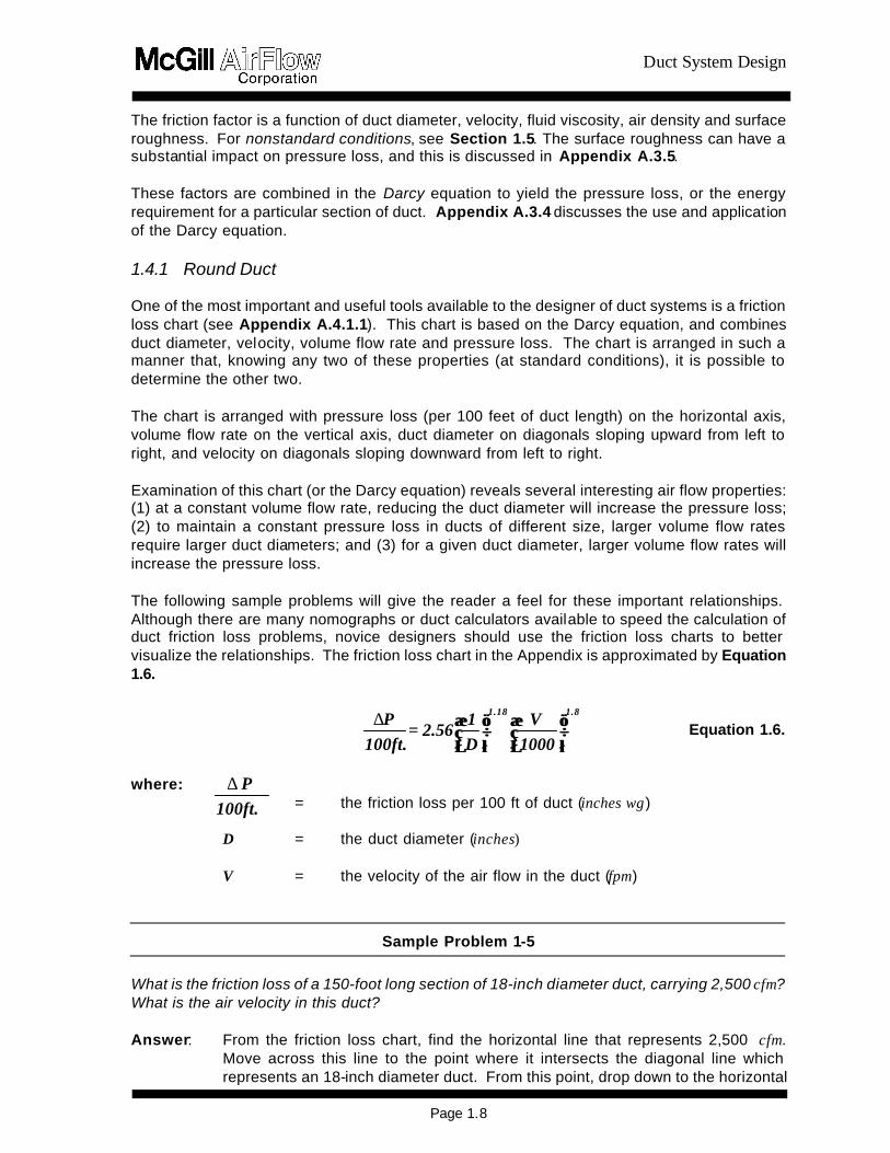
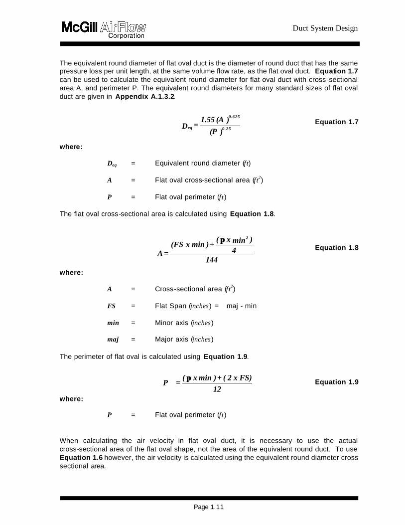
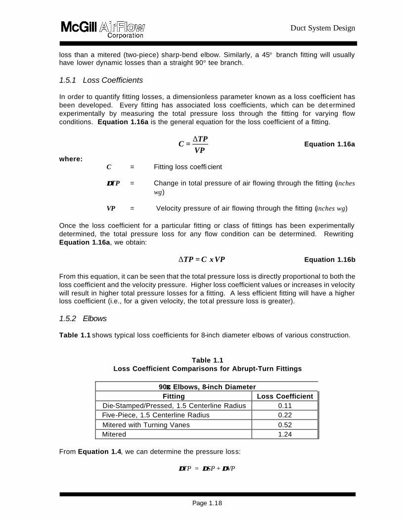
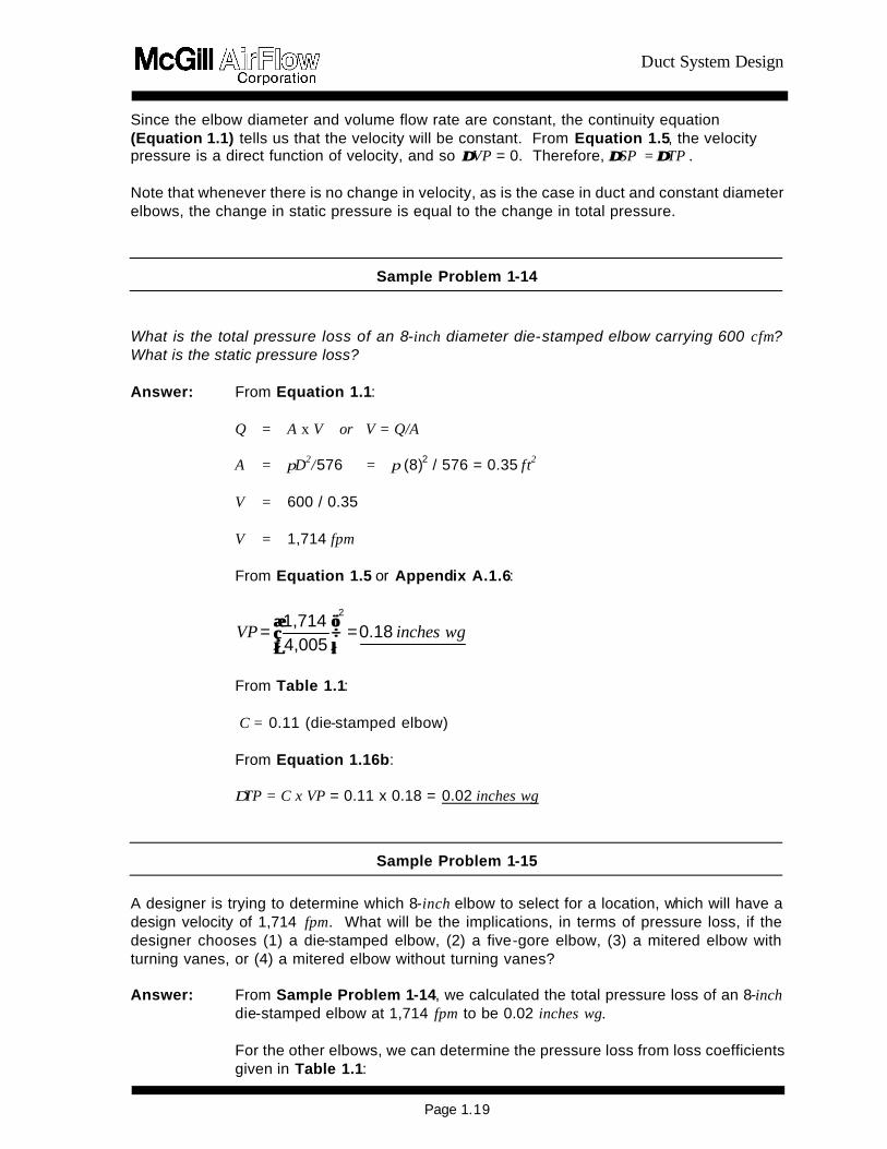
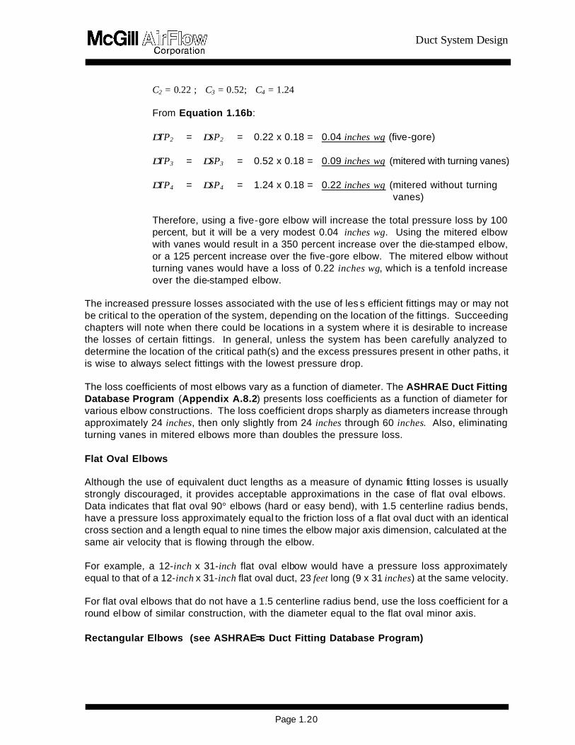
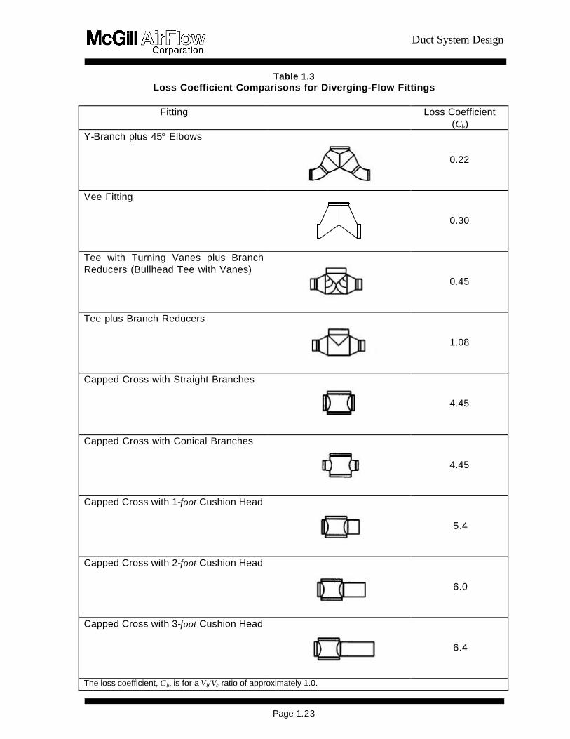
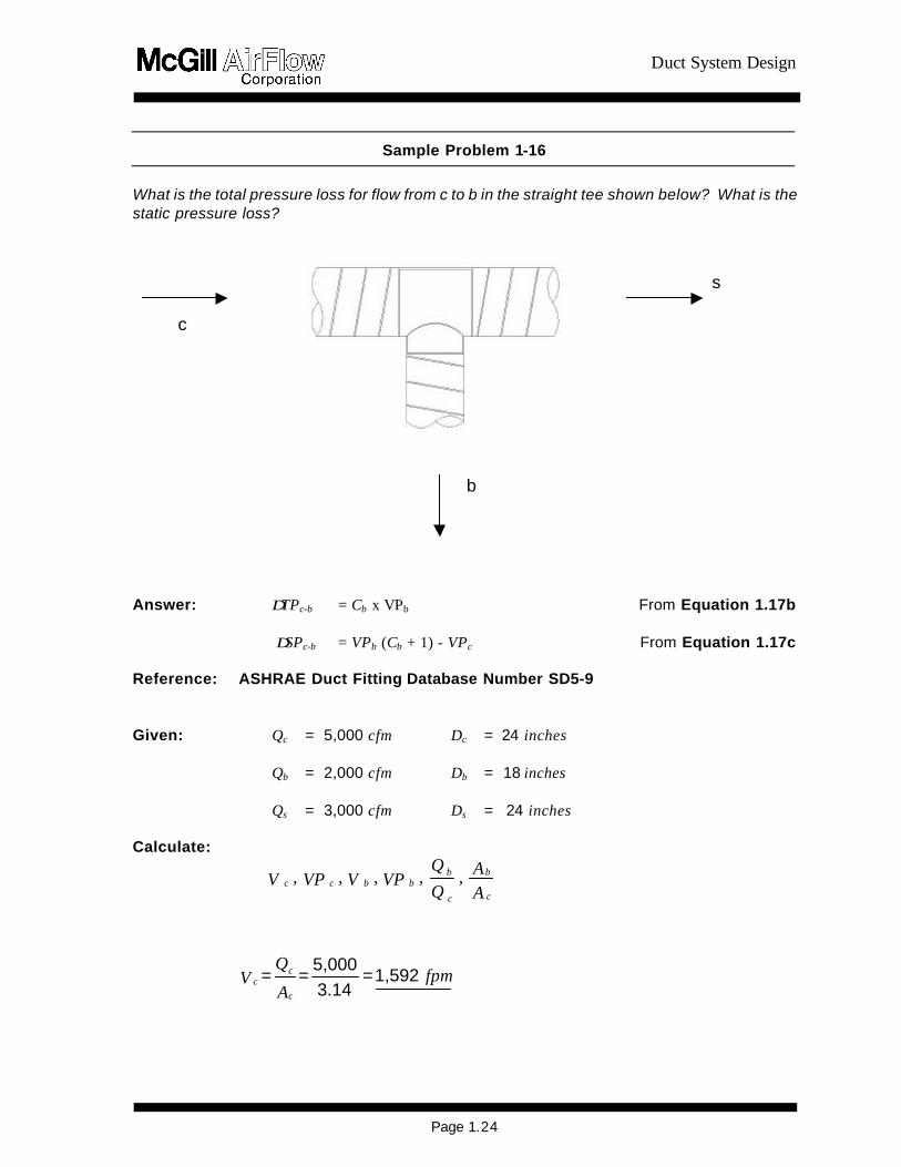
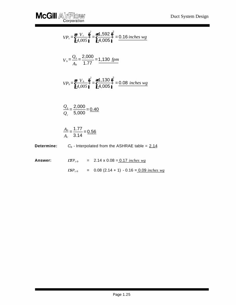
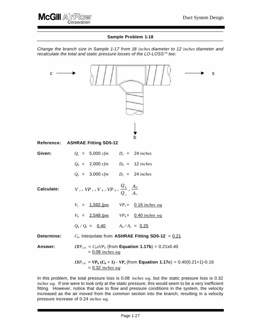
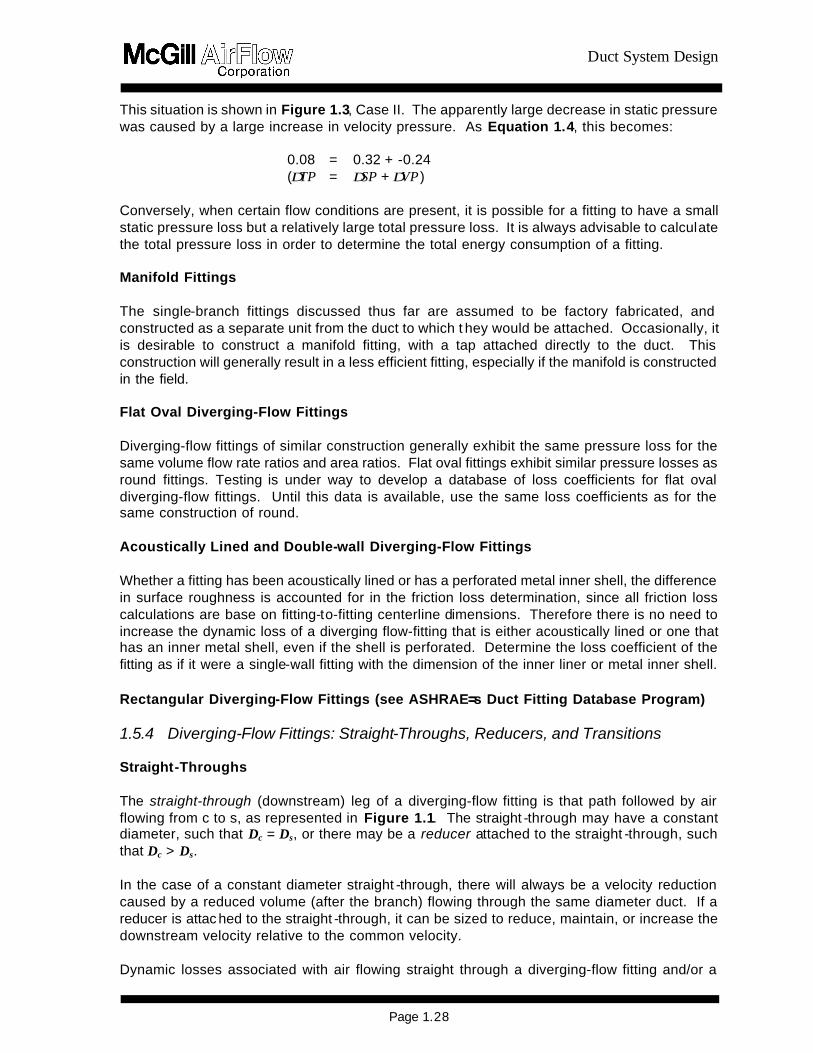
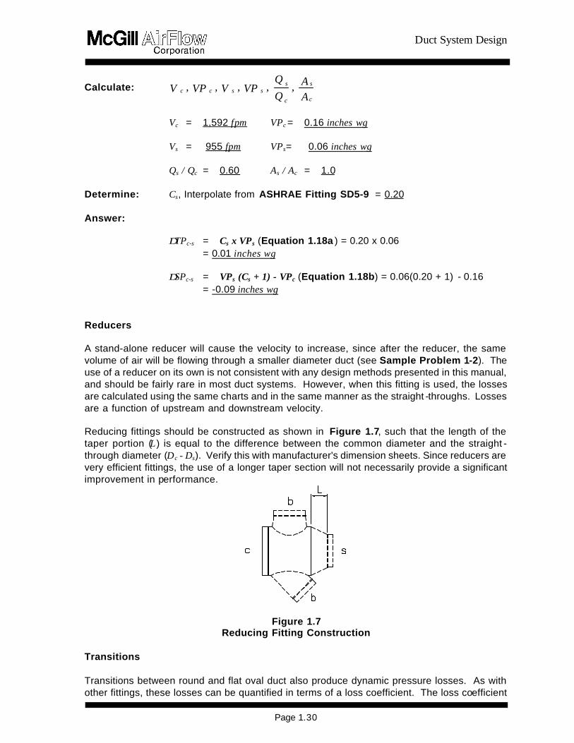
Duct System Design

Page 134

In this case the heel-tapped elbow and the conical tee will have nearly the same total pressure loss in the 90E bend direction The heel-tapped elbow provides a significant performance increase over the straight tee but has a higher loss than the LO-LOSST M tee branch The straight-through leg of the heel-tapped elbow is slightly more efficient than the straight -throughs of the tees

The best fitting though based strictly on efficiency would appear to be the LO-LOSST M tee However bear in mind that all three tee fittings will require substantial strai ght-through reducers (28 inches to 15 inches) which will generally be at least 12 inches long (Figure 17) and will add substantially to the cost of the fitting If a compromise between cost and performance is desired the heel-tapped elbow may still be the best choice for these flow situations Also increased loss may help balance the leg in which this fitting resides

Note that in Sample Problem 1-21 the total pressure is lower than the static pressure by 003 inches wg in all cases due to the increase in velocity pressure (003 inches wg) from common to both straight-through and branch In the form of Equation 14

∆TPc-b = ∆SPc-b - 003 ∆TPc-s = ∆SPc-s - 003

Crosses Cross fittings are those which have two taps located at the same cross section of a main or trunk duct Usually these taps will be constructed so that they discharge air in diametrically opposed directions The pressure loss of the taps on a cross fitting depends to a large extent on the cross-sectional area reduction of the straight-through duct For straight -through area reductions of less that 20 percent the branch losses through either tap of a cross fitting will be the same as those for a single-branch fitting with identical tap construction For example a conical cross (a cross with conical taps) that has a straight -through of 24 inches reducing to 22 inches would have an area reduction of 16 percent Since this is less than 20 percent the branch losses for either tap would be found from the direct-read charts in ASHRAE Fittings SD5-9 through SD5-17 For crosses where the straight -through area reduction exceeds 20 percent use the loss coefficients presented in ASHRAE Fittings SD5-23 through SD5-26 The three curves shown are for varying percentage area reductions and apply for all tap constructions Use interpolation to find loss coefficients for area reductions between these curves Use Equations 117b and 117c for determining the total and static pressure losses of each branch Split Fittings Split fittings are diverging-flow fittings where the air divides into two branches each of which turns at 90E to the main There is no straight-through leg The most common types of split fittings are the Vee Y-branch and the bullhead tee The Y-branches are the most efficient split fittings however they are more expensive than Vees and may be more expensive than bullhead tees Bullhead tees should always be specified with turning vanes ASHRAE Fittings SD5-18 19 and 21 presents drawings and loss

Duct System Design

Page 135

coefficients data for Y-branches bullhead tees with turning vanes bullhead tees without turning vanes and capped crosses The capped cross is discussed in the following section Use Equations 117b and 117c for determining the total and static pressure losses Capped Fittings Capped fittings are those in which the main or straight -through is completely closed off The most common use for a capped fitting is in locations where it is expected that future expansion will require additional ducting at which time the cap can be removed and the duct run continued In general the use of capped fittings is strongly discouraged For both single-branch fittings and crosses the performance is severely degraded if the main is capped Where these fittings are unavoidable SD5-2 includes a curve for capped crosses Use Equations 117b and 117c for determining the total and static pressure losses Close -Coupled Fittings After air flows through any type of fitting a certain length of straight duct is required to re-establish the flow profile of the airstream Simply stated it takes a certain distance for air to recover from a disturbance produced by a fitting If the airstream encounters a second fitting before it has had a chance to recover from a previous disturbance the effect of the second fitting will be more pronounced than if it had been located in a long run of straight duct Generally two elbows in series will have the same loss as the sum of the individual elbows The exception to this is when the second elbow has an additional change in direction such that the air is not flowing parallel to the first flow For this case as much as an additional 100 percent of the combined losses should be added unless the elbows are at least 10 diameters apart The loss of two tees in series is a function of the spacing between the tees although the loss coefficient of the upstream tee is not significantly affected The loss coefficient of the downstream tee actually decreases at half-diameter spacing At two-diameter spacing however the downstream loss coefficient is significantly higher The loss coeffi cient gradually decreases back to its original value at 10 diameters To account for the increased pressure loss at two-diameter spacing add 100 percent of the calculated loss This can be decreased as the diameter spacing between tees becomes greater Appendix A99 has a more detailed discussion of the effect of spacing of tees Couplings Slip couplings which are inserted inside duct sections and are therefore exposed to the air stream are generally used to join two adjacent duct sections Fittings which connect directly to duct sections do not require couplings and fittings which are connected directly to other fittings usually have an outside coupling Losses associated with duct couplings are very low When slip couplings are separated by 10 to 20 feet of duct their effects are negligible However in the event it is necessary to calculate the loss due to duct couplings Appendix A42 presents a table of loss coefficients versus coupling diameter Use Equations 117b and 117c for determining the total and static pressure losses As can be seen from the loss coefficient values it is normally quite acceptable to ignore these losses when calculating system pressure losses Experience has shown that even poorly made and undersized couplings have negligible losses The resulting loss coefficient may be two to three times that of a slip coupling

Duct System Design

Page 136

but this is still a very low value Offsets Offsets are required to change the location of a duct run horizontally vertically or both This is most often necessary to avoid interference with some obstruction along the duct run Offsets are usually constructed with two or more elbows joined by a suitable length of straight duct Due to the almost limitless number of offsets that could be created there are no tables or charts in this manual for the calculation of these losses It is suggested that offset losses be obtained by adding the losses of the individual elbows and duct which form the offset and if necessary adding a factor for any close-coupling effects that may exist Bellmouths The bellmouth fitting is used as an intake or entrance to a duct usually from a plenum or fan housing There is a substantial advantage in having a smooth radiused entrance as opposed to a square-edged entrance Loss coefficients for bellmouths are presented in ASHRAE Fittings SD1-1 SD1-2 and SD1-3 To calculate the total and static pressure losses use (transition loss) Equations 119a and 119b Expanders Increasing the duct diameter upstream-to-downstream in a supply air system is not a recommended design practice Abrupt expanders are very inefficient fittings in that their loss coefficients are always 10 or greater This means that the entire upstream velocity head is lost and unrecoverable This can be shown by substituting a unity loss coefficient into Equations 118a and 118b

∆TPc-s = 10 x VPc = VPc ∆SPc-s = VPc (10 - 10) + VPs = VPs

Therefore although the static pressure loss may be small the total pressure loss is equal to (at least) the entire upstream velocity pressure Exits Exits are fittings that discharge air into the surrounding environment Refer to ASHRAE Fittings SD1-1 and SD1-2 (plenums) SD2-1 to SD2-6 (atmosphere) and SD7-1 to SD7-5 (fans) for loss coefficients of round exits Refer to SR1-1 (plenums) SR2-1 to SR2-6 (atmosphere) and SR7-1 to SR7-17 (fans) for loss coefficients of rectangular exits Increasing the duct size at an exit is advantageous in minimizing pressure loss Obstructions In-line losses common to supply systems also must be taken into account Refer to ASHRAE=s Duct Fitting Database CD9-1 to CD9-3 for loss coefficients of round dampers CR9-1 to CR9-7 for loss coefficients of rectangular dampers CD8-1 to CD8-8 for loss coefficients of round silencers CR8-1 to CR8-4 for loss coefficients of rectangular silencers CR8-5 to CR8-8 for loss coefficients of coils CR8-9 to CR8-11 for loss coefficients of VAV boxes and CD6-1 to CD6-4 for loss coefficients of other round obstructions

Duct System Design

Page 137

156 Nonstandard Conditions In Section 145 equations were given for correcting the calculated friction loss of a system for nonstandard conditions of temperature andor elevation Since velocity pressure is a function of air density (see Appendix A33) and since all dynamic fitting losses are a function of velocity pressure an additional correction must be made to the calculated fitting losses whenever there are substantial variations from standard conditions If a density-corrected velocity pressure (Appendix A33) is used to calculate all dynamic fitting losses then no further corrections (except friction loss corrections) are required If the pressure losses are calculated assuming standard conditions the results can be corrected by multiplying by the ratio of actual density diverging by standard density For most HVAC applications this ratio can be calculated as shown in Equation 120

ββ

ρρρρ

29921x

460) + T(530

= astd

act Equation 120

where

ρρact = Actual density (lbmft3) ρρstd = Standard density (lbmft3) Ta = Actual air temperature (EF ) ββ = Actual barometric pressure (inches Hg)

The corrected total static and velocity pressure can be calculated as follows

ρρρρ

std

actstdact x TP= TP ∆∆ Equation 121

ρρρρ

std

actstdact x SP= SP ∆∆ Equation 122

ρρρρ

std

actstdact x VP= VP ∆∆ Equation 123

where

∆∆TPact = Total pressure loss at actual conditions (inches wg) ∆∆TPstd = Total pressure loss at standard conditions (inches wg)

Duct System Design

Page 138

wginches x TPTPstd

act stdb-cact b-c 015= 086 x 017 ==

ρρρρ

∆∆

wginches x SPSPstd

act stdb-cact b-c 008 = 086 x 009 ==

ρρρρ

∆∆

∆∆SPact = Static pressure loss at actual conditions (inches wg) ∆∆SPstd = Static pressure loss at standard conditions (inches wg) ∆∆VPact = Change in velocity pressure calculated at actual conditions (inches

wg) ∆∆VPstd = Change in velocity pressure calculated at standard conditions (inches

wg) Density correction factors are tabulated in Appendix A15 Often for systems operating at normal HVAC temperatures (70E 30EF ) and elevations less than 1500 feet above sea level these corrections can be neglected When Equations 121 andor 122 are applied to the aggregate pressure loss of an entire system instead of to the individual fi tting components the resulting pressures are not necessarily accurate This is because the friction correction factors (Section 145) are calculated in a different manner from the dynamic loss correction factors discussed above The accuracy depends on the ratio of duct length versus number of fittings and on the deviation from standard conditions

Sample Problem 1-22

Determine the effect on the total and static pressure losses of the straight tee of Sample Problem 1-16 if the air temperature is 55EF and the elevation is 5000 feet Answer From Sample Problem 1-16 at standard conditions

wginchesSP

wginchesTP

stdb-c

stdb-c

009 =

017 =

∆

∆

From Appendix A15

086 = ρρρρ

std

act (interpolation required)

From Equation 121

From Equation 122

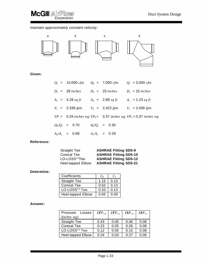
Duct System Design

Page 135

coefficients data for Y-branches bullhead tees with turning vanes bullhead tees without turning vanes and capped crosses The capped cross is discussed in the following section Use Equations 117b and 117c for determining the total and static pressure losses Capped Fittings Capped fittings are those in which the main or straight -through is completely closed off The most common use for a capped fitting is in locations where it is expected that future expansion will require additional ducting at which time the cap can be removed and the duct run continued In general the use of capped fittings is strongly discouraged For both single-branch fittings and crosses the performance is severely degraded if the main is capped Where these fittings are unavoidable SD5-2 includes a curve for capped crosses Use Equations 117b and 117c for determining the total and static pressure losses Close -Coupled Fittings After air flows through any type of fitting a certain length of straight duct is required to re-establish the flow profile of the airstream Simply stated it takes a certain distance for air to recover from a disturbance produced by a fitting If the airstream encounters a second fitting before it has had a chance to recover from a previous disturbance the effect of the second fitting will be more pronounced than if it had been located in a long run of straight duct Generally two elbows in series will have the same loss as the sum of the individual elbows The exception to this is when the second elbow has an additional change in direction such that the air is not flowing parallel to the first flow For this case as much as an additional 100 percent of the combined losses should be added unless the elbows are at least 10 diameters apart The loss of two tees in series is a function of the spacing between the tees although the loss coefficient of the upstream tee is not significantly affected The loss coefficient of the downstream tee actually decreases at half-diameter spacing At two-diameter spacing however the downstream loss coefficient is significantly higher The loss coeffi cient gradually decreases back to its original value at 10 diameters To account for the increased pressure loss at two-diameter spacing add 100 percent of the calculated loss This can be decreased as the diameter spacing between tees becomes greater Appendix A99 has a more detailed discussion of the effect of spacing of tees Couplings Slip couplings which are inserted inside duct sections and are therefore exposed to the air stream are generally used to join two adjacent duct sections Fittings which connect directly to duct sections do not require couplings and fittings which are connected directly to other fittings usually have an outside coupling Losses associated with duct couplings are very low When slip couplings are separated by 10 to 20 feet of duct their effects are negligible However in the event it is necessary to calculate the loss due to duct couplings Appendix A42 presents a table of loss coefficients versus coupling diameter Use Equations 117b and 117c for determining the total and static pressure losses As can be seen from the loss coefficient values it is normally quite acceptable to ignore these losses when calculating system pressure losses Experience has shown that even poorly made and undersized couplings have negligible losses The resulting loss coefficient may be two to three times that of a slip coupling

Duct System Design

Page 136

but this is still a very low value Offsets Offsets are required to change the location of a duct run horizontally vertically or both This is most often necessary to avoid interference with some obstruction along the duct run Offsets are usually constructed with two or more elbows joined by a suitable length of straight duct Due to the almost limitless number of offsets that could be created there are no tables or charts in this manual for the calculation of these losses It is suggested that offset losses be obtained by adding the losses of the individual elbows and duct which form the offset and if necessary adding a factor for any close-coupling effects that may exist Bellmouths The bellmouth fitting is used as an intake or entrance to a duct usually from a plenum or fan housing There is a substantial advantage in having a smooth radiused entrance as opposed to a square-edged entrance Loss coefficients for bellmouths are presented in ASHRAE Fittings SD1-1 SD1-2 and SD1-3 To calculate the total and static pressure losses use (transition loss) Equations 119a and 119b Expanders Increasing the duct diameter upstream-to-downstream in a supply air system is not a recommended design practice Abrupt expanders are very inefficient fittings in that their loss coefficients are always 10 or greater This means that the entire upstream velocity head is lost and unrecoverable This can be shown by substituting a unity loss coefficient into Equations 118a and 118b

∆TPc-s = 10 x VPc = VPc ∆SPc-s = VPc (10 - 10) + VPs = VPs

Therefore although the static pressure loss may be small the total pressure loss is equal to (at least) the entire upstream velocity pressure Exits Exits are fittings that discharge air into the surrounding environment Refer to ASHRAE Fittings SD1-1 and SD1-2 (plenums) SD2-1 to SD2-6 (atmosphere) and SD7-1 to SD7-5 (fans) for loss coefficients of round exits Refer to SR1-1 (plenums) SR2-1 to SR2-6 (atmosphere) and SR7-1 to SR7-17 (fans) for loss coefficients of rectangular exits Increasing the duct size at an exit is advantageous in minimizing pressure loss Obstructions In-line losses common to supply systems also must be taken into account Refer to ASHRAE=s Duct Fitting Database CD9-1 to CD9-3 for loss coefficients of round dampers CR9-1 to CR9-7 for loss coefficients of rectangular dampers CD8-1 to CD8-8 for loss coefficients of round silencers CR8-1 to CR8-4 for loss coefficients of rectangular silencers CR8-5 to CR8-8 for loss coefficients of coils CR8-9 to CR8-11 for loss coefficients of VAV boxes and CD6-1 to CD6-4 for loss coefficients of other round obstructions

Duct System Design

Page 137

156 Nonstandard Conditions In Section 145 equations were given for correcting the calculated friction loss of a system for nonstandard conditions of temperature andor elevation Since velocity pressure is a function of air density (see Appendix A33) and since all dynamic fitting losses are a function of velocity pressure an additional correction must be made to the calculated fitting losses whenever there are substantial variations from standard conditions If a density-corrected velocity pressure (Appendix A33) is used to calculate all dynamic fitting losses then no further corrections (except friction loss corrections) are required If the pressure losses are calculated assuming standard conditions the results can be corrected by multiplying by the ratio of actual density diverging by standard density For most HVAC applications this ratio can be calculated as shown in Equation 120

ββ

ρρρρ

29921x

460) + T(530

= astd

act Equation 120

where

ρρact = Actual density (lbmft3) ρρstd = Standard density (lbmft3) Ta = Actual air temperature (EF ) ββ = Actual barometric pressure (inches Hg)

The corrected total static and velocity pressure can be calculated as follows

ρρρρ

std

actstdact x TP= TP ∆∆ Equation 121

ρρρρ

std

actstdact x SP= SP ∆∆ Equation 122

ρρρρ

std

actstdact x VP= VP ∆∆ Equation 123

where

∆∆TPact = Total pressure loss at actual conditions (inches wg) ∆∆TPstd = Total pressure loss at standard conditions (inches wg)

Duct System Design

Page 138

wginches x TPTPstd

act stdb-cact b-c 015= 086 x 017 ==

ρρρρ

∆∆

wginches x SPSPstd

act stdb-cact b-c 008 = 086 x 009 ==

ρρρρ

∆∆

∆∆SPact = Static pressure loss at actual conditions (inches wg) ∆∆SPstd = Static pressure loss at standard conditions (inches wg) ∆∆VPact = Change in velocity pressure calculated at actual conditions (inches

wg) ∆∆VPstd = Change in velocity pressure calculated at standard conditions (inches

wg) Density correction factors are tabulated in Appendix A15 Often for systems operating at normal HVAC temperatures (70E 30EF ) and elevations less than 1500 feet above sea level these corrections can be neglected When Equations 121 andor 122 are applied to the aggregate pressure loss of an entire system instead of to the individual fi tting components the resulting pressures are not necessarily accurate This is because the friction correction factors (Section 145) are calculated in a different manner from the dynamic loss correction factors discussed above The accuracy depends on the ratio of duct length versus number of fittings and on the deviation from standard conditions

Sample Problem 1-22

Determine the effect on the total and static pressure losses of the straight tee of Sample Problem 1-16 if the air temperature is 55EF and the elevation is 5000 feet Answer From Sample Problem 1-16 at standard conditions

wginchesSP

wginchesTP

stdb-c

stdb-c

009 =

017 =

∆

∆

From Appendix A15

086 = ρρρρ

std

act (interpolation required)

From Equation 121

From Equation 122

Duct System Design

Page 136

but this is still a very low value Offsets Offsets are required to change the location of a duct run horizontally vertically or both This is most often necessary to avoid interference with some obstruction along the duct run Offsets are usually constructed with two or more elbows joined by a suitable length of straight duct Due to the almost limitless number of offsets that could be created there are no tables or charts in this manual for the calculation of these losses It is suggested that offset losses be obtained by adding the losses of the individual elbows and duct which form the offset and if necessary adding a factor for any close-coupling effects that may exist Bellmouths The bellmouth fitting is used as an intake or entrance to a duct usually from a plenum or fan housing There is a substantial advantage in having a smooth radiused entrance as opposed to a square-edged entrance Loss coefficients for bellmouths are presented in ASHRAE Fittings SD1-1 SD1-2 and SD1-3 To calculate the total and static pressure losses use (transition loss) Equations 119a and 119b Expanders Increasing the duct diameter upstream-to-downstream in a supply air system is not a recommended design practice Abrupt expanders are very inefficient fittings in that their loss coefficients are always 10 or greater This means that the entire upstream velocity head is lost and unrecoverable This can be shown by substituting a unity loss coefficient into Equations 118a and 118b

∆TPc-s = 10 x VPc = VPc ∆SPc-s = VPc (10 - 10) + VPs = VPs

Therefore although the static pressure loss may be small the total pressure loss is equal to (at least) the entire upstream velocity pressure Exits Exits are fittings that discharge air into the surrounding environment Refer to ASHRAE Fittings SD1-1 and SD1-2 (plenums) SD2-1 to SD2-6 (atmosphere) and SD7-1 to SD7-5 (fans) for loss coefficients of round exits Refer to SR1-1 (plenums) SR2-1 to SR2-6 (atmosphere) and SR7-1 to SR7-17 (fans) for loss coefficients of rectangular exits Increasing the duct size at an exit is advantageous in minimizing pressure loss Obstructions In-line losses common to supply systems also must be taken into account Refer to ASHRAE=s Duct Fitting Database CD9-1 to CD9-3 for loss coefficients of round dampers CR9-1 to CR9-7 for loss coefficients of rectangular dampers CD8-1 to CD8-8 for loss coefficients of round silencers CR8-1 to CR8-4 for loss coefficients of rectangular silencers CR8-5 to CR8-8 for loss coefficients of coils CR8-9 to CR8-11 for loss coefficients of VAV boxes and CD6-1 to CD6-4 for loss coefficients of other round obstructions

Duct System Design

Page 137

156 Nonstandard Conditions In Section 145 equations were given for correcting the calculated friction loss of a system for nonstandard conditions of temperature andor elevation Since velocity pressure is a function of air density (see Appendix A33) and since all dynamic fitting losses are a function of velocity pressure an additional correction must be made to the calculated fitting losses whenever there are substantial variations from standard conditions If a density-corrected velocity pressure (Appendix A33) is used to calculate all dynamic fitting losses then no further corrections (except friction loss corrections) are required If the pressure losses are calculated assuming standard conditions the results can be corrected by multiplying by the ratio of actual density diverging by standard density For most HVAC applications this ratio can be calculated as shown in Equation 120

ββ

ρρρρ

29921x

460) + T(530

= astd

act Equation 120

where

ρρact = Actual density (lbmft3) ρρstd = Standard density (lbmft3) Ta = Actual air temperature (EF ) ββ = Actual barometric pressure (inches Hg)

The corrected total static and velocity pressure can be calculated as follows

ρρρρ

std

actstdact x TP= TP ∆∆ Equation 121

ρρρρ

std

actstdact x SP= SP ∆∆ Equation 122

ρρρρ

std

actstdact x VP= VP ∆∆ Equation 123

where

∆∆TPact = Total pressure loss at actual conditions (inches wg) ∆∆TPstd = Total pressure loss at standard conditions (inches wg)

Duct System Design

Page 138

wginches x TPTPstd

act stdb-cact b-c 015= 086 x 017 ==

ρρρρ

∆∆

wginches x SPSPstd

act stdb-cact b-c 008 = 086 x 009 ==

ρρρρ

∆∆

∆∆SPact = Static pressure loss at actual conditions (inches wg) ∆∆SPstd = Static pressure loss at standard conditions (inches wg) ∆∆VPact = Change in velocity pressure calculated at actual conditions (inches

wg) ∆∆VPstd = Change in velocity pressure calculated at standard conditions (inches

wg) Density correction factors are tabulated in Appendix A15 Often for systems operating at normal HVAC temperatures (70E 30EF ) and elevations less than 1500 feet above sea level these corrections can be neglected When Equations 121 andor 122 are applied to the aggregate pressure loss of an entire system instead of to the individual fi tting components the resulting pressures are not necessarily accurate This is because the friction correction factors (Section 145) are calculated in a different manner from the dynamic loss correction factors discussed above The accuracy depends on the ratio of duct length versus number of fittings and on the deviation from standard conditions

Sample Problem 1-22

Determine the effect on the total and static pressure losses of the straight tee of Sample Problem 1-16 if the air temperature is 55EF and the elevation is 5000 feet Answer From Sample Problem 1-16 at standard conditions

wginchesSP

wginchesTP

stdb-c

stdb-c

009 =

017 =

∆

∆

From Appendix A15

086 = ρρρρ

std

act (interpolation required)

From Equation 121

From Equation 122

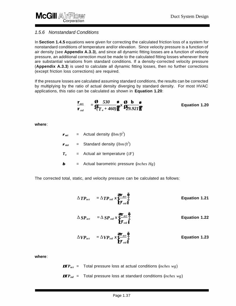
Duct System Design

Page 137

156 Nonstandard Conditions In Section 145 equations were given for correcting the calculated friction loss of a system for nonstandard conditions of temperature andor elevation Since velocity pressure is a function of air density (see Appendix A33) and since all dynamic fitting losses are a function of velocity pressure an additional correction must be made to the calculated fitting losses whenever there are substantial variations from standard conditions If a density-corrected velocity pressure (Appendix A33) is used to calculate all dynamic fitting losses then no further corrections (except friction loss corrections) are required If the pressure losses are calculated assuming standard conditions the results can be corrected by multiplying by the ratio of actual density diverging by standard density For most HVAC applications this ratio can be calculated as shown in Equation 120

ββ

ρρρρ

29921x

460) + T(530

= astd

act Equation 120

where

ρρact = Actual density (lbmft3) ρρstd = Standard density (lbmft3) Ta = Actual air temperature (EF ) ββ = Actual barometric pressure (inches Hg)

The corrected total static and velocity pressure can be calculated as follows

ρρρρ

std

actstdact x TP= TP ∆∆ Equation 121

ρρρρ

std

actstdact x SP= SP ∆∆ Equation 122

ρρρρ

std

actstdact x VP= VP ∆∆ Equation 123

where

∆∆TPact = Total pressure loss at actual conditions (inches wg) ∆∆TPstd = Total pressure loss at standard conditions (inches wg)

Duct System Design

Page 138

wginches x TPTPstd

act stdb-cact b-c 015= 086 x 017 ==

ρρρρ

∆∆

wginches x SPSPstd

act stdb-cact b-c 008 = 086 x 009 ==

ρρρρ

∆∆

∆∆SPact = Static pressure loss at actual conditions (inches wg) ∆∆SPstd = Static pressure loss at standard conditions (inches wg) ∆∆VPact = Change in velocity pressure calculated at actual conditions (inches

wg) ∆∆VPstd = Change in velocity pressure calculated at standard conditions (inches

wg) Density correction factors are tabulated in Appendix A15 Often for systems operating at normal HVAC temperatures (70E 30EF ) and elevations less than 1500 feet above sea level these corrections can be neglected When Equations 121 andor 122 are applied to the aggregate pressure loss of an entire system instead of to the individual fi tting components the resulting pressures are not necessarily accurate This is because the friction correction factors (Section 145) are calculated in a different manner from the dynamic loss correction factors discussed above The accuracy depends on the ratio of duct length versus number of fittings and on the deviation from standard conditions

Sample Problem 1-22

Determine the effect on the total and static pressure losses of the straight tee of Sample Problem 1-16 if the air temperature is 55EF and the elevation is 5000 feet Answer From Sample Problem 1-16 at standard conditions

wginchesSP

wginchesTP

stdb-c

stdb-c

009 =

017 =

∆

∆

From Appendix A15

086 = ρρρρ

std

act (interpolation required)

From Equation 121

From Equation 122

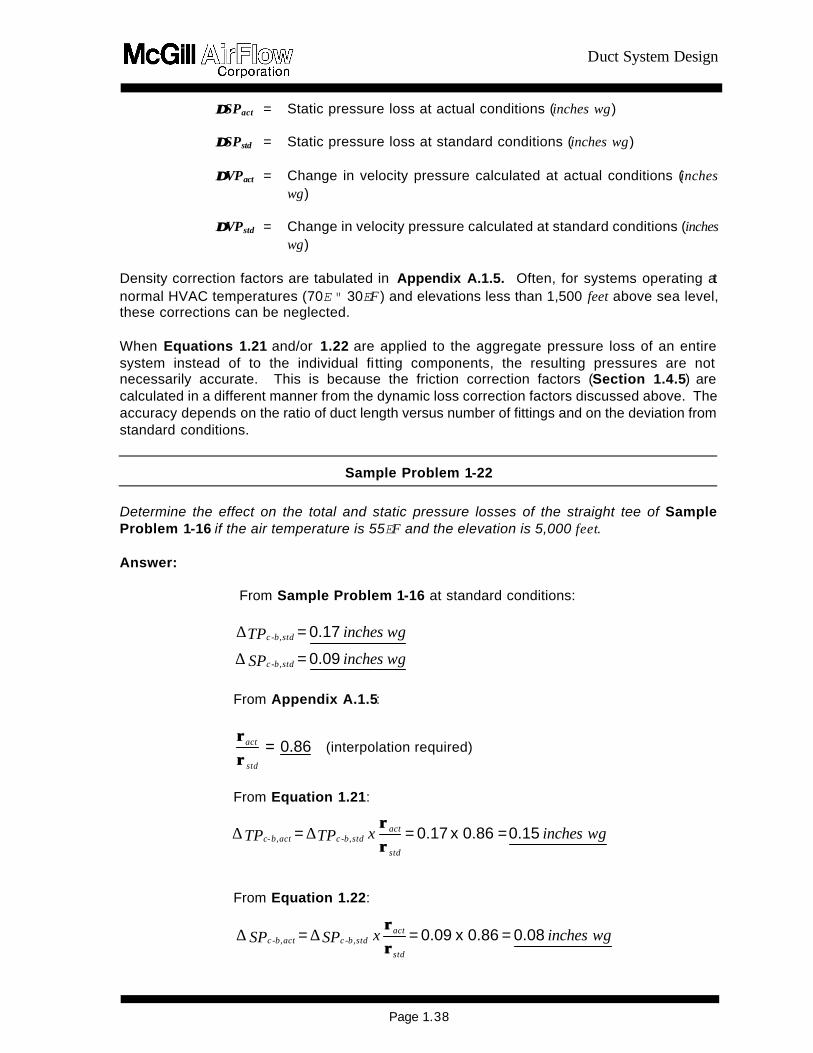
Duct System Design

Page 138

wginches x TPTPstd

act stdb-cact b-c 015= 086 x 017 ==

ρρρρ

∆∆

wginches x SPSPstd

act stdb-cact b-c 008 = 086 x 009 ==

ρρρρ

∆∆

∆∆SPact = Static pressure loss at actual conditions (inches wg) ∆∆SPstd = Static pressure loss at standard conditions (inches wg) ∆∆VPact = Change in velocity pressure calculated at actual conditions (inches

wg) ∆∆VPstd = Change in velocity pressure calculated at standard conditions (inches

wg) Density correction factors are tabulated in Appendix A15 Often for systems operating at normal HVAC temperatures (70E 30EF ) and elevations less than 1500 feet above sea level these corrections can be neglected When Equations 121 andor 122 are applied to the aggregate pressure loss of an entire system instead of to the individual fi tting components the resulting pressures are not necessarily accurate This is because the friction correction factors (Section 145) are calculated in a different manner from the dynamic loss correction factors discussed above The accuracy depends on the ratio of duct length versus number of fittings and on the deviation from standard conditions

Sample Problem 1-22

Determine the effect on the total and static pressure losses of the straight tee of Sample Problem 1-16 if the air temperature is 55EF and the elevation is 5000 feet Answer From Sample Problem 1-16 at standard conditions

wginchesSP

wginchesTP

stdb-c

stdb-c

009 =

017 =

∆

∆

From Appendix A15

086 = ρρρρ

std

act (interpolation required)

From Equation 121

From Equation 122