the g-invariant and catenary data of a matroid · the g-invariant and catenary data of a matroid...

THE G-INVARIANT AND CATENARY DATA OF A MATROID

JOSEPH E. BONIN AND JOSEPH P.S. KUNG

ABSTRACT. The catenary data of a matroid M of rank r on n elements is the vec-tor (ν(M ; a0, a1, . . . , ar)), indexed by compositions (a0, a1, . . . , ar), where a0 ≥ 0,ai > 0 for i ≥ 1, and a0+a1+ · · ·+ar = n, with the coordinate ν(M ; a0, a1, . . . , ar)

equal to the number of maximal chains or flags (X0, X1, . . . , Xr) of flats or closed setssuch that Xi has rank i, |X0| = a0, and |Xi −Xi−1| = ai. We show that the catenarydata of M contains the same information about M as its G-invariant, which was definedby H. Derksen [J. Algebr. Combin. 30 (2009) 43–86]. The Tutte polynomial is a special-ization of the G-invariant. We show that many known results for the Tutte polynomial haveanalogs for the G-invariant. In particular, we show that for many matroid constructions, theG-invariant of the construction can be calculated from the G-invariants of the constituentsand that the G-invariant of a matroid can be calculated from its size, the isomorphism classof the lattice of cyclic flats with lattice elements labeled by the rank and size of the under-lying set. We also show that the number of flats and cyclic flats of a given rank and size canbe derived from the G-invariant, that the G-invariant of M is reconstructible from the deckof G-invariants of restrictions ofM to its copoints, and that, apart from free extensions andcoextensions, one can detect whether a matroid is a free product from its G-invariant.

1. THE G-INVARIANT

Motivated by work on the F -invariant by Billera, Jia, and Reiner [1], Derksen intro-duced the G-invariant for matroids and polymatroids in [9]. Together with Fink, Derksenshowed in [10] that it is a universal valuative invariant for subdivisions of matroid basepolytopes.

Let M be a rank-r matroid with rank function r and closure operator cl on the set{1, 2, . . . , n}. The rank sequence r(π) = r1r2 . . . rn of a permutation π on {1, 2, . . . , n}is the sequence defined by r1 = r({π(1)}) and for j ≥ 2,

rj = r({π(1), π(2), . . . , π(j)})− r({π(1), π(2), . . . , π(j − 1)}).In a rank sequence, rj is 0 or 1, there are exactly r 1’s, and the set {π(j) : rj = 1} is abasis of M . The rank sequence r(π) is an (n, r)-sequence, that is, a sequence of n terms,r of which are 1 and the other n− r of which are 0.

Let [r] be a variable or formal symbol, one for each (n, r)-sequence, and let G(n, r)be the vector space (over a field of characteristic zero) of dimension

(nr

)consisting of all

formal linear combinations of such symbols. The G-invariant and its coefficients gr(M)are defined by

G(M) =∑r

gr(M)[r] =∑π

[r(π)]

where the sum is over all n! permutations of {1, 2, . . . , n}. (This definition is essentiallyDerksen’s. We just replace a quasisymmetric function constructed from r by the symbol[r].) A specialization of the G-invariant with values in an abelian group A is a function

Date: September 23, 2017.1991 Mathematics Subject Classification. Primary 52B40, 05B35.

1

2 The G-invariant and catenary data of a matroid to appear, Advances in Applied Mathematics

assigning a value in A to each symbol [r]. Specializations may be given directly (as inTheorem 1.1) or indirectly. In particular, if L is a linear transformation from G(n, r) to avector space V , then the assignment [r] 7→ L([r]) gives a specialization.

Recall that the Tutte polynomial T (M ;x, y) of a rank-r matroid M on the set E isdefined by

T (M ;x, y) =∑A⊆E

(x− 1)r−r(A)(y − 1)|A|−r(A).

Derksen [9] showed that the G-invariant specializes to the Tutte polynomial. In the nexttheorem, we state his specialization without using quasisymmetric functions.

Theorem 1.1 (Derksen). LetM be a rank-r matroid on a set of n elements. Then the Tuttepolynomial T (M ;x, y) can be obtained from G(M) by the specialization

[r] 7→n∑

m=0

(x− 1)r−wt(r1r2...rm)(y − 1)m−wt(r1r2...rm)

m!(n−m)!,

where wt(r1r2 . . . rm) is the number of 1’s in the initial segment r1r2 . . . rm of r.

In this paper, we study the G-invariant from a combinatorial point of view. After someorder-theoretic preliminaries in Section 2, we begin in Section 3 by determining the exactcombinatorial information contained in the G-invariant. This information is encoded in thecatenary data, a vector or array of integers that records the number of flags or maximalchains of flats with given sizes. The G-invariant and catenary data contain the same in-formation; indeed, the catenary data are the coefficients of the G-invariant when expandedin a new basis of G(n, r) called the γ-basis. In Section 4, we study how the G-invariantand catenary data behave under matroid constructions. Many of the known results sayingthat the Tutte polynomial of a construction can be calculated from the Tutte polynomialsof its constituents have counterparts for the G-invariant. We show in Section 5 that manyparameters of a matroid not derivable from the Tutte polynomial can be derived from theG-invariant. In addition, we show, in Section 6, that the G-invariant can be reconstructedfrom several decks, giving analogs of reconstructibility results for the Tutte polynomial. InSection 7, extending a result of Eberhardt [12] for the Tutte polynomial, we show that theG-invariant is determined by the isomorphism type of the lattice of cyclic flats, along withthe size and rank of the cyclic flat that corresponds to each element in the lattice. In thefinal section, we show that, except for free extensions and coextensions, whether a matroidis a free product can be detected from its G-invariant.

Although we focus on matroids, we remark that the G-invariant of matroids constructedfrom graphs, such as cycle or bicircular matroids, should have many applications in graphtheory. For example, whether a graph has a Hamiltonian cycle is not deducible from theTutte polynomial of the graph but is deducible from the G-invariant of its cycle matroid(Corollary 5.3).

2. PARTIAL ORDERS ON SEQUENCES AND COMPOSITIONS

We use the notation 0a for a sequence of a 0’s and 1b for a sequence of b 1’s. An(n, r)-composition is a length-(r + 1) integer sequence (a0, a1, a2, . . . , ar) satisfying theinequalities a0 ≥ 0 and aj > 0 for 1 ≤ j ≤ r, together with the equality

a0 + a1 + a2 + · · ·+ ar = n.

The correspondence

0a010a1−110a2−1 . . . 10ar−1 ←→ (a0, a1, a2, . . . , ar)

The G-invariant and catenary data of a matroid to appear, Advances in Applied Mathematics 3

gives a bijection between the set of (n, r)-sequences and the set of (n, r)-compositions. Inthis paper, we identify an (n, r)-sequence and its corresponding (n, r)-composition.

We also need a partial order on (n, r)-sequences. If s and t are (n, r)-sequences, thent D s if

t1 + t2 + · · ·+ tj ≥ s1 + s2 + · · ·+ sj

for every index j; in other words, reading from the left, there are always at least as many1’s in t as there are in s. This order has maximum 1r0n−r and minimum 0n−r1r. Underthe bijection, D defines a partial order on (n, r)-compositions given by (b0, b1, . . . , br) D(a0, a1, . . . , ar) if and only if for every index j,

b0 + b1 + · · ·+ bj ≤ a0 + a1 + · · ·+ aj .

This order is a suborder of the reversed dominance order on compositions. While thislink plays no role in what we do, we note that the partial order D on (n, r)-sequences isa distributive lattice that is isomorphic to a sublattice of Young’s partition lattice (see [18,p. 288]).

3. CATENARY DATA

Let M be a rank-r matroid on a set E of size n. A flag (Xi) = (X0, X1, . . . , Xr) is amaximal chain

cl(∅) = X0 ⊂ X1 ⊂ X2 ⊂ · · · ⊂ Xr−1 ⊂ Xr = E,

where Xj is a rank-j flat of M . The composition comp((Xi)) of the flag (Xi) is the(n, r)-composition (a0, a1, a2, . . . , ar), where a0 = |X0|, and for positive j,

aj = |Xj −Xj−1|.Thus, a0 is the number of loops in M . Also, the rank sequence 0a010a1−1 . . . 10ar−1

corresponding to comp((Xi)) is the rank sequence of each of the a0!a1! · · · ar! permuta-tions that, for all positive j, puts the elements of Xj−1 before those of the set-differenceXj −Xj−1.

We use the notation (t)k for the falling factorial t(t − 1)(t − 2) · · · (t − k + 1), thenumber of sequences of k distinct objects chosen from a set of t objects. For an (n, r)-sequence s with composition (a0, a1, . . . , ar), let γ(a0, a1, . . . , ar), and its coefficientsc(a0,a1,...,ar)(b0, b1, . . . , br) be defined by

γ(a0, a1, . . . , ar) =∑

(b0,b1,...,br)

c(a0,a1,...,ar)(b0, b1, . . . , br)[0b010b1−1 . . . 10br−1]

=∑

(bj)D(aj)

(a0)b0

(r∏j=1

aj

(aj − 1 +

(j−1∑i=0

ai − bi))

bj−1

)[0b010b1−1 . . . 10br−1],

where the second sum ranges over all compositions with (b0, b1, . . . , br) D (a0, a1, . . . , ar).For example,

γ(0, 1, 1, 4) = 24 [111000],

γ(0, 1, 2, 3) = 36 [111000] + 12 [110100],

γ(0, 1, 3, 2) = 36 [111000] + 24 [110100] + 12 [110010],

γ(0, 1, 4, 1) = 24 [111000] + 24 [110100] + 24 [110010] + 24 [110001].

Note that, by definition, the coefficient c(a0,a1,...,ar)(b0, b1, . . . , br) is non-zero if and onlyif (b0, b1, . . . , br) D (a0, a1, . . . , ar). Hence the matrix (c(a0,a1,...,ar)(b0, b1, . . . , br)) is


a lower triangular matrix. In particular, the linear combinations γ(a0, a1, . . . , ar), where(a0, a1, . . . , ar) ranges over all (n, r)-compositions, form a basis, called the γ-basis, forthe vector space G(n, r).

With each permutation π, we get an ordered basis (π(i1), π(i2), . . . , π(ir)) from theterms in its rank sequence r1r2 . . . rn with rij = 1, where i1 < i2 < · · · < ir. This basisdetermines a flag, denoted flag(π), obtained by setting X0 = cl(∅) and

Xj = cl({π(i1), π(i2), . . . , π(ij)}).

Lemma 3.1. Let (Xi) be a flag of M with composition (a0, a1, . . . , ar). Then∑π : flag(π)=(Xi)

[r(π)] = γ(a0, a1, . . . , ar).

In particular, the sum on the left hand side depends only on comp((Xi)).

Proof. Let π be a permutation whose rank sequence r(π) equals 0b010b1−110b2−1 . . . 10br−1.Then, by the Mac Lane-Steinitz exchange property for closure, flag(π) = (Xi) if and onlyif

π(1), π(2), . . . , π(b0) ∈ X0,

π(b0 + 1) ∈ X1 −X0,

π(b0 + 2), . . . , π(b0 + b1) ∈ X1,

...π(b0 + b1 + · · ·+ bj−1 + 1) ∈ Xj −Xj−1,

π(b0 + b1 + · · ·+ bj−1 + 2), . . . , π(b0 + b1 + · · ·+ bj−1 + bj) ∈ Xj ,

...π(b0 + b1 + · · ·+ br−1 + 1) ∈ Xr −Xr−1,

π(b0 + b1 + · · ·+ br−1 + 2), . . . , π(n) ∈ Xr.

Such a permutation π exists if and only if (b0, b1, . . . , br) D (a0, a1, . . . , ar) and all suchpermutations can be found by choosing a length-b0 sequence of distinct elements from X0

(a set of size a0), an element fromX1−X0 (a set of size a1), a length-(b1−1) sequence ofdistinct elements from the subset of elements in X1 ∪X0 not chosen earlier (a set of size(a1−1)+(a0−b0)), an element fromX2−X1 (a set of size a2), a length-(b2−1) sequenceof distinct elements from the subset of elements inX2∪X1∪X0 not chosen earlier (a set ofsize (a2−1)+(a1 +a0)−(b1 +b0)), and so on. Thus there are c(a0,a1,...,ar)(b0, b1, . . . , br)such permutations π. �

The ideas in the proof of Lemma 3.1 give the next result.

Lemma 3.2. For a flag (Xi) ofM with composition (a0, a1, . . . , ar), there are a1a2 · · · arordered bases (e1, e2, . . . , er) of M with cl({e1, e2, . . . , ei}) = Xi for 1 ≤ i ≤ r.

For an (n, r)-composition (a0, a1, . . . , ar), let ν(M ; a0, a1, . . . , ar) be the number offlags (Xi) in M with composition (a0, a1, . . . , ar). The catenary data of M is the

(nr

)-

dimensional vector (ν(M ; a0, a1, . . . , ar)) indexed by (n, r)-compositions. When givingthe catenary data of a specific matroid, we usually give only the coordinates that might benon-zero; when a coordinate is not given, it is zero.


Theorem 3.3. The G-invariant of M is determined by its catenary data and conversely. Inparticular,

(3.1) G(M) =∑

(a0,a1,...,ar)

ν(M ; a0, a1, . . . , ar) γ(a0, a1, . . . , ar).

Proof. Partitioning the permutations π on E according to their flags, using Lemma 3.1,and then partitioning the flags according to their compositions, we have

G(M) =∑(Xi)

( ∑flag(π)=(Xi)

[r(π)]

)

=∑(Xi)

γ(|X0|, |X1 −X0|, . . . , |Xr −Xr−1|)

=∑

(a0,a1,...,ar)

ν(M ; a0, a1, . . . , ar) γ(a0, a1, . . . , ar). �

Since equation (3.1) is obtained by partitioning terms in a sum (with no cancellation),writing the G-invariant in the symbol basis requires at least as many terms as writing it inthe γ-basis. The next example shows that the γ-basis may require far fewer terms than thesymbol basis.

Example 3.4. A perfect matroid design (Young and Edmonds [21]; see also Welsh [19,Section 12.5]) is a matroid in which flats of the same rank have the same size. Thus,for such a matroid M , there is a sequence (α0, α1, . . . , αr), where r = r(M), such that|F | = αi for all flats F of rank i in M . For example, the rank-r projective geometryPG(r − 1, q) over the finite field GF(q) is a perfect matroid design with the sequence offlat sizes being

(0, 1, q + 1, q2 + q + 1, . . . , qr−1 + qr−2 + · · ·+ q + 1).

Another example is the rank-r affine geometry AG(r−1, q) over GF(q), with its sequencebeing (0, 1, q, q2, . . . , qr−1). If a rank-i flat X is contained in exactly t flats of rank i+ 1,say Xj , for 1 ≤ j ≤ t, then the t differences Xj −X partition the set of elements not inX , and |Xj −X| = αi+1 − αi, so t is (αr − αi)/(αi+1 − αi). Therefore

ν(M ;α0, α1 − α0, α2 − α1, . . . , αr − αr−1) =

r−1∏i=0

αr − αiαi+1 − αi

,

and this accounts for all flags in M . (Indeed, a matroid is a perfect matroid design if andonly if exactly one coefficient ν(M ; a0, a1, . . . , ar) is nonzero.) Thus,

G(M) =

(r−1∏i=0

αr − αiαi+1 − αi

)γ(α0, α1 − α0, α2 − α1, . . . , αr − αr−1).

In particular,

G(PG(r − 1, q)

)=

(r−1∏i=0

qr−i − 1

q − 1

)γ(0, 1, q, q2, . . . , qr−1),

and

G(AG(r − 1, q)

)= qr−1

(r−1∏i=1

qr−i − 1

q − 1

)γ(0, 1, q − 1, q2 − q, . . . , qr−1 − qr−2).


M

x

N

FIGURE 1. The smallest pair of matroids with the same G-invariant andcatenary data.

Example 3.5. The matroids M and N in Figure 1, the two smallest matroids that have thesame Tutte polynomial [4], also have the same catenary data, namely,

ν( · ; 0, 1, 2, 3) = 6, ν( · ; 0, 1, 1, 4) = 18.

This agrees with Derksen’s calculation in [9] that their G-invariant equals

72[110100] + 648[111000].

The following proposition (whose proof is immediate) gives a recursion on restrictionsto copoints (that is, rank-(r − 1) flats) for catenary data.

Proposition 3.6. Let (a0, a1, . . . , ar) be an (n, r)-composition. Then

ν(M ; a0, a1, . . . , ar−1, ar) =∑

X a copoint, |E−X|=ar

ν(M |X; a0, a1, . . . , ar−1).

Proposition 3.6 allows us to compute the catenary data of paving matroids (see also[13]). Recall that a rank-r matroid M is paving if all circuits have r or r + 1 elements.Note that a matroid M is paving if and only if every symbol [r] that occurs with non-zerocoefficient in its G-invariant starts with r − 1 1’s.

Theorem 3.7. Let M be a rank-r paving matroid on {1, 2, . . . , n} with fr−1(m) copointswith m elements. Then M has catenary data:

ν(M ; 0, 1, 1, , . . . , 1︸︷︷︸r−2

,m− r + 2, n−m) = fr−1(m) · (m)r−2.

All simple rank-3 matroids are paving, so we have explicit formulas for their G-invariantsand catenary data. This includes the matroids in Example 3.5.

Example 3.8. The cycle matroidM(K4) of the complete graphK4, has three 2-point linesand four 3-point lines; hence

ν(M(K4); 0, 1, 1, 4) = 6, ν(M(K4); 0, 1, 2, 3) = 12.

and

G(M(K4)) = 6 γ(0, 1, 1, 4) + 12 γ(0, 1, 2, 3) = 576 [111000] + 144 [110100].

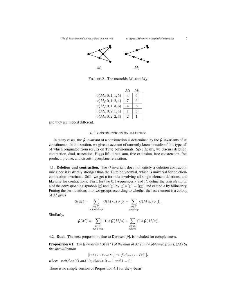
We end this section with two more examples, the matroids M1 and M2 in Figure 2.Brylawski [4, p. 268] showed that they are the smallest pair of non-paving matroids withthe same Tutte polynomial, but Derksen [9] showed that their G-invariants are distinct. Thecatenary data of these two matroids are given in the table


M1 M2

FIGURE 2. The matroids M1 and M2.

M1 M2

ν(Mi; 0, 1, 1, 5) 4 6

ν(Mi; 0, 1, 2, 4) 7 3

ν(Mi; 0, 1, 3, 3) 4 6

ν(Mi; 0, 2, 1, 4) 1 3

ν(Mi; 0, 2, 2, 3) 2 1

and they are indeed different.

4. CONSTRUCTIONS ON MATROIDS

In many cases, the G-invariant of a construction is determined by the G-invariants of itsconstituents. In this section, we give an account of currently known results of this type, allof which originated from results on Tutte polynomials. Specifically, we discuss deletion,contraction, dual, truncation, Higgs lift, direct sum, free extension, free coextension, freeproduct, q-cone, and circuit-hyperplane relaxation.

4.1. Deletion and contraction. The G-invariant does not satisfy a deletion-contractionrule since it is strictly stronger than the Tutte polynomial, which is universal for deletion-contraction invariants. Still, we get a formula involving all single-element deletions, andlikewise for contractions. First, for two 0, 1-sequences r and r′, define the concatenation� of the corresponding symbols [r] and [r′] by [r] � [r′] = [rr′] and extend � by bilinearity.Putting the permutations into two groups according to whether the last element is a coloopof M gives

G(M) =∑a∈E,

not a coloop

G(M\a) � [0] +∑a∈E,

a coloop

G(M\a) � [1].

Similarly,

G(M) =∑a∈E,

not a loop

[1] � G(M/a) +∑a∈E,a loop

[0] � G(M/a).

4.2. Dual. The next proposition, due to Derksen [9], is included for completeness.

Proposition 4.1. The G-invariant G(M∗) of the dual of M can be obtained from G(M) bythe specialization

[r1r2 . . . rn−1rn] 7→ [rnrn−1 . . . r2r1],

where¯switches 0’s and 1’s, that is, 0 = 1 and 1 = 0.

There is no simple version of Proposition 4.1 for the γ-basis.


4.3. Truncation and Higgs lift. The truncation Trun(M) of a matroid M of positiverank is the matroid on the same set whose bases are the independent sets of M that havesize r(M)− 1. The construction dual to truncation is the free or Higgs lift [14] defined byLift(M) = (Trun(M∗))∗ for a matroid M with at least one circuit.

Proposition 4.2. Let M be a matroid having positive rank. Then G(Trun(M)) can beobtained from G(M) by the specialization [r] 7→ [r↓], where r↓ is the sequence obtainedfrom r by replacing the right-most 1 by 0. Expressed in the γ-basis, G(Trun(M)) can beobtained by the specialization given by the linear transformation G(n, r) → G(n, r − 1)defined on the γ-basis by γ(a0, a1, . . . , ar) 7→ γ(a0, a1, . . . , ar−1 + ar).

Let M have at least one circuit. Then G(Lift(M)) can be obtained from G(M) by thespecialization [r] 7→ [r↑], where r↑ is obtained from r by replacing the left-most 0 by 1.

4.4. Direct sum. We first define a shuffle. Let (α1, α2, . . . , αm) and (β1, β2, . . . , βn) besequences and P be a subset of {1, 2, . . . ,m+n} of size m. The shuffle sh((αi), (βj);P )is the length-(m + n) sequence obtained by inserting the sequence (αi) in order into thepositions in P and the sequence (βj) in order into the remaining positions. For example,

sh((α1, α2, α3, α4), (β1, β2, β3); {1, 3, 4, 7}) = (α1, β1, α2, α3, β2, β3, α4).

If [r] and [s] are symbols, the first in G(n1, r1) and the second in G(n2, r2), then theirshuffle product [r] o [s] is the following linear combination in G(n1 + n2, r1 + r2):

[r] o [s] =∑

P⊆{1,2,...,n1+n2},|P |=n1

[sh(r, s;P )].

The shuffle product o is extended to G(n1, r1)× G(n1, r1) by bilinearity.The direct sumM1⊕M2 of the matroidsMi with rank and rank functions ri on disjoint

sets Ei is the matroid on the set E1 ∪E2 with rank function rM1⊕M2where, for Xi ⊆ Ei,

(4.1) rM1⊕M2(X1 ∪X2) = r1(X1) + r2(X2).

From the fact that the rank sequence of a shuffle of two permutations is the shuffle oftheir rank sequences, we obtain the following result.

Proposition 4.3. The G-invariant of the direct sum M1 ⊕M2 is given by the formula

G(M1 ⊕M2) = G(M1) o G(M2).

The next proposition follows easily from the fact that the lattice of flats L(M1⊕M2) ofthe direct sum is the direct productL(M1)×L(M2) of the lattices of flats of the summands,together with formula (4.1).

Proposition 4.4. The catenary data of the direct sum M1 ⊕M2 can be calculated in thefollowing way: for an (|E1| + |E2|, r1 + r2)-composition (a0 + b0, c1, c2, . . . , cr1+r2),where a0 and b0 are the numbers of loops in M1 and M2, respectively, we have

ν(M1⊕M2; a0+b0, c1, . . . , cr1+r2) =∑

((ai),(bj),P )

ν(M1; a0, a1, . . . , ar1) ν(M2; b0, b1, . . . , br2)

where the sum is over all triples ((a1, . . . , ar1), (b1, . . . , br2), P ) with |P | = r1 and

sh((a1, . . . , ar1), (b1, . . . , br2);P ) = (c1, c2, . . . , cr1+r2).

The next result treats the effect on the G-invariant of adding a coloop or loop.


Corollary 4.5. The G-invariant G(M ⊕ U1,1) can be obtained from G(M) by the special-ization

[r1r2 . . . rn] 7→ [1r1r2 . . . rn] +

n∑j=1

[r1 . . . rj1 . . . rn]

and G(M ⊕ U0,1) can be obtained from G(M) by the specialization

[r1r2 . . . rn] 7→ [0r1r2 . . . rn] +

n∑j=1

[r1 . . . rj0 . . . rn].

There is also a simple description of the effect of adding or removing loops from amatroid using the γ-basis.

Proposition 4.6. Let M be a loopless rank-r matroid. Then when expressed in the γ-basis, the G-invariants G(M ⊕ U0,h) and G(M) can be obtained from each other by thespecializations

γ(h, a1, a2, . . . , ar)←→ γ(0, a1, a2, . . . , ar).

WhileM has exactly a0 loops if and only if some term of the form ν(M ; a0, a1, . . . , ar)is positive, the number of coloops is the greatest integer k for which some compositionending in k ones has ν(M ; a0, a1, . . . , 1, 1) > 0.

In the cycle matroid M(Kr+1) of the complete graph, there are 2r − 1 copoints. For1 ≤ m < b(r + 1)/2c, there are

(r+1m

)copoints isomorphic to M(Kr+1−m) ⊕M(Km),

with an additional 12

(r+1

(r+1)/2

)copoints isomorphic to M(K(r+1)/2) ⊕ M(K(r+1)/2) if

r + 1 is even. Hence, by Propositions 3.6 and 4.4, the catenary data of M(Kr+1) can beobtained recursively from the catenary data of lower-rank cycle matroids M(Km). Thisrecursion is straightforward but complicated. Similar recursions exist for the catenary dataof other matroids (such as bicircular matroids) constructed from complete graphs.

Example 4.7. ConsiderM(K5). InM(K5), there are five copoints isomorphic toM(K4)and ten isomorphic toM(K3)⊕M(K2). The catenary data ofM(K4) is given in Example3.8. Since M(K3)⊕M(K2) ∼= U2,3 ⊕ U1,1, Proposition 4.4 yields its catenary data:

ν(M(K3)⊕M(K2); 0, 1, 1, 2) = 6, ν(M(K3)⊕M(K2); 0, 1, 2, 1) = 3.

We can now use Proposition 3.6 to obtain the catenary data of M(K5):

ν(M(K5); 0, 1, 2, 3, 4) = 5 · 12 = 60,

ν(M(K5); 0, 1, 1, 4, 4) = 5 · 6 = 30,

ν(M(K5); 0, 1, 1, 2, 6) = 10 · 6 = 60,

ν(M(K5); 0, 1, 2, 1, 6) = 10 · 3 = 30.

The Dowling matroidsQr(G) based on the finite groupG generalize the cycle matroidsM(Kr+1) (see [11]). In Qr(G), there are [(|G| + 1)r − 1]/|G| copoints. When |G| ≥ 2and 0 ≤ m ≤ r−1, there are

(rm

)|G|r−m−1 copoints isomorphic toQm(G)⊕M(Kr−m).

Thus, by Lemma 3.6, the catenary data ofQr(G) can be obtained from lower-rank Dowlingmatroids or cycle matroids of complete graphs by a recursion depending only on the order|G|. The next result follows by induction starting with the observation that Q1(G) isisomorphic to U1,1.

Proposition 4.8. The G-invariant of the Dowling matroid Qr(G) depends only on r and|G|.


4.5. Free extension and coextension. Given a matroidM and an element x not inE(M),the free extension M + x is the matroid on E(M) ∪ x whose bases are the bases of M orthe sets of the form B ∪ x where B is a basis of a copoint of M . Equivalently,

M + x = Trun(M ⊕ U1,1),

where U1,1 is the rank-1 matroid on the set {x}. The construction dual to free extension isthe free coextension M × x, defined by M × x = (M∗ + x)∗. This equals the Higgs liftLift(M ⊕ U0,1), where U0,1 is the rank-0 matroid on the set {x}.

Proposition 4.9. The G-invariant of the free extension M + x is obtained from G(M) bythe specialization

[r1r2 . . . rn] 7→ [1r1r2 . . . rn]↓ +

n∑j=1

[r1 . . . rj1 . . . rn]↓,

and the G-invariant of the free coextension M × x is obtained by

[r1r2 . . . rn] 7→ [0r1r2 . . . rn]↑ +

n∑j=1

[r1 . . . rj0 . . . rn]↑.

A freedom (or nested) matroid is obtained from a loop or a coloop by a sequence of freeextensions or additions of a coloop. Thus, one can recursively compute the G-invariant ofa freedom matroid using Corollary 4.5 and Proposition 4.9.

Example 4.10. The matroid N in Figure 1 is the free extension of N\x. The G-invariantof N\x is 96 [11100] + 24 [11010]. Each occurrence of [11100] in G(N\x) gives rise tosix terms in the free extension in the following way. First insert a 1 to obtain

[111100] + [111100] + [111100] + [111100] + [111010] + [111001]

and then change the right-most 1 to 0

[111000] + [111000] + [111000] + [111000] + [111000] + [111000].

Likewise, each occurrence of [11010] gives rise to six terms:

[111000] + [111000] + [111000] + [110100] + [110100] + [110100].

From this, we obtain

G(N) = (96 · 6 + 3 · 24) [111000] + 3 · 24 [110100] = 648 [111000] + 72 [110100].

4.6. Free product. The free product is a non-commutative matroid operation defined byCrapo and Schmitt [7]. Given an ordered pair M1 and M2 of matroids of ranks r1 and r2

on disjoint sets E1 and E2, the free product M1 2M2 is the matroid on E1 ∪ E2 whosebases are the subsets B of E1 ∪E2 of size r1 + r2 such that B ∩E1 is independent in M1

and B ∩ E2 spans M2. The rank function of M1 2M2 is given as follows: for Xi ⊆ Ei,

(4.2) rM12M2(X1 ∪X2) = min{r1(E1) + r2(X2), r1(X1) + |X2|}.

The free product U1,1 2 M is the free coextension of M , while M 2 U0,1 is the freeextension of M .

Proposition 4.11. The G-invariant of the free product M1 2M2 can be calculated fromthe G-invariants of M1 and M2.


Proof. LetE1 = {1, 2, . . . ,m} andE2 = {m+1,m+2, . . . ,m+n}. Let [ri] be symbolsthat occur in G(Mi), so ri is the rank sequence of a permutation πi on Ei. While G(Mi)does not give πi, we can calculate the rank sequence of a shuffle π = sh(π1, π2;P ) fromthe triple (r1, r2, P ). Given j with 1 ≤ j ≤ m+n, let X1 = {π(1), π(2), . . . , π(j)}∩E1

and X2 = {π(1), π(2), . . . , π(j)} ∩ E2, so the set {π(1), π(2), . . . , π(j)} is the disjointunion of X1 and X2. Note that |X1| = |P ∩ {1, 2, . . . , j}| and |X2| = j − |X1|, and thatri(Xi) is the number of 1’s in the first |Xi| positions in ri. By equation (4.2), the rank of{π(1), π(2), . . . , π(j)} inM12M2 can be found from r1(E1), r2(X2), r1(X1), and |X2|,and hence, from (r1, r2, P ). Applying this procedure starting from j = 1 yields the ranksequence of sh(π1, π2;P ) from the triple (r1, r2, P ).

Each permutation of {1, 2, . . . ,m + n} has exactly one representation as a shuffle ofpermutations πi of Ei, so the multiset of rank sequences r(π), over all permutations π{1, 2, . . . ,m+ n}, can be obtained by calculating the multiset of rank sequences obtainedfrom the triples (r1, r2, P ), where ri ranges over the multiset of rank sequences that occurin G(Mi) and P ranges over all m-subsets of {1, 2, . . . ,m + n}. In this way we obtainG(M1 2M2) from G(M1) and G(M2). �

Example 4.12. Let M1 = U1,2 ⊕ U1,1 and M2 = U1,3 ⊕ U1,2 on disjoint sets. Then,G(M1) = 4 [110] + 2 [101] and G(M2) = 72 [11000] + 36 [10100] + 12 [10010]. Thefree product M1 2M2 is a rank-4 matroid on a set of size 8. By the computation shownin the table below, the triple (101, 10010, {3, 4, 5}) gives the rank sequence 11100010 inM1 2M2. Repeating this procedure 2 · 3 · 56 times, we obtain G(M1 2M2).

j |X1| |X2| r1(X1) r2(X2) min{r1(E1) + r2(X2), r1(X1) + |X2|}1 0 1 0 1 min{2 + 1, 0 + 1} = 1

2 0 2 0 1 min{2 + 1, 0 + 2} = 2

3 1 2 1 1 min{2 + 1, 1 + 2} = 3

4 2 2 1 1 min{2 + 1, 1 + 2} = 3

5 3 2 2 1 min{2 + 1, 2 + 2} = 3

6 3 3 2 1 min{2 + 1, 2 + 3} = 3

7 3 4 2 2 min{2 + 2, 2 + 4} = 4

8 3 5 2 2 min{2 + 2, 2 + 5} = 4

4.7. q-cone. In his study of tangential blocks, Whittle [20] introduced q-cones (originallycalled q-lifts) of GF(q)-representable simple matroids.

Definition 4.13. Let M be a simple GF(q)-representable rank-r matroid and choose arepresentation of M in the rank-(r + 1) projective geometry PG(r, q), that is, a set E ofpoints in PG(r, q) so that the restriction PG(r, q)|E is isomorphic to M . Let A 7→ A bethe closure operator of PG(r, q). Choose a point a in PG(r, q) not in the linear hyperplaneE and let E′ be the union ⋃

p∈E{a, p}.

The matroid PG(r, q)|E′ is the q-cone of M with base E and apex a.

A GF(q)-representable matroid M may have inequivalent representations, so differentchoices of E may yield non-isomorphic q-cones of M : Oxley and Whittle [17] gave ex-amples of matroids with inequivalent representations that yield non-isomorphic q-cones.However, using a formula for the characteristic polynomial of q-cones due to Kung [15,Section 8.6], Bonin and Qin [3] showed that the Tutte polynomial of a q-cone of M can


be calculated from the Tutte polynomial of M and so depends only on M . We next treat asimilar result for the G-invariant.

Proposition 4.14. Let M be a simple GF(q)-representable matroid. The catenary data ofa q-cone M ′ of M can be calculated from the catenary data of M . Thus, the G-invariantof a q-cone M ′ depends only on G(M) (not on M or the representation).

Proof. LetM ′ be the q-cone ofM with baseE and apex a. IdentifyM with the restrictionPG(r, q)|E. For a flag

∅ = Y0 ⊂ Y1 ⊂ Y2 ⊂ · · · ⊂ Yr−1 ⊂ Yr ⊂ Yr+1 = E′

of M ′, letXi = clM ′(Yi ∪ a) ∩ E.

Since E is closed in M ′, the set Xi is a flat of M . The jump of the flag (Yi) is the least jwith a ∈ Yj . It follows that Xj−1 = Xj and that (X0, X1, . . . , Xj−1, Xj+1, . . . , Xr+1) isa flag in M , which we call the projection of (Yi) onto M .

Given a flag (Xi) inM with composition (a0, a1, . . . , ar), we obtain all flags (Yi) inM ′

with projection (Xi) and jump j as follows. For a fixed ordered basis (b1, b2, . . . , br) ofMwithXi = clM ({b1, b2, . . . , bi}), choose a sequence b′1, b

′2, . . . , b

′j−1 with b′i ∈ {a, bi}−a,

and set

Yi =

{clM ′({b′1, b′2, . . . , b′i}) if 0 ≤ i ≤ j − 1,clM ′(Xi−1 ∪ a) if j ≤ i ≤ r + 1.

It is easy to check that all flags in M ′ with projection (Xi) and jump j arise exactly oncethis way, and, due to the choice of b′1, b

′2, . . . , b

′j−1, there are qj−1 such flags. Also,

|Yi| ={|Xi| if 0 ≤ i ≤ j − 1,q|Xi−1|+ 1 if j ≤ i ≤ r + 1,

so a flag (Xi) inM with composition (a0, a1, . . . , ar) is the projection of qj−1 flags inM ′

with jump j, and these flags all have composition

(a0, a1, . . . , aj−1, (a0 + a1 + · · ·+ aj−1)(q − 1) + 1, ajq, aj+1q, . . . , arq).

Thus, we get the catenary data of M ′ from that of M . �

Example 4.15. The matroids M and N in Figure 1 are representable over the field GF(q)whenever q is a prime power with q > 3. They have the same catenary data, so theirq-cones have the same catenary data. The catenary data of M is ν(M ; 0, 1, 2, 3) = 6 andν(M ; 0, 1, 1, 4) = 18. Each of the six flags with composition (0, 1, 2, 3) is the projectionof

(1) one flag with jump 1 and composition (0, 1, q, 2q, 3q),(2) q flags with jump 2 and composition (0, 1, q, 2q, 3q),(3) q2 flags with jump 3 and composition (0, 1, 2, 3q − 2, 3q),(4) q3 flags with jump 4 and composition (0, 1, 2, 3, 6q − 5).

This and a similar calculation for the other 18 flags ofM give the catenary data for a q-coneM ′:

ν(M ′; 0, 1, q, 2q, 3q) = 6(1 + q), ν(M ′; 0, 1, q, q, 4q) = 18(1 + q),

ν(M ′; 0, 1, 2, 3q − 2, 3q) = 6q2, ν(M ′; 0, 1, 1, 2q − 1, 4q) = 18q2,

ν(M ′; 0, 1, 2, 3, 6q − 5) = 6q3, ν(M ′; 0, 1, 1, 4, 6q − 5) = 18q3.


4.8. Circuit-hyperplane relaxation. Recall that if X is a both a circuit and a hyperplane(that is, copoint) ofM , then the corresponding circuit-hyperplane relaxation is the matroidon the same set whose bases are those of M along with X . The next result is easy andextends a well-known result about Tutte polynomials.

Proposition 4.16. If M ′ is obtained from the rank-r matroid M on an n-element set byrelaxing a circuit-hyperplane, then

G(M ′)− G(M) = r! (n− r)! ([1r0n−r]− [1r−1010n−r−1]).

Equivalently, the only compositions for which ν(M) and ν(M ′) differ are the following:

ν(M ′; 0, 1, . . . , 1, n− r + 1) = ν(M ; 0, 1, . . . , 1, n− r + 1) + r!

and

ν(M ′; 0, 1, . . . , 1, 2, n− r) = ν(M ; 0, 1, . . . , 1, 2, n− r)− r!

2.

5. DERIVING MATROID PARAMETERS FROM THE G-INVARIANT

Since the Tutte polynomial is a specialization of the G-invariant, any matroid parameterthat is derivable from the Tutte polynomial is derivable from the G-invariant or catenarydata. An easy but important example is the number b(M) of bases of a matroid M . In-deed, the coefficient of the maximum symbol [1r0n−r] in G(M) equals r!(n − r)!b(M).Alternatively, by Lemma 3.2,

b(M) =1

r!

∑(a0,a1,...,ar)

ν(M ; a0, a1, . . . , ar) a1a2 · · · ar.

In this section, we identify some of the parameters of a matroid that are derivable from theG-invariant but not from the Tutte polynomial.

The result motivating this section is that the number fk(s) of flats of rank k and sizes can be derived from the G-invariant. As the matroid M1 in Figure 2 has two 2-pointlines whereas M2 has three, but T (M1;x, y) = T (M2;x, y), the Tutte polynomial doesnot determine all numbers fk(s). However, for a rank-r matroid and a given rank k, themaximum size mk of a rank-k flat and the number fk(mk) is derivable from T (M ;x, y).Indeed, mk is the greatest integer m for which the monomial (x − 1)r−k(y − 1)m−k

occurs in T (M ;x, y) with non-zero coefficient and fk(mk) is that coefficient. As shownin Section 5 of [6], fk(s) is derivable from T (M ;x, y) for each s with mk−1 < s ≤ mk.

Let M be a rank-r matroid on n elements. Fix integers h and k with 0 ≤ h ≤ k ≤ r,and let (sh, sh+1, . . . , sk) be a sequence of positive integers. For h < j ≤ k, let s′j =sj − sj−1. An (h, k; sh, sh+1, . . . , sk)-chain is a (saturated) chain (Xh, Xh+1, . . . , Xk)of flats such that r(Xj) = j and |Xj | = sj for h ≤ j ≤ k. For a rank-h flat X with|X| = sh and a rank-k flat Y with |Y | = sk, let FX,Y (sh, sh+1, . . . , sk) be the numberof (h, k; sh, sh+1, . . . , sk)-chains (X,Xh+1, . . . , Xk−1, Y ) starting with the flat X andending with the flat Y . Finally, let

Fh,k(sh, sh+1, . . . , sk) =∑

|X|=sh,|Y |=sk

FX,Y (sh, sh+1, . . . , sk),

so Fh,k(sh, sh+1, . . . , sk) is the number of (h, k; sh, sh+1, . . . , sk)-chains. When h = k,each chain collapses to a rank-k flat, and fk(s) = Fk,k(s), where s = sk.

In the next lemma, we shall think of elements in the γ-basis as variables and linearcombinations in G(n, r) as polynomials in those variables, so one can multiply them aspolynomials.


Lemma 5.1. Let 0 ≤ h ≤ k ≤ r. Then∑X a flat, r(X)=h, |X|=shY a flat, r(Y )=k, |Y |=sk

G(M |X)FX,Y (sh, sh+1, . . . , sk−1, sk)G(M/Y )

=∑(aj)

ν(M ; a0, a1, . . . , ah, s′h+1, . . . , s

′k, ak+1, . . . , ar)γ(a0, a1, . . . , ah)γ(0, ak+1, . . . , ar),

where the sum ranges over all (n, r)-compositions

(a0, . . . , ah, s′h+1, . . . , s

′k−1, s

′k, ak+1, . . . , ar)

such that a0 + a1 + · · ·+ ah = sh and ak+1 + ak+2 + · · ·+ ar = n− sk.

Proof. For a rank-h flat X with |X| = sh and a rank-k flat Y with |Y | = sk, let

ν(M ; a0, a1, . . . , ah−1, X, s′h+1, . . . , s

′k−1, Y, ak+1, . . . , ar)

be the number of chains (Xi) in M satisfying r(Xj) = j, |X0| = a0, |Xj −Xj−1| = ajfor 1 ≤ j < h and k < j ≤ r, Xh = X , Xk = Y , and |Xj −Xj−1| = s′j for h < j ≤ k.Then

ν(M ; a0, a1, . . . , ah−1, X, s′h+1, . . . , s

′k−1, Y, ak+1, . . . , ar)

= ν(M |X; a0, a1, . . . , ah−1, ah)FX,Y (sh, sh+1, . . . , sk−1, sk)ν(M/Y ; 0, ak+1, . . . , ar).

Hence,∑(aj)

ν(M ; a0, a1, . . . , ah−1, X, s′h+1, . . . , s

′k−1, Y, ak+1, . . . , ar)γ(a0, a1, . . . , ah)γ(0, ak+1, . . . , ar)

= G(M |X)FX,Y (sh, sh+1, . . . , sk−1, sk)G(M/Y ).

Summing over all flats X and Y having the stated rank and size, we obtain∑X,Y

G(M |X)FX,Y (sh, sh+1, . . . , sk)G(M/Y )

=∑(aj)

∑X,Y

ν(M ; a0, a1, . . . , ah−1, X, s′h+1, . . . , s

′k−1, Y, ak+1, . . . , ar)

× γ(a0, a1, . . . , ah)γ(0, ak+1, . . . , ar)

=∑(aj)

ν(M ; a0, a1, . . . , ah−1, ah, s′h+1, . . . , s

′k−1, s

′k, ak+1, . . . , ar)

× γ(a0, a1, . . . , ah)γ(0, ak+1, . . . , ar). �

Proposition 5.2. The numbers Fh,k(sh, sh+1, . . . , sk) and in particular, fk(s), are deriv-able from the catenary data. Also, if fk(s) = 1 and F is the unique flat of rank k and sizes, then both G(M |F ) and G(M/F ) can be derived from G(M).

Proof. For the first assertion, specialize all the symbols in the equation in Lemma 5.1 to 1.Then we have G(M |X) = sh! and G(M/Y ) = (n − sk)!, and the sum on the left equalssh!(n− sk)!Fh,k(sh, sh+1, . . . , sk). Since the sum on the right can be calculated from thecatenary data of M , we can derive Fh,k(sh, sh+1, . . . , sk). For the second assertion, to getG(M |F ), take X = F and Y = E(M); to get G(M/F ), take X = cl(∅) and Y = F . �


Corollary 5.3. The number of cocircuits of size s, the number of circuits of size s, and thenumber of cyclic sets (that is, unions of circuits) of size s and rank j are derivable from thecatenary data. In particular, one can deduce whether the matroid has a spanning circuit,so one can determine whether a graph is Hamiltonian from the G-invariant of its cyclematroid.

Proof. A cocircuit is the complement of a copoint; hence, the number of cocircuits of sizet equals fr−1(n − t). Circuits in M are cocircuits in the dual M∗. Finally, a set is cyclicif and only if it is a union of cocircuits in M∗, that is, its complement is a flat of M∗. �

The matroids in Figure 2 show that none of the parameters in Corollary 5.3 is determinedby the Tutte polynomial.

Proposition 5.2 can be used to derive fk(s, c), the number of rank-k flats X of size ssuch that the restriction M |X has exactly c coloops. The number fk(s, 0) is the number ofcyclic flats (that is, flats without coloops) of rank k and size s. We use the following easylemma.

Lemma 5.4. Let (X0, X1, . . . , Xr) be a flag with composition (a0, a1, . . . , ar). Then therestriction M |Xi+1 is the direct sum of M |Xi and a coloop if and only if ai+1 = 1.

Proposition 5.5. The number fk(s, c) is derivable from the G-invariant.

Proof. For j with 0 ≤ j ≤ k, the numbers fk(s, j) satisfy the linear equations, one foreach c with 0 ≤ c ≤ k,

k∑j=c

fk(s, j)j!

(j − c)!= Fk−c,k(s− c, s− c+ 1, s− c+ 2, . . . , s),

where the sequence s − c, s − c + 1, s + c + 2, . . . , s increases by 1 at each step. To seethis, note that the chains that Fk−c,k(s−c, s−c+1, . . . , s) counts are obtained by pickinga rank-k size-s flat that has exactly j coloops with c ≤ j ≤ k, and going down from rankk to rank k − c by deleting c of the j coloops one by one in some order. As the systemof linear equations is triangular with diagonal entries equal to c!, we can solve it to getfk(s, c). �

Much of the interest in the G-invariant has centered on the fact that it is a universalvaluative invariant, so we end this section by relating our work to that part of the theory.For brevity, we address these remarks to readers who are already familiar with valuativeinvariants as discussed in [9]. We show that the parameters studied in this section arevaluative invariants.

To make explicit the dependence on the matroidM , we shall write, for example, fk(M ; s)instead of fk(s). We shall use two results from the theory of valuative invariants. The firstis the basic theorem of Derksen [9] that specializations of the G-invariant, in particular,the G-invariant coefficients gr(M), are valuative invariants. The second is the easy lemmathat if u and v are valuative invariants on size-n rank-r matroids, then so is any linearcombination αnru+ βnrv, where αnr and βnr depend only on n and r.

Theorem 5.6. The following parameters are valuative invariants:

ν(M ; ai), Fh,k(M ; si), fk(M ; s), and fk(M ; s, c).

Proof. The catenary data is obtained from the G-invariant by a change of basis in G(n, r).Hence, ν(M ; ai) is a linear combination of gr(M); explicitly, ν(M ; ai) is obtained fromthe vector of G-invariant coefficients by applying the inverse of [c(a0,a1,...,ar)(b0, b1, . . . , br)],


a matrix depending only on n and r. Hence, ν(M ; ai) is a valuative invariant. In the nota-tion of Lemma 5.1, the number Fh,k(M ; sh, . . . , sk) is given in terms of the catenary databy

1

sh!(n− sk)!

∑(aj)

γ1(a0, . . . , ah)γ1(0, ak+1, . . . , ar)ν(M ; a0, . . . , ah, s′h+1, . . . , s

′k, ak+1, . . . , ar),

where the numbers γ1(a0, . . . , ah) and γ1(0, ak+1, . . . , ar) are obtained from γ(a0, . . . , ah)and γ(0, ak+1, . . . , ar) by specializing all symbols to 1, and depend only on h, k, sh, sk,n, and r. Hence Fh,k(M ; si) and fk(M ; s) are valuative invariants. Finally, the numbersfk(M ; s, c) are obtained from the numbers Fh,k(M ; si) by solving a system of equationswith coefficients depending only on k, s, and c; hence, they are valuative invariants aswell. �

6. RECONSTRUCTING THE G-INVARIANT FROM DECKS

Let G(n, r) be the subspace of G(n, r) that is spanned by the γ-basis elements that areindexed by compositions that start with 0. The circle product � is the binary operationfrom G(n1, r1)× G(n2, r2) to G(n1 + n2, r1 + r2) defined by

γ(a0, a1, . . . , ar1)� γ(0, b1, . . . , br2) = γ(a0, a1, . . . , ar1 , b1, b2, . . . , br2)

on γ-basis elements and extended to G(n1, r1) × G(n2, r2) by bilinearity. Let Fk denotethe set of all rank-k flats in a matroidM . The next lemma shows that only the sets Fk havea property that is a key to the work in this section.

Lemma 6.1. For a set A of flats of a matroid M , the following statements are equivalent:

(1) A = Fk for some k with 0 ≤ k ≤ r(M), and(2) each flag of M contains exactly one flat in A.

Proof. It is immediate that statement (1) implies statement (2). Now assume that statement(2) holds. We claim that statement (1) holds where k is max{r(X) : X ∈ A}. A routineexchange argument shows that if S and T are distinct flats in Fk, then there is a sequenceS,U, . . . , T of flats in Fk such that the intersection of each pair of consecutive flats hasrank k − 1. If A 6= Fk, then from such a sequence with S ∈ Fk ∩ A and T ∈ Fk − A,we get flats X ∈ Fk ∩ A and Y ∈ Fk − A with r(X ∩ Y ) = k − 1. Extend a flag (Zi)of M |(X ∩ Y ) to a flag (Xi) of M that contains X , and, separately, to a flag (Yi) of Mthat contains Y . Observe that at least one of (Xi) or (Yi) contradicts statement (2); thus,statement (1) holds. �

Theorem 6.2 (The slicing formula). LetM be a rank-r matroidM . For k with 0 ≤ k ≤ r,

G(M) =∑X∈Fk

G(M |X)� G(M/X).

Thus,

G(M) =1

r + 1

∑X∈L(M)

G(M |X)� G(M/X).

Proof. A flat X in Fk determines the set

FX = {(Xi) : Xk = X}


of flags intersecting Fk at X . These subsets partition the set of all flags into |Fk| blocks.Using this partition and Theorem 3.3, we obtain

G(M) =∑X∈Fk

( ∑(Xi)∈FX

γ(|X0|, |X1 −X0|, . . . , |Xr −Xr−1|)

)

=∑X∈Fk

( ∑(Xi)∈FX

γ(|X0|, |X1 −X0|, . . . , |X −Xk−1|)� γ(0, |Xk+1 −X|, . . . , |Xr −Xr−1|)

)

=∑X∈Fk

G(M |X)� G(M/X). �

Corollary 6.3. For any k with 0 ≤ k ≤ r(M), the G-invariant of M can be reconstructedfrom the deck, or unlabeled multiset,

{(G(M |X),G(M/X)) : X ∈ Fk}of ordered pairs of G-invariants.

To get the dual result, recall that deletion and contraction are dual operations, that is,(M\X)∗ = M∗/X and (M/X)∗ = M∗\X . As noted in the proof of Corollary 5.3, aset X is a flat of M if and only if its complement, E − X , is a cyclic set of M∗. Also,rM (X) = k if and only if r(M) − k = |E −X| − rM∗(E −X), where the right side isthe nullity of E−X in M∗. If we replace M with its dual M∗, set Y = E−X , and applyProposition 4.1, we get the following reconstruction result.

Corollary 6.4. For any j with 0 ≤ j ≤ r(M∗), the G-invariant ofM can be reconstructedfrom the deck

{(G(M |Y ),G(M/Y )) : Y a cyclic set of M of nullity j}.

Two special cases of Corollary 6.3 occur at the bottom and top of the lattice L(M) offlats. Recall that the girth of a matroid is the minimum size of a circuit in it. If M has girthat least g + 2 and X is a rank-g flat, then M |X is isomorphic to Ug,g and

G(M |X) = g!γ(0, 1, 1, . . . , 1︸︷︷︸g

).

By Theorem 6.2,

G(M) = g!γ(0, 1, 1, . . . , 1)�

∑X∈Fg

G(M/X)

.

Corollary 6.5. If M has girth at least g + 2, then G(M) can be reconstructed from thedeck

{(G(M/X) : X ∈ Fg}.In particular, if M is a simple matroid, then G(M) can be reconstructed from the deck{G(M/x) : x an element of M}. Dually, if M has n elements and each cocircuit ofM has more than t elements, so each set of size n − t spans M , then G(M) can bereconstructed from the deck

{(G(M |Y ) : Y a cyclic set of M with |Y | = n− t}.

The other special case gives another perspective on Proposition 3.6, which is equivalentto the corollary that we derive next. If M has n elements and X is a copoint of M , thenM/X = U1,n−|X| and G(M/X) = γ(0, n− |X|). Hence we get the following result.


Corollary 6.6. The G-invariant of M can be reconstructed from the number n of elementsin M and the deck of G-invariants of copoints.

Corollary 6.6 is motivated by the theorem of Brylawski [5] that the Tutte polynomial isreconstructible from the deck of unlabeled restrictions to copoints. With the next lemma,we can strengthen Corollary 6.6.

Lemma 6.7. The number n of elements of M can be reconstructed from the deck of G-invariants of copoints.

Proof. The proof is an adaptation of Brylawski’s argument. We begin with an identity.Using the notation in Section 5,

Fh,k−1(sh, sh+1, . . . , sk−1)(n− sk−1) =∑sk

Fh,k(sh, sh+1, . . . , sk−1, sk)(sk − sk−1).

This identity holds because both sides equal the number of triples

((Xh, Xh+1, . . . , Xk−1), x,X),

where |Xi| = si, the element x is not in Xk−1, and X = cl(Xk−1 ∪ x). In particular,

fh(sh)(n− sh) =∑sh+1

Fh,h+1(sh, sh+1)(sh+1 − sh).

Iterating the identity, we obtain

fh(sh) =∑sh+1

Fh,h+1(sh, sh+1)(sh+1 − sh)

(n− sh)

=∑

sh+1,sh+2

Fh,h+2(sh, sh+1, sh+2)(sh+1 − sh)(sh+2 − sh+1)

(n− sh)(n− sh+1)

...

=∑

sh+1,sh+2,...,sr−1

Fh,r−1(sh, sh+1, . . . , sr−1)

r−2∏j=h

sj+1 − sjn− sj

.

Let s0 be the number of loops in M . Then, since f0(s0) = 1, we have

(6.1) 1 =∑

s1,s2,...,sr−1

F0,r−1(s0, s1, s2, . . . , sr−1)

r−2∏j=0

sj+1 − sjn− sj

.

In addition, we also have

F0,r−1(s0, s1, s2, . . . , sr−1) =∑

copointX, |X|=sr−1

ν(M |X; s0, s1−s0, s2−s1, . . . , sr−1−sr−2),

and hence, we can calculate the right-hand side of equation (6.1) given the deck {G(M |X) :X ∈ Fr−1}, and solve for n. The number n of elements is a solution greater thanmax{sr−1}, the maximum number of elements in a copoint, and this solution is uniquesince the right-hand side is a strictly decreasing function in n. In other words, equation(6.1), and hence the deck, determines the number of elements in M . �

Corollary 6.6 and Lemma 6.7 yield the following result.

Theorem 6.8. The G-invariant of M can be reconstructed from the deck {G(M |X) :X a copoint}. Dually, we can reconstruct G(M) from the deck {G(M/Y ) : Y a circuit}.


The proof of the first assertion in Theorem 6.8 does not use the G-invariants G(M |X)individually but the sums

H(M ; s) =∑

X a copoint,|X|=s

G(M |X).

Hence, we have the following theorem giving the exact information needed to reconstructG(M) from a deck derived from copoints.

Theorem 6.9. The G-invariant G(M) and the deck {H(M ; s)} (consisting of the sumsH(M ; s) that are non-zero) can be constructed from each other.

7. CONFIGURATIONS

The main result in this section, Theorem 7.3, extends a result by Eberhardt [12] for theTutte polynomial (Theorem 7.1 below) to the G-invariant. We also show that the converseof Theorem 7.3 is false.

These results use the configuration of a matroid, which Eberhardt defined. Recall thata set X in a matroid M is cyclic if X is a union of circuits, or, equivalently, M |X has nocoloops. The set Z(M) of cyclic flats of M , ordered by inclusion, is a lattice. The joinX ∨ Y in Z(M) is cl(X ∪ Y ), as in the lattice of flats; the meet X ∧ Y is the union ofthe circuits in X ∩ Y . It is well-known that a matroid M is determined by E(M) and thepairs (X, r(X)) for X ∈ Z(M). If deleting all coloops of a matroid M yields M ′, thenwe easily get G(M) from G(M ′), so we focus on matroids without coloops. (Similarly,focusing on matroids that also have no loops, as in the proof of Theorem 7.3, is justified.)The configuration of a matroidM with no coloops is the triple (L, s, ρ) where L is a latticethat is isomorphic to Z(M), and s and ρ are functions on L where if x ∈ L correspondsto X ∈ Z(M), then s(x) = |X| and ρ(x) = r(X). The configuration does not recordthe cyclic flats, and we do not distinguish between L and lattices isomorphic to it, so non-isomorphic matroids (such as the pair in Figure 1) may have the same configuration. Twopaving matroids of the same rank r with the same number fr−1(s) of size-s copoints, foreach s, have the same configuration. Gimenez constructed a set of n! non-paving matroidsof rank 2n+ 2 on 4n+ 5 elements, all with the same configuration (see [2, Theorem 5.7]).We now state Eberhardt’s result.

Theorem 7.1. For a matroid with no coloops, its Tutte polynomial can be derived from itsconfiguration.

We use Theorem 7.1 to prove Theorem 7.3. (With these techniques, one can give anotherproof of Theorem 7.1 since knowing T (M ;x, y) is equivalent to knowing, for each pair i,j, the number of subsets ofE(M) of size i and rank j, and an inclusion/exclusion argumentlike that in the proof of Lemma 7.3.2 shows that the configuration gives the number of suchsubsets. We use only a special case of Theorem 7.1, namely, the configuration gives thenumber of bases.) We also use the following elementary lemma about cyclic flats.

Lemma 7.2. Assume that M has neither loops nor coloops. If X is any cyclic flat of M ,then Z(M |X) is the interval [∅, X] in Z(M), and

Z(M/X) = {F −X : F ∈ Z(M) and X ⊆ F},so the lattice Z(M/X) is isomorphic to the interval [X,E(M)] in Z(M). Thus, fromthe configuration of M , we get the configuration of any restriction to, or contraction by,a cyclic flat of M . Likewise, the configuration of the truncation Trun(M) can be derivedfrom that of M .


Theorem 7.3. For a matroid M with no coloops, its catenary data, and so G(M), can bederived from its configuration.

Proof. As noted above, we can make the further assumption thatM has no loops. Let ι(N)denote the number of independent copoints of a matroid N , and b(N) denote its numberof bases. The proof is built on two lemmas.

Lemma 7.3.1. If, for each chain ∅ = D0 ⊂ D1 ⊂ · · · ⊂ Dt = E(M) in Z(M), we haveeach r(Di) and ι(M |Di/Di−1), then we can compute the catenary data of M .

Proof. Let ∅ = X0 ⊂ X1 ⊂ · · · ⊂ Xr = E(M) be a flag of flats of M , so r = r(M).Each flatXi is the disjoint union of the setUi of coloops ofM |Xi and a cyclic flat Fi ofM .Thus, F0 ⊆ F1 ⊆ · · · ⊆ Fr. Since M has neither loops nor coloops, U0 = F0 = ∅ = Urand Fr = E(M). Let ∅ = D0 ⊂ D1 ⊂ · · · ⊂ Dt = E(M) be the distinct cyclic flatsamong F0, F1, . . . , Fr, and let U = U1 ∪ U2 ∪ · · · ∪ Ur−1. Thus, |U | = r − t. We callD0, D1, . . . , Dt and U the cyclic flats and set of coloops of the flag. For i with 1 ≤ i ≤ t,let Wi = U ∩ (Di −Di−1), which may be empty. Fix i with 1 ≤ i < t. Let j be the leastinteger with Di ⊆ Xj , so Uj = Xj −Di. Delete all elements of Uj from the flats in thechain X0 ⊂ X1 ⊂ · · · ⊂ Xj ; the distinct flats that remain form a chain, and the greatest isDi and the one of rank r(Di) − 1 is Di−1 ∪Wi. Thus, Wi is an independent copoint ofM |Di/Di−1.

Conversely, let ∅ = D0 ⊂ D1 ⊂ · · · ⊂ Dt = E(M) be a chain of cyclic flats.For each i with 1 ≤ i ≤ t, let Wi be an independent copoint of M |Di/Di−1 and setU = W1 ∪W2 ∪ · · · ∪Wt (so |U | = r− t). There are flags of flats of M whose cyclic flatsand set of coloops are D0, D1, . . . , Dt and U , and we obtain all such flags in the followingway. Take any permutation π of U ∪ {D1, . . . , Dt} in which, for each i, all elements ofWi, and all Dk with k < i, are to the left of Di. To get a flag from π, successively adjointo ∅ the elements in initial segments of π.

We next find the contributions of these flags to the catenary data of M . With the typeof permutation π described above, there are t associated integer compositions, each with tparts, namely, for each i, we have the integer composition |Wi| = ai1 + ai2 + · · · + aitwhere aij is the number of elements of Wi that are between Dj−1 and Dj in π. Thus, ifj > i, then aij = 0. We call the lower-triangular t × t matrices A = (aij) the matrixof compositions of π. A lower-triangular t × t matrix with non-negative integer entriesis a matrix of compositions for some such permutation π if and only if its row sums are|W1|, |W2|, . . . , |Wt|. Let a′j be the sum of the entries in column j of A, which is thenumber of elements between Dj−1 and Dj in π. The composition of the flag that we getfrom any permutation π whose matrix of compositions is A is(

0, 1, . . . , 1︸︷︷︸a′1

, |D1| − |W1|, 1, . . . , 1︸︷︷︸a′2

, |D2| − |W1 ∪W2|, . . . , 1, . . . , 1︸︷︷︸a′t

, |Dt| − (r − t)),

and the number of such permutations π ist∏i=1

(|Wi|

ai1, ai2, . . . , aii

)a′i!,

where the multinomial coefficient accounts for choosing the aij elements of Wi that willbe between Dj−1 and Dj , and the factorial accounts for permutations of the elements thatare between Di−1 and Di.

Thus, what the chainD0, D1, . . . , Dt in Z(M) and the setsW1,W2, . . . ,Wt contributeto the catenary data can be found from just the t numbers |W1|, |W2|, . . . , |Wt|. Since


|Wi| = r(M |Di/Di−1) − 1 and Wi can be any independent copoint of M |Di/Di−1, thecatenary data of M can be computed from the data r(Di) and ι(M |Di/Di−1), over allchains in Z(M) that include ∅ and E(M), as Lemma 7.3.1 asserts. �

Lemma 7.3.2. We can compute ι(N) if we have (i) b(Trun(N)) as well as (ii) for eachchain ∅ = F0 ⊂ F1 ⊂ · · · ⊂ Fp ⊂ E(N) in Z(N), the numbers b(N |Fk/Fk−1), for1 ≤ k ≤ p, and b(Trun(N/Fp)).

Proof. Note that b(Trun(N)) is the number of independent sets of size r(N) − 1 in N .Set Z ′ = {F ∈ Z(N) : 0 < r(F ) < r(N)}. For F ∈ Z ′, let

AF = {I ⊂ E : r(I) = |I| = r(N)− 1 and cl(I ∩ F ) = F}.Thus,

ι(N) = b(Trun(N))−∣∣∣ ⋃F∈Z′

AF

∣∣∣,so by inclusion/exclusion,

(7.1) ι(N) = b(Trun(N)) +∑

S⊆Z′,S 6=∅

(−1)|S|∣∣∣ ⋂F∈S

AF

∣∣∣.Note that if I ∈ AF1

∩ AF2for F1, F2 ∈ Z ′, then I ∩ (F1 ∨ F2) spans F1 ∨ F2 (recall,

F1 ∨ F2 = cl(F1 ∪ F2)); thus r(F1 ∨ F2) ≤ r(I) < r(N), so F1 ∨ F2 ∈ Z ′, andI ∈ AF1∨F2

; hence, AF1∩AF2

= AF1∩AF2

∩AF1∨F2. Now assume that F1 and F2 are

incomparable, so F1 ∨ F2 properly contains both of them. If F1 and F2 are in a subset Sof Z ′, and if S′ is the symmetric difference S4{F1 ∨F2}, then (−1)|S| = −(−1)|S

′| and⋂F∈S

AF =⋂F∈S′

AF ,

so such terms could cancel in the sum in equation (7.1). Pair off such terms as follows: takea linear extension ≤ of the order ⊆ on Z ′ and, if a subset S of Z ′ contains incomparablecyclic flats, let F1 and F2 be such a pair for which (F1, F2) is least in the lexicographicorder that ≤ induces on Z ′ × Z ′; cancel the term in the sum in equation (7.1) that arisesfrom S with the one that arises from S′ = S4{F1 ∨ F2}. These cancellations leave

(7.2) ι(N) = b(Trun(N)) +∑

nonempty chainsS⊆Z′

(−1)|S|∣∣∣ ⋂F∈S

AF

∣∣∣.Now let S be a chain in this sum, say consisting of F1 ⊂ F2 ⊂ · · · ⊂ Fp. The independentsets in

⋂pi=1AFi

are the union of a basis of N |F1, a basis of N |Fk/Fk−1, for 1 < k ≤ p,and a basis of Trun(N/Fp). Thus,

∣∣⋂pi=1AFi

∣∣, and so ι(N), can be found from the datagiven in Lemma 7.3.2. �

With these lemmas, we now prove Theorem 7.3. Let (L, s, ρ) be the configurationof M . Chains ∅ = D0 ⊂ D1 ⊂ · · · ⊂ Dt = E(M) in Z(M) correspond to chains0 = x0 < x1 < · · · < xt = 1 in L, where 0 and 1 are the least and greatest elements ofL. The configuration of M |Di/Di−1 consists of the interval [xi−1, xi] in L along with themaps y 7→ s(y) − s(xi−1) and y 7→ ρ(y) − ρ(xi−1). (For what we do with such minors(e.g., construct more such minors and find their configurations), working with the matroidis equivalent to working with its configuration; to make it easier to follow, in the rest ofthe proof we use the matroid.) The only other data we need in order to apply Lemma 7.3.1is ι(M |Di/Di−1). Lemma 7.3.2 reduces this to data that, by Theorem 7.1, can be derivedfrom the configuration of M |Di/Di−1 and hence from that of M . Specifically, letting N


beM |Di/Di−1, we have its configuration, say (L′, s′, ρ′), and the chains in L′ correspondto those in Z(N), and we get the configurations of Trun(N) and each N |Fk/Fk−1 andTrun(N/Fp) in Lemma 7.3.2. Thus, we get the number of bases of Trun(N) and eachN |Fk/Fk−1 and Trun(N/Fp) by Theorem 7.1, so, as needed, by Lemma 7.3.2 we getι(N). �

By Proposition 4.8, Dowling matroids of the same rank based on groups of the samefinite order have the same G-invariant. Here we prove that, for r ≥ 4, Dowling matroidsbased on non-isomorphic finite groups have different configurations; thus, the converse ofTheorem 7.3 is false. We first recall the few facts about these matroids that we use. Let Gbe a finite group and r a positive integer. The set on which the Dowling matroid Qr(G) isdefined consists of the r +

(r2

)|G| elements

(P1) p1, p2, . . . , pr, and(P2) aij for each a ∈ G and i, j ∈ {1, 2, . . . , r} with i 6= j, where aji = (a−1)ij .

The lines (rank-2 flats) of Qr(G) are of three types:(L1) `ij := {pi, pj} ∪ {aij : a ∈ G}, where |{i, j}| = 2,(L2) {aij , bjk, (ab)ik}, where a, b ∈ G and |{i, j, k}| = 3, and(L3) {pi, ajk} with |{i, j, k}| = 3, and {ahi, bjk} with |{h, i, j, k}| = 4.

The set {p1, p2, . . . , pr} is a basis of Qr(G); each element of Qr(G) is in some line that isspanned by two elements in this basis. For each t with 2 ≤ t ≤ r, the restriction of Qr(G)to the closure of any t-element subset of {p1, p2, . . . , pr} is isomorphic to Qt(G) and sohas t+

(t2

)|G| elements; if |G| ≥ 4 (the leastm for which there are non-isomorphic groups

of order m), then all other flats of rank t are strictly smaller.

Proposition 7.4. For r ≥ 4 and finite groups G and G, if the Dowling matroids Qr(G)

and Qr(G) have the same configuration, then G and G are isomorphic.

Proof. Assume that |G| = |G| ≥ 4. By the hypothesis, there is a lattice isomorphismφ : Z(Qr(G)) → Z(Qr(G)) that preserves the rank and size of each cyclic flat. Letcl be the closure operator of Qr(G), and cl′ that of Qr(G). Applying the last remarkbefore the proposition with t = 4 shows that, with relabeling if needed, we may assumethat φ(cl({p1, p2, p3, p4})) = cl′({p1, p2, p3, p4}). By restricting to these flats, we mayassume that r = 4. Likewise, we may assume that φ(cl({pi, pj , pk})) = cl′({pi, pj , pk})whenever {i, j, k} ⊂ {1, 2, 3, 4}. We will show that Q3(G) and Q3(G) are isomorphic.The following result by Dowling [11, Theorem 8] then completes the proof: for r ≥ 3,the matroids Qr(G) and Qr(G) are isomorphic if and only if the groups G and G areisomorphic.

The singleton flats {aij} are not in Z(Q4(G)), but we show that they induce certainpartitions of sets of 3-point lines in Z(Q4(G)). Let i, j, s, t be 1, 2, 3, 4 in some order. LetPijs be the set of 3-point lines in the plane cl({pi, pj , ps}). For a ∈ G, set

P aijs = {` ∈ Pijs : aij ∈ `}.

Thus, {P aijs : a ∈ G} is a partition of Pijs. With Pijt and P bijt defined similarly, take` ∈ P

aijs and `′ ∈ P

bijt . By the remarks above, if a 6= b, then cl(` ∪ `′) is Q4(G),

while if a = b, then cl(` ∪ `′) is a cyclic flat of rank 3. Now cl(` ∪ `′) ∈ Z(Q4(G))

and the same observations hold for Q4(G), so the isomorphism φ maps the blocks P aijs

and Paijt in the partitions of Pijs and Pijt to their counterparts (written, for instance,

as P cijs ) in Q4(G). Thus, for {i, j} ⊂ {1, 2, 3, 4}, there is a bijection ψij : G → G


with φ(Paijs ) = P

(ψij(a))ijs and φ(P

aijt ) = P

(ψij(a))ijt . Putting these maps together, we

have a bijection ψ : Q4(G) → Q4(G) with ψ(pi) = pi and ψ(aij) = (ψij(a))ij for{i, j} ⊂ {1, 2, 3, 4} and a ∈ G. A 3-point line ` = {aij , bjk, (ab)ik} of Q4(G) is in theequivalence classes P aijk , P bjki , and P (ab)ik

j , so φ(`) is in the equivalence classes Pψ(aij)k ,

Pψ(bjk)i , and Pψ((ab)ik)

j , and so φ(`) = ψ(`). Thus, since ψ also clearly preserves thelines of type (L1), the restriction of ψ to cl({p1, p2, p3}) shows that Q3(G) and Q3(G) areisomorphic, so, by Dowling’s result, G and G are isomorphic. �

8. DETECTING FREE PRODUCTS

The Tutte polynomial reflects direct sums in a remarkably faithful way. In [16], Merino,de Mier, and Noy showed that the Tutte polynomial T (M ;x, y) factors as A(x, y)B(x, y),for polynomials A(x, y) and B(x, y) over Z, if and only if A(x, y) and B(x, y) are theTutte polynomials of the constituents in some direct sum factorization ofM . By that resultand Theorem 1.1, from G(M) one can deduce whether M is a direct sum; however, wedo not know whether the G-invariants of the constituents are determined by G(M). In thissection we prove a result of this type for free products.

As noted earlier, the free productM2U0,1 is the free extension ofM , while U1,12M isthe free coextension. The matroids in Figure 1 show that the G-invariant cannot detect freeextensions (hence, coextensions). Thus, we consider only proper free products M1 2M2,by which we mean that each of M1 and M2 has at least two cyclic flats. Below we reducethe problem to sharp free products, which are proper free products M1 2M2 in which M1

has no coloops andM2 has no loops. A pinchpoint of the latticeZ(M) of cyclic flats ofMis a cyclic flat, neither the maximum nor the minimum, that each cyclic flat either containsor is contained in. We now state our main result.

Theorem 8.1. From G(M), one can deduce whether M is a proper free product. Also,for each pinchpoint X of Z(M), the G-invariants of the constituents of the correspondingsharp free product factorization of M can be derived from G(M) and r(X).

We use [8, Proposition 6.1], which we cite next.

Lemma 8.2. Let M1 and M2 be matroids on disjoint ground sets. Set

Z ′ =(Z(M1)− {E(M1)}

)∪ {E(M1) ∪ Y : Y ∈ Z(M2)− {∅} }.

If the factorization M1 2M2 is sharp, then Z(M) is Z ′ ∪ {E(M1)}; otherwise it is Z ′.

We first explain a reduction that we use: from each proper factorization of M , we geta sharp factorization of M . Let M be the proper free product M1 2M2. It follows fromLemma 8.2 that Z(M) has a pinchpoint. In particular, if the factorization is sharp, thenE(M1) is a pinchpoint. If M1 has coloops, then the maximum flat in Z(M1) (which is notE(M1)) is a pinchpoint of Z(M). If Y is any set of coloops of M1, then another properfactorization ofM is (M1\Y )2((M |Y )2M2), and (M |Y )2M2 applies free coextensionto M2 a total of |Y | times. If Y is the set of all coloops of M1, then the factorization(M1\Y )2((M |Y )2M2) ofM is sharp. Likewise, ifM2 has loops, thenE(M1)∪clM2

(∅)is a pinchpoint of Z(M). If Y ⊆ clM2

(∅), then another proper factorization of M is(M1 2 (M2|Y ))2 (M2\Y ), and M1 2 (M2|Y ) applies free extension to M1 a total of |Y |times. If Y = clM2(∅), then the factorization (M1 2 (M2|Y )) 2 (M2\Y ) of M is sharp.Thus, finding the sharp factorizations of M is the crux of the problem. The next lemma(which recasts [8, Theorem 6.3]) relates this more precisely to the pinchpoints of Z(M).


Lemma 8.3. A matroid M is a proper free product if and only if the lattice Z(M) has apinchpoint. Furthermore, the map X 7→ (M |X) 2 (M/X) is a bijection from the set ofpinchpoints of Z(M) onto the set of sharp free product factorizations of M .

We now prove the main result of this section.

Proof of Theorem 8.1. Recall from Section 5 that from G(M) we can deduce the numberfk(s) of flats, and the number fk(s, 0) of cyclic flats, of rank k and size s in M . Set

C = {k : 0 < k < r(M) and∑s

fk(s, 0) = 1},

so k ∈ C if and only if 0 < k < r(M) and exactly one cyclic flat of M has rank k. Therank of any candidate pinchpoint is in C, so if C = ∅, then M is not a proper free product.When C 6= ∅, we test each k ∈ C as follows.

Let X be the unique cyclic flat of rank k. Set s0 = |X|. If fk(s0) > 1, then there is anon-cyclic flat F of rank k and size s0. The flat Y obtained from F by deleting the coloopsof M |F is cyclic, and s0 − |Y | = |F − Y | = k − r(Y ). If Y ⊂ X , then comparing rankand size shows thatM |X has coloops (the elements ofX−Y ), contrary toX being cyclic.Hence, Y 6⊂ X , so X is not a pinchpoint. Thus, if X is a pinchpoint, then fk(s0) = 1.

Now assume that X is the only flat of rank k and size s0. By Proposition 5.2, fromG(M), we get G(M |X) and G(M/X). Thus, by Proposition 5.5 we can derive the numberof cyclic flats in M |X and in M/X . Now X is a pinchpoint of M if and only if (i) thenumber of cyclic flats in M |X equals the number of cyclic flats of rank at most k in M ,and (ii) the number of cyclic flats in M/X equals the number of cyclic flats of rank atleast k in M . Thus, we can detect pinchpoints, and for any pinchpoint X , we can deriveG(M |X) and G(M/X). �

ACKNOWLEDGMENTS

We thank the referees for their careful reading and constructive comments.

REFERENCES

[1] L.J. Billera, N. Jia, V. Reiner, A quasisymmetric function for matroids, European J. Combin. 30 (2009)1727–1757.

[2] J. Bonin, A. de Mier, The lattice of cyclic flats of a matroid, Ann. Comb. 12 (2008) 155–170.[3] J. Bonin, H. Qin, Tutte polynomials of q-cones, Discrete Math. 232 (2001) 95–103.[4] T. Brylawski, A decomposition for combinatorial geometries, Trans. Amer. Math. Soc. 171 (1972) 235–282.[5] T. Brylawski, Hyperplane reconstruction of the Tutte polynomial of a geometric lattice, Discrete Math. 35

(1981) 25–38.[6] T. Brylawski, The Tutte polynomial part I: General theory, in: Matroid theory and its applications, C.I.M.E.

Summer School, 83, Springer, Heidelberg, 2010, pp. 125–275.[7] H. Crapo, W.R. Schmitt, The free product of matroids, European J. Combin. 26 (2005) 1060–1065.[8] H. Crapo, W.R. Schmitt, A unique factorization theorem for matroids, J. Combin. Theory Ser. A 112 (2005)

222–249.[9] H. Derksen, Symmetric and quasi-symmetric functions associated to polymatroids, J. Algebraic Combin.

30 (2009) 43–86.[10] H. Derksen, A. Fink, Valuative invariants for polymatroids, Adv. Math. 225 (2010) 1840–1892.[11] T.A. Dowling, A class of geometric lattices based on finite groups, J. Combinatorial Theory Ser. B 14 (1973)

61–86.[12] J. Eberhardt, Computing the Tutte polynomial of a matroid from its lattice of cyclic flats, Electron. J. Com-

bin. 21 (2014) Paper 3.47, 12.[13] M.J. Falk, J.P.S. Kung, Algebras and valuations related to the Tutte polynomial, in: Handbook of the Tutte

polynomial, to appear.[14] D.A. Higgs, Strong maps of geometries, J. Combinatorial Theory 5 (1968) 185–191.


[15] J.P.S. Kung, Critical problems, in: Matroid theory, J. Bonin, J.G. Oxley, B. Servatius, eds., Amer. Math.Soc., Providence, RI, 1996, pp. 1–127.

[16] C. Merino, A. de Mier, M. Noy, Irreducibility of the Tutte polynomial of a connected matroid, J. Combin.Theory Ser. B 83 (2001) 298–304.

[17] J.G. Oxley, G. Whittle, On the non-uniqueness of q-cones of matroids, Discrete Math. 218 (2000) 271–275.[18] R.P. Stanley, Enumerative Combinatorics, volume 2, Cambridge University Press, Cambridge, 2011.[19] D.J.A. Welsh, Matroid Theory, Academic Press, London, 1976.[20] G. Whittle, q-lifts of tangential k-blocks, J. London Math. Soc. (2) 39 (1989) 9–15.[21] P. Young, J. Edmonds, Matroid designs, J. Res. Nat. Bur. Standards Sect. B 77B (1973) 15–44.

(J. Bonin) DEPARTMENT OF MATHEMATICS, THE GEORGE WASHINGTON UNIVERSITY, WASHINGTON,D.C. 20052, USA

E-mail address, J. Bonin: [email protected]

(J.P.S. Kung) DEPARTMENT OF MATHEMATICS, UNIVERSITY OF NORTH TEXAS, DENTON, TX 76203,USA

E-mail address, J.P.S. Kung: [email protected]

the g-invariant and catenary data of a matroid · the g-invariant and catenary data of a matroid...

Documents