arX

iv:1

611.

0062

9v1

[ast

ro-p

h.S

R]

2 N

ov 2

016

MNRAS 000, 1–13 (2016) Preprint 3 November 2016 Compiled using MNRAS LATEX style file v3.0

The Gaia DR1 Mass-Radius Relation for White Dwarfs

P.-E. Tremblay1⋆, N. Gentile-Fusillo1, R. Raddi1, S. Jordan2, C. Besson3,B. T. Gänsicke1, S. G. Parsons4, D. Koester5, T. Marsh1, R. Bohlin6, J. Kalirai61Department of Physics, University of Warwick, CV4 7AL, Coventry, UK2Astronomisches Rechen-Institut, Zentrum für Astronomie der Universität Heidelberg, D-69120 Heidelberg, Germany3Arts et Métiers ParisTech Centre de Bordeaux-Talence, Esplanade des Arts et Métiers, 33400 Talence, France4Department of Physics and Astronomy, University of Sheffield, S3 7RH, Sheffield, UK5Institut für Theoretische Physik und Astrophysik, Universität Kiel, D-24098 Kiel, Germany6Space Telescope Science Institute, 3700 San Martin Drive, Baltimore, MD 21218, USA

Accepted XXX. Received YYY; in original form ZZZ

ABSTRACTTheGaia Data Release 1 (DR1) sample of white dwarf parallaxes is presented, including 6directly observed degenerates and 46 white dwarfs in wide binaries. This data set is combinedwith spectroscopic atmospheric parameters to study the white dwarf mass-radius relationship(MRR). Gaia parallaxes andG magnitudes are used to derive model atmosphere dependentwhite dwarf radii, which can then be compared to the predictions of a theoretical MRR. Wefind a good agreement betweenGaia DR1 parallaxes, published effective temperatures (Teff)and surface gravities (logg), and theoretical MRRs. As it was the case forHipparcos, theprecision of the data does not allow for the characterisation of hydrogen envelope masses.The uncertainties on the spectroscopic atmospheric parameters are found to dominate the errorbudget and current error estimates for well-known and bright white dwarfs may be slightlyoptimistic. With the much largerGaiaDR2 white dwarf sample it will be possible to explorethe MRR over a much wider range of mass,Teff , and spectral types.

Key words: white dwarfs – stars: fundamental parameters – stars: interiors – parallaxes –stars: distances

1 INTRODUCTION

The white dwarf mass-radius relationship (MRR) is fundamentalto many aspects of astrophysics. At one end of the spectrum, theupper mass limit first derived byChandrasekhar(1931) is the cen-tral basis of our understanding of type Ia supernovae, standard can-dles that can be used to measure the expansion of the Universe(Riess et al. 1998; Perlmutter et al. 1999). On the other hand, theMRR is an essential ingredient to compute white dwarf massesfrom spectroscopy, photometry, or gravitational redshiftmeasure-ments (see, e.g.,Koester et al. 1979; Shipman 1979; Koester 1987;Bergeron et al. 1992, 2001; Falcon et al. 2012). These massescalibrate the semi-empirical initial to final mass relationforwhite dwarfs in clusters and wide binaries (see, e.g.,Weidemann2000; Catalán et al. 2008; Kalirai et al. 2008; Williams et al. 2009;Casewell et al. 2009; Dobbie et al. 2012; Cummings et al. 2016).These results unlock the potential for white dwarfs to be used tounderstand the chemical evolution of galaxies (Kalirai et al. 2014),date old stellar populations (Hansen et al. 2007; Kalirai 2012), andtrace the local star formation history (Tremblay et al. 2014).

On the theoretical side, the first MRRs that were uti-lized assumed a zero temperature fully degenerate core

⋆ E-mail: P-E.Tremblay@warwick.ac.uk

(Hamada & Salpeter 1961). The predictions have now im-proved to include the finite temperature of C and O nuclei inthe interior and the non-degenerate upper layers of He and H(Wood 1995; Hansen 1999; Fontaine et al. 2001; Salaris et al.2010; Althaus et al. 2010a). The MRRs were also extended tolower and higher mass ranges, with calculations for He and O/Necores, respectively (Althaus et al. 2007, 2013). The total massof the gravitationally stratified H, He, and C/O layers in whitedwarfs is poorly constrained since we can only see the top layerfrom the outside. While there are some constraints on the interiorstructure of white dwarfs from asteroseismology (Fontaine et al.1992; Romero et al. 2012, 2013; Giammichele et al. 2016), thewhite dwarf cooling sequence in clusters (Hansen et al. 2015;Goldsbury et al. 2016), and convective mixing studies (Sion 1984;Tremblay & Bergeron 2008; Bergeron et al. 2011), a theoreticalMRR assuming a specific interior stratification is usually preferred(Iben & Tutukov 1984; Fontaine et al. 2001; Althaus et al. 2010b).For hydrogen-atmosphere DA white dwarfs, most studies assumethick hydrogen layers withqH = MH/Mtot = 10−4, which is anestimate of the maximum hydrogen mass for residual nuclearburning (Iben & Tutukov 1984). More detailed calculations forthe maximum H envelope mass as a function of the white dwarfmass have also been employed (Althaus et al. 2010b). On theother hand, thin H-layers (qH = 10−10) are often used for helium

c© 2016 The Authors

2 Tremblay et al.

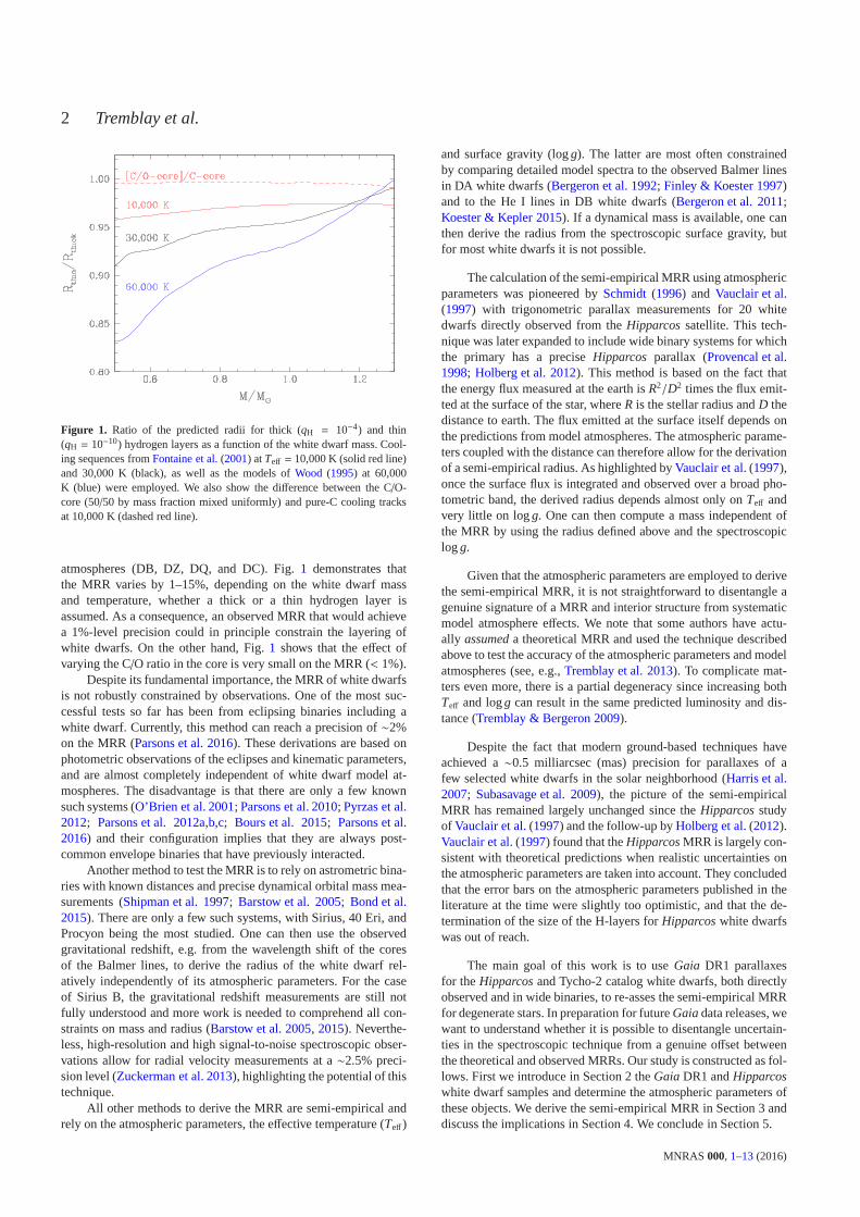
Figure 1. Ratio of the predicted radii for thick (qH = 10−4) and thin(qH = 10−10) hydrogen layers as a function of the white dwarf mass. Cool-ing sequences fromFontaine et al.(2001) atTeff = 10,000 K (solid red line)and 30,000 K (black), as well as the models ofWood (1995) at 60,000K (blue) were employed. We also show the difference between the C/O-core (50/50 by mass fraction mixed uniformly) and pure-C cooling tracksat 10,000 K (dashed red line).

atmospheres (DB, DZ, DQ, and DC). Fig.1 demonstrates thatthe MRR varies by 1–15%, depending on the white dwarf massand temperature, whether a thick or a thin hydrogen layer isassumed. As a consequence, an observed MRR that would achievea 1%-level precision could in principle constrain the layering ofwhite dwarfs. On the other hand, Fig.1 shows that the effect ofvarying the C/O ratio in the core is very small on the MRR (< 1%).

Despite its fundamental importance, the MRR of white dwarfsis not robustly constrained by observations. One of the mostsuc-cessful tests so far has been from eclipsing binaries including awhite dwarf. Currently, this method can reach a precision of∼2%on the MRR (Parsons et al. 2016). These derivations are based onphotometric observations of the eclipses and kinematic parameters,and are almost completely independent of white dwarf model at-mospheres. The disadvantage is that there are only a few knownsuch systems (O’Brien et al. 2001; Parsons et al. 2010; Pyrzas et al.2012; Parsons et al. 2012a,b,c; Bours et al. 2015; Parsons et al.2016) and their configuration implies that they are always post-common envelope binaries that have previously interacted.

Another method to test the MRR is to rely on astrometric bina-ries with known distances and precise dynamical orbital mass mea-surements (Shipman et al. 1997; Barstow et al. 2005; Bond et al.2015). There are only a few such systems, with Sirius, 40 Eri, andProcyon being the most studied. One can then use the observedgravitational redshift, e.g. from the wavelength shift of the coresof the Balmer lines, to derive the radius of the white dwarf rel-atively independently of its atmospheric parameters. For the caseof Sirius B, the gravitational redshift measurements are still notfully understood and more work is needed to comprehend all con-straints on mass and radius (Barstow et al. 2005, 2015). Neverthe-less, high-resolution and high signal-to-noise spectroscopic obser-vations allow for radial velocity measurements at a∼2.5% preci-sion level (Zuckerman et al. 2013), highlighting the potential of thistechnique.

All other methods to derive the MRR are semi-empirical andrely on the atmospheric parameters, the effective temperature (Teff)

and surface gravity (logg). The latter are most often constrainedby comparing detailed model spectra to the observed Balmer linesin DA white dwarfs (Bergeron et al. 1992; Finley & Koester 1997)and to the He I lines in DB white dwarfs (Bergeron et al. 2011;Koester & Kepler 2015). If a dynamical mass is available, one canthen derive the radius from the spectroscopic surface gravity, butfor most white dwarfs it is not possible.

The calculation of the semi-empirical MRR using atmosphericparameters was pioneered bySchmidt (1996) and Vauclair et al.(1997) with trigonometric parallax measurements for 20 whitedwarfs directly observed from theHipparcossatellite. This tech-nique was later expanded to include wide binary systems for whichthe primary has a preciseHipparcos parallax (Provencal et al.1998; Holberg et al. 2012). This method is based on the fact thatthe energy flux measured at the earth isR2/D2 times the flux emit-ted at the surface of the star, whereR is the stellar radius andD thedistance to earth. The flux emitted at the surface itself depends onthe predictions from model atmospheres. The atmospheric parame-ters coupled with the distance can therefore allow for the derivationof a semi-empirical radius. As highlighted byVauclair et al.(1997),once the surface flux is integrated and observed over a broad pho-tometric band, the derived radius depends almost only onTeff andvery little on logg. One can then compute a mass independent ofthe MRR by using the radius defined above and the spectroscopiclogg.

Given that the atmospheric parameters are employed to derivethe semi-empirical MRR, it is not straightforward to disentangle agenuine signature of a MRR and interior structure from systematicmodel atmosphere effects. We note that some authors have actu-ally assumeda theoretical MRR and used the technique describedabove to test the accuracy of the atmospheric parameters andmodelatmospheres (see, e.g.,Tremblay et al. 2013). To complicate mat-ters even more, there is a partial degeneracy since increasing bothTeff and logg can result in the same predicted luminosity and dis-tance (Tremblay & Bergeron 2009).

Despite the fact that modern ground-based techniques haveachieved a∼0.5 milliarcsec (mas) precision for parallaxes of afew selected white dwarfs in the solar neighborhood (Harris et al.2007; Subasavage et al. 2009), the picture of the semi-empiricalMRR has remained largely unchanged since theHipparcosstudyof Vauclair et al.(1997) and the follow-up byHolberg et al.(2012).Vauclair et al.(1997) found that theHipparcosMRR is largely con-sistent with theoretical predictions when realistic uncertainties onthe atmospheric parameters are taken into account. They concludedthat the error bars on the atmospheric parameters publishedin theliterature at the time were slightly too optimistic, and that the de-termination of the size of the H-layers forHipparcoswhite dwarfswas out of reach.

The main goal of this work is to useGaia DR1 parallaxesfor theHipparcosand Tycho-2 catalog white dwarfs, both directlyobserved and in wide binaries, to re-asses the semi-empirical MRRfor degenerate stars. In preparation for futureGaiadata releases, wewant to understand whether it is possible to disentangle uncertain-ties in the spectroscopic technique from a genuine offset betweenthe theoretical and observed MRRs. Our study is constructedas fol-lows. First we introduce in Section 2 theGaiaDR1 andHipparcoswhite dwarf samples and determine the atmospheric parameters ofthese objects. We derive the semi-empirical MRR in Section 3anddiscuss the implications in Section 4. We conclude in Section 5.

MNRAS 000, 1–13 (2016)

The Gaia DR1 Mass-Radius Relation for White Dwarfs3

2 THE GAIA DR1 SAMPLE

The European Space Agency (ESA) astrometric missionGaia isthe successor of theHipparcosmission and increases by orders ofmagnitude the precision and number of sources.Gaia will deter-mine positions, parallaxes, and proper motions for∼1% of the starsin the Galaxy, and the catalog will be complete for the full sky forV . 20 mag (Perryman et al. 2001). The final data release will in-clude between 250,000 and 500,000 white dwarfs, and among those95% will have a parallax precision better than 10% (Torres et al.2005; Carrasco et al. 2014). The final catalog will also includeGpassband photometry, low-resolution spectrophotometry in the blue(BP, 330–680 nm) and red (RP, 640–1000 nm), and (for brightstars,G . 15) higher-resolution spectroscopy in the region of theCa triplet around 860 nm with the Radial Velocity Spectrometer(Jordi et al. 2010; Carrasco et al. 2014).

The Gaia DR1 is limited to G passband photometry andthe five-parameter astrometric solution for stars in commonwiththe Hipparcosand Tycho-2 catalogs (Michalik et al. 2014, 2015;Lindegren et al. 2016; Gaia Collaboration 2016). However, not allHipparcos and Tycho-2 stars are found inGaia DR1 owing tosource filtering. In particular, sources with extremely blue or redcolours do not appear in the catalog (Gaia Collaboration 2016).Unfortunately, this significantly reduces the size of theGaia DR1white dwarf sample, with most of the bright and close single de-generates missing.

We have cross-matched theHipparcosand Tycho-2 catalogswith Simbad as well as the White Dwarf Catalog (McCook & Sion1999). A search radius of 10′′ around the reference coordinates wasemployed and all objects classified as white dwarfs were looked atmanually. Our method eliminates all objects that are not known tobe white dwarfs and wide binaries for which the stellar remnant isat a separation larger than∼10′′ to theHipparcosor Tycho-2 star.We have identified 25 white dwarfs for which the bright degener-ate star itself is part of theHipparcos(22 objects) or Tycho-2 (3objects) catalogs. Those objects are shown in Table1 with V mag-nitudes along withHipparcosparallax values fromvan Leeuwen(2007) or alternative ground measurements if available in the lit-erature. The sample includes allHipparcoswhite dwarfs studiedby Vauclair et al.(1997) though we have classified WD 0426+588and WD 1544−377 as wide binaries (Tables2 and3) since theHip-parcosstar is actually the companion. We include WD 2117+539for which theHipparcosparallax solution was rejected during thereduction process. WD 2007−303 and WD 2341+322 areHippar-cosdegenerates not inVauclair et al.(1997) while WD 0439+466,WD 0621−376, and WD 2211−495 are Tycho-2 white dwarfs.For HZ 43 (WD 1314+293), theHipparcos parallax is knownto be inconsistent with the predicted MRR (Vauclair et al. 1997),and we take instead the value from the Yale Parallax Catalog(van Altena et al. 1994). Only 6 of theHipparcoswhite dwarfs andnone of the Tycho-2 degenerates are present inGaia DR1 owingto source filtering. TheGaia DR1 parallaxes andG magnitudesare identified in Table1. In addition to the random errors avail-able in the catalog, we have added a systematic error of 0.3 mas(Gaia Collaboration 2016).

Our limited search radius of 10′′ aroundHipparcosand Tycho-2 coordinates, which was designed to recover all white dwarfs thatare directly inGaia DR1, does not allow to build a meaningfulsample of wide binaries. A list of white dwarfs that are in commonproper motion pairs withHipparcosor Tycho-2 stars was compiledfrom the literature (Silvestri et al. 2002; Gould & Chanamé 2004;Holberg et al. 2013; Zuckerman 2014). Our aim is not to have a

complete sample but rather to include most knownGaia DR1 starswith wide degenerate companions. The 62 selected binary systemsare identified in Table2 along with their angular separation. Amongthose, 39 are primary stars withHipparcosparallaxes collected inTable3, and 23 are Tycho-2 stars with no prior distance measure-ments. We have found 46 of these primary stars inGaiaDR1, withparallaxes identified in Table3. The resulting physical separationslead to orbital periods longer than those of Procyon and Sirius (> 40yr), hence these orbital motions should have a minor impact on par-allax determinations. We can derive the semi-empirical MRRformembers of wide binaries in the same way as we do for directly ob-served white dwarfs.Gaia DR1G magnitudes are available for 43of the white dwarf companions, whileV magnitudes can be foundin the literature for most systems.

Our search has also recovered a large number of white dwarfsin unresolved binaries, often in Sirius-like systems wherethe de-generate star is only visible in the UV (Holberg et al. 2003). When-ever there was no optical spectroscopy for these objects, wehaveneglected them from our sample, since their atmospheric parame-ters are significantly less precise than for the white dwarfsidentifiedin Tables1 and3. This includes WD 1736+133 and WD 1132−325,even though they are separated by more than 4′′ from their brightcompanion (Holberg et al. 2013).

2.1 Spectroscopic Parameters

Precise atmospheric parameters determined from spectroscopic fitsare a critical ingredient to extract the semi-empirical MRR. As aconsequence, we have ensured that we have a homogeneous deter-mination of the atmospheric parameters by using the same mod-els and fitting technique for the whole sample as much as fea-sible. Whenever possible, atmospheric parameters for DA whitedwarfs are taken fromGianninas et al.(2011), or in a few casesfrom Tremblay et al.(2011) andLimoges et al.(2015). These stud-ies are based on the model spectra fromTremblay et al.(2011), and3D corrections fromTremblay et al.(2013) were applied when ap-propriate. The uncertainties inGianninas et al.(2011) are the sumof the formalχ2 errors and external errors of 1.2% inTeff and 0.038dex in logg. The latter were determined by observing selected starson different nights and at different sites (Liebert et al. 2005). Thereare five DA white dwarfs, all in wide binaries, that are not partof theGianninas et al.(2011) sample. For WD 0315−011,ǫ Ret B,WD 0842+490, WD 1209−060, and HS 2229+2335, we use the at-mospheric parameters ofCatalán et al.(2008), Farihi et al.(2011),Vennes et al.(1997), Kawka & Vennes(2010), and Koester et al.(2009), respectively. Except forFarihi et al.(2011), these studieswere performed prior to the inclusion of theTremblay & Bergeron(2009) Stark profiles, hence we have corrected for this effect us-ing fig. 12 ofTremblay & Bergeron(2009) and added 3D correc-tions when appropriate. Finally, WD 0221+399, WD 0433+270,WD 751−252, WD 1750+098, and WD 2253+054 have very weakBalmer lines, hence they have no spectroscopic gravities.

A few hot white dwarfs that are identified with spectral typeDA+BP (or DAO+BP) have the so-called Balmer line problem(Werner 1996). In those cases, theGianninas et al.(2011) solutionis with CNO added to the model atmospheres. We also note thatthe optical spectrum of HZ 43 employed byGianninas et al.(2011)shows some evidence of contamination from the close M dwarfcompanion. As a consequence, the error bars for this star should betaken with some caution.

For the DB white dwarfs WD 0615−591, WD 0845−188,and WD 2129+004, we use the atmospheric parameters from

MNRAS 000, 1–13 (2016)

4 Tremblay et al.

Table 1. Parallaxes of Directly Observed White Dwarfs

WD Alt. Name HIP/Tycho ID π (Gaia) G (Gaia) π (other) Ref V Ref SpT Teff log(g) (spec) Ref[mas] [mag] [mas] [mag] [K] [cm2/s]

0046+051 vMa 2 HIP 3829 ... ... 234.60 (5.90) 1 12.37 (0.02) 4 DZ 6220(180) ... 100148+467 GD 279 HIP 8709 ... ... 64.53 (3.40) 1 12.44 (0.03) 4 DA 14,000 (280) 8.04 (0.04) 110227+050 Feige 22 HIP 11650 ... ... 37.52 (5.17) 1 12.78 (0.01) 4 DA 19,920 (310) 7.93 (0.05) 110232+035 Feige 24 HIP 12031 13.06 (1.06) 12.177 (0.004) 10.90 (3.94) 1 12.41 (0.01) 4 DA+dM 66,950 (1440) 7.40 (0.07) 110310−688 LB 3303 HIP 14754 ... ... 97.66 (1.85) 1 11.39 (0.01) 5 DA 16,860 (240) 8.09 (0.04) 110439+466 SH 2-216 TYC 3343-1571-1 ... ... 7.76 (0.33) 2 12.62 (0.03) 6 DAO+BP 86,980 (2390) 7.23 (0.08) 110501+527 G 191-B2B HIP 23692 ... ... 16.70 (2.97) 1 11.78 (0.01) 4 DA 60,920 (990) 7.55 (0.05) 110621−376 TYC 7613-1087-1 TYC 7613-1087-1 ... ... ... ... 12.09 (0.03) 6 DA+BP 66,060 (1140) 7.12 (0.05) 110644+375 He 3 HIP 32560 ... ... 63.53 (3.55) 1 12.06 (0.01) 4 DA 22,290 (340) 8.10 (0.05) 111134+300 GD 140 HIP 56662 ... ... 63.26 (3.60) 1 12.49 (0.02) 4 DA 22,470 (340) 8.56 (0.05) 111142−645 L 145-141 HIP 57367 215.78 (0.57) 11.410 (0.002) 215.80 (1.25) 1 11.51 (0.01) 5 DQ 7970 (220) ... 101314+293 HZ 43A HIP 64766 17.23 (0.77) 12.907 (0.002) 15.50 (3.40)2 12.91 (0.03) 4 DA+dM 56,800 (1250) 7.89 (0.07) 111327−083 Wolf 485A HIP 65877 ... ... 57.55 (3.85) 1 12.34 (0.01) 5 DA 14,570 (240) 7.99 (0.04) 111337+705 G 238-44 HIP 66578 ... ... 38.29 (3.02) 1 12.77 (0.01) 7 DA 21,290 (330) 7.93 (0.05) 111620−391 CD−38 10980 HIP 80300 ... ... 76.00 (2.56) 1 11.01 (0.01) 4 DA 25,980 (370) 7.96 (0.04) 111647+591 G 226-29 HIP 82257 91.04 (0.80) 12.288 (0.001) 94.04 (2.67) 1 12.24 (0.03) 4 DAV 12,510 (200) 8.34 (0.05) 11, 121917−077 LDS 678A HIP 95071 95.10 (0.77) 12.248 (0.001) 91.31 (4.02) 1 12.29 (0.01) 5 DBQA 10,400 (360) ... 102007−303 L 565-18 HIP 99438 ... ... 61.09 (4.51) 1 12.24 (0.01) 5 DA 16,150 (230) 7.98 (0.04) 112032+248 Wolf 1346 HIP 101516 ... ... 64.32 (2.58) 1 11.55 (0.01) 5 DA 20,700 (320) 8.02 (0.05) 112039−202 L 711-10 HIP 102207 ... ... 48.22 (3.77) 1 12.40 (0.01) 5 DA 20,160 (300) 7.98 (0.04) 112117+539 G 231-40 TYC 3953-480-1 57.76 (0.99) 12.411 (0.001) 50.70 (7.00) 3 12.33 (0.01) 4 DA 14,680 (240) 7.91 (0.05) 112149+021 G 93-48 HIP 107968 ... ... 37.51 (4.41) 1 12.74 (0.01) 8 DA 18,170 (270) 8.01 (0.04) 112211−495 TYC 8441-1261-1 TYC 8441-1261-1 ... ... ... ... 11.71 (0.01) 9 DA+BP 71,530 (1530) 7.46 (0.06) 112341+322 LP 347-4 HIP 117059 ... ... 58.39 (11.79) 1 12.93 (0.05) 4 DA 13,100 (200) 8.02 (0.04) 11, 12

Notes. TheGaiauncertainties include both the random errors and a systematic error of 0.3 mas (Gaia Collaboration 2016). Only spectroscopic logg determinations are included and not thederivations based on the parallax measurements. DA+BP stands for a DA white dwarf with the Balmer line problem (see Section 2.1).References. 1) van Leeuwen(2007), 2) Harris et al.(2007), 3) van Altena et al.(1994), 4) Vauclair et al.(1997), 5) Koen et al.(2010), 6) McCook & Sion(1999), 7) Landolt & Uomoto(2007), 8) Landolt (2009), 9) Marsh et al.(1997), 10)Giammichele et al.(2012), 11)Gianninas et al.(2011), 12)Tremblay et al.(2013).

Bergeron et al.(2011). Even though they are in the regimeTeff <

16, 000 K, where spectroscopic logg determinations are unreliable(Bergeron et al. 2011; Koester & Kepler 2015), we keep them inthe sample as Section 3 demonstrates that they are in agreementwith the theoretical MRRs when parallaxes are available. How-ever, we make no attempt to determine whether a thin H-layer ismore appropriate for these objects, as suggested from the lack ofhydrogen at the surface. On the other hand, WD 0551+123 andWD 1917−077 are too cool for a meaningful logg determinationfrom the He I lines.

For 15 DC, 1 probable DB, 4 DQ, 4 DZ, and 2 probable whitedwarfs, there are no spectroscopic logg determinations, hence noindependent mass determinations apart from using the parallaxesand magnitudes from Tables1 and3, combined with a theoreticalMRR. We do not perform such mass determinations as it is out-side the scope of this work to review the photometric fits of theseobjects. We only include the 48 DA and 2 DB white dwarfs withspectroscopic logg values and at least one parallax measurement inour analysis.

3 THE MASS-RADIUS RELATION

We employ the method ofVauclair et al.(1997) to study the semi-empirical MRR. The first step is to define the surface flux in ergsec−1 cm−2 Å−1 from the predicted emergent monochromatic Ed-dington fluxHλ,

Fsurface= 4πHλ(Teff , logg) , (1)

where we have explicitly included the dependence on the atmo-spheric parameters. The flux measured at the earth is

fearth=R2

D2Fsurface, (2)

which fully accounts for limb-darkening. However, the flux is usu-ally integrated over some characteristic photometric passband, suchas Johnson-Kron-CousinsV or Gaia G, and measured by a photon-counting device. Conversely, a surface magnitudemo can be pre-dicted

mo = −2.5 log

∫

S(λ)Fsurfaceλdλ∫

S(λ)λdλ

+CS , (3)

whereS(λ) is the total system quantum efficiency andCs is thezero point. The zero point for theV filter is defined from theVega magnitude of+0.026 which results inCV = −21.0607(Holberg & Bergeron 2006). If we use the same procedure asHolberg & Bergeron(2006) for theGaia Gfilter where Vega has amagnitude of+0.03 (Jordi et al. 2010), we obtainCG = −21.48050.The radius is then found from

logR/R⊙ = 0.2(mo −m) − logπ[arcsec]+ 7.64697, (4)

whereπ is the trigonometric parallax in arcsec,m is the apparentmagnitude, and the constant is log(parsec/R⊙).

A correction for interstellar extinction could be necessaryfor white dwarfs with parallaxes smaller than about 20 mas(Genest-Beaulieu & Bergeron 2014). For the magnitude-limited di-rectly observedHipparcoswhite dwarf sample, this corresponds toTeff & 50, 000 K, including G191−B2B which is suggested to havea small reddening ofE(B−V) = 0.0005 (Bohlin et al. 2014). Never-theless, it is difficult to calculate individual corrections that wouldbe appropriate for our sample, and we neglect this effect.

The emergent fluxes from the model atmospheres of

MNRAS 000, 1–13 (2016)

The Gaia DR1 Mass-Radius Relation for White Dwarfs5

Table 2. White Dwarfs in Wide Binaries: Binary Parameters

WD Alt. Name Primary HIP/Tycho ID V (primary) Sep. Ref[mag] [arcsec]

0030+444 G 172-4 BD+43 100 HIP 2600 10.28 28.8 10042+140 LP 466-033 BD+13 99 HIP 3550 9.79 62.4 10148+641 G 244-36 G 244-37 TYC 4040-1662-1 11.38 12.1 20220+222 G 94-B5B HD 14784 TYC 1221-1534-1 8.24 26.9 30221+399 LP 196-060 BD+39 539 TYC 2835-349-1 9.84 40.5 10250−007 LP 591-177 HD 17998 TYC 4700-510-1 9.11 27.4 10304+154 LP 471-52 LP 471-51 TYC 1225-1388-1 11.49 20.6 10315−011 LP 592-80 BD−01 469 HIP 15383 5.37 46.1 10355+255 NLTT 12250 HD 283255 TYC 1817-1583-1 10.82 16.0 30400−346 NLTT 12412 HD 25535 HIP 18824 6.73 64.1 10413−077 40 Eri B 40 Eri A HIP 19849 4.43 83.4 10415−594 ǫ Ret B ǫ Ret HIP 19921 4.44 12.9 10426+588 Stein 2051B LHS 26 HIP 21088 10.98 8.9 10433+270 G 39-27 HD 283750 HIP 21482 8.42 124 10551+123 NLTT 15768 HD 39570 HIP 27878 7.76 89.8 10615−591 BPM 18164 HD 44120 HIP 29788 6.43 40.7 10642−166 Sirius B Sirius A HIP 32349 −1.46 8.1 10642−285 LP 895-41 CD−28 3358 TYC 6533-994-1 10.57 16.1 10658+712 LP 34-137 BD+71 380 HIP 34082 9.34 28.7 10736+053 Procyon B Procyon HIP 37279 0.37 4.8 10743−336 VB 03 HD 63077 HIP 37853 5.37 868 10751−252 SCR J0753-2524 NLTT 18618 HIP 38594 9.72 400 40842+490 HD 74389B HD 74389 HIP 42994 7.48 20.1 10845−188 LP 786-6 NLTT 20261 TYC 6020-1448-1 11.23 30.2 11009−184 WT 1759 BD−17 3088 HIP 49973 9.91 399 11043−188 LP 791-55 BD−18 3019A HIP 52621 11.21 7.1 21107−257 LP 849-059 HD 96941 HIP 54530 8.69 100.2 11120+073 LP 552-49 LP 552-48 HIP 55605 10.38 23.2 21130+189 LP 433-6 LP 433-7 TYC 1438-418-2 11.15 154.5 11133+619 LP 94-65 LP 94-66 TYC 4153-706-1 11.77 17.72 11209−060 LP 674-029 HD 106092 HIP 59519 10.14 203 11304+227 SDSS J1307+2227 BD+23 2539 TYC 1456-876-1 9.75 20.5 11354+340 G 165-B5B BD+34 2473 HIP 68145 9.08 55.7 11455+300 NLTT 38926 BD+30 2592 HIP 73224 9.73 25.9 11501+301 LP 326-74 LP 326-75 TYC 2023-1076-1 12.14 88.4 11542+729 LP 42-164 LP 42-163 HIC 76902 10.85 18.4 11544−377 L 481-60 HD 140901 HIP 77358 6.01 14.8 11554+215 PG 1554+215 BD+21 2850 TYC 1502-1772-1 10.16 75.7 51619+123 PG 1619+123 HD 147528 HIP 80182 8.19 62.5 11623+022 NLTT 42785 BD+02 3101 HIP 80522 10.07 9.6 11623−540 L 266-196 L 266-195 TYC 8712-1589-1 11.92 39.7 21659−531 BPM 24602 BPM 24601 HIP 83431 5.29 113.5 11706+332 G 181-B5B BD+33 2834 HIP 83899 8.59 37.6 11710+683 LP 70-172 LP 70-171 TYC 4421-2830-1 11.46 27.8 11743−132 G 154-B5B G 154-B5A HIP 86938 11.91 32.2 21750+098 G 140-B1B HD 162867 TYC 1011-534-1 9.41 24.7 11848+688 NLTT 47097 BD+68 1027 HIP 92306 9.72 33.9 12048+809 LP 25-436 BD+80 670 TYC 4598-133-1 9.08 18.56 12054−050 NLTT 50189 Ross 193 HIP 103393 11.92 15.5 62129+000 LP 638−004 BD−00 4234 HIP 106335 9.89 133 12154−512 BPM 27606 CD−51 13128 HIP 108405 10.49 28.5 3

PM J21117+0120 ... ... TYC 527-72-1 10.65 33.5 52217+211 LP 460-003 BD+20 5125 HIP 110218 10.07 83.2 1

HS 2229+2335 ... HD 213545 TYC 2219-1647-1 8.40 110.10 5SDSS J2245−1002 PB 7181 BD−10 5983 TYC 5815-1030-1 10.30 60.4 5

2253+054 NLTT 55300 GJ 4304 HIP 113244 11.21 17.1 22253+812 LP 002-697 G 242-15 TYC 4613-31-1 11.80 7.2 22253−081 BD−08 5980B HD 216777 HIP 113231 8.01 41.8 12258+406 G 216-B14B G 216-B14A TYC 3220-1119-1 11.57 26.1 12301+762 LP 027-275 HD 218028 HIP 113786 8.75 13.4 12344−266 NLTT 57958 CD−27 16448 HIP 117308 11.46 13.2 22350−083 G 273-B1B BD−08 6206 TYC 5831-189-1 11.00 23.7 1

References. 1) Holberg et al.(2013), 2) Silvestri et al.(2002), 3) Oswalt & Strunk(1994), 4) Zuckerman(2014), 5)this work, 6)Gould & Chanamé(2004).

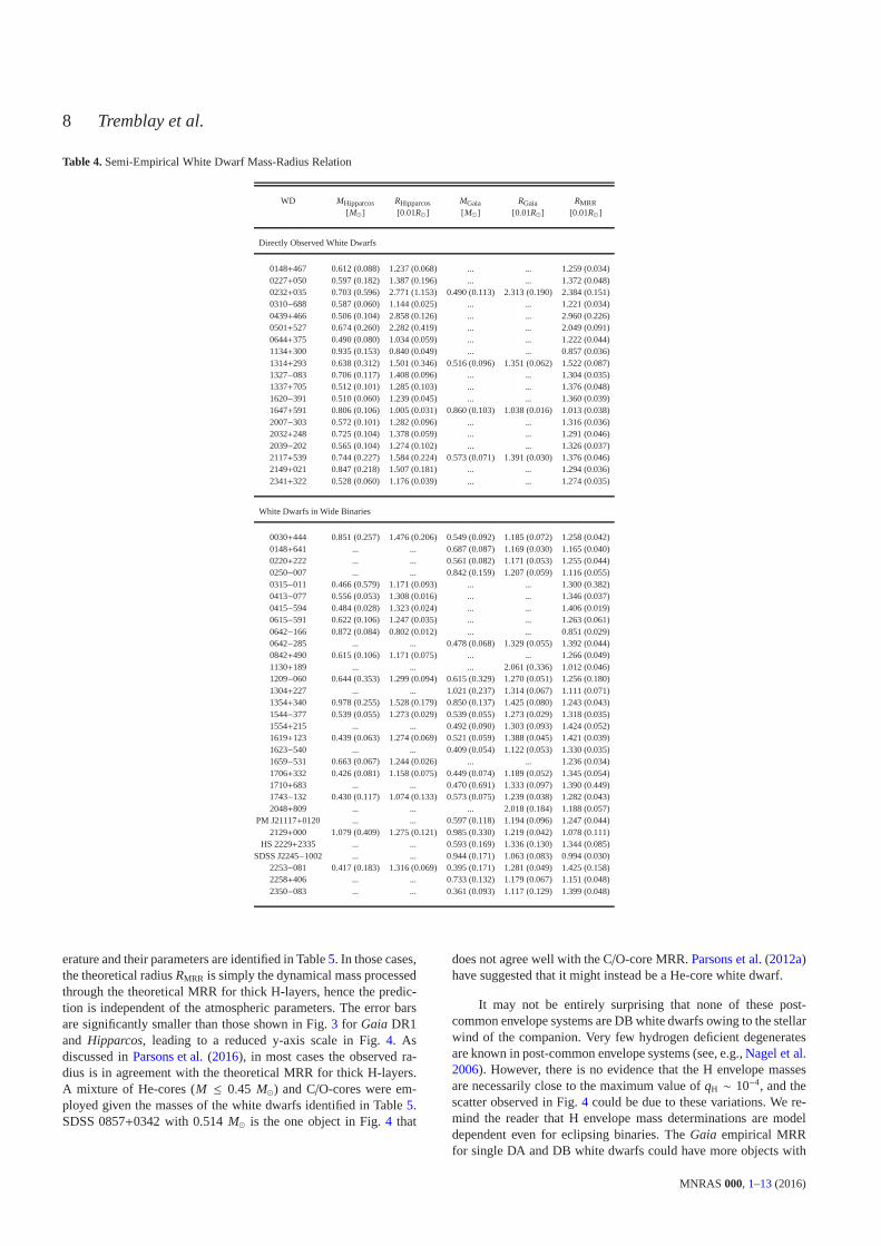
Tremblay et al.(2011) were integrated over theGaia G passbandusing Eq.3 as was done in the preparatory work ofCarrasco et al.(2014). The resulting radiiRGaia from Eq. 4 are given in Table4.The results using instead theHipparcosor ground-based parallaxes(RHipparcos) are also shown in Table4. In those cases, we have stillemployed the apparentGaia Gmagnitudes when available.

Traditionally, the next step has been to compute a mass inde-

pendently of the MRR by combining the radii determined abovewith the spectroscopic logg. These masses are given in Table4 andpresented in a M-R diagram in Fig.2 for both theGaia DR1 (toppanel) andHipparcosparallaxes (bottom panel). We note that theerrors typically form elongated ellipses (Holberg et al. 2012) cor-responding to the fact thatM is a function ofR2. Furthermore, thepredicted positions on the M-R diagram depend onTeff, as illus-

MNRAS 000, 1–13 (2016)

6 Tremblay et al.

Table 3. Parallaxes of White Dwarfs in Wide Binaries

WD Alt. Name π (Gaia) G (Gaia) π (other) Ref V Ref SpT Teff log(g) (spec) Ref[mas] [mag] [mas] [mag] [K] [cm2/s]

0030+444 G 172-4 13.97 (0.80) 16.550 (0.002) 11.22 (1.52) 1 16.44 (0.05) 2 DA 10,270 (150) 8.03 (0.05) 12, 130042+140 LP 466-033 17.41 (0.57) 18.405 (0.005) 14.38 (1.44) 1 18.79 (0.05) 3 DZA 5070 (90) ... 140148+641 G 244-36 57.63 (0.70) 13.938 (0.001) ... ... 14.00 (0.05)2 DA 9000 (130) 8.14 (0.05) 12, 130220+222 G 94-B5B 12.74 (0.55) ... ... ... 15.83 (0.05) 2 DA 16,240 (280) 8.05 (0.05) 120221+399 LP 196-060 24.30 (0.55) 17.071 (0.002) ... ... 17.39 (0.05) 2 DA 6250 (140) 8.30 (0.23) 12, 130250−007 LP 591-177 21.00 (0.89) 16.291 (0.003) ... ... 16.40 (0.05) 2 DA 8410 (130) 8.20 (0.07) 12, 130304+154 LP 471-52 ... 19.11 (0.01) ... ... 20.20 (0.10) 2 DC: ... ... 20315−011 LP 592-80 ... 17.493 (0.003) 14.89 (0.84) 1 17.20 (0.10) 2DA 7520 (260) 7.97 (0.45) 15, 16, 130355+255 NLTT 12250 14.75 (0.57) 18.237 (0.004) ... ... 16.80 (0.10) 2 DC: ... ... 20400−346 NLTT 12412 ... 17.417 (0.002) 19.35 (0.63) 1 17.82 (0.05)4 DC 5100 (100) ... 40413−077 40 Eri B ... ... 200.62 (0.23) 1 9.520 (0.05) 2 DA 17,100 (260) 7.95 (0.04) 120415−594 ǫ Ret B ... ... 54.83 (0.15) 1 12.50 (0.05) 2 DA 15,310 (350) 7.88(0.08) 170426+588 Stein 2051B 181.50 (0.92) ... 181.36 (3.67) 1 12.44 (0.05) 2 DC 7180 (180) ... 70433+270 G 39-27 57.22 (0.58) 15.531 (0.001) 55.66 (1.43) 1 15.79 (0.06) 5 DA 5630 (100) ... 70551+123 NLTT 15768 ... 15.758 (0.002) 8.68 (0.81) 1 15.87 (0.05) 4 DB 13,200 (900) ... 40615−591 BPM 18164 ... ... 26.72 (0.29) 1 14.09 (0.10) 2 DB 15,750 (370) 8.04 (0.07) 180642−166 Sirius B ... ... 380.11 (1.26) 1 8.440 (0.06) 6 DA 25,970 (380) 8.57 (0.04) 120642−285 LP 895-41 15.34 (0.54) 16.422 (0.002) ... ... 16.60 (0.05) 2 DA 9280 (130) 7.87 (0.05) 12, 130658+712 LP 34-137 13.04 (0.68) 18.627 (0.004) 12.27 (1.37) 1 19.20 (0.10) 2 DC ... ... 20736+053 Procyon B ... ... 284.56 (1.26) 1 10.94 (0.05) 7 DQZ 7870 (430) ... 70743−336 VB 03 ... ... 65.75 (0.51) 1 16.59 (0.05) 4 DC 4460 (100) ... 70751−252 SCR0753-2524 56.23 (0.56) 15.99 (0.07) 51.52 (1.46) 1 16.27 (0.05) 7 DA 5090 (140) ... 70842+490 HD 74389B ... ... 8.97 (0.57) 1 15.00 (0.05) 2 DA 40,250 (300) 8.09 (0.05) 19, 160845−188 LP 786-6 ... 15.648 (0.002) ... ... 15.68 (0.03) 8 DB 17,470 (420) 8.15 (0.08) 181009−184 WT 1759 ... 15.280 (0.002) 58.20 (1.67) 1 15.44 (0.05) 7 DZ 6040 (360) ... 71043−188 LP 791-55 52.59 (0.69) ... 49.95 (2.26) ... 15.52 (0.05) 7DQpec 5780 (90) ... 71107−257 LP 849-059 24.18 (0.55) 17.273 (0.002) 24.90 (0.98) 1 16.79 (0.05) 2 DC ... ... 21120+073 LP 552-49 ... 17.159 (0.003) 31.12 (2.35) 1 17.49 (0.05) 2DC 4460 (110) ... 201130+189 LP 433-6 4.63 (0.73) 17.569 (0.003) ... ... 17.60 (0.10) 2 DA 10,950 (190) 8.34 (0.06) 12, 131133+619 LP 94-65 7.05 (0.80) 18.358 (0.002) ... ... 17.70 (0.10) 2 DZ ... ... 21209−060 LP 674-029 22.69 (0.79) 16.878 (0.004) 22.18 (1.49) 1 17.26 (0.05) 2 DA 6590 (100) 8.02 (0.22) 41304+227 SDSS J1307+2227 12.96 (0.58) 16.491 (0.002) ... ... 16.20 (0.10) 2 DA 10,280 (180) 8.21 (0.09) 12, 131354+340 G 165-B5B 10.79 (0.58) 16.023 (0.004) 10.06 (1.15) 1 16.17 (0.01) 5 DA 14,490 (290) 8.06 (0.05) 121455+300 NLTT 38926 15.48 (0.55) 18.418 (0.004) 16.51 (1.66) 1 20.16 (0.10) 9 ... ... ... 91501+301 LP 326-74 12.56 (1.06) 17.654 (0.001) ... ... 17.70 (0.10) 2 DC 7250 ... 211542+729 LP 42-164 13.44 (0.52) 18.077 (0.004) 16.10 (2.48) 1 18.06 (0.05) 10 DC ... ... 101544−377 L 481-60 65.57 (0.74) 13.003 (0.001) 65.13 (0.40) 1 12.80(0.05) 2 DA 10,380 (150) 7.96 (0.04) 12, 131554+215 PG 1554+215 9.73 (0.68) ... ... ... 15.26 (0.01) 5 DA 27,320 (410) 7.90(0.05) 121619+123 PG 1619+123 17.70 (0.53) ... 19.29 (1.02) 1 14.66 (0.05) 2 DA 17,150 (260) 7.87 (0.04) 121623+022 NLTT 42785 20.59 (0.61) 17.50 (0.01) 17.64 (2.12) 1 17.42(0.05) 9 DC ... ... 101623−540 L 266-196 21.82 (0.66) 15.445 (0.002) ... ... 15.74 (0.05) 2 DA 11,280 (170) 7.95 (0.04) 12, 131659−531 BPM 24602 ... ... 36.73 (0.63) 1 13.47 (0.05) 2 DA 15,570 (230) 8.07 (0.04) 121706+332 G 181-B5B 13.98 (0.53) 15.970 (0.002) 14.35 (0.87) 1 15.90 (0.05) 2 DA 13,560 (390) 7.94 (0.06) 12, 131710+683 LP 70-172 17.98 (0.75) 17.259 (0.007) ... ... 17.50 (0.05) 2 DA 6630 (230) 7.86 (0.51) 12, 131743−132 G 154-B5B 25.97 (0.75) 14.604 (0.002) 29.96 (3.63) 1 14.22 (0.05) 2 DA 12,920 (210) 8.01 (0.05) 12, 131750+098 G 140-B1B 22.80 (0.53) 15.615 (0.002) ... ... 15.72 (0.05) 2 DA 9520 ... 121848+688 NLTT 47097 11.09 (0.52) 17.342 (0.004) 12.68 (0.76) 1 17.18 (0.05) 9 ... ... ... 92048+809 LP 25-436 11.67 (1.02) 16.434 (0.002) ... ... 16.59 (0.05) 2 DA 8450 (130) 8.11 (0.07) 12, 132054−050 NLTT 50189 62.15 (0.73) ... 56.54 (3.92) 1 16.69 (0.05) 7 DC 4340 (80) ... 72129+000 LP 638-004 23.16 (0.52) ... 22.13 (2.01) 1 14.67 (0.03) 8 DB 14,380 (350) 8.26 (0.14) 182154−512 BPM 27606 66.13 (0.75) 14.477 (0.001) 62.61 (2.92) 1 14.74 (0.03) 7 DQP 7190 (90) ... 7

PM J21117+0120 ... 16.37 (1.00) 15.266 (0.002) ... ... ... ... DA 16,570(100) 8.06 (0.05) 202217+211 LP 460-003 18.76 (0.60) 17.672 (0.004) 20.30 (1.40) 1 17.69 (0.05) 2 DC ... ... 22

HS 2229+2335 ... 9.02 (0.85) 15.992 (0.004) ... ... 16.01 (0.09) 5 DA 20,000 (500) 7.96 (0.09) 23, 16SDSS J2245−1002 PB 7181 16.72 (1.29) ... ... ... 17.02 (0.05) 11 DA 8700 (30) 8.36 (0.04) 11, 13

2253+054 NLTT 55300 40.06 (1.09) ... 40.89 (2.12) 1 15.71 (0.05) 2 DA 6240 (150) 8.60 (0.24) 12, 132253+812 LP 002-697 ... 17.543 (0.003) ... ... 17.30 (0.10) 2 DC: ... ... 22253−081 BD−08 5980B 27.97 (0.54) 16.311 (0.002) 27.22 (1.12) 1 16.50 (0.05) 2 DA 6770 (130) 7.82 (0.18) 12, 132258+406 G 216-B14B 13.96 (0.73) 16.676 (0.002) ... ... 15.50 (0.10) 2 DA 9910 (150) 8.16 (0.06) 12, 132301+762 LP 027-275 15.60 (0.56) ... 14.97 (0.79) 1 16.35 (0.05) 2 DC ... ... 242344−266 NLTT 57958 21.50 (0.55) 16.673 (0.008) 20.03 (3.04) 1 16.59 (0.05) 2 DB: ... ... 22350−083 G 273-B1B 9.96 (1.13) ... ... ... 16.18 (0.10) 2 DA 19,270 (310) 7.90 (0.05) 12

Notes. The Gaia uncertainties include both the random errors and a systematic error of 0.3 mas (Gaia Collaboration 2016). Only spectroscopic logg determinations are in-cluded and not the derivations based on the parallax measurements. Spectral types with the ":" symbol are uncertain.References. 1) van Leeuwen(2007), 2) McCook & Sion(1999), 3) Kilic et al. (2010), 4) Kawka & Vennes(2010), 5) Zacharias et al.(2012), 6) Holberg et al.(1984), 7) Giammichele et al.(2012), 8) Landolt & Uomoto(2007), 9)Gould & Chanamé(2004), 10)Holberg et al.(2013), 11) Tremblay et al.(2011), 12)Gianninas et al.(2011), 13) Tremblay et al.(2013), 14) Kilic et al. (2010), 15) Catalán et al.(2008), 16) Tremblay & Bergeron(2009), 17) Farihi et al.(2011), 18) Bergeron et al.(2011), 19) Vennes et al.(1997), 20) Limoges et al.(2015), 21) Girven et al.(2011), 22)Hintzen(1986), 23)Koester et al.(2009), 24)Greenstein(1984).

MNRAS 000, 1–13 (2016)

The Gaia DR1 Mass-Radius Relation for White Dwarfs7

trated in Fig.2 by the theoretical MRRs fromWood (1995) andFontaine et al.(2001) with thick H-layers at 10,000, 30,000, and60,000 K. For these reasons, it is not straightforward to interpretthe results in a M-R diagram. In particular, the data points in Fig.2,both for theGaiaDR1 andHipparcossamples, do not form a clearsequence of decreasing radius as a function of increasing mass as inthe predicted MRR. This is in part caused by observational uncer-tainties, the fact that most white dwarfs in the sample have similarmasses around∼0.6 M⊙, and that for a given mass the radius willchange as a function ofTeff.

WD 1130+189 and WD 2048+809 are two peculiar whitedwarfs inGaia DR1 for which the observed radiiRGaia are abouttwice the predicted values. Given the surface gravities, this wouldlead to spurious observed masses well above the Chandrasekharmass limit. The natural explanation for this behaviour is thatthese wide binaries are actually rare triple systems with unre-solved double degenerates (O’Brien et al. 2001; Andrews et al.2016; Maxted et al. 2000). These white dwarfs had no parallaxmeasurements until now and were not known to be double degen-erates. However, high-resolution observations of WD 2048+809show peculiar line cores that can not be explained by rotationor magnetic fields (Karl et al. 2005). Liebert et al. (1991) andTremblay et al.(2011) have shown that double DA white dwarfscan almost perfectly mimic a single DA in spectroscopic and pho-tometric analyses. As a consequence, it may not be surprising thatGaia is able to reveal for the first time the double degenerate natureof these objects.

In the following, we compare theobservedradius RGaia orRHipparcosdefined by Eq.4 to a predictedradiusRMRR drawn fromtheoretical MRRs and spectroscopic atmospheric parameters, anapproach also favoured byHolberg et al.(2012). We note that nei-ther quantity is purely observed or purely predicted and both de-pend on the spectroscopic atmospheric parameters, hence modelatmospheres. Nevertheless,RGaia depends almost only onTeff whileRMRR depends largely on logg. Theoretical MRRs with thick H-layers (qH = 10−4) were employed for our standard derivation. ForM > 0.45 M⊙, we use the evolutionary sequences ofFontaine et al.(2001, Teff ≤ 30,000 K, C/O-core 50/50 by mass fraction mixeduniformly) and Wood (1995, Teff > 30,000 K, pure C-core).For lower masses we use the He-core sequences ofAlthaus et al.(2001).

Fig. 3 comparesRGaia (top panel) andRHipparcos(bottom panel)to RMRR. The dotted black line centered on zero illustrates a perfectmatch between observations and theory for thick H-layers, whilethe dashed red line shows the match to an illustrative theoreticalMRR with thin H-layers (qH = 10−10) at 0.6 M⊙. On average,the data agree with the theoretical MRR for thick H-layers within0.99σ and 0.98σ for GaiaDR1 andHipparcos, respectively, and nosignificant systematic offset is observed (neglecting the suspecteddouble degenerates). The observed uncertainties for both samplesdo not allow, however, for meaningful constraints on H envelopemasses. The error bars are only slightly smaller for theGaia DR1sample compared toHipparcos. There are two reasons for this be-haviour. First of all, most of theGaia DR1 white dwarfs are com-panions to fairly distant but bright primary stars with parallaxes.While the absolute parallax error is on average 3 times smaller inGaiaDR1, the relative errors (σπ/π) are comparable with 5.05% inGaiaDR1 and 7.06% for pre-Gaiameasurements. Furthermore, theuncertainties from the atmospheric parameters become the domi-nant contribution for theGaia DR1 sample (see Section 4.2). Theimplications of these results are further discussed in Section 4.

Figure 2. (Top:)semi-empirical MRR usingGaiaDR1 and atmospheric pa-rameters defined in Table1 for directly observed white dwarfs (solid circles)and in Table3 for wide binaries (open circles). Numerical values are givenin Table4. Theoretical MRRs forqH = 10−4 (Wood 1995; Fontaine et al.2001) at 10,000 K (red), 30,000 K (black), and 60,000 K (blue) are alsoshown. The data points are also colour coded based on theirTeff and theclosest corresponding theoretical sequence.(Bottom:) Similar to the toppanel but with pre-Gaia parallax measurements (mostly fromHipparcos)identified in Tables1 and3. We still rely onGaia Gmagnitudes when avail-able.

4 DISCUSSION

4.1 Comparison with Other Empirical Mass-RadiusRelations

Our results can be compared to two empirical MRRs not drawnfrom Gaia DR1. Fig.4 (top panel) shows an independent analysisfor eclipsing and/or tidally distorted extremely low-mass (ELM)He-core white dwarf systems that provide model-independent radii(Hermes et al. 2014; Gianninas et al. 2014). The data are repro-duced from table 7 ofTremblay et al.(2015) where 3D model at-mosphere corrections were applied. The theoretical radiusRMRR istaken from the spectroscopic atmospheric parameters and the He-core MRR, similarly to our main analysis. The agreement withthetheoretical He-core MRR for thick H-layers is on average withinerror bars. This result suggests that the consistency between thetheoretical MRR and spectroscopic atmospheric parametersholdsin the ELM regime as well.

Fig.4 (bottom panel) also shows the results for eclipsing bina-ries where masses and radii are both directly constrained from theeclipses and orbital parameters. The selected systems fromthe lit-

MNRAS 000, 1–13 (2016)

8 Tremblay et al.

Table 4. Semi-Empirical White Dwarf Mass-Radius Relation

WD MHipparcos RHipparcos MGaia RGaia RMRR[M⊙ ] [0.01R⊙ ] [ M⊙ ] [0.01R⊙] [0.01R⊙ ]

Directly Observed White Dwarfs

0148+467 0.612 (0.088) 1.237 (0.068) ... ... 1.259 (0.034)0227+050 0.597 (0.182) 1.387 (0.196) ... ... 1.372 (0.048)0232+035 0.703 (0.596) 2.771 (1.153) 0.490 (0.113) 2.313 (0.190)2.384 (0.151)0310−688 0.587 (0.060) 1.144 (0.025) ... ... 1.221 (0.034)0439+466 0.506 (0.104) 2.858 (0.126) ... ... 2.960 (0.226)0501+527 0.674 (0.260) 2.282 (0.419) ... ... 2.049 (0.091)0644+375 0.490 (0.080) 1.034 (0.059) ... ... 1.222 (0.044)1134+300 0.935 (0.153) 0.840 (0.049) ... ... 0.857 (0.036)1314+293 0.638 (0.312) 1.501 (0.346) 0.516 (0.096) 1.351 (0.062)1.522 (0.087)1327−083 0.706 (0.117) 1.408 (0.096) ... ... 1.304 (0.035)1337+705 0.512 (0.101) 1.285 (0.103) ... ... 1.376 (0.048)1620−391 0.510 (0.060) 1.239 (0.045) ... ... 1.360 (0.039)1647+591 0.806 (0.106) 1.005 (0.031) 0.860 (0.103) 1.038 (0.016)1.013 (0.038)2007−303 0.572 (0.101) 1.282 (0.096) ... ... 1.316 (0.036)2032+248 0.725 (0.104) 1.378 (0.059) ... ... 1.291 (0.046)2039−202 0.565 (0.104) 1.274 (0.102) ... ... 1.326 (0.037)2117+539 0.744 (0.227) 1.584 (0.224) 0.573 (0.071) 1.391 (0.030)1.376 (0.046)2149+021 0.847 (0.218) 1.507 (0.181) ... ... 1.294 (0.036)2341+322 0.528 (0.060) 1.176 (0.039) ... ... 1.274 (0.035)

White Dwarfs in Wide Binaries

0030+444 0.851 (0.257) 1.476 (0.206) 0.549 (0.092) 1.185 (0.072)1.258 (0.042)0148+641 ... ... 0.687 (0.087) 1.169 (0.030) 1.165 (0.040)0220+222 ... ... 0.561 (0.082) 1.171 (0.053) 1.255 (0.044)0250−007 ... ... 0.842 (0.159) 1.207 (0.059) 1.116 (0.055)0315−011 0.466 (0.579) 1.171 (0.093) ... ... 1.300 (0.382)0413−077 0.556 (0.053) 1.308 (0.016) ... ... 1.346 (0.037)0415−594 0.484 (0.028) 1.323 (0.024) ... ... 1.406 (0.019)0615−591 0.622 (0.106) 1.247 (0.035) ... ... 1.263 (0.061)0642−166 0.872 (0.084) 0.802 (0.012) ... ... 0.851 (0.029)0642−285 ... ... 0.478 (0.068) 1.329 (0.055) 1.392 (0.044)0842+490 0.615 (0.106) 1.171 (0.075) ... ... 1.266 (0.049)1130+189 ... ... ... 2.061 (0.336) 1.012 (0.046)1209−060 0.644 (0.353) 1.299 (0.094) 0.615 (0.329) 1.270 (0.051)1.256 (0.180)1304+227 ... ... 1.021 (0.237) 1.314 (0.067) 1.111 (0.071)1354+340 0.978 (0.255) 1.528 (0.179) 0.850 (0.137) 1.425 (0.080)1.243 (0.043)1544−377 0.539 (0.055) 1.273 (0.029) 0.539 (0.055) 1.273 (0.029)1.318 (0.035)1554+215 ... ... 0.492 (0.090) 1.303 (0.093) 1.424 (0.052)1619+123 0.439 (0.063) 1.274 (0.069) 0.521 (0.059) 1.388 (0.045)1.421 (0.039)1623−540 ... ... 0.409 (0.054) 1.122 (0.053) 1.330 (0.035)1659−531 0.663 (0.067) 1.244 (0.026) ... ... 1.236 (0.034)1706+332 0.426 (0.081) 1.158 (0.075) 0.449 (0.074) 1.189 (0.052)1.345 (0.054)1710+683 ... ... 0.470 (0.691) 1.333 (0.097) 1.390 (0.449)1743−132 0.430 (0.117) 1.074 (0.133) 0.573 (0.075) 1.239 (0.038)1.282 (0.043)2048+809 ... ... ... 2.018 (0.184) 1.188 (0.057)

PM J21117+0120 ... ... 0.597 (0.118) 1.194 (0.096) 1.247 (0.044)2129+000 1.079 (0.409) 1.275 (0.121) 0.985 (0.330) 1.219 (0.042)1.078 (0.111)

HS 2229+2335 ... ... 0.593 (0.169) 1.336 (0.130) 1.344 (0.085)SDSS J2245−1002 ... ... 0.944 (0.171) 1.063 (0.083) 0.994 (0.030)

2253−081 0.417 (0.183) 1.316 (0.069) 0.395 (0.171) 1.281 (0.049)1.425 (0.158)2258+406 ... ... 0.733 (0.132) 1.179 (0.067) 1.151 (0.048)2350−083 ... ... 0.361 (0.093) 1.117 (0.129) 1.399 (0.048)

erature and their parameters are identified in Table5. In those cases,the theoretical radiusRMRR is simply the dynamical mass processedthrough the theoretical MRR for thick H-layers, hence the predic-tion is independent of the atmospheric parameters. The error barsare significantly smaller than those shown in Fig.3 for Gaia DR1and Hipparcos, leading to a reduced y-axis scale in Fig.4. Asdiscussed inParsons et al.(2016), in most cases the observed ra-dius is in agreement with the theoretical MRR for thick H-layers.A mixture of He-cores (M ≤ 0.45 M⊙) and C/O-cores were em-ployed given the masses of the white dwarfs identified in Table 5.SDSS 0857+0342 with 0.514M⊙ is the one object in Fig.4 that

does not agree well with the C/O-core MRR.Parsons et al.(2012a)have suggested that it might instead be a He-core white dwarf.

It may not be entirely surprising that none of these post-common envelope systems are DB white dwarfs owing to the stellarwind of the companion. Very few hydrogen deficient degeneratesare known in post-common envelope systems (see, e.g.,Nagel et al.2006). However, there is no evidence that the H envelope massesare necessarily close to the maximum value ofqH ∼ 10−4, and thescatter observed in Fig.4 could be due to these variations. We re-mind the reader that H envelope mass determinations are modeldependent even for eclipsing binaries. TheGaia empirical MRRfor single DA and DB white dwarfs could have more objects with

MNRAS 000, 1–13 (2016)

The Gaia DR1 Mass-Radius Relation for White Dwarfs9

Figure 3. (Top:)Differences (in %) between observedGaiaDR1 radiiRGaia

(Eq.4) and predicted radiiRMRR drawn from the MRR with thick H-layers(qH = 10−4) as a function of logTeff . Error bars for logTeff are omittedfor clarity. Directly observed white dwarfs from Table1 are representedby solid circles while wide binaries from Table3 are illustrated by opencircles. Numerical values are identified in Table4. The dotted line∆R = 0is shown as a reference and the dashed red line is for a MRR relation withthin H-layers (qH = 10−10) at 0.6M⊙. (Bottom:)Similar to the top panel butwith pre-Gaia parallax measurements (mostly fromHipparcos) identifiedin Tables1 and3. We still rely onGaia Gmagnitudes when available. Thebenchmark cases 40 Eri B (cooler) and Sirius B (warmer) are shown in red.

very thin H-layers, but there is no clear indication that therelationwould be significantly different. In particular, the results of Fig.4for eclipsing binaries strongly suggest that theoretical MRRs arein agreement with observations. The semi-empirical MRR fortheGaiaDR1 sample in Fig.3 supports this conclusion, but it also indi-cates that the spectroscopic atmospheric parameters are onaverageconsistent withGaia DR1 parallaxes. In futureGaia data releases,the results from eclipsing binaries may provide the key to disentan-gle a genuine observed signature of the white dwarf MRR from asystematic effect from model atmospheres.

Finally, we note thatBergeron et al.(2007) compared gravi-tational redshift measurements with spectroscopically determinedlogg and a theoretical MRR, but the comparison remained incon-clusive because of the large uncertainties associated withthe red-shift velocities.

Figure 4. (Top:) Differences (in %) between observed radiiRELM and pre-dicted He-core radiiRMRR as a function of logTeff for the sample of He-coreELM white dwarfs fromGianninas et al.(2014) with 3D corrections fromTremblay et al.(2015). Error bars for logTeff are omitted for clarity andnumerical values are presented inTremblay et al.(2015). The dotted line∆R = 0 is shown as a reference and the dashed red line is for a He-coreMRR relation with thin H-layers at 0.3M⊙. (Bottom:)Differences betweenobserved radiiReclipse and predicted radiiRMRR for eclipsing binaries forwhich there is an independent derivation of both the mass andradius. Theobserved sample of both He- and C/O-core white dwarfs drawn from theliterature is described in Table5. The dashed red line is for a MRR relationwith thin H-layers at 0.6M⊙.

4.2 Precision of the Atmospheric Parameters

The studies ofVauclair et al.(1997) and Provencal et al.(1998)have pioneered the derivation of the semi-empirical MRR forwhitedwarfs using preciseHipparcosparallaxes. Our work withGaiaDR1 parallaxes is in continuation of this goal. We remind thereaderthat such observed MRR is still highly dependent on the whitedwarf atmospheric parameters, hence model atmospheres. Inpre-vious studies, parallax errors were often dominant, but with GaiaDR1 parallaxes, errors on spectroscopic atmospheric parametersare becoming the most important. Fig.5 illustrates the error budgeton RGaia − RMRR derived in Fig.3 and demonstrates that the un-certainties onTeff and logg marginally dominate. The number andprecision of parallaxes will increase significantly with futureGaiadata releases. In particular, the individual parallaxes inDR2 will

MNRAS 000, 1–13 (2016)

10 Tremblay et al.

Table 5. Empirical Mass-Radius Relation from Eclipsing Binaries

Name Meclipse Reclipse RMRR Teff Ref[M⊙ ] [0.01R⊙ ] [0.01R⊙ ] [K]

NN Ser 0.535 (0.012) 2.08 (0.02) 2.16 (0.08) 63000 (3000) 1V471 Tau 0.840 (0.050) 1.07 (0.07) 1.06 (0.07) 34500 (1000) 2

SDSS J1210+3347 0.415 (0.010) 1.59 (0.05) 1.61 (0.03) 6000 (200) 3SDSS J1212−0123 0.439 (0.002) 1.68 (0.03) 1.75 (0.01) 17710 (40) 4

GK Vir 0.562 (0.014) 1.70 (0.03) 1.76 (0.06) 50000 (670) 4SDSS 0138−0016 0.529 (0.010) 1.31 (0.03) 1.32 (0.01) 3570 (100) 5SDSS 0857+0342 0.514 (0.049) 2.47 (0.08) 1.74 (0.15) 37400 (400) 6

CSS 41177A 0.378 (0.023) 2.224 (0.041) 2.39 (0.22) 22500 (60) 7CSS 41177B 0.316 (0.011) 2.066 (0.042) 2.21 (0.06) 11860 (280) 7

QS Vir 0.781 (0.013) 1.068 (0.007) 1.064 (0.016) 14220 (350) 8

References. 1) Parsons et al.(2010), 2) O’Brien et al. (2001), 3) Pyrzas et al.(2012), 4)Parsons et al.(2012b), 5) Parsons et al.(2012c), 6) Parsons et al.(2012a), 7) Bours et al.(2015), 8) Parsons et al.(2016).

Figure 5. Average error budget in the comparison of observed radii (RGaiaorRHipparcos) and predicted radii (RMRR) in Fig. 3. The different uncertaintiesare identified in the legend.

have significantly higher individual precision due to a longer mea-surement time (22 months instead of 11 months, which is already36% of the total mission time). Systematic errors are also expectedto decrease significantly resulting from a more sophisticated cali-bration, including a better definition of the line spread function, theapplication of a chromaticity correction, a more accurate calibra-tion of the basic angle variation, and a calibration and correction ofmicro clanks. On the other hand, it is not expected that the preci-sion on the atmospheric parameters will markedly improve anytimesoon.

We propose that the bright and well-studied single DA whitedwarfs in theHipparcos sample, unfortunately largely missingfrom Gaia DR1, may be used as a benchmark to understandthe precision of the semi-empirical MRR of futureGaia data re-leases. We will now assess the possibility of improving the preci-sion on the atmospheric parameters for these white dwarfs, tak-ing WD 1327−083 as an example. There are three steps in theBalmer line fitting procedure that could introduce errors; uncer-tainties in the spectroscopic data, issues with the fitting procedure,and inaccuracies in the model atmospheres. To illustrate this, wehave derived the atmospheric parameters of WD 1327−083 using anumber of observations and methods. In Fig.6 we display the pub-lishedGianninas et al.(2011) atmospheric parameters based on onespectrum. The formalχ2 uncertainty is represented by the smallerdash-dotted ellipse. We remind the reader that the error bars from

Gianninas et al.(2011) combine in quadrature this formalχ2 errorand a fixed external error of 1.2% inTeff and 0.038 dex in logg,resulting in the corresponding 1σ and 2σ error ellipses shown inFig. 6.

First of all, we rely on 12 alternative spectra forWD 1327−083. These are all high signal-to-noise (S/N >

50) observations that were fitted with the same model atmo-spheres (Tremblay et al. 2011) and the same fitting code as inGianninas et al.(2011). In all cases the formalχ2 error is very sim-ilar to the one illustrated in Fig.6 for the spectrum selected inGianninas et al.(2011). We employ 7 spectra taken by the Mon-treal group from different sites (black filled points in Fig.6) inaddition to the one selected inGianninas et al.(2011). We alsorely on 3 UVES/VLT spectra taken as part of the SPY survey(Koester et al. 2009), shown with cyan filled circles in Fig.6. Addi-tionally, new observations were secured. The first one is a high S/NX-SHOOTER/VLT spectrum taken on programme 097.D-0424(A).The Balmer lines suggest a significantly warmer temperature(bluefilled circle) than the average in Fig.6. However, the calibratedspectra show a smaller than predicted flux in the blue, suggest-ing the offset could be caused by slit losses during the observa-tions. Finally, we have recently obtained STIS spectrophotometryfor WD 1327−083 underHubble Space Telescopeprogram 14213as shown in Fig.7. The Balmer lines were fitted and a solution (redfilled circle in Fig.6) very similar to that ofGianninas et al.(2011)was obtained.

The atmospheric parameters in Fig.6, determined from dif-ferent spectroscopic data, show a relatively large scatterthat issignificantly higher than theχ2 error, confirming that external er-rors from the data reduction must be accounted for. The scatterappears slightly larger than the systematic uncertainty estimatedby Liebert et al.(2005) andGianninas et al.(2011) from a similarprocedure. However, one could argue that some of the observationsselected in this work should have a lower weight in the averagesince they show minor deficiencies in their instrumental setup orflux calibration.

The STIS spectrophotometry, which is calibrated using thethree hot (Teff > 30, 000 K) white dwarfs GD 71, GD 153, andG191−B2B (Bohlin et al. 2014), also permits the determination ofthe atmospheric parameters based on the continuum flux. The sur-face gravity was fixed at logg = 8.0 since the sensitivity of thecontinuum flux to this parameter is much smaller than the sen-sitivity to Teff. The blue wing and central portion of Lyα wereremoved from the fit because the observed flux is very small inthis region. Fig.7 shows our best-fit model (red) compared to thesolution using theTeff value fromGianninas et al.(2011) in blue.The solution is clearly driven by the UV flux, and aTeff value of14,830 K, about 250 K larger than that ofGianninas et al.(2011),is required to fit the observations. The STIS photometric solutionis added to Fig.6 (dotted red line). It is reassuring that there isa good consistency between STIS spectrophotometry and whitedwarf atmospheric parameters both for current hotter flux standardsand this cooler object. A full discussion about using this whitedwarf as a STIS spectrophotometric standard will be reported else-where. As an independent test, we have also used UBVRIJHK datadrawn fromKoen et al.(2010) and 2MASS (Cutri et al. 2003) tofit a temperature of 14,285± 900 K. The large error is due to thefact that this photometric data set does not include the UV whichis the most sensitive toTeff. We refrain from using theGALEXFUV and NUV fluxes since there is a significant systematic off-set between observed and synthetic fluxes in the magnitude rangeof WD 1327−083 (Camarota & Holberg 2014). The results are re-

MNRAS 000, 1–13 (2016)

The Gaia DR1 Mass-Radius Relation for White Dwarfs11

Figure 6. Characterisation of the atmospheric parameters forWD 1327−083 using different observations and model atmospheres.The standard atmospheric parameters fromGianninas et al.(2011) usedthroughout this work are represented by their 1σ and 2σ error ellipses(solid black). The smaller formalχ2 error is represented by a dash-dottedellipse. Different Balmer line solutions based on the same model atmo-spheres and fitting technique but alternative spectra are shown with solidcircles. The alternative spectra are drawn from the Montreal group (black),the UVES instrument (SPY survey, cyan), X-SHOOTER (blue), and STISspectrophotometry (red). We also show the alternative solutions employingthe model atmospheres ofKoester(2010) with open circles. The formalχ2 error is very similar for all solutions. Finally, we show ourbest fits ofthe continuum flux of STIS spectrophotometry (dotted red, see Fig.7) andUBVRIJHK photometry (dashed magenta,σTeff = 900 K). For photometricfits we have fixed the surface gravity at logg = 8.0.

ported in Fig.6 (dashed magenta), though because of the large er-ror, the UBVRIJHKTeff value is fully consistent with the STISspectrophotometry.

Finally, we have performed the same analysis but using in-stead the model atmospheres ofKoester(2010) including the Starkbroadening profiles ofTremblay & Bergeron(2009). The resultsare shown in Fig.6 with open circles for fits of the Balmer lines.The meanTeff value is shifted by−295 K and the mean logg valueby −0.06 dex, which is in both cases slightly larger than the pub-lished error bars. In the case of the STIS and UBVRIJHK photo-metric fits, we find essentially the sameTeff values with both gridsof models.

Fig. 6 demonstrates that for the particular case ofWD 1327−083, the 1σ error bars fromGianninas et al.(2011) are areasonable but likely optimistic estimate of theTeff-logg uncertain-ties. It is perhaps not surprising since they did not consider alterna-tive model grids or photometric solutions in their uncertainties. Wehave not explicitly considered the effect of the fitting techniques,which would increase even more the scatter between the differentsolutions. However, changing the fitting method would not pro-vide a fully independent diagnostic since it is influenced byboththe data reduction and systematic uncertainties in the model atmo-sphere grids.

It is outside the scope of this work to review the differences be-tween the model grids or to re-observe spectroscopically all whitedwarfs for which we currently have parallaxes. Nevertheless, wesuggest that this should be done ahead ofGaia DR2 for a bench-mark sample of bright white dwarfs. We can nevertheless makeafew additional observations. If we allow the uncertaintieson the at-

Figure 7. STIS spectrophotometric observations of WD 1327−083 as afunction of wavelength. The predicted flux from the model atmospheres ofTremblay et al.(2011) using the atmospheric parameters ofGianninas et al.(2011) is shown in blue (solid,Teff = 14, 570 K, logg = 7.99), and the bestfit is shown in red (dotted,Teff = 14, 830 K with logg fixed at 8.0), whichis almost coincident with the observations on this scale.

mospheric parameters to increase by a very conservative factor oftwo following our discussion above, 21/26 GaiaDR1 white dwarfsagree within error bars with thick H-layers while 22/26 are con-sistent with thin H-layers. These results suggest that given the pre-cision on the atmospheric parameters, the theoretical MRR is en-tirely consistent with the observations. Furthermore, thedistinctionbetween thin and thick H-layers forGaiaDR1 white dwarfs is stillout of reach, as it was the case forHipparcos.

5 CONCLUSIONS

The Gaia DR1 sample of parallaxes was presented for 6 directlyobserved white dwarfs and 46 members of wide binaries. By com-bining this data set with spectroscopic atmospheric parameters, wehave derived the semi-empirical MRR relation for white dwarfs.We find that, on average, there is a good agreement betweenGaiaparallaxes, publishedTeff and logg, and theoretical MRRs. It is notpossible, however, to conclude that both the model atmospheres andinterior models are individually consistent with observations. Thereare other combinations ofTeff, logg, and H envelope masses thatcould agree withGaia DR1 parallaxes. However, the good agree-ment between observed and predicted radii for eclipsing binaries,which are insensitive to model atmospheres, suggest that both theatmospheric parameters and theoretical MRRs are consistent withGaiaDR1.

Starting withGaiaDR2, it will be feasible to derive the semi-empirical MRR for thousands of white dwarfs. Assuming system-atic parallax errors will be significantly reduced, it will be possibleto take advantage of large number statistics and compute a preciseoffset between the observed and predicted MRRs forTeff , mass,and spectral type bins. Alternatively, since the mass and radius arederived quantities, the parallax distances could be directly com-pared to predicted spectroscopic distances (Holberg et al. 2008).However, it may be difficult to interpret the results in terms of theprecision of the model atmospheres and evolutionary models. Inde-pendent constraints from eclipsing binaries, as well as a more care-

MNRAS 000, 1–13 (2016)

12 Tremblay et al.

ful assessment of the error bars for bright and well known whitedwarfs, may still be necessary to fully understandGaiadata.

ACKNOWLEDGEMENTS

This project has received funding from the European ResearchCouncil (ERC) under the European Union’s Horizon 2020 researchand innovation programme (grant agreements No 677706 - WD3Dand No 320964 - WDTracer). TRM is grateful to the Science andTechnology Facilities Council for financial support in the form ofgrant No ST/L000733. This work has made use of data from theESA space mission Gaia, processed by the Gaia Data Process-ing and Analysis Consortium (DPAC). Funding for the DPAC hasbeen provided by national institutions, in particular the institutionsparticipating in the Gaia Multilateral Agreement. The Gaiamis-sion website ishttp://www.cosmos.esa.int/gaia . This workis based on observations made with the NASA/ESA Hubble SpaceTelescope, obtained at the Space Telescope Science Institute, whichis operated by the Association of Universities for Researchin As-tronomy, Inc., under NASA contract NAS 5-26555. These observa-tions are associated with programme #14213. This paper is basedon observations made with ESO Telescopes under programme ID097.D-0424(A).

REFERENCES

Althaus, L. G., Serenelli, A. M., & Benvenuto, O. G. 2001, MNRAS, 323,471

Althaus, L. G., García-Berro, E., Isern, J., Córsico, A. H.,& Rohrmann,R. D. 2007, A&A, 465, 249

Althaus, L. G., Córsico, A. H., Isern, J., & García-Berro, E.2010a, A&ARv,18, 471

Althaus, L. G., Córsico, A. H., Bischoff-Kim, A., et al. 2010b, ApJ, 717,897

Althaus, L. G., Miller Bertolami, M. M., & Córsico, A. H. 2013, A&A, 557,A19

Andrews, J. J., Agüeros, M., Brown, W. R., et al. 2016, ApJ, 828, 38Barstow, M. A., Bond, H. E., Holberg, J. B., et al. 2005, MNRAS, 362, 1134Barstow, M. A., Bond, H. E., Burleigh, M. R., et al. 2015, in 19th European

Workshop on White Dwarfs, ASP Conference Series, ed. P. Dufour, P.Bergeron & G. Fontaine (San Francisco: ASP), 493, 307

Bergeron, P., Saffer, R. A., & Liebert, J. 1992, ApJ, 394, 228Bergeron, P., Leggett, S. K., & Ruiz, M. T. 2001, ApJS, 133, 413Bergeron, P., Gianninas, A., & Boudreault, S. 2007, Proc. 15th European

Workshop on White Dwarfs, ed. R. Napiwotzki & M. Burleigh (SanFrancisco, CA: ASP), 372, 29

Bergeron, P., Wesemael, F., Dufour, P., et al. 2011, ApJ, 737, 28Bohlin, R. C., Gordon, K. D., & Tremblay, P.-E. 2014, PASP, 126, 711Bond, H. E., Gilliland, R. L., Schaefer, G. H., et al. 2015, ApJ, 813, 106Bours, M. C. P., Marsh, T. R., Gänsicke, B. T., & Parsons, S. G.2015,

MNRAS, 448, 601Camarota, L., & Holberg, J. B. 2014, MNRAS, 438, 3111Catalán, S., Isern, J., García-Berro, E., & Ribas, I. 2008, MNRAS, 387,

1693Carrasco, J. M., Catalán, S., Jordi, C., et al. 2014, A&A, 565, A11Casewell, S. L., Dobbie, P. D., Napiwotzki, R., et al. 2009, MNRAS, 395,

1795Chandrasekhar, S. 1931, ApJ, 74, 81Cohen, M., Megeath, S. T., Hammersley, P. L., Martín-Luis, F., & Stauffer,

J. 2003, AJ, 125, 2645Cummings, J. D., Kalirai, J. S., Tremblay, P.-E., Ramirez-Ruiz, E., & Berg-

eron, P. 2016, ApJ, 820, L18Cutri, R. M., Skrutskie, M. F., van Dyk, S., et al. 2003, VizieR Online Data

Catalog, 2246

Dobbie, P. D., Day-Jones, A., Williams, K. A., et al. 2012, MNRAS, 423,2815

Falcon, R. E., Winget, D. E., Montgomery, M. H., & Williams, K. A. 2012,ApJ, 757, 116

Farihi, J., Burleigh, M. R., Holberg, J. B., Casewell, S. L.,& Barstow, M. A.2011, MNRAS, 417, 1735

Finley, D. S., & Koester, D. 1997, ApJ, 489, L79Fontaine, G., Brassard, P., Bergeron, P., & Wesemael, F. 1992, ApJ, 399,

L91Fontaine, G., Brassard, P., & Bergeron, P. 2001, PASP, 113, 409Gaia Collaboration, Brown, A. G. A., Vallenari, A., et al. 2016,

arXiv:1609.04172Giammichele, N., Bergeron, P., & Dufour, P. 2012, ApJS, 199,29Giammichele, N., Fontaine, G., Brassard, P., & Charpinet, S. 2016, ApJS,

223,Gianninas, A., Bergeron, P., & Ruiz, M. T. 2011, ApJ, 743, 138Gianninas, A., Dufour, P., Kilic, M., et al. 2014, ApJ, 794, 35Girven, J., Gänsicke, B. T., Steeghs, D., & Koester, D. 2011,MNRAS, 417,

1210Genest-Beaulieu, C., & Bergeron, P. 2014, ApJ, 796, 128Goldsbury, R., Heyl, J., Richer, H. B., Kalirai, J. S., & Tremblay, P. E. 2016,

ApJ, 821, 27Gould, A., & Chanamé, J. 2004, ApJS, 150, 455Greenstein, J. L. 1984, ApJ, 276, 602Hamada, T., & Salpeter, E. E. 1961, ApJ134, 683Hansen, B. M. S. 1999, ApJ, 520, 680Hansen, B. M. S., Anderson, J., Brewer, J., et al. 2007, ApJ, 671, 380Hansen, B. M. S., Richer, H., Kalirai, J., et al. 2015, ApJ, 809, 141Harris, H. C., Dahn, C. C., Canzian, B., et al. 2007, AJ, 133, 631Hermes, J. J., Brown, W. R., Kilic, M., et al. 2014, ApJ, 792, 39Hintzen, P. 1986, AJ, 92, 431Holberg, J. B., Wesemael, F., & Hubeny, I. 1984, ApJ, 280, 679Holberg, J. B., Barstow, M. A., & Burleigh, M. R. 2003, ApJS, 147, 145Holberg, J. B., & Bergeron, P. 2006, AJ, 132, 1221Holberg, J. B., Bergeron, P., & Gianninas, A. 2008, AJ, 135, 1239Holberg, J. B., Oswalt, T. D., & Barstow, M. A. 2012, AJ, 143, 68Holberg, J. B., Oswalt, T. D., Sion, E. M., Barstow, M. A., & Burleigh,

M. R. 2013, MNRAS, 435, 2077Iben, I., Jr., & Tutukov, A. V. 1984, ApJ, 282, 615Jordi, C., Gebran, M., Carrasco, J. M., et al. 2010, A&A, 523,A48Kalirai, J. S., et al. 2008, ApJ, 676, 594Kalirai, J. S. 2012, Nature, 486, 90Kalirai, J. S., Marigo, P., & Tremblay, P.-E. 2014, ApJ, 782,17Karl, C. A., Napiwotzki, R., Heber, U., et al. 2005, A&A, 434,637Kawka, A., & Vennes, S. 2010, in Binaries - Key to Comprehension of

the Universe, ASP Conference Series, ed. A. Prsa and M. Zejda(SanFrancisco: ASP), 435, 189

Kilic, M., Leggett, S. K., Tremblay, P.-E., et al. 2010, ApJS, 190, 77Koen, C., Kilkenny, D., van Wyk, F., & Marang, F. 2010, MNRAS,403,

1949Koester, D., Schulz, H., & Weidemann, V. 1979, A&A, 76, 262Koester, D. 1987, ApJ, 322, 852Koester, D., Voss, B., Napiwotzki, R., et al. 2009, A&A, 505,441Koester D., 2010, Mem. Soc. Astron. Ital., 81, 921Koester, D., & Kepler, S. O. 2015, A&A, 583, A86Landolt, A. U., & Uomoto, A. K. 2007, AJ, 133, 768Landolt, A. U. 2009, AJ, 137, 4186Liebert, J., Bergeron, P., & Saffer, R.A. 1991, 7th European Workshop on

White Dwarfs, NATO ASI Series, ed. G. Vauclair & E. M. Sion (Dor-drecht: Kluwer), 409

Liebert, J., Bergeron, P., & Holberg, J. B. 2005, ApJS, 156, 47Limoges, M.-M., Bergeron, P., & Lépine, S. 2015, ApJS, 219, 19Lindegren, L., Lammers, U., Bastian, U., et al. 2016, arXiv:1609.04303Marsh, M. C., Barstow, M. A., Buckley, D. A., et al. 1997, MNRAS, 286,

369Maxted, P. F. L., Marsh, T. R., Moran, C. K. J., & Han, Z. 2000, MNRAS,

314, 334McCook, G. P., & Sion, E. M. 1999, ApJS, 121, 1

MNRAS 000, 1–13 (2016)

The Gaia DR1 Mass-Radius Relation for White Dwarfs13

Michalik, D., Lindegren, L., Hobbs, D., & Lammers, U. 2014, A&A, 571,A85

Michalik, D., Lindegren, L., & Hobbs, D. 2015, A&A, 574, A115Nagel, T., Schuh, S., Kusterer, D.-J., et al. 2006, A&A, 448,L25Oswalt, T. D., & Strunk, D. 1994, Bulletin of the American Astronomical

Society, 26, 28.09O’Brien, M. S., Bond, H. E., & Sion, E. M. 2001, ApJ, 563, 971Parsons, S. G., Marsh, T. R., Copperwheat, C. M., et al. 2010,MNRAS,

402, 2591Parsons, S. G., Marsh, T. R., Gänsicke, B. T., et al. 2012b, MNRAS, 420,

3281Parsons, S. G., Gänsicke, B. T., Marsh, T. R., et al. 2012c, MNRAS, 426,

1950Parsons, S. G., Marsh, T. R., Gänsicke, B. T., et al. 2012a, MNRAS, 419,

304Parsons, S. G., Hill, C. A., Marsh, T. R., et al. 2016, MNRAS, 458, 2793Perlmutter, S., et al. 1999, ApJ, 517, 565Perryman, M. A. C., de Boer, K. S., Gilmore, G., et al. 2001, A&A, 369,

339Provencal, J. L., Shipman, H. L., Høg, E., & Thejll, P. 1998, ApJ, 494, 759Pyrzas, S., Gänsicke, B. T., Brady, S., et al. 2012, MNRAS, 419, 817Riess, A. G., et al. 1998, AJ, 116, 1009Romero, A. D., Córsico, A. H., Althaus, L. G., et al. 2012, MNRAS, 420,

1462Romero, A. D., Kepler, S. O., Córsico, A. H., Althaus, L. G., &Fraga, L.

2013, ApJ, 779, 58Salaris, M., Cassisi, S., Pietrinferni, A., Kowalski, P. M., & Isern, J. 2010,

ApJ, 716, 1241Schmidt, H. 1996, A&A, 311, 852Shipman, H. L. 1979, ApJ, 228, 240Shipman, H. L., Provencal, J. L., Høg, E., & Thejll, P. 1997, ApJ, 488, L43Silvestri, N. M., Oswalt, T. D., & Hawley, S. L. 2002, AJ, 124,1118Sion, E. M. 1984, ApJ, 282, 612Subasavage, J. P., Jao, W.-C., Henry, T. J., et al. 2009, AJ, 137, 4547Tokovinin, A., & Lépine, S. 2012, AJ, 144, 102Torres, S., García-Berro, E., Isern, J., & Figueras, F. 2005, MNRAS, 360,

1381Tremblay, P.-E., & Bergeron, P. 2008, ApJ, 672, 1144Tremblay, P.-E., & Bergeron, P. 2009, ApJ, 696, 1755Tremblay, P.-E., Bergeron, P., & Gianninas, A. 2011, ApJ, 730, 128Tremblay, P.-E., Ludwig, H.-G., Steffen, M., & Freytag, B. 2013, A&A,

559, A104Tremblay, P.-E., Kalirai, J. S., Soderblom, D. R., Cignoni,M., & Cum-

mings, J. 2014, ApJ, 791, 92Tremblay, P.-E., Gianninas, A., Kilic, M., et al. 2015, ApJ,809, 148van Altena, W. F., Lee, J. T., & Hoffleit, E. D. 1994, The General Catalogue

of Trigonometric Parallaxes (New Haven: Yale University Observatory)van Leeuwen, F. 2007, A&A, 474, 653Vauclair, G., Schmidt, H., Koester, D., & Allard, N. 1997, A&A, 325, 1055Vennes, S., Thejll, P. A., Génova Galvan, R., & Dupuis, J. 1997, ApJ, 480,

714Weidemann, V. 2000, A&A, 363, 647Werner, K. 1996, ApJ, 457, L39Williams, K. A., Bolte, M., & Koester, D. 2009, ApJ, 693, 355Wood, M. A. 1995, in 9th European Workshop on White Dwarfs, ed. D.

Koester & K. Werner (Springer: Berlin), 41Zacharias, N., Finch, C. T., Girard, T. M., et al. 2012, VizieR Online Data

Catalog, 1322Zuckerman, B., Xu, S., Klein, B., & Jura, M. 2013, ApJ, 770, 140Zuckerman, B. 2014, ApJ, 791, L27

This paper has been typeset from a TEX/LATEX file prepared by the author.

MNRAS 000, 1–13 (2016)