MNRAS 000, 1–15 (2017) Preprint 11 July 2017 Compiled using MNRAS LATEX style file v3.0

Towards a three-dimensional distribution of the molecular clouds inthe Galactic Centre

Qing-Zeng Yan,1,2,3? A. J. Walsh,2 J. R. Dawson,4,5 J. P. Macquart, 2 R. Blackwell,6

M. G. Burton,7,8 G. Rowell,6 Bo Zhang,1 Ye Xu,9 Zheng-Hong Tang,1 P. J. Hancock,21 Shanghai Astronomical Observatory, Chinese Academy of Sciences, Shanghai 200030, China2 International Centre for Radio Astronomy Research, Curtin University, GPO Box U1987, Perth WA 6845, Australia3 University of Chinese Academy of Sciences, 19A Yuquanlu, Beijing 100049, China4 Department of Physics and Astronomy and MQ Research Centre in Astronomy, Astrophysics and Astrophotonics, Macquarie University, NSW 2109, Australia5 Australia Telescope National Facility, CSIRO Astronomy and Space Science, PO Boc 76, Epping, NSW 1710, Australia6 School of Physical Sciences, University of Adelaide 5005, South Australia, Australia7 School of Physics, University of New South Wales 2052, New South Wales, Australia8 Armagh Observatory & Planetarium, College Hill, Armagh BT61 9DG, Northern Ireland, United Kingdom9 Purple Mountain Observatory, Chinese Academy of Science, Nanjing 210008, China;

Accepted 2017 July 7. Received 2017 June 30; in original form 2017 March 29

ABSTRACT

We present a study of the three-dimensional structure of the molecular clouds in theGalactic Centre (GC) using CO emission and OH absorption lines. Two CO isotopologuelines, 12CO (J = 1 → 0) and 13CO (J = 1 → 0), and four OH ground-state transitions,surveyed by the Southern Parkes Large-Area Survey in Hydroxyl (SPLASH), contribute tothis study. We develop a novel method to calculate the OH column density, excitation tem-perature, and optical depth precisely using all four OH lines, and we employ it to derive athree-dimensional model for the distribution of molecular clouds in the GC for six slices inGalactic latitude. The angular resolution of the data is 15.5′, which at the distance of the GC(8.34 kpc) is equivalent to 38 pc. We find that the total mass of OH in the GC is in the range2400-5100 M�. The face-on view at a Galactic latitude of b = 0◦ displays a bar-like structurewith an inclination angle of 67.5±2.1◦ with respect to the line of sight. No ring-like structurein the GC is evident in our data, likely due to the low spatial resolution of the CO and OHmaps.

Key words: ISM: clouds – ISM: molecules – ISM: structure – ISM: kinematics and dynamics– Galaxy: centre – Galaxy: kinematics and dynamics

1 INTRODUCTION

The Central Molecular Zone (CMZ), within about 500 pc of theGalactic Centre (GC), is a unique region of the Milky Way (Mor-ris & Serabyn 1996). Although the CMZ covers a small range ofGalactic longitude, from l = −1◦ to approximately +1.5◦, it is alarge reservoir of molecular clouds, the total mass of which is about5.3× 107M� (Pierce-Price et al. 2000). The densities (Jones et al.2012, 2013; Longmore et al. 2013), temperatures (Mills & Morris2013; Ao et al. 2013; Ginsburg et al. 2016), and turbulence (Okaet al. 2001; Shetty et al. 2012) of molecular clouds in the CMZ areall higher than in the Galactic disk. This region contains a largediversity of observed molecules, and is characterised by abundantstar formation activity (Yusef-Zadeh et al. 2009; Walsh et al. 2011;

? E-mail: qzyan@shao.ac.cn (SHAO)

Kruijssen et al. 2014; Corby et al. 2015; Lu et al. 2015), making theCMZ a valuable place to study molecular clouds and star formationprocesses in the Milky Way.

However, because of the edge-on view from our Solar System,the structure of molecular clouds in the CMZ is still unclear. TheHi-GAL survey (Molinari et al. 2010), performed with Herschelin the far infrared, suggested that the CMZ consists of a twisted100 pc ring with a mass of ∼ 3 × 107M� (Molinari et al. 2011),tracing stable x2 orbits, whose major axes are perpendicular to thebar (Contopoulos & Papayannopoulos 1980; Binney et al. 1991).Recently, however, Kruijssen et al. (2015) suggested that the orbitsof clouds in the CMZ are open rather than closed, in contrast to thering structure proposed by Molinari et al. (2011).

Sawada et al. (2004) proposed a method to calculate the rela-tive position of molecular clouds with respect to the GC involvingCO emission and OH absorption lines that, unlike previous stud-

c© 2017 The Authors

arX

iv:1

707.

0237

8v1

[as

tro-

ph.G

A]

8 J

ul 2

017

2 Q. Z. Yan et al.

ies (e.g. Binney et al. 1991; Kruijssen et al. 2015), is independent ofdynamical models. They assumed that the diffuse radio continuumemission in the GC is axisymmetric and used the absorption depthof the OH 1667-MHz line to estimate the background emission,enabling them to derive the relative position of molecular clouds inthe GC. This work confirmed the existence of a bar-like structure inthe GC. Their model adopted a uniform value for the OH excitationtemperature and a uniform ratio of CO brightness temperatures toOH optical depths. Thus the accuracy of the model may have beenimpacted if significant variations in excitation temperature exist, orif the some of the 12CO (J = 1 → 0) features emanate fromoptically thick regions.

The Southern Parkes Large-Area Survey in Hydroxyl(SPLASH; Dawson et al. (2014) provides an opportunity to im-prove the model of Sawada et al. (2004) with greatly improvedsensitivity. SPLASH, performed with the Parkes 64-m telescope,observed all four OH ground-state transitions, consisting of twomain lines (1665- and 1667-MHz) and two satellite lines (1612-and 1720-MHz) over the CMZ region. These four transitions en-able us to confine the optical depth and excitation temperature, andhence significantly improve the model of Sawada et al. (2004).

In order to test the orbital model proposed by Kruijssen et al.(2015), we refine the method of Sawada et al. (2004), by using spa-tial information derived from all four OH ground-state transitionsfrom the SPLASH, combined with 12CO (J = 1 → 0) data ob-served by the Harvard-Smithsonian Center for Astrophysics (CfA)1.2m telescope (Dame et al. 2001) and 13CO (J = 1 → 0) dataobserved by the Mopra 22-m telescope. Details of our observationsare presented in §2. We summarize the principle and assumptionsof the method in §3. In §4 we present a method to compute the OHoptical depth and excitation temperature precisely, together witha means of estimating the level of background continuum emis-sion and the relative positions of OH clouds along the line of sight.Combining the face-on views of different Galactic latitudes, we in-vestigate the three-dimensional structure of the molecular clouds inthe CMZ in §5 and discuss its implications in §6. Our conclusionsare presented in §7.

2 OBSERVATIONS

2.1 CO data

In our calculation, we use two CO isotopologue spectral lines:12CO (J = 1 → 0) and 13CO (J = 1 → 0). The 12CO (J =1 → 0) data is part of a complete CO survey of the Milky Way,conducted by Dame et al. (2001). This survey was performed withtwo similar 1.2-m telescopes: one is at the CfA of Harvard Uni-versity in America and the other is at Cerro Tololo Inter-AmericanObservatory in Chile. For the GC, the observation was performedby the latter telescope whose full width at half-maximum (FWHM)is 8.8′ at the frequency of 12CO (J = 1 → 0), approximately115 GHz (Bitran et al. 1997). The spatial sampling interval within1◦ of the Galactic plane was 7.5′, with a velocity resolution of 1.3km s−1, and the corresponding root mean square (rms, σ) of thespectral noise was 0.10 K. The 12CO (J = 1 → 0) data wassmoothed using a Gaussian kernel with a FWHM of 12.8′, to matchthe effective resolution (15.5′) of the OH spectra.

The 13CO (J = 1 → 0) data is part of a new high res-olution survey of the Southern Galactic Plane in CO (describedin Burton et al. (2013)) performed with the 22-m Mopra telescope.The particular data set used here is part of a sub-project on the

CMZ (Blackwell 2017), which covers −1.5◦ <= l <= 3.5◦ and

−0.5◦ <= b <= 1.0◦, in the three principal isotopologues of CO(12CO, 13CO, and C18O). The data were obtained at 0.6′ and 0.1km s−1 angular and spectral resolution through the technique ofon-the-fly mapping.

The methodology of obtaining and reducing the data set is de-scribed in Burton et al. (2013), with particular issues relevant to theCMZ further elucidated in Blackwell (2017). These issues include:(1) refinements to the method of baselining the spectra, given thewide emission lines in the CMZ; (2) the removal of reference beamcontamination, a particular issue with the CMZ due to the extendeddistribution of line emission; (3) and a better identification (and re-moval) of bad data points before processing. The full Mopra CMZCO data set will be made publicly available following the publica-tion of Blackwell (2017), where a full description of these issues isgiven.

For this analysis, a preliminary version of the 13CO (J =1→ 0) data was provided at 3.0′ and 2 km s−1 angular and spectralresolution. The 13CO (J = 1 → 0) data was smoothed usinga Gaussian kernel with a FWHM of 15.2′, and was subsequentlyregridded to a pixel resolution of 7.5′.

2.2 OH data

The OH data constitutes part of SPLASH. A study of the pilot re-gion of SPLASH is presented by Dawson et al. (2014) along witha detailed description of the observations. SPLASH, which coversthe GC, provides sensitive, unbiased, and fully sampled spectra offour ground-state 18-cm transitions of OH at 1612-, 1665-, 1667-,and 1720-MHz. Here, we present a brief review of the observationsand detail our additional efforts to obtain good spectral baselinesfor the data in the GC region.

SPLASH was performed with the Australia Telescope Na-tional Facility (ATNF) 64-m Parkes telescope. Similar to the pilotregion, the GC was covered by on-the-fly mapping of 2◦×2◦ tiles,where each tile was observed 10 times. The interval between scanrows was 4.2′, oversampling the Parkes beam, which has a FWHMof ∼12.2′ at 1720 MHz. The data presented in this paper cover aGalactic Longitude range of −6◦ <= l <= 6◦, while the range inGalactic latitude is −2◦ <= b <= 2◦.

We used ASAP1, a software package to extract both spectrallines and the continuum, in conjunction with the SPLASH data re-duction pipeline, which performs bandpass calibration, followingDawson et al. (2014).

We produce the baselines of spectra by blanking out the emis-sion or absorption features in each 4-second, bandpass-calibratedintegration, linearly interpolating over the gap, and heavily smooth-ing. This procedure worked well for SPLASH pilot regions,whereas for the GC, we found the baselines were inaccurate be-cause of the high continuum level and large velocity dispersion ofthe lines. In order to produce flat baselines, we improved the proce-dure for SPLASH pilot regions by performing an iterative processof 3D line detection and masking.

Our processing iterated over the data three times. Each time,we use the data cubes produced by previous process to improve themask files, which is essential to obtain good spectral baselines.

For the first iteration no mask files were provided, and spec-tral identification was done by the LINEFINDER of ASAP. Specif-ically, after masking bright features and interpolating over the

1 http://svn.atnf.csiro.au/trac/asap

MNRAS 000, 1–15 (2017)

Distribution of GC molecular clouds 3

masked channels, we smooth with a Gaussian kernel of σ = 45km s−1 to obtain the baseline solution, which is then subtracted.This roughly-baselined data was then gridded into a datacube (seebelow for details on the gridding procedure).

Before computing baseline solutions a second time, we usedDUCHAMP (Whiting 2012), which is a three-dimensional sourcefinding software package, to create mask files of all detected vox-els in the satellite lines using the data cubes produced in the firstiteration. However, for the main lines, due to the spectral overlapcaused by close rest frequencies and large velocity dispersions, thebaseline modelling is inaccurate. Therefore we applied the maskedvelocity ranges of satellite lines to two main lines. With these maskfiles, we ran the pipeline again, which produced much better base-lines.

In the third iteration, we manually unmasked some absorptionfeatures above the baselines of the main lines. We found that someabsorption features of the main lines were above zero level, and thisis due to the large velocity dispersion, which renders the baselinesinaccurate. This typically occurred near the velocity range wherethe two main lines contaminate each other. With the manually mod-ified mask files, we ran the pipeline a third time. The final baselinesof the satellite lines are more accurate, while the brightness temper-atures of the main lines near manually unmasked channels mightbe still slightly higher than their true values. However, because anyfurther correction would be model-dependent, we decided not tocorrect for this effect.

The high levels of continuum emission in the immediate vicin-ity of Sgr A* raised concerns that some of our Parkes observationswere affected by saturation. To check this, we observed this smallregion with a higher attenuation setting. We found that the tele-scope was indeed saturated within about one beam size of the peakof continuum emission with the normal SPLASH attenuation set-tings. Therefore, we replaced the spectra where Parkes was satu-rated with observations taken with the higher attenuation setting.

Both the spectral and continuum emission are corrected tomain-beam brightness temperatures, according to the daily obser-vations of the ATNF standard calibrator source PKS B1934-638.

The data cubes of the four OH spectral lines are producedwith the GRIDZILLA2 software package. Data were gridded witha Gaussian kernel of FWHM 20′ with a cutoff radius of 10′, anda pixel size of 3′, resulting in an effective resolution of ∼ 15.5′.At the spatial and spectral resolution of 15.5′ and 0.18 km s−1, thefinal noise level of the spectra is about 0.1 K. Because the pixelresolution (7.5′) of CO spectra is approximately half of the spatialresolution of OH spectra, we regridded the OH data to match thepixel resolution of 12CO (J = 1→ 0) with the MIRIAD softwarepackage (Sault et al. 1995).

2.3 Continuum

Because SPLASH only measures the difference between the ONand OFF positions, we add back the level of continuum emission atOFF positions, which is estimated according to 1.4 GHz continuummap of the HI Parkes All-Sky Survey (HIPASS) (Calabretta et al.2014).

The brightness temperature of the OFF positions at 1.4 GHzis about 8 K. After subtracting the Cosmic Microwave Background

2 http://www.atnf.csiro.au/computing/software/livedata/

(CMB), we estimated the brightness temperatures at the frequen-cies of four OH lines using a spectral index of -2.7 (Platania et al.2003) and added the brightness temperature of the OFF positionson the continuum emission observed by SPLASH. The levels ofcontinuum emission (not including the CMB) at the OFF positionsare 3.7, 3.4, 3.4, and 3.1 K for the 1612-, 1665-, 1667-, and 1720-MHz lines, respectively. The fluctuations of observations at differ-ent epochs indicate that the uncertainty is less than 10 percent forthe continuum emission.

3 THE MODEL

Sawada et al. (2004) proposed a method to calculate the relative po-sition of molecular clouds along the line of sight to the GC by com-bining information from CO emission and OH absorption, basedon four assumptions. First, they assume that the CO emission andOH absorption features at a particular velocity correspond to thesame location in space. Secondly, they assume the optical depthof OH is proportional to the brightness temperature of CO, whichtraces the amount of molecular clouds. Thirdly, they assign the ex-citation temperature of OH at 1667 MHz a uniform value. Theirfourth assumption is that the diffuse continuum emission in the GCis optically thin and axisymmetric, which can be modelled by threeGaussian components.

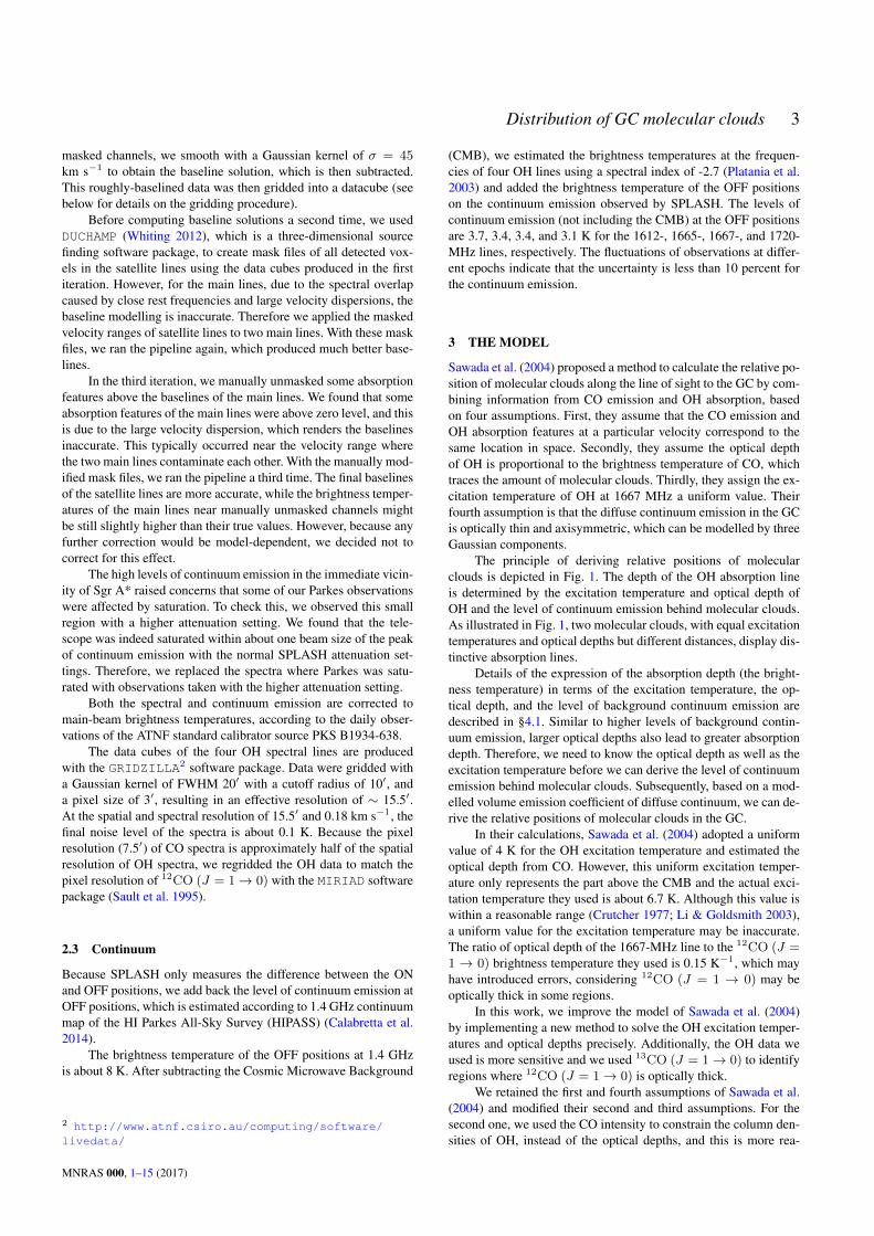
The principle of deriving relative positions of molecularclouds is depicted in Fig. 1. The depth of the OH absorption lineis determined by the excitation temperature and optical depth ofOH and the level of continuum emission behind molecular clouds.As illustrated in Fig. 1, two molecular clouds, with equal excitationtemperatures and optical depths but different distances, display dis-tinctive absorption lines.

Details of the expression of the absorption depth (the bright-ness temperature) in terms of the excitation temperature, the op-tical depth, and the level of background continuum emission aredescribed in §4.1. Similar to higher levels of background contin-uum emission, larger optical depths also lead to greater absorptiondepth. Therefore, we need to know the optical depth as well as theexcitation temperature before we can derive the level of continuumemission behind molecular clouds. Subsequently, based on a mod-elled volume emission coefficient of diffuse continuum, we can de-rive the relative positions of molecular clouds in the GC.

In their calculations, Sawada et al. (2004) adopted a uniformvalue of 4 K for the OH excitation temperature and estimated theoptical depth from CO. However, this uniform excitation temper-ature only represents the part above the CMB and the actual exci-tation temperature they used is about 6.7 K. Although this value iswithin a reasonable range (Crutcher 1977; Li & Goldsmith 2003),a uniform value for the excitation temperature may be inaccurate.The ratio of optical depth of the 1667-MHz line to the 12CO (J =1 → 0) brightness temperature they used is 0.15 K−1, which mayhave introduced errors, considering 12CO (J = 1 → 0) may beoptically thick in some regions.

In this work, we improve the model of Sawada et al. (2004)by implementing a new method to solve the OH excitation temper-atures and optical depths precisely. Additionally, the OH data weused is more sensitive and we used 13CO (J = 1→ 0) to identifyregions where 12CO (J = 1→ 0) is optically thick.

We retained the first and fourth assumptions of Sawada et al.(2004) and modified their second and third assumptions. For thesecond one, we used the CO intensity to constrain the column den-sities of OH, instead of the optical depths, and this is more rea-

MNRAS 000, 1–15 (2017)

4 Q. Z. Yan et al.

Y

X

The Galactic Centre

Diffuse Continuum EmissionLine of Sight

A Shallow OH Absorption Line

A Deep OH Absorption Line

COOH

A Near Cloudet

A Far Cloudet

Figure 1. Principles of deriving the relative positions of molecular clouds,which is reproduced from Sawada et al. (2004, Figure 3). The black dashedlines and red lines represent CO emission and OH absorption lines, respec-tively.

sonable, because the CO intensity is roughly proportional to thecolumn density, if CO emission is optically thin. For the third one,we abandoned the assumption of a uniform excitation temperature,and alternatively, we assume that the excitation temperatures of thetwo main lines are equal and no assumptions about excitation tem-peratures of the satellite lines are made.

We summarise these four assumptions as

(i) The CO emission and OH absorption features at a particularvelocity correspond to the same location in space.

(ii) The column density of OH at ground states, N(OH), is pro-portional to the brightness temperature of 12CO (J = 1 → 0),meaning N(OH) = f × TCO, where f is a constant.

(iii) The excitation temperatures of the two main lines are equal.(iv) The diffuse continuum emission in the GC is optically thin

and axisymmetric, and it can be modelled by three Gaussian com-ponents.

4 SOLVING OH EXCITATION TEMPERATURES

In this section, we propose a new method to calculate the col-umn densities, excitation temperatures, and optical depths of OHprecisely, which significantly improves on the model proposed bySawada et al. (2004). The kernel of the idea is to express the OHexcitation temperatures and optical depths in terms of the four col-umn densities of the OH ground state hyperfine levels, which aresolvable provided that all four lines have been observed.

In many cases of practical interest the background emissionand brightness temperature of an absorption line are observable.However, the situation is more difficult for the complicated GC re-gion, because the fraction of the observed background emissionarising from behind the OH cloud is unknown, and this requiresextra effort to model. In the following two subsections, we first dis-cuss the simple case in which the background is known, and thenintroduce the treatment as applied to the GC region.

4.1 Known background continuum

Before we deal with the GC, we introduce the simple case in whichthe background continuum emission is known. The basic equation

F = 2 N1

F = 1 N2

F = 2 N3

F = 1 N4

2Π3/2

J = 3/2

+

−

1720 1612

1667

1665

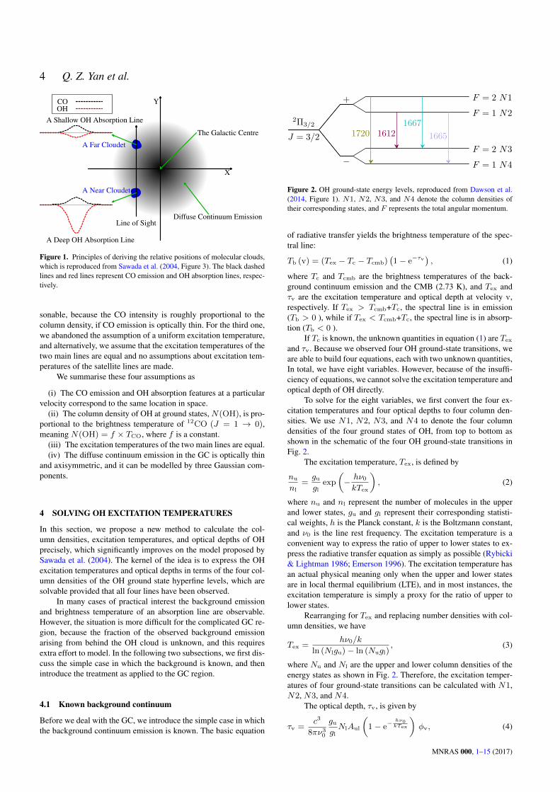
Figure 2. OH ground-state energy levels, reproduced from Dawson et al.(2014, Figure 1). N1, N2, N3, and N4 denote the column densities oftheir corresponding states, and F represents the total angular momentum.

of radiative transfer yields the brightness temperature of the spec-tral line:

Tb (v) = (Tex − Tc − Tcmb)(1− e−τv

), (1)

where Tc and Tcmb are the brightness temperatures of the back-ground continuum emission and the CMB (2.73 K), and Tex andτv are the excitation temperature and optical depth at velocity v,respectively. If Tex > Tcmb+Tc, the spectral line is in emission(Tb > 0 ), while if Tex < Tcmb+Tc, the spectral line is in absorp-tion (Tb < 0 ).

If Tc is known, the unknown quantities in equation (1) are Tex

and τv. Because we observed four OH ground-state transitions, weare able to build four equations, each with two unknown quantities,In total, we have eight variables. However, because of the insuffi-ciency of equations, we cannot solve the excitation temperature andoptical depth of OH directly.

To solve for the eight variables, we first convert the four ex-citation temperatures and four optical depths to four column den-sities. We use N1, N2, N3, and N4 to denote the four columndensities of the four ground states of OH, from top to bottom asshown in the schematic of the four OH ground-state transitions inFig. 2.

The excitation temperature, Tex, is defined by

nu

nl=gugl

exp

(− hν0kTex

), (2)

where nu and nl represent the number of molecules in the upperand lower states, gu and gl represent their corresponding statisti-cal weights, h is the Planck constant, k is the Boltzmann constant,and ν0 is the line rest frequency. The excitation temperature is aconvenient way to express the ratio of upper to lower states to ex-press the radiative transfer equation as simply as possible (Rybicki& Lightman 1986; Emerson 1996). The excitation temperature hasan actual physical meaning only when the upper and lower statesare in local thermal equilibrium (LTE), and in most instances, theexcitation temperature is simply a proxy for the ratio of upper tolower states.

Rearranging for Tex and replacing number densities with col-umn densities, we have

Tex =hν0/k

ln (Nlgu)− ln (Nugl), (3)

where Nu and Nl are the upper and lower column densities of theenergy states as shown in Fig. 2. Therefore, the excitation temper-atures of four ground-state transitions can be calculated with N1,N2, N3, and N4.

The optical depth, τv, is given by

τv =c3

8πν30

guglNlAul

(1− e

− hν0kTex

)φv, (4)

MNRAS 000, 1–15 (2017)

Distribution of GC molecular clouds 5

Table 1. Parameters of the four ground-state transitions of OH.

Line Rest frequency Einstein-A coefficient(MHz) (10−11 s−1)

1612-MHz 1612.231 1.3021665-MHz 1665.402 7.1771667-MHz 1667.359 7.7781720-MHz 1720.530 0.9496

where Nl is the column density of molecules at the lower energylevel, Aul is the Einstein-A coefficient, and φv is the normalizedprofile. After substituting equation (3) into equation (4), we have

τv =c3

8πν30Aul

(guglNl −Nu

)φv. (5)

Clearly, the optical depth is also a function of the column density,and all four optical depths can be calculated with the column den-sities of the four ground states.

Mathematically, the independent equations (3) and (5) repre-sent a transformation between the pairs of variables (Nl, Nu) and(Tex, τv). Substituting equations (3) and (5) into equation (1), weobtain an equation with only column densities as variables. Wehence obtain four equations with only four unknowns, which maybe solved. This can be done only because all four OH ground-statetransitions share four energy levels, which means the excitationtemperatures and optical depths of four OH ground-state transitionsare not entirely independent. After obtaining the column densities,the calculation of excitation temperatures and optical depths is triv-ial.

4.2 The Galactic Centre

In this subsection we consider the special case of the GC. The dif-ficulties mainly arise from two problems: the two main lines con-taminate each other because the velocity dispersion is large, andthe level of background continuum behind OH clouds is unknown.The first problem eliminates one equation, while the second one in-troduces an extra variable. We solve the two problems according tothe second and third assumptions listed in §3.

The assumption about the main-line excitation temperatureprovides an equation. Typically, the positive-velocity part of the1667-MHz line is mixed with the negative-velocity part of the1665-MHz line over a particular velocity range, meaning one equa-tion is eliminated, and only three equations remain. Crutcher (1977,1979) found that while the main line Tex are generally within 1-2 Kof each other, even small departures from equal main-line Tex cancause significant errors in column density estimates in cases whereequal Tex is assumed. However, we are using column densities toestimate excitation temperatures, and the OH column densities arewell constrained by the 12CO (J = 1 → 0) brightness temper-ature. Therefore, the uncertainty caused by this assumption is notsignificant, and we describe this effect in §5.3.

Specifically, the assumption about the main line Tex is ex-pressed as

Tex1665 = Tex1667, (6)

where Tex1665 and Tex1667 are excitation temperatures of 1665-and 1667-MHz lines, respectively. In contrast, the excitation tem-peratures of the two satellite lines are in general unequal and sig-nificantly different to the excitation temperature of the two main

0 2 4 6 8 10 12 1412 CO (J=1→0) Brightness temperature (K)

0.2

0.0

0.2

0.4

0.6

0.8

1.0

1.2

13C

O(J

=1→

0) B

right

ness

tem

pera

ture

(K)

12 CO (J=1→0) optically thick12 CO (J=1→0) optically thin

Figure 3. The brightness temperature of 12CO (J = 1 → 0) versus13CO (J = 1→ 0). The green line, which passes through the origin witha slope of 0.066±0.020, was fitted with data whose brightness temperatureof 12CO (J = 1→ 0) is greater than 6.5 K. The blue area is the coveragewithin 2σ (σ = 0.12 K) of the residual, where 12CO (J = 1 → 0) emis-sion is mostly optically thin, while beyond this blue area, marked in red, the12CO (J = 1→ 0) emission is mostly optically thick.

lines. Equation (6) can serve as the fourth equation, and thereforewe still have four equations for the GC.

The second problem introduces an extra variable. At first itwould seem we have to solve another four parameters, correspond-ing to the four background continuum levels for the four OH tran-sitions. However, the fraction of continuum emission behind OHclouds for the four OH lines should be equal. Therefore, we onlyneed to add one parameter, Tc, which is the background continuumemission at any given frequency, say at 1665 MHz, and the back-ground continuum levels of the other three lines can then be derivedusing the ratio between overall continuum emissions measured foreach line.

We now have five variables to solve, but only four equationsin hand. We supplement this system with data from CO to createthe fifth equation, assuming the column densities of CO and OHare proportional. This is possible since the column density of COin a single velocity channel is roughly proportional to its brightnesstemperature multiplied by the bandwidth of the channel if the COspectral line is optically thin.

Compared with 12CO (J = 1 → 0), 13CO (J = 1 → 0) isa better tracer of CO column densities. However, 13CO (J = 1→0) is not visible in all positions. Although 12CO (J = 1 → 0)emission is often optically thick, the situation in the GC is notsevere due to the large velocity dispersion. The resolution of ourdata is ∼38 pc, and at this size scale, the optically thick effectis further diminished by beam averaging. Consequently, we use12CO (J = 1 → 0) and artificially scale it in places where the12CO/13CO intensity ratio suggests it is optically thick.

To detect regions where the 12CO (J = 1 → 0) line is opti-cally thick, we compare the brightness temperature of 12CO (J =1 → 0) versus 13CO (J = 1 → 0), as shown in Fig. 3,where all values less than 3σ are excluded. Assuming a uni-form 12CO/13CO abundance ratio, the brightness temperaturesof 12CO (J = 1 → 0) should be linearly proportional tothe 13CO (J = 1 → 0) emission if they are both optically

MNRAS 000, 1–15 (2017)

6 Q. Z. Yan et al.

thin. We therefore fitted a line to the 12CO (J = 1 → 0) to13CO (J = 1 → 0) relation, restricting the fit to the region with12CO (J = 1 → 0) brightness temperatures exceeding 6.5 K toavoid the large amount of 12CO (J = 1 → 0) emission that ap-pears to be optically thick in the region < 6.5K.

The fitted line (using linear least squares with y-intercept =0), delineated in green in Fig. 3, has a slope of 0.066±0.020, yield-ing a 12CO/13CO intensity ratio of about 15.2. The uncertainty isgiven by the difference between the fitted slope constrained to passthrough the origin and the fitted slope without this constraint. Al-though Oka et al. (1998) suggests a value of 5.19, this value couldchange with observations obtained with different beam filling fac-tors. Because 12CO (J = 1 → 0) clouds are more extended than13CO (J = 1 → 0) clouds, large beam sizes diminish the bright-ness temperature of 13CO (J = 1 → 0) and increase the valueof 12CO/13CO intensity ratio. The Nobeyama Radio Observatory(NRO) 45-m telescope used by Oka et al. (1998) had a FWHM ofabout 17′′ at 100 GHz, and this angular resolution is much higherthan that of Parkes at 1666 MHz. Consequently, the variation of the12CO/13CO intensity ratio suggests that the beam filling factorsof 12CO (J = 1 → 0) and 13CO (J = 1 → 0) are significantlydifferent.

In Fig. 3, the region within 2σ (σ = 0.12 K) of the residual ismarked with blue, where 12CO (J = 1 → 0) emission is roughlyoptically thin and the optically thick effect if not evident, becausethey are linearly correlated with 13CO (J = 1 → 0). Althoughsome points possessing large 12CO (J = 1 → 0) brightness tem-peratures are also likely optically thick, we keep those points un-corrected, because there are too few such points to significantlyaffect the outcome. Consequently, we only did the correction forthose points in the red region of Fig. 3, where 12CO (J = 1→ 0)brightness temperatures are saturated. For the data in the red re-gion, we replaced the 12CO (J = 1 → 0) brightness temperaturewith the 13CO (J = 1→ 0) temperatures divided by 0.066 – i.e.,the points in the red region were moved horizontally onto the greenline.

In Fig. 3, 12CO (J = 1 → 0) brightness temperatures inthe optically thick state are lower than some 12CO (J = 1 → 0)brightness temperatures in the optically thin state. This is becausewhen 12CO (J = 1 → 0) is optically thick, the brightness tem-perature approaches the excitation temperature. The optically thickspectra can only see the outer parts of molecular clouds, and theouter parts of molecular clouds usually have lower excitation tem-peratures. After the correction, 12CO (J = 1→ 0) data is roughlyproportional to 13CO (J = 1→ 0) data.

We use self-absorption spectra of 12CO (J = 1 → 0)to demonstrate this behaviour. The line centres of self-absorptionspectra towards molecular cores are lower than their adjacent ve-locity components. For instance, the average 12CO (J = 1 → 0)spectrum of an H II region N14 (Yan et al. 2016, Figure 1) showsa deep dip in the line centre, and this effect is more evident com-pared with the single-pixel spectrum (Yan et al. 2016, Figure 29).Consequently, beam averaging can diminish the effect of opticallythick regions.

Now, we can replace the column densities of 12CO (J = 1→0) with their corrected brightness temperatures. The fifth equationis expressed as

N1 +N2 +N3 +N4 = f1234 × TCO, (7)

where N1, N2, N3, and N4 are column densities of four OHground states, TCO is the corrected brightness temperature of12CO (J = 1 → 0), and f1234 is the ratio of the sum of column

densities of OH ground states to the 12CO (J = 1→ 0) brightnesstemperature. Although f1234 can be estimated from observationstowards the Galactic disk, we determine f1234 more accurately bya method discussed below in subsection 5.2.

Now, for the GC, we have five parameters and five equations,and we can solve them simultaneously. In this model, the largestuncertainty comes from equation (7). In the rest of this section, wepresent the system of equations and its method of solution.

4.3 The system of equations

Here we write out the system of equations explicitly. We choosethe background continuum level of 1665-MHz line, Tc, as the fifthvariable, and the background continuum levels of the other threelines is

Tc1667 = f1667Tc,Tc1612 = f1612Tc,Tc1720 = f1720Tc,

(8)

where Tc1667, Tc1612, and Tc1720 are background continuum emis-sion levels behind molecular clouds at the frequencies of the 1667-,1612-, and 1720-MHz lines and f1667, f1612, and f1720 are theirratios to the value of 1665-MHz line, respectively. As mentionedabove, f1667, f1612, and f1720 can be calculated from the mea-sured overall continuum emission, because for a particular voxel,the fraction of continuum emission behind molecular clouds is thesame for all four lines.

In order to simplify our model, we use Texm to denote theexcitation temperature of the two main lines. The frequencies of1665-, 1667-, 1612-, and 1720-MHz lines are denoted by ν1665,ν1667, ν1612, and ν1720, and their optical depths at a velocity of vare denoted by τv1665, τv1667, τv1612, and τv1720, respectively. Thestatistical weight of each level can be calculated with their totalangular momentums (Barrett 1964). The Einstein-A coefficients ofthe four lines were calculated by Destombes et al. (1977) and listedin Table 1. We use A1612, A1665, A1667, and A1720 to denote theEinstein-A coefficients of the four lines. The parameters of the fourOH ground-state transitions are summarised in Table 1.

Using the fact thatN1 andN2 can be derived from Texm,N3andN4, we replacedN1 andN2 with Texm. Equivalently, we onlyneed to constrain the sum of N3 and N4, and therefore equation(7) is modified to

N3 +N4 = f × TCO. (9)

The value of f in equation (9) is roughly half of f1234 in equa-tions (7).

Now, we only have to deal with four parameters, which areTexm, Tc,N3, andN4, because equation (6) has already been used.Denoting the brightness temperatures of the four lines at a velocityof v by T1665(v), T1667(v), T1612(v), and T1720(v), we write outthe equations as

(Texm − Tc − Tcmb) (1− e−τvmain) = Tbmain (v)(

hν1612/kln(3N3)−ln(5N2)

− f1612Tc − Tcmb

) (1− e−τv1612

)= Tb1612 (v)(

hν1720/kln(5N4)−ln(3N1)

− f1720Tc − Tcmb

) (1− e−τv1720

)= Tb1720 (v)

N3 +N4 = f × TCO,

(10)

MNRAS 000, 1–15 (2017)

Distribution of GC molecular clouds 7

where

Tcmb = 2.73 K,

N1 = N3 exp(−hν1667kTexm

),

N2 = N4 exp(−hν1665kTexm

),

Tbmain (v) = Tb1665 (v) or Tb1667 (v) ,

τvmain = c3

8πν31665A1665 (N4 −N2)φv or c3

8πν31667A1667 (N3 −N1)φv,

τv1612 = c3

8πν31612A1612

(35N3 −N2

)φv,

τv1720 = c3

8πν31720A1720

(53N4 −N1

)φv.

(11)

4.4 Solving the system of equations

The non-linear system of equations (10) was solved numerically.Because we solve the system of equation (10) channel by channel,φv, the line profile, becomes approximately constant over a singlechannel. Due to normalization, the value of φv equals the reciprocalof the velocity interval between channels.

In order to examine the uniqueness and acquire an approxi-mate initial solution, we simplified equation (10) by linearising theequation of 1720-MHz line, because this line possesses the small-est Einstein-A coefficient and has the smallest optical depth. Wefurther assume hν/(kTex1720) � 1, which is generally satisfiedif the excitation temperature of the 1720-MHz line, Tex1720, is notexceedingly low. Therefore, we have

Tex1720 = hν1720/kln(5N4)−ln(3N1)

≈ hν1720k

5N45N4−3N1

(12)

and

1− e−τv1720 ≈ τv1720. (13)

Now, the equation of 1720-MHz line is linear with respect toN3 and N4. Combining with N3 + N4 = f × TCO, we cansolveN3 andN4 with respect to Tc and Texm. Substituting the ex-pression of N3 and N4 to the main line and 1612-MHz equations,we acquire two equations with respect to Tc and Texm, which ismuch easier to solve numerically. For this two-equation system, wesearched the solution over a grid of the possible solutions space,and found that uniqueness is satisfied.

We adopted an initial value of 7 K for Texm, and the initialvalue of Tc is set to be half of the observed total continuum emis-sion. After solving Tc and Texm, we calculated the value ofN3 andN4, and equation (10) can be solved numerically based on theseinitial solutions.

5 RESULTS

In this section, we present a 3D structure of the molecular clouds inthe GC by displaying the slices along the Galactic latitude. Sawadaet al. (2004) only provided the face-on view (relative to the Galacticdisk) of b = 0◦, while we calculated the face-on views of b = -0.375◦, -0.25◦, -0.125◦, 0◦, 0.125◦, and 0.25◦, constituting a 3Dstructure of the GC.

Based on the background continuum level solved by equation(10) and the modelled volume emission coefficient of the contin-uum emission in the GC, we calculated the position of the molec-ular clouds along the line of sight. The position was determined

−6−4−202460

50

100

150

200

250

300

T con

t (K)

b=0.25 ◦a1 = 13.6 K, σ1 = 0.20 ◦

a2 = 20.8 K, σ2 = 0.78 ◦

a3 = 13.8 K, σ3 = 12.53 ◦

−6−4−202460

50

100

150

200

250

300

T con

t (K)

b=0.125 ◦a1 = 72.9 K, σ1 = 0.17 ◦

a2 = 37.3 K, σ2 = 0.76 ◦

a3 = 14.4 K, σ3 = 15.06 ◦

−6−4−202460

50

100

150

200

250

300T c

ont (

K)b=0 ◦a1 = 190.8 K, σ1 = 0.14 ◦

a2 = 64.6 K, σ2 = 0.68 ◦

a3 = 16.7 K, σ3 = 7.61 ◦

−6−4−202460

50

100

150

200

250

300

T cont (

K)

b=−0.125 ◦a1 = 162.0 K, σ1 = 0.15 ◦

a2 = 57.8 K, σ2 = 0.69 ◦

a3 = 17.1 K, σ3 = 6.41 ◦

−6−4−202460

50

100

150

200

250

300

T cont (

K)

b=−0.25 ◦a1 = 69.3 K, σ1 = 0.17 ◦

a2 = 37.1 K, σ2 = 0.78 ◦

a3 = 14.8 K, σ3 = 7.35 ◦

−6−4−20246Galactic longitude ( ◦ )

0

50

100

150

200

250

300

T con

t (K)

b=−0.375 ◦a1 = 11.8 K, σ1 = 0.30 ◦

a2 = 22.0 K, σ2 = 0.87 ◦

a3 = 13.0 K, σ3 = 7.98 ◦

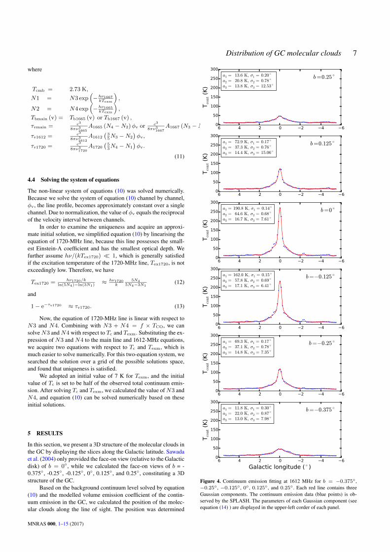
Figure 4. Continuum emission fitting at 1612 MHz for b = −0.375◦,−0.25◦, −0.125◦, 0◦, 0.125◦, and 0.25◦. Each red line contains threeGaussian components. The continuum emission data (blue points) is ob-served by the SPLASH. The parameters of each Gaussian component (seeequation (14) ) are displayed in the upper-left corder of each panel.

MNRAS 000, 1–15 (2017)

8 Q. Z. Yan et al.

by integrating the modelled volume emission coefficient from neg-ative infinity to the position of molecular clouds, making the in-tegration equal the background continuum level. Although 20 cmcontinuum observations (Law et al. 2008), which have a higher spa-tial resolution than the Parkes data, suggest that the centre of thecontinuum emission is Sgr A*, whose Galactic coordinate is about(l, b) = (−0.06◦,−0.05◦) , we set l = 0◦ as the centre of the con-tinuum emission, because Sgr A* is not far from (l, b) = (0◦, 0◦).

In our calculation, we adopt a distance to the GC of 8.34kpc (Reid et al. 2014), resulting in a physical resolution of 38 pcfor the CMZ.

5.1 Fitting diffuse continuum emission

The fitting of the diffuse continuum emission in the GC is impor-tant, because locations of molecular molecular clouds along the lineof sight hinge on the distribution of the continuum volume emissioncoefficient.

Because we found that only at the range of −0.375◦ ≤ b ≤0.25◦, the number of molecular clouds is significant, we focusedon the calculation of the pixels within this range, including b = -0.375◦, -0.25◦, -0.125◦, 0◦, 0.125◦, and 0.25◦.

Following Sawada et al. (2004), we fitted the diffuse contin-uum emission along the Galactic longitude using three Gaussiancomponents. Because the spatial resolution of our data is unableto resolve Sgr A*, which is the centre of the diffuse continuumemission, we simply assigned the mean position of Gaussian com-ponents l = 0◦. The integration of observed continuum emissionis carried out using the distance from Sgr A* to the line of sight in-stead of Galactic longitude. We express this distance with degreesusing a linear conversion factor of 145.56 pc degree−1, and its dif-ference with Galactic longitude is less than 0.01◦ for l = 5◦.

The observed continuum emission, which is integrated all overthe line of sight, can be expressed as

Tcont (l) = a1 exp(− x2

2σ21

)+a2 exp

(− x2

2σ22

)+a3 exp

(− x2

2σ23

)(14)

where l is the Galactic longitude in degrees, x = 8340 ×sin (l) /145.56, and a and σ represent the height of the curve’speak and the standard deviation, respectively.

We display the parameters of all Gaussian components at 1612MHz in Fig. 4. Generally, the diffuse continuum emission in theCMZ is well fitted by three Gaussian components, indicating theaxisymmetric assumption of the continuum emission is reasonable.

5.2 Determining the column density ratio of OH to CO

So far, the value of f , the only free parameter in equation (10), re-mains undetermined. f affects the estimate of continuum emissionlevels behind OH clouds, thereby altering positions of molecularclouds in the CMZ. Because most of the molecular clouds are inthe CMZ (within 500 pc of the GC), it is reasonable to assign f avalue that maximises the proportion of pixels within the CMZ.

Before we searched for this value, we estimated f accord-ing to the observations towards other regions of the Milky Way.Goicoechea et al. (2011) estimated the column densities of OH inthe Orion Bar photodissociation region (PDR) to be greater than1× 1019 m−2. However, this value is the result of integration overa large velocity range, and therefore we consider column densitiesof OH integrated over one single channel of about 1 × 1018 m−2,around which we searched the optimum value for f .

2 3 4 5 6 7[N3 (OH)+N4 (OH)]/TCO ( 1×1018m−2 K−1 )

0.35

0.36

0.37

0.38

0.39

0.40

0.41

0.42

0.43

Prop

ortio

n of pixels with

in 500

pc of th

e GC

N3 (OH)+N4 (OH) = 4.7 × 1018 × [TCO1 K

] m−2

b = 0 ◦

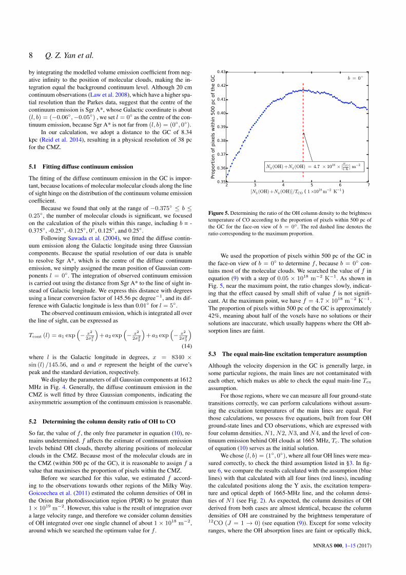
Figure 5. Determining the ratio of the OH column density to the brightnesstemperature of CO according to the proportion of pixels within 500 pc ofthe GC for the face-on view of b = 0◦. The red dashed line denotes theratio corresponding to the maximum proportion.

We used the proportion of pixels within 500 pc of the GC inthe face-on view of b = 0◦ to determine f , because b = 0◦ con-tains most of the molecular clouds. We searched the value of f inequation (9) with a step of 0.05 × 1018 m−2 K−1. As shown inFig. 5, near the maximum point, the ratio changes slowly, indicat-ing that the effect caused by small shift of value f is not signifi-cant. At the maximum point, we have f = 4.7 × 1018 m−2 K−1.The proportion of pixels within 500 pc of the GC is approximately42%, meaning about half of the voxels have no solutions or theirsolutions are inaccurate, which usually happens where the OH ab-sorption lines are faint.

5.3 The equal main-line excitation temperature assumption

Although the velocity dispersion in the GC is generally large, insome particular regions, the main lines are not contaminated witheach other, which makes us able to check the equal main-line Tex

assumption.For those regions, where we can measure all four ground-state

transitions correctly, we can perform calculations without assum-ing the excitation temperatures of the main lines are equal. Forthose calculations, we possess five equations, built from four OHground-state lines and CO observations, which are expressed withfour column densities, N1, N2, N3, and N4, and the level of con-tinuum emission behind OH clouds at 1665 MHz, Tc. The solutionof equation (10) serves as the initial solution.

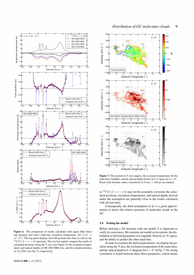
We chose (l, b) = (1◦, 0◦), where all four OH lines were mea-sured correctly, to check the third assumption listed in §3. In fig-ure 6, we compare the results calculated with the assumption (bluelines) with that calculated with all four lines (red lines), incudingthe calculated positions along the Y axis, the excitation tempera-ture and optical depth of 1665-MHz line, and the column densi-ties of N1 (see Fig. 2). As expected, the column densities of OHderived from both cases are almost identical, because the columndensities of OH are constrained by the brightness temperature of12CO (J = 1 → 0) (see equation (9)). Except for some velocityranges, where the OH absorption lines are faint or optically thick,

MNRAS 000, 1–15 (2017)

Distribution of GC molecular clouds 9

−150 −100 −50 0 50 100 150 200 250Velocity (km s−1 )

−15

−10

−5

0

5

10

15

20

Brig

htne

ss te

mpe

ratu

re (K

) (l, b) = (1 ◦ , 0 ◦ ) 12CO (J=1→0)OH 1665-MHzOH 1667-MHzOH 1612-MHzOH 1720-MHz

−150 −100 −50 0 50 100 150 200 250Velocity (km s−1 )

−400

−200

0

200

400

Y-ax

is p

ositi

on (p

c)

Equal main-line TexUnequal main-line Tex

−150 −100 −50 0 50 100 150 200 250Velocity (km s−1 )

0

5

10

15

20

25

30

Exci

tatio

n te

mpe

ratu

re (K

) OH 1665-MHz Equal main-line TexUnequal main-line Tex

−150 −100 −50 0 50 100 150 200 250Velocity (km s−1 )

0

2

4

6

8

10

12

14

16

Optic

al d

epth

OH 1665-MHzEqual main-line TexUnequal main-line Tex

−150 −100 −50 0 50 100 150 200 250Velocity (km s−1 )

0.0

0.5

1.0

1.5

2.0

2.5

3.0

3.5

4.0

N1(O

H) (1

019m−3

)

Equal main-line TexUnequal main-line Tex

Figure 6. The comparison of results calculated with equal (blue lines)and unequal (red lines) main-line excitation temperature, for (l, b) =(1◦, 0◦). The top panel displays four OH ground-state lines as well as the12CO (J = 1→ 0) spectrum. The rest four panels compare the results ofcalculated positions along the Y axis (see Figure 9), the excitation temper-atures and optical depths of OH 1665-MHz line, and the column densitiesof N1(OH) (see Fig. 2), respectively.

−3−2−101234Galactic longitude ( ◦ )

−300

−200

−100

0

100

200

300

Velo

city

(km

s−1

)

Y-axis position

b=0 ◦

−3−2−101234Galactic longitude ( ◦ )

−300

−200

−100

0

100

200

300

Velo

city

(km

s−1

)

Excitation temperature (Main lines)

b=0 ◦

−3−2−101234Galactic longitude ( ◦ )

−300

−200

−100

0

100

200

300

Velo

city

(km

s−1

)

Optical depth

b=0 ◦

0

1

2

3

−450

−300

−150

0

150

300

450

pc

0

5

10

15

20

K

Figure 7. The position in Y axis (upper), the excitation temperature for themain lines (middle), and the optical depth (lower) in L-V space for b = 0◦.Pixels with absolute values of positions in Y axis > 500 pc are masked.

or 12CO (J = 1→ 0) may not be accurately corrected, the calcu-lated positions, excitation temperatures, and optical depths derivedunder the assumption are generally close to the results calculatedwith all four lines.

Consequently, the third assumption in §3 is a good approxi-mation to derive the relative positions of molecular clouds in theGC.

5.4 Testing the model

Before deriving a 3D structure with our model, it is important toverify its correctness. We examine our model on two points: the dis-tribution of derived parameters in Longitude-Velocity (L-V) space,and the ability to predict the other main line.

In order to examine the derived parameters, we display the po-sition along the Y axis, the excitation temperature of the main lines,and the optical depth in L-V diagram for b = 0◦ in Fig. 7. No strongcorrelation is found between these three parameters, which means

MNRAS 000, 1–15 (2017)

10 Q. Z. Yan et al.

the position, excitation temperature, and the optical depth are gen-erally independent. Along the line of sight, the derived parametersare roughly continuous, and this continuity also exist along the ve-locity axis. This result is consistent with the expectation that molec-ular clouds, which are close in L-V space, should have adjacentpositions.

In our calculation, we use only one of the two main lines (seeequation 10), and the brightness temperature of the other main linecan be calculated by our model according to the column densities.Therefore, how well can we reproduce the other main line is a vi-tal indicator of the correctness of our model. The regions wherethe two main lines are not contaminated by each other provide theopportunity to check the prediction of the other main line.

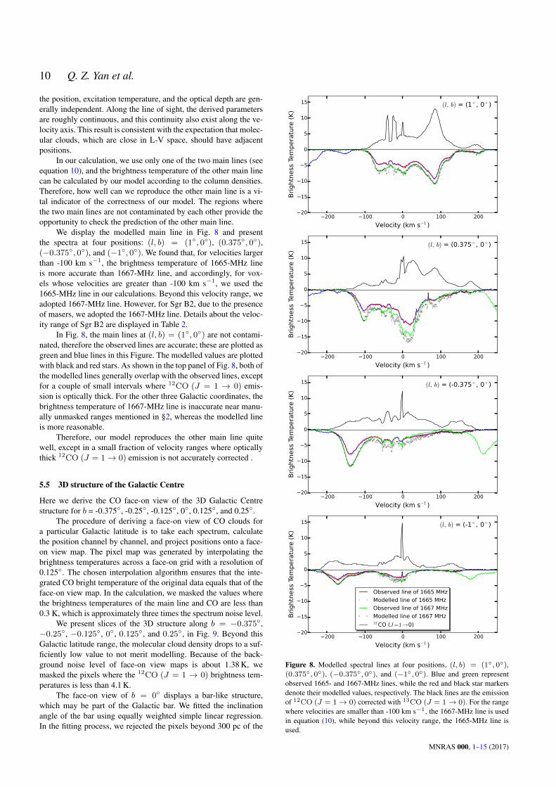
We display the modelled main line in Fig. 8 and presentthe spectra at four positions: (l, b) = (1◦, 0◦), (0.375◦, 0◦),(−0.375◦, 0◦), and (−1◦, 0◦). We found that, for velocities largerthan -100 km s−1, the brightness temperature of 1665-MHz lineis more accurate than 1667-MHz line, and accordingly, for vox-els whose velocities are greater than -100 km s−1, we used the1665-MHz line in our calculations. Beyond this velocity range, weadopted 1667-MHz line. However, for Sgr B2, due to the presenceof masers, we adopted the 1667-MHz line. Details about the veloc-ity range of Sgr B2 are displayed in Table 2.

In Fig. 8, the main lines at (l, b) = (1◦, 0◦) are not contami-nated, therefore the observed lines are accurate; these are plotted asgreen and blue lines in this Figure. The modelled values are plottedwith black and red stars. As shown in the top panel of Fig. 8, both ofthe modelled lines generally overlap with the observed lines, exceptfor a couple of small intervals where 12CO (J = 1 → 0) emis-sion is optically thick. For the other three Galactic coordinates, thebrightness temperature of 1667-MHz line is inaccurate near manu-ally unmasked ranges mentioned in §2, whereas the modelled lineis more reasonable.

Therefore, our model reproduces the other main line quitewell, except in a small fraction of velocity ranges where opticallythick 12CO (J = 1→ 0) emission is not accurately corrected .

5.5 3D structure of the Galactic Centre

Here we derive the CO face-on view of the 3D Galactic Centrestructure for b = -0.375◦, -0.25◦, -0.125◦, 0◦, 0.125◦, and 0.25◦.

The procedure of deriving a face-on view of CO clouds fora particular Galactic latitude is to take each spectrum, calculatethe position channel by channel, and project positions onto a face-on view map. The pixel map was generated by interpolating thebrightness temperatures across a face-on grid with a resolution of0.125◦. The chosen interpolation algorithm ensures that the inte-grated CO bright temperature of the original data equals that of theface-on view map. In the calculation, we masked the values wherethe brightness temperatures of the main line and CO are less than0.3 K, which is approximately three times the spectrum noise level.

We present slices of the 3D structure along b = −0.375◦,−0.25◦, −0.125◦, 0◦, 0.125◦, and 0.25◦, in Fig. 9. Beyond thisGalactic latitude range, the molecular cloud density drops to a suf-ficiently low value to not merit modelling. Because of the back-ground noise level of face-on view maps is about 1.38 K, wemasked the pixels where the 12CO (J = 1 → 0) brightness tem-peratures is less than 4.1 K.

The face-on view of b = 0◦ displays a bar-like structure,which may be part of the Galactic bar. We fitted the inclinationangle of the bar using equally weighted simple linear regression.In the fitting process, we rejected the pixels beyond 300 pc of the

−200 −100 0 100 200Velocity (km s−1 )

−20

−15

−10

−5

0

5

10

15

Brig

htne

ss Te

mpe

ratu

re (K

)

(l, b) = (1 ◦ , 0 ◦ )

−200 −100 0 100 200Velocity (km s−1 )

−20

−15

−10

−5

0

5

10

15

Brig

htne

ss Te

mpe

ratu

re (K

)

(l, b) = (0.375 ◦ , 0 ◦ )

−200 −100 0 100 200Velocity (km s−1 )

−20

−15

−10

−5

0

5

10

15

Brig

htne

ss Te

mpe

ratu

re (K

)

(l, b) = (-0.375 ◦ , 0 ◦ )

−200 −100 0 100 200Velocity (km s−1 )

−20

−15

−10

−5

0

5

10

15

Brig

htne

ss Te

mpe

ratu

re (K

)

(l, b) = (-1 ◦ , 0 ◦ )

Observed line of 1665 MHzModelled line of 1665 MHzObserved line of 1667 MHzModelled line of 1667 MHz12 CO (J=1→0)

Figure 8. Modelled spectral lines at four positions, (l, b) = (1◦, 0◦),(0.375◦, 0◦), (−0.375◦, 0◦), and (−1◦, 0◦). Blue and green representobserved 1665- and 1667-MHz lines, while the red and black star markersdenote their modelled values, respectively. The black lines are the emissionof 12CO (J = 1→ 0) corrected with 13CO (J = 1→ 0). For the rangewhere velocities are smaller than -100 km s−1, the 1667-MHz line is usedin equation (10), while beyond this velocity range, the 1665-MHz line isused.

MNRAS 000, 1–15 (2017)

Distribution of GC molecular clouds 11

0

250

-250

500

-500

Y (p

c)

The Sun

b=0.25 ◦ b=0.25 ◦

0

250

-250

500

-500

Y (p

c)

b=0.125 ◦ b=0.125 ◦

0

250

-250

500

-500

Y (p

c)

67.5 ◦

b=0 ◦ b=0 ◦

0

250

-250

500

-500

Y (p

c)

b=−0.125 ◦ b=−0.125 ◦

0

250

-250

500

-500

Y (p

c)

b=−0.25 ◦ b=−0.25 ◦

0

250

-250

500

-500

Y (p

c)

0250 -250500 -500X (pc)

b=−0.375 ◦

0250 -250500 -500X (pc)

b=−0.375 ◦

10 100K km s−1

−150 0 150km s−1

Figure 9. Face-on views of CO clouds for b = −0.375◦, −0.25◦,−0.125◦, 0◦, 0.125◦, and 0.25◦. The left panels are face-on view of eachGalactic latitude, and the right panels are the distributions of velocitieswhich are intensity weighted. The originate of X and Y axes is Sgr A*,and X = 0 corresponds to l = 0◦. We masked the pixels where the integralbrightness temperature is less than 4.1 K km s−1 (3σ).

0

100

-100

200

-200

300

-300

400

Y (pc)

0100 -100200 -200300 -300400X (pc)

The Sun

67.5 ◦

25

50

100

200

400

K km

s−1

Figure 10. The face-on view of all molecular clouds in the GC integratedacross six slices. The inclination angle is fitted with the molecular clouds atb = 0◦, as shown in Fig. 9.

GC and those pixels whose integral bright temperatures are greaterthan 7 K km s−1 (5σ), in order to avoid involving unrelated noise.We find that the inclination angle with respect to the line of sightalong l = 0◦ is 67.5± 2.1◦, as shown in Fig. 9.

In the right panels of Fig. 9, positive velocities dominate thepositive Galactic longitudes, while negative velocities dominate thenegative Galactic longitudes, indicating the molecular clouds arerotating around Sgr A*.

Fig. 10 displays the distribution of all of the molecular cloudsintegrated over all Galactic latitudes. A bar-like structure is evidentfrom the distribution, but the data do not reveal any strong evidencefor a ring-like structure.

We calculated the total mass of OH in the GC. Because themajority of OH molecules are in the ground states, their total massdetected in these states roughly represents the total mass of OH.We counted the molecular clouds within 500 pc of the GC, andfound the total mass of OH in the GC is 2400 M�, which is alower limit. However, if we convert all the 12CO (J = 1 → 0)brightness temperatures into OH columndensity using the value off determined in §5.2 and a typical excitation temperature of 7 K,we found the total mass of OH in the GC is 5100 M�, which is anupper limit.

6 DISCUSSION

6.1 OH excitation temperatures

In order to further check the reliability of our model, we comparethe excitation temperature derived by our model with the valuesdetermined by previous work, although most of the previous ob-servations were performed towards the Galactic Disk instead of theGC. We display the main line excitation temperature calculated byour model for b = 0◦ in Fig. 11.

Crutcher (1977) solved excitation temperatures directly, byconstructing equations from the observations towards ON and OFFpositions of two radio continuum sources W40 and 3C 123. Theirsolutions suggest that the excitation temperatures of the main lines

MNRAS 000, 1–15 (2017)

12 Q. Z. Yan et al.

are both close to 6 K, although the difference of the excitation tem-peratures between main lines can occasionally reach 3 K. Their re-sults support the assumption that the excitation temperatures of themain lines are approximately equal.

The OH excitation temperature can also be determined usingon and off spectra of a single OH line towards compact backgroundcontinuum sources. However, this method requires high spatialresolution. Using the NanÃgay radio telescope, whose FWHM isabout 3.5′ at 1666 MHz, Dickey et al. (1981) performed an OH sur-vey of 58 H I absorption regions against extragalactic backgroundcontinuum sources and found that 16 regions show OH absorptionor emission. These 16 regions show a large dispersion in Galacticlongitude but are generally located within 15◦ of the Galactic plane.They derived the OH excitation temperature using OH absorptionlines on the background continuum sources and OH emission linesoff the background continuum sources. They found that the OHexcitation temperature is in the range 4-8 K. Colgan et al. (1989)performed a similar study using the Arecibo telescope and foundthe averaged main-line excitation temperature is in the range 4-13K.

Another way to estimate the excitation temperature of OH isbased on LTE, assuming the excitation temperature of the two mainlines is equal and the ratio of optical depths of 1665- to 1667-MHz lines is 5/9 (Knapp & Kerr 1973). Li & Goldsmith (2003)performed a OH and H I survey of 31 dark clouds, and with theLTE assumption, they found that the excitation temperature of OHis generally greater than 5 K and less than 9 K.

Instead of assuming LTE, Crutcher (1979) solved the excita-tion temperatures for both the main lines using observations ob-tained with the Arecibo and Vermilion River Observatory (VRO)telescopes. They found that the excitation temperature of the twomain lines is in the range 3-8 K and the anomaly of the main-lineexcitation temperatures is 1-2 K.

As illustrated in Fig. 11, most of the excitation temperatures ofOH main lines calculated by our model are in a reasonable range.A small number of low values are present in the bottom left, whereboth CO emission and OH absorption lines are faint. The reasonis that when OH absorption lines are faint, equation (6) may beunable to impose sufficient constraints on the optical depth, leadingto higher optical depths and lower excitation temperatures.

6.2 Effect of low spatial resolution

Because our model is based on CO and OH spectral information,the impact of spatial resolution may be significant.

The spectral features of small scale components can be dimin-ished due to beam averaging. For instance, we failed to identify thefeature of the Brick (G0.253+0.016) feature, which is a high-massmolecular clump lacking star formation activity (Longmore et al.2012). The size of the Brick is approximately 4′ (Henshaw et al.2016), and its 35 km s−1 component is not evident in either CO orOH spectra. Consequently, we cannot determine the position of theBrick on the face-on view map.

The low spatial resolution of the data can fail to trace the struc-ture near Sgr A*, where the brightness of the continuum emissionvaries rapidly. For molecular clouds in front of Sgr A*, the absorp-tion depth of OH should be deep, because the background contin-uum level is high. However, due to the low spatial resolution, theabsorption depth is diminished, which makes the calculated back-ground continuum level lower than true values. Consequently, onthe face-on map, the molecular clouds are moved backward alongthe line of sight to match a lower level of continuum emission,

0 5 10 15 2012CO (J=1→0) Brightness Temperature (K)

0

5

10

15

20

Excitatio

n Tempe

rature of the

main lin

es (K

)

b = 0 ◦

Figure 11. Excitation temperature of the main OH line versus the brightnesstemperature of 12CO (J = 1 → 0) for b = 0◦. The red horizontal linerepresent 5 K level.

thereby leaving a blank area in front of Sgr A*, as shown in theface-on view of b = 0◦ in Fig. 9.

As an example, we examined the Y-axis position of Arm Iand Arm II, as defined in Sofue (1995), at (l, b) = (0.5◦, 0◦). Thevelocity of Arm I and Arm II are ∼30 and ∼87 km s−1 (Sofue2017), respectively, and their Y-axis positions are -52 pc (averagedover the velocity range 25-35 km s−1) and 50 pc (averaged overthe velocity range 85-90 km s−1), respectively. Although they arealready well separated, the true distance between Arm I and Arm IImay be larger than 102 pc.

In addition to the OH and CO spectra, the insufficient resolu-tion of the continuum can also affect our result. We assume a cylin-drical continuum for each slice. However, if an unresolved molec-ular cloud is closer to the Galactic plane, we have underestimatedthe continuum level when deriving its position. On the contrary, ifthe cloud is further from the Galactic plane, then we have overesti-mated the continuum level.

In order to illustrate this effect, we examined two slices, b =−0.125◦ and b = −0.25◦. Considering a cloud (Y-axis position= 0 pc) at (l, b) = (0.5◦,−0.125◦), if the continuum at (l, b) =(0.5◦,−0.25◦) is used to derive the position, its corresponding Y-axis position is ∼-73 pc. Those clouds with negative Y-axis po-sitions (< −100 pc) are pushed beyond the CMZ (Y-axis posi-tion < −1000 pc). Conversely, if the continuum level at (l, b) =(0.5◦,−0.125◦) is used to derived the position, clouds with a Y-axis position of 0 pc at coordinates (l, b) = (0.5◦,−0.25◦) wouldbe found to have a measured Y-axis position of ∼44 pc. Cloudswith negative Y-axis positions are measured to have much smallerabsolute values. In both cases, if a molecular cloud has positiveY-axis position (further away from Sgr A*), the uncertainty of itsposition is not large (generally less than 38 pc). However, these un-certainties are upper limits, and because the spectra and continuumhave been averaged simultaneously, the real uncertainty is smaller.

If high spatial resolution data are used, the blank area (seeFig. 9) in front of Sgr A* will shrink and more details about thestructure in the CMZ will emerge.

MNRAS 000, 1–15 (2017)

Distribution of GC molecular clouds 13

Table 2. Parameters of five subregions in the GC.

Name Coordinate Velocity Face-on position(l, b) (km s−1) (pc, pc)

Sgr A*a ( -0.06◦, -0.05◦) ... (0, 0)Sgr B2b ( 0.68◦, -0.04◦) [60, 64] (90, -45)Sgr Cc ( -0.57◦, -0.09◦) [-65, -55] (-93, 147)20 km s−1 cloudd (-0.13◦, -0.08◦) [18, 22] (-18, 17)50 km s−1 cloudd (-0.02◦, -0.07◦) [47, 53] (0, 22)

a Petrov et al. (2011)b Reid et al. (2009)c Kendrew et al. (2013)d Pierce-Price et al. (2000)

6.3 Effect of extra continuum emission

Overall, the diffuse continuum emission is well fitted by threeGaussian components, but small fluctuations are present, as shownin Fig. 4. Those fluctuations might be able to affect the apparentpositions of molecular clouds calculated by our model.

Towards high-mass star-forming regions, for instance, Sgr B2,the observed continuum emission is slightly higher than the mod-elled values due to extra free-free emission from H II regions. Forthose molecular clouds behind a high-mass star-forming region, theapparent positions are not affected, because the background emis-sion level derived from equation (10) is still correct.

For the molecular clouds in front of high-mass star-formingregions, although the background continuum level derived fromequation (10) is still correct, this continuum level contains free-free emission, which cannot be modelled by Gaussian components.Consequently, the molecular clouds may be artificially moved for-ward along the line of sight, in order to match a slightly higherbackground continuum level, generating a gap between the star-forming regions and the molecular clouds in front of it.

However, we did not identify this gap along the line of sightof Sgr B2. Therefore we suppose this gap is not large, and our datais inadequate to resolve this gap due to the insufficient spatial reso-lution.

6.4 Comparing with other models

Many models have been proposed to explain the 3D structure ofmolecular clouds in the GC. Three main types of models are com-petitive (see Henshaw et al. 2016, for a review). One model char-acterises the GC with a pattern of two spiral arms (Scoville et al.1974; Sofue 1995; Sawada et al. 2004), while another interpretsthe molecular clouds as a being distributed on a closed ellipticalorbit (Binney et al. 1991; Molinari et al. 2011). Yet another expla-nation, proposed by Kruijssen et al. (2015), suggests that the orbitsof the gas streams in the CMZ are open rather than closed.

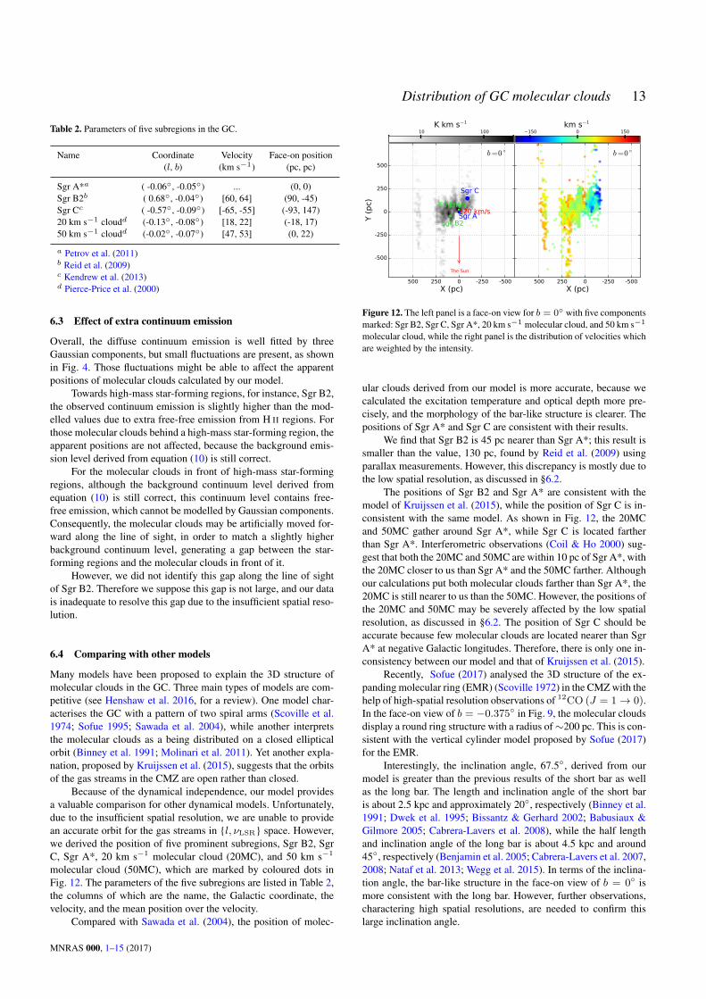
Because of the dynamical independence, our model providesa valuable comparison for other dynamical models. Unfortunately,due to the insufficient spatial resolution, we are unable to providean accurate orbit for the gas streams in {l, νLSR} space. However,we derived the position of five prominent subregions, Sgr B2, SgrC, Sgr A*, 20 km s−1 molecular cloud (20MC), and 50 km s−1

molecular cloud (50MC), which are marked by coloured dots inFig. 12. The parameters of the five subregions are listed in Table 2,the columns of which are the name, the Galactic coordinate, thevelocity, and the mean position over the velocity.

Compared with Sawada et al. (2004), the position of molec-

0

250

-250

500

-500

Y (p

c)

0250 -250500 -500X (pc)

The Sun

20 km/sSgr A ∗Sgr B2

50 km/s

Sgr C

b=0 ◦

0250 -250500 -500X (pc)

b=0 ◦

10 100K km s−1

−150 0 150km s−1

Figure 12. The left panel is a face-on view for b = 0◦ with five componentsmarked: Sgr B2, Sgr C, Sgr A*, 20 km s−1 molecular cloud, and 50 km s−1

molecular cloud, while the right panel is the distribution of velocities whichare weighted by the intensity.

ular clouds derived from our model is more accurate, because wecalculated the excitation temperature and optical depth more pre-cisely, and the morphology of the bar-like structure is clearer. Thepositions of Sgr A* and Sgr C are consistent with their results.

We find that Sgr B2 is 45 pc nearer than Sgr A*; this result issmaller than the value, 130 pc, found by Reid et al. (2009) usingparallax measurements. However, this discrepancy is mostly due tothe low spatial resolution, as discussed in §6.2.

The positions of Sgr B2 and Sgr A* are consistent with themodel of Kruijssen et al. (2015), while the position of Sgr C is in-consistent with the same model. As shown in Fig. 12, the 20MCand 50MC gather around Sgr A*, while Sgr C is located fartherthan Sgr A*. Interferometric observations (Coil & Ho 2000) sug-gest that both the 20MC and 50MC are within 10 pc of Sgr A*, withthe 20MC closer to us than Sgr A* and the 50MC farther. Althoughour calculations put both molecular clouds farther than Sgr A*, the20MC is still nearer to us than the 50MC. However, the positions ofthe 20MC and 50MC may be severely affected by the low spatialresolution, as discussed in §6.2. The position of Sgr C should beaccurate because few molecular clouds are located nearer than SgrA* at negative Galactic longitudes. Therefore, there is only one in-consistency between our model and that of Kruijssen et al. (2015).

Recently, Sofue (2017) analysed the 3D structure of the ex-panding molecular ring (EMR) (Scoville 1972) in the CMZ with thehelp of high-spatial resolution observations of 12CO (J = 1→ 0).In the face-on view of b = −0.375◦ in Fig. 9, the molecular cloudsdisplay a round ring structure with a radius of∼200 pc. This is con-sistent with the vertical cylinder model proposed by Sofue (2017)for the EMR.

Interestingly, the inclination angle, 67.5◦, derived from ourmodel is greater than the previous results of the short bar as wellas the long bar. The length and inclination angle of the short baris about 2.5 kpc and approximately 20◦, respectively (Binney et al.1991; Dwek et al. 1995; Bissantz & Gerhard 2002; Babusiaux &Gilmore 2005; Cabrera-Lavers et al. 2008), while the half lengthand inclination angle of the long bar is about 4.5 kpc and around45◦, respectively (Benjamin et al. 2005; Cabrera-Lavers et al. 2007,2008; Nataf et al. 2013; Wegg et al. 2015). In terms of the inclina-tion angle, the bar-like structure in the face-on view of b = 0◦ ismore consistent with the long bar. However, further observations,charactering high spatial resolutions, are needed to confirm thislarge inclination angle.

MNRAS 000, 1–15 (2017)

14 Q. Z. Yan et al.

6.5 Future improvements in our model

Obviously, our model hinges on the spatial resolution of the data.We already have interferometric OH data in hand, observed withthe Karl G. Jansky Very Large Array (JVLA), which possesses amuch higher spatial resolution than the Parkes data. Combiningthe 12CO (J = 1 → 0) and 13CO (J = 1 → 0) data ob-tained with Mopra and the OH data of the Galactic ASKAP (theAustralian Square Kilometre Array Pathfinder telescope) Survey(GASKAP) (Dickey et al. 2013), we will be able to improve ourresults significantly, which we intend to do in a future paper. Underthe scrutiny of high angular resolution (better than 2 pc at a distanceof 8.34 kpc), the blank area in front of Sgr A* will shrink and wewill be able to resolve the Brick, the 20MC, and the 50MC. Mostimportantly, the ring structure near Sgr A* will become clear.

7 CONCLUSIONS

We have presented a 3D model of the GC, which is independent ofdynamics, with the help of CO emission and OH absorption lines.We use 13CO (J = 1 → 0) data from Mopra to identify regionswhere 12CO (J = 1 → 0) emission may be optically thick. TheOH data, which are part of SPLASH, include four OH ground-statetransitions: 1612-, 1665-, 1667- and 1720-MHz lines. The angularresolution of OH and CO data is 15.5′, and with a distance of 8.34kpc to the GC, the corresponding physical resolution is about 38pc.

We developed a novel method to calculate the column densi-ties, excitation temperatures, and optical depths of the OH ground-state transitions precisely. For the regions where the level of contin-uum emission behind molecular clouds is observable, the four col-umn densities may be solved from the equations constructed fromobservations of four ground-state transitions. For the GC, where thetwo main lines contaminate each other and the background contin-uum level is unknown, we assume that the excitation temperatureof the two main lines are equal and the column densities of OH areproportional to the brightness temperature of CO, enabling us to de-rive the level of background continuum behind molecular clouds.

Based on a well modelled volume emission coefficient of thediffuse continuum emission in the GC, we derived the face-on viewfor b = -0.375◦, -0.25◦, -0.125◦, 0◦, 0.125◦, and 0.25◦, forming a3D structure of the molecular clouds. The face-on view of b = 0◦

displays a bar-like structure with an inclination angel of 67.5±2.1◦with respect to the line of sight along l = 0◦. This angle is generallygreater than the value derived by previous works. Due to the lowspatial resolution of the data, we are unable to resolve the structureof molecular clouds near Sgr A* where the continuum emissionvaries rapidly.

We found the amount of OH in the CMZ is at least 2400 M�and could be as much as 5100 M�.

ACKNOWLEDGEMENTS

We would like to thank Sam McSweeney for his helpful report.This work was partly sponsored by the 100 Talents Project ofthe Chinese Academy of Sciences, the National Science Founda-tion of China (Grants No. 11673066, 11673051, and 11233007),and the Natural Science Foundation of Shanghai under grant15ZR1446900.

REFERENCES

Ao Y., et al., 2013, A&A, 550, A135Babusiaux C., Gilmore G., 2005, MNRAS, 358, 1309Barrett A. H., 1964, IEEE Transactions on Military Electronics, 8, 156Benjamin R. A., et al., 2005, ApJ, 630, L149Binney J., Gerhard O. E., Stark A. A., Bally J., Uchida K. I., 1991, MNRAS,

252, 210Bissantz N., Gerhard O., 2002, MNRAS, 330, 591Bitran M., Alvarez H., Bronfman L., May J., Thaddeus P., 1997, AAPS, 125Blackwell R., 2017, In preparationBurton M. G., et al., 2013, PASA, 30, e044Cabrera-Lavers A., Hammersley P. L., González-Fernández C., López-

Corredoira M., Garzón F., Mahoney T. J., 2007, A&A, 465, 825Cabrera-Lavers A., González-Fernández C., Garzón F., Hammersley P. L.,

López-Corredoira M., 2008, A&A, 491, 781Calabretta M. R., Staveley-Smith L., Barnes D. G., 2014, Publ. Astron. Soc.

Australia, 31, e007Coil A. L., Ho P. T. P., 2000, ApJ, 533, 245Colgan S. W. J., Salpeter E. E., Terzian Y., 1989, ApJ, 336, 231Contopoulos G., Papayannopoulos T., 1980, A&A, 92, 33Corby J. F., et al., 2015, MNRAS, 452, 3969Crutcher R. M., 1977, ApJ, 216, 308Crutcher R. M., 1979, ApJ, 234, 881Dame T. M., Hartmann D., Thaddeus P., 2001, ApJ, 547, 792Dawson J. R., et al., 2014, MNRAS, 439, 1596Destombes J. L., Marliere C., Baudry A., Brillet J., 1977, A&A, 60, 55Dickey J. M., Crovisier J., Kazes I., 1981, A&A, 98, 271Dickey J. M., et al., 2013, Publ. Astron. Soc. Australia, 30, e003Dwek E., et al., 1995, ApJ, 445, 716Emerson D., 1996, Interpreting Astronomical Spectra. Wiley-VCHGinsburg A., et al., 2016, A&A, 586, A50Goicoechea J. R., et al., 2011, A&A, 530, L16Henshaw J. D., et al., 2016, MNRAS, 457, 2675Jones P. A., et al., 2012, MNRAS, 419, 2961Jones P. A., Burton M. G., Cunningham M. R., Tothill N. F. H., Walsh A. J.,

2013, MNRAS, 433, 221Kendrew S., Ginsburg A., Johnston K., Beuther H., Bally J., Cyganowski

C. J., Battersby C., 2013, ApJ, 775, L50Knapp G. R., Kerr F. J., 1973, AJ, 78, 453Kruijssen J. M. D., Longmore S. N., Elmegreen B. G., Murray N., Bally J.,

Testi L., Kennicutt R. C., 2014, MNRAS, 440, 3370Kruijssen J. M. D., Dale J. E., Longmore S. N., 2015, MNRAS, 447, 1059Law C. J., Yusef-Zadeh F., Cotton W. D., Maddalena R. J., 2008, ApJS,

177, 255Li D., Goldsmith P. F., 2003, ApJ, 585, 823Longmore S. N., et al., 2012, ApJ, 746, 117Longmore S. N., et al., 2013, MNRAS, 429, 987Lu X., Zhang Q., Kauffmann J., Pillai T., Longmore S. N., Kruijssen

J. M. D., Battersby C., Gu Q., 2015, ApJ, 814, L18Mills E. A. C., Morris M. R., 2013, ApJ, 772, 105Molinari S., et al., 2010, PASP, 122, 314Molinari S., et al., 2011, ApJ, 735, L33Morris M., Serabyn E., 1996, ARA&A, 34, 645Nataf D. M., et al., 2013, ApJ, 769, 88Oka T., Hasegawa T., Sato F., Tsuboi M., Miyazaki A., 1998, ApJS, 118,

455Oka T., Hasegawa T., Sato F., Tsuboi M., Miyazaki A., Sugimoto M., 2001,

ApJ, 562, 348Petrov L., Kovalev Y. Y., Fomalont E. B., Gordon D., 2011, AJ, 142, 35Pierce-Price D., et al., 2000, ApJ, 545, L121Platania P., Burigana C., Maino D., Caserini E., Bersanelli M., Cappellini

B., Mennella A., 2003, A&A, 410, 847Reid M. J., Menten K. M., Zheng X. W., Brunthaler A., Xu Y., 2009, ApJ,

705, 1548Reid M. J., et al., 2014, ApJ, 783, 130Rybicki G. B., Lightman A. P., 1986, Radiative Processes in Astrophysics.

Wiley-VCH

MNRAS 000, 1–15 (2017)

Distribution of GC molecular clouds 15

Sault R. J., Teuben P. J., Wright M. C. H., 1995, in Shaw R. A., PayneH. E., Hayes J. J. E., eds, Astronomical Society of the Pacific Confer-ence Series Vol. 77, Astronomical Data Analysis Software and SystemsIV. p. 433 (arXiv:astro-ph/0612759)

Sawada T., Hasegawa T., Handa T., Cohen R. J., 2004, MNRAS, 349, 1167Scoville N. Z., 1972, ApJ, 175, L127Scoville N. Z., Solomon P. M., Jefferts K. B., 1974, ApJ, 187, L63Shetty R., Beaumont C. N., Burton M. G., Kelly B. C., Klessen R. S., 2012,

MNRAS, 425, 720Sofue Y., 1995, PASJ, 47, 527Sofue Y., 2017, preprint, (arXiv:1706.00157)Walsh A. J., et al., 2011, MNRAS, 416, 1764Wegg C., Gerhard O., Portail M., 2015, MNRAS, 450, 4050Whiting M. T., 2012, MNRAS, 421, 3242Yan Q.-z., Xu Y., Zhang B., Lu D.-r., Chen X., Tang Z.-h., 2016, AJ, 152,

117Yusef-Zadeh F., et al., 2009, ApJ, 702, 178

This paper has been typeset from a TEX/LATEX file prepared by the author.

MNRAS 000, 1–15 (2017)