The General Linear Model A talk for dummies, by dummies

Meghan Morley and Anne Urai

Where are we headed?

•  A delicious analogy •  The General Linear Model equation

•  What do the variables mean? •  How does this relate to fMRI?

•  Minimizing error

Analogy: Reverse Cookery Start with finished product and try to explain how it is made... –  You specify which ingredients

to add (X) –  For each ingredient, GLM

finds the quantities (β) that produce the best reproduction

–  Then if you tried to make the cake with what you know about X and β then the error would be the difference between the original cake/data and yours! exxy ++= 2211 ββ

The General Linear Model

eXy += βThe General Linear Model Describes a response (y), such as the BOLD response in a voxel, in terms of all its contributing factors (xβ) in a linear combination, whilst also accounting for the contribution of error (e).

The General Linear Model

eXy += βDependent variable Describes a response (such as the BOLD response in a single voxel, taken from an fMRI scan)

The General Linear Model

eXy += βIndependent Variable aka. Predictor e.g. Experimental conditions (Embodies all available knowledge about experimentally controlled factors and potential confounds)

Parameters (aka regression coefficient/beta weights)

Quantifies how much each predictor (X) independently influences the dependent variable (Y) The slope of the line

The General Linear Model

eXy += β

X

Y

The General Linear Model

eXy += βError Variance in the data (y) which is not explained by the linear combination of predictors (x)

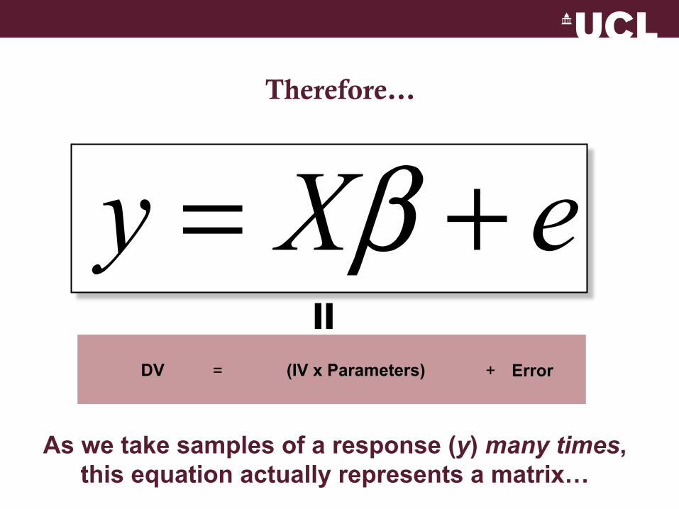
Therefore…

eXy += β(IV x Parameters) =

DV = + Error

As we take samples of a response (y) many times, this equation actually represents a matrix…

…the GLM matrix

= Single voxel

...over time

One response…

BOLD signal

Time

Each predictor (x) has an expected signal time course, which contributes to y

residuals fMRI signal

Time

Y: Observed Data

= +

Residual

+ 1 × 2 × 3 × +

X1 X2 X3

X: Predictors

Parameters (β)

•  Beta is the slope of the regression line   Quantifies a specific predictor’s (x) contribution to y.

  The parameter (β) chosen for a model should minimise the error (reducing the amount of variance in y which is left unexplained)

Y

X

The design matrix does not account for all of y

  If we plot our observations (n) on a graph these will not fall in a straight line

  This is a result of uncontrolled influences (other than x) on y

  This contribution to y is called the error

(or residual)

  Minimising the difference between the response predicted by the model (y) and the actual response (y) minimises the error of the model

Y

^

Generation Shadowing Baseline

Measured

X1 X2 X3

”Known”

≈

We have our set of hypothetical time-series: x1, x2, x3....

....and our data

We find the best parameter values by modelling...

...the best parameter will miminise the error in the model

Generation Shadowing Baseline

4 3 2

≈

1 0 2 1 0 1 0

+ β3*

”Unknown” parameters

+ β2* β1*

Generation Shadowing Baseline

≈ + β3*

Here, there is a lot of residual variance in y which is unexplained by the model (error)

4 3 2 1 0

β1*

Not brilliant

2 1 0

0 0 3

1 0

+ β2*

Generation Shadowing Baseline

+ β3*

1 0

β1*

2 1 0

1 0 4

1 0

+ β2*

Still not great

4 3 2

≈

...and the same goes here

Generation Shadowing Baseline

≈

4 3 2

≈ + β2* + β1*

1 0

β0* + β3*

1 0

β1*

1 0

+ β2*

2 1 0

0.83 0.16 2.98

...but here we have a good fit, with minimal error

Generation Shadowing Baseline

+ β2* + β1* β3* ≈ ≈

3 2 1

In other words:

≈ + β2* + β1*

1 0

β0* + β3*

1 0

β1*

1 0

+ β2*

2 1 0

0.68 0.82 2.17

...and the same model can fit different data – just use different parameters

Generation Shadowing Baseline

+ β2* + β1* β0* ≈ ≈ ≈

3 2 1

Doesn’t care:

≈ + β2* + β1*

1 0

β0* + β3*

1 0

β1*

1 0

+ β2*

2 1 0

0.03 0.06 2.04

...as you can see

Different data (y)

Different parameters ()

The same predictors (x)

⎥⎥⎥

⎦

⎤

⎢⎢⎢

⎣

⎡=

98.216.083.0

β

beta_0001.img

beta_0002.img

⎥⎥⎥

⎦

⎤

⎢⎢⎢

⎣

⎡=

04.206.003.0

β

⎥⎥⎥

⎦

⎤

⎢⎢⎢

⎣

⎡=

17.282.068.0

β

beta_0003.img

So the same model can be used across all voxels of the brain, just using different paramteres

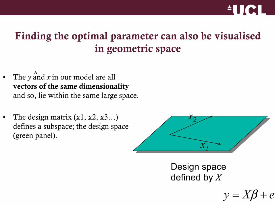
•  The y and x in our model are all vectors of the same dimensionality and so, lie within the same large space.

•  The design matrix (x1, x2, x3…) defines a subspace; the design space (green panel).

eXy += β

Finding the optimal parameter can also be visualised in geometric space

Design space defined by X

x1

x2

^

Parameters determine the co-ordinates of the predicted response (y) within this space

•  The actual data (y) however, lie outside this space.

•  So there is always a difference between the predicted y and actual y

y

x1

x2 ˆ y ^

^

•  So the GLM aims find the projection of y on the design space which minimises the error of the model

(minimises the difference between predicted y and actual y)

We need to minimise the difference between predicted y and actual y

y

e (minimise)

x1

x2 ˆ y ^

^

^

…So the best parameter will position y so that the error vector between y and y is orthogonal to the design space (minimising the error)

The smallest error vector is orthogonal to the design space…

y

e

x1

x2 ˆ y

^ ^

How do we find the parameter which produces minimal error?

The optimal parameter can be calculated using

Ordinary Least Squares

yXXX TT 1)(ˆ −=βA statistical method for estimating unknown parameters from sampled data

- minimizing the difference between predicted data and observed data.

å =

N

t t e

1

2 = minimum

Overview of SPM

Realignment Smoothing

Normalisation

General linear model

Image time-series

Parameter estimates

Design matrix

Template

Kernel

Gaussian field theory

p <0.05

Statistical inference

fMRI data Single voxel analyzed across many different time points

Y = BOLD signal at each time point from that voxel

BOLD signal

Time

An fMRI experiment

Is there a change in the BOLD response between the two conditions?

Applying the GLM

exxy ++= 2211 ββ

BOLD response at each time point at chosen voxel

Predictors that explain the data

How much each predictor explains the data (Coefficient)

Variance in the data that cannot be explained by the predictors (noise)

β = 0.44

Statistical Parametric Mapping •  Null

hypothesis: your effect of interest explains none of your data.

•  Is the task significally different? Statistical Inference

eg. P<0.05

Problems

1.  BOLD signal is not a simple on/off 2.  Low-frequency noise 3.  Assumptions about the nature of the error 4.  Physiological confounds

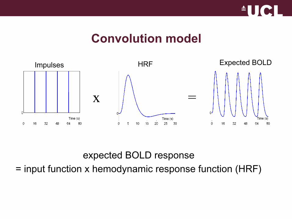
expected BOLD response = input function x hemodynamic response function (HRF)

x =

Impulses HRF Expected BOLD

Convolution model

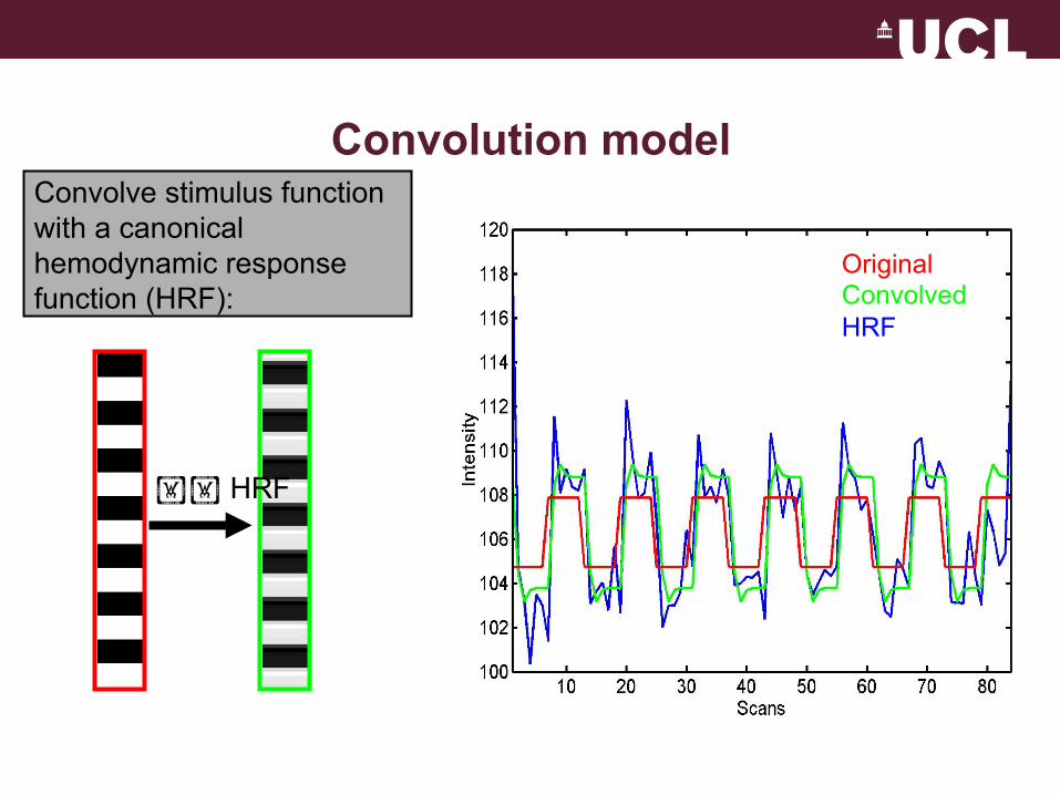
Convolve stimulus function with a canonical hemodynamic response function (HRF):

HRF

Original Convolved HRF

Convolution model

discrete cosine transform (DCT)

set

Adjusting for low frequencies

Adjusting for low frequencies

Blue = data Black = mean + low-frequency drift Green = predicted response, taking into account low-frequency drift red = predicted response, NOT taking into account low-frequency drift

GLM Assumptions

1. Errors are normally distributed - smoothing

2. Error is the same in each & every measurement point

3. There is no correlation between errors at different time points/data points

x

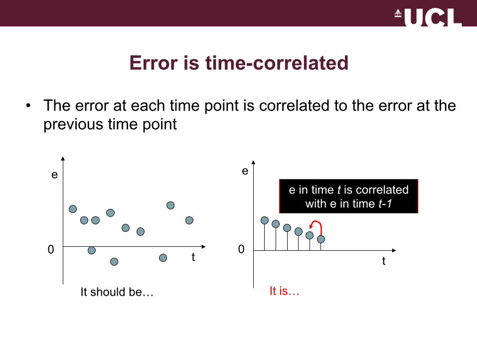
Error is time-correlated

•  The error at each time point is correlated to the error at the previous time point

0

It is…

t

e e in time t is correlated

with e in time t-1

It should be…

0 t

e

Autoregressive Model

•  Temporal autocorrelation: in y = Xβ + e over time et = aet-1 + ε

•  ‘Whitening’

•  To compensate for inflated t-value

Physiological Confounds

•  head movements

•  arterial pulsations

•  breathing

•  eye blinks (visual cortex)

•  adaptation affects, fatigue, changes in attention to task

(Predictors x Parameters...)

To recap...

exxy ++= 2211 ββ=

Response = + Error

Thanks to...

•  Previous years MfD slides (2009-2010)

•  Dr. Guillaume Flandin