the generalized distributive law - information...

IEEE TRANSACTIONS ON INFORMATION THEORY, VOL. 46, NO. 2, MARCH 2000 325

The Generalized Distributive LawSrinivas M. Aji and Robert J. McEliece, Fellow, IEEE

Abstract—In this semitutorial paper we discuss a generalmessage passing algorithm, which we call the generalized dis-tributive law (GDL). The GDL is a synthesis of the work of manyauthors in the information theory, digital communications, signalprocessing, statistics, and artificial intelligence communities. Itincludes as special cases the Baum–Welch algorithm, the fastFourier transform (FFT) on any finite Abelian group, the Gal-lager–Tanner–Wiberg decoding algorithm, Viterbi’s algorithm,the BCJR algorithm, Pearl’s “belief propagation” algorithm, theShafer–Shenoy probability propagation algorithm, and the turbodecoding algorithm. Although this algorithm is guaranteed to giveexact answers only in certain cases (the “junction tree” condition),unfortunately not including the cases of GTW with cycles orturbo decoding, there is much experimental evidence, and a fewtheorems, suggesting that it often works approximately even whenit is not supposed to.

Index Terms—Belief propagation, distributive law, graphicalmodels, junction trees, turbo codes.

I. INTRODUCTION

T HE humble distributive law, in its simplest form, states that. The left side of this equation involves

three arithmetic operations (one addition and two multiplica-tions), whereas the right side needs only two. Thus the distribu-tive law gives us a “fast algorithm” for computing . Theobject of this paper is to demonstrate that the distributive lawcan be vastly generalized, and that this generalization leads toa large family of fast algorithms, including Viterbi’s algorithmand the fast Fourier transform (FFT).To give a better idea of thepotential power of the distributive law and to introduce the view-point we shall take in this paper, we offer the following example.

Example 1.1:Let and be givenreal-valued functions, where, , , and are variables takingvalues in a finite set with elements. Suppose we are giventhe task of computing tables of the values of and ,defined as follows:

(1.1)

(1.2)

Manuscript received July 8, 1998; revised September 23, 1999. This workwas supported by NSF under Grant NCR-9505975, AFOSR under Grant5F49620-97-1-0313, and a Grant from Qualcomm. A portion of McEliece’scontribution was performed at the Sony Corporation in Tokyo, Japan, while hewas a holder of a Sony Sabbatical Chair. Preliminary versions of this paperwere presented at the IEEE International Symposium on Information Theory,Ulm, Germany, June 1997, and at ISCTA 1997, Ambleside U.K., July 1997.

The authors are with the Department of Electrical Engineering, CaliforniaInstitute of Technology, Pasadena, CA 91125 USA (e-mail: {mas; rjm}@sys-tems.caltech.edu).

Communicated by F. R. Kschischang, Associate Editor for Coding Theory.Publisher Item Identifier S 0018-9448(00)01679-5.

(We summarize (1.1) by saying that is obtained by“marginalizing out” the variables and from the function

. Similarly, is obtained by marginalizingout , , and from the same function.) How many arithmeticoperations (additions and multiplications) are required for thistask? If we proceed in the obvious way, we notice that for eachof the values of there are terms in the sum defining

, each term requiring one addition and one multiplica-tion, so that the total number of arithmetic operations requiredfor the computation of is . Similarly, computing

requires operations, so computing both andusing the direct method requires operations.

On the other hand, because of the distributive law, the sum in(1.1) factors

(1.3)

Using this fact, we can simplify the computation of .First we compute tables of the functions anddefined by

(1.4)

which requires a total of additions. Then we computethe values of using the formula (cf. (1.3))

(1.5)

which requires multiplications. Thus by exploiting the dis-tributive law, we can reduce the total number of operations re-quired to compute from to . Similarly, thedistributive law tells us that (1.2) can be written as

(1.6)

where is as defined in (1.4). Thus if we precompute atable of the values of ( operations), and then use (1.6)( further operations), we only need operations (ascompared to for the direct method) to compute the valuesof .

Finally, we observe that to computeboth andusing the simplifications afforded by (1.3) and (1.6), we onlyneed to compute once, which means that we can compute

0018–9448/00$10.00 © 2000 IEEE

326 IEEE TRANSACTIONS ON INFORMATION THEORY, VOL. 46, NO. 2, MARCH 2000

the values of and with a total of onlyoperations, as compared to for the direct method.

The simplification in Example 1.1 was easy to accomplish,and the gains were relatively modest. In more complicatedcases, it can be much harder to see the best way to reorganizethe calculations, but the computational savings can be dramatic.It is the object of this paper to show that problems of the typedescribed in Example 1.1 have a wide range of applicability,and to describe a general procedure, which we called thegen-eralized distributive law(GDL), for solving them efficiently.Roughly speaking, the GDL accomplishes its goal by passingmessages in a communications network whose underlyinggraph is a tree.

Important special cases of the GDL have appeared manytimes previously. In this paper, for example, we will demon-strate that the GDL includes as special cases the fast Hadamardtransform, Viterbi’s algorithm, the BCJR algorithm, theGallager–Tanner–Wiberg decoding algorithm (when the under-lying graph is cycle-free), and certain “probability propagation”algorithms known in the artificial intelligence community.With a little more work, we could have added the FFT on anyfinite Abelian group, the Baum–Welch “forward-backward”algorithm, and discrete-state Kalman filtering. Although thispaper contains relatively little that is essentially new (forexample, the 1990 paper of Shafer and Shenoy [33] describesan algorithm similar to the one we present in Section III), webelieve it is worthwhile to present a simply stated algorithmof such wide applicability, which gives a unified treatment ofa great many algorithms whose relationship to each other wasnot fully understood, if sensed at all.

Here is an outline of the paper. In Section II, we will state ageneral computational problem we call the MPF (“marginalizea product function”) problem, and show by example thata number of classical problems are instances of it. Theseproblems include computing the discrete Hadamard transform,maximum-likelihood decoding of a linear code over a memo-ryless channel, probabilistic inference in Bayesian networks,a “probabilistic state machine” problem, and matrix chainmultiplication. In Section III, we shall give an exact algorithmfor solving the MPF problem (the GDL) which often givesan efficient solution to the MPF problem. In Section IV wewill discuss the problem of finding junction trees (the formalname for the GDL’s communication network), and “solve”the example instances of the MPF problem given in SectionII, thereby deriving, among other things, the fast Hadamardtransform and Viterbi’s algorithm. In Section V we will discussthe computational complexity of the GDL. (A proof of thecorrectness of the GDL is given in the Appendix.)

In Section VI, we give a brief history of the GDL. Finally,in Section VII, we speculate on the possible existence of anefficient class of approximate, iterative, algorithms for solvingthe MPF problem, obtained by allowing the communication net-work to have cycles. This speculation is based partly on the factthat two experimentally successful decoding algorithms, viz.,the GTW algorithm for low-density parity-check codes, and theturbo decoding algorithm, can be viewed as an application ofthe GDL methodology on networks with cycles, and partly on

some recent theoretical work on GDL-like algorithms on graphswith a single cycle.

Although this paper is semitutorial, it contains a number ofthings which have not appeared previously. Beside the gener-ality of our exposition, these include:

• A de-emphasis ofa priori graphical models, and an em-phasis on algorithms to construct graphical models to fitthe given problem.

• A number of nonprobabilistic applications, including theFFT.

• A careful discussion of message scheduling, and a proofof the correctness of a large class of possible schedules.

• A precise measure of the computational complexity of theGDL.

Finally, we note that while this paper was being written,Kschischang, Frey, and Loeliger [41] were simultaneouslyand independently working out a similar synthesis. And whilethe final forms of the two papers have turned out to be quitedifferent, anyone interested in the results of this paper shouldhave a look at the alternative formulation in [41].

II. THE MPF PROBLEM

The GDL can greatly reduce the number of additions andmultiplications required in a certain class of computationalproblems. It turns out that much of the power of the GDL isdue to the fact that it applies to situations in which the notionsof addition and multiplication are themselves generalized. Theappropriate framework for this generalization is the commuta-tive semiring.

Definition: A commutative semiringis a set , together withtwo binary operations called “” and “ ”, which satisfy the fol-lowing three axioms:

S1. The operation “ ” is associative and commutative, andthere is an additive identity element called “” such that

for all . (This axiom makesa commutative monoid.)

S2. The operation “” is also associative and commutative,and there is a multiplicative identity element called “”such that for all . (Thus is alsoa commutative monoid.)

S3. Thedistributive lawholds, i.e.,

for all triples from .

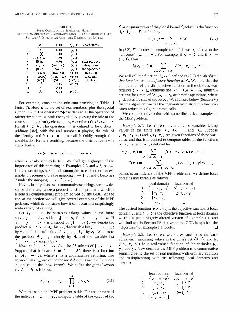
The difference between a semiring and a ring is that in asemiring, additive inverses need not exist, i.e., is onlyrequired to be a monoid, not a group. Thus every commutativering is automatically a commutative semiring. For example, theset of real or complex numbers, with ordinary addition and mul-tiplication, forms a commutative semiring. Similarly, the set ofpolynomials in one or more indeterminates over any commu-tative ring forms a commutative semiring. However, there aremany other commutative semirings, some of which are summa-rized in Table I. (In semirings 4–8, the set is an interval ofreal numbers with the possible addition of .)

AJI AND MCELIECE: THE GENERALIZED DISTRIBUTIVE LAW 327

TABLE ISOME COMMUTATIVE SEMIRINGS. HERE A

DENOTES ANARBITRARY COMMUTATIVE RING, S IS AN ARBITRARY FINITE

SET, AND � DENOTES ANARBITRARY DISTRIBUTIVE LATTICE

For example, consider the min-sum semiring in Table I(entry 7). Here is the set of real numbers, plus the specialsymbol “ .” The operation “ ” is defined as the operation oftaking the minimum, with the symbol playing the role of thecorresponding identity element, i.e., we definefor all . The operation “” is defined to beordinaryaddition [sic], with the real number playing the role ofthe identity, and for all . Oddly enough, thiscombination forms a semiring, because the distributive law isequivalent to

which is easily seen to be true. We shall get a glimpse of theimportance of this semiring in Examples 2.3 and 4.3, below.(In fact, semirings 5–8 are all isomorphic to each other; for ex-ample, 5 becomes 6 via the mapping , and 6 becomes7 under the mapping .)

Having briefly discussed commutative semirings, we now de-scribe the “marginalize a product function” problem, which isa general computational problem solved by the GDL. At theend of the section we will give several examples of the MPFproblem, which demonstrate how it can occur in a surprisinglywide variety of settings.

Let be variables taking values in the finitesets , with for . If

is a subset of , we denote theproduct by , the variable listby , and the cardinality of , i.e., , by . We denotethe product simply by , and the variable list

simply by .Now let be subsets of .

Suppose that for each , there is a function, where is a commutative semiring. The

variable lists are called thelocal domainsand the functionsare called thelocal kernels. We define theglobal kernel

as follows:

(2.1)

With this setup, the MPF problem is this: For one or more ofthe indices , compute a table of the values of the

-marginalizationof the global kernel , which is the function, defined by

(2.2)

In (2.2), denotes the complement of the setrelative to the“universe” . For example, if , and if

, then

We will call the function defined in (2.2) theth objec-tive function, or theobjective functionat . We note that thecomputation of theth objective function in the obvious wayrequires additions and multipli-cations, for a total of arithmetic operations, where

denotes the size of the set. We shall see below (Section V)that the algorithm we call the “generalized distributive law” canoften reduce this figure dramatically.

We conclude this section with some illustrative examples ofthe MPF problem.

Example 2.1:Let , , , and be variables takingvalues in the finite sets , , , and . Suppose

and are given functions of these vari-ables, and that it is desired to compute tables of the functions

and defined by

ptThis is an instance of the MPF problem, if we define localdomains and kernels as follows:

local domain local kernel

The desired function is the objective function at localdomain , and is the objective function at local domain. This is just a slightly altered version of Example 1.1, and

we shall see in Section IV that when the GDL is applied, the“algorithm” of Example 1.1 results.

Example 2.2:Let , , , , , and be six vari-ables, each assuming values in the binary set , and let

be a real-valued function of the variables,, and . Now consider the MPF problem (the commutative

semiring being the set of real numbers with ordinary additionand multiplication) with the following local domains andkernels:



Here the global kernel, i.e., the product of the local kernels, is

and the objective function at the local domain is

which is the Hadamard transformof the original function[17]. Thus the problem of computing the Hada-

mard transform is a special case of the MPF problem. (Astraightforward generalization of this example shows that theproblem of computing the Fourier transform over any finiteAbelian group is also a special case of the MPF problem. Whilethe kernel for the Hadamard transform is of diagonal form, ingeneral, the kernel will only be lower triangular. See [1, Ch.3] for the details.) We shall see below in Example 4.2 that theGDL algorithm, when applied to this set of local domains andkernels, yields thefastHadamard transform.

Example 2.3: (Wiberg [39]). Consider the binarylinear code defined by the parity-check matrix

Suppose that an unknown codeword from thiscode is transmitted over a discrete memoryless channel, and thatthe vector is received. The “likelihood” of aparticular codeword is then

(2.3)

where the ’s are the transition probabilities of thechannel. Themaximum-likelihood decoding problemis thatof finding the codeword that maximizes the expression in(2.3). Now consider the MPF problem with the followingdomains and kernels, using the min-sum semiring (semiringfrom Table I). There is one local domain for each codewordcoordinate and one for each row of the parity-check matrix.


......

Here is a function that indicates whether a given paritycheck is satisfied, or not. For example, at the local domain

, which corresponds to the first row of theparity-check matrix, we have

ifif

Fig. 1. The Bayesian network in Example 2.4.

The global kernel is then

ifis a codeword

ifis not a codeword.

Thus the objective function at the local domain is

all codewords for which

It follows that the value of for which is smallest isthe value of theth component of a maximum-likelihood code-word, i.e., a codeword for which islargest. A straightforward extension of this example shows thatthe problem of maximum-likelihood decoding of an arbitrarylinear block code is a special case of the MPF problem. We shallsee in Example 4.3 that when the GDL is applied to problemsof this type, the Gallager–Tanner–Wiberg decoding algorithmresults.

Example 2.4:Consider the directed acylic graph (DAG)inFig. 1.1 In a DAG, the “parents” of a vertex, denoted , arethose vertices (if any) which lie immediately “above”. Thus inFig. 1, , and . Let us associate arandom variable with each of the vertices, and assume that eachrandom variable is dependent only on its “parents,” i.e., the jointdensity function factors as follows:

1This example is taken from [29], in whichB stands for burglary,E is forearthquake,A is for alarm sound,R is for radio report, andW is for Watson’scall.


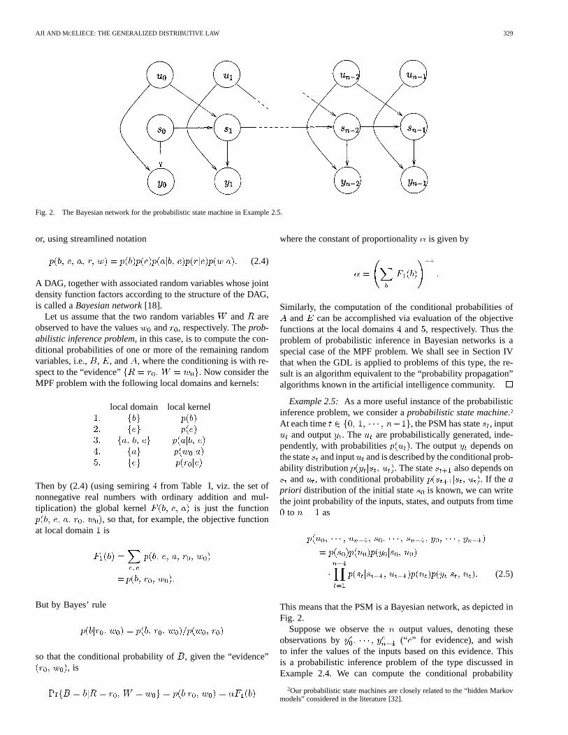
Fig. 2. The Bayesian network for the probabilistic state machine in Example 2.5.

or, using streamlined notation

(2.4)

A DAG, together with associated random variables whose jointdensity function factors according to the structure of the DAG,is called aBayesian network[18].

Let us assume that the two random variablesand areobserved to have the values and , respectively. Theprob-abilistic inference problem, in this case, is to compute the con-ditional probabilities of one or more of the remaining randomvariables, i.e., , , and , where the conditioning is with re-spect to the “evidence” . Now consider theMPF problem with the following local domains and kernels:


Then by (2.4) (using semiring from Table I, viz. the set ofnonnegative real numbers with ordinary addition and mul-tiplication) the global kernel is just the function

, so that, for example, the objective functionat local domain is

But by Bayes’ rule

so that the conditional probability of , given the “evidence”, is

where the constant of proportionalityis given by

Similarly, the computation of the conditional probabilities ofand can be accomplished via evaluation of the objective

functions at the local domainsand , respectively. Thus theproblem of probabilistic inference in Bayesian networks is aspecial case of the MPF problem. We shall see in Section IVthat when the GDL is applied to problems of this type, the re-sult is an algorithm equivalent to the “probability propagation”algorithms known in the artificial intelligence community.

Example 2.5:As a more useful instance of the probabilisticinference problem, we consider aprobabilistic state machine.2

At each time , the PSM has state, inputand output . The are probabilistically generated, inde-

pendently, with probabilities . The output depends onthe state and input and is described by the conditional prob-ability distribution . The state also depends on

and , with conditional probability . If the apriori distribution of the initial state is known, we can writethe joint probability of the inputs, states, and outputs from time

to as

(2.5)

This means that the PSM is a Bayesian network, as depicted inFig. 2.

Suppose we observe the output values, denoting theseobservations by (“ ” for evidence), and wishto infer the values of the inputs based on this evidence. Thisis a probabilistic inference problem of the type discussed inExample 2.4. We can compute the conditional probability

2Our probabilistic state machines are closely related to the “hidden Markovmodels” considered in the literature [32].


by taking the joint probability in(2.5) with the observed values of and marginalizing out allthe ’s and all but one of the ’s. This is an instance of theMPF problem, with the following local domains and kernels(illustrated for ):


This model includes, as a special case, convolutionalcodes, as follows. The state transition is deterministic, whichmeans that whenand otherwise. Assuming a memorylesschannel, the output is probabilistically dependent on ,which is a deterministic function of the state and input, and so

. Marginalizing the product offunctions in (2.5) in the sum-product and max-product semir-ings will then give us the maximum-likelihood inputsymbolsorinputblock, respectively. As we shall see below (Example 4.5),when the GDL is applied here, we get algorithms equivalent tothe BCJR and Viterbi decoding algorithms.3

Example 2.6:Let be a matrix with entries ina commutative semiring, for . We denote the en-tries in by , where for , is avariable taking values in a set with elements. Suppose wewant to compute the product

Then for we have by definition

(2.6)

and an easy induction argument gives the generalization

(2.7)(Note that (2.7) suggests that the number of arithmetic opera-tions required to multiply thesematrices is .) Thus

3To obtain an algorithm equivalent to Viterbi’s, it is necessary to take the neg-ative logarithm of (2.5) before performing the marginalization in the min-sumsemiring.

Fig. 3. The trellis corresponding to the multiplication of three matrices, ofsizes2 � 3, 3 � 3, and3 � 2. The(i; j)th entry in the matrix product is thesum of the weights of all paths froma to b .

multiplying matrices can be formulated as the following MPFproblem:


...

the desired result being the objective function at local domain.

As an alternative interpretation of (2.7), consider a trellis ofdepth , with vertex set , and an edge of weight

connecting the vertices and .If we define the weight of a path as the sum of the weights ofthe component edges, then as defined in (2.7) rep-resents the sum of the weights of all paths fromto . Forexample, Fig. 3 shows the trellis corresponding to the multipli-cation of three matrices, of sizes , , and . If thecomputation is done in the min-sum semiring, the interpretationis that is the weight of a minimum-weight path from

to .We shall see in Section IV that if the GDL is applied to the

matrix multiplication problem, a number of different algorithmsresult, corresponding to the different ways of parenthesizing theexpression . If the parenthesization is

(illustrated for ), and the computation is in the min-sumsemiring, Viterbi’s algorithm results.

III. T HE GDL: AN ALGORITHM FOR SOLVING THE MPFPROBLEM

If the elements of stand in a certain special relationshipto each other, then an algorithm for solving the MPF problemcan be based on the notion of “message passing.” The requiredrelationship is that the local domains can be organized into ajunction tree[18]. What this means is that the elements of


Fig. 4. A junction tree.

can be attached as labels to the vertices of a graph-theoretic tree, such that for any two vertices and , the intersection of

the corresponding labels, viz. , is a subset of the label oneach vertex on the unique path fromto . Alternatively, thesubgraph of consisting of those vertices whose label includesthe element, together with the edges connecting these vertices,is connected, for .

For example, consider the following five local domains:

local domain

These local domains can be organized into a junction tree, asshown in Fig. 4. For example, the unique path from vertextovertex is , and , as required.

On the other hand, the following set of four local domainscannot be organized into a junction tree, as can be easily veri-fied.

local domain

However, by adjoining two “dummy domains”

local domain

to the collection, we can devise a junction tree, as shown inFig. 5.

(In Section IV, we give a simple algorithm for decidingwhether or not a given set of local domains can be organizedinto a junction tree, for constructing one if it does exist, and forfinding appropriate dummy domains if it does not.)

In the “junction tree” algorithm, which is what we call thegeneralized distributive law(GDL), if and are connectedby an edge (indicated by the notation ), the (directed)“message” from to is a table containing the values of afunction . Initially, all such functions are de-fined to be identically (the semiring’s multiplicative identity);

Fig. 5. A junction tree which includes the local domainsfx ; x g,fx ; x g,fx ; x g, andfx ; x g.

and when a particular message is updated, the followingrule is used:

(3.1)A good way to remember (3.1) is to think of the junction treeas a communication network, in which an edge fromtois a transmission line that “filters out” dependence on all vari-ables but those common to and . (The filtering is done bymarginalization.) When the vertex wishes to send a messageto , it forms the product of its local kernel with all messages ithas received from its neighbors other than, and transmits theproduct to over the transmission line.

Similarly, the “state” of a vertex is defined to be a tablecontaining the values of a function . Initially,is defined to be the local kernel , but when is updated,the following rule is used:

(3.2)

In words, the state of a vertex is the product of its local kernelwith each of the messages it has received from its neighbors. Thebasic idea is that after sufficiently many messages have beenpassed, will be the objective function at , as definedin (2.2).

The question remains as to the scheduling of the messagepassing and the state computation. Here we consider only twospecial cases, thesingle-vertexproblem, in which the goal is tocompute the objective function at only one vertex, and theall-verticesproblem, where the goal is to compute the objectivefunction at all vertices.4

For the single-vertex problem, the natural (serial) sched-uling of the GDL begins by directing each edge toward the

4We do not consider the problem of evaluating the objective function atk ver-tices, where1 < k < M . However, as we will see in Section V, the complexityof theM -vertex GDL is at most four times as large as the1-vertex GDL, so it isreasonably efficient to solve thek-vertex problem using theM -vertex solution.


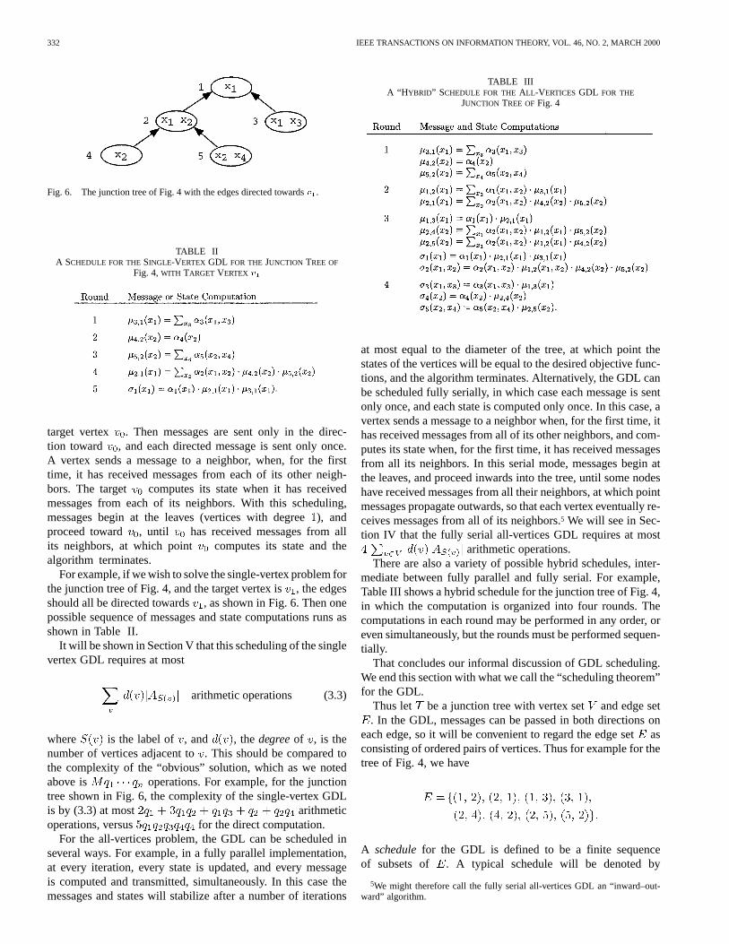
Fig. 6. The junction tree of Fig. 4 with the edges directed towardsv .

TABLE IIA SCHEDULE FOR THESINGLE-VERTEX GDL FOR THEJUNCTION TREE OF

Fig. 4,WITH TARGET VERTEX v

target vertex . Then messages are sent only in the direc-tion toward , and each directed message is sent only once.A vertex sends a message to a neighbor, when, for the firsttime, it has received messages from each of its other neigh-bors. The target computes its state when it has receivedmessages from each of its neighbors. With this scheduling,messages begin at the leaves (vertices with degree), andproceed toward , until has received messages from allits neighbors, at which point computes its state and thealgorithm terminates.

For example, if we wish to solve the single-vertex problem forthe junction tree of Fig. 4, and the target vertex is, the edgesshould all be directed towards, as shown in Fig. 6. Then onepossible sequence of messages and state computations runs asshown in Table II.

It will be shown in Section V that this scheduling of the singlevertex GDL requires at most

arithmetic operations (3.3)

where is the label of , and , thedegreeof , is thenumber of vertices adjacent to. This should be compared tothe complexity of the “obvious” solution, which as we notedabove is operations. For example, for the junctiontree shown in Fig. 6, the complexity of the single-vertex GDLis by (3.3) at most arithmeticoperations, versus for the direct computation.

For the all-vertices problem, the GDL can be scheduled inseveral ways. For example, in a fully parallel implementation,at every iteration, every state is updated, and every messageis computed and transmitted, simultaneously. In this case themessages and states will stabilize after a number of iterations

TABLE IIIA “H YBRID” SCHEDULE FOR THEALL-VERTICESGDL FOR THE

JUNCTION TREE OFFig. 4

at most equal to the diameter of the tree, at which point thestates of the vertices will be equal to the desired objective func-tions, and the algorithm terminates. Alternatively, the GDL canbe scheduled fully serially, in which case each message is sentonly once, and each state is computed only once. In this case, avertex sends a message to a neighbor when, for the first time, ithas received messages from all of its other neighbors, and com-putes its state when, for the first time, it has received messagesfrom all its neighbors. In this serial mode, messages begin atthe leaves, and proceed inwards into the tree, until some nodeshave received messages from all their neighbors, at which pointmessages propagate outwards, so that each vertex eventually re-ceives messages from all of its neighbors.5 We will see in Sec-tion IV that the fully serial all-vertices GDL requires at most

arithmetic operations.There are also a variety of possible hybrid schedules, inter-

mediate between fully parallel and fully serial. For example,Table III shows a hybrid schedule for the junction tree of Fig. 4,in which the computation is organized into four rounds. Thecomputations in each round may be performed in any order, oreven simultaneously, but the rounds must be performed sequen-tially.

That concludes our informal discussion of GDL scheduling.We end this section with what we call the “scheduling theorem”for the GDL.

Thus let be a junction tree with vertex set and edge set. In the GDL, messages can be passed in both directions on

each edge, so it will be convenient to regard the edge setasconsisting of ordered pairs of vertices. Thus for example for thetree of Fig. 4, we have

A schedulefor the GDL is defined to be a finite sequenceof subsets of . A typical schedule will be denoted by

5We might therefore call the fully serial all-vertices GDL an “inward–out-ward” algorithm.


Fig. 7. The message trellis for the junction tree in Fig. 4 under the scheduleof Table II viz.,E = f(3; 1)g, E = f(4; 2)g, E = f(5; 2)g, E =f(2; 1)g.

. The idea is that is the set of mes-sages that are updated during theth round of the algorithm. InTables II and III, for example, the corresponding schedules are

Table II

Table III

Given a schedule , the correspondingmessage trellisis a finite directed graph with vertex set

, in which a typical element is denoted by ,for . The only allowed edges are of the form

; and is an edge in the mes-sage trellis if either or . The message trellisesfor the junction tree of Fig. 4, under the schedules of Tables IIand III, are shown in Figs. 7 and 8, respectively. (In these fig-ures, the shaded boxes indicate which local kernels are knownto which vertices at any time. For example, in Fig. 7, we can seethat knowledge of the local kernels , , and has reached

at time . We will elaborate on this notion of “knowl-edge” in the Appendix.)

Theorem 3.1 (GDL Scheduling):After the completion of themessage passing described by the schedule

the state at vertex will be the th objective as defined in (3.2)if and only if there is a path from to in the corre-sponding message trellis, for .

A proof of Theorem 3.1 will be found in the Appendix, butFigs. 7 and 8 illustrate the idea. For example, in Fig. 8, we seethat there is a path from each of to ,which means (by the scheduling theorem) that after two roundsof message passing, the state atwill be the desired objectivefunction. This is why, in Table III, we are able to computein round 3. Theorem 3.1 immediately implies the correctness of

Fig. 8. The message trellis for the junction tree in Fig. 4, under the scheduleof Table III, viz.,E = f(3; 1); (4; 2); (5; 2)g,E = f(1; 2); (2; 1)g, andE = f(1; 3); (2; 4); (2; 5)g.

Fig. 9. (a) The local domain graph and (b) one junction tree for the localdomains and kernels in Example 2.1.

the single-vertex and all-vertices serial GDL described earlierin this section.

IV. CONSTRUCTINGJUNCTION TREES

In Section III we showed that if we can construct a junctiontree with the local domains as vertex labels, we can devise amessage-passing algorithm to solve the MPF problem. But doessuch a junction tree exist? And if not, what can be done? In thissection we will answer these questions.

It is easy to decide whether or not a junction tree exists. Thekey is thelocal domain graph , which is a weighted com-


Fig. 10. Constructing a junction tree for the local domainsf1; 2g, f2; 3g, f3; 4g, andf4; 1g by triangulating the moral graph.

plete graph with vertices , one for each local do-main, with the weight of the edge defined by

If , we will say that is contained in . Denoteby the weight of a maximal-weight spanning tree of .6

Finally, define

Theorem 4.1: , with equality if and only if thereis a junction tree. If , then any maximal-weightspanning tree of is a junction tree.

Proof: For each , denote by the numberof sets which contain the variable . Note that

Let be any spanning tree of , and let denote thenumber of edges in which contain . Clearly

Furthermore, , since the subgraph of inducedby the vertices containing has no cycles, and equality holdsif and only if is connected, i.e., a tree. It follows then that

with equality if and only if each subgraph is connected, i.e.,if is a junction tree.

Example 4.1:Here we continue Example 2.1. The LD graphis shown in Fig. 9(a). Here .A maximal weight spanning tree is shown in Fig. 9(b), and itsweight is , so by Theorem 4.1, this is a junction tree, a fact

6A maximal-weight spanning tree can easily be found with Prim’s “greedy”algorithm [27, Ch. 3], [9, Sec. 24.2]. In brief, Prim’s algorithm works bygrowing the tree one edge at a time, always choosing a new edge of maximalweight.

that can easily be checked directly. If we apply the GDL to thisjunction tree, we get the “algorithm” described in our introduc-tory Example 1.1 (if we use the schedule ,where , , and

).

If no junction tree exists with the given vertex labels, all isnot lost. We can always find a junction tree withvertices suchthat each is asubsetof the th vertex label, so that each localkernel may be associated with theth vertex, by regardingit as a function of the variables involved in the label. The keyto this construction is themoral graph7 which is the undirectedgraph with vertex set equal to the set of variables ,and having an edge betweenand if there is a local domainwhich contains both and .

Given a cycle in a graph, achord is an edge between twovertices on the cycle which do not appear consecutively in thecycle. A graph istriangulated if every simple cycle (i.e., onewith no repeated vertices) of length larger than three has a chord.

In [18], it is shown that the cliques (maximal complete sub-graphs) of a graph can be the vertex labels of a junction tree ifand only if the graph is triangulated. Thus to form a junctiontree with vertex labels such that each of the local domains iscontained in some vertex label, we form the moral graph, addenough edges to the moral graph so that the resulting graph istriangulated, and then form a junction tree with the cliques ofthis graph as vertex labels. Each of the original local domainswill be a subset of at least one of these cliques. We can then at-tach the original local domains as “leaves” to the clique junctiontree, thereby obtaining a junction tree for the original set of localdomains and kernels, plus extra local domains corresponding tothe cliques in the moral graph. We can then associate one ofthe local kernels attached to each of the cliques to that clique,and delete the corresponding leaf. In this way we will have con-structed a junction tree for the original set of local kernels, withsome of the local domains enlarged to include extra variables.However, this construction is far from unique, and the choicesthat must be made (which edges to add to the moral graph, howto assign local kernels to the enlarged local domains) make theprocedure more of an art than a science.

7The whimsical term “moral graph” originally referred to the graph obtainedfrom a DAG by drawing edges between—“marrying”—each of the parents of agiven vertex [23].


Fig. 11. The LD graph for the local domains and kernels in Example 2.2. (Alledges have weight1.) There is no junction tree.

Fig. 12. The moral graph (top) and a triangulated moral graph (bottom) for thelocal domains and kernels in Example 2.2.

For example, suppose the local domains and local kernels are


As we observed above, these local domains cannot be organizedinto a junction tree. The moral graph for these domains is shownin Fig. 10(a) (solid lines). This graph is not triangulated, but theaddition of the edge 2–4 (dashed line) makes it so. The cliquesin the triangulated graph are and , and thesesets can be made the labels in a junction tree (Fig. 10(b)). We canattach the original four local domains as leaves to this junctiontree, as shown in Fig. 10(c) (note that this graph is identicalto the junction tree in Fig. 5). Finally, we can assign the localkernel at to the local domain , and the localkernel at to the local domain , thereby obtainingthe junction tree shown in Fig. 10(d). What we have done, ineffect, is to modify the original local domains by enlarging two

Fig. 13. Constructing a junction tree for Example 4.2.

of them, and viewing the associated local kernels as functionson the enlarged local domains:


The difficulty is that we must enlarge the local domains enoughso that they will support a junction tree, but not so much thatthe resulting algorithm will be unmanageably complex. We willreturn to the issue of junction tree complexity in Section V.

The next example illustrates this procedure in a more practicalsetting.

Example 4.2:Here we continue Example 2.2. The local do-main graph is shown in Fig. 11. Since all edges have weight,any spanning tree will have weight, but .Thus by Theorem 4.1, the local domains cannot be organizedinto a junction tree, so we need to consider the moral graph,which is shown in Fig. 12(a). It is not triangulated (e.g., thecycle formed by vertices , , , and has no chord), but itcan be triangulated by the addition of three additional edges, asshown in Fig. 12(b). There are exactly three cliques in the trian-gulated moral graph, viz., , ,and . These three sets can be organized into aunique junction tree, and each of the original five local domainsis a subset of exactly one of these, as shown in Fig. 13(a). If wewant a unique local domain for each of the five local kernels, wecan retain two of the original local domains, thus obtaining thejunction tree shown in Fig. 13(b). Since this is a “single-vertex”problem, to apply the GDL, we first direct each of the edgestowards the target vertex, which in this case is .It is now a straightforward exercise to show that the (serial,one-vertex) GDL, when applied to this directed junction tree,


Fig. 14. A junction tree for Example 4.3.

yields the usual “fast” Hadamard transform. More generally, byextending the method in this example, it is possible to show thatthe FFT on any finite Abelian group, as described, e.g., in [8] or[31], can be derived from an application of the GDL.8

Example 4.3:Here we continue Example 2.3. In this case,the local domains can be organized as a junction tree. Onesuch tree is shown in Fig. 14. It can be shown that the GDL,when applied to the junction tree of Fig. 14, yields the Gal-lager–Tanner–Wiberg algorithm [15], [34], [39] for decodinglinear codes defined by cycle-free graphs. Indeed, Fig. 14is identical to the “Tanner graph” cited by Wiberg [39] fordecoding this particular code.

Example 4.4:Here we continue Example 2.4. The local do-mains can be arranged into a junction tree, as shown in Fig. 15.(In general, the junction tree has the same topology as DAG,if the DAG is cycle-free.) The GDL algorithm, when appliedto the junction tree of Fig. 15, is equivalent to certain algo-rithms which are known in the artificial intelligence commu-nity for solving the probabilistic inference problem on Bayesiannetworks whose associated DAG’s are cycle-free; in particular,Pearl’s “belief propagation” algorithm [29], and the “probabilitypropagation” algorithm of Shafer and Shenoy [33].

Example 4.5:Here we continue Example 2.5, the proba-bilistic state machine. In this case the local domains can beorganized into a junction tree, as illustrated in Fig. 16 for thecase . The GDL algorithm, applied to the junction tree ofFig. 16, gives us essentially the BCJR [5] and Viterbi [37][11]algorithms, respectively. (For Viterbi’s algorithm, we take thenegative logarithm of the objective function in (2.5), and use themin-sum semiring, with a single target vertex, preferably the“last” , which in Fig. 16 is . For the BCJR algorithm,we use the objective function in (2.5) as it stands, and use thesum–product semiring, and evaluate the objective function ateach of the vertices , for . In both cases,the appropriate schedule is fully serial.)

8For this, see [1], where it is observed that the moral graph for the DFT overa finite Abelian groupG is triangulated if and only ifG is a cyclic group ofprime-power order. In all other cases, it is necessary to triangulate the moralgraph, as we have done in this example.

Fig. 15. A junction tree for Example 4.4. This figure should be compared toFig. 1.

Example 4.6:Here we continue Example 2.6, the matrixmultiplication problem. It is easy to see that for , there isno junction tree for the original set of local domains, becausethe corresponding moral graph is a cycle of length . It ispossible to show that for the product ofmatrices, there are

possible triangulations of the moral graph, which are in one-to-one correspondence with the different ways to parenthesize theexpression . For example, the parenthesization

corresponds to the triangulation shown in Fig. 17.Thus the problem of finding an optimal junction tree is iden-

tical to the problem of finding an optimal parenthesization. Forexample, in the case , illustrated in Fig. 18, there are twodifferent triangulations of the moral graph, which lead, via thetechniques described in this section, to the two junction treesshown in the lower part of Fig. 18. With the top vertex as thetarget, the GDL applied to each of these trees computes theproduct . The left junction tree corresponds to paren-thesizing the product as and requires

arithmetic operations, whereas the right junc-tion tree corresponds to and requires

operations. Thus which tree one prefers depends on therelative size of the matrices. For example, if , ,

, and , the left junction tree requires 15 000 oper-ations and the right junction tree takes 150 000. (This exampleis taken from [9].)

As we discussed in Example 2.6, the matrix multiplicationproblem is equivalent to a trellis path problem. In particular,if the computations are in the min-sum semiring, the problemis that of finding the shortest paths in the trellis. If the moralgraph is triangulated as shown in Fig. 17, the resulting junctiontree yields an algorithm identical to Viterbi’s algorithm. ThusViterbi’s algorithm can be viewed as an algorithm for multi-


Fig. 16. A junction tree for the probabilistic state machine (illustrated forn = 4).

Fig. 17. The triangulation of the moral graph corresponding to theparenthesization((� � � (M M ) � � �)M )M .

Fig. 18. The moral graph for Example 4.6, triangulated in two ways, andthe corresponding junction trees. The left junction tree corresponds to theparenthesization(M M )M , and the one on the right corresponds toM (M M ).

plying a chain of matrices in the min-sum semiring. (This con-nection is explored in more detail in [4].)

V. COMPLEXITY OF THE GDL

In this section we will provide complexity estimates for theserial versions of the GDL discussed in Section III. Here bycomplexity we mean thearithmetic complexity, i.e., the totalnumber of (semiring) additions and/or multiplications requiredto compute the desired objective functions.

We begin by rewriting the message and state computation for-mulas (3.1) and (3.2), using slightly different notation. The mes-sage from vertex to vertex is defined as (cf. (3.1))

(5.1)and the state of vertexis defined as (cf. (3.2))

(5.2)

We first consider the single-vertex problem, supposing thatis the target. For each , there is exactly one edge

directed from toward . We suppose that this edge is .To compute the message as defined in (5.1) for aparticular value of requires9 additions and

multiplications, where is the degreeof the vertex . Using simplified but (we hope) self-explanatorynotation we rewrite this as follows:

additions, and

multiplications.

But there are

possibilities for , so the entire message re-quires

additions, and

multiplications.

The total number of arithmetic operations required to send mes-sages toward along each of the edges of the tree is thus

additions

multiplications.

When all the messages have been computed and transmitted,the algorithm terminates with the computation of the state at

, defined by (5.2). This state computation requiresfurther multiplications, so that the total is

additions

multiplications.

9Here we are assuming that the addition (multiplication) ofN elements ofSrequiresN � 1 binary additions (multiplications).


Thus the grand total number of additions and multiplications is

(5.3)

where if is an edge, its “size” is defined to be.

Note that the formula in (5.3) gives the upper bound

(5.4)

mentioned in Section III.The formula in (5.3) can be rewritten in a useful alternative

way, if we define the “complexity” of the edge as

(5.5)

With this definition, the formula in (5.3) becomes

(5.6)

For example, for the junction tree of Fig. 4, there are four edgesand

so that

We next briefly consider the all-vertices problem. Here a mes-sage must be sent over each edge, in both directions, and thestate must be computed at each vertex. If this is done followingthe ideas above in the obvious way, the resulting complexity is

. However, we may reduce this by noticing thatif is a set of numbers, it is possible to computeall the products of of the ’s with at mostmultiplications, rather than the obvious . We do this byprecomputing the quantities , ,

, , and ,, , ,

using multiplications. Then if denotes the productof all the ’s except for , we have , , ,

, , using a further multipli-cations, for a total of . With one further multiplication( ), we can compute .10

Returning now to the serial implementation of the all-vertexGDL, each vertex must pass a message to each of its neigh-bors. Vertex will have incoming messages, and (prior tomarginalization) each outgoing message will be the product of

of these messages with the local kernel at. For itsown state computation, also needs the product of all in-coming messages with the local kernel. By the above argument,all this can be done with at most multiplications for eachof the values of the variables in the local domain at. Thusthe number of multiplications required is at most .The marginalizations during the message computations remain

10One of the referees has noted that the trick described in this paragraph isitself an application of the GDL; it has the same structure as the forward–back-ward algorithm applied to a trellis representing a repetition code of lengthd.

as in the single-vertex case, and, summed over all messages, re-quire

additions. Thus the total number of arithmetic operations is nomore than , which shows that the complexity ofthe all-vertices GDL is at worst a fixed constant times that ofthe single-vertex GDL. Therefore, we feel justified indefiningthe complexity of a junction tree, irrespective of which objec-tive functions are sought, by (5.3) or (5.6). (In [23], the com-plexity of a similar, but not identical, algorithm was shown to beupper-bounded by . This bound is strictlygreater than the bound in (5.4).)

In Section IV, we saw that in many cases and theLD graph has more than one maximal-weight spanning tree. Inview of the results in this section, in such cases it is desirableto find the maximal-weight spanning tree with as smallas possible. It is easy to modify Prim’s algorithm to do this. InPrim’s algorithm, the basic step is to add to the growing treea maximal-weight edge which does not form a cycle. If thereare several choices with the same weight, choose one whosecomplexity, as defined by (5.5), is as small as possible. The treethat results is guaranteed to be a minimum-complexity junctiontree [19]. In fact, we used this technique to find minimum-com-plexity junction trees in Examples 4.1, 4.3, 4.4, and 4.5.

We conclude this section with two examples which illustratethe difficulty of finding the minimum-complexity junctiontree for a given marginalization problem. Consider first thelocal domains , , , and . There isa unique junction tree with these sets as vertex labels, shownin Fig. 19(a). By (5.3), the complexity of this junction tree is

. Now suppose we artificially enlarge the local domainto . Then the modified set of local domains, viz.,, , , and can be organized into

the junction tree shown in Fig. 19(b), whose complexity is, which is less than that of the original tree as

long as .As the second example, we consider the domains ,

, , and , which can be organizedinto a unique junction tree (Fig. 20(a)). If we adjoin the domain

, however, we can build a junction tree (Fig. 20(b))whose complexity is lower than the original one, provided that

is much larger than any of the other’s. (It is known that theproblem of finding the “best” triangulation of a given graph isNP-complete [40], where “best” refers to having the minimummaximum clique size.)

VI. A B RIEF HISTORY OF THEGDL

Important algorithms whose essential underlying idea is theexploitation of the distributive law to simplify a marginaliza-tion problem have been discovered many times in the past. Mostof these algorithms fall into one of three broad categories:de-coding algorithms, the“forward–backward algorithm,”andar-tificial intelligence algorithms. In this section we will summa-rize these three parallel threads


Fig. 19. Enlarging a local domain can lower the junction tree complexity.

Fig. 20. Adding an extra local domain can lower the junction tree complexity.

• Decoding Algorithms

The earliest occurrence of a GDL-like algorithm that we areaware of is Gallager’s 1962 algorithm for decoding low-den-sity parity-check codes [15] [16]. Gallager was aware that hisalgorithm could be proved to be correct only when the under-lying graphical structure had no cycles, but also noted that itgave good experimental results even when cycles were present.Gallager’s work attracted little attention for 20 years, but in1981 Tanner [34], realizing the importance of Gallager’s work,made an important generalization of low-density parity-checkcodes, introduced the “Tanner graph” viewpoint, and recast Gal-lager’s algorithm in explicit message-passing form. Tanner’swork itself went relatively unnoticed until the 1996 thesis ofWiberg [39], which showed that the message-passing Tannergraph decoding algorithm could be used not only to describeGallager’s algorithm, but also Viterbi’s and BCJR’s. Wibergtoo understood the importance of the cycle-free condition, butnevertheless observed that the turbo decoding algorithm was aninstance of the Gallager–Tanner–Wiberg algorithm on a graph-ical structure with cycles. Wiberg explicitly considered both the

sum-product and min-sum semirings, and speculated on the pos-sibility of further generalizations to what he called “universalalgebras” (our semirings).

In an independent series of developments, in 1967 Viterbi[37] invented his celebrated algorithm for maximum-likelihooddecoding (minimizing sequence error probability) of convolu-tional codes. Seven years later (1974), Bahl, Cocke, Jelinek, andRaviv [5] published a “forward–backward” decoding algorithm(see next bullet) for minimizing the bit-error probability of con-volutional codes. The close relationship between these two al-gorithms was immediately recognized by Forney [11]. Althoughthese algorithms did not apparently lead anyone to discover aclass of algorithms of GDL-like generality, with hindsight wecan see that all the essential ideas were present.

• The Forward–Backward Algorithm

The forward–backward algorithm (also known as the-stepin the Baum–Welch algorithm) was invented in 1962 by LloydWelch, and seems to have first appeared in the unclassified liter-ature in two independent 1966 publications [6], [7]. It appearedexplicitly as an algorithm for tracking the states of a Markovchain in the early 1970’s [5], [26] (see also the survey arti-cles [30] and [32]). A similar algorithm (in min-sum form) ap-peared in a 1971 paper on equalization [35]. The algorithm wasconnected to the optimization literature in 1987 [36], where asemiring-type generalization was given.

• Artificial Intelligence

The relevant research in the artificial intelligence (AI) com-munity began relatively late, but it has evolved quickly. Theactivity began in the 1980’s with the work of Kim and Pearl[20] and Pearl [29]. Pearl’s “belief propagation” algorithm, asit has come to be known, is a message-passing algorithm forsolving the probabilistic inference problem on a Bayesian net-work whose DAG contains no (undirected) cycles. Soon after-wards, Lauritzen and Spiegelhalter [23] obtained an equivalentalgorithm, and moreover generalized it to arbitrary DAG’s byintroducing the triangulation procedure. The notion of junctiontrees (under the name “Markov tree”) was explicitly introducedby Shafer and Shenoy [33]. A recent book by Jensen [18] is agood introduction to most of this material. A recent unificationof many of these concepts called “bucket elimination” appearsin [10], and a recent paper by Lauritzen and Jensen [22] abstractsthe MPF problem still further, so that the marginalization is doneaxiomatically, rather than by summation.

In any case, by early 1996, the relevance of these AI algo-rithms had become apparent to researchers in the informationtheory community [21] [28]. Conversely, the AI community hasbecome excited by the developments in the information theorycommunity [14] [38], which demonstrate that these algorithmscan be successful on graphs with cycles. We discuss this is inthe next section.

VII. I TERATIVE AND APPROXIMATEVERSIONS OF THEGDL

Although the GDL can be proved to be correct only when thelocal domains can be organized into a junction tree, the com-putations of the messages and states in (3.1) and (3.2) make


sense whenever the local domains are organized as vertex la-bels on any kind of a connected graph, whether it is a junctiontree or not. On such a junction graph, there is no notion of “ter-mination,” since messages may travel around the cycles indefi-nitely. Instead, one hopes that after sufficiently many messageshave been passed, the states of the selected vertices will beap-proximately equalto the desired objective functions. This hopeis based on a large body of experimental evidence, and someemerging theory.

• Experimental Evidence

It is now known that an application of the GDL, or one ofits close relatives, to an appropriate junction graph with cycles,gives both the Gallager–Tanner–Wiberg algorithm for low-den-sity parity-check codes [24], [25], [28] ,[39], the turbo decodingalgorithm [21], [28], [39]. Both of these decoding algorithmshave proved to be extraordinarily effective experimentally, de-spite the fact that there are as yet no general theorems that ex-plain their behavior.

• Emerging Theory: Single-Cycle Junction Graphs

Recently, a number of authors [1]–[3], [12], [38], [39] havestudied the behavior of the iterative GDL on junction graphswhich have exactly one cycle. It seems fair to say that, at least forthe sum-product and the min-sum semirings, the iterative GDLis fairly well understood in this case, and the results imply, forexample, that iterative decoding is effective for most tail-bitingcodes. Although these results shed no direct light on the problemof the behavior of the GDL on multicycle junction graphs, likethose associated with Gallager codes or turbo codes, this is nev-ertheless an encouraging step.

APPENDIX APROOF OF THESCHEDULING THEOREM

Summary:In this appendix, we will give a proof of the Sched-uling Theorem 3.1, which will prove the correctness of the GDL.The key to the proof is Corollary A.4, which tells us that at everystage of the algorithm, the state at a given vertex is the appro-priately marginalized product of a subset of the local kernels.Informally, we say that at time, the state at vertex is themarginalized product of the local kernels which are currently“known” to . Given this result, the remaining problem is to un-derstand how knowledge of the local kernels is disseminated tothe vertices of the junction tree under a given schedule. As weshall see, this “knowledge dissemination” can be described re-cursively as follows:

• Rule (1): Initially , each vertex knows only itsown local kernel .

• Rule (2): If a directed edge is activated at time, i.e., if , then vertex learns all the local

kernels known to at time .

The proof of Theorem 3.1 then follows quickly from these rules.

We begin by introducing some notation. Let be a func-tion of the variable list , and let be an arbitrary subset of

Fig. 21. A junction tree for Lemma A.1.

Fig. 22. A junction tree for Lemma A.2.

. We denote by the function of the vari-able list obtained by “marginalizing out” the variables in

which are not in :

Lemma A.1: If , then

Proof: (Note first that Lemma A.1 is a special case of thesingle-vertex GDL, with the following local domains and ker-nels.


The appropriate junction tree is shown in Fig. 21.)To see that the assertion is true, note that the variables not

marginalized out in the function are those indexedby . The variables not marginalized out inare those indexed by . But by the hypothesis ,these two sets are equal.

Lemma A.2:Let , for be local kernels,and consider the MPF problem of computing

(A.1)

If no variable which is marginalized out in (A.1) occurs in morethan one local kernel, i.e., if for , then

Proof: (Lemma A.2 is also a special case of the single-vertex GDL, with the following local domains and kernels:


......

...

The appropriate junction tree is shown in Fig. 22.)


In any case, Lemma A.2 is a simple consequence of the dis-tributive law: Since each variable being marginalized out in(A.1) occurs in at most one local kernel, it is allowable to takethe other local kernels out of the sum by distributivity. As anexample, we have

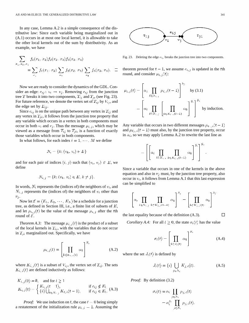
Now we are ready to consider the dynamics of the GDL. Con-sider an edge: . Removing from the junctiontree breaks it into two components, and (see Fig. 23).For future reference, we denote the vertex set ofby , andthe edge set by .

Since is on the unique path between any vertex inandany vertex in , it follows from the junction tree property thatany variable which occurs in a vertex in both components mustoccur in both and . Thus the message , which may beviewed as a message from to , is a function of exactlythose variables which occur in both components.

In what follows, for each index we define

and for each pair of indices such that , wedefine

In words, represents the (indices of) the neighbors of, andrepresents the (indices of) the neighbors ofother than

.Now let be a schedule for a junction

tree, as defined in Section III, i.e., a finite list of subsets of,and let be the value of the message after the thround of .

Theorem A.3:The message is the product of a subsetof the local kernels in , with the variables that do not occurin marginalized out. Specifically, we have

(A.2)

where is a subset of , the vertex set of . The setsare defined inductively as follows:

and forifif (A.3)

Proof: We use induction on, the case being simplya restatement of the initialization rule . Assuming the

Fig. 23. Deleting the edgee breaks the junction tree into two components.

theorem proved for , we assume is updated in thethround, and consider :

by (3.1)

by induction.

Any variable that occurs in two different messagesand must also, by the junction tree property, occurin , so we may apply Lemma A.2 to rewrite the last line as

Since a variable that occurs in one of the kernels in the aboveequation and also in must, by the junction tree property, alsooccur in , it follows from Lemma A.1 that this last expressioncan be simplified to

the last equality because of the definition (A.3).

Corollary A.4: For all , the state has the value

(A.4)

where the set is defined by

(A.5)

Proof: By definition (3.2)


(We know that , since the kernel is by definition afunction only of the variables involved in the local domain.)By Theorem A.3, this can be written as

But by the junction tree property, any variable that occurs intwo of the bracketed terms must also occur in, so that byLemma A.2

by the definition (A.5)

Theorem A.3 tells us that at time, the message from tois the appropriately marginalized product of a subset of the

local kernels, viz., , and Corollary A.4tells us that at time, the state of vertex is the appropri-ately marginalized product of a subset of the local kernels, viz.,

, which we think of as the subset of local ker-nels which are “known” to at time . Given these results, theremaining problem is to understand how knowledge of the localkernels is disseminated to the vertices of the junction tree undera given schedule. A study of (A.5), which gives the relationshipbetween what is known at the vertexand what is known bythe incoming edges, together with the message update rules in(A.3), provides a nice recursive description of exactly how thisinformation is disseminated:

• Rule (1): Initially , each vertex knows only itsown local kernel .

• Rule (2): If a directed edge is activated at time,i.e., if , then vertex learns all the localkernels previously known to at time .

We shall now use these rules to prove Theorem 3.1.Theorem 3.1 asserts thatknows each of the local kernels

at time if and only if there is a path in themessage trellis from to , for all .We will now prove the slightly more general statement thatknows at time if and only if there is a path in themessage trellis from to .

To this end, let us first show that if knows at ,then there must be a path in the message trellis from to

. Because we are in a tree, there is a unique path fromto , say

where and . Denote by the first (smallest)time index for which knows . Then by Rule 2 and an easyinduction argument, we have

(A.6)

(In words, knowledge of must pass sequentially tothroughthe vertices of the path .) In view of (A.6), we have thefollowing path from to inthe message trellis from to :

(A.7)

Conversely, suppose there is a path from to inthe message trellis. Then since apart from “pauses” at a givenvertex, this path in the message trellis must be the unique path

from to , Rule 2 implies that knowledge of the kernelsequentially passes through the vertices on the path,

finally reaching at time .This completes the proof of Theorem 3.1.

REFERENCES

[1] S. M. Aji, “Graphical models and iterative decoding,” Ph.D. dissertation,Cal. Inst. Technol., Pasadena, CA, 1999.

[2] S. M. Aji, G. B. Horn, and R. J. McEliece, “On the convergence of it-erative decoding on graphs with a single cycle,” inProc. 32nd Conf.Information Sciences and Systems, Princeton, NJ, Mar. 1998.

[3] S. M. Aji, G. B. Horn, R. J. McEliece, and M. Xu, “Iterative min-sumdecoding of tail-biting codes,” inProc. IEEE Information Theory Work-shop, Killarney, Ireland, June 1998, pp. 68–69.

[4] S. M. Aji, R. J. McEliece, and M. Xu, “Viterbi’s algorithm and matrixmultiplication,” in Proc. 33rd Conf. Information Sciences and Systems,Baltimore, MD, Mar. 1999.

[5] L. R. Bahl, J. Cocke, F. Jelinek, and J. Raviv, “Optimal decoding of linearcodes for minimizing symbol error rate,”IEEE Trans. Inform. Theory,vol. IT-20, pp. 284–287, Mar. 1974.

[6] L. E. Baum and T. Petrie, “Statistical inference for probabilisticfunctions of finite-state Markov chains,”Ann. Math. Stat, vol. 37, pp.1559–1563, 1966.

[7] R. W. Chang and J. C. Hancock, “On receiver structures for channelshaving memory,”IEEE Trans. Inform. Theory, vol. IT-12, pp. 463–468,Oct. 1966.

[8] J. W. Cooley and J. W. Tukey, “An algorithm for the machine calculationof complex Fourier series,”Math. Comp., vol. 19, p. 297, Apr. 1965.

[9] T. H. Cormen, C. E. Leiserson, and R. L. Rivest,Introduction to Algo-rithms. Cambridge, MA: MIT–McGraw-Hill, 1990.

[10] R. Dechter, “Bucket elimination: A unifying framework for probabilisticinference,”Artificial Intell., vol. 113, pp. 41–85, 1999.

[11] G. D. Forney Jr., “The Viterbi algorithm,”Proc. IEEE, vol. 61, pp.268–278, Mar. 1973.

[12] G. D. Forney Jr., F. R. Kschischang, and B. Marcus, “Iterative decodingof tail-biting trellises,” in IEEE Information Theory Workshop, SanDiego, CA, Feb. 1998, pp. 11–12.

[13] B. J. Frey, “Bayesian networks for pattern classification, data compres-sion, and channel coding,” Ph.D. dissertation, Univ. Toronto, Toronto,ON, Canada, 1997.

[14] B. J. Frey and D. J. C. MacKay, “A revolution: Belief propagation ingraphs with cycles,” inAdvances in Neural Information Processing Sys-tems, M. I. Jordan, M. I. Kearns, and S. A. Solla, Eds. Cambridge, MA:MIT Press, 1998, pp. 470–485.

[15] R. G. Gallager, “Low-density parity-check codes,”IRE Trans. Inform.Theory, vol. IT-8, pp. 21–28, Jan. 1962.

[16] , Low-Density Parity-Check Codes. Cambridge, MA: MIT Press,1963.

[17] R. C. Gonzalez and R. E. Woods,Digital Image Processing. Reading,MA: Addison-Wesley, 1992.

[18] F. V. Jensen,An Introduction to Bayesian Networks. New York:Springer-Verlag, 1996.

[19] F. V. Jensen and F. Jensen, “Optimal junction trees,” inProc. 10th Conf.Uncertainty in Artificial Intelligence, R. L. de Mantaras and D. Poole,Eds. San Francisco, CA, 1994, pp. 360–366.

[20] J. H. Kim and J. Pearl, “A computational model for causal and diagnosticreasoning,” inProc. 8th Int. Joint Conf. Artificial Intelligence, 1983, pp.190–193.


[21] F. R. Kschischang and B. J. Frey, “Iterative decoding of compound codesby probability propagation in graphical models,”IEEE J. Select. AreasCommun., vol. 16, pp. 219–230, Feb. 1998.

[22] S. L. Lauritzen and F. V. Jensen, “Local computation with valuationsfrom a commutative semigroup,”Ann. Math. AI, vol. 21, no. 1, pp.51–69, 1997.

[23] S. L. Lauritzen and D. J. Spiegelhalter, “Local computation with proba-bilities on graphical structures and their application to expert systems,”J. Roy. Statist. Soc. B, pp. 157–224, 1988.

[24] D. J. C. MacKay and R. M. Neal, “Good codes based on very sparse ma-trices,” inCryptography and Coding, 5th IMA Conf., ser. Springer Lec-ture Notes in Computer Science No. 1025. Berlin, Germany: Springer-Verlag, 1995, pp. 100–111.

[25] , “Near Shannon limit performance of low density parity-checkcodes,”Electron. Lett., vol. 33, pp. 457–458, 1996.

[26] P. L. McAdam, L. R. Welch, and C. L. Weber, “M.A.P. bit decodingof convolutional codes,” inProc. 1972 IEEE Int. Symp. InformationTheory, Asilomar, CA, Jan. 1972, p. 91.

[27] R. J. McEliece, R. B. Ash, and C. Ash,Introduction to Discrete Mathe-matics. New York: Random House, 1989.

[28] R. J. McEliece, D. J. C. MacKay, and J. -F. Cheng, “Turbo decodingas an instance of Pearl’s belief propagation algorithm,”IEEE J. Select.Areas Comm., vol. 16, pp. 140–152, Feb. 1998.

[29] J. Pearl,Probabilistic Reasoning in Intelligent Systems. San Mateo,CA: Morgan Kaufmann, 1988.

[30] A. M. Poritz, “Hidden Markov models: A guided tour,” inProc. 1988IEEE Conf. Acoustics, Speech, and Signal Processing, vol. 1, pp. 7–13.

[31] E. C. Posner, “Combinatorial structures in planetary reconnaissance,” inError Correcting Codes, H. B. Mann, Ed. New York: Wiley, 1968.

[32] L. Rabiner, “A tutorial on hidden Markov models and selected applica-tions in speech recognition,”Proc. IEEE, vol. 77, pp. 257–285, 1989.

[33] G. R. Shafer and P. P. Shenoy, “Probability propagation,”Ann. Math.Art. Intel., vol. 2, pp. 327–352, 1990.

[34] R. M. Tanner, “A recursive approach to low complexity codes,”IEEETrans. Inform. Theory, vol. IT-27, pp. 533–547, Sep. 1981.

[35] G. Ungerboeck, “Nonlinear equalization of binary signals in Gaussiannoise,”IEEE Trans. Commun. Technol., vol. COM-19, pp. 1128–1137,Dec. 1971.

[36] S. Verdú and V. Poor, “Abstract dynamic programming models undercommutativity conditions,”SIAM J. Contr. Optimiz., vol. 25, pp.990–1006, July 1987.

[37] A. J. Viterbi, “Error bounds for convolutional codes and an asymptoti-cally optimum decoding algorithm,”IEEE Trans. Inform. Theory, vol.IT-13, pp. 260–269, Apr. 1967.

[38] Y. Weiss, “Correctness of local probability propagation in graphicalmodels with loops,”Neural Comput., vol. 12, pp. 1–41, 2000.

[39] N. Wiberg, “Codes and decoding on general graphs ,” dissertation no.440, Linkoping Studies in Science and Technology, Linkoping, Sweden,1996.

[40] M. Yannakakis, “Computing the minimum fill-in is NP-complete,”SIAM J. Alg. Discr. Methods, vol. 2, pp. 77–79, 1981.

[41] F. R. Kschischang, B. J. Frey, and H.-A. Loeliger, “Factor graphs andthe sum-product algorithm,”IEEE Trans. Inform. Theory, submitted forpublication.

the generalized distributive law - information...

Documents