the generalized whittaker functions for su(2 1) … 6 (1999),477–526. the generalized whittaker...
TRANSCRIPT

J. Math. Sci. Univ. Tokyo6 (1999), 477–526.
The Generalized Whittaker Functions for SU(2, 1)
and the Fourier Expansion of Automorphic Forms
By Yoshi-hiro Ishikawa
Abstract. Explicit form of Fourier expansion of automorphicforms plays an important role in the theory. Here we investigate thecase of SU(2, 1) and give an explicit formula of generalized Whittakerfunctions for the standard representations of the group. Together witha result of [K-O], we obtain a form of fully developed Fourier expansionof automorphic forms belonging to arbitrary standard representations.
Introduction
In the theory of automorphic forms, Fourier expansion of modular forms
is a fundamental tool for investigation. For example, coefficients of the
expansion can be used for construction of L-functions. In spite of this
importance, the theory of Fourier expansion of automorphic forms seems
still in very primitive state.
Our concern in this paper is to have a theory of fully developed Fourier
expansion of modular forms on SU(2, 1), the real special unitary group of
signature (2+, 1−). To have such a theory we need Whittaker functions and
generalized Whittaker functions of the standard representations of SU(2, 1).
A quite explicit result is obtained by Koseki-Oda [K-O] for Whittaker func-
tions. The remaining problem for our purpose is to consider the generalized
Whittaker functions. This is the theme of the present paper.
The peculiarity of the case of SU(2, 1), different from the case of SL2(R),
is that the maximal unipotent subgroup N is not abelian. It is isomorphic
to the Heisenberg group of dimension three, and has infinite-dimensional
irreducible unitary representations σ, which are called Stone von Neumann
representations. Together with unitary characters they constitute the uni-
tary dual of N . The Fourier expansion of automorphic forms on SU(2, 1) is
1991 Mathematics Subject Classification. Primary 11F70; Secondary 11F30, 22E30,33C15.
477

478 Yoshi-hiro Ishikawa
to consider irreducible decomposition of the restriction π|N of automorphic
representations π with respect to N . Therefore we have to handle those
terms which corresponds to the Stone von Neumann representations.
Naive formulation of the problem is to investigate intertwiners in
HomN (π|N , σ) which is isomorphic to HomG(π, IndGNσ) by Frobenius reci-
procity. But this fails in general, since the intertwining space in question
is infinite-dimensional. The right formulation of the problem is given by
introducing a larger group R containing N .
Here is the formulation of our main result. Let P be the minimal para-
bolic subgroup of SU(2, 1) with a Levi decomposition L N . Let S be the
maximal closed subgroup of L which acts trivially on the center Z(N) of N .
The group R is the semidirect product S and N . We want to investigate
the intertwining space HomG(π, IndGRη) for certain unitary irreducible rep-
resentations η of R, and the images of intertwiners: these are the space of
generalized Whittaker functionals and the space of generalized Whittaker
functions, respectively.
Our main result is to obtain an explicit formula for the radial part of
such generalized Whittaker functions with special K-type. Simultaneously
we have the archimedean local multiplicity one theorem for the intertwin-
ing space, which generalizes that of Shalika [Sha] to the setting above.
As a bonus, we obtain a sufficient condition for one-dimensionality of the
intertwining space in terms of the parameters of representations (Theorem
3.3.5, Theorem 4.2.4). Consequently we have an explicit form of the Fourier
expansion of automorphic forms, which separates the finite part (i.e. the
coefficients) and the archimedean part (i.e. the generalized Whittaker func-
tions) in each term of the expansion (Theorem 5.3.1).
We should remark that Piatetski-Shapiro announced the multiplicity
one theorem of “Heisenberg model” for the irreducible representations of
U(3) over local fields more than two decades ago ([PS] p.589). Gelbart and
Rogawski used this result as a crucial step to investigate automorphic L-
functions obtained from Fourier-Jacobi expansion ([Ge-Ro] p.452). Over the
real field, this result is a part of our Thorems (3.3.5) and (4.2.4). However,
up to the present, any of these authors did not publish their proof.
The difficult part of our investigation is the case where π is of the
large discrete series representation of SU(2, 1). For such representations
our method of proof uses fundamental results of Yamashita [Ya2].

The Generalized Whittaker Functions 479
Though the author needs the result of this paper for investigation of
automorphic forms, he also believes that it is interesting for the problem of
realization in generalized Gelfand-Graev representations.
Let us explain the contents of this paper more in detail. Firstly in §1,
after recalling some basic results about generalized Gelfand-Graev represen-
tations, we define generalized Whittaker functions with given K-type for
irreducible admissible representations π of a real semisimple Lie group G. In
§§2.1 we fix some notation for the structure of the group G = SU(2, 1) and
its Lie algebra. In §§2.2 we shortly summarize necessary facts on parameter-
ization of irreducible K-module τλ in K and Clebsch-Gordan decomposition
of τλ ⊗AdpC. In §§2.3 we construct irreducible unitary representation ηµ,ψ
of R concretely on L2(R) by using the theory of Weil representations. We
calculate explicitly the η-action of n = LieN on a basis of L2(R) consist-
ing of Hermite functions for the computation of the A-radial part of shift
operators in later sections. In §§2.4 we briefly recall Harish-Chandra ’s pa-
rameterization of the discrete series representations and the principal series
representations of SU(2, 1). The core of this paper is the section §3, which
treats the case of a discrete series representation. Here we use a fundamen-
tal result of Yamashita which characterizes the A-radial part of generalized
Whittaker functions of discrete series representations by means of Schmid
operators [Ya2]. We recall in §§3.1 the definition of the Schmid operators
and a result of Yamashita as Proposition 3.1.1. The first half of §§3.2 is
devoted to explicit calculation of the A-radial part of Schmid operators in
terms of the coefficient functions ck’s of a generalized Whittaker function for
discrete series representation with minimal K-type. We obtain a system of
difference-differential equations satisfied by ck’s (Proposition 3.2.4, Propo-
sition 3.2.5, Proposition 3.2.6). Finally in §§3.3 we give an explicit formula
for ck’s (Theorem 3.3.2, Theorem 3.3.4) by solving the differential equa-
tions in Proposition 3.3.1, Proposition 3.3.3. As an immediate corollary we
have the multiplicity one theorem for the generalized Whittaker model for
the discrete series representations (Theorem 3.3.5). The case of a principal
series representation is treated in §4. We also obtain an explicit formula
of the generalized Whittaker functions and the multiplicity one theorem in
this case (Theorem 4.2.4). The rest of this paper §5 is an application of
the explicit formula obtained in previous sections to the theory of Fourier
expansion of automorphic forms on SU(2, 1). Among others we can define

480 Yoshi-hiro Ishikawa
normalized Fourier coefficients of automorphic forms in Theorem 5.3.1.
Acknowledgment . I would like to express my sincere gratitude to my
supervisor, Professor Takayuki Oda, who introduced me to his project on
generalized spherical functions and guided me patiently through my Ph.D.
studies with constant warm encouragement. Also I thank Masao Tsuzuki,
many discussions with whom were always helpful and fruitful.
1. Generalized Whittaker Models
1.1. The space of the generalized Whittaker functionals
Firstly in this subsection, we define the space of the generalized Whit-
taker functionals for an irreducible admissible representation (π,Hπ) of a
real semisimple group.
Let G be a connected real semisimple Lie group with finite center and
K its maximal compact subgroup. We denote by θ the Cartan involution
associated to K. Take a minimal parabolic subgroup P of G with a Levi
decomposition: P = L N, where N is the unipotent radical of P and L is
the θ-invariant reductive part of P (i.e. the Levi subgroup). The action of L
on N by conjugation induces its action on the unitary dual N of N . Hence
putting Sξ the stabilizer of the class of a unitary representation (ξ,S) of N
in L, we can extend (ξ,S) to a unique projective representation (ξ,S) of
Sξ N .
Under some condition, we can get (ξ,S) as a representation of Sξ N ,
not a projective representation. Let n be the Lie algebra of N . Assume ξ
corresponds to the coadjoint orbit of X∗ ∈ n∗ in the Kirillov theory (cf [Co-
Gr]). Let X be the element of g = LieG determined by 〈X∗, Z〉 = B(θX, Z).
Here Z ∈ n and B is the Killing form of g. Denote by H the semisimple
element of the sl2-triple containing X.
Proposition 1.1.1 ([Ya] Prop 2.2). When the subspace g(1) := X ∈g | [H, X] = X of Lie algebra g admits an Ad(Sξ)-invariant complex struc-
ture, (ξ,S) is extendable to a unitary representation ξ of Sξ N acting on
the same representation space with ξ.
We remark that the assertion in the proposition above is valid in the
case of G = SU(2, 1).
The Generalized Whittaker Functions 481
We assume the condition of Proposition 1.1.1 is satisfied throughout this
section. Denote the group Sξ N by Rξ. Let η be a unitary representation
of Rξ defined by c′⊗ ξ. Here, c′ := c⊗ 1N is the extension of an irreducible
representation c of Sξ trivially on N .
Consider a space
C∞η (Rξ\G) := f : G→ S∞ | f is a C∞-function satisfying,
f(rg) = η(r).f(g), ∀r ∈ Rξ ,∀g ∈ G
on which G acts via right translation. We call this C∞-induced represen-
tation IndGRξη of G the reduced generalized Gelfand-Graev representation.
Here, we used the standard notation that S∞ means the subspace consisting
of all smooth vectors in S.
We can now define the space of the generalized Whittaker functionals as
the space of intertwining operators.
Definition. For an irreducible admissible representation (π,Hπ) of
G, we denote the underlining (gC, K)-module of π by the same symbol π.
We call the space of intertwiners
Iπ,η := Hom(gC,K)(π∗, IndGRξη)
of (gC, K)-modules the space of the algebraic generalized Whittaker func-
tionals. Here gC is the complexification of the Lie algebra g of G and π∗
denotes the contragredient (gC, K)-module of π.
1.2. Generalized Whittaker functions with fixed K-type
In order to investigate algebraic generalized Whittaker functionals l ∈Iπ,η, we study the functions l(v∗) ∈ IndGRξη : the image of vectors v∗ be-
longing to (π∗,Hπ∗) by l. To describe these functions explicitly, we specify
a K-type of π and consider vectors v∗ belonging to this K-type.
Let (τ, Vτ ) be a K-type of π, that is, τ occurs in the decomposition of
π as K-module: π|K = ⊕τ∈K [π : τ ]τ. Choose a K-equivariant injection
ιτ : τ → π, and pullback a generalized Whittaker functional l by this
injection ιτ :
Hom(gC,K)(π∗, IndGRξη) l → ι∗τ (l) ∈ HomK(τ∗, IndGRξη|K).
482 Yoshi-hiro Ishikawa
Here we note the isomorphism
HomK(τ∗, IndGRξη|K) ∼= (IndGRξη|K ⊗ τ)K .
The latter space is defined by(C∞η (Rξ\G)⊗C Vτ
)K ∼= C∞η,τ (Rξ\G/K)
:=
ϕ : G→ S∞ ⊗C Vλ
∣∣∣∣∣ϕ is a C∞-function satisfying
ϕ(rgk) = η(r)τλ(k)−1.ϕ(g),
∀r ∈ R ,∀g ∈ G ,∀k ∈ K
.
We study functions F ∈ C∞η,τ (Rξ\G/K) representing ι∗τ (l). By definition,
l(v∗)(g) = 〈v∗, F (g)〉K ,
v∗ ∈ V ∗τ . Here 〈 , 〉K means the canonical pairing of K-modules V ∗
τ and
Vτ .
Definition. We call the above function F corresponding to ι∗τ (l),l ∈ Iπ,η the algebraic generalized Whittaker function associated to repre-
sentation π with K-type τ . Moreover if we impose the slowly increasing
condition for the A-radial part F |A of F , such a function is called the
generalized Whittaker function(see subsection 3.3). Here A is the vector
subgroup of G of which Lie algebra is the maximal abelian subalgebra of g.
We investigate these functions in the following setting
G = SU(2, 1)
ξ : an infinite-dimensional irreducible unitary representation of N
π : a discrete series representation of G (resp.
a principal series representation of G)
τ : the minimal K-type of π (resp.
the corner K-type of π)
and give an explicit formula for F and the multiplicity one property of Iπ,ηsimultaneously by constructing F .

The Generalized Whittaker Functions 483
2. The Structure of Lie Groups and Parameterization of
Representations
In this section we give a glossary on the group structure of SU(2, 1)
and representations for later use. We first fix realizations and give explicit
coordinates of various subgroups and their Lie algebras. It is crucial for
our explicit calculation of generalized Whittaker functions. We also recall
parameterization of representations of these groups.
2.1. Subgroups, subalgebras and root space decomposition
Subgroups and their realizations. We denote by diag(X1, X2, X3)
a diagonal matrix of degree 3 with (i, i)-entry Xi for each i (1 i 3). Put I2,1 := diag(1, 1,−1). Then we realize the identity component of
the stabilizer group SU(2, 1) of the Hermitian form of three variables with
signature (2+, 1−) as
g ∈ SL(3, C)|tgI2,1g = I2,1.
Here tg is the transpose of g, and g the complex conjugate of g. We denote
the group by G. Let
G = NAK
be the Iwasawa decomposition of G. Then in this realization, a maximal
compact subgroup K of G can be written as
K = (
k1 0
0 k2
)∈ G | k1 ∈ U(2), k2 ∈ U(1), k2 det k1 = 1.
Here U(n) is the unitary group of degree n. The Euclidean subgroup A is
A = ar :=
r+r−1
2r−r−1
2
1r−r−1
2r+r−1
2
| r ∈ R>0.
The maximal unipotent subgroup N is isomorphic to the Heisenberg group
H(R2) of dimension 3. Here H(R2) is the set (x, y; t) ∈ R3 with a group
law (x, y; t)(x′, y′; t′) = (x+x′, y +y′; t+ t′+xy′−yx′). Note that the group
law above is different from usual one. See (2.1.1).
484 Yoshi-hiro Ishikawa
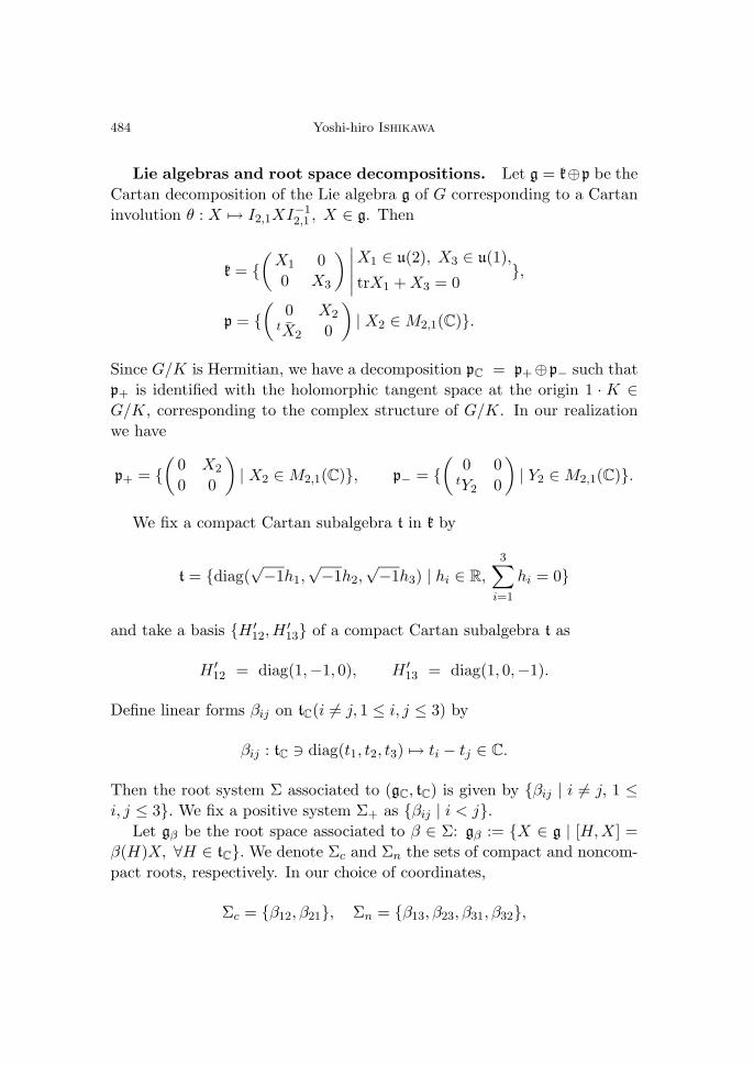
Lie algebras and root space decompositions. Let g = k⊕p be the
Cartan decomposition of the Lie algebra g of G corresponding to a Cartan
involution θ : X → I2,1XI−12,1 , X ∈ g. Then
k = (
X1 0
0 X3
) ∣∣∣∣∣X1 ∈ u(2), X3 ∈ u(1),
trX1 + X3 = 0,
p = (
0 X2tX2 0
)| X2 ∈M2,1(C).
Since G/K is Hermitian, we have a decomposition pC = p+⊕p− such that
p+ is identified with the holomorphic tangent space at the origin 1 · K ∈G/K, corresponding to the complex structure of G/K. In our realization
we have
p+ = (
0 X2
0 0
)| X2 ∈M2,1(C), p− =
(0 0
tY2 0
)| Y2 ∈M2,1(C).
We fix a compact Cartan subalgebra t in k by
t = diag(√−1h1,
√−1h2,
√−1h3) | hi ∈ R,
3∑i=1
hi = 0
and take a basis H ′12, H ′
13 of a compact Cartan subalgebra t as
H ′12 = diag(1,−1, 0), H ′
13 = diag(1, 0,−1).
Define linear forms βij on tC(i = j, 1 ≤ i, j ≤ 3) by
βij : tC diag(t1, t2, t3) → ti − tj ∈ C.
Then the root system Σ associated to (gC, tC) is given by βij | i = j, 1 ≤i, j ≤ 3. We fix a positive system Σ+ as βij | i < j.
Let gβ be the root space associated to β ∈ Σ: gβ := X ∈ g | [H, X] =
β(H)X, ∀H ∈ tC. We denote Σc and Σn the sets of compact and noncom-
pact roots, respectively. In our choice of coordinates,
Σc = β12, β21, Σn = β13, β23, β31, β32,
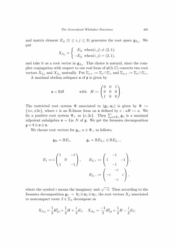
The Generalized Whittaker Functions 485
and matrix element Eij (1 ≤ i, j ≤ 3) generates the root space gβij . We
put
Xβij =
Eij when(i, j) = (2, 1);
−Eij when(i, j) = (2, 1),
and take it as a root vector in gβij . This choice is natural, since the com-
plex conjugation with respect to our real form of sl(3, C) converts two root
vectors Xβij and Xβji mutually. Put Σc,+ := Σc∩Σ+ and Σn,+ := Σn∩Σ+.
A maximal abelian subspace a of p is given by
a = RH with H :=
0 0 1
0 0 0
1 0 0
.
The restricted root system Ψ associated to (gC, aC) is given by Ψ :=
±e,±2e, where e is an R-linear form on a defined by e : aH → a. We
fix a positive root system Ψ+ as e, 2e. Then∑
α∈Ψ+gα is a maximal
nilpotent subalgebra n = Lie N of g. We get the Iwasawa decomposition
g = k⊕ a⊕ n.
We choose root vectors for gα, α ∈ Ψ+ as follows,
g2e = RE1, ge = RE2,+ ⊕ RE2,−,
E1 := i
1 −1
0
1 −1
, E2,+ :=
−1
1 −1
−1
,
E2,− :=
−i
−i i
−i
,
where the symbol i means the imaginary unit√−1. Then according to the
Iwasawa decomposition gC = kC⊕ aC⊕nC, the root vectors Xβ associated
to noncompact roots β ∈ Σn decompose as
Xβ13 =1
2H ′
13 +1
2H +
i
2E1; Xβ31 =
−1
2H ′
13 +1
2H − i
2E1;

486 Yoshi-hiro Ishikawa
Xβ23 = −Xβ21 −1
2E2,+ −
i
2E2,−; Xβ32 = −Xβ12 −
1
2E2,+ +
i
2E2,−.
This will be used to calculate the action of Schmid operators, defined in
subsection 3.1, on the A-radial part of generalized Whittaker functions.
The exponential coordinate of N . We prepare the exponential co-
ordinate of N = expn which will be used for description of generalized
theta functions in subsection 5.2. As is well-known, for a connected simply
connected nilpotent Lie group the exponential map gives a diffeomorphism
between the group and its Lie algebra (cf. [Co-Gr] p.13). Therefore we can
take the basis E2,±, E1 of n as a coordinate of N . The group law of N is
translated into
Y ∗X := log((exp Y )(exp X)
).
The Campbell-Baker-Hausdorff formula says that
Y ∗X = Y + X + 12 [Y, X] + 1
12 [Y, [Y, X]]− 112 [X, [Y, X]] + · · ·
= Y + X + 12 [Y, X].
The second equality follows from the 2-step nilpotency of n. If Y = mE2,++
nE2,− + kE1, X = xE2,+ + yE2,− + zE1, then
Y ∗X = Y + X + 122(my − nx)E1(2.1.1)
= (m + x)E2,+ + (n + y)E2,− + (k + z + (my − nx))E1,
because of the relation [E2,+, E2,−] = 2E1. We abbreviate the element
exp(xE2,+ + yE2,− + zE1) of N as (x, y; z). This is utilized for solving the
differential equations for generalized theta functions (Theorem 5.2.1).
2.2. Representations of maximal compact subgroup K
Here we summarize necessary facts on representations of K from [K-O].
Parameterization of irreducible K-modules. The set L+T of Σc,+-
dominant T -integral weights is given by L+T = (m, n) ∈ Z
⊕2|m ≥ n. For
each µ = (µ1, µ2) ∈ L+T , the vector space Vµ spanned by vµk | 0 ≤ k ≤ dµ
with kC-action as
τµ(Z)vµk = (µ1 + µ2)vµk ,
τµ(H′12)v
µk = (2k − dµ)v
µk , τµ(H
′13)v
µk = (k + µ2)v
µk ,
τµ(Xβ12 )vµk = (k + 1)vµk+1, τµ(Xβ21 )v
µk = (k − dµ − 1)vµk−1

The Generalized Whittaker Functions 487
gives an irreducible K-module (τµ, Vµ) via the highest weight theory. Here
Z denotes a generator 2H ′13 −H ′
12 of the center.
Tensor products with pC. We regard the 4-dimensional vector space
pC as a kC-module via the adjoint representation ad. Then p+ and p− are
invariant subspaces, and
p+ = CXβ13 ⊕ CXβ23∼= Vβ13 , p− = CXβ32 ⊕ CXβ31
∼= Vβ32 .
Given an irreducible K-module Vµ we have Vµ ⊗ pC = (Vµ ⊗ p+) ⊕ (Vµ ⊗p−), and Clebsch-Gordan’s theorem tells us the following decomposition of
Vµ ⊗ p±:
Vµ ⊗ p+∼= Vµ+β13 ⊕ Vµ+β23 , Vµ ⊗ p− ∼= Vµ+β32 ⊕ Vµ+β31
Here we understand Vν = (0) if ν ∈ LT is not dominant. We hence have
Vµ ⊗ pC∼= V +
µ ⊕ V −µ ;
V +µ := Vµ+β13 ⊕ Vµ+β32 , V −
µ := Vµ−β13 ⊕ Vµ−β32 ,
under the above convention.
The decompositions of Vµ ⊗ pC induce the following projectors:
p+β13
(µ) : Vµ ⊗ pC → Vµ+β13 , p+β23
(µ) : Vµ ⊗ pC → Vµ−β32 ,
p−β23(µ) : Vµ ⊗ pC → Vµ+β32 , p−β13
(µ) : Vµ ⊗ pC → Vµ−β13 .
In terms of vµk, they are expressed as follows:
Proposition 2.2.1 ([K-O] Prop 2.3).
p+β13
(µ)(vµk ⊗Xβ13 ) = (k + 1)vµ+βk+1
13, p+β23
(µ)(vµk ⊗Xβ13 ) = −vµ−βk
32,
p+β13
(µ)(vµk ⊗Xβ23 ) = (dµ − k + 1)vµ+βk
13, p+β23
(µ)(vµk ⊗Xβ23 ) = vµ−βk−1
32,
p−β23(µ)(vµk ⊗Xβ32 ) = −(k + 1)vµ+β
k+132, p−β13
(µ)(vµk ⊗Xβ32 ) = vµ−βk
13,
p−β23(µ)(vµk ⊗Xβ31 ) = (dµ − k + 1)vµ+β
k32, p−β13
(µ)(vµk ⊗Xβ31 ) = vµ−βk−1
13,
for k = 1, . . . , dλ. Here one should note that dµ±β13 = dµ±β32 = dµ ± 1.

488 Yoshi-hiro Ishikawa
2.3. Representation theory of the group R
We construct the unitary representations of R with nontrivial central
characters, which are necessary for our purpose.
The stabilizer Sξ of representation with nontrivial central char-
acter. Here we give an explicit form of the stabilizing group Sξ of the class
of ξ when ξ is an infinite-dimensional irreducible unitary representation of
N in order to construct concretely the unitary representation η explained
in subsection 1.1.
Note that the maximal unipotent subgroup N of G is the Heisenberg
group H(R2) of dimension 3. Recall that the unitary dual N of N consists
of unitary characters and infinite-dimensional irreducible unitary represen-
tations by the Stone-von Neumann theorem:
Proposition 2.3.1. Every irreducible unitary representation σ of
H(R2) is either of two cases:
a) If the central character ψ of σ is trivial, σ is a one-dimensional repre-
sentation i.e. a unitary character.
b) If the central character ψ of σ is non-trivial, σ is a unique infinite-
dimensional irreducible unitary representation, up to unitary equivalence.
We call σ in the case(b) a Stone von Neumann representation. Let σ be
a Stone von Neumann representation of N . The equivalence class of σ in
N is completely determined by its central character ψ. Let L be the Levi
subgroup of P , and Z(N) the center of N . Then L acts both on N and
Z(N) by conjugation. Hence the stabilizer S of σ in L is the centralizer of
Z(N). In particular S is independent of σ and of the following form
S = diag(α, β, α−1) ∈ G′ | α, β ∈ U(1), αβα−1 = 1.
Since the action of S on N by conjugation is faithful, S can be regarded
as a subgroup of the automorphism group of N . Passing to the abelianized
subgroup Nab = N/[N : N ] of N , we have
S → Aut N → Aut Nab.
Since Nab is identified with R⊕2, Aut Nab ∼= GL2(R). Composing all these
identifications, we get an isomorphism between S and SO(2)
S
diag(α, β, α−1)
→ AutN →→
GL2(R) ⊃ SO(2),
R(3θ)

The Generalized Whittaker Functions 489
by putting α = eiθ, β = e−2iθ, θ ∈ [0, 2π), where R(3θ) means the rotation
of angle −3θ.
Representations of R with nontrivial central characters. Here
we fix a model of a Stone von Neumann representation σ. By L2(R) we
denote the space of square integrable functions on R. For each element
(x, y; t) ∈ H(R2) and a function Φ ∈ L2(R), define
(2.3.1) ρψ
((x, y; t)
).Φ(ξ) = ψ(t + 2ξy + xy)Φ(ξ + x).
Then ρψ : H(R2) → Aut(L2(R)) is an infinite-dimensional irreducible uni-
tary representation with central character ψ, called the Shrodinger model
of a Stone von Neumann representation. Our model differs from usual one.
Since the commutation relation [E2,+, E2,−] = 2E1 between the basis of n
is different from the Heisenberg commutation relation by 2.
We extend the representation ρψ of N to the representation of R by
using the theory of Weil representation. As is well-known, the two-fold
covering SL2(R) of SL2(R) has a unitary representation (ωψ, L2(R)). This
is obtained as the intertwiner of representations ρψ and ρgψ of the Heisenberg
group H(R2) whose central characters are the same, by virtue of Proposition
2.3.1(b). Here the representation ρgψ is given by
ρgψ : H(R2) (x, y; t) → ρψ((x, y)g; t) ∈ Aut(L2(R)).
From the construction above, we have the canonical extension
ωψ × ρψ : SL2(R) H(R2)→ Aut(L2(R)).
Identifying S, N with SO(2), H(R2) respectively, the semidirect product
R = S N is regarded as a subgroup of SL2(R) H(R2). Let R denote
the pullback S N ∼= SO(2) H(R2) of R by the covering
pr × id : SL2(R) H(R2) SL2(R) H(R2).
Then tensoring an odd character χ of SO(2) to (ωψ × ρψ)|R, we have a
representation of R
χ⊗ (ωψ × ρψ)|R
: R = S N → Aut(L2(R)).

490 Yoshi-hiro Ishikawa
We denote this representation by (η, L2(R)). A character of SO(2) is called
odd, if it does not factor through the covering SO(2) SO(2).
Now we fix a description of odd characters. The covering SO(2) SO(2) is identified with the twice homomorphism SO(2)→ SO(2); R(θ) →R(2θ). Hence the characters of SO(2) is identified with 1
2Z, if we identify
these of SO(2) with Z. Therefore odd characters χµ of SO(2) is parame-
terized by some elements µ = m + 12 in 1
2Z\Z (m ∈ Z).
Here is a diagram explaining the above construction
R = S N SL2(R) H(R2)ωψ×ρψ−−−−→ Aut(L2(R)) pr×id
R = S N −−−→ SL2(R) H(R2).
The representations of R with non-trivial central characters are ex-
hausted by these representations constructed above.
Lemma 2.3.2. The unitary induced representation IndRNρψ of R has a
direct sum decomposition:
IndRNρψ ∼=⊕
µ∈ 12
Z\Z
χµ ⊗ (ωψ × ρψ).
Proof. The induced representation IndRNρψ of R = S N is isomor-
phic to RegS ⊗ (ωψ × ρψ), where RegS is the regular representation of S
(cf. [Ya] p.399, Lemma 2.5). Since S ∼= SO(2), RegS decomposes as a direct
sum of characters:
RegS∼=
⊕µ∈ 1
2Z
χµ.
Therefore IndRNρψ, which is identified with Ker(R → R)-invariant part of
IndRNρψ, has the decomposition stated above.
A basis of η and the action of LieN . It is well known that Hermite
functions
hj(ξ) := (−1)jeξ2/2 dj
dξje−ξ2 ,

The Generalized Whittaker Functions 491
j = 0, 1, 2, . . . form an orthogonal Hilbert basis of L2(R).
Lemma 2.3.3. The subspace of smooth vectors in L2(R) is the Schwartz
space S(R), and the action of root vectors E1, E2,+, E2,− on S(R) through
the underlining Harish-Chandra module of ηµ,ψs = χµ ⊗ (ωψ × ρψ)|R
are as
follows:
η(E1).hj =√−1shj ,
η(E2,+).hj =−1
2hj+1 + jhj−1, η(E2,−).hj =
√−1shj+1 + 2
√−1sjhj−1,
where ψs is an additive character R t → eist ∈ U(1) of R with parameter
s ∈ R\0.
Proof. Differentiate Schodinger model (2.3.1) in the exponential co-
ordinate. Then we have
ρψs(E1).Φ(ξ) =√−1sΦ(ξ),
ρψs(E2,+).Φ(ξ) =d
dξΦ(ξ), ρψs(E2,−).Φ(ξ) = 2
√−1sξ · Φ(ξ),
where Φ ∈ S(R). The well-known recurrence relations on Hermite polyno-
mials:
H ′j(ξ) = 2j ·Hj−1(ξ),
Hj+1(ξ)− 2ξ ·Hj(ξ) + 2j ·Hj−1(ξ) = 0
(cf. [Er] p.193) tell us the assertion of Lemma.
These formulae will be used in calculation of the radial parts of the
Schmid operators and the Casimir operator (Proposition 3.2.3, Proposition
4.2.1).
2.4. The standard representations of G
Since G is of real rank one, the standard representations of G consist
of discrete series representations and principal series representations. We
briefly recall Harish-Chandra’s parameterization of the discrete series, and
the K-type decomposition of the standard representations.
The discrete series representations. Let Ξ denote the set of all Σ-
regular Σc,+-dominant T -integral weights Λ ∈ LT of tC and let Gd denote
492 Yoshi-hiro Ishikawa
the set of all equivalence classes of discrete series representations of G.
By a result of Harish-Chandra, there is a bijection between Ξ and Gd. A
member belonging to the class corresponding to Λ ∈ Ξ is said to have the
Harish-Chandra parameter Λ and denoted by πΛ.
Under identification of the weight lattice LT with Z⊕2, we have
Ξ = Λ = (Λ1, Λ2) ∈ Z⊕2 | Λ1 > Λ2, Λ1Λ2 = 0.
This set decomposes into three disjoint subsets ΞJ = Λ ∈ Ξ | 〈Λ, β〉 >
0, ∀β ∈ Σ+J correspond to positive root systems Σ+
J (J = I, II, III) com-
patible with the positive compact root system Σc,+ fixed before as β12.We fix Σ+
J ’s as follows
Σ+I := β12, β13, β23,
Σ+II := β12, β32, β13,
Σ+III := β12, β32, β31.
Note these three are translate into each other by the action of the Weyl
group W (g, t)/W (k, t). Then by the inner product on LT induced from the
Killing form we can see easily
Ξ+I = (Λ1, Λ2) ∈ Z
⊕2| Λ1 > Λ2 > 0 ,Ξ+II = (Λ1, Λ2) ∈ Z
⊕2| Λ1 > 0 > Λ2 ,Ξ+III = (Λ1, Λ2) ∈ Z
⊕2| 0 > Λ1 > Λ2 .
Representations parameterized by Ξ+I (resp.Ξ+
III) are called the holomor-
phic discrete series representations (resp. the antiholomorphic discrete se-
ries representations). In the remaining case, discrete series representations
whose Harish-Chandra parameters Λ’s belong to Ξ+II are the large discrete
series representations in the sense of Vogan [Vo].
The Blattner formula tells us the K-type decomposition of the discrete
series representation πΛ as follows.
πΛ|K = ⊕µ∈L+T (Λ)[πΛ : τµ]τµ

The Generalized Whittaker Functions 493
where the set L+T (Λ) of parameters of the K-types of πΛ is given by
L+T (Λ) =
λ + m1β13 + m2β23 | m1, m2 ≥ 0 ∈ Z when Λ ∈ Ξ+
I ,
λ + m1β13 + m2β32 | m1, m2 ≥ 0 ∈ Z when Λ ∈ Ξ+II ,
λ + m1β31 + m2β32 | m1, m2 ≥ 0 ∈ Z when Λ ∈ Ξ+III .
When Λ ∈ ΞJ , λ in the formula above is described as
λ = Λ− ρc + ρJn
(Λ1 + 1, Λ2 + 2) when J = I,
(Λ1, Λ2) when J = II,
(Λ1 − 2, Λ2 − 1) when J = III,
where ρc is the half-sum of the compact positive roots and ρJn of the non-
compact ones in Σ+J . This λ is the highest weight of the minimal K-type
of πΛ which is called the Blattner parameter. About the multiplicity we
remark that all [πΛ : τµ] is one for G = SU(2, 1). That is the multiplicity
free property for K-types is valid.
The principal series representations. Let
P = NAM
be the Langlands decomposition of P . We note M is isomorphic to U(1).
For characters eν : ar → rν+2 (ν ∈ C) of A and χλ0 : diag(eiθ, e−2iθ, eiθ) →eiλ0θ (λ0 ∈ Z) of M , the induced representation πλ0,ν = IndGP (1N⊗eν⊗χλ0)
is called the principal series representation of G. The representation space
of πλ0,ν is given by
f : G→ C | f is a C∞-function satisfying,
f(narmg) = rν+2χλ0(m)f(g), ∀narm ∈ P ,∀g ∈ G.
By the Frobenius reciprocity, we have the K-type decomposition:
πλ0,ν |K = ⊕µ∈L+T (λ0)[πλ0,ν : τµ]τµ
with multiplicities [πλ0,ν : τµ] = 1, where the set L+T (λ0) of parameters of
the K-types of πλ0,ν is given by
L+T (λ0) = (−λ0,−λ0) + m1β13 + m2β32 | m1, m2 ≥ 0 ∈ Z.
The principal series representation πλ0,ν has only one K-type τ(−λ0,−λ0)
whose dimension is one. We call it the corner K-type of πλ0,ν .

494 Yoshi-hiro Ishikawa
3. The Case of Discrete Series Representations
Here we treat discrete series representations and have the multiplicity
one theorem for such representations. Our method is to solve the system
of partial differential equations which characterize generalized Whittaker
functions and to give an explicit form of these functions.
3.1. Yamashita’s characterization
In this subsection we give a variant of a result of Yamashita, in a suitable
form for our use, which characterizes the space of the algebraic minimal K-
type generalized Whittaker functionals for discrete series representations.
This is fundamental for our purpose.
We denote the space of Vλ-valued functions on G with the τλ-equi-
variance by
C∞τλ
(G/K) := ϕ : G→ Vλ | ϕ is a C∞-function satisfying
ϕ(gk) = τλ(k)−1.ϕ(g) ,∀g ∈ G ,∀k ∈ K.
We can regard pC as a K-module through the adjoint representation AdpC.
The differential operator
∇τλ : C∞τλ
(G/K)→ C∞τλ⊗AdpC
(G/K)
defined by
∇τλϕ :=4∑
i=1
RXiϕ⊗Xi,
is a K-homomorphism. Here Xi (i = 1, . . . , 4) is an orthonormal basis of
p with respect to the Killing form on g and RXϕ means the right differential
of function ϕ by X ∈ g : RXϕ(g) = ddtϕ(g exp tX)|t=0. The operator ∇τλ
is called the Schmid operator . We take C(Xβ +X−β), C√−1(Xβ−X−β) as
orthonormal basis of pC, where β is β13 or β23 and C is a positive constant
depending on the normalization of the fixed Killing form. Then, using this
basis, the Schmid operator ∇τλ can be written as
∇τλϕ = 2C2∑
β=β13,β23
RX−βϕ⊗Xβ + 2C2∑
β=β13,β23
RXβϕ⊗X−β.
The Generalized Whittaker Functions 495
Here we note that Xβ13 , Xβ23 is the set of root vectors corresponding
to positive noncompact roots. The above description of ∇τλ in two terms
corresponds to the decomposition of pC = p+ ⊕ p−.
Now we define two differential operators
∇±τλ
: C∞τλ
(G/K)→ C∞τλ⊗Adp±
(G/K)
as
∇+τλ
ϕ := RX−β13ϕ⊗Xβ13 + RX−β23
ϕ⊗Xβ23 ,
∇−τλ
ϕ := RXβ13ϕ⊗X−β13 + RXβ23
ϕ⊗X−β23 .
For later use, we prepare the ±β-shift operators for every positive noncom-
pact root β ∈ Σn,+ and λ ∈ L+T .
D±βτλ
: C∞τλ
(G/K)→ C∞τλ±β (G/K)
D±βτλ
ϕ(g) := p±β(∇±
τλϕ(g)
).
Here p±β are the projectors τλ ⊗Adp± τλ±β defined in subsection 2.2.
All the operators constructed above can be defined similarly for the space
C∞η,τλ
(R\G/K) :=
ϕ : G→ S(R)⊗C Vλ
∣∣∣∣∣ϕ is a C∞-function satisfying
ϕ(rgk) = η(r)τλ(k)−1.ϕ(g),
∀r ∈ R ,∀g ∈ G ,∀k ∈ K
.
We denote these by the same symbols:
∇η,τλ : C∞η,τλ
(R\G/K) → C∞η,τλ⊗AdpC
(R\G/K),
∇±η,τλ
: C∞η,τλ
(R\G/K) → C∞η,τλ⊗Adp±
(R\G/K),
D±βη,τλ
: C∞η,τλ
(R\G/K) → C∞η,τλ±β (R\G/K).
Choose a K-homomorphism ιτλ : Vλ → HπΛ and consider the restriction
map
Hom(gC,K)(H∗πΛ
, C∞η (R\G))→ HomK(V ∗
λ , C∞η (R\G)),
induced from ιτλ . By the canonical isomorphism
HomK(V ∗λ , C∞
η (R\G)) ∼=(C∞η (R\G)⊗C Vλ
)K,

496 Yoshi-hiro Ishikawa
where ( )K means the subspace fixed by K, the restriction homomorphism
induces
Hom(gC,K)(H∗πΛ
, C∞η (R\G))→ C∞
η,τλ(R\G/K).
Proposition 3.1.1 ([Ya2] Theorem 2.4). Let πΛ be a discrete series
representation of G of the Harish-Chandra parameter Λ ∈ ΞJ , the Blat-
tner parameter λ = Λ+ρJ −2ρc. Let η be the representation constructed in
subsection 2.3. Assume Λ is far from walls, then the image of
Hom(gC,K)(π∗Λ, IndGRη) in C∞
η,τλ(R\G/K) by the correspondence above is
characterized by
(D) : D−βη,τλ
.F = 0 (∀β ∈ Σ+J ∩ Σn).
In short
IτλπΛ,η∼=
⋂β∈Σ+
J ∩Σn
Ker D−βη,τλ
,
where IτλπΛ,ηis the intertwining space Hom(gC,K)(τ
∗λ , IndGRη).
Naturally our generalized Whittaker functions satisfies the above system
of differential equations (D).
3.2. Difference-differential equations for coefficients
Radial part of Schmid operators. For the representation (η, L2(R))
constructed in subsection 2.3 and for any finite dimensional K-module W ,
we denote the space of the smooth S(R)⊗C W -valued functions on A by
C∞(A ; S(R)⊗C W ) := φ : A→ S(R)⊗C W | C∞-function.
Let
resA : C∞η,τλ
(R\G/K) → C∞(A ; S(R)⊗C Vλ),
resA,± : C∞η,τλ⊗Adp±
(R\G/K) → C∞(A;S(R)⊗C Vλ ⊗C p±)
be the restriction maps to A. Then we define the radial part R(∇±η,τλ
) of
∇±η,τλ
on the image of resA by
R(∇±η,τλ
).(resAϕ) = resA,±(∇±η,τλ
.ϕ).

The Generalized Whittaker Functions 497
Let us denote by φ and ∂ the restriction to A of ϕ ∈ C∞η,τλ
(R\G/K) and of
the generator H of a, respectively; ∂φ = (H.ϕ)|A. We remark ∂ = r ddr : the
Euler operator in the variable r.
Proposition 3.2.1 ([K-O] Prop 4.1). Let φ be the above element in
C∞(A ; S(R)⊗C Vλ). Then the radial part R(∇+η,τλ
) of ∇+η,τλ
is given by
(i) R(∇+η,τλ
).φ
=1
2∂ −
√−1r2η(E1)− 4.(φ⊗Xβ13) +
1
2(τλ ⊗Adp+)(H ′
13).(φ⊗Xβ13)
− 1
2rη(E2,+)−
√−1η(E2,−).(φ⊗Xβ23) + (τλ ⊗Adp+)(Xβ12).(φ⊗Xβ23).
Similarly for the radial part R(∇−η,τλ
) of ∇−η,τλ
, we have†
(ii) R(∇−η,τλ
).φ
=1
2∂ +
√−1r2η(E1)− 4.(φ⊗Xβ31)−
1
2(τλ ⊗Adp−)(H ′
13).(φ⊗Xβ31)
− 1
2rη(E2,+) +
√−1η(E2,−).(φ⊗Xβ32)+(τλ ⊗Adp−)(Xβ21).(φ⊗Xβ32).
Compatibility of S-type and K-type. Here we investigate the com-
patibility of the action of S from left hand side and the action of K or M
from right hand side for the function φ = resAϕ, ϕ ∈ C∞η,τλ
(R\G/K).
If we write φ = ϕ|A ∈ C∞(A ; S(R)⊗C Vλ) as
φ(a) =
∞∑j=0
dλ∑k=0
cjk(a)(hj ⊗ vλk
)in terms of bases hj |j ∈ N and vλk |k = 0, . . . , dλ of S(R) and Vλ respec-
tively, the compatibility of S-action and K-action implies the vanishing of
many coefficients cjk. Here is the precise statement.
Recall the representation (η,S(R)) of R is of the form χµ⊗ (ωψ×ρψ)|R.
Here χµ is an odd character of S ∼= SO(2) parameterized by a half integer
µ.
†In [K-O], there is a misprint in the formula (ii). The sign − after ∂ is + correctly.

498 Yoshi-hiro Ishikawa
Lemma 3.2.2. (1) The image of resA in C∞(A ; S(R) ⊗C Vλ) is zero
unless−λ1 + 2λ2
3∈ Z and
−λ1 + 2λ2
3≤ 1
2− µ.
(2) Assume the condition above in (1) holds, then the A-radial part φ of
ϕ ∈ C∞η,τλ
(R\G/K) is written as
φ(ar) =
dλ∑k=0
ck(ar)(hj ⊗ vλk
),
where ck(ar)’s are C∞-functions on A and the index j is given by
(3.2.1) j = k − 2λ1 − λ2
3− 1
2− µ.
Proof. We calculate φ(mam−1), m ∈ S = M, a ∈ A in two different
ways.
First, M = ZK(A), mam−1 = a for any a ∈ A and m ∈M , therefore
φ(mam−1) = φ(a).
Second, since M = S ⊂ R and φ is a function which comes from ϕ ∈C∞η,τλ
(R\G/K),
φ(mam−1) = η(m)τλ(m−1)−1.φ(a)
=
∞∑j=0
dλ∑k=0
cjk(a)(
η(m).hj
)⊗(τλ(m).vλk
).
Here we note the action η decomposes into two parts: η = χµ⊗(ωψ×ρψ)|R
,
whereχµ : S
diag(eiθ, e−2iθ, eiθ)
∼= SO(2)
→ R(3θ)
→ U(1)
→ e−iµ3θ
and
(ωψ × ρψ)(R(3θ)
).hj = e−i3θ(j+ 1
2)hj .

The Generalized Whittaker Functions 499
For the τλ-action on vλk , noting m = exp iθ(2H ′12 −H ′
13), we know
τλ(m).vλk = ei(3k−2λ1+λ2)θvλk .
Hence we have
φ(mam−1) =∞∑j=0
dλ∑k=0
cjk(a)ei(−3µ−3j− 32+3k−2λ1+λ2)θ
(hj ⊗ vλk
).
Since this is equal to φ(a),
cjk(a) = cjk(a)ei(−3µ−3j− 32+3k−2λ1+λ2)θ
for all θ ∈ R. Therefore the function cjk is identically zero unless the
equality
j = k − 2λ1−λ23 − 1
2 − µ
holds. Here we note j, k ∈ N, 0 ≤ k ≤ dλ, µ ∈ 32Z\Z, above linear relation
between j and k tells the assertion of Lemma.
Difference-differential equations for coefficients. As we saw
before, Yamashita’s characterization tells that the function F in
C∞η,τλ
(R\G/K), which comes from l ∈ IπΛ,η, satisfies the system of dif-
ferential equations (D) in Proposition 3.1.1. Since F is determined by the
A-radial part φ = F |A, and φ is determined by the dλ + 1 coefficient func-
tions ck(ar) (k = 0, . . . , dλ) in Lemma 3.2.2, we first write down the A-radial
part R(D−βη,τλ) of the β-shift operators D−β
η,τλ in terms of coefficient functions
ck(ar)’s of φ.
Proposition 3.2.3. Let φ be any function in C∞(A ; S(R) ⊗C Vλ)
which is the A-radial part of ϕ ∈ C∞η,τλ
(R\G/K). By using Lemma 3.2.2,
we can express φ as
φ(ar) =
dλ∑k=0
ck(ar)(hjµ,λ(k) ⊗ vλk
),

500 Yoshi-hiro Ishikawa
where we denote k − 2λ1−λ23 − 1
2 − µ by jµ,λ(k). Then for an arbitrary
noncompact root β, the action of the A-radial part R(D−βη,τλ) of the β-shift
operator is given in terms of ck’s as follows:
R(D−βη,τλ
)φ(ar) =
dλ−β∑k=0
c−βk (ar)
(hjµ,λ(k) ⊗ vλ−β
k
)with
c−β23
k (ar) =1
2(dλ − k + 1)(∂ + k − λ2 − sr2).ck(ar)(3.2.2)
− k1 + 2s
2r · ck−1(ar),
c−β13
k (ar) =1
2(∂ + k − 2dλ − λ2 − 1− sr2).ck+1(ar)(3.2.3)
+1 + 2s
2r · ck(ar),
c−β32
k (ar) =−1
2(∂ − k + λ2 − 2 + sr2).ck(ar)(3.2.4)
+ (1 + 2s)(jµ,λ(k) + 1)r · ck+1(ar),
c−β31
k (ar) =1
2k(∂ − k + λ2 + 2dλ + 1 + sr2).ck−1(ar)(3.2.5)
− (dλ − k + 1)(1 + 2s)(jµ,λ(k) + 1)r · ck(ar).
Proof. We show here calculation only for c−β32
k (ar), since others are
exactly similar.
R(D−β32η,τλ
).φ(ar) = (1S(R) ⊗ p+β23
(λ))(R(∇+η,τλ
).φ)
=1
2∂ −
√−1r2η(E1)− 4.
dλ∑k=0
ck(ar)hjµ,λ(k) ⊗ p+β23
(λ).(vλk ⊗Xβ13)
+1
2p+β23
(λ)(τλ+β13 ⊕ τλ−β32)(H′13)
.
dλ∑k=0
ck(ar)hjµ,λ(k) ⊗ p+β23
(λ).(vλk ⊗Xβ13)

The Generalized Whittaker Functions 501
− 1
2rη(E2,+)−
√−1η(E2,−).
dλ∑k=0
ck(ar)hjµ,λ(k) ⊗ p+β23
(λ).(vλk ⊗Xβ23)
+ p+β23
(λ)(τλ+β13 ⊕ τλ−β32)(Xβ12)
.
dλ∑k=0
ck(ar)hjµ,λ(k) ⊗ p+β23
(λ).(vλk ⊗Xβ23)
=− 1
2∂ −
√−1r2η(E1)− 4.
dλ−1∑k=0
ck(ar)(hjµ,λ(k) ⊗ vλ−β32
k
)− 1
2τλ−β32(H
′13).
dλ−1∑k=0
ck(ar)(hjµ,λ(k) ⊗ vλ−β32
k
)− 1
2rη(E2,+)−
√−1η(E2,−).
dλ∑k=1
ck(ar)(hjµ,λ(k) ⊗ vλ−β32
k−1
)+ τλ−β12(Xβ12).
dλ∑k=1
ck(ar)(hjµ,λ(k) ⊗ vλ−β32
k−1
).
Abbreviate λ− β32 as ν. Then, noting dν = dλ − 1,
R(D−β32η,τλ
).φ(ar)(3.2.6)
= − 1
2
dν∑k=0
(∂ − 4).ck(ar)(hjµ,λ(k) ⊗ vνk
)+
1
2
dν∑k=0
√−1r2 · ck(ar)
(η(E1).hjµ,λ(k) ⊗ vνk
)− 1
2
dν∑k=0
ck(ar)(hjµ,λ(k) ⊗ τν(
H ′12 + Z
2).vνk
)− 1
2
dν∑k′=0
r · ck′+1(ar)(η(E2,+)−
√−1η(E2,−).hjµ,λ(k′+1) ⊗ vνk′
)+
dν+1∑k=1
ck(ar)(hjµ,λ(k) ⊗ τν(Xβ12).v
νk−1
).

502 Yoshi-hiro Ishikawa
Here we recall the τλ-action on standard basis in subsection 2.2
τν(H′12).v
νk = (2k − (dλ − 1)) · vνk
τν(Z).vνk = (ν1 + ν2) · vνk = (dλ + 2λ2 + 3) · vνkτν(Xβ12).v
νk−1 = k · vνk .
Put these into the above formula (3.2.6), then we complete the calculation
for k. The result is
R(D−β32η,τλ
).φ(ar)
= − 1
2
dν∑k=0
(∂ − 4) + (k + λ2 + 2)− 2k.ck(ar)(hjµ,λ(k) ⊗ vνk
)+
1
2
dν∑k=0
√−1r2 · ck(ar)
(η(E1).hjµ,λ(k) ⊗ vνk
)− 1
2
dν∑k′=0
r · ck′+1(ar)(η(E2,+)−
√−1η(E2,−).hjµ,λ(k′+1) ⊗ vνk′
).
Next we use the η-action on the basis hj of S(R) prepared in Lemma
2.3.3. Then
R(D−β32η,τλ
).φ(ar)
= − 1
2
dν∑k=0
(∂ − k + λ2 − 2).ck(ar)(hjµ,λ(k) ⊗ vνk
)+
1
2
dν∑k=0
√−1r2 · ck(ar)
(√−1shjµ,λ(k) ⊗ vνk
)− 1
2
dν∑k=0
r · ck+1(ar)
−1− 2s
2hjµ,λ(k+1)+1 ⊗ vνk
− 1
2
dν∑k=0
r · ck+1(ar)
+(1 + 2s)jµ,λ(k + 1)hjµ,λ(k+1)−1 ⊗ vνk
= − 1
2
dν∑k=0
(∂ − k + λ2 − 2 + sr2).ck(ar)(hjµ,λ(k) ⊗ vνk
)

The Generalized Whittaker Functions 503
− 1
2
dν∑k=0
−1− 2s
2r · ck+1(ar)
(hjµ,λ(k)+2 ⊗ vνk
)− 1
2
dν∑k=0
(1 + 2s)r jµ,λ(k + 1) · ck+1(ar)(hjµ,λ(k) ⊗ vνk
)= − 1
2
dν∑k=0
(∂ − k + λ2 − 2 + sr2).ck(ar)
+ (1 + 2s)(jµ,λ(k) + 1)r · ck+1(ar)(
hjµ,λ(k) ⊗ vνk).
In the last equality, we use the fact that unless the indices of bases hj and vksatisfy the linear relation (3.2.1) of Lemma 3.2.2, the coefficient ck of hj⊗vkis identically zero. Now we accomplished the calculation of the action of
the radial part R(D−β32η,τλ ) of β32-shift operator D−β32
η,τλ . Rewrite it by the
coefficient functions, then we have (3.2.4) described in Proposition.
Using the above Proposition 3.2.3, we can write the differential equa-
tions (D) in Proposition 3.1.1 in terms of the coefficient functions ck of
the A-radial part φ of the algebraic generalized Whittaker function F ∈C∞η,τλ
(R\G/K), which comes from l ∈ IπΛ,η.
First we investigate the case of the large discrete series representation
which is most interesting for us among the discrete series. The Fourier-
Jacobi expansion of automorphic forms belonging to the representations
was not classically unknown, whereas holomorphic ones are investigated in
[PS2].
Proposition 3.2.4. Assume that the Harish-Chandra parameter Λ of
π belongs to ΞII and let F ∈ C∞η,τλ
(R\G/K) be in the image of an element
l of the intertwining space IπΛ,η by the correspondence of subsection 1.2.
Then the system of differential equations in Proposition 3.1.1 is equivalent
to the following system of difference-differential equations for the coefficient
functions ck’s of the A-radial part of F .
(A+µ,λ)k :
(∂ + A+
λk(r)).cjµλ(k),k(ar)
= −(1 + 2s)(jµ,λ(k) + 1)r · cjµλ(k+1),k+1(ar),
(B−µ,λ)k :
(∂ + B−
λk(r)).cjµλ(k),k+1(ar) = −1 + 2s
2r · cjµλ(k−1),k(ar),

504 Yoshi-hiro Ishikawa
where
A+λk(r) = sr2 + (λ2 − 2− k)
B−λk(r) = −sr2 − (λ2 + 2dλ − k)− 1.
Proof. Recall that we fixed Σ+II as β12, β32, β13, so Σ+
II ∩ Σn =
β32, β13. Hence combining the investigation of subsection 3.2, the system
(D) is equivalent to two differential equations
R(D−β32η,τλ
).φ = 0,
R(D−β13η,τλ
).φ = 0,
where φ is the A-radial part of F . These are equivalent to the fact that all
coefficient functions c−βk (β = β32, β13) in the recurrence relations (3.2.3),
(3.2.4) are zero, which is the statement of Proposition.
In the same manner we can derive the system of difference-differential
equations satisfied by the coefficient functions of the A-radial part of ele-
ments F ’s of C∞η,τλ
(R\G/K) when πΛ is a holomorphic or an antiholomor-
phic discrete series representation (i.e.Λ ∈ ΞI or ∈ ΞIII).
Proposition 3.2.5. Assume that the Harish-Chandra parameter Λ of
π belongs to ΞI , then the system of differential equation in Proposition
3.1.1 for F which is in the image of an element of IπΛ,η is equivalent to the
following system for the coefficient functions ck’s of F |A.
(A−µ,λ)k : (dλ − k + 1)
(∂ + A−
λk(r)).cjµλ(k),k(ar)
= k1 + 2s
2r · cjµλ(k−1),k−1(ar),
(B−µ,λ)k :
(∂ + B−
λk(r)).cjµλ(k),k+1(ar) = −1 + 2s
2r · cjµλ(k−1),k(ar),
where
A−λk(r) = −sr2 − (λ2 − k)

The Generalized Whittaker Functions 505
B−λk(r) = −sr2 − (λ2 + 2dλ − k)− 1.
Proposition 3.2.6. When the Harish-Chandra parameter Λ of π be-
longs to ΞIII , the system of differential equations in Proposition 3.1.1 is
equivalent to the following system of difference-differential equations for
the coefficient functions ck’s of F |A.
(A+µ,λ)k :
(∂ + A+
λk(r)).cjµλ(k),k(ar)
= −(1 + 2s)(jµ,λ(k) + 1)r · cjµλ(k+1),k+1(ar),
(B+µ,λ)k : k
(∂ + B+
λk(r)).cjµλ(k),k−1(ar)
= (dλ − k + 1)(1 + 2s)(jµ,λ(k) + 1)r · cjµλ(k+1),k(ar),
where
A+λk(r) = sr2 + (λ2 − 2− k)
B+λk(r) = sr2 + (λ2 + 2dλ − k + 1).
The details of computations of the above two proposition are omitted.
They are direct consequence of Proposition 3.2.3.
3.3. An explicit formula and the multiplicity one theorem
In the previous subsection we obtain the system of difference-differential
equations satisfied by the coefficient functions ck’s of the algebraic general-
ized Whittaker function F ∈ C∞η,τλ
(R\G/K) which comes from l ∈ IπΛ,η. In
this subsection we solve this. Firstly we eliminate the difference term from
the system and get the differential equation for each coefficient function
ck. After some calculation, we find that differential equations in question is
equivalent to the classical Whittaker equations. The moderate growth con-
dition for F transfered to the moderate growth condition for the classical
Whittaker function. Hence we have an explicit formula of the generalized
Whittaker functions and the multiplicity one theorem for the discrete series
representation of SU(2, 1).
An explicit formula for coefficients. Now we are in a position to
formulate the generalized Whittaker functions with analytic condition. Let

506 Yoshi-hiro Ishikawa
us define the generalized Whittaker model for the representation π of G with
K-type τ as follow
Whτη(π)
:= F ∈ C∞η,τ (R\G/K) | F |A(ar) is of moderate growth when r →∞,
l(v∗) = 〈v∗, F (·)〉K , l ∈ Iπ,η, v∗ ∈ V ∗τ .
We call the elements in the space above the generalized Whittaker functions
associated to the representation π with K-type τ . Here moderate growth
means that the coefficient functions ck’s of F |A satisfy |ck(ar)| < CrN for
some constants C, N > 0.
We first work in the case of the large discrete series representation for
the same reason with previous subsection.
Proposition 3.3.1. Let φ = F |A be a function in C∞(A ; S(R)⊗C Vλ)
which comes from l ∈ Hom(gC,K)(πΛ, IndGRη), Λ ∈ ΣII . Functions ck’s are
the coefficient functions of φ expanded with respect to the bases hj and
vλk. Then each ck (0 ≤ k ≤ dλ − 1) satisfies the following differential
equation.
(Γµλ)IIk : ∂2 − (2dλ + 4)∂ + Gk(r).ck(ar) = 0,
where
Gk(r) = − s2r4 − 2(λ2 − k + dλ − 1)s + (jk + 1)(1 + 2s)2/2r2
− (k − 2dλ − λ2 − 2)(k − λ2 + 2).
Here we abbreviated jµλ(k) as jk.
Proof. The task is elimination of the difference term from the system
of difference-differential equations (A+µλ)k and (B−
µλ)k (k = 0, . . . , dλ − 1)
obtained in Proposition 3.2.4. We neglect the suffix jµλ(k) since it does
not contribute to this proof. Differentiate the equation (A+µλ)k by the Euler
operator ∂, then we get
(3.3.1) ∂2.ck + ∂.A+k · ck + A+
k · ∂ck = −(1 + 2s)(jk + 1)r(ck+1 + ∂.ck+1).
The Generalized Whittaker Functions 507
In order to cancel the term containing ck+1, we add (A+µλ)k multiplied by
(B−k − 1) and (B−
µλ)k multiplied by −(1+2s)(jk +1)r to the above formula
(3.3.1). Then we have a differential equation for ck of second order:
∂2.ck+(A+k +B−
k −1)∂.ck+(∂.A+k −A+
k +A+k B−
k −(1+2s)2(jk+1)r2/2)ck = 0.
Compute the coefficient of ∂.ck and ck using the form of A+k and B−
k de-
scribed in Proposition 3.2.4, we have the differential equation of Proposi-
tion.
As a result, we obtain an explicit formula of the coefficient functions
ck’s of the minimal K-type generalized Whittaker functions for the large
discrete series representations.
Theorem 3.3.2. The coefficient functions ck’s of the A-radial part of
the minimal K-type generalized Whittaker functions F ’s ∈ Whτλη (πΛ) for
the large discrete series representations πΛ’s (Λ ∈ ΣII) of SU(2, 1) are of
the form
ck(ar) = γIIk × rdλ+1W
κ,k−λ1
2
(|s|r2)
with parameters
κ = −(λ2 − k + dλ − 1)s− (jk + 1)(2s + 1)2/4/2|s|,
k = 0, . . . , dλ. Here variable ar is an element of A, γIIk is a constant,
λ = (λ1, λ2) is the Blattner parameter which coincides with Harish-Chandra
parameter Λ ∈ ΣII = (λ1, λ2) ∈ Z⊕2 | λ1 > 0 > λ2 in this case. For jk =
jµλ(k), see Proposition 3.2.3. Wκ,m(x) is the classical Whittaker function
which can be expressed by the integral
Wκ,m(x) =e−
x2 xκ
Γ(m− κ + 12)
∫ ∞
0tm−κ+ 1
2 (1 +t
x)m+κ− 1
2 e−tdt
t
when Re(m− κ + 12) > 0 and x > 0.
Proof. Change the variable r by√
x/|s|, and set
ck(ar) =
x
|s|
dλ+1
2
uk(x),

508 Yoshi-hiro Ishikawa
k = 0, . . . , dλ, then noting ∂ = r ddr , we find that the differential equations
(Γµλ)IIk turn into the classical Whittaker differential equations
d2
dx2+
(−1
4+−(λ2 − k + dλ − 1)s− (jk + 1)(2s + 1)2/4/2|s|
x
+14 − (dλ + 2)2/4 + (k − 2dλ − λ2 − 2)(k − λ2 + 2)/4
x2
)uk(x) = 0.
Calculation shows that the coefficient of x−2 equals to 14 −m2 with m =
(k − λ1)/2. We obtain the unique solution Wκ,m(x) of moderate growth
and the claimed formula for ck(ar).
Here we normalize the constant multiples of ck’s. By the recurrence
formula (B−µλ)k , we have
−1 + 2s
2γIIk+1
ck =
(d
dr− sr − λ2 + dλ − k + 1
r
).rd+1Wκ,µ(|s|r2)
= 2srd+2W ′κ,µ(|s|r2)− srd+2Wκ,µ(|s|r2) + 2µrdWκ,µ(|s|r2).
Here µ = k−λ12 . The differentiation formula
d
dz
[e−z/2zµ−
12 Wκ,µ(|s|r2)
]= −e−z/2zµ−1Wκ+ 1
2,µ− 1
2(|s|r2)
is satisfied by Wκ,µ(z) in general (cf. [M-O-S] p.302, l.1). From this we have
−1 + 2s
2γIIk+1
ck = −2√
sckγIIk
.
Normalize the constants γIIk ’s by γII
d = 1, then we get
γIIk =
(4√
s
1 + 2s
)dλ−k
.
By using (A+µλ)k, we can get the same result after a little bit more compli-
cated calculation.

The Generalized Whittaker Functions 509
Now let us discuss the cases of the holomorphic and the antiholomorphic
discrete series representations. In these cases the differential equations sat-
isfied by the coefficient functions are of the first order. Consequently the
solutions are essentially exponential functions.
Proposition 3.3.3. Let φ = F |A be a function in C∞(A ; S(R) ⊗C
Vλ) which comes from l ∈ Hom(gC,K)(πΛ, IndGRη). Functions ck’s are the
coefficient functions of φ expanded with respect to the bases hn and vλk.Then each ck (0 ≤ k ≤ dλ + 1) satisfies the following differential equation
(Γµλ)Jk : ∂ + Gk(r).ck(ar) = 0 (J = I or II),
where
Gk(r) =
−sr2 − (λ2 + k) when Λ ∈ ΣI ;
sr2 + (λ2 + k) when Λ ∈ ΣIII .
Hence we have an explicit formula of ck’s.
Theorem 3.3.4. The coefficient functions ck’s of the A-radial part
of the minimal K-type generalized Whittaker functions F ’s ∈ Whτλη (πΛ)
for the holomorphic (resp. antiholomorphic) discrete series representations
πΛ’s (Λ ∈ ΣI(resp.ΣIII)) of SU(2, 1) are of the form
ck(ar) = γIk × rλ2+kesr
2/2,
k = 0, . . . , dλ with s < 0, (resp.
ck(ar) = γIIIk × r−λ2−ke−sr2/2,
k = 0, . . . , dλ with s > 0). Here variable ar is an element of A and γIk, γIII
k
are constants.
By the same procedure in the large discrete series case, we have normal-
ized constant multiples
γIk =
(4
1 + 2s
)dλ−k
(dλ − k)!,

510 Yoshi-hiro Ishikawa
γIIIk =
(2
1 + 2s
)k−1 k∏l=1
l
jl + 1,
k = 0, . . . , dλ.
Remark. These explicit formulae of generalized Whittaker functions
for the holomorphic and the antiholomolphic discrete series representations
are compatible with the classical theory of Fourier-Jacobi expansion of holo-
morphic modular forms on SU(2, 1), or on the associated symmetric domain
SU(2, 1)/K. Since these results are well-known, we omitted the details of
these cases in this paper. We just remark here that the conditions on the
parameter s of the central character of ρψs in Theorem 3.3.4 are the conse-
quence of the moderate growth condition on Whτλη (πΛ).
The multiplicity one theorem for the discrete series. Assemble
the parts prepared in previous subsections, then we obtain simultaneously
the multiplicity one theorem and an explicit form of elements in the min-
imal K-type generalized Whittaker model Whτλη (π) for the discrete series
representations π’s of SU(2, 1).
In order to formulate the multiplicity one theorem we have to introduce
a (gC, K)-submodule Aη(R\G) of C∞η (R\G).
Aη(R\G) :=
f ∈ C∞
η (R\G)
∣∣∣∣∣cf,h is right K-finite and
cf,h|A(ar) is of moderate growth
when r →∞, ∀h ∈ (η,S(R))
,
where cf,h is a C-valued function on G defined as cf,h(g) := (f(g), h)η and
cf,h|A is the A-radial part of cf,h. Here ( , )η means the inner product on
L2(R). It is easy to see that Aη(R\G) is a (gC, K)-submodule of C∞η (R\G).
In fact, clearly it is a continuous K-submodule, hence stable under the
action of k = LieK. The action of any element of a also stabilizes this
submodule. The action of X ∈ n is given by
cf,h(ar exp tX) = cf,h(ar exp tXa−1r · ar) = η(Ad(ar)X).cf,h(ar).
Recall
R(E1).cf,h|A(ar) = r2(η(E1).cf,h)|A(ar),
The Generalized Whittaker Functions 511
R(E2,±).cf,h|A(ar) = r(η(E2,±).cf,h)|A(ar).
Therefore the action of generators E1, E2,± of n also stabilizes this submod-
ule. Hence it is stable under the action of the whole g.
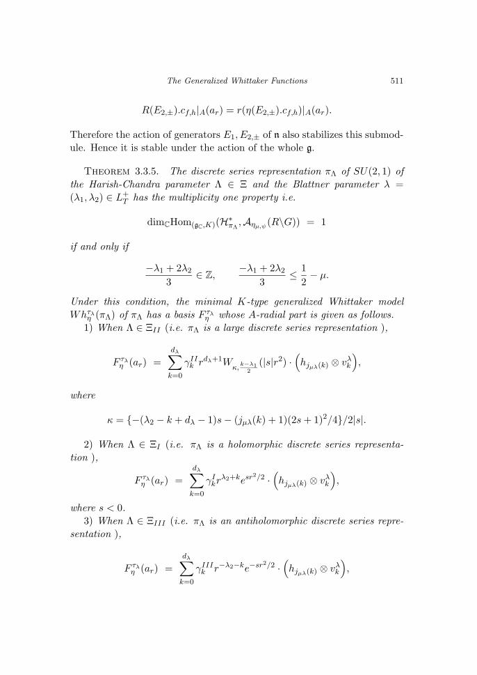
Theorem 3.3.5. The discrete series representation πΛ of SU(2, 1) of
the Harish-Chandra parameter Λ ∈ Ξ and the Blattner parameter λ =
(λ1, λ2) ∈ L+T has the multiplicity one property i.e.
dimCHom(gC,K)(H∗πΛ
,Aηµ,ψ(R\G)) = 1
if and only if
−λ1 + 2λ2
3∈ Z,
−λ1 + 2λ2
3≤ 1
2− µ.
Under this condition, the minimal K-type generalized Whittaker model
Whτλη (πΛ) of πΛ has a basis F τλ
η whose A-radial part is given as follows.
1) When Λ ∈ ΞII (i.e. πΛ is a large discrete series representation ),
F τλη (ar) =
dλ∑k=0
γIIk rdλ+1W
κ,k−λ1
2
(|s|r2) ·(
hjµλ(k) ⊗ vλk
),
where
κ = −(λ2 − k + dλ − 1)s− (jµλ(k) + 1)(2s + 1)2/4/2|s|.
2) When Λ ∈ ΞI (i.e. πΛ is a holomorphic discrete series representa-
tion ),
F τλη (ar) =
dλ∑k=0
γIkrλ2+kesr
2/2 ·(
hjµλ(k) ⊗ vλk
),
where s < 0.
3) When Λ ∈ ΞIII (i.e. πΛ is an antiholomorphic discrete series repre-
sentation ),
F τλη (ar) =
dλ∑k=0
γIIIk r−λ2−ke−sr2/2 ·
(hjµλ(k) ⊗ vλk
),

512 Yoshi-hiro Ishikawa
where s > 0.
Here r ∈ R>0, and the index of each basis hj of η is
jµλ(k) = k − 2λ1 − λ2
3− 1
2− µ.
Proof. The generalized Whittaker functions F ∈ Whτλη (πΛ) corre-
spond to the generalized Whittaker functionals l ∈ Hom(gC,K)(H∗πΛ
,
Aηµ,ψ(R\G)) are characterized as the solutions of (D) in Proposition 3.1.1
which satisfy the moderate growth condition. As we saw before the sys-
tem of differential equations (D) turn into differential equations (Γµλ)Jk
(J = I, II, III) for coefficient functions ck’s of F in Proposition 3.3.1
and Proposition 3.3.3. The moderate growth condition on F is translated
into that the coefficient functions are of moderate growth when r tends to
infinity. Recalling that the coefficient function is not a trivial function if
and only if
(3.3.2)−λ1 + 2λ2
3∈ Z,
−λ1 + 2λ2
3≤ 1
2− µ,
we know that differential equation (Γµλ)Jk has a non-trivial moderate growth
solution exactly when (3.3.2) holds. Hence we have the first half of the
assertion of Theorem. The rest is obvious. Indeed it is a direct consequence
of Theorem 3.3.2 and Theorem 3.3.4. Just arrange ck’s into
F (ar) =
dλ∑k=0
γJk ck(ar)
(hj ⊗ vλk
),
we have a basis of Whτλη (πΛ) of the form above.
4. The Case of Principal Series Representations
The preceding section was devoted to the discrete series case. We now
study in this section the principal series case and give an explicit formula
of the corner K-type generalized Whittaker functions. In this case, we
can obtain the differential equation satisfied by the generalized Whittaker
function in a much simpler way than the case of the discrete series rep-
resentations. We have only to calculate the A-radial part of the Casimir
operator explicitly in terms of coefficient functions.

The Generalized Whittaker Functions 513
4.1. Radial part of the Casimir operator
In this subsection we give the A-radial part of the Casimir operator.
Take
θ(E1), θ(E2,+), θ(E2,−), H, M1, E1, E2,+, E2,−as a basis of g where M1 =
√−1(H ′
13 −H ′23). Then the Casimir operator
can be defined by
Ω =1
2H2 − 1
6M2
1 −1
2E1θ(E1) + E2,+θ(E2,+) + E2,−θ(E2,−) − 2H1
with appropriate normalization of the Killing form. The eigen-value of Ω
can be calculated as 12ν2 + 1
6λ02 − 2 (cf. [K-O] 7.3 p.997).
The Casimir operator Ω ∈ U(gC) defines a unique differential operator R(Ω)
on the image of the restriction map resA : C∞η,τ (R\G/K)→ C∞(A ; S(R)⊗C
Vτ ) by
R(Ω).φ = (Ω.ϕ)|A.
Here we used the notation in subsection 3.2; φ means the restriction of
ϕ ∈ C∞η,τ (R\G/K) to A. We call R(Ω) the A-radial part of the Casimir
operator Ω, which is given as follows.
Proposition 4.1.1. Let φ ∈ C∞(A ; S(R)⊗C Vτ ) be the A-radial part
of ϕ ∈ C∞η,τ (R\G/K). Then the radial part R(Ω) of Ω is given by
R(Ω).φ =1
2∂2 − 4∂ +
1
3λ0
2 + r4η(E1)2
− 2√−1r2η(E1)τ(H ′
13) + r2(η(E2,+)2 + η(E2,−)2)
+ 2rη(E2+)τ(Xβ12 + Xβ21) + 2√−1rη(E2−)τ(Xβ12 −Xβ21)φ.
Proof. Decompose the opposite θ(E) of E as
θ(E) = (θ(E) + E)− E.
Here the symbol E represents either E1 or E2,±. Noting θ(E)+E ∈ k, E ∈n, we have
R(θ(E)).φ(ar) = τ(θ(E) + E).φ(ar)−R(E).φ(ar).

514 Yoshi-hiro Ishikawa
The action of k can be computed directly
θ(E1) + E1 = 2iH ′13,
θ(E2,+) + E2,+ = −2Xβ12 − 2Xβ21 ,
θ(E2,−) + E2,− = −2iXβ12 + 2iXβ21 .
Recall that the A-radial parts of E, H and M1 are given as
R(E1).φ(ar) = r2(η(E1).ϕ)|A(ar), R(E2,±).φ(ar) = r(η(E2,±).ϕ)|A(ar),
R(H).φ(ar) = ∂.φ|A(ar), R(M1).φ(ar) =√−1λ0 · φ|A(ar),
respectively. Then we get the assertion of Proposition.
4.2. An explicit formula and the multiplicity one theorem
Let F be the generalized Whittaker function associated to the principal
series representation πλ0,ν with the corner K-type τ(−λ0,−λ0) corresponding
to the generalized Whittaker functional l ∈ Iτ(−λ0,−λ0)πλ0,ν
,η . Since the func-
tion l(v∗) = 〈v∗, F ( )〉K ∈ IndGRη, v∗ ∈ τ∗(−λ0,−λ0) is an eigen-vector for
the Casimir operator Ω with eigen-value 12ν2 + 1
6λ02 − 2, F satisfies the
differential equation
(4.2.1) Ω.F = (1
2ν2 +
1
6λ0
2 − 2)F
accordingly.
Because of the one-dimensionality of the corner K-type of πλ0,ν , a func-
tion F which comes from l ∈ Hom(gC,K)(πλ0,ν , IndGRη) can be expanded as
F (g) = c0(g)(hj0 ⊗ v0
),
where v0 is a fixed generator of Vτ(−λ0,−λ0)and hj0 is the basis of S(R)
with j0 = −λ03 − 1
2 − µ (cf. subsection 3.2). Then we have the differential
equation for the A-radial part of c0.
Proposition 4.2.1. Let c0 be the coefficient function of the A-radial
part of F which comes from l ∈ Hom(gC,K)(τ(−λ0,−λ0), IndGRη). Then c0
satisfies the differential equation
(Γν)PS0 : ∂2 − 4∂ + G(r).c0(ar) = 0

The Generalized Whittaker Functions 515
with
G(r) = −s2r4 − 2λ0s + (2j0 + 1)(1 + 4s2)/2r2 − (ν2 − 4).
Proof. The assertion of Proposition is an immediate consequence of
(4.2.1) and Proposition 4.1.1. Indeed we first remark that the third line of
the expression of R(Ω) in Proposition 4.1.1 does not contribute to the action
on c0, since τ(−λ0,−λ0)(Xβ12) = τ(−λ0,−λ0)(Xβ21) = 0 for one dimensional
representation τ(−λ0,−λ0). We need only
τ(H ′13).v0 = −λ0v0.
Secondly using Lemma 2.3.3, we can see
η(E1)2.hj = −s2hj ,
η(E2,+)2.hj =1
4hj+2 −
2j + 1
2hj + j(j − 1)hj−2,(4.2.2)
η(E2,−)2.hj = −s2hj+2 − 2(2j + 1)s2hj − 4j(j − 1)s2hj−2,(4.2.3)
by direct computation. Again the one-dimensionality of the corner K-type
makes the η-action above much simpler. It forces all the terms but the
middle ones of the right hand side of (4.2.2), (4.2.3) vanish. Therefore we
have (Γν)PS0 .
We solve (Γν)PS0 and obtain an explicit form of the coefficient function
of the corner K-type generalized Whittaker function.
Theorem 4.2.2. The coefficient functions c0 of the A-radial part of the
corner K-type generalized Whittaker functions F ’s ∈ Whτ(−λ0,−λ0)η (πλ0,ν)
for the principal series representations πλ0,ν ’s of SU(2, 1) are of the form
c0(ar) = (const.)× rWκ, ν2(|s|r2)
with parameters
κ = −λ0s− (2j0 + 1)(4s2 + 1)/4/2|s|.

516 Yoshi-hiro Ishikawa
Here ar is an element of A, ν is the infinitesimal character of πλ0,ν , j0 =
−λ03 − 1
2 − µ, and Wκ,m(x) is the classical Whittaker function.
Proof. The procedure is quite similar to the case of the large discrete
series representation (Theorem 3.3.2). We just change the variable r by√x/|s|, and set
c0(ar) =
x
|s|
12
u0(x)
in order to transform (Γν)PS0 into the standard form
d2
dx2+
(−1
4+−λ0s− (2j0 + 1)(4s2 + 1)/4/2|s|
x
+14 − (ν2 )2
x2
)u0(x) = 0.
Here is a variant of the recent result of Tsuzuki which can be considered
to be an analogue of Proposition 3.1.1.
Proposition 4.2.3 ([Tsu] Theorem 9.2.1). Let πλ0,ν be an irreducible
principal series representation of G with the corner K-type τ(−λ0,−λ0), the
infinitesimal character ν and η be the representation in subsection 2.3. Then
the image of Hom(gC,K)(π∗λ0,ν
, IndGRη) by the correspondence of subsection
1.2 in C∞η,τ(−λ0,−λ0)
(R\G/K) is characterized by
R(Ω).F = (1
2ν2 +
1
6λ0
2 − 2) · F.
In short
Iτ(−λ0,−λ0)πλ0,ν
∼= Ker (R(Ω)− 1
2ν2 − 1
6λ0
2 + 2),
where Iτ(−λ0,−λ0)πλ0,ν
is the intertwining space Hom(gC,K)(τ∗(−λ0,−λ0), IndGRη).
The multiplicity one theorem for the principal series. By virtue
of Proposition 4.2.3, we have the next multiplicity one result for the prin-
cipal series representations.

The Generalized Whittaker Functions 517
Theorem 4.2.4. The irreducible principal series representation πλ0,ν
of SU(2, 1) has the multiplicity one property i.e.
dimCHom(gC,K)(π∗λ0,ν ,Aηµ,ψ(R\G)) = 1
if and only if
(4.2.4) −λ0
3− 1
2− µ ∈ Z≥0.
Under this condition, the corner K-type generalized Whittaker model
Whτ(−λ0,−λ0)η (πλ0,ν) has a basis F
τ(−λ0,−λ0)η whose A-radial part is given by
Fτ(−λ0,−λ0)η (ar) = rWκ, ν
2(|s|r2) ·
(hj0 ⊗ v0
),
where
κ = −λ0s− (2j0 + 1)(4s2 + 1)/4/2|s|.Here r ∈ R>0, and the index of the basis hj0 of η is
(4.2.5) j0 = −λ0
3− 1
2− µ.
Proof. The linear relation (3.2.1) of indices j and k turns into (4.2.5).
From the fact that j0 ∈ Z≥0, we have (4.2.4) as the necessary condition.
Conversely when (4.2.5) is valid, we can built up F of Proposition 4.2.3 by
defining its A-radial part via
F (ar) = rWκ,m(|s|r2) ·(
hj0 ⊗ v0
),
which satisfies the moderate growth condition.
5. The Fourier Expansion
Having explicit formulae of Whittaker and generalized Whittaker func-
tions for the standard representations of SU(2, 1) at our disposal, we are
ready to develop the theory of Fourier expansion of automorphic forms on
SU(2, 1) belonging to arbitrary standard representations.

518 Yoshi-hiro Ishikawa
5.1. The formulation of the Fourier expansion
We first formulate the Fourier expansion of automorphic forms by using
the spectral decomposition theory. The following argument works for an
arbitrary non-cocompact discrete subgroup Γ of G. But, for the sake of
simplicity, we assume that Γ is a congruence subgroup such that NΓ =
N ∩Γ contains (1, 0; 0) and (0, 1; 0) in the exponential coordinate of N . For
example group Γ = G ∩ SL3(Z[i]) satisfies the condition. In fact, for this
Γ, NΓ contains elements
(x, y; z) =
1− 12 |w|2 + (xy + z)i −w 1
2 |w|2 − (xy + z)i
w 1 −w
−12 |w|2 + (xy + z)i −w 1 + 1
2 |w|2 − (xy + z)i
,
w = x + yi ∈ (1 + i)Z[i], z ∈ Z. Here i means√−1 and |w|2 = x2 + y2.
Let Φ be an automorphic form on G with respect to Γ belonging to π with
K-type τ .
As NΓ\N is compact, the irreducible decomposition of the right regular
representation RegN of N on L2(NΓ\N) is given by
L2(NΓ\N) = ⊕σ∈N
mσ · Sσ,
where (σ,Sσ) is an NΓ-invariant unitary representation of N and mσ is
the multiplicity of the representation σ in RegN . This reads that a naive
Fourier expansion of Φ along N should be
Φ(ng) =∑σ∈N
mσ∑i=1
F π,τσ,(i)(ng),
where σ runs through the NΓ-invariant unitary representations of N . Here
F π,τσ,(i) is a smooth function in n ∈ N belonging to the i-th copy S(i)
σ of Sσ(i = 1, . . . , mσ). As we saw in Proposition 2.3.1, the unitary dual N of N
is exhausted by unitary characters ψu,v’s parameterized by (u, v) ∈ R2 and
infinite-dimensional irreducible unitary representations ρψs ’s determined by
their nontrivial central characters ψs’s: Stone von Neumann representa-
tions. When σ is a unitary character, its multiplicity mψu,v is one. Hence
we have
Φ(ng) =∑ψu,v
F π,τψu,v
(ng) +∑ρψs
mρ∑i=1
F π,τρψs ,(i)
(ng).

The Generalized Whittaker Functions 519
Expanding this with respect to the standard basis vτk dτk=0 of Vτ , we have
Φ(ng) =∑(u,v)
( dτ∑k=0
fπ,τ ;kψu,v
(ng)vτk
)+∑s
mρ∑i=1
( dτ∑k=0
f π,τ ;kρψs ,(i)
(ng)vτk
).
Parameters (u, v) and s run through discrete subsets of R2 and R\0 re-
spectively, which are determined by NΓ-invariantness.
But this formulation fails in general as we mentioned in introduction.
When σ is a Stone von Neumann representation ρψs , the generalized
Gelfant-Graev representation IndGNρψs , where the function f π,τ ;kρψs ,(i)
belongs,
is huge in the meaning below. To investigate the function f π,τ ;kρψs ,(i)
is to study
the intertwining space HomN (π∗|N , ρψs) which is isomorphic to
HomG(π∗, IndGNρψs) by Frobenius reciprocity. However this space is infinite-
dimensional and uncontrollable.
Now we remove the difficulty above and give a correct formulation of the
Fourier expansion of automorphic forms. Because of the next identifications
(see Lemma 2.3.2)
IndGNρψs∼= IndGR
(IndRNρψs
)ker(R→R)
∼= IndGR
(RegS ⊗ (ωψs × ρψs)|R
)ker(R→R)
∼= IndGR
(⊕
µ∈ 12
Z\Z
χµ ⊗ (ωψs × ρψs)|R)
∼=⊕
µ∈ 12
Z\Z
IndGR
(χµ ⊗ (ωψs × ρψs)|R
),
the intertwining space in question decomposes as
HomG(π∗, IndGNρψs)∼=
⊕µ∈ 1
2Z\Z
HomG(π∗, IndGRηχµψs).
We abbreviated χµ ⊗ (ωψs × ρψs)|R as ηχµψs . Accordingly, the function
fπ,τ ;kρψs ,(i)
can be expressed as
fπ,τ ;kρψs ,(i)
=∑
µ∈ 12
Z\Z
f π, τ ;kηχµψs ,(i)
,

520 Yoshi-hiro Ishikawa
where f π, τ ;kηχµψs ,(i)
’s are functions in the space of IndGRηχµ,ψs . Note that the
space
HomG(π∗, IndGRηχµ,ψs)
is the space of the generalized Whittaker functionals and the dimension of
it is always at most one. Hence we have a fine expansion:
Φ(ng) =∑(u,v)
( dτ∑k=0
fπ,τ ;kψu,v
(ng)vτk
)+∑s
mρ∑i=1
( dτ∑k=0
∑µ∈ 1
2Z\Z
f π, τ ;kηχµψs ,(i)
(ng)vτk
).
Here is the Fourier expansion of a Vτ -valued automorphic form Φ on G
along N :
Φ(ng) =∑(u,v)
( dτ∑k=0
c Φ,τ ;kψu,v
(g) · ψu,v(n)vτk
)
+∑s
mρ∑i=1
( dτ∑k=0
∑µ∈ 1
2Z\Z
∑j∈N
c Φ , τ ; kηχµψs (i) ; j(g) · θρψs (i)
j (n)vτk
),
where θρψs (i)j j∈N is a basis of the i-th copy S(i)
ρψs ⊂ L2(NΓ\N) of Sρψs .
5.2. Generalized theta functions
In the explicit formulae of generalized Whittaker functions obtained in
subsection 3.3 and subsection 4.2, the Hermitian functions hj appeared, as
the consequence of our choice of a basis of the Shrodinger model (ρψs ,S(R))
of a Stone von Neumann representation σ of N . In this subsection, we
construct θρψs (i)j in L2(NΓ\N) as the image of hj by an N -intertwiner
T : S(R)→ L2(NΓ\N).
In other word, we realize a Stone von Neumann representation σ in
L2(NΓ\N). For the purpose, we write down the Hermite descending op-
erator by elements of U(n) and translate it by T . Then we have the dif-
ferential equation which is satisfied by the image θρψs (i)0 = T (h0) of h0.
Using quasi-periodicity of θρψs (i)0 , which comes from NΓ-invariantness, we

The Generalized Whittaker Functions 521
can solve the differential equation and obtain an explicit form of θρψs (i)0 .
Finally, by using the raising operator recursively, we obtain the following
form of θρψs (i)j = T (hj). Essentially the same argument can be found in
[Mum].
Theorem 5.2.1. (1) The image of N -intertwiner T in L2(NΓ\N) is
zero unless the central character’s parameter s of the Schrodinger model
ρψs is of the form
s = 2πM,
where M is a non-zero integer.
(2) Assume s = 2πM (M ∈ Z\0), then there are 2|M| non-trivial N -inter-
twiners T (i) : S(R) → L2(NΓ\N), where i = 1, . . . , 2|M|. Moreover we can
take
(5.2.1) θ5, (i)0 (x, y; z) =
∑k∈Z
e−(x+ i+2||k2
)2/2 · e[(i + 2|M|k)y + Mxy + Mz]
as the image θ5, (i)0 of h0 by T (i). As for the image θ
5, (i)j of hj by T (i),
(5.2.2) θ5, (i)j (x, y; z) =
∑k∈Z
hj
(x +
i + 2|M|k2M
)· e[(i + 2|M|k)y + Mxy + Mz]
can be taken. Here we denote e2π√−1X by e[X] and exp(xE2,++yE2,−+zE1)
by (x, y; z) (the exponential coordinate on N ; see subsection 2.1).
Proof. The generator E1 of the center of n acts on θ ∈ L2(NΓ\N) by
multiplying√−1s; the derivative of ψs at 0. By the relation (2.1.1),(
RegN (exp tE2,+).θ)(
exp(xE2,+ + yE2,− + zE1))
= θ(
exp((x + t)E2,+ + yE2,− + (z − yt)E1))
,
hence we have
RegN (E2,+) =∂
∂x−√−1sy.
Similarly
RegN (E2,−) =∂
∂y+√−1sx.
522 Yoshi-hiro Ishikawa
Note that the zero-th Hermite function h0(ξ) is annihilated by the descend-
ing operator a = ξ + ddξ . This operator is written as
a =1
2√−1s
ρψs(E2,−) + ρψs(E2,+)
on the Srodinger model (ρψs ,S(R)), accordingly
a =1
2√−1s
(∂
∂y+√−1sx) + (
∂
∂x−√−1sy)
on the realization of σ in L2(NΓ\N). Therefore θρψs , (i)0 satisfies the differ-
ential equation
(5.2.3)
(∂
∂x−√−1sy) +
1
2√−1s
(∂
∂y+√−1sx)
.θρψs , (i)0
)(x, y; z) = 0.
On the coordinate E1, we can separate the variable z as
θρψs , (i)0 (x, y; z) = G0(x, y) · e
√−1sz.
The NΓ-invariantness of θρψs , (i)0 requires that the parameter s should be
of the form s = 2πM, M ∈ Z, and that the function G0 should satisfy a
quasi-periodicity;
(5.2.4) G0(x + m, y + n) = G0(x, y) · e√−1s(nx−my),
for n, m ∈ Z (cf. 2.1.1). Set G0(x, y)e2π√−15xy = G0(x, y), then the differ-
ential equation (5.2.3) and the quasi-periodicity (5.2.4) turn into
∂
∂x+ x +
1
2√−1s
∂
∂y
G0(x, y) = 0,(5.2.5)
G0(x + m, y + n) = G0(x, y) · e−4π√−15my,(5.2.6)
for n, m ∈ Z. By the assumption on Γ, G0(x, y) is periodic in variable y
with period 1. Partial Fourier expansion of G0 in y tells
G0(x, y) =∑k′∈Z
g0,k′(x)e2π√−1k′y.

The Generalized Whittaker Functions 523
In terms of g0,k′ , (5.2.5) and (5.2.6) fall into
d
dx+ x +
k′
2M
g0,k′(x) = 0,
g0,k′(x + m) = g0,k′+25m(x),
for all m ∈ Z. By taking m = 1, which is possible because of our choice of
Γ, we know that the solution space for (5.2.5) is of dimension 2|M| and has
a basis consisting of
∑k∈Z
e−(x+ i+2||k2
)2/2 · e[(i + 2|M|k)y],
i = 1, . . . , 2|M|. This gives (5.2.1) and the claim that there are 2|M| non-trivial
N -intertwiners T (i)’s.
The raising operator a† = ξ − ddξ is written as
a† =1
2√−1s
(∂
∂y+√−1sx)− (
∂
∂x−√−1sy).
The action of a† on the k′-th term (k′ = i + 2|M|k)
e−(x+k′/2)2
2 · e[k′y + Mxy + Mz]
of θ5, (i)0 becomes the action on e−
(x+k′/2)22 = h0(x + k′/2M):
a†.h0(ξ) = − d
dξh0(ξ) + ξ · h0(ξ),
where ξ = x + k′/2M. This is equal to h1(ξ) = h1(x + k′/2M) by definition of
the Hermite function. Recursively, we have the expression (5.2.2) of θ5, (i)j .
Proposition 5.2.2. Theta functions constructed above satisfy the or-
thogonality;
(θ5, (i)j , θ
5, (i′)j′ )L2 = 2jj!
√πδjj′δii′ .

524 Yoshi-hiro Ishikawa
Here δmn denotes the Kronecker symbol and ( , )L2 means the inner product
on L2(NΓ\N) normalized as
(f, g)L2 :=
∫N
f(n)g(n)dn,
where f, g ∈ L2(NΓ\N), dn is the NΓ-invariant Haar measure on N carried
from the Lebesgue measure on R3.
Proof. Easily seen by the orthogonality of the Hermite functions.
5.3. An explicit form of the Fourier expansion
Now we can give an explicit form of the Fourier expansion of an auto-
morphic form belonging to an arbitrary standard representation π with a
special K-type.
Theorem 5.3.1. Let Φ be an automorphic form on SU(2, 1) belonging
to π with K-type τ . Then the Fourier expansion of Φ is given as follows.
i) When π is a discrete series representation πΛ with Blattner parameter
λ = (λ1, λ2) ∈ Z⊕2, put jk = k − 2λ1−λ2
3 − 12 − µ and take the minimal
K-type τλ as τ .
i-1) The case of large discrete series i.e. π = πΛ, Λ ∈ Ξ+II
Φ(nar) = C Φ0,0 · rdλ+2 · 1N (n)vλλ1
+∑
(5,5′)∈Z2\(0,0)
CΦ5,5′
( dλ∑k=0
γkrdλ+ 32 W0,k−λ1(4π
√M2 + M′2r)
· ψ2π5,2π5′(n)vλk
)+
∑5∈Z\0
2|5|∑i=1
∑µ∈ 1
2Z\Z
C Φµ,5, (i)
( dλ∑k=0
γIIk rdλ+1W
κ,k−λ1
2
(2π|M|r2)
· θ5, (i)jk(n)vλk
),
where
κ = −(λ2 − k + dλ − 1)2πM− (jk + 1)(4πM + 1)2/4/4π|M|.

The Generalized Whittaker Functions 525
i-2) The case of holomorphic discrete series i.e. π = πΛ, Λ ∈ Ξ+I
Φ(nar) =∞∑
−5=0
2|5|∑i=1
∑µ∈ 1
2Z\Z
C Φµ,5, (i)
( dλ∑k=0
γIkrλ2+keπ5r
2 · θ5, (i)jk(n)vλk
).
i-3) The case of antiholomorphic discrete series i.e. π = πΛ, Λ ∈ Ξ+III
Φ(nar) =∞∑5=0
25∑i=1
∑µ∈ 1
2Z\Z
C Φµ,5, (i)
( dλ∑k=0
γIIIk r−λ2−ke−π5r2 · θ5, (i)jk
(n)vλk
).
In these cases, the index µ runs over half integers which satisfy jk ≥ 0.
ii) When π is a principal series representation πλ0,ν = IndGP (1N ⊗eν⊗χλ0),
put j0 = −λ03 − 1
2 − µ and take the corner K-type τ(−λ0,−λ0) as τ .
Φ(nar) = C Φ0,0 · rν+2 · 1N (n)v0
+∑
(5,5′)∈Z2\(0,0)
C Φ5,5′ · r
32 W0,ν(4π
√M2 + M′2r) · ψ2π5,2π5′(n)v0
+∑
5∈Z\0
2|5|∑i=1
∑µ∈ 1
2Z\Z
C Φµ,5, (i) · rWκ, ν
2(2π|M|r2) · θ5, (i)j0
(n)v0,
where
κ = −λ02πM− (2j0 + 1)(16π2M2 + 1)/4/4π|M|.
In this case, the index µ runs over half integers such that −µ ≥ λ03 + 1
2 .
Generalized theta functions θ5, (i)j ’s are given in (5.2.1), (5, 2, 2). We call
C Φ5,5′’s, C Φ
µ,5, (i)’s the Fourier coefficients of Φ.
Proof. This is an immediate consequence of our previous argument.
Here we just note that parameters appearing in explicit formulae (Theorem
3.3.5, Theorem 4.2.4 and [K-O] Theorem 4.5, l.12 p.998) s and η+η− should
be of the form 2πM, M ∈ Z\0 and −4π2(M2 + M′2), (M, M′) ∈ Z2\(0, 0) by
the same reason in proof of Theorem 5.2.1.

526 Yoshi-hiro Ishikawa
References
[Co-Gr] Corwin, L. and F. P. Greenleaf, Representation of nilpotent Lie groupsand their applications Part1:Basic theory and examples, CambridgeStudies in Adv. Math. 18 (1990).
[Er] Erderlyi, A. et al., Higher Transcendental functions, Vol.2, McGraw-Hillbook company, inc., (1953).
[Ge-Ro] Gelbart, S. and J. Rogawski, L-functions and Fourier-Jacobi coefficientsfor the unitary group U(3), Invent. Math. 105 (1991), 445–472.
[K-O] Koseki, H. and T. Oda, Whittaker functions for the large discrete seriesrepresentations of SU(2, 1) and related zeta integral, Publ. RIMS KyotoUniv. 31 (1995), 959–999.
[M-O-S] Magnus, W., Oberhettinger, F. and R. P. Soni, Formulas and Theoremsfor the Special Functions of Mathematical Physics, 3rd ed., Springer-Verlag, (1966).
[Mum] Mumford, D., Tata Lectures on Theta III , Birkhauser, Progress in Math-ematics, 97 (1991).
[PS] Piatetski-Shapiro, I., Tate theory for reductive groups and distinguishedrepresentations, Proc. Int. Cong. Math., Helsinki (1978), 585–590.
[PS2] Piatetski-Shapiro, I., Automorphic Functions and the Geometry of theClassical Domains, Gordon and Breach, N.Y., (1969).
[Sch] Schmid, W., On realization of the discrete series of a semisimple Liegroup, Rice University Studies 56 (1970), 99–108.
[Sha] Shalika, J. A., The multiplicity one theorem for GLn, Ann. of Math. 100(1974), 171–193.
[Tsu] Tsuzuki, M., Real Shintani functions and multiplicity free property forthe symmetric pair (SU(2, 1), S(U(1, 1)× U(1))), preprint, (1996).
[Vo] Vogan, D. Jr., Gelfand Kirillov dimension for Harish-Chandra modules,Invent. Math. 49 (1978), 75–98.
[Ya] Yamashita, H., Finite multiplicity theorems for induced representationsof semisimple Lie groups II: Applications to generalized Gelfand-Graevrepresentations , J. Math. Kyoto Univ. 28 (1988), 383–444.
[Ya2] Yamashita, H., Embedding of discrete series into induced representationsof semisimple Lie groups I: General theory and the case of SU(2, 2),Japan. J. Math. 16 (1990), 31–95.
(Received November 13, 1998)(Revised February 17, 1999)
The Graduate School of Natural Science and TechnologyOkayama UniversityNaka 3-1-1, Tushima, Okayama700-8530, JapanE-mail: [email protected]