the geodesic problem in quasimetric spacesqlxia/research/geodesic.pdfthe geodesic problem in...

J Geom Anal (2009) 19: 452–479DOI 10.1007/s12220-008-9065-4

The Geodesic Problem in Quasimetric Spaces

Qinglan Xia

Received: 30 July 2008 / Published online: 7 February 2009© Mathematica Josephina, Inc. 2009. This article is published with open access at Springerlink.com

Abstract In this article, we study the geodesic problem in a generalized metricspace, in which the distance function satisfies a relaxed triangle inequality d(x, y) ≤σ(d(x, z) + d(z, y)) for some constant σ ≥ 1, rather than the usual triangle inequal-ity. Such a space is called a quasimetric space. We show that many well-known re-sults in metric spaces (e.g. Ascoli-Arzelà theorem) still hold in quasimetric spaces.Moreover, we explore conditions under which a quasimetric will induce an intrinsicmetric. As an example, we introduce a family of quasimetrics on the space of atomicprobability measures. The associated intrinsic metrics induced by these quasimetricscoincide with the dα metric studied early in the study of branching structures arisen inramified optimal transportation. An optimal transport path between two atomic prob-ability measures typically has a “tree shaped” branching structure. Here, we showthat these optimal transport paths turn out to be geodesics in these intrinsic metricspaces.

Keywords Optimal transport path · Quasimetric · Geodesic distance · Branchingstructure

Mathematics Subject Classification (2000) Primary 54E25 · 51F99 · Secondary49Q20 · 90B18

1 Introduction

This article aims at studying some classical analysis problems in semimetric spaces,in which the distance is not required to satisfy the triangle inequity. During the au-

This work is supported by an NSF grant DMS-0710714.

Q. Xia (�)Department of Mathematics, University of California at Davis, Davis, CA 95616, USAe-mail: [email protected]: http://math.ucdavis.edu/~qlxia

mailto:[email protected]

http://math.ucdavis.edu/~qlxia

The Geodesic Problem in Quasimetric Spaces 453

thor’s recent study of optimal transport path between probability measures, he ob-serves that there exists a family of very interesting semimetrics on the space ofatomic probability measures. These semimetrics satisfy a relaxed triangle inequalityd(x, y) ≤ σ(d(x, z)+d(z, y)) for some constant σ ≥ 1, rather than the usual triangleinequality. Such semimetric spaces are called quasimetric spaces1 in [6]. Moreover,these family of quasimetrics indeed induce a family of intrinsic metrics on the spaceof atomic probability measures. Furthermore, optimal transport paths studied earlyin [10–14] etc turn out to be exactly geodesics in these induced metric spaces. Thisobservation motivates us to study the geodesic problem in quasimetric spaces in thisarticle. Other closely related works on ramified optimal transportation may be foundin [3–5, 7] etc.

This article is organized as follows. In Sect. 2, we first introduce the concept aswell as some basic properties of quasimetric spaces, then we extend some well-knownresults (e.g. Ascoli-Arzelà theorem) about continuous functions in metric spaces tocontinuous functions in quasimetric spaces. After that, in Sect. 3, we consider thegeodesic problem in quasimetric spaces. We show that every continuous quasimetricwill induce an intrinsic pseudometric on the space. In case that the quasimetric isnice enough (e.g. either “ideal” or “perfect” in the sense of Definition 2.5 or Defini-tion 3.14), then the quasimetric will indeed induce an intrinsic metric. In the end, wespend the last section in discussing our motivation example: optimal transport pathsbetween atomic probability measures. We first introduce a family of quasimetrics onthe space of atomic probability measures. Each of these quasimetric is both idealand perfect, and thus it induces an intrinsic metric on the space of atomic probabilitymeasures. We showed that the dα-metrics introduced in [10] is simply the intrinsicmetrics induced by these quasimetrics. Furthermore, each geodesic in these lengthspaces corresponds to an optimal transport path studied in [10].

2 Continuous Maps in Quasimetric Spaces

2.1 Quasimetric Spaces

Definition 2.1 Let X be any nonempty set. A function J : X × X → R is called aquasimetric if for any x, y, z ∈ X, we have

(1) (non-negativity) J (x, y) ≥ 0;(2) (identity of indiscernibles) J (x, y) = 0 if and only if x = y

(3) (symmetry) J (x, y) = J (y, x);(4) (relaxed triangle inequality) J (x, y) ≤ σ [J (x, z) + J (z, y)] for some constant

σ ≥ 1.

When J is a quasimetric on X, the pair (X,J ) is called a quasimetric space. Letσ(J ) denote the smallest number σ satisfying condition (2.1).

1When this article was submitted, the author used the term “nearmetric” as in [8] instead of “quasimetric”.Later, Professor Nigel Kalton kindly let the author know the term “quasimetric” used in the book [6]. Thus,in the final version of the article, we replaced the previous term “nearmetric” with this more suitable term“quasimetric”.

454 Q. Xia

Every metric space is clearly a quasimetric space with σ = 1.

Example 2.2 Suppose d is a metric on a nonempty set X. Then, for any β > 1,λ ≥ 0,μ > 0, J (x, y) = λd(x, y) + μd(x, y)β is typically not a metric on X. How-ever, J defines a quasimetric on X with σ(J ) ≤ 2β−1. Indeed,

J (x, y) = λd(x, y) + μd (x, y)β

≤ λ[d(x, z) + d(y, z)

]+ μ[d(x, z) + d(y, z)

]β

≤ λ[d(x, z) + d(y, z)

]+ 2β−1μ[d(x, z)β + d(y, z)β

]

≤ 2β−1 [J (x, z) + J (z, y)].

In Section 4 we will provide a family of interesting quasimetrics on the space ofatomic probability measures.

More generally, suppose J is a distance function on X satisfying condi-tions (2.1), (2.1), (2.1) in Definition 2.1. For each n, let σn(J ) be the smallest numberσn ≥ 1 satisfying

J (x1, xn+1) ≤ σn

n∑

i=1

J (xi, xi+1) , (2.1)

for any x1, . . . , xn+1 ∈ X. In particular, σ1(J ) = 1 and σ2(J ) = σ(J ).

Lemma 2.3 Suppose (X,J ) is a quasimetric space. Then, for each n,

σn (J ) ≤ σ (J )n−1 .

Proof We show this using the mathematical induction. It is trivial when n = 1 or 2.Then, from condition (2.1), we see that for any n and any points {x1, x2, . . . , xn} inX, we have

J (x1, xn) ≤ σ (J ) (J (x1, xn−1) + J (xn−1, xn))

≤ σ (J )

(

σ (J )n−2n−2∑

i=1

J (xi, xi+1) + J (xn−1, xn)

)

≤ σ (J )n−1n−1∑

i=1

J (xi, xi+1) since σ (J ) ≥ 1.

Therefore, σn(J ) ≤ σ(J )n−1 for all n. �

Proposition 2.4 Suppose (X,J ) is a quasimetric space. Then, for each n and m in N,

σnm (J ) ≤ σn (J )σm (J ) .


Proof Note that, for any {x1, x2, . . . , xmn+1} in X, from (2.1), we have

J (x1, xmn+1)

≤ σn (J )(J (x1, xm+1) + J (xm+1, x2m+1) + · · · + J

(x(n−1)m+1, xnm+1

))

≤ σn (J )

⎛

⎝σm (J )

m∑

i=1

J (xi, xi+1) + · · · + σm (J )

nm∑

i=(n−1)m+1

J (xi, xi+1)

⎞

⎠

= σn (J )σm (J )

nm∑

i=1

J (xi, xi+1) .

Therefore,

σnm (J ) ≤ σn (J )σm (J ) . �

Clearly, σn(J ) is nondecreasing as n increases. Thus, we define

σ∞ (J ) := limn

σn (J ) (2.2)

for any quasimetric J on X.

Definition 2.5 Suppose J is a quasimetric on X. If σ∞(J ) < ∞, then J is called anideal quasimetric on X.

Note that J is an ideal quasimetric if and only if for some σ ≥ 1,

J (x, y) ≤ σ

n∑

i=1

J (xi, xi+1) , (2.3)

for any finitely many points x1,. . . , xn+1 ∈ X with x1 = x, xn+1 = y. The smallest σ

satisfying (2.3) is just σ∞(J ).A sequence {xn} is convergent to x in a quasimetric space (X,J ) if J (xn, x) → 0,

and we denote it by xnJ→ x. A sequence {xn} is Cauchy in (X,J ) if for any ε > 0,

there exists an N ∈ N such that J (xn, xm) ≤ ε for all n,m ≥ N . Since J (xn, xm) ≤σ(J )(J (xn, x) + J (x, xm)), it follows that every convergent sequence in (X,J ) is aCauchy sequence. If every Cauchy sequence in (X,J ) is convergent, then we say J

is a complete quasimetric on X. A quasimetric J on X always gives a topology on X

where a subset A is closed if it contains every point a ∈ X for which there is somesequence ai ∈ A with limi→∞ J (ai, a) = 0.

Definition 2.6 A quasimetric J on X is continuous if for any convergent sequences

xnJ→ x, yn

J→ y, we have

J (xn, yn) → J (x, y) , as n → ∞. (2.4)

456 Q. Xia

If for any convergent sequences xnJ→ x, yn

J→ y, we have

J (x, y) ≤ lim infn

J (xn, yn) , (2.5)

then we say J is lower semicontinuous.

For instance, suppose J satisfies conditions (2.1), (2.1), (2.1) in Definition 2.1,and also the following condition

|J (x, y) − J (z,w)| ≤ σ (J (x, z) + J (w,y)) (2.6)

for any x, y, z,w ∈ X and some σ ≥ 1. By setting z = w, we get J (x, y) ≤σ [J (x, z) + J (z, y)], and hence J is a quasimetric on X. Also, since for each n,

|J (xn, yn) − J (x, y)| ≤ σ (J (x, xn) + J (y, yn)) ,

J is automatically satisfying the continuous condition (2.4 ) in this case. When J isindeed a metric on X, then (2.6) trivially holds.

2.2 Continuous Maps in Quasimetric Spaces

In this section, we extend some well-known results (see for instance in [9] or [1])about continuous maps in metric spaces to continuous maps in quasimetric spaces.

Suppose (X,J ) is a quasimetric space, and K is a compact metric space with ametric dK . A map f : K → (X,J ) is continuous if J (f (xn), f (x)) → 0 in X when-ever dK(xn, x) → 0 in K as n → ∞. A map f : K → (X,J ) is uniformly contin-uous if for every ε > 0, there exists a δ > 0 such that J (f (x), f (y)) ≤ ε wheneverx, y ∈ K with dK(x, y) ≤ δ. A map f : K → (X,J ) is Lipschitz if there exists aconstant C ≥ 0 such that

J (f (x) , f (y)) ≤ CdK(x, y)

for any x, y ∈ K . Let C(K, (X,J )) be the family of all continuous maps from K to(X,J ), and Lip(K, (X,J )) be the family of all Lipschitz maps from K to (X,J ).

Proposition 2.7 Suppose J is a continuous quasimetric on X. Then, every continu-ous map f : K → (X,J ) is uniformly continuous.

Proof Suppose f : K → (X,J ) is continuous. If f is not uniformly continuous, thenthere exists an ε > 0, and two sequences {xn}, {yn} in K such that d(xn, yn) ≤ 1

n, but

J (f (xn), f (yn)) ≥ ε. By the compactness of K and taking subsequence if necessary,we may assume that both {xn} and {yn} converge to the same point x∗ ∈ K . So, bythe continuity of J in (2.4) and the continuity of f at x∗, we have

0 = J(f(x∗) , f

(x∗))= lim

n→∞J (f (xn) , f (yn)) ≥ ε.

A contradiction. Thus, f must be uniformly continuous. �


For any maps f,h : K → (X,J ), let

J∞ (f,h) := supx∈K

J (f (x) ,h (x)) . (2.7)

If J∞(fn, f ) → 0, then we say that fn is uniformly convergent to f .

Proposition 2.8 Suppose J is a quasimetric on X. Then, J∞ is a quasimetric onC(K, (X,J )).

Proof For any f,h ∈ C(K, (X,J )), by definition (2.7), we have J∞(f,h) ≥ 0 andJ∞(f,h) = J∞(h,f ). Also, J∞(f,h) = 0 if and only if f (x) = h(x) for all x ∈ K .Moreover, for any g ∈ C(K, (X,J )),

J∞ (f,h) = supx∈K

J (f (x) ,h (x))

≤ supx∈K

σ (J )[J (f (x) , g (x)) + J (g (x) ,h (x))

]

≤ σ (J )

[supx∈K

J (f (x) , g (x)) + supx∈K

J (g (x) ,h (x))

]

= σ (J )[J∞ (f, g) + J∞ (g,h)

].

Therefore, (C(K, (X,J )), J∞) is also a quasimetric space. �

Proposition 2.9 Suppose {fn : K → (X,J )} is a sequence of continuous maps. IfJ∞(fn, f ) → 0, then f is also continuous.

Proof Since J∞(fn, f ) → 0, for any ε > 0 , there exists an n such that

supx∈K

J (fn (x) , f (x)) ≤ ε/3. (2.8)

For any x ∈ K , since fn is continuous at x, there exists a δ = δ(x) > 0 such thatJ (fn(x), fn(y)) ≤ ε/3 whenever y ∈ K with dK(x, y) ≤ δ. Therefore, by lemma 2.3and (2.8), we have

J (f (x) , f (y)) ≤ σ (J )2 [J (f (x) , fn (x)) + J (fn (x) , fn (y))

+ J (fn (y) , f (y))]

≤ εσ (J )2

and thus f is continuous at every x ∈ K . �

Theorem 2.10 Suppose (X,J ) is a complete quasimetric space and J is lowersemicontinuous. Then, the space (C(K, (X,J )), J∞) is also a complete quasimet-ric space.

458 Q. Xia

Proof Let {fn} be any Cauchy sequence in C(K, (X,J )) with respect to J∞. That is,for any ε > 0, there exists an N such that whenever m,n ≥ N , we have J∞(fn, fm) ≤ε. So, for each x ∈ K , {fn(x)} is Cauchy in X. Since X is complete, {fn(x)} con-verges to some f (x) ∈ X with respect to J . Now,

J∞ (fn, f ) = supx∈K

J (fn (x) , f (x))

≤ supx∈K

limm→∞J (fn (x) , fm (x)) , because J is lower semicontinuous

≤ lim supm→∞

[supx∈K

J (fn (x) , fm (x))

]≤ ε

So, J∞(fn, f ) → 0. By proposition 2.9, f is continuous. Hence, by proposition 2.8,J∞ is a complete quasimetric on C(K, (X,J )). �

Definition 2.11 A subset F of C(K, (X,J )) is equicontinuous if for every x ∈ K

and ε > 0, there is a δ = δ(x, ε) > 0, such that whenever y ∈ K with dK(x, y) ≤ δ,we have J (f (x), f (y)) ≤ ε for all f ∈ F .

Now, we have the following Ascoli-Arzelà theorem in quasimetric spaces:

Theorem 2.12 Suppose (X,J ) is a complete quasimetric space and J is lower semi-continuous. A subset F of (C(K, (X,J )), J∞) is precompact if and only if it isbounded and equicontinuous.

Proof Suppose F is a precompact (i.e. every sequence has a convergent subsequence)subset of C(K, (X,J )). Then, for each fixed ε > 0 , there exists a finite subset{f1, . . . , fk} of F such that

F ⊂k⋃

i=1

Bε/3 (fi) , (2.9)

where the notation Bε(g) = {h ∈ C(K, (X,J ))|J∞(g,h) < ε}. Otherwise, for anyfinite subset {f1, . . . , fk}, there exists an fk+1 /∈⋃k

i=1 Bε/3(fi), and thus we get asequence {fk} in F . Since J∞(fm,fn) ≥ ε/3 for any m = n, we know {fn} does notcontain any Cauchy subsequence, which contradicts to F being precompact. There-fore, (2.9) must be true, which also implies that F is bounded.

Now, for any x ∈ K and each fi in (2.9), there exists a δi > 0 such that whenevery ∈ K with dK(x, y) < δi , we have J (fi(x), fi(y)) ≤ ε

3 . For every f ∈ F , by (2.9),there is an 1 ≤ i ≤ k such that J∞(f,fi) ≤ ε

3 . We conclude that for any y ∈ K withdK(x, y) < δ = min{δ1, . . . , δk}, we have

J (f (x) , f (y)) ≤ σ (J )2 [J (f (x) , fi (x)) + J (fi (x) , fi (y)) + J (fi (y) , f (y))]

≤ εσ (J )2 .

Therefore, F is equicontinuous at every x ∈ K .


On the other hand, suppose F is equicontinuous and bounded. Then, for any se-quence {fn} in F , by using the diagonal process and taking subsequence if necessary,we may assume {fn} is convergent to f on a countable dense subset S in K . Wenow prove that {fn} is Cauchy in C(K, (X,J )) with respect to J∞. Indeed, for anyε > 0, since F is equicontinuous and K is compact, there exists a finite many points{r1, . . . , rk} in S such that for any x ∈ K , there is a ri , such that

J (fn (x) , fn (ri)) ≤ ε

3

for all n. Now, whenever m,n are large enough, for all x ∈ K ,

J (fn (x) , fm (x))

≤ σ (J )2 [J (fn (x) , fn (ri)) + J (fn (ri) , fm (ri)) + J (fm (ri) , fm (x))]

≤ σ (J )2 ε.

Therefore, {fn} is a Cauchy sequence in C(K, (X,J )). By the completeness ofC(K, (X,J )) stated in theorem 2.10, the sequence {fn} is convergent with respectto J∞. Thus, F is precompact. �

Corollary 2.13 Suppose (X,J ) is a complete quasimetric space and J is lower semi-continuous. A subset F of C(K, (X,J )) is sequentially compact with respect to J∞if and only if it is closed, bounded and equicontinuous.

3 Intrinsic Metrics Induced by Quasimetrics

This section is devoted to study the geodesic problem in a quasimetric space (X,J ).Let [a, b] be a bounded closed interval.

Definition 3.1 Let N be a natural number. A curve f ∈ C([a, b], (X,J )) is called anN -piecewise metric Lipschitz curve in (X,J ) if there exists a partition

Pf = {a = a0 < a1 < · · · < aN = b}of [a, b] such that for each i = 0,1, . . . ,N − 1,

(1) J is a metric on the subset f ([ai, ai+1]) of X and(2) the restriction of f on [ai, ai+1] is Lipschitz.

Here, requiring J to be a metric on f ([ai, ai+1]) is the same as asking it to satisfythe triangle inequality: J (f (t1), f (t2)) ≤ J (f (t1), f (t2)) + J (f (t2), f (t3)) for anyt1, t2, t3 ∈ [ai, ai+1]. Let

PN ([a, b] , (X,J ))

be the family of all N−piecewise metric Lipschitz curves in (X,J ), and P ([a, b],(X,J )) be the union of PN([a, b], (X,J )) over all N ’s.

460 Q. Xia

3.1 Length of Rectifiable Curves

Recall that when (X,d) is a metric space, and f : [a, b] → (X,d) is a (continuous)curve. Then, one may define its length as

L(f ) = supP

VP (f ) ∈ [0,+∞] ,

where the supremum is over all partitions P of [a, b], and VP (f ) is the variation off over the partition P = {a = t0 < t1 < · · · < tN = b} given by

VP (f ) =N∑

i=1

d (f (ti−1) , f (ti)) .

In case f is Lipschitz, an equivalent formula for the length of f is

L(f ) =∫ b

a

∣∣f (t)∣∣ddt,

where |f (t)|d is the metric derivative of f at f (t) defined by

∣∣f (t)∣∣d

:= lims→t

d (f (s) , f (t))

|s − t | ,

provided the limit exists. When f is Lipschitz, |f (t)|d exists almost everywhere, andis bounded and measurable in t .

Now, suppose (X,J ) is a quasimetric space, and f ∈ PN([a, b], (X,J )). Thenon each interval [ai, ai+1], f : [ai, ai+1] → (X,J ) is a Lipschitz curve in the metricspace (f ([ai, ai+1]), J ), and thus the length of the restriction of f on [ai, ai+1] iswell defined. As a result, we may define the length of f to be

L(f ) :=N−1∑

i=0

L(f [ai ,ai+1]

).

In other words, we have

Definition 3.2 For any f ∈ PN([a, b], (X,J )), the length of f is defined as

LJ (f ) :=∫ b

a

∣∣f (t)∣∣J

dt,

where the metric derivative

∣∣f (t)∣∣J

:= lims→t

J (f (s) , f (t))

|s − t |provided the limit exists. We may simply write LJ (f ) as L(f ) if J is obvious.


Lemma 3.3 Suppose J is a continuous quasimetric on X, C > 0 is a constant, andP = {a = a0 < a1 < · · · < aN = b} is a partition of the interval [a, b]. Then, for anyx, y ∈ X, the family

F ={

f ∈ C ([a, b] , (X,J )) : f (a) = x,f (b) = y, and J is a metric on

f ([ai, ai+1]) and Lip(f [ai ,ai+1]) ≤ C, for each i = 0, . . . ,N − 1

}

is a bounded, closed and equicontinuous subset of C([a, b], (X,J )). Moreover, if fn

is uniformly convergent to f in J∞, then,

L(f ) ≤ lim infn

L (fn) .

Proof For any g ∈ F and any t ∈ [a, b], we have t ∈ [aj , aj+1] for some j ≤ N − 1and

J (g (t) , x) = J (g (t) , g (a))

= σ (J )j

⎛

⎝j−1∑

i=0

J (g (ai) , g (ai+1)) + J(g(aj

), g (t)

)⎞

⎠

≤ σ (J )j C |t − a| ≤ Cσ (J )N−1 |b − a|Therefore, F is bounded.

Suppose {fn} is any convergent sequence in F with respect to J∞ with f ∈C([a, b], (X,J )) being the limit. Then, for each fixed i, and any t1, t2, t3 ∈ [ai, ai+1],we have

J (fn (t1) , fn (t2)) ≤ J (fn (t1) , fn (t3)) + J (fn (t3) , fn (t2))

and

J (fn (t1) , fn (t2)) ≤ C |t1 − t2| .Let n → ∞, we have J is a metric on f ([ai, ai+1]) and Lip(f [ai, ai+1]) ≤ C.Therefore, f ∈ F . This shows that F is closed and also equicontinuous. Moreover,for any partition Q of [ai, ai+1], the variation

VQ

(f [ai, ai+1

])= limn

VQ

((fn) [ai, ai+1

])≤ lim infn

L((fn) [ai, ai+1

]).

So,

L(f [ai, ai+1

])= supQ

VQ

(f [ai, ai+1

])≤ lim infn

L(fn[ai, ai+1

]).

Hence,

L(f ) =N−1∑

i=0

L(f [ai ,ai+1]

)≤

N−1∑

i=0

lim infn

L(fn[ai ,ai+1]

)= lim inf

nL (fn) .

�

462 Q. Xia

Proposition 3.4 Suppose (X,J ) is a quasimetric space, and f ∈ PN([a, b], (X,J )).If L(f ) = 0, then f is a constant map.

Proof L(f ) = 0 implies that L(f [ai ,ai+1]) = 0 for each i. Thus, f is a constant on[ai, ai+1] for each i. Since f is continuous, f is a constant on [a, b]. �

Since any Lipschitz curve in a metric space has an arc parametrization, by applyingarc parametrizations piecewisely, we also have

Proposition 3.5 (Reparametrization) For any f ∈ PN([a, b], (X,J )) and L =L(f ), there exists a homeomorphism φ : [0,L] → [a, b] so that γ = f ◦ φ ∈PN([0,L], (X,J )) has |γ (t)|J = 1 almost everywhere in [0,L].

3.2 The Geodesic Problem

Let N be a fixed natural number. For any x, y ∈ X, we consider the geodesic problem

min{L(f )} (3.1)

among all f in the family

PathN (x, y) = {f ∈ PN ([0,1] , (X,J )) with f (0) = x;f (1) = y} .

Note that, by a linear change of variable, one may replace [0,1] in PathN(x, y)

by any closed interval [a, b] without changing the infimum value in the geodesicproblem (3.1).

Definition 3.6 Suppose J is a quasimetric on X. For any x, y ∈ X, and N ∈ N, define

D(N)J (x, y) = inf {LJ (f ) : f ∈ PathN (x, y)}

whenever PathN(x, y) is not empty, and set D(N)J (x, y) = ∞ when PathN(x, y) is

empty. Since D(N)J (x, y) is a decreasing function of N , we define

DJ (x, y) = limN→∞D

(N)J (x, y) .

Theorem 3.7 Suppose J is a continuous complete quasimetric on a nonempty set X.For any N ∈ N, and x, y ∈ X, the geodesic problem (3.1) admits a solution f ∈PathN(x, y) provided that PathN(x, y) is not empty. So, L(f ) = D

(N)J (x, y).

Proof Suppose PathN(x, y) is not empty. Let L = inf{L(f ) : f ∈ PathN(x, y)}. Notethat for each f ∈ PathN(x, y), we have

J (x, y) ≤ σ (J )N−1N−1∑

i=0

J (f (ai) , f (ai+1))


≤ σ (J )N−1N−1∑

i=0

L(f [ai ,ai+1]

)= σ (J )N−1 L(f ) .

This implies that if L = 0, then we have J (x, y) = 0. Therefore, x = y and the con-stant f (t) ≡ x is the desired solution.

So, without losing generality, we may assume that L > 0. Let {fn} be a lengthminimizing sequence in PathN(x, y) with L(fn) → L. Let

Pfn ={

0 = a(n)0 < a

(n)1 < · · · < a

(n)N = 1

}

be the partition of [0,1], associated with fn. By reparametrization if necessary, wemay assume that each fn is Lipschitz with Lip(fn) ≤ 1.5L on [a(n)

i , a(n)i+1] for each

i = 0, . . . ,N − 1. Then, by choosing a subsequence if necessary, we may assumethat each sequence {a(n)

i } is convergent to some point ai as n → ∞ for each i =0,1, . . . ,N . Using a linear change of variable, we may assume that for each i, a

(n)i =

ai and Lip(fn) ≤ 2L on [ai, ai+1]. Now, {fn} is a sequence in the family

F ={

f ∈ C ([0,1] , (X,J )) : f (0) = x,f (1) = y, and J is a metric on

f ([ai, ai+1]) and Lip(f [ai ,ai+1]) ≤ 2L, for each i = 0, . . . ,N − 1

}

.

By Lemma 3.3, F is a bounded, closed and equicontinuous subset of C([0,1], (X,J )).By the Ascoli-Arzelà theorem shown in corollary 2.13, a subsequence {fnk

} of {fn}in F is uniformly convergent to some f ∈ F with respect to J∞. By the lower semi-continuity of L in the family F , we have L(f ) ≤ lim infk L(fnk

) = L. Therefore,f is a length minimizer in PathN(x, y). �

Note that each D(N)J is a semimetric2 on X in the sense that D

(N)J (x, y) ≥ 0,

D(N)J (x, y) = 0 if and only if x = y, and D

(N)J (x, y) = D

(N)J (y, x). In general, D

(N)J

may fail to satisfy the triangle inequality. Nevertheless, we have

D(n+m)J (x, y) ≤ D

(n)J (x, z) + D

(m)J (z, y)

for any m,n and x, y, z ∈ X. As a result, by letting N → ∞, we have

Proposition 3.8 Suppose J is a quasimetric on X, then DJ is a peudometric3 on X.

Since DJ is a pseudometric, DJ is a metric on X if and only if

DJ (x, y) > 0 whenever x = y.

2A function d : X × X → [0,+∞) is a semimetric on X if d satisfies conditions (2.1), (2.1), (2.1) inDefinition 2.1. So, a semimetric d is not required to satisfy the triangle inequality.3A function d : X × X → [0,+∞) is a pseudometric on X if d satisfies conditions (2.1), (2.1) in Defini-tion 2.1, and the triangle inequality d(x, y) ≤ d(x, z) + d(z, y) for any x, y, z ∈ X. But d(x, y) = 0 doesnot necessarily imply x = y.

464 Q. Xia

When DJ becomes a metric on X. This metric is called the intrinsic metric, or geo-desic distance, on X induced by the quasimetric J .

3.3 Examples of Metrics Induced by Quasimetrics

Now, we are interested in cases that DJ is indeed a metric on X.

3.3.1 Ideal Quasimetrics

Let J be any semimetric on X. For any x, y ∈ X, we set

dJ (x, y)

to be the infimum ofn−1∑

i=1

J (xi, xi+1)

over all finitely many points x1, . . . , xn ∈ X with x1 = x and xn = y.This dJ defines a pseudometric on X, but not necessarily a metric on X.

Example 3.9 For instance, let X = [0,1] and J (x, y) = |x − y|p for some p > 1defines a quasimetric on X. Then, for each n,

dJ (0,1) ≤n−1∑

i=0

J

(i

n,i + 1

n

)

=n−1∑

i=0

(1

n

)p

= 1

np−1→ 0 as n → ∞.

Thus, dJ (0,1) = 0, but 0 = 1. Hence dJ is not a metric on X. Also, note that inthis example, PathN(x, y) is empty whenever x = y. Thus, DJ (x, y) = ∞ wheneverx = y.

As in the case of DJ , dJ is a metric on X if and only if

dJ (x, y) > 0 whenever x = y.

Note also that

dJ (x, y) ≤ D(N)J (x, y)

for each N , and thus,

dJ (x, y) ≤ DJ (x, y) .

Therefore, dJ (x, y) > 0 will automatically imply DJ (x, y) > 0. As a result, we have

Proposition 3.10 Suppose J is a quasimetric on X. If dJ is a metric on X andDJ (x, y) < ∞ for every x, y ∈ X, then DJ also defines a metric on X.


Remark 3.11 When J is indeed a metric on X, then both dJ and DJ are metrics. Inthis case, dJ is just the metric J itself, while DJ is the intrinsic metric induced by J .

In general, by means of definition, we have

dJ (x, y) ≤ J (x, y) ≤ σ∞ (J ) dJ (x, y) ,

where σ∞(J ) is defined as in (2.2).Now, suppose J is an ideal quasimetric, then σ∞(J ) < ∞ and J satisfies the

condition

J (x1, xn) ≤ σ∞ (J )

n−1∑

i=1

J (xi, xi+1)

for any finitely many points {x1, x2, . . . , xn} ⊂ X. Clearly, we have the followingproposition:

Proposition 3.12 Suppose (X,J ) is an ideal quasimetric space. Then for any N andany f ∈ PN([a, b], (X,J )), we have

J (f (a) , f (b)) ≤ σ∞ (J )L (f ) .

Lemma 3.13 Suppose J is an ideal quasimetric on X. Then, dJ is a metric on X.Moreover, if DJ (x, y) < ∞ for every x, y ∈ X, then DJ also defines a metric on X.

Proof This is simply because when x = y, dJ (x, y) ≥ 1σ∞(J )

J (x, y) > 0. �

3.3.2 Perfect Quasimetrics

Here is another kind of quasimetric J which also induces a metric DJ .

Definition 3.14 A quasimetric J on X is a perfect near metric if for any x, y ∈ X, thevalue D

(N)J (x, y) becomes a real valued constant DJ (x, y) when N is large enough.

Since for each N , D(N)J (x, y) = 0 if and only if x = y, we have the following

theorem.

Proposition 3.15 On a perfect quasimetric space (X,J ), DJ defines a metric on X.

When J is indeed a metric on X, then for each N , the metric D(N)J agrees with

the intrinsic metric induced by J . Thus, every metric space is automatically a perfectquasimetric space. In Sect. 4, we will discuss a family of very important perfectquasimetric spaces, which are not metric spaces.

Theorem 3.16 Suppose (X,J ) is a perfect quasimetric space, and the geodesic prob-lem (3.1) has solution for N large enough. Then, (X,DJ ) is a length space in the

466 Q. Xia

sense that for every x, y ∈ X, there exists a curve f : [0,L] → (X,DJ ) such thatf (0) = x, f (L) = y and

DJ (f (t) , f (s)) = |t − s|for every t, s ∈ [0,L] where L = DJ (x, y).

Proof For every x, y ∈ X, since (X,J ) is a perfect quasimetric space, we haveD

(N)J (x, y) = DJ (x, y) < ∞ whenever N is large enough. Now, for each large

enough N , there exists a curve f : [0,L] → (X,J ) such that f is the length min-imizer in PathN(x, y) with L(f ) = D

(N)J (x, y) = DJ (x, y). Without losing general-

ity, we may assume f has its arc parametrization. Now for any 0 ≤ s < t ≤ L, wehave

DJ (f (s) , f (t)) ≤ L(f [s,t]

)=∫ t

s

∣∣f∣∣J

dt = t − s.

Similarly, DJ (f (0), f (s)) ≤ s and DJ (f (t), f (L)) ≤ L − t . Thus, we have

L = DJ (x, y) ≤ DJ (f (0) , f (s)) + DJ (f (s) , f (t)) + DJ (f (t) , f (L))

≤ s + (t − s) + (L − t) = L.

Therefore, all inequalities becomes equalities at every step and for any t, s ∈ [0,L],we have DJ (f (t), f (s)) = |t − s|. �

Corollary 3.17 Suppose J is a complete, continuous, perfect quasimetric on X.Then, (X,DJ ) is a length space.

The curve f in Theorem 3.16 is called a geodesic from x to y in the perfectquasimetric space (X,J ).

4 Optimal Transport Paths as Geodesics

We now begin to introduce a family of both ideal and perfect quasimetrics on thespace of atomic probability measures.

4.1 A Family of Quasimetrics on the Space of Atomic Probability Measures

Let (Y, d) be any metric space. For any y ∈ Y , let δy be the Dirac measure centeredat y. An atomic probability measure in Y is in the form of

m∑

i=1

aiδyi

with distinct points yi ∈ Y , and ai > 0 with∑m

i=1 ai = 1.


Given two atomic probability measures

a =m∑

i=1

aiδxiand b =

n∑

j=1

bj δyj(4.1)

in Y , a transport plan from a to b is an atomic probability measure

γ =m∑

i=1

n∑

j=1

γij δ(xi ,yj ) (4.2)

in the product space Y × Y such that

m∑

i=1

γij = bj andn∑

j=1

γij = ai (4.3)

for each i and j . Let Plan(a,b) be the space of all transport plans from a to b.For any α < 1, we now introduce the functional Hα on transport plans. For any

atomic probability measure γ in Y × Y of the form (4.2), we define

Hα (γ ) :=m∑

i=1

n∑

j=1

(γij

)αd(xi, yj

),

where d is the given metric on Y .Using Hα , we may define

Definition 4.1 For any two atomic probability measures a,b on Y , and α < 1, define

Jα (a,b) := min {Hα (γ ) : γ ∈ Plan (a,b)} .

For any given natural number N ∈ N, let AN(Y ) be the space of all atomic proba-bility measures

m∑

i=1

aiδxi

on Y with m ≤ N , and A(Y ) =⋃N AN(Y ) be the space of all atomic probabilitymeasures on Y .

Proposition 4.2 Jα defines a quasimetric on AN(Y ) with σ(Jα) ≤ N1−α .

Proof For any a,b ∈ AN(Y ) in the form of (4.1), clearly Jα(a,b) ≥ 0 and Jα(a,b) =Jα(b,a).

If Jα(a,b) = 0, then there exists a γ ∈ Plan(a,b) such that Hα(γ ) = 0. Thus,d(xi, yj ) = 0 whenever γij = 0. Since {yj }’s are distinct, at most one of γij can benonzero for each i. On the other hand, by (4.3), at least one of γij must be nonzero

468 Q. Xia

for each i. Therefore, for each i, there is a unique j = σ(i) such that xi = yj andγij = ai = bj . This shows that a = b.

Now, we prove that J satisfies the relaxed triangle inequality as in condition (2.1)in Definition 2.1. Indeed, for any

a =m∑

i=1

aiδxi, b =

n∑

j=1

bj δyjand c =

h∑

k=1

ckδzk

in AN(Y ), and any

uca =

m∑

i=1

h∑

k=1

uikδ(xi ,zk) ∈ Path (a, c) , τbc =

n∑

j=1

h∑

k=1

τkj δ(zk,yj ) ∈ Path (c,b) ,

we denote

γij =h∑

k=1

uikτkj

ck

for each i, j . Note that

m∑

i=1

γij =m∑

i=1

(h∑

k=1

uikτkj

ck

)

=h∑

k=1

(m∑

i=1

uikτkj

ck

)

=h∑

k=1

τkj = bj

and similarly∑

j γij = ai . Therefore, we find a transport plan

γ =m∑

i=1

n∑

j=1

γij δ(xi ,yj ) ∈ Plan (a,b) .

We now want to show

Hα (γ ) ≤ N(Hα

(uc

a)+ Hα

(τb

c

)).

Indeed,

Hα (γ ) =m∑

i=1

n∑

j=1

(γij

)αd(xi, yj

)=m∑

i=1

n∑

j=1

(h∑

k=1

uikτkj

ck

)α

d(xi, yj

)

≤m∑

i=1

n∑

j=1

h∑

k=1

(uikτkj

ck

)α (d (xi, zk) + d

(zk, yj

)), because α < 1

=m∑

i=1

h∑

k=1

⎛

⎝n∑

j=1

(uikτkj

ck

)α⎞

⎠d (xi, zk)

+n∑

j=1

h∑

k=1

(m∑

i=1

(uikτkj

ck

)α)

d(zk, yj

)


≤ N1−α

⎛

⎝m∑

i=1

h∑

k=1

(uik)α d (xi, zk) +

n∑

j=1

h∑

k=1

(τkj

)αd(zk, yj

)⎞

⎠

= N1−α(Hα

(uc

a)+ Hα

(τb

c

)),

where the 2nd inequality follows from the inequality∑N

i=1(ti)α ≤ N1−α(

∑Ni=1 ti )

α .Therefore, by taking infimum, we have

Jα (a,b) ≤ N1−α (Jα (a, c) + Jα (c,b)) . �

Proposition 4.3 Suppose (Y, d) is a complete metric space. Then, Jα is a completequasimetric on AN(Y ).

Proof Let {an} be any Cauchy sequence in AN(Y ). Then, for any ε > 0, there existsa natural number N , such that

Jα (an,am) ≤ ε

whenever n,m ≥ N . Note that each atomic probability measure an may be expressedas

an =N∑

i=1

a(n)i δ

x(n)i

for some a(n)i ≥ 0,

∑Ni=1 a

(n)i = 1 and x

(n)i ∈ Y .

Now, let γ (n,m) be an Hα minimizer in Plan(an,am) with

Jα (an,am) = Hα

(γ (n,m)

).

This transport plan γ (n,m) is expressed as

γ (n,m) =N∑

i,j=1

γ(n,m)ij δ(

x(n)i ,x

(m)j

)

for some γ(n,m)ij ≥ 0 with

∑Ni=1 γ

(n,m)ij = a

(m)j and

∑Nj=1 γ

(n,m)ij = a

(n)i for all i, j =

1,2, . . . ,N .By picking a subsequence if necessary, without losing generality, we may use the

diagonal argument and assume that for all i, j = 1,2, . . . ,N and all n ≥ N

γ(n,m)ij → γ

(n)ij

as m → ∞. Then, for each i, j and each n ≥ N , we have

N∑

i=1

γ(n)ij = lim

m→∞

N∑

i=1

γ(n,m)ij = lim

m→∞a(m)j and

N∑

j=1

γ(n)ij = a

(n)i . (4.4)

470 Q. Xia

Let

aj = limm→∞a

(m)j

for each j . If aj > 0, then by (4.4), there exists an i such that γ(n)ij > 0. So

d(x

(n)i , x

(m)j

)≤ Hα(γ (n,m))

[γ (n,m)ij ]α

= Jα(an,am)

[γ (n,m)ij ]α

which implies that{x

(m)j

}∞m=1

is a Cauchy sequence in the complete metric space (Y, d). Thus, x(m)j → xj as m →

∞ for some xj ∈ Y .Let

a =∑

aj >0

aj δxj∈ AN (Y )

and for each n ≥ N , let

γ (n) =∑

ij

γ(n)ij δ(

x(n)i ,xj

).

Then, γ (n) ∈ Plan(an,a) and

Jα (an,a) ≤ Hα

(γ (n)

)

=∑

ij

[γ

(n)ij

]αd(x

(n)i , xj

)

= limm→∞

∑

ij

[γ

(n,m)ij

]αd(x

(n)i , x

(m)j

)

= limm→∞Jα (an,am) ≤ ε.

Therefore, {an} is (subsequentially) convergent to a in (AN(Y ), Jα). This shows thatAN(Y ) is complete with respect to the quasimetric Jα . �

Note that, in general, Jα may fail to be a metric on AN(Y ) as demonstrated in thefollowing example.

Example 4.4 For any α < 1, let y be a positive real number. Then, we consider threeatomic measures in Y = R

2 :

a = 1

2δ(−1,y+1) + 1

2δ(1,y+1), b = δ(0,0) and c = δ(0,y).


Then,

Jα (a, c) + Jα (c,b) − Jα (a,b)

= 2

(1

2

)α √2 + y − 2

(1

2

)α√1 + (y + 1)2 < 0

whenever y is large enough. Thus, Jα does not satisfy the triangle inequality.

4.2 Optimal Transport Paths between Atomic Probability Measures

Now, we want to show that the quasimetric Jα is both ideal and perfect. To achievethese results, we first recall some concepts about optimal transport paths betweenprobability measures as studied in [10].

Let a and b be two fixed atomic probability measures in the form of (4.1).

Definition 4.5 A transport path from a to b is a weighted directed graph G consistsof a vertex set V (G), a directed edge set E(G) and a weight function

w : E (G) → (0,+∞)

such that {x1,x2, . . . , xk} ∪ {y1, y2, . . . , yl} ⊂ V (G) and for any vertex v ∈ V (G),

∑

e∈E(G)

e−=v

w (e) =∑

e∈E(G)

e+=v

w (e) +

⎧⎪⎪⎨

⎪⎪⎩

ai, if v = xi for some i = 1, . . . , k,

−bj , if v = yj for some j = 1, . . . , l,

0, otherwise

(4.5)

where e− and e+denotes the starting and ending endpoints of each edge e ∈ E(G).

Remark 4.6 The balance equation (4.5) simply means that the total mass flows intov equals to the total mass flows out of v. When G is viewed as a polyhedral chain orcurrent, (4.5) can be simply expressed as

∂G = b − a.

Also, when G is viewed as a vector valued measure, the balance equation is simply

div(G) = a − b

in the sense of distributions.

Let Path(a,b) be the space of all transport paths from a to b.

Definition 4.7 For any α ≤ 1, and any G ∈ Path(a,b), define

Mα (G) :=∑

e∈E(G)

w (e)α length (e) .

472 Q. Xia

Remark 4.8 In [10], the parameter α was restricted in [0,1]. Later, the author ob-served that α < 0 is also very interesting, and related to studying the dimension offractals. So, negative α is also allowed here.

We first recite two lemmas that were proved in [10, Proposition 2.1] and [10,Definition 7.1 and Lemma 7.1] respectively.

Lemma 4.9 For any transport path G ∈ Path(a,b), there exists another transportpath G ∈ Path(a,b) such that

Mα

(G)

≤ Mα (G) ,

the set of vertices V (G) ⊂ V (G) and G contains no cycles.

Here, a weighted directed graph G = {V (G),E(G),W : E(G) → (0,1]} containsa cycle if for some k ≥ 3, there exists a list of distinct vertices {v1, v2, . . . , vk} inV (G) such that for each i = 1, . . . , k, either the segment [vi, vi+1] or [vi+1, vi] is adirected edge in E(G), with the agreement that vk+1 = v1. When a directed graph G

contains no cycles, it becomes a directed tree.

Lemma 4.10 For any transport path G ∈ Path(a,b) containing no cycles, there ex-ists

(1) an m × n real matrix

u = (uij

)with

uij ≥ 0,

m∑

i=1

uij = bj ,

n∑

j=1

uij = ai for each i, j andm∑

i=1

n∑

j=1

uij = 1,

(2) and an m × n matrix

g = (gij

)

with each gij is either 0 or an oriented polyhedral curve gij from xi to yj ,

such that

G =∑

i,j

uij gij

as real coefficients polyhedral chains.

By means of Lemma 4.9, it is easy to see that for each α ≤ 1, there exists anoptimal transport path in Path(a,b) which minimizes the cost functional Mα .

For the sake of visualization we provide some numerical simulations (see theforthcoming paper [15]) for different values of α.


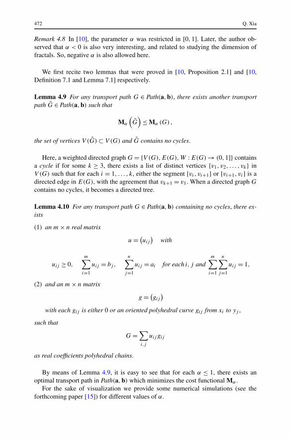
Fig. 1 A family of optimal transport paths from 50 random points to a single point

Example 4.11 Let {xi} be 50 random points in the square [0,1] × [0,1]. Then, {xi}determines an atomic probability measure

a =50∑

i=1

1

50δxi

.

Let b = δO where O = (0,0) is the origin. Then an optimal transport path from a tob looks like Fig. 1 with α = 1,0.75,0.5 and 0.25 respectively.

Example 4.12 Let {xi} be 100 random points in the rectangle [−2.5,2.5] × [0,1].Then, {xi} determines an atomic probability measure

a =100∑

i=1

1

100δxi

.

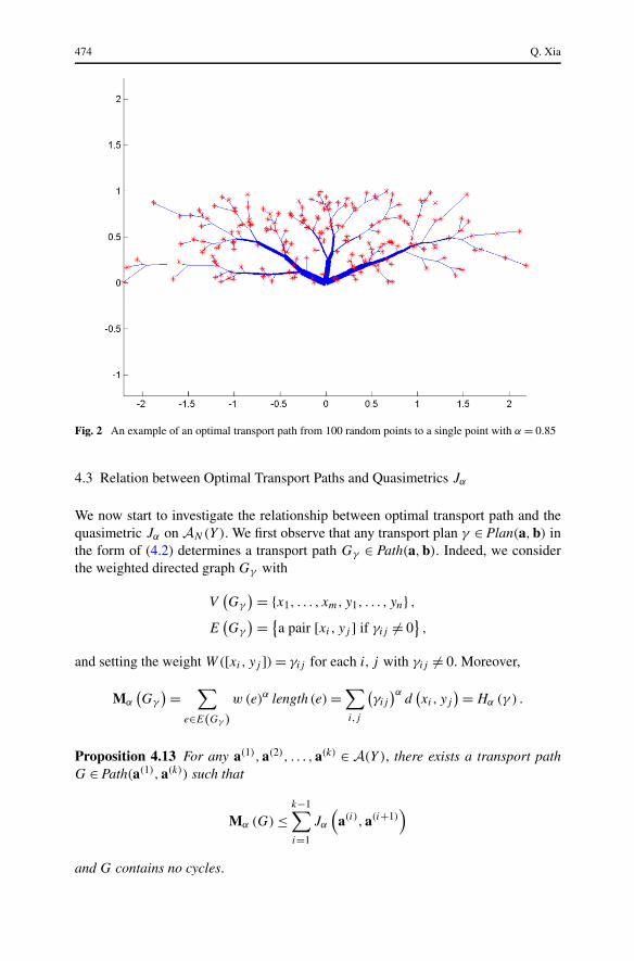
Let b = δO where O = (0,0) is the origin, and let α = 0.85. Then an optimal trans-port path from a to b looks like Fig. 2.

474 Q. Xia

Fig. 2 An example of an optimal transport path from 100 random points to a single point with α = 0.85

4.3 Relation between Optimal Transport Paths and Quasimetrics Jα

We now start to investigate the relationship between optimal transport path and thequasimetric Jα on AN(Y ). We first observe that any transport plan γ ∈ Plan(a,b) inthe form of (4.2) determines a transport path Gγ ∈ Path(a,b). Indeed, we considerthe weighted directed graph Gγ with

V(Gγ

) = {x1, . . . , xm, y1, . . . , yn} ,

E(Gγ

) = {a pair [xi, yj ] if γij = 0},

and setting the weight W([xi, yj ]) = γij for each i, j with γij = 0. Moreover,

Mα

(Gγ

)=∑

e∈E(Gγ )

w (e)α length (e) =∑

i,j

(γij

)αd(xi, yj

)= Hα (γ ) .

Proposition 4.13 For any a(1),a(2), . . . ,a(k) ∈ A(Y ), there exists a transport pathG ∈ Path(a(1),a(k)) such that

Mα (G) ≤k−1∑

i=1

Jα

(a(i),a(i+1)

)

and G contains no cycles.


Proof Let γi be an optimal transport path from a(i) to a(i+1), for each i =1,2, . . . , k − 1. Each γi determines a transport path Gγi

∈ Path(a(i),a(i+1)) as above.Then, viewed as real coefficients polyhedral chains,

G =k−1∑

i=1

Gγi

is a transport path from a(1) to a(k). Moreover, we have

Mα (G) ≤k−1∑

i=1

Mα

(Gγi

)=k−1∑

i=1

Hα (γi) =k−1∑

i=1

Jα

(a(i),a(i+1)

).

By Lemma 4.9, there exists a transport path G from a(1) to a(k) such that G containsno cycles, V (G) ⊂ V (G), and

Mα

(G)

≤ Mα (G) ≤k−1∑

i=1

Jα

(a(i),a(i+1)

).

�

Theorem 4.14 Jα is an ideal quasimetric on AN(Y ) with σ∞(Jα) ≤ N2(1−α).

Proof For any k ∈ N and any points {a(1),a(2), . . . ,a(k)} ⊂ AN(Y ), by proposi-tion 4.13, there exists a transport path G ∈ Path(a(1),a(k)) such that

Mα (G) ≤k−1∑

i=1

Jα

(a(i),a(i+1)

)

and G contains no cycles. Moreover, by Lemma 4.10, there exists a matrix (uij ) ofreal numbers and a metric (gij ) of polyhedral curves such that

G =∑

ij

uij gij

as real coefficients polyhedral chains. Let

γ =∑

ij

uij δ(xi ,yj )

be any transport plan in Plan(a(1),a(k)). Then,

Hα (γ ) =∑

ij

(uij

)αd(xi, yj

)≤∑

ij

(uij

)αlength

(gij

)

=∑

e∈E(G)

⎛

⎝∑

gij contains e

(uij

)α⎞

⎠ length (e)

476 Q. Xia

≤∑

e

⎛

⎝N2(1−α)

⎛

⎝∑

gij contains e

uij

⎞

⎠

α⎞

⎠ length (e)

= N2(1−α)∑

e∈E(G)

(w (e))α length (e)

= N2(1−α)Mα (G) ≤ N2(1−α)

k−1∑

i=1

Jα

(a(i),a(i+1)

).

Therefore,

Jα

(a(1),a(k)

)≤ N2(1−α)

k−1∑

i=1

Jα

(a(i),a(i+1)

)

and thus Jα is an ideal quasimetric on AN(Y ) with σ∞(Jα) ≤ N2(1−α). �

Suppose (Y, d) is a geodesic metric space. That is, for any x, y ∈ Y , there existsa Lipschitz curve �x,y : [0,1] → (Y, d) with �x,y(0) = x, �x,y(1) = y and lengthL(�x,y) = d(x, y).

Lemma 4.15 Suppose (Y, d) is a geodesic metric space. Let G ∈ Path(a,b) forsome a,b ∈AN(Y ). If each edge of G is a geodesic curve between its endpointsin the metric space Y , then there exists a piecewise metric Lipschitz curve g ∈PNG

([0,1], (AN(Y ), Jα)) such that

LJα (g) = Mα (G) ,

where NG is total number of edges in the graph G.

Proof We may prove it using the mathematical induction on NG. When NG = 1, G

itself is a geodesic in Y . Then, it is clearly true in this case. Now, assume NG > 1.Pick an edge e of G with its starting endpoint e− being a vertex in a. Let

a = a + w (e) (δe+ − δe−) ,

where e+ is the targeting endpoint of the directed edge e, and w(e) is the as-sociated weight on e. Removing edge e from G, we get another transport pathG ∈ Path(a, b). Then, N

G= NG − 1 ≥ 1. By the principle of the mathematical in-

duction, we may assume that G corresponds to a piecewise metric Lipschitz curveg ∈ PN

G([0,1], (AN(Y ), Jα)) such that

LJα (g) = Mα

(G)

.

Now, let

g (t) ={

g( tλ), 0 ≤ t ≤ λ,

�e(t−λ1−λ

), λ ≤ t ≤ 1,


where λ = NG−1NG

, and �e is the associated geodesic in Y from e− to e+. Then, g ∈PNG

([0,1], (AN(Y ), Jα)) and

LJα (g) = LJα (g) + LJα (�e) = Mα

(G)

+ w (e)α length (e) = Mα (G) . �

Remark 4.16 From this lemma, we see that for any transport path G ∈ Path(a,b) ina geodesic metric space (Y, d), we have a simple formula for the transport cost:

Mα (G) =∫ 1

0|g (t)|Jα

dt.

On the other hand, in [2], the authors studied another kind of ramified transportationin which the cost of a path is given by

∫ 1

0|g (t)|W J (g (t)) dt

where W is the Wasserstein distance on probability measures, and J is some functionon the space of atomic probability measures. It is interesting to see this differencebetween these two different approaches.

Theorem 4.17 Suppose (Y, d) is a geodesic metric space. Then, Jα is a perfect qua-simetric on AN(Y ), and thus it induces a metric DJα on AN(Y ).

Proof Suppose a,b are two points in AN(Y ). For any f ∈ Pk([0,1], (AN(Y ), Jα))

with f (0) = a and f (1) = b, there exists a partition P = {0 = a0 < · · · < ak = 1} of[0,1] such that Jα is a metric on f ([ai, ai+1]) and f [ai ,ai+1] is Lipschitz for eachi = 0,1, . . . , k − 1. Let xi = f (ai) for each i, by Proposition 4.13, there exists atransport path G from f (0) = a to f (1) = b such that

Mα (G) ≤∑

Jα (xi, xi+1) ≤∑

i

L(f [ai ,ai+1]

)= L(f )

and G contains no cycles.When (Y, d) is a geodesic metric space, each edge of G isrealized by a geodesic curve between its endpoints. By Lemma 4.15, G determinesa curve g ∈ PNG

([0,1], (AN(Y ), Jα)) with L(g) = Mα(G) ≤ L(f ). Since a,b ∈AN(Y ) and G ∈ Path(a,b), the total number of vertices of G with degree one isno more than 2N . Since G contains no cycles, the total number NG of edges ofG is no more than 4N − 3. Thus, g ∈ P4N−3([0,1], (AN(Y ), Jα)). Hence, for anya,b ∈ AN(Y ),

D(k)Jα

(a,b) = D(4N−3)Jα

(a,b)

for any k ≥ 4N − 3. This shows that Jα is a perfect quasimetric on AN(Y ). �

Corollary 4.18 Suppose (Y, d) is a geodesic metric space. Then, for any a,b ∈AN(Y ) and α ≤ 1, we have

DJα (a,b) = min {Mα (G) : G ∈ Path (a,b)} .

478 Q. Xia

Proof Let G be any optimal transport path from a to b. From the proof of the abovetheorem, we see DJα(a,b) ≤ Mα(G) ≤ L(f ) for any f ∈ Pk([0,1], (AN(Y ), Jα))

with k ≥ 4N − 3. Hence, DJα(a,b) = Mα(G). �

Corollary 4.19 Suppose (Y, d) is a geodesic metric space. Then, (AN(Y ),DJα ) is alength space.

Proof By Corollary 4.18, each optimal transport path G determines a solution g tothe geodesic problem (3.1). Then, by Theorem 3.16, (AN(Y ),DJα ) becomes a lengthspace. �

Since A1(Y ) ⊂ A2(Y ) ⊂ · · · ⊂ AN(Y ) ⊂ · · · , and (AN(Y ),DJα ) is a length spacefor each N , we have

Proposition 4.20 Suppose (Y, d) is a geodesic metric space. Then, DJα is a metricon the space A(Y ) of all atomic probability measures on Y . Moreover, (A(Y ),DJα )

is a length space.

We now give some conclusive remarks.

Remark 4.21 In [10], we defined dα(a,b) := min{Mα(G) : G ∈ Path(a,b)} for0 ≤ α < 1 and showed that dα defines a metric on the space of (atomic) probabil-ity measures. Moreover, we showed (A(Y ), dα) is a length space. Now, from Corol-lary 4.18, we see that dα = DJα . That is, the metric dα is just the intrinsic metric onA(Y ) induced by the quasimetric Jα . Proposition 4.20 simply gives another proofof (A(Y ), dα) being a length space. Furthermore, an optimal transport path studiedin [10] is simply a geodesic in the length space (A(Y ),DJα ).

Remark 4.22 Suppose (Y, d) is a geodesic metric space, and Pα(Y ) is the comple-tion of the metric space (A(Y ),DJα ). Then, (Pα(Y ),DJα ) is also a length space.A geodesic in the length space (Pα(Y ),DJα ) is also called an optimal transport pathbetween its endpoints.

Open Access This article is distributed under the terms of the Creative Commons Attribution Noncom-mercial License which permits any noncommercial use, distribution, and reproduction in any medium,provided the original author(s) and source are credited.

References

1. Ambrosio, L., Paolo, T.: Topics on Analysis in Metric Spaces. Oxford University Press, Oxford(2004)

2. Brancolini, A., Buttazzo, G., Santambrogio, F.: Path functions over Wasserstein spaces. J. Eur. Math.Soc. 8(3), 415–434 (2006)

3. Bernot, M., Caselles, V., Morel, J.: Traffic plans. Publ. Mat. 49(2), 417–451 (2005)4. De Pauw, T., Hardt, R.: Size minimization and approximating problems. Calc. Var. Partial Differ. Equ.

17, 405–442 (2003)5. Gilbert, E.N.: Minimum cost communication networks. Bell Syst. Technol. J. 46, 2209–2227 (1967)6. Heinonen, J.: Lectures on Analysis on Metric Spaces. Springer, New York (2001)


7. Maddalena, F., Solimini, S., Morel, J.M.: A variational model of irrigation patterns. Interfaces FreeBound. 5(4), 391–416 (2003)

8. Fagin, R., Kumar, R., Sivakumar, D.: Comparing Top k Lists. SIAM J. Discrete Math. 17(1), 134–160(2003)

9. Hunter, J., Nachtergaele, B.: Applied Analysis. World Scientific, Singapore (2001)10. Xia, Q.: Optimal paths related to transport problems. Commun. Contemp. Math. 5(2), 251–279 (2003)11. Xia, Q.: Interior regularity of optimal transport paths. Calc. Var. Partial Differ. Equ. 20(3), 283–299

(2004)12. Xia, Q.: Boundary regularity of optimal transport paths. Preprint13. Xia, Q.: The formation of a tree leaf. ESAIM Control Optim. Calc. Var. 13(2), 359–377 (2007)14. Xia, Q.: An application of optimal transport paths to urban transport networks. Discrete Contin. Dyn.

Syst. 2005, 904–910 (2005)15. Xia, Q.: Numerical simulations of optimal transport paths. Preprint

the geodesic problem in quasimetric spacesqlxia/research/geodesic.pdfthe geodesic problem in...

Documents