the geometry of optimal transportation · the geometry of optimal transportation wilfrid gangbo...

Acta Math., 177 (1996), 113-161 (~) 1996 by Institut Mittag-LeiYler. All rights reserved

The geometry of optimal transportation

WILFRID GANGBO

Georgia Institute of Technology Atlanta, GA, U.S.A.

b y

and ROBERT J. MCCANN

Brown University Providence, RI, U.S.A.

and

Inst i tut des Hautes Etudes Scientifiques Bures-sur- Yvette, France

C o n t e n t s

Introduction . . . . . . . . . . . . . . . . . . . . . . . . . . . . . . . . . . . . 113 1. Summary of main results . . . . . . . . . . . . . . . . . . . . . . . . 120 2. Background on optimal measures . . . . . . . . . . . . . . . . . . . 126

Part I. Strictly convex costs . . . . . . . . . . . . . . . . . . . . . . . . . . 133 3. Existence and uniqueness of optimal maps . . . . . . . . . . . . . 133 4. Characterization of the optimal map . . . . . . . . . . . . . . . . . 137

Part II. Costs which are strictly concave as a function of d i s t a n c e . . . 141 5. The role of optimal maps . . . . . . . . . . . . . . . . . . . . . . . . 141 6. Uniqueness of optimal solutions . . . . . . . . . . . . . . . . . . . . 144

Part III. Appendices . . . . . . . . . . . . . . . . . . . . . . . . . . . . . . . 148 A. Legendre transforms and conjugate costs . . . . . . . . . . . . . . 148 B. Examples of c-concave potentials . . . . . . . . . . . . . . . . . . . 152 C. Regularity of c-concave potentials . . . . . . . . . . . . . . . . . . 154

References . . . . . . . . . . . . . . . . . . . . . . . . . . . . . . . . . . . . . 159

In tro d u c t io n

In 1781, Monge [30] formulated a quest ion which occurs na tu ra l ly in economics: Given

two sets U, V c R d of equal volume, find the op t imal volume-preserving ma p between

them, where op t imal i ty is measured against a cost funct ion c(x,y)~>0. One views the

first set as being uniformly filled with mass, and c(x, y) as being the cost per un i t

mass for t r anspor t ing mater ia l from x E U to y E V; the opt imal map minimizes the tota l

cost of red is t r ibut ing the mass of U th rough V. Monge took the Eucl idean dis tance

c(x, y) = Ix -Y] to be his cost funct ion, bu t even for this special case, two centuries elapsed

Both authors gratefully acknowledge the support provided by postdoctoral fellowships: WG at the Mathematical Sciences Research Institute, Berkeley, CA, and RJM from the Natural Sciences and Engineering Research Council of Canada.

114 W. G A N G B O A N D R . J . M C C A N N

before Sudakov [42] showed that such a map exists. In the meantime, Monge's problem

turned out to be the prototype for a class of questions arising in differential geometry,

infinite-dimensional linear programming, functional analysis, mathematical economics

and in probability and statistics--for references see [31], [26]; the Academy of Paris

offered a prize for its solution [16], which was claimed by Appell [5], while Kantorovich

received a Nobel prize for related work in economics [23].

What must have been apparent from the beginning was that the solution would not

be unique [5], [21]. Even on the line the reason is clear: in order to shift a row of books

one place to the right on a bookshelf, two equally efficient algorithms present themselves:

(i) shift each book one place to the right; (ii) move the leftmost book to the right-hand

side, leaving the remaining books fixed. More recently, two separate lines of authors--

including Brenier on the one hand and Knott and Smith, Cuesta-Albertos, Matrs and

Tuero-Dfaz, Riischendorf and Rachev, and Abdellaoui and Heinich on the other--have

realized that for the distance squared c(x, y ) = l x - y l 2, not only does an optimal map

exist which is unique [7], [11], [8], [2], [12], but it is characterized as the gradient of

a convex function [25], [7], [40], [38], [8]. Founded on the Kantorovich approach, their

methods apply equally well to non-uniform distributions of mass throughout R d, as to

uniform distributions on U and V; all that matters is that the total masses be equal.

The novelty of this result is that, like Riemann's mapping theorem in the plane, it

singles out a map with preferred geometry between U and V; a polar factorization

theorem for vector fields [7] and a Brunn-Minkowski inequality for measures [28] are

among its consequences. In the wake of these discoveries, many fundamental questions

stand exposed: What features of the cost function determine existence and uniqueness

of optimal maps? What geometrical properties characterize the maps for other costs?

Can this geometry be exploited fruitfully in applications? Finally, we note that concave

functions of the distance ] x - y I form the most interesting class of costs: from an economic

point of view, they represent shipping costs which increase with the distance, even while

the cost per mile shipped goes down.

Here these questions are resolved for costs from two important classes: c(x, y)- -

h ( x - y ) with h strictly convex, or c(x,y)=l(Ix-yl) with l~>0 strictly concave. For

convex costs, a theory parallel to that for distance squared has been developed: the

optimal map exists and is uniquely characterized by its geometry. This map (5) depends

explicitly on the gradient of the cost, or rather on its inverse map (Vh)-1, which indicates

why strict convexity or concavity should be essential for uniqueness. Although explicit

solutions are more awkward to obtain, we have no reason to believe that they should

be any worse behaved than those for distance squared (see e.g. the regularity theory

developed by Caffarelli [9] when c ( x , y ) = l x - y [ 2 ) .

THE G E O M E T R Y OF O P T I M A L T R A N S P O R T A T I O N 115

For concave functions of the distance, the picture which emerges is rather different.

Here the optimal maps will not be smooth, but display an intricate structure which--

for us--was unexpected; it seems equally fascinating from the mathematical and the

economic point of view. A separate paper explores this structure fully on the line [29],

where the situation is already far from simple and our conclusions yield some striking

implications. To describe one effect in economic terms: the concavity of the cost function

favors a long trip and a short trip over two trips of average length; as a result, it can be

efficient for two trucks carrying the same commodity to pass each other traveling opposite

directions on the highway: one truck must be a local supplier, the other on a longer haul.

In optimal solutions, such 'pathologies' may nest on many scales, leading to a natural

hierarchy among regions of supply (and of demand). For the present we are content to

prove existence and uniqueness results, both on the line and in higher dimensions, which

characterize the solutions geometrically. As for convex costs, the results are obtained

through constructive geometrical arguments requiring only minimal hypotheses on the

mass distributions.

To state the problem more precisely requires a bit of notation. Let f14 (R d) denote

the space of non-negative Borel measures on R d with finite total mass, and ~ ( R d) the

subset of probability measures--measures for which # [Rd]= l .

Definition 0.1. A measure # EA 4 (R d) and a Borel map s:~cRd---*R n induce a

(Borel) measure s # # on R'~--called the push-forward of # through s - -and defined by

s##[Y]:=p[s-l(V)] for Borel V C R n.

One says that s pushes # forward to s##. If s is defined #-almost everywhere, one

may also say that s is measure-preserving between # and s##; then the push-forward

s # # will be a probability measure if # is. It is worth pointing out that s# maps f l~(R d)

linearly to A4(R'~). For a Borel function S on R n, the change of variables theorem states

that, when either integral is defined,

= s (i)

Monge's problem generalizes thus: Given two measures #, vE:p(Rd), is the infimum

inf f c ( x , s ( x ) ) dp(x) (2) J

attained among mappings s which push # forward to u, and, if so, what is the optimal

map? Here the measures # and v, which need not be discrete, might represent the

distributions for production and consumption of some commodity. The problem would

then be to decide which producer should supply each consumer for total t ransportat ion

116 W . G A N G B O A N D R . J . M C C A N N

costs to be a minimum. Although Monge and his successors had deep insights into (2) (see

e.g. [18]), this problem remained unsolved due to its non-linearity in s, and intractability

of the set of mappings pushing forward # to ~.

In 1942, a breakthrough was achieved by Kantorovich [21], [22], who formulated a

relaxed version of the problem as a linear optimization on a convex domain. Instead

of minimizing over maps which push # forward to v, he considered joint measures 7E

P(R d • R d) which have # and v as their marginals: #[U] =7[U x R d] and 7[R d x U] = b'[U]

for Borel U c R d. The set of such measures, denoted F(#, v), forms a convex subset of

~O(Rd • Rd). Kantorovich's problem was to minimize the transport cost

C(7) := / c(x, y) dT(x, y) (3)

among joint measures 7 in F(#, ~), to obtain

inf C(~/). (4)

Linearity makes the Kantorovich problem radically simpler than that of Monge;

a continuity-compactness argument at least guarantees that the infimum (4) will be

attained. Moreover, the Kantorovich minimum provides a lower bound for that of

Monge: whenever s # # = u , the map o n R d taking x to ( x , s ( x ) ) E R d x R d pushes #

forward to ( i d x s ) # p E F ( # , v ) ; a change of variables (1) shows that the Kantorovich

cost C((id • s)##) coincides with the Monge cost of the mapping s. Thus Kantorovich's

infimum encompasses a larger class of objects than that of Monge.

Rephrasing our questions in this framework: Can a mapping s which solves the

Monge problem be recovered from a Kantorovich solution ~--i.e., will a minimizer ~ for

C(.) be of the form ( id• Under what conditions will solutions s and ~/ to the

Monge and Kantorovich problems be unique? Can the optimal maps be characterized

geometrically? Is there a qualitative (but rigorous) theory of their features?

For strictly convex cost functions c(x, y ) = h ( x - y ) (satisfying a condition at infinity)

our results will be as follows: Assuming that # is absolutely continuous with respect to

Lebesgue, it is true that the optimal solution ~ to the Kantorovich problem is unique.

Moreover ~/=(id • s)##, so the Monge problem is solved as well. The optimal map is of

the form

s ( x ) = x - V h - 1 ( V • ( x ) ) , (5)

and it is uniquely characterized by a geometrical condition known as c-concavity of the

potential r R d ~ RU { - c~ }. This characterization adapts t he work of Rfischendorf [34],

[35, esp. (73)] from the Kantorovich setting (with general costs) to that of Monge. Dis-

covered independently by us [20] and Caffarelli [10], it encompasses both recent progress

T H E G E O M E T R Y O F O P T I M A L T R A N S P O R T A T I O N 117

in this direction [41], [13], [36], [37] and the earlier work of Brenier and others on the

cost h ( x ) = �89 Ix[2--which is special in that is has the identity map ~Th=id as its gradient;

the optimal map s ( x ) = x - V r turns out to be pure gradient for this cost. When #

fails to be absolutely continuous but the cost is a derivative smoother, our conclusions

persist as long as # vanishes on any rectifiable set of dimension d - 1.

For the economically relevant costs--c(x, y) a strictly concave function of the dis-

tance I x - y [ - - t h e Kantorovich minimizer 7 need not be of the form (id • s )# # unless

the measures # and v are disjointly supported. Rather, because c is a metric on R d,

the mass which is common to # and v must not be moved; it can be subtracted from

the diagonal of 7. What remains will be a joint measure % having the positive and

negative parts of # - ~ for marginals. If the mass of # o : = [ # - ~ ] + and ~o :=[~-#]+ is

not too densely interwoven, and #o vanishes on rectifiable sets of dimension d - l , then

7 will be unique and % = ( i d x s)#po. The optimal mapping s can be quite complex--as

a one-dimensional analysis indicates--but it is derived from a potential r through (5)

(see Figure 1) in any case. However, a slightly stronger condition than c-concavity of

characterizes the solution.

Regarding the hypothesis on # we mention the following: certainly p cannot con-

centrate on sets which are too small if it is to be pushed forward to every possible

measure v. But how small is too small? For costs which norm R d, Sudakov proposed

dimension d - 1 as a quantitative condition to ensure existence of an optimal map [42].

When c(x, y ) = l x - y l 2, McCann verified sufficiency of this condition both for existence

and uniqueness of optimal maps [27]. A more precise relationship between p and c

was formulated by Cuesta-Albertos and Tuero-Dfaz; it implies existence and unique-

ness results for quite general costs when the target measure v is discrete: ~:=~i )~i~x~ [14], [2], [1].

Before concluding this introduction, there are two further issues which cannot go

unmentioned: our methods of proof, and the duality theory which--in the past - -has been

the principle tool for investigating the Monge-Kantorovich problem. The spirit of our

proof can be apprehended in the context (already well understood [15], [19]) of strictly

convex costs on the line. Let #, v E P ( R ) be measures on the real line, the first without

atoms, #[{x}]=0, and consider the optimal joint measure 7EF(# , v) corresponding to

a cost c(x, y). Any two points (x, y) and (x', y') from the support of 7, meaning the

smallest closed set in R x R which carries the full mass of 7, will satisfy the inequality

c(x, y) +c(x', y') < c(x, y') +c(x', y); (6)

otherwise it would be more efficient to move mass from x to y~ and x ~ to y. For c(x, y)= h(x-y), strict convexity of h and (6 ) imp ly (x'-x)(y'-y)~O; in other words, sp t7

118 W. GANGBO AND R.J. MCCANN

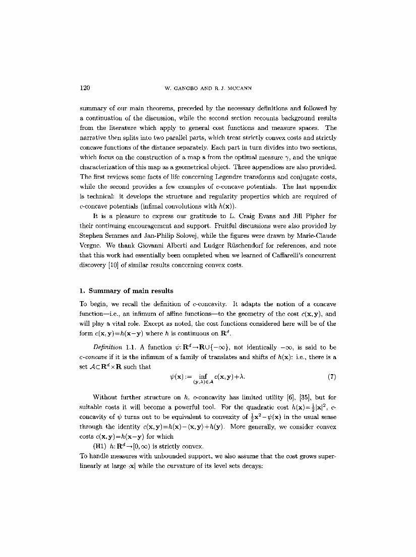
r - ' ) + A

/ Ra /

Y0 =S(X0)

(a) For strictly convex costs c(x, y ) = h ( x - y ) .

' I X o

/ ,,, R a /

y0 = s ( x o )

(b) For c(x,y)=-h(x-y)=l([x-y[) with l strictly concave and increasing.

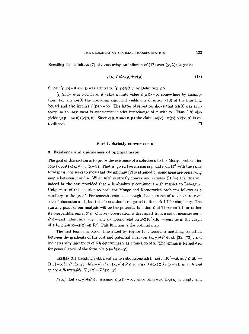
Fig. 1. The optimal map yo=s(xo) may be visualized by finding a shifted translate of h(x) which is tangent to the potential r at xo; then V~b(xo)=Vh(xo-Yo), D2r D2h(xo-Yo) and (xo, Yo)E0er Where r is differentiable, strict convexity of h guarantees this translate to be unique.

will be a mono tone subse t of the plane. A p a r t from ver t ica l s e g m e n t s - - o f which there

can only be coun tab ly many- - - such a set is con ta ined in the g raph of a non-decreas ing

funct ion s: R - * R . This funct ion is the op t ima l map . The fact t h a t # has no a t o m s

means t h a t none of i ts mass concen t ra t e s under ver t ica l segments in sp t % and is used

to verify v=s##. I t is not ha rd to show t h a t only one non-dec reas ing m a p pushes #

forward to v, so s is uniquely d e t e r m i n e d # -a lmos t everywhere .


The generalization of this argument to higher dimensions was explored in [27] to

sharpen results for the cost c(x, y ) = Ix -y l2 ; our proof follows the strategy there. At the

same time, we build on many ideas introduced to the t ransportat ion problem by other au-

thors. The connection of c-concavity with mass transport was first explored by Rfischen-

dorf [35], who used it to characterize the optimal measures 7 of Kantorovich; he later

constructed certain unique optimal maps for convex costs [36, w The related notion of

c-cyclical monotonicity is also essential; formulated by Smith and Knott [41] in analogy

with a classical notion of Rockafellar [32], it supplements inequality (6). One fact that

continues to amaze us is tha t - - fo r the costs c(x, y) we deal wi th- -not a single desirable

property of concave functions has failed to have a serviceable analog among c-concave

functions. Even the kernel of Aleksandrov's uniqueness proof [4] for surfaces of prescribed

integral curvature is preserved in our uniqueness argument. A non-negligible part of our

effort in this paper has been devoted to developing the theory of c-concave functions as

a general tool, and we hope that this theory may prove useful in other applications.

Since the literature on the Monge-Kantorovich problem is vast and fragmented [31],

we have endeavoured to present a t reatment which is largely self-contained. In the

background section and appendices, we have therefore collected together some results

which could also be found elsewhere. Absent from the discussion is any reference to the

maximization problem dual to (4), discovered by Kantorovich [21] for cost functions which

metrize R d. Subsequently developed by many authors, duality theory flourished into a

powerful tool for exploring mass transport and similar problems; quite general Monge-

Kantorovich duality relations were obtained by Kellerer in [24], and further references

are there given. Our results are not predicated on that theory, but rather, imply duality

as a result. One advantage of this approach is that the main theorems and their proofs

are seen to be purely geometrical-- they require few assumptions, and do not rely even on

finiteness of the infimum (4). However, the potential r that we construct can generally

be shown to be the maximizer for a suitable dual problem. This fact is clearer from our

work in [20], where many of these results were first announced; a completely different

approach, based on the Euler-Lagrange equation for the dual problem, is given there.

A main conclusion, both there and here, is that for the cost functions we deal with, the

potential r constructed geometrically or extracted as a solution to some

dual problem---specifies both which direction and how far to move the mass of # which

sits near x. If the cost is not strictly convex--so that Vh is not one-to-one--uniqueness

may fail, and further information be required to determine an optimal mapping; for

radial costs c(x, y ) - - / ( I x - y l ) , the potential specifies the direction of transport but not

the distance cf. [42], [18] and Figure 1.

The remainder of this paper is organized as follows: The first section provides a

120 W. G A N G B O AND R . J . M C C A N N

summary of our main theorems, preceded by the necessary definitions and followed by

a continuation of the discussion, while the second section recounts background results

from the literature which apply to general cost functions and measure spaces. The

narrative then splits into two parallel parts, which treat strictly convex costs and strictly

concave functions of the distance separately. Each part in turn divides into two sections,

which focus on the construction of a map s from the optimal measure % and the unique

characterization of this map as a geometrical object. Three appendices are also provided.

The first reviews some facts of life concerning Legendre transforms and conjugate costs,

while the second provides a few examples of c-concave potentials. The last appendix

is technical: it develops the structure and regularity properties which are required of

c-concave potentials (infimal convolutions with h(x)).

It is a pleasure to express our gratitude to L. Craig Evans and Jill Pipher for

their continuing encouragement and support. Fruitful discussions were also provided by

Stephen Semmes and Jan-Philip Solovej, while the figures were drawn by Marie-Claude

Vergne. We thank Giovanni Alberti and Ludger Rfischendorf for references, and note

that this work had essentially been completed when we learned of Caffarelli's concurrent

discovery [10] of similar results concerning convex costs.

1. S u m m a r y o f m a i n r e su l t s

To begin, we recall the definition of c-concavity. It adapts the notion of a concave

function--i.e., an infimum of affine funct ions-- to the geometry of the cost c(x, y) , and

will play a vital role. Except as noted, the cost functions considered here will be of the

form c(x, y ) = h ( x - y ) where h is continuous on R d.

Definition 1.1. A function ~ : R d - * R U { - o c } , not identically - c o , is said to be

c-concave if it is the infimum of a family of translates and shifts of h(x): i.e., there is a

set . A c R d • such that

r inf c (x ,y )+A. (7) (y,A)EA

Without further structure on h, c-concavity has limited utility [6], [35], but for

suitable costs it will become a powerful tool. For the quadratic cost h(x)--i 2 Ixl , c-

concavity of r turns out to be equivalent to convexity of �89 in the usual sense

through the identity c ( x , y ) = h ( x ) - ( x , y ) + h ( y ) . More generally, we consider convex

costs c(x, y ) = h ( x - y ) for which

(H1) h: Rd--* [0, oc) is strictly convex.

To handle measures with unbounded support, we also assume that the cost grows super-

linearly at large Ix] while the curvature of its level sets decays:

THE GEOMETRY OF OPTIMAL TRANSPORTATION 121

(H2) Given height r < o c and angle 0E(0,~r): whenever p E R d is far enough from

the origin, one can find a cone

K(r ,O ,~ ,p ) := {x C Rd I Lx-pL.IzL cos(�89 <~ (z ,x-p) 4 rLzl} (8)

with vertex at p (and z e R d \ { 0 } ) on which h(x) assumes its maximum at p;

(H3) l imh(x ) / Ix ]=+cc as [xl~oc.

Cost functions satisfying (H1)-(H3) include all quadratic costs h(x)-- (x, Px) with P pos-

itive definite, and radial costs h(x)=l(Ixl) which grow faster than linearly. Occasionally,

we relax strict convexity or require additional smoothness:

(H4) h: Rd--*R is convex;

(Hh) h(x) is differentiable and its gradient is locally Lipschitz: hEClio'l(Rd).

For these costs, e-concavity generalizes concavity in the usual sense, but we shall show

that it is almost as strong a notion. In particular, except for a set of dimension d - l , a

c-concave function r will be differentiable where it is finite; it will be twice differentiable

almost everywhere in the sense of Aleksandrov [39, notes to w

With some final definitions, our first main theorem is stated. We say that a joint

m e a s u r e ~ e ~ : ) ( R d x R d) is optimal if it minimizes C(~/) among the measures F(it, u) which

share its marginals, # and u. Since differentiability of the cost is not assumed, we define

(Vh) - i :--Vh* through the Legendre transform (10) in its absence. As before, id denotes

the identity mapping i d ( x ) = x on R d, while o denotes composition.

THEOREM 1.2 (for strictly convex costs). Fix c ( x , y ) = h ( x - y ) with h strictly con-

vex satisfying (H1)-(H3), and Borel probability measures # and u on R d. I f # is abso-

lutely continuous with respect to Lebesgue then

(i) there is a c-concave function ~b on R d for which the map s : = i d - ( V h ) - i o V ~ b

pushes # forward to u;

(ii) this map s(x) is uniquely determined (p-almost everywhere) by (i);

(iii) the joint measure V := (id • s) #it is optimal;

(iv) ~/ is the only optimal measure in F(#, u)--except (trivially) when C(V)=c~.

If It fails to be absolutely continuous with respect to Lebesgue but vanishes on rectifiable

sets of dimension d - l , then (i)-(iv) continue to hold provided

Here a rectifiable set of dimension d - 1 refers to any Borel set U c R d which may be

covered using countably many (d-1)-dimensional Lipschitz submanifolds of R d. (1)

(1) Remark added in proof. A l t h o u g h not proven here, the t h e o r e m s r ema in t rue even if one insis ts t h a t the covering subman i fo lds be g raphs of differences of convex functions: ( c - c ) -hype r su r f ace s in t he language of Zaji6ek [43].

122 W. G A N G B O AND R . J . M C C A N N

To illustrate the theorem in an elementary context, we verify the optimality of

t ( x ) = A x - z when # and L, are translated dilates of each other: ~ , :=t## [13]. For ,~>0,

z E R d and convex costs c(x, y ) - - h ( x - y), observe the c-concavity of

r := ( 1 - A ) - l h ( x ( 1 - A ) +z)

proved in Lemma B.1 (iv)-(vi) (if,X= 1 take • (x) := (x, Vh(z))). This potential r induces

the map s = t through (5). Since t pushes forward # to ~, it must be the unique map of

Theorem 1.2.

Motivated by economics, we now turn to costs of the form c(x, y ) = l ( I x - y l ) , where

l: [0, c~)--* [0, oc) is strictly concave. The optimal solutions for these costs respect different

symmetries. It will often be convenient to assume continuity of the cost (at the origin)

and l(O)=O, but these additional restrictions are not required for Theorem 1.4. With

a few caveats, our results could also be extended to strictly concave functions l which

increase from l(O)=-c<~, but we restrict our attention to l~>0 instead. For these costs, l

will be strictly increasing as a consequence of its concavity.

With this second class of costs come two new complications. Since c(x, y) induces

a metric on R d, any mass which is shared between #, v E ~ ( R ~) must not be moved by

a transportat ion plan 0/ that purports to be optimal. This mass is defined through the

Jordan decomposition of # - v into its unique representation #o - Vo as a difference of two

non-negative mutually singular measures: #o:=[#-u]+ and Uo:=[u-#]+. The shared

mass # A u : = # - # o = u - u o is the maximal measure in M ( R d) to be dominated by both #

and L,. Since one expects to find this mass on the diagonal subspace D:={(x , x) IxeR a} of R d • d under 3', it is convenient to denote the restriction of 3" to the diagonal by

3'd[S]:=3'[SND]. The off-diagonal restriction 3`0 is then given by 3`o=3`-3`4.

The second complication is the singularity in c (x ,y ) at x - -y , which renders c-

concavity too feeble to characterize the optimal map uniquely. For this reason, a re-

finement must be introduced to monitor the location V c R d of the singularity:

Definition 1.3. Let V c R d. A c-concave function ~b on R d is said to be the c-

transform of a function on V if (7) holds with A c V x R .

A moment 's reflection reveals the existence of some function r V---*RU{-cc} for

which

r = i n f c(x, y) - r (9)

whenever Definition 1.3 is satisfied.

Finally, as with convex costs, it is a vital feature of h(x)=l([x[) that the gradient

map Vh be invertible on its image. This follows from strict concavity of l~>0 since


II(A)>~0 will be one-to-one. Should differentiability of l fail, we define (Vh) -1 :=Vh*

using (11) this time. The support s p t # of a measure # E M ( R d) refers to the smallest

closed set U c R d of full mass: #[U]=#[Rd].

THEOREM 1.4 (for strictly concave cost as a function of distance). Use l: [0, oc)--*

[0, cc) strictly concave to define c (x ,y ) :=h(x -y ) : - - l ( [x -y] ) . Let # and u be Borel

probability measures on R d and define #o: - - [# -~]+ and ~o :=[u -# ]+ . If #o vanishes on

spt Uo and on rectifiable sets of dimension d - 1 then

(i) the c-transform r of some function on sptuo induces a map s :=

i d - ( V h ) - 1 o V r which pushes #o forward to no;

(ii) the map s(x) is uniquely determined #o-almost everywhere by (i);

(iii) there is a unique optimal measure "y in F(#, u)--except when C(V)=ec;

(iv) the restriction of v to the diagonal is given by 9 ' d - - ( i d •

(v) the off-diagonal part of "~=~d~-~[o is given by ~ o = ( i d x s ) # p o .

The hypotheses of this theorem are satisfied when # and u are given by continuous

densities f, gEC(R d) with respect to Lebesgue: d # ( x ) = f ( x ) d x and du(y)=g(y)dy.

Alternately, if f ( x ) = x v ( X ) and g(Y)=Xv(Y) are characteristic functions of two equal

volume se ts - -an open set U and a closed set V - - t h en Theorem 1.4 yields an optimal

map given by s ( x ) = x on UAV.

As for convex costs, explicit solutions may be computed to problems with appropriate

symmetry. For concave functions of the distance, suitable symmetries include reflection

through a sphere or through a plane (for details refer to Appendix B):

Example 1.5 (reflections). Take c and # from Theorem 1.4. If # is supported on the

unit ball, then the spherical inversion s (x ) :=x / Ix ] 2 will be the optimal map between #

and s##. If # vanishes on the half-space xl >0 in R d, then reflection through the plane

Xl =0 will be the optimal map between # and its mirror image.

Explicit solutions may also be obtained whenever the target measure u concentrates

on finitely many points: spt v = { y l , Y2, .-., Yk}. The initial measure # is arbitrary pro-

vided it vanishes on small enough sets. For convex costs, we also need Remark 4.6: the

potential r of Theorem 1.2 may be assumed to be the c-transform of a function on spt u.

Example 1.6 (target measures of finite support). Take #, u, c and h from The-

orem 1.2 or 1.4. If s p t v = { y l , y 2 , . . . , y k } C R d then the optimal map is of the form

s (x )=x -Vh*(V~b(x ) ) , where r is the c-transform of a function on spt u. In view of (9),

r inf c(x, y j )+Aj . j = l , . . . , k

From this family of maps, the unique solution is selected by finding any k constants

Aj E R consistent with the mass constraints #[s- 1 (yj)] = ~ [yj], j = 1, ..., k.


The constants Aj should be easy to compute numerically; indeed, we speculate that

flowing along the vector field vj ()U,..., Ak):=#[s -1 (Y j ) ] - v[yj] through R k will always

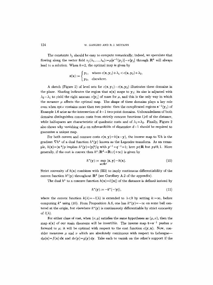
lead to a solution. When k=2, the optimal map is given by

f Yl, where c(x, yl)+A1 <c(x , y2)+A2, S(X) / Y2, elsewhere.

A sketch (Figure 2) of level sets for c(x, y l ) - C ( x , y2) illustrates these domains in

the plane. Shading indicates the region that s(x) maps to Yl; its size is adjusted with

A2-A1 to yield the right amount ~[Yl] of mass for #, and this is the only way in which

the measure p affects the optimal map. The shape of these domains plays a key role

even when spt v contains more than two points: then the complicated regions s -1 (yj) of

Example 1.6 arise as the intersection of k - 1 two-point domains. Unboundedness of both

domains distinguishes convex costs from strictly concave functions l ~>0 of the distance,

while half-spaces are characteristic of quadratic costs and of A1 =A2. Finally, Figure 2

also shows why vanishing of # on submanifolds of dimension d - 1 should be required to

guarantee a unique map.

For both convex and concave costs c(x, y ) = h ( x - y ) , the inverse map to Vh is the

gradient Vh* of a dual function h*(y) known as the Legendre transform. As an exam-

ple, h(x)=lxlP/p implies h*(y)=lylq/q with p - l + q - l = l ; here p e a but p#0, 1. More

generally, if the cost is convex then h*: Rd--+RU{+c~} is given by

h*(y) := sup ( x , y ) - h ( x ) . (10) X6R d

Strict convexity of h(x) combines with (H3) to imply continuous differentiability of the

convex function h* (y) throughout R d (see Corollary A.2 of the appendix).

The dual h* to a concave function h(x)--/(Ixl) of the distance is defined instead by

h*(y) := -k* (-]yl) , (11)

where the convex function k(.~)=-l(A) is extended to A<0 by setting k:=c~, before

computing k* using (10). From Proposition A.6, one has h * ( y ) = - c ~ on some ball cen-

tered at the origin, but elsewhere h* (y) is continuously differentiable by strict concavity

of

For either class of cost, when (v, #) satisfies the same hypotheses as (#, v), then the

map s(x) of our main theorems will be invertible. The inverse map t = s -1 pushes v

forward to #; it will be optimal with respect to the cost function c(y, x). Now, con-

sider measures # and v which are absolutely continuous with respect to Lebesgue--

d # ( x ) = f ( x ) dx and d , ( y ) = g ( y ) dy. Take each to vanish on the other's support if the


- 2

- 4

- 4 - 2 0 2

(a) c(x, y ) : rx-y] 3

/ - 4

y l Y2

- 2 0 2

(b) c(x, y ) = [ x - y l 2

4

- 2

- 4

- 4

Y2

- 2 0 2 4 - 4 - 2 0 2 (c) c(x,y)----[x-y[ (d) c ( x , y ) = [ x - y l 1/2

Fig. 2. A few optimal maps to measures which concentrate at two points y2 ~ ( 1 , 0 ) = - y l in

the plane. Shading indicates the region mapped to Yl; its complement is mapped to Y2.

126 W. G A N G B O AND R . J . MCCANN

cost is concave. Then the transformation y = s ( x ) represents a change of variables (1)

between # and u, so--formally at least (neglecting regularity issues)--its Jacobian deter-

minant Ds(x) satisfies g(s(x))Idet D s ( x ) l = f ( x ). The potential r satisfies the partial

differential equation

g ( x - Vh* (Vr d e t [ I - D2h * (Vr162 = i f ( x ) . (12)

Our main theorems may be interpreted as providing existence and uniqueness results

concerning c-concave solutions to (12) in a measure-theoretic (i.e., very weak) sense. The

plus sign corresponds to convex costs, and the minus sign to concave functions h(x)--

/(Ixl) of the distance, reflecting the local behaviour of the optimal map: orientation-

preserving in the former (convex) case and orientation-reversing in the latter case. As

Caffarelli pointed out to us, this may be seen by expressing the Jacobian

Ds(x) -- D2h * ( V r 1 6 2

as the product of D2h * with a non-negative matrix. The second factor is positive semi-

definite by the c-concavity(2) of r (see Figure 1), while the first factor D2h * has either

no negative eigenvalues or one negative eigenvalue, depending on the convexity of h

and h*, or their concavity as increasing functions of Ixl. If h ( x ) - 1 2 - ~ l x l , then D2h*=I

and equation (12) reduces to the Monge-Amp~re equation [7]; Caffarelli has developed

a regularity theory [9] which justifies the formal discussion in this case. However, the

discontinuities in V r points where V r when the cost is concave--are also of

interest: they divide spt # into the regions on which one may hope for smooth transport.

A summary of our notation is shown in Table 1.

2. B a c k g r o u n d o n o p t i m a l m e a s u r e s

In this section, we review some background material germane to our further develop-

ments. Principally, this involves recounting connections between optimal mass trans-

port, c-concave functions and c-cyclically monotone sets established in the work of

Riischendorf [34], [35], and Smith and Knott [41].

To emphasize the generality of the arguments, this section alone is formulated not in

the Euclidean space R d, but on a pair of locally compact, a-compact, second countable

Hausdorff spaces X and Y. The Borel probability measures on X are denoted by P (X ) ,

while the mass transport problem becomes: Find the measure ~/ which minimizes the

(2) Which implies that (x,s(x))E0cr in Definition 2.6 through Proposition 3.4 (ii) or Proposi- tion 6.1.

THE GEOMETRY OF OPTIMAL TRANSPORTATION

Table 1

127

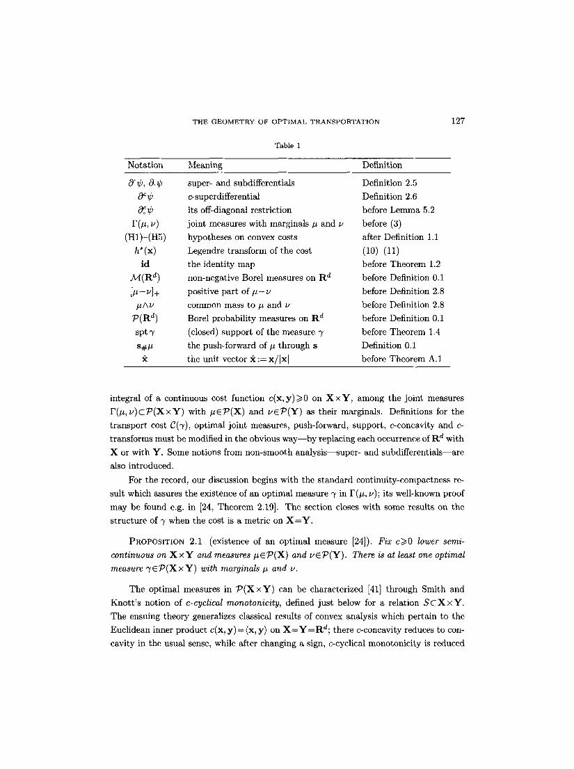
Notation Meaning Definition

0"r c9.r super- and subdifferentials Definition 2.5

Ocr c-superdifferential Definition 2.6

v0o~r its off-diagonal restriction before Lemma 5.2

F(#, v) joint measures with marginals # and v before (3)

(H1)-(H5) hypotheses on convex costs after Definition 1.1

h*(x) Legendre transform of the cost (10)-(11)

id the identity map before Theorem 1.2

.M(R d) non-negative Borel measures on R d before Definition 0.1

[p-u]+ positive part of # - ~ before Definition 2.8

#Av common mass to p and v before Definition 2.8

~:~(R d) Borel probability measures on R d before Definition 0.1

spt 9, (closed) support of the measure "7 before Theorem 1.4

s## the push-forward of # through s Definition 0.1

the unit vector ~ : = x / I x I before Theorem A.1

integral of a continuous cost function c(x,y)~>0 on X • among the joint measures

F(#,v)CT~(X• with #ET'(X) and vET'(Y) as their marginals. Definitions for the

transport cost C(9'), optimal joint measures, push-forward, support, c-concavity and c-

transforms must be modified in the obvious way--by replacing each occurrence of R d with

X or with Y. Some notions from non-smooth analysis--super- and subdifferentials--are

also introduced.

For the record, our discussion begins with the standard continuity-compactness re-

sult which assures the existence of an optimal measure 9, in F(#, v); its well-known proof

may be found e.g. in [24, Theorem 2.19]. The section closes with some results on the

structure of "r when the cost is a metric on X--Y.

PROPOSITION 2.1 (existence of an optimal measure [24]). Fix c>~O lower semi-

continuous on X x Y and measures #ETa(X) and vET~(Y). There is at least one optimal

measure "yEP(XxY) with marginals # and v.

The optimal measures in P ( X • can be characterized [41] through Smith and

Knott 's notion of c-cyclical monotonicity, defined just below for a relation S c X x Y .

The ensuing theory generalizes classical results of convex analysis which pertain to the

Euclidean inner product c(x, y ) = ( x , y) on X = Y = R d ; there c-concavity reduces to con-

cavity in the usual sense, while after changing a sign, c-cyclical monotonicity is reduced


to the cyclical monotonicity of Rockafellar by the observation that any permutation can

be expressed as a product of commuting cycles [32].

Definition 2.2. A subset S c X x Y is called c-cyclically monotone if for any finite

number of points (xj, y j )ES , j = l ... n, and permutation a on n-letters,

n n

c(x , yj) < c(xa(j), yj). (13) j = l j = l

For finite sets S, c-cyclical monotonicity means that the points of origin x and desti-

nations y related by (x, y) E S have been paired so as to minimize the total transportation

cost ~-~-s c(x, y). This intrepretation motivates the following theorem, first derived by

Smith and Knott from the duality-based characterization of Riischendorf [35]. The proof

given here uses a direct argument of Abdellaoui and Heinich [2] instead; it shows that

c-cyclically monotone support plays the role of an Euler-Lagrange condition for optimal

measures on X x Y.

THEOREM 2.3 (optimal measures have c-cyclically monotone support). Fix a con-

tinuous function c(x,y)~>0 on X x Y . If the measure 7 E P ( X x Y ) is optimal and

C(~t) < oo then ~1 has c-cyclically monotone support.

Proof. Before beginning the proof, a useful perspective from probability theory is

recalled" Given a collection of measures #j EP(X) ( j = 1, ..., n), there exists a probability

space (~, B, r/) such that each #j can be represented as the push-forward of r / through

a (Borel) map rrj:gt-+X. The demonstration is easy: let r/:=#l x . . . x # n be product

measure on the Borel subsets of ~ : = X n, and take rrj(xl, . . . ,xn) :=xj to be projection

onto the j t h copy of X. Also, recall that if U c X is a Borel set of mass A:=#[U]>0, one

can define the normalized restriction of # to U: it is the probability measure assigning

mass )~-I#[VNU] to V c X .

Now, suppose ~/ is optimal; i.e., minimizes C(. ) among the measures in P ( X x Y )

sharing its marginals. Unless 3, has c-cyclically monotone support, there is an integer n

and permutation a on n letters such that the function

f ( x l , ..., xn; Yl, ..., y ~ ) : = ~ c(xa(j), y j ) - c(xj, yj) j = l

takes a negative value at some points (xl, y l ) , ..., (Xn, Yn)espt % These points can be

used to construct a more efficient perturbation of ~ as follows. Since f is continu-

ous, there exist (compact) neighbourhoods U j c X of xj and V j c Y of y j such that

f ( u l , ..., un ;v l , . . . ,vn)<0 whenever u j e U j and vjEVj. Moreover, A:=infj 'y[Uj • Vii


will be positive because (xj, y j )E sp t 7. Let ~j E P ( X x Y) denote the normalized restric-

tion of ~/to Uj x Vj. Introducing a factor of n lest the ~/j fail to be disjointly supported,

one can subtract ~-'~j )~'~j/n from ~y and be left with a positive measure.

For each j , choose a Borel map w----*(uj(w),vj(w)) from ~ to X x Y such that 7 j =

(uj x v j ) # y ; this map takes its values in the compact set Uj x Vj. Define the positive

measure

7' :='Y+ An-1 E ( u o ( j ) x v j ) # ~ - ( u j x vj)#~?. j = l

Then 7 ' E T ) ( X x Y ) shares the marginals of 7, while using (1) to compute its cost con-

tradicts the optimMity of ~,: since the integrand f will be negative,

n

C(7 ' ) - ( : (7) = A n - l ~ E c(u~(j), v j ) - c ( u j , v j ) dr] < 0. j = l

Thus 7 must have c-cyclically monotone support. []

A more powerful reformulation exploits convexity to show that all of the optimal

measures in F(#, u) have support on the same c-cyclically monotone set.

COROLLARY 2.4. Fix #ET'(X), u E P ( Y ) and a continuous function c(x, y ) ) 0 on

X x Y . Unless C(. ) = cx~ throughout F(tt, u), there is a c-cyclically monotone set S C X x Y

containing the supports of all optimal measures 7 in F(#, u).

Proof. Let S : = U s p t y , where the union is over the optimal measures y in F(p, ~).

We shall show S to be c-cyclically monotone by verifying (13). Therefore, choose any

finite number of points ( x j , y j ) E S indexed by j = l , . . . , n and a permutation a on n

letters. For each j , the definition of S guarantees an optimal measure 7j EF(#, u) with

(xj, y j ) E spt ~j. Define the convex combination 7 := (1/n) ~-~j 7y. Since F(#, u) is a convex

set and C(. ) is a linear functional, 7EF(tt , u) and C('~)=C(~/j); thus 7 is also optimal.

By Theorem 2.3, spt 7 is c-cyclically monotone. But spt 7 contains spt 7j for each j , and

in particular the points (xj, yj) , so (13) is implied. []

Rockafellar's main result in [32] exposed the connection between gradients of concave

functions and cyclically monotone sets: it showed that a concave potential could be

constructed from any cyclically monotone set. Smith and Knott observed that this

relationship extends to c-concave functions and c-cyclically monotone sets. To state the

theorem precisely requires some generalized notions of gradient, which continue to be

useful throughout:

130 W. G A N G B O A N D R , J , M C C A N N

Definition 2.5. A function r Rd---RU{+o~} is superdifferentiable at x E R d if r

is finite and there exists y E R d such that

r ~< r + (v, y) +o(Iv]) (14)

for small vER4; here o(A)/A must tend to zero with A.

A pair (x, y) belongs to the superdifferential O 'r215 R d of ~b if r is finite and

(14) holds, in which case y is called a supergradient of r at x; such supergradients y

comprise the set 0" r d, while for V c R d we define O'r 0"r The

analogous notions of subdifferentiability, subgradients and the subdifferential O.~b are

defined by reversing inequality (14). It is not hard to see that a real-valued function will

be differentiable at x precisely when it is both super- and subdifferentiable there; then

or162 ={re(x)}. A function ~b: Rd--*RU{-c~} is said to be concave if AE(0, 1) implies that

r (1 -A)r162

whenever the latter is finite. The function r is excluded by convention. For con-

cave functions the error term will vanish in (14): the inequality r162

holds for all (x,y)E0"r and the supergradients of ~b parameterize supporting hyper-

planes of graph(C) at (x, r To provide a notion analogous to supporting hyperplanes

in the context of c-concave functions, a c-superdifferential is defined in the following way

[35] (cf. Figure 1):

Definition 2.6. The c-superdifferential 0cr of ~b: X--*RU{-cx~} consists of the pairs

( x , y ) E X x Y for which ~b(v)~<r if vEX.

Alternately, (x,y)E0c~b means that c ( v , y ) - r assumes its minimum at v=x .

We define 0 ~ r to consist of those y for which (x,y)e0~r while Ocr

Uxey 0~r for V c X . In our applications c(x, y) is continuous, so a c-concave potential r will be upper

semi-continuous from its definition. As a consequence, v~r will be a closed subset of

X • Y- -an observation which will be useful later. With this notation, Smith and Knott's

generalization [41] of the Rockafellar theorem [32] can be stated. Its proof is drawn

from [37].

THEOREM 2.7 (c-concave potentials from c-cyclically monotone sets). For S c X •

to be c-cyclically monotone, it is necessary and sufficient that S C OC~b for some c-concave r x~Ru{-oo}.

Proof. Sufficiency is easy: c-concavity of r implies that 0~r is c-cyclicMly monotone.

To see this, choose n points (x j ,y j ) from 0 ~ and a permutation a on n-letters. We


invoke c-concavity only to know that ~: X--~RU{-co} is finite at some pEX; then taking

(x ,y ) := (x j , y j ) and v : = p in Definition 2.6 implies that r is finite, while taking

v:=x~(j) implies r - r ~<c(x~(j), yj) - c ( x j , yj) . Summing this inequality over

j = 1, ..., n yields (13), whence 0cr is c-cyclically monotone.

To prove necessity, one needs to construct a suitable potential r from a c-cyclically

monotone set S c f t l • Since (13) holds true for the cycle a=(12 . . .n ) in

particular, the construction of [37, Lemma 2.1] yields a c-concave ~p on f t l : = X with

ScOCr Taking Ft:=W(S) with W(x, y)=y when applying this lemma forces r to be the

c-transform of a function on ~2. []

We record this last observation as a corollary to the proof:

COROLLARY 2.8. Let S c X x Y be c-cyclically monotone, and let ~rP(S) denote the

projection of S onto Y through the map W(x,y) :=y . Then ScOCr for the c-transform

r X--*RU{-c~} of a function on W(S).

Combining Theorems 2.3 and 2.7 makes it clear that if a measure 7 solves the

Kantorovich problem on F(#, v) it will necessarily be supported in the c-supergradient of

a c-concave potential r Indeed, this fact was already appreciated by Rfischendorf, who

recognized that its converse (sufficiency) also holds true [35]. Our main conclusions will

be recovered from an analysis of r and 0cr when X = Y = R d. Before embarking on that

analysis, we conclude this review by casting into the present framework a few variants

on well-known results which apply when c(x, y) is a metric and X = Y . We assume that

c(x, y) satisfies the triangle inequality strictly:

c(x, y) < c(x, p) +c(p, y) (15)

unless p = x or p--y. In this case, any mass which is common to # and v will stay in its

place, and can be subtracted from the diagonal of any optimal measure %

PROPOSITION 2.9 (any mass stays in place if it can). Let # , v E P ( X ) and denote

their shared mass by /~Av:=/~-[/~-v]+. The restriction "[d of any joint measure "yE

F(#, u) to the diagonal D:={(x, x)l x e X } satisfies

~/d ~< (id x id)#(#Au). (16)

When c(x, y) is a metric on X satisfying the strict triangle inequality (15) and 7 has

c-cyclically monotone support, then (16) becomes an equality.

Proof. Let ~r(x,y):=x and ~r '(x,y):=y denote projections from X x X to X, and

decompose -l=Td+'Yo into its diagonal and off-diagonal parts, so that "Yd is supported

132 W. GANGBO AND R.J . MCCANN

on D and coincides with 7 there. From spt ~/d C D it is easily verified that the marginals

of "~d coincide: denote them by ~ : = 7 r ~ d = T V ~ [ d . M o r e o v e r 7 d = ( i d • Defining

#o:-=~#~yo and ~o:--Tr~#7o, linearity 7r#~/=Tr#%+Tr#~/d makes it clear that # = # o + ~ and

y = ~o +/3. These measures are all non-negative, so 3 ~< #A v is established and implies (16).

Assume therefore that q, has c-cyclically monotone support. It remains to show only that

#o and Vo are mutually singular measures, so that # o - ~ o gives the Jordan decomposition

of # - v . Then # A v : = # - # o = ~ and (16) becomes an equality.

To prove tha t / to and ~o are mutually singular requires a set U of full measure for

#o with zero measure for Co. Define S = s p t q , \ D and take U:=Tr(S); both sets are a-

compact, hence Borel. Since S is a set of full measure for %, U has full measure for

#o=~#%. Similarly, V=~ ' (S ) has full measure for ~o. We argue by contradiction that

U and V are disjoint, thereby establishing the proposition. Suppose pEUMV, meaning

that there exist x, y E X , both different from p, such that (x ,p) and (p ,y ) lie in spt')'.

Applying the two-point inequality (n--2) for c-cyclically monotonicity (13) to spt ? yields

c(x, p )+c (p , y) ~< c(x, y ) + c ( p , p).

Since c ( p , p ) = 0 , the strict triangle inequality (15) is violated. The only conclusion is

that U and V are disjoint and the proof is complete. []

COROLLARY 2.10 (metric costs with fixed-penalty for transport). Fix a continuous

metric c(x, y) on X satisfying the triangle inequality strictly, and define a discontinuous

cost by ~(x ,y ) := c (x ,y ) for x ~ y and c ( x , x ) = - ~ < 0 . A joint measure ~ , E P ( X x X ) is

optimal for ~ if and only if it is optimal for c.

Proof. Follows easily from Theorems 2.3, 2.9 and C(~)=C(? ) -~? [D] . []

As the last proposition suggests, when c(x ,y) is a metric the diagonal D c X x X

plays a distinguished role among c-cyclically monotone sets. A final lemma shows that D

is contained in the c-superdifferential of every c-concave function lb. Equivalently, D can

be added to any c-cyclically monotone set without spoiling the c-cyclical monotonicity.

Finiteness of lb is a useful corollary, while Kantorovich's observation that r will be

Lipschitz continuous relative to the metric c is also deduced; cf. [21].

LEMMA 2.11 (c-concavity and the diagonal for metrics). Let c(x, y) be a metric on

X and r be c-concave. Then

(i) ~ is real-valued and Lipschitz with constant 1 relative to c(x, y);

(ii) for every p E X one has ( p , p ) E 0 c r

Proof. (ii) Let x, y, p E X and hER. The triangle inequality implies that

c(x, y ) + A ~< c(x, p ) + c(p, y ) + A. (17)


Recalling the definition (7) of c-concavity, a~ infimum of (17) over (y, A)e.A yields

r < c(x, p) +r (18)

Since c(p, p)=O and p was arbitrary, (p, p)E0~r by Definition 2.6.

(i) Since r is c-concave, it takes a finite value r somewhere by assump-

tion. For any p E X the preceding argument yields one direction (18) of the Lipschitz

bound and also implies r The latter observation shows that x E X was arbi-

trary, so the argument is symmetrical under interchange of x with p. Thus (18) also

yields r 1 6 2 ~<c(p, x). Since c(p, x )=c(x , p) the claim I~b(x)-~b(p)l <c(x, p) is es-

tablished. []

Part I. Str ict ly convex costs

3. Exis tence and uniqueness of opt imal maps

The goal of this section is to prove the existence of a solution s to the Monge problem for

convex costs c(x, y ) = h ( x - y ) . That is, given two measures ~ and v on R d with the same

total mass, one seeks to show that the infimum (2) is attained by some measure-preserving

map s between # and ~. When h(x) is strictly convex and satisfies (H1)-(H3), this will

indeed be the case provided that # is absolutely continuous with respect to Lebesgue.

Uniqueness of this solution to both the Monge and Kantorovich problems follows as a

corollary to the proof. For smooth costs it is enough that no mass of # concentrate on

sets of dimension d - 1, but this observation is relegated to Remark 4.7 for simplicity. The

starting point of our analysis will be the potential function r of Theorem 2.7, or rather

its c-superdifferential 0cr Our key observation is that apart from a set of measure zero,

0c~b--and indeed any c-cyclically monotone relation ScRdx Rd--must lie in the graph

of a function x-*s(x) on R d. This function is the optimal map.

The first lemma is basic. Illustrated by Figure 1, it asserts a matching condition

between the gradients of the cost and potential whenever ( x, y)E0~r cf. [35, (73)], and

indicates why injectivity of Vh determines y as a function of x. The lemma is formulated

for general costs of the form c(x, y ) = h ( x - y ) .

LEMMA 3.1 (relating c-differentials to subdifferentials). Let h: a d----~R and r Rd--*

RU{-oo}. If c (x ,y) - -h(x-y) then (x ,y)E0~r implies 04b(x)cO.h(x-y); when h and r are differentiable, V~b(x)=Vh(x -y ) .

Proof. Let (x,y)e0~r Assume r since otherwise 04b(x) is empty and


there is nothing to prove. If zE0.r then sub- and c-superdifferentiability of r yield

r +o(Ivl) < r

r + h ( x + v - y) - h(x-y)

for small v E R d. In other words, zE 0 .h (x -y ) , and so the first claim is proved. Differen-

tiability implies the second claim because then 0 . r162 while 0 . h ( x - y ) - -

{Vh(x-y)} . []

In view of this lemma, the business at hand is to prove some differentiability result

for the potential r Strict convexity of h(x) ensures the invertibility of Vh. The next

theorem--proved in Appendix C--asserts that a c-concave potential ~ is locally Lipschitz.

If the cost is a derivative smoother, then ~ satisfies a local property known as semi-

concavity; introduced by Douglis [17] to select unique solutions for the Hamilton-Jacobi

equation, it implies all the smoothness enjoyed by concave functions.

Definition 3.2. A function r Rd--*RU{-c~} is said to be locally semi-concave at

p E R d if there is a constant A<c~ which makes r 2 concave on some (small) open

ball centered at p.

THEOREM 3.3 (regularity of c-concave potentials). Let r be c-

concave for some convex c ( x , y ) - - h ( x - y ) with h satisfying (H2)-(H4). Then there is a

convex set K C R d with interior ~t:=int K such that 12C {xi~(x ) > - o c } C K. Moreover,

r is locally Lipschitz on ~, and if hEC~olc (R d) then r will be locally semi-concave on ~.

Proof. Proposition C.3 yields the convex set K with interior 12 such that 12C

{ ~ > - c c } C K . Moreover, r is locally bounded on ~. Thus r is locally Lipschitz on

gt by Corollary C.5, and locally semi-concave if hEClol(Rd) . []

We use convexity of K only to know that outside of ~, the set where r is finite has

zero volume (indeed, is contained in a Lipschitz submanifold of dimension d -1) . Inside ~,

Rademacher's theorem shows that the gradient Vr is defined almost everywhere. When

r is locally semi-concave, results of Zaji6ek [43] (or Alberti [3]) imply that the subset of

~t where differentiability fails is rectifiable of dimension d - 1.

The next lamina and its corollary verify that any c-cyclically monotone set will lie

in the graph of a map. The facts we exploit concerning the Legendre transform h* (y) of

a convex cost (10) are summarized in Appendix A.

PROPOSITION 3.4 (c-superdifferentials lie in the graph of a map). Fix c (x ,y )=

h ( x - y ) satisfying (H1)-(H3) and a c-concave r on R d. Let d o m e and domVr denote

the respective sets in R d on which r is finite, and differentiable. Then


(i) s (x ) :=x-Vh*(Vr defines a Borel map from domVr to Rd;

(ii) 0Cr whenever xEdom r e ;

(iii) 0C~b(x) is empty unless xEdom~b;

(iv) the set dom r Vr has Lebesgue measure zero.

Proof. (i) Theorem 3.3 shows that r is continuous on the interior fl of dome. Since

its gradient is obtained as the pointwise limit of a sequence of continuous approximants

(finite differences), Vr is Borel measurable on the (Borel) subset dom Vr where it

can be defined. Since Vh* is continuous by Corollary A.2, the measurability of s(x) is

established.

(ii) Since ~b is differentiable at xEdomV~b it is bounded nearby, so from Proposi-

tion C.4 we conclude that 0Cr is non-empty. Choosing yE0~b(x), Lemma 3.1 yields

Vr (x) E 0. h ( x - y). Corollary A.2 then shows that x - y-=- Vh* (~'r (x))---or equivalently

y--s(x)- -and establishes 0Cr

(iii) Part of the definition for c-concavity of r Rn---~RU{-c~} asserts finiteness of

r for some y e a d. Since (x, y )e0~r implies r162 y ) - c ( x , y), one has

x E d o m r whenever 0~r is non-empty.

(iv) Theorem 3.3 shows r to be locally Lipschitz on the interior of dom r while

the boundary of domr lies in the boundary of a convex subset of R d and hence has

Lebesgue measure zero. In the interior, Rademacher's theorem yields r differentiable

almost everywhere, whence dom r Vr has Lebesgue measure zero. []

COROLLARY 3.5 (c-cyclically monotone sets lie in the graph of a map). Let c(x, y) =

h ( x - y ) satisfy (H1)-(H3) and s c R d • d be c-cyclically monotone. Then there is a

(Borel) set N C R d of zero measure for which (x,y) and (x,z) in S with y ~ z implies

x E N .

Proof. Let S c R d x R d be c-cyclically monotone. Theorem 2.7, due to Smith and

Knott, asserts the existence of a c-concave function ~b with ScO~b. Proposition 3.4

provides a Borel set N:--dom r V• of zero measure for which (x, y) and (x, z) in

SCOc~p but x ~ Y imply y = z = x - V h * ( V ~ ( x ) ) . []

Armed with this knowledge, we are ready to derive a measure-preserving map from

existence of the corresponding potential. The argument generalizes [29, Proposition 10].

PROPOSITION 3.6 (measure-preserving maps from c-concave potentials). Let c(x, y)

= h ( x - y ) satisfy (H1)-(H3), and suppose that a joint measure "~e~(RdxR d) has sup-

port in 0cr for some c-concave function r on I t d. Let # and v denote the marginals

of 7EF(p,~'). / f r is differentiable #-almost everywhere, then s(x):=x-Vh*(V~b(x))

pushes # forward to v. In fact, 7=( id •


Proof. To begin, we observe from Proposition 3.4 (i) that s(x) is a Borel map defined

p-almost everywhere: the (Borel) set dom Vr where ~ is differentiable carries the full

mass of p by hypothesis. It remains to check (id x s ) # # = % from which s # p = v follows

immediately.

To complete the proof, it suffices to show that the measure (id x s )#p coincides with

on products U x V of Borel sets U, V c R d ; the semi-algebra of such products generates

all Borel sets in R d x R d. Therefore, define S := {(x, y) E0cr Ixedom Vr For (x, y) aS ,

Proposition 3.4 (ii) implies y--s(x) , so

( u x v ) n s = ( (Uns -1 (v) ) x R ~) nS. (19)

Being the intersection of two sets having full measure for ? - - t he closed set Ocr and the

Borel set d o m V C x R ~ - - t h e set S is Borel with full measure. Thus ^/[ZNS]=?[Z] for

Z c R d x R d. Applied to (19), this yields

?[U x V] = "7[(Vn s -1 (V)) x R d] = # [Uns -1 (V)] = (id x s)#p[U x Y].

7EF(#, L,) implies the second equation; Definition 0.1 implies the third. []

These two propositions combine with results of w to yield the existence and unique-

ness of optimal solutions to the Monge and Kantorovich problems with strictly convex

cost:

THEOREM 3.7 (existence and uniqueness of optimal maps). Fix a cost c ( x , y ) =

h ( x - y ) , where h strictly convex satisfies (H1)-(H3), and two Borel probability measures

# and v on R d. I f p is absolutely continuous with respect to Lebesgue and (4) is finite,

then there is a unique optimal measure ~/ in F(p,~). The optimal ~ = ( i d x s ) # # is given

by a map s ( x ) = x - V h * ( V r pushing # forward to ~, through a c-concave potential

1) on R d.

Proof. Our Corollary 2.4 to Smith and Knott 's theorem yields a c-cyclically mono-

tone set S c R d x R 4 which contains the supports of all optimal measures in F(#,v) .

A c-concave function r on R d with ScOC~) is provided by Smith and Knott 's next

observation--Theorem 2.7. Now suppose that ~CF(#, ~) is optimal; there is at least one

such measure by Proposition 2.1. Then spt~/C0Cr The map 7r (x ,y)=x on R d x R d

pushes ~ forward to p=lr#~/, while projecting the closed set 0~r to a a-compact set of

full measure for #. Proposition 3.4 (iii)-(iv) shows that ~ ( 0 ~ r 1 6 2 and combines

with absolute continuity of # to ensure that r is differentiable #-almost everywhere.

Proposition 3.6 then shows that s(x) pushes # forward to v while "~ coincides with the

measure ( i dxs )#p . This measure is completely determined by p and r so it must be

the only optimal measure in F(#, ~). []


4. Characterization of the opt imal map

For cost functions c(x, y ) = h ( x - y ) with h strictly convex, the last section showed that

when VEF(#, ~) is optimal---or indeed if -~ has c-cyclically monotone support--then it

is determined by a map s (x ) - -x -Vh*(Vr which solves the Monge problem. The

potential r will be c-concave and "y=(id• The results of the present section show

that only one measure in F(#, ~) has c-cyclically monotone support, while only one

mapping s= id-Vh*o~7r can push # forward to ~ and also have r c-concave: this

geometry is characteristic of % As in [27], the argument avoids integrability issues by

relying on geometric ideas which can be traced further back to Aleksandrov's uniqueness

proof for convex surfaces with prescribed Gaussian curvature [4]. The same assumptions

are required that lead to existence of s: the left marginal of V must vanish on sets of

measure zero or dimension d - 1 , depending on the smoothness of h.

The idea of the proof is that if another map t = i d - V h * o V r is induced by some

c-concave r then unless s = t holds/z-almost everywere, a set 0er can be constructed

to have less mass for s## than for t#~. We begin with two lemmas concerning c-

superdifferentials and c-concave functions which generalize Aleksandrov's observations

about supporting hyperplanes for concave functions. The idea is to start by supposing

that c(x, y)+A dominates the function r but fails to dominate r and then increase

A until c(x,y)-+-A is tangent to r At the point of tangency, it is obvious that r

dominates r In what follows, Oc~b-l(V) denotes the set of x C R d for which 0~r

intersects V C R d.

LEMMA 4.1. Let c: Rd• Rd---+R, and suppose that r and r map R d into R U ( - c ~ }.

Define U:={x[~p(x)>r and X:=Oc~-I(Oer Then X c U .

Proof. Let x e X . Then there is a uEU with yE0Cr such that (x,y)e0r For

all v E R ~, the definition of 0r162 and 0~b yields

r ~< r +c(v, y ) - c ( u , y),

~p(u) ~< ~b(x) +c(u, y ) - c ( x , y).

Noting that r162 these inequalities imply

r < r y ) - c ( x , y). (20)

Evaluating at v - -x yields xEU. Since xE X was arbitrary, X c U . []

Remark 4.2. If c(x, y ) = h ( x - y ) satisfies (H1)-(H3) while r and r are both differ-

entiable and c-concave, then by Proposition 3.4 (ii), the last lemma shows that when

x - Vh* (Vr (x)) = u - Vh* (Vr and r (u) > r then ~b (x) > r (x).


LEMMA 4.3. Take r r U and X as in Lemma 4.1 while c(x, y ) = h ( x - y ) satisfies

(H1)-(H3). Let r be c-concave on R d and continuous at p E R d with r 1 6 2 /f

0Cr and 0Cr are disjoint then p lies a positive distance from X .

Proof. To produce a contradiction, suppose that a sequence x , E X converges to p.

Then there exist unEU with ynE0Cr such that (xn,yn)E0cr Proposition C.4

guarantees that the yn are bounded since Xn"-*p. A subsequence must converge to a

limit point yn~Yo, and (P, Yo) lies in the closed set 0~r The hypotheses then yield

yo~0Cr and r so there is some v E R d for which

r > c(v, Yo)-c(P, Yo). (21)

On the other hand, the same logic which led to (20) yields

r < r

Since r is continuous at r the large n limit x~--.p and yn--~yo contradicts (21):

r < c(v, Yo)-C(P, Yo). []

THEOREM 4.4 (geometrical characterization of the optimal map). Fix a cost

c(x, y ) = h ( x - y ) where h strictly convex satisfies (Sl)-(S3), and measures #, uEP(Rd) .

If # is absolutely continuous with respect to Lebesgue then a map s pushing # forward to

u is uniquely determined #-almost everywhere by the requirement that it be of the form

s ( x ) = x - V h * ( V r for some c-concave ~ on R d.

Proof. Suppose that in addition to r and s, a second c-concave potential r exists

for which t(x):=x-Vh*(Vr pushes # forward to t##=s##=u. In any case t and s

are defined p-almost everywhere, and unless they coincide there exists some pER d at

which both

(i) r and r are differentiable but s (p)~ t (p) , and

(ii) p is a Lebesgue point for d # ( x ) = f ( x ) d x with positive density f (p )>0 .

Here f E L I ( R d) is the Radon-Nikodym derivative of # with respect to Lebesgue.

Subtracting constants from both potentials yields r 1 6 2 without affecting

the maps t and s. From (i) it is clear that Vr162 so motivated by the lemmas

we define U:----{xEint domr162162 Here int d o m e denotes the interior of the

set on which r is finite; on it r is continuous (by Theorem 3.3) while r is upper semi-

continuous, being an infimum of translates and shifts of h(x). A contradiction will be

derived by showing that the push-forwards s## and t##--alleged to coincide must

differ on V:=Ocr ~[S-1 (V)] < ~[V] • p[t-1 (Y)]. (22)


This set V is Borel--in fact a-compact--since U is open while 0cr is closed.

The second inequality is easy: t (x) is defined for #-almost every xEU, while Propo-

sition 3.4 (ii) implies { t (x )} - -OCr or equivalently x E t - l ( Y ) . Thus

< -l(v)].

To prove the first inequality, observe that s - l ( V ) C 0 C r -~ (V) follows from the same

proposition. Now s - l ( V ) c i n t d o m r combines with Lemma 4.1 to imply s - I ( V ) c U ,

whence

< [vl.

Strict inequality is not yet apparent, but it will be derived from Lemma 4.3. Indeed

0Cr1 6 2 so the lemma provides a neighbourhood fl of p that

is disjoint from s - l ( V ) C 0 ~ r It remains to verify that a little bit of the mass of #

in U lies in f~, which will imply strict inequality in (22) and complete the proof.

This follows from our choice of p. Translate #, r and r so that p = 0 and consider

the cone C : = { x ] ( x , V ~ ( p ) - V r 1 8 9 Differentiability (i) of r and r at p = 0

yields

r - r = (x, V r Vr +o(Ixl).

Thus x e C sufficiently small implies xEU. Since p is a Lebesgue point (ii), the average

value of f (x ) over CNBr(p) must converge to f ( p ) > 0 as r shrinks to zero. For small r,

this set lies both in U and in ~, so # [UNi t ]>0 and (22) is established. []

Summarizing our results for convex costs:

MAIN THEOREM 4.5 (strictly convex costs). Fix c ( x , y ) = h ( x - y ) where h strictly

convex satisfies (H1)-(H3), and Borel probability measures tt and v on R d. I f # is

absolutely continuous with respect to Lebesgue, then

(i) there is a c-concave function r on R d such that the map s ( x ) : = x - V h * ( V r

pushes # forward to v;

(ii) the map s(x) is unique--up to a set of measure zero for #;

(iii) "y:=(id x s )## is the only measure in F(#, v) with c-cyclically monotone support.

I f the target measure v satisfies the same hypothesis as tt, then

(iv) "y=(t x id )#v for some inverse map t: Rd--*R a, and

(v) t ( s ( x ) ) = x #-almost everywhere, while s ( t ( y ) ) = y v-almost everywhere.

Proof. (i) For any tt, v e p ( R d ) , there is a joint measure with c-cyclicMly

monotone support: when (4) is finite this follows from Theorem 2.3 with Proposition 2.1,

while more generally "y may be constructed as in [29, Theorem 12]. Smith and Knott 's

result--Theorem 2.7--guarantees the existence of a c-concave potential r on R d with


0CCDsP t 7. The map 7r(x, y ) = x on Rd • R d pushes 7 forward to p=Tr#7, while project-

ing the closed set 0cr to a a-compact set 7r(0~r of full measure for p. Proposition 3.4

shows that r is differentiable y-almost everywhere on zr(0r162 while Proposition 3.6

shows that s ( x ) : = - x - V h * ( V r pushes # forward to v; it also expresses 7 in terms of

s and p.

(ii)-(iii) There is only one such map s by Theorem 4.4. Thus 3 , = ( i d • is

uniquely determined by p, ~ and c-cyclical monotonicity of its support.

(iv) Define 5 ( x , y ) : = c ( y , x ) and ~ e r ( v , p ) by ~[VxU]:=7[UxV]. Then ~ has 5-

cyclically monotone support. The result (i) just established provides a map t (y ) such

that ~ = (id • t )#v , or equivalently 7 = (t x id)#t4

(v) Since 7 = ( i d x s ) # p = ( t x i d ) # v , there are sets U, V c R d of full mass p [ U ] = l

and t,[V] = 1 such that x E U implies (x, s(x)) E spt 7 while y E V implies (t (y), y) E spt 7.

Moreover, spt 7 is c-cyclically monotone: Corollary 3.5 yields a set N C R d of zero measure

for p such that (x ,y ) and (x ,z) in sp t7 with y # z imply x e N . Choose y from the set

VNt-I(U\N) which has full mass for v. On one hand ( t ( y ) , y ) E s p t T , while on the

other ( t ( y ) , s ( t ( y ) ) ) e s p t 7. Since t ( y ) ~ g one concludes that s ( t ( y ) ) = y . By symmetry

t ( s ( x ) ) = x holds on a set of full measure for p. []

Remark 4.6. In fact, one may even assume the potential r of the theorem to be the

c-transform (9) of a function on spt v. This is clear from the proof of part (i), where we

can appeal to Corollary 2.8 instead of Theorem 2.7.

Remark 4.7 (results for more concentrated measures). If the convex cost c(x, y ) =

h ( x - y ) is a derivative smoother than Lipschitz, hEC~o~(Rd), then all our results--

Theorems 3.7, 4.4 and 4 . 5 ~ x t e n d to measures which fail to be absolutely continuous

with respect to Lebesgue, provided p vanishes on Lipschitz submanifolds of dimension

d - 1 and hence on rectifiable sets. Of course, the cost must still satisfy (H1)-(H3).

The existence part of this assertion is clear: in the proof of Theorem 3.7 abso-

lute continuity was used only to know that finiteness implies differentiability y-almost

everywhere for c-concave potentials r on Rd:

p[dom ~b\dom Vr = 0 (23)

I,I d was a consequence of Proposition 3.4 (iv). Now if heCio c ( R ) , then Theorem 3.3 shows

r to be locally semi-concave on the interior of d o m e , where by Proposition C.6 its

differentiability can fail only on a rectifiable set of dimension d - 1 . The same theorem

shows that the boundary of d o m r is contained in the boundary of a convex set--hence

a Lipschitz submanifold of dimension d - 1 . Thus (23) holds provided p vanishes on

rectifiable sets of dimension d - 1.


On the other hand, to prove the uniqueness result of Theorem 4.4, it was necessary

to find a point where (i) both r and r are differentiable, with r162 but s (p )~ t (p ) ,

and (ii) each neighbourhood of p intersects ( r 1 6 2 in a set carrying positive mass un-

der #. When # was absolutely continuous with respect to Lebesgue, the second condition

was fulfilled by choosing a Lebesgue point of/~ with positive density. However, when r

and r are locally semi-concave and # vanishes on sets of dimension d - 1 , then (ii) follows

from (i) for any pEspt #. This can be deduced from a version of the implicit function

theorem [29, Theorem 17] which shows that near a point where V r 1 6 2 1 6 2 the set

( ~ = ~ ) is given by a Lipschitz function of d - 1 variables. The full argument may be

found in the proof of Theorem 6.3.

Proof of Theorem 1.2. Our argument uses results proved for # absolutely continuous

with respect to Lebesgue, which Remark 4.7 extends to the case where # merely vanishes

on rectifiable sets of dimension d - 1 but heCl~lc (Rd).

(i)-(ii) are already asserted by Theorem 4.5.

(iii)-(iv) By Proposition 2.1, there is a measure ~/which minimizes C(. ) on F(#, v).

If C(7)=c~, there is nothing further to prove. If C(~)<co then 7 has c-cyclically mono-

tone support by Abdellaoui and Heinich's argument in Theorem 2.3. Thus ? coincides

with the unique measure of Theorem 4.5, and the results (iii)-(iv) follow immediately.

Two points deserve further comment. A standard measure-theoretic argument shows

that if ( i d x s ) # # = ( i d • then s(x)-- t (x) holds #-almost everywhere. Thus the

optimal map is unique. Finally, when h(x) is differentiable, Corollary A.2 establishes the

identity (Vh)-I=Vh *. []

P a r t II . C o s t s w h i c h are s t r i c t l y c o n c a v e as a f u n c t i o n o f d i s t a n c e

5. T h e ro le o f o p t i m a l m a p s

At this point, we return to the economically natural costs c(x,y)=l(]x-y]) given by

strictly concave functions l ~>0 of the distance. For these costs, an optimal measure ~ for

Kantorovich's problem does not generally lead to a solution s of the Monge problem unless

its marginals #, vET~(R d) are disjointly supported. The main difference stems from the

fact that the cost gives a metric on R d, which satisfies the strict triangle inequality (15).

The results summarized in w therefore imply that any mass which is common to p

and v will stay in its place; it can be subtracted from the diagonal of % After doing so,

what remains will be a measure of the form (id • s)# [p-v]+ under suitable hypotheses

on # - v . The map s is given by s ( x ) = x - V h * ( V ~ ( x ) ) where the potential r is the

c-transform of a function on spt [v-#]+. The main goal of this section is to confirm this


description of "y by demonstrating the existence of s.

We begin by verifying that c(x, y) is a metric on R d and satisfies the triangle inequal-

ity strictly. This elementary lemma combines with the results of w to put fundamental

limitations on the geometry of c-cyclically monotone sets.

LEMMA 5.1 (concave costs metrize Rd). I f l: [0, oc)--*[0, oc) is strictly concave and

l(O) =0, then c(x, y) : - - / ( [x-y[) defines a metric on R d and c(x, y) <c(x, p)+c(p, y) un-

less p = x or p--y.

Proof. Since I(A) is strictly concave on [0, c~) and yet remains positive, it must

increase strictly. Thus c(x, y)--0 precisely when x = y . Symmetry is obvious under x ~ y ,

so the only thing to verify is the strict triangle inequality. Therefore, let x, y, p E R d

with p different from both x and y. Define A: - - [x -p [+[p-y[ . Then [ x - p I = ( 1 - t ) A

and [p-yI=tA for some rE(0, 1). Since A~0, invoking strict concavity of l together

with l(O)=O yields c(x, p ) - - l ( ( 1 - t ) A § and c(p, y ) = l ( ( 1 - t ) O + t A ) > t / ( A ) .

These inequalities sum to c(x, p)§ y)>I(A). On the other hand, the usual triangle

inequality states that A~>ix-y[, so monotonicity of/implies l (A)>~l( ix-y[)=c(x, y). []

For any optimal measure ~EF(#, v), Proposition 2.9 can now be invoked to conclude

that any mass common to #, vET~(R d) will be located on the diagonal D:--{(x, x)} in

R d x R d. Here we proceed by assuming that # and v have no mass in common, to

develop a theory which parallels the convex case, before returning to full generality in

our main theorem. Since DcOCr whenever r is c-concave (Lemma 2.11), it will be

convenient to restrict our attention to the off-diagonal part 0~r {(x, y)E0cr [x~y} of

the c-superdifferential; 0~r \ {x} and 0~r 0o~b(x) are defined in

the obvious way. As for convex costs, a lemma will be required relating differentiability

to c-superdifferentiability through the conjugate cost h* from (11).

LEMMA 5.2 (the c-superdifferential lies in the graph of a map). Let c(x,y) :=

h ( x - y ) : - - l ( i x - y [ ) be continuous with /(A)>~0 strictly concave, and suppose that r

Ftd--*R is differentiable at some x E R d. Then yE0oCr implies that h* is differen-

tiable at r e ( x ) and that y = x - V h * ( V r

Proof. Let yE0oCr Then Lemma 3.1 yields the subgradient V r

Since x ~ y , the cost h is also superdifferentiable at x - y by Corollary A.5, hence differ-

entiable with V h ( x - y ) = V r This gradient does not vanish since h(x)=l( ix[) with

I(A)~>0 strictly concave and hence strictly increasing. Proposition A.6 (ii)-(iii) implies

both (V~b(x),x-y)E0"h* and differentiability of h* at Vr whence Vh*(Vr

x - y . []


For the c-transform ~ of a function on a closed set V c R d, a converse is provided in

the next section. Our present priority is a regularity result for r outside of V:

PROPOSITION 5.3 (local semi-concavity for c-transforms). Take V c R d to be closed

and define c ( x , y ) : = h ( x - y ) : = l ( I x - y ] ) on R d, where l:[0, oc)--*R is concave non-

decreasing. Then the c-transform ~ of any function on V will be locally semi-concave on R d \ v .

Proof. Let p E R d be separated from V by a distance greater than ~>0. We shall

show local semi-concavity of r at p. Define ~>0 using the right-derivative 2r +)

of l at E. Then the function l e (A)=l(A)-~A 2 is concave on [~, c~), and non-increasing

since l'~(r Extend this function to A~<r by making le()~) constant-valued there.

Then h~(x):=le(ixl) will be concave on Rd: taking x, y E R d and 0 < t < l implies

h~( ( 1 - t ) x + ty ) >1 le( (1 - t ) l x i+ t lY l )

>1 (1 - t )h~ (x )+ th~(y ) .

Note that h ( x ) = h e ( x ) + ~ x 2 whenever Ix[ ~>~. For a small enough ball U around p, taking

xEU and y E V implies ] x - y l > c . Then (7) yields

r inf h ~ ( x - y ) - 2 ~ ( x , y ) + ~ y 2 + a , (y,(~)eA

where A c V x R since r is the c-transform of a function on V. Thus r 2 is mani-

festly concave on U: it is the infimum of a family of concave functions of xEU. Local

semi-concavity of r is established at p. []

PROPOSITION 5.4 (a map between marginals with disjoint support). Fix c(x,y):--

h ( x - y ) : - - l ( Ix-yl ) continuous with l( )~)>~O strictly concave, and measures #, vET~(Rd).

Suppose that a joint measure ~EF(#, v) is supported on Oc~bDspt ~, where r R d - , R is

the c-transform of a function on spt ~. I f # vanishes on spt p and on rectifiable sets of

dimension d - l , then the map s(x) :=x-Wh*(~7r pushes # forward to v. In fact,

~/= (id • s)##.

Proof. To begin, one would like to know that the map s(x) is Borel and defined

#-almost everywhere. Proposition 5.3 shows r to be locally semi-concave on the open

set ~ : = R d \ s p t v, so differentiability of r can only fail on a rectifiable set of dimension

d - 1 in ~ by Proposition C.6. The hypotheses on # ensure #[~]=1, and that the map

Vr is defined #-almost everywhere. Moreover, ~ • spt ~, is a set of full measure for ~.

Since it is disjoint from the diagonal D cFtd• R d, one obtains ~[0~r = 1 because spt ~ is

contained in the closed set 0c~b. Therefore, define S := {(x, y) E0~Cr Vr where


dom Vr denotes the subset of 12 on which r is differentiable. For (x, y )E S, Lemma 5.2

implies that s is defined at x and y- -s (x) . Thus s is defined on the projection of S onto

R d by 7r(x, y ) = x ; it is a Borel map since Propositions C.6 and A.6 show that V r and

Vh* are. Moreover, the set 7r(S) is Borel and has full measure for #: both 0o~b and

7r(0~r are a-compact, so 7c(S)=zc(O~or is the intersection of two Borel sets

with full measure.

The verification that (id • s ) # # = 7 and s # # = ~ proceeds as in the proof of Proposi-

tion 3.6: we have just seen that y - - s (x ) if (x, y ) E S , from which (19) is immediate; the

remainder of the proof is identical. []

At this point, an argument parallel to the proof of Theorem 3.7 would lead to

the analogous results for costs c ( x , y ) = l ( [ x - y l ) given by concave functions l~>0 of the

distance. Since existence and uniqueness of optimal maps for the Monge problem follow

from our main theorem in any case, we proceed toward its demonstration.

6. Uniqueness of optimal solutions

The goal of this final section is to prove the uniqueness of measures ~ on Rd• R d

with fixed marginals #,~E~P(R d) and c-cyclically monotone support. Here the cost

c(x, y ) = / ( i x - y l ) is given by a strictly concave function l~>0 of the distance. Preceding

developments reduce this problem to the case in which # and ~ are mutually singular, and

one would then like to know that there is a unique map s ( x ) = x - V h * ( V ~ ( x ) ) pushing

# forward to v derived from the c-transform ~ of a function on spt ~. As it turns out,

this will be the case provided that # concentrates no mass on the closed set spt ~, nor on

sets of dimension d - 1.

The proof parallels the development for convex costs in w but this time attention is

focused on the off-diagonal part 0~b:--{(x, y ) E 0 c r [ x ~ y } of the c-superdifferential of ~b.

For V C R d, we define 0~b -1 ( V ) c R d to consist of those x which are related to some y E V

by (x,y)E0o~r For c-concave r Lemma 2.11 (and Lemma 5.1) shows that the diagonal

part of 0c~b carries no information about ~b. The next proposition characterizes 0 ~ ; at

points where s(x) is defined. It provides a converse to Lemma 5.2.

PROPOSITION 6.1 (c-superdifferentiability of c-transforms). Fix c(x, y ) : = h ( x - y ) : =

/ ( I x - y [ ) continuous with l( A ) >~O strictly concave, and a closed set V C R d. Let r Rd--*R

be the c-transform of a function on V and suppose that s ( x ) : = x - V h * ( V r can be

defined at some p E R d \ y ; (i.e., r is differentiable at p, and h* at Vr Then

0oCr = {s(p)}.

Proof. From Lemma 5.2 it is already clear that 0~r {s(p)}. One need only prove


that 0oCr is non-empty. Therefore, assume that s(p) is defined at some p E R d \ V .

Because ~b is the c-transform of a function on V, there is a sequence (yn, c~,~)E fl.C V • R

such that

r = linm c(p, Yn) +c~,~. (24)

As is shown below, the ]Y~I must be bounded. We first assume this bound to complete

the proof. Since the lynl are bounded, a subsequence must converge to a limit yn--~y in

the closed set V. Certainly y ~ p since p is outside of V. On the other hand, yE0~r

since for all x E R d (7) and (24) imply

r ~< inf c(x, y , ) - b ~ , (25) n

~< c(x, y ) + r y). (26)

It remains only to bound the ]YnI. To produce a contradiction, suppose that a

subsequence diverges in a direction : ~ - - ~ . Then IP-Ynl is bounded away from zero

by 5>0. Corollary A.5 shows that there is a supergradient w~E0"c(p-y,~) for each n,

while Lemma A.4 shows that the wn must be bounded: the right-derivative of I is positive

decreasing, so 1~($ +) ~> Iw,~ ]. The ]Y,~I can only diverge if Iw,~ I tends to l'(c~):--infx l'(A+).

Taking a subsequence if necessary ensures that the w,~ converge to a limit w El t d. The

uniform superdifferentiability of h in Corollary A.5 gives

h (p -y ,~+x) <~ h ( p - y ~ ) + (x, w~) +O~(x 2)

for arbitrary x E l t d and O6(x 2) independent of n. Combined with (25) this yields

r ~< r + (x, w) +O~ (x2),

where the large n limit has been taken using (24). Thus wE0"~b(p). On the other

hand, differentiability of r at p implies 0'~b(p)={V~(p)}, whence w = V r Now

(w, p - s ( p ) ) e0"h* follows from the definition of s(p). Since [w[<~l'(5 +) <supx> 0 I'(A)

one cannot have s ( p ) = p without contradicting Proposition A.6 (iv). Thus s ( p ) ~ p and

the same proposition yields ( p - s ( p ) , w ) E O ' h . Lemma A.4 gives ([p-s(p)[ , [w[)E0"l.

Since I(A) is strictly concave, [w[ >l'(oc) whence the yn are bounded. []

LEMMA 6.2. Let c ( x , y ) : = h ( x - y ) : = l ( i x - Y ] ) be continuous with I(A)~>0 strictly

concave. Take both r162 to vanish at a point p E R d where r is locally semi-

concave. If U:={xI r162 and X:=Ocor162 then X c U . Moreover, if

p - V h * ( V r is defined but is not in 0Cr then p lies a positive distance from X.

Proof. Lemma 4.1, which was proved for all costs, yields X c U immediately from

0oC~bC0Cr the only thing to prove is that p is not from the closure of X. To pro-

duce a contradiction, suppose that x n E X converges to p. Then there exist unEU with


Yn e OCr such that (xn, Yn) e 0~r Corollary C.8 implies that the Yn converge to Yo :=

p-Vh*(Vr Since yo~0Cr and r (21) holds for some v e R d. A contra-

diction is derived by the remainder of the argument which proved Lemma 4.3. []

THEOREM 6.3 (uniqueness of optimal maps). Fix c(x, y ) : = h ( x - y ) : = l ( I x - y l ) con-

tinuous with I(A)>~0 strictly concave, and measures #,vEp(Rd) . Let # vanish on a

closed set Y_~spt u and on rectifiable sets of dimension d - 1 . A map of the form s(x)=

x-Vh*(Vr with r R d ~ R the c-transform of a function on Y, is uniquely deter-

mined #-almost everywhere by the requirement that s##--u.

Proof. Suppose that r Rd-*R satisfies the same hypotheses as r and that both

t(x) :=x-Vh*(Vr and s(x) push # forward to v. Then both t and s must be defined

#-almost everywhere, while Proposition 5.3 shows r and r to be locally semi-concave on

the open set ~t:=Rd\y . This set has full mass #[~]=1 by hypothesis. As in the proof of

Theorem 4.4, a contradiction will be derived if there is any point pE~nsp t ~t at which

both t(p) and s(p) are defined but do not coincide. Then Vr162 though both

gradients exist, while subtracting constants from each potential yields r162

without changing the map t or s. By the local semi-concavity at p, one can express r 1 6 2

as the difference of two concave functions r 2 and r Ax 2 near p. Then a non-

smooth implicit function theorem [29, Theorem 17] applies: since r 1 6 2 vanishes at p but

has non-zero gradient, there is a neighbourhood of p on which r 1 6 2 occurs precisely on

the graph of a Lipschitz function of d - 1 variables. This set has zero measure for #. On

the other hand, all of the neighbourhoods of pEspt # must have positive measure for #.

Exchanging the roles of ~ and r if necessary, U :={xER d Ir162 intersects each

such neighbourhood B in a set with positive #-measure.

The continuity of r and r shown in Lemma 2.11 ensures that U is open and 0cr

is closed, whence V:=Ocr is a-compact. As before, the contradiction is obtained by

showing that the push-forwards s## and t## disagree on V:

~[s-1 (V)] < #[V] < #[t -1 (Y)]. (27)

This is derived from t (p) r in the following way:

One knows that s(p)Cp and also that s(p)~0oCr {t(p)} from Proposition 6.1.

Thus the hypotheses of Lemma 6.2 are satisfied. As a consequence, O~r but

excludes a neighbourhood B of pEspt#. Now #[BNU]>0 by construction, whence

#[OC~r The strict inequality (27) is derived by noting that #[s-l(V)]=

#[~tns-l(V)], while f l N s - I ( V ) c O ~ r follows from Proposition 6.1.

The second inequality in (27) is established by observing that U and {xeUnf l [

t(x) is defined} have the same mass for #; the latter set is seen to be contained in

t - l (V) by applying Proposition 6.1 to r []


Our conclusions for costs which are strictly concave as a function of distance are

summarized by the following theorem. It assumes continuity of the cost function c(x, y ) - -

but this assumption can be relaxed through Corollary 2.10 to allow a discontinuous drop

at the origin. Such a drop represents a fixed penalty (per unit mass) for initiating

mot ion--a "loading cost" in economics.

MAIN THEOREM 6.4 (strictly concave cost as a function of distance). Fix c(x, y ) : =

h ( x - y ) : = l ( [ x - y I ) continuous with l(A)>~0 strictly concave and l (0)=0. Given two mea-

sures # , v E p ( R d ) , define Po:----[#-v]+ and Vo:=[v-#]+ , and assume that #o vanishes

on spt Vo and on rectifiable sets of dimension d - 1. Then

(i) there is a unique measure 7EF(#, v) with c-cyclically monotone support;

(ii) its restriction to the diagonal is given by 7d=( id • i d ) # ( # - # o ) ;

(iii) the c-transform ~: Rd--*R of some function on sptvo induces a map s :=

i d - ( V h ) * o~7r which pushes #o forward to Vo;

(iv) the map s(x) of (iii) is unique--up to a set of zero measure for #o;

(v) the off-diagonal part of~f=~/d+% is given by % = ( i d x s ) # # o .

I f vo also vanishes on spt#o and on rectifiable sets of dimension d - l , then

(vi) there exists an inverse map t (y ) such that % = ( t x i d ) # ~ o , and

(vii) t ( s ( x ) ) = x almost everywhere with respect to #o while s ( t ( y ) ) = y almost every-

where with respect to vo.

Proof. (i) Once again, the existence of a joint measure ~/EF(#, ~) with c-cyclically

monotone support follows either from Theorem 2.3 and Proposition 2.1 (when C(~/)< r

or from [29, Theorem 12] otherwise. Denote the restriction of "y to the diagonal by ~/d,

and the off-diagonal remainder by ~o----~'--~d. If we succeed in establishing the rest of this

theorem, uniqueness of ~/is an immediate corollary: the off-diagonal part % = (id • s )##o

will be uniquely determined by # and v through (iii)-(v), while (ii) gives the restriction

of "y to the diagonal.

(ii) Propositions 2.9 and 5.1 verify that " ~ d = ( i d x i d ) # ( # - # o ) .

(iii)-(v) On the other hand %EF(#o, Vo) and, like % has c-cyclically monotone

support. Noting spt % C spt #o • spt Vo, Corollary 2.8 yields spt % C 0cr where ~b: R d --,

R U { - o c } is the c-transform of a function on spt ~'o. In fact, r is finite-valued by

Lemma 2.11. In general, % will have mass A -1 :--~o[R d • d] less than one, but ATo is a

probability measure with the same support as %; otherwise % = 0 and there is nothing

to prove. Moreover, A3,oEF(A#o, AVo) so Proposition 5.4 shows that A%=(idxs)#A/zo .

Linearity of (id • s )# completes the proof of (v) and of (iii).

(iv) Since the map s in (iii) pushes A#o forward to Ago, it is uniquely determined

#o-almost everywhere in view of Theorem 6.3.

148 W. GANGBO AND R.J . MCCANN

(vi) Let ~EF(v, #) denote the measure defined by ~[U x V]=~/[V • U]. Then ~ has

c-cyclically monotone support. If Vo vanishes on spt #o and on rectifiable sets of dimen-

sion d - l , (iii)-(v) guarantee the c-transform r on a function on spt#o for which the

map t ( y ) : - - y - V h * ( V r yields ~o--(id • t)#Vo. This is equivalent to (vi).

(vii) Since po[spt Vo]=Vo[spt #o]=0, (vi) implies a set VcRd\sptpo of full measure

for Vo, on which y E V implies t (y ) r but (y , t (y ) )Espt~o . Let UCR d be the

(Borel) set on which s(x) is defined. Then #o[U]=l, which with po=t#Vo implies that

t - l ( U ) must carry the full mass of 90. Now assume y E t - l ( U ) n V . Then s is defined

at t ( y ) E R d \ s p t 9o while ( t ( y ) , y )Esp t%C0Cr Proposition 6.1 yields t ( y ) ~ y when

applied to r and y- - s ( t (y ) ) when applied to r Thus y- - s ( t (y ) ) holds on a set of full

measure for 90. The other half of (vii) follows by symmetry. []

Proof of Theorem 1.4. Assume first that the cost c(x, y) is continuous and vanishes

when x--y . Then (i)-(ii) are asserted by Theorem 6.4.

(iii)-(v) Proposition 2.1 yields an optimal measure ~/in F(#, v). if C(~/)=oo, there is

nothing more to prove. Otherwise, 7 has c-cyclically monotone support by Theorem 2.3 so

it coincides with the unique measure of Theorem 6.4. Results (iii)-(v) follow immediately.

Of course, the fact that c(O)=O is completely irrelevant: none of the assertions in

the theorem are sensitive to the addition of an overall constant to c(x, y); for probability

measures -y the only effect is to shift C(7) by the same constant, while the class of c-

concave functions is not modified. We therefore proceed to the case of discontinuous

c o s t s .

Any strictly concave function/(A)/>0 of A~0 must increase with A; it must also be

continuous except at A=0. Thus there is a continuous function ~(x, y) which agrees with

c(x,y):=l(]x-y]) except that ~(0)~>c(0). Apart from an irrelevant additive constant,

is a continuous metric on R d which by Lemma 5.1 satisfies the triangle inequality

strictly. Corollary 2.10 then asserts that the optimal measures for c and ~ coincide. Thus

conclusions (i)-(v) are implied for the discontinuous cost c by the statements already

proved for ~, and the observation that the ~-transform and c-transform of a function on

spt 9o coincide on Rd \ sp t 90. []

Part III. Appendices

A. Legendre transforms and conjugate costs

This appendix begins by recalling basic properties of the Legendre transform for convex

functions, and proceeds to deduce the corresponding properties of the conjugate h* (y)


to a cost function h(x)=l(Ix]) given by a concave function l~>0 of the distance. As usual,

denotes the unit vector in the direction of xERd\{0} .

The first theorem summarizes Theorems 12.2, 26.1, 26.3 and Corollaries 23.5.1,

25.5.1 of Rockafellar's text [33]; in his language, h is assumed to be closed--meaning

lower semi-continuous--and proper--meaning finite somewhere, while the assertion of

(iii) is that h* be essentially smooth. By convention, we exclude h:=co from the class

of convex functions. Implications for strictly convex costs h(x) which grow superlinearly

(H3) are summarized as a corollary.

THEOREM A.1 (Legendre transforms [33]). Let h:Rd-*RU{+co} be lower semi-

continuous and convex, and define its Legendre transform h*(y) by (10). Then h* satis-

fies the same assumptions as h, while

(i) (x ,y)E0.h if and only if (y,x)EO.h*;

(ii) the Legendre transform of h* is h, that is, h=h**;

(iii) strict convexity of h implies h* differentiable where it is subdifferentiable;

(iv) differentiability of h(x) on an open set ~ c R d implies hECI(~) .

COROLLARY A.2 (inverting the gradient of a strictly convex cost). I f h(x) strictly

convex satisfies (Ul) and (H3), then its iegendre transform h* (y) will be continuously

differentiable on R d. Moreover, x=Vh*(y) if and only if yE0.h(x).

Proof. The function h(x) was assumed to take non-negative real values through-

out R d and be strictly convex by (H1); it is therefore continuous and Theorem A.1

applies. Thus h*:Rd--*RU{+co} is convex, and claim (i) combines with claim (iii) to

show equivalence of (x,y)E0.h with x=Vh*(y) . It remains only to prove h*(y)<co

on Rd: then h* (y) will be subdifferentiable by its convexity, differentiable everywhere in

view of claim (iii), and continuously differentiable by claim (iv).

Suppose not: let h* (y) =co. Then (10) yields a sequence x~ E R d for which

0 < (x,~, y ) - h(xn) (28)

increases without bound. Since h~>0, the xn diverge to infinity, but a subsequence can be

extracted whose direction vectors ~n converge to a limit ~r on the unit sphere. From (28),

l imsuph(x,~)/Ixni<(~,y)<c~. This contradicts (H3) and completes the proof. []

To address concave functions of the distance, we restate Theorem A. 1 after changing

a sign, adding a remark about monotonicity.

THEOREM A.3 (concave Legendre transforms on the line). Let l: R-~RU(-CO} be

upper semi-continuous and concave. Define its dual function l~ through

the Legendre transform (10) of k : = - l . Then l ~ satisfies the same hypotheses as l, and


(i) (A,~)E0"I if and only if (~,A)EO'l~

(ii) the dual function of 1 ~ is l, that is, l=l~176

(iii) strict concavity of l implies 1 ~ differentiable where it is superdifferentiable;

(iv) l~ is non-decreasing if and only if l ( A ) = - c o for all/~<0.

Proof. From its definition, one verifies l ~ to be the concave Legendre transform of l:

l~ i n f ~)~-l(.~).

Then (i)-(iii) follow by a change of sign from the corresponding statements in Theo-

rem A.1. Assertion (iv) is easily proved: to verify the only if implication suppose that

l ( -A) is finite at some ~>0; we shall show that l ~ decreases somewhere. Being concave, l

must be superdifferentiable at -A (or some nearby point): ( -A, ~)EO'l. Then (i) implies

that 1 ~ is finite at ~ and decreasing to its right: l~176162

To prove the converse, suppose that l ~ decreases somewhere. Then one has (~,-A) E

O'l ~ for some ~ E R and A>0. Invoking (i) once again yields ( -~ ,~)E0"I , from which one

concludes finiteness of I(-A). []

An elementary lemma relates the superdifferential of h(x):--l([x]) to that of I(A).

LEMMA A.4 (the superdifferential of the cost). Let I(A) be concave non-decreasing

on A~>0 and define h(x):=l(ix[) on R d. Unless h is a constant: (x ,y )E0"h if and only

if (Ix[, [y[)E0"l with y = l y l ~ and x ~ 0 .

Proof. Fix xE R d \ {0} and suppose I(A) admits ~ as a superderivative at Ix[: (Ix[, ~) E

0"l. Since l is concave non-decreasing, ~>0, while for CER,

l([xi+e) <~ l(]xl) +E ~. (29)

Now h ( x + v ) = l ( ] x ] + r where r ~) +o(IvI), cf. (32). It follows immediately from

(29) that h is superdifferentiable at x with (x, r 0"h. On the other hand, since l(zk) is

concave, non-decreasing and non-constant, h cannot be superdifferentiable at the origin:

it grows linearly in every direction, or h ( 0 ) = - c o .

Now let (x ,y )E0 'h , so x r while for small v E R d,

h ( x + v ) ~< h (x )+ (v, y) +o(Ivl).

Spherical symmetry of h forces y to be parallel to x: otherwise a slight rotation x + v : - -

x cos t~- i ix ] sin0 of x in the direction z : = y - ( ( y , ~)):~ would contradict h ( x + v ) - - h ( x )

for 0 sufficiently small. Moreover, taking v : = e ~ yields (29), with ~:=(fr y)+o(1) . Thus

(lxI, (~, y) )E O'l, which concludes the lemma: l Yl = • (~, Y) holds with a plus sign since l

cannot decrease. []


COROLLARY A.5 (uniform superdifferentiability of the cost). Let l and h be real-

valued in the lemma above. Then h(x) is superdifferentiable on Rd\{0}. Moreover, for

5>0, there is a real function Oh(A) tending to zero linearly with [AI, such that ]x[>5, �9 yE0"h(x) and v E R d imply

h(x+v) ~< h(x)+ <v, y> +05 (v2). (30)

Proof. For A>0, the concave function l admits a supergradient ~E0"h(A): for example, take its left derivative ~--I'(A-). If [xI--A, the lemma implies (x,~:~)E0"h, so h(x) is superdifferentiable at x.

Now suppose ( x, y)E 0" h. The opposite implication of the lemma yields y - - ~ with ([x[,~)E0"l so (29) holds. Moreover, ~>0. If v E R d, then h ( x + v ) = l ( i x [ + e ) where

:= v/x § v> -Ixl < v)§

(31)

(32)

the inequality follows from v / ~ - ~ < 1+ �89 By concavity of l, its left derivative l ' (A-)

is a non-increasing function of A. Assume ]x]>5 so that ~<.~1'(5-). Together with (29) and (32), this assumption yields (30):

[] h (x+v) ~< h(x) + ( ~ , v) +v21'(5 -)/25.

PROPOSITION A.6 (the conjugate cost). Let h(x):--l(txl) be continuous on R d with

l(A) strictly concave increasing on A>/O. Define the dual function h*:Rd--*RU{-r via (11). For some R~O,

(i) h*(y) is continuously differentiable on ly i>R while h * = - c o on lYi<R; (ii) (y,x)E0"h* with x # 0 if and only if (x,y)E0"h with y # 0 ; (iii) if (y, x)E0"h* then x=Vh*(y) ;

(iv) if (y, 0)E0"h* then lY] ~>sup~>0 l'(A).

Proof. Extend l to R by defining l ( A ) = - o c for A<0. If 1 ~ is defined as in Theo- rem A.3 then h*(y)=l~ moreover, l~ R---~RU{-oc} is itself upper semi-continuous and concave non-decreasing with l ~ (~)=-c~ where ~ <0.

(ii) Let (x,y)E0"h with y#0 . Then h cannot be constant. Lemma A.4 yields x#0 , but x=tx l# and (lxl, lyl)eO'l. Then Theorem A.3 (i) implies (]Yl, ]xl)E 0"l~ Since }x] and lY] do not vanish, h* cannot be constant and the the reverse implication of Lemma A.4 yields (y,x)E0"h*. This proves the if part of the claim. Since we have not used strict

concavity of I(A), the only if statement follows immediately from the duality between l and l ~ expressed in Theorem A.3 (ii).

152 W . G A N G B O A N D R . J . M C C A N N

(i) Since I~ is non-decreasing and not identically - c o , there is some R E R such

that l~ for A < R while l ~ is finite-valued for A>R. By concavity, l ~ is continuous

and superdifferentiable on A >R; Theorem A.3 (iii) shows that l ~ is differentiable where

superdifferentiable, which combines with Theorem A.1 (iv) to yield continuous differen-

tiability on A >R. Thus h* (y) is continuously differentiable on lY] > R while h* ( y ) = c o

on ]yi<R.

(iii) As has just been noted, l ~ is differentiable where superdifferentiable. The same

holds true for h*(y)=l~ in view of Lemma A.4.

(iv) Finally, assume (y, 0)EO'h*. If h* is non-constant, Lemma A.4 yields (]Yl, 0)E

O'l~ result which is obvious when h* is constant. Thus (0, ]yi)E0"l by Theorem A.3 (i).

Since the derivative of l cannot increase, lyI ~> l'(A) whenever l is differentiable at A > 0. []

B. E x a m p l e s o f c - concave p o t e n t i a l s

In this appendix we do nothing more than present a few examples of c-concave potentials.

For strictly convex costs or concave functions l ~> 0 of the distance, they verify the claims

made in w about the respective optimality of translations and dilations, or reflections, of R d.

LEMMA B. 1 (examples of c-concave potentials). Let c(x, y ) = h ( x - y ) convex satisfy

(H3)-(H4). F/x z E R d, r e R and a c-concave function r on R d. Then the following

functions • are also c-concave on Rd:

(i) r

(ii) the infimum r of a family of c-concave functions (except C:- - -co) ;

(iii) the shifted translate r 1 6 2 +r ;

(iv) the dilation r162 by a factor r~>l;

(v) the linear function r z);

(vi) any (upper semi-)continuous concave function r Rd--*RU{-CO}.

Proof. (i)-(iii) The first three claims are apparent from the definition (7) of c-

concavity; they require no special features of the cost function h(x).

(iv) First suppose r and let A:=r -1. Then 0<A~<I, so for x, y E R d convexity of

the cost h implies

h (Ax) ~< A h ( x - (1 - A)y) + (1 - A)h(Ay).

Equality holds if x = y . Thus

h(Ax)/A-- inf c ( x , ( 1 - A ) y ) + ( 1 - A ) ) ~ - l h ( A y ) (33) yER d


is manifestly c-concave. For a general c-concave r one obtains

r = inf A - l h ( A ( x - y ) ) +A-lc~ (34) (Ay,c~)EA

from (7). The c-concavity of r follows from (ii) (iii) and (33).

(v) In view of (H3), the continuous function h ( x ) - ( x , z} assumes its minimum at

some x = p in Rd:

h ( p ) - ( p , z} ~< h ( x - y ) - ( x - y , z}

for x, y E R d, with equality when x - y - - p . Thus

(x, z) = inf c(x, y) + ( y + p , z ) - h(p); (35) y E R ~

its c-concavity (7) as a function of x is manifest.

(vi) Any upper semi-continuous concave function r can be represented as an infimum

of affine functions (as in Theorem A.1 (ii) for example); its c-concavity therefore follows

from (ii)-(iii) and (v). []

For strictly convex costs, this lemma was invoked to check optimality of translations

and dilations on R d. In this context claim (vi) is equivalent to an observation of Smith

and Knott [41]; see also Riischendorf [36], [37].

To verify optimality for the reflections of Example 1.5 when the cost is a strictly

concave function l/> 0 of the distance, our argument will be less direct. It relies on a simple

observation about the transportation problem on the line [28]: if the full mass of # E P ( R )

lies to the left of spt u, then the optimal map of # onto u will be orientation-reversing.

Indeed, it will be the unique non-increasing map s: R--*R pushing # forward to u E P ( R ) ,

which exists whenever p is free from point masses. Taking Lebesgue measure on [0, 1]

for #, and its image under the inversion s(x)= 1/x for u, one concludes that the map s is

optimal between # and s##. (Better yet, replace Lebesgue measure by d#(x) := �89 to

avoid infinite transport cost.) In view of Theorem 1.4 this means that s can be expressed

in the form s(x)=x-(l')-l(r where r is the c-transform of a function on [1, cx~).

(Here l()~):=l([Al) for A<0.) Defining r162 o n R d, it follows that r is the c-

transform of a function on the complement R d \ B of the unit ball. Invoking Theorem 1.4

again with h(x):=/(Ixl) establishes Example 1.5: s ( x ) : = x - •h* (V~(x)) =x / Ix l 2 must

be the optimal map between any measure # and its spherical reflection s # # provided

spt # = B . If spt #CB, a slight refinement is required: the optimal map will still be given

by the c-transform of a function on Rd\B, and coincides with s (x )=x / Ix ] 2 in view of

Theorem 6.3.

The same analysis adapts easily to the case of reflection through a hyperplane instead

of a sphere. Instead of Lebesgue measure on the unit interval, one considers the reflection


s(x) : = - x of some measure # which has a first moment, and is given by a non-vanishing

density throughout spt # = ( - r 0].

C. R e g u l a r i t y o f c - c o n c a v e p o t e n t i a l s

This appendix explores the extent to which a c-concave potential r inherits structure and

smoothness from a convex cost c(x, y ) = h ( x - y ) . Its primary purpose is to assemble the

necessary machinery to prove Theorem 3.3, which was central to the analysis in w167 3 and 4. 1,1 d When hE Cio r ( R ) the potential will be locally semi-concave, and therefore share all the

regularity enjoyed by concave functions---e.g, two derivatives almost everywhere--as a

consequence. Otherwise ~p will be locally Lipschitz where finite. The proof is divided into

three main propositions; it is here that the technical restrictions (H2)-(H4) on convex

costs play a role.

We begin by recalling a standard estimate showing that the c-transform ~p: Rd-~

R U { - r of any function on a bounded set V is locally Lipschitz throughout R d.

LEMMA C. 1 (locally Lipschitz). Suppose c: R d • R d'-'* R to be locally Lipschitz. Then

the c-transform ~p of any function on a bounded set V c R d will be locally Lipschitz on R d.

Remark on proof. Fixing any ball U c R d, c(x, y) satisfies a global Lipschitz bound

on U• Thus ~p(x) is an infimum (9) of functions c ( x , y ) - r indexed by y E V and

satisfying a uniform Lipschitz bound on U. By assumption ~p is finite somewhere, and it

is then well known that ~p satisfies the same Lipschitz condition on U. []

When the cost is a derivative smoother--c(x, y) in Cllol(R d • R d ) - - a more novel

estimate yields local semi-concavity of ~p. For notational simplicity only, the proof here

is restricted to costs taking the form c(x, y ) = h ( x - y ) .

PROPOSITION C.2 (locally semi-concave). Let c ( x , y ) = h ( x - y ) with heC~o ~(R~).

Then the c-transform ~p of any function on a bounded set V c R d will be locally semi-

concave on R d.

Proof. We first check that the cost h(x) itself is semi-concave on any open ball

~ c R d : that is, for A<cc sufficiently large, the function h ~ ( x ) : - - h ( x ) - A x 2 should be

concave on ~. To see that this is true, let 2A be the Lipschitz bound for Vh on ~. Since

x, y E ~ imply I V h ( x ) - V h ( y ) l ~ < 2 ~ l x - y l , one obtains

0 > / ( V h ( x ) - ~Th(y), x - y ) - 2 A I x - y l 2 = ( V h x ( x ) - Vh~ (y), x - y ) .

This monotonicity relation and differentiability of hA(x) imply that hA(x) is concave

on ~ [39, Theorem 1.5.9].


Now, consider the c-transform ~ of a function on V: it will be of the form (7) with

~ 4 c V • Let U be an open ball around x E R d, and let ~ be large enough to contain

U - V : = { x - y l x E U , yCV}. Taking ~ large enough to ensure hA concave on gt, one has

r inf h ~ ( x - y ) - 2 / ~ ( x , y ) + A y 2 + ~ . (y , f )EA

The infimum is over a family of concave functions of xEU, whence r 1 2 ~Ax itself is

concave on U. Thus local semi-concavity of r is established at arbitrary x c R d. []

As the first lemma shows, the c-transform r of a function on a bounded set V c R d

will be finite throughout R d. Thus the smoothness results alone imply Theorem 3.3 in

this case. The remainder of this appendix exploits (H2)-(H3) to extend the theorem

to the c-concave potentials arising when spt v is unbounded. The intuitions derive from

Figure 1.

Recall that r is locally bounded at p E R d if there exists R < c ~ such that Ir

holds on a neighbourhood of p.

PROPOSITION C.3 (locally bounded on a convex domain). Let c ( x , y ) = h ( x - y )

continuous satisfy (H2) and fix a c-concave r on R d. Define the convex hull K of the

set where ~ is finite. Then r is locally bounded throughout the interior of K .

Proof. Suppose that r fails to be locally bounded at p E R d. We shall show that p

lies on the boundary of an open half-space H~. (p) := {x I (i, x - p) > 0} in which r (x) = - r

Then { x [ r will be disjoint from H~.(p), so its convex hull K will be disjoint as

well. Since p cannot lie in the interior of K, the proposition will have been established.

To prove ~ = - r on some open half-space, recall that any c-concave ~ nmst be finite

at some v E R d. Thus A c R d • is non-empty in (7), and it follows immediately that

is bounded above by a shifted translate of the continuous function h(x) on R d. On

the other hand, ~ can certainly fail to be bounded below in each neighbourhood of p.

In this case there is a sequence pn--~p with ~ ( p n ) < - n . Recalling the definition (7) of

r there is a sequence (Yn, An)eA such that

C(pn, Yn) TAn ~ --n. (36)

Applied at v, where ~ is finite, the same definition couples with (36) to yield

r ~ c(v, yn) - c (pn , Y n ) - n .

Since c (x ,y ) is continuous and Pn--*P, certainly ]ynl--~c~ to avoid contradicting r

- r For each n, choose the height rn and direction in of the largest cone (8) with


vertex P n - Y n such that K(rn, 7r/(1 + r ~ l ) , in, Pn --Yn)C {X Ih(x)~<h(pn-Yn)}; we allow

O~rn ~oo. Since [Pn--Yn[ diverges with n, the curvature condition (H2) on level sets of

h implies rn-~Oo with n. Extracting a subsequence if necessary ensures that the unit

vectors Zn converge to a limit ~ E R d on the unit sphere.

Now, suppose that x E H~. (p) so that (i, x - p } > 0. Taking n sufficiently large ensures

]X-PnlCOs ~ l+ l / rn <(Zn ,X-pn )<rn ,

since the left and right bounds have zero and infinity as their limits. Thus

x E K ( r n , l + l / r n , ~ n , P n )

follows from (8), and c(x, yn)~<c(pn, Yn) from our construction. Combining (7) with (36)

yields

•(X) < C(X, yn)+/~n < - n .

Since n can be arbitrarily large, ~b(x)=-oc. Because xEH~.(p) was arbitrary, the propo-

sition is proved. []

PROPOSITION C.4 (local boundedness of c-superdifferentials). Let c(x, y) = h ( x - y )

convex satisfy (H3)-(H4), and fix a c-concave r on R d. If r is bounded on some neighbourhood of a compact, non-empty set U c R d, then 0cr is bounded and non-empty.

Proof. The proposition consists of two claims to be established in parallel: c-super-

differentiability of r on U and boundedness of O~b(U). Since r is bounded on a neigh-

bourhood of the compact set U, there is a 0 < 5 < 1 and R < o c such that I r when-

ever [ x - p l < 6 and pEU. Suppose that a sequence (Yn, An)ER d • satisfies

!b(x) ~< c(x, yn)+An, (37)

for all x E R d, while

C(Xn,Yn)WA n < R (38)

holds for each n and some x n E U. The last paragraph shows that the [Yn[ are bounded;

for the moment, we assume this bound to complete the proof.

Fix pEU. By the c-concavity (7) of r there is a sequence (Yn, An) such that

c(p, yn)+An converges to r it may be taken to satisfy (37)-(38) with xn :=p .

Since the Yn are bounded, a limit point Yn-*Y may be extracted after replacing the

(Yn, An) with a subsequence. The An will converge to A : - - r The large n

limit of (37) shows that y is a c-supergradient of r at p e U . Thus 0cr cannot


be empty. On the other hand, any sequence y~E0cr for which x~EU satisfies

(37)-(38) with An=r Yn) by definition. The bound on lY,d therefore shows

that O~r must be bounded.

It remains to show that (37)-(38) imply a bound on the y n E R d. If not, some

subsequence l Y~ ]---~cc escapes to infinity; setting v,~ : = x ~ - y ~ , we may assume ]vnl > 1

since all the x~ lie in a bounded set U. Use the 6>0 above to define a sequence ~,~:=

1-~lVnt -1 which converges to 1. Evaluated at x = x , ~ + ( ~ - l ) v ~ , (37)-(38) combine

with the lower bound - R < ~ ( x ) to yield

2R >~ h ( v ~ ) - h ( ~ v n ) .

Since h is convex, this difference may be bounded using a subgradient z~ E0 .h(~v~) :

2R ) Zn) (39)

= (Vn/lVn] , Zn). (40)

On the other hand, being a subgradient also implies

h(0) ) h(~nVn)+(Zn, O--~nVn).

Since the (,~ > 1 - ~ > 0 are bounded away from zero and I v~ I -~ co, dividing by I~nVn I ~ OO

yields lim inf (zn, vn)/Iv~ ] ) l im inf h(~vn)/l~v,, I. Assumption (H3) ensures that both of

these limits diverge, yielding a contradiction with(40). The only conclusion must be that

the y~ were bounded. []

COROLLARY C.5. Let c ( x , y ) = h ( x - y ) convex satisfy (H3)-(H4), and r be c-con-

cave on R d. Then r is locally Lipschitz wherever it is locally bounded. Moreover, if

heQk (ae), then ~ is locally semi-concave wherever it is locally bounded.

Proof. If r is locally bounded at p E R d, it is possible to choose a compact neigh-

bourhood U of p with ~ bounded in a neighbourhood of U. Since a single point u forms

a bounded set by itself, Proposition C.4 implies c-superdifferentiability of ~ at uE U. It

follows that equality holds in

r inf c ( x , y ) - c ( u , y ) + r (41) yE0Cr

uEU

for all xEU. This infimum is manifestly the c-transform of a function on Or162 Propo-

sition C.4 implies that OttO(U) is bounded. Since any convex function h will be locally

Lipschitz, Lemma C.1 implies the infimum in (41) to be a locally Lipschitz function of


x E R d. If h~tqo c (R d) then Proposition C.2 implies this infimum to be locally semi-

concave on a d. Since ~ coincides with this infimum throughout U, it is locally Lipschitz

or semi-concave at p, according to the smoothness of h. []

As a proposition without proof, we summarize the differentiability properties of semi-

concave potentials. Such potentials differ from concave functions locally by something

smooth (Definition 3.2), so they immediately inherit all the (i) continuity [39, w

(ii) differentiability [43, Theorem 1] or [3], (iii) continuous differentiability [33, w

and (iv) second differentiability [39, notes to w of concave functions. Measurability of

V~ follows from continuity of r as in Proposition 3.4 (i).

PROPOSITION C.6 (differentiability of semi-concave potentials). Let r gt--+R be

locally semi-concave on an open set g t c R d. Then

(i) r is continuous on ~, so V r is a Borel map on the set where it can be defined;

(ii) differentiability of r fails only on a rectifiable set of dimension d - l ;

(iii) /f (Xn,Yn)Ehq'r is a sequence with Xn--+p in ~t, then the Yn accumulate on

0"~(p); in particular, i r e is differentiable at x then yn--~Vr

(iv) the map ~7r is differentiable almost everywhere on ~ in the sense of Aleksandrov

[39, w

Finally, to close the circle of ideas, a companion lemma to Lamina 3.1 is provided.

It allows us to derive a c-differential continuity result for c-transforms which facilitates

the uniqueness proof.

LEMMA C.7 (relating c-differentials to superdifferentials). Let both h and r map

R d to R while c ( x , y ) : = h ( x - y ) . I f (x,y)E0c~ then O ' h ( x - y ) C O ' r

Proof. Let (x, y ) E 0 ~ . If h fails to be superdifferentiable at x - y , there is nothing

to prove. Therefore, assume zE0"h(x-y) . Combined with c-superdifferentiability of r

this yields

r ~< r + h ( x + v - y ) - h ( x - y )

< r + <v, z> +o(Ivl)

for small v E R d. Thus zE0'r []

COROLLARY C.8 (c-differential continuity). Fix c(x, y ) : = h ( x - y ) : = l ( i x - y ] ) con-

tinuous with I(A)~>0 strictly concave, and let ~: Rd--~R be locally semi-concave at p E R d.

Assume that s (x ) :=x-Vh*(Vr is defined at p. Then (x~,yn)E0~r with xn-+p

implies Yn-+s(P).

Proof. Let (xn, Yn)E 0~r with x,~-+p. Since xn ~Yn, Corollary A.5 provides super-

gradients w ~ E O ' h ( x n - y n ) , which by Lemma C.7 also lie in WnE0'r Since r


was assumed to be differentiable a t p = l i m x n and locally semi-concave, Propos i t ion C.6

yields w,~- -~7r On the o ther hand, Propos i t ion A.6 provides a conjugate cost h*,

cont inuously differentiable at V r (p), for which x n - Yn : ~Th* (Wn). Thus the Yn converge

to p - Vh* (~7~b(p)) = s ( p ) . []

R e f e r e n c e s

[1] ABDELLAOUI, W., D@termination d 'un couple optimal du probl~me de Monge-Kantorovitch. C. R. Acad. Sci. Paris Sdr. I Math., 319 (1994), 981-984.

[2] ABDELLAOUI, T. ~z HEINICH, H., Sur la distance de deux lois dans le cas vectoriel. C. R. Acad. Sci. Paris Sdr. I Math., 319 (1994), 397-400.

[3] ALBERTI, G., On the structure of singular sets of convex functions. Calc. Var. Partial Differential Equations, 2 (1994), 17-27.

[4] ALEKSANDROV, A.D., Existence and uniqueness of a convex surface with a given integral curvature. C. R. (Doktady) Acad. Sci. URSS (N. S.), 35 (1942), 131-134.

[5] APPELL, P., M~moire sur les d@blais et les remblais des syst~mes continues ou discontinues. Mdmoires prdsentds par divers Savants dt l'Acad@mie des Sciences de l'Institut de ~rance, Paris, I. N., 29 (1887), 1-208.

[6] BALDER, E. J., An extension of duality-stability relations to non-convex optimization problems. SIAM J. Control Optim., 15 (1977), 329-343.

[7] BRENIER, V., D@composition polaire et r@arrangement monotone des champs de vecteurs. C. R. Acad. Sci. Paris Sdr. I Math., 305 (1987), 805-808.

[8] - - Polar factorization and monotone rearrangement of vector-valued functions. Comm. Pure Appl. Math., 44 (1991), 375-417.

[9] CAFFARELLI, L., The regularity of mappings with a convex potential. Y. Amer. Math. Soc., 5 (1992), 99-104.

[10] - - Allocation maps with general cost functions, in Partial Differential Equations and Ap- plications (P. Marcellini, G. Talenti and E. Vesintini, eds.), pp. 29 35. Lecture Notes in Pure and Appl. Math., 177. Dekker, New York, 1996.

[11] CUESTA-ALBERTOS, J .A . & MATRAN, C., Notes on the Wasserstein metric in Hilbert spaces. Ann. Probab., 17 (1989), 1264-1276.

[12] CUESTA-ALBERTOS, J .A. , MATRs C. ~z TUERO-DiAz, A., Properties of the optimal maps for the L2-Monge-Kantorovich transportation problem. Preprint.

[13] CUESTA-ALBERTOS, J .A. , Ri)SCHENDORF, L. ~: TUERO-DIAZ, A., Optimal coupling of multivariate distributions and stochastic processes. J. Multivariate Anal., 46 (1993), 335-361.

[14] CUESTA-ALBERTOS, J .A. 8z TUERO-DIAz, A., A characterization for the solution of the Monge-Kantorovich mass transference problem. Statist. Probab. Lett., 16 (1993), 147-152.

[15] DALL'AGLIO, G., Sugli estremi dei momenti delle funzioni di ripartizione-doppia. Ann. Scuola Norm. Sup. Pisa Cl. Sci. (3), 10 (1956), 35-74.

[16] DARBOUX, G', Prix Bordin (g@om@trie). C. R. Acad. Sci. Paris, 101 (1885), 1312-1316. [17] DOUGLIS, A., Solutions in the large for multi-dimensional non-linear partial differential

equations of first order. Ann. Inst. Fourier (Grenoble), 15:2 (1965), 1-35. [18] EVANS, L. C. ~ GANGBO, W., Differential equations methods for the Monge-Kantorovich

mass transfer problem. Preprint.

160 V~Z. GANGBO AND R.J. MCCANN

[19] FRI~CttET, M., Sur la distance de deux lois de probabilit@. C. R. Acad. Sci. Paris, 244 (1957), 689-692.

[20] GANGBO, W. & MCCANN, R. J., Optimal maps in Monge's mass transport problem. U. R. Acad. Sci. Paris Sdr. I Math., 321 (1995), 1653-1658.

[21] KANTOROVICH, L., On the translocation of masses. C. R. (Doklady) Acad. Sci. URSS (N. S.), 37 (1942), 199-201.

[22] On a problem of Monge. Uspekhi Mat. Nauk., 3 (1948), 225-226 (in Russian). [23] KATZ, B.S. (editor), Nobel Laureates in Economic Sciences: A Biographical Dictionary.

Garland Publishing Inc., New York, 1989. [24] KELLERER, H.G. , Duality theorems for marginal problems. Z. Wahrsch. Verw. Gebiete,

67 (1984), 399-432. [25] KNOTT, M. & SMITH, C.S., On the optimal mapping of distributions. J. Optim. Theory

Appl., 43 (1984), 39-49. [26] LEVIN, V. L., General Monge-Kantorovich problem and its applications in measure theory

and mathematical economics, in Functional Analysis, Optimization, and Mathematical Economics (L. J. Leifman, ed.), pp. 141-176. Oxford Univ. Press, New York, 1990.

[27] MCCANN, R.J . , Existence and uniqueness of monotone measure-preserving maps. Duke Math. J., 80 (1995), 309-323.

[28] A convexity principle for interacting gases. To appear in Adv. in Math. [29] - - Exact solutions to the transportation problem on the line. To appear. [30] MONGE, G., M@moire sur la th@orie des d6blais et de remblais. Histoire de l'Acaddmie

Royale des Sciences de Paris, avec les Mgmoires de Mathdmatiquc et de Physique pour la m~me annde, 1781, pp. 666-704.

[31] RACHEV, S. W., The Monge-Kantorovich mass transference problem and its stochastic applications. Theory Probab. Appl., 29 (1984), 647 676.

[32] ROCKAFELLAR, R. W., Characterization of the subdifferentials of convex functions. Pacific J. Math., 17 (1966), 497-510.

[33] - - Convex Analysis. Princeton Univ. Press, Princeton, N J, 1972. [34] R['JSCHENDORF, L., Bounds for distributions with multivariate marginals, in Stochastic

Orders and Decision Under Risk (K. Mosler and M. Scarsini, eds.), pp. 285-310. IMS Lecture Notes--Monograph Series. Inst. of Math. Statist., Hayward, CA, 1991.

[35] Fr@chet bounds and their applications, in Advances in Probability Distributions with Given Margmals (G. Dall'Aglio et al., eds.), pp. 151 187. Math. Appl., 67. Kluwer Acad. Publ., Dordrecht, 1991.

[36] - - Optimal solutions of multivariate coupling problems. Appl. Math. (Warszaw), 23 (1995), 325-338.

[37] - - On c-optimal random variables. Statist. Probab. Lett., 27 (1996), 267-270. [38] RI)SCHENDORF, L. ~ RACHEV, S.T. , A characterization of random variables with mini-

mum L2-distance. J. Multivariate Anal., 32 (1990), 48-54. [39] SCHNEIDER, R., Convex Bodies: The Brunn-Minkowski Theory. Cambridge Univ. Press,

Cambridge, 1993. [40] SMITH, C. ~ KNOTT, M., On the optimal transportation of distributions. J. Optim. Theory

Appl., 52 (1987), 323-329. [41] - - On Hoeffding-Fr@chet bounds and cyclic monotone relations. J. Multivariate Anal.,

40 (1992), 328-334. [42] SUDAKOV, V. N., Geometric problems in the theory of infinite-dimensional probability dis-

tributions. Proc. Steklov Inst. Math., 141 (1979), 1-178. [43] ZAJICEK, L., On the differentiation of convex functions in finite and infinite dimensional

spaces. Czechoslovak Math. J., 29 (104) (1979), 340-348.


WILFRID GANGBO School of Mathematics Georgia Insti tute of Technology Atlanta, GA 30332 U.S.A. gangbo~math.gatech.edu

Received May 7, 1996

ROBERT J. MCCANN Department of Mathematics Brown University Providence, RI 02912 U.S.A. mccann~math.brown.edu and

Inst i tut des Hantes Etudes Scientifiques 91440 Bures-sur-Yvette France

the geometry of optimal transportation · the geometry of optimal transportation wilfrid gangbo...

Documents