The Geometry of theQuantum Hall EffectDam Thanh Son (University of Chicago)

7th Crete Regional Meeting in String Theory

Refs:

DTS arXiv:1306.0638ongoing work with Siavash Golkar and Dung NguyenCarlos Hoyos, DTS arXiv:1109.2651DTS, M.Wingate cond-mat/0509786

Plan

• Review of quantum Hall physics

• Summary of results

• Nonrelativistic diffeomorphism

• Construction of the action

Integer quantum Hall state

n=1

n=2

n=3

Energy gap

degeneracy B

2⇡⇥Area

Fractional quantum Hall state

n=1

n=2

n=3

Huge ground state degeneracy without interactions

FQHE: interactions lift degeneracy

exp: the system is gapped at some values of filling fraction

⌫ =n

B/2⇡⌫ =

1

3,1

5, · · ·

Laughlin’s filling factors

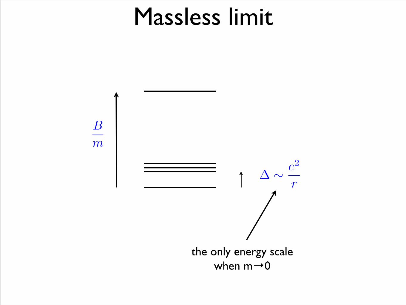
Massless limit

B

m

� ⇠ e2

r

the only energy scalewhen m→0

Laughlin’s wave function

• In the symmetric gauge LLL states are

(z) = f(z)e�|z2|/4`2

(z) =Y

hiji

(zi � zj)3Y

i

e�|zi|2/4`2

Laughlin’s guess for the ground state wave fn ⌫ = 1/3

Not exact, although seems to be very good approximationimplies equal-time correlators, not at unequal times

Effective field theory

• Effective field theory: captures low-energy dynamics

• What are the low-energy degrees of freedom of a quantum Hall state?

• there are none (in the bulk): energy gap

• Thus the effective Lagrangian is polynomial over external fields and derivatives (generating functional)

Chern-Simons action

• To lowest order in derivatives:

S =�

4�

�d3x �µ��Aµ��A�

encodes Hall conductivity

�xy =�

2�

e2

�

Jµ =�S

�Aµ

Jy

= �xy

Ex

⇢ =⌫

2⇡B

Another formulation of CS theory

is the current

at the same time is the Lagrange multiplier enforcing

aµ = Aµ + @µ'

L =⌫

4⇡✏µ⌫�aµ@⌫a� � jµ(@µ'�Aµ + aµ)

jµ =�S

�Aµ

Note: is the phase of the condensate of composite bosons (ZHK)'

Universality beyond CS

Higher-derivatives corrections: of dynamical, not topological nature, hence non universal?

But there is universality beyond the CS action

Hall viscosityFollowing the evolution of the QH state with changing metric

hij = hij(t), deth = 1

2-dim space

nonzero Berry curvature

hT11 � T22i ⇠ ⌘Ah12

h11 � h22

h12

However in CS theory Tµ⌫ = 0

universal (not renormalizedby interactions)

Symmetries of NR theory

Microscopic theory

Dµ� � (�µ � iAµ)�

Invariance under time-independent diff ξ=ξ(x):

DTS, M.Wingate 2006

�Ai = ��k�kAi �Ak�i�k

�� = ��k�k�

�A0 = �⇠k@kA0

�hij = �ri⇠j �rj⇠i

S =

Zd

3x

ph

i

2

†$Dt � h

ij

2mDi

†Dj +

g

4m

F12ph

†

�

NR diffeomorphism

• These transformations can be generalized to be time-dependent: ξ=ξ(t,x)

Galilean transformations: special case ξi=vit

�� = ��k�k�

�A0 = �⇠k@kA0 �Ak ⇠k +

g

4"ij@i(hjk ⇠

k)

�Ai = ��k�kAi �Ak�i�k �mhik ⇠

k

�hij = �ri⇠j �rj⇠i

g = 0 version can be understood as NR reduction of relativistic diffeomorphism invariance

NR reductionStart with complex scalar field

Take nonrelativistic limit:

� = e�imcx0 ��2mc

S = �Zdx

p�g(gµ⌫Dµ�

⇤D⌫�+m

2�

⇤�)

gµ⌫ =

0

BB@

�1 +2↵0

mc2↵j

mc

↵i

mchij

1

CCA

Dµ� = (@µ � iAµ)�

S =

Zd

3x

ph

i

2

†$Dt � h

ij

2mDi

†Dj

�

Dµ = @µ � i(Aµ + ↵µ)

Relativistic diffeomorphism

: gauge transform

: general coordinate transformations

� = e�imcx0 ��2mc⇠0

⇠i

gµ⌫ =

0

BB@

�1 +2↵0

mc2↵j

mc

↵i

mchij

1

CCA

under diff Aµ = Aµ + ↵µ

�A0 = �⇠k@kA0

�Ai = ��k�kAi �Ak�i�k �mhik ⇠

k

�Ak ⇠k

Interactions

• Interactions can be introduced that preserve nonrelativistic diffeomorphism

• interactions mediated by fields

• For example, Yukawa interactions

�� = �⇠k@k�

S = S0 +

Zd

3x

ph�

† +

Zd

3x

ph(hij

@i�@j�+M

2�)

Is CS action invariant?

• CS action is gauge invariant, Galilei invariant

• but not diffeomorphism invariant

does not transform like a one-form Aµ

�SCS =⌫m

2⇡

Zd

3x ✏

ijEihjk ⇠

k g = 0

�A0 = �⇠k@kA0 �Ak ⇠k +

g

4"ij@i(hjk ⇠

k)

�Ai = ��k�kAi �Ak�i�k �mhik ⇠

k

�Aµ = �⇠k@kAµ �Ak@µ⇠k

Aµ = Aµ + ↵µ

Is CS action invariant?

• CS action is gauge invariant, Galilei invariant

• but not diffeomorphism invariant

does not transform like a one-form Aµ

�SCS =⌫m

2⇡

Zd

3x ✏

ijEihjk ⇠

k g = 0

�A0 = �⇠k@kA0 �Ak ⇠k +

g

4"ij@i(hjk ⇠

k)

�Ai = ��k�kAi �Ak�i�k �mhik ⇠

k

�Aµ = �⇠k@kAµ �Ak@µ⇠k

Aµ = Aµ + ↵µ

Requirements for EFT

• Respect general coordinate invariance

• Reproduce all topological properties of the quantum Hall state

• Have regular limit of

LLL degenerate with zero energy for any metric and B(Aharonov-Casher)

m ! 0, g = 2

Sg[A0, Ai, hij ]

What kind of geometry

• System does not live in a 3D Riemann space

• 2D Riemann manifold at any time slice

• can parallel transport along equal-time slices, but not between different times

Velocity vector v

Use v to transform objects from one time slice to another

t+�t

v�t

Cartan 1923-1924Reformulation of Newton’s theory of gravity

Cartan 1923-1924Reformulation of Newton’s theory of gravity

Cartan 1923-1924Reformulation of Newton’s theory of gravity

Cartan 1923-1924Reformulation of Newton’s theory of gravity

Cartan 1923-1924Reformulation of Newton’s theory of gravity

Cartan 1923-1924Reformulation of Newton’s theory of gravity

Cartan 1923-1924Reformulation of Newton’s theory of gravity

Newton-Cartan geometry

dn = 0 ) n = dt

nµvµ = 1

dn = 0

choose t to be time coordinate

(hµ⌫ , nµ, vµ) hµ⌫n⌫ = 0

hµ⌫h⌫� = �µ� � vµn� hµ⌫v⌫ = 0

hµ⌫ =

✓0 00 hij

◆hµ⌫ =

✓v2 �vj�vi hij

◆

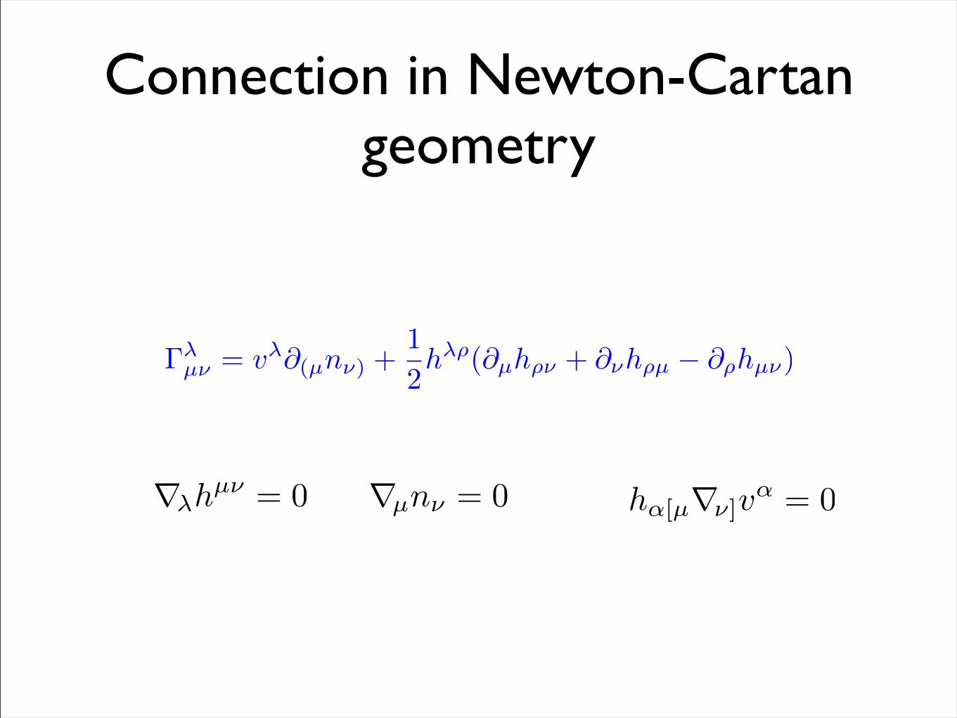
Connection in Newton-Cartan geometry

rµn⌫ = 0r�hµ⌫ = 0 h↵[µr⌫]v

↵ = 0

��µ⌫ = v�@(µn⌫) +

1

2h�⇢(@µh⇢⌫ + @⌫h⇢µ � @⇢hµ⌫)

Higher-dimensional interpretation

x

M = (x�, x

µ)

gMN =

✓0 n⌫

nµ hµ⌫

◆gMN =

✓0 v⌫

vµ hµ⌫

◆

��µ⌫ = v�@(µn⌫) +

1

2h�⇢(@µh⇢⌫ + @⌫h⇢µ � @⇢hµ⌫)

�LMN =

1

2gLR(@MgRN + @NgRM � @RgMN )

Improved gauge potentials

• With v one can construct a gauge potential that transforms as a one-form

Ai = Ai +mvi

�Aµ = �⇠k@kAµ � Ak@µ⇠k

What is v? Should be dynamically determined

A0 = A0 �mv2

2� g

4"ij@ivj

Effective field theory

related to “shift”

Dµ' = @µ'� Aµ + aµ�s!µ

Integrating out ⇢, vi, aµ

effective action for ) Aµ, hij

S =⌫

4⇡

Zd

3x ✏

µ⌫�aµ@⌫a� �

Zd

3x

ph ⇢v

µDµ'

+S0[⇢, vi, hij ]+

Zd

3x

g � 2

8m✏

µ⌫�nµF⌫�

Spin connection

e1

e2

!µ =1

2✏abea⌫rµe

b⌫

=1

2✏abeai@te

bi +

1

2✏ij@ivj

!0 =1

2✏abeair0e

bi

nonzeroin flat space�1�2 � �2�1 =

12�

g R

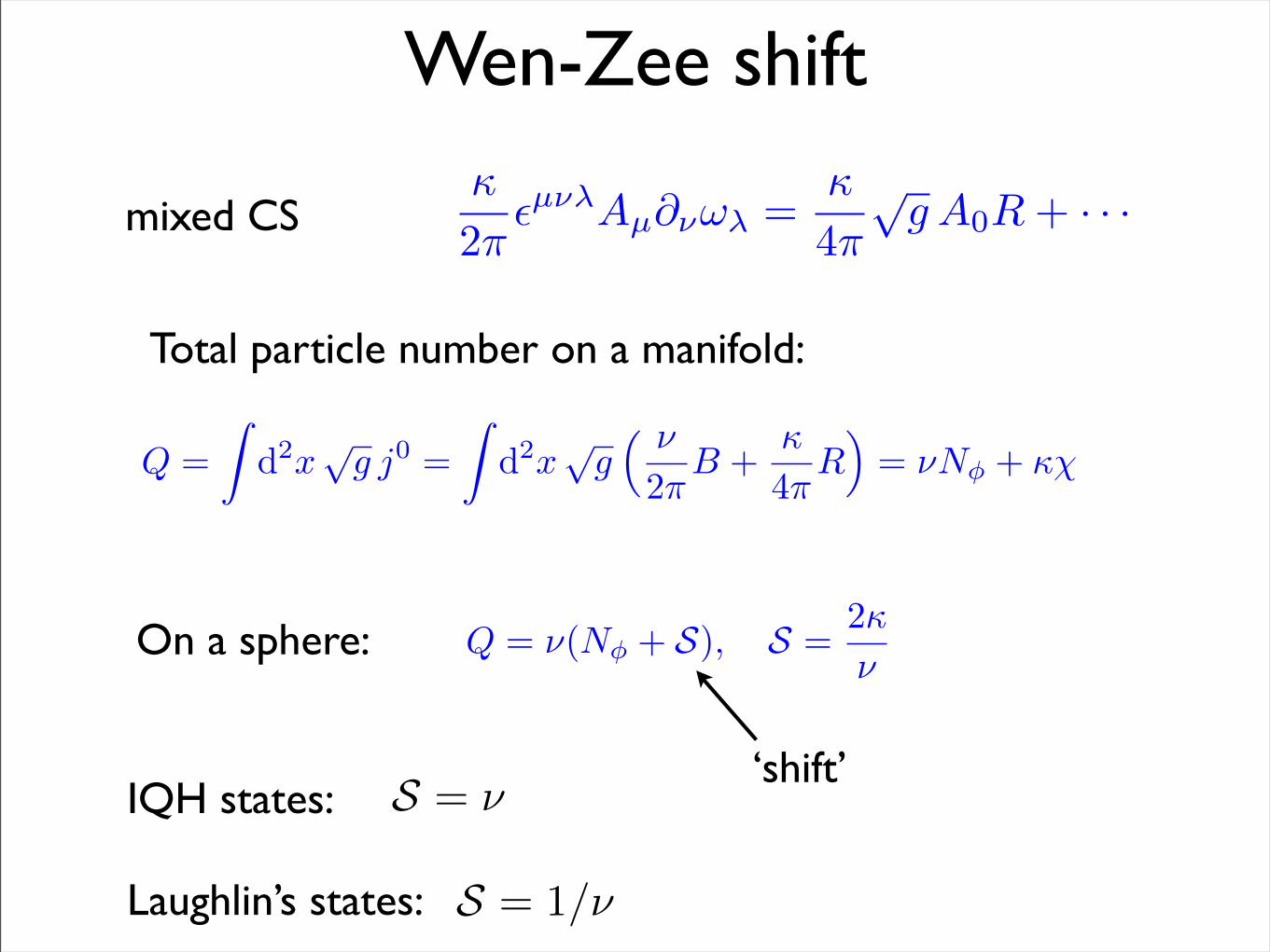
Wen-Zee shift�

2��µ��Aµ���� =

�

4�

�g A0R + · · ·

Q =�

d2x�

g j0 =�

d2x�

g� �

2�B +

�

4�R

�= �N� + ��

Total particle number on a manifold:

IQH states:

Laughlin’s states:

On a sphere: Q = �(N� + S), S =2�

�

‘shift’S = ⌫

S = 1/⌫

mixed CS

Shift for IQH states

N� + 1

N� + 3

N� + 5

Q = nN� + n2 = n(N� + n)

Physical consequences

• Kohn’s theorem

• Hall viscosity

• Hall conductivity: universal to order q^2

• Structure factor

Kohn’s theorem

Constant B, Response to homogeneous, time dependent E(t) independent of interactions: motion of center of mass

mvi = Ei + ✏ijvjB

Hall viscosity from WZ term

SWZ = � �B

16��ijhik�thjk + · · ·

derived by N.Read previously

hTxy

(Txx

� Tyy

)i ⇠ i⌘a!

⌘a =1

4S⇢

Avron, Seiler, Zograf

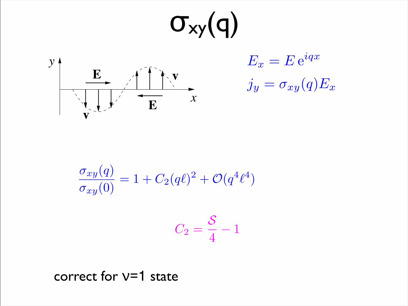
σxy(q)y

v

E

E

vx

Ex = E eiqx

jy = �xy(q)Ex

�xy(q)�xy(0)

= 1 + C2(q�)2 +O(q4�4)

C2 =S4� 1

correct for ν=1 state

Structure factor and shift

• Non-universal part of the action: leading contributions are

�zzF (i@t)�zz

positivity of spectral densities of stress-stress correlators:equal time density-density corr

Inequality saturated by Laughlin’s wave function

�µ⌫ = £vhµ⌫

(Haldane 2009)limk!0

s(k)

(k`)4� |S � 1|

8

Conclusion and outlook

• Quantum Hall states naturally live in Newton-Cartan geometry

• Symmetry determines the q^2 correction to Hall conductivity, other physical quantities

• Further questions:

• edge states?

• Relationship with conformal field theories?

• Meaning of Laughlin’s wave function?

• Implications for holographic realizations?

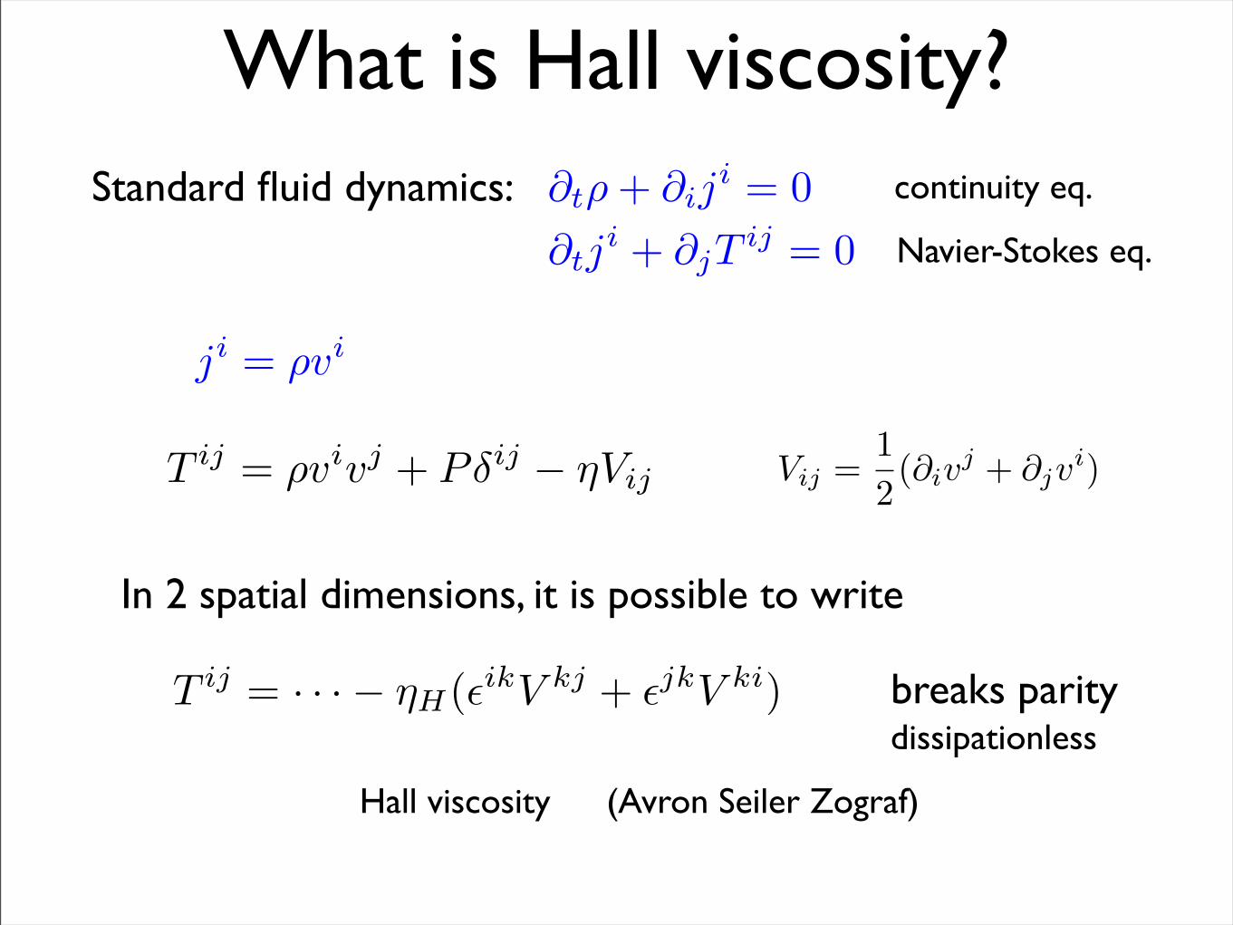
What is Hall viscosity?

ji = �vi

T ij = �vivj + P �ij � �Vij Vij =12(�iv

j + �jvi)

In 2 spatial dimensions, it is possible to write

T ij = · · ·� �H(�ikV kj + �jkV ki)

Hall viscosity (Avron Seiler Zograf)

breaks parity

Standard fluid dynamics: �t� + �iji = 0

�tji + �jT

ij = 0continuity eq.

Navier-Stokes eq.

dissipationless

Hall viscosity in picture

Hall shear stress

Physical interpretation

• First term: Hall viscosity

yv

E

E

vx

�xvy + �yvx �= 0

Txx = Txx(x) �= 0

additional force Fx~∂x Txx

Hall effect: additional contribution to vy

Physical interpretation (II)

• 2nd term: more complicated interpretation

Fluid has nonzero angular velocity

�(x) =12�xvy = �cE�

x(x)2B

�B = 2mc�/e

Coriolis=Lorentz

Hall fluid is diamagnetic: d� = �MdB

M is spatially dependent M=M(x)

Extra contribution to current j = c z��M

Current ~ gradient of magnetization

j = c z��M