The Global Structure of UTLS Ozone in GEOS-5: A Multi-

Year Assimilation of EOS Aura Data

Krzysztof Wargan1,2, Steven Pawson1, Mark A. Olsen3,4, Jacquelyn C. Witte2,3,

Anne R. Douglass3, Jerald R. Ziemke3,4, Susan E. Strahan3,5, J. Eric Nielsen1,2

1 Global Modeling and Assimilation Office, Code 610.1, NASA Goddard Space Flight

Center, Greenbelt, MD

2 Science Systems and Applications Inc., Lanham, MD

3 Atmospheric Chemistry and Dynamics Laboratory, Code 614, NASA Goddard Space

Flight Center, Greenbelt, MD

4 Goddard Earth Sciences, Technology and Research Center, Morgan State University,

Baltimore, MD.

5 Goddard Earth Sciences, Technology and Research Center, Universities Space

Research Association, Columbia, MD

Correspondence: Krzysztof.Wargan-1@nasa.gov

https://ntrs.nasa.gov/search.jsp?R=20150000790 2018-07-14T00:00:33+00:00Z

Abstract

Eight years of ozone measurements retrieved from the Ozone Monitoring Instrument

(OMI) and the Microwave Limb Sounder, both on the EOS Aura satellite, have been

assimilated into the Goddard Earth Observing System version 5 (GEOS-5) data

assimilation system. This study thoroughly evaluates this assimilated product,

highlighting its potential for science. The impact of observations on the GEOS-5 system

is explored by examining the spatial distribution of the observation-minus-forecast

statistics. Independent data are used for product validation. The correlation coefficient of

the lower-stratospheric ozone column with ozonesondes is 0.99 and the bias is 0.5%,

indicating the success of the assimilation in reproducing the ozone variability in that

layer. The upper-tropospheric assimilated ozone column is about 10% lower than the

ozonesonde column but the correlation is still high (0.87). The assimilation is shown to

realistically capture the sharp cross-tropopause gradient in ozone mixing ratio.

Occurrence of transport-driven low ozone laminae in the assimilation system is similar to

that obtained from the High Resolution Dynamics Limb Sounder (HIRDLS) above the

400 K potential temperature surface but the assimilation produces fewer laminae than

seen by HIRDLS below that surface. Although the assimilation produces 5 – 8 fewer

occurrences per day (up to ~20%) during the three years of HIRDLS data, the interannual

variability is captured correctly. This data-driven assimilated product is complementary

to ozone fields generated from chemistry and transport models. Applications include

study of the radiative forcing by ozone and tracer transport near the tropopause.

1. Introduction

This work describes and evaluates an eight-year long record of six-hourly global maps of

ozone produced by NASA’s Goddard Earth Observing System Version 5 (GEOS-5) data

assimilation system informed by total ozone observations from the Ozone Monitoring

Instrument (OMI) and stratospheric profile data provided by the Microwave Limb

Sounder (MLS). Both instruments fly on the Earth Observing System Aura satellite (EOS

Aura, launched in July 2004) and are still operational. In the past, several techniques

were developed to produce global maps of tropospheric ozone columns using combined

information from these two data sources. Schoeberl et al. [2007] employed a trajectory

method to propagate MLS observations and calculate the stratospheric ozone columns.

These were subsequently subtracted from the OMI total column measurements to obtain

the tropospheric ozone residual. Ziemke et al. [2011] used MLS observations binned into

a latitude-longitude grid collocated with gridded OMI data to generate a six-year global

climatology of stratospheric and tropospheric ozone columns. Stajner et al. [2008] and

Wargan et al. [2010] assimilated OMI and MLS data into the GEOS-4 data assimilation

system (a predecessor of GEOS-5). Their work demonstrated good agreement of the

assimilated product on synoptic time scales with independent observations in upper

troposphere – lower stratosphere (UTLS), in particular, as compared to data from aircraft

measurements.

The present work aims to investigate the realism of ozone structures in the UTLS in an

assimilation of MLS and OMI observations from 2005 to 2012. The assimilation is

performed using Version 5.7.2 of the GEOS-5 data assimilation system. While this study

focuses on the region between 500 hPa and 50 hPa, Ziemke et al. [2014] conducted a

detailed evaluation of the tropospheric ozone from this analysis with two other products

derived from OMI and MLS data (a tropospheric residual method and ozone profiles

retrieved from OMI-measured radiances). That work also includes an extensive

comparison of these three products with the Global Modeling Initiative chemical

transport model [Duncan et al., 2008; Strahan et al., 2007], which simulates global ozone

fields using a photochemical mechanism and transport driven by GEOS-5 meteorological

analysis but does not utilize any ozone data.

The production of global, three-dimensional ozone distributions derived from

observations, that resolve the ozone structure in the vicinity of the tropopause is

motivated by the importance of the ozone distribution to both climate forcing and

transport processes. Ozone in the UTLS plays an important role in the forcing of climate

and also impacts background tropospheric ozone levels that influence regional air quality.

The vertical distribution of ozone in the stratosphere and troposphere is important for

climate forcing, largely because of the dominant warming impact of tropospheric ozone,

which is partly offset by a weaker cooling impact of stratospheric ozone [e.g., Lacis et

al., 1990]. Radiative cooling by water vapor and warming by ozone have been proposed

as a possible explanation for the existence and maintenance of the tropopause inversion

layer in the lowermost extratropical stratosphere [Randel et al., 2007]. The sensitivity of

the outgoing long wave radiation to the ozone distribution was emphasized by a study of

radiative fluxes from the Tropospheric Emission Sounder (TES) by Worden et al. [2011].

Shindell et al. [2013] used these TES observations in conjunction with a climate model to

separate the climate forcing by ozone loss caused by halocarbons from that of ozone

increases caused by air pollution, each of which led to changes in both tropospheric and

stratospheric ozone.

In-situ observations contain too little spatio-temporal information to fully describe the

structure and budget of ozone in the UTLS. Operational, nadir-sounding satellite

datasets, including the long Solar Backscattered Ultraviolet (SBUV) record, provide

climate-quality constraints on total ozone, but do not resolve vertical structure below

about 20 km altitude [Kramarova et al., 2013], and therefore do not separate stratospheric

and tropospheric ozone from each other. Limb-profiling observations present the best

potential for quantifying ozone and its vertical structure through the stratosphere and into

the upper troposphere, although the observation errors are typically large below the

tropopause, where clouds and water vapor impact radiative transfer. The High-Resolution

Dynamic Limb Sounder (HIRDLS) on EOS Aura provides ozone information with ~1 km

vertical resolution in the UTLS from 2005-2007 [Gille et al., 2008; Nardi et al., 2008]. It

was used by Olsen et al. [2010] to study low ozone laminae in the lower stratosphere

associated with transport from the tropics to the mid-latitudes. That study found less

irreversible transport of ozone in the year with the most filaments, a counterintuitive

result that motivates the desire to study year-to-year variability with a longer time series.

The vertical resolution of the MLS ozone data used here is ~2.5 km in the UTLS [Livesey

et al., 2008; Froidevaux et al., 2008] and the vertical resolution of the GEOS-5 model

grid is close to 1 km in that layer of the atmosphere. Olsen et al. [2008] used the GMI

model driven by GEOS-4 assimilated winds at this resolution and showed that the

analysis winds have sufficient transport information in the vertical to reproduce a lamina

transport event observed by HIRDLS in the lower stratosphere. Case studies done by

Semane et al., [2007], El Amraoui et al., [2010], and Barré et al. [2013] demonstrated the

ability of assimilated ozone data from limb sounders to represent individual deep

stratospheric intrusion events. The work delineated above illustrates the value of a multi-

year analysis and a statistical evaluation of the capabilities that assimilation of MLS data

offers.

The system used in this study consists of a general circulation model (GCM) and a

statistical data analysis module, which will be described in Section 2. Later sections

examine the following aspects of UTLS in GEOS-5:

1. An assessment of the constraints imposed by MLS and OMI observations in the

assimilation system, in conjunction with the role of the underlying background

(forecast) states generated by the general circulation model (the model component

of GEOS-5) informed by assimilated meteorological data (Section 3).

2. The realism of the assimilated ozone profiles and partial columns compared to

ozonesondes (Section 4).

3. An assessment of ozone filaments in GEOS-5, including their structure and

frequency of occurrence (Section 5). A validation of the morphology of these

events against HIRDLS observations for 2005-2007 is followed by a calculation

of interannual variations between 2005 and 2012.

After these results, the conclusions are linked with an outline of possible applications of

GEOS-5 analyses of OMI and MLS ozone.

We stress that the assimilated ozone discussed in this study is fundamentally a data-

driven product. As such, it is complementary to the output obtained from full-chemistry

and transport models such as the Global Modeling Initiative (GMI) project. This work is

also an evaluation of the data assimilation system configuration that (after several

modifications) will be used in an upcoming Modern-Era Retrospective analysis for

Research and Applications version 2 (MERRA-2) reanalysis project currently carried out

at NASA’s Global Modeling and Assimilation Office.

2. Ozone Assimilation in GEOS-5

This section presents details of the configuration of GEOS-5, focusing on the ozone data

and structure of the data assimilation system.

2.1 The GEOS-5 Data Assimilation System

In atmospheric data assimilation, measurements of various components of the state of the

atmosphere at a given time are combined with a three-dimensional gridded representation

of atmospheric fields obtained from a general circulation model (hereafter: model)

integration. This is done in a statistically optimal way, by taking into account

observational and model forecast errors. This blended new set of fields, termed the

analysis, is then used to generate an initial condition for a short (here, 6-hourly) model

forecast which produces the background fields for the next assimilation cycle. For

example, Kalnay [2003] and Cohn [1997] explain theory of data assimilation in detail. A

review of data assimilation methodology applied to chemical constituents, including

ozone, can be found in [Lahoz et al., 2007].

The GEOS-5.7.2 DAS is an established configuration of GEOS-5 that was used to

generate officially released GEOS-5 data products between August 18, 2011, and June

11, 2013. The “production” configuration ran with a resolution of 0.3125° (longitude) ×

0.25° (latitude), with 72 layers between the surface and 0.01hPa. The configuration used

in this work has horizontal resolution of 2.5°×2.0° and the same 72 layers. GEOS-5.7.2

includes some scientific advances and enhanced capabilities over GEOS-5.2.0, the

version of GEOS-5 used in the Modern-Era Retrospective analysis for Research and

Applications MERRA [Rienecker et al., 2011]: improvements to physical processes in

the underlying forecast model [Molod et al., 2012] and additional data ingestion

capabilities (for newer infrared sounders and for Global Positioning System Radio-

Occultation data). The latter were not used to generate the present product. The observing

system pertinent to meteorology here is the same as in MERRA.

The meteorological analysis in GEOS-5 is performed four times daily, using six-hour

model forecasts (backgrounds) and observations within a ±3-hour window of the analysis

time. The objective of the optimization is to produce an analysis field for which a cost

function constructed from the observation-minus-analysis (O-A) residuals is minimized

subject to assumed forecast and observation error statistics [Cohn, 1997]. The Gridpoint

Statistical Interpolation (GSI) [Wu et al., 2002, Purser et al., 2003a,b] optimally

combines in-situ observations, retrieved quantities, and satellite-based infrared and

microwave radiances along with the backgrounds to produce the analyses. Ozone

analyses are impacted only by OMI and MLS observations. In GSI, the analysis of the

meteorological fields includes cross-coupling among fields, but ozone is essentially a

univariate analysis embedded within the minimization vector. In the configuration used

in this study, a climatological ozone field was coupled to the radiation code in the GCM,

so the assimilated ozone field did not impact the meteorological forecasts (backgrounds).

We found that coupling the assimilated ozone with meteorology instead would not alter

the results of this work.

2.2 Ozone-specific aspects of GEOS-5

Chemistry in the GCM

The model includes stratospheric ozone production rates and loss frequencies, following

Stajner et al. [2008]. This month-dependent parameterization was obtained from a two-

dimensional chemistry and transport model simulation and corrected using data from the

Upper Atmosphere Research Satellite reference climatology. However, the ozone

chemistry time scale in the UTLS and in the troposphere is of the order of weeks

(compared to daily data insertion) so that in practice the analysis is insensitive to

chemistry parameterization in that region. Unlike Stajner et al. [2008], tropospheric

ozone chemistry has been deliberately simplified in this study: no chemical production or

loss is computed and the only removal mechanism is by dry deposition at the surface,

derived using a climatological distribution of Normalized Difference Vegetation Index

and deposition velocities computed using standard algorithms [Rienecker et al., 2008]. A

tropospheric ozone chemistry parameterization is unnecessary because the typical

chemical timescales for background ozone in the free troposphere are long compared to

the frequency of data insertion in this assimilation (approximately once a day for a given

location).

OMI observations and their treatment

The OMI instrument [Levelt et al., 2006] is a nadir-viewing spectrometer that measures

visible and ultraviolet backscattered solar radiation in the 270-550 nm wavelength range

with a spectral resolution of ~0.5 nm. The wide swath, of 2600 km, is sampled by a

sensor array that covers the cross-track and spectral domains. The 60 cross-track pixels

(rows) yield a spatial resolution at nadir of 13 km (along-track) km × 24 km (across-

track). The row width increases to about 180 km at the outer extremes [Levelt et al.,

2006]. The two outer rows on each side of the swath were not used because of large solar

zenith angle changes that occur along the wide outer pixels and make the product less

accurate. Since 2008, an external blockage has rendered about half of the rows unusable

(this is referred to as “row anomaly”). Following guidance from the OMI instrument

team (J. Joiner, personal communication) and in the interest of data consistency row

numbers 25-60 have been excluded for the entire period of this study, even though the

row anomalies did not exist before 2008. The assimilation uses ozone columns retrieved

for rows 3-24 of OMI for the entire period. With this row selection the width of the OMI

swath is about 1,100 km. The total column observations from OMI are made over the

sun-lit atmosphere. In particular, there are no OMI data in the polar night. Only

observations made at solar zenith angles less than 84° are used.

We use OMI total column ozone retrievals from collection 3 data, version-8.5 retrieval

algorithm. An extensive validation of the OMI ozone was done by McPeters et al.

[2008]. This algorithm is modified from the OMTO3 algorithm previously applied to

retrieve data from the Total Ozone Mapping Spectrometer instruments. The use of a

more realistic cloud pressure retrieval algorithm [Joiner and Vasilkov, 2006] leads to

significantly improved total ozone retrievals over cloudy areas compared with earlier

versions. A detailed description of the algorithm can be found in the algorithm theoretical

basis document available at http://eospso.gsfc.nasa.gov/atbd-category/49. The OMI

ozone columns include information from the measurement and climatological a priori

information in layers where there is reduced sensitivity of the OMI measurements to

ozone. Version 8.5 uses the Labow-Logan-McPeters two-dimensional climatology

derived from ozonesonde and satellite data [McPeters et al., 2007]. The a priori provides

much of the information in the retrievals in the lower troposphere, where clouds and

aerosols affect radiances, and where the sensitivity to ozone is reduced by Rayleigh

scattering. To account for these effects, each OMI ozone retrieval includes additional

information about the efficiency factors (εi) and a priori profiles (yiprior). These are given

on 11 layers, each approximately 5 km thick. An appropriate OMI observation operator

has been implemented into the GSI algorithm to ensure that the information content of

the OMI data is correctly included. The operator computes the observation-minus-

forecast (O-F) residual as:

𝑂 𝐹 𝑦𝑜 𝑦𝑖𝑝𝑟𝑖𝑜𝑟 𝜀

𝑖𝑥𝑖

𝑓𝑜𝑟𝑒𝑐𝑎𝑠𝑡 𝑦𝑖𝑝𝑟𝑖𝑜𝑟

𝑖 ,

where yo and xforecast denote the retrieved OMI total ozone and the forecast ozone

interpolated to the observation location and integrated within each of the 11 layers for

which the efficiency factors are provided. The O-F residuals, scaled according to

observation and background errors, determine the analysis increment that is added to the

background (forecast) ozone to yield the analysis state [Cohn, 1997].

Because the observation density of OMI is substantially larger than the analysis grid, and

in order to reduce the large number of observations for computational efficiency, the data

are thinned over 150-km grid boxes prior to the analysis. A total of ~12,000 OMI

observations per day are assimilated.

Assimilation of MLS ozone data

MLS measures microwave emissions from the atmospheric limb in a broad spectral

region, allowing for retrievals of a large number of trace constituents as well as

temperature and pressure [Waters et al., 2006]. This work uses ozone profiles from

version 3.3 of the MLS retrieval algorithm [Livesey et al., 2008, 2011], in which ozone

information is derived from 25 spectral channels in a spectral band centered at 240 GHz.

The ozone mixing ratios from MLS are reported on 55 layers. The 38 layers between 261

hPa and 0.02 hPa were used in this work based on recommendations from the MLS

science team. The vertical resolution of the MLS ozone data ranges from 2.5 km in the

middle stratosphere to 6 km in the mesosphere [Livesey et al., 2008; Froidevaux et al.,

2008].

A single MLS profile is a set of discrete point values at retrieval levels. Because the

GEOS-5 system represents layer-averaged concentrations, the MLS retrievals were first

converted to layer averages on the 37 mid-points (the geometric mean of the pressure

values at each two consecutive levels) of the MLS grid. The center of the lowest

assimilated layer is thus 237 hPa. The observation operator applied for MLS data in GSI

is then a straightforward layer averaging of the background field and spatial interpolation

to the observation locations. No attempt has been made to account for the two-

dimensional structure of the MLS retrievals: the 200-300 km along-line-of-sight footprint

is roughly comparable to the GEOS-5 grid-box size at the resolution used in this work. A

pre-assimilation data selection is done following the quality guidelines provided in

Livesey et al. [2011].

We emphasize that no bias correction is applied to the MLS data prior to or during

assimilation. Instead, the observation errors for MLS ozone are calculated as the square

root of the sum of squares of the reported precision and accuracy so that observations

with large random or systematic error are given less weight in the assimilation and their

impact on the analysis is reduced as a result. For the mid-layer averages, the error is

specified as the larger of the values at the two bounding levels. The computed mean

observation error in the northern extratropics is about 5% throughout most of the

stratosphere down to 75 hPa and increases to about 20% at 237 hPa. We stress that

precision errors (given in parts per million by volume) vary from observation to

observation. Specific values of the calculated observation error used in the assimilation

are available in the assimilation auxiliary output stream.

A high bias exists for the MLS levels at pressure levels 261 hPa and 215 hPa. Table 1

contains the values of the bias separated by four latitude bands evaluated using

ozonesondes in 2010 (see Section 4). The relative bias at 261 hPa ranges from 21%

between 60°N – 90°N to 46% in the northern middle latitudes. The MLS – sondes

differences at 215 hPa are much smaller and disappear at higher levels. The reported

accuracy (systematic) error for these levels is higher than for the rest of the assimilated

profile. The ~ 20% combined (accuracy with precision) MLS error at the bottom of the

profile is large compared to the background error assumed by the assimilation system (at

most 10% and as low as 2.5% for tropospheric ozone concentrations, see next

subsection). Consequently, the analysis ozone at these levels is dominated by the model

values and the impact of MLS observations is less than elsewhere in the stratosphere.

This error dependent impact will be evaluated in Section 3.

Background error covariances for the ozone analysis

When combining the background states with observations, GSI takes into account both

observation and background (forecast) errors as well as spatial correlations of the latter.

These correlations are used by the analysis algorithm to spread the information from a

data location onto its close neighborhood in the horizontal and vertical directions. Since

the UTLS ozone exhibits sharp gradients, particularly across the tropopause, the

background error covariances should be prescribed with caution in order to avoid

excessive smoothing. In older versions of the GSI these correlations were read in from a

lookup table. In this work the approach has been modified: Following Stajner et al.

[2008] and Wargan et al. [2010], the background error standard deviation for ozone is

assumed to be proportional to the forecast ozone concentration at each grid point. The

height-dependent constant of proportionality was tuned using a series of short

experiments validated against ozone sonde data and such that the resulting assimilated

ozone fields yield smooth zonal and temporal means. In the troposphere, the coefficient

is set to 0.1 (i.e. the background error standard deviation is 10% of the local ozone from

the latest 6-hourly forecast). The best results were obtained when the coefficient was

reduced by a factor of four in the stratosphere relative to the troposphere. For the

purpose of this algorithm the tropopause is defined as the 0.1 ppmv ozone isopleth. In

particular, the air present in stratospheric intrusions is treated as stratospheric. The

primary consequence of this choice of background errors is that relatively large analysis

increments in the stratosphere are prevented from excessively affecting the much lower

upper concentrations below the tropopause.

Other details of the ozone assimilation

In addition to the ozone data screening, the OMI and MLS observations undergo ‘online’

quality control within the GSI prior to analysis. Values for which the ratio of the

calculated observation-minus-forecast (O-F) residual to the observation error is greater

than 10.0 are discarded. In practice, this occurs very infrequently: only up to a few MLS

observations a day are discarded, most of them in the mesosphere.

OMI and MLS observations are the only data that impact ozone in this implementation of

GEOS-5. Both instruments provide an almost unbroken measurement record during the

eight-year period of this analysis, with data gaps that rarely exceed a few days. The major

concern is the period from March 27 through April 18, 2011, when MLS data were not

available owing to a problem with the instrument. In order to evaluate the potential

impacts of the analysis ozone drift resulting from this data gap, an experiment in which

MLS observations were turned off was conducted for the same period in 2010 and the

results were compared with the full analysis. South of 30°S between 260 hPa and 30 hPa

the “no MLS experiment” ozone experiences an approximately linear decrease resulting

in concentrations 10%-18% lower then in the MLS analysis after 3 weeks. Between 30°S

and 30°N lower stratospheric ozone decreases by ~10% during the first 10 days and

stabilizes afterwards. In the northern extratropics there is an alternating pattern of steady

decrease (~10% over the first three weeks) and an increase between 200 hPa and 50 hPa

by approximately the same amount. In the middle stratosphere there is an increase from

10% (30°S - 30°N) to as much as 25% (90°S - 60°S) over the duration of the experiment.

In the northern hemisphere these values are smaller: about 3% increase between 30°N

and 60°N and a decrease by 3% in the high latitudes. The alternating patterns of

increasing and decreasing mixing ratios amount to partial cancellation in the total column

as expected from the fact that total ozone is constrained by OMI data in both

experiments.

3. Performance of the GEOS-5 Assimilation System

This section shows results describing the GEOS-5 system performance as related to

ozone. The purpose is to demonstrate the credibility of the assimilation system and to

discuss results that describe the regions where the model and the EOS Aura observations

do and do not agree. This is done by examining the spatial distributions, magnitude and

behavior of the observation-minus-forecast (O-F) residuals (which measure the

discrepancy between the six-hourly model forecast and data) and comparing them with

the observation-minus-analysis (O-A) differences. Because, by design, the data

assimilation algorithm brings ozone concentrations closer to the observed values the O-A

fields are expected to be smaller than the O-Fs. The extent to which this reduction takes

place depends on relative magnitudes of observation and background errors.

Figure 1 shows profiles of the mean and standard deviation of O-F and O-A for MLS

ozone mixing ratios in the northern hemisphere extratropics (NH: 30°N-90°N) as a

function of pressure for June - August 2010. The standard deviation of O-F increases

almost linearly with altitude, from about 0.06 ppmv near 237 hPa to about 0.11 ppmv

near 10 hPa. Except at the lowest two layers (centered at 237 hPa and 196 hPa), the mean

O-Fs are very small, with weak positive values in the low stratosphere that change sign

by the middle stratosphere. Below about 20 hPa the analysis has only a small impact on

the mean ozone (the mean O-F and O-A profiles seen in Figure 1(b) are very similar –

and close to zero) but there is a clear improvement in the standard deviation (Figure 1(a)).

Two separate assimilation experiments, omitting either the MLS or OMI observations

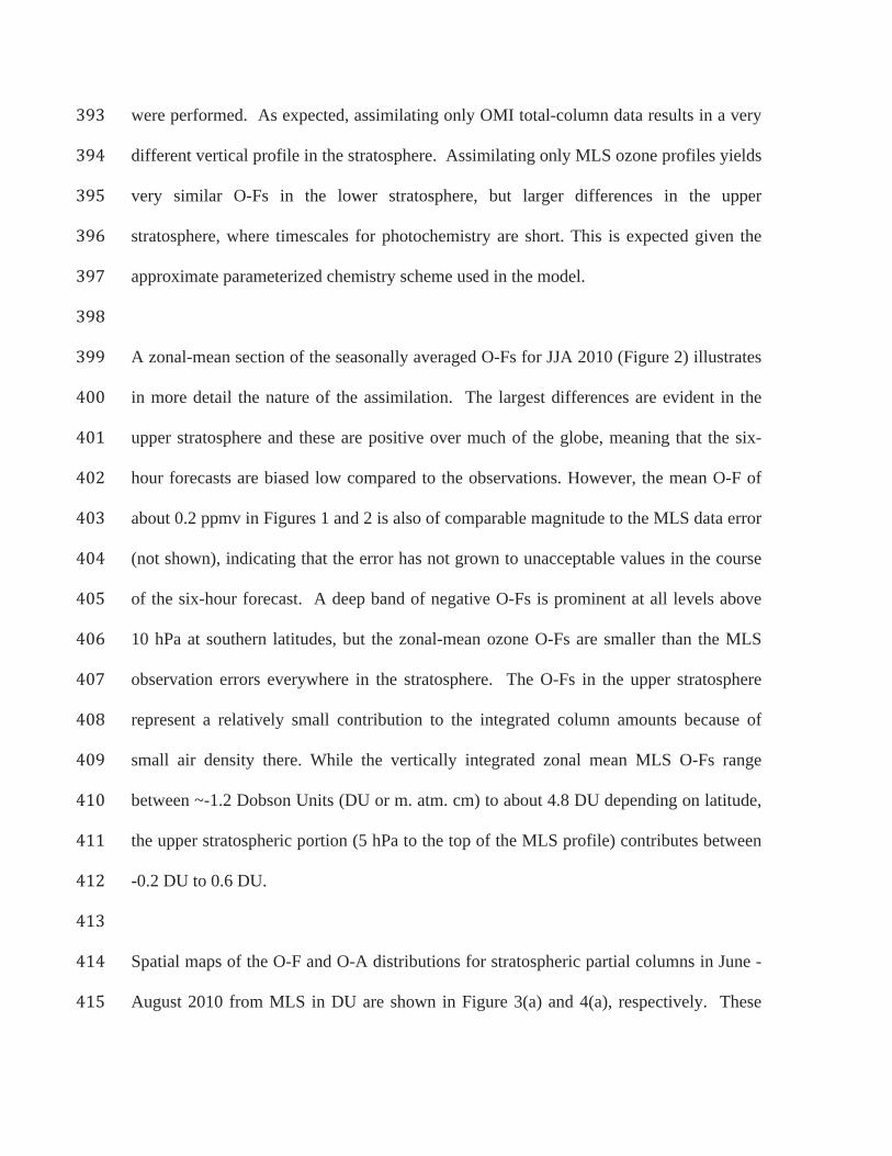
were performed. As expected, assimilating only OMI total-column data results in a very

different vertical profile in the stratosphere. Assimilating only MLS ozone profiles yields

very similar O-Fs in the lower stratosphere, but larger differences in the upper

stratosphere, where timescales for photochemistry are short. This is expected given the

approximate parameterized chemistry scheme used in the model.

A zonal-mean section of the seasonally averaged O-Fs for JJA 2010 (Figure 2) illustrates

in more detail the nature of the assimilation. The largest differences are evident in the

upper stratosphere and these are positive over much of the globe, meaning that the six-

hour forecasts are biased low compared to the observations. However, the mean O-F of

about 0.2 ppmv in Figures 1 and 2 is also of comparable magnitude to the MLS data error

(not shown), indicating that the error has not grown to unacceptable values in the course

of the six-hour forecast. A deep band of negative O-Fs is prominent at all levels above

10 hPa at southern latitudes, but the zonal-mean ozone O-Fs are smaller than the MLS

observation errors everywhere in the stratosphere. The O-Fs in the upper stratosphere

represent a relatively small contribution to the integrated column amounts because of

small air density there. While the vertically integrated zonal mean MLS O-Fs range

between ~-1.2 Dobson Units (DU or m. atm. cm) to about 4.8 DU depending on latitude,

the upper stratospheric portion (5 hPa to the top of the MLS profile) contributes between

-0.2 DU to 0.6 DU.

Spatial maps of the O-F and O-A distributions for stratospheric partial columns in June -

August 2010 from MLS in DU are shown in Figure 3(a) and 4(a), respectively. These

seasonal maps were computed off-line using the six-hourly information from the

analyses. In these computations, and throughout this study (except the ozone-based

criterion used in the definition of background errors and discussed in Section 2.2), the

tropopause is diagnosed differently in the tropics and the extratropics. In the 10°S –

10°N latitude band, the tropopause pressure is assumed to be 100hPa. Elsewhere, a

dynamic definition is used, based on the potential vorticity expressed in “Potential

Vorticity Units” (where one PVU = 10-6 K m2 s-1 kg-1). Following Holton et al., [1995]

the pressure of the 2 PVU isopleth is used as the tropopause.

The mean O-F for the stratospheric ozone column (Figure 3(a)) reveals positive values,

with the six-hour forecasts containing less ozone than in the MLS observations, at almost

all locations, the exceptions being widespread areas with negative values at southern high

latitudes and smaller regions with weaker negative values over the tropical Atlantic

Ocean, the north-east part of the North American continent, South East Asia, and the

Arabian Peninsula. This is broadly consistent with the zonal-mean O-Fs in Figure 2, but

illustrating some zonal asymmetries. The high O-F bias in the northern middle latitudes

and elsewhere arises from the mean profile shape in Figures 1 and 2, where the positive

O-Fs between 200 hPa and 100 hPa along with the increased air density make these

layers the dominant contributors to the stratospheric partial-column O-F. The analysis

tends to reduce these systematic biases, with O-As systematically smaller than the O-Fs

in all locations as shown in Figure 4(a). The remaining, tropospheric portion of the MLS

partial column O-F between 237 hPa (wherever the tropopause lies above that level) and

the tropopause is shown in Figure 3(b). The values range from 0 DU to 2 DU with largest

O-Fs over the Atlantic, Africa, the Indian Ocean and between Australia and South

America.

Figure 3(c) shows the spatial distribution of the O-F field for OMI total ozone for June -

August 2010, computed according to Equation (1). There are several features of note,

discussed in turn.

1. The O-F residuals are generally positive over land, especially in regions known to

be dominated by strong pollution. For example, patches of large positive O-Fs

over the west coast of equatorial Africa and in eastern parts of Asia are located in

regions known to have strong tropospheric ozone precursor emissions from

biomass burning and anthropogenic emissions. The O-F fields reflect the fact that

these ozone production sources are absent in the model.

2. Over much of the Pacific the O-F for total ozone is negative. The strongest

negative values are aligned with regions of intense precipitation, including the

Intertropical Convergence Zone, the South Pacific Convergence Zone and the

Monsoon Trough over the Maritime continent. This suggests that either there is

too little lofting of ozone-poor air from the maritime boundary layer in the model

or that the air being lofted has more ozone than in the real atmosphere. There

exists evidence for the convective transport being too shallow in at least the

MERRA version of the GEOS-5 model [Wright and Fueglistaler, 2013]

3. A prominent band of positive O-Fs is evident over the Southern Ocean, at the

seasonal extreme of the OMI observations. In this region the ozone observations

are made at high solar zenith angles and are have larger uncertainty than

elsewhere. The strong positive O-Fs for OMI are, however, collocated with the

band of negative O-Fs for MLS stratospheric partial columns (Figure 3(a)). All of

these features carry, with smaller magnitudes, into the corresponding O-A fields.

This leakage of a potential error in the OMI observations into the stratosphere of

the analysis suggests that the OMI data are being given too much weight in the

analysis system at these latitudes. Future work will address this potential

discrepancy, by increasing the observation error on OMI data near the polar night.

Over elevated terrain (e.g., the Andes, the Rocky Mountains, and the Himalayan

Plateau) there are prominent regions of negative O-F in the OMI data. This is a

consequence of the fact that the climatological a priori ozone values used in the

retrievals are zonally symmetric and therefore overestimate the a priori ozone

over elevated areas (G. Labow, personal communication, 2013). Since the

analysis subtracts the a priori, as described in Section 2, large negative O-Fs arise.

It is an artifact of the settings and data used.

The corresponding O-As are shown in Figure 4 for reference. As expected the

assimilation leads to reductions of the model – observations discrepancies. One

noteworthy aspect in Figures 3 and 4 is the fact that the O-As for the upper tropospheric

portion of MLS observations are almost unchanged from the positive values of the O-Fs

as seen by comparing panels (b) of both figures. This arises from the larger error values

for MLS ozone in this region and the use of the OMI data alongside MLS in the analysis.

The outcome that the analysis does not draw to the MLS observations in the upper

troposphere means that the O-As remain high there – the known high bias quantified in

Table 1 in the MLS V3.3 retrievals (see Section 2) has a negligible impact on the analysis

owing to the large observation errors.

These features illustrate an overall success of the GEOS-5 analysis in matching the OMI

and MLS observations with the model backgrounds, yet also point to regions where the

assimilation system (including the use of the input observations) need improvements in

the future.

The final part of this evaluation considers the time series of O-F and O-A statistics

through 2010 (Figure 5). Seasonal variations in the stratospheric partial column from

MLS demonstrate the success of the analysis in reducing the background errors (to the

levels determined by the MLS data accuracy). A similar error reduction is evident for the

OMI weighted total-column O-Fs, where the O-As are reduced to around zero for the

entire year. Consistent with the discussion of MLS errors, there is very little reduction of

the MLS O-Fs in the upper troposphere (panel (b)).

4. Validation using Independent Ozone Observations

This section presents the results of comparisons between the assimilated ozone data and

independent observations from ozonesondes at a variety of locations, mostly over

northern hemisphere and tropical landmasses (Figure 6). Following a discussion of the

stratospheric ozone column, the main focus is on the lower stratosphere (LS), defined as

the atmospheric layer between the tropopause and the 50-hPa surface, and the upper

troposphere (UT), the layer between the 500-hPa surface and the tropopause. The entire

troposphere is examined in detail by Ziemke et al. [2014]. It is important to keep in mind

that the analysis ozone at any given grid-point represents the grid-box average rather than

a point value and therefore it does not account for the variability of the ozone field within

that box. Some differences between the analyses and the sondes may be due to differing

air masses arising from spatial and temporal mismatches, as well as horizontal

displacement of the sonde far from its launch location as a it ascends.

4.1 Comparison with ozonesonde observations at Hohenpeissenberg

Ozone sondes are launched regularly at the Hohenpeissenberg station (47°48’N, 11°E),

providing the dense time series of in-situ observations that has been studied in detail by

Steinbrecht et al. [1998] and references therein. This subsection compares the analyzed

fields with the Hohenpeissenberg record, using 1016 soundings between the years 2005

and 2012. This evaluation examines ozone changes associated with a transport event in

late March 2007, followed by a more rigorous statistical comparison for the eight-year

period of this analysis.

Figure 7 shows the evolution of the analysis ozone and potential vorticity from GEOS-5

over Hohenpeissenberg between March 15 and 31, 2007. High ozone and PV values

between March 19 and March 25 mark the passage of a cyclonic anomaly from higher

latitudes over this location. At 100 hPa, ozone sharply increases from about 10 mPa to

about 18 mPa on March 19, and similar increases are evident over the 200 hPa - 70 hPa

layer. A simultaneous increase of the pressure of the 2 PVU isopleth denotes a sharp

drop in the tropopause altitude at this time. Four soundings from Hohenpeissenberg are

available for the evaluation. These took place on March 14, 22, 23, and 28, 2007. Ozone

partial pressures from the sondes and the GEOS-5 analyses (Figure 8) reveal the success

of the analysis in capturing the changing shape of the ozone profile, especially the large

increase of ozone in the 200-70hPa layer on March 22. The spacing of the GEOS-5

levels is about 1 km near the tropopause so the finest scales of the vertical ozone

variations are not captured in the analyses: examples are a narrow feature in the sonde

data near 50 hPa on March 22 and the oscillatory structure on March 28. We emphasize

again that sondes measure point values while the analysis represents grid-cell mean ozone

concentrations. However, the analyses capture the sharp vertical gradients seen in Figure

8 above the tropopause very well.

The remainder of this section focuses on comparisons of tropopause to 50 hPa columns,

as these de-emphasize the smaller vertical scales.

Figure 9 compares the integrated LS ozone column from GEOS-5 with the

Hohenpeissenberg sondes over 2005-2012. Such comparisons are made by first

horizontally interpolating the GEOS-5 ozone concentrations to the sonde location and

then integrating both profiles in the vertical to obtain LS and UT columns. The analysis

time closest to the sounding is used so that the time separation never exceeds three hours.

Transport events like that in March 2007 occur often in this record and Figure 9

illustrates the broad competency of the analysis in capturing such excursions from the

smoother seasonal cycle as seen by comparing the time series of Hohenpeissenberg data

and sonde-analysis differences. There is an overall good agreement between the analysis

and the sonde data: the mean sonde-minus-analysis difference and the standard deviation

are 1.43 DU and 8.1 DU, respectively. However, the bias varies from year to year, from -

3.94 DU (-3.86%) in 2005 to 3.79 DU (3.44%) in 2009. The correlation between sondes

and analysis is 0.98. The distributions of the sonde data and analysis (panel (b)) exhibit

similar behavior: a maximum at about 70 DU and long tail at high values. The

Kolmogorov-Smirnov test yields a p-value of 0.44 providing strong support to the

hypothesis that the two samples are drawn from the same probability distribution. The

distribution of the sonde-analysis differences, shown in panel (d), is close to Gaussian

with some outliers on the positive side. Stratospheric ozone column in the middle

latitudes exhibits an annual cycle with a springtime maximum resulting from transport of

ozone from its photochemical source in the tropical stratosphere by the Brewer-Dobson

circulation. This annual cycle is modulated by large year-to-year variability and high-

frequency changes due to varying synoptic conditions. This large spectrum of variability

seen in the sonde data is closely matched by ozone from the assimilation.

4.2 Statistical comparisons with ozonesondes

The evaluation presented using Hohenpeissenberg data illustrates the vital role of in-situ

observations to evaluate the global ozone analyses. About 16,000 Electrochemical

Concentration Cell (ECC) sonde observations are available between 2005 and 2012, on

the inhomogeneous network shown in Figure 6. The main data sources are the archives

from the Network for the Detection for Atmospheric Composition Change (NDACC)

(http://www.ndsc.ncep.noaa.gov/) and the Southern Hemisphere Additional Ozonesondes

(SHADOZ) [Thompson et al., 2003]. Additional data from field campaigns are also

included in this comparison. Note that with the exception of the Antarctic stations, almost

no observations are available south of the southern hemisphere subtropics. Komhyr et al.

[1995] found that the ECC precision was of the order of ±5% in the region between 200

hPa and 10 hPa. Below 200 hPa, the precision is estimated to be between –7% and

+17%, with the higher errors found in the presence of steep gradients and where ozone

concentrations are near zero. More recent chamber experiments (conducted in the

environmental simulation facility at the Research Centre Juelich) revealed precision

estimates better than ±(3–5)% and an accuracy of about ±(5–10)% up to 30 km altitude

[Smit et al., 2007].

Figure 10 shows the distribution of sonde-to-analysis ozone comparisons for the UT and

the LS, using all sondes between 2005 and 2012. The vertical extents of the UT and LS

layers are computed for each analysis time from the GEOS-5 meteorological fields as

defined in Section 3 and are the same for the analysis and sonde data. In the LS, the

analysis is higher than the sonde data by 0.5 DU (about 0.5%) and the standard deviation

of the differences is 8.63 DU (Figure 10(b)). The dependence of these statistics on the

latitude band is summarized in Table 2. The largest bias is found in the tropics (8.85%)

and the smallest in the northern middle latitudes (less than 0.5%). The correlation

between the two data sets is 0.99, indicating that the assimilation system accurately

represents the variability and distributions of LS ozone partial columns. The shape of the

distribution of the sonde-minus-analysis differences (Figure 10(b)) departs from Gaussian

slightly, with a more narrow maximum and fatter tails. The fat positive tail is explained

by occasional large positive excursions seen in the sonde data but not fully captured by

this 2°×2.5° analysis. A number of such events are evident in Figure 9(a) in the form of

sharp spikes in the sonde time series.

Typical column values in the UT are an order of magnitude smaller than in the LS and

this gradient is captured by the assimilation (Figure 10(c)). This demonstrates that the

assimilation reproduces sharp vertical gradients in the tropopause region despite

relatively low vertical resolution of the assimilated data. Analyzed ozone in the UT is

biased low by 1.16 DU (9.26%) with respect to the sondes. The standard deviation of the

differences and the correlation coefficient are 2.82 DU and 0.87, respectively. These

statistics have some latitudinal dependence, as summarized in Table 3. The best

agreement is in the northern high and middle latitudes. The discrepancy between the

analysis and sonde data is largest in the tropics, however, we stress that the data sampling

is sparse south of 30°N.

Figure 11 and Table 4 show the seasonal dependence of the UT comparisons computed

from all available data. The best agreement with sondes is in December-February and

March-May when the relative bias with respect to sonde data is about 7% and 8%,

respectively. In the other two seasons the bias and standard deviation of the sonde –

analysis differences are higher, however the correlation coefficient remains high at 0.81

(June-August) and 0.88 (September-November).

There is also some interannual variability in sonde and analysis statistics, illustrated by

time series of annual mean and standard deviation of the sonde data and sonde – analysis

differences in different latitude bands (Figure 12). In the northern extratropics the bias

and standard deviation of differences vary by about 1 DU between years. Between 30°S –

30°N these numbers are close to about 2 DU for the bias and standard deviation. Standard

deviations of the sonde-minus-analysis differences are consistently less than those of the

sonde data in each year, indicating the presence of useful information in the analysis.

While these comparisons focus on latitudes north of 30°S, we will briefly discuss the

southern high latitudes. In June, July and August the analysis ozone in the LS is biased

high by 3.81 DU with respect to sondes south of 60°S. The bias is 3.34 % of the mean

sonde ozone. The standard deviation of the differences is 9.89 DU and the sonde –

analysis correlation is 0.93 (0.83 in the UT). This high bias is larger than anywhere north

of 30°S and larger than the global average (-0.5 DU), consistent with strongly positive

analysis increments along the coast of Antarctica resulting from large O-Fs discussed in

Section 3.

4.3 Summary of the Evaluation

This section has demonstrated that the ozone distribution in GEOS-5, when MLS and

OMI retrievals are assimilated, is in excellent agreement with the sonde observations in

the lower stratosphere. That evaluation extends the results of Stajner et al. [2008], who

found stratospheric columns that were in good accord with Stratospheric Aerosol and Gas

Experiment (SAGE-II) observations when MLS and OMI data were assimilated into an

offline system driven by GEOS-4 meteorology.

Constraining upper tropospheric ozone in GEOS-5 through data assimilation is an

emerging capability. Low biases in the tropospheric ozone have been reported in other

data products derived from OMI and MLS observations using tropospheric residual

techniques, most recently by Ziemke et al. [2014]. The bias there arises from the high

bias in the lowest used levels of MLS, quantified in Table 1, that gets subtracted from the

OMI total ozone resulting in an underestimation in the troposphere. This is not the

primary cause of the low tropospheric bias in this analysis because, as shown in previous

sections, owing to relatively large observation errors assigned to the lowest UTLS levels

the MLS bias has very little (if any) impact on the analysis. In particular, comparisons

with ozonesondes reveal only a 0.5 DU (0.5%) positive bias in the LS. In the real world,

UT ozone has several sources: transport of ozone-rich air from urban pollution sources, in

situ production from odd-nitrogen family produced by lightning, and stratospheric

intrusions. While the latter process is included in the current GEOS-5 system (limited by

its capability to resolve the fine-scale features of the intrusions), the others are not. The

present runs did not use a tropospheric chemistry mechanism, so in-situ sources of ozone

through lightning- and pollution-induced NOx sources are absent. Surface emissions of

ozone precursors are not included and details of their impacts on UT ozone also require a

more thorough investigation of convective transport in GEOS-5. In addition, the

sensitivity of OMI data to ozone the lowermost troposphere is limited, leading to

underestimated ozone mixing ratio below the 500 hPa pressure level – and, through

transport, in the UT. The importance of the lower stratosphere in this context is

reinforced by the results of Ziemke et al. [2014] who found that the analysis is lower than

ozonesondes by 3.99 DU globally compared to 1.16 DU in the UT as shown here. It

follows that the analysis underestimates ozone below 500 hPa by over 2.8 DU – the bulk

of the error arises from the lower troposphere.

Despite the shortcomings, the current form of the GEOS-5 ozone assimilation system

does accurately capture the character of the sharp ozone gradients around the tropopause,

thus delineating between stratospheric and tropospheric ozone fields.

5. Ozone Laminae near the Tropopause

Ozone fields near the tropopause display a highly variable structure. The irreversible

transport of stratospheric air into the troposphere is a source of tropospheric ozone (Olsen

et al. [2004] and references therein). In the lower stratosphere the ozone budget is

affected by the occurrence of low-ozone laminae, created by the poleward isentropic

transport of tropical air by planetary waves [Dobson, 1973]. Such laminae have been

identified by Olsen et al. [2010] in ozone retrievals from HIRDLS [Gille et al., 2008;

Nardi et al., 2008]. The high vertical resolution (~1 km) of HIRDLS data provides

information on ozone laminar structures in the UTLS unavailable from lower vertical

resolution limb sounders. Given that the vertical grid of GEOS-5 has a spacing of about

1 km in the UTLS, it is reasonable to expect that the resolved vertical scales defined by

the transport field may represent such laminae, even though the MLS vertical grid is too

coarse to resolve them. This expectation is supported by the results of Olsen et al. [2008]

who studied an example of intrusion of lower stratospheric tropical air into the northern

middle latitudes in January 2006 and demonstrated that the GMI chemistry and transport

model driven by assimilated wind fields reproduced the feature in an excellent agreement

with HIRDLS observations. Their model had the same vertical and horizontal resolution

as the GEOS-5 GCM used in this study.

Figure 13 shows two laminar structures in the ozone field on April 8 and April 15, 2007.

The plots compare structures retrieved from HIRDLS measurements with those from

collocated GEOS-5 analysis ozone in the northern middle latitudes. Both data sets were

interpolated to isentropic vertical coordinates for this comparison The examples show

thin low-ozone layers separating the stratospheric air from ozone-rich filaments below.

On both days, the GEOS-5 analysis reproduces the overall shape of these structures as

well as sharp gradients between stratospheric and upper-tropospheric ozone content. On

April 15, the maximum vertical gradient at the minimum ozone mixing ratio is nearly

horizontal between 40°N – 50°N in the constant potential temperature coordinate,

indicating isentropic transport of air from lower latitudes. The thickness of these low

ozone layers is about 1 km; this is approximately the vertical resolution of the analysis in

the UTLS (~1.1 km above 200 hPa and ~0.8 km immediately below) and should be

contrasted with much coarser resolution of the MLS data (2.5 km – 3 km).

An automated low-ozone lamina detection algorithm was applied to the HIRDLS data

and the along-track collocated analysis. This methodology is described in detail in Olsen

et al. [2010]. The algorithm identifies low ozone layers by applying the following

criteria:

• The difference between the ozone concentration at the base of the lamina and the

minimum ozone concentration within the layer (magnitude) must be greater than

the sum of HIRDLS precisions at these locations.

• The difference between potential temperature at the layer top and bottom

(thickness) must not exceed 60 K (about 2.5 km).

• A structure is registered as a low-ozone lamina if it is consistent across at least

three consecutive HIRDLS profiles.

Zonal low ozone laminae counts for February and April 2007 are shown in Figure 14.

There is an overall agreement in the spatial distribution of the number and vertical extent

of the laminae between HIRDLS and the assimilation, except at lower levels (380 K –

400 K) where the counts are underestimated in the analysis. This result implies that ozone

transport in the stratosphere is well represented in the analysis but the structure near the

tropopause and, in particular the quality of cross-tropopause transport requires further

evaluation. We note that, some features in HIRDLS profiles that are identified as laminae

may be due to noise in the retrievals [Olsen et al., 2010]. The maximum number of low-

ozone laminae occurs between 400 K and 460 K in April. The vertical distribution of the

laminae detected in the HIRDLS data is more compact in April than in February. Both of

these characteristics from the HIRDLS data are reproduced in the analysis. The total

number of detected laminae is underestimated in the analysis in both months, but the

statistics of laminae thickness and magnitude (defined as the relative difference between

the maximum and minimum ozone mixing ratio across a lamina) are very close in both

data sets (see Table 5).

An eight-year long record of the annual mean number of low ozone laminae (expressed

as number of laminae per day) from the analysis is shown in Figure 15 along with results

from HIRDLS data for the first three years. The analysis displays notable interannual

variability with the maximum number of laminae in 2006 associated with a major

stratospheric sudden warming that occurred in that year. This is consistent with the data

and the results of Olsen et al. [2010]. Similar to the monthly statistics above, the mean

number of laminae is less by 5 – 8 per day in the analysis than in HIRDLS data but the

interannual differences are captured at least qualitatively.

6. Conclusions and Discussion

A new global ozone product was obtained by assimilating EOS Aura OMI and MLS data

into a GEOS-5 DAS for 2005 through 2012. This expands on prior experiments in which

EOS Aura observations were assimilated into GEOS-4 [Stajner et al., 2008; Wargan et

al., 2010] for a much shorter period. The focus of this work was on the fidelity of ozone

distributions in the upper troposphere and lower stratosphere (UTLS).

As demonstrated in Section 3 the MLS profile data act in the assimilation system to

constrain the analysis stratosphere and their impact is weighed according to the

combination of background and observation errors. In particular, the impact of the lowest

MLS levels, where there is a positive bias in the data, is less than elsewhere. With the

stratospheric ozone constrained by MLS, the observation – forecast residuals for OMI

display a structure consistent with deficiencies of the model in the troposphere:

underestimation of ozone over land and a low bias over ocean, especially in regions of

strong convection.

Compared to ozonesondes, the GEOS-5 analysis performs extremely well in the lower

stratosphere. The bias and standard deviation of the assimilation – sonde differences are

within about 1% and 10%, respectively, and the correlation between the two data sets is

0.99. A larger, season-dependent bias (9%– 14%) exists in the upper troposphere but the

correlation is still high, over 0.8, indicating an accurate representation of the analysis

ozone variability. The fact that the analyzed ozone in the UT is not as good as the LS is

expected because stratospheric chemistry is adequately represented in the model, while in

the troposphere important ozone sources are absent. This introduces a low bias in the

model forecast ozone that is subsequently propagated into the analysis. Any bias that

originates in the lower troposphere is not likely to be completely corrected by

assimilation because of low sensitivity of backscattered UV signal to the lowermost

atmosphere.

The analysis of transport-related low-ozone laminae in the tropopause region in the

GEOS-5 analyses of MLS and OMI data demonstrates a moderate success of this system.

Given that the high-resolution HIRDLS profiles are available for only three years, the use

of the MLS+OMI assimilation to extend this record is of some value. Although the

present system underestimates the number of laminae by about 20% compared to

HIRDLS, it is possible that this will improve in future GEOS-5 systems with a higher

vertical resolution near the tropopause (in planning), especially when used with a finer

horizontal scale, as in near-real-time and reanalysis [e.g., Rienecker et al., 2011]. In

addition, an independent estimate of the lamina statistics is desirable since some of the

features derived from HIRDLS may be spurious [Olsen et al., 2010] The present study

opens opportunities for analyzing the details of the UTLS tracer transport processes, -

complementary to model studies.

Given the limited vertical resolution of MLS, we conclude that the high correlation

between the analysis ozone and sonde observations as well as the accurate representation

of laminae is a consequence of the fidelity of transport driven by assimilated GEOS-5

meteorological fields.

This study has presented a benchmark of a complex assimilation system that projects

along-track satellite observations to high-frequency global maps of ozone. A companion

study [Ziemke et al., 2014] examines the integrity of tropospheric ozone maps computed

from the assimilated products in this work with those using other methods. The primary

conclusion of that work was that the GEOS-5 assimilation was the best method of

deriving tropospheric ozone fields from OMI and MLS owing to the frequency and

continuity of the records it produces and its vertical resolution. Future studies using this

GEOS-5 system, or modifications of it, will address tracer transport in the UTLS in the

presence of stratospheric sudden warmings and interpretation of the upper tropospheric

ozone content in a dynamical framework. This product can be also used as a priori in

ozone retrieval algorithms in radiance data processing and in research examining

radiative forcing by ozone.

The success of this experiment provides a strong justification for assimilating the MLS

and OMI ozone observations in atmospheric reanalyses. Consequently, these data will be

used in MERRA-2, the follow-on to the MERRA reanalysis [Rienecker et al., 2011].

Acknowledgements

This research was funded by NASA, largely through the Modeling, Analysis and

Prediction Program. High-performance computing resources were provided by NASA’s

HEC program, with generous allocations on the NASA Climate Computing Service

(NCCS) machines. We are grateful to P.K. Bhartia, and Joanna Joiner for discussions

regarding OMI retrievals and efficiency functions, which led to a substantially improved

representation of OMI data in GEOS-5. We thank Gordon Labow for his insight into the

details of how the ozone climatology was used in the OMI processing.

The complete set of assimilated ozone and meteorological fields used in this study can be

obtained by contacting the corresponding author.

References

Barré, J., El Amraoui, L., Ricaud, P., Lahoz, W. A., Attié, J.-L., Peuch, V.-H., Josse, B.,

and Marécal, V. (2013) Diagnosing the transition layer at extratropical latitudes using

MLS O3 and MOPITT CO analyses, Atmos. Chem. Phys., 13, 7225-7240,

doi:10.5194/acp-13-7225-2013.

Cohn, S.E. (1997), An Introduction to Estimation Theory. J.Met.Soc of Japan, Vol. 75,

No. 1B, pp. 257 – 288.

Dobson, G. M. B. (1973), The laminated structure of the ozone in the atmosphere, Q. J.

R. Meteorol. Soc., 99, 599–607.

Duncan, B. N., J. J. West, Y. Yoshida, et al. (2008) The influence of European pollution

on ozone in the Near East and northern Africa, Atmos. Chem. Phys., 8, 22-2283.

El Amraoui, L., Attié, J.-L., Semane, N., Claeyman, M., Peuch, V.-H., Warner, J.,

Ricaud, P., Cammas, J.-P., Piacentini, A., Josse, B., Cariolle, D., Massart, S., and

Bencherif, H. (2010). Midlatitude stratosphere – troposphere exchange as diagnosed by

MLS O3 and MOPITT CO assimilated fields, Atmos. Chem. Phys., 10, 2175-2194,

doi:10.5194/acp-10-2175-2010.

Froidevaux, L., et al. (2008), Validation of Aura Microwave Limb Sounder stratospheric

ozone measurements, J. Geophys. Res., 113(D15), D15S20, doi:10.1029/2007JD008771.

Gille, J., et al. (2008), High-resolution dynamics limb sounder: Experiment overview,

recovery, and validation of initial temperature data, J. Geophys. Res., 113(D16), D16S43,

doi:10.1029/2007JD008824.

Holton, J. R., P. H. Haynes, A. R. Douglass, R. B. Rood, and L. Pfister (1995),

Stratosphere‐troposphere exchange, Rev. Geophys., 33(4), 403–439.

Joiner, J. and Vasilkov, A. P.: First results from the OMI Rotational Raman Scattering

Cloud Pressure Algorithm, IEEE T. Geosci. Remote, 44, 1272–1282, 2006.

Kalnay, E. (2003). Atmospheric Modeling, Data Assimilation and Predictability.

Cambridge Univ. Press

Komhyr W. D., R. A. Barnes, G. B. Brothers, J. A. Lathrop, J. B. Kerr, and D. P.

Opperman (1995), Electrochemical concentration cell ozonesonde performance

evaluation during STOIC 1989. J. Geophys. Res. 100: 9231–9244.

Kramarova, N., P. K. Bhartia, S. Frith, R. McPeters, and R. Stolarski (2013), Interpreting

SBUV smoothing errors: An example using the Quasi-biennial oscillation, Atmos. Meas.

Tech. Discuss., 6, 2,721–2,749, doi:10.5194/amtd-6-2721-2013.

Lacis, A., D.J. Wuebbles, and J.A. Logan (1990) Radiative forcing of climate by changes

in the vertical distribution of ozone. J. Geophys. Res. 95, 9971-9981.

Lahoz, W. A., Errera, Q., Swinbank, R., and Fonteyn, D. (2007) Data assimilation of

stratospheric constituents: a review, Atmos. Chem. Phys., 7, 5745-5773, doi:10.5194/acp-

7-5745-2007.

Levelt, P. F., G. H. J. V. D. Oord, M. R. Dobber, A. Mälkki, H. Visser, J. D. Vries, P.

Stammes, J. O. V. Lundell, and H. Saari (2006), The Ozone Monitoring Instrument, IEEE

Trans. Geosci. Remote Sens., 44, 1093–1101, doi:10.1109/TGRS.2006.872333.

Livesey, N. J., et al. (2008), Validation of Aura microwave limb sounder O3 and CO

observations in the upper troposphere and lower stratosphere, J. Geophys. Res.,

113(D15), D15S02, doi:10.1029/2007JD008805.

Livesey N. J., W. G. Read, L. Froidevaux, A. Lambert, G. L. Manney, H. C. Pumphrey,

M. L. Santee, M. J. Schwartz, S. Wang, R. E. Cofield, D. T. Cuddy, R. A. Fuller, R. F.

Jarnot, J. H. Jiang, B. W. Knosp, P. C. Stek, P. A. Wagner, and D. L. Wu. (2011).

Version 3.3 Level 2 data quality and description document. Available at

http://mls.jpl.nasa.gov/data/v3-3_data_quality_document.pdf

McPeters, R. D., G. J. Labow, and J. A. Logan (2007), Ozone climatological profiles for

satellite retrieval algorithms, J. Geophys. Res., 112, D05308,

doi:10.1029/2005JD006823.

McPeters, R. D., et al. (2008). Validation of the Aura Ozone Monitoring Instrument total

column ozone product, J. Geophys. Res., 113, D15S14, doi:10.1029/2007JD008802.

Molod, A., L. Takacs, M. Suarez, J. Bacmeister, I.-S. Song, and A. Eichmann (2012).

The GEOS-5 Atmospheric General Circulation Model: Mean Climate and Development

from MERRA to Fortuna. NASA Technical Report Series on Global Modeling and Data

Assimilation, NASA TM—2012-104606, Vol. 28, 117 pp.

Nardi, B., et al. (2008), Initial validation of ozone measurements from the High

Resolution Dynamics Limb Sounder, J. Geophys. Res., 113(D16), D16S36,

doi:10.1029/2007JD008837.

Olsen, M. A., M. R. Schoeberl, and A. R. Douglass (2004), Stratosphere-troposphere

exchange of mass and ozone, J. Geophys. Res., 109, D24114,

doi:10.1029/2004JD005186.

Olsen, M. A., A. R. Douglass, P. A. Newman, J. C. Gille, B. Nardi, V. A. Yudin, D. E.

Kinnison, and R. Khosravi (2008), HIRDLS observations and simulation of a lower

stratospheric intrusion of tropical air to high latitudes, Geophys. Res. Lett., 35, L21813,

doi:10.1029/2008GL035514.

Olsen, M. A., A. R. Douglass, M. R. Schoeberl, J. M. Rodriquez, and Y. Yoshida (2010),

Interannual variability of ozone in the winter lower stratosphere and the relationship to

lamina and irreversible transport, J. Geophys. Res., 115, D15305,

doi:10.1029/2009JD013004.

Purser, R. J., W.-S. Wu, D. F. Parrish, and N. M. Roberts (2003a), Numerical aspects of

the application of recursive filters to variational statistical analysis. Part I: spatially

homogeneous and isotropic Gaussian covariances, Mon. Wea. Rev., 131, 1524-1535.

Purser, R. J., W.-S. Wu, D. F. Parrish, and N. M. Roberts (2003b), Numerical aspects of

the application of recursive filters to variational statistical analysis. Part II:

spatially inhomogeneous and anisotropic general covariances, Mon. Wea. Rev., 131, pp.

1536-1548.

Randel, W. J., F. Wu, and P. Forster (2007). The extratropical tropopause inversion layer:

Global observations with GPS data, and a radiative forcing mechanism. J. Atmos. Sci.,

64, 4489–4496.

Rienecker, M.M., M.J. Suarez, R. Todling, J. Bacmeister, L. Takacs, H.-C. Liu, W. Gu,

M. Sienkiewicz, R.D. Koster, R. Gelaro, I. Stajner, and J.E. Nielsen (2008). The GEOS-5

Data Assimilation System— Documentation of Versions 5.0.1, 5.1.0, and 5.2.0, NASA

Tech. Memo (2008) NASATM-2008-104606.

Rienecker, M.M., M.J. Suarez, R. Gelaro, R. Todling, J. Bacmeister, E. Liu, M.G.

Bosilovich, S.D. Schubert, L. Takacs, G.-K. Kim, S.E. Bloom, J. Chen, D. Collins, A.

Conaty, A. da Silva, W. Gu, J. Joiner, R.D. Koster, R. Lucchesi, A. Molod, T. Owens, S.

Pawson, P. Pegion, C.R. Redder, R. Reichle, F.R. Robertson, A.G. Ruddick, M.

Sienkiewicz, J. Woollen (2011), MERRA - NASA’s Modern-Era Retrospective Analysis

for Research and Applications, J. Climate, 24, doi: 10.1175/JCLI-D-11-00015.1.

Schoeberl, M. R., et al. (2007), A trajectory-based estimate of the tropospheric ozone

column using the residual method, J. Geophys. Res., 112, D24S49,

doi:10.1029/2007JD008773.

Semane, N., Peuch, V.-H., El Amraoui, L., Bencherif, H., Massart, S., Cariolle, D., Attié,

J.-L. and Abida, R. (2007), An observed and analysed stratospheric ozone intrusion over

the high Canadian Arctic UTLS region during the summer of 2003. Q.J.R. Meteorol.

Soc., 133: 171–178. doi: 10.1002/qj.141.

Smit, H. G. J., et al. (2007), Assessment of the performance of ECC-ozonesondes under

quasi-flight conditions in the environmental simulation chamber: Insights from the

Juelich Ozone Sonde Intercomparison Experiment (JOSIE), J. Geophys. Res., 112,

D19306, doi:10.1029/2006JD007308.

Shindell, D., et al. (2013): Attribution of historical ozone forcing to anthropogenic

emissions. Nature Clim. Change, doi:10.1038/nclimate1835

Stajner, I., et al. (2008), Assimilated ozone from EOS-Aura: Evaluation of the tropopause

region and tropospheric columns, J. Geophys. Res., 113, D16S32,

doi:10.1029/2007JD008863.

Steinbrecht, W., H. Claude, U. Köhler, and K. P. Hoinka (1998), Correlations between

tropopause height and total ozone: Implications for long-term changes, J. Geophys. Res.,

103(D15), 19183–19192, doi:10.1029/98JD01929.

Strahan, S. E., Duncan, B. N., and Hoor, P. (2007) Observationally derived transport

diagnostics for the lowermost stratosphere and their application to the GMI chemistry and

transport model, Atmos. Chem. Phys., 7, 2435-2445, doi:10.5194/acp-7-2435-2007.

Thompson, A. M., et al. (2003), Southern Hemisphere Additional Ozonesondes

(SHADOZ) 1998–2000 tropical ozone climatology 1. Comparison with Total Ozone

Mapping Spectrometer (TOMS) and ground-based measurements, J. Geophys. Res., 108,

8238, doi:10.1029/2001JD000967, D2.

Waters, J. W. and Co-authors (2006). The Earth Observing System Microwave Limb

Sounder (EOS MLS) on the Aura satellite. IEEE Trans. Geosci. Remote Sens., 44, 1075–

1092.

Wargan, K., S. Pawson, I. Stajner, and V. Thouret (2010), Spatial structure of assimilated

ozone in the upper troposphere and lower stratosphere, J. Geophys. Res., 115, D24316,

doi:10.1029/2010JD013941.

Worden, H. M., K. W. Bowman, S. S. Kulawik, and A. M. Aghedo (2011), Sensitivity of

outgoing longwave radiative flux to the global vertical distribution of ozone characterized

by instantaneous radiative kernels from Aura-TES, J. Geophys. Res., 116, D14115,

doi:10.1029/2010JD015101.

Wright, J. S. and Fueglistaler, S.: Large differences in reanalyses of diabatic heating in

the tropical upper troposphere and lower stratosphere (2013). Atmos. Chem. Phys., 13,

9565-9576, doi:10.5194/acp-13-9565-2013.

Wu, W.-S., R. J. Purser, and D. F. Parrish (2002), Three-dimensional variational analysis

with spatially inhomogeneous covariances, Mon. Wea. Rev., 130, 2905-2916.

Ziemke, J. R., S. Chandra, G. J. Labow, P. K. Bhartia, L. Froidevaux, and J. C. Witte

(2011), A global climatology of tropospheric and stratospheric ozone derived from Aura

OMI and MLS measurements, Atmos. Chem. Phys., 11, 9237–9251, doi:10.5194/acp-11-

9237-2011.

Ziemke, J. R., et al. (2014), Assessment and applications of NASA ozone data products

derived from Aura OMI/MLS satellite measurements in context of the GMI chemical

transport model, J. Geophys. Res. Atmos., 119, doi:10.1002/2013JD020914.

Table 1. Mean MLS minus ozonesondes differences averaged over four latitude

bands in 2010 at the lowest two levels used in this studya

60°N-90°N 30°N-60°N 30°S-30°N South of 30°S 216 hPa 0.05 ppmv

21% 0.06 ppmv

46% 0.02 ppmv

33% 0.03 ppmv

38% 215 hPa 0.02 ppmv

5% 0.04 ppmv

17% 0.01 ppmv

17% 0.01 ppmv

8% a The values are expressed in parts per million by volume and as percentage of the sonde

mean.

Table 2. Statistical description of the sonde-minus-analysis of the LS ozone column

separated into latitude bandsa

Bias [DU] (analysis - sondes)

Standard Deviation

[DU]

Relative bias [%]

Correlation Slope Number of

sondes All sondes 0.50 8.63 0.54 0.99 0.94 18,377 60°N-90°N -2.08 12.30 -1.75 0.97 0.87 2,548 30°N-60°N 0.43 8.54 0.42 0.98 0.91 9,784 30°S-30°N 1.94 2.77 8.85 0.97 0.92 3,736 aAll available sondes between 2005 and 2012 were used.

Table 3. Statistical description of the sonde-minus-analysis of the UT ozone column

separated into latitude bandsa

Bias [DU] Standard Deviation

[DU]

Relative bias [%]

Correlation Slope Number of

sondes All sondes 1.16 2.82 9.26 0.87 0.71 18,588 60°N-90°N 0.88 1.70 9.88 0.88 0.79 2,553 30°N-60°N 1.02 2.59 7,87 0.85 0.78 9,892 30°S-30°N 2.45 3.83 14.30 0.75 0.44 3,834 aAll available sondes between 2005 and 2012 were used. Note that the number of sondes

here is greater than in Table 2. This is because there is a small number of soundings that

do not reach the 50 hPa pressure surface but that do reach the tropopause.

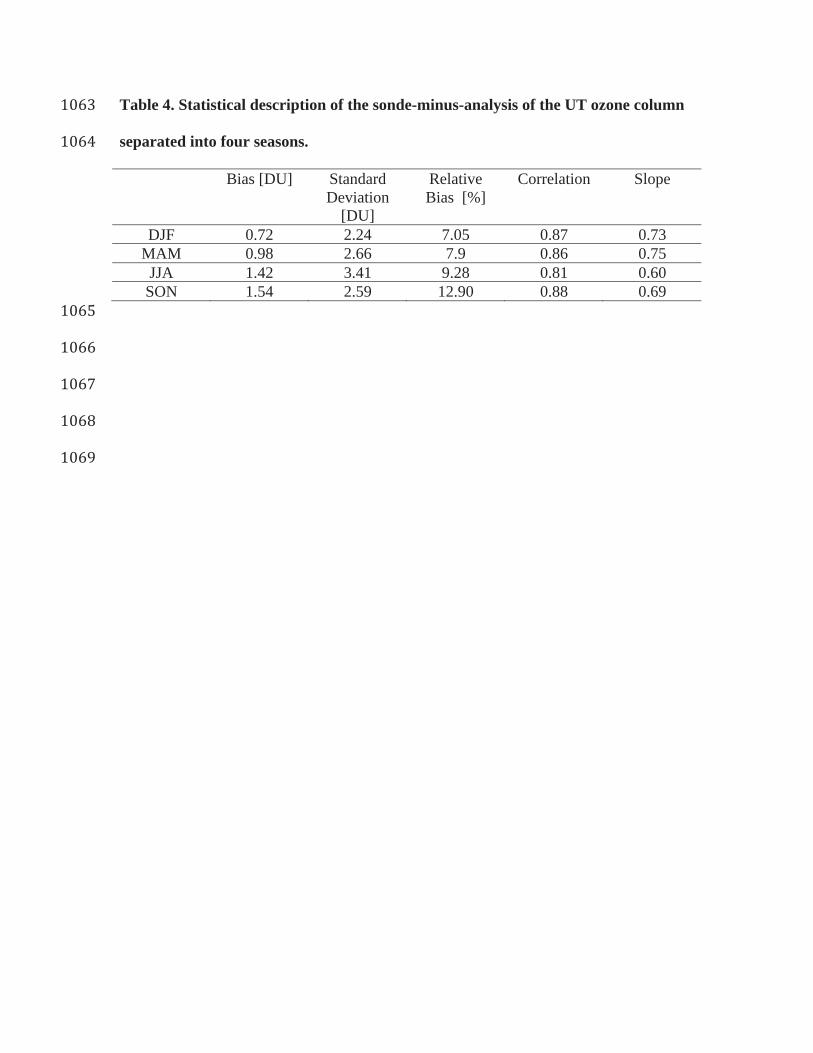
Table 4. Statistical description of the sonde-minus-analysis of the UT ozone column

separated into four seasons.

Bias [DU] Standard Deviation

[DU]

Relative Bias [%]

Correlation Slope

DJF 0.72 2.24 7.05 0.87 0.73 MAM 0.98 2.66 7.9 0.86 0.75 JJA 1.42 3.41 9.28 0.81 0.60 SON 1.54 2.59 12.90 0.88 0.69

Table 5. Distributions and physical descriptions of the low-ozone laminae

determined from HIRDLS retrievals and from the GEOS-5 MLS+OMI analysesa

HIRDLS, February

Analysis, February

HIRDLS, April Analysis, April

Thickness (mean [K])

42.83 42.40 43.82 44.93

Thickness (standard

deviation [K])

9.98 8.70 9.44 8.88

Magnitude (mean [%])

27.15 25.66 31.40 30.32

Magnitude (standard

deviation [%])

11.86 11.69 12.12 11.45

Count 590 386 1131 807 a Results are shown for February and April, corresponding to the plots shown in Figure

14.

Figure 1. Altitudinal profiles of (a) the standard deviations and (b) the means of the

O-F and O-A residuals for Microwave Limb Sounder (MLS) ozone mixing ratios,

for June, July and August 2010, in the 30°°N-90°N latitude band. Units are part per

million by volume (ppmv).

Figure 2. Zonal mean MLS O-Fs in June – August 2010 (shaded) and the mean

background ozone from 6-hourly forecasts (contours).

Figure 3. The spatial distribution of the mean O-F residuals for partial ozone

columns, averaged over June-July –August (JJA) 2010. (a) The stratospheric

portion of the MLS profile, obtained by integrating MLS O-F profiles between the

tropopause and 0.01hPa. (b) For the upper tropospheric portion of the MLS profile

measurements, integrated between 237 hPa and the tropopause. (c) For the Ozone

Monitoring Instrument (OMI), weighted by the column-specific efficiency factors

(according to Eq. 1). In (a, b) the tropopause is defined as the 100 hPa surface

between 10°S – 10°N and the 2 PVU surface elsewhere.

Figure 4. As in Figure 3B, but for the observation-minus-analysis (O-A) fields.

Figure 5. Time series of the global-mean, six-hourly O-F (red) and O-A (green)

statistics (DU) from the ozone analysis. Data are shown for (a) the MLS

stratospheric column; (b) the MLS upper tropospheric column; and (c) the OMI

weighted column. These three panels show time series for the same three layers as

annual mean maps shown in Figures 3 and 4.

Figure 6. Locations of the ECC ozone sondes for the years 2005 - 2012 used in this

study, shown separately for North America, Europe, and the globe. Each station is

marked by a white plus sign and a filled black circle scaled by the number of

soundings at that location.

Figure 7. Evolution of analyses of ozone partial pressure (shaded) and potential

vorticity (contours) at the GEOS-5 grid location above Hohenpeissenberg between

March 15 and March 31 2007. Values are available every six hours. The 2 PVU

line, which defines the tropopause in this study, is shown in green.

Figure 8. Ozone profiles from Hohenpeissenberg sondes (solid) and the GEOS-5

analyses (dashed) on March 14 (a), 22 (b), 23 (c), and 28 (d), 2007. The GEOS-5

values are shown on the vertical grid of the model, indicated by the solid black dots.

0 5 10 15 20 25Ozone [mPa]

1000

600

300

200

100

60

30

20

10

Pre

ssur

e [h

Pa]

(a)

March 140 5 10 15 20 25

Ozone [mPa]

1000

600

300

200

100

60

30

20

10(b)

March 220 5 10 15 20 25

Ozone [mPa]

1000

600

300

200

100

60

30

20

10(c)

March 230 5 10 15 20 25

Ozone [mPa]

1000

600

300

200

100

60

30

20

10(d)

March 28

Figure 9. A comparison of lower stratospheric (LS) ozone partial columns in milli-

atmospheric centimeters (Dobson Units, DU) at Hohenpeissenberg (47°°48’N, 11°E).

Analyses from GEOS-5 were sampled at the times of 1016 in-situ sonde observations

made between 2005 and 2012. (a) Time series from the sondes. (b) The probability

distribution function (p.d.f.) computed for the sonde observation (black) and the

GEOS-5 analysis (red). (c) Time series of the sonde-minus-analysis differences

together with the 1-σ and 2-σ intervals (the blue dashed and dotted lines,

respectively). (d) the p.d.f. of the sonde-analysis differences (stepped), a Gaussian fit

to this distribution (smooth black curve), and the Gaussian probability density

function with the mean and standard deviation as computed from the sonde –

analysis differences (blue) . The bin sizes used to compute the distributions in

panels (b) and (d) are 12 DU and 2 DU, respectively.

Figure 10. Comparisons of the analyzed UTLS ozone with the collocated ozonesonde

observations. (a) Scatter plot of the lower stratospheric partial column, integrated

between the tropopause and 50hPa. The thick black line represents a linear fit to the

data plotted. (b) The binned distribution of the sonde-minus-analysis differences

(stepped line) along with a Gaussian fit to this distribution (smooth curve). Panels

(c) and (d) show the equivalent plots for the upper tropospheric layer (500 hPa to

the tropopause). This comparison includes about 16,000 sonde observations, with

no sorting by their spatial or seasonal locations.

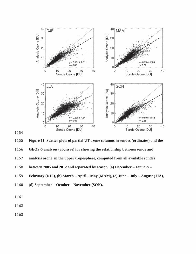
Figure 11. Scatter plots of partial UT ozone columns in sondes (ordinates) and the

GEOS-5 analyses (abcissae) for showing the relationship between sonde and

analysis ozone in the upper troposphere, computed from all available sondes

between 2005 and 2012 and separated by season. (a) December – January –

February (DJF), (b) March – April – May (MAM), (c) June – July – August (JJA),

(d) September – October – November (SON).

Figure 12. Time series of annual-mean UT sonde ozone statistics. (left column:

panels a, c, e) The mean partial columns (DU: black diamonds) and the mean

sonde-minus-analysis differences (open diamonds) and (right column: panels b, d, f)

standard deviations of the same quantities. Results are shown for (top row: panels

a, b) 60°°N-90°N, (middle row: panels c, d) 30°N-60°N, and (bottom row: panels e, f)

30°S-30°N.

Figure 13. Cross-sections of the UTLS ozone as a function of latitude and potential

temperature from HIRDLS (left) and the analysis (right) at 156°°W on April 8th 2007

(top) and 157°W on April 15th 2007 (bottom)

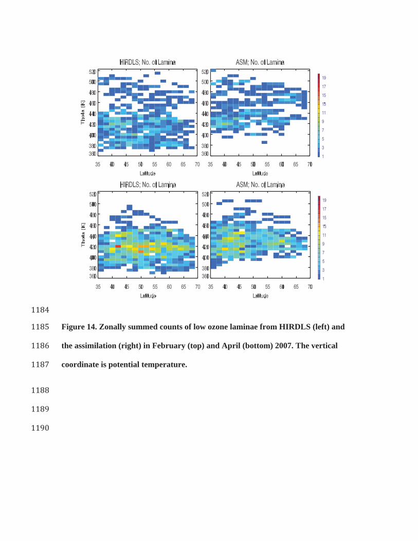
Figure 14. Zonally summed counts of low ozone laminae from HIRDLS (left) and

the assimilation (right) in February (top) and April (bottom) 2007. The vertical

coordinate is potential temperature.

Figure 15. Mean number of laminae identified per day in February-May for each

year in the NH mid-latitudes between 340 K and 550 K potential

temperature. Results from GEOS-5 analysis (blue) are compared to the three years

of available HIRDLS observations (red).