The Governance of Perpetual Financial Intermediaries

José Penalva Universidad Carlos III

Madrid, Spain E-mail: jpenalva@emp.uc3m.es

Jos van Bommel University of Oxford

Oxford, United Kingdom E-mail: jos.vanbommel@sbs.ox.ac.uk

This version: May 2009

1

The Governance of Perpetual Financial Intermediaries

In this paper we investigate the risk sharing potential of financial

intermediaries in an overlapping generations economy with agents who

may need to consume before a long term investment opportunity pays

off. We find that the allocations that intermediaries can offer are

constrained by the temptation of the living to liquidate the institutions’

assets and share the proceeds amongst themselves. We characterize a

renegotiation constraint for perpetual financial intermediaries, and show

that only institutions that can avoid side trading and the rolling over of

deposits, can improve on the market allocation.

JEL Classification: G21, D91

Keywords: Financial Intermediation, Overlapping Generations,

2

1. Introduction

One of the main services that financial intermediaries - such as banks, pension funds, and

insurance companies - are purported to provide is insurance against liquidity risk. One

way these institutions share intergenerational liquidity risk is by holding asset buffers

over time. The current paper shows that the risk sharing ability of these perpetual

institutions is limited because their living members can unilaterally decide to sell all, or

part of, the institution’s assets and reallocate the proceeds amongst themselves, to the

detriment of future generations.

This paper extends the existing literature that commences with the seminal papers of

Edgeworth (1888), Bryant (1980) and Diamond and Dybvig (1983) that show how

financial intermediaries can share risk in economies were production comes with

gestation lags and assets are illiquid. Diamond and Dybvig (1983) show that if agents

face the risk of having to consume before a long term asset pays off, a bank is able to

offer a consumption schedule in which early consumers are ex post subsidized by late

consumers. Jacklin (1987) and Bhattacharya and Gale (1987) however show that the

presence of a market poses a constraint on the risk sharing ability of intermediaries.

These papers have been followed up by an extensive literature on bank risk sharing.1

An important strand in this risk sharing literature considers the role of financial

intermediaries in overlapping generations (OLG) economies. A common feature of these

models is that financial intermediaries hold buffers of liquid and illiquid productive assets

to smooth consumption (Allen and Gale, 1997), or to take better advantage of productive

technologies (Qi, 1994).

In this paper we argue that buffer holding intermediaries are potentially subject to a

renegotiation whereby the living stakeholders make themselves uniformly better off by

changing the status quo payout and investment rules. If we take the overlapping

1 E.g. Haubrich and King (1990), Hellwig (1994) and von Thadden (1997, 1998) provide an additional critique of Diamond Dybvig risk sharing. Wallace (1988), Gorton and Penachi (1990), and Diamond (1997) suggest conditions under which banks can offer superior risk sharing.

3

generations concept seriously, and do not rely on altruism or an infinitely lived

enforcement mechanism, we need to consider the threat of such renegotiations.

Our analysis uses a model that extends the simple Diamond (1965) OLG economy, where

the young are endowed with a consumption surplus and the old face a deficit. The

economy features a two-period productive technology that returns R >1 and storage.

Agents have Diamond Dybvig (1983) preferences: they live either one or two periods and

consume at the end of their life. This model has been studied by Qi (1994), Bhattacharya

and Padilla (1998), and Fulghieri and Rovelli (1998), among others. Like them, we

analyze under what conditions a financial intermediary can improve on the allocation that

obtains in a market economy.

The novel feature of this paper is that we assume that intermediaries are controlled by

their living members. To model the intermediaries’ governance structure we assume that

depositors periodically decide to discontinue the status quo payoff and investment

regime, and adopt a feasible alternative allocation. To do this, we let a randomly chosen

depositor suggest an alternative allocation, and assume that it is accepted if it makes all

all other living depositors better off.

We show that a renegotiation of the intermediary’s status quo risk sharing and investment

rule may occur if the intermediary’s payoff schedule is too generous. The reason is that

the perpetual asset buffer that supports a generous payoff may be liquidated and sold to

non-depositors, so that an even more generous schedule can be offered to the living

depositors. Although such a redistribution is an out of equilibrium event, it poses

constraint on the set of equilibrium allocations. We characterize a renegotiation

constraint that defines a convex set of permissible payment schedules so that no feasible

alternative regime that uniformly improves the living depositors’ welfare exists.

We find that the renegotiation constraint depends on the industry structure. If the

economy has many intermediaries competing with each other, the constraint is stronger

than if there is a single monopolist intermediary. The reason for this is that in the former

situation, renegotiating institutions can potentially sell assets to each other. This makes

renegotiation attractive at lower asset buffer levels. On the other hand, a liquidating

4

monopolist institution can only sell existing capital to newborn generations. Because

newborns have lower values for intermediate projects, monopolists can maintain larger

asset buffers without being subject to renegotiation by its stakeholders.

Both in the competition and monopoly case, we find the renegotiation constraint to be

very restrictive, and not met by several allocations suggested in the incumbent literature.

Interestingly, we also find that, for both competition and monopoly, the market allocation

is on the boundary of the constraint set.

However, since the market allocation is generally not the welfare maximizing allocation

within the constrained set, there is still scope for intermediation. We show that an

institution that caters to risk averse agents can achieve an allocation that is superior to the

market allocation if it can avoid side trade and prohibit the rolling over of deposits.

Institutions that cater to risk tolerant agents can improve on the market equilibrium under

a weaker condition: they only need to impede the sale (or securitization) of deposits.

In an early paper that analyzes the merits of intermediaries in an OLG Diamond Dybvig

economy, Qi (1994) identifies the problem that anonymous late consumers may mimic

early consumers, and roll over their deposits. For sufficiently risk averse agents, this

gives rise to an allocation with r2 = r12, were r1 and r2 denote the consumption of early

and late consumers respectively. The scalability of the long term project determines the

equilibrium allocation, which may well have Rr >1 .2 Bhattacharya and Padilla (1996)

however point out that if interbank deposits are allowed, Qi's allocation is not sustainable

because intermediaries would open deposits with each other instead of investing in the

technology. They then show that a government that taxes late consumers and subsidizes

newborns can achieve Qi’s allocation, and even the first best allocation.3 Fulghieri and

2 Qi (1994) assumes that the maximum per period investment is unity. This gives rise to r1 =

RR>ε−

ε−ε−+ε)1(2)1(42

, where ε is the probability of becoming an early consumer.

3 Bhattacharya and Padilla (1996) consider three different tax-subsidy regimes. To achieve first best, an age

dependent tax-subsidy scheme is required.

5

Rovelli (1998) show that the ability of intermediaries to discriminate on age also enables

them to attain the first best allocation.

In contrast, we argue that neither taxation nor age verification is sufficient to ensure the

first best allocation, as it is not renegotiation proof. To obtain the allocations suggested in

the literature, the economy requires, apart from the power to tax or verify depositor’s

ages, an infinitely lived enforcer who acts in the interest of all - present and future -

generations. Without an infinitely lived enforcement mechanism, intermediaries’ risk

sharing potential is severely constrained, by the temptation of the living generations to

renegotiate the risk sharing contract, and ostracize future generations.

Our paper is thus similar in spirit as Prescott and Rios-Rull (2000), who show that, in an

economy without capital, the threat looms that the young generations abandon the old,

and instead restart the economy. In our model, agents form intermediaries that transport a

stock of intermediate projects between generations. Such a capital buffer can potentially

improve welfare. However, at the same time it is the source of a natural intragenerational

conflict. Because we assume that the intermediary is governed by the living, and future

generations have not vote, this conflict results in a constraint on risk sharing.

It is important to note that in our analysis there is no aggregate risk, which implies that all

equilibria are deterministic and stationary. Gordon and Varian (1988) and Allen and Gale

(1997) investigate the role of perpetual financial intermediaries in an economy where

there is aggregate (output) risk. In Gordon and Varian (1988), a government takes the

role of the intermediary. The authors show that such a perpetual institution could

redistribute stochastic labor income over several generations so as to increase overall

welfare. As limitations to such intergenerational smoothing they mention the stochastic

nature of intertemporal asset transfers, moral hazard on the part of the workforce, and, as

we do, the institution’s governance. In Allen and Gale (1997), there is no labor and moral

hazard, while there is a safe asset. They show that a banking system can improve welfare

vis-à-vis a market economy by holding a buffer of safe assets, which is depleted

whenever the risky output falls short of its expectation, and replenished otherwise. Using

a result of Schechtmann (1976), they show that such a system can offer its stakeholders

the expected value of the stochastic output in all except a negligible number of periods.

6

Allen and Gale (1997) also point out that such a buffer holding financial system is fragile,

because agents abandon it as soon as it underfunded. Our results suggest that even if

agents can be forced to join an underfunded system, smoothing will be hampered due tot

the temptation of contemporaneous generations to seize any potential surplus.

The remainder of this paper is organized as follows: the next section describes the OLG

model. In section 3 we examine the market economy equilibrium to provide a benchmark

for the coalition equilibrium, and to analyze the agents' outside option. In section 4 we

describe the coalition, including its governance structure, and analyze the equilibrium.

Section 5 presents a discussion and interpretation of our findings. Section 6 concludes.

Proofs are in the appendix.

2. The OLG Diamond Dybvig economy

The object of our study is an infinite horizon economy with a boundless sequence of

overlapping generations of atomistic agents. A new generation, of size normalized to one,

is born on every date. Agents are born with an endowment of one unit of a homogeneous

good that can be used for consumption or as an input for production. Agents who enter

the economy at date t can be of two types: with probability ε agents are impatient and live

for one period only; with probability 1-ε they are patient and live for two periods.

Agents born at t who are impatient consume at t+1, while patient ones consume at t+2.

All agents have expected utility preferences with an instantaneous utility functions U(·)

that is increasing, strictly concave and twice-continuously differentiable. We also assume

that agents are sufficiently risk averse: the relative risk aversion coefficient of U() is

everywhere greater than one.

Agents born at date t learn their type after t but before t+1. Types may be verifiable. We

assume that the population is large enough so that there is no uncertainty on the aggregate

distribution of agents in the population.4 Hence, at any date t, the population contains 3-ε

4 This is usually justified in terms of the law of large numbers. Duffie and Sun (2007) provide a rigorous

formulation of independent random matching for a continuum population such that the law of large

numbers holds exactly.

7

agents: 1-ε patient agents born at t-2, 1 agents born at t-1 who know their type, and 1

newborns who do not know their type yet. In between dates there are 2-ε agents: 1 young,

and 1-ε old.

The economy is endowed with two technologies to produce goods over time. The first

technology, storage, allows agents to costlessly transfer consumption from one period to

the next. The second technology, the long term technology allows agents to convert one

unit of consumption at date t into R>1 units of consumption at t+2. This technology

cannot be interrupted at t+1. In the following we will look for equilibrium allocations

{ } Ζ∈ttt CC 21, , where itC denotes the consumption of i-year olds at time t.

2.1. Production scalability, Pareto efficiency, and equilibrium startability.

An issue that is somewhat ignored in the literature and which becomes of particular

importance when studying the Pareto efficient allocation is that of the extent to which the

production technology can be scaled. Qi (1994) suggested a maximum periodic

investment in the long term technology of unity. Subsequent papers have followed this

assumption. We will see however that this assumption has the potential to confound

fundamentally different allocations. For this reason we assume that the long term project

can be scaled up to a multiple of the size of the population’s aggregate endowment, X >1.

Then, the socially optimal allocation is 1)1(21 +−== RXCC tt , for all t. This allocation is

attained by periodically investing the maximum amount X in the long term technology.

The periodic consumption can be found by subtracting from the periodic good inflows,

XR+1 (XR from production and 1 from endowments), the periodic investment outflows X.

An additional problem arises if rather than consider stationary equilibria, one were to

start the economy from scratch. If the economy has a starting date, the interesting

intragenarational allocations (such as social optimal allocation) cannot be obtained

immediately. In order to obtain the stationary allocations in an economy with a starting

date, early generations need to build an asset buffer to obtain the optimal periodic

investment. Although startability is not the central theme of our paper, it will be

discussed in a later section.

8

3. The market economy

In this section we analyze the equilibrium allocation in an economy where agents of

different types and generations trade securities that are backed by one period old capital

(investments in the production technology). We shall call these securities projects. In the

following we let pt denote the date t price of a project started with one unit of

consumption good at t-1, and which hence pays R goods at t+1. Due to their atomistic

nature, agents are price takers.

In the capital market economy agents have access to three investment vehicles: the

production technology, projects, and storage. They can invest when born and, if they are

patient, on their first birthday. We define the key decision variables as follows: 0tx is the

number of projects bought by a newborn agent at date t, 1tx is the number of projects

bought by a patient one-year-old at date t. Similarly, 0ty and 1

ty denote the amount

invested in the production technology by newborn and patient one-year-olds respectively,

while 0tz and 1

tz denote the amounts stored by newborn and patient one-year-olds at t.5

Naturally, all surviving agents choose their investments so as to maximize expected

utility. We formulate an agent’s problem recursively, and start the analysis with the

problem of a patient one year old. Let 01

01

01

1−−− ++= ttttt zpyRxm denote the wealth, in

number of goods, of a one year old agent at date t. We further define the value function

( )1tmV as the maximum expected utility a patient one year old can obtain:

( ) ( )1111

1111

,,max

ttttttt

t zpyRxUzyxmV ++= + (1)

1111ttttt zypxm ++≥ (2)

5 Throughout this article, superscripts denote generations, and subscripts denote decision, transaction, and

consumption dates.

9

The maximand in (1) is the patient agent’s utility from consumption ( )21+tCU , expression

(2) is her budget constraint. Because impatient agents consume on their first birthday, we

have that the newborn’s maximization problem is:

( ) ( )001

0001

0000 )1(,,

maxtttttttt

tttzypxVzypxU zyx ++ε−+++ε ++ (3)

0001 tttt zypx ++≥ (4)

The arguments in the U() and V() functions in (3) is a t-born agent’s first birthday wealth, 1

1+tm , expression (4) is his/her budget constraint. In equilibrium, all agents maximize

expected utility and markets clear. The market clearing condition requires that the

aggregate investment on date t, denoted yt, equals the aggregate holdings of projects on

date t+1:

t xxyy ttttt ∀ε−+=ε−+≡ ++1

10

110 )1()1(y (5)

We define a capital market equilibrium as follows:

Definition: An equilibrium for the market economy is a sequence of prices Zttp ∈}{ and

investment decisions Zttttttt zzyyxx ∈},,,,,{ 101010 such that (i) for all t, every agent maximizes

his expected utility and (ii) markets clear.

In the appendix we show that there exist infinite stationary two-periodic equilibria, with

the following properties:

PROPOSITION 1 (market equilibrium):

In any market equilibrium we have, for all t ∈ Z:

(i) t

tt pRpRp =∈ +1],,1[

(ii) RC pC ttt == 21 ,

10

(iii) If 1>tp then 11−−ε−= R

pR tty and 010 == tt zz

Note that there is a continuum of equilibria, all of which have two-periodic prices and

allocations. The requirement that pt+1 = R/pt can be seen as a no arbitrage condition: the

one period return on primary investments must be equal to the one period return in the

secondary market. In the interior equilibria ( pt∈(1,R) ), aggregate investment is

determinate, and there is no storage. If we impose that patient one-year olds do not invest

in the production technology ( 01 =ty ∀ t) then the other asset allocation decisions

( 100 ,, ttt xxy ) are determinate and strictly positive.

Although the OLG Diamond Dybvig model has been studied in the literature, the inherent

two-periodicity has not been documented before.6 Previous papers that investigate the

OLG DD model focus on the one-periodic special equilibrium, where pt = R ∀ t, which

offers all agents an allocation of { } { }RRCC tt ,, 21 = . Naturally, this non-cyclical allocation

is the Pareto optimal one for sufficiently risk averse agents, so that it may be that it is the

social attractiveness of the one-periodic equilibrium that lead Bhattacharya and Padilla

(1996) and Fulghieri and Rovelli (1998) to disregard the cyclical equilibria.

Notice that the market equilibrium cannot offer the Pareto optimal allocation: the

socially optimal allocation requires X > 1 projects to be started on every date. Because the

agents are the only economic actors in the market equilibrium, they cannot be forced to

keep such a capital buffer alive.

3.1. The startable market equilibrium

6 Bhattacharya, Fulghieri and Rovelli (1998) mention mention two price equilibriums, the

one-periodic one (pt = R ∀ t), and the corner equilibriuim pt = {..,1,R,1,..}. We show that any price

process with ptpt+1 = R is an equilibrium price process.

11

If the economy has a starting period ( = 0t ), the first generation determines which of the

above mentioned stationary equilibria is played. Since there is no secondary market at

date zero, and the only alternative to investing is storing, the first generation solves:

( )0 0 1 0 00 1

(1 ) (1 ) (1 )maxy

RU y y p U y y Rp

⎛ ⎞− + + − − +⎜ ⎟

⎝ ⎠ε ε (3)

Since the first derivative of (3)’s maximand is positive for all p1 > 1, first generation

agents invest their entire endowment in the technology, so that we have:

PROPOSITION 2 (startable market equilibrium)

In the {0}+ ∪Z economy we have = 1oddp , =evenp R , 0 = = 1eveny y , = 1oddy −ε .

Proposition 2 shows that even though the agents' concave utility function makes the one-

periodic stationary equilibrium the most desirable from an overall welfare perspective, it

is the least desirable, most cyclical, equilibrium that obtains.

4. Financial Intermediaries

We now investigate whether a financial intermediary can improve on the capital market

allocation. We will consider two distinct settings. First we will consider a monopolist

intermediary, such as a social security plan imposed by a government. Then we will

consider competition, the situation where there is a large number of financial

intermediaries that act as price takers for deposits. Banks or insurance companies are

natural examples.

Following the literature, we assume that a financial intermediary offers depositors a

demandable debt security in exchange for their endowment. This security can be

exchanged for 1r units of consumption by impatient depositors on the period after making

a deposit, or for 2r units by patient agents after two periods.

In addition, we model the governance of the intermediary. In particular we assume that it

is governed by its living members, who periodically decide on the investment and the pay

out schedule {r1,r2}. In the following we shall limit our attention to stationary coalitions,

12

and denote their periodic investment y. A coalition is thus described by a vector {y,r1,r2}.

Given that it is governed by its ex-ante identical depositors, for any stationary investment

level, any equilibrium allocation solves:

( ) ( )21,)1( max

21

rUrUrr

εε −+ (4)

We shall limit our analysis to institutions who make promises {r1,r2} that are feasible in

the short and long term and assume that institutions (if there are more than one), are of

constant size.7 Hence, problem (4) is maximized subject to the internal budget constraint:

1 2(1 ) 1r r y yR+ − + ≤ +ε ε (5)

The left hand side of (5), which will be binding in a stationary equilibrium, gives the

period outflows: to impatient and patient depositors, and new investment. The right hand

side gives the periodic inflow: from new depositors and from maturing projects. Between

periods, the institution holds 2y projects: y new projects, that have just been started, and y

mature projects, that are about to pay off.

In addition, any stationary investment level must also satisfy the external budget

constraint, which is due to the limited scalability of the production technology:

Xy ≤ (6)

If we solve (4)-(6) we see that the optimal solution is increasing in y so that an institution

wishing to maximize the welfare of its members will try to reach the highest level of

investment consistent with the external constraint (6). This implies that in the

intermediated economy the first best allocation could potentially be obtained. However,

we need to account for the temptation of the institutions’ living members to liquidate and

distribute the institutions’ assets leads to additional constraints on the intermediary’s risk

sharing potential.

7 That is, we rule out Ponzi schemes. The reason that coalition sizes are constant is that they have asset

buffers with stationary pay-off vectors which cannot be offered to an increasing number of depositors

without diluting the current depositors.

13

4.1. The governance structure of financial intermediaries

Following the incumbent literature, we treat the intermediary as a withdrawal menu and

an asset buffer. In the stationary Diamond Dybvig model, the institution determines the

withdrawal rules upon foundation. Because once established the withdrawal rights cannot

be renegotiated, the DD-bank can be interpreted as an automatic cash dispenser.8

For an OLG economy, the cash dispenser interpretation is problematic because OLG

institutions must not only dispense cash, to current and future generations, but also accept

new deposits, and make investments. In the extant literature it is assumed that these

actions are predetermined by an exogenous welfare maximizer so as to provide welfare to

all the institution's (present and future) depositors.

In practice, such institutions (banks, insurance companies, governmental organizations,

pension funds, etc.) are governed by a sequence of stakeholder cohorts, consisting of

mortal individuals. Consistent with this reality, we study institutions that are exclusively

governed by their living members.

To model the governance of the institution we assume that in between payoff dates,

general depositors’ meetings take place, in which every depositor is allowed to vote for

motions that propose to change the stationary {r1,r2} schedule.

A randomly appointed chairperson is allowed to propose an alternative schedule,

},,{ 1212+ttt rrr , which represent the payoffs in the period immediately following the meeting,

(denoted, t) to the two year olds and to the impatient one year olds, and in period t+1 to

the two year olds.

The alternative proposal is implemented if it obtains unanimous support. We consider the

unanimity rule as it ensures that no depositor can be expropriated. Clearly, if it were

possible to approve a rule with less than unanimous support, coalitions of depositors

could form a voting majority and approve sharing rules that expropriated those depositors

8 The cash dispenser interpretation was first suggested by Wallace (1988).

14

outside the coalition, which would undermine the existence of intermediaries in the first

place.

Unanimity also guarantees that any alternative payoff schedule needs to be feasible to be

accepted. This means that it has to be possible for the new proposal to be financed by the

dividends of terminated projects and, possibly, the sale of some of the intermediate assets

owned by the institution. In the following we let ξ stand for the number of intermediate

projects sold by a renegotiating institution, and p(ξ) the price per project obtained.

The reason for analyzing possible renegotiations is that in a stationary equilibrium they

cannot occur. That is, perpetual intermediaries cannot offer depositors schedules that

give rise to renegotiation. Hence we define a stationary coalition equilibrium as follows:

DEFINITION: A stationary intermediary equilibrium is characterized by a vector

( )* * *1 2, ,y r r that meets the external budget constraint (6), the internal budget constraint (5)

with equality, and the following renegotiation constraint:

* * 11 2 1 2( ) (1 ) ( ) ( ) (1 ) ( )t tU r U r U r U r ++ − ≥ + −ε ε ε ε (7)

and *2 2( ) ( )tU r U r≥ (8)

12 1 2 , , t t tr r r +∀ that meet the following feasibility constraints:

)()1( 12 ξξ+≤ε+ε− pRy rr *tt (9)

( )Ry r *t ξ−≤ε− +12)1( (10)

],0[ *y ∈ξ∀

Equations (7) and (8) require that is impossible to make all coalition members better off

by staging a feasible raid on the institution’s assets. The set of feasible deviations is

constrained by the coalition’s existing assets, characterized by *y , and the market outside

the coalition. The left hand side of inequality (9) denotes the maximum payout in the

period immediately following a renegotiation, for a given number of intermediate

15

projects sold ξ. Inequality (10) gives the maximum payout, to patient two year olds, two

periods after the renegotiation.

Notice that our equilibrium definition specifies equilibrium allocations instead of

equilibrium strategies. Naturally, the equilibrium strategies that support the equilibrium

allocation are that the chairman only suggests proposals that will be accepted and that

agents only vote in favor of a proposal if it is feasible and makes them weakly better off.

In the context of our model of governance, this constraint requires that the chairperson

should not be able to profit from making the following proposal:

"Next period, all two-year olds receive r2 goods. One-year olds can choose between 2r

R projects or 1r goods. Anything left over is for me. "

Clearly, all agents would (weakly) accept the above proposal. Under the proposal, the

young will self-select into patient and impatient types at the next date, and hence

consume r1 if impatient or r2 if patient, the same as their scheduled consumption in the

status quo. Hence, upon a renegotiation of the above kind, the two-year olds would be left

with a minimum of 1yR r−ε goods and 2(1 ) ryR

− −ε projects. Since the projects need to

be exchanged for consumption goods the amount of intermediate assets that has to be

sold is:

)1()1()1( 212

−−ε−+ε=ε−−≡ξ RR

RrRrRry (11

To arrive at the final term, we eliminate y by using the binding internal budget constraint

(5). To meet the renegotiation constraint, the proceeds from selling ξ plus the leftover

goods cannot be greater than the scheduled payment under the coalition. Hence, the

renegotiation constraint can be written as:

21 )1()( rryRp ε−≤ε−+ξξ (12)

16

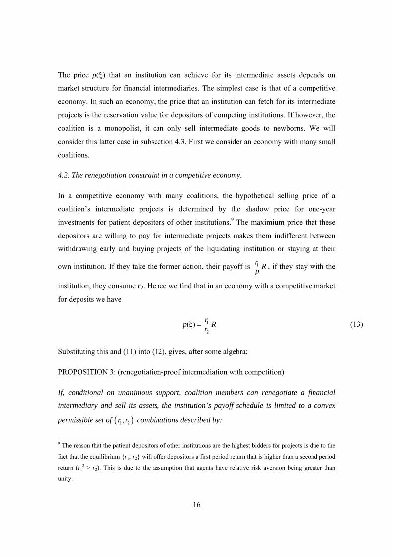
The price p(ξ) that an institution can achieve for its intermediate assets depends on

market structure for financial intermediaries. The simplest case is that of a competitive

economy. In such an economy, the price that an institution can fetch for its intermediate

projects is the reservation value for depositors of competing institutions. If however, the

coalition is a monopolist, it can only sell intermediate goods to newborns. We will

consider this latter case in subsection 4.3. First we consider an economy with many small

coalitions.

4.2. The renegotiation constraint in a competitive economy.

In a competitive economy with many coalitions, the hypothetical selling price of a

coalition’s intermediate projects is determined by the shadow price for one-year

investments for patient depositors of other institutions.9 The maximium price that these

depositors are willing to pay for intermediate projects makes them indifferent between

withdrawing early and buying projects of the liquidating institution or staying at their

own institution. If they take the former action, their payoff is Rpr1 , if they stay with the

institution, they consume r2. Hence we find that in an economy with a competitive market

for deposits we have

Rrrp2

1)( =ξ (13)

Substituting this and (11) into (12), gives, after some algebra:

PROPOSITION 3: (renegotiation-proof intermediation with competition)

If, conditional on unanimous support, coalition members can renegotiate a financial

intermediary and sell its assets, the institution’s payoff schedule is limited to a convex

permissible set of ( )1 2,r r combinations described by:

9 The reason that the patient depositors of other institutions are the highest bidders for projects is due to the

fact that the equilibrium {r1, r2} will offer depositors a first period return that is higher than a second period

return (r12 > r2). This is due to the assumption that agents have relative risk aversion being greater than

unity.

17

⎟⎠⎞⎜

⎝⎛ ε−ε−ε−+++−ε−≤ )1(4)21(2)1(2

1 211

21

212 RrRrrRrRr (14)

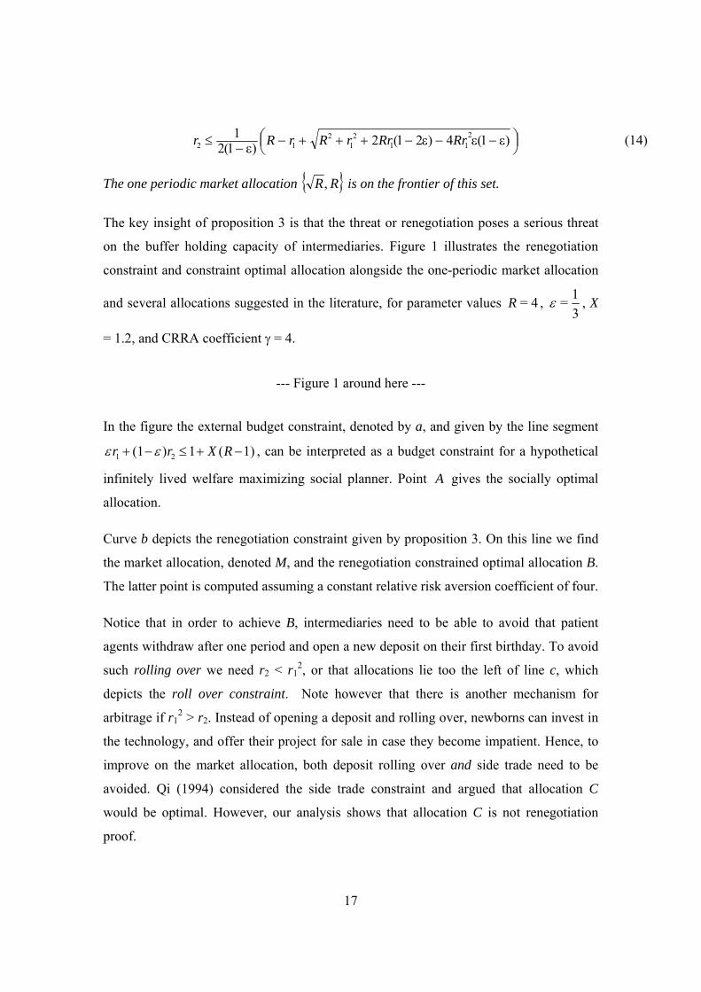
The one periodic market allocation { }RR, is on the frontier of this set.

The key insight of proposition 3 is that the threat or renegotiation poses a serious threat

on the buffer holding capacity of intermediaries. Figure 1 illustrates the renegotiation

constraint and constraint optimal allocation alongside the one-periodic market allocation

and several allocations suggested in the literature, for parameter values = 4R , 1=3

ε , X

= 1.2, and CRRA coefficient γ = 4.

--- Figure 1 around here ---

In the figure the external budget constraint, denoted by a, and given by the line segment

1 2(1 ) 1 ( 1)r r X R+ − ≤ + −ε ε , can be interpreted as a budget constraint for a hypothetical

infinitely lived welfare maximizing social planner. Point A gives the socially optimal

allocation.

Curve b depicts the renegotiation constraint given by proposition 3. On this line we find

the market allocation, denoted M, and the renegotiation constrained optimal allocation B.

The latter point is computed assuming a constant relative risk aversion coefficient of four.

Notice that in order to achieve B, intermediaries need to be able to avoid that patient

agents withdraw after one period and open a new deposit on their first birthday. To avoid

such rolling over we need r2 < r12, or that allocations lie too the left of line c, which

depicts the roll over constraint. Note however that there is another mechanism for

arbitrage if r12 > r2. Instead of opening a deposit and rolling over, newborns can invest in

the technology, and offer their project for sale in case they become impatient. Hence, to

improve on the market allocation, both deposit rolling over and side trade need to be

avoided. Qi (1994) considered the side trade constraint and argued that allocation C

would be optimal. However, our analysis shows that allocation C is not renegotiation

proof.

18

Bhattacharya and Padilla (1996) provide another argument why allocation C cannot be

obtained in a contestable market: offering r2 > R would invite competing coalitions to

invest with each other instead of in the production technology. Bhattacharya and Padilla

then show that C can be attained if there is a government that taxes income (or

consumption) and offers proportional investment subsidies to newborns. If the

government can offer age-dependent subsidy which is proportional on investment,

allocation D can be obtained, and if the subsidy can be conditioned on the optimal

investment level, it can enforce the Pareto optimal allocation A.

As can be seen from the figure, none of the three government transfer schemes suggested

by Bhattacharya and Padilla (1996) are renegotiation proof. As long as the renegotiation

constraint d lies to the left of the external budget constraint, a motion that calls for an

immediate cancellation of the suggested tax-subsidy schemes would gain the vote of the

entire living population, and unravel allocations A, B and C . This is because between

periods all living agents have already received the subsidy, while only future, unborn

generations benefit from subsequent subsidies.

Fulghieri and Rovelli (1998) show that allocation E can be obtained if intermediaries can

condition payoffs on the age of the depositor, and side trade is ruled out, while the

interbank arbitrage constraint, depicted by d, which requires r1, r2 ≤ R , is binding.10

4.3. A monopoly intermediary.

A reason for the limited potential for intergenerational risk sharing could be the fact that

financial intermediaries operate in competitive markets. We now consider a monopoly

intermediary and find that also in this setting a renegotiation constraint applies.

As established above, a key element of the renegotiation proof criterion is the p(ξ)

function, which denotes the price that a financial intermediary can obtain when it

10 In their paper allocation E coincides with allocation A, because they assumed X = 1. In our view, line d

does not necessarily pass through A. Whether allocation E provides more or less intergenerational welfare

than allocation C or D depends on the model's parameters, in particular on the maximum profitable

investment X.

19

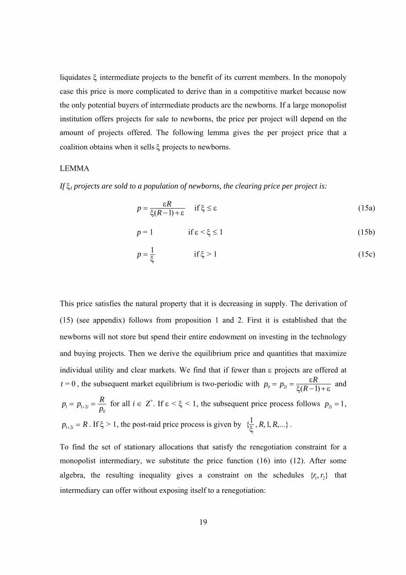
liquidates ξ intermediate projects to the benefit of its current members. In the monopoly

case this price is more complicated to derive than in a competitive market because now

the only potential buyers of intermediate products are the newborns. If a large monopolist

institution offers projects for sale to newborns, the price per project will depend on the

amount of projects offered. The following lemma gives the per project price that a

coalition obtains when it sells ξ projects to newborns.

LEMMA

If ξt projects are sold to a population of newborns, the clearing price per project is:

ε+−ξε= )1(RRp if ξ ≤ ε (15a)

p = 1 if ε < ξ ≤ 1 (15b)

ξ= 1p if ξ > 1 (15c)

This price satisfies the natural property that it is decreasing in supply. The derivation of

(15) (see appendix) follows from proposition 1 and 2. First it is established that the

newborns will not store but spend their entire endowment on investing in the technology

and buying projects. Then we derive the equilibrium price and quantities that maximize

individual utility and clear markets. We find that if fewer than ε projects are offered at

= 0t , the subsequent market equilibrium is two-periodic with ε+−ξε== )1(20 RRpp i and

0211 p

Rpp i == + for all i ∈ Z+. If ε < ξ < 1, the subsequent price process follows 12 =ip ,

Rp i =+21 . If ξ > 1, the post-raid price process is given by ,...},1,,1{ R Rξ .

To find the set of stationary allocations that satisfy the renegotiation constraint for a

monopolist intermediary, we substitute the price function (16) into (12). After some

algebra, the resulting inequality gives a constraint on the schedules },{ 21 rr that

intermediary can offer without exposing itself to a renegotiation:

20

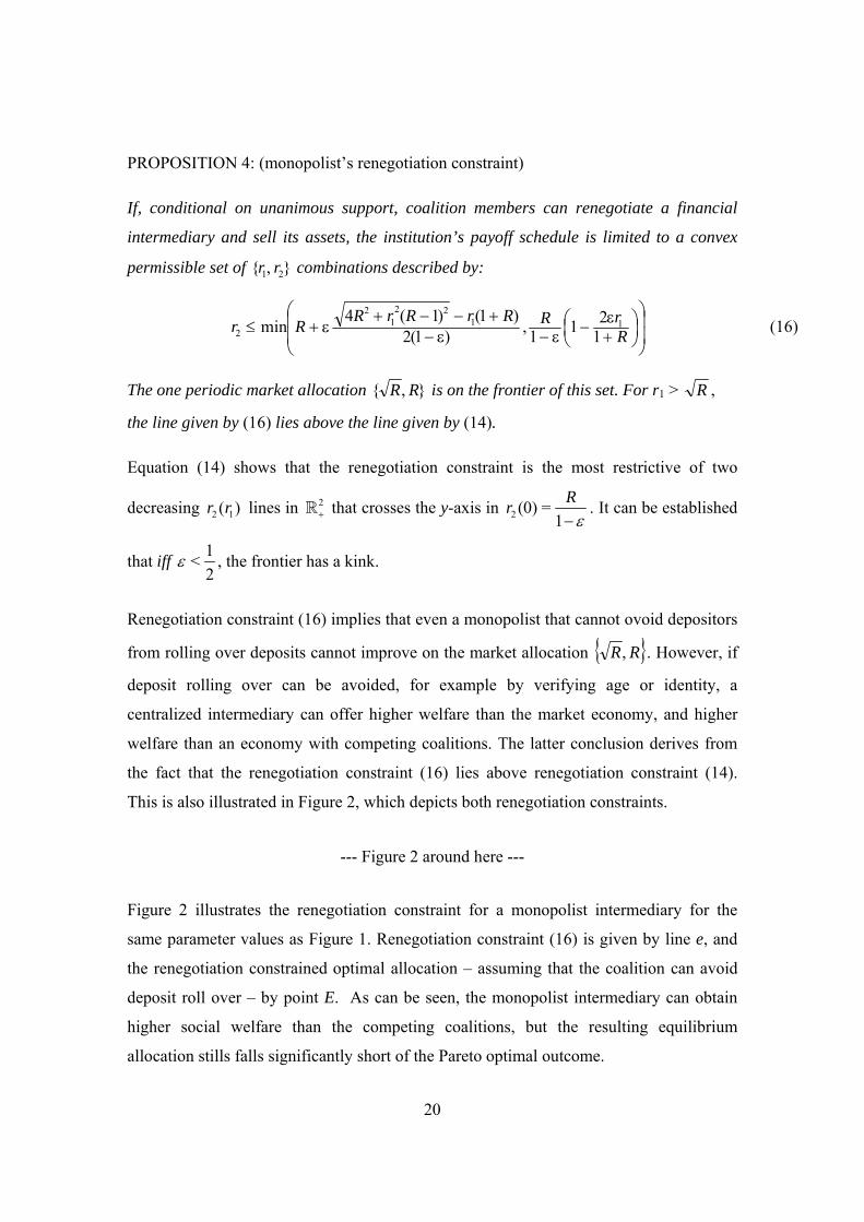
PROPOSITION 4: (monopolist’s renegotiation constraint)

If, conditional on unanimous support, coalition members can renegotiate a financial

intermediary and sell its assets, the institution’s payoff schedule is limited to a convex

permissible set of },{ 21 rr combinations described by:

⎟⎟

⎠

⎞

⎜⎜

⎝

⎛⎟⎠⎞

⎜⎝⎛

+ε−ε−ε−

+−−+ε+≤ R

rRRrRrRRr 1211,)1(2

)1()1(4min 1122

12

2 (16)

The one periodic market allocation },{ RR is on the frontier of this set. For r1 > R ,

the line given by (16) lies above the line given by (14).

Equation (14) shows that the renegotiation constraint is the most restrictive of two

decreasing 2 1( )r r lines in 2+R that crosses the y-axis in 2 (0) =

1Rr−ε

. It can be established

that iff 1<2

ε , the frontier has a kink.

Renegotiation constraint (16) implies that even a monopolist that cannot ovoid depositors

from rolling over deposits cannot improve on the market allocation { }RR, . However, if

deposit rolling over can be avoided, for example by verifying age or identity, a

centralized intermediary can offer higher welfare than the market economy, and higher

welfare than an economy with competing coalitions. The latter conclusion derives from

the fact that the renegotiation constraint (16) lies above renegotiation constraint (14).

This is also illustrated in Figure 2, which depicts both renegotiation constraints.

--- Figure 2 around here ---

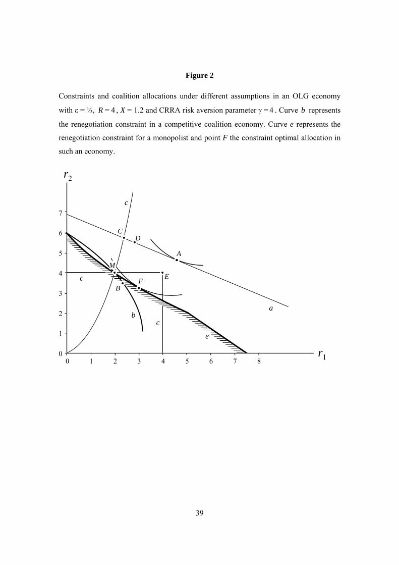
Figure 2 illustrates the renegotiation constraint for a monopolist intermediary for the

same parameter values as Figure 1. Renegotiation constraint (16) is given by line e, and

the renegotiation constrained optimal allocation – assuming that the coalition can avoid

deposit roll over – by point E. As can be seen, the monopolist intermediary can obtain

higher social welfare than the competing coalitions, but the resulting equilibrium

allocation stills falls significantly short of the Pareto optimal outcome.

21

4.4. Equilibrium

So far we have only characterized the renegotiation constraints, and the identified the

constrained optimal allocations. However, there are more equilibria that can obtain. In

this section we narrow down the feasible allocations to equilibrium allocations.

First we observe that allocations to the left of line b (and e, for the monopolist) cannot be

equilibria because the depositors can rearrange the payoffs for the young generation

without terminating the institution. This is the case because internal budget constraints

have slopes larger than the renegotiation constraints (14) and (16), as is illustrated in

Figure 3. Similarly, allocations on b that lie to the North-West of B (on e and above F, for

the monopoly case) cannot be equilibria. This is because they are associated with asset

buffers (y) than are higher than the optimal allocation E. A coalition with allocation

above B (F) could make all depositors better off by reducing its buffer. To further refine

the set of equilibrium allocations we observe that a stationary coalition equilibrium must

solve:

1 21 2

max ( ) (1 ) ( ), U r U rr r ε + − ε (17)

subject to internal budget constraint (5) and bank raid constraint (14) or (16).

That is, an equilibrium coalition allocation must maximize the expected utility of the

young generation, subject to the budget constraint that comes with the stationary

investment level *y . It can be shown that allocations {r1,r2} that solve (17) unconstrained

by the renegotiation threat lie on the 45 degree line, so that the stationary equilibrium

allocation lies either on the 45 degree line, or on the frontier of the permissible set above

the 45 degree line, as in figure 3.

--- Figure 3 around here ---

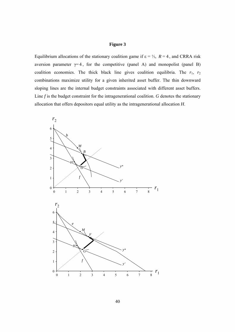
Figure 3 depicts the set of stationary equilibrium allocations if R = 4, 13ε = and γ = 4, for

a coalition that can avoid roll-over arbitrage. The thick bold line identifies the set of

equilibrium allocations. The thin downward sloping straight lines are the internal budget

constraints associated with coalition buffers y. The set of equilibria is a line segment wich

22

is bounded below by the allocation on the 45 degree line that offers agents the reservation

utility they can obtain by playing intragenerational Diamond-Dybvig. Line f gives the

budget constraint of the intragenerational DD coalition, and H marks the optimal

intragenerational DD allocation for γ = 4.11

5. Discussion

In the previous section we derived the set of renegotiation proof equilibria in an

intermediated economy under a series of abstract assumption. The default way to

interpret the object of our study the perpetual institution, is as a deposit taking bank.

However, other financial intermediaries fit the description of our institution, probably

even better. Insurance mutuals, defined benefit pension plans, social security schemes

and endowment funds all hold buffers and have sharing rules that are prone to

renegotiations. In this section we discuss how our conclusions apply to a more realistic

setting.

5.1 Altruism and renegotiation costs.

In our model we assume that as soon as a small surplus for the incumbent depositors

becomes available, they will seize it through renegotiation, even though it hurts the

newborns. It can be easily conjectured that if depositors have some degree of altruism,

they would resist the temptation to renegotiate so that larger asset buffers, periodic

investment and increased payout rules are sustainable. Tabellini (1990, 1991),

investigates how altruism and majority voting can sustain government debt, and social

security systems. It is important however that agent generations care not only about their

child and grandchild generation, but about all their offspring generations. It can be shown

that if agents only care about the welfare of their immediate offspring, the renegotiation

constraint as given by (14) and (16) are unaltered. In this case, we need to consider the

coalition as having, on any date, 3-ε members, and owning y intermediate projects and Ry

+ 1 units of consumption goods. The newborns can be made equally good of as under the

11 In the intragenerational DD equilibrium the coalition stores goods. The G allocation maximizes ex ante

utility subject to the budget constraint 1 21 (1 ) 1r rRε + − ε = . See Diamond and Dybvig (1983).

23

status quo by offering them Rr2)1( ε− goods (which they immediately invest), and 1r

Rε

projects. Impatient one year olds require εr1 goods and two-year olds require (1-ε)r2

goods. If these agents are just satisfied, the patient one-year olds have thus

212 )1()1(1 rrR

rRy ε−−ε−ε−−+ ξ=ε−−== Rry 2)1(... goods and R

ry 1ε− projects to

satisfy their consumption needs. Clearly the projects turn into cash, and the goods can be

invested into ξ projects, and sold on the next period. Hence, to avoid a renegotiation with

the consent of one subsequent generation, we once again need equation (12) to hold.

One way to commit to altruism is to institutionalize ‘charters’ or ‘constitutions’, which

are meant to prohibit (future) generations to raid a perpetual institution’s assets. Many

financial mutuals stipulate in their charter that in case of a voluntary liquidation, leftover

proceeds must go to third party stakeholders, such as charities. Although we believe that

such efforts can enable the existence of sizable perpetual buffers, there must certainly be

a limit. After all, constitutions and charters can be changed by the living.12 Nevertheless,

it is reasonable to assume that there are some dead weight renegotiation costs associated

with the self interested liquidation of the asset buffer of perpetual institution. Clearly such

costs relax the renegotiation constraint, making more desirable allocations sustainable.

5.2. Aggregate risk

In our model we assumed away aggregate risk. As a consequence, the presented

equilibrium is deterministic: once an institution is operating {y,r1,r2}, it will do so

forever. Although the threat of renegotiation constraints the set of allocations, voluntary

liquidations will never happen: renegotiation is an out of equilibrium event.

Hence the objective of our intermediary is not intergenerational smoothing. If the payoff

to the long term production technology, or the aggregate liquidity needs, is stochastic, an

12 This is even the case for small intermediaries in large economies that recur to society (or ‘the law’) to

avoid a self interested liquidation of their perpetual buffer. If an institution stipulates that upon liquidation,

proceeds will go to a third party (e.g. a charity), this party automatically becomes a stakeholder. If the

alternative is continuation, the third party can surely be convinced to agree with a liquidation in which it

will not receive all proceeds (or to reward the intermediary’s immediate managers for liquidating)

24

opportunity for intergenerational smoothing appears. Solving our model with a stochastic

R~ instead of a fixed R is very complicated, and beyond the scope of this paper.

Nevertheless, it can be conjectured that market values of intermediary’s asset buffers will

be stochastic too. If intermediaries hold on to fixed payoff schedules while attempting to

maintain fluctuating asset buffers, a renegotiation is bound to obtain eventually when the

buffer swells sufficiently, even in the presence of finite dead weight renegotiation costs.

Clearly, when such a renegotiation eventually obtains, it leads to enhanced payoff rules

for the living generations. Because such increased payoff rules are unlikely to be

sustainable, they are bound to eventually cause involuntary liquidation or even crises in

bad times.13

5.3. Side trade constraints.

Apart from the renegotiation constraint, we corroborate that the side trade constraint

(Jacklin, 1987) hinders optimal risk sharing. If agents are risk averse, the social optimal

stipulates a wealth transfer from late to early consumers. However, if agents are allowed

to roll over their deposits, or circumvent the intermediary through side trading (by

investing in the long term technology and offering it for sale to depositors in case of

becoming impatient) the best feasible allocation is the allocation achieved in the market

economy. A natural constraint to side trading is adverse selection: We argue (as does

Freeman (1988)), that, unlike perpetual reputation bearing institutions, mortal illiquid

agents will find the selling of secondary projects (and hence side trading) costly.

The rolling over of deposits can be prevented too. Fulghieri and Rovelli (1998) suggest

that intermediaries only offer deposits to newborns. Another way to prevent the rolling

over of deposits is to deny repeat customers, or to require withdrawing depositors to

consume their payoffs. Or better, still, through type verification. Age, consumption, and

redeposit restrictions are indeed imposed by social security plans and pension funds.

Insurance companies engage in type verification.

13 A case in point is the recent failure of Equitable Life, the world's oldest life insurance firm, and the pension fund crisis that is currently plaguing many industrialized economies. These are often attributed to excessive generosity during good times. See for example, "Equitable Life: The blame game" (The Economist, April 14th, 2005, p. 70).

25

6. Summary and conclusion

In this article we re-examine risk sharing in overlapping generations economies. Such

risk sharing obtains through intergenerational trade or through financial intermediaries.

Incumbent models in the literature show how financial intermediaries can improve on the

market economy by accumulating buffers to smooth consumption or exploit productive

technologies. We argue that such buffers may tempt the institution’s contemporary

stakeholders to renegotiate the payoffs, to the detriment of successive generations.

We show that if stationary schedules can substituted by a schedule that improves the

welfare of all living agents, perpetual financial intermediaries are severely constrained in

the allocations they can offer. We characterize a renegotiation constraint, and find that

most intergenerational coalition allocations suggested in the literature do not satisfy it.

Moreover, we find that the one-periodic market equilibrium is barely permissible if

perpetual institutions are controlled by the living generations only.

Institutions that cater to risk averse agents are also constrained by the ability of late

consumers to mimic early consumers, and withdraw their claim early, either for

redepositing or purchasing secondary assets in the market. Institutions that cannot

prohibit this behavior cannot improve on the market equilibrium.

26

27

Appendix A: Proofs of propositions and lemma

PROOF OF PROPOSITION 1

Clearly, in the suggested set of equilibria all agents maximize expected utility, by (1) and

(2). These are the only equilibria because iff 1 > (<)t tp p + R , solving (1) gives

1= = 1t ty y − ( 1= = 0t ty y − ), in which case (2) leads to = 0tp ( )∞ , a contradiction.

To find the periodic investment process, replace 1t

Rp −

by tp in the market clearing

condition (2), and solve for ty . We find:

11

1

(1 ) (1 )(1 )= = 1 (1 )t t tt t t t

t

y y pp y y py

−−

−

− + − −⇔ + − −

ε εε

(A1)

Because aggregate investment has to be two-periodic too, we have

1 2 1 1= 1 (1 ) = 1 (1 )t t t t ty y p y p− − − −+ − − + − −ε ε (A2)

Substitute the rhs of (A2) into the rhs of (A1), then replace 1t tp p − with R , and rewrite:

= 1 (1 )t t ty p R y R− − − +ε ε (A3)

From which the investment process given in proposition 1 follows immediately. Q.E.D.

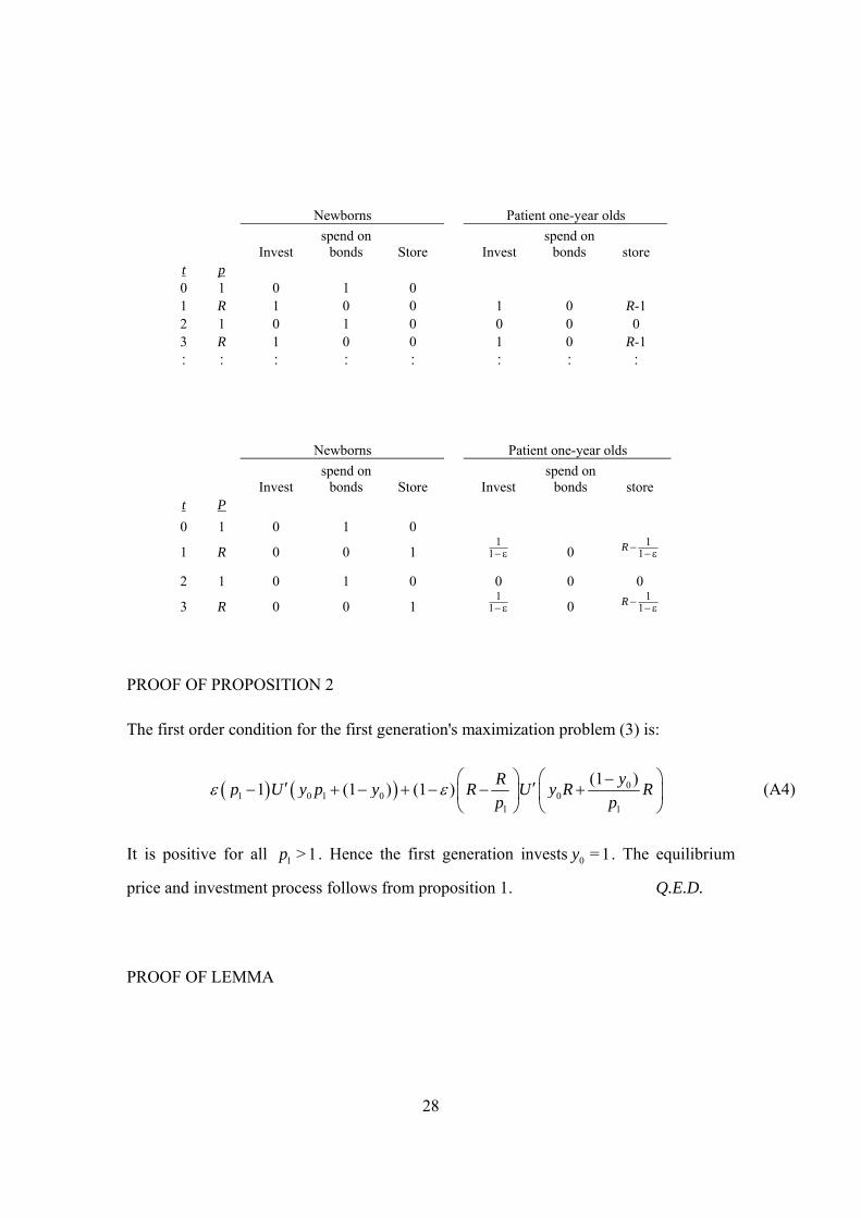
The equilibrium price process {1,R,1,R} can be supported by many investment and

storage schedules },,,,,,,{ 11

01

11

01

1010++++ tttttttt zzyyzzyy . In this equilibrium not even aggregate

investment or storage is defined. The reason for this multiciplicity is that for the unlucky

generations, the return on projects and investment equals the return on storage. Below are

two (of many) schedules that support the most cyclical price process.

28

Newborns Patient one-year olds

Invest spend on

bonds Store Invest spend on

bonds store t p 0 1 0 1 0 1 R 1 0 0 1 0 R-1 2 1 0 1 0 0 0 0 3 R 1 0 0 1 0 R-1 : : : : : : : :

Newborns Patient one-year olds

Invest spend on

bonds Store Invest spend on

bonds store t P 0 1 0 1 0

1 R 0 0 1 1

1− ε

0 1

1R − −ε

2 1 0 1 0 0 0 0

3 R 0 0 1 1

1− ε

0 1

1R − −ε

PROOF OF PROPOSITION 2

The first order condition for the first generation's maximization problem (3) is:

( ) ( ) 01 0 1 0 0

1 1

(1 )1 (1 ) (1 ) yRp U y p y R U y R Rp p

⎛ ⎞ ⎛ ⎞−′ ′− + − + − − +⎜ ⎟ ⎜ ⎟⎝ ⎠ ⎝ ⎠

ε ε (A4)

It is positive for all 1 > 1p . Hence the first generation invests 0 = 1y . The equilibrium

price and investment process follows from proposition 1. Q.E.D.

PROOF OF LEMMA

29

First we prove that the first generation agents will not store but spend their entire

endowment on buying the x projects and on investing in the technology. Denote 0z the

amount stored, and as before, denote 0y the amount invested in the technology. The first

generation solves:

0 0 1 0 0 0 0 0 00 0 0 1

(1 ) (1 ) (1 )maxy

R R RU z y p z y U y R z y zp p p

⎛ ⎞⎛ ⎞ ⎛ ⎞+ + − − + − + − − +⎜ ⎟⎜ ⎟ ⎜ ⎟⎜ ⎟⎝ ⎠ ⎝ ⎠⎝ ⎠

ε ε (A5)

Of which the first derivative with respect to 0z is:

( ) ( )0 0 1 0

[ ] = 1 (1 ) 1E U R R RU Uz p p p

⎛ ⎞ ⎛ ⎞∂ ′ ′− ⋅ + − − ⋅⎜ ⎟ ⎜ ⎟∂ ⎝ ⎠ ⎝ ⎠ε ε (A6)

Which is negative for all 0 <p R . This proves that the first generation does not store.

To find the clearing price in a liquidating sale, we first consider an interior solution in

which all agents spend their entire endowment on projects and on investing. In such an

equilibrium, ty solves (1) for all t , so that 0

=oddRpp

and 0=evenp p .

The market clearing conditions are:

00

1= ypx− (A7)

1

1

(1 ) (1 )(1 )= > 0

t tt

tt

Ry ypp t

y

−−

− + − −∀

ε

ε (A8)

Equation (A8) implies that ty is two-periodic. From proposition 1 we know that:

= 1 > 0.1

tt

R py tR−

− ∀−

ε (A9)

From equation (A8) it also follows that 0 = eveny y so that:

00 = 1 .

1R pyR−

−−

ε (A10)

30

Substitute (A10) into (A7) to find expression (16a). If >x ε , (16a) results in 0 < 1p , and

by proposition 1, to a 1 >p R . This in turn implies (from (A9)) that 1 > 1y , contradicting

our assumption of an interior solution.

Trivially, if more than ε projects are offered, the price they fetch will not be less than

unity ((16b) of lemma), unless more than one projects are offered. In the latter case all the

goods of the first generation goes to buying projects, so that the price per project is 1x

((16c) of lemma). Q.E.D.

PROOF OF PROPOSITION 3

We look for a function 2 1( | , )r r Rε so that (15) holds with equality. This expression is the

frontier of the permissible set. If (16a) describes the price equation, we can find the

frontier by substituting (16a) in (15):

1 2 2

1 21 2

1 2 2

(1 ) 1 (1 )(1 ) 11 (1 ) 0

(1 ) 1 1(1 ) ( 1)1

r r r Rr rR R R r r

r r r RRR R

+ − −⎛ ⎞− −⎜ ⎟ + − −−⎝ ⎠ + − − − =+ − − −⎛ ⎞− − − +⎜ ⎟−⎝ ⎠

ε ε ε εε ε ε ε

ε ε ε ε (A11)

Which can be written as a quadratic equation in 2r , of which the positive root is:

2 2 2

1 12

4 ( 1) (1 )2(1 )

R r R r Rr R

+ − − += +

−ε

ε (A12)

This gives us the first part of (17). If (16b) is the relevant price equation, we need to

substitute this into (15). We obtain:

( ) ( )1 2 1 221 2

(1 ) 1 (1 ) 1(1 ) (1 )

( 1) ( 1)r r r rr R r r

R R R+ − − + − −

− − + − = −− −

ε ε ε εε ε ε (A13)

Which, after some algebra, becomes:

31

( )2 1

2(1 ) (1 ) 1

R Rr rR

= −− − +

εε ε

(A14)

The second part of (17). Finally, if (16c) is the relevant price equation, we get for (15):

( )1 21 2

(1 ) 11 (1 )

( 1)r r

R r rR

+ − −+ − ≤ −

−ε ε

ε ε (A15)

Which reduces to:

12

11

rr −≤

−εε

(A16)

Observe that the price-equation ((16a)-(16c)) can be written as:

01( ) = ( ) = min max ,1 ,

( 1)Rp x p x

x R x⎛ ⎞⎛ ⎞⎜ ⎟⎜ ⎟− +⎝ ⎠⎝ ⎠

εε

(A17)

Because the number of projects sold in a raid is 2 1 2(1 )(1 ) = ... =( 1)

r R r r RyR R R

+ − −− −

−ε εε ,

which increases in both 1r and 2r , we may combine (A12), (A14) and (A16) to describe

the permissible as follows:

( )

2 2 21 1 1

2 1

4 ( 1) (1 ) 12max min , ,2(1 ) (1 ) (1 ) 1 1

R r R r R rR Rr R rR

⎛ ⎞⎛ ⎞+ − − + −⎜ ⎟⎜ ⎟≤ + −⎜ ⎟⎜ ⎟− − − + −⎝ ⎠⎝ ⎠

εεεε ε ε ε

(A18)

Because the minimum of the first and second term is always greater than the third term

(in the relevant region 1 2, > 0r r ) we can omit the outer max-operator. The proposition

that { },R R lies on the frontier can be proven by substitution. Q.E.D.

PROOF OF PROPOSITON 4

We prove proposition 4 in four steps. We first show that the problem (21)-(22), if

unconstrained by bank raid constraint (17), has a solution with r1 = r2. Second we prove

that the crossing point of the first and second component of (17) lies above the 45 degree

32

line. Third, we proof that the slope of the first component of (17) is greater than the slope

of budget constraint (22), and finally we prove uniqueness of point E.

Due to non-satiability (22) is binding, so that we rewrite (21) as:

*

1 11

1 ( 1)max ( ) (1 ) (1 ) (1 )y RU r U rr

⎛ ⎞+ − εε + − ε −⎜ ⎟− ε − ε⎝ ⎠

(A19)

The first order condition of which is:

*1 1'( ) ' ( 1) 0(1 )U r U y R rε⎛ ⎞ε − ε − − =⎜ ⎟− ε⎝ ⎠

(A20)

proving that r1 = r2.

For the second part of the proof, we observe that the second component of (17),

2 12

1 (1 )(1 )R Rr r

R= −

− − +ε

ε ε, crosses the 45 degree line at 1

(1 )1

R RrR R+

=− + +ε ε

. We need to

show that this is greater than first component of (17), 2 2 2

1 14 ( 1) (1 )2(1 )

R r R r RR

+ − − ++

−ε

ε

evaluated at 1(1 )

1R Rr

R R+

=− + +ε ε

. Or, we need to show that:

2 2 2 22

2(1 ) ( 1) (1 )4

(1 ) 1(1 )1 2(1 )

R R R R RRR R R RR R R

R R

+ − ++ −

− + + − + ++≥ +

− + + −ε ε ε ε

εε ε ε

(A21)

Multiplying both sides by 1 R R− + +ε ε , dividing by R, canceling terms, then dividing

both sides by ε, and multiplying sides by 2(1-ε) gives:

2 2 2 2(1 ) 2( 1)(1 ) 4(1 ) (1 ) ( 1)R R R R R R+ − − − ≥ − + + + + −ε ε ε (A22)

And hence

( )22 2 2 24(1 ) (1 ) ( 1) (1 ) 2( 1)(1 ) 0R R R R R R− + + + + − − + − − − ≤ε ε ε (A23)

Collecting terms eventually gives:

33

3 24 ( 1) 4( 1) 0R R− − − − ≤ε (A24)

Which clearly holds for all [0,1]∈ε and 1R ≥ .

The slope of the first component of (17), is

2 2 2 2

1 1 12 2 2

1 1

4 ( 1) (1 ) ( 1) (1 )2(1 ) 2(1 ) 4 ( 1)

R r R r R r RR Rr R r R

⎛ ⎞ ⎛ ⎞+ − − + −∂ ⎜ ⎟ ⎜ ⎟+ = − +⎜ ⎟ ⎜ ⎟∂ − − + −⎝ ⎠ ⎝ ⎠

εεε ε

(A25)

For a given y′ , the budget constraint (22) can be written as

12

1 ( 1)(1 )

y R rr′+ − −

=−

εε

(A26)

The slope of which is 11r−

−εε

.

To prove the third step we thus need to show that:

2

11 2 2 2

1

( 1)1 (1 )2 4 ( 1)

r Rr RR r R

⎛ ⎞−⎜ ⎟≥ − +⎜ ⎟+ −⎝ ⎠

(A27)

or:

( ) 2 2 2 21 1 12 1 4 ( 1) ( 1)r R R r R r R+ + + − ≥ − (A28)

After squaring both sides and simplifying this becomes:

( ) ( )( )( )2 4 3 21 1 1 14 ( 1) ( 1) ( 1) ( 1) 4 0R r R r R R R r R Rr− + + + + + + + ≥ (A29)

Which holds for all 1 0r ≥ and 1R ≥ , because all terms of the left hand side are positive.

To prove that point E is unique we only need to establish that the second order derivative

of the first component of (17) is positive in the relevant range. We find:

( )

2 2 2 2 2 22 2 11 1 1 12

2 2 2 2 2 2 21 1 1

4 ( 1) (1 ) 4 ( 1)( 1)2(1 ) 2(1 ) 4 ( 1) 4 ( 1)

R r R r R R r R rRRr R r R R r R

⎛ ⎞⎛ ⎞+ − − + + − −∂ ε − ⎜ ⎟⎜ ⎟+ ε =− ε − ε ⎜ ⎟⎜ ⎟∂ + − + −⎝ ⎠ ⎝ ⎠

(A30)

34

Which is clearly positive over the relevant range. Q.E.D.

PROOF OF PROPOSITON 5

Uniqueness of the equilibrium follows from the fact that the maximized expected utility

of the first generation decreases in *y while the maximized expected utility of the

stationary generation increases in *y . This proves that there is a *y where the maximized

expected utilities are equal. As long as the point H stays on the diagonal, risk aversion

does not affect the utility of the stationary generation, but decreases the utility of the first

generation. Hence we find that with decreasing risk aversion, the point H moves upward

along the black line in Figure 2. Q.E.D.

35

References

Allen, F., Gale, D. (1997) Financial markets, intermediaries, and intertemporal smoothing, Journal of Political Economy 105, 523-545.

Bencivenga, V.R., Smith, B.D. (1991) Financial intermediation and endogenous growth, Review of Economic Studies 58, 195-210.

Bhattacharya, S., Gale, D. (1987) Preference shocks, liquidity, and central bank policy, in: W.A. Barnett and K.J. Singleton (eds.) "New approaches to monetary economics", Cambridge University Press, Cambridge, 69-88.

Bhattacharya, S., Padilla, A.J. (1996) Dynamic Banking: A reconsideration, Review of Financial Studies 9, 1003-1031.

Bhattacharya, S., Fulghieri, P., Rovelli, R. (1998) Financial intermediation versus stock markets in a dynamic intertemporal model, Journal of Institutional and Theoretical Economics 154, 1, 291-319.

Bryant, J. (1980) A model of reserves, bank runs, and deposit insurance, Journal of Banking and Finance 4, 335-344.

Diamond, D.W., Dybvig, P.H. (1983) Bank runs, Deposit insurance and liquidity, Journal of Political Economy 91, 401-419.

Diamond, D.W. (1997) Liquidity, banks, and markets, Journal of Political Economy 105, 928-956.

Dutta, J., Kapur, S. (1998) Liquidity preference and financial intermediation, Review of Economic Studies 65, 551-572.

Edgeworth, F.Y. (1888) The Mathematical Theory of Banking, Journal of the Royal Statistical Society LI, 113-127.

Esteban, J. (1986) A characterization of the core of overlapping generations economies: An exact consumption-loan model of interest with or without the social contrivance of money, Journal of Economic Theory 39, 439-456.

36

Freeman, S. (1988) Banking as the provision of liquidity, Journal of Business, 61, 45-64.

Fulghieri, P., Rovelli, R. (1998) Capital markets, financial intermediaries, and liquidity supply, Journal of Banking and Finance 22, 1157-1179.

Gorton, G., Pennacchi, G. (1990) Financial intermediaries and liquidity creation, Journal of Finance 45, 49-71.

Haubrich, J.G., King, R.G. (1990) Banking and Insurance, Journal of Monetary Economics 26, 361-386.

Hellwig, M.F. (1994) Liquidity provision, banking, and the allocation of interest rate risk, European Economic Review 38, 1363-1389.

Hendricks, K., Judd, K., Kovenock, D. (1980) A note on the core of overlapping generation models, Economic Letters 6, 95-97.

Jacklin, C.J. (1987) Demand deposits, Trading restrictions, and risk sharing, in: E. Prescott and N. Wallace (eds) ``Contractual Arrangements for Intertemporal Trade'', University of Minnesota Press, Minneapolis, 26-47.

Phelps,E.S. (1961) The golden rule of accumulation: a fable for growthmen, American Economic Review 51, 638-643.

Prescott, E.C., Rios-Rull. J.V. (2000) On the equilibrium concept for overlapping generations organizations Federal Reserve Bank of Minneapolis Research Department Staff Report 282.

Qi,J. (1994) Bank liquidity and stability in an overlapping generations model, Review of Financial Studies 7, 389-417.

Qian, Y., John, K., John, T.A. (2004) Financial system design and liquidity provision by banks and markets in a dynamic economy, Journal of International Money and Finance 23, 385-403.

Samuelson, P.A. (1958) An exact consumption-loan model of interest with or without the social contrivance of money, Journal of Political Economy 66, 467-482.

37

Shell, K. (1971) Notes on the economics of infinity, Journal of Political Economy 79, 1002-1011.

Tabellini, G. (1991) The politics of intergenerational distribution, Journal of Political Economy, 99, 335-357.

Tabellini, G. (2000) A positive theory of social security, Scandinavian Journal of Economics, 102, 523-545.

von Thadden, E.L. (1997) The term structure of investment and the bank's insurance function, European Economic Review 41, 1355-1374.

von Thadden, E.L. (1998) Intermediated versus direct investment: optimal liquidity provision and dynamic incentive compatibility Journal of Financial Intermediation, 7, 177-197.

Wallace, N. (1988) Another attempt to explain an illiquid banking system: the diamond and dybvig model with sequential service taken seriously Quarterly Review of the Federal Reserve Bank of Minneapolis, 3-16.

38

Figure 1

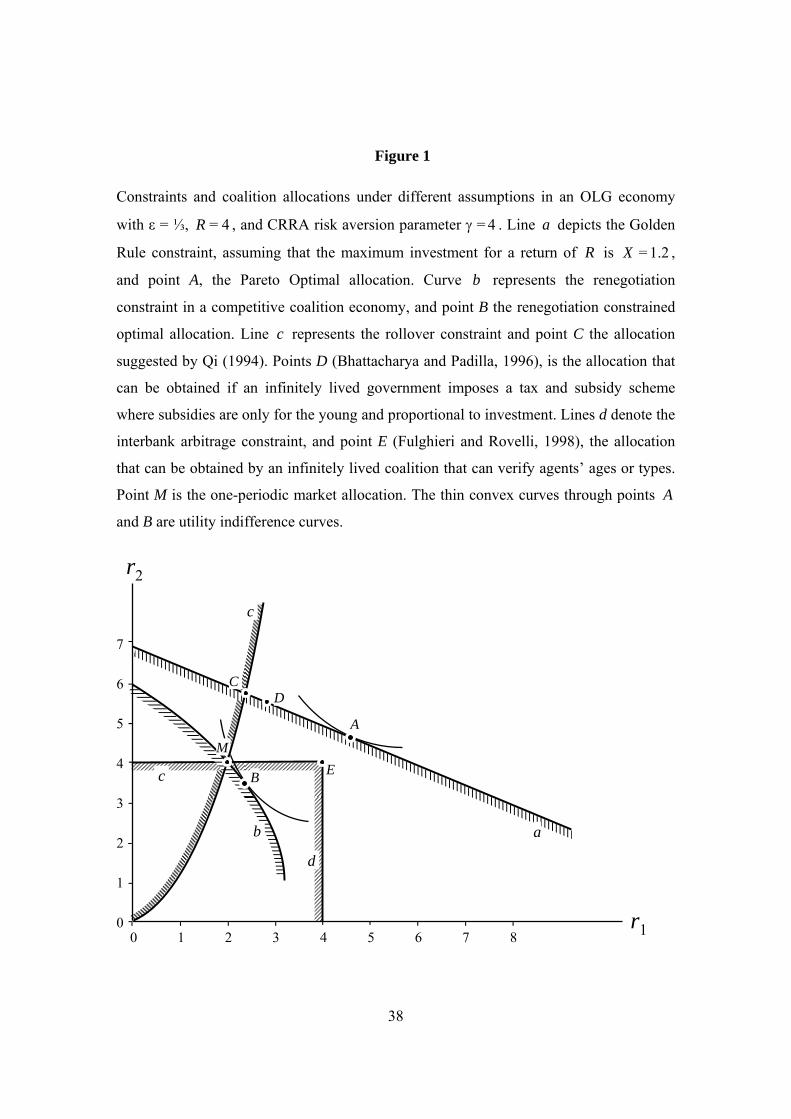
Constraints and coalition allocations under different assumptions in an OLG economy

with ε = ⅓, = 4R , and CRRA risk aversion parameter γ = 4 . Line a depicts the Golden

Rule constraint, assuming that the maximum investment for a return of R is = 1.2X ,

and point A, the Pareto Optimal allocation. Curve b represents the renegotiation

constraint in a competitive coalition economy, and point B the renegotiation constrained

optimal allocation. Line c represents the rollover constraint and point C the allocation

suggested by Qi (1994). Points D (Bhattacharya and Padilla, 1996), is the allocation that

can be obtained if an infinitely lived government imposes a tax and subsidy scheme

where subsidies are only for the young and proportional to investment. Lines d denote the

interbank arbitrage constraint, and point E (Fulghieri and Rovelli, 1998), the allocation

that can be obtained by an infinitely lived coalition that can verify agents’ ages or types.

Point M is the one-periodic market allocation. The thin convex curves through points A

and B are utility indifference curves.

0

1

2

3

4

5

7

0 1 2 3 4 5 6 7 8

6

-

-

-

-

-

-

-

- - - - - - - - - -

D

E B

a

c

d

c

r1

r2

AM

b

C

39

Figure 2

Constraints and coalition allocations under different assumptions in an OLG economy

with ε = ⅓, = 4R , X = 1.2 and CRRA risk aversion parameter γ = 4 . Curve b represents

the renegotiation constraint in a competitive coalition economy. Curve e represents the

renegotiation constraint for a monopolist and point F the constraint optimal allocation in

such an economy.

0

1

2

3

4

5

7

0 1 2 3 4 5 6 7 8

6

-

-

-

-

-

-

-

- - - - - - - - - -

D

E F

a

c

c

c

e

r1

r2

A

C

b

M

B

40

Figure 3

Equilibrium allocations of the stationary coalition game if ε = ⅓, = 4R , and CRRA risk

aversion parameter γ= 4 , for the competitive (panel A) and monopolist (panel B)

coalition economies. The thick black line gives coalition equilibria. The r1, r2

combinations maximize utility for a given inherited asset buffer. The thin downward

sloping lines are the internal budget constraints associated with different asset buffers.

Line f is the budget constraint for the intragenerational coalition. G denotes the stationary

allocation that offers depositors equal utility as the intragenerational allocation H.

G

0

1

2

3

4

5

0 1 2 3 4 5 6 7 8

6 -

-

-

-

-

-

- - - - - - - - - - r1

r2

H

f

y*

y’

b

BM

0

1

2

3

4

5

0 1 2 3 4 5 6 7 8

6 -

-

-

-

-

-

- - - - - - - - - -

e

r1

r2

F

H

f

M

y*

y’

G

41

Comments:

- we cannot follow your proposed “theory of the firm” line of argument because it

could be argued that our case is one of incomplete contracting (the impossibility

of current and future generations to credibly contract with each other). We could

battle such arguments but it would detract from the paper. Let’s try to stick to the

renegotiation proofness

- this brings me to a second point: renegotiation-proof is a well-established concept

in game theory. It’s Standard meaning is not the one we are using so we should

also avoid the phrase (lit review Bolton 90EuropeanER)

- Main vocabulary

o Financial institution, institutions

o Constraint: renegotiation constraint, deposit increase, SGFI constraint,

bounty

o Renegotiation: sharing, increase deposits, …

o Assets: capital