the graduate school department of chemistry calculation of
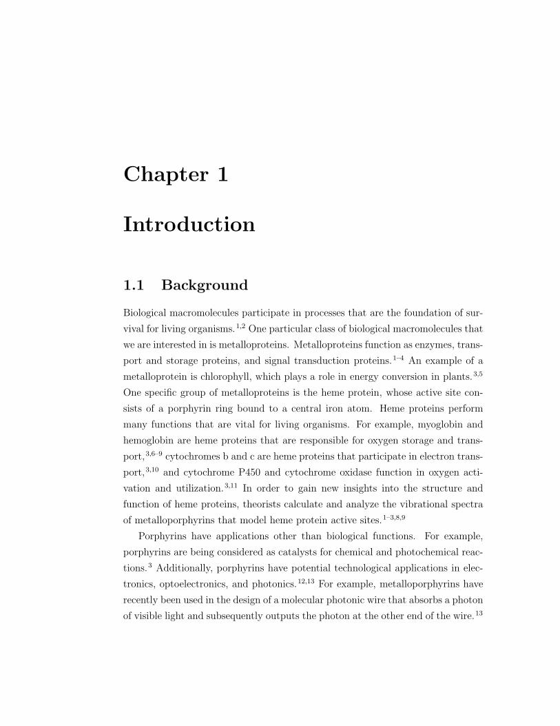
TRANSCRIPT
The Pennsylvania State University
The Graduate School
Department of Chemistry
CALCULATION OF ABSOLUTE RESONANCE RAMAN
INTENSITIES
A Thesis in
Chemistry
by
Krista A. Kane
c© 2009 Krista A. Kane
Submitted in Partial Fulfillment
of the Requirements
for the Degree of
Master of Science
December 2009

The thesis of Krista A. Kane was reviewed and approved∗ by the following:
Lasse Jensen
Assistant Professor of Chemistry
Thesis Advisor
John V. Badding
Professor of Chemistry
Mark Maroncelli
Professor of Chemistry
Barbara Garrison
Shapiro Professor of Chemistry
Head, Department of Chemistry
∗Signatures are on file in the Graduate School.

Abstract
We present the resonance Raman (RR) spectra of uracil, rhodamine 6G (R6G) andiron(II) porphyrin with imidazole and CO ligands (FePImCO) calculated usingdensity functional theory (DFT). The absolute RR intensities were determined us-ing both the vibronic theory and the short-time approximation. We found that theabsolute RR intensities calculated using the short-time approximation are overesti-mated compared to those calculated using the vibronic theory. This is attributed tothe sensitivity of the short-time approximation to the damping parameter. Uracilis not affected by vibronic coupling and so the absolute RR intensities calculatedusing both methods should be comparable. Despite the agreement obtained in therelative RR intensities, the absolute RR intensities calculated using the short-timeapproximation are severely overestimated compared to those calculated using thevibronic theory. In addition, the absolute RR intensities of R6G, computed us-ing the vibronic theory, are only slightly underestimated compared to experiment,which is attributed to the neglect of solvent effects in the calculations. The absoluteRR intensities calculated using vibronic theory correctly resulted in an increase inthe relative RR intensity of the low-frequency Raman bands for molecules thatexperience vibronic coupling (i.e. R6G and FePImCO), but was not observed inthe RR spectra calculated using the short-time approximation.
iii
Table of Contents
List of Figures vi
List of Tables vii
Acknowledgments viii
Chapter 1Introduction 11.1 Background . . . . . . . . . . . . . . . . . . . . . . . . . . . . . . . 11.2 Raman Spectroscopy . . . . . . . . . . . . . . . . . . . . . . . . . . 31.3 Resonance Raman Spectroscopy . . . . . . . . . . . . . . . . . . . . 61.4 Objective . . . . . . . . . . . . . . . . . . . . . . . . . . . . . . . . 6
Chapter 2Theoretical Methods 92.1 Background . . . . . . . . . . . . . . . . . . . . . . . . . . . . . . . 92.2 Vibronic Theory . . . . . . . . . . . . . . . . . . . . . . . . . . . . . 9
2.2.1 Transform Theory . . . . . . . . . . . . . . . . . . . . . . . . 112.2.2 Short-time Approximation . . . . . . . . . . . . . . . . . . . 152.2.3 Polarizability Gradient Model . . . . . . . . . . . . . . . . . 152.2.4 RR Differential Cross-Sections . . . . . . . . . . . . . . . . . 16
2.3 Time-Dependent Approach . . . . . . . . . . . . . . . . . . . . . . . 162.4 Computational Method . . . . . . . . . . . . . . . . . . . . . . . . . 18
Chapter 3Results 203.1 2-bromo-2-methylpropane . . . . . . . . . . . . . . . . . . . . . . . 203.2 Carbon Disulfide . . . . . . . . . . . . . . . . . . . . . . . . . . . . 213.3 Uracil . . . . . . . . . . . . . . . . . . . . . . . . . . . . . . . . . . 223.4 Rhodamine 6G . . . . . . . . . . . . . . . . . . . . . . . . . . . . . 26
iv

3.5 Iron(II) Porphyrin with Imidazole and CO Ligands . . . . . . . . . 31
Chapter 4Conclusions and Future Directions 36
Bibliography 38
v

List of Figures
1.1 Energy-level diagram for IR absorption, Rayleigh Scattering, StokesRaman Scattering, and Anti-Stokes Raman Scattering. . . . . . . . 5
1.2 Energy-level diagram for pre-resonance and resonance Raman spec-troscopy. . . . . . . . . . . . . . . . . . . . . . . . . . . . . . . . . . 7
2.1 Pictorial definition of the dimensionless displacement, ∆. . . . . . . 132.2 Pictorial representation of RR scattering according to the time-
dependent approach. . . . . . . . . . . . . . . . . . . . . . . . . . . 18
3.1 Ball and stick model of uracil. . . . . . . . . . . . . . . . . . . . . . 223.2 (a)Calculated absorption spectrum of uracil. (b) Experimental
absorption spectrum of uracil, 6-methyluracil, 1,3-dimethyluracil,thymine, and 5-fluorouracil in water at room temperature. . . . . . 24
3.3 Simulated RR spectra of uracil with 262 nm excitation. . . . . . . . 253.4 Experimental RR spectrum of uracil in water with 266 nm excitation. 253.5 Ball and stick model of R6G. . . . . . . . . . . . . . . . . . . . . . 273.6 (a) Calculated absorption spectrum of R6G. (b) Experimental ab-
sorption spectrum of R6G in methanol. . . . . . . . . . . . . . . . . 283.7 Simulated RR spectra of R6G with 473 nm excitation. . . . . . . . 293.8 Experimental RR spectrum of R6G in methanol with 532 nm exci-
tation. . . . . . . . . . . . . . . . . . . . . . . . . . . . . . . . . . . 293.9 Ball and stick model of FePImCO. . . . . . . . . . . . . . . . . . . 313.10 (a) Calculated absorption spectrum of FePImCO for the B band.
(b) Calculated absorption spectrum of FePImCO for the Q band. . 333.11 Calculated RR spectra of FePImCO. . . . . . . . . . . . . . . . . . 35
vi
List of Tables
3.1 Comparison of DFT results with reported experimental and theo-retical values for the Raman differential cross-sections of 2B2MP at633 nm excitation. . . . . . . . . . . . . . . . . . . . . . . . . . . . 20
3.2 Comparison of DFT results in vacuum at 186 nm excitation withexperimental values in cyclohexane at 208.8 nm excitation for theRR total cross-sections of CS2. . . . . . . . . . . . . . . . . . . . . . 21
3.3 Comparison of DFT results (gas phase) upon 473 nm excitationwith experimental values for the RR total cross-sections of R6G inmethanol at 532 nm excitation (the corresponding transition). . . . 30
vii
Acknowledgments
I would like to thank Lasse Jensen for his guidance and support on my researchat Penn State. I would also like to thank the entire Jensen group, especially SethMorton for all of his help. I would like to thank my committee members: Dr. JohnBadding, Dr. Mark Maroncelli, and Dr. Coray Colina for taking the time to beon my committee. Last, but not least, I would also like to thank my family andfriends for their continued love and support.
viii
Chapter 1
Introduction
1.1 Background
Biological macromolecules participate in processes that are the foundation of sur-
vival for living organisms.1,2 One particular class of biological macromolecules that
we are interested in is metalloproteins. Metalloproteins function as enzymes, trans-
port and storage proteins, and signal transduction proteins.1–4 An example of a
metalloprotein is chlorophyll, which plays a role in energy conversion in plants.3,5
One specific group of metalloproteins is the heme protein, whose active site con-
sists of a porphyrin ring bound to a central iron atom. Heme proteins perform
many functions that are vital for living organisms. For example, myoglobin and
hemoglobin are heme proteins that are responsible for oxygen storage and trans-
port,3,6–9 cytochromes b and c are heme proteins that participate in electron trans-
port,3,10 and cytochrome P450 and cytochrome oxidase function in oxygen acti-
vation and utilization.3,11 In order to gain new insights into the structure and
function of heme proteins, theorists calculate and analyze the vibrational spectra
of metalloporphyrins that model heme protein active sites.1–3,8,9
Porphyrins have applications other than biological functions. For example,
porphyrins are being considered as catalysts for chemical and photochemical reac-
tions.3 Additionally, porphyrins have potential technological applications in elec-
tronics, optoelectronics, and photonics.12,13 For example, metalloporphyrins have
recently been used in the design of a molecular photonic wire that absorbs a photon
of visible light and subsequently outputs the photon at the other end of the wire.13

2
The ability of metalloporphyrins to undergo oxidation/reduction allows them to
act as the off/on ”switching element” in the molecular photonic wire. Zinc por-
phyrins are being investigated for their applications in dye-sensitized solar cells
(DSSCs).14,15
The function of biological macromolecules is dictated by their specific three-
dimensional structure.4 One tool we use to investigate biologically relevant mole-
cules is vibrational spectroscopy. One advantage of vibrational spectroscopy over
other spectroscopic techniques is that it can provide detailed structural informa-
tion that can be used to identify compounds, unlike UV-vis absorption and fluores-
cence.2 Although X-ray crystallography and nuclear magnetic resonance (NMR)
spectroscopy can be used to obtain structural information, vibrational spectroscopy
can also provide information about dynamics.2 A second advantage is that vibra-
tional spectroscopy can be used to analyze samples that are in solid, liquid, or
gas states or even in monolayers.2 This is beneficial because it allows us to obtain
information about molecules in their native states. In particular, many biological
macromolecules exist in an aqueous environment and so vibrational spectroscopy
allows us to analyze them in their natural surroundings.
The two main vibrational spectroscopy techniques are infrared (IR) and Ra-
man spectroscopy.2 As the size of the molecule of interest increases, the number of
vibrational modes also increases, which complicates the vibrational spectra. There
are 3N-5 vibrational modes for linear molecules (3 translational and 2 rotational)
and 3N-6 vibrational modes for non-linear molecules (3 translational and 3 rota-
tional), where N is the number of atoms.2,16,17 As a result of the increasing number
of vibrational bands with larger molecules, the IR and Raman spectra become more
complex and the individual bands become difficult to identify. In this case, reso-
nance Raman spectroscopy (RRS) can be used to selectively enhance vibrational
bands related to a specific chromophore within the much larger biological macro-
molecule of interest.2,16–24 As a result, an understanding of how the properties of
the chromophore contribute to the overall function of the protein can be obtained.
The sensitivity and selectivity of RRS makes it a powerful tool with a variety
of applications. RRS is particularly useful for studying biological systems because
it can be used as a tool to probe the structure and dynamics of a particular excited
state associated with a specific chromophore in a much larger protein.25 RRS is

3
useful in the characterization of peptide and protein secondary structure because
excitation of the π → π∗ transition of the peptide backbone leads to an enhance-
ment of the amide vibrations.26,27 A recent article in Chemical & Engineering News
(C&EN) reviewed the application of IR and RRS to investigate amyloids, which
are protein clumps that are related to neurological diseases, such as Alzheimer’s
and Parkinson’s.28 Structural information about amyloids can be obtained from
X-ray crystallography and solid-state NMR, however these techniques cannot be
used to study intermediate states of species, which are suspected to be responsible
for these diseases. In contrast, deep-ultraviolet RRS can be used to analyze the
structure and fibrilization mechanism of amyloids. In addition, RRS can be used
to structurally characterize carbon nanotubes.29–31
1.2 Raman Spectroscopy
Raman spectroscopy is a powerful tool for analyzing molecular vibrational frequen-
cies.16,17 In Raman spectroscopy, a photon interacts with a molecule which results
in the photon being remitted with either the same energy or a different energy
as the original photon. Most of the photons given off by the molecule have the
same energy as the incident photon. This process is known as elastic or Rayleigh
scattering. However, a small fraction of the photons (one in one million) will be
remitted with an energy different from the incident photon. This process is known
as inelastic or Raman scattering. The difference in energy between the emitted
and incident photon corresponds to a vibrational normal mode frequency. The
vibrations can provide detailed information about chemical bonds leading to an
understanding of the ground state structure and dynamics of a molecular system.
The peaks in a Raman spectrum are known as either Stokes or anti-Stokes lines
depending on if the energy difference between the original and remitted photon is
positive or negative, respectively.16,17 Stokes lines represent a transition from a
lower vibrational level in the ground electronic state to a higher vibrational level
of the ground electronic state. This process requires the molecule to absorb some
energy from the incident photon and the emitted photon therefore has less energy
than the original photon. In contrast, anti-Stokes lines represent a transition from
a higher vibrational level of the ground electronic state to a lower vibrational level

4
of the ground electronic state. Thus, energy is given off in this type of transition
and the emitted photon therefore has more energy than the original photon. Stokes
lines are more intense than anti-Stokes lines because they represent a transition
beginning from a more populated state. It is therefore common to only present
the Stokes lines in a Raman spectrum.
Sir Chandrasekhara Venakta Raman discovered the Raman effect in 1928.16,17
Raman’s interest in light scattering began with his curiosity about the blue color
of the Mediterranean sea. Raman showed that the sea’s color is a result of the light
scattering by water molecules. Subsequently, Raman investigated the scattering of
light by water and other liquids and for all of the molecules studied, described his
observations as a ”feeble fluorescence” because they produced such a weak signal.
Raman scattering was an immediate sensation; as around 70 papers concerning
the Raman effect had been published by the end of 1928.17 Raman was awarded
the Nobel Prize in physics in 1930.17 Raman spectroscopy became a more active
field of study with the advent of the laser in the early to mid-1960’s because lasers
emit light of a single wavelength, producing more concentrated photons, and as a
result a stronger signal.16,17
Both Raman and infrared (IR) spectroscopy can be used to investigate vibra-
tional transitions in molecules.16,17,32 The vibrational frequencies that appear in the
Raman and IR spectrum may differ from one another as a result of the symmetry
of the molecule. The Raman and IR spectra are specific for the molecule of inter-
est. For this reason, the application of both Raman and IR spectroscopy is a useful
tool for the identification of unknown compounds. While Raman spectroscopy is a
two-photon process, IR spectroscopy is a one photon event. IR absorption is due to
a resonance between the frequency of the incident IR radiation and the vibrational
frequency of a certain normal mode of vibration. Molecules that are IR active
experience a change in dipole moment with respect to its vibrational motion. In
contrast, molecules that are Raman active undergo a change in polarizability with
respect to its vibrational motion.
Although similar information is obtained from both Raman and IR spectro-
scopy, differences among these two techniques can be identified in the energy-level
diagram, shown in Figure 1.1. For both Stokes Raman scattering and IR ab-
sorption, the initial state is the zeroth vibrational level of the ground electronic
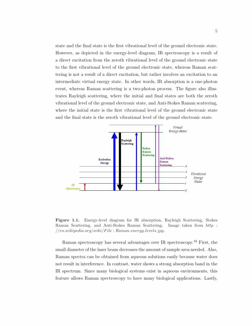
5
state and the final state is the first vibrational level of the ground electronic state.
However, as depicted in the energy-level diagram, IR spectroscopy is a result of
a direct excitation from the zeroth vibrational level of the ground electronic state
to the first vibrational level of the ground electronic state, whereas Raman scat-
tering is not a result of a direct excitation, but rather involves an excitation to an
intermediate virtual energy state. In other words, IR absorption is a one-photon
event, whereas Raman scattering is a two-photon process. The figure also illus-
trates Rayleigh scattering, where the initial and final states are both the zeroth
vibrational level of the ground electronic state, and Anti-Stokes Raman scattering,
where the initial state is the first vibrational level of the ground electronic state
and the final state is the zeroth vibrational level of the ground electronic state.
Figure 1.1. Energy-level diagram for IR absorption, Rayleigh Scattering, StokesRaman Scattering, and Anti-Stokes Raman Scattering. Image taken from http ://en.wikipedia.org/wiki/F ile : Raman energy levels.jpg.
Raman spectroscopy has several advantages over IR spectroscopy.32 First, the
small diameter of the laser beam decreases the amount of sample area needed. Also,
Raman spectra can be obtained from aqueous solutions easily because water does
not result in interference. In contrast, water shows a strong absorption band in the
IR spectrum. Since many biological systems exist in aqueous environments, this
feature allows Raman spectroscopy to have many biological applications. Lastly,

6
Raman spectra can be obtained from air-sensitive compounds by utilizing a sealed
glass tube. In IR spectroscopy, the glass tube would interfere with the signal
because it absorbs IR radiation. The main disadvantages of Raman spectroscopy
are that the signal is weak and also the use of a laser can lead to fluorescence in
the spectrum, which can conceal the Raman bands.32
1.3 Resonance Raman Spectroscopy
Resonance Raman spectroscopy (RRS) can be used to enhance molecular vibra-
tional frequencies due to a particular electronic transition by a factor of as much as
106.16–24 In RRS the incident light is adjusted to a specific energy that corresponds
with the energy of the electronic transition of interest for a particular molecule.
As a result, only the vibrational frequencies associated with that specific electronic
transition are evident in the RR spectrum. Thus, RRS can provide information
about the excited state structure and dynamics. Theoretical calculations of the
RR spectrum are useful in the determination of these properties, whereas it may
be difficult to ascertain this information from experimental data.33,34 Furthermore,
comparison of the theoretical RR spectrum with the experimental RR spectrum
can lead to the improvement of the theoretical methods utilized to calculate RR
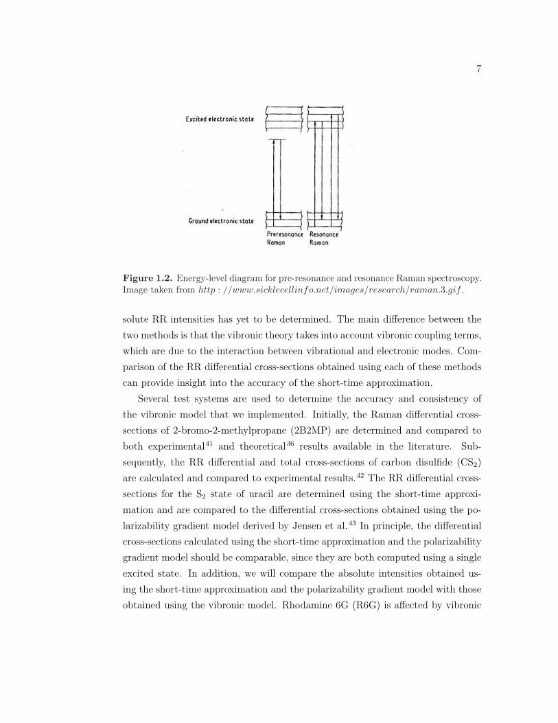
spectra.33 Figure 1.2 gives a general energy-level diagram for pre-resonance and
resonance Raman spectroscopy.
1.4 Objective
A frequent trend is to simply determine the relative RR intensities, which is ac-
ceptable in order to analyze and assign the RR spectra. However, we are interested
in determining the absolute RR intensities presented as differential cross-sections.
Determination of the absolute RR intensities is necessary in order to assess the en-
hancement factors in surface enhanced resonance Raman spectroscopy (SERRS).35,36 We have used density functional theory (DFT) to calculate the RR spectra
using two different theoretical methods: vibronic theory18–20,37–39 and short-time
approximation.21,22,40 While implementation of the short-time approximation is
much simpler than the vibronic theory, it’s validity in the determination of the ab-
7
Figure 1.2. Energy-level diagram for pre-resonance and resonance Raman spectroscopy.Image taken from http : //www.sicklecellinfo.net/images/research/raman.3.gif .
solute RR intensities has yet to be determined. The main difference between the
two methods is that the vibronic theory takes into account vibronic coupling terms,
which are due to the interaction between vibrational and electronic modes. Com-
parison of the RR differential cross-sections obtained using each of these methods
can provide insight into the accuracy of the short-time approximation.
Several test systems are used to determine the accuracy and consistency of
the vibronic model that we implemented. Initially, the Raman differential cross-
sections of 2-bromo-2-methylpropane (2B2MP) are determined and compared to
both experimental41 and theoretical36 results available in the literature. Sub-
sequently, the RR differential and total cross-sections of carbon disulfide (CS2)
are calculated and compared to experimental results.42 The RR differential cross-
sections for the S2 state of uracil are determined using the short-time approxi-
mation and are compared to the differential cross-sections obtained using the po-
larizability gradient model derived by Jensen et al.43 In principle, the differential
cross-sections calculated using the short-time approximation and the polarizability
gradient model should be comparable, since they are both computed using a single
excited state. In addition, we will compare the absolute intensities obtained us-
ing the short-time approximation and the polarizability gradient model with those
obtained using the vibronic model. Rhodamine 6G (R6G) is affected by vibronic
8
coupling and so this is an ideal system to observe the vibronic coupling effects
in the RR spectrum.33 As a result, we would expect to observe differences in the
RR differential cross-sections calculated using the two different methods under
investigation. Furthermore, experimental absolute intensities have recently been
reported.35 Iron(II) porphyrin with imidazole and CO ligands (FePImCO) is used
as a model system for understanding larger biologically relevant molecules contain-
ing a heme group, such as myoglobin, hemoglobin, or cytochrome c.8 FePImCO
experiences vibronic coupling and will be an interesting case used to investigate
the accuracy of the intensities derived from the vibronic versus the short-time
approximation.
Chapter 2
Theoretical Methods
2.1 Background
In this chapter, we review the basic aspects of RR scattering theory. In 1925,
Hendrik Kramers and Werner Heisenberg developed the Kramers-Heisenberg dis-
persion formula, which describes the scattering cross-section of a photon by an
atomic electron.44 In 1927, Paul Dirac developed the quantum mechanical deriva-
tion for this equation using perturbation theory.45 Due to the complexity of the
Kramers-Heisenberg-Dirac (KHD) formalism, several different approximations to
the KHD formalism have been proposed. The two main simplifications to the
KHD formalism are the vibronic theory and the time-dependent approach. We
will discuss both of these methods in this chapter.
2.2 Vibronic Theory
The vibronic theory18–20,37–39 was introduced by Albrecht and co-workers.18–20 The
vibronic theory uses the Born-Oppenheimer approximation, which separates the
vibronic states into products of electronic and vibrational states. Subsequently, the
transition dipole moment is expanded in a Taylor series in the nuclear coordinates.
The result of the expansion is a sum of different terms, known as the Albrecht
A,B,C, and D terms, that contribute to the RR intensities. The A term corresponds
to the Franck-Condon type scattering, which describes the RR intensity based on
the electronic transition dipole moment and also the vibrational overlap integrals.
10
Therefore, the Franck-Condon mechanism is most important for strong transitions
that have large dipole moments and large vibrational overlap integrals. The B
term describes the Herzberg-Teller type scattering, which involves the vibronic
coupling between two excited electronic states. This term is neglected because
taking into consideration coupling to more than one excited electronic state is
rarely necessary. The C term takes into account the vibronic coupling between the
ground electronic state and an excited electronic state. The C term is considered to
be negligible because of the large energy separation between the ground and excited
electronic states. Finally, the D term considers the vibronic coupling between an
excited electronic state to two other excited states. This term is likely to be
small and is therefore not considered. Each of these terms is expressed as a sum
over intermediate vibrational states in the resonant excited electronic state. As
a result, the calculation becomes computationally challenging for larger molecules
with many vibrational modes.17
In order to further simplify the vibronic theory, five assumptions are introduced.
First, the Born-Oppenheimer approximation is utilized. The Born-Oppenheimer
approximation states that since the the electrons are so much less massive than
the nuclei, the electrons move much faster than the nuclei and the electronic and
nuclear motion can therefore be separated. Second, only Franck-Condon-type scat-
tering is considered. Since the nuclei move much more slowly than the electrons,
the electronic transitions are considered to be vertical transitions. Third, the ex-
citation frequency is in resonance with only one excited state. Fourth, the ground
and excited electronic state potential energy surfaces are considered to be har-
monic. Last, the excited and ground electronic state normal coordinates vary from
one another only by their equilibrium positions so that the frequencies for the
ground and excited state vibrations are the same. These assumptions lead to the
consideration of only the Albrecht A term, which for vibrational RR scattering is
of the form:
[α(ωL)]f,i = µ2∑ν
〈f |ν〉 〈ν|i〉ωνi − ωL − iΓ (2.1)
where α(ωL) is the polarizability tensor, µ is the electronic transition dipole mo-
ment, |f〉 is the final vibrational level of the ground electronic state, |i〉 is the initial
vibrational level of the ground electronic state, |ν〉 is the intermediate vibrational
11
level of the excited electronic state, ωL is the frequency of the incident radiation,
Γ is the line width (half width at half maximum of the absorption band), and ωνi
is the frequency associated with the normal mode of interest. The polarizability
tensor can be expanded in terms of the normal modes to give:
[α(ωL)]f,i = µ2∑ν1
...∑ν3N−6
〈f1|ν1〉 〈ν1|i1〉∏3N−6
j=2 | 〈νj|0j〉 |2ω0 +
∑3N−6j νjωj − ωL − iΓ
(2.2)
where ωνi is given by:
ωνi = ω0 +3N−6∑j=1
νjωj (2.3)
where ω0 is the frequency corresponding to the transition from the ground elec-
tronic state to the resonant electronic state for the zeroth vibrational level, ωj is the
frequency of the jth normal mode, and νj is the vibrational quantum number of the
jth normal mode. The term | 〈νj|0j〉 |2 is also known as the Franck-Condon term,
which will be discussed in more depth later in this chapter. In equation 2.2, the
subscript 1 denotes the normal mode of interest. The RR intensity is proportional
to the square of the polarizability tensor.
2.2.1 Transform Theory
The original transform theory was derived by Hizhnyakov and Tehver46 and in-
volves utilizing the experimental absorption spectrum and the Kramers-Kronig
transform of the experimental absorption spectrum in order to determine the RR
intensities. The absorption cross-section is given by:
σA(ωL) ∝ ωLIm([αxx(ωL)]0,0 + [αyy(ωL)]0,0 + [αzz(ωL)]0,0) (2.4)
After substituting equation 2.2 into equation 2.4 and averaging over the various
molecular orientations, the absorption cross-section can be rewritten as:
σA(ωL) = ωLµ2∑ν1
| 〈ν1|01〉 |2∑ν2
...∑ν3N−6
∏3N−6j=2 | 〈νj|0j〉 |2Γ
(ω0 +
∑3N−6j=1 νjωj − ωL
)2
+ Γ2
(2.5)
12
Applying the intensity shift function to equation 2.5, which simply results in a
slightly shifted absorption spectrum, gives:
S(ωL − ν1ω1) =∑ν2
...∑ν3N−6
∏3N−6j=2 | 〈νj|0j〉 |2Γ
(ω0 − (ωL − ν1ω1) +
∑3N−6j=2 νjωj
)2
+ Γ2
(2.6)
The Kramers-Kronig transform of the intensity shift function is given by:
T (ωL − ν1Ω1) =
∑ν1
...∑ν3N−6
∏3N−6j=2 | 〈νj|0j〉 |2(ω0 − (ωL − ν1ω1) +
∑3N−6j=2 νjωj)
(ω0 − (ωL − ν1ω1) +∑3N−6
j=2 νjωj)2 + Γ2(2.7)
Using the definition of the intensity shift function, the absorption cross-section can
be rewritten as:
σA(ωL) ∝ ωLµ2∑ν1
| 〈ν1|01〉 |2S(ωL − ν1ω1) (2.8)
Substituting the intensity shift function and the Kramers-Kronig transform into
equation 2.2 gives the polarizability tensor for the i1 → f1 transition:
[α(ωL)]f,i = µ2
[∑ν1
〈11|ν1〉 〈ν1|01〉T (ωL − ν1ω1)
+ i∑ν1
〈11|ν1〉 〈ν1|01〉S(ωL − ν1ω1)
](2.9)
where the polarizability tensor has been separated into real and imaginary parts.
The Franck-Condon factors can be expressed in terms of the dimensionless
displacements, represented by ∆, of the excited state equilibrium structure. The
dimensionless displacement is the change in the excited state equilibrium position
relative to the ground state equilibrium position along the normal coordinate of
vibration j. Figure 2.1 pictorially defines the dimensionless displacement. Several
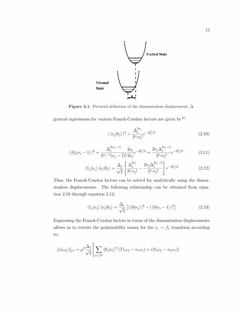
13
Figure 2.1. Pictorial definition of the dimensionless displacement, ∆.
general expressions for various Franck-Condon factors are given by47:
| 〈νj|0j〉 |2 =∆
2νjj
2νjνj!e−∆2
j/2 (2.10)
| 〈0j|νj − 1〉 |2 =∆
2(νj−1)j
2νj−1(νj − 1)!
2νj2νj
e−∆2j/2 =
2νj∆2νj−2j
2νjνj!e−∆2
j/2 (2.11)
〈1j|νj〉 〈νj|0j〉 =∆j√
2
[∆
2νjj
2νjνj!− 2νj∆
2νj−2j
2νjνj!
]e−∆2
j/2 (2.12)
Thus, the Franck-Condon factors can be solved for analytically using the dimen-
sionless displacements. The following relationship can be obtained from equa-
tion 2.10 through equation 2.12:
〈1j|νj〉 〈νj|0j〉 =∆j√
2
[| 〈0|νj〉 |2 − | 〈0|νj − 1〉 |2] (2.13)
Expressing the Franck-Condon factors in terms of the dimensionless displacements
allows us to rewrite the polarizability tensor for the i1 → f1 transition according
to:
[α(ωL)]f,i = µ2 ∆1√2
[ ∑ν1≥0
〈01|ν1〉2 (T (ωL − ν1ω1) + iS(ωL − ν1ω1))

14
−∑ν1≥0
〈01|ν1〉2 (T (ωL − (ν1 + 1)ω1) + iS(ωL − (ν1 + 1)ω1))
](2.14)
The polarizability tensor and absorption cross-section can be given as:
[α(ωL)] ∝ µ2 ∆1√2
[Φ(ωL)− Φ(ωL − ω1)] (2.15)
and
σA(ωL) ∝ ωLµ2ImΦ(ωL) (2.16)
where the function Φ(ωL) is given by:
Φ(ωL) =∑ν1
| 〈01|ν1〉 |2(T (ωL − ν1ω1) + iS(ωL − ν1ω1)) (2.17)
Since the square of the polarizability tensor is equivalent to the relative RR inten-
sity, the RR intensity for the transition from the ground electronic state, |i〉, to
the final vibrational level of the ground electronic state, |f〉, for normal mode j is
given by:
Ij(ωL) = µ4∆2j
2|Φ(ωL)− Φ(ωL − ωj)|2 (2.18)
In the original transform theory, the quantity |Φ(ωL) − Φ(ωL − ωj)|2, given
in equation 2.18, is determined from the experimental absorption spectrum and
its Kramers-Kronig transform. Since the real and imaginary parts of Φ(ωL) form
a Kramers-Kronig transform pair, the imaginary part of Φ(ωL) that is obtained
from the experimental absorption spectrum can be used to solve for the imaginary
part of Φ(ωL) using the Cauchy principle-value integral which relates the real and
imaginary parts of Φ(ωL).
The method we used to calculate the RR intensities is based on the trans-
form theory derived by Peticolas and Rush.48 This method was also adopted more
recently by Neugebauer and Hess49 and also Guthmuller and Champagne.33,34
According to this theoretical approach, the quantity |Φ(ωL) − Φ(ωL − ωj)|2 was
calculated from the sum-over-vibrational states where Φ(ωL) is given by:
Φ(ωL) =∑ν
∏3N−6j | 〈νj|0j〉 |2
ω0 +∑3N−6
j νjωj − ωL − iΓ(2.19)

15
The equation used to solve for Φ(ωL), equation 2.19, is identical to the polariz-
ability tensor given by the vibronic theory, equation 2.1. Thus, from a theoretical
perspective, the transform theory is synonymous with the vibronic theory. All of
the quantities involved in equations 2.18 and 2.19 are determined from quantum
chemical calculations, except for Γ. As already mentioned, Γ is the line width
of the absorption band (equal to half of the full width at half maximum). Thus,
Γ is inversely proportional to the lifetime. Γ is an adjustable parameter, whose
value can be approximated from the experimental absorption spectrum. Finally,
the absorption spectra and RR spectra were calculated using Equations 2.16 and
2.18, respectively.
2.2.2 Short-time Approximation
A simplification of the vibronic theory is the short-time approximation.21,22,40
Within the short-time approximation, the RR intensity for normal mode j is given
by:
Ij =(µ
Γ
)4
ω2j∆
2j (2.20)
where µ is the electronic transition dipole moment, Γ is the adjustable damping
parameter, ωj is the frequency of normal mode j, and ∆j is the dimensionless dis-
placement of normal mode j. Assuming displaced harmonic oscillators, the relative
RR intensities are equal to the square of the excited state gradient, according to:
(∂E
∂qj
)
qj=0
= ωj(qj −∆j)|qj=0 = −ωj∆j (2.21)
where(∂E∂qj
)qj=0
is the partial derivative of the excited state electronic energy with
respect to a ground state normal mode at the ground state equilibrium position.
Note that the RR intensity, calculated using the short-time approximation, is in-
dependent of the frequency of the incident radiation.
2.2.3 Polarizability Gradient Model
The RR spectra calculated using the short-time approximation and the vibronic
theory for uracil are compared to the RR spectra calculated using the polarizabil-

16
ity gradient model developed by Jensen et al.43 Using the polarizability gradient
model, we calculate the RR intensities from the derivative of the real and imag-
inary parts of the frequency-dependent polarizability with respect to the normal
coordinates. Within the polarizability gradient model, the RR scattering factor is
given by:
Ij = 45α′2j + 7γ′2j (2.22)
where α′2p is the derivative of the isotropic polarizability with respect to normal
mode j and γ′2j is the derivative of the anisotropic polarizability with respect to
normal mode j.
2.2.4 RR Differential Cross-Sections
The absolute RR intensities are presented as the differential RR cross-section (units
of cm2/sr). The differential cross-section for Stokes scattering is given by:
dσ
dΩ= Kj
[12Ij45
](2.23)
where Ij is the RR scattering factor obtained from equation 2.18, equation 2.20,
or equation 2.22 in units of A4/amu and Kj is given by:
Kj =π2
ε20(νL − νj)4
(h
8π2cνj
) (1
1− e−hcνjkBT
)(2.24)
where ε0 is the permittivity of vacuum, c is the speed of light in units of m/s, h is
the Planck constant, kB is the Boltzmann constant, T is the temperature (taken
to be 300 K), νL is the frequency of the incident radiation in units of cm−1, and
νj is the frequency of normal mode j in units of cm−1.43,50
2.3 Time-Dependent Approach
Another method for the calculation of RR intensities is the time-dependent ap-
proach21,23,24,51,52 derived by Heller and co-workers. The advantage of the time-
dependent approach is that the need to perform a computationally challenging
sum over the excited vibrational states is eliminated by taking into consideration

17
the time dependence of the RR scattering phenomenon. Starting with the polar-
izability tensor given by equation 2.1, where we have substituted ~ωνi = Eν − Eiand ~ωL = EL, we have:
[α(ωL)]f,i = µ2∑ν
〈f |ν〉 〈ν|i〉(Eν − Ei − EL − iΓ)
(2.25)
First, the sum over states polarizability tensor is converted into a fully equivalent
time-dependent formulation. The denominator in Equation 2.25 is expressed as a
half-Fourier transform to obtain:
[α(ω)]f,i = µ2 i
~
∫ ∞
0
∑ν
〈f |ν〉 〈ν|i〉 e[i(EL+Ei−Eν+Γ)t/~]dt (2.26)
Next since 〈ν|e−iHt/~ = 〈ν|e−iEνt/~, where H is the excited state vibrational Hamil-
tonian, we have:
[α(ωL)]f,i = µ2 i
~
∫ ∞
0
∑ν
〈f |ν〉 ⟨ν|e−iHt/~|i⟩ e[i(EL+Ei+Γ)t/~]dt (2.27)
If we consider the time-propagator e−iHt/~ to operate on |i〉, then e−iHt/~|i〉 = |i(t)〉.The complete expression for the polarizability tensor is then:
[α(ωL)]f,i = µ2 i
~
∫ ∞
0
〈f |i(t)〉 e[i(EL+Ei+Γ)t/~]dt (2.28)
Since the RR intensity is proportional to the square of the polarizability tensor,
we have:
Ii→f ∝ µ4
∣∣∣∣i
~
∫ ∞
0
〈f |i(t)〉 e[i(EL+Ei+Γ)t/~]dt
∣∣∣∣2
(2.29)
Figure 2.2 is a pictorial representation of the time-dependent approach. In this
figure, El is the energy of the incident radiation and Es is the energy of the scattered
photons. The RR intensity depends on the time-dependent overlap 〈f |i(t)〉, where
|i(t)〉 represents the motion of the nuclei upon the transition from the ground to
the excited electronic state. Therefore, the time-dependent overlap describes how
the geometry of the molecule changes from the ground state equilibrium position
to the excited state equilibrium position.
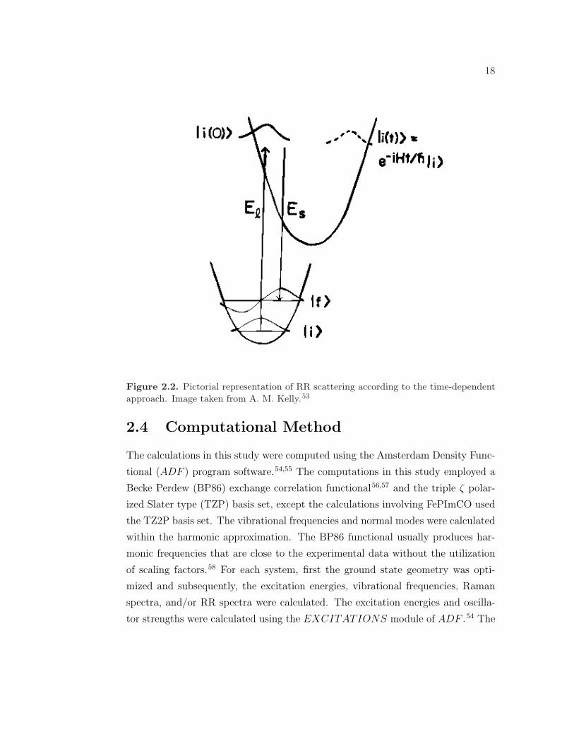
18
Figure 2.2. Pictorial representation of RR scattering according to the time-dependentapproach. Image taken from A. M. Kelly.53
2.4 Computational Method
The calculations in this study were computed using the Amsterdam Density Func-
tional (ADF ) program software.54,55 The computations in this study employed a
Becke Perdew (BP86) exchange correlation functional56,57 and the triple ζ polar-
ized Slater type (TZP) basis set, except the calculations involving FePImCO used
the TZ2P basis set. The vibrational frequencies and normal modes were calculated
within the harmonic approximation. The BP86 functional usually produces har-
monic frequencies that are close to the experimental data without the utilization
of scaling factors.58 For each system, first the ground state geometry was opti-
mized and subsequently, the excitation energies, vibrational frequencies, Raman
spectra, and/or RR spectra were calculated. The excitation energies and oscilla-
tor strengths were calculated using the EXCITATIONS module of ADF .54 The

19
dimensionless displacements that are used to calculate the RR intensities were
computed using the V IBRON module of ADF .54 The Franck-Condon factors
used to calculated Φ(ωL) are obtained using the two-dimensional array method of
Ruhoff and Ratner.59 We implemented a program to calculate the Franck-Condon
factors. Jensen et al. described the procedure used to obtain the RR intensities
calculated using the polarizability gradient model.43 The absolute Raman and RR
intensities are given as differential cross-sections. For all of the molecules studied,
the sum of the Franck-Condon factors was greater than or equal to 0.96.

Chapter 3
Results
3.1 2-bromo-2-methylpropane
The accuracy of the absolute non-resonance Raman intensities was determined us-
ing 2-bromo-2-methylpropane (2B2MP). 2B2MP is a small molecule and there are
both experimental and theoretical Raman differential cross-sections for 2B2MP
available in the literature. In fact, Le Ru et al.36 suggested that 2B2MP be used
as a standard for experimentally determining the absolute Raman intensities. Ta-
ble 3.1 compares the DFT results obtained in this study with reported experimental
values41 and also reported DFT results36 for the Raman differential cross-sections
of 2B2MP in vacuum at 633 nm excitation. The reported DFT results were ob-
Table 3.1. Comparison of DFT results with reported experimental values41 and alsoreported DFT results36 for the Raman active modes of 2B2MP at 633 nm excitation.All values correspond to the gas phase of 2B2MP. a Frequency in units of cm−1; b
Depolarization ratio; c I in units of A4/amu; d Differential Raman cross-section in unitsof 10−32cm2/sr.
DFT DFT36 Exp.41
νa pb Ic dσdΩ
dνa pb Ic dσ
dΩ
d dσdΩ
d
279 0.29 6.37 105 293 0.26 8.97 130 144483 0.18 22.6 167 509 0.18 23.7 159 169780 0.68 12.8 50.0 800 0.63 14.3 53.4 44.0
tained using the Gaussian program package60,61 at the B3LYP62,63/6-311++G(d,p)
level of theory. As a result of the implementation of different theoretical meth-
21
ods and basis sets, slight differences are expected between our DFT results and
the reported DFT results. Overall, we obtain excellent agreement with both the
reported experimental and theoretical results.
3.2 Carbon Disulfide
The accuracy of the absolute RR intensities was determined using CS2 as a test
case. Table 3.2 compares the RR total cross-section of CS2 in vacuum at 186 nm
excitation calculated using the vibronic theory method with a Γ = 0.05 eV with
the experimental42 RR total cross-section of CS2 in cyclohexane upon 208.8 nm
excitation (the experimental excitation wavelength corresponding to the theoret-
ical excitation wavelength used). Table 3.2 presents the RR intensities as total
cross-sections (rather than differential cross-sections). The total cross-section and
Table 3.2. Comparison of DFT results in vacuum at 186 nm excitation with experi-mental values42 in cyclohexane at 208.8 nm excitation for the RR total cross-sectionsof CS2. The total cross-section is for the fundamental frequency at 652 cm−1 and wascalculated using vibronic theory with a Γ = 0.05 eV. a Frequency in units of cm−1; b
RR differential cross-section in units of 10−23cm2/sr; c RR total cross-section in unitsof 10−23cm2.
DFT Experimental42
νa dσdΩ
bσc νa σc
652 0.971 10 653 77
differential cross-section are related through the following equation:
σ =8π
3
(1 + 2ρ
1 + ρ
)(dσ
dΩ
)(3.1)
where σ is the total cross-section and ρ is the depolarization ratio.64 In converting
from the differential cross-section to the total cross-section, the depolarization ratio
was assumed to be 1/3 since only one excited state is considered. The RR total
cross-section calculated using DFT is about a factor of 8 lower than that obtained
experimentally, which is attributed to either solvent effects or exchange correlation
functional and basis set effects. Applying the local field correction to the calculated
total cross-section in order to take into account the solvent (cyclohexane) effects
22
results in an increase of the calculated cross-sections by a factor of approximately
three. While the calculated total cross-sections are closer to the experimental
cross-sections with the local field correction, the calculated cross-sections are still
lower than the experimental cross-sections. Thus, it will be necessary to include
solvent effects in order to obtain the absolute RR intensities.
3.3 Uracil
Uracil is a six-membered pyrimidine found in RNA.65 Uracil is a relatively small
molecule, making it a suitable system on which to perform quantum mechanical
calculations. In addition, there are both experimental65 and theoretical43,48,49 stud-
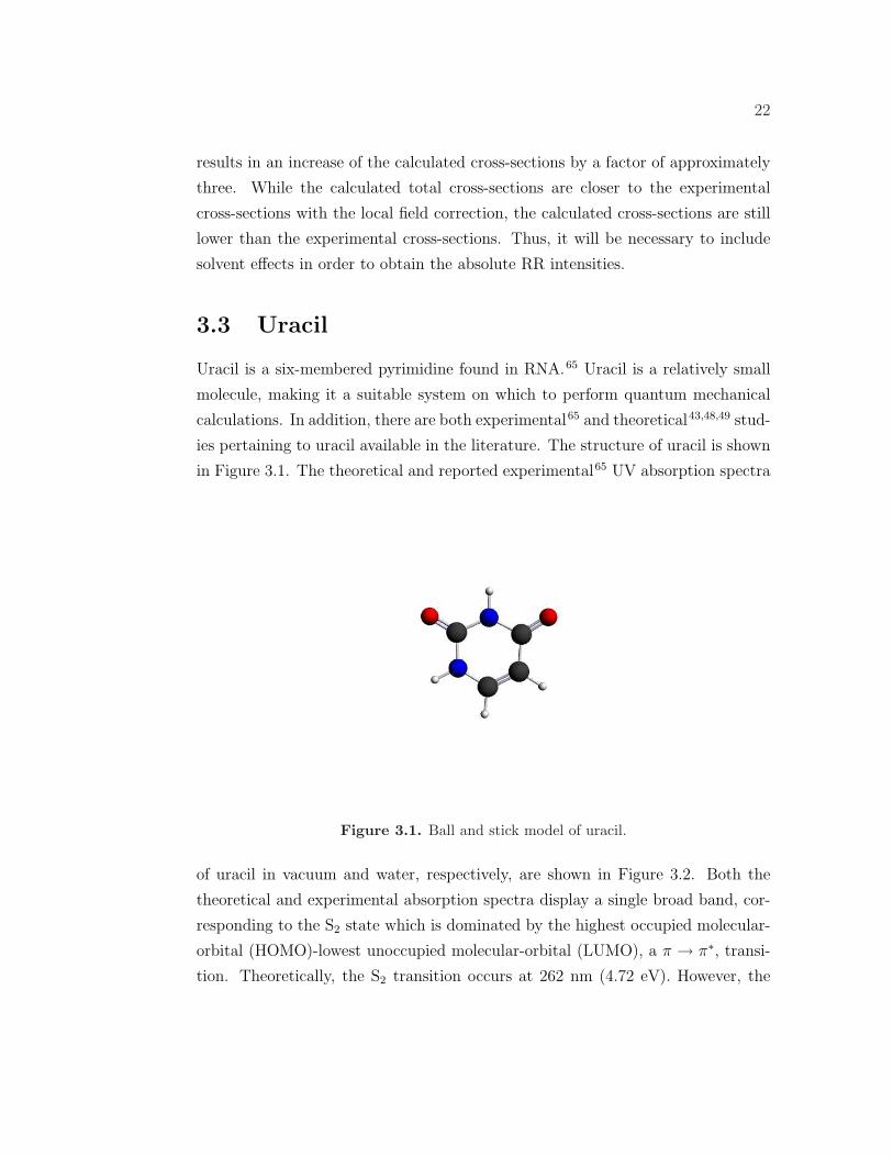
ies pertaining to uracil available in the literature. The structure of uracil is shown
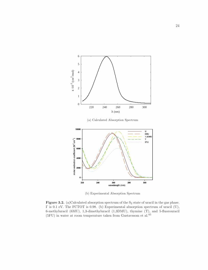
in Figure 3.1. The theoretical and reported experimental65 UV absorption spectra
Figure 3.1. Ball and stick model of uracil.
of uracil in vacuum and water, respectively, are shown in Figure 3.2. Both the
theoretical and experimental absorption spectra display a single broad band, cor-
responding to the S2 state which is dominated by the highest occupied molecular-
orbital (HOMO)-lowest unoccupied molecular-orbital (LUMO), a π → π∗, transi-
tion. Theoretically, the S2 transition occurs at 262 nm (4.72 eV). However, the

23
wavelength of maximum absorption occurs at 243 nm (5.10 eV). This shift is a
result of the inclusion of vibronic coupling in the calculation of the absorption
spectrum. In comparison, the experimental wavelength of maximum absorption is
259 nm (4.79 eV). Differences in the absorption maxima are attributed to solvent
effects. The RR spectra are calculated at 262 nm.
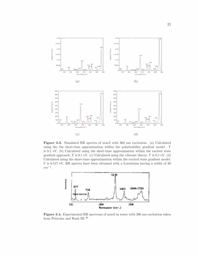
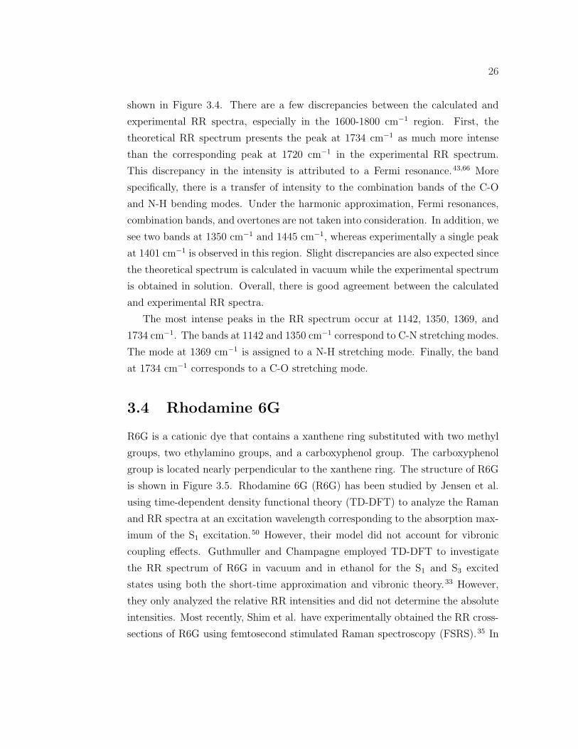
We calculated the RR spectra of uracil using three different methods and the
results are displayed in Figure 3.3. The absolute RR intensities obtained using the
polarizability gradient model, Figure 3.3(a), and the excited state gradient model,
Figure 3.3(b), are comparable, which is expected since both of these methods take
into consideration only a single excited state. The damping factor is 0.1 eV for
both of these spectra.
Additionally, the RR spectrum of uracil was calculated using the vibronic the-
ory with a Γ = 0.1 eV. Uracil is not expected to be affected by vibronic coupling,
as it lacks the presence of vibronic fine structure in the absorption spectrum, in-
dicating that the differential cross-sections obtained using the vibronic theory and
short-time approximation should be similar. Indeed, we find that the spectra cal-
culated using both short-time approximation methods, Figures 3.3(a) and 3.3(b),
and the vibronic theory, Figure 3.3(c), result in the same relative intensities, but
very different absolute intensities. In fact, the vibronic theory method predicts
absolute intensities that are a factor of 600 smaller than those calculated using the
short-time approximation. This is attributed to the sensitivity of the short-time
approximation to the damping parameter. While the absolute RR intensities cal-
culated using the vibronic theory are only slightly impacted by the value of the
damping factor, the short-time approximation is extremely sensitive to the value
of the damping factor, since the intensities scale as 1/Γ4. We find that in order for
the RR spectrum calculated using the vibronic theory to have the same absolute
RR intensities as the RR spectrum calculated using the short-time approximation,
the damping factor must be 0.517 eV for the short-time approximation, as shown
in Figure 3.3(d). This value of Γ is much larger than expected from the absorption
spectra. The value of the damping factor must therefore be selected very care-
fully for the short-time approximation even when the relative RR intensities are
reasonable.
The experimental RR spectrum of uracil in water with 266 nm excitation is
24
0
1
2
3
4
5
6
220 240 260 280 300
ε /1
0-3 (
cm2 /m
ol)
λ (nm)
(a) Calculated Absorption Spectrum
(b) Experimental Absorption Spectrum
Figure 3.2. (a)Calculated absorption spectrum of the S2 state of uracil in the gas phase.Γ is 0.1 eV. The FCTOT is 0.98. (b) Experimental absorption spectrum of uracil (U),6-methyluracil (6MU), 1,3-dimethyluracil (1,3DMU), thymine (T), and 5-fluorouracil(5FU) in water at room temperature taken from Gustavssom et al.65
25
0
500000
1e+06
1.5e+06
2e+06
2.5e+06
3e+06
600 800 1000 1200 1400 1600 1800
dσ/d
Ω (
10-3
2 cm2 /s
r)
wave number (cm-1)
539748
9309641053
1145
1189
13541370
1447
16171699
1740
(a)
0
500000
1e+06
1.5e+06
2e+06
2.5e+06
3e+06
600 800 1000 1200 1400 1600 1800
dσ/
dΩ (
10-3
2 cm2 /s
r)
wave number (cm-1)
538
745
927 9631052
1142
1191
13501369
1445
1613
1695
1734
(b)
0
500
1000
1500
2000
2500
3000
3500
4000
4500
600 800 1000 1200 1400 1600 1800
dσ/
dΩ (
10-3
2 cm2 /s
r)
wave number (cm-1)
538
745
927 9631052
1142
1191
1350
1369
1445
1613
1695
1734
(c)
0
500
1000
1500
2000
2500
3000
3500
4000
4500
600 800 1000 1200 1400 1600 1800
dσ/
dΩ (
10-3
2 cm2 /s
r)
wave number (cm-1)
538745
927 9631052
1142
1191
13501369
1445
1613
1695
1734
(d)
Figure 3.3. Simulated RR spectra of uracil with 262 nm excitation. (a) Calculatedusing the the short-time approximation within the polarizability gradient model. Γis 0.1 eV. (b) Calculated using the short-time approximation within the excited stategradient approach. Γ is 0.1 eV. (c) Calculated using the vibronic theory. Γ is 0.1 eV. (d)Calculated using the short-time approximation within the excited state gradient model.Γ is 0.517 eV. RR spectra have been obtained with a Lorentzian having a width of 20cm−1.
Figure 3.4. Experimental RR spectrum of uracil in water with 266 nm excitation takenfrom Peticolas and Rush III.48
26
shown in Figure 3.4. There are a few discrepancies between the calculated and
experimental RR spectra, especially in the 1600-1800 cm−1 region. First, the
theoretical RR spectrum presents the peak at 1734 cm−1 as much more intense
than the corresponding peak at 1720 cm−1 in the experimental RR spectrum.
This discrepancy in the intensity is attributed to a Fermi resonance.43,66 More
specifically, there is a transfer of intensity to the combination bands of the C-O
and N-H bending modes. Under the harmonic approximation, Fermi resonances,
combination bands, and overtones are not taken into consideration. In addition, we
see two bands at 1350 cm−1 and 1445 cm−1, whereas experimentally a single peak
at 1401 cm−1 is observed in this region. Slight discrepancies are also expected since
the theoretical spectrum is calculated in vacuum while the experimental spectrum
is obtained in solution. Overall, there is good agreement between the calculated
and experimental RR spectra.
The most intense peaks in the RR spectrum occur at 1142, 1350, 1369, and
1734 cm−1. The bands at 1142 and 1350 cm−1 correspond to C-N stretching modes.
The mode at 1369 cm−1 is assigned to a N-H stretching mode. Finally, the band
at 1734 cm−1 corresponds to a C-O stretching mode.
3.4 Rhodamine 6G
R6G is a cationic dye that contains a xanthene ring substituted with two methyl
groups, two ethylamino groups, and a carboxyphenol group. The carboxyphenol
group is located nearly perpendicular to the xanthene ring. The structure of R6G
is shown in Figure 3.5. Rhodamine 6G (R6G) has been studied by Jensen et al.
using time-dependent density functional theory (TD-DFT) to analyze the Raman
and RR spectra at an excitation wavelength corresponding to the absorption max-
imum of the S1 excitation.50 However, their model did not account for vibronic
coupling effects. Guthmuller and Champagne employed TD-DFT to investigate
the RR spectrum of R6G in vacuum and in ethanol for the S1 and S3 excited
states using both the short-time approximation and vibronic theory.33 However,
they only analyzed the relative RR intensities and did not determine the absolute
intensities. Most recently, Shim et al. have experimentally obtained the RR cross-
sections of R6G using femtosecond stimulated Raman spectroscopy (FSRS).35 In

27
Figure 3.5. Ball and stick model of R6G.
addition, R6G is being used as a prototype molecule in single molecule surface en-
hanced resonance Raman spectroscopy (SERRS).67,68 SERRS is a technique that
enhances Raman scattering due to both resonance with the electronic transition
and also interaction with the metal surface by a factor of 1014-1015, which enables
SERRS to be utilized for single molecule detection.50,67,68
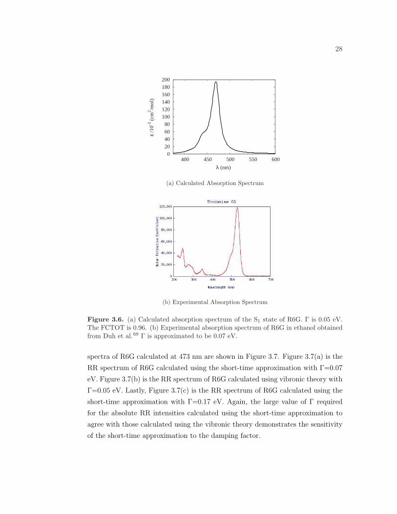
The calculated and experimental69 absorption spectra of R6G in vacuum and
ethanol, respectively, are shown in Figure 3.6. The calculated absorption spectrum
shows a strong band at 473 nm (2.62 eV) corresponding to the S0 → S1 transition.
In excellent agreement with our calculation, Jensen and Schatz calculated the S1
excitation to occur at 474 nm (2.62 eV) using the BP86 functional for R6G in
vacuum.50 The experimental absorption spectrum of R6G in ethanol has a wave-
length of maximum absorption at 530 nm (2.34 eV). The theoretical absorption
spectrum is slightly blue shifted compared to the experimental spectrum, which
can be attributed to solvent effects. Both the calculated and experimental absorp-
tion spectra have a weak shoulder, indicating the importance of vibronic coupling
effects. The RR spectra are calculated at 473 nm in order to obtain the maximum
enhancement.
The Raman bands in an experimental RR spectrum of R6G are concealed by
fluorescence. However, theoretical calculation of the RR spectrum of R6G can
give us insight about the RR spectrum and the absolute RR intensities. The RR
28
0 20 40 60 80
100 120 140 160 180 200
400 450 500 550 600
ε /1
0-3 (
cm2 /m
ol)
λ (nm)
(a) Calculated Absorption Spectrum
(b) Experimental Absorption Spectrum
Figure 3.6. (a) Calculated absorption spectrum of the S1 state of R6G. Γ is 0.05 eV.The FCTOT is 0.96. (b) Experimental absorption spectrum of R6G in ethanol obtainedfrom Duh et al.69 Γ is approximated to be 0.07 eV.
spectra of R6G calculated at 473 nm are shown in Figure 3.7. Figure 3.7(a) is the
RR spectrum of R6G calculated using the short-time approximation with Γ=0.07
eV. Figure 3.7(b) is the RR spectrum of R6G calculated using vibronic theory with
Γ=0.05 eV. Lastly, Figure 3.7(c) is the RR spectrum of R6G calculated using the
short-time approximation with Γ=0.17 eV. Again, the large value of Γ required
for the absolute RR intensities calculated using the short-time approximation to
agree with those calculated using the vibronic theory demonstrates the sensitivity
of the short-time approximation to the damping factor.

29
0
5e+06
1e+07
1.5e+07
2e+07
2.5e+07
600 800 1000 1200 1400 1600 1800
dσ/
dΩ (
10-3
2 cm2 /s
r)
wave number (cm-1)
608
692760 913
10281070
11121182
1241
12801343
1404
1469
1494
1546
1638
(a) Short-time Approximation, Γ = 0.07 eV
0
100000
200000
300000
400000
500000
600000
700000
800000
600 800 1000 1200 1400 1600 1800
dσ/
dΩ (
10-3
2 cm2 /s
r)
wave number (cm-1)
608
692
760
913
1028
1070
11121182
12411280
1343
1404
14691494
1546
1638
(b) Vibronic Theory Approach, Γ = 0.05eV
0
100000
200000
300000
400000
500000
600000
700000
800000
600 800 1000 1200 1400 1600 1800
dσ/
dΩ (
10-3
2 cm2 /s
r)
wave number (cm-1)
608
692
760913
1028
1070
11121182
12411280
1343
1404
14691494
1546
1638
(c) Short-time Approximation, Γ = 0.17 eV
Figure 3.7. Simulated RR spectrum of rhodamine 6G with 473 nm excitation. (a) Cal-culated using the short-time approximation. Γ is 0.07 eV. (b) Calculated using vibronictheory. Γ is 0.05 eV. (c) Calculated using the short-time approximation. Γ is 0.17 eV.RR spectra have been broadened with a Lorentzian having a width of 20 cm−1.
Figure 3.8. Experimental RR spectrum of R6G in methanol with 532 nm excitationfrom Shim et al.35
30
As expected, the relative intensities of the RR peaks calculated using the short-
time approximation and the vibronic theory are not in agreement due to vibronic
coupling effects. The low-frequency modes at 608 and 760 cm−1 gain intensity com-
pared to the strong peak at 1638 cm−1 upon incorporation of vibronic coupling
effects. This result agrees with both Guthmuller and Champagne34 and the ex-
perimental spectrum. Guthmuller and Champagne found that the vibronic theory
was needed to accurately reproduce the RR spectrum of R6G in resonance with
the S1 excitation. Guthmuller and Champange obtained better agreement with
the experimental spectrum because they incorporated solvent and utilized a hy-
brid functional. The experimental spectrum is shown in Figure 3.8.35,70 Figure 3.8
only displays the relative RR intensities of R6G in methanol with 532 nm exci-
tation. Calculation of the RR spectra of R6G with both the vibronic theory and
the short-time approximation highlights the importance of incorporating vibronic
coupling effects into the calculation of the RR spectrum.
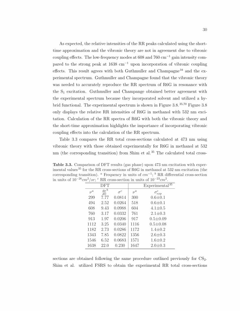
Table 3.3 compares the RR total cross-sections calculated at 473 nm using
vibronic theory with those obtained experimentally for R6G in methanol at 532
nm (the corresponding transition) from Shim et al.35 The calculated total cross-
Table 3.3. Comparison of DFT results (gas phase) upon 473 nm excitation with exper-imental values35 for the RR cross-sections of R6G in methanol at 532 nm excitation (thecorresponding transition). a Frequency in units of cm−1; b RR differential cross-sectionin units of 10−26cm2/sr; c RR cross-section in units of 10−23cm2.
DFT Experimental35
νa dσdΩ
bσc νa σcexp
299 7.77 0.0814 300 0.6±0.1494 2.52 0.0264 518 0.6±0.1608 9.43 0.0988 604 4.1±0.5760 3.17 0.0332 761 2.1±0.3913 1.97 0.0206 917 0.5±0.091112 3.25 0.0340 1116 0.5±0.081182 2.73 0.0286 1172 1.4±0.21343 7.85 0.0822 1356 2.6±0.31546 6.52 0.0683 1571 1.6±0.21638 22.0 0.230 1647 2.0±0.3
sections are obtained following the same procedure outlined previously for CS2.
Shim et al. utilized FSRS to obtain the experimental RR total cross-sections

31
measured using methanol as an internal reference. The calculated total cross-
sections are lower than the experimental values by a factor ranging from 10 to 60.
Again, this can be attributed to solvent effects or choice of exchange correlation
functional and basis set. In addition, since the RR intensities scale as µ4, even
minor underestimations of the transition dipole moments will have a major effect
on the total cross-sections.
3.5 Iron(II) Porphyrin with Imidazole and CO
Ligands
Iron(II) porphyrin with imidazole and CO ligands (FePImCO) is an ideal model
system for larger biologically relevant molecules containing a heme group, such as
myoglobin, hemoglobin, or cytochrome c because it mimics the active sites of these
heme proteins complexed with carbon monoxide. The structure of FePImCO is
shown in Figure 3.9. The structure of metalloporphyrins consists of four pyrrole
Figure 3.9. Ball and stick model of FePImCO.
groups connected by methine bridges. Each pyrrole group is bonded to the central
metal atom through the nitrogen atom.3 The iron atom sits in the plane of the
porphyrin ring and the Fe-C-O bond angle is 180 degrees, which has been reported
previously.71,72 The C-O bond distance is 1.16 A, the Fe-CO bond distance is 1.76
A, the Fe-NIm bond distance is 2.07 A, and the Fe-NP bond distance is 2.00 A.

32
These bond distances are in good agreement with experimental bond distances
for Fe(TPP)(CO)(Py) (TPP = tetraphenylporphyrin dianion and Py = pyridine)
of 1.12 A, 1.77 A, 2.10 A, and 2.02 A, respectively73 and also with theoretically
calculated bond distances for FePImCO of 1.165 A, 1.733 A, 1.966 A, and 1.983
A, respectively.74
Metalloporphyrins experience strong absorption in the visible region of the
electromagnetic spectrum and are colored complexes due to the highly conjugated
tetrapyrrole unit.3 A weak Q and a strong B (Soret) absorption band are char-
acteristic of metalloporphyrins and can be explained by Gouterman’s four-orbital
model. Gouterman’s four-orbital model describes the Q and B bands as transitions
between the close-lying HOMO orbitals, a1u and a2u, and the doubly degenerate
LUMO orbitals, eg. The interaction of the nearly degenerate a11ue
1g and a1
2ue1g con-
figurations leads to a high-lying state and also a low-lying state. The B band
corresponds to the high-lying state, in which the transition dipoles of the two con-
figurations add together. In contrast, the Q band corresponds to the low-lying
state, in which the transition dipoles of the two configurations almost cancel. The
B band typically occurs around 380-400 nm and the Q band typically occurs be-
tween 500-600 nm.3,12
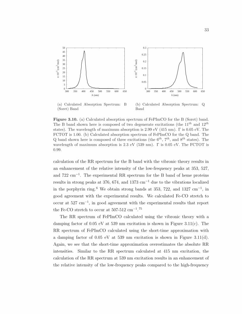
Figure 3.10(a) shows the calculated absorption spectrum of the B band with a Γ
= 0.05 eV. The B band is composed of two degenerate excitations, the S11 and S12
states. The wavelength of maximum absorption is 415 nm (2.99 eV). Therefore, the
RR spectrum is calculated at 415 nm in order to obtain maximum enhancement.
Figure 3.10(b) shows the calculated absorption spectrum of the Q band with a Γ
= 0.05 eV. The Q band is composed of three close-lying excitations, the S6, S7,
and S8 states. The wavelength of maximum absorption is 539 nm (2.3 eV). The
RR spectrum is therefore calculated at 539 nm. Both the B and Q bands display
a shoulder to the blue of the wavelength of maximum absorption, indicating that
vibronic coupling will have effects on the RR spectrum.
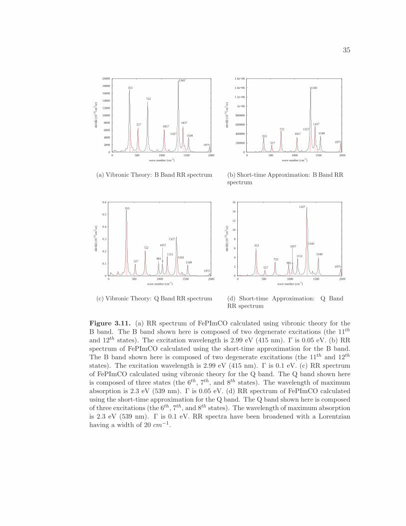
The RR spectrum of FePImCO calculated using the vibronic theory with a
damping factor of 0.05 eV at 415 nm excitation is shown in Figure 3.11(a). The
RR spectrum of FePImCO calculated using the short-time approximation with
a damping factor of 0.05 eV at 415 nm excitation is shown in Figure 3.11(b).
The short-time approximation overestimates the absolute RR intensities. The
33
0
5
10
15
20
25
30
35
40
45
50
300 350 400 450 500 550 600 650
ε /1
0-3 (
cm2 /m
ol)
λ (nm)
(a) Calculated Absorption Spectrum: B(Soret) Band
0
0.05
0.1
0.15
0.2
0.25
0.3
300 350 400 450 500 550 600 650
ε /1
0-3 (
cm2 /m
ol)
λ (nm)
(b) Calculated Absorption Spectrum: QBand
Figure 3.10. (a) Calculated absorption spectrum of FePImCO for the B (Soret) band.The B band shown here is composed of two degenerate excitations (the 11th and 12th
states). The wavelength of maximum absorption is 2.99 eV (415 nm). Γ is 0.05 eV. TheFCTOT is 1.00. (b) Calculated absorption spectrum of FePImCO for the Q band. TheQ band shown here is composed of three excitations (the 6th, 7th, and 8th states). Thewavelength of maximum absorption is 2.3 eV (539 nm). Γ is 0.05 eV. The FCTOT is0.99.
calculation of the RR spectrum for the B band with the vibronic theory results in
an enhancement of the relative intensity of the low-frequency peaks at 353, 527,
and 722 cm−1. The experimental RR spectrum for the B band of heme proteins
results in strong peaks at 376, 674, and 1373 cm−1 due to the vibrations localized
in the porphyrin ring.6 We obtain strong bands at 353, 722, and 1327 cm−1, in
good agreement with the experimental results. We calculated Fe-CO stretch to
occur at 527 cm−1, in good agreement with the experimental results that report
the Fe-CO stretch to occur at 507-512 cm−1.75
The RR spectrum of FePImCO calculated using the vibronic theory with a
damping factor of 0.05 eV at 539 nm excitation is shown in Figure 3.11(c). The
RR spectrum of FePImCO calculated using the short-time approximation with
a damping factor of 0.05 eV at 539 nm excitation is shown in Figure 3.11(d).
Again, we see that the short-time approximation overestimates the absolute RR
intensities. Similar to the RR spectrum calculated at 415 nm excitation, the
calculation of the RR spectrum at 539 nm excitation results in an enhancement of
the relative intensity of the low-frequency peaks compared to the high-frequency
34
peaks with the vibronic theory compared to the short-time approximation. The RR
peak at 353 cm−1 displays the most drastic enhancement in relative intensity. In
fact, the peak at 353 cm−1 becomes even more intense than the band at 1327 cm−1,
which was the most intense peak in the RR spectrum calculated using the short-
time approximation. The RR spectra of FePImCO demonstrate the importance
of including vibronic coupling effects in the calculation of the RR spectrum and
also highlight the shortcomings of the short-time approximation for calculating
absolute RR intensities.
35
0
2000
4000
6000
8000
10000
12000
14000
16000
18000
20000
0 500 1000 1500 2000
dσ/
dΩ (
10-3
2 cm2 /s
r)
wave number (cm-1)
353
527
722
1057
1327
1343
1437
1549
1975
(a) Vibronic Theory: B Band RR spectrum
0
200000
400000
600000
800000
1e+06
1.2e+06
1.4e+06
1.6e+06
0 500 1000 1500 2000
dσ/
dΩ (
10-3
2 cm2 /s
r)
wave number (cm-1)
353
527
722
1057
1327
1343
1437
1549
1975
(b) Short-time Approximation: B Band RRspectrum
0
0.1
0.2
0.3
0.4
0.5
0.6
0 500 1000 1500 2000
dσ/
dΩ (
10-3
2 cm2 /s
r)
wave number (cm-1)
353
527
722
981
1057
1151
1327
1343
1549
1975
(c) Vibronic Theory: Q Band RR spectrum
0
2
4
6
8
10
12
14
16
0 500 1000 1500 2000
dσ/
dΩ (
10-3
2 cm2 /s
r)
wave number (cm-1)
353
527
722981
1057
1151
1327
1343
1549
1975
(d) Short-time Approximation: Q BandRR spectrum
Figure 3.11. (a) RR spectrum of FePImCO calculated using vibronic theory for theB band. The B band shown here is composed of two degenerate excitations (the 11th
and 12th states). The excitation wavelength is 2.99 eV (415 nm). Γ is 0.05 eV. (b) RRspectrum of FePImCO calculated using the short-time approximation for the B band.The B band shown here is composed of two degenerate excitations (the 11th and 12th
states). The excitation wavelength is 2.99 eV (415 nm). Γ is 0.1 eV. (c) RR spectrumof FePImCO calculated using vibronic theory for the Q band. The Q band shown hereis composed of three states (the 6th, 7th, and 8th states). The wavelength of maximumabsorption is 2.3 eV (539 nm). Γ is 0.05 eV. (d) RR spectrum of FePImCO calculatedusing the short-time approximation for the Q band. The Q band shown here is composedof three excitations (the 6th, 7th, and 8th states). The wavelength of maximum absorptionis 2.3 eV (539 nm). Γ is 0.1 eV. RR spectra have been broadened with a Lorentzianhaving a width of 20 cm−1.

Chapter 4
Conclusions and Future
Directions
This study has been interested in the calculation of absolute RR intensities using
DFT. The non-resonance Raman differential cross-sections for 2B2MP calculated
using DFT are in excellent agreement with experimental Raman differential cross-
sections. The RR total cross-sections calculated for CS2 and R6G are lower than
those obtained experimentally, indicating that DFT underestimates the absolute
RR intensities, which is most likely a result of the neglect of solvent effects. How-
ever, it is also possible that the choice of exchange correlation functional and basis
set resulted in underestimations of the absolute RR intensites. The absolute RR
intensities depend on the fourth power of the electronic transition dipole moment,
so even small underestimations of the electronic transition dipole moment signifi-
cantly affects the caclulated absolute RR intensites.
In particular, the two models used to predict the absolute RR intensities were
the short-time approximation and the vibronic theory. The short-time approxima-
tion was found to severely overestimate the absolute RR intensities in the cases
of uracil, R6G, and FePImCO. The intensities calculated using the short-time ap-
proximation are very sensitive to the damping factor, whereas, the vibronic theory
is less dependent on the damping factor. This makes the vibronic theory more
dependable than the short-time approximation.
The vibronic theory has been shown to be necessary for the calculation of the
RR spectra of systems affected by vibronic coupling. For the systems analyzed
37
in this study that are affected by vibronic coupling (i.e. R6G and FePImCO),
inclusion of vibronic coupling enhances the relative intensity of the low-frequency
modes compared to the high-frequency modes. These enhancements were not
detected using the short-time approximation.
Future calculations of the RR spectra could implement the time-dependent
approach. This makes sense from a computational perspective because it will result
in more efficient calculations of the RR spectra. The vibronic theory method, which
involves the sum-over-states computation becomes tedious for large systems that
involve many vibrational states.
An additional future direction would be to include solvent in the calculations
of the RR spectra, since it is likely that solvent impacts the absolute RR cross-
sections. Furthermore, the systems we are interested in investigating model bio-
logically relevant molecules, which usually exist in an aqueous environment. The
solvent could be modeled using either explicit water molecules or a solvent contin-
uum model.
Bibliography
[1] Gremlich, H.-U.; Yan, B., Eds.; Infrared and Raman Spectroscopy of Biolog-ical Materials; Marcel Dekker: New York, 2001.
[2] Siebert, F.; Hildebrandt, P. Vibrational Spectroscopy in Life Science; Wiley-VCH: Weinheim, 2008.
[3] Kalyanasundaram, K. Photochemistry of Polypryridine and Porphyrin Com-plexes; volume 28 Academic Press Inc.: San Diego, CA, 1992.
[4] Nelson, D. L.; Cox, M. M. Lehninger Principles of Biochemistry; W.H. Free-man: New York, 2004.
[5] Lutz, M. Biospectroscopy 1995, 1, 313-327.
[6] Hu, S.; Smith, K.; Spiro, T. J. Am. Chem. Soc. 1996, 118, 12638-12646.
[7] Spiro, T. G. Resonance Raman Spectroscopy 1974, 7, 339-344.
[8] Spiro, T. G.; Kozlowski, P. M.; Zgierski, M. Z. J. Raman Spec. 1998, 29,869-879.
[9] Spiro, T. G.; Kozlowski, P. M. J. Am. Chem. Soc. 1998, 120, 4524-4525.
[10] Andrade, A.; Misoguti, L.; Neto, N. B.; Zilio, S.; Mendonca, C. XXVIENFMC-Annals of Optics 2003, 96,.
[11] Schelvis, Johannes, P.; Deinum, G.; Varotsis, C. A.; Ferguson-Miller, S.;Babcock, G. T. J. Am. Chem. Soc. 1997, 119, 8409-8416.
[12] Baerends, E.; Ricciardi, G.; Rosa, A.; van Gisbergen, S. Coordination Chem-istry Reviews 2002, 230, 5-27.
[13] Wagner, Richard, W.; Lindsey, J. S.; Seth, J.; Palaniappan, V.; Bocian, D. F.J. Am. Chem. Soc. 1996, 118, 3996-3997.
[14] Rochford, J.; Chu, D.; Hagfeldt, A.; Galoppini, E. J. Am. Chem. Soc. 2007,129, 4655-4665.
39
[15] Rochford, J.; Galoppini, E. Langmuir 2008, 24, 5366-5374.
[16] Lewis, I. R.; Edwards, H. G. Handbook of Raman Spectroscopy; MarcelDekker, Inc.: New York, NY, 2001.
[17] Long, D. A. The Raman Effect; John Wiley & Sons, Inc.: New York, 2002.
[18] Albrecht, A. J. Chem. Phys. 1961, 34, 1476-1484.
[19] Tang, J.; Albrecht, A. J. Chem. Phys. 1968, 49, 1144-1154.
[20] Albrecht, A.; Hutley, M. J. Chem. Phys. 1971, 55, 4438-4443.
[21] Heller, E.; Sundberg, R.; Tannor, D. J. Phys. Chem. 982, 86, 1822-1833.
[22] Myers, A. B. Chem. Rev. 1996, 96, 911-926.
[23] Lee, S.; Heller, E. J. Chem. Phys. 1979, 71, 4777-4788.
[24] Heller, E. Acc. Chem. Res. 1981, 14, 368-375.
[25] Spiro, T. G. J. Am. Chem. Soc. 1974, 7, 339-344.
[26] Fodor, S. P.; Rava, R. P.; Hays, T. R.; Spiro, T. G. J. Am. Chem. Soc.1989, 107, 1520-1529.
[27] Song, S.; Asher, S. A. J. Am. Chem. Soc. 1974, 111, 4295-4305.
[28] Arnaud, C. H. Chemical & Engineering News 2009, 87, 10-14.
[29] Jorio, A.; Fantini, C.; Dantas, M.; Pimenta, M.; Filho, A. S.; Sam-sonidze, G.; Brar, V.; Dresselhaus, G.; Dresselhaus, M.; A.K., S.; Unlu, M.;Goldberg, B.; Saito, R. Phys. Rev. B 2002, 66, 115411.
[30] Jorio, A.; Santos, A.; Ribeiro, H.; Fantini, C.; Souza, M.; Vieira, J.;Furtado, C.; Jiang, J.; Saito, R.; Balzano, L.; Resasco, D.; Pimenta, M.Phys. Rev. B 2005, 72, 075207.
[31] Dresselhaus, M.; Eklund, P. Advances in Physics 2000, 49, 705-814.
[32] Brown, C. W.; Ferraro, J. R.; Nakamoto, K. Introductory Raman Spec-troscopy; Academic Press Inc.: USA, 2003.
[33] Guthmuller, J.; Champagne, B. J. Phys. Chem. A 2008, 112, 3215-3223.
[34] Guthmuller, J.; Champagne, B. J. Chem. Phys. 2007, 127, 164507.
[35] Shim, S.; Stuart, Christina, M.; Mathies, R. A. Comput. Phys. Commun.2008, 9, 697-699.
40
[36] Le Ru, E. C.; Blackie, E.; Meyer, M.; Etchegoin, P. J. Phys. Chem. C 2007,111, 13794-13803.
[37] Negri, F.; di Donato, E.; Tommasini, M.; Castiglioni, C.; Zerbi, G.;Mullen, K. J. Chem. Phys. 2004, 120, 11889-11900.
[38] Warshel, A.; Dauber, P. J. Chem. Phys. 1977, 66, 5477-5488.
[39] Johnson, B.; Peticolas, W. Ann. Rev. Phys. Chem. 1976, 27, 465-521.
[40] Neugebauer, J.; Baerends, E.; Efremov, E.; Ariese, F.; Gooijer, C. J. Phys.Chem. A 2005, 109, 2100-2106.
[41] Schrotter, H.; Kloeckner, H. Raman scattering cross sections in gases andliquids. In Raman Spectroscopy of Gases and Liquids, Vol. 11; Weber, A.,Ed.; Springer-Verlag Berlin: Heidelberg, Germany, 1979.
[42] Myers, A. B.; Li, B.; Ci, X. J. Chem. Phys. 1988, 89, 161876.
[43] Jensen, L.; Zhao, L. L.; Autschbach, J.; Schatz, G. C. J. Chem. Phys. 2005,123, 174110.
[44] Kramers, H.; Heisenberg, W. Z. Phys. 1925, 31, 681-708.
[45] Dirac, P. Proc. R. Soc. (London) 1927, 114, 710-728.
[46] Hizhnyakov, V.; Tehver, I. Phys. Status Solidi 1967, 21, 755-768.
[47] Blazej, D. C.; Peticolas, W. L. J. Chem. Phys. 1980, 72, 3134-3142.
[48] Peticolas, W. L.; Rush III, T. J. Comp. Chem. 1995, 16, 1261-1271.
[49] Neugebauer, J.; Hess, B. A. J. Chem. Phys. 2004, 120, 11564.
[50] Jensen, L.; Schatz, G. C. J. Phys. Chem. A 2006, 110, 5973-5977.
[51] Lilichenk, M.; Tittelbach-Helmrich, D.; Verhoeven, J. W.; Gould, I. R.;Myers, A. B. J. Chem. Phys. 1998, 109, 10958.
[52] Biswas, N.; Umpathy, S. J. Chem. Phys. 2003, 118, 5526-5537.
[53] Kelly, A. M. J. Phys. Chem. A 1999, 103, 6891-6903.
[54] Baerends, E.; Autschbach, J.; Berces, A.; Bo, C.; Boerrigter, P.; Cavallo, L.;Chong, D.; Deng, L.; Dickson, R.; Ellis, D. E. e. a. “Amsterdam densityfunctional”, http://www.scm.com, 2008.
[55] te Velde, G.; Bickelhaupt, F.; Baerends, E.; Guerra, C. F.; van Gisbergen, S.;Snijders, J.; Ziegler, T. J. Comp. Chem. 2001, 22, 931-967.

41
[56] Becke, A. Phys. Rev. A 1988, 38, 3098-3100.
[57] Perdew, J. Phys. Rev. B 1986, 33, 8822-8824.
[58] Neugebauer, J.; Hess, B. A. J. Chem. Phys. 2003, 118, 7215-7225.
[59] Ruhoff, P. T.; Ratner, M. A. Int. J. Quant. Chem. 2000, 77, 383-392.
[60] Frisch, M. et al. “Gaussian 03”, http://www.gaussian.com/, 2003 Gaussian,Inc., Wallingford CT 2003.
[61] Frisch, M. et al. “Gaussian; Technical Report”, 2003.
[62] Becke, A. J. Chem. Phys. 1993, 98, 5648-5652.
[63] Lee, C.; Yang, W.; Parr, R. Phys. Rev. B 1988, 37, 785-789.
[64] Li, B.; Myers, A. B. J. Phys. Chem. 1990, 94, 4051-4054.
[65] Gustavssom, T.; Bnysz, k.; Lazzarotto, E.; Markovitsi, D.; Scalmani, G.;Frisch, M. J.; Barone, V.; Improta, R. J. Am. Chem. Soc. 2006, 128, 607-619.
[66] Szczesniak, M.; Nowak, M.; Rostkowska, H.; Szxzepaniak, K.; Person, W.;Shugar, D. J. Am. Chem. Soc. 1983, 105, 5969-5976.
[67] Hildebrandt, P.; Stockburger, M. J. Phys. Chem. 1984, 88, 5935-5944.
[68] Michaels, A.; Nirmal, M.; Brus, L. J. Am. Chem. Soc. 1999, 121, 9932-9939.
[69] Du, H.; Fuh, R.; Li, J.; Corkan, A.; Lindsey, J. Photochemistry and Pho-tobiology 1998, 68, 141-142.
[70] Guthmuller, J.; Champagne, B. Comput. Phys. Commun. 2008, 9, 1667-1669.
[71] Rovira, C.; Kunc, K.; Hutter, J.; Pietro, B.; Parrinello, M. J. QuantumChemistry 1997, 69, 31-35.
[72] Ohta, T.; Pal, B.; Kitagawa, T. J. Phys. Chem. B 2005, 109, 21110-21117.
[73] Peng, S.-M.; Ibers, J. A. J. Am. Chem. Soc. 1976, 98, 8032-8036.
[74] Ghosh, A.; Bocian, D. F. J. Chem. Phys. 1996, 100, 6363-6367.
[75] Tsubaki, M.; Srivastava, R.; Yu, N. Biochemistry 1982, 21, 1132-1140.