the great depression in belgium: an open-economy analysis · the great depression in belgium: an...

The Great Depression in Belgium:an Open-Economy Analysis

L. Pensieroso

Discussion Paper 2010-23

The Great Depression in Belgium: an

Open-Economy Analysis∗

Luca Pensieroso†

May 31, 2010

Abstract

This paper studies the Great Depression in Belgium within theopen-economy dynamic general equilibrium approach. Results fromthe simulations show that a two-good model with total factor produc-tivity shocks and nominal exchange rate shocks can account for mostof the 1929-1934 output drop. The data mimicking ability of the modelis good along other dimensions as well, most notably hours worked,the consumption price index and the terms of trade. The model isalso able to catch some of the dynamics of imports and exports.

Keywords: Great Depression, Belgium, Dynamic Stochas-

tic General Equilibrium, Open Economy

JEL Classification: N14 F41 E13

∗I am indebted with Raf Wouters for his precious guidance on this work. I wouldlike to thank Philippe Jeanfils, Giulio Nicoletti, Olivier Pierrard, Celine Poilly and HenriSneessens for useful suggestions on an earlier version. This paper was presented at the23rd meeting of the European Economic Association in Milan. I would like to thank par-ticipants at the meeting as well as Anna Batyra and David de la Croix for interestingcomments. Michel Juillard helped me with the Dynare codes. The usual disclaimers ap-ply. Financial support from the National Bank of Belgium (Junior Trainee Program 2007),from the Belgian French-speaking Community (Grant ARC 03/08-302 “New Macroeco-nomic Perspectives on Development”) and from the Belgian Federal Government (GrantPAI P6/07 “Economic Policy and Finance in the Global Equilibrium Analysis and SocialEvaluation”) is gratefully acknowledged.

†Charge de Recherches FRS - FNRS, IRES, Universite catholique de Louvain. E-mail:[email protected]

1

1 Introduction

Recent years have witnessed a revival of interest for the Great Depressionof the 1930s. In a seminal contribution, Cole and Ohanian (1999) have forthe first time applied the dynamic general equilibrium (DGE) analysis to theinterpretation of the US Great Depression. Thereafter, several authors haveentered this promising field, with major contributions by Bordo, Erceg, andEvans (2000), Christiano, Motto, and Rostagno (2004), Cole and Ohanian(2004), Kehoe and Prescott (2002), Weder (2006), among others.1 For allthe questions that such a methodology arises in historical analysis,2 it isdoubtless that the emergence of this new stream of literature has openedinteresting new perspectives on the theme.

A controversial feature of this literature is its main focus on a closed-economy, nation-by-nation analysis. Although the international dimensionof the Great Depression has long been recognised as a fundamental trait ofthe event by historians,3 DGE macroeconomists have instead mostly con-centrated on idiosyncratic shocks for single countries in a closed-economyperspective.4

The aim of this paper is to move this literature one step forward, bytaking in consideration an open-economy scenario for the analysis of theBelgian case.

To encompass the open-economy dimension is likely to be important forBelgium. Openness to international trade in goods and services has tradi-tionally been a distinctive feature of the Belgian economy. Data shows thatduring the 1930s both the ratios imports/output and exports/output werearound 30%, a high value by the standards of the time.5 In 1931, Belgium wasthe fifth world exporter, after the United States, Germany, Great Britain andFrance.6 There is unanimity among historians on the fact that a completeunderstanding of the Belgian Great Depression cannot be achieved withoutconsidering the additional constraints that bound Belgium as a consequenceof its open-economy nature.7

Accordingly, the Belgian case is in principle suitable for analysis withinthe small-open-economy framework in modern macroeconomics. Originally

1See Pensieroso (2007b) for a survey.2See De Vroey and Pensieroso (2006) and Temin (2008).3Kindleberger (1973) Eichengreen and Temin (2000).4Besides the works quoted in the main text, Beaudry and Portier (2002) deal with

France, Cole and Ohanian (2002) with the United Kingdom, Fisher and Hornstein (2002)with Germany, Pensieroso (2007a) with Belgium.

5Data taken from Buyst (1997).6See Vanthemsche (1987).7See Cassiers (1989), Hogg (1986), Mommen (1994).

2

advanced by Mendoza (1991) in a pure real-business-cycle (RBC) set up, thisclass of models was recently extended by Galı and Monacelli (2005) to a NewKeynesian framework, encompassing imperfect competition, price stickinessand monetary policy.

Section 3 considers the effects of unexpected TFP shocks in a model wherethe economy trades only in bonds with the rest of the world and takes theinterest rate as given. Results shows that the pure intertemporal dimensionstressed by Mendoza’s analysis might have played a role in accounting forthe Great Depression in Belgium.

To enrich this initial analysis, the rest of the paper takes up the challengeto adapt the model to the peculiarities of the Belgian industrial structure, asthey have been singled out by the historians.

According to Cassiers (1989), the interwar Belgian economy can be thoughtof as sharply divided into two macro sectors, the domestic and the interna-tional sector. These two sectors were different under many respects, rangingfrom labour unionization to capital intensity, from the average firm dimen-sion to the price setting process. Hence, the argument runs, the two sectorsbehaved differently during the Depression. In particular, they responded dif-ferently to the deflationary pressure of the 1930s. Figure 1 shows evidence fordifferent price indices. While the cost-of-living, the retail and the wholesaleprice indices all decreased appreciably between 1929 and 1934, the wholesaleprice index plummeted more dramatically than the other two. As it is tra-ditionally retained that the wholesale price reflects more the prices of goodsthat are traded internationally, while both the cost-of-living and the retailprices put more weight on domestic goods, this feature suggests that thedeflation of the 1930s hit more the international than the domestic sector.

At the light of this argument, an appropriate way to model Belgium inthe interwar era might be to consider an open economy with two sectors, oneproducing tradeable, the other non tradeable goods. This is the way I shallexplore in Section 4, drawing inspiration from the work by Stockman andTesar (1995).

The rest of the paper is structured as follows. In Section 2, I shall brieflypresent selected data for the interwar Belgium. In Section 3, I shall dis-cuss a first exercise based on the Mendoza’s one-good open-economy RBCframework. Section 4 extends the analysis to a benchmark two-sector, open-economy model. In Section 5, I shall present a simple framework encom-passing nominal exchange rate shocks. Finally, Section 6 summarizes theargument and draws some preliminary conclusions.

3

2 History and data

The traditional story about the Great Depression in Belgium focuses on theexchange rate system.8 After the Depression spread from the United Statesto Europe, Belgium decided to stick to the Gold Standard, together withFrance, the Netherlands, Switzerland, Poland and Czechoslovakia. Such adecision was natural, as Belgium orbited around France, and France fearedthe inflationary pressure that could result from a devaluation. On the otherhand, it was also a problematic decision to take, with respect to what wascontemporaneously happening in the United Kingdom. The United King-dom, a major commercial partner for Belgium, exited the Gold Standard asearly as in 1931. This put the big Belgian firms producing for the Britishmarket in an uneasy position. As they where price takers abroad, their sellingprice in sterling was fixed. However, as the sterling lost value with respectto the Belgian franc, their profitability was suddenly diminished. In facts,many of them faced big losses. To ease the situation of the export sectorand yet keep the Belgian franc anchored to the Gold Standard, the BelgianGovernment implemented a series of deflationary measures. These includedmeasures of public finance like increases in income tax, indirect taxes andtariffs, or reductions in pensions and unemployment benefits. Other mea-sures were more directly targeted to lowering the production costs at home,in particular wages. Wage earners opposed a fierce resistance to wage reduc-tion, even if, eventually, they accepted significant drops in the nominal wage.The unemployment rate jumped up from 1.7% in 1929 to 20.2% in 1932(Goossens (1988)). The situation got worse and worse until the Governmentdecided to abandon the Gold Bloc, and devaluated the Belgian franc by 28%,following the advise by the Louvain School. The devaluation prompted therecovery, with output exceeding its 1929 value already in 1937.

This traditional account finds support from the raw data.Figure 1 shows the exchange rate of the Belgian franc with the British

pound and the French franc. The value of the Belgian franc in terms of theBritish pound increased steadily from 1930 to 1934, to decrease after the1935 devaluation. The value of the Belgian franc with respect to the Frenchfranc was fixed until 1934. It decreased between 1935 and 1936, to increasesoon after the French devaluation.

The deflationary pressure induced by an overvalued franc, and reinforcedby the deflationary policy of the Belgian government is evident from the priceand interest rates data. The early 1930s were a period of strong deflation,with the retail (‘cpi’), cost-of-living and wholesale (‘ppi’) price indices all

8See Baudhuin (1946) and Cassiers (1995).

4

falling dramatically till 1934, and increasing a bit after the 1935 devaluationof the Belgian Franc. As already mentioned above, the dynamics of thewholesale price index is much more accentuated than that of the other two.

Nominal interest rates were decreasing until 1931, then increasing till 1933and then slightly decreasing till 1937. The behaviour of the real interest ratereflects the strong deflationary pressure. The real interest rate was high andpositive in the early 1930s, and negative after the 1935 devaluation of theBelgian franc.

The real side of the economy suffered from a dramatic downturn as well.Figure 2 shows data about output and its components (top-right panel).According to these data, Belgium entered the Great Depression after 1931.In 1934, real output (‘gnp’ in the graph) was 10% below the 1929 level. Thefigure was 40 % for investments (‘i’), 20% for exports (‘x’), 17% for imports(‘m’). Consumption (‘c’) witnessed only a minor decrease.

Employment (‘l’) dropped cumulatively of a good 20%, to witness a slighttendency to recovery from 1934 onwards. Nominal wages decreased by 20%between 1929 and 1935. Such a decrease was not enough to cope with thedecreasing prices. Consequently, real wages increased by about 10% in thesame period. After 1935, both the nominal and the real wage series increasedappreciably.

The fact that output starts decreasing only in 1931, and the increasingpattern of all the real aggregate variables but for consumption after 1935look like a vindication of the traditional view about the monetary originsof the Great Depression in Belgium, although the persistent high level ofunemployment is hard to explain within that framework.

However, if we look at the evidence through the lens of neoclassical theory,i.e. by looking at the data in deviations from trend, a different pictureemerges (top-left panel).9

In effect, according to this theory-based inspection of the evidence, Bel-gium entered the Great Depression soon after 1929, with the major drop inoutput being between 1930 and 1934. After that, output stayed constantlybelow the trend, showing no sign of recovery.

Investments decreased sharply all over the decade, up to being 65% belowtrend in 1939.

The depression did not affect consumption before 1931, when the series

9Data have been detrended using a linear filter, as in Cole and Ohanian (1999). Specif-ically, I have measured the average growth factor of the Belgian economy in the 20thcentury, after excluding World Wars I and II and the Great Depression as well. Then,after assuming 1929 as the base year, I have taken the measured trend out of the data. Ob-viously, neither the labour series nor the prices are detrended. The detrending techniqueis explained more in details in Pensieroso (2007a).

5

start decreasing. Thereafter, consumption followed a decreasing path, beingalmost 20% below trend in 1939.

Real wages (‘w’) were above trend in the early 1930s, but below trendfrom 1933 on.

The current account deficit was increasing at the beginning of the period,as exports fell faster than the decreasing imports.10 Things are different forthe late 1930s, when the faster recovery of exports with respect to importsimplies a decreasing deficit in 1935, and an increasing surplus from 1936 untilthe end of the period. The terms of trade, here defined as the price of exportsover the price of imports, had a swinging pattern, increasing till 1933, thendecreasing till 1936, then increasing again.

3 The one-good model

There are two kind of gain from international trade, the intertemporal and theinfratemporal gain. The intertemporal gain stems from the fact that inter-national trade enlarges the possibility for a country to smooth consumptionover time. The infratemporal gain relates to comparative advantages amongcountries producing different goods.

In order to provide a throughout assessment of the role of internationalfactors in accounting for the Great Depression in Belgium, I shall explore thetwo aspects separately. I shall first study a model with intertemporal gainsfrom trade only. A viable candidate is a standard small-open-economy RBCframework with technology shocks.11 In a second step, I shall delve into theissues related to the infratemporal gains from trade, introducing a two-goodopen-economy framework. Finally, the two aspects will be both taken intoaccount in a more general model.

3.1 The model

The model economy produces one good, Y , using capital K and labour L,according to a Cobb-Douglas production function

yt = estkαt (µtlt)

1−α (1)

It is assumed that the economy can exchange assets with the rest of theworld. These assets pay a constant real interest rate r∗. The small-open-

10Belgium current account was in deficit (between 2% and 4% of GNP) throughout the1929-1935 period and in surplus (between 1% and 2% of GNP) later on.

11The model is similar to Mendoza (1991).

6

economy assumption implies that the domestic economy cannot influencethe value of r∗. No labour migration is allowed.

Let bt be the value of per-capita net foreign assets held by the representa-tive household at the end of period t−1. I define the current account balancein period t, CAt, as the variation of the net claims of a country over the restof the world:

CAt ≡ bt+1 − bt.

The economy is populated by infinitely living representative households,who choose per-capita consumption, c, and leisure, 1− l, so as to maximisetheir utility function, subject to a budget constraint.

max{ct,lt,kt+1,bt+1}∞t=0

Et

∞�

t=0

βt [ln(ct) + φ ln(1− lt)], (2)

under the constraints:

ct + kt+1 + bt+1 ≤ (1− δ)kt + yt + (1 + r∗)bt,

yt = estkαt (µtlt)

1−α,

st = ρst−1 + vt,

µt = γtµ0

0 < ρ < 1,

k0 = given,

b0 = given,

s0 = given.

In the formulation above, lowercase letters stand for per capita.The economy is trend stationary, with γ being the growth factor of the

labour augmenting technological progress, µ. I assumed that the stochasticcomponent of total factor productivity, es, follows an autoregressive processof order one. The residuals from such a process, v, are the technology shockI will feed in the model.

I assume rational expectations. Computing the first order conditionsof this problem, and detrending all the variable, the relevant equations forcharacterising a solution are:

1

ct=

β

γ(1 + r∗)

1

ct+1; (3)

7

1− δ + αest+1

�kt+1

lt+1

�α−1

= 1 + r∗; (4)

γ(kt+1 + bt+1) = (1 + r∗)bt + (1− δ)kt + est kαt l1−α

t − ct; (5)

φ

1− lt=

1

ctest(1− α)

�kt

lt

�α

; (6)

Equation (4) is a no-arbitrage condition between home capital and bonds,whereas Equations (3), (5) and (6) are the open-economy version of thestandard Euler equation, budget constraint and labour supply, respectively.

The steady state of this class of open-economy models turns out to beconsistent with any initial level of net assets (Correia, Neves, and Rebelo(1995), Kim and Kose (2003)). This multiple-equilibria feature introduces astationarity problem in the model: at steady state, a country with higher netassets holdings will be able to afford higher trade deficits, and therefore higherconsumption levels. As a consequence, any shock, even if trend-stationary,will have permanent effects on assets and therefore on consumption. Thisintroduces a random-walk component in the model.

Many ways exist to solve this problem (Schmitt-Grohe and Uribe (2003)).I chose to impose a risk premium on the real interest rate paid or receivedby the domestic economy. The idea is that the lower the net asset holding ofthe country, or, when b is negative, the higher its foreign debt, the higher theinterest rate it has to pay to borrow more will be. So, in the model above,we can substitute r∗ with

rt = r∗ + ψ(e−bt − 1). (7)

This formulation stationarises the model, as the steady state level of b isnow determined by the Euler equation, and turns out to be a function of r∗

and ψ only.

3.2 Calibration and simulation

The model’s structural parameters are calibrated as shown in Table 1. Theunit period is the year. The parameters α, the capital share in the CobbDouglas production function, and δ, the depreciation rate of capital, arefixed accordingly, as in Cole and Ohanian (1999).

The parameter β is calibrated so that the steady-state real interest rate,net of the depreciation rate δ is equal to 5.6%, which is the average measuredvalue for Belgium in the 1929-1938 period.

8

The secular growth factor of the Belgian economy, γ, is obtained by takingthe average growth rate of the Belgian GDP per capita between 1900-1994,excluding World Wars I and II, and the Great Depression as well.

The preference for leisure, φ, is calibrated so that hours worked are 1/3in equilibrium.

The autoregressive coefficient of TFP, ρ, is calibrated by running anAR(1) regression on the log of the measured detrended TFP.

The calibration of the parameter ψ was somewhat problematic. The 0.001value was chosen so that the absolute value of the negative interest ratedifferential between Belgium and the rest of the World does not exceed 10basis points, which is the limit spread suggested by Benigno and Thoenissen(2006).12

The steady-state world interest rate is given at r∗ = γβ − 1. I assume the

economy to be in steady state in 1929. In the model, the steady-state valueof current account is assumed to be 0, as are the initial and steady-statevalues of net foreign assets. I feed in the vector of TFP shocks obtained afterregressing the log of detrended TFP as an AR(1).13

Figure 3 shows the results of this simulation, and compare them with theresult of a simulation run on the closed-economy version of this model, e.g.the same model without bonds, where the interest rate is endogenous.

The model is able to account for about 35% of the peak-to-trough dropin the output data, and for almost 50% of the consumption drop.

The model fully accounts for the behaviour of investments in the 1929-1934 period. After 1934, the investment patterns in the model is far toovolatile to be compared to the data.14

12I considered also two other possible values: 0.465, the value that allows the model tomatch the standard deviation of CA

Y in the data; and 0.000742, the value for a similar modelcalibrated by Schmitt-Grohe and Uribe (2003) on contemporary Canadian data. In thecase of ψ = 0.465, results show that the model overlaps with the closed-economy version.In the case ψ = 0.000742, the model’s reaction to the TFP shock is more pronounced thanin the benchmark calibration. This leads to conclude that the lower the value of ψ, thestronger the autocorrelation in the variable b, and therefore the stronger the propagationmechanism of the model. All in all, the benchmark value chosen in the text is conservative,although in line with the accepted practice in the literature, which is to assign a low valueto this parameter.

13Simulations are run assuming rational expectations, but not perfect foresight of theshock. Agents are surprised by the contemporary shock, and assume future shocks to bezero. Kehoe and Prescott (2008) refers to this assumption as myopic foresight.

14Such a feature is in full accordance with standard results in the literature: small-open-economy RBC models tend to accentuate the investments volatility. The typical small openeconomy RBC model encompasses adjustment costs on capital to obviate this problem.Intuitively, the presence of adjustment costs on capital will kill the excess volatility shownby the model at the end of the decade. At the same time, it is likely to worsen the

9

β 0.975γ 1.03δ 0.1α 0.33φ 1.78ρ 0.99ψ 0.001r∗ γ

β − 1

Table 1: Calibration of parameters

The labour dynamics is not accounted for by the model.As is evident from the comparison with the closed-economy simulation,

the qualitative behaviour of the model economy is on the whole comparable tothat of a standard closed-economy RBC model. We notice, however, a slightimprovement in the quantitative dimension, especially as far as output andconsumption are concerned: generally speaking, the model is more responsiveto the impulse. The labour dynamics is poorly accounted for by both themodels, while the open-economy model fares much better in accounting forthe investment drop, yet at the price of having a too volatile investmentbehaviour after 1934.

The open-economy model also improves slightly on its close-economycounterpart in accounting for the long-duration of the Great Depression inBelgium.

On the minus side, the fact that the model economy is now slightly moreresponsive to the technological shock makes it more at variance with the datathan its closed-economy counterpart when the onset of the Great Depressionis concerned. In facts, both output and consumption accentuate their above-trend path in the early 1930s.

From this exercise, I conclude that the extension of the closed-economyanalysis to a scenario that considers only the intertemporal gains from inter-national trade is a useful refinement of the model.

As the historians put much weight on the trade-related aspects of theGreat Depression in Belgium, next section is devoted to the task of enrichingthis analysis, so as to take into account the infratemporal as well as theintertemporal gains from trade.

predictive capacity of the model for the initial drop.

10

4 The two-good model

In this section, I shall introduce a two-sector structure in the model. The ideais to allow the model economy to have the kind of sectorial unbalances thatare considered important by Cassiers (1989) and Hogg (1986) to understandthe Belgian Great Depression. To this end, I modelled the Belgian economyas an open economy with two sectors, one producing a tradeable good, yT ,the other a non-tradeable one, yN .15 Production functions in both sectorsare Cobb-Douglas with constant return to scale:

yN = esN(kN)

ι(lN)

1−ι; (8)

yT = esT(kT )

ν(lT )

1−ν. (9)

The variable sj stands for total factor productivity in sector j, for j =N, T . Both labour and capital are assumed to be mobile across sectors, butnot internationally. To begin with, and in order to isolate the effects of theinfratemporal gains from trade only, I shall temporarily exclude assets fromthe model. This means that the interest rate is endogenous.

The tradeable good can be exported, x, consumed, cT , or invested inboth the sectors. I labeled iT,j the tradeable good invested in sector j. Thenon-tradeable good can be consumed, cN , or invested in both the sectors,iN,j.

The economy imports consumption and investment goods, cM and iM

respectively.Aggregate consumption, c, is expressed as a Cobb-Douglas index of cN ,

cT and cM :

c = (cN)ac(cT )bc(cM)(1−ac−bc). (10)

Aggregate investment in sector j is expressed as a Cobb-Douglas indexof iN,j, iT,j and iM,j:

ij = (iN,j)ai,j(iT,j)bi,j(iM,j)(1−ai,j−bi,j). (11)

All variables are per capita, and when suitable, detrended. Prices areexpressed in terms of the tradeable good, whose price is therefore taken asthe numeraire (pT = 1). I assumed perfect competition.

The model can be solved adopting a stepwise procedure. First, in eachperiod t, given preferences, endowments and technical conditions, households

15A similar model was proposed by Perri and Quadrini (2002) for the Great Depressionin Italy.

11

determine the optimal allocation between different kind of goods, given thetotal amount of consumption and investment. This problem is static by itsnature.

Second, households have to decide how to allocate wealth intertemporally,thereby determining the consumption and savings plans. This is the dynamicpart of the model.

The two parts together fully determine the intertemporal path of all thevariables involved.

4.1 The static problem

4.1.1 Firms

The firm in sector j chooses capital and labour so as to maximize its profitsin period t,

Πj = pjyj − wjlj − pi,jrjkj, (12)

given the constraints (8) and (9). In the profit equation (12), pi,j is the priceindex for aggregate investment in sector j, and will be defined later on.

The first order conditions for this problem gives the demand schedulesfor labour and capital in sector j:

wN =pN(1− ι)yN

lN; (13)

wT =(1− ν)yT

lT; (14)

rNpi,N =pN ιyN

kN; (15)

rT pi,T =νyT

kT. (16)

4.1.2 Households

Given total consumption ct, households choose to consume non-tradeable,tradeable and imported goods so as to maximize equation (10), subject to

pNcN + cT + pMcM = pcc.

The solution to this problem gives the infratemporal demand for cN , cT

and cM as a function of both their respective price relative to pc and totalconsumption c:

12

cN =accpc

pN; (17)

cT = bccpc; (18)

cM =(1− ac − bc)cpc

pM. (19)

The price index pc is defined as the minimum expenditure Z ≡ pcc suchthat c = 1. This amounts to

pc =(pN)

ac(pM)1−ac−bc

(ac)ac(bc)bc(1− ac − bc)1−ac−bc

. (20)

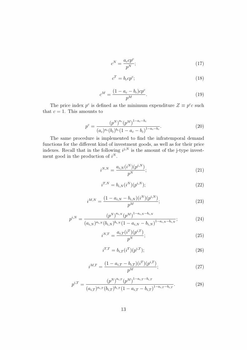
The same procedure is implemented to find the infratemporal demandfunctions for the different kind of investment goods, as well as for their priceindexes. Recall that in the following ij,N is the amount of the j-type invest-ment good in the production of iN .

iN,N =ai,N(iN)(pi,N)

pN; (21)

iT,N = bi,N(iN)(pi,N); (22)

iM,N =(1− ai,N − bi,N)(iN)(pi,N)

pM; (23)

pi,N =(pN)

ai,N (pM)1−ai,N−bi,N

(ai,N)ai,N (bi,N)bi,N (1− ai,N − bi,N)1−ai,N−bi,N; (24)

iN,T =ai,T (iT )(pi,T )

pN; (25)

iT,T = bi,T (iT )(pi,T ); (26)

iM,T =(1− ai,T − bi,T )(iT )(pi,T )

pM; (27)

pi,T =(pN)

ai,T (pM)1−ai,T−bi,T

(ai,T )ai,T (bi,T )bi,T (1− ai,T − bi,T )1−ai,T−bi,T. (28)

13

4.2 The dynamic problem

Households take their saving decisions by solving the following maximizationproblem:

max{ct,lNt ,lTt ,kN

t+1,kTt+1}∞t=0

Et

∞�

t=0

βt [ln(ct) + φ ln(1− lt)], (29)

subject to

γkNt+1 = (1− δ)kN

t + iNt ; (30)

γkTt+1 = (1− δ)kT

t + iTt ; (31)

wNt lNt + wT

t lTt + rNt (pi,N)kN

t + rTt (pi,T )kT

t = (pct)ct + (pi,N

t )iNt + (pi,Tt )iTt ; (32)

lt = lNt + lTt . (33)

Here, I have assumed a log-log utility function in total consumption andleisure.

The solution to problem (29) gives the rules for the intertemporal alloca-tion of consumption, e.g. the Euler equations for kN and kT , and the laboursupply schedules.

γ

ct

pi,Nt

pct

= βEt

�(1 + rN

t+1 − δ)1

ct+1

pi,Nt+1

pct+1

�; (34)

γ

ct

pi,Tt

pct

= βEt

�(1 + rT

t+1 − δ)1

ct+1

pi,Tt+1

pct+1

�; (35)

φ

1− lt=

1

ctpct

wNt ; (36)

φ

1− lt=

1

ctpct

wTt ; (37)

14

4.3 Equilibrium conditions

To close the model, I need to specify the demand for exports and the equi-librium conditions for the trade account.

Concerning the trade account, I assumed

xt = pMt (cM

t + iM,Nt + iM,T

t ), (38)

meaning that the trade account is balanced in any period. This is consistentwith the hypothesis of internationally immobile capital.

The specification of the demand for export is somewhat troublesome, asI have not modelled the behavior of the rest of the World. In the following,I shall assume

xt = am

�1

pMt

�ζ

, (39)

where ζ < 0 is the elasticity of export demand from the rest of the world tothe terms of trade (remember that pT

t = 1, ∀t). The variable am stands forthe “autonomous” components of the export demand.

Finally, I need to add the equilibrium conditions equating the productionsof tradeable and non-tradeable goods to their respective demands.

yNt = cN

t + iN,Nt + iN,T

t , (40)

yTt = cT

t + iT,Nt + iT,T

t + xt. (41)

4.4 Calibration

Table 2 shows the chosen calibration for the structural parameters of themodel.

The values of β, γ and δ are fixed as in Section 3.The values of ν and ι are calibrated so as to reproduce a specific aspect

of the Belgian interwar economy. According to Cassiers (1989), in 1930, theinternational, or “unsheltered” sector employed 56% of the total number ofemployees. I have taken this to mean that in the model, the ratio lT

l shouldbe 0.56 in steady state, and calibrated ν and ι accordingly. They turn outto be 0.49 and 0.66 respectively. 16

16In Stockman and Tesar (1995), who estimate them as an average value for Germany,Italy, USA, Canada and Japan, the values for ν and ι are 0.49 and 0.54, respectively.Results from a simulation run with the values from Stockman and Tesar (1995) show noappreciable difference with respect to those obtained with the calibration advanced in thetext.

15

β 0.975am 0.08γ 1.03δ 0.1ν 0.49ι 0.66ζ -1φ 1.59ρN 0.99ρT 0.99ac 0.61bc 0.29ai,N 0.78bi,N 0.22ai,T 0.37bi,T 0.10λ 0.49

Table 2: Calibration of parameters.

The preference for leisure, φ, is calibrated so that in the steady state totalhours worked are 1/3 of total available time.

The autonomous component of export demand, am, is calibrated so thatpM = 1 in steady state.

The elasticity of export demand to the terms of trade, ζ, is fixed to -1,consistently with the Cobb-Douglas structure of the import demand.

The share parameters ac, bc, ai,N , bi,N , ai,T and bi,T are calibrated usingthe 1965 input-output matrix for Belgium (Institut National de Statistique(1970)). The attribution of sectors to the tradeable or non tradeable categoryfollows Plasmans, Michalak, and Fornero (2006). The parameters ac and bc

are computed as the share of domestic tradeable and non-tradeable goodson total final domestic consumption. The parameters ai,N , bi,N , ai,T and bi,T

are calibrated as follows. Using data for the gross fixed capital formation,I have computed the shares IM,N

IN , IM,T

IT , and IN

IT . Then, I have made the

assumption that ai,N

bi,N= ai,T

bi,T= IN

IT . In other words, I have assumed thatIN,N

IT,N = IN,T

IT,T = IN

IT . Given that the share of imported investments in sector j,IM,j

Ij , is the complement to 1 of ai,j and bi,j, and given the values of IN andIT , for j = (N, T ) I have a system of two equations that can be solved for

16

ai,j and bi,j.17

I shall assume that the sectorial TFPs are subject to zero-mean i.i.dshocks of the AR(1) kind.

sNt = ρNsN

t−1 + vNt , (42)

sTt = ρT sT

t−1 + vTt . (43)

We do not have a clear-cut empirical counterpart for sectorial productivitysN and sT . In their stead, I used the aggregate productivity shock estimatedin Pensieroso (2007a). I assumed the following relationship between sectorialand aggregate TFP:

st = λsNt + (1− λ)sT

t ,

with λ = 0.49 being the weight of the on tradeable sector in the 1965input-output matrix. I also took ρN and ρT from Pensieroso (2007a), assum-ing that the sectorial autoregressive coefficient for TFP is the same as theone estimated there for the whole economy.

4.5 Impulse response functions

Before applying the model to the Great Depression in Belgium, it is usefulto study the impulse response functions (IRF) to the technology shock inthe tradeable sector. This will help our understanding of the working of thismodel and the subsequent ones as well.

Figures 4, 5, 6 and 7 show the IRF of the model to a 1% standard deviationpositive shock to productivity in the tradeable sector vT

t . Only the variablesaffected by the shock are graphed.

The increase in productivity in the tradeable sector has an obvious directeffect on yT (‘yt’ in the graphs). Given the production function (9), this im-plies an increase in labour and capital demand in the tradeable sector (‘lt’,‘kt’). Obviously, as capital is a stock, it is the correspondent flow variable tobear the brunt of adjustment: investment in the tradeable sector (‘it’) must

17The use of modern data to single out the sectorial structure of the economy in the1930s is obviously questionable. In particular, such a practice is likely to overestimate theweight of the non tradeable sector, for the latter includes services, whose value added waspossibly higher in the 1960s than in the 1930s. For comparison, I report here the valueof the share parameters in the work by Perri and Quadrini (2002), who analyse the GreatDepression in Italy: ac = 0.6, bc = 0.2, ai,N = 0.6, bi,N = 0.2, ai,T = 0.3 and bi,T = 2/5.(I thank Fabrizio Perri for providing me their Gauss code, from which I have deducedthose numbers).

17

increase. Given the labour supply (37), wages in the tradeable sector mustincrease to cope with the excess demand of labour. The increase in invest-ment causes the interest rate in the tradeable sector (‘rt’) to increase, so asto equate saving and investment, according to the Euler equation (35). Notethat, accordingly, the pattern of aggregate consumption (‘c’) is increasing intime, before reverting toward the steady state.

The increased efficiency in the tradeable sector causes a decrease in theprice of the tradeable good. As the latter is the numeraire here, such a de-crease will translate to an increase in all the other prices. This leads to asubstitution effect from non-tradeable and imported goods towards trade-ables. However, an income (wealth) effect is also at work here. The increasein the TFP of the tradeable sector makes households richer. They will buyrelatively more tradeable goods, but they will also buy more goods in general.Moreover, as tradeable goods are used also in the accumulation of capital inthe non-tradeable sector, there is a further transmission mechanism for theshock to influence the non-tradeable production (‘yn’) as well. This explainswhy iNt (‘in’) increases as well. Such a mechanism is reinforced by the factthat also the accumulation of capital in the tradeable sector is made upon thethree goods, which in Equation (11) are assumed to be imperfect substitutes.

Note that Equations (36) and (37) ensure that wages in terms of trade-able good are equal in both sector, which is a logical consequence of thelabour mobility assumption. Plugging such equality into the labour demands(13) and (14) gives us a better understanding of what is happening in thenon-tradeable sector. As pN

t (‘pn’) is increasing, the wage in terms of non-tradeable good - i.e. the labour cost in terms of production good - is decreas-ing, which adds to the income effect mentioned above, and helps to explainwhy lNt (‘lno’) increases even more than lTt . Such a feature also explain whyboth iNt and rN

t (‘rn’) move more than iTt and rTt , respectively: the higher

level of employment implies an higher capital demand.Concerning the trade account, total import m, defined as m = cM +

iM,N + iM,T , is constant, meaning that its components move in such way tooffset each other. The reason is that the increase in pM (‘pm’) causes export(‘x’) to increase as well, as clear from equation (39). What is more, given|ζ| = 1, export must move on a one-to-one basis with the price of import.This requires the total amount of import to be constant, if the equilibriumof the trade balance is to be preserved.

4.6 Simulation: the Great Depression

In this section, the time series of aggregate variables from the simulatedmodel are plotted against selected evidence on the Great Depression in Bel-

18

gium. The objective is to assess how much of the Belgian Great Depressioncan be accounted for by plugging the measured productivity shock into themodel developed above.

As this model is intended to test the view of the historians based on sec-torial asymmetries and external shocks, I have assumed that the productivityshock hit only the tradeable sector, and calibrated the vector s

T such thatsT=s.

I assume that the economy was in steady state in 1929. Then, I fed inthe computed {vT}1939

1929 series, and run the simulation.Results from the simulation are shown in Figures 8, 9, 10 and 11 (green

line).The measured pattern for the TFP shock is positive in the first three years

of the Depression, and negative thereafter. This explains the qualitative be-haviour of consumption, export, output in the tradeable sector, investment,real wages and the price indices. In the model, all these variables witness aboom in 1930-31, a pattern at variance with the data. The model-economydo not return to trend after the 1935 devaluation, a pattern in accordancewith the data.

Quantitatively, the model fails to account for the dynamics of both capitalrelated variables and labour. In the model, the cumulative drop in consump-tion between 1929 and 1934 in only about 2%, compared with more than 15%in the detrended data. Results are better for what concerns output. The cu-mulative drop of the tradeable production is about 12%, compared with anoverall fall in detrended output of over 20%. Output in the non-tradeablesector barely moves in the simulation.

Export falls cumulatively of a good 10%, accounting for roughly a thirdof the observed drop in the data. As expected, import do no move in themodel, whereas they decrease by almost 30% in the data.

Both the terms of trade and the consumption price index are accountedfor reasonably well, but for the initial downturn. On the contrary, the modelis not able to reproduce a key feature of the data, the pattern of the CPI/PPIindex, expressed in the model by pN

t .The lesson to be drawn from this exercise is twofold. First, the two-

sector structure is a promising framework to analyse the Great Depression inBelgium. It allows us to partially account for many trade-related variablesand price indices, while still being reasonably simple. Second, the absenceof bonds is a major shortcoming of the model. On top of implying a tradebalance constantly in equilibrium - which is at variance with the data -such an assumption makes the model missing the behaviour of import byconstruction. This suggests that the intertemporal gain from trade mighthave played a non-negligible role for Belgium in the 1930s.

19

4.7 The model with bonds

For this reason, I shall now reintroduce the possibility for the model economyto exchange assets with the rest of the world, as in Section 3. These assetsare denominated in terms of the tradeable good, and pay a constant realinterest rate of r∗, which is assumed to be exogenously determined. Usingthe notation from Section 3, equation (38) becomes accordingly

xt = pMt (cM

t + iM,Nt + iM,T

t ) + γbt+1 − bt, (44)

while the uncovered interest parity will hold, with the presence of a risk-premium term to ensure stationarity:

rNt = rT

t = r∗ + ψ(e−bt − 1). (45)

The parameter ψ is calibrated as in Section 3.Figures 12, 13, 14 and 15 show the IRF of the model to a 1% standard

deviation positive shock to TFP in the tradeable sector.Compared to the previous exercise, we do not observe significant changes

in the patterns of aggregate consumption, exports, real wages and the priceindices. However, there are obvious differences stemming from the differentbehaviour of imports. The higher demand for investment and the incomeeffect on consumption both imply a higher demand for imported goods. Theeconomy finance the increase in import with a deficit in the current account.This explains why the price of import increases slightly less than in theprevious exercise. It also explains the short-lived increase in the interest ratein the tradeable sector: the excess demand for investment is satisfied alsoout of debt, and not entirely out of domestic saving anymore.

4.8 The model with bonds and real wage rigidity

A second suitable modification of the benchmark model concerns the flexibleprice hypothesis adopted so far. Results suggest that we need some rigid-ity (some additional ‘wedge’ in the sense of Chari, Kehoe, and McGrattan(2007)) to strengthen the transmission mechanism of the model, and get abetter accounting of the data. If we look at the historical narrative, thereis evidence of wage rigidity in the tradeable sector. As I have recalled inthe Introduction, according to Cassiers (1989), the open-economy nature ofBelgium caused it to be sharply divided into a sheltered domestic sector andan unsheltered international one. Those macro-sectors behaved differentlyduring the contraction. Following the British Pound devaluation in 1931,firms in the international sector were forced to deflate product prices, con-trary to what happened to the domestic sector, that was relatively isolated

20

from the international turbulence. Consequently, firms in the internationalsector asked for full-scale wage reductions, in order to cope with the shrinkingmark-up due to the price deflation. As the international sector was highlyunionised, such a call met with fierce resistance by the workers. Hence, thehistorical plausibility of the hypothesis of real wage rigidity in the tradeablesector.

This section serves the scope of enriching the model with this additionalfeature.

The simplest possible way of modelling sectorial real wage rigidity is tosubstitute equation (37) with

wTt = κwT

t−1 + (1− κ)ctpc

tφ

1− lt. (46)

Equation (46) makes real wages in the tradeable sector a weighted averageof the previous period sectorial real wage and the equilibrium sectorial realwage, with κ being the proportion of the household that sticks to the previousperiod wage.18 Obviously, the higher κ, the higher the percentage of workersnot behaving according to the max-utility-of-leisure criterion, and thereforethe stronger the rigidity I impose on the model. I calibrated the value of κby approximating it with the Union membership. We know from Cassiers(1989) that Union membership in Belgium was above 35% by 1920. Thispercentage increased by 28% between 1929 and 1933. A recent survey byBlanchflower (2007) fixes this value to 42% in 1970 and 55% at the end ofthe 1990s. As I have assumed that lT

l is 0.56 in steady state, I have chosen κequal to 0.8, meaning that I assume that 80% and 44% of the labour force,respectively in the tradeable sector and in the whole economy was unionised,and consequently stuck to the previous period wage.19

To disentangle how the response of the model to the shock differs from theflexible wage scenario, Figures 16, 17, 18 and 19 plot the IRF of the modelwith bonds and real wage rigidity to a 1% standard deviation positive shockto TFP in the tradeable sector. It is immediately evident that wage rigidity

18This oversimplified formulation only serves the scope of assessing the quantitativerelevance of the asymmetric wage rigidity hypothesis. As explained by Blanchard andGalı (2007), such a formulation is parsimonious and yet general, being compatible withseveral models of wage rigidity. Moreover, one important feature of this formulation isthat wage staggering results from distortions and not from preferences, which leaves thefirst best solution unaffected.

19The benchmark value of the parameter κ in Blanchard and Galı (2007) is 0.9. Theychose it such that half of the shock disappears in 6 periods. In their model, however, thewage rigidity is not limited to one sector but concerns the entire economy, and the modelis calibrated on a quarterly basis. In my case, the chosen value implies that half of theshock disappear in 2 years.

21

in the tradeable sector enhances the quantitative response of the model tothe shock. Labour supply in the tradeable sector is now more elastic thanbefore, which makes hours worked in the tradeable sector increase more thanbefore. Consequently, part of the labour force shifts from the non-tradeableto the tradeable sector. This causes wages to increase relatively more inthe non-tradeable sector, giving start to a recovery of hours worked in thenon-tradeable sector that actually overshoot the steady state level. Anotherconsequence of wage rigidity is the stronger increase in the price levels. Thisis particularly important for the terms of trade (‘pm’), whose increase causesexport to increase more than in the benchmark case. Interestingly enough,such an increase is not enough to compensate for the excess demand forinvestment, resulting in an increased trade deficit. The investment boom isexplained by capital accumulation in the tradeable sector.

We can now repeat the exercise of Section 4.6 with the modified model.The black lines in Figures 8, 9, 10 and 11 show the result from simulating thismodel with bonds and real wage rigidity subject to the measured productivityshock.

The introduction of bonds and sectorial real wage rigidity causes themodel to give an overall better accounting of the data. The model is inparticular relatively good in accounting for the behaviour of the terms oftrade and the consumption price index. It also has a better dynamics forimports and exports. Imports are more than 5% below trend in 1934 inthe model, compared to a 30% in the data. For exports the numbers are abit less than 20% and almost 30% respectively. In the model, hours workeddrops cumulatively of a good 6%, compared with a 20% in the data. Thedecrease in real wage in the non-tradeable sector is far stronger than what isobserved in the aggregate data, while the pattern of the tradeable real wagemimics the aggregate one almost perfectly. The cumulative drop in outputin the tradeable sector account for almost 100% of the total output dropin the data. Output in the non-tradeable sector barely moves at all. Theimprovement over the benchmark model is almost not appreciable for whatconcerns aggregate consumption, and minor for what concerns investmentand the real interest rates. The model is still not able to catch the cpi

ppi relativeprice behaviour. The simulations also show a far too volatile pattern formany variables after the 1935 devaluation, suggesting that the perfect capitalmobility assumption needs to be edulcorated by some kind of adjustmentcosts.

From this exercise, I conclude that a ‘wedge’ in the labour market and theintertemporal gain from trade help the model to get a better data mimickingability. Still, there is room for improvement. The model is not able toreproduce a major part of the behaviour of investment and consumption.

22

Moreover, as TFP was above trend in 1930-31, we lack a plausible story forthe onset of the Great Depression.

So far, the analysis has neglected the monetary dimension. However,monetary turbulencies over the nominal exchange rate has long been thehistorians favourite explanation of the Great Depression in Belgium. Giventhat the model formulated above in real terms does not fully account for thedata, next section investigates whether introducing money into the model isa viable way to obtain better results.

5 The Role of the exchange rate: a simple

monetary framework

This section introduce a second impulse mechanism on top of the TFP shockconsidered so far: the nominal exchange rate shock. The idea is to makethe model suitable to consider the effects of the monetary policy carried outby the National Bank of Belgium to stick to the Gold Standard. Such apolicy has traditionally been considered a major cause of the Belgian GreatDepression.

The model is the same as in Section 4.8, but for the choice of the numeraire.Instead of measuring values in terms of the tradeable domestic good, whichis the meaning of the assumption pT = 1, I shall have variables expressed interms of Belgian Francs. This means that pT must be introduced back intothe formulas. For instance, equations (18) and (20) becomes

cT =bccpc

pT, (47)

pc =(pN)

ac(pT )bc(pM)

1−ac−bc

(ac)ac(bc)bc(1− ac − bc)1−ac−bc

. (48)

All the equations concerning the tradeable sector are modified accord-ingly.

I have added two more equations to close the model.

pXt = pT

t , (49)

pMt = p∗Tt et, (50)

The first equation formalises what was previously implicit: in perfectcompetition, and with no transportation costs the price in Belgian Francsof the tradeable good exported abroad must be the same as the price in

23

Belgian Francs of the tradeable good at home (law of one price). The secondequation applies the law on one price the foreign good: its price in Belgianfrancs must be the same both in Belgium and abroad. The variable e is thenominal exchange rate between the Belgian franc and the ‘currency’ of therest of the world. The latter should obviously be intended as a bundle ofcurrencies. The nominal exchange rate is expressed in terms of the foreigncurrency (i.e. how many BF you need to have 1 unit of the bundle currency).In the simulations, the value of e is determined as a trade-weighted averageof the nominal exchange rate between the Belgian Franc and a bundle ofcurrencies from France, the Netherlands, Germany, the United Kingdom andthe United States.20 The price of foreign tradeable good is assumed to beconstant and exogenous. Therefore the price level depends upon both thenominal exchange rate and the world price for tradeable. Inflation dependsentirely on the nominal exchange rate.

I assumed that the (non-modelled) National Bank of Belgium has a goldparity target, and implements monetary policy accordingly. This means thatthe Bank cannot react to unilateral devaluations or revaluations by othercountries, as doing so would imply changing the gold content of the Belgianfranc. So the Bank limits herself to adjust the money supply in such a waythat the nominal parity of the Belgian franc with gold is compatible with thetrade balance.

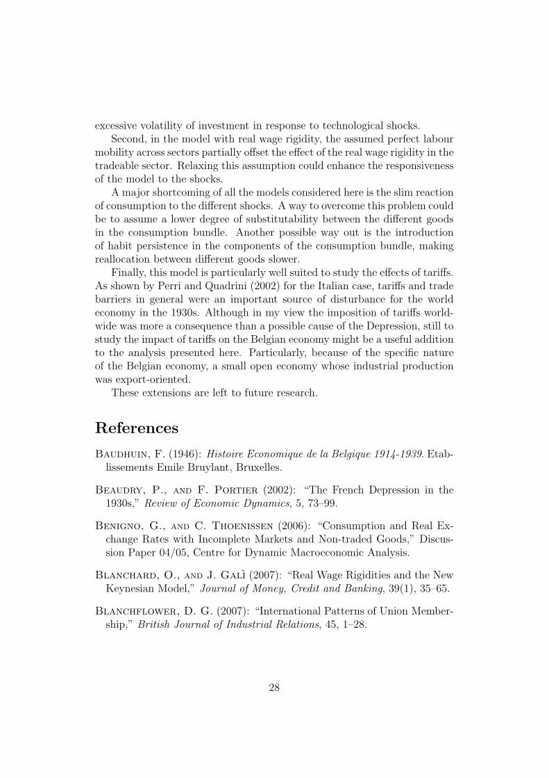
Before taking the model to the Depression data, it is again interestingto study the IRF of the model to three possible shocks. To this purpose,Figures 20, 21, 22 and 23 plot the IRF to the three shocks separately. Theblue line is the IRF of the model to a 1% standard deviation positive shockto the nominal exchange rate. The red line is the IRF of the model to a 1%standard deviation positive shock to the tradeable sector productivity. Theblack line is the IRF of the model to a 1% standard deviation positive shockto the non-tradeable sector productivity.

First consider the productivity shock to the tradeable sector. The in-creased efficiency in production causes the price of tradeables to decrease, asbefore. However, given that the tradeable good is not the numeraire any-more, such a decrease does not translate automatically into an inflationarypressure. The price of imports stays constant, as it is now determined bythe nominal exchange rate and by the world price for tradeable goods, andI assumed them both constant. In the previous exercise, we were unable tomake the distinction between the real and the monetary effect of the TFPvariation. Here we can. If the nominal exchange rate could move in responseto the TFP shock, the IRF would have the same pattern as before. As it

20Those Countries together received about 62% of the total Belgian exports in 1929.

24

happens, the constancy of the nominal exchange rate implies a deflationarypressure instead. Exports increases, a consequence of the higher efficiencyof the domestic economy in producing tradeables. Imports increasing morethan exports, the current account witnesses a small deficit lasting more than10 periods. Imports increase out of an income effect.

The shock to the productivity of tradeables causes output in the tradeablesector to increase. The shift in the labour demand coupled with the wagerigidity in the tradeable sector should cause an increase in the real wage wedo not apparently observe in the IRF. I say ‘apparently’, because what isgraphed as ‘wt’ is the wages expressed in terms of the numeraire. So, in thismodel, ‘wt’ stands for the nominal wage. However, if the nominal wage isdeflated with the consumption price, the increase in the real wage becomesappreciable. Hours worked in both sectors move little. The shock transmitsto the non-tradeable sector exactly as before, i.e. via the accumulation ofcapital.

Consider now the productivity shock in the non-tradeable sector. A shockon the non-tradeable TFP increases production in the non-tradeable sectorand decreases the relative price P N

P T . Mutatis mutandis, the transmissionmechanism within the non-tradeable sector via the labour demand is thesame as before. The same holds true for the transmission mechanism to thetradeable sector, via the accumulation of capital. A feature which is note-worthy is the greater overall impact of the TFP shock in the non-tradeablesector vis a vis the TFP shock in the tradeable sector. Such a difference isdue in part to the role played by the rest of the world in influencing the dy-namics of the tradeable sector. But most of the difference is explained by themajor weight that non-tradeables holds in the consumption and investmentaggregators.

As the nominal exchange rate remains stable, the shock to the productiv-ity of the non-tradeables produces a decrease in exports on impact. Tradeablegood production has become relatively less efficient. The initial positive in-come effect on imports is stronger than in the tradeable TFP shock case.The two effects combined imply a deeper deficit of the current accounts thatlasts 10 years before turning into a surplus.

Finally, let us consider the IRF to the nominal exchange rate shock.21

A positive shock on e means a devaluation of the nominal exchange rate:more Belgian francs are needed to buy one unit of the bundle-currency. Asexpected, this has inflationary effects on impact. Imports are costlier, exports

21As I have assumed that the National Bank of Belgium implemented monetary policyby pegging the nominal exchange rate to gold, in this model a nominal exchange rateshock is to be intended as a unilateral policy change by the foreign monetary authority.

25

cheaper, yet the current account remains fully balanced. Apparently the realexchange rate remains constant, with pM adjusting so a to offset the variationin e. Like any monetary shock, the temporary nominal exchange rate shockhas a short-lived impact on the real economy, due to the wage rigidity inthe tradeable sector. Notice that Equation (46) now describes a nominalwage rigidity (wages are measured in terms of Belgian francs), as opposedto the previous real model, where it described a real wage rigidity (wageswere measured in terms of tradeable good). The nominal wage rigidity inthe tradeable sector implies that the inflationary shock is not balanced by asuitable increase in wT . This implies a decrease in the real wage measuredeither as production cost (i.e. divided by pT ), or as purchasing power (i.e.divided by pc). Such a decrease has an obvious positive if not enduringimpact on the economy.

Now that the transmission mechanism of the model is clearer, it is timeto use the model to account for the Depression data.

If we assume that the 1929 exchange rate between the Belgian Francand the bundle currency is the equilibrium value, then we can interpret thevariations of e during the 1930s as exchange rate shocks, coming from theinteraction between the monetary policy of the National Bank of Belgiumand those of the other monetary authorities.

Given the calibration of the parameters, I fed in both the measured ex-change rate and the TFP shocks, and studied the response of the monetarymodel with nominal wage rigidity and bonds. Notice that, given that theexchange rate gives us already the asymmetry we wanted, there is no reasonto limit the productivity shock to the tradeable sector only. Therefore, inthe simulations below the TFP shock affects both the sectors.

The blue lines in Figures 8, 9, 10 and 11 show the results from the simu-lations.22

The model accounts for almost 50% of the cumulative drop in hoursworked between 1929 and 1934. The decrease in tradeable production inthe model accounts for almost all the observed cumulative drop of aggregateoutput between 1929 and 1934. In 1934, output in the non-tradeable sectoris about 7% below trend in the simulation. The dynamics of imports andexports are still not accounted for in a satisfactory manner. The improvementfor consumption is tiny as well. The model matches both the CPI and termsof trade reasonably well, although, like the other models above, it is notable to catch the CPI/PPI dynamics. The devaluation of the Belgian franc

22In an exercise not shown here, I have carried out the same simulations assuming perfectforesight of both the TFP and the exchange rate shocks, instead of rational expectationsonly. This was done to assess the robustness of the results, that indeed do not changeappreciably.

26

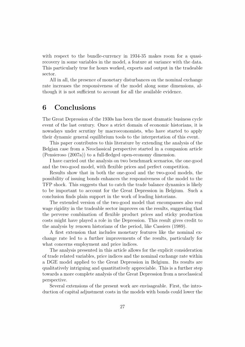
with respect to the bundle-currency in 1934-35 makes room for a quasi-recovery in some variables in the model, a feature at variance with the data.This particularly true for hours worked, exports and output in the tradeablesector.

All in all, the presence of monetary disturbances on the nominal exchangerate increases the responsiveness of the model along some dimensions, al-though it is not sufficient to account for all the available evidence.

6 Conclusions

The Great Depression of the 1930s has been the most dramatic business cycleevent of the last century. Once a strict domain of economic historians, it isnowadays under scrutiny by macroeconomists, who have started to applytheir dynamic general equilibrium tools to the interpretation of this event.

This paper contributes to this literature by extending the analysis of theBelgian case from a Neoclassical perspective started in a companion article(Pensieroso (2007a)) to a full-fledged open-economy dimension.

I have carried out the analysis on two benchmark scenarios, the one-goodand the two-good model, with flexible prices and perfect competition.

Results show that in both the one-good and the two-good models, thepossibility of issuing bonds enhances the responsiveness of the model to theTFP shock. This suggests that to catch the trade balance dynamics is likelyto be important to account for the Great Depression in Belgium. Such aconclusion finds plain support in the work of leading historians.

The extended version of the two-good model that encompasses also realwage rigidity in the tradeable sector improves on the results, suggesting thatthe perverse combination of flexible product prices and sticky productioncosts might have played a role in the Depression. This result gives credit tothe analysis by renown historians of the period, like Cassiers (1989).

A first extension that includes monetary features like the nominal ex-change rate led to a further improvements of the results, particularly forwhat concerns employment and price indices.

The analysis presented in this article allows for the explicit considerationof trade related variables, price indices and the nominal exchange rate withina DGE model applied to the Great Depression in Belgium. Its results arequalitatively intriguing and quantitatively appreciable. This is a further steptowards a more complete analysis of the Great Depression from a neoclassicalperspective.

Several extensions of the present work are envisageable. First, the intro-duction of capital adjustment costs in the models with bonds could lower the

27

excessive volatility of investment in response to technological shocks.Second, in the model with real wage rigidity, the assumed perfect labour

mobility across sectors partially offset the effect of the real wage rigidity in thetradeable sector. Relaxing this assumption could enhance the responsivenessof the model to the shocks.

A major shortcoming of all the models considered here is the slim reactionof consumption to the different shocks. A way to overcome this problem couldbe to assume a lower degree of substitutability between the different goodsin the consumption bundle. Another possible way out is the introductionof habit persistence in the components of the consumption bundle, makingreallocation between different goods slower.

Finally, this model is particularly well suited to study the effects of tariffs.As shown by Perri and Quadrini (2002) for the Italian case, tariffs and tradebarriers in general were an important source of disturbance for the worldeconomy in the 1930s. Although in my view the imposition of tariffs world-wide was more a consequence than a possible cause of the Depression, still tostudy the impact of tariffs on the Belgian economy might be a useful additionto the analysis presented here. Particularly, because of the specific natureof the Belgian economy, a small open economy whose industrial productionwas export-oriented.

These extensions are left to future research.

References

Baudhuin, F. (1946): Histoire Economique de la Belgique 1914-1939. Etab-lissements Emile Bruylant, Bruxelles.

Beaudry, P., and F. Portier (2002): “The French Depression in the1930s,” Review of Economic Dynamics, 5, 73–99.

Benigno, G., and C. Thoenissen (2006): “Consumption and Real Ex-change Rates with Incomplete Markets and Non-traded Goods,” Discus-sion Paper 04/05, Centre for Dynamic Macroeconomic Analysis.

Blanchard, O., and J. Galı (2007): “Real Wage Rigidities and the NewKeynesian Model,” Journal of Money, Credit and Banking, 39(1), 35–65.

Blanchflower, D. G. (2007): “International Patterns of Union Member-ship,” British Journal of Industrial Relations, 45, 1–28.

28

Bordo, M. D., C. J. Erceg, and C. L. Evans (2000): “Money, StickyWages and the Great Depression,” American Economic Review, 90, 1447–1463.

Buyst, E. (1997): “New GNP Estimates for the Belgian Economy duringthe Interwar Period,” Review of Income and Wealth, 43, 357–375.

Cassiers, I. (1989): Croissance, Crise et Regulation en Economie Ouverte:La Belgique entre les Deux Guerres. De Boeck Universite, Bruxelles.

(1995): “Managing the Franc in Belgium and France: The Eco-nomic Consequences of Exchange-Rate Policies, 1925-1936,” in Banking,Currency and Finance in Europe between the Wars, ed. by C. Feinstein.Clarendon Press, Oxford.

Chari, V. V., P. J. Kehoe, and E. R. McGrattan (2007): “BusinessCycle Accounting,” Econometrica, 75(3), 781–836.

Christiano, L., R. Motto, and M. Rostagno (2004): “The Great De-pression and the Friedman-Schwartz Hypothesis,” Working Paper 10255,National Bureau of Economic Research.

Cole, H. L., and L. E. Ohanian (1999): “The Great Depression in theUnited States from a Neoclassical Perspective,” Federal Reserve of Min-neapolis Quarterly Review, 23, 2–24.

(2002): “The Great UK Depression: A Puzzle and a Possible Res-olution,” Review of Economic Dynamics, 5, 19–44.

(2004): “New Deal Policies and the Persistence of the Great De-pression: A General Equilibrium Analysis,” Journal of Political Economy,112, 779–816.

Correia, I., J. C. Neves, and S. Rebelo (1995): “Business Cycles in aSmall Open Economy,” European Economic Review, 39, 1089–1113.

De Vroey, M., and L. Pensieroso (2006): “Real Business Cycle The-ory and the Great Depression: the Abandonement of the AbstentionistViewpoint,” Contributions to Macroeconomics, 6, issue 1, article 13.

Eichengreen, B., and P. Temin (2000): “The Gold Standard and theGreat Depression,” Contemporary European History, 9, 183–207.

29

Fisher, J. D. M., and A. Hornstein (2002): “The Role of Real Wages,Productivity, and Fiscal Policy in Germany’s Great Depression 1928-37,”Review of Economic Dynamics, 5, 100–127.

Galı, J., and T. Monacelli (2005): “Monetary Policy and Echange RateVolatility in a Small Open Economy,” Review of Economic Studies, 72,707–734.

Goossens, M. (1988): “The Belgian Labour Market during the InterwarPeriod,” in The Economic Development of Belgium since 1870, ed. by H. V.der Wee, and J. Blomme, pp. 417–429. Elgar, Cheltenham, 1997.

Hogg, R. L. (1986): Structural Rigidities and Policy Inertia in Inter-WarBelgium. Royal Academy of Belgium, Bruxelles.

Institut National de Statistique (1970): “Tableau Entrees-Sorties dela Belgique pour 1965,” Etudes Statistiques 22.

Kehoe, T. J., and E. Prescott (2008): “Using the General EquilibriumGrowth Model to Study Great Depressions: a Reply to Temin,” ResearchDepartment Staff Report 418, Federal Reserve Bank of Minneapolis.

Kehoe, T. J., and E. C. Prescott (2002): “Great Depressions of the20th Century,” Review of Economic Dynamics, 5, 1–18.

Kim, S. H., and M. A. Kose (2003): “Dynamics of Open-EconomyBusiness-Cycle Models: Role of the Discount Factor,” Macroeconomic Dy-namics, 7, 263–290.

Kindleberger, C. P. (1973): The World in Depression. University ofCalifornia Press, Berkley.

Mendoza, E. G. (1991): “Real Business Cycles in a Small Open Economy,”American Economic Review, 81, 797–818.

Mommen, A. (1994): The Belgian Economy in the Twentieth Century.Routledge, London.

Pensieroso, L. (2007a): “The Great Depression in Belgium from a Neo-classical Perspective,” Discussion Paper 2007-25, Universite catholique deLouvain.

Pensieroso, L. (2007b): “Real Business Cycle Models of the Great De-pression: A Critical Survey,” Journal of Economic Surveys, 21, 110–142.

30

Perri, F., and V. Quadrini (2002): “The Great Depression in Italy:Trade Restrictions and Real Wage Rigidities,” Review of Economic Dy-namics, 5, 128–151.

Plasmans, J., T. Michalak, and J. Fornero (2006): “Simulation,Estimation and Welfare Implications of Monetary Policies in a 3-CountryNOEM Model,” Working Paper Research 94, National Bank of Belgium.

Schmitt-Grohe, S., and M. Uribe (2003): “Closing Small Open Econ-omy Models,” Journal of International Economics, 61, 163–185.

Stockman, A. C., and L. L. Tesar (1995): “Tastes and Technologyin a Two-Country Model of the Business Cycle: Explaining InternationalComovements,” American Economic Review, 85, 168–185.

Temin, P. (2008): “Real Business Cycle Views of the Great Depression andRecent Events: a Review of Timothy J. Kehoe and Edward C. Prescott’sGreat Depressions of the Twentieth Century,” Journal of Economic Liter-ature, 46, 669–684.

Vanthemsche, G. (1987): “The Economic Action of the Belgian Stateduring the Crisis of the 1930s,” in The Economic Development of Belgiumsince 1870, ed. by H. V. der Wee, and J. Blomme, pp. 337–356. Elgar,Cheltenham, 1997.

Weder, M. (2006): “The Role of Preference Shocks and Capital Utilizationin the Great Depression,” International Economic Review, 47, 1247–1268.

31

Figures

1929 1930 1931 1932 1933 1934 1935 1936 1937 193855

60

65

70

75

80

85

90

95

100

105prices

1929 1930 1931 1932 1933 1934 1935 1936 1937 1938100

105

110

115

120

125

130

135

140

145relative prices

1929 1930 1931 1932 1933 1934 1935 1936 1937 1938−5

0

5

10

15

20interest rates

1929 1930 1931 1932 1933 1934 1935 1936 1937 193880

100

120

140

160

180

200exchange rates

retailwholesaleliving

terms of trade (px/pm)cpi/ppi

realnominal

BF for 1 £BF for 100 FF

Figure 1: Data on prices, interest rates and selected exchange rates in Bel-gium, 1929-1938. Indices, 1929=100. Source: Pensieroso (2007a)

32

1929 1930 1931 1932 1933 1934 1935 1936 1937 193840

50

60

70

80

90

100

110detrended output

1929 1930 1931 1932 1933 1934 1935 1936 1937 193850

60

70

80

90

100

110

120undetrended output

1929 1930 1931 1932 1933 1934 1935 1936 1937 193875

80

85

90

95

100

105Employment and detrended real wages

1929 1930 1931 1932 1933 1934 1935 1936 1937 193880

85

90

95

100

105

110

115

120Undetrended wages

gnpcixm

gnpcixm

lw

nominalreal

Figure 2: Data on detrended and undetrended output, its components, andthe labour market in Belgium, 1929-1938. Indices, 1929 = 100. Source:Pensieroso (2007a)

33

1929 1930 1931 1932 1933 1934 1935 1936 1937 193875

80

85

90

95

100

105c

1929 1930 1931 1932 1933 1934 1935 1936 1937 193820

40

60

80

100

120

140i

1929 1930 1931 1932 1933 1934 1935 1936 1937 193875

80

85

90

95

100

105l

1929 1930 1931 1932 1933 1934 1935 1936 1937 193875

80

85

90

95

100

105y

open economy modelclosed economy modeldata

Figure 3: Simulation. One-good closed-economy versus open-economy modelwith estimated tfp shocks

34

5 10 15 200

2

4

6x 10−3 s

5 10 15 200

0.5

1x 10−3 x

5 10 15 200

0.5

1x 10−3 c

5 10 15 20−5

0

5

10

15x 10−4 cn

5 10 15 200

0.5

1x 10−3 ct

5 10 15 20−2

−1.5

−1

−0.5

0x 10−5 cm

5 10 15 200

2

4

6

8x 10−4 kt

5 10 15 200

2

4

6

8x 10−3 kn

5 10 15 200

0.005

0.01

0.015st

Figure 4: IRF, model with TFP shocks in the tradeable sector

35

5 10 15 200

0.5

1

1.5x 10−4 lno

5 10 15 200

2

4

6

8x 10−5 lt

5 10 15 200

2

4

6

8x 10−4 itn

5 10 15 200

0.5

1

1.5x 10−4 itt

5 10 15 200

0.5

1

1.5x 10−3 inn

5 10 15 20−1

0

1

2x 10−4 int

5 10 15 200

1

2

3

4x 10−8 imn

5 10 15 200

0.5

1

1.5

2x 10−5 imt

5 10 15 200

0.5

1

1.5x 10−4 it


36

5 10 15 200

0.5

1

1.5x 10−3 in

5 10 15 200

2

4

6

8x 10−3 wt

5 10 15 200

2

4

6

8x 10−3 wn

5 10 15 200

2

4

6x 10−3 pn

5 10 15 200

0.005

0.01

0.015pc

5 10 15 200

0.005

0.01

0.015

0.02pit

5 10 15 200

0.005

0.01pin

5 10 15 200

1

2

3x 10−3 yn

5 10 15 200

1

2

3x 10−3 yt


37

5 10 15 200

1

x 10−4 rt

5 10 15 200

1

2

3

4x 10−4 rn

5 10 15 200

0.002

0.004

0.006

0.008

0.01

0.012pm

5 10 15 200

1

2

x 10−4 l


38

1929 1930 1931 1932 1933 1934 1935 1936 1937 193875

80

85

90

95

100

105c

money+bond+wagedatabenchmarkbond+wage

1929 1930 1931 1932 1933 1934 1935 1936 1937 193875

80

85

90

95

100

105yn

1929 1930 1931 1932 1933 1934 1935 1936 1937 193875

80

85

90

95

100

105

110yt

1929 1930 1931 1932 1933 1934 1935 1936 1937 193860

70

80

90

100

110x

1929 1930 1931 1932 1933 1934 1935 1936 1937 193860

70

80

90

100

110

120m

1929 1930 1931 1932 1933 1934 1935 1936 1937 193875

80

85

90

95

100

105l

Figure 8: Simulations with the two-sector models. Red line: data. Greenline: model with TFP shocks in the tradeable sector. Black line: model withbonds, wage rigidity in the tradeable sector and TFP shocks in the tradeablesector. Blue line: model with money, bonds, wage rigidity in the tradeablesector, aggregate TFP shocks and exchange rate shocks.

39

1929 1930 1931 1932 1933 1934 1935 1936 1937 193885

90

95

100

105

110kn


1929 1930 1931 1932 1933 1934 1935 1936 1937 193885

90

95

100

105

110kt

1929 1930 1931 1932 1933 1934 1935 1936 1937 193840

50

60

70

80

90

100

110in

1929 1930 1931 1932 1933 1934 1935 1936 1937 193840

60

80

100

120it

1929 1930 1931 1932 1933 1934 1935 1936 1937 193885

90

95

100

105rn

1929 1930 1931 1932 1933 1934 1935 1936 1937 193896

97

98

99

100

101

102rt


40

1929 1930 1931 1932 1933 1934 1935 1936 1937 193875

80

85

90

95

100

105

110real wage N


1929 1930 1931 1932 1933 1934 1935 1936 1937 193885

90

95

100

105

110

115real wage T

1929 1930 1931 1932 1933 1934 1935 1936 1937 193860

70

80

90

100

110pc

1929 1930 1931 1932 1933 1934 1935 1936 1937 193880

85

90

95

100

105

110pm/px

1929 1930 1931 1932 1933 1934 1935 1936 1937 193860

80

100

120

140

160pn/pt


41

1929 1930 1931 1932 1933 1934 1935 1936 1937 193860

70

80

90

100

110pin

1929 1930 1931 1932 1933 1934 1935 1936 1937 193860

70

80

90

100

110pit

1929 1930 1931 1932 1933 1934 1935 1936 1937 193892

94

96

98

100

102

104sn

1929 1930 1931 1932 1933 1934 1935 1936 1937 193885

90

95

100

105st

1929 1930 1931 1932 1933 1934 1935 1936 1937 193892

94

96

98

100

102

104s


1929 1930 1931 1932 1933 1934 1935 1936 1937 1938

0.65

0.7

0.75

0.8

0.85

0.9

0.95

1e


42

5 10 15 200

2

4

6x 10−3 s

5 10 15 200

0.5

1x 10−3 x

5 10 15 200

0.5

1x 10−3 c

5 10 15 20−5

0

5

10x 10−4 cn

5 10 15 200

0.5

1x 10−3 ct

5 10 15 20−10

−5

0

5x 10−5 cm

5 10 15 200

2

4

6

8x 10−4 kt

5 10 15 200

2

4

6

8x 10−3 kn

5 10 15 200

0.005

0.01

0.015st

Figure 12: IRF, model with bonds and TFP shocks in the tradeable sector

43

5 10 15 200

1

x 10−4 lno

5 10 15 200

0.5

1

1.5x 10−4 lt

5 10 15 200

2

4

6

8x 10−4 itn

5 10 15 200

1

2

3

4x 10−4 itt

5 10 15 200

0.5

1

1.5x 10−3 inn

5 10 15 200

2

4

6

8x 10−4 int

5 10 15 20−5

0

5x 10−8 imn

5 10 15 20−2

0

2

4

6x 10−4 imt

5 10 15 200

2

4

6x 10−4 it


44

5 10 15 200

0.5

1

1.5x 10−3 in

5 10 15 200

0.005

0.01wt

5 10 15 200

0.005

0.01wn

5 10 15 200

2

4

6x 10−3 pn

5 10 15 200

0.005

0.01

0.015pc

5 10 15 200

0.005

0.01

0.015

0.02pit

5 10 15 200

0.005

0.01pin

5 10 15 200

1

2

3x 10−3 yn

5 10 15 200

1

2

3x 10−3 yt


45

5 10 15 20−2

0

2

4x 10−4 rt

5 10 15 200

2

4

6x 10−4 rn

5 10 15 200

0.005

0.01

0.015pm

5 10 15 200

1

2

3

4x 10−4 l

5 10 15 20−2

0

2

4

6x 10−4 m

5 10 15 20−1

−0.5

0

0.5

1x 10−3 bond


46

5 10 15 200

2

4

6x 10−3 s

5 10 15 200

0.5

1

1.5x 10−3 x

5 10 15 200

0.5

1x 10−3 c

5 10 15 20−1

0

1

2x 10−3 cn

5 10 15 200

0.5

1

1.5

2x 10−3 ct

5 10 15 20−10

−5

0

5x 10−5 cm

5 10 15 200

2

4

6

8x 10−4 kt

5 10 15 200

2

4

6

8x 10−3 kn

5 10 15 200

0.005

0.01

0.015st

Figure 16: IRF, model with bonds, wage rigidity in the tradeable sector andTFP shocks in the tradeable sector

47

5 10 15 20−2

−1

0

1

2x 10−4 lno

5 10 15 200

1

2

3x 10−3 lt

5 10 15 200

0.5

1x 10−3 itn

5 10 15 200

1

2

3

4x 10−4 itt

5 10 15 200

0.5

1

1.5x 10−3 inn

5 10 15 20−5

0

5

10x 10−4 int

5 10 15 20−5

0

5

10x 10−8 imn

5 10 15 20−5

0

5

10x 10−4 imt

5 10 15 200

2

4

6

8x 10−4 it


48

5 10 15 200

0.5

1

1.5x 10−3 in

5 10 15 200

2

4

6

8x 10−3 wt

5 10 15 200

0.005

0.01

0.015wn

5 10 15 200

0.005

0.01pn

5 10 15 200

0.01

0.02

0.03pc

5 10 15 200

0.01

0.02

0.03pit

5 10 15 200

0.005

0.01

0.015pin

5 10 15 20−1

0

1

2

3x 10−3 yn

5 10 15 200

2

4

6x 10−3 yt


49

5 10 15 20−2

0

2

4x 10−4 rt

5 10 15 200

2

4

6x 10−4 rn

5 10 15 200

0.005

0.01

0.015

0.02pm

5 10 15 200

0.5

1

1.5

2x 10−3 l

5 10 15 20−5

0

5

10x 10−4 m

5 10 15 20−1

0

1

2x 10−3 bond


50

0 5 10 15 20−0.5

0

0.5

1

1.5

2

2.5x 10−3 C

E shockST shockSN shock

0 5 10 15 20−5

0

5

10

15

20x 10−3 YN


0 5 10 15 20−0.5

0

0.5

1

1.5

2

2.5

3x 10−3 YT


0 5 10 15 20−2

0

2

4

6

8

10x 10−4 X


0 5 10 15 20−0.5

0

0.5

1

1.5

2

2.5x 10−3 M


0 5 10 15 20−5

0

5

10

15x 10−4 L


Figure 20: IRF, model with bonds, nominal wage rigidity in the tradeablesector, nominal exchange rate shocks and aggregate TFP shocks. Blue line:IRF to a 1% standard deviation positive shock to the nominal exchange rate.Red line: IRF to a 1% standard deviation positive shock to the tradeable sec-tor productivity. Black line: is the IRF to a 1% standard deviation positiveshock to the non-tradeable sector productivity.

51

0 5 10 15 20−0.005

0

0.005

0.01

0.015

0.02

0.025

0.03KN


0 5 10 15 20−0.5

0

0.5

1

1.5

2

2.5x 10−3 KT


0 5 10 15 20−1

0

1

2

3

4x 10−3 IN


0 5 10 15 20−5

0

5

10

15

20x 10−4 IT


0 5 10 15 20−5

0

5

10

15

20x 10−4 RN


0 5 10 15 20−2

0

2

4

6

8x 10−4 RT



52

0 5 10 15 20−0.01

−0.005

0

0.005

0.01WN


0 5 10 15 20−5

−4

−3

−2

−1

0

1

2x 10−3 WT


0 5 10 15 20−0.03

−0.02

−0.01

0

0.01

0.02PC


0 5 10 15 20−0.015

−0.01

−0.005

0

0.005

0.01PX


0 5 10 15 200

0.002

0.004

0.006

0.008

0.01

0.012PM


0 5 10 15 20−0.015

−0.01

−0.005

0

0.005

0.01PT



53

0 5 10 15 20−0.015

−0.01

−0.005

0

0.005

0.01PN


0 5 10 15 20−0.02

−0.015

−0.01

−0.005

0

0.005

0.01PIN


0 5 10 15 20−0.02

−0.01

0

0.01

0.02PIT


0 5 10 15 20−5

0

5

10

15x 10−4 LT


0 5 10 15 20−2

0

2

4

6

8x 10−4 LN


0 5 10 15 20−3

−2

−1

0

1

2

3x 10−3 Bond



54

ISSN 1379-244X D/2010/3082/023

the great depression in belgium: an open-economy analysis · the great depression in belgium: an...

Documents