the group-lasso: two novel ... - stanford universityhastie/theses/michael_lim.pdf · the...
TRANSCRIPT

THE GROUP-LASSO: TWO NOVEL APPLICATIONS
A DISSERTATION
SUBMITTED TO THE DEPARTMENT OF STATISTICS
AND THE COMMITTEE ON GRADUATE STUDIES
OF STANFORD UNIVERSITY
IN PARTIAL FULFILLMENT OF THE REQUIREMENTS
FOR THE DEGREE OF
DOCTOR OF PHILOSOPHY
Michael Lim
August 2013

Preface
This thesis deals with two problems: learning linear interaction models, and elec-
troencephalography (EEG) source estimation in the visual cortex. These are quite
different problems, but they have a common theme that brings them together: we
propose solutions to each that are based on the group-lasso. The group-lasso was
first introduced in [49], and is an example of regularization applied to a supervised
learning problem.
Learning interactions is a diffcult problem because of the number of variables in-
volved. With a million variables (as in the case of genome wide association studies
(GWAS), we are already looking at a candidate interaction search space of about a
trillion terms. Even if the computational problems are overcome, there is still the
statistical issue of spurious correlations and low signal to noise ratios inherent in
these problems. Past approaches to this problem such as hierNet [5] and logic regres-
sion [33] are limited in either their computational feasibility or the types of variables
they can accommodate. Our contribution here is glinternet, a method for learn-
ing pairwise interactions via hierarchical group-lasso regularization. We demonstrate
that glinternet is competitive with current methods (where these methods are fea-
sible), but also that it has the added advantage of being able to accommodate both
categorical variables with arbitrary numbers of levels as well as continuous variables.
glinternet is available as a package on CRAN for the statistical software R.
Our EEG source problem arises from visual activation studies. Here, subjects are
given visual stimuli, and their neural response is measured in a non-invasive manner
through the use the sensors (or channels) placed around the subject’s head. The
goal is to recover the underlying neural activity (the sources) that are responsible for
iv
the observations recorded with these sensors. One method that is currently used to
perform source inversion is called the minimum norm, which applies ridge regression
to the observed sensor readings. We make two contributions in this domain. First,
we show that the group-lasso outperforms the minimum norm inversion, and that the
group-lasso performance improves with the number of subjects. This occurs because
the group-lasso is able to pool information across multiple subjects, whereas the
minimum norm is inherently unable to do so. A post-processing step may be applied
to the minimum norm estimates by averaging across multiple subjects. Our second
contribution consists of showing that averaging within appropriately defined regions
of interest (ROIs) in the visual cortex across multiple subjects is able to dramatically
boost the performance of both the minimum norm and group-lasso solutions, and
also improves with the number of subjects. These two contributions, to the best of
our knowledge, are novel results.
There are four chapters in this thesis. Chapter 1 introduces the group-lasso and
describes some of its properties. Chapter 2 consists of the interaction learning prob-
lem. We make clear the problem statement, make the case for hierarchical interaction
models, and then present our solution. The EEG source estimation problem is tackled
in Chapter 3. We introduce the problem, discuss past approaches and why they are
inadequate before presenting our solution that is based on the group-lasso. Finally,
we conclude with a discussion in Chapter 4.
v

Acknowledgements
I would like to thank my advisor, Trevor “The Major” Hastie, for his guidance over
the past 3 years. Prior to starting my studies at Stanford, I was often advised to
place the utmost importance on picking an advisor, because the advisor can make or
break your experience. I confess I did not heed any of that, but if I had to go back
and rechoose, it would still have to be Trevor. He has not just been an academic
advisor but also a mentor and friend.
I also thank my committee members Rob, Jonathan, Brad, and Tony for their
willingness to listen, advise, and taking the time to be on my committee.
Thanks also go out to my collaborators Tony, Justin, and Benoit, without whom
the EEG work would not have been possible. The collaboration gave me the oppor-
tunity to learn about EEG signal estimation, a field I would likely have never come
across otherwise.
Thanks to my friends both within and outside the statistics department. Our
discussions have often impacted my approach to thinking about problems, and have
helped a great deal toward the completion of this work. Special thanks to CS and
Noah for computational and programming discussions. And thanks to CS, Winston,
Alexandra, and Tian Tsong for pre-release glinternet testing. Rahul was also
instrumental in optimization pointers.
Special thanks to my fiancee Flora, who has waited (im)patiently for the past
four years for me to finish up. Without her support and motivation, I could not have
graduated.
Finally, I thank my parents who have dedicated their lives to raising me. I dedicate
this work to them.
vi

Contents
Preface iv
Acknowledgements vi
1 Introduction and preliminaries 1
1.1 The lasso . . . . . . . . . . . . . . . . . . . . . . . . . . . . . . . . . 1
1.2 The group-lasso . . . . . . . . . . . . . . . . . . . . . . . . . . . . . . 2
1.2.1 Extending the group-lasso to matrix-valued coefficients . . . . 4
2 Learning interactions 5
2.1 Introduction . . . . . . . . . . . . . . . . . . . . . . . . . . . . . . . . 5
2.1.1 A simulated example . . . . . . . . . . . . . . . . . . . . . . . 7
2.1.2 Organization of Chapter 2 . . . . . . . . . . . . . . . . . . . . 8
2.2 Background and notation . . . . . . . . . . . . . . . . . . . . . . . . . 8
2.2.1 Definition of interaction for categorical variables . . . . . . . . 9
2.2.2 Weak and strong hierarchy . . . . . . . . . . . . . . . . . . . . 9
2.2.3 First order interaction model . . . . . . . . . . . . . . . . . . 10
2.3 Methodology and results . . . . . . . . . . . . . . . . . . . . . . . . . 11
2.3.1 Strong hierarchy through overlapped group-lasso . . . . . . . . 11
2.3.2 Equivalence with unconstrained group-lasso . . . . . . . . . . 14
2.3.3 Properties of the glinternet estimators . . . . . . . . . . . 17
2.3.4 Interaction between a categorical variable and a continuous
variable . . . . . . . . . . . . . . . . . . . . . . . . . . . . . . 18
2.3.5 Interaction between two continuous variables . . . . . . . . . . 21
vii

2.4 Variable screening . . . . . . . . . . . . . . . . . . . . . . . . . . . . . 22
2.4.1 Screening with boosted trees . . . . . . . . . . . . . . . . . . . 23
2.4.2 An adaptive screening procedure . . . . . . . . . . . . . . . . 24
2.5 Related work and approaches . . . . . . . . . . . . . . . . . . . . . . 25
2.5.1 Logic regression [33] . . . . . . . . . . . . . . . . . . . . . . . 26
2.5.2 Composite absolute penalties [50] . . . . . . . . . . . . . . . . 26
2.5.3 hierNet [5] . . . . . . . . . . . . . . . . . . . . . . . . . . . . . 27
2.6 Simulation study . . . . . . . . . . . . . . . . . . . . . . . . . . . . . 28
2.6.1 False discovery rates . . . . . . . . . . . . . . . . . . . . . . . 28
2.6.2 Feasibility . . . . . . . . . . . . . . . . . . . . . . . . . . . . . 29
2.7 Real data examples . . . . . . . . . . . . . . . . . . . . . . . . . . . . 31
2.7.1 South African heart disease data . . . . . . . . . . . . . . . . 32
2.7.2 Spambase . . . . . . . . . . . . . . . . . . . . . . . . . . . . . 33
2.7.3 Dorothea . . . . . . . . . . . . . . . . . . . . . . . . . . . . . 33
2.7.4 Genome-wide association study . . . . . . . . . . . . . . . . . 34
2.8 Algorithm details . . . . . . . . . . . . . . . . . . . . . . . . . . . . . 38
2.8.1 Defining the group penalties γ . . . . . . . . . . . . . . . . . . 38
2.8.2 Fitting the group-lasso . . . . . . . . . . . . . . . . . . . . . . 39
2.9 Discussion . . . . . . . . . . . . . . . . . . . . . . . . . . . . . . . . . 41
3 EEG source estimation 42
3.1 Introduction . . . . . . . . . . . . . . . . . . . . . . . . . . . . . . . . 42
3.1.1 Past approaches . . . . . . . . . . . . . . . . . . . . . . . . . . 42
3.1.2 Assimilating information from multiple subjects . . . . . . . . 44
3.1.3 This thesis . . . . . . . . . . . . . . . . . . . . . . . . . . . . . 44
3.2 Notation . . . . . . . . . . . . . . . . . . . . . . . . . . . . . . . . . . 47
3.3 Methodology . . . . . . . . . . . . . . . . . . . . . . . . . . . . . . . 48
3.3.1 Defining regions of interest (ROIs) in the visual cortex . . . . 48
3.3.2 Collaborative effect from multiple subjects . . . . . . . . . . . 49
3.3.3 Imposing temporal smoothness . . . . . . . . . . . . . . . . . 53
3.3.4 Recovering the activity in the original space . . . . . . . . . . 54
viii

3.3.5 Model selection . . . . . . . . . . . . . . . . . . . . . . . . . . 55
3.4 Results . . . . . . . . . . . . . . . . . . . . . . . . . . . . . . . . . . . 55
3.4.1 Experimental setup . . . . . . . . . . . . . . . . . . . . . . . . 55
3.4.2 A single subject . . . . . . . . . . . . . . . . . . . . . . . . . . 56
3.4.3 5 subjects . . . . . . . . . . . . . . . . . . . . . . . . . . . . . 57
3.4.4 Better performance with more subjects . . . . . . . . . . . . . 59
3.5 Algorithm details . . . . . . . . . . . . . . . . . . . . . . . . . . . . . 61
3.5.1 Cyclic group-wise coordinate descent . . . . . . . . . . . . . . 62
3.5.2 Determining the group penalty modifiers γi . . . . . . . . . . 63
3.6 Discussion . . . . . . . . . . . . . . . . . . . . . . . . . . . . . . . . . 65
4 Conclusion 67
A Model selection details 68
Bibliography 72
ix

List of Tables
2.1 Anova for linear model fitted to first interaction term that was discovered. 36
2.2 Anova for linear logistic regression done separately on each of the two
true interaction terms. . . . . . . . . . . . . . . . . . . . . . . . . . . 37
x

List of Figures
2.1 False discovery rate vs number of discovered interactions . . . . . . . 7
2.2 Simulation results for continuous variables: Average false discovery
rate and standard errors from 100 simulation runs. . . . . . . . . . . 30
2.3 Left: Best wallclock time over 10 runs for discovering 10 interactions.
Right: log scale. . . . . . . . . . . . . . . . . . . . . . . . . . . . . . 31
2.4 Performance of methods on 20 train-test splits of the South African
heart disease data. . . . . . . . . . . . . . . . . . . . . . . . . . . . . 32
2.5 Performance on the Spambase data. . . . . . . . . . . . . . . . . . . . 33
2.6 Performance on dorothea . . . . . . . . . . . . . . . . . . . . . . . . . 35
3.1 Schematic of the group-lasso settling disputes. The true areas are
shaded pink and green. The blue region is stronger in subject 1, but
pink and green still get chosen over the blue because of their aggregate
strength across the other 5 subjects. . . . . . . . . . . . . . . . . . . . 46
3.2 Performance of the group-lasso and minimum norm on one instance of
simulated data for a one and five subjects. Vertical lines correspond
to the solutions chosen by optimizing the GCV error curve for each
method. Note that GCV errors are computed with the observations
(and their fitted values), while MSE measures goodness of fit to the
activity, which explains the difference in scale between the two. Red:
group-lasso. Blue: minimum norm. . . . . . . . . . . . . . . . . . . . 57
xi

3.3 MSE from dimension reduction by principal components and temporal
smoothing with right singular vectors of Y, averaged over 100 simula-
tions. A large portion of the MSE is due to the dimension reduction
from taking the first 5 principal components for each ROI. . . . . . . 59
3.4 Performance of the group-lasso and minimum norm as a function of the
number of subjects. Plots are of averages from 20 simulations. Vertical
lines are standard error bars. . . . . . . . . . . . . . . . . . . . . . . . 60
3.5 AUC obtained after post-processing the recovered activity by averaging
across subjects. Plots are of average values over the same 20 data
instances from before, along with standard error bars. Notice that the
group-lasso with 2 subjects often outperforms the minimum norm with
25 subjects. . . . . . . . . . . . . . . . . . . . . . . . . . . . . . . . . 61
A.1 Estimated degrees of freedom (using (A.1)) vs true df. Red line:
Using formula (A.1) without any ridge penalty to β0 results in an
estimate that is biased downward. Blue line: In our experiments, a
ridge penalty of 1.0817× 10⁴ works well. . . . . . . . . . . . . . . . . 70
A.2 Variance of β0 as a function of ridge parameter. Vertical line corre-
sponds to 1.0817 × 10⁴ that is found to work well in our degrees of
freedom simulations. . . . . . . . . . . . . . . . . . . . . . . . . . . . 71
xii

Chapter 1
Introduction and preliminaries
In this chapter, we introduce the lasso and the group-lasso. The group-lasso can be
viewed as an extension of the lasso to groups of variables, and is the common theme
running throughout the thesis.
1.1 The lasso
Regularization plays an important role in statistics and machine learning. One ex-
ample arises in the context of linear models applied to large datasets. Advances in
technology has made it possible to store ever larger amounts of data, and while the
number of observations has increased dramatically, so too has the number of fea-
tures. In fact, the number of features often exceeds the number of data points; this
is commonly referred to as the “p > n” problem. The linear regression problem is
ill-posed in this situation because there is no unique solution: there are infinitely
many coefficient vectors that give the same fit.
A popular approach in supervised learning problems of this type is to use regular-
ization, such as adding a squared L2 penalty of the form ‖β‖22 or a L1 penalty of the
form ‖β‖1 to the model coefficients. The latter type of penalty has been the focus of
much research since its introduction in [40], and is called the lasso. The lasso obtains
1

CHAPTER 1. INTRODUCTION AND PRELIMINARIES 2
the estimates β as the solution to
argminµ,β L(Y,X;µ, β) + λ‖β‖1, (1.1)
where Y is a vector of observations, X is the feature matrix (or design matrix), µ is
the intercept, and β is the vector of coefficients to be estimated. L can be any loss
function, most commonly squared error loss
L(Y,X;µ, β) =1
2‖Y − µ · 1−Xβ‖22 (1.2)
if the observations Y are quantitative, or logistic loss
L(Y,X;µ, β) = −[YT (µ · 1 + Xβ)− 1T log (1 + exp(µ · 1 + Xβ))
](1.3)
if the observations are binary (log and exp taken component wise).
The L1 penalty has the effect of performing variable selection by setting some of
the coefficients to zero. The parameter λ controls the amount of regularization, and
for large enough values, all the coefficients will be estimated to be zero.
1.2 The group-lasso
There is a group analog to the lasso, called the group-lasso [49], that sets groups
of coefficients to zero. Suppose there are p groups of variables (possibly of different
sizes), and let the feature matrix for group i be denoted by Xi. Let Y denote the
vector of observations. The group-lasso obtains the estimates βj, j = 1, . . . , p, as the
solution to
argminµ,β1
2‖Y − µ · 1−
p∑j=1
Xjβj‖22 + λ
p∑j=1
γj‖βj‖2. (1.4)
Note that the L2 penalty in (1.4) is not squared, and that if each group consists of only
one variable, this reduces to the lasso criterion in (1.1). Just as the lasso performs
variable selection by estimating some of the coefficients to be zero, the group-lasso

CHAPTER 1. INTRODUCTION AND PRELIMINARIES 3
does selection on the group level: it is able to zero out groups of coefficients. If an
estimate βi is nonzero, then all its components are usually nonzero.
The parameter λ controls the amount of regularization, with larger values implying
more regularization. When λ is large enough, all the coefficients will be estimated as
zero. The γ’s allow each group to be penalized to different extents, which allows us to
penalize some groups more (or less) than others. To solve (1.4), we start with λ large
enough so that all estimates are zero. Decreasing λ along a grid of values results in a
path of solutions, from which an optimal λ can be chosen by cross validation or some
model selection procedure. In particular, for the EEG source estimation problem, we
use generalized cross validation (GCV) [14] with a heuristic for the degrees of freedom
using the results in [22].
The Karush-Kuhn-Tucker (KKT) optimality conditions for the group-lasso are
simple to compute and check. For group i, they are
‖XTi (Y − Y)‖2 < γiλ if βi = 0 (1.5)
‖XTi (Y − Y)‖2 = γiλ if βi 6= 0. (1.6)
where Y = µ·1+∑p
i=1 Xiβ is the vector of fitted values. The group-lasso is commonly
fit with some form of gradient descent, and convergence can be confirmed by checking
that the solutions satisfy the KKT conditions. We use an adaptive version of fast
iterative soft thresholding (FISTA) [3] and cyclic group-wise coordinate descent in
our applications. See Sections 2.8 and 3.5 for more details.
Adding a ridge penalty to (1.4) results in the group analog of the elastic-net:
argminµ,β1
2
∥∥∥∥∥Y − µ · 1−p∑j=1
Xjβj
∥∥∥∥∥2
2
+ λ
p∑j=1
γj‖βj‖2 + α‖β‖22. (1.7)
The squared L2 penalty in (1.7) applies to the entire coefficient vector β. This allows
us to reduce the variance in the estimates βi, and having α > 0 is helpful in our
EEG experiments. Now that we have two parameters λ and α, a two-dimensional
grid search has to be done to select optimal values for them. Since this can be
computationally intensive, we keep α fixed and do the grid search only on λ. We

CHAPTER 1. INTRODUCTION AND PRELIMINARIES 4
discuss how we select α in Appendix A.
The overlapped group-lasso is a variant of the group-lasso where the groups of
variables are allowed to have overlaps, i.e. some variables can show up in more than
one group. However, each time a variable shows up in a group, it gets a new coefficient.
For example, if a variable is included in 3 groups, then it has 3 coefficients that need
to be estimated. We refer the reader to [21] for more details.
1.2.1 Extending the group-lasso to matrix-valued coefficients
Our description of the group-lasso above treated the coefficients β as a vector. Since
the EEG source activity at a single time point is a vector, and we wish to recover
the activity over several time points, we need to be able to handle the case where the
coefficients are matrices. This can be done via a straightforward extension of (1.7).
As before let Xi denote the feature matrix for group i and let Y be the N ×T matrix
of observations.
argminµ,β1
2
∥∥∥∥∥Y − 1µt −p∑j=1
Xjβj
∥∥∥∥∥2
F
+ λ
p∑j=1
γj‖βj‖F + α‖β‖2F . (1.8)
We now have T intercepts (one for each column of Y), and we use the Frobenius
norm ‖ · ‖F instead of the L2 norm. The solutions have the same property as before
in that if βi is nonzero, then all its components are usually nonzero.

Chapter 2
Learning interactions
Our first application of the group-lasso is in the context of learning linear pairwise
interaction models via hierarchical group-lasso regularization. We begin by defining
what an interaction means and describing the difficulty of the problem.
2.1 Introduction
Given an observed response and explanatory variables, we expect interactions to be
present if the response cannot be explained by additive functions of the variables.
The following definition makes this more precise.
Definition 1. When a function f(x, y) cannot be expressed as g(x) + h(y) for some
functions g and h, we say that there is an interaction in f between x and y.
Interactions of single nucleotide polymorphisms (SNPs) are thought to play a
role in cancer [36] and other diseases. Modeling interactions has also served the
recommender systems community well: latent factor models (matrix factorization)
aim to capture user-item interactions that measure a user’s affinity for a particular
item, and are the state of the art in predictive power [23]. In lookalike-selection, a
problem that is of interest in computational advertising, one looks for features that
most separates a group of observations from its complement, and it is conceivable
that interactions among the features can play an important role.
5

CHAPTER 2. LEARNING INTERACTIONS 6
There are many challenges, the first of which is a problem of scalability. Even
with 10,000 variables, we are already looking at a 50 × 106-dimensional space of
possible interaction pairs. Complicating the matter are correlations amongst the
variables, which makes learning even harder. Finally, in some applications, sample
sizes are relatively small and the signal to noise ratio is low. For example, genome
wide association studies (GWAS) can involve hundreds of thousands or millions of
variables, but only several thousand observations. Since the number of interactions is
on the order of the square of the number of variables, computational considerations
quickly become an issue.
Finding interactions is an example of the “p > n” problem where there are more
features or variables than observations. This is a natural setting for regularization,
and the idea behind our method is to set up main effects and interactions (to be
defined later) as a group of variables, and then we perform selection via the group-
lasso.
Discovering interactions is an area of active research; see, for example, [5] and [7].
In this thesis, we introduce glinternet, a method for learning first-order interac-
tions that can be applied to categorical variables with arbitrary numbers of levels,
continuous variables, and combinations of the two. Our approach consists of two
phases: a screening stage (for large problems) that gives a candidate set of main
effects and interactions, followed by variable selection on the candidate set with the
group-lasso. We introduce two screening procedures, the first of which is inspired by
our observation that boosting with depth-2 trees naturally gives rise to an interaction
selection process that enforces hierarchy: an interaction cannot be chosen until a split
has been made on one of its two associated main effects. The second method is an
adaptive procedure that is based on the strong rules [41] for discarding predictors in
lasso-type problems. We show in Section 2.3 how the group-lasso penalty naturally
enforces strong hierarchy in the resulting solutions.
We can now give an overview of our method:
1. If required, screen the variables to get a candidate set C of interactions and
their associated main effects. Otherwise, take C to consist of all main effects
and pairwise interactions.

CHAPTER 2. LEARNING INTERACTIONS 7
2. Fit a group-lasso on C with a grid of values for the regularization parameter.
Start with λ = λmax for which all estimates are zero. As we decrease λ, we
allow more terms to enter the model, and we stop once a user-specified number
of interactions have been discovered. Alternatively, we can choose λ using any
model selection technique such as cross validation.
2.1.1 A simulated example
As a first example, we perform 100 simulations with 500 3-level categorical variables
and 800 quantitative observations. There are 10 main effects and 10 interactions in
the ground truth, and the noise level is chosen to give a signal to noise ratio of one.
We run glinternet without any screening, and stop after ten interactions have been
found. The average false discovery rate and standard errors are plotted as a function
of the number of interactions found in Figure 2.1.
● ●
●
●●
●
●
●
●
●
●
0.0
0.1
0.2
0.3
0 1 2 3 4 5 6 7 8 9 10Number of interactions found
Fals
e di
scov
ery
rate
Figure 2.1: False discovery rate vs number of discovered interactions

CHAPTER 2. LEARNING INTERACTIONS 8
2.1.2 Organization of Chapter 2
The rest of the chapter is organized as follows. Section 2.2 introduces basic notions
and notation. In section 2.3, we introduce the group-lasso and how it fits into our
framework for finding interactions. We also show how glinternet is equivalent to
an overlapping grouped lasso. We discuss screening in Section 2.4, and give sev-
eral examples with both synthetic and real datasets in Section 2.7 before going into
algorithmic details in Section 2.8. We conclude with a discussion in Section 2.9.
2.2 Background and notation
We use the random variables Y to denote the observed response, F to denote a
categorical feature, and Z to denote a continuous feature. We use L to denote the
number of levels that F can take. For simplicity of notation we will use the first
L positive integers to represent these L levels, so that F takes values in the set
{i ∈ Z : 1 ≤ i ≤ L}. Each categorical variable has an associated random variable
X ∈ RL with a 1 that indicates which level F takes, and 0 everywhere else.
When there are p categorical (or continuous) features, we will use subscripts to
index them, i.e. F1, . . . , Fp. Boldface font will always be reserved for vectors or
matrices that comprise of realizations of these random variables. For example, Y is
the n-vector of observations of the random variable Y , F is the n-vector of realizations
of the random variable F , and Z is the n-vector of realizations of the random variable
Z. Similarly, X is a n × L indicator matrix whose i-th row consists of a 1 in the
Fi-th column and 0 everywhere else. We use a n× (Li · Lj) indicator matrix Xi:j to
represent the interaction Fi : Fj. We will write
Xi:j = Xi ∗Xj, (2.1)
where the first Lj columns of Xi:j are obtained by taking the elementwise products
between the first column of Xi and the columns of Xj, and likewise for the other

CHAPTER 2. LEARNING INTERACTIONS 9
columns. For example,(a b
c d
)∗
(e f
g h
)=
(ae af be bf
cg ch dg dh
). (2.2)
2.2.1 Definition of interaction for categorical variables
To see how Definition 1 applies to this setting, let E(Y |F1 = i, F2 = j) = µij, the
conditional mean of Y given that F1 takes level i, and F2 takes level j. There are 4
possible cases:
1. µij = µ (no main effects, no interactions)
2. µij = µ+ θi1 (one main effect F1)
3. µij = µ+ θi1 + θj2 (two main effects)
4. µij = µ+ θi1 + θj2 + θij1:2 (main effects and interaction)
Note that all but the first case is overparametrized, and the usual procedure is to
impose sum constraints on the main effects and interactions:
L1∑i=1
θi1 = 0,
L2∑j=1
θj2 = 0 (2.3)
and
L1∑i=1
θij1:2 = 0 for fixed j,
L2∑j=1
θij1:2 = 0 for fixed i. (2.4)
In what follows, θi, i = 1, · · · , p, will represent the main effect coefficients, and θi:j
will denote the interaction coefficients. We will use the terms “main effect coefficients”
and “main effects” interchangeably, and likewise for interactions.
2.2.2 Weak and strong hierarchy
An interaction model is said to obey strong hierarchy if an interaction can be present

CHAPTER 2. LEARNING INTERACTIONS 10
only if both of its main effects are present. Weak hierarchy is obeyed as long as either
of its main effects are present. Since main effects as defined above can be viewed
as deviations from the global mean, and interactions are deviations from the main
effects, it rarely make sense to have interactions without main effects. This leads us
to prefer interaction models that are hierarchical. We will see in Section 2.3 that
glinternet produces estimates that obey strong hierarchy.
2.2.3 First order interaction model
Our model for a quantitative response Y is given by
Y = µ+
p∑i=1
Xiθi +∑i<j
Xi:jθi:j + ε (2.5)
where ε ∼ N(0, σ2). For binary responses, we have
logit(P(Y = 1|X)) = µ+
p∑i=1
Xiθi +∑i<j
Xi:jθi:j. (2.6)
We fit these models by minimizing an appropriate choice of loss function L. Because
the models are still overparametrized, we impose the relevant constraints for the
coefficients θ (see (2.3) and (2.4)). We can thus cast the problem of fitting a first-
order interaction model as an optimization problem with constraints:
argminµ,θ L(Y,Xi:i≤p,Xi:j;µ, θ) (2.7)
subject to the relevant constraints. L can be any loss function, typically squared error
loss for the quantitative response model given by
L(Y,Xi:i≤p,Xi:j;µ, θ) =1
2
∥∥∥∥∥Y − µ · 1−p∑i=1
Xiθi +∑i<j
Xi:jθi:j
∥∥∥∥∥2
2
, (2.8)

CHAPTER 2. LEARNING INTERACTIONS 11
and logistic loss for the binomial response model given by
L(Y,Xi:i≤p,Xi:j;µ, θ) = −
[YT (µ · 1 +
p∑i=1
Xiθi +∑i<j
Xi:jθi:j)
− 1T log
(1 + exp(µ · 1 +
p∑i=1
Xiθi +∑i<j
Xi:jθi:j)
)], (2.9)
where the log and exp are taken component-wise.
Because the coefficients in (2.7) are unpenalized, the solutions θi satisfy strong
hierarchy (they are usually all nonzero). If p+
(p
2
)> n, this problem is ill-posed,
resulting in infinitely many solutions. Adding a ridge penalty is one way to tackle
this problem, and the solutions will also satisfy strong hierarchy. The question then
arises as to how to fit interaction models whose solutions are sparse (variable selection
effect) and also satisfy hierarchy. A lasso penalty will achieve sparsity, but there is
no guarantee that the solutions will have any form of hierarchy. This is the goal of
this work.
2.3 Methodology and results
We want to fit the first order interaction model in a way that obeys strong hierarchy.
We show in Section 2.3.1 how this can be achieved by adding an overlapped group-
lasso penalty to the objective in (2.7). We then show how this constrained overlapped
group-lasso problem can be conveniently solved via an unconstrained group-lasso
(without overlaps).
2.3.1 Strong hierarchy through overlapped group-lasso
Adding an overlapped group-lasso penalty to (2.7) is one way of obtaining solutions
that satisfy the strong hierarchy property. The results that follow hold for both
squared error and logistic loss, but we focus on the former for clarity.
Consider the case where there are two categorical variables F1 and F2 with L1 and

CHAPTER 2. LEARNING INTERACTIONS 12
L2 levels respectively. Their indicator matrices are given by X1 and X2. We solve
argminµ,α,α1
2
∥∥∥∥∥∥∥∥Y − µ · 1−X1α1 −X2α2 − [X1 X2 X1:2]
α1
α2
α1:2
∥∥∥∥∥∥∥∥2
2
+ λ
(‖α1‖2 + ‖α2‖2 +
√L2‖α1‖22 + L1‖α2‖22 + ‖α1:2‖22
)(2.10)
subject to
L1∑i=1
αi1 = 0,
L2∑j=1
αj2 = 0,
L1∑i=1
αi1 = 0,
L2∑j=1
αj2 = 0 (2.11)
and
L1∑i=1
αij1:2 = 0 for fixed j,
L2∑j=1
αij1:2 = 0 for fixed i. (2.12)
Notice that Xi, i = 1, 2 each have two different coefficient vectors αi and αi, resulting
in an overlapped penalty. It follows that the actual main effects θ1 and θ2 are given
by
θ1 = α1 + α1 (2.13)
θ2 = α2 + α2 (2.14)
The√L2‖α1‖22 + L1‖α2‖22 + ‖α1:2‖22 term results in estimates that satisfy strong hi-
erarchy, because either ˆα1 = ˆα2 = α1:2 = 0 or all are nonzero, i.e. interactions are
always present with both main effects.
The constants L1 and L2 are chosen to put α1, α2, and α1:2 on the same scale. To
motivate this, note that we can write
X1α1 = X1:2[α1, . . . , α1︸ ︷︷ ︸L2 copies
]T , (2.15)

CHAPTER 2. LEARNING INTERACTIONS 13
and similarly for X2α2. We now have a representation for α1 and α2 with respect to
the space defined by X1:2, so that they are “comparable” to α1:2. We then have
‖[α1, . . . , α1︸ ︷︷ ︸L2 copies
]‖22 = L2‖α1‖22 (2.16)
and likewise for α2. More details are given in Section 2.3.2 below.
The estimated main effects and interactions can be recovered as
θ1 = α1 + ˆα1 (2.17)
θ2 = α2 + ˆα2 (2.18)
θ1:2 = α1:2. (2.19)
Because of the “all zero” or “all nonzero” property of the group-lasso estimates men-
tioned above, we also have
θ1:2 6= 0 =⇒ θ1 6= 0 and θ2 6= 0. (2.20)
The overlapped group-lasso with constraints is conceptually simple, but care must
be taken in how we parametrize the constraints. This is especially so because we
penalize the coefficients, and any representation of the problem that does not preserve
symmetry will result in unequal penalization schemes for the coefficients. The problem
becomes more tedious as the number of variables and levels grows. We now show how
to solve the overlapped group-lasso problem by solving an equivalent unconstrained
group-lasso problem. This is advantageous because
1. the problem can be represented in a symmetric way, thus avoiding the need for
careful choices of parametrization, and
2. we only have to fit a group-lasso without constraints on the coefficients, which
is a well-studied problem.

CHAPTER 2. LEARNING INTERACTIONS 14
2.3.2 Equivalence with unconstrained group-lasso
We show that the overlapped group-lasso above can be solved with a simple group-
lasso. We will need two Lemmas. The first shows that because we fit an intercept in
the model, the estimated coefficients β for categorical variables will have mean zero.
Lemma 1. Let X be an indicator matrix. Then the solution β to
argminµ,β1
2‖Y − µ · 1−Xβ‖22 + λ‖β‖2 (2.21)
satisfies
¯β = 0. (2.22)
The same is true for logistic loss.
Proof. Because X is an indicator matrix, each row consists of exactly a single 1 (all
other entries 0), so that
X · c1 = c1 (2.23)
for any constant c. It follows that if µ and β are solutions, then so are µ + c1 and
β − c1. But the norm ‖β − c1‖2 is minimized for c =¯β.
The next Lemma states that if we include two intercepts in the model, one pe-
nalized and the other unpenalized, then the penalized intercept will be estimated to
be zero. This is because we can achieve the same fit with a lower penalty by taking
µ←− µ+ µ.
Lemma 2. The optimization problem
argminµ,µ,β1
2‖Y − µ · 1− µ · 1− . . .‖22 + λ
√‖µ‖22 + ‖β‖22 (2.24)
has solution ˆµ = 0 for all λ > 0. The same result holds for logistic loss.

CHAPTER 2. LEARNING INTERACTIONS 15
The next theorem shows how the overlapped group-lasso in Section 2.3.1 reduces
to a group-lasso.
Theorem 1. Solving the constrained optimization problem (2.10) - (2.12) in Section
2.3.1 is equivalent to solving the unconstrained problem
argminµ,β1
2‖Y − µ · 1−X1β1 −X2β2 −X1:2β1:2‖22
+ λ (‖β1‖2 + ‖β2‖2 + ‖β1:2‖2) . (2.25)
Proof. We need to show that the group-lasso objective can be equivalently written as
an overlapped group-lasso with the appropriate constraints on the parameters. We
begin by rewriting (2.10) as
argminµ,µ,α,α1
2
∥∥∥∥∥∥∥∥∥∥Y − µ · 1−X1α1 −X2α2 − [1 X1 X2 X1:2]
µ
α1
α2
α1:2
∥∥∥∥∥∥∥∥∥∥
2
2
+ λ
(‖α1‖2 + ‖α2‖2 +
√L1L2‖µ‖22 + L2‖α1‖22 + L1‖α2‖22 + ‖α1:2‖22
). (2.26)
By Lemma 2, we will estimate ˆµ = 0. Therefore we have not changed the solutions
in any way.
Lemma 1 shows that the first two constraints in (2.11) are satisfied by the esti-
mated main effects β1 and β2. We now show that
‖β1:2‖2 =√L1L2‖µ‖22 + L2‖α1‖22 + L1‖α2‖22 + ‖α1:2‖22 (2.27)
where the α1, α2, and α1:2 satisfy the constraints in (2.11) and (2.12).
For fixed levels i and j, we can decompose β1:2 (see [35]) as
βij1:2 = β··1:2 + (βi·1:2 − β··1:2) + (β·j1:2 − β··1:2) + (βij1:2 − βi·1:2 − β·j1:2 + β··1:2) (2.28)
≡ µ+ αi1 + αj2 + αij1:2. (2.29)

CHAPTER 2. LEARNING INTERACTIONS 16
It follows that the whole (L1L2)-vector β1:2 can be written as
β1:2 = 1µ+ Z1α1 + Z2α2 + α1:2, (2.30)
where Z1 is a L1L2 × L1 indicator matrix of the form1L2×1 0 · · · 0
0 1L2×1 · · · 0
0 0. . . 0
0 0 0 1L2×1
︸ ︷︷ ︸
L1 columns
(2.31)
and Z2 is a L1L2 × L2 indicator matrix of the form
L1 copies
IL2×L2
...
IL2×L2
(2.32)
It follows that
Z1α1 = (α11, . . . , α
11︸ ︷︷ ︸
L2 copies
, α21, . . . , α
21︸ ︷︷ ︸
L2 copies
, . . . , αL11 , . . . , α
L11︸ ︷︷ ︸
L2 copies
)T (2.33)
and
Z2α2 = (α12, . . . , α
L22 , α
12, . . . , α
L22 , . . . , α
12, . . . , α
L22 )T . (2.34)
Note that α1, α2, and α1:2, by definition, satisfy the constraints (2.11) and (2.12).
This can be used to show, by direct calculation, that the four additive components
in (2.30) are mutually orthogonal, so that we can write
‖β1:2‖22 = ‖1µ‖22 + ‖Z1α1‖22 + ‖Z2α2‖22 + ‖α1:2‖22 (2.35)
= L1L2‖µ‖22 + L2‖α1‖22 + L1‖α2‖22 + ‖α1:2‖22. (2.36)

CHAPTER 2. LEARNING INTERACTIONS 17
We have shown that the penalty in the group-lasso problem is equivalent to the
penalty in the constrained overlapped group-lasso. It remains to show that the loss
functions in both problems are also the same. Since X1:2Z1 = X1 and X1:2Z2 = X2,
this can be seen by a direct computation:
X1:2β1:2 = X1:2(1µ+ Z1α1 + Z2α2 + α1:2) (2.37)
= 1µ+ X1α1 + X2α2 + X1:2α1:2 (2.38)
= [1 X1 X2 X1:2]
µ
α1
α2
α1:2
(2.39)
Theorem 1 shows that we can use the group-lasso to obtain estimates that satisfy
strong hierarchy, without solving the overlapped group-lasso with constraints. The
theorem also shows that the main effects and interactions can be extracted with
θ1 = β1 + ˆα1 (2.40)
θ2 = β2 + ˆα2 (2.41)
θ1:2 = α1:2. (2.42)
We discuss the properties of the glinternet estimates in the next section.
2.3.3 Properties of the glinternet estimators
While glinternet treats the problem as a group-lasso, examining the equivalent
overlapped group-lasso version makes it easier to draw insights about the behaviour
of the method under various scenarios. Recall that the overlapped penalty for two
variables is given by
‖α1‖2 + ‖α2‖2 +√L2‖α1‖22 + L1‖α2‖22 + ‖α1:2‖22. (2.43)

CHAPTER 2. LEARNING INTERACTIONS 18
If the ground truth is additive, i.e. α1:2 = 0, then α1 and α2 will be estimated to be
zero (in the noiseless case). This is because for L1, L2 ≥ 2 and a, b ≥ 0, we have
√L2a2 + L1b2 ≥ a+ b. (2.44)
Thus it is advantageous to place all the main effects in α1 and α2, because doing
so results in a smaller penalty. Therefore, if the truth has no interactions, then
glinternet picks out only main effects.
If an interaction was present (α1:2 > 0), the derivative of the penalty term with
respect to α1:2 is
α1:2√L2‖α1‖22 + L1‖α2‖22 + ‖α1:2‖22
. (2.45)
The presence of main effects allows this derivative to be smaller, thus allowing the
algorithm to pay a smaller penalty (as compared to no main effects present) for
making α1:2 nonzero. This shows interactions whose main effects are also present are
discovered before pure interactions.
2.3.4 Interaction between a categorical variable and a con-
tinuous variable
We describe how to extend Theorem 1 to interaction between a continuous variable
and a categorical variable.
Consider the case where we have a categorical variable F with L levels, and a
continuous variable Z. Let µi = E[Y |F = i, Z = z]. There are four cases:
• µi = µ (no main effects, no interactions)
• µi = µ+ θi1 (main effect F )
• µi = µ+ θi1 + θ2z (two main effects)
• µi = µ+ θi1 + θ2z + θi1:2z (main effects and interaction)

CHAPTER 2. LEARNING INTERACTIONS 19
As before, we impose the constraints∑L
i=1 θi1 = 0 and
∑Li=1 θ
i1:2 = 0. An overlapped
group-lasso of the form
argminµ,α,α1
2
∥∥∥∥∥∥∥∥Y − µ · 1−Xα1 − Zα2 − [X Z (X ∗ Z)]
α1
α2
α1:2
∥∥∥∥∥∥∥∥2
2
+ λ
(‖α1‖2 + ‖α2‖2 +
√‖α1‖22 + L‖α2‖22 + ‖α1:2‖22
)(2.46)
subject to
L∑i=1
αi1 = 0,L∑i=1
αi1 = 0,L∑i=1
αi1:2 = 0 (2.47)
allows us to obtain estimates of the interaction term that satisfy strong hierarchy.
This is again due to the nature of the square root term in the penalty. The actual
main effects and interactions can be recovered as
θ1 = α1 + ˆα1 (2.48)
θ2 = α2 + ˆα2 (2.49)
θ1:2 = α1:2. (2.50)
We have the following extension of Theorem 1:
Theorem 2. Solving the constrained overlapped group-lasso above is equivalent to
solving
argminµ,β1
2‖Y − µ · 1−Xβ1 − Zβ2 − (X ∗ [1 Z])β1:2‖22
+ λ (‖β1‖2 + ‖β2‖2 + ‖β1:2‖2) . (2.51)

CHAPTER 2. LEARNING INTERACTIONS 20
Proof. We proceed as in the proof of Theorem 1 and introduce an additional param-
eter µ into the overlapped objective:
argminµ,µ,α,α1
2
∥∥∥∥∥∥∥∥∥∥Y − µ · 1−Xα1 − Zα2 − [1 X Z (X ∗ Z)]
µ
α1
α2
α1:2
∥∥∥∥∥∥∥∥∥∥
2
2
+ λ
(‖α1‖2 + ‖α2‖2 +
√L‖µ‖22 + ‖α1‖22 + L‖α2‖22 + ‖α1:2‖22
)(2.52)
As before, this does not change the solutions because we will have ˆµ = 0 (see Lemma
2).
Decompose the 2L-vector β1:2 into[η1
η2
], (2.53)
where η1 and η2 both have dimension L× 1. Apply the anova decomposition to both
to obtain
ηi1 = η·1 + (ηi1 − η·1) (2.54)
≡ µ+ αi1 (2.55)
and
ηi2 = η·2 + (ηi2 − η·2) (2.56)
≡ α2 + αi1:2. (2.57)
Note that α1 is a (L×1)-vector that satisfies∑L
i=1 αi2 = 0, and likewise for α1:2. This
allows us to write
β1:2 =
[µ · 1L×1α2 · 1L×1
]+
[α1
α1:2
](2.58)

CHAPTER 2. LEARNING INTERACTIONS 21
It follows that
‖β1:2‖22 = L‖µ‖22 + ‖α1‖22 + L‖α2‖22 + ‖α1:2‖22, (2.59)
which shows that the penalties in both problems are equivalent. A direct computation
shows that the loss functions are also equivalent:
(X ∗ [1 Z])β1:2 = [X (X ∗ Z)]β1:2 (2.60)
= [X (X ∗ Z)]
([µ · 1L×1α2 · 1L×1
]+
[α1
α1:2
])(2.61)
= µ · 1 + Xα1 + Zα2 + (X ∗ Z)α1:2. (2.62)
Theorem 2 allows us to accommodate interactions between continuous and cate-
gorical variables by simply parametrizing the interaction term as X ∗ [1 Z], where
X is the indicator matrix representation for categorical variables that we have been
using all along. We then proceed as before with a group-lasso.
2.3.5 Interaction between two continuous variables
We have seen that the appropriate representations for the interaction terms are
• X1 ∗X2 = X1:2 for categorical variables
• X ∗ [1 Z] = [X (X ∗ Z)] for one categorical variable and one continuous
variable.
How should we represent the interaction between two continuous variables? Let Z1
and Z2 be two continuous variables. One might guess by now that the appropriate
form of the interaction term is given by
Z1:2 = [1 Z1] ∗ [1 Z2] (2.63)
= [1 Z1 Z2 (Z1 ∗ Z2)]. (2.64)
CHAPTER 2. LEARNING INTERACTIONS 22
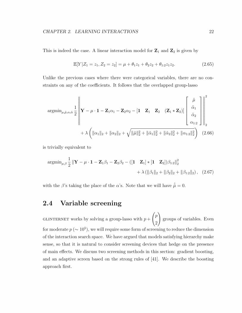
This is indeed the case. A linear interaction model for Z1 and Z2 is given by
E[Y |Z1 = z1, Z2 = z2] = µ+ θ1z1 + θ2z2 + θ1:2z1z2. (2.65)
Unlike the previous cases where there were categorical variables, there are no con-
straints on any of the coefficients. It follows that the overlapped group-lasso
argminµ,µ,α,α1
2
∥∥∥∥∥∥∥∥∥∥Y − µ · 1− Z1α1 − Z2α2 − [1 Z1 Z2 (Z1 ∗ Z2)]
µ
α1
α2
α1:2
∥∥∥∥∥∥∥∥∥∥
2
2
+ λ
(‖α1‖2 + ‖α2‖2 +
√‖µ‖22 + ‖α1‖22 + ‖α2‖22 + ‖α1:2‖22
)(2.66)
is trivially equivalent to
argminµ,β1
2‖Y − µ · 1− Z1β1 − Z2β2 − ([1 Z1] ∗ [1 Z2])β1:2‖22
+ λ (‖β1‖2 + ‖β2‖2 + ‖β1:2‖2) , (2.67)
with the β’s taking the place of the α’s. Note that we will have ˆµ = 0.
2.4 Variable screening
glinternet works by solving a group-lasso with p+
(p
2
)groups of variables. Even
for moderate p (∼ 105), we will require some form of screening to reduce the dimension
of the interaction search space. We have argued that models satisfying hierarchy make
sense, so that it is natural to consider screening devices that hedge on the presence
of main effects. We discuss two screening methods in this section: gradient boosting,
and an adaptive screen based on the strong rules of [41]. We describe the boosting
approach first.
CHAPTER 2. LEARNING INTERACTIONS 23
2.4.1 Screening with boosted trees
AdaBoost [11] and gradient boosting [12] are effective approaches to building ensem-
bles of weak learners such as decision trees. One of the advantages of trees is that
they are able to model nonlinear effects and high-order interactions. For example,
a depth-2 tree essentially represents an interaction between the variables involved in
the two splits, which suggests that boosting with depth-2 trees is a way of building
a first-order interaction model. Note that the interactions are hierarchical, because
in finding the optimal first split, the boosting algorithm is looking for the best main
effect. The subsequent split is then made, conditioned on the first split.
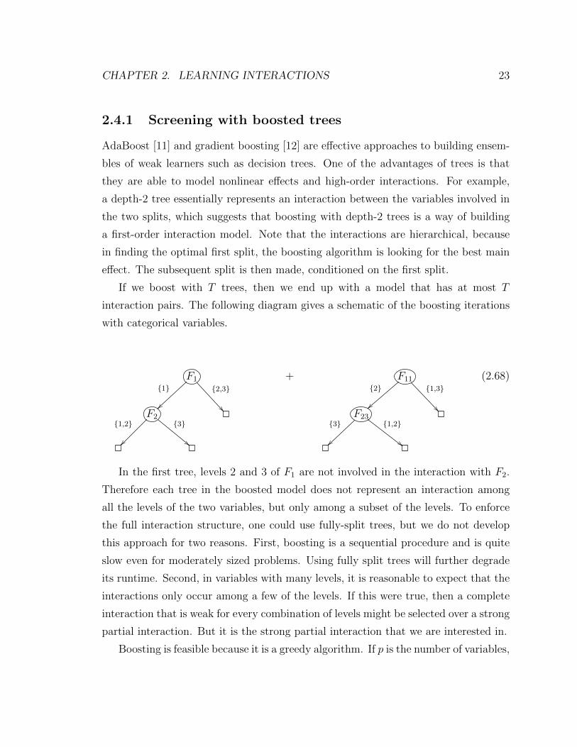
If we boost with T trees, then we end up with a model that has at most T
interaction pairs. The following diagram gives a schematic of the boosting iterations
with categorical variables.
F1
{1}
~~
{2,3}
��F2
{1,2}
��
{3}
""
+ F11
{2}
}}
{1,3}
��F23
{3}
~~
{1,2}
##
(2.68)
In the first tree, levels 2 and 3 of F1 are not involved in the interaction with F2.
Therefore each tree in the boosted model does not represent an interaction among
all the levels of the two variables, but only among a subset of the levels. To enforce
the full interaction structure, one could use fully-split trees, but we do not develop
this approach for two reasons. First, boosting is a sequential procedure and is quite
slow even for moderately sized problems. Using fully split trees will further degrade
its runtime. Second, in variables with many levels, it is reasonable to expect that the
interactions only occur among a few of the levels. If this were true, then a complete
interaction that is weak for every combination of levels might be selected over a strong
partial interaction. But it is the strong partial interaction that we are interested in.
Boosting is feasible because it is a greedy algorithm. If p is the number of variables,

CHAPTER 2. LEARNING INTERACTIONS 24
an exhaustive search involves O(p2) variables, whereas boosting operates with O(p).
To use the boosted model as a screening device for interaction candidates, we take
the set of all unique interactions from the collection of trees. For example, in our
schematic above, we would add F1:2 and F11:23 to our candidate set of interactions.
In our experiments, using boosting as a screen did not perform as well as we hoped.
There is the issue of selecting tuning parameters such as the amount of shrinkage and
the number of trees to use. Lowering the shrinkage and increasing the number of
trees improves false discovery rates, but at a significant cost to speed. In the next
section, we describe a screening approach that is based on computing inner products
that is efficient and that can be integrated with the strong rules for the group-lasso.
2.4.2 An adaptive screening procedure
The strong rules [41] for lasso-type problems are effective heuristics for discarding
large numbers of variables that are likely to be redundant. As a result, the strong rules
can dramatically speed up the convergence of algorithms because they can concentrate
on a smaller set (we call this the strong set) of variables that are more likely to be
nonzero. The strong rules are not safe, however, meaning that it is possible that some
of the discarded variables are actually supposed to be nonzero. Because of this, after
our algorithm has converged on the strong set, we have to check the KKT conditions
on the discarded set. Those variables that do not satisfy the conditions then have
to be added to the current set of nonzero variables, and we fit on this expanded set.
This happens rarely in our experience, i.e. the discarded variables tend to remain
zero after the algorithm has converged on the strong set, which means we rarely have
to do multiple rounds of fitting for any given value of the regularization paramter λ.
The strong rules for the group-lasso involve computing si = ‖XTi (Y − Y)‖2 for
every group of variables Xi, and then discarding a group i if si < 2λcurrent−λprevious.
If this is feasible for all p+
(p
2
)groups, then there is no need for screening; we simply
fit the group-lasso on those groups that pass the strong rules filter. Otherwise, we
approximate this by screening only on the groups that correspond to main effects.
We then take the candidate set of interactions to consist of all pairwise interactions
CHAPTER 2. LEARNING INTERACTIONS 25
between the variables that passed this screen. Note that because the KKT conditions
for group i are (see Section 1.2)
si < λ if βi = 0 (2.69)
si = λ if βi 6= 0, (2.70)
we will have already computed the si for the strong rules from checking the KKT
conditions for the solutions at the previous λ. This allows us to integrate screening
with the strong rules in an efficient manner. An example will illustrate.
Suppose we have 10,000 variables (∼ 50 × 106 possible interactions), but we are
computationally limited to a group-lasso with 106 groups. Assume we have the fit for
λ = λk, and want to move on to λk+1. Let rλk = Y−Yλk denote the current residual.
At this point, the variable scores si = ‖XTi rλk‖2 have already been computed from
checking the KKT conditions at the solutions for λk. We restrict ourselves to the
10,000 variables, and take the 100 with the highest scores. Denote this set by T λk+1
100 .
The candidate set of variables for the group-lasso is then given by T λk+1
100 together with
the pairwise interactions between all 10,000 variables and T λk+1
100 . Because this gives
a candidate set with about 100×10, 000 = 106 terms, the compuation is now feasible.
We then compute the group-lasso on this candidate set, and repeat the procudure
with the new residual rλk+1.
This screen is easy to compute since it is based on inner products. Moreover, they
can be computed in parallel. The procedure also integrates well with the strong rules
by reusing inner products computed from the fit for a previous λ.
2.5 Related work and approaches
We describe some past and related approaches to discovering interactions. We give a
short synopsis of how they work, and say why they are inadequate for our purposes.
The method most similar to ours is hierNet.

CHAPTER 2. LEARNING INTERACTIONS 26
2.5.1 Logic regression [33]
Logic regression finds boolean combinations of variables that have high predictive
power of the response variable. For example, a combination might look like
(F1 and F3) or F5. (2.71)
This is an example of an interaction that is of higher-order than what glinternet
handles, and is an appealing aspect of logic regression. However, logic regression does
not accommodate continuous variables or categorical variables with more than two
levels. We do not make comparisons with logic regression in our simulations for this
reason.
2.5.2 Composite absolute penalties [50]
Like glinternet, this is also a penalty-based approach. CAP employs penalties of
the form
‖(βi, βj)‖γ1 + ‖βj‖γ2 (2.72)
where γ1 > 1. Such a penalty ensures that βi 6= 0 whenever βj 6= 0. It is possible that
βi 6= 0 but βj = 0. In other words, the penalty makes βj hierarchically dependent on
βi: it can only be nonzero after βi becomes nonzero. It is thus possible to use CAP
penalties to build interaction models that satisfy hierarchy. For example, a penalty
of the form ‖(θ1, θ2, θ1:2)‖2 + ‖θ1:2‖2 will result in estimates that satisfy θ1:2 6= 0 =⇒θ1 6= 0 and θ2 6= 0. We can thus build a linear interaction model for two categorical
variables by solving
argminµ,θ1
2‖Y − µ · 1−X1θ1 −X2θ2 −X1:2θ1:2‖22
+ λ(‖(θ1, θ2, θ1:2)‖2 + ‖θ1:2‖2) (2.73)

CHAPTER 2. LEARNING INTERACTIONS 27
subject to (2.3) and (2.4). We see that the CAP approach differs from glinternet
in that we have to solve a constrained optimization problem. The form of the penal-
ties are also different: the interaction coefficient in CAP is penalized twice, whereas
glinternet penalizes it once. This, together with the constraints, results in a more
difficult optimization problem, and it is not obvious what the relationship between
the two algorithms’ solutions would be.
2.5.3 hierNet [5]
This is a method that, like glinternet, seeks to find interaction estimates that obey
hierarchy with regularization. The optimization problem that hierNet solves is
argminµ,β,θ1
2
n∑i=1
(yi − µ− xTi β −1
2xTi θxi)
2 + λ1T (β+ + β−) +λ
2‖θ‖1 (2.74)
subject to
θ = θT , ‖θj‖1 ≤ β+j + β−j , β
+j ≥ 0, β−j ≥ 0. (2.75)
The main effects are represented by β, and interactions are given by θ. The first con-
straint enforces symmetry in the interaction coefficients. β+j and β−j are the positive
and negative parts of βj, and are given by β+j = max(0, βj) and β−j = −min(0, βj)
respectively. The constraint ‖θj‖1 ≤ β+j + β−j implies that if some components of the
j-th row of θ are estimated to be nonzero, then the main effect βj will also be esti-
mated to be nonzero. Since θj corresponds to interactions between the j-th variable
and all the other variables, this implies that the solutions to the hierNet objective
satisfy weak hierarchy. One can think of β+j + β−j as a budget for the amount of
interactions that are allowed to be nonzero.
The hierNet objective can be modified to obtain solutions that satisfy strong hier-
archy, which makes it in principle comparable to glinternet. Currently, hierNet is
only able to accommodate binary and continuous variables, and is practically limited
to fitting models with fewer than 1000 variables.

CHAPTER 2. LEARNING INTERACTIONS 28
2.6 Simulation study
We perform simulations to see if glinternet is competitive with existing methods.
hierNet is a natural benchmark because it also tries to find interactions subject to
hierarchical constraints. Because hierNet only works with continuous variables and
2-level categorical variables, we include gradient boosting as a competitor for the
scenarios where hierNet cannot be used.
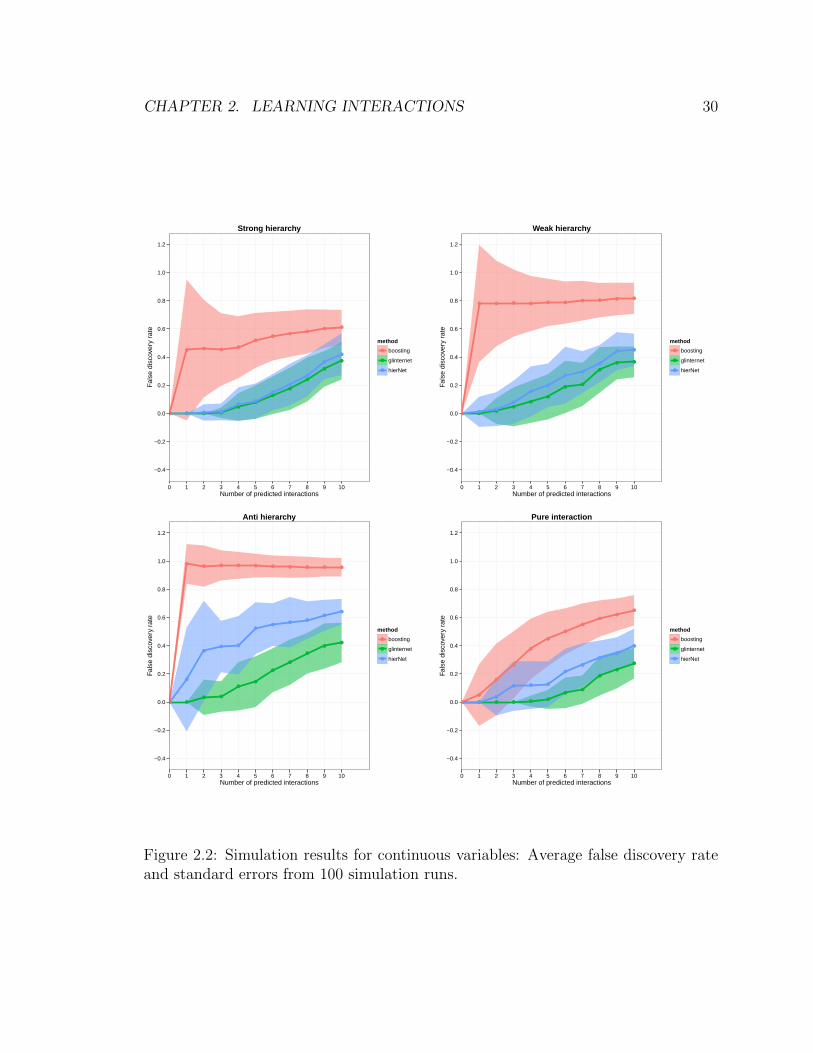
2.6.1 False discovery rates
We simulate 4 different setups:
1. Truth obeys strong hierarchy. The interactions are only among pairs of nonzero
main effects.
2. Truth obeys weak hierarchy. Each interaction has only one of its main effects
present.
3. Truth is anti-hierarchical. The interactions are only among pairs of main effects
that are not present.
4. Truth is pure interaction. There are no main effects present, only interactions.
Each case is generated with n = 500 observations and p = 30 continuous variables,
with a signal to noise ratio of 1. Where applicable, there are 10 main effects and/or
10 interactions in the ground truth. The interaction and main effect coefficients are
sampled from N(0, 1), so that the variance in the observations should be split equally
between main effects and interactions.
Boosting is done with 5000 depth-2 trees and a learning rate of 0.001. Each tree
represents a candidate interaction, and we can compute the improvement to fit due
to this candidate pair. Summing up the improvement over the 5000 trees gives a
score for each interaction pair, which can then be used to order the pairs. We then
compute the false discovery rate as a function of rank. For glinternet and hierNet,
we obtain a path of solutions and compute the false discovery rate as a function of the

CHAPTER 2. LEARNING INTERACTIONS 29
number of interactions discovered. The default setting for hierNet is to impose weak
hierarchy, and we use this except in the cases where the ground truth has strong
hierarchy. In these cases, we set hierNet to impose strong hierarchy. We also set
“diagonal=FALSE” to disable quadratic terms.
We plot the average false discovery rate with standard error bars as a function
of the number of predicted interactions in Figure 2.2. The results are from 100
simulation runs. We see that glinternet is competitive with hierNet when the truth
obeys strong or weak hierarchy, and does better when the truth is anti-hierarchical.
This is expected because hierNet requires the presence of main effects as a budget for
interactions, whereas glinternet can still esimate an interaction to be nonzero even
though none of its main effects are present. Boosting is not competitive, especially in
the anti-hierarchical case. This is because the first split in a tree is effectively looking
for a main effect.
Both glinternet and hierNet perform comparably in these simulations. If all the
variables are continuous, there do not seem to be compelling reasons to choose one
over the other.
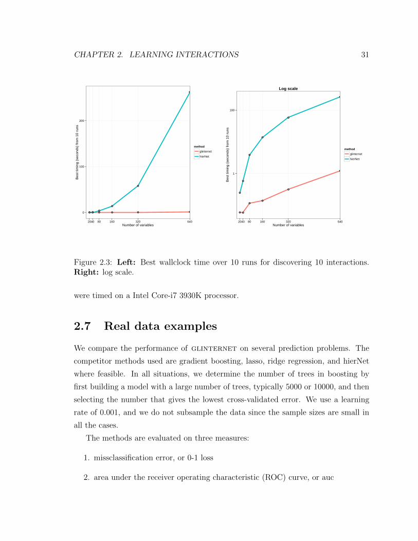
2.6.2 Feasibility
To the best of our knowledge, hierNet is the only readily available package for learn-
ing interactions among continuous variables in a hierarchical manner. Therefore it is
natural to use hierNet as a speed benchmark. We generate data in which the ground
truth has strong hierarchy as in Section 2.6.1, but with n = 1000 quantitative obser-
vations and p = 20, 40, 80, 160, 320, 640 continuous variables. We set each method to
find 10 interactions. While hierNet does not allow the user to specify the number of
interactions to discover, we get around this by fitting a path of values, then selecting
the regularization parameter that corresponds to 10 nonzero estimated interactions.
We then refit hierNet along a path that terminates with this choice of parameter, and
time this run. Both software packages are compiled with the same options. Figure
2.3 shows the best time recorded for each method over 10 runs. These simulations
CHAPTER 2. LEARNING INTERACTIONS 30
● ● ● ●
●
●
●
●
●
●
●
● ● ● ●
●●
●
●
●
●
●
●
● ● ●●
●
●●
●● ●
−0.4
−0.2
0.0
0.2
0.4
0.6
0.8
1.0
1.2
0 1 2 3 4 5 6 7 8 9 10Number of predicted interactions
Fals
e di
scov
ery
rate
method
●
●
●
boosting
glinternet
hierNet
Strong hierarchy
● ●●
●
●
●
●●
●
● ●
●●
●
●
●
●
●●
●
● ●
●
● ● ● ● ● ●● ● ● ●
−0.4
−0.2
0.0
0.2
0.4
0.6
0.8
1.0
1.2
0 1 2 3 4 5 6 7 8 9 10Number of predicted interactions
Fals
e di
scov
ery
rate
method
●
●
●
boosting
glinternet
hierNet
Weak hierarchy
● ●
● ●
●
●
●
●
●
●●
●
●
●
● ●
●●
●●
●●
●
●● ● ● ● ● ● ● ● ●
−0.4
−0.2
0.0
0.2
0.4
0.6
0.8
1.0
1.2
0 1 2 3 4 5 6 7 8 9 10Number of predicted interactions
Fals
e di
scov
ery
rate
method
●
●
●
boosting
glinternet
hierNet
Anti hierarchy
● ● ● ● ●●
●●
●
●
●
● ●
●
● ● ●
●
●
●
●
●
●
●
●
●
●
●
●
●
●●
●
−0.4
−0.2
0.0
0.2
0.4
0.6
0.8
1.0
1.2
0 1 2 3 4 5 6 7 8 9 10Number of predicted interactions
Fals
e di
scov
ery
rate
method
●
●
●
boosting
glinternet
hierNet
Pure interaction
Figure 2.2: Simulation results for continuous variables: Average false discovery rateand standard errors from 100 simulation runs.
CHAPTER 2. LEARNING INTERACTIONS 31
● ● ● ● ● ●● ●●
●
●
●
0
100
200
2040 80 160 320 640Number of variables
Bes
t tim
ing
(sec
onds
) fr
om 1
0 ru
ns
method
glinternet
hierNet
● ●
●
●
●
●
●
●
●
●
●
●
1
100
2040 80 160 320 640Number of variables
Bes
t tim
ing
(sec
onds
) fr
om 1
0 ru
ns
method
glinternet
hierNet
Log scale
Figure 2.3: Left: Best wallclock time over 10 runs for discovering 10 interactions.Right: log scale.
were timed on a Intel Core-i7 3930K processor.
2.7 Real data examples
We compare the performance of glinternet on several prediction problems. The
competitor methods used are gradient boosting, lasso, ridge regression, and hierNet
where feasible. In all situations, we determine the number of trees in boosting by
first building a model with a large number of trees, typically 5000 or 10000, and then
selecting the number that gives the lowest cross-validated error. We use a learning
rate of 0.001, and we do not subsample the data since the sample sizes are small in
all the cases.
The methods are evaluated on three measures:
1. missclassification error, or 0-1 loss
2. area under the receiver operating characteristic (ROC) curve, or auc

CHAPTER 2. LEARNING INTERACTIONS 32
●
●
●
●
●
●
0.20
0.25
0.30
0.70
0.75
0.80
0.85
0.90
0.5
0.6
0−1 lossauc
cross entropy
boosting glinternet hierNet lasso ridge
type
test
train
Performance over 20 train/test splits of the data
Figure 2.4: Performance of methods on 20 train-test splits of the South African heartdisease data.
3. cross entropy, given by − 1n
∑ni=1 [yi log(yi) + (1− yi) log(1− yi)].
2.7.1 South African heart disease data
The data consists of 462 males from a high risk region for heart disease in South
Africa. The task is to predict which subjects had coronary heart disease using risk
factors such as cumulative tobacco, blood pressure, and family history of heart disease.
We randomly split the data into 362-100 train-test examples, and tuned each method
on the training data using 10-fold cross validation before comparing the prediction
performance on the held out test data. This splitting process was carried out 20
times, and Figure 2.4 summarizes the results. The methods are all comparable, with
no distinct winner.
CHAPTER 2. LEARNING INTERACTIONS 33
0.00
0.02
0.04
0.06
0.00
0.25
0.50
0.75
1.00
0.00
0.05
0.10
0.15
0.20
0−1 lossauc
cross entropy
boosting glinternet hierNet lasso ridge
type
test
train
Figure 2.5: Performance on the Spambase data.
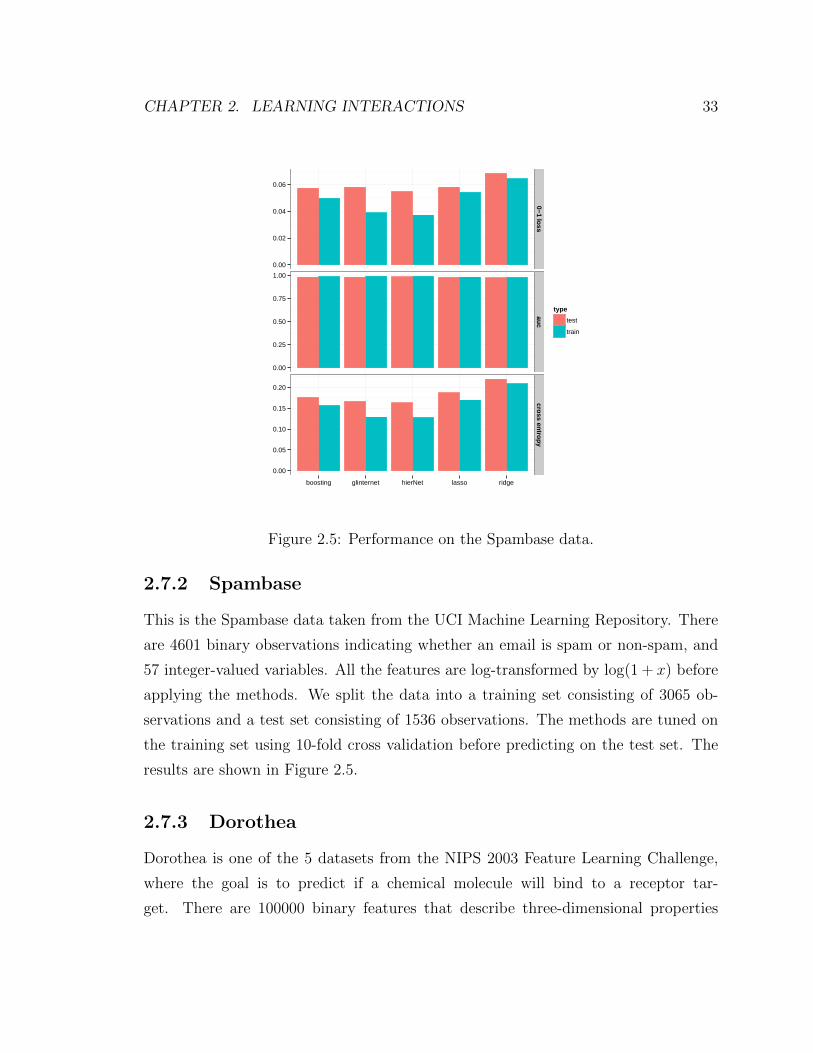
2.7.2 Spambase
This is the Spambase data taken from the UCI Machine Learning Repository. There
are 4601 binary observations indicating whether an email is spam or non-spam, and
57 integer-valued variables. All the features are log-transformed by log(1 + x) before
applying the methods. We split the data into a training set consisting of 3065 ob-
servations and a test set consisting of 1536 observations. The methods are tuned on
the training set using 10-fold cross validation before predicting on the test set. The
results are shown in Figure 2.5.
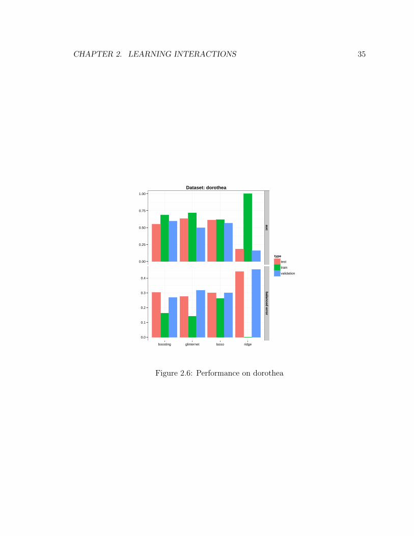
2.7.3 Dorothea
Dorothea is one of the 5 datasets from the NIPS 2003 Feature Learning Challenge,
where the goal is to predict if a chemical molecule will bind to a receptor tar-
get. There are 100000 binary features that describe three-dimensional properties

CHAPTER 2. LEARNING INTERACTIONS 34
of the molecules, half of which are probes that have nothing to do with the re-
sponse. The training, validation, and test sets consist of 800, 350, and 800 observa-
tions respectively. More details about how the data were prepared can be found at
http://archive.ics.uci.edu/ml/datasets/Dorothea.
We run glinternet with screening on 1000 main effects, which results in about
100 million candidate interaction pairs. The validation set was used to tune all the
methods. We then predict on the test set with the chosen models and submitted
the results online for scoring. The best model chosen by glinternet made use of
93 features, compared with the 9 features chosen by L1-penalized logistic regression
(lasso). Figure 2.6 summarizes the performance for each method. We see that glin-
ternet has a slight advantage over the lasso, indicating that interactions might be
important for this problem. Boosting did not perform well in our false discovery rate
simulations, which could be one of the reasons why it does not do well here despite
taking interactions into account.
2.7.4 Genome-wide association study
We use the simulated rheumatoid arthritis data (replicate 1) from Problem 3 in Ge-
netic Analysis Workshop 15. Affliction status was determined by a genetic/environmental
model to mimic the familial pattern of arthritis; full details can be found in [28]. The
authors simulated a large population of nuclear families consisting of two parents and
two offspring. We are then provided with 1500 randomly chosen families with an
affected sibling pair (ASP), and 2,000 unaffected families as a control group. For the
control families, we only have data from one randomly chosen sibling. Therefore we
also sample one sibling from each of the 1,500 ASPs to obtain 1,500 cases.
There are 9,187 single nucleotide polymorphism (SNP) markers on chromosomes
1 through 22 that are designed to mimic a 10K SNP chip set, and a dense set of
17,820 SNPs on chromosome 6 that approximate the density of a 300K SNP set.
Since 210 of the SNPs on chromosome 6 are found in both the dense and non-dense
sets, we made sure to include them only once in our analysis. This gives us a total of
CHAPTER 2. LEARNING INTERACTIONS 35
0.00
0.25
0.50
0.75
1.00
0.0
0.1
0.2
0.3
0.4
aucbalanced error
boosting glinternet lasso ridge
type
test
train
validation
Dataset: dorothea
Figure 2.6: Performance on dorothea

CHAPTER 2. LEARNING INTERACTIONS 36
9187− 210 + 17820 = 26797 SNPs, all of which are 3-level categorical variables.
We are also provided with phenotype data, and we include sex, age, smoking
history, and the DR alleles from father and mother in our analysis. Sex and smoking
history are 2-level categorical variables, while age is continuous. Each DR allele is
a 3-level categorical variable, and we combine the father and mother alleles in an
unordered way to obtain a 6-level DR variable. In total, we have 26,801 variables and
3,500 training examples.
We run glinternet (without screening) on a grid of values for λ that starts with
the empty model. The first two variables found are main effects:
• SNP6 305
• denseSNP6 6873
Following that, an interaction denseSNP6 6881:denseSNP6 6882 gets picked up. We
now proceed to analyze this result.
Two of the interactions listed in the answer sheet provided with the data are:
locus A with DR, and locus C with DR. There is also a main effect from DR. The
closest SNP to the given position of locus A is SNP16 31 on chromosome 16, so we
take this SNP to represent locus A. The given position for locus C corresponds to
denseSNP6 3437, and we use this SNP for locus C. While it looks like none of the
true variables are to be found in the list above, these discovered variables have very
strong association with the true variables.
If we fit a linear logistic regression model with our first discovered pair dens-
eSNP6 6881:denseSNP6 6882, the main effect denseSNP6 6882 and the interaction
terms are both significant:
Df Dev Resid. Dev P(> χ2)NULL 4780.4
denseSNP6 6881 1 1.61 4778.7 0.20386denseSNP6 6882 2 1255.68 3523.1 <2e-16
denseSNP6 6881:denseSNP6 6882 1 5.02 3518.0 0.02508
Table 2.1: Anova for linear model fitted to first interaction term that was discovered.

CHAPTER 2. LEARNING INTERACTIONS 37
A χ2 test for independence between denseSNP6 6882 and DR gives a p-value of
less than 1e-15, so that glinternet has effectively selected an interaction with DR.
However, denseSNP6 6881 has little association with loci A and C. The question then
arises as to why we did not find the true interactions with DR. To investigate, we fit a
linear logistic regression model separately to each of the two true interaction pairs. In
both cases, the main effect DR is significant (p-value < 1e− 15), but the interaction
term is not:
Df Dev Resid. Dev P(> χ2)NULL 4780.4
SNP16 31 2 3.08 4777.3 0.2147DR 5 2383.39 2393.9 <2e-16
SNP16 31:DR 10 9.56 2384.3 0.4797
NULL 4780.4denseSNP6 3437 2 1.30 4779.1 0.5223
DR 5 2384.18 2394.9 <2e-16denseSNP6 3437:DR 8 5.88 2389.0 0.6604
Table 2.2: Anova for linear logistic regression done separately on each of the two trueinteraction terms.
Therefore it is somewhat unsurprising that glinternet did not pick these inter-
actions.
This example also illustrates how the the group-lasso penalty in glinternet
helps in discovering interactions (see Section 2.3.3). We mentioned above that dens-
eSNP6 6881:denseSNP6 6882 is significant if fit by itself in a linear logistic model
(Table 2.1). But if we now fit this interaction in the presence of the two main effects
SNP6 305 and denseSNP6 6873, it is not significant:
Df Dev Resid. Dev P(> χ2)NULL 4780.4
SNP6 305 2 2140.18 2640.2 <2e-16denseSNP6 6873 2 382.61 2257.6 <2e-16
denseSNP6 6881:denseSNP6 6882 4 3.06 2254.5 0.5473

CHAPTER 2. LEARNING INTERACTIONS 38
This suggests that fitting the two main effects fully has explained away most of
the effect from the interaction. But because glinternet regularizes the coefficients
of these main effects, they are not fully fit, and this allows glinternet to discover
the interaction.
The anova analyses above suggest that the true interactions are difficult to find in
this GWAS dataset. Despite having to search through a space of about 360 million
interaction pairs, glinternet was able to find variables that are strongly associated
with the truth. This illustrates the difficulty of the interaction-learning problem:
even if the computational challenges are met, the statistical issues are perhaps the
dominant factor.
2.8 Algorithm details
We describe the algorithm used in glinternet for solving the group-lasso opti-
mization problem. Since the algorithm applies to the group-lasso in general and not
specifically for learning interactions, we will use Y as before to denote the n-vector of
observed responses, but X = [X1 X2 . . . Xp] will now denote a generic feature
matrix whose columns fall into p groups.
2.8.1 Defining the group penalties γ
Recall that the group-lasso solves the optimization problem
argminβ L(Y,X; β) + λ
p∑i=1
γi‖βi‖2, (2.76)
where L(Y,X; β) is the negative log-likelihood function. This is given by
L(Y,X; β) =1
2n‖Y −Xβ‖22 (2.77)

CHAPTER 2. LEARNING INTERACTIONS 39
for squared error loss, and
L(Y,X, β) = − 1
n
[YT (Xβ)− 1T log(1 + exp(Xβ))
](2.78)
for logistic loss (log and exp are taken component-wise). Each βi is a vector of
coefficients for group i. When each group consists of only one variable, this reduces
to the lasso.
The γi allow us to penalize some groups more (or less) than others. We want to
choose the γi so that if the signal were pure noise, then all the groups are equally
likely to be nonzero. Because the quantity ‖XTi (Y − Y)‖2 determines whether the
group Xi is zero or not (see the KKT conditions (1.5)), we define γi via a null model
as follows. Let ε ∼ (0, I). Then we have
γ2i = E‖XTi ε‖22 (2.79)
= tr XTi Xi (2.80)
= ‖Xi‖2F . (2.81)
Therefore we take γi = ‖Xi‖F , the Frobenius norm of the matrix Xi. In the case
where the Xi are orthonormal matrices with pi columns, we recover γi =√pi, which is
the value proposed in [49]. In our case, the indicator matrices for categorical variables
all have Frobenius norm equal to√n, so we can simply take γi = 1 for all i. The
case where continuous variables are present is not as straightforward, but we can
normalize all the groups to have Frobenius norm one, which then allows us to take
γi = 1 for i = 1, . . . , p.
2.8.2 Fitting the group-lasso
Fast iterative soft thresholding (FISTA) [3] is a popular approach for computing the
lasso estimates. This is essentially a first order method with Nesterov style accelera-
tion through the use of a momentum factor. Because the group-lasso can be viewed
as a more general version of the lasso, it is unsurprising that FISTA can be adapted
for the group-lasso with minimal changes. This gives us important advantages:
CHAPTER 2. LEARNING INTERACTIONS 40
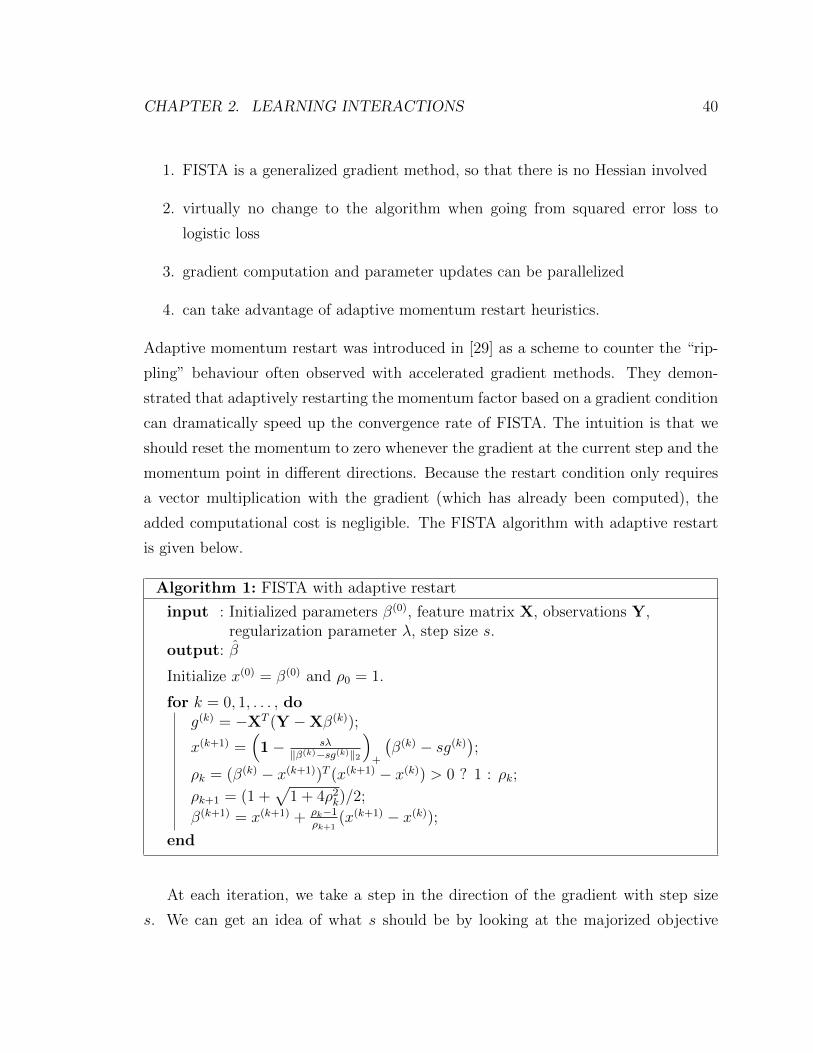
1. FISTA is a generalized gradient method, so that there is no Hessian involved
2. virtually no change to the algorithm when going from squared error loss to
logistic loss
3. gradient computation and parameter updates can be parallelized
4. can take advantage of adaptive momentum restart heuristics.
Adaptive momentum restart was introduced in [29] as a scheme to counter the “rip-
pling” behaviour often observed with accelerated gradient methods. They demon-
strated that adaptively restarting the momentum factor based on a gradient condition
can dramatically speed up the convergence rate of FISTA. The intuition is that we
should reset the momentum to zero whenever the gradient at the current step and the
momentum point in different directions. Because the restart condition only requires
a vector multiplication with the gradient (which has already been computed), the
added computational cost is negligible. The FISTA algorithm with adaptive restart
is given below.
Algorithm 1: FISTA with adaptive restart
input : Initialized parameters β(0), feature matrix X, observations Y,regularization parameter λ, step size s.
output: β
Initialize x(0) = β(0) and ρ0 = 1.
for k = 0, 1, . . . , dog(k) = −XT (Y −Xβ(k));
x(k+1) =(1− sλ
‖β(k)−sg(k)‖2
)+
(β(k) − sg(k)
);
ρk = (β(k) − x(k+1))T (x(k+1) − x(k)) > 0 ? 1 : ρk;
ρk+1 = (1 +√
1 + 4ρ2k)/2;
β(k+1) = x(k+1) + ρk−1ρk+1
(x(k+1) − x(k));end
At each iteration, we take a step in the direction of the gradient with step size
s. We can get an idea of what s should be by looking at the majorized objective

CHAPTER 2. LEARNING INTERACTIONS 41
function about a fixed point β0:
M(β) = L(Y,X; β0) + (β − β0)Tg(β0) +1
2s‖β − β0‖22 + λ
p∑i=1
‖βi‖2. (2.82)
Here, g(β0) is the gradient of the negative log-likelihood L(Y,X; β) evaluated at
β0. Majorization-minimization schemes for convex optimization choose s sufficiently
small so that the LHS of (2.82) is upper bounded by the RHS. One strategy is to
start with a large step size, then backtrack until this condition is satisfied. We use
an approach that is mentioned in [4] that adaptively initializes the step size with
s =‖β(k) − β(k−1)‖2‖gk − gk−1‖2
. (2.83)
We then backtrack from this initialized value if necessary by multiplying s with
some 0 < α < 1. The interested reader may refer to [37] for more details about
majorization-minimization schemes for the group-lasso.
2.9 Discussion
We introduced glinternet, a method for learning linear interaction models that
satisfy strong hierarchy. We demonstrated that the method is comparable with past
approaches, but has the added advantage of being able to accommodate both cate-
gorical and continuous variables on a larger scale. We illustrated the method with
several examples using real and simulated data, and also showed that glinternet
can be applied to genome wide association studies.
glinternet is available on CRAN as a package for the statistical software R.

Chapter 3
EEG source estimation
We now turn to our second application: EEG source estimation via the group-lasso
for matrix-valued features. We begin by giving an overview of the problem, past
work, and why current methods are inadequate for our purposes.
3.1 Introduction
Non-invasive recordings of human brain activity through electroencephalography (EEG)
or magnetoencelphalography (MEG) are of value for both basic science and clinical
applications in sensory, cognitive, and affective neuroscience. These methods provide
high-temporal resolution measures of neural activity. When combined with inverse
modeling techniques, they also provide information about the underlying distribution
of neural activity.
3.1.1 Past approaches
The first approach to electromagnetic source localization involved fitting of a single
equivalent current dipole to scalp EEG measurements ( [34], [44]). Starting in the
1990’s, distributed inverse solutions based on the minimum L2 norm (also known as
ridge regression) approach began to appear ( [9], [18], [31], [46]). These methods
model the underlying source distribution as a large set of elementary currents either
42

CHAPTER 3. EEG SOURCE ESTIMATION 43
distributed throughout the intra-cranial volume or constrained to gray matter. Be-
cause the distributed inverse problem is heavily under-determined, there are infinitely
many solutions that will recreate the observed signal perfectly. Regularized methods
are able to circumvent this problem by penalizing the estimated coefficients, so that
one obtains not just a unique source solution, but one that is also more sensible. The
L2 penalty is based on source power: many weakly activated sources are preferred
over fewer but stronger sources [39]. Because of this L2 minimum norm solutions are
blurry and contain inverted sign “ghost sources” [17].
Following this early work, alternative penalty functions with Lp norms where p < 2
have been applied to the EEG/MEG inverse problem ( [15], [26], [43]). A L1 (lasso)
penalty [40] results in estimates of the sources where only a small number of the
vertices are nonzero. This has the advantage of being able to produce estimates that
are highly localized. However, these approaches can be unstable, and this has limited
their wide-spread application: their susceptibility to noise and independent estimation
at each time-point causes the highly focal recovered sources to shift unpredictably
from locus to locus over time.
Spatial smoothing can alleviate the instability of L1-penalized methods, but at
the expense of the focality of the source estimate. Alternatively, temporal constraints
can be imposed to promote smoothness without sacrificing focality ( [13], [16], [30],
[32], [47], [48]).
A more recent development is to use an elastic-net type of penalty ( [51], [25]).
These penalties employ a combination of L1 and L2 penalties to reap the benefits
that each has to offer. They retain the sparsity of the recovered sources that a pure
L1 penalty provides, while the L2 penalty serves as a smoother that takes care of the
instabilities in the L1 solution. The method we propose in this thesis builds on the
elastic-net approach by extending it to groups of vertices on a cortical surface mesh:
we are able to obtain sparsity on the group level while maintaining smoothness.
CHAPTER 3. EEG SOURCE ESTIMATION 44
3.1.2 Assimilating information from multiple subjects
The approaches mentioned above have largely been applied in the context of single-
subject source recovery. One reason is that the methods are inherently unable to pool
information across multiple subjects. For example, the L2 minimum norm approach
on S subjects decouples into S individual minimum norm problems, each of which can
be solved independently of the others. Pooling can be achieved via a post-processing
step. For example, one could average the recovered sources across subjects to get a
final estimate.
Instabilities in sparse solutions also pose a problem when performing multi-subject
analyses in a common anatomical framework: individual, highly sparse activations
tend to not overlap in the common space, leading to low levels of statistical significance
with the statistical parametric mapping approaches that are used. A previous solution
to this problem uses a hierarchical Bayes technique that fits a Gaussian process with
a choice of kernel that imposes group structure ( [19], [24]). This framework also
utilizes a common anatomical space for inversion in which a template cortical surface
is fit to the brains of each individual subject [27].
3.1.3 This thesis
We develop a new source inversion procedure that is based on a generalization of the
L1 penalty called the group-lasso [49]. While the L1 penalty works by setting the
estimates for single sources to zero, the group-lasso is able to zero out sources as a
group. In other words, if we label some sources as belonging to the same group, then
either all the sources in this group will be estimated to be zero, or all are nonzero
(some can be zero by random chance, but this is rare).
This property of the group-lasso allows us to avoid using a template procedure to
provide a common space for inversion. Instead, we provide a principled approach to
defining groups. This approach is based on individually measured regions of interest
(ROIs) determined by functional MRI (fMRI). In the example presented here, ROIs
are determined for the visual system with retinotopic mapping via fMRI ( [1], [2], [8]).
The visual system contains several topographic maps of the visual field and these
CHAPTER 3. EEG SOURCE ESTIMATION 45
maps correspond to distinct visual areas that have different functional properties.
The location of these areas is only loosely constrained to sulci and gyri, particularly
as moves from V1 and V2, located in and around the calcarine sulcus to higher order,
extra-striate areas. Separating the source via inverse methods is particularly difficult
in the visual system because the ROIs can be in close spatial proximity and because
of the complexities that result from folding and positioning of the surface of the brain
with respect to itself and the sensors. In general, these effects cause some regions to
be aliased with others in the inverse, effectively competing with each other in claiming
responsibility for the signal. There can also be negative correlations within an area
due to tissue orientation effects which create cancellation, i.e. instead of region A
correctly showing signal x and region B signal 0, A shows signal x + y and B signal
y, because the y cancels out.
Because the ROIs provide a functional grouping of the sources in visual activation
studies, the group-lasso naturally applies to this setting. The group-lasso will estimate
the sources for an entire ROI to be zero or nonzero, and thus pinpoints which areas
are responsible for generating the signal. A second advantage of the group-lasso is
that it is able to pool information across multiple subjects in a way that improves
the source estimates for individual subjects. In this case a group is the union of the
vertices in the corresponding ROIs across the subjects. Recall that the same ROI can
have different orientations from subject to subject, so that in some subjects, a ROI
might have weak explanatory power for the signal (due to cancellation or correlation
with other ROIs), but this same ROI could be strong in other subjects. The group-
lasso “settles disputes” by giving the responsibility to the region that appears to be
strongest in aggregate over all the subjects. This is illustrated in Figure 3.1.
In the cartoon, we illustrate the brains of six subjects and 3 different ROIs are
indicated. The strength of the shading indicates the strength of the recovered signal.
In reality the pink and the green ROIs are activated. Due to different positioning and
aliasing in their separate forward matrices, in some subjects some of this activation is
attributed to the blue ROI. In particular, in subject 1 the blue ROI is stronger than
the green. The group-lasso ties the corresponding ROIs across subjects together. It
decides collectively, for example, that green is on, in which case it will be on in all
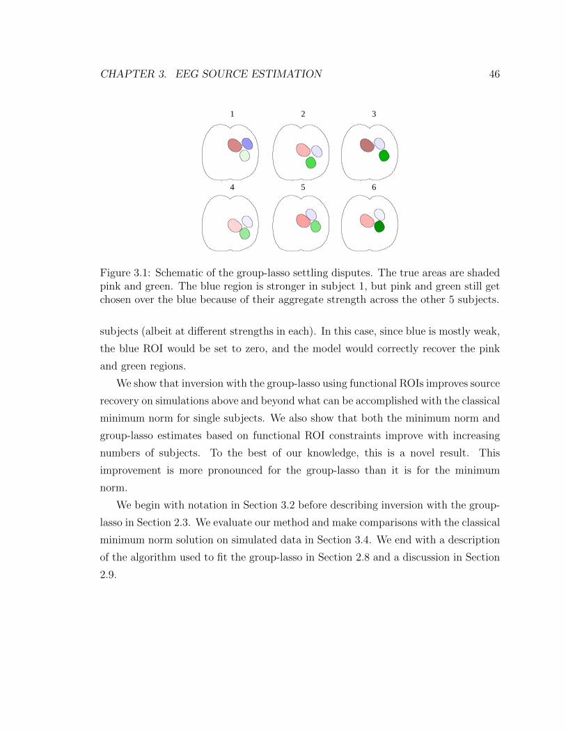
CHAPTER 3. EEG SOURCE ESTIMATION 46
1 2 3
4 5 6
Figure 3.1: Schematic of the group-lasso settling disputes. The true areas are shadedpink and green. The blue region is stronger in subject 1, but pink and green still getchosen over the blue because of their aggregate strength across the other 5 subjects.
subjects (albeit at different strengths in each). In this case, since blue is mostly weak,
the blue ROI would be set to zero, and the model would correctly recover the pink
and green regions.
We show that inversion with the group-lasso using functional ROIs improves source
recovery on simulations above and beyond what can be accomplished with the classical
minimum norm for single subjects. We also show that both the minimum norm and
group-lasso estimates based on functional ROI constraints improve with increasing
numbers of subjects. To the best of our knowledge, this is a novel result. This
improvement is more pronounced for the group-lasso than it is for the minimum
norm.
We begin with notation in Section 3.2 before describing inversion with the group-
lasso in Section 2.3. We evaluate our method and make comparisons with the classical
minimum norm solution on simulated data in Section 3.4. We end with a description
of the algorithm used to fit the group-lasso in Section 2.8 and a discussion in Section
2.9.
CHAPTER 3. EEG SOURCE ESTIMATION 47
3.2 Notation
We set forth notation that will be used throughout this thesis. We define 18 ROIs
per subject (see Section 3.3.1 for details). Let pi, i = 1, . . . , 18 denote the number
of vertices in the i-th ROI, and let Fi, i = 1, . . . , 18 denote the forward matrix for
the i-th ROI. We use Y to represent the N × T matrix consisting of N observations
along T time points, and βi is the pi × T matrix of neural activity in the i-th ROI
that we wish to recover. The overall forward matrix is denoted by
F = [F1,F2, . . . ,F18], (3.1)
and
β =
β1
β2...
β18
(3.2)
is the overall matrix of neural activity. When referring to multiple subjects, we use
superscripts to index the subject, so that Fki is the N × pki forward matrix for subject
k’s i-th ROI, and similarly for the overall forwards Fk. Note that Fki and Fl
i can have
different numbers of columns, and that there is in general no correspondence between
the individual elements of βki and βli.
The forward model that relates the neural activity to the sensor observations can
now be expressed as
Y = Fβ + ε (3.3)
=18∑i=1
Fiβi + ε, (3.4)
where ε is a noise term, typically assumed to be distributed as N(0, σ2I). More
complicated models with correlated noise may be more realistic, but are beyond the
scope of this work.

CHAPTER 3. EEG SOURCE ESTIMATION 48
3.3 Methodology
3.3.1 Defining regions of interest (ROIs) in the visual cortex
As noted above, grouping of features for group-lasso estimation benefits from a ratio-
nal basis for defining the groups and here we exploit the multiple retinotopic mappings
of the visual field onto the visual cortex to comprise the basis for group formation.
For purposes of the present analysis, we defined the detailed 3D shape of each of 18
visual ROIs in 25 participants (V1-L, V1-R, V2v-L, V2v-R, V2d-L, V2d-R, V3v-L,
V3v-R, V3d-L, V3d-R, V4-L, V4-R, V3A-L, V3A-R, LOC-L, LOC-R, MT-L, MT-R).
These definitions are based on high-resolution T1 anatomical scans combined w func-
tional MRI scans (fMRI). Structural and functional MRI scanning was conducted at
3T (Siemens Tim Trio, Erlangen, Germany) using a 12-channel head coil. We ac-
quired a T1-weighted MRI dataset (3-D MP-RAGE sequence, 0.8 × 0.8 × 0.8 mm3
and a 3-D T2-weighted dataset (SE sequence at 1× 1× 1 mm3 resolution) for tissue
segmentation and registration with the functional scans. For fMRI, we employed a
single-shot, gradient-echo EPI sequence (TR/TE = 2000/28 ms, flip angle 80, 126
volumes per run) with a vertex size of 1.7× 1.7× 2 mm3 (128× 128 acquisition ma-
trix, 220 mm FOV, bandwidth 1860 Hz/pixel, echo spacing 0.71 ms). We acquired
30 slices without gaps, positioned in the transverse-to-coronal plane approximately
parallel to the corpus callosum and covering the whole cerebrum. Once per session,
a 2-D SE T1-weighted volume was acquired with the same slice specifications as the
functional series in order to facilitate registration of the fMRI data to the anatomical
scan.
The FreeSurfer software package (http://surfer.nmr.mgh.harvard.edu) was used
to perform gray and white matter segmentation to define a cortical surface mesh
with accurate surface normals. The FreeSurfer package extracts both gray/white
and gray/cerebrospinal fluid (CSF) boundaries, but these surfaces can have different
surface orientations. In particular, the gray/white boundary has sharp gyri (the
curvature changes rapidly) and smooth sulci (slowly changing surface curvature),
while the gray/CSF boundary is the inverse, with smooth gyri and sharp sulci. We
created a new surface that had a similar curvature for both gyri and sulci, avoiding

CHAPTER 3. EEG SOURCE ESTIMATION 49
these curvature discontinuities. The new surface generated by interpolating a position
that was midway between the gray/white surface and the gray/CSF surface.
The highest accuracy for source-imaging is obtained when there is an accurate
model that connects activity at each location on the surface of cortex with how it will
be measured at the scalp. To generate realistic scalp topographies, we made separate
forward models for each participant in the study using the Boundary Element Method
(BEM) with conductivity models that were derived from the T1 and T2 weighted MRI
scans of each observer. The FSL toolbox (http://www.fmrib.ox.ac.uk/fsl/) was also
used to segment contiguous volume regions for the scalp, outer skull, and inner skull
and to convert these MRI volumes into inner skull, outer skull, and scalp surfaces [38].
The general procedures for the scans used to define the visual areas (head stabi-
lization, visual display system, etc) are standard and have been described in detail
elsewhere [6]. Retinotopic field mapping defined ROIs for visual cortical areas V1,
V2v, V2d, V3v, V3d, V3A, and V4 in each hemisphere ( [42], [45]). ROIs corre-
sponding to hMT+ were identified using low contrast motion stimuli similar to those
described in [20]. In this study, the fMRI data was used purely to define ROIs for
the EEG analysis.
3.3.2 Collaborative effect from multiple subjects
The “all zero or all nonzero” property of the group-lasso estimates allows the group-
lasso to pool information across multiple subjects; see Section 3.1.3 for a graphical
illustration of this. We thus expect the results of inversion to improve with the number
of subjects. One way to make use of the data from multiple subjects is to build a large
forward matrix by stacking the individual matrices from each subject, and similarly
for the observations. We do not do this because accounting for the different ROI
sizes across subjects can get messy, and we also want to impose both spatial (across
vertices) and temporal smoothness in the recovered activity. The dimension reduction
that results from smoothing also leads to computational speedups.
Because column c of a subject’s forward matrix measures the contribution of vertex
c to each of the N sensors, we expect neighboring vertices to have roughly the same

CHAPTER 3. EEG SOURCE ESTIMATION 50
contribution, that is, the contributions should vary smoothly as we travese the vertices
in a ROI. We thus expect the forward matrices Fi to be low rank where most of the
variation can be captured by the top few principal components. We use 5 components
because the orientation of a ROI can be parametrized with 3 spatial coordinates along
with 2 rotation angles, and this seems to work well in our experiments. This method
of spatial smoothing respects the borders of the functional areas: smoothing does
not occur across areas that may differ in their functional specificity, as might happen
with a purely spatial smoothing such as that used in LORETA [31].
Recall that Fki denotes the N×pki forward matrix of subject k that corresponds to
ROI i. Let Pki denote the pki × 5 matrix consisting of the first 5 right singular vectors
of the centered Fki . The columns of Pk
i are a smooth basis across the space of vertices,
and we can impose spatial smoothness on the recovered activity by constraining βki
to this basis:
βki = Pki β′ki . (3.5)
It follows that each β′ki is a 5×T matrix. The observed signal contribution from ROI
i in subject k can then be written as
Fki β
ki = Fk
iPki β′ki (3.6)
= Xki β′ki , (3.7)
where
Xki = Fk
iPki (3.8)
is the N × 5 matrix consisting of the first 5 principal components of Fki . We call
Xki the derived forward matrix for ROI i in subject k. The overall derived forward

CHAPTER 3. EEG SOURCE ESTIMATION 51
matrix for S subjects can then be constructed by
X =
X1
1 · · · X118
X21 · · · X2
18
. . . · · · . . .
XS1 · · · XS
18
. (3.9)
We can write X in more compact form (recall that subscripts index ROIs and super-
scripts index subjects) by
X = [X1,X2, . . . ,X18], (3.10)
where
Xi =
X1i
X2i
. . .
XSi
. (3.11)
Similarly, we construct the spatially smoothed activity for S subjects for ROI i by
writing
β′i =
β′1i
β′2i...
β′Si
. (3.12)
Combining observations from various subjects is more straightforward, and can

CHAPTER 3. EEG SOURCE ESTIMATION 52
be done by simply stacking the observations:
Y =
Y1
Y2
...
YS
. (3.13)
The group-lasso objective for the derived forward matrices Xi and the spatially
smoothed activity β′ can now be written as
argminµ,β′1
2
∥∥∥∥∥Y − 1µt −18∑i=1
Xiβ′i
∥∥∥∥∥2
F
+ λ18∑i=1
γi‖β′i‖F + α‖β′‖2F . (3.14)
The group-lasso has an important advantage that none of the previously men-
tioned methods have. Because a group now consists of a single ROI across multiple
subjects, there is a collaborative effect in that as long as a ROI has a strong signal
in enough subjects, we will estimate that ROI to be nonzero even in those subjects
where that ROI is not quite lighting up. Consider subject 1 in Figure 3.1. The blue
region (wrong) appears to be stronger than the green region (correct). This could
be due to the blue region being highly correlated with the green region, noise in the
data, or some other region that is cancelling out the signal from the green region. In
any case, the blue region is competing with the green region for attention, and if we
tried to recover the activity with subject 1 alone, the group-lasso is likely to pick the
blue region over the green region, resulting in a mistake. But if we fit the group-lasso
on all 6 subjects, the other 5 subjects would clearly vote in favor of the green over the
blue, and as a result, we will select the green region for subject 1. And because the
blue region is zeroed out in the other 5 subjects, it will also be zeroed out in subject
1, i.e. there is no competition from the blue region, and the green region can be fully
fit to the signal. This is to be constrasted with a method like the minimum norm
or elastic-net, where both methods would be happy with dividing the signal between
the green and blue regions in order to get the best fit, so that both would be nonzero.

CHAPTER 3. EEG SOURCE ESTIMATION 53
The minimum norm and elastic-net are inherently unable to pool information
across subjects. Any such pooling has to be done manually as a postprocessing step,
such as averaging the estimated sources over the multiple subjects. Naturally, this
can be done for the group-lasso as well. We expect this pooling effect to be stronger
as the number of subjects increases, and we show in Section 3.4 that this is indeed
the case.
3.3.3 Imposing temporal smoothness
In the spirit of the previous section, it is reasonable to assume that the neural activity
also varies smoothly over time, and we can impose temporal smoothness in the esti-
mated source by finding a suitable basis for the time component. The right singular
vectors of Y are a natural basis for the temporal component:
YN×T = UN×NDN×TVtT×T . (3.15)
The singular value decomposition is also used in [13] to obtain the principal directions
along the time axis, but there they use 5 singular vectors. We fix the dimension d
of this basis by taking as many singular vectors as we need to explain 99% of the
variance of Y. In particular, this is given by
d = argmink
{k :
∑ki=1 d
2ii∑N
i=1 d2ii
≥ 0.99
}. (3.16)
In our experiments, this number is typically 2. Let Vd be the matrix consisting of
the first d columns of V. We restrict β′ to the space spanned by Vd by setting
β′ = βVtd. (3.17)
Applying this restriction to (3.14) gives
argminµ,β1
2
∥∥∥∥∥Y − 1µt −18∑i=1
XiβiVtd
∥∥∥∥∥2
F
+ λ
18∑i=1
γi‖βiVtd‖F + α‖βVt
d‖2F . (3.18)

CHAPTER 3. EEG SOURCE ESTIMATION 54
Because Vd is orthonormal, this is equivalent to
argminµ,β1
2
∥∥∥∥∥Y − 1µt −18∑i=1
Xiβi
∥∥∥∥∥2
F
+ λ18∑i=1
γi‖βi‖F + α‖β‖2F , (3.19)
where Y = YVd is the N × d matrix of temporally smoothed observations.
After spatial and temporal smoothing, we have, for S subjects, the NS×d matrix
Y of smoothed observations, the NS × (S · 18 · 5) derived forward matrix X, and
the (S · 18 · 5) × d matrix β of smoothed activity that we need to estimate. This is
achieved by solving (3.19).
3.3.4 Recovering the activity in the original space
We transform the estimated ˆβ back to the original space by reversing the temporal
smoothing and dimension reduction operations. We illustrate for a single subject.
Let
P =
P1
. . .
P18
(3.20)
denote the block diagonal matrix consisting of the Pi’s in (3.5). From (3.5), it is clear
that reversing the spatial smoothing can be done by left-multiplying our solution ˆβ
by P. Similarly, (3.17) shows that right-multiplying by Vtd reverses the temporal
smoothing. To summarize, our estimate of the source activity in the original space is
given by
β = P ˆβVtd. (3.21)

CHAPTER 3. EEG SOURCE ESTIMATION 55
3.3.5 Model selection
Generalized cross validation (GCV) is one method of model selection that is intuitively
simple and widely used. Let Y be the N×T -matrix of observations, and Y the fitted
values. The GCV error for this fit is given by
1NT‖Y − Y‖2F
(1− df(Y)NT
)2, (3.22)
where df(Y) is the degrees of freedom for Y. Fitting the group-lasso along a grid of
λ values results in a GCV error curve. We then pick the λ that gives the minimum
value on this curve. Full details on determining the degrees of freedom df(Y) for the
group-lasso solutions and selecting the α parameter in (1.8) are given in Appendix
A.
3.4 Results
We make comparisons between the group-lasso and minimum norm methods through
simulation. We also evaluate the methods on multiple subjects (up to 25), and demon-
strate that the effectiveness of the group-lasso increases with the number of subjects.
The minimum norm method does not inherently pool information across multiple
subjects, but we can average the recovered acitivity across subjects for each ROI as
a post-processing step. This ROI-based averaging improves performance for both the
group-lasso and the minimum norm. We begin by describing the simulation process.
3.4.1 Experimental setup
We select ROIs V2v-L and V4-R as the ground truth. These areas are separated
by about a centimeter, on average, and exhibit considerable cross-talk between their
forward vectors. The neural activity in each is generated as follows. For each region we
randomly sample a number from {1, 1.1, 1.2, . . . , 1.9, 2, 2.1, . . . , 9.9, 10}, then assign a
randomly chosen cluster within that region with this value. This cluster comprises
about 30% of the total size of the region. Therefore V2v-L and V4-R each have

CHAPTER 3. EEG SOURCE ESTIMATION 56
constant activity in about 30% of their vertices. We then pass the activity through
the forward model to obtain the observed time courses Y. We add Gaussian white
noise to Y to obtain a signal to noise ratio of 0.32. In all cases, we take N = 128
observations/sensors and T = 91 time points.
The methods are evaluated on 3 measures (see [8] for more details):
1. Area under the ROC curve (AUC)
2. Mean squared error (MSE) on the neural activity, given by 1NT‖β − β‖2F
3. Relative energy, given by the ratio between the normalized energies contained
in the estimate of the active sources and the global distribution:∑i∈AEest(i)∑iEest(i)
, (3.23)
where A is the set of active vertices in the true neural activity and Eest(i) is
the energy of the estimated signal at vertex i.
For a single subject, we compute these metrics for each of the T time points, then
take the average. For multiple subjects, we compute this time average separately for
each subject, and then take the average across all subjects.
3.4.2 A single subject
We illustrate the performance of the group-lasso inversion for a single subject on
one instance of simulated data. Because both the group-lasso and minimum norm
methods produce a sequence of fits, we can visualize their performance as we move
along their solution paths. One way to do this is to plot their performance as a
function of variance explained (r2) on the training data. The r2 is defined by
r2 = 1− ‖Y − Y‖2F‖Y − Y‖2F
(3.24)
where Y is the fit and Y is the matrix whose i-th column is the mean of the i-th
column of Y. We plot the 3 metrics as a function of r2 in Figure 3.2.
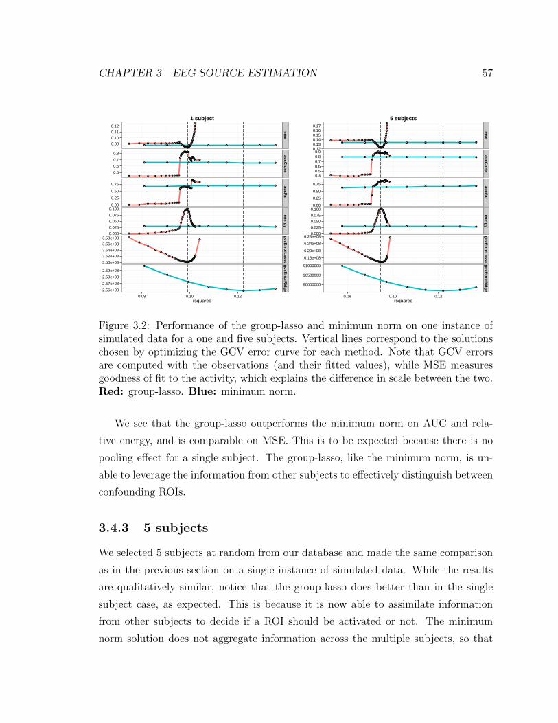
CHAPTER 3. EEG SOURCE ESTIMATION 57
● ● ● ● ● ● ● ● ● ●●●●●●●●●●●●●●●●●●
●●●●●●●●●●●●
●
●
●
●
●
● ● ● ● ● ● ● ●
● ● ● ● ● ● ● ● ● ●●●
●●●●●●●●●●●●●●●
●●●●●●●
●●●●●●●●●● ●
● ● ● ● ● ● ● ●
● ●● ● ● ● ● ● ● ●●●
●●●●●●●●●●●●●●●●●●●●●●
●●●●●●●●●● ●
● ● ● ● ● ● ● ●
● ● ● ● ● ● ● ● ● ●●●●
●
●
●
●●●●●●
●●●●●●●●●●●●●●●●●●●●●●
●● ● ● ● ● ● ● ●
●
●
●
●
●
●●
●● ●●●●●●●●●●●●●●●●●●●●
●●●●●●●●
●●●●●●●
●
●
●
●
●
●● ●
●
0.09
0.10
0.11
0.12
0.5
0.6
0.7
0.8
0.00
0.25
0.50
0.75
0.000
0.025
0.050
0.075
0.100
3.50e+08
3.52e+08
3.54e+08
3.56e+08
3.58e+08
2.56e+08
2.57e+08
2.58e+08
2.59e+08m
seaucC
loseaucFar
energygcvE
rrorLassogcvE
rrorRidge
0.08 0.10 0.12rsquared
1 subject
● ● ● ● ● ● ● ● ●●●●●●●●●●●●●●●●●●●●●
●●●●●●●●●
●
●
●
●
●
● ● ● ● ● ● ● ●
● ● ● ● ●● ● ● ●●
●
●●●●●●
●●●●●●●●●●●●●●●●●
●●●●●●●●●
●● ● ● ● ● ● ● ●
● ● ● ● ●● ● ● ●●
●
●●●●●●●●●●●
●●●●●●●●●●●●●●●●●●●●●
●
● ● ● ● ● ● ● ●
● ● ● ● ● ● ● ● ●●●
●
●
●●●●
●
●●●●
●●●●●●●●●●●●●●●●●●●●●
●● ● ● ● ● ● ● ●
●
●
●
●
●●
●●
●●●●●●●●●●●●●●●●●●●●●●●●●●●●
●●●●●●●
●
●
●
●
●
●●
●
●
0.120.130.140.150.160.17
0.40.50.60.70.80.9
0.00
0.25
0.50
0.75
0.000
0.025
0.050
0.075
0.100
6.16e+08
6.20e+08
6.24e+08
6.28e+08
90000000
90500000
91000000
mse
aucClose
aucFarenergy
gcvErrorLasso
gcvErrorR
idge
0.08 0.10 0.12rsquared
5 subjects
Figure 3.2: Performance of the group-lasso and minimum norm on one instance ofsimulated data for a one and five subjects. Vertical lines correspond to the solutionschosen by optimizing the GCV error curve for each method. Note that GCV errorsare computed with the observations (and their fitted values), while MSE measuresgoodness of fit to the activity, which explains the difference in scale between the two.Red: group-lasso. Blue: minimum norm.
We see that the group-lasso outperforms the minimum norm on AUC and rela-
tive energy, and is comparable on MSE. This is to be expected because there is no
pooling effect for a single subject. The group-lasso, like the minimum norm, is un-
able to leverage the information from other subjects to effectively distinguish between
confounding ROIs.
3.4.3 5 subjects
We selected 5 subjects at random from our database and made the same comparison
as in the previous section on a single instance of simulated data. While the results
are qualitatively similar, notice that the group-lasso does better than in the single
subject case, as expected. This is because it is now able to assimilate information
from other subjects to decide if a ROI should be activated or not. The minimum
norm solution does not aggregate information across the multiple subjects, so that

CHAPTER 3. EEG SOURCE ESTIMATION 58
its performance is similar to the single subject case.
Notice that the group-lasso solution near the end of the path exhibits large MSE
in both the 1 and 5 subject cases. This is is likely due to the spatial smoothing and
temporal smoothing, but mostly due to the former. To see this, we generate activity
β for a single subject, then compute
‖β −PPTβ‖2F (3.25)
for varying numbers of principal components, and
‖β − βVdVTd ‖2F (3.26)
for varying d (P and Vd defined in Sections 3.3.2 and 3.3.3). These computations
tell us how we can expect to perform on MSE if we knew the true activity β, but
subjected it to the smoothness constraints.

CHAPTER 3. EEG SOURCE ESTIMATION 59
0.0
0.1
0.2
0.3
0 1 2 3 4 5 6 7 8 9Number of principal components or right singular vectors of Y
MS
E
mseFromPCA of forward matricesTemporal smoothing
Figure 3.3: MSE from dimension reduction by principal components and temporalsmoothing with right singular vectors of Y, averaged over 100 simulations. A largeportion of the MSE is due to the dimension reduction from taking the first 5 principalcomponents for each ROI.
The observed MSE is on the order of that seen in Figure 3.2. The rapid increase in
MSE is also due to an increase in variance as we decrease the amount of regularization.
For a single subject, there are Nd observations and 18 · 5 · d parameters (see the end
of Section 3.3.3), so that as λ ↓ 0, we approach a near-saturated fit.
3.4.4 Better performance with more subjects
We next investigate how the performance of the group-lasso scales with the number
of subjects. We take 1, 2, 4, 8, 16, and 25 subjects, and for each situation, we fit the
group-lasso and minimum norm methods on 20 different instances of simulated data.
We then compute the average performance across the 20 simulations.
The metrics, along with standard error bars, are plotted as a function of the
number of subjects in Figure 3.4.
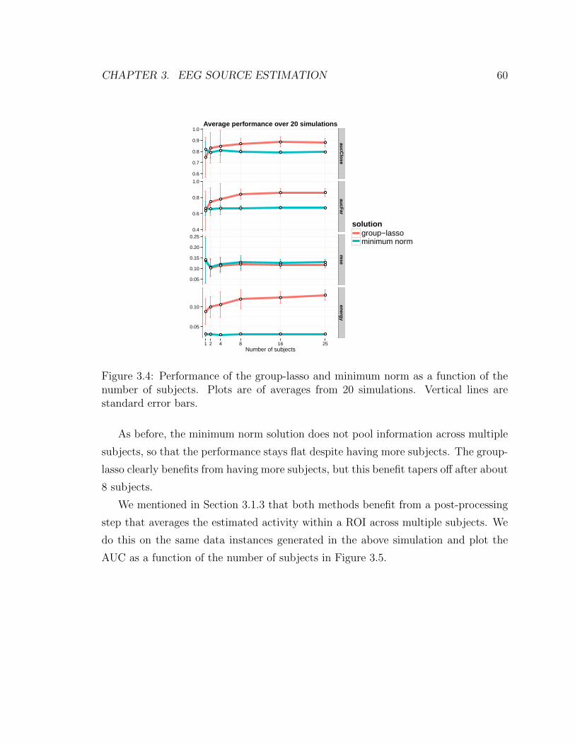
CHAPTER 3. EEG SOURCE ESTIMATION 60
●●
● ● ● ●
●
●●
●● ●
● ● ● ● ● ●●
●●
●● ●
●
●●
● ● ●●
●●
● ● ●
● ● ● ● ● ●
●
●●
●●
●
0.6
0.7
0.8
0.9
1.0
0.4
0.6
0.8
1.0
0.05
0.10
0.15
0.20
0.25
0.05
0.10
aucClose
aucFarm
seenergy
1 2 4 8 16 25Number of subjects
solutiongroup−lassominimum norm
Average performance over 20 simulations
Figure 3.4: Performance of the group-lasso and minimum norm as a function of thenumber of subjects. Plots are of averages from 20 simulations. Vertical lines arestandard error bars.
As before, the minimum norm solution does not pool information across multiple
subjects, so that the performance stays flat despite having more subjects. The group-
lasso clearly benefits from having more subjects, but this benefit tapers off after about
8 subjects.
We mentioned in Section 3.1.3 that both methods benefit from a post-processing
step that averages the estimated activity within a ROI across multiple subjects. We
do this on the same data instances generated in the above simulation and plot the
AUC as a function of the number of subjects in Figure 3.5.

CHAPTER 3. EEG SOURCE ESTIMATION 61
●
●
●
●
●
●
●
●
●
●
●●
0.6
0.8
1.0
1 2 4 8 16 25Number of subjects
AU
C
solutiongroup−lassominimum norm
AUC from averaging recovered activity
Figure 3.5: AUC obtained after post-processing the recovered activity by averagingacross subjects. Plots are of average values over the same 20 data instances frombefore, along with standard error bars. Notice that the group-lasso with 2 subjectsoften outperforms the minimum norm with 25 subjects.
Both methods get a substantial boost from ROI-based averaging across subjects,
and performance improves as the number of subjects is increased. This is a novel
result, and is distinct from with the effect shown in Figure 3.4. There, the performance
gain is due to the “majority vote” mechanism of the group-lasso as illustrated in
Figure 3.1. Post-processing the recovered activity by ROI averaging serves to further
reduce the variance in the estimates, thus resulting in a higher AUC for not just the
group-lasso, but also for the minimum norm.
3.5 Algorithm details
We describe the algorithm used to obtain the solutions to (1.8). Cyclic group-wise
coordinate descent works well when we have a small number of groups (18 ROIs in

CHAPTER 3. EEG SOURCE ESTIMATION 62
our case). The idea is to update the coefficients for a single group while holding the
coefficients for all other groups fixed. If we cycle through all the groups repeatedly,
we will converge on a solution. Let Y be the matrix of observations, and let X =
[X1, . . . ,Xp] be the matrix of features that consists of p groups.
3.5.1 Cyclic group-wise coordinate descent
Let λ and α be fixed, and suppose we want to perform the update for group k. Let
β1, . . . , βp be the current estimates with current residual given by r = Y−∑p
i=1 Xiβi,
and let rk = r + Xkβk be the partial residual for group k. If βk = 0, the gradient
equation for βk is given by
XTk rk = λγksk, (3.27)
where sk ∈ {z : ‖z‖F ≤ 1}. It follows that βk = 0 if ‖XTk rk‖F < λγk. If βk 6= 0, the
gradient condition for optimality is given by(XTkXk + (
λγk
‖βk‖F+ 2α)I
)βk = XT
k rk (3.28)
We can solve for βk by first solving for ‖βk‖F and then plugging the result into (3.28).
Take the singular value decomposition Xk = UkDkVTk and rewrite (3.28) as
[D2k‖βk‖F + (λγk + 2α‖βk‖F )I
]−1DkU
Tk rk = VT
k
βk
‖βk‖F. (3.29)
Take the Frobenius norm on both sides to obtain∥∥∥∥[D2k‖βk‖F + (λγk + 2α‖βk‖F )I
]−1DkU
Tk rk
∥∥∥∥2F
= 1. (3.30)
Let f(θ) =∥∥[D2
kθ + (λγk + 2αθ)I]−1DkUTk rk∥∥2F−1. To find ‖βk‖F , we need only find

CHAPTER 3. EEG SOURCE ESTIMATION 63
θ0 such that f(θ0) = 0. We do this with Newton-Rhapson by reiterating
θ ←− θ − η f(θ)
f ′(θ), (3.31)
where η is the step size and
f ′(θ) = −2∥∥∥[D2
kθ + (λγk + 2αθ)I]− 3
2 (D2k + 2αI)
12 DkU
Tk rk
∥∥∥2F. (3.32)
In our experience, f(θ) tends to be quite linear around θ0, so that very few Newton
iterations are required for convergence. Having obtained θ0, we update βk with
βk ←−(
XTkXk + (
λγk
θ0+ 2α)I
)−1XTk rk. (3.33)
We now cycle through all the groups until convergence. The full algorithm is presented
in Algorithm 2. In practice, because we are fitting the group-lasso along a sequence of
λ, we will initialize β1, . . . , βp with the estimates from the previous λ in the sequence.
These “warm starts” give a significant speed advantage in our experience.
3.5.2 Determining the group penalty modifiers γi
The γi in (1.8) allow us to have different penalties for different groups. This is useful
because a larger group can be more likely to have a stronger correlation with the
response than a small group, just by random chance. Having different penalties thus
allows us to put different-sized groups on the same scale.
Recall that βk = 0 if the following gradient condition is met:
‖XTk rk‖F < λγk. (3.34)
It follows that we can determine an appropriate group penalty modifier by computing
the expected value of the LHS if the signal were pure noise. Let ε ∼ (0, I). Then we

CHAPTER 3. EEG SOURCE ESTIMATION 64
Algorithm 2: Cyclic group-wise coordinate descent
input : Y, X1, . . . ,Xp, λ, γ1, . . . , γp, α
output: β1, . . . , βp
Initialize r = Y − Y, β1 = 0, . . . , βp = 0. Let Xk = UkDkVTk be the singular
decomposition of Xk.
Iterate till convergence:
for k ← 1 to p do
rk = r + Xkβk;if ‖XT
k rk‖F < λγk then
βk ←− 0;endelse
βk ←−[XTkXk + (λγk
θ+ 2α)I
]−1XTk rk;
where θ is the root of ‖ [D2kθ + (λγk + 2α)I]
−1DkU
Tk rk‖F = 1
end
r←− rk −Xkβk;
end
return β1, . . . , βp
CHAPTER 3. EEG SOURCE ESTIMATION 65
have
γ2k = E‖XTk ε‖2F (3.35)
= E tr εTXkXTk ε (3.36)
= trEεTXkXTk ε (3.37)
= tr XTkXk (3.38)
= ‖Xk‖2F . (3.39)
Therefore we take γk = ‖Xk‖F , the Frobenius norm of Xk. Note that if Xk is
orthonormal, then γk =√pk, which is the penalty modifier proposed in [49].
3.6 Discussion
This work introduces a new approach toward EEG source estimation in the visual
cortex using the group-lasso. Because the group-lasso selects variables in a group-wise
manner, we do not require a template procedure to provide a common space for source
inversion. Instead, we use ROIs that are determined by fMRI to define the groups.
We show how to combine data from multiple subjects while imposing spatial and
temporal smoothness on the recovered activity. The “pooling effect” of the group-
lasso suggests that its performance should improve with the number of subjects, and
we verified this with simulated experiments. In particular, the performance of the
group-lasso is comparable to that of the traditional minimum norm solution, but as
the number of subjects increases, there is a significant performance boost for the
group-lasso over the minimum norm.
We also show that while the minimum norm does not inherently pool information
across multiple subjects, it still benefits from a post-processing step in which the
recovered activity is averaged across subjects. This, to the best of our knowledge, is a
novel result. Of course, this averaging can also be applied to the group-lasso solution,
which leads to a further performance increase beyond that already obtained from its
inherent pooling effect.
The effectiveness of the group-lasso can lead to other interesting possibilities. The

CHAPTER 3. EEG SOURCE ESTIMATION 66
overlapped group-lasso is a special case of the group-lasso in which a variable can show
up in more than one group. It follows that the overlapped group-lasso might be a
good choice for source inversion in cases where the ROIs have overlaps.
Another aspect of ROI-wise source inversion that we have not explored is sparsity
within a ROI. It is possible that the source activity is only present in some fraction of
the ROI, so that a solution that is sparse within a ROI is desirable. If this is the case,
an additional L1 penalty of the form ‖β‖1 can be added to the group-lasso penalty
to impose sparsity. This results in what is known as the sparse-group lasso (see [37]
for details). This, along with the overlapped group-lasso, will be addressed in future
work.

Chapter 4
Conclusion
We applied the group-lasso to two problems from different domains. In the interaction
learning problem, an overlapped group-lasso penalty allowed us to obtain estimates
that satisfy strong hierarchy: if an interaction is estimated to be nonzero, then its
associated main effects will also be estimated to be nonzero. We showed that the
resulting complicated constrained optimization problem can be tackled by solving an
unconstrained problem that gives equivalent solutions. This is the basis for glin-
ternet, which will be available as a R package on CRAN.
The availability of regions of interest in the visual cortex was a key ingredient
in our solution. Because these ROIs define a functional grouping of the vertices in
the visual cortex, it fitted naturally into the group-lasso framework. We showed that
the group-lasso benefits from having data from multiple subjects, resulting in better
performance over the standard minimum norm solution. We also demonstrated that
both the group-lasso and the minimum norm benefit from a post-processing step in
which the recovered activity is averaged (within ROI) across multiple subjects.
67

Appendix A
Model selection details
To the best of our knowledge, there is no analytic form for the degrees of freedom for
the group-lasso. We use the results in [22] as a heuristic for estimating the degree
of freedom. Suppose there are G groups of variables with sizes p1, . . . , pG. Let β0
denote the full ordinary least squares fit, βi the group-lasso estimate for group i, and
Y the fit. Then if the feature matrix X = [X1, . . . ,XG] is orthonormal, an unbiased
estimate of the degrees of freedom is given by
df(Y) =G∑i=1
1(‖βi‖2 > 0) +G∑i=1
(pi − 1)‖βi‖2‖β0
i ‖2. (A.1)
Because X is not orthonormal in our application (see Section 3.3.2), we do not expect
this formula to hold exactly. Simulations show that the estimate given by (A.1) can
be biased low, which results in an overly optimistic GCV error rate. The bias is due to
large variance in β0, making the contribution from the ‖βi‖2‖β0i ‖2
term negligible. Adding
a ridge penalty to β0 largely eliminates this problem. To verify this, we generate data
according to the following setup.
Let Yfixed be a fixed N × T matrix of observations. If Y = Yfixed + ε with
68
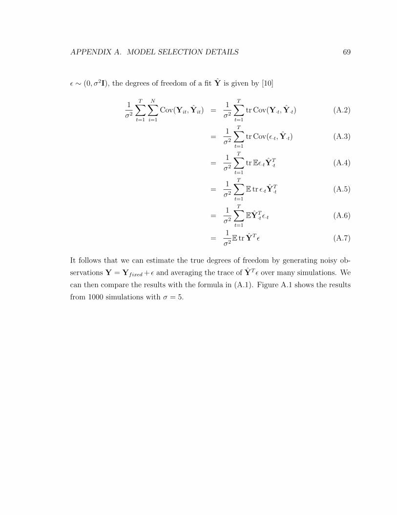
APPENDIX A. MODEL SELECTION DETAILS 69
ε ∼ (0, σ2I), the degrees of freedom of a fit Y is given by [10]
1
σ2
T∑t=1
N∑i=1
Cov(Yit, Yit) =1
σ2
T∑t=1
tr Cov(Y·t, Y·t) (A.2)
=1
σ2
T∑t=1
tr Cov(ε·t, Y·t) (A.3)
=1
σ2
T∑t=1
trEε·tYT·t (A.4)
=1
σ2
T∑t=1
E tr ε·tYT·t (A.5)
=1
σ2
T∑t=1
EYT·t ε·t (A.6)
=1
σ2E tr YT ε (A.7)
It follows that we can estimate the true degrees of freedom by generating noisy ob-
servations Y = Yfixed + ε and averaging the trace of YT ε over many simulations. We
can then compare the results with the formula in (A.1). Figure A.1 shows the results
from 1000 simulations with σ = 5.

APPENDIX A. MODEL SELECTION DETAILS 70
0
10
20
30
40
50
0 10 20 30 40True df
Est
imat
ed d
f
ridge parameter1.0817e40
Figure A.1: Estimated degrees of freedom (using (A.1)) vs true df. Red line: Usingformula (A.1) without any ridge penalty to β0 results in an estimate that is biaseddownward. Blue line: In our experiments, a ridge penalty of 1.0817 × 10⁴ workswell.
Figure A.2 shows that adding a ridge penalty can dramatically reduce the variance
in β0.
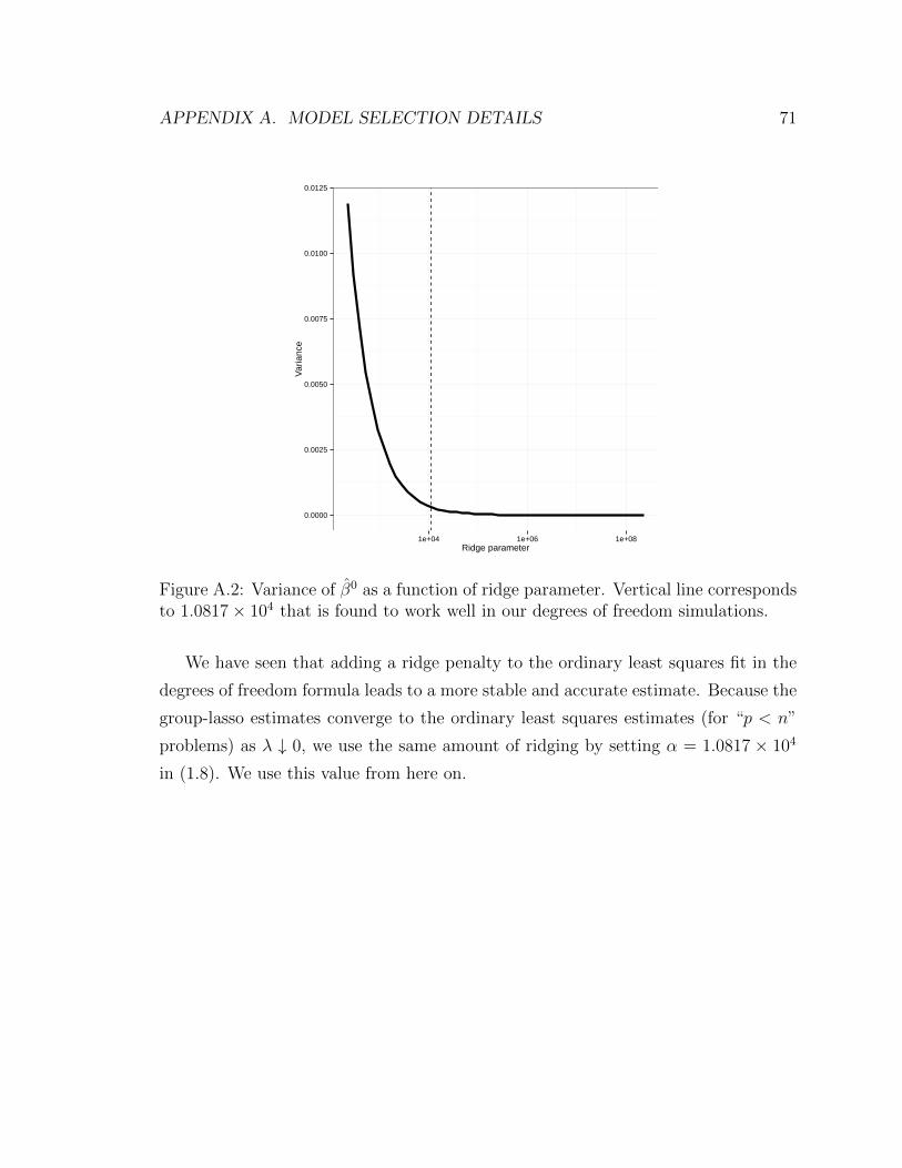
APPENDIX A. MODEL SELECTION DETAILS 71
0.0000
0.0025
0.0050
0.0075
0.0100
0.0125
1e+04 1e+06 1e+08Ridge parameter
Var
ianc
e
Figure A.2: Variance of β0 as a function of ridge parameter. Vertical line correspondsto 1.0817× 10⁴ that is found to work well in our degrees of freedom simulations.
We have seen that adding a ridge penalty to the ordinary least squares fit in the
degrees of freedom formula leads to a more stable and accurate estimate. Because the
group-lasso estimates converge to the ordinary least squares estimates (for “p < n”
problems) as λ ↓ 0, we use the same amount of ridging by setting α = 1.0817 × 10⁴
in (1.8). We use this value from here on.

Bibliography
[1] J.M. Ales and A.M. Norcia. Assessing direction-specific adaptation using the
steady-state visual evoked potential: results from eeg source imaging. Journal
of Vision, 9(7)(8):1–13, 2009.
[2] L. G. Appelbaum, A. R. Wade, V. Y. Vildavski, M. W. Pettet, and A. M.
Norcia. Cue-invariant networks for figure and background processing in human
visual cortex. J Neurosci, 26(45):11695–708, 2006.
[3] Amir Beck and Marc Teboulle. A fast iterative shrinkage-thresholding algorithm
for linear inverse problems. SIAM J. Img. Sci., 2(1):183–202, March 2009.
[4] StephenR. Becker, EmmanuelJ. Candes, and MichaelC. Grant. Templates for
convex cone problems with applications to sparse signal recovery. Mathematical
Programming Computation, 3(3):165–218, 2011.
[5] J. Bien et al. A lasso for hierarchical interactions. The Annals of Statistics, 2013.
[6] AA Brewer, J Liu, AR Wade, and BA Wandell. Visual field maps and stimulus
selectivity in human ventral occipital cortex. Nat Neurosci, 8:1102–1109, 2005.
[7] C.C.M. Chen, H. Schwender, J. Keith, R. Nunkesser, K. Mengersen, and
P. Macrossan. Methods for identifying snp interactions: A review on varia-
tions of logic regression, random forest and bayesian logistic regression. Com-
putational Biology and Bioinformatics, IEEE/ACM Transactions on, 8(6):1580
–1591, nov.-dec. 2011.
72

BIBLIOGRAPHY 73
[8] B. R. Cottereau, J. M. Ales, and A. M. Norcia. Increasing the accuracy of elec-
tromagnetic inverses using functional area source correlation constraints. Hum
Brain Mapp, 33(11):2694–713, 2012.
[9] A. Dale and M. Sereno. Improved localization of cortical activity by combining
eeg and meg with mri cortical surface reconstruction: a linear approach. J Cogn
Neurosci, 5(162-176), 1993.
[10] Bradley Efron. How Biased is the Apparent Error Rate of a Prediction Rule?
Journal of the American Statistical Association, 81(394):461–470, 1986.
[11] Yoav Freund and Robert E. Schapire. A decision-theoretic generalization of
on-line learning and an application to boosting. In Proceedings of the Second
European Conference on Computational Learning Theory, EuroCOLT ’95, pages
23–37, London, UK, UK, 1995. Springer-Verlag.
[12] Jerome H. Friedman. Greedy Function Approximation: A Gradient Boosting
Machine. In Annals of Statistics, volume 29, pages 1189–1232, 2000.
[13] K. Friston, L. Harrison, J. Daunizeau, S. Kiebel, C. Phillips, N. Trujillo-Barreto,
R. Henson, G. Flandin, and J. Mattout. Multiple sparse priors for the m/eeg
inverse problem. Neuroimage, 39(3):1104–20, 2008.
[14] G. Golub et al. Generalized cross-validation as a method for choosing a good
ridge parameter. Technometrics, 21(2):215–223, 1979.
[15] I. F. Gorodnitsky, J. S. George, and B. D. Rao. Neuromagnetic source imaging
with focuss: a recursive weighted minimum norm algorithm. Electroencephalogr
Clin Neurophysiol, 95(4):231–51, 1995.
[16] A. Gramfort, M. Kowalski, and M. Hamalainen. Mixed-norm estimates for the
m/eeg inverse problem using accelerated gradient methods. Phys Med Biol,
57(7):1937–61, 2012.

BIBLIOGRAPHY 74
[17] R. Grech, T. Cassar, J. Muscat, K. P. Camilleri, S. G. Fabri, M. Zervakis, P. Xan-
thopoulos, V. Sakkalis, and B. Vanrumste. Review on solving the inverse problem
in eeg source analysis. J Neuroeng Rehabil, 5:25, 2008.
[18] M. Hamalainen, R. Ilmoniemi, J. Knuutila, and O. Lounasmaa. Magnetoen-
cephalography: theory, instrumetation and applications to the non-invasive
study of human brain function. Rev. Mod. Phys., 65:413–497, 1993.
[19] R. N. Henson, D. G. Wakeman, V. Litvak, and K. J. Friston. A parametric em-
pirical bayesian framework for the eeg/meg inverse problem: Generative models
for multi-subject and multi-modal integration. Front Hum Neurosci, 5:76, 2011.
[20] AC Huk, RF Dougherty, and DJ Heeger. Retinotopy and functional subdivision
of human areas mt and mst. J Neurosci, 22:7195–7205, 2002.
[21] Laurent Jacob, Guillaume Obozinski, and Jean-Philippe Vert. Group lasso with
overlap and graph lasso. In Proceedings of the 26th Annual International Con-
ference on Machine Learning, ICML ’09, pages 433–440, New York, NY, USA,
2009. ACM.
[22] K. Kato. On the degrees of freedom in shrinkage estimation. Journal of Multi-
variate Analysis, 100 (7):1338–1352, 2009.
[23] Yehuda Koren. Collaborative filtering with temporal dynamics. In Proceedings
of the 15th ACM SIGKDD international conference on Knowledge discovery and
data mining (KDD’09), 2009.
[24] V. Litvak and K. Friston. Electromagnetic source reconstruction for group stud-
ies. Neuroimage, 42(4):1490–8, 2008.
[25] E. Martinez-Montes et al. Identifying complex brain networks using penalized
regression methods. J. Biol. Phys, 34(3-4):315–323, 2008.
[26] K. Matsuura and Y. Okabe. Selective minimum-norm solution of the biomagnetic
inverse problem. IEEE Trans Biomed Eng, 42(6):608–15, 1995.
BIBLIOGRAPHY 75
[27] J. Mattout, R. N. Henson, and K. J. Friston. Canonical source reconstruction
for meg. Comput Intell Neurosci, page 67613, 2007.
[28] MB Miller, M Li, G Lind, and S-Y Jang. Problem 3: Simulated rheumatoid
arthritis data. BMC Proceedings 1 (Suppl1):S4, 2007.
[29] B. O’Donoghue and E. Candes. Adaptive restart for accelerated gradient
schemes. Foundations of Computational Mathematics, 2012.
[30] W. Ou, M. S. Hamalainen, and P. Golland. A distributed spatio-temporal
eeg/meg inverse solver. Neuroimage, 44(3):932–46, 2009.
[31] R. D. Pascual-Marqui, C. M. Michel, and D. Lehmann. Low resolution elec-
tromagnetic tomography: a new method for localizing electrical activity in the
brain. Int J Psychophysiol, 18(1):49–65, 1994.
[32] C. Phillips, J. Mattout, M. D. Rugg, P. Maquet, and K. J. Friston. An empiri-
cal bayesian solution to the source reconstruction problem in eeg. Neuroimage,
24(4):997–1011, 2005.
[33] LeBlanc ML Ruczinski I, Kooperberg C. Logic regression. Journal of Computa-
tional and Graphical Statistics, 12(3):475–511, 2003.
[34] S. Rush and D. A. Driscoll. Eeg electrode sensitivity–an application of reciprocity.
IEEE Trans Biomed Eng, 16(1):15–22, 1969.
[35] L. Scheffe. The Analysis of Variance. Wiley, 1959.
[36] Holger Schwender and Katja Ickstadt. Identification of snp interactions using
logic regression. Biostatistics, 9(1):187–198, 2008.
[37] N. Simon, J. Friedman, T. Hastie, and R. Tibshirani. A sparse-group lasso.
Journal of Computational and Graphical Statistics, 22(2):231–245, 2013.
[38] SM Smith. Fast robust automated brain extraction. Hum Brain Mapp, 17:143–
155, 2002.
BIBLIOGRAPHY 76
[39] A Tarantola. Inverse Problem Theory and Methods for Model Parameter Esti-
mation. Society for Industrial and Applied Mathematics, Philadelphia, 2005.
[40] Robert Tibshirani. Regression shrinkage and selection via the lasso. Journal of
the Royal Statistical Society - Series B: Statistical Methodology, 58(1):267–288,
1996.
[41] R. Tibshirani et al. Strong rules for discarding predictors in lasso-type problems.
Journal of the Royal Statistical Society: Series B (Statistical Methodology), 2012.
[42] RB Tootell and N Hadjikhani. Where is dorsal v4 in human visual cortex?
retinotopic, topographic and functional evidence. Cereb Cortex, 11:298–311,
2001.
[43] K. Uutela, M. Hamalainen, and E. Somersalo. Visualization of magnetoen-
cephalographic data using minimum current estimates. Neuroimage, 10(2):173–
80, 1999.
[44] Jr. Vaughan, H. G. and W. Ritter. The sources of auditory evoked responses
recorded from the human scalp. Electroencephalogr Clin Neurophysiol, 28(4):360–
7, 1970.
[45] AR Wade, AA Brewer, JW Rieger, and BA Wandell. Functional measurements
of human ventral occipital cortex: Retinotopy and colour. Philos Trans R Soc
Lond B Biol Sci, 357:963–973, 2002.
[46] J. Z. Wang, S. J. Williamson, and L. Kaufman. Magnetic source images deter-
mined by a lead-field analysis: the unique minimum-norm least-squares estima-
tion. IEEE Trans Biomed Eng, 39(7):665–75, 1992.
[47] D. Wipf and S. Nagarajan. A unified bayesian framework for meg/eeg source
imaging. Neuroimage, 44(3):947–66, 2009.
[48] D. P. Wipf, J. P. Owen, H. T. Attias, K. Sekihara, and S. S. Nagarajan. Robust
bayesian estimation of the location, orientation, and time course of multiple
correlated neural sources using meg. Neuroimage, 49(1):641–55, 2010.

BIBLIOGRAPHY 77
[49] Ming Yuan and Yi Lin. Model selection and estimation in regression with grouped
variables. Journal of the Royal Statistical Society - Series B: Statistical Method-
ology, 68(1):49–67, 2006.
[50] P. Zhao, G. Rocha, and B. Yu. Grouped and hierarchical model selection through
composite absolute penalties. The Annals of Statistics, 37 (6A):3468–3497, 2009.
[51] Hui Zou and Trevor Hastie. Regularization and variable selection via the elastic
net. Journal of the Royal Statistical Society, Series B, 67:301–320, 2005.

Michael Lim
I certify that I have read this dissertation and that, in my opinion, it
is fully adequate in scope and quality as a dissertation for the degree
of Doctor of Philosophy.
(Trevor Hastie) Principal Adviser
I certify that I have read this dissertation and that, in my opinion, it
is fully adequate in scope and quality as a dissertation for the degree
of Doctor of Philosophy.
(Robert Tibshirani)
I certify that I have read this dissertation and that, in my opinion, it
is fully adequate in scope and quality as a dissertation for the degree
of Doctor of Philosophy.
(Jonathan Taylor)
Approved for the University Committee on Graduate Studies