the halloween indicator, “sell in may and go away”: an
TRANSCRIPT

Electronic copy available at: http://ssrn.com/abstract=2154873
The Halloween indicator, “Sell in May and go
Away”: an even bigger puzzle
Ben Jacobsen
*
University of Edinburgh Business School
Cherry Y. Zhang
Nottingham University Business School, China
Our simple new test for the Sell in May effect shows it not only defies stock market
efficiency but also challenges the existence of a positive risk return trade off. When we
examine the effect using all historical data for all stock market indices worldwide, we only
find evidence of a significant positive ‘risk return’-trade-off during summer (May-October)
in Mauritius. Pooling all country data we find excess returns during summer are
significantly negative (-1.2% based on 33,348 monthly returns). Over the full year we find
a positive estimate for the equity premium of 3.7% annually (t-value 7.65).
* Corresponding Author: University of Edinburgh Business School, 29 Buccleuch Place, Edinburgh, Scotland
EH8 9JS, United Kingdom, Tel: +44 131 651 5978

Electronic copy available at: http://ssrn.com/abstract=2154873
2
1. Introduction
Since 2002 when Bouman and Jacobsen published their study on the Halloween Indicator,
also known as the ‘Sell in May and go away’ effect, in the American Economic Review
their study has stirred a fierce debate both in the academic literature and the popular press.
Bouman and Jacobsen (2002) find that returns during winter (November through April) are
significantly higher than during summer (May-October) in 36 out of the 37 countries in
their study. As it was a new market efficiency anomaly they called it: ‘another puzzle’
One purpose of this paper is to rigorously re-examine the Halloween or Sell in May puzzle
and address issues raised in the debate on data mining, sample selection bias, statistical
problems, outliers and economic significance.1 More importantly, we also add a simple new
test for this market wisdom. We add this new test for two reasons. Firstly, one could argue
that the test in Bouman and Jacobsen (2002) is not a proper test of the Sell in May effect.
Bouman and Jacobsen test whether winter returns are higher than summer returns. However,
all the market wisdom suggests, is that one should not invest in stock markets during the
summer months. So a better test of the adage would be whether summer returns are
significantly higher than short term interest rates. If excess returns are not significantly
different from zero, or even negative, it makes no sense for risk averse investors to invest in
the stock market during summer. This is the new test we perform.2 The second reason for
this new test is that it reveals another, mostly ignored, aspect of the Sell in May effect. Not
only would the market wisdom defy market efficiency because returns vary predictably
with the seasons. It would also challenge the existence of a positive risk return trade off
during a substantial part of the year and predictably so.3 This would suggest a violation of
one of the most fundamental relations in finance. For that reason we want to be as thorough
as we can and consider all stock markets worldwide using the full history of stock market
1 See for instance, Maberly & Pierce, 2003; Maberly & Pierce, 2004; Lucey & Zhao, 2007; Zhang & Jacobsen,
2012; Powell, Shi, Smith, & Whaley, 2009. 2 In the Bouman and Jacobsen test, summer returns may be lower than winter returns but if summer returns
are higher than the short term interest rates it might still pay to stay in the stock market. 3 This test is also interesting as we still lack a proper explanation on what causes the effect (see for instance,
Jacobsen & Marquering, 2008) and this tests cast doubt on explanations that rely only on behavioral changes
in risk aversion to explain the effect. Investors have to become systematically risk seeking to explain zero or
negative equity premia in the long run.

3
indices available for each market.4 We are not aware of any study to date which has done
so but this seems probably the best safeguard against data mining and sample selection bias.
Or, as an author on the Seeking Alpha website described our approach: “it is the lethal
weapon against skepticism.”5
Our data consists of all 109 stock markets with stock market indices in the world for which
price indices exist. The sample starts with the UK stock market in 1693 and ends with the
addition of the stock market of Syrian Arab Republic which starts in 2010.6 For our tests
for the historical equity premia we rely on total return data and short term interest rates
which are jointly available for 65 stock markets.7 For each individual market we use all
historical data available for that market. An additional advantage of this approach is, that
we get what might be one of the most accurate cross country estimates of the equity
premium. An estimate based on all historical total return data and short term interest data
available world wide. On average we find an historical estimate for the equity premium
based on the 33,348 observations for these 65 countries of 3.7% annually (significant with
a t-value of 7.65). While lower than 4.5% estimated in Dimson, Marsh and Staunton (2011),
the good news of our study is that this more extended international evidence also suggests
there is an equity premium.
Results are less comforting when we consider whether excess returns in summer are
significantly higher than zero. In none of the 65 countries for which we have total returns
and short term interest rates available –with the exception of Mauritius - can we reject a
Sell in May effect based on our new test. For no other stock market in the world do we find
evidence of significantly positive excess returns during summer, or, in other words, a
4 Another reason why we use all data in all countries is that Zhang and Jacobsen (2012) show even with an
extremely large sample for just one country (the same UK data set we use here) it is hard to determine
whether monthly anomalies exist. The problem is the same as put forward by Lakonishok and Schmidt (1988):
To detect monthly anomalies one needs samples of at least ninety years, or longer, to get any reliable
estimates. Looking at all historical data across all countries seems the best remedy. It seems fair to say that at
least this makes the ‘Sell in May’ effect the most extensively tested anomaly in the world. 5 http://seekingalpha.com/article/1183461-seasonal-patterns-in-stock-markets-319-years-of-evidence.
6 Initially, we find 143 countries with active stock exchanges. But many newly established markets only trade
a limited number of stocks and do not maintain a market index. We exclude Cambodia, Laos, Fiji and
Zimbabwe as they have fewer than a year of observations. 7 While we have the data for Brazil as well we exclude them because of long periods of hyperinflation.

4
positive risk return trade off. Figure 1 summarises our main result. It plots the risk premia
during the summer months for 65 countries.
Please insert Figure 1 here
Unfortunately, these results are not only not significantly positive, they are in most cases
not even marginally positive. In 46 countries the excess returns during summer have been
negative, and in 9 significantly so. Only Mauritius shows a significant positive relation
between risk and return in summer and only at the 10% level. Overall based on 33,348
observations we find that average stock market returns (including dividends) during May to
October have been 1.17% (or 0.20% per month) lower than the short term interest rate and
these negative excess returns are significantly different from zero (t-value of -3.36). This
absence of evidence of an equity premium during summer motivated the part of ‘an even
bigger puzzle’ in our title. Only in the winter months do we find evidence of a positive risk
return relation. Average excess returns from November to April are 4.89% or (0.41% per
month) and these are significant with a t-value of 14.52. Of course, risk would be an
obvious (partial) explanation but if anything standard deviations are higher during
summer.8
The evidence on negative risk premia we report here suggests that the Halloween effect
differs from other seasonalities like for instance the same month seasonal reported by
Heston and Sadka (2008, 2010) or ‘Day-of-the-week’-effect. Both seasonals are recently
considered by Keloharju, Linnainmaa, and Nyberg (2013) and they find these seasonals
may be risk related if risk factor loadings may not accrue evenly through the year.
Apart from this new violation of the risk return trade off, there are more reasons why the
Sell in May effect seems to be the anomalous anomaly and remains interesting to study.
8 In Appendix 3 we test this possibility in more detail using GARCH(1,1) models where we can assess risk
differences in conjunction with differences in mean returns between summer and winter. In 23 out of the 57
countries (and also for the world market index) for which we have enough data to test for risk differences, we
find that risk is significantly higher in summer than winter. Winter shows significantly higher risk only in 13
countries. This suggests that not only stock market returns may be lower during summer. If anything, after
correcting for Sell in May mean effects and volatility clustering effects, volatility may be higher too, further
increasing the puzzle on the risk return trade off.

5
The adage has been ‘publicly available information’ for a very long time even before the
Bouman and Jacobsen (2002) sample.9 Nevertheless, it seems to defy economic gravity. It
does not disappear or reverse itself, as theory dictates it should (Campbell, 2000 and
Schwert, 2002), or seems to happen to many other anomalies (Dimson and Marsh, 1999
and McLean and Pontiff 2014). In fact, a number of papers have appeared recently that find
some results similar to ours with respect to the Bouman and Jacobsen (2002) out of sample
evidence.10
The fact that trading on this strategy is particularly simple makes its continued
existence even more surprising.
Apart from our new test for a Sell in May effect, our comprehensive dataset allows us to
revisit the old test in Bouman and Jacobsen (2002). Moreover, we deal with the important
issues raised in the debate which followed their publication. In short, we find that - based
on all available data - none of the criticism survives closer scrutiny. Here are our main
findings.
Overall, the 56,679 monthly observations over 319 years show a strong Halloween effect
when measured the way as suggested in Bouman and Jacobsen (2002). Winter returns –
November through April - are 4.5% (t-value 11.42) higher than summer returns. The
Halloween effect is prevailing around the world to the extent that the mean returns are
higher for the period of November-April than for May-October in 82 out of 109 countries.
The difference is statistically significant in 35 countries, compared to only 2 countries
having significantly higher May-October returns. Our evidence reveals that the size of the
Halloween effect does vary cross-nation. It is stronger in developed and emerging markets
than in frontier and rarely studied markets. Geographically, the Halloween effect is more
prevalent in countries located in Europe, North America and Asia than in other areas. As
we show, however, this may also be due to the small sample sizes yet available for many of
these newly emerged markets. The effect is even more robust in our total return and risk
premium estimates. Out of the 65 markets, 58 total market returns (and 56 risk premium
9 As we show here the market wisdom was already reported in 1935 and at that time already well known, at
least in the United Kingdom. 10
See for instance, Andrade, Chhaochharia, & Fuerst, 2012; Grimbacher, Swinkels, & van Vliet, 2010;
Jacobsen & Visaltanachoti, 2009.

6
series) show positive point estimates for a Halloween effect, and for 34 (and 32) markets
these results are statistically significant.
Using time series subsample period analysis by pooling all market indices together, we
show over 31 ten-year sub-periods 24 have November-April returns higher than the May-
October returns. The difference becomes statistically significant in the last 50 years starting
from the 1960s. The difference in these two 6-month period returns is very persistent and
economically large ranging from 5.08% to 8.91% for the most recent five 10-year sub-
periods. The world index from Global Financial Data reveals a similar trend. Subsample
period analysis of 28 individual countries with data available for over 60 years also
confirms this strengthening trend in the Halloween effect. More specifically, measured over
all these countries the Halloween effect emerges around the 1960s, with 27 out of these 28
countries revealing positive coefficient estimates in the 10 year sub-period of 1961-1970.
Both the magnitude and statistical significance of the Halloween effect keeps increasing
over time, with the sub-period 1991 to 2000 showing the strongest Halloween effect among
countries. Consistent with country by country whole sample period results, the Halloween
effect is stronger in Western European countries.
We show the economic significance of the Halloween effect by investigating the out-of-
sample performance of the trading strategy in the 37 countries used in Bouman and
Jacobsen (2002). The Halloween effect is present in all 37 countries for the out-of-sample
period September 1998 to July 2011. The out-of-sample gains from the Halloween strategy
are still higher than the buy and hold strategy in 31 of the 37 countries; after taking risk into
account, the Halloween strategy outperforms the buy and hold strategy in 36 of the 37
countries. In addition, given that the United Kingdom is the home of this old market
wisdom (and has shown a Halloween effect throughout its history) we examine the
performance consistency of the trading strategy using long time series of over 300 years of
UK data. The result shows that investors with a longer horizon would have had remarkable
odds beating the market using this trading strategy: Over 80% for investment horizons over
5 years; and over 90% for horizons over 10 years, with returns on average around 3 times
higher than the market.

7
We also address a number of methodological issues concerning the sample size, impact of
time varying volatility, outliers and problems with statistical inference using UK long time
series data of over 300 year. In particular, extending the evidence in Zhang and Jacobsen
(2012), we revisit the UK evidence and provide rolling regressions for the Halloween effect
with a large sample size of 100-year time intervals. The results show that the Halloween
effect is most often significant if measured this way. Although even within this long sample
there are subsamples where the effect is not always significant. Point estimates are always
positive based on traditional regressions, but estimates taking GARCH effects into account
or outlier robust regressions occasionally show negative point estimates halfway through
the previous century.
This dataset also allows us to test an argument put forward by Powell et al. (2009). They
question the accuracy of the statistical inference drawn from standard OLS estimation with
Newey and West (1987) standard errors when the regressor is persistent, or has a highly
autocorrelated dummy variable and the dependent variable is positively autocorrelated.
They suggest that this may affect the statistical significance of the Halloween effect. This
argument has been echoed in Ferson (2007). With the benefit of long time series data, we
address this concern by regressions using 6 monthly, rather than monthly, returns. The bias
if any seems marginal at best. We find almost similar standard errors regardless of whether
we use the 6-month intervals, or the monthly data, to estimate the effect.
We feel our paper adds to the literature in a number of ways. Firstly, we provide the lethal
weapon to answer the skeptics when it comes to the Sell in May effect by looking at all
available data. Based on all historical returns of 109 countries the Halloween effect seems a
bigger puzzle than we may have realised before.
Secondly, we introduce a simple new tests that not only shows that the Halloween effect is
interesting from a market efficiency point of view but highlights how the empirical
evidence systematically seems to violate the positive long run relation we would expect to
see between risk and return. In this sense we reveal what may be the most puzzling aspect
8
of this phenomenon: in no country – apart from Mauritius – do we find evidence of a
significantly positive risk premium during the summer months. One could argue this seems
to pose a major challenge for conventional asset pricing theory.
Thirdly, an interesting by-product and one might call this another contribution is that we
provide a new estimate for the equity premium (3.7%) using probably the largest cross
county data set over the most historically long period available.
Fourthly, we show how none of the arguments against the existence of the Halloween effect
put forward to date survives closer scrutiny. The effect holds out-of-sample and cannot be
explained by outliers, or the frequency used (monthly or six monthly) to measure it. The
effect is economically large and seems to be increasing in the last fifty years. Even when in
doubt of the statistical evidence, it seems that investors may want to give this effect the
benefit of the doubt, as trading strategies suggest a high chance of outperforming the
market for investors with a horizon of five years or more. Of course, just as with in-sample
results, past out-of-sample data do not guarantee future out-of-sample results. In short the
results we provide here suggest that, based on all country evidence, there is a Halloween or
Sell in May effect. While it may not be present in all countries, all the time, it most often is.
Last but not least, our results help to contribute on answering what may cause the effect, it
seems that given all the statistical issues it might be difficult to rely on cross sectional
evidence to find a definite answer. What we can say is that any explanation should allow
for time variation in the effect and should be able to explain why the effect has increased so
strongly in the last fifty years. If we assume human behaviour does not change over time
this seems to rule out just behavioural explanations and suggest changes in society play a
role. Additionally, and maybe more importantly from a theoretical perspective, this
explanation should also be able to account for the negative excess returns during the May-
October period in stock markets around the world. While it seems unlikely that we will
ever find a smoking gun, the circumstantial evidence we report confirms more recent
empirical evidence (Kaustia and Rantapuska, 2012 and Zhang, 2014) that vacations are the

9
most likely explanation. At least, the vacation explanation is consistent with all empirical
evidence to date.
2 A short background on the Sell in May or Halloween effect
Bouman and Jacobsen (2002) test for the existence of a seasonal effect based on the old
market wisdom ‘Sell in May and go away’ so named because investors should sell their
stocks in May because markets tend to go down during summer. While many people in the
US are unfamiliar with this saying there is a similar indicator known as the Halloween
indicator, which suggests leaving the market in May and coming back after Halloween (31
October). Bouman and Jacobsen (2002) find that summer returns (May through October)
are substantially lower than winter returns (November through April) in 36 of the 37
countries over the period from January 1970 through to August 1998. They find no
evidence that the effect can be explained by factors like risk, cross correlation between
markets, or – except for the US - the January effect. Jacobsen, Mamun and Visaltanachoti
(2005) show that the Halloween effect is a market wide phenomenon, which is not related
to the common anomalies such as size, Book to Market ratios and dividend yield. Jacobsen
and Visaltanachoti (2009) investigate the Halloween effect among US stock market sectors.
They find the effects is strongest in production related sectors.
The Halloween effect is also studied in Arabic stock markets by Zarour (2007) and in Asian
stock markets by Lean (2011). Zarour (2007) finds that the Halloween effect is present in 7
of the 9 Arabic markets in the sample period from 1991 to 2004. Lean (2011) investigates 6
Asian countries for the period 1991 to 2008, and shows that the Halloween effect is only
significant in Malaysia and Singapore if modelled with OLS, but that 3 additional countries
(China, India and Japan) become statistically significant when time varying volatility is
modelled explicitly using GARCH models.
While Bouman and Jacobsen (2002) cannot trace the origin of this market wisdom, they are
able to find a quote from the Financial Times dating back to 1964 before the start of their
sample. This makes the anomaly particularly interesting. Contrary to, for instance, the
January effect (Wachtel, 1942), the Halloween effect is not data driven inference, but based

10
on an old market wisdom that investors could have been aware of. This reduces the
likelihood of data mining.11
Bouman and Jacobsen investigate several possible explanations,
but find none, although they cannot reject that the Halloween effect might be caused by
summer vacations, which would also explain why the effect is predominantly European.
Our long-term history of UK data is especially interesting, as the United Kingdom is the
home of the market wisdom “Sell in May and go away”. Popular wisdom suggests that the
effect originated from the English upper class spending winter months in London, but
spending summer away from the stock market on their estates in the country: An extended
version of summer vacations as we know them today. Jacobsen and Bouman (2002) report
a quote from 1964 in the Financial Times as the oldest reference they could find at the time.
With more and more information becoming accessible online we can now report a written
mention of the market wisdom “Sell in May” in the Financial Times of Friday 10 of May
1935. It states: “A shrewd North Country correspondent who likes stock exchange flutter
now and again writes me that he and his friends are at present drawing in their horns on the
strength of the old adage ‘Sell in May and go away.’” The suggestion is that, at that time, it
is already an old market saying. This is confirmed by a more recent article in the Telegraph
in 2005.12
In the article “Should you ‘Sell in May and buy another day?’” the journalist
George Trefgarne refers to Douglas Eaton, who in that year was 88 and was still working as
a broker at Walker, Cripps, Weddle & Beck. “He says he remembers old brokers using the
adage when he first worked on the floor of the exchange as a Blue Button, or messenger, in
1934. ‘It was always sell in May,’ he says. ‘I think it came about because that is when so
many of those who originate the business in the market start to take their holidays, go to
Lord’s, [Lord’s cricket ground] and all that sort of thing.’” Thus, if the Sell-in-May
anomaly should be significantly present in one country over a long period, one would
expect it to be the United Kingdom. Many of the early newspaper articles link the adage to
vacation behaviour.
11
For instance, an implication is that Bouman and Jacobsen (2002) need not consider all possible
combinations of six month periods. 12
http://www.telegraph.co.uk/finance/2914779/Should-you-sell-in-May-and-buy-another-day.html

11
Gerlach (2007) attributes the significantly higher 3-month returns from October through
December in the US market to higher macroeconomic news announcements during the
period. Gugten (2010) finds, however, that macroeconomic news announcements have no
effect on the Halloween anomaly.
Bouman and Jacobsen (2002) find that only summer vacations as a possible explanation
survive closer scrutiny. This might either be caused by changing risk aversion, or liquidity
constraints. They report that the size of the effect is significantly related to both length and
timing of vacations and also to the impact of vacations on trading activity in different
countries. Hong and Yu (2009) show that trading activity is lower during the three summer
holiday months in many countries. The evidence in these papers supports the popular
wisdom, but probably the most convincing evidence to date comes from recent studies by
Zhang (2014) and Kaustia and Rantapuska (2012). Zhang looks at vacation data in 34
countries and finds strong support for vacation behaviour as an explanation for the lower
summer return effect, especially among European countries. Kaustia and Rantapuska (2012)
consider actual trading decisions of Finnish investors and find these trades to be consistent
with the vacation hypothesis. They also report evidence which is inconsistent with the
Seasonal Affective Disorder (SAD) hypothesis put forward by Kamstra, Kramer and Levi
(2003). Kamstra, Kramer and Levi (2003) document a similar pattern in stock returns, but
attribute it to mood changes of investors caused by a Seasonal Affective Disorder. Not only,
however, does the new evidence in Kaustia and Rantapuska (2012) not support the SAD
hypothesis, but the Kamstra, Kramer and Levy (2003) study itself has been critisiced in a
number of papers for its methodological flaws (for instance, Kelly & Meschke, 2010; Keef
& Khaled, 2011; Jacobsen & Marquering, 2008, 2009). By itself this does not mean,
however, that the SAD effect could not play a role in financial markets. But our evidence of
the absence of such an effect in some periods, coupled with a strong increase in the
prevalence of this effect in the last fifty years seems hard to reconcile with a SAD effect. If
it was a mood effect one would expect it to be relatively constant over time. Moreover,
increased risk aversion caused by SAD might explain lower returns but still would not
explain persistent negative excess returns or negative risk premia as we report here. The
same argument also applies for a mood effect caused by temperature changes, as suggested

12
by Cao and Wei (2005), who find a high correlation with temperature and stock market
returns.
The long time series data we use here allows us to address a number of methodological
issues that have emerged regarding testing for the Halloween effect. In particular, there has
been a debate on the robustness of the Halloween effect under alternative model
specifications. For example, Maberly and Pierce (2004) re-examine the Halloween effect in
the US market for the period to 1998 and argue that the Halloween effect in the US is
caused by two extreme negative returns in October 1987 and August 1998. Using a similar
methodology, Maberly and Pierce (2003) claim that the Halloween effect is only present in
the Japanese market before 1986. Haggard and Witte (2010) show, however, that the
identification of the two extreme outliers lacks an objective basis. Using a robust regression
technique that limits the influence of outliers, they find that the Halloween effect is robust
from outliers and significant for the period of 1954 to 2008.
Using 20-year sub-period analysis over the period of 1926 to 2002, Lucey and Zhao (2007)
reconfirm the finding of Bouman and Jacobsen (2002) that the Halloween effect in the US
may be related to the January effect. Haggard and Witte (2010) show, however, that the
insignificant Halloween effect may be attributed to the small sample size used, which
reduces the power of the test. With long time series data of 17 countries for over 90 years,
we are able to reduce the impact of outliers, as well as increase the sample size in
examining the out of sample robustness and the persistence of the Halloween effect in these
countries. As we noted earlier, Powell et al. (2009) question the accuracy of the statistical
inference drawn from standard OLS estimation with Newey and West (1987) standard
errors when the regressor is persistent, or has a highly autocorrelated dummy variable, and
the dependent variable is positively autocorrelated. This argument by itself may seem
strange as a regression with a dummy variable is nothing else than a difference in mean test.
Still, it may be worthwhile to explicitly address the issue.

13
3. Data and Methodology
We collect monthly price index data from Global Financial Data (GFD), Datastream13
, and
individual stock exchanges for all the countries in the world that have stock market indices
available. Initially, we find a total of 143 countries with active stock exchanges, but many
newly established markets only trade a limited number of stocks and do not maintain a
market index. We also require the countries to have at least one year of data to be included
in the analysis14
. As a result our sample size reduces to 109 countries, consisting of all 24
developed markets, 21 emerging markets, 30 frontier markets classified by the MSCI
market classification framework and an additional 34 countries that are not included in the
MSCI market classification. We denote them as rarely studied markets.15
Our sample has
of course a considerable geographical coverage: we have 16 African countries, 19 countries
in Asia, 39 countries from Europe, 13 countries located in the Middle East, 11 countries
from North America and 9 from South America, as well as 2 countries in Oceania. We also
obtain total return indices and risk free rate data for 65 countries16
in order to address the
possible impact of dividend payments and reveal the pattern of market risk premiums. This
smaller sample covers all the stock markets for which we can find total market return
indices. We use Treasury bills or the nearest comparable short term instrument as the proxy
for risk free rates. Appendix 1 presents the sources and sample periods of the price index,
total return index and the proxy of the risk free rate for each country grouped on the basis
of their MSCI market classification and geographic region. For many of the countries, the
time series almost cover the entire trading history of their stock market. In particular, we
have over 310 years of monthly market index prices for the United Kingdom, more than
13
When data is available from both GFD and Datastream , we choose the one with longer sample periods. 14
Cambodia, Laos, Fiji and Zimbabwe are excluded from our sample due to insufficient observations. 15
Our market classification is based on “MSCI Global Investable Market Indices Methodology” published in
August 2011. MSCI classifies markets based on economic development, size and liquidity, as well as market
accessibility. In addition to the developed market and emerging markets, MSCI launched frontier market
indices in 2007; they define the frontier markets as “all equity markets not included in the MSCI Emerging
Market Index that (1) demonstrate a relative openness and accessibility for foreign investors, (2) are generally
not considered as part of the developed market universe, (3) do not belong to countries undergoing a period of
extreme economic or political instability, (4) a minimum of two companies with securities eligible for the
Standard Index” (p.58). The countries classified as rarely studied markets in our sample are not necessarily
the countries that are less developed than the frontier markets; they can be countries that are considered part
of the developed markets’ universe with relatively small size; for example, Luxembourg and Iceland; which
are excluded from the developed market category by MSCI. 16
We excluded Brazil from the sample even we do have the date of total returns and short term interest rates,
because of the extremely high observations due to the hyper inflation from 1980s to 1994.

14
210 years for the United States and over 100 years data for another 7 countries. The world
index is the GFD world price index and GFD world return index that goes back to 1919 and
1926 respectively17
, the information for the index is provided in the first row. For the price
indices, there are 28 countries in total having data available for over 60 years. These long
time series data allows us to examine the evolution of the Halloween effect by conducting
sub-period analysis. Although the countries with long time series data in our sample are
primarily developed European and North American countries, we do have over 100 years
data for Australia, South Africa and Japan, and over 90 years data for India. We also have
countries with very small sample size; for example, there are 13 countries with data for less
than 10 years. All price indices are quoted at local currency, except Georgia where the only
index data available is in USD.
Apart from our new test on whether excess returns in summer are significantly positive we
also investigate the statistical significance of the Halloween effect using the Halloween
dummy regression model the traditional way:
(1)
where is the continuously compounded monthly index returns and is the Halloween
dummy, which equals one if the month falls in the period of November through April and is
zero otherwise. If a Halloween effect is present we expect the coefficient estimate to be
significantly positive, as it represents the difference between the mean returns for the two
6-month periods of November-April and May-October.
17
The index is capitalisation weighted starting from 1970 and using the same countries that are included in
the MSCI indices. Prior to 1970, the index consists of North America 44% (USA 41%, Canada 3%), Europe
44% (United Kingdom 12%, Germany 8%, France 8%, Italy 4%, Switzerland 2.5%, the Netherlands 2.5%,
Belgium 2%, Spain 2%, Denmark 1%, Norway 1% and Sweden 1%), Asia and the Far East 12% (Japan 6%,
India 2%, Australia 2%, South Africa Gold 1%, South Africa Industrials 1%), weighted in January 1919. The
country weights were assumed unchanged until 1970. The local index values were converted into a dollar
index by dividing the local index by the exchange rate.
15
4. Price Returns, Risk Premiums and Dividend Yields
4.1. Overall results
We first calculate continuously compounded monthly returns for both price indices and
total return indices. We also estimate the risk premiums for the countries by subtracting
monthly risk free rate from the total return series. Table 1 presents summary statistics of
the price returns, total returns and risk premiums.
Please insert Table 1 around here
The top section of the table shows the annualised mean returns and standard deviations for
the world index and pooled countries. The statistics for the price returns are calculated from
56,679 sample observations over 109 countries from year 1693 to 2011, and the results for
the total return and risk premium are computed based on 33,348 observations from 65
countries for the period 1694 to 2011. The average price returns and total returns are 9.2%
and 10.8% over the entire sample, if we only consider the 65 countries that have total return
data available, the mean capital gain is about 7% per annum, which lead to an estimation of
the historical average dividend yield of 3.8%. This result coincides with a similar dividend
yield of 3.6% inferred from the world total return and price return indices over the period
1926-2011.
Figure 2 plots 30-year moving averages of total returns, price returns, risk premiums and
dividend yield from pooled 65 countries over the period 1694 to 2011. In Figure 3 we zoom
in on the more recent period as for that period results are based on a larger number of
countries. Figure 2 makes clear that dividend yield weights a large portion of total returns
in the first two centuries, in fact, dividend is almost the sole contributor to the total returns
up to around 1850s. The weight of the price returns starts catching up since 1910s. We
observe a continuous trend of declining dividend yields accompanied with increased price

16
returns over the recent 50 years beginning from 1960s. For example, the dividend yield
only weights for 30% of the total return in the latest 30-year observation.18
Please insert Figure 2 and 3 around here
For individual countries, we observe lower mean returns with relatively smaller standard
deviations for countries in developed markets than the other markets, and the emerging
market tends to have the highest average returns with the largest volatility. For example,
the average annualised price returns for all developed markets in our sample is 6.5%, which
is only about one-third of the average return of the emerging markets (16.8%) and just over
half the size of the frontier markets (11.4%) and the rarely studied markets (10.8%).
Meanwhile, the volatility for the emerging markets is among the highest, with an
annualised standard deviation of 35.2% comparing to 21% for the developed markets, and
29.3% and 33.5% for the frontier and rarely studied markets. Despite of a smaller sample
size, total returns reveal a similar pattern, the mean returns (standard deviations) are 9.5%
(20.9%), 16.4% (33.5%), 12.7% (29.4%) and 5.4% (38.8%) for developed, emerging,
frontier and rarely studied markets, respectively. The highest increase in monthly index
returns is 213.1%% in Uganda in October 2007 and the largest plunge in index prices in a
single month is 465.7% in Egypt in July 2008 (Note that because we use log returns, drops
of more than 100% are possible). The unequal sample size among the countries does,
however, make direct comparison across nations difficult. We address this by applying sub-
period analysis in the later sections of the paper.
Table 1 also reveals some interesting observations about the risk premium. The pooled 65
countries’ result over 318-years history suggests an average and significant risk premium of
3.7%. This is a bit lower than 4.5% estimated in Dimson, Marsh and Staunton (2011) using
19 countries data over the period 1900 to 2011, but its confirms their argument that a 6%
risk premium commonly used in finance text books is too high. The green line of Figure 2
depicts a 30-year moving average of the risk premiums of the pooled countries. The risk
18
It seems this offsetting trend between dividend yield and price returns are driven by three major markets:
UK, US and Australia, the level of dividend yields tend to be quite fixed over time for other countries. In
Appendix 2 we plot the 30-year moving averages for 11 countries that have data available for over 60 years.

17
premiums rarely excess 4% in the first 230 years. It grows up to 10% in the late 1940s, then
gradually declines to about 3% in the latest observation. This confirms the widely held
believe that the high risk premium in the recent past may be due to the exceptional growth
in the economies around the world.
4.2 Total returns and risk premiums in summer and winter
The total return data and short term interest rates allow us to investigate the behaviour of
risk premiums in summer and winter. As we discussed before “Sell in May and go away”
suggests leaving the stock market altogether. Even summer returns are significantly lower
than winter returns, investors might still be better off to remain in the market if these
returns are greater than the risk free rate. Hence, one could argue that a better test of the
Sell in May effect is whether excess returns are positive during summer. If summer returns
are not significantly different from (or even significantly lower than) interest rates the
market wisdom seems to holds. The results of this test will, of course, correlate positively
with the Bouman and Jacobsen (2002) test. While the Bouman and Jacobsen (2002) reveals
an interesting pattern, the advantages of our new test are two-fold. Firstly, this test is more
in line with the actual market wisdom, and, additionally, this new test illustrates much more
clearly what makes the anomaly interesting beyond a market efficiency point of view. It not
only violates the notion that returns should be difficult to predict, but also that there is no
risk return trade off during long predictable time periods. In Figure 4 we plot the risk
premia in summer (as in Figure 1) but add the winter risk premia for comparison.
Please insert Figure 4 around here.
Table 2 compares the total return and risk premium between two 6-month periods for 65
markets. For comparison we also include the Halloween dummy based on the old test.
Please insert Table 2 around here
18
We observe the presence of negative summer risk premium in 45 out of 65 countries. In 8
countries these risk premia are significantly below zero. Average excess summer returns
are lower than winter returns for most of the countries except for 8 markets. Summer
returns tend to be insignificant even before deducting the risk free rates. This is in striking
contrast with winter (excess) returns which are often significantly greater than zero,
especially in developed and emerging markets. When we pool the data we find that over the
entire 33348 monthly observations, the average risk premium during 6-month summer
period is -1.17% (t-value 3.36) compared with 4.89% (t-value 14.52) during the winter
months period. This negative excess return during summer is worrying from a risk return
perspective. Why would risk averse investors invest during summer if all historical data tell
them that if past returns offer any indications for future returns, these returns are likely to
be negative? Note that this finding also indicates that explanations solely based on changes
in risk aversion of investors might not fully explain the effect. The coefficient estimates of
the Halloween dummy is statistically significant in 34 (and 32) of the 65 countries’ total
return indices (and risk premium indices), which is even more pronounced than the results
for our price return indices as we will show below.19
Substantial risk differences might
explain a huge difference in returns between summer and winter. However, simple standard
deviations do not indicate a difference. If anything risk is higher during summer. We
address in more detail later in Appendix 3
5. The Halloween indicator revisited
As noted before the existence of a Halloween effect has been debated. It may be good to
consider some of the arguments put forward in the debate. We do this based on the old test
which allows comparison with previous results in the literature. We also use price indices
as this allows us to test an even bigger sample of countries (and as we have shown above
dividends hardly seem to affect results). Moreover, we include some additional tests that
may help shed further light on what or what may not cause this effect.
19
This also reinforces the finding of Zhang and Jacobsen (2013) that there is no strong seasonal effect in
dividend payments.

19
5.1 Out of sample performance
To be relevant we must first insure that the Halloween effect still exists beyond the original
Bouman and Jacobsen (2002) study. Their analysis ends in August 1998. Campbell (2000)
and Schwert (2002) suggest that if an anomaly is truly anomalous, it should be quickly
arbitraged away by rational investors. (Note that this argument also should have applied to
the Bouman and Jacobsen (2002) study itself, as the market wisdom was known before
their sample period.). Many anomalies indeed seem to follow the theoretical prediction.
McLean and Pontiff (2014) investigates the performance of 95 published stock return
predictors out of sample and post publication, they show that predictor’s return declines 31%
on average after taking statistical biases into account.
To investigate whether the Halloween effect has weakened, we start with an out of sample
test of the Halloween effect in the 37 countries examined in Bouman and Jacobsen (2002).
Table 3 compares in-sample performance for the period 1970 to August 199820
with out-of-
sample performance for the period of September 1998 to November 2011. The in-sample
test using a different dataset presents similar results to Bouman and Jacobsen (2002), with
stock market returns from November through April being higher than from May through
October in 34 of the 37 countries, and the difference being statistically significant in 20 of
the countries. Although a small sample size may reduce the power of the test, the out of
sample performance is still very impressive. All 37 countries show positive point estimates
of the Halloween effect. For 15 countries the effect is statistically significant out of sample.
The Halloween effect seems not to have weakened in the recent years. Moreover, the point
estimates in the out-of-sample test of 18 countries are even higher than for the in-sample
test. The average coefficient estimate in the out-of-sample testing is 8.9%, compared to 8.2%
in the in-sample test. Columns 4 and 7 show the percentage of years that November-April
returns beats May-October returns in the sample for each country. Most of the countries
have a value greater than 50%, suggesting that the positive Halloween effect is not due to
20
In their study, they have 18 countries’ data starting from January 1970, 1 country starting in 1973 and 18
countries starting from 1988. Our in-sample test begins from 1970 for those countries with data available in
our sample prior to 1970. We use the earliest data available in our dataset (refer to Table 1 for the starting
data of each country) for the 7 countries for which data starts later than 1970.
20
outliers. It is over 10 years since Bouman and Jacobsen (2002) published their study, the
Halloween effect still remain significant making it an even more puzzling anomaly.
Please insert Table 3 around here
5.2 Overall results
Using all historical data for all countries available seems the most logical way to deal with
sample selection bias and data mining issues. All 56,679 monthly observations for all 109
countries over 319 years combined (reported in the first row of Table 4) give a general
impression of how strong the Halloween effect is. The average 6-month winter return
(November through April) is 6.9%, compared to the summer return (May through October)
of 2.4%. This difference between winter and summer returns is 4.5%, highly significant
with a t-value of 11.42. Despite the possibility that the statistical significance might be
overstated due to cross correlations between markets, these results do provide an overall
feeling of the strength of the Halloween effect. To control for these cross correlations we
consider the Halloween effect using the world index returns in the second row. These
reveal a similar result. The average 6-month winter return is 4.5% (t-value 3.64) higher
than the 6-month summer return.
Please insert Table 4 around here
5.3 Country by country analysis
Many explanations suggest cross-country variations of the strength of the Halloween effect.
This section conducts the most comprehensive cross-nation Halloween effect analysis on
all 109 countries with stock market indices available. The evidence shows that the
Halloween effect is prevalent around the world to the extent that the mean returns are

21
higher for the period of November-April than for May-October in 82 out of 109 countries
and that the difference is statistically significant in 35 countries, compared to only 2
countries having significantly higher May-October returns.
5.3.1 Market development status, geographical location and the Halloween effect
Figure 5(A-D) plots the November-April and the May-October price returns for all 109
countries in four charts grouped by market classification, each chart is ordered by
descending summer returns. An overall picture is that the Halloween effect is more
pronounced in developed and emerging markets than in the frontier and rarely studied
markets. Figure 5-A compares the two 6-month period returns for the 24 developed markets;
with Finland being the only exception, 23 countries exhibit higher average November-April
returns than May-October returns. The differences are quite large for many countries
primarily due to the low returns during May-October, with 12 countries even having
negative average returns for the period May-October. The chart for emerging markets
(Figure 5-B) shows a similar pattern; 19 of the 21 countries have November-April returns
that exceed the May-October returns, and 7 countries have negative mean returns for May-
October. As we move to the frontier and rarely studied markets, this pattern becomes less
distinctive. Figures 5-C and 5-D reveal that 21 out of 30 (70%) countries in the frontier
markets and 19 out of 34 (56%) countries in the rarely studied markets have November-
April returns greater than their May-October returns.
Please insert Figure 5 around here
Table 4 provides statistical support for the Halloween effect across countries. The table
reports average values and standard deviations for the two 6-month period returns, the
coefficient estimates and t-statistics for the Halloween regression Equation (1), as well as
the percentage of years that the November-April returns beat the May-October returns for
each country. The countries are grouped based on market classifications and geographical
regions. For the developed markets, a statistically significant Halloween effect is prevalent
not only among the European countries, but also among the countries located in Asia and
22
North America. In fact, the strongest Halloween effect in our sample is in Japan, which has
a difference in returns of 8.3% with a t-statistic of 3.37. The Halloween effect is
statistically significant in 17 out of 24 (71%) developed markets. The Middle East and
Oceania are the only two continents where none of the countries exhibit a significant
Halloween effect. This difference in the two 6-month returns cannot be justified by risk
measured with standard deviations, since we observe similar or even lower standard
deviations in the November-April returns. The number of countries with a statistically
significant Halloween effect reduces as we move to less developed markets. Among 21
emerging countries, 10 countries have November-April returns significantly higher than
their May-October returns. The Halloween effect is more prevalent in Asian and European
countries than in other regions. Brazil is the only country in North and South America
where we find a significant effect. For the frontier markets, although over 70% (21/30) of
the countries show higher average returns during November-April than during May-
October, only 4 countries have significant t-statistics. For the rarely studied markets, the
countries with a significant Halloween effect drops to 4 out of 34. At this stage we are still
not able to identify the root of this seasonal anomaly, nonetheless, over the total 109
countries, we only observe 2 countries (Bangladesh and Nepal from the frontier and rarely
studied markets groups) to have a statistically significant negative Halloween effect; the
overall picture, so far at least, suggests that the Halloween effect is a puzzling anomaly that
prevails around the world. Another interesting observation that might be noted from the
table is that, among the countries with a significant Halloween effect, the difference
between two 6-month period returns is much larger for the countries in the emerging,
frontier and rarely studied markets than for the countries in the developed markets. The
average difference in 6-month returns among countries with significant Halloween effect in
the developed markets is 5.7%, comparing to 13.5% in the emerging markets, 20.6% in the
frontier markets and 14% in the rarely studied markets. However, we need to be careful
before making any judgement on the finding since the sample size tends to be smaller in
emerging, frontier and rarely studied markets. In addition, the observations in those newly
emerged markets tend to be more recent. If the overall strength of the Halloween effect is
stronger in recent samples than in earlier samples, we may observe higher point estimates
for the countries with shorter sample periods. We will address this issue by conducting

23
cross sectional comparison within the same time interval using sub-period analysis in
Section 5.4.
5.4 The evolution of the Halloween effect over time
5.4.1 Pooled sub-sample period regression analysis
We provide an overview of how the Halloween effect has evolved over time using time
series analysis by pooling all countries in our sample together. This gives us a long time
series data from 1693 to 2011. We divide the entire sample into thirty-one 10-year sub-
periods21
and compare the two 6-month period returns in Table 5. These sub-period
estimates allow us to detect whether there is any trend over time in general. The second
column reports the number of countries in each sub-period. There is only one country in the
sample during the entire eighteenth century, increasing to 6 countries by the end of 1900.
The number of countries expands rapidly in the late twentieth century and reaches 108 in
the most recent subsample period. Columns 4 to 7 report the mean returns and standard
deviations for the two 6-month periods. The average 6-month return over the entire sample
during November-April is 6.9%, compared to only 2.4% for the period of May-October.
Figure 6 graphically plots the 6-month return differences of 31 10-year sub-periods; 24 of
the 31 10-year sub-periods have November-April returns higher than their May-October
returns. In addition, there is not much difference between the volatilities in the two 6-month
periods; if anything, the standard deviation in November-April tends to be even lower than
in May-October. For example, the 6-month standard deviation over the entire sample is
17.3% for November-April and 19.9% for May-October, indicating that the higher return is
not due to higher risk, at least measured by the second moment. Columns 8 and 9 of Table
5 show the Halloween coefficients of Equation (1) and the corresponding t-statistics
corrected with Newey-West standard errors. Although the November-April returns are
frequently higher than the May-October returns, the t-statistics are not consistently
significant until the 1960s. For the most recent 50 years, the Halloween effect is very
persistent and economically large. The November-April returns are over 5% higher than the
21
To be precise, the first sub-period is 8 years from 1693-1710 and the last sub-period is about 11 years from
2001 to July 2011.

24
May-October returns in all of the sub-periods, and this difference is strongly significant at
the 1% level.22
We report the percentage of times that November-April returns beat May-
October returns in the last column. This non-parametric test provides consistent evidence
with the parametric regression test; 24 of the 31 sub-periods have greater returns for the
period of November-April than for May-October for over 50% of the years.
Please insert Table 5 and Figure 6 around here
The standard errors estimated from pooled OLS regressions may be biased due to cross-
sectional correlations between countries. Thus, we also reveal the trend of the Halloween
effect in the Global Financial Data’s world index returns from 1919 to 2011. Figure 7 plots
the Halloween effects using 10-year, 30-year and 50-year rolling window regressions. The
dark solid line shows the coefficient estimates of the effect, and we also indicate the upper
and lower 95% confidence intervels for the estimates with lighter dotted lines. The plots
reveal that the Halloween effect is quite prevelant over the previous century. For example,
with a 50-year rolling window, the Halloween effect is almost always significantly positive.
Even with a 10-year rolling window, which is a considerably small sample size, the
coefficient estimates only appears negative in the 1940s around the World War II period. In
addition, all of the plots exhibit an increasing trend of the Halloween effect starting from
around the 1950s and 1960s. The point estimates have become quite stable since the 1960s.
Please insert Figure 7 around here
5.4.2 Country by country subsample period analysis
Understanding how persistent the Halloween effect is and when it emerged and became
prevalent among countries is important since it may help to validate some explanations,
22
We acknowledge that there are many problems with this simple pooled OLS regression technique. Our
intention here is, however, only to provide the reader with a general indication on the trend of the Halloween
effect over time. The panel data analysis using a random effects model also gives a similar conclusions.

25
while ruling out others. To be specific, if the Halloween effect is related to some
fundamental factors that do not change over time, one would expect a very persistent
Halloween effect in the markets. If the Halloween effect is triggered by some fundamental
changes of institutional factors in the economy, we would expect to observe the Halloween
effect emerging around the same period. Alternatively, if the Halloween effect is simply a
fluke or a market mistake, we would expect arbitragers to take the riskless profit away, with
a weakening Halloween effect following its discovery. Longer time series data is essential
for the subsample period analysis. In this section, we divide countries with over 60 years’
data into several 10-year subsample periods to test whether or not there is any persistence
of the Halloween effect in the market. Despite small sample size may reduce the power of
the test, we choose 10-year subsamples for the purpose to reveal the trend of the Halloween
effect. Table 6 presents the sub-period results for 28 countries that meet the sample size
criterion, grouped according to market classification and regions. It consists of 20 countries
from the developed markets, 6 from the emerging markets and 2 from the rarely studied
markets. Geographically, we have 14 countries in Europe, 2 countries in Oceania, 2
countries in Asia, 1 African country, 3 North American countries, and 5 countries from
South America. The table reports coefficient estimates and t-statistics of the Halloween
effect regression for the whole sample period and 11 sub-sample periods. The sub-period
analysis not only enables us to investigate the persistence of the effect for each individual
country, but it also allows a direct comparison of the size of the anomaly between countries
within the same time frame. The Halloween effect seems to be a phenomenon that emerges
from the 1960s and has become stronger over time, especially among the European
countries. The coefficient estimates become positive in 27 of the 28 countries, in which 4
are statistically significant during the 10 year period from 1961 to 1970. The number of
countries with statistically significant Halloween effect keeps growing with time. Sub-
period 1991-2000 shows the strongest Halloween effect especially for the Western
European countries. Of 27 countries, 25 have lower average May-October returns than the
rest of the year, in which 14 countries are statistically significant, this group comprises of
all the Western European countries except Denmark. In addition, the sizes of the Halloween
effects are much stronger in European countries than in other areas. Although the most
recent 10 year period reveals a weaker Halloween effect, the higher November-April

26
returns are present in all the markets except Chile. For the five 10-year sub-periods since
1960, the point estimates are persistently positive in Japan, Canada, the United States,
Australia, New Zealand, South Africa and almost all western European countries except
Denmark, Finland and Portugal. Countries like Austria, Finland, Portugal and South Africa
that do not have a Halloween effect over the whole sample also exhibit a significant
Halloween effect in the recent sub-periods. The sizes of the Halloween effect in recent
subsample periods are also considerably larger compared to the earlier sub-periods and
whole sample periods. Since the data for most of the emerging/frontier/rarely studied
markets that have a Halloween effect starts within the past 30 years, if we focus our
comparison to the most recent 30 year sub-periods, the difference in size of the Halloween
effect between the developed markets and less developed markets noted in the previous
section in Table 4 is reduced substantially: The average size of the coefficient estimates for
the countries with significant Halloween effect in developed markets is 12.7% for the
period of 2000-2011, 15% for 1991-2000 and 16.5% for 1981-1990. The Halloween effect
does not appear in Israel, India, and all the countries located in South American area.
Please insert Table 6 around here
6. Economic significance
6.1 Out-of-sample performance in 37 countries examined in Bouman and Jacobsen
(2002)
Bouman and Jacobsen (2002 ) develop a simple trading strategy based on the Halloween
indicator and the Sell-in-May effect, which invests in a market portfolio at the end of
October for six months and sells the portfolio at the beginning of May, using the proceeds
to purchase risk free short term Treasury bills and hold these from the beginning of May to
the end of October. They find that the Halloween strategy outperforms a buy and hold
strategy even after taking transaction costs into account. We investigate the out-of-sample
performance of this trading strategy in this section.

27
Please insert Table 7 around here
Our approach is to see how investors might profit from the Halloween effect if they follow
the Halloween trading strategies from November 1998 to April 2011. Table 7 shows the
out-of-sample performance of the Halloween trading strategy relative to the Buy and Hold
strategy of the 37 countries originally tested in Bouman and Jacobsen (2002). We use 3-
month Treasury Bill Yields in the local currency of each country as the risk free rate. The
annualised average returns reported in the second and the fifth columns reveal that the
Halloween strategy frequently beats a buy and hold strategy. The Halloween strategy
returns are higher than the buy and hold strategy in 31 of the 37 markets. The standard
deviations of the Halloween strategy are always lower than the buy and hold strategy, this
leads the Sharpe ratios of the Halloween strategy to be higher than the buy and hold
strategy in all 37 markets except Chile. The finding indicates that after the publication of
Bouman and Jacobsen (2002), investors using the Halloween strategy are still able to make
higher risk adjusted returns than using the buy and hold strategy.
6.2 Long term performance of the Halloween strategy in the UK data
With the availability of long time series data for UK stock market returns, we are able to
examine the performance of this Halloween strategy over 300 years. Investigating the long
term performance of the strategy in the UK market is especially interesting, since the
United Kingdom is the origin of the market adage “Sell in May and go away”. This has
been referred to as an old market saying as early as 1935, indicating that UK investors are
aware of the trading strategy over a long time period.
Table 8 presents the performance of the Halloween strategy relative to the buy and hold
strategy over different subsample periods.
Please insert Table 8 around here

28
The average annual returns reported in the second and the fifth columns reveal that the
Halloween strategy consistently beats a buy and hold strategy over the whole sample period,
and in all 100-year and 50-year subsamples. It only underperforms the buy and hold
strategy in one out of ten of the 30-year subsamples (1941-1970). The magnitude with
which the Halloween strategy outperforms the market is also considerable. For example,
the returns of the Halloween strategy are almost three times as large as the market returns
over the whole sample. In addition, the risk of the Halloween strategy, as measured by the
standard deviation of the annual returns is, in general, smaller than for the buy and hold
strategy. This is evident in all of the sample periods we examine. Sharpe ratios for each
strategy are shown in the fourth and seventh columns. Sharpe ratios for the Halloween
strategy are unanimously higher than those for the buy and hold strategy. Table 8 also
reveals the persistence of the outperformance of the Halloween strategy within each of the
subsample periods by indicating the percentage of years that the Halloween strategy beats
the buy and hold strategy. Over the whole sample period, the Halloween strategy
outperforms the buy and hold strategy 63.09% (200/317) of the years. All of the 100-year
and 50-year subsample periods have a winning rate higher than 50%. Only one of the 30-
year subsamples has a winning rate below 50% (1941-1970, 43.33%).
Most investors will, however, have shorter investment horizons than the subsample periods
used above. Using this large sample of observations allows us a realistic indication of the
strategy over different short term investment horizons. Table 9 contains our results. It
compares the descriptive statistics of both strategies over incremental investment horizons,
ranging from one year to twenty years. Returns, standard deviations, and maximum and
minimum values are annualised to make the statistics of different holding periods
comparable. The upper panel shows the results calculated from overlapping samples and
the lower panel contains the results for non-overlapping samples.
Please insert Table 9 around here.

29
The two sampling methods produce similar results. For every horizon, average returns are
significantly higher for the Halloween strategy: Roughly three times as high as for the buy
and hold strategy. For shorter horizons the standard deviation is lower for the Halloween
strategy than for the buy and hold strategy. For longer investment horizons, however, the
standard deviation is higher. This seems to be the result of positive skewness, indicating
that we observe more extreme positive returns for the Halloween strategy than for the buy
and hold strategy. The frequency distribution plots in Figure 8 confirm this. The graphs
reveal that the returns of the Halloween strategy produce less extreme negative values, and
more extreme positive values, than the buy and hold strategy.
Please insert figure 8 around here.
This is also confirmed if we consider the maximum and minimum returns of the strategies
shown in Table 9. Except for the one-year holding horizon, the maximum returns for the
Halloween strategy of different investment horizons are always higher than for the buy and
hold strategy, whereas the minimum returns are always lower for the buy and hold strategy.
The last column of Table 9 presents the percentage of times that the Halloween strategy
outperforms the buy and hold strategy. The results calculated from the overlapping sample
indicate that, for example, when investing in the Halloween strategy for any two-year
horizon over the 317 years, an investor would have a 70.57% chance of beating the market.
The percentage of winnings computed from the non-overlapping sample, shown in the
lower panel, yield similar results. Once we expand the holding period for the Halloween
trading strategy, the possibility of beating the market increases dramatically. If an investor
uses a Halloween strategy with an investment horizon of five years, the chances of beating
the market rises to 82.11%. As the horizon expands to ten years this probability increases to
a striking 91.56%.
As a last indication of the persistency of the Halloween strategy in the UK market over
time, in Figure 9 we compare the cumulative annual return over the three centuries. The
buy and hold strategy hardly shows any increase in wealth until 1950 (note that this is a

30
price index and the series do not include dividends). The cumulative wealth of the
Halloween strategy increases gradually over time and at an even faster rate since 1950.
Please insert figure 9 around here
7. Methodological issues
7.1 Sample Size and the Halloween effect
From Table 4, we observe that the Halloween effect is stronger in the developed markets
than in the other markets. The sample size for the developed market tends, however, to be
considerably larger than the sample size for the emerging, frontier, or rarely studied,
markets. For example, the country with the smallest sample size among developed markets
is Norway, which has 40 years data starting from 1970, while the sample starting date for
many less developed countries is around the 1990s, or even after 2000. The difference in
the strength of the Halloween effect between developed markets with large sized samples
and other markets with small sized samples may not have any meaningful implication, as it
may just be caused by noise. The importance of a large sample size to cope with noisy data
is emphasized in Lakonishok and Smidt (1988), in that:
“Monthly data provides a good illustration of Black's (1986) point about the
difficulty of testing hypotheses with noisy data. It is quite possible that some
month is indeed unique, but even with 90 years of data the standard deviation of
the mean monthly return is very high (around 0.5 percent). Therefore, unless the
unique month outperforms other months by more than 1 percent, it would not be
identified as a special month.”
We examine whether there is a possible linkage between the Halloween effect and the
sample size among countries. Figure 10 plots each country’s number of observations
against its Halloween regression t-statistics. Two solid lines at indicate 5%

31
significance level, and two dotted lines at indicate a 10% significance level.
The graph reveals that a small sample size seems to have some adverse effects on detecting
a significant Halloween effect. In particular, a large proportion of countries with an
insignificant Halloween effect is concentrated in the area of below 500 (around 40 years)
observations, with most of the negative coefficient estimates from those countries with less
than 360 (30 years) observations. As the sample size increases, the proportion of countries
with a significant Halloween effect increases as well.
Please insert Figure 10 around here
If we follow the advice of Lakonishok and Schmidt (1988) to the letter and only consider
countries for which we have stock market data for more than ninety years, we find strong
evidence of a Halloween effect. It is significantly present in 13 out of these 17 countries
and the world market index. Three countries (Australia, India and South Africa have
positive coefficients that are not significant and only for Finland we find a negative but not
significant Halloween effect.)
The long time series of over 300 years UK monthly stock market index returns allows us to
address this issue in another way using rolling windows larger than 90 years. Figure 11
extends the evidence in Zhang and Jacobsen (2012) and shows the Halloween effect of the
UK market over 100-year rolling window regressions. The dark solid line indicates the
estimates of the Halloween effect, and the light dotted lines show the 95% confidence
interval calculated based on Newey-West standard errors. The Halloween effect seems to
be persistently present in the UK market for a long time period. Point estimates for the
effect are always positive, and the size of the effect is quite stable in the eighteenth and
nineteenth centuries. Even with this large sample size, however, the effect is not always
statistically significant. The first half of the
twentieth century shows a weakening
Halloween effect. Consistent with the results of the world index in Figure 7 and the sub-
sample period analysis in Table 5 and 6, the Halloween effect keeps increasing in strength
starting from the second half of the twentieth century.

32
Please insert figure 11 around here.
7.2 Time varying volatility and outliers
To verify the impact of volatility clustering and outliers in the monthly index return we also
show the rolling window estimates controlling for conditional heteroscedasticity using a
GARCH model (Figure 12) and outliers using OLS robust regressions (Figure 13). We use
a GARCH (1, 1) model, since this simple parsimonious representation generally captures
volatility clustering well in monthly data with a window of 50 years or more (Jacobsen &
Dannenburg, 2003). The model is given by:
( )
(2)
For the robust regression, we use the M-estimation introduced by Huber (1973), which is
considered appropriate when the dependent variable may contain outliers.
Please insert figure 12 and figure 13 around here
The results from the GARCH rolling window are consistent with the OLS regressions. The
estimates of the Halloween effect are always positive over the three centuries, and the
strength of the effect reduces during the first half of the twentieth century, while it
increases in the second half of the century. Although the result from the robust regressions
reveals a similar trend, the point estimates become negative during the 1940s and 1950s.
7.3 Measuring the effect with a six month dummy
Powell et al. (2009) question the accuracy of the statistical inference drawn from standard
OLS estimation with Newey and West (1987) standard errors when the regressor is

33
persistent, or has a highly autocorrelated dummy variable and the dependent variable is
positively autocorrelated. They suggest that this may affect the statistical significance of the
Halloween effect. This argument has been echoed in Ferson (2007). However, it is easy to
show that this is not a concern here. We find that statistical significance is not affected if
we examine the statistical significance of the Halloween effect using 6-month summer and
winter returns. By construction, this half-yearly Halloween dummy is negatively
autocorrelated. Powell et al. (2009) show that the confidence intervals actually narrow
relative to conventional confidence intervals when the regressor’s autocorrelation is
negative. This causes the standard t-statistics to under-reject, rather than over-reject, the
null hypothesis of no effect. Thus, as a robustness check, it seems safe to test the
Halloween effect using standard t-statistics adjusted with Newey and West (1987) standard
errors from semi-annual return data. Table 10 presents the coefficient estimates and t-
statistics.
Please insert Table 10 around here.
The results drawn from semi-annual data do not change our earlier conclusion based on
monthly returns. If anything, these results show an even stronger Halloween effect. The
periods with significant Halloween effects in our earlier tests remain statistically significant,
with t-values based on semi-annual data. The first hundred years (1693-1800) period was
not statistically significant using the monthly data, but now becomes significant at the 10%
level. As a final test, we use a simple equality in means test. In this case, we also reject the
hypothesis that summer and winter returns are different, with almost the same, highly
significant, t-value (4.20).

34
8. Conclusion
This study investigates the Halloween effect for 109 countries market price returns and 66
market total returns and risk premium over all the periods for which data is available.
Based on 33,348 monthly returns, we find an overall historical market risk premium of
3.7%, however, this premium is solely contributed from the returns generated from
November-April, overall, summer returns (May-October) is significantly lower than the
risk free rate by 1.17%, 46 out of 66 market show negative average risk premium during
summer time. This finding does not only challenge the notion of market efficiency but also
defies traditional economic theory in an even more fundamental way.
The Halloween effect is prevailing around the world to the extent that mean price returns
are higher for the period of November-April than for May-October in 81 out of 108
countries, and the difference is statistically significant in 35 countries compared to only 2
countries having significantly higher May-October returns. The results are even stronger if
we consider total returns and risk premiums: 58 out of 66 (56 out of 66) countries show
positive point estimates on the Halloween effect in the total return (risk premium) series, in
which the effect is statistically significant in 34 (32) countries. Our evidence reveals that
the size of the Halloween effect does vary cross-nation. It is stronger in developed and
emerging markets than in frontier and rarely studied markets. Geographically, the
Halloween effect is more prevalent in countries located in Europe, North America and Asia
than in other areas. Subsample period analysis shows that the strongest Halloween effect
among countries are observed in the past 50 years since 1960 and concentrated in
developed Western European countries.
The Halloween effect is still present out-of-sample in the 37 countries used in Bouman and
Jacobsen (2002). The out-of-sample risk adjusted payoff from the Halloween trading
strategy is still higher than for the buy and hold strategy in 36 of the 37 countries. When
considering trading strategies assuming different investment horizons, the UK evidence
reveals that investors with a long horizon would have remarkable odds of beating the
market; with, for example, an investment horizon of 5 years, the chances that the

35
Halloween strategy outperforms the buy and hold strategy is 80%, with the probability of
beating the market increasing to 90% if we expand the investment horizon to 10 years.
Overall, our evidence suggests that the Halloween effect is a strong market anomaly that
has strengthened rather than weakened in the recent years. Plausible explanations of the
Halloween effect should be able to allow for time variation in the effect and explain why
the effect has strengthened in the last 50 years.

36
References
Andrade, S. C., Chhaochharia, V., & Fuerst, M. (2012). "Sell in May and Go Away" Just
Won't Go Away. Working Paper, University of Miami.
Bouman, S., & Jacobsen, B. (2002). The Halloween indicator,"Sell in May and go away":
Another puzzle. American Economic Review, 92, 1618-1635.
Campbell, J. Y. (2000). Asset pricing at the millennium. Journal of Finance, 55, 1515-1567.
Cao, M., & Wei, J. (2005). Stock market returns: A note on temperature anomaly. Journal
of Banking & Finance, 29, 1559-1573.
David, M. R., & Pontiff, J. (2004). Does academic research destroy stock return
predictability. working Paper, Available at SSRN: http://ssrn.com/abstract=2156623.
Dimson, E., & Marsh, P. (1999). Murphy's law and market anomalies. Journal of Portfolio
Management, 25(2), 53-69.
Dimson, E., Marsh, P., & Staunton, M. (2011). Equity Premia Around the World. Working
Paper.
Ferson, W. E. (2007). Market efficiency and forecasting: UK: Elsevier. ISBN# 978-0-7506-
8321-0.
Gerlach, J. R. (2007). Macroeconomic news and stock market calendar and wealther
anomalies. Journal of Financial Research, XXX(2), 283-300.
Grimbacher, S. B., Swinkels, L. A. P., & Vliet, P. V. (2010). An Anatomy of Calendar
Effects. Working Paper, Erasmus Univeristy Rotterdam, Robeco Investment
Soluation & Research, Robeco Asset management.
Gugten, T. v. d. (2010). Stock market calendar anomalies and macroeconomic news
announcements. Working Paper, Erasmus University Rotterdam.
Haggard, K. S., & Witte, H. D. (2010). The Halloween effect: Trick or treat? International
Review of Financial Analysis, 19(5), 379-387.
Heston, S. L. and R. Sadka (2008). Seasonality in the cross-section of stock returns.
Journal of Financial Economics 87(2), 418–445.
Heston, S. L. and R. Sadka (2010). Seasonality in the cross-section of stock returns: The
international evidence. Journal of Financial and Quantitative Analysis 45(5), 1133–
1160.
Hong, H., & Yu, J. (2009). Gone fishin': Seasonality in trading activity and asset prices.
Journal of Financial Markets, 12, 672-702.
Jacobsen, B., & Marquering, W. (2008). Is it the weather? Journal of Banking & Finance,
32, 526-540.
Jacobsen, B., & Marquering, W. (2009). Is it the weather? Response. Journal of Banking &
Finance, 33, 583-587.
Jacobsen, B., & Visaltanachoti, N. (2009). The Halloween Effect in US Sectors. Financial
Review, 44(3), 437-459.
Jacobsen, B., Mamun, A., & Visaltanachoti, N. (2005). Seasonal, Size and Value
Anomalies. Working Paper, Massey Univeristy, University of Saskatchewan.
Kamstra, M. J., Kramer, L. A., & Levi, M. (2003). Winter Blues: A SAD Stock Market
Cycle. American Economic Review, 93(1), 324-343.
Kaustia, M., & Rantapuska, E. (2012). Does mood affect trading behavior? Working Paper,
Aalto University School of Economics.
37
Keef, S. P., & Khaled, M. S. (2011). A review of the seasonal affective disorder hypothesis.
Journal of Socio-Economics, 40, 959-967.
Kelly, P. J., & Meschke, F. (2010). Sentiment and stock returns: The SAD anomaly
revisited. Journal of Banking & Finance, 34, 1308-1326.
Keloharju, M., and Linnainmaa, J. T. & Nyberg, P. M., Common Factors in Stock Market
Seasonalities (2013). Fama-Miller Working Paper; Chicago Booth Research Paper
No. 13-15. Available at SSRN: http://ssrn.com/abstract=2224246
Lakonishok, J., & Smidt, S. (1988). Are seasonal anomalies real? A ninety-year perspective.
Review of Fianncial Studies, 1(4), 403-425.
Lean, H. H. (2011). The Halloween puzzle in selected Asian stock markets. Int. Journal of
Economics and Management 5(1), 216-225.
Lucey, B. M, & Zhao, S. (2007). Halloween or January? Yet another puzzle. International
Review of Financial Analysis, 17, 1055-1069.
Maberly, E. D., & Pierce, R. M. (2003). The Halloween Effect and Japanese Equity Prices:
Myth or Exploitable Anomaly. Asia-Pacific Financial Markets, 10, 319-334.
Maberly, E. D., & Pierce, R. P. (2004). Stock market efficiency withstands another
challenge: Solving the "sell in May/ buy after Halloween" puzzle. Econ Journal
Watch, 1, 29-46.
Moller, N., & Zilca, S. (2008). The evolution of the January effect. Journal of Banking &
Finance, 32, 447-457.
Newey, W. K., & West, K. D. (1987). A simple, positive semi-definite, heteroskedasticity
and autocorrelation consistent covariance matrix. Econometrica, 55, 7003-7708.
Powell, J. G., Shi, J., Smith, T., & Whaley, R. E. (2009). Political regimes, business cycles,
seasonalities, and returns. Journal of Banking & Finance, 33, 1112-1128.
Schwert, W. G. (2002). Anomalies and market efficiency. In G. M. Constantinides, M.
Harris, & R. M. Stulz (Eds.), Handbook of Economics and Finance. Amsterdam,
Netherlands: North-Holland.
Sullivan, R., Timmermann, A., & White, H. (2001). Dangers of data mining: The case of
calendar effects in stock returns. Journal of Econometrics, 105, 249-286.
Wachtel, S. B. (1942). Certain Observations on Seasonal Movements in Stock Prices.
Journal of Business, 15(2), 184-193.
Zarour, B. A. (2007). The Halloween effect anomaly: Evidence from some Arab countries
equity markets. Studies in Business and Economics, 13(1), 68-76.
Zhang, C. Y., & Jacobsen, B. (2013). Are monthly seasonals real? A three century
perspective. Review of Finance, 17(5), 1743-1785.
Zhang, C.Y. (2014) Vacation behaviours and seasonal patterns of stock market returns,
Working Paper FMA 2014.

38
Table 1. Summary statistics for market price returns, total returns and risk premiums
The table presents starting date, ending date and number of observations, as well as some basic descriptive statistics, for 109 market price indices, 65 market total return indices, and the
world index. The statistics for pooled price returns are calculated based on 109 stock market price indices, while for pooled total returns and risk premiums are calculated based on 65
stock market total return indices. Risk premium is the difference between monthly total market returns and risk free rates. Mean and standard deviation expressed as percentage are
annualised by multiplying by 12 and √ , t-value shows if the mean is significantly different from zero. Countries are grouped based on the MSCI market classification and geographical
regions. *** denotes significance at 1% level; **denotes significance at 5% level; *denotes significance at 10% level.
Start End Obs Mean St Dev Start End Obs Mean St Dev Mean St Dev
02-1919 07-2011 1110 4.17 3.03 *** 13.23 01-1926 07-2011 1027 8.38 5.29 *** 14.67 - - -
02-1693 07-2011 56679 9.24 24.05 *** 26.39 - - - - - - - - -
- - - - - - 09-1694 07-2011 33348 10.75 22.69 *** 24.99 3.72 7.65 *** 25.10
Developed Asia Hong Kong 08-1964 07-2011 564 11.52 2.44 ** 32.42 01-1970 07-2011 499 15.79 3.01 *** 33.81 9.85 1.87 * 33.95
Japan 08-1914 07-2011 1154 6.30 2.84 *** 21.77 01-1921 07-2011 1077 10.91 5.10 *** 20.27 5.82 2.86 *** 18.91
Singapore 08-1965 07-2011 552 7.04 2.05 ** 23.32 08-1973 07-2011 456 6.69 1.56 26.52 2.39 0.55 26.57
Europe Austria 02-1922 07-2011 1018 9.04 3.02 *** 27.52 01-1970 07-2011 499 7.43 2.44 ** 19.67 1.43 0.47 19.71
Belgium 02-1897 07-2011 1302 3.91 2.27 ** 17.90 01-1951 07-2011 727 8.85 4.54 *** 15.19 2.81 1.44 15.21
Denmark 01-1921 07-2011 1086 4.31 3.18 *** 12.87 01-1970 07-2011 499 11.51 4.28 *** 17.35 3.72 1.37 16.66
Finland 11-1912 07-2011 1179 8.30 4.01 *** 20.51 11-1912 07-2011 1179 13.14 6.25 *** 20.84 6.36 3.02 *** 20.89
France 01-1898 07-2011 1348 6.67 3.76 *** 18.82 01-1898 07-2011 1348 10.08 5.61 *** 19.02 4.92 2.66 *** 19.19
Germany 01-1870 07-2011 1692 2.55 1.21 25.03 01-1870 07-2011 1692 5.71 1.88 * 36.07 0.60 0.20 36.10
Greece 01-1954 07-2011 690 9.51 2.74 *** 26.33 01-1977 07-2011 415 14.12 2.57 ** 32.37 2.47 0.45 32.29
Ireland 02-1934 07-2011 930 5.67 3.06 *** 16.29 01-1973 07-2011 463 10.67 2.84 *** 23.35 2.81 0.75 23.31
Italy 10-1905 07-2011 1264 5.44 2.33 ** 23.95 01-1925 07-2011 1038 10.30 3.78 *** 25.34 3.86 1.42 25.36
Europe Netherlands 02-1919 07-2011 1086 3.65 2.05 ** 16.97 01-1951 07-2011 727 10.31 4.71 *** 17.05 6.00 2.73 *** 17.11
Norway 01-1970 07-2011 499 10.81 2.86 *** 24.37 02-1980 07-2011 378 11.71 2.54 ** 25.86 3.59 0.78 25.95
Portugal 01-1934 07-2011 897 6.09 1.70 * 30.93 02-1988 07-2011 282 3.98 0.98 19.68 -2.18 -0.53 19.81
Spain 01-1915 07-2011 1116 5.35 2.98 *** 17.31 04-1940 07-2011 856 11.35 5.32 *** 18.01 4.70 2.20 ** 18.08
Sweden 01-1906 07-2011 1265 5.50 3.35 *** 16.86 01-1919 07-2011 1111 9.65 5.42 *** 17.13 4.39 2.46 ** 17.15
Switzerland 01-1914 07-2011 1155 3.19 2.05 ** 15.24 02-1966 07-2011 546 6.92 2.85 *** 16.41 3.76 1.54 16.45
United
Kingdom
02/1693 07-2011 3817 1.44 1.86 * 13.86 09-1694 07-2011 3798 6.52 9.20 *** 12.61 2.10 2.96 *** 12.61
Mid East Israel 02-1949 05-2011 748 23.66 8.08 *** 23.12 01-1993 05-2011 221 9.90 1.89 * 22.49 1.93 0.37 22.52
Canada 12-1917 07-2011 1124 5.03 3.02 *** 16.12 03-1934 07-2011 929 9.41 5.50 *** 15.05 4.85 2.82 *** 15.14
United States 09/1791 07-2011 2639 2.81 2.77 *** 15.06 02-1800 07-2011 2538 8.10 7.77 *** 15.17 4.07 3.90 *** 15.21
Oceania Australia 02/1875 07-2011 1638 4.99 4.31 *** 13.51 07-1928 07-2011 997 10.87 6.33 *** 15.65 5.66 3.29 *** 15.69
New Zealand 01-1931 07-2011 967 4.33 2.73 *** 14.22 07-1986 07-2011 301 5.00 1.34 18.67 -3.01 -0.80 18.91
Pooled 109 countries
Pooled 65 countries
North
America
World
Status Region Country Price Return
t-value t-value t-value
Total Return Risk Premium
39
Table 1. (continued)
Start End Obs Mean St Dev Start End Obs Mean St Dev Mean St Dev
Emerging Africa Egypt 01-1993 07-2011 222 -7.37 -0.28 112.88 10-1996 07-2011 177 13.91 1.71 * 31.22 4.93 0.61 31.25
Morocco 01-1988 07-2011 279 13.49 4.36 *** 14.93 04-1994 07-2011 208 13.78 3.65 *** 15.71 8.77 2.33 ** 15.69
South Africa 02-1910 07-2011 1218 7.67 4.61 *** 16.76 02-1960 07-2011 618 15.19 5.03 *** 21.68 6.05 1.99 ** 21.75
Asia China 01-1991 07-2011 247 14.83 1.40 48.14 01-1993 07-2011 223 0.01 0.00 36.12 -4.86 -0.58 36.23
India 08-1920 07-2011 1080 5.88 2.89 *** 19.26 01-1988 07-2011 283 17.48 2.70 *** 31.47 4.09 0.62 28.51
Indonesia 04-1983 07-2011 340 13.13 2.25 ** 31.02 01-1988 07-2011 283 19.50 2.40 ** 39.45 5.40 0.66 39.77
Korea 02-1962 07-2011 592 13.47 2.42 ** 39.03 02-1962 07-2011 592 21.53 3.83 *** 39.52 9.23 1.64 39.53
Malaysia 01-1974 07-2011 451 7.29 1.64 27.19 01-1974 07-2011 451 9.69 2.10 ** 28.24 5.40 1.17 28.30
Philippines 01-1953 07-2011 703 2.87 0.76 28.93 01-1982 07-2011 355 15.23 2.80 *** 29.57 2.65 0.49 29.65
Taiwan 02-1967 07-2011 534 10.16 2.04 ** 33.21 01-1988 07-2011 283 8.02 1.11 34.95 4.18 0.58 34.99
Thailand 05-1975 07-2011 435 6.70 1.38 29.14 05-1975 07-2011 435 11.60 2.27 ** 30.84 6.58 1.15 30.66
Europe Czech
Republic
10-1993 07-2011 214 7.07 0.99 30.06 12-1993 07-2011 212 10.46 1.60 27.48 5.30 0.81 27.61
Hungary 01-1995 07-2011 199 16.01 2.10 ** 30.99 01-1995 07-2011 199 16.21 2.13 ** 30.92 3.72 0.49 30.80
Poland 05-1994 07-2011 207 5.28 0.66 33.44 05-1994 07-2011 207 8.43 1.09 32.12 -3.60 -0.46 32.39
Russia 10-1993 07-2011 213 41.72 3.42 *** 51.37 01-1995 06-2011 198 16.05 1.13 57.44 -8.42 -0.63 51.58
Turkey 02-1986 07-2011 306 43.29 4.07 *** 53.65 02-1986 07-2011 306 47.51 4.48 *** 53.53 -5.58 -0.53 53.49
North
America
Mexico 02-1930 07-2011 978 16.21 5.70 *** 25.66 01-1988 07-2011 283 26.33 4.64 *** 27.54 6.82 1.23 26.88
Brazil 01-1990 07-2011 258 67.65 5.56 *** 56.46 - - - - - - - - -
Chile 01-1927 07-2011 1015 27.36 8.52 *** 29.53 01-1983 07-2011 546 18.94 6.05 *** 21.13 9.28 3.01 *** 20.82
Colombia 02-1927 07-2011 1014 9.74 4.49 *** 19.94 01-1988 07-2011 283 16.92 1.44 57.05 -2.33 -0.20 57.50
Peru 01-1933 07-2011 943 31.15 7.05 *** 39.15 01-1993 07-2011 223 20.66 2.73 *** 32.62 10.61 1.39 32.84
Frontier Africa Botswana 06-1989 07-2011 266 19.29 6.18 *** 14.70 - - - - - - - - -
Ghana 01-1996 07-2011 187 11.62 2.48 ** 18.49 - - - - - - - - -
Kenya 02-1990 07-2011 258 7.11 1.38 23.94 - - - - - - - - -
Mauritius 08-1989 07-2011 264 13.16 3.76 *** 16.42 08-1989 07-2011 264 18.09 5.20 *** 16.33 9.34 2.67 *** 16.45
Nigeria 01-1988 07-2011 280 20.69 4.62 *** 21.61 - - - - - - - - -
Tunisia 01-1996 07-2011 187 3.44 0.82 16.62 - - - - - - - - -
South
America
Status Region Country Total Return Risk Premium
t-value t-value t-value
Price Return
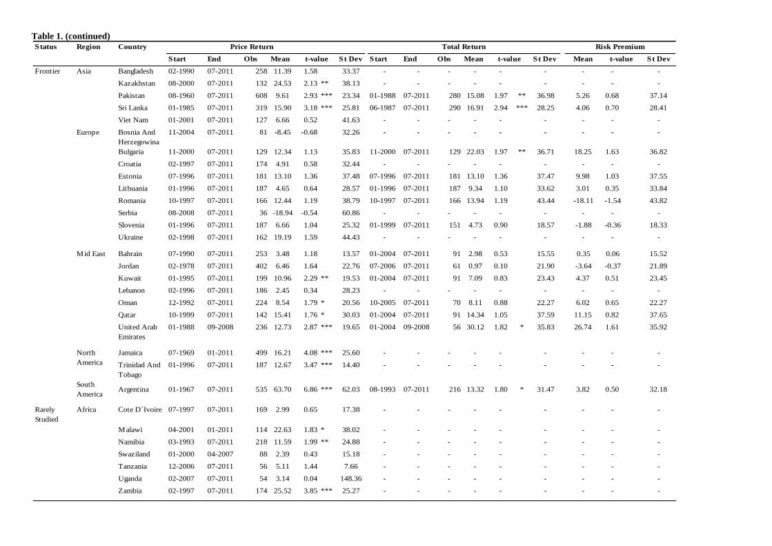
40
Table 1. (continued)
Start End Obs Mean St Dev Start End Obs Mean St Dev Mean St Dev
Frontier Asia Bangladesh 02-1990 07-2011 258 11.39 1.58 33.37 - - - - - - - - -
Kazakhstan 08-2000 07-2011 132 24.53 2.13 ** 38.13 - - - - - - - - -
Pakistan 08-1960 07-2011 608 9.61 2.93 *** 23.34 01-1988 07-2011 280 15.08 1.97 ** 36.98 5.26 0.68 37.14
Sri Lanka 01-1985 07-2011 319 15.90 3.18 *** 25.81 06-1987 07-2011 290 16.91 2.94 *** 28.25 4.06 0.70 28.41
Viet Nam 01-2001 07-2011 127 6.66 0.52 41.63 - - - - - - - - -
Europe Bosnia And
Herzegowina
11-2004 07-2011 81 -8.45 -0.68 32.26 - - - - - - - - -
Bulgaria 11-2000 07-2011 129 12.34 1.13 35.83 11-2000 07-2011 129 22.03 1.97 ** 36.71 18.25 1.63 36.82
Croatia 02-1997 07-2011 174 4.91 0.58 32.44 - - - - - - - - -
Estonia 07-1996 07-2011 181 13.10 1.36 37.48 07-1996 07-2011 181 13.10 1.36 37.47 9.98 1.03 37.55
Lithuania 01-1996 07-2011 187 4.65 0.64 28.57 01-1996 07-2011 187 9.34 1.10 33.62 3.01 0.35 33.84
Romania 10-1997 07-2011 166 12.44 1.19 38.79 10-1997 07-2011 166 13.94 1.19 43.44 -18.11 -1.54 43.82
Serbia 08-2008 07-2011 36 -18.94 -0.54 60.86 - - - - - - - - -
Slovenia 01-1996 07-2011 187 6.66 1.04 25.32 01-1999 07-2011 151 4.73 0.90 18.57 -1.88 -0.36 18.33
Ukraine 02-1998 07-2011 162 19.19 1.59 44.43 - - - - - - - - -
Mid East Bahrain 07-1990 07-2011 253 3.48 1.18 13.57 01-2004 07-2011 91 2.98 0.53 15.55 0.35 0.06 15.52
Jordan 02-1978 07-2011 402 6.46 1.64 22.76 07-2006 07-2011 61 0.97 0.10 21.90 -3.64 -0.37 21.89
Kuwait 01-1995 07-2011 199 10.96 2.29 ** 19.53 01-2004 07-2011 91 7.09 0.83 23.43 4.37 0.51 23.45
Lebanon 02-1996 07-2011 186 2.45 0.34 28.23 - - - - - - - - -
Oman 12-1992 07-2011 224 8.54 1.79 * 20.56 10-2005 07-2011 70 8.11 0.88 22.27 6.02 0.65 22.27
Qatar 10-1999 07-2011 142 15.41 1.76 * 30.03 01-2004 07-2011 91 14.34 1.05 37.59 11.15 0.82 37.65
United Arab
Emirates
01-1988 09-2008 236 12.73 2.87 *** 19.65 01-2004 09-2008 56 30.12 1.82 * 35.83 26.74 1.61 35.92
Jamaica 07-1969 01-2011 499 16.21 4.08 *** 25.60 - - - - - - - - -
Trinidad And
Tobago
01-1996 07-2011 187 12.67 3.47 *** 14.40 - - - - - - - - -
South
AmericaArgentina 01-1967 07-2011 535 63.70 6.86 *** 62.03 08-1993 07-2011 216 13.32 1.80 * 31.47 3.82 0.50 32.18
Africa Cote D`Ivoire 07-1997 07-2011 169 2.99 0.65 17.38 - - - - - - - - -
Malawi 04-2001 01-2011 114 22.63 1.83 * 38.02 - - - - - - - - -
Namibia 03-1993 07-2011 218 11.59 1.99 ** 24.88 - - - - - - - - -
Swaziland 01-2000 04-2007 88 2.39 0.43 15.18 - - - - - - - - -
Tanzania 12-2006 07-2011 56 5.11 1.44 7.66 - - - - - - - - -
Uganda 02-2007 07-2011 54 3.14 0.04 148.36 - - - - - - - - -
Zambia 02-1997 07-2011 174 25.52 3.85 *** 25.27 - - - - - - - - -
Status Region Country Total Return Risk Premium
t-value t-value t-value
Price Return
North
America
Rarely
Studied

41
Table 1. (continued)
Start End Obs Mean St Dev Start End Obs Mean St Dev Mean St Dev
Asia Kyrgyzstan 01-2000 05-2011 137 6.68 0.53 42.52 - - - - - - - - -
Mongolia 09-1995 05-2011 189 29.33 2.42 ** 48.16 - - - - - - - - -
Nepal 01-1996 07-2011 186 3.56 0.61 23.03 - - - - - - - - -
Europe Cyprus 01-1984 07-2011 331 2.98 0.46 34.04 01-1993 07-2011 223 6.14 0.66 39.90 1.75 0.19 39.91
Georgia 11-2008 07-2011 33 32.74 0.79 68.50 - - - - - - - - -
Iceland 01-1993 07-2011 223 2.47 0.29 36.53 07-2002 07-2011 109 -6.19 -0.37 50.17 -15.60 -0.93 50.65
Latvia 02-1996 07-2011 186 9.89 1.11 35.18 05-1996 07-2011 183 10.74 1.18 35.57 5.87 0.65 35.51
Luxembourg 01-1954 07-2011 691 8.17 3.69 *** 16.79 01-1985 07-2011 319 10.10 2.59 *** 20.13 4.78 1.22 20.16
Macedonia 11-2001 07-2011 117 12.50 1.03 37.87 - - - - - - - - -
Malta 01-1996 07-2011 187 7.51 1.57 18.89 02-2000 07-2011 138 1.40 0.28 17.24 -1.92 -0.38 17.32
Montenegro 04-2003 07-2011 100 29.25 1.90 * 44.42 - - - - - - - - -
Slovak
Republic
10-1993 07-2011 214 4.54 0.59 32.33 - - - - - - - - -
Mid East Iran 04-1990 06-2011 255 25.90 6.36 *** 18.77 - - - - - - - - -
Iraq 11-2004 07-2011 79 10.88 0.47 59.11 - - - - - - - - -
Palestine 08-1997 07-2011 166 11.48 1.05 40.51 - - - - - - - - -
Saudi Arabia 01-1993 07-2011 222 6.59 1.21 23.43 - - - - - - - - -
Syrian Arab
Republic
01-2010 07-2011 19 2.70 0.12 28.18 - - - - - - - - -
Bahamas 12-2002 07-2011 98 5.67 2.06 ** 7.87 - - - - - - - - -
Barbados 04-1989 02-2011 263 4.24 1.42 13.99 - - - - - - - - -
Bermuda 09-1996 10-2010 170 1.78 0.33 20.48 - - - - - - - - -
Costa Rica 10-1997 02-2011 161 13.90 2.37 ** 21.48 - - - - - - - - -
El Salvador 01-2004 07-2011 91 7.41 2.53 ** 8.07 - - - - - - - - -
Panama 01-1993 07-2011 223 14.08 5.43 *** 11.18 - - - - - - - - -
Ecuador 02-1994 07-2011 210 1.80 0.32 23.17 - - - - - - - - -
Paraguay 11-1993 09-2008 176 11.15 4.06 *** 10.52 - - - - - - - - -
Uruguay 02-1925 12-1995 848 13.10 2.65 *** 41.57 - - - - - - - - -
Venezuela 01-1937 07-2011 891 13.51 4.94 *** 23.59 12-1996 12-2003 84 10.16 0.70 38.19 -11.72 -0.80 38.83
Status Region Country Price Return
North
America
South
America
Risk Premium
t-value t-value t-value
Total Return
Rarely
Studied

42
Table 2 Halloween effect in market total returns and risk premiums This table provides two 6-month period (November-April and May-October) mean returns, standard deviations (at percentage), and t-values of the zero mean test of the two periods, as
well as the coefficient estimates and t-statistics for the Halloween effect regression for 65 markets and world index’s total returns and risk premiums. represents
the 6-month mean returns difference between November-April and May-October. T-values are adjusted using Newey-West standard errors. The 6-month mean returns (standard
deviations) are calculated by multiplying monthly returns (standard deviations) by 6 (√ ).
*** denotes significance at 1% level; **denotes significance at 5% level; *denotes significance at 10% level. Countries are grouped based on the MSCI market classification and
geographical regions.
Status Region Country
Mean St Dev Mean St Dev βHal Mean St Dev Mean St Dev βHal
6.59 9.61 6.35 *** 1.78 11.00 1.50 4.81 3.45 *** - - - - - - - -
8.46 17.29 25.82 *** 2.29 17.95 6.71 *** 6.18 12.76 *** 4.89 17.39 14.52 *** -1.17 18.01 -3.36 *** 6.06 12.28 ***
Developed Asia Hong Kong 9.63 23.76 2.62 *** 6.15 24.08 1.64 3.49 0.66 6.62 23.81 1.80 * 3.21 24.20 0.86 3.41 0.64
Japan 9.74 15.29 6.03 *** 1.18 13.10 0.86 8.56 3.61 *** 6.55 14.13 4.31 *** -0.74 12.39 -0.56 7.29 3.75 ***
Singapore 7.89 17.06 2.85 *** -1.20 20.17 -0.37 9.09 1.96 * 5.76 17.07 2.08 ** -3.37 20.26 -1.03 9.13 1.96 *
Europe Austria 8.86 12.58 4.55 *** -1.45 14.85 -0.63 10.31 3.37 *** 5.87 12.61 3.00 *** -4.46 14.89 -1.93 * 10.33 3.37 ***
Belgium 8.40 10.13 6.47 *** 0.44 11.10 0.31 7.97 4.18 *** 5.38 10.09 4.14 *** -2.57 11.15 -1.80 * 7.95 4.17 ***
Denmark 7.45 11.68 4.12 *** 4.05 12.82 2.04 ** 3.39 1.51 3.20 11.29 1.74 * 0.52 12.25 0.26 2.68 1.17
Finland 9.81 14.89 6.53 *** 3.33 14.48 2.28 ** 6.47 2.98 *** 6.39 14.89 4.25 *** -0.03 14.53 -0.02 6.42 2.96 ***
France 8.50 13.66 6.60 *** 1.57 13.09 1.27 6.94 3.42 *** 6.03 13.72 4.56 *** -1.12 13.25 -0.87 7.14 3.39 ***
Germany 7.51 21.50 4.14 *** -1.78 28.85 -0.73 9.29 3.03 *** 4.96 21.46 2.74 *** -4.34 28.88 -1.79 * 9.30 3.03 ***
Greece 10.80 22.38 2.84 *** 3.30 23.34 0.83 7.49 1.27 5.06 22.27 1.34 -2.60 23.32 -0.66 7.66 1.30
Ireland 12.28 15.39 4.96 *** -1.64 17.13 -0.59 13.92 4.01 *** 8.23 15.33 3.34 *** -5.45 17.15 -1.97 ** 13.68 3.95 ***
Italy 8.44 17.61 4.46 *** 1.84 18.13 0.94 6.60 2.33 ** 5.36 17.56 2.84 *** -1.49 18.20 -0.76 6.85 2.50 **
Netherlands 9.58 11.01 6.78 *** 0.73 12.79 0.44 8.85 4.24 *** 7.43 11.05 5.24 *** -1.45 12.84 -0.88 8.88 4.23 ***
Norway 9.64 17.35 3.12 *** 2.08 19.10 0.61 7.56 1.68 * 5.57 17.44 1.79 * -1.99 19.16 -0.58 7.56 1.68 *
Portugal 6.13 13.07 2.27 ** -2.15 14.56 -0.72 8.28 1.90 * 3.06 13.23 1.12 -5.24 14.60 -1.74 * 8.30 1.90 *
Spain 9.19 12.64 6.13 *** 2.18 12.69 1.45 7.01 3.54 *** 5.92 12.69 3.94 *** -1.19 12.76 -0.79 7.12 3.58 ***
Sweden 8.01 12.32 6.26 *** 1.64 11.78 1.34 6.37 3.65 *** 5.39 12.30 4.22 *** -1.01 11.83 -0.82 6.40 3.64 ***
Switzerland 6.42 10.34 4.19 *** 0.50 12.65 0.27 5.92 2.61 *** 4.92 10.39 3.19 *** -1.15 12.69 -0.61 6.07 2.67 ***
United Kingdom 4.54 8.81 9.17 *** 1.98 8.99 3.92 *** 2.56 3.71 *** 2.31 8.79 4.68 *** -0.21 9.04 -0.42 2.52 3.65 ***
Mid East Israel 9.06 16.04 2.44 ** 0.73 15.65 0.20 8.33 2.08 ** 5.11 16.07 1.38 -3.30 15.68 -0.90 8.41 2.10 **
North America Canada 7.64 9.75 6.89 *** 1.78 11.35 1.38 5.87 3.59 *** 5.37 9.80 4.82 *** -0.51 11.44 -0.39 5.88 3.58 ***
United States 4.91 10.03 7.11 *** 3.20 11.38 4.09 *** 1.71 1.65 * 2.89 10.04 4.18 *** 1.18 11.41 1.51 1.70 1.65 *
Oceania Australia 6.31 9.72 5.91 *** 4.56 12.26 3.39 *** 1.74 1.04 3.70 9.72 3.47 *** 1.97 12.32 1.45 1.73 1.03
New Zealand 1.93 11.77 0.82 3.07 14.52 1.06 -1.14 -0.33 -2.10 12.10 -0.87 -0.92 14.60 -0.32 -1.18 -0.33
Emerging Africa Egypt 13.38 23.64 2.18 ** 0.46 20.16 0.09 12.92 2.07 ** 8.96 23.64 1.46 -4.11 20.21 -0.78 13.07 2.09 **
Morocco 12.95 11.74 4.57 *** 0.95 9.92 0.40 12.00 3.20 *** 10.46 11.78 3.68 *** -1.57 9.85 -0.67 12.04 3.21 ***
South Africa 10.77 14.46 5.34 *** 4.42 16.07 1.98 ** 6.34 1.73 * 6.20 14.48 3.07 *** -0.15 16.17 -0.07 6.35 1.72 *
World
Pooled 65 countries
May-Oct
Risk Premium
Halloween
t-value t-value t-value t-value t-value t-value
Total Return
Nov-Apr May-Oct Halloween Nov-Apr

43
Status Region Country
Mean St Dev Mean St Dev βHal Mean St Dev Mean St Dev βHal
Emerging Asia China -1.60 25.12 -0.28 1.63 26.05 0.27 -3.24 -0.39 -4.04 25.21 -0.69 -0.81 26.11 -0.13 -3.23 -0.39
India 9.63 22.74 2.06 ** 7.85 21.83 1.74 * 1.78 0.27 3.09 20.58 0.65 0.99 19.79 0.22 2.10 0.32
Indonesia 18.11 25.84 3.41 *** 1.33 29.52 0.22 16.78 2.07 ** 11.05 25.67 2.09 ** -5.71 30.10 -0.92 16.76 2.06 **
Korea 17.08 29.07 4.12 *** 4.49 26.58 1.19 12.59 1.92 * 10.90 29.12 2.63 *** -1.63 26.58 -0.43 12.53 1.91 *
Malaysia 9.55 18.75 3.13 *** 0.12 20.99 0.04 9.43 1.98 ** 7.42 18.74 2.43 ** -2.04 21.04 -0.59 9.46 1.99 **
Philippines 9.70 18.30 2.89 *** 5.51 23.26 1.29 4.19 0.83 3.13 18.22 0.93 -0.47 23.39 -0.11 3.60 0.71
Taiwan 14.83 23.84 3.02 *** -6.88 24.86 -1.34 21.71 2.91 *** 12.91 23.81 2.64 *** -8.81 24.94 -1.71 * 21.72 2.91 ***
Thailand 8.16 19.14 2.56 ** 3.47 24.16 0.87 4.69 0.87 5.38 18.79 1.53 1.27 24.18 0.28 4.12 0.75
Europe Czech Republic 9.56 21.35 1.89 * 0.82 17.18 0.20 8.75 1.73 * 7.00 21.41 1.38 -1.77 17.29 -0.43 8.77 1.72 *
Hungary 14.23 20.71 2.80 *** 1.92 22.80 0.34 12.30 2.12 ** 7.98 20.53 1.59 -4.31 22.76 -0.77 12.29 2.11 **
Poland 12.61 19.81 2.63 *** -3.95 24.86 -0.66 16.56 2.73 *** 6.72 19.72 1.41 -10.09 25.25 -1.67 * 16.80 2.76 ***
Russia 19.51 34.85 2.29 ** -3.70 45.44 -0.33 23.21 1.54 1.00 36.35 0.11 -9.71 36.67 -1.01 10.71 0.75
Turkey 29.61 39.76 3.76 *** 17.89 35.82 2.52 ** 11.72 1.16 2.70 39.22 0.35 -8.32 36.37 -1.15 11.01 1.10
North America Mexico 17.25 19.24 4.36 *** 9.06 19.63 2.24 ** 8.19 1.76 * 6.35 18.57 1.66 * 0.47 19.42 0.12 5.88 1.20
South America Chile 11.44 14.92 5.18 *** 7.48 14.94 3.37 *** 3.97 1.02 6.43 14.55 2.99 *** 2.83 14.87 1.28 3.60 0.93
Colombia 8.24 54.02 0.74 8.69 18.42 2.29 ** -0.45 -0.04 -1.51 54.40 -0.13 -0.82 18.91 -0.21 -0.69 -0.06
Peru 13.16 22.69 2.51 ** 7.47 23.49 1.37 5.69 0.66 8.24 22.85 1.56 2.34 23.64 0.43 5.90 0.69
Frontier Africa Mauritius 9.09 11.72 3.64 *** 9.00 11.42 3.70 *** 0.09 0.03 4.66 11.78 1.85 * 4.68 11.49 1.91 * -0.02 -0.01
Asia Pakistan 13.04 26.91 2.34 ** 2.04 25.26 0.39 11.00 1.83 * 8.14 27.04 1.45 -2.88 25.33 -0.55 11.01 1.82 *
Sri Lanka 6.30 20.07 1.54 10.58 19.91 2.62 *** -4.28 -0.65 -0.14 20.09 -0.03 4.16 20.09 1.02 -4.30 -0.65
Europe Bulgaria 12.56 24.41 1.71 * 9.39 27.67 1.10 3.17 0.22 10.70 24.49 1.45 7.47 27.75 0.87 3.23 0.23
Estonia 17.48 25.91 2.61 *** -4.26 26.46 -0.63 21.74 2.58 ** 15.95 25.94 2.38 ** -5.85 26.53 -0.86 21.80 2.58 **
Lithuania 9.35 25.08 1.48 -0.06 22.35 -0.01 9.42 1.04 6.09 25.13 0.95 -3.08 22.63 -0.53 9.17 1.02
Romania 12.56 31.03 1.51 1.24 30.40 0.15 11.32 1.07 -4.03 31.33 -0.48 -14.20 30.67 -1.71 * 10.18 0.94
Slovenia 0.79 13.57 0.21 3.96 12.73 1.10 -3.16 -0.78 -3.18 13.25 -0.84 1.27 12.69 0.35 -4.45 -1.10
Mid East Bahrain 2.51 10.37 0.67 0.45 11.71 0.10 2.06 0.34 1.21 10.39 0.32 -0.89 11.64 -0.21 2.09 0.35
Jordan 1.45 13.24 0.25 -0.45 17.60 -0.06 1.90 0.39 -0.80 13.23 -0.14 -2.80 17.61 -0.36 2.00 0.41
Kuwait 1.76 17.95 0.27 5.37 15.18 0.97 -3.61 -0.66 0.37 17.98 0.06 4.04 15.21 0.73 -3.68 -0.66
Oman 4.19 12.55 0.82 3.91 18.75 0.50 0.28 0.03 3.16 12.61 0.61 2.86 18.69 0.36 0.30 0.03
Qatar 9.87 31.54 0.87 4.41 20.61 0.59 5.46 0.44 8.35 31.62 0.73 2.74 20.62 0.36 5.61 0.45
United Arab
Emirates
20.38 25.66 1.68 * 10.11 25.31 0.88 10.26 0.52 18.77 25.77 1.55 8.34 25.33 0.72 10.43 0.53
South America Argentina 12.08 24.07 2.13 ** 1.24 20.14 0.26 10.84 1.36 7.27 24.64 1.25 -3.46 20.55 -0.71 10.74 1.38
Rarely Studied Europe Cyprus 0.53 25.09 0.09 5.63 31.13 0.78 -5.11 -0.55 -1.64 25.06 -0.28 3.43 31.13 0.47 -5.07 -0.54
Iceland 0.82 22.67 0.11 -6.93 44.80 -0.47 7.75 0.69 -4.04 23.12 -0.52 -11.50 45.10 -0.77 7.46 0.67
Latvia 8.21 23.24 1.37 2.62 26.95 0.38 5.59 0.56 5.81 23.27 0.97 0.15 26.87 0.02 5.67 0.58
Luxembourg 12.05 12.17 5.11 *** -1.99 15.56 -0.66 14.03 3.36 *** 9.37 12.20 3.97 *** -4.64 15.58 -1.53 14.01 3.34 ***
Malta 2.36 13.76 0.58 -0.95 10.44 -0.31 3.31 0.80 0.73 13.82 0.18 -2.64 10.53 -0.85 3.37 0.81
South America Venezuela -1.27 20.84 -0.16 11.43 32.07 0.94 -12.70 -0.81 -11.96 20.97 -1.51 0.24 32.77 0.02 -12.19 -0.75
Total Return Risk Premium
Halloween
t-value
Nov-Apr May-Oct Halloween Nov-Apr May-Oct
t-value t-value t-value t-value t-value

44
Table 3. In-sample and out-of-sample comparison of the Halloween effect
The table shows the coefficient estimates and t-statistics for the regression , as well
as the percentage of times that November-April returns beat May-October returns for the in-sample
period and out of sample period of 37 countries. The in-sample period refers to the sample period
examined in Bouman and Jacobsen (2002) and runs from January 1970 (or the earliest date in our sample
depending on data availability) to August 1998. The out-of-sample period is from September 1998 to July
2011. The coefficient β represents the 6-month return difference between November-April and May-
October. T-values are adjusted using Newey-West standard errors. *** denotes significance at 1% level;
**denotes significance at 5% level; *denotes significance at 10% level.
IN SAMPLE OUT OF SAMPLE
Country β t-value %+ β t-value %+
Argentina 3.64 0.28 0.66 15.26 1.51 0.57
Australia 5.39 1.49 0.59 2.91 0.89 0.50
Austria 8.79 2.72 *** 0.69 14.11 2.84 *** 0.71
Belgium 12.44 5.21 *** 0.90 6.96 1.48 0.71
Brazil 37.43 1.72 * 0.67 9.58 1.29 0.50
Canada 7.72 2.57 ** 0.69 5.98 1.54 0.50
Chile -7.44 -0.7 0.45 1.43 0.37 0.57
Denmark 3.82 1.55 0.66 4.89 1.19 0.71
Finland 9.28 3.01 *** 0.76 12.42 1.74 * 0.64
France 14.22 3.99 *** 0.79 9.59 2.32 ** 0.64
Germany 8.34 2.91 *** 0.69 11.61 2.35 ** 0.79
Greece 10.96 1.94 * 0.62 3.99 0.55 0.50
Hong Kong 5.18 0.75 0.66 0.11 0.01 0.43
Indonesia 12.60 1.5 0.56 14.60 1.89 * 0.57
Ireland 8.42 2.17 ** 0.62 13.77 2.70 *** 0.79
Italy 14.98 3.59 *** 0.76 14.18 2.85 *** 0.71
Japan 7.76 2.41 ** 0.76 11.83 2.14 ** 0.64
Jordan 4.52 1.08 0.52 3.06 0.72 0.43
Korea 1.67 0.43 0.55 12.82 1.70 * 0.71
Malaysia 12.86 1.9 * 0.68 5.83 1.04 0.57
Mexico 5.06 0.82 0.59 8.15 1.36 0.50
Netherlands 11.86 4.1 *** 0.86 10.38 1.93 * 0.64
New Zealand 3.12 0.83 0.52 4.31 1.41 0.64
Norway 6.34 1.38 0.52 10.36 1.69 * 0.57
Philippines 13.01 1.96 * 0.62 2.56 0.36 0.43
Portugal 3.59 0.34 0.67 8.37 1.67 * 0.79
Russia -6.37 -0.15 0.50 26.62 2.41 ** 0.79
Singapore 7.78 1.52 0.62 4.74 0.78 0.50
South Africa 6.21 1.18 0.59 1.98 0.35 0.50
Spain 11.91 3.31 *** 0.76 6.09 1.26 0.71
Sweden 11.70 3.44 *** 0.76 13.80 2.95 *** 0.79
Switzerland 6.29 2.2 ** 0.72 5.03 1.30 0.71
Taiwan 20.11 3.44 *** 0.72 15.00 1.69 * 0.79
Thailand -0.29 -0.04 0.42 5.64 0.66 0.50
Turkey 0.73 0.05 0.46 18.75 1.48 0.50
United Kingdom 12.37 2.89 *** 0.59 6.56 1.85 * 0.64
United States 5.82 2.45 ** 0.72 4.90 1.57 0.57

45
Table 4. Cross country analysis – market price returns
This table provides two 6-month (November-April and May-October) mean returns and standard deviations at percentage, the
coefficient estimates and t-statistics for the regression , as well as percentage of times that November-April
return beats May-October return for 109 countries’ market index and the world index. represents the 6-month mean returns
difference between November-April and May-October. T-values are adjusted using Newey-West standard errors. The 6-month mean
returns (standard deviations) are calculated by multiplying monthly returns (standard deviations) by 6 (√ ).
*** denotes significance at 1% level; **denotes significance at 5% level; *denotes significance at 10% level. Countries are grouped
based on the MSCI market classification and geographical regions.
Status Region Start Date End
Date Country
Nov-Apr May-Oct Halloween Effect
Mean St Dev Mean St Dev β t-value %+
Pooled 109
Countries
02/1693 07-2011 - 6.88 17.34 2.35 19.86 4.53 11.42 *** 58%
World 02-1919 07-2011 - 4.35 8.75 -0.18 9.84 4.53 3.64 *** 67%
Developed Asia 11-1964 07-2011 Hong Kong 7.08 22.48 4.44 23.39 2.64 0.55 58%
11-1914 07-2011 Japan 7.31 16.05 -1.00 14.52 8.31 3.37 *** 66%
11-1965 07-2011 Singapore 6.91 15.79 0.13 17.08 6.78 1.87 * 60%
Europe 02-1922 07-2011 Austria 5.35 17.31 3.69 21.41 1.66 0.41 56%
02/1897 07-2011 Belgium 3.99 12.03 -0.10 13.22 4.09 2.61 *** 62%
01-1921 07-2011 Denmark 3.74 9.15 0.56 9.01 3.18 2.59 *** 64%
11-1912 07-2011 Finland 4.08 14.14 4.22 14.87 -0.14 -0.06 50%
01/1898 07-2011 France 7.05 13.50 -0.39 12.95 7.45 3.69 *** 66%
01/1870 07-2011 Germany 4.09 14.36 -1.53 20.44 5.63 2.42 ** 59%
01-1954 07-2011 Greece 8.65 18.50 0.84 18.63 7.81 2.10 ** 55%
02-1934 07-2011 Ireland 6.14 10.85 -0.48 12.01 6.62 3.63 *** 69%
11-1905 07-2011 Italy 6.11 16.89 -0.69 16.88 6.80 2.75 *** 60%
02-1919 07-2011 Netherlands 5.62 10.90 -1.97 12.83 7.59 4.28 *** 67%
01-1970 07-2011 Norway 9.19 16.18 1.60 18.13 7.58 2.06 ** 55%
01-1934 07-2011 Portugal 4.87 26.91 1.21 15.20 3.66 0.95 62%
01-1915 07-2011 Spain 6.26 12.47 -0.91 11.83 7.16 4.18 *** 69%
01-1906 07-2011 Sweden 5.52 12.32 -0.03 11.41 5.56 3.34 *** 63%
01-1914 07-2011 Switzerland 3.91 9.41 -0.73 11.92 4.64 3.09 *** 66%
02/1693 07-2011 United Kingdom 2.40 9.34 -0.96 10.19 3.37 4.34 *** 59%
Mid East 02-1949 05-2011 Israel 13.56 16.74 10.09 15.93 3.46 1.43 62%
North
America
12-1917 07-2011 Canada 5.29 9.94 -0.28 12.61 5.57 3.59 *** 61%
11/1791 07-2011 United States 2.24 9.98 0.57 11.27 1.67 1.67 * 57%
Oceania 02/1875 07-2011 Australia 3.11 8.59 1.88 10.43 1.22 1.12 53%
01-1931 07-2011 New Zealand 2.69 9.71 1.63 10.39 1.06 0.65 51%
Emerging Africa 01-1993 07-2011 Egypt 14.89 22.01 -
22.26
110.45 37.15 1.31 58%
01-1988 07-2011 Morocco 12.40 10.92 1.05 9.67 11.35 3.68 *** 71%
02-1910 07-2011 South Africa 4.78 11.59 2.89 12.10 1.88 0.90 53%
Asia 01-1991 07-2011 China 12.75 26.86 2.04 39.99 10.72 1.00 67%
11-1920 07-2011 India 3.52 13.63 2.35 13.61 1.17 0.57 45%
04-1983 07-2011 Indonesia 13.40 21.29 -0.18 22.27 13.58 2.30 ** 55%
02-1962 07-2011 Korea 12.25 28.77 1.26 26.24 11.00 1.71 * 62%
01-1974 07-2011 Malaysia 8.86 18.56 -1.59 19.69 10.46 2.17 ** 63%
01-1953 07-2011 Philippines 6.23 19.59 -3.37 21.13 9.60 2.31 ** 58%
02-1967 07-2011 Taiwan 13.74 21.48 -3.58 24.87 17.31 3.76 *** 76%
11-1975 07-2011 Thailand 4.29 17.99 2.42 22.93 1.87 0.35 46%
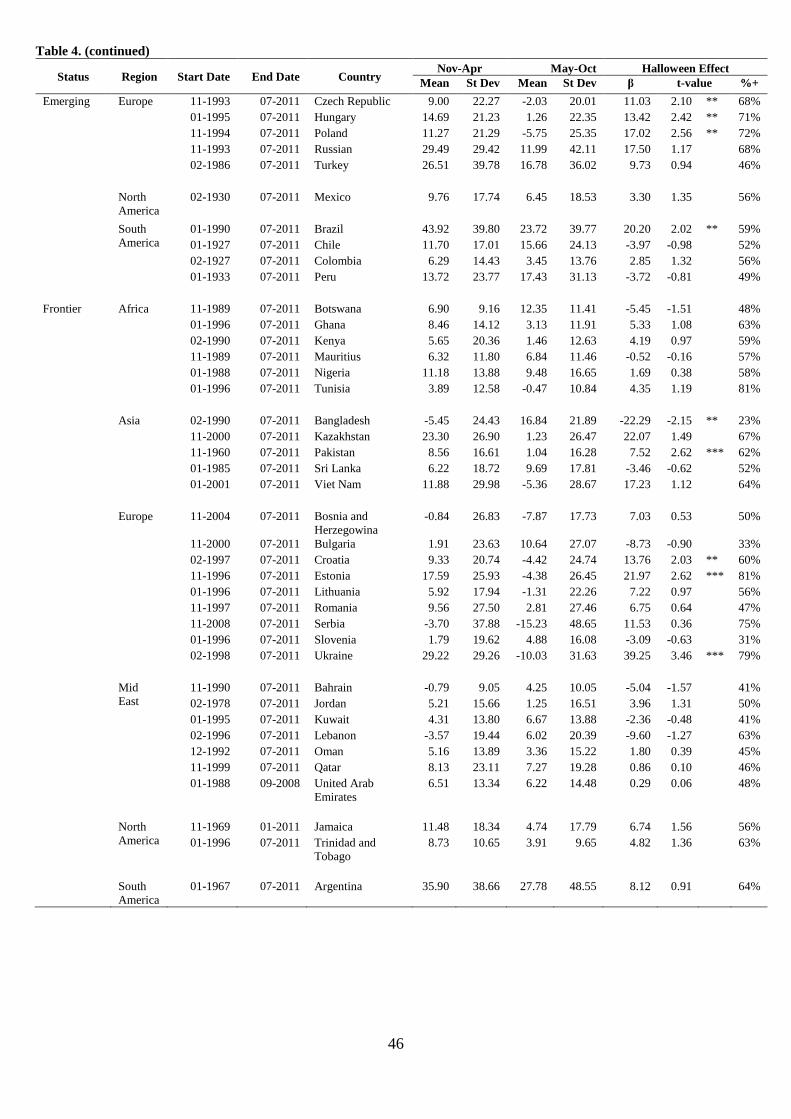
46
Table 4. (continued)
Status Region Start Date End Date Country Nov-Apr May-Oct Halloween Effect
Mean St Dev Mean St Dev β t-value %+
Emerging Europe 11-1993 07-2011 Czech Republic 9.00 22.27 -2.03 20.01 11.03 2.10 ** 68%
01-1995 07-2011 Hungary 14.69 21.23 1.26 22.35 13.42 2.42 ** 71%
11-1994 07-2011 Poland 11.27 21.29 -5.75 25.35 17.02 2.56 ** 72%
11-1993 07-2011 Russian 29.49 29.42 11.99 42.11 17.50 1.17 68%
02-1986 07-2011 Turkey 26.51 39.78 16.78 36.02 9.73 0.94 46%
North
America
02-1930 07-2011 Mexico 9.76 17.74 6.45 18.53 3.30 1.35 56%
South
America
01-1990 07-2011 Brazil 43.92 39.80 23.72 39.77 20.20 2.02 ** 59%
01-1927 07-2011 Chile 11.70 17.01 15.66 24.13 -3.97 -0.98 52%
02-1927 07-2011 Colombia 6.29 14.43 3.45 13.76 2.85 1.32 56%
01-1933 07-2011 Peru 13.72 23.77 17.43 31.13 -3.72 -0.81 49%
Frontier Africa 11-1989 07-2011 Botswana 6.90 9.16 12.35 11.41 -5.45 -1.51 48%
01-1996 07-2011 Ghana 8.46 14.12 3.13 11.91 5.33 1.08 63%
02-1990 07-2011 Kenya 5.65 20.36 1.46 12.63 4.19 0.97 59%
11-1989 07-2011 Mauritius 6.32 11.80 6.84 11.46 -0.52 -0.16 57%
01-1988 07-2011 Nigeria 11.18 13.88 9.48 16.65 1.69 0.38 58%
01-1996 07-2011 Tunisia 3.89 12.58 -0.47 10.84 4.35 1.19 81%
Asia 02-1990 07-2011 Bangladesh -5.45 24.43 16.84 21.89 -22.29 -2.15 ** 23%
11-2000 07-2011 Kazakhstan 23.30 26.90 1.23 26.47 22.07 1.49 67%
11-1960 07-2011 Pakistan 8.56 16.61 1.04 16.28 7.52 2.62 *** 62%
01-1985 07-2011 Sri Lanka 6.22 18.72 9.69 17.81 -3.46 -0.62 52%
01-2001 07-2011 Viet Nam 11.88 29.98 -5.36 28.67 17.23 1.12 64%
Europe 11-2004 07-2011 Bosnia and
Herzegowina
-0.84 26.83 -7.87 17.73 7.03 0.53 50%
11-2000 07-2011 Bulgaria 1.91 23.63 10.64 27.07 -8.73 -0.90 33%
02-1997 07-2011 Croatia 9.33 20.74 -4.42 24.74 13.76 2.03 ** 60%
11-1996 07-2011 Estonia 17.59 25.93 -4.38 26.45 21.97 2.62 *** 81%
01-1996 07-2011 Lithuania 5.92 17.94 -1.31 22.26 7.22 0.97 56%
11-1997 07-2011 Romania 9.56 27.50 2.81 27.46 6.75 0.64 47%
11-2008 07-2011 Serbia -3.70 37.88 -15.23 48.65 11.53 0.36 75%
01-1996 07-2011 Slovenia 1.79 19.62 4.88 16.08 -3.09 -0.63 31%
02-1998 07-2011 Ukraine 29.22 29.26 -10.03 31.63 39.25 3.46 *** 79%
Mid
East
11-1990 07-2011 Bahrain -0.79 9.05 4.25 10.05 -5.04 -1.57 41%
02-1978 07-2011 Jordan 5.21 15.66 1.25 16.51 3.96 1.31 50%
01-1995 07-2011 Kuwait 4.31 13.80 6.67 13.88 -2.36 -0.48 41%
02-1996 07-2011 Lebanon -3.57 19.44 6.02 20.39 -9.60 -1.27 63%
12-1992 07-2011 Oman 5.16 13.89 3.36 15.22 1.80 0.39 45%
11-1999 07-2011 Qatar 8.13 23.11 7.27 19.28 0.86 0.10 46%
01-1988 09-2008 United Arab
Emirates
6.51 13.34 6.22 14.48 0.29 0.06 48%
North
America
11-1969 01-2011 Jamaica 11.48 18.34 4.74 17.79 6.74 1.56 56%
01-1996 07-2011 Trinidad and
Tobago
8.73 10.65 3.91 9.65 4.82 1.36 63%
South
America
01-1967 07-2011 Argentina 35.90 38.66 27.78 48.55 8.12 0.91 64%

47
Table 4. (continued)
Status Region Start Date End Date Country Nov-Apr May-Oct Halloween Effect
Mean St Dev Mean St Dev β t-value %+
Rarely
Studied
Africa 11-1997 07-2011 Cote D`Ivoire 3.66 11.87 -0.65 12.69 4.31 1.08 80%
04-2001 01-2011 Malawi 11.87 26.66 10.82 27.31 1.05 0.09 18%
03-1993 07-2011 Namibia 10.93 15.14 0.66 19.60 10.26 1.84 * 68%
01-2000 04-2007 Swaziland 2.15 14.14 0.15 4.96 2.00 0.38 13%
12-2006 07-2011 Tanzania 1.30 2.95 3.91 7.22 -2.62 -0.86 17%
02-2007 07-2011 Uganda 14.46 21.78 -11.32 147.99 25.78 1.33 80%
02-1997 07-2011 Zambia 7.34 15.70 18.18 19.64 -10.84 -1.62 47%
Asia 01-2000 05-2011 Kyrgyzstan 13.05 32.15 -6.80 27.34 19.84 2.12 ** 75%
11-1995 05-2011 Mongolia 13.33 31.09 16.04 37.03 -2.71 -0.25 41%
01-1996 07-2011 Nepal -4.54 16.90 8.11 15.30 -12.65 -2.18 ** 31%
Europe 01-1984 07-2011 Cyprus 1.07 22.59 1.91 25.53 -0.84 -0.13 61%
11-2008 07-2011 Georgia 2.50 59.57 33.02 31.03 -30.52 -0.87 50%
01-1993 07-2011 Iceland 4.52 17.91 -2.08 31.93 6.60 1.10 58%
02-1996 07-2011 Latvia 8.32 23.17 1.56 26.53 6.76 0.70 69%
01-1954 07-2011 Luxembourg 8.72 10.63 -0.56 12.74 9.28 3.78 *** 71%
11-2001 07-2011 Macedonia 4.39 27.27 8.21 26.47 -3.82 -0.30 55%
01-1996 07-2011 Malta 6.39 15.09 1.09 11.33 5.30 1.17 69%
04-2003 07-2011 Montenegro 13.08 29.86 16.11 33.11 -3.02 -0.19 56%
11-1993 07-2011 Slovak Republic 6.74 28.41 -2.29 15.19 9.03 1.16 68%
Mid East 04-1990 06-2011 Iran 11.43 10.97 14.46 15.24 -3.03 -0.71 55%
11-2004 07-2011 Iraq 15.88 40.08 -6.41 43.71 22.29 0.65 50%
11-1997 07-2011 Palestine 10.42 35.87 1.06 18.90 9.36 1.18 73%
01-1993 07-2011 Saudi Arabia 3.87 16.52 2.72 16.68 1.15 0.24 53%
01-2010 07-2011 Syrian Arab
Republic
-7.26 21.16 10.92 18.89 -18.18 -1.05 0%
North
America
12-2002 07-2011 Bahamas 3.67 6.25 1.96 4.78 1.71 0.79 40%
04-1989 02-2011 Barbados 0.37 8.52 3.85 11.08 -3.48 -1.15 43%
11-1996 10-2010 Bermuda 1.23 15.28 0.55 13.75 0.68 0.10 60%
11-1997 02-2011 Costa Rica 7.42 17.57 6.46 12.36 0.96 0.17 47%
01-2004 07-2011 El Salvador 2.82 7.17 4.61 3.70 -1.78 -0.59 13%
01-1993 07-2011 Panama 7.09 8.15 6.99 7.68 0.10 0.03 53%
02-1994 07-2011 Ecuador -1.95 15.05 3.74 17.61 -5.69 -1.08 56%
11-1993 09-2008 Paraguay 3.40 7.24 7.85 7.58 -4.45 -1.48 19%
02-1925 12-1995 Uruguay 14.86 34.28 -1.80 23.03 16.66 3.73 *** 62%
01-1937 07-2011 Venezuela 6.70 16.52 6.81 16.85 -0.10 -0.05 53%

48
Table 5. Pooled 10-year sub-period analysis
This table provides mean 6-month returns and standard deviations for two periods (November-April and May-October), the
coefficient estimates and t-statistics for the regression , as well as the percentage of times that the
November-April return beats the May-October return for 31 ten-year subsample periods. represents 6-month mean returns
differences between November-April and May-October. T-values are adjusted using Newey-West standard errors. The 6-
month mean returns (standard deviations) are calculated by multiplying monthly returns (standard deviations) by 6 (√ ).
*** denotes significance at 1% level; **denotes significance at 5% level; *denotes significance at 10% level.
Period No of
Countries
Sample
Size
Nov-Apr May-Oct Halloween Effect % of
Positive Mean St Dev Mean St Dev β t-value
1693-2011 109 56679 6.88 17.34 2.35 19.86 4.53 11.42 *** 58%
1693-1710 1 215 -0.07 14.13 -3.70 15.40 3.63 0.83 61%
1711-1720 1 120 8.72 12.38 -2.01 32.95 10.73 1.14 60%
1721-1730 1 120 -1.63 7.90 -0.63 8.58 -1.00 -0.40 50%
1731-1740 1 120 0.64 2.93 -2.59 4.96 3.24 2.04 ** 80%
1741-1750 1 120 -0.65 4.72 2.10 3.68 -2.75 -1.75 * 20%
1751-1760 1 120 -0.75 3.12 -2.13 2.94 1.39 1.43 80%
1761-1770 1 120 2.65 5.41 -1.36 6.10 4.00 1.52 70%
1771-1780 1 120 -1.16 5.60 -0.75 3.77 -0.41 -0.14 60%
1781-1790 1 120 3.32 5.52 -1.10 5.19 4.41 1.93 * 70%
1791-1800 2 232 -0.76 7.34 0.97 7.06 -1.72 -0.85 50%
1801-1810 2 240 0.43 4.64 0.03 5.36 0.40 0.26 30%
1811-1820 2 240 0.62 3.88 -2.15 4.30 2.77 1.95 * 70%
1821-1830 2 240 2.40 17.00 -1.51 6.50 3.91 0.84 70%
1831-1840 2 240 -0.75 7.64 -0.82 7.06 0.07 0.03 55%
1841-1850 2 240 1.17 8.69 -0.16 7.09 1.32 0.46 60%
1851-1860 2 240 1.39 10.13 -3.48 10.16 4.86 1.04 75%
1861-1870 3 252 3.60 7.52 2.50 9.30 1.10 0.39 52%
1871-1880 4 431 1.06 8.96 -0.02 9.24 1.08 0.45 53%
1881-1890 4 480 -0.40 5.61 1.89 5.91 -2.29 -1.54 43%
1891-1900 6 563 2.24 6.97 0.10 7.34 2.15 1.12 62%
1901-1910 9 854 1.83 6.16 0.51 6.72 1.33 0.95 51%
1911-1920 16 1383 -0.90 11.71 -0.61 10.88 -0.29 -0.16 55%
1921-1930 22 2313 2.54 13.54 -0.36 18.76 2.90 1.34 63%
1931-1940 27 2977 1.85 13.60 0.22 14.85 1.63 0.80 54%
1941-1950 28 3182 3.12 14.85 3.09 15.87 0.03 0.02 45%
1951-1960 32 3628 4.05 10.01 4.91 10.11 -0.86 -0.77 46%
1961-1970 39 4211 4.80 13.56 -0.76 13.49 5.56 4.63 *** 64%
1971-1980 42 4831 9.09 20.05 4.00 18.44 5.08 2.88 *** 60%
1981-1990 57 5558 14.90 22.98 8.79 26.48 6.12 2.79 *** 64%
1991-2000 96 9151 11.56 21.12 2.65 21.42 8.91 5.50 *** 63%
2001-2011 108 12908 7.09 18.58 1.45 25.61 5.64 3.40 *** 57%

49
Table 6. Country by country sub-periods analysis
This table provide the coefficient estimates and t-statistics for the regression , for 28 countries that have data
available over 60 years and the world market over the whole sample period and several 10-year sub-periods. The coefficient estimate
represents 6-month mean returns differences between November-April and May-October. T-values are adjusted using Newey-West
standard errors. *** denotes significance at 1% level; **denotes significance at 5% level; *denotes significance at 10% level.
βHal βHal βHal βHal βHal βHal
Developed Asia Japan 08/1914 07/2011 8.31 3.60 *** - - -3.26 -0.37 6.27 1.52 9.67 1.77 * 24.64 1.77 *
Mid East Israel 02/1949 05/2011 3.46 1.09 - - - - - - - - 4.71 0.84
Canada 12/1917 07/2011 5.57 3.34 *** - - -3.47 -0.86 4.58 1.01 3.81 0.50 -1.09 -0.27
UnitedStates 09/1791 07/2011 1.67 1.66 * 0.85 0.70 -0.68 -0.15 6.70 1.31 -10.19 -1.08 -3.31 -0.68
Oceania Australia 02/1875 07/2011 1.22 1.07 -1.29 -0.92 6.64 2.28 ** -1.17 -0.31 -2.67 -0.72 -2.75 -0.98
New Zealand 01/1931 07/2011 1.06 0.66 - - - - - - -1.62 -0.47 -1.09 -0.54
Austria 02/1922 07/2011 1.66 0.44 - - - - -29.99 -1.26 9.31 1.09 -9.11 -0.44
Belgium 02/1897 07/2011 4.09 2.47 ** 0.43 0.11 -1.27 -0.21 -3.18 -0.42 1.88 0.23 -2.93 -0.56
Denmark 01/1921 07/2011 3.18 2.20 ** - - - - 1.08 0.27 -1.58 -0.49 0.53 0.20
Finland 11/1912 07/2011 -0.14 -0.06 - - -19.35 -2.00 ** -0.77 -0.16 -6.42 -1.62 -18.20 -1.93 *
France 01/1898 07/2011 7.45 3.87 *** 2.62 1.35 4.34 0.82 2.95 0.54 16.90 2.47 ** -8.86 -0.85
Germany 01/1870 07/2011 5.63 2.44 ** -0.65 -0.41 -3.07 -0.39 22.54 1.05 11.54 1.98 * 12.31 0.82
Ireland 02/1934 07/2011 6.62 3.35 *** - - - - - - 4.66 1.72 * 1.84 1.05
Italy 10/1905 07/2011 6.80 2.67 *** 6.77 2.19 ** 3.96 0.63 3.77 0.58 -4.06 -0.73 6.77 0.40
Netherlands 02/1919 07/2011 7.59 4.05 *** - - -13.92 -1.19 6.31 1.18 -2.04 -0.30 7.62 1.37
Portugal 01/1934 07/2011 3.66 0.94 - - - - - - 5.52 0.96 1.18 0.26
Spain 01/1915 07/2011 7.16 3.75 *** - - 5.80 1.51 8.58 2.06 ** 10.85 1.18 0.39 0.07
Sweden 01/1906 07/2011 5.56 3.14 *** 0.47 0.09 5.11 1.23 6.81 1.52 -4.74 -0.56 1.27 0.45
Switzerland 01/1914 07/2011 4.64 2.94 *** - - 9.03 1.61 0.67 0.19 4.19 0.66 -2.92 -1.10
United
Kingdom
02/1693 07/2011 3.37 4.06 *** 2.54 2.75 *** -1.39 -0.62 1.68 0.66 1.22 0.21 -0.70 -0.20
Emerging Africa South Africa 02/1910 07/2011 1.88 0.97 4.29 0.80 -5.07 -1.57 -2.62 -0.97 5.57 0.97 -1.87 -0.48
Asia India 08/1920 07/2011 1.17 0.52 - - - - 1.64 0.46 -2.33 -0.54 -3.28 -0.71
Chile 01/1927 07/2011 -3.97 -0.94 - - - - 6.80 0.80 4.39 0.53 -5.85 -1.69 *
Colombia 02/1927 07/2011 2.85 1.20 - - - - -3.52 -0.79 -2.66 -0.47 -5.31 -1.21
Mexico 02/1930 07/2011 3.30 1.13 - - - - 6.37 0.64 -4.37 -0.90 0.58 0.18
Peru 01/1933 07/2011 -3.72 -0.68 - - - - - - -2.09 -0.61 -1.25 -0.33
Uruguay 02/1925 12/1995 16.66 3.52 *** - - - - 25.42 1.44 4.92 0.40 9.85 1.31
Venezuela 01/1937 07/2011 -0.10 -0.04 - - - - - - 1.97 0.33 1.54 0.62
World 02/1919 07/2011 4.53 3.31 *** - - -7.89 -1.47 6.60 2.25 ** 0.50 0.10 -2.58 -0.81
Western
Europe
Least
Developed
Central/ South
America & the
Caribbean
Central/South
America &the
Caribbean
1911-1920 1921-1930 1931-1940 1941-1950
t-value t-value t-value t-value t-value t-valueStatus Region Country
Whole Sample Prior to 1911
North America
Start
Date
End
Date

50
Table 6. Continued
βHal βHal βHal βHal βHal βHal
Developed Asia Japan 08/1914 07/2011 -4.32 -0.72 8.66 1.53 10.74 1.99 ** 10.53 1.91 * 6.06 0.99 11.27 1.53
Mid East Israel 02/1949 05/2011 -0.78 -0.10 5.30 1.20 -2.07 -0.25 3.90 0.40 6.41 0.85 7.85 1.30 *
North America Canada 12/1917 07/2011 6.56 1.50 9.61 2.98 *** 9.27 1.66 * 8.82 1.53 5.21 1.19 6.20 1.20
UnitedStates 09/1791 07/2011 5.02 1.40 5.54 1.47 6.66 1.50 6.62 1.42 4.20 1.38 5.65 1.17
Oceania Australia 02/1875 07/2011 -3.35 -0.97 4.03 0.96 5.52 0.80 6.11 0.85 7.02 1.63 1.87 0.40
New Zealand 01/1931 07/2011 -6.51 -2.17 ** 3.25 1.16 8.41 1.69 * 0.79 0.10 2.26 0.44 2.87 0.73
Western
Europe
Austria 02/1922 07/2011 -10.52 -2.11 ** 6.17 1.15 4.16 1.67 * 10.91 1.56 13.40 2.25 ** 14.88 1.96
Belgium 02/1897 07/2011 -3.22 -1.09 7.50 2.54 ** 10.92 2.73 *** 12.85 2.30 ** 12.01 2.95 *** 8.10 1.27
Denmark 01/1921 07/2011 3.45 1.77 * 8.96 3.07 *** -1.85 -0.43 5.44 0.94 6.41 1.24 6.05 0.99
Finland 11/1912 07/2011 -2.43 -0.49 -1.28 -0.39 7.88 1.50 8.38 1.56 21.11 2.52 ** 5.21 0.58
France 01/1898 07/2011 1.30 0.26 11.78 2.53 ** 7.12 1.03 20.45 3.47 *** 16.77 3.65 *** 8.54 1.40
Germany 01/1870 07/2011 -5.19 -0.97 5.17 1.10 9.80 2.04 ** 5.31 0.93 13.88 2.67 *** 9.94 1.45 *
Ireland 02/1934 07/2011 -0.88 -0.31 3.68 1.17 4.56 0.64 8.81 1.27 16.27 2.83 *** 13.08 1.77
Italy 10/1905 07/2011 -7.44 -1.58 5.49 1.02 1.02 0.12 22.48 2.54 ** 23.97 3.67 *** 11.71 1.93 *
Netherlands 02/1919 07/2011 3.19 0.75 7.50 1.58 16.04 3.07 *** 11.72 2.54 ** 12.39 2.67 *** 9.28 1.26
Portugal 01/1934 07/2011 1.39 0.56 2.22 0.74 -2.90 -0.09 -1.63 -0.12 14.01 1.98 ** 8.11 1.21
Spain 01/1915 07/2011 3.20 0.80 1.65 0.47 10.36 1.76 * 9.88 1.19 16.95 2.86 *** 4.87 0.77
Sweden 01/1906 07/2011 -4.33 -1.36 2.85 0.68 14.37 3.61 *** 8.79 1.26 16.76 2.37 ** 11.12 1.65
Switzerland 01/1914 07/2011 3.39 0.78 7.74 1.40 8.08 1.49 3.54 0.79 9.74 2.20 ** 4.86 0.89
UnitedKingdom 02/1693 07/2011 -2.19 -0.49 7.09 1.54 17.13 1.71 * 14.93 2.90 *** 7.34 1.99 ** 6.30 1.24
Emerging Africa South Africa 02/1910 07/2011 -6.08 -1.66 * 9.37 1.22 2.25 0.25 0.27 0.03 14.12 2.10 ** 2.69 0.40
Asia India 08/1920 07/2011 -1.42 -0.46 1.96 0.70 6.78 1.59 -4.52 -0.63 11.67 0.94 0.16 0.02
Chile 01/1927 07/2011 -11.77 -1.32 2.87 0.33 -40.24 -1.68 * 13.29 1.74 * 2.79 0.36 -1.55 -0.33
Colombia 02/1927 07/2011 1.73 0.87 3.13 1.40 7.31 1.46 -3.35 -0.37 12.83 1.14 10.83 1.25
Mexico 02/1930 07/2011 2.35 0.93 2.40 1.28 21.87 2.50 ** -14.49 -1.00 7.86 0.86 9.19 1.39
Peru 01/1933 07/2011 -2.50 -1.29 0.24 0.23 -8.22 -0.92 -29.37 -0.91 -0.83 -0.06 13.63 1.29
Uruguay 02/1925 12/1995 1.56 0.28 0.51 0.04 9.26 0.88 55.39 2.95 *** - - - -
Venezuela 01/1937 07/2011 -1.97 -0.50 1.99 0.97 -3.85 -0.82 1.75 0.18 -1.30 -0.11 0.03 0.00
World 02/1919 07/2011 2.34 0.89 5.77 1.98 ** 7.27 1.58 10.66 2.16 ** 5.77 1.84 * 6.49 1.18
Least
Developed
t-value
Central/South
America & the
Caribbean
Central/South
America & the
Caribbean
Start
Date
End
Date
1961-1970 1971-1980 1981-1990 1991-2000 2001-2011
t-value t-value t-value t-value t-valueStatus Region Country
1951-1960

51
Table 7. Out-of-sample Performance of Buy & Hold strategy versus Halloween strategy
The table presents the annualized average returns, standard deviations in percentages, and Sharpe ratios of the buy
and hold strategy and the Halloween strategy, as well as the percentage of years that the Halloween strategy
outperforms the Buy & Hold strategy for the sample period from October 1998 to April 2011.
Country Buy & Hold Strategy Halloween Strategy Percentage
of Winning Return St Dev Sharpe Return St Dev Sharpe
Argentina 18.67 32.19 0.58 21.53 24.15 0.89 38%
Australia 4.92 13.29 0.37 6.42 8.56 0.75 46%
Austria 6.68 20.59 0.32 11.43 12.15 0.94 46%
Belgium 0.46 17.78 0.03 4.50 12.09 0.37 38%
Brazil 17.25 26.54 0.65 21.52 19.37 1.11 54%
Canada 6.47 16.03 0.40 7.96 10.61 0.75 31%
Chile 15.23 14.34 1.06 10.66 10.89 0.98 38%
Denmark 6.78 18.58 0.36 6.47 12.71 0.51 23%
Finland 4.14 30.05 0.14 9.14 23.26 0.39 38%
France 2.29 19.05 0.12 6.85 12.86 0.53 38%
Germany 1.78 22.20 0.08 7.66 15.16 0.51 46%
Greece -3.28 28.81 -0.11 1.81 19.10 0.09 54%
Hong Kong 6.79 23.59 0.29 5.74 16.42 0.35 38%
Indonesia 20.33 27.92 0.73 19.03 18.34 1.04 23%
Ireland -2.87 22.17 -0.13 6.74 13.85 0.49 46%
Italy -0.51 20.54 -0.02 7.30 15.09 0.48 46%
Japan -2.56 20.73 -0.12 4.74 13.58 0.35 62%
Jordan 8.96 20.47 0.44 7.70 14.86 0.52 46%
Korea 13.54 28.44 0.48 15.90 20.99 0.76 46%
Malaysia 10.65 20.92 0.51 10.94 16.14 0.68 23%
Mexico 17.64 22.10 0.80 18.60 16.09 1.16 38%
Netherlands -0.95 20.91 -0.05 5.59 13.36 0.42 46%
New Zealand 1.60 13.13 0.12 5.78 8.61 0.67 62%
Norway 10.71 22.97 0.47 12.50 14.69 0.85 38%
Philippines 7.21 23.57 0.31 9.59 16.05 0.60 38%
Portugal -2.47 19.46 -0.13 3.83 13.44 0.29 46%
Russia 33.89 38.71 0.88 36.05 28.23 1.28 38%
Singapore 6.94 22.86 0.30 7.67 14.37 0.53 31%
South Africa 14.35 19.31 0.74 13.11 13.36 0.98 31%
Spain 2.90 19.69 0.15 5.57 13.64 0.41 38%
Sweden 5.90 21.57 0.27 10.74 15.46 0.69 38%
Switzerland 0.86 14.53 0.06 3.02 10.25 0.29 54%
Taiwan 1.83 26.92 0.07 9.75 18.53 0.53 54%
Thailand 9.55 27.84 0.34 10.80 18.53 0.58 54%
Turkey 27.61 45.88 0.60 38.98 38.52 1.01 46%
United Kingdom 1.85 15.15 0.12 6.23 9.79 0.64 46%
United States 1.73 16.28 0.11 5.02 11.32 0.44 46%
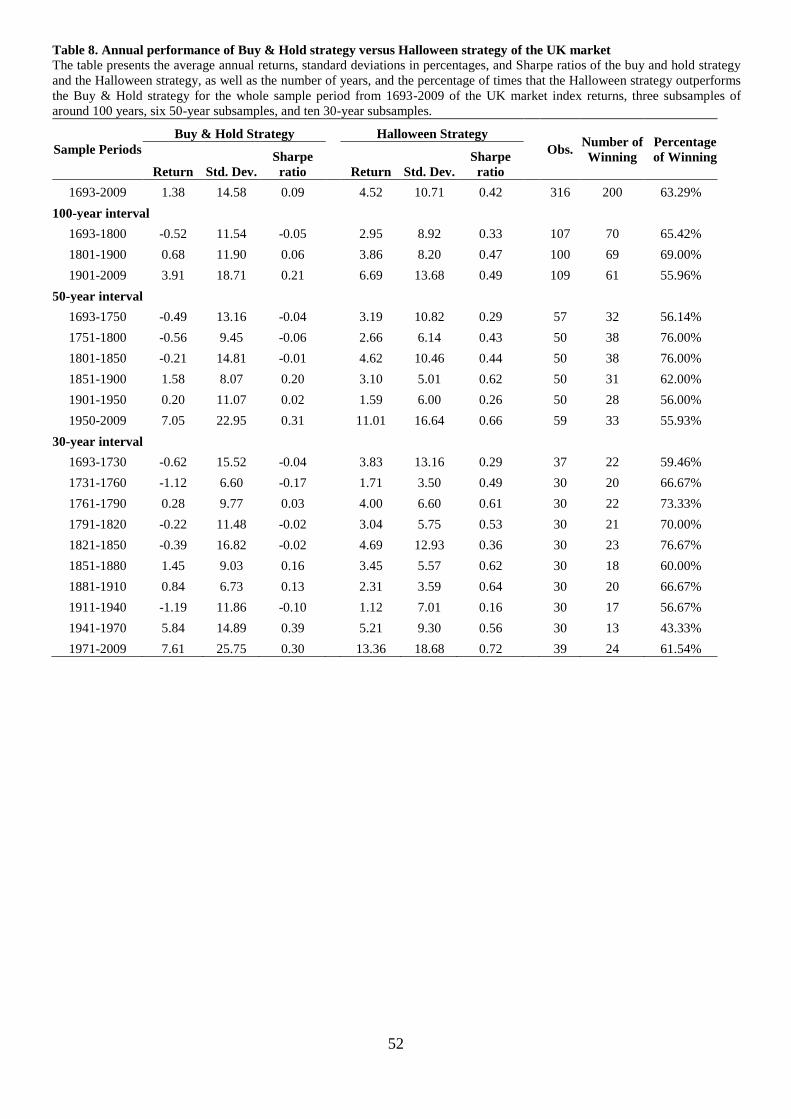
52
Table 8. Annual performance of Buy & Hold strategy versus Halloween strategy of the UK market
The table presents the average annual returns, standard deviations in percentages, and Sharpe ratios of the buy and hold strategy
and the Halloween strategy, as well as the number of years, and the percentage of times that the Halloween strategy outperforms
the Buy & Hold strategy for the whole sample period from 1693-2009 of the UK market index returns, three subsamples of
around 100 years, six 50-year subsamples, and ten 30-year subsamples.
Sample Periods
Buy & Hold Strategy Halloween Strategy
Obs. Number of
Winning
Percentage
of Winning Return Std. Dev.
Sharpe
ratio Return Std. Dev.
Sharpe
ratio
1693-2009 1.38 14.58 0.09 4.52 10.71 0.42 316 200 63.29%
100-year interval
1693-1800 -0.52 11.54 -0.05 2.95 8.92 0.33 107 70 65.42%
1801-1900 0.68 11.90 0.06 3.86 8.20 0.47 100 69 69.00%
1901-2009 3.91 18.71 0.21 6.69 13.68 0.49 109 61 55.96%
50-year interval
1693-1750 -0.49 13.16 -0.04 3.19 10.82 0.29 57 32 56.14%
1751-1800 -0.56 9.45 -0.06 2.66 6.14 0.43 50 38 76.00%
1801-1850 -0.21 14.81 -0.01 4.62 10.46 0.44 50 38 76.00%
1851-1900 1.58 8.07 0.20 3.10 5.01 0.62 50 31 62.00%
1901-1950 0.20 11.07 0.02 1.59 6.00 0.26 50 28 56.00%
1950-2009 7.05 22.95 0.31 11.01 16.64 0.66 59 33 55.93%
30-year interval
1693-1730 -0.62 15.52 -0.04 3.83 13.16 0.29 37 22 59.46%
1731-1760 -1.12 6.60 -0.17 1.71 3.50 0.49 30 20 66.67%
1761-1790 0.28 9.77 0.03 4.00 6.60 0.61 30 22 73.33%
1791-1820 -0.22 11.48 -0.02 3.04 5.75 0.53 30 21 70.00%
1821-1850 -0.39 16.82 -0.02 4.69 12.93 0.36 30 23 76.67%
1851-1880 1.45 9.03 0.16 3.45 5.57 0.62 30 18 60.00%
1881-1910 0.84 6.73 0.13 2.31 3.59 0.64 30 20 66.67%
1911-1940 -1.19 11.86 -0.10 1.12 7.01 0.16 30 17 56.67%
1941-1970 5.84 14.89 0.39 5.21 9.30 0.56 30 13 43.33%
1971-2009 7.61 25.75 0.30 13.36 18.68 0.72 39 24 61.54%

53
Table 9. Strategy performance over different trading horizons of the UK market
The table shows average returns, standard deviations, skewness, and the maximum and minimum values of the buy and hold strategy and the Halloween strategy for different holding
horizons from one year to twenty years of the UN market index returns from 1693-2009. The average returns and the standard deviations are annualised by dividing the total returns
(standard deviations) by n (√ ). The No. of Winning and the % of Winning are the number of times and the percentage of times that the Halloween strategy beats the Buy & Hold
strategy, respectively. The upper panel presents the results calculated using the overlapping sample, and the lower panel are the results from the non-overlapping sample.
Holding
Horizon
Overlapping Sample
Buy & Hold Strategy Halloween Strategy Obs.
No. of
Win % Win
Return St. Dev. Skewness Maximum Minimum Return St. Dev. Skewness Maximum Minimum
1-Year 1.38 14.58 0.12 86.01 -80.60 4.52 10.71 2.06 83.59 -30.96 317 200 63.09%
2-Year 1.42 14.50 -0.39 41.03 -59.11 4.56 11.16 1.60 59.91 -28.78 316 223 70.57%
3-Year 1.50 14.00 0.10 38.85 -35.39 4.61 11.09 1.75 46.05 -11.12 315 236 74.92%
4-Year 1.55 13.50 0.31 29.79 -25.50 4.63 11.40 1.58 35.02 -7.86 314 250 79.62%
5-Year 1.59 13.12 0.58 24.68 -16.06 4.64 11.92 1.59 33.33 -6.28 313 257 82.11%
6-Year 1.60 12.96 0.77 24.56 -15.91 4.65 12.34 1.66 29.53 -3.66 312 258 82.69%
7-Year 1.60 12.75 1.01 22.05 -12.75 4.65 12.76 1.76 29.35 -4.07 311 267 85.85%
8-Year 1.59 12.67 1.27 21.79 -10.89 4.66 13.21 1.81 27.33 -2.46 310 271 87.42%
9-Year 1.59 12.78 1.35 21.67 -7.98 4.66 13.73 1.87 27.15 -2.83 309 281 90.94%
10-Year 1.61 13.00 1.43 21.82 -8.16 4.67 14.23 1.91 27.06 -2.89 308 282 91.56%
15-Year 1.63 13.98 1.56 19.27 -6.52 4.67 16.27 2.04 24.81 -0.20 303 282 93.07%
20-Year 1.61 14.75 1.72 15.62 -3.56 4.64 17.82 2.04 20.57 0.18 298 281 94.30%
Non-Overlapping Sample
Buy & Hold Strategy Halloween Strategy Obs.
No. of
Win % Win
Return St. Dev. Skewness Maximum Minimum Return St. Dev. Skewness Maximum Minimum
1-Year - - - - - - - - - - - - -
2-Year 1.33 16.35 -0.59 41.03 -59.11 4.53 12.50 1.66 59.91 -28.78 158 110 69.62%
3-Year 1.46 16.12 0.15 38.85 -35.39 4.55 12.51 2.22 46.05 -11.12 105 80 76.19%
4-Year 1.33 15.87 -0.14 21.70 -25.50 4.53 11.63 1.01 23.35 -7.86 79 60 75.95%
5-Year 1.46 13.36 -0.01 16.46 -16.06 4.55 11.49 1.01 22.53 -6.28 63 51 80.95%
6-Year 1.37 16.41 0.72 24.56 -15.91 4.52 14.23 2.23 29.53 -3.01 52 42 80.77%
7-Year 1.46 13.39 0.79 18.44 -8.76 4.55 13.55 1.15 20.27 -4.07 45 41 91.11%
8-Year 1.37 11.73 1.13 14.43 -6.98 4.52 12.58 1.64 20.17 -1.70 39 36 92.31%
9-Year 1.46 13.15 0.99 15.75 -7.98 4.55 14.06 1.85 21.66 -2.40 35 32 91.43%
10-Year 1.30 11.82 1.19 12.72 -5.45 4.51 13.80 1.73 18.57 -1.51 31 29 93.55%
15-Year 1.46 15.36 0.88 12.33 -4.08 4.55 16.47 1.77 17.75 0.38 21 20 95.24%
20-Year 1.24 15.36 1.53 9.16 -2.51 4.36 18.77 2.39 17.34 0.18 15 14 93.33%

54
Table 10. Halloween effect semi-annual data versus monthly data
The table compares the regression results of the Halloween effect using
semi-annual data and monthly data. Coefficient estimates are in
percentage terms. T-statistics are calculated based on Newey-West
standard errors. The sample is sub-divided into three sub-periods of
approximately 100-year intervals and six sub-periods of 50-year intervals. ***
denotes significance at the 1% level; **
denotes significance at 5% level; * denotes significance at 10% level
Sample
Periods
Semi-annual data Monthly data
β t-value β t-value
1693-2009 3.36 4.39***
0.56 4.26***
100-year Interval
1693-1800 2.03 1.71* 0.34 1.6
1801-1900 3.14 3.03***
0.52 2.71***
1901-2009 4.87 3.04***
0.80 3.03***
50-year Interval
1693-1750 2.83 1.47 0.48 1.29
1751-1800 1.10 0.88 0.18 0.93
1801-1850 5.06 2.88***
0.84 2.29**
1851-1900 1.22 1.33 0.20 1.46
1901-1950 0.67 0.4 0.08 0.31
1951-2009 8.43 3.59***
1.40 3.33***

55
Figure 1. Summer (May-October) risk premiums for 65 countries
-15.00
-10.00
-5.00
0.00
5.00
10.00
UA
E
Bu
lgar
ia
Mau
riti
us
Sri
Lan
ka
Ku
wai
t
Cy
pru
s
HK
Om
an
Ch
ile
Qat
ar
Per
u
Au
stra
lia
Slo
ven
ia
Thai
land
US
Ind
ia
Den
mar
k
Mex
ico
Ven
ezuel
a
Lat
via
Fin
lan
d
Sou
th A
fric
a
UK
Phil
ipp
ines
Can
ada
Jap
an
Ch
ina
Co
lom
bia
Bah
rain
NZ
Sw
eden
Fra
nce
Sw
itze
rlan
d
Spai
n
Net
her
lan
ds
Ital
y
Moro
cco
Ko
rea
Cze
ch R
epu
bli
c
No
rway
Mal
aysi
a
Bel
giu
m
Gre
ece
Mal
ta
Jord
an
Pak
ista
n
Lit
hu
ania
Isra
el
Sin
gap
ore
Arg
enti
na
Egy
pt
Hu
ng
ary
Ger
man
y
Au
stri
a
Lux
emb
ou
rg
Port
ugal
Irel
and
Ind
on
esia
Est
on
ia
Turk
ey
Tai
wan
Ru
ssia
Pola
nd
Icel
and
Ro
man
ia
Ret
urn
(%
)
Country

56
Figure 2. 30-year moving average of pooled 65 countries’ price returns, total returns, risk premiums and dividend yield
for the period 1694 to 2011.
-5.0
0.0
5.0
10.0
15.0
20.0
169
4
170
2
171
0
171
8
172
6
173
4
174
2
175
0
175
8
176
6
177
4
178
2
179
0
179
8
180
6
181
4
182
2
183
0
183
8
184
6
185
4
186
2
187
0
187
8
188
6
189
4
190
2
191
0
191
8
192
6
193
4
194
2
195
0
195
8
196
6
197
4
198
2
199
0
199
8
200
6
Ret
urn
(%
)
Year
Total Return Price Return
Risk Premium Dividend Yield

57
Figure 3. 30-year moving average of pooled 65 countries’ price returns, total returns, risk premiums and dividend yield
for the period 1951 to 2011.
0.0
2.0
4.0
6.0
8.0
10.0
12.0
14.0
16.0
18.01
95
1
195
3
195
5
195
7
195
9
196
1
196
3
196
5
196
7
196
9
197
1
197
3
197
5
197
7
197
9
198
1
198
3
198
5
198
7
198
9
199
1
199
3
199
5
199
7
199
9
200
1
200
3
200
5
200
7
200
9
201
1
Ret
urn
(%
)
Year
Total Return Price Return
Risk Premium Dividend Yield

58
Figure 4. Summer (May-October) and Winter (November-April) risk premiums for 65 countries
-15.00
-10.00
-5.00
0.00
5.00
10.00
15.00
20.00U
AE
Bulg
aria
Mau
riti
us
Sri
Lan
ka
Kuw
ait
Cypru
sH
K
Om
an
Chil
e
Qat
ar
Per
u
Aust
rali
a
Slo
ven
ia
Thai
land
US
India
Den
mar
k
Mex
ico
Ven
ezuel
a
Lat
via
Fin
land
South
Afr
ica
UK
Phil
ipp
ines
Can
ada
Japan
Chin
a
Colo
mbia
Bah
rain
NZ
Sw
eden
Fra
nce
Sw
itze
rlan
d
Spai
n
Net
her
land
s
Ital
y
Moro
cco
Kore
a
Cze
ch R
epu
bli
c
Norw
ay
Mal
aysi
a
Bel
giu
m
Gre
ece
Mal
ta
Jord
an
Pak
ista
n
Lit
huan
ia
Isra
el
Sin
gap
ore
Arg
enti
na
Egy
pt
Hun
gar
y
Ger
man
y
Aust
ria
Lux
embo
urg
Port
ug
al
Irel
and
Indo
nes
ia
Est
onia
Turk
ey
Tai
wan
Russ
ia
Pola
nd
Icel
and
Rom
ania
Ret
urn
(%
)
Country

59
Figure 5. Two 6-month sub-period (November-April and October-May) returns comparison for the developed markets,
emerging markets, frontier markets and rarely studied markets
(A)
(B)
-2.00
0.00
2.00
4.00
6.00
8.00
10.00
12.00
14.00
Isra
el
Ho
ng K
on
g
Fin
lan
d
Au
stri
a
Au
stra
lia
New
Zea
lan
d
No
rway
Po
rtu
gal
Gre
ece
Un
ited
Sta
tes
Den
mar
k
Sin
gap
ore
Sw
eden
Bel
giu
m
Can
ada
Fra
nce
Irel
and
Ital
y
Sw
itze
rlan
d
Sp
ain
Un
ited
Kin
gd
om
Jap
an
Ger
man
y
Net
her
lan
ds
Ret
urn
(%
)
Country
Developed Markets
-30.00
-20.00
-10.00
0.00
10.00
20.00
30.00
40.00
50.00
Bra
zil
Per
u
Tu
rkey
Chil
e
Russ
ian
Mex
ico
Colo
mb
ia
So
uth
Afr
ica
Th
aila
nd
Ind
ia
Chin
a
Hu
ngar
y
Ko
rea
Mo
rocc
o
Ind
ones
ia
Mal
aysi
a
Cze
ch R
epu
bli
c
Ph
ilip
pin
es
Tai
wan
Po
lan
d
Eg
yp
t
Ret
urn
(%
)
Country
Emerging Markets
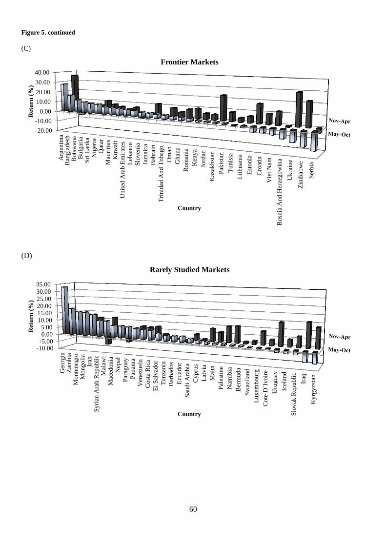
60
Figure 5. continued
(C)
(D)
-20.00
-10.00
0.00
10.00
20.00
30.00
40.00
Arg
enti
na
Ban
gla
des
hB
ots
wan
aB
ulg
aria
Sri
Lan
ka
Nig
eria
Qat
arM
auri
tiu
sK
uw
ait
Un
ited
Ara
b E
mir
ates
Leb
ano
n
Slo
ven
ia
Jam
aica
Bah
rain
Tri
nid
ad A
nd T
obag
o
Om
an
Gh
ana
Rom
ania
Ken
ya
Jord
an
Kaz
akh
stan
Pak
ista
n
Tu
nis
ia
Lit
hu
ania
Est
on
ia
Cro
atia
Vie
t N
am
Bosn
ia A
nd
Her
zego
win
a
Uk
rain
e
Zim
bab
we
Ser
bia
Retu
rn
(%
)
Country
Frontier Markets
-10.00-5.000.005.00
10.0015.0020.0025.0030.0035.00
Geo
rgia
Zam
bia
Mo
nte
neg
roM
ong
oli
aIr
anS
yri
an A
rab
Rep
ubli
cM
alaw
iM
aced
on
iaN
epal
Par
aguay
Pan
ama
Ven
ezu
ela
Cost
a R
ica
El
Sal
vad
or
Tan
zania
Bar
bad
os
Ecu
ado
r
Sau
di
Ara
bia
Cyp
rus
Lat
via
Mal
ta
Pal
esti
ne
Nam
ibia
Ber
mu
da
Sw
azil
and
Lu
xem
bou
rg
Cote
D`I
voir
e
Uru
gu
ay
Icel
and
Slo
vak
Rep
ub
lic
Iraq
Ky
rgy
zsta
n
Ret
urn
(%
)
Country
Rarely Studied Markets

61
Figure 6. Size of the Halloween effect (difference between 6-month returns November-April and May-October) for 31 ten-year sub-periods from 109 pooled countries over the
period 1693-2011
-4.00
-2.00
0.00
2.00
4.00
6.00
8.00
10.00
12.00
169
3-1
710
171
1-1
720
172
1-1
730
173
1-1
740
174
1-1
750
175
1-1
760
176
1-1
770
177
1-1
780
178
1-1
790
179
1-1
800
180
1-1
810
181
1-1
820
182
1-1
830
183
1-1
840
184
1-1
850
185
1-1
860
186
1-1
870
187
1-1
880
188
1-1
890
189
1-1
900
190
1-1
910
191
1-1
920
192
1-1
930
193
1-1
940
194
1-1
950
195
1-1
960
196
1-1
970
197
1-1
980
198
1-1
990
199
1-2
000
200
1-2
011
Ret
urn
s (%
)
10 Year Sub-periods
Halloween Effect
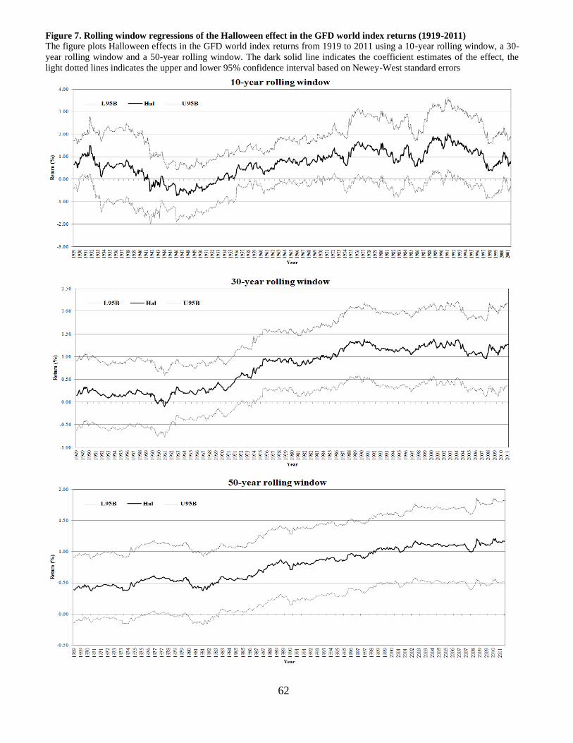
62
Figure 7. Rolling window regressions of the Halloween effect in the GFD world index returns (1919-2011)
The figure plots Halloween effects in the GFD world index returns from 1919 to 2011 using a 10-year rolling window, a 30-
year rolling window and a 50-year rolling window. The dark solid line indicates the coefficient estimates of the effect, the
light dotted lines indicates the upper and lower 95% confidence interval based on Newey-West standard errors

63
Figure 8. Return frequency distribution of Buy & Hold strategy and Halloween strategy
The figure shows the return frequencies of the Buy & Hold strategy and the Halloween strategy for the holding periods of seven years, ten years, fifteen years and twenty years. The
returns are annualised and expressed in percentages.
0
10
20
30
40
50
60
70
80
90
-12 -8 -4 0 4 8 12 16 20 24 28
Fre
qu
ency
7-year Return (%)
Buy & Hold
Halloween
0
20
40
60
80
100
120
-6 -4 -2 0 2 4 6 8 10 12 14 16 18 20 22 24 26
Fre
qu
ency
15-year Return (%)
Buy & Hold
Halloween
0
10
20
30
40
50
60
70
80
90
100
-8 -6 -4 -2 0 2 4 6 8 10121416182022242628
Freq
uen
cy
10-year Return (%)
Buy & Hold
Halloween
0
20
40
60
80
100
120
140
-4 -2 0 2 4 6 8 10 12 14 16 18 20 22
Freq
uen
cy
20-year Return (%)
Buy & Hold
Halloween

64
Figure 9. End of period wealth for the buy and hold strategy and the Halloween strategy for the period 1693 to 2009
-2
0
2
4
6
8
10
12
14
16
16
93
17
02
17
11
17
20
17
29
17
38
17
47
17
56
17
65
17
74
17
83
17
92
18
01
18
10
18
19
18
28
18
37
18
46
18
55
18
64
18
73
18
82
18
91
19
00
19
09
19
18
19
27
19
36
19
45
19
54
19
63
19
72
19
81
19
90
19
99
20
08
%R
etu
rns
Year
Buy & Hold
Halloween

65
Figure 10. Halloween effect & sample size
-3.00
-2.00
-1.00
0.00
1.00
2.00
3.00
4.00
5.00
0 500 1000 1500 2000 2500 3000 3500 4000
t-st
atis
tic
Sample Size

66
Figure 11. UK Halloween effect 100-year rolling window OLS regressions
The figure plots 100-year rolling window estimates of the Halloween effect for the UK monthly stock market index returns over the period 1693 to 2010. The dark
solid line indicates the coefficient estimates of the effect, the light dotted lines show the upper and lower 95% bounds calculated based on Newey-West standard
errors.
-0.40
-0.20
0.00
0.20
0.40
0.60
0.80
1.00
1.20
1.40
1.601
79
3
17
97
18
02
18
06
18
11
18
15
18
20
18
24
18
29
18
33
18
38
18
42
18
47
18
51
18
56
18
60
18
65
18
69
18
74
18
78
18
83
18
87
18
92
18
96
19
01
19
05
19
10
19
14
19
19
19
23
19
28
19
32
19
37
19
41
19
46
19
50
19
55
19
59
19
64
19
68
19
73
19
77
19
82
19
86
19
91
19
95
20
00
20
04
20
09
Cal
en
dar
Mo
nth
Eff
ect
(%
)
Year
L95B Hal U95B

67
Figure 12. UK Halloween effect 100-year rolling window regressions estimated with GARCH (1,1)
The figure plots 100-year rolling window estimates of the Halloween effect based on time varying volatility GARCH (1,1) model for the UK monthly stock market
index returns over the period 1693 to 2010. The dark solid line indicates the coefficient estimates of the effect and the light dotted lines show the upper and lower 95%
bounds.
-0.20
0.00
0.20
0.40
0.60
0.80
1.001
79
3
17
97
18
02
18
06
18
11
18
15
18
20
18
24
18
29
18
33
18
38
18
42
18
47
18
51
18
56
18
60
18
65
18
69
18
74
18
78
18
83
18
87
18
92
18
96
19
01
19
05
19
10
19
14
19
19
19
23
19
28
19
32
19
37
19
41
19
46
19
50
19
55
19
59
19
64
19
68
19
73
19
77
19
82
19
86
19
91
19
95
20
00
20
04
20
09
Cal
en
dar
Mo
nth
Eff
ect
(%
)
Year
L95B Hal U95B
68
Figure 13. UK Halloween effect 100-year rolling window regressions estimated with Robust Regressions
The figure plots 100-year rolling window estimates of the Halloween effect from robust regressions based on M-estimation introduced in Huber (1973) for the UK monthly
stock market index returns over the period 1693 to 2010. The dark solid line indicates the coefficient estimates of the effect and the light dotted lines show the upper and
lower 95% bounds.
-0.60
-0.40
-0.20
0.00
0.20
0.40
0.60
0.80
1.001
79
3
179
7
180
1
180
5
180
9
181
3
181
7
182
1
182
5
182
9
183
3
183
7
184
2
184
6
185
0
185
4
185
8
186
2
186
6
187
0
187
4
187
8
188
2
188
6
189
1
189
5
189
9
190
3
190
7
191
1
191
5
191
9
192
3
192
7
193
1
193
5
194
0
194
4
194
8
195
2
195
6
196
0
196
4
196
8
197
2
197
6
198
0
198
4
198
9
199
3
199
7
200
1
200
5
200
9
Ca
len
da
r M
on
th E
ffec
t (%
)
Year
L95B Hal U95B

69
Appendix 1. Data sources
Status Region Country Market Price Index Name Sample Period
Market Total Return Indices Proxy for the Risk Free Rate Sample Period
Start End Start End
World GFD World Price Index 02-1919 07-2011 GFD World Return Index - 01-1926 12-2012
Developed Asia Hong
Kong
Hong Kong Hang Seng Composite
Index
08-1964 07-2011 Hang Seng Composite Return
Index
Hong Kong 3-month HIBOR 01-1970 07-2011
Japan Nikkei 225 Stock Average
(w/GFD extension)
08-1914 07-2011 Japan Topix Total Return Index Japan Overnight LIBOR , Japan 3-
month Treasury Bill Yield from
Jan 1960
01-1921 07-2011
Singapore Singapore FTSE All-Share Index 08-1965 07-2011 Singapore SE Return Index Singapore 3-month SIBOR 08-1973 07-2011
Europe Austria Austria Wiener Boersekammer
Share Index (WBKI)
02-1922 07-2011 Vienna SE ATX Total Return
Index
Austria 3-month Treasury Bill Rate
from Jan 1970, Europe 3-mth
EURIBOR from Dec 1990
01-1970 07-2011
Belgium Brussels All-Share Price Index
(w/GFD extension)
02-1897 07-2011 Brussels All-Share Return Index
(GFD extension)
Belgium 3-month Treasury Bill
Yield
01-1951 07-2011
Denmark OMX Copenhagen All-Share
Price Index
01-1921 07-2011 OMX Copenhagen All-Share
Gross Index
Denmark National Bank Discount
Rate, Denmark 3-month Treasury
Bill Yield from Jan 1976
01-1970 07-2011
Finland OMX Helsinki All-Share Price
Index
11-1912 07-2011 OMX Helsinki All-Share Gross
Index
Finland Central Bank Discount
Rate, Bank of Finland Repo Rate
from Dec 1977
11-1912 07-2011
France France CAC All-Tradable Index
(w/GFD extension)
01-1898 07-2011 France CAC All-Tradable Total
Return Index
Bank of France Discount Rate,
France 3-month Treasury Bill
Yield from Jan 1931
01-1898 07-2011
Germany Germany CDAX Composite Index
(w/GFD extension)
01-1870 07-2011 Germany CDAX Total Return
Index (w/GFD extension)
Germany Bundesbank Discount
Rate, Germany 3-month Treasury
Bill Yield from Jan 1953
01-1870 07-2011
Greece Athens SE General Index (w/GFD
extension)
01-1954 07-2011 ASE Total Return General Index Bank of Greece Discount Rate,
Greece 3-month Treasury Bill
Yield from Jan 1980
01-1977 07-2011
Ireland Ireland ISEQ Overall Price Index
(w/GFD extension)
02-1934 07-2011 Datastream Global Equity
Indices
Ireland 3-month Treasury Bill
Yield
01-1973 07-2011
Italy Banca Commerciale Italiana Index
(w/GFD extension)
10-1905 07-2011 Italy BCI Global Return Index
(w/GFD extension)
Bank of Italy Discount Rate, Italy
3-month Treasury Bill Yield from
Jan 1940
01-1925 07-2011

70
Appendix 1. (continued)
Status Region Country Market Price Index Name Sample Period
Market Total Return Indices Proxy for the Risk Free Rate Sample Period
Start End Start End
Developed Europe Netherlands Netherlands All-Share Price
Index (w/GFD extension
02-1919 07-2011 Netherlands All-Share Return
Index (w/GFD extensio
Netherlands 3-month Treasury
Bill Yield
01-1951 07-2011
Norway Oslo SE All-Share Index 01-1970 07-2011 Datastream Global Equity
Indices
Norway 3-month OIBOR 02-1980 07-2011
Portugal Oporto PSI-20 Index 01-1934 07-2011 Lisbon BVL General Return
Index
Portugal 3-month Treasury Bill
Yield
02-1988 07-2011
Spain Madrid SE General Index
(w/GFD extension)
01-1915 07-2011 Barcelona SE-30 Return Index
(w/GFD extension)
Bank of Spain Discount Rate,
Spain 3-month MIBOR from Jun
1973 , Spain 3-month T-Bill Yield
from Jul 1982
04-1940 07-2011
Sweden Sweden OMX Aff?rsv?rldens
General Index
01-1906 07-2011 OMX Stockholm Benchmark
Gross Index (GFD extension
Sweden Riksbank Reference Rate,
Sweden 3-month Treasury Bill
Yield from Jan 1955
01-1919 07-2011
Switzerland Switzerland Price Index (w/GFD
extension)
01-1914 07-2011 Swiss Performance Index Switzerland Overnight LIBOR,
Switzerland 3-month Secondary
Market T-Bill Yield from Jan
1980
02-1966 07-2011
United
Kingdom
UK FTSE All-Share Index
(w/GFD extension)
02/1693 07-2011 UK FTSE All-Share Return
Index (w/GFD extension)
UK 3-month Treasury Bill Yield,
Bank of England Base Lending
Rate from Jan 1900
09-1694 07-2011
Mid East Israel Tel Aviv All-Share Index 02-1949 05-2011 Datastream Global Equity
Indices
Israel 3-month Treasury Bill
Yield
01-1993 05-2011
North
America
Canada Canada S&P/TSX 300 Composite
(w/GFD extension)
12-1917 07-2011 Canada S&P/TSX-300 Total
Return Index
Canada 3-month Treasury Bill
Yield
03-1934 07-2011
United
States
S&P 500 Composite Price Index
(w/GFD extension)
09/1791 07-2011 S&P 500 Total Return Index
(w/GFD extension)
GFD Central Bank Discount Rate
Index at annual frequency
(interest rates are treated as same
every month within a year), USA
Government 90-day T-Bills
Secondary Market from Jan 1920
02-1800 07-2011
Oceania Australia Australia ASX All-Ordinaries
(w/GFD extension)
02/1875 07-2011 Australia ASX Accumulation
Index-All Ordinaries
Australia 3-month Treasury Bill
Yield from Jul 1928
07-1928 07-2011
New
Zealand
New Zealand SE All-Share
Capital Index
01-1931 07-2011 New Zealand SE Gross All-
Share Index
New Zealand 3-month Treasury
Bill Yield
07-1986 07-2011

71
Appendix 1. (continued)
Status Region Country Market Price Index Name Sample Period
Market Total Return Indices Proxy for the Risk Free Rate Sample Period
Start End Start End
Emerging Africa Egypt Cairo SE EFG General Index 01-1993 07-2011 Datastream Global Equity
Indices
Egypt 3-month Treasury Bill
Yields
10-1996 07-2011
Morocco Casablanca Financial Group 25
Share Index
01-1988 07-2011 Datastream Global Equity
Indices
Morocco Interbank Offer Rate,
Morocco 3-month Treasury Bill
Yield from Jan 2008
04-1994 07-2011
South
Africa
FTSE/JSE All-Share Index
(w/GFD extension)
02-1910 07-2011 Johannesburg SE Return Index South Africa 3-month Treasury
Bill Yield
02-1960 07-2011
Asia China Shanghai SE Composite 01-1991 07-2011 China Stock Return Index China Central Bank Discount Rate,
China 3 Month Repo on Treasury
Bills from Mar 1990
01-1993 07-2011
India Bombay SE Sensitive Index
(w/GFD extension)
08-1920 07-2011 India Stocks Total Return Index India 3-month Treasury Bill Yield 01-1988 07-2011
Indonesia Jakarta SE Composite Index 04-1983 07-2011 Indonesia Stock Return Index Indonesia Overnight Interbank
Rate, Indonesia 3-month JIBOR
from Dec 1993
01-1988 07-2011
Korea Korea SE Stock Price Index
(KOSPI)
02-1962 07-2011 Korea Stocks Total Return Index Bank of Korea Discount Rate,
Korea Overnight Interbank Rate
Aug 1976
02-1962 07-2011
Malaysia Malaysia KLSE Composite 01-1974 07-2011 Kuala Lumpur SE Return Index Malaysia 3-month T-bill Discount
Rate
01-1974 07-2011
Philippines Manila SE Composite Index 01-1953 07-2011 Philippines Return Stock Index Philippines 3-month Treasury Bill
Yield
01-1982 07-2011
Taiwan Taiwan SE Capitalization
Weighted Index
02-1967 07-2011 Taiwan FTSE/TSE-50 Return
Index
Taiwan 3-month T-bill Yield 01-1988 07-2011
Thailand Thailand SET General Index 05-1975 07-2011 Bangkok SE Return Index Bank of Thailand 1-day
Repurchase Rate, Thailand 3-
month Treasury Bill Yield Jan
1977
05-1975 07-2011
Europe Czech
Republic
Prague SE PX Index 10-1993 07-2011 Datastream Global Equity
Indices
Czech Republic 3-month Treasury
Bill Yield
12-1993 07-2011
Hungary Vienna OETEB Hungary Traded
Index (Forint)
01-1995 07-2011 Budapest Stock Exchange Index
(BUX)
Hungary 3-month Treasury Bill
Yield
01-1995 07-2011
Poland Warsaw SE 20-Share Composite 05-1994 07-2011 Warsaw SE General Index
(WIG)
Poland 3-month WIBOR 05-1994 07-2011
Russia Russia AK&M Composite (50
shares)
10-1993 07-2011 Russian Depository Total Return
Index
Russia 3-month Treasury Bill
Yield
01-1995 06-2011
Turkey Istanbul SE IMKB-100 Price
Index
02-1986 07-2011 Turkey ISE-100 Total Return
Index
Turkey 3-6 month Treasury Bill
Yield
02-1986 07-2011

72
Appendix 1. (continued)
Status Region Country Market Price Index Name Sample Period
Market Total Return Indices Proxy for the Risk Free Rate Sample Period
Start End Start End
Emerging North
America
Mexico Mexico SE Indice de Precios y
Cotizaciones (IPC)
02-1930 07-2011 Mexico SE Return Index Mexico 3-month Cetes Yield 01-1988 07-2011
South
America
Brazil MSCI Brazil 01-1990 07-2011 - - - -
Chile Santiago SE Indice General de
Precios de Acciones
01-1927 07-2011 Santiago SE Return Index Chile Central Bank Mimimum
Interest Rate, Chile Repo 7 Day
from Aug 1994
01-1983 07-2011
Colombia Colombia IGBC General Index
(w/GFD extension)
02-1927 07-2011 Colombia Stock Return Index Colombia Bank of the Republic
Discount Rate, Colombia TBS
Interbank Rate from Jan 1989,
Colombia 3-month Treasury Bill
Yield from Jan 1998
01-1988 07-2011
Peru Lima SE General Index (w/GFD
extension)
01-1933 07-2011 Peru Stock Return Index Central Bank of Peru Discount
Rate, Peru Interbank Offer Rate
Sep 1995
01-1993 07-2011
Frontier Africa Botswana Botswana SE Domestic
Companies Index
06-1989 07-2011 - -
Ghana Standard and Poor's Ghana Broad
Market Index
01-1996 07-2011 - -
Kenya Kenya Nairobi Stock Exchange 02-1990 07-2011 - -
Mauritius Securities Exchange of Mauritius
Index (SEMDEX)
08-1989 07-2011 Mauritius Semdex Total Return
Index Rupees
Mauritius Interbank Overnight
Rate, Mauritius 3-month Treasury
Bill Yield from Dec 1996
08-1989 07-2011
Nigeria Nigeria SE Index 01-1988 07-2011 - -
Tunisia Standard and Poor's Tunisia Broad
Market Index
01-1996 07-2011 - -
- -
Asia Bangladesh Bangladesh Stock Exchange All
Share Price
02-1990 07-2011 - -
Kazakhstan Kazakhstan SE KASE Index 08-2000 07-2011 - -
Pakistan Pakistan Karachi SE-100 Index 08-1960 07-2011 Pakistan Stock Return Index Pakistan Overnight Repo Rate,
Pakistan 3-month Treasury Bill
Rate from Mar 1991
01-1988 07-2011
Sri Lanka Colombo SE All-Share Index 01-1985 07-2011 Datastream Global Equity
Indices
Sri Lanka 3-month Treasury Bill
Yield
06-1987 07-2011
Viet Nam Viet Nam Stock Exchange Index 01-2001 07-2011 - -

73
Appendix 1. (continued)
Status Region Country Market Price Index Name Sample Period
Market Total Return Indices Proxy for the Risk Free Rate Sample Period
Start End Start End
Frontier Europe Bosnia And
Herzegowina
Sarajevo SE Bosnian Investment
Funds Index
11-2004 07-2011 - -
Bulgaria Bulgaria SE SOFIX Index 11-2000 07-2011 Datastream Global Equity
Indices
Bulgaria 1-Mth Sofibor 11-2000 07-2011
Croatia Croatia Bourse Index (CROBEX) 02-1997 07-2011 - -
Estonia OMX Tallinn (Omxt) 07-1996 07-2011 OMX Talinn SE Total Return
Index
Europe 3-mth EURIBOR 07-1996 07-2011
Lithuania Standard and Poor's Lithuania
Broad Market Index
01-1996 07-2011 OMX Vilnius VILSE Total
Return Index
Lithuania 3-month Treasury Bill
Yield
01-1996 07-2011
Romania Bucharest SE Index in Lei 10-1997 07-2011 Datastream Global Equity
Indices
Romania National Bank
Refinancing Rate
10-1997 07-2011
Serbia MSCI Serbia 08-2008 07-2011 - -
Slovenia HSBC Slovenia Euro 01-1996 07-2011 Datastream Global Equity
Indices
Slovenia 3-month T-bill Yield 01-1999 07-2011
Ukraine Ukraine PFTS OTC Index 02-1998 07-2011 - -
Mid East Bahrain Bahrain BSE Composite Index 07-1990 07-2011 Datastream Global Equity
Indices
Bahrain 3-month Treasury Bill
Yield
01-2004 07-2011
Jordan Jordan AFM General Index 02-1978 07-2011 Datastream Global Equity
Indices
Jordan 6-12-month Treasury Bill
Yield
07-2006 07-2011
Kuwait Kuwait SE Index 01-1995 07-2011 Datastream Global Equity
Indices
Kuwait 3-month Interbank Offer
Rate
01-2004 07-2011
Lebanon Beirut Stock Exchange Index 02-1996 07-2011 - -
Oman Muscat Stock Market General
Index
12-1992 07-2011 Datastream Global Equity
Indices
Oman 3-month Interbank Rate 10-2005 07-2011
Qatar Qatar SE Index 10-1999 07-2011 Datastream Global Equity
Indices
Qatar 3-month Interbank Rate 01-2004 07-2011
United Arab
Emirates
United Arab Emirates SE Index 01-1988 09-2008 Datastream Global Equity
Indices
United Arab Emirate 3-month
Interbank Rate
01-2004 09-2008
North
America
Jamaica Jamaica Stock Exchange All-
Share Composite Index
07-1969 01-2011 - -
Trinidad
And Tobago
Standard and Poor's Trinidad and
Tobago Broad Market Index
01-1996 07-2011 - -
South
America
Argentina Buenos Aires SE General Index
(IVBNG)
01-1967 07-2011 Datastream Global Equity
Indices
Argentina Interbank up to 15 day-
term
08-1993 07-2011

74
Appendix 1. (continued)
Status Region Country Market Price Index Name Sample Period
Market Total Return Indices Proxy for the Risk Free Rate Sample Period
Start End Start End
Rarely
Studied
Africa Cote
D`Ivoire
Cote d'Ivoire Stock Market Index 07-1997 07-2011 - -
Malawi Malawi SE Index 04-2001 01-2011 - -
Namibia Namibia Stock Exchange Overall
Index
03-1993 07-2011 - -
Swaziland Swaziland Stock Market Index 01-2000 04-2007 - -
Tanzania Dar-Es-Saleem SE Index 12-2006 07-2011 - -
Uganda USE All Share Index 02-2007 07-2011 - -
Zambia Zambia Lusaka All Share (n/a) 02-1997 07-2011 - -
Asia Kyrgyzstan Kyrgyz Stock Exchange Index 01-2000 05-2011 - -
Mongolia Mongolia SE Top-20 Index 09-1995 05-2011 - -
Nepal Nepal NEPSE Stock Index 01-1996 07-2011 - -
Europe Cyprus Cyprus CSE All Share Composite 01-1984 07-2011 Datastream Global Equity
Indices
Cyprus 3-month Treasury Bill
Yield, Europe 3-mth EURIBOR
from Nov 1982
01-1993 07-2011
Georgia Standard and Poor's/IFCG
Extended Front 150 Georgia
Dollar
11-2008 07-2011 - -
Iceland OMX Iceland All-Share Price
Index
01-1993 07-2011 OMX Iceland All-Share Gross
Index
Iceland 3-month Treasury Bill
Yield
07-2002 07-2011
Latvia Nomura Latvia 02-1996 07-2011 OMX Riga SE Total Return
Index
Latvia 3-month Treasury Bill
Yield
05-1996 07-2011
Luxembourg Luxembourg SE LUXX Index
(w/GFD extension)
01-1954 07-2011 Luxembourg SE Total Return
Index
Europe 3-mth EURIBOR 01-1985 07-2011
Macedonia Macedonia MBI-10 Index 11-2001 07-2011
Malta Malta SE Index 01-1996 07-2011 Datastream Global Equity
Indices
Malta 3-month T-bill Yield 02-2000 07-2011
Montenegro Montenegro NEX-20 Index 04-2003 07-2011 - -
Slovak
Republic
Bratislava SE SAX Index 10-1993 07-2011 - -
75
Appendix 1. (continued)
Status Region Country Market Price Index Name Sample Period
Market Total Return Indices Proxy for the Risk Free Rate Sample Period
Start End Start End
Rarely
Studied
Mid East Iran Tehran SE Price Index (TEPIX) 04-1990 06-2011 - -
Iraq Iraq SE ISX Index 11-2004 07-2011 - -
Palestine Palestine Al-Quds Index 08-1997 07-2011 - -
Saudi
Arabia
Saudi Arabia Tadawul SE Index 01-1993 07-2011 - -
Syrian
Arab
Republic
Damascus Securities Exchange
Weighted Index
01-2010 07-2011 - -
North
America
Bahamas BISX All Share Index 12-2002 07-2011 - -
Barbados Barbados SE Local Stock Index 04-1989 02-2011 - -
Bermuda Bermuda Royal Gazette BSX
Composite Index
09-1996 10-2010 - -
Costa Rica BCT Corp. Costa Rica Stock
Market Index
10-1997 02-2011 - -
El
Salvador
El Salvador Stock Market Index 01-2004 07-2011 - -
Panama Panama Stock Exchange Index
(BVPSI)
01-1993 07-2011 - -
South
America
Ecuador Ecuador Bolsa de Valores de
Guayaquil (Dollars)
02-1994 07-2011 - -
Paraguay Asuncion SE PDV General Index 11-1993 09-2008 - -
Uruguay Uruguay Stock Exchange Index 02-1925 12-1995 - -
Venezuela Caracas SE General Index (w/GFD
extension)
01-1937 07-2011 Datastream Global Equity
Indices
Venezuela 3-month Treasury Bill
Yields
12-1996 12-2003

76
Appendix 2. 30-year moving average of price returns, total returns, risk premiums and dividend yield for individual countries
that have over 60 years data available, the charts are arranged by descending order of sample size
-0.4
-0.2
0
0.2
0.4
0.6
0.8
1
1.2
1.4
1.6
16
94
17
00
17
06
17
12
17
18
17
24
17
30
17
36
17
42
17
48
17
54
17
60
17
66
17
72
17
78
17
84
17
90
17
96
18
02
18
08
18
14
18
20
18
26
18
32
18
38
18
44
18
50
18
56
18
62
18
68
18
74
18
80
18
86
18
92
18
98
19
04
19
10
19
16
19
22
19
28
19
34
19
40
19
46
19
52
19
58
19
64
19
70
19
76
19
82
19
88
19
94
20
00
20
06
Retu
rn
(%
)
Year
United Kingdom
Price Return Total Return
Risk Premium Dividend Yield
-0.4
-0.2
0
0.2
0.4
0.6
0.8
1
1.2
18
00
18
04
18
08
18
12
18
16
18
20
18
24
18
28
18
32
18
36
18
40
18
44
18
48
18
52
18
56
18
60
18
64
18
68
18
72
18
76
18
80
18
84
18
88
18
92
18
96
19
00
19
04
19
08
19
12
19
16
19
20
19
24
19
28
19
32
19
36
19
40
19
44
19
48
19
52
19
56
19
60
19
64
19
68
19
72
19
76
19
80
19
84
19
88
19
92
19
96
20
00
20
04
20
08
Retu
rn
(%
)
Year
United States
Price Return Total Return
Risk Premium Dividend Yield

77
Appendix 2. Continued
-1
-0.5
0
0.5
1
1.5
18
70
18
73
18
76
18
79
18
82
18
85
18
88
18
91
18
94
18
97
19
00
19
03
19
06
19
09
19
12
19
15
19
18
19
21
19
24
19
27
19
30
19
33
19
36
19
39
19
42
19
45
19
48
19
51
19
54
19
57
19
60
19
63
19
66
19
69
19
72
19
75
19
78
19
81
19
84
19
87
19
90
19
93
19
96
19
99
20
02
20
05
20
08
20
11
Retu
rn
(%
)
Year
Germany
Price Return Total Return
Risk Premium Dividend Yield
0
0.2
0.4
0.6
0.8
1
1.2
1.4
19
28
19
30
19
32
19
34
19
36
19
38
19
40
19
42
19
44
19
46
19
48
19
50
19
52
19
54
19
56
19
58
19
60
19
62
19
64
19
66
19
68
19
70
19
72
19
74
19
76
19
78
19
80
19
82
19
84
19
86
19
88
19
90
19
92
19
94
19
96
19
98
20
00
20
02
20
04
20
06
20
08
20
10
Retu
rn
(%
)
Year
Australia
Price Return Total Return
Risk Premium Dividend Yield

78
Appendix 2. Continued
-0.2
0
0.2
0.4
0.6
0.8
1
1.2
1.4
1.6
18
98
19
01
19
04
19
07
19
10
19
13
19
16
19
19
19
22
19
25
19
28
19
31
19
34
19
37
19
40
19
43
19
46
19
49
19
52
19
55
19
58
19
61
19
64
19
67
19
70
19
73
19
76
19
79
19
82
19
85
19
88
19
91
19
94
19
97
20
00
20
03
20
06
20
09
Retu
rn
(%
)
Year
France
Price Return Total Return
Risk Premium Dividend Yield
0
0.2
0.4
0.6
0.8
1
1.2
1.4
1.6
1.8
2
19
12
19
14
19
16
19
18
19
20
19
22
19
24
19
26
19
28
19
30
19
32
19
34
19
36
19
38
19
40
19
42
19
44
19
46
19
48
19
50
19
52
19
54
19
56
19
58
19
60
19
62
19
64
19
66
19
68
19
70
19
72
19
74
19
76
19
78
19
80
19
82
19
84
19
86
19
88
19
90
19
92
19
94
19
96
19
98
20
00
20
02
20
04
20
06
20
08
20
10
Retu
rn
(%
)
Year
Finland
Price Return Total Return
Risk Premium Dividend Yield
79
Appendix 2. Continued
-1
-0.5
0
0.5
1
1.5
2
19
19
19
21
19
23
19
25
19
27
19
29
19
31
19
33
19
35
19
37
19
39
19
41
19
43
19
45
19
47
19
49
19
51
19
53
19
55
19
57
19
59
19
61
19
63
19
65
19
67
19
69
19
71
19
73
19
75
19
77
19
79
19
81
19
83
19
85
19
87
19
89
19
91
19
93
19
95
19
97
19
99
20
01
20
03
20
05
20
07
20
09
20
11
Retu
rn
(%
)
Year
Sweden
Price Return Total Return
Risk Premium Dividend Yield
-1
-0.5
0
0.5
1
1.5
2
19
21
19
23
19
25
19
27
19
29
19
31
19
33
19
35
19
37
19
39
19
41
19
43
19
45
19
47
19
49
19
51
19
53
19
55
19
57
19
59
19
61
19
63
19
65
19
67
19
69
19
71
19
73
19
75
19
77
19
79
19
81
19
83
19
85
19
87
19
89
19
91
19
93
19
95
19
97
19
99
20
01
20
03
20
05
20
07
20
09
20
11
Retu
rn
(%
)
Year
Japan
Price Return Total Return
Risk Premium Dividend Yield
80
Appendix 2. Continued
-0.5
0
0.5
1
1.5
2
19
25
19
27
19
29
19
31
19
33
19
35
19
37
19
39
19
41
19
43
19
45
19
47
19
49
19
51
19
53
19
55
19
57
19
59
19
61
19
63
19
65
19
67
19
69
19
71
19
73
19
75
19
77
19
79
19
81
19
83
19
85
19
87
19
89
19
91
19
93
19
95
19
97
19
99
20
01
20
03
20
05
20
07
20
09
20
11
Retu
rn
(%
)
Year
Italy
Price Return Total Return
Risk Premium Dividend Yield
0
0.2
0.4
0.6
0.8
1
1.2
19
34
19
36
19
38
19
40
19
42
19
44
19
46
19
48
19
50
19
52
19
54
19
56
19
58
19
60
19
62
19
64
19
66
19
68
19
70
19
72
19
74
19
76
19
78
19
80
19
82
19
84
19
86
19
88
19
90
19
92
19
94
19
96
19
98
20
00
20
02
20
04
20
06
20
08
20
10
Retu
rn
Year
Canada
Price Return Total Return
Risk Premium Dividend Yield

81
Appendix 2. Continued
0
0.2
0.4
0.6
0.8
1
1.2
1.4
19
40
19
42
19
44
19
46
19
48
19
50
19
52
19
54
19
56
19
58
19
60
19
62
19
64
19
66
19
68
19
70
19
72
19
74
19
76
19
78
19
80
19
82
19
84
19
86
19
88
19
90
19
92
19
94
19
96
19
98
20
00
20
02
20
04
20
06
20
08
20
10
Retu
rn
(%
)
Year
Spain
Price Return Total Return
Risk Premium Dividend Yield
0
0.2
0.4
0.6
0.8
1
1.2
1.4
19
51
19
53
19
55
19
57
19
59
19
61
19
63
19
65
19
67
19
69
19
71
19
73
19
75
19
77
19
79
19
81
19
83
19
85
19
87
19
89
19
91
19
93
19
95
19
97
19
99
20
01
20
03
20
05
20
07
20
09
20
11
Retu
rn
s
Year
Netherlands
Price Return Total Return
Risk Premium Dividend Yield
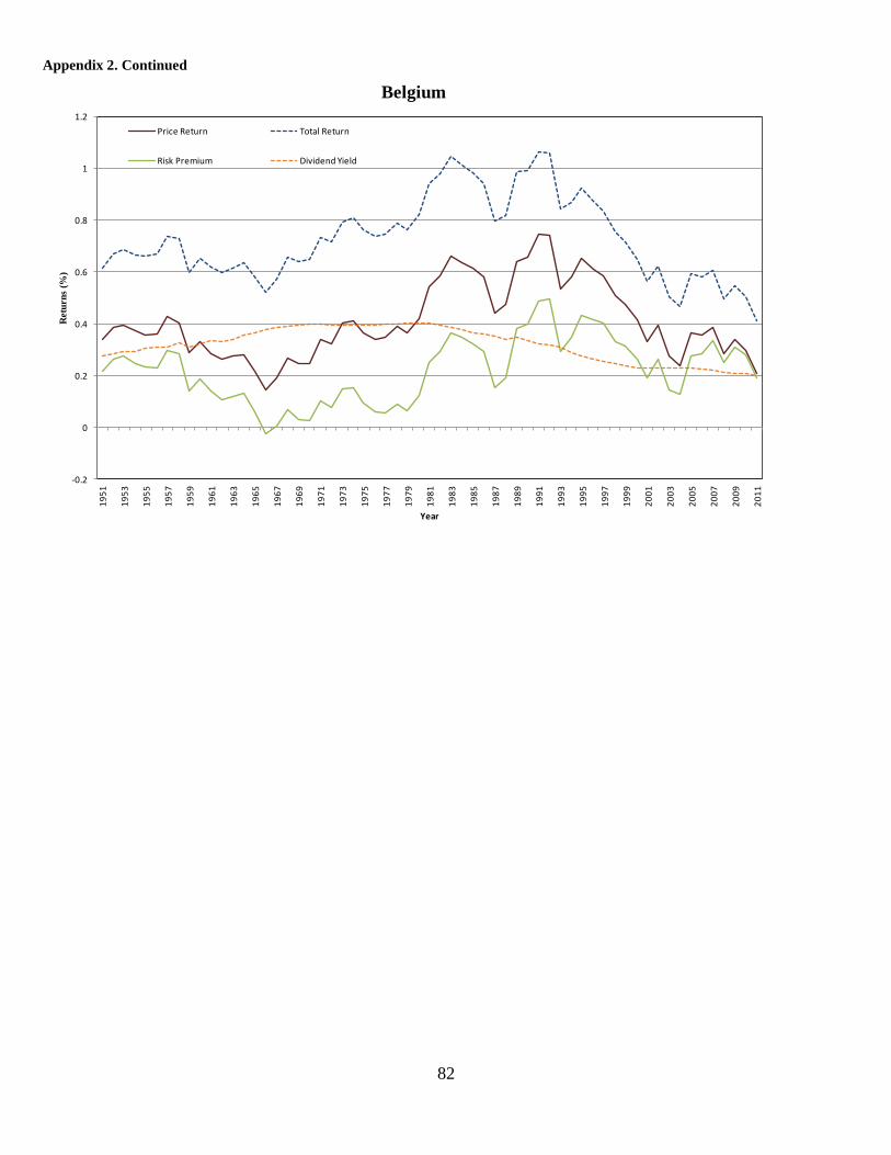
82
Appendix 2. Continued
-0.2
0
0.2
0.4
0.6
0.8
1
1.2
19
51
19
53
19
55
19
57
19
59
19
61
19
63
19
65
19
67
19
69
19
71
19
73
19
75
19
77
19
79
19
81
19
83
19
85
19
87
19
89
19
91
19
93
19
95
19
97
19
99
20
01
20
03
20
05
20
07
20
09
20
11
Retu
rn
s (%
)
Year
Belgium
Price Return Total Return
Risk Premium Dividend Yield

83
Appendix 3. Halloween effect in both mean and variance
We use GARCH (1,1) with a Halloween dummy in the variance equation (Equation 2) to model a Halloween
seasonal in the mean and variance of returns.
,
( )
(2)
We include world index and 57 countries that have price indices data available for over 20 years. Table 11
reports the Halloween effects in returns and in variance for the world and individual markets. In theory, if there
is a significantly higher winter return, we would expect the variance to be higher in winter than in summer.
However, 35 of the 57 countries actually have a smaller variance in winter than in summer, in which 23 are
even significant. This evidence suggests risk difference can not explain the existence of the Halloween effect, if
anything, the risk in summer months is strikingly higher than winter months.

84
Table 11. Halloween effect -GARCH (1,1)-M model
This table provides the results for the Halloween effect estimated with GARCH (1,1) in mean model: , (
)
for 57 countries that have data for over 20 years and the world
index. is the Halloween dummy that equals one if the month falls in the period of November through April. T-values are
adjusted using Newey-West standard errors.
*** denotes significance at 1% level; **denotes significance at 5% level; *denotes significance at 10% level. Countries are
grouped based on the MSCI market classification and geographical regions.
Status Region Start Date End Date Country
βH βv
Developed Asia 11-1964 07-2011 Hong Kong 1.11 1.88 * -11.52 -3.62 ***
11-1914 07-2011 Japan 0.89 2.88 *** -2.70 -6.17 ***
11-1965 07-2011 Singapore 0.81 1.68 * -4.36 -2.88 ***
Europe 02-1922 07-2011 Austria 1.09 3.53 *** 3.82 10.13 ***
02/1897 07-2011 Belgium 0.24 1.22 -0.79 -1.42
01-1921 07-2011 Denmark 0.30 1.85 * -0.32 -1.11
11-1912 07-2011 Finland -0.28 -1.15 -2.52 -5.31 ***
01/1898 07-2011 France 0.60 2.92 *** -1.84 -7.59 ***
01/1870 07-2011 Germany 0.42 1.03 -23.76 -63.32 ***
01-1954 07-2011 Greece 0.74 2.11 ** 0.39 0.39
02-1934 07-2011 Ireland 0.08 0.59 -0.19 -1.57
11-1905 07-2011 Italy 0.44 1.32 -2.90 -2.79 ***
02-1919 07-2011 Netherlands 1.03 3.35 *** -3.76 -5.80 ***
01-1970 07-2011 Norway 0.99 1.41 -7.93 -3.50 ***
01-1934 07-2011 Portugal 0.83 3.72 *** 0.59 1.45
01-1915 07-2011 Spain 0.57 2.48 ** 0.18 0.35
01-1906 07-2011 Sweden 0.23 1.06 -0.98 -2.08 **
01-1914 07-2011 Switzerland 0.41 1.66 * -3.38 -9.41 ***
02/1693 07-2011 UnitedKingdom 0.25 3.46 *** -0.24 -3.78 ***
Mid East 02-1949 05-2011 Israel 0.57 1.51 1.77 1.44
North America 12-1917 07-2011 Canada 0.55 2.37 ** -2.24 -4.36 ***
11/1791 07-2011 UnitedStates 0.10 1.00 -0.24 -2.06 **
Oceania 02/1875 07-2011 Australia 0.08 0.66 -1.12 -6.07 ***
01-1931 07-2011 New Zealand 0.02 0.11 -0.40 -1.88 *
Emerging Africa 01-1988 07-2011 Morocco 0.91 1.89 * 4.48 3.33 ***
02-1910 07-2011 South Africa -0.06 -0.30 0.32 0.94
Asia 01-1991 07-2011 China 0.62 0.56 -3.42 -0.42
11-1920 07-2011 India 0.08 0.44 0.68 6.25 ***
04-1983 07-2011 Indonesia 1.35 2.25 ** -5.19 -2.57 ***
02-1962 07-2011 Korea -0.19 -0.34 2.12 0.89
01-1974 07-2011 Malaysia 1.32 2.35 ** -1.58 -0.83
01-1953 07-2011 Philippines 0.67 1.16 -1.55 -0.69
02-1967 07-2011 Taiwan 1.63 2.93 *** 3.94 2.52 **
11-1975 07-2011 Thailand 0.06 0.12 -7.20 -3.72 ***
Europe 02-1986 07-2011 Turkey -0.08 -0.05 33.68 2.51 **
North America 02-1930 07-2011 Mexico 0.19 1.53 0.04 0.33
South America 01-1990 07-2011 Brazil 1.02 0.91 -12.47 -2.35 **
01-1927 07-2011 Chile -0.29 -0.86 -5.06 -8.56 ***
02-1927 07-2011 Colombia 0.11 0.58 0.93 4.18 ***
01-1933 07-2011 Peru -0.15 -1.19 1.63 22.69 ***
Halloween Effect Variance
t-value t-value

85
Table 11. continued
Status Region Start Date End Date Country
βH βv
Frontier Africa 11-1989 07-2011 Botswana 0.58 2.05 ** 1.18 2.04 **
02-1990 07-2011 Kenya 0.68 1.12 5.57 2.71 ***
11-1989 07-2011 Mauritius 0.29 0.54 -1.29 -1.01
01-1988 07-2011 Nigeria -0.04 -0.11 -3.16 -2.33 **
Asia 02-1990 07-2011 Bangladesh -1.60 -1.54 -5.69 -1.14
11-1960 07-2011 Pakistan 0.64 2.00 ** -0.29 -0.39
01-1985 07-2011 Sri Lanka -0.34 -0.39 -1.06 -0.21
Mid East 11-1990 07-2011 Bahrain -0.44 -0.97 1.95 0.96
02-1978 07-2011 Jordan 0.42 1.01 0.45 0.47
North America 11-1969 01-2011 Jamaica 0.01 0.02 -3.23 -1.19
South America 01-1967 07-2011 Argentina 0.74 0.94 -8.56 -1.90 *
Rarely Studied Europe 01-1984 07-2011 Cyprus -0.07 -0.14 2.07 2.92 ***
01-1954 07-2011 Luxembourg 0.60 1.97 ** -2.20 -3.00 ***
Mid East 04-1990 06-2011 Iran -0.08 -0.11 -3.71 -1.14
North America 04-1989 02-2011 Barbados -0.09 -0.27 3.13 6.39 ***
02-1925 12-1995 Uruguay 0.93 1.54 86.25 22.31 ***
01-1937 07-2011 Venezuela 0.10 0.51 0.76 4.05 ***
World 02-1919 07-2011 - 0.51 2.38 ** -1.21 -3.21 ***
t-value t-value
Halloween Effect Variance