the hippocampus as a cognitive graph

The Hippocampus as a Cognitive Graph

R O B E R T U . M U L L E R , * M A T T STEAD,* andJANOS P A C H ~;

From the *Department of Physiology, State University of New York, Brooklyn, Brooklyn, New York 11203; and *Department of Computer Science, City College of New York, and Courant Institute of Mathematical Sciences, NewYork University, New York 10012

ABSTRACT A theory of cognitive mapping is developed that depends only on accepted properties of hippocampal function, namely, long-term potentiation, the place cell phenome- non, and the associative or recurrent connections made among CA3 pyramidal ceils. It is proposed that the distance between the firing fields of connected pairs of CA3 place cells is encoded as synaptic resistance (reciprocal synaptic strength). The encoding occurs because pairs of ceils with coincident or overlapping fields will tend to fire together in time, thereby causing a decrease in synaptic resistance via long-term potentiation; in contrast, ceils with widely separated fields will tend never to fire together, causing no change or perhaps (via long-term depression) an increase in synaptic resistance. A network whose connection pattern mimics that of CA3 and whose connection weights are proportional to synaptic resistance can be formally treated as a weighted, directed graph. In such a graph, a "node" is assigned to each CA3 cell and two nodes are connected by a "directed edge" if and only if the two corresponding cells are connected by a synapse. Weighted, directed graphs can be searched for an optimal path between any pair of nodes with standard algorithms. Here, we are interested in finding the path along which the sum of the synaptic resistances from one cell to another is minimal. Since each cell is a place cell, such a path also corresponds to a path in two-dimensional space. Our basic finding is that minimizing the sum of the synaptic resistances along a path in neural space yields the shortest (optimal) path in unobstructed two-dimensional space, so long as the connectivity of the network is great enough. In addition to being able to find geodesics in unobstructed space, the same network enables solutions to the "detour" and "shortcut" problems, in which it is necessary to find an optimal path around a newly introduced barrier and to take a shorter path through a hole opened up in a preexisting barrier, respectively. We argue that the ability to solve such problems qualifies the proposed hippocampal object as a cognitive map. Graph theory thus provides a sort of existence proof demonstrating that the hippocampus contains the necessary information to function as a map, in the sense postulated by others (O'Keefe,J., and L. Nadel. 1978. The Hippocampus as a Cognitive Map. Clarendon Press, Oxford, UK). It is also possible that the cognitive mapping functions of the hippocampus are carried out by parallel graph searching algorithms implemented as neural processes. This possibility has the great attraction that the hippocampus could then operate in much the same way to find paths in general problem space; it would only be necessary for pyramidal cells to exhibit a strong nonpositional firing correlate. Key words: place ceils Q cognitive map Q hippocampal long-term potentiation * graph theory, neural applications �9 rat navigation, computer model

I N T R O D U C T I O N

Cognitive Maps

Dating back at least to the work of To lman (1932, 1948), the not ion has been enter ta ined that rats are en- dowed with mapqike representat ions of their environments. The existence of these "cognitive maps" is in- ferred f rom the ways in which rats solve certain spatial problems. Because the problems seem difficult and the

Address correspondence to Dr. Robert U. Muller, Department of Physiology, SUNY-Brooklyn, 450 Clarkson Ave., Box 31, Brooklyn, NY 11203. Fax: (718) 270-3103; [email protected]

solutions seem efficient and intelligent, one imagines that rats must use information about the overall structure or geometry of their surroundings while solving these problems. In short, maps are postulated because it is believed that no simpler problem-solving mechanism will do.

As an aside, we note that not everyone accepts this reasoning, and that even advocates must maintain a healthy skepticism about maps (see Terrace, 1984). Nevertheless, the behavioral evidence in favor of maps is quite convincing, and the reader is referred to com- pendious reviews by O'Keefe and Nadel (1978) and Gallistel (1990). In this paper, we take for granted that

663 J. GEN. PHYSlOL.�9 The Rockefeller University Press" 0022-1295/96/06/663/32 $2.00 Volume 107 June 1996 663-694

Dow

nloaded from http://rupress.org/jgp/article-pdf/107/6/663/1143956/663.pdf by guest on 21 January 2022

various animal species, and particularly rats, have cognitive maps.

Accepting the existence of maps, it is natural to ask how they are implemented. From comparative (cross- species) behavioral studies, it is clear that map-like representations can be supported by nervous systems of widely varying anatomy; they are found in insects, am- phibia, reptiles, birds, and mammals (Gallistel, 1990). The strong implication is that there is not a unique way of representing global information about the environment. Rather, in the course of evolution, a variety of mapping systems seem to have developed, presumably because it is useful to know where you are and how to get to where you want to go.

The Neural Basis of a Cognitive Map

Although comparative work may suggest that maps can be implemented in many ways, it is a more difficult task to understand how a particular map might function. In the first place, it might be difficult to locate a map, even if a particular part of a nervous system is preferentially associated with mapping. For example, a decrease in the ability to solve spatial problems after destruction of a part of the brain might result from disconnecting the putative map from its inputs or outputs, as well as from damaging the map itself. Similarly, the existence of a map would not necessarily be revealed by single- cell recordings because the encoding of spatial information might be distributed across cells in a very complicated fashion.

Despite these possibilities, there seems to be one map that is at least partly localized and whose opera- tions are sufficiently simple to be detectable in the discharge of individual neurons. This putative map was revealed by recordings from hippocampal neurons in freely moving rats by O'Keefe and Dostrovsky (1971). The seminal discovery of O'Keefe and Dostrovsky was that the discharge of many hippocampal neurons is location specific; they fire rapidly only when the rat's head is in a restricted part of the recording apparatus. Such units, now called "place cells" (O'Keefe, 1976), are pyramidal cells of the CA3 and CA1 regions of the hippocampus. The existence of place cells has been corroborated by many workers (Olton et al., 1978; Muller et al., 1987), and although their firing is not ide- ally location specific (Muller et al., 1991b), there are circumstances in which discharge is independent of the direction that the head points in the environment (Muller et al., 1994).

The place cell p h e n o m e n o n is so striking that it immediately convinced O'Keefe and Dostrovsky that the hippocampus is the locus of a map. In the view of O'Keefe (see, for example, O'Keefe, 1991), this map is a Euclidean representat ion of the environment; it allows the computat ion of distances and angles in the en-

vironment, thereby permitting solutions to spatial problems. An alternative view is that the spatial functions of the hippocampus are special cases of more general computations (see Cohen and Eichenbaum, 1993). A recent set of brief papers (Nadel, 1991) lays out the thoughts of many workers in this area.

The position taken in this paper is in fundamental agreement with O'Keefe: We think that place cells re- veal a hippocampal map. Our primary purpose is to show that there is a realistic way in which synaptic connections in the hippocampus can store a map-like representation of the environment. By "map-like" we mean that the representation can be used to solve specific, difficult spatial problems.

The map-like representat ion is built from place cells, long-term potentiation, and the circuitry of the CA3 port ion of the hippocampus. In this scheme, the mapping information is stored in the strengths of CA3 --) CA3 synapses that connect pairs of pyramidal /place cells. The scheme is both parsimonious and precise, but is not comprehensive. That is, we at tempt to prove formally that the required information could be stored in the stated way but do not at tempt to explain ei ther how place cells come to exist nor how the stored information could be extracted by accepted neural opera- tions. Retrieval as it might go on in the nervous system is considered only in the Discussion.

It is useful to comment also on the supposition by O'Keefe that mapping is the sole function of the hippocampus. A contrary supposition has been expressed by Eichenbaum that mapping is a special case of a more general computational process. We take it as a major strength of the ideas proposed here that they fit ei ther of these views. O'Keefe's position is strengthened if it is true that pyramidal cells act strictly as place cells. If pyramidal cells can also represent nonspatial aspects of the situation, the same circuitry permits solutions of nonspatial problems, and Eichenbaum's position is strengthened. In this paper, we deal only with place cells and location-specific firing but regard as open the question of whether the hippocampus may serve more general functions.

Storing Mapping Information

The central idea in this paper is that key information in the hippocampal map, namely, distance in the environment, is represented as the strength of Hebbian synapses (embodied as N-methyl-D-aspartate [NMDA] 1- based, long-term potentiation [LTP]-modifiable synapses) that connect place cell pairs. Specifically, we propose that the strength of a synapse made by a pair

IAbbreviations used in this paper: EEG, electroencephalogram; LTD. long-term depression; LTP, long-term potentiation; NMDA, N-methyl- o-aspartate.

664 The Hippocampus as a Cognitive Graph

Dow


of place cells is a decreasing function of the distance in two-dimensional (2-D) space between the firing fields of the cells (Muller et al., 1991). If there is a barrier between the two fields when the synaptic resistance is set, the distance is how far the rat must go to get from one field to the other, and not the Euclidian distance.

The argument for supposing that synaptic strength should decrease with distance between field pairs is as follows:

(a) Consider a pair of place cells with coincident firing fields, as shown in Fig. 1, A1 and A2. Because the fields are coincident, the two cells will often fire in close temporal order. The timing of the firing of the cell in A2 relative to that in A1 is seen in the point-process cross-correlation in Fig. 1 B, which shows that there are many short (<500 ms) intervals. If the cells are connec ted by a Hebbian synapse, the short intervals between pre- and postsynaptic spikes are expected to cause increased synaptic strength. As is stated more fully below, when it is possible for the strength of the synapse to be modified, the strength is assumed never to get so great that discharge of the presynaptic cell is an important determinant of discharge of the postsynaptic cell. Thus, we imagine that the short intervals indicate only that the fields are near each other (similar to common stimulus driving) and do not indicate a causal relationship between presynaptic and postsynaptic action potentials.

(b) Now consider a pair of cells whose fields are far apart, as in Fig. 2, A1 and A2. In this case, the rat cannot move from one field to the other in a time short enough to permit the two cells to fire in close temporal order, as is visible in Fig. 2 B. Since the cells rarely if ever fire together, the Hebbian synapse should remain weak. For intermediate cases, synapses should have intermediate strengths.

In previous work, it was shown that synaptic strength changes (ASij) made according to a simple Hebbian rule lead to a relationship of the expected form between distance and synaptic strength (Muller et al., 1991a):

A~.j = f . ~ , (1)

where fl is the firing frequency of the presynaptic place cell and f is the firing frequency of the postsynaptic place cell. This rule is unrealistic since it permits synaptic strength to increase without limit. In the present work, however, the form of the strengthening rule is not critical for two reasons. First, having established that even a minimal rule allows distance to be encoded as synaptic strength, we now use explicit functions to set synaptic strength from the distance. The issue of how to do the encoding more realistically is left in abey- ance. Second, we show in Results that the method of storing mapping information works as long as synaptic

strength decreases with distance, regardless of the exact strength--distance function. The implication is that there are few constraints on the strengthening rule.

In the example using Eq. 1, the probability that each cell discharges in a time interval is strictly determined by the position of the rat's head. The probability function is maximal at the center of the firing field and decreases in Gaussian fashion in all directions away from the center. The frequency of each cell is averaged over a time span called the "LTP permissive interval," which was taken as 300 ms from the work of Brown et al. (1989). The sequences of head positions is from paths rats actually took as they retrieved randomly scattered food pellets in a cylindrical apparatus.

A computed example of the relationship between the synaptic strength and distance between firing field centers is shown in Fig. 3. As expected, the synaptic strength decreases with distance and falls to zero if the distance is great enough. Note that synaptic strengths are modified in the desired way during exploration and no explicit teaching mechanism is required. Muller et al. (1991a) showed that the broadness of the s t rength- distance function is very sensitive to changes in field size. In contrast, changing the LTP permissive interval over a fairly wide range had little effect on the shape of the strength-distance function. This is likely because the time-average firing rate is so strongly de termined by whether or not the rat is in the field so long as the averaging time is short compared with the time spent in the field. The insensitivity of the strength-distance function to the LTP interval is encouraging because it suggests that the theory will be robust as understanding of the temporal properties of LTP advances. It is also encouraging that the various time and distance scales are mutually compatible; there is no need to use un- physiologic values for LTP interval, firing rate, speed of movement by the rat, or field size.

If distance in the environment can be encoded as synaptic strength, it is reasonable to ask if such information is sufficient to implement a cognitive map. To sharpen up the question, however, we really ask whether such an encoding can be used to calculate efficient paths through the environment. Our main content ion is that the answer is yes. We will use the methods of graph theory to show that the information is in fact available. The argument is straightforward: We demon- strate that the requisite information is present by solving certain difficult spatial problems with graph-searching algorithms applied to a network of place cells. If the information is not there, no algorithm can compute the required paths.

Three limitations on inferences that can be drawn from the p roof must be noted. First, the p roof assumes that the encoding actually takes place. The arguments that point towards the encoding are attractive but in no

665 MULLER ET AL.

Dow


FmuR~ 2

Dow


sense guarantee that the postulated informat ion is stored. Second, even if the information is there, it is not necessarily available to the rat. Finally, even if the informat ion is used by the rat, the p roo f does not necessarily mean that the neural process of extracting mapp ing informat ion bears a close similarity to the graph algorithm.

An additional r equ i r emen t of the model is that synaptic strength must never get so great that presynaptic action potentials can cause 1:1 driving of postsynapfic action potentials. There are two unfor tunate conse- quences if such driving is possible. First, because Heb- bian conjunct ion o f pre- and postsynaptic activity always occurs, synapfic strength will go to the m a x i m u m value and stay there.

The second difficulty with 1:1 driving is that the firing field of the presynaptic cell would become par t of the field of the postsynaptic cell; specificity would be lost (Hasselmo and Bower, 1993; Hasselmo and Schnell, 1994). By dealing only with writing but not reading of distance information, we do not have to confront any of these issues immediately. It is clear, however, that if the informat ion is stored in synapses between place cells, the informat ion can be read only if the presynaptic cells play a major role in discharging the postsynaptic cell. For the theory to be complete, it is therefore necessary that synaptic modifiability be turned off when distance informat ion is read. In the discussion, we speculate on how reading and writing are separated in time.

There are indications that the contacts between presynaptic pyramidal cells and their postsynapfic partners are indeed quite weak. There is evidence that a given pyramidal cell makes no contact or jus t one contact with interneurons. In addition, the statistics of quantal release between pairs o f pyramidal cells again suggest

at most one contact, and, fur thermore , that the contact releases at one t ransmit ter quan tum at most for each action potential (Balshakov and Siegelbaum, 1995).

Which Synapses Store the Map Information ?

A second main idea in this pape r concerns the identity of the synapses in which the m a p p i n g informat ion is proposed to be stored. As is true of many other schemes to explain spatial or nonspatial operat ions of the hippocampus, we focus on the recur ren t or lateral synapses that are made between pairs of CA3 place cells (see Traub and Miles, 1991). This synaptic class is by no means the only candidate in which to store m a p p i n g information. Other possibilities are the contacts f rom entorhinal cortex (EC) cells onto dentate granule (DG) cells and the Schaffer collateral project ion f rom CA3 to CA1. Synaptic classes EC --~ DG and CA3 ~ CA1 are both considered to be NMDA-based, LTP-modifiable synapses with Hebbian logic (see, for example, Brown et al., 1989). There is also growing evidence that CA3 --~ CA3 synapses also show NMDA-based LTP (Miles and Wong, 1987; Jaffe and Johns ton , 1990; Jeffreys and Traub, 1993).

There are still o ther candidate synaptic classes. The mossy fiber project ion f rom dentate granule cells to CA3 pyramidal cells also shows LTP, but the biophysics and possibly the logic of the modifiability are different (Jaffe and Johnston, 1990). Moreover, pathways f rom entorhinal cortex directly to CA3 and CA1 exist and show LTP (Buzsaki, 1988), a l though the nature of the modifiability is not well characterized.

Given this embar rassment of riches, there are several reasonable ways in which mapp ing information might be distributed across synapses. Nevertheless, we believe that there is a major advantage to focusing on the CA3 ---) CA3 network. We contend that a network of connec-

FIGURE 1. Description of the discharge properties of a pair of simultaneously recorded hippocampal place cells with overlapping firing fields. (A1) The first cell had its field against the apparatus wall at ,'-q 1:30. The discharge rate of this cell is relatively low, as shown by the color code to the left, which indicates the median rate (in spikes/s) for each color category. (A2) The field of the second cell is somewhat larger than that of the first, and the first rate is considerably greater (see color scale) but is in almost the same part of the apparatus. There are two very strong indications that the two cells are independent. First, they were recorded from different microwires. Second, the timing of action potentials was very different on the short scale (ms). (B) Cross-channel spike histogram. Each count in the histogram denotes the existence of an interval between a spike fired by the first cell and a spike fired by the second cell. The key features of the histogram are the great excess of counts at short intervals (< 1 s) and the strong peak near zero. If one of the two cells directly contacted the other via an LTP- modifiable synapse, the existence of many short intervals would tend to cause synaptic strength to increase (synaptic resistance to decrease).

FIGURE 2. Description of the discharge properties of a pair of simultaneously recorded hippocampal place cells with separated firing fields. (A1) The first cell had its field near the apparatus wall at "-~7:30. This cell fired quite briskly; the median rate in the highest rate category (purple) was 17.5 spikes/s. (A2) The second cell is the same as in Fig. 1 A2 its field is well away from that of the first unit. (B) Cross- channel spike histogram. In contrast to the clear peak near t = 0 for the overlapping firing fields in Fig. 1 B, there is a min imum near t = 0 and two maxima at ~ - 3 s and +3.5 s. If one of the two cells directly contacted the o ther via an LTP-modifiable synapse, the large n u m b e r of long intervals and the near absence of short intervals would tend to leave synaptic strength unchanged or to produce a reduction via LTD. Note that the asymmetry of the histogram is caused by the behavior of the rat; there are more counts at positive than negative intervals because the rat tended to walk more often from the field of the first cell to the field of the second cell.

667 MULLER ET AL.

Dow


1,0

0.8

�9 ~.. 0.6

r~ ~ 0.4

N ~ 0.2

0.0 0 5

. . . . ~ . . . . k . . . . i . . , , 310 10 15 20 25

Distance Between Field Centers (Pixels)

A

CA3 -> CA1 Schaffer Collateral Projection

FIGURE 3. An example of a calculated strength-distance function. The strength of a given synapse is calculated from the simple Hebbian rule of Eq. 1. Firing rate was strictly determined from the animal's position in the following way. (a) The current position was taken from a time series of positions recorded as a real rat ran inside of a cylindrical apparatus. (b) The time-averaged firing rate at the current position was a Gaussian function of the distance from a field center for the cell. In the present case, the standard deviation of the Gaussian was three pixel-edge lengths and the peak rate was 30 spikes/s. (c) The time-average rate was used in conjunction with a random number generator to determine if the cell did or did not fire in the current 1 /60th s. (d) If the firing rate of both the pre- and postsynapfic cells was greater than zero averaged over 300 ms, the strength of the synapse was increased according to Eq. 1. In the actual simulation, a total of 600 cells were scattered across the surface of the cylinder, and each cell was connected to eight o ther cells for a total of 4,800 synapses. All synaptic strength calculations were done at once, using a single time series of positions. In the graph, strength at a given distance is the mean strength of many synapses, such that the distance between the field centers of the pre- and postsynaptic cells was in the range n < d < n + 1. Normalization was done after taking the averages.

t i o n s a m o n g cel ls o f a s i n g l e k i n d h a s s t r o n g e r i s o m o r -

p h i s m s to 2-D s p a c e t h a n a n e t w o r k i n w h i c h c o n n e c -

t i o n s a r e m a d e i n o n e d i r e c t i o n f r o m ce l l s o f o n e class

o n t o ce l l s o f a d i f f e r e n t class. W e n o w a t t e m p t to j u s t i f y

t h i s c l a i m .

The Connectivity of Networks and the Connectivity of Space

C o n s i d e r t h e s u i t a b i l i t y o f two d i f f e r e n t k i n d s o f n e u r a l

c o n n e c t i o n s f o r r e p r e s e n t i n g t h e p r o p e r t i e s o f s p a c e .

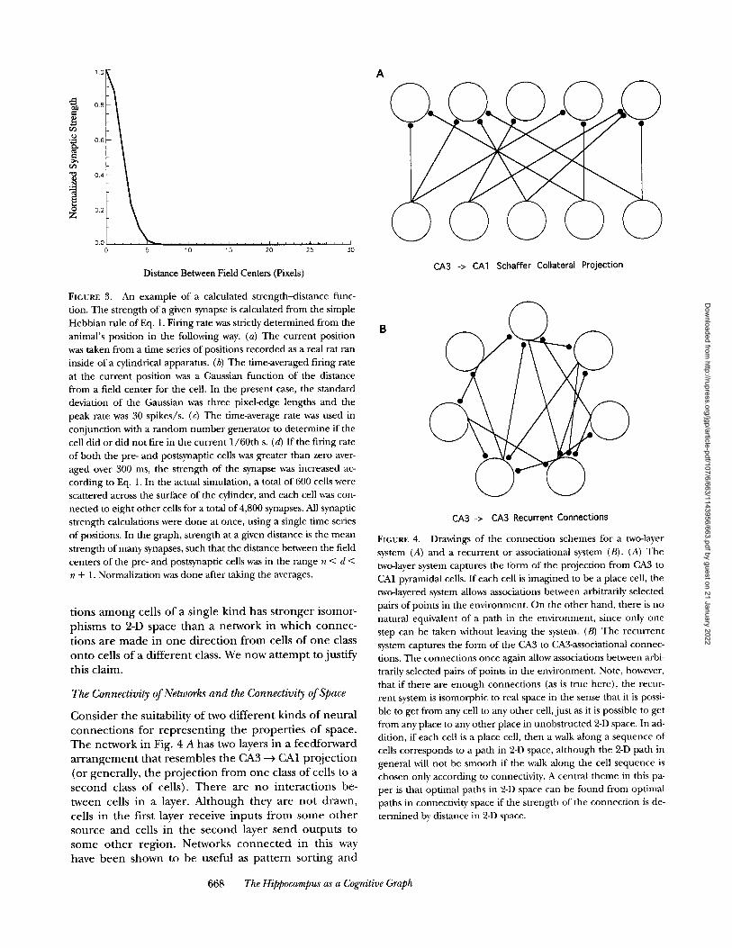
T h e n e t w o r k in Fig. 4 A h a s two layers i n a f e e d f o r w a r d

a r r a n g e m e n t t h a t r e s e m b l e s t h e CA 3 ---> CA1 p r o j e c t i o n

( o r g e n e r a l l y , t h e p r o j e c t i o n f r o m o n e class o f cel ls to a

s e c o n d class o f ce l l s ) . T h e r e a r e n o i n t e r a c t i o n s be -

t w e e n cel ls in a layer . A l t h o u g h t h e y a r e n o t d r a w n ,

cel ls i n t h e f i r s t l aye r r e c e i v e i n p u t s f r o m s o m e o t h e r

s o u r c e a n d ce l l s i n t h e s e c o n d l a y e r s e n d o u t p u t s to

s o m e o t h e r r e g i o n . N e t w o r k s c o n n e c t e d i n t h i s way

h a v e b e e n s h o w n to b e u s e f u l as p a t t e r n s o r t i n g a n d

CA3 -> CA3 Recurrent Connections

FIGURE 4. Drawings of the connect ion schemes for a two-layer system (A) and a recurrent or associational system (B). (A) The two-layer system captures the form of the projection from CA3 to CA1 pyramidal cells. If each cell is imagined to be a place cell, the two-layered system allows associations between arbitrarily selected pairs of points in the environment. On the other hand, there is no natural equivalent of a path in the environment, since only one step can be taken without leaving the system. (B) The recurrent system captures the form of the CA3 to CA3-associational connections. The connections once again allow associations between arbitrarily selected pairs of points in the environment. Note, however, that if there are enough connections (as is true here), the recurrent system is isomorphic to real space in the sense that it is possible to get from any cell to any other cell,just as it is possible to get from any place to any other place in unobstructed 2-D space. In addition, if each cell is a place cell, then a walk along a sequence of cells corresponds to a path in 2-D space, al though the 2-D path in general will not be smooth if the walk along the cell sequence is chosen only according to connectivity. A central theme in this paper is that optimal paths in 2-D space can be found from optimal paths in connectivity space if the strength of the connect ion is determined by distance in 2-D space.


Dow


recognition devices (Kohonen, 1984), especially if there are three cell layers connected by two sets of projections, as in basic back propagat ion schemes (Rumel- hart et al., 1986).

The single-layer, recurrent network in Fig. 4 B is pat- terned after the CA3 ---) CA3 circuitry but could equally well stand for any neural system in which cells of a single class are mutually interconnected. No interactions with cells in o ther layers are drawn, al though again one expects there to be inputs and outputs. Recurrent or "peer-to-peer" networks function as autocorrelators that can do pat tern completion, where a f ragment of a stimulus configuration allows recall of the entire configuration (Kohonen, 1984).

In the feedforward network of Fig. 4 A, only sequences of two cells are possible, regardless of the number of cells in each layer and of the density of connections. Since place cell firing fields occur with about equal frequency everywhere in the environment (Muller et al., 1987), if the connect ion density between cell pairs is high enough, the network can store distances between every pair of points in the environment. Nev- ertheless, there is no way to use a two-layered structure to calculate paths in 2-D space, since only pairwise but not higher order sequences of cells occur in network space. 2 In o ther words, there is no way to make paths in the environment correspond to paths in the network.

The recurrent network in Fig. 4 B also permits the storage of distances between pairs of points in the environment . In addition, however, the recurrent network provides a direct analogy between environmental and network paths. If the network is connected richly enough, it is possible to find a path from any cell to any other cell. Since each cell is a place cell, a path in neural space immediately corresponds to a path in the surroundings. Thus, the recurrent network allows for chains of arbitrary length, in the same way that arbitrarily long paths are generated by locomotion. More- over, because firing fields occur everywhere in the environment , and because there are so many CA3 place cells (~250,000 per side; Amaral et al., 1990), if it is possible to find a neural path from any cell to any other cell, there must be corresponding paths in the environment from any place to any other place; the network shares with 2-D space the property that any place is accessible from any other place (you can get from there f rom here) .

The existence of paths through network space and the existence of corresponding paths through 2-D

2yeckel and Berger (1990) demonstrated that a single shock to the perforant path can excite the same hippocampal elements two or more times because of loops that involve the hippocampus. Pathways of this kind, or a recurrent network in CA1 (Christian and Dudek, 1988; Thomson and Radpour, 1991), are possible alternatives to the recurrent CA3 network considered here.

669 MULLER ET AL.

space is a key property of recurrent place cell networks. The possibility of paths through 2-D space does not, however, necessarily mean that the paths are physically reasonable. Imagine that the probability of connect ion between a pair of cells is independen t of where their firing fields are in the environment. Under these circumstances, going from a presynaptic cell to a postsynaptic cell might be associated with a large j u mp in 2-D space. Thus, smooth paths in neural space need not correspond to smooth or even possible paths in the surroundings.

This difficulty is resolved by taking into account not just whether two cells are connected, but also the strength of the connection. In particular, if the synaptic strength approaches zero, two cells can be considered to be unconnec ted even if the anatomical junct ion exists. In our theory of synaptic strengthening, strength remains near zero if the firing fields of two cells are sufficiently far apart. At once, this means that cell sequences in neural space such that the synaptic weights are all strong correspond fairly well to real paths in the environment; jumps of arbitrarily great distance no longer occur in the representation. This does not mean that the representat ion or map can generate direct, efficient paths, a matter that remains to be demonstrated. What it does mean is that a recurrent network of place cells can be strongly isomorphic to 2-D space if the strength of the recurrent connections decreases with distance, as may happen if the place cells are connected by LTP-modifiable synapses.

What Spatial Problems Must Be Solvable to Call a Representation a Map ?

We now turn to a key question concerning the proposed embodiment of a map: Does the map contain enough information to permit solutions of spatial problems? To answer this question affirmatively, it is necessary only to show that there is some method, no matter how unrealistic, that can generate the required solutions using the stored information; the solutions cannot be generated if the information is not there.

A much more difficult problem is to find a plausible neural mechanism that is capable of finding solutions. It is yet more difficult to show that any proposed mechanism is actually used to generate the paths rats are observed to take. In this paper, we deal mainly with the easiest issue: whether the recurrent network stores enough information about the structure of the environment to solve three spatial problems. These problems are selected because the ability of rats to solve them suggests the existence of maps in the first place.

The first problem concerns the ability to find the straight-line path between any pair of points in the environment, so that any point can serve as a starting location and any other point can serve as a goal. This ability

Dow


is closely associated with the h idden goal p rob lem ex- emplified by the Morris swimming task (Morris, 1981) and especially the variant designed by Whishaw (1985).

The second p rob lem concerns the ability to find an optimal de tour when a more efficient route is suddenly blocked (Poucet et al., 1983). The selection of the best de tour should be done by operat ions on the existing map and must not require the generat ion of a new map. If the proposed representat ion is not flexible enough to find detours, in our j u d g m e n t it would not be appropr ia te to call it a map.

The final p rob lem involves the capacity to find shortcuts when a path is suddenly opened that is more efficient than the cur rent best path (Poucet, 1993). Again, it is critical whether the system can produce the shortcut without generat ing a new map. I f this is possible, it may be concluded that the substrate for the new path already exists in the map, as would be true if the map represented the overall structure of the environment .

Note that the three tests of the mapp ing scheme are all variants of what may be called the "geodesic problem," in which optimal solutions are simply shortest paths. It is not clear if the mapp ing system deals with motivation or t ime as well as geometry in the process of path selection, but in the current t rea tment only geometry is considered.

Searching for Paths in a Model of the CA3 Recurrent Network

Having stated the criteria for de termining if a network contains enough information to be considered a map, it is necessary to decide how to look for the required paths. The me th od used here is to treat the network as a graph, in which cells are in terpre ted as nodes (or ver- tices) and axons plus synapses are in terpre ted as edges. One node is connected to ano ther by a directed edge if and only if an axon branch of the node corresponding to the first cell makes a synaptic contact with the node cor responding to the second cell. The graphs of interest are weighted because each synapse has a certain strength and are directed because information flows in only one direction across a synapse. 3 In Methods, an al- gor i thm is described that allows optimal paths to be found according to sequences of synaptic weights. The critical question is then whether opt imal paths in neural space are also optimal paths in 2-D space.

It is worth not ing that the intuitive distinctions drawn above between feedforward and recur ren t networks have formal parallels in graph theory (Harary, 1969). A directed graph (A --~ B does not imply B ~ A) is said to be "strongly" connected if it is possible to walk f rom any

3This does not preclude the possibility of a retrograde signal sent during modification of synaptic strength via LTP, Information flow is meant to include only the effect that the presynaptic cell has on the likelihood of discharge of the postsynaptic cell.

node to any other node using a sequence of properly directed edges. We ment ion two other related notions of connectedness. A directed graph is called "unilater- ally" connected if, for any two nodes, it is possible to walk f rom at least one of them to the other using a sequence of proper ly directed edges. Finally, we say that a directed graph is "weakly" connected if one can walk f rom any node to any o ther node not necessarily re- specting the direction of edges; this is likely true of feedforward networks such as the CA3 ---) CA1 projection. We argue that the strong connectedness of the CA3 --~ CA3 network allows it to mimic the connectedness of space, something that the weak connectedness of the CA3 ~ CA1 projection does not permit . Experi- mental results (Miles and Wong, 1983) and numerical calculations (Traub and Miles, 1991; see also Results) indicate that the anatomical divergence and convergence in the recurrent CA3 --~ CA3 network is great enough to make the network strongly connected.

To conclude, we refer to some origins of the ideas presented here. As far as we know, the first s ta tement that temporal coincidence of firing might produce functional aggregates of place cells via LTP was by Bliss (1979), in a commenta ry on the work of O 'Keefe and Nadel (1979). The aggregates were composed of all the cells that fired in a given place, and their significance was thought to be increased accuracy of localization of the rat. A second source for the present work is the topological mapp ing theory of Deutsch (1960) and the presentat ion of the theory by Gallistel (1980). This theory has no specific neural embodiment , but it states that navigation may depend on associations between neighbor ing regions of space and on the absence of associations between distant regions of space.

M E T H O D S

Experimental Foundations

One requirement for implementing the graph model is a description of place cell discharge. We begin by briefly describing the behavioral situation for recording and then summarize some important aspects of place cell activity.

Behavioral conditions. Detailed methods used for training rats, implanting electrodes, discriminating and recording single cells, and tracking rats are given elsewhere (Muller et al., 1987). In brief, place cell recordings were made as rats ran around in walled apparatuses of simple geometric shape. The most commonly used apparatus was a cylinder 76 cm in diameter and 50 cm high. The wall of the cylinder was gray except for a white cue card that covered about one-fourth of the circumference. Hun- gry rats were trained to scamper over the whole surface of the cylinder to retrieve 20-mg food pellets, so that place cell firing rate could be measured everywhere. Since the rats ran almost contin- ually, positional firing variations cannot easily be ascribed to ten- dencies of rats to do discharge-related things in certain places. Under the stated circumstances, place cells have several well- characterized properties, which are considered next.


Dow


Place cellproperties. (a) Place cell discharge is location specific. This is the defining property of place cells; their firing rate is largely de te rmined by the position of the rat 's head in the environment . There are known deviations from ideal location-specific firing. For example, the positional firing pat tern is more precise when the h ippocampal e lec t roencephalogram (EEG) is in "theta" mode than otherwise (Kubie et al., 1985), and firing ceases if the rat is immobilized (Foster et al., 1989). Nevertheless, firing is intense only when the rat 's head is in a delimited firing field (see below).

(b) In the cylinder, firing is i n d e p e n d e n t of head direction (Muller et al., 1994). In this paper, we consider only omnidirectional firing. We note, however, that place cells are often directionally selective when recorded on an eight-arm maze or a l inear runway (McNaughton et al., 1983; O'Keefe and Recce, 1993; Muller et al., 1994). We argue in the discussion that the graph model handles directional and omnidirectional firing equally well.

(c) Positional firing patterns are stationary over time intervals of weeks or months (Muller et al., 1987; Thompson and Best, 1990). If a given place cell is recorded with the rat in a familiar envi ronment , its positional firing pat tern seems to be the same no matter how many times the rat is removed and replaced into the environment .

(d) Positional firing patterns are characterized by "firing fields." A place cell discharges rapidly only when the head is in a continuous, restricted port ion of the apparatus. Outside such a field, the firing rate is virtually zero. Examples of firing fields are shown in Figs. 1, 2, and 13. Most cells have only one field, but a few have two (Muller et al., 1987; Sharp et al., 1990;Jung and Mc- Naughton, 1993). Here, we do not consider cells with more than one field since it is clear that they will interfere with the graph searching scheme. As noted, for example, by Shapiro and Heth- er ington (1993), the existence and significance of cells with multiple fields must be settled for a theory to be complete.

(e) Firing fields vary in several ways including size (area), in- tensity (peak discharge rate), and shape. Nevertheless, for simplicity of computat ion, Muller et al. (1991a) imagined that the iso-rate contours are circular or are circles t runcated by the wall of the cylinder. The same assumptions are made here.

The stated propert ies are compatible with the idea that the strength of a Hebbian synapse that connects a pair of place cells should decrease with the distance between the firing fields of the cells (Muller et al., 1991a). Because the real s t rength-dis tance function is unknown (if indeed one exists), synaptic strengths in networks are calculated from one of several explicitly stated functions of the distance between firing fields. Several effects of varying the s t rength-dis tance function, or, more correctly, the reciprocal "resistance--distance" function, are shown in Results. The reason for using resistance-distance functions is stated below.

Building the network. For simplicity, the networks to be analyzed are modeled as r andom graphs, in which the probability of a connect ion is the same for all pairs of cells. There is no question that this assumption is wrong in detail since it is agreed that the density of recurrent CA3 --4 CA3 connect ions varies with the position of the presynaptic cell in the pyramidal cell layer (Miles and Wong, 1986; Ishizuka et al., 1990; Li et al., 1993; Bernhard and Wheal, 1994). The same workers agree, however, that recurrent connect ions are widespread and massive. In the absence of a specific role for the partial specificity of connections, ou r main interest is in whether networks of the size of CA3 and connect ion

density of CA3 are likely to be strongly connected, i.e., that it is possible to "walk" a long a chain of cell ~ synapse ~ cell ~ synapse, etc., and reach any cell from any starting cell. As stated in the Introduct ion, strongly connected networks share with unobstructed 2-D space the property that it is possible to get from any place to any o ther place. This property underl ies our analysis, and, accordingly, it is the first topic dealt with in Results.

A random network is characterized by two parameters, namely, the number of cells and the number of output connections made by each cell. In graph theory, the n u m b e r of output connect ions is called outdegree, a not ion that corresponds precisely to the neu- roanatomical idea of divergence. (Similarly, "indegree" corresponds to convergence.) The total n u m b e r of ou tpu t connect ions is the product of the n u m b e r of cells and the divergence. Because synapses are made between cell pairs, the total n u m b e r of ou tpu t connect ions is equal to the total n u m b e r of input connect ions (number of cells times average convergence) (see Bollobas, 1985).

Once the numeric parameters for a network are chosen, the units are randomly connected with the following constraints:

(a) Every cell has the same divergence (is presynaptic to the same n u m b e r of postsynaptic cells). Al though the mean convergence must equal the divergence, the convergence varies from cell to cell. For small networks, the convergence will have a Pois- son distribution. For networks the size of CA3, the convergence would have a normal distribution.

(b) A cell cannot contact itself, which means that "autapses" are precluded. In graph theory, the concept equivalent to an au- tapse is a loop, in which a node has an edge with itself. Changing this condi t ion would have little effect on any of our results.

(c) A cell is no t allowed to contact ano the r cell twice. (In graph theory, this is equivalent to saying that there are no parallel edges.) There is empirical evidence that suggests this is true (Balshakov and Siegelbaum, 1995). If multiple contacts do in fact occur, permit t ing only one contact can be viewed as lumping together all the synapses. This approximation is not necessarily correct, depend ing on how the multiple synapses are distributed on the dendri t ic tree.

The resulting network is then tested for strong connectivity. If it is not strongly connected, it is discarded and a new random network is built. A surprisingly low divergence is necessary to virtually ensure that the network is strongly connected (see Results).

Once a network is known to be strongly connected, a weight is assigned to each synapse in a two-step process. First, each cell is assigned a location in 2-D space for its firing field. This does not imply any relationship between the identity of a cell and the location of its firing field. To the contrary, the assignment is done randomly, in accord with our belief that the pyramidal cell layer is not topographically mapped onto the apparatus floor (Muller et al., 1987; Kubie et al., 1992). Accessible space is divided into pixels, and at least one cell is assigned to each pixel. In the model, each pixel is taken to be the field center for one or more place cells. In the present calculations, the accessible space is a circle that contains 756 pixels. The radius of the cylinder is ~15.3 pixel-edge lengths. Our considerations pertain to a scale such that a pixel is a square ~3 .3 cm on a side, and the diameter of the circle is ~100 cm. The size of the circle falls within the range of cylinder diameters (76-200 cm) in which we have recorded place cells. In this range, place cell propert ies are nearly constant, although fields in larger diameter cylinders are somewhat larger (Muller and Kubie, 1987).

671 MULLER ET AL,

Dow


After field locations are assigned, each synapse is given a strength according to the distance between the field centers of the cells it connects. As stated above, reciprocal strengths (synaptic resistances) are assigned using one of several resistance-distance functions, which share the property that resistance is a monotonically increasing function of the distance between field centers. At this point the network is complete and ready to be tested for whether it contains sufficient information to solve the navigational problems proposed in the Introduction as hallmarks of mapping.

Finding optimal paths in synaptic resistance space and 2-D space. Formally, the completed network is a random, directed, weighted graph. It consists of a set of nodes, the cells, which are connected by a set of edges, the axons and the endings made by axons on other cells. The graph is random because the connections between cell pairs are set up randomly. It is directed because information can move in only one direction across synapses. It is weighted because the strength of the synaptic connections can vary.

The central problem is whether the graph can be used to find best paths from a start to a goal in 2-D space. The proposed solution is to use a standard algorithm to find best paths in the graph. Since each cell is a place cell, any path in the graph corresponds to a path in 2-D space. The question is whether optimal paths in the graph correspond to optimal paths through the environment. If the correspondence exists, it will have been proved that the network stores enough information to act as map.

Optimal paths in the strongly connected weighted graphs were found with Dijkstra's algorithm (Sedgewick, 1987; Even, 1979). Dijkstra's algorithm finds the path from a start node to an end node that minimizes the sum of the weights. The algorithm works by constructing a simplification of the original graph in the form of a "tree" rooted at the starting node. The tree is simpler than the original graph because it contains no cyclic path such that it is possible to get from a node back to itself. Once built, the tree contains the minimal path from the starting node to every other node and is called a minimum spanning tree.

To build the minimal spanning tree, nodes are divided into three classes: those already known to be part of the tree, those in a fringe that has been visited but that are not yet part of the tree, and, finally, those not yet known to exist. The current state of the fringe is maintained in a list called a priority queue in which the values for nodes determine how the search is made. Initially, the spanning tree consists of only the starting node, and the priority queue is empty. In the first step, all the nodes adjacent (reachable) from the starting node are put onto the priority queue. Next, one of these nodes is attached to the spanning tree (according to the priorities in the queue), and all nodes attached to it are put into the queue. This cycle is repeated until there are no unvisited nodes left. The tree is then finished by attaching the rest of the nodes in the fringe to the tree.

The preceding description of finding a spanning tree makes it clear that the art form is in the assignment of priorities to nodes in the queue. It is not in the scope of this paper to explain how the assignments are made, but it may be clear that the searching process can be varied by changing assignments. For example, if nodes are added to the fringe by always looking at nodes adjacent to the first node on the queue, a "depth-first" search results. If, instead, nodes are added by looking at nodes adjacent to all nodes currently on the queue, a "breadth-first" search is per- formed. For Dijkstra's algorithm, a more complex assignment of

priority is made (Sedgewick, 1987). Dijkstra's algorithm is not optimal for sparse graphs, our main interest, but it is fast enough for small sparse graphs with available computers. For sparse graphs, algorithms exist that run in time proportional to (E + N) log N, where E is the number of edges and N is the number of nodes.

One methodological problem remains to be considered. The path-searching algorithms are designed to find paths along which the sum of the weights is minimized. Clearly, something is wrong if the weights are taken to be synaptic strengths, since a path in the network of minimal synaptic strengths would be a long path in the environment.

It is also clear, however, that the difficulty arises only because synapses are usually characterized by strength and not by its reciprocal, which may be called synaptic resistance (see, for example, Hebb, 1949). If synaptic resistance is used to specify the weight of each connection, then a search algorithm will find paths along which the sum of the synaptic resistances is minimal, and these will be short paths in the environment. It is more convenient to use synaptic resistance in Dijkstra's algorithm simply because large resistances are associated with long distances in the environment and small resistances with short distances in the environment. It is important to realize that substituting synaptic resistance for synaptic strength in no way compromises the graph model. There is nothing more fundamental about synaptic strength than synaptic resistance; they are related in just the same way as electrical conductance and electrical resistance.

R E S U L T S

IS the CA3 Network Strongly Connected?

As s t a t ed in M e t h o d s , r a n d o m g r a p h s a r e u s e d to

m i m i c t h e CA3 r e c u r r e n t c o n n e c t i o n n e t w o r k . I n s u c h

g r a p h s , t h e p r o b a b i l i t y t ha t a ce l l c o n t a c t s any o t h e r

ce l l is a c o n s t a n t . I t is c lea r , h o w e v e r , t h a t t h e p r o b a b i l -

ity t h a t a CA3 ce l l c o n t a c t s a n o t h e r var ies wi th t h e loca-

t i on o f b o t h t h e p r e s y n a p t i c cel l a n d pos t synap t i c cel l

in t h e CA3 layer. F o r e x a m p l e , r e c o r d i n g s f r o m pyrami -

da l cel ls in l o n g i t u d i n a l s l ices o f CA3 r e v e a l e d t h a t

m o n o s y n a p t i c CA3 ~ CA3 c o n t a c t s a r e m a d e o v e r l o n g

sep ta l to t e m p o r a l d i s t a n c e s a n d o v e r t h e w h o l e w i d t h

o f CA3 f r o m t h e h i lus to t h e b o r d e r wi th CA2 (Miles e t

al., 1988) . N e v e r t h e l e s s , t h e y f o u n d a g r a d i e n t a l o n g

t h e l e n g t h o f t h e h i p p o c a m p u s , s u c h t h a t t h e p r o b a b i l -

ity o f c o n t a c t was m a r k e d l y l o w e r i f t h e cel ls w e r e sepa-

r a t e d by two- th i rds o f t h e l e n g t h c o m p a r e d wi th o n e -

t h i r d o f t h e l e n g t h . R e c e n t l y , Li e t al. (1993) t r a c e d t h e

c o n n e c t i o n s o f i n d i v i d u a l CA3 p y r a m i d a l cel ls a n d

f o u n d severa l p a t t e r n s o f c o n t a c t specif ic i ty . F o r e x a m -

p le , t hey saw t h a t cel ls in a b a n d o f CA3 pa ra l l e l to t h e

s e p t a l - t e m p o r a l axis t e n d e d to c o n t a c t o t h e r cel ls in t h e

s a m e b a n d . I n t e r e s t i ng ly , t h e y also s h o w e d t h a t t h e de-

c r e a s e o f c o n t a c t p r o b a b i l i t y away f r o m t h e ce l l b o d y is

s o m e t i m e s n o t m o n o t o n i c ; t h e y f o u n d c l ea r osc i l l a t ions

o f t h e n u m b e r o f c o n t a c t s f o r s o m e cel ls a l o n g t h e

s e p t o - t e m p o r a l axis. I n l i g h t o f c o n t a c t specif ic i ty , a r a n d o m g r a p h c a n n o t


Dow


capture the full richness of the CA3 connect ion pat- A 100 tern. It is therefore necessary to say in jus t what way random graphs are adequate models for a CA3-based cognitive map. In the Introduct ion, we argued that an ad- 0 75

vantage of using a strongly connec ted graph to store a o map is that the strong connectivity is isomorphic to a

fundamenta l proper ty of 2-D space: It is possible to get ~ 0~ anywhere f rom anywhere else. It is therefore essential for us to assess if the CA3 network is strongly connected. In our scheme, once it is reasonable to assume ~ 025 strong connectivity for the recur ren t pathway, the use ~" of r a n d o m graphs as models is acceptable.

Our a rgumen t that the CA3 network is strongly connected rests on calculations done on r andom graphs 0 0 0

with 250,000 nodes, which is about the n u m b e r of cells in the CA3 region of rats (Amaral et al., 1990). This is reasonable since recent work has shown that there are B place cells in the ventral ( temporal) as well as the dorsal (septal) h ippocampus (Poucet et al., 1994; Jung et al., 1994). 10"

For each of 20,000 r andom graphs, the divergence was initially set to 1 and the graph was tested for strong connectedness. If the graph was not connected, the di- _~'~

k 9 10 .2 vergence of each node was increased by 1 and connect- ~

u edness was again tested. The cycle of testing for connectedness and increasing divergence was repeated until the divergence became great enough that the graph

o = 10-3 was connected. This task is possible with relatively limited comput ing resources because graphs with 250,000 r nodes are virtually certain to be strongly connec ted with divergences as small as 20 or so.

The results of this computa t ional p rocedure are presented in Fig. 5 A as a survivor plot; the fraction of nonconnec ted graphs is shown as a funct ion of divergence. When the same data are plot ted on a log survivor scale (Fig. 5 B), the decay of the function is well fit as a single exponent ia l for divergences larger than ~15, as expected f rom graph theory (Bollobas, 1985). The decay constant is such that an inc rement of 2.5 in divergence yields a 10-fold decrease in the probabili ty that a graph is not connected. Extrapolat ion shows that the probability that a g raph is not connected reaches 10 -lz when the divergence is only ~30 . (By bolder extrapolation, the probabili ty that a graph of 250,000 nodes with a divergence of 5,000 is not connec ted is r'-'10-2,200.)

Thus, the divergence necessary to virtually insure strong connectivity in a r andom graph is minuscule compa red with the real divergence of the CA3 network, which is est imated to be between 5,000 and 15,000. The lower value comes f rom the pairwise recordings of Miles and Wong (1986) and the higher value f rom the anatomical work of Li et al. (1993). A third way of mea- suring the connect ions per cell is provided by Amaral et al. (1991). They estimated a convergence for CA3 cells o f ~6,000 by count ing the n u m b e r of spines per

I I I

20 22 24

Fraction Connected = 3 . 3 2 x 1 0 s e ̀ l"a2~

R = 0.999973

10 4

14

FIGURE 5.

I

12 14 16 18

Divergence

i i i k i i i

15 16 17 18 19 20 21

Divergence

Plots of the n u m b e r of nonconnec ted graphs of 250,000 nodes as a function of the divergence (outdegree) of nodes in the graph. In this Monte Carlo calculation, 20,000 graphs were constructed and tested for being connected at each divergence. (A) The n u m b e r of nonconnec ted graphs is plotted on a linear scale to show that the number approaches zero at small divergences. (B) The number of nonconnec ted graphs is replotted on a logarithmic axis against divergence in the range 15-20. As expected from graph theory, the number of nonconnected graphs is an exponentially decreasing function of divergence with a decay constant of almost exactly 1.0. Note that the function is noisier at divergences of 19 and 20, where only a few graphs are expected to be nonconnected. R is the correlation between the number of nonconnec ted graphs and the divergence; its minuscule deviation from 1.0 indicates that the fit is very close. The equation of the re- gression line indicates that the n u m b e r of nonconnec ted graphs is expected to be very small (,-.~10 -2,21~ when the divergence (D) is 5,000, which is about the right value if the connect ion probability for any pair of pyramidal cells is ~0.02.

673 MULLER ET AL.

Dow


cell on the part of the dendritic tree known to receive recurrent contacts. This n u m b e r is directly comparable to the divergence estimates since the average convergence must be identical to the average divergence in a recurrent network.

The fact that the measured divergence and convergence of CA3 units is at least 100 times greater than is necessary to virtually insure strong connectivity in a r andom graph is by no means a p roof that the CA3 network is strongly connected. One can imagine a vast n u m b e r of contact schemes that preclude some cells f rom affecting other cells because the required path does not exist. On the other hand, it would take very little randomness to reach strong connectivity. An astro- nomically large majority of all connect ion patterns are strongly connected with 250,000 cells and a divergence of 6,000. Put ano ther way, if only ~0 .5% of the connections were random, strong connectedness is virtually ensured. Returning to the anatomical data, the axonal distributions found by Li et al. (1993) show many interesting regularities, but unless the small scale contact patterns are much more restricted than the axonal patterns, the network is assuredly strongly connected.

Exper imental data relevant to the stated conclusion were obtained by Miles and Wong (1983), who recorded and stimulated single cells in transverse CA3 slices. They induced rhythmic bursts of activity in such slices by blocking GABA A inhibition. Such bursts likely involved synchronous activity in the whole pyramidal cell populat ion since every recorded cell part icipated in the bursts. In 10 out of 36 cells, repetitive intracellular stimulation was found to affect the entire population. For it to be concluded that the network is strongly connected, stimulation of every cell must be able to influence the bursts; it is not enough that every cell par- ticipates. The results of Miles and Wong (1983) are therefore at odds with our bel ief that the network must be strongly connected. It is possible, however, that the cuts made . to produce the CA3 transverse slice severed many axons near their cell bodies, so that such cells could alter the t iming of bursts.

Are There Enough Synapses in CA3 for the Proposed Representation ?

A key feature of the p roposed representat ion is that each synapse stores a unique piece of information, the distance between the firing fields of the pre- and postsynaptic cells. In a fixed environment , each place cell has a stable firing field, so there is no ambiguity about which distance a given synapse represents. In addition, since only one env i ronment is being considered, the prob lem of interference due to individual cells having different firing fields in different environments does not arise, and it is pos tponed until the Dis- cussion. Here, we ask whether there are enough CA3 ---)

CA3 synapses to store all the distances in a single environment .

It is first necessary to estimate the n u m b e r of points in the environment , since the n u m b e r of distances is the square of the n u m b e r of points. We imagine that the surface of the apparatus is divided into equal area, mutually exclusive square regions (pixels). The size of each pixel is taken to be equal to the area of the projection of a rat 's head onto the horizontal plane, ~ 6 cm 2. The area of the 76-cm diameter cylinder we have used for much of our work is ~4,534 cm 2, so there are 756 pixels. The n u m b e r of directed distances to be represented is then 7562 if there is more than one place cell per pixel. Having more than one place cell in a pixel allows there to be connect ions that represent zero distance, even though a cell may not contact itself. I f there is only one cell per pixel, the n u m b e r of distances is 756 • 755.

Since, on the average, all CA3 pyramidal cells are pre- and postsynaptic to the same n u m b e r of synapses, the n u m b e r of CA3 ~ CA3 synapses, S, is:

S= C(C-1)PM, (2)

where C is the n u m b e r of pyramidal cells and PM is the probability that a cell is directly presynaptic to ano ther cell. Estimates of the n u m b e r of CA3 pyramidal cells range f rom ~250,000 to 300,000 (Amaral et al., 1990; Bernard and Wheal, 1994). As measured with pairwise intracellular recordings, PM is ~0.02 (Traub and Miles, 1991). (Anatomical techniques suggest considerably higher values for PM; Li et al., 1993.) Taking the lower values for the n u m b e r of pyramidal cells and for PM, the total n u m b e r of connections is ~1.25 • 10 9. Divid- ing the n u m b e r of CA3 ~ CA3 synapses by the n u m b e r of distances, each of the 5.71 • 105 distances is represented by ~2,200 synapses! We conclude that the number of synapses is so large that the proposed representation is certainly feasible if all the synapses are used for a single environment . Because the directed distance between each pair of points can be stored many times, one can imagine schemes that use some form of averaging to reduce errors in the representation.

One re f inement of Eq. 2 is worth br ief consideration. It is commonly observed (Muller and Kubie, 1987; Thompson and Best, 1989) that a fraction of dis- criminable pyramidal cells are silent in a given environment . The silent fraction (~) is substantial, with estimates ranging f rom ~ 5 0 to 90% of the pyramidal cell populat ion. Silent cells do not affect the state of o ther cells in the ne twork- - they are informational dead ends. Eq. 2 may therefore be rewritten as

S = Ca(Ca- 1)PM,

where Ca, the n u m b e r of active cells, is C(1 - F~). If F~ is 0.5, the n u m b e r of synapses available to store pairwise


Dow


distance is reduced by 75% and is down by 99% if F~ is 0.9. Even in this extreme case, however, there are still >20 synapses available to store each pairwise distance in the environment. The conclusion that there are enough synapses to store a detailed representat ion is thereby reinforced. The issue of multiple copies for the representat ion of the distance between each pair of points is fur ther treated in the Discussion. We now turn to the question of whether the network stores enough information to act as a map.

Problem 1: Finding a Straight Path between Any Pair of Points in Free Space

The fundamental mapping problem is to calculate the shortest path between any pair of points in the environment, using information stored in the map. If no bar- t ier exists between the pair of points, the shortest path is of course a straight line; in this section we consider only unobstructed space.

As described before, the proposed map has the form of a strongly connected random graph. Each node (cell equivalent) of the graph is associated with a position in 2-D space and is therefore an analog of a place cell. 2-D space is divided into equal area square pixels, and equal numbers of cells are assigned to each pixel. This mimics the even distribution of firing fields over the surface of the apparatus (Muller et al., 1987). At least one node is associated with each pixel. Given 250,000 CA3 cells, ~330 cells would be assigned to each pixel if we at tempted to preserve the size of the neural system. In reality, however, very few cells must be assigned to each pixel for it to be possible to find optimal paths (see below). For this reason and for purposes of re- stricting the size of the computations to practical values, we devote only one to five cells to each pixel.

A basic characteristic of the network is the number of connections made by each node (outdegree or divergence). In accordance with the relatively constant number of connections sent by each CA3 pyramidal cell, the divergence is assumed to be the same for every node in a graph. The divergence determines not only whether the graph is strongly connected, but also how closely shortest paths correspond to straight lines.

The connect ion weights in the graph (synaptic resistances) are a function of the distance between the 2-D points for each pair of connected nodes. We begin by considering a very simple function, and later show the effects of changing the relationship between synaptic resistance and distance. The function has the following properties: (a) The coordinate space is discrete. The only allowable distances are f rom pixel center to pixel center. The first few possible distances are 0.0, 1.0, 1.41, 2.0, 2.24, etc. (b) When the distance is 0.0, the synaptic resistance is greater than zero. In more usual terms, this means there is a maximum synaptic strength.

A distance of 0.0 is possible only when more than one node is associated with a pixel. In most cases treated here, a single node is associated with each pixel, so the lowest resistance is associated with distances of 1.0. (c) When distance (D) is 1.0 or greater, resistance (R) is given by

R = kD if D < Dmax

R = R~nmod if D > Dm~,,

(3a)

(3b)

where k is a constant. Rm~x is the highest possible resistance for modif ied synapses. /)max is chosen such that R = Rmax at D = Dm~. This is useful since it yields the same range of R for all values of k. In turn, it becomes possible to vary k without altering the permissible range of synaptic strengths, a range presumably set by the biophysics of the synapses. The effects of changing k and of introducing nonl inear resistance-distance functions are treated below. The resistance of an unmodif ied synapse, P~nmod, is arbitrarily set to the very large value of 1 0 6 , which has the effect of excluding unmodif ied synapses from sequences of cells.

Fig. 6 A shows an example of a linear resistance-distance function, for k = 2 (Dmax -= 5.0). This function is used in all simulations unless otherwise stated. The corresponding (i.e., reciprocal) strength--distance function is shown in Fig. 6 B, which was scaled to make it similar to the computed strength--distance relationship of Fig. 3.

The best available path in 2-D space is found as follows. First, a starting point and a goal point are selected. Next, the graph is searched for a node whose associated 2-D position is at the start; there must be at least one because every pixel has at least one associated node. If several nodes are found, one is randomly selected. In the same way, a node whose 2-D position is at the goal is selected. Next, the shortest path between the nodes is found by minimizing the sum of the synaptic resistances along the path. Finally, the path in the network is converted to a path in 2-D space by listing the positions of the nodes. It is then possible to draw the 2-D path or to calculate the total distance traversed by sum- ming the distances from node position to node position.

Fig. 7, which illustrates typical paths at different divergences, summarizes the fundamental results of the graph analysis. First, there is always a path from the start to the end point because only strongly connec ted graphs are analyzed. When the divergence is very low (outdegree = 8), the computed paths are unrealistic in that they can involve jumps across large distances (not shown). Jumps arise when the best available path contains one or more synapses whose resistance is unmodified. Since the unmodif ied weight is the same for all synapses between nodes whose positions are far ther apart than the critical distance (Dma~), the total resis-

675 MULLER ET AL.

Dow


A

l x l 0 6 ~

10

0

0

Runmo d

2 4 6 8 10

B 0.5

0.4

0.3 r~

0.2

0.1

Distance (Pixel Edge Lengths)

I I I I I ' J I , ~ , I = , , I

2 4 6 8


I = I ]

10

FIGU~ 6. Linear resistance-distance function (A) and the corresponding strength--distance function (B). (A) The relationship between distance and function is linear over the distance range 1-5 pixel-edge lengths. The point at D = 0 is set slightly greater than zero to indicate that there is a maximum value for synaptic strength. For D > 5 pixel-edge lengths (at k = 2; see text), synaptic resistance is set to a very high value (1 • 106) to indicate that there is a minimal value for synaptic strength even as distance grows without limit. Neither the imposition of a minimum nor of a maximum synaptic resistance is necessary for proper performance of the graph-searching algorithm. The imposition of a sudden jump to a maximum resistance is convenient, however, to allow nonlinear functions to be simply described (see Fig. 12 A). (B) The strength-distance relationship depicted here is the reciprocal of the resistance-distance relationship of A, although the value at D = 0 is not plotted to allow a useful strength scale. The strength- distance relationship may be compared with the curve in Fig. 4.

A

Low Divergence

B

Medium Divergence

C

High Divergence

FIGURE 7. Examples of paths when the graph searching algorithm minimized the sum of the synaptic resistances along neural paths from a cell whose field is centered at start (5) to a cell whose field is centered at goal (G). The Euclidean distance from start to goal is 25.46 pixel- edge lengths. The degree to which the path approximates a straight line increases with divergence. The number of cells required for the low divergence path (A) is 19 and the path is 65.6 pixel-edge lengths long. For medium divergence (B), the number of cells is 11 and the path length is 31.4. For high divergence (C), the number of cells is 9 and the path length is 25.58.

tance is m i n i m i z e d by m i n i m i z i n g the n u m b e r of such steps, even if they j u m p across a great distance. Graphs with saltatory best paths occur only at very low diver-

gences a n d are n o t cons ide red fur ther . As the d ivergence of the ne twork increases, steps in

the best pa th are m a d e only over plausible distances.

W h e n the d ivergence is still r a the r low (ou tdegree = 24), the a lgor i thm finds m e a n d e r i n g , ineff ic ient paths. As i l lustrated in Fig. 7 A, such paths may con ta in seg- men t s that cross each other. As the d ivergence gets h ighe r (ou tdegree = 64 a n d 192), the paths progres-

sively approach a straight l ine (Fig. 7, B a n d C). Thus, the accuracy of paths improves as the connect ivi ty gets richer. The re la t ionsh ip be tween pa th l eng th a n d divergence is shown numer ica l ly in Fig. 8. The hor izonta l l ine at ~25 .5 pixel-edge lengths represents the straight- l ine dis tance be tween the start (26,26) a nd e n d (8,8) points. W h e n the d ivergence is 24, the m e a n path for six calculat ions is 43.9. At a d ivergence of 64, the average pa th is 27.99, a 10% error. Finally, when the divergence is 192, the path is 25.58, an e r ror of only 0.47%.


Dow


55

50

45

40

35

30

25

20

Euclidean Distance

, I ~ L i I I , , a , I , , i , I

50 100 150 200

Divergence

A lX108

/

15

_ . - - ~ . . . . . - ~ �9

/ Is I j

2 4 6 8 10 12

Run,~

k = l . . . . . k=2 - - - - - k = 3

Rm~

14

FIGURE 8. Length of the computed best path as a function of the divergence of cells in the network. The underlying resistance-distance function is shown in Fig. 6 A (and k = 2 in Fig. 9 A). The path length rapidly decreases as the paths straighten out and are only a few percent above the Euclidian ideal for divergence >150.

I t is t h e r e f o r e c lea r tha t the weights in h igh diver- g e n c e g r aphs con t a in e n o u g h i n f o r m a t i o n to al low cal- cu l a t i on o f an a lmos t - s t ra igh t l ine s e g m e n t b e t w e e n ar- b i t ra r i ly c h o s e n pa i rs o f 2-D points . A c c o r d i n g to this c r i t e r ion , the ne twork qual i f ies as a map .

Varying the "Width" of the Resistance-Distance Function

Mul le r e t al. (1991) showed tha t i nc rea s ing the d i ame- te r o f s i m u l a t e d f i r ing f ie lds s t rongly r educes the rap id- ity with which synapt ic s t r eng th falls off with d i s t ance b e t w e e n f i r ing f ie ld pairs . Since synapt ic s t r eng th a n d res i s tance a re r ec ip roca l ly r e l a t ed , i nc rea s ing f ie ld di- a m e t e r m u s t also r e d u c e the ra te a t which res is tance grows with d is tance . Fo r brevity, we t h e r e f o r e say tha t i nc r ea s ing f ie ld d i a m e t e r inc reases the wid th o f the re- s i s t a n c e - d i s t a n c e func t ion . Fig. 9 A shows t h r e e l i nea r r e s i s t a n c e - d i s t a n c e func t ions , for k = 1, 2, a n d 3, wi th k = 1 y i e ld ing the b r o a d e s t func t ion . In Fig. 9 B, p a t h l e n g t h is p l o t t e d aga ins t d ive rgence for the t h r e e func- t ions. T h e m i d d l e curve in Fig. 9 B is i den t i ca l to tha t in Fig. 8. T h e lower curve, which a p p r o a c h e s the Eucl id- ian idea l very rapidly , is for the b r o a d e s t r e s i s t ance -d i s - t ance r e l a t ionsh ip ; c o r r e s p o n d i n g l y , the u p p e r curve in Fig. 9 B is for the na r rowes t r e l a t i o n s h i p in Fig. 9 A. Thus , n a r r o w e r r e s i s t a n c e - d i s t a n c e func t ions l e ad to less e f f ic ien t pa ths at equa l d ive rgence . F r o m the ef fec t o f varying the res i s tance- -d is tance func t ion , it wou ld s eem tha t progress ive ly i nc rea s ing Dmax ( ana log o f f ie ld rad ius ) w o u l d be advan tageous . A n a d d i t i o n a l cons id- e r a t i on suggests, however , t ha t diff icul t ies arise if wid th inc reases w i thou t l imit .

T h e diff icul ty occurs w h e n bes t pa ths m u s t be f o u n d in e n v i r o n m e n t s whose b o u n d a r i e s a re n o t everywhere


B

6~ F 55 ';, k = 1

o ~ i . . . . . . . . . k=3

\ "" \\ """,,,

30 \ .," .... "..--'-..

;~ Euclidian 25 ~ - Distance

20 0 50 100 150 200

Divergence

FIGURE 9. The effects on computed paths of varying the distance constant in linear resistance-distance functions. (A) Three resistance distance functions for k = 1, 2, and 3. Resistance grows most slowly for k = 3 and most rapidly for k = 1. For each function, the value of resistance jumps to a high value when R reaches 10.0. In terms of firing fields, a small value of k corresponds to large fields and a large value to small fields. (B) Length of the computed best path as a function of the divergence of cells in the network for three values of k in the linear resistance-distance functions. For large fields (k = 1), the best available path rapidly converges on the Euclidian distance, As field size gets smaller, the length of the best available paths becomes significantly longer. Note, however, that the computed path length is a respectable approximation to the ideal even for k = 3.

6 7 7 M U L L E R ET AL.

Dow


convex. Cons ider a pair o f cells with large fields that partially overlap. As a consequence , shor t t ime intervals between presynapt ic and postsynaptic spikes are guar- an teed to occur, and the synaptic resistance is sure to decrease. In the scheme presen ted here, the decrease o f synaptic resistance is pure ly a func t ion o f the t empo- ral firing proper t ies o f the inpu t and receptive cells. There fore , since paths tollow the straight line between field cen te r pairs, the line s egmen t of ten cuts far into the concavity. The difficulty is shown in Fig. 10, where paths f rom one cusp to the o the r inside a lune-shaped region are drawn. In Fig. 10 A, Dma• (i.e., field diameter) is large, and, as expected, segments o f best paths enc roach deeply in " forb idden" territory. In fact, ifDma x were larger, the best pa th could j u m p f rom one cusp to the other . Also as expected, when Dm~• is reduced , best paths e n c r o a c h only minimally on the fo rb idden region (Fig. 10 B). We conc lude that in te rmedia te values o f Dma~ p r o d u c e bet ter paths than e i ther very small or very large values. It seems clear that the theory is bol- s tered by f inding that simple a rgumen t s pu t b o u n d s on field size, which is a crucial variable.

Varying the Number of Nodes in the Graph

The divergence necessary to virtually insure s t rong connectivity for a r a n d o m graph o f 756 nodes is only ~6 . In contrast , at Dmax = 5.0, a d ivergence upwards o f 150 is requi red for the best pa th in 2-D space to be nearly straight. In this case, the fract ion o f nodes directly connec ted to a single n o d e is N20%, well in excess o f any reasonable estimate o f the probabil i ty o f a contac t between a r a n d o m l y selected pair o f CA3 cells.

F~GURE 10. Examples of best available paths in an environment with a concavity. The problem is to get from start (S) to goal (G) while staying in the shaded, lune-shaped area. (A) The distance constant is set to a low value (large fields). The result is that the best available paths cut across forbidden territory. (B) With the distance constant set to a high value (small fields), the paths stay within the shaded region.

We now argue that the h igh fractional connectivi ty is merely a result o f using the minimal n u m b e r o f nodes in the graph. The a r g u m e n t is p resen ted in Fig. 11, which shows the path l e n g t h / d i v e r g e n c e relat ionship for when one, two, three, four, or five nodes are as- s igned to each pixel. Since the curves virtually superimpose, the n u m b e r o f nodes (in this range) is a free pa- rameter , and the probabil i ty an arbitrary pair o f nodes is c o n n e c t e d can jus t as well be 4 as 20%. Thus, the theory does no t require unreasonab ly high contac t probability. Note that the n u m b e r o f nodes per pixel c a n n o t grow wi thout limit; at fixed divergence, the network will no t stay c o n n e c t e d if the n u m b e r o f nodes gets very large. For a d ivergence o f 150, the network becomes unlikely to be c o n n e c t e d if it contains ~ 1 • 10 l~ nodes, ~'.~104 times the n u m b e r o f cells in the rat h ippocampus .

How Path Accuracy Depends on the Shape of the Resistance-Distance Function

Up to now, pa th calculat ions have been m a d e using linear res is tance-dis tance functions. Since the empir ical funct ion is unknown, it is impor t an t to ask if g o o d per-

80

70

~ 6o

~ 5o

~ 40

.~ 3o

20

0

~ Euclidian Distance

I I I I

50 100 150 200

Divergence

Varying the number of cells in the network does not FIGURE 11. change the accuracy of best available paths. The number of cells was changed by putting 1, 1.5, 2, 2.5, 3, and 3.5 cells at each of the 756 pixels in the apparatus. For integer values of cells per pixel, 1, 2, or three cells were put at each pixel. For half-integer values, the locations of the extra 378 cells were randomly chosen without replacement from the 756 possible locations. The key result is that there is no systematic change of the best path length; in the stated range of cells per pixel, the best paths are almost perfectly fixed by the divergence. This means that the fractional divergence required for good solutions can be brought within accepted values (probability of 0.02-0.10 that a pair of cells is monosynaptically connected). Linear resistance---distance function with k = 2.


Dow


formance of the best path algorithm requires linearity, or if performance is acceptable in the face of major changes in the resistance-distance relationship. Again, the best path is selected by minimizing the sum of the resistances for sequences of cells beginning with a cell whose field is at the start location and ending with a cell whose field is at the goal location. Performance is judged by comparing the total distance along the sequence of firing fields with the length of the straight line segment that connects the start to the goal.

The linear resistance-distance function with O m a x • 5 (k = 2) is reproduced in Fig. 12 A along with a hyperbolic function that accelerates towards greater distance and a second hyperbolic function that decelerates. The hyperbolic functions are chosen so that they coincide with the linear one at D = 0 and D = Dmax. The equation for the accelerating function is

W = 11.0/(11.0 - 2D) - 0.9, (4)

and for the decelerating function

W = 11.1 - l l / ( 1 . 8 D + 1). (5)

In ei ther case, Wis set to a very high value if D > Dma x. Properties of the best paths for the three resistance-

distance functions are summarized in Fig. 12, B, C, and D. The average path length associated with each function is shown in Fig. 12 B: For the linear function, the average path is only 0.5% longer than the Euclidean path when the divergence is 192. For the decelerating function the error is 4.3%, and it is 12.0% for the accelerating function at the same divergence.

A second property of best paths, illustrated in Fig. 12 C, is the number of nodes necessary to get f rom the start to the end. For the linear function, the number of steps progressively decreases, in parallel with the decrease of path length. A similar result is seen for the decelerating function, al though the number of nodes is consistently less than for the linear function. In contrast, the number of nodes in the best path does not decrease for the accelerating function; to the contrary, there is an upward trend with higher divergence.

The tendency for the accelerating function to take more steps in highly connected networks seems anoma- lous. The reason for this behavior is, however, quite simple. For an accelerating resistance-distance function, it is always true that:

W(Dab) + W(Dbc) < W(Dab + Dbc), (6)

where Dab is the distance between points a and b in 2-D space. Since the shortest path algorithm minimizes the sum of the resistances along the path, it will select paths with smaller steps over paths with shorter total distance in 2-D space. Note that this selection does not require that two paths ab ---> bc and ac exist for any specific pair of points ac. The algorithm makes an exhaustive search,

and it is the sum of the resistances along the entire path that is minimized. Consider two paths consisting of different nodes (except for the start and end nodes). If the first happens to contain two short steps and the other has none, the algorithm will choose the first even if its length in 2-D space is a little longer.

A similar argument explains why the decelerating function consistently leads to paths with smaller numbers of steps, even though the paths are not as short as those associated with the linear function. In this case,

W(Dab) + W(Dbc) > W(Dab + Dbc), (7)

so that smaller weight sums are associated with paths in- volving few nodes. Of course, the intermediate case,

W(Dab) + W(Dbc) = W(Dab + Dbc), (8)

means that the path-searching algorithm will find best paths that optimize distance itself.

The effect of the shape of the resistance-distance function on what is optimized can be summarized by calculating the average 2-D distance moved between each pair of nodes in the path ("average step size"). As shown in Fig. 12 D, average step size is quite constant for the linear function over the whole divergence range. In contrast, average step size increases modestly for the decelerating function and decreases quite strongly for the accelerating function. Some implications of the ability to control the nature of paths according to the relationship between synaptic resistance and distance are considered in the Discussion.

Having objectively described the paths produced by two rather arbitrary nonlinear, monotonically increasing resistance-distance functions, we turn briefly to the difficult problem of judging the quality of the paths. By inspection of plotted paths, it is our opinion that the illustrated nonlinear functions produce rather good performance. The paths for the accelerating function look somewhat bet ter than the one in Fig. 7 B, where the error is "-'22%, although not nearly as good as the near- ideal path of Fig. 7 C. As might be expected for the decelerating function where the error was ,-~4%, the paths are quite close to the ideal line segment.

Reasonable performance is also seen for certain other nonlinear resistance-distance relationships. These include a step function, where resistance is a constant low value for D ~/)max and a constant high value otherwise, and an exponential for which resistance rises very rapidly with distance. On the other hand, there exist resistance--distance functions that do considerably more poorly. For example, if resistance varies with the square of distance, paths are too long by 20.3% at a divergence of 192 and are clearly less efficient than those computed with the accelerating hyperbolic function. Never- theless, it seems that a variety of monotonically increasing resistance-distance functions yield paths that are vi-

679 MULLER ET AL.

Dow


A

,.r

I x 1 0 6 ~ ..... ~" R - - ~ . ~ u n m o d

............... ...-~-'~" ;-- = "-I .... R~ax

~ ~ ~ . I / / I lll t ~ - - L inear

- Dece le ra t ing

Acce le ra t i ng

, , r ' ~ -~W, , "~ , , t . . . . t . . . . I . . . . ~ . . . .

0 1 2 3 4 5 6

B 55

.~ 50

~ 45

% ~ 40

~ 35

~ 3o e-

-~ 25

20

,'i ' ' - - Linear

';; -- -- - Decelerating

i\ ~', ......... Accelerating

~ . .... "~.'" "" Euc l id ian - - ~ "~ ~ ~ D is tance

i l J i l l l i l l l , I I I L J L i l

0 50 1~ 150 2 ~

Distance (Pixel Edge Lengths) Divergence

C

. E

Z

20

10

,,'.

,,' . ,- . . . . . ,' ', ,, "L , / ' , . """ ""',,:" "', . ' " , . . . " "'"

", ,

Decelerating Accelerating

k

i i , i I i i , r I , J i i I , , i i I

0 50 100 150 200

D

e~ ~ 3

-~ 2

- - Linear -- -- - Decelerating . . . . . . . . . Accelerating

r-\ .._ _ /\ /x._ _

' - , . . _ ,

, , . . . o - - - , , , %- " % . . . .

I I I I I I I I I I I I I I I I I

0 50 100 150

I

200

Divergence Divergence

FIGURE 12. Effects o f varying the shape o f the res i s tance-d is tance funct ion . (A) Plots o f the th ree funct ions . T h e l inear func t ion (solid line) is for k = 2. T h e o t h e r two func t ions are app rox i ma t ions to hype rbo las c h o s e n to m a t c h the l inea r f u n c t i o n a t D = 0 a n d D = 5

pixel-edge lengths . O n e func t ion (short dashes) is re fe r red to as "decelerat ing" in the text; the o t h e r as "accelerating." (B) T h e l inear func-

t ion p roduces be t te r pa ths at any divergence, bu t each o f the o t h e r func t ions yields reasonably good results, a l t h o u g h the dece le ra t ing

func t ion is clearly m o r e accurate . (C) T h e n u m b e r o f cells in the best available pa th decreases with d ivergence for the l inear res is tance-dis-

tance funct ion . T h e s ame is t rue for the dece le ra t ing funct ion , which in fact t ends to min imize the n u m b e r o f cells r a the r t h an the dis-

tance. In contrast , the acce lera t ing res i s tance-d is tance func t ion takes m o r e a n d m o r e steps as the d ivergence increases. This effect, which

is d iscussed m o r e comple te ly in the text, h a p p e n s because the accelera t ing func t ion causes the g raph- sea rch ing a lgor i thm to take shor t s teps to min imize the s u m o f the resis tances in the path. (D) As expec ted if the pa ths are approx imate ly the s ame l eng th a n d the n u m b e r

o f cells varies as stated, the dis tance covered be tween the f i r ing fields o f ad jacen t f ir ing fields grows with d ivergence for the dece le ra t ing

funct ion , is invar iant to d ivergence for the l inear func t ion , a n d decreases with d ivergence for the accelera t ing funct ion .

Dow


sually rather close to the ideal. We conclude that the graph model does not depend on there being a linear relationship between resistance and distance. It should therefore be rather robust as more is learned about the biophysics of NMDA-based LTP, which is, after all, the prime determinant of the resistance-distance function.

We now return to asking how well the graph representation mimics a map.

Problem 2: Finding Detours around a Barrier

A second key navigational problem is to calculate efficient, intelligent paths from start to goal after a barrier is put into a familiar environment. The solution to this problem should not involve ad hoc assumptions about the effects of barriers. To the contrary, a solution would be adequate only if known effects of barriers could naturally be integrated with the scheme that finds straight lines in unobstructed space.

Muller and Kubie (1987) found that the most common effect of putting barriers into the environment is to suppress the discharge of cells with fields in the vicinity of the barrier (see Fig. 13). When the barrier bi- sected a firing field, the cell generally fired at a greatly reduced rate in the whole firing field. In contrast, when the barrier was put far from a field, firing was not reduced, even when the barrier interfered with the view of the demonstrably salient white cue card from the position of the field. Thus, the barrier effect is local; it suppresses firing in nearby but not distant fields. An in- dication that firing is affected by the mechanical and not sensory features of a barrier is that a transparent barrier is as effective as an opaque barrier in suppress- ing discharge. In contrast, if the lead base used to an- chor either barrier was put into the field, little reduction of discharge was seen, again suggesting that firing field suppression is caused by changes in possible mo- tions near the barrier.

The strong reduction of place cell discharge near a barrier suggests a way to incorporate the barrier effect into the graph model. We reason as follows: If place cell firing near a barrier ceased entirely, the activity of other cells would not be further affected if the now- quiet cells were removed from the network. In the graph model, there is no analog of discharge, but the insignificance of cells with fields near a barrier can be mimicked by setting to the unmodif ied level the resistances of synapses they make with other cells. When this is done, cells with fields near the barrier are effectively removed from the network.

Imagine now that a barrier is inserted between a start point (labeled S) and a goal point (labeled G), such that the line between the points is the perpendicular bi- sector of the barrier and such that the barrier lies haft- way between S and G, as in Fig. 14 B. The barrier is drawn as a black bar surrounded by a gray rectangular zone that represents the area over which the barrier suppresses firing. For each node whose associated 2-D position lies in the gray rectangle, every output weight to a connected node is set to the unmodified level.

When the path-searching algorithm is applied to the modified graph, it finds nearly ideal paths, as shown by the 10 superimposed examples in Fig. 14 B. As expected from symmetry, about half the paths go around the barrier to the left and about half to the right. When the barrier is slid to the left, paths that go to the right are significantly shorter and are found by the algorithm (Fig. 14 A). Similarly, when the barrier is slid to the right, the algorithm selects paths that go to the left (Fig. 14 C). We conclude that the representation is easily adapted to the known effects of barriers to allow the path-searching algorithm to find optimal paths a round barriers. Thus, the graph representation qualifies as a map on these grounds as well.

As stated, the method of finding detours has a major

FIGURE 13. An exper- iment on the effects of putting a barrier into a firing field. (A) The firing field of a place cell with no obstruction in the apparatus. The median rate in each color category is as follows (in spikes/s): yellow, 0.0; orange, 0.59; red, 1.53; green, 4.44; blue, 12.0; purple, 27.1. (B) Positional firing pattern with a barrier bi-

secting the field. The color code is the same as in A, so that it is evident that the discharge rate has dramatically decreased. When trans- lated into the language of connectivity, the decreased firing in the vicinity of a barrier is enough to allow the graph-searching algorithm to find good paths around a barrier, as shown in Fig. 14.

6 8 1 M U L L E R ET AL.

Dow


FIGURE 14. Best available paths around a barrier. In this figure as well as Figs. 15 and 16, a resistance-distance function resem- bling the accelerating function in Fig. 12 A was used. The function yields calculated paths that are not so close to optimal that they superimpose. The variability on suc- cessive runs, due to the use of the random number generator in connecting the graph, makes it possible to show several paths that are fairly different from each other. (A) With the barrier pushed towards the left, the 10 paths all go to the right. (B) With the barrier centered on the line that connects the start (S) and goal (G), about half the calculated paths go to the left and about half to the right. (C) As expected, if the barrier is set to the right, all 10 paths go around it to the left.

defect. Specifically, if all f i r ing is suppressed nea r the barr ier , a "spatial scotoma" develops in the representa- t ion since all i n f o r m a t i o n abou t the reg ion n e a r the bar r ie r is lost. This loss causes the a lgor i thm to f ind n o n o p t i m a l paths be tween cer ta in pairs of poin ts in the e n v i r o n m e n t . For example , if the start a n d goal points lie on a l ine paral lel to and nea r the barr ier , the algo- r i t hm does no t f ind the straight l ine. Ind i rec t paths of the k ind i l lustrated in Fig. 15 A are ins tead genera ted ,

FIGURE 15. For detours to be found, synaptic resistances in the vicinity of the barrier must be set to the unmodified value. An un- desirable consequence shown in A is that straight paths parallel to the barrier that go through the region of very high resistance synapses are excluded, even though they are kinematically possible. In the text, a method of filling in the scotoma is proposed that involves the recruit- ment of place cells that were previously silent in the environment. The paths in B show that the solution is sat- isfactory.

even t h o u g h there is no mechan ica l h i n d r a n c e to fol-

lowing the straight l ine. An in te res t ing way to fix the defect is to recru i t previ-

ously si lent cells. It is agreed that a large fract ion of place cells have no f i r ing field in any given envi ron-

men t ; est imates range f rom ~ 8 0 % ( T h o m s o n and Best, 1989) down to ~ 5 0 % (Muller a n d Kubie, 1987; Qu i rk et al., 1992). W h e n the e n v i r o n m e n t is changed , previ-

ously si lent cells may acqui re f i r ing fields (Muller and Kubie, 1987; Bostock et al., 1991).

For the scotoma to be "filled in," it is first necessary that previously si lent cells develop f i r ing fields in the vicinity of the barrier. Someth ing similar to the suggested

process was seen for a single place cell by Mul le r a n d Kubie (1987). This cell had a small f i r ing field n e a r the cyl inder wall. W h e n a bar r ie r was pu t in to the field, the cell be ga n to fire over a m u c h larger area, all a r o u n d the barr ier . This is no t precisely what is r equ i r ed for removing the scotoma, b u t it shows that the ba r r i e r can be associated with increased as well as decreased firing.

Assuming that new fields develop in the vicinity of the barr ier , the H e b b i a n modi f ica t ion process will come in to play if the rat explores n e a r the barr ier , a n d distances in the erstwhile sco toma are now rep re sen t ed


Dow


by the strengths of a new set of synapses. In this reorga- nized representation, connections between the recruited cells straighten out paths that are expected to be parallel to the barrier, as shown in Fig. 15 B. Thus, solving the de tour p rob lem with a graph model does not ne- cessitate the generat ion of nonopt imal paths.

Problem 3: Finding Shortcuts when They Become Available

We now show how the graph scheme can generate shortcut paths through a new hole in a previously solid barrier. In this case, the barr ier is imagined to have been in the same place dur ing the animal 's entire exper ience in the environment , so that there are place cells with fields everywhere in the environment , including near the barrier. In general, cells whose fields are near each other in 2-D space but are separated by the barr ier will be connec ted by weak synapses because long times are required to get f rom the region of one field to the region of the other.

If a hole big enough for the rat to get through is made in the barr ier and the rat explores the hole, cells with fields separated by jus t the thickness of the barr ier will begin to fire at the same time. For two such cells that happen to be connected, the synapse will strengthen. With no additional assumptions, paths that pass through the hole are selected as optimal paths in synaptic resistance space. In this way, the shortcut p rob lem is solved, as shown in Fig. 16, so that the graph representat ion qualifies as a map on these grounds as well. The nature of the p roposed solution to the shortcut p rob lem is contrasted with other possible solutions in the Discussion.

Reconstructing the Environment from Information Stored in the Recurrent Synapses

According to the three criteria stated in the Introduc- tion, the p roposed representat ion of the env i ronment in CA3 is a map, since it was demonst ra ted that the informat ion stored in the synapses permits calculations of geodesics, including detours and shortcuts. We now ask if the representat ion is a map in even a s tronger sense: Does the network in some way contain an image of the environment? We in no sense wish to imply that the nervous system "views" such an image, but only that the information to reconstruct an image of the envi- r o n m e n t is present.

In effect, the stored information consists of a list of places and, for each place, a list of distances to other places. Tha t is, each place cell is associated with a position in the environment , and the synapses made by each cell encode the distance of the cell's field to the field of each postsynaptic cell. We now ask if the relative positions of the firing fields can be reconstructed f rom the given information. It should be stressed that no information whatsoever is available about the coor- dinates of firing fields in any 2-D coordinate system;

Shortcuts

FIGURe 16. A demon- stration that the graph- searching algorithm can find optimal paths through a hole in a preexisting barrier. The hole is offset slightly to the right from the straight line that connects the start (S) and goal (G). The best available paths bend in the expected way.

only distances are known. 4 Reconstructions have been a t t empted only for the linear resistance-distance function, in which the synaptic resistance is propor t ional to 2-D distance. We imagine that reconstructions made with o ther resistance-distance functions could not be both self-consistent and planar. Reconstructions are made using only local distances, which corresponds to assuming that the radius of the resistance-distance function is small compared with the largest dimension of the region that contains the points. We know, however, that reconstruct ion works regardless of restric- tions put on the distance between point pairs.

One way of testing if the distances uniquely determine relative positions is to ask whether the structure fo rmed by connect ing field locations to each other is rigid, even though all that a given connect ion specifies is the distance between a pair of field locations. The concept of rigidity is explained in Fig. 17. In Fig. 17 A, distances are known for field pairs AB, BC, and AC, so that the relative positions of the fields are fixed. On the o ther hand, since the only given distance to field D is f rom field A, field D can be located anywhere on the circle of radius AD drawn a round A. The quadrilateral in Fig. 17 B also is not rigid, since it can be de fo rmed by, for example, moving both fields A and B equal distances in the same direction. By contrast, the shape in Fig. 17 C is rigid; it cannot be de fo rmed while respect- ing all the distances.

To de termine if a network is associated with a rigid format ion of firing fields, an exhaustive search is made for a small rigid formation. If one is found, it is used as a "seed." Tha t is, searches are made to de te rmine if

4An equivalent problem is to determine the approximate shape of the United States from a list of cities, where each city has an associated list of distances to other cities. It is intuitively clear that by constructing triangles it is possible to recover the unique layout of the cities relative to each other. The reconstruction turns out to be possible even if only small fractions of all the distances are available, and even if distances are known only over a small fraction of the largest dimension of the US.

683 MULLER ET AL,

Dow


A

? �9

f

" , / / \

x x / \ / x x / \

FIGURE 17. Rigidity of sets of points separated by known distances. It is possible to reconstruct the arrangement of a set of points in 2-D space if enough information is available about the distances that separate pairs of points; once enough distances are known, the relative positions of all points are fixed and the structure is said to be rigid. In A, it is imagined that the distances AB, BC, and ACare all known. In this case, nodes A, B, and C will in general lie on a trian- gle, which is a rigid structure in that no point can be inde- pendently moved without vio- lating what is known about the distances. In contrast, if only the distance AD to a fourth point is known, D may lie anywhere on the circle centered on A with no con- flicts. (B) An example of a nonrigid structure. The quadrilateral can be deformed as shown without changing any of the distances. (C) If the di- agonals are added to the quadrilateral, the structure becomes rigid. The process of determining whether there is enough distance information to Fix the relative positions of a set of points starts with a search for a small rigid object. (See text for additional description.)

cells c o n n e c t e d to cells in the seed a re also r ig idly at- t a c h e d to the seed. I f t h e r e a re such cells, the same search is m a d e on the a u g m e n t e d seed a n d the seed grows. I f it grows to i nc lude all cells, the f o r m a t i o n is known to be r igid, a n d the relat ive pos i t ions o f f ields a re u n i q u e l y d e t e r m i n e d . We first show tha t r econ- s t ruc t ion is poss ib le a n d ask how m u c h connec t iv i ty is necessary for ne tworks o f d i f f e ren t sizes to be r igid.

A n o r ig ina l 2-D set o f 400 poin ts , each c o n n e c t e d to 20 n e a r b y poin ts , is shown in Fig. 18 A. Fo r conve- n ience , the po in t s a re p u t in to the c o o r d i n a t e system given on the axes. T h e r e c o n s t r u c t e d set o f po in t s is shown in Fig. 18 B. By inspec t ion , i t is c lea r tha t the re- cons t ruc t i on o f relat ive pos i t ions is exact , a l t h o u g h the po in t s a re t rans la ted , ro ta t ed , a n d m i r r o r re f lec ted . Since the c o o r d i n a t e s a re on ly a conven i ence , these dif-

f e r ences have no d e e p s ignif icance. In fact, t r ans la t ion , ro t a t ion , a n d re f l ec t ion are ca l led r ig id t r a n s fo rma t ions s ince they p rese rve the s t ruc tu re o f objects . F r o m the abi l i ty to r e c o n s t r u c t the e n v i r o n m e n t , we c o n c l u d e tha t the synapt ic weight r e p r e s e n t a t i o n con ta ins a "latent" image o f the e n v i r o n m e n t which can be m a d e ex- pl ic i t ( "deve loped" ) by the s ta ted r e c o n s t r u c t i o n process. I t is u n c l e a r if the ra t has access to this a spec t o f the r e p r e s e n t a t i o n , b u t at least it is there .

We c o n c l u d e Results by showing tha t the connec t iv i ty o f the CA3 ne tw ork is so g rea t as to vir tual ly ensu re tha t an equ iva len t g r a p h is r igid. In this a r g u m e n t , we ig- n o r e the d i r ec t iona l i t y o f c o n n e c t i o n s s ince d i s t ance in the p l a n e is spec i f i ed j u s t as well by one-way as by two- way connec t ions .

A n u n d i r e c t e d g r a p h o f n n o d e s is said to be con-


Dow


A B

300

250

200

;~ ~5o

100

50

0

4 �9 � 9 1 7 6 . .

..,." ~,.l: " '.~'~',r:. .:. :": -'.. ?.." �9 ~ ; . . , g o : . o , .

: ~ ~ . . ~ "

. . . . , ~ : , = ' : - r 1 4 9 .

�9 : ~ . 0 . " . �9 �9 ~ , . . r -'}',t ~ "

�9 , . . . *. ~.o o .." : , : *. :~. . . . . � 9

�9 . . : ? . . . . ~ �9 �9 :~ �9 : 7 . : - ; . - .

..- .:. ".-, -,:.. ,,: ~"" �9 . . 0 � 9 r

0 0 �9 : * � 9

I . . . . I . . . . I . . . . I . . . . I . . . . I . . . . I , ,

50 100 150 200 250 300

X

50

0

-50

-100

-150

-200

-250

-100 - 5 0

�9 . . : , . . :, ",~.. :...... �9 . . , . . ... : " , ~ : . "

�9 . �9 . ,m , . " . . ' i , � 9162 . . t . � 9 , - . . . . . ~ :,. . " , ~ ; . .

�9 . ~ . " . . . , ~ ". ~ - . ~ . ' . . * . ,, a �9 . . . o �9 �9 I , ~ l e . s ~ . ~ .

"t , . " : " " f . : " " . " " . : �9 , . , . �9 . ' . , . : . ; . .

�9 "o * �9

�9 : ; . ; . " . - .

, . � 9

~

. . 1 . . . . I . . . . I , , , . 1 . . . . I . . . . I . . . . I

0 50 100 150 200 250

X

FIGURE 18. Reconstruction of a set of points from distance information. (A) The locations of the original set of 400 points are shown in an arbitrarily chosen coordinate system. The distance from each point to 20 other nearby points is the only information provided for the construction process. (B) The outcome of reconstruction is shown by plotting the calculated locations in the same coordinate system. Note that the structure of the original is preserved, although the composite object has trans- lated, rotated, and undergone a mirror transformation.

nected if it is possible to walk f rom any node to any o ther node along edges of the graph. More generally, a graph is called k-connected (k is a positive integer) if the graph remains connec ted after removing any k - 1 of its nodes. According to Menger ' s theorem, a graph is k-connected if and only if any pair of its nodes can be connec ted by k different paths that share only the endpoints as nodes (Harary, 1969). It is a necessary but not sufficient condit ion that every node must be of at least degree k (have at least k edges) for a graph to be k connected.

A key result in graph theory is that the probability that a randomly chosen, undirected graph with n nodes and m = n(c + log n)/2 edges is connec ted approaches e x p [ - e x p ( - c ) ] , where c is a constant and n approaches infinity (Erdos and Renyi, 1959); some numerical values are given in Bollobas and Thomason (1985). Specifically, undirected graphs with 250,000 nodes are connec ted with probabili ty of >0.99 if c = 5. The n u m b e r of edges in such a graph is ~2,179,000, so that the required average divergence (edges /nodes) is ~8.72.

Once the graph is connec ted (i.e., 1 connected) , connectivity increases rapidly as additional edges are added. A randomly chosen graph with n nodes and ~ n [ l o g n + k log(log n ) ] / 2 edges is almost certain to be k connected. If k is 6 (see below), a graph with 250,000 nodes is almost certain to be k connec ted when the average divergence is ~27.5. In fact, a r andom graph is almost certain to be k connec ted as soon as every node has k connections, even though this condit ion is not sufficient for all graphs (see above).

In our model , the approach to k connectivity occurs even more rapidly than for the completely r andom graph. This is because we construct our graphs such that each node is connec ted to k other randomly con-

6 8 5 M U L L E R E T A L .

nected nodes. Thus, the condit ion stated above for k connectivity is automatically satisfied. In fact, even though the graph contains only m = kn edges, the probabili ty that it is k connec ted approaches 1 very quickly as n gets larger (Fenner and Frieze, 1982).

The significance of the considerations about k connectivity comes f rom a result of Lovasz and Yemini (1982), who showed that every 6-connected graph whose edges represent (generic) edges in the plane must be rigid. In the present situation, with n = 250,000, m = pn 2, and the connect ion probabili ty P = 0.02 (Miles and Wong, 1986), the n u m b e r of edges is enormously greater than 6n. In fact, with P = 0.02, a rigid map will be induced with as few as ~300 pyramidal cells; the lower bound for the n u m b e r of cells to ensure rigidity is a very small fraction of the n u m b e r of pyramidal cells�9 This is impor tan t because the silent cell p h e n o m e n o n lowers the effective n u m b e r of place cells in a given env i ronment to between 10 and 50% of the n u m b e r of pyramidal cells (Thompson and Best, 1989; Muller and Kubie, 1987). Thus, the network can store an image of the env i ronment even if a more realistic es- t imate of the n u m b e r of place cells in the representation is used.

D I S C U S S I O N

A central feature of the graph theory of cognitive mapping is that the strength of LTP-modifiable synapses between pairs of place cells encodes the 2-D distance between the centers of their firing fields (Muller et al., 1991). The possibility of encoding distances in 2-D space in a straightforward way is attractive for a n u m b e r of reasons. For example, it provides a role for place cells beyond signaling the current location of the rat, and it give rationales for why place cells should be con-

Dow


nected to each other at all, and why the connections should be LTP modifiable.

The t reatment in Results deals only with a single environment . In a fixed environment, each synapse between a pair of place cells encodes exactly one distance and nothing else. The supposition that a synapse represents a single atomic fact stands in great contrast to the more usual idea that the strength of a synapse is mean- ingful only in the context of the strengths of a large number synapses (see, for example, Kohonen, 1984). For most of the Discussion, considerations are restricted to a single environment, but at the end atten- tion is paid to how multiple environments can be represented without destructive interference.

Encoding Distance in Single Synapses

Before dealing with properties of place cell networks, it is important to make explicit some difficulties in precisely encoding distance as synaptic resistance. First, an unambiguous encoding requires the rat to spend equal times in all parts of the apparatus. If, as is really the case, dwell time is nonuniform, Hebbian synapses will represent where the rat actually went as well as the distance between field centers. Second, firing fields are assumed to differ only according to location. This is em- phatically untrue: Fields differ f rom each other in terms of size and peak rate. For both reasons, variations in synaptic strength are expected even for field pairs whose centers are equal distances apart.

We have not yet investigated how such variations affect the quality of shortest paths. One possibility is that graph searching can yield good paths even though synaptic strength depends on individual place cell properties and the behavioral proclivities of the rat. This possibility arises because the distance between every pair of points in the environment is very likely represented by many individual synapses. The searching process will tend to include the lowest resistance synapse from the set of synapses that represents each pair of points, thereby reducing the effects of the variance. Below, we consider a different solution, in which the network ac- tively minimizes variations of synaptic strength because of factors other than distance.

Another difficulty in the proposed encoding has to do with field shape. If fields are not radially symmetric, the notion of distance itself becomes complicated. For example, in a rectangular or square apparatus, a firing field may be linear and run along almost the entire length of the wall (Muller et al., 1987). Given such shapes, it may be more appropriate to think of synaptic strength as encoding the degree of overlap of field pairs, rather than distance. We have not yet tried to ob- tain paths from a network in which weights are assigned according to overlap instead of distance.

Storing a Representation of the Environment in a Recurrent Network of CA3 Place Cells

In the Introduction, we proposed to call a navigational system map-like if it permit ted solutions to three shortest-path problems. The central finding in this paper is that a network of place cells strongly connected by synapses whose resistances encode distance satisfies the proposal. To build such a network, it is necessary that the place cell fields cover the environment and that the rat explores the whole environment so that synaptic weights can be set according to the temporal overlap of firing of connected cell pairs. The rat must visit all parts of the environment, but it need not take all possible paths. An important feature of the scheme is that learning is unsupervised; it takes place during exploration.

We began the Results with numerical arguments that the CA3 ~ CA3 network is strongly connected. A major idea at this level is that the strongly connected network has an essential isomorphism to 2-D space: It is possible to get from any cell in the network to any other cell just as it is possible to get to any point in 2-D space from any other point. We also pointed out that every path in neural space (sequence of cell ~ synapse ---> cell ---> synapse, etc.) corresponds to a path in 2-D space, and that the number of connections is sufficient to represent the environment with high fidelity.

We then investigated the kinds of paths that such a network makes possible to find in unobstructed space. We found that the best paths in 2-D space associated with best paths in neural space approached straight line segments as the number of edges per node (divergence) of the network increased. The path quality was shown also to depend on the exact relationship between resistance and distance, although each of a selection of different relationships yielded rather good results.

Although not proved, we believe that straight line solutions in 2-D space are found only when the resistance-distance relationship is linear. If the relationship is nonlinear, the length of the best path is greater than the length of the straight line segment from start to goal, and the system is non-Euclidean. By way of speculation, we note that changes in the represented distance between two points in 2-D space can occur if the resistance-distance function is altered. This provides a way of modifying paths according to non-spatial factors, and is a way of introducing motivational concepts such as attraction or avoidance into the scheme.

In our view, the viability of the graph approach was strongly bolstered by the ease with which the outcome of barrier experiments could be incorporated to generate solutions to the detour problem, the second of the three mapping problems. Muller and Kubie (1987) showed that place cell firing was generally suppressed when a barrier was inserted to bisect a firing field. We


Dow


now interpre t the empirical result as mean ing that cells with fields in the vicinity of the barr ier are effectively removed f rom the network: I f they cannot fire, they cannot influence the activity of o ther cells. The barr ier effect has an immedia te translation into the realm of synaptic weights: I f the output weights of cells with fields in the vicinity of the barr ier are set to the unmodified level, such cells are effectively removed f rom the network. When this is done, the graph-searching algo- r i thm immediately finds near-optimal paths, with no other alterations in the network. By taking into account the existence of cells whose fields are enhanced by the barrier, it was shown that the scotoma caused by setting synaptic weights to zero could be filled in, so that the new set of weights accurately represents the al tered to- pography of the environment .

We also showed that the graph approach provides a natural solution to the third mapp ing problem, that of finding shortcuts. Behavioral work predicts that the rat will reexplore the por t ion of an env i ronment in which a change is detected (Poucet et al., 1986). In the present case, this means that the rat will go to the vicinity of a gap that is made in a preexisting barrier. When the rat is near the gap, a synapse that connects a cell pair whose fields are on opposite sides of the existing barr ier should s t rengthen when the head enters the gap because the two cells can now fire together in time.

Does this mechanism for solving the shortcut problem involve cognitive mapping? If cognitive mapp ing means direct use of geometr ic knowledge of the environment , the answer must be negative; the rat does not "know" before it approaches the gap that it is a shortcut. Note, however, that since the rat would be expected to walk up to the gap to reexplore and then to go through, one imagines that the behavior would not appea r to be very different than if insight learning using global informat ion about the env i ronment were involved. Based on our at tempts to date, it seems to be a very difficult p rob lem to design a behavioral experi- men t that can distinguish between a topological and exploratory explanat ion of shortcut behavior on the one hand and a "true" mapp ing explanat ion on the other.

Two additional points in the Results should be reca- pitulated. First, by analyzing paths in environments with nonconvex boundaries , it was found that increasing field size without limit would generate paths that more seriously encroach on forbidden regions. Since decreasing field size without limit will eventually ex- haust the ability of a fixed n u m b e r of synapses to represent the distance between all position pairs, it seems that there is an opt imal field size, whose scale turns out to be about the size of the rat.

The final demonst ra t ion bears directly on the question of how closely the strongly connec ted network of

CA3 place cells approximates a map. We showed that the shape of the env i ronment can be reconstructed f rom distance informat ion stored in CA3 ~ CA3 synapses, so that the network contains an image of the environment . It is unknown if the animal has access to such global information, jus t as it is unknown if neural machinery exists to extract opt imal paths. Nevertheless, it is encouraging that aspects of the overall structure of the env i ronment can be represented using only local information.

As so far developed, the graph theory treats only the CA3 recurrent network; it ignores the rest of A m m o n ' s Horn , the dentate gyrus, entorhinal cortex, and the subiculum, all of which process positional signals. It also ignores the head direction system whose activity is seen in the postsubiculum and anterior thalamus (Taube et al., 1990a, b; Taube, 1995). It is encouraging that the core of a viable theory can appeal to such a restricted part of the available machinery, but it is evident that the focus on CA3 means that the theory is incomplete. Also indicative of incompleteness is the inattention to correlations between the behavioral state of the rat and the state of the h ippocampal EEG. Some speculation in this regard is made below.

Although incomplete, the graph scheme is also parsimonious and specific. We assume only the existence of CA3 place cells, the anatomy of the CA3 ---) CA3 recurrent connections, and the LTP-modifiability of the connections. The first two claims are well-established facts about the h ippocampus. The third is compat ible with the limited evidence so far available and is also expected by analogy with the CA3 ~ CA1 synapses that are known to be LTP-modifiable. The path results depend only on the simultaneous existence of the three assumed propert ies in a single region of the nervous system. The scheme is also conservative in the sense that the stored informat ion is strictly associative, such that associative strength falls off with distance between the firing fields of connec ted place cell pairs. Hebbian synapses are eminent ly suited for storing this sort of information.

A biophysical question worth raising is whether CA3 --~ CA3 synapses show long-term depression (LTD) as well as LTP (see, for example, Levy et al., 1990; Stanton and Sejnowski, 1989). Unquestionably, uncompensa ted LTP will eventually cause synaptic strength to saturate (i.e., minimize synaptic resistance). It is therefore critical whether LTD causes synaptic resistance to increase via a process independen t of LTP, or whether LTD truly reverses the effects of LTP. If LTD operates via a different mechanism, the saturation p rob lem still exists. If, instead, LTD reverses LTP, synaptic resistance can reflect the ongoing relationship of the activity of the pre- and postsynaptic e lements and not simply the integral of the activities over u n b o u n d e d time intervals.

687 MuI~I~E~ ET AL.

Dow


For the rest of the Discussion, we assume that LTP and LTD are names for processes running in opposite directions, a l though the evidence is by no means conclu- sive. This assumption is implicit in our scheme of how the operat ion of the network could reduce the dependence of synaptic strength on behavior, thereby mak- ing the p roposed representat ion more map-like by a kind of renormalizat ion.

How an Environmental Representation Might Be Built

The positional firing distributions of place cells are stable when a rat is put into a certain familiar apparatus. The same cells in general have markedly different distributions when recorded in a second (or third) familiar apparatus, but, again, the distributions are stable. In particular, if recordings are made alternately in the two apparatuses, the positional firing of individual cells reli- ably j umps f rom one distribution to the o ther (Bostock et al., 1991). These results have two fundamenta l implications. First, they are possible only if there is some neural memory of each of the familiar apparatuses; otherwise, fields could not be stable in each environ- men t but would be mutable between environments. The time scale of this form of m em ory is on the order of months. Second, there must exist a recognit ion process whereby the representat ion of a familiar environ- men t is activated or recalled only when the rat is in the appropr ia te environment . This recall process, which is imagined to be similar to the sort of pat tern recognition proposed by several authors (e.g., McNaughton and Morris, 1987; Rolls, 1989) is very fast. Informal tests show us that discharge begins as the rat is lowered into the firing field of a target cell, 20 cm or more above the ground (Kubie and Muller, unpubl ished results). Cor- respondingly, no discharge is seen if the rat is lowered onto the floor outside the firing field. (A corollary of these results is that firing fields have 3-D extents.)

We now ask what happens if the recognit ion process does not find a match for a familiar environment . Pre- sumably, a new representat ion must be genera ted for the unfamiliar environment , after which the representation will be stable and capable of reactivation. In the context of the graph theory, we imagine that the new representat ion is set up as follows.

(a) A certain fraction of the pyramidal cells is allo- cated to be place cells in the new environment . In the simplest case, the fraction is the same for all environments, regardless of the complexity of the env i ronment or the task. It is also imagined that the cells are randomly selected with rep lacement f rom among the pyramidal cells; a given cell may be a place cell in many environments. We refer to the selected cells as the active subset of pyramidal cells. The notion that the active subset is only a fraction of the pyramidal cell population comes f rom the "silent place cell" p h e n o m e n o n

(Kubie and Ranck, 1983; Muller and Kubie, 1987; Thomp- son and Best, 1990). It is commonly found that units that are robust place cells in one env i ronment are virtually inactive in a second. In addition, the inactivity is stable for an environment .

(b) Up to now, only three studies on the initiation of a new representat ion have been published (Hill, 1978; Bostock et al., 1991; Wilson and McNaughton, 1993). These are in ag reement that the stationary firing patterns of individual place cells are rapidly established. In the work of Hill and of Wilson and McNaughton, stationary firing began on the first pass of the rat through the field; Bostock et al. (1991; Plate 3), saw an interval of ~ 3 min in which the cell was silent in the new environment , after which the new positional firing pat tern was stable. We therefore assume that place cells are quickly assigned to fire in certain places.

(c) Accordingly, the creation of the graph takes place after reliable location-specific firing has begun. Simula- tions of how graph weights are established suggest that it takes several minutes before they approach ideal values (Muller et al., 1991). In our view and in ag reement with the criticisms of Burgess et al. (1994), it would be preferable for the map to be rapidly generated. It would also be preferable if the graph weights were less sensitive to the history of the rat 's behavior.

(d) To speed up format ion of the graph and to make graph weights more purely geometric, it seems necessary to imagine a cooperative mechanism that operates at the level of the network instead of individual synapses. Such large-scale mechanisms would reflect processes occurr ing synchronously in many cells and therefore should be detectable by recording the hippocampal EEG.

The two most striking EEG p h e n o m e n a are theta and "sharp waves." The theta rhythm consists of 5-9 Hz sine-like waves that are seen when the rat locomotes. Sharp waves occur during an EEG state called large irregular activity and are seen when the rat is quietly alert or engaged in repetitive activities such as chewing or grooming (Vanderwolf, 1969). We will consider a possible role for theta rhythm below.

In ag reement with Buzsaki (1989), we assume that sharp waves are a network-level mechanism that could serve to modify synaptic weights. Sharp waves reflect the nearly simultaneous activation of clusters of pyramidal cells (Buzsaki, 1992). In this view, sharp waves are nonspatial processes that accelerate graph format ion and increase conformance of graph weights to the geometry of the environment . In other words, it is our guess that sharp waves, in conjunct ion with constraints imposed by 2-D space, can specify the required renor- malization of weights.

(e) As stated in the Introduct ion, grave problems occur if synapses get so strong that the presynaptic cell


Dow


can cause 1:1 discharge of the postsynaptic cell. On the other hand, if the presynaptic cell can never strongly participate in firing the postsynaptic cell, it is unclear how the strength of the synapse can be read in the process of reading the map. There are several ways in which these two very different requirements for synaptic strength can both be satisfied. For example, Traub et al. (1992) suggested that weights are set when the hippocampal EEG is in the theta state and accessed when the EEG shows large irregular activity.

The foregoing scenario outlines how a graph could come to represent the environment, how the representation might be formed rapidly, and how its numerical features could be independen t of the time sequence of positions occupied by the rat. We now consider how the representat ion could be read and used.

Using a Graph to Get Therefrom Here

It is perhaps tautological to say that a map-like representation can be used to find paths through 2-D space only if the endpoints of the path are themselves represented. Since every path must start at the rat's current location, the discharge of place cells provides a representation of all path origins. In contrast, it is not clear how path terminations (or goals) are represented, nor whether the representat ion exists within Ammon's horn or associated areas. The lack of any obvious goal- related discharge in Ammon's horn led Burgess et al. (1994) to propose that goal cells exist in the subiculum. A very recent repor t by Gothard et al. (1994) suggests that activity of the sort to be expected for representation of goals is detectable in hippocampal pyramidal cells, but there may be other interpretations of the firing correlates found by Gothard et al.

In the absence of strong empirical evidence about goal representation, and in keeping with our focus on CA3, we will assume that path terminations are encoded as the discharge of CA3 pyramidal cells: When the goal is chosen, units associated with the goal location begin to discharge. As an aside, it is interesting to consider the appearance of the time-averaged positional discharge pattern of such units. If goal units are variants of place cells, they would look like "noisy" place cells; discharge would be seen any place in the apparatus from which the rat went directly to the region of the cell's firing field. It is also possible to imagine that goal cells have no ordinary firing field, so that they would appear to discharge at a relatively low (time- averaged) rate over the whole surface of the apparatus. In ei ther case, goal-related firing would be put in register by shifting spikes to be associated with later positions, as seen by Gothard et al. (1994). That is, goal- related discharge would precede the rat's arrival at the goal by a time interval de termined by the distance trav- eled and the running speed.

Returning to the issue of using the graph, we take as given the activity of cells associated with the rat's current location, the activity of cells associated with the goal location, and the connectivity and synaptic weights in the CA3 --) CA3 recurrent network. It is a relatively easy task to imagine a way in which a rat could follow an already selected path. It is more difficult to describe a neural process by which the path is selected. Accord- ingly, our speculations on how to accomplish the first task are more specific than for the second.

In regard to following a path, a critical feature of a graph representat ion is that a best path consists of a discrete sequence of place cells; presumably, following a best path consists of moving along the sequence of field locations that correspond to the cell sequence. We therefore suggest that the discrete nature of the cell sequence is respected such that the rat moves from cell to cell in neural space (and from field to field in 2-D space) in synchrony with the theta rhythm; one step in the cell sequence is executed for each theta cycle. Note that this requires only that the distance from field center to field center is covered in a them cycle; it does not require that the firing fields of the cells cover nonover- lapping regions. To the contrary, if field width is great enough that it takes several theta cycles for the rat to traverse the width (O'Keefe and Recce, 1993), overlap of firing for cells in the sequence is expected.

The supposition that movement along the cell sequence is tied to a cyclic process provides a great reduction in the difficulty of understanding how the graph is used: Since the putative navigational system returns to the same state in each theta cycle except for progress along the path, the path-following problem is reduced to the question of how a step in the correct direction is made from the current position. It is only at this point that we imagine that the compass-like directional system revealed by head direction cells (Taube et al., 1990a, b; Taube, 1995) comes into play. Our working hypothesis is that the fundamental job of the directional system is to put paths found by the omnidirectional positional system into register with the environment. In support of this content ion is the almost ideal separation of the hippocampal positional signal f rom the postsubicular and thalamic directional signals. In addition, preliminary evidence suggests that the directional system can be destroyed while leaving place cell firing largely intact (Dudchenko et al., 1995). Similarly, it appears that the hippocampal positional system can be destroyed without seriously affecting the directional system (Golob and Taube, 1995). A brief description of how the directional system could allow paths to be put into register with the environment is given by Muller et al. (1996).

A major difficulty associated with tying movement to theta cycles arises if all fields are the same size. A conse-

6 8 9 MULLER ET AL.

Dow


quence is that theta frequency should increase when running speed is faster; under the assumption of equal size fields, the sequence of positions can be traversed more rapidly only if the sequence of cells is followed more rapidly. O'Keefe and Recce (1993) proposed the same relationship for different reasons. Whishaw and Vanderwolf (1973) found theta frequency was independent of running speed in a running wheel. Buzsaki et al. (1982) repor ted some variation in theta frequency with running speed not nearly enough to support the idea that theta is a clock for steps in 2-D space.

A variation on the notion that theta cycles correspond to steps in a list of cells is more realistic in the sense that it recognizes that firing fields have different sizes. The notion is that when the rat runs faster, its path is represented by cells with larger fields. In this variant, there is no need for large changes in theta frequency with changes in running speed.

Returning to the general issue of path selection, it is hard to know without simulation if any given scheme is realistic. We note, however, that it is possible to imagine neural embodiments of graph-searching algorithms, and that certain algorithms are particularly suit- able for execution by a highly parallel array of synchro- nized coequal processors. Ford's algorithm (Even, 1979) falls into this class and is quite interesting because it finds in parallel the distance from a given node to all other nodes. One common feature of shortest path algorithms is their reliance on "marking" nodes as having already been visited during the search process. Short-term potentiat ion is an ideal candidate for marking in the CA3 network, since it allows storage of labile information in the same set of synapses used to represent connectivity in the environment, presumably without interference. Note that this introduces a third form of memory into our scheme in addition to the form that detects familiar environments and activates their representations, and the form that stores distances.

When is path selection carried out? We agree with Schmajuk and Thieme (1992) that path selection may be accomplished during immobility. For this to be possible, the rat's brain must be able to compute the relative efficiency of all possible paths from the current position to the goal by searching the postulated map-like representat ion of the environment. Is there any behavioral evidence that points to the existence of a path selection process? Schmajuk and Thieme (1992), following Tolman (1932), discussed the idea that head-scan- ning movements at maze choice points are a componen t of a process called "vicarious trial and error" (Tolman, 1932). Vicarious trial and error encapsulates the idea that paths can be selected by computat ion without the need for concurrent locomotion. We imagine, again in agreement with Schmajuk, that the process carried out during immobility must be fast (and possibly of low spa-

tial resolution), whereas a slower, real time process is needed during path execution.

As a last speculation on using the graph, it is tempt- ing to suppose that path searching is accomplished during the CA1 sharp waves ment ioned above. CA1 sharp waves are a p rominent feature of the large irregular activity pattern of EEG that occurs during immobility in the rat. The ensemble events that cause CA1 sharp waves, however, are generated in CA3 (Buzsaki et al., 1992).

Storing Multiple Representations in CA3

This paper is devoted to the question of how mapping information about a single environment can be stored. We nevertheless briefly address the essential question of how the same network can be used to store maps of several environments. With enough environments, there cannot be enough cells to "cover" each environment unless each place cell has several firing fields. The issue is therefore whether many environments can be represented without crippling mutual interference.

In the simple model presented, each synapse stores exactly one fact about the world, namely, the distance between a pair of points in the immediate environment. If an additional fact (say, the distance between another pair of points) must be stored in the same synapse, the encoding is degraded. It is therefore certain that interference occurs if each pyramidal cell functions as a place cell in each environment. On the other hand, it has often been argued that, among other ad- vantages, sparse representations reduce interference (Kohonen, 1984; Treves and Rolls, 1992; McNaughton and Morris, 1987). Since many individual pyramidal cells are place cells in some environments and are silent in others, the encoding is sparse. We find, however, that taking the silent place cell p h e n o m e n o n into account is insufficient; objectionable interference occurs when just two representations are stored in the same network if they share a small percentage (< 1%) of the synapses. Thus, the encoding runs into a serious difficulty as soon as the problem of multiple environments is broached.

We are therefore led to present three speculative schemes that show that the 1:1 encoding of distance as synaptic resistance is compatible with the requi rement to store maps of two or more environments. The first scheme is easy to understand, al though it is not very easily swallowed. Here, we imagine that the synapses used to map a given environment exist only when the rat is in that environment (or perhaps is thinking about the environment) . The interference problem is elimi- nated because the representations are effectively stored in different sets of synapses. This scheme requires the


Dow


synapses to be made and broken in the time it takes the animal to move from one environment to another. Currently, there are no indications that rate constants for synapse destruction and formation in the hippocampus are high enough, but major variations in the number of synapses occur in <24 h (Wooley and McEwen, 1993, 1994). Spine stem shortening (possibly leading to synapse withdrawal) can take place in minutes in honey bee neurons (Brandon and Coss, 1982), bringing the time scale fairly close to what is required. A less controversial mechanism to accomplish a similar result would be for certain endings to be turned on and off by presynaptic inhibition, but unfortunately there is no evidence for axo-axonic synapses in Ammon's horn.

A second scheme for storing multiple environments uses constraints imposed by the structure of 2-D space. It is possible algorithmically to identify inconsistent synaptic resistances (encoded distances) if they are inten- tionally in t roduced into an otherwise correct map. We imagine that there might be neural means to accomplish this task, so that inappropriate path segments would be removed from consideration by the searching algorithm.

The final scheme takes place cell activity into consideration. The silent place cell p h e n o m e n o n suggests that pyramidal cells are assigned independent ly but with replacement to different environments, so that there is a unique active subset for each environment (Bostock et al., 1991). From previous arguments, we suppose that many cells fire at each location in an environment . Then, a unique part of the active subset discharges at each position in the environment. Under these circumstances, cells in the active subset assigned to locations near the rat's current location would be preferentially activated compared with cells that receive connections that were "inappropriately" strengthened in ano ther environment.

In conclusion, we think that the number of CA3 CA3 synapses is so large that many independen t representations can be supported. The schemes presented above suggest to us that the numbers are sufficient, even given the added constraint of storing a distance in each synapse.

Comparisons with Other Neural Theories of Navigation

Recently, several interesting theoretical papers have been published on how hippocampal place cells, postsubicular head direction cells, and units in related structures can help account for the navigational abili- ties of rats. The theories we have in mind are those that are strongly tied to a realistic view of the neural structures, their connectivity, and the activity of their cells on the one hand, and locomotor behavior on the other. These include work by Wan et al. (1994a, b),

Worden (1992), Sharp (1991), O'Keefe's group (Bur- gess et al., 1994), Schmajuk (Schmajuk and Thieme, 1992; Schmajuk and Blair, 1993a, b), McNaughton et al. (1994), and Hether ington and Shapiro (1993).

Of the theories cited, the scheme presented here is most closely related to the work of Hether ington and Shapiro (1993), who are directly concerned with storing mapping information in the CA3 ---) CA3 synapses, and to the notions of Schmajuk and Thieme (1992), who focus on storing adjacency information. Our model is quite different f rom the geometric model of Burgess et al. (1994), but it shares goal cells as elements. The graph theory presented here also has a great deal in common with the theory of Deutsch (1960) and the rather similar proposal of Lieblich and Arbib (1982), who dealt less with the specific neural im- plementat ion of the navigational system.

It is worthwhile to expand briefly on a major differ- ence between our theory and that of Burgess et al. (1994). In the work of Burgess et al. (1994), the firing of individual cells is the essential focus, and the essential computat ion is current location, based on how rapidly each cell discharges. In contrast, in our work, the conjoint firing of pairs of cells is the essential focus, and the essential computation concerns distance, based on the action potential trains of the pair of cells.

Nei ther view of the place cell p h e n o m e n o n is complete or fully correct. Nevertheless, it is our content ion that the graph theory is superior to the Euclidean theory, at least in regard to the empirical evidence concerning directional selectivity of place ceils. We have demonstra ted that individual cells can be omnidirectional in open fields but directionally tuned on the eight-arm maze (Muller et al., 1994). For graph theory, the great differences possible for directional selectivity present no problem: Paths in neural space are always unidirectional, regardless of the directional selectivity of place cells. In contrast, it is hard to see how a Euclid- ian processing system designed to extract absolute position from the conjoint firing of place cells could work if the firing was directional in some environments and not in others, since in one case the active set of place cells would be constant and in the other case it would change dramatically.

Concluding Remarks

In our opinion, graph theory provides a realistic model for cognitive mapping and even provides a glimpse of what a cognitive map actually might be. Nevertheless, the scheme is not wedded to cognitive mapping (in the same way it is not wedded to directional selectivity). Specifically, if CA3 pyramidal cells can fire in conjunction with something other than position (and head direction in some circumstances), information about such a correlate would be stored in CA3 --) CA3 syn-

691 MULLER ET AL.

Dow


apses. The i n f o r m a t i o n would measure the dis tance between the states associated with rapid f i r ing in each of the c o n n e c t e d cells. Presumably, such i n f o r m a t i o n

would p e r m i t op t imal paths to be f o u n d in a m o r e gen-

eral p r o b l e m space t han 2-D space. O u r view a bou t whe the r the rat h i p p o c a m p u s is preferent ia l ly involved with space (see Nadel , 1991) therefore d e p e n d s largely o n the ques t ion of whe the r pyramidal cells can fire in nonspa t i a l modes. If they can, (see, for example ,

E i c h e n b a u m et al., 1994) cognit ive m a p p i n g mus t be

r ega rded as a special case of a more genera l type of

compu ta t ion . Finally, there is the ques t ion of e x p e r i m e n t a l predic-

t ions a n d test ing of the model . A centra l ques t ion is whe the r dis tance in the e n v i r o n m e n t can be e n c o d e d as synaptic s t rength. Interest ingly, this ques t ion can be

a p p r o a c h e d in h i p p o c a m p a l slices. In out l ine , one would f ind a pair of pyramidal cells such that one is pre-

synaptic to the other. The or ig inal resistance of the synapse would t hen be measured . Next, bo th the pre- and

postsynaptic cells would be s t imula ted by replaying in to each the ac t ion po ten t ia l t ime series of two cells simultaneously r eco rded f rom a freely mov ing rat. Finally, the resistance of the synapse would be remeasured . The g raph m o d e l predicts that the synaptic resistance

shou ld decrease if the fields of the two s imul taneous ly

r eco rded cells overlap, a n d shou ld be u n c h a n g e d or increased if the fields are far apart. If the first o rde r ex- p e r i m e n t were successful, it would t hen be possible to go on to character ize the form of the resis tance-distance func t ion .

The authors thank Drs. John Kubie and Howard Eichenbaum for comments on earlier versions of this paper. They also thank the reviewers for valuable constructive criticisms. Their efforts are responsible for many improvements in the accuracy and readability of the text. R.U. Muller thanks Dr. Steven Baer for conversations that touched on several of the issues raised in this paper.

The work presented here was supported by National Institutes of Health grants NS-20686 and NS-14497.

Original version received 8August 1995 and accepted version received 9February 1996.

R E F E R E N C E S

Amaral, D.G., N. Ishizuka, and B. Claiborne. 1990. Neurons, numbers and the hippocampal network. Prog. Brain Res. 83:l-11.

Balshakov, V.Y., and S.A. Siegelbaum. 1995. Regulation of hippocampal transmitter release during development and long-term potentiation. Science (Wash. DC). 269:1730-1734.

Bernard, C., and H.V. Wheal. 1994. Model of local connectivity patterns in CA3 and CA1 areas of the hippocampus. Hippocampus. 4: 497-529.

Bliss, T.V.P. 1979. O'Keefe and Nadel's three-stage model for hippocampal representation of space. Behav. Brain Sci. 2:496-497.

Bollobas, B. 1985. Random Graphs. Academic Press, Inc., New York. 447 pp.

Bollobas, B., and A.G. Thomason. 1985. Random graphs of small order. In Random Graphs: Annals of Discrete Mathematics. North-Holland, Amsterdam. 47-97.

Bostock, E.J., R.U. Muller, andJ.L. Kubie. 1991. Experience dependent modification of place cell firing. Hippocampus. 1 : 193-206.

Brandon,J.G., and R.G. Coss. 1982. Rapid dendritic spine shortening during one trial learning: the honeybee's first orientation flight. Brain lies. 252:51-61.

Brown, T.H., A.H. Ganong, E.W. Kairass, C.L. Keenan, and S.R. Kelso. 1989. Long-term potentiation in two synaptic systems of the hippocampal brain slice. In Neural Models of Plasticity. J.H. Byrne and W.O. Berry, editors. Academic Press, San Diego.

Burgess, N.,J. O'Keefe, and M. Recce. 1994. Toward a mechanism for navigation by the rat hippocampus. In Proceedings of the 2nd Annual Computation and Neural Systems Meeting CNS'93. Klu- wer Academic Publishers, Norwell, MA.

Buzsaki, G. 1988. Polysynaptic long-term potentiation: a physiological role of the perforant path-C~3/CA1 pyramidal cell synapse.

Brain Res. 455:192-195. Buzsaki, G. 1989. Two-stage model of memory trace formation: a

role for "noisy" brain states. Neuroscience. 31:551-570. Buzsaki, G., E. Grastyan,J. Haubenreiser, J. Czopf, and L. Kellenyi.

1982. Hippocampal slow wave activity: sources of controversy. In Neuronal Plasticity and Synapse Formation. C. Ajmone-Marsan and H. Matthies, editors. Raven Press, NewYork. 511-529.

Buzsaki, G., Z. Horvath, R. Urioste, J. Hetke, and K. Wise. 1992. High-frequency network oscillation in the hippocampus. Science (Wash. DC). 256:1025-1027.

Christian, E., and F. Dudek. 1988. Electrophysiological evidence from glutamate microapplications for local excitatory circuits in the CA1 area of rat hippocampal slices. J. Neurophysiol. (Bethesda). 59:110-123.

Cohen, N.J., and H. Eichenbaum. 1993. Memory, amnesia and the hippocampal system. MIT Press, Cambridge, MA. 330 pp.

Dentsch, J.A. 1960. The structural basis of behavior. University of Chicago Press, Chicago, IL.

Dudchenko, P.,J.P. Goodridge, andJ.S. Taube. 1995. The effect of lesions of the postsubiculum on hippocampal place activity. Soc. Neurosci. Abstr. 21:945.

Erdos, P., and A. Renyi. 1959. On random graphs. I. Publ. Math De- brecen. 6:290-297.

Even, S. 1979. Graph Algorithms. Computer Science Press, Madi- son, WI. 11-18.

Fenner, T.I., and A.M. Frieze. 1982. On the connectivity of random m-orientable graphs and digraphs. Combinatorica. 2:347-359.

Foster, T.C., C.A. Castro, and B.L. McNaughton. 1989. Spatial selectivity of rat hippocampal neurons: dependence on prepared- ness for movement. Science (Wash. DC). 244:1580-1582.


Dow


Gallistel, R. 1980. The Organization of Action: A New Synthesis. Lawrence Erlbaum Associates, Inc., Hillsdale, NJ. 432 pp.

Gallistel, R. 1990. The Organization of Learning. MIT Press, Cam- bridge, MA. 648 pp.

Golob, E.J., and J.S. Taube. 1995. Head direction cells recorded from rats with hippocampal lesions. Soc. Neurosci. Abstr. 21:945.

Gothard, K.M., W,E. Skaggs, W.M. Moore, and B.L. McNaughton. 1994. Behavioral correlates of hippocampal CA1 cells in a land- mark navigation task. Soc. Neurosci. Abstr. 20:1207.

Harary, F. 1969. Graph Theory. Addison-Wesley, Reading, MA. 274 pp. Hasselmo, M.E., andJ.M. Bower. 1993. Acetylcholine and memory.

Trends Neurosci. 16:218-220. Hasselmo, M.E., and E. Schnell. 1994. Laminar selectivity of the

cholinergic suppression of synaptic transmission in rat hippocampal region CAI: computational modeling and brain slice physiology.J. Neurosci. 14:3898-3914.

Hebb, D.O. 1949. The organization of behavior. John Wiley & Sons, Inc., New York. 334 pp.

Hetherington, P.A., and M.L. Shapiro. 1993. A simple network model simulates hippocampal place fields. II. Computing goal- directed trajectories and memory fields. Behav. Neurosci. 107:434- 443.

Hill, A.J. 1978. First occurrence of hippocampal spatial tiring in a new environment. Exp. Neurol. 62:282-297.

Ishizuka, N., J. Weber, and D.G. Amaral. 1990. Organization of in- trahippocampal projections originating from CA3 pyramidal cells in the rat.J. Comp. Neurol. 295:580-623.

Jaffe, D., and D. Johnston. 1990. Induction of long-term potentiation at hippocampal mossy-tiber synapses follows a Hebbian rule. J. Neurophysiol. (Bethesda). 64:948--960.

Jeffreys, J.G.R., and R.D. Traub. 1993. Synchronization of CA3 pyramidal neurons by NMDA-mediated excitatory synaptic potentials in hippocampal slices incubated in low magnesium solutions. J. Physiol. (Camb.). 452:32p.

Jung, M.W., and B.L. McNaughton. 1993. Spatial selectivity of unit activity in the hippocampal granular layer. Hippocampus. 3:165-182.

Jung, M.W., S.I. Wiener, and B.L. McNaughton. 1994. Comparison of spatial firing characteristics of units in dorsal and ventral hippocampus of the rat. J. Neurosci. 14:7347-7356.

Kohonen, T. 1984. Self organization and associative memory. 2nd ed. Springer-Verlag, Berlin.

Kubie, J.L., R.U. Muller, and S.E. Fox. 1985. Firing fields of place cells: interim report. In Electrical Activity of the Archichortex. G. Buzsaki and C.H. Vanderwolf, editors. Hungarian Academy of Sciences, Budapest.

Kubie, J.L., R.U. Muller, E.S. Hawley, and C.P. Jia. 1992. Evidence that the hippocampal place cell representation of multiple environments is not strictly topographic. Soc. Neurosci. Abstr. 18:1062. (Abstr.)

Kubie, J.L., and J.B. Ranck, Jr. 1983. Sensory-behavioral correlates of individual hippocampal neurons in three situations: space and context. In Neurobiology of the Hippocampus. W. Seifert, editor. Academic Press, Inc., New York. 433-447.

Levy, W.B., C.M. Colbert, and N.L. Desmond. 1990. Elemental adaptive processes of neurons and synapses: a statistical/computational perspective. In Neuroscience and Connectionist Theory. M.A. Gluck and D.E. Rumelhart, editors. Lawrence Erlbaum As- sociates, Inc. Hillsdale, NJ.

Li, X.G., P. Somogyi, A. Ylinen, and G. Buzsaki. 1993. The hippocampal CA3 network: an in vivo intracellular labeling study. J. Comp. Neurol. 338:1-29.

Lieblich, I., and M.A. Arbib. 1982. Multiple representations of space underlying behavior. Behav. Brain. Sci. 5:627-659.

Lovasz, L., and Y. Yemini. 1982. On generic rigidity in the plane. SIAM (Soc. Ind. Appl. Math. ) J. Algebraic and Discrete. Methods. 3:91-98.

693 MULLER ET AL.

McNaughton, B.L., C.A. Barnes, andJ. O'Keefe. 1983. The contri- butions of position, direction and velocity to single unit activity in the hippocampus of freely moving rats. Exp. Brain Res. 52:41--49.

McNaughton, B.L.,J.J. Knierim, and M.A. Wilson. 1994. Vector encoding and the vestibular foundations of spatial cognition: neu- rophysiological and computational mechanisms. In The Cogni- tive Neurosciences. M. Gazzaniga, editor. MIT Press, Cambridge, MA.

McNaughton, B.L., and R.G.M. Morris. 1987. Hippocampal synaptic enhancement and information storage in a distributed memory system. Trends Neurosci. 10:408-415.

Miles, R., R.D. Traub, and R.K.S. Wong. 1988. Spread of synchronous tiring in longitudinal slices from the CA3 region of the hippocampus.J. Neurophysiol. (Bethesda). 60:1481-1496.

Miles, R., and R.ILS, Wong. 1983. Single neurones can initiate syn- chronized population discharge in the hippocampus. Nature (Lond.). 306:371-373.

Miles, R., and R.K.S. Wong. 1986. Excitatory synaptic interactions between CA3 neurones in the guinea-pig hippocampus.J. Physiol. (Camb.). 373:397-418.

Miles, R., and R.ILS. Wong. 1987. Latent synaptic pathways revealed after tetanic stimulation in the hippocampus. Nature (Lond.). 329:724-726.

Morris, R.G.M. 1981. Spatial localization does not require the pres- ence of local cues. Learn. Motiv. 12:239-260.

Muller, R.U., E. Bostock, J. Taube, andJ.L. Kubie. 1994. On the directional firing properties of hippocampal place cells. J. Neurosci. 14:7235-7251.

Muller, R.U., andJ.L. Kubie. 1987. The effects of changes in the environment on the spatial tiring of hippocampal complex-spike cells.J. Neurosci. 7:1951-1968.

Muller, R.U., J.L. Kubie, E.M. Bostock, J.S. Taube, and G. Quirk. 1991b. Spatial firing correlates of neurons in the hippocampal formation of freely moving rats. In Brain and Space. J. Paillard, editor. Oxford University Press, Oxford, UK. 296-333.

Muller, R.U.,J.L. Kubie, andJ.B. Ranck, Jr. 1987. Spatial firing patterns of hippocampal complex-spike cells in a fixed environment.J. Neurosci. 7:1935-1950.

Muller, R.U., J.L. Kubie, and R. Saypoff. 1991a. The hippocampus as a cognitive graph. Abridged version. Hippocampus. 1:243-246.

Muller, R.U., J.B. Ranck, Jr., and J.S. Taube. 1996. Head direction cells: properties and functional significance. Curt. Opin. Neuro- biol. In press.

Nadel, L. 1991. The hippocampus and space revisited. Hippocam- pus. 1:221-229.

O'Keefe,J. 1976. Place units in the hippocampus of the freely moving rat. Exp. Neurol. 51:78-109.

O'Keefe, J, 1991. The hippocampal cognitive map and computational strategies. In Brain and Space. J. Paillard, editor. Oxford University Press, Oxford, UK. 273-295.

O'Keefe, J., and J. Dostrovsky. 1971. The hippocampus as spatial map. Preliminary evidence from unit activity in the freely moving rat. Brain Res. 34:171-175.

O'Keefe, J , and L. Nadel. 1978. The Hippocampus as a Cognitive Map. Clarendon Press, Oxford, UK. 570 pp.

O'Keefe,J., and L. Nadel. 1979. Precis of O'Keefe and Nadel's 'The hippocampus of a cognitive map.' Brain Behav. Sci. 2:487-494.

O'Keefe,J., and M,L. Recce. 1993. Phase relationship between hippocampal place units and the EEG theta rhythm. Hippocampus. 3: 317-330.

Olton, D.S., M. Branch, and P.J. Best. 1978. Spatial correlates of hippocampal unit activity. Exp. Neurol. 58:387--409.

Poucet, B. 1993. Spatial cognitive maps in animals: new hypotheses on their structure and neural mechanisms. Psychol. Rev. 100:163- 182.

Dow


Poucet, B., N. Chapuis, M. Durup, and C. Thinus-Blanc. 1986. A study of exploratory behavior as an index of spatial knowledge in hamsters. Anita. Learn. Behav. 14:93-100.

Poucet, B., C. Thinus-Blanc, and N. Chapuis. 1983. Route planning in cats, in relation to the visibility of the goal. Anim. Behav. 31: 594-599.

Poucet, B., C. Thinus-Blanc, and R.U. Muller. 1994. Place cells in the ventral hippocampus of rats. NeuroReport. 5:2045-2048.

Quirk, G.J., R.U. Muller, J.L. Kubie, andJ.B. Ranck, Jr. 1992. The positional firing properties of medial entorhinal neurons: description and comparison with hippocampal place cells.J. Neuro- sci. 12:1945-1963.

Rolls, E.T. 1989. Functions of neuronal networks in the hippocampus and neocortex in memory. In Neural Models of Plasticity: Ex- perimental and Theoretical Approaches. J.H. Byrne and W.O. Berry, editors. Academic Press, NewYork. 240-265.

Rumelhart, D.E., G.E. Hinton, and R.J. Williams. 1986. Learning in- ternal representations by error propagation. In Parallel Distrib- uted Processing. Vol. 1. D.E. Rumelhart and J. McClelland, editors. MIT Press, Cambridge, MA.

Schmajuk, N.A., and H.T. Blair. 1993a. Place learning and the dynamics of spatial navigation: a neural network approach. Adapt. Behav. 1:353-385.

Schmajuk, N.A., and H.T. Blair. 1993b. Stimulus configuration, spatial learning and hippocampal function. Behav. Brain Res. 59: 103-117.

Schmajuk, N.A., and A.D. Thieme. 1992. Purposive behavior and cognitive mapping: a neural network model. Biol. Cybern. 67:165- 174.

Sedgewick, R. 1987. Algorithms. 2nd ed. Addison-Wesley, New York. 451-468.

Shapiro, M.L., and P.A. Hetherington. 1993. A simple network model simulates hippocampal place fields: parametric analyses and physiological predictions. Behav. Neurosci. 107:34-50.

Sharp, P.E. 1991. Computer simulation of hippocampal place cells. Psychobiology. 19:103-115.

Sharp, P.E., J.L. Knbie, and R.U. Muller. 1990. Properties of hippocarnpal neurons in a visually symmetric environment: contri- butions of multiple sensory cues and mnemonic processes.J. Neu- rosci. 10:3093-3105.

Stanton, P.K., and T. Sejnowski. 1989. Associative long-term depression in the hippocampus induced by hebbian covariance. Nature (Lond.). 339:215-218.

Taube,J.S. 1995. Head direction cells recorded in the anterior tha- lantic nuclei of freely moving rats.J. Neurosci. 15:70--86.

Taube,J.S., R.U. Muller, andJ.B. Ranck, Jr. 1990a. Head direction cells recorded from the postsubiculum in freely moving rats. I. Description and quantitative analysis..]. Neurosci. 10:420-435.

Terrace, H.S. 1984. Animal cognition. In Animal Cognition. H.L. Roitblat, T.G. Bever, and H.S. Terrace, editors. Lawrence Erl- banm Associates, Inc., Hillsdale, NJ. 7-28.

Thompson, L.T., and P.J. Best. 1989. Place cells and silent cells in the hippocampus of freely-behaving rats. J. Neurosci. 9:2382- 2390.

Thompson, L.T., and P.J. Best. 1990. Long-term stability of the

place-field activity of single units recorded from the dorsal hippocampus of freely behaving rats. Brain Res. 509:299-308.

Thomson, A., and S. Radpour. 1991. Excitatory connections between CA1 pyramidal cells revealed by spike triggered averaging in slices of rat hippocampus are partially NMDA receptor mediated. Eur. J. Neurosci. 3:587-601.

Tolman, E.C. 1932. Purposive Behavior in Animals and Men. Cen- tury, NewYork. 462 pp.

Tolman, E.C. 1948. Cognitive maps in rats and men. Psychol. Rev. 40:60-70.

Traub, R.D., and R. Miles. 1991. Neuronal Networks of the Hippo- campus. Cambridge University Press, Cambridge, UK. 281 pp.

Traub, R.D., R. Miles, R.U. Muller, and A.I. Gulyas. 1992. Func- tional organization of the hippocampal CA3 region: implications for epilepsy, brain waves and spatial behaviour. Network. 3:465- 488.

Treves, A., and E.T. Rolls. 1992. Computational constraints suggest the need for two distinct input systems to the hippocarnpal CA3 network. Hippocampus. 2:189-200.

Vanderwolf, C.H. 1969. Hippocampal electrical activity and volun- tary movement in the rat. Electroencephalogr. Clin. Neur~physiol. 26: 407-418.

Wan, H.S., D.S. Touretzky, and A.D. Redish. 1994a. Computing goal locations from place codes. Proceedings of the 16th Annual Conference of the Cognitive Sciences Society. Lawrence Earl- baum Associates, Hillsdale, NJ. 922-927.

Wan, H.S., D.S. Touretzky, and A.D. Redish. 1994b. Towards a computational theory of rat navigation. In Proceedings of the 1993 Connectionist Models Smnmer School. M.C. Mozer, P. Smolen- sky, D.S. Touretzky, J.L. Elman, and A.S. Weigand. Lawrence Erl- baum Associates, Inc., Hillsdale, NJ. 11-19.

Whishaw, 1.Q. 1985. Formation of a place learning-set in the rat: a new procedure for neurobehavioral studies. Physiol. & Behav. 35: 139-143,

Whishaw, I.Q., and C.H. Vanderwolf. 1973. Hippocampal EEG and behavior: changes in amplitude and frequency of RSA (theta rhythm) associated with spontaneous and learned movement patterns in rats and cats. Behav. Biol. 8:461-484.

Wilson, M., and B.L. McNaughton. 1993. Dynamics of the hippocampal ensemble code for space. Science (Wash. DC). 261:1055- 1058.

Wooley, C.S., and B.S. McEwen. 1993. Roles of estradiol and progesterone in regulation of hippocampal dendritic spine density during the estrous cycle in the rat. J. Comp. Neurol. 336:293- 306.

Wooley, C.S., and B.S. McEwen. 1994. Estradiol regulates hippocampal dendritic spine density via an AZmethyl-o-aspartate receptor-dependent mechanism.J. Neurosci. 14:7680-7687.

Worden, R. 1992. Navigation by fragment fitting: a theory of hippocampal function. Hippocampus. 2:165--187.

Yeckel, M.F., and T.W. Berger. 1990. Feedforward excitation of the hippocampus by afferents from the entorhinal cortex: redefini- tion of the role of the trisynaptic pathway. Proc. Natl. Acad. Sci. USA. 87:5832-5836.


Dow


the hippocampus as a cognitive graph

Documents