the hydrodynamic damping force on a cylinder in
TRANSCRIPT

E L S E V I E R
Applied Ocean Research 17 (1995) 291-300 Copyright © 1996 Elsevier Science Limited Printed in Great Britain. All rights reserved
0141-1187/95/$09.50
The hydrodynamic damping force on a cylinder in oscillatory, very-high-Reynolds-number flows
A. M. Cobbin, P. K. Stansby Hydrodynamics Research Group. Civil Engineering Division, Manchester Sciwol of Engineering, University of Manchester,
Mancliester M13 9PL. UK
§1
P. W. Duck
Department of Mathematics, University of Mancliester. Mancliester Ml3 9PL, UK
(Received 11 August 1995; revised 23 November 1995)
The time-dependent, attached, oscillatory, turbulent boundary-layer flow over a smooth circular cylinder is modelled. The problem is reduced to the solution of a number of analogous flat-plate problems, a technique that is applicable if the fluid particle amplitude is small compared with the diameter of the cylinder. Each flat-plate problem is treated using an algebraic, two-layer, mixing-length turbulence model, modified to simulate eff'ects at transitional Reynolds numbers, these modifications being made with reference to existing results for flat plates obtained experimentally and by direct numerical simulation. The drag (damping) force in phase with the flow velocity is obtained from the surface shear stress and boundary-layer displacement thickness distributions. This force is of practical importance in offshore engineering at very high Reynolds numbers, where there is a lack of experimental, theoretical or numerical data. Copyright © 1 9 9 6 Elsevier Science Ltd.
1 INTRODUCTION
The hydrodynamic drag force on a flexibly mounted circular cylinder in a viscous fluid causes its amplitude to decay from an initially imposed value at a rate which exceeds that due to mechanical damping alone. This phenomena has been the subject of fundamental investigations for many years, e.g. Stokes' and Sarpkaya^^ and is of considerable practical importance to offshore engineers, particularly in relation to the design of tension leg platforms (TLPs). The phenomenon has generally been investigated by considering the sinusoidal motion of a cylinder in still water or the sinusoidal flow around a fixed cylinder. This is the problem we consider here, for the case of small-amplitude motion.
The total in-line force per unit length of the cylinder is given by the formulation originally presented by Morison et air' and usually referred to as Morison's equation. The force is assumed to be given by a linear sum of the drag (in phase with the fluid velocity) and inertia (in phase with the fluid acceleration) forces as
F = p/ColC/oolt/co + 7 T P / 2 C M - ^ (1)
where p is the density of the fluid, / is the radius of the circular cylinder and i7oo is the velocity of the onset flow [Uooit) = Uocoscot where UQ is the maximum far-field fluid velocity, co the angular frequency and t the time]. Despite the limitations of such an approach to the representation of the force, as summarised by Sarpkaya,"* this description of the components of the force is used since the majority of results are expressed in this form. The drag and inertia coefficients, CD and C M respectively, are usually derived by Fourier analysis of the force, e.g. Sarpkaya,^ giving
2 7 r
3 r F cost . , .
2 7 r
4^0 f F s i n f .
291

292 A. M. Cobbin et al.
where ? = ai^. I t is the drag coefficient and resultant hydrodynamic drag force that are the principal subjects of this paper.
To date, all the theoretical studies have been for laminar flow, including, notably the work of Stokes,' Stuart,^ Riley,^'^ and Wang.^ Stokes' approach was to consider the flow as a two-part stream-function problem. This led to the prediction of forces acting on the cylinder in terms of surface shear stress and pressure forces. Sarpkaya presented these results in terms of the coefficients of drag and inertia which are more familiar to offshore engineers
CD = | T T 3 ^ ~ ' [(•n-/?)-j + (TT/?)"' + OinjirV
as /? - 00 (4)
C M = 2 + 4(TT^)-2 + 0(TT/?)
^ - 00 as (5)
where K and P are the Keulegan-Carpenter and Stokes numbers, respectively, and are defined in terms of Ug, co, / and the kinematic viscosity v as
K = TTUQ
col
2(Jof
JXV
(6)
(7)
Wang extended this analysis to OiP"^'^) by considering the flow as an inner-outer perturbation problem. Wang's predictions in terms of coefficients of drag due to shear and pressure were presented by Sarpkaya in terms of coefficients of drag and inertia as
CD • U ( 7 T i ? ) - ' - ^ ( T r / ? ) - i + .
KcR = 5.778)3-5(1 -t-0.205;S-ï + . . . ) (10)
as ^ — 00 (8)
Therefore, this critical Keulegan-Carpenter number is an important guide to the upper limit to the validity of the approach of Wang.^ The implications to the regime of the validity of the current method will also be discussed.
In this paper, we derive the damping force on the basis that the oscillatory flow in the cylinder boundary-layer is locally equivalent to the analogous flow over a flat-plate, an approach we might expect to improve as K decreases. The latter has been the subject of much research: analytical,' numerical'^ and experimental.'^''^ We have studied a wide range of Reynolds numbers from laminar to transitional and fully turbulent flow. The force on the cylinder will be shown to require the surface shear stress distribution and the time derivative of the displacement thickness around the surface. These quantities are produced from numerical solutions of the flat-plate boundary-layer equations using eddy-viscosity models for turbulent flow. The Baldwin-Lomax'^ two-layer model is applied and the k-e model of Jones and Launder'^ is also briefly considered. This modelling is appraised and adjusted where necessary to be consistent with available experimental measurements and direct numerical simulation (DNS) predictions of surface shear stress (for the flat-plate case).
This method of force calculation relates directly to its physical origins and wil l , in the laminar flow case, be shown to give identical results to the analytical theories of Stokes' and Wang.^ Forces are derived up to Reynolds numbers of 10^ (based on the amplitude of oscillation velocity and cyhnder radius), a regime which is of considerable practical importance in offshore engineering. D i rect comparisons cannot be made with experiment,^' '''• '^ since these studies relate to relatively low Reynolds numbers.
C M = 2 + 4(7TiS)-2 + (TT/3)-2 + . . .
as ^ 00 (9)
Equations (8) and (9) differ from eqns (6) and (7) only in the last terms. Both solutions give almost identical results in their range of validity, i.e. for X « : 1 and ^ » 1.
Comparison with CD and C M from eqns (8) and (9) has been made with experimental results^ and has shown good agreement for i f < 2 for the relatively small values of P needed for laminar flow. It is important to note that very careful experimentation is needed because the drag force is very small in relation to the inertia force. However, at larger values of P, the flow becomes subject to unstable, axially periodic vortices of the Taylor-Görtler type, as observed experimentally by Honji '° and investigated theoretically by H a l l . " These so-called Honj i instabilities produce an increase in the drag coefficient as a result of their formation. Hall's critical Keulegan-Carpenter number, above which the flow becomes subject to these instabilities, is given by
2 F O R M U L A T I O N
As previously stated, the problem may be defined by two important and fundamental flow parameters, namely K and p. We assume that AT < 1 and ^ » 1 throughout. The former ensures analytical progress whilst the latter ensures the development of a boundary layer on the body of the cyhnder which is thin compared to the dimensions of the body We shall show that two distinct regions of flow develop. An outer region which is inviscid and irrotational and an inner region which is viscous and subject to wall-generated turbulence. In this inner region, the nature of the turbulence is dependent on the amplitude Reynolds number, given by
COV ITT (11)
This parameter is often referred to as the steady-streaming Reynolds number since it has been found to be crucial in previous laminar studies in determining

Very-high-Reynolds-number flows 293
the nature of the steady-streaming component of the flow. In this paper, we shaU not be considering such effects since, in laminar conditions, steady-streaming is a second-order effect having a negligible effect on the drag force, as shown by Wang.' For turbulent conditions, we assume this is also to be the case since steady streaming is likely to be a laminar phenomenon (only driven now by a turbulent boundary layer at the cylinder surface). For further details of steady streaming, the reader is referred to Stuart,^ Riley'^'^ and Wang.'
I f we take /, f/o and 1/co to be, respectively, the characteristic length, velocity and time scales of the flow, then the non-dimensional Navier-Stokes equations in cylindrical polar (r, 9) form can be reduced to the following equation for i / / :
f M l _ ^JLl.\ _ A v ^ l = 0 dt nr\dedr drdO) TTjS J ^
(12)
where (// is the stream function which is defined from the
radial and tangential velocity components (u, v) as
u =
V = -
1 31//
r d9 dip
dr (13)
The impermeable boundary and far-field flow condi
tions are respectively given by
(«;v)
(// = 0 on r = 1 (14)
(cosöcos?, - s i n ö c o s O as r - oo (15)
Note that we initially consider the flow to be l a m i n a r -assuming that this is the case outside the boundary layer
Using the method of asymptotic expansions, we perturb the stream function as follows
(16)
Thus, as ^ 00, the leading-order solution satisfies
'1 I-( dt Trr \
Since {u, v) -
K-^l, then
( C O S 0 C O S Ï , - s i n ö c o s ï ) as r ^ 00 and
V > o = 0 (18)
Therefore, the leading-order outer flow is 0(1) , irrotational, inviscid and the solution therefore is simply
ipo = sin 6 \ r )
cos? (19)
This solution completely neglects viscous effects which we know to be important in the boundary layer. Also, we note that the no-slip boundary condition cannot be satisfied by this outer flow. Therefore, we introduce a boundary-layer rescaling as r — 1, so as to make another
dominant balance. This boundary layer wil l have thickness 0[ (v /co) ' ' ^ ] due to the diffusion of vorticity of period 27r/co. Thus, we expand
r=\^-p-^Y
(20)
Matching the inner and outer expansions, we derive
the following important condition linking t//o and Yo
3^0
dY
d^)^
dr (21)
We shall now proceed to find i/zi in terms of the displacement thickness of the boundary layer. From eqns (19) and (21), we expect
To - 27sin 0cos ? -f ƒ (Ö, t. Rs) as 7 - 00 (22)
for some ƒ (0, t,Rs). We introduce the Rs dependency in anticipation of the inclusion of turbulence effects. Matching leads to
ipi = fie.t.Rs) on r = l (23)
Following the previous argument for (/̂ o, V^(//i = 0 everywhere outside the boundary layer, hence tp\ is also irrotafional, and so
~ 2 s i n ö c o s / ( > - - 1) + ^ - ï / ( ö ,
as /• — 1 (24)
This gives an effective displacement of the boundary, and the displacement thickness 5^(0, t, Rs) may be defined by
f<,9,t,Rs) = - 2 ^ 2 s i n ö c o s ; 5^(9, t, Rs) (25)
where the displacement thickness must be obtained by solving the boundary-layer equations. I t is convenient to introduce the pseudo-displacement thickness 0^{9,t,Rs) = - 2 sin 0cos r 5^(9. t.Rs) so that
f{9.t.Rs) = p-^5^(9.t,Rs).
Since ƒ is a function of Rs (which may be viewed as a function of 0), i t is convenient to Fourier decompose this function over the interval - r r < Ö < TT so as to obtain the general formulation for (//i. Since (//i — 0 as r ^ 00, the solution for will take the form
(//I = ^ r~" [a„it) cosn9 + b„(t) s in«0] n=l
where the Fourier coefficients are given by
TT
an{t) = - [ ƒ cos«0 dö for « = 1, 2,. TT J
bnit)
n 1 r ^ •
— / sin « TT J
9 d9 for « = 1,2,
(26)
(27)
(28)

294 A. M. Cobbin et al.
However, ƒ is an odd periodic function of 6 with period 2TT, therefore a„ = 0 for all n and b,, = 0 for all even values of n. Thus the only non-zero Fourier coeflScients are the odd values of b„. Therefore the outer stream-function is given by
/ n (// = sin 0 r cos;
\ r /
X '•"'^""'"^2«-i(0 sin(2K - 1)0 + 0 ( ^ - ' ) n=l
(29)
A velocity potential <̂ exists in this region, which is related to the stream-function ip by the Cauchy-Riemann equations
M _ I M dr ~ r de
1 9<j) _ dqj
Therefore, this velocity potential is given by
/ n <i = cos 0 r + - cosr
\ rJ CO
- ^ - i ^r<2"-"Z72H-i(Ocos(2n- 1)0 + O ( ^ - ' )
(30)
«=1 (31)
In the inner region, we resort to the boundary-layer equations with the effects of curvature on the diffusion processes neglected; this approach is valid provided K «; 1. Thus the governing equation in the boundary-layer for Vo = (3Yo/3T) is given by
3vo
dt
with boundary conditions
V o - 2 c o s ? s i n 0 as Y ^ <x>
and
Vo = 0 on F = 0
(33)
(34)
where Ve = 1 + Vt is the non-dimensionalised effective viscosity and Vt is the non-dimensionalised eddy viscosity
The eddy viscosity is defined by the two-layer algebraic turbulence model of Baldwin and Lomax'^ such that in this case Vt = Vt{Y, t, VQ, RS sin^ 0). I t is convenient at this stage to write
Vo = 2vo sin 0
<5̂ = 25d sin 0
Rs Rs = (35)
4sin^0
so that the sin 0 dependency is removed from the governing equation which becomes
3vo
dt = smt + dY \ 'dY/ (36)
with revised boundary conditions
Vo -* - cos ? as T — CX3 (37)
Vo = 0 on 7 = 0 (38)
As a resuh we write Vt = V t ( 7 t,vo,Rs). Thus, we have locally converted the cylinder problem to the analogous flat-plate problem in which the turbulence modelling is dependent on the parameter Rs, i.e. for the cylinder with amplitude,Reynolds number Rs, a given 0-station is modelled by a corresponding flat-plate problem with amplitude Reynolds number Rg. For further details, see the following section.
Once the solution has been computed over a complete cycle for a given value of Rs, it may be Fourier decomposed temporally. This process was repeated for a finite set of values and a table of solutions corresponding to the set of Rs values was constructed. I f solutions are required for intermediate Rs values, then they can be interpolated from this table. Fourier decomposition is important in reducing the amount of data required to describe a particular solution since otherwise the data would have had to be stored at many discrete time points. Fourier decomposition allows data to be stored as a small number of Fourier coeflBcients and also somewhat simplifies the overall solution procedure (e.g. in the evaluation of time derivatives). Thus, the flat-plate pseudo-displacement thickness was written in terms of the Fourier series
= ^ + X [<^m(ö) cosm? + d,n(6) sinmt]
where the Fourier coefficients are given by
(39)
3 / dvn\
= 2 s i n r s i n 0 + — ( ^ v e ^ j (32) ^,„(0) =
1
TT J -rr
(5d cos mt dt for m = 0, 1 , . . . (40)
4 , (0)
TT
1 f x * sinm; dt for m= 1,2,... (41)
The flat-plate velocity gradient at the wall can also be Fourier decomposed in a similar manner
3vo
37 = ^ + X [emid)cosmt + f,„{9)smfnt]
Y=Q «1=1
(42)
where the Fourier coefficients are given by
TT
3vo e™(0)
]_ •
rr .
f,„{0) = n
dY
dvp
dY
cos mt dt for m = 0, 1,
(43)
Y=0 sinmt dt for m = I, 2,
(44)

Very-high-Reynolds-number flows 295
Rearranging eqn (36) and integrating wit l i respect to Y across the boundary-layer gives
9vo dY
d5:
y=o dt
thus relating the Fourier coefficients by
e,n = md,i, for m=l,2,...
f,„ = -mciii for m = 1, 2 , . . .
(45)
(46)
(47)
This provides a useful check on the numerical convergence of the solution. Furthermore, provided complete periodicity of the solution has been achieved, the even-numbered coefficients will be zero. The time-dependent coefficients of drag due to shear A and pressure Dp can thus be calculated. These are defined per unit length of the cylinder as
Cs = pUil
2V2 VTT J
3vo
dY sin e d ö (48)
and
Cp = pU^l
TT
K .
2n f d^
dt 0
2Tr2 . sm^
^/2nR:'
cos 9 d0 1 = 1
dt n 11=1
c o s ( 2 « - l )0cos0 d0
(49)
where bjn-i is the (2« - l ) t h component of the Fourier coefficient as defined in eqn (28). Furthermore, as a consequence of eqn (45), the 0{R~^'^) terms in eqns (48) and (49) will be equal (to within numerical accuracy).
The two integrals were evaluated by numerical integration and the solution at each 0-station was thus given by its corresponding flat-plate problem with amplitude Reynolds number Rs. Since computations were made for a finite set of values of Rs, a simple two-point Lagrangian (linear) interpolation scheme was used to find the required force solution. Thus, since the force on the cylinder is given hy F = (Cs + CP)pIUQ, we can then derive the coefficients of drag and inertia as previously defined in eqns (2) and (3).
3 TURBULENCE M O D E L A N D N U M E R I C A L SCHEME
As already stated, the Baldwin-Lomax'^ turbulence model was used to describe the eddy viscosity distribution across the boundary layer. The algebraic model was developed from that of Cebeci" with modifications that avoid the necessity of finding the edge of the boundary layer by using the vorticity distribution to determine length scales; these are important modifications since they make the model easier to use in practice. This particular turbulence model was chosen since it is tried and tested and has been shown to be applicable to a wide variety of different flow conditions. For further details explaining the model formulation and choice of model constants, the reader is referred to Baldwin and Lo-max.'^ The eddy viscosity is given by an inner and outer formulation
V - I ^"'^ - I (Vt)
inner — -^C
outer Y > Yc (50)
where Tc is the smallest value of Y at which the values for the inner and outer formulae are equal.
In the inner region, a Prandtl-van Driest^'' formulation is used
where /„, is the mixing length:
lm = k i Y [ l - e - ^ j
Q. is the vorticity
and
Q = dvp
dY
In the outer region
Y=0
(Vt)c (f ' RikjCcpFwFK
where
% = the smaller of TMAX-^MAX
C W K T M A X ^ M A X
FMAX
(51)
(52)
(53)
(54)
(55)
(56)
The quantities TMAX and FMAX are determined f rom the function
F(Y) = T | Q I - Q A* V /
(57)
The quantity FMAX is the maximum value of F ( T ) that occurs in a profile and FMAX is the value of Y at which

296 A. M. Cobbin et al.
it occurs. The function is the Klebanoff intermittency factor given by
. . 5 . 5 (^y (58)
and UMAX is the maximum value of the velocity vo in the profile. The constants in the above formula are given by
= 0.4
A"- = 26
kl = 0.00168
= 1.6
CwK = 0.25
CK = 0.3 (59)
In its original form, the Baldwin-Lomax model used an 'on-off ' switch to simulate the effect of transition to turbulence. This was achieved by setting the eddy viscosity to be zero everywhere in a profile for which the maximum computed value of the eddy viscosity was less than a specified value. However, the flow under consideration is essentially different to the steady flows for which this turbulence switch was originally intended. In oscillatory flow, there is a complex interrelation between the turbulence and the acceleration of the flow. During the acceleration portion of the cycle, there is a tendency for the flow to resort towards the laminar state, whilst high turbulent intensity is associated with the deceleration portion. The relatively gradual laminarization effects tend to be too subtle for the turbulence switch to simulate. Therefore, the turbulence switch was removed and a more progressive transition was produced to fit experimental and DNS data by the introduction of a Vt multiplier such that Vt = ( v t ) B L ^ ( ? ^ s ) , where (v t )BL is the unmodified form of the eddy viscosity. M{Rs) was formulated as
0 for i ? s < 5 x l 0 ^
- [ 1 - ( | C 0 S « | ) 5 ]
for 5x 10̂ < : R s <2.5x 10̂
M{Rs) =
^ [1 + ( | c o s « | ) 5 ]
for 2 . 5 X 1 0 5 < : R , < 4 . 5 x l 0 5
1 for i ? s > 4.5x10'
(60)
where a = Tr[(:Rs/4 x 10=) - (1/8)]. The low-Reynolds-number k-s model of Jones and
Launder'^ was also considered using a code provided by Justesen.^' The results were very similar to those from the unmodified Baldwin-Lomax model, although there appeared to be some difficulty with the numerical convergence in the transition region. There seemed little point
in also modifying this model to fit DNS and experimental data in the transition zone and its use was not pursued further.
The parabolic boundary-layer equadon for vo [eqn (36)] was solved by the use of a second-order numerical solution procedure. This was achieved by discretising the equation using a second-order finite-difference scheme in Y, and a semi-implicit Crank-Nicolson scheme temporally. A constant mesh size was used in time and a logarithmically increasing mesh across the boundary layer so as to ensure the high resolution necessary near the wall. The boundary-layer equation was solved for a range of Rs values using approximate profiles or profiles calculated at other Rs for the initial conditions. The computations proceeded until a steady periodic state was reached; this was usually achieved within a few cycles. Numerical convergence to a steady state was hastened by updating the velocity profile at the start of each new cycle by taking the average of that profile and that f rom half a period earlier, when the velocity at the edge of the boundary layer was at its maximum magnitude. This effectively reduced any transients due to initial conditions.
4 RESULTS A N D DISCUSSION
Before we focus our attention on the results of the circular cylinder problem, it is instructive to examine the flat-plate problem in detail. We shall compare the results of our modified turbulence model with the DNS'^ and experimental*^'''' results. The most frequently presented results relate to the friction factor and the phase lead of the maximum wall shear stress. The friction factor is defined as
/ w = 2 (61)
where Twm is the maximum wall shear stress per cycle. The phase lead 4>vi is defined as the phase angle between the maximum wall shear stress and the maximum free-stream velocity The phase lead is so defined in terms of the maximum values of these two quantities due to the non-sinusoidal nature of the wall shear stress in transitional and nearly fully turbulent conditions. In the laminar case, these are given by ƒ„ = 2R~^''^ and 0 w = 45°, respectively Figures 1 and 2 depict the model results compared with those of the DNS and experimental data, including transitional and nearly fully turbulent conditions. Below about Rg ~ I X 10^, the flow is essentially laminar in nature. Above this Rs value, the results start to deviate significantly from the laminar solution. This is characterised by an increase in the friction factor (relative to the laminar value) and a reduction in the phase lead. Variation with Rs becomes more gradual once the

Very-high-Reynolds-number flows 297
10 -2
Fig. 1. Friction factor diagram. Laminar formulation
(—), present results ( • ) , the experimental results of
Jensen et alP (<>) and Kamphius" (•) and the DNS
results of Spalart and Baldwin'^ (0) .
Fig. 3. Boundary-layer thickness factor diagram. Lami
nar formulation (—) and present results (•) .
Fig. 2. Phase lead of the maximum wall shear stress.
Laminar formulation (—), present results ( • ) , the ex
perimental results of Jensen et al. (") and the DNS
results of Spalart and Baldwin'^ (0 ) .
nearly fully turbulent conditions are reached above about Rs^ I x 10^.
I n this turbulent regime, the model results accord well with the experimental results. The model only slightly overpredicts the friction factor and phase lead. In the transitional region, the model also gives good predictions, although the model predicts transition slightly too early. This can be explained by the fact that the Baldwin-Lomax" model is essentially a high-Reynolds-number model, and even with the optimisations presented in this
Fig. 4. Phase lag of the maximum pseudo-displacement
thickness. Laminar formulation (—) and present results
(•)•
paper, there is still difficulty in accurately modelling the transition region. The results are nevertheless in close agreement with the experimental results of Jensen et al.P which lie somewhere in between the experimental and DNS data of Kamphius''* and Spalart and Baldwin,'^ respectively.
The pseudo-displacement thickness and its phase lag determine the pressure distribution around the cylinder. A thickness factor is defined as
/ d = 5iC/o
(62)
298 A. M. Cobbin et ai
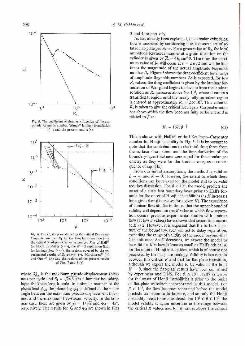
Fig. 5. The coefficient of drag as a function of the amplitude Reynolds number. Wang's' laminar formulation
(—) and the present results (•) .
10^ 106 10^ 10^2
Fig. 6. The (/?, K) plane depicting the critical Keulegan-Carpenter number Kj for the flat-plate transition (—), the critical Keulegan-Carpenter number KQK of H a l l ' ' for Honj i instability ( ) , Xhs K a 2 separation limit
for laminar fiow (• • • ) . the regions covered by the experimental results of Sarpkaya^ (<>), Marthinsen" ( + ) and Otter'^ (x) and the regions of the present results
of Figs 7 and 8 («).
where is the maximum pseudo-displacement thickness per cycle and 5\ = ^Ivjuo is a laminar boundary-layer thickness length scale. In a similar manner to the phase lead 0 w , the phase lag 0 d is defined as the phase angle between the maximum pseudo-displacement thickness and the maximum free-stream velocity. In the laminar case, these are given by /d = 1/V2 and <pA = 45°, respectively. The resuhs for fa and 0 d are shown in Figs
3 and 4, respectively
As has already been explained, the circular cylindrical flow is modelled by considering it as a discrete set of related flat-plate problems. For a given value of Rs, the local amplitude Reynolds number at a given ö-station on the cylinder is given by Rs = 4Rs sin^ 9. Therefore the maximum value of Rs will occur at 9 = ±TT/2 and wil l be four times the magnitude of the actual amplitude Reynolds number Rs. Figure 5 shows the drag coefficient for a range of amplitude Reynolds numbers. As is expected, for low Rs values, the drag coefficient is given by the laminar formulation of Wang and begins to deviate f rom the laminar solution as Rs increases above 5 X 10'', where it enters a transitional region until the nearly fully turbulent region is entered at approximately i?s ~ 2 x 10^ This value of Rs is taken to give the critical Keulegan-Carpenter number above which the flow becomes fully turbulent and is related to (i as
KT = 1621)3-5 (63)
This is shown with Hall 's" critical Keulegan-Carpenter number for Honj i instability in Fig. 6. I t is important to note that the contributions to the total drag force from the surface shear stress and the time-derivative of the boundary-layer thickness were equal for the circular geometry as they were for the laminar case, as a consequence of eqn (45)
From our initial assumptions, the method is valid as ^ 00 and K ^ 0. However, the extent to which these
conditions can be relaxed for the model still to be valid requires discussion. For P > 10', the model predicts the onset of a turbulent boundary layer prior to Hafl's formula for the onset of Honji '° instabihties (as K increases for a given /? or /? increases for a given fC). The experience of laminar flow studies indicates that the upper bound of validity will depend on the K value at which flow separation occurs: previous experimental studies with laminar flow (at low P values) have shown that separation occurs at i<: ~ 2. However, it is expected that the turbulent nature of the boundary-layer will act to delay separation, extending the range of validity of the model beyond K ~ 2 in this case. As K decreases, we expect the model to be valid for K values at least as small as Hall's critical K for the onset of Honj i instabilities, which is of course not predicted by the flat-plate analogy. Validity is less certain between this critical K and that for flat-plate transidon, although we expect the model to be valid in the limit K ^ 0, since the flat-plate results have been confirmed by experiment and DNS. For /? < 10', Hall's criterion for the onset of Honj i instabilities is prior to the onset of flat-plate transition incorporated in this model. For ^ < 10 ,̂ the flow becomes separated before the model predicts transition to turbulence, and so only the Honj i instabihty needs to be considered. For 10^ < < 10', the model vahdity is again uncertain in the range between the critical K values and for K values above the critical

Very-high-Reynolds-number flows
]0°
299
Fig. 7. Tlie coefficient of drag as a function of the
Keulegan-Carpenter number for ^ = 1 X 10'". Wang's'
laminar formulation (—) and the present results (•) .
value for flat-plate transition, the model is expected to be valid before separation occurs.
A graph of CD VS K for a very high P of 10'° is depicted in Fig. 7, showing the effect of turbulence as K increases. The region occupied by Fig. 7 in the (K, P ) plane is depicted in Fig. 6.
To give some indication of the magnitude of overall damping on a TLP configuration, we calculate the contribution from the four circular columns of the Snorre TLP in sway motion in still water to be 0.1% of critical. A 5 m amplitude typical of storm conditions was used. The column diameter was 25 m and the natural period 80 s. These and other details v/ere provided by Dr T. Marthin-sen. There will also be contributions to damping from the pontoons (of rounded square section), the cables and the risers. I n practice, of course, damping occurs in wave conditions and so damping in still water conditions can only give a rough estimate of magnitude. However, the techniques developed in this paper could be extended for incorporation in a diffraction analysis of TLP response.
The P value for this example is 5.787 X 10^ and a graph of CD VS K for this P is shown in Fig. 8. The value of K for this example is about unity The region occupied by Fig. 8 in the {K, P ) plane is shown in Fig. 6 and iïT « 1 occurs in a region where the model is expected to be valid. (It must be remembered that we assume a smooth surface and that any surface roughness wil l increase damping further.) The regions of availabüity of experimental data known to the authors are also shown in Fig. 6 and it can be seen that the P values are well below those required for this example. The data can also be shown to be generally below the critical K for flat-plate transition, spanning flow conditions f rom separation (K > 2) to the critical K for Honji instability and below. Comparison of results from the model presented here with experimental
10-
1 0 - 2 I I I I I M l 1 I 1 I 1 1 I I
1 0
K
Fig. 8. The coefficient of drag as a function of the
Keulegan-Carpenter number for p = S.lSlx 10'', relat
ing to the Snorre TLP in sway motion. Wang's' laminar
formulation (—) and the present results ( • ) .
data is thus not meaningful. The difficulty of experimentation at very high Reynolds numbers and low Keulegan-Carpenter numbers is discussed by Marthinsen''^ and Ot-ter.'s
The next development in this project will be to apply the flat-plate data for surface shear stress and boundary-layer displacement to cylinders of general cross-secdonal shape through the use of conformal transformations.
5 CONCLUSIONS
The sinusoidal flow about a fixed circular cylinder has been solved by an asymptotic matching method in which the inner boundary-layer region was considered as a number of analogous flat-plate problems, solved by the use of a finite-difference method. This is acceptable at high Reynolds numbers and low Keulegan-Carpenter numbers. Cases were computed where the amplitude Reynolds number was sufficiently large for the boundary layer forming on the cylinder to become turbulent. The Baldwin-Lomax'^ mixing-length turbulence model was adapted for sinusoidal flow by the introduction of a Vt multipher function to simulate the effects of transition on the surface shear stress observed experimentally. The drag (damping) force in phase with the flow velocity is obtained from the surface shear stress and the time derivative of boundary-layer thickness distributions.
The development of wall-generated turbulence in the boundary layer was found to cause an increase in the

300 A. M. Cobbin et al.
drag coefficient (compared to the laminar solution) as ex
pected. Experimental, theoretical or DNS data do not ex
ist for very high Reynolds numbers, so comparisons are
not possible. Moreover, there is an uncertainty as to the
interrelation of the Hon j i ' " - " instabilities with flat-plate
transitions to turbulence. I t is expected that the model
is valid for K values greater than the critical values for
flat-plate or Honj i instability (whichever is greater) until
separation occurs. Validity is uncertain between the criti
cal K values. A t low /? values, the well-known results for
laminar flow are reproduced.
Furthermore, it is shown why the contributions to
the drag force from the surface shear stress and the
time-derivative of the boundary-layer thickness distribu
tion are always equal, both for laminar and turbulent
boundary-layers, for the case of the circular geometry
ACKNOWLEDGEMENTS
This work was sponsored by EPSRC through M T D Ltd .
The authors wish to thank Dr Peter Justesen for supply
ing a copy of his k-e turbulence model code and Dr Tom
Marthinsen of Saga Petroleum, Norway for providing in
formation about the Snorre TLP.
REFERENCES
1. Stokes, G. G. , On the effect of the internal friction of fluids on the motion of pendulums. Cambr. Phil. Trans.,IX (1851) 8.
2. Sarpkaya, T , Forces on cylinders and spheres in a sinu-soidally oscillating fluid. J. App. Mech., 42 (1975) 32-7.
3. Sarpkaya, T , Force on a circular cylinder in a viscous oscillatory flow at low Keulegan-Carpenter numbers. J. Fluid Meek, 165 (1986) 61-71.
4. Sarpkaya, T , Wave forces on cylindrical piles. The Sea 9A, Wiley, 1990, pp. 169-95.
5. Morison, J. R., O'Brien, M. R, Johnson, J W. & Schaaf, S. A., The force exerted by surface waves on piles. Petroleum Trans, 189 (1950) 149-57.
6. Stuart, I T , Double boundary-layers in oscillating viscous flows. J. Fluid Mech., 2 (1966) 673-87.
7. Riley, N., Oscillating viscous flows. Mathemadka, 12 (1965) 161-75.
8. Riley, N., Oscillating viscous flows. Review and extension. J. Ins Maths Applies, 3 (1967) 419-34.
9. Wang, C , On high frequency oscillatory viscous flows J. Fluid Mecli., 32 (1968) 5-68.
10. Honji, H. , Streaked flow around an oscillating circular cylinder. J. Fluid Mech., 107 (1980) 509-20.
11. Hall, P., On the stability of the unsteady boundary layer on a cylinder oscillating transversely in a viscous fluid. J. Fluid Mech., 146 (1984) 347-67.
12. Spalart, R R. & Baldwin, B. S., Direct simulation of a turbulent oscillating boundary layer. Turbulent Shear Flows, Springer, 1989, pp. 417-40.
13. Jensen, B. L . , Sumer, B. M. & Fredsoe, I, Boundary-layers at high Reynolds numbers. / Fluid Mech., 206 (1989) 265¬97.
14. Kamphius, J. W., Friction factor under oscillatory waves. J. Waterway. Harbour Coastal Engng Div. ASCE, 101 (1975) 135^4.
15. Baldwin, B. S. & Lomax, H. , Thin layer approximation and algebraic model for separated turbulent flows. AIAA 16th Aerospace Sciences Meeting, 1978.
16. Jones, W. P. & Launder, B. E . , The prediction of laminarization with a two-equation model of turbulence. Int. J. Heat Mass Transfer, 15 (1972) 301-14.
17. Marthinsen, T , Hydrodynamics in T L P design. Proc Eighth Joint Int Conf on Offshore Mechanics and Polar Engineering (OMPE), 1989.
18. Otter, A., Damping forces on a cylinder oscillating in a viscous fluid. Appl Ocean Res, 12 (1990) 153-5.
19. Cebeci, T , Calculation of compressible turbulent boundary layers with heat and mass transfer AIAA 3rd Fluid and Plasma Dynamics Conf, 1970.
20. van Driest, E . R., On turbulent flow near a wall. J. Aero. Sci, 23 (1956) 1007-11.
21. Justesen, R & Spalart, R R., Two-equation turbulence modelling of oscillatory boundary layers. AIAA 28th Aerospace Sciences Meeting, 1990.