the ice, cloud, and land elevation satellite 2 mission: a
TRANSCRIPT

1
The Ice, Cloud, and Land Elevation Satellite – 2 Mission: A Global Geolocated 1
Photon Product Derived From the Advanced Topographic Laser Altimeter 2
System 3
4
Thomas A. Neumanna, Anthony J. Martinoa, Thorsten Markusa, Sungkoo Baeb, Megan 5
R. Bocka,c, Anita C. Brennera,d, Kelly M. Brunta,e, John Cavanaugha, Stanley T. 6
Fernandesf, David W. Hancocka,g, Kaitlin Harbecka,g, Jeffrey Leea,g, Nathan T. Kurtza, 7
Philip J. Luersa, Scott B. Luthckea, Lori Magruderb, Teresa A. Penningtona,g, Luis 8
Ramos-Izquierdoa, Timothy Rebolda,h, Jonah Skoogf, Taylor C. Thomasa,h 9
10
a NASA Goddard Space Flight Center, Greenbelt, MD United States 11
b Applied Research Laboratory, University of Texas, Austin, TX United States 12
c ADNET Systems, Inc., Lanham, MD United States 13
d Sigma Space Corporation, Lanham, MD United States 14
e University of Maryland, College Park, MD United States 15
f Northrop Grumman Innovation Systems, Gilbert, AZ United States 16
g KBR, Greenbelt, MD United States 17
h Emergent Space Technologies, Laurel, MD United States 18
19
Abstract 20
The Ice, Cloud, and land Elevation Satellite – 2 (ICESat-2) observatory was launched 21
on 15 September 2018 to measure ice sheet and glacier elevation change, sea ice 22
freeboard, and enable the determination of the heights of Earth’s forests. ICESat-2’s 23

2
laser altimeter, the Advanced Topographic Laser Altimeter System (ATLAS) uses 24
green (532 nm) laser light and single-photon sensitive detection to measure time of 25
flight and subsequently surface height along each of its six beams. In this paper, we 26
describe the major components of ATLAS, including the transmitter, the receiver and 27
the components of the timing system. We present the major components of the 28
ICESat-2 observatory, including the Global Positioning System, star trackers and 29
inertial measurement unit. The ICESat-2 Level 1B data product (ATL02) provides the 30
precise photon round-trip time of flight, among other data. The ICESat-2 Level 2A 31
data product (ATL03) combines the photon times of flight with the observatory 32
position and attitude to determine the geodetic location (i.e. the latitude, longitude 33
and height) of the ground bounce point of photons detected by ATLAS. The ATL03 34
data product is used by higher-level (Level 3A) surface-specific data products to 35
determine glacier and ice sheet height, sea ice freeboard, vegetation canopy height, 36
ocean surface topography, and inland water body height. 37
38
39
Highlights 40
• Describes the ICESat-2 Observatory and its sole instrument: the Advanced 41
Topographic Laser Altimeter System (ATLAS) 42
• Presents the structure and major contents of the ICESat-2 Level 1B data 43
product (ATL02; photon times of flight) 44
• Presents the structure and major contents of the ICESat-2 Level 2A data 45
product (ATL03; Global Geolocated Photons) 46

3
47
1. Introduction 48
The National Aeronautics and Space Administration (NASA) launched the Ice, Cloud, 49
and Land Elevation Satellite – 2 (ICESat-2) mission on 15 September 2018 to 50
measure changes in land ice elevation and sea-ice freeboard, and enable 51
determination of vegetation canopy height globally (Markus et al., 2017). A follow-52
on of the ICESat laser altimetry mission was recommended by the National Research 53
Council (National Research Council, 2007). Thus, ICESat-2 builds upon the heritage 54
of the ICESat mission (Zwally et al., 2002; Schutz et al., 2005) and uses round-trip 55
travel time of laser light from the observatory to Earth as the fundamental 56
measurement. During the development of mission objectives and requirements, the 57
science community made clear from lessons learned that duplication of ICESat would 58
not suffice. The science objectives for ICESat-2 are as follows: 59
60
-Quantify polar ice-sheet contributions to current and recent sea-level change and the 61
linkages to climate conditions; 62
63
-Quantify regional signatures of ice-sheet changes to assess mechanisms driving those 64
changes and improve predictive ice sheet models; this includes quantifying the regional 65
evolution of ice-sheet change, such as how changes at outlet glacier termini propagate 66
inward; 67
68

4
-Estimate sea-ice thickness to examine ice/ocean/atmosphere exchanges of energy, 69
mass and moisture; 70
71
-Measure vegetation canopy height as a basis for estimating large-scale biomass and 72
biomass change. 73
74
The first objective corresponds to ICESat’s sole science objective. Results from 75
ICESat, however, showed that an ICESat follow-on must allow researchers to readily 76
distinguish elevation change from the elevation uncertainty due to imperfect 77
pointing control over the outlet glaciers along the margins of Greenland and 78
Antarctica because those areas are where changes are the most rapid. This 79
requirement led to the formulation of the second objective, which strongly directed 80
the ICESat-2 science requirements and the design of the mission. For example, 81
ICESat-2 needed multiple beams in order to monitor those rapidly changing regions 82
with the necessary accuracy and precision. The traceability from science objectives 83
to science requirements and subsequently to mission design and implementation is 84
discussed in detail in Markus et al. (2017). Furthermore, results from ICESat proved 85
that spaceborne laser altimetry is sufficiently precise to retrieve sea-ice freeboard 86
and ultimately calculate sea-ice thickness. Consequently, the determination of the 87
sea-ice thickness is an official science objective for ICESat-2. Because only 1/10th of 88
the sea ice thickness is above sea level, this objective was the driver for much of the 89
vertical precision requirements such as timing as discussed in Markus et al. (2017). 90
91
5
Because much of the mission design, and vertical and horizontal accuracy and 92
precision requirements, are driven by the land- and sea-ice scientific objectives, the 93
fourth objective exists largely to ensure that ICESat-2 is collecting, processing, and 94
archiving scientifically viable data around the globe. 95
96
The sole instrument on the ICESat-2 observatory is the Advanced Topographic Laser 97
Altimeter System (ATLAS). In designing ATLAS, close attention was paid to the 98
successes and limitations of the GLAS (Geoscience Laser Altimeter System) 99
instrument flown on the original ICESat mission (Abshire et al., 2005; Webb et al., 100
2012). Both lidars were designed, assembled, and tested at NASA Goddard Space 101
Flight Center, bringing substantial heritage and insight forward to the ICESat-2 102
mission and ATLAS. 103
104
ATLAS splits a single output laser pulse into six beams (arranged into three pairs of 105
beams) of low-pulse energy green (532 nm) laser light at a pulse repetition 106
frequency (PRF) of 10 kHz. The arrangement of pairs of beams allows for 107
measurement of the surface slope in both the along- and across-track directions with 108
a single pass, enabling determination of height change from any two passes over the 109
same site. The single-photon sensitive detection strategy (Degnan, 2002) allows 110
individual photon times of flight (TOF) to be determined with a precision of 800 111
picoseconds. 112
113
The footprint size of the laser on the ground is ~17 m. The small footprint size 114

6
together with the TOF and PRF requirements ensure that sea surface height 115
measurements within sea-ice leads have a vertical precision of 3 cm. The resulting 116
height measurements can be aggregated in order to meet the overall ICESat-2 117
science requirements (Markus et al., 2017). To determine the pointing direction of 118
ATLAS, the ICESat-2 observatory carries state-of-the-art star trackers and an inertial 119
measurement unit (IMU) mounted on the ATLAS optical bench. To determine the 3-D 120
position of the observatory center of mass, the observatory also carries redundant 121
dual-frequency Global Positioning System (GPS) systems. The ATLAS TOF data are 122
combined with the observatory position and attitude to produce a geolocation for 123
each photon in the resulting data product. 124
125
The ICESat-2 Science Unit Converted Telemetry Level 1B data product (identified as 126
ATL02; Martino et al., 2018) provides the ATLAS TOF, ATLAS housekeeping data, and 127
the other data necessary for science data processing such as GPS and attitude data. 128
The ICESat-2 Global Geolocated Photon Level 2A data product (identified as ATL03; 129
Neumann et al., 2018) provides the latitude, longitude and ellipsoidal height of 130
photons detected by the ATLAS instrument. The ATL03 product is used as the 131
foundation for other surface-specific geophysical data products such as sea ice 132
(ATL07; Kwok et al., 2016), land ice (ATL06; Smith et al., this issue), and vegetation 133
canopy height (ATL08; Neuenschwander and Pitts, in review). All ICESat-2 data 134
products are provided in the Hierarchical Data Format – version 5 (HDF-5) format 135
and will be made available through the National Snow and Ice Data Center (NSIDC - 136
https://nsidc.org/data/icesat-2). 137
7
138
In this paper, we describe the ICESat-2 observatory, the major systems of the ATLAS 139
instrument, including the components of the transmitter, receiver, the timing system 140
and active alignment subsystems. The approach to monitoring the internal range 141
bias of ATLAS is described, along with other major features of the primary ATLAS 142
data. We also review the anticipated radiometric performance and timing precision 143
of ATLAS. We summarize the components of the spacecraft bus that are relevant to 144
the ICESat-2 data products and performance. We combine these primary outputs of 145
the ICESat-2 observatory into an overview of the two low level data products: the 146
Level 1B product (ATL02), and the Level 2A product (ATL03). 147
148
2. The ICESat-2 Observatory 149
The ICESat-2 mission consists of two major components: the observatory in space, 150
and the ground system which downlinks data from the observatory and generates 151
the ICESat-2 data product suite. The observatory (Figure 1) is composed of two 152
components as well: the ATLAS instrument which is a lidar system and records 153
photon arrival times; and the spacecraft bus which provides power, via solar arrays, 154
the Global Positioning System (GPS) receivers and antennae and communications 155
antennae among other instrumentation. 156
157
2.1 The ATLAS Instrument 158
The ATLAS instrument has three principal systems: the transmitter that generates 159
the laser pulses, the receiver where photons are detected and timed, and the 160
8
alignment monitoring and control system which includes the laser reference system 161
(LRS) to determine the laser pointing direction. These systems together provide 162
TOF, position and pointing that are needed to retrieve precise photon height 163
estimates. Some of the major characteristics of the contributing systems are 164
summarized in Table 1 and described in more detail below. 165
166
2.1.1 Transmitter 167
The components of the ATLAS transmitter include: the lasers, the Laser Sampling 168
Assembly, Beam Shaping Optics, the Beam Steering Mechanism (BSM), and the 169
Diffractive Optical Element (Figure 2). ATLAS carries two lasers (primary and 170
redundant), only one of which is active at a time. The Laser Sampling Assembly 171
samples a portion of the transmitted light and routes it to the Start Pulse Detector, 172
which times the outgoing laser pulse. The Beam Shaping Optics sets the beam 173
divergence (i.e. the angular measure of the beam diameter as a function of distance 174
from ATLAS) , while the BSM ensures that the transmitted beams are aligned with 175
the fields of view of the receiver. Lastly, the Diffractive Optical Element splits the 176
single outgoing beam into 6 beams. 177
178
The core of the ATLAS transmitter are the lasers, which were designed and 179
fabricated by Fibertek, Inc. (Sawruk et al., 2015). Based on the requirements for a 180
narrow pulse width (< 1.5 ns), variable pulse energy of up to 1.2 millijoule (mJ) 181
(adjustable from 0.2 up to 1.2 mJ), and 10 kHz PRF, Fibertek designed a master 182
oscillator / power amplifier (MOPA) based laser transmitter. The design uses a 183

9
Nd:YVO4 gain crystal to generate infrared (1064 nm) light with the required pulse 184
width, which is then frequency-doubled to produce green 532 nm laser light. 185
Although the conversion to 532 nm reduces the overall laser efficiency compared 186
with a 1064 nm transmitted beam, green light was selected based on the maturity of 187
photon-sensitive detector technology for that wavelength. This selection minimized 188
the overall risk and maximized the overall system throughput from transmitter to 189
receiver. We expect the central wavelength of the laser (532.272 0.15 nm) to 190
change very slowly over time, if at all, due to aging effects. A single laser is expected 191
to meet the nominal three-year mission duration, or approximately one trillion 192
pulses. 193
194
After exiting the laser module, the outgoing beam from the operational laser travels 195
along a common optical path after a polarizing beam combiner, and is sampled by 196
the Laser Sampling Assembly, which removes < 1% of the outgoing beam energy to 197
monitor the stability of the central wavelength as well as to provide the precise laser 198
transmit time (described in Section 2.1.3). When coupled with the arrival time of 199
returning photons, the laser transmit time enables the determination of TOF, the 200
fundamental ATLAS measurement. 201
202
The outgoing beam is shaped by several optics (indicated by Beam Shaping Optics in 203
Figure 2) to generate the required beam divergence giving a nominal footprint 204
diameter of ~17 m at ICESat-2’s 500 km average orbital altitude. The pointing vector 205
of the laser beam is determined by the position of the BSM, which provides the 206

10
means for active beam steering to ensure alignment with the receiver (further 207
discussed in section 2.1.4). The BSM contains redundant hardware to mitigate 208
against the risk of a mechanism failure. 209
210
The single output beam is split into six primary beams by the Diffractive Optical 211
Element (DOE) prior to exiting the ATLAS instrument. As the light exits the DOE, all 212
beam information (pointing direction, shape, strength) becomes beam-specific. As 213
such, the DOE is the last common reference point of the six beams. 214
215
Approximately 80% of the laser pulse energy is partitioned into the six primary 216
outgoing laser beams, while 20% is lost to higher-order modes. At the nominal laser 217
power setting, this means that ~660 microjoules (J) of the ~835 J pulse is used, 218
and ~175 J are lost to higher-order modes. The total available laser energy 219
precluded the scenario of having six strong beams; as a result the six primary beams 220
generated by the DOE have unequal energy, with three relatively strong beams and 221
three relatively weak beams. Given the energy losses along the optical path in the 222
laser transmission, the strong beams each contain ~21% of the transmitted energy 223
(~175 J per pulse) and the weak beams share the remaining energy, each having 224
~5.2% (~ 45 J per pulse). As such, the energy ratio of the strong and weak beams is 225
approximately 4:1. The strong and weak beams have transmit energy levels to within 226
approximately 10% of the mean values (i.e. 175 17 J per pulse for the strong 227
beams and 45 5 J per pulse for the weak beams). 228
229

11
The strong/weak configuration for the ATLAS beams was designed to enhance 230
radiometric dynamic range, thus accommodating the disparate energy levels 231
required to meet the primary science objectives (Markus et al., 2017). It is expected 232
that both the strong and weak beams will provide sufficient signal-to-noise ratios for 233
altimetry measurements over bright surfaces such as sea ice and ice sheets, while the 234
strong beams will be the primary means for ranging to low-reflectivity targets, such 235
as oceans and, at times, over vegetation (see section 2.2 for an outline of surface 236
types). 237
238
In summary, the ATLAS transmitter will generate the six beams needed to achieve 239
the multidisciplinary science objectives of the ICESat-2 mission. The transmitted 240
pulses are narrow (<1.5 ns), use 532 nm laser light, and generate ~17 m diameter 241
footprints on the ground. The combination of the laser PRF and spacecraft velocity 242
of ~7 km/sec produce footprints on the ground spaced ~0.7 m along track, resulting 243
in substantial overlap between shots. This represents a substantial improvement in 244
along-track resolution over the ICESat mission, which generated non-overlapping 245
footprints on the ground of ~70 m diameter spaced ~150 m along track. Over the 246
first nine months of the mission, the ATLAS transmitter components are working on-247
orbit as designed and are performing as expected. 248
249
2.1.2 Receiver 250
Within the ATLAS receiver (Figure 3), light is collected and focused onto the receiver 251
optics by the telescope. The figure, finish and coating of the telescope surface is 252

12
optimized for transmission of green light. The light from each of the six beams is 253
focused onto fiber optic cables dedicated to each beam. At ICESat-2’s nominal 254
altitude, this generates a 45 m diameter field of view on the ground (see section 255
2.1.4). Background light is first rejected by pass band coarse filters, and then by 256
optical etalon filters centered at the nominal laser output central wavelength. The 257
central wavelengths of both the transmitted laser beam as well as the pass band of 258
the etalon filters are tunable over a 30 pm range by adjusting their respective 259
temperatures via the ATLAS avionics system. Feedback for this wavelength 260
matching is provided by both the received signal strength and the Wavelength 261
Tracking Optical and Electronics Module (WTOM/WTEM), which samples a fraction 262
of the laser energy and directs it through an optical filter assembly that is identical to 263
the receiver background filters. Based on pre-launch testing, we expect to retune the 264
optical etalon filters on orbit approximately twice a year to match the laser transmit 265
wavelength. 266
267
The output of the filters is fiber-coupled to one of two sets of single-photon sensitive 268
photo-cathode array photomultiplier tubes (PMTs) in the detector modules which 269
convert optical energy into electrical pulses (Figure 4). ATLAS uses 16-element 270
PMTs manufactured by Hamamatsu with pixels arranged in a 4x4 pattern. Each 271
channel of a single PMT is used independently for each of the three strong beams to 272
provide 16 independent electrical outputs, while for the weak beams (which are ~ ¼ 273
the optical power of the strong beams) detector channels are combined to a 2x2 274
array. As such, ATLAS has 60 electrical outputs which are mapped to 60 independent 275
13
timing channels. Test data show that incoming light is distributed uniformly to each 276
channel of a strong or weak beam (to within 10%), which is an important 277
consideration for estimating detector gain during periods of high throughput. While 278
we expect a single set of detectors to survive for the duration of the mission, ATLAS 279
has a second set of redundant detectors. The switch from the primary to the 280
redundant set of detectors is accomplished via a set of six moveable mirrors. 281
282
Overall, the optical throughput of the ATLAS receiver was measured to be 40% in 283
pre-launch testing. Over the mission lifetime, we expect degradation of the ATLAS 284
receiver throughput due to aging and contamination effects, and expect the end-of-285
life throughput to be greater than 35%. The efficiency of the PMTs in converting 286
optical energy to electrical pulses has been measured to be ~15%, and the gain can 287
be adjusted as needed by manipulating the bias voltage to maintain consistent 288
performance throughout the mission. Combined, the overall efficiency of the ATLAS 289
receiver is ~ 6%. Over the first nine months of the mission, the ATLAS receiver 290
components are performing as designed. 291
292
2.1.3 Time of Flight Design 293
The electrical output of the detector timing channels are routed to photon-counting 294
electronics (PCE) cards that enable precise timing of received photon events. ATLAS 295
contains three PCE cards, each handling the output of a single strong beam (16 296
channels), a single weak beam (four channels) and two channels from the start pulse 297
detector used for timing start pulses. The PCE cards are similar to those developed 298

14
for the airborne Multiple Altimeter Beam Experimental Lidar (MABEL) instrument 299
(McGill et al., 2013). 300
301
Each PCE card is sent times from a free-running 100 MHz clock to measure coarse 302
times of photon arrivals at the ~10 ns level, and a chain of sequential delay cells is 303
used to measure fine times at the 180-200 picosecond level. The transmitted data 304
include the coarse and fine time components of events from each PCE and other data 305
needed to cross-calibrate times between PCEs. A free-running counter driven by an 306
Ultra Stable Oscillator (USO) is latched by the GPS 1 pulse per second signal from the 307
spacecraft. The same free-running counter is latched by an internal 1 pulse per 308
second signal. This allows the internal timing of ATLAS to be matched to the GPS 309
time. The stability of the USO frequency is a primary consideration in estimating 310
height change to meet the requirements of the mission (Markus et al., 2017), as drift 311
in USO frequency has a first-order impact on our ability to precisely measure photon 312
TOF. Ground processing uses these components to determine the absolute time of 313
ATLAS events, including laser firing times and photon arrival times, to calculate 314
round-trip TOF. 315
316
ATLAS uses on-board software to limit the number of time-tagged photon events and 317
reduce the overall data volume telemetered to ground stations. A digital-elevation 318
model (DEM), an estimate of the surface relief (Leigh et al., 2014), and a surface 319
classification mask are used to constrain the time tags to those received photons 320
most likely to have been reflected from Earth’s surface. This window of time-tagged 321

15
photons is called the Range Window. Individual ATLAS transmitted pulses are 322
separated in flight by ~15 km; the vertical span of time-tagged photons varies from a 323
maximum of 6 km over areas on Earth with substantial surface relief to a minimum 324
of ~1 km over surfaces with minimal relief. This narrower Range Window reduces 325
the number of photons that ATLAS must time tag to search for the surface echoes of 326
most interest. The span of photon time tags is further reduced by forming 327
histograms of photon time tags to statistically determine the photon events most 328
likely reflected from the Earth’s surface. The span of photon time tags telemetered 329
to ground (called the Telemetry Band or Bands) processing varies from up to 3 km 330
over rugged mountain topography to ~40 m over the oceans, and the Telemetry 331
Band width is re-evaluated every 200 pulses. 332
333
2.1.4 Alignment and alignment monitoring 334
Owing to the tight tolerance between the receiver field of view for an individual 335
beam and the diameter of a reflected laser beam, keeping the transmitted laser light 336
within the receiver field of view is a primary challenge for ATLAS. The instrument’s 337
Alignment Monitoring and Control System (AMCS) (Figure 5) provides a means to 338
evaluate the co-alignment between the transmitter and receiver. 339
340
The Telescope Alignment and Monitoring System (TAMS) consists of a LED source 341
coupled to four fiber optics to generate a rectangular pattern of beams at the 342
telescope focal plane. These beams are projected from the focal plane through the 343
telescope aperture. A portion of these beams is sampled using a lateral transfer 344

16
retroreflector (LTR) and routed to an imager on the laser side of the laser reference 345
system (LRS) mounted on the optical bench. The resulting image of the TAMS spots 346
enables determination of the telescope pointing vector. The pointing vector of the 347
transmitted beams is provided by routing a small fraction (<< 1 %) of the 348
transmitted energy for each of the six outgoing beams to the same imager using a 349
second LTR. By comparing the relative positions of the TAMS spots and laser spots 350
within the same image on the laser side of the LRS, the AMCS determines the relative 351
alignment of the transmitter and receiver. If necessary, the AMCS generates 352
corrections to the position of the BSM which adjusts the pointing vector for the laser 353
beam prior to its separation into six beams by the DOE. To prevent potentially 354
unstable corrections to the BSM position, the AMCS calculates the relative position of 355
the TAMS and laser spots at a higher rate (50 Hz) than corrections to the BSM are 356
commanded (10 Hz). Pre-launch data during whole-instrument testing has 357
demonstrated that the AMCS is able to correct for short timescale perturbations 358
(vibrations due to nearby activities, such as walking) as well as long timescale 359
perturbations (such as thermal effects of clean room air conditioning on/off cycles). 360
On orbit, the main driver of alignment change is the time-varying thermal condition 361
of the ATLAS components both around an orbit and seasonally. 362
363
In the event that the AMCS system is not able to align the transmitted laser beams 364
with the receiver fields of view for all six beams simultaneously, the radiometric 365
throughput for those misaligned beams will be diminished. For a moderate degree of 366
misalignment, some fraction of the returning laser pulse will be clipped and the 367

17
number of photons collected by the ATLAS telescope will be reduced. Those photons 368
that do enter the receiver field of view will be biased to one side of the field of view. 369
The net effect will be to reduce the surface height precision for those beams affected, 370
owing to a reduced number of signal photons available for further analysis. The 371
limiting case would be a total loss of overlap between the returning photons and the 372
receiver field of view. In this case the photon loss is total, and these beams would 373
not be used in further data processing. Over the first nine months of the mission, we 374
have found no evidence of photon loss due to misalignment in our initial on-orbit 375
data. 376
377
While the AMCS provides routine corrections to the transmit and receive alignment 378
algorithm, we also will conduct periodic calibration scans of the BSM to 379
systematically sweep the transmitted laser beams across the receiver fields of view 380
to determine a new center position. Since the BSM steers all six beams 381
simultaneously it may not be possible to perfectly center all six beams 382
simultaneously within their respective fields of view. In such an event, the BSM 383
position will be optimized to capture the maximum number of returned photons 384
across all six beams, using data from the BSM calibration scans. We have conducted 385
such scans frequently during ATLAS commissioning during the first 60 days on orbit, 386
and will do so as needed thereafter during nominal operations. Over the first nine 387
months of the mission, the ATLAS alignment has been very stable, with BSM changes 388
on the order of a few (< 10) microradians. At the nominal altitude, this represents a 389
movement of the laser spots by about 1/3 the diameter of the laser footprints. 390

18
391
2.1.5 Time of flight bias and bias monitoring 392
While the primary purpose of ATLAS is to measure photon round-trip time of flight, 393
meeting the high-precision height measurement requirements (Markus et al., 2017) 394
requires close attention to and correction for internal timing drifts within ATLAS. 395
Prior to launch, a rigorous testing program characterized the range difference 396
between beams to a fixed target in ambient conditions, as well as during thermal-397
vacuum testing for a range of instrument states. This testing determined that the 398
range reported by ATLAS will vary by less than a millimeter depending on the 399
instrument state and temperature. On orbit, the Transmitter Echo Path (TEP) 400
provides a means to monitor time-of-flight changes within ATLAS. 401
402
The TEP routes a portion of the light used to measure the time of the start pulse from 403
the start pulse detector into the receive path just prior to the optical filters for two of 404
the strong beams (ATLAS beams 1 and 3). The optical power in this internal 405
pathway is small, amounting to approximately one photon every ~20 laser transmit 406
pulses. The TEP photons have a time of flight of approximately 20 nanoseconds 407
given the length of the fiber optics that provide the pathway from the start pulse 408
detector. Monitoring changes in the distribution of TEP-based photons over time can 409
reveal changes in the ATLAS reported time of flight (i.e. a range bias change). The 410
path traversed by the TEP photons include the aspects of ATLAS we expect to be 411
most sensitive to temperature changes and ageing effects (e.g. the PMTs and 412
electrical pathways). While it is possible that changes in the transmit or receive 413

19
optics not sampled by the TEP could cause changes in the reported photon time of 414
flight, a change in the position of such components by more than a few hundredths of 415
a millimeter would likely be due to some catastrophic change (e.g. a broken or 416
unbounded optic). 417
418
Photons travel along the TEP any time the laser is transmitting. At times, the TEP-419
based photons will arrive within the range window where the on-board software is 420
searching for surface-reflected photons. In this circumstance, ATLAS will telemeter 421
the TEP-based photon data along with the surface-reflected photon data, and ground 422
processing will assign them to the correct start pulse to yield a ~20 nanosecond time 423
of flight (as opposed to a ~3.3 millisecond time of flight for surface-reflected 424
photons). We expect TEP-based photons to arrive at nearly the same time as 425
photons reflected from the Earth approximately twice per orbit. Although this will 426
not impact nominal science operation, ATLAS can be commanded to telemeter only 427
TEP-based photons during calibration activities. Using TEP-based photons, we will 428
characterize the changes in ATLAS range bias throughout one or more orbits early in 429
the mission, and repeat this calibration periodically as needed. 430
431
TEP-based photons also sample a substantial fraction of the components 432
contributing to the ATLAS impulse-response function (see section 4.6 for a detailed 433
description). By aggregating TEP-based photons, an estimate of this function can be 434
constructed in ground processing, and changes in this function can be monitored. 435
436

20
2.1.6 Dead time 437
The full waveform GLAS altimeter instrument onboard ICESat was susceptible to 438
detector saturation in those cases where relatively high-energy return pulses 439
overwhelmed the capability of the automatic gain control on the 1064 nm detectors 440
(Sun et al., 2017). The resulting saturation led to returned waveforms that were 441
either clipped or artificially wide (Fricker et al., 2005). While the PMT detector 442
elements do not suffer from saturation, they are discrete detectors and therefore 443
susceptible to dead-time effects (Williamson et al., 1988; Sharma and Walker, 1992). 444
Dead time is the time period after a detected photon event during which the detector 445
is unable to detect another photon event. This means that a photon arriving in close 446
temporal proximity to a prior photon event will not be detected. In some cases, 447
during periods of high throughput, a detector channel remains blind to subsequent 448
photon arrivals if those additional photons arrive at the same channel during the 449
dead time period, thus extending the effective dead time, perhaps significantly. 450
451
ATLAS has three features which are each intended to partially mitigate the dead time 452
effect. First, the ATLAS PMTs are 16-pixel photo-cathode array PMTs. By 453
distributing the light uniformly across the detector pixels (16 unique pixels for each 454
strong beam; four unique pixels for each weak beam; Figure 4), this design reduces 455
the probability that dead time effects will be realized. Second, ATLAS uses a dead 456
time circuit to limit the pulse interarrival time in a timing channel to greater than 3 457
ns (nominally 3.2 ns), so as to avoid hardware-specific dead times that could be 458
different among channels. Third, the corresponding beam and detector channel that 459

21
recorded each detected photon is preserved in the telemetered data. Consequently, 460
it is possible to monitor the effective gain of the pixels in a given beam to estimate 461
the probability and magnitude of dead time effects. Pre-launch data with a range of 462
photon inter-arrival times have been used to estimate the radiometric and ranging 463
degradation of ATLAS due to dead time effects. This functionality has proven to be 464
useful in characterizing ATLAS’ initial on-orbit performance. 465
466
2.2 Expected ATLAS performance 467
Despite the narrow bandpass filtering implemented on ATLAS to constrain the 468
received light to 532.272 0.15 nm, there remains a significant amount of sunlight at 469
that wavelength when ATLAS is ranging to the sun-lit Earth. These solar background 470
photons are reflected off the Earth’s surface, and some fraction of them enter the 471
ATLAS telescope and are recorded by the receiver electronics. The rate of 472
background photons recorded by ATLAS varies primarily with the sun angle, but also 473
with the atmospheric and Earth reflectivity at 532 nm. In regions with high solar 474
angle and reflectance, background photon rates of ~10 MHz have been measured (or 475
10 million background photons per second; or about 1 photon every 3 m in height) 476
for any given beam; the rate at any specific location will be a function of the 477
reflectance in the ATLAS field of view and solar angle. The ~10 MHz value is 478
observed with clear skies over the ice sheet interior in summer. The presence of 479
background photons increases the expected standard deviation of the return pulse 480
from the ice sheet interior by about 50% to ~2.5 cm and ~5 cm for the strong and 481
weak beams, respectively (Markus et al., 2017, Table 1). 482

22
483
We developed a variety of design cases based on targets of interest to predict the 484
ability of the ATLAS instrument to provide data with sufficient precision and 485
accuracy to satisfy the mission science requirements (Markus et al., 2017). During 486
ATLAS design and testing, these design cases were used as a benchmark to evaluate 487
the ATLAS timing and radiometric performance. The number of signal photons 488
expected per shot is a function of the surface reflectance and losses in the 489
atmosphere combined with the ATLAS radiometric model. The temporal 490
distribution of the returned photons is primarily a function of the interaction of the 491
transmitted pulse (~1.5 ns pulse width) with the surface slope and roughness over 492
the laser footprint area both of which broaden the return pulse. In addition, the 493
surface reflectance and atmospheric optical depth have a first-order effect on the 494
number of returned signal photons per shot. Over relatively flat reflective surfaces, 495
such as the interior of the Antarctic ice sheet (surface reflectance 0.9; optical depth 496
of atmosphere 0.21), we expect ~7 signal photons per shot for the strong beams and 497
~1.75 signal photons per shot for the weak beams on average. Due to the relatively 498
flat and smooth ice sheet interior, we expect little pulse spreading or slope-induced 499
geolocation error, leading to a standard deviation of the signal photons averaged 500
over 100 shots of ~1.5 cm and ~2.8 cm for the strong and weak beams respectively. 501
502
Over low reflectivity targets, such as ocean water, both the signal photon rates and 503
background photon rates are significantly reduced. For the dark ocean water in sea 504
ice leads (i.e. the gaps between highly reflective sea ice where ocean water is visible; 505
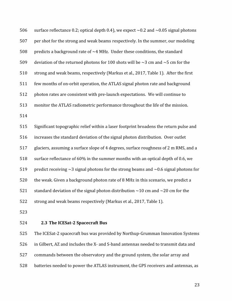
23
surface reflectance 0.2; optical depth 0.4), we expect ~0.2 and ~0.05 signal photons 506
per shot for the strong and weak beams respectively. In the summer, our modeling 507
predicts a background rate of ~4 MHz. Under these conditions, the standard 508
deviation of the returned photons for 100 shots will be ~3 cm and ~5 cm for the 509
strong and weak beams, respectively (Markus et al., 2017, Table 1). After the first 510
few months of on-orbit operation, the ATLAS signal photon rate and background 511
photon rates are consistent with pre-launch expectations. We will continue to 512
monitor the ATLAS radiometric performance throughout the life of the mission. 513
514
Significant topographic relief within a laser footprint broadens the return pulse and 515
increases the standard deviation of the signal photon distribution. Over outlet 516
glaciers, assuming a surface slope of 4 degrees, surface roughness of 2 m RMS, and a 517
surface reflectance of 60% in the summer months with an optical depth of 0.6, we 518
predict receiving ~3 signal photons for the strong beams and ~0.6 signal photons for 519
the weak. Given a background photon rate of 8 MHz in this scenario, we predict a 520
standard deviation of the signal photon distribution ~10 cm and ~20 cm for the 521
strong and weak beams respectively (Markus et al., 2017, Table 1). 522
523
2.3 The ICESat-2 Spacecraft Bus 524
The ICESat-2 spacecraft bus was provided by Northup-Grumman Innovation Systems 525
in Gilbert, AZ and includes the X- and S-band antennas needed to transmit data and 526
commands between the observatory and the ground system, the solar array and 527
batteries needed to power the ATLAS instrument, the GPS receivers and antennas, as 528

24
well as the necessary hardware for adjusting the observatory attitude and altitude. 529
Additional components typically on the spacecraft bus (such as the star trackers and 530
IMU) are mounted on the ATLAS optical bench, as noted above. 531
532
The GPS hardware on the ICESat-2 spacecraft bus was developed and provided by 533
RUAG Holding AG, which has supplied similar systems for the European Space 534
Agency’s Sentinel missions (Montenbruck et al., 2017) among others. The ICESat-2 535
spacecraft carries redundant GPS receivers and antennas to mitigate against single-536
point failures. These data are the primary input to the precision orbit determination, 537
described in more detail below. In addition, the spacecraft carries a nadir-mounted 538
retroreflector for satellite laser ranging for orbit verification (Pearlman et al., 2002). 539
540
The Instrument Mounted Spacecraft Components (IMSC) assembly is mounted to the 541
ATLAS optical bench. The IMSC has two HYDRA star tracker optical heads provided 542
by Sodern (Blarre et al., 2010) that have been used on many spacecraft (e.g. ESA’s 543
Sentinel missions). Each HYDRA optical head has a 16x16 degree field of view 544
focused on a 1024x1024 pixel Active Pixel Sensor (CMOS) detector. The heads 545
operate concurrently at 10Hz, tracking up to 15 stars each, and communicate with a 546
separate star tracker electronics unit mounted on the Spacecraft bus. Attitude data 547
supplied by the optical heads is processed with the data provided by a Northrop 548
Grumman Scalable Space Inertial Reference Unit (SSIRU) to determine the 549
observatory attitude, and ultimately, the pointing vector for each of the six ATLAS 550
beams, as described below. The SSIRU comprises four Hemispherical Resonator 551

25
Gyros in a 3-for-4 redundant pyramid arrangement, along with redundant Processor 552
Power Supply Module boards. The SSIRU has exceptional bias and alignment 553
stability as well as low noise, which are critical to meeting ICESat-2 attitude 554
estimation performance requirements. 555
556
3. The ATL02 Data Product: Science Unit Converted Telemetry 557
The ATL02 data product (Martino et al., 2018) converts the low-level telemetry from 558
the observatory and applies calibrations to the primary photon data to generate 559
precise photon times of flight. The ATL02 data product includes separate groups for 560
possible TEP photons, housekeeping temperatures and voltages from ATLAS, and the 561
data necessary to determine the pointing direction of the ATLAS laser beams (e.g. 562
data from the GPS, LRS, and star trackers). In the ATL02 data structure, the /atlas 563
group contains the science data of interest to most users. The altimetry data (such as 564
photon time of flight) is organized according to PCE card into the /atlas/pcex 565
subgroups, where x refers to the pce card number. The 566
/atlas/pcex/algorithm_science group contains the data used for precise time of day 567
and data alignment between s the three PCE cards. The groups /gpsr, /lrs, and /sc 568
contain data used to determine the precise orbit and pointing vectors of the ATLAS 569
laser beams. 570
571
3.1 Time of flight 572
As noted above, each of the three PCE cards use two timing channels to record start 573
pulse information. The transmit pulse generated by ATLAS has a full-width at half 574
26
maximum duration of less than 1.5 nanoseconds (Sawruk et al., 2015) but is slightly 575
asymmetric. To account for this asymmetry, and possible changes in the pulse skew 576
through time, ATLAS measures the time that the laser pulse crosses two energy 577
thresholds on the rising and falling edges of the transmit pulse, as depicted in Figure 578
6. The time that the transmit pulse crosses the leading lower threshold is recorded 579
by each of the three PCEs, and provides a means to cross-calibrate times among the 580
PCEs. In addition, each PCE records one of the remaining three times (leading edge 581
upper threshold, falling edge upper threshold, or falling edge lower threshold). In 582
ground processing, these 6 times are combined to calculate the centroid of the four 583
crossing times, after co-aligning the times using the leading lower threshold crossing 584
time for each PCE to produce a single start time for each pulse. 585
586
The combination of ICESat-2’s orbit altitude and the laser transmitter PRF results in 587
~30 transmitted and reflected laser pulses in transit to and from the observatory at 588
any given time. The precise number of pulses in flight depends on a combination of 589
the orbit altitude and Earth’s topography at a given location. Consequently, the times 590
of transmitted laser pulses and received photon time tags must be aligned in ground 591
processing before a precise time-of-flight of any given photon can be determined. 592
Errors in this time alignment would manifest as ~15 km errors in the reported range 593
and are relatively easily detected in post-processing analysis. A consequence of the 594
spacing of transmit pulses in flight is that reflections from high clouds in the 595
atmosphere above 15 km can be folded into the ground return; e.g. there is a height 596
ambiguity between returns from 16 km above the surface and 1 km above the 597

27
surface. 598
599
In addition to the timing processes described above, calibrations for temperature 600
and voltage variations in the timing electronics and PMTs (among other 601
components) must be applied. These calibrations are based primarily on pre-launch 602
testing of the temperature and voltage sensitivities of the individual components and 603
the variations in the pixel-to-pixel performance of the photon timing system. Post-604
launch calibration relies on changes in the TEP-based photon times of flight, and 605
housekeeping temperature and voltage data. Internal to each PCE is a calibration 606
timing chain that measures how far a signal can travel during a 10 ns USO clock 607
period. The calibration timing chain is averaged over 256 times, and telemetered 608
once per second. Since the calibration timing chain is on the same silicon as the 609
photon counting timing chains, this gives an in-situ measurement of any changes in 610
the timing chain due to voltage or temperature. Analysis of reported heights for 611
well-surveyed parts of Earth will provide an additional check on the relative 612
consistency of photon heights among the six beams as well as the absolute height 613
through comparison with ground-based GPS surveys (Brunt et al., 2017; Brunt et al., 614
2019) or high resolution airborne lidar data sets (Magruder and Brunt, 2018). 615
616
Based on pre-launch data analysis, we expect the calibrated individual photon times 617
of flight to be accurate to ~770 picoseconds one sigma, or ~23 cm in two-way range. 618
The primary contributors to the TOF accuracy are the transmit pulse width (~1.5 619
nanoseconds full width at half max) and the received photon timing uncertainty 620

28
(~400 picoseconds one sigma) owing to the characteristics of the timing electronics. 621
Based on initial on-orbit data, ATLAS is meeting it’s TOF accuracy requirements. 622
623
The precise time of flight (ph_tof) with all calibrations applied for every received 624
photon telemetered to the ground is included in the ICESat-2 ATL02 data product in 625
the /atlas/pcex/altimetry/strong(weak)/photons subgroup. The data product is 626
organized by PCE card number (where pcex refers to PCE 1, 2 or 3) and several 627
subgroups differentiate time of flight data, TEP data, and housekeeping data, among 628
other categories. 629
630
3.2 Transmitter Echo Path (TEP) Photons 631
TEP-based photons have a much shorter time of flight (~20 ns) than photons 632
traveling to and from the Earth (~3.3 ms). As such, in ATL02 ground processing, 633
photons arriving ~10 to ~40 nanoseconds after a laser transmit pulse are identified 634
as possible TEP photons. Since at times TEP photons will arrive at the same time as 635
photons used for altimetry, possible TEP photons are included in the ATL02 data 636
product in both the general photon cloud (aligned to the appropriate start pulse) and 637
if present in a separate group of possible TEP photons (aligned with a much earlier 638
start pulse) in the group /atlas/pcex/tep. 639
640
3.3 Other Parameters 641
The ATL02 data product converts raw data into engineering units for those data 642
streams used to determine photon geolocation. Where appropriate, calibrations are 643

29
applied to event timing, but for the most part, data from the LRS and spacecraft 644
components used in the attitude or orbit determination are passed on without 645
further modification. The ATL02 Algorithm Theoretical Basis Document (Martino et 646
al., 2018) describes these other parameters; the full ATL02 data dictonary of the data 647
product structure is available through NSIDC 648
(https://nsidc.org/sites/nsidc.org/files/technical-references/ATL02-data-649
dictionary-v001.pdf). 650
651
4. The ATL03 Data Product: Global Geolocated Photons 652
To meet the mission science requirements (Markus et al., 2017) the individual 653
photon times of flight from the ATL02 data product are combined with the laser 654
pointing vectors and the position of the ICESat-2 observatory in orbit to determine 655
the latitude, longitude and height of individual received photon events with respect 656
to the WGS-84 ellipsoid. These geolocated photons are the main component of the 657
ATL03 data product (Neumann et al., 2018). ATL03 also includes: a coarse 658
discrimination between likely signal and likely background photon events; a surface 659
classification to identify regions of land, ocean, land ice, sea ice, and inland water in 660
the data product; several geophysical corrections to the photon heights to account 661
for tides and atmospheric effects; metrics for the rate of background photon events; 662
metrics for the ATLAS system-impulse response function; and a number of other 663
ATLAS parameters which are useful to higher-level data products. 664
665
Organizationally, parameters associated with specific beams are in top-level groups 666

30
in the ATL03 data product identified by ground track. For example, data from 667
ground track 2L are found in the /gt2L/ group, and similarly for other ground tracks. 668
Parameters common to all ground tracks (such as the spacecraft orientation 669
parameter) are found in top-level groups such as /orbit_info/ or /ancillary_data/. 670
The full ATL03 data dictionary is available through NSIDC 671
(https://nsidc.org/sites/nsidc.org/files/technical-references/ATL03-data-672
dictionary-v001.pdf). 673
674
Both ATL02 and ATL03 data granules contain some distance of along-track data. One 675
orbit of data is broken up into 14 granules. The granule boundaries (or granule 676
regions) limit the granule size (nominally less than 4 GB) and where possible will 677
simplify the formation of higher-level data products by limiting the number of 678
granules needed to form a particular higher-level product. Granule boundaries are 679
along lines of latitude and are depicted in Figure 7 and span about 20 degrees of 680
latitude (or ~2200km), and are summarized in Table 2. 681
682
4.1 Footprint Pattern 683
The footprint pattern formed by the intersection of the ATLAS laser beams with the 684
Earth’s surface is shown in Figure 8, and is described in Markus et al. (2017). The 685
ATL03 ground tracks formed by consecutive footprints are defined from left to right 686
in the direction of travel as (ground track (GT) 1L, GT 1R, GT 2L, etc...). The mapping 687
between beam numbering convention on ATL02 and the ground track convention of 688
ATL03 (and higher-level products) is managed through the use of an observatory 689

31
orientation parameter. The ICESat-2 observatory will be re-oriented approximately 690
twice a year to maximize sun illumination on the solar arrays. When ATLAS is 691
oriented in the forward orientation, the weak beams are on the left side of the beam 692
pair, and are associated with ground tracks 1L, 2L, and 3L (Figure 8). In addition, the 693
weak and strong beams are pitched relative to each other such that, when ATLAS is 694
in the forward orientation, the weak beams lead the strong beams by ~2.5 km. 695
When ATLAS is oriented in the backward orientation, the relative positions of weak 696
and strong beams change; the strong beams are on the left side of the ground track 697
pairs and lead the weak beams. 698
699
Over the polar regions, the ICESat-2 observatory is pointed toward the same track 700
every 91 days, allowing seasonal height changes to be determined. Over the course 701
of 91 days, the observatory samples 1387 such tracks, called Reference Ground 702
Tracks (RGTs). Controlled pointing to the RGTs began in early April 2019. In the 703
mid-latitudes, the goal of the ICESat-2 ecosystem science community is to fill in the 704
gaps between RGTs, so the operations plan calls for a systematic off-pointing over 705
the first two years of the mission to create as dense a mapping of canopy and ground 706
heights as possible (see Markus et al., 2017, Figure 10). 707
708
4.2 Photon Geolocation and Ellipsoidal Height 709
To generate the geolocated height measurements of most interest to science, two 710
additional components are needed: the pointing vectors of the ATLAS laser beams, 711
and the position of the observatory in orbit. These two components are provided by 712

32
Precision Pointing Determination (PPD), and Precision Orbit Determination (POD). 713
The time of flight, pointing direction and orbit position data are combined in the 714
geolocation algorithm to provide a latitude, longitude and height for each photon 715
telemetered by ATLAS. 716
717
The LRS is one of the most specialized devices in the PPD system. It consists of two 718
imagers/trackers that are coaxially positioned and point in opposite directions. The 719
LRS laser-side imager is used to determine the relative positions of the six ATLAS 720
laser spot centroids to the four TAMS spots. These laser spot centroids help derive 721
the pointing vector of each beam in the instrument reference frame. The LRS stellar-722
side imager was designed to observe stars in its field of view to determine the 723
attitude of the satellite through the Precision Attitude Determination (PAD). The PAD 724
uses the data streams from an onboard IMU and two spacecraft star trackers (SSTs) 725
in an Extended Kalman Filter (EKF). The LRS stellar-side information is not currently 726
used, owing to larger than expected sunglint on the stellar side camera, and larger 727
than expected chromatic aberration. The EKF solution indicates the LRS orientation 728
in the international celestial reference frame (ICRF). The final PPD product is 729
generated by transforming the laser pointing vectors to ICRF using the knowledge of 730
the alignment between laser-side and stellar-side. A similar approach and strategy 731
for PPD was used for ICESat (Schutz et. al, 2008). The operational PPD algorithm was 732
developed by the University of Texas at Austin Applied Research Laboratories and 733
the Center for Space Research (Bae and Webb, 2016) and provides a 50 Hz time 734
series for laser pointing unit vectors and their uncertainties for each of the ATLAS six 735
33
beams to be used within the geolocation process. Although the loss of the LRS 736
stellar-side information is unfortunate, the PPD process (and ultimate photon 737
geolocation) is meeting mission requirements, as described below. 738
739
The algorithm to determine the position of the ICESat-2 observatory in space uses 740
the GEODYN platform, which was developed by NASA Goddard Space Flight Center 741
and employs detailed measurement and force modeling along with a reduced 742
dynamic solution technique (Luthcke et al., 2003). GEODYN was used to solve for 743
precision orbits for a variety of planetary and earth science missions, including 744
ICESat. For ICESat-2, the POD uses the GEODYN software package along with the 745
dual-frequency pseudorange and carrier range data from the onboard GPS receiver 746
as well as Satellite Laser Ranging data to model the position of the observatory also 747
in the ICRF. We expect to know the position of the observatory center of mass (CoM) 748
to less than 3 cm radially. Early analysis of on-orbit data suggest that this is 749
achievable. 750
751
The inputs to the photon geolocation algorithm are the round-trip photon time of 752
flight, the transmit time of the associated laser pulse, the spacecraft position and 753
velocity, and the spacecraft attitude- all expressed in the Earth Centered Inertial 754
(ECI) coordinate frame. The spacecraft attitude, more specifically, is represented by 755
the pointing vectors for each outgoing beam with appropriate corrections for 756
velocity aberration. Additionally, the process requires determination of the laser 757
and detector offsets with respect to the spacecraft center of mass at the transmit 758

34
time of the laser pulse. 759
760
Spacecraft translational motion between the laser fire time and the photon receive 761
time creates a disparity between the photon path to the Earth and the photon path 762
back to the observatory. The rigorous geolocation and altimeter measurement 763
models perform the light time solution to accommodate the travel time disparity and 764
apply the necessary spacecraft velocity aberration correction for the purpose of 765
precision in the direct altimetry. However, for the purposes of geolocation only, 766
ICESat-2 uses a simple and sub-millimeter accurate approximation that avoids the 767
need for the light time solution modeling. This approximation effectively accounts 768
for the mean motion of the spacecraft over the course of the photon’s flight time and 769
allows us to solve for the photon bounce point in ECI. 770
771
Atmospheric refraction plays a critical role in the bounce point determination but is 772
difficult to determine without the coordinates of the bounce point. To mitigate this 773
issue an approximate bounce point is calculated using the spacecraft pointing vector, 774
the laser pointing vector, and the two-way range. This gives an initial atmospheric 775
refraction correction which is used to determine the photon receive time, and the 776
position of the spacecraft center of mass at the photon receive time. 777
778
Once time of flight, position and pointing parameters are determined the bounce 779
point is a simple vector calculation to produce the location in ECI. The ECI position is 780
then converted to earth centered fixed (ECF) coordinates by accounting for the 781

35
precession, nutation, the spin, and polar motion of the Earth. And lastly, the ground 782
bounce point is transformed into the international terrestrial reference frame (ITRF; 783
Petit and Luzum 2010) as latitude, longitude, and elevation with respect to the WGS-784
84 (G1150) ellipsoid based on ITRF 2014 (ae = 6378137 m, 1/f = 298.257223563). At 785
this point in the geolocation determination, we refine the refraction correction and 786
tropospheric delay parameters, and re-geolocate the photon following the procedure 787
above. 788
789
Instead of precisely geolocating every received photon, which would be 790
computationally expensive, the process geolocates a single photon in every ~20m 791
along-track segment on the surface. These are referred to as the reference photons. 792
The reference photon is chosen from among the high-confidence likely signal 793
photons (should any be present). If no high-confidence photons are found, we use 794
either a medium- or low-confidence photon. Failing that, we use a likely background 795
photon as the reference photon. Finally, static and time varying instrument pointing, 796
ranging and timing biases are applied to correct for on-orbit instrument variations. 797
These biases are estimated from the rigorous direct altimetry range residual analysis 798
using special spacecraft conical calibration maneuvers and from dynamic crossovers 799
(Luthcke et al. 2000 and 2005). 800
801
A detailed geolocation budget based on all subsystem performance requirements 802
and current best estimates of ranging, timing, positioning and pointing has been 803
established to track the quality of the geolocation solution pre-launch. Once on-orbit 804

36
these estimates evolve to include post-calibration assessments for understanding of 805
the performance through full system development and testing. The mission 806
requirement for single photon horizontal geolocation is 6.5 m one sigma. The best 807
estimate of this accuracy pre-launch is 4.9 m one sigma, but finalizing the on-orbit 808
value will require several months of calibration and validation data sampling over 809
the full sun-orbit geometry. 810
Estimating the errors in the resulting photon latitude, longitude, and ellipsoidal 811
height are described thoroughly by Luthcke et al. (2018). These uncertainties are 812
largely determined by the accuracy of the primary input data- spacecraft attitude, 813
position and the photon time of flight. We assume the position uncertainties, 814
represented in the ECI coordinate frame and separated into radial, along-track and 815
cross-track components, have zero mean. The ranging errors are decomposed into 816
contributions from time-of-flight measurement, instrument bias estimate and errors 817
attributed to atmospheric path delay. The attitude or pointing errors are determined 818
within the precision pointing determination algorithm (Bae et. al, 2016), also 819
expressed in the ECI frame. The contributions from each error source are combined 820
and represented to the user in the ECF coordinate system and subsequently the 821
geodetic frame. The ATL03 data product reports the uncertainty for latitude, 822
longitude and elevation on each reference photon. 823
824
Although any given transmitted laser pulse may have between 0 and ~12 returned 825
signal photons in addition to background photons, each received photon is aligned 826
with a specific laser transmit pulse. As such, the along-track time for each received 827

37
photon (the absolute event time) associated with a given transmit laser pulse is the 828
same and corresponds to the laser transmit time. Additional data is available on the 829
product to determine the ground bounce time of the photons, if desired. The 830
latitude, longitude and height of each photon is unique, due to the non-nadir pointing 831
angle of any of the six ATLAS beams and the topography of the Earth’s surface. 832
833
The latitude, longitude and height (along with the associated uncertainties) of each 834
telemetered photon event (lat_ph, lon_ph, h_ph) are provided on the ICESat-2 ATL03 835
data product, grouped according to ground track. Data at the photon rate (e.g. 836
latitude, longitude, height) are in the /gtx/heights group for each ground track. Data 837
at the geolocation segment rate (nominally ~20m) are in the /gtx/geolocation group 838
for each ground track. 839
840
4.3 Surface Classification Masks 841
ATL03 includes a set of surface classification masks which tessellates the Earth into 842
land, ocean, sea ice, land ice, and inland water areas. These classification masks 843
overlap by ~20 km and ensure that surface-specific higher-level geophysical data 844
products are provided with the appropriate photons from ATL03. The surface 845
classification masks are not exclusive; several areas on Earth have more than one 846
classification (e.g. land and ocean) due to overlap between surface types (for 847
example along coasts) or due to non-unique definitions (land and land ice). In those 848
regions that have multiple classification a higher-level geophysical product will be 849
produced for each representative class. Higher-level data products further trim the 850

38
set of photons that are used in those products (e.g. the higher-level sea ice data 851
products exclude areas of open ocean). 852
853
4.4 Photon Classification Algorithm 854
The telemetered photon events contain both signal and background photon events. 855
ATL03 processing uses an algorithm to provide an initial discrimination between 856
signal and background photon events (Neumann et al., 2018). The goal of this 857
algorithm is to identify all the signal photon events while classifying as few as 858
possible of the background photon events erroneously as signal. The algorithm 859
generates along-track histograms, identifies likely signal photon events by finding 860
regions where the photon event rate is significantly larger than the background 861
photon event rate, and uses surface-specific parameter choices to optimize 862
performance over land, ocean, sea ice, land ice and inland water. 863
864
The initial task in the overall signal finding is to determine the background photon 865
event rate. The vertical span of telemetered photon events is limited (30 m to 3000 866
m), so the downlinked photon data is not optimal for calculating a robust 867
background count rate. However, for atmospheric research (Palm, et al. 2018), 868
ICESat-2 telemeters histograms of the sums of all photons over four hundred laser 869
transmit pulses (0.04 s; ~280 m along-track) in 30 m vertical bins for ~14 km in 870
height. These histograms, referred to as atmospheric histograms, include photons 871
reflected off atmospheric layers, background photons and surface-reflected photons. 872
After removing the relatively few bins that may contain signal photon events from 873

39
these atmospheric histograms, the algorithm uses the remaining bins to estimate the 874
background photon event rate. Nominally, the atmospheric histograms will only be 875
downlinked for the strong beams. The weak beam background photon event rate is 876
calculated from the strong beam atmospheric histogram after consideration of the 877
fore/aft offset between the weak and strong beams. When an atmospheric 878
histogram is not available, the photon cloud itself is used to determine the 879
background count rate. The background photon rate used in further analysis is 880
reported on the ATL03 data product. 881
882
The algorithm uses the resulting background rate to determine a threshold to 883
identify likely signal photons. It then generates a histogram of photon ellipsoidal 884
heights and distinguishes signal photons from background photons based on the 885
signal threshold. If the initial choice of along-track and vertical bin sizes does not find 886
signal, the along-track integration and/or vertical bin heights are increased until 887
either signal is identified or limits on the bin size are reached. Depending on the 888
signal-to-noise ratio, photons are classified as high-confidence signal (SNR 100), 889
medium-confidence signal (100 > SNR 40), low confidence signal (40 > SNR 3), or 890
likely background (SNR < 3). Data from each beam and for each potential surface 891
type are considered independently for the ellipsoidal histogramming procedure 892
(except for the background rate calculation). 893
894
Over sloping surfaces, the surface photons can be spread over a range of heights so 895
that they are not readily found with ellipsoidal histogramming. To identify these, a 896

40
histogram is generated relative to an angled surface, where the angle is either 897
defined by the surrounding signal photons identified through ellipsoidal histograms 898
(if extant) or by testing a range of plausible surface slope angles. This procedure is 899
referred to as slant histogramming. An example of the photon classification 900
algorithm output is shown in Figure 9 for a strong beam. 901
902
Since the signal-to-noise ratio is larger for the strong beam than the weak beam, the 903
strong beam should provide a better definition of the surface than the weak beam. 904
The ground tracks of a strong and weak beam pair are parallel to each other, and 905
separated by ~90 m, so the slopes of the resultant surface profiles should be similar 906
in most cases. Therefore, for the weak beam of each pair, the algorithm uses the 907
surface profile found in the strong beam to guide slant histogramming of the 908
adjacent weak beam. 909
910
In general, each higher-level data product requires ATL03 to identify likely signal 911
photon events within +/- 10 m of the surface. Since the ATL03 algorithm uses 912
histograms, the vertical resolution at which signal photons are selected is directly 913
proportional to the histogram bin size. All photons in a given bin are either classified 914
as signal or background events. One of the design requirements of the algorithm is to 915
classify photons at the finest resolution possible and use the smallest possible bin 916
size. When the vertical span of likely signal photons is less than ~20 m, we flag 917
additional photons to ensure that higher level products always consider a vertical 918
column of photons spanning at least 20 m. 919

41
920
On the ATL03 product, the photon classification is given by the signal_conf_ph 921
parameter in the /gtx/heights group for each beam. As noted above, the algorithm 922
uses surface-specific choices to classify photons slightly differently depending on the 923
surface type. As such, the signal_conf_ph array has five values for each photon (or is 924
dimensioned as 5 x N, where N is the number of photons), corresponding to the five 925
surface types (land, ocean, sea ice, land ice, inland water). Specific values are 4 (high 926
confidence signal), 3 (medium confidence signal), 2 (low confidence signal), 1 (likely 927
background but flagged to insure at least 20 m of photons are flagged), 0 (likely 928
background), -1 (surface type not present), and -2 (likely TEP photons). The 929
parameters used to classify photons from a given ATL03 data granule are also 930
provided on that data granule. 931
932
4.5 Geophysical Corrections 933
To readily compare ATL03 signal photon heights collected from the same location at 934
different times and to facilitate comparisons with other data sources, photon heights 935
are corrected for several geophysical phenomena. These corrections are globally 936
defined (taking a value of zero where appropriate) and are designed to be easily 937
removed by an end user to allow application of a regional model that better captures 938
local variation. 939
940
The set of geophysical corrections applied on the ATL03 data product include solid 941
earth tides, ocean loading, solid earth pole tide, ocean pole tide, and the wet and dry 942

42
atmospheric delays. Additional reference parameters on the ATL03 data product 943
include the EGM2008 geoid, the ocean tide as given by the GOT4.8 model (Ray, 1999, 944
updated), and the MOG2D dynamic atmospheric correction / inverted barometer as 945
calculated by AVISO (http://www.aviso.oceanobs.com/en/data/products/auxiliary-946
products/atmospheric-corrections.html). The full set of corrections is described in 947
Markus et al. (2017) and more thoroughly in Neumann et al. (2018). The resulting 948
geophysically-corrected photon heights (HGC) in the ATL03 data product are 949
therefore: 950
HGC = HP - HOPT - HOL - HSEPT - HSET - HTCA 951 952
where Hp is the photon height about the WGS-84 ellipsoid, HOPT is the height of the 953
ocean pole tide, HOL is the height of the ocean load tide, HSEPT is the height of the solid 954
earth pole tide, HSET is the height of the solid earth tide, and HTCA is the height of the 955
total column atmospheric delay correction. All values are beam-specific, are 956
calculated at the geolocation segment rate (~20 m), and are found in the 957
/gtx/geophys_corr group on ATL03. End users who prefer to remove one or more of 958
these corrections can do so by adding the relevant terms (e.g. HOL) to HGC. 959
960
4.6 System Impulse Response Function 961
To determine high-quality geolocated Earth surface heights, it is necessary to refine 962
the coarse signal finding provided on the ATL03 data product. Higher-level 963
algorithms use strategies specific to each surface type, which take into consideration 964
the science questions of greatest interest and the geophysical phenomena specific to 965
each surface type. For example, the interior of the ice sheets has a large surface 966

43
reflectivity at 532 nm, allowing a relatively short length-scale product to be 967
generated (~40 m along track; Smith et al., this issue), while over the ocean the small 968
surface reflectivity requires aggregating likely signal photon events over longer 969
distances (~7000 m, or one second of along-track data). Higher-level data products 970
use the system impulse response function of ATLAS in order to improve surface 971
height estimates (e.g. through deconvolution). 972
973
As noted above, the TEP provides a means to monitor both the on-orbit range bias 974
change and the average system impulse response function for the two strong beams. 975
Each ATL03 data granule includes the most recent accepted measurement set of TEP 976
photons and provides a histogram of their transmit times in the 977
/atlas_impulse_response group. 978
979
Given the low rate at which TEP photon events are generated (approximately 1 980
photon per 20 ATLAS laser transmit pulses), a significant number of TEP photons 981
must be aggregated to adequately act as a proxy for the average ATLAS impulse 982
response function. ATL03 aggregates at least 2000 possible TEP photons (identified 983
in the ATL02 data product) into a single estimate of the ATLAS system impulse 984
response function. These photons are histogrammed into 50 ps wide bins, the 985
background rate is determined (after excluding the region with the TEP return), and 986
subtracted from each bin. The resulting histogram is then scaled to unit area (Figure 987
10). It is important to note that the resulting ATLAS system impulse response 988
function estimate is an average over the duration that likely TEP photons have been 989

44
aggregated over (~seconds to minutes), and short timescale shot-to-shot variation is 990
not captured. However, higher-level data products (e.g. Smith et al., this issue) 991
aggregate data from many consecutive shots negating the need for shot-based 992
impulse-response function. 993
994
During nominal operation, likely TEP photon events are telemetered along with the 995
likely surface echoes approximately twice per orbit. Given that there are 14 granules 996
per orbit (see Figure 7), this means that for any particular ATL03 data granule, the 997
TEP data may come from a different part of the orbit. ATL03 provides the TEP data 998
collected most recently in time with respect to a prior or subsequent ATL03 data 999
granule. 1000
1001
5. ATL03 Data Validation 1002
We developed a plan to validate the geolocations of the received photon events 1003
reported on ATL03. The validation plan includes: a statistical analysis of the ICESat-1004
2 ground-track crossovers; comparisons of ATL03 photon heights with airborne 1005
datasets; comparisons of ATL03 photon heights with ground-based datasets; and 1006
comparisons of ATL03 photon latitude, longitude and height with known locations of 1007
corner cube retroreflectors (CCRs). These assessments are made on data posted at 1008
the photon rate (in the /heights group for each ground track). 1009
1010
A crossover analysis (Luthcke et al., 2005) will be used to assess the internal 1011
consistency of ATL03 ellipsoidal heights. These analyses compare heights of data 1012

45
from both ascending and descending ICESat-2 ground tracks, specifically where 1013
these tracks intersect, or cross one another, within a given 24-hour period. Further, 1014
we limit these analyses to ice sheet interior regions (Figure 11), where the surface is 1015
flat (slope << 1) and errors associated with geolocation are minimized. Since these 1016
analyses are restricted to ATL03 data and do not include ground-truth data from an 1017
outside source, this is an assessment of repeatability (or ground-measurement 1018
relative accuracy). 1019
1020
Direct comparison of ATL03 ellipsoidal heights with ground truth will be used to 1021
assess the absolute bias, or accuracy of the data. There are two ground-based 1022
surveys on ice sheets designed to validate ATL03 photon heights. The first is a 7 km 1023
along-track traverse near Summit Station, Greenland (Brunt et al., 2017). While this 1024
traverse does not represent a long length-scale of data, this survey has been 1025
conducted monthly since August 2006 (Siegfried et al., 2011) and represents the 1026
longest and densest time series of height measurements in the center of an ice sheet. 1027
This traverse will continue through the three-year nominal mission duration. 1028
1029
A second ground-based survey, the 88S Traverse (Brunt et al., 2019), will be used for 1030
ATL03 ellipsoidal height validation. The traverse intersects the data-dense region of 1031
ICESat-2 ground tracks, near the 88S line of latitude approximately 224 km north of 1032
South Pole Station, Antarctica. The 300 km traverse is a long length scale of data and 1033
intersects approximately 277 ICESat-2 ground tracks. The first two traverses were 1034
conducted during the 2017-18 and 2018-19 Antarctic field seasons; two additional 1035

46
annual traverses will be conducted during the nominal mission duration. 1036
1037
Data from the Summit and 88S traverses have been used to provide error 1038
assessments for three different NASA Operation IceBridge airborne laser altimeters 1039
(Brunt et al., 2017; Brunt et al., 2019). Knowledge of the airborne instrument error 1040
(absolute height accuracy and surface-measurement precision) enables height data 1041
from these instruments to be used for direct comparisons with ATL03 ellipsoidal 1042
heights; further these comparisons can be made on longer length-scales than what is 1043
reasonable for a ground-based campaign (>300 km). Thus, many of the flights 1044
associated with the Operation IceBridge campaigns have been designed to meet the 1045
mission goals of the airborne campaign and to simultaneously provide large datasets 1046
for ICESat-2 validation, including flights along the Summit and 88S ground-based 1047
traverses. Operation IceBridge data was used to assess the sea ice freeboard 1048
retrievals from CryoSat-2 (Yi et al., 2018) and a similar approach will be used to 1049
assess ICESat-2 sea ice freeboard estimates. 1050
1051
The accuracy of ATL03’s photon geolocation will be assessed by direct comparison of 1052
photons reflected from corner cube retroreflectors (CCRs; Magruder and Brunt, 1053
2018) with independently measured locations. Whereas the previous validation 1054
strategies only addressed ellipsoidal height, a CCR analysis also includes latitude and 1055
longitude evaluation. A series of arrays of CCRs have been deployed along the 88S 1056
Traverse and at White Sands Missile Range, NM (Magruder et al., 2007) (Figure 12). 1057
The latitude and longitude of the CCRs are known based on precise GPS 1058

47
measurements of the location of the staffs holding the CCR, and the relative height of 1059
the CCR above the surface is also measured. The size of the glass prisms has been 1060
optimized for the ATLAS wavelength and velocity of the ICESat-2 observatory. 1061
1062
6. Summary 1063
The Ice, Cloud and Land Elevation Satellite-2 (ICESat-2) observatory carries a state-1064
of-the-art laser ranging instrument (ATLAS). The ATLAS laser generates a single 532 1065
nm laser pulse that is split into six beams from an orbit 500 km above Earth’s surface 1066
and records the transmit time of these laser pulses. The ATLAS receiver system 1067
records the arrival time of the returning laser light by single-photon sensitive 1068
detectors. The precise photon times of flight are determined from these transmit 1069
and receive times and are provided in the ATL02 data product, among other data. 1070
The ATL03 data product combines the photon time of flight with observatory 1071
attitude and position data to determine the geodetic location (latitude, longitude and 1072
height) for each photon in the ATL02 data product. The quality of the ATL03 1073
geolocation solutions is validated through comparison with independent 1074
measurement from aircraft and ground surveys. The ATL03 product is the primary 1075
input to higher-level products that enable science discovery across many scientific 1076
fields, including the study of glaciers and ice sheets, sea ice, terrestrial ecology, 1077
oceanography, atmospheric science, and inland water hydrology. 1078
1079
7. Acknowledgements 1080
We express our gratitude to the hundreds of people at NASA Goddard Space Flight 1081

48
Center and contracting partners (notably Northrop Grumman Innovation Systems) 1082
that conceived, designed, and created ICESat-2 Mission, the ICESat-2 Observatory, 1083
and the ATLAS instrument. We thank Dr. Helen Fricker, Dr. Tom Armitage, and two 1084
anonymous reviewers for comments that substantially improved this manuscript. 1085
Thanks to Aimée Gibbons for assistance with several figures. 1086
1087

49
Figure Captions 1088
1089
Figure 1. The ICESat-2 observatory. Laser light is transmitted and returns to the 1090
nadir-looking face of the observatory (upper); the star trackers and GPS antennas 1091
are on the zenith-looking face (lower). 1092
1093
Figure 2. The major components of the ATLAS transmitter. Components discussed 1094
in the text include the two laser transmitters, the Laser Sampling Assembly, the 1095
Beam Shaping Optics, Beam Steering Mechanism, and the Diffractive Optical Element. 1096
Arrows denote the optical path through the transmitter; arrow width is a proxy for 1097
relative energy. 1098
1099
Figure 3. Schematic of the ATLAS receiver. Major components described in the text 1100
are the Telescope, Optical Fibers, Optical Filters, and Detector Modules. Green 1101
arrows denote the optical path; red arrows denote communication and commanding 1102
from the ATLAS avionics system; dark green arrows denote the Telescope Alignment 1103
and Monitoring System (TAMS) path, which is described in Section 2.1.4 and shown 1104
in Figure 5. 1105
1106
Figure 4. Design of the ATLAS multi-pixel photo-multiplier tube configuration for 1107
the three weak and three strong beams. Each strong beam uses the 16 pixels 1108
(numbered 1 – 16) individually to generate 16 independent electrical outputs, while 1109
each weak beam combines four pixels together to effectively create a four-pixel 1110

50
detector (pixels PA, PB, PC, and PD) to generate four independent electrical outputs. 1111
1112
Figure 5. Primary components of the ATLAS Alignment Monitoring and Control 1113
System (AMCS). The AMCS provides a means to keep the transmitted laser light from 1114
the beam steering mechanism (BSM) aligned with the receiver fields of view. Bright 1115
green arrows indicate the pathway of 532 nm green light; red arrows indicate power 1116
and commanding from the avionics system; dark green arrows indicate the pathway 1117
of light from the Telescope Alignment and Monitoring System (TAMS) light source. A 1118
portion of the transmitted beams and TAMS beams are routed to the Laser Reference 1119
System (LRS) using lateral transmit retroreflectors (LTRs). 1120
1121
Figure 6. The ATLAS start pulse is timed at four places along the transmitted pulse 1122
profile. Each PCE card records the time of the leading lower crossing time, as well as 1123
one other crossing time. By recording a common event across all cards, the times of 1124
events can be aligned. 1125
1126
Figure 7. ATL03 regions. Region boundaries are used as boundaries between 1127
ATL02 data granules. Each complete orbit is broken into 14 distinct granules as 1128
indicated. 1129
1130
Figure 8. The ATLAS beam pattern on the ground changes depending on the 1131
orientation of the ICESat-2 observatory. The pattern on top corresponds to traveling 1132
in the forward (+x) orientation, while the pattern on the bottom corresponds to 1133

51
traveling in the backward (-x) orientation. The numbers indicate the corresponding 1134
ATLAS beam, while the L/R mapping are used on the ATL03 and higher-level data 1135
products. The two strong beams with the TEP are ATLAS beams 1 and 3. Derived 1136
from Markus et al. (2017), Figure 2. 1137
1138
Figure 9. Top: Signal and background photons collected by ATLAS over Greenland, 9 1139
November 2018. Bottom: Resulting classification of high-confidence (blue), medium-1140
confidence (red), and low-confidence (green) likely signal photons. Inset shows 1141
detail of photon cloud over water surface. 1142
1143
Figure 10. A normalized histogram of transmitter echo path (TEP) photons. The x-1144
axis is the TEP photon time of flight (TOF) in nanoseconds, and y-axis is normalized 1145
counts. Histogram bins are 50 ps wide, and the histogram is composed of TEP 1146
photons from 3,308,000 unique laser fires, or about 300,000 TEP photons. 1147
1148
Figure 11. Masks used for ICESat-2 crossover analysis. The red and green polygons 1149
represent the regions used for the crossover analysis. The red polygon on the East 1150
Antarctic Ice Sheet was chosen based on a height mask (2400 m.a.s.l.); the green 1151
polygon was added to incorporate some data from the West Antarctic Ice Sheet. The 1152
yellow points represent the crossovers that occurred during a single day (there are 1153
generally around 100 per day). 1154
1155
Figure 12. CCR deployment. Left: a CCR being deployed along the 88S Traverse, 1156

52
with the precise latitude and longitude being surveyed with a GPS. Right: a CCR 1157
mounted on the top of a bamboo pole along the 88S Traverse. 1158

53
References: 1159
Abshire, J.B., Sun, X., Riris, H., Sirota, J.M., McGarry, J.F., Palm, S., Yi, D., Liiva, P., 2005. 1160
Geoscience Laser Altimeter System (GLAS) on the ICESat Mission: On-orbit 1161
measurement performance. Geophys. Res. Lett, 32(L21S02), doi: 1162
10.1029/2005GL024028. 1163
1164
Bae, S. and Webb, C.E., 2017. Precision Attitude Determination with an extended 1165
Kalman filter to measure ice sheet elevation. Journal of Guidance, Control, and 1166
Dynamics, 40(9), 2335-2340, doi:10.2514/1.G002715. 1167
1168
Blarre L., Ouaknine, J., Oddo-Marcel, L., Martinez, P.E., 2006. High accuracy Sodern 1169
Star Trackers: Recent improvements proposed on SED36 and HYDRA Star Trackers, 1170
AIAA Guidance, Navigation, and Control Conference, doi:10.2514/6.2006-6046. 1171
1172
Brunt, K.M., Hawley, R., Lutz, E., Studinger, M., Sonntag, J., Hofton, M., Andrews, L., 1173
and Neumann, T., 2017. Assessment of NASA airborne laser altimetry data using 1174
ground-based GPS data near Summit Station, Greenland, The Cryosphere, 11, 681–1175
692, doi:10.5194/tc-11-681-2017. 1176
1177
Brunt, K.M., Neumann, T., and Larsen, C.F., 2019. Assessment of altimetry using 1178
ground-based GPS data from the 88S Traverse, Antarctica, in support of ICESat-2, 1179
The Cryosphere, 13, 579-590, doi:10.5194/tc-2018-160. 1180
1181

54
Degnan, J.J., 2002. Photon-counting multikilohertz microlaser altimeters for airborne 1182
and spaceborne topographic measurements, Journal of Geodynamics, 34, 503-549. 1183
1184
Fricker, H. A, Borsa, A. Minster, B., Carajabal, C., Quinn, K., Bills, B., 2005. Assessment 1185
of ICESat performance at the Salar de Uyuni, Bolivia. Geophys. Res. Lett., 32(L21S06), 1186
doi:10.1029/2005GL023423. 1187
1188
Kwok, R., Cunningham, G. F., Hoffmann, J., Markus, T., 2016. Testing the ice-water 1189
discrimination and freeboard retrieval algorithms for the ICESat-2 mission, Remote 1190
Sensing of the Environment, 183, 13-25. 10.1016/j.rse.2016.05.011. 1191
1192
Leigh, H.W., Magruder, L.A., Carabajal, C.C., Saba, J.L., McGarry, J.F., 2014. 1193
Development of onboard digital elevation and relief databases for ICESat-2, IEEE 1194
Transactions on Geoscience and Remote Sensing, 53(4), 1195
10.1109/TGRS.2014.2352277. 1196
1197
Luthcke, S.B., Rowlands, D.D., McCarthy, J.J., Stoneking, E., Pavlis, D.E., 2000. 1198
Spaceborne laser altimeter pointing bias calibration from range residual analysis, 1199
Journal of Spacecraft and Rockets, 37(3), 374-384. 1200
1201
Luthcke, S.B., Carabajal, C.C., Rowlands, D.D. 2002. Enhanced geolocation of 1202
spaceborne laser altimeter surface returns: Parameter calibration from the 1203

55
simultaneous reduction of altimeter range and navigation tracking data. Journal of 1204
Geodynamics, 34(3-4), 447-475. 1205
1206
Luthcke, S. B., Zelensky, N.P. Rowlands, D.D., Lemoine, F.G., Williams, T.A., 2003. The 1207
1-centimeter orbit: JASON-1 Precise Orbit Determination using GPS, SLR, DORIS, and 1208
altimeter data. Marine Geodesy, 26(3-4), doi:10.1080/714044529. 1209
1210
Luthcke, S. B., Rowlands, D.D., Williams, T.A., Sirota, M., 2005. Calibration and 1211
reduction of ICESat geolocation errors and the impact on ice sheet elevation change 1212
detection. Geophysical Research Letters, 32(21). doi:10.1029/2005GL023689. 1213
1214
Luthcke, S.B., Pennington, T., Rebold, T., Thomas, T., 2018. Ice, Cloud, and land 1215
Elevation Satellite (ICESat-2) Project Algorithm Theoretical Basis Document for the 1216
ICESat-2 Receive Photon Geolocation. 1217
1218
McGill M., Markus, T., Scott, V.S., Neumann, T., 2013. The multiple altimeter beam 1219
experimental lidar (MABEL): An airborne simulator for the ICESat-2 mission. J. 1220
Atmos. Ocean. Technol. 30(2), 345-352, doi:10.1175/JTECH-D-12.00076.1. 1221
1222
Magruder, L.A., Webb, C.E., Urban, T.J., Silverberg, E.C., Schutz, B.E., 2007. ICESat 1223
altimetry data product verification at White Sands Space Harbor. IEEE Transactions 1224
on Geoscience and Remote Sensing, 45(1), 147-155, 1225
doi:/10.1109/TGRS.2006.885070. 1226

56
1227
Magruder, L.A., Brunt, K.M., 2018. Performance analysis of airborne photon-counting 1228
lidar data in preparation of ICESat-2, IEEE Transactions on Geoscience and Remote 1229
Sensing, 56(5), 2911–2918, doi:10.1109/TGRS.2017.2786659. 1230
1231
Markus, T., Neumann, T., Martino, A., Abdalati, W., Brunt, K., Csatho, B., Farrell, S., 1232
Fricker, H., Gardner, A., Harding, D., Jasinski, M., Kwok, R., Magruder, L., Lubin, D., 1233
Luthcke, S., Morison, J., Nelson, R., Neuenschwander, A., Palm, S., Popescu, S., Shum, 1234
C.K., Schutz, B.E., Smith, B., Yang, Y., Zwally, H.J., 2017. The Ice, Cloud and land 1235
Elevation Satellite-2 (ICESat-2): Science requirements, concept, and implementation. 1236
Remote Sensing of the Environment, 190, 260-273, doi: 10.1016/j.rse.2016.12.029. 1237
1238
Martino, A.J., Bock, M.R., Jones R.L. III, Neumann, T.A., Hancock, D.W., Dabney, P.W., 1239
Webb, C.E., 2018. Ice Cloud and Land Elevation Satellite – 2 Project Algorithm 1240
Theoretical Basis Document for ATL02 (Level-1B) data product processing. 1241
https://icesat-2.gsfc.nasa.gov/science/data-products. 1242
1243
Montenbruck, O., Hackel, S., Jäggi, A., 2017. Precise orbit determination of the 1244
Sentinel-3A altimetry satellite using ambiguity-fixed GPS carrier phase observations. 1245
Journal of Geodesy, 92(7), 711-726, doi:10.1007/s00190-017-1090-2. 1246
1247

57
National Research Council, Earth Science and Applications from Space: National 1248
Imperatives for the Next Decade and Beyond. Washington, D.C.: The National 1249
Academies Press. https://doi.og/10.17226/11820. 1250
1251
Neuenschwander, A., Pitts, K., 2018. The ATL08 Land and Vegetation Product for the 1252
ICESat-2 Mission. Remote Sensing of Environment, Remote Sensing of Environment, 1253
221, 247-259, https://doi.org/10.1016/j.rse.2018.11.005. 1254
1255
Neumann, T.A., Brenner, A.C., Hancock, D.W., Karbeck, K., Luthcke, S., Robbins, J., 1256
Saba, J., Gibbons, A., 2018. Ice, Cloud, and Land Elevation Satellite-2 Project 1257
Algorithm Theoretical Basis Document for Global Geolocated Photons (ATL03). 1258
https://icesat-2.gsfc.nasa.gov/science/data-products. 1259
1260
Palm, S., Yang, Y, Herzfeld, U., 2018. ICESat-2 Algorithm Theoretical Basis Document 1261
for the Atmosphere, Part 1: Level 2 and 3 Data Products. https://icesat-1262
2.gsfc.nasa.gov/science/data-products. 1263
1264
Pearlman, M.R., Degnan, J.J., Bosworth, J., 2002. The international laser ranging 1265
service, Advances in Space Research, 30(2), 135-143, doi: 10.1016/S0273-1266
1177(02)00277-6. 1267
1268
Petit, G., Luzum, B., 2010. IERS Conventions (2010), IERS Technical Note No. 36, 1269
International Earth Rotation and Reference System Service. 1270

58
1271
Ray, R.D., 1999. A global ocean tide model from Topex/Poseidon altimetry: GOT99.2, 1272
NASA Tech Memo 209478. 1273
1274
Sawruk, N.W., Burns, P.M., Edwards, R.E., Wysocki, T., VanTuijl, A., Litvinovitch, V., 1275
Sullivan, E., Hovis, F.E., 2015. ICESat-2 laser technology readiness level evolution, 1276
Solid State Lasers CCIV: Technology and Devices, SPIE 9342, doi: 1277
10.1117/12.2080531. 1278
1279
Schutz, B.E., Zwally, H.J., Shuman, C.A., Hancock, D., DiMarzio, J.P., 2008. Overview of 1280
the ICESat mission, Geophys. Res. Lett., 32(21), doi:10. 1029/2005GL024009. 1281
1282
Schutz, B.E., Bae, S., Smith, N., Sirota, M., 2008. Precision orbit and attitude 1283
determination for ICESat, Advances in Astronautical Sciences. 1284
1285
Sharma, A., Walker, J.G., 1992. Paralyzable and nonparalyzable deadtime analysis in 1286
spatial photon counting. Review of Scientific Instruments 63 (5784), 1287
doi:10.1063/1.1143364. 1288
1289
Siegfried, M.R., Hawley, R.L., Burkhart, J.F., 2011, High-resolution ground-based GPS 1290
measurements show intercampaign bias in ICESat elevation data near Summit, 1291
Greenland. IEEE Transactions on Geoscience and Remote Sensing, 49(9), 3393-3400. 1292
1293

59
Smith, B.E., Fricker, H.A., Holschuh, N., Gardner, A.S., Adusumilli, S., Brunt, K.M., 1294
Bsatho, B., Harbeck, K., Huth, A., Neumann, T.A., Nilsson, J., Siegfried, M.R., this issue, 1295
Land ice height-retreival algorithms for NASA’s ICESat-2 photon-counting laser 1296
altimeter. Remote Sensing of the Environment, in press. 1297
1298
Sun, X., Abshire, J.B., Borsa, A.A., Fricker, H.A., Yi, D., Dimarzio, J.P., Neumann, G.A., 1299
2017. ICESat/GLAS altimetry measurements: received signal dynamic range and 1300
saturation correction. IEEE Transactions on Geoscience and Remote Sensing, 55(10), 1301
5440-5454. 1302
1303
Webb, C., Zwally, H., Abdalati, W., 2012. The Ice, Cloud, and land Elevation Satellite 1304
(ICESat) Summary Mission Timeline and Performance Relative to Pre-Launch 1305
Mission Success Criteria. NASA Technical Report, NASA/TM-2013-217512. 1306
1307
Williamson, J.A., Kendall-Tobias, M.W., Buhl, M., Seibert, M., 1988. Statistical 1308
evaluation of dead time effects and pulse pileup in fast photon counting. 1309
Introduction of the sequential model. Analytical Chemistry, 60(20), 2198-2203, 1310
doi:10.1021/ac00171a007. 1311
1312
Yi, D., Kurtz, N., Harbeck, J., Kwok, R., Hendricks, S., Ricker, R., 2018. Comparing 1313
coincident elevation and freeboard from IceBridge and five different CryoSat-2 1314
retrackers. IEEE Transactions on Geoscience and Remote Sensing, 99, 1315
doi:10.1109/TGRS.2018.2865257. 1316

60
1317
Zwally, H.J., Schutz, B., Abdalati, W., Abshire, J., Bentley, C., Brenner, A., Bufton, J., 1318
Dezio, J., Hancock, D., Harding, D., Herring, T., Minster, B., Quinn, K., Palm, S., 1319
Spinhirne, J., Thomas, R., 2002. ICESat’s laser measurements of polar ice, atmosphere, 1320
ocean, and land. Journal of Geodynamics, 34, 405-445. 1321
1322
1323
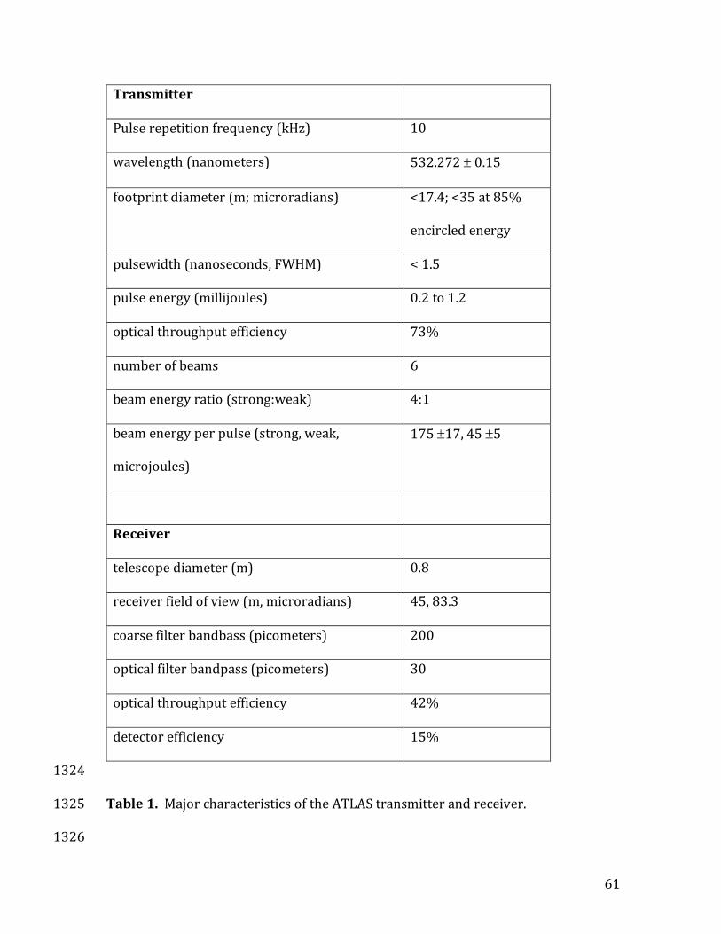
61
Transmitter
Pulse repetition frequency (kHz) 10
wavelength (nanometers) 532.272 0.15
footprint diameter (m; microradians) <17.4; <35 at 85%
encircled energy
pulsewidth (nanoseconds, FWHM) < 1.5
pulse energy (millijoules) 0.2 to 1.2
optical throughput efficiency 73%
number of beams 6
beam energy ratio (strong:weak) 4:1
beam energy per pulse (strong, weak,
microjoules)
175 17, 45 5
Receiver
telescope diameter (m) 0.8
receiver field of view (m, microradians) 45, 83.3
coarse filter bandbass (picometers) 200
optical filter bandpass (picometers) 30
optical throughput efficiency 42%
detector efficiency 15%
1324
Table 1. Major characteristics of the ATLAS transmitter and receiver. 1325
1326

62
Region
Number
Ascending / descending Beginning
latitude
Ending latitude
1 Ascending equator 27 N
2 Ascending 27 N 59.5 N
3 Ascending 59.5 N 80 N
4 Ascending / Descending 80 N 80 N
5 Descending 80 N 59.5 N
6 Descending 59.5 N 27 N
7 Descending 27 N equator
8 Descending Equator 27 S
9 Descending 27 S 50 S
10 Descending 50 S 79 S
11 Descending / Ascending 79 S 79 S
12 Ascending 79 S 50 S
13 Ascending 50 S 27 S
14 Ascending 27 S Equator
1327
Table 2. Geographic boundaries of ATL02 and ATL03 granules. 1328
1329

63
1330 ATLAS Advanced Topographic Laser Altimeter System
AMCS Alignment Monitoring and Control System
ATL02 ICESat-2 Science Unit Converted Telemetry Level 1B Data
Product
ATL03 ICESat-2 Global Geolocation Photon Level 2A Data Product
BSM Beam Steering Mechanism
CCR Corner Cube Retroreflector
CoM Observatory Center of Mass
DOE Diffractive Optical Element
ECF Earth Centered, Fixed
ECI Earth Centered, Inertial
EKF Extended Kalman Filter
ESA European Space Agency
GLAS Geosciences Laser Altimeter System
ICESat Ice Cloud and Land Elevation Satellite
ICESat-2 Ice Cloud and Land Elevation Satellite - 2
ICRF International Celestial Reference Frame
IERS International Earth Rotation and Reference System
IMSC Instrument Mounted Spacecraft Components
IMU Inertial Measurement Unit
ITRF International Terrestrial Reference Frame
LRS Laser Reference System
LTR Lateral Transfer Retroreflector
MABEL Multiple Altimeter Beam Experimental Lidar
MRF Master Reference Frame
PAD Precision Attitude Determination
PCE Photon-Counting Electronics
PMT Photomultiplier Tube
POD Precision Orbit Determination
PPD Precision Pointing Determination
PRF Pulse Repetition Frequency
RGT Reference Ground Track
SPD Start Pulse Detector
SSIRU Scalable Space Inertial Reference System
SST Spacecraft Star Tracker
TAMS Telescope Alignment and Monitoring System
TEP Transmitter Echo Path
TOF Time of Flight

64
USO Ultra Stable Oscillator
WGS World Geodetic System
WTOM/WTEM Wavelength Tracking Optical / Electronics Module
ZRP Zero Range Point
1331 1332 Table 3. Glossary of acronyms used in text. 1333

65
1334
1335
Figure 1. The ICESat-2 observatory. Laser light is transmitted and returns to the 1336
nadir-looking face of the observatory (upper); the star trackers and GPS antennas 1337
are on the zenith-looking face (lower). 1338
1339
Laser Reference System
Spacecraft Star Trackers
GPS Antennas

66
1340
1341
Figure 2. The major components of the ATLAS transmitter. Components discussed 1342
in the text include the two laser transmitters, the Laser Sampling Assembly, the 1343
Beam Shaping Optics, Beam Steering Mechanism, and the Diffractive Optical Element. 1344
Arrows denote the optical path through the transmitter; arrow width is a proxy for 1345
relative energy. 1346
1347

67
1348
1349
Figure 3. Schematic of the ATLAS receiver. Major components described in the text 1350
are the Telescope, Optical Fibers, Optical Filters, and Detector Modules. Green 1351
arrows denote the optical path; red arrows denote communication and commanding 1352
from the ATLAS avionics system; dark green arrows denote the Telescope Alignment 1353
and Monitoring System (TAMS) path, which is described in Section 2.1.4 and shown 1354
in Figure 5. 1355
1356
1357

68
1358
1359
Figure 4. Design of the ATLAS multi-pixel photo-multiplier tube configuration for 1360
the three weak and three strong beams. Each strong beam uses the 16 pixels 1361
(numbered 1 – 16) individually to generate 16 independent electrical outputs, while 1362
each weak beam combines four pixels together to effectively create a four-pixel 1363
detector (pixels PA, PB, PC, and PD) to generate four independent electrical outputs. 1364
1365

69
1366
1367
Figure 5. Primary components of the ATLAS Alignment Monitoring and Control 1368
System (AMCS). The AMCS provides a means to keep the transmitted laser light from 1369
the beam steering mechanism (BSM) aligned with the receiver fields of view. Bright 1370
green arrows indicate the pathway of 532 nm green light; red arrows indicate power 1371
and commanding from the avionics system; dark green arrows indicate the pathway 1372
of light from the Telescope Alignment and Monitoring System (TAMS) light source. A 1373
portion of the transmitted beams and TAMS beams are routed to the Laser Reference 1374
System (LRS) using lateral transmit retroreflectors (LTRs). 1375
1376

70
1377
1378
Figure 6. The ATLAS start pulse is timed at four places along the transmitted pulse 1379
profile. Each PCE card records the time of the leading lower crossing time, as well as 1380
one other crossing time. By recording a common event across all cards, the times of 1381
events can be aligned. 1382
1383

71
1384
1385
Figure 7. ATL03 regions. Region boundaries are used as boundaries between 1386
ATL02 data granules. Each complete orbit is broken into 14 distinct granules as 1387
indicated. 1388
1389

72
1390
1391
Figure 8. The ATLAS beam pattern on the ground changes depending on the 1392
orientation of the ICESat-2 observatory. The pattern on top corresponds to traveling 1393
in the forward (+x) orientation, while the pattern on the bottom corresponds to 1394

73
traveling in the backward (-x) orientation. The numbers indicate the corresponding 1395
ATLAS beam, while the L/R mapping are used on the ATL03 and higher-level data 1396
products. The two strong beams with the TEP are ATLAS beams 1 and 3. Derived 1397
from Markus et al. (2017), Figure 2. 1398
1399

74
1400
1401
Figure 9. Top: Signal and background photons collected by ATLAS over Greenland, 9 1402
November 2018. Bottom: Resulting classification of high-confidence (blue), medium-1403
confidence (red), and low-confidence (green) likely signal photons. Inset shows 1404
detail of photon cloud over water surface. 1405
1406

75
1407 Figure 10. A normalized histogram of transmitter echo path (TEP) photons. The x-1408
axis is the TEP photon time of flight (TOF) in nanoseconds, and y-axis is normalized 1409
counts. Histogram bins are 50 ps wide, and the histogram is composed of TEP 1410
photons from 3,308,000 unique laser fires, or about 300,000 TEP photons. 1411
1412
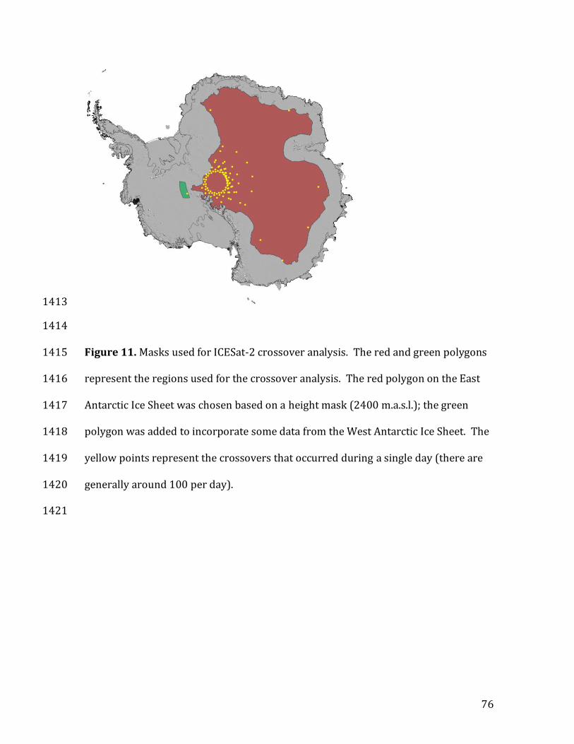
76
1413
1414
Figure 11. Masks used for ICESat-2 crossover analysis. The red and green polygons 1415
represent the regions used for the crossover analysis. The red polygon on the East 1416
Antarctic Ice Sheet was chosen based on a height mask (2400 m.a.s.l.); the green 1417
polygon was added to incorporate some data from the West Antarctic Ice Sheet. The 1418
yellow points represent the crossovers that occurred during a single day (there are 1419
generally around 100 per day). 1420
1421

77
1422
1423
Figure 12. CCR deployment. Left: a CCR being deployed along the 88S Traverse, 1424
with the precise latitude and longitude being surveyed with a GPS. Right: a CCR 1425
mounted on the top of a bamboo pole along the 88S Traverse. 1426
1427