the icelandic low as a predictor of the gulf stream north
TRANSCRIPT

The Icelandic Low as a Predictor of the Gulf Stream North Wall Position
ALEJANDRA SANCHEZ-FRANKS
National Oceanography Centre, Southampton, United Kingdom
SULTAN HAMEED AND ROBERT E. WILSON
School of Marine and Atmospheric Sciences, Stony Brook University, Stony Brook, New York
(Manuscript received 24 November 2014, in final form 6 November 2015)
ABSTRACT
TheGulf Stream’s north wall east of Cape Hatteras marks the abrupt change in velocity and water properties
between the slope sea to the north and theGulf Stream itself. An index of the north wall position constructed by
Taylor and Stephens, calledGulf Stream north wall (GSNW), is analyzed in terms of interannual changes in the
Icelandic low (IL) pressure anomaly and longitudinal displacement. Sea surface temperature (SST) composites
suggest that when IL pressure is anomalously low, there are lower temperatures in the Labrador Sea and south
of theGrandBanks. Two years later, warmSST anomalies are seen over theNorthernRecirculationGyre and a
northward shift in the GSNW occurs. Similar changes in SSTs occur during winters in which the IL is anom-
alously west, resulting in a northward displacement of the GSNW 3 years later. Although time lags of 2 and 3
years between the IL and the GSNW are used in the calculations, it is shown that lags with respect to each
atmospheric variable are statistically significant at the 5% level over a range of years. Utilizing the appropriate
time lags between the GSNW index and the IL pressure and longitude, as well as the Southern Oscillation
index, a regression prediction scheme is developed for forecasting the GSNW with a lead time of 1 year. This
scheme, which uses only prior information, was used to forecast the GSNW from 1994 to 2015. The correlation
between the observed and forecasted values for 1994–2014 was 0.60, significant at the 1% level. The predicted
value for 2015 indicates a small northward shift of the GSNW from its 2014 position.
1. Introduction
Labrador Sea Water (LSW), formed in convective
processes in the Labrador Sea, makes up the upper
component of the deep western boundary current in
theNorthAtlantic. The deep western boundary current
crosses under the Gulf Stream near 368N, an important
region of interaction between the two different water
masses. Hydrographic and tracer surveys of the cross-
over region show that a part of the LSW transported by
the deep western boundary current turns away from the
shore at the crossover and becomes incorporated
with the northern part of the Gulf Stream (Pickart
and Smethie 1993; Bower and Hunt 2000). At the
northern edge of the Gulf Stream, where its warm
waters meet the cold Labrador Sea–derived flow, a
sharp temperature gradient known as the Gulf Stream
north wall (GSNW) is created. Interannual fluctuations
of the latitude at which the GSNW occurs are associ-
ated with changes in sea surface temperature (SST)
distribution northward and thus with regional climate
and plankton distributions.
The analysis presented in this paper is based on the
GSNW index of Taylor and Stephens (1980, 1998). This
index has been used in studies of plankton abundance in
the eastern North Atlantic, the North Sea (Taylor 1995;
Planque and Taylor 1998), Narragansett Bay (Borkman
and Smayda 2009), and lakes in Ireland (Jennings and
Allott 2006). From current measurements in the slope
sea, Bane et al. (1988) found the southwestward shelf-
break current is stronger when the Gulf Stream is lo-
cated more to the north and closer onshore, and it is
weaker when the Gulf Stream is situated farther south,
offshore. They suggested that this relationship is driven
by the Gulf Stream’s impact on the Northern Re-
circulation Gyre from both its shift in position and the
shedding of warm core rings. Following Csanady and
Corresponding author address: Sultan Hameed, School of Ma-
rine and Atmospheric Sciences, Stony Brook University, 125 En-
deavour Hall, Stony Brook, NY 11794-5000.
E-mail: [email protected]
MARCH 2016 SANCHEZ - FRANKS ET AL . 817
DOI: 10.1175/JPO-D-14-0244.1
� 2016 American Meteorological SocietyUnauthenticated | Downloaded 11/21/21 12:07 AM UTC

Hamilton (1988), the slope sea is defined here as the
region of ocean located between the continental shelf
and the Gulf Stream, extending from Cape Hatteras to
the tail of the Grand Banks.
Taylor and Stephens (1998) also showed that the
GSNW is significantly correlated to the North Atlantic
Oscillation (NAO). They presented a regression model
of the GSNW using a 1-yr lagged GSNW and a 2-yr
lagged NAO index. In this scheme, southward (north-
ward) anomalies of the GSNW latitude are associated
with a low (high) NAO phase. Taylor et al. (1998)
showed that more of the GSNW’s variability could be
explained when the Southern Oscillation index (SOI),
lagged 2 years, was added as an independent variable in
the regression equation. They found that, for 1966–97,
60% of the GSNW’s variance was explained using the
GSNW (lagged 1 year) and the NAO (lagged 2 years);
another 9% was explained by the SOI, also lagged
2 years. Later, Hameed and Piontkovski (2004) discov-
ered that the variance of the GSNW explained in the
regression model of Taylor and Stephens (1998) in-
creased significantly when the NAO was decoupled into
its component centers of action, the Icelandic low (IL)
and the Azores high (AH), characterized by their pres-
sure, latitude, and longitude. Their regressionmodel was
dominated by the IL pressure (lagged 2 years) and IL
longitude (lagged 3 years). The direct contribution, or
partial correlation coefficient, of theAH to the variation
of the GSNW was insignificant. Because the northerly
winds around the IL cause cooling in the Labrador Sea,
their results suggested that variations in the southward
flow of LSW are an important influence on the GSNW
position.
This paper has a threefold purpose. First, we report
that the relationship between the GSNW and the IL
pressure and longitude position described by Hameed
and Piontkovski (2004) has been maintained up to
present. Second, we examine SST anomalies in the
North Atlantic for winters when the IL pressure is
anomalously low (high), and for winters in which the IL
longitude has shifted anomalously west (east). These
anomalies are indicative of dynamical changes in the
ocean consequent to changes in wind stress and heat
fluxes that accompany the fluctuations in the strength
and position of the IL. A third purpose of this paper is to
show that GSNW can be forecasted at least 1 year in
advance. Noting that the GSNW is correlated with IL
pressure and longitude position and the SOI, each with a
2–3-yr lag, we develop a statistical model for predicting
GSNW position with a lead time of 1 year, using only
prior information. This is used to make 1- and 2-yr-
forward forecasts of GSNW position for each year from
1994 to 2015.
2. Update of relationship between the Icelandiclow and the Gulf Stream north wall
The GSNW dataset used here is the index computed
by Taylor and Stephens (1980) from the first principal
component of the position of the north wall’s latitude
from six different longitudes: 798, 758, 728, 708, 678, and658W. The temperature measurements used to identify
the Gulf Stream position have been collected since 1966
by the U.S. Naval Oceanographic Office, NOAA, the
Oceanographic Monthly Summary, and the U.S. Navy.
(Both monthly and annual means are available at http://
www.pml-gulfstream.org.uk/default.htm.) To maintain
continuity with previous studies of the GSNW, this pa-
per uses only annual means of the index.
The second dataset used was the IL pressure and
longitude indices, constructed from gridded NCEP–
NCAR reanalysis monthly sea level pressure (SLP) data
(Kalnay et al. 1996) as described by Hameed and
Piontkovski (2004). Objective indices for the IL are
calculated by using the air mass distribution over its
domain. By examining the monthly SLP maps over the
North Atlantic since 1900, the latitude–longitude do-
main of the IL was chosen as 408–758N, 908W–208E. Themonthly averaged pressure of the IL is then estimated as
the area-weighted mean pressure over all the grid points
in the domain where the pressure is less than a threshold
value of 1014mb. The longitude position index is de-
fined as the pressure-weighted longitudinal location of
the centroid of the air mass over the grid points where
the pressure is less than the threshold value. Further
details on the calculation of the indices are given by
Hameed and Piontkovski (2004).
Hameed and Piontkovski (2004) investigated the re-
lationship between the GSNW and the NAO for the years
1966–2000. By decoupling the NAO into the IL and the
AH, they found that the largest correlations with the
GSNWwerewith the ILpressure lagged 2 years and the IL
longitude lagged 3 years. The first two rows of Table 1 give
the statistics of these correlations for the 1966–2000 years.
We have updated these results for 1966–2014 (bottom two
rows of Table 1) and find the lagged correlations between
GSNW and IL pressure and longitude have stayed robust
through the longer period. Since GSNW and IL pressure
and longitude have significant autocorrelations, the effec-
tive sample size n0 for the correlations was estimated using
the method of Quenouille (1953) as
n0 5 n/(11 2r1r01 1 2r
2r02 1 2r
3r03 1 . . . ) ,
where n is the number of data in each series, r1 and r01 arethe autocorrelations at lag 1 in the two data series, r2 and
r02 the autocorrelations at lag 2, etc.
818 JOURNAL OF PHYS ICAL OCEANOGRAPHY VOLUME 46
Unauthenticated | Downloaded 11/21/21 12:07 AM UTC

3. Time lags between changes in the IL and theGSNW
There are multiple intraseasonal and interannual time
scales for variations in the IL pressure and position.
Similarly, there are multiple time scales that influence
the western boundary current. As a result the time lags
between the changes in the IL and changes in GSNW
vary over a range of years. Hameed and Piontkovski
(2004) showed correlations with lags of 0–5 years in their
Table 1, where it was seen that the correlations between
IL pressure and GSNW were statistically significant for
lags of 0, 1, and 2 years, and for IL longitude the cor-
relations for 3- and 4-yr lags were statistically significant.
However, the percentage of GSNW variance explained
was maximized for a 2-yr lag for IL pressure and a 3-yr
lag for IL longitude. The lags at which the correlations
are statistically significant for the extended data, 1966–
2014, are shown in Table 2, where we again see that the
correlations ofGSNWand IL pressure are significant for
lags of 0, 1, and 2 years and those for IL longitude are
significant for lags of 3 and 4 years at the 5% level. The
table shows the interesting result that the correlation
between the NAO and GSNW is statistically significant
for lags of 0, 1, and 2 years. The highest correlation is at a
lag of 1 year, although a lag of 2 years with respect to the
NAO was used in the regression model of Taylor and
Stephens (1998). Table 2 also indicates that the corre-
lation between the SOI and the GSNW is statistically
significant with only the lag of 2 years. The physical
mechanism that would explain this relationship between
El Niño–Southern Oscillation and GSNW remains
unidentified.
Bower andHunt (2000) deployed floats at the levels of
upper LSW (800m) and overflow water (3000m) in the
deep western boundary current between the Grand
Banks and Cape Hatteras to measure the spreading
rates of these two water masses. They estimated mean
advection velocities along the upper LSW as 2–4 cm s21.
These estimates translate to a travel time of 2–4 years
for a water parcel to travel the 1700km between the
Grand Banks and Cape Hatteras, consistent with the
multiyear lag times between the IL and the GSNW
shown in Table 2.
Using a combination of altimetric and hydrographic
(CTD) data, Han et al. (2010) measured Labrador
Current transport between the 600- and 3400-m isobaths
in the Labrador Sea north of the Hamilton Bank (568N)
over 1993–2004. They found the multiyear changes in
the Labrador Current transport to be primarily baro-
tropic and positively correlated with the NAO at zero
lag. This suggests Labrador Sea circulation responds to
atmospheric variability within a year.
4. SST response to IL variations
In this section, relationships between IL pressure and
longitudinal position and the distribution of SST in the
North Atlantic are examined. NOAA Optimum In-
terpolated (OI) SST version 2 data available from 1981
to 2012 with a 18 3 18 resolution are used for the SST
composites. The SST data may be found on NOAA’s
physical sciences division website (http://www.esrl.noaa.
gov/psd/data/gridded/data.noaa.oisst.v2.html).
Figure 1a shows a composite of SST anomalies during
1981–2012 in winters [December–February (DJF)] for
which the area-averaged IL pressure was more than one
standard deviation lower than its mean value (1989,
1990, 1995, and 2007). Cold anomalies of 20.18to21.08C extend from themouth of the Labrador Sea to
the southeast and east of Greenland and southward of
the Grand Banks and the Scotian Shelf, as would be
expected from the impact of intensified cyclonic winds
that accompany very low IL pressures. Figure 1b shows
SST anomalies 2 years later, that is, winters with a 2-yr
lag with respect to those shown in Fig. 1a, where the cold
SST anomalies south of the Grand Banks, observed 2
years prior, have been replaced by warm SSTs in the
range of 0.28–1.08C, suggesting a northward shift of the
GSNW. Warm anomalies in the slope sea were attrib-
uted by Rossby and Benway (2000) to a reduction of
cold water flux from the Labrador shelf, consistent with
the warm temperature anomalies south of the Grand
Banks in Fig. 1b. We note the cold SST anomaly in the
Gulf of Maine is not consistent with this picture. An
TABLE 2. Correlation between the GSNW and the atmospheric
variables with lags from 0 to 5 years. Results in bold indicate the
correlation coefficient is significant at the 5% level.
Variable/lag 0 1 2 3 4 5
NAO 0.46 0.52 0.39 0.16 0.08 0.18
IL pressure 20.40 20.40 20.52 20.22 20.19 20.26
IL longitude 20.01 0.07 20.01 20.40 20.42 20.21
SOI 20.08 0.10 20.29 20.08 20.02 20.08
TABLE 1. The sample size n, the effective sample size n0, and the
correlation coefficient r between the GSNW and IL pressure
(lagged 2 years), and longitude position (lagged 3 years) compared
between the 1966–2000 and 1966–2014 periods. All correlation
coefficients are statistically significant at the 1% level.
Variable n n0 r
IL pressure 1966–2000 35 21 20.59
IL longitude 1966–2000 35 25 20.50
IL pressure 1966–2014 49 30 20.52
IL longitude 1966–2014 49 37 20.40
MARCH 2016 SANCHEZ - FRANKS ET AL . 819
Unauthenticated | Downloaded 11/21/21 12:07 AM UTC

estimate of the mean Gulf Stream path is superposed
(black line) on the SST in all panels of Fig. 1 using the
Canadian marine environmental data service (MEDS).
The MEDS mean Gulf Stream position is estimated
from SST anomalies at every degree longitude between
758 and 508W.
Figure 1c depicts composite SST anomalies in the
winters when the IL longitude was displaced westward
by more than one standard deviation of its mean longi-
tudinal position (1985, 1987, 1991, 1992, 1996, 2003, and
2006). Cold SST anomalies of 20.28 to 20.58C are seen
in the Labrador Sea, extending eastward and southward
to the Grand Banks and the Scotian Shelf and to the
eastern side of the North Atlantic. Figure 1d shows the
composite SST anomalies 3 years after those shown in
Fig. 1c, that is, lagged 3 years with respect to extreme
westward positioning of the IL, as is suggested by the
correlation calculations (Table 2). SST anomalies in
Fig. 1d are warmer south of theGrand Banks and Scotian
Shelf in comparison with the anomalously west IL
longitude (Fig. 1c), indicating a reduction in the spilling
of cold waters from the north into the slope sea, as
hypothesized by Rossby and Benway (2000).
Analogous to the anomalously low and anomalously
west IL pressures in Fig. 1, anomalously high and
anomalously east IL pressures are considered in Fig. 2.
Figure 2a shows winter SST anomaly composites for
anomalously high IL pressures (1996, 2001, 2004, 2006,
2010, and 2011) at zero-year lag.Warm anomalies of 0.58to 1.08C are observed in the Labrador Sea, east of
Newfoundland, and in the Gulf of St. Lawrence, and
cool anomalies of 20.38 to 21.08C are apparent along
the U.S. eastern seaboard (Fig. 2a). Contrary to the SST
structure depicted in the anomalously low IL pressure
years (Fig. 1a), during anomalously high IL pressure
winters, the IL pressure system is decreased in strength
FIG. 1. Winter (DJF) composite SST anomalies (8C) for the time range 1981–2012. Shown for the IL pressure
during its lowest years (a) with no lag and (b) with a 2-yr lag and the IL longitude during its westernmost years
(c) with no lag and (d) with a 3-yr lag. The mean Gulf Stream path is superimposed (black line) on the SST
anomalies. The winter average for a particular winter is the average of theDecember value of the previous year and
January and February values of the current year. The thin lines represent the 1000- and 3500-m isobaths.
820 JOURNAL OF PHYS ICAL OCEANOGRAPHY VOLUME 46
Unauthenticated | Downloaded 11/21/21 12:07 AM UTC

and conditions in the northeast Atlantic are milder,
leading to the observed warm SST anomalies (Fig. 2a).
Figure 2b shows SST anomalies for anomalously high IL
pressure 2 years after those shown in Fig. 2a. The mag-
nitude and the coverage of the warm SST anomalies are
decreased (in comparison to Fig. 2a) in the Labrador
Sea, east of Newfoundland, and in the Gulf of St. Law-
rence and the Scotian Shelf. Further, comparing Fig. 1b
with Fig. 2b, SSTs south of Grand Banks are found
warmer in Fig. 1b (2 years after IL pressure was anom-
alously low) than in Fig. 2b (2 years after the IL pressure
was anomalously high). This reduction in warm SSTs is
suggestive of a displacement south in GSNW position.
Figure 2c presents SST anomalies for winters where
the IL longitude was situated eastward bymore than one
standard deviation from its mean position (1983, 1984,
1994, 1995, 1999, and 2005). Warm SST anomalies
dominate in a zonal band between the Mid-Atlantic
Bight and just southeast of the Grand Banks, and strong
cool SST anomalies are observed in the Labrador Sea
and south and east of Greenland (Fig. 2c). Similar to the
anomalously high IL pressure conditions (Fig. 2a),
anomalously east IL longitude (Fig. 2b) should depict
warm SSTs in the general northeast Atlantic, opposite
the pattern depicted during anomalously west IL lon-
gitudes (Fig. 1c). However, warm SSTs in Fig. 2b are
only observed in the zonal band between the Mid-
Atlantic Bight and the region southeast of the Grand
Banks. The anomalously cool region in the Labrador
Sea is unexplained and deserves further consideration.
In Fig. 2d, 3 years after the IL longitude is at its east-
ernmost, cool SST anomalies in the range of 20.38to21.08C are observed in the neighborhood of the warm
zonal band observed in Fig. 2c. The cooling of the SST
anomalies near the Scotian Shelf and south of the
Grand Banks 3 years after the IL longitude is at its
easternmost (Fig. 2d) suggests a displacement south of
the GSNW, just as warm anomalies in westernmost IL
FIG. 2. Winter (DJF) composite SST anomalies (8C) for the time range 1981–2012. Shown for the IL pressure
during its highest years (a) with no lag and (b) with a 2-yr lag and the IL longitude during its easternmost years
(c) with no lag and (d) with a 3-yr lag. TheGulf Stream path is superimposed (black line) on the SST anomalies. The
thin lines represent the 1000- and 3500-m isobaths.
MARCH 2016 SANCHEZ - FRANKS ET AL . 821
Unauthenticated | Downloaded 11/21/21 12:07 AM UTC

longitude, 3-yr lagged (Fig. 1d), suggest a northward
shift in the GSNW.
Statistical significance of SST differences between
the winters in which the IL pressure was anomalously
low during the 1981–2012 period and the winters when
the IL pressure was anomalously high are shown in
Fig. 3a. This was carried out by doing a t test for the
difference in the two mean temperatures at each grid
point. Areas with p values less than 0.1 are seen in the
Labrador Sea, south and east of Newfoundland, near
the GSNW and in regions to the south. A similar test
comparing winters in which the IL was situated
anomalously west and anomalously east, shown in
Fig. 3b, displays statistically significant differences
near the GSNW and a small area in the Labrador Sea.
The impact of changes in the IL pressure can be seen
in heat fluxes as well (Fig. 4). One-degree gridded net
ocean surface heat flux data were used to make com-
posites for winter (DJF) heat flux during anomalously
low IL pressure years 1989, 1990, 1995, and 2007
(Fig. 4a) and during anomalously high IL pressure years
1996, 2001, 2004, and 2006 (Fig. 4b). The net heat flux
(positive downward) used to construct these ensembles
represents combined OAFlux and ISCCP products
provided by the WHOI OAFlux project (http://oaflux.
whoi.edu) funded by the NOAA Climate Observations
andMonitoring (COM) program, available from 1983 to
2009. The net heat flux Qnet is defined as
Qnet
5 SW2LW2LH2 SH,
where SW is the net downward shortwave radiation, LW
is the net upward longwave radiation, LH is the latent
heat flux, and SH is the sensible heat flux.
The composite net surface heat flux for anomalously
low IL pressure years emphasizes negative heat flux in
the Labrador and Greenland Seas as well as in the vi-
cinity of the Gulf Stream (Fig. 4a). This negative heat
flux has direct impact on mixed layer temperature and
on deep convection. Heat flux for IL pressure during
anomalously high pressure years (Fig. 4b) exhibits a
similar pattern but with reduced magnitude in the
Labrador and Greenland Seas, whereas negative heat
flux in the Gulf Stream region has extended slightly
south. Taking the difference between the IL low pres-
sure years and IL high pressure years (Fig. 4c) shows the
significantly stronger winter cooling in the Labrador and
Greenland Seas (;50–80Wm22), which could lead to
reduced mixed layer temperature and enhanced deep
convection. These anomalies aremarkedly reduced over
the Gulf Stream. For comparison, Fig. 4d shows the
difference in winter SSTs between anomalously low IL
pressure and anomalously high IL pressure years. Neg-
ative SST anomalies dominate the Labrador and Ir-
minger Seas, the Scotian Shelf, and the Grand Banks
(Fig. 4d). This pattern is similar to that observed in
Fig. 4c, suggesting SST difference is linked to net heat
flux changes. In general, comparison of Figs. 4c and 4d
indicates that the intensified cooling in the subpolar gyre
in IL low-pressure years spreads to large areas of the
North Atlantic by ocean circulation.
5. Forecasting the GSNW position
Taylor and Stephens (1998) and Taylor et al. (1998)
showed that the GSNW is autocorrelated with a lag of
1 year and correlated with the NAO and SOI, each
with a 2-yr lag. Thus, it should be possible to forecast the
FIG. 3. (a) The p values of SST differences betweenwinters during 1981–2012 inwhich ILpressurewas anomalously
low and winters in which IL pressure was anomalously high. (b) The p values of SST differences between winters in
which IL was located anomalously westward and winters in which IL was located anomalously eastward. The black
line represents the mean position of the Gulf Stream. The thin lines are the 1000- and 3500-m isobaths.
822 JOURNAL OF PHYS ICAL OCEANOGRAPHY VOLUME 46
Unauthenticated | Downloaded 11/21/21 12:07 AM UTC

GSNW at least 1 year ahead using these variables. A
reliable scheme for predicting the GSNW should have
practical value in view of the GSNW’s known impact on
plankton distribution in the North Atlantic.
Taylor and Gangopadhyay (2001) used the one-
dimensional model developed by Behringer et al.
(1979) to hindcast the interannual variations in the lat-
itude of the GSNW. The model was forced by the
monthly NAO index with a lag of 1 year. Based on the
results presented in Table 1 and by Taylor and Stephens
(1998) and Taylor et al. (1998), we developed a re-
gression prediction model for the GSNW as
GSNWi5aGSNW
i211bILP
i221cILL
i231dSOI
i221e ,
where i represents a particular year and the subscripts of
the independent variables represent the lag for each.
The variables a, b, c, and d are regression coefficients
and e is the residual. In the first step, we developed a
regression using the data from 1966 to 1993; the re-
gression coefficients obtained were used to predict the
GSNW index for 1994. Then, moving 1 year forward by
developing a regression equation for 1966–94, we
obtained a prediction for 1995, and so on until we had
forecasts for each of the years during 1994–2015. In each
of these calculations only prior information was used to
make the prediction. These are 1-yr forecasts because
the observed GSNW latitude from the previous year is
used in predicting its value for the next year. In Fig. 5a,
the solid line shows the observed values of the GSNW
index and the dashed line shows the 1-yr-ahead pre-
dicted values. The amplitude of variations in the ob-
servations is underestimated by the predicted values.
However, the maxima in the northward shifts of the
GSNW in 1995, 2000, 2006, and 2009 are captured in the
predicted values. Similarly, the extreme southward
FIG. 4. Composite of net surface heat flux (positive downward) for (a) anomalously low IL pressure years and
(b) anomalously high IL pressure years. (c) Difference in ensemble net surface heat flux between anomalously low
and anomalously high IL pressure years and (d) difference in SST anomalies between anomalously low and anom-
alously high IL pressure. The units for net surface heat flux and SST are in Wm22 and degrees Celsius, respectively.
The black line represents the mean position of the Gulf Stream. The thin lines are the 1000- and 3500-m isobaths.
MARCH 2016 SANCHEZ - FRANKS ET AL . 823
Unauthenticated | Downloaded 11/21/21 12:07 AM UTC

shifts in 1998 and 2008 are reproduced in the predicted
values. The correlation coefficient between the observed
and forecasted values during 1994–2014 is 0.60 (signifi-
cant at the 1% level) and the mean absolute error
(MAE) is 0.53. We tested the stability of this prediction
scheme by examining the values of R and MAE for four
different durations. These are shown in Table 3, where it
is seen that the correlation coefficient and the MAE
were stable as the length of the forecast period in-
creased. We note the MAE is defined here as
MAE51
n�n
i51
����fi2 y
i
����,
where fi is the predicted GSNW value and yi is the ob-
served GSNW value.
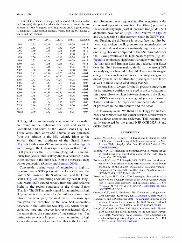
Table 4 gives the coefficients in the prediction model
for the years 1994–2014. All variables were normalized
to zero mean and unit standard deviation before com-
puting the regressions. The table indicates that the IL
pressure was the largest contributor to the forecasted
value in the 1990s, but GSNW lagged 1 year was the
largest contributor after the early 2000s. The contribu-
tions of IL longitude and the SOI fluctuated throughout
this period.
The 2-yr-ahead forecasts were also made using the
same scheme. For this purpose, we used the 1-yr fore-
casted value of the GSNW as a predictor in the re-
gression equation. Comparison with the observed
GSNW locations is shown in Fig. 5b. The 2-yr forecast
also shows some skill. Correlation between the observed
and forecasted values is 0.43 (slightly below the 5%
significance level) and theMAE is 0.67; however, the 2-yr
forecast is inferior to the 1-yr forecast in terms of both the
correlation coefficient and theMAE. Both the 1- and 2-yr
forecasts suggest that the annually averaged GSNW for
2015 will be slightly north of its value in 2014, as seen in
Figs. 5a and 5b.
As a further check on consistency, cross correlations
between GSNW and IL pressure during 1966–94, and
then for each succeeding year until 2014, were also cal-
culated (not shown here). Themaximum correlationwas
found to be always with a lag of 2 years. A similar con-
sistency was found in the correlation of GSNW with IL
longitude being maximum at the lag of 3 years. How-
ever, the lag for maximum correlation between GSNW
and the NAO index fluctuated between 1 and 2 years.
6. Conclusions
The results presented in this paper show that a fore-
cast of the GSNW position, as given by Taylor and
Stephens’ (1998) GSNW index, is possible with a lead
time of 1 year. The forecast uses only prior information
on the following predictors: IL pressure (ILP; 2-yr lag-
ged), the IL longitude (ILL; 3-yr lagged), the SOI (2-yr
lagged), and the GSNW index (1-yr lagged). One-year
forecasts of GSNW position were made for each of the
years 1994–2015. Correlation between the forecasted
and observed values for 1994–2014 was 0.60, significant
at 1% level. The forecast for 2015 suggests that the an-
nually averaged GSNW will be slightly north of its 2014
position. Forecasts of the GSNW index can have useful
applications to fisheries as it has been shown to be re-
lated to variations of plankton in several regions of the
North Atlantic.
Impact of IL pressure and its longitude on SST in the
North Atlantic was also investigated. During years of
anomalously low IL pressure, cool SSTs in the northern
half of the North Atlantic subpolar gyre (specifically the
region extending from the mouth of the Labrador Sea
south to the Scotian Shelf and east toward the European
continent) are observed (Fig. 1a). This SST structure is
characteristic of an intensified IL pressure system, which
leads to a reduced mixed layer temperature and en-
hanced deep winter convection in the Labrador and
Greenland Seas region as shown by the negative heat
flux patterns in Fig. 4a. The cool SSTs and increase in
deep winter convection lead to warm SST anomalies
south of the Grand Banks and east of the Scotian Shelf 2
years later (Fig. 1b). Similarly, during winters when the
FIG. 5. Comparison of predicted (dashed lines) and observed
(solid lines) GSNW position. (top) Forecasts made 1 year ahead
and (b) forecasts made 2 years ahead.
TABLE 3. Correlation coefficient R and the MAE during four
segments of the forecast period. All correlations are significant at
the 5% level.
1994–2002 1994–2005 1994–2008 1994–2014
R 0.65 0.65 0.65 0.60
MAE 0.63 0.57 0.53 0.53
824 JOURNAL OF PHYS ICAL OCEANOGRAPHY VOLUME 46
Unauthenticated | Downloaded 11/21/21 12:07 AM UTC
IL longitude is anomalously west, cool SST anomalies
are found in the Labrador Sea, east and south of
Greenland, and south of the Grand Banks (Fig. 1c).
Three years later, warm SST anomalies are perceived
from the latitude of the Mid-Atlantic Bight to the
Scotian Shelf and southeast of the Grand Banks
(Fig. 1d). Both warm SST anomalies depicted in Figs. 1b
and 1d suggest the GSNWexperiences a northward shift
2 (3) years after the IL pressure (longitude) is anoma-
lously low (west). This is likely due to a decrease in cool
water sources to the slope sea, from the increased deep
winter convection (Rossby and Benway 2000).
Conversely, during years of anomalously high IL
pressure, warm SSTs permeate the Labrador Sea, the
Gulf of St. Lawrence, the Scotian Shelf, and the Grand
Banks (Fig. 2a), and during anomalously east IL longi-
tude, warm SSTs extend zonally from the Mid-Atlantic
Bight to the region southeast of the Grand Banks
(Fig. 2c). The SST anomaly signal for anomalously high
IL pressure is as expected for the milder cyclonic con-
ditions that accompany the weakened IL pressure sys-
tem [with the exception of the cool SST anomalies
observed in the Labrador Sea (Fig. 2c), which are un-
explained here and deserve further consideration]. At
the same time, the composite of net surface heat flux
during winters where IL pressure was anomalously high
show a decrease in net surface heat flux in the Labrador
and Greenland Seas region (Fig. 4b), suggesting a de-
crease in deep winter convection. Two (three) years after
the anomalously high (east) IL pressure (longitude), SST
anomalies have cooled (Figs. 2 b,d) relative to Figs. 2a
and 2c, suggesting a displacement south in GSNW posi-
tion. Further, the difference in net surface heat flux be-
tween years when the IL pressure was anomalously low
and years when it was anomalously high was consid-
ered (Fig. 4c) and compared to the SST anomalies for
the IL low-pressure and IL high-pressure years (Fig. 4d).
Figure 4c emphasized significantly strongerwinter signal in
the Labrador and Irminger Seas and reduced heat fluxes
over the Gulf Stream region, similar to the strong SST
anomaly signal observed in Fig. 4d. These results suggest
changes in ocean temperatures in the subpolar gyre in-
duced by the IL can be attributed to changes in heat fluxes
as well as those due to wind stress changes.
We note lags of 2 years for the IL pressure and 3 years
for its longitude position were used in the calculations in
this paper. However, lags between changes in the IL and
the GSNW can vary over a range of years as shown in
Table 3 and are to be expected from the variable nature
of processes in the atmosphere and the ocean.
Acknowledgments. We thank C. N. Flagg for his feed-
back and comments on the earlier versions of this work as
well as three anonymous reviewers. This research was
partly supported by the grants NSF OCE-0825418 and
OCE-1060752.
REFERENCES
Bane, J. M., Jr., O. B. Brown, R. H. Evans, and P. Hamilton, 1988:
Gulf Stream remote forcing of shelfbreak currents in the Mid-
Atlantic Bight. Geophys. Res. Lett., 15, 405–407, doi:10.1029/
GL015i005p00405.
Behringer, D., L. Regier, andH. Stommel, 1979: Thermal feedback
on wind-stress as a contributing cause of the Gulf Stream.
J. Mar. Res., 37, 699–709.Borkman, D. G., and T. J. Smayda, 2009: Gulf Stream position and
winter NAO as drivers of long-term variations in the bloom
phenology of the diatom Skeletonema costatum ‘‘species-
complex’’ in Narragansett Bay, RI, USA. J. Plankton Res., 31,
1407–1425, doi:10.1093/plankt/fbp072.
Bower, A. S., and H. D. Hunt, 2000: Lagrangian observations of the
deep western boundary current in the North Atlantic Ocean.
Part I: Large-scale pathways and spreading rates. J. Phys.
Oceanogr., 30, 764–783, doi:10.1175/1520-0485(2000)030,0764:
LOOTDW.2.0.CO;2.
Csanady, G.T., and P. Hamilton, 1988: Circulation of slope water.
Cont. Shelf Res., 8, 565–624, doi:10.1016/0278-4343(88)90068-4.
Hameed, S., and S. Piontkovski, 2004: The dominant influence of the
Icelandic Low on the position of the Gulf Stream northwall.
Geophys. Res. Lett., 31, L09303, doi:10.1029/2004GL019561.
Han,G., K.Ohashi, N. Chen, P. G.Myers, N. Nunes, and J. Fischer,
2010: Decline and partial rebound of the Labrador Current
1993–2004: Monitoring ocean currents from altimetric and
conductivity-temperature-depth data. J. Geophys. Res., 115,
C12012, doi:10.1029/2009JC006091.
TABLE 4. Coefficients of the prediction model. The columns list
(left to right) the year for which the forecast is made; the co-
efficients of GSNW lagged 1 year, IL pressure (ILP) lagged 2 years,
IL longitude (ILL) position lagged 3 years, and the SOI lagged 2
years; and the residual.
GSNWi21 ILPi22 ILLi23 SOIi22 Residual
1994 0.35 20.48 20.32 20.29 20.15
1995 0.35 20.48 20.33 20.29 20.15
1996 0.40 20.49 20.35 20.30 20.11
1997 0.29 20.53 20.39 20.30 20.16
1998 0.30 20.51 20.42 20.28 20.17
1999 0.32 20.48 20.37 20.29 20.15
2000 0.31 20.48 20.38 20.28 20.14
2001 0.31 20.46 20.37 20.35 20.11
2002 0.38 20.46 20.34 20.30 20.06
2003 0.41 20.46 20.33 20.28 20.04
2004 0.43 20.44 20.32 20.27 20.03
2005 0.43 20.43 20.31 20.28 20.06
2006 0.44 20.43 20.31 20.28 20.06
2007 0.44 20.42 20.35 20.26 20.04
2008 0.44 20.42 20.35 20.26 20.04
2009 0.46 20.38 20.33 20.26 20.02
2010 0.48 20.34 20.29 20.26 20.04
2011 0.48 20.34 20.29 20.26 20.04
2012 0.48 20.34 20.29 20.27 20.05
2013 0.46 20.33 20.30 20.30 20.02
2014 0.48 20.32 20.31 20.27 20.02
Mean 0.40 20.42 20.33 20.28 20.07
MARCH 2016 SANCHEZ - FRANKS ET AL . 825
Unauthenticated | Downloaded 11/21/21 12:07 AM UTC

Jennings, E., and N. Allott, 2006: Position of the Gulf Stream in-
fluences lake nitrate concentrations in SW Ireland.Aquat. Sci.,
68, 482–489, doi:10.1007/s00027-006-0847-0.
Kalnay, E., and Coauthors, 1996: The NCEP/NCAR 40-Year Re-
analysis Project. Bull. Amer. Meteor. Soc., 77, 437–471,
doi:10.1175/1520-0477(1996)077,0437:TNYRP.2.0.CO;2.
Pickart, R. S., and W. M. Smethie, 1993: How does the deep
western boundary current cross the Gulf Stream? J. Phys.
Oceanogr., 23, 2602–2616, doi:10.1175/1520-0485(1993)023,2602:
HDTDWB.2.0.CO;2.
Planque, B., and A. H. Taylor, 1998: Long-term changes in zooplank-
ton and the climate of theNorthAtlantic. J.Mar. Sci., 55, 644–654.Quenouille, M. H., 1953: Associated Measurements. Butterworth
Scientific, 241 pp.
Rossby, T., and R. Benway, 2000: Slow variations in mean path of
theGulf Streameast of CapeHatteras.Geophys. Res. Lett., 27,
117–120, doi:10.1029/1999GL002356.
Taylor,A.H., 1995:North–south shifts of theGulf Stream and their
climatic connection with the abundance of zooplankton in the
UK and its surrounding areas. ICES J. Mar. Sci., 52, 711–721,
doi:10.1016/1054-3139(95)80084-0.
——, and J. A. Stephens, 1980: Latitudinal displacements of the
Gulf Stream (1966 to 1977) and their relation to changes in
temperature and zooplankton abundance in the NE Atlantic.
Oceanol. Acta, 3 (2), 145–149.
——, and ——, 1998: The North Atlantic Oscillation and the lati-
tude of the Gulf Stream. Tellus, 50A, 134–142, doi:10.1034/
j.1600-0870.1998.00010.x.
——, and A. Gangopadhyay, 2001: A simple model of interannual
displacements of the Gulf Stream. J. Geophys. Res., 106,
13 849–13 860, doi:10.1029/1999JC000147.
——, M. B. Jordan, and J. A. Stephens, 1998: Gulf Stream shifts
following ENSO events. Nature, 393, 638, doi:10.1038/
31380.
826 JOURNAL OF PHYS ICAL OCEANOGRAPHY VOLUME 46
Unauthenticated | Downloaded 11/21/21 12:07 AM UTC