1

The Impact of Adds and Deletes on the Returns of Stock Indexes

March, 2003

Applied Finance Project Haas MFE Program

Prepared by:

Jim Quinn &

Frank Wang

2

Acknowledgements

The authors thank Dow Jones & Company for financially supporting this project, and for allowing us to select and evolve the topic for the research. Rich Ciuba and John Prestbo from Dow Jones also provided us with the insights of an index provider, and provided data for the Dow Jones stock indexes. We appreciate the help of our faculty advisor, Terry Marsh, who reviewed our work as well as providing us with access to the QuantalPRO factor model and database. In addition, we appreciate the helpful comments provided by Rob Maxim, Indro Fedrigo, Paul Pfleiderer and Larry Tint from Quantal, Ananth Madhavan from ITG Corporation, and David Pyle from Haas Business School.

About the Authors

Jim Quinn and Frank Wang are recent graduates from the Masters Program in Financial Engineering at Haas Business School, UC Berkeley. This research was the subject of their Applied Finance Project. Any questions concerning the paper can be directed to Jim Quinn at quinn@haas.berkeley.edu or Frank Wang at fwang@haas.berkeley.edu

3

Table of Contents 1.0 Introduction Page 4 2.0 Overview of Broad-Based U.S. Indexes Page 5 3.0 Event Studies Page 8 4.0 Drag on Index Returns from Reconstitution of the Index Page 12 5.0 Optimizing Rebalancing Policies Page 14 6.0 Conclusions Page 16 7.0 Moving Toward a More Fund-friendly Index Page 17 Appendices Appendix A: Policies of Major U.S. Index Providers Page 18 Appendix B: Event Study Paper Page 24 Appendix C: Optimization Model Page 45 Tables 2.1 Reconstitution Policies of Major U.S. Indexes Page 7 2.2 Reconstitution Policies of Major U.S. indexes-Continued Page 9 3.1 MCAR for Index Additions Page 11 3.2 Influences of Investment Universe and Popularity on Market Impact Page 11 4.1 Drag on Index Return Induced by Turnover and Market Impact Page 14

Figures 2.1 Buffer Zones-Conceptual Diagram Page 8 3.1 Theoretical Pattern of Abnormal Returns Page 9 3.2 Volatility and Daily Turnover by Market Cap Page 12 5.1 Turnover and Tracking Error versus Buffer Zone Page 15 Bibliography Page 54

4

Abstract The S&P effect is well known. Stocks that are added to the S&P 500 index have in the past exhibited significant positive abnormal returns immediately after the announcement and continued to earn abnormal returns through the effective date of the index change. A portion of the abnormal return has reversed after the effective date. In this paper we report the results of event studies we performed on additions to the S&P 500 and four other indexes, the S&P 1500, Russell 3000, NASDAQ 100, and Dow Jones Total Market index, for the period 1999-2002. We explore the drag on investment returns that is caused by the reversal of the abnormal return. A model is also developed that allows an index provider to simulate the consequences of variety of index reconstitution policies on index turnover.

1.0 Introduction

Indexing has become an increasingly popular way of investing in equities over the past 20 years. It is estimated that more than 10% of the U.S. stock market is held in index funds. The most popular index replicated by index funds is the S&P 500 for large-cap investors, followed by the Russell 2000, which is tracked by small-cap investors. Indexers hold approximately 10% of the S&P 500 and 6% of the Russell 2000. In addition to S&P and Russell, other U.S. stock index providers include Dow Jones, MSCI, NASDAQ and Wilshire. Index providers recognize that investors replicate their indexes in an attempt to track a segment of the stock market. Therefore the criteria for inclusion in an index often addresses “investibility” in some way, for example, by selecting stocks for inclusion that are easily bought or sold. Index reconstitution policies can also address investibility. Stock index providers periodically reconstitute their indexes, in order to better represent the segment of the market that they are attempting to proxy. During the reconstitution stocks are added to and deleted from the index. Index Fund managers execute trades to buy the adds and sell the deletes around the effective date of the reconstitution. This trading activity appears to cause market impact. Stocks added to the index, for example, have in the past exhibited abnormal returns prior to the effective date of the reconstitution, and negative returns for the few weeks following the reconstitution. This pattern of returns results in a “hidden cost” of indexing. An indexer will be affected by market impact if his trades are large enough on their own, or if the timing of those trades is such that he is trading simultaneously with other indexers who are executing the same trades. For example, let’s say that a portfolio manager is managing a $800 Million index fund that tracks the S&P 500 index and a constituent is added to the index that sells for $25 per share and has a market cap of $1 Billion. Since the total market cap of the S&P 500 is approximately $8 Trillion, the new entry will make up 0.00125% of the index. Therefore the fund must purchase $100,000 or 4000 shares. This trade might not result in market impact. However if an $80 Billion

5

fund does the same trade, they will be purchasing 400,000 shares or $10 Million, which could plausibly result in market impact, since the average daily volume for additions to the S&P 500 is typically only 500,000 to 5,000,000 shares. Nevertheless, regardless of the size of the trade, if the small fund is executing their trade at the same time as other indexers, they will tend to be impacted by the trades of others. This paper investigates the drag on index returns associated with additions to and deletions from broad-based U.S. stock indexes. Event studies are conducted on the additions to the S&P 1500, Russell 3000, Dow Jones U.S. Total Market Index (TMI) and the NASDAQ 100, similar to those previously conducted by other authors on the S&P 500 index. The results of the event study are reported in Section 3 of this paper and a full report is included as Appendix B. At inception, the “investibility” of the stocks chosen for the index will be an important determinant of rebalancing costs. Given the choice of a target universe/criteria, rebalancing costs can be kept to a minimum if companies are never replaced in the index, except when they cease to exist, due to say a liquidation or a merger. However, if this strategy is employed, at some point the index will cease to be representative of the market segment it is attempting to index. Section 5 of this paper explores alternative index reconstitution policies from the perspective of index turnover. Alternative reconstitution policies are then applied as inputs to a model and the turnover is simulated. Finally, a measure similar to tracking error is proposed to assess the representativeness drift of the index. For each rebalance policy the index turnover is assessed along with the representativeness drift. The model results are reported in Section 5 of this paper and a more complete report is included as Appendix C. 2.0 Overview of Broad-based U.S. Stock Indexes

In this section we provide an overview of the major broad-based U.S. stock indexes. More detail on these indexes and their rebalancing policies is provided in Appendix A.

Wilshire 5000 • The Wilshire 5000 index essentially consists of all of the exchange-listed stocks

in the United States. The number of stocks in the index varies, and there are currently about 6500 stocks represented in the index. Since all stocks are included, index reconstitution is not an issue for this index. Stocks of new IPOs are added to the index and companies are removed when they merge with another company or are delisted from an exchange.

Russell 3000

• The Russell Index family includes the Russell 1000 and the Russell 2000. For the Russell Index family all of the U.S. Exchange-traded stocks are ranked by market capitalization. The top 1000 stocks are included in the Russell 1000 and stocks with rankings of 1001 to 3000 are included in the Russell 2000. For ranking purposes, the market caps are float-adjusted. This means that if another

6

corporation or insiders own a portion of a company’s stock, that portion is excluded from the market cap when the rankings are done.

S & P 1500

• The S&P family of indexes uses three indexes to represent the U.S. market. The S&P 500 consists of 500 stocks selected to represent the large cap market segment. The S&P 400 consists of 400 stocks selected to represent the mid-cap market segment. The S&P 600 consists of 600 stocks selected to represent the small cap market segment. S&P has a committee that selects the stocks for each index. It is not done strictly by market capitalization, as they attempt to balance representation by various market sectors, and they incorporate a profitability screen into their selection process

Dow Jones Total Market Index

• The Dow Jones Total Market index (TMI) includes three sub-indexes, large cap, mid-cap and small-cap. The TMI currently includes approximately 1600 stocks, and the index attempts to capture approximately 95% of the U.S. market cap. Approximately 70% of the US market cap is captured in the large cap index, 20% in the mid-cap index and 5% in the small cap index. The market cap rankings for inclusion in the TMI are float adjusted.

MSCI US Index

• The Morgan Stanley Capital International (MSCI) US indexes include the top 2500 US stocks as ranked by float-adjusted market cap. The top 300 are considered large cap, the next 450 are mid-cap, and the remaining 1750 are small cap. MSCI attempts to achieve an 85% free-float adjusted representation within each industrial group, within each country.

Table 2.1 Reconstitution Policies for Major U.S. Stock Indexes Index Reconstitution

Frequency Inclusion Criteria

Buffer Zone?

Russell Indexes Annual Market Cap No

S&P Indexes Quarterly Market Cap, sector balance

Yes

NASDAQ 100 Annual Market Cap Yes

Dow Jones TMI Quarterly Market Cap Yes

MSCI U.S. Quarterly Market Cap, sector balance

Yes

7

The reconstitution policies for a few U.S. Stock indexes are discussed below and summarized in Table 2.1. The frequency of reconstitution is usually either quarterly or annually. In addition to the periodic reconstitutions, interim changes are made for several reasons, including mergers, spinoffs, and delistings. The inclusion criteria for the indexes being considered in this paper are usually float-adjusted market capitalization. A float adjustment is made to exclude the portion of a firm’s market cap that represents insiders’ shares and cross-holdings by other corporations. S&P and MSCI include some additional criteria, for example they attempt to achieve a balanced sector representation when they select companies for their indexes. The Russell Indexes apply the same criteria for reconstitution as they do for the initial index construction. For example, the Russell 3000 always includes the top 3000 ranked U.S. companies by float-adjusted market capitalization immediately after reconstitution. This policy results in several hundred add and deletes from the index each year. The other indexes have implemented a buffer zone concept into their reconstitutions. The idea of the buffer zone is to limit the number of stocks being added to and deleted from the indexes by requiring a stock entering the index to penetrate the upper bound of the buffer zone, and a stock leaving the index to penetrate the lower bound of the buffer zone. The buffer zone concept is depicted in Figure 2.1. Figure 2.1 Buffer Zones-Conceptual Diagram

We define the transparency of reconstitution as the level to which investors can predict the new additions and deletions based on published reconstitution policies. The Russell indexes are very transparent, since the add/delete rules are strict, and investors can predict the adds/deletes based on readily available market data, such as market

Cumulative Market Cap

Largest..

Large Cap.. 65%

70% 68%72%

. 75%Mid Cap .

. 85%90% 88%

92%Small Cap 100% 95%

Smallest

Index Category

Buffer Zone A

Buffer Zone B

8

capitalization and free float. Similarly, the Dow Jones Total Market index has a transparent reconstitution policy. The S&P index reconstitution, on the other hand, is not transparent, because a committee makes the add/delete decisions, with only the general guidelines published. All of the indexes included in Table 2.2 announce the changes to their index one week to three weeks prior to the effective date of the change. Table 2.2 Reconstitution Policies for Major U.S. Stock Indexes-(Continued) Index Transparency of

Reconstitution Changes Announced

Russell 3000 Yes 3 weeks prior

S&P 1500 No 1-5 days prior

NASDAQ 100 Yes 5 days prior

Dow Jones TMI Yes 2 weeks prior

MSCI U.S. Somewhat 2 weeks prior

3.0 Event Studies The drag on index returns is caused by turnover and is a function of both the turnover of the index and the market impact of the buy and sells. We conducted event studies to understand the market impact for added and deleted stocks during the index reconstitution of the S&P, Russell, NASDAQ and Dow Jones Indexes. Event studies were conducted in order to gain an understanding of how index rebalancing affected the returns of companies being added to or deleted from the S&P 500, S&P 1500, Russell 3000, Nasdaq 100, and Dow Jones U.S. Total Market indexes from 2000 through 2002. A full event study paper is provided in Appendix B. Consistent with the findings of previous studies on this topic, the average excess returns for companies being added to the index were positive between the date the addition is announced and the effective date of the rebalance. After the effective date the returns were negative. A stylized pattern of abnormal returns is illustrated in Figure 3.1.

9

Figure 3.1 Stylized Pattern of Abnormal Returns

Abnormal Return Due to Reconstitution

0

0.02

0.04

0.06

0.08

0.1

0.12

0.14

-60 -40 -20 0 20 40 60

Days

Cu

mu

lati

ve R

etu

rn

Transparent Opaque

In Figure 3.1, Day 0 indicates the date at which the stocks are added to the index. In the case of the opaque index (indicated in red on the diagram), a committee subjectively makes the decisions regarding which stocks are added and deleted from the index.(e.g. S&P 500) Therefore it is difficult to predict when a new stock will be added to an opaque index. The official announcement comes a few days prior to the effective date and then the price of the stock is bid up. The run-up in price prior to the effective date is due partially to a revaluing of the stock based on increased value based on its inclusion in the index (long-term effect) and partially due to short-term liquidity constraints. (short-term effect) Similar to the effect of large block trades, after the traders that are demanding liquidity leave the market, the price of the stock falls to a new equilibrium level, reversing a short-term run-up. Index investors should be concerned about the short-term price spike, because they are paying for the liquidity that is being demanded by them and their fellow indexers. It is this short-term effect that creates the drag on investment returns. In this example, the abnormal return of the stock during the run-up phase was 12% and during the retracement phase the abnormal return was -9%, with the long-term equilibrium level 3% above the original level. Therefore, the net impact of index inclusion of the added stock in this example is 9%.

10

The behavior of the transparent index (indicated in blue) follows the same general pattern, with the following exception. Since the market participants can predict which stocks will be added and deleted based on the index provider’s established quantitative policy, traders do not need to wait until the announcement date to take action. Indexers can purchase the stock early in anticipation of its addition to the index. In addition, risk arbitrageurs purchase the stocks early, and hope to sell for a profit on or near the effective date of the reconstitution. This causes the run-up in price to be more gradual for the transparent index. We conducted event studies on the following US indexes.

S&P 500 S&P 1500 Russell 3000 Dow Jones Total Market Index (TMI) NASDAQ 100

These indexes cover a wide range of stock types (from large cap to small cap), rebalance transparency (from transparent to opaque), and popularity (from minimal $ tracking the index to high $ tracking the index). The following conclusions were drawn from the event studies:

The market impact discussed in the previous section was apparent in all indexes except the Dow Jones TMI. For all of the indexes except the TMI, indexers that were directly tracking the index held at least 2% of the market cap of the index. The percentage tracking the TMI index is about 0.001%

The magnitude of the effect is higher for indexes with a higher percentage of

market capitalization held by indexers and for indexes that consist of less liquid stocks.

The short-term and long-term trends discussed above have been relatively

consistent from year to year. A precise measurement of the market impact cannot be made directly from the event studies, but it can be estimated. In Table 3.1, which contains the estimates, we have defined the market impact as the mean cumulative abnormal return (MCAR) for the period starting on the effective date of the index reconstitution and ending 50 days thereafter. MCARs are also provided for other time frames, prior to and after the rebalance date. Additional data tables and figures depicting the MCAR for stocks added to the S&P, Russell, NASDAQ, and Dow Jones indexes are included in the Event Study paper. (Appendix B)

11

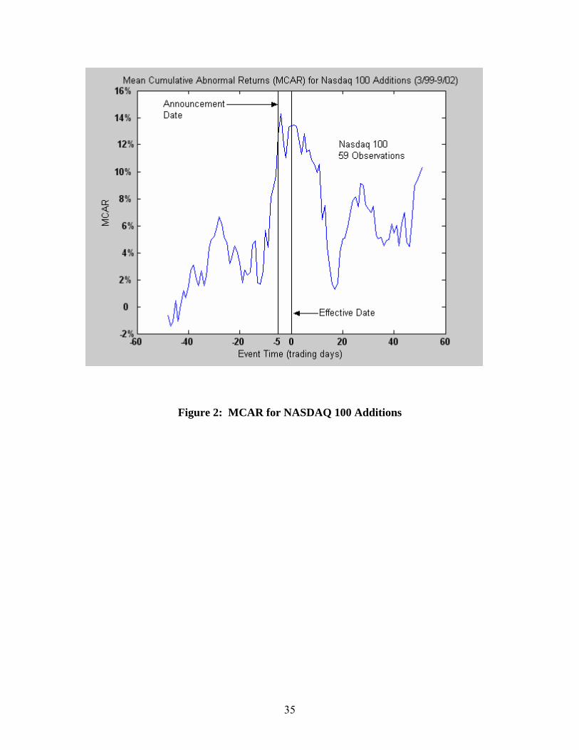
Table 3.1 Mean Cumulative Abnormal Returns for various intervals for additions to S&P, Russell, NASDAQ and Dow Jones Indexes Description S&P 500 S&P1500 Russell 3000 NASDAQ 100 Dow Jones TMINo. of Observations 49 407 2009 59 225 MCAR(0) - MCAR(-49) 14.0% 10.5% 17.8% 13.4% -1.4% MCAR(0) - MCAR(-20) 13.2% 10.3% 9.3% 10.2% 1.1% MCAR(0) - MCAR(-15) 12.1% 9.6% 5.9% 8.8% 1.1% MCAR(0) - MCAR(-10) 11.8% 9.6% 7.5% 7.8% 2.0% MCAR(0) - MCAR(-5) 9.8% 8.5% 5.3% 0.7% -0.2% MCAR(5) - MCAR(0) -4.5% -2.8% -2.6% -0.6% -2.4% MCAR(10) - MCAR(0) -2.5% -4.1% -1.5% -3.5% -1.6% MCAR(15) - MCAR(0) -2.9% -4.8% -2.6% -10.6% -2.6% MCAR(20) - MCAR(0) -4.5% -6.1% -7.6% -8.4% -1.0% MCAR(50) - MCAR(0) -9.4% -8.2% -11.6% -3.7% 0% Total Run up 14.0% 10.5% 17.8% 13.4% NA Total Retracement 9.4% 8.2% 11.6% 3.7% NA Percent Retracement 67% 78% 65% 28% NA It should be noted that the results for the S&P 500 and NASDAQ 100, were based on relatively fewer observations. However, there is a large body of literature for earlier years of rebalancing of the S&P 500, and the results of this study are generally consistent with the results of those earlier studies. In Table 3.2 we compare the percent of the index held by indexers with the estimated market impact that was observed during the index reconstitutions. We did not include the S&P 1500 or the Russell 3000 in this table, because the percentage held by indexers varies across the sub-indexes (Russell 3000 includes Russell 1000 and 2000, while S&P 1500 includes S&P 500, 400, and 600). Table 3.2 Influence of Investment Universe and Popularity on Market Impact Index Investment

Universe % market cap owned by indexers

Market impact: additions to index

S&P 500 U.S. Large Cap 10%+ 5% Russell 2000 U.S. Small Cap 6% 10% NASDAQ 100 NASDAQ only 3% 3% Dow Jones US TMI U.S. Broad Market 0.001% 0 Note: In Table 3.2 we used data from Beneish & Whaley (2002) since their study included more observations of additions to the S&P 500. The magnitude of the market impact is influenced by two primary factors. First the demand for the stocks being added to the index is driven by the amount of money tracking the index. This was calculated as % of the market cap of the index stocks owned by indexers. If the demand is minimal, there will be no market impact. If there is market

12

impact, the magnitude of the impact is also influenced by the liquidity of the stocks being added and deleted. The liquidity of the adds and deletes reflects the investibility of the target universe for the index. Two of the parameters that influence liquidity are the daily turnover and volatility. A volatile stock with low daily turnover will tend to be impacted more than a non-volatile stock with high turnover. In Figure 3.2 we plot the volatility and turnover for top 4500 US stocks. As indicated in Figure 3.2 small market cap stocks tend to be more volatile and have little turnover. This may explain why the market impact for the Russell 2000 is greater than that of the S&P 500, even though more money is tracking the S&P 500. The market cap of the additions to and deletions from the NASDAQ 100 is between that of the S&P 500 and Russell 2000, and less money is tracking that index. Figure 3.2 Volatility and Daily Turnover by Market Cap

0%

5%

10%

15%

1 801 1601 2401 3201 4001

Stock Mkt Cap Ranking

Volatility

Avg Daily Turnover

4.0 Drag on Index Returns from Reconstitution of the Index Management fees for portfolio mangers are typically quoted in terms of a percentage of money under management. The drag on index returns associated with index changes can also be thought of in this way. This way, we will be able to express the index drag in terms that an investor can relate to. Index Drag (as a % of Assets) = Turnover x Average Cost per Trade in % In this equation turnover is expressed as a decimal. For example if the Russell 2000 were to add 400 stocks to the index that represent 15% of the market cap of the index, and delete 400 stocks from the index that represent 10% of the index, the turnover for the index would be 0.25. The average cost per trade in the above equation is expressed as a percentage of the notional value of the trade. For example, if the trading cost is $1 per share for a stock that sells for $50 per share the cost of the trade is 2%. The average cost per trade is simply a weighted average of the individual trading costs for each stock, weighted by the $ value of each trade.

13

One of the reasons that investors choose index funds is that they are buy-and-hold investors, seeking to minimize trading and management costs. Clearly, both low turnover and a low cost per trade are desirable with respect to the goal of reducing trading costs. Therefore, the index investor should consider the turnover of the index when making his investment decision. For index portfolio managers, the index provider determines the turnover, since the manager does not make investment decisions. All of the index providers mentioned above publish their reconstitution policy, so investors and portfolio managers can determine if the policy is consistent with their investment objectives. As indicated above, by selecting an index to track, a money manager will be assuming the index provider’s reconstitution policy and thus be subject to the associated turnover when he rebalances. In addition, the index that is selected will affect the average cost per trade due to rebalancing. The average cost per trade is strongly influenced by the amount of money tracking a given index. This is due to the market impact that occurs when the rebalancing trades are executed and the market impact is usually a much more significant portion of the overall trade cost than commissions and bid/ask spread. If the policy adopted by the indexer is to exactly replicate or closely track the index, then they will be buying and selling stocks at the close on the effective date of the index rebalance. Therefore they assume the full effect of the drag on the index returns caused by the reconstitution. If the charter of the fund is sufficiently flexible to allow for some tracking error, the indexer will be able to trade before and after the effective date of the index change, thus reducing the drag. This allows the investor to “beat the index”. In this case a more transparent index will give the indexer an advantage, since he can more easily trade prior to the actual rebalancing, and thus avoid some of the market impact. For example, if the rebalancing rules are published and based on readily available information, such as market capitalization, free float, and shares outstanding, the indexer can in essence predict the changes that will be made to the index, even prior to the official announcement of what stocks will be added and deleted. Estimates of drag on index returns induced by turnover and market impact are shown in Table 4.1. To put these numbers in perspective, large institutional investors will often pay their portfolio manager less than 10 basis points (bps) per year in index fund management fees. Based on historical results, a good portfolio manager with a flexible tracking policy could have outperformed the index, simply by timing his trades well.

14

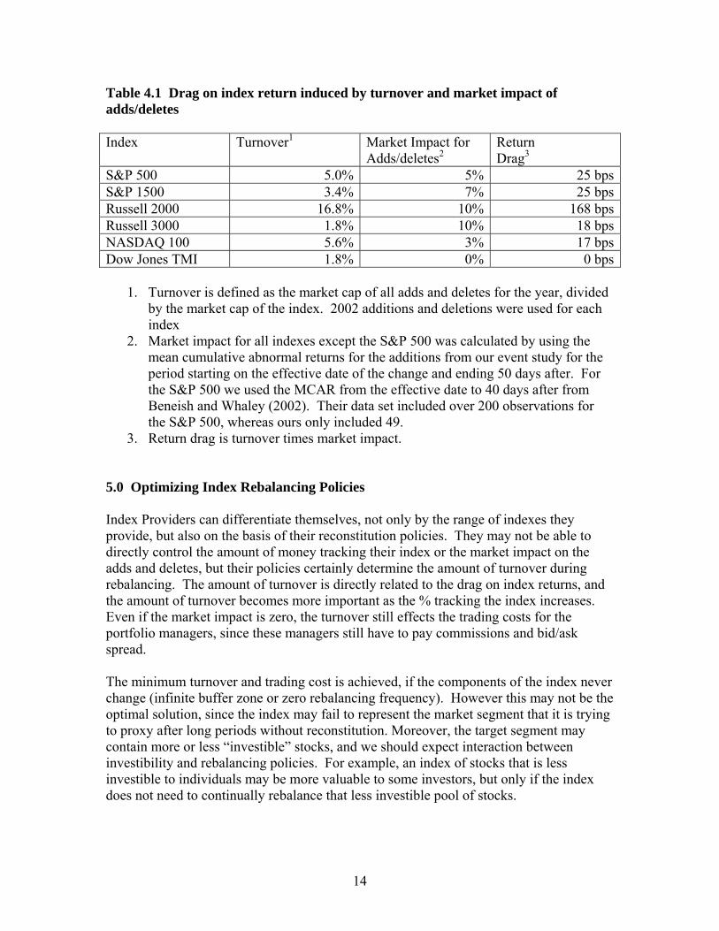
Table 4.1 Drag on index return induced by turnover and market impact of adds/deletes Index Turnover1 Market Impact for

Adds/deletes2 Return Drag3

S&P 500 5.0% 5% 25 bpsS&P 1500 3.4% 7% 25 bpsRussell 2000 16.8% 10% 168 bpsRussell 3000 1.8% 10% 18 bpsNASDAQ 100 5.6% 3% 17 bpsDow Jones TMI 1.8% 0% 0 bps

1. Turnover is defined as the market cap of all adds and deletes for the year, divided by the market cap of the index. 2002 additions and deletions were used for each index

2. Market impact for all indexes except the S&P 500 was calculated by using the mean cumulative abnormal returns for the additions from our event study for the period starting on the effective date of the change and ending 50 days after. For the S&P 500 we used the MCAR from the effective date to 40 days after from Beneish and Whaley (2002). Their data set included over 200 observations for the S&P 500, whereas ours only included 49.

3. Return drag is turnover times market impact. 5.0 Optimizing Index Rebalancing Policies Index Providers can differentiate themselves, not only by the range of indexes they provide, but also on the basis of their reconstitution policies. They may not be able to directly control the amount of money tracking their index or the market impact on the adds and deletes, but their policies certainly determine the amount of turnover during rebalancing. The amount of turnover is directly related to the drag on index returns, and the amount of turnover becomes more important as the % tracking the index increases. Even if the market impact is zero, the turnover still effects the trading costs for the portfolio managers, since these managers still have to pay commissions and bid/ask spread. The minimum turnover and trading cost is achieved, if the components of the index never change (infinite buffer zone or zero rebalancing frequency). However this may not be the optimal solution, since the index may fail to represent the market segment that it is trying to proxy after long periods without reconstitution. Moreover, the target segment may contain more or less “investible” stocks, and we should expect interaction between investibility and rebalancing policies. For example, an index of stocks that is less investible to individuals may be more valuable to some investors, but only if the index does not need to continually rebalance that less investible pool of stocks.

15

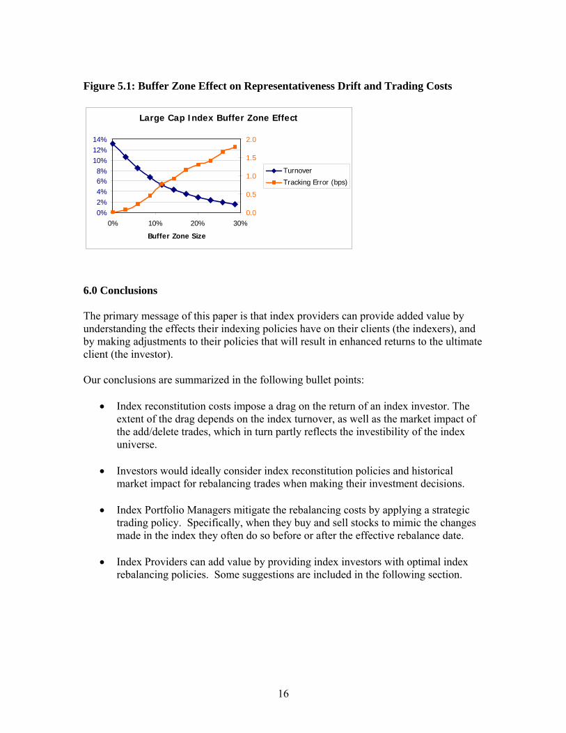
Ideally the index provider should minimize the trading costs associated with reconstitution, subject to some desired error in tracking the target segment. The tracking error here refers to the difference between the reconstituted index with a buffer zone and the reconstituted index with no buffer zone, and we will refer to it as representativeness drift, in order to distinguish it from the term tracking error, which has a specific meaning to index portfolio managers. As a part of this project we built a model that predicts the amount of turnover and rebalancing costs for a given index, along with the associated tracking error, given a rebalancing policy that involves buffer zones. The model can be used to test various rebalancing policies and determine the tracking error and turnover associated with each policy. The model uses simulations to predict the number and market capitalization of additions to and deletions from an index given a reconstitution policy and a time horizon between reconstitution events. The model accepts as inputs the ticker symbols and market caps of all stocks in the index’s universe. The factor exposures and idiosyncratic risk for each stock in the universe are also included as inputs. The universe includes both stocks that are currently in the index and stocks that are currently not in the index. The future market cap is simulated for each stock, using the QuantalPRO multi-factor model. We conducted 1000 simulations for the future market caps of the stocks in the universe. Then, for each simulation, the number of adds and deletes and the associated market caps of the adds and deletes are calculated for each buffer zone being considered. This way we were able to assess the turnover for each simulation. The average turnover was calculated by taking the mean turnover for all of the simulations for a given policy. The representativeness drift between a no buffer zone policy and the subject policy is also calculated for each simulation and the mean is calculated for the representativeness drift. The relationship of the turnover and the representativeness drift with the buffer zone size is depicted in Figure 5.1. The buffer zone size is defined as the market cap of all stocks within the buffer zone divided by the market cap of the entire index. As expected the trading cost decreases and the representativeness drift increases as the buffer zone size increases. Using this model, an index provider could establish a reconstitution policy that minimizes rebalance turnover and trading costs, subject to a representativeness drift constraint. The representativeness drift is labeled in the diagram as tracking error.

16

Figure 5.1: Buffer Zone Effect on Representativeness Drift and Trading Costs 6.0 Conclusions The primary message of this paper is that index providers can provide added value by understanding the effects their indexing policies have on their clients (the indexers), and by making adjustments to their policies that will result in enhanced returns to the ultimate client (the investor). Our conclusions are summarized in the following bullet points:

• Index reconstitution costs impose a drag on the return of an index investor. The extent of the drag depends on the index turnover, as well as the market impact of the add/delete trades, which in turn partly reflects the investibility of the index universe.

• Investors would ideally consider index reconstitution policies and historical

market impact for rebalancing trades when making their investment decisions.

• Index Portfolio Managers mitigate the rebalancing costs by applying a strategic trading policy. Specifically, when they buy and sell stocks to mimic the changes made in the index they often do so before or after the effective rebalance date.

• Index Providers can add value by providing index investors with optimal index

rebalancing policies. Some suggestions are included in the following section.

Large Cap Index Buffer Zone Effect

0%2%4%6%8%

10%12%14%

0% 10% 20% 30%

Buffer Zone Size

0.0

0.5

1.0

1.5

2.0

Turnover

Tracking Error (bps)

17

7.0 Moving toward a more fund-friendly index A few ideas are provided below that would make an index more fund-friendly.

• Several indexers have already adopted the buffer zone concept, in order to reduce the amount of index turnover. Based on our research, we believe that using buffer zones is a good idea. Index providers may want to review the parameters of the buffer zone to see if it is possible to widen the buffer zone and still maintain representativeness, given the market segment of the stocks targeted in the index.

• All things considered, it appears that a transparent rebalancing policy is

advantageous to the investor. This is because it gives the index portfolio manager more flexibility with respect to the timing of his trades, and reduction of market impact. However, for portfolio managers that are constrained by very tight tracking error requirements may find a less transparent index less problematic.

• Index providers may also want to consider alternative policies, such as phasing in

the new stocks over a period of weeks or months. This might appeal to an index portfolio manager who does not want to deviate widely from the official components of the index, but wants to reduce rebalancing costs

Index providers have established buffer zone and frequency-of-reconstitution policies in order to balance the turnover of the index with representativeness. In this paper we have quantified both of these concepts. The model we developed may be useful to index providers who want to fine-tune their reconstitution policies to meet the needs of the investment community. By quantifying the concepts of turnover and representativeness, we believe that the index providers can better communicate with the investors, and this will ultimately allow them to tailor their policies to meet the investors’ needs.

18

S&P Indexes Inclusion Criteria

• Screening process starts with all U.S. publicly traded companies. • Non-US companies (ADRs) are not considered, except a few Canadian and

European industrial companies that were included in the index long time ago and now are considered “grandfathered.”

• REITs and other types of funds are excluded. • Top 500 stocks are large cap, next 400 are mid-cap, and bottom 600 stocks are

small cap.

• Market capitalization ranges for the three indexes are over $3 billion for the S&P 500, $900 million to $3 billion for the S&P 400, and $250 billion to $900 million for the S&P 600.

• The ratio of annual dollar value traded to market capitalization must be at least

0.3.

• Public float of at least 50% is required for the 500, and 40% for the 400 and 600. Once included in an index, the weight in the index is determined by total market cap, not float-adjusted market cap.

• To be added to the index, the firm must have four consecutive quarters of

profitability.

• Sector balance is a factor that S&P considers when making additions to the index. The Global Industrial Classification System is used.

• Define value and growth investment style using a single-factor (Price-to-Book

Ratio) approach. Value and growth groups are mutually exclusive. Deletion Criteria

• Companies involved in mergers.

• Companies that significantly deviate from the inclusion criteria.

• Since 1996, S&P has been more actively applied the rule regarding significant

deviations from the inclusion criteria, which has resulted in more deletions from the index, due to lack of representativeness.

19

Russell Indexes

• Index includes the top 3000 stocks in the U.S. by float-adjusted market capitalization measure. The Russell 1000 are the 1000 largest stocks and the Russell 2000 are stocks ranked 1001 through 3000.

• All classes of common stock combined for market cap purposes, then the

common stock class with the highest trading volume selected to represent company in the index.

• U.S. companies like Tyco, Schlumberger, etc that are incorporated outside of the

U.S. are not included.

• Companies may leave the index during the course of the year if acquired, delisted or if the company’s stock moves to the pink sheets or bulletin board.

• Upon merger, the capitalization will move to the acquiring company’s stock.

• The only additions between reconstitutions are for spin-offs.

• On a monthly basis indexes are updated for shares outstanding based on SEC

reporting, if a change of greater than 5% occurred.

• Major corporate actions like secondary offerings are reflected on the ex-date.

• Annual reconstitution is done based on market cap rankings from May 31 data. The reconstitution goes into effect on June 30.

• Russell 1000 and Russell 2000 have different criteria for growth/value.

• For the value and growth indexes, stocks are ranked by adjusted book:price and

I/B/E/S forecast for long-term growth mean. These are combined into a Composite Value Score (CVS).

• The adjustment for book value adds back in writeoffs from book value required

under FASB.

• The stocks are ranked by the CVS score and a probability algorithm is applied to the CVS distribution to assign growth and value weights to each stock.

• Approximately 70% of the stocks are assigned 100% to growth or value and for

the other 30%, their market cap is split up between growth and value, with percentages that are appropriate 80:20, 50:50, 30:70, and so on.

20

Dow Jones Global Indexes

• The Dow Jones U.S. Total Market Index is part of this index group, and is the index that represents the U.S. market.

• Dow Jones Global Index (DJGI) stocks are grouped into 89 industry subgroups,

which roll up into 51 industry groups, 18 market sectors and 10 economic sectors.

• Country level indexes provided for 34 countries. For country indexes, 95% of the free-float market cap is covered which comprise the large cap, mid-cap and small cap subindexes

• Weighting is done by float-adjusted market cap. The float adjustments will only

be made if the shares from cross-ownership, government ownership, insiders, and restricted shares exceed 5% of the outstanding shares.

• The universe of stocks includes all common shares that have not been excluded

for liquidity reasons. Securities that have had more than 10 nontrading days during the past quarter are excluded.

• The indexes cover 95% of the underlying free-float market cap at the country

level. Free-float market caps above the 70th percentile are large caps. 90th percentile is the cut-off for mid-caps. All remaining stocks are small caps.

• Stocks within the bottom 0.01% of the universe by turnover are excluded from the

indexes.

• Quarterly reviews are conducted in March, June, September, and December. Component changes and share changes become effective at the opening on the first Monday after the third Friday of the review month. Constituent changes will be announced at least 2 business days prior to the implementation date but are usually announced 2 weeks prior.

• During the quarterly review, new large cap and mid-cap companies (IPOs) are

assigned to the large-cap and mid-cap indexes based on the 70% and 90% cutoffs.

• Current large cap components that rank above the 75th percentile are retained in the large-cap index. Current mid-cap components that rank between the 67.5th and 92.5th percentiles are retained in the mid-cap index.

• Current mid-cap or small cap companies that rank above the 67.5th percentile are

reclassified as large caps. Current small cap companies that rank above the 85th percentile are reclassified as mid-caps.

• Stocks are added to the small cap index until the total universe coverage reaches

95%.

21

• If the number of outstanding shares change by more than 10% due to a corporate

action, the shares total will be adjusted immediately after the close in trading on the day of the event. Otherwise shares outstanding will be adjusted during the quarterly review.

• Extraordinary events such as delistings, bankruptcies, mergers, and takeovers will

be addressed with immediate changes to the indexes. For spinoffs, all of the companies that spin off of a constituent will be included in the DJGI family. All involved companies will be subject to an eligibility check at the next quarterly review.

• If two constituent companies merge their component positions will be replaced

with the new company immediately. If an index constituent merges with a non-component, its component position will be replaced with the new company immediately.

• If an index company is acquired by a non-component company, it will be replaced

by the acquiring company immediately.

• The Dow Jones Index Oversight committee may at its discretion remove a company it determines to be in extreme financial distress.

• If a company enters bankruptcy, it will be removed from the index and be eligible

fro re-inclusion when it emerges from bankruptcy.

• If an index component is delisted by its primary market due to failure to meet financial or regulatory requirements it will be removed from the index.

MSCI US Indexes

Initial Set-up and Adjustments:

• Index includes the top 2500 stocks in the U.S. by float-adjusted market capitalization measure

• Non-US companies may be considered based on factors, such as equity market

trading activity, shareholder base and operation distribution • REITs and other types of funds are excluded. • Top 300 stocks are large cap, next 450 are mid-cap, and bottom 1750 stocks are

small cap

22

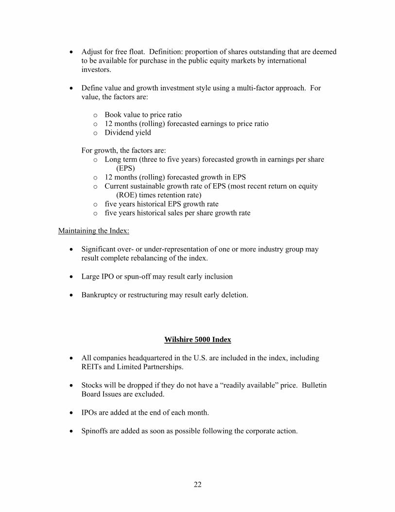
• Adjust for free float. Definition: proportion of shares outstanding that are deemed to be available for purchase in the public equity markets by international investors.

• Define value and growth investment style using a multi-factor approach. For

value, the factors are:

o Book value to price ratio o 12 months (rolling) forecasted earnings to price ratio o Dividend yield

For growth, the factors are:

o Long term (three to five years) forecasted growth in earnings per share (EPS)

o 12 months (rolling) forecasted growth in EPS o Current sustainable growth rate of EPS (most recent return on equity

(ROE) times retention rate) o five years historical EPS growth rate o five years historical sales per share growth rate

Maintaining the Index:

• Significant over- or under-representation of one or more industry group may result complete rebalancing of the index.

• Large IPO or spun-off may result early inclusion • Bankruptcy or restructuring may result early deletion.

Wilshire 5000 Index

• All companies headquartered in the U.S. are included in the index, including REITs and Limited Partnerships.

• Stocks will be dropped if they do not have a “readily available” price. Bulletin

Board Issues are excluded.

• IPOs are added at the end of each month.

• Spinoffs are added as soon as possible following the corporate action.

23

Nasdaq 100 Index

• The universe of stocks for the NASDAQ 100 includes all stocks of non-financial companies listed on the NASDAQ. To be eligible, the stock must also trade an average of 200,000 shares per day, and have been listed on an exchange for at least two years.

• The NASDAQ 100 was established in 1998, and initially included the top 100

non-financial NASDAQ stocks ranked by float-adjusted market cap.

• Stocks are deleted from the index, if they are delisted from the NASDAQ or if they merge with another company, or if the float-adjusted market cap falls to less than 0.1% of the entire index for two consecutive months

• Stocks are also deleted from the index each December, if their float-adjusted

market cap rank falls below 150.

• When a stock is deleted, it is replaced by the stock with the highest float-adjusted market cap, which is not currently in the index.

• Announcements of additions and deletions are done 5 days in advance of the

effective date.

24

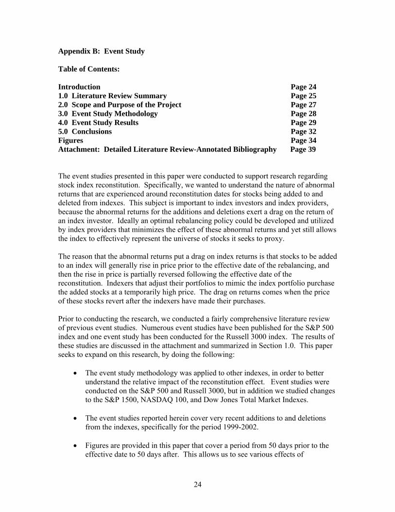
Appendix B: Event Study Table of Contents: Introduction Page 24 1.0 Literature Review Summary Page 25 2.0 Scope and Purpose of the Project Page 27 3.0 Event Study Methodology Page 28 4.0 Event Study Results Page 29 5.0 Conclusions Page 32 Figures Page 34 Attachment: Detailed Literature Review-Annotated Bibliography Page 39 The event studies presented in this paper were conducted to support research regarding stock index reconstitution. Specifically, we wanted to understand the nature of abnormal returns that are experienced around reconstitution dates for stocks being added to and deleted from indexes. This subject is important to index investors and index providers, because the abnormal returns for the additions and deletions exert a drag on the return of an index investor. Ideally an optimal rebalancing policy could be developed and utilized by index providers that minimizes the effect of these abnormal returns and yet still allows the index to effectively represent the universe of stocks it seeks to proxy. The reason that the abnormal returns put a drag on index returns is that stocks to be added to an index will generally rise in price prior to the effective date of the rebalancing, and then the rise in price is partially reversed following the effective date of the reconstitution. Indexers that adjust their portfolios to mimic the index portfolio purchase the added stocks at a temporarily high price. The drag on returns comes when the price of these stocks revert after the indexers have made their purchases. Prior to conducting the research, we conducted a fairly comprehensive literature review of previous event studies. Numerous event studies have been published for the S&P 500 index and one event study has been conducted for the Russell 3000 index. The results of these studies are discussed in the attachment and summarized in Section 1.0. This paper seeks to expand on this research, by doing the following:

• The event study methodology was applied to other indexes, in order to better understand the relative impact of the reconstitution effect. Event studies were conducted on the S&P 500 and Russell 3000, but in addition we studied changes to the S&P 1500, NASDAQ 100, and Dow Jones Total Market Indexes.

• The event studies reported herein cover very recent additions to and deletions

from the indexes, specifically for the period 1999-2002.

• Figures are provided in this paper that cover a period from 50 days prior to the effective date to 50 days after. This allows us to see various effects of

25

rebalancing. (e.g. the effect of the relative transparency of the index rebalancing policy can be seen in the observed pattern of abnormal returns, particularly prior to the announcement date of the index.)

1.0 Literature Review A fairly comprehensive literature review of previous event studies is included as Attachment 1 to this Paper. With one exception, all of the event studies were concerned with additions to and deletions from the S&P 500 index. Presumably the interest in the S&P 500 rebalancing is due to the large amount of money tracking this index. For these studies, the data regarding additions is much more copious than for deletions. This is because, until recently, S&P only deleted firms due to an impending merger, or if the firm filed for bankruptcy or was delisted from a major exchange. A summary of each paper is provided in the attachment; in this section only an aggregated list of conclusions is provided. S&P 500 Event Studies

• Prior to 1989, S&P announced their index additions and deletions after the close of trading, and the change became effective the next day.

• After 1989, S&P has generally announced the index changes between one and

five days prior to the effective date for the change

• There was over a 4000-fold increase of funds directly tracking the S&P index over the period where the event studies were conducted.(1974-2001) An estimated $170 Million was tracking the index in 1974, increasing to an estimated $800 Billion in 2001.

• All studies found a statistically significant positive abnormal return between the

close of trading on the day of the announcement of an addition and the open the next day. Furthermore, this abnormal return has increased over time, as the amount of funds tracking the S&P 500 increased. The abnormal return was on the order of less than 1% in the 1970s, 3% in the 1980s, and almost 6% in the 1990s.

• For studies of additions after 1989, where there was more than one day between

the announcement and the effective date, abnormal returns on the order of 3% were reported between the open of trading the day after the announcement and the close on the effective date of the change.

• There is wide disagreement regarding the extent to which the abnormal returns

between the announcement and the effective date are reversed after the effective date. However, when viewing the event studies as a whole it is clear that some reversion does occur.

26

• Researchers have proposed at least three reasons for the abnormal returns that the additions to the index exhibit between the announcement date and the effective date.

The price pressure hypothesis explains that the abnormal returns are a result of

the excess short-term demand from indexers who need to purchase the stocks being added to the index around the effective date of the rebalance. Under this scenario, prices are temporarily forced higher in the same way that prices would be forced higher for a large block trade.

The information hypothesis claims that most if not all of the price increase is

permanent. The argument is that inclusion in the index is good news, since after inclusion the stock will receive more analyst coverage, leading to more trading, and lower bid/ask spreads. The lower expected transaction costs leads to a lower required risk premium and thus a higher price.

The imperfect substitutes hypothesis says that after inclusion in the index, a

lower number of shares of the stock will be available to non-index investors, and that perfect substitutes for the stock are not available. This theory is consistent with long-term downward sloping demand curves for stocks.

• Both the information hypothesis and the imperfect substitutes hypothesis predict a

permanent price increase for stocks added to the S&P 500 index. The price pressure hypothesis leads to a short-term increase in the price of the stock, which is reversed after the effective date of the change to the index. Since there does appear to be both a long-term and short-term component to the abnormal returns that additions experience prior to the effective date, all three of these hypotheses may have some validity.

• A few of the event studies looked at deletions from the S&P 500, as well as the

additions. For deletions, the effect is, in essence, a mirror image from that of the additions. The stocks to be deleted decrease in price immediately after the announcement, and continue to decrease between the announcement and the effective date. The downtrend is reversed on the effective date, as the stock prices increase following the effective date of the index change.

Russell 3000 Event Study Madhavan (2002) found qualitatively similar results to those described above when he studied the Russell 3000. The returns for the additions exhibited an uptrend between the announcement date and the effective date, and that trend was reversed after the effective date. For deletions the opposite effect was noted, except the returns did not recover in the month following the deletion. There are three significant differences between the Russell 3000 results and the S&P 500 results.

27

• The first is that the price trend for the deletions did not reverse after the effective date, as mentioned above. An explanation for this behavior is not readily apparent.

• The second is that the abnormal returns for the stocks being added to the index

and the negative abnormal returns for the stocks being deleted from the index, began long before the announcement date. This can be explained based on the differences in rebalancing policies between the Russell 3000 and the S&P 500. Russell’s policy is transparent, which means it is based on widely disclosed quantitative rules that are applied strictly to observed market capitalizations. The result is that Russell 3000 additions and deletions can be predicted quite accurately prior to the announcement. This allows both indexers and risk arbitrageurs to take positions in these stocks early, and the result is that the price trend noted between the announcement date and the effective date in the S&P studies starts before the announcement with the Russell 3000.

• The third difference is that the magnitude of the overall abnormal returns for the

additions and deletions is higher for the Russell than for the S&P. 2.0 Scope and Purpose of the Project The purpose of this project is to document the abnormal returns of adds to and deletes from a variety of indexes, and thereby to gain a better understanding of what drives these abnormal returns. An understanding of the drivers for the abnormal returns could allow index providers to craft more beneficial polices for those investing in their indexes. In addition, a better understanding of these abnormal returns may assist an investor in deciding which index to track. Finally an improved understanding of the abnormal returns should allow investment managers to develop trading strategies that minimize the drag on their portfolio and “beat the index.” The desired audiences for this paper are index providers, investors, and portfolio managers. It is not intended to be an academic paper, although academics may find the results of interest. Specifically, we do not seek to enter the debate concerning the relative merits of the price pressure hypothesis, the imperfect substitutes hypothesis or the liquidity hypothesis. Based on the research we conducted, we believe that all of these theories may have merit. Central to our conclusions, however, is the finding that the effects of price pressure are apparent and significant. Furthermore, the price pressure caused by index reconstitution can be costly to investors in index funds. Consistent with the likely needs of our intended audience, we attempt to present the results in a format where they can be easily viewed and understood. We intentionally keep the discussion of mathematical equations and statistics to a minimum, preferring to focus our attention on the pattern of returns that has been observed, what might cause those patterns, and what impact those patterns have on investors. The following data sets were used in this study:

28

• All S&P 1500 additions for the period from January, 2000 through September,

2002: These additions and the effective date for each addition are reported on S&P’s website. The S&P 1500 includes the S&P 500 (large cap), the S&P 400 (mid-cap), and S&P 600 (small-cap). In this data set only new additions to the S&P 1500 were included. For example, if a stock was deleted from the S&P 400 and added to the S&P 500 it was not included. As a subset of the S&P 1500 data set, we also evaluated stocks that were not previously part of the S&P 1500, that were added to the S&P 500.

• All Russell 3000 additions and deletions for the period 1999 through 2002:

Frank Russell Company provided us with the list of additions and deletions. Since Russell only rebalances once per year, the effective dates for these additions and deletions are always the last day in June of each year. The vast majority of the additions to the Russell 3000 were also additions to the Russell 2000

• All additions to the Dow Jones Total Market Index (TMI), from November, 2000

through September 2002: In October, 2000, Dow Jones changed its criteria for inclusion in the TMI from total market cap, to float-adjusted market cap. Therefore the data set includes all of the additions done after this policy change.

• All additions to the Nasdaq 100 index from March, 1999 to September, 2002.

This includes almost all of the additions that have been made to the Nasdaq 100 over the history of the index. Additions prior to March, 1999 were excluded, because the Nasdaq 100 trust (exchange-traded fund that tracks the Nasdaq 100) did not start trading until then. This study could be updated to include the 15 additions to the NASDAQ 100 in December, 2002, once a sufficient amount of time passes to evaluate the returns for the period following this effective date.

3.0 Event Study Methodology Most of the previous event studies that we summarized in the attachment followed a general procedure that was documented by Brown and Warner (1985). The event studies presented in this report also follow that procedure. A brief discussion of the data acquisition and analysis is presented in this section. Daily prices and returns were collected for all of the stocks in the event studies, using the QuantalPRO database. The QuantalPRO database archives historical closing prices and returns, as well as other information, like factor sensitivities and trading volume. The daily returns used in this study are log returns as typically used in empirical finance studies. The log return is defined as follows:

29

Daily log return = ln(P2/P1) {where daily log return is today’s log return, P2 is today’s closing price and P1 is yesterdays closing price} We will hereinafter refer to the log returns as daily returns. The daily returns were adjusted for market movements by subtracting the return for the S&P depository receipts from the daily stock return. The S&P depository receipts (SPY) is an exchange traded fund that tracks the S&P 500. This is a very liquid exchange traded fund that closely tracks the value of the S&P 500. The opening price for the SPY is actually a more accurate representation of the value of the S&P 500 than the opening prices recorded for the S&P 500 itself. Since it takes a few minutes for all of the S&P 500 stocks to open, often the reported opening price for the S&P 500 index is the same as the closing price for the previous day, even when the portfolio of stocks in the S&P 500 has gapped up or down. We refer to the stock’s return minus the market return as the abnormal return. Abnormal returns (AR) were calculated for each stock for each day during the study period. The event day is defined as the effective date for the rebalance of the index. The calendar day for each stock is translated into event time by indexing the dates to the effective date. Event time is the number of trading days before or after the effective date of the index rebalance. For example, if the index rebalance date was February 10, 2003, the date when translated into event time for February 3, 2003 would be –5. Cumulative abnormal return (CAR) is defined as the accumulation of returns from a starting point forward. For example, if the starting point was event day –49 as shown in many of the figures, the CAR for event day –45 would be AR-49+AR-48+AR-47+AR-46+AR-45 . Finally, the Mean Cumulative abnormal return is the mean value for CARs of all of the stocks that are included in the specific study. 4.0 Event Study Results A graphical presentations of the results is included in the Figures section of this report. For each index being studied, we present a graph of MCAR versus event time. Event day 0 (the effective date of the addition to the index) is shown on the graph as a vertical line. We have plotted the S&P 500 and S&P 1500 results on the same graph, for the convenience of the reader. The number of observations and the years included in the study are also indicated on the graphs. Since we had a substantial number of observations for the Russell 3000, we decided to also analyze the data on a yearly basis for that index, so we have included four additional plots for that purpose. We did not analyze the deleted stocks from all of the indexes in the study, since many of the deleted stocks were deleted for reasons such as mergers or bankruptcies. However, all of the deletes from the Russell 3000 in June of each year are done strictly based on market capitalization. The other deletes from the Russell 3000 that occurred throughout the year for reasons such as bankruptcies or mergers are not included in our dataset.

30

Table 4.1, shown below, reports the difference in Mean Cumulative Abnormal Returns for different time intervals. The first five entries in the table represent different time intervals before the rebalance date and the last five entries represent the returns for various time intervals after the rebalance date. For example, the first entry indicates the MCAR from 50 days before the effective date of the rebalance to the effective date. Likewise the last entry is the return from the rebalance date to 50 days after. Therefore, the first five entries can be thought of as different measures of the run-up in price prior to the rebalance, and the last five entries can be thought of as different measures of the reversion in the stock prices after the transitory buying pressure has subsided and the stock prices move back to new equilibrium prices. The stocks being added to the S&P, Russell, and NASDAQ indexes clearly exhibit an abnormal return prior to the index rebalance date. The pattern of these returns differs between the three indexes. The Russell and NASDAQ indexes have transparent rules for how they do their rebalancing, and these rules are based on readily available market capitalization. This means that indexers or liquidity providers can purchase stocks that are highly likely to be added before they are announced. The stocks to be added to the S&P indexes are selected by a committee, and announced 1 to 5 days prior to the effective date. Therefore most of the abnormal return comes immediately prior to the effective date for the S&P, whereas the buying is more spread out for the Russell and NASDAQ. In addition to indexers purchasing their shares early, there are liquidity providers who buy the additions early, so they can sell them to the indexers around the effective date for a profit. As indicated in the table, it appears that a portion of the increase in prices for the additions is temporary and a portion is permanent. Relating back to the various hypotheses that were summarized in the literature review, this means that the price-pressure hypothesis is responsible for a portion of the abnormal return experienced by stocks being added to a major index. For the Dow Jones TMI index, there is essentially no run-up in price prior to the effective date of the index. This is not a surprising result since indexers hold a very small portion of the market cap of the component stocks. Therefore, when the Dow Jones TMI rebalances, we might expect that only a minor temporary demand imbalance would be created for the stocks being added to that index, whereas for the other indexes the excess demand is significant.

31

Table 4.1 Mean Cumulative Abnormal Returns for various time intervals for additions to S&P, Russell, NASDAQ and Dow Jones Indexes: Years 1999-2002 Description S&P 500 S&P1500 Russell 3000 NASDAQ 100 Dow Jones TMINo. of Observations 49 407 2009 59 225 MCAR(0) - MCAR(-49) 14.0% 10.5% 17.8% 13.4% -1.4% MCAR(0) - MCAR(-20) 13.2% 10.3% 9.3% 10.2% 1.1% MCAR(0) - MCAR(-15) 12.1% 9.6% 5.9% 8.8% 1.1% MCAR(0) - MCAR(-10) 11.8% 9.6% 7.5% 7.8% 2.0% MCAR(0) - MCAR(-5) 9.8% 8.5% 5.3% 0.7% -0.2% MCAR(5) - MCAR(0) -4.5% -2.8% -2.6% -0.6% -2.4% MCAR(10) - MCAR(0) -2.5% -4.1% -1.5% -3.5% -1.6% MCAR(15) - MCAR(0) -2.9% -4.8% -2.6% -10.6% -2.6% MCAR(20) - MCAR(0) -4.5% -6.1% -7.6% -8.4% -1.0% MCAR(50) - MCAR(0) -9.4% -8.2% -11.6% -3.7% 0% Total Run up 14.0% 10.5% 17.8% 13.4% NA Total Reversal 9.4% 8.2% 11.6% 3.7% NA Percent Reversal 67% 78% 65% 28% NA In Table 4.2 the additions to the Russell 3000 are segregated by year, to see how the returns have varied from year to year. An abnormal return prior the effective date of the reconstitution is apparent for all years, though the magnitude varies. There is also a reversal of the abnormal return after the effective date in each year, but the extent of the reversal is varies also. Table 4.2 Mean Cumulative Abnormal Returns for various time intervals for additions to the Russell 3000 in 1999, 2000, 2001, and 2002 Russell 3000 Additions Return Period 1999 2000 2001 2002 1999-2002 MCAR(0) - MCAR(-50) 9.7% 18.8% 25.0% 15.9% 17.8% MCAR(0) - MCAR(-20) 7.7% 16.8% 3.8% 6.8% 9.3% MCAR(0) - MCAR(-15) 6.2% 5.3% 5.0% 7.6% 5.9% MCAR(0) - MCAR(-10) 10.5% 8.3% 5.1% 6.1% 7.5% MCAR(0) - MCAR(-5) 6.6% 3.6% 7.9% 3.0% 5.3% MCAR(5) - MCAR(0) -1.7% -0.9% -3.2% -5.3% -2.6% MCAR(10) - MCAR(0) -0.6% 1.1% -4.5% -2.3% -1.5% MCAR(15) - MCAR(0) -2.2% -1.8% -4.7% -1.4% -2.6% MCAR(20) - MCAR(0) -5.7% -11.6% -6.5% -4.9% -7.6% MCAR(50) - MCAR(0) -12.4% -14.7% -9.2% -9.0% -11.6% Total Run up 9.7% 18.8% 25% 15.9% 17.8% Total Reversal 12.4% 14.7% 9.2% 9.0% 11.6% Percent Reversal 128% 78% 37% 57% 65% While the main focus of this paper is additions to the major indexes, we did look at deletions from the Russell 3000. The pattern of returns prior to the effective date of the rebalance are opposite from that of the additions. The pattern is consistent with a

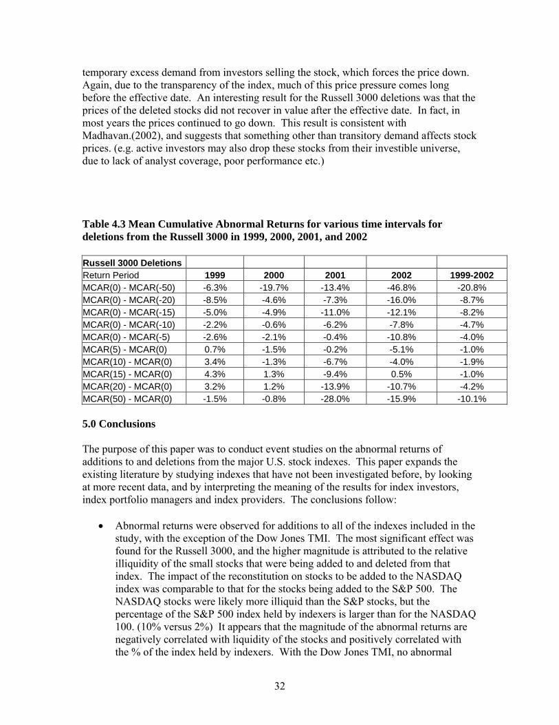
32

temporary excess demand from investors selling the stock, which forces the price down. Again, due to the transparency of the index, much of this price pressure comes long before the effective date. An interesting result for the Russell 3000 deletions was that the prices of the deleted stocks did not recover in value after the effective date. In fact, in most years the prices continued to go down. This result is consistent with Madhavan.(2002), and suggests that something other than transitory demand affects stock prices. (e.g. active investors may also drop these stocks from their investible universe, due to lack of analyst coverage, poor performance etc.) Table 4.3 Mean Cumulative Abnormal Returns for various time intervals for deletions from the Russell 3000 in 1999, 2000, 2001, and 2002 Russell 3000 Deletions Return Period 1999 2000 2001 2002 1999-2002 MCAR(0) - MCAR(-50) -6.3% -19.7% -13.4% -46.8% -20.8% MCAR(0) - MCAR(-20) -8.5% -4.6% -7.3% -16.0% -8.7% MCAR(0) - MCAR(-15) -5.0% -4.9% -11.0% -12.1% -8.2% MCAR(0) - MCAR(-10) -2.2% -0.6% -6.2% -7.8% -4.7% MCAR(0) - MCAR(-5) -2.6% -2.1% -0.4% -10.8% -4.0% MCAR(5) - MCAR(0) 0.7% -1.5% -0.2% -5.1% -1.0% MCAR(10) - MCAR(0) 3.4% -1.3% -6.7% -4.0% -1.9% MCAR(15) - MCAR(0) 4.3% 1.3% -9.4% 0.5% -1.0% MCAR(20) - MCAR(0) 3.2% 1.2% -13.9% -10.7% -4.2% MCAR(50) - MCAR(0) -1.5% -0.8% -28.0% -15.9% -10.1% 5.0 Conclusions The purpose of this paper was to conduct event studies on the abnormal returns of additions to and deletions from the major U.S. stock indexes. This paper expands the existing literature by studying indexes that have not been investigated before, by looking at more recent data, and by interpreting the meaning of the results for index investors, index portfolio managers and index providers. The conclusions follow:

• Abnormal returns were observed for additions to all of the indexes included in the study, with the exception of the Dow Jones TMI. The most significant effect was found for the Russell 3000, and the higher magnitude is attributed to the relative illiquidity of the small stocks that were being added to and deleted from that index. The impact of the reconstitution on stocks to be added to the NASDAQ index was comparable to that for the stocks being added to the S&P 500. The NASDAQ stocks were likely more illiquid than the S&P stocks, but the percentage of the S&P 500 index held by indexers is larger than for the NASDAQ 100. (10% versus 2%) It appears that the magnitude of the abnormal returns are negatively correlated with liquidity of the stocks and positively correlated with the % of the index held by indexers. With the Dow Jones TMI, no abnormal

33

returns were found, which is what we would expect since only 0.001% of the index is held by index funds.

• One effect of the index transparency can be observed by viewing the abnormal

returns. The NASDAQ and Russell indexes both have transparent rebalancing policies, which results in the abnormal returns being spread over a longer time period prior to the effective date of the rebalance. A sharp rise in abnormal returns is noted for the S&P indexes between the announcement date and the effective date, and this is likely due to their more closed reconstitution policy.

• Surprisingly, particularly for those who believe in efficient markets, these well-

known rebalancing effects do not appear to have gone away over the course of time, nor are they obviously explained by shifts in the riskiness of the stocks involved. One might think that speculators and risk arbitrageurs would trade away the profits using the strategy of buying the stocks to be added and selling the stocks to be deleted, but the abnormal returns still seem to persist.

• Index portfolio managers that ease up their tracking error constraints around the

time of the rebalancing activities, may be able to get better prices by trading before and after the effective date of the rebalance. This would have allowed them to consistently outperform the index in the past.

• Index investors could use knowledge of the pattern of returns to make better

decisions on what index to track. The drag on investment returns induced by the index reconstitution does not occur if an index is selected that is not tracked by a large percentage of investors. If the investor wants to invest in an index that is tracked by many other investors, he should be careful to select an investment manager who has the flexibility to trade prior to or after the effective date of the rebalance.

• Index providers could reduce the drag on the returns of their index by adjusting

their policies so that fewer trades are executed each year. Several indexes already address this issue by imposing a buffer zone around the borderlines for the index to make it more difficult for an existing member of the index to be deleted or a new member to be added. It also appears that a transparent rebalancing policy gives the portfolio managers more latitude with respect to how their trades are executed, and therefore transparency is beneficial.

34

Event Study Figures

Figure 1: MCAR for S&P 500 and S&P 1500 Additions

35

Figure 2: MCAR for NASDAQ 100 Additions

36

Figure 3: MCAR for Dow Jones Total Market Index Additions

37

Figure 4: MCAR for Russell 3000 additions with breakout of annual results

38

Figure 5: MCAR for Russell 3000 additions with breakout of annual results

39

Attachment to Appendix B Literature Review-Annotated Bibliography: Index Rebalancing Event Studies (See Bibliography for List of References) Goetzmann and Gary (1986) The authors studied a portfolio of 7 stocks that were removed from the S&P 500 on November 30, 1983. They found a large negative return of 1.9% after correcting for the general market movement. The price drop was attributed to an expected decrease in the quantity and quality of future analyst coverage for these stocks. They state that “the label or S&P seal of approval seems to carry with it broadly understood implications. Removal of that seal has an adverse effect”. Schleifer (1986) The author studied 246 firms that were added to the S&P 500 index from 1966-1983. Schleifer found that prior to September 1976 there was no significant price increase on the announcement date. In contrast, since September, 1976, there was a 2.79% abnormal announcement day (AD) return, which is statistically significant. He found that share prices decline subsequent to the effective date of the addition, but the declines are not statistically significant, and the magnitude of the declines are smaller than the increase prior to the effective day. Schleifer suggests that the abnormal returns from stock inclusion in the S&P 500 seem to have grown over time, parallel to the growth of index funds. Schleifer discusses some of the arguments that are proposed to suggest that there is information content in the inclusion in the index, since S&P may be viewed as “certifying” the quality of the firms it adds, but he suggests that this informational value is not very great. Schleifer discusses the argument that inclusion in the S&P 500 will increase analyst coverage and therefore make the stock more valuable, because the stock will be traded more often, leading to smaller bid ask spreads and thus lower future transaction costs. However, he dismisses this argument after evaluating differences between stocks added to the index that were already well-known and relatively unknown stocks, since both of these groups exhibited similar AD returns. He proposes the imperfect substitutes hypothesis, stating there is a long-term downward sloping demand function for stocks, and the price change is permanent. Harris & Gurel (1986) The authors found that the prices of stocks added to the S&P 500 index increased by more than 3% after the addition is announced, and the increase in price is nearly fully

40

reversed after 3 weeks. The results are consistent with the price-pressure hypothesis. Their study included additions to the index from 1973-1983. They found that the mean excess return on the first day following the announcement from 1973-1977 was 0.21%, while it is 3.13% for the 1978-1983 period. They attributed the increase in the magnitude of the price effects to the substantial increase in funds indexed to the S&P 500, over the period 1973-1983. There was an approximate 10-fold increase in indexed funds between the first sub-period and the second sub-period. Harris and Gurel also suggest that since the price effects are not present in the initial years (when index funds were small), it is unlikely that the new information is the cause of the initial price increase. Jain (1987) The author studied the returns of 87 stocks that were added to the S&P 500 from 1977-1983. On average these firms earned a large positive 3.07% excess return on the day following the announcement. The author also looks at the excess returns earned by firms being added to S&P supplementary indexes, and found a 2.93% excess return during the first day after the announcement. Since these stocks are not included in the indexers’ portfolios, the author concludes that the increase in price of stocks added to the S&P 500 is not due to the temporary price pressure from indexers buying the stocks. The author also studies the returns of 22 firms that were removed from the S&P 500 and finds an excess return on the first day of -1.16%. In summary, Jain concludes that the price increase on the first trading day after an announcement that a stock will be added to the S&P 500 provides evidence that the S&P decisions have information content, and the increased demand by index fund managers does not explain these excess returns. Pruitt and Wei (1989) The authors studied the institutional ownership holdings for 250 firms added to the S&P 500 index from 1973-1986. They performed a cross-sectional regression of the 1-day post-listing abnormal return and the net change in institutional ownership. The estimated regression equation is ARi = 0.88 + 3.43 (NDIFi). The test statistics for the intercept and slope are 9.18 and 3.43, respectively. The conclusion is that their study presents a direct empirical test of Schliefer’s and Harris and Gurel’s earlier conjecture that institutional buying and selling pressure is responsible for the abnormal returns observed for a security following its initial listing on or deletion from the S&P 500. Further, they conclude that the observed small net change in institutional holdings following listing on the S&P 500 index suggests that the required liquidity resulting from the demand of index funds is being supplied by other, non-index institutions. Dhillon and Johnson (1991) The authors examine 187 additions to the S&P 500 between 1978 and 1988. 86 of these additions were in the period 1978-1983 and 101 additions were in the period 1984-1988. For the 1984-1988 period they found a large return of 3.334% on the announcement day. After 60 trading days the prices declined by 1.31%, but were still above their pre-announcement level. The authors also looked at the prices of call and put options on the

41

stocks that were being added to the index. They found an increase in the price of the call options and a decrease in the price of the put options, implying that the options traders believed that the price change would be permanent. If they believed the effect was temporary, the prices would not have gone up for the call options. If the traders bid up the prices of the calls due to higher anticipated volatility after the stock is added to the index, then put prices would have gone up as well. The authors also study the prices of bonds issued by companies added to the S&P 500, and find that the bond prices go up as well. In conclusion, Dhillon and Johnson contend that all of the evidence in their study is consistent with the information hypothesis and not the price-pressure hypothesis. Beneish and Whaley (1996) The authors published the first event study on the returns of stocks added to the S&P 500 index after S&P changed their policy regarding the effective date of the announced changes. In the previous studies the changes were effective immediately after the announcement. Starting in October, 1989 the S&P generally announced the changes 5 days prior to the effective date of the change. Beneish and Whaley study 103 additions between 1986-1992. 33 of these additions occurred after S&P changed their announcement policy. The authors first looked at the trading volume on the announcement day, and found that the volume was 10.6 times the average daily volume when the announcement day and the effective day coincided. When the announcement day was 5 days prior to the effective day, the volume was 3.5 times normal on the announcement day, 7.2 times normal on the days between announcement and effective, and 10.6 times normal on the effective day. Summing these figures the trading volume between the announcement day and the effective day was 21.3 times normal. The most likely explanation for the increase in overall trading volume is the greater demand by risk arbitrageurs. Although the trading volume declines as time passes after the effective day, it is still 55% above the pre-announcement volumes as far as 60 days after the announcement. Furthermore, while the trading volume is persistent after the effective day, the increase in trade size is not. An explanation that is consistent with these results is that the stock is now part of the S&P 500 basket that is used in the arbitrage with the S&P 500 futures and options. Beneish and Whaley discuss the hypotheses that have been put forward in an attempt to explain the increase in price of the stocks added to the S&P 500. They reject the idea that the stock is more valuable because it is more liquid, since their study of bid-ask spreads does not indicate a decrease after a stock is added to the index. The authors found very large abnormal returns between the announcement day and the effective day of the addition. The average abnormal returns were 3.7% for the first sub-period (old announcement policy) and 5.9% for the second sub-period (new announcement policy). The authors attribute the increase in abnormal returns to the presence of risk arbitrageurs. They also find that much of the price increase is permanent, with the average abnormal return from the announcement day to 10 days after the effective day being 4.7%. The announcements are made after the market close. The average return from the close on the announcement day to the open on the following day is 4.4%, while the return from the open to close on that day is 0.6%. The stock price does continue to rise from the open the

42

day following the announcement to the close on the effective day by 1.5%, but this rise is not statistically significant. The stock price falls by approximately 2% on the day following the effective day, as the risk arbitrageurs who were unable to unwind their positions on the effective day sell their stock. The authors note that on average the strategy of buying on the open after the announcement and selling at he close on the effective day yields a profit of 4%, without including trading costs. The authors expect that as more index funds buy their stocks earlier, all of the rise in price will occur between the close on the announcement day and the following open, which will eliminate the opportunity for the risk arbitrageurs to profit. Lynch and Mendenhall (1997) The authors analyze price and volume data for firms that were added to and deleted from the S&P 500 from March 1990 to April 1995. They were able to construct a portfolio of 34 clean additions and 15 clean deletions. The clean additions and deletions excluded firms that were going through a merger or spin-off, and excluded firms that would not be traded by index funds. For additions, they found an abnormal return of 3.2% for the day following the announcement, and a 3.8% abnormal return between the close on the day after the announcement and the close the day before the effective date. The authors also document a significant negative abnormal return following the effective date of the addition. Lynch and Mendenhall claim that the significant abnormal returns following the announcement are consistent with semi-strong market efficiency. However, the return between the day after the announcement and the effective date is a violation of market efficiency, in that trading rules could be developed with publicly available information that would lead to abnormal returns. The price reversal after the addition or deletion strongly suggests the existence of temporary price effects, caused by index fund trading. The authors also find that the cumulative abnormal return for additions from the day following the announcement through the price reversal is weakly positive. They claim that this provides evidence in support of downward sloping demand curves for stocks, as suggested by Schleifer (1986) Beneish and Whaley (2002) The authors study all stocks added to and deleted from the S&P 500 over the period from January, 1996 to December, 2001. 220 additions to the index were included in this study. During this period there were 49 deletions of stocks due to a “lack of representativeness” Prior to 1996, S&P only deleted stocks that merged with or was acquired by another company or filed bankruptcy. In this paper, Beneish and Whaley investigate whether the abnormal return that additions have between the day after the announcement and the effective day of the rebalance persists. In their previous paper, they suggest that this abnormal return may disappear over time. The authors segment the additions into those where the change became effective the day after the announcement(Panel A), and those where there were at least two days between the announcement date and the effective date( Panel B). For Panel A, the abnormal return from the close on the day of the announcement and the open the next day was

43

8.15% across the 32 stocks in the sample. This compares with 5.97% found in Beneish and Whaley (1996). Panel B shows an abnormal return of 5.76% from the close on the announcement day to the open the next morning and 3.11% from the open on the day after the announcement to the close on the effective day. The corresponding results in the 1996 report are 2.55% and 3.7%. Both the Panel A results and the Panel B results support the notion that the increase in indexing over time has caused more exaggerated price reactions for stocks added to the index. The S&P effect has not gone away. For deletions, the stock price of a deleted stock falls by 6.21% from the close of trading on the announcement day to the open the next day, and then by another 8.31% from the open on the announcement day to the close on the effective day. The latter return represents a trading opportunity. The trader would short the deleted stock and buy SPDRs. The authors also report an extraordinarily high abnormal return of 23.69% for deleted stocks after the effective date, but note that the abnormal return is driven by a handful of stocks. Madhaven (2002) The author studies the returns of stocks added to and deleted from the Russell 3000 index over the period from 1996-2001. The total number of stocks included in the study is not reported, but the author does indicate that there were 527 additions and 291 deletions from the Russell 3000 in 2001. There were less deletions than additions, because stocks are deleted from the index throughout the year, but only added at the end of June. A spread portfolio is constructed, long the additions and short the deletions. The return of the spread portfolio shows a mean return over the six-year period of 15.1% in June alone, with a cumulative rise from March of 35%. The effects of the reconstitution are much larger than the corresponding S&P 500 effects, reflecting lower overall liquidity of the Russell stocks. The author also documents sharp price movements around the effective date of the reconstitution, and the spikes do not perfectly coincide with the reconstitution date, indicating that traders only imperfectly anticipate order imbalances related to reconstitution. In the study, Madhaven controls for risk, firm size and the value-growth factor. After controlling for these factors, additions have a positive return of 15.1% and deletions have a negative return of 11%. The regression analysis suggests the return movements are functions of changes in liquidity and price pressure. The price pressure effect is a temporary effect and the liquidity effect is a long-term effect (improved liquidity resulting from being part of the index). Finally, Madhaven notes that there are significant rewards to providing liquidity during the reconstitution. Such a strategy, however is typically undiversified, involves high trading costs, and faces price risk as the positions are unwound. These factors help explain the persistence of the Russell effect over time.

44

Jankovskis (2002) The author conducts a study that compares monthly returns of the S&P 600 with the Russell 2000. Both of these indexes are small-cap, but the average market capitalization of the S&P 600 is higher than that of the Russell 2000. In addition, the turnover for the Russell 2000 is much higher than that of the S&P 600. He finds that over the period from 1994-2001, the returns of the Russell 2000 lag the returns of the S&P 600 by 2.3% per year. The author attributes at least 1.8% of the difference in returns to the Russell 2000 reconstitution policy. The Russell 2000 reconstitutes their index once per year. The new index consists of the stocks ranked 1001 to 3000 by float adjusted market cap as of the end of May. The effective date of the rebalance is the last day of June. The rebalance rules for the Russell 2000 are very transparent, which makes it easy for speculators to predict the additions and deletions from the index. The speculators buy the additions and sell the deletions prior to the effective date of the rebalance, which leads to high prices for the additions and low prices for the deletions on the effective date. The Russell 2000 under performs the S&P 600 during the months of July and August, by 1.47% and 0.44% respectively, and this under-performance is due to the price reversal that occurs after the effective date. The underperformance is statistically significant at the 90% level. The author goes on to conclude that if the downward bias of the Russell 2000 performance was corrected for, the widely held belief that active management is better suited to small stocks than to large stocks may be overturned.

45

Appendix C: Index Reconstitution Optimization Model Table of Contents

1. Scope and Purpose of the Model Page 45

2. Model Methodology Page 45

3. Results Page 49

4. Conclusions Page 50

Optimization Model Figures Page 51 The purpose of the work discussed in this paper is to assist index providers with optimization of their reconstitution policies. An approach was developed to simulate numerous possible future stock price movement scenarios. Under each scenario the turnover of a particular reconstitution policy is assessed. This way, alternative reconstitution policies could be tested to determine the turnover and trading costs associated with each potential policy. In addition, the difference in representativeness of the index is assessed for each reconstitution policy. 1. Scope and Purpose of the Model

The simulation model was constructed to estimate the impact of various index reconstitution policies on portfolio turnover and index representativeness. Index providers can use this model to evaluate alternative reconstitution policies in order to minimize the rebalancing costs while keeping the representativeness of the index within a desired range. Index portfolio managers and investors can use this model as a part of their index selection process. The model can help them identify the index with the lowest drag on return due to rebalancing from a pool of candidates that meet the managers’ investment objectives. 2. Model Methodology

The model focuses on two variables typically found in index reconstitution rules, the buffer zone around the market capitalization cutoff line and the frequency of reconstitution. We take as a given the “investibility” characteristics of stocks that the index provider chose to include in the index, which in turn will be driven by the target

46

objective for an index investor. Figure 1 depicts the operation of the model. Implementation of the model involves four major steps:

1. Rank the universe of stocks by market capitalization and input the factor exposures (B) and idiosyncratic risk terms (D) for each stock. Simulate the price movements of each stock using the factor model.

2. Rerank the stocks by the new market capitalization, and develop a trading list that

is consistent with the index reconstitution policy selected.

3. Input the amount of money tracking the index and apply a trading cost model to assess the trading cost for each simulation.

4. Compare the change in representativeness between the current rebalancing policy

and one that is designed to achieve the best representation with the same rebalancing frequency.

2.a Source of data and assumptions

The model requires the following inputs:

• Initial market capitalization, price per share and 50-day average daily trading volume of all stocks in the index qualification universe (in our case, we took the top 4700 stocks that cover 99.9% of total U.S. market capitalization and their information on January 8, 2003).

• Factor sensitivities and idiosyncratic risk for each stock • Risk-neutral expected rate of return for the market portfolio • Amount of money directly tracking the index as a percentage of index market cap • Index reconstitution policy

With the exception of the last piece of data, which we gathered from the index providers’ websites, all the other data came from the Quantal PRO database. The Quantal PRO database archives historical closing prices and returns, as well as other information, like factor sensitivities and trading volume. In order to provide a consistent basis for all reconstitution policies, we made the following simpifying assumptions in the model. (all of these assumptions could be readily generalized):

• The factor loadings and idiosyncratic risks are stable over the investment horizon (longest simulation is for one year).

• Risk-neutral expected rate of return is zero for all index portfolios • Market impact of “aggregated block trade” at reconstitution effective day can be

modeled using event study data

47

2.b Multi-factor based return simulation Factor models are commonly used to explain price movements in stocks. The basis of a factor model is that each stock has sensitivity to various market-wide factors, and the return of a stock is described by the following equation: Ri = Bi1F1 + Bi2F2 + Bi3F3 + ……BikFk + εi (1) Where Ri is equal to the return of the stock i (i=1,2…..n), Bik is the factor exposure of stock i to factor k, Fk is the movement of the factor( k=1,2 ….k), and ε is the idiosyncratic risk and ρ(εj, εk) = 0 for j ≠ k. The factor movements can be specified as a normally distributed random process with a mean of 0 and a standard deviation of 1. Each stock has its own idiosyncratic risk (ε) that also follows independent normally distributed random process with a mean of 0 and the stock–specific component of return, ε. Equation (1) is expressed in matrix notation as follows: R = BF +D (2) For example, if 20 factors express the movements in stock prices, each stock i will have factor sensitivities Bi1 through Bi20, and an idiosyncratic risk of Di. For given factor exposures or sensitivities, the price movements of stocks with a low idiosyncratic risk will be more fully explained by those factors than stocks with a high idiosyncratic risk. The random processes for each factor movement are uncorrelated with each other and uncorrelated with the random process for the idiosyncratic risk term. The volatility of the return is calculated as follows: σ = (BB’ + D)ii1/2 (3) Finally, the price of a stock in time T, conditional on the stock price at time t and (in the Quantal model) the time 0 parameters μ and σ , can be represented by the following equation: S(T) = S(0) exp((μ - ½ σ2)d t + σ √t dz) (4) Using the factor model allows us to capture the covariation between the prices of stocks in the universe. A simplified result of the return simulation is depicted in Figure 2. In our consideration of different index reconstitution policies here, we take as a given the index’s objective of providing exposure to the chosen universe of stocks; less “investible” stocks in the universe will result in higher rebalancing costs for a given policy, but on the

48

other hand may make a fund based on the index more attractive in satisfying investor objectives. Given the choice of the stocks for the universe, we consider how policies that result in less frequent or less complete reconstitution decrease turnover and decrease the index’s tracking of the universe. Given the factor model underlying the stocks in the universe, the latter can be quantitatively measured by the increase in the projected tracking error that will occur between the index and the universe if the index is less frequently or less fully reconstituted. 2.c Market impact estimation We used the analytical approach to block trades from previous studies (Keim & Madhavan and Madhavan & Cheng), and then fit our model with the empirical results from our event study of index adds and deletes. We estimated the market impact using a multi-variable regression analysis. The result is shown as following: Market Impact = 0.1092 + 0.8080 / Stock Price – 0.0187 x ln (Market Cap) + (2 x Trade Size – 0.24 x Trade Size 2 + 0.01 x Trade Size 3) (5) Besides the “aggregate trade size” of all indexers, the model also takes the price of the stock and market capitalization as inputs. Stock price is a good indicator for the stock’s bid-ask spread. The higher priced stocks tend to have a narrower spread in percentage terms. The market capitalization can be used as a proxy for the stock’s average daily turnover ratio and volatility. The large cap stocks tend to have high turnover and low volatility and vice versa. Thus, the price impact for these stocks tends to be lower compared to illiquid small-cap stocks. Previous published models by Kiem and Madhavan(1998), included a dummy variable that represents the market (NASDAQ or NYSE) where the stock is traded. We eliminated the dummy variable, since the difference in trading costs is not as significant as it was when the model was published. Previous research also indicated that the market impact of buy and sell orders are different because of the different information content. In our model, we assume the buy and sell market impact is the same for index fund traders since they should be able to convince other traders that their trades are information neutral. Some of our assumptions were based on previous studies and observations, mainly: • Madhavan and Cheng(1997) estimated that the price impact of block trades on the

DJIA 30 stocks (very liquid, very large cap) was 15 to 18 basis points in 1997 • Keim and Madhavan (1998) found that commission costs were about 0.20 percent.

They also estimate that round-trip costs for index traders are 1.09 percent, for value traders, 0.45 percent and for technical traders, 2.04 percent.

49

• We also used ITG’s Agency Cost Estimator (ACE) model to check our results. The ACE model is widely used by institutional investors to predict the market impact of large trades. We found that our trading costs were very close to the trading costs estimated by the ACE model, especially when the amount traded was less than 30% of the average daily volume.

2.d Representativeness drift estimation We used the simulation model to compare the size of index turnover and the change in representativeness associated with buffer zone and frequency rules in different reconstitution policies. The calculation of the size of each trade list is straightforward. For example if the index were to add 400 stocks to the index representing 15% of the market cap of the index, and delete 400 stocks from the index that represent 10% of the index, the turnover for the index would be 0.25. The representativeness drift between two portfolios can be calculated using the same equation that portfolio managers use to assess tracking error: Tracking Error = (W1 – W2)’ (B B’ + D)1/2 (W1 – W2) (6) W1 and W2 are component weight vectors of each portfolio Index providers must balance trading cost minimization with the goal of maintaining a representative index, given their initial choice of a target segment of stocks. For example, the Russell 2000 uses an annual index reconstitution to maintain an index of U.S. stocks ranked from 1001 to 3000 by float-adjusted market capitalization. This process ensures that the factor exposure of the Russell 2000 index portfolio upon reconstitution matches the factor exposure of these 2000 U.S. stocks, but this objective is accomplished at a cost. By some estimates the return of the Russell 2000 index lags the return of other indices that use the same universe of stocks by as much as 1% to 2% per year due to the high trading costs associated with index reconstitution. (Jankovskis, 2002) On the other end of the spectrum would be a hypothetical index that never deletes a stock from the index once it establishes the index portfolio, except for cases of delistings and mergers. This index would minimize trading costs, but over time it would become less representative of the basket of stocks it was attempting to track (e.g. a “small-cap” basket of stocks). Index providers should use the end users’ (portfolio managers) consensus coefficient, λ that measures the manager’s willingness to make the trade-off between trading cost and representativeness drift to determine the optimal point on this spectrum, so the end users of the index will agree on the magnitude of trade cost and representation trade-off. 3. Results The relationship of the turnover and the tracking error with the buffer zone size is depicted in Figure 3.

50

The buffer zone size is defined as the market cap of all stocks within a buffer zone divided by the market cap of the entire index. As expected, the index turnover decreases and the tracking error increases as the buffer zone size increases. It is not surprising to see that buffer zone technique has a greater impact on mid-cap category than the large-cap category since as the market cap of a stock decreases, its liquidity falls and its volatility rises. Implementing a buffer zone will help small or mid-cap indexers to eliminate more unnecessary movement in and out of the index around the margins. The impact of the buffer zone is not as strong with the large-cap index. We also evaluated the effect of the frequency of reconstitution on the index turnover. We evaluated quarterly, semi-annual and annual reconstitution, for a variety of buffer zone sizes. The results are depicted in Figure 4. For buffer zone sizes greater than 4%, the turnover is essentially the same whether quarterly, semi-annual, or annual reconstitution is employed. However, for indexes without a buffer zone, the annual turnover is significantly higher as the frequency of reconstitution increases. Perhaps this is the reason that Russell reconstitutes their index annually, while Dow Jones and S&P reconstitute quarterly. 4. Conclusions Index providers have established buffer zone and frequency of reconstitution policies in order to balance the turnover of the index with a measure of representativeness. In this paper we have quantified both of these concepts. The model we developed may be useful to index providers who want to fine-tune their reconstitution policies to meet the needs of the investment community. By expressing the concepts of turnover and representativeness quantitatively, we believe that the index providers can better communicate with the investors, and this will ultimately allow them to tailor their policies to meet the investors’ needs. As a future research project, the model discussed in this paper could be reconfigured to be used by a portfolio manager instead of an index provider. In this case the portfolio manager would track an index such as the Russell 2000, but implement a buffer zone concept, to “dial-in” a desired amount of turnover or representativeness drift. In this case, the representativeness drift discussed in this paper would represent his tracking error versus the Russell index at reconstitution.

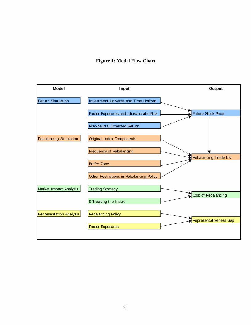
51

Figure 1: Model Flow Chart

Model Input Output

Return Simulation Investment Universe and Time Horizon

Factor Exposures and Idiosyncratic Risk Future Stock Price

Risk-neutral Expected Return

Rebalancing Simulation Original Index Components

Frequency of Rebalancing

Rebalancing Trade List

Buffer Zone

Other Restrictions in Rebalancing Policy

Market Impact Analysis Trading Strategy

Cost of Rebalancing

$ Tracking the Index

Representation Analysis Rebalancing Policy

Representativeness Gap

Factor Exposures

52

Figure 2: Example of Simulation and Market Cap Ranking

Figure 3: Buffer Zone Effect

Stocks Ranking Mkt Cap Mkt Cap Ranking Stocks

MSFT 1 300 290 1 GE270 2 INTC

GE 2 250 250 3 MSFT

C 3 200

INTC 4 10090 4 C

Simulation

time

Large Cap Index Buffer Zone Effect

0%2%4%6%8%

10%12%14%

0% 10% 20% 30%

Buffer Zone Size

0.0

0.5

1.0

1.5

2.0

Turnover

Tracking Error (bps)

Mid Cap Index Buffer Zone Effect

0%

10%

20%

30%

40%

50%

0% 20% 40% 60%

Buffer Zone Size

0.0

5.0

10.0

15.0

20.0

25.0

Turnover

RepresentativenessGap (bps)

53

Figure 4: Reconstitution Frequency Effect

Large Cap Rebalancing Frequency

0%5%

10%15%20%25%30%

0% 1% 2% 3% 4% 5%

Size of Buffer Zone

An

nu

aliz

ed T

urn

over

Annual

Semi-Annual

Quarter

Mid Cap Rebalancing Frequency

0%20%40%60%80%

100%120%

0% 1% 2% 3% 4% 5%

Size of Buffer Zone

An

nu

aliz

ed T

urn

over

Annual

Semi-Annual

Quarter

54

Bibliography Amihud, Yakov, and Haim Mendolson, 1986, “Asset pricing and the bid ask spread” Journal of Financial Economics 14, 223-249 Beneish, M, and J. Gardner, 1995. “Information Costs and Liquidity Effects in the Dow Jones Industrial Average Listing Changes”, “Journal of Financial and Quantitative Analysis, Vol. 30, No. 1 (March): 135-157 Beneish, Messod, and Robert Whaley, 1996, “The Anatomy of the ‘S&P Game’: The effects of Changing Rules”, The Journal of Finance, 51 December, pp1909-30 Beneish, Messod, and Robert Whaley, 2002, “S&P 500 Index Replacements, A new game in town”, Journal of Portfolio Management, Fall 2002. Brown, S., and J Warner, 1985, “Using Daily Stock Returns: The Case for Event Studies” Journal of Financial Economics, 14:3-31 Cooper, Daniel, and Geoffrey Woglom, 2001, “The S&P 500 Effect: Not such good news in the long run”, working paper Dhillon, U., and H. Johnson. 1991. “Changes in the S&P 500 List” Journal of Business, Vol. 64 No. 1, (March): 75-85 Gastineau, G., 2002, “Equity Index Funds Have Lost Their Way” Forthcoming, Journal of Portfolio Management Goetzmann, W., and M Garry. 1986 “Does Delisting from the S&P 500 Affect Stock Price?” Financial Analysts Journal, Vol. 42 No. 2 (March/April):64-69 Harris, L. and E. Gurel. 1986 “Price and Volume Effects Associated with Changes in the S&P 500 List: New Evidence for the Existence of Price Pressures” Journal of Finance, Vol. 41, No. 4 (September): 815-829 Holthausen, R., R Leftwich and D Mayers 1990, “Large Block Transactions, the speed of response and temporary and permanent stock-price effects” Journal of Financial Economics 26: 71-95 Jain, P., 1987. “The Effect on Stock Price of Inclusion or Exclusion from the S&P 500” Financial Analysts Journal, Vol. 43, No. 1 (January/February):58-65 Jankovskis, Peter, 2002, “The Not-so Perfect Index, the Impact of the Russell 2000 Rebalancing on Small Cap Performance”, www.journalofindexes.com, Second Quarter, 2002

55

Keim, D. and A. Madhavan, 1996, “The Upstairs Market for Large-Block Transactions Analysis and Measurement of Price Effects”, Review of Financial Studies, Spring, 1996, Vol. 9, No. 1, pp. 1-36 Keim, D. and A. Madhavan. 1998. “The Costs of Institutional Equity Trades: An Overview” Financial Analysts Journal, Vol 54, No. 4 (July/August): 50-69 Keim, D. 1999. “An Analysis of Mutual Fund Design: The Case for Investing in Small Cap Stocks” Journal of Financial Economics, Vol. 51 No. 3 (February):173-194 Kraus, A. and H.R. Stoll, 1972, “Price Impacts of Block Trading on the NewYork Stock Exchange”, The Journal of Finance, June 1972, pp569-88 Lynch, Anthony W. and Richard Mendenhall, 1997, “New Evidence on Stock Price Effects Associated with Changes in the S&P 500 Index”, Journal of Business, 70, No. 3 pp351-83 Madhavan, A, and M Cheng, “In Search for Liquidity: Block Trades in the Upstairs Markets” Review of Financial Studies, Spring 1997, Vol. 10, No. 1, pp 175-203 Madhaven, Ananth, 2002, “Index Reconstitution and Equity Returns”, working paper, (July 30, 2002 version) (Posted on the webpage for ITG, Inc.) Madhaven, Ananth, and Kewei Ming, 2002, “The Hidden Costs of Index Rebalancing: A Case Study of the S&P 500 Composition Changes of July 19, 2002”, working paper (September 3, 2002 version) (Posted on the webpage for ITG, Inc.) Malkiel, Burton, and Alexsander Radisich, 2001, “The Growth of Index Funds and the Pricing of Equity Securities”, The Journal of Portfolio Management, Winter, pp9-21 Pruitt, S. and K. Wei. 1989. “Institutional Ownership and Changes in the S&P 500” Journal of Finance, Vol. 44, No. 2 (June):509-513 Schleifer, A., 1986 “Do demand curves for stocks slope down?” Journal of Finance 41:579-90 Sofianos, George, 1993 Index Arbitrage Profitability”, Journal of Derivatives 1, 6-20