The Impact of Artificial Intelligence on the Labor Market

Michael Webb∗

Stanford University

January 2020

Latest version: https://web.stanford.edu/∼mww/webb jmp.pdf

Abstract

I develop a new method to predict the impacts of any technology on occupations. I use theoverlap between the text of job task descriptions and the text of patents to construct a measure ofthe exposure of tasks to automation. I first apply the method to historical cases such as softwareand industrial robots. I establish that occupations I measure as highly exposed to previousautomation technologies saw declines in employment and wages over the relevant periods. Iuse the fitted parameters from the case studies to predict the impacts of artificial intelligence.I find that, in contrast to software and robots, AI is directed at high-skilled tasks. Under theassumption that historical patterns of long-run substitution will continue, I estimate that AI willreduce 90:10 wage inequality, but will not affect the top 1%.

Keywords: artificial intelligence, robotics, technology, patents, occupationsJEL-codes: J23, J24, O33

∗Email: mww@stanford.edu. I am grateful to David Autor, Nick Bloom, Tim Bresnahan, Erik Brynjolfsson, Raj Chetty,Diane Coyle, Matthew Gentzkow, Caroline Hoxby, Xavier Jaravel, Chad Jones, Pete Klenow, Luigi Pistaferri, Will Rafey,Isaac Sorkin, and John Van Reenen for helpful comments and suggestions. I thank Ashi Agrawal, Trey Connelly, AndrewHan, Arshia Hashemi, Dan Kang, Gene Lewis, Cooper Raterink, and Greg Thornton for excellent research assistance. Iacknowledge financial support from the Future of Life Institute FLI-RFP-AI1 program, grant #2016-158713 (5388); the 2019Stanford HAI Seed Grant Program; and the Institute for Research in the Social Sciences (IRiSS) at Stanford University.

New technologies create winners and losers in the labor market. They change relative demands

for occupations, even as they improve productivity and standards of living.1 Understanding these

distributional consequences is important for many purposes. For example, it allows policymakers

to design appropriate education and skills policies, and helps individuals make good choices about

what careers to pursue.

Today, one technology is causing particular anxiety about job displacement: artificial intelligence.

Artificial intelligence, or machine learning, refers to algorithms that learn to complete tasks by

identifying statistical patterns in data, rather than following instructions provided by humans. This

technology has recently achieved superhuman performance across a wide range of economically

valuable tasks. Some of these tasks are associated with high-wage occupations, such as radiologists,

while others are associated with low-wage occupations, such as agricultural workers. At a time

when rising inequality is a major social and political issue, it is unclear whether AI will increase

inequality by, say, further displacing production workers, or reduce it by displacing doctors and

lawyers.

In this paper, I develop a new method for identifying which tasks can be automated by any

particular technology. This allows me to construct a measure of the “exposure” of occupations

to that technology. I first apply the measure to two historical case studies, software and robots. I

document the tasks that patents describe these technologies as performing, characterize the kinds of

people who work in exposed occupations, and study the relationship between my exposure scores

and changes in employment and wages. I then apply the method to artificial intelligence. I show

that AI exposure is highest for high-skilled occupations, suggesting that AI will affect very different

people than software and robots. Finally, I impose the assumption that the historical relationship

between exposure scores and wage changes will persist, and use this relationship to estimate the

potential impacts of artificial intelligence on inequality.

The measure developed in this paper is based on the following key idea. The text of patents

contains information about what technologies do, and the text of job descriptions contains informa-

tion about the tasks people do in their jobs. These two text corpuses can be combined to quantify

how much patenting in a particular technology has been directed at the tasks of any particular

occupation. This is therefore a measure of the tasks from which labor may be “displaced”, in the

canonical task-based model of Acemoglu and Restrepo (2018).

I use verb-noun pairs to quantify the “overlap” between patents and tasks. Suppose a doctor’s

job description includes the task “diagnose patient’s condition”. I use a natural language processing

1For example, a large literature, starting with Autor, Levy, and Murnane (2003), has documented how softwarereduced demand for workers performing routine tasks while increasing it for workers performing problem-solving andcomplex interpersonal tasks.

1

algorithm to extract the verb-noun pairs from this task, which in this case would be “diagnose

condition”. I then quantify how many patents corresponding to a given technology contain similar

verb-noun pairs, such as “diagnose disease”. I use the prevalence of such patents to assign a score

to the task, and aggregate these task-level scores to the occupation level.

What can we learn from a measure of the tasks for which technology can substitute for human

labor? As a framework for applying the measure, I develop a version of the Acemoglu and Restrepo

(2018) task-based model, in which automation occurs at the task level. I add occupations to the

model, so that occupations produce output using tasks, and firms produce output using occupations.

The model shows that the impact of task-level automation on occupation demand is ambiguous.

The intuition is simple. If half of an occupation’s tasks are automated, that will reduce labor demand

per unit of the occupation’s output. But it might reduce the price of the occupation’s output so

much that demand for it increases enough to offset the reduction in labor demand, perhaps even

producing a net increase in labor demand for the occupation. Similar opposing forces operate at

other levels of the model. This means that without strong restrictions on the values of the various

elasticity of substitution parameters, it is impossible to sign the net impacts of task-level substitution

on the demand for occupations.

To study the performance of my measure empirically, and so help resolve this theoretical

ambiguity, I analyze two historical episodes, software and robots. I chose these episodes because

they affected many occupations in many industries. This breadth of impact is important because I

use occupation-industries cells as the unit of analysis in my regressions. Moreover, because these

technologies are so recent, they are more likely to be informative about how the economy will

respond to artificial intelligence.

For each technology, I first document the tasks the patents describe it as performing. Patents

most frequently describe robots as cleaning, moving, welding, and assembling various objects. By

contrast, they describe software as recording, storing, and producing information, and executing

programs, logic, and rules. When I aggregate from the task to the occupation level, I find that

occupations most exposed to robots include various kinds of materials movers in factories and

warehouses, and tenders of factory equipment, both of which have seen automation by robots. Least-

exposed occupations include payroll clerks, artistic performers, and clergy. These do not primarily

involve the kinds of repetitive manual tasks that robots automate. Occupations most exposed to

software include broadcast equipment operators, plant operators, and parking lot attendants, all of

which have seen computers take over large parts of their tasks. Least-exposed occupations include

barbers, podiatrists, and postal service mail carriers. These are occupations that have substantial

manual components that are not easy to hard-code in advance, and, in many cases, interpersonal

2

components too.

Next, I study the kinds of individuals who work in occupations that are highly exposed to

each technology. I find that individuals with less than high school education, and in low-wage

occupations, are most exposed to robots. Men under age 30 are most exposed, consistent with

robots’ substituting for what might be termed “muscle” tasks. For software, exposure is decreasing

with education, but much less sharply than for robots, with individuals in middle-wage occupations

most exposed. This is consistent with the literature on polarization, which has found that I.T. has

reduced demand for middle-wage jobs while increasing it for low- and high-wage jobs. Just as for

robots, men are much more exposed to software than women. This reflects the fact that women

have historically clustered more in occupations requiring complex interpersonal interaction tasks,

which software is not capable of performing.

I conclude the case studies by estimating the relationship between my measure of occupation

exposure and changes in employment and wages over the period 1980 to 2010. Although I cannot

attribute causality to the exposure scores, moving from the 25th to the 75th percentile of exposure

to robots is associated with a decline in within-industry employment shares of between 9 and

18%, and a decline in wages of between 8 and 14%, depending on the specification. For software,

the magnitudes are smaller, with declines of 7-11% and 2-6%, respectively. I address potential

endogeneity from a variety of sources. Changes in product demand, such as from trade, could be

affecting industries in which these technologies are used. When I compare occupations within the

same industry, however, I find that the occupations exposed to software and robots have declined

much more than those that are not exposed. There were large changes in skill supplies over this

period, and the results are robust to controlling for skill levels. Thus, although I cannot isolate the

causal effect of these technologies, the pattern of results provides suggestive evidence that they

reduced employment and wages in exposed occupations.

In the final part of the paper, I apply the method to artificial intelligence. I first provide purely

descriptive results on exposure. After that, I make additional assumptions that allow me to quantify

artificial intelligence’s potential impacts on inequality.

Patents describe artificial intelligence performing tasks such as predicting prognosis and treat-

ment, detecting cancer, identifying damage, and detecting fraud. These are tasks involved in medical

imaging and treatment, insurance adjusting, and fraud analysis, all areas that are currently seeing

high levels of AI research and development. Notice that these activities are of a very different kind

to those identified for robots and software. Whereas robots perform “muscle” tasks and software

performs routine information processing, AI performs tasks that involve detecting patterns, making

judgments, and optimization. Most-exposed occupations include clinical laboratory technicians,

3

chemical engineers, optometrists, and power plant operators. These all involve tasks that have

already been successfully automated by AI. While these are all high-skilled jobs, it is worth noting

that there are also low-skilled jobs that are highly exposed to AI. For example, production jobs that

involve inspection and quality control are exposed. However, these constitute a small proportion of

low-skill jobs.

Consistent with these results, I find that high-skill occupations are most exposed to AI, with

exposure peaking at about the ninetieth percentile. While individuals with low levels of education

are somewhat exposed to AI, it is those with college degrees, including Master’s degrees, who are

most exposed. Moreover, as might be expected from the fact that AI-exposed jobs are predominantly

those involving high levels of education and accumulated experience, it is older workers who are

most exposed to AI, with younger workers much less so.

These descriptive results clearly indicate that AI will affect very different occupations, and so

different kinds of people, than software and robots. Without imposing additional assumptions,

however, I cannot say what these impacts will be, or even whether they will be positive or negative.

Thus, to quantify AI’s potential impacts on inequality, I end the paper by making the strong

assumption that the relationship between AI exposure and changes in wages will have the same

sign, and the same linear relationship, as for software and robots. Under this assumption, I calculate

the wage distribution for different potential magnitudes of the relationship between AI exposure

and wage changes. I find that AI is projected to reduce inequality measured as the ratio of the 90th

to the 10th percentile of wages. On the other hand, it is projected to increase inequality at the top of

the distribution, measured as the ratio of the 99th to the 90th percentile. Applying the estimated

software coefficient to AI, I project a 4% decrease in 90:10 inequality; using the robot coefficient, the

decrease is 9%.

These results should be interpreted with caution. First, they rely on a constant mapping between

exposure and changes in demand. In the context of the model, I am assuming that the structural

parameters remain constant. Based on the results of the case studies, this seems a reasonable

prior, though the evidence is only suggestive. Second, there are a number of measurement issues,

particularly concerning top earners, that mean my results may understate the impacts on inequality.

Third, I cannot rule out that AI will produce impacts other than via task-level substitution, such as

via new tasks and purely labor-augmenting technical change. To affect my results, the distribution

of impacts on labor demand due to these other channels would need to be correlated with the

distribution of impacts due to substitution. While I cannot rule this out, there is no strong a priori

reason to expect it to be the case.

Fourth, there is the question of timing. It is too early in the development of AI to know how much

4

more of the technology there is to be developed, and too early also to know how long it will take to

be adopted. The results in this paper concern only the applications of artificial intelligence that

have been described in patents to date. Finally, this paper’s results do not describe what happens to

individuals in exposed occupations. For example, individuals in occupations exposed to software

and robots that saw decreases in demand could have suffered wage declines or unemployment, or

they could have moved to different jobs for which demand was strong. Edin et al. (2019) find that

individuals in shrinking occupations see substantial wage penalties and increases in unemployment,

suggesting that, on average, negative occupation impacts translate into negative individual impacts.

This paper makes three contributions to the literature. The first contribution is a general-purpose

measurement of technology. Many influential papers have constructed careful measures of exposure

to particular technologies.2 These measures are all “ad hoc”, having been manually created to

capture individual economists’ subjective understanding of the nature of particular technologies.

This requires substantial technical knowledge on the part of the economist, and such knowledge

is hard to acquire for frontier technologies. The measure developed in this paper, by contrast, is

objective, easy to replicate, and can be applied to any technology, including both those whose

impacts have already occurred, and those whose impacts lie mostly in the future.

The second contribution is to the literature on the impacts of automation on jobs and wages.

A large literature studies the relationship between adoption of particular technologies and labor

market impacts.3 These papers tend to study a single technology, often using data that is only

at the industry level, or at the firm level within a single sector. A contribution of this paper is to

apply the same methodology consistently across several different episodes of technological change,

across the whole economy, using the same research design. A key result that emerges from this

exercise is that technologies are very different from each other, and so impact very different kinds

of people. However, the exercise also produces suggestive evidence that the relevant structural

parameters could be somewhat constant over time, making it possible to predict the impacts of new

technologies based on their capabilities.

Finally, this paper contributes to a burgeoning literature that tries to predict the impacts of AI

specifically.4 This literature relies on expert surveys, usually of computer scientists. With new

technologies such as AI, experts have had little time to understand the full range of the technology’s

potential use cases in different areas of the economy. As Brynjolfsson and Mitchell have written2For example, Autor, Levy, and Murnane (2003), Acemoglu and Autor (2011), Autor and Dorn (2013), and Graetz and

Michaels (2018).3For IT, see, for example, Krueger (1993) and Michaels, Natraj, and Van Reenen (2013); for broadband, Akerman,

Gaarder, and Mogstad (2015); and for robots, Graetz and Michaels (2018) and Acemoglu and Restrepo (2017). A paperthat uses a more general measure of automation is Bessen et al. (2019).

4Examples include Frey and Osborne (2017), Arntz, Gregory, and Zierahn (2017) , Grace et al. (2017), Manyika et al.(2017), Brynjolfsson, Mitchell, and Rock (2018), and Felten, Raj, and Seamans (2017).

5

(Brynjolfsson and Mitchell 2017), there is “no widely shared agreement on the tasks where ML

systems excel, and thus little agreement on the specific expected impacts on the workforce and on

the economy more broadly.” The measure developed in this paper offers a broad, objective answer

to this question by aggregating the knowledge and ideas of inventors and companies patenting

in every area of the economy. Moreover, because it is fully automated, it can be re-calculated

continuously to incorporate new applications of AI as they are developed.

The rest of this paper proceeds as follows. In Section I, I outline the model and discuss the

economics of automation more broadly. In Section 2, I describe the data used. Section 3 describes

the method for calculating exposure scores. Section 4 describes the robots case study, while Section

5 describes the software case study. Section 6 turns to AI. Section 7 concludes.

1 Model

There are many channels through which a technology can affect labor demand. Understanding

these channels is important for interpreting the empirical analyses that use my measure in the rest

of the paper. In this section, I develop a simple model that illustrates some of the most important

channels, and briefly discuss a number of other considerations.

1.1 Model setup

I develop a simple, static task-based model in the spirit of Acemoglu and Restrepo (2018). In that

model, the economy produces a unique final good by combining tasks in a CES production function.

Some tasks can be technologically automated, while others can only be performed by humans.

My model departs from Acemoglu and Restrepo (2018)’s in that I add occupations as a unit of

analysis. My measure of automation exposure is at the occupation level, so understanding how

technology affects demand for occupations is crucial for establishing what we can learn from my

measure. It is important, too, for studying technology’s distributional consequences. Whereas

Acemoglu and Restrepo (2018)’s focus is on the labor share overall, mine is on how technology

differentially affects different parts of the labor market. Occupations are the most natural unit

through which to analyze this.5

5Another difference is that in Acemoglu and Restrepo (2018), the set of tasks is not fixed, so that new tasks mayreplace old tasks. In my model, I fix the set of tasks. This simplification makes the analysis more tractable. It also moreclosely matches my empirical setting, since I do not measure the reallocation of tasks across occupations. I discuss thisissue further below.

6

1.2 Environment

The economy consists of a single firm that produces a unique final good.6 The firm produces the

good, X, by combining the output of different occupations, Oi, in a constant elasticity of substitution

production function with elasticity parameter ρ:

X =

∑iαiO

ρi

1ρ

.

Each occupation, Oi, produces its output by combining the output of a number of tasks. These

tasks are denoted Ti, j, where j indexes tasks. The task outputs are combined in another constant

elasticity of substitution production function with a different elasticity parameter, ρt (t is for “task”):

Oi =

∑jα jT

ρti, j

1ρt

.

Some of these tasks can be automated, while others cannot. Tasks that are automated can be

performed either by humans, H, or machines, R. 7 Humans and machines are perfect substitutes at

the task level. Tasks that are not automated can be performed only by humans:

Ti, j =

Hi, j + Ai, jRi, j if automation feasible;

Hi, j otherwise.

Human productivity is normalized to one. However, machine productivity can increase over

time (for a given feasible task). I denote machine productivity by Ai, j.

The firm takes the wage of human labor in occupation Oi, wi, as given. Similarly, it takes as

given the rental rate of a machine, r. Clearly, in this setup, the firm will employ exclusively human

labor for task j in occupation i if wi <r

Ai, j, and exclusively machines if the inequality is reversed. A

task’s being infeasible to automate is therefore equivalent to Ai, j = 0.

1.3 Impact of automation on labor demand

How does a change in machine productivity affect the firm’s demand for human labor by occupation?

First, consider a setup in which there is a single occupation with two tasks, only one of which can

6The assumption of a single firm is not substantive. It would be easy to write the model with many firms; I discuss amodel with many industries below.

7To fix ideas, one can think of R as corresponding to robots; however, R here refers to any kind of automationtechnology.

7

ρ = -10

ρ = -0.5

ρ = 0.6

ρ = 0.8

.6.8

11.

21.

4D

eman

d fo

r hum

ans i

n oc

cupa

tion

1

0 20 40 60 80 100Machine productivity

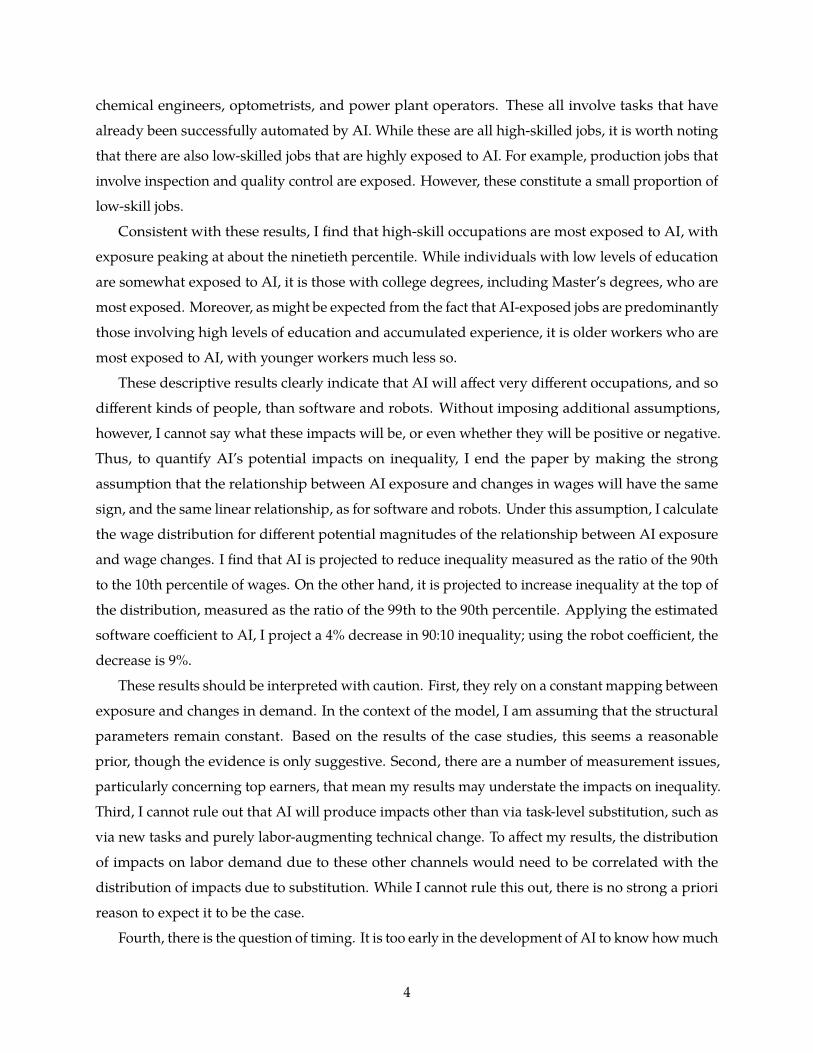
Figure 1: Model simulation results: demand for humans in occupation 1 (occupation being auto-mated) as a function of robot productivity, for different values of firm-level elasticity of substitutionparameter ρ. Task-level elasticity of substitution parameter ρt is fixed at −10.

be automated. There are two levels of demand to consider: the firm’s demand per unit of output,

and the total units of output demanded by consumers. As machine productivity increases, the

firm’s demand for human workers per unit of output will unambiguously decrease. The human

workers will be fully displaced from the automatable task; to the extent the two tasks are substitutes,

fewer human workers will be demanded to perform the non-automatable task too. However, this

automation reduces the cost of the final good, and hence its price, leading consumers to demand

more of it.8 This increase in final demand offsets the reduction in per-unit labor demand, and could

even lead to a net increase in labor demand. This scenario has been developed in detail in the

literature. For example, Bessen (2015) argues that ATMs, which automate some of the tasks of bank

tellers, increased demand for that occupation by reducing the cost of opening new bank branches.

While bank tellers per branch decreased, banks opened sufficiently many new branches that the

overall number of tellers increased.

To bring an additional channel into focus, consider a setup with two occupations, in which

each occupation consists of two tasks. In the first occupation, one task can be automated, while the

other can only be performed by a human. In the second occupation, neither task can be automated.

8These two effects are analogous to what Acemoglu and Restrepo (2018) call the “displacement” and “productivity”effects, respectively.

8

Figure 1 displays firm demand for the first occupation as the machine productivity parameter A1,1

increases from 1, which is equal to human productivity, to 100. The task-level elasticity parameter

is set to ρt = −10, so that tasks are complements in production. Each line corresponds to a different

value of the firm-level elasticity parameter, from ρ = −10 (occupations are strong complements) to

ρ = 0.8 (occupations are strong substitutes).

The figure shows that when the two occupations are highly substitutable, the firm’s cost-

minimizing choice is to demand relatively more of occupation 1, the occupation that has been

partially automated. The intuition for this is simple. Because the level of machine productivity is

high, this increases the productivity of occupation 1, leading the firm to demand more of it. The

tasks within occupation 1 are complements, however, so the firm still needs to hire lots of humans

to perform the human-only task. For ρ > 0.5, this channel is sufficiently strong to cause a net

increase in the firm’s demand for human workers in occupation 1 — even though this occupation

is the one that is being automated. As an example of occupations that are substitutes, consider

operations analysts and industrial technicians, both of which improve efficiency on a factory floor.

The operations analysts develop mathematical models of the factory and simulate them. It is easy

to see how automation of the simulation task could make the operations analysts so much more

productive that the firm would hire more operations analysts and fewer industrial technicians

per unit of output. Note that this effect is driven entirely by the substitutability of occupations in

production, and has nothing to do with the elasticity of consumer demand.9

1.4 Discussion and implications for empirical analysis

The analysis so far has illustrated displacement and productivity effects in an economy with a

single firm. The productivity effect operates at two levels. Inside the firm, the substitutability of

occupations in production affects how automation changes the firm’s demand for occupations per

unit of the final good produced. Outside the firm, price changes affect consumers’ demand for the

final good. Overall, then, the impact of task-level automation on the demand for occupations is

theoretically ambiguous. Without making strong restrictions on the various elasticity of substitution

parameters, it is impossible to sign the direction of impacts.

The method I develop in this paper allows me to identify the tasks for which technology can

substitute for human labor. I am therefore able to estimate empirically the relationship between the

extent to which an occupation’s tasks can be replaced by technology and changes in demand for

that occupation. Given the theoretical ambiguity of the model, this is an interesting question in

its own right. It will also be informative about how much we can learn from the measure about

9Of course, the consumer demand channel also operates in this setting.

9

the potential impacts of AI. In the rest of this paper, I analyze two historical case studies, and find

that, in both, there is a negative relationship between my measure and changes in employment and

wages by occupation. This shows that the balance of forces favored substitution in the past, and

may move our priors toward thinking that the same will be true in the future.

To further set the stage for the empirical analysis, several extensions to the model merit attention.

First, consider an economy with multiple industries. Industries employ different combinations

of occupations, which have different opportunities for automation. Automation in one industry

changes the relative prices of the final goods of all industries. This change in relative prices leads

consumers to change their consumption bundles. If preferences are nonhomothetic, moreover,

automation also causes demand changes due to wealth effects. Because different industries employ

different occupations, these changes in final demand affect occupation demand. To handle this

complexity, I confine most of my analysis to studying within-industry changes in the relative

demand for occupations. This helps to isolate those changes in demand for occupations that are

due to task-level substitution on the production side, the chief object of my analysis, rather than

those due to changes in consumers’ incomes and the prices they face.

Second, there is a richer set of ways that technology can impact production. In addition to

automating existing tasks, technology can create entirely new tasks. These tasks can be ones

involved in producing new goods, or the result of an increase in the scope of occupations in existing

industries. Technology can also induce the reorganization of tasks among occupations. Finally, it

can create purely factor-augmenting technological change.10

Are these other demand-side factors likely to bias my results? It seems likely that the technologies

studied in this paper may produce, for example, purely labor-augmenting technical change that

advantages some types of labor over others. For these to affect my conclusions about the occupations

harmed due to task-level substitution, however, the distribution of impacts on labor demand due to

labor-augmenting technical change would need to be correlated with the distribution of impacts

due to substitution. A priori, there is no strong reason to expect this to be so. The example of

software offers some empirical support for this idea. Autor, Levy, and Murnane (2003) show that

software complements tasks with high abstract content, and substitutes for tasks with high routine

content. How much do these different types of task content overlap within occupations? Regressing

one measure on the other, I find that the variation in the routine task content of occupations10All of these can be seen in the example of the steamship, which replaced sailboats in the late nineteenth century

(Chin, Juhn, and Thompson 2006). The steamship was a new good, with a different production process from sailboats.Consumers substituted away from sailboat transportation into steamship transportation. This reduced demand formariners who were skilled in handling a ship’s sails, but not by automating sail handling. It created new tasks, such astending the steamship’s engines and shoveling coal into its boiler, and reorganized the tasks done by existing seafaringoccupations. Finally, improvements in the efficiency of the steam engine were a form of pure capital-augmentingtechnological change.

10

explains only 2% of the variation in their abstract task content. This suggests that “routineness” is

independently useful as a measure of potential displacement due to software, and that its usefulness

is not diminished by the existence of other types of tasks that software complements. Indeed, a

large literature on “routine-biased technical change” has used measures of routineness for just this

purpose. The other factors, such as new tasks and endogeneous occupational scope, are subject

to much ongoing research. Insofar as substituted tasks within an occupation are replaced by new

tasks that increase demand for the occupation, this will attenuate my results.

Finally, consider workers’ occupational choices and human capital investments. If the supply of

each occupation is fixed, reductions in demand affect only wages. If, instead, workers can change

occupations, then changes in demand can affect both employment and wages. This has important

implications for welfare. For example, suppose that radiologists and truck drivers are equally

exposed to automation. Suppose further that radiologists have highly specialized human capital,

such that no other occupation open to them pays close to their current wage, whereas truck drivers

have many outside options that pay a similar wage to their current job. In this case, because of

their different outside options, radiologists would see much greater reductions in wages due to

automation than truck drivers, even though both were equally exposed to automation.

Will my results, then, be informative about the incidence of these technologies? In the absence

of longitudinal data that allows me to follow individuals over time, there is a limited amount I can

say. However, other work offers suggestive evidence. Edin et al. (2019) use administrative data

from Sweden to show that workers who faced occupational decline over the period 1986-2013 saw

substantial declines in lifetime earnings. If a similar pattern holds in the US, then my occupation-

level results will point towards the individuals who are harmed by this task-level substitution.

Research using longitudinal data from the US is thus a priority for future research.

2 Data

The method for constructing my measure of the exposure to occupations requires two sources of

text: patents and job descriptions. The main empirical results require data on employment and

wages for occupation-industry cells, as well as various controls.

2.1 Patent data

I use Google Patents Public Data, provided by IFI CLAIMS Patent Services.11 The fields I use are

the title, abstract, and CPC codes, as I describe further below.11Data accessed via Google BigQuery at https://console.cloud.google.com/marketplace/details/google patents

public datasets/google-patents-public-data.

11

2.2 Job descriptions data

For job descriptions, I use the O*NET database of occupations and tasks. This database is produced

by an agency of the US Department of Labor, and is the successor to the Dictionary of Occupational

Titles (DOT). These dictionaries were originally created in the 1930s to “furnish public employment

offices... with information and techniques that will facilitate proper classification and placement of

work seekers” (U.S Employment Service 1939). O*NET describes 964 occupations. A set of tasks is

listed for each occupation, described in natural language. For example, a doctor’s task is “interpret

tests to diagnose patient’s condition”. Occupations and tasks have various additional metadata,

such as numerical scores indicating interpersonal or analytical skills required. These metadata have

been widely used by economists.12 For this paper, I just use the text itself. Each task is also given

scores that indicate its importance and frequency in the occupation. I use these scores to weight

tasks within occupations.

2.3 Employment/wage data (Census/ACS)

To measure the relationship between my measure and changes in wages and employment, I use

individual-level microdata from the US Census 1960-2000 and from the ACS 2000-2018, provided

by IPUMS (Ruggles et al. 2019). For my main analysis sample, I restrict to individuals in work

between the ages of 18 and 65, and calculate average wages and the proportion of hours worked

in each industry-occupation cell. I use various other Census variables for controls and additional

analyses, such as age, gender, and level of education. I use the measure of offshorability developed

by Firpo, Fortin, and Lemieux (2011) and standardized in Autor and Dorn (2013), and the measure

of occupational licensing developed by Kleiner and Xu (2017). For all these analyses, I use the

“occ1990dd” occupational classification developed by Dorn (2009) and extended by Deming (2017),

and the IPUMS “ind1990” industry classification. Full details are provided in Appendix B.

3 Method

In this section, I describe how I construct a new, objective measure of the exposure of tasks to

automation by quantifying the overlap between the text of patents and the text of job descriptions.

In the following sections, I construct my measure and study its performance separately for each

technology case study.

12Examples include Howell and Wolff (1991), Autor, Levy, and Murnane (2003), and Deming (2017).

12

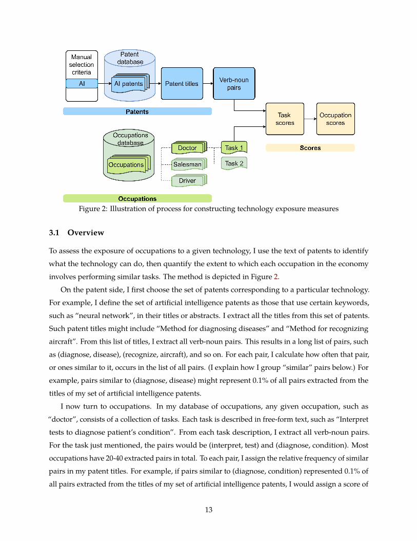
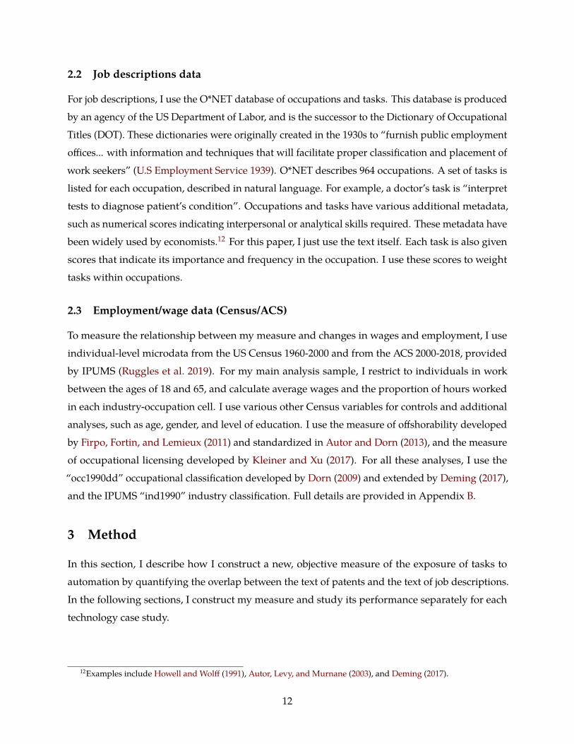
Figure 2: Illustration of process for constructing technology exposure measures

3.1 Overview

To assess the exposure of occupations to a given technology, I use the text of patents to identify

what the technology can do, then quantify the extent to which each occupation in the economy

involves performing similar tasks. The method is depicted in Figure 2.

On the patent side, I first choose the set of patents corresponding to a particular technology.

For example, I define the set of artificial intelligence patents as those that use certain keywords,

such as “neural network”, in their titles or abstracts. I extract all the titles from this set of patents.

Such patent titles might include “Method for diagnosing diseases” and “Method for recognizing

aircraft”. From this list of titles, I extract all verb-noun pairs. This results in a long list of pairs, such

as (diagnose, disease), (recognize, aircraft), and so on. For each pair, I calculate how often that pair,

or ones similar to it, occurs in the list of all pairs. (I explain how I group “similar” pairs below.) For

example, pairs similar to (diagnose, disease) might represent 0.1% of all pairs extracted from the

titles of my set of artificial intelligence patents.

I now turn to occupations. In my database of occupations, any given occupation, such as

“doctor”, consists of a collection of tasks. Each task is described in free-form text, such as “Interpret

tests to diagnose patient’s condition”. From each task description, I extract all verb-noun pairs.

For the task just mentioned, the pairs would be (interpret, test) and (diagnose, condition). Most

occupations have 20-40 extracted pairs in total. To each pair, I assign the relative frequency of similar

pairs in my patent titles. For example, if pairs similar to (diagnose, condition) represented 0.1% of

all pairs extracted from the titles of my set of artificial intelligence patents, I would assign a score of

13

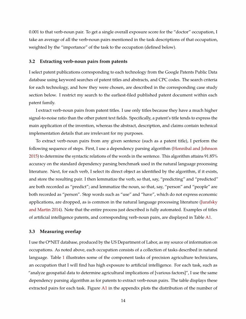
0.001 to that verb-noun pair. To get a single overall exposure score for the “doctor” occupation, I

take an average of all the verb-noun pairs mentioned in the task descriptions of that occupation,

weighted by the “importance” of the task to the occupation (defined below).

3.2 Extracting verb-noun pairs from patents

I select patent publications corresponding to each technology from the Google Patents Public Data

database using keyword searches of patent titles and abstracts, and CPC codes. The search criteria

for each technology, and how they were chosen, are described in the corresponding case study

section below. I restrict my search to the earliest-filed published patent document within each

patent family.

I extract verb-noun pairs from patent titles. I use only titles because they have a much higher

signal-to-noise ratio than the other patent text fields. Specifically, a patent’s title tends to express the

main application of the invention, whereas the abstract, description, and claims contain technical

implementation details that are irrelevant for my purposes.

To extract verb-noun pairs from any given sentence (such as a patent title), I perform the

following sequence of steps. First, I use a dependency parsing algorithm (Honnibal and Johnson

2015) to determine the syntactic relations of the words in the sentence. This algorithm attains 91.85%

accuracy on the standard dependency parsing benchmark used in the natural language processing

literature. Next, for each verb, I select its direct object as identified by the algorithm, if it exists,

and store the resulting pair. I then lemmatize the verb, so that, say, “predicting” and “predicted”

are both recorded as “predict”; and lemmatize the noun, so that, say, “person” and “people” are

both recorded as “person”. Stop words such as “use” and “have”, which do not express economic

applications, are dropped, as is common in the natural language processing literature (Jurafsky

and Martin 2014). Note that the entire process just described is fully automated. Examples of titles

of artificial intelligence patents, and corresponding verb-noun pairs, are displayed in Table A1.

3.3 Measuring overlap

I use the O*NET database, produced by the US Department of Labor, as my source of information on

occupations. As noted above, each occupation consists of a collection of tasks described in natural

language. Table 1 illustrates some of the component tasks of precision agriculture technicians,

an occupation that I will find has high exposure to artificial intelligence. For each task, such as

“analyze geospatial data to determine agricultural implications of [various factors]”, I use the same

dependency parsing algorithm as for patents to extract verb-noun pairs. The table displays these

extracted pairs for each task. Figure A1 in the appendix plots the distribution of the number of

14

Table 1: Tasks and exposure scores for precision agriculture technicians.

Task Weight inoccupation

Extracted pairs AI exposurescore x100

Use geospatial technology to develop soil sampling grids oridentify sampling sites for testing characteristics such asnitrogen, phosphorus, or potassium content, ph, ormicronutrients.

0.050 (develop, grid) 0.050

(identify, site) 0.234

(test, characteristic) 0.084

Document and maintain records of precision agricultureinformation.

0.049 (maintain, record) 0.000

Analyze geospatial data to determine agriculturalimplications of factors such as soil quality, terrain, fieldproductivity, fertilizers, or weather conditions.

0.048 (analyze, datum) 0.469

(determine, implication) 0.837

Apply precision agriculture information to specifically reducethe negative environmental impacts of farming practices.

0.048 (apply, information) 0.000

(reduce, impact) 0.151

Install, calibrate, or maintain sensors, mechanical controls,GPS-based vehicle guidance systems, or computer settings.

0.045 (maintain, sensor) 0.000

Identify areas in need of pesticide treatment by analyzinggeospatial data to determine insect movement and damagepatterns.

0.038 (identify, area) 0.234

(analyze, datum) 0.469

(determine, movement) 0.502

Notes: Table displays six of the twenty-two tasks recorded for precision agriculture technicians in the O*NET database.For each task, the weight is an average of the frequency, importance, and relevance of that task to the occupation, asspecified in O*NET, with weights scaled to sum to one. The verb-noun pairs in the third column are extracted fromthe task text by a dependency parsing algorithm. The AI exposure score for an extracted pair is equal to the relativefrequency of similar pairs in the titles of AI patents. The score multiplied by 100 is thus a percentage; for example, pairssimilar to “determine implications” represent 0.84% of pairs extracted from AI patents.

15

verb-noun pairs extracted across occupations. The vast majority of occupations (92%) have more

than 15 extracted pairs in total, and most (76%) have more than 20 extracted pairs.

Before calculating an exposure score for each verb-noun pair, I first group the nouns in each

pair into conceptual categories. I do this because the nouns used in O*NET task descriptions are

quite general, whereas the nouns used in patents vary in their generality. For example, if an O*NET

task verb-noun pair refers to “animals”, and a patent verb-noun pair refers to “mammals”, I want

to account for the fact that “mammal” is an instance of “animal”. This would not be possible using

a thesaurus, since “mammal” and “animal” are not synonyms.

Instead, I use WordNet (Miller 1995), a database developed at Princeton University that groups

nouns into a hierarchy of concepts. For example, the ancestors of “economist” are “social scientist”,

“scientist”, “person”, “causal agent”, “physical entity”, and “entity”. At each conceptual level, the

conceptual categories are mutually exclusive. This allows me to assign each of the nouns occurring

in my verb-noun pairs to a single conceptual category, for a given conceptual level. I use “aggregated

verb-noun pair” to refer to a pair consisting of a verb and a noun conceptual category. For the

conceptual level that includes “person”, for example, “recognize economist” would be part of the

aggregated verb-noun pair “recognize person”.

In choosing the conceptual level at which to group the nouns, I face a trade-off between specificity

and coverage. For example, if I group into categories at the conceptual level of “dog”, I lose all

words that exist only at a more general level, such as “mammal” and “animal”. Figure A3 in the

appendix displays the share of verb-noun pairs extracted from O*NET tasks that would be lost for

this reason at each level of aggregation. Due to the level of generality at which O*NET tasks are

expressed, I would lose more than a quarter of all verb-noun pairs if I grouped at WordNet level 5,

for example. (Levels with higher numbers are more specific.) I therefore use WordNet level 3 for

my main results, and re-run my analyses at levels 2, 4, and 5 to check their sensitivity. While the

level of aggregation does make some difference, the results for these other levels are qualitatively

very similar to my baseline specification.

3.4 Measuring the exposure of occupations

I now describe how I calculate an occupation’s final exposure score using the set of aggregated

verb-noun pairs extracted from its task descriptions. Denote the set of technologies T. For a given

technology, t ∈ T, let f tc denote the raw count of occurrences of aggregated verb-noun pair c extracted

from technology t patent titles, and let Ct denote the full set of aggregated verb-noun pairs for

technology t. The relative frequency, r f tc , of aggregated verb-noun pair c in technology t patent

titles is

16

r f tc =

f tc∑

c∈Ct f tc.

I assign to each of the task-level aggregated verb-noun pairs that pair’s relative frequency, r f tc ,

in technology t patent titles. These scores for artificial intelligence are displayed in the final column

of Table 1.

For each occupation i, I then take a weighted average of these task-level scores to produce an

overall technology t exposure score for the occupation,

Exposurei,t =

∑k∈Ki

[wk,i ·

∑c∈Sk

r f tc]

∑k∈Ki

[wk,i · |{c : c ∈ Sk}|

] .In this expression, Ki is the set of tasks in occupation i, and Sk is the set of verb-noun pairs

extracted from task k ∈ Ki. Finally, wk,i, the weight of task k within occupation i, is an average of the

frequency, importance, and relevance of task k to occupation i, as specified in the O*NET database,

with weights scaled to sum to one.

An occupation’s exposure score for technology t thus expresses the intensity of patenting activity

in technology t directed towards the tasks in that occupation. Figure A2 in the online appendix

shows the distribution of AI scores across occupations.

4 Application: Robots

In this section, I apply the method to a first historical case study: robots. After some brief background,

I describe the construction of the measure for robots, and present the key results, including most

and least exposed tasks and occupations. I then present descriptive evidence on the distributional

impact of robots. The section concludes with an analysis of the relationship between exposure and

changes in wages and employment.

4.1 Background and definition

This case study focuses on industrial robots. Industrial robots are robots used in manufacturing,

rather than robots used, for example, in surgery, or in other parts of the service sector. The reason

for the restriction is that industrial robots have seen by the far the most adoption, whereas service

sector robots are more nascent. Industrial robots also have a standardized definition, ISO 8373, that

is used for constructing measures of adoption. Robots are defined as “an automatically controlled,

reprogrammable, multipurpose manipulator programmable in three or more axes, which may be

17

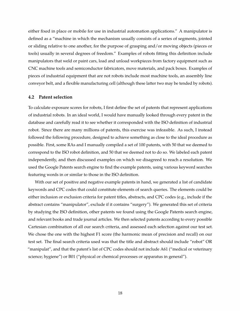
either fixed in place or mobile for use in industrial automation applications.” A manipulator is

defined as a “machine in which the mechanism usually consists of a series of segments, jointed

or sliding relative to one another, for the purpose of grasping and/or moving objects (pieces or

tools) usually in several degrees of freedom.” Examples of robots fitting this definition include

manipulators that weld or paint cars, load and unload workpieces from factory equipment such as

CNC machine tools and semiconductor fabricators, move materials, and pack boxes. Examples of

pieces of industrial equipment that are not robots include most machine tools, an assembly line

conveyor belt, and a flexible manufacturing cell (although these latter two may be tended by robots).

4.2 Patent selection

To calculate exposure scores for robots, I first define the set of patents that represent applications

of industrial robots. In an ideal world, I would have manually looked through every patent in the

database and carefully read it to see whether it corresponded with the ISO definition of industrial

robot. Since there are many millions of patents, this exercise was infeasible. As such, I instead

followed the following procedure, designed to achieve something as close to the ideal procedure as

possible. First, some RAs and I manually compiled a set of 100 patents, with 50 that we deemed to

correspond to the ISO robot definition, and 50 that we deemed not to do so. We labeled each patent

independently, and then discussed examples on which we disagreed to reach a resolution. We

used the Google Patents search engine to find the example patents, using various keyword searches

featuring words in or similar to those in the ISO definition.

With our set of positive and negative example patents in hand, we generated a list of candidate

keywords and CPC codes that could constitute elements of search queries. The elements could be

either inclusion or exclusion criteria for patent titles, abstracts, and CPC codes (e.g., include if the

abstract contains “manipulator”, exclude if it contains “surgery”). We generated this set of criteria

by studying the ISO definition, other patents we found using the Google Patents search engine,

and relevant books and trade journal articles. We then selected patents according to every possible

Cartesian combination of all our search criteria, and assessed each selection against our test set.

We chose the one with the highest F1 score (the harmonic mean of precision and recall) on our

test set. The final search criteria used was that the title and abstract should include “robot” OR

“manipulat”, and that the patent’s list of CPC codes should not include A61 (“medical or veterinary

science; hygiene”) or B01 (“physical or chemical processes or apparatus in general”).

18

Table 2: Top extracted verbs and characteristic nouns for robots.

Verb Example nouns Verb Example nouns

clean surface, wafer, window, glass, floor,tool, casting, instrument

walk robot, structure, base, stairs, circuit,trolley, platform, maze

control robot, arm, motion, position,manipulator, motor, path, force

carry substrate, wafer, tray, vehicle,workpiece, tool, object, pallet

weld wire, part, tong, electrode, sensor,component, nozzle

detect position, state, collision, obstacle,force, angle, leak, load, landmine

move robot, body, object, arm, tool, part,substrate, workpiece

drive unit, wheel, motor, belt, rotor, vehicle,automobile, actuator

Notes: This table lists the top eight verbs by pair frequency extracted from the title text of patents corresponding to robots,together with characteristic direct objects for each verb chosen manually to illustrate a range of applications. Patentscorresponding to each technology are selected using a keyword search. A dependency parsing algorithm is used toextract verbs and their direct objects from patent titles.

4.3 Measurement results

Top verb-noun pairs from patents Table 2 presents the most frequent verbs and illustrative nouns

extracted from the robot patents. They include cleaning floors, surfaces, and instruments; moving

arms, substrates, and workpieces; welding wires and parts; detecting surfaces, loads, and mines;

and assembling vehicles, cabinets, and windshields. These correspond to a wide variety of major

applications of robots, particularly in semiconductor and automobile manufacturing, two industries

that have seen major adoption of robots.

There are also some verb-noun pairs that likely reflect noise in the measure, such as cleaning a

robot, controlling an actuator, and detecting a load. For the most part, this noise seems unlikely

to affect the results, since job descriptions do not mention such robotically instrumental activities.

However, it is possible that some human tasks, such as those involving cleaning, will receive higher

scores than they “ought” to because of, for example, the semantic similarity between cleaning a

robot and cleaning other things.

Most and least exposed occupations Table 3 displays the five occupations most exposed to robots,

and the five occupations least exposed. I find that the most-exposed occupations include various

kinds of materials movers in factories and warehouses, and tenders of factory equipment. Many

of these occupations have in fact seen robot-driven automation. For example, one might naively

expect both truck driving and forklift truck driving to be automated, given they involve similar

activities. However, the method correctly identifies that forklift truck driving (i.e., materials moving

19

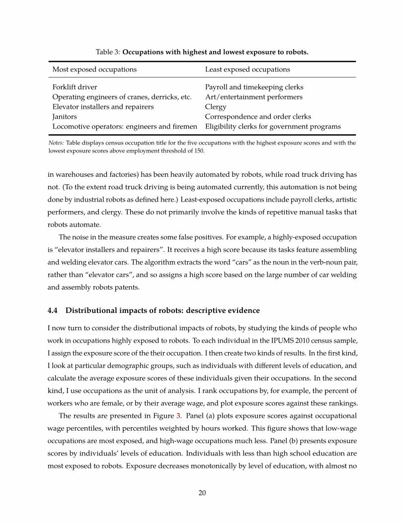
Table 3: Occupations with highest and lowest exposure to robots.

Most exposed occupations Least exposed occupations

Forklift driver Payroll and timekeeping clerksOperating engineers of cranes, derricks, etc. Art/entertainment performersElevator installers and repairers ClergyJanitors Correspondence and order clerksLocomotive operators: engineers and firemen Eligibility clerks for government programs

Notes: Table displays census occupation title for the five occupations with the highest exposure scores and with thelowest exposure scores above employment threshold of 150.

in warehouses and factories) has been heavily automated by robots, while road truck driving has

not. (To the extent road truck driving is being automated currently, this automation is not being

done by industrial robots as defined here.) Least-exposed occupations include payroll clerks, artistic

performers, and clergy. These do not primarily involve the kinds of repetitive manual tasks that

robots automate.

The noise in the measure creates some false positives. For example, a highly-exposed occupation

is “elevator installers and repairers”. It receives a high score because its tasks feature assembling

and welding elevator cars. The algorithm extracts the word “cars” as the noun in the verb-noun pair,

rather than “elevator cars”, and so assigns a high score based on the large number of car welding

and assembly robots patents.

4.4 Distributional impacts of robots: descriptive evidence

I now turn to consider the distributional impacts of robots, by studying the kinds of people who

work in occupations highly exposed to robots. To each individual in the IPUMS 2010 census sample,

I assign the exposure score of the their occupation. I then create two kinds of results. In the first kind,

I look at particular demographic groups, such as individuals with different levels of education, and

calculate the average exposure scores of these individuals given their occupations. In the second

kind, I use occupations as the unit of analysis. I rank occupations by, for example, the percent of

workers who are female, or by their average wage, and plot exposure scores against these rankings.

The results are presented in Figure 3. Panel (a) plots exposure scores against occupational

wage percentiles, with percentiles weighted by hours worked. This figure shows that low-wage

occupations are most exposed, and high-wage occupations much less. Panel (b) presents exposure

scores by individuals’ levels of education. Individuals with less than high school education are

most exposed to robots. Exposure decreases monotonically by level of education, with almost no

20

-.6-.4

-.20

.2.4

Stan

dard

ized

scor

es

0 20 40 60 80 100Occupational wage percentile

(a) Smoothed scores by occupational wage percentile0

2040

6080

Expo

sure

per

cent

ile

< HS HS Some coll. Bachelors Masters

(b) Exposure by level of education

3040

5060

70Ex

posu

re p

erce

ntile

0 20 40 60 80 100Percent of female workers in occupation

(c) Exposure by percent of female workers in occupa-tion

4045

5055

Expo

sure

per

cent

ile

20 30 40 50 60Age

(d) Exposure by age.

Figure 3: Exposure to robots by demographic groupNotes: Plot (a) shows the average of standardized occupation-level exposure scores for robots by occupational wagepercentile rank using a locally weighted smoothing regression (bandwidth 0.8 with 100 observations), following Acemogluand Autor (2011). Wage percentiles are measured as the employment-weighted percentile rank of an occupation’s meanhourly wage in the May 2016 Occupational Employment Statistics. Plot (b) is a bar graph showing the exposure scorepercentile for robots averaged across all industry-occupation observations, weighted by 2010 total employment ingiven educational category. Plot (c) is a binscatter. The x-axis is the percent of workers in an industry-occupationobservation reported female in the 2010 census. Plot (d) is a binscatter. The x-axis is the average age of workers in anindustry-occupation observation in the 2010 census.

21

exposure for those with master’s degrees. This is consistent with the results by occupational wage

percentile.

Panel (c) plots average exposure scores for occupations by percent of female workers. This shows

that occupations whose workers are predominantly male are much more exposed to robots than

occupations with a primarily female workforce. This is consistent with the clustering of men in

production jobs in manufacturing, which are very exposed to robots, while women are more likely

to work in jobs with a high level of interpersonal content, which are much less exposed. Finally,

Panel (d) shows the results by individuals’ age. I find that workers in their 20s are much more

likely to be exposed to robots than workers in their 30s and above. This reflects the fact that young

workers are much more likely to be engaged in manual work.

It bears reiterating that in this section I am only studying the types of people who work in

exposed occupations. This is different from studying what happens to those people. For example,

affected individuals could have suffered wage declines or unemployment, or they could have moved

to different jobs for which demand was strong. I discuss this issue further below.

4.5 Relationship between exposure and changes in wages and employment

As discussed in the model section above, the net effect of task-level substitution on demand for

occupations is theoretically ambiguous, due to the countervailing productivity and displacement

channels. I now study empirically the relationship between my measure of occupation exposure to

robots and changes in employment and wages over the period 1980 to 2010. The overall pattern of

results, for this and the other case studies, provides suggestive evidence that, over the long run,

task-level substitution results in occupation-level declines in employment and wages.

4.5.1 Empirical strategy

To study the relationship between exposure scores and changes in employment and wages, I estimate

variations of the following regression:

∆yo,i,t = αi + βExpo + γZo + εo,i,t.

In this specification, the unit of observation is an occupation-industry-year cell, such as welders

in auto manufacturing in 1980, with o denoting occupation, i industry, and t year. The dependent

variable is a long difference from 1980 to 2010 of an outcome variable of interest, such as wages.

On the right-hand side, I include industry fixed effects; Expo is the exposure of the occupation to

robots; and the vector of controls Zo contains occupation-level variables such as terciles of average

22

years of education.

As described in the model section, the use of occupation-industry-year cells helps to isolate

changes in the demand for occupations that are due to task-level substitution on the production

side, rather than those due to changes in consumers’ incomes and the prices they face. For example,

trade with China has substantially reduced demand for textiles produced in the US. If I used only

occupations as the unit of observation, then if there was a correlation between occupations exposed

to robots and occupations in industries exposed to trade with China, I would conflate these two

forces in the estimation. Instead, I study changes in relative labor demand within industries. For

example, if, within textile industries, the share of textile machine operatives in employment has

decreased, while that of managers has increased, this is more likely to be a function of factors

affecting production, rather than factors affecting demand.

In constructing a measure of change in employment, I face issues of entry and exit of occupation-

industry cells. Because of these zero-valued observations, reflecting new and obsolete jobs, I cannot

use log changes. Instead, I follow the literature and use DHS changes. Also known as arc percentage

change or percent change relative to the midpoint, DHS is a symmetric measure of the growth

rate defined as the difference of two values divided by their average (Davis, Haltiwanger, and

Schuh 1996). This results in a second-order approximation of the log change for growth rates near

zero; values are restricted to being between -2 and 2, with -2 and 2 representing exit and entry

respectively.

For wages, I use the log change in real weekly wages for full-time, full-year workers in each cell.

For exposure scores, I transform the raw scores to be in employment-weighted percentiles. Thus, a

score of 90 means that 10% of workers work in occupations with a higher exposure score. Industries

are in the IPUMS IND1990 consistent industry classification; this classification is used to construct

the occupation-industry cells, and also for industry fixed effects. Standard errors are clustered by

industry. Finally, the sample is restricted to industries within the manufacturing sector.

4.5.2 Results

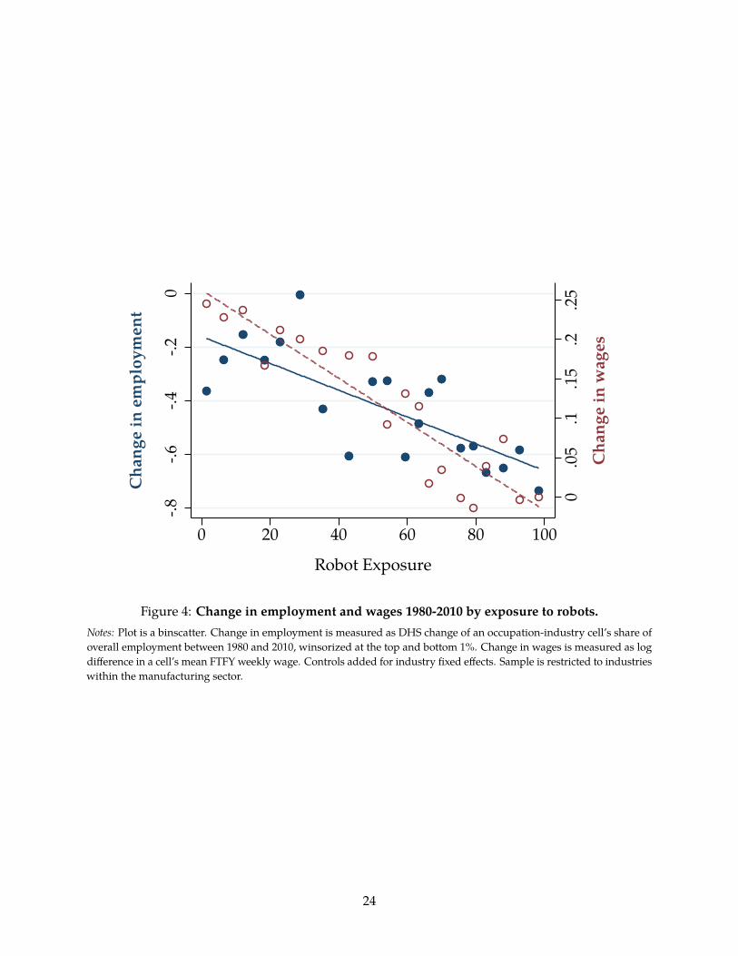
Figure 4 is a residual binscatter at the occupation-industry level showing the relationship between

robot exposure and changes in employment (blue line, left axis) and changes in wages (red line,

right axis), after controlling for industry fixed effects. Regression results corresponding to the

binscatter are presented in Tables 4 and 5. The first column does not control for industry fixed

effects; these are added in column (2). The controls added in the remaining columns are discussed

below.

These results are quantitatively large. Although I cannot attribute causality to the exposure

23

0.0

5.1

.15

.2.2

5C

hang

e in

wag

es

-.8-.6

-.4-.2

0

Cha

nge

in e

mpl

oym

ent

0 20 40 60 80 100

Robot Exposure

Figure 4: Change in employment and wages 1980-2010 by exposure to robots.Notes: Plot is a binscatter. Change in employment is measured as DHS change of an occupation-industry cell’s share ofoverall employment between 1980 and 2010, winsorized at the top and bottom 1%. Change in wages is measured as logdifference in a cell’s mean FTFY weekly wage. Controls added for industry fixed effects. Sample is restricted to industrieswithin the manufacturing sector.

24

Table 4: Change in wages vs. exposure to robots, 1980-2010.

(1) (2) (3) (4) (5)

Exposure -0.29∗∗∗ -0.28∗∗∗ -0.26∗∗∗ -0.16∗∗∗ -0.22∗∗∗(0.02) (0.02) (0.02) (0.03) (0.03)

Offshorability 0.84∗ 0.82∗ -2.29∗∗∗(0.44) (0.44) (0.50)

Medium education 7.84∗∗∗ 9.52∗∗∗(1.75) (1.67)

High education 10.22∗∗∗ 27.73∗∗∗(1.89) (2.01)

Wage -0.07∗∗∗(0.01)

Wage squared 0.00∗∗(0.00)

Adjusted R2 0.042 0.094 0.095 0.101 0.163Industry FEs X X X XObservations 6,708 6,708 6,708 6,708 6,708

Notes: Each observation is an occupation-industry cell. Dependent variable is 100x change in log wage between 1980 and2010 winsorized at the top and bottom 1%. Education variables are terciles of average years of education for occupation-industry cells in 1980. Wages are cells’ mean weekly wage for full-time, full-year workers in 1980. Offshorability is anoccupation-level measure from Autor and Dorn (2013). Sample is restricted to industries within the manufacturing sector.Standard errors are clustered by industry. * p<0.10, ** p<0.05, *** p<0.01.

scores, moving from the 25th to the 75th percentile of exposure to robots is associated with a decline

in industry employment share of between 9 and 18%, depending on the specification, and a decline

in wages of between 8 and 14%. Recall that these are within-industry effects. Thus, these results are

not simply showing that manufacturing jobs are exposed to robots, and manufacturing has (for

other reasons) declined. Rather, they show that within each manufacturing industry, the particular

occupations exposed to robots have declined much more than those that are not exposed.

There are a number of potential source of endogeneity, which I now address. First, I consider the

possibility that there were other changes occurring on the production side beyond robots. A major

force occurring over this time period was the rise of offshoring. I control for an occupation-level

index of offshorability in column (3) of the two regression tables, and find that it does not affect my

25

Table 5: Change in employment vs. exposure to robots, 1980-2010.

(1) (2) (3) (4) (5)

Exposure -0.37∗∗∗ -0.36∗∗∗ -0.35∗∗∗ -0.18∗∗∗ -0.16∗∗∗(0.03) (0.03) (0.03) (0.03) (0.03)

Offshorability 0.78 0.93∗ 2.02∗∗∗(0.54) (0.55) (0.55)

Medium education -0.26 -1.20(1.54) (1.54)

High education 21.39∗∗∗ 14.42∗∗∗(2.43) (2.40)

Wage 0.04∗∗∗(0.00)

Wage squared -0.00∗∗∗(0.00)

Adjusted R2 0.018 0.129 0.129 0.141 0.147Industry FEs X X X XObservations 14,065 14,065 14,065 14,065 14,065

Notes: Each observation is an occupation-industry cell. Dependent variable is 100x DHS change of a cell’s share of overallemployment between 1980 and 2010, winsorized at the top and bottom 1%. Education variables are terciles of averageyears of education for occupation-industry cells in 1980. Wages are cells’ mean weekly wage for full-time, full-yearworkers in 1980. Offshorability is an occupation-level measure from Autor and Dorn (2013). Observations are weightedby cell’s labor supply, averaged between 1980 and 2010. Sample is restricted to industries within the manufacturingsector. Standard errors are clustered by industry. * p<0.10, ** p<0.05, *** p<0.01.

results.

Second, there changes on the product demand side that could be affecting my results. The

industry fixed effects should absorb changes due to factors such as trade and shifting preferences

that affect demand for products. However, the industry classification is somewhat coarse. There are

only 82 industries I can consistently measure in manufacturing. It is therefore possible that there

are changes in product demand occurring within industries. To the extent these are correlated with

the use of robots in production, these could be biasing my results. It seems most likely that changes

in preferences and trade-induced shifts in demand would both point in the direction of favoring

higher-quality products. If robots were consistently associated with products of a particular kind,

26

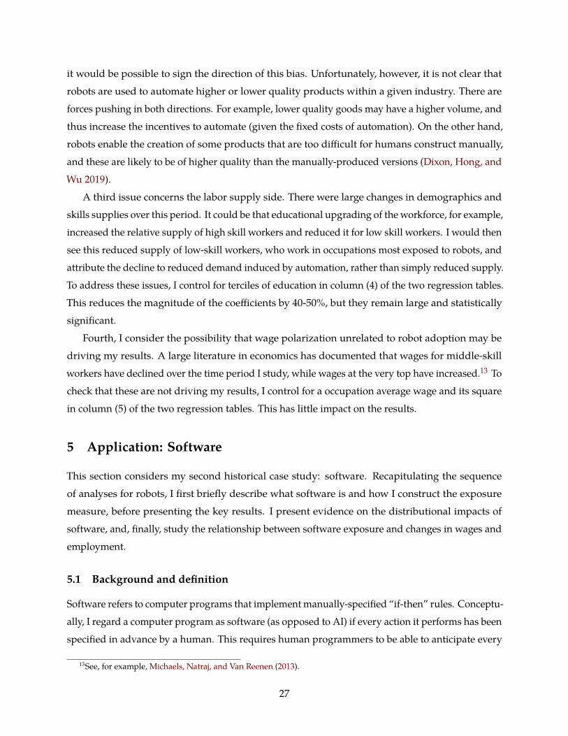
it would be possible to sign the direction of this bias. Unfortunately, however, it is not clear that

robots are used to automate higher or lower quality products within a given industry. There are

forces pushing in both directions. For example, lower quality goods may have a higher volume, and

thus increase the incentives to automate (given the fixed costs of automation). On the other hand,

robots enable the creation of some products that are too difficult for humans construct manually,

and these are likely to be of higher quality than the manually-produced versions (Dixon, Hong, and

Wu 2019).

A third issue concerns the labor supply side. There were large changes in demographics and

skills supplies over this period. It could be that educational upgrading of the workforce, for example,

increased the relative supply of high skill workers and reduced it for low skill workers. I would then

see this reduced supply of low-skill workers, who work in occupations most exposed to robots, and

attribute the decline to reduced demand induced by automation, rather than simply reduced supply.

To address these issues, I control for terciles of education in column (4) of the two regression tables.

This reduces the magnitude of the coefficients by 40-50%, but they remain large and statistically

significant.

Fourth, I consider the possibility that wage polarization unrelated to robot adoption may be

driving my results. A large literature in economics has documented that wages for middle-skill

workers have declined over the time period I study, while wages at the very top have increased.13 To

check that these are not driving my results, I control for a occupation average wage and its square

in column (5) of the two regression tables. This has little impact on the results.

5 Application: Software

This section considers my second historical case study: software. Recapitulating the sequence

of analyses for robots, I first briefly describe what software is and how I construct the exposure

measure, before presenting the key results. I present evidence on the distributional impacts of

software, and, finally, study the relationship between software exposure and changes in wages and

employment.

5.1 Background and definition

Software refers to computer programs that implement manually-specified “if-then” rules. Conceptu-

ally, I regard a computer program as software (as opposed to AI) if every action it performs has been

specified in advance by a human. This requires human programmers to be able to anticipate every

13See, for example, Michaels, Natraj, and Van Reenen (2013).

27

Table 6: Top extracted verbs and characteristic nouns for software.

Verb Example nouns Verb Example nouns

record data, position, log, location,reservation, transaction

detect defect, error, malware, fault,condition, movement

store program, data, information, image,instruction, value

generate data, image, file, report, map, key,password, animation, diagram

control access, display, unit, image, device,power, motor

measure rate, performance, time, distance,thickness

reproduce data, picture, media, file, sequence,speech, item, document, selection

receive signal, data, information, message,order, request, instruction, command

Notes: This table lists the top eight verbs by pair frequency extracted from the title text of patents corresponding tosoftware, together with characteristic direct objects for each verb chosen manually to illustrate a range of applications.Patents corresponding to each technology are selected using a keyword search. A dependency parsing algorithm is usedto extract verbs and their direct objects from patent titles.

contingency, and also to be able to describe the steps required to complete the task. Examples of

software include most applications we use on our computers, such as word processing, spreadsheet

software, and web browsers, as well as business applications such as enterprise resource planning

and reservation and ticketing systems.

5.2 Patent selection

To calculate exposure scores for software, I first define the set of patents that represent software

applications. Unlike for robots, where I had to construct my own definition, there is already

a standard definition of software patents in the literature. This was developed in Bessen and

Hunt (2007). In that paper, the authors follow a variant of the procedure I followed for robots: they

manually created a “test set” of patents that they labeled as either software or not software, identified

candidate key terms, and constructed a keyword search algorithm using these terms that they then

validated against their test set. Their final search algorithm require one of the keywords “software”,

“computer”, or “program” to be present, and none of the keywords “chip”, “semiconductor”, “bus”,

“circuity”, or “circuitry” to be present. This algorithm has a recall rate (fraction of “true” software

patents retrieved) of 78%, and a false discovery rate of 16% on their test set.

5.3 Measurement results

Top verb-noun pairs from patents Table 6 presents the most frequent verbs and illustrative nouns

extracted from the software patents. They include recording information, reservations, and locations;

28

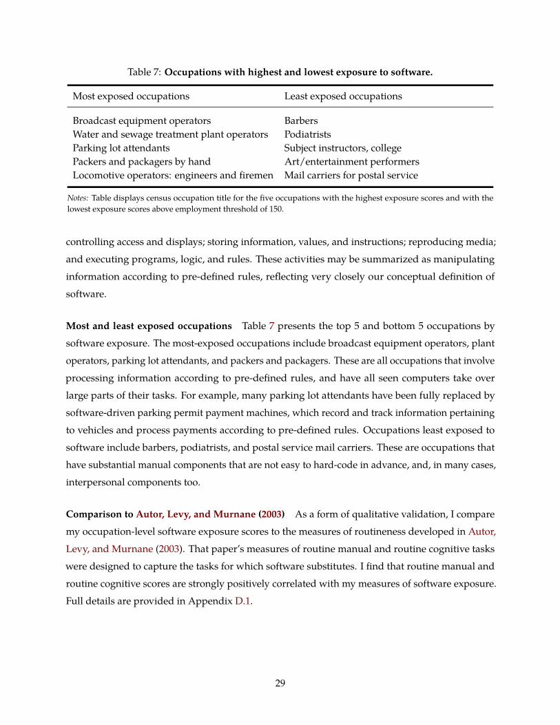
Table 7: Occupations with highest and lowest exposure to software.

Most exposed occupations Least exposed occupations

Broadcast equipment operators BarbersWater and sewage treatment plant operators PodiatristsParking lot attendants Subject instructors, collegePackers and packagers by hand Art/entertainment performersLocomotive operators: engineers and firemen Mail carriers for postal service

Notes: Table displays census occupation title for the five occupations with the highest exposure scores and with thelowest exposure scores above employment threshold of 150.

controlling access and displays; storing information, values, and instructions; reproducing media;

and executing programs, logic, and rules. These activities may be summarized as manipulating

information according to pre-defined rules, reflecting very closely our conceptual definition of

software.

Most and least exposed occupations Table 7 presents the top 5 and bottom 5 occupations by

software exposure. The most-exposed occupations include broadcast equipment operators, plant

operators, parking lot attendants, and packers and packagers. These are all occupations that involve

processing information according to pre-defined rules, and have all seen computers take over

large parts of their tasks. For example, many parking lot attendants have been fully replaced by

software-driven parking permit payment machines, which record and track information pertaining

to vehicles and process payments according to pre-defined rules. Occupations least exposed to

software include barbers, podiatrists, and postal service mail carriers. These are occupations that

have substantial manual components that are not easy to hard-code in advance, and, in many cases,

interpersonal components too.

Comparison to Autor, Levy, and Murnane (2003) As a form of qualitative validation, I compare

my occupation-level software exposure scores to the measures of routineness developed in Autor,

Levy, and Murnane (2003). That paper’s measures of routine manual and routine cognitive tasks

were designed to capture the tasks for which software substitutes. I find that routine manual and

routine cognitive scores are strongly positively correlated with my measures of software exposure.

Full details are provided in Appendix D.1.

29

-.3-.2

-.10

.1.2

Stan

dard

ized

scor

es

0 20 40 60 80 100Occupational wage percentile

(a) Smoothed scores by occupational wage percentile0

2040

60Ex

posu

re p

erce

ntile

< HS HS Some coll. Bachelors Masters

(b) Exposure by level of education

3040

5060

70Ex

posu

re p

erce

ntile

0 20 40 60 80 100Percent of female workers in occupation

(c) Exposure by percent of female workers in occupa-tion

3840

4244

46Ex

posu

re p

erce

ntile

20 30 40 50 60Age

(d) Exposure by age.

Figure 5: Exposure to software by demographic groupNotes: Plot (a) shows the average of standardized occupation-level exposure scores for software by occupational wagepercentile rank using a locally weighted smoothing regression (bandwidth 0.8 with 100 observations), following Acemogluand Autor (2011). Wage percentiles are measured as the employment-weighted percentile rank of an occupation’s meanhourly wage in the May 2016 Occupational Employment Statistics. Plot (b) is a bar graph showing the exposure scorepercentile for software averaged across all industry-occupation observations, weighted by 2010 total employment ingiven educational category. Plot (c) is a binscatter. The x-axis is the percent of workers in an industry-occupationobservation reported female in the 2010 census. Plot (d) is a binscatter. The x-axis is the average age of workers in anindustry-occupation observation in the 2010 census.

30

5.4 Distributional impacts of software: descriptive evidence

To examine the distributional impacts of software, I study the kinds of people who work in occupa-

tions highly exposed to software, following the same analysis procedure as for robots. The results

are presented in Figure 5. Panel (a), exposure scores by occupational wage percentile, shows that

middle-wage occupations are most exposed to software. This is consistent with the literature on

polarization, which has found that I.T. has reduced demand for middle-wage jobs while increasing

it for low- and high-wage jobs.14 Panel (b) presents exposure scores by individuals’ levels of educa-

tion. With robots, exposure was sharply decreasing with education. For software, exposure is still

decreasing with education, but much less sharply.

Panel (c) plots average exposure scores against percent of female workers in occupation. This

shows that occupations whose workers are predominantly male are much more exposed to software

than occupations with a primarily female workforce. This might be surprising, given that much of

the office work taken over by software has traditionally been performed by women. However, woman

also cluster in occupations requiring complex interpersonal interaction tasks, which software is not

capable of performing. Finally, panel (d) shows that software exposure is moderately increasing in

age.

5.5 Relationship between exposure and changes in wages and employment

To study the relationship between occupations’ exposure to software and changes in wages and

employment, I follow the same empirical strategy as for robots, described in Section 4.5.1. The only

difference is that whereas I restrict the sample for robots to industries in the manufacturing sector,

for software, I use all industries.

Figure 6 is a residual binscatter at the occupation-industry level showing the relationship

between robot exposure and changes in employment (blue line, left axis) and changes in wages (red

line, right axis), after controlling for industry fixed effects. Regression results corresponding to the

binscatter are presented in Tables 8 and 9. The sequence of columns is the same as for robots.

These results are quantitatively large, but not as large as for robots. For example, moving from

the 25th to the 75th percentile of exposure to software is associated with a decline in within-industry

employment shares of between 7 and 11%, and a decline in wages of between 2 and 6%.

These results for software face potential endogeneity from a similar set of sources to robots.

Tables 8 and 9 present results controlling for offshorability, education, and wage polarization. The

coefficient on exposure scores is robust to these controls in the employment regressions, with the

14See, for example, Michaels, Natraj, and Van Reenen (2013).

31

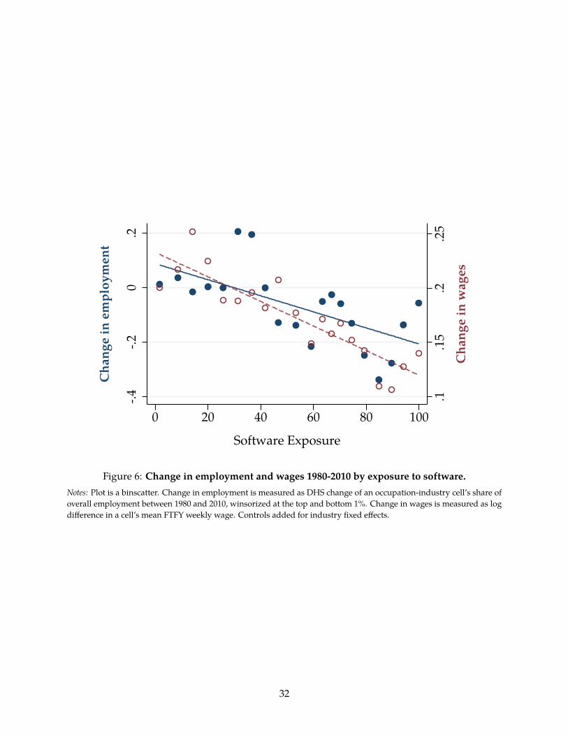
.1.1

5.2

.25

Cha

nge

in w

ages

-.4-.2

0.2

Cha

nge

in e

mpl

oym

ent

0 20 40 60 80 100

Software Exposure

Figure 6: Change in employment and wages 1980-2010 by exposure to software.Notes: Plot is a binscatter. Change in employment is measured as DHS change of an occupation-industry cell’s share ofoverall employment between 1980 and 2010, winsorized at the top and bottom 1%. Change in wages is measured as logdifference in a cell’s mean FTFY weekly wage. Controls added for industry fixed effects.

32

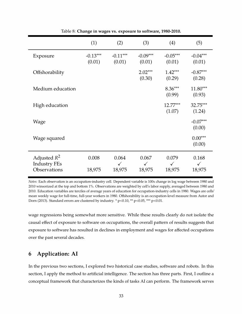
Table 8: Change in wages vs. exposure to software, 1980-2010.

(1) (2) (3) (4) (5)

Exposure -0.13∗∗∗ -0.11∗∗∗ -0.09∗∗∗ -0.05∗∗∗ -0.04∗∗∗(0.01) (0.01) (0.01) (0.01) (0.01)

Offshorability 2.02∗∗∗ 1.42∗∗∗ -0.87∗∗∗(0.30) (0.29) (0.28)

Medium education 8.36∗∗∗ 11.80∗∗∗(0.99) (0.93)

High education 12.77∗∗∗ 32.75∗∗∗(1.07) (1.24)

Wage -0.07∗∗∗(0.00)

Wage squared 0.00∗∗∗(0.00)

Adjusted R2 0.008 0.064 0.067 0.079 0.168Industry FEs X X X XObservations 18,975 18,975 18,975 18,975 18,975

Notes: Each observation is an occupation-industry cell. Dependent variable is 100x change in log wage between 1980 and2010 winsorized at the top and bottom 1%. Observations are weighted by cell’s labor supply, averaged between 1980 and2010. Education variables are terciles of average years of education for occupation-industry cells in 1980. Wages are cells’mean weekly wage for full-time, full-year workers in 1980. Offshorability is an occupation-level measure from Autor andDorn (2013). Standard errors are clustered by industry. * p<0.10, ** p<0.05, *** p<0.01.

wage regressions being somewhat more sensitive. While these results clearly do not isolate the

causal effect of exposure to software on occupations, the overall pattern of results suggests that

exposure to software has resulted in declines in employment and wages for affected occupations

over the past several decades.

6 Application: AI

In the previous two sections, I explored two historical case studies, software and robots. In this

section, I apply the method to artificial intelligence. The section has three parts. First, I outline a

conceptual framework that characterizes the kinds of tasks AI can perform. The framework serves

33

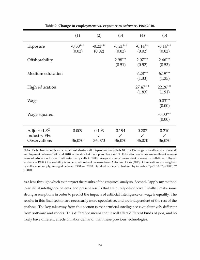
Table 9: Change in employment vs. exposure to software, 1980-2010.

(1) (2) (3) (4) (5)

Exposure -0.30∗∗∗ -0.22∗∗∗ -0.21∗∗∗ -0.14∗∗∗ -0.14∗∗∗(0.02) (0.02) (0.02) (0.02) (0.02)

Offshorability 2.98∗∗∗ 2.07∗∗∗ 2.66∗∗∗(0.51) (0.52) (0.53)

Medium education 7.28∗∗∗ 6.19∗∗∗(1.33) (1.35)

High education 27.47∗∗∗ 22.26∗∗∗(1.83) (1.91)

Wage 0.03∗∗∗(0.00)

Wage squared -0.00∗∗∗(0.00)

Adjusted R2 0.009 0.193 0.194 0.207 0.210Industry FEs X X X XObservations 36,070 36,070 36,070 36,070 36,070

Notes: Each observation is an occupation-industry cell. Dependent variable is 100x DHS change of a cell’s share of overallemployment between 1980 and 2010, winsorized at the top and bottom 1%. Education variables are terciles of averageyears of education for occupation-industry cells in 1980. Wages are cells’ mean weekly wage for full-time, full-yearworkers in 1980. Offshorability is an occupation-level measure from Autor and Dorn (2013). Observations are weightedby cell’s labor supply, averaged between 1980 and 2010. Standard errors are clustered by industry. * p<0.10, ** p<0.05, ***p<0.01.

as a lens through which to interpret the results of the empirical analysis. Second, I apply my method

to artificial intelligence patents, and present results that are purely descriptive. Finally, I make some

strong assumptions in order to predict the impacts of artificial intelligence on wage inequality. The

results in this final section are necessarily more speculative, and are independent of the rest of the

analysis. The key takeaway from this section is that artificial intelligence is qualitatively different

from software and robots. This difference means that it will affect different kinds of jobs, and so

likely have different effects on labor demand, than these previous technologies.

34

6.1 Definitions and conceptual framework

In this subsection, I first define artificial intelligence, then use this definition to elaborate a conceptual

framework that characterizes the kinds of tasks that artificial intelligence can perform. I developed

this framework through more than 50 interviews with computer scientists at the forefront of AI

research.

Definitions I use the term artificial intelligence to refer to machine learning algorithms. Specif-

ically, I have in mind two kinds of machine learning algorithms: supervised learning and rein-

forcement learning algorithms. I define these further below. I recognize that artificial intelligence

has broader scope, and my use is not meant prescriptively. My focus is motivated by the dramatic

practical advances in supervised and reinforcement learning in recent years (Krizhevsky, Sutskever,

and Hinton 2012; Mnih et al. 2015) and their broad economic applicability.

The definition of supervised learning is as follows. A supervised learning algorithm learns

functions that map inputs into outputs from training data consisting of example input-output pairs.

One of the simplest examples of a supervised learning algorithm is linear regression. With linear

regression, the inputs are the independent variables, and the output is the dependent variable.

Supervised learning extends beyond the standard uses of linear regression in economics along

two dimensions. First, it allows for a much more flexible relationship between the inputs and

the outputs. Second, inputs and outputs may be any kind of data, such as text or images. For

instance, a supervised learning algorithm may learn a function that maps an image (input) into a

textual description of the image (output), using a bank of examples of image-description pairs. With

appropriate training data, it could learn to map a customer’s financial history into their likelihood

of repaying a loan, or sentences in one language into another. The algorithm learns the statistical

relationships present in the training data, so, in a loose sense, the data must “contain” enough

information for it to learn the function.

A reinforcement learning algorithm, by contrast, learns how to take actions in a dynamic environ-

ment in order to achieve an objective. This sounds like the definition of optimal control, and, indeed,

dynamic programming is an example of a reinforcement learning algorithm. However, whereas

dynamic programming is typically used with environments that have a very low-dimensional state

space, recent research in reinforcement learning has enabled the application of similar principles

to more complex settings, such as three-dimensional physical environments. Examples might be

controlling the fingers of a robot hand to perform dextrous manipulation, operating the machinery

in a factory to optimize energy efficiency, or exchanging messages with a human to troubleshoot

a technical problem. These algorithms learn by a kind of trial-and-error, so, in order to succeed,

35

they require experiments in the environment, or a good simulator of it, and a way of evaluating

performance.

Conceptual framework These requirements suggest three constraints on the kinds of tasks that

can be performed by artificial intelligence algorithms. First, there must be enough of the right kind

of training data available. Second, the task must have an objective that is easy to measure. Third,

the algorithm must have access to the “levers” it needs to complete the task. I now describe each

constraint in more detail, and give examples of tasks that do and do not satisfy each one.

First, consider data availability. This is important for both supervised and reinforcement learning,

but in different ways. In supervised learning, there must be enough examples of the task being done

correctly for the algorithm to learn from. Certain kinds of information are regularly stored at scale,

like system logs, sensor data, and records kept by humans. Some tasks, such as operating a power

plant or auditing a company’s accounts, involve processing such information and little else. This

makes them a good target for supervised learning. Other tasks, like discussing a treatment plan

with a patient or advising a student on their research, consist of interactions that are not usually

recorded, perhaps because doing so would be unethical or illegal. This makes training data difficult

to obtain. Data must also be sufficiently comprehensive. A company may have enough recordings

of customer support interactions to train an algorithm to answer queries about its current products.

But as soon as it releases a new product, new training data will be required. In general, tasks with

stable, systematic relationships between inputs and decisions, such as sorting agricultural products,

translating languages, or interpreting medical images, are much easier to learn than tasks with

frequent changes or one-off exceptions, such as those handled by customer service supervisors,

flight attendants, or any kind of team leader.

In reinforcement learning, learning by trial-and-error takes the place of learning from examples.

Experimentation by an algorithm in the real world can be costly or unethical, so learning in simula-

tion is often preferred (Rusu et al. 2016). A simulator may itself be learned from observational data,

again requiring that such data be available (Rezende, Mohamed, and Wierstra 2014). Alternatively,

a human could build a simulator manually. This may be possible for human-designed systems, like

robots or industrial processes, and for well-understood aspects of the natural world, like classical

mechanics. But manually building a simulator of a human to interact with would be more difficult.

This means that, in practice, robotic locomotion and dextrous manipulation are more amenable to

reinforcement learning than, say, motivational speaking, product development, or public relations.

For the same reason, physical activities in contexts like assembly lines that are strictly regimented,

hence easy to simulate, are easier to learn than physical activities in more variable contexts like

36

construction sites, homes, or offices.

The second constraint on the kinds of tasks amenable to artificial intelligence is that they

must have an objective that is easy to measure. This is because algorithms need to evaluate their

performance in order to improve. Optimizing for energy efficiency is possible because energy

efficiency is easily measurable. But it is less easy to measure success in tasks like writing a corporate

strategy, negotiating an agreement, leading a team, or even tidying a room, and optimizing a

misspecified objective can be highly counterproductive (Amodei et al. 2016). Delayed feedback,

which characterizes many activities, makes learning even harder (Sutton 1984). An algorithm could

ask for guidance from a human (Christiano et al. 2017), but a human may not have the patience

to give it, especially if they are a paying customer. Most algorithms also need too many examples

to be able to learn from a single human in real time. Tasks with objectives that can be evaluated

immediately and automatically, such as maximizing the click-through rate of an ad, or minimizing

the materials costs of a computer chip, are thus easier for algorithms to learn than tasks with

“fuzzier” or longer-term objectives, such as many managerial activities.

The final constraint is the action space, or “levers”, available to the algorithm. Most humans can

walk and speak, many can sign contracts, and some can get the president on the phone. Algorithms,

by contrast, run on silicon chips. They interact with the world only by issuing electronic commands

to other systems via human-constructed interfaces. These interfaces may be costly to create, such

as when physical equipment or legacy software systems are involved (David 1990). Prudence or

regulation may limit interfaces that pose safety, operational, financial, or other kinds of risk. And

many activities, such as those of investigative journalists, executive recruiters, or managers, depend

on human relationships, which are hard for algorithms to acquire. All these severely limit the kinds

of tasks amenable to automation of any kind, including artificial intelligence.

Relationship of artificial intelligence to robots and software How does artificial intelligence

differ from software? With artificial intelligence, the human programmer defines the learning

algorithm, which then learns for itself from data or experimentation how to achieve an objective.

With software, as noted above, the human programmer must code a sequence of “if-then” steps

that directly completes the task (Autor, Levy, and Murnane 2002). Many applications, such as

algorithms for self-driving cars, involve a mixture of both, so the distinction is not always clean. In

the labor economics literature, tasks whose execution steps can be expressed as a codified sequence

of instructions by a programmer have been labeled “routine” (Autor, Levy, and Murnane 2003).

Tasks for which it is impractical to write down the execution steps are known as “non-routine”.

Software can therefore carry out routine tasks, in this sense, but not non-routine ones. In principle,

37

artificial intelligence is not limited to routine tasks, and, indeed, I find using my method that many

non-routine tasks are highly exposed to artificial intelligence.

What about robots? Robots are physical pieces of equipment. To do anything useful, such a

piece of equipment must be given instructions. Historically, these instructions have been provided

by software. This means that each robot action must be specified in advance. Variability in the

physical environment, and in the task itself, must therefore be kept to a minimum, since any change

necessities an expensive re-programming of the robot. Moreover, many useful tasks, such as picking

up arbitrary objects in a warehouse, are so variable by definition that it is impossible to program

them using software. This picture changes with artificial intelligence. Within the constraints

described in the previous section, an algorithm can learn for itself how to map information about

the environment, such as visual and tactile data from the robot’s sensors, into instructions sent to

the robot’s actuators. This means that many tasks it was impossible to program robots to do using

traditional software methods may now become possible using artificial intelligence.

6.2 Patent selection and descriptives

To select artificial intelligence patents, I use search terms corresponding to the definition presented

above. The terms are “supervised learning” and “reinforcement learning”, together with “neural

network” and “deep learning”. Neural networks are the general-purpose function approximators

used in both supervised and reinforcement learning, and “deep” neural networks have been a key

driver of the recent success in applications. The use of deep neural networks in machine learning is

often described as “deep learning”.

6.3 Measurement results

Table 10 presents the most frequent verbs and illustrative nouns extracted from artificial intelli-

gence patents. They include recognizing speech and voices, predicting prognosis and treatment,

recognizing images and detecting cancel, identifying damage, and detecting fraud. These are tasks

involved in, for example, medical imaging and treatment, insurance adjusting, and fraud analysis,

all areas that are currently seeing high levels of AI research and development. Notably, these

activities are of a very different kind to those identified for robots and software. Whereas robots

perform “muscle” tasks and software performs routine information processing, AI performs tasks

that involve detecting patterns, making judgments, and optimization.

The fact that AI performs different tasks from robots and software suggests that it is likely

to affect different occupations. Indeed, I find that the set of occupations exposed to AI is very

different to that exposed to robots and software. The most and least exposed occupations are

38

Table 10: Top extracted verbs and characteristic nouns for AI.

Verb Example nouns Verb Example nouns

recognize pattern, image, speech, face, voice,automobile, emotion, gesture, disease

determine state, similarity, relevance,importance, characteristic, strategy,risk

predict quality, performance, fault, behavior,traffic, prognosis

control process, emission, traffic, engine,robot, turbine, plant

detect signal, abnormality, defect, object,fraud, event, spammer, human, cancer

generate image, rating, lexicon, warning,description, recommendation

identify object, type, damage, illegality,classification, relationship,importance

classify data, object, image, pattern, signal,text, electrogram, speech, motion

Notes: This table lists the top eight verbs by pair frequency extracted from the title text of patents corresponding to AI,together with characteristic direct objects for each verb chosen manually to illustrate a range of applications. Patentscorresponding to each technology are selected using a keyword search. A dependency parsing algorithm is used toextract verbs and their direct objects from patent titles.

displayed in Table 11. Consider some of the occupations most exposed to AI. Clinical laboratory

technicians perform the visual and analytical work of identifying pathologies from medical tests; AI

applications have now been developed to automate much of this work (Janowczyk and Madabhushi

2016). Chemical engineers design and operate chemical production processes. AI algorithms are

particularly well-suited to these discovery and optimization tasks, and are already being used in

such applications (Agrawal, McHale, and Oettl 2019; Goh, Hodas, and Vishnu 2017). Optometrists

detect diseases in the eye. Optometry is the area of medicine that has seen perhaps the most success

of AI algorithms to date (De Fauw et al. 2018). Finally, power plant operators control all kinds of

equipment to generate the right amount of power in a safe and energy efficient manner. To date,

several companies who run power plants and data centers have replaced manual human operation

with AI algorithms, which are able to achieve much more efficient operation than human engineers

(Lazic et al. 2018).

While these are all high-skilled jobs, it is worth noting that there are also low-skilled jobs that

are highly exposed to AI. For example, many production jobs that involve inspection and quality

control are exposed to AI. However, as we will see in the next section, these jobs constitute a small

proportion of the low-skill workforce, meaning that low-skilled jobs are less exposed to AI on an

employment-weighted basis.

The occupations least exposed to AI include college professors, food preparation workers, and

postal service mail carriers. We can loosely split these occupations into three categories. First, there

39

Table 11: Occupations with highest and lowest exposure to artificial intelligence.

Most exposed occupations Least exposed occupations

Clinical laboratory technicians Animal caretakers, except farmChemical engineers Food preparation workersOptometrists Mail carriers for postal servicePower plant operators Subject instructors, collegeDispatchers Art/entertainment performers

Notes: Table displays census occupation title for the five occupations with the highest exposure scores and with thelowest exposure scores above employment threshold of 150.

are high-skill occupations that involve reasoning about situations that have never been seen before,

such as various kinds of researcher. Second, there are occupations of all skill levels that involve

interpersonal skill, such as teachers and managers. Third, there is manual work that occurs in

non-factory environments, and that often involves some element of interpersonal skill too, such as

baristas, food preparation workers, or massage therapists.

6.3.1 Industry case studies

To draw out these differences, it is instructive to consider sets of superficially similar occupations

in the same industry. First, consider legal occupations. The large number of companies working

on artificial intelligence for the law makes it tempting to conclude that lawyers will soon be made

obsolete. However, my results suggest that two other occupations, paralegals and administrative

law judges, are much more exposed to AI than lawyers themselves. The reason for this is clear

from their tasks. Paralegals spend most of their time reviewing documents. These tasks, such

as reviewing contracts for unusual clauses, are highly amenable to automation using AI. This is

because the objectives can be clearly specified (e.g., “score this clause for how common it is in

contracts of this type”), and there exist large amounts of relevant training data, often in the public

domain. Administrative law judges, similarly, spend most of their time making judgments on

cases that are highly standardized and for which the law is settled. By contrast, lawyers spend

much of their time conferring with clients and colleagues, representing clients in negotiations and

court cases, and working on cases for which sufficient precedent does not exist for an algorithm

to be trained successfully. This mix of interpersonal work and handling novel situations renders

them only very lightly exposed to AI. This conclusion matches other work that has considered this

question. Remus and Levy (2017) conduct a careful manual study of laywers’ time use, based on

data from a legal billing software vendor. For each category of activity, they identify the amount of

40

the activity it is possible to automate, based on a detailed examination of the technical details and

currently available commercial products. They, too, find that the vast majority of lawers’ time is

spent on activities that are not amenable to artificial intelligence.

Second, consider healthcare occupations. Again, the high degree of media attention devoted to

the use of artificial intelligence in certain healthcare tasks, such as diagnosis, makes it easy to assume

that doctors will be most impacted by artificial intelligence. My exposure scores for healthcare

occupations suggest that this is an incomplete picture. Doctors do have some exposure to AI,

given their task of diagnosing conditions, which is highly exposed. However, their work contains

substantial interpersonal components, meaning they are only lightly exposed overall. Nurses are

similar: some parts of their jobs, such as monitoring patients for changes in condition, are highly

exposed to AI, while other parts, such as talking to patients, preparing them for treatments, and

coordinating with healthcare team members, are not. By contrast, some more specialized medical

occupations are highly exposed. Medical technicians, optometrists, and pathologists all specialize

in precisely the things that AI automates, meaning they are highly exposed. Lower-skill healthcare

occupations, such as home health care aides, are much less exposed, given highly variable physical

and interpersonal activities they perform.

6.4 Distributional impacts: descriptive evidence

I now turn to the distributional impacts of artificial intelligence. First, I present purely descriptive

evidence on the kinds of people who work in occupations that are exposed to artificial intelligence.

In the next section, I make some strong additional assumptions in order to make predictions about

employment and wage impacts.

Figure 7 presents distributional results as for robots and software. Panel (a) plots exposure

scores against occupational wage percentiles, with percentiles weighted by hours worked. This

figure shows that low-wage occupations are least exposed, and high-wage occupations much more

exposed. Together, these two panels reflect the fact that the things AI is good at — activities

involving detecting patterns, judgment, and optimization — tend to be performed by higher-skill

workers. As noted above, there are low-skilled jobs that are highly exposed to AI, such as production

jobs involving inspection and quality control. However, these jobs constitute a small proportion

of the low-skill workforce. Low-skilled people today are much more likely to work in face-to-face

service occupations, such as in retail and food service, that are less exposed to AI. Panel (b) presents

exposure scores by individuals’ levels of education. AI has the opposite pattern to robots and

software: exposure is increasing in education, with those with master’s degrees most exposed.

Panel (c) plots average exposure scores against percent of female workers in occupation. In this

41

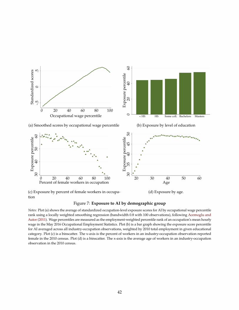
-.50

.5St

anda

rdiz

ed sc

ores

0 20 40 60 80 100Occupational wage percentile

(a) Smoothed scores by occupational wage percentile0

2040

60Ex

posu

re p

erce

ntile

< HS HS Some coll. Bachelors Masters

(b) Exposure by level of education

3040

5060

Expo

sure

per

cent

ile

0 20 40 60 80 100Percent of female workers in occupation

(c) Exposure by percent of female workers in occupa-tion

3035

4045

50Ex

posu

re p

erce

ntile

20 30 40 50 60Age

(d) Exposure by age.

Figure 7: Exposure to AI by demographic groupNotes: Plot (a) shows the average of standardized occupation-level exposure scores for AI by occupational wage percentilerank using a locally weighted smoothing regression (bandwidth 0.8 with 100 observations), following Acemoglu andAutor (2011). Wage percentiles are measured as the employment-weighted percentile rank of an occupation’s mean hourlywage in the May 2016 Occupational Employment Statistics. Plot (b) is a bar graph showing the exposure score percentilefor AI averaged across all industry-occupation observations, weighted by 2010 total employment in given educationalcategory. Plot (c) is a binscatter. The x-axis is the percent of workers in an industry-occupation observation reportedfemale in the 2010 census. Plot (d) is a binscatter. The x-axis is the average age of workers in an industry-occupationobservation in the 2010 census.

42

respect, AI looks much more the other technologies, with “male” jobs much more exposed to AI

than “female” ones. This reflects the fact that men have historically been much more likely than

women to work in the technical jobs exposed to AI, while, again, women have been more likely to

work in roles requiring more interpersonal skill, which are less exposed to AI.

Finally, Panel (d) shows the results by individuals’ age. As might be expected from the fact that

AI-exposed jobs are predominantly those involving high levels of education, judgment, and therefore

accumulated experience, it is older workers who are most exposed to AI. Younger workers are

barely exposed at all. This means that AI potentially represents a “triple wammy” for older workers.

First, older workers tend to be less mobile than younger workers, in terms of both occupation and

geography, making it more difficult for them to adapt. They also have fewer years of working life

remaining, making educational and training investments less attractive for them. Second, there

are increasingly many of them, due to the aging of the Baby Boomer generation. So the supply of

this demographic is substantially increasing. These first two issues would be potentially negative

for any automation technology. The third issue is that AI, in particular, is predicted to impact

precisely the occupations that older workers predominantly work in. If the impacts of exposure

to AI are negative, these negative impacts may therefore be more concentrated on older workers

than the impacts of software and robots. On the other hand, there is some evidence that most

changes in employment by occupation occur via the entry margin, that is, fewer young workers

joining the occupation, than via the exit margin, that is, more older workers leaving it (voluntarily

or involuntarily) (Webb and Chandler 2018). As such, the impacts on individuals are likely to be

more nuanced than a simple calculation of exposure by demographic would suggest.

6.5 Potential impacts on inequality

This section moves from purely descriptive results about the occupations and groups exposed

to AI to a quantification of its potential impacts on inequality. To do this, I make the additional

assumption that the relationship between AI exposure and changes in wages will have the same

negative, approximately linear relationship as the relationship that existed between exposure to

software and robots and changes in wages. There are, of course, reasons why this may not be the

case, which I explore below. The results in this section simply extrapolate directly from the patterns

identified in the historical case studies, and explore the consequences for inequality given the very

different occupations that are exposed to AI compared to robots and software.

Under the assumption of a linear, negative relationship between AI exposure and changes in

wages, I calculate the wage distribution for different potential magnitudes of this relationship. I

take the average wage for every occupation in 2010, and adjust each one by its AI exposure score

43

90:10

99:90

.85

.9.9

51

1.05

Ratio

(201

0 =

1)

0 .001 .002 .003 .004 .005Coefficient on exposure (x -1)

Figure 8: Potential impacts of artificial intelligence on inequality.Notes: Ratios calculated from the percentiles of wage ∗ eβ∗exposure for various values of β, the coefficient on exposure in aregression with change in log wages as the dependent variable. The sign of the coefficient has been flipped.

Wage elasticity (software)

Wage elasticity (robots)

multiplied by a sequence of coefficient values ranging from 0 to 0.005. This range reflects the range

of coefficient estimates on exposure scores that I estimate in the wage regressions for robots and

software. In those regressions, the dependent variable was the change in log wages between 1980

and 2010. This range therefore represents impacts that took several decades to occur for software

and robots. For each value of the coefficient, I re-calculate the percentiles of the distribution of

average wages across occupations. I then calculate the ratios of the 90th to the 10th percentile of

wages, and the ratio of the 99th to the 90th percentile.

Figure 8 plots these ratios as a function of the magnitude of the exposure coefficient. A marginal

increase in the exposure coefficient, which corresponds to a greater impact of AI, is associated

with a marginal decline in the 90:10 ratio, but a marginal increase in the 99:90 ratio. A coefficient

on exposure equivalent to that estimated for software is associated with a 4% decrease in 90:10

inequality; using the coefficient estimated for robots, the decrease is 9%. In other words, AI could

compress wages in the middle of the distribution, but expand inequality at the top. The pattern for

the 90:10 ratio reflects the fact that high-wage occupations are relatively more exposed to AI than

low-wage occupations. The pattern for the 99:90 ratio reflects the fact that the very highest-paid

occupations, such as CEOs and professionals, are less exposed.

44

6.6 Discussion

These results should be interpreted with caution. First, they rely on a constant mapping between

my exposure scores and changes in demand. In the language of the model, they require that the

structural parameters of the elasticities of substitution at various levels remain constant. This does

not seem unreasonable, but it is certainly a strong assumption. The fact that the relationship between

exposure scores and changes in wages was negative for both historical case studies shows that the

balance of forces favored substitution in the past. This may move our priors toward thinking that

the same will be true in the future. To the extent this relationship no longer holds, however, these

projected impacts will be invalid.

Second, when considering the impacts on inequality, a number of measurement issues arise. For

example, there have been substantial changes in the way that top earners receive their income in

recent decades (Smith et al. 2019), and these are not captured in my exercise. I also do not capture

the fact that owners of capital may benefit from artificial intelligence (Freeman 2015). As such, it is

likely that I am understating the increase in 99/90 inequality that may result from AI.

Third, I cannot rule out that AI will produce purely labor-augmenting technical change that

will advantage some types of labor over others. As noted in the model section, however, for this to

affect my results, the distribution of impacts on labor demand due to labor-augmenting technical

change would need to be correlated with the distribution of impacts due to substitution. The same

goes for the other ways in which technology affects labor demand, such as product rather than

task-level substitution. There is no a priori reason to think this would be the case, though this is an

important direction for further research.

Finally, there is the question of timing. While there is some relationship between the time pattern

of patenting and that of technology adoption, we are too early in the development of AI to know

how much more of the technology there is to be developed, and too early also to know how long it

will take to be adopted. If history is a guide, the main impacts on the labor market may not appear

for three decades (Jovanovic and Rousseau 2005; Yates 2005). AI could be faster to diffuse than

previous technologies, given the lack of a need to manually specify its rules of operation. However,

it could also be slower, given its vast data requirements and the need for other complementary

investments (Brynjolfsson, Rock, and Syverson 2018).

7 Conclusion

This paper has developed a new method for identifying the exposure of occupations to different

technologies, and applied it to two historical case studies, software and robots, and to artificial

45

intelligence. The results leave little room for doubt that artificial intelligence is likely to affect very

different kinds of occupations, and so different kinds of workers, than software and robots. Whereas

low-skill occupations are most exposed to robots, and middle-skill occupations are most exposed

to software, it is high-skill occupations that are most exposed to artificial intelligence. Moreover,

artificial intelligence is much more likely to affect highly-educated and older workers than these

previous technologies.

Substantial uncertainty about the impacts of artificial intelligence remains. While the method

developed in this paper captures the tasks for which AI substitutes, it is possible that AI will also

complement some kinds of tasks, with different effects on labor demand. Moreover, the impacts

on workers depend not just on labor demand, the focus of this paper, but also on labor supply.

In particular, future patterns of human capital investment and occupational mobility will have

important effects on equilibrium employment and wages. Artificial intelligence may also affect

the labor market through more indirect channels. For example, it may lead to the creation of new

products, which could affect labor demand, and to more efficient delivery of education, which

could affect labor supply. For all these reasons, the results presented in this paper should be seen

only as a first step towards estimating the labor market impacts of artificial intelligence.

46

References

Acemoglu, Daron and David H Autor. 2011. “Skills, Tasks and Technologies: Implications for

Employment and Earnings.” In Handbook of Labor Economics. Vol. 4, Part B, , ed. David Card and

Orley Ashenfelter, 1043–1171. Elsevier.

Acemoglu, Daron and Pascual Restrepo. 2017. “Robots and Jobs: Evidence from US Labor Markets.”

NBER Working Paper Series w23285.

Acemoglu, Daron and Pascual Restrepo. 2018. “The Race between Man and Machine: Implica-

tions of Technology for Growth, Factor Shares, and Employment.” American Economic Review,

108(6): 1488–1542.

Agrawal, Ajay, John McHale, and Alexander Oettl. 2019. “Artificial Intelligence, Scientific Discov-

ery, and Commercial Innovation.” Working Paper.

Akerman, Anders, Ingvil Gaarder, and Magne Mogstad. 2015. “The Skill Complementarity of

Broadband Internet.” The Quarterly Journal of Economics, 130(4): 1781–1824.

Amodei, Dario, Chris Olah, Jacob Steinhardt, Paul Christiano, John Schulman, and Dan Mane.

2016. “Concrete Problems in AI Safety.” arXiv cs.AI.

Arntz, Melanie, Terry Gregory, and Ulrich Zierahn. 2017. “Revisiting the risk of automation.”

Economics Letters, 159: 157–160.

Autor, David H and David Dorn. 2013. “The Growth of Low-Skill Service Jobs and the Polarization

of the US Labor Market.” The American Economic Review, 103(5): 1553–1597.

Autor, David H, Frank S Levy, and Richard J Murnane. 2002. “Upstairs, Downstairs: Computers

And Skills On Two Floors Of A Large Bank.” Industrial and Labor Relations Review, 55(3): 432–447.

Autor, David H, Frank S Levy, and Richard J Murnane. 2003. “The Skill Content of Recent Techno-

logical Change: An Empirical Exploration.” The Quarterly Journal of Economics, 118(4): 1279–1333.

Bessen, James. 2015. Learning by Doing: The Real Connection Between Innovation, Wages, and Wealth.

Yale University Press.

Bessen, James E, Maarten Goos, Anna Salomons, and Wiljan Van den Berge. 2019. “Automatic

Reaction-What Happens to Workers at Firms that Automate?” Boston Univ. School of Law, Law and

Economics Research Paper.

47

Brynjolfsson, Erik and Tom Mitchell. 2017. “What Can Machine Learning Do? Workforce Impli-

cations.” Science, 358(6370): 1530–1534.

Brynjolfsson, Erik, Daniel Rock, and Chad Syverson. 2018. “The Productivity J-curve: How

Intangibles Complement General Purpose Technologies.” NBER Working Paper Series w25148.

Brynjolfsson, Erik, Tom Mitchell, and Daniel Rock. 2018. “What Can Machines Learn, and What

Does It Mean for Occupations and the Economy?” Vol. 108, 43–47.

Chin, Aimee, Chinhui Juhn, and Peter Thompson. 2006. “Technical Change and the Demand for

Skills during the Second Industrial Revolution: Evidence from the Merchant Marine, 1891–1912.”

The Review of Economics and Statistics, 88(3): 572–578.

Christiano, Paul, Jan Leike, Tom B Brown, Miljan Martic, Shane Legg, and Dario Amodei. 2017.

“Deep Reinforcement Learning from Human Preferences.” arXiv stat.ML.

David, Paul A. 1990. “The Dynamo and the Computer: An Historical Perspective on the Modern

Productivity Paradox.” The American Economic Review, 80(2): 355–361.

Davis, Steven J, John Haltiwanger, and Scott Schuh. 1996. “Job creation and job destruction.”

De Fauw, Jeffrey, Joseph R Ledsam, Bernardino Romera-Paredes, Stanislav Nikolov, Nenad

Tomasev, Sam Blackwell, Harry Askham, Xavier Glorot, Brendan OâĂŹDonoghue, Daniel

Visentin, et al. 2018. “Clinically Applicable Deep Learning for Diagnosis and Referral in Retinal

Disease.” Nature medicine, 24(9): 1342.

Deming, David J. 2017. “The Growing Importance of Social Skills in the Labor Market.” The Quarterly

Journal of Economics, 132(4): 1593–1640.

Dixon, Jay, Bryan Hong, and Lynn Wu. 2019. “The Employment Consequences of Robots: Firm-

Level Evidence.” Available at SSRN 3422581.

Dorn, David. 2009. “Essays on Inequality, Spatial Interaction, and the Demand for Skills.” PhD diss.

Verlag nicht ermittelbar.

Edin, Per-Anders, Tiernan Evans, Georg Graetz, Sofia Hernnas, Guy Michaels, et al. 2019. “In-

dividual Consequences of Occupational Decline.” Centre for Economic Performance, LSE.

Felten, Edward W, Manav Raj, and Robert Seamans. 2017. “Linking Advances in Artificial Intelli-

gence to Skills, Occupations, and Industries.” Working Paper.

48

Firpo, Sergio, Nicole M Fortin, and Thomas Lemieux. 2011. “Occupational Tasks and Changes in

the Wage Structure.” IZA Discussion Paper.

Freeman, Richard B. 2015. “Who Owns the Robots Rules the World.” IZA World of Labor.

Frey, Carl Benedikt and Michael A Osborne. 2017. “The Future of Employment: How Susceptible

are Jobs to Computerisation?” Technological Forecasting and Social Change, 114: 254–280.

Goh, Garrett B, Nathan O Hodas, and Abhinav Vishnu. 2017. “Deep learning for Computational

Chemistry.” Journal of Computational Chemistry, 38(16): 1291–1307.

Grace, Katja, John Salvatier, Allan Dafoe, Baobao Zhang, and Owain Evans. 2017. “When Will

AI Exceed Human Performance? Evidence from AI Experts.” arXiv cs.AI.

Graetz, Georg and Guy Michaels. 2018. “Robots at Work.” Review of Economics and Statistics,

100(5): 753–768.

Honnibal, Matthew and Mark Johnson. 2015. “An Improved Non-monotonic Transition System

for Dependency Parsing.” EMNLP, 1373–1378.

Howell, David R and Edward N Wolff. 1991. “Trends in the Growth and Distribution of Skills in

the U.S. Workplace, 1960–1985.” Industrial and Labor Relations Review.

Janowczyk, Andrew and Anant Madabhushi. 2016. “Deep Learning for Digital Pathology Image

Analysis: A Comprehensive Tutorial with Selected Use Cases.” Journal of Pathology Informatics, 7.

Jovanovic, Boyan and Peter L Rousseau. 2005. “General Purpose Technologies.” In Handbook of

Economic Growth. Vol. 1, Part B, , ed. Philippe Aghion and Steven N. Durlauf, 1181–1224. Elsevier.

Jurafsky, Dan and James H Martin. 2014. Speech and Language Processing. Vol. 3, Pearson London.

Kleiner, Morris and Ming Xu. 2017. “Occupational Licensing and Labor Market Fluidity.”

Manuscript, University of Minnesota.

Krizhevsky, Alex, Ilya Sutskever, and Geoffrey E Hinton. 2012. “ImageNet Classification with

Deep Convolutional Neural Networks.” Advances in Neural Information Processing Systems, 1097–

1105.

Krueger, Alan B. 1993. “How Computers Have Changed the Wage Structure: Evidence from

Microdata, 1984–1989.” The Quarterly Journal of Economics, 108(1): 33–60.

49

Lazic, Nevena, Craig Boutilier, Tyler Lu, Eehern Wong, Binz Roy, MK Ryu, and Greg Imwalle.

2018. “Data Center Cooling Using Model-Predictive Control.” 3814–3823.

Manyika, James, Jacques Bughin, Michael Chui, Mehdi Miremadi, Katy George, Paul Willmott,

and Martin Dewhurst. 2017. “Harnessing Automation for a Future That Works.” McKinsey

Global Institute.

Michaels, Guy, Ashwini Natraj, and John Van Reenen. 2013. “Has ICT Polarized Skill Demand?

Evidence from Eleven Countries over Twenty-Five Years.” The Review of Economics and Statistics,

96(1): 60–77.

Miller, George A. 1995. “WordNet: A Lexical Database for English.” Communications of the ACM,

38(11): 39–41.

Mnih, Volodymyr, Koray Kavukcuoglu, David Silver, Andrei A Rusu, Joel Veness, Marc G Belle-

mare, Alex Graves, Martin Riedmiller, Andreas K Fidjeland, Georg Ostrovski, Stig Petersen,

Charles Beattie, Amir Sadik, Ioannis Antonoglou, Helen King, Dharshan Kumaran, Daan

Wierstra, Shane Legg, and Demis Hassabis. 2015. “Human-Level Control through Deep Rein-

forcement Learning.” Nature, 518(7540): 529–533.

Remus, Dana and Frank S Levy. 2017. “Can Robots Be Lawyers: Computers, Lawyers, and the

Practice of Law.” The Georgetown Journal of Legal Ethics, 30: 501–558.

Rezende, Danilo Jimenez, Shakir Mohamed, and Daan Wierstra. 2014. “Stochastic Backpropaga-

tion and Approximate Inference in Deep Generative Models.” arXiv preprint arXiv:1401. 4082.

Ruggles, Steven, Sarah Flood, Ronald Goeken, Josiah Grover, Erin Meyer, Jose Pacas, and

Matthew Sobek. 2019. “IPUMS USA: Version 9.0 [dataset], 2019.”

Rusu, Andrei A, Matej Vecerik, Thomas Rothorl, Nicolas Heess, Razvan Pascanu, and Raia Had-

sell. 2016. “Sim-to-Real Robot Learning from Pixels with Progressive Nets.” arXiv cs.RO.

Smith, Matthew, Danny Yagan, Owen M Zidar, and Eric Zwick. 2019. “Capitalists in the Twenty-

first Century.” NBER Working Paper Series 25442.

Sutton, Richard Stuart. 1984. “Temporal Credit Assignment in Reinforcement Learning.” PhD diss.

University of Massachusetts Amherst.

U.S Employment Service. 1939. Dictionary of Occupational Titles. U.S. Government Printing Office.

50

Webb, Michael and Daniel Chandler. 2018. “How Does Automation Destroy Jobs? The ’Mother

Machine’ in British Manufacturing, 2000-2015.” Stanford Mimeo.

Yates, JoAnne. 2005. Structuring the Information Age: Life Insurance and Technology in the Twentieth

Century. JHU Press.

51

A How to access this paper’s data

This paper’s data are available at the following URL: http://www.michaelwebb.co.

B Data appendix

US Census My primary source of data is population survey data extracted from U.S. census

records and the American Community Survey 2010 sample in the Integrated Public Use Microdata

Series (IPUMS USA). The sample is restricted to those age 18-65 who worked in the previous year.

I clean the IPUMS data using code modified from the replication files of Acemoglu and Autor

(2011). The weighting variable throughout is the “labor-supply weight”, obtained by multiplying

the IPUMS survey person weight (PERWT) by fraction of full-time work for each observation.

The total labor-supply weight value of an industry-occupation observation is thus the number of

full-time-equivalent (FTE) employees in that industry-occupation cell.

I additionally create a “demographic-controlled” labor-supply weight value in order to account

for changes in demographics since 1980. I first identify demographic cells by sex, race (black, white,

other), education category (did not complete high school, completed high school, some college, four-

year college degree), and age category (using 5-year buckets). The demographic-controlled weight

for 2010 is then calculated by fixing the relative weight of each cell at 1980 levels, i.e., multiplying

each observation by the ratio of that cell’s total 1980 weight to the cell’s total 2010 weight.

To construct the wage variables, I calculate real (2016 dollars) weekly wages in 1980 and 2010 for

full-time-full-year (FTFY, more than 35 hrs/week and 40 wks/year) workers, 98% winsorized on

full earnings sample by year. I collapse the census data into industry-occupation-year observations

using the ind1990 and occ1990dd classifications.

The education control variable I use in my regressions is the labor-supply-weighted tercile of

average years of education for industry-occupation cells in 1980.

Offshorability and RTI measures Offshorability is an occupation-level measure of the potential

for an occupation to be offshored. Note that this does not measure the extent to which offshoring

has actually occurred. The measure is an aggregation of several variables from the O*NET database.

It “captures the degree to which an occupation requires either direct interpersonal interaction or

proximity to a specific work location” (Autor and Dorn 2013).

The RTI (Routine Task Intensity) index, developed by Autor and Dorn (2013), is a measure of

the routineness of an occupation. It is designed to capture potential for automation. To build the

RTI score, occupations are given routine, abstract, and manual task content scores according to

52

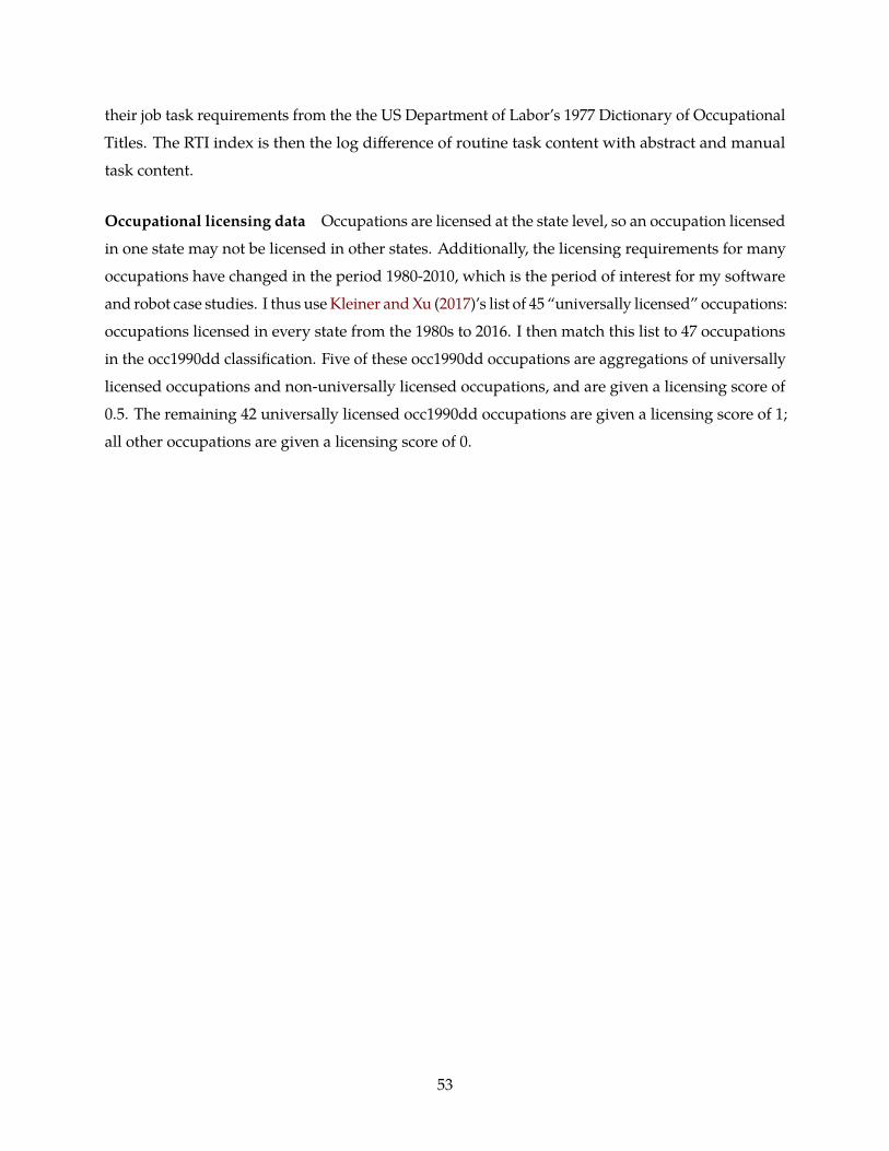
their job task requirements from the the US Department of Labor’s 1977 Dictionary of Occupational

Titles. The RTI index is then the log difference of routine task content with abstract and manual

task content.

Occupational licensing data Occupations are licensed at the state level, so an occupation licensed

in one state may not be licensed in other states. Additionally, the licensing requirements for many

occupations have changed in the period 1980-2010, which is the period of interest for my software

and robot case studies. I thus use Kleiner and Xu (2017)’s list of 45 “universally licensed” occupations:

occupations licensed in every state from the 1980s to 2016. I then match this list to 47 occupations

in the occ1990dd classification. Five of these occ1990dd occupations are aggregations of universally

licensed occupations and non-universally licensed occupations, and are given a licensing score of

0.5. The remaining 42 universally licensed occ1990dd occupations are given a licensing score of 1;

all other occupations are given a licensing score of 0.

53

C Supplementary exposure score figures

Table A1: Extracting capabilities from patent titles.

Text Extracted pairs

Adaptive system and method for predicting response times in aservice environment

(predict, time)

Method of and apparatus for determining optimum deliveryroute for articles

(determine, route)

Methods and apparatus for reinforcement learning

Device for forecasting total power demand (forecast, demand)

Method and device for classifying images on basis ofconvolutional neural network

(classify, image)

A method for diagnosing food allergy (diagnose, allergy)

Neural network language model training method and device andvoice recognition method

Automatic butterfly species identification system and method,and portable terminal having automatic butterfly speciesidentification function using the same

(have, function),(use, same)

Notes: Table displays a set of titles of artificial intelligence patents and corresponding verb-objectpairs extracted automatically using a dependency parsing algorithm, as described in the maintext. Stop words such as “use” and “have”, which do not express applications, are droppedfrom subsequent analysis.

54

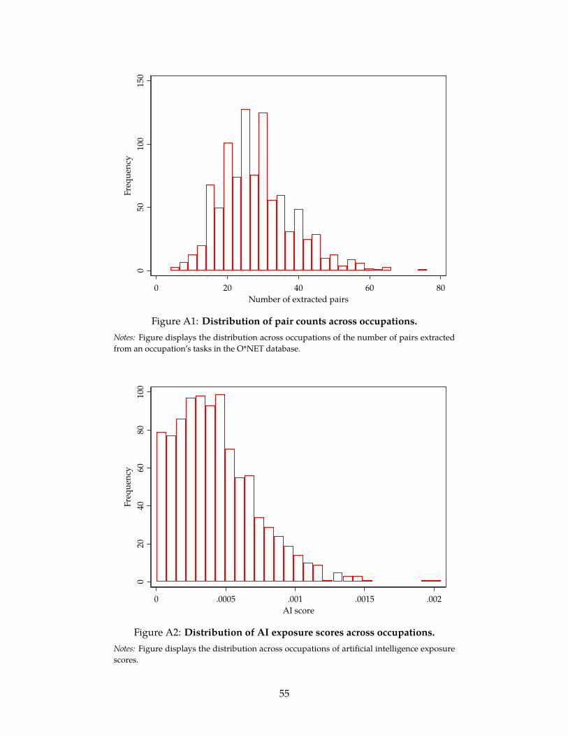
050

100

150

Freq

uenc

y

0 20 40 60 80Number of extracted pairs

Figure A1: Distribution of pair counts across occupations.Notes: Figure displays the distribution across occupations of the number of pairs extractedfrom an occupation’s tasks in the O*NET database.

020

4060

8010

0Fr

eque

ncy

0 .0005 .001 .0015 .002AI score

Figure A2: Distribution of AI exposure scores across occupations.Notes: Figure displays the distribution across occupations of artificial intelligence exposurescores.

55

0.2

.4.6

.81

Shar

e of

task

pai

rs lo

st

0 5 10 15WordNet level

Figure A3: Share of task pairs lost by WordNet aggregation level.Notes: WordNet assigns all nouns to positions in a conceptual hierarchy. For example, theancestors of “dog” include “carnivore”, “mammal”, “vertebrate”, “animal”, and “physicalentity”. I group together nouns in the same conceptual category, for a given WordNet level. If Iaggregated at the level of “dog”, I would lose all words that exist only at a more general level,such as “mammal” and “animal”. This figure displays the share of verb-noun pairs extractedfrom O*NET tasks that would be lost for this reason at each level of aggregation. (Levels withhigher numbers are more specific.)

56

D Comparison of exposure scores to routineness measures

To study the relationship between my approach and the influential “routineness” approach, I regress

my exposure scores for each technology on the five occupation routineness measures developed in

Autor, Levy, and Murnane (2003) and Acemoglu and Autor (2011). These routineness measures are

hand-crafted composites of job characteristic scores provided in O*NET; for example, the “routine

cognitive” measure combines O*NET scores for how structured an occupation’s work is and the

importance of “repeating the same tasks”. Further details on the construction of these measures

are provided in Appendix D.2.

The results are plotted in Figure A4. The coefficient on the non-routine cognitive analytic

measure is exceptionally high for artificial intelligence and much lower for software, suggesting

that artificial intelligence has a set of non-routine capabilities that fundamentally distinguish it

from software. The coefficients on the interpersonal measure are low for all three technologies,

suggesting that, for now, interpersonal tasks will be harder to automate than other activities. The

high non-routine manual scores reflect the fact that this score captures controlling equipment,

which is a capability to some extent of all three technologies.

D.1 Comparison to Autor, Levy, and Murnane (2003)

As a further comparison exercise, I directly assess my software exposure scores against the findings

in Autor, Levy, and Murnane (2003). I find that my method independently recovers that paper’s key

qualitative results.

In that paper, the authors argue that software should substitute for routine cognitive and routine

manual tasks, and complement non-routine cognitive tasks. To test these theoretical predictions

empirically, the authors study how the change in computer use in an industry is related to the

change in the mix of jobs in that industry over various time periods. Specifically, in Table III they

regress the average routine cognitive score of jobs in an industry, for various time periods, on change

in computer use in that industry. They do the same for routine manual scores, non-routine cognitive

analytic scores, and non-routine cognitive interpersonal scores. They exclude non-routine manual

scores from their analysis.

They find that increased computer use is associated with rises in an industry’s use of non-

routine cognitive analytic occupations, larger rises in use of non-routine cognitive interactive

occupations, falls in use of routine cognitive occupations, and even larger falls in use of routine

manual occupations.

Figure A5 shows the results of four regressions based on the measure of exposure to software

57

Routine cognitive

Routine manual

Non-routine cognitive: analytic

Non-routine cognitive: interpersonal

Non-routine manual

-.2 0 .2 .4 .6

Software AI Robots

Figure A4: Occupation-level regression results.Notes: Plot shows the coefficient estimates and 95% confidence intervals from each of three regressions, one per technology.The specification is Exposurei,t = RoutineCogi+RoutineMani+NonRoutineCogAi+NonRoutineCogIi+NonRoutineMani+εi,t,where i indexes occupation, t indexes technology, and Exposurei,t measures the intensity of patenting in technology tdirected towards the capabilities involved in occupation i. Exposure scores and routineness measures are each standard-ized to have a mean of zero and a cross-occupation standard deviation of one. For the standardizations and regressions,observations are weighted by employment reported in the May 2016 Occupational Employment Statistics. Each regressionhas n = 961 occupations, and the R2 statistics are 14.1%, 14.7%, and 38.2% for software, AI, and robots respectively.

58

Routine cognitive

Routine manual

Non-routine cognitive: analytic

Non-routine cognitive: interpersonal

-.2 0 .2 .4

Figure A5: Simple linear regression results for software.Notes: Plot shows the coefficient estimates and 95% confidence intervals from four simple linear regressions. Occupation-level routineness scores defined in Acemoglu and Autor (2011), which are updated versions of those in Autor, Levy, andMurnane (2003), are regressed on standardized occupation-level exposure scores calculated from software patent textand O*NET data. The routineness scores are functions of quantitative occupational characteristic scores provided inO*NET, as described in Section D.2. The specifications are RoutineCognitivei = Exposurei,So f tware + εi, RoutineManuali =Exposurei,So f tware + εi, and so on, where i indexes occupation. Observations are weighted by employment reported inthe May 2016 Occupational Employment Statistics. Each regression has 961 observations, and the R2 statistics are3.3%, 12.4%, 2.9%, and 3.8% for the routine cognitive, routine manual, non-routine cognitive analytic, and non-routinecognitive interpersonal regressions respectively.

that I develop in this paper. In each case, observations are occupations, and the independent variable

is my software exposure score for each occupation. I regress each of the four occupation-level

routine/non-routine scores used in Autor, Levy, and Murnane (2003) separately on my software

exposure score. I find that routine manual scores have the strongest positive association with the

software exposure score, followed by routine cognitive scores, while the association between the non-

routine cognitive scores and the software exposure score is negative. In other words, occupations

with high routine manual and routine cognitive scores make intensive use of capabilities that feature

in software patents, while occupations with high non-routine cognitive scores do not make intensive

use of such capabilities. My measure thus independently recovers the key qualitative results of

the Autor, Levy, and Murnane (2003) framework, i.e., the substitutability of software for routine

cognitive and routine manual occupations, using only patent text and job descriptions as input.

59

D.2 Construction of routine/non-routine occupation measures

The creators of the O*NET database score each occupation along many characteristics, such as

the extent to which it involves “being exact or accurate” or “coaching/developing others”. These

measures were hand-combined by Acemoglu and Autor (2011), updating Autor, Levy, and Mur-

nane (2003), into composite “routine” (i.e., software-amenable) and “non-routine” scores for each

occupation. We use these measures to characterize our exposure scores at various points in the text.

The component O*NET scales used to produce each score are as follows:

Routine cognitive 4.C.3.b.7 Importance of repeating the same tasks

4.C.3.b.4 Importance of being exact or accurate

4.C.3.b.8 Structured v. Unstructured work (reverse)

Routine manual 4.C.3.d.3 Pace determined by speed of equipment

4.A.3.a.3 Controlling machines and processes

4.C.2.d.1.i Spend time making repetitive motions

Non-routine cognitive: analytic 4.A.2.a.4 Analyzing data/information

4.A.2.b.2 Thinking creatively

4.A.4.a.1 Interpreting information for others

Non-routine cognitive: interpersonal 4.A.4.a.4 Establishing and maintaining personal relationships

4.A.4.b.4 Guiding, directing and motivating subordinates

4.A.4.b.5 Coaching/developing others

Non-routine manual 4.A.3.a.4 Operating vehicles, mechanized devices, or equipment

1.A.2.a.2 Manual dexterity

1.A.1.f.1 Spatial orientation

4.C.2.d.1.g Spend time using hands to handle, control or feel objects,

tools or controls

I use the replication code provided for Acemoglu and Autor (2011) to generate these measures

for O*NET v22.0.

60