the impact of car pollution on infant federal reserve bank
TRANSCRIPT

Fe
dera
l Res
erve
Ban
k of
Chi
cago
The Impact of Car Pollution on Infant and Child Health: Evidence from Emissions Cheating
Diane Alexander and Hannes Schwandt
REVISED
November 25, 2019
WP 2019-04
https://doi.org/10.21033/wp-2019-04
*Working papers are not edited, and all opinions and errors are the responsibility of the author(s). The views expressed do not necessarily reflect the views of the Federal Reserve Bank of Chicago or the Federal Reserve System.
The Impact of Car Pollution on Infant and Child Health:
Evidence from Emissions Cheating ∗
Diane Alexander
Federal Reserve Bank of Chicago
Hannes Schwandt
Northwestern University
November 25, 2019
Abstract
Car exhaust is a major source of air pollution, but little is known about its impacts on popula-tion health due to socioeconomic selection, measurement error, and avoidance behaviors. Weexploit the dispersion of emissions-cheating diesel cars—which secretly polluted up to 150times as much as gasoline cars—across the United States from 2008-2015 as a unique oppor-tunity to overcome these empirical challenges and measure the health impacts of car pollution.Using the universe of vehicle registrations, we demonstrate that a 10 percent cheating-inducedincrease in car exhaust increases rates of low birth weight and acute asthma attacks amongchildren by 1.9 and 8.0 percent, respectively. These health impacts occur at all pollution levelsand across the entire socioeconomic spectrum.
∗Diane Alexander ([email protected]) is an economist at the Federal Reserve Bank of Chicago. HannesSchwandt ([email protected]) is an assistant professor of economics at the School for Education and SocialPolicy at Northwestern University. We are thankful to Wes Austin, David Chan, Janet Currie, Daisy Dai, Mark Dug-gan, Liran Einav, Amy Finkelstein, Meredith Fowlie, Joshua Graff Zivin, Eckard Helmers, Solomon Hsiang, StefanHeblich, Emily Oster, James Sallee, Molly Schnell, Ana Tur-Prats, Reed Walker, and seminar participants at StanfordUniversity, Federal Reserve Bank of Chicago, UC San Diego, University of Kansas, Federal Reserve Bank of Cleve-land, Cal Poly San Luis Obispo, DePaul University, Ohio State University, UC Berkeley, University of Chicago Booth,Tulane University, and University of Illinois Urbana-Champaign, and conference participants at the NBER SummerInstitute, the Midwest Health Economics Conference, Chicago Booth Junior Health Economics Summit, GEA Bonn,and the Barcelona GSE Summer Forum. We are grateful to Leah Plachinski and Avinash Moorthy, who providedexcellent research assistance. IHS Markit did not participate in the analysis; all views and conclusions expressed arethose of the authors, and cannot be attributed to the Federal Reserve Bank of Chicago, the Federal Reserve System, orIHS Markit.
1 Introduction
The impacts of car pollution and their optimal regulation are the subject of an ongoing and con-
tentious academic and policy debate in the United States, Europe, and around the world. Yet,
little empirical evidence exists on the impacts of car exhaust on health outcomes. Although it is
well established that air pollution has negative impacts on population health (Chay and Green-
stone, 2003a,b; Currie and Neidell, 2005; Chen et al., 2013; Deschenes et al., 2017; Deryugina
et al., 2019), the existing quasi-experimental evidence is largely based on measures of overall air
pollution without identifying the contribution of car pollution. Two pioneering papers have stud-
ied the health impacts of car pollution on disadvantaged infants—those born to mothers residing
next to highway toll stations and those sick enough to die in response to weekly traffic variation
(Currie and Walker, 2011; Knittel et al., 2016)—but these estimates might not be generalizable.
Whether moderate levels of car pollution impact the health of the general population remains an
open question.1,2
This gap in knowledge is perhaps surprising, as car exhaust is omnipresent on a daily basis
across the entire population. Even for the wealthiest members of society, there is no escape from
car exhaust. Moreover, as car pollution can be regulated in many ways and at relatively low costs
(Fowlie et al., 2012), accurately measuring its health impacts is crucial to evaluate the costs and
benefits of different regulations and their enforcement. Finally, because consumers are exposed at
least partly to their own vehicle’s pollution (Harik et al., 2017), informing society about the health
consequences of car exhaust could profoundly impact consumer choice.
Empirical evidence on the health impacts of car pollution is scarce due to several well-known
1Notably, both the current and the previous U.S. administrations have based their car emissions regulations on thenotion that the causal evidence linking traffic-related air pollution to health, in particular health at birth, is “insufficient”and “inadequate”(US EPA, 2012, 2018). These regulations draw on a meta study (HEI, 2010) that concludes theevidence of impacts on birth outcomes is “inadequate and insufficient" and the evidence of impacts on mortality is“suggestive but not sufficient.” The evidence is deemed sufficient to conclude a causal relationship only in the case ofthe exacerbation of asthma. For recent quasi-experimental evidence of traffic-related pollution impacts on asthma, seeMarcus (2017) and Simeonova et al. (2018).
2Anderson (forthcoming)—another related paper studying a relatively disadvantaged population—documents mor-tality impacts of car pollution for elderly Los Angeles residents living next to highways, exploiting the fact that down-wind neighborhoods get more pollution on average. He et al. (forthcoming) focus on the high pollution environmentof a mega city, studying the health impacts of pollution from diesel cargo trucks in São Paulo.
1

threats to causal inference, including socio-economic selection, avoidance behavior, and measure-
ment error. In this paper, we exploit a unique natural experiment that overcomes these empirical
challenges.
In 2008, a new generation of supposedly clean diesel passenger cars was introduced to the
U.S. market.3 These new diesel cars were marketed to environmentally conscious consumers, with
advertising emphasizing the power and mileage typical for diesel engines in combination with
unprecedented low emissions levels. Clean diesel cars won the Green Car of the Year Award in
2009 and 2010, and quickly gained market share. By 2015, over 600,000 cars with clean diesel
technology were sold in the United States. In the fall of 2015, however, it was discovered that
these cars covertly activated equipment during emissions tests that reduced emissions below of-
ficial thresholds, and then reversed course after testing. In street use, a single “clean diesel” car
could pollute as much nitrogen oxide (NOX; a precursor to fine particulate matter and ground-level
ozone) as 150 equivalent gasoline cars.4 Hereafter, we refer to cars with “clean diesel” technology
as cheating diesel cars.
The dispersion of these cheating diesel cars across the United States gives us a unique op-
portunity to measure the causal effect of car pollution on infant and child health. This natural
experiment provides several unique features. First, it is typically difficult to infer causal effects
from observed correlations of health and car pollution, as wealthier individuals tend to sort into
less-polluted areas and drive newer, less-polluting cars. The fast roll-out of cheating diesel cars
provides us with plausibly exogenous variation in car pollution exposure across the entire socio-
economic spectrum of the United States. Second, it is well established that people avoid known
pollution, which can mute estimated impacts of air pollution on health (Neidell, 2009). Moder-
ate pollution increases stemming from cheating diesel cars, a source unknown to the population,
are less likely to induce avoidance behaviors, allowing us to cleanly estimate the full impact of
pollution. Third, air pollution comes from a multitude of sources, making it difficult to identify
3These cars were first introduced by Volkswagen (Volkswagen AG, Audi AG, and Volkswagen Group of America,collectively “VW”) in 2008 with their TDI Clean Diesel series. Fiat Chrysler Automobiles (FCA) entered the “cleandiesel” market in 2013 with their EcoDiesel series. For a complete list, see Table A.15.
4See Sections 2.2 and 2.3 for details on the emissions scandal and on the emissions levels of cheating diesel cars.
2
contributions from cars, and it is measured coarsely with pollution monitors stationed in a minority
of U.S. counties. This implies low statistical power and potential attenuation bias for correlational
studies of pollution (Lleras-Muney, 2010). We use the universe of car registrations to track how
cheating diesel cars spread across the country and link these data to detailed information on each
birth conceived between 2007 and 2015. This setting provides rich and spatially detailed variation
in car pollution.
We find that counties with increasing shares of cheating diesel cars experienced large increases
both in air pollution and in the share of infants born with poor birth outcomes. We show that
for each additional cheating diesel car per 1,000 cars—approximately equivalent to a 10 percent
cheating-induced increase in car exhaust—there is a deterioration of 2.0 percent in air quality in-
dices for fine particulate matter (PM2.5) and a 1.9 percent increase in the rate of low birth weight.
We find similar effects on larger particulates (PM10; 2.2 percent) and ozone (1.3 percent), as well
as reductions in average birth weight (-6.2 grams) and gestation length (-0.016 weeks). Effects are
observed across the entire socio-economic spectrum, and are particularly pronounced among ad-
vantaged groups, such as non-Hispanic white mothers with a college degree. Effects on pollution
and health outcomes are approximately linear and not affected by baseline pollution levels. Over-
all, we estimate that the 607,781 cheating diesel cars sold from 2008 to 2015 led to an additional
38,611 infants born with low birth weight.5 Finally, we also find an 8.0 percent increase in asthma
emergency department (ED) visits among young children for each additional cheating diesel car
per 1,000 cars in a subsample of five states.
A potential concern is that our estimates may be confounded by changes in county or maternal
characteristics that are correlated with increasing cheating diesel shares. We address this concern
by analyzing the impact of gasoline versions of cheating diesel cars (hereafter “cheating” gas)
that were marketed to and purchased by a similar population, but which did not pollute above
emissions standards (that is, they did not cheat). We find that neither pollution nor birth outcomes
are affected by a county’s share of “cheating” gas cars, even though mothers giving birth in counties
5This number is equivalent to 1.7 percent of the overall 2.22 million low birth weight singleton births in the UnitedStates over the same period.
3
with high “cheating” gas shares have similar socioeconomic characteristics as mothers in counties
with high cheating diesel shares. We further show that maternal characteristics do not change
systematically over time in counties with increasing cheating diesel shares. These results suggest
that our estimates are not driven by compositional changes in the type of mothers giving birth, nor
by unobserved characteristics correlated with preferences for new car types or particular brands.
To benchmark our pollution estimates, we use emission measures from tail-pipe tests of cheat-
ing diesel cars to calculate how much we would expect ambient air pollution to increase due to
their introduction.6 This calculation suggests an increase in PM2.5 of 0.2 to 6 percent for each ad-
ditional cheating diesel car per 1,000 cars. Our estimate of a 2.0 percent increase in ambient PM2.5
lies squarely within this range, and implies that passenger cars contribute around 20 percent of
the overall fine particulate matter in complier counties. Our estimated impacts on birth outcomes
are large. The implied causal health effects of car pollution from an IV specification are four to
eight times larger than the pollution-health relationship estimated in cross-sectional studies (e.g.
Hyder et al. (2014)), largely due to measurement error that attenuates cross-sectional estimates.
We further show that our estimated impacts are similar or stronger than quasi-experimental studies
that have focused on rarer outcomes and more disadvantaged populations (Chay and Greenstone,
2003a,b; Currie and Walker, 2011; Knittel et al., 2016).
This paper makes several contributions to the existing literature. We provide the first causal evi-
dence that moderate variation in car pollution impairs fetal development and child health across the
entire population. This finding builds on a large body of correlational as well as quasi-experimental
studies linking overall air pollution to population health.7 Our estimates demonstrate that car pol-
6We build on existing studies which have used pollution estimates from cheating diesel car tail-pipe tests to predictcounty-level excess NOX pollution (Barrett et al., 2015; Holland et al., 2016; Chossière et al., 2017). These papersthen use air pollution integrated assessment models to predict how excess NOX pollution transforms into PM2.5
and ozone, and then impacts mortality. Mortality impacts are predicted using estimates of the mortality-pollutionrelationship from correlational studies. Estimates range between 46 and 59 U.S.-wide excess deaths caused by VW’scheating diesel cars. Although a direct comparison with our results is difficult (as these studies only report estimatesfor NOX but not for PM2.5 or ozone), we show that our estimates are in line with the car tail-pipe test parametersupon which these papers are based.
7See Pope et al. (2002); Peters et al. (2004); Ponce et al. (2005); Stieb et al. (2012); Volk et al. (2013); Vrijheidet al. (2016); Cohen et al. (2017); Heft-Neal et al. (2018), Ransom and Pope (1992); Pope et al. (1992); Schwartz(1994); Bell et al. (2004); Neidell (2004); Luechinger (2014); Schlenker and Walker (2016); Currie and Schwandt(2016); Halliday et al. (2018); Anderson (forthcoming), Dominici et al. (2014), Currie et al. (2014) among others, for
4

lution plays an important causal role in this relationship, and suggest that correlational studies
severely underestimate the true health costs of car pollution. Our results suggest that the strong
direct health impacts of car exhaust need to be accounted when creating regulations aimed at re-
ducing car emissions.
Second, the existing literature often finds pollution effects that are concentrated on disadvan-
taged populations, and suggests several potential mechanisms for this observed effect heterogene-
ity: poorer populations might be more exposed to pollution, they might be more susceptible to
health impairments due to lower baseline health, or they might have less access to health care to
treat the symptoms of exposure (Currie et al., 2014; Bell et al., 2005). We find health impacts that
are not limited to disadvantaged groups, which demonstrates that good baseline health and health
care access do not fully buffer the impacts of car pollution, and emphasizes the role of exposure.
Reductions in car pollution are likely to provide society-wide benefits.
Third, while much of the existing literature estimates pollution effects net of protective re-
sponses to observable changes in pollution, we interpret our estimates as the full, unmuted impact
of car pollution exposure. In line with this interpretation, our results imply health elasticities that
are at the upper end of the range of estimates provided by the quasi-experimental pollution liter-
ature (Chay and Greenstone, 2003a,b; Currie and Walker, 2011; Knittel et al., 2016), despite the
focus of this literature on more disadvantaged complier populations. Our estimates are particu-
larly relevant for settings when the harm of pollution exposure is unknown to the population either
due to unawareness of the pollution (Moretti and Neidell, 2011) or because the pollution level is
considered safe, as tends to be the case for moderate levels of car pollution.
Fourth, the existing quasi-experimental literature often relies on daily or weekly variation in
pollution (e.g. Knittel et al. (2016)). This focus on short-term exposure can overstate long-term
effects if it captures “harvesting,” or understate them if impacts increase with length of exposure (a
notable exception is Anderson (forthcoming)). Our setting provides medium-term pollution varia-
tion which allows us to compare exposure differences across entire pregnancy periods. Given our
additional references. An important related literature analyzes the health impacts of retrofitting school buses (Beattyand Shimshack, 2011; Austin et al., 2019) and the removal of cargo trucks in a high pollution city (He et al., 2018).
5
focus on health at birth, we essentially estimate the impacts of life-time exposure since conception.
Moreover, our estimates likely imply costly long-term impacts of pollution, as poor health at birth
has been linked to negative effects on health, human capital, and economic outcomes throughout
the life-cycle.8 At the same time, our estimates represent lower bounds for the overall effect on
the population as there are likely to be additional negative impacts on health and productivity of
pollution exposure at older ages.9
Our analysis provides important insights for policy makers and society at large. First, the
approximately linear health effects of pollution in the observed range calls into question the notion
that there is a “safe level” of car pollution. We show that moderate variation in car pollution
harms health even in counties with pollution levels below the EPA’s safety threshold. This insight
is informative for the current policy debate in the U.S. over whether regulators should account
for environmental harm from pollution that occurs at levels below the EPA threshold (Friedman,
2019). More broadly, our results speak to the efficacy of regulation aimed at reducing emissions
from diesel and fossil fuel powered cars, e.g. the banning of high emissions cars. Such bans are
becoming increasingly popular—already Brussels, Hamburg, Paris, and Madrid have implemented
limited bans on diesel cars, and dozens of other cities are planning to implement bans on cars
powered by diesel or all fossil fuels over the next decade. Our results suggest that the implied
improvements in air pollution and population health may justify even relatively distortive policies.
Second, our study is the first to show that cheating diesel cars had measurable impacts on
ambient air pollution and population health. This is important information for a prominent industry
scandal that already has been one of the costliest in recent history. To date, Volkswagen has paid
about $25 billion in fines to the U.S. government and in compensation to owners of cheating diesel
cars. Our results demonstrate that the group of individuals harmed by the emissions cheating
8See Almond et al. (2005); Russell et al. (2007) for direct medical costs of low birth weight. See McCormick(1985); Aylward et al. (1989); Roth et al. (2004); Currie and Almond (2011); Case et al. (2005); Black et al. (2007);Oreopoulos et al. (2008); Almond et al. (2018); Elder et al. (2019), among others, for long-term effects. Isen et al.(2017) directly link adult productivity to pollution exposure during pregnancy.
9See Currie et al. (2009a); Zivin and Neidell (2012); Adhvaryu et al. (2016); Lavy et al. (2016); Chang et al. (2016);Meyer and Pagel (2017); Archsmith et al. (2018); Borgschulte et al. (2018); Bishop et al. (2018); Austin et al. (2019);Chang et al. (2019); He et al. (2019); Heissel et al. (2019); Kahn and Li (2019); Hollingsworth and Rudik (2019);Zheng et al. (2019), among others.
6
widely expands beyond Volkswagen’s customer base.
Finally, we note that the diesel emissions cheating scandal was not a result of insufficient reg-
ulation but of insufficient enforcement. Our results emphasize that resources spent on the enforce-
ment of car pollution regulation are well invested if they decrease the likelihood that car makers
will cheat, and are in line with other recent work showing strategic responses to uneven enforce-
ment of environmental regulations (Zou, 2018). This conclusion is particularly relevant in the
face of recent budget cuts to regulatory bodies in the United States, and the current trend toward
deregulation and industry self-regulation.
The remainder of the paper is organized as follows. Section 2 provides background information
on diesel pollution and emissions cheating. Sections 3 and 4 describe our data sources and the
empirical strategy. Results are presented in Section 5; Section 6 concludes.
2 Background
2.1 Diesel versus gasoline
The two predominant fuel technologies worldwide for passenger cars and light-duty trucks are
diesel and gasoline. Both diesel and gasoline originate as crude oil, which refineries then process
into different types of fuel. Diesel, however, is less refined, heavier and oilier than gasoline, and
has a higher energy density due to its longer carbon chains. This higher energy density, combined
with the compressed combustion technology of diesel engines, means that diesel engines are more
powerful and run more efficiently, using less fuel than gasoline engines. This efficiency advantage
suggests that diesel engines emit less carbon dioxide (CO2), an important greenhouse gas, though
the extent to which CO2 improvements are actually realized remains controversial (Helmers et al.,
2019).
The main drawback to diesel engines is that diesel fuel does not burn as cleanly as gasoline,
emitting high levels of particulate matter (PM2.5 and PM10) and nitrogen oxides (NOX). NOX
is a precursor compound to both additional particulate matter and ground-level ozone, the main
7
component of smog.10 Both particulate matter and ozone are associated with decreases in lung
function, asthma exacerbations, increases in hospital visits for respiratory causes, and mortality.11
Although diesel cars have enjoyed high popularity and strong political support in Europe since
the 1990s (with a market share of above 50 percent among new cars (Cames and Helmers, 2013)),
historically there has been very low demand for them in the United States, due both to consumer
preferences and the lack of favorable regulation as found in Europe. Moreover, tightening U.S.
air pollution standards made it increasingly difficult for manufacturers to produce competitively
priced diesel cars meeting those standards.
2.2 The diesel emissions cheating scandal
In the mid-2000s, VW engineers began developing a new diesel engine (TDI Clean Diesel) de-
signed to meet tightening U.S. emissions standards for passenger vehicles (Department of Justice,
2017). These new engines appeared to have all the benefits of diesel vehicles—strong perfor-
mance and fuel efficiency—without the downside of high pollution. VW heavily advertised this
new diesel line in national U.S. print, television advertisements (including the 2010 Super Bowl),
and social media campaigns, promoting it to environmentally conscious consumers some of whom
began buying diesel vehicles for the first time. TDI Clean Diesel models won the “Green Car
of the Year” award both in 2009 and 2010, and VW quickly became the largest seller of light-
duty diesel vehicles in the United States. Among advertised claims for the emissions system of
the new clean diesel line were that it “reduces smog-causing nitrogen oxides by up to 90 percent
when compared with past generations of diesel technologies sold in the United States,” and it has
“fewer NOX emissions than comparable gasoline engines.” Advertisements began with headings
such as “Hybrids? They’re so last year [...] now going green doesn’t have to feel like you’re going
green” (Federal Trade Commission, 2016). Fiat Chrysler Automobiles (FCA) entered the market
in 2013 with their EcoDiesel series. By the end of 2015, nearly 550,000 of VW’s TDI Clean Diesel
10See Hodan and Barnard (2004); Lin and Cheng (2007).11See, for example, Di et al. (2017); Gent et al. (2003); Jerrett et al. (2009); Mar and Koenig (2009); Medina-Ramon
et al. (2006); Pope et al. (2002).
8

vehicles and 60,000 of FCA’s EcoDiesel vehicles were registered across the United States.
In the fall of 2015, the Environmental Protection Agency (EPA) made public that VW’s TDI
Clean Diesel models were far from clean, emitting NOX at as much as 4,000 percent above the
legal limit, evidently as a trade-off for enabling more powerful and durable engine performance
(Department of Justice, 2017). Despite their dramatic pollution levels, these vehicles had previ-
ously passed standard EPA drive cycle tests due to “defeat devices,” i.e. illegal software designed
to cheat emissions tests. Specifically, the software recognized when a car was undergoing an emis-
sions test, and adjusted components (such as catalytic converters or valves used to recycle some of
the exhaust gases) to reduce pollutant emission to legally compliant levels for the duration of the
test. As these additional procedures lowered the engine’s performance and were costly to main-
tain at a permanent level, they were switched off by the software during regular driving. The
EPA’s probe into the TDI Clean Diesel cars led it to conclude in January 2017 that cars equipped
with FCA’s EcoDiesel engine contained similar illegal software. A list of all models issued EPA
violations is found in Table A.15.
2.3 Emissions from cheating diesel cars
To our knowledge, this analysis is the first to empirically measure the effect of the cheating diesel
cars on ambient air pollution. However, on-road tail pipe emissions of the cheating diesel cars
were measured by researchers at West Virginia University, who first noted on a dynamometer the
large NOX emissions discrepancies between on-road and standard EPA tests (CAFEE, 2014). This
study found that depending on the test route, the cheating diesel cars emitted NOX at 5 to 35
times the amount permitted by the US-EPA Tier2-Bin5 standard (0.07 g/mi). The full extent of the
cheating was revealed during follow-up testing conducted by the California Air Resources Board
in conjunction with the the EPA, which found that VW cheating diesel vehicles emitted 10 to 40
times the NOX emissions permitted by the EPA (0.7-2.4 g/mi). In contrast, a typical new gasoline
car in this period emitted NOX at well below the EPA limit; the median among light-duty make-
9
models was just 0.016 g/mi for model year 2010 vehicles.12 Thus, a single cheating VW diesel
car emits as much NOX as 44 to 150 gasoline cars of equivalent model years, and an increase
of one cheating car per thousand can be thought of as an equivalent increase in car pollution by
approximately 4.3 to 14.9 percent.13
To assess the plausibility of our estimates, it is helpful to consider the contribution of car
exhaust to overall air pollution. In the EPA’s National Emissions Inventory Report (United States
Environmental Protection Agency, 2014), 43 percent of NOX emissions were attributed to on-road
mobile emission sources. The total contribution of on-road mobile sources to PM2.5 and ozone,
however, are more difficult to quantify.
PM2.5 is both emitted directly from cars and created by secondary formation from precursor
emissions such as NOX (Hodan and Barnard, 2004; Lin and Cheng, 2007). In the 2014 National
Emissions Inventory Report, 5.6 percent of PM2.5 emissions were attributed to on-road mobile
sources. However, this number does not take into account the secondary formation of PM2.5,
which has been shown to contribute more to ambient PM2.5 than primary emissions (Zawacki et al.,
2018). An alternative, reduced-form way to quantify the contribution of cars to ambient pollution
is to look at the change in pollutants throughout a given day, measuring the increase in pollution
during rush hour compared to midday levels. Such an analysis results in a 43 percent change in
cars’ contribution to PM2.5.14 Using the most and least conservative estimates for the amount of
NOX emissions from the cheating cars and the contribution of cars to overall PM2.5 generates a
range of expected increases from an additional cheating car per 1,000 cars from 0.2 to 6 percent.15
12Authors’ calculations from the EPA’s Certified Vehicle Test Results Report Data files for cars andlight trucks (https://www.epa.gov/compliance-and-fuel-economy-data/annual-certification-data-vehicles-engines-and-equipment).
13We assume that each cheating diesel car replaces a gasoline car, hence it would increase car pollution by theequivalent of 43 to 149 gasoline cars. It is difficult to know, however, the NOX emissions of a typical non-cheatingdiesel car, as the EPA data on NOX emissions by make-model is only comprehensive starting in 2010, when nearly allof the diesel cars were cheating. However, the non-cheating diesel car tested by CAFEE (2014) was found in on-roadtesting to emit NOX at around the threshold allowed by the EPA of 0.07 g/mi, which would imply that the cheatingdiesel cars emitted as much NOX as roughly 10 to 40 non-cheating diesel cars.
14Authors’ analysis using data from the subsample of PM2.5 monitoring stations submitting hourly readings from2015-2017, weekdays only, calculating annual averages of hourly pollution readings and then calculating ((pollutionreading in highest hour)-(pollution reading in lowest hour))/(mean pollution). Hourly readings were not commonlyreported until 2015.
15Cheating VW vehicles emitted 10 to 40 times the NOX emissions permitted by the EPA, or 0.7-2.4 g/mi. Cheating
10
Although the precise contribution of on-road sources to ambient PM2.5 is thus unknown, we would
expect a 10 percent increase in car exhaust to translate to an increase in measured PM2.5 of around
2 percent if 20 percent of PM2.5 near monitoring stations was caused by on-road mobile sources.
The processes of ground-level ozone formation and accumulation are likewise complex re-
actions between NOX and volatile organic compounds (VOC) in the lower atmosphere, in the
presence of sunlight (EPA, 2018). NOX emissions generally contribute more to ozone than VOC
emissions, however, suggesting a large potential role for the cheating diesel cars (Zawacki et al.,
2018). As with particulate matter, we do not attempt to model these pathways directly, but rather
the link between NOXemissions from cars and ambient ozone levels.
3 Data
3.1 Vehicle registration data
Our main independent variables of interest come from vehicle registration data purchased from
IHS Markit. These data contain county-level vehicle registration snapshots of the entire stock of
passenger cars and light trucks (referred to collectively as “cars” throughout the paper) from 2007,
2011, and 2015.16 Each snapshot contains the county-level car total, the number of cars of each
diesel make-model-vehicle year (which allows us to identify cheating diesel cars—listed in Table
A.15), and the number of analogous gas cars for each make-model-vehicle year with a diesel option
FCA diesel cars emitted 5 to 20 times the EPA NOX limit, or 0.35-1.2 g/mi. Estimates of the fraction of PM2.5
attributable to cars vary from 5.6 percent using EPA estimates of primary emissions to 43 percent using variationbetween rush hour peaks and troughs. Using conservative estimates of NOX emissions from cheating cars and thecontribution of cars to overall PM2.5 (0.7 g/mi and 5.6 percent, respectively), an additional cheating car per thousandwould increase PM2.5 by 0.2 percent (one cheating car is equivalent to 44 comparable gas cars, which is equivalentto increasing car pollution by 4.3 percent; 0.043 x 0.056). Using the high end of the range (NOX emissions of 2.4g/mi and 40 percent of PM2.5 from cars), an additional cheating car per thousand would increase PM2.5 by 6 percent(one cheating car is equivalent to 150 comparable gas cars, which is equivalent to increasing the fleet by 14.9 percent;(0.149 x 0.40)).
16Light trucks are defined as those with gross vehicle weight ratings from 1 to 3, which covers vehicles up to 14,000pounds. Examples of vehicles in the highest weight class included in our data are the Ford F-350, the Ram 3500, andthe Hummer H1.
11
(to identify “cheating” gas cars—gas versions of cheating models).17
We use the information on the vehicle model year and county of registration to interpolate
diesel registrations and gas car analogues between snapshot years. For example, we assume that
a 2009 model year vehicle (first sold in 2008) that was registered in a county in 2015 was also
registered in that county from 2008 or 2009 to 2014.18 The total number of cars registered in each
county is imputed linearly between 2007, 2011, and 2015, as we only have the make-model-year
subtotals for cars with a diesel option. We construct the county-level number of cheating diesel
cars, non-cheating diesel cars, and “cheating” gas cars per 1,000 cars.
We consider the cheating diesel cars’ share of the vehicle stock as our explanatory variable
for two main reasons. First, we believe the most relevant counterfactual to purchasing a cheating
car is purchasing a non-cheating car. Thus, we want our measure of exposure to be a measure
of the composition of the passenger vehicle stock rather than a measure of the absolute number
of cars. Second, we want a measure of an average individual’s (or pollution monitor’s) exposure
to the pollution of a cheating car. Our measure captures the fact that an extra cheating car in
a uniformly densely populated county such as Cook County, IL is less likely to drive by any
particular individual in the county, compared to the same car in the similarly sized but less evenly
populated Champaign County, IL. However, we also show the robustness of our main results to
using the number of cheating diesel cars per county-level population and per square mile of county
land area.17The IHS Markit Vehicles in Operation data used in Figures 1-7, A.1-A.5, and Tables 1-7 and A.1-A.12 are based
on a snapshots taken by IHS Markit (12/2007, 12/2011, 12/2015). These figures reflect a total vehicle populationbased on the location of the vehicle operators as reported in vehicle registrations, and not based on where the vehicleis primarily driven. These figures also include complete information on light vehicle registrations, including rentals,fleets, and retail. Copyright @ IHS Markit 2019, all rights reserved.
18We use sales data to assign a fraction of cars to the year before the model year, to take into account the fact that75 percent of new cars were purchased in the model year, and 25 percent were purchased in the previous year. Formore details, see Section A.1.2.2. The model-year based extrapolation works if the number of passenger vehicles thatare sold or moved out of county is small relative to the stock of registered vehicles. We can check the validity of thisextrapolation by comparing the 2011 counts constructed by rolling back the 2015 data by county and model year tothe actual counts of registered vehicles in 2011. The process works very well—the correlation between the predictednumber of emissions-cheating diesels registered in 2011 and the actual number in 2011 is 0.992.
12
3.2 Pollution data
Our measures of air pollution are constructed from air quality data from the EPA. The Clean Air
Act requires every state to establish a network of air monitoring stations that take daily readings of
criteria pollutants, of which we consider fine particulate matter (PM2.5), particulate matter (PM10),
nitrogen dioxide (NO2), carbon monoxide (CO), and ozone (O3). For each pollutant, we construct
three county-month level measures: the average concentration, an air quality index, and the number
of poor air quality days. The air quality index is scaled from 0–500, and is based on methodology
from the EPA (see Section A.1.2). Poor air quality days are defined as days when the air quality
index exceeds 51.
There are three main caveats with these data. First, the number of air monitoring stations varies
across pollutants. Coverage is best for PM2.5 and ozone, with monitors in 556 and 731 counties in
2015, respectively, whereas fewer monitoring stations measure NO2 (monitors in 232 counties in
2015). Thus, we have qualified information about the direct effect of the cheating diesel cars on
NO2, a component of NOx, which was the main pollutant excessively emitted by cheating diesel
cars. However, as mentioned above, NO2 is a primary precursor for PM2.5 and ozone (Hodan
and Barnard, 2004; Lin and Cheng, 2007). Lin and Cheng (2007) find that the majority of NO2
converts to particulate nitrate (a component of PM2.5) within a few days. Hence, increases in NOx
will directly translate into increases in PM2.5 and ozone, pollutants that are well monitored and
that are the most relevant for health impacts.19
Second, monitors and monitoring stations are added and discontinued frequently over the sam-
ple time. Furthermore, Grainger et al. (2016) provide evidence that regulatory agencies in compli-
ance with federal air quality standards strategically avoid pollution hotspots when choosing new
monitor locations. Systematic placement of new monitors in areas with less pollution could distort
the time trend of county-level pollution if we averaged across all available monitors in each period.
As a conservative approach, we use only one monitoring station per county to hold fixed the phys-
19PM2.5 and ozone are considered the most relevant in terms of health impacts of air pollution (for reviews, seeHoek et al. (2013); World Health Organization (2013)), and are to a large extent caused by road transportation (Camesand Helmers, 2013; Chossière et al., 2017).
13
ical area where pollution is being measured over time. For each county and pollutant, we choose
the monitoring station with the most readings over our period and construct a county-month level
panel of pollution measures from 2007 to 2015. We show that results are very stable if we use
alternative measures based on several monitors per county.20
A third caveat is that even the longest-running monitor locations are not randomly assigned
within a county. Monitors are often located in or near cities (Muller et al., 2018), so that the sample
of counties with monitors tends to be more urban than the overall U.S. population. Moreover, if
regulators on average strategically place monitors away from pollution sources, and car pollution
is very local, we could underestimate the effect of the cheating cars on pollution. However, the
high pollution levels of cheating diesel cars were not known to regulators, and over 85 percent
of the monitors we use predate the emissions cheating cars. Hence, it is unlikely that regulators
strategically placed monitors in order to avoid the pollution generated by cheating diesel cars.21
For PM2.5, we can complement the monitor-based measure with an alternative which com-
bines satellite observations of aerosol optical depth, simulations from a chemical transport model,
and information from EPA monitors (van Donkelaar et al., 2019).22 There are advantages and
disadvantages to this alternative measure. On the positive side, the satellite-based measure offers
estimates of monthly PM2.5 for all counties in the US, rather than just the subsample with a PM2.5
monitoring station. On the negative side, satellite-based estimates are not direct measures, and
prediction errors appear both to be important and not well understood. In particular, Fowlie et al.
(2019) suggest that satellite estimates are biased down at high PM2.5 concentrations.
20We develop a procedure which averages across multiple monitoring stations at the county-month level, whileholding the geographical distribution of the monitoring stations fixed. In particular, we allow more than one monitorper county (for example up to two monitors per county), but only use observations where all monitors report pollutionmeasures to avoid compositional changes from new monitors being added in different parts of the county.
21Relatedly, Zou (2018) shows that when pollution is measured intermittently (on six-day cycles), air quality isworse on unmonitored days—suggesting strategic behavior over time as well as over the initial location of the monitor.As the source of pollution is unknown in our context and the monitoring data aggregated to the monthly level, we donot believe this type of high-frequency, strategic behavior will impact our analysis.
22We are grateful to Wes Austin for providing us with cleaned county-month-level PM 2.5 satellite data.
14
3.3 Birth data
Our first set of health outcomes comes from the U.S. National Vital Statistics System’s birth records
from 2007 to 2015. These data contain detailed information on all births in the United States,
including county and month of birth, demographic information about the mother, and health out-
comes for the infant, and are collapsed to the county-conception month. Conception month is cal-
culated by taking the gestational age in weeks and dividing by 4.345, rounding gestation months
to the nearest integer, and subtracting months of gestation from the birth month.
Our preferred measures of infant health are county-month average birth weight and the county-
month level fraction of babies born at low birth weight (less than 2500 grams). Birth weight is
often used as a summary measure of infant health, and low birth weight in particular is associated
with a range of poor outcomes, both health-related and economic, such as schooling and earnings
(Black et al., 2007; Almond et al., 2018). We further analyze county-month average gestational
age in weeks and the rate of premature birth (gestational age of less than 37 weeks). Birth weight
and gestational age are both commonly used summary measures of infant health.
3.4 Emergency department discharge data
Our second set of health outcomes comes from State Emergency Department Databases (SEDD)
from the Agency for Healthcare Research and Quality’s Healthcare Cost and Utilization Project
(HCUP), which contain the number of emergency department (ED) visits over time, by diagnosis,
from 2007 to 2015. We focus on the number of visits with a primary diagnosis of asthma, which
is known to be triggered by poor air quality and has been shown to be correlated with exposure to
traffic-borne pollutants (Gauderman et al., 2005).23 In particular, we construct the number of ED
visits for asthma per 1,000 people at the county-quarter level. We also break down this measure by
patient age, as young children are most likely to be affected.
Although the HCUP data are very detailed, there are two important caveats. First, the ED dis-
charge data do not include records for patients who were admitted through the ED. This limitation
23We use ICD-9 code 493 and ICD-10 code J45.
15

means that the data are not well suited for analyzing more-severe health outcomes, such as strokes
or heart attacks, which typically result in a hospital admission. Second, we are limited by financial
considerations to a small subsample of states: Arizona, New Jersey, Kentucky, Rhode Island, and
Florida, providing us with 228 counties.
3.5 Other data
Our analysis further includes annual data on county characteristics from the U.S. Census Bureau’s
Small Area Income and Poverty Estimates program (SAIPE) and the Census Bureau’s Population
Estimates program (county-year level population, median income, fraction in poverty, fraction of
children in poverty, and fraction white), as well as the annual number of vehicle-miles driven by
state according to the Federal Highway Administration.
3.6 Cheating diesel over space and time
Figures 1A and 1B show the distribution of non-cheating diesel cars in 2007 and 2015. Non-
cheating diesel is strongly clustered in the western part of the United States, particularly in less-
populated rural states (these are mainly light-duty trucks). While there has been a slight increase
in the fraction of non-cheating diesel cars between 2007 and 2015, the spatial distribution is stable
over time. The pattern looks very different for the distribution of cheating diesel cars in Figures
1C and 1D. The 2007 map is blank as the first cheating diesel cars were not sold until 2008. By
2015, over 600,000 cheating diesel cars were sold (Figure A.1 shows annual registration counts),
clustered on the West Coast, the upper Midwest, and New England–areas that are typically thought
of as relatively wealthy and environmentally conscious. The distribution of “cheating” gas models
looks very similar to the cheating diesel map (see Figure A.2) indicating that diesel and gas model
were marketed to similar areas (they were also similarly priced; for details see Table A.14).
Figure 2 shows how the distribution of different car types is related to counties’ median income
in the 2015 cross-section. The left figure shows average median income across percentiles of
counties, ranked by their share of non-cheating diesel cars. Counties with high shares of non-
16
cheating diesel have somewhat lower median income than counties with fewer diesel cars (in line
with income gradients for overall air pollution (Muller et al., 2018)). The blue dots in the right
panel show that this relationship is reversed for cheating diesel cars. Counties with higher shares
of cheating diesel cars in 2015 have higher median incomes than those with lower shares. The
relationship is close to linear across the entire distribution, and it is strong: the median income in
the top percentile is almost twice as high as in the bottom percentile. The hollow green circles in
the right panel of Figure 2 show median income when counties are ranked instead by their share of
“cheating” gas models. T’he relationship is very similar to the cheating diesel gradient, suggesting
that areas in which people purchased many cheating diesel cars are similar to areas with many
“cheating” gas models. The same holds true for a broad set of maternal characteristics (Figures 7
and A.7).
3.7 Summary statistics
Table 1 shows summary statistics at the county-year-month level for the overall sample of counties,
for the sample of counties with a PM2.5 monitor, and for terciles ordered by the share of cheating
diesel in 2015.24 The upper panel shows counties’ car registration characteristics, demograph-
ics, and pollution outcomes. The lower panel shows birth outcomes and maternal characteristics,
restricted to county-year-month observations with non-zero births. We include observations with
zero births in the main pollution regressions in order to maximize the power of the analysis, though
results are unchanged if only county-year-months with non-zero births are used.
Comparing the first two columns, PM2.5 monitors are placed in counties that are more popu-
lated and that have slightly lower poverty rates and higher median incomes than the full sample of
counties. Birth outcomes and maternal characteristics are relatively similar between the full sam-
ple and the PM2.5 monitor sample. In line with Figure 2, median income increases across terciles
24Table A.1 shows summary statistics for the subsample of the five states for which we have HCUP data on emer-gency department discharges. As in the overall sample, counties with higher shares of cheating diesel cars tend to havehigher median incomes and lower poverty. Asthma rates are hump-shaped, with the highest occurrence in the secondtercile and slightly lower rates in the bottom tercile than in the top tercile.
17
of the 2015 cheating diesel share. A higher cheating diesel share is also associated with a larger
population, a higher number of cars and miles driven, and lower poverty rates. Despite having
more cars, PM2.5 and PM10 levels are lower on average in counties with a higher cheating diesel
share. Mothers giving birth in counties with higher cheating diesel shares are more likely to be
white, married, more educated, and less likely to smoke during pregnancy. Not surprisingly, given
the positive selection of mothers, these counties have better average birth outcomes: higher birth
weight and longer gestation length.
4 Empirical strategy
We seek to estimate the effect of car pollution on health. Given well-measured experimental
variation in car pollution at the county-time level (Pct), we would run the following regression
Healthct = α + βln (Pct) + εct (1)
with β measuring the effect of a percent increase in car pollution on health. Running this
regression in available observational data likely results in a biased estimate due to endogeneity
and measurement error, and is nearly impossible to run due to lack of data on car pollution. As
discussed previously, we argue that the number of cheating diesel cars provides a well-measured
(conditionally) exogenous source of car pollution. Our preferred measure of exposure to cheating
diesel cars is the number of such cars per 1,000 cars in a county (cDct).
How do changes in cDct relate to changes in total car pollution within a county? First, the
pollution stemming from one gasoline car (pi) can be decomposed into miles driven times the
pollution per mile
pit = mit ∗ (poll/m)i (2)
Then, assuming that cars are either gasoline or cheating diesel cars, that all cars in a county drive
18
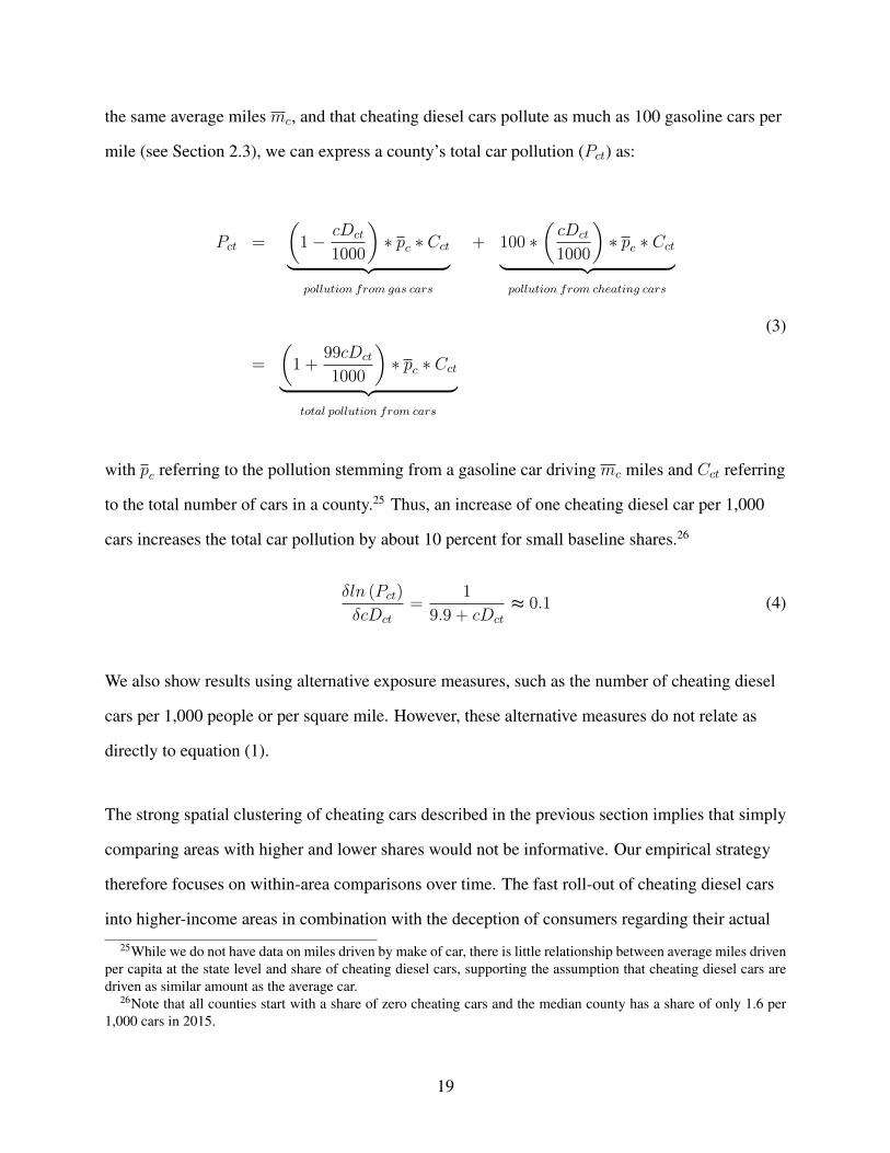
the same average miles mc, and that cheating diesel cars pollute as much as 100 gasoline cars per
mile (see Section 2.3), we can express a county’s total car pollution (Pct) as:
Pct =
(1− cDct
1000
)∗ pc ∗ Cct︸ ︷︷ ︸ + 100 ∗
(cDct
1000
)∗ pc ∗ Cct︸ ︷︷ ︸
pollution from gas cars pollution from cheating cars
=
(1 +
99cDct
1000
)∗ pc ∗ Cct︸ ︷︷ ︸
total pollution from cars
(3)
with pc referring to the pollution stemming from a gasoline car driving mc miles and Cct referring
to the total number of cars in a county.25 Thus, an increase of one cheating diesel car per 1,000
cars increases the total car pollution by about 10 percent for small baseline shares.26
δln (Pct)
δcDct
=1
9.9 + cDct
≈ 0.1 (4)
We also show results using alternative exposure measures, such as the number of cheating diesel
cars per 1,000 people or per square mile. However, these alternative measures do not relate as
directly to equation (1).
The strong spatial clustering of cheating cars described in the previous section implies that simply
comparing areas with higher and lower shares would not be informative. Our empirical strategy
therefore focuses on within-area comparisons over time. The fast roll-out of cheating diesel cars
into higher-income areas in combination with the deception of consumers regarding their actual
25While we do not have data on miles driven by make of car, there is little relationship between average miles drivenper capita at the state level and share of cheating diesel cars, supporting the assumption that cheating diesel cars aredriven as similar amount as the average car.
26Note that all counties start with a share of zero cheating cars and the median county has a share of only 1.6 per1,000 cars in 2015.
19

pollution levels provides us with identifying variation for a complier population of particular
interest. We will run several versions of the following regression:
Outcomect = α + β1cDct + β2cGct + λc + λt + δXct + εct (5)
where c indicates the county and t the time period (either monthly or annually). The dependent
variable Outcome refers to pollution, birth, or health outcomes (for birth outcomes t refers to the
conception month or year). The main regressor of interest is cD, referring to the number of
cheating diesel cars per 1,000 registered cars in a county. cG is the share of “cheating” gas cars
per 1,000 cars. λc and λt are county and time fixed effects and Xct are time-varying county
characteristics.27 The data are collapsed at the county-month level (we also show results using the
micro-level data and data collapsed to the county-year), and standard errors are clustered at the
county level. Observations in birth outcome regressions are weighted by the number of births.
When we focus on subgroups of mothers with various demographic characteristics, we use the
individual level micro data.
Finally, we present results from instrumental variable (IV) specifications in which we use the
cheating diesel share as instrument for PM2.5 and ozone. In regressions that include both PM2.5
and ozone, we interact the cheating diesel share with county-specific weather conditions (which
differently mediate the transformation of car exhaust into PM2.5 and ozone) to obtain additional
instruments (Knittel et al., 2016).
4.1 Identification
The inclusion of county and time fixed effects means that we compare changes in areas with in-
creasing cheating diesel shares (treatment counties) to overall time trends in the data. This is
27Included characteristics are share of non-cheating diesel cars per 1,000 cars, log total cars, log population, povertyrate, child poverty rate, and median income. Birth outcome regressions include additional controls for the followingmaternal characteristics: fraction of mothers that are hispanic, black, married, smoking during pregnancy, average age,and education bins.
20

essentially a difference-in-difference approach, with the identifying assumption that any trend de-
viations in the outcomes of treatment counties are driven by the changes in the cheating diesel
share. There is a common set of threats to this framework.
Increases in cheating diesel shares might be correlated with or driven by simultaneous socio-
economic changes that increase pollution and worsen health outcomes. A direct way to test for such
violation of the exclusion restriction is balancing regressions that use socio-economic indicators as
dependent variables on the left of the regression equation (Pei et al., 2018). We will show balancing
results both in binned scatter plots and in regression form.
Our estimates could also be confounded by selection due to unobserved characteristics, such
as tastes for new cars. We report the effects of counties’ “cheating” gas shares to explore the role
of such factors. As discussed above, the type of counties with high cheating diesel shares are very
similar in terms of socio-economic characteristics to counties with high “cheating” gas shares. If
our results were driven by selection, we would expect to find similar effects of cheating diesel and
“cheating” gas cars on health outcomes.
While we think of the share of “cheating” gas cars as akin to a placebo conceptually, we are
only able to separately identify the effects of the two different types of cars because they have
slightly different patterns of dispersion. As we show in Figure A.3, both cheating diesel cars and
the equivalent gas models achieve higher market shares in counties with stronger preexisting de-
mand for these Volkswagen models. However, counties with both strong preexisting Volkswagen
demand and higher initial diesel shares accumulate somewhat more cheating diesel models relative
to “cheating” gas cars.28 Intuitively, the accumulation of both cheating diesel and “cheating” gas
cars are driven by brand preferences, while the difference between the two types is driven by pref-
erences for and availability of diesel fuel. Importantly, we will show that only cheating diesel cars
are associated with higher pollution and worse health outcomes, and this relationship is virtually
identical regardless of whether we also control for “cheating” gas cars.
28Using data on diesel fuel availability in North Carolina, we can further show that both initial diesel shares andratios of cheating diesel to “cheating” gas models in a county are correlated with the fraction of gas stations with adiesel pump (see Figure A.4).
21
Another potential concern are differential trends in treatment and control counties occurring
already before the treatment. Similarly, a spurious relationship in our setting could be caused
by strong outliers in single time periods. It would not be plausible if effects were driven by an
individual period despite the gradual dispersion of cheating diesel cars. We explore pretrends and
the role of individual years using an event study approach.
Finally, effects could be driven by changes in control areas, for example, if poorer counties with
few cheating diesel cars (“control counties”) experienced improvements in pollution and health
for reasons unrelated to diesel car penetration. Figure A.1 shows no evidence of a trend change
in pollution for such control counties. We also present robustness checks in which we exclude
counties with few cheating diesel cars.
5 Results
5.1 Effect of diesel emissions on pollution
We find large and statistically significant effects of the cheating diesel cars on air pollution. This
relationship is demonstrated semi-parametrically in Figure 3A, which shows binned scatter plots
of fine particulate matter air quality plotted against the fraction of cheating diesel, with county
fixed effects, time fixed effects, and vehicle composition variables partialled out. While there is
a strong relationship between the fraction of emissions cheating cars and PM2.5, there is no such
relationship for “cheating” gas cars (3B shows analogous plots with the “cheating” gas share on
the y-axis).
The first panel of Table 2 reports effects on the air quality index (AQI) for the five analyzed
pollutants. We find strongly significant effects of cheating diesel cars on PM2.5, PM10, and ozone.
An additional cheating car per 1,000 increases the AQI for those three pollutants by 1.99 percent,
2.20 percent, and 1.33 percent, respectively. Effects on CO and NO2 are not significant at the 5
percent level. The second row shows the coefficients on the share of “cheating” gas cars. Point
estimates are small and imprecisely estimated but negative across all pollutants, which is what
22

one would expect given that these are newer models, and, absent the emissions cheating scandal,
newer models tend to be cleaner. The last line of each panel reports the p-value of a test of equality
between the cheating gas and cheating diesel coefficients; in nearly every case where the effect of
the cheating diesel cars on pollution is significant, we can also reject that the coefficients on the
diesel and gas versions are the same.29
The air quality index is particularly useful for comparing the magnitudes of the effects across
the pollutants, which have very different mean concentrations. Figure 4 plots the point estimates
in Table 2A, which helps summarize the results visually: there is a large effect of the fraction of
cheating diesel cars on air pollution, in particular on PM2.5, PM10, and ozone. Conversely, when a
larger share of the vehicle stock is made up of “cheating” gas cars, there is if anything slightly less
pollution.30
Panels B and C of Table 2 show results for mean pollutant concentration and for the number
of days with an AQI above 51. For the mean concentration, we are able to use both a monitor and
satellite-based measure of PM2.5. Columns 1 and 2 of Panel B show that our results are nearly
identical across the two measures of fine particulate matter, despite the large change in the sample
of counties. For the coarsest measure of air quality (number of poor air quality days), we also
find that the cheating diesel cars are associated with more days with elevated levels of NO2. The
effects on PM2.5 and ozone remain highly significant with similar magnitudes in percentage terms
across all three measures, while the effects on the other pollutants are less robust—perhaps due to
a smaller sample of counties with monitoring stations.
5.1.1 Spatial lag model
One potential weakness of our empirical strategy is that it could underestimate the effects of cheat-
ing diesel cars on pollution where substantial spillovers of pollution exist across counties. Such
spillovers could occur either because many cars drive across county borders, or because the air
29For brevity we do not show separate regressions including and excluding the control for “cheating” gas cars;however, excluding this variable from the regression has no effect on the point estimate for cheating diesel cars.
30Non-cheating diesel cars are also associated with slightly worse pollution outcomes (see Figure A.5).
23
pollution quickly spreads across space. We investigate the importance of spillovers empirically in
Table A.3, which examines the effects of cheating cars in neighboring counties on pollution levels.
For counties with a PM2.5 monitor, we run a horse race between the effect of the fraction
of cheating cars in the county itself and the fraction of cheating cars in counties within varying
distance bands of the monitor county (1–20 miles, 20–40 miles, and 40–60 miles). This strategy
strongly decreases the number of observations, as counties are fairly large, and we can only conduct
this analysis on counties with a PM2.5 monitor that have neighboring counties within the different
distance bands.
Columns 1 and 4 of Table A.3 replicate our main results from Table 2 for PM2.5 concentration
and air quality index, and columns 2 and 5 show that our results are nearly identical within the
subsample of counties with neighboring counties in the three distance bands. The stability and
precision of our baseline effects in the smaller sample suggest that the model is informative, despite
the fairly severe data restriction. Columns 3 and 6 show that the effect of cheating diesel cars on
pollution loads entirely onto the market penetration within the county, and there is no statistically
significant effect of cheating cars in neighboring counties. These results suggest that effects of
cheating diesel cars on pollution are largely concentrated on the county of the owners’ residence,
bolstering the validity of our identification strategy.
Together, Tables 2 and A.3 show strong evidence that cheating diesel cars increased air pol-
lution. In the next section we consider whether these increases in local air pollution affect fetal
development.
5.2 Effect of diesel emissions on health at birth
We find that the market share of cheating diesel cars is associated with worse birth outcomes. This
relationship is again first demonstrated semi-parametrically in Figure 5A, which shows binned
scatter plots of birth outcomes plotted against the fraction of cheating diesel, with county fixed
effects, time fixed effects, and vehicle composition variables partialled out. As with particulate
matter in Figure 3, for both average birth weight and average fraction born at low birth weight,
24
there is a clear and striking linear relationship between the fraction of emissions cheating vehicles
and worse birth outcomes. Again, this relationship only exists with the fraction of cheating diesel
cars—the line for “cheating” gas in Panel B of Figure 5 is essentially flat, suggesting that there is
no correlation with birth weight despite very similar patterns of selection.
The effects of cheating cars on birth outcomes are presented in regression form in Table 3, with
the addition of time-varying county-level controls. The first two columns of Table 3, Panel A show
that cheating diesel cars have a strongly negative impact on average birth weight. There is no such
association, however, for the share of “cheating” gas cars. When we include both shares in the same
regression in column 2, the coefficient on “cheating” gas cars is small and insignificant, while the
coefficient on cheating diesel cars is essentially unchanged (again, we can formally reject equality
between the coefficients on cheating diesel and “cheating” gas cars in all cases). The coefficient in
the second column indicates that each additional cheating diesel car per 1,000 cars decreases birth
weight by about 6.2 grams, or 0.19 percent. This effect is highly significant with a t-value of 8.3.
The next two columns of Table 3, Panel A show cheating diesel cars also strongly affect low
birth weight rates, with an impact of 0.12 percentage points (1.9 percent) for every additional
car and a t-value of 5.5. The fraction of cheating diesel vehicles is also associated with lower
gestational age at birth and higher rates of preterm birth, though with a considerably smaller mag-
nitude when compared to birth weight (see Table 3, Panel B). An additional cheating diesel car per
thousand decreases gestational age by 0.016 weeks. However, these effects are much smaller in
magnitude (a 0.04 percent decrease for every additional cheating car) compared to the impacts on
birth weight. The effects of cheating cars on prematurity rates are larger (0.07 percentage points,
or 0.7 percent), though less precisely estimated, with a t-value of 1.7. Figure 6 plots the point
estimates from Table 3, again emphasizing the large effect of the fraction of cheating diesel cars
on birth outcomes, relative to the economically and statistically insignificant effects of the share
of the “cheating” gas cars. Figure A.6 shows the corresponding binned scatter plot for gestational
age: as suggested by the regression results in Table 3, Panel B, the relationship between gestational
25

age and the cheating cars, though present, is smaller and less precise.31
5.2.1 Balancing regressions
Our analysis has shown that increases in the share of cheating diesel vehicles are associated with
lower birth weight. This relationship is not present for the fraction of “cheating” gas vehicles, sug-
gesting that effects are not simply driven by differential trends in affluent areas with preferences
for newer cars or particular brands. However, areas with increasing cheating diesel shares might
undergo socioeconomic changes in other dimensions that are not captured by the comparison with
the “cheating” gas areas. Figure 2 shows that the selection into these two car types is similar, but
there is not a one-to-one relationship (otherwise we also could not estimate the effects indepen-
dently) and the selection into cheating diesel that is independent from the selection into “cheating”
gas potentially could be sufficient to create an association with birth outcomes.
Our regressions control for a broad set of time-varying county characteristics, and the finding
that their inclusion has little effect on our estimates suggests that omitted variable bias does not
play a big role (Tables A.10 and A.11). As Pei et al. (2018) show, however, a more powerful
test of the orthogonality condition is provided by balancing regressions with county characteristics
as dependent variables. Table A.2 shows corresponding balancing regressions using the baseline
specification described in equation 1. As one would expect from the patterns in Figure 7, the
coefficients on the cheating diesel share are small and insignificant in most cases. Only for college
education is the effect significant at above the 5 percent level (though very small compared to the
unconditional relationship). Importantly, however, the effect is positive, a selection that would
work against our finding negative impacts on birth outcomes.
In a similar vein, Figure 7 shows binned scatter plots of maternal characteristics on the cheating
diesel share, both for the cross-sectional unconditional relationship in 2015 (on the left) as well as
from 2007 to 2015 after partialling out county and time fixed effects (on the right). As reflected
31Note that the “cheating” gas share has a positive (though quantitatively small) impact on gestation length, whichis in line with the potential reversed effects on pollution discussed in the previous section. However, unlike the rela-tionship between cheating diesel cars and birth outcomes, this positive association is not robust across specifications.
26
in the summary statistics, the unconditional relationship is strongly positive for all indicators of
higher socioeconomic status. However, when county and time effects are partialled out, the rela-
tionship becomes flat in all cases. These patterns are similar when ordering counties by the share
of “cheating” gas, as shown in Figure A.7.
5.2.2 Event study figures
Figure A.8 shows the coefficients of interaction terms of year dummies with counties’ 2015 share
of cheating diesel and “cheating” gas from regressions that include the baseline set of controls with
the sample period running from 2004 to 2015 (2006 is the reference period). As this figure shows,
the impacts on birth weight and the low birth weight rate systematically increase along with the
gradual roll-out of cheating diesel cars (Figure A.1), and this pattern does not follow a pretrend. For
“cheating” gas, on the other hand, there is no systematical pattern and most confidence intervals
include zero. The pattern for PM2.5 and ozone shown in the two bottom figures is more noisy, in
line with the poor measurement of local pollution. However, the overall pattern is similar, with
positive effects systematically appearing in the later years and no evidence of pretrends.
5.3 Effects for socio-economic subgroups
Panel A of Table 4 shows effects of cheating diesel on birth weight for socioeconomic subgroups,
using disaggregated individual-level data. Column 1 shows effects for 16.5 million births to non-
Hispanic white mothers, while the second column focuses on 4.6 million births to black mothers.
Existing literature indicates that more disadvantaged minority mothers typically are more affected
by adverse pregnancy conditions, with larger negative effects on birth outcomes (Currie et al.,
2014). This is not the case here: effects of cheating diesel cars on birth weight are more than 50
percent larger for non-Hispanic white mothers than for black mothers. One reason for the effect
difference might be spatial segregation within counties, with higher effective shares of cheating
diesel cars driving in areas with more non-Hispanic white mothers.
Columns 3 and 4 of Table 4 restrict the sample by education, comparing mothers with a college
27
degree to mothers without any college education. Point estimates are slightly larger for mothers
with more education, but the difference is quantitatively small and not statistically significant.
Comparing this effect difference to the estimates across the racial subgroups suggests that racial
segregation is stronger than spatial sorting based on education.
The last two columns of Table 4 combine racial and educational characteristics to focus on
particularly advantaged and disadvantaged mothers. Restricting the college-educated subgroup
to non-Hispanic white mothers somewhat decreases the sample size (8.87 million to 6.3 million
births), but the estimated effect barely changes. However, the group of black mothers without
a college degree is reduced to 2.45 million births and the average birth weight is substantially
lower than in the other subgroups. The effect of the cheating diesel share for this particularly
disadvantaged group is less than half the size of the baseline effect, and it is not significantly
different from zero.
Panel B of Table 4 shows corresponding results for the low birth weight rate. For this outcome,
effects are more similar across more and less disadvantaged subgroups. However, low birth weight
baseline rates in those groups are very different, with much larger rates of low birth weight babies
among disadvantaged groups. This implies that the same estimated effect in terms of percentage
points reflects a much smaller relative effect for more disadvantaged subgroups. In other words,
an additional cheating diesel car per 1,000 increases low birth weight cases by a similar number
among advantaged and disadvantaged mothers, even though there are many more births close to
the low birth weight cutoff at the risk of being pushed below the threshold among disadvantaged
mothers.
5.4 Interaction with pollution baseline levels
The subgroup analysis suggests that more advantaged mothers are particularly affected by cheating
diesel cars. These results already indirectly suggest that the effects of the cheating cars are not
limited to areas with very high baseline pollution, as low income mothers disproportionately reside
in these areas. However, we can directly investigate the role of baseline pollution and nonlinear
28

effects in our data. For our main birth outcomes, in Table 5 we interact the cheating diesel share
with two measures of baseline PM2.5 pollution: the normalized average level in 2007 and 2008
(mean zero and standard deviation one), and whether a county is designated by the EPA as out of
compliance with air quality standards.
As foreshadowed by the linearity of the cheating diesel effect documented in Figure 3, we find
that the effects of cheating diesel cars on birth outcomes do not differ across areas with higher or
lower baseline levels of PM2.5, or in areas that are or are not in attainment with EPA-allowed levels
of PM2.5 (Table 5). These results concord nicely with the fact that damages from car pollution
occur across the entire socioeconomic spectrum, and emphasize the importance of car pollution
and PM2.5 for population health even below EPA-allowed concentrations.
5.5 Instrumental variable regressions
Under the arguably plausible assumption that health outcomes are impacted by cheating diesel
cars only through their effect on pollution, we can also use an IV strategy to benchmark the health
effects of a car pollution-induced change in ambient air quality. Table 6 shows IV regressions of
birth outcomes on car pollution with the cheating diesel share as instrument, as well as analogous
cross-sectional OLS regressions with month-by-year fixed effects for comparison. As ozone and
particulate matter are not always measured in the same places, we maximize sample size by using
the satellite-based measure of PM2.5 (which is available for all counties), and the monitor-based
measure ozone. We start with regressions that only consider PM2.5—the car pollutant most relevant
for health and that we find most consistently affected by cheating diesel cars—and then add ozone.
We find that the IV point estimates of the effect of PM2.5 on birth outcomes are four to eight
times larger than the OLS point estimates. As columns 1 and 4 in Panel A show, a 1 µg/m3 in-
crease in mean PM 2.5 decreases birth weight by 4.4 grams in the OLS regression and by 31 grams
in the IV (0.18 and 0.7 percentage points for low birth weight, respectively, Panel B). Socioeco-
nomic selection would typically bias the OLS estimate upwards, while measurement error has the
potential to cause attenuation toward zero. In Table A.7, we provide evidence in support of the
29

role of measurement error; limiting measurement error by focusing on small counties or satellite
data substantially increases the OLS but has little impact on the IV point estimates. This finding
of OLS estimates that are small compared to IV is very common in the quasi-experimental pol-
lution literature (Chay and Greenstone, 2003b; Knittel et al., 2016; Schlenker and Walker, 2016;
Deryugina et al., 2019).
Although it is standard in the literature to focus on a single pollutant when considering the
effect of pollution on health, car pollution contains more than particulate matter; the IV estimate
of the PM2.5 effect might be too large if cheating diesel cars also impact birth outcomes via other
pollutants, such as ozone (Benmarhnia et al., 2017). Although including ozone measurements
decreases the sample from around 190,000 to 50,000 observations, we show in columns 2 and 5
that this sample restriction does not change the estimated effect of PM2.5. Column 6 includes both
PM2.5 and ozone as endogenous explanatory variables. As an additional instrument, we use the
share cheating diesel cars interacted with the maximum monthly temperature, as ozone formation
is influenced by ambient temperature.
Results suggest that our measured impacts on infant health run through PM2.5. The point
estimate of the effect of PM2.5 on birth outcomes is essentially unchanged when ozone is included,
while the IV coefficient on ozone is insignificant and wrong-signed.32 Taking column 4 as our
baseline specification, we find that a car pollution-induced increase in mean PM2.5 by one µg/m3
(or 12.25 percent) reduces birth weight by 31 grams (or 0.93 percent), while it increases the rate
of low birth weight by 0.7 percentage points (or 13.44 percent), implying elasticities of 0.09 and
1.10, respectively.
32Note that point estimates have large magnitudes due to the low mean ozone level in the sample. Further notethat the first stage F -stat is 6.1, indicating that instruments are weak. This is mainly due to the weak relationship ofcheating diesel cars with mean ozone levels (see Table 2). The relationship is stronger for ozone AQI, and in TableA.8 we repeat the OLS and IV regressions using the pollutant AQI rather than their mean concentration levels. Thefirst stage F -stat is close to 10, but the IV estimate of the effect of ozone on birth weight remains insignificant andreversely signed.
30
5.6 Effect of diesel emissions on asthma
As our emergency department discharge data cover just five states, we first verify that cheating
diesel cars are still associated with higher concentrations of fine particulate matter pollution in this
subsample. In column 1 of Table 7, we replicate the effect of the cheating cars on PM2.5 from
Table 2, and in column 2 we run the same regression on the subsample of counties for which we
have emergency department discharge data. Even in this small subsample we find strong effects of
the cheating cars on PM2.5, with a point estimate even larger than that for the entire United States.
Cheating cars are associated with more emergency department visits for asthma among young
children. Columns 3 through 6 of Table 7 consider the effect of cheating diesel cars on the rates
of emergency department visits for asthma—first for everyone, and then separated by age groups.
The overall relationship between cheating diesel cars and emergency department asthma visits is
not statistically significant (column 3). However, we see large and precisely measured increases
in the number of emergency department asthma visits for young children. An additional cheating
diesel car per thousand is associated with an increase of 0.27 visits per quarter per 1,000 children
age 0 to 4—an increase of 8 percent.
5.7 Robustness
Section A.1.1 shows that our main results are robust to a broad set of alternative specification
choices, different levels of aggregation, choices about weighting, varying the number of monitoring
stations used, alternative controls, separating the diesel VW and FCA cars, splitting the sample by
the market penetration of cheating cars, dropping the least exposed counties, dropping counties out
of compliance with the National Ambient Air Quality Standards, and alternative ways of defining
exposure.
31

5.8 Discussion of magnitudes
In this section we discuss the magnitudes of our effect sizes, placing them in context with what
is already known about these and similar relationships. The discussion is complicated by missing
general information as well as uncertainty about the specifics of the underlying mechanisms, both
for the pollution and the health impacts. Despite the lack of a direct comparison, our reading of
the current evidence suggests that our effect sizes are reasonable, considering what prior work has
found for related outcomes and sub-populations.
An additional cheating diesel car per thousand cars increases the air quality indices of PM2.5,
PM10, and ozone by 2.0 percent, 2.2 percent, and 13 percent, respectively (see Table 2A). Using a
range of estimates from the environmental science literature on the contribution of cars to overall
particulate matter, in Section 2.3 we show a back-of-the-envelope calculation based on existing
estimates that suggest a range of a 0.2 to 6 percent increase in PM2.5 and ozone pollution for each
cheating diesel car. Although this calculation relies on many simplifying assumptions to fill gaps in
the literature, it places our estimates within a reasonable range. In addition, our estimates suggest
that approximately 20 percent of overall ambient PM2.5 originates from passenger cars in complier
counties.
It is more difficult to benchmark our effects on birth outcomes, as little is known about the pa-
rameters of the biological mechanisms that translate PM2.5 and ozone into fetal and infant health.
Moreover, to the best of our knowledge, our study provides the first quasi-experimental (or instru-
mental variable) estimate of PM2.5 on birth outcomes so we cannot compare our results directly
to previous quasi-experimental estimates. One natural benchmark are the cross-sectional OLS es-
timates presented in Tables 6 and A.7. Similarly to the epidemiological literature on pollution
and birth outcomes, we find that a unit increase in a county’s PM2.5 pollution is associated with
birth weight reductions of 2.5 to 8.2 grams (see Table A.7). Similarly, Hyder et al. (2014) report
reductions in birthweight of 2.5 to 7.9 grams for the same change in PM2.5. However, our IV es-
timates are many times larger than the OLS coefficient, and we argue that the latter are attenuated
by measurement error while our IV strategy corrects for this bias.
32

A number of important quasi-experimental studies have looked at the impact of overall pollu-
tion and high-frequency variation in traffic on infant mortality. Although these studies look at a
(fortunately) rare outcome in a more disadvantaged population, we can still compare the relative
effects on infant mortality to our estimated impact on low birth weight. Knittel et al. (2016) report
a 1.03 elasticity of infant mortality with respect to traffic-induced weekly PM10 changes, and Chay
and Greenstone (2003a,b) find elasticities of 0.35 percent to 0.45 percent with respect to recession-
induced total suspended particulates variation.33 Our estimated elasticity of low birth weight with
respect to PM2.5 of 1.10 is at the upper end of this range.
Another closely related quasi-experimental study is Currie and Walker (2011), which shows
that the decrease in traffic congestion caused by the introduction of electronic toll collection is
associated with a decrease in low birth weight of 12 percent for mothers in direct proximity to
toll stations. Although no direct comparison to our effect magnitudes is possible as pollution
impacts are not reported, the authors cite a government report stating that delays (a proxy for
traffic) dropped by 85 percent after the introduction of electronic toll collection. Our IV estimate
suggests that it would take a 60 percent decrease in car pollution to decrease low birth weight by 12
percent. Again, our estimate is if anything larger than the implied IV in Currie and Walker (2011),
despite the strongly negative selection of mothers living next to highway toll stations.
Finally, our largest effects in percent terms are those on asthma visits by young children to
emergency departments. The most closely related study in this regard is a recent working paper
looking at the effect of congestion pricing in Stockholm (Simeonova et al., 2018). This study found
that congestion pricing led to reductions in PM2.5 of 15 to 20 percent and decreases in emergency
department visits for young children of 12 to 47 percent (Simeonova et al., 2018). Scaled by the
change in pollution, our magnitudes are similar to those found in Stockholm: for a 7.5 percent
increase in PM2.5, we find an 8 percent decrease in the rate of asthma emergency department visits
for young children. A few other papers look at the effect of air pollution on asthma and find
similarly large effects, but focus on different pollutants. He et al. (forthcoming) document that
33Currie and Neidell (2005) and Currie et al. (2009b) find impacts for CO, a pollutant our study is not suited toidentify and for which Knittel et al. (2016) do not find traffic-related impacts.
33
a 17.86 percent reduction in NOx reduces respiratory admissions among children by 9.1 percent
in the of a highly polluted megacity. Marcus (2017) finds that regulations in California requiring
cleaner-burning gasoline decrease NO2, CO, and SO2 by 2, 6, and 11 percent, and also decrease
asthma hospitalizations by 3 to 8 percent for children living near highways. Schlenker and Walker
(2016) use air traffic network delays originating in the eastern United States as an instrument for
pollution in California, and find that a one standard deviation increase in CO pollution is associated
with a 37 percent increase in asthma hospital visits for children under 5 years.34 Lastly, using
variation in PM10 from seasonal openings and closings of a steel mill in Utah, Pope (1989) finds
that in months with average PM10 levels greater than or equal to 50 µg/m3, average hospital
admissions for children for respiratory disease (including asthma) increased by 89 percent. Thus,
although large, we believe our results on asthma are plausible.
6 Conclusion
In this paper, we use emissions cheating diesel cars as a natural experiment to measure the effects
of car pollution on population health. We find that an additional cheating diesel car per thousand,
which can be thought of as an increase in passenger car pollution of around ten percent, increases
PM2.5 and ozone by 2.0 and 1.3 percent, respectively. The same increase in the effective level of car
pollution increases the low birth weight rate by 1.9 percent and ED visits for young children by 8
percent. We contribute to the literature on pollution and health by showing in a causal framework
that car exhaust is an important contributor to overall ambient pollution and that car pollution
impairs population health at all pollution levels and across the entire socio-economic spectrum.
We focus on health at birth and in early childhood because of its importance over the entire life-
cycle, and because exposure to pollution affects these outcomes over relatively short time horizons.
Exploring health as well as productivity impacts among individuals exposed at older ages would
34A 1 standard deviation increase in PM2.5 would be an increase of 3.8µg/m3, which is six times the effect of anadditional cheating car in the HCUP sample. Thus, a 1 standard deviation increase in PM2.5 from cheating cars wouldbe associated with a 48 percent increase in asthma ED visits.
34

be a fruitful path for future research, though it might take time for the impacts on some of those
outcomes to be measurable in data.
Our paper has three main takeaways for policy makers. First, car pollution is a society-wide
health threat. Although more research is needed to measure and explore the entire distribution
of damages, our results suggest that a singular focus on disadvantaged populations living close to
pollution hotspots misses the larger picture. Second, regulators, consumers, and communities need
to be informed about these broader health costs of car pollution. Diesel cars, which if insufficiently
filtered, cause more PM2.5 and ozone than gasoline cars, should be a primary focus. Third, strong
regulation needs to be paired with strong enforcement to be successful, as tightening regulations
can increase the returns to cheating (Reynaert and Sallee, 2018). In the past, most of the policy
discussion around limiting emissions from cars has focused on how strict to make emissions limits
rather than on how to ensure they are followed. This deficit in enforcement has been laid bare as a
result of the emissions cheating scandals, and as a result, both the United States and the European
Union are making changes to how pollution limits are enforced.
35
ReferencesAdhvaryu, Achyuta, Namrata Kala, and Anant Nyshadham, “Management and shocks to
worker productivity,” Technical Report, International Growth Centre Working Paper F-35143-INC-1 2016.
Almond, Douglas, Janet Currie, and Valentina Duque, “Childhood circumstances and adultoutcomes: Act II,” Journal of Economic Literature, 2018, 56 (4), 1360–1446.
, Kenneth Y Chay, and David S Lee, “The costs of low birth weight,” The Quarterly Journalof Economics, 2005, 120 (3), 1031–1083.
Anderson, Michael L, “As the Wind Blows: The Effects of Long-Term Exposure to Air Pollutionon Mortality,” Journal of the European Economic Association, forthcoming.
Archsmith, James, Anthony Heyes, and Soodeh Saberian, “Air quality and error quantity: Pol-lution and performance in a high-skilled, quality-focused occupation,” Journal of the Associa-tion of Environmental and Resource Economists, 2018, 5 (4), 827–863.
Austin, Wes, Garth Heutel, and Daniel Kreisman, “School Bus Emissions, Student Health andAcademic Performance,” Economics of Education Review, 2019.
Aylward, Glen P., Steven I. Pfeiffer, Anne Wright, and Steven J. Verhulst, “Outcome studies oflow birthweight infants published in the last decade: A metaanalysis,” The Journal of Pediatrics,1989, 115 (4), 515–520.
Barrett, Steven RH, Raymond L Speth, Sebastian D Eastham, Irene C Dedoussi, AkshayAshok, Robert Malina, and David W Keith, “Impact of the Volkswagen emissions controldefeat device on U.S. public health,” Environmental Research Letters, 2015, 10 (11), 114005.
Beatty, Timothy KM and Jay P Shimshack, “School buses, diesel emissions, and respiratoryhealth,” Journal of Health Economics, 2011, 30 (5), 987–999.
Bell, Michelle L, Aidan McDermott, Scott L Zeger, Jonathan M Samet, and Francesca Do-minici, “Ozone and short-term mortality in 95 US urban communities, 1987-2000,” Journal ofthe American Medical Association, 2004, 292 (19), 2372–2378.
Bell, Michelle L., Marie S. O’Neill, Luis A. Cifuentes, Alfesio L.F. Braga, Collin Green, ArizeNweke, Jorge Rogat, and Katherine Sibold, “Challenges and recommendations for the studyof socioeconomic factors and air pollution health effects,” Environmental Science and Policy,2005, 8 (5), 525–533.
Benmarhnia, Tarik, Prashant Bharadwaj, and Mauricio Romero, “Using Instrumental Vari-ables under Partial Observability of Endogenous Variables for Assessing Effects of Air Pollutionon Health.”,” 2017.
Bishop, Kelly C., Jonathan D. Ketcham, and Nicolai V. Kuminoff, “Hazed and confused: Theeffect of air pollution on dementia,” Technical Report, NBER Working Paper No. 24970 2018.
36
Black, Sandra, Paul Devereux, and Kjell Salvanes, “From the cradle to the labor market? Theeffect of birth weight on adult outcomes,” Quarterly Journal of Economics, 2007, 122 (1), 409–439.
Borgschulte, Mark, David Molitor, and Eric Zou, “Air Pollution and the Labor Market: Evi-dence from Wildfire Smoke,” 2018. Working Paper.
Cames, Michel and Eckard Helmers, “Critical evaluation of the European diesel car boom–global comparison, environmental effect and various national strategies,” Environmental Sci-ences Europe, 2013, 25 (15).
Case, Anne, Angela Fertig, and Christina Paxson, “The lasting impact of childhood health andcircumstance,” Journal of Health Economics, 2005, 24 (2), 365–389.
Center for Alternative Fuels, Engines and Emissions, “In-use emissions testing of light-dutydiesel vehicles in the United States,” 2014.
Chang, Tom, Joshua Graff Zivin, Tal Gross, and Matthew Neidell, “Particulate pollution andthe productivity of pear packers,” American Economic Journal: Economic Policy, 2016, 8 (3),141–169.
, , , and , “The effect of pollution on worker productivity: evidence from call-centerworkers in China,” American Economic Journal: Applied Economics, 2019, 11 (1), 151–172.
Chay, Kenneth Y. and Michael Greenstone, “Air quality, infant mortality, and the Clean Air Actof 1970,” Technical Report, NBER Working Paper No. 10053 2003.
and , “The Impact of Air Pollution on Infant Mortality: Evidence from Geographic Variationin Pollution Shocks Induced by a Recession,” The Quarterly Journal of Economics, 2003, 118(3), 1121–1167.
Chen, Yuyu, Avraham Ebenstein, Michael Greenstone, and Hongbin Li, “Evidence on theimpact of sustained exposure to air pollution on life expectancy from China’s Huai River policy,”Proceedings of the National Academy of Sciences, 2013, 110 (32), 12936–12941.
Chossière, Guillaume P., Robert Malina, Akshay Ashok, Irene C. Dedoussi, Sebastian D.Eastham, Raymond L. Speth, and Steven R.H. Barrett, “Public health impacts of excess NOxemissions from Volkswagen diesel passenger vehicles in Germany,” Environmental ResearchLetters, 2017, 12 (3), 034014.
Cohen, Aaron J., Michael Brauer, Richard Burnett, H. Ross Anderson, Joseph Frostad, KaraEstep, Kalpana Balakrishnan, Bert Brunekreef, Lalit Dandona, Rakhi Dandona et al., “Es-timates and 25-Year trends of the global burden of disease attributable to ambient air pollution:an analysis of data from the Global Burden of Diseases Study 2015,” The Lancet, 2017, 389(10082), 1907–1918.
Currie, Janet and Douglas Almond, “Human capital development before age five,” Handbook ofLabor Economics, 2011, 4, 1315–1486.
37
and Hannes Schwandt, “The 9/11 dust cloud and pregnancy outcomes: a reconsideration,”Journal of Human Resources, 2016, 51 (4), 805–831.
and Matthew Neidell, “Air pollution and infant health: what can we learn from California’srecent experience?,” The Quarterly Journal of Economics, 2005, 120 (3), 1003–1030.
and Reed Walker, “Traffic congestion and infant health: evidence from E-ZPass,” AmericanEconomic Journal: Applied Economics, 2011, 3 (1), 65–90.
, Eric Hanushek, E. Megan Kahn, Matthew Neidell, and Steven Rivkin, “Does pollutionincrease school absences?,” Review of Economics and Statistics, 2009, 91 (4), 672–694.
, Joshua Graff Zivin, Jamie Mullins, and Matthew Neidell, “What do we know about short-and long-term effects of early-life exposure to pollution?,” Annu. Rev. Resour. Econ., 2014, 6(1), 217–247.
, Matthew Neidell, and Johannes F Schmieder, “Air pollution and infant health: Lessons fromNew Jersey,” Journal of Health Economics, 2009, 28 (3), 688–703.
Department of Justice, “Volkswagen AG agrees to plead guilty and pay $4.3 billion in criminaland civil penalties; Six Volkswagen executives and employees are indicted in connection withconspiracy to cheat U.S. emissions tests,” Press Release Number 17-037, 2017.
Deryugina, Tatyana, Garth Heutel, Nolan H Miller, David Molitor, and Julian Reif, “Themortality and medical costs of air pollution: evidence from changes in wind direction,” TechnicalReport, NBER Working Paper No. 22796 2019.
Deschenes, Olivier, Michael Greenstone, and Joseph S Shapiro, “Defensive investments and thedemand for air quality: Evidence from the NOx budget program,” American Economic Review,2017, 107 (10), 2958–89.
Di, Qian, Lingzhen Dai, Yun Wang, Antonella Zanobetti, Christine Choirat, Joel D.Schwartz, and Francesca Dominici, “Association of short-term exposure to air pollution withmortality in older adults,” Journal of the American Medical Association, 2017, 318 (24), 2446–2456.
Dominici, Francesca, Michael Greenstone, and Cass R Sunstein, “Particulate matter matters,”Science, 2014, 344 (6181), 257–259.
Druckenmiller, Hanna and Solomon Hsiang, “Accounting for Unobservable Heterogeneity inCross Section Using Spatial First Differences,” Technical Report, NBER Working Paper No.25177 2018.
Elder, Todd, David N. Figlio, Scott A. Imberman, and Claudia Persico, “The Role of NeonatalHealth in the Incidence of Childhood Disability,” Technical Report, NBER Working Paper No.25828 2019.
Environmental Protection Agency, “Control of Air Pollution From Motor Vehicles: Tier 3 MotorVehicle Emission and Fuel Standards; Final Rule,” Federal Register, April 2018, 79 (81).
38
Federal Trade Commission, “Complaint: FTC v. Volkswagen USA,” United States DistrictCourt, Northern District of California, San Francisco Division, 2016.
Fowler, Christopher S., Leif Jensen, and Danielle Rhubart, “Assessing U.S. Labor MarketDelineations for Containment, Economic Core, and Wage Correlation,” Technical Report 2018.
Fowlie, Meredith, Christopher R Knittel, and Catherine Wolfram, “Sacred cars? Cost-effective regulation of stationary and nonstationary pollution sources,” American EconomicJournal: Economic Policy, 2012, 4 (1), 98–126.
, Edward Rubin, and Reed Walker, “Bringing Satellite-Based Air Quality Estimates Down toEarth,” Technical Report, Energy Institute at Haas 2019.
Friedman, Lisa, “E.P.A. Plans to Get Thousands of Pollution Deaths Off the Books by ChangingIts Math,” New York Times, May 2019.
Gauderman, W. James, Edward Avol, Fred Lurmann, Nino Kuenzli, Frank Gilliland, JohnPeters, and Rob McConnell, “Childhood asthma and exposure to traffic and nitrogen dioxide,”Epidemiology, 2005, 16 (6), 737–743.
Gent, Janneane F., Elizabeth W. Triche, Theodore R. Holford, Kathleen Belanger, Michael B.Bracken, William S. Beckett, and Brian P. Leaderer, “Association of low-level ozone and fineparticles with respiratory symptoms in children with asthma,” Journal of the American MedicalAssociation, 2003, 290 (14), 1859–1867.
Grainger, Corbett, Andrew Schreiber, and Wonjun Chang, “Do regulators strategically avoidpollution hotspots when siting monitors? Evidence from remote sensing of air pollution,” 2016.
Halliday, Timothy J, John Lynham, and Aureo de Paula, “Vog: Using Volcanic Eruptions toEstimate the Health Costs of Particulates,” The Economic Journal, 07 2018, 129 (620), 1782–1816.
Harik, G, M El-Fadel, A Shihadeh, I Alameddine, and M Hatzopoulou, “Is in-cabin exposureto carbon monoxide and fine particulate matter amplified by the vehicle’s self-pollution poten-tial? Quantifying the rate of exhaust intrusion,” Transportation research part D: transport andenvironment, 2017, 54, 225–238.
He, Jiaxiu, Haoming Liu, and Alberto Salvo, “Severe air pollution and labor productivity: evi-dence from industrial towns in China,” American Economic Journal: Applied Economics, 2019,11 (1), 173–201.
, Nelson Gouveia, and Alberto Salvo, “External effects of diesel trucks circulating inside theSao Paulo megacity,” Journal of the European Economic Association, 2018, 17 (3), 947–989.
, , and , “External Effects of Diesel Trucks Circulating Inside the Sao Paulo Megacity,”Journal of the European Economic Association, forthcoming.
Heft-Neal, Sam, Jennifer Burney, Eran Bendavid, and Marshall Burke, “Robust relationshipbetween air quality and infant mortality in Africa,” Nature, 2018, 559 (7713), 254–258.
39
HEI, “Traffic-related air pollution: a critical review of the literature on emissions, exposure, andhealth effects,” Technical Report 17, Health Effects Institute. Panel on the Health Effects ofTraffic-Related Air Pollution 2010.
Heissel, Jennifer, Claudia Persico, and David Simon, “Does pollution drive achievement? Theeffect of traffic pollution on academic performance,” Technical Report, NBER Working PaperNo. 25489 2019.
Helmers, Eckard, Joana Leitão, Uwe Tietge, and Tim Butler, “CO2-equivalent emissions fromEuropean passenger vehicles in the years 1995–2015 based on real-world use: assessing theclimate benefit of the European diesel boom,” Atmospheric Environment, 2019, 198, 122–132.
Hodan, William M. and William R. Barnard, “Evaluating the contribution of PM2.5 precursorgases and re-entrained road emissions to mobile source PM2.5 particulate matter emissions,”Technical Report, Prepared by MACTEC under contract to the Federal Highway Administration2004.
Hoek, Gerard, Ranjini M Krishnan, Rob Beelen, Annette Peters, Bart Ostro, BertBrunekreef, and Joel D Kaufman, “Long-term air pollution exposure and cardio-respiratorymortality: a review,” Environmental Health, 2013, 12 (43).
Holland, Stephen P, Erin T Mansur, Nicholas Z Muller, and Andrew J Yates, “Damages andexpected deaths due to Excess NOx Emissions from 2009 to 2015 Volkswagen diesel vehicles,”Environmental Science & Technology, 2016, 50 (3), 1111–1117.
Hollingsworth, Alex and Ivan Rudik, “The social cost of leaded gasoline: Evidence from regu-latory exemptions,” Technical Report, Working Paper 2019.
Hyder, Ayaz, Hyung Joo Lee, Keita Ebisu, Petros Koutrakis, Kathleen Belanger, andMichelle Lee Bell, “PM2.5 exposure and birth outcomes: use of satellite- and monitor-baseddata,” Epidemiology, 2014, 25 (1), 58.
Isen, Adam, Maya Rossin-Slater, and W. Reed Walker, “Every breath you take–every dollaryou’ll make: the long-term consequences of the Clean Air Act of 1970,” Journal of PoliticalEconomy, 2017, 125 (3), 848–902.
Jerrett, Michael, Richard T. Burnett, C. Arden Pope, Kazuhiko Ito, George Thurston, DanielKrewski, Yuanli Shi, Eugenia Calle, and Michael Thun, “Long-term ozone exposure andmortality,” New England Journal of Medicine, 2009, 360 (11), 1085–1095.
Kahn, Matthew E. and Pei Li, “The effect of pollution and heat on high skill public sector workerproductivity in China,” Technical Report, NBER Working Paper No. 25594 2019.
Knittel, Christopher R, Douglas L Miller, and Nicholas J Sanders, “Caution, drivers! Childrenpresent: traffic, pollution, and infant health,” Review of Economics and Statistics, 2016, 98 (2),350–366.
40

Lavy, Victor, Avraham Ebenstein, and Sefi Roth, “The long run economic consequences ofhigh-stakes examinations: evidence from transitory variation in pollution,” American EconomicJournal: Applied Economics, 2016, 8 (4), 36–65.
Lin, Y.C. and M.T. Cheng, “Evaluation of formation rates of NO2 to gaseous and particulatenitrate in the urban atmosphere,” Atmospheric Environment, 2007, 41 (9), 1903–1910.
Lleras-Muney, Adriana, “The needs of the army using compulsory relocation in the military toestimate the effect of air pollutants on children’s health,” Journal of Human Resources, 2010,45 (3), 549–590.
Luechinger, Simon, “Air pollution and infant mortality: a natural experiment from power plantdesulfurization,” Journal of Health Economics, 2014, 37, 219–231.
Mar, Therese F. and Jane Q. Koenig, “Relationship between visits to emergency departmentsfor asthma and ozone exposure in greater Seattle, Washington,” Annals of Allergy, Asthma, andImmunology, 2009, 103 (6), 474–479.
Marcus, Michelle, “On the road to recovery: Gasoline content regulations and child health,” Jour-nal of Health Economics, 2017, 54, 98–123.
McCormick, Marie C., “The contribution of low birth weight to infant mortality and childhoodmorbidity,” New England Journal of Medicine, 1985, 312 (2), 82–90.
Medina-Ramon, Mercedes, Antonella Zanobetti, and Joel Schwartz, “The effect of ozone andPM10 on hospital admissions for pneumonia and chronic obstructive pulmonary disease: a na-tional multicity study,” American Journal of Epidemiology, 2006, 163 (6), 579–588.
Meyer, Steffen and Michaela Pagel, “Fresh air eases work–The effect of air quality on individualinvestor activity,” Technical Report, NBER Working Paper No. 24048 2017.
Moretti, Enrico and Matthew Neidell, “Pollution, health, and avoidance behavior evidence fromthe ports of Los Angeles,” Journal of human Resources, 2011, 46 (1), 154–175.
Muller, Nicholas Z, Peter Hans Matthews, and Virginia Wiltshire-Gordon, “The distributionof income is worse than you think: Including pollution impacts into measures of income in-equality,” PLOS One, 2018, 13 (3), e0192461.
Neidell, Matthew, “Information, avoidance behavior, and health the effect of ozone on asthmahospitalizations,” Journal of Human resources, 2009, 44 (2), 450–478.
Neidell, Matthew J, “Air pollution, health, and socio-economic status: the effect of outdoor airquality on childhood asthma,” Journal of health economics, 2004, 23 (6), 1209–1236.
Oreopoulos, Philip, Mark Stabile, Leslie Roos, and Randy Walld, “The short, medium, andlong term effects of poor infant health,” Journal of Human Resources, 2008, 43 (1), 88–138.
Pei, Zhuan, Jorn-Steffen Pischke, and Hannes Schwandt, “Poorly measured confounders aremore useful on the left than on the right,” Journal of Business and Economic Statistics, 2018.
41

Peters, Annette, Stephanie Von Klot, Margit Heier, Ines Trentinaglia, Allmut Hörmann,H Erich Wichmann, and Hannelore Löwel, “Exposure to traffic and the onset of myocardialinfarction,” New England Journal of Medicine, 2004, 351 (17), 1721–1730.
Ponce, Ninez A, Katherine J Hoggatt, Michelle Wilhelm, and Beate Ritz, “Preterm birth:the interaction of traffic-related air pollution with economic hardship in Los Angeles neigh-borhoods,” American Journal of Epidemiology, 2005, 162 (2), 140–148.
Pope, C. Arden, “Respiratory disease associated with community air pollution and a steel mill,Utah Valley,” American Journal of Public Health, 1989, 79 (5), 623–628.
, Joel Schwartz, and Michael R Ransom, “Daily mortality and PM10 pollution in Utah Valley,”Archives of Environmental Health: An International Journal, 1992, 47 (3), 211–217.
, Richard T. Burnett, Michael J. Thun, Eugenia E. Calle, Daniel Krewski, Kazuhiko Ito,and George D. Thurston, “Lung cancer, cardiopulmonary mortality, and long-term exposureto fine particulate air pollution,” Journal of the American Medical Association, 2002, 87 (9),1132–1141.
Ransom, Michael R and C. Arden Pope, “Elementary school absences and PM10 pollution inUtah Valley,” Environmental Research, 1992, 58 (1-2), 204–219.
Reynaert, Mathias and James Sallee, “Who benefits when firms game corrective policies?,”Technical Report, Mimeo 2018.
Roth, Jeffrey, David N. Figlio, Yuwen Chen, Mario Ariet, Randolph L. Carter, Michael B.Resnick, and Steven B. Morse, “Maternal and infant factors associated with excess kinder-garten costs,” Pediatrics, 2004, 114 (3), 720–728.
Russell, Rebecca B, Nancy S Green, Claudia A Steiner, Susan Meikle, Jennifer L Howse,Karalee Poschman, Todd Dias, Lisa Potetz, Michael J Davidoff, Karla Damus et al., “Costof hospitalization for preterm and low birth weight infants in the United States,” Pediatrics,2007, 120 (1), e1–e9.
Schlenker, Wolfram and Reed Walker, “Airports, air pollution, and contemporaneous health,”The Review of Economic Studies, 2016, 83 (2), 768–809.
Schwartz, Joel, “Air pollution and daily mortality: a review and meta analysis,” EnvironmentalResearch, 1994, 64 (1), 36–52.
Simeonova, Emilia, Janet Currie, Peter Nilsson, and Reed Walker, “Congestion pricing, airpollution and children’s health,” Technical Report, NBER Working Paper No. 24410 2018.
Stieb, David M, Li Chen, Maysoon Eshoul, and Stan Judek, “Ambient air pollution, birthweight and preterm birth: a systematic review and meta-analysis,” Environmental Research,2012, 117, 100–111.
United States Environmental Protection Agency, “National Emissions Inventory Report,” Tech-nical Report 2014.
42
, “Technical Assistance Document for the RepReport of Daily Air Quality—the Air QualityIndex (AQI),” Technical Report, EPA-454/B-16-002 2016.
US EPA, “EPA and NHTSA Set Standards to Reduce Greenhouse Gases and Improve Fuel Econ-omy for Model Years 2017-2025 Cars and Light Trucks (PDF),” Federal Register, 2012, 77(199).
, “The Safer and Affordable Fuel Efficient Vehicles Proposed Rule for Model Years 2021-2026.,”Federal Register, 2018, 83 (165).
van Donkelaar, Aaron, Randall V. Martin, Chi Li, and Richard T. Burnett, “Regional Es-timates of Chemical Composition of Fine Particulate Matter Using a Combined Geoscience-Statistical Method with Information from Satellites, Models, and Monitors,” Environmental Sci-ence & Technology, 2019, 53 (5), 2595–2611.
Volk, Heather E, Fred Lurmann, Bryan Penfold, Irva Hertz-Picciotto, and Rob McConnell,“Traffic-related air pollution, particulate matter, and autism,” JAMA Psychiatry, 2013, 70 (1),71–77.
Vrijheid, Martine, Maribel Casas, Mireia Gascon, Damaskini Valvi, and Mark Nieuwenhui-jsen, “Environmental pollutants and child health—a review of recent concerns,” InternationalJournal of Hygiene and Environmental Health, 2016, 219 (4-5), 331–342.
World Health Organization, “Review of evidence on health aspects of air pollution–REVIHAAPProject,” Technical Report, Regional Office for Europe 2013.
Zawacki, Margaret, Kirk Baker, Sharon Phillips, Kenneth Davidson, and Philip Wolfe, “Mo-bile source contribution to ambient ozone and particulate matter in 2025,” Atmospheric Environ-ment, 2018, 188, 129–141.
Zheng, Siqi, Jianghao Wang, Cong Sun, Xiaonan Zhang, and Matthew E. Kahn, “Air pollu-tion lowers Chinese urbanites’ expressed happiness on social media,” Nature Human Behaviour,2019, 21, 1.
Zivin, Joshua Graff and Matthew J. Neidell, “The impact of pollution on worker productivity,”American Economic Review, 2012, 102 (7), 3652–3673.
Zou, Eric, “Unwatched Pollution: The Effect of Intermittent Monitoring on Air Quality,” Techni-cal Report 2018.
43

7 FiguresFi
gure
1:C
ount
y-le
veld
istr
ibut
ion
ofdi
esel
cars
Not
es:
Num
bero
fnon
-che
atin
gan
dch
eatin
gdi
esel
cars
per1
,000
cars
and
light
-dut
ytr
ucks
regi
ster
edat
the
coun
ty-l
evel
in20
07an
d20
15.C
heat
ing
dies
elca
rsar
em
ake-
mod
el-m
odel
year
sex
pose
din
the
emis
sion
sch
eatin
gsc
anda
ls,f
rom
IHS
Mar
kit(
for
aco
mpl
ete
listo
fch
eatin
gca
rsse
eTa
ble
A.1
5).
Non
-che
atin
gdi
esel
cars
are
dies
elca
rsno
tinc
lude
din
the
emis
sion
sch
eatin
gsc
anda
ls.
44
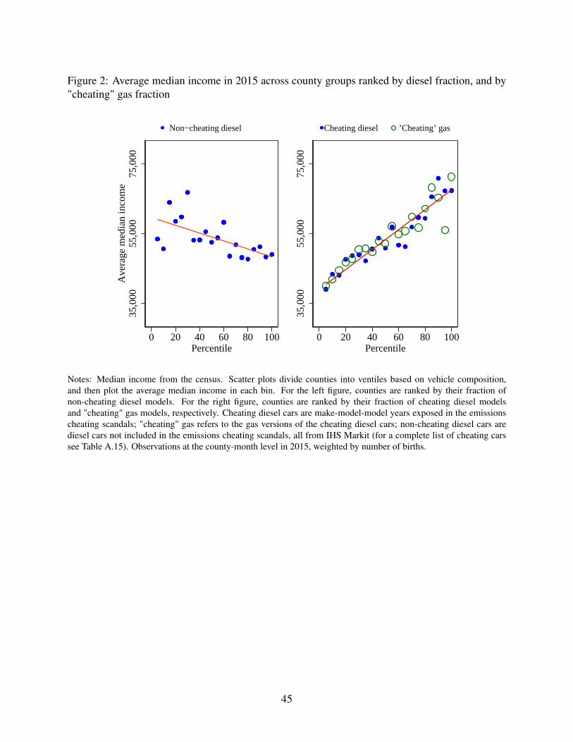
Figure 2: Average median income in 2015 across county groups ranked by diesel fraction, and by"cheating" gas fraction
35,0
0055
,000
75,0
00A
vera
ge m
edia
n in
com
e
0 20 40 60 80 100Percentile
Non−cheating diesel
35,0
0055
,000
75,0
00
0 20 40 60 80 100Percentile
Cheating diesel ’Cheating’ gas
Notes: Median income from the census. Scatter plots divide counties into ventiles based on vehicle composition,and then plot the average median income in each bin. For the left figure, counties are ranked by their fraction ofnon-cheating diesel models. For the right figure, counties are ranked by their fraction of cheating diesel modelsand "cheating" gas models, respectively. Cheating diesel cars are make-model-model years exposed in the emissionscheating scandals; "cheating" gas refers to the gas versions of the cheating diesel cars; non-cheating diesel cars arediesel cars not included in the emissions cheating scandals, all from IHS Markit (for a complete list of cheating carssee Table A.15). Observations at the county-month level in 2015, weighted by number of births.
45
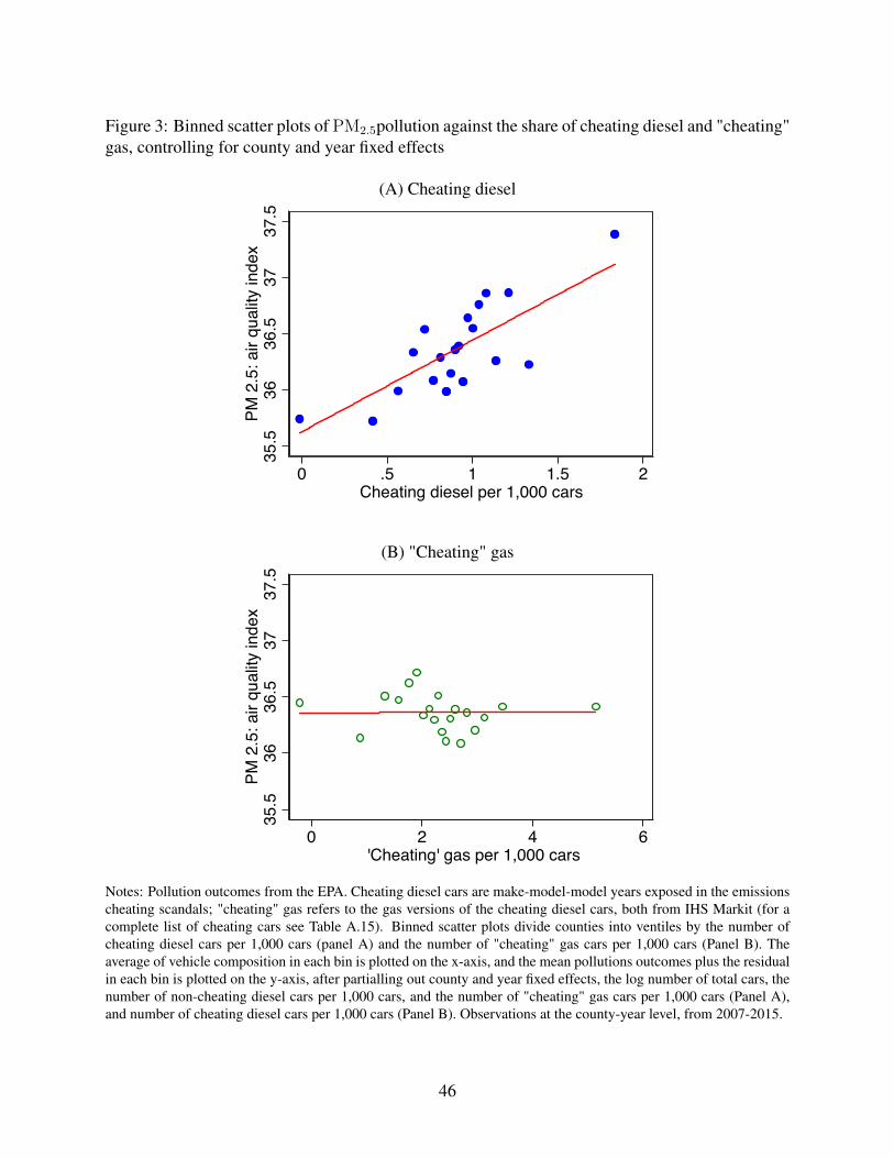
Figure 3: Binned scatter plots of PM2.5pollution against the share of cheating diesel and "cheating"gas, controlling for county and year fixed effects
(A) Cheating diesel
35.5
3636
.537
37.5
PM 2
.5: a
ir qu
ality
inde
x
0 .5 1 1.5 2Cheating diesel per 1,000 cars
(B) "Cheating" gas
35.5
3636
.537
37.5
PM 2
.5: a
ir qu
ality
inde
x
0 2 4 6 'Cheating' gas per 1,000 cars
Notes: Pollution outcomes from the EPA. Cheating diesel cars are make-model-model years exposed in the emissionscheating scandals; "cheating" gas refers to the gas versions of the cheating diesel cars, both from IHS Markit (for acomplete list of cheating cars see Table A.15). Binned scatter plots divide counties into ventiles by the number ofcheating diesel cars per 1,000 cars (panel A) and the number of "cheating" gas cars per 1,000 cars (Panel B). Theaverage of vehicle composition in each bin is plotted on the x-axis, and the mean pollutions outcomes plus the residualin each bin is plotted on the y-axis, after partialling out county and year fixed effects, the log number of total cars, thenumber of non-cheating diesel cars per 1,000 cars, and the number of "cheating" gas cars per 1,000 cars (Panel A),and number of cheating diesel cars per 1,000 cars (Panel B). Observations at the county-year level, from 2007-2015.
46
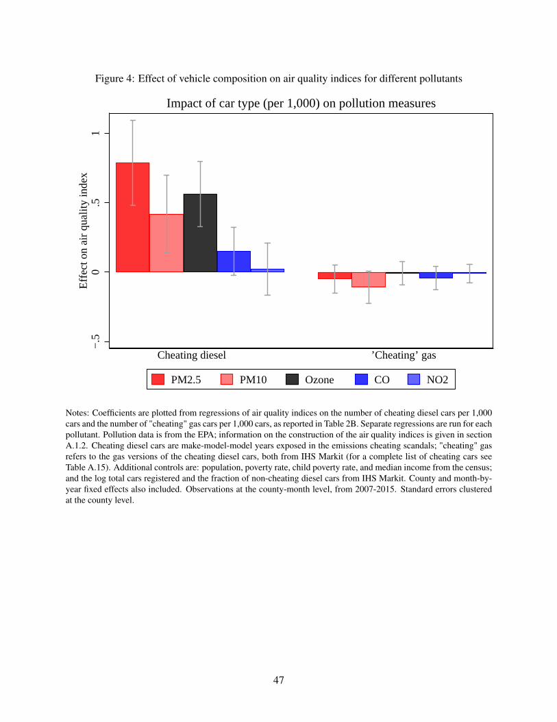
Figure 4: Effect of vehicle composition on air quality indices for different pollutants
−.5
0.5
1E
ffect
on
air
qual
ity in
dex
Cheating diesel ’Cheating’ gas
PM2.5 PM10 Ozone CO NO2
Impact of car type (per 1,000) on pollution measures
Notes: Coefficients are plotted from regressions of air quality indices on the number of cheating diesel cars per 1,000cars and the number of "cheating" gas cars per 1,000 cars, as reported in Table 2B. Separate regressions are run for eachpollutant. Pollution data is from the EPA; information on the construction of the air quality indices is given in sectionA.1.2. Cheating diesel cars are make-model-model years exposed in the emissions cheating scandals; "cheating" gasrefers to the gas versions of the cheating diesel cars, both from IHS Markit (for a complete list of cheating cars seeTable A.15). Additional controls are: population, poverty rate, child poverty rate, and median income from the census;and the log total cars registered and the fraction of non-cheating diesel cars from IHS Markit. County and month-by-year fixed effects also included. Observations at the county-month level, from 2007-2015. Standard errors clusteredat the county level.
47

Figure 5: Binned scatter plots of birth weight and low birth weight rates against the share ofcheating diesel and "cheating" gas, controlling for county and year fixed effects
(A) Cheating diesel
Birth weight Low birth weight (<2,500g)
3290
3295
3300
3305
3310
Birth
wei
ght (
g)
0 .5 1 1.5 2Cheating diesel per 1,000 cars
6.2
6.3
6.4
6.5
Low
birt
h w
eigh
t (<2
,500
g)
0 .5 1 1.5 2Cheating diesel per 1,000 cars
(B) "Cheating" gas
Birth weight Low birth weight (<2,500g)
3290
3295
3300
3305
3310
Birth
wei
ght (
g)
0 2 4 6 'Cheating' gas per 1,000 cars
6.2
6.3
6.4
6.5
Low
birt
h w
eigh
t (<2
,500
g)
0 2 4 6 'Cheating' gas per 1,000 cars
Notes: Birth weight and fraction low birth weight from birth certificate data. Cheating diesel cars are make-model-model years exposed in the emissions cheating scandals; "cheating" gas refers to the gas versions of the cheating dieselcars, both from IHS Markit (for a complete list of cheating cars see Table A.15). Binned scatter plots divide countiesinto ventiles by the number of cheating diesel cars per 1,000 cars (panel A) and the number of "cheating" gas carsper 1,000 cars (Panel B). The average of vehicle composition in each bin is plotted on the x-axis, and the mean birthoutcomes plus the residual in each bin is plotted on the y-axis, after partialling out county and year fixed effects, thelog number of total cars, the number of non-cheating diesel cars per 1,000 cars, and the number of "cheating" gas carsper 1,000 cars (Panel A), and number of cheating diesel cars per 1,000 cars (Panel B). Observations at the county-yearlevel, from 2007-2015, weighted by the number of births in the county-year.
48
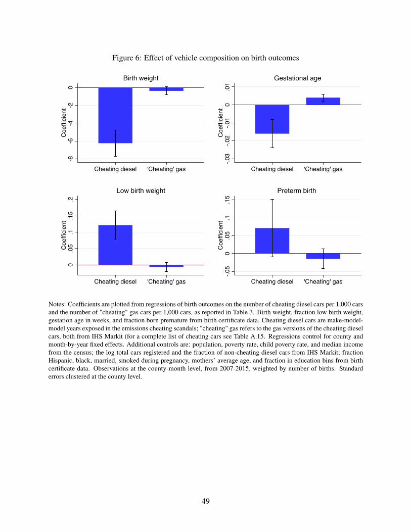
Figure 6: Effect of vehicle composition on birth outcomes-8
-6-4
-20
Coe
ffici
ent
Cheating diesel 'Cheating' gas
Birth weight
-.03
-.02
-.01
0.0
1C
oeffi
cien
t
Cheating diesel 'Cheating' gas
Gestational age0
.05
.1.1
5.2
Coe
ffici
ent
Cheating diesel 'Cheating' gas
Low birth weight
-.05
0.0
5.1
.15
Coe
ffici
ent
Cheating diesel 'Cheating' gas
Preterm birth
Notes: Coefficients are plotted from regressions of birth outcomes on the number of cheating diesel cars per 1,000 carsand the number of "cheating" gas cars per 1,000 cars, as reported in Table 3. Birth weight, fraction low birth weight,gestation age in weeks, and fraction born premature from birth certificate data. Cheating diesel cars are make-model-model years exposed in the emissions cheating scandals; "cheating" gas refers to the gas versions of the cheating dieselcars, both from IHS Markit (for a complete list of cheating cars see Table A.15. Regressions control for county andmonth-by-year fixed effects. Additional controls are: population, poverty rate, child poverty rate, and median incomefrom the census; the log total cars registered and the fraction of non-cheating diesel cars from IHS Markit; fractionHispanic, black, married, smoked during pregnancy, mothers’ average age, and fraction in education bins from birthcertificate data. Observations at the county-month level, from 2007-2015, weighted by number of births. Standarderrors clustered at the county level.
49

Figure 7: Binned scatter plots of maternal characteristics against the share of cheating dieselMedian income
4000
050
000
6000
070
000
8000
0
0 2 4 6Cheating diesel per 1,000 cars
Unconditional
4000
050
000
6000
070
000
8000
0
0 .5 1 1.5 2Cheating diesel per 1,000 cars
County & year FEs
Maternal age Fraction black mothers
2728
2930
31M
othe
r's a
ge
0 2 4 6Cheating diesel per 1,000 cars
Unconditional
2728
2930
31M
othe
r's a
ge
0 .5 1 1.5 2Cheating diesel per 1,000 cars
County & year FEs
010
2030
Pct.
blac
k m
othe
rs
0 2 4 6Cheating diesel per 1,000 cars
Unconditional
010
2030
Pct.
blac
k m
othe
rs0 .5 1 1.5 2
Cheating diesel per 1,000 cars
County & year FEs
Fraction married mothers Fraction college educated mothers
4050
6070
80Pc
t. m
arrie
d m
othe
rs
0 2 4 6Cheating diesel per 1,000 cars
Unconditional
4050
6070
80Pc
t. m
arrie
d m
othe
rs
0 .5 1 1.5 2Cheating diesel per 1,000 cars
County & year FEs
2030
4050
Pct.
colle
ge-e
duca
ted
mot
hers
0 2 4 6Cheating diesel per 1,000 cars
Unconditional
2030
4050
Pct.
colle
ge-e
duca
ted
mot
hers
0 .5 1 1.5 2Cheating diesel per 1,000 cars
County & year FEs
Notes: Median income from the census, maternal characteristics from birth certificate data. Cheating diesel cars aremake-model-model years exposed in the emissions cheating scandals, from IHS Markit (for a complete list of cheatingcars see Table A.15). The left plot of each pair is a binned scatter plot with the number of cheating diesel cars per1,000 cars in 2015 on the x-axis and the maternal characteristic on the y-axis. The right plot shows a binned scatterplot of the same maternal characteristic against the number of cheating diesel cars per 1,000 cars, but now using theentire time period (2007-2015), and partialling out county and year fixed effects. Observations at the county-yearlevel, weighted by the number of births in the county-year.
50
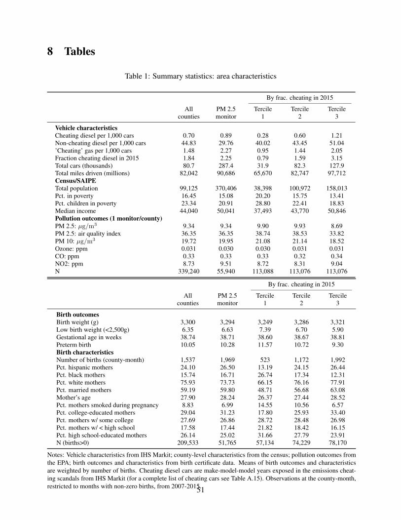
8 Tables
Table 1: Summary statistics: area characteristics
By frac. cheating in 2015
Allcounties
PM 2.5monitor
Tercile1
Tercile2
Tercile3
Vehicle characteristicsCheating diesel per 1,000 cars 0.70 0.89 0.28 0.60 1.21Non-cheating diesel per 1,000 cars 44.83 29.76 40.02 43.45 51.04’Cheating’ gas per 1,000 cars 1.48 2.27 0.95 1.44 2.05Fraction cheating diesel in 2015 1.84 2.25 0.79 1.59 3.15Total cars (thousands) 80.7 287.4 31.9 82.3 127.9Total miles driven (millions) 82,042 90,686 65,670 82,747 97,712Census/SAIPETotal population 99,125 370,406 38,398 100,972 158,013Pct. in poverty 16.45 15.08 20.20 15.75 13.41Pct. children in poverty 23.34 20.91 28.80 22.41 18.83Median income 44,040 50,041 37,493 43,770 50,846Pollution outcomes (1 monitor/county)PM 2.5: µg/m3 9.34 9.34 9.90 9.93 8.69PM 2.5: air quality index 36.35 36.35 38.74 38.53 33.82PM 10: µg/m3 19.72 19.95 21.08 21.14 18.52Ozone: ppm 0.031 0.030 0.030 0.031 0.031CO: ppm 0.33 0.33 0.33 0.32 0.34NO2: ppm 8.73 9.51 8.72 8.31 9.04N 339,240 55,940 113,088 113,076 113,076
By frac. cheating in 2015
Allcounties
PM 2.5monitor
Tercile1
Tercile2
Tercile3
Birth outcomesBirth weight (g) 3,300 3,294 3,249 3,286 3,321Low birth weight (<2,500g) 6.35 6.63 7.39 6.70 5.90Gestational age in weeks 38.74 38.71 38.60 38.67 38.81Preterm birth 10.05 10.28 11.57 10.72 9.30Birth characteristicsNumber of births (county-month) 1,537 1,969 523 1,172 1,992Pct. hispanic mothers 24.10 26.50 13.19 24.15 26.44Pct. black mothers 15.74 16.71 26.74 17.34 12.31Pct. white mothers 75.93 73.73 66.15 76.16 77.91Pct. married mothers 59.19 59.80 48.71 56.68 63.08Mother’s age 27.90 28.24 26.37 27.44 28.52Pct. mothers smoked during pregnancy 8.83 6.99 14.55 10.56 6.57Pct. college-educated mothers 29.04 31.23 17.80 25.93 33.40Pct. mothers w/ some college 27.69 26.86 28.72 28.48 26.98Pct. mothers w/ < high school 17.58 17.44 21.82 18.42 16.15Pct. high school-educated mothers 26.14 25.02 31.66 27.79 23.91N (births>0) 209,533 51,765 57,134 74,229 78,170
Notes: Vehicle characteristics from IHS Markit; county-level characteristics from the census; pollution outcomes fromthe EPA; birth outcomes and characteristics from birth certificate data. Means of birth outcomes and characteristicsare weighted by number of births. Cheating diesel cars are make-model-model years exposed in the emissions cheat-ing scandals from IHS Markit (for a complete list of cheating cars see Table A.15). Observations at the county-month,restricted to months with non-zero births, from 2007-2015.51

Table 2: Effect of vehicle composition on pollution
A: Air quality index
PM 2.5 PM 10 Ozone CO NO2(1) (2) (3) (4) (5)
Cheating diesel per 1,000 cars 0.79∗∗∗ 0.42∗∗∗ 0.56∗∗∗ 0.15∗ 0.022(0.16) (0.14) (0.12) (0.089) (0.095)
’Cheating’ gas per 1,000 cars -0.049 -0.11∗ -0.010 -0.043 -0.010(0.051) (0.059) (0.043) (0.043) (0.035)
FEs: county, time Yes Yes Yes Yes Yes
Observations 55,940 34,766 64,206 18,392 23,401R2 0.532 0.582 0.613 0.684 0.867Mean dep. var. 39.72 19.12 41.99 8.513 20.29P-value (β1 = β2) 0.000 0.002 0.000 0.079 0.772
B: Mean pollutant concentration (µg/m3 for PM2.5 and PM10, ppm for CO and NO2)
PM 2.5 PM 2.5, sat. PM 10 Ozone CO NO2(1) (2) (3) (4) (5) (6)
Cheating diesel per 1,000 cars 0.26∗∗∗ 0.23∗∗∗ 0.30 0.00015∗ 0.015∗∗ 0.024(0.049) (0.015) (0.22) (0.000079) (0.0068) (0.066)
’Cheating’ gas per 1,000 cars -0.016 -0.018∗∗∗ -0.070 0.000045 -0.0042 -0.027(0.016) (0.0059) (0.081) (0.000030) (0.0031) (0.029)
FEs: county, time Yes Yes Yes Yes Yes Yes
Observations 55,940 336,576 34,766 64,206 18,392 23,401R2 0.483 0.588 0.474 0.686 0.599 0.861Mean dep. var. 10.46 8.905 21.01 .03026 .4309 10.58P-value (β1 = β2) 0.000 0.000 0.164 0.276 0.020 0.538
C: Number of days with air quality index>51
PM 2.5 PM 10 Ozone CO NO2(1) (2) (3) (4) (5)
Cheating diesel per 1,000 cars 0.39∗∗∗ 0.045 0.29∗∗∗ 0.0039 0.060∗∗
(0.11) (0.039) (0.061) (0.0027) (0.027)’Cheating’ gas per 1,000 cars -0.063∗ -0.016 0.031 0.0013 -0.011
(0.033) (0.020) (0.024) (0.0019) (0.015)FEs: county, time Yes Yes Yes Yes Yes
Observations 55,940 34,766 64,206 18,392 23,401R2 0.498 0.463 0.567 0.134 0.395Mean dep. var. 4.344 .5336 5.42 .08829 .7376P-value (β1 = β2) 0.000 0.193 0.001 0.404 0.051
Notes: Pollution monitor data from the EPA, satellite data from van Donkelaar et al. (2019); information on theconstruction of the air quality indices in section A.1.2. Cheating diesel cars are make-model-model years exposedin the emissions cheating scandals; "cheating" gas refers to the gas versions of the cheating diesel cars, both fromIHS Markit (for a complete list of cheating cars see Table A.15). "FEs: county, time" refer to county and month-by-year fixed effects. Additional controls are: population, poverty rate, child poverty rate, and median incomefrom the census; and the log total cars registered and the fraction of non-cheating diesel cars from IHS Markit.Observations at the county-month level, from 2007-2015. Standard errors clustered at the county level.
52
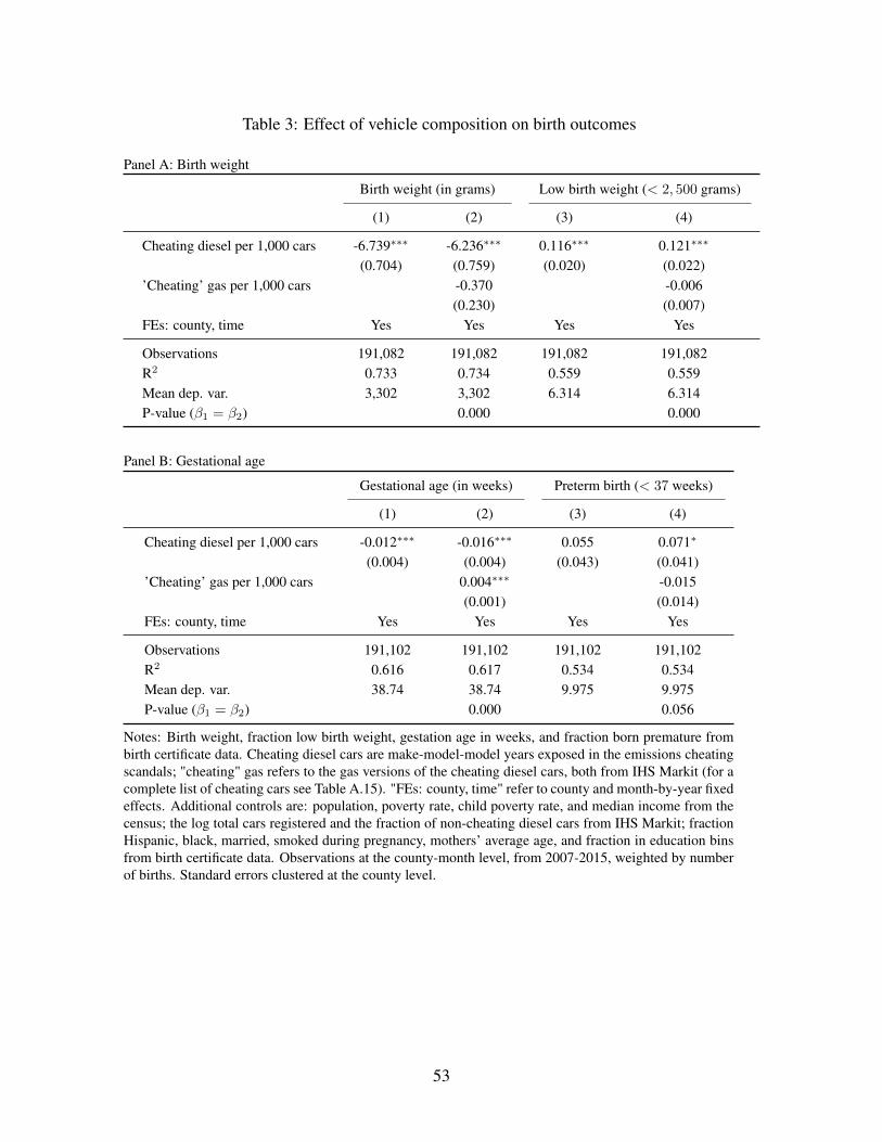
Table 3: Effect of vehicle composition on birth outcomes
Panel A: Birth weight
Birth weight (in grams) Low birth weight (< 2, 500 grams)
(1) (2) (3) (4)
Cheating diesel per 1,000 cars -6.739∗∗∗ -6.236∗∗∗ 0.116∗∗∗ 0.121∗∗∗
(0.704) (0.759) (0.020) (0.022)’Cheating’ gas per 1,000 cars -0.370 -0.006
(0.230) (0.007)FEs: county, time Yes Yes Yes Yes
Observations 191,082 191,082 191,082 191,082R2 0.733 0.734 0.559 0.559Mean dep. var. 3,302 3,302 6.314 6.314P-value (β1 = β2) 0.000 0.000
Panel B: Gestational age
Gestational age (in weeks) Preterm birth (< 37 weeks)
(1) (2) (3) (4)
Cheating diesel per 1,000 cars -0.012∗∗∗ -0.016∗∗∗ 0.055 0.071∗
(0.004) (0.004) (0.043) (0.041)’Cheating’ gas per 1,000 cars 0.004∗∗∗ -0.015
(0.001) (0.014)FEs: county, time Yes Yes Yes Yes
Observations 191,102 191,102 191,102 191,102R2 0.616 0.617 0.534 0.534Mean dep. var. 38.74 38.74 9.975 9.975P-value (β1 = β2) 0.000 0.056
Notes: Birth weight, fraction low birth weight, gestation age in weeks, and fraction born premature frombirth certificate data. Cheating diesel cars are make-model-model years exposed in the emissions cheatingscandals; "cheating" gas refers to the gas versions of the cheating diesel cars, both from IHS Markit (for acomplete list of cheating cars see Table A.15). "FEs: county, time" refer to county and month-by-year fixedeffects. Additional controls are: population, poverty rate, child poverty rate, and median income from thecensus; the log total cars registered and the fraction of non-cheating diesel cars from IHS Markit; fractionHispanic, black, married, smoked during pregnancy, mothers’ average age, and fraction in education binsfrom birth certificate data. Observations at the county-month level, from 2007-2015, weighted by numberof births. Standard errors clustered at the county level.
53

Table 4: Effect of vehicle composition on birth weight by subgroups (micro data)
Panel A: Birth weight (in grams)
(1) (2) (3) (4) (5) (6)
nHwhite BlackCollegedegree
No collegenHwhitecollege
Blackno college
Cheating diesel per 1,000 cars -6.66∗∗∗ -4.23∗∗ -6.33∗∗∗ -6.10∗∗∗ -6.25∗∗∗ -2.61(0.79) (1.86) (0.85) (0.91) (0.84) (1.94)
’Cheating’ gas per 1,000 cars -0.27 -0.16 -0.44 -0.17 -0.56∗ -0.31(0.25) (0.41) (0.31) (0.28) (0.29) (0.52)
FE: county, time Yes Yes Yes Yes Yes Yes
Observations 16,536,223 4,587,491 8,870,725 13,333,095 6,298,914 2,452,613R2 0.043 0.028 0.036 0.048 0.013 0.029Mean dep. var. 3366.0 3122.0 3379.7 3246.7 3431.1 3086.1P-value (β1 = β2) 0.000 0.051 0.000 0.000 0.000 0.310
Panel B: Low birth weight (<2,500g)
(1) (2) (3) (4) (5) (6)
nHwhite BlackCollegedegree
No collegenHwhitecollege
Blackno college
Cheating diesel per 1,000 cars 0.12∗∗∗ 0.13∗ 0.091∗∗∗ 0.16∗∗∗ 0.076∗∗∗ 0.087(0.022) (0.070) (0.024) (0.029) (0.023) (0.089)
’Cheating’ gas per 1,000 cars -0.016∗∗∗ 0.0029 -0.0041 -0.0087 -0.0045 0.028(0.0057) (0.017) (0.0073) (0.011) (0.0058) (0.024)
FE: county, time Yes Yes Yes Yes Yes Yes
Observations 16,536,223 4,587,491 8,870,725 13,333,095 6,298,914 2,452,613R2 0.016 0.012 0.009 0.018 0.004 0.013Mean dep. var. 5.15 11.0 4.46 7.50 3.67 11.9P-value (β1 = β2) 0.000 0.101 0.000 0.000 0.002 0.557
Notes: Birth weight and low birth weight indicator from birth certificate data. nHwhite refers to non-Hispanicwhite mothers. Cheating diesel cars are make-model-model years exposed in the emissions cheating scandals;"cheating" gas refers to the gas versions of the cheating diesel cars, both from IHS Markit (for a complete list ofcheating cars see Table A.15). "FEs: county, time" refer to county and month-by-year fixed effects. Additionalcontrols are: population, poverty rate, child poverty rate, and median income from the census; the log total carsregistered and the fraction of non-cheating diesel cars from IHS Markit; Hispanic, black, white, married, age,and education bins from birth certificate data. Observations at the individual level, from 2007-2015. Standarderrors clustered at the county level.
54
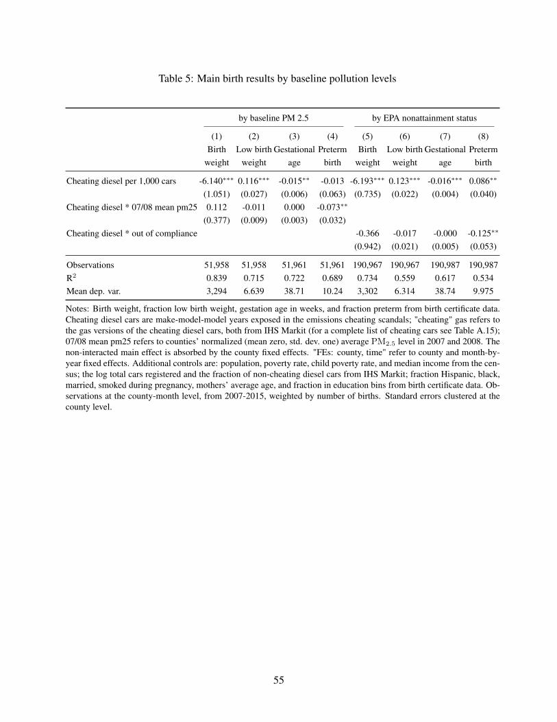
Table 5: Main birth results by baseline pollution levels
by baseline PM 2.5 by EPA nonattainment status
(1) (2) (3) (4) (5) (6) (7) (8)Birth
weightLow birth
weightGestational
agePreterm
birthBirth
weightLow birth
weightGestational
agePreterm
birth
Cheating diesel per 1,000 cars -6.140∗∗∗ 0.116∗∗∗ -0.015∗∗ -0.013 -6.193∗∗∗ 0.123∗∗∗ -0.016∗∗∗ 0.086∗∗
(1.051) (0.027) (0.006) (0.063) (0.735) (0.022) (0.004) (0.040)Cheating diesel * 07/08 mean pm25 0.112 -0.011 0.000 -0.073∗∗
(0.377) (0.009) (0.003) (0.032)Cheating diesel * out of compliance -0.366 -0.017 -0.000 -0.125∗∗
(0.942) (0.021) (0.005) (0.053)
Observations 51,958 51,958 51,961 51,961 190,967 190,967 190,987 190,987R2 0.839 0.715 0.722 0.689 0.734 0.559 0.617 0.534Mean dep. var. 3,294 6.639 38.71 10.24 3,302 6.314 38.74 9.975
Notes: Birth weight, fraction low birth weight, gestation age in weeks, and fraction preterm from birth certificate data.Cheating diesel cars are make-model-model years exposed in the emissions cheating scandals; "cheating" gas refers tothe gas versions of the cheating diesel cars, both from IHS Markit (for a complete list of cheating cars see Table A.15);07/08 mean pm25 refers to counties’ normalized (mean zero, std. dev. one) average PM2.5 level in 2007 and 2008. Thenon-interacted main effect is absorbed by the county fixed effects. "FEs: county, time" refer to county and month-by-year fixed effects. Additional controls are: population, poverty rate, child poverty rate, and median income from the cen-sus; the log total cars registered and the fraction of non-cheating diesel cars from IHS Markit; fraction Hispanic, black,married, smoked during pregnancy, mothers’ average age, and fraction in education bins from birth certificate data. Ob-servations at the county-month level, from 2007-2015, weighted by number of births. Standard errors clustered at thecounty level.
55
Table 6: OLS and IV regressions of birth weight on mean PM 2.5 (µg/m3) and ozone (ppm)
Panel A: Birth weight (in grams)
Cross-sectional OLS Instrumental variable
(1) (2) (3) (4) (5) (6)
Mean PM 2.5 -4.386∗∗∗ -4.011∗∗∗ -4.120∗∗∗ -30.92∗∗∗ -30.72∗∗∗ -33.09∗∗∗
(0.553) (0.885) (0.849) (5.687) (6.768) (8.064)Mean ozone -414.8 7190.8
(339.3) (5171.6)Ozone sample No Yes Yes No Yes YesFEs: time Yes Yes Yes No No NoFEs: county, time No No No Yes Yes Yes
First stage F-stat 186 69.3 6.1Mean dep. var. 3,341 3,324 3,324 3,341 3,324 3,324Mean PM 2.5 8.16 8.43 8.43 8.16 8.43 8.43Mean ozone 0.031 0.031 0.031 0.031 0.031 0.031Observations 189,711 50,714 50,714 189,711 50,714 50,714
Panel B: Low birth weight (<2,500g)
Cross-sectional OLS Instrumental variable
(1) (2) (3) (4) (5) (6)
Mean PM 2.5 0.184∗∗∗ 0.162∗∗∗ 0.154∗∗∗ 0.699∗∗∗ 0.694∗∗∗ 0.760∗∗∗
(0.0127) (0.0208) (0.0207) (0.192) (0.234) (0.261)Mean ozone -27.45∗∗∗ -131.3
(7.669) (139.1)Ozone sample No Yes Yes No Yes YesFEs: time Yes Yes Yes No No NoFEs: county, time No No No Yes Yes Yes
First stage F-stat 186 69.3 6.1Mean dep. var. 5.2 5.74 5.74 5.2 5.74 5.74Mean PM 2.5 8.16 8.43 8.43 8.16 8.43 8.43Mean ozone 0.031 0.031 0.031 0.031 0.031 0.031Observations 189,711 50,714 50,714 189,711 50,714 50,714
Notes: Birth weight and fraction low birth weight from birth certificate data; mean PM 2.5 from van Donkelaar et al.(2019) satellite data; mean ozone from the EPA data. Cross-sectional OLS refers to regressions of birth outcomes onthe pollution measure and month-by-year fixed effects. Instrumental variables (IV) refers to IV regressions of birthoutcomes on pollution with the cheating diesel share as instrument. Column 6 includes the interaction of the cheatingdiesel share with the maximum monthly temperature as an additional instrument. "FEs: county, time" indicates in-clusion of county and month-by-year fixed effects. IV regressions further control for: population, poverty rate, childpoverty rate, and median income from the census; the log total cars registered and the fraction of non-cheating dieselcars from IHS Markit; fraction Hispanic, black, married, smoked during pregnancy, mothers’ average age, and frac-tion in education bins from birth certificate data. Observations at the county-month level, from 2007-2015. Standarderrors clustered at the county level.
56
Table 7: Effect of vehicle composition on asthma visits to the emergency department
PM 2.5 (mean) Visits to ED per 1,000
(1) (2) (3) (4) (5) (6)Full
sampleHCUPsample
All ages 0-4 5-24 25-44
Cheating diesel per 1,000 cars 0.26∗∗∗ 0.64∗∗∗ -0.04 0.27∗∗ -0.01 -0.01(0.05) (0.15) (0.02) (0.12) (0.04) (0.03)
’Cheating’ gas per 1,000 cars -0.02 0.01 -0.00 -0.06∗∗ -0.01 -0.00(0.02) (0.02) (0.01) (0.03) (0.01) (0.01)
FEs: county, time Yes Yes Yes Yes Yes Yes
Observations 55,940 5,657 6,756 6,756 6,756 6,756R2 0.483 0.629 0.864 0.789 0.752 0.828Mean dep. var. 10.1 8.556 1.212 3.385 1.727 1.193States 51 5 5 5 5 5Counties 685 67 228 228 228 228P-value (β1 = β2) 0.000 0.000 0.201 0.023 0.952 0.904
Notes: Column 1 repeats column 2 from Table 2A. Column 2 replicates this specification for for statesincluded in the HCUP sample (AZ, RI, NJ, FL, KY). Controls in columns 1 and 2 are the same as inTable 2. Number of asthma emergency department visits per 1,000 people from the HCUP ED data(columns 3-6). When the dependent variable is the number of visits for a specific age range, the de-nominator is the number of people in the same age range from the census. Cheating diesel cars aremake-model-model years exposed in the emissions cheating scandals; "cheating" gas refers to the gasversions of the cheating diesel cars, both from IHS Markit (for a complete list of cheating cars see Ta-ble A.15). "FEs: county, time" refer to county and quarter-by-year fixed effects. Additional controlsare: population, population in relevant age group, poverty rate, child poverty rate, and median incomefrom the census; the log total cars registered and the fraction of non-cheating diesel cars from IHSMarkit; average fraction of ED visits that are black, Hispanic, female, covered by Medicaid, coveredby private insurance, the average length of stay, and the average number of deaths from the HCUPdata. Observations in columns 3-6 at the county-quarter level, from 2007-2015, weighted by county-level population in the relevant age group. Standard errors clustered at the county level.
57
A.1 Appendix (for online publication)
A.1.1 Additional robustness exercises
Table A.4 shows the robustness of our main results to a broad set of alternative specification
choices. Columns 1 through 8 show results for birth weight, while columns 9 through 16 present
results for PM2.5. Columns 1 and 9 repeat our preferred specification, for comparison.
A.1.1.1 Different car manufacturers
First, in columns 2 and 10, we estimate the effect of the cheating diesel VW and FCA cars sepa-
rately. For both the pollution and birth outcomes, the effects of an additional cheating VW diesel
car per thousand are consistent with our main results, and precisely measured. The effect of an ad-
ditional cheating FCA car per thousand is very imprecise, which is not surprising given that these
cars only entered the market in model year 2014 and our data only go through 2015.
A.1.1.2 Different types of counties
Second, we show that the effect size per car is similar in counties with higher and lower market
penetration of the cheating vehicles. The regressions in columns 3–4 and 11–12 divide the sample
into counties with an above or below median concentration of cheating diesel vehicles in 2015;
the similarity of the point estimates across these two samples suggests that the effects of pollution
from the cheating diesel cars on birth outcomes are relatively linear. Columns 5 and 13 drop states
in the bottom quintile of the fraction cheating diesel cars in 2015. Columns 6 and 14 drop counties
designated to be in non-attainment status with the National Ambient Air Quality Standards in
2005. TOur pollution results are also unaffected when we limit the sample to include only county-
months with non-missing birth information (the overlap between the pollution monitor sample and
the birth outcomes sample in Table 3).
58

A.1.1.3 Different exposure measures
Third, we show that our results are robust to alternative ways of defining exposure. Our preferred
specification uses the fraction of the vehicle fleet that is cheating as the exposure measure. Alter-
natively, we could have defined the variable as the number of cheating cars per square mile. We
prefer our measure, as there are many counties where only part of the county is populated and thus
scaling by area would distort the exposure measure toward an artificially lower exposure in more
rural areas. However, we show in columns 7–8 and 15–16 that the results are similar when we de-
fine cheating diesel by cheating cars per square mile, or cheating cars per 1,000 people.Our results
are also robust to varying the number of monitoring stations included in our pollution outcome
variables, though most counties have at most one monitoring station (results available on request).
A.1.1.4 Different weighting and aggregation
Although our primary specification is weighted (by the number of births for birth outcomes and
by population for the number of emergency department visits), the results are very similar if we
leave the regressions unweighted. Table A.5 show our main results on birth outcomes using an
unweighted specification. The resulting estimates for the effect of cheating diesel cars on health
outcomes are nearly identical.
Our results are also robust to different levels of aggregation. Table A.9 shows that our re-
sults are very similar if we collapse our data to either the annual or commuting zone level, while
regressions using disaggregated individual-level data are shown in Table 4.
A.1.1.5 Different controls
In addition to varying the specification, Tables A.10 and A.11 show the robustness of our results to
different sets of fixed effects and controls. The first column shows the raw association between the
fraction of cheating diesel cars and health outcomes. For all birth outcomes, more cheating cars
is associated with better birth outcomes, reflecting the fact that these cars are being purchased in
generally wealthier areas (see Figure 2). This positive correlation is eliminated when county-level
59
controls are added (column 2). When county and month-by-year fixed effects are added, we see
a strong negative association emerge between the share of cheating diesel cars in a county and
birth weight. In columns 3 and 4 we add county and month-by-year fixed effects, first alone, and
then with the county-level controls. Although the county-level controls are not very important as
long as we include county fixed effects, using within-county variation is important. Our results
are also robust to including a wide range of county-month temperature and precipitation controls,
and our results for ozone are stronger in the summer than the winter, which makes sense as ozone
requires sunlight and heat for production (see Table A.12).35 Our results are also robust to including
various economic controls, such as unemployment rate and refinancing volume, to control for the
any potential confounding effects of the subprime mortgage crisis and the great recession (results
available upon request). Finally, the share of cheating diesel cars does not affect birth rates in our
sample, in line with the lack of compositional impacts shown in Figure 7 (results available upon
request).
A.1.2 Technical details
A.1.2.1 Air quality index
The EPA’s air quality index is scaled from 0-500 and broken into levels of health-risk categories:
0-50 – Level of health concern = Good; 51-100 – Level of health concern = Moderate; 101-150 –
Level of health concern = Unhealthy for sensitive groups; 151-200 – Level of concern = Unhealthy;
301-500 – Level of concern = Hazardous.
For each pollutant, “cut-points” are used to determine what the value of the AQI will be for
a given measurement of that pollutant. While the scale has remained the same over time (100
is always considered the cutoff beyond which the air quality is unhealthy), the relevant cut-points
35Additionally, we have used a spatial first differences (SFD) specifications, a recently developed approach whichanalyzes differences between adjacent counties instead of deviations from country-wide trends (Druckenmiller andHsiang, 2018). In our setting, the SFD approach has limited statistical power due to sample reductions in first differ-ences (all counties adjacent to small counties with zero births are dropped) as well as potential treatment spilloversbetween counties. Despite this loss in power, the SFD estimates are similar to our baseline results (available uponrequest).
60

have changed over the time period studied in this paper. Thus, we construct an internally consistent
air quality index for each pollutant using the bins given in the most recent AQI documentation
and actual pollution measurements (May 2016, see Figure A.13), rather than relying on the AQI
numbers published by the EPA.
The formula for converting daily pollution measures to a daily air quality index is reproduced
below. First, the maximum concentration of the pollutant is determined (for particulate matter, this
is also the mean), the relevant cut-points are found, and the index is calculated according to the
formula:
AQIp =AQIHigh − AQILowBPHigh −BPLow
∗ (Concentrationp −BPLow) + AQILow (A.1)
with AQIHigh = AQI for upper cut-point ;AQILow = AQI for lower cut-point ; BPHigh = Upper
cut-point concentration ; and BPLow = Lower cut-point concentration.
The maximum and mean are the same for particulate matter because of the way it is measured;
a filter is placed outside for the relevant time period, and then the amount of particulates collected
is measured. Thus, there is just one measure per day, and the maximum is the same as the mean.
A.1.2.2 Cheating diesel cars per county per year
When we roll back the make-model-model year dataset of the stock of registered vehicles per
county in 2015 to construct an annual measure, we need to consider that model years are sold both
in the calendar year corresponding with the model year and in the previous year. Considering that
a sizable fraction of new cars are purchased prior to the model year is important, because our goal
is to correctly construct the number of cheating cars in each county and each year.
We use a secondary dataset of car sales at the county-make-model level (Experian Autocount
data, from 2008-2017) to construct make-model specific measures of the share of vehicles pur-
chased in the vehicle year (relative to the previous year) for make-models with cheating diesel
cars. These shares range from 0.56 to 0.9 (available on request). For each make-model, we as-
sign this fraction of make-models to the model year, and the remaining cars to the prior year. The
61
Autocount data does not allow us to separate sales of diesel and gas powered cars, so the fraction
purchased in the model year is the same for the cheating diesel and "cheating" gas cars.
For the number of non-cheating diesel cars, we use a similar smoothing procedure. Again
using the 2008-2017 Autocount sales data, we calculate the fraction of all vehicles purchased in
the model year (0.7518) and use this share to roll back the number of diesels. As is the case with
the model-specific measure, this statistic combines gas and diesel vehicles.
62
A.2 Appendix Figures
Figure A.1: Cheating diesel cars and particulate matter over time
Panel A: Stock of cheating diesel cars
020
0,00
040
0,00
060
0,00
0N
umbe
r of c
heat
ing
dies
el c
ars
2007 2011 2015Year
Panel B: Share cheating diesel cars and mean PM2.5
01
23
Che
atin
g di
esel
car
s pe
r 1,0
00
7080
9010
011
0M
ean
PM25
(200
7=10
0)
2005 2007 2009 2011 2013 2015Year
Cheating diesel cars (low) Cheating diesel cars (high)Mean PM25 (low) Mean PM25 (high)
Low/high refers to bottom/top 2015 cheating terciles
Notes: Panel A shows the total number of cheating diesel cars registered in the United States by year. In panel B, thesolid lines show the mean PM 2.5 level and the average cheating diesel share in the top tercile of counties in terms ofthe 2015 cheating diesel share. The dashed lines show the respective averages for the bottom tercile. Cheating dieselcars are make-model-model years exposed in the emissions cheating scandals, from IHS Markit (for a complete listof cheating cars see Table A.15). Mean PM2.5 from the EPA data, normalized to the 2007 average. “Low diesel”counties are those in the bottom tercile of fraction of cheating diesel, “high diesel” counties are those in the top tercileof fraction of cheating diesel. Data at the county-year level, from 2005-2015.
63

Figure A.2: County-level distribution of cheating diesel and “cheating” gas cars in 2015
A: Cheating diesel cars, 2015
B: “Cheating” gas cars, 2015
Notes: Number of cheating diesel and “cheating” gas cars per 1,000 cars and light-duty trucks registered at the county-level in 2015. Cheating diesel cars are make-model-model years exposed in the emissions cheating scandals, from IHSMarkit (for a complete list of cheating cars see Table A.15). Non-cheating diesel cars are diesel cars not included inthe emissions cheating scandals.
64
Figure A.3: Binscatter plots of 2015 cheating diesel and “cheating” gas across 2007 VW marketshares, by 2007 diesel share
05
1015
0 .5 1 1.5 0 .5 1 1.5
Below median diesel share in 2007 Above median diesel share in 2007
Cheating diesel 'Cheating' gas
Che
atin
g ca
rs p
er 1
,000
in 2
015
VW market share in 2007
Notes: Separate Binscatter plots by Volkswagen 2007 market share, for counties below and above 2007 (non-cheating)diesel share. Cheating diesel and “cheating” gas shares increase with the 2007 VW market share but the effect isstronger in counties with low (non-cheating) diesel shares for “cheating” gas. Cheating diesel cars are make-model-model years exposed in the emissions cheating scandals; "cheating" gas refers to the gas versions of the cheating dieselcars, both from IHS Markit (for a complete list of cheating cars see Table A.15).
65
Figure A.4: Distribution of cheating diesel cars and diesel fuel in North Carolina
Notes: Number of cheating diesel and “cheating” gas cars per 1,000 cars and light-duty trucks registered at the county-level in 2015. Cheating diesel cars are make-model-model years exposed in the emissions cheating scandals, fromIHS Markit (for a complete list of cheating cars see Table A.15). “Cheating” gas cars are the gasoline versions ofthe cheating make-model-years. Data on diesel fuel availability for North Carolina is provided by the North CarolinaDepartment of Agriculture and Consumer Services, shared with GIS through the NC OneMap program, and is thefraction of gas stations with at least one diesel fuel nozzle at the county level in 2017.
66
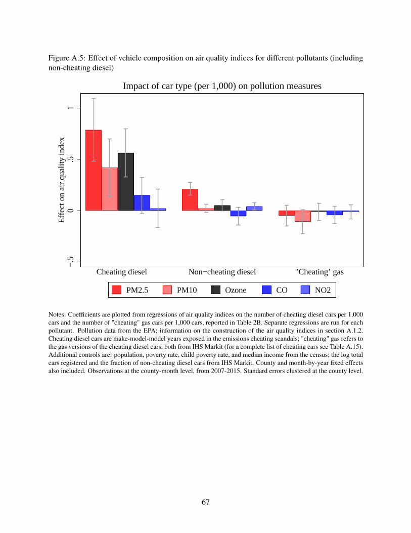
Figure A.5: Effect of vehicle composition on air quality indices for different pollutants (includingnon-cheating diesel)
−.5
0.5
1E
ffect
on
air
qual
ity in
dex
Cheating diesel Non−cheating diesel ’Cheating’ gas
PM2.5 PM10 Ozone CO NO2
Impact of car type (per 1,000) on pollution measures
Notes: Coefficients are plotted from regressions of air quality indices on the number of cheating diesel cars per 1,000cars and the number of "cheating" gas cars per 1,000 cars, reported in Table 2B. Separate regressions are run for eachpollutant. Pollution data from the EPA; information on the construction of the air quality indices in section A.1.2.Cheating diesel cars are make-model-model years exposed in the emissions cheating scandals; "cheating" gas refers tothe gas versions of the cheating diesel cars, both from IHS Markit (for a complete list of cheating cars see Table A.15).Additional controls are: population, poverty rate, child poverty rate, and median income from the census; the log totalcars registered and the fraction of non-cheating diesel cars from IHS Markit. County and month-by-year fixed effectsalso included. Observations at the county-month level, from 2007-2015. Standard errors clustered at the county level.
67
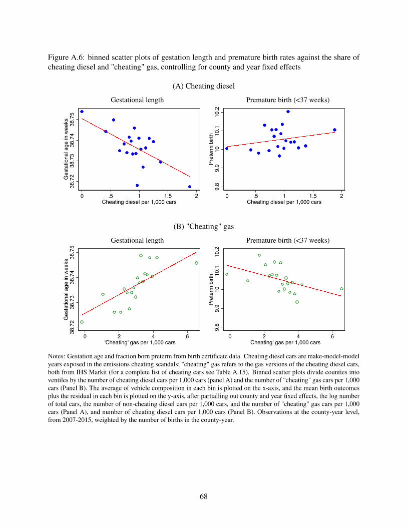
Figure A.6: binned scatter plots of gestation length and premature birth rates against the share ofcheating diesel and "cheating" gas, controlling for county and year fixed effects
(A) Cheating diesel
Gestational length Premature birth (<37 weeks)
38.7
238
.73
38.7
438
.75
Ges
tatio
nal a
ge in
wee
ks
0 .5 1 1.5 2Cheating diesel per 1,000 cars
9.8
9.9
1010
.110
.2Pr
eter
m b
irth
0 .5 1 1.5 2Cheating diesel per 1,000 cars
(B) "Cheating" gas
Gestational length Premature birth (<37 weeks)
38.7
238
.73
38.7
438
.75
Ges
tatio
nal a
ge in
wee
ks
0 2 4 6 'Cheating' gas per 1,000 cars
9.8
9.9
1010
.110
.2Pr
eter
m b
irth
0 2 4 6 'Cheating' gas per 1,000 cars
Notes: Gestation age and fraction born preterm from birth certificate data. Cheating diesel cars are make-model-modelyears exposed in the emissions cheating scandals; "cheating" gas refers to the gas versions of the cheating diesel cars,both from IHS Markit (for a complete list of cheating cars see Table A.15). Binned scatter plots divide counties intoventiles by the number of cheating diesel cars per 1,000 cars (panel A) and the number of "cheating" gas cars per 1,000cars (Panel B). The average of vehicle composition in each bin is plotted on the x-axis, and the mean birth outcomesplus the residual in each bin is plotted on the y-axis, after partialling out county and year fixed effects, the log numberof total cars, the number of non-cheating diesel cars per 1,000 cars, and the number of "cheating" gas cars per 1,000cars (Panel A), and number of cheating diesel cars per 1,000 cars (Panel B). Observations at the county-year level,from 2007-2015, weighted by the number of births in the county-year.
68

Figure A.7: Binned scatter plots of maternal characteristics against the share of "cheating" gasMedian income
4000
050
000
6000
070
000
0 20 'Cheating' gas per 1,000 cars
Unconditional
4000
050
000
6000
070
000
0 2 4 6 'Cheating' gas per 1,000 cars
County & year FEs
Maternal age Fraction black mothers
2628
3032
Mot
her's
age
0 20 'Cheating' gas per 1,000 cars
Unconditional
2628
3032
Mot
her's
age
0 2 4 6 'Cheating' gas per 1,000 cars
County & year FEs
1015
2025
Pct.
blac
k m
othe
rs
0 20 'Cheating' gas per 1,000 cars
Unconditional
1015
2025
Pct.
blac
k m
othe
rs0 2 4 6
'Cheating' gas per 1,000 cars
County & year FEs
Fraction married mothers Fraction college educated mothers
5055
6065
70Pc
t. m
arrie
d m
othe
rs
0 20 'Cheating' gas per 1,000 cars
Unconditional
5055
6065
70Pc
t. m
arrie
d m
othe
rs
0 2 4 6 'Cheating' gas per 1,000 cars
County & year FEs
2030
4050
Pct.
colle
ge-e
duca
ted
mot
hers
0 20 'Cheating' gas per 1,000 cars
Unconditional
2030
4050
Pct.
colle
ge-e
duca
ted
mot
hers
0 2 4 6 'Cheating' gas per 1,000 cars
County & year FEs
Notes: Median income from the census, maternal characteristics from birth certificate data. Cheating diesel cars aremake-model-model years exposed in the emissions cheating scandals; "cheating" gas refers to the gas versions of thecheating diesel cars, both from IHS Markit (for a complete list of cheating cars see Table A.15). The left plot ofeach pair is a binned scatter plot with the number of "cheating" gas cars per 1,000 cars in 2015 on the x-axis, andthe maternal characteristic on the y-axis. In the right plot is a binned scatter plot of the same maternal characteristicagainst the number of "cheating" gas per 1,000 cars, but now using the entire time period (2007-2015), and partiallingout county and year fixed effects. Observations at the county-year level, weighted by the number of births in thecounty-year.
69
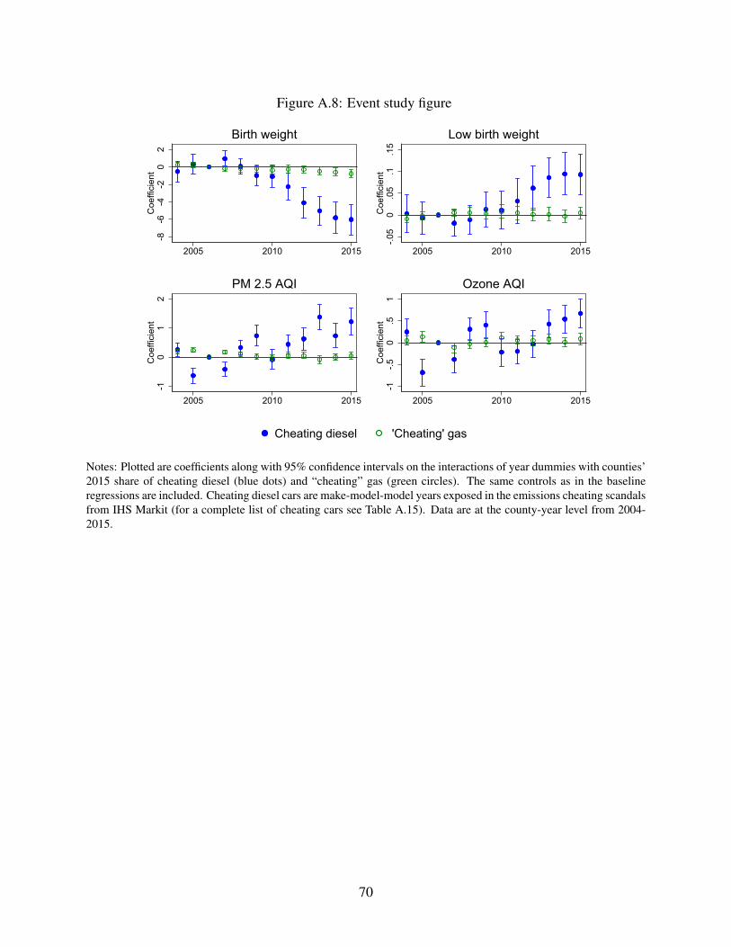
Figure A.8: Event study figure
-8-6
-4-2
02
Coe
ffici
ent
2005 2010 2015
Birth weight
-.05
0.0
5.1
.15
Coe
ffici
ent
2005 2010 2015
Low birth weight
-10
12
Coe
ffici
ent
2005 2010 2015
PM 2.5 AQI
-1-.5
0.5
1C
oeffi
cien
t
2005 2010 2015
Ozone AQI
Cheating diesel 'Cheating' gas
Notes: Plotted are coefficients along with 95% confidence intervals on the interactions of year dummies with counties’2015 share of cheating diesel (blue dots) and “cheating” gas (green circles). The same controls as in the baselineregressions are included. Cheating diesel cars are make-model-model years exposed in the emissions cheating scandalsfrom IHS Markit (for a complete list of cheating cars see Table A.15). Data are at the county-year level from 2004-2015.
70

A.3 Appendix Tables
Table A.1: Summary statistics: HCUP sample characteristics
By frac. cheating in 2015
Allcounties
PM 2.5monitor
Tercile1
Tercile2
Tercile3
Health outcomesAsthma ED visits per 1,000 1.21 1.25 1.00 1.48 1.07Asthma ED visits per 1,000, ages 0-4 3.37 3.52 2.26 4.21 2.95Asthma ED visits per 1,000, ages 5-24 1.73 1.78 1.37 2.03 1.58Census/SAIPETotal population 1,055,605 1,365,429 35,781 1,061,646 1,128,399Pct. in poverty 15.0 14.8 23.7 16.0 13.7Pct. children in poverty 21.4 21.0 32.7 22.7 19.7Pct. white 61.4 56.3 88.6 49.1 66.8Median income 51,143 51,812 34,517 48,069 54,255Vehicle characteristicsCheating diesel per 1,000 cars 0.84 0.83 0.23 0.64 1.01Non cheating diesel per 1,000 cars 18.38 15.65 31.55 16.13 18.76’Cheating’ gas per 1,000 cars 3.63 3.96 0.87 3.94 3.65
Observations 8,208 1,882 2,736 2,736 2,736
Notes: Health outcomes from HCUP; county-level characteristics from the census; vehicle character-istics from IHS Markit. Cheating diesel cars are make-model-model years exposed in the emissionscheating scandals; "cheating" gas refers to the gas versions of the cheating diesel cars, both from IHSMarkit (for a complete list of cheating cars see Table A.15). Observations at the county-quarter levelfrom 2007-2015, weighted by population.
71
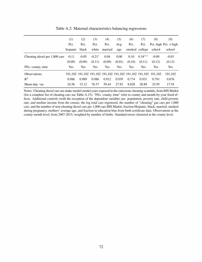
Table A.2: Maternal characteristics balancing regressions
(1) (2) (3) (4) (5) (6) (7) (8) (9)
Pct.
hispanic
Pct.
black
Pct.
white
Pct.
married
Avg.
age
Pct.
smoked
Pct.
college
Pct. high
school
Pct. < high
school
Cheating diesel per 1,000 cars -0.11 -0.05 -0.21∗ 0.04 0.00 0.10 0.34∗∗∗ -0.09 -0.03
(0.09) (0.09) (0.11) (0.09) (0.01) (0.10) (0.11) (0.12) (0.13)
FEs: county, time Yes Yes Yes Yes Yes Yes Yes Yes Yes
Observations 191,102 191,102 191,102 191,102 191,102 191,102 191,102 191,102 191,102
R2 0.986 0.989 0.986 0.912 0.939 0.774 0.931 0.791 0.876
Mean dep. var. 24.56 15.12 76.37 59.44 27.92 8.828 28.89 25.95 17.54
Notes: Cheating diesel cars are make-model-model years exposed in the emissions cheating scandals, from IHS Markit(for a complete list of cheating cars see Table A.15). "FEs: county, time" refer to county and month-by-year fixed ef-fects. Additional controls (with the exception of the dependent variable) are: population, poverty rate, child povertyrate, and median income from the census; the log total cars registered, the number of "cheating" gas cars per 1,000cars, and the number of non-cheating diesel cars per 1,000 cars IHS Markit; fraction Hispanic, black, married, smokedduring pregnancy, mothers’ average age, and fraction in education bins from birth certificate data. Observations at thecounty-month level, from 2007-2015, weighted by number of births. Standard errors clustered at the county level.
72
Table A.3: Effect of vehicle composition on pollution by distance
PM 2.5 AQI PM 2.5 concentration
(1) (2) (3) (4) (5) (6)
Cheating diesel per 1,000 cars 0.80∗∗∗ 0.94∗∗∗ 0.77∗ 0.27∗∗∗ 0.32∗∗∗ 0.23∗
(0.16) (0.28) (0.46) (0.05) (0.09) (0.14)Cheating diesel per 1,000 cars: 1-20 mi 0.41 0.10
(0.54) (0.15)Cheating diesel per 1,000 cars: 20-40 mi -0.01 0.04
(0.50) (0.16)Cheating diesel per 1,000 cars: 40-60 mi -0.06 0.05
(0.51) (0.16)’Cheating’ gas per 1,000 cars -0.02 0.07 0.06 -0.01 0.02 0.02
(0.05) (0.07) (0.12) (0.02) (0.02) (0.04)’Cheating’ gas per 1,000 cars: 1-20 mi -0.04 0.01
(0.14) (0.04)’Cheating’ gas per 1,000 cars: 20-40 mi -0.07 -0.03
(0.14) (0.04)’Cheating’ gas per 1,000 cars: 40-60 mi 0.26∗ 0.06
(0.15) (0.05)FEs: county, time Yes Yes Yes Yes Yes Yes
Observations 55,940 12,602 12,602 55,940 12,602 12,602R2 0.531 0.625 0.628 0.482 0.611 0.614Mean dep. var. 36.35 39.63 39.63 9.338 10.26 10.26Monitors 824 151 151 824 151 151
Notes: Pollution data from the EPA. AQI stands for air quality index; information on the constructionof the air quality indices in section A.1.2. Distance between counties calculated as the distance betweencounty centroids using geodetic distances. The vehicle composition variables in the distance bands areconstructed by dividing the total number of each car type among all counties in the distance band bythe total number of cars among all counties in the distance band. Additional controls are: the log totalcars registered and the fraction of non-cheating diesel cars from IHS Markit, as well as month by yearfixed effects and county fixed effects. Columns 2 and 4 replicate columns 1 and 3 in the subsample withat least one neighbor with a county centroid within 20 miles. Cheating diesel cars are make-model-model years exposed in the emissions cheating scandals; "cheating" gas refers to the gas versions ofthe cheating diesel cars, both from IHS Markit (for a complete list of cheating cars see Table A.15)."FEs: county, time" refer to county and month-by-year fixed effects. Also included in columns 3 and6: log(total cars), log(total cars): 1-20 miles, log(total cars): 20-40 miles, log(total cars): 40-60 miles,non-cheating diesel, non-cheating diesel: 1-20 miles, non-cheating diesel: 20-40 miles, non-cheatingdiesel: 40-60 miles. Observations at the county-month level, from 2007-2015. Standard errors clus-tered at the county level.
73

Tabl
eA
.4:A
ltern
ativ
esp
ecifi
catio
ns
Bir
thw
eigh
tPM
2.5
(1)
(2)
(3)
(4)
(5)
(6)
(7)
(8)
(9)
(10)
(11)
(12)
(13)
(14)
(15)
(16)
Mai
nre
sult
By
scan
dal
Abo
vem
edia
nB
elow
med
ian
Dro
plo
waf
f.D
rop
nona
t.C
ars/
area
Car
s/po
pM
ain
resu
ltB
ysc
anda
lA
bove
med
ian
Bel
owm
edia
nD
rop
low
aff.
Dro
pno
nat.
Car
s/ar
eaC
ars/
pop
Che
atin
gdi
esel
per1
,000
cars
-6.2
4∗∗∗
-6.2
0∗∗∗
-9.0
9∗-7
.00∗
∗∗-8
.02∗
∗∗0.
26∗∗
∗0.
26∗∗
∗-0
.12
0.26
∗∗∗
0.29
∗∗∗
(0.7
6)(0
.86)
(5.0
5)(1
.26)
(1.3
6)(0
.05)
(0.0
6)(0
.22)
(0.0
5)(0
.05)
Che
atin
gV
Wpe
r1,0
00ca
rs-6
.43∗
∗∗0.
30∗∗
∗
(0.8
1)(0
.05)
Che
atin
gFi
atC
per1
,000
cars
-0.9
9-0
.31
(4.8
0)(0
.24)
’Che
atin
g’ga
spe
r1,0
00ca
rs-0
.37
-0.3
5-0
.36
-0.3
90.
460.
94-0
.02
-0.0
2-0
.04∗
0.02
-0.0
0-0
.06∗
∗∗
(0.2
3)(0
.23)
(0.2
2)(0
.51)
(0.4
8)(0
.64)
(0.0
2)(0
.02)
(0.0
2)(0
.03)
(0.0
2)(0
.02)
Che
atin
gdi
esel
per1
0m
i2-1
5.29
∗∗∗
0.21
(4.2
2)(0
.22)
’Che
atin
g’ga
spe
r10
mi2
-0.5
70.
02(0
.55)
(0.0
5)C
heat
ing
dies
elpe
r1,0
00po
p-6
.78∗
∗∗0.
30∗∗
∗
(0.8
6)(0
.05)
’Che
atin
g’ga
spe
r1,0
00po
p0.
12-0
.02∗
∗
(0.2
2)(0
.01)
FEs:
coun
ty,t
ime
Yes
Yes
Yes
Yes
Yes
Yes
Yes
Yes
Yes
Yes
Yes
Yes
Yes
Yes
Yes
Yes
Obs
erva
tions
191,
082
191,
082
101,
489
87,2
7715
6,41
417
1,99
919
1,08
219
1,08
255
,940
55,9
4034
,759
20,0
5146
,678
41,4
8355
,940
55,9
40R2
0.73
40.
734
0.75
60.
665
0.35
00.
344
0.73
30.
733
0.48
30.
483
0.46
00.
560
0.46
80.
433
0.48
00.
482
Mea
nde
p.va
r.3,
302
3,30
23,
314
3,27
23,
348
3,34
53,
302
3,30
29.
338
9.33
88.
929
10.0
89.
348.
672
9.33
89.
338
P-va
lue
(β1=β2)
0.00
00.
000
0.00
00.
099
0.00
00.
000
0.00
10.
000
0.00
00.
000
0.00
00.
555
0.00
00.
000
0.42
80.
000
Not
es:
Bir
thw
eigh
tfro
mbi
rth
cert
ifica
teda
ta;P
M2.5
from
the
EPA
data
.A
bove
and
belo
wm
edia
nre
fers
toth
eco
unty
-lev
elfr
actio
nof
chea
ting
dies
elca
rsin
2015
.T
he"D
rop
low
aff."
spec
ifica
tion
drop
sst
ates
inth
ebo
ttom
quin
tile
offr
actio
nch
eatin
gdi
esel
cars
in20
15;
"Dro
pno
nat."
drop
sco
untie
sde
sign
ated
tobe
inno
n-at
tain
men
tsta
tus
with
the
Nat
iona
lAm
bien
tAir
Qua
lity
Stan
dard
sin
2005
.Che
atin
gdi
esel
cars
are
mak
e-m
odel
-mod
elye
ars
expo
sed
inth
eem
issi
ons
chea
ting
scan
-da
ls;"
chea
ting"
gas
refe
rsto
the
gas
vers
ions
ofth
ech
eatin
gdi
esel
cars
,bot
hfr
omIH
SM
arki
t(fo
raco
mpl
ete
listo
fche
atin
gca
rsse
eTa
ble
A.1
5).C
heat
ing
VW
cars
are
chea
ting
dies
elca
rsfr
omth
eVo
lksw
agen
emis
sion
sch
eatin
gsc
anda
l;ch
eatin
gFi
atC
are
are
chea
ting
dies
elca
rsfr
omth
eFi
at-C
hrys
lere
mis
sion
sch
eatin
gsc
anda
l."F
Es:
coun
ty,t
ime"
refe
rto
coun
tyan
dm
onth
-by-
year
fixed
effe
cts.
Add
ition
alco
ntro
lsar
e:po
pula
tion,
pove
rty
rate
,chi
ldpo
vert
yra
te,a
ndm
edia
nin
com
efr
omth
ece
nsus
;the
log
tota
lcar
sre
gist
ered
and
the
frac
tion
ofno
n-ch
eatin
gdi
esel
cars
from
IHS
Mar
kit;
frac
tion
His
pani
c,bl
ack,
mar
ried
,sm
oked
duri
ngpr
egna
ncy,
mot
hers
’av
erag
eag
e,an
dfr
actio
nin
educ
atio
nbi
nsfr
ombi
rth
cert
ifica
teda
ta(c
ontr
ols
from
birt
hda
taon
lyin
clud
edin
colu
mns
1-8)
.Obs
erva
tions
atth
eco
unty
-mon
thle
vel,
from
2007
-201
5.C
olum
ns1-
8w
eigh
ted
bynu
mbe
rofb
irth
s.St
anda
rder
rors
clus
tere
dat
the
coun
tyle
vel.
74

Table A.5: Effect of vehicle composition on birth outcomes (unweighted regressions)
Panel A: Birth weight
Birth weight (in grams) Low birth weight (< 2, 500 grams)
(1) (2) (3) (4)
Cheating diesel per 1,000 cars -6.757∗∗∗ -7.339∗∗∗ 0.158∗∗∗ 0.178∗∗∗
(1.158) (1.243) (0.042) (0.044)’Cheating’ gas per 1,000 cars 0.349 -0.014
(0.470) (0.016)FEs: county, time Yes Yes Yes Yes
Observations 191,082 191,082 191,082 191,082R2 0.347 0.347 0.222 0.222Mean dep. var. 3,342 3,342 5.199 5.199P-value (β1 = β2) 0.000 0.000
Panel B: Gestational age
Gestational age (in weeks) Preterm birth (< 37 weeks)
(1) (2) (3) (4)
Cheating diesel per 1,000 cars -0.009 -0.012∗ 0.086 0.063(0.006) (0.007) (0.064) (0.067)
’Cheating’ gas per 1,000 cars 0.003 0.028(0.002) (0.023)
FEs: county, time Yes Yes Yes Yes
Observations 191,102 191,102 191,102 191,102R2 0.235 0.235 0.209 0.209Mean dep. var. 38.92 38.92 8.854 8.854P-value (β1 = β2) 0.046 0.652
Notes: Birth weight, fraction low birth weight, gestation age in weeks, and fraction born premature frombirth certificate data. Cheating diesel cars are make-model-model years exposed in the emissions cheatingscandals; "cheating" gas refers to the gas versions of the cheating diesel cars, both from IHS Markit (fora complete list of cheating cars see Table A.15). "FEs: county, time" refer to county and month-by-yearfixed effects. Additional controls are: population, poverty rate, child poverty rate, and median income fromthe census; the log total cars registered and the fraction of non-cheating diesel cars from IHS Markit; frac-tion Hispanic, black, married, smoked during pregnancy, mothers’ average age, and fraction in educationbins from birth certificate data. Observations at the county-month level, from 2007-2015. Standard errorsclustered at the county level.
75

Table A.6: Effect of vehicle composition on asthma visits to the emergency department (un-weighted regressions)
PM 2.5 (mean) Visits to ED per 1,000
(1) (2) (3) (4) (5) (6)Full
sampleHCUPsample
All ages 0-4 5-24 25-44
Cheating diesel per 1,000 cars 0.26∗∗∗ 0.64∗∗∗ 0.03 0.28∗∗∗ 0.08∗∗ 0.03(0.05) (0.15) (0.02) (0.11) (0.04) (0.03)
’Cheating’ gas per 1,000 cars -0.02 0.01 -0.01 -0.05 -0.03∗∗∗ -0.00(0.02) (0.02) (0.01) (0.03) (0.01) (0.01)
FEs: county, time Yes Yes Yes Yes Yes Yes
Observations 55,940 5,657 6,756 6,756 6,756 6,756R2 0.483 0.629 0.682 0.420 0.527 0.500Mean dep. var. 9.338 8.804 1.026 2.628 1.447 1.097States 51 5 5 5 5 5Counties 685 67 228 228 228 228P-value (β1 = β2) 0.000 0.000 0.183 0.012 0.022 0.375
Notes: Column 1 repeats column 2 from Table 2A. Column 2 replicates this specification for for statesincluded in the HCUP sample (AZ, RI, NJ, FL, KY). Controls in columns 1 and 2 are the same as in Table2. Number of asthma emergency department visits per 1,000 people from the HCUP ED data (columns3-6). When the dependent variable is the number of visits for a specific age range, the denominator is thenumber of people in the same age range from the census. Cheating diesel cars are make-model-modelyears exposed in the emissions cheating scandals; "cheating" gas refers to the gas versions of the cheat-ing diesel cars, both from IHS Markit (for a complete list of cheating cars see Table A.15). "FEs: county,time" refer to county and quarter-by-year fixed effects. Additional controls are: population, populationin relevant age group, poverty rate, child poverty rate, and median income from the census; the log to-tal cars registered and the fraction of non-cheating diesel cars from IHS Markit; average fraction of EDvisits that are black, hispanic, female, covered by Medicaid, covered by private insurance, the averagelength of stay, and the average number of deaths from the HCUP data. Observations in columns 3-6 atthe county-quarter level, from 2007-2015. Standard errors clustered at the county level.
76

Table A.7: OLS and IV regressions of birth weight on PM 2.5 (µg/m3) across different samplesand measures
Dependent variable: Birth weight (in grams)
Cross-sectional OLS Instrumental variable
(1) (2) (3) (4) (5) (6) (7) (8)
BaselineSmall
countiesBaseline
Smallcounties
BaselineSmall
countiesBaseline
Smallcounties
Mean PM 2.5 (monitor) -2.558∗∗∗ -4.897∗∗∗ -36.37∗∗∗ -50.20∗∗
(0.593) (1.018) (8.153) (24.00)Mean PM 2.5 (satellite) -5.581∗∗∗ -8.217∗∗∗ -30.92∗∗∗ -30.08∗∗∗
(0.549) (0.802) (5.687) (11.51)FEs: time Yes Yes Yes Yes No No No NoFEs: county, time No No No No Yes Yes Yes Yes
First stage F-stat 33.9 5.98 186 51.7Mean dep. var. 3,314 3,310 3,338 3,344 3,316 3,312 3,341 3,349Observations 51,760 25,728 207,852 104,726 46,265 22,496 189,711 93,384
Notes: Birth weight from birth certificate data; mean PM 2.5 monitor data from the EPA data; mean PM 2.5 satel-lite data from van Donkelaar et al. (2019). Columns 2, 4, 6, 7 restrict the sample to counties smaller than the mediancounty area. Cross-sectional OLS refers to regressions of birth weight on the pollution measure and month-by-yearfixed effects. Instrumental variables (IV) refers to IV regressions of birth outcomes on pollution with the cheatingdiesel share as instrument. "FEs: county, time" indicates inclusion of county and month-by-year fixed effects. IV re-gressions further control for: population, poverty rate, child poverty rate, and median income from the census; the logtotal cars registered and the fraction of non-cheating diesel cars from IHS Markit; fraction Hispanic, black, married,smoked during pregnancy, mothers’ average age, and fraction in education bins from birth certificate data. Observa-tions at the county-month level, from 2007-2015. Standard errors clustered at the county level.
77
Table A.8: OLS and IV regressions of birth weight on PM 2.5 AQI and ozone AQI
Panel A: Birth weight (in grams)
Cross-sectional OLS Instrumental variable
(1) (2) (3) (4) (5) (6)
PM 2.5 (AQI) -1.172∗∗∗ -1.081∗∗∗ -1.002∗∗∗ -9.507∗∗∗ -9.647∗∗∗ -12.32∗∗∗
(0.150) (0.244) (0.239) (1.775) (2.203) (3.522)Ozone (AQI) -0.907∗∗∗ 4.927
(0.192) (3.119)Ozone sample No Yes Yes No Yes YesFEs: time Yes Yes Yes No No NoFEs: county, time No No No Yes Yes Yes
First stage F-stat 153 55.1 9.43Mean dep. var. 3,341 3,324 3,324 3,341 3,324 3,324Mean PM 2.5 33.6 34.7 34.7 33.6 34.7 34.7Mean ozone 40.2 40.2 40.2 40.2 40.2 40.2Observations 189,711 50,714 50,714 189,711 50,714 50,714
Panel B: Low birth weight (<2,500g)
Cross-sectional OLS Instrumental variable
(1) (2) (3) (4) (5) (6)
PM 2.5 (AQI) 0.0493∗∗∗ 0.0443∗∗∗ 0.0443∗∗∗ 0.215∗∗∗ 0.218∗∗∗ 0.277∗∗
(0.00338) (0.00562) (0.00569) (0.0594) (0.0748) (0.108)Ozone (AQI) -0.0000445 -0.0958
(0.00471) (0.0831)Ozone sample No Yes Yes No Yes YesFEs: time Yes Yes Yes No No NoFEs: county, time No No No Yes Yes Yes
First stage F-stat 153 55.1 9.43Mean dep. var. 5.2 5.74 5.74 5.2 5.74 5.74Mean PM 2.5 33.6 34.7 34.7 33.6 34.7 34.7Mean ozone 40.2 40.2 40.2 40.2 40.2 40.2Observations 189,711 50,714 50,714 189,711 50,714 50,714
Notes: Birth weight and fraction low birth weight from birth certificate data; mean PM 2.5 from van Donkelaar et al.(2019) satellite data; mean ozone from the EPA data. Cross-sectional OLS refers to regressions of birth outcomes onthe pollution measure and month-by-year fixed effects. Instrumental variables (IV) refers to IV regressions of birthoutcomes on pollution with the cheating diesel share as instrument. Column 6 includes the interaction of the cheatingdiesel share with the maximum monthly temperature as an additional instrument. "FEs: county, time" indicates in-clusion of county and month-by-year fixed effects. IV regressions further control for: population, poverty rate, childpoverty rate, and median income from the census; the log total cars registered and the fraction of non-cheating dieselcars from IHS Markit; fraction Hispanic, black, married, smoked during pregnancy, mothers’ average age, and frac-tion in education bins from birth certificate data. Observations at the county-month level, from 2007-2015. Standarderrors clustered at the county level.
78

Table A.9: Robustness: Alternative levels of aggregation
Panel A: Annual Data(1) (2) (3) (4)
Birthweight
Low birthweight
Gestationalage
Pretermbirth
Cheating diesel per 1,000 cars -6.06∗∗∗ 0.12∗∗∗ -0.02∗∗∗ 0.07(0.83) (0.02) (0.00) (0.04)
’Cheating’ gas per 1,000 cars -0.46∗ -0.00 0.00∗∗ -0.02(0.28) (0.01) (0.00) (0.01)
FEs: county, time Yes Yes Yes Yes
Observations 21,469 21,469 21,472 21,472R2 0.944 0.907 0.876 0.864Mean dep. var. 3,302 6.316 38.74 9.979P-value (β1 = β2) 0.000 0.000 0.000 0.069
Panel B: Commuting Zone Level Data
(1) (2) (3) (4)Birth
weightLow birth
weightGestational
agePreterm
birth
Cheating diesel per 1,000 cars -7.82∗∗∗ 0.13∗∗∗ -0.02∗∗∗ 0.07(0.96) (0.03) (0.01) (0.06)
’Cheating’ gas per 1,000 cars -0.43 0.00 0.00 -0.00(0.29) (0.01) (0.00) (0.02)
FEs: cz, time Yes Yes Yes Yes
Observations 58,959 58,959 58,959 58,959R2 0.839 0.646 0.737 0.629Mean dep. var. 3,302 6.313 38.74 9.977P-value (β1 = β2) 0.000 0.000 0.001 0.207
Notes: Birth weight, fraction low birth weight, gestation age in weeks, and fractionpreterm from birth certificate data. Cheating diesel cars are make-model-model yearsexposed in the emissions cheating scandals; "cheating" gas refers to the gas versions ofthe cheating diesel cars, both from IHS Markit (for a complete list of cheating cars seeTable A.15). "FEs: county, time" refer to county and year fixed effects. Additional con-trols are: population, poverty rate, child poverty rate, and median income from the cen-sus; the log total cars registered and the fraction of non-cheating diesel cars from IHSMarkit; fraction Hispanic, black, married, smoked during pregnancy, mothers’ averageage, and fraction in education bins from birth certificate data. Observations in Panel Aat the county-year level, observations in Panel B at the commuting zone-month level,from 2007-2015, weighted by number of births. Standard errors clustered at the countyor commuting zone level. 2010 commuting zone definitions from Fowler et al. (2018)used in Panel B.
79

Table A.10: Effect of fraction diesel on birth weight, using different sets of controls
Panel A: Birth weight
(1) (2) (3) (4) (5) (6) (7) (8) (9)
Cheating diesel per 1,000 cars 28.321∗∗∗ 0.311 -6.820∗∗∗ -6.739∗∗∗ 29.914∗∗∗ 2.191 -6.326∗∗∗ -6.236∗∗∗ -5.678∗∗∗
(3.517) (2.641) (0.721) (0.704) (3.334) (2.700) (0.811) (0.759) (0.745)’Cheating’ gas per 1,000 cars -1.577∗ -1.934∗∗∗ -0.369 -0.370 -0.445∗
(0.837) (0.422) (0.233) (0.230) (0.237)County covars No Yes No Yes No Yes No Yes YesFEs: county, time No No Yes Yes No No Yes Yes YesExtended controls No No No No No No No No Yes
Observations 209,511 191,082 209,511 191,082 209,511 191,082 209,511 191,082 165,564R2 0.061 0.437 0.721 0.733 0.094 0.439 0.721 0.734 0.734Mean dep. var. 3,300 3,302 3,300 3,302 3,300 3,302 3,300 3,302 3,302P-value (β1 = β2) 0.000 0.148 0.000 0.000 0.000
Panel B: Low birth weight
(1) (2) (3) (4) (5) (6) (7) (8) (9)
Cheating diesel per 1,000 cars -0.581∗∗∗ 0.078 0.105∗∗∗ 0.116∗∗∗ -0.492∗∗∗ 0.112 0.117∗∗∗ 0.121∗∗∗ 0.104∗∗∗
(0.092) (0.065) (0.021) (0.020) (0.086) (0.069) (0.023) (0.022) (0.023)’Cheating’ gas per 1,000 cars -0.073∗∗∗ -0.035∗∗∗ -0.011∗ -0.006 -0.003
(0.020) (0.013) (0.006) (0.007) (0.007)County covars No Yes No Yes No Yes No Yes YesFEs: county, time No No Yes Yes No No Yes Yes YesExtended controls No No No No No No No No Yes
Observations 209,511 191,082 209,511 191,082 209,511 191,082 209,511 191,082 165,564R2 0.026 0.334 0.551 0.559 0.090 0.334 0.551 0.559 0.560Mean dep. var. 6.35 6.314 6.35 6.314 6.35 6.314 6.35 6.314 6.31P-value (β1 = β2) 0.000 0.047 0.000 0.000 0.000
Notes: Birth weight and fraction low birth weight from birth certificate data. Cheating diesel cars are make-model-modelyears exposed in the emissions cheating scandals; "cheating" gas refers to the gas versions of the cheating diesel cars, bothfrom IHS Markit (for a complete list of cheating cars see Table A.15). "FEs: county, time" refer to county and month-by-yearfixed effects. County-level covariates are: population, poverty rate, child poverty rate, and median income from the census;the log total cars registered and the fraction of non-cheating diesel cars from IHS Markit; fraction Hispanic, black, married,smoked during pregnancy, mothers’ average age, and fraction in education bins from birth certificate data. Additional con-trols in column 9 are county-level unemployment rates and the ratio of new cars from Experian autocount data (available from2009-2015) to total registered cars. Observations at the county-month level, from 2007-2015, weighted by number of births.Standard errors clustered at the county level.
80

Table A.11: Effect of fraction diesel on gestational age, using different sets of controls
Panel A: Gestational age
(1) (2) (3) (4) (5) (6) (7) (8) (9)
Cheating diesel per 1,000 cars 0.113∗∗∗ 0.040∗∗∗ -0.011∗∗ -0.012∗∗∗ 0.114∗∗∗ 0.043∗∗∗ -0.015∗∗∗ -0.016∗∗∗ -0.015∗∗∗
(0.012) (0.010) (0.004) (0.004) (0.013) (0.011) (0.005) (0.004) (0.004)’Cheating’ gas per 1,000 cars -0.002 -0.001 0.004∗∗∗ 0.004∗∗∗ 0.003∗∗
(0.003) (0.002) (0.001) (0.001) (0.001)County covars No Yes No Yes No Yes No Yes YesFEs: county, time No No Yes Yes No No Yes Yes YesExtended controls No No No No No No No No Yes
Observations 209,535 191,102 209,535 191,102 209,535 191,102 209,535 191,102 165,584R2 0.065 0.286 0.614 0.616 0.090 0.287 0.614 0.617 0.620Mean dep. var. 38.74 38.74 38.74 38.74 38.74 38.74 38.74 38.74 38.75P-value (β1 = β2) 0.000 0.000 0.000 0.000 0.000
Panel B: Preterm births(1) (2) (3) (4) (5) (6) (7) (8) (9)
Cheating diesel per 1,000 cars -1.134∗∗∗ -0.188∗∗ 0.011 0.055 -1.080∗∗∗ -0.202∗∗ 0.041 0.071∗ 0.043(0.123) (0.095) (0.047) (0.043) (0.138) (0.103) (0.045) (0.041) (0.040)
’Cheating’ gas per 1,000 cars -0.043 0.023 -0.026∗ -0.015 -0.011(0.040) (0.029) (0.014) (0.014) (0.012)
County covars No Yes No Yes No Yes No Yes YesFEs: county, time No No Yes Yes No No Yes Yes YesExtended controls No No No No No No No No Yes
Observations 209,535 191,102 209,535 191,102 209,535 191,102 209,535 191,102 165,584R2 0.074 0.309 0.526 0.534 0.097 0.309 0.526 0.534 0.538Mean dep. var. 10.05 9.975 10.05 9.975 10.05 9.975 10.05 9.975 9.882P-value (β1 = β2) 0.000 0.057 0.168 0.056 0.225
Notes: Gestation age in weeks and fraction born premature from birth certificate data. Cheating diesel cars are make-model-model years exposed in the emissions cheating scandals; "cheating" gas refers to the gas versions of the cheating diesel cars,both from IHS Markit (for a complete list of cheating cars see Table A.15). "FEs: county, time" refer to county and month-by-year fixed effects. County-level covariates are: population, poverty rate, child poverty rate, and median income from thecensus; the log total cars registered and the fraction of non-cheating diesel cars from IHS Markit; fraction Hispanic, black,married, smoked during pregnancy, mothers’ average age, and fraction in education bins from birth certificate data. Additionalcontrols in column 9 are county-level unemployment rates and the ratio of new cars from Experian autocount data (availablefrom 2009-2015) to total registered cars. Observations at the county-month level, from 2007-2015, weighted by number ofbirths. Standard errors clustered at the county level.
81

Tabl
eA
.12:
Rob
ustn
ess
tow
eath
erco
ntro
ls
Mai
nre
sults
Incl
udin
gw
eath
erco
ntro
lsB
yse
ason
(1)
(2)
(3)
(4)
(5)
(6)
(7)
(8)
(9)
(10)
PM2.
5A
QI
Ozo
neA
QI
Bir
thw
eigh
tL
owbi
rth
wei
ght
PM2.
5A
QI
Ozo
neA
QI
Bir
thw
eigh
tL
owbi
rth
wei
ght
Ozo
ne:
win
ter
Ozo
ne:
sum
mer
Che
atin
gdi
esel
per1
,000
cars
0.79
∗∗∗
0.58
∗∗∗
-6.1
9∗∗∗
0.12
∗∗∗
0.75
∗∗∗
0.40
∗∗∗
-6.1
9∗∗∗
0.12
∗∗∗
-0.1
30.
80∗∗
∗
(0.1
6)(0
.12)
(0.7
6)(0
.02)
(0.1
4)(0
.11)
(0.7
6)(0
.02)
(0.1
2)(0
.23)
’Che
atin
g’ga
spe
r1,0
00ca
rs-0
.03
-0.0
1-0
.37
-0.0
1-0
.03
-0.0
5-0
.37
-0.0
1-0
.08∗
∗-0
.12
(0.0
5)(0
.04)
(0.2
3)(0
.01)
(0.0
5)(0
.04)
(0.2
3)(0
.01)
(0.0
4)(0
.08)
FEs:
coun
ty,t
ime
Yes
Yes
Yes
Yes
Yes
Yes
Yes
Yes
Yes
Yes
Wea
ther
cont
rols
No
No
No
No
Yes
Yes
Yes
Yes
No
No
Wei
ghte
dby
popu
latio
nN
oN
oY
esY
esN
oN
oY
esY
esN
oN
o
Obs
erva
tions
55,1
2063
,903
189,
540
189,
540
55,1
2063
,903
189,
540
189,
540
10,3
2319
,241
R2
0.53
30.
613
0.73
30.
560
0.58
30.
679
0.73
30.
560
0.70
80.
698
Mea
nde
p.va
r.36
.53
40.3
53,
302
6.31
736
.53
40.3
53,
302
6.31
729
.02
47.2
2P-
valu
e(β
1=β2)
0.00
00.
000
0.00
00.
000
0.00
00.
000
0.00
00.
000
0.67
70.
001
Not
es:
Che
atin
gdi
esel
cars
are
mak
e-m
odel
-mod
elye
ars
expo
sed
inth
eem
issi
ons
chea
ting
scan
dals
;"ch
eatin
g"ga
sre
fers
toth
ega
sve
r-si
ons
ofth
ech
eatin
gdi
esel
cars
,bot
hfr
omIH
SM
arki
t(fo
ra
com
plet
elis
tof
chea
ting
cars
see
Tabl
eA
.15)
."F
Es:
coun
ty,t
ime"
refe
rto
coun
tyan
dm
onth
-by-
year
fixed
effe
cts.
"Wea
ther
cont
rols
"in
clud
ein
form
atio
non
tem
pera
ture
and
prec
ipita
tion
from
the
PRIS
Mcl
imat
egr
oup
atO
rego
nSt
ate;
thes
est
atis
tics
are
atth
eco
unty
-mon
thle
vela
ndar
eca
lcul
ated
from
daily
data
.Wea
ther
data
cove
rsal
lUS
coun
ties
exce
ptth
ose
inH
awai
iand
Ala
ska;
colu
mns
1-4
repl
icat
eou
rmai
nre
sults
inth
issu
bsam
ple.
Wea
ther
cont
rols
incl
uded
inco
lum
ns5-
8ar
epr
ecip
itatio
n(m
axim
um,m
ean,
min
imum
,sta
ndar
dde
viat
ion)
,max
imum
tem
pera
ture
(max
imum
,mea
n,m
inim
um,s
tand
ard
deva
tion)
,and
mea
nte
mpe
ratu
re(m
axim
um,m
ean,
min
imum
,sta
ndar
dde
vatio
n).
Prec
ipita
tion
unit
ism
illim
eter
,and
tem
pera
ture
unit
isC
elsi
us.
Add
i-tio
nalc
ontr
ols
are
the
sam
eas
inTa
ble
2fo
rth
epo
llutio
nou
tcom
esan
dTa
ble
4fo
rth
ebi
rth
outc
omes
.O
bser
vatio
nsat
the
coun
ty-m
onth
leve
l,fr
om20
07-2
015,
and
birt
hou
tcom
ere
gres
sion
sar
ew
eigh
ted
bynu
mbe
rofb
irth
s.St
anda
rder
rors
clus
tere
dat
the
coun
tyle
vel.
82
Table A.13: Current EPA Breakpoints for the Air Quality Index (May 2016)
Notes: table reproduced from (United States Environmental Protection Agency, 2016).
Table A.14: Original manufacturer’s suggested retail price (MSRP) of cheating diesel models
Make/model Model year Gas model, Diesel model,original MSRP original MSRP
VW Jetta 2009 17340 21990VW Beetle 2013 19795 23295VW Beetle Convertible 2013 24995 27895VW Passat 2012 19995 25995Audi A3 2010 27270 29950VW Jetta Sportwagen 2009 18999 23590VW Golf 2010 17620 22155VW Golf SportWagen* 2015 22215 25415VW Touareg 2009 39300 42800Audi A7 Quattro 2014 64500 66900Audi A8 2014 75100 82500Audi Q5 Quattro 2014 37300 46500Audi Q7 2009 43500 50900Porsche Cayenne 2013 48850 55750Jeep Grand Cherokee 2014 29945 34445RAM 1500 (crew cab) 2014 24500 27300
Notes: Unless otherwise specified, original MSRP was taken from www.newcartestdrive.com/reviews; wewere unable to find the original MSRP for the 2014 Audi A6 Quattro.2015 VW Golf SportWagen: https://www.caranddriver.com/news/a15357836/2015-volkswagen-golf-sportwagen-pricing-announced-starts-at-22215/2014 Audi A8: https://www.autotrader.com/Audi/A8/20142014 Audi Q5 Quattro: https://www.autotrader.com/Audi/Q5/20142013 Porsche Cayenne: https://www.autotrader.com/Porsche/Cayenne/20132014 RAM 1500: https://www.kbb.com/ram/1500-crew-cab/2014/2014 Jeep Grand Cherokee: https://www.autotrader.com/Jeep/Grand+Cherokee/2014 andhttps://www.kbb.com/jeep/grand-cherokee/2014/
83

Table A.15: Cheating diesel make-model-model years
Panel A Panel B Panel C
Make-model Year Make-model Year Make-model Year
VW Jetta 2009-2015 VW Touareg 2014 VW Touareg 2009-2016VW Jetta SportWagen 2009-2014 Porsche Cayenne 2015 Porsche Cayenne 2013-2016VW Golf 2010-2015 Audi A6 Quattro 2016 Audi A6 Quattro 2014-2016VW Golf SportWagen 2015 Audi A7 Quattro 2016 Audi A7 Quattro 2014-2016VW Beetle 2012-2015 Audi A8 2016 Audi A8 2014-2016VW Beetle Convertible 2012-2015 Audi A8L 2016 Audi A8L 2014-2016VW Passat 2012-2015 Audi Q5 2016 Audi Q5 2014-2016Audi A3 2010-2015 Audi Q7 2009/2016
Panel D
Make-model Year
FAC Dodge Ram 1500 2014-2016FAC Jeep Grand Cherokee 2014-2016
September 18, 2015: EPA informs Volkswagen that it has violated the Clean Air Act by installingdefeat devices on several 2009-2015 model year vehicles. The 2.0 liter diesel vehicles (and modelyears) that were listed in this letter as being in violation of the Clean Air Act are listed in Table,Panel A.November 2, 2015: The EPAs investigation into Volkswagen reveals that the auto manufacturer alsoinstalled defeat devices on several model year 2014-2016 3.0 liter diesel vehicles. These vehicles arelisted in Table, Panel B.November 19, 2015: During a meeting with the EPA, Volkswagen officials reveal that the use of de-feat devices in its 3.0 liter diesel vehicles extends beyond what was listed in the Clean Air Act viola-tion the EPA issued to Volkswagen on November 2, 2015. Volkswagen admitted that all of their 3.0liter diesel vehicles from 2009 to 2016 were implanted with defeat devices. These vehicles/modelyears are listed in Table, Panel C.January 12, 2017: The EPA notified Fiat Chrysler of Clean Air Act violations. The EPA discoveredthat like Volkswagen Fiat Chrysler had equipped several of its 3.0 liter diesel vehicles with defeatdevices. These vehicles/model years are listed in Table, Panel D.
84