the impact of climate change on residential energy demand ...€¦ · the impact of climate change...
TRANSCRIPT

The Impact of Climate Change on Residential Energy Demand: A Case Study of
Australia1
Nnaemeka Vincent Emodia,*, Taha Chaiechib, A.B.M. Rabiul Begc
a,bEconomics and Marketing Academic Group, College of Business, Law and Governance, Division of Tropical
Environments and Societies, James Cook University, PO Box 6811, Cairns QLD 4870 Australia.
cEconomics and Marketing Academic Group, College of Business, Law and Governance, Division of Tropical
Environments and Societies, James Cook University, PO Box 6811, Cairns QLD 4870 Australia.
*Corresponding author: [email protected]
Abstract:
Residential energy consumption varies across regions or state within a country. The differences are mainly due to climatic
and socioeconomic conditions which exhibit seasonal patterns. The aim of this study is to explore the short- and long-run
influence of the climatic and socioeconomic factors on residential energy demand, using the two Australian states as a case
study: New South Wales and Queensland. Due to the stationarity of the datasets, a split-sample Autoregressive Distributed
Lag (ARDL) model was applied in order to capture the seasonal influences of climate and socioeconomic factors. The long
run coefficients of the climate variables and predictions from a global climate model (CESM1-CAM5) were used to
calculate the future impact of climate change on energy demand. The results of the ARDL model indicate that the short
and the long run sensitivity of residents in the two states in Australia were not uniformed. During the summer months on
the short run, a one unit increase in CDD lead to a change in residential per capita energy demand by 0.14% in NSW and
0.41% in QLD. Welfare losses represented as expenditures were positive on the short and long run with increasing
elasticities across the seasons in the states of NSW and QLD. The disposable income parameters show that residents of
NSW treat energy as an inferior good in the most part of the year, while energy is a normal good in QLD during autumn
and winter seasons on the long-run. The results of CESM1-CAM5 projections show a uniform decline in HDD across the
periods in the two Australian states from the 2030s to 2090s, while CDD increases across the states. Energy demand is
projected to increase in QLD and NSW by 355 kgoe and 1,583 kgoe respectively, under the RCP 8.5 as compared to the
base case in 2014. The increase in climate change conditions and seasonal variability needs to be considered when planning
for future energy demand in the Australian residential sector.
1 This conference paper is part of an ongoing study investigating the impact of climate change on residential energy demand in seven Australian States.

1. Introduction
Regional energy consumption patterns vary substantially and differ from one country to the other (Fullerton et al., 2015).
The differences are mainly due to factors such as socioeconomic and climatic conditions which exhibit seasonal patterns
(Ball et al., 2016; Golley et al., 2012; Oladokun and Odesola, 2015). On socioeconomic factors, studies have documented
the influence of household income, energy price and population growth on energy demand in the residential sector
(Bhattacharjee and Reichard, 2011; Fan et al., 2015; Rhodes et al., 2016). The literature has also shown that past climatic
conditions had an impact on residential consumption behaviour and future climate projections show increasing energy
demand during the summer, but decreasing demand during winter months (Aebischer et al., 2007; Auffhammer and Mansur,
2014; Golombek et al., 2012). The residential sector accounts for 15% of the global energy use and rising population
indicates that this share of energy demand in the residential sector will likely increase in the future (EIA, 2011).
Energy consumption in residential buildings contribute to a major share of global environmental concerns (Urge-Vorsatz
et al., 2013). The major consumptions in buildings have been attributed to the increase in cooling and heating demand in
most regions of the world with share varying between 18% and 73% (Ürge-Vorsatz et al., 2015). In Australia, the residential
sector accounts for about 11% to the total end-use energy demand in which 40% is used for space conditioning alone
(Science, 2015). Australia’s population growth has increased about 1.4% from 2014 – 2015, but regional population growth
vary with the state of Victoria growing at 1.7%, New South Wales 1.4%, Western Australia 1.3% and Queensland 1.3%
among others (Statistics, 2016a). Regional population growth differences can insert pressures on utility companies to
expand power generation, transmission, and distribution capacities (Syed and Penney, 2011; Teske et al., 2016; Zabel and
Economics, 2009).
More compounding is the issue of climate change and seasonal variations which can cause peaking of energy demand in a
particular region (Ahmed et al., 2012; De Cian et al., 2007; Head et al., 2014). Therefore, understanding the influence of
climatic factors on energy demand and how the seasonal variations will affect energy planning is necessary for Australia.
Other previous limited studies in the literature have examined the impact of climate change on energy demand in Australia.
Among these studies are Howden and Crimp (2001), Thatcher (2007), Guan (2009), Wang et al. (2010), Fan and Hyndman
(2011), Newton and Tucker (2011), Ren et al. (2011), Ahmed et al. (2012). The studies show that changes in climate
conditions will lead to variations in electricity demand in Australia during the periods 2030s, 2050s, and 2100s. However,
these studies have not explored the short- and long-run influence of climatic and socioeconomic factors on energy demand.
Further, the implications of seasonal expenditures, income, population and price changes on energy demand in the
residential sector have not been well researched in the literature, except for Ahmed et al. (2012) who explored the seasonal
relationship between electricity demand and temperature changes. However, Ahmed study focused on the total energy
demand in NSW alone, but the current study intends to improve and extend the previous studies by examining the short-
and long run relationship between residential energy demand, climatic and socioeconomic factors using a split-sample
Autoregressive Distributed Lag (ARDL) model. This study also estimates the future climate induced impact on per capita
demand for the two states in Australia.
The rest of this paper is organised as follows: Section 2 describes the methodological approach applied in this study. The
results and discussion are presented in Section 3 which includes the diagnostic and stability test, and the climate change
projections. While Section 5 is the concluding part of the study.

2. Methodological Approach
The methodological approach for examining the impact of climate change on residential energy demand is presented in
Figure 1. In the first step, three types of data were retrieved and they are energy data, which were transformed into per
capita energy consumption; socioeconomic data which include expenditures, income, population and energy price; the
weather dataset retrieved were max and the minimum temperature data converted into CDD and HDD. The unit root test
was then carried out to ascertain the stationarity of the datasets and the results showed that the datasets include variables
integrated into both I(0) and I(1). The Autoregressive distributed lag (ARDL) model was used to estimate the long-run
relationship between the variables. The datasets were split into the four seasons which are summer, autumn, winter and
spring seasons. The split sample approach to the ARDL model ensured that statistical issues such as serial correlation and
heteroscedasticity were avoided.
Figure 1. Methodological Approach
This was followed by a diagnostic and stability test of the split sample ARDL model. In the second stage, future temperature
datasets were generated from global climate models (GCM) under the four Intergovernmental Panel on Climate Change
(IPCC) Representative Concentration Pathways. The future temperatures were converted to CDD and HDD for four time
periods which are the 2030s, 2050s, 2070s, and 2090s. The monthly percentage change in CDD and HDD were multiplied
with the long-run coefficients obtained from the split sample ARDL model in the first stage. This identified the demand
response to changes in CDD and HDD. In the third stage, the future per capita energy demand was calculated using

projected energy demand and population growth rates. Using the projected per capita energy demand and the demand
response to changes in CDD and HDDD, the future changes in per capita energy demand under climate change condition
were estimated. The full details of the unit root test (the results of the unit root test for New South Wales and Queensland
are presented in Appendix A), the split-sample ARDL model and data source are described in Emodi at al. (forthcoming).
The proposed ARDL model for every season takes the form:
log 𝑃𝐸𝑠𝑡 = 𝑎0 + 𝑎1 log 𝐸𝑋𝑠𝑡⏟ (+)
+ 𝑎2 log𝐷𝐼𝑠𝑡⏟ (-)
+ 𝑎3 𝑃𝑂𝑃𝑠𝑡⏟ (+)
+ 𝑎4 𝐶𝐷𝐷𝑠𝑡⏟ (+)
+ 𝑎5 𝐻𝐷𝐷𝑠𝑡⏟ (-)
+ 𝑎6 log 𝐴𝑉𝑃𝑠𝑡⏟ (-)
+ 𝜀𝑡 (1)
Where s represents the state (New South Wales and Queensland) at time t. ln represents the natural logs of the variables in
the equation. PE represents per capita energy consumption. EX represents expenditures on energy commodities. DI is the
disposable income per capita. POP is the population growth rate. CDD and HDD are cooling degree days and heating
degree days respectively. AVP is the average energy price indices taken after the summation of electricity and natural gas
indices. 𝜀𝑡 is the error term, and 𝑎0, 𝑎1, 𝑎2, 𝑎3, 𝑎4, 𝑎5 and 𝑎6 are the elasticities to be estimated. The signs in parenthesis
represent the expected behaviour independent variables. Welfare impact, measured here as expenditures is expected to
increase per capita energy consumption and vary in different seasons or state under observation. The rise in residential
disposable income per capita is expected to increase per capita energy consumption if energy is treated as a normal goods.
Seasonal growth in population is expected to increase the per capita energy consumption of a state. The CDD and HDD
hypothesis is based on the assumption that cooling requirement will be higher during the summer and the global rise in
temperatures will result in the decrease in heating requirement (Al-Obaidi et al., 2014). Following economic theory, the
increase in energy price is associated with the decrease in energy demand (Platchkov and Pollitt, 2011; Sorrell, 2015; Stern,
2004). The ARDL model applied in this study are for the four seasons and presented as follows:
∆ log(𝑃𝐸𝑡) = 𝑎0 +∑𝑎𝑖∆ log(𝑃𝐸𝑡−1)+∑𝑏𝑖 ∆ log(𝐸𝑋𝑡−1) +∑𝑐𝑖 ∆ log(𝐷𝐼𝑡−1)+
𝑞2
𝑖=0
𝑞1
𝑖=0
𝑝
𝑖=1
∑𝑑𝑖∆𝑃𝑂𝑃𝑡−1
𝑞3
𝑖=0
+∑𝑒𝑖∆𝐶𝐷𝐷𝑡−1
𝑞4
𝑖=0
+∑𝑓𝑖∆𝐻𝐷𝐷𝑡−1
𝑞5
𝑖=0
+∑𝑔𝑖∆log(𝐴𝑉𝑃𝑡−1)
𝑞6
𝑖=0
+ 𝑎1 log 𝐸𝑋𝑠𝑡 + 𝑎2 log𝐷𝐼𝑠𝑡 + 𝑎3𝑃𝑂𝑃𝑠𝑡 + 𝑎4𝐶𝐷𝐷𝑠𝑡
+ 𝑎5𝐻𝐷𝐷𝑠𝑡 + 𝑎6 log 𝐴𝑉𝑃𝑠𝑡 + 𝜀𝑡 (2)
Where all variables are as previously defined. The parameter functions 𝑎𝑖 , 𝑏𝑖 , 𝑐𝑖, 𝑑𝑖, 𝑒𝑖, 𝑓𝑖, and 𝑔𝑖 are the short-run dynamic
coefficients of the underlying ARDL model, while 𝑎1, 𝑎2, 𝑎3, 𝑎4, 𝑎5, and 𝑎6 are the long run multipliers. The lag orders
of the ARDL (𝑝,𝑞1,𝑞2, 𝑞3, 𝑞4, 𝑞5, and 𝑞6) model in the five variables was selected using the Akaike Information Criterion
(AIC). The monthly datasets were separated into four seasons as follows: summer (December – February); autumn (March
– May); winter (June – August); and spring (September – November). Since the monthly dataset for the period 1990M01
to 2014M12 and separated by four seasons, each model estimation for a state in a particular season contained 75
observations per variable. It is important to note that during the F-statistics test, each variable were considered as dependent
variables in the ARDL regression model, but only results were level relationship or cointegration exist were reported as
shown in Table 1. From the results of the bounds test using the F-statistics, it is clear that cointegration exists between the
variables presented in Equation 2 and the null hypothesis of no level relationship is rejected.

Table 1. Results of the Bounds Test
State Seasons Model/Lags F-statistics Decision
New South
Wales
Summer ARDL (6, 3, 1, 1, 7, 0) 6.72*** Cointegration
Autumn ARDL (6, 3, 0, 3, 8, 0) 4.82*** Cointegration
Winter ARDL (3, 3, 0, 0, 6, 2) 7.60*** Cointegration
Spring ARDL (6, 3, 0, 1, 3, 3) 7.46*** Cointegration
Queensland
Summer ARDL (8, 8, 7, 8, 8, 3) 4.28** Cointegration
Autumn ARDL (1, 6, 3, 0, 2, 0) 5.88*** Cointegration
Winter ARDL (1, 6, 3, 0, 6, 0) 5.90*** Cointegration
Spring ARDL (1, 6, 3, 3, 3, 8) 6.32*** Cointegration Note: The relevant critical value bounds are available in Table C1 (iii) Case III (with an unrestricted intercept with no trend; number of repressors [k] =
5) in Pesaran et al. (2001, page 300). * indicates significance at 10%, ** indicates significance at 5%, *** indicates significance at 1%.
3. Results and Analysis
3.1. Results From the ARDL Model
The results for the short- and long-run coefficients for the states of New South Wales and Queensland under four seasons
are presented in Table 2. The results indicate that during the summer months on the short-run, a one unit increase in CDD
lead to a change in residential per capita energy demand by 0.14% in New South Wales (NSW). In Queensland (QLD), the
CDD during the summer months on the short-run leads to a 0.41% increase in QLD, while HDD deceases per capita energy
demand by -2.8%. Cooling demand during the autumn season was higher than the summer in NSW (1.1%) on the long-run
and 0.32% on the short-run, while QLD showed a negative sensitivity to temperature changes during the autumn season.
Moving from summer to autumn months, NSW residents increases their per capita energy demand due to the increase in
cooling requirement. The coefficients in the winter months indicate that cold weather leads QLD residents to increase per
capita energy consumption due to heating requirements. During spring, NSW were more sensitive to changes in CDD and
HDD than QLD where the coefficients were insignificant. A related study such as Ahmed et al. (2012) showed that
electricity users in NSW positively react to changes in CDD only during the summer and spring season. The results is are
comparable to those obtained from this study, but this study presents two feats which differ from Ahmed et al (2012); (i)
short and long run sensitivity to temperature changes and (ii) total energy demand which includes electricity and other
household fuels.
Change in energy consumer’s welfare represented as a log of expenditures on fuels positively increased per capita energy
demand in the short and long run with increasing elasticities across the seasons in the states of NSW and QLD. The positive
sign implies that seasonal differences increase energy consumers spending which may affect their welfare situation. This
will depend on the consumer’s income earnings and the prices of energy commodities which slightly differ from one state
to the other. A consumer’s final income after tax (or disposable income per capita as used in this study) may determine
how their welfare may be affected due to changes in seasonal energy demand. Chester (2013) study show that rising
expenditures on electricity in low-income households in Australia may have a major negative impact on their social
wellbeing, physical discomfort, reduced enjoyment of life, financial stress, loneliness and social isolation. This welfare
changes affect full time and part-time workers who may have to decrease spending on education to further their job prospect,
household feeding, clothing their children and taking them to social events, paying for their insurance, to be able to pay
their energy bills. However, participants in Chester (2013) study stated that they will have to make an adjustment to their
living standards which include a tendency to live in the dark, spend a shorter time in the shower, reduce home entertainment,
cooking and have more arguments with household members over efforts to reduce energy consumption. However, as
income varies across the states, one may consider how energy is treated across the states.

Table 2. Short-run and long-run coefficients using ARDL bound test
Sea
son
s
Variables
New South Wales Queensland
Short-run Long-run Short-run Long-run
Su
mm
er
LogEX 0.45*** 0.47** 0.27*** 0.30***
LogDI -0.29 -0.59** -0.17** 2.77E-2
Pop 1.63 -0.51 5.28 3.16
CDD 1.38E-3** 2.02E-3 2.14E-4 4.1E-3**
HDD -7.18E-4 -4.72E-4 -4.3E-3 -2.79E-2*
LogAVP 4.52E-3 2.97E-3 -0.14*** -0.48
R2 0.63 0.93
Adj. R2 0.41 0.73
S.E. of Reg. 0.02 0.01
SSR 0.01 0.00
F-stat. 2.94*** 4.74***
D-W stat 1.91 2.19
Au
tum
n
LogEX 0.67*** 0.70*** 0.12*** 0.23***
LogDI -0.55** -0.34** 0.21*** 0.21**
Pop 2.53 -5.66 -6.02** -4.89*
CDD 3.15E-3** 1.1E-2** -3.9E-4* -1.99E-3**
HDD 6.1E-6 3.7E-5 1.87E-4 2.51E-4*
LogAVP 0.24** 0.15** -0.20*** -0.13
R2 0.76 0.75
Adj. R2 0.59 0.66
S.E. of Reg. 0.01 0.01
SSR 0.01 0.00
F-stat. 4.64*** 8.17***
D-W stat 1.65 1.74
Win
ter
LogEX 0.44*** 0.57*** 0.15*** 0.14**
LogDI -1.09*** -0.73*** 0.29*** 0.21**
Pop 1.41** 0.94** 5.82 5.52
CDD -3.91E-2** -0.19*** -3.21E-3** -1.85E-2**
HDD -1.43E-3 -2.5E-3 6.48E-4** 6.14E-4**
LogAVP 0.22** 0.14** -0.19*** -0.10
R2 0.60 0.76
Adj. R2 0.43 0.64
S.E. of Reg. 0.02 0.01
SSR 0.01 0.00
F-stat. 3.50*** 6.50***
D-W stat 1.85 1.98
Sp
rin
g
LogEX 0.39** 0.44*** 0.17*** 0.29***
LogDI -0.63*** -0.35** 0.35*** 0.13
Pop -1.81** -1.60 18.50*** -0.92
CDD 3.12E-3** 5.30E-3 -3.34E-4 5.53E-4
HDD 2.46E-3*** 4.02E-3*** -5.9E-5* -2.12E-2
LogAVP -5.69E-2 -3.18E-2 -8.49E-2 -8.45E-2
R2 0.64 0.81
Adj. R2 0.46 0.64
S.E. of Reg. 0.02 0.01
SSR 0.01 0.00
F-stat. 3.63*** 4.84***
D-W stat 1.84 1.75 Note: LogPE: log of per capita energy consumption, LogEX: log of expenditures of energy commodity, LogDI: log of disposable income per capita, POP:
population; CDD: cooling degree days, HDD: heating degree days, AVP: average price indices of energy (electricity and natural gas). * p<0.05, ** p<0.01,
*** p<0.001. R2: R-squared, Adj. R2: Adjusted R-squared, S.E. of Reg: Standard Error of Regression, SSR: Sum of Squared Residuals, F-stat: F-statistics
for the regression model, D-W stat: Durbin Watson statistic test for autocorrelation.

In Table 2, disposable income per capita parameters for the two Australian states indicates that the residents of NSW treat
energy as an inferior good in almost all the seasons. For QLD, the results show that energy is a normal good during the
autumn and winter seasons on the long run. The estimates imply that in states where energy is treated as an inferior good
(NSW), a percentage increase in disposable income per capita is associated with a percentage decrease in residential energy
consumption in the short and long run, according to their respective seasons. In states where energy is a normal good
(QLD), an increase in consumer’s disposable income leads to an increase in energy consumption. There are some possible
reasons why energy is treated as an inferior good; residential household may adopt more energy efficient practice or
appliances (e.g. retrofitting) or switch to renewable energy technology when their income increases. If residents in NSW
earn more disposable income in most part of the year, the utility providers should expect less system overload than expected.
However, this depends on the changes in population growth within the year because if a resident with more disposable
income migrate to into the state, a gradual increase in energy demand may be expected (Sudhakara, 2004).
The provision of energy commodities and capacity expansion of public utilities are usually in response to the growth in
demand. The growth in demand may arise due to changes in population growth, which may exhibit seasonal patterns or
migration of resident from other states or countries. This may exert some pressure on utility providers in order to meet the
growing demand in their respective states. The changes in population growth as presented in Table 2 increases per capita
energy demand in NSW during the winter in the short and long run, while changes in population in the spring season causes
a reduction in energy demand. This results somewhat differ from Ahmed et al. (2012) study where the population was
observed to influence electricity increase during the summer and autumn. However, this may be due to the consumption of
other fuels such as natural gas which are significantly higher during the winter season (De Cian et al., 2007; Directorate,
2015). In QLD, population growth only influenced energy demand during the spring season. Inter-city and inter-state
movement are crucial for city and utility planners, and policymakers (also energy policymakers alike) so that they will be
able to ascertain the increase in their consumer base.
Energy demand response to changes in price enables policymakers and utility companies to ascertain how consumers will
react to changes in energy policies in relation to price changes. Results shows that price elasticity of energy demand in the
short and long run in the state of NSW during the autumn was 0.24 and 0.15, while the winter months were 0.22 and 0.14.
This implies that during the autumn and winter months in NSW, energy consumers respond positively to the increase in
energy price. This is in contrast with the economic theory of price elasticity where energy demand decreases as energy
price increases, holding all other factors constant. However, QLD price elasticity during the summer was -0.14%, autumn
-0.20%, and winter -0.19%. Price elasticity were observed to decrease in the long run as compared to their respective short
run estimates which differs from studies such as Kamerschen and Porter (2004) who found price elasticities to be -0.386
on the short run and -0.85 on the long run in the USA.
An important question may arise why price elasticities vary from one from one season to another. This may be due to the
choices available for consumers to either substitute one energy commodity or technology to the other (e.g. use gas for
heating during winter and electricity for air conditioning during the summer); wear more clothes and rely on their retrofitted
buildings for insulation during the winter; or have a building designed to allow more inflow of air. Fan and Hyndman (2011)
study showed that price elasticity varies between seasons and consumer’s price response are stronger during the winter
than the summer in most periods of the day.

3.2. Diagnostic and Stability Test
In modelling the dynamic behaviour of residential energy demand, short run adjustment factor was incorporated into the
long-run relationship specified in Equation (13). This is part of a diagnostic test that involves substituting an error correction
term (ECT) for the variables in levels. Pesaran et al. (2001) advised that an ECT should be substituted in for the variables
since it has a more parsimonious specification that the ARDL in Equation (14). The ECT is the one period lag residuals
from the initial model presented in Equation (13) and the Equation for the short run ECT model:
∆ log(𝑃𝐸𝑡) = 𝑎0 +∑𝑎𝑖∆ log(𝑃𝐸𝑡−1)+∑𝑏𝑖 ∆ log(𝐸𝑋𝑡−1) +∑𝑐𝑖 ∆ log(𝐷𝐼𝑡−1)+
𝑞2
𝑖=0
𝑞1
𝑖=0
𝑝
𝑖=1
∑𝑑𝑖∆𝑃𝑂𝑃𝑡−1
𝑞3
𝑖=0
+∑𝑒𝑖∆𝐶𝐷𝐷𝑡−1
𝑞4
𝑖=0
+∑𝑓𝑖∆𝐻𝐷𝐷𝑡−1
𝑞5
𝑖=0
+∑𝑔𝑖∆log(𝐴𝑉𝑃𝑡−1)
𝑞6
𝑖=0
+ ℎ𝑖𝐸𝐶𝑇𝑡−1 + 𝜀𝑡 (3)
Where all variables are as previously defined and the ECT is the deviations of energy consumption from its long run mean
which was estimated by ordinary least squares. The coefficient measures the speed of adjustment in current per capita
energy consumption to the previous disequilibrium demand value. The coefficients of the ECT (-1) should have a negative
sign and should be significant (Enders, 2004). The results of the short-run ECT for the seasonal ARDL model are presented
in Table 3. The results indicate that the ECT in the two states were significant and had the negative sign in the four seasons.
More specifically, the ECT in NSW was significant and has a coefficient of -0.44 (summer), -0.45 (autumn), -0.58 (winter)
and -0.67 (spring). This implies that during the summer when demand is above or below equilibrium, energy consumption
adjusts by 44% in the previous season. The adjustment is higher for autumn, winter and spring in NSW. Also, one can
observe that about 30% of expenditures respond to the disequilibrium which occurs within the last period after the shock
during the summer months. The speed of adjustments across the four seasons in the two Australian states were not
uniformed and the issue related to the seasonal variations in the speed of adjustment merits further investigation in the
future.
Table 3. ARDL Bound Test with an Error Correction Term (ECT)
Seasons Variables New South Wales Queensland
Summer
LogEX 0.31** 0.26***
LogDI -0.52*** -0.16**
Pop 1.71 4.73
CDD 1.45E-3*** 3.0E-4
HDD -2.28E-4 -4.91E-3
LogAVP 0.11 -0.14***
ECT (-1) -0.44*** -0.97***
R2 0.81 0.94
Adj. R2 0.67 0.74
S.E. of Reg. 0.01 0.01
SSR 0.01 0.00
F-stat. 3.78*** 4.75***
D-W Stat 1.95 2.06
HTT 27.43 (x2: 0.34) 35.87 (x2: 0.92)
SCT 0.30 (x2: 0.86) 9.01 (x2: 0.10)
Autumn LogEX 0.54*** 0.11***
LogDI -0.54** 0.20***

Pop 2.08 -4.69***
CDD 3.93E-3*** -4.12E-4*
HDD 5.4E-5 1.73E-4
LogAVP 0.25** -0.21***
ECT (-1) -0.45*** -0.80***
R2 0.81 0.77
Adj. R2 0.67 0.67
S.E. of Reg. 0.01 0.01
SSR 0.01 0.00
F-stat. 5.93*** 8.22***
D-W Stat 1.72 1.77
HTT 37.42 (x2: 0.10) 30.84 (x2: 0.10)
SCT 8.594 (x2: 0.10) 2.77 (x2: 0.25)
Winter
LogEX 0.41*** 0.14***
LogDI -1.03*** 0.29***
Pop 1.35** 7.60**
CDD -3.74E-2** -2.82E-3**
HDD -1.33E-3 6.73E-4***
LogAVP 0.20** -0.21***
ECT (-1) -0.58*** -1.01***
R2 0.62 0.78
Adj. R2 0.44 0.66
S.E. of Reg. 0.02 0.01
SSR 0.01 0.00
F-stat. 3.53*** 6.76***
D-W Stat 1.82 1.99
HTT 31.96 (x2: 0.10) 37.36 (x2: 0.10)
SCT 2.096 (x2: 0.35) 0.02 (x2: 0.99)
Spring
LogEX 0.27* 0.15***
LogDI -0.60*** 0.32***
Pop -1.68** 16.72***
CDD 3.32E-3** -2.77E-4
HDD 2.25E-3*** -4.0E-4
LogAVP -4.05E-2 -9.01E-2
ECT (-1) -0.67*** -1.18***
R2 0.67 0.82
Adj. R2 0.50 0.65
S.E. of Reg. 0.02 0.01
SSR 0.01 0.00
F-stat. 3.90*** 4.93***
D-W Stat 1.80 1.72
HTT 25.26 (x2: 0.34) 42.97 (x2: 0.88)
SCT 1.65(x2: 0.43) 1.78 (x2: 0.41) Note: LogPE: log of per capita energy consumption, LogEX: log of expenditures of energy commodity, LogDI: log of disposable income per capita, POP:
population; CDD: cooling degree days, HDD: heating degree days, AVP: average price indices of energy (electricity and natural gas). * p<0.05, ** p<0.01,
*** p<0.001. R2: R-squared, Adj. R2: Adjusted R-squared, S.E. of Reg: Standard Error of Regression, SSR: Sum of Squared Residuals, F-stat: F-statistics
for the regression model, D-W stat: Durbin Watson statistic test for autocorrelation, HTT: Heteroscedasticity Test (Breusch-Pagan-Godfrey), SCT: Serial
Correlation Test (Breusch-Godfrey).
Other diagnostic test includes testing for serial correlation (Durbin Watson and Breusch-Godfrey tests) and
heteroscedasticity (Breusch-Pagan-Godfrey test), and the results are presented in Table 4 where the null of both
homoscedasticity and no serial correlation was accepted. Finally, the stability of the long-run coefficient was tested on the
short-run dynamics after the error correction term was estimated. This was analysed through the cumulative sum of
recursive residuals (CUSUM) and the CUSUM of square (CUSUMSQ) proposed by Brown et al. (1975). This is used to
test for parameter stability as recommended by Pesaran and Pesaran (1997). The plot of the CUSUM and CUSUMSQ for
all the seasons in the states within Australia are shown in Appendix B. The results clearly indicate the absence of instability

of the parameter coefficients because the plot of the CUSUM and CUSUMSQ statistics falls within 5% confidence interval
of parameter stability for all the models in each season.
3.3. Climate Change Projections for States in Australia
This section applies the regression model developed within the ARDL model framework to project the possible impact of
changes in cooling and heating degree days on residential energy demand. In the initial attempt, the growth rates from the
following Australian government documents were applied:
Energy consumption projections up to 2050 for all states in Australia developed by the Bureau of Resources and
Energy Economics (Syed and Penney, 2011);
Population and income projections by states in Australia up to 2101 from the Australian Bureau of Statistics (Statistics,
2016b).
The growth rates were kept constant up to 2104 and the per capita energy demand was calculated from the projected energy
and population datasets. To explore the potential impact of climate change, temperature projections were retrieved from
Global Climate Models (GCMs) under the Coupled Model Intercomparison Project Phase 5 (CMIP5). The CMIP5
comprises of the latest generation of GCMs with a horizontal spatial resolution of around 200 km which gets significantly
finer over time. Following the recommendations of “Climate Change in Australia” developed and operated by the
Commonwealth Scientific and Industrial Research Organization (CSIRO) on model selection based on model performance,
the Community Earth System Model version 1 that includes the Community Atmospheric Model version 5 (CESM1-CAM5)
was selected. The CESM1-CAM5 selection was based on its ability to generate the required datasets which were maximum
and minimum temperatures under the four IPCC Representative Concentration Pathways2 (RCP) and model performance
based on their M-scores3. For a more detailed description of the CESM1-CAM5 model, see (Meehl et al., 2013).
The four RCPs used in this study are RCP 2.6, RCP 4.5, RCP 6.0, and RCP 8.5 which follows the expected range of
radiative forcing values by 2100 relative to preindustrial values (Weyant et al., 2009). The CESM1-CAM5 model projected
changes in future temperatures from the historical period of 1986 to 2005. The projected time periods were for the 2030s
(2016-2045), 2050s (2036-2065), 2070s (2056-2085) and 2090s (2075-2104). The future CDD and HDD was calculated
from the generated temperature changes and the percentage difference between the degree days was obtained. Since the
historical datasets were used to estimate past relationship between energy consumption and climate variables, the future
scenarios will be estimated by multiplying the percentage change in CDD and HDD (i.e. ∆𝐶𝐷𝐷 and ∆𝐻𝐷𝐷) with the long
run coefficients estimated from the ARDL model in Equation (2). This approach is done under the assumption that future
socioeconomic parameters does not change and replicates the past period of observation. Multiplying the long run
coefficients with changes in the future degree days gives the expected demand response to temperature changes in the
respective states when ceteris paribus.
2 The RCPs are somewhat consistent with socioeconomic assumptions based on the possible changes in human GHG emissions. Global annual GHG
emission is assumed to peak between 2010 and 2020 and decline substantially in the RCP 2.6; emission peak around 2040 and decline in RCP 4.5,
emissions peak around 2080 and decline in RCP 6.0; but continue to rise throughout the 21st century in the RCP 8.5 (Meinshausen, M., Smith, S. J., Calvin, K., Daniel, J. S., Kainuma, M., Lamarque, J., Matsumoto, K., Montzka, S., Raper, S., and Riahi, K. (2011). The RCP greenhouse gas
concentrations and their extensions from 1765 to 2300. Climatic change 109, 213.) 3 See Table 5.2.2 in Page 60 of Chapter 5 – Evaluation of Climate Models – Climate Change in Australia (https://www.climatechangeinaustralia.gov.au/media/ccia/2.1.6/cms_page_media/168/CCIA_2015_NRM_TR_Chapter%205.pdf).

Although the CESM1-CAM5 model forecast was from the 2030s to 2090s, an increase in annual mean temperature for the
period 2075-2104 under the RCP 2.6 was 5.40C – 5.50C for NSW and 9.90C in QLD as compared to historical period 1986
to 2005. A substantial increase in annual mean temperatures was predicted in the RCP 4.5, RCP 6.0 and RCP 8.5. For
example, in the RCP 8.5, annual mean temperatures increase by 8.10C – 8.50C in NSW and around 120C in QLD (see
Figure 2). The predictions show that QLD will experience higher mean temperatures during the 2090s, as compared to
NSW. On a monthly basis, higher temperatures were more pronounced during the summer and spring seasons across the
states.
Figure 2. Increase in Annual Temperatures for the Period 2075-2104 compared to Historic Period 1986 – 2005
(under RCP 8.5)
The predicted future temperatures by CESM1-CAM5 was used to calculate the future CDD and HDD on a daily basis and
aggregated to a month and period wise pattern as shown in Figure 3. The results show a uniform decline in the heating
requirement across the periods in the two states. On a monthly basis, CDD increases during November and peak around
January and thereafter declines around the month of March. More specifically, NSW cooling demand will be on the increase
during the month of February which will peak during the 2090s. More heating requirement is observed in QLD during the
2090s as compared to other periods, while CDD will rapidly decline by 2090.
0
2
4
6
8
10
12
14
NSW QLD
Tem
per
atu
re (
0 C)
RCP 2.6 RCP 4.5 RCP 6.0 RCP 8.5

Figure 3. Future Cooling and Heating Degree Days for the Periods 2030s (2016-2045), 2050s (2036-2065), 2070s
(2056-2085), and 2090s (2075-2104) under the IPCC Representative Concentration Pathways for New South Wales
and Queensland
New South Wales
Queensland
The expected energy demand response to changes in temperature are based on historical, socioeconomic parameters
estimated in the previous section. The response, represented as the percentage change in per capita energy consumption is
seasonally not uniform across the months within each state as shown in Figure 4. Allowing for ceteris paribus, the most
annual increase in per capital energy demand for NSW are expected during the summer period (December) during the
2030s, which shifts back to the spring period (November) from 2050s to 2090s. Similarly, the annual increase during the

summer is expected to reach an average of 30%, then demand will gradually increase during the spring month of November
from the 2050s to 2070s, then drop to an average of 20% by the end of the century.
In QLD, higher per capita energy demand may occur during the end of autumn (May) and the middle of the spring season
(October – November) across the periods. This study will like to reiterate that the projections are based on the estimation
in the previous section following the assumption of ceteris paribus throughout the period of observation. The decrease in
per capita energy demand due to climate change was also estimated to occur during the month of March in NSW, February
and December in QLD.
Figure 4. Changes in Per Capita Energy Demand for the Periods 2030s (2016-2045), 2050s (2036-2065), 2070s (2056-
2085), and 2090s (2075-2104) under the IPCC Representative Concentration Pathways for New South Wales and
Queensland
New South Wales
Queensland

From the projections in Figure 4, the growth in per capita energy demand and projected energy demand were calculated
and presented in Figure 5. The results show that climate conditions in the IPCC RCP 8.5 will increase per capita energy
demand to around 37% in NSW during the mid-century, which will decline to 23% by the end of the century. This will
increase energy demand by 1,583 kgoe under the RCP 8.5 as compared to the base case scenario in 2014. The state of QLD
is expected to have a minimal increase of 355 kgoe (RCP 8.5) by the year 2104 as compared to 2014.
Figure 5. Growth in Per Capita Energy Demand and Projected Energy Demand for the Periods 2030s (2016-2045),
2050s (2036-2065), 2070s (2056-2085), and 2090s (2075-2104) under the IPCC Representative Concentration
Pathways for New South Wales and Queensland
New South Wales
Queensland

4. Conclusions
The aim of this study was to assess the impact of temperature changes caused by climate change on energy demand in the
residential sector and socioeconomic factors in state of NSW and QLD in Australia. The results of the ARDL model indicate
that the short and long run sensitivity of residents in the two states in Australia were not uniformed. During the summer
months on the short run, a one unit increase in CDD lead to a change in residential per capita energy demand by 0.14% in
NSW and 0.41% in QLD. On the long run, a one unit change in HDD leads to a decrease in per capita energy demand by
-2.8% in QLD. The CDD was higher during autumn than summer in NSW, while QLD has lower sensitivity to temperature
changes during the autumn. During the spring months, NSW is more sensitive to changes in degree days than the state of
QLD. On the socioeconomic parameters, welfare losses represented as expenditures were positive on in the short and long
run with increasing elasticities across the seasons in the states of NSW and QLD, indicating higher welfare losses due to
seasonal differences. The disposable income parameters show that resident of NSW treat energy as an inferior good in the
most part of the year. Price elasticity was observed to decrease in the long run as compared to their respective short run
estimates across the states.
Planning for the future increase in energy demand is a major concern for policymakers and utility companies. This increase,
as shown in this study depends on a climatic factor such as temperatures temperature changes as well as socioeconomic
factors such as population growth, price and disposable income. Generally, welfare losses due to seasonal expenditures are
expected to be higher in the longer term as temperature increases across the two states in Australia. However, this will
depend on the personal income available to the residents of each state because changes to income level affect consumer’s
behaviour. As this study show, residential energy consumers change their consumption behaviour in different states and
season. It should be noted that higher disposable income may not lead to higher energy consumption as consumers may
decide to be more energy efficient and switch to renewable energy technologies. Furthermore, the availability of substitutes
to the energy consumer will make energy prices inelastic and an inferior good. Therefore, rising income may not cause an
increase in energy demand as more awareness on energy efficiency and renewable energy is on the rise.
Seasonal migration of people across the states presents another challenging issue to utility companies who tend to plan for
increasing customer base. If the changes in population growth in a state are well anticipated, then policymakers and utility
companies can better plan for capacity expansion. However, the gap between non-climate and climate change factors differ
as the global temperature is on the rise, hence policymakers need adequate planning for peak seasons. Further, seasonal
variability may cause an increase in underutilized installed capacity required to meet cooling requirement during the
summer seasons. On the other hand, the decrease during the winter months may not easily be offset by the increase during
the summer months. Therefore, adaptive measures such as peak saving needs to be implemented, especially for air
conditioner use during the peak periods during the summer. Alternatively, improving the energy efficiency of residential
building can increase the adaptative capacity of Australian states requiring increased heating demand, while increasing the
adoption of energy efficient air conditioners and renewable energy technologies for states experiencing higher cooling
requirement. Also, energy commodities can be traded with other states requiring peak demand, when a state has a decrease
in peak energy demand.

References
Aebischer, B., Catenazzi, G., and Jakob, M. (2007). Impact of climate change on thermal comfort, heating and cooling
energy demand in Europe. In "Proceedings eceee", pp. 23-26.
Ahmed, T., Muttaqi, K. M., and Agalgaonkar, A. P. (2012). Climate change impacts on electricity demand in the State of
New South Wales, Australia. Applied Energy 98, 376-383.
Al-Obaidi, K. M., Ismail, M., and Abdul Rahman, A. M. (2014). Passive cooling techniques through reflective and
radiative roofs in tropical houses in Southeast Asia: A literature review. Frontiers of Architectural Research 3,
283-297.
Auffhammer, M., and Mansur, E. T. (2014). Measuring climatic impacts on energy consumption: A review of the
empirical literature. Energy Economics 46, 522-530.
Ball, A., Ahmad, S., McCluskey, C., Pham, P., Ahn, I., Dawson, L., Nguyen, T., and Nowakowski, D. (2016). Australian
energy update. (I. a. S. Department of Industry, Australian energy update 2016, Canberra, September, ed.).
Bhattacharjee, S., and Reichard, G. (2011). Socio-economic factors affecting individual household energy consumption:
A systematic review. In "ASME 2011 5th International Conference on Energy Sustainability", pp. 891-901.
American Society of Mechanical Engineers.
Chester, L. (2013). The impacts and consequences for low-income Australian households of rising energy prices.
University of Sydney.
De Cian, E., Lanzi, E., and Roson, R. (2007). The impact of temperature change on energy demand: a dynamic panel
analysis.
Directorate, E. a. P. (2015). Electricity and Natural Gas Consumption Trends in the Australian Capital Territory 2009-
2013. (E. a. P. Directorate, ed.). Australian Capital Territory Government Environment and Planning Australia.
EIA, U. (2011). Annual energy review. Energy Information Administration, US Department of Energy: Washington, DC
www. eia. doe. gov/emeu/aer.
Emodi, N. V., Chaiechi, T., and Beg, R. A. B. M. (Forthcoming). Climate Change Impact on Energy Demand: A case
study of Australia.
Enders, W. (2004). Applied econometric time series, by walter. Technometrics 46, 264.
Fan, J.-L., Tang, B.-J., Yu, H., Hou, Y.-B., and Wei, Y.-M. (2015). Impact of climatic factors on monthly electricity
consumption of China’s sectors. Natural Hazards 75, 2027-2037.
Fan, S., and Hyndman, R. J. (2011). The price elasticity of electricity demand in South Australia. Energy Policy 39,
3709-3719.
Fullerton, T. M., Resendez, I. M., and Walke, A. G. (2015). Upward Sloping Demand for a Normal Good? Residential
Electricity in Arkansas. International Journal of Energy Economics and Policy 5.
Golley, J., Meagher, D., and Xin, M. (2012). Chinese household consumption, energy requirements and carbon
emissions.
Golombek, R., Kittelsen, S. A. C., and Haddeland, I. (2012). Climate change: impacts on electricity markets in Western
Europe. Climatic Change 113, 357-370.
Guan, L. (2009). Implication of global warming on air-conditioned office buildings in Australia. Building Research &
Information 37, 43-54.
Head, L., Adams, M., McGregor, H. V., and Toole, S. (2014). Climate change and Australia. Wiley Interdisciplinary
Reviews: Climate Change 5, 175-197.
Howden, S., and Crimp, S. (2001). Effect of climate and climate change on electricity demand in Australia. In
"Integrating Models for Natural Resources Management Across Disciplines, Issues and Scales. Proceedings of
the International Congress on Modelling and Simulation", pp. 655-660.
Kamerschen, D. R., and Porter, D. V. (2004). The demand for residential, industrial and total electricity, 1973–1998.
Energy Economics 26, 87-100.
Meehl, G. A., Washington, W. M., Arblaster, J. M., Hu, A., Teng, H., Kay, J. E., Gettelman, A., Lawrence, D. M.,
Sanderson, B. M., and Strand, W. G. (2013). Climate change projections in CESM1 (CAM5) compared to
CCSM4. Journal of Climate 26, 6287-6308.
Meinshausen, M., Smith, S. J., Calvin, K., Daniel, J. S., Kainuma, M., Lamarque, J., Matsumoto, K., Montzka, S., Raper,
S., and Riahi, K. (2011). The RCP greenhouse gas concentrations and their extensions from 1765 to 2300.
Climatic change 109, 213.
Newton, P. W., and Tucker, S. N. (2011). Pathways to decarbonizing the housing sector: a scenario analysis. Building
Research & Information 39, 34-50.
Oladokun, M. G., and Odesola, I. A. (2015). Household energy consumption and carbon emissions for sustainable cities
– A critical review of modelling approaches. International Journal of Sustainable Built Environment 4, 231-247.
Pesaran, M. H., and Pesaran, B. (1997). "Working with Microfit 4.0: interactive econometric analysis;[Windows
version]," Oxford University Press.
Pesaran, M. H., Shin, Y., and Smith, R. J. (2001). Bounds testing approaches to the analysis of level relationships.
Journal of applied econometrics 16, 289-326.
Platchkov, L. M., and Pollitt, M. G. (2011). The economics of energy (and electricity) demand. The Future of Electricity
Demand: Customers, Citizens and Loads 69, 17.
Ren, Z., Chen, Z., and Wang, X. (2011). Climate change adaptation pathways for Australian residential buildings.
Building and Environment 46, 2398-2412.
Rhodes, J. D., Imane Bouhou, N.-E., Upshaw, C. R., Blackhurst, M. F., and Webber, M. E. (2016). Residential energy
retrofits in a cooling climate. Journal of Building Engineering.
Science, D. o. I. a. (2015). Residential Energy Baseline Study: Australia. (D. o. I. a. S. o. b. o. t. t.-T. E. E. E. E.
Program, ed.). EnergyConsult PTY LTD, Victoria, Australia.
Sorrell, S. (2015). Reducing energy demand: A review of issues, challenges and approaches. Renewable and Sustainable
Energy Reviews 47, 74-82.
Statistics, A. B. o. (2016a). Regional Population Growth, Australia (Table 3218.0).
Statistics, A. B. o. (2016b). Regional Population Growth, Australia (Table 3218.0). Australia Bureau of Statistics
Australia.
Stern, D. I. (2004). Economic growth and energy. Encyclopedia of Energy 2.
Sudhakara, B. (2004). Economic and social dimensions of household energy use: a case study of India.
Syed, A., and Penney, K. (2011). Australian energy projections to 2034–35. Bureau of Resources and Energy Economics,
Canberra.
Teske, S., Dominish, E., Ison, N., and Maras, K. (2016). "100% Renewable Energy for Australia-Decarbonising
Australia’s Energy Sector within one Generation." ISF for GetUp! and Solar Citizens.
Thatcher, M. J. (2007). Modelling changes to electricity demand load duration curves as a consequence of predicted
climate change for Australia. Energy 32, 1647-1659.
Ürge-Vorsatz, D., Cabeza, L. F., Serrano, S., Barreneche, C., and Petrichenko, K. (2015). Heating and cooling energy
trends and drivers in buildings. Renewable and Sustainable Energy Reviews 41, 85-98.
Urge-Vorsatz, D., Petrichenko, K., Staniec, M., and Eom, J. (2013). Energy use in buildings in a long-term perspective.
Current Opinion in Environmental Sustainability 5, 141-151.
Wang, X., Chen, D., and Ren, Z. (2010). Assessment of climate change impact on residential building heating and
cooling energy requirement in Australia. Building and Environment 45, 1663-1682.
Weyant, J., Azar, C., Kainuma, M., Kejun, J., Nakicenovic, N., Shukla, P., La Rovere, E., and Yohe, G. (2009). Report of
2.6 versus 2.9 Watts/m2 RCPP evaluation panel. Integrated Assessment Modeling Consortium.
Zabel, G., and Economics, E. (2009). Peak People: The Interrelationship between Population Growth and Energy
Resources. Energy Bulletin 20.
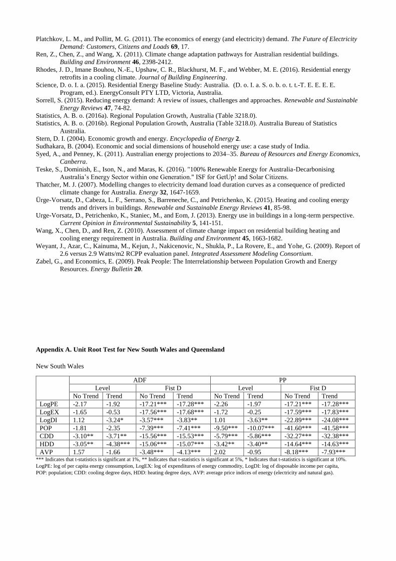
Appendix A. Unit Root Test for New South Wales and Queensland
New South Wales
ADF PP
Level Fist D Level Fist D
No Trend Trend No Trend Trend No Trend Trend No Trend Trend
LogPE -2.17 -1.92 -17.21*** -17.28*** -2.26 -1.97 -17.21*** -17.28***
LogEX -1.65 -0.53 -17.56*** -17.68*** -1.72 -0.25 -17.59*** -17.83***
LogDI 1.12 -3.24* -3.57*** -3.83** 1.01 -3.63** -22.89*** -24.08***
POP -1.81 -2.35 -7.39*** -7.41*** -9.50*** -10.07*** -41.60*** -41.58***
CDD -3.10** -3.71** -15.56*** -15.53*** -5.79*** -5.86*** -32.27*** -32.38***
HDD -3.05** -4.38*** -15.06*** -15.07*** -3.42** -3.40** -14.64*** -14.63***
AVP 1.57 -1.66 -3.48*** -4.13*** 2.02 -0.95 -8.18*** -7.93*** *** Indicates that t-statistics is significant at 1%, ** Indicates that t-statistics is significant at 5%, * Indicates that t-statistics is significant at 10%.
LogPE: log of per capita energy consumption, LogEX: log of expenditures of energy commodity, LogDI: log of disposable income per capita,
POP: population; CDD: cooling degree days, HDD: heating degree days, AVP: average price indices of energy (electricity and natural gas).

Queensland
ADF PP
Level Fist D Level Fist D
No Trend Trend No Trend Trend No Trend Trend No Trend Trend
LogPE -1.70 0.22 -3.32** -3.97** -2.02 -0.51 -17.76*** -18.97***
LogEX -1.68 -0.69 -17.50*** -17.62*** -1.72 -0.54 -27.52*** -17.70***
LogDI -0.77 -1.79 -3.08** -3.09 -0.37 -1.86 -19.49*** -19.46***
POP -1.39 -1.42 -6.29*** -6.33*** -8.07*** -7.80*** -41.39*** -41.63***
CDD -3.50*** -3.43** -18.09*** -18.08*** -5.46*** -5.27*** -25.36*** -28.01***
HDD -3.77*** -3.98** -24.85*** -24.80*** -3.90*** -3.84** -21.78*** -22.84***
AVP 1.85 -0.63 -3.03** -3.92** 4.38 -0.03 -7.37*** -6.88*** *** Indicates that t-statistics is significant at 1%, ** Indicates that t-statistics is significant at 5%, * Indicates that t-statistics is significant at 10%.
LogPE: log of per capita energy consumption, LogEX: log of expenditures of energy commodity, LogDI: log of disposable income per capita,
POP: population; CDD: cooling degree days, HDD: heating degree days, AVP: average price indices of energy (electricity and natural gas).
Appendix A. Plots of CUSUM and CUSUMSQ for the ARDL Model for New South Wales and Queensland
New South Wales
Queensland