the impact of credit scoring on consumer...

RAND Journal of EconomicsVol. 44, No. 2, Summer 2013pp. 249–274

The impact of credit scoring on consumerlending

Liran Einav∗Mark Jenkins∗∗and

Jonathan Levin∗

We study the adoption of automated credit scoring at a large auto finance company and thechanges it enabled in lending practices. Credit scoring appears to have increased profits byroughly a thousand dollars per loan. We identify two distinct benefits of risk classification: theability to screen high-risk borrowers and the ability to target more generous loans to lower-riskborrowers. We show that these had effects of similar magnitude. We also document that creditscoring compressed profitability across dealerships, and provide evidence consistent with theview that credit scoring may have substituted for varying qualities of local information.

1. Introduction

� Over the last two decades, consumer lending has become increasingly sophisticated aslenders have moved from traditional interview-based underwriting to a reliance on data-drivenmodels to assess and price credit risk. This article presents a snapshot of this transition. Wedescribe the magnitude and channels by which the adoption of credit scoring affected loanoriginations, repayment and defaults, and profitability at a large auto finance company. Althoughthe study, by design, is focused on a single company, and its experience surely has idiosyncrasies,we suspect that many of our findings may be illustrative of similar transitions at other companies,which taken together have revolutionized markets for consumer credit.

As late as the early 1990s, most lenders were still using a single “house rate” and relied oninterview procedures to screen borrowers (Johnson, 1992). As data storage and computing costs

∗Stanford University and NBER; [email protected], [email protected].∗∗University of Pennsylvania; [email protected] thank Luke Stein for excellent research assistance, Will Adams for his contributions to this project, and two anonymousreferees, the editor, Chris Knittel, Ulrike Malmendier, Vikrant Vig, and seminar participants at IO Fest 2008 at Stanford,the 2009 AEA annual meeting in San Francisco, the 2011 AEA annual meeting in Denver, and the 2009 NBER IO summermeeting in Cambridge, Massachusetts, for helpful comments. We acknowledge support from the Stanford Institute forEconomic Policy Research, the National Science Foundation (Einav and Levin), and the Center for Advanced Study inthe Behavioral Sciences (Levin). Earlier drafts of this article were circulated with the title “The Impact of InformationTechnology on Consumer Lending.”

Copyright C© 2013, RAND. 249

250 / THE RAND JOURNAL OF ECONOMICS

fell, and underwriting technology improved, lenders increasingly began to use estimates of defaultrisk to price individual loans. Today, automated credit scoring has become a standard input into thepricing of mortgages, auto loans, and unsecured credit. Using data from the Survey of ConsumerFinances, Edelberg (2006) documents the extent of this transformation. She finds that as a resultthe correlation between loan pricing and estimated and realized default risk has sharply increased.Grodzicki (2012) documents a similar pattern in the credit card industry and ties it specificallyto lenders’ investments in information technology. Other articles provide related although moreindirect evidence of these effects in the context of small business lending by banks (Frame,Srinivasan, and Woosley, 2001; Petersen and Rajan, 2002; Akhavein, Frame, and White, 2005).

These studies rely either on aggregated data or survey measures of realized loans that allowus to see how the correlation of interest rates and default risk has increased over time. However,whereas the near-universal adoption of credit scoring techniques indicates their value to lenders,there is relatively little specific evidence on exactly how the benefits are realized, the size of theeffects, and their organizational impacts. By focusing more narrowly, we are able to complementexisting studies by using detailed applicant- and loan-level data to identify the specific channelsby which credit scoring impacts loan originations and outcomes, as well as the magnitude of theseeffects.

We begin in Section 2 by describing the setting of our case study. The data come from anauto finance company that specializes in the low-income, high-risk consumer market. The marketis particularly well suited for studying informational problems facing lenders. Default risk is highand recovery values are low, so profitability hinges on identifying better risks in the applicantpool (Adams, Einav, and Levin, 2009; Einav, Jenkins, and Levin, 2012). Loan applicants alsovary substantially in their risk of default, and their characteristics and credit histories provideprospective information about this risk. The potential value from stratifying borrowers can beseen in the fact that the top third of borrowers in terms of predicted risk are about 20 percentagepoints more likely to default than the bottom third.

Until 2001, the company relied on uniform loan pricing and traditional interviews to screenborrowers. The company then contracted with an external credit scoring company that usedcredit bureau reports and historical data from the company to provide estimates of default riskthat could be used to price loans. Starting in June 2001, the company shifted to a centralizedrisk-based pricing regime, in which new loan applicants were assigned a credit score, and thescore determined the minimum down payment required for purchase and the set of cars for whichfinancing would be available. Our empirical analysis in this article focuses on describing theshort-run effects of this change, using applicant-level and loan-level data about loans originateda year before and a year after the date when credit scoring was implemented.

In Section 3, we present and calibrate a stylized two-period model, which helps guide oursubsequent empirical approach. The model illustrates two distinct responses that result frombeing able to classify applicants as higher or lower risk. When faced with a high-risk applicant,the lender optimally increases the down payment and reduces the quality of the car, and thus theloan amount. Both effects lead to a fall in the probability of sale and a rise in the repayment rate.When faced with a lower-risk applicant, the lender optimally lowers the down payment and raisescar quality, increasing the probability of sale and the amount of credit extended. In each case,the profit per loan and overall expected profit increase. These results motivate us to focus on theheterogeneous effect of credit scoring across applicant pools of different risks.

In Section 4, we present the empirical analysis. The availability of detailed transaction-leveldata from before and after the adoption of scoring allows for a straightforward empirical approach.We first classify potential borrowers by assigning each loan applicant to a credit category usinga rule that mirrors the lender’s assignment following adoption. We then construct measuresof profitability and related performance metrics—“close rates” on auto purchases, car choices,financing decisions, repayment behavior and recoveries—and compare these metrics, both onaggregate and for the stratified groups, before and after the advent of credit scoring. Finally, wetranslate the changes into dollar terms by decomposing profits into separate components: the

C© RAND 2013.

EINAV, JENKINS, AND LEVIN / 251

probability the applicant becomes a borrower, the size of the investment in each borrower, andthe return in terms of loan payments actually made.

We find that the adoption of credit scoring, and the changes it enabled in lending increasedprofits by roughly 1,000 dollars per loan. The effect is substantial: at the time, the average loanprincipal was around 9,000 dollars. We also analyze an alternative measure of profitability, theprofit (or “net revenue”) per loan applicant. After the adoption of credit scoring, loan originationsfell, but the profit per applicant still increased, from $751 to $1,070, or by roughly 42%.

Consistent with the theoretical model, we identify two distinct channels through which betterinformation improved loan profitability. First, credit scoring allowed the lender to set differentdown payment requirements for different applicants. High-risk applicants saw their required downpayment increase by more than 25%, creating a higher hurdle to obtain financing. Close rates forthis group fell notably, and also default rates, consistent with the idea that higher-risk borrowerswere screened out by the higher down payment requirement. Translating this into dollar terms,we find that improved loan repayment was largely responsible for what we measure to be about a1,200 dollar increase in profit per high-risk loan.

We estimate a similar increase in profitability for lower-risk loans, but the mechanismis different. Required down payments and close rates changed little for lower-risk applicants.Instead, consistent with the model, we observe that car quality and average loan sizes increasedsubstantially. Default rates did not change much, and hence the larger loans had a substantialprofit impact due to the high interest rates charged in this setting. For lower-risk loans, theincreased “size” of each investment is largely responsible for the dollar increase in profit. Hence,the two channels through which credit scoring theoretically increases profitability in the modelboth appear to be operative and substantial in the data.

A useful feature of the episode we study is that most salient features of the lending environ-ment, such as advertising, car pricing, sales force incentives, and the composition of the applicantpool, remained stable during the periods before and after credit scoring was adopted. This makesfor a relatively clean observational setting. At the same time, concerns about identification canbe raised for any before-and-after study, and given that we compare outcomes before and after asingle change in company policy, we cannot rule out definitively that there was some underlyingconfounding change in the environment. A variety of robustness checks, however, support theinterpretation we have outlined. In particular, we show that the inclusion of controls for applicantquality and local economic conditions has little effect on any qualitative conclusions one mightdraw. Our conclusions about the effects of down payment requirements and loan sizes are alsoconsistent with results in Adams, Einav, and Levin (2009) and Einav, Jenkins, and Levin (2012),which use data from the same lender but rely on more recent data and a different identificationstrategy that relies on sharp changes in pricing schedules for different groups of loan applicants.

The last section examines the differential impact of credit scoring across dealerships inorder to gauge its organizational implications. Research by Stein (2002) and others suggeststhat automated loan underwriting might involve a trade-off, with the increased use of “hard”information crowding out the production and use of “soft” information (see also Berger et al.,2005). This line of thinking indicates that credit scoring might reduce profitability differencesacross dealerships, particularly if, in the absence of scoring, dealers differ in their ability to tailorloan terms to buyers.1 We show that prior to credit scoring, there was in fact dramatic variationacross dealerships in profitability, related primarily to differences in default rates and the matchingof cars to borrowers. The advent of credit scoring compressed this variation, as one might expectfrom the increased reliance on companywide guidelines. Although almost all dealerships becamemore profitable, the relative improvement was greater for dealerships that had higher default ratesand less pronounced matching of cars to borrowers of different risks, the two dimensions thatcredit scoring tried to address.

1 Bloom et al. (2011) provide an interesting analysis of the multiple possible effects of information technologyadoption on organizations.

C© RAND 2013.


2. Data and environment

� The lending environment. The company we study specializes in making auto loans toconsumers with low incomes or poor credit records. During the period we study, the company’saverage loan applicant had an annual household income of around 28,000 dollars, which wouldput him at around the 33rd percentile in the United States (Current Population Survey, 2001).Almost a third of the applicants had no bank account, and only 14% owned their own home. Alarge majority of loan applicants had a FICO score below 600, which is the 35th percentile in theU.S. population and would not qualify for a prime mortgage. Low FICO scores frequently reflecta history of loan delinquencies or defaults, which is consistent with the credit histories of the loanapplicants in our data. Over the six months prior to their loan application, more than half of thecompany’s applicants were delinquent on at least 25% of their debt. This type of credit historymakes it highly unlikely the applicants in our data could obtain a standard “prime” auto loan.

The lending process in the market operates as follows. Consumers fill out an applicationwhen they arrive at a dealership. They work with a sales representative and the dealership managerto select a vehicle and discuss financing terms. About 40% of the loan applicants we observepurchase a car. The purchased cars typically are five to seven years old, with odometer readingsin the 65,000 to 100,000 mile range. The average sale price is 8,000 or 9,000 dollars, whichrepresents a notable markup over the dealer cost (see Table 1). Buyers are required to make adown payment but usually finance about 90% of the purchase price. The financing terms arerelatively standard across our sample. Buyers are expected to make regular payments at thedealership for a fixed term, typically around three years, and interest rates are high, reflecting therisk of the borrower pool. Annual interest rates average close to 30% in our sample.

A central feature of the market is that consumers tend to be tightly cash constrained. Inearlier work, we use abrupt changes in the pricing schedule to estimate demand elasticities(Adams, Einav, and Levin, 2009). A striking finding was that every hundred dollar increase inthe minimum down payment reduces the purchase probability of an applicant by two to threepercentage points. Moreover, more than 40% of buyers pay exactly the minimum amount down,and these “marginal” purchasers represent substantially worse default risks than buyers who paymore than the minimum down (Einav, Jenkins, and Levin, 2012).

The role of the down payment in screening out marginal buyers is important for understandinghow risk-based pricing affects loan originations. In the period prior to the adoption of creditscoring, all buyers were required to make a down payment of at least 600 dollars. After creditscoring was put in place, minimum down payments were held constant or even modestly decreasedfor lower-risk borrowers but increased to as much as 1,500 dollars for high risks. As we will see,this increase helps explain why the fraction of applicants purchasing a car, and the subsequentdefault rate, fell in the period after credit scoring was adopted.

As can be seen in Table 1, defaults during the repayment period are common and tend tooccur relatively early in the repayment period. About 35% of loans default during the first year ofrepayment. Less than 40% are repaid in full.2 Following a default, the lender attempts to recoverthe car, and generally succeeds, but frictions in the recovery process result in a relatively lowdollar value of recoveries after expenses are netted out (Jenkins, 2010). The average recovery inour sample was around 1,200 dollars, or around 25% of the original dealer cost of the car priorto the transaction.3

The combination of early defaults and low recoveries means that transaction outcomes havea bimodal pattern. Early defaults tend to result in losses, whereas fully paid loans can be quite

2 These are significantly higher default rates than those reported by Heitfield and Sabarwal (2004) in their study ofsecuritized subprime auto loans, reflecting the relatively poor credit quality of the borrowers in our sample even comparedto other subprime populations.

3 This is for several reasons. In more than a quarter of defaults, for instance, it is hard to find the borrower, leadingto a lengthy and costly recovery process. About a third of defaults are directly associated with a decrease in car value,such as mechanical breakdowns, car theft, and accidents (without maintaining appropriate insurance). See Jenkins (2010)for more details.

C© RAND 2013.


TABLE 1 Summary Statistics

January–December 2000 July 2001–June 2002

Standard StandardMean Deviation 5% 95% Mean Deviation 5% 95%

Applicant characteristics N = 1.00 N = 0.88Applicant demographics

Monthly income 2,214 973 1,204 4,000 2,256 975 1,238 4,000Residual monthly income 1,715 985 748 3,525 1,843 1,024 824 3,750Debt-to-income ratio 0.26 0.16 0.03 0.48 0.25 0.12 0.10 0.45Car purchased 0.43 0.37

Transaction characteristics N = 0.43 N = 0.32Buyer characteristics

Monthly income 2,319 973 1,300 4,088 2,410 984 1,360 4,286Residual monthly income 1,723 1,079 753 3,800 1,859 1,122 790 4,018Debt-to-income ratio 0.32 0.13 0.15 0.49 0.32 0.10 0.16 0.47

Car characteristicsCar cost 4,954 863 3,571 6,346 5,273 1,015 3,717 6,944Car age (years) 6.4 1.8 4 9 5.5 1.7 3 9Odometer (miles) 88,668 17,822 57,746 113,856 81,810 18,048 50,242 108,381Inventory age (days) 68 62 13 178 72 63 13 184Lot age (days) 40 57 1 145 43 58 1 152

Purchase characteristicsSale price 8,370 930 6,907 9,795 9,368 1,297 7,307 11,495Down payment 740 451 200 1,500 1,003 502 600 1,900Loan term (months) 34.1 3.0 30.0 37.0 36.6 3.9 32.0 42.0APR 0.288 0.019 0.259 0.299 0.284 0.026 0.219 0.299Monthly payment 362 65 298 421 374 42 306 442

Loan performanceOutcomes

Default 0.67 0.62Fraction of payments made 0.57 0.37 0.05 1.00 0.59 0.37 0.06 1.00Loan payments excluding

down payment6,113 3,916 653 11,837 7,146 4,441 766 13,636

Recovery (all sales) 691 951 0 2,530 923 1,216 0 3,224Recovery (all defaults) 1,032 999 1 2,848 1,483 1,243 73 3,665

Components of profitsGross operating revenue 7,557 3,530 2,284 12,706 9,084 3,901 3,013 14,744Total cost 5,810 965 4,301 7,378 6,193 1,099 4,518 8,012Net operating revenue 1,746 3,401 −3,434 6,144 2,891 3,727 −3,005 7,620

Note: Residual monthly income = Residual monthly income after debt payments. To preserve confidentiality of thecompany that provided the data, the number of observations is normalized by the number of applicant in year 2000, N (N>> 10,000). Loan payments, recovery amount, gross operating revenue are in present value (PV). Total cost includes carcost, taxes and fees, and shortfalls when value of trade-in does not cover down payment. Net operating revenue equalsgross operating revenue minus total cost.

profitable. Figure 1 documents this pattern by showing the distribution of transaction-level returns.For each sale, we computed the present value of borrower payments—the down payment, loanpayments, and recovery in the event of default—discounted back to the date of sale. We use a10% discount rate, which seems to be in line with industry standards. Neither the calculationhere nor similar calculations later in the article are very sensitive to using a somewhat higher orlower number.4 We then divided the present value of borrower payments by the dealer cost of thecar, providing an overall rate of return on each transaction. The striking bimodal distribution ofreturns presented in Figure 1 illustrates the benefits of being able to identify the more creditworthyapplicants from those who are relatively more likely to default.

4 Specifically, we ran all the analyses using discount rates of 5% and 15%, and the results hardly change.

C© RAND 2013.


FIGURE 1

DISTRIBUTION OF PER-LOAN RATE OF RETURN

0

0.01

0.02

0.03

0.04

0.05

0.06

0.07

0.08

0.09

–1 –0.5 0 0.5 1 1.5 >2.0

Fre

qu

ency

Net operating revenue/total cost

Paid loans

Defaulted loans

Note: Net operating profits = down payment + PV of loan payments + PV of recoveries − total cost. The histogram usesall observations used in the subsequent analysis, pooling the preperiod and postperiod (see Table 1).

� Implementation of credit scoring. The lender we study adopted credit scoring towardthe end of June 2001.5 Prior to this time, the company did not use the credit bureau historiesof prospective borrowers. Employees at the dealership were responsible for eliciting informationfrom applicants during the sales process, and much of this information was not formally recorded.Prospective buyers were asked for basic information about their income, family and work status,scheduled debt payments, and so forth, and as noted above all buyers were required to make atleast a 600 dollar down payment. This traditional approach to lending was typical of the high-riskauto loan market at that time.

With the adoption of credit scoring, the company began to pull information from the majorcredit bureaus and use a proprietary algorithm to assess each applicant’s risk profile. The scoringalgorithm achieves impressive risk stratification. If we look at loans made in the first year aftercredit scoring began, borrowers in the top third of the applicant pool in terms of expected riskwere 1.65 times as likely to repay a loan in full as borrowers in the bottom third (50.3% comparedto 30.5%, respectively).

The company uses the assigned credit score in several ways. As described above, a primaryuse of scoring is to establish a schedule for minimum down payments. Each applicant is requiredto pay at least some fixed dollar amount down; the amount depends on the applicant’s credit scorebut not on the car being purchased. The credit scores are also used to match customers withappropriate cars. An applicant deemed a better risk is eligible to obtain financing for a largerrange of vehicles, in particular newer, lower-mileage cars that are more expensive. Applicantswith better credit scores, however, do not qualify for any kind of automatic price discount. Finally,

5 To the best of our knowledge (which relies on conversations with the company’s executives), there was nothingparticularly special about the timing of implementation. In fact, many executives associate the company’s idea to adoptautomated credit scoring with the hiring of a senior executive who had quantitative background (and affection) in the late1990s. Developing, testing, and implementing the idea has taken several years.

C© RAND 2013.


borrowers at a given dealership pay similar interest rates regardless of their credit score, as therates are constrained by usury laws, and are clustered at, or close to, the relevant state interestrate cap.

A natural question is why the company uses its own scoring algorithm rather than a potentiallycheaper metric available from the credit bureaus. One view is that a specialized scoring modelmay have particular value for niche markets such as this one. Standard credit models are designedto broadly assess the entire range of consumers, whereas those in our data are clustered at the lowend of the credit spectrum. Lending to this part of the distribution requires separating consumerswith transitory bad records from persistently bad risks, as opposed to simply identifying red flagsin a consumer’s history.6

� Data. We focus our analysis on the precredit scoring period from January 2000 throughDecember 2000, and the postscoring period from July 2001 to June 2002. We drop the first halfof 2001, when the company adopted a simple income cutoff to set minimum down paymentsin anticipation of credit scoring.7 Finally, we include applications and sales data only fromdealerships for which we have complete data for both the pre- and postscoring periods.8

We compare full-year periods rather than shorter pre- and postwindows for two reasons.First, the market has strong seasonality patterns: business peaks from February to April, whenmany prospective buyers receive income tax rebates that facilitate down payments (Adams, Einav,and Levin, 2009), and there is a slowdown around the December holidays. Second, although wecan point to a specific date in late June 2001 on which dealers were required to use applicantcredit scores in lending decisions, the practical day-to-day adjustments required for a successfulimplementation started earlier and continued later, which makes it more interesting to analyzechanges over a moderate time period rather than a very narrow window.9

On the other hand, one reason to focus on a single year rather than longer run effects isthat we are able to consider a period where other features of the lending environment remainedconstant. During the period we study, the sales and financing process and the incentive structurefor salespeople and dealership managers were stable.10 We also have little reason to believe thatthe inflow of prospective buyers into dealerships was affected by the implementation of creditscoring. The company did not change its marketing, and customers have little way of knowingthe specific financing terms for which they qualify without visiting the dealership and filling outthe loan application. This stability can be seen in Table 1. Applicant characteristics are similarbefore and after credit scoring went into effect. This stability is a feature of our focus on therelatively short run effect of credit scoring. The advent of credit scoring may affect the populationof applicants over longer periods, perhaps through reputation or word of mouth.

A qualification is that the number (but not the composition) of loan applicants was somewhatlower in the year after credit scoring, only 88% of the number in the year before scoring.11 Weare not aware of notable changes in the competitive environment, but a possible explanation is

6 Indeed, beyond the standard and generally used FICO score, the credit bureaus also sell lenders more specializedscores, associated with default risks in specific markets, such as mortgages or auto loans. Presumably, the benefit froma proprietary and customized algorithm is higher, as the credit product is less standard and/or the customer base is lessrepresentative of the general population.

7 We have looked at this period in some detail, although we do not report the analysis. Perhaps not surprisingly, thisintermediate approach led to intermediate outcomes.

8 In Adams, Einav, and Levin (2009) and Einav, Jenkins, and Levin (2012), we use data from the postscoring period,allowing us to expand the number of dealerships, applicants, and borrowers in the postperiod by roughly 50% relative tothe (already large amount of) data we use here.

9 We looked at time-series pictures around the implementation date, but between the seasonality and month-to-monthvariability it is hard to draw very sharp conclusions about the exact pace and timing of outcome changes.

10 In fact, in late June 2002, the company significantly altered the incentive structure that governs loan origination.Thus, using data on loans originated after June 2002 would potentially confound the effects of credit scoring and incentives.

11 Note that to preserve the company’s confidentiality, we do not report the exact number of loan applicants inTable 1. Instead, we report numbers of applicants and buyers as fractions of the number of loan applicants in 2000. Forstatistical inference purposes, these numbers are all quite large.

C© RAND 2013.


the broader macroeconomy. Economic growth was fairly strong through the first half of 2000 butslowed until the fourth quarter of 2001. To account for this in our analysis, we use data on localunemployment rates and local housing prices as controls in our empirical specifications. We alsofocus on the screening of applicants, the characteristics of loans made to borrowers, and theirsubsequent performance rather than try to explain the flow of customers into dealerships.

Table 1 shows significant changes in these basic operating metrics between the prescoringand postscoring periods. The fraction of applicants who became buyers (the “close rate”) droppedby about 15%, the average quality of cars sold increased (e.g., the average odometer read was 7,000miles lower after credit scoring), transaction prices and down payments were significantly higher,defaults were lower, and loan revenues substantially increased. Overall, the firm’s profitabilityincreased markedly over the period, both on a per-transaction and a per-applicant basis.

3. Credit scoring and lender behavior

� In this section, we present an empirically motivated model that helps in guiding and inter-preting our empirical results. The model illustrates how a lender might use better credit scoringinformation to increase down payment requirements for higher-risk borrowers and at the sametime increase car quality for lower-risk borrowers, and how each of these channels can generateincreased profits. The theoretical analysis motivates our empirical strategy, in which we examinethe effect of credit scoring separately for higher- and lower-risk borrowers, and focus on differentmechanisms for each group.

� A model of subprime borrowing. The model is a simplified version of the one we developin Einav, Jenkins, and Levin (2012). In the first period, the customer arrives at the dealership andis offered a car of value V at a price P , of which D must be paid as down payment while P − Dcan be borrowed. The loan carries an interest rate R. If the customer decides to purchase, hechooses in the second period whether to repay the loan or default.

The customer’s problem is to maximize utility across the two periods. Customers vary intheir available cash in the two periods, which we denote by Y1 and Y2. If a customer does notpurchase, he consumes his available cash each period and receives utility ln(Y1) + β ln(Y2), whereβ is the between-period discount factor. If a customer does purchase, his first-period utility isV + ln(Y1 − D). In the second period, if he repays the loan obligation L = R(P − D), his utilityis V + ln(Y2 − L). If he defaults, he loses the car and receives utility ln(Y2).

We model customer heterogeneity by assuming that customers vary in their available cash,so that (Y1,Y2) are drawn from a censored joint normal distribution, where(

Y ∗1

Y ∗2

)∼ N

((μ1θ

μ2θ

),

(σ 2

1 ρσ1σ2

ρσ1σ2 σ 22

)), (1)

with ρ ≥ 0, and Yt = max(Y∗t, ε) for t = 1, 2.12 The parameter θ ∈ {L , H} indicates a consumer’s

risk type, with L denoting “low-risk” and H denoting “high risk.” In particular, μ1L ≥ μ1H andμ2L ≥ μ2H , so high-risk customers on average have less cash. Each customer knows his risk type,and learns Yt before making his time t decision. The lender never observes a customer’s cashposition but can obtain information about his risk type with effective credit scoring.

We adopt a simplified, but in our case fairly realistic, approach to modelling the lender’sproblem. We assume that the value of the car V is purely a function of its cost to the dealer,V = αC . We also assume that the price P is determined by a fixed markup over cost, P = C + M ,

12 We assume ε is a small positive number, specifically ε = 0.02, although the exact choice is not particularlyimportant. As will be clear, in the model customers with low enough amount of cash will not buy the loan in period 1 andwill default in period 2, making the distribution of cash at the lower end of the support inconsequential for the customer’soptimal decision and for the firm’s profits.

C© RAND 2013.


and that both the markup M and the interest rate R are given exogenously.13 These assumptionsallow us to focus on the lender’s choice of car cost C (or equivalently, value V ) and requireddown payment D, as the key decisions that affect profitability.

To solve the model, we start with the customer’s problem and work backward from the secondperiod. Having purchased, it is optimal to repay the loan if V + ln(Y2 − L) ≥ ln(Y2). Repaymentis infeasible if Y2 < L , but if the customer has sufficient funds, he will repay if

Y2 · (1 − e−V ) ≥ L . (2)

The customer’s expected utility from purchase is

UP = V + ln(Y1 − D) + βEY2|Y1,θ [max{V + ln(Y2 − L), ln(Y2)}]. (3)

The borrower purchases if this value is greater than U0 = ln(Y1) + βEY2|Y1,θ [ln(Y2)].The purchasing decision also follows a threshold rule. If we subtract U0 from UP and

rearrange the terms, we see that it is optimal to purchase if

Y1 · (1 − e−V −β�Uθ (Y1)) ≥ D, (4)

where �Uθ (Y1) = EY2|Y1,θ [max{V + ln(1 − L/Y2), 0}] is the customer’s option value from beingable to repay the loan and keep the car in the second period. The value of this option is higherfor customers with higher Y1 (because ρ ≥ 0). So provided that the price is not prohibitive,individuals purchase in the first period if they have sufficient cash.

The lender’s problem is to choose the required down payment D and the car cost C , givenborrower behavior. Both choices involve trade-offs. A higher down payment can reduce theprobability of sale by causing lower-income customers not to purchase but raise the chance ofrepayment because of the smaller loan size and stronger cash position of those who do purchase.Offering more valuable cars raises the customer’s benefits and costs in both periods, and a priorihas an ambiguous effect on both purchasing and repayment. The interaction of the down paymentand car quality also is not obvious. All else equal, a lender might be inclined to raise the requireddown payment for more expensive cars, unless the more expensive cars were being targeted at abetter borrower population.

� Fitting the model to data. To examine the effect of credit scoring, we calibrate the modelto match observed data on purchasing and repayment outcomes in the prescoring period. We firstchoose values for the parameters in the borrower’s utility function: α = 0.2 and β = 0.9. We thenset prices to their approximate averages in the prescoring period: D = $600, C = $5,500, M =$2,500, and R = 1.4. The latter approximates the total repayment amount per dollar borrowed ona loan with an interest rate of 29.9% and a 42 month term. Finally, we set ρ = 0.5 and calibratethe remaining distributional parameters μ1L , μ1H , μ2L , μ2H , σ1, and σ2 to match six observedmoments in the data.

Table 2 shows our six matched moments and calibrated parameters. The moments includethe probability of sale and probability of default for both types of borrowers at the prices notedabove, the semielasticity of the close rate with respect to changes in the required down payment(3% per $100), and the semielasticity of the default rate with respect to changes in loan size (1%per $100). The latter two values are taken from Adams, Einav, and Levin (2009).

Figure 2 provides intuition for the model by plotting customers in the space of (Y1,Y2).Customers with low Y1 do not purchase and, conditional on purchase, customers with low Y2

default. Roughly, our calibration procedure matches the probability of purchase for each type of

13 In practice, the lender we study offered the majority of loans at the state interest rate cap, and in the time periodwe consider here, did not vary the markup across cars. Later it moved to a system where more costly cars had higher(dollar) markups. Another simplification in this model is that although many borrowers pay the minimum down paymentchosen by the lender, borrowers can choose to pay more up front and some do, although the amounts are never very largerelative to the overall loan size.

C© RAND 2013.


TABLE 2 Model Calibration

Actual Model Calibrated CalibratedValue Value Parameter Value

Demand MomentProbability of purchase: high-risk applicants 23% 24% μ1H 0Probability of purchase: low-risk applicants 57% 58% μ1L 1,100Probability of default: high-risk borrowers 70% 70% μ2H 9,500Probability of default: low-risk borrowers 50% 50% μ2L 13,500Change in close rate per $100 change in minimum down 3% 4% σ 1 1,200Change in default rate per $100 change in loan size 1% 1% σ 2 8,000

Optimal PricesOptimal minimum down without scoring $600 $700 ω 0.35Optimal car cost without scoring $5,500 $5,000 ψ 1,800

Note: This table shows calibrated moments and parameters for the model presented in Section 3. The first six rowsshow the parameters of two bivariate normal distributions of applicant characteristics, one for high-risk types and onefor low-risk types. The parameters μ1H and μ1L are the mean purchase period liquidities (Y1) for high-risk types andlow-risk types, respectively; μ2h and μ1L are the mean repayement period liquidities (Y2) for high-risk types and low-risktypes, respectively and σ 1 and σ 2 are the variances of Y1 of Y2, respectively, for both risk types. As described in section3, the calibration roughly matches the probability of purchase for each type of borrower by shifting the mean of eachtype’s Y1 distribution, and the probability of default by shifting the mean of Y2. The effect of down payment on purchaseprobability is matched by shifting σ 1, and the effect of loan size on the default rate is matched by shifting the mean of σ 2.In both cases, conditional on matching the prescoring period. The last two rows show two parameters of the lender’s profitfunction: the fraction of the original car cost recovered in the event of default (ω) and the fixed cost of administering aloan (ψ). These parameters are calibrated by matching the lender’s observed pricing decisions in the prescoring period.

borrower by shifting the mean of each type’s Y1 distribution, and the probability of default byshifting the mean of Y2. Lower-risk types have a higherμ1, corresponding to their observed higherprobability of purchase, and a higher μ2, corresponding to their lower probability of default. Thefigure shows the lower-risk distribution above and to the right of the high-risk distribution. Theeffect of down payment on purchase probability is matched by shifting σ1, and the effect of loansize on the default rate is matched by shifting σ2. In both cases, conditional on matching the othermoments, a higher variance corresponds to a lessened sensitivity.

The final step in the calibration is to choose parameters for the lender’s profit function sothat the optimal down payments and car costs match observed down payments and costs in thepreperiod. The lender’s expected profit from a type θ customer is

πθ (C, D) = qθ (C, D)[D + zθ (C, D) − C], (5)

where qθ (C, D) is the probability that the customer purchases the car, and zθ (C, D) is theexpected value of loan payments conditional on purchase. To match the data, we write zθ (D,C) =pθL + (1 − pθ )(κL + ωC) − ψ , where pθ is the probability of repayment by a type θ borrower,κ is a parameter intended to capture the fraction of payments typically made prior to a default,ω is the fraction of the original car cost recovered if there is a default, and ψ is the fixed cost ofadministering a loan. We set κ = 0.37 based on Adams, Einav, and Levin (2009). We then chooseω = 0.35 and ψ = $1, 800 so that the prescoring D and (average) C are profit maximizing,assuming the lender cannot distinguish between types.

� Credit scoring and pricing. We assume that credit scoring allows the lender to separatelyidentify low- and high-risk borrowers, that is, to observe θ . With no knowledge of types, thelender chooses C and D to maximize profits over the population of applicants, that is,

maxD,C

∑θ∈{L ,H}

πθ (C, D) · wθ =∑

θ∈{L ,H}qθ (C, D)[D + zθ (c, D) − C] · wθ, (6)

where wθ is the fraction of type θ customers in the applicant pool. With credit scoring, the lenderchooses (CL, DL) and (CH , DH ) to separately maximize πL(C, D) and πH (C, D).

C© RAND 2013.


FIGURE 2

ILLUSTRATION OF CALIBRATED MODEL

–20

–10

0

10

20

30

40

–4.0 –3.0 –2.0 –1.0 0.0 1.0 2.0 3.0 4.0

Repa

ymen

t per

iod

liqui

dity

($00

0s)

Purchase period liquidity ($000s)

Distribu�on of high-risk types (H)

Distribu�on of low-risk types (L)

Down payment requirement

Purchase threshold for H types

Purchase threshold for L types

Repayment threshold

$870$840 Purchase & repay

Purchase & default

Don't purchase

Note: This figure illustrates the model presented in Section 3. The figure shows a two-dimensional space of applicantcharacteristics. The x axis represents the applicant’s cash in hand at the time of purchase. The y axis represents theapplicant’s cash generated in the repayment period. Negative values can be viewed as truncated at zero. Each ellipse is anisodensity curve from the bivariate normal distribution of applicants of each type, as determined by the model calibration.The calibration assumes that the means of Y1 and Y2 differ for the two types, but the covariance matrices of Y1 and Y2for both types are the same. This assumption can be relaxed without changing the qualitative implications of the model.Based on the calibration, low-risk applicants have a higher mean liquidity at purchase and a higher mean repaymentliquidity. The former implies that low-risk applicants are more likely to purchase, because a necessary condition forpurchase is that cash on hand is greater than the minimum down payment. The latter implies that, conditional on purchase,they are less likely to default, because full repayment requires that repayment liquidity exceeds the repayment amount.Thresholds for purchase and repayment are shown with dashes.

Changes in C and D have multiple effects: on the probability of purchase, the resultingdistribution of borrower incomes and the probability of repayment, and on profits directly, holdingfixed the applicant’s behavior. This makes it hard to obtain general comparative statics predictionsabout the effects of credit scoring, but with the calibrated model we obtain clear results. From theprescoring baseline of D = 700 and C = 5,000, the lender optimally uses credit scoring to raisethe down payment for high risks to DH = 900, lower the car quality for high risks to CH = 4,600,and conversely lower the down payment for lower risks and raise their car quality.

Figure 3 illustrates the optimal choice of down payment and car cost for the three relevantcases: low-risk customers, high-risk customers, and unidentified customers (who are low risk withprobability wL and high risk with probability wH ). When the lender lowers the down paymentand raises car quality for the lower risks, their probability of sale increases, their repaymentrate decreases, and the profit per loan and expected profit increase. For high-risk customers, theincrease in down payment and reduction in car quality lead to a fall in the probability of sale anda rise in the repayment rate. Again, both the profit per loan and expected profit increase.

These theoretical predictions guide our empirical analysis, which examines the effect ofcredit scoring on higher-and lower-risk applicants separately. Specifically, the model predicts thatfor high-risk applicants, credit scoring can raise profits by allowing better screening of marginalapplicants. In contrast, for lower-risk applicants, credit scoring can raise profits by allowing them

C© RAND 2013.


FIGURE 3

OPTIMAL DOWN PAYMENTS BY TYPE

($200)

($100)

$0

$100

$200

$300

$400

$500

$600

$0 $200 $400 $600 $800 $1,000 $1,200 $1,400

Expe

cted

pro

fit p

er a

pplic

ant

Down payment requirement

High types

Low types

Average

C* = $5,000

C* = $4,600

C* = $5,300

CH = C003,6$ H = $4,300

Note: This chart shows the relationship between expected profits per applicant and down payment requirements underdifferent credit scoring regimes. Each curve plots expected profit per applicant as a function of the minimum down payment,conditional on a fixed vehicle cost, as computed using the calibrated model described in Section 3. The vehicle cost foreach curve is chosen to maximize the expected profit per applicant. The three curves represent optimal pricing for low-riskapplicants (top curve), high-risk applicants (bottom curve), and a weighted average of the two types (middle curve). Thefigure shows that the optimal down payment is increasing in the borrower risk level. The small dashed lines show expectedprofits per applicant as a function of vehicle cost, conditional on a fixed down payment, for low-risk borrowers. Thesecurves illustrate how the optimal vehicle cost is determined. Similar curves can be drawn for high-risk applicants.

to borrow more. As we will see in the next section, these same mechanisms are observed in ourdata.

4. Empirical strategy

� Constructing matched applicant pools. The adoption of credit scoring allowed the com-pany to make systematically different offers to loan applicants with different risk profiles. Ouranalysis therefore compares the experiences of different types of loan applicants in the periodsbefore and after scoring was adopted. For the period subsequent to adoption, we observe the creditscore assigned by the company and the relevant information on which it was based, although notthe exact algorithm. For the period prior to adoption, the lender collected less detailed data; weobserve basic financial and demographic information for each applicant rather than a completecredit history.

To obtain comparable risk groups in the two periods, we construct a risk measure thatclassifies applicants into low, medium, and high risk using variables that are in the data forboth periods and then use this risk classification for both periods. To do this, we model eachapplicant’s risk as a function of his or her household income and debt-to-income ratio. We assigneach applicant to a cell based on the decile of his or her household income and debt-to-incomeratio. We then assign each cell a risk category in a way that minimizes the distance in thepostscoring period between our assignment and the company’s, subject to the constraint that ourclassification be monotone in both household credit variables. The Appendix provides details onthe procedure.14

14 We also experimented with several other classification schemes and obtained similar results.

C© RAND 2013.


TABLE 3 Summary Statistics by Applicants’ Predicted Credit Grade

January–December 2000 July 2001–June 2002

Low Medium High Low Medium HighRisk Risk Risk Risk Risk Risk

Applicant characteristicsNumber of applicants N = 0.22 N = 0.40 N = 0.38 N = 0.18 N = 0.34 N = 0.35Applicant demographics

Monthly income 3,528 2,130 1,557 3,620 2,152 1,646Residual monthly income 2,776 1,569 1,270 2,915 1,639 1,483Debt-to-income ratio 0.26 0.30 0.22 0.24 0.29 0.20Car purchased 0.57 0.55 0.23 0.57 0.53 0.12

Transaction characteristicsNumber of buyers N = 0.12 N = 0.22 N = 0.09 N = 0.10 N = 0.18 N = 0.04

Buyer characteristicsMonthly income 3,424 2,042 1,453 3,459 2,032 1,387Residual monthly income 2,670 1,461 1,042 2,718 1,479 1,318Debt-to-income ratio 0.28 0.33 0.34 0.27 0.34 0.37

Car characteristicsCar cost 5,235 4,949 4,569 5,602 5,212 4,707Car age (years) 6.3 6.4 6.7 5.4 5.6 5.8Odometer miles 89,593 88,735 87,198 81,924 81,823 81,471Inventory age (days) 63 67 75 64 74 84Lot age (days) 35 40 47 36 45 55

Purchase characteristicsSale price 8,703 8,391 7,851 9,828 9,302 8,504Down payment 762 725 746 996 995 1,055Loan term (months) 34.2 34.1 34.1 37.1 36.5 36.0APR 0.288 0.287 0.288 0.283 0.284 0.285Monthly payment 380 363 334 391 372 339

Loan performanceOutcomes

Default 0.62 0.68 0.70 0.59 0.64 0.62Fraction of payments made 0.63 0.56 0.54 0.62 0.58 0.59Loan payments excluding down

payment6,912 5,979 5,319 7,864 6,914 6,340

Recovery amount (all sales) 710 709 620 1,016 926 679Recovery amount (all defaults) 1,146 1,036 881 1,710 1,449 1,088

Components of profitsGross operating revenue 8,400 7,424 6,695 9,890 8,845 8,085Total cost 6,134 5,807 5,364 6,565 6,126 5,548Net operating revenue 2,267 1,617 1,331 3,325 2,719 2,536

Note: See notes to Table 1 for sample size and variable definitions.

Table 3 provides summary statistics for each risk category in the periods before and after thecredit scoring. Low- and medium-risk applicants were much more likely to become buyers thanhigh-risk applicants, and this difference increased in the postscoring period. Lower-risk buyersalso tended to purchase more expensive cars in both periods. This difference also increased in thelater period. Finally, despite taking larger loans, the lower-risk applicants have lower default rates.

One point to emphasize is that our risk classification is imperfect. Ideally, we would haveaccess to full credit histories for all applicants and construct risk groups by applying the company’salgorithm retrospectively to the prescoring applicants. Relative to this approach, our constructionmay classify as lower risk some applicants who the company treated as high risk, and viceversa. As a result, when we look at the differential effect of credit scoring on low- and high-risk applicants, our estimates may underestimate the impact of credit scoring. As we will see,however, the differential effects we observe are quite large even with our current classificationscheme.

C© RAND 2013.


� Measuring the effect. We measure the effect of credit scoring by estimating the changein different outcome variables between the pre period (January–December 2000) and the postperiod (July 2001–June 2002).

The results we report rely on regressions of the following form:

yi = αR(i) + βR(i) Di + Xiγ + εi , (7)

where i is an individual, yi is an outcome variable of interest, R(i) is the individual’s risk category(low, medium, or high), Di is a dummy variable equal to one if the individual appeared at thedealership following the advent of credit scoring (that is, in the postperiod), and Xi is a set ofcontrols.

From this model, we can define

ypre,r = E[yi |Di = 0, R(i) = r ] = αr + E[Xi |Di = 0, R(i) = r ]γ, (8)

ypost,r = E[yi |Di = 1, R(i) = r ] = αr + βr + E[Xi |Di = 1, R(i) = r ]γ, (9)

so that ypre,r is the expected outcome for an applicant of risk type r with average characteristicsin the pre period, and ypost,r is the equivalent quantity for the postperiod.

Their difference, �yr = ypost,r − ypre,r, is

�yr = βr + (E[Xi |Di = 1, R(i) = r ] − E[Xi |Di = 0, R(i) = r ])γ. (10)

That is, the change in outcomes for risk group r can be decomposed into the estimated coefficientβr , which we interpret as the effect of credit scoring, and the effect of changes in observablecovariates within the risk group.

If both the pool of applicants and broader economic conditions were identical before andafter the policy change, the second component of �yr will be zero, and βr will reflect the samedifferences between the average outcomes for group r across the time periods observed in ourearlier summary statistics. To the extent that the applicant pool and economic conditions changed,�yr will differ from βr . Below we report estimates of βr for regressions that gradually add morecontrols, allowing us to see the contribution of observable shifts in applicant characteristics andeconomic conditions. We discussed above that changes in the applicant pool were limited; thisis reflected below in the fact that controlling for the composition of the applicant pool has littleeffect on our estimates of βr .

One limitation to our observational data approach is that we cannot rule out some unob-served change in the lending environment that might have contributed to, or even independentlygenerated, the effects we document below. We believe the latter is highly unlikely. The inclusionof observed controls does not attenuate the estimated effects, and the set of confounding eventsrequired to generate all the predicted effects we observe would need to be quite special. It is pos-sible that there was some broad ongoing trend in the attitude of borrowers that we do not accountfor. If so, one might expect it to have had a fairly uniform effect on the risk groups we construct.In this case, the differences (across risk categories) between the βr s that we emphasize belowwill still be informative about the impact of credit scoring. Many of the other unaccounted-forchanges that naturally come to mind (a large layoff, or the opening of a local competitor) wouldlikely to have had a targeted effect at certain dealerships. The inclusion of dealership dummiesaccounts for these possibilities to some extent, and we also will see in Section 6 that essentiallyall dealerships experienced similar qualitative changes between the two periods, something wemight not expect if there were important local, risk-group specific, unobserved trends.

� Profitability and other outcomes of interest. To assess the effect of credit scoring, it isuseful to identify several measures of profitability. In the short run, it seems natural to take theflow of applicants as given, and to view the firm’s objective as maximizing per-applicant profits.

C© RAND 2013.


We can write the operating profits from applicant i as

�i = Salei · [DPi + LPi + RECi − Ci ]. (11)

Here Salei is an indicator variable equal to 1 if i buys a car, DPi is the down payment, Ci is thecost of the car offered to i , LPi is the present value of loan payments, and RECi is the presentvalues of recoveries in the event of default (or zero if the loan is fully repaid).15 In our data, LPi

depends primarily on the transaction price (which after subtracting the down payment determinesthe loan principal), and whether and when default occurs. More generally, it depends on the loanlength and the interest rate, but as these did not change much with credit scoring, we do notdiscuss them separately.

In the longer run, and particularly in obtaining external financing, one may be more interestedin the rate of return on capital. Restricting attention to buyers rather than applicants, we can definethe return on sale i as

�i/Ci = DPi/Ci + LPi/Ci + RECi/Ci − 1. (12)

Below, we report regressions where the outcomes of interest are per-applicant profit and itscomponents, and regressions where the sample is buyers but the dependent variables are rate ofreturn and its components. As we will see, the approaches yield similar insights, but a comparisonis useful to facilitate interpretation.

5. Empirical results

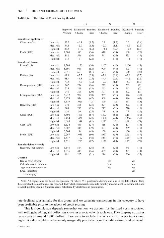
� We report our regression results in Table 4. In Table 4a, we measure profit and its componentsin dollar terms. In Table 4b, the dependent variables are normalized by the car cost, so theyrepresent rates of return. Each panel has a similar structure. For each outcome of interest, wereport in the leftmost column its grade-specific average before credit scoring, and the remainingcolumns report estimates of the effect of credit scoring, βr . Column (1) presents these estimateswith no additional controls (essentially replicating the summary statistics of Table 3). In column(2), we add dealership and calendar month fixed effects, and the household total (monthly)income, residual income, and debt-to-income ratio of each applicant or buyer. In column (3),we also include measures of local economic conditions (at the MSA in which the dealership islocated) at the time of sale and over the initial 12 months of the loan.16 The first set of covariatesis intended to control for compositional changes in the applicant or buyer pool within a givencredit category. The economic indicators are intended to account for local changes that mightimpact close rates or borrower repayment.

� The effect of credit scoring on profitability. All of our specifications show a very strongeffect of credit scoring on profitability. We estimate that profits per transaction increased by over1,000 dollars for each risk category, with the rate of return on capital increasing by 15%–20%depending on the exact specification. At a per-applicant level, we find that profits increased byalmost 600 dollars for lower-risk applicants and by 546 dollars for medium-risk applicants. Wefind a slight decrease in profitability per applicant for high risks, reflecting the fact that the close

15 As mentioned earlier, we use an annual interest rate of 10% to value the stream of payments and recoveries, andalso experimented (in unreported regressions) with rates of 5% and 15% and verified that this assumed rate does not driveany of the results.

16 Specifically, we construct 10 variables to capture local economic conditions. Six are related to local unemploymentrates: the average level, average change, and standard deviation of (monthly) local unemployment rates in the previous6 months and subsequent 12 months. The last four variables are the annual changes in the (quarterly) local housing priceindex and rental price index for the previous 6 months and subsequent 12 months. All these local economic conditionvariables are measured as deviations from the sample mean of that variable in each month. This is because the effect of anational trend in any variable cannot be separately identified from the effect of credit scoring, which is what we seek tomeasure.

C© RAND 2013.


TABLE 4a The Effect of Credit Scoring (Levels)

(1) (2) (3)

Preperiod Estimated Standard Estimated Standard Estimated StandardAverage Change Error Change Error Change Error

Sample: all applicantsClose rate (%) Low risk 57.3 −0.4 (1.2) 0.7 (1.2) 0.5 (0.4)

Med. risk 54.5 −2.0 (1.3) −2.0 (1.1) −1.9 (0.3)High risk 23.5 −11.6 (1.0) −10.8 (0.9) −10.8 (0.3)

Profit ($US) Low risk 1,300 595 (36) 618 (33) 608 (25)Med. risk 882 546 (36) 541 (34) 535 (19)High risk 313 −11 (22) −7 (18) −12 (19)

Sample: all buyersPrice ($US) Low risk 8,703 1,125 (56) 1,107 (52) 1,100 (13)

Med. risk 8,391 911 (52) 900 (48) 892 (10)High risk 7,851 653 (61) 621 (54) 620 (20)

Default (%) Low risk 61.9 −2.5 (0.9) −2.8 (0.9) −2.8 (0.7)Med. risk 68.4 −4.5 (0.7) −4.4 (0.6) −4.3 (0.5)High risk 70.4 −8.0 (0.9) −7.2 (1.1) −6.9 (1.0)

Down payment ($US) Low risk 762 234 (16) 229 (15) 232 (6)Med. risk 725 269 (13) 261 (12) 262 (5)High risk 746 309 (20) 307 (18) 302 (9)

Loan payments ($US) Low risk 6,912 952 (70) 969 (71) 946 (57)Med. risk 5,979 934 (47) 909 (43) 884 (43)High risk 5,319 1,021 (101) 890 (108) 837 (83)

Recovery ($US) Low risk 710 306 (23) 297 (22) 292 (15)Med. risk 709 217 (23) 217 (21) 210 (11)High risk 620 59 (25) 76 (22) 77 (21)

Gross ($US) Low risk 8,400 1,490 (67) 1,493 (68) 1,467 (50)Med. risk 7,424 1,421 (43) 1,388 (40) 1,356 (38)High risk 6,695 1,389 (92) 1,272 (101) 1,215 (73)

Cost ($US) Low risk 6,134 431 (37) 416 (36) 407 (13)Med. risk 5,807 319 (39) 301 (34) 289 (10)High risk 5,364 184 (49) 150 (41) 150 (19)

Profit ($US) Low risk 2,267 1,059 (60) 1,077 (59) 1,061 (49)Med. risk 1,617 1,102 (48) 1,087 (43) 1,067 (37)High risk 1,331 1,205 (87) 1,122 (89) 1,065 (71)

Sample: defaulters onlyRecovery (per default) Low risk 1,146 564 (26) 557 (26) 545 (19)

Med. risk 1,036 413 (26) 409 (24) 393 (14)High risk 881 207 (31) 214 (26) 206 (27)

ControlsDealer fixed effects Yes YesCalendar month dummies Yes YesApplicant characteristics Yes YesLocal indicators∗ Yes

risk category

Note: All regressions are based on equation (7), where D is postperiod dummy and y is in the left column. Onlythe estimated beta coefficients are reported. Individual characteristics include monthly income, debt-to-income ratio andresidual monthly income. Standard errors (clustered by dealer) are in parentheses.

rate declined substantially for this group, and we calculate transactions in this category to havebeen profitable prior to the advent of credit scoring.

This last conclusion depends somewhat on how we account for the fixed costs associatedwith selling, handling, and collection activities associated with each loan. The company estimatesthese costs at around 1,000 dollars. If we were to include this as a cost for every transaction,high-risk sales would have been only marginally profitable prior to credit scoring, and we would

C© RAND 2013.


TABLE 4b The Effect of Credit Scoring (Rates of return)

(1) (2) (3)

Preperiod Estimated Standard Estimated Standard Estimated StandardAverage Change Error Change Error Change Error

Sample: all buyersDown payment/cost (%) Low risk 12.5 2.9 (0.3) 2.8 (0.2) 2.9 (0.1)

Med. risk 12.6 3.9 (0.2) 3.9 (0.2) 3.9 (0.1)High risk 14.0 5.6 (0.4) 5.6 (0.4) 5.5 (0.1)

Loan payments/cost (%) Low risk 113.8 7.4 (1.1) 8.0 (1.0) 7.7 (0.9)Med. risk 104.1 10.2 (1.1) 10.1 (0.9) 9.9 (0.7)High risk 100.3 15.8 (1.9) 14.4 (1.8) 13.4 (1.4)

Recovery/cost (%) Low risk 11.5 3.8 (0.3) 3.7 (0.3) 3.6 (0.2)Med. risk 12.1 2.8 (0.3) 2.8 (0.3) 2.8 (0.2)High risk 11.4 0.6 (0.4) 0.9 (0.4) 1.0 (0.3)

Gross/cost (%) Low risk 138.1 14.0 (1.0) 14.4 (0.9) 14.2 (0.8)Med. risk 129.0 16.9 (0.9) 16.8 (0.8) 16.5 (0.6)High risk 125.9 21.9 (1.7) 20.9 (1.6) 19.8 (1.2)

Profit/cost (%) Low risk 38.1 14.0 (1.0) 14.4 (0.9) 14.2 (0.8)Med. risk 29.0 16.9 (0.9) 16.8 (0.8) 16.5 (0.6)High risk 25.9 21.9 (1.7) 20.9 (1.6) 19.8 (1.2)

Sample: defaulters onlyRecovery/cost (%) Low risk 18.6 7.1 (0.4) 7.1 (0.4) 7.0 (0.3)

Med. risk 17.7 5.6 (0.3) 5.6 (0.3) 5.4 (0.2)High risk 16.3 3.1 (0.5) 3.2 (0.4) 3.2 (0.4)

ControlsDealer fixed effects Yes YesCalendar month dummies Yes YesApplicant characteristics Yes YesLocal indicators∗ Yes

risk category

Note: All regressions are based on equation (7), where D is postperiod dummy and y is in the left column. Onlythe estimated beta coefficients are reported. Individual characteristics include monthly income, debt-to-income ratio andresidual monthly income. Standard errors (clustered by dealer) are in parentheses.

conclude that profits per applicant increased by 105 dollars per applicant for the highest-riskcategory.17 This adjustment also makes the rate of return effects even more dramatic, implyingmore than a doubling.

� How did profits increase? To understand the source of the profitability gains, it is usefulto look at the separate components of profit. Here we focus discussion mainly on the estimatesin the first column of Table 4. What we want to emphasize is the very different channels throughwhich profits increased for the better and worse risk groups.

The story is apparent for high risks. Before credit scoring, almost one in four applicants inour high-risk category became a buyer; with credit scoring, this was cut by half. A likely causeof this change was the required down payment, which increased from 600 dollars prior to scoringto more than 1,000 dollars for the highest-risk applicants. As noted above, increases in the downpayment requirement have a remarkably large impact on purchasing decisions, and also lead to abetter selection—that is, buyers who are just able to come up with the minimum down paymentturn out to be substantially worse risks than buyers for whom this constraint is not binding (Einav,Jenkins, and Levin, 2012). The results in Table 4a are consistent with this selection effect. Default

17 This adjustment has little impact on the change in profitability from low- and medium-risk applicants becauseclose rates for these groups hardly changed. Specifically, with the adjustment we estimate the effect on profits for low andmedium risks to be 598 and 566 dollars per applicant, respectively (compared to 595 and 546 reported earlier).

C© RAND 2013.


rates for buyers in the highest-risk category fell from 70% to 62%, leading to about a 1,000 dollarincrease in repayments.

Credit scoring had a very different effect on the lower-risk applicants. For applicants withbetter risk scores, the company did not raise the minimum down payment requirement, and indeedclose rates remained virtually the same. Nevertheless, profitability increased dramatically. Herethe biggest factor appears to have been that lower-risk applicants were allowed to take largerloans, leading them to purchase better cars, and leading the company to raise its markups onthese cars. The incentive for the company to do this can be seen clearly in Table 4b. Prior tocredit scoring, the transaction rate of return was significantly higher for lower-risk buyers than forhigher-risk buyers (38% vs. 26%–29%). With the ability to identify these buyers, it was possibleto extend them more credit. Table 4a shows the significant increase in car cost for the lower-riskbuyers (431 dollars), an even greater increase—due to increased markups—in the price of thesecars (1,125 dollars), and also the increase relative to buyers in higher-risk categories.

To see how these different effects aggregate into an overall change in profit per buyer,consider the high-risk buyers first. Their down payments increased by 309 dollars, and loanpayments by 1,021, from which we need to subtract a modest 184 dollar increase in car costs.Incorporating a small increase in recoveries leads to the 1,205 increase in profit per buyer reportedin Table 4a. For the lower-risk buyers, car costs and car prices increased much more, by 431 dollarsand 1,125 dollars, respectively, and also loan sizes, because the increase in down payments (of234 dollars) did not increase enough to offset it. The increase in profitability of 1,059 dollorscan therefore be attributed almost entirely to the larger stream of loan payments received on thelarger loans, almost 1,000 dollars per buyer, plus a 306 dollar increase in recoveries reflecting theinitially higher quality of the cars.

� Potential confounding factors. The preceding discussion focused on the first column ofTables 4a and 4b, in which we make no attempt to control for compositional or macroeconomicchanges that might impact our results. Column (2) adds dealer and calendar month fixed effects,as well as individual characteristics. As we describe below, dealership performance varies sub-stantially, and we have already mentioned the seasonality effects in the data. Nevertheless, theinclusion of these variables has virtually no effect on our estimates. This basically reflects thefact that within each of our credit categories, the composition of applicants and buyers did notchange very much during the evaluation period, neither across dealers, nor across months, nor interms of individual characteristics.18

Column (3) of Tables 4a and 4b reports on specifications where we control for local (MSA-level) economic indicators related to unemployment and housing and rental prices (see footnote16). The results remain qualitatively similar. We estimate an increase in profit per buyer of 1,061dollars for lower risks and 1,065 dollars for high risks when we include the full set of controls,compared to 1,059 and 1,205 dollars in the baseline specification. The changes in the estimates ofthe profit components are also small, with nothing in the results leading us to revisit the qualitativeinterpretations above.

6. Differential effects across dealerships

� In this final part of the article, we investigate the effect of the implementation of company-wide credit scoring on specific dealerships. We start by documenting the heterogeneity acrossdealerships prior to credit scoring, and highlighting two specific differences between more andless profitable dealerships. We then measure the effect of credit scoring at each dealership anddocument that although credit scoring improved performance at virtually all dealerships, the

18 The results do not change noticeably if we leave out the individual characteristics (household income and debt-to-income ratio), or if we add additional characteristics (that we have only for buyers) such as the number of dependentsor the time that the buyer has been living at his current address.

C© RAND 2013.


effect was bigger at poorly performing dealerships, leading to a compression in performanceacross dealerships.

� Dealership heterogeneity. Table 5 presents summary statistics for “high” and “low”-performing dealerships. To construct the table, we rank dealerships by their profit per appli-cant in the precredit scoring period. Table 5a shows statistics for the top third of dealerships, andTable 5b for the bottom third.

Dealerships in the top third were dramatically more profitable than dealerships in the bottomthird, earning about 600–800 dollars more per sale. The difference does not appear to be drivenby the composition of the applicant pools, which are similar on observables. We make thispoint more rigorously below in the context of a regression model for profitability that includesdealership fixed effects along with controls for applicant quality. Absent observable differences inthe applicant pool, what may then generate the heterogeneity in profitability? Possibilities include:(i) better selection (on unobservables) of borrowers out of the applicant pool, (ii) better sorting ofborrowers to cars, and (iii) better extraction of profits from otherwise identical transactions, suchas due to better collection or recoveries.

A closer inspection of Table 5 indicates that, indeed, top-performing dealerships had a greaterdifference between the cars sold to high- and lower-risk borrowers. Although all dealerships sold,on average, more expensive cars to lower-risk borrowers, the difference is notably greater fortop-performing dealerships, consistent with these dealerships being better at assessing borrowersprior to credit scoring. Specifically, the two groups of dealerships sold similar cars to lower-riskapplicants, but the more profitable dealerships sold cheaper cars (by roughly 200 dollars) tomedium- and high-risk borrowers. The more profitable dealerships also had significantly lowerdefault rates, particularly for medium- and high-risk borrowers. The difference in repayment ratessuggests that higher-performing dealerships were either more effective in their collection effortsor that their borrowers were more inclined to repay for reasons that we cannot account for evenwith the rich individual-level borrower characteristics in our data.

Motivated by these observations, we can now link back to the model of Section 3 andconsider two dimensions along which dealership may vary. One is the ability to convert salesto profits, via the function zd

θ(C, D), which is now allowed to vary with dealership d. For

example, better collection efforts could be captured by more profitable dealerships having ahigher value of pθ and/or κ . This dimension of heterogeneity is unlikely to be significantlyaffected by the implementation of credit scoring. The second dimension on which dealershipsmay vary is their ability—prior to the availability of centralized credit scoring information—touse “soft information” to identify differences in repayment risk of potential borrowers. Suppose,for instance, that prior to credit scoring, dealerships were able to observe an imperfect (binary)signal of borrower quality, and that at dealership d, a perceived lower-risk borrower was in factlower risk with probability wd

L = λd + (1 − λd)wL . With this parameterization, a value of λd = 0implies that the dealership has no soft information, whereas λd = 1 implies that the dealershipcould replicate the later credit scoring. The calibrated model implies that dealerships with a higherλd can match cars to borrowers more effectively, leading to a greater difference between the carsthey assign to lower-risk and high-risk borrowers. We therefore interpret this difference as a proxyfor dealership information. (We also note that even for a dealership with λd = 1, the advent ofcredit scoring would have a positive effect because company headquarters went from mandatinga uniform down payment requirement to setting differentiated down payment requirements.)

The rest of this section presents evidence on the differential impact of credit scoring acrossdealerships. This investigation links somewhat to an interesting hypothesis in the organizationaleconomics literature that the adoption of “hard-information” technologies such as quantitative riskassessment may crowd out the use of “soft information” obtained at the dealership level (Stein,2002) and may reduce profitability differences across dealerships. In our specific setting, the firststatement is true almost by design, as after the implementation of credit scoring, dealerships hadto follow not only companywide policies regarding minimum down payment requirement but also

C© RAND 2013.


TA

BL

E5a

Sum

mar

ySt

atis

tics

for

Hig

h-P

repe

riod

-Pro

fitD

eale

rs

Pre

dict

edG

rade

:Low

Ris

kP

redi

cted

Gra

de:M

ediu

mR

isk

Pre

dict

edG

rade

:Hig

hR

isk

Pre

Post

Cha

nge

Pre

Post

Cha

nge

Pre

Post

Cha

nge

App

lica

ntch

arac

teri

stic

sN

umbe

rof

appl

ican

tsN

=0.

075

N=

0.06

0N

=0.

124

N=

0.10

6N

=0.

128

N=

0.11

4A

ppli

cant

dem

ogra

phic

sM

onth

lyin

com

e3,

569

3,69

612

72,

142

2,15

816

1,53

61,

644

108

Res

idua

lmon

thly

inco

me

2,78

13,

016

235

1,57

91,

665

861,

249

1,49

224

3D

ebt-

to-i

ncom

era

tio

0.27

0.24

−0.0

30.

300.

29−0

.01

0.23

0.20

−0.0

2C

arpu

rcha

sed

0.61

0.59

−0.0

20.

600.

58−0

.03

0.29

0.15

−0.1

4T

rans

acti

onch

arac

teri

stic

sN

umbe

rof

buye

rsN

=0.

046

N=

0.03

5N

=0.

075

N=

0.06

2N

=0.

038

N=

0.01

7B

uyer

char

acte

rist

ics

Mon

thly

inco

me

3,46

63,

551

862,

073

2,04

7−2

61,

447

1,39

2−5

4R

esid

ualm

onth

lyin

com

e2,

675

2,85

117

61,

498

1,53

032

1,03

11,

335

303

Deb

t-to

-inc

ome

rati

o0.

290.

27−0

.02

0.33

0.32

0.00

0.34

0.36

0.02

Car

char

acte

rist

ics

Car

cost

5,21

95,

585

366

4,84

85,

190

342

4,43

84,

583

145

Car

age

(yea

rs)

6.6

5.6

−1.0

6.8

5.7

−1.1

7.1

5.9

−1.1

Odo

met

erm

iles

89,6

8583

,366

−6,3

1988

,713

82,6

63−6

,050

87,2

4981

,527

−5,7

21In

vent

ory

age

(day

s)63

653

6675

871

777

Lot

age

(day

s)34

384

3847

943

508

Pur

chas

ech

arac

teri

stic

sS

ale

pric

e8,

647

9,68

51,

039

8,27

79,

194

917

7,73

68,

396

660

Dow

npa

ymen

t74

397

022

768

697

629

170

01,

008

308

Loa

nte

rm(m

onth

s)34

.137

.93.

733

.737

.23.

533

.536

.53.

0A

PR

0.29

60.

295

−0.0

010.

296

0.29

4−0

.002

0.29

50.

290

−0.0

05M

onth

lypa

ymen

t39

138

5−6

369

367

−233

933

3−6

Loa

npe

rfor

man

ceO

utco

mes

Def

ault

0.58

0.57

−0.0

10.

630.

61−0

.03

0.66

0.59

−0.0

7Fr

acti

onof

paym

ents

mad

e0.

660.

65−0

.02

0.61

0.61

0.00

0.59

0.62

0.04

Loa

npa

ymen

tsex

clud

ing

dow

npa

ymen

t7,

307

8,18

287

66,

445

7,29

785

25,

698

6,63

093

2R

ecov

ery

amou

nt(a

llsa

les)

604

916

312

576

831

256

509

589

80R

ecov

ery

amou

nt(a

llde

faul

ts)

1,04

41,

610

566

909

1,37

346

476

91,

002

233

Com

pone

nts

ofpr

ofits

Gro

ssop

erat

ing

reve

nue

8,67

110

,083

1,41

27,

720

9,11

41,

394

6,92

48,

243

1,32

0To

talc

ost

6,08

36,

497

414

5,63

86,

043

405

5,16

85,

385

216

Net

oper

atin

gre

venu

e2,

588

3,58

699

92,

082

3,07

198

91,

755

2,85

81,

103

Not

e:In

clud

esde

aler

sin

top

thir

dby

prep

erio

dne

tope

rati

ngre

venu

epe

rap

plic

ant.

See

note

sto

Tabl

e1

for

sam

ple

size

and

vari

able

defi

nati

ons.

C© RAND 2013.


TA

BL

E5b

Sum

mar

ySt

atis

tics

for

Low

-Pre

peri

od-P

rofit

Dea

lers

Pre

dict

edG

rade

:Low

Ris

kP

redi

cted

Gra

de:M

ediu

mR

isk

Pre

dict

edG

rade

:Hig

hR

isk

Pre

Post

Cha

nge

Pre

Post

Cha

nge

Pre

Post

Cha

nge

App

lica

ntch

arac

teri

stic

sN

umbe

rof

appl

ican

tsN

=0.

071

N=

0.05

9N

=0.

138

N=

0.11

5N

=0.

137

N=

0.12

2A

ppli

cant

dem

ogra

phic

sM

onth

lyin

com

e3,

492

3,58

896

2,13

52,

149

151,

564

1,65

389

Res

idua

lmon

thly

inco

me

2,75

02,

905

155

1,57

51,

634

591,

279

1,48

520

6D

ebt-

to-i

ncom

era

tio

0.25

0.24

−0.0

10.

290.

290.

000.

210.

20−0

.02

Car

purc

hase

d0.

510.

550.

030.

460.

480.

010.

170.

09−0

.08

Tra

nsac

tion

char

acte

rist

ics

Num

ber

ofbu

yers

N=

0.03

6N

=0.

032

N=

0.06

4N

=0.

055

N=

0.02

3N

=0.

011

Buy

erch

arac

teri

stic

sM

onth

lyin

com

e3,

390

3,40

010

2,00

52,

017

121,

469

1,38

8−8

1R

esid

ualm

onth

lyin

com

e2,

626

2,68

357

1,39

81,

453

551,

049

1,37

432

5D

ebt-

to-i

ncom

era

tio

0.28

0.28

0.00

0.34

0.34

0.00

0.33

0.37

0.04

Car

char

acte

rist

ics

Car

cost

5,20

45,

598

394

4,99

25,

193

201

4,66

24,

815

152

Car

age

(yea

rs)

6.2

5.3

−0.8

6.1

5.6

−0.5

6.3

5.8

−0.5

Odo

met

erm

iles

88,5

4480

,496

−8,0

4887

,440

81,3

67−6

,073

86,1

4682

,235

−3,9

11In

vent

ory

age

(day

s)67

66−1

7178

781

9717

Lot

age

(day

s)38

36−2

4346

351

6413

Pur

chas

ech

arac

teri

stic

sS

ale

pric

e8,

830

10,1

781,

347

8,59

89,

593

995

8,08

68,

705

619

Dow

npa

ymen

t76

91,

001

232

745

1,00

425

979

51,

056

262

Loa

nte

rm(m

onth

s)34

.636

.92.

434

.736

.41.

735

.135

.80.

7A

PR

0.27

00.

260

−0.0

100.

270

0.26

4−0

.006

0.27

20.

273

0.00

1M

onth

lypa

ymen

t36

839

325

356

375

1932

734

417

Loa

npe

rfor

man

ceO

utco

mes

Def

ault

0.65

0.62

−0.0

30.

730.

67−0

.06

0.74

0.65

−0.1

0Fr

acti

onof

paym

ents

mad

e0.

590.

600.

010.

510.

550.

040.

490.

570.

08L

oan

paym

ents

excl

udin

gdo

wn

paym

ent

6,50

87,

596

1,08

85,

522

6,61

01,

088

4,95

06,

138

1,18

8R

ecov

ery

amou

nt(a

llsa

les)

760

1,09

533

580

898

417

672

270

2−2

0R

ecov

ery

amou

nt(a

llde

faul

ts)

1,16

81,

773

606

1,10

91,

465

356

974

1,08

811

4C

ompo

nent

sof

profi

tsG

ross

oper

atin

gre

venu

e8,

057

9,70

81,

651

7,08

68,

609

1,52

26,

472

7,90

11,

429

Tota

lcos

t6,

072

6,55

848

55,

832

6,11

528

35,

466

5,66

119

6N

etop

erat

ing

reve

nue

1,98

43,

150

1,16

51,

254

2,49

31,

239

1,00

62,

239

1,23

3

Not

e:In

clud

esde

aler

sin

bott

omth

ird

bypr

eper

iod

neto

pera

ting

reve

nue

per

appl

ican

t.S

eeno

tes

toTa

ble

1fo

rsa

mpl

esi

zean

dva

riab

lede

fini

tion

s.

C© RAND 2013.


FIGURE 4

0.00

0.50

1.00

1.50

2.00

2.50

0.00 0.50 1.00 1.50 2.00

Kern

el d

ensi

ty

Dealership profit per applicant/average profit per applicant

Preperiod Postperiod

0.00

0.50

1.00

1.50

2.00

2.50

0.00 0.50 1.00 1.50 2.00

Kern

el d

ensi

ty

Dealership profit per applicant/average profit per applicant

Preperiod Postperiod

(a) VARIATION IN DEALERSHIP PROFITABILITY PRE-AND POSTSCORING

(b) VARIATION IN DEALERSHIP PROFITABILITY WITH FULL SET OF CONTROLS

Note: Each of the graphs presents estimates from a regression of the form of equation (13), with profit per applicant as thedependent variable. The preperiod graph plots a kernel density of the estimated alpha divided by the mean alpha acrossdealerships, and the postperiod graph plots a kernel density of the estimated alpha+beta, also divided by the mean acrossdealerships. Panel (a) uses no other controls (except credit grade fixed effects), and Panel (b) uses a full set of controls(as in column (3) of Table 4).

regarding the matching of cars to potential borrowers, where they previously had more discretion.Nevertheless, to the extent that dealerships varied in other dimensions, such as their ability toencourage repayment, profitability need not converge.

� Specification and results. To measure how the adoption of credit scoring affected indi-vidual dealerships, we adapt our earlier regression model to allow the effect of credit scoring tovary across dealerships:

yi = αd(i) + βd(i) Dt + δR(i) + Xiη + υi . (13)

As before, i is an individual, yi an outcome variable of interest, d(i) is the dealership involvedin the transaction, R(i) is the individual’s risk category (low, medium, or high), Di is a dummyvariable that takes the value of 1 in the postscoring period, and Xi is a set of other controls. Weseparate the credit category dummies from the rest of the controls because we vary the set of Xs but

C© RAND 2013.


FIGURE 5

20%

15%

10%

5%

0%

5%

10%

50% 60% 70% 80%

Chan

ge in

def

ault

rate

40%

20%

0%

20%

40%

60%

80%

100%

120%

140%

50% 60% 70% 80%

Chan

ge in

pro

fit p

er a

pplic

ant

Preperiod default rate

$400

$200

$0

$200

$400

$600

$800

$1,000

$1,200

$1,400

$200 $400 $600 $800 $1,000 $1,200Chan

ge in

hig

h-lo

w c

ost s

prea

d

40%

20%

0%

20%

40%

60%

80%

100%

120%

140%

$200 $400 $600 $800 $1,000 $1,200Chan

ge in

pro

fit p

er a

pplic

ant

Preperiod high-low cost spread

(a) DEFAULT RATE AND CHANGE BY DEALER (b) HIGH-LOW VEHICHLE COST SPREAD AND CHANGE BY DEALER

(c) CHANGE IN PROFITABILITY VS. PRE-PERIOD DEFAULT RATE (d) CHANGE IN PROFITABILITY VS. PRE-PERIOD COST SPREAD

–

–

–

–

–

–

–

–

–

–

Preperiod default rate Preperiod high-low cost spread

Note: Each point on the charts represents a dealership. The x axes on the upper and lower panels show two measuresof preperiod dealership performance: the default rate and the high-low vehicle cost spread. The default rate for eachdealership in a period is calculated as total defaults on loans originated in the period divided by total originations in theperiod. The high-low vehicle cost spread for each dealership in a period is calculated as the average vehicle cost forlow-risk borrowers minus the average vehicle cost for high-risk borrowers originated in the period. Profit per applicantis calculated as total dealership net revenue (see Table 1 for definition) from loans originated in each period, divided bytotal applications in each period. In all panels, change is postperiod minus preperiod.

always control for credit category. In this specification, the coefficient αd represents the dealershipeffect prior to credit scoring, whereas the coefficient βd represents the dealership-specific effectof credit scoring. The sum αd + βd is the dealership effect after credit scoring.

For our main analysis, the outcome of interest is the dollar profit per applicant (analyses ofthe other metrics of profits used in Table 4 reveal an almost identical pattern). We estimate theregression without controls and then with a full set of controls (as in column (3) of Table 4).Using either specification, the dealership effects are less dispersed after credit scoring. Withoutcontrols, the coefficient of variation of the estimated αds is 0.304, and the coefficient of variationof the postscoring dealership effects, the αd + βds, is 0.237. Dispersion drops by 22%. With afull set of controls, we find a similarly sharp reduction. The coefficient of variation of dealershipeffects falls from 0.232 to 0.165 (29%).

Figure 4 presents a graphical illustration of the estimates. It plots the cross-sectional dis-tribution of dealership profitability before and after the implementation of credit scoring. Inparticular, define α and β to be the average of (respectively) the αds and the βds, so that αd/ α

is the (normalized) profitability of dealership d prior to credit scoring, and (αd + βd)/(α + β)is the (normalized) profitability after credit scoring. Figure 4 plots the distribution of αd/α and(αd + βd/(α + β)), first using the estimates without controls (Panel (a)) and then the estimateswith the full set of controls (Panel (b)). Both plots show that after credit scoring, dealershipprofitability had a tighter distribution.

In Figure 5, we present evidence that the homogenization of profits across dealershipsappears to be associated with the implementation of credit scoring rather than reflecting someunobserved time trend. Motivated by the patterns in Table 5, we sort dealerships based on twoprescoring performance measures that plausibly capture dealership differences in the use of softinformation prior to credit scoring: the difference between the cars assigned to lower-risk and

C© RAND 2013.


high-risk borrowers, and the default rate. Panels (a) and (b) show that the heterogeneity in bothmetrics was reduced after credit scoring. The vast majority of the dealerships increased the spreadof car values assigned to lower-risk and high-risk borrowers, and dealerships that originally hada lower spread had a greater increase. Similarly, default rates declined at the vast majority ofdealerships, and the decline was greater at dealerships with higher default rates prior to creditscoring. Panels (c) and (d) show that these effects were associated with profit increases. As thefigure makes clear, almost all dealerships experienced an increase in profitability, but dealershipswith the smallest spread in car values for low- and high-risk borrowers, and with the highestdefault rates, experienced the greatest increases in profits.

7. Conclusions

� In this article, we report detailed results on the adoption of automated credit scoring andthe changes it enabled in lending at a large auto finance company. The adoption of credit scoringtechnology led to a large increase in profitability. Lending to the highest-risk applicants contracteddue to more stringent down payment requirements, and lending to lower-risk borrowers expanded,driven by more generous financing for higher-quality, and more expensive cars. We find that theseeffects were remarkably consistent across dealerships, and that the impact of credit scoring helpedto compress large performance differences across dealerships.

Several aspects of our analysis may be interesting to follow up in other contexts. Much of theacademic and practitioner literature emphasizes how better information about customers enablesmore efficient screening of marginal borrowers; our work highlights how improved credit scoringalso allows better customization of contract terms to inframarginal borrowers. A related point isthat in our setting the relevant margin of adjustment following the advent of credit scoring wasnot the interest rate but rather the down payment and maximum loan size, that is, the amount ofleverage borrowers were allowed to take on. It has become increasingly clear that this leverageaspect of consumer borrowing, particularly in regard to the subprime market, deserves muchmore attention than it has generally received.

Appendix

In this appendix we provide more details about the construction of the matched applicant pool. Recall that the mainchallenge arises because the company did not credit score applicants in the preperiod and, moreover, did not collectall the individual characteristics that are used as inputs for the (proprietary) credit scoring algorithm. Therefore, toconstruct our matched applicant pools, we need to construct our own credit scoring algorithm, which relies on theindividual characteristics that are observed both before and after credit scoring, income and debt-to-income ratio. To doso, we assume that applicants can be of one of three risk categories—high, medium, or low—and use the actual riskclassification from the post period as a guide.

Formally, the problem we try to solve is to find a function f : R2+ → {high,medium, low}, which maps applicants’

income and debt-to-income ratio into one of the three risk categories. A naive approach (which turns out to do reasonablywell) is to use the postcredit scoring period, and in particular the high-/medium-/low-risk category each applicant inthe postperiod is classified as (by the company), and run an ordered probit regression of this classification on incomeand debt-to-income. Because the goal is to predict well, we allow for flexible functional form by generating 10 deciledummies for income and debt-to-income ratio and fully interacting them. Given the estimation results, we then computethe predicted values for the predicted latent variable, order them over the 100 cells, and assign a risk category to eachcell accordingly, in order to match the overall distribution of high-, medium-, and low-risk categories in the postperioddata (which are 29%, 46%, and 25%, respectively). We then assign each applicant in the preperiod data a credit categorybased on his or her income and debt-to-income cell. Table A1(a) presents the results. It shows that the risk category isclose to monotone in both income and debt-to-income ratio. That higher-income applicants are generally lower risk isintuitive. It turns out that, in our data, higher debt is also associated with lower risk. Presumably, for this population,higher debt is associated with the extension of credit by other lenders, which serves to indicate creditworthy behavior,and this underlying correlation dominates any likely effect of debt burden on default risk.

Our actual risk categorization is a small modification of the above-described procedure. Motivated by the fewcases of nonmonotonicities in Table A1(a) which are likely driven by sampling errors — we reran this prediction model,under the restriction that f (·) is (weakly) monotone in both income and debt-to-income ratio, again characterizing eachindividual by the interaction of his income and debt-to-income decile dummy variables. Among the set of monotonemappings, we seek a mapping that meets two objectives: it matches the individual’s actual credit score, and it accurately

C© RAND 2013.


TABLE A1 Results from risk prediction model

Debt-to-income ratio (%) decile

1 2 3 4 5 6 7 8 9 10<10.3 10.3–14.2 14.2–17 17–20 20–23.5 23.5–27.5 27.5–31.8 31.8–36.4 36.4–41.8 >41.8

Monthly income decile1 (<1,350)2 (1,350–1,500)3 (1,500–1,663)4 (1,663–1,800)5 (1,800–2,000)6 (2,000–2,200)7 (2,200–2,500)8 (2,500–2,837)9 (2,837–3,464)10 (>3,464)

Debt-to-income ratio (%) decile

1 2 3 4 5 6 7 8 9 10<10.3 10.3–14.2 14.2–17 17–20 20–23.5 23.5–27.5 27.5–31.8 31.8–36.4 36.4–41.8 >41.8

Monthly income decile1 (<1,350)2 (1,350–1,500)3 (1,500–1,663)4 (1,663–1,800)5 (1,800–2,000)6 (2,000–2,200)7 (2,200–2,500)8 (2,500–2,837)9 (2,837–3,464)10 (>3,464)

(a) Results based on an ordered probit model

(b) Results based on the full model

Legend:

Predicted low risk

Predicted medium risk

Predicted high risk

predicts the fraction in the population of each risk category (as classified by the company in the postperiod). Letsi ∈ {H,M, L} be applicant i’s actual credit category and f (xi ) ∈ {H,M, L} be individual i’s predicted credit category.We then parameterize a loss function over prediction models, so that the optimal prediction model f (·) (within the set ofmonotone models) minimizes

σ1

∑i

I (si �= f (xi )) + σ2

∑i

(I (si = L , f (xi ) = H ) + I (si = H, f (xi ) = L))

+ω∑

j∈{H,M,L}

∣∣∣∣∣∑

i

I ( f (xi ) = j) −∑

i

I (si = j)

∣∣∣∣∣ , (A1)

where ω, σ1, and σ2 are nonnegative parameters. That is, the first component in the loss function penalizes for wrongpredictions, the second component increases the penalty for “really bad” predictions (predicting high risk although actualscore is low risk, and vice versa), and the third component penalizes against deviation from the overall mix of high,medium, and low risks in the population.

We solve this constrained optimization problem numerically, by searching over the entire set of monotone functions.Based on many different trials, it seems that the prediction model is largely insensitive to the exact values of the weightsσ1, σ2, and ω. The results presented in the article use weights of σ1 = 1, σ2 = 3, and ω = 8. Table A1b reports itspredictions. As one can see, it is similar to the results obtained from the ordered probit model (table A1a), but it imposesmonotonicity and is slightly different for some marginal cells.

References

ADAMS, W., EINAV, L., AND LEVIN, J. “Liquidity Constraints and Imperfect Information in Subprime Lending.” AmericanEconomic Review, Vol. 99 (2009), pp. 49–84.

AKHAVEIN, J., FRAME, W.S., AND WHITE, L.J. “The Diffusion of Financial Innovations: An Examination of the Adoption ofSmall Business Credit Scoring by Large Banking Organizations.” Journal of Business, Vol. 78 (2005), pp. 577–596.

C© RAND 2013.


BERGER, A.N., MILLER, N.H., PETERSEN, M.A., RAJAN, R.G., AND STEIN, J.C. “Does Function Follow OrganizationalForm? Evidence from the Lending Practices of Large and Small Banks.” Journal of Financial Economics, Vol. 76(2005), pp. 237–269.

BLOOM, N., GARICANO, L., SADUN, R., AND VAN REENEN, J. “The Distinct Effects of Information Technology andCommunication Technology on Firm Organization.” Manuscript, Stanford University. www.stanford.edu/∼nbloom/BGSV_2011.pdf, 2011.

EDELBERG, W. “Risk-Based Pricing of Interest Rates for Consumer Loans.” Journal of Monetary Economics, Vol. 53(2006), pp. 2283–2298.

EINAV, L., JENKINS, M., AND LEVIN, J. “Contract Pricing in Consumer Credit Markets.” Econometrica, Vol. 80 (2012),pp. 1387–1432.

FRAME, W.S., SRINIVASAN, A., AND WOOSLEY, L. “The Effect of Credit Scoring on Small-Business Lending.” Journal ofMoney, Credit and Banking, Vol. 33 (2001), pp. 813–825.

GRODZICKI, D. “The Evolution of Competition in the Credit Card Industry.” Manuscript, Stanford University.www.stanford.edu/∼danielg3/DanielGrodzicki_CreditCards_Sep20_2012.pdf, 2012.

HEITFIELD, E. AND SABARWAL, T. “What Drives Default and Prepayment on Subprime Auto Loans?” Journal of RealEstate Finance and Economics, Vol. 29 (2004), pp. 457–477.

JENKINS, M. “Measuring the Costs of Ex Post Moral Hazard in Secured Lending.” PhD Thesis, Stanford University, 2010.JOHNSON, R.W. “Legal, Social and Economic Issues in Implementing Scoring in the United States.” In J.N. Crook, D.B.

Edelman, and L.C. Thomas, eds., Credit Scoring and Credit Control: Based on the Proceedings of a Conferenceon Credit Scoring and Credit Control. New York: Oxford University Press, 1992.

PETERSEN, M.A. AND RAJAN, R.G. “Does Distance Still Matter? The Information Revolution in Small Business Lending.”Journal of Finance, Vol. 57 (2002), pp. 2533–2670.

STEIN, J.C. “Information Production and Capital Allocation: Decentralized versus Hierarchical Firms.” Journal of Finance,Vol. 57 (2002), pp. 1891–1922.

C© RAND 2013.

the impact of credit scoring on consumer...

Documents